MITOCW | 16. Solar Cell Characterization

The following content is provided under a Creative Commons license. Your support

will help MIT OpenCourseWare continue to offer high quality educational resources

for free. To make a donation or view additional materials from hundreds of MIT

courses, visit MIT OpenCourseWare at ocw.mit.edu.

PROFESSOR: So I'm going to describe the basic classification of solar cell characterization

methods. And then I'll describe some of the characterization tools that are used to

measure Jsc losses and other tools are used to measure VOC and fill factor losses.

So we're getting a sense of the lay of the land. Let me ask you how would you

characterize-- how would you create a taxonomy of solar cell characterization

techniques?

Those of you might have a little bit more experience might actually have used a few

characterization techniques in your laboratories. What taxonomy would you use?

How would you slice the pie of all these characterization techniques? Go. What are

ways to divide the characterization universe into distinct groupings? How about we

start-- go ahead. Yeah?

AUDIENCE: Performance and performance losses.

PROFESSOR: Yeah so we can describe based on the economic variables like efficiency and then

within efficiency Jsc, Voc, fill factor, mechanical yield, reliability. These are all

parameters that can lump into a cost model and ultimately impact the cost-- dollars

per watt, let's say of a PV panel. Excellent, so we can describe it based on

performance.

If we dive into performance a little more, what are some of the properties that affect

performance? We have electrical properties, optical properties, mechanical,

thermal. So we can break up characterization techniques based on the properties

that they probe. And we can also characterize-- we can create a taxonomy of

characterization techniques based on how fast they are, whether it's something that

you have to sit around and twiddle your thumbs for a half or two hours to get done

1

or something that gets done in 10 milliseconds of which there are several

characterization techniques.

What would the 10 millisecond variety enable you to do? In a manufacturing

environment? Yeah?

AUDIENCE: Sort them.

PROFESSOR: Sort them. Test them. Measure them-- every single cell coming through. So you

might have a bar code like one of those fancy two-dimensional bar codes laser

marked on each single wafer going through your line so you can trace it back in

your MES system all the way back to the crystal that was grown or from the thin film

growth chamber where it was deposited. So, yes, you have inline and shall we say,

the inline characterization techniques and what are called offline characterization

techniques, which tend to be lower throughput.

You can think of the inline characterization techniques as being in the line of the

manufacturing environment and the offline as being those techniques that are sitting

in your laboratory waiting to be used in the R&D lab, which might be next door to the

manufacturing line. Device performance metric affected-- that addresses the

efficiency point up here. And then by property tested-- electrical, structural, optical,

mechanical.

So if you talk to somebody who works in a PV company, she will likely give you a

break down based on number three right here. OK, these are the techniques that

we have in our inspection system and those are the techniques that I have over

there in the R&D lab. If you talk to somebody who is giving a fundamental course in

materials science, they are likely to pick part number one way up there and give you

the breakdown based on the properties that are probed.

I'm going to opt for number two today in lecture not because it's any better or worse

than all the others, but just because that's the metric that we care about right now

as we're trying to probe dollars per watt that relates to our quiz and our homework,

but also relates to the ultimate economic driver of solar.

2

So we will keep this in mind that we might need to ferret out references for the

different techniques in different textbooks or different papers based on whether

they're probing electrical structural optical mechanical properties of our solar cells.

But we're going to be focused on efficiency-- short circuit, current, open circuit,

voltage, fill factor.

So let's go ahead and dive into that. We are going to first start with techniques to

measure Jsc or short circuit current losses. And some of these slides are going to

be repeats. And the reason they're repeats is because the first time you saw it OK,

you sort of kind of got it. You went to the lab, made your devices, tested them. And

now all of a sudden, you have a much stronger background with which to

understand.

We're going to start by discussing the optical components just very briefly and then

spectra response and minority carrier diffusion length, revisiting some of these

concepts that we have already seen, but now with the benefit of having all of our

background knowledge. The spectrophotometer measures specular and diffuse

reflectance and transmission.

All right, let's break that down. Specular reflectance-- specu lar-- Latin. So specular

reflectance means light comes in and out pretty much at the same angle relative to

the surface normal. So if you come in from here, it's going to bounce out light there

right at the same angle relative to the surface normal.

Diffuse reflectance means that if you shine light in a certain angle, it's going to

reflect back not necessarily at that angle. You could have a distribution. A

Lambertian scatterer might qualify. And reflectance in transmission-- we talked

about different optical losses of a solar cell material. Reflectance means that light

comes back off the surface. Transmission means that light did not get absorbed. So

it went through the material and didn't get absorbed. That is an optical loss as well.

So the spectrophotometer is useful for measuring these different loss mechanisms.

And it can tease apart the specular from the diffuse reflectance, giving you some

indication, some idea, of how the surface is behaving and what you might do to

3

improve it. So the spectrophotometer is useful in that regard. In terms of increasing

absorption, we talked about various methods to increase absorption. Those who

attended Eli Yablonovitch's talk heard about many more.

The goal here is essentially to increase the optical path length by texturing your

surface, for instance. The physical thickness can remain very low. And, again, just

to refresh ourselves if we decrease the thickness of our devices but manage to

have very good like trapping, what happens to our excess carrier density? It goes

up, right? Because now we have more carriers being generated in a smaller volume

so the carrier density increases.

And as the carry density goes up, that means the separation of the quasi-Fermi

energies increases, which means the maximum voltage extractable from or devices

increases as well. So there's a strong push right now in the field to go thinner and

thinner devices. That also has the added benefit economically of using less

material. So we want to decrease the thickness by improving our optical trapping--

our light trapping.

Another benefit is it allows carriers to be absorbed closer to the junction, which

increases the probability of collection. And we talked about this during the very

beginning of class how you might texture your surface. But now we actually saw it in

producing our cells. So this is an example-- an SCM image-- of textured silicon. In

that particular case, this was an alkali etch on a single crystalline sample probably of

1 0 0 orientation so that these edges of the pyramids are 1 1 1 planes.

You could also achieve a similar, although not identically, looking result if you have

performed an acidic etch, which would be isotropic in nature. So the light comes in

for the textured surface. Some of it goes into the device. Notice that Snell's law is in

effect. So the light bent or was refracted. And some of the light is reflected off the

surface.

Now, because of the texturization, you get that second-chance absorption. So the

light has two bounces before leaving, which means that the probability of the light

getting absorbed is 1 minus r quantity squared. And so you get an enhanced

4

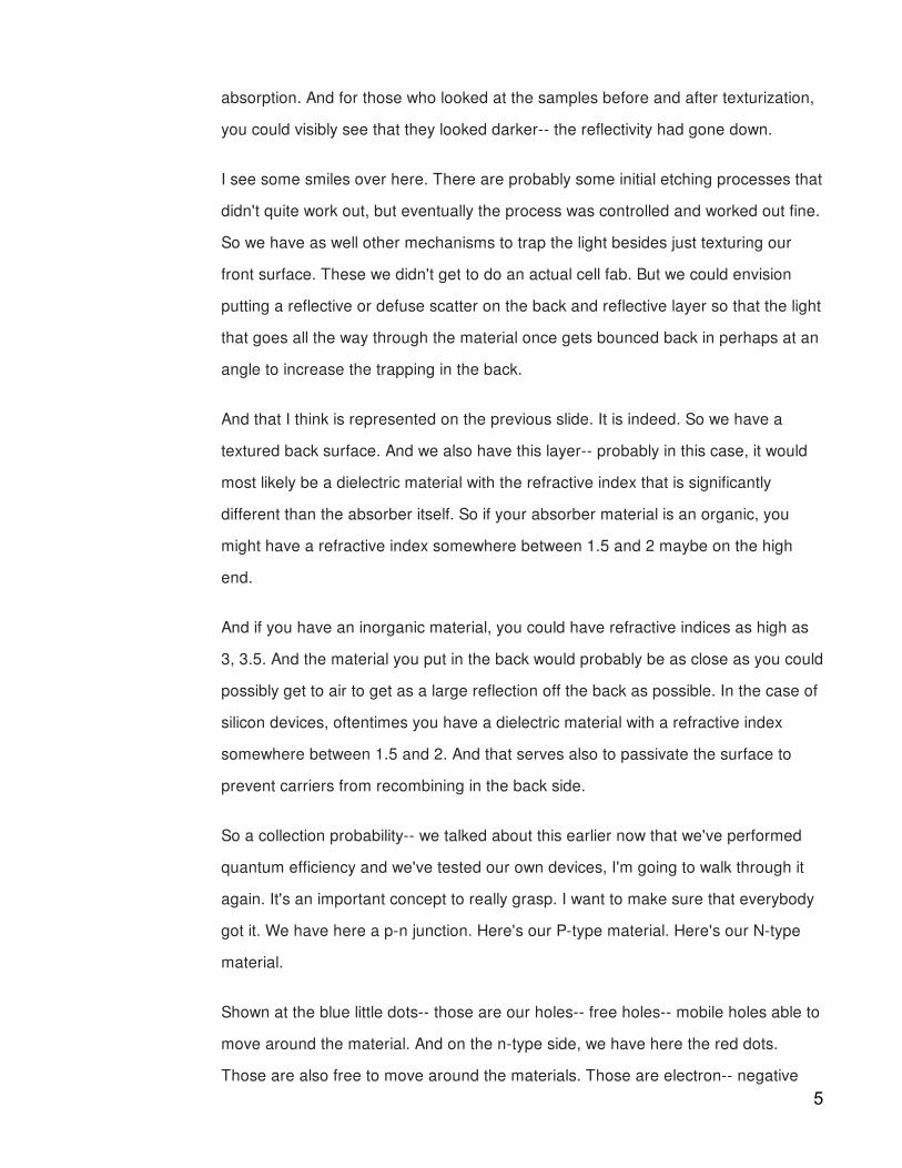
absorption. And for those who looked at the samples before and after texturization,

you could visibly see that they looked darker-- the reflectivity had gone down.

I see some smiles over here. There are probably some initial etching processes that

didn't quite work out, but eventually the process was controlled and worked out fine.

So we have as well other mechanisms to trap the light besides just texturing our

front surface. These we didn't get to do an actual cell fab. But we could envision

putting a reflective or defuse scatter on the back and reflective layer so that the light

that goes all the way through the material once gets bounced back in perhaps at an

angle to increase the trapping in the back.

And that I think is represented on the previous slide. It is indeed. So we have a

textured back surface. And we also have this layer-- probably in this case, it would

most likely be a dielectric material with the refractive index that is significantly

different than the absorber itself. So if your absorber material is an organic, you

might have a refractive index somewhere between 1.5 and 2 maybe on the high

end.

And if you have an inorganic material, you could have refractive indices as high as

3, 3.5. And the material you put in the back would probably be as close as you could

possibly get to air to get as a large reflection off the back as possible. In the case of

silicon devices, oftentimes you have a dielectric material with a refractive index

somewhere between 1.5 and 2. And that serves also to passivate the surface to

prevent carriers from recombining in the back side.

So a collection probability-- we talked about this earlier now that we've performed

quantum efficiency and we've tested our own devices, I'm going to walk through it

again. It's an important concept to really grasp. I want to make sure that everybody

got it. We have here a p-n junction. Here's our P-type material. Here's our N-type

material.

Shown at the blue little dots-- those are our holes-- free holes-- mobile holes able to

move around the material. And on the n-type side, we have here the red dots.

Those are also free to move around the materials. Those are electron-- negative5

charged carriers. Omitted from this diagram-- omitted from this diagram is the fixed

charge associated with each connectivity type. We have, for example, fixed negative

charge from the ionized acceptors and the p-type and fixed positive charge from the

ionized donors. And the n-type-- we've omitted it for clarity.

We note that an electric field builds up here at the junction between. And that

sweeps carriers into one side or another so that if light comes in and generates a

pair of charges-- due to charge neutrality, it generates a pair-- a positive and a

negative-- the charge carrier type will be swept across the junction and the other will

remain inside of the material. And so to be more precise about the exact motion that

occurs with the carriers, we have at first a diffusion process until the electric field

starts becoming large and then finally drift across that junction. And that's what

generates the current inside of a solar cell device.

So collection probability means that light-- a light-generated-- a photo-generated

minority carrier can readily recombine. But if the carrier reaches the edge of the

space charge region, the minority carrier can be swept across and collected. So the

probability of collection means for every electron hole pair that I generate at a

certain depth, what is the probability that the minority carrier will make it across a

junction.

And this is what we're probing in spectral response. Yes?

AUDIENCE: How long is the exciton diffusion in silicon?

PROFESSOR: Great question. The exciton in silicon has a binding energy less than kt, which

means at room temperature, the exciton readily dissociates. So the exciton diffusion

length can only be measured at lower temperatures. At room temperature, you

essentially just discuss minority carriers. And the minority carrier diffusion length--

let's revert it in terms of lifetime and then do the translation to diffusion length.

In terms of lifetimes, one typically has a range between a microsecond to a

millisecond-- millisecond being on the high end. It can go as high as five

milliseconds even. And so if you revert that into a diffusion length, one microsecond

6

lifetime would correspond to a 50-micron diffusion length. And then you can do the

rest of the conversion from there just taking the square root sign into account. So it

can be rather long on the order of the thickness of the solar cell devices.

Now those length skills, which we were talking about hundreds of microns-- maybe

even a thousand microns. Compare that now to 10-nanometer diffusion length say

for an exciton in a polymer blend material. Then you have to reconsider your device

architecture. And how you're going to actually collect them.

So this is a very generic picture, which could easily be substituted. Instead of n-type,

p-type, it could be easily substituted by say polymer 1 and polymer 2 that just have

the right band alignment to separate charge. Then it gets a little more complicated

as well. Here we're assuming that the carriers that are swept across the junction

can move easily away from the junction. In a polymer, not always so.

You might have charge accumulation right at the edge of the space charge region,

which creates its own field, which counteracts the built-in field here and also inhibits

current flow. So things get a lot more complicated as you venture away from the

simple case of say a well-behaved what it was called in this case a homo junction,

meaning a p-n junction created from the same material on both sides-- silicon just

n-type an p-type.

If you have a hetero junction comprised of two different materials, you may have

additional effects occurring. But it's always helpful to think about the motion of

carriers from the perspective of drift and diffusion. And if you're ever in doubt, you

can begin thinking about the process in terms of delta T's-- small increments of time

where you imagine light coming in generating an electron hole pair, imagining what

happens as that carrier moves to the junction then moves across the junction.

And then what happens? Does it immediately get collected? Does it stay there?

What happens next? Is there a potential-- an attractive potential between the

carriers on either side of that junction. So asking those sorts of questions can help

you walk through and troubleshoot what exactly is going wrong with your device.

7

Collection probability-- so we take this diagram that we just on the previous slide--

this one right here. And we say, if light were to come in and generate an electron

hole pair right here, then I would expect very high probability of collection, meaning

the minority carrier would be swept across. The majority carrier would stay on this

side. And presuming that they can get from here to the contacts-- big assumption--

but assuming that they can-- then the probability of collection of those carries will be

very, very high.

But if my light comes in deep within the device and generates an electron hole pair,

the minority carrier will have to cruise through-- you can think about it. It may be a

nice, tasty chicken in the Everglades National Park trying to make its way over from

that side all the way over to the junction and across. The minority carrier is at risk of

recombining. And many of them don't make it. So we have the following graph-- the

collection probability versus distance into the device where this yellow region

represents the space charge region-- where the probability of collection is very high.

And as you move away from the space charge region, the probability of collection

decreases. And you can see it decreases exponentially as a function of distance

from the space charge region. The reason you have almost-- not exactly symmetric-

- these are two different decay constants, but they're both exponential functions on

either side-- is because over here on what ostensibly would be the-- what did we

call it-- the p-type side-- the electrons would be the minority carriers. And over the

n-type side, the holes are the minority carriers. And each one is trying to get to the

other side.

So the collection probability is actually the collection probability of minority carriers--

the precise definition of which is changing from one side of the junction to the other.

On one side of the junction, the electrons are the minority carriers. And on the other

side, the holes are the minority carriers.

So by probing at different wavelengths of light, we essentially change the optical

absorption coefficient of the material, which means that the light will get absorbed at

different depths. So we might have a very short wavelength light that probes up

8

here. And then, say light is coming in from this side-- so short wavelengths light gets

absorbed near the front surface. And then longer, longer, longer, and longer, and

longer wavelengths until we're deep within the material. And we can flush out

exactly what the current collection probability would be as a function of depth.

Then we essentially take that data knowing the generation rate and the collection

probability. We can tease out the minority carrier diffusion length using the

spectrophotometer. So let me show you examples of good and bad cells. This

would be a bad solar cell and a good solar cell device right over here. The good

solar cell has a high internal quantum efficiency out to longer wavelengths.

And as we know from the very second lecture of our class, the longer wavelengths

get absorbed deeper into the device further from the junction. And so you can see

this tail off occurring. Actually, the tail off is somewhere in this region right here for

this device is occurring within the bulk. At some point, the device just isn't thick

enough to absorb all the light. So there is an inevitable drop toward longer

wavelengths.

But the bad cell doesn't an even poorer job of collecting these longer wavelengths.

And that's in part because the minority carrier diffusion length of that particular cell

was much lower or save the minority carrier diffusion length of the material which

comprise the cell is much lower than the good cell.

So if you come in with a longer wavelength for light-- let's say maybe 933

nanometers in silicon that would give an absorption depth of around 100 microns--

that's pretty far from the junction-- now you would have a much lower probability in

the bad cell of collecting than the good cell. And that's precisely because the

diffusion length is lower.

So integrated over all of the wavelengths, one obtains the short-circuit current. And

the method of measurement was the spectrophotometer. Now, I understand most of

you opted to choose Sun's Voc for your one characterization tool to apply to your

cells. Did anybody choose a spectrophotometer? Show of hands. Anybody?

9

AUDIENCE: It was broken.

PROFESSOR: It was broken, yeah, so the filter wheel was down. That was it. So let's see, the filter

wheel-- the filter wheel. Let's go fixing this. Here it is. So the filter wheel was broken.

So essentially, the polychromatic light source was shining through a filter wheel

which was selecting one wavelength of light. The monochrometer, of course, was

helping as well and eventually on to the solar cell sample, which was shown in front

of the light.

So that's the way in principle spectral response works. And one variant of spectral

response-- that's for the full device. You typically have an illuminated area of a few

millimeters squared or maybe even a few centimeters squared. But let's say that

wasn't good enough for you. You knew you had an inhomogeneous material and

you want to probe the inhomogeneity across your device.

You had a large device maybe about that big-- a few 10s of centimeters squared.

And you want to probe the distribution of minority carrier diffusion lengths across

your device. How would you do that? Well, in one incarnation, you would use a

much more finely-focused beam. Instead of having something on the order of a

millimeter, you might shrink the beam spot size down to the range of single microns.

And then use an xy stepper motor to scan across your device. And that's precisely

what this does right here.

This white piece is the xy stage. And this black head right here is essentially

comprised of several lasers that will shine on to the sample. Now, you need a few

different wavelengths of light to really flesh out this curve to determine the minority

carrier diffusion length from this curve. And so the laser light is typically chosen at

very auspicious wavelengths to maximize utility in this particular type of evaluation.

And so we have usually four-- a minimum three. You can always fit a line through

two data points-- so a minimum three laser wavelengths and usually about four or

more to process the quantum efficiency as a function of position. And so the xy

stage moves the sample around and the laser head-- or moves the laser head

around while the sample stays fixed and you map out the current response at each

10

point on the device, obtaining a map that looks much like this right here where this

is on the y scale or the z scale, sorry, you have from 0 to 120-micron diffusion

length on that particular solar cell device.

And points 3, 1, and 2 represent regions in which the minority carrier diffusion with

was calculated using the method that we have discussed in the previous lectures--

the Paul Basore method. So we have a map of minority carrier diffusion length

across our device. Some regions are underperforming. Other regions are

performing rather well.

And we can see that in general, these lower-cost materials tend to be fairly

inhomogeneous in terms of their performance response. And if you really want to

get fancy and say, my goodness, if I spend all this time mapping my device, I'm not

going to get through many devices during my Ph.D. I'm going tour have to make do

with very poor statistics. How do I speed this up?

Some very clever people have figured out that if you fire your laser diode

simultaneously but with different frequencies-- each of them with its own frequency--

you can deconvolute the current response of your device using a Fourier transform

to pick out the current response at each portion of the frequency space-- in other

words, decouple the different wavelengths of light. So it's a little clever method

involving Fourier transforms and lock-in method to speed up the measurement a

little bit-- small aisde-- small footnote there.

Important-- minority carrier diffusion length. That's of utmost importance. So we can

relate the diffusion length directly back to our IV curve via the saturation current--

via the J nought or I nought, depending on whether you're looking at density or

absolute amount.

Let's shift gears a bit. I want to talk about the Voc measurements and fill factor loss

measurements. So how do you determine losses in Voc and fill factor? Before I

jump into this, does anybody have any questions about Jsc loss mechanisms? So

sad that the spectrophotometer wasn't up and running. Sniff. It should be fixed

relatively soon, right Joe? It's fixed now? All right. So we have I think David Berney

11

Needleman is back on board, right?

AUDIENCE: Rupac is.

PROFESSOR: Rupac as well, yeah. So if we have folks who still want to measure their devices

using spectrophotometer measurement, we can probably make arrangements for

say what, 10 cells to be measured? Something in that range?

AUDIENCE: There were only three people who want to do it originally.

PROFESSOR: OK, let's fit them in-- the three people who wanted to do them. And we'll have our

full data set. Good. So let's describe fill factor and VOC losses. And this is venturing

into operating conditions. Under short circuit conditions, how much power is running

through the solar cell device? Power defined as current voltage product.

AUDIENCE: Zero.

PROFESSOR: Zero, why is that?

AUDIENCE: No voltage.

PROFESSOR: No voltage, right? So you're not testing your solar cell under ideal operating

conditions. It's an artificial operating condition simply to probe a bulk property

characteristics-- to minimize the effect of the junction. Now, if you really want to see

how does is the junction behaving-- how that charge separation going-- you might

want to venture into forward bias conditions and eventually into open circuit voltage

conditions to really test what the junction quality is instead of just probing bulk

properties.

So let's talk about some of the measurement techniques to really get to the heart of

how are solar cells performing. It's helpful to do the Jsc measurements. It helps you

predict what might be some of the loss mechanisms later on. But for this really gets

at the meat of it. IV curve measurements-- check. We studied that. We did that in

the laboratory. And I think we have a pretty good sense of what's going on there

now.

12

Series resistance losses-- we talked earlier in the class about context and sheet

resistance losses. Now we'll go back to it again just to revisit so we have the

materials necessary to write up the report here on this project. Shunt resistance--

specifically in shunt resistance we'll talk about lock-in thermography and

electroluminescence. And finally, we'll have a small slide on Suns-Voc and talk

about that as well since I know the majority of you selected that as your

measurement tool.

All right, so open circuit voltage-- reading straight off the slide here. "If the collected

light-generated carriers are not extracted in the solar cell, but instead remain, then

a charge separation exists across, meaning there's a buildup of charge. And the

charge separation reduces the electric field in the depletion region, which reduces

the barrier to diffusion current and causes the diffusion current to flow.

In words, if you have light coming into your device, but you're not able to extract the

charges from either side to make sure that the chemical potential is equal on both

sides, the chemical potential will change on either side. You'll have a buildup of one

charge type on one side of the junction and build up of the opposite charge type on

the other side of the junction. And so that will shift the Fermi energy on the other

side of the junction and result in a bias of your device and eventually counteract the

built-in electric field to the point where the diffusion current is now enabled to flow.

All this sounding familiar to folks. It might be a little rusty. But it's this all there. So

the idea now is to begin probing that junction condition. We talked about the ideal

diode equation. And now we're going to piece through it once again. This is your

current density here. And I believe if you really want to be precise about this, you

should use straight current and not current density-- the reason being if you look at

current resistance product, that gives you voltage. But current density resistance

product gives you essentially a voltage density, which is not a unit that we typically

use.

So just keep that in mind as a small, little asterisk. This equation is often used in PV.

That little unit conversion issue is generally ignored, but you might want to flag it for

13

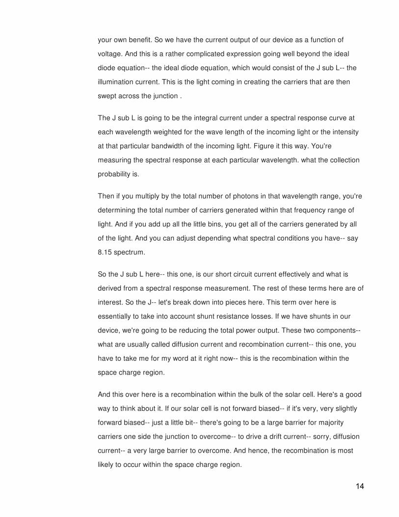
your own benefit. So we have the current output of our device as a function of

voltage. And this is a rather complicated expression going well beyond the ideal

diode equation-- the ideal diode equation, which would consist of the J sub L-- the

illumination current. This is the light coming in creating the carriers that are then

swept across the junction .

The J sub L is going to be the integral current under a spectral response curve at

each wavelength weighted for the wave length of the incoming light or the intensity

at that particular bandwidth of the incoming light. Figure it this way. You're

measuring the spectral response at each particular wavelength. what the collection

probability is.

Then if you multiply by the total number of photons in that wavelength range, you're

determining the total number of carriers generated within that frequency range of

light. And if you add up all the little bins, you get all of the carriers generated by all

of the light. And you can adjust depending what spectral conditions you have-- say

8.15 spectrum.

So the J sub L here-- this one, is our short circuit current effectively and what is

derived from a spectral response measurement. The rest of these terms here are of

interest. So the J-- let's break down into pieces here. This term over here is

essentially to take into account shunt resistance losses. If we have shunts in our

device, we're going to be reducing the total power output. These two components--

what are usually called diffusion current and recombination current-- this one, you

have to take me for my word at it right now-- this is the recombination within the

space charge region.

And this over here is a recombination within the bulk of the solar cell. Here's a good

way to think about it. If our solar cell is not forward biased-- if it's very, very slightly

forward biased-- just a little bit-- there's going to be a large barrier for majority

carriers one side the junction to overcome-- to drive a drift current-- sorry, diffusion

current-- a very large barrier to overcome. And hence, the recombination is most

likely to occur within the space charge region.

14

The carriers aren't likely to overcome that barrier, get into the bulk, and recombine

there. Whereas if we are under large forward bias conditions, now the carriers can

very easily go over that barrier and recombine in the bulk. So this term right here

dominates under low forward-bias conditions. And this term over here dominates

under larger forward bias conditions.

And that's why you see when you plot your IV curve on log linear scale, you see

essentially two flat points on your IV curve. Let me forward that to the next slide

right here. So this is log of current versus linear voltage. And you see one flat

portion right here and another flat portion right here before the series resistance

begins to dominate at too high voltage. And your shunt resistance dominates at too

low voltage.

This flat portion right there is being driven by recombination within the space charge

region. Why? Well, the forward bias voltage isn't enough to really lower that barrier

enough to allow the carriers deep within the bulk to recombine. So the carriers are

recombining in the space charge region. Whereas here, they are recombining within

the bulk.

So this is a more complicated expression for the IV characteristics of a solar cell

device. Not always are these precise mechanisms at work. If you have a new

material system that you're working with, there might be different re combination

mechanisms at work. There might be charged accumulation effects at work.

But they can all be encapsulated in some form of current voltage expression. Think

of the IV characteristics of the solar cell similar to say the constitutive relations of a

complex viscoelastic material where you have say a nice, linear elastic component,

a dashpot component. So you have a very complex expression describing the

stress-strain relationship in the material. A similar thing goes on here with the solar

cell where you're describing the current voltage relationship if you understand all of

the mechanisms driving carrier recombination in your material and charge

separation.

You can come up with an expression that describes very precisely the IV

15

characteristics. But if you change material systems, you may not necessarily be able

to transition the same models over. It's helpful to start with them. But sooner or later

you might decide, well, gee, I have to make some modifications.

All right, OK, series resistance-- we already studied this before, but just a quick

refresher. We have the series resistance of the bulk. We have the series resistance

of the emitter. And then we have the series resistance of the contacts as we contact

the device and then the series resistance within the contact itself. So at least four

different components of series resistance in our device that are all lumped together

when we express our IV curve in this manner. We all lump them together in that R

sub S. Question?

AUDIENCE: Without going through the math, is there a simple explanation where the 2 comes

from?

PROFESSOR: Yeah so simple explanation, if you would like, is mostly where the Fermi energy is

sitting relative to the conduction or valence band. And the space charge region-- the

quasi neutral region is closer to mid gap as opposed to closer to bandage. Hand

wavy-- if you really want to get into it, I spent about three months studying this as a

graduate student. The 1 and the 2-- the ideality factor, which is to show more

precisely. It's the number that comes before the kT for each of these.

That's called the ideality factor. It typically expresses N sub 1 or N sub 2. In this

case I just substituted straight out for a 1 and a 2. Those numbers aren't always 1

and 2. As a matter of fact, especially the G nought 1-- the bulk recombination

current, depending on where the defect levels lie, it can be somewhere between say

1.1 and 1.4 typically.

And beautiful thesis work done by a fellow in Australia hold on-- Keith McIntosh And

the title of the thesis is called "Humps, Bumps, and Lumps." It's all about non

idealities within an IV curve. So if you're really curious about that, "Humps, Bumps,

and Lumps," by McIntosh I believe was the name.

So we talked about series resistance already. Hold that-- put that in your RAM.

16

That's our R sub S right over here. That's our R sub S. And our shunt-- you want to

hold this other component in your RAM. So that's the picture to have of our series.

This is our shunt. This is a p-n junction. This is your n plus region. And this is your p.

And this is looking at the electron energy in 3D.

So we typically take a slice out like that just like this. And we draw the electron

energy as a function of position in a nice little wavy form that we typically do to

describe the p-n junction.

What's being described right here is adding a leader dimension-- a spatial

dimension in what's shown as the abscissa in this plot and showing what is a

weakness in the p-n junction. It could be a localized defect. This could be a shard of

metal that happened to lie in the wrong place in your device and fire through,

essentially when you did the firing step to adhere the metal to create the contact. It

could have gone straight through the p-n junction and contacted the other side.

It could be a charged dislocation. It could be structural defect, but a local reduction

in the barrier height. Now where is the electron going to go if you have a diffusion

current? It's going to be crowding through that little, localized, reduction in the

energy barrier. And you're going to have a higher current flowing through the

specific region.

So how to measure that? Well, if I make sure my full IV curve like this, it might

manifest itself as some reduced shunt resistance. So you'll have a larger current

flowing through it at lower bias voltages. But how do I know what's going on?

Without some spatial-- a spatially-resolved measurement tool, I am in the dark-- no

pun intended.

So I have to figure out how to measure the current flow as a function of position.

Now somebody thought about this a while. And they said, ha, well, let me get this

straight. If I apply a known bias voltage to my device, I'm going to get some current

flowing through it. And that current-- what I read out of the whole device

microscopically has some spatial distribution to it.

17

Let me think about this. OK, so current times voltage is power. And power

generates heat. So if I have a current crowding at some portion of my device, I'm

going to be generating a large amount of heat as the carriers flow through that

specific region. So if I have some method of measuring the heat-- the heat

distribution across my device is very, very sensitive-- I might be able to divide that

heat measurement-- if calibrated properly to determine total power-- I might be able

to divide that heat measurement by voltage so I know the applied bias voltage to my

device.

I take my power, divide it by the voltage, and I get the current as a function of xy

position. So I can map out my dark IV curve at any arbitrary bias voltage condition.

Let's say I want to do the measurement at 0.4 volts forward bias. I apply 0.4 volts

across my device. And I just measure the heat distribution. And in the calibrated

measurement, you can see how the dark current is distributed-- how the diffusion

current is distributed.

And that's what lock-in thermography is all about. This is a somewhat typical image.

It's still very noisy because it was a very fast image. But you have here a solar cell

device. You can barely make out the contact grid right here. And then the fingers

are moving down separated by about this much. On this particular image, you can

see the fingers or the dark shadow of the fingers right here.

And you see bright spots 1, 2, 3, 4, 5, 6, 7 across the device, indicating regions

where more current is flowing. Aha! So I'm beginning to figure out that, well, this

dark IV curve that I have right here-- this large amount of current flowing through

my device at lower bias voltages. That's not all uniformly distributed. But it's rather

concentrated in specific areas where I have weaknesses in my p-n junction under

low forward bias voltages.

And then at larger forward bias voltages once this barrier is significantly reduced, I

may have more carriers going through in regions of smaller minority carrier diffusion

length. Why? Well, because if the carrier goes in and recombines quickly because

the diffusion length is very short, that means there's one less carrier in there, which

18

means that now there's a greater driving force for diffusion.

And another care is going to come in and recombine too and another carrier and

recombine too. And so now you have a larger diffusion current going into the

regions of lower minority carrier diffusion length. Let's look at a few lock-in

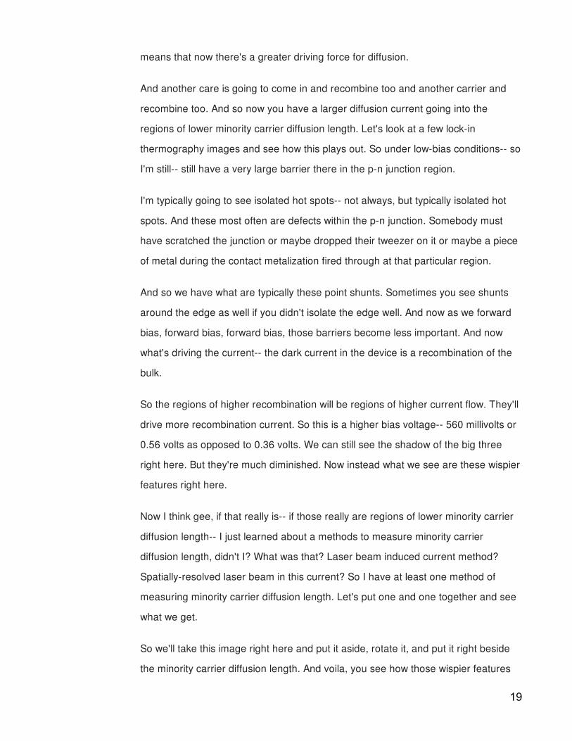
thermography images and see how this plays out. So under low-bias conditions-- so

I'm still-- still have a very large barrier there in the p-n junction region.

I'm typically going to see isolated hot spots-- not always, but typically isolated hot

spots. And these most often are defects within the p-n junction. Somebody must

have scratched the junction or maybe dropped their tweezer on it or maybe a piece

of metal during the contact metalization fired through at that particular region.

And so we have what are typically these point shunts. Sometimes you see shunts

around the edge as well if you didn't isolate the edge well. And now as we forward

bias, forward bias, forward bias, those barriers become less important. And now

what's driving the current-- the dark current in the device is a recombination of the

bulk.

So the regions of higher recombination will be regions of higher current flow. They'll

drive more recombination current. So this is a higher bias voltage-- 560 millivolts or

0.56 volts as opposed to 0.36 volts. We can still see the shadow of the big three

right here. But they're much diminished. Now instead what we see are these wispier

features right here.

Now I think gee, if that really is-- if those really are regions of lower minority carrier

diffusion length-- I just learned about a methods to measure minority carrier

diffusion length, didn't I? What was that? Laser beam induced current method?

Spatially-resolved laser beam in this current? So I have at least one method of

measuring minority carrier diffusion length. Let's put one and one together and see

what we get.

So we'll take this image right here and put it aside, rotate it, and put it right beside

the minority carrier diffusion length. And voila, you see how those wispier features

19

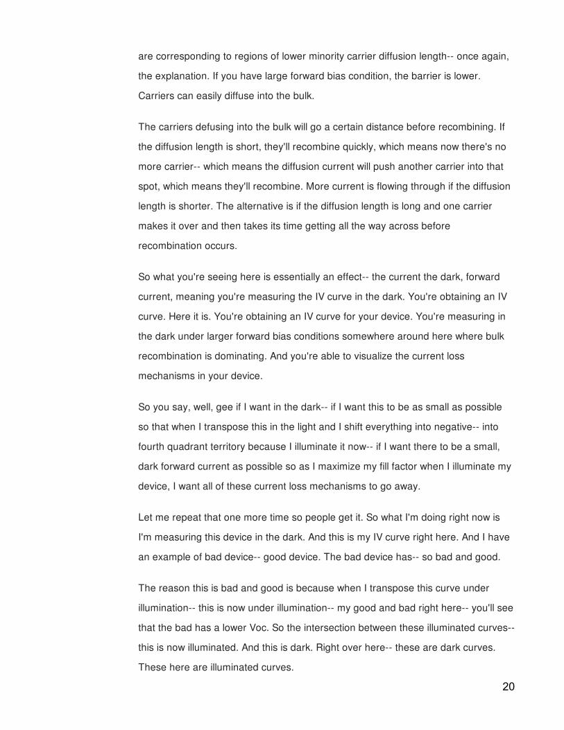
are corresponding to regions of lower minority carrier diffusion length-- once again,

the explanation. If you have large forward bias condition, the barrier is lower.

Carriers can easily diffuse into the bulk.

The carriers defusing into the bulk will go a certain distance before recombining. If

the diffusion length is short, they'll recombine quickly, which means now there's no

more carrier-- which means the diffusion current will push another carrier into that

spot, which means they'll recombine. More current is flowing through if the diffusion

length is shorter. The alternative is if the diffusion length is long and one carrier

makes it over and then takes its time getting all the way across before

recombination occurs.

So what you're seeing here is essentially an effect-- the current the dark, forward

current, meaning you're measuring the IV curve in the dark. You're obtaining an IV

curve. Here it is. You're obtaining an IV curve for your device. You're measuring in

the dark under larger forward bias conditions somewhere around here where bulk

recombination is dominating. And you're able to visualize the current loss

mechanisms in your device.

So you say, well, gee if I want in the dark-- if I want this to be as small as possible

so that when I transpose this in the light and I shift everything into negative-- into

fourth quadrant territory because I illuminate it now-- if I want there to be a small,

dark forward current as possible so as I maximize my fill factor when I illuminate my

device, I want all of these current loss mechanisms to go away.

Let me repeat that one more time so people get it. So what I'm doing right now is

I'm measuring this device in the dark. And this is my IV curve right here. And I have

an example of bad device-- good device. The bad device has-- so bad and good.

The reason this is bad and good is because when I transpose this curve under

illumination-- this is now under illumination-- my good and bad right here-- you'll see

that the bad has a lower Voc. So the intersection between these illuminated curves--

this is now illuminated. And this is dark. Right over here-- these are dark curves.

These here are illuminated curves.

20

The intersection between the illuminated curve and the x-axis denotes the open

circuit voltage. And you see that the larger this current is in the dark the earlier

you're going to intersect with your x-axis-- the lower the voltage output of your

device will be-- the lower the maximum power point will be. So want in the dark

when you measure the IV curve, you want that current to be as small as possible in

the dark.

And, obviously, when you illuminate it, you want this jump to be as large as possible.

And you want this to almost look like a box to have a large fill factor. So if we say,

OK, we want this to be small because we want a large fill factor, somehow we have

to know where the current loss mechanisms are occurring. And that's where we

have lock-in thermography available to us we can visualize it.

You say, well, to do lock-in thermography well, I'm going to need an-- indium

antimonide-- sorry, yeah that would be it. It would be an indium antimonide camera

sensitive to the 3 to 5 micron wavelength range that might cost $70,000 to get a

good one with high frame rates. The lock-in system-- I don't know if I have that

money.

I can go over and borrow Professor Buonassisi's system and use it there. Or if my

shunts are big enough, I can just use straight-out thermionic sheets or

thermochromic sheets, rather, sorry. So you can take these liquid crystals and slap

them because your device and measure the heat distribution straight up just by

making sure you have good thermal contact between your cell and your

thermochromic sheets, which cost about $100.

Now the reason we use the lock-in thermogrpahy and not these thermochromic

sheets is this curve right here. This is lock-in thermography sensitivity versus

integration time. And we're getting into the 10 microKelvin range, which is

rattlesnake territory. That's how the rattlesnakes are able to sense heat and reach

out to you is because they have those little organs that look like little, black-- they're

integrating spheres to be honest-- small, little spot to open up.

21

Rattlesnake-- that's why the sidewinder missile. Anybody? F 16s? Hornets? No. If

you're into aviation, there's a special type of heat seeking missile developed I think

in the 1950s that uses a device not dissimilar from the rattlesnakes heat sensing

organs. Regardless, I digress, we're looking at about a 10 microKelvin sensitivity in

this lock-in thermography technique, which is very sensitive-- can measure under

low forward bias conditions and hence useful.

So that pretty much sums up lock-in thermography. It is a difficult technique to wrap

your brain around. So for those of you who got 75% of it, congratulations. That was

really, really well done. For those who got about 25% of my explanations today,

don't worry. You're not alone. It just takes a lot of thinking it through exactly where is

the current flowing as a function of bias condition? What does that do to my IV

curve? And then what does it do in a two-dimensional regime when I'm measuring

heat output? It's is a very complicated thing.

Thankfully there is an entire book lock-in thermography written by Otwin

Breitenstein. I gave to you today a paper-- in one of the papers that I distributed

today-- the one that has the PSSA written on it-- this one. That paper is by Otwin

Breitenstein from the Max Planck Institute of Microstructure Physics in Halle,

Germany about two a half and a half hours south of Berlin. And this describes in

more detail that which I attempted to get across in class today.

He with Martin Langenkamp have also written a book on lock-in thermography. So if

you're interested in more information, that's where to go. In your handout set today,

we also have a classic paper on series resistance effects of solar cell

measurements. This one is from '63-- yes, 1963. Classic paper worth the read if

you're in that regime making devices that are series resistance limited. It's more

optional reading for folks.

And let's venture forward. Folks who did these scanning Elbit techniques for a while

really found value in measuring as a function of spatially-resolved manner down to a

micron in spatial resolution the electrical output of a solar cell device. And then they

thought to themselves, well, goodness, if we measure with one micron spot size, it's

22

going to take us a week to get a measurement across a full area solar device, if not

longer.

And if we measure say with the 200 nanometer spot size using some sort of X-ray

technique and we accumulate for say two seconds a point, it can take 10,000 years

to map out a full-size solar cell device, literally, do the math. And they said is there

an easier way for us to acquire information that does not rely on scanning-- on point

by point, step by step measurements.

And they thought about it long and hard they said, well, gee, these new, handheld,

digital cameras coming out on the market are pretty cool. What technology do they

rely on? Oh, it's a CCD-- Charge Couple Display that visualizes or images over a

large area the output of a device. And that's exactly how the lock-in thermography

techniques were developed here with this imaging camera-- in that case, an indium

antimonice CCD.

And they said, well, what other wavelengths emit-- in what other wavelength does a

solar cell emit? We know that it emits heat. And heat is typically in the 3 to 5 micron

wavelengths regime, maybe even as high as 10 microns depending on what

temperature. And we know that as well we can have band to band emission inside

of a solar cell that would emit around the band gap energy.

So let's set up a camera to image the band-to-band recombination intensity or the

band-to-band illumination intensity. And that's what this paper is about. This is

wavelength. This is intensity. This is the emission spectrum of a solar cell. So if you

were to measure what colors-- what color light does a solar cell emit after you pump

current into it, this isn't is more or less the spectrum.

So we have the thermal radiation shown over here. This is longer wavelength light.

That's the heat that it gives off. That's what indicates current flow inside of the

device. There is the band to band luminescence right here. And we'll neglect the

other two for now. Those are more advanced concepts. But the band to band

luminescence is essentially just the recombination of a carrier from the conduction

band to the valence band-- recombination-- very straightforward.

23

And the recombination intensity is inversely proportional to the minority carrier

lifetime. Why is that? This was that quote remember who attended Eli Yablonovich's

talk. He was saying, it's completely counter intuitive. Do you remember specifically

what he was referring to in this? Let me show you an image here.

AUDIENCE: That you want your device to emit more light for higher device performance.

PROFESSOR: Exactly, yeah, so what is going on here? We have our tau-- one of our tau effective-

- or one of over lifetime what we're measuring. This is our effective lifetime that

we're measuring. And we have one over tau. Let's call it non-radiative. So we have

non-radiative recombination mechanisms. This comprises Shockley-Read-Hall

recombination-- Auger recombination-- a bunch of different recombination

mechanisms.

And then we have one of our tau radiative, which is essentially this recombination

mechanism shown right here, which is just the band-to-band recombination. So if

you have defects around, that will lower the lifetime-- the non-radioactive lifetime. If

you have tons and tons of defects, the carriers will most likely recombine through

the defects and not through the band-to-band

They will only recombine with band-to-band if there is nothing-- no other

recombination path left available to them. It's a question of probability. So if this is

really, really short-- non-radiative recombination lifetime is really, really short

because a defect density is very, very large. So the lifetime due to non-radiative

recombination mechanisms is very short, then that's tau effective is also going to be

very short.

And very few carriers are going to recombine radiatively. Conversely, if we have a

very clean material-- virtually defect-free-- this non-radiative lifetime is then going to

be out the roof. And now we're going to be limited instead by the radiative lifetime.

And so tau effective will be more similar to radiative. Now an interesting thing

happens when you have a radiative recombination event. As the name would

suggest, it emits light.

24

And that light can be detected by a CCD camera on your body. So what you have--

there you go. What you have right here is a solar cell device that is being biased so

current is flowing into the device. And now the map what you're seeing is indicative

of radiative recombination, why? Because nearby the cell, it's essentially a very

similar mechanism or similar set up to what we saw right here where we had bias

voltage across the device and imaging not with an infrared camera, but now with a

camera matched to the band gap energy.

This could be an indium gallium arsenide camera or say silicon camera, depending

on the precise band gap. And you're imaging the radiative recombination as a

function of xy position across your wafer. So these darker regions here on the

bottom and on the right-- sorry left-- the other right. They indicate regions of lower

minority carrier diffusion length. Why? Because there's less radiative recombination

because this term in those regions is very, very small so that there's not much

radiative recombination going on.

Whereas these other regions here that appear brighter have a lot more radiative

recombination going on. Any questions about that? Yeah?

AUDIENCE: What fraction of these radiative recombinations are reabsorbed by the material? Is it

possible to figure that out to a high degree so you can get a quantitative sense of

how much is radiating?

PROFESSOR: Sure. The question pertains to photon recycling and how many photons that are

radiatively emitted get reabsorbed by the material. That would depend on the

optical path length inside of the material of carriers being generated in the material.

And you assume that carrier generation is fairly isotropic in nature-- that there is not

any preferred direction unless you have a dyed molecule that's designed in a

certain way to emit light in a certain orientation.

So you can assume that the carrier mission in most materials as isotropic in nature.

And then it's just a question of ray tracing to figure out what the optical path length

is. Compare that to the optical absorption coefficient in the material, and you get

your answer-- what fraction of light gets reabsorbed.

25

All right, I can sense where we're reaching threshold here in terms of new

information gathered. I'm just going to briefly go over the Suns-Voc at the very end .

And the Suns-Voc technique is useful as we saw during class because as this paper

right here by Ron Sinton and Andres Cuevas-- this one-- I know you definitely have

this one.

This paper essentially describes the functioning of the technique. On page number

two on the upper, left-hand side, so figure 2, we essentially have the figure that was

determined on the screen during the measurements. So for those of you close

enough to the monitor to actually watch the measurement being taken in the Suns-

Voc, you saw the light intensity decaying exponentially. So the light intensity is a

flash bulb, poof, and decayed exponentially.

The open circuit voltage measured by the device-- so you had this solar cell device

sitting on the platen with a little probe coming in and a 50 megaohm resistor

connected in series-- very little current flowing through that external circuit. But it's

measuring the voltage. So it's essentially maintaining the solar cell in open circuit

voltage conditions while the flash is decaying.

And it's measuring the open circuit voltage across the device at each illumination

intensity as the pulse decays. So you can see the time scale here is on the order of

a few 10s of milliseconds-- so a very fast measurement. The electronics response

time has to be very fast. It tells you what the RC time constant of the circuit is.

And you can notice that the voltage-- the open circuit voltage decays linearly when

the illumination intensity decays exponentially. Why is that ?

AUDIENCE: Natural log.

PROFESSOR: This is a natural log-- so what Joe showed to you yesterday or on Thursday in class

is how the voltage output of a solar cell varies by illumination intensity. So there's a

logarithmic dependence there. So that's why you take the log of the exponentially

decaying light intensity and you obtain a linear relation that's the open circuit voltage

decline as a function of time.26

decline as a function of time.

So we can derive an IV characteristic by translating that open circuit voltage into an

implied bias voltage. And knowing the short circuit current density up front

essentially by measuring it by measuring the solar cell device in a solar simulator,

we can obtain the short circuit current density. We pin both curves up here at the

measured short circuit current density. And then we plot both curves out-- the IV

curve and the Suns-Voc curve.

Now the Suns-Voc curve is similar to the IV curve with only one difference. There's

no current or very, very little current flowing through the external circuit, which

means there isn't any real power flowing through the external circuit, which means if

we go back to our expression right here-- if we have no current flowing through, that

J is equal to zero. And now that R sub S term disappears.

So we've come up with a clever way to drop all of our R sub S out of that

expression. And the only thing that matters essentially is to some degree shunt. But

this is essentially the highest IV curve that one could possibly obtain in the absence

of series resistance. And that's what you see right here. That's this delta in between

your illuminated IV curve-- what is measured using the solar simulator-- and your

Suns-Voc curve, which is measured in the absence of series resistance.

Now this works well with most materials. If you have a very high capacitance in your

device, you'll want to look very carefully at this decay-- at the light intensity decay. If

your capacitance and your device is very large, it might actually flatten out the

voltage response. So you want to make sure that the time-- the RC time constant of

your device is matched to the flash bulb decay time.

That's just one word of warning for those working on high voltage or organic

materials. Any questions on the Sun-Voc measurement? This gives you what's

called an implied IV curve. And that is-- we could say in the best case scenario what

you would get from the solar cell in the absence of any series resistance losses.

AUDIENCE: The last question-- Voc-- that's not a solar simulator in any way is it?

27

PROFESSOR: No.

AUDIENCE: Is that important?

PROFESSOR: Yeah, it is important. It would be different-- in essence, it would be a different

current response if you didn't have the same exact solar spectrum. Now, that's a

very important point. If you're venturing outside of, say, silicon-based devices, and

you're more sensitive to the infrared or the UV, you really want to make sure that

you measure the intensity as a function of wavelength output of that bulb.

Otherwise, you might be higher or lower during the Suns-Voc measurement. For a

silicon-based device, the majority falls within the specified regime. Down here--

actually right here on this diagram-- that a little spot right there-- that is a small

calibration solar cell of known short-circuit current and open circuit voltage. That's

used to calibrate for other silicon devices if you're moving away from silicon, that

becomes an issue.

Correctable-- you can make sure the spectral response-- or the spectral radiance of

that light source and compare it to the solar simulator and do the normalization

accordingly. Here's what I recommend. With the last 15 minutes of class, I wanted

to catch each of the teams and talk about your class projects just to make sure that

things were rolling along. I have feelers out to some of the mentors who haven't

responded yet. And so I just wanted to touch base with each of you for about three

minutes just make sure everything is rolling along.

28