Embed Size (px)
Citation preview

Ministry of Higher Education and Scientific Research
University of Baghdad
Institute of Laser for Postgraduate Studies
Mitigation of Distortion in WDM Systems
Based on Optical Phase Conjugation
A Thesis Submitted to the Institute of Laser for
Postgraduate Studies, University of Baghdad in Partial
Fulfillment of the Requirements for the Degree of
Doctor of Philosophy in Laser / Electronics and
Communication Engineering
By
Adnan Sabbar Abbas
B.Sc. Electrical Engineering - 2005
M. Sc. Electronics and Communication - 2012
2017 AD 1439 AH

Ministry of Higher Education and Scientific Research
University of Baghdad
Institute of Laser for Postgraduate Studies
Mitigation of Distortion in WDM Systems
Based on Optical Phase Conjugation
A Thesis Submitted to the Institute of Laser for
Postgraduate Studies, University of Baghdad in Partial
Fulfillment of the Requirements for the Degree of
Doctor of Philosophy in Laser / Electronics and
Communication Engineering
By
Adnan Sabbar Abbas
B.Sc. Electrical Engineering - 2005
M. Sc. Electronics and Communication - 2012
Supervisor
Prof. Dr. Mazin M. Elias
2017 AD 1439 AH

سورة يوسف )76(


i
Dedication
To my family

ii
Acknowledgements
I would like to express the deepest gratitude to my research supervisor
Prof. Mazin M. Elias for providing constant encouragement, inspiring
guidance and insightful discussions throughout the period of this work.
My grateful thanks go to Prof. Dr. Abdul Hadi M. Al-Janabi, Dean
of the Institute of Laser for Postgraduate Studies, for his unlimited
encouragement and support during my research work. Special thanks are
gone to Asst. Prof. Dr. Mohammed K. Thaher, Asst. Dean of the Institute,
and Dr. Ziyad A. Taha, head of the Engineering and Industrial Applications
Department, for their continuous advices and support.
Great thanks and appreciation to Prof. Raad S. Fyath, College of
Engineering, Al-Nahrain University. I appreciate all his contributions of
time, ideas, and great help to make my Ph.D. experience productive and
stimulating.
My thanks go to all the faculty members of the Institute, especially to
Dr. Hussein A. Jawad, Dr. Shelan K. Tawfeeq, Dr. Tahreer S Mansoor,
and Dr. Zaineb F. Mahdi, for their valuable suggestions and advices during
my study time.
Great appreciation and thanks to Prof. Dr. Mahmoud Shahabadi
who hosted me in his group at Tehran University, college of Computer and
Electrical Engineering (ECE), Iran. I also would like to appreciate all
colleagues of Photonic Research Laboratory at ECE. They have been a
source of friendships as well as good advice and collaboration.
I would like to extend my gratitude to all my friends and colleagues at
the Institute of laser for postgraduate studies.
Finally I am indebted to my family who were very patient and
encouraging during all the period of my study.
Adnan

iii
Abstract
Today, fiber-optic communication systems are considered the
backbone of telecommunication systems and networks. Optical fiber is an
excellent transmission medium due to its low loss, high bandwidth and
robustness. However, linear and nonlinear impairments of an optical fiber
lead to signal distortions. Propagation impairments accumulate over fiber
distance and seriously distort the signal in high-capacity, long-haul fiber-
optic communication systems. Transmission performance can be
significantly improved by compensating for fiber dispersion and nonlinear
distortions.
This thesis investigates the performance of advanced fiber-optic
communication systems incorporating Optical Phase Conjugations (OPC)
technique for mitigation of linear and nonlinear signal phase distortions. The
OPC is achieved using Four-Wave Mixing (FWM) process in Highly
Nonlinear Fiber (HNLF). Two compensation configurations are investigated
and compared, one uses one OPC inserted in the mid-link point (Mid-Span
OPC (MS-OPC)) while the other configuration uses multiple OPCs
distributed along the link.
The work in this thesis falls into two main parts. In the first part, the
effect of polarization on the performance of a dual-pump HNLF-based OPC
(HNLF-OPC) is investigated analytically using a set of eight Nonlinear
Schrödinger Equations (NLSEs). These equations describe the propagation
of the orthogonal components of the two pumps, signal, and the generated
idler. Practical assumptions are applied to derive expressions describing the
dependence of FWM gain and conversion efficiency on the States Of
Polarization (SOP) of the four waves. The results reveal that the use of two
orthogonal linearly-polarized pumps leads to an OPC whose characteristics
is independent of the signal polarization.

iv
The second part of the thesis simulates the performance of two high-bit rate,
long-haul, and Wavelength Division Multiplexing (WDM) systems
incorporating HNLF-OPC compensation technique. The results are obtained
using Optisystem v14.1 software package for both MS-and multiple-OPC
configurations. Both WDM systems use long-haul distributed Raman
amplified (DRA) link with 320 Gbps (8×40 Gbps) Polarization Division
Multiplexing (PDM) Non-Return-to-Zero On-Off-Keying (NRZ-OOK) and
2.048 Tbps (8×256 Gbps) PDM 16-states quadrature-amplitude modulation
(16-QAM).
Simulation results show that the use of multiple-OPC compensation
technique offers an improvement in system performance over a MS-OPC
compensation technique.
In single channel PDM NRZ-OOK 40 Gbps transmission, the use of
multiple-OPC compensation technique provides an improvement in
achieved maximum Q-factor of ~2 dB compared to the MS-OPC
compensation technique. Furthermore, the transmission reach at the Hard
Decision-Forward Error Correction (HD-FEC) limit is enlarged by 24.2%
when the multiple-OPC configuration is used. In WDM system, the Q-factor
is improves by 0.62 dB when a multiple-OPC compensation technique is
used over the MS-OPC technique.
In single channel PDM 16QAM 256 Gbps transmission, the use of
multiple-OPC shows a 1.35 dB improvement in Q-factor over the MS-OPC
case. In the WDM system, using multiple-OPC increased the nonlinear
threshold by ~2 dB compared to the case of MS-OPC, showing 0.62 dB
improvement in Q-factor over the MS-OPC compensation scheme.

v
List of Contents
Acknowledgements ii
Abstract iii
List of Contents v
List of Symbols vii
List of Abbreviations ix
List of Tables xii
List of Figures xiii
Chapter One: Introduction 1
1.1 Overview 2
1.2 Objectives of the Thesis 8
1.3 Fiber-optic communication Systems Impairments 9
1.4 Nonlinearity Compensation Techniques in Fiber-optic
communication Systems
21
1.5 Literature Survey 26
1.6 Thesis Outlines 32
Chapter Two: Theoretical Background 33
2.1 Introduction 34
2.2 Maxwell’s Equations and Wave Equation 34
2.3 Nonlinear Schrödinger Equation 37
2.4 FWM-Based OPC 38
2.5 Advanced Techniques in Long-Haul, High-Speed Fiber-optic
communication Systems
41
Chapter Three: Analysis of Dispersion and Nonlinearity
Mitigation in WDM systems
55
3.1 Introduction 56
3.2 Basic Concepts of HNLF-Based Optical Phase Conjugation 57

vi
3.3 Analysis of Dual-Pump Polarization-Aligned HNLF-OPC 59
3.4 Effect of Polarization on the FWM Process in HNLF-OPC 67
3.5 FWM Parametric Gain 77
3.6 Conversion Efficiency 80
3.7 Calculated Results Related to HNLF-OPC Conversion
Efficiency
85
Chapter Four: Simulation Results, Discussion, Conclusions,
and Suggestion for Future Works
95
4.1 Introduction 96
4.2 Compensation of Fiber Dispersion and Nonlinearity using
HNLF-based OPC
96
4.3 Dispersion and Nonlinearity Mitigation using HNLF-based
OPC
101
4.4 Thesis Conclusions 118
4.5 Suggestions for Future Works 119
References 121
Publications and Conferences 128
Appendix A A1

vii
List of Symbols
Symbols Description
𝐴 Amplitude of the optical field
𝐴𝑒𝑓𝑓 Effective fiber core area
𝑩 Magnetic flux density
B Bit rate
Bm Modal birefringence
𝑐 Speed of light in vacuum
D Dispersion parameter
𝑫 Electric flux density
𝑑𝑠𝑝 Walk-off parameter
𝑬 Electric field vector
F Frequency
𝑔 Parametric gain coefficient
𝑔𝑅 Raman-gain coefficient
𝑯 Magnetic field vector
𝑱 Current density
𝑘 Effective phase mismatch
𝛥𝑘 Phase-matching parameter
L Length of the optical fiber
𝐿𝑒𝑓𝑓 Effective length
𝑴 Magnetic polarization
𝑛 Linear refractive index
𝑛2 Nonlinear refractive index
𝑷 Electric polarization
𝑃0𝑐𝑟 Critical Raman power
𝑄𝑠𝑝𝑚 Nonlinear phase shift due to cross phase
modulation
viii
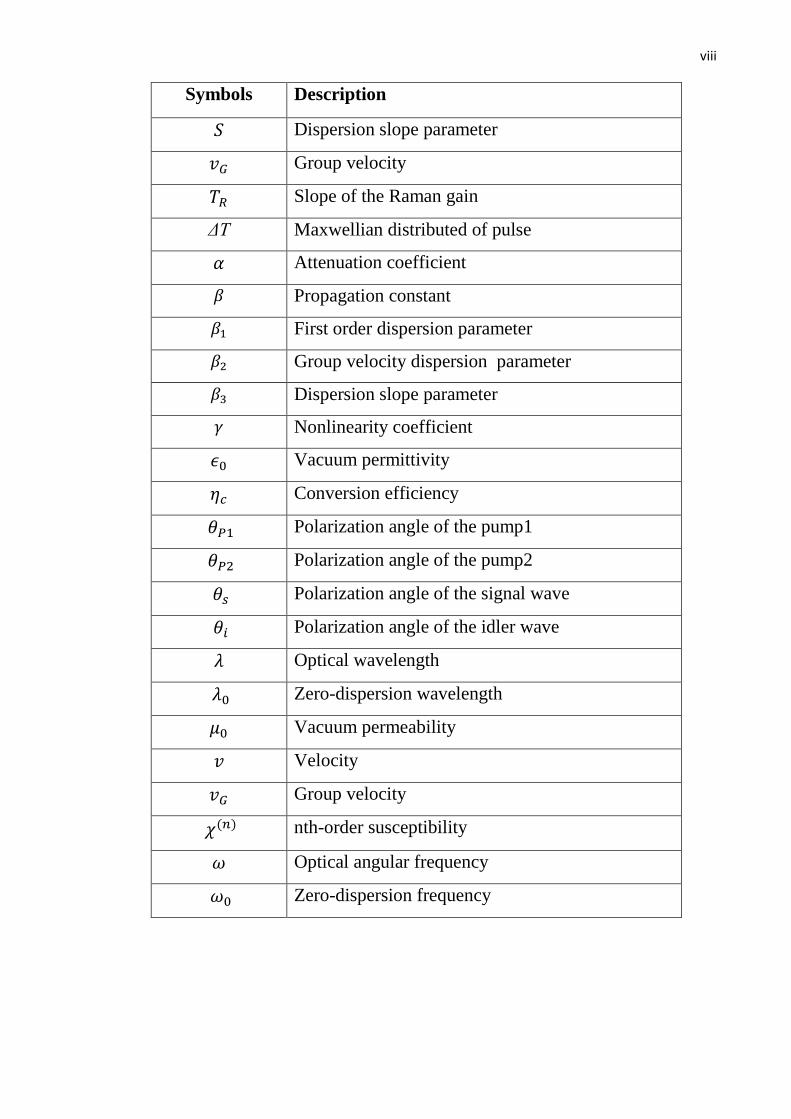
Symbols Description
𝑆 Dispersion slope parameter
𝑣𝐺 Group velocity
𝑇𝑅 Slope of the Raman gain
ΔT Maxwellian distributed of pulse
𝛼 Attenuation coefficient
𝛽 Propagation constant
𝛽1 First order dispersion parameter
𝛽2 Group velocity dispersion parameter
𝛽3 Dispersion slope parameter
𝛾 Nonlinearity coefficient
𝜖0 Vacuum permittivity
𝜂𝑐 Conversion efficiency
𝜃𝑃1 Polarization angle of the pump1
𝜃𝑃2 Polarization angle of the pump2
𝜃𝑠 Polarization angle of the signal wave
𝜃𝑖 Polarization angle of the idler wave
𝜆 Optical wavelength
𝜆0 Zero-dispersion wavelength
𝜇0 Vacuum permeability
𝑣 Velocity
𝑣𝐺 Group velocity
𝜒(𝑛) nth-order susceptibility
𝜔 Optical angular frequency
𝜔0 Zero-dispersion frequency

ix
List of Abbreviations
Abbreviation Description
ASE Amplified Spontaneous Emission
ASK Amplitude Shift Keying
BER Bit Error Rate
BPSK Binary Phase Shift Keying
BSG Bit-Sequence Generator
CD Chromatic Dispersion
DBP Digital Back Propagation
DCF Dispersion Compensation Fiber
DD Direct Detection
DFWM Degenerate Four-Wave Mixing
DGD Differential Group Delay
DRA Distributed Raman Amplifier
DSF Dispersion Shifted Fiber
DSP Digital Signal Processing
EDFA Erbium-Doped Fiber Amplifier
FDM Frequency-Division Multiplexing
FEC Forward Error Correction
FOPA Fiber Optic Parametric Amplifier
FWM Four-Wave Mixing
GVD Group Velocity Dispersion
HD-FEC Hard Decision-Forward Error Correction
HDF Highly Dispersion Fiber
HNLF Highly Nonlinear Fiber
HNLF-OPC Highly Nonlinear Fiber Based-Optical Phase Conjugation
IM Intensity Modulation
IM-DD Intensity Modulation-Direct Detection
x
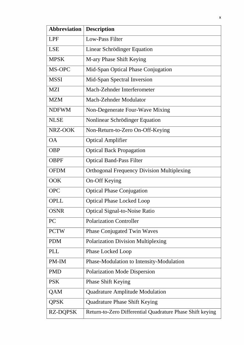
Abbreviation Description
LPF Low-Pass Filter
LSE Linear Schrödinger Equation
MPSK M-ary Phase Shift Keying
MS-OPC Mid-Span Optical Phase Conjugation
MSSI Mid-Span Spectral Inversion
MZI Mach-Zehnder Interferometer
MZM Mach-Zehnder Modulator
NDFWM Non-Degenerate Four-Wave Mixing
NLSE Nonlinear Schrödinger Equation
NRZ-OOK Non-Return-to-Zero On-Off-Keying
OA Optical Amplifier
OBP Optical Back Propagation
OBPF Optical Band-Pass Filter
OFDM Orthogonal Frequency Division Multiplexing
OOK On-Off Keying
OPC Optical Phase Conjugation
OPLL Optical Phase Locked Loop
OSNR Optical Signal-to-Noise Ratio
PC Polarization Controller
PCTW Phase Conjugated Twin Waves
PDM Polarization Division Multiplexing
PLL Phase Locked Loop
PM-IM Phase-Modulation to Intensity-Modulation
PMD Polarization Mode Dispersion
PSK Phase Shift Keying
QAM Quadrature Amplitude Modulation
QPSK Quadrature Phase Shift Keying
RZ-DQPSK Return-to-Zero Differential Quadrature Phase Shift keying

xi
Abbreviation Description
SBS Stimulated Brillouin Scattering
SOP States Of Polarization
SPM Self-Phase Modulation
SRS Stimulated Raman Scattering
SSMF Standard Single-Mode Fiber
TE Transverse Electric
TM Transverse Magnetic
WDM Wavelength Division Multiplexing
WSS Wavelength Selective Switch
XPM Cross-Phase Modulation

xii
List of Tables
NO. Title of table Page
2.1 Summary of symbol rate for different forms of
modulation formats. 46
3.1 Parameters values of single-pump HNLF-OPC and
dual-pump HNLF-OPC1 and HNLF-OPC2 63

xiii
List of Figures
NO. TITLE OF FIGURE PAGE
1.1
Measured loss spectrum of a single-mode silica fiber
(solid line) with the calculated spectra for some of
the loss mechanisms contributing to the overall fiber
attenuation (dashed and dotted lines)
10
1.2
Dispersion characteristic of a typical standard single
mode fiber as a function of wavelength and
frequency.
12
1.3
Poincaré sphere. S1, S2, and S3 are the stocks
parameters. The forth parameter S4 is calculated
from 𝑆42 = 𝑆1
2 + 𝑆22 + 𝑆3
2.
13
1.4 Random birefringence and the resulted DGD for a
pulse launched into a fiber at 45o 14
1.5 Walk-off between two waves at wavelength λ1 and
λ2 after propagation over the distance L. 19
1.6 Waveforms of non-degenerated four-wave mixing. 20
1.7 Waveforms of degenerated four-wave mixing. 20
1.8
Schematic diagram of the fiber nonlinearity
compensation system using digital back-propagation
technique.
22
1.9 Illustration of nonlinearity cancellation based on
phase-conjugated twin waves. 23
1.10 Optical pack-propagation module in WDM system 24
2.1 Generation a conjugated idler using four-wave
mixing. 39
2.2
(a) OOK signal constellation diagram, and (b) is the
modulated binary ASK signal corresponding to a
baseband input data
42
2.3
(a) Generation of BPSK signal using Mach-Zehnder
interferometer, (b) constellation diagram of the
BPSK signal, and (c) is the modulated BPSK signal
corresponding to a baseband input data.
44
2.4 (a) Generation of QPSK and 8PSK signals, and (b)
Constellation diagrams of QPSK and 8PSK signals. 45
2.5 Constellation diagram of the 8QAM, 16QAM,
32QAM, and 64QAM. 45

xiv
NO. TITLE OF FIGURE PAGE
2.6
Simplified block diagram for wavelength division
multiplexing system including MUX: Multiplexer,
DMUX: Demultiplexer, and Tx (Rx): Single-
channel optical transmitter (receiver).
47
2.7 Examples of linear, circular, and elliptical
polarization states 48
2.8 Model for lumped amplification using EDFA. 49
2.9
(a) Forward pumped-distributed Raman amplified
link, and (b) Backward pumped-distributed Raman
amplified link.
51
2.10 Schematic illustration of spontaneous Raman
scattering. 52
2.11
Normalized Raman gain for fused silica when the
pump and Stokes waves are co-polarized (solid
curve). The dotted curve shows the situation in
which the pump and stokes waves are orthogonally
polarized.
53
3.1
Schematic diagram of the optical phase conjugation
device including erbium-doped fiber amplifiers
(EDFAs), optical band-pass filter (OBPF),
polarization controller (PC), highly nonlinear fiber
(HNLF), and wavelength selective switch (WSS).
58
3.2
Schematic diagram of the optical spectrum at the
HNLF output, λ0 denotes, zero dispersion
wavelength.
58
3.3
Analytical and numerical conversion efficiencies of
the single-pump HNLF-OPC with (a) 0.5 W pump
power, and (b) 1 W pump power.
64
3.4
Analytical and numerical conversion efficiencies of
HNLF-OPC1 with the parameters values listed in
Table (3.1) when the length of the HNLF is (a) 0.5
km, and (b) 0.8 km.
65
3.5
Analytical and numerical conversion efficiencies of
HNLF-OPC2 with the parameters values listed in
Table (3.1). 66

xv
NO. TITLE OF FIGURE PAGE
3.6 Schematic diagram to analyze the effect of
polarization on FWM in highly nonlinear fiber. 67
3.7
(a) Variation of the parametric gain of the TE
component with different values of γPTE product,
and (b) Variation of the parametric gain of the TM
component with different values of γPTM product.
80
3.8
Conversion efficiency as a function of signal
wavelength when the signal and both pumps are
linearly copolarized along TE axis for (a) HNLF-
OPC1, and (b) HNLF-OPC2.
87
3.9
Variation of the maximum conversion efficiency as
a function of signal polarization angle when the two
pumps are linearly copolarized along the TE axis for
(a) HNLF-OPC1, and (b) HNLF-OPC2.
88
3.10
Variation of the maximum conversion efficiency as
a function of signal polarization angle when the two
pumps are linearly copolarized along TM axis for (a)
HNLF-OPC1, and (b) HNLF-OPC2.
89
3.11
Conversion efficiencies as a function of signal
wavelength with orthogonally polarized pumps for
(a) HNLF-OPC1, and (b) HNLF-OPC2.
91
3.12
Variation of conversion efficiencies as a function of
signal wavelength with different associated values of
orthogonally polarized pump powers for (a) HNLF-
OPC1, and (b) HNLF-OPC2.
92
3.13
Conversion efficiency as a function of signal
polarization angle for (a) HNLF-OPC1 and (b)
HNLF-OPC2, with orthogonal polarization pumps.
93
4.1
(a) Single channel transmission system with MS-
OPC configuration, (b) 8-channel WDM
transmission system with MS-OPC configuration,
(c) Single channel transmission system with
multiple-OPC configuration, and (d) 8-channel
WDM transmission system with multiple-OPC
configuration.
100

xvi
NO. TITLE OF FIGURE PAGE
4.2
Transmitter for a single channel including Binary
sequence generator (BSG), non-return-to-zero
pulse generator (NRZ), Mach–Zehnder modulator
(MZM), polarization splitter, polarization combiner,
erbium-doped fiber amplifier (EDFA), and optical
attenuator.
102
4.3
Receiver for a single channel including polarization
splitter (PS), photodetector PIN, optical low-pass
filter (LPF), and eye diagram analyzer.
102
4.4 Spectrum of the transmitted optical signal. 103
4.5 Spectrum of the pump1 and pump2. 103
4.6 Waves spectrum at (a) HNLF input and (b) HNLF
output. 104
4.7 Spectrum of the conjugated idler at the output of the
first OPC device. 105
4.8 Waves spectrum at (a) HNLF input and (b) HNLF
output at the second OPC device. 106
4.9 Spectrum of the received optical signal. 107
4.10
Calculated Q-factor as a function of a signal
launched power for (a) (X-Polarization), and (b) (Y-
Polarization), for single channel transmission after
912 km. The insets represent the eye diagrams of the
received signal at the optimum launched powers.
108
4.11
Variation Q-factors as a function of a transmission
reach for single channel, (a) X-Polarization and (b)
Y-Polarization.
109
4.12 Spectrum of the multiplexed 8-channels of the
WDM signal. 110
4.13 Waves spectrum at (a) HNLF input and (b) HNLF
output at the first OPC device. 110
4.14 Waves spectrum at (a) HNLF input and (b) HNLF
output at the second OPC device. 111
4.15 Spectrum of the received WDM signals. 112
4.16 Calculated Q-factor as a function of a signal
launched power (a) X – Polarization (b) Y – 113

xvii
NO. TITLE OF FIGURE PAGE
Polarization, for a middle channel operating at
frequency of 190.2 THz for an 8-channel WDM
signal transmission after 912 km.
4.17
Schematic of the simulation setup corresponding to
8-channel WDM system (a) MS-OPC configuration,
(b) multiple-OPC configuration, (c) Transmitter for
a single channel including sequence generator (SG),
pulse generator (PG), Mach-Zehnder modulator
(MZM), polarization combiner (PC), polarization
splitter (PS), and optical attenuator, and (d) Receiver
for a single channel.
115
4.18
Calculated Q-factor as a function of a signal
launched power for single channel scenario after 912
km transmission. The insets show the recovered
constellation diagrams for both polarization
components corresponding to multiple-OPCs
configuration at the optimum signal launched power.
116
4.19
Calculated Q factor as a function of number of fiber
spans for a single channel transmission. Insets show
the recovered constellation diagrams for the multiple
OPCs and MS-OPC after 1824 km transmission (24
spans).
117
4.20
Calculated Q-factor as a function of launched signal
power for the middle channel of an 8-channel WDM
system after 912 km transmission. The insets show
the recovered constellation diagrams for both
polarization components corresponding to multiple
OPCs configuration at the optimum signal launched
power.
117
4.21
BER as a function of WDM channel number
evaluated at the corresponding optimum signal
launched powers.
118

1
CHAPTER ONE
Introduction

2
CHAPTER ONE
Introduction
1.1 Overview
The fiber-optic communication system is the simplest kind of
lightwave system, consists of a transmitter, followed by an optical fiber as a
transmission channel, and then a receiver. The evolution of fiber-optic
communications has been promoted along with the advent of the above three
major components. In 1960, the invention and the realization of laser [1]
provided a coherent source for transmitting information using lightwaves. In
1966, the optical fiber was firstly used as a lightwave transmission medium
despite the fact that optical fiber at that time suffered unacceptable loss (over
1000 dB/Km). Since then, strenuous efforts have been made to reduce the
losses of the optical fiber. In 1979, the low loss fiber was realized at the
operating wavelength of 1550 nm with a loss of 0.2 dB/Km. The
simultaneous availability of stable optical source (laser) and a low-loss
optical fiber led to a rapid development of fiber-optic communication
systems, which can be grouped into five distinct generations. A commonly
used figure of merit for point-to-point communication systems is the bit rate-
distance product, BL, where B is the bit rate and L is the repeater spacing. In
every generation, BL increases initially but then begins to saturate as the
technology matures. Each new generation brings a fundamental change that
helps to improve the system performance further [2].
The first-generation of lightwave systems operated near 800 nm and
used GaAs semiconductor lasers. The operating bit rate was 45 Mb/s and
allowed repeater spacings of up to 10 Km. The repeater spacing of the first-

3
generation lightwave systems was limited by fiber dispersion which lead to
pulse-spreading at the operating wavelength of 800 nm. In 1970s that the
repeater spacing increased considerably by operating the lightwave system
in the wavelength region near 1300 nm, where optical fibers exhibit
minimum dispersion, furthermore, fiber loss is below 1 dB/Km. This
realization led to a worldwide effort for the development of InGaAsP
semiconductor lasers and detectors operating near 1300 nm [3].
The second generation of fiber-optic communication systems became
available in the early 1980s, but the bit rate of early systems was limited to
below 100 Mb/s because of intermodal dispersion in multimode fibers. This
limitation was overcome by the use of single-mode fibers. By 1987, second-
generation lightwave systems, operating at bit rates of up to 1.7 Gb/s with a
repeater spacing of about 50 Km, were commercially available. The repeater
spacing of the second-generation lightwave systems was limited by the fiber
losses at the operating wavelength of 1300 nm (typically 0.5 dB/km). Losses
of silica fibers become minimum near 1550 nm. Indeed, a 0.2 dB/Km loss
was realized in 1979 in this spectral region. The drawbacks of 1550 nm
systems were a large fiber dispersion near 1550 nm, and the conventional
InGaAsP semiconductor lasers could not be used because of pulse spreading
occurring as a result of simultaneous oscillation of several longitudinal
modes. The dispersion problem can be overcome either by using dispersion-
shifted fibers designed to have minimum dispersion near 1550 nm or by
limiting the laser spectrum to a single longitudinal mode. For a Dispersion
Shifted Fiber (DSF) the zero Chromatic Dispersion (CD) is shifted to
minimum-loss window at 1550 nm from 1300 nm by controlling the
waveguide dispersion and dopant-dependent material dispersion such that
transmission fiber with both low dispersion and low attenuation can be
achieved. Third-generation lightwave systems operating at 2.5 Gb/s became
available commercially in 1990. Such systems are capable of operating at a

4
bit rate of up to 10 Gb/s. The best performance is achieved using dispersion-
shifted fibers in combination with lasers oscillating in a single longitudinal
mode [4].
A drawback of third-generation 1550 nm systems is that the signal is
regenerated periodically by using optoelectronic repeaters, spaced apart
typically by 60 - 70 Km, in which the optical signal is first convert to the
electrical current and then regenerate by modulating an optical source. The
repeater spacing can be increased by making use of a homodyne or
heterodyne detection schemes because its use improves receiver sensitivity.
These optoelectronic regenerating procedures are not suitable for multi-
channel lightwave systems because each single wavelength needs a separate
optoelectronic repeater, which leads to high cost and excessive system
complexity. Another obstacle of using electronic repeaters is that due to high
data rate in fiber-optic communication systems, the high speed electronic
devises are required which is very hard and expensive to make [2].
The fourth generation of lightwave systems makes use of optical
amplification for increasing the repeater spacing and of WDM for increasing
the bit rate. The advent of optical amplifiers, which amplify the optical bit
stream directly without requiring conversion of the signal to the electric
domain, revolutionized the development of fiber-optic communication
systems. Only adding noise to the signal, optical amplifiers are especially
valuable for WDM lightwave systems as they can amplify many channels
simultaneously. The optical amplification was first realized using
semiconductor laser amplifiers in 1983, then Raman amplifiers in 1986 [5],
and later using optically pumped rare earth Erbium-Doped Fiber Amplifier
(EDFA) in 1987 [6]. The low-noise, high-gain and wide-band amplification
characteristics of EDFAs stimulated the development of transmitting signal
using multiple carriers simultaneously, which can be implemented using a
WDM scheme. WDM is basically the same as the Frequency-Division

5
Multiplexing (FDM) as the wavelength and frequency are related 𝜆 = 𝑣/𝑓
where 𝑣 is the speed of light and 𝑓 is the frequency. The advent of the WDM
technique started a revolution in fiber-optic communication networks due to
the fact that the capacity of the system can be increased simply by increasing
the number of channels without deploying more fibers. That resulted in
doubling of the system capacity every 6 months or so, and led to lightwave
systems operating at a bit rate of 10 Tb/s by 2001 [3]. Commercial terrestrial
systems with the capacity of 1.6 Tb/s were available by the end of 2000, and
the plans were underway to extend the capacity toward 6.4 Tb/s. Given that
the first-generation systems had a capacity of 45 Mb/s in 1980, it is
remarkable that the capacity has jumped by a factor of more than 10,000 over
a period of 20 years [2].
The fifth-generation of fiber-optic communication systems is
concerned with extending the wavelength range over which a WDM system
can operate simultaneously. While WDM systems can greatly improve the
capacity of fiber optic transmission systems by increasing the number of
channels, achievable data rate is limited by the bandwidth of optical
amplifiers and ultimately by the fiber itself. The conventional wavelength
window, known as the C-band, covers the wavelength range 1530 – 1570
nm. It is being extended on both the long- and short-wavelength sides,
resulting in the L- and S-bands, respectively. The Raman amplification
technique can be used for signals in all three wavelength bands. Moreover, a
new kind of fiber, known as the dry fiber has been developed with the
property that fiber losses are small over the entire wavelength region
extending from 1300 to 1650 nm. Availability of such fibers and new
amplification schemes may lead to lightwave systems with thousands of
WDM channels [2].
The fifth-generation systems also attempt to increase the data rate of
each channel within the WDM signal. This could be addressed by improving

6
the signal spectral efficiency [7]. The signal spectral efficiency is measured
in bit/s/Hz, and can be increased using various spectrally efficient
modulation schemes, such as M-ary Phase Shift Keying (MPSK),
Quadrature Amplitude Modulation (QAM), and PDM technique. In fiber-
optical transmission systems the transmitted signal power cannot be arbitrary
large due to the fiber nonlinearity and therefore it requires a high-sensitivity
optical receiver for a noise-limited transmission system. The power
efficiency can be improved by minimizing the required average signal power
or Optical Signal to Noise Ratio (OSNR) at a given level of Bit Error Rate
(BER). In a conventional fiber optic communication system, the intensity of
the optical carrier is modulated by the electrical information signal and at the
receiver, the optical signal, transmitted through fiber link, is directly detected
by a photo-diode acting as a square law detector, and converted into the
electrical domain.
This simple deployment of Intensity Modulation (IM) on the
transmitter side and Direct Detection (DD) at the receiver end called
Intensity Modulation-Direct Detection (IM-DD) scheme. Apparently, due to
the power law of a photo-diode, the phase information of the transmitted
signal is lost when direct detection is used, which prevents the use of phase-
modulated modulation schemes, like MPSK and QAM. Therefore, both
spectral efficiency and power efficiency are limited in a fiber-optic system
using direct detection [2].
In contrast, like many wireline and wireless telecommunication
systems, homodyne or heterodyne detection schemes can be introduced to
fiber-optic communications. This kind of system are referred to as coherent
fiber-optic systems. The coherent fiber-optic communication systems have
been extensively studied during 1980s due to high receiver sensitivity [8].
However, coherent communication systems were not commercialized
because of the practical issues associated with Phase Locked Loops (PLLs)

7
to align the phase of local oscillator with the output of the fiber optic link
and with the emergence of the EDFA, the former advantage of a higher
receiver sensitivity compared to direct detection disappeared, the more so as
the components were complex and costly [9].
Nowadays however, coherent optical systems are reappearing as an
area of interest. The linewidth requirements have relaxed and sub-megahertz
linewidth lasers have recently been developed. More recently, the high-speed
Digital Signal Processing (DSP) available allows for the implementation of
critical operations like phase locking, frequency synchronization and
polarization control in the electronic domain through digital means. Former
concepts for carrier synchronization with Optical Phase Locked Loops
(OPLL) can be replaced by subcarrier OPLLs or digital phase estimation.
Thus, under the new circumstances, the chances of cost effectively
manufacturing stable coherent receivers are increasing.
In addition to the already mentioned potentials of spectral efficiency,
coherent detection provides several advantages. Coherent detection is very
beneficial within the design of optical high-order modulation systems,
because all the optical field parameters (amplitude, phase frequency and
polarization) are available in the electrical domain. Therefore, the
demodulation schemes are not limited to the detection of phase differences
as for direct detection, but arbitrary modulation formats and modulation
constellations can be received.
Furthermore, the preservation of the temporal phase enables more
effective methods for the adaptive electronic compensation of transmission
impairments like chromatic dispersion and nonlinearities. When used in
WDM systems, coherent receivers can offer tunability and enable very small
channel spacings, since channel separation can be performed by high-
selective electrical filtering [10].

8
It is expected that the demand in the growing system and the capacity
of the network remain to deal with more-bandwidth requiring technologies
such as voice and video over internet protocol, TV satellite channels, and
video conferences. To stay in step with the growth of the data capacity
requirement, new technologies to improve the fiber-optic communication
systems are in great need. On the other hand, systems must be carefully
studied and designed [11].
The major transmission performance degradation of long-haul, large-
capacity fiber-optic communication systems comes from fiber non ideal
transmission characteristics (such as attenuation, dispersion, optical fiber
nonlinearity caused by Kerr effect, polarization-mode dispersion), optical
amplifier noise accumulation, and interaction among them [12,13].
The way to achieve high performance fiber-optic communication
systems has been studied widely by different research groups around the
world. However, the complicated interaction between system impairments
makes the study of fiber-optic communication systems a difficult task. This
thesis focuses on the study of the fiber dispersion and nonlinearity mitigation
in fiber-optic communication systems.
1.2 Objectives of the Thesis
The main objective of this work is to compensate linear and nonlinear
distortions in large-capacity, long-haul fiber-optic communication systems.
These distortions are originated from the interaction of fiber dispersion and
fiber nonlinearity that is caused by Kerr effect. This goal may be achieved
through the following steps

9
Developing numerical and analytical models to characterize fiber
transmission characteristics in the presence of dispersion and
optical nonlinearities.
Implementation of compensation methods to compensate the fiber
nonlinearities in fiber-optic communication systems.
Applying the proposed mitigation methods to fiber-optic
communication systems with different modulation formats.
1.3 Fiber-optic communication Systems Impairments
The effects that degrade the optical signal when it is propagating in an
optical fiber are usually divided into linear and nonlinear effects. This section
discusses briefly these effects in fiber-optic communication systems.
1.3.1 Linear Impairments
Linear Schrödinger Equation (LSE) well describes the linear
impairments in optical fiber, where the propagation constant (𝛽) is firstly
expanded into a Taylor series about the carrier frequency, here in, the series
expansion includes only the first three terms. Under this assumption, the LSE
can be given by [14]
𝜕𝑨
𝜕𝑧+
𝛼
2𝐴 + 𝛽1
𝜕𝑨
𝜕𝑡+
𝑗
2𝛽2
𝜕2𝑨
𝜕𝑡2−
1
6 𝛽3
𝜕3𝑨
𝜕𝑡3= 0 (1.1)
where 𝑨 is the amplitude of the optical field, 𝛼 is the attenuation coefficient, 𝛽1
is associated to the group velocity, while the parameter 𝛽2 represents
dispersion of the group velocity and is responsible for pulse broadening, and
𝛽3 is the third-order dispersion parameter.
10
1.3.1.1 Fiber Attenuation
The optical wave propagation in optical fiber is accompanied by
power loss. The main reasons behind power loss are due to material light
absorption, Rayleigh and Mie linear scattering. Beer’s law governs the decay
of optical power in a lossy fiber extended in the z direction and it can be
written as
𝑃(𝑧) = 𝑃(0) exp(−𝛼𝑧) (1.2)
where 𝑃(0) is the launched power into the fiber.
Optical fibers are designed with low levels of attenuation coefficients
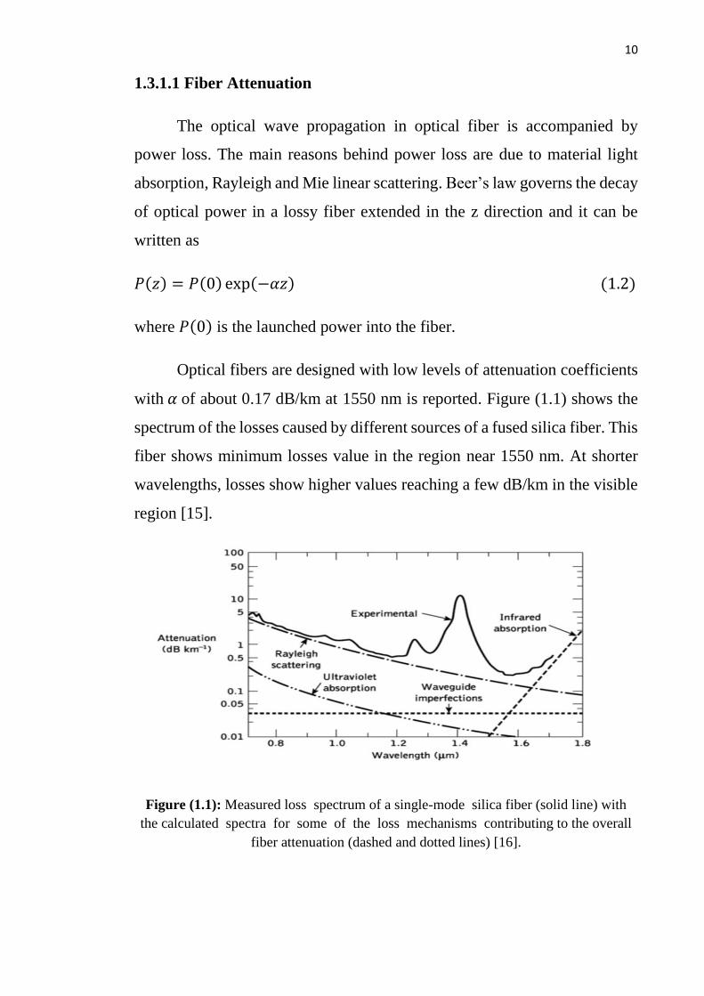
with 𝛼 of about 0.17 dB/km at 1550 nm is reported. Figure (1.1) shows the
spectrum of the losses caused by different sources of a fused silica fiber. This
fiber shows minimum losses value in the region near 1550 nm. At shorter
wavelengths, losses show higher values reaching a few dB/km in the visible
region [15].
Figure (1.1): Measured loss spectrum of a single-mode silica fiber (solid line) with
the calculated spectra for some of the loss mechanisms contributing to the overall
fiber attenuation (dashed and dotted lines) [16].

11
1.3.1.2 Chromatic Dispersion
After attenuation, dispersion is considered the next limiting factor that
determines how much and how far information can be transmitted on the
fiber link. From Eqn. (1.1), 𝛽1 controls the propagation speed of the envelope
of the optical pulse along the fiber [14]
𝛽1 =1
𝑣𝐺=
1
𝑐(𝑛 + 𝜔
𝑑𝑛
𝑑𝜔) (1.3)
where 𝑛 is the linear refractive index, 𝜔 is the optical frequency, and 𝑐 is the
speed of light in vacuum. The Group Velocity Dispersion (GVD) is the main
reason behind optical pulse broadening during the propagation. In Eqn. (1.1),
𝛽2 is the GVD parameter and given by [14]
𝛽2 =1
𝑐(2
𝑑𝑛
𝑑𝜔+ 𝜔
𝑑2𝑛
𝑑𝜔2) (1.4)
𝛽1 is related to the dispersion parameter 𝐷 which can be obtained by taking
the first derivative of 𝛽1 with respect to the wavelength
𝐷 =𝑑𝛽
1
𝑑𝜆= −
2𝜋𝑐
𝜆2𝛽
2≈
𝜆
𝑐∙
𝑑2𝑛
𝑑𝜆2 (1.5)
Return to Eqn. (1.1) again, 𝛽3 = 𝑑𝛽2 𝑑𝜔 ⁄ is considered as the GVD
slope parameter, which is associated to the dispersion slope parameter 𝑆 [16]
𝑆 =𝑑𝛽
2
𝑑𝜆= −
4𝜋𝑐2
𝜆3𝛽
2+ (
2𝜋𝑐
𝜆2)
2
𝛽3 (1.6)
For transmission in the region of zero dispersion i.e. 𝛽2 = 0, the GVD
slope becomes dominant and must be taken into account.
If one introduces a retarded time frame 𝑇 = 𝑡 − 𝑧 𝑣𝐺⁄ , which moves
with the signal at the group velocity, then 𝛽1 will be eliminated from Eqn.
(1.1). Furthermore, when Standard Single-Mode Fibers (SSMFs) or other

12
types with sufficiently high GVD are used, then the effect of the GVD slope
can be neglected. Under these conditions Eqn. (1.1) can be written as [16]
𝜕𝑨
𝜕𝑧+
𝛼
2𝑨 +
𝑗
2𝛽2
𝜕2𝑨
𝜕𝑡2= 0 (1.7)
In silica SSMF, the total dispersion profile is determined by the
waveguide dispersion and the material dispersion. The summation of those
two parameters gives the dispersion profile depicted in Fig. (1.2). The zero
dispersion wavelength is located at 1324 nm and D = 16 ps/km/nm at 1550
nm. The material dispersion is related to the nature of the fused silica, and
hence it cannot be changed. However, the effective refractive index of the
fiber controls the waveguide dispersion. By changing the index profile,
different fibers such as Dispersion Compensating Fiber (DCF) with 𝐷 =
−80 𝑝𝑠/𝑘𝑚/𝑛𝑚 and non-zero dispersion shifted fiber with 𝐷 = 4 𝑝𝑠/𝑘𝑚/
𝑛𝑚 can be manufactured. [16].
Figure (1.2): Dispersion characteristic of a typical standard single mode fiber as a
function of wavelength and frequency [8].

13
1.3.1.3 Polarization Mode Dispersion
Polarization of light is an electromagnetic wave property that
describes the direction of fluctuation of the transverse electric field. In
SSMF, there exists two orthogonal polarization states, which are denoted
here as x and y. Polarization of light can be described by representation of
Stokes parameters, which can be straight forward expressed by using
Poincaré sphere. The Poincaré sphere consists of four stocks parameters in
terms of optical power as shown in Fig. (1.3) to visualize the SOP. SSMFs
support two polarization modes simultaneously transmitting. These two
polarization modes are orthogonal to each other. But the modes
orthogonality can be changed due to temperature fluctuations and fiber
birefringence caused by mechanical stress [2,17].
Figure (1.3): Poincaré sphere. S1, S2, and S3 are the stockes parameters. The forth
parameter S4 is calculated from 𝑆42 = 𝑆1
2 + 𝑆22 + 𝑆3
2 [17].
14
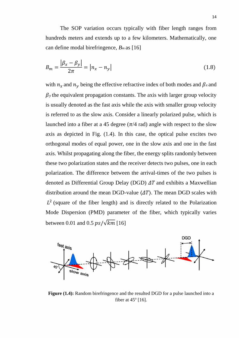
The SOP variation occurs typically with fiber length ranges from
hundreds meters and extends up to a few kilometers. Mathematically, one
can define modal birefringence, Bm as [16]
𝐵𝑚 =|𝛽𝑥 − 𝛽𝑦|
2𝜋= |𝑛𝑥 − 𝑛𝑦| (1.8)
with 𝑛𝑥 and 𝑛𝑦 being the effective refractive index of both modes and 𝛽𝑥 and
𝛽𝑦 the equivalent propagation constants. The axis with larger group velocity
is usually denoted as the fast axis while the axis with smaller group velocity
is referred to as the slow axis. Consider a linearly polarized pulse, which is
launched into a fiber at a 45 degree (𝜋/4 rad) angle with respect to the slow
axis as depicted in Fig. (1.4). In this case, the optical pulse excites two
orthogonal modes of equal power, one in the slow axis and one in the fast
axis. Whilst propagating along the fiber, the energy splits randomly between
these two polarization states and the receiver detects two pulses, one in each
polarization. The difference between the arrival-times of the two pulses is
denoted as Differential Group Delay (DGD) 𝛥𝑇 and exhibits a Maxwellian
distribution around the mean DGD-value ⟨𝛥𝑇⟩. The mean DGD scales with
𝐿2 (square of the fiber length) and is directly related to the Polarization
Mode Dispersion (PMD) parameter of the fiber, which typically varies
between 0.01 and 0.5 𝑝𝑠/√𝑘𝑚 [16]
Figure (1.4): Random birefringence and the resulted DGD for a pulse launched into a
fiber at 45o [16].

15
1.3.2 Nonlinear Impairments
The response of the optical fiber and all the dielectric materials to the
light becomes nonlinear for intense electromagnetic fields. The silica is not
considered in nature as a highly nonlinear material, but sometimes the fiber
geometry that leads to confine the light to a small cross-section for long fiber
lengths can makes nonlinear effects [10]. Fiber nonlinearities consist
generally of two main groups. The first group is related to nonlinear
refractive index, and these nonlinearities are called (Kerr effect). The other
type of nonlinearities is associated to the nonlinear optical scattering. The
fiber refractive index depends on the light intensity, and hence due to this
dependency, the Kerr effect is produced. Fiber nonlinearities in this category
are represented by Self-Phase Modulation (SPM), Cross-Phase Modulation
(XPM), and FWM. On other hand, parametric interaction between the light
and materials is caused by the stimulated scattering effects. Stimulated
scattering effects occur in two types, the first is called Stimulated Raman
Scattering (SRS) and the other is Stimulated Brillouin Scattering (SBS). The
stimulated scattering effect has threshold power level as a condition at which
the nonlinear effects manifest themselves. However, Kerr effect does not
have such threshold [18]. The Raman backscattering and SBS may cause
severe performance degradations in dense bidirectional WDM systems. By
extending Eqn. (1.1) to include the nonlinear propagation effects, one obtains
the NLSE defined in Eqn. (1.9) [14]
𝜕𝑨
𝜕𝑧+
𝛼
2𝑨 + 𝛽1
𝜕𝑨
𝜕𝑡+
𝑗
2𝛽2
𝜕2𝑨
𝜕𝑡2−
1
6 𝛽3
𝜕3𝑨
𝜕𝑡3= 𝑗𝛾|𝐴|2𝑨 (1.9)
The refractive index (ñ) of an optical fiber consists of a linear part n
and a nonlinear part 𝑛2, the later depends on the optical intensity in the fiber
(Kerr effect) [14]

16
ñ = 𝑛 + 𝑛2|𝑨|2 (1.10)
The fiber nonlinearity coefficient 𝛾 in Eqn. (1.9) is related to 𝑛2 and
the effective core area 𝐴𝑒𝑓𝑓 at the center frequency 𝜔0 by [14]
𝛾(𝜔0) =𝜔0 𝑛2
𝑐 𝐴𝑒𝑓𝑓 (1.11)
The amplitude of the optical field 𝑨 in Eqn. (1.1) can be decomposed
into three interacting field components 𝑨0, 𝑨1 and 𝑨2 which describe the two
pumps and signal with 𝛥𝛽 describing the phase relationship between them.
To explain the influence of nonlinearity, one can restrict the analysis to
small-signal distortions, and separate Eqn. (1.1) into three coupled equations.
For 𝐴0 component, the NLSE becomes [14]
𝜕𝑨0
𝜕𝑧+
𝛼
2𝑨0 +
𝑗
2𝛽2
𝜕2𝑨0
𝜕𝑡2= 𝑗𝛾|𝑨0|2𝑨0 + 2𝑗𝛾(|𝑨1|2 + |𝑨2|2)𝑨0
+𝑗𝛾 ∑ 𝑨𝑙𝑨𝑚𝑨𝑙+𝑚∗ 𝑒𝑗∆𝛽𝑧
𝑙≠𝑚
(1.12)
where ∆𝛽 is the linear phase mismatch.
In Eqn. (1.12), the SPM, XPM, and FWM are represented by the three
parts of the right hand side, respectively. In SPM, the nonlinear phase shift
caused by the power of the 𝑨0 component itself is considered, while XPM
describes the nonlinear phase shift that induced due to the contribution of the
optical powers of neighboring channels. FWM describes a mixing process
between all channels satisfying 𝑘 = 𝑙 + 𝑚 − 𝑛 [16].
1.3.2.1 Self-Phase Modulation
If one assumes single signal propagation, (i.e. no XPM and FWM as
defined in Eqn. (1.1)) and neglect chromatic dispersion, the solution to Eqn.
(1.1) has the following form [2]

17
𝑨(𝑧. 𝑇) = 𝑨(0. 𝑇) 𝑒𝑥𝑝 (− 𝛼
2 𝑧) 𝑒𝑥𝑝(𝑗Ø𝑠𝑝𝑚) (1.13)
where 𝑇 is the pulse duration, 𝛼 is attenuation coefficient, and Ø𝑠𝑝𝑚 is the
nonlinear phase distortion caused by the SPM. The nonlinear phase shift
acquired due to SPM is dependent on the intensity profile of the waveform
and the fiber effective length, and it is proportional directly to the optical
power [16]
Ø𝑠𝑝𝑚 = 𝛾𝐿𝑒𝑓𝑓|𝐴|2 (1.14)
Furthermore, Ø𝑠𝑝𝑚 scales with the effective fiber length 𝐿𝑒𝑓𝑓, which
includes the exponential decay of power profile [16]
𝐿𝑒𝑓𝑓 =1 − exp (−𝛼𝐿)
𝛼≈
1
𝛼 (for suifficiently long fibers) (1.15)
Note that in absence of chromatic dispersion, SPM does not change
the pulse shape, while the interaction of SPM with dispersion results in pulse
distortion due to Phase-Modulation to Intensity-Modulation (PM-IM)
conversion of the phase distortion Ø𝑠𝑝𝑚. In the latter case, the time
dependent nonlinear phase shift induces carrier frequency fluctuations,
which are referred to as chirp [16]
𝛿𝜔(𝑇) = −𝜕𝛿Ø𝑠𝑝𝑚(𝑇)
𝜕𝑇 (1.16)
The chirp generates new frequency components leading to spectral
broadening in dispersive media, increasing for fast pulse rise times since the
shape of 𝜙𝑠𝑝𝑚(𝑇) is proportional to the pulse shape. In a response to the
SPM phase shift, the leading edge of the pulses experiences a frequency
reduction and the trailing edge a frequency increase.

18
1.3.2.2 Cross-Phase Modulation
By analogy to SPM, XPM is also a result of a nonlinear phase shift in
an optical field. With SPM, the nonlinear phase shift in an optical signal is
due to time-dependent power fluctuations in the wavelength channel itself.
XPM, in contrast, covers the influence of the nonlinear phase shift induced
by an orthogonal polarization (polarization multiplex) or neighboring
wavelength channels (wavelength division multiplexing). Referring to Eqn.
(1.12) and consider the second term on the right hand side. One can find an
expression for the nonlinear phase shift due to two neighboring channels 𝑨2
and 𝑨3 [16]
Ø𝑋𝑃𝑀(𝑧. 𝑇) = 𝛾𝐿𝑒𝑓𝑓2 (∫ |𝑨2(0. 𝑇 + 𝑑𝑠𝑝𝑧′)exp (
𝑗
2𝛽2𝜔2
2𝑧′)|2
𝑧
0
𝑑𝑧′
+ ∫ |𝑨3(0. 𝑇 + 𝑑𝑠𝑝𝑧′)exp (𝑗
2𝛽2𝜔3
2𝑧′)|2
𝑑𝑧′
𝑧
0
) (1.17)
This expression can be generalized to express the nonlinear phase shift
induced on central channel 𝑨𝑠 due to XPM, by summing up the contributions
of all neighboring waves [16]
Ø𝑋𝑃𝑀(𝑧. 𝑇) = 𝛾𝐿𝑒𝑓𝑓2 ∑ |𝐴𝑝(0. 𝑇 + 𝑑𝑠𝑝𝑧′)exp (
𝑗
2𝛽2𝜔𝑝
2𝑧′)|2
𝑑𝑧′ (1.18)
𝑝≠1
where 𝜔𝑝 is the angular frequency of the neighboring wave that caused the
nonlinear phase shift on the signal due to XPM.
Due to the different group velocities of each WDM-channel the
symbol patterns of the interacting channels walk-off from the central channel
as displayed in figure (1.5). This effect is described by the walk-off
parameter 𝑑𝑠𝑝 [16]

19
𝑑𝑠𝑝 ≈ 𝐷 ∙ (𝜆𝑠 − 𝜆𝑝) (1.19)
where D is the dispersion parameter, 𝜆𝑠 and 𝜆𝑝 are the wavelengths of the
central and the neighboring waves, respectively.
A higher walk-off parameter helps decorrelate XPM contributions
along the transmission link and reduces the variance of the XPM distortion.
Eqn. (1.18) shows that Ø𝑋𝑃𝑀 depends on the adjacent channels power profile
and is therefore, similarly to SPM, stronger within the effective length of the
fiber. Furthermore, the nonlinear phase shift depends also on the
accumulated dispersion of the interfering channels. Since the signal peak-to-
average power ratio is generally smaller for larger values of accumulated
dispersion. It is justified to say that highly dispersed channels induce less
severe XPM-distortions [16].
Figure (1.5): Walk-off between two waves at wavelength λ1 and λ2 after propagation
over the distance L [16].
1.3.2.3 Four-Wave Mixing
This nonlinear effect comes from the nonlinear response of material
bound electrons to the electromagnetic fields. The nonlinear effect is
classified as a second order parametric process if the second-order
susceptibility 𝜒(2) is responsible for this effect. While the effect that depends
on the third-order susceptibility 𝜒(3) is classified as third-order parametric

20
process. In isotropic medium such as silica optical fiber, 𝜒(2) is almost
vanished. Thus, the effects of the second-order processes can be ignored in
silica fibers. FWM is a third-order parametric processes that occurs due to
nonlinear interaction among three or four optical waves simultaneously
forming a Non-Degenerate Four-Wave Mixing (NDFWM) where two pumps
at frequency 𝜔𝑝1 and 𝜔𝑝2 (𝜔𝑝1 ≠ 𝜔𝑝2) co-propagate with the signal at
frequency 𝜔𝑠 in nonlinear medium; an idler wave at frequency 𝜔𝑖 = 𝜔𝑝1 +
𝜔𝑝2 − 𝜔𝑠 is generated (see Figure 1.6) [19].
Figure (1.6): Waveforms of non-degenerated four-wave mixing.
If an intense pump at frequency 𝜔𝑝 and a signal at frequency 𝜔𝑠 are
injected into the nonlinear medium together, an idler wave at frequency 𝜔𝑖 =
2𝜔𝑝 − 𝜔𝑠 will be generated efficiently if the phase-matched condition is
satisfied (see Figure (1.7)). This nonlinear process is called Degenerate
FWM (DFWM), [19].
Figure (1.7): Waveforms of degenerated four-wave mixing.

21
The phase mismatch plays an important role in FWM process; if the
phase mismatch is almost zero, significant FWM can be achieved. This
condition is satisfied only by matching the frequencies of all the interacting
waves, as well as the wave vectors [14]. The phase-matching condition
required for this process is 𝛥𝑘 = 0 where
∆𝑘 = 𝛽𝑠 + 𝛽𝑖 − 𝛽𝑃1 − 𝛽𝑃2 = (𝑛𝑠𝜔𝑠 + 𝑛𝑖𝜔𝑖 − 𝑛𝑃1𝜔𝑃1 − 𝑛𝑃2𝜔𝑃2) 𝑐⁄ (1.20)
Here 𝑛𝑃1.𝑃2.𝑠.&𝑖 are the effective mode indices at the frequencies 𝜔𝑃1.𝑃2.𝑠.&𝑖.
1.4 Nonlinearity Compensation Techniques in Fiber-optic
communication Systems
Fiber-optic communication technology has been growing rapidly
during recent decades to meet the increase of data capacity to be
transmitted over the optical link. The broad development of fiber-optic
communication has started from 1980s after the use of optical equipment
that enhance the performance of optical systems such as low-loss SSMF,
EDFA, and the use of various multiplexing techniques. Besides that,
advanced modulation formats in coherent transmission systems enable
high-speed, large-capacity, and long-haul transmission system. Currently,
the transmission capacity of fiber-optic communication systems is mainly
limited by the dispersion and fiber nonlinearity caused by Kerr effect. At
low levels of signal power, transmission performance is limited by
Amplified Spontaneous Emission (ASE) noise, so the capacity can be
enhanced by increasing signal power to increase OSNR. However, with
high signal power, fiber nonlinear effects dominate and make it impossible
to enhance transmission performance by simply increasing signal power.
Different optical and digital electronic compensation techniques have

22
been proposed in the literature to partially or completely compensate for
fiber chromatic dispersion and nonlinearities [20].
1.4.1 Digital Back-Propagation Algorithm
The Digital Back-Propagation (DBP) algorithm is done by digitally
inverting the distortions due to the chromatic dispersion and fiber
nonlinearities. This process is done by the re-propagating of the received
signal into a designed virtual link. This virtual link is characterized by
inverse dispersion and nonlinear coefficients with respect to the original
fiber link (see Fig. (1.8)). DBP is an effective compensation technique for
dispersion and Kerr nonlinearities especially for single channel
transmission systems [21]. However, due to the complexity of design and
manufacturing, DBP compensation method is not suitable to be used in
the WDM systems in long-haul transmission link [22].
Figure (1.8): Schematic diagram of the fiber nonlinearity compensation system using
digital back-propagation technique.
1.4.2 Frequency-Referenced Transmission
In this method, the canceling of the nonlinear distortions due to Kerr
effect is achieved with the help of the optical carrier stability. If the optical
carriers have a sufficient degree of mutual coherence, the nonlinear wave
interaction in optical fiber can be substantially reverted. By this approach,
all transmitted carriers are generated from a stable optical frequency

23
comb, in order to conserve a locked frequency separation. Such strategy
is proved to benefit multi-channel nonlinearity compensation performed
at the transmitter, with the use of nonlinear pre-distortion [23].
1.4.3 Phase-Conjugated Twin-Waves
Compensation of fiber nonlinearity can be achieved using a method
of Phase Conjugated Twin Waves (PCTWs). In this method, the nonlinear
distortions caused by Kerr effect of a pair of phase conjugated twin waves
are anti-correlated and as a result, nonlinear distortions due to signal-
signal nonlinear interactions are canceled by coherent superposition of the
conjugated twin waves (see Fig. (1.9)). Experimentally, two orthogonal
polarizations are used as twin waves and the data modulated on one
polarization is the conjugation copy of that of the other polarization [24].
Figure (1.9): Illustration of nonlinearity cancellation based on phase-conjugated twin
waves.

24
1.4.4 Optical Back-Propagation
Optical Back Propagation (OBP) has been proposed for the
compensation of chromatic dispersion and fiber nonlinearity by placing an
OBP device at the fiber output. The OBP module usually consists of Highly
Dispersion Fiber (HDFs) and nonlinearity compensators (see Fig. (1.10)).
These optical elements used to undo fiber distortions by reversing signal
propagation. The nonlinearity compensator makes a phase shift that is equal
in magnitude to the nonlinear phase shift caused by fiber propagation, but of
course, opposite in sign. The effective negative nonlinear coefficient of the
nonlinearity compensator is realized using two segments of HNLFs. This
OBP scheme shows good transmission performance, however, it requires
very good alignment in polarization between pumps and signal, and hence,
the complexity of the receiver is significantly increased [25].
Figure (1.10): Optical pack-propagation module in WDM system [25].
1.4.5 Mid-Span Optical Phase Conjugation
Another interesting technique to mitigate fiber nonlinearity is by using
OPC fixed in the middle of the optical link, a scheme known as Mid-Span
Spectral Inversion (MSSI) [22,26]. This method firstly used for channel
dispersion compensation, lately extended to show that OPC at the mid-point

25
of the link can also compensate nonlinear distortions. In a MSSI link, the
phase of the signals is conjugated and the spectrum is inverted at the mid-
point of the optical link. The signal phase distortion that accumulated from
the first part of the link due to fiber dispersion and Kerr effect now has
opposite phase in the second part of the link. Consequently, the effects in the
second part of the optical link after the OPC cancel out the impairments of
the first part. To achieve full nonlinearity mitigation, the mid-way OPC must
be located exactly at the mid-point of the optical link, which can reduce the
flexibility of optically routed networks because the ‘mid-way’ point is
difficult to identify. Moreover, the mid-point of the link can be changed with
time. In addition, in the mid-span OPC compensation scheme, the
wavelength of the phase-conjugated signal is different compared to the
original transmitted signal and this required extra complexity in the receiver
design.
In this thesis, a dispersion and fiber nonlinearity mitigation using
multiple OPCs placed in the optical link is introduced. In this method, the
phase of the signal is conjugated after every certain length of the fiber and
the phase conjugation is repeated after another equal length fiber. Therefore,
the dispersion and fiber nonlinearities can be compensated along the optical
link, not only at fiber end. This compensation scheme allows dynamic
routing of the signals. Another advantage of using this scheme is that the
signal wavelength can be conserved at the receiver using even number of
OPC devices. This reduces the complexity of the receiver. Using multiple-
OPC compensation scheme, a large capacity, high speed, and long-haul
fiber-optic communication systems with high performance can be designed.
Furthermore, the multiple-OPC compensation scheme is transparent to the
modulation formats and suitable to single channel transmission as well as to
WDM systems.
26
1.5 Literature Survey
This section reviews some of the works related the use of OPC
technique in advanced fiber-optic communication systems which is the
research area of this thesis.
In 2006, Jansen et al. [27] employed OPC for the mitigation of fiber
dispersion and nonlinearity due to Kerr effect. In this work, 16×42.7 Gb/s
NRZ is transmitted over an 800 km straight line of SSMF. An OPC device
was used to get difference frequency generation in a periodically poled
lithium-niobate waveguide, in order to achieve high conversion efficiency
and transparent WDM operation. The principle of the use of OPC as a
polarization-independent OPC subsystem was discussed. Then, the use of
OPC for fiber dispersion and nonlinearity compensation in WDM long-haul
transmission system was investigated. The results reveal that the
transmission reach can be increased by 50% when the OPC is inserted in the
transmission link with the help of DCF. The results show an improvement in
the Q factor up to 4 dB due to the nonlinearity compensation resulting from
the nonlinear phase noise. Then, the performance of an ultra-long haul WDM
transmission system of 22×20 Gb/s Return-to-Zero Differential Quadrature
Phase Shift keying (RZ-DQPSK) over same link was discussed. The results
show that the use of OPC can completely compensate the fiber dispersion
and nonlinear impairments. Comparing the results with those of a system
using a DCF for fiber dispersion compensation shows a 44% increase in
transmission reach when OPC is employed.
In 2007, Kaewplung and Kikuchi [28] proposed the use of MS-OPC
with DRA for simultaneous mitigation of fiber attenuation, chromatic
dispersion, and fiber nonlinearity caused by Kerr effect in ultra-long haul
transmission link. DRA helps to provide symmetrical power profile along
the link and the power becomes identical with respect to the midpoint of the

27
system where the OPC device is fixed. Then, the fiber dispersion and the
nonlinear distortions caused by the Kerr effect are almost completely
mitigated by the OPC. Numerical simulation results demonstrate that, by
employing the flat power maps with a span of 40 km, a single-wavelength
signal whose data rate is 160 Gb/s can be successfully transmitted over 5000
km at Q-factor 7 dB, and the Kerr effect is sufficiently suppressed near
limitation due to the nonlinear accumulation of noise.
In 2012, Morshed et al. [29] reported through the simulation that
OPC based on FWM for MSSI can be improved by splitting HNLF into
two parts separated by an optical filter to suppress the XPM around the
pump. Simulation results show an improvement of the maximum signal
quality, Q-factor, by 1 dB in a 10×80 km 4QAM 224 Gb/s CO-OFDM
system with MSSI. The simulation results of the proposed OPC was
compared with the system in which a conventional OPC is used and
showed an improvement in terms of Q factor.
In 2014, Ros et al. [30] investigated experimentally the use of a dual-
pump Fiber Optic Parametric Amplifier (FOPA)-based optical phase
conjugation to achieve MSSI in order to mitigate the fiber nonlinearity for
a signal consisting of five channels each of 112 Gb/s per polarization (WDM-
PDM 16-QAM signal) over 800 km dispersion-compensated optical link.
The polarization insensitive operation of the designed OPC device using a
dual-pump FOPA was demonstrated. The results show an improvement in
the value of the maximum Q-factor provided by the compensation scheme
for different dispersion-managed transmission lengths with clear
improvement reported for all the lengths considered. In the nonlinear regime,
the nonlinearity compensation provided by OPC enables improvements of
the Q-factor of 0.56 dB, 0.71 dB and 0.9 dB, for 480 km, 640 km and 800
km, respectively, provided only 1 dB higher power per channel is launched
in the spans. The OPC operation allows reaching BERs below the HD-FEC

28
threshold (3.85×10⁻³) for 800 km transmission and the results show better
performance when compared with a direct transmission link.
In 2014, Sackey et al. [31] presented experimental and numerical
extension for their work reported in [30]. They used a particular link of
4×100 km SSMF spans employing backward pumping DRA. The
transmitter and receiver configuration are the same as in the previous
work. A dual-pump polarization-independent FOPA was used as a mid-
link OPC. In single channel transmission, an improvement of 1.1 dB in Q-
factor was achieved. While the Q-factor improvement of the five-channel
WDM system is 0.8 dB. The experimental results are in good agreement
with numerical simulations ones. Maximum transmission reach of 2400
km was obtained through simulation for a WDM system using mid-link
OPC.
In 2014, Hu et al. [32] proposed multiple-OPC on an 8-channel
WDM PDM quadrature phase-shift keying (QPSK) 1Tb/s data signal
enabling a 6000 km transmission reach. Best performance is obtained for
600 km OPC span length and the results were compared experimentally
with the case of MS-OPC and the direct link. The proposed method shows
better performance than with MS-OPC and without OPC. The results
show that the optimum launched power is still at -7 dBm when the FOPA
without OPC is used, but the Q-factor is reduced by 1.4 dB compared to
the case of a direct link (without FOPA). After 3600 km transmission, for
the case of FOPA with MS-OPC, the optimum launch power is increased
by 3 dB, but the optimized Q-factor is still 0.4 dB lower than without
FOPA. For the case of FOPA with multiple- OPC, the optimum launch
power is increased by about 5 dB, resulting in Q-factor improvement of
0.5 dB higher than the case without FOPA and 0.9 dB higher than the case
of FOPA with MS-OPC.

29
In 2014, Sackey et al. [33] demonstrated experimentally a
polarization-independent FOPA-based OPC with different values of the
On-Off gain to transmit a test signal of 112 Gb/s PDM 16-QAM signals
in a 5 channel 50-GHz spacing WDM system. Investigation of signal and
generated idler shows OSNR penalties below 1 dB for single channel and
a 5 channel WDM cases at 5 dB On-Off gain and at a BER of 10-4. The
maximum polarization dependent gain was also measured to be below 0.5
dB across a wavelength range from 1542.5 nm to 1565 nm. The proposed
scheme is very useful for in-line OPC applications at 5 dB gain for gain-
transparent operation with minimal penalty from the FOPA.
In 2015, Ros et al. [34] demonstrated a fiber nonlinearity
compensation scheme by OPC in a WDM PDM 16-QAM system. Improved
received signal quality was reported for both dispersion-compensated and
dispersion-uncompensated transmission and a comparison with DBP scheme
was investigated. The received Q-factor for the center channel is shown as a
function of the power launched into each span for the two scenarios. In both
cases application of the OPC device increases the optimum transmission
power as well as the maximum received Q-factor with improvements of
around 0.9 dB over 800 km transmission and 1.1 dB over 400 km
transmission for the two link configurations. For the dispersion-compensated
link, the use of OPC for 800 km transmission results in the same performance
as 640 km straight transmission, increasing the reach by 25%.
In 2016, Yoshima et al. [35] demonstrated experimentally fiber
nonlinearity compensation for two 10 Gbaud (60 Gb/s) 64-QAM signals
using MS-OPC in a 400 km EDFA-amplified transmission link. The system
was tested in a WDM environment using a single OPC to simultaneously
conjugate two WDM signal bands. This provides twice the usable bandwidth
when compared to conventional schemes. Q-factor improvement of more
30
than 1.7 dB was achieved for channels in the two bands when OPC was in
place.
Also in 2016, Hu et al. [36] demonstrated multiple optical phase
conjugation of an 8-channel WDM PDM 16-QAM signal achieving total bit
rate of 2.048 Tb/s in a 900 km SSMF transmission experiment. In both
single-channel and WDM cases, by using repeated OPC, the system
performance was demonstrated to be improved over both the case of MS-
OPC and the case of no OPC. The system performance was evaluated by the
Q-factor (calculated from BER) measured with various launched powers.
In 2017, Hu et al. [26] investigated experimentally the use of multiple-
OPC to fiber nonlinearity compensation in single-channel and WDM
transmission systems. They used two signals with different modulation
formats, the first is 8×32-Gbaud PDM QPSK signal, and the second is 8×32-
Gbaud PDM 16-QAM signal. The total bit rates of 1.024 Tb/s and 2.048 Tb/s
for the first and second signals, respectively. They compared their results
with the scheme of single MS-OPC and with direct transmission link. The
proposed method shows improved performance in terms of a best achievable
Q factor after transmission and the nonlinear threshold. In addition, the
signal wavelength can be preserved at the receiver using even number of
OPCs. The results prove that the proposed technique is transparent to the
modulation formats and effective for different optical transmission links. The
WDM PDM QPSK signal band is transmitted over a long-haul DRA by
employing multiple-OPC. In this system, 5 dB and 2 dB increasing in the
nonlinear threshold were obtained compared to the case of no OPC and MS-
OPC, respectively. While in WDM PDM 16-QAM signal transmission, the
nonlinear thresholds are increased by 7 dB and 1 dB compared to the case of
no OPC and MS-OPC, respectively.

31
It is clear from this survey that OPC can be adapted as an effective
technique to compensate the combined effect of fiber chromatic dispersion
and nonlinearities. Most of the researchers focus on using MS-OPC for this
purpose from cost point of view. The benefits gained by using multiple-OPC
technique have been addressed by few researchers in this field. Their results
are deduced mainly on experimental investigation without considerable
attention to SOPs of the associated pumps and signal as the main issue. In
this thesis, this issue is addressed theoretically and by simulation using
commercial software packages, namely Optisystem v. 14.1. The theoretical
results are found to be in good agreement with experimental data reported in
reference [29]. The theoretical modeling and simulation results can be used
to design multi-span HNLF-OPC devices which can offer flat spectral
conversion efficiency with less sensitivity to signal polarization. These
devices are suitable for mitigation of linear and linear phase distortions
associated with transmitted signals in high-bit rate and long-haul WDM
systems incorporating high-order modulation formats.
1.6 Thesis Outlines
This thesis consists of four chapters; the rest three chapters are
organized as follows
Chapter 2 introduces background information of optical pulse
propagation starting with Maxwell's equations until reaching the complete
NLSE which well describes the pulse propagation through optical fiber.
Furthermore, coherent fiber-optic communication systems, multiplexing
techniques, and advanced modulation formats are presented.
Chapter 3 investigates analytically the performance of dual-pump
HNLF-OPC in the presence of SOP misalignment hence the signal and the

32
two pumps expressions are derived to characterize the fiber-optic
communication system incorporating HNLF-OPC device for mitigating the
effects of fiber dispersion and nonlinearities that is caused by Kerr effect.
FWM parametric gain and conversion efficiency as a function of signal and
pumps SOPs in both MS-OPC and multiple-OPC configurations are
considered here.
Chapter 4 present and discuss the simulation results of proposed
compensation systems and compare the obtained results with published
experimental ones. Finally, discussion of the future steps that can be taken to
improve this work will be provided.

33
Chapter Two
Theoretical Background
34
Chapter Two
Theoretical Background
2.1 Introduction
This chapter presents the basic theory for a propagation of
electromagnetic wave in nonlinear dispersive optical fiber. Basic concepts of
the optical pulses propagation into single mode fibers starting from
Maxwell’s equations are given. Maxwell’s equations are used as the
mathematical framework to introduce the NLSE which well describes the
principles of optical pulse propagation in dispersive nonlinear fiber. This
chapter presents the principle of the operation of OPC based on FWM
process in a HNLF. The techniques that enable long-haul, large-capacity, and
high-speed fiber-optic communication systems are also briefly mentioned in
this chapter.
2.2 Maxwell’s Equations and Optical Wave Equation
Similar to all electromagnetic phenomena, optical pulse propagation
in fibers, either in linear or nonlinear regimes, is governed by the basic
Maxwell’s equations [37]
𝜵 × 𝑬 = −𝜕𝑩
𝜕𝑡 (2.1𝑎)
𝜵 × 𝑯 = 𝑱 +𝜕𝑫
𝜕𝑡 (2.1𝑏)

35
𝜵. 𝑫 = 𝜌 (2.1𝑐)
𝜵. 𝑩 = 0 (2.1𝑑)
where 𝑬 and 𝑯 are the electric and magnetic fields vectors, respectively,
𝑫 and 𝑩 are associated electric and magnetic flux densities, respectively, 𝑱 is
the current density, and 𝜌 represents the electromagnetic field source. In
optical fibers, which are dielectric transmission media, 𝑱 = 0 and 𝜌 = 0.
𝑫 and 𝑩 are generated as a response of the medium to the propagating
electric and magnetic fields 𝑬 and 𝑯. respectively, [37]
𝑫 = 𝜖0𝑬 + 𝑷 (2.2𝑎)
𝑩 = 𝜇0𝑯 + 𝑴 (2.2𝑏)
where 𝜖0 and 𝜇0 are the permittivity and permeability in the vacuum,
respectively, 𝑷 is the induced electric polarization while 𝑴 represents the
induced magnetic polarization. Note that the value of the magnetic
polarization is equal to zero for non-magnetic mediums as in optical fibers.
The propagation of optical pulses in optical fiber is controlled by
Maxwell’s equations and governed by the following wave equation [14]
𝛁 × 𝛁 × 𝑬 = − 1
𝑐2
𝜕2𝑬
𝜕𝑡2 − 𝜇0
𝜕2𝑷
𝜕𝑡2 (2.3)
where c is the light vacuum speed and the relation 𝜇0𝜖0 = 1/𝑐2 is used.
The induced polarization 𝑷 at position r in the fiber consists of two
parts
𝑷𝑇(𝑟. 𝑡) = 𝑷𝐿(𝑟. 𝑡) + 𝑷𝑁𝐿(𝑟. 𝑡) (2.4)

36
where 𝑷𝐿 is the linear polarization and 𝑷𝑁𝐿 is the nonlinear polarization. The
linear part 𝑷𝐿(𝑟. 𝑡) is related to the electric field by the first order
susceptibility 𝜒(1) [14]
𝑷𝐿(𝑟. 𝑡) = 𝜖0 𝜒(1) 𝑬 = 𝜖0 ∫ 𝜒(1)
𝑡
−∞
(𝑡 − 𝑡′). 𝑬(𝑟. 𝑡′)𝑑𝑡′ (2.5)
In optical fiber, the nonlinear polarization often comes from the third
order susceptibility 𝜒(3) and hence [14]
𝑷𝑁𝐿(𝑟. 𝑡) = 𝜖0 𝜒(3) ⋮ 𝑬𝑬𝑬
= 𝜖0 ∫ 𝑑𝑡1
𝑡
−∞
∫ 𝑑𝑡2
𝑡
−∞
∫ 𝑑𝑡3
𝑡
−∞
× 𝜒(3)(𝑡 − 𝑡1. 𝑡 − 𝑡2. 𝑡 − 𝑡3)
⋮ 𝑬(𝑟. 𝑡1)𝑬(𝑟. 𝑡2)𝑬(𝑟. 𝑡3) (2.6)
where 𝜒(3) is a tenser of fourth rank which contains 81 terms. In isotropic
media, like a silica fiber operating away from any resonance, the independent
terms in 𝜒(3) is reduced to be only one [14].
Equations (2.4) to (2.6) can be used in the wave Eqn. (2.3) to obtain
the propagation equation of the optical pulse in nonlinear dispersive fibers.
Before that, some practical assumptions are to be considered to solve Eqn.
(2.3) [37].
i) Nonlinear polarization is considered as a small perturbation of a linear
polarization and the polarization remains constant along the fiber.
ii) The small refractive index difference between the fiber core and
cladding is neglected and the spectral width of the wave is much less
than the center frequency of the wave, considering a quasi-
monochromatic assumption. This leads to the use of the approximation
of slowly varying envelope in the time domain.

37
iii) The propagation constant is approximated by only few terms of the
expansion of Taylor series around the carrier frequency, and hence the
propagation constant can be expressed as [38]
𝛽(𝜔) = 𝛽0 + (𝜔 − 𝜔0)𝛽1 +1
2(𝜔 − 𝜔0)2𝛽2 +
1
6(𝜔 − 𝜔0)3𝛽3 (2.7)
where 𝛽0 = 𝛽(𝜔0) and other parameters are given as
𝛽𝑚 = (𝑑𝑚𝛽
𝑑𝜔𝑚)𝜔=𝜔0
. (m = 1. 2. 3. … … … ) (2.8)
The parameters 𝛽1 and 𝛽2 are given in Eqns. (1.3) and (1.4),
respectively.
The third-order term and beyond in equation (2.7) can be ignored as
long as the quasi-monochromatic assumption is assumed. However, when
the center of the signal wavelength is at or near the zero-dispersion
wavelength, the second-order term of the propagation constant 𝛽2 is
negligible and therefore the 𝛽3 term should be taken into account [39].
2.3 Nonlinear Schrödinger Equation
If the propagating electric field 𝐴(𝑧. 𝑡) propagates toward +𝑧
direction and it is linearly polarized toward x direction, Eqn. (1.9) that
governs the evolution of the slow-varying complex envelope of the optical
pulses along a SSMF can be written as follow [14,37]
𝜕𝑨(𝑧. 𝑡)
𝜕𝑧+
𝛼
2𝐴(𝑧. 𝑡) + 𝛽1
𝜕𝑨(𝑧. 𝑡)
𝜕𝑡+
𝑗
2𝛽2
𝜕2𝑨(𝑧. 𝑡)
𝜕𝑡2−
1
6 𝛽3
𝜕3𝑨(𝑧. 𝑡)
𝜕𝑡3
= −𝑗𝛾 |𝑨(𝑧. 𝑡)|2 𝑨(𝑧. 𝑡) (2.9)
where 𝑧 is the spatial longitudinal coordinate.

38
Equation (2.9) is usually called generalized NLSE. This equation
describes the optical pulse propagation in a SSMF. This equation is
applicable for propagation of short optical pulses with width as low as (~50
fs). This is associated to a spectral width of (~20THz) [14].
If the optical pulse width is much less than 1ps, the effect of SRS and
the self-steepening should be included in the NLSE, then equation (2.9) can
be written as [14, 38]:
𝜕𝑨(𝑧. 𝑡)
𝜕𝑧+
𝛼
2𝑨(𝑧. 𝑡) + 𝛽1
𝜕𝑨(𝑧. 𝑡)
𝜕𝑡+
𝑗
2𝛽2
𝜕2𝑨(𝑧. 𝑡)
𝜕𝑡2−
1
6𝛽3
𝜕3𝑨(𝑧. 𝑡)
𝜕𝑡3
= −𝑗𝛾 |𝑨(𝑧. 𝑡)|2 𝑨(𝑧. 𝑡) + 𝑗𝛾𝑇𝑅 𝜕
𝜕𝑡|𝑨(𝑧. 𝑡)|2 𝑨(𝑧. 𝑡)
−𝛾
𝜔0
𝜕
𝜕𝑡|𝑨(𝑧. 𝑡)|2 𝑨(𝑧. 𝑡) (2.10)
where 𝑇𝑅 is the Raman gain slope (~5 fs). However, at higher pulse width
(wider than 1 ps), the SRS and the self-steepening effect terms can be ignored
compared to the Kerr effect term.
2.4 FWM-Based OPC
FWM is an important nonlinear process occurs in optical fibers. It is
useful in many applications such as phase conjugation and wavelength
conversion [40, 41]. In the conventional NDFWM processes in a nonlinear
medium, a two pumps and a weak signal are simultaneously injected into the
medium. As a result of the nonlinear interaction among these waves, an idler
or conjugate wave can be generated when the phase-matching condition is
met (see Fig. (2.1)). Using FWM-based OPC, the restoration of temporal
pulses in optical fibers can be achieved, and hence, the pulse shape can be
restored after being affected by fiber dispersion and nonlinearity. This leads
to a restoration of the shape of the propagated pulse in a fiber as the pulse

39
propagates through another fiber after conjugation of its phase, and hence,
undoes the chromatic dispersion and fiber nonlinearity induced by the
original pulse. As a result of these important properties, FWM-based OPC
has received much attention in long-haul fiber-optic communication systems
[27]. A phase conjugation with high efficiency becomes possible with fairly
high input powers and this may lead to an optimum fiber length of maximum
conversion efficiency.
Figure (2.1): Generation of a conjugated idler using four-wave mixing.
Consider non-degenerate FWM in a HNLF where all the four
frequencies (two pumps, signal and idler) are different. In this process, two
pump waves at frequencies (𝜔𝑝1) and (𝜔𝑝2), and signal wave (to be phase
conjugated) at frequency (𝜔𝑠) are launched into a HNLF generating an idler
wave with an optical frequency (𝜔𝑖 = ω 𝑝1 + 𝜔𝑝2 − 𝜔𝑠), the total electric
field is expressed as [42]
𝑬 = 1
2 �̇� ∑ exp[𝑗(𝛽𝑛𝑧 − 𝜔𝑛𝑡)] + 𝑐. 𝑐.
4
𝑛=1
(2.11)
where c.c. stands for complex conjugate mirror.
The nonlinear polarization parameter 𝑷𝑁𝐿 can be expanded in the
same form as 𝑬

40
𝑷𝑵𝑳 = 1
2 �̇� ∑ 𝑷𝒏 exp[𝑗(𝛽𝑛𝑧 − 𝜔𝑛𝑡)] + 𝑐. 𝑐.
4
𝑛=1
(2.12)
Substituting Eqns. (2.11) and (2.12) into the wave equation together
with a linear part of the polarization that has similar expression, and
neglecting all the time dependence terms of field components, yields the
following set of coupled NLSES in terms of the complex amplitudes of these
waves [19,37]
𝑑𝑨𝑝1(𝑧)
𝑑𝑧=
−𝛼
2𝑨𝑝1(𝑧)
+ 𝑗𝛾[│𝑨𝑝1(𝑧)│2 + 2│𝑨𝑝2(𝑧)│2 + 2│𝑨𝑠(𝑧)│2 + 2│𝑨𝑖(𝑧)│2 ]𝑨𝑝1(𝑧)
+ 2𝑗𝛾𝑨𝑝2∗ (𝑧)𝑨𝑠(𝑧)𝑨𝑖(𝑧) exp(𝑗𝛥𝑘𝑧) (2.13𝑎)
𝑑𝑨𝑝2(𝑧)
𝑑𝑧=
−𝛼
2𝑨𝑝2(𝑧)
+ 𝑗𝛾[2│𝑨𝑝1(𝑧)│2 + │𝑨𝑝2(𝑧)│2 + 2│𝑨𝑠(𝑧)│2 + 2│𝑨𝑖(𝑧)│2 ]𝑨𝑝2(𝑧)
+ 2𝑗𝛾𝑨𝑝1∗ (𝑧)𝑨𝑠(𝑧)𝑨𝑖(𝑧) exp(𝑗𝛥𝑘𝑧) (2.13𝑏)
𝑑𝑨𝑠(𝑧)
𝑑𝑧=
−𝛼
2𝑨𝑠(𝑧)
+ 𝑗𝛾[2│𝑨𝑝1(𝑧)│2 + 2│𝑨𝑝2(𝑧)│2 + │𝑨𝑠(𝑧)│2 + 2│𝑨𝑖(𝑧)│2 ]𝑨𝑠(𝑧)
+ 2𝑗𝛾 𝑨𝑖∗(𝑧)𝑨𝑝1(𝑧)𝑨𝑝2(𝑧) exp(−𝑗𝛥𝑘𝑧) (2.13𝑐)
𝑑𝑨𝑖(𝑧)
𝑑𝑧=
−𝛼
2𝐴𝑖(𝑧)
+ 𝑗𝛾[2│𝑨𝑝1(𝑧)│2 + 2│𝑨𝑝2(𝑧)│2 + 2│𝑨𝑠(𝑧)│2 + │𝑨𝑖(𝑧)│2 ]𝑨𝑖(𝑧)
+ 2𝑗𝛾 𝑨𝑠∗(𝑧)𝑨𝑝1(𝑧)𝑨𝑝2(𝑧) exp(−𝑗𝛥𝑘𝑧) (2.13𝑑)
where, 𝑨𝑝1(𝑧), 𝑨𝑝2(𝑧) 𝑨𝑠(𝑧), and 𝑨𝑖(𝑧) are the electric field of the pump1,
pump2, signal, and idler waves, respectively. Further, 𝑧 is the direction of
propagation, and 𝛥𝑘 is the wave-vector mismatch given in Eqn. (1.20).

41
2.5 Advanced Techniques in Long-Haul, High-Speed Fiber-optic
communication Systems
This section covers some key technologies that enable long-haul,
large-capacity fiber-optic communications beyond 1 Tb/s, such as high-order
modulation formats, different multiplexing techniques, and optical
amplifiers.
2.5.1 Optical Modulation Formats
Fiber-optic communication systems are forming the main
infrastructure that enables a high performance, large-capacity and long-haul
global data network. Modern advanced applications such as high definition
video conferences, satellite television channels, and complex internet
applications have become affordable with the help of the fiber-optic
communication [43,44]. The need for higher data rate signals transportation,
and at the same time, reduction of the construction cost, have led to use the
optical networks with high spectral efficiencies. Advanced optical
modulation formats have been playing a great rule to design the advanced
fiber-optic communication systems [45].
In this subsection, some of the optical modulation formats are
presented briefly which are suitable for optically routed WDM networks
such as amplitude-shift keying (ASK), phase-shift keying (PSK), and
quadrature-amplitude modulation (QAM).
a) Amplitude Shift keying
Optical Amplitude Shift Keying (ASK) is a type of amplitude
modulation in which the digital data is represented by variations of

42
the amplitude of an optical carrier wave. In binary ASK system, the binary
digit of the input signal is represented by transmitting a constant amplitude
carrier wave with constant carrier frequency for time duration of T seconds
per bit. In ASK, each symbol contains only one bit. Therefore, the symbol
rate (number of transmitted symbol per second) is equal to the bit rate. The
simplest and most common method to generate the ASK signal uses a switch.
The presence of a carrier wave indicates a binary 1 and absence of the carrier
wave to indicate a binary 0. This type of modulation is usually called On-Off
Keying (OOK) [16]. Figure (2.1a) shows the OOK constellation diagram.
From this diagram, it is clear that the choice of the threshold is critical to the
performance of the receiver. OOK receiver needs an adaptable amplitude
threshold, this can be achieved by an automatic gain control in order to
ensure setting of the optimal threshold. Figure (2.1b) explains the ASK
waveforms with simple on-off binary method to send a series of four bits
‘1001’ [46].
Figure (2.2): (a) OOK signal constellation diagram, and (b) is the modulated binary
ASK signal corresponding to a baseband input data [46].
b) Phase Shift Keying
Phase Shift Keying (PSK) is a one of the most important digital
modulation formats in fiber-optic communication systems. PSK modulation

43
process conveys data by modulating the phase of the optical carrier wave.
PSK uses a specific number of phases, a symbol of an equal number of bits
is encoded by each phase. The PSK demodulator is designed with high
accuracy to deal with the phase of each received symbol and this phase must
be defined by the modulator, and then maps it back to the bit stream of each
symbol, thus recovering the original data. This is achieved if the receiver is
able to compare the phases of the received symbols to a reference symbols,
such system is well known to be called coherent detection system. PSK is
classified into many types depending on number of bit per symbol [37].
i) Binary Phase-Shift Keying (BPSK) encodes one bit per symbol by
modulating the carrier wave in two phase states (0 and π) as illustrated in
Fig. (2.3) [16, 37] BPSK signal can be generated using a Mach-Zehnder
Interferometer (MZI) which consists of two nested phase modulators. This
phase modulator is used to manipulate the relative phase between the two
branches and to achieve either constructive or destructive interference at the
output. The MZI is driven in push-pull mode around its zero-transmission
point, to achieve a relative phase of π radians [16]. The BPSK modulated
signal can be given by the following two equations
𝑆1 = 𝐴 cos(𝜔𝑐𝑡) (2.14𝑎)
𝑆0 = −𝐴 cos(𝜔𝑐𝑡) (2.14𝑏)
where 𝑆1 and 𝑆0 are the two input states (1 and 0), and 𝜔𝑐 is the angular
carrier frequency.

44
Figure (2.3): (a) Generation of BPSK signal using Mach-Zehnder interferometer, (b)
constellation diagram of the BPSK signal, and (c) is the modulated BPSK signal
corresponding to a baseband input data [37].
ii) Quadrature phase-shift keying (QPSK) contains 4 phase states
separated by π/2 rad from each other (see Figure (2.4b)) [37, 46]. QPSK
encodes 2 bits per symbol. QPSK can be represented effectively by two
BPSK systems (I and Q), and hence achieve the same performance but twice
the bandwidth efficiency. QPSK is often generated by two nested MZI. One
of the optical outputs is then phase shifted by π/2 rad and combined with the
other signal (see Figure (2.4)).
iii) Eight phase-shift keying (8PSK) encodes 3 bits per symbol with 8 phase-
states [46], equally spaced with a phase difference of π/4 rad as depicted in
Fig. (2.4). It can be generated by using a QPSK transmitter followed by a
phase-modulator, which shifts the phase between 0 and π/4 rad. Note, that it
is possible to encode 16 different phase states and obtain 16PSK if an 8PSK
transmitter is preceded by an additional phase-modulator shifting the signals
phase between 0 and π/8 rad.

45
Figure (2.4): (a) Generation of QPSK and 8PSK signals, and (b) Constellation diagrams
of QPSK and 8PSK signals, D1 – D3 are the binary data [46].
c) Quadrature Amplitude Modulation
QAM is an important type of modulation formats which is widely used
for modulating data signals onto a carrier in fiber-optic communication
systems. It provides number of advantages compared to the other modulation
formats such as ASK and PSK. QAM is a signal with two carriers shifted in
phase by 90˚, they are modulated to produce an output that varies in both
amplitude and phase. QAM is considered as a mixture of amplitude and
phase modulation because of the presence of both amplitude and phase in the
output signal. Many forms of QAM constellation are often used and some of
the most common forms are 4QAM, 8QAM, 16QAM, 32 QAM, 64 QAM.
Figure (2.5) explains the constellation diagram of some types of QAM
signals depending on the number of points in each electrical constellation
diagram [47].
Figure (2.5): Constellation diagram of the 8QAM, 16QAM, 32QAM, and 64QAM.

46
QAM enables higher data rates with respect to the conventional
amplitude and phase modulation schemes. When QAM is used, the points of
the electrical constellation diagram are normally arranged either in a square
grid with equal vertical and horizontal spacing or in star form. The higher
order modulation formats utilizing more points on the constellation enables
transmitting more than one bit per symbol, and hence, increases the data rate
of the system. However, the electrical constellation points are relatively
closer together and therefore more possibility to be affected by noise and
data errors arises. Table (2.1) gives a summary for the symbol rates of
different forms of QAM and PSK.
Table (2.1): Summary of symbol rate for different forms of modulation formats.
Modulation Bit per symbol Symbol rate
BPSK 1 Bit rate
QPSK 2 1/2 Bit rate
8PSK 3 1/3 Bit rate
16-QAM 4 1/4 Bit rate
32-QAM 5 1/5 Bit rate
64-QAM 6 1/6 Bit rate
Although QAM is used to increase the efficiency of different
communication systems by utilizing both phase and amplitude variations,
unfortunately it has many disadvantages [48]. For example, the states are
closer together, therefore it is more affected by noise, and hence a lower level
of noise is needed to drift the received symbol from the correct decision
point. In phase or frequency modulation, the receivers are able to use
amplifiers that are able to reduce the effect of amplitude noise, and results in
improvement in the noise reliance. This property is not existent with QAM
because of its dependence on the signal amplitude. Second, when a signal is
phase or frequency modulated, there is no need to use linear amplifiers, while
in QAM, that includes an amplitude component, amplification linearity must

47
be taken into account. But the linear amplifiers have many disadvantages
such as, high power consumption and low amplification efficiency.
2.5.2 Wavelength Division Multiplexing
Multiplexing of signals at different wavelengths through the same optical
fiber leads to multiplying transmission capacity. WDM (see Fig. ((2.6)) is
one of the promising techniques used for increasing transmission capacity in
fiber-optic communication systems. WDM is a technique that multiplex
number of optical signals at different wavelengths, each signal is modulated
independently by different electrical bit streams [2].
Figure (2.6): Simplified block diagram for wavelength division multiplexing system
including MUX: Multiplexer, DMUX: Demultiplexer, and Tx (Rx): Single-channel
optical transmitter (receiver).
This technique allows multiple optical signals to be transmitted at
same the time through the same optical fiber, therefore, increases the
capacity of the system transmission significantly. An optical multiplexer
with suitable number of channels is used to combine the signals and an
optical wavelength division demultiplexer is used to separate the signals at
the receiving end. The separated optical signals at different wavelengths can
be then distributed into different detectors.

48
2.5.3 Polarization Division Multiplexing
Optical PDM is based on independently transmitting two modulated
signals over orthogonal polarizations of the same optical wavelength and
therefore doubling the transmission capacity. In optics, the SOP is the shape
of direction of propagation of the electric field vector of the optical signal in
a constant plane. Figure (2.7) shows the linear, circular, and elliptical
polarization states.
Linear polarization is obtained when the direction of the electric
wave propagation is constant over a certain axis (the electric-field vectors
along with 𝑬𝑥 and 𝑬𝑦 directions are in phase). When 𝑬𝑥 and 𝑬𝑦 are exactly
ninety degree out of phase, one has a circular polarization. There are right-
handed or left-handed circular/elliptical polarizations, depending on which
direction the electric field vector rotates, that is, if the electric field vector is
seen rotating clockwise or counterclockwise.
Figure (2.7): Examples of linear, circular, and elliptical polarization states [39].
2.5.4 Optical Amplifiers
Fiber attenuation that is caused by absorption loss, coupling loss,
bending losses, and different types of scattering limits the transmission
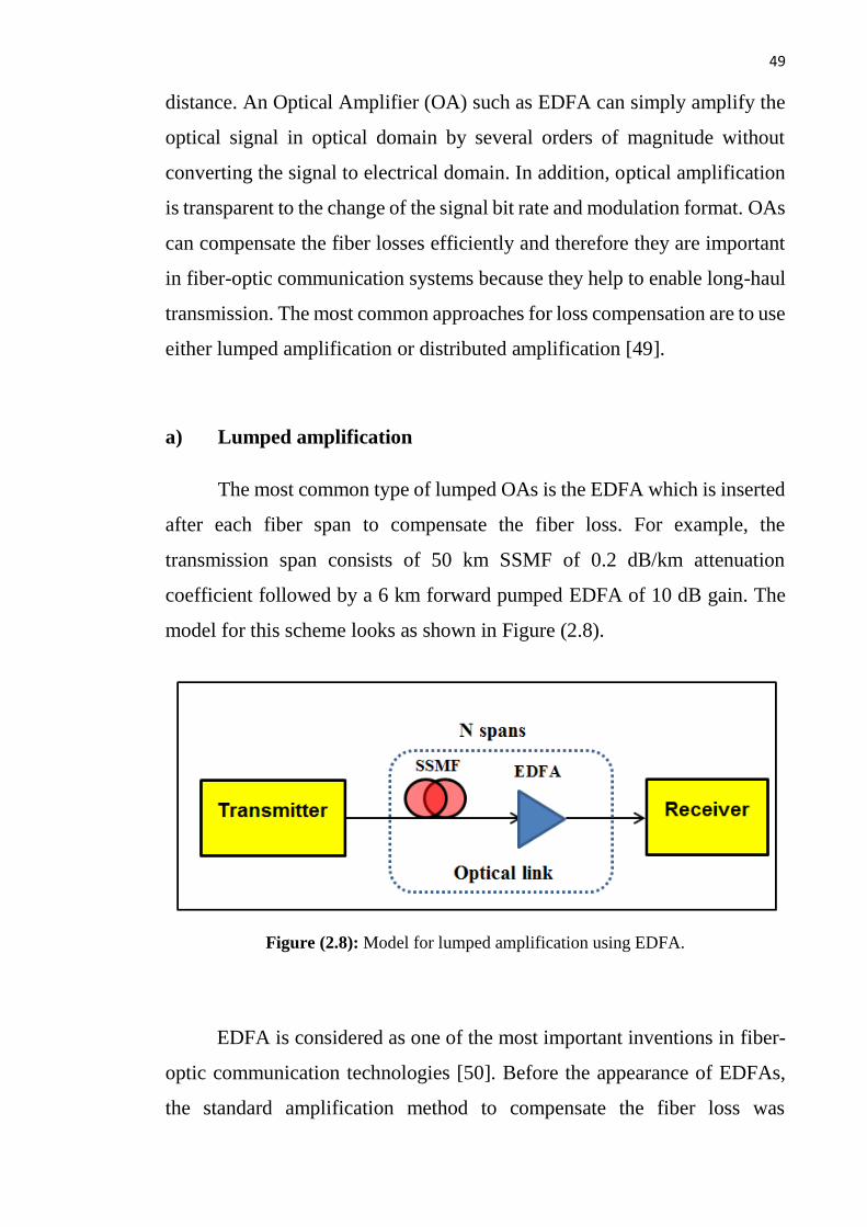
49
distance. An Optical Amplifier (OA) such as EDFA can simply amplify the
optical signal in optical domain by several orders of magnitude without
converting the signal to electrical domain. In addition, optical amplification
is transparent to the change of the signal bit rate and modulation format. OAs
can compensate the fiber losses efficiently and therefore they are important
in fiber-optic communication systems because they help to enable long-haul
transmission. The most common approaches for loss compensation are to use
either lumped amplification or distributed amplification [49].
a) Lumped amplification
The most common type of lumped OAs is the EDFA which is inserted
after each fiber span to compensate the fiber loss. For example, the
transmission span consists of 50 km SSMF of 0.2 dB/km attenuation
coefficient followed by a 6 km forward pumped EDFA of 10 dB gain. The
model for this scheme looks as shown in Figure (2.8).
Figure (2.8): Model for lumped amplification using EDFA.
EDFA is considered as one of the most important inventions in fiber-
optic communication technologies [50]. Before the appearance of EDFAs,
the standard amplification method to compensate the fiber loss was

50
electronic signal regenerators fixed in the optical transmission link. The
electronic regenerator consists of a photodetector, DSP, electrical amplifier,
and an optical transmitter. The regenerator receives the optical signal and
converts it into electrical signal, then amplifies it and performs the
conversion from electrical to optical domains, and finally retransmission of
the regenerated optical signal. However, electronic devices that used in
regenerators will prevent exploitation of the huge bandwidth of the optical
fiber. Moreover, if the system capacity is increased, all the electronic
repeaters must be replaced because they would be designed to a specific bit
rate and modulation format.
b) Distributed Amplification
One of the most important types of distributed amplifiers is SRS-based
OA which is called Distributed Raman Amplifier (DRA). Pump power and
signal is injected into the fiber using pump coupler. Figures (2.9a) and (2.9b)
illustrate the DRA with forward and backward Raman pumping,
respectively. DRA has become a very attractive amplification principle in
modern high-speed, long-haul, and broadband fiber-optic communication
systems. Raman amplifier provides better performance in L band
amplification and it also provides a flat gain profile compared to the other
discrete amplifier types [51]. The accumulation of amplifier noise is reduced
significantly if the DRA is used within the link because the level of the signal
power is kept from decreasing to very low values, as it can occur when
discrete EDFAs amplifiers are used. Therefore, the level of the maximum
signal power can be reduced without accumulating significant amplifier
noise. Reduction of the input signal power level also leads to reduce the
effects of fiber nonlinearities [52].

51
Figure (2.9): (a) Forward pumped-distributed Raman amplified link, and (b) Backward
pumped-distributed Raman amplified link.
Raman amplification is a function to the frequency difference between
the signal frequency and pump frequency. The basic theory of the Raman
effect can be concluded by a transition of molecule from the ground state to
the virtual state and finally to the vibrational excited state, a photon with
energy ħ𝜔𝑝is converted by a molecule to another photon at lower frequency
with energy of ħ𝜔𝑠, when the molecule is transitioned to a new vibrational
excited state (Fig. (2.10)) [14].

52
Figure (2.10): Schematic illustration of spontaneous Raman scattering [14].
From a practical view, energy can be transferred from a pump to the
signal which has lower frequency; as a result, the signal (Stocks wave) is
amplified. The following equation describes the primary growth of the
Raman Stokes wave [14]
𝑑𝐼𝑠
𝑑𝑧= 𝑔𝑅𝐼𝑝𝐼𝑠 (2.15)
where 𝐼𝑃 and 𝐼𝑆 are the Raman pump and Stokes intensities, respectively, 𝑔𝑅
is the Raman-gain coefficient which is associated with the value of the cross
section of spontaneous Raman scattering. 𝑔𝑅 is a function to the frequency
difference between the pump wave and the Stokes. It also depends
significantly on the SOP of the pump and Stokes, it shows higher values if
the pump and Stocks are co-polarized.
Figure (2.11) shows 𝑔𝑅 variation with the frequency shift between
Raman pump and the Stocks for an optical fiber made from silica [14].

53
Figure (2.11): Normalized Raman gain for fused silica when the pump and Stokes waves
are co-polarized (solid curve). The dotted curve shows the situation in which the pump
and stokes waves are orthogonally polarized [14].
From Fig. (2.11), 𝑔𝑅 is maximum when the frequency of the stokes
wave is shifted from the pump frequency into lower frequency by about 13.2
THz, if the pump power is greater than the threshold Raman pump. Equations
(2.16a) and (2.16b) provide the critical Raman pump power which is
required to reach the value of the Raman threshold in the case of forward and
backward pumping, respectively. The Raman-gain spectrum is assumed to
have a Lorentzian shape here [14]
𝑔𝑅𝑃0
𝑐𝑟𝐿𝑒𝑓𝑓
𝐴𝑒𝑓𝑓≈ 16 (𝑓𝑜𝑟𝑤𝑎𝑟𝑑 𝑝𝑢𝑚𝑝𝑖𝑛𝑔) (2.16𝑎)
𝑔𝑅𝑃0𝑐𝑟𝐿𝑒𝑓𝑓
𝐴𝑒𝑓𝑓≈ 20 (𝑏𝑎𝑐𝑘𝑤𝑎𝑟𝑑 𝑝𝑢𝑚𝑝𝑖𝑛𝑔) (2.16𝑏)
where 𝑃0𝑐𝑟 is the critical Raman pump power, (it is the Raman pump power
required to reach the threshold Raman effect), 𝐴𝑒𝑓𝑓 is the effective core area
of the fiber and it can be given by 𝐴𝑒𝑓𝑓 = 𝜋𝑤2. The width parameter w
depends on the V parameter of fiber , 𝐿𝑒𝑓𝑓 is the effective fiber length and
it is given by

54
𝐿𝑒𝑓𝑓 = [1 − exp (−𝛼𝑝𝐿)] 𝛼𝑝⁄ (2.17)
where 𝛼𝑝 is the fiber loss at the Raman pump frequency. Equation (2.17)
depicted that the fiber effective length is reduced from 𝐿𝑒𝑓𝑓 to 𝐿 due to the
fiber loss.

55
Chapter Three
Analysis of HNLF-Based Optical Phase Conjugation

56
Chapter Three
Analysis of HNLF-Based Optical Phase Conjugation
3.1 Introduction
A comprehensive analysis was performed in this chapter to address the
effect of SOPs of associated waveforms on the performance of dual-pump
HNLF-OPC. The analysis starts with set of coupled NLSEs for each of the
two orthogonal SOPs. Approximate analytical solutions were developed
under the assumption that the pump powers control the fiber nonlinearity
(i.e., relatively high pump powers compared with signal power and hence the
power of the generated idler). For comparison purposes, results related to
linearly-polarized case are given. Section 3.2 gives some basic concepts that
are related to the principle of operation of the HNLF-OPC. The performance
of single- and dual-pump FWM in optical fibers is well addressed in the
literature under the assumption of polarization alignment. A summary of the
results related to single-polarization HNLF-OPC is given in section 3.3, (for
more detailed analysis, refer to Appendix A). The effect of SOPs associated
with the two pumps, signal, and idler is given in section 3.4. The output
equations of signal wave, conjugated idler, and conversion efficiency are
presented in section 3.5. In section 3.6, the expressions of the signal and
idler waves at the end of the HNLF, as well as, the conversion efficiency are
presented. And finally some results related to the HNLF-OPC conversion
efficiency are given in section 3.7.

57
3.2 Basic Concepts of HNLF-Based Optical Phase Conjugation
OPC generates one or more idler waves during the process of FWM in
a nonlinear medium such as HNLF. Since each idler is a phase-conjugated
replica of the correspondinng signal, the idler contains all the information of
the signal and thus it can be used for signal phase conjugation. Optical signal
propagation in a nonlinear, dispersive, and lossy medium can be well
described by the NLSE given in Eqn. (2.9) assuming a slowly varying
envelope approximation. The complex conjugate of Eqn. (2.9, p.p. 36 ) can
be expressed as
𝜕𝑨∗(𝑧. 𝑡)
𝜕𝑧+
𝛼
2𝑨∗(𝑧. 𝑡) + 𝛽1
𝜕𝑨∗(𝑧. 𝑡)
𝜕𝑡−
𝑗
2𝛽2
𝜕2𝑨∗(𝑧. 𝑡)
𝜕𝑡2
− 1
6 𝛽3
𝜕3𝑨∗(𝑧. 𝑡)
𝜕𝑡3= 𝑗𝛾 |𝑨∗(𝑧. 𝑡)|2 𝑨∗(𝑧. 𝑡) (3.1)
where * denotes the complex conjugate operation. From Eqn. (3.1), it can be
observed that the sign of both chromatic dispersion term 𝛽2 and the Kerr
effect term 𝛾 are reversed. Therefore, the GVD induced chirp and nonlinear
distortion due to Kerr effect that occur after OPC will cancel the GVD
induced chirp and nonlinear distortion due to Kerr effect occuring before
OPC. Thus, in a transmission link with a fully symmetric fiber before and
after the OPC, full GVD and nonliniarity compensation can be acheived by
placing the OPC in the midlink.
Figure (3.1) represtnts a schematic diagram of the dual-pump HNLF-
OPC. The setup consists of two CW pump sources whose outputs are
seperatly amplified by two optical EDFAs. The ASE noise is suppressed
using two Optical Band-Pass Filters (OBPFs). The SOPs of the pumps are
controlled via two polarization controllers (PCs) placed after the OBPFs. The
two pumps are multiplexed together using WDM coupler, this coupler is
used here because it helps to reduce the insertion loss compared with the
other types of couplers. The signal and the two pumps are combined together
and the resultant signal then launched into the HNLF. The conjugated idlers

58
will be generated via process of FWM. The wavelength selective switch
(WSS) then chooses either the signal or the conjugated idler.
Figure (3.1): Schematic diagram of the optical phase conjugation device including
erbium-doped fiber amplifier (EDFAs), optical band-pass filter (OBPF), polarization
controller (PC), highly nonlinear fiber (HNLF), and wavelength selective switch (WSS).
The four waves (pump1, pump2, signal, and conjugated idler) that
interact in the OPC system of Fig. (3.1) can be described by four coupled
NLSEs described by Eqns. (2.13a-d, p.p. 39). Figure (3.2) shows the optical
spectrum of all the four waves at the output of the HNLF. The amplified
signal exits across one port of the WSS while the conjugated idler exits from
the other port of the WSS.
Figure (3.2): Schematic diagram of the optical spectrum at the HNLF output, λ0
denotes, zero dispersion wavelength.

59
3.3 Analysis of Dual-Pump Polarization-Aligned HNLF-OPC
A dual-pump HNLF-OPC employing NDFWM process has several
advantages over a single-pump counterpart which is based on degenerate
FWM. The most important advantage is that the dual-pump HNLF-OPC can
provide relatively high and flat gain when it is used as parametric amplifier.
Further, it provides high and flat conversion efficiency over a much wider
bandwidth than what is possible with a single-pump HNLF-OPC and thus it
can be used efficiently as an OPC device with the WDM systems.
In this section, the analysis of NDFWM-based OPC in HNLF using
dual-pump configuration is summarized in the absence of polarization effect
and the result will be used in the next sections for comparison purposes. The
final aim is to find an expression describing the conversion efficiency of the
OPC device. The model is based on a set of NLSEs (Eqns. (2.13a-d))
describing the propagation of the pumps, signal and conjugated idler
waveforms through the HNLF. Exact analytical solution of these coupled
equations is very complex. Therefore, to solve the coupled equations exactly,
a numerical approach is required. However, some assumptions are
introduced to provide an approximate analytical solution. The results of the
approximate analytical solution are verified with a numerical solution using
Matlab software.
3.3.1 Approximate Analytical Analysis
The analysis given in this subsection stands heavily on the results
reported in references [14, 18, 20] which address FWM in SSMF. To develop
an approximate analytical model for the NDFWM, some considerable
assumptions should be taken into account. Firstly, a scalar case is considered
with all four fields that are linearly co-polarized along the propagation axis
of a birefringent fiber (+z direction) such that they maintain their SOPs
during propagation. Secondly, the four waves are oscillating at

60
frequencies 𝜔𝑝1, 𝜔𝑝2, 𝜔𝑠, and 𝜔𝑖, these four waves are linearly polarized
along x axis. Thirdly, the pump waves are much more intense than the other
waves and remain undepleted during the FWM process. Fourthly, the small
frequency difference among the four waves is neglected when the nonlinear
coefficient is calculated, so that, 𝛾𝑝1 ≈ 𝛾𝑝2 ≈ 𝛾𝑠 ≈ 𝛾𝑖 ≈ 𝛾. Finally, the
effective fiber attenuation is neglected, this is satisfied when the OAs
compensate the fiber losses. Under these assumptions, Eqns. (2.13a, p.p. 39)
and (2.13b, p.p. 39) can be simplified to
𝑑𝑨𝑝1(𝑧)
𝑑𝑧= 𝑗𝛾[𝑃𝑝1 + 2𝑃𝑝2]𝑨𝑝1(𝑧) (3.2𝑎)
𝑑𝑨𝑝2(𝑧)
𝑑𝑧= 𝑗𝛾[2𝑃𝑝1 + 𝑃𝑝2]𝑨𝑝2(𝑧) (3.2𝑏)
where 𝑃𝑝1 = |𝑨𝑝1(0)|2
𝑎𝑛𝑑 𝑃𝑝2 = |𝑨𝑝2(0)|2 are the incident pump powers
at the HNLF input 𝑧 = 0. The approximate analytical solution of Eqns.
(3.2a) and (3.2b) can be expressed as (see Appendix A)
𝑨𝑝1(𝑧) = 𝑨𝑝1(0) 𝑒𝑥𝑝(𝑗𝛾[𝑃𝑝1 + 2𝑃𝑝2]𝑧) (3.3𝑎)
𝑨𝑝2(𝑧) = 𝑨𝑝2(0) 𝑒𝑥𝑝(𝑗𝛾[2𝑃𝑝1 + 𝑃𝑝2]𝑧) (3.3𝑎)
Now, to find the signal amplitude 𝑨𝑠(𝑧) and idler amplitude 𝑨𝑖(𝑧),
Eqns. (2.13c, pp. 39) and (2.13d, pp. 39) can be written under same previous
assumptions as
𝑑𝑨𝑠(𝑧)
𝑑𝑧= 2𝑗𝛾([𝑃𝑝1 + 𝑃𝑝2]𝑨𝑠(𝑧) + 𝑨𝑖
∗(𝑧)𝑨𝑝1(𝑧)𝑨𝑝2(𝑧) exp(−𝑗𝛥𝑘𝑧)) (3.4𝑎)
𝑑𝑨𝑖∗(𝑧)
𝑑𝑧= −2𝑗𝛾([𝑃𝑝1 + 𝑃𝑝2]𝑨𝑖
∗(𝑧) + 𝑨𝑠(𝑧)𝑨𝑝1∗ (𝑧)𝑨𝑝2
∗ (𝑧) exp(𝑗𝛥𝑘𝑧)) (3.4𝑏)
Solution of Eqns. (3.4a) and (3.4b) with the help of Eqns. (3.3a) and
(3.3b) can be written as (see Appendix A)

61
𝑨𝑠(𝑧) = 𝑨𝑠(0) (𝑐𝑜𝑠ℎ (𝑔𝑧) +𝑗𝑘
2𝑔 𝑠𝑖𝑛ℎ (𝑔𝑧))
× 𝑒𝑥𝑝 (𝑗 3𝛾(𝑃𝑝1 + 𝑃𝑝2) − ∆𝑘
2𝑧) (3.5𝑎)
𝑨𝑖∗(𝑧) = 𝑨𝑠(0) (
−𝑗2𝛾 𝑨𝑝1∗ (0) 𝑨𝑝2
∗ (0)
𝑔) 𝑠𝑖𝑛ℎ(𝑔𝑧)
× 𝑒𝑥𝑝 (−𝑗 3𝛾(𝑃𝑝1 + 𝑃𝑝2) − ∆𝑘
2𝑧) (3.5𝑏)
where 𝑔 is the parametric gain coefficient and it can be given by
𝑔 = √4𝛾2𝑃𝑝1𝑃𝑝2 − (𝑘 2)⁄ 2 (3.6)
Further, 𝑘 is the total phase mismatch and it is given by
𝑘 = ∆𝑘 + 𝛾(𝑃𝑝1 + 𝑃𝑝2) (3.7)
where ∆𝑘 represents the linear phase mismatch and is defined in Eqn. (1.20).
From Eqn. (3.5a), the optical signal power can be expressed as
𝑃𝑠(𝑧) = 𝑃𝑠(0) [𝑐𝑜𝑠ℎ2(𝑔𝑧) +𝑘2
4𝑔2 sinh2(𝑔𝑧)] (3.8)
Using the hyperbolic functions property (𝑐𝑜𝑠ℎ2(𝑥) = 1 + 𝑠𝑖𝑛ℎ2(𝑥)). Eqn.
(3.9) at the end of the fiber where 𝑧 = 𝐿 can be written as
𝑃𝑠(𝐿) = 𝑃𝑠(0) [1 + (1 +𝑘2
4𝑔2) sinh2(𝑔𝐿)] (3.9)
The signal and the idler in the HNLF are amplified together during the
process of FWM, and hence, it can be concluded that the difference between
the signal power and the idler power is only the signal launched power at 𝑧 =
0. Therefore, the idler power can be given by 𝑃𝑖(𝑧) = 𝑃𝑠(𝑧) − 𝑃𝑠(0). Thus,
from Eqn. (3.5b), the optical idler power at the end of the fiber can be
obtained from the following equation

62
𝑃𝑖(𝐿) = 𝑃𝑠(0) [(1 +𝑘2
4𝑔2) sinh2(𝑔𝐿)] (3.10)
From Eqn. (3.10), the power of the idler wave depends on the signal
launched power and it is directly generated after applying the input signal to
the fiber. The pump sources feed the signal and idler waves with some energy
and hence amplify the signal and generated idler as well. The idler power is
proportional directly to the square of the fiber length when 𝑔𝐿 ≪ 1. When a
product of 𝑔𝐿 becomes more than 1, both the original signal and the
converted idler grow exponentially with fiber length and parametric gain. In
this case, the idler amplitude becomes almost equal to the signal amplitude
at the HNLF output because they are amplified together along the fiber
length. The idler wave carries the phase-converted data which is similar to
the original signal data.
The conversion efficiency 𝜂𝑐 of the HNLF-OPC (defined as the ratio
of the converted idler power at the fiber output 𝑧 = 𝐿 to the signal power at
the HNLF input 𝑧 = 0) can be calculated from Eqn. (3.10) as follow
𝜂𝑐 ≡𝑃𝑖(𝐿)
𝑃𝑠(0)= (1 +
𝑘2
4𝑔2) sinh2(𝑔𝐿) (3.11)
The same analysis can be performed in the case of a single-pump
configuration to evaluate the performance of the HNLF-OPC operation. The
conversion efficiency in this case can be obtained also from Eqn. (3.11), with
a single pump power 𝑃𝑝, but the phase mismatch is 𝑘 = ∆𝑘 + 2𝛾𝑃𝑝, and the
parametric gain is 𝑔 = √(2𝛾𝑃𝑝)2
− (𝑘 2⁄ )2.
3.3.2 Numerical Solution
To validate the analytical approximate solution of the set of four
NLSEs given in Eqns. (2.13a-d), comparisons were made versus the results

63
based on numerical solution using MATLAB code. The results reveal that
the numerical solution is in excellent agreement with the analytical
approximate solution in both single-pump and dual-pump configurations,
and hence serves to validate the use of Eqn. (3.11). This conclusion is
verified for two sets of dual-pump HNLF-OPC parameter values (see Tables
(3.1)), which will be used later in chapter four.
Table (3.1): Parameters values of single-pump HNLF-OPC and dual-pump HNLF-
OPC1 and HNLF-OPC2
Parameter Single pump Dual pump
HNLF-OPC1 HNLF-OPC2
Power of pump1 (W) 0.5 0.5 0.3
Power of pump2 (W) - 0.5 0.3
Pump1 wavelength (nm) 1550.106 1502.6 1567.06
Pump2 wavelength (nm) - 1600.6 1589.74
Length of the HNLF (km) 2.5 0.5 0.5
Attenuation coefficient of
the HNLF (dB/km) 0.5 0.5 0.5
Nonlinear coefficient of the
HNLF (W-1.km-1) 2 10 20
Nonlinear refractive index
(m2/W) 26×10-21 26×10-21 26×10-21
Effective core area of the
HNLF (μm2) 52.7 10 5.7
Group velocity dispersion
of the HNLF (ps/nm/km) 16.75 16.75 16.75
Dispersion slope of the
HNLF (ps/nm2/km) 0.1 0.1 0.1
Zero-dispersion wavelength
of the HNLF (nm) 1550 1550 1578.3
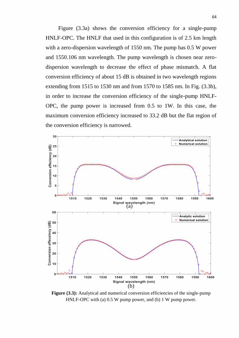
64
Figure (3.3a) shows the conversion efficiency for a single-pump
HNLF-OPC. The HNLF that used in this configuration is of 2.5 km length
with a zero-dispersion wavelength of 1550 nm. The pump has 0.5 W power
and 1550.106 nm wavelength. The pump wavelength is chosen near zero-
dispersion wavelength to decrease the effect of phase mismatch. A flat
conversion efficiency of about 15 dB is obtained in two wavelength regions
extending from 1515 to 1530 nm and from 1570 to 1585 nm. In Fig. (3.3b),
in order to increase the conversion efficiency of the single-pump HNLF-
OPC, the pump power is increased from 0.5 to 1W. In this case, the
maximum conversion efficiency increased to 33.2 dB but the flat region of
the conversion efficiency is narrowed.
Figure (3.3): Analytical and numerical conversion efficiencies of the single-pump
HNLF-OPC with (a) 0.5 W pump power, and (b) 1 W pump power.
(a)
(b)

65
The dual-pump HNLF-OPC configuration provides higher conversion
efficiency over a wider wavelength region compared to the single-pump
configuration. Figure (3.4a) compares the conversion efficiency of the dual-
pump HNLF-OPC1, calculated analytically and numerically. The HNLF has
1550 nm zero-dispersion wavelength and 0.5 km length. Other HNLF-OPC1
parameters used in this example are given in Table (3.1). In this figure, a
constant conversion efficiency of about 37 dB is obtained over a wide-
wavelength region extending from 1510 to 1590 nm.
Recall that the analytical solution is conducted under the assumption
that the pump powers remain undepleted over the fiber. However, the HNLF
length can be increased to obtain higher values of conversion efficiency. In
this case, the depletion of pump may take place and the conversion efficiency
will show a difference between the analytical and numerical solutions. For
example, in Fig. (3.4b), the length of the HNLF is increased from 0.5 to 0.8
km. The calculated numerical and analytical conversion efficiencies are 55
and 65 dB, respectively.
Figure (3.4): Analytical and numerical conversion efficiencies of HNLF-OPC1 with the
parameters values listed in Table (3.1) when the length of the HNLF is (a) 0.5 km, and
(b) 0.8 km.
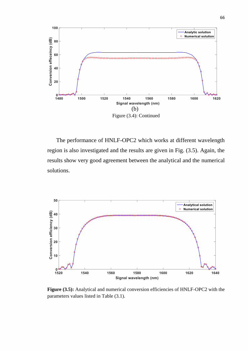
66
Figure (3.4): Continued
The performance of HNLF-OPC2 which works at different wavelength
region is also investigated and the results are given in Fig. (3.5). Again, the
results show very good agreement between the analytical and the numerical
solutions.
Figure (3.5): Analytical and numerical conversion efficiencies of HNLF-OPC2 with the
parameters values listed in Table (3.1).
(b)

67
3.4 Effect of Polarization on the FWM Process in HNLF-OPC
In the previous section, the theory assumes that the all propagating
waves are aligned linear polarization states along the fiber length. However,
this condition is difficult to be satisfied. The SOP of propagating light
randomly changes along the fiber length due to external perturbations, such
as fiber bending and asymmetrical fiber cross section. In this section, the
performance of FWM operating under general polarization states is
investigated due to its importance in fiber-optic communications.
3.4.1 Mathematical Framework
Consider the general case where the incident two pumps and signal
have the polarization angles 𝜃𝑃1, 𝜃𝑃2 and 𝜃𝑠, respectively, measured against
the TE-axis (see Fig. (3.6)). Each of these waves can be decomposed into
Transvers Electric (TE) and Transvers Magnetic (TM) modes.
Figure (3.6): Schematic diagram to analyze the effect of polarization on FWM in highly
nonlinear fiber.

68
The FWM occurs only among waves with the same polarization mode.
In this case, (Eqns. (2.13a-d)) can be rewritten for each polarization mode
leading to a set of eight coupled equations.
𝑑𝑨𝑝1𝑇𝐸(𝑧)
𝑑𝑧=
−𝛼𝑝1𝑇𝐸
2𝑨𝑝1𝑇𝐸(𝑧)
+ 𝑗𝛾𝑝1𝑇𝐸[│𝑨𝑝1𝑇𝐸(𝑧)│2 + 2│𝑨𝑝2𝑇𝐸(𝑧)│2 + 2│𝑨𝑠𝑇𝐸(𝑧)│2
+ 2│𝑨𝑖𝑇𝐸(𝑧)│2 ]𝑨𝑝1𝑇𝐸(𝑧)
+ 2𝑗𝛾𝑨𝑝2𝑇𝐸∗ (𝑧)𝑨𝑠𝑇𝐸(𝑧)𝑨𝑖𝑇𝐸(𝑧) exp(𝑗𝛥𝑘𝑇𝐸𝑧) (3.12𝑎)
𝑑𝑨𝑝1𝑇𝑀(𝑧)
𝑑𝑧=
−𝛼𝑝1𝑇𝑀
2𝑨𝑝1𝑇𝑀(𝑧)
+ 𝑗𝛾𝑝1𝑇𝑀[│𝑨𝑝1𝑇𝑀(𝑧)│2 + 2│𝑨𝑝2𝑇𝑀(𝑧)│2 + 2│𝑨𝑠𝑇𝑀(𝑧)│2
+ 2│𝑨𝑖𝑇𝑀(𝑧)│2 ]𝑨𝑝1𝑇𝑀(𝑧)
+ 2𝑗𝛾𝑨𝑝2𝑇𝑀∗ (𝑧)𝑨𝑠𝑇𝑀(𝑧)𝑨𝑖𝑇𝑀(𝑧) exp(𝑗𝛥𝑘𝑇𝑀𝑧) (3.12𝑏)
𝑑𝑨𝑝2𝑇𝐸(𝑧)
𝑑𝑧=
−𝛼𝑝2𝑇𝐸
2𝑨𝑝2𝑇𝐸(𝑧)
+ 𝑗𝛾𝑝2𝑇𝐸[2│𝑨𝑝1𝑇𝐸(𝑧)│2 + │𝑨𝑝2𝑇𝐸(𝑧)│2 + 2│𝑨𝑠𝑇𝐸(𝑧)│2
+ 2│𝑨𝑖𝑇𝐸(𝑧)│2 ]𝑨𝑝2𝑇𝐸(𝑧)
+ 2𝑗𝛾𝑨𝑝1𝑇𝐸∗ (𝑧)𝑨𝑠𝑇𝐸(𝑧)𝑨𝑖𝑇𝐸(𝑧) exp(𝑗𝛥𝑘𝑇𝐸𝑧) (3.12𝑐)
𝑑𝑨𝑝2𝑇𝑀(𝑧)
𝑑𝑧=
−𝛼𝑝2𝑇𝑀
2𝑨𝑝2𝑇𝑀(𝑧)
+ 𝑗𝛾𝑝2𝑇𝑀[2│𝑨𝑝1𝑇𝑀(𝑧)│2 + │𝑨𝑝2𝑇𝑀(𝑧)│2 + 2│𝑨𝑠𝑇𝑀(𝑧)│2
+ 2│𝑨𝑖𝑇𝑀(𝑧)│2 ]𝑨𝑝2𝑇𝑀(𝑧)
+ 2𝑗𝛾𝑨𝑝1𝑇𝑀∗ (𝑧)𝑨𝑠𝑇𝑀(𝑧)𝑨𝑖𝑇𝑀(𝑧) exp(𝑗𝛥𝑘𝑇𝑀𝑧) (3.12𝑑)
𝑑𝑨𝑠𝑇𝐸(𝑧)
𝑑𝑧=
−𝛼𝑠𝑇𝐸
2𝑨𝑠𝑇𝐸(𝑧)
+ 𝑗𝛾𝑠𝑇𝐸[2│𝑨𝑝1𝑇𝐸(𝑧)│2 + 2│𝑨𝑝2𝑇𝐸(𝑧)│2 + │𝑨𝑠𝑇𝐸(𝑧)│2
+ 2│𝑨𝑖𝑇𝐸(𝑧)│2 ]𝑨𝑠𝑇𝐸(𝑧)
+ 2𝑗𝛾 𝑨𝑖𝑇𝐸∗ (𝑧)𝑨𝑝1𝑇𝐸(𝑧)𝑨𝑝2𝑇𝐸(𝑧) exp(−𝑗𝛥𝑘𝑇𝐸𝑧) (3.12𝑒)

69
𝑑𝑨𝑠𝑇𝑀(𝑧)
𝑑𝑧=
−𝛼𝑠𝑇𝑀
2𝑨𝑠𝑇𝑀(𝑧)
+ 𝑗𝛾𝑠𝑇𝑀[2│𝑨𝑝1𝑇𝑀(𝑧)│2 + 2│𝑨𝑝2𝑇𝑀(𝑧)│2 + │𝑨𝑠𝑇𝑀(𝑧)│2
+ 2│𝑨𝑖𝑇𝑀(𝑧)│2 ]𝑨𝑠𝑇𝑀(𝑧)
+ 2𝑗𝛾 𝑨𝑖𝑇𝑀∗ (𝑧)𝑨𝑝1𝑇𝑀(𝑧)𝑨𝑝2𝑇𝑀(𝑧) exp(−𝑗𝛥𝑘𝑇𝑀𝑧) (3.12𝑓)
𝑑𝑨𝑖𝑇𝐸(𝑧)
𝑑𝑧=
−𝛼𝑖𝑇𝐸
2𝑨𝑖𝑇𝐸(𝑧)
+ 𝑗𝛾𝑖𝑇𝐸[2│𝑨𝑝1𝑇𝐸(𝑧)│2 + 2│𝑨𝑝2𝑇𝐸(𝑧)│2 + 2│𝑨𝑠𝑇𝐸(𝑧)│2
+ │𝑨𝑖𝑇𝐸(𝑧)│2 ]𝑨𝑖𝑇𝐸(𝑧)
+ 2𝑗𝛾 𝑨𝑠𝑇𝐸∗ (𝑧)𝑨𝑝1𝑇𝐸(𝑧)𝑨𝑝2𝑇𝐸(𝑧) exp(−𝑗𝛥𝑘𝑇𝐸𝑧) (3.12𝑔)
𝑑𝑨𝑖𝑇𝑀(𝑧)
𝑑𝑧=
−𝛼𝑖𝑇𝑀
2𝑨𝑖𝑇𝑀(𝑧)
+ 𝑗𝛾𝑖𝑇𝑀[2│𝑨𝑝1𝑇𝑀(𝑧)│2 + 2│𝑨𝑝2𝑇𝑀(𝑧)│2 + 2│𝑨𝑠𝑇𝑀(𝑧)│2
+ │𝑨𝑖𝑇𝑀(𝑧)│2 ]𝑨𝑖𝑇𝑀(𝑧)
+ 2𝑗𝛾 𝑨𝑠𝑇𝑀∗ (𝑧)𝑨𝑝1𝑇𝑀(𝑧)𝑨𝑝2𝑇𝑀(𝑧) exp(−𝑗𝛥𝑘𝑇𝑀𝑧) (3.12ℎ)
In Eqns. (3.12a-h), the subscript TE (TM) denotes TE (TM) wave
component. The TE and TM wave components of the two pumps and signal
powers coupled to the HNLF can be expressed as
𝑃𝑃1𝑇𝐸(0) = 𝐶𝑇𝐸 𝑃𝑃10 𝑐𝑜𝑠2(𝜃𝑃1) (3.13𝑎)
𝑃𝑃1𝑇𝑀(0) = 𝐶𝑇𝑀 𝑃𝑃10 𝑠𝑖𝑛2(𝜃𝑃1) (3.13𝑏)
𝑃𝑃2𝑇𝐸(0) = 𝐶𝑇𝐸 𝑃𝑃20 𝑐𝑜𝑠2(𝜃𝑃2) (3.13𝑐)
𝑃𝑃2𝑇𝑀(0) = 𝐶𝑇𝑀 𝑃𝑃20 𝑠𝑖𝑛2(𝜃𝑃2) (3.13𝑑)
𝑃𝑠𝑇𝐸(0) = 𝐶𝑇𝐸 𝑃𝑠0 𝑐𝑜𝑠2(𝜃𝑠) (3.13𝑒)
𝑃𝑠𝑇𝑀(0) = 𝐶𝑇𝑀 𝑃𝑠0 𝑠𝑖𝑛2(𝜃𝑠) (3.13𝑓)
where 𝐶𝑇𝐸 (𝐶𝑇𝑀) is the relative coupling efficiency for TE (TM) mode, and
the linear phase mismatch for TE (TM) wave components are given by
70
𝛥𝑘𝑇𝐸 = 𝛽𝑠𝑇𝐸 + 𝛽𝑐𝑇𝐸 − 𝛽𝑃1𝑇𝐸 − 𝛽𝑃2𝑇𝐸 (3.14𝑎)
𝛥𝑘𝑇𝑀 = 𝛽𝑠𝑇𝑀 + 𝛽𝑐𝑇𝑀 − 𝛽𝑃1𝑇𝑀 − 𝛽𝑃2𝑇𝑀 (3.14𝑏)
It can be considered that all the propagating waves are in the same
wavelength region. Therefore, the linear-loss coefficients of all the waves
are almost equal (𝛼𝑝1𝑇𝐸 = 𝛼𝑝1𝑇𝑀 = 𝛼𝑝2𝑇𝐸 = 𝛼𝑝2𝑇𝑀 = 𝛼𝑠𝑇𝐸 = 𝛼𝑠𝑇𝑀 =
𝛼𝑖𝑇𝐸 = 𝛼𝑖𝑇𝑀 = 𝛼). Further, the nonlinear parameters can be assumed equal
for all the waves too (𝛾𝑝1𝑇𝐸 = 𝛾𝑝1𝑇𝑀 = 𝛾𝑝2𝑇𝐸 = 𝛾𝑝2𝑇𝑀 = 𝛾𝑠𝑇𝐸 = 𝛾𝑠𝑇𝑀 =
𝛾𝑖𝑇𝐸 = 𝛾𝑖𝑇𝑀 = 𝛾).
3.4.2 Applying Practical Assumptions
Exact analytical solution of Eqns. (3.12a-h) is very difficult because of
their complexity. However, some practical assumptions must be taken into
account to get the approximate analytical solution
i) The effects of SPM and XPM are negligible.
ii) The optical power of the two pump waves control the fiber
nonlinearity
iii) The pump powers remain undepleted during the FWM process.
iv) The effective attenuation coefficient 𝛼 is negligible.
Under these assumptions, Eqns. (3.12a-d) can be simplified to
𝑑𝑨𝑝1𝑇𝐸(𝑧)
𝑑𝑧= 𝑗𝛾[𝑃𝑃1𝑇𝐸 + 2𝑃𝑃2𝑇𝐸] 𝑨𝑝1𝑇𝐸(𝑧) (3.15𝑎)
𝑑𝑨𝑝1𝑇𝑀(𝑧)
𝑑𝑧= 𝑗𝛾[𝑃𝑃1𝑇𝑀 + 2𝑃𝑃2𝑇𝑀]𝑨𝑝1𝑇𝑀(𝑧) (3.15𝑏)
𝑑𝑨𝑝2𝑇𝐸(𝑧)
𝑑𝑧= 𝑗𝛾[2𝑃𝑃1𝑇𝐸 + 𝑃𝑃2𝑇𝐸]𝑨𝑝2𝑇𝐸(𝑧) (3.15𝑐)
𝑑𝑨𝑝2𝑇𝑀(𝑧)
𝑑𝑧= 𝑗𝛾[2𝑃𝑃1𝑇𝑀 + 𝑃𝑃2𝑇𝑀]𝑨𝑝2𝑇𝑀(𝑧) (3.15𝑑)

71
where│𝑨𝑝𝑗𝑘(𝑧)│2 = 𝑃𝑃𝑗𝑘, (𝑗 = 1. 2 𝑎𝑛𝑑 𝑘 = 𝑇𝐸. 𝑇𝑀) are the pump
powers of the corresponding components. Integrating both sides of Eqns.
(3.15a-d) yields
∫1
𝑨𝑝1𝑇𝐸(𝑧)𝑑𝑨𝑝1𝑇𝐸(𝑧) = ∫ 𝑗𝛾[𝑃𝑃1𝑇𝐸 + 2𝑃𝑃2𝑇𝐸] 𝑑𝑧 (3.16𝑎)
∫1
𝑨𝑝1𝑇𝑀(𝑧)𝑑𝑨𝑝1𝑇𝑀(𝑧) = ∫ 𝑗𝛾[𝑃𝑃1𝑇𝑀 + 2𝑃𝑃2𝑇𝑀] 𝑑𝑧 (3.16𝑏)
∫1
𝑨𝑝2𝑇𝐸(𝑧)𝑑𝑨𝑝2𝑇𝐸(𝑧) = ∫ 𝑗𝛾[2𝑃𝑃1𝑇𝐸 + 𝑃𝑃2𝑇𝐸] 𝑑𝑧 (3.16𝑐)
∫1
𝑨𝑝2𝑇𝑀(𝑧)𝑑𝑨𝑝2𝑇𝑀(𝑧) = ∫ 𝑗𝛾[2𝑃𝑃1𝑇𝑀 + 𝑃𝑃2𝑇𝑀] 𝑑𝑧 (3.16𝑑)
Equations (3.16a-d) can be solved as follow
𝑙𝑛 (𝑨𝑝1𝑇𝐸(𝑧)) = 𝑗𝛾[𝑃𝑃1𝑇𝐸 + 2𝑃𝑃2𝑇𝐸] 𝑧 + 𝐶10 (3.17𝑎)
𝑙𝑛 (𝑨𝑝1𝑇𝑀(𝑧)) = 𝑗𝛾[𝑃𝑃1𝑇𝑀 + 2𝑃𝑃2𝑇𝑀] 𝑧 + 𝐶20 (3.17𝑏)
𝑙𝑛 (𝑨𝑝2𝑇𝐸(𝑧)) = 𝑗𝛾[2𝑃𝑃1𝑇𝐸 + 𝑃𝑃2𝑇𝐸] 𝑧 + 𝐶30 (3.17𝑐)
𝑙𝑛 (𝑨𝑝2𝑇𝑀(𝑧)) = 𝑗𝛾[2𝑃𝑃1𝑇𝑀 + 𝑃𝑃2𝑇𝑀] 𝑧 + 𝐶40 (3.17𝑑)
where 𝐶𝑗0. (𝑗 = 1 − 4) are the integration constants. Let 𝐶𝑗1 = exp(𝐶𝑗0),
then by taking exponential for both sides to Eqns. (3.17a-d) yields
𝑨𝑝1𝑇𝐸(𝑧) = 𝐶11 𝑒𝑥𝑝(𝑗𝛾[𝑃𝑃1𝑇𝐸 + 2𝑃𝑃2𝑇𝐸] 𝑧) (3.18𝑎)
𝑨𝑝1𝑇𝑀(𝑧) = 𝐶12 𝑒𝑥𝑝(𝑗𝛾[𝑃𝑃1𝑇𝑀 + 2𝑃𝑃2𝑇𝑀] 𝑧) (3.18𝑏)
𝑨𝑝2𝑇𝐸(𝑧) = 𝐶13 𝑒𝑥𝑝(𝑗𝛾[2𝑃𝑃1𝑇𝐸 + 𝑃𝑃2𝑇𝐸] 𝑧) (3.18𝑐)
𝑨𝑝2𝑇𝑀(𝑧) = 𝐶14 𝑒𝑥𝑝(𝑗𝛾[2𝑃𝑃1𝑇𝑀 + 𝑃𝑃2𝑇𝑀] 𝑧) (3.18𝑑)
where 𝐶11 = 𝑨𝑝1𝑇𝐸(0), 𝐶12 = 𝑨𝑝1𝑇𝑀(0), 𝐶13 = 𝑨𝑝2𝑇𝐸(0), and 𝐶14 =
𝑨𝑝2𝑇𝑀(0) are the integration constants obtained from the initial conditions

72
when 𝑧 = 0 is applied to Eqns. (3.18a-d). Then, inserting these values into
Eqns. (3.18a-d) produces
𝑨𝑝1𝑇𝐸(𝑧) = 𝑨𝑝1𝑇𝐸(0) 𝑒𝑥𝑝(𝑗𝛾[𝑃𝑃1𝑇𝐸 + 2𝑃𝑃2𝑇𝐸] 𝑧) (3.19𝑎)
𝑨𝑝1𝑇𝑀(𝑧) = 𝑨𝑝1𝑇𝑀(0) 𝑒𝑥𝑝(𝑗𝛾[𝑃𝑃1𝑇𝑀 + 2𝑃𝑃2𝑇𝑀] 𝑧) (3.19𝑏)
𝑨𝑝2𝑇𝐸(𝑧) = 𝑨𝑝2𝑇𝐸(0) 𝑒𝑥𝑝(𝑗𝛾[2𝑃𝑃1𝑇𝐸 + 𝑃𝑃2𝑇𝐸] 𝑧) (3.19𝑐)
𝑨𝑝2𝑇𝑀(𝑧) = 𝑨𝑝2𝑇𝑀(0) 𝑒𝑥𝑝(𝑗𝛾[2𝑃𝑃1𝑇𝑀 + 𝑃𝑃2𝑇𝑀] 𝑧) (3.19𝑑)
The complex conjugations of Eqns. (3.19a-d) can be written as
𝑨𝑝1𝑇𝐸∗ (𝑧) = 𝑨𝑝1𝑇𝐸
∗ (0) 𝑒𝑥𝑝(−𝑗𝛾[𝑃𝑃1𝑇𝐸 + 2𝑃𝑃2𝑇𝐸] 𝑧) (3.20𝑎)
𝑨𝑝1𝑇𝑀∗ (𝑧) = 𝑨𝑝1𝑇𝑀
∗ (0) 𝑒𝑥𝑝(−𝑗𝛾[𝑃𝑃1𝑇𝑀 + 2𝑃𝑃2𝑇𝑀] 𝑧) (3.20𝑏)
𝑨𝑝2𝑇𝐸∗ (𝑧) = 𝑨𝑝2𝑇𝐸
∗ (0) 𝑒𝑥𝑝(−𝑗𝛾[2𝑃𝑃1𝑇𝐸 + 𝑃𝑃2𝑇𝐸] 𝑧) (3.20𝑐)
𝑨𝑝2𝑇𝑀∗ (𝑧) = 𝑨𝑝2𝑇𝑀
∗ (0) 𝑒𝑥𝑝(−𝑗𝛾[2𝑃𝑃1𝑇𝑀 + 𝑃𝑃2𝑇𝑀] 𝑧) (3.20𝑑)
Now, to solve Eqns. (3.12e-h), the same previous assumptions are
applied and these equations can be written in the following forms
𝑑𝑨𝑠𝑇𝐸(𝑧)
𝑑𝑧= 2𝑗𝛾([𝑃𝑃1𝑇𝐸 + 𝑃𝑃2𝑇𝐸]𝑨𝑠𝑇𝐸(𝑧)
+ 𝑨𝑖𝑇𝐸∗ (𝑧)𝑨𝑝1𝑇𝐸(𝑧)𝑨𝑝2𝑇𝐸(𝑧) exp(−𝑗𝛥𝑘𝑇𝐸𝑧)) (3.21𝑎)
𝑑𝑨𝑠𝑇𝑀(𝑧)
𝑑𝑧= 2𝑗𝛾([𝑃𝑃1𝑇𝑀 + 𝑃𝑃2𝑇𝑀]𝑨𝑠𝑇𝑀(𝑧)
+ 𝑨𝑖𝑇𝑀∗ (𝑧)𝑨𝑝1𝑇𝑀(𝑧)𝑨𝑝2𝑇𝑀(𝑧) exp(−𝑗𝛥𝑘𝑇𝑀𝑧)) (3.21𝑏)
𝑑𝑨𝑖𝑇𝐸∗ (𝑧)
𝑑𝑧= −2𝑗𝛾([𝑃𝑃1𝑇𝐸 + 𝑃𝑃2𝑇𝐸]𝑨𝑖𝑇𝐸(𝑧)
+ 𝑨𝑠𝑇𝐸(𝑧) 𝑨𝑝1𝑇𝐸∗ (𝑧) 𝑨𝑝2𝑇𝐸
∗ (𝑧) exp(𝑗𝛥𝑘𝑇𝐸𝑧)) (3.21𝑐)
𝑑𝑨𝑖𝑇𝑀∗ (𝑧)
𝑑𝑧= −2𝑗𝛾([𝑃𝑃1𝑇𝑀 + 𝑃𝑃2𝑇𝑀]𝑨𝑖𝑇𝑀(𝑧)
+ 𝑨𝑠𝑇𝑀(𝑧) 𝑨𝑝1𝑇𝑀∗ (𝑧) 𝑨𝑝2𝑇𝑀
∗ (𝑧) exp(𝑗𝛥𝑘𝑇𝑀𝑧)) (3.21𝑑)

73
Substituting Eqns. (3.19a and 3.19c) into Eqn. (3.21a), Eqns. (3.19b
and 3.19d) into Eqn. (3.19b), Eqns. (3.20a and 3.20c) into Eqn. (3.21c), and
Eqns. (3.20b and 3.20d) into Eqn. (3.21d) yields
𝑑𝑨𝑠𝑇𝐸(𝑧)
𝑑𝑧= 2𝑗𝛾([𝑃𝑃1𝑇𝐸 + 𝑃𝑃2𝑇𝐸]𝑨𝑠𝑇𝐸(𝑧) + 𝑨𝑖𝑇𝐸
∗ (𝑧)𝑨𝑝1𝑇𝐸(0) 𝑒𝑥𝑝(𝑗𝛾[𝑃𝑃1𝑇𝐸 +
2𝑃𝑃2𝑇𝐸] 𝑧)𝑨𝑝2𝑇𝐸(0) 𝑒𝑥𝑝(𝑗𝛾[2𝑃𝑃1𝑇𝐸 + 𝑃𝑃2𝑇𝐸] 𝑧) exp(−𝑗𝛥𝑘𝑇𝐸𝑧)) (3.22𝑎)
𝑑𝑨𝑠𝑇𝑀(𝑧)
𝑑𝑧= 2𝑗𝛾([𝑃𝑃1𝑇𝑀 + 𝑃𝑃2𝑇𝑀]𝑨𝑠𝑇𝑀(𝑧) + 𝑨𝑖𝑇𝑀
∗ (𝑧)𝑨𝑝1𝑇𝑀(0) 𝑒𝑥𝑝(𝑗𝛾[𝑃𝑃1𝑇𝑀 +
2𝑃𝑃2𝑇𝑀] 𝑧)𝑨𝑝2𝑇𝑀(0) 𝑒𝑥𝑝(𝑗𝛾[2𝑃𝑃1𝑇𝑀 + 𝑃𝑃2𝑇𝑀] 𝑧) exp(−𝑗𝛥𝑘𝑇𝑀𝑧)) (3.22𝑏)
𝑑𝑨𝑖𝑇𝐸∗ (𝑧)
𝑑𝑧= −2𝑗𝛾([𝑃𝑃1𝑇𝐸 + 𝑃𝑃2𝑇𝐸]𝑨𝑖𝑇𝐸(𝑧) + 𝑨𝑠𝑇𝐸(𝑧) 𝑨𝑝1𝑇𝐸
∗ (0) 𝑒𝑥𝑝(−𝑗𝛾[𝑃𝑃1𝑇𝐸 +
2𝑃𝑃2𝑇𝐸] 𝑧) 𝑨𝑝2𝑇𝐸∗ (0) 𝑒𝑥𝑝(−𝑗𝛾[2𝑃𝑃1𝑇𝐸 +
𝑃𝑃2𝑇𝐸] 𝑧) exp(𝑗𝛥𝑘𝑇𝐸𝑧)) (3.22𝑐)
𝑑𝑨𝑖𝑇𝑀∗ (𝑧)
𝑑𝑧= −2𝑗𝛾([𝑃𝑃1𝑇𝑀 + 𝑃𝑃2𝑇𝑀]𝑨𝑖𝑇𝑀(𝑧) + 𝑨𝑠𝑇𝑀(𝑧)𝑨𝑝1𝑇𝑀
∗ (0)𝑒𝑥𝑝(−𝑗𝛾[𝑃𝑃1𝑇𝑀 +
2𝑃𝑃2𝑇𝑀] 𝑧) 𝑨𝑝2𝑇𝑀∗ (0)𝑒𝑥𝑝(−𝑗𝛾[2𝑃𝑃1𝑇𝑀 + 𝑃𝑃2𝑇𝑀] 𝑧) 𝑒𝑥𝑝(𝑗𝛥𝑘𝑇𝑀𝑧)) (3.22𝑑)
Simplifying Eqns. (3.22a-d) mathematically yields
𝑑𝑨𝑠𝑇𝐸(𝑧)
𝑑𝑧= 2𝑗𝛾([𝑃𝑃1𝑇𝐸 + 𝑃𝑃2𝑇𝐸]𝑨𝑠𝑇𝐸(𝑧)
+ 𝑨𝑖𝑇𝐸∗ (𝑧)𝑨𝑝1𝑇𝐸(0) 𝑨𝑝2𝑇𝐸(0) exp(−𝑗𝑅𝑇𝐸𝑧)) (3.23𝑎)
𝑑𝑨𝑠𝑇𝑀(𝑧)
𝑑𝑧= 2𝑗𝛾([𝑃𝑃1𝑇𝑀 + 𝑃𝑃2𝑇𝑀]𝑨𝑠𝑇𝑀(𝑧)
+ 𝑨𝑖𝑇𝑀∗ (𝑧)𝑨𝑝1𝑇𝑀(0) 𝑨𝑝2𝑇𝑀(0) exp(−𝑗𝑅𝑇𝑀𝑧)) (3.23𝑏)
𝑑𝑨𝑖𝑇𝐸∗ (𝑧)
𝑑𝑧= −2𝑗𝛾([𝑃𝑃1𝑇𝐸 + 𝑃𝑃2𝑇𝐸]𝑨𝑖𝑇𝐸(𝑧)
+ 𝑨𝑠𝑇𝐸(𝑧) 𝑨𝑝1𝑇𝐸∗ (0) 𝑨𝑝2𝑇𝐸
∗ (0) exp(𝑗𝑅𝑇𝐸𝑧)) (3.23𝑐)
𝑑𝑨𝑖𝑇𝑀∗ (𝑧)
𝑑𝑧= −2𝑗𝛾([𝑃𝑃1𝑇𝑀 + 𝑃𝑃2𝑇𝑀]𝑨𝑖𝑇𝑀(𝑧)
+ 𝑨𝑠𝑇𝑀(𝑧) 𝑨𝑝1𝑇𝑀∗ (0) 𝑨𝑝2𝑇𝑀
∗ (0) exp(𝑗𝑅𝑇𝑀𝑧)) (3.23𝑑)
where

74
𝑅𝑇𝐸 = 𝛥𝑘𝑇𝐸 − 3𝛾(𝑃𝑃1𝑇𝐸 + 𝑃𝑃2𝑇𝐸) (3.24𝑎)
𝑅𝑇𝑀 = 𝛥𝑘𝑇𝑀 − 3𝛾(𝑃𝑃1𝑇𝑀 + 𝑃𝑃2𝑇𝑀) (3.24𝑏)
3.4.3 Variation of Signal and Idler Waveforms Along the Fiber
To solve Eqns. (3.23a-d), the following equations are introduced
𝑩𝑠𝑇𝐸(𝑧) = 𝑨𝑠𝑇𝐸(𝑧) 𝑒𝑥𝑝(−2𝑗𝛾[𝑃𝑃1𝑇𝐸 + 𝑃𝑃2𝑇𝐸]𝑧) (3.25𝑎)
𝑩𝑠𝑇𝑀(𝑧) = 𝑨𝑠𝑇𝑀(𝑧) 𝑒𝑥𝑝(−2𝑗𝛾[𝑃𝑃1𝑇𝑀 + 𝑃𝑃2𝑇𝑀]𝑧) (3.25𝑏)
𝑩𝑖𝑇𝐸∗ (𝑧) = 𝑨𝑖𝑇𝐸
∗ (𝑧) 𝑒𝑥𝑝(2𝑗𝛾[𝑃𝑃1𝑇𝐸 + 𝑃𝑃2𝑇𝐸]𝑧) (3.25𝑐)
𝑩𝑖𝑇𝑀∗ (𝑧) = 𝑨𝑖𝑇𝑀
∗ (𝑧) 𝑒𝑥𝑝(2𝑗𝛾[𝑃𝑃1𝑇𝑀 + 𝑃𝑃2𝑇𝑀]𝑧) (3.25𝑑)
Differentiating Eqns. (3.25a-d) with respect to z gives
𝑑𝑩𝑠𝑇𝐸(𝑧)
𝑑𝑧= 𝑨𝑠𝑇𝐸(𝑧) (−2𝑗𝛾[𝑃𝑃1𝑇𝐸 + 𝑃𝑃2𝑇𝐸]) 𝑒𝑥𝑝(−2𝑗𝛾[𝑃𝑃1𝑇𝐸 + 𝑃𝑃2𝑇𝐸]𝑧)
+𝑑𝑨𝑠𝑇𝐸(𝑧)
𝑑𝑧 𝑒𝑥𝑝(−2𝑗𝛾[𝑃𝑃1𝑇𝐸 + 𝑃𝑃2𝑇𝐸]𝑧) (3.26𝑎)
𝑑𝑩𝑠𝑇𝑀(𝑧)
𝑑𝑧= 𝑨𝑠𝑇𝑀(𝑧) (−2𝑗𝛾[𝑃𝑃1𝑇𝑀 + 𝑃𝑃2𝑇𝑀]) 𝑒𝑥𝑝(−2𝑗𝛾[𝑃𝑃1𝑇𝑀 + 𝑃𝑃2𝑇𝑀]𝑧)
+𝑑𝑨𝑠𝑇𝑀(𝑧)
𝑑𝑧 𝑒𝑥𝑝(−2𝑗𝛾[𝑃𝑃1𝑇𝑀 + 𝑃𝑃2𝑇𝑀]𝑧) (3.26𝑏)
𝑑𝑩𝑖𝑇𝐸∗ (𝑧)
𝑑𝑧= 𝑨𝑖𝑇𝐸
∗ (𝑧) (2𝑗𝛾[𝑃𝑃1𝑇𝐸 + 𝑃𝑃2𝑇𝐸]) 𝑒𝑥𝑝(2𝑗𝛾[𝑃𝑃1𝑇𝐸 + 𝑃𝑃2𝑇𝐸]𝑧)
+ 𝑑𝑨𝑖𝑇𝐸
∗ (𝑧)
𝑑𝑧 𝑒𝑥𝑝(2𝑗𝛾[𝑃𝑃1𝑇𝐸 + 𝑃𝑃2𝑇𝐸]𝑧) (3.26𝑐)
𝑑𝑩𝑖𝑇𝑀∗ (𝑧)
𝑑𝑧= 𝑨𝑖𝑇𝑀
∗ (𝑧) (2𝑗𝛾[𝑃𝑃1𝑇𝑀 + 𝑃𝑃2𝑇𝑀]) 𝑒𝑥𝑝(2𝑗𝛾[𝑃𝑃1𝑇𝑀 + 𝑃𝑃2𝑇𝑀]𝑧)
+ 𝑑𝑨𝑖𝑇𝑀
∗ (𝑧)
𝑑𝑧 𝑒𝑥𝑝(2𝑗𝛾[𝑃𝑃1𝑇𝑀 + 𝑃𝑃2𝑇𝑀]𝑧) (3.26𝑑)
Substituting Eqns. (3.23a-d) into Eqns. (3.26a-d) yields

75
𝑑𝑩𝑠𝑇𝐸(𝑧)
𝑑𝑧= 𝑨𝑠𝑇𝐸(𝑧) (−2𝑗𝛾[𝑃𝑃1𝑇𝐸 + 𝑃𝑃2𝑇𝐸]) 𝑒𝑥𝑝(−2𝑗𝛾[𝑃𝑃1𝑇𝐸 + 𝑃𝑃2𝑇𝐸]𝑧)
+ 2𝑗𝛾([𝑃𝑃1𝑇𝐸 + 𝑃𝑃2𝑇𝐸]𝑨𝑠𝑇𝐸(𝑧) 𝑒𝑥𝑝(−2𝑗𝛾[𝑃𝑃1𝑇𝐸 + 𝑃𝑃2𝑇𝐸]𝑧))
+ 2𝑗𝛾 𝑨𝑖𝑇𝐸∗ (𝑧)𝑨𝑝1𝑇𝐸(0)𝑨𝑝2𝑇𝐸(0) exp(−𝑗𝜃𝑇𝐸𝑧) 𝑒𝑥𝑝(−2𝑗𝛾[𝑃𝑃1𝑇𝐸
+ 𝑃𝑃2𝑇𝐸]𝑧) (3.27𝑎)
𝑑𝑩𝑠𝑇𝑀(𝑧)
𝑑𝑧= 𝑨𝑠𝑇𝑀(𝑧) (−2𝑗𝛾[𝑃𝑃1𝑇𝑀 + 𝑃𝑃2𝑇𝑀]) 𝑒𝑥𝑝(−2𝑗𝛾[𝑃𝑃1𝑇𝑀 + 𝑃𝑃2𝑇𝑀]𝑧)
+ 2𝑗𝛾([𝑃𝑃1𝑇𝑀 + 𝑃𝑃2𝑇𝑀]𝑨𝑠𝑇𝑀(𝑧) 𝑒𝑥𝑝(−2𝑗𝛾[𝑃𝑃1𝑇𝑀 + 𝑃𝑃2𝑇𝑀]𝑧))
+ 2𝑗𝛾 𝑨𝑖𝑇𝑀∗ (𝑧)𝑨𝑝1𝑇𝑀(0)𝑨𝑝2𝑇𝑀(0) exp(−𝑗𝜃𝑇𝑀𝑧) 𝑒𝑥𝑝(−2𝑗𝛾[𝑃𝑃1𝑇𝑀
+ 𝑃𝑃2𝑇𝑀]𝑧) (3.27𝑏)
𝑑𝑩𝑖𝑇𝐸∗ (𝑧)
𝑑𝑧= 𝑨𝑖𝑇𝐸
∗ (𝑧) (2𝑗𝛾[𝑃𝑃1𝑇𝐸 + 𝑃𝑃2𝑇𝐸]) 𝑒𝑥𝑝(2𝑗𝛾[𝑃𝑃1𝑇𝐸 + 𝑃𝑃2𝑇𝐸]𝑧)
− 2𝑗𝛾[𝑃𝑃1𝑇𝐸 + 𝑃𝑃2𝑇𝐸]𝑨𝑖𝑇𝐸∗ (𝑧) 𝑒𝑥𝑝(2𝑗𝛾[𝑃𝑃1𝑇𝐸 + 𝑃𝑃2𝑇𝐸]𝑧)
− 2𝑗𝛾𝑨𝑠𝑇𝐸(𝑧) 𝑨𝑝1𝑇𝐸∗ (0) 𝑨𝑝2𝑇𝐸
∗ (0) exp(𝑗𝜃𝑇𝐸𝑧) 𝑒𝑥𝑝(2𝑗𝛾[𝑃𝑃1𝑇𝐸
+ 𝑃𝑃2𝑇𝐸]𝑧) (3.27𝑐)
𝑑𝑩𝑖𝑇𝑀∗ (𝑧)
𝑑𝑧= 𝑨𝑖𝑇𝑀
∗ (𝑧) (2𝑗𝛾[𝑃𝑃1𝑇𝑀 + 𝑃𝑃2𝑇𝑀]) 𝑒𝑥𝑝(2𝑗𝛾[𝑃𝑃1𝑇𝑀 + 𝑃𝑃2𝑇𝑀]𝑧)
− 2𝑗𝛾 [𝑃𝑃1𝑇𝑀 + 𝑃𝑃2𝑇𝑀]𝑨𝑖𝑇𝑀∗ (𝑧) 𝑒𝑥𝑝(2𝑗𝛾[𝑃𝑃1𝑇𝑀 + 𝑃𝑃2𝑇𝑀]𝑧)
− 2𝑗𝛾𝑨𝑠𝑇𝑀(𝑧) 𝑨𝑝1𝑇𝑀∗ (0) 𝑨𝑝2𝑇𝑀
∗ (0) exp(𝑗𝜃𝑇𝑀𝑧)𝑒𝑥𝑝(2𝑗𝛾[𝑃𝑃1𝑇𝑀
+ 𝑃𝑃2𝑇𝑀]𝑧) (3.27𝑑)
Simplifying Eqns. (3.27a-d) produces
𝑑𝑩𝑠𝑇𝐸(𝑧)
𝑑𝑧= 2𝑗𝛾 𝑨𝑖𝑇𝐸
∗ (𝑧)𝑨𝑝1𝑇𝐸(0)𝑨𝑝2𝑇𝐸(0) exp(−𝑗𝑅𝑇𝐸𝑧) 𝑒𝑥𝑝(−2𝑗𝛾[𝑃𝑃1𝑇𝐸
+ 𝑃𝑃2𝑇𝐸]𝑧) (3.28𝑎)
𝑑𝑩𝑠𝑇𝑀(𝑧)
𝑑𝑧= 2𝑗𝛾 𝑨𝑖𝑇𝑀
∗ (𝑧)𝑨𝑝1𝑇𝑀(0)𝑨𝑝2𝑇𝑀(0) exp(−𝑗𝑅𝑇𝑀𝑧) 𝑒𝑥𝑝(−2𝑗𝛾[𝑃𝑃1𝑇𝑀
+ 𝑃𝑃2𝑇𝑀]𝑧) (3.28𝑏)

76
𝑑𝑩𝑖𝑇𝐸∗ (𝑧)
𝑑𝑧= −2𝑗𝛾𝑨𝑠𝑇𝐸(𝑧) 𝑨𝑝1𝑇𝐸
∗ (0) 𝑨𝑝2𝑇𝐸∗ (0) exp(𝑗𝑅𝑇𝐸𝑧) 𝑒𝑥𝑝(2𝑗𝛾[𝑃𝑃1𝑇𝐸
+ 𝑃𝑃2𝑇𝐸]𝑧) (3.28𝑐)
𝑑𝑩𝑖𝑇𝑀∗ (𝑧)
𝑑𝑧= −2𝑗𝛾𝑨𝑠𝑇𝑀(𝑧) 𝑨𝑝1𝑇𝑀
∗ (0) 𝑨𝑝2𝑇𝑀∗ (0) exp(𝑗𝑅𝑇𝑀𝑧)𝑒𝑥𝑝(2𝑗𝛾[𝑃𝑃1𝑇𝑀
+ 𝑃𝑃2𝑇𝑀]𝑧) (3.28𝑑)
From Eqns. (3.25a-d), 𝑨𝑠𝑇𝐸(𝑧). 𝑨𝑠𝑇𝑀(𝑧). 𝑨𝑖𝑇𝐸∗ (𝑧). and 𝑨𝑖𝑇𝑀
∗ (𝑧) can
be written as
𝑨𝑠𝑇𝐸(𝑧) = 𝑩𝑠𝑇𝐸(𝑧) 𝑒𝑥𝑝(2𝑗𝛾[𝑃𝑃1𝑇𝐸 + 𝑃𝑃2𝑇𝐸]𝑧) (3.29𝑎)
𝑨𝑠𝑇𝑀(𝑧) = 𝑩𝑠𝑇𝑀(𝑧)𝑒𝑥𝑝(2𝑗𝛾[𝑃𝑃1𝑇𝑀 + 𝑃𝑃2𝑇𝑀]𝑧) (3.29𝑏)
𝑨𝑖𝑇𝐸∗ (𝑧) = 𝑩𝑖𝑇𝐸
∗ (𝑧) 𝑒𝑥𝑝(−2𝑗𝛾[𝑃𝑃1𝑇𝐸 + 𝑃𝑃2𝑇𝐸]𝑧) (3.29𝑐)
𝑨𝑖𝑇𝑀∗ (𝑧) = 𝑩𝑖𝑇𝑀
∗ (𝑧)𝑒𝑥𝑝(−2𝑗𝛾[𝑃𝑃1𝑇𝑀 + 𝑃𝑃2𝑇𝑀]𝑧) (3.29𝑑)
Substituting Eqns. (3.29a-d) into Eqns. (3.28a-d) yields
𝑑𝑩𝑠𝑇𝐸(𝑧)
𝑑𝑧= 2𝑗𝛾 𝑩𝑖𝑇𝐸
∗ (𝑧) 𝑨𝑝1𝑇𝐸(0)𝑨𝑝2𝑇𝐸(0) 𝑒𝑥𝑝(−𝑗𝑘𝑇𝐸𝑧) (3.30𝑎)
𝑑𝑩𝑠𝑇𝑀(𝑧)
𝑑𝑧= 2𝑗𝛾 𝑩𝑖𝑇𝑀
∗ (𝑧) 𝑨𝑝1𝑇𝑀(0)𝑨𝑝2𝑇𝑀(0) exp(−𝑗𝑘𝑇𝑀𝑧) (3.30𝑏)
𝑑𝑩𝑖𝑇𝐸∗ (𝑧)
𝑑𝑧= −2𝑗𝛾𝑩𝑠𝑇𝐸(𝑧) 𝑨𝑝1𝑇𝐸
∗ (0) 𝑨𝑝2𝑇𝐸∗ (0) exp(𝑗𝑘𝑇𝐸𝑧) (3.30𝑐)
𝑑𝑩𝑖𝑇𝑀∗ (𝑧)
𝑑𝑧= −2𝑗𝛾𝑩𝑠𝑇𝑀(𝑧) 𝑨𝑝1𝑇𝑀
∗ (0) 𝑨𝑝2𝑇𝑀∗ (0) exp(𝑗𝑘𝑇𝑀𝑧) (3.30𝑑)
where 𝑘𝑇𝐸 𝑎𝑛𝑑 𝑘𝑇𝑀 is the effective phase mismatch for the 𝑘𝑇𝐸 𝑎𝑛𝑑 𝑘𝑇𝑀
wave components and they are given by
𝑘𝑇𝐸 = ∆𝑘𝑇𝐸 + 𝛾(𝑃𝑃1𝑇𝐸 + 𝑃𝑃2𝑇𝐸) (3.31𝑎)
𝑘𝑇𝑀 = ∆𝑘𝑇𝑀 + 𝛾(𝑃𝑃1𝑇𝑀 + 𝑃𝑃2𝑇𝑀) (3.31𝑏)
The effective phase mismatch plays an important role in the process
of FWM and hence in its applications such as parametric amplifier and phase
conjugation. The linear phase mismatch ∆𝑘𝑇𝐸(𝑇𝑀) depends directly on the

77
interacting waves frequencies. The second part of Eqns. (3.31a) and (3.31b)
represent the nonlinear phase mismatch terms, which depend on the pumps
intensity. Better FWM performance is achieved when the effective phase
mismatch vanishes or becomes near to zero.
3.5 FWM Parametric Gain
The effective phase mismatch and the parametric gain (𝑔) are the two
parameters that can evaluate the performance of the FWM process. The
effective phase mismatch is given in the previous subsection. However, to
derive the formula of the parametric gain and to study its effect in corporation
with the effective phase mismatch on the FWM process, the previous
analytical analysis is continued. Taking the second derivative of Eqns.
(3.30a-d) with respect to z yields
𝑑2𝑩𝑠𝑇𝐸(𝑧)
𝑑𝑧2= 2𝑗𝛾 𝑨𝑝1𝑇𝐸(0)𝑨𝑝2𝑇𝐸(0) [𝑩𝑖𝑇𝐸
∗ (𝑧) (−𝑗𝑘𝑇𝐸)𝑒𝑥𝑝(−𝑗𝑘𝑇𝐸𝑧)
+𝑑𝑩𝑖𝑇𝐸
∗ (𝑧)
𝑑𝑧 𝑒𝑥𝑝(−𝑗𝑘𝑇𝐸𝑧) ] (3.32𝑎)
𝑑2𝑩𝑠𝑇𝑀(𝑧)
𝑑𝑧2= 2𝑗𝛾 𝑨𝑝1𝑇𝑀(0)𝑨𝑝2𝑇𝑀(0) [𝑩𝑖𝑇𝑀
∗ (𝑧) (−𝑗𝑘𝑇𝑀)𝑒𝑥𝑝(−𝑗𝑘𝑇𝑀𝑧)
+𝑑𝐵𝑖𝑇𝑀
∗ (𝑧)
𝑑𝑧 𝑒𝑥𝑝(−𝑗𝑘𝑇𝑀𝑧) ] (3.32𝑏)
𝑑2𝑩𝑖𝑇𝐸∗ (𝑧)
𝑑𝑧2= −2𝑗𝛾 𝑨𝑝1𝑇𝐸
∗ (0) 𝑨𝑝2𝑇𝐸∗ (0) [𝑩𝑠𝑇𝐸(𝑧) (𝑗𝑘𝑇𝐸) exp(𝑗𝑘𝑇𝐸𝑧)
+𝑑𝑩𝑠𝑇𝐸(𝑧)
𝑑𝑧 exp(𝑗𝑘𝑇𝐸𝑧)] (3.32𝑐)
𝑑2𝑩𝑖𝑇𝑀∗ (𝑧)
𝑑𝑧2= −2𝑗𝛾 𝑨𝑝1𝑇𝑀
∗ (0) 𝑨𝑝2𝑇𝑀∗ (0) [𝑩𝑠𝑇𝑀(𝑧) (𝑗𝑘𝑇𝑀) exp(𝑗𝑘𝑇𝑀𝑧)
+𝑑𝑩𝑠𝑇𝑀(𝑧)
𝑑𝑧 exp(𝑗𝑘𝑇𝑀𝑧)] (3.32𝑑)

78
From Eqns. (3.30a-d), one can get the following expressions
𝑩𝑖𝑇𝐸∗ (𝑧) =
1
2𝑗𝛾 𝑨𝑝1𝑇𝐸(0)𝑨𝑝2𝑇𝐸(0) 𝑒𝑥𝑝(−𝑗𝑘𝑇𝐸𝑧) 𝑑𝑩𝑠𝑇𝐸(𝑧)
𝑑𝑧 (3.33𝑎)
𝑩𝑖𝑇𝑀∗ (𝑧) =
1
2𝑗𝛾 𝑨𝑝1𝑇𝑀(0)𝑨𝑝2𝑇𝑀(0) exp(−𝑗𝑘𝑇𝑀𝑧) 𝑑𝑩𝑠𝑇𝑀(𝑧)
𝑑𝑧 (3.33𝑏)
𝑩𝑠𝑇𝐸(𝑧) =−1
2𝑗𝛾 𝑨𝑝1𝑇𝐸∗ (0) 𝑨𝑝2𝑇𝐸
∗ (0) exp(𝑗𝑘𝑇𝐸𝑧) 𝑑𝑩𝑖𝑇𝐸
∗ (𝑧)
𝑑𝑧 (3.33𝑐)
𝑩𝑠𝑇𝑀(𝑧) =−1
2𝑗𝛾 𝑨𝑝1𝑇𝑀∗ (0) 𝑨𝑝2𝑇𝑀
∗ (0) exp(𝑗𝑘𝑇𝑀𝑧)
𝑑𝑩𝑖𝑇𝑀∗ (𝑧)
𝑑𝑧 (3.33𝑑)
Substituting Eqns. (3.33a) and (3.30c) into Eqn. (3.32a), Eqns. (3.33b)
and (3.30d) into Eqn. (3.32b), Eqns. (3.33c) and (3.30a) into Eqn. (3.32c),
and Eqns. (3.33d) and (3.30b) into Eqn. (3.32d) yields
𝑑2𝑩𝑠𝑇𝐸(𝑧)
𝑑𝑧2+ 𝑗𝑘𝑇𝐸
𝑑𝑩𝑠𝑇𝐸(𝑧)
𝑑𝑧− 4𝛾2𝑃𝑃1𝑇𝐸 𝑃𝑃2𝑇𝐸 𝐵𝑠𝑇𝐸(𝑧) = 0 (3.34𝑎)
𝑑2𝑩𝑠𝑇𝑀(𝑧)
𝑑𝑧2 + 𝑗𝑘𝑇𝐸
𝑑𝑩𝑠𝑇𝑀(𝑧)
𝑑𝑧− 4𝛾2𝑃𝑃1𝑇𝑀 𝑃𝑃2𝑇𝑀 𝐵𝑠𝑇𝑀(𝑧) = 0 (3.34𝑏)
𝑑2𝑩𝑖𝑇𝐸∗ (𝑧)
𝑑𝑧2− 𝑗𝑘𝑇𝐸
𝑑𝑩𝑖𝑇𝐸∗ (𝑧)
𝑑𝑧− 4𝛾2𝑃𝑃1𝑇𝐸 𝑃𝑃2𝑇𝐸 𝐵𝑖𝑇𝐸
∗ (𝑧) = 0 (3.34𝑐)
𝑑2𝑩𝑖𝑇𝑀∗ (𝑧)
𝑑𝑧2− 𝑗𝑘𝑇𝐸
𝑑𝑩𝑖𝑇𝑀∗ (𝑧)
𝑑𝑧− 4𝛾2𝑃𝑃1𝑇𝑀 𝑃𝑃2𝑇𝑀 𝐵𝑖𝑇𝑀
∗ (𝑧) = 0 (3.34𝑑)
The general solutions of Eqns. (3.34a-d) are given as
𝑩𝑠𝑇𝐸(𝑧) = [𝐶1 exp(𝑔𝑇𝐸 𝑧) + 𝐶2 exp(−𝑔𝑇𝐸 𝑧) ] exp (−𝑗𝑘𝑇𝐸
2 𝑧) (3.35𝑎)
𝑩𝑠𝑇𝑀(𝑧) = [𝐶3 exp(𝑔𝑇𝑀 𝑧) + 𝐶4 exp(−𝑔𝑇𝑀 𝑧) ] exp (−𝑗𝑘𝑇𝑀
2 𝑧) (3.35𝑏)
𝑩𝑖𝑇𝐸∗ (𝑧) = [𝐶5 exp(𝑔𝑇𝐸 𝑧) + 𝐶6 exp(−𝑔𝑇𝐸 𝑧) ] exp (𝑗
𝑘𝑇𝐸
2 𝑧) (3.35𝑐)
𝑩𝑖𝑇𝑀∗ (𝑧) = [𝐶7 exp(𝑔𝑇𝑀 𝑧) + 𝐶8 exp(−𝑔𝑇𝑀 𝑧) ] exp (𝑗
𝑘𝑇𝑀
2 𝑧) (3.35𝑑)

79
where 𝐶𝑗 . (𝑗 = 1 − 8) are constants determined from the boundary conditions
and 𝑔𝑇𝐸 and 𝑔𝑇𝑀 is the parametric gain of the TE and TM wave components,
respectively, and they are given by
𝑔𝑇𝐸 = √(2𝛾√𝑃𝑃1𝑇𝐸 𝑃𝑃2𝑇𝐸)2
− (𝑘𝑇𝐸
2)
2
(3.36𝑎)
𝑔𝑇𝑀 = √(2𝛾√𝑃𝑃1𝑇𝑀 𝑃𝑃2𝑇𝑀)2
− (𝑘𝑇𝑀
2)
2
(3.36𝑏)
It is logically that the maximum parametric gain is obtained when the
phase mismatch decays to zero. This condition reduces Eqns. (3.36a) and
(3.36b) to
(𝑔𝑇𝐸)𝑀𝐴𝑋 = 2𝛾√𝑃𝑃1𝑇𝐸 𝑃𝑃2𝑇𝐸 (3.37𝑎)
(𝑔𝑇𝑀)𝑀𝐴𝑋 = 2𝛾√𝑃𝑃1𝑇𝑀 𝑃𝑃2𝑇𝑀 (3.37𝑏)
One assumes that the two pumps have the same power and SOP, then
𝑃𝑃1𝑇𝐸 = 𝑃𝑃2𝑇𝐸 = 𝑃𝑇𝐸 and 𝑃𝑃1𝑇𝑀 = 𝑃𝑃2𝑇𝑀 = 𝑃𝑇𝑀. Under these two
assumptions, (𝑔𝑇𝐸)𝑀𝐴𝑋 and (𝑔𝑇𝑀)𝑀𝐴𝑋 can be given by
(𝑔𝑇𝐸)𝑀𝐴𝑋 = 2𝛾𝑃𝑇𝐸 (3.38𝑎)
(𝑔𝑇𝑀)𝑀𝐴𝑋 = 2𝛾𝑃𝑇𝑀 (3.38𝑏)
Figures (3.7a) and (3.7b) show the variation of the parametric gain
coefficient with the linear phase mismatch for different values of 𝛾𝑃𝑇𝐸 and
𝛾𝑃𝑇𝑀. Note that the peak of the parametric gain in both figures are shifted
from ∆𝑘 = 0, due to the effects of fiber nonlinearities.

80
Figure (3.7): (a) Variation of the parametric gain of the TE component with different
values of γPTE product, and (b) Variation of the parametric gain of the TM component
with different values of γPTM product.
3.6 Conversion Efficiency
In this section, derivation of the conversion efficiency in dual-pump
HNLF-OPC is addressed. The conversion efficiency is a parameter that
evaluates the performance of the OPC device. This parameter with linearly
polarized waves is well studied in literature. However, the effect of
polarization is taken into account in this section to calculate the HNLF-OPC
conversion efficiency. Applying 𝑧 = 0 to Eqns. (3.35a-d) produces
𝐵𝑠𝑇𝐸(0) = 𝐶1 + 𝐶2 (3.39𝑎)
𝐵𝑠𝑇𝑀(0) = 𝐶3 + 𝐶4 (3.39𝑏)

81
𝐶5 + 𝐶6 = 0 (3.39𝑐)
𝐶7 + 𝐶8 = 0 (3.39𝑑)
Note that only the signal and the two pumps are launched to the HNLF
at 𝑧 = 0, and hence, 𝑩𝑖𝑇𝐸∗ (0) = 𝑩𝑖𝑇𝑀
∗ (0) = 0. Taking the derivative of
Eqns. (3.35a-d) with respect to z yields
𝑑𝑩𝑠𝑇𝐸(𝑧)
𝑑𝑧= [𝐶1 exp(𝑔𝑇𝐸 𝑧) + 𝐶2 exp(−𝑔𝑇𝐸 𝑧) ] (−𝑗
𝑘𝑇𝐸
2) exp (−𝑗
𝑘𝑇𝐸
2 𝑧)
+ [𝑔𝑇𝐸𝐶1 exp(𝑔𝑇𝐸 𝑧)
− 𝑔𝑇𝐸 𝐶2exp (−𝑔𝑇𝐸 𝑧)] exp (−𝑗𝑘𝑇𝐸
2 𝑧) (3.40𝑎)
𝑑𝑩𝑠𝑇𝑀(𝑧)
𝑑𝑧= [𝐶3 exp(𝑔𝑇𝑀 𝑧) + 𝐶4 exp(−𝑔𝑇𝑀 𝑧) ] (−𝑗
𝑘𝑇𝑀
2) exp (−𝑗
𝑘𝑇𝑀
2 𝑧)
+ [𝑔𝑇𝑀𝐶3 exp(𝑔𝑇𝑀 𝑧)
− 𝑔𝑇𝑀 𝐶4exp (−𝑔𝑇𝑀 𝑧)] exp (−𝑗𝑘𝑇𝑀
2 𝑧) (3.40𝑏)
𝑑𝑩𝑖𝑇𝐸∗ (𝑧)
𝑑𝑧= [𝐶5 exp(𝑔𝑇𝐸 𝑧) + 𝐶6 exp(−𝑔𝑇𝐸 𝑧) ] (𝑗
𝑘𝑇𝐸
2) exp (𝑗
𝑘𝑇𝐸
2 𝑧)
+ [𝑔𝑇𝐸𝐶5 exp(𝑔𝑇𝐸 𝑧)
− 𝑔𝑇𝐸𝐶6 exp(−𝑔𝑇𝐸 𝑧) ] exp (𝑗𝑘𝑇𝐸
2 𝑧) (3.40𝑐)
𝑑𝑩𝑖𝑇𝑀∗ (𝑧)
𝑑𝑧= [𝐶7 exp(𝑔𝑇𝑀 𝑧) + 𝐶8 exp(−𝑔𝑇𝑀 𝑧) ] (𝑗
𝑘𝑇𝑀
2) exp (𝑗
𝑘𝑇𝑀
2 𝑧)
+ [𝑔𝑇𝑀 𝐶7 exp(𝑔𝑇𝑀 𝑧)
− 𝑔𝑇𝑀𝐶8 exp(−𝑔𝑇𝑀 𝑧) ] exp (𝑗𝑘𝑇𝑀
2 𝑧) (3.40𝑑)
Equating Eqns. (3.40a-d) with Eqns. (3.30a-d) and applying the
primary conditions at 𝑧 = 0, (i.e. 𝑩𝑖𝑇𝐸∗ (0) = 0. and 𝑩𝑖𝑇𝑀
∗ (0) = 0) yields
(𝐶1 + 𝐶2) (−𝑗𝑘𝑇𝐸
2) + 𝑔𝑇𝐸(𝐶1 − 𝐶2) = 0 (3.41𝑎)
(𝐶1 + 𝐶2) (−𝑗𝑘𝑇𝑀
2) + 𝑔𝑇𝑀(𝐶1 − 𝐶2) = 0 (3.41𝑏)

82
−2𝑗𝛾𝑩𝑠𝑇𝐸(0) 𝑨𝑝1𝑇𝐸∗ (0) 𝑨𝑝2𝑇𝐸
∗ (0) = (𝐶5 + 𝐶6) (𝑗𝑘𝑇𝐸
2) + 𝑔𝑇𝐸(𝐶5 − 𝐶6) (3.41𝑐)
−2𝑗𝛾𝑩𝑠𝑇𝑀(0)𝑨𝑝1𝑇𝑀∗ (0) 𝑨𝑝2𝑇𝑀
∗ (0) = (𝐶7 + 𝐶8) (𝑗𝑘𝑇𝑀
2) + 𝑔𝑇𝑀(𝐶7 − 𝐶8) (3.41𝑑)
Solving Eqns. (3.39a-d) and Eqns. (3.41a-d) produces
𝐶1 =1
2 (1 +
𝑗𝑘𝑇𝐸
2𝑔𝑇𝐸
) 𝑩𝑠𝑇𝐸(0) (3.42𝑎)
𝐶2 =1
2 (1 −
𝑗𝑘𝑇𝐸
2𝑔𝑇𝐸
) 𝑩𝑠𝑇𝐸(0) (3.42𝑏)
𝐶3 =1
2 (1 +
𝑗𝑘𝑇𝑀
2𝑔𝑇𝑀
) 𝑩𝑠𝑇𝑀(0) (3.42𝑐)
𝐶4 =1
2 (1 −
𝑗𝑘𝑇𝑀
2𝑔𝑇𝑀
) 𝑩𝑠𝑇𝑀(0) (3.42𝑑)
𝐶5 =−𝑗𝛾𝑩𝑠𝑇𝐸(0) 𝑨𝑝1𝑇𝐸
∗ (0) 𝑨𝑝2𝑇𝐸∗ (0)
𝑔𝑇𝐸
(3.42𝑒)
𝐶6 = 𝑗𝛾𝑩𝑠𝑇𝐸(0) 𝑨𝑝1𝑇𝐸
∗ (0) 𝑨𝑝2𝑇𝐸∗ (0)
𝑔𝑇𝐸
(3.42𝑓)
𝐶7 =−𝑗𝛾𝑩𝑠𝑇𝑀(0) 𝑨𝑝1𝑇𝑀
∗ (0) 𝑨𝑝2𝑇𝑀∗ (0)
𝑔𝑇𝑀
(3.42𝑔)
𝐶8 = 𝑗𝛾𝑩𝑠𝑇𝑀(0) 𝑨𝑝1𝑇𝑀
∗ (0) 𝑨𝑝2𝑇𝑀∗ (0)
𝑔𝑇𝑀
(3.42ℎ)
Substituting 𝐶1 𝑎𝑛𝑑 𝐶2 into Eqn. (3.35a), 𝐶3 𝑎𝑛𝑑 𝐶4 into Eqn.
(3.35b), 𝐶5 𝑎𝑛𝑑 𝐶6 into Eqn. (3.35c), and 𝐶7 𝑎𝑛𝑑 𝐶8 into Eqn. (3.35d),
yields after simplification
𝑩𝑠𝑇𝐸(𝑧) = [𝑩𝑠𝑇𝐸(0) (cosh (𝑔𝑇𝐸𝑧) +𝑗𝑘𝑇𝐸
2𝑔𝑇𝐸
sinh (𝑔𝑇𝐸𝑧))]
∗ exp (−𝑗𝑘𝑇𝐸
2 𝑧) (3.43𝑎)

83
𝑩𝑠𝑇𝑀(𝑧) = [𝑩𝑠𝑇𝑀(0) (cosh (𝑔𝑇𝑀𝑧) +𝑗𝑘𝑇𝑀
2𝑔𝑇𝑀
sinh (𝑔𝑇𝑀𝑧))]
∗ exp (−𝑗𝑘𝑇𝑀
2 𝑧) (3.43𝑏)
𝑩𝑖𝑇𝐸∗ (𝑧) = [
−2𝑗𝛾𝑩𝑠𝑇𝐸(0) 𝑨𝑝1𝑇𝐸∗ (0) 𝑨𝑝2𝑇𝐸
∗ (0)
𝑔𝑇𝐸
sinh (𝑔𝑇𝐸𝑧)]
∗ exp (𝑗𝑘𝑇𝐸
2 𝑧) (3.43𝑐)
𝑩𝑖𝑇𝑀∗ (𝑧) = [
−2𝑗𝛾𝑩𝑠𝑇𝑀(0) 𝑨𝑝1𝑇𝑀∗ (0) 𝑨𝑝2𝑇𝑀
∗ (0)
𝑔𝑇𝑀
sinh (𝑔𝑇𝑀𝑧)]
∗ exp (𝑗𝑘𝑇𝑀
2 𝑧) (3.43𝑑)
where the following hyperbolic function properties are used
𝑐𝑜𝑠ℎ(𝑥) =𝑒𝑥𝑝 (𝑔
𝑇𝐸(𝑇𝑀)𝑧) + 𝑒𝑥𝑝 (−𝑔
𝑇𝐸(𝑇𝑀)𝑧)
2
𝑠𝑖𝑛ℎ(𝑥) =𝑒𝑥𝑝 (𝑔
𝑇𝐸(𝑇𝑀)𝑧) − 𝑒𝑥𝑝 (−𝑔
𝑇𝐸(𝑇𝑀)𝑧)
2
Return back to Eqns. (3.26a-d) to find expressions describing
𝑨𝑠𝑇𝐸(𝑧). 𝑨𝑠𝑇𝑀(𝑧). 𝑨𝑖𝑇𝐸∗ (𝑧). and 𝑨𝑖𝑇𝑀
∗ (𝑧)
𝑨𝑠𝑇𝐸(𝑧) = 𝑩𝑠𝑇𝐸(𝑧) 𝑒𝑥𝑝(2𝑗𝛾[𝑃𝑃1𝑇𝐸 + 𝑃𝑃2𝑇𝐸]𝑧) (3.44𝑎)
𝑨𝑠𝑇𝑀(𝑧) = 𝑩𝑠𝑇𝑀(𝑧) 𝑒𝑥𝑝(2𝑗𝛾[𝑃𝑃1𝑇𝑀 + 𝑃𝑃2𝑇𝑀]𝑧) (3.44𝑏)
𝑨𝑖𝑇𝐸∗ (𝑧) = 𝑩𝑖𝑇𝐸
∗ (𝑧) 𝑒𝑥𝑝(−2𝑗𝛾[𝑃𝑃1𝑇𝐸 + 𝑃𝑃2𝑇𝐸]𝑧) (3.44𝑎)
𝑨𝑖𝑇𝑀∗ (𝑧) = 𝑩𝑖𝑇𝑀
∗ (𝑧) 𝑒𝑥𝑝(−2𝑗𝛾[𝑃𝑃1𝑇𝑀 + 𝑃𝑃2𝑇𝑀]𝑧) (3.44𝑎)
Substituting Eqns. (3.43a-d) into Eqns. (3.44a-d) yields
𝑨𝑠𝑇𝐸(𝑧) = [𝑨𝑠𝑇𝐸(0) (cosh(𝑔𝑇𝐸𝑧) +𝑗𝑘𝑇𝐸
2𝑔𝑇𝐸
sinh(𝑔𝑇𝐸𝑧))]
∗ exp [−𝑗 (𝑘𝑇𝐸
2− 2𝛾(𝑃𝑃1𝑇𝐸 + 𝑃𝑃2𝑇𝐸)) 𝑧] (3.45𝑎)
84
𝑨𝑠𝑇𝑀(𝑧) = [𝑨𝑠𝑇𝑀(0) (cosh (𝑔𝑇𝑀𝑧) +𝑗𝑘𝑇𝑀
2𝑔𝑇𝑀
sinh (𝑔𝑇𝑀𝑧))]
∗ exp [−𝑗 (𝑘𝑇𝑀
2− 2𝛾(𝑃𝑃1𝑇𝑀 + 𝑃𝑃2𝑇𝑀)) 𝑧] (3.45𝑏)
𝑨𝑖𝑇𝐸∗ (𝑧) = [
−2𝑗𝛾𝑩𝑠𝑇𝐸(0) 𝑨𝑝1𝑇𝐸∗ (0) 𝑨𝑝2𝑇𝐸
∗ (0)
𝑔𝑇𝐸
sinh (𝑔𝑇𝐸𝑧)]
× exp [𝑗 (𝑘𝑇𝐸
2− 2𝛾(𝑃𝑃1𝑇𝐸 + 𝑃𝑃2𝑇𝐸)) 𝑧] (3.45𝑐)
𝑨𝑖𝑇𝑀∗ (𝑧) = [
−2𝑗𝛾𝑩𝑠𝑇𝑀(0) 𝑨𝑝1𝑇𝑀∗ (0) 𝑨𝑝2𝑇𝑀
∗ (0)
𝑔𝑇𝑀
sinh (𝑔𝑇𝑀𝑧)]
× exp [𝑗 (𝑘𝑇𝑀
2− 2𝛾(𝑃𝑃1𝑇𝑀 + 𝑃𝑃2𝑇𝑀)) 𝑧] (3.45𝑑)
3.6.1 Signal and Idler Wave Equations
At the HNLF output, there are two waves expected to be seen, the
amplified signal wave and the conjugated idler wave. From Eqns. (3.45a)
and (3.45b), the power of the signal of the TE and TM component at the
HNLF output can be expressed as
𝑃𝑠𝑇𝐸(𝑧) = [𝑃𝑠𝑇𝐸(0) (cosh2(𝑔𝑇𝐸𝑧) +𝑘𝑇𝐸
2
4𝑔𝑇𝐸2
sinh2(𝑔𝑇𝐸𝑧))] (3.46𝑎)
𝑃𝑠𝑇𝑀(𝑧) = [𝑃𝑠𝑇𝑀(0) (cosh2(𝑔𝑇𝑀𝑧) +𝑘𝑇𝑀
2
4𝑔𝑇𝑀2
sinh2(𝑔𝑇𝑀𝑧))] (3.46𝑏)
Using the hyperbolic functions property 𝑐𝑜𝑠ℎ2 (𝑔𝑇𝐸(𝑇𝑀)
𝑧) = 1 +
𝑠𝑖𝑛ℎ2 (𝑔𝑇𝐸(𝑇𝑀)
𝑧). Eqns. (3.46a) and (3.46b) can be written at the end of the
fiber (z = L) as
𝑃𝑠𝑇𝐸(𝐿) = [𝑃𝑠𝑇𝐸(0) (cosh2(𝑔𝑇𝐸𝐿) +𝑘𝑇𝐸
2
4𝑔𝑇𝐸2
sinh2(𝑔𝑇𝐸𝐿))] (3.47𝑎)

85
𝑃𝑠𝑇𝑀(𝐿) = [𝑃𝑠𝑇𝑀(0) (cosh2(𝑔𝑇𝑀𝐿) +𝑘𝑇𝑀
2
4𝑔𝑇𝑀2
sinh2(𝑔𝑇𝑀𝐿))] (3.47𝑏)
The signal and the idler waves are equally amplified during the FWM
process in the HNLF, but the difference between them is only the signal
launched power, and hence, the idler power for TE and TM components can
be calculated at any point of z as
𝑃𝑖𝑇𝐸(𝑧) = 𝑃𝑠𝑇𝐸(𝑧) − 𝑃𝑠𝑇𝐸(0)
𝑃𝑖𝑇𝐸(𝑧) = 𝑃𝑠𝑇𝐸(𝑧) − 𝑃𝑠𝑇𝐸(0)
Therefore, from Eqns. (3.47a) and (3.47b), the optical power of the
orthogonal components of the idler wave can be calculated at the end of the
fiber (z = L) and the result is
𝑃𝑖𝑇𝐸(𝐿) = [𝑃𝑠𝑇𝐸(0) ((1 +𝑘𝑇𝐸
2
4𝑔𝑇𝐸2
) sinh2(𝑔𝑇𝐸𝐿))] (3.48𝑎)
𝑃𝑖𝑇𝑀(𝐿) = [𝑃𝑠𝑇𝑀(0) ((1 +𝑘𝑇𝑀
2
4𝑔𝑇𝑀2
) sinh2(𝑔𝑇𝑀𝐿))] (3.48𝑏)
3.6.2 Expression of the Conversion Efficiency
From Eqns. (3.48a) and (3.48b), it can be concluded that the idler wave
components 𝑃𝑖𝑇𝐸(𝐿) and 𝑃𝑖𝑇𝑀(𝐿) are generated when the signal power is
launched into the fiber. The idler components powers increase with the
square of the fiber length 𝐿2 when 𝑔𝑇𝐸(𝑀)𝐿 ≪ 1. When the distance is
increased to satisfy 𝑔𝑇𝐸(𝑀)𝐿 > 1, both signal and idler waves would be
growing exponentially. At the HNLF output, the signal and the idler waves
may be at same level because they are all amplified together along the fiber.
The total signal and idler powers for TE and TM components at the
HNLF output can be expressed as
86
𝑃𝑠(𝐿) = |𝑨𝑠𝑇𝐸(𝐿)|2 + |𝑨𝑠𝑇𝑀(𝐿)|2 = 𝑃𝑠𝑇𝐸(𝐿) + 𝑃𝑠𝑇𝑀(𝐿) (3.49𝑎)
𝑃𝑖(𝐿) = |𝑨𝑖𝑇𝐸(𝐿)|2 + |𝑨𝑖𝑇𝑀(𝐿)|2 = 𝑃𝑖𝑇𝐸(𝐿) + 𝑃𝑖𝑇𝑀(𝐿) (3.49𝑏)
Substituting Eqns. (3.47a-b), (3.48a-b), and (3.13e-f) into Eqns.
(3.49a-b) yields
𝑃𝑖(𝐿) = [𝐶𝑇𝐸 𝑃𝑠0 𝑐𝑜𝑠2(𝜃𝑠) ((1 +𝑘𝑇𝐸
2
4𝑔𝑇𝐸2
) sinh2(𝑔𝑇𝐸𝐿))]
+ [𝐶𝑇𝑀 𝑃𝑠0 𝑠𝑖𝑛2(𝜃𝑠) ((1 +𝑘𝑇𝑀
2
4𝑔𝑇𝑀2
) sinh2(𝑔𝑇𝑀𝐿))] (3.50𝑎)
𝑃𝑠(𝐿) = [𝐶𝑇𝐸 𝑃𝑠0 𝑐𝑜𝑠2(𝜃𝑠) (1 + (1 +𝑘𝑇𝐸
2
4𝑔𝑇𝐸2
) sinh2(𝑔𝑇𝐸𝐿))]
+ [𝐶𝑇𝑀 𝑃𝑠0 𝑠𝑖𝑛2(𝜃𝑠) (1 + (1 +𝑘𝑇𝑀
2
4𝑔𝑇𝑀2
) sinh2(𝑔𝑇𝑀𝐿))] (3.50𝑏)
The total launched signal power is given by
𝑃𝑠(0) = [𝐶𝑇𝐸 𝑃𝑠0 𝑐𝑜𝑠2(𝜃𝑠)] + [𝐶𝑇𝑀 𝑃𝑠0 𝑠𝑖𝑛2(𝜃𝑠)] (3.51)
The conversion efficiency at the HNLF output is the then given by
𝜂𝑐 ≡𝑃𝑖(𝐿)
𝑃𝑠(0)= [𝐶𝑇𝐸 𝑐𝑜𝑠2(𝜃𝑠) ((1 +
𝑘𝑇𝐸2
4𝑔𝑇𝐸2
) sinh2(𝑔𝑇𝐸𝐿))
+ 𝐶𝑇𝑀 𝑠𝑖𝑛2(𝜃𝑠) ((1 +𝑘𝑇𝑀
2
4𝑔𝑇𝑀2
) sinh2(𝑔𝑇𝑀𝐿))]
/[𝐶𝑇𝐸 𝑐𝑜𝑠2(𝜃𝑠) + 𝐶𝑇𝑀 𝑠𝑖𝑛2(𝜃𝑠)] (3.52)
3.7 Calculated Results Related to HNLF-OPC Conversion Efficiency
The obtained conversion efficiency expression defined in Eqn. (3.52)
is well evaluating the performance of the HNLF-OPC devices when the
effect of SOPs of the pumps and signal waves is included in the study. The
following figures show the conversion efficiency in the wavelength region
around the zero-dispersion wavelength for different system parameters.
Firstly, the signal and both pumps are assumed linearly co-polarized,
in this case, the HNLF-OPC provides maximum conversion efficiency.
Figures (3.8a) and (3.8b) show the conversion efficiency spectra for the

87
HNLF-OPC1 and HNLF-OPC2, respectively, when the signal and both
pumps are linearly copolarized along TE axis. In Fig. (3.8a), HNLF-OPC1
shows a flat maximum conversion of about 37.4 dB for a wide wavelength
region extending from 1510 to 1590 nm. In Fig. (3.8b), the HNLF-OPC2
offers a flat conversion efficiency of about 39 dB extending from 1550 to
1610 nm.
Figure (3.8): Conversion efficiency as a function of signal wavelength when the signal
and both pumps are linearly copolarized along TE axis for (a) HNLF-OPC1, and (b)
HNLF-OPC2.
The conversion efficiencies in Figs. (3.8a) and (3.8b) are obtained
based on the assumption that the signal and the two pumps are linearly
(a)
(b)

88
copolarized initially and maintain their SOPs during propagation inside the
HNLF. However, the FWM process is highly polarization-dependent
because it requires conservation of angular momenta among the four
interacting waves.
In practice, the SOPs of the input pumps can be chosen, but the SOP
of the input signal is often arbitrary. Furthermore, in PDM signals, two
orthogonally polarized signals are sent simultaneously in same fiber.
However, to investigate this issue, Figs (3.9a) and (3.9b) illustrate the
variation of the maximum conversion efficiencies for HNLF-OPC1 and
HNLF-OPC2, respectively, as a function of the signal polarization angle. In
these figures, the two pumps are linearly copolarized along the TE axis.
Figure (3.9): Variation of the maximum conversion efficiency as a function of signal
polarization angle when the two pumps are linearly copolarized along the TE axis for (a)
HNLF-OPC1, and (b) HNLF-OPC2.
(a)

89
Figure (3.9): continued.
Figures (3.10a) and (3.10b) show the variation of the maximum
conversion efficiencies for HNLF-OPC1 and HNLF-OPC2 as a function to
the signal polarization angle, respectively when the two pumps are linearly
copolarized along the TM axis.
Figure (3.10): Variation of the maximum conversion efficiency as a function of signal
polarization angle when the two pumps are linearly copolarized along TM axis for (a)
HNLF-OPC1, and (b) HNLF-OPC2.
(b)
(a)

90
Figure (3.10): continued.
Figures (3.9) and (3.10) show that the conversion efficiency is
strongly polarization dependent because of an intrinsic angular-momentum
conservation requirement. This polarization sensitivity is an obstacle to the
practical implementation of OPC devices in fiber-optic communication
systems. To solve this problem, polarization-independent HNLF-OPC
device is investigated here using linearly orthogonal polarized pumps.
Unfortunately, the conversion efficiency is reduced dramatically when
linearly orthogonal polarized pumps are used due to the nonlinear coupling
efficiency. However, the reduction in the conversion efficiency can be
compensated using higher pump powers.
Figures (3.11a) and (3.11b) show the conversion efficiencies spectra
as a function signal wavelength for HNLF-OPC1 and HNLF-OPC2,
respectively, when pumps are orthogonally polarized. In Fig. (3.11a), the
maximum conversion efficiency of the HNLF-OPC1 is reduced by 58.3%
compared to the case when the signal and the two pumps are linearly
copolarized. In Fig. (3.11b), the maximum conversion efficiency of the
HNLF-OPC2 is also reduced by 56.3% compared with the case when the
signal and the two pumps are linearly copolarized.
(b)

91
Figure (3.11): Conversion efficiencies as a function of signal wavelength with
orthogonally polarized pumps for (a) HNLF-OPC1, and (b) HNLF-OPC2.
To compensate the reduction of the conversion efficiencies associated
with orthogonally polarized pumps, the pump powers should be increased.
In Fig. (3.12a), HNLF-OPC1 gives maximum conversion efficiencies of
15.6, 26.5, and 37.4 dB when both pump powers are 0.5, 0.75, and 1 W,
respectively. Figure (3.12b) shows that the maximum conversion efficincy
increases from 17.7 dB to 32.8 dB in HNLF-OPC2 when each of the pump
powers is increased 0.2 W. Morever, a maximum conversion efficiency of
(a)
(b)

92
47.8 dB is obtained when each power of the orthogonally polarized pump
powers increase by 0.4 W.
Figure (3.12): Variation of conversion efficiencies as a function of signal wavelength
with different associated values of orthogonally polarized pump powers for (a) HNLF-
OPC1, and (b) HNLF-OPC2.
Figures (3.13a) and (3.13b) show the conversion efficiencies as a
function of signal polarization angle for HNLF-OPC1 and HNLF-OPC2,
respectively. The results are obtained for different values of orthogonally
polarized pump powers.
(a)
(b)

93
Figure (3.13): Conversion efficiency as a function of signal polarization angle for (a)
HNLF-OPC1 and (b) HNLF-OPC2, with orthogonal polarization pumps.
Note that the conversion efficiency are almost independent of signal
polarization angle. It is clear that the HNLF-OPC device becomes
polarization independent for any two orthogonally polarized pumps.
It is worth to discuss the dependence of conversion efficiency of a
dual-pump HNLF-OPC driven by two orthogonal pumps (i.e., θP1–θP2 = 90˚)
on signal polarization. The pumps components along the signal polarization
(a)
(b)

94
vector are given by PP1cos2(θP1–θS) and PP2cos2(θP2–θS) = PP2sin2(θP1–θS).
Thus, one can treat the OPC as driven by an equivalent single pump of power
(PP)eq = PP1cos2(θP1–θS) + PP2sin2(θP1–θS) whose polarization is aligned with
the signal polarization. For equal pump powers PP1 = PP2, the equivalent
pump power (PP)eq = PP1 = PP2. This condition makes the OPC to behave as
a polarization-independent device. This conclusion is illustrated in Figs.
(3.13a) and (3.13b) where the conversion efficiency of HNLF-OPC is
depicted as a function of signal polarization angle.

95
Chapter Four
Simulation Results, Discussion, Conclusions, and
Suggestions for future works

96
Chapter Four
Simulation Results, Discussion, Conclusions, and
Suggestions for future works
4.1 Introduction
In the previous chapters, the effects of OPC-based mitigation of
dispersion and Kerr effect nonlinearities have been discussed. This
chapter presents the simulation results of the fiber-optic communication
system employing OPC with different high order-modulation formats.
First, the system parameters and simulation setup are given. Section 4.2
introduces the usage of MS-OPC and multiple-OPC compensation
schemes. Sections 4.3 presents the simulation results of fiber-optic
communication systems with NRZ-OOK, and 16-QAM modulation
formats. The main conclusions drawn from this study and some suggestion
for future work are given in sections 4.4 and 4.5, respectively. The results
are obtained using Optisystem v.14.1 software and compared with
experimental data reported in the literature.
4.2 Mitigation of Fiber Dispersion and Nonlinearity using HNLF-based
OPC
Fiber dispersion and nonlinearity caused by Kerr effect are considered
to be the major obstacles in the development of long-haul and large-capacity
fiber-optic communication systems. OPC is the most promising way to
address this problem. This section explores the effect of OPC on the
performance of the fiber-optic communication systems employing different

97
modulation formats. The results of multiple-OPC compensation scheme are
compared with those of MS-OPC counterpart.
4.2.1 Mid-Span OPC Compensation Scheme
MS-OPC is a technique which can compensate distortion due to fiber
dispersion and nonlinearities. MS-OPC, which is sometimes called mid-span
spectral inversion, can be used for simultaneous multi-channel dispersion
and nonlinearity compensation. In MS-OPC compensation scheme, the
optical link is divided into two equal parts and the OPC device is placed at
the midpoint of the optical link (see Figs. (4.1a) and (4.1b)). Therefore, the
accumulated phase shift due to dispersion and nonlinearities in the first half
of the fiber is inverted by the OPC, and subsequently compensated through
the second half of the fiber path. Nonlinearity compensation based on MS-
OPC is implemented by FWM process in HNLF.
The MS-OPC is investigated in two different fiber-optic
communication systems employing different modulation formats, NRZ-On-
Off Keying, and 16-QAM, for both, single-channel and multi-channel
transmission systems. Figure (4.1a) illustrates a single-channel transmission
system with a MS-OPC compensation scheme. The signal is generated by an
optical transmitter and amplified by an EDFA before launching to the first
part of the optical link. The optical link consists of n spans of SSMF forming
the first half, the OPC device, another n spans of SSMF forming the second
half of the link, and coherent optical receiver. Each span of the SSMF is
backward pumped with a Raman pump to achieve a symmetric power profile
along the fiber spans.
An 8-channel WDM transmission system with MS-OPC is depicted in
Fig. (4.1b). The WDM channels are combined using an optical WDM

98
multiplexer and, after amplification with an EDFA, the multiplexed signal is
launched into the optical first part of the optical link. At the receiver end, the
WDM channels are demultiplexed using an optical demultiplexer.
4.2.2 Multiple-OPC Compensation Scheme
In a MS-OPC system, the OPC device must be fixed exactly at the
middle of the link to accomplish complete dispersion and nonlinearity
compensation. However, the mid-link point may change over time.
Furthermore, the similarity of the two parts of the optical link is sometimes
difficult to achieve.
In contrast, multiple-OPC scheme allows phase conjugation of the
transmitted signal after every certain distance of transmission and
conjugating the phase again after another transmission with the same length.
Therefore, the fiber nonlinearity can be compensated along the optical link,
instead of just at the end of the transmission, which helps to maintain the
signal from degradation along the optical link. Another advantage of using
the multiple-OPC scheme is that the signal wavelength can be maintained
unchanged if an even number of OPCs is used which leads to a reduction in
the complexity of the receiver device.
Figure (4.1c) depicts a single-channel transmission system with
multiple-OPC compensation scheme. The multiple-OPC configuration uses
the same transmitter and receiver that are used in the MS-OPC compensation
scheme. However, the optical link now consists of more than two parts
separated by a suitable number of OPC devices.
The first and the last part of the optical link consist of n×L km SSMF,
while the middle part consists of 2n×L km SSMF. Each SSMF span is
backward pumped with a Raman pump to achieve a symmetric power profile

99
along the fiber spans. The accumulated phase shift due to dispersion and
nonlinearities in the first part of the fiber is inverted by the first OPC device.
This phase shift is compensated at the midpoint of the second part of the fiber
path. Therefore, full fiber dispersion and nonlinearity compensation can be
achieved at the end of the optical link.
An fiber-optic communication system with 8-channel WDM
transmission system using multiple-OPC compensation scheme is explained
in Fig. (4.1d). The WDM channels are combined using an optical WDM
multiplexer and, after amplification with an EDFA, the WDM signal is
launched into the first part of the optical link. At the receiver end, the WDM
channels are demultiplexed using an optical demultiplexer.
As both MS-OPC and multiple-OPC are promising compensation
techniques, a direct comparison between the two schemes for higher order
modulation format is of high interest.
In next subsections, an investigation of Kerr nonlinearity mitigation
using multiple-OPC compensation scheme is performed with a comparison
of the results with MS-OPC compensation scheme for up to 912 km
transmission in a dispersion-unmanaged DRA link.

100
Figure (4.1): (a) Single channel transmission system with MS-OPC configuration, (b)
8-channel WDM transmission system with MS-OPC configuration, (c) Single channel
transmission system with multiple-OPC configuration, and (d) 8-channel WDM
transmission system with multiple-OPC configuration.
(d)
(c)
(b)
(a)

101
4.3 Dispersion and Nonlinearity Compensation using HNLF-OPC
The performance of dispersion and nonlinearity compensation are
investigated using the multiple-OPC with a single-channel and multi-
channel systems over a transmission link of 912 km length. The results are
compared with that based on using MS-OPC and also with experimental data
reported in the literature. Simulation results are presented for NRZ-OOK and
16-QAM fiber-optic communication systems. Some of the parameters values
used in the simulation are selected to match those used in the published
experimental work [26].
4.3.1 NRZ-OOK Signaling
Initially, the multiple-OPC compensation scheme is investigated in 40 Gb/s
NRZ-OOK single-channel operating at 190.2 THz (center channel in the
WDM system). The transmission length is 912 km and consists of three
spans before OPC1 and after OPC2, and 6 spans in the middle part of the link.
The results are compared with that of the MS-OPC compensation scheme.
Figure (4.2) illustrates the construction of the NRZ-OOK transmitter. The
Bit-Sequence Generator (BSG) generates the binary data to be transmitted
while the NRZ pulse generator forms each bit as a NRZ pulse. Then the
sequence of pulses is modulated with optical CW carrier using Mach-
Zehnder Modulator (MZM). Both polarization signal components are
combined together using polarization combiner (PC). Then the signal is
amplified and filtered before it is launched to the fiber span. In WDM system,
eight channels with a frequency starting from 190 to 190.35 THz with 50
GHz frequency spacing are multiplexed together using WDM multiplexer.

102
Figure (4.2): Transmitter for a single channel including Binary sequence generator
(BSG), non-return-to-zero pulse generator (NRZ), Mach–Zehnder modulator (MZM),
polarization splitter, polarization combiner, erbium-doped fiber amplifier (EDFA), and
optical attenuator.
Figure (4.3) illustrates the receiver structure of the NRZ-OOK
signaling. It consists of polarization splitter to separate X and Y polarization
components. Each polarization part has a PIN Photodetector to convert the
received signal from optical to electrical domain. Finally, the converted
electrical signal is filtered using low pass filter.
Figure (4.3): Receiver for a single channel including polarization splitter (PS),
photodetector PIN, optical low-pass filter (LPF), and eye diagram analyzer.

103
Figures (4.4a) and (4.4b) show the spectrum of the transmitted optical
signal at frequency of 190.2 THz (λ= 1576.2 nm) before and after the OBPF,
respectively.
Figure (4.4): Spectrum of the transmitted optical signal.
Figure (4.5) shows the spectrum of the pump1 and pump2 at frequency
of 191.3 THz (λ= 1567.06 nm) and 188.58 THz (λ= 1589.74 nm),
respectively.
Figure (4.5): Spectrum of the pump1 and pump2.
PUMP1
PUMP2
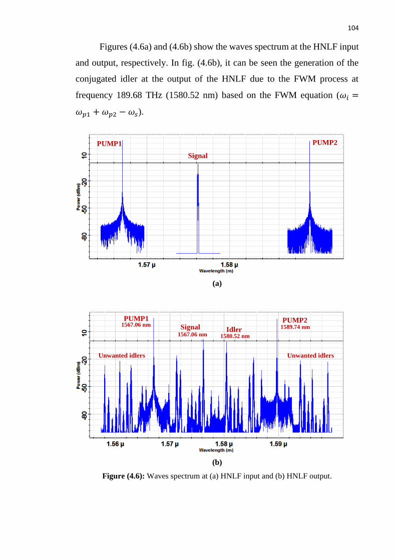
104
Figures (4.6a) and (4.6b) show the waves spectrum at the HNLF input
and output, respectively. In fig. (4.6b), it can be seen the generation of the
conjugated idler at the output of the HNLF due to the FWM process at
frequency 189.68 THz (1580.52 nm) based on the FWM equation (𝜔𝑖 =
𝜔𝑝1 + 𝜔𝑝2 − 𝜔𝑠).
(a)
(b)
Figure (4.6): Waves spectrum at (a) HNLF input and (b) HNLF output.
PUMP1
Signal 1567.06 nm
1567.06 nm Idler
1580.52 nm
1589.74 nm PUMP2
Unwanted idlers Unwanted idlers
PUMP2
PUMP1
Signal

105
The preceding discussion assumes that only the nondegenerate FWM
process, contributes in the HNLF. In reality, the situation is much more
complicated because the degenerate FWM process associated with each
pump occurs simultaneously. In fact, it turns out that the combination of
degenerate and nondegenerate FWM processes can create many other
unwanted idlers as shown in fig. (4.6b).
Figure (4.7) shows the spectrum of the conjugated idler at the output
of OPC device.
Figure (4.7): Spectrum of the conjugated idler at the output of the first OPC device.
The conjugated idler then transmitted across a second part of the
optical link. At the second OPC device, the process of OPC will repeated
again.
Figures (4.8a) and (4.8b) show the waves spectrum of the HNLF input
and output at the second OPC device, respectively. In fig. (4.8b), a new
conjugated idler at the output of the HNLF due to the FWM process was
generated at frequency 190.2 THz (1576.2 nm), which is similar to the
original transmitted signal.
Idler
1580.52 nm

106
(a)
(b)
Figure (4.8): Waves spectrum at (a) HNLF input and (b) HNLF output at the second
OPC device.
Signal 1567.06 nm
PUMP2
PUMP1
Idler
PUMP1
PUMP2
1580.52 nm
1580.52 nm
Idler

107
Figure (4.9) shows the spectrum of the received optical signal.
Figure (4.9): Spectrum of the received optical signal.
Figure (4.10a) displays the variation of the Q-factor with launched
power. It can be seen from this figure that the maximum Q-factor of X-
polarization component for the case with multiple-OPC compensation
scheme is 17 dB at a launch power of 3 dBm. This indicates an improvement
in performance of 1.2 dB compared to the maximum Q-factor for the MS-
OPC compensation scheme.
For the Y-polarization component (see Fig (4.4b)), the maximum Q-
factor with the multiple-OPC compensation scheme is 17.7 dB at a launch
power of 4 dBm showing 1.8 dB improvement compared to the case of MS-
OPC compensation scheme. The insets in the Figs. (4.10a) and (4.10b)
illustrate the eye diagrams of the received signal (X and Y– Polarization
components) at the corresponding optimum launched powers.

108
Figure (4.10): Calculated Q-factor as a function of a signal launched power for (a) (X-
Polarization), and (b) (Y-Polarization), for single channel transmission after 912 km.
The insets represent the eye diagrams of the received signal at the optimum launched
powers.
Figures (4.11a) and (4.11b) compare the performance of the multiple-
OPC and MS-OPC confgurations in terms of the total length of the optical
link for the single channel transmission for both polarization components.
The results show that the transmission reach at the HD-FEC limit
(BER=3.85×10⁻³) is enlarged by 24.2% when the multiple-OPC
configuration is used.
(a)
(b)

109
Figure (4.11): Variation Q-factors as a function of a transmission reach for single
channel, (a) X-Polarization and (b) Y-Polarization.
The calculations are performed further to investigate the performance
of the 8-channel WDM system. At the transmitter, eight channels at
frequencies extending from 190 THz to 190.35 THz (50-GHz channel
spacing). Figure (4.12) shows the spectrum of the multiplexed eight
channels.
(b)
(a)

110
Figure (4.12): Spectrum of the multiplexed 8-channels of the WDM signal.
Figures (4.13a) and (4.13b) show the spectrum of the HNLF input and
output at the first OPC device, respectively. An eight conjugated idlers were
generated due to the process of FWM in the HNLF with frequencies
extending from 189.86 THz to 189.51 THz (50 GHz channel spacing).
(a)
Figure (4.13): Waves spectrum at (a) HNLF input and (b) HNLF output at the first
OPC device.
PUMP2
WDM Signals
PUMP1

111
(b)
(b)
Figure (4.13): Continued.
After transmitting the output signals of the first OPC device over a
second part of the optical link, an OPC process is performed again at the
second OPC device generating new eight idlers similar in frequency to the
original input signals. Figures (4.14a) and (4.14b) show the spectrum of the
HNLF input and output at the second OPC device, respectively.
(a)
Figure (4.14): Waves spectrum at (a) HNLF input and (b) HNLF output at the second
OPC device.
Idlers Signals
PUMP1 PUMP2
PUMP2 PUMP1
Idlers

112
(b)
Figure (4.14): continued
Figure (4.15) shows the spectrum of the received signals before the
demultiplexing.
Figure (4.15): Spectrum of the received WDM signals.
The performance of the middle channel at frequency 190.2 THz of the
WDM signal is deduced after transmission of 912 km for signal launched
powers ranging from -10 dBm to +10 dBm, as shown in Fig. (4.16). The Q-
factor improves by 0.62 dB when a multiple-OPC compensation scheme is
used as compared with the MS-OPC scheme.
PUMP2 PUMP1
Idlers Signals

113
Figure (4.16): Calculated Q-factor as a function of a signal launched power (a) X –
Polarization (b) Y – Polarization, for a middle channel operating at frequency of 190.2
THz for an 8-channel WDM signal transmission after 912 km.
4.3.2 16-QAM Signaling
The system under investigation in this subsection operates with 16-
QAM signaling and 256 Gb/s bit rate. Figures (4.17a) and (4.17b) show the
simulation setup using MS-OPC and multiple-OPC, respectively. The
corresponding transmitter and receiver block diagrams are illustrated in Figs.
(4.17c) and (4.17d), respectively.
The MS-OPC configuration consists of a 8×256 Gb/s WDM PDM 16-
QAM transmitter, six 76 km SSMF spans forming the first half of the link,
the OPC device, another six 76 km SSMF spans forming the second half of
the link, and a coherent receiver. The multiple-OPC configuration uses the
same transmitter and receiver, but the optical link consists of three parts
(b)
(a)

114
separated by two OPC devices each of the first and the last parts consist of
three 76 km SSMF, while the middle part consists of six 76 km SSMF. Each
span in both configurations is backward pumped with a Raman pump to
achieve a symmetric power profile along the fiber spans. The transmitter has
eight CW laser sources (from 190 THz to 190.35 THz with 50 GHz channel
spacing) modulated by the corresponding data to generate the WDM signals
(see Fig. 4.17c). After combining all the eight WDM channels by the WDM
multiplexer, the 8×256 Gb/s WDM PDM 16-QAM signal is amplified with
an EDFA. The ASE noise is suppressed by an optical BPF. An EDFA and
optical attenuator are used to control the signal power launched to the fiber
spans.
At the receiving end, (Fig. 4.17d), the received WDM signal is
demultiplexed and each of the channels is polarization-demultiplexed and
converted into an electrical domain using coherent 16-QAM dual
polarization receiver. The DSP used for each single channel helps in
recovering the incoming transmission signal after coherent detection. The
decision component processes the electrical signal channels received from
the DSP stage, normalizes the electrical amplitudes of both polarization
channels to the respective 16-QAM grid and performs a decision on each
received symbol based on normalized threshold settings. Finally, 16-QAM
decoders are used to decode the two parallel 16-QAM M-ary symbol
sequences into binary output signals.
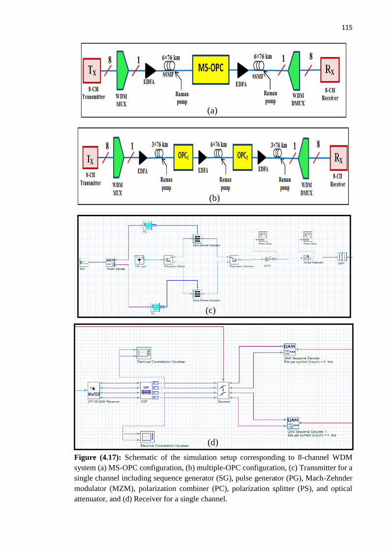
115
Figure (4.17): Schematic of the simulation setup corresponding to 8-channel WDM
system (a) MS-OPC configuration, (b) multiple-OPC configuration, (c) Transmitter for a
single channel including sequence generator (SG), pulse generator (PG), Mach-Zehnder
modulator (MZM), polarization combiner (PC), polarization splitter (PS), and optical
attenuator, and (d) Receiver for a single channel.
(b)
(c)
(d)
(a)

116
First, the BER of a single-channel (at 190.2 THz) is deduced. The
launched signal power to the fiber link is adjusted from -9 dBm to +3 dBm
by tuning the gain of the EDFA and the optical attenuator located at the
transmitter output. Figure (4.18) shows the Q-factor for the single channel
after 912 km transmission versus launched signal power. For the case of MS-
OPC, the optimum launched power is about −2 dBm, while in the multiple-
OPC scenario, it increases by 4 dB to be about 2 dBm with a 1.35 dB
improvement in Q-factor. These results are compared with experimental
ones that is given in [26] showing good agreement.
Figure (4.18): Calculated Q-factor as a function of a signal launched power for single
channel scenario after 912 km transmission. The insets show the recovered constellation
diagrams for both polarization components corresponding to multiple-OPCs
configuration at the optimum signal launched power.
Figure (4.19) compares the performance of the multiple-OPC and MS-
OPC confgurations in terms of the total length of the optical link for the
single channel transmission. The results show that the transmission reach at
the HD-FEC limit is enlarged by 30.7% when the multiple-OPC
configuration is used.
Y-Polarization
X-Polarization

117
Figure (4.19): Calculated Q factor as a function of number of fiber spans for a single
channel transmission. Insets show the recovered constellation diagrams for the multiple
OPCs and MS-OPC after 1824 km transmission (24 spans).
The calculations are carried further to investigate the performance of
the 8-channel WDM system. The performance of the central channel at
frequency 190.2 THz of the WDM signal is deduced after transmission of
912 km for signal launch powers started from -9 dBm to +3 dBm, as shown
in Fig. (4.20). For the case of MS-OPC, the optimum launch power is around
−2 dBm. For the case of multiple-OPC, the optimum launch power increases
to 0 dBm, and the Q-factor is improved by 0.62 dB, deduced at optimum
signal powers associated with the two cases.
Figure (4.20): Calculated Q-factor as a function of launched signal power for the middle
channel of an 8-channel WDM system after 912 km transmission. The insets show the
recovered constellation diagrams for both polarization components corresponding to
multiple OPCs configuration at the optimum signal launched power.
Y-Polarization
X-Polarization
X-Polarization Y-Polarization
X-Polarization Y-Polarization
2 dBm
-2 dBm

118
Figure (4.21) shows the BER for all the 8 channels after 912 km at the
optimum signal launched power for each configuration. For the multiple-
OPC system, the BERs of all channels except channel 8, are under the HD-
FEC limit. A minimum BER of 1.14×10⁻³ is observed in channel 7.
4.4 Thesis Conclusions
Mitigation of fiber dispersion and nonlinear distortions in advanced
fiber-optic communication systems have been investigated both theoretically
and by simulation. The effect of SOP on the performance of a dual-pump
HNLF-OPC has been analyzed using a set of eight coupled NLSEs. Further,
the transmission performance of two long-haul fiber-optic communication
systems incorporating multiple-OPC compensation scheme has been
simulated and the results are compared with published experimental data.
The two systems use 8-channel WDM technique with each channel adopting
PDM NRZ-OOK and PDM-16QAM modulation with bit rates of 40 Gb/s
and 256 Gb/s, respectively.
The main conclusions drawn from investigation of polarization effect
in a dual-pump OPC are
Figure (4.21): BER as a function of WDM channel number evaluated at the corresponding
optimum signal launched powers.

119
(i) The maximum conversion efficiency is obtained when the signal and
the two pumps are all copolarized, while the conversion efficiency
becomes almost zero when the signal wave is orthogonal to the two
copolarized pumps.
(ii) The analytical investigation shows that the use of a pair of orthogonally
polarized pumps can provide polarization-independent conversion
efficiency, but this conversion efficiency is lower compared with the
case of copolarized waves and this efficiency can be increased by
increasing the pump powers.
The simulation of the two advanced optical systems reveals the
following main findings
(i) In PDM-NRZ-OOK signal transmission, the use of multiple-OPC
provides better transmission performance when compared to MS-OPC
in both, single channel and WDM signal transmission. Moreover, the
results show that the transmission reach at the HD-FEC limit can be
enlarged when the multiple-OPC configuration is used.
(ii) In PDM-16QAM signal, single channel transmission using multiple-
OPC shows a 1.35 dB improvement in Q-factor over the MS-OPC case.
In the WDM system, using multiple-OPC increases the nonlinear
threshold by ~2 dB compared with the case of MS-OPC, showing 0.62
dB improvement in Q-factor over the MS-OPC compensation scheme.
4.5 Suggestions for Future Work
Possible future extension for the work included in this thesis may
cover the following points
(i) This thesis provides theoretical analysis and simulation results of fiber
nonlinear effects in the presence of the polarization effects and
discusses the optical compensation techniques. Experimental research

120
is one of the most important future works to validate the theoretical
models and to measure the performance of different optical
compensation schemes for mitigating fiber nonlinear effects.
(ii) The research described in this thesis is focused on the investigation of
single-carrier transmission, where a single optical carrier is modulated
and transmitted in wavelength window, significantly broader than the
symbol rate. To increase spectral efficiency it is possible to pack
channels at a symbol rate spacing, which is denoted OFDM with
presence of the polarization effect. Although, nonlinear compensation
algorithms were already applied in the literature to OFDM, the effect of
the polarization has not been investigated and a comprehensive study
on potential performance improvement is not available in either case.
(iii) The system under investigation in this thesis can be expanded to be has
higher-order modulation formats, hence increase the transmitted data
bit rate. Furthermore, the transmission reach can be enlarged to cover a
wide area.
(iv) Design of an OPC device using photonic crystal fiber instead of the
HNLF.
121
References
[1] H. Grupp, "Dynamics of Science-Based Innovation," Sprinter-Verlq
Berlin · Heidelberg 1992.
[2] G. P. Agrawal, "Fiber-optic communication systems," John Wiley &
Sons, 4th edition, 2010.
[3] G. P. Agrawal, "Light wave technology telecommunication Systems,"
John Wiley & Sons, Inc. 2005.
[4] O. D. D. Soares, " Trends in optical fibre metrology and standards,"
Springer-Science & Business Media, BV. 1994.
[5] S. Olonkins, I. Stankunovs, A. Alsevska, L. Gegere, and V. Bobrovs,
"Investigation of in-line Distributed Raman Amplifiers with Co and
Counter-propagating Pumping Schemes," Progress In Electromagnetic
Research Symposium (PIERS), Shanghai, China, Aug. 2016.
[6] B. Bouzid, "Analysis and review of erbium doped fiber amplifier,"
Electronics, Communications and Photonics Conference (SIECPC),
Fira, Greece, April 2013.
[7] S. Aleksic, "Towards Fifth-Generation (5G) Optical Transport
Networks" 17th International Conference on Transparent Optical
Networks (ICTON), Budapest, Hungary, Jul. 2015.
[8] K. Kikuchi, "Fundamentals of coherent optical fiber communications,"
IEEE Journal of Lightwave Technology, vol. 34, no. 1, pp. 157-179,
Jan. 2016.
[9] M. Nakazawa, K. Kikuchi, T. Miyazaki, "High spectral density optical
communication technologies," Springer-Verlag Berlin Heidelberg,
2010.
[10] M. Seimetz, " High-Order modulation for optical fiber transmission,"
Springer-Verlag Berlin Heidelberg, 2009.

122
[11] R. J. Essiambre and R. W. Tkach, "Capacity Trends and Limits of
Optical Communication Networks," in Proceedings of the IEEE, vol.
100, no. 5, pp. 1035-1055, May 2012.
[12] M. Asvial and A. A. S. Paramitha M. P, "Analysis of high order
dispersion and nonlinear effects in fiber optic transmission with Non
Linear Schrodinger Equation model," 2015 International Conference on
Quality in Research (QiR), Lombok, pp. 145-150, Aug. 2015.
[13] C. Behrens, R. I. Killey, S. J. Savory, M. Chen and P. Bayvel,
"Nonlinear Distortion in Transmission of Higher Order Modulation
Formats," in IEEE Photonics Technology Letters, vol. 22, no. 15, pp.
1111-1113, Aug. 2010.
[14] G. P. Agrawal, "Nonlinear Fiber Optics: Academic Press," 1995.
[15] Y. Yamamoto, Y. Kawaguchi and M. Hirano, "Low-Loss and Low-
Nonlinearity Pure-Silica-Core Fiber for C- and L-band Broadband
Transmission," in Journal of Lightwave Technology, vol. 34, no. 2, pp.
321-326, Jan. 2016.
[16] C. Behrens, "Mitigation of nonlinear impairments for advanced optical
modulation formats," UCL (University College London), 2012.
[17] G. J. Foschini and C. D. Poole, "Statistical theory of polarization
dispersion in single mode fibers," IEEE Journal of Lightwave
Technology, vol. 9, no. 11, pp. 1439-1456, Nov. 1991.
[18] J. Toulouse, "Optical nonlinearities in fibers: review, recent examples,
and systems applications," IEEE Journal of Lightwave Technology,
vol. 23, no. 11, pp. 3625-3641, Nov. 2005.
[19] L. He, J. Niu, Y. Sun and Y. Ji, "The four wave mixing effects in
quantum key distribution based on conventional WDM network,"
International Conference on Optical Internet (COIN), Jeju, South
Korea, pp. 1-2, Aug. 2014.

123
[20] J. M. Senior, "Optical fiber communications principles and practice,"
Pearson Education Limited, 3rd edition, 2009.
[21] M. Secondini, S. Rommel, F. Fresi, E. Forestieri, G. Meloni, and L.
Potì," Coherent 100G nonlinear compensation with single-step digital
backpropagation", International Conference on Optical Network
Design and Modeling (ONDM), Pisa, Italy, pp. 63-67 May, 2015.
[22] I. Sackey, F. D. Ros, J. K. Fischer, T. Richter, M. Jazayerifar, C.
Peucheret, K. Petermann, and C. Schubert, "Kerr nonlinearity
mitigation: mid-link spectral inversion versus digital backpropagation
in 5×28-GBd PDM 16-QAM signal transmission," IEEE Journal of
Lightwave Technology, vol. 33, no. 9, pp. 1821-1827, May1, 1 2015.
[23] E. Porto da Silva, F. da Ros and D. Zibar, "Performance of multi-
channel DBP with long-haul frequency-referenced transmission,"
Optical Fiber Communications Conference and Exhibition (OFC),
Anaheim, USA, pp. 1-3, Aug. 2016.
[24] X. Liu, A. R. Chraplyvy, P. J. Winzer, R. W. Tkach, and S.
Chandrasekhar, “Phase-conjugated twin waves for communication
beyond the Kerr nonlinearity limit,” National Photonics, vol. 7, no. 7,
pp. 560–568, May 2013.
[25] U. Sahu and B. C. Jinaga." Compensation of fiber nonlinear
impairments using optical back propagation", International
Conference on Microwave, Fiber-optic communication Engineering,
December 2015.
[26] H. Hu, R. M. Jopson, A H. Gnauck, S. Randel,and S. Chandrasekhar
"Fiber nonlinearity mitigation of WDM-PDM QPSK/16-QAM signals
using fiber-optic parametric amplifiers based multiple optical phase
conjugations," Optical Express, vol. 25, no. 3, pp. 1618-1628, Feb.
2017.
[27] S. L. Jansen, D. van den Borne, P. M. Krummrich, S. Spalter, G. D.
Khoe and H. de Waardt, "Long-haul DWDM transmission systems

124
employing optical phase conjugation," IEEE Journal of Selected
Topics in Quantum Electronics, vol. 12, no. 4, pp. 505-520, Jul.-Aug.
2006.
[28] P. Kaewplung and K. Kikuchi, "Simultaneous cancellation of fiber
loss, dispersion, and Kerr effect in ultra-long-haul optical fiber
transmission by midway optical phase conjugation incorporated with
distributed Raman amplification," IEEE Journal of Lightwave
Technology, vol. 25, no. 10, pp. 3035-3050, Oct. 2007.
[29] M. Morshed, A. J. Lowery, and L. B. Du, “Improving performance of
optical conjugation by splitting the nonlinear element,” Optics
Express, vol. 21, no. 4, pp. 4567–4577, Feb. 2013.
[30] F. Da Ros, I. Sackey, R. Elschner, T. Richter, C. Meuer, M. Nölle, M.
Jazayerifar, K. Petermann, C. Peucheret, and C. Schubert, "Kerr
nonlinearity compensation in a 5×28-GBd PDM 16-QAM WDM
system using fiber-based optical phase conjugation," The European
Conference on Fiber-optic communication (ECOC), pp. 1-3, Cannes,
France, Sept. 2014.
[31] I. Sackey, F. D. Ros, M. Jazayerifar, T. Richter, C. Meuer, M. Nölle,
L. Molle, C. Peucheret, K. Petermann, and C. Schubert, “Kerr
nonlinearity mitigation in 5 × 28-GBd PDM 16-QAM signal
transmission over a dispersion-uncompensated link with backward-
pumped distributed Raman amplification”, Optical Express vol. 22,
no. 22, pp. 27381-27391, Oct. 2014.
[32] H. Hu et al., "Fiber nonlinearity compensation of an 8-channel WDM
PDM-QPSK signal using multiple phase conjugations," Optical Fiber
Communications Conference and Exhibition (OFC), pp. 1-3, San
Francisco, USA, Mar. 2014.

125
[33] I. Sackey, F. D. Ros, T. Richter, R. Elschner, M. Jazayerifar, C. Meuer,
C. Peucheret, K. Petermann, and C. Schubert, "Design and
performance evaluation of an OPC device using a dual-pump
polarization-independent FOPA," The European Conference on Fiber-
optic communication (ECOC), pp. 1-3, Cannes, France, 2014.
[34] F. D. Ros, I. Sackey, M. Jazayerifar, T. Richter, C. Meuer, M. Nölle,
L. Molle, K. Petermann, J. K. Fischer, and C. Schubert, "Optical phase
conjugation for nonlinearity compensation in WDM PDM 16-QAM
transmission over dispersion-compensated and dispersion
uncompensated links," IEEE Summer Topicals Meeting Series
(SUM), pp. 1-3, Nassau, Bahamas, Jul. 2015.
[35] S. Yoshima, Z. Liu, Y. Sun, K. R. Bottrill, F. Parmigiani, P.
Petropoulos, and D. J. Richardson, "Nonlinearity mitigation for multi-
channel 64-QAM signals in a deployed fiber link through optical
phase conjugation," Optical Fiber Communication Conference, pp. 1-
3, Anaheim, USA, Mar. 2016.
[36] H. Hu, R. M. Jopson, A. H. Gnauck, D. Pilori, S. Randel and S.
Chandrasekhar, "Fiber nonlinearity compensation by repeated phase
conjugation in 2.048-Tbit/s WDM transmission of PDM 16-QAM
channels," Optical Fiber Communications Conference and Exhibition
(OFC), pp. 1-3, Anaheim, USA, Mar. 2016.
[37] L. N. Binh,"Advanced digital fiber-optic communications", Taylor &
Francis Group, LLC, 2nd edition, 2015.
[38] J. K. Show," Mathematical Principles of Optical Fiber
Communications", the Society for Industrial and Applied
Mathematics, 2004.
[39] J. A. Buck, "Fundamentals of Optical Fibers," John wiely & Sons, Inc.,
1995.
[40] M. Karasek, J. Kanka, P. Honzatko, J. Vojtech and J. Radil, "10 Gb/s
and 40 Gb/s Multi-Wavelength Conversion Based on Nonlinear

126
Effects in HNLF," International Conference on Transparent Optical
Networks, Nottingham, 2006.
[41] H. Hu, R. M. Jopson, A. H. Gnauck, M. Dinu, S. Chandrasekhar, C.
Xie, and S. Randel, "Parametric Amplification, Wavelength
Conversion, and Phase Conjugation of a 2.048-Tbit/s WDM PDM 16-
QAM Signal," IEEE Journal of Lightwave Technology, vol. 33, no. 7,
pp. 1286-1291, Apr. 2015.
[42] M. Baillot, T. Chartier and M. Joindot, "Multiple four-wave mixing in
optical fibres," 2014 The European Conference on Fiber-optic
communication (ECOC), Cannes, France, pp. 1-3, Sept. 2014.
[43] Casimer DeCusatis, "Handbook of Fiber Optic Data communications,
A Practical Guide to Optical Networking," Elsevier Inc. 3rd edition,
2008.
[44] Reinhold Noé, "Essentials of Modern Optical Fiber Communication,"
Springer, 2010.
[45] G. W. Lu, T. Sakamoto, A. Chiba, T. Kawanishi, T. Miyazaki, K.
Higuma, M. Sudo, and J. Ichikawa, "Monolithically integrated quad
mach-zehnder IQ modulator for generation of advanced optical
modulation formats," 9th International Conference on Fiber-optic
communications and Networks (ICOCN 2010), Nanjing, China, pp.
222-224, Oct. 2010.
[46] G. W. Lu, "Optical signal processing for advanced optical modulation
format," IEEE Photonics Society Summer Topics, pp. 170-171, Playa
del Carmen, Mexico, Jul. 2010.
[47] B. B. Purkayastha, and K. K. Sarma, "A Digital Phase Locked Loop
based Signal and Symbol Recovery System for Wireless Channel,"
Springer, 2015.
[48] Y. Zhang, F. Zhang and S. Pan, "Generation of Frequency-Multiplied
and Phase-Coded Signal Using an Optical Polarization Division

127
Multiplexing Modulator," IEEE Transactions on Microwave Theory
and Techniques, vol. 65, no. 2, pp. 651-660, Feb. 2017.
[49] B. Zhu et al., "Large-area low-loss fibers and advanced amplifiers for
high-capacity long-haul optical networks [Invited]," in IEEE/OSA
Journal of Fiber-optic communications and Networking, vol. 8, no. 7,
pp. A55-A63, Jul. 2016.
[50] Afsal S. et al., "A novel approach for the enhancement of Fiber optic
communication using EDFA," 2016 International Conference on
Wireless Communications, Signal Processing and Networking
(WiSPNET), pp. 23-27, Chennai, India, March 2016.
[51] C. Clivati et al., "Distributed Raman Optical Amplification in Phase
Coherent Transfer of Optical Frequencies," IEEE Photonics
Technology Letters, vol. 25, no. 17, pp. 1711-1714, Sept. 2013.
[52] A. F. Evans, J. Grochocinski, A. Rahman, C. Reynolds and M.
Vasilyev, "Distributed amplification: how Raman gain impacts
other fiber nonlinearities," Optical Fiber Communication
Conference and Exhibit, pp. MA7-MA7, Anaheim, USA, Mar.
2001.

128
Publications and Conferences
1. Adnan A. Abbas, Mazin M. Elias, and Raad S. Fyath, "Fiber
nonlinearity compensation of WDM-PDM 16-QAM signaling using
multiple optical phase conjugations over a distributed Raman-
amplified link," Photonic Network Communications, Accepted.
2. Adnan A. Abbas, Mazin M. Elias, and Raad S. Fyath, "Comprehensive
Analysis of HNLF-Based Optical Phase Conjugation in the Presence
of Polarization Misalignment," Journal of Engineering and Applied
Science, Accepted.
3. Adnan A. Abbas, Mazin M. Elias, and Raad. S. Fyath, “Investigation
of Polarization Effects on Highly Nonlinear Fiber-Based Optical
Phase Conjugation” Presented on the second conference of
postgraduate researchers (CPGR2017), Al-Nahrain university,
October 2017.

A1
Appendix A
Detailed Analysis of Dual-Pump Polarization-Aligned HNLF-OPC
The aim of this appendix is to present an analytical solution for the pumps,
signal, and conjugated idler waves equations in the absences of the
polarization effect. The analytical solution of the pumps equations starts
from Eqns. (3.2a) and (3.2b) as follow
𝑑𝐴𝑝1(𝑧)
𝑑𝑧= 𝑗𝛾[𝑃𝑝1 + 2𝑃𝑝2]𝐴𝑝1(𝑧) (𝐴1)
𝑑𝐴𝑝2(𝑧)
𝑑𝑧= 𝑗𝛾[2𝑃𝑝1 + 𝑃𝑝2]𝐴𝑝2(𝑧) (𝐴2)
where 𝑃𝑝1 = |𝐴𝑝1(0)|2
𝑎𝑛𝑑 𝑃𝑝2 = |𝐴𝑝2(0)|2 are the incident pump powers
at 𝑧 = 0.
Integrating both side of Eqns. (A1) and (A2) with respect to z yields
∫1
𝐴𝑝1(𝑧)𝑑𝐴𝑝1(𝑧) = ∫ 𝑗𝛾[𝑃𝑝1 + 2𝑃𝑝2]𝑑𝑧 (𝐴3)
∫1
𝐴𝑝2(𝑧)𝑑𝐴𝑝2(𝑧) = ∫ 𝑗𝛾[2𝑃𝑝1 + 𝑃𝑝2]𝑑𝑧 (𝐴4)
Solutions of Eqns. (A3) and (A4) are given by
𝑙𝑛 (𝐴𝑝1(𝑧)) = 𝑗𝛾[𝑃𝑝1 + 2𝑃𝑝2]𝑧 + 𝐶1 (𝐴5)
𝑙𝑛 (𝐴𝑝2(𝑧)) = 𝑗𝛾[2𝑃𝑝1 + 𝑃𝑝2]𝑧 + 𝐶2 (𝐴6)
Taking exponential for both side in the Eqns. (A5) and (A6) with 𝐶11 =
exp(𝐶1) and 𝐶22 = exp(𝐶2) gives
𝐴𝑝1(𝑧) = 𝐶11 𝑒𝑥𝑝(𝑗𝛾[𝑃𝑝1 + 2𝑃𝑝2]𝑧) (𝐴7)
𝐴𝑝2(𝑧) = 𝐶22 𝑒𝑥𝑝(𝑗𝛾[2𝑃𝑝1 + 𝑃𝑝2]𝑧) (𝐴8)

A2
where 𝐶11 = 𝐴𝑝1(0) and 𝐶22 = 𝐴𝑝2(0) are the integration constant and they
are obtained from the initial conditions at 𝑧 = 0. Therefore, pumps powers
equations can be given by
𝐴𝑝1(𝑧) = 𝐴𝑝1(0) 𝑒𝑥𝑝(𝑗𝛾[𝑃𝑝1 + 2𝑃𝑝2]𝑧) (𝐴9)
𝐴𝑝2(𝑧) = 𝐴𝑝2(0) 𝑒𝑥𝑝(𝑗𝛾[2𝑃𝑝1 + 𝑃𝑝2]𝑧) (𝐴10)
The analytical solution of the signal and conjugated idler equations starts
from Eqns. (3.4a) and (3.4b)
𝑑𝐴𝑠(𝑧)
𝑑𝑧= 2𝑗𝛾([𝑃𝑝1 + 𝑃𝑝2]𝐴𝑠(𝑧) + 𝐴𝑖
∗(𝑧)𝐴𝑝1(𝑧)𝐴𝑝2(𝑧) exp(−𝑗𝛥𝑘𝑧)) (𝐴11)
𝑑𝐴𝑖∗(𝑧)
𝑑𝑧= −2𝑗𝛾([𝑃𝑝1 + 𝑃𝑝2]𝐴𝑖
∗(𝑧) + 𝐴𝑠(𝑧)𝐴𝑝1∗ (𝑧)𝐴𝑝2
∗ (𝑧) exp(𝑗𝛥𝑘𝑧)) (𝐴12)
Substituting Eqns. (A9) and (A10) into Eqns. (A11) and (A12) yields
𝑑𝐴𝑠(𝑧)
𝑑𝑧= 2𝑗𝛾([𝑃𝑝1 + 𝑃𝑝2]𝐴𝑠(𝑧)
+ 𝐴𝑖∗(𝑧)𝐴𝑝1(0) 𝑒𝑥𝑝(𝑗𝛾[𝑃𝑝1 + 2𝑃𝑝2]𝑧) 𝐴𝑝2(0) 𝑒𝑥𝑝(𝑗𝛾[2𝑃𝑝1
+ 𝑃𝑝2]𝑧) exp(−𝑗𝛥𝑘𝑧)) (𝐴13)
𝑑𝐴𝑖∗(𝑧)
𝑑𝑧= −2𝑗𝛾([𝑃𝑝1 + 𝑃𝑝2]𝐴𝑖
∗(𝑧)
+ 𝐴𝑠(𝑧)𝐴𝑝1∗ (0) 𝑒𝑥𝑝(−𝑗𝛾[𝑃𝑝1 + 2𝑃𝑝2]𝑧)𝐴𝑝2
∗ (0) 𝑒𝑥𝑝(−𝑗𝛾[2𝑃𝑝1
+ 𝑃𝑝2]𝑧) exp(𝑗𝛥𝑘𝑧)) (𝐴14)
For simplification, let 𝜃 = (∆𝑘 − 3𝛾(𝑃𝑝1 + 𝑃𝑝2)), Eqns. (A13) and (A14)
will be
𝑑𝐴𝑠(𝑧)
𝑑𝑧= 2𝑗𝛾 ((𝑃𝑝1 + 𝑃𝑝2)𝐴𝑠(𝑧) + 𝐴𝑖
∗(𝑧)𝐴𝑝1(0) 𝐴𝑝2(0) exp(−𝑗𝜃𝑧)) (𝐴15)
𝑑𝐴𝑖∗(𝑧)
𝑑𝑧= −2𝑗𝛾 ((𝑃𝑝1 + 𝑃𝑝2)𝐴𝑖
∗(𝑧) + 𝐴𝑠(𝑧)𝐴𝑝1∗ (0) 𝐴𝑝2
∗ (0) 𝑒𝑥𝑝(𝑗𝜃𝑧)) (𝐴16)
To solve Eqns. (A15) and (A16), let

A3
𝐵𝑠(𝑧) = 𝐴𝑠(𝑧)𝑒𝑥𝑝(−2𝑗𝛾(𝑃𝑝1 + 𝑃𝑝2)𝑧) (𝐴17)
𝐵𝑖∗(𝑧) = 𝐴𝑖
∗(𝑧)𝑒𝑥𝑝(2𝑗𝛾(𝑃𝑝1 + 𝑃𝑝2)𝑧) (𝐴18)
Differentiating Eqns. (A17) and (A18) with respect to z yields
𝑑𝐵𝑠(𝑧)
𝑑𝑧= 𝐴𝑠(𝑧) (−2𝑗𝛾(𝑃𝑝1 + 𝑃𝑝2)) 𝑒𝑥𝑝(−2𝑗𝛾(𝑃𝑝1 + 𝑃𝑝2)𝑧)
+𝑑𝐴𝑠(𝑧)
𝑑𝑧 𝑒𝑥𝑝(−2𝑗𝛾(𝑃𝑝1 + 𝑃𝑝2)𝑧) (𝐴19)
𝑑𝐵𝑖∗(𝑧)
𝑑𝑧= 𝐴𝑖
∗(𝑧) (2𝑗𝛾(𝑃𝑝1 + 𝑃𝑝2)) 𝑒𝑥𝑝(2𝑗𝛾(𝑃𝑝1 + 𝑃𝑝2)𝑧)
+ 𝑑𝐴𝑖
∗(𝑧)
𝑑𝑧 𝑒𝑥𝑝(2𝑗𝛾(𝑃𝑝1 + 𝑃𝑝2)𝑧) (𝐴20)
Substituting Eqns. (A15) and (A16) into Eqns. (A19) and (A20)
𝑑𝐵𝑠(𝑧)
𝑑𝑧= 𝐴𝑠(𝑧) (−2𝑗𝛾(𝑃𝑝1 + 𝑃𝑝2)) 𝑒𝑥𝑝(−2𝑗𝛾(𝑃𝑝1 + 𝑃𝑝2)𝑧)
+ 2𝑗𝛾(𝑃𝑝1 + 𝑃𝑝2)𝐴𝑠(𝑧) 𝑒𝑥𝑝(−2𝑗𝛾(𝑃𝑝1 + 𝑃𝑝2)𝑧)
+ 2𝑗𝛾 𝐴𝑖∗(𝑧)𝐴𝑝1(0) 𝐴𝑝2(0) exp(−𝑗𝜃𝑧) 𝑒𝑥𝑝(−2𝑗𝛾(𝑃𝑝1
+ 𝑃𝑝2)𝑧) (𝐴21)
𝑑𝐵𝑖∗(𝑧)
𝑑𝑧= 𝐴𝑖
∗(𝑧) (2𝑗𝛾(𝑃𝑝1 + 𝑃𝑝2)) 𝑒𝑥𝑝(2𝑗𝛾(𝑃𝑝1 + 𝑃𝑝2)𝑧)
− 2𝑗𝛾 (𝑃𝑝1 + 𝑃𝑝2)𝐴𝑖∗(𝑧) 𝑒𝑥𝑝(2𝑗𝛾(𝑃𝑝1 + 𝑃𝑝2)𝑧)
− 2𝑗𝛾 𝐴𝑠(𝑧)𝐴𝑝1∗ (0) 𝐴𝑝2
∗ (0) 𝑒𝑥𝑝(𝑗𝜃𝑧) 𝑒𝑥𝑝(2𝑗𝛾(𝑃𝑝1
+ 𝑃𝑝2)𝑧) (𝐴22)
Equations (3.19) and (3.20), after simplification, can be written as follow
𝑑𝐵𝑠(𝑧)
𝑑𝑧= 2𝑗𝛾𝐴𝑝1(0) 𝐴𝑝2(0) exp(−𝑗𝜃𝑧)𝐴𝑖
∗(𝑧) 𝑒𝑥𝑝(−2𝑗𝛾(𝑃𝑝1 + 𝑃𝑝2)𝑧) (𝐴23)
𝑑𝐵𝑖∗(𝑧)
𝑑𝑧= − 2𝑗𝛾 𝐴𝑝1
∗ (0) 𝐴𝑝2∗ (0) 𝑒𝑥𝑝(𝑗𝜃𝑧) 𝐴𝑠(𝑧) 𝑒𝑥𝑝(2𝑗𝛾(𝑃𝑝1 + 𝑃𝑝2)𝑧) (𝐴24)
From Eqns. (A17) and (A18), 𝐴𝑠(𝑧) and 𝐴𝑖∗(𝑧) can be given by
𝐴𝑠(𝑧) = 𝐵𝑠(𝑧)𝑒𝑥𝑝(2𝑗𝛾(𝑃𝑝1 + 𝑃𝑝2)𝑧) (𝐴25)
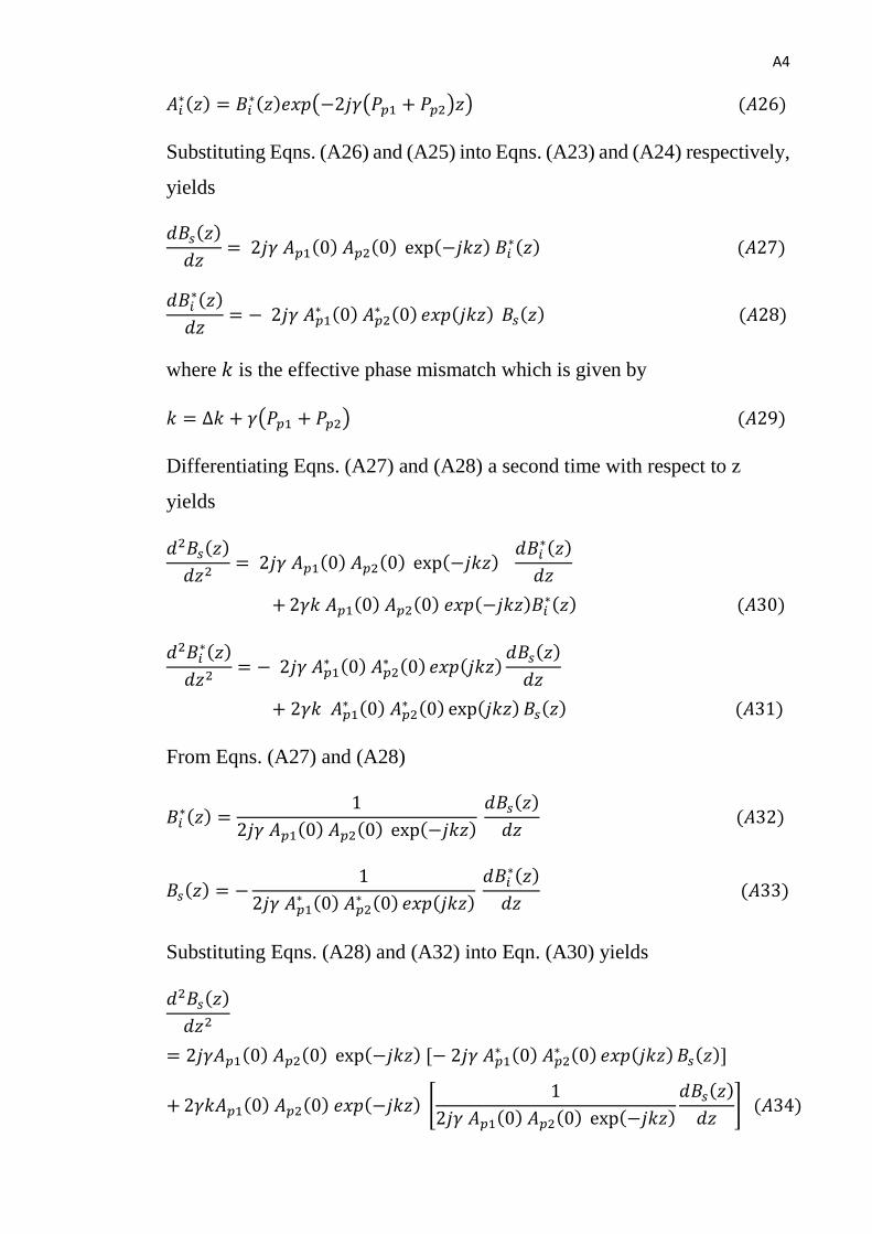
A4
𝐴𝑖∗(𝑧) = 𝐵𝑖
∗(𝑧)𝑒𝑥𝑝(−2𝑗𝛾(𝑃𝑝1 + 𝑃𝑝2)𝑧) (𝐴26)
Substituting Eqns. (A26) and (A25) into Eqns. (A23) and (A24) respectively,
yields
𝑑𝐵𝑠(𝑧)
𝑑𝑧= 2𝑗𝛾 𝐴𝑝1(0) 𝐴𝑝2(0) exp(−𝑗𝑘𝑧) 𝐵𝑖
∗(𝑧) (𝐴27)
𝑑𝐵𝑖∗(𝑧)
𝑑𝑧= − 2𝑗𝛾 𝐴𝑝1
∗ (0) 𝐴𝑝2∗ (0) 𝑒𝑥𝑝(𝑗𝑘𝑧) 𝐵𝑠(𝑧) (𝐴28)
where 𝑘 is the effective phase mismatch which is given by
𝑘 = ∆𝑘 + 𝛾(𝑃𝑝1 + 𝑃𝑝2) (𝐴29)
Differentiating Eqns. (A27) and (A28) a second time with respect to z
yields
𝑑2𝐵𝑠(𝑧)
𝑑𝑧2= 2𝑗𝛾 𝐴𝑝1(0) 𝐴𝑝2(0) exp(−𝑗𝑘𝑧)
𝑑𝐵𝑖∗(𝑧)
𝑑𝑧
+ 2𝛾𝑘 𝐴𝑝1(0) 𝐴𝑝2(0) 𝑒𝑥𝑝(−𝑗𝑘𝑧)𝐵𝑖∗(𝑧) (𝐴30)
𝑑2𝐵𝑖∗(𝑧)
𝑑𝑧2= − 2𝑗𝛾 𝐴𝑝1
∗ (0) 𝐴𝑝2∗ (0) 𝑒𝑥𝑝(𝑗𝑘𝑧)
𝑑𝐵𝑠(𝑧)
𝑑𝑧
+ 2𝛾𝑘 𝐴𝑝1∗ (0) 𝐴𝑝2
∗ (0) exp(𝑗𝑘𝑧) 𝐵𝑠(𝑧) (𝐴31)
From Eqns. (A27) and (A28)
𝐵𝑖∗(𝑧) =
1
2𝑗𝛾 𝐴𝑝1(0) 𝐴𝑝2(0) exp(−𝑗𝑘𝑧) 𝑑𝐵𝑠(𝑧)
𝑑𝑧 (𝐴32)
𝐵𝑠(𝑧) = −1
2𝑗𝛾 𝐴𝑝1∗ (0) 𝐴𝑝2
∗ (0) 𝑒𝑥𝑝(𝑗𝑘𝑧) 𝑑𝐵𝑖
∗(𝑧)
𝑑𝑧 (𝐴33)
Substituting Eqns. (A28) and (A32) into Eqn. (A30) yields
𝑑2𝐵𝑠(𝑧)
𝑑𝑧2
= 2𝑗𝛾𝐴𝑝1(0) 𝐴𝑝2(0) exp(−𝑗𝑘𝑧) [− 2𝑗𝛾 𝐴𝑝1∗ (0) 𝐴𝑝2
∗ (0) 𝑒𝑥𝑝(𝑗𝑘𝑧) 𝐵𝑠(𝑧)]
+ 2𝛾𝑘𝐴𝑝1(0) 𝐴𝑝2(0) 𝑒𝑥𝑝(−𝑗𝑘𝑧) [1
2𝑗𝛾 𝐴𝑝1(0) 𝐴𝑝2(0) exp(−𝑗𝑘𝑧)
𝑑𝐵𝑠(𝑧)
𝑑𝑧] (𝐴34)

A5
Then Substituting Eqns. (A27) and (A33) into Eqn. (A31) yields
𝑑2𝐵𝑖∗(𝑧)
𝑑𝑧2
= −2𝑗𝛾 𝐴𝑝1∗ (0) 𝐴𝑝2
∗ (0) 𝑒𝑥𝑝(𝑗𝑘𝑧) [2𝑗𝛾 𝐴𝑝1(0) 𝐴𝑝2(0) exp(−𝑗𝑘𝑧) 𝐵𝑖∗(𝑧)]
+ 2𝛾𝑘 𝐴𝑝1∗ (0) 𝐴𝑝2
∗ (0) exp(𝑗𝑘𝑧) [−1
2𝑗𝛾 𝐴𝑝1∗ (0) 𝐴𝑝2
∗ (0) 𝑒𝑥𝑝(𝑗𝑘𝑧) 𝑑𝐵𝑖
∗(𝑧)
𝑑𝑧] (𝐴35)
Then, from Eqns. (A34) and (A35) the following second-order ordinary
differential equations can be obtained
𝑑2𝐵𝑠(𝑧)
𝑑𝑧2+ 𝑗𝑘
𝑑𝐵𝑠(𝑧)
𝑑𝑧− 4𝛾2𝑃𝑝1𝑃𝑝2 𝐵𝑠(𝑧) = 0 (𝐴36)
𝑑2𝐵𝑖∗(𝑧)
𝑑𝑧2− 𝑗𝑘
𝑑𝐵𝑖∗(𝑧)
𝑑𝑧− 4𝛾2𝑃𝑝1𝑃𝑝2 𝐵𝑖
∗(𝑧) = 0 (𝐴37)
The general solutions of Eqns. (A36) and (A37) can be found as follow
𝐵𝑠(𝑧) = [𝐶1 exp(𝑔𝑧) + 𝐶2 exp(−𝑔𝑧)] exp (−𝑗 𝑘
2𝑧) (𝐴38)
𝐵𝑖∗(𝑧) = [𝐶3 exp(𝑔𝑧) + 𝐶4 exp(−𝑔𝑧)] exp (𝑗
𝑘
2𝑧) (𝐴39)
where the parametric gain coefficient 𝑔 = √4𝛾2𝑃𝑝1𝑃𝑝2 − (𝑘 2)⁄ 2. Further, 𝐶1,
𝐶2, 𝐶3, and 𝐶4 are constants determined from the boundary conditions.
Applying 𝑧 = 0 in Eqn. (A38), yields
𝐵𝑠(0) = 𝐶1 + 𝐶2 (𝐴40)
Differentiating Eqn. (A38) with respect to z gives
𝑑𝐵𝑠(𝑧)
𝑑𝑧= [𝐶1 exp(𝑔𝑧) + 𝐶2 exp(−𝑔𝑧)] exp (−𝑗
𝑘
2𝑧) (−𝑗
𝑘
2)
+ exp (−𝑗 𝑘
2𝑧) [𝑔𝐶1 exp(𝑔𝑧) − 𝑔𝐶2exp (−𝑔𝑧)] (𝐴41)
Equating Eqns. (A41) and (A27) with the primary condition 𝑧 = 0 gives

A6
2𝑗𝛾 𝐴𝑝1(0) 𝐴𝑝2(0) exp(−𝑗𝑘𝑧) 𝐵𝑖∗(0) = [𝐶1 + 𝐶2] (−𝑗
𝑘
2) + 𝑔[𝐶1 − 𝐶2] (𝐴42)
Applying 𝐵𝑖∗(0) = 0, (idler wave at 𝑧 = 0)
𝑔[𝐶1 − 𝐶2] = [𝐶1 + 𝐶2] (𝑗 𝑘
2) (𝐴43)
Solving Eqns. (A40) and (A43) produces
𝐶1 =1
2 (1 +
𝑗𝑘
2𝑔) 𝐵𝑠(0) and 𝐶2 =
1
2 (1 −
𝑗𝑘
2𝑔) 𝐵𝑠(0)
Now, similar method is used to find 𝐶3and 𝐶4, therefore
𝐶3 =−𝑗𝛾 𝐴𝑝1
∗ (0) 𝐴𝑝2∗ (0) 𝐵𝑠(0)
𝑔 and 𝐶4 =
𝑗𝛾 𝐴𝑝1∗ (0) 𝐴𝑝2
∗ (0) 𝐵𝑠(0)
𝑔
Substituting 𝐶1 𝑎𝑛𝑑 𝐶2 into Eqn. (A38) and 𝐶3 𝑎𝑛𝑑 𝐶4 into Eqn. (A39) and
simplifying these equations yields
𝐵𝑠(𝑧) = 𝐵𝑠(0) [(𝑒𝑥𝑝(𝑔𝑧) + 𝑒𝑥𝑝(−𝑔𝑧)
2)
+𝑗𝑘
2𝑔 (
𝑒𝑥𝑝(𝑔𝑧) − 𝑒𝑥𝑝(−𝑔𝑧)
2)] 𝑒𝑥𝑝 (−𝑗
𝑘
2𝑧) (𝐴44)
𝐵𝑖∗(𝑧) = [
−𝑗𝛾 𝐴𝑝1∗ (0) 𝐴𝑝2
∗ (0) 𝐵𝑠(0)
𝑔𝑒𝑥𝑝(𝑔𝑧)
+𝑗𝛾 𝐴𝑝1
∗ (0) 𝐴𝑝2∗ (0) 𝐵𝑠(0)
𝑔 𝑒𝑥𝑝(−𝑔𝑧) ] 𝑒𝑥𝑝 (𝑗
𝑘
2𝑧) (𝐴45)
Using the formulas
𝑐𝑜𝑠ℎ(𝑥) =𝑒𝑥𝑝(𝑥)+𝑒𝑥𝑝(−𝑥)
2 and 𝑠𝑖𝑛ℎ(𝑥) =
𝑒𝑥𝑝(𝑥)−𝑒𝑥𝑝(−𝑥)
2
𝐵𝑠(𝑧) = 𝐵𝑠(0) [cosh (𝑔𝑧) +𝑗𝑘
2𝑔 sinh (𝑔𝑧)] exp (−𝑗
𝑘
2𝑧) (𝐴46)
𝐵𝑖∗(𝑧) =
−𝑗2𝛾 𝐴𝑝1∗ (0) 𝐴𝑝2
∗ (0) 𝐵𝑠(0) sinh(gz)
𝑔 exp (𝑗
𝑘
2𝑧) (𝐴47)
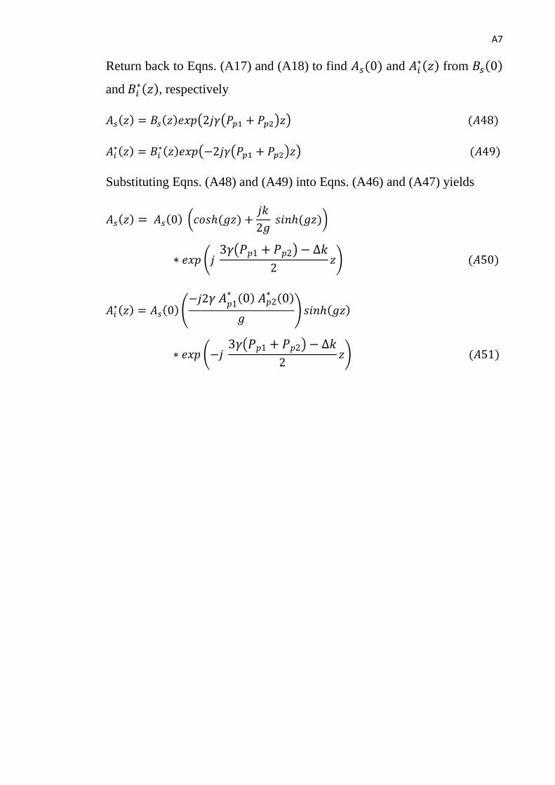
A7
Return back to Eqns. (A17) and (A18) to find 𝐴𝑠(0) and 𝐴𝑖∗(𝑧) from 𝐵𝑠(0)
and 𝐵𝑖∗(𝑧), respectively
𝐴𝑠(𝑧) = 𝐵𝑠(𝑧)𝑒𝑥𝑝(2𝑗𝛾(𝑃𝑝1 + 𝑃𝑝2)𝑧) (𝐴48)
𝐴𝑖∗(𝑧) = 𝐵𝑖
∗(𝑧)𝑒𝑥𝑝(−2𝑗𝛾(𝑃𝑝1 + 𝑃𝑝2)𝑧) (𝐴49)
Substituting Eqns. (A48) and (A49) into Eqns. (A46) and (A47) yields
𝐴𝑠(𝑧) = 𝐴𝑠(0) (𝑐𝑜𝑠ℎ (𝑔𝑧) +𝑗𝑘
2𝑔 𝑠𝑖𝑛ℎ (𝑔𝑧))
∗ 𝑒𝑥𝑝 (𝑗 3𝛾(𝑃𝑝1 + 𝑃𝑝2) − ∆𝑘
2𝑧) (𝐴50)
𝐴𝑖∗(𝑧) = 𝐴𝑠(0) (
−𝑗2𝛾 𝐴𝑝1∗ (0) 𝐴𝑝2
∗ (0)
𝑔) 𝑠𝑖𝑛ℎ(𝑔𝑧)
∗ 𝑒𝑥𝑝 (−𝑗 3𝛾(𝑃𝑝1 + 𝑃𝑝2) − ∆𝑘
2𝑧) (𝐴51)