MITIGATION OF COLLAPSE RISK IN VULNERABLE CONCRETE BUILDINGS

By

Lisa Matchulat

A Report on Research Sponsored by

THE NATIONAL SCIENCE FOUNDATION AWARD NUMBER 0618804 THROUGH THE PACIFIC EARTHQUAKE ENGINEERING RESEARCH

CENTER

Structural Engineering and Engineering Materials SM Report No. 93

January 2009

THE UNIVERSITY OF KANSAS CENTER FOR RESEARCH, INC. 2385 Irving Hill Road – Campus West, Lawrence, Kansas 66045

MITIGATION OF COLLAPSE RISK IN VULNERABLE CONCRETE BUILDINGS

By

Lisa Matchulat

A Report on Research Sponsored by

THE NATIONAL SCIENCE FOUNDATION AWARD NUMBER 0618804 THROUGH THE PACIFIC EARTHQUAKE ENGINEERING RESEARCH CENTER

Structural Engineering and Engineering Materials SM Report No. 93

THE UNIVERSITY OF KANSAS CENTER FOR RESEARCH, INC. LAWRENCE, KANSAS 66045

January 2009

iii

ABSTRACT

The goal of this study is to investigate the collapse risk of reinforced concrete

building columns constructed prior to the mid-1970’s, subjected to cyclic lateral

loading. These columns have reinforcement details deemed inadequate by modern

seismic design standards, and as such are vulnerable to collapse. Testing of two full-

scale, shear-critical column specimens was carried out at the NEES-MAST facility at

the University of Minnesota. The test specimens had nominally identical material

and reinforcement properties. The primary test variable was the applied axial load,

which was held constant at 500 kips and 340 kips for the first and second specimens,

respectively. The specimens were subjected to increasing lateral displacement cycles

until axial load carrying capacity was lost. The thesis discusses the observed lateral

and axial load resisting behavior, and analyzes the measured responses of the

columns up to and beyond the lateral drift at which they were able to sustain axial

load. Test results indicate that column behavior was significantly influenced by the

magnitude of the applied axial load, and that the ratio of axial load to gross axial

capacity of the longitudinal reinforcement is a key parameter in identifying columns

in which axial failure occurs simultaneously with shear failure.

iv

ACKNOWLEDGEMENTS

Primary financial support for this project was provided by the National

Science Foundation under award number 0618804 through the Pacific Earthquake

Engineering Research Center. This support is gratefully acknowledged.

Many individuals deserve thanks for their help and advice throughout the

course of this project. I would like to thank Dr. Adolfo Matamoros for taking me on

as a research assistant, and for his guidance and support throughout the project.

The staff at the NEES-MAST facility at the University of Minnesota were an

invaluable asset to the project’s success. I would especially like to thank Paul

Bergson, Angela Kingsley, Carol Shield, Jonathan Messier, and Drew Daugherty for

their wealth of knowledge, their ingenuity, and their patience throughout the testing

process. In addition, the involvement of Kurt Henkhaus and Julio Ramirez from

Purdue University during the planning, instrumentation, and testing phases of the

project is greatly appreciated.

I would like to thank everyone at the University of Kansas who helped

contribute to the successful fabrication of the test specimens. Travis Malone

provided a great deal of instruction and advice in the early construction phases of the

project. Our student hourly workers, Emily Reimer and Vinur Kaul, were extremely

valuable and I owe much of the success of our strain gages to their diligent work. Jim

Weaver also provided much-needed support and expertise throughout the

construction process. The addition of Charlie Woods to the project team midway

through the testing phase was more helpful than I can express. Thank you for your

v

teamwork, your dedication, and your friendship. I would like to extend a special

thanks to Mike Briggs for his help and guidance throughout the writing process. I

can’t express how much your editing assistance and emotional support has meant to

me. In addition, the help from all the other graduate students with formwork

construction, specimen casting, and general morale boosting on a daily basis is

gratefully acknowledged and has made this experience one I will remember fondly.

Finally, I would like to thank my family for their continued love and support

throughout my graduate studies. You have always been there to provide advice,

understanding, and emotional support whenever I’ve needed it. I truly could not have

finished this without your love and encouragement and for that I am eternally grateful

to each of you.

vi

TABLE OF CONTENTS

ABSTRACT................................................................................................................. iii

ACKNOWLEDGEMENTS......................................................................................... iv

TABLE OF CONTENTS............................................................................................. vi

LIST OF FIGURES ................................................................................................... viii

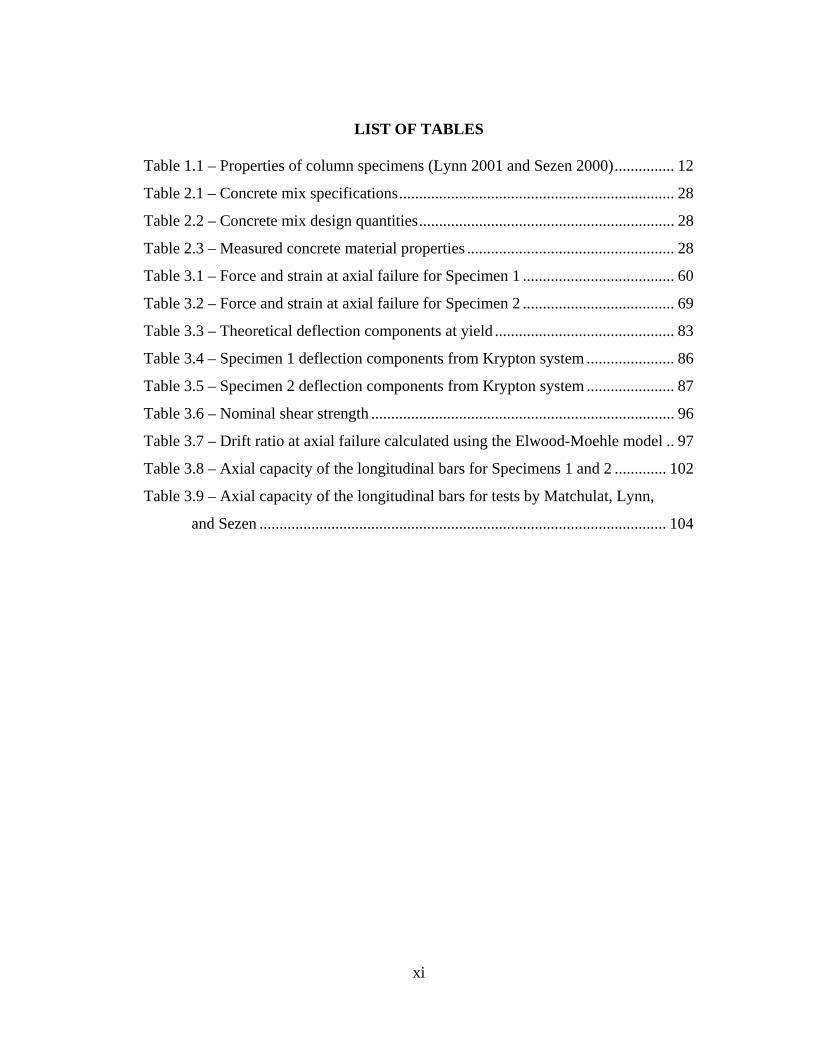
LIST OF TABLES....................................................................................................... xi

CHAPTER 1: BACKGROUND AND PREVIOUS RESEARCH............................... 1

1.1 Introduction................................................................................................. 1

1.2 Background................................................................................................. 2

1.3 Previous Research..................................................................................... 11

1.4 Objectives and Scope................................................................................ 18

CHAPTER 2: EXPERIMENTAL PROGRAM.......................................................... 19

2.1 Introduction............................................................................................... 19

2.2 Specimen Description ............................................................................... 19

2.3 Material Properties.................................................................................... 27

2.4 Specimen Construction ............................................................................. 30

2.5 Test Setup.................................................................................................. 35

2.6 Loading and Displacement History .......................................................... 38

2.7 Instrumentation ......................................................................................... 41

2.8 Telepresence ............................................................................................. 47

CHAPTER 3: TEST RESULTS ................................................................................. 51

3.1 Introduction............................................................................................... 51

3.2 Damage Progression – Specimen 1........................................................... 51

3.3 Damage Progression – Specimen 2........................................................... 61

3.4 Load-Deflection Response........................................................................ 70

3.5 Moment-Curvature Analysis..................................................................... 75

3.6 Deflection Components ............................................................................ 80

3.7 Measured Bar Strain Analysis .................................................................. 91

3.8 Shear Strength........................................................................................... 95

vii

3.9 Comparison to Elwood-Moehle Axial Failure Model .............................. 96

3.10 Axial Capacity of Longitudinal Reinforcement........................................ 98

CHAPTER 4: SUMMARY AND CONCLUSIONS................................................ 106

4.1 Summary ................................................................................................. 106

4.2 Conclusions............................................................................................. 107

REFERENCES ......................................................................................................... 110

viii

LIST OF FIGURES

Figure 1.1 – Deformation of columns loaded in double curvature ............................... 3

Figure 1.2 – Typical load-deflection response (Specimen 2CLD12 – Sezen 2000)..... 3

Figure 1.3 – Failure envelopes for reinforced concrete columns.................................. 4

Figure 1.4 – Shear-controlled axial failure envelopes .................................................. 5

Figure 1.5 – Flexure-controlled axial failure envelopes ............................................... 7

Figure 1.6 – Flexural-shear axial failure envelopes...................................................... 8

Figure 1.7 – Lateral load-deflection responses for different axial load levels.............. 9

Figure 1.8 – Vertical deformation-lateral drift responses for different axial

load levels ....................................................................................................... 10

Figure 1.9 – Typical column specimen configuration (Lynn 2001 and Sezen 2000). 13

Figure 1.10 – Free body diagram of column forces after shear failure....................... 14

Figure 1.11 – Elwood-Moehle model for drift ratio at axial failure

(Specimen 3CLH18 – Lynn 2001).................................................................. 17

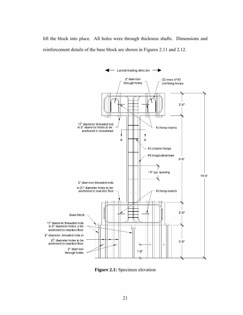
Figure 2.1 – Specimen elevation................................................................................. 21

Figure 2.2 – Column cross-section ............................................................................. 22

Figure 2.3 – Bottom beam elevation........................................................................... 22

Figure 2.4 – Bottom beam hole layout........................................................................ 23

Figure 2.5 – Bottom beam reinforcement layout ........................................................ 23

Figure 2.6 – Bottom beam hoop insert layout............................................................. 24

Figure 2.7 – Top beam elevation ................................................................................ 24

Figure 2.8 – Top beam hole layout ............................................................................. 25

Figure 2.9 – Top beam reinforcement layout.............................................................. 25

Figure 2.10 – Top beam hoop insert layout ................................................................ 25

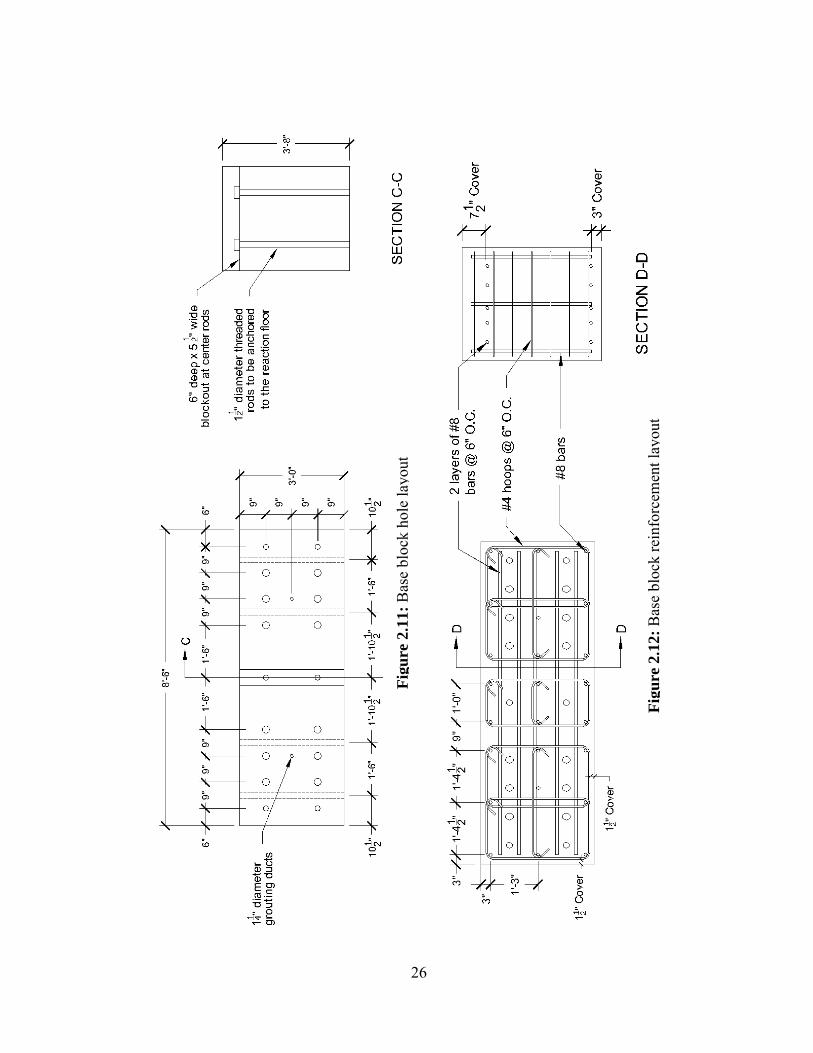
Figure 2.11 – Base block hole layout.......................................................................... 26

Figure 2.12 – Base block reinforcement layout .......................................................... 26

Figure 2.13 – Stress-strain relationship for No. 9 ASTM A706 reinforcing steel...... 29

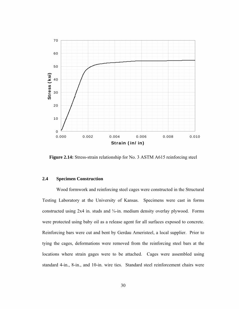
Figure 2.14 – Stress-strain relationship for No. 3 ASTM A615 reinforcing steel...... 30

Figure 2.15 – Specimen formwork ............................................................................. 32

ix

Figure 2.16 – Typical specimen reinforcing cage....................................................... 32

Figure 2.17 – Reinforcing cage in form, prior to casting............................................ 33

Figure 2.18 – Internal vibration during concrete placement....................................... 33

Figure 2.19 – Finished column test specimen............................................................. 34

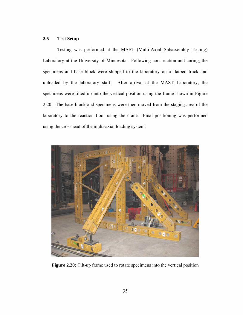
Figure 2.20 – Tilt-up frame used to rotate specimens into the vertical position ........ 35

Figure 2.21 – Top beam connection to the crosshead................................................. 37

Figure 2.22 – Test configuration................................................................................. 37

Figure 2.23 – Displacement history used for both specimens .................................... 39

Figure 2.24 – Strain gage placement........................................................................... 42

Figure 2.25 – Strain gage locations and labeling........................................................ 43

Figure 2.26 – LVDT and string potentiometer placement.......................................... 44

Figure 2.27 – LVDT attachment to the column.......................................................... 45

Figure 2.28 – String potentiometer attachment to the reference frame ...................... 46

Figure 2.29 – Telepresence camera tower .................................................................. 47

Figure 2.30 – Telepresence camera tower layout ....................................................... 48

Figure 2.31 – Photo tagger and Krypton LED layout................................................. 50

Figure 3.1 – Specimen 1 crack pattern at a drift ratio of 0.25%................................. 55

Figure 3.2 – Specimen 1 crack pattern at a drift ratio of 0.50%................................. 56

Figure 3.3 – Specimen 1 crack pattern at a drift ratio of 0.75%................................. 57

Figure 3.4 – Specimen 1 crack pattern at a drift ratio of 1.00% (after axial failure).. 58

Figure 3.5 – Specimen 1 condition at the end of the test ............................................ 59

Figure 3.6 – Axial strain-axial force response for Specimen 1................................... 60

Figure 3.7 – Specimen 2 crack pattern at a drift ratio of 0.50%................................. 64

Figure 3.8 – Specimen 2 crack pattern at a drift ratio of 0.75%................................. 65

Figure 3.9 – Specimen 2 crack pattern at a drift ratio of 1.00%................................. 66

Figure 3.10 – Specimen 2 crack pattern at a drift ratio of 1.25% (after axial failure) 67

Figure 3.11 – Specimen 2 condition at the end of the test .......................................... 68

Figure 3.12 – Axial strain-axial force response for Specimen 2................................. 69

Figure 3.13 – Lateral load-lateral drift responses ....................................................... 71

x

Figure 3.14 – Axial strain-lateral drift responses........................................................ 74

Figure 3.15 – Moment-curvature responses................................................................ 77

Figure 3.16 – Curvature profiles................................................................................. 79

Figure 3.17 – Deflection profiles ................................................................................ 81

Figure 3.18 – Deflection components......................................................................... 85

Figure 3.19 – Flexure and shear deflection components ............................................ 89

Figure 3.20 – Effective shear modulus at increasing drift ratios ................................ 90

Figure 3.21 – Measured bar strain in the longitudinal reinforcement at the beam-

column interfaces for Specimen 1................................................................... 92

Figure 3.22 – Measured bar strain in the longitudinal reinforcement at the beam-

column interfaces for Specimen 2................................................................... 92

Figure 3.23 – Measured bar strain in the transverse hoops for Specimen 1 ............... 94

Figure 3.24 – Measured bar strain in the transverse hoops for Specimen 2 ............... 94

Figure 3.25 – Measured and calculated drift ratios at axial failure ............................ 97

Figure 3.26 – Ratios of axial load to gross axial capacity and plastic capacity

to buckling capacity ...................................................................................... 105

xi

LIST OF TABLES

Table 1.1 – Properties of column specimens (Lynn 2001 and Sezen 2000)............... 12

Table 2.1 – Concrete mix specifications..................................................................... 28

Table 2.2 – Concrete mix design quantities................................................................ 28

Table 2.3 – Measured concrete material properties .................................................... 28

Table 3.1 – Force and strain at axial failure for Specimen 1 ...................................... 60

Table 3.2 – Force and strain at axial failure for Specimen 2 ...................................... 69

Table 3.3 – Theoretical deflection components at yield ............................................. 83

Table 3.4 – Specimen 1 deflection components from Krypton system ...................... 86

Table 3.5 – Specimen 2 deflection components from Krypton system ...................... 87

Table 3.6 – Nominal shear strength ............................................................................ 96

Table 3.7 – Drift ratio at axial failure calculated using the Elwood-Moehle model .. 97

Table 3.8 – Axial capacity of the longitudinal bars for Specimens 1 and 2 ............. 102

Table 3.9 – Axial capacity of the longitudinal bars for tests by Matchulat, Lynn,

and Sezen ...................................................................................................... 104

1

CHAPTER 1: BACKGROUND AND PREVIOUS RESEARCH

1.1 Introduction

Poor seismic performance of some reinforced concrete building columns

designed and constructed prior to the mid-1970s has raised concern and interest in

identifying those most vulnerable to collapse. Post-earthquake damage investigation

and research have led to modifications in design codes in an effort to achieve ductile

column behavior. This is essential to limit the loss of life in buildings during

earthquakes. The most noteworthy update in seismic design procedures followed the

1971 San Fernando Earthquake. While a great deal of effort has been dedicated to

improving design provisions, much remains unknown regarding the loss of axial

capacity of existing reinforced concrete columns, constructed prior to the mid-1970s.

The majority of these columns have widely spaced transverse reinforcement, which

provides little lateral restraint to the longitudinal reinforcement and negligible

confinement to the core concrete during seismic loading. As such, many of these

columns would be deemed inadequate by modern design standards. Thus, engineers

and government entities are in dire need of identifying those that have the greatest

risk of collapse and pose the biggest threat in terms of potential loss of life.

Characterizing not only the shear capacity, but the ability of these columns to sustain

axial load carrying capacity beyond the point of shear failure, is of paramount

interest. This Chapter discusses the previous experimental and analytical research

into the failure behavior and drift capacity of reinforced concrete columns with

2

similar detailing to those constructed prior to the mid-1970s, when subjected to cyclic

lateral loading.

1.2 Background

1.2.1 General Load-Deflection Response

Much of the current research into the axial capacity of concrete columns under

cyclic lateral loading is based on tests of full-length columns loaded in double

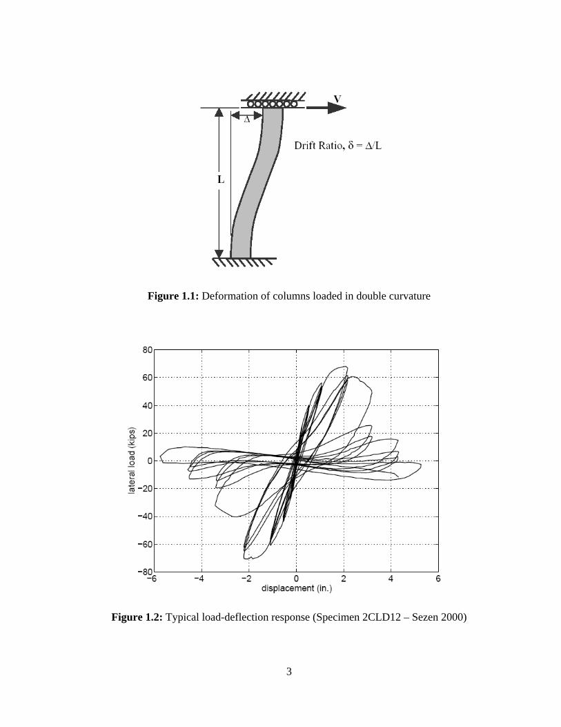
curvature to examine the deformation response. The typical deformed shape of the

columns is as shown in Figure 1.1. This double curvature shape is similar to that of

many columns in reinforced concrete moment-resisting frames subjected to lateral

loading. A representative load-deflection response curve for these columns is shown

in Figure 1.2.

In typical test loading protocols, a column is subjected to cyclic lateral loading,

with peak deflection increasing in successive load cycles, as depicted in Figure 1.2.

After the column reaches its maximum lateral load carrying capacity, the combination

of crack propagation in the column along with increased column displacement, leads

to the deterioration of both lateral and axial load carrying capacity and eventually

results in axial failure (Elwood 2004). Comparison of columns with differing heights

is accommodated by dividing the lateral displacement by the height of the column as

shown in Figure 1.1, yielding a drift ratio δ. The drift ratios at axial failure for

various test specimens can then be examined to determine the effects different

parameters have on column strength and ductility.

3

Figure 1.1: Deformation of columns loaded in double curvature

Figure 1.2: Typical load-deflection response (Specimen 2CLD12 – Sezen 2000)

4

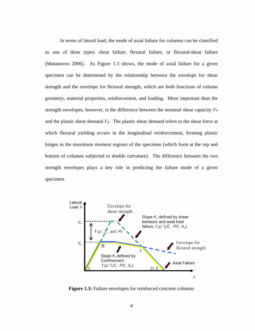
In terms of lateral load, the mode of axial failure for columns can be classified

as one of three types: shear failure, flexural failure, or flexural-shear failure

(Matamoros 2006). As Figure 1.3 shows, the mode of axial failure for a given

specimen can be determined by the relationship between the envelope for shear

strength and the envelope for flexural strength, which are both functions of column

geometry, material properties, reinforcement, and loading. More important than the

strength envelopes, however, is the difference between the nominal shear capacity Vn

and the plastic shear demand Vp. The plastic shear demand refers to the shear force at

which flexural yielding occurs in the longitudinal reinforcement, forming plastic

hinges in the maximum moment regions of the specimen (which form at the top and

bottom of columns subjected to double curvature). The difference between the two

strength envelopes plays a key role in predicting the failure mode of a given

specimen.

Figure 1.3: Failure envelopes for reinforced concrete columns

5

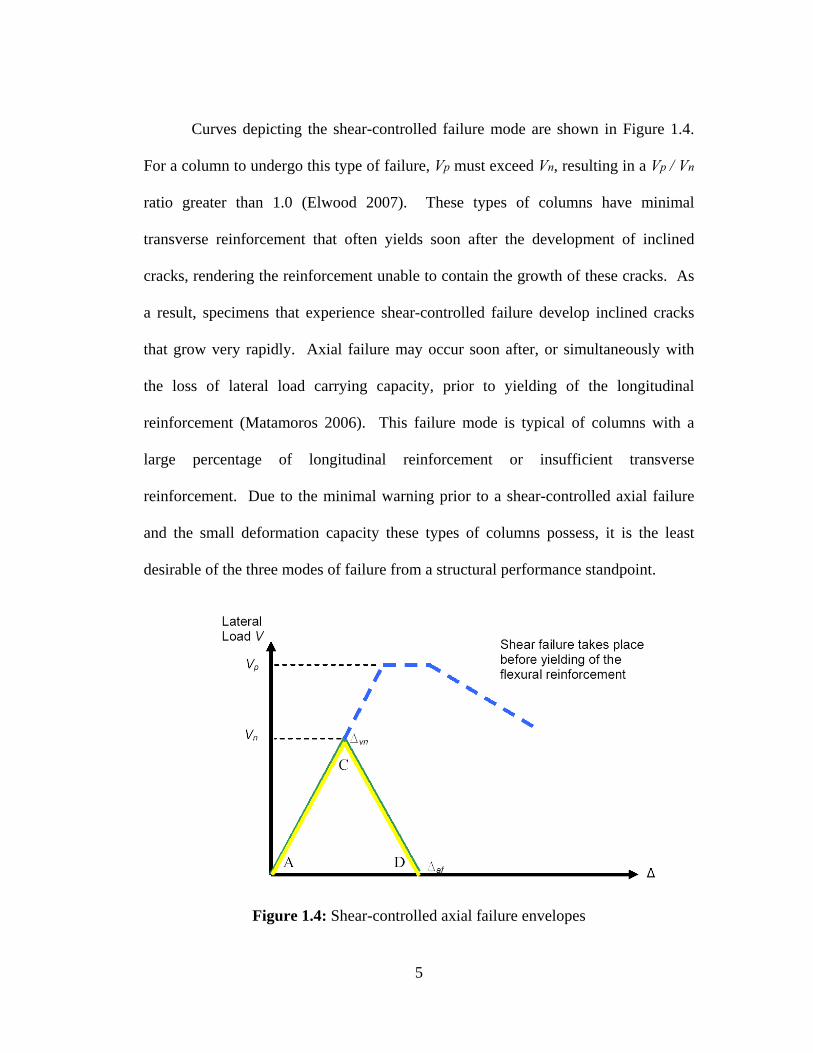
Curves depicting the shear-controlled failure mode are shown in Figure 1.4.

For a column to undergo this type of failure, Vp must exceed Vn, resulting in a Vp / Vn

ratio greater than 1.0 (Elwood 2007). These types of columns have minimal

transverse reinforcement that often yields soon after the development of inclined

cracks, rendering the reinforcement unable to contain the growth of these cracks. As

a result, specimens that experience shear-controlled failure develop inclined cracks

that grow very rapidly. Axial failure may occur soon after, or simultaneously with

the loss of lateral load carrying capacity, prior to yielding of the longitudinal

reinforcement (Matamoros 2006). This failure mode is typical of columns with a

large percentage of longitudinal reinforcement or insufficient transverse

reinforcement. Due to the minimal warning prior to a shear-controlled axial failure

and the small deformation capacity these types of columns possess, it is the least

desirable of the three modes of failure from a structural performance standpoint.

Figure 1.4: Shear-controlled axial failure envelopes

6

Curves depicting the flexure-controlled failure mode are illustrated in Figure

1.5. This type of failure occurs when the applied lateral load causes yielding in the

longitudinal reinforcing steel. Yielding can be identified by an increase in the lateral

displacement of the specimen while the lateral load remains nearly constant.

Yielding is also evidenced by the gradual formation of horizontal flexural cracks on

the column faces subjected to flexural tension. These cracks grow at a much slower

rate than those formed during shear failure, and as a result, they provide greater

warning prior to axial failure. Furthermore, yielding of the longitudinal

reinforcement allows for much greater lateral deformation, and the column is

generally able to maintain axial capacity up to a much higher lateral displacement

than a column controlled by shear failure. At displacements beyond yielding of the

longitudinal reinforcement, spalling of the concrete cover often occurs in the

maximum moment regions of the specimen, leading to a reduction in axial capacity.

During flexure-controlled failure, Vn significantly exceeds Vp, and yields a Vp / Vn

ratio less than 0.6 (Elwood 2007). As a result, the envelope for flexural strength

controls and the column ultimately fails due to P-Δ effects before the two envelopes

intersect.

The third and final failure mode, flexural-shear failure, is a combination of the

previous two. As shown in Figure 1.6, this failure mode results when Vn is slightly

higher than Vp, yielding a Vp / Vn ratio between 0.6 and 1.0 (Elwood 2007). During

this type of failure, the specimen is taken through three major phases of damage:

flexural yielding, shear failure, and ultimately axial failure. The first of these phases,

7

flexural yielding, occurs just as it does in the flexure-controlled failure mode, with the

formation of horizontal flexural cracks and large increases in lateral displacement.

As lateral loading continues, the horizontal flexural cracks continue to grow deeper

into the specimen along an incline, developing into shear cracks. This results in a

significant reduction in lateral load carrying capacity. Researchers often assume that

shear failure has taken place when the lateral load decreases to 80% of its maximum

value (Elwood 2005). As the column is subjected to further lateral displacement

cycles, the loss in lateral load carrying capacity translates into a loss of axial load

carrying capacity. Ultimate axial failure occurs when the lateral load resistance of the

specimen deteriorates to approximately zero.

Figure 1.5: Flexure-controlled axial failure envelopes

8

Figure 1.6: Flexural-shear axial failure envelopes

1.2.2 Effect of Axial Load on Drift Capacity

The magnitude of the axial load applied to a column undergoing cyclic lateral

loading has a significant effect on both the drift capacity and the behavior of the

column near axial failure. In general, large axial loads result in low drift ratios at

failure, while low axial loads correspond to larger drift ratios. This relationship can

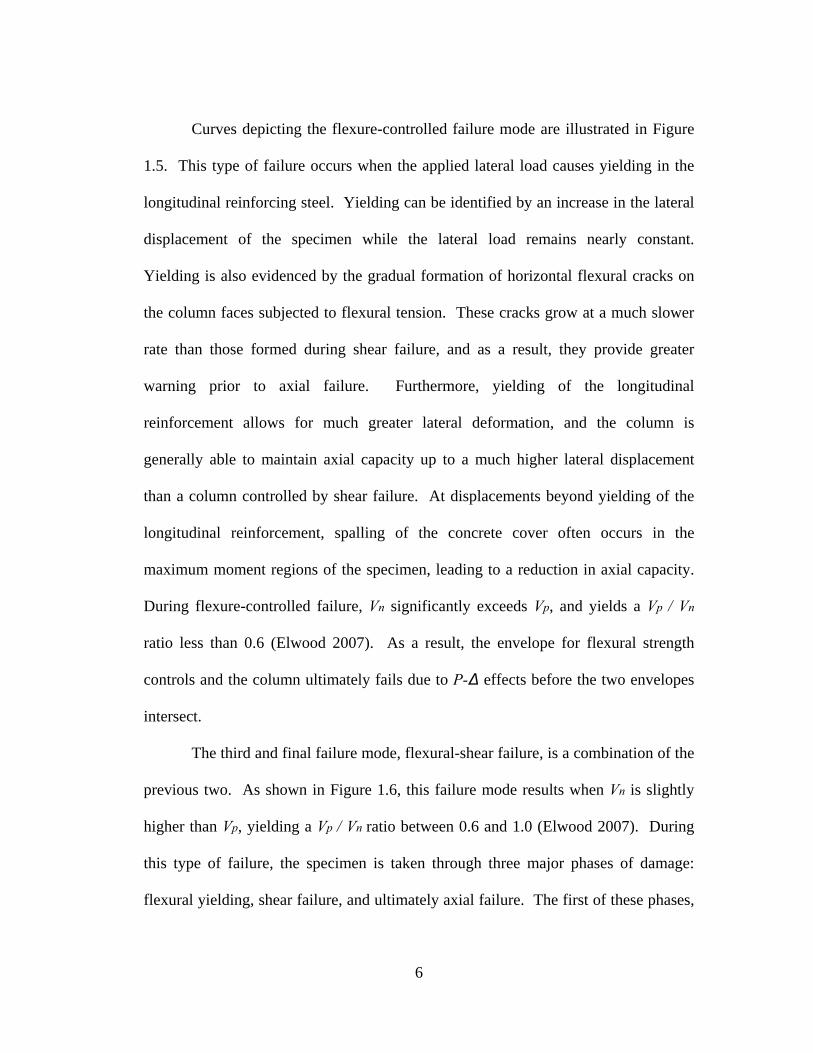
clearly be seen in Figure 1.7 from tests performed by Nakamura and Yoshimura

(2002). The first and second graphs show the lateral load-deflection responses of two

specimens with axial load ratios of 0.18 and 0.27 g cA f ′ , respectively. The lower axial

load specimen was able to maintain axial capacity up to a drift ratio of 20.6%, while

the specimen with the high axial load experienced axial failure at a drift ratio of only

3.0%. Studies by Saatcioglu (1989), Lynn (2001), and Sezen (2000) also report

similar findings.

9

Figure 1.7: Lateral load-deflection responses for different axial load levels

(a) 0.18 g cA f ′ , (b) 0.27 g cA f ′

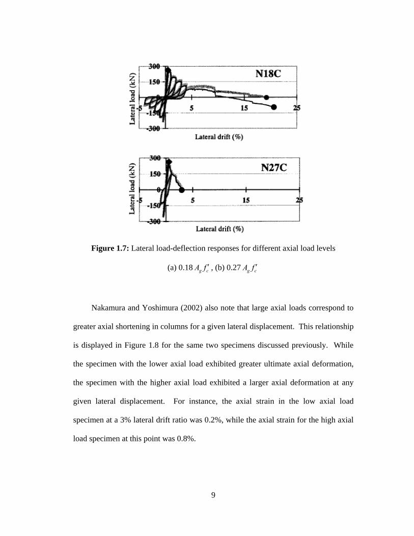
Nakamura and Yoshimura (2002) also note that large axial loads correspond to

greater axial shortening in columns for a given lateral displacement. This relationship

is displayed in Figure 1.8 for the same two specimens discussed previously. While

the specimen with the lower axial load exhibited greater ultimate axial deformation,

the specimen with the higher axial load exhibited a larger axial deformation at any

given lateral displacement. For instance, the axial strain in the low axial load

specimen at a 3% lateral drift ratio was 0.2%, while the axial strain for the high axial

load specimen at this point was 0.8%.

10

Figure 1.8: Vertical deformation-lateral drift responses for different axial load levels

(a) 0.18 g cA f ′ , (b) 0.27 g cA f ′

The level of axial load has also been shown to exert significant influence on

the ultimate failure mode. In general, a large axial load increases the likelihood of a

brittle shear failure, while lower axial loads tend to result in flexural or flexural-shear

failures. In research performed by Sezen (2000), two columns with identical

properties, designed to have the same lateral force at yield, were tested under

different axial load levels. The column subjected to the lighter load reached flexural

yielding prior to failing in shear. Continued lateral cycling resulted in additional loss

of lateral load carrying capacity. At the end of testing, the lateral resistance had

11

degraded to effectively zero, but the column was still able to maintain axial load

carrying capacity. The column with the higher load, however, experienced sudden,

simultaneous shear and axial failure following the formation of a large inclined crack.

The drastic difference in failure modes emphasizes the importance of differentiating

between columns based on axial load level when performing seismic evaluations.

1.3 Previous Research

1.3.1 Lynn (2001) and Sezen (2000) Experimental Research

Concern regarding the vulnerability of reinforced concrete columns designed

and constructed prior to the mid-1970s, and the lack of experimental data related to

their behavior has lead to studies performed at the University of California, Berkeley

by Lynn (2001) and Sezen (2000). In both studies, full-scale reinforced concrete

building columns were tested under cyclic lateral loading until the columns could no

longer sustain axial load carrying capacity. The loading, boundary conditions, and

detailing of the test specimens were very similar to those tested in the present study.

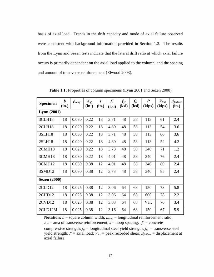
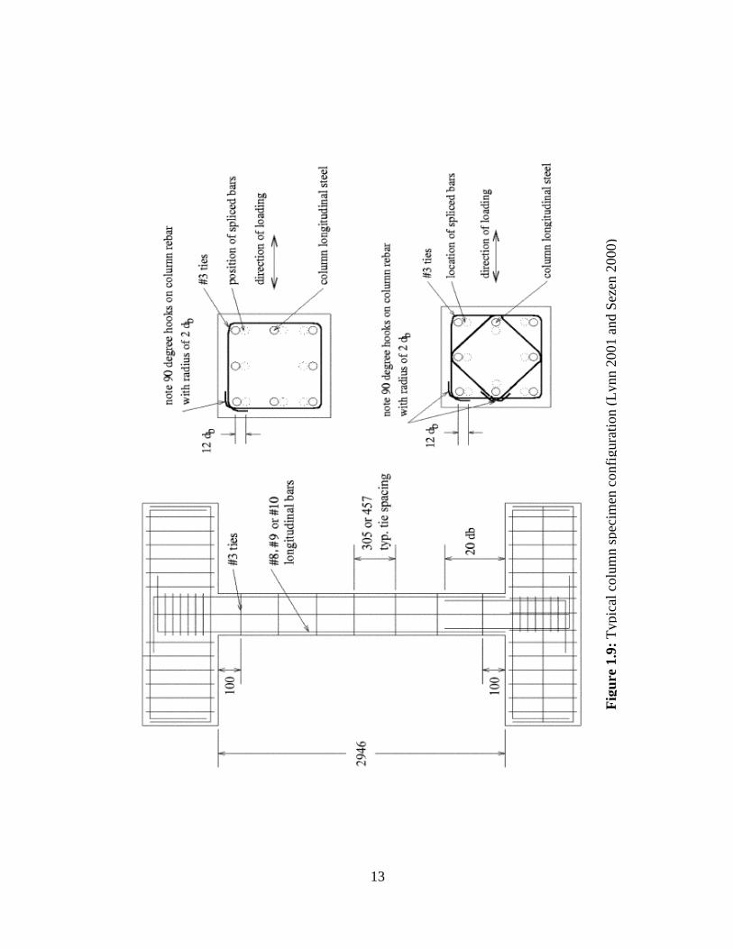
Table 1.1 lists specimen details, material properties, and axial failure data for tests

performed by Lynn and Sezen; Figure 1.9 illustrates typical specimen configuration.

The displacement protocol for the specimens applied a series of lateral

displacement cycles of increasing amplitudes, with three cycles at each displacement

value. After axial failure was observed, the tests were concluded. The specimens of

particular interest to the present study were those that experienced shear-controlled

axial failure, as well as those that provided a comparison of column behavior on the

12

basis of axial load. Trends in the drift capacity and mode of axial failure observed

were consistent with background information provided in Section 1.2. The results

from the Lynn and Sezen tests indicate that the lateral drift ratio at which axial failure

occurs is primarily dependent on the axial load applied to the column, and the spacing

and amount of transverse reinforcement (Elwood 2003).

Table 1.1: Properties of column specimens (Lynn 2001 and Sezen 2000)

Specimen b (in.)

ρlong

Ast (in2)

s (in.)

cf ′ (ksi)

fyl (ksi)

fyt (ksi)

P (kips)

Vtest (kips)

Δfailure(in.)

Lynn (2001)

3CLH18 18 0.030 0.22 18 3.71 48 58 113 61 2.4

2CLH18 18 0.020 0.22 18 4.80 48 58 113 54 3.6

3SLH18 18 0.030 0.22 18 3.71 48 58 113 60 3.6

2SLH18 18 0.020 0.22 18 4.80 48 58 113 52 4.2

2CMH18 18 0.020 0.22 18 3.73 48 58 340 71 1.2

3CMH18 18 0.030 0.22 18 4.01 48 58 340 76 2.4

3CMD12 18 0.030 0.38 12 4.01 48 58 340 80 2.4

3SMD12 18 0.030 0.38 12 3.73 48 58 340 85 2.4

Sezen (2000)

2CLD12 18 0.025 0.38 12 3.06 64 68 150 73 5.8

2CHD12 18 0.025 0.38 12 3.06 64 68 600 78 2.2

2CVD12 18 0.025 0.38 12 3.03 64 68 Var. 70 3.4

2CLD12M 18 0.025 0.38 12 3.16 64 68 150 67 5.9

Notation: b = square column width; ρlong = longitudinal reinforcement ratio; Ast = area of transverse reinforcement; s = hoop spacing; cf ′= concrete compressive strength; fyl = longitudinal steel yield strength; fyt = transverse steel yield strength; P = axial load; Vtest = peak recorded shear; Δfailure = displacement at axial failure

13

Figu

re 1

.9: T

ypic

al c

olum

n sp

ecim

en c

onfig

urat

ion

(Lyn

n 20

01 a

nd S

ezen

200

0)

14

1.3.2 Elwood-Moehle (2003) Axial Capacity Model

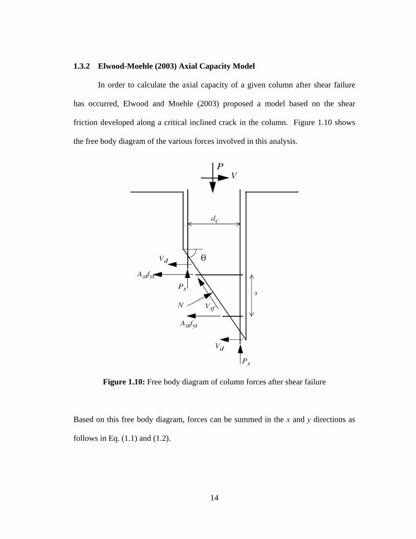
In order to calculate the axial capacity of a given column after shear failure

has occurred, Elwood and Moehle (2003) proposed a model based on the shear

friction developed along a critical inclined crack in the column. Figure 1.10 shows

the free body diagram of the various forces involved in this analysis.

Figure 1.10: Free body diagram of column forces after shear failure

Based on this free body diagram, forces can be summed in the x and y directions as

follows in Eq. (1.1) and (1.2).

15

sin cos tanst yt cx sf bars d

A f dF N V V n V

sθ θ θΣ → + = + + (1.1)

cos siny sf bars sF P N V n Pθ θΣ → = + + (1.2)

Where:

N = normal force on inclined shear-failure plane (kips)

θ = angle from horizontal of critical shear-failure plane (degrees)

V = shear force (kips)

Vsf = shear friction force along inclined shear-failure plane (kips)

Ast = area of transverse reinforcement (in2)

fyt = yield strength of transverse reinforcement (ksi)

dc = depth of core (centerline to centerline of hoops, in.)

s = spacing of transverse reinforcement (in.)

nbars = number of longitudinal reinforcing bars

Vd = shear resistance due to dowel action of longitudinal steel (kips)

P = axial load (kips)

Ps = axial load supported by longitudinal reinforcement (kips)

The final term in Eq. (1.1) is the shear resistance provided by dowel action in the

longitudinal reinforcement, which has decreasing effectiveness as the spacing of the

transverse reinforcement increases. In buildings most vulnerable to collapse, columns

have a large hoop spacing and thus nbarsVd goes to zero, so this component is

neglected in the final model. Also, the V term on the left side of this equation can be

16

ignored, as the shear force drops to effectively zero at the point of axial failure. As a

result, Eq. (1.1) can be rewritten as follows in Eq. (1.3).

sin cos tanst yt csf

A f dN V

sθ θ θ= + (1.3)

Equilibrium Eq. (1.2) and (1.3) can be combined into Eq. (1.4) to solve for the axial

capacity of the column.

1 tantantan

st yt cbars s

A f dP n P

sμ θθθ μ

⎛ ⎞+= +⎜ ⎟−⎝ ⎠

(1.4)

Elwood recommends using a value of 65° for the critical crack angle, based on

empirical results from tests performed by Lynn (2001) and Sezen (2000). In addition,

the effective shear friction coefficient μ is approximated using Eq. (1.5).

100tan 04

μ θ δ= − ≥ (1.5)

Where:

μ = effective shear friction coefficient

δ = lateral drift ratio at axial failure

Equation (1.6) incorporates Eq. (1.5) into the Eq. (1.4), creating the axial capacity

model that predicts the lateral drift ratio at axial failure.

17

24 1 tan100

tantanst yt c

sPA f d

θδ

θθ

+=

⎛ ⎞+ ⎜ ⎟⎜ ⎟

⎝ ⎠

(1.6)

Thus, the model suggests that lateral drift ratio δ at axial failure is inversely

proportional to both the applied axial load P and the spacing of the transverse

reinforcement s, and directly related to the amount of transverse reinforcement Ast.

This behavior is consistent with the experimental results obtained by Lynn (2001) and

Sezen (2000). Figure 1.11 shows a graphical representation of the relationship

between axial load and drift ratio at axial failure predicted by the Elwood-Moehle

failure model for Specimen 3CLH18, tested by Lynn (2001).

0.0

0.5

1.0

1.5

2.0

2.5

3.0

3.5

4.0

0 100 200 300 400 500 600

Axial Load (kips)

Dri

ft R

atio

(%)

Figure 1.11: Elwood-Moehle model for drift ratio at axial failure

(Specimen 3CLH18 – Lynn 2001)

18

1.4 Objectives and Scope

The purpose of this study was to obtain additional information on the behavior

of columns subjected to cyclic lateral loading that are vulnerable to shear and axial

failure. The main objective of experimental investigation was to examine the effect

of axial load level on the drift capacity and axial failure mode of the columns. The

experimental program was comprised of two columns, with identical dimensions and

detailing, subjected to two different levels of axial load. Testing was performed up to

and beyond the point of initial axial failure. The information provided by this study is

intended to be used to evaluate the ability of existing methods to calculate the drift

capacity of reinforced concrete columns vulnerable to collapse, and to investigate

their load resisting behavior near axial failure. The two experiments were designed

so that the lateral load capacity of the columns would be controlled by shear, to focus

on columns most vulnerable to axial failure during earthquakes.

19

CHAPTER 2: EXPERIMENTAL PROGRAM

2.1 Introduction

Two full-scale concrete columns were tested as part of a research program to

study the collapse risk of reinforced concrete building columns designed and

constructed prior to the mid-1970’s. The columns were subjected to high levels of

axial load and the lateral load capacity was limited by shear strength. The intent of

the two tests was to provide information that would help identify columns in which

simultaneous shear and axial failure take place. Both specimens were cast in the

Structural Testing Laboratory at the University of Kansas and were tested at the

NEES-MAST facility at the University of Minnesota (http://nees.umn.edu). The

columns were loaded in double curvature, to simulate the boundary conditions and

response of a typical moment-resisting frame in an actual reinforced concrete

building. The primary test variable was the axial load level, while the quantity and

distribution of reinforcement, column geometry, and target concrete compressive

strength remained constant. The general specimen dimensions and test configuration

were selected to be similar to specimens tested by Lynn (2001), to allow for

comparison of results.

2.2 Specimen Description

The column element in both specimens had a clear height of 9-ft, 8-in. and an

18-in. by 18-in. square cross-section. At the top and bottom of each column, beam

elements were cast to allow for connection to the reaction floor of the laboratory and

20

the crosshead of the multi-axial loading system. Each beam element was 7-ft long by

2-ft, 4-in. wide by 2-ft, 6-in. deep. To limit the contribution of beam deformations to

the overall lateral deformation of the column, the beams were conservatively

reinforced so that their flexural stiffness would be much greater than that of the

column. In addition to limiting the deformation of the beams during testing, the use

of a strong-beam, weak-column configuration ensured that damage would occur

within the column section. Figures 2.1 through 2.10 show the column and beam

dimensions and reinforcement details.

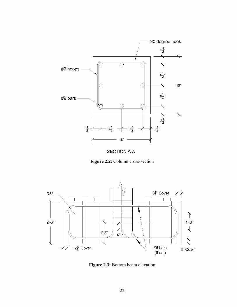
The longitudinal reinforcement consisted of eight No. 9 bars, which

corresponds to a reinforcement ratio of 0.025. Longitudinal bars were placed

uniformly around the perimeter of the cross-section, with 2½ in. of cover to the center

of the bars. All bars were continuous and contained no lap splices. The column bars

extended into the top and bottom beams, where a 90° bend was placed as shown in

Figure 2.1. Transverse reinforcement consisted of No. 3 closed hoops. All column

hoops had hooks with 90º bends and a 5db extension beyond the hook. Hoops were

spaced at 18 in. center-to-center along the full height of the columns.

During testing, the specimens were fixed to an 8-ft, 6-in. long by 3-ft wide by

3-ft, 8-in. tall concrete base block to adjust for the height of the loading system. The

procedure used to fix the specimens to the base block and the reaction floor is

described in detail in Section 2.5. The block was cast with twelve 2½-in. diameter

vertical holes and six 2-in. diameter vertical holes used to secure the block to the floor

with threaded steel rods. Four additional 2-in. diameter horizontal holes were cast to

21

lift the block into place. All holes were through thickness shafts. Dimensions and

reinforcement details of the base block are shown in Figures 2.11 and 2.12.

Figure 2.1: Specimen elevation

22

Figure 2.2: Column cross-section

Figure 2.3: Bottom beam elevation

23

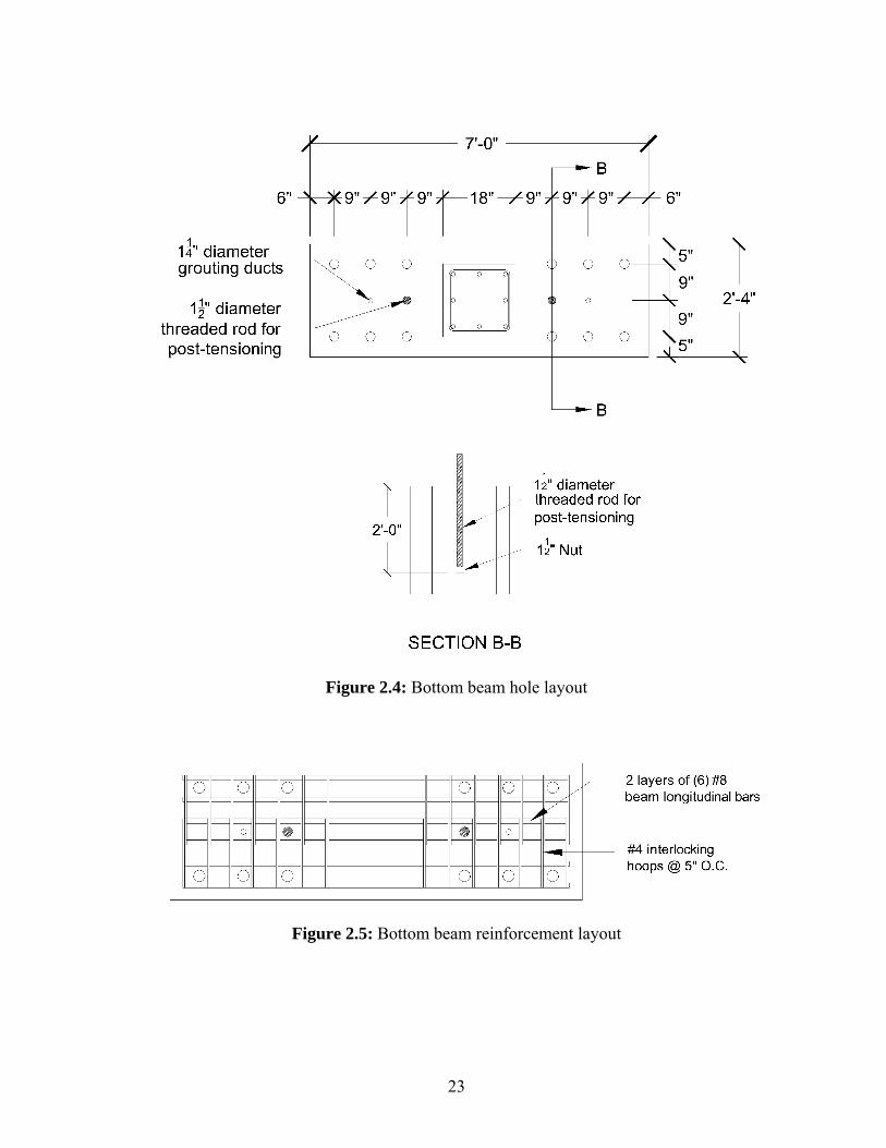
Figure 2.4: Bottom beam hole layout

Figure 2.5: Bottom beam reinforcement layout

24

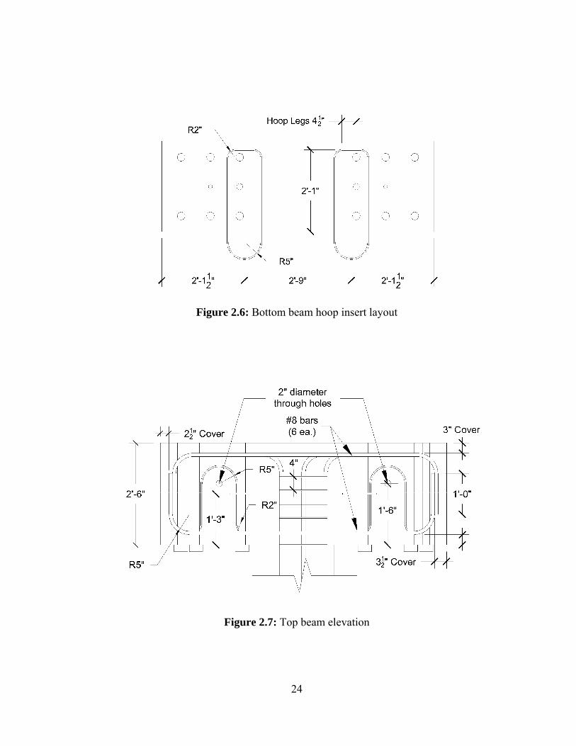
Figure 2.6: Bottom beam hoop insert layout

Figure 2.7: Top beam elevation

25

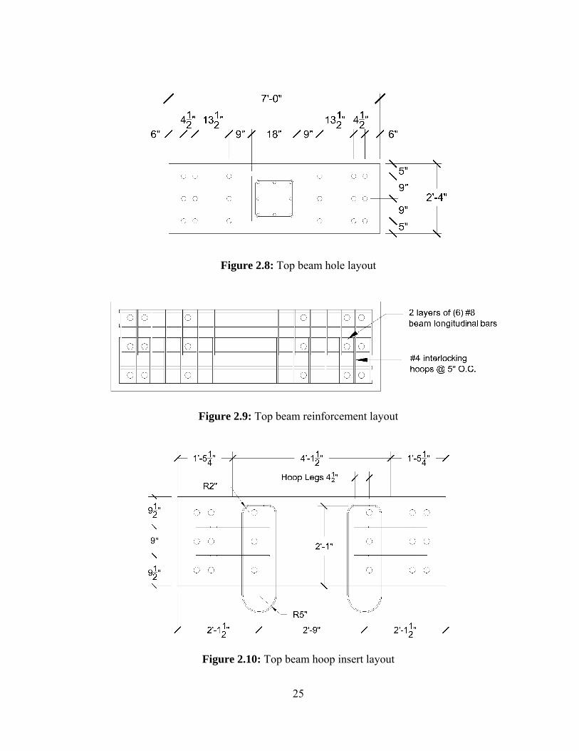
Figure 2.8: Top beam hole layout

Figure 2.9: Top beam reinforcement layout

Figure 2.10: Top beam hoop insert layout

26

Figu

re 2

.11:

Bas

e bl

ock

hole

layo

ut

Figu

re 2

.12:

Bas

e bl

ock

rein

forc

emen

t lay

out

27

2.3 Material Properties

2.3.1 Concrete

The target compressive strength of the concrete cf ′ was 3000 psi. The

concrete mix had normal-weight aggregate with a maximum aggregate size of ¾ in.

Mix specifications and design quantities for the concrete are shown in Tables 2.1 and

2.2. The concrete was supplied by LRM Industries, a local ready-mix supplier.

Twenty-four 6-in. diameter by 12-in. tall standard cylindrical compressive strength

specimens and two 6-in. by 6-in. by 22-in. flexural strength specimens were cast from

the middle third of each batch. Compressive and flexural strength specimens were

cured and stored with the column specimens to match the concrete properties of the

columns as accurately as possible.

Compressive strength tests were performed at 7, 14, 21, and 28 days after

casting, as well as on the final day of column testing, in accordance with ASTM C 39.

The compressive strengths listed in Table 2.3 represent the average strength

determined using two cylinders for the 7, 14, and 21-day tests, and three cylinders for

the 28-day and test day strengths. Two flexural strength tests and one modulus of

elasticity test were also conducted on the final day of column testing, in accordance

with ASTM C 78 and ASTM C 469, respectively. The average flexural strength fr

and modulus of elasticity Ec for each of the two specimens are also listed in Table

2.3.

28

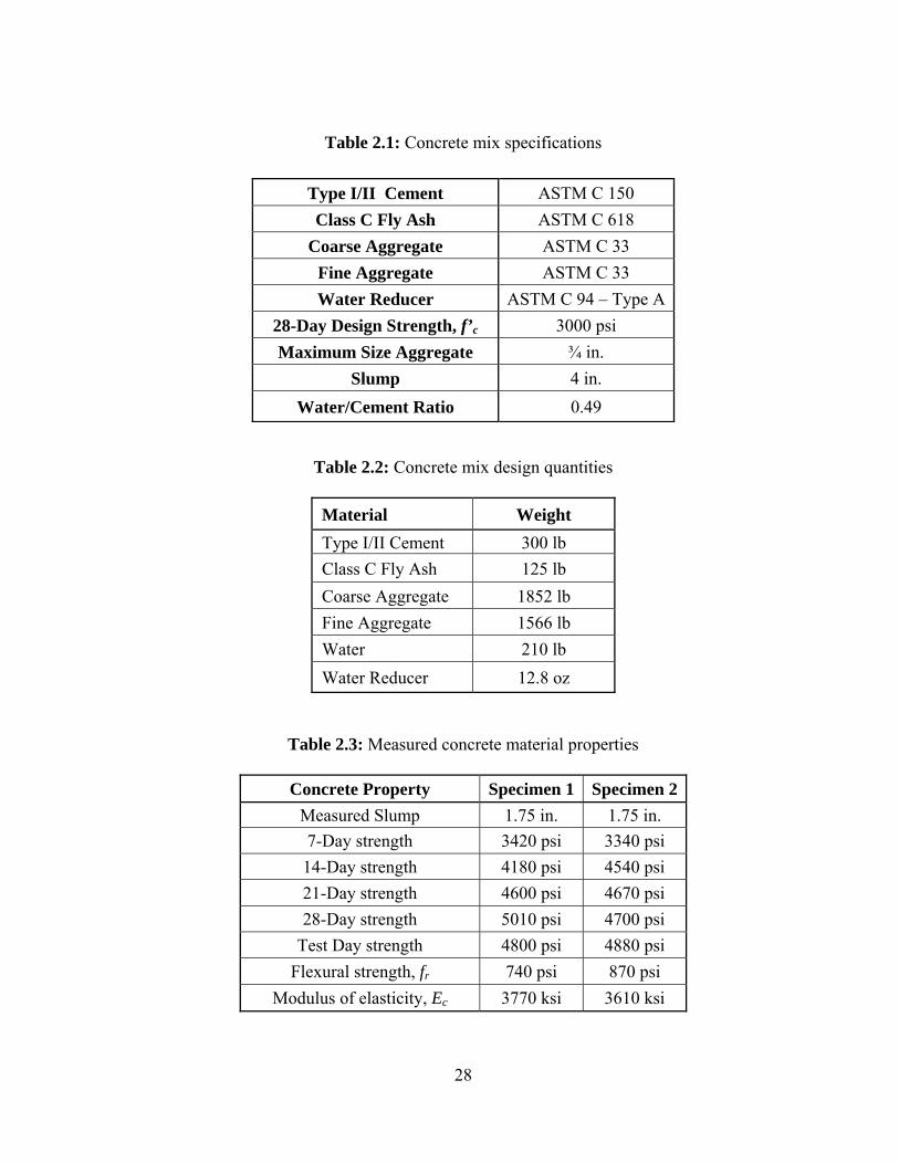
Table 2.1: Concrete mix specifications

Table 2.2: Concrete mix design quantities

Material Weight Type I/II Cement 300 lb Class C Fly Ash 125 lb Coarse Aggregate 1852 lb Fine Aggregate 1566 lb Water 210 lb Water Reducer 12.8 oz

Table 2.3: Measured concrete material properties

Concrete Property Specimen 1 Specimen 2 Measured Slump 1.75 in. 1.75 in. 7-Day strength 3420 psi 3340 psi 14-Day strength 4180 psi 4540 psi 21-Day strength 4600 psi 4670 psi 28-Day strength 5010 psi 4700 psi

Test Day strength 4800 psi 4880 psi Flexural strength, fr 740 psi 870 psi

Modulus of elasticity, Ec 3770 ksi 3610 ksi

Type I/II Cement ASTM C 150 Class C Fly Ash ASTM C 618

Coarse Aggregate ASTM C 33 Fine Aggregate ASTM C 33 Water Reducer ASTM C 94 – Type A

28-Day Design Strength, f’c 3000 psi Maximum Size Aggregate ¾ in.

Slump 4 in. Water/Cement Ratio 0.49

29

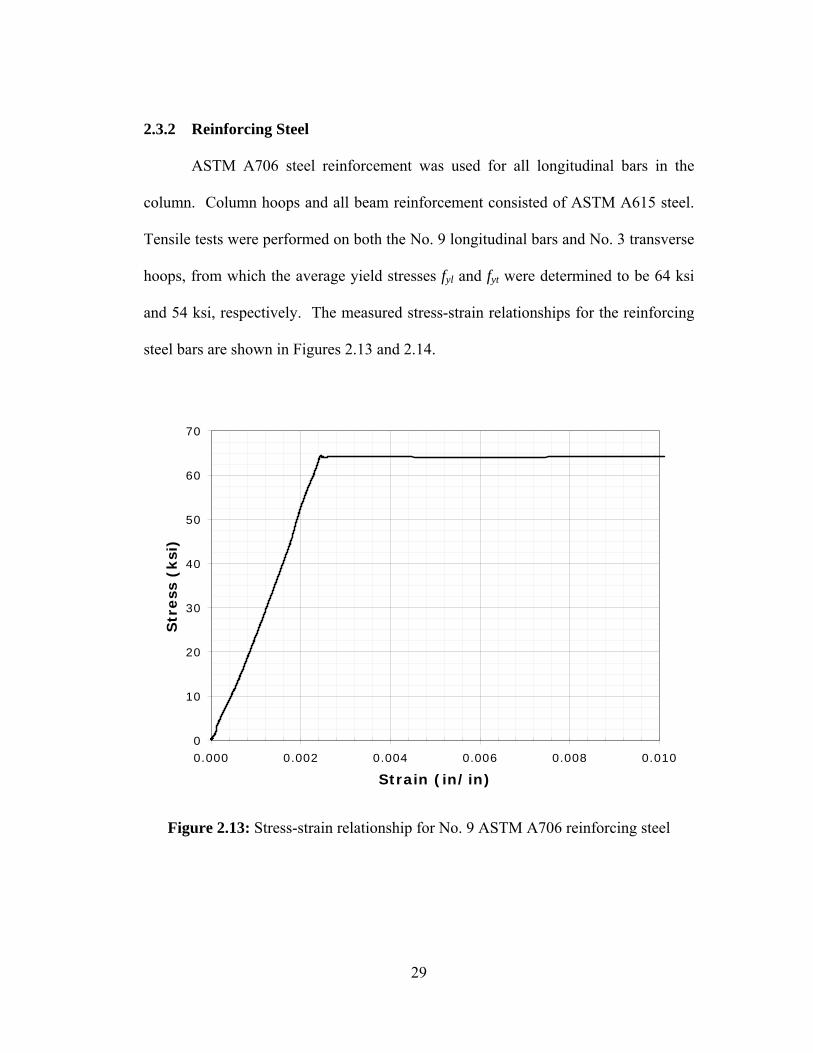
2.3.2 Reinforcing Steel

ASTM A706 steel reinforcement was used for all longitudinal bars in the

column. Column hoops and all beam reinforcement consisted of ASTM A615 steel.

Tensile tests were performed on both the No. 9 longitudinal bars and No. 3 transverse

hoops, from which the average yield stresses fyl and fyt were determined to be 64 ksi

and 54 ksi, respectively. The measured stress-strain relationships for the reinforcing

steel bars are shown in Figures 2.13 and 2.14.

0

10

20

30

40

50

60

70

0.000 0.002 0.004 0.006 0.008 0.010

Strain (in/in)

Str

ess

(ksi

)

Figure 2.13: Stress-strain relationship for No. 9 ASTM A706 reinforcing steel

30

0

10

20

30

40

50

60

70

0.000 0.002 0.004 0.006 0.008 0.010

Strain (in/in)

Str

ess

(ksi

)

Figure 2.14: Stress-strain relationship for No. 3 ASTM A615 reinforcing steel

2.4 Specimen Construction

Wood formwork and reinforcing steel cages were constructed in the Structural

Testing Laboratory at the University of Kansas. Specimens were cast in forms

constructed using 2x4 in. studs and ¾-in. medium density overlay plywood. Forms

were protected using baby oil as a release agent for all surfaces exposed to concrete.

Reinforcing bars were cut and bent by Gerdau Ameristeel, a local supplier. Prior to

tying the cages, deformations were removed from the reinforcing steel bars at the

locations where strain gages were to be attached. Cages were assembled using

standard 4-in., 8-in., and 10-in. wire ties. Standard steel reinforcement chairs were

31

attached to reinforcing bars in both the beam and column regions as necessary, to

achieve cover tolerances. Formwork and typical reinforcing cages are shown in

Figures 2.15 through 2.17.

Strain gages were obtained from Vishay Micro-Measurements. A total of 60

CEA-06, ¼-in. long, 120-Ω gages were attached to the longitudinal reinforcing bars,

and 16 CEA-06, ⅛-in. long, 120-Ω gages were attached to the column hoops. Prior to

attaching the strain gages, the surface of the reinforcement was cleaned and prepared

according to specifications provided by the manufacturer. After the gages were

attached, they were sealed with wax and covered with M-Coat J, a protective coating

used to shield the gages from damage during casting.

The specimens were cast in the horizontal position, using a single batch of

five cubic yards of concrete per specimen. The concrete was placed in two lifts, with

samples taken for strength specimens between the two lifts. The concrete was

consolidated by internal vibration to minimize the presence of voids, as shown in

Figure 2.18. Following placement and vibration of the second lift, the top surface of

the specimen was struck off and finished using hand trowels. Figure 2.19 shows a

photograph of a specimen immediately following finishing procedures. Afterward,

the specimen was covered with wet burlap and plastic sheeting. Wood formwork was

stripped after four days of moist curing and the specimens were air-dried as they were

stored inside the Structural Testing Laboratory until they were ready to be transported

to the MAST Laboratory.

32

Figure 2.15: Specimen formwork

Figure 2.16: Typical specimen reinforcing cage

33

Figure 2.17: Reinforcing cage in form, prior to casting

Figure 2.18: Internal vibration during concrete placement

34

Figure 2.19: Finished column test specimen

In order to prevent cracking during handling and transport, two 1½-in.

diameter threaded rods were cast into the bottom beam, and placed through openings

in the top beam, 9 in. from either side of the column. Each rod was instrumented with

strain gages assembled into a full Wheatstone bridge configuration to form a load

cell, which was used to monitor the force in the rod. Each rod was tensioned to 30

kips (approximately 0.02 cg fA ′ per rod) using 1½-in. diameter torque nuts over 8-in.

by 8-in. by 1½-in. thick plate washers.

35

2.5 Test Setup

Testing was performed at the MAST (Multi-Axial Subassembly Testing)

Laboratory at the University of Minnesota. Following construction and curing, the

specimens and base block were shipped to the laboratory on a flatbed truck and

unloaded by the laboratory staff. After arrival at the MAST Laboratory, the

specimens were tilted up into the vertical position using the frame shown in Figure

2.20. The base block and specimens were then moved from the staging area of the

laboratory to the reaction floor using the crane. Final positioning was performed

using the crosshead of the multi-axial loading system.

Figure 2.20: Tilt-up frame used to rotate specimens into the vertical position

36

The base block was post-tensioned to the reaction floor using six 1½-in.

diameter ASTM A193 Grade B7 threaded rods, 1½-in. standard nuts, and 1½-in. thick

A36 steel plate washers. UltraCal 30 grout was poured through two 1¼-in. diameter

holes in either side of the base block to ensure uniform contact and load distribution

to the reaction floor. Following final positioning of the base block, the column

specimen was placed on top of the base block. After placement, the specimen was

post-tensioned to the reaction floor using twelve 2-in. diameter ASTM A193 Grade

B7 threaded rods, passing through ducts in the base block. The rods were fastened to

the specimen using 2-in. torque nuts, and 1½-in. thick A36 steel plate washers.

UltraCal 30 grout was used again to fill all voids at the base block-column specimen

interface to obtain uniform load distribution. After the instrumentation was attached

to the specimen, as discussed in Section 2.7, the top beam was post-tensioned to the

crosshead, as shown in Figure 2.21, using eighteen 1½-in. diameter ASTM A193

Grade B7 threaded rods, 1½-in. torque nuts, and 1½-in. thick A36 steel plate washers.

Grout was then poured through holes in the crosshead to achieve uniform load

distribution to the top beam.

Figure 2.22 shows the testing assembly that was used to induce axial and

lateral loads. Specimens were loaded axially using four 330-kip hydraulic actuators

attached to each of the four arms of the crosshead. Lateral loading was applied by

two 440-kip hydraulic actuators, attached horizontally to the side of the crosshead.

All actuators were capable of operating in either force or displacement control mode,

allowing for independent control of all degrees of freedom.

37

Figure 2.21: Top beam connection to the crosshead

Figure 2.22: Test configuration

Crosshead

Specimen

Horizontal Actuators

Vertical Actuators

38

2.6 Loading and Displacement History

The axial load applied to each specimen was maintained at a constant value

throughout the first phase of both tests to simulate the behavior of an interior building

column. For the first test, axial load remained constant at a load of 500 kips. This

corresponded to approximately 0.50 cg fA ′ using the target concrete compressive

strength of 3000 psi and 0.32 cg fA ′ using the measured compressive strength of 4800

psi. The axial load for the second test was maintained constant at 340 kips, which

corresponded to 0.35 cg fA ′ and 0.22 cg fA ′ based on the target and measured

compressive strengths, respectively.

The maximum lateral displacement was maintained constant for sets of three

cycles and was increased after each set of three cycles was completed. The peak

displacement for each set of three cycles was established on the basis of drift ratio.

Peak drift ratios used for each set of cycles began at 0.125% and were subsequently

set at 0.25% increments, up to a drift ratio of 1.50%. Beyond a drift ratio of 1.50%,

the magnitude of each increment was changed to 0.50%, up to axial failure. The

applied displacement history is shown in Figure 2.23.

39

-2.5

-2.0

-1.5

-1.0

-0.50.0

0.5

1.0

1.5

2.0

2.5

Drift Ratio (%)

Figu

re 2

.23:

Dis

plac

emen

t his

tory

use

d fo

r bot

h sp

ecim

ens

40

During testing, the vertical actuators were programmed to run simultaneously

in force-control mode to maintain a constant axial load, and in displacement-control

mode to prevent rotation of the top beam. Horizontal actuators were programmed to

operate in displacement-control mode, according to the displacement history shown

in Figure 2.23. Lateral loading was applied in the east-west direction, defined such

that east was considered positive displacement. The horizontal actuators were also

used to restrain motion in the north-south direction. During testing, the maximum

north-south displacement that was measured was approximately 0.004 in. for both

tests. The maximum measured east-west rotation of the top beam for both tests was

0.001 degrees. The maximum recorded slip of the bottom beam with respect to the

floor was 0.005 in. for the first test and 0.01 in. for the second test.

An axial failure event was defined as a loss of 10% of the axial load carrying

capacity. At this point, the vertical actuators were programmed to shift from force-

control mode to displacement-control mode, such that the actuators would retain the

vertical displacement of the column at the time of axial failure. Following an axial

failure event, the system was transitioned back to force-control mode in the vertical

direction, under a reduced axial load, and the standard displacement protocol was

continued. When the damage in the columns was deemed too severe, the

displacement protocol was modified such that the vertical deformation was increased

uniformly, while maintaining a constant level of maximum lateral displacement. This

modification to the displacement protocol was intended to measure the residual axial

capacity of the columns.

41

2.7 Instrumentation

During each test, 124 channels of data were recorded. This included 76 strain

gages, 23 Linear Variable Differential Transformers (LVDTs), 11 string

potentiometers, and 14 load and displacement channels set up to monitor the motion

of the crosshead. Additional derived channels were also set up to calculate various

parameters such as column shortening and uplift at the base of the column, for

reference during testing. All data was acquired and stored using the data acquisition

system at the MAST Laboratory. The recording frequency for the data acquisition

system was set at 1.0 Hz. for testing and 0.10 Hz. for overnight monitoring purposes.

Data acquisition began prior to applying axial load. After loading, all instrumentation

channels were reset to zero before initiating the lateral loading protocol. Because all

recorded strain gage channels were reset to zero after application of the axial load,

additional derived channels were created to correct the readings by adding back in the

strain induced during axial loading.

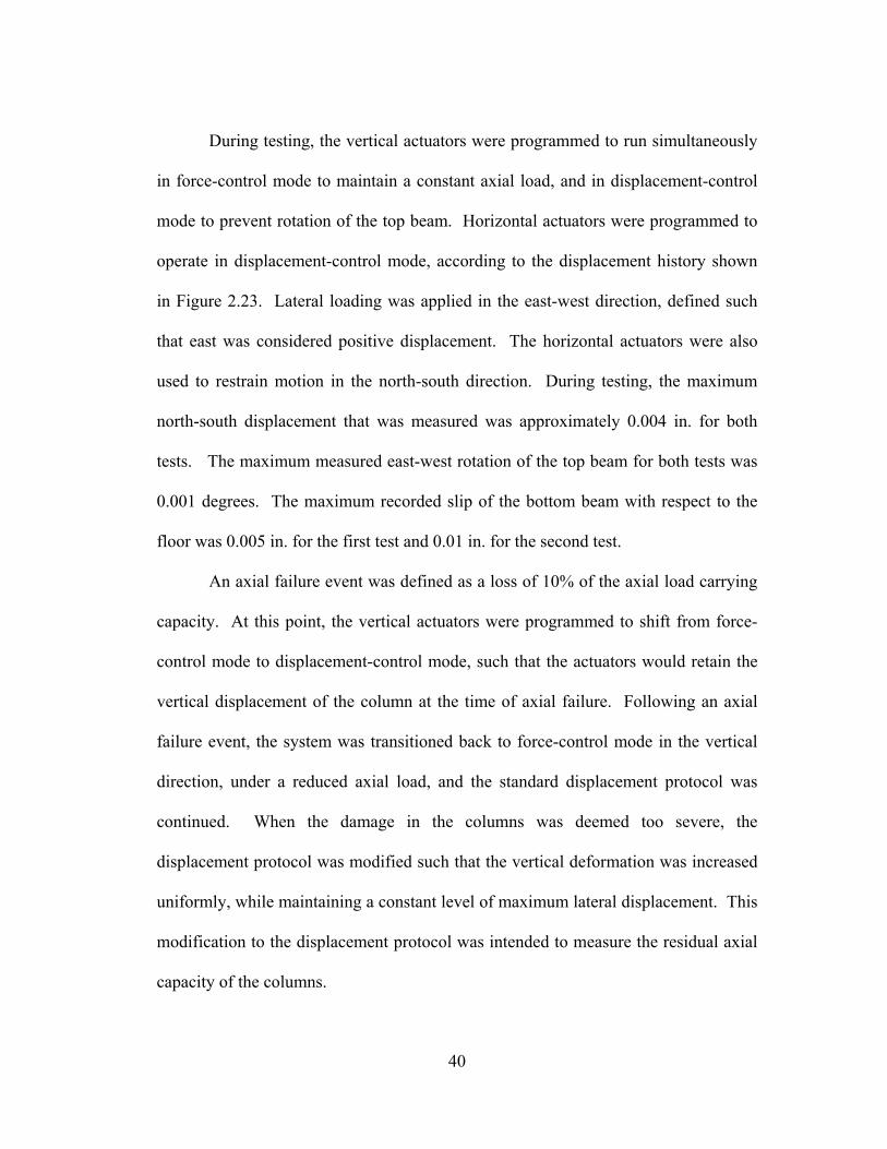
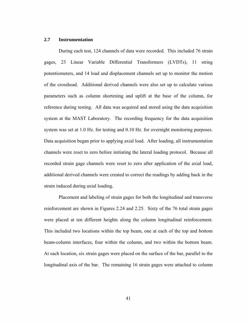
Placement and labeling of strain gages for both the longitudinal and transverse

reinforcement are shown in Figures 2.24 and 2.25. Sixty of the 76 total strain gages

were placed at ten different heights along the column longitudinal reinforcement.

This included two locations within the top beam, one at each of the top and bottom

beam-column interfaces, four within the column, and two within the bottom beam.

At each location, six strain gages were placed on the surface of the bar, parallel to the

longitudinal axis of the bar. The remaining 16 strain gages were attached to column

42

hoops 1, 2, 5, and 6. On each hoop, two gages were attached to each of the faces of

the hoop parallel to the lateral loading direction, as shown in Figure 2.25.

Figure 2.24: Strain gage placement

43

Figure 2.25: Strain gage locations and labeling

LVDTs were attached along the height of the column, as shown in Figure

2.26, to measure relative vertical, diagonal, and horizontal displacements within the

column. Attachments were made to the column using aluminum brackets that were

connected to threaded rods embedded at 19-in. intervals along the surface of the

column, as shown in Figure 2.27. Depending on the anticipated displacement at a

particular location, LVDTs with a total range of either 2.0 or 1.0 in. were used.

Additional LVDTs with a range of 1.0 in. were attached from the bottom beam to

reference frames connected to the reaction floor to measure slip and uplift at the base

of the specimen.

44

Figure 2.26: LVDT and string potentiometer placement

45

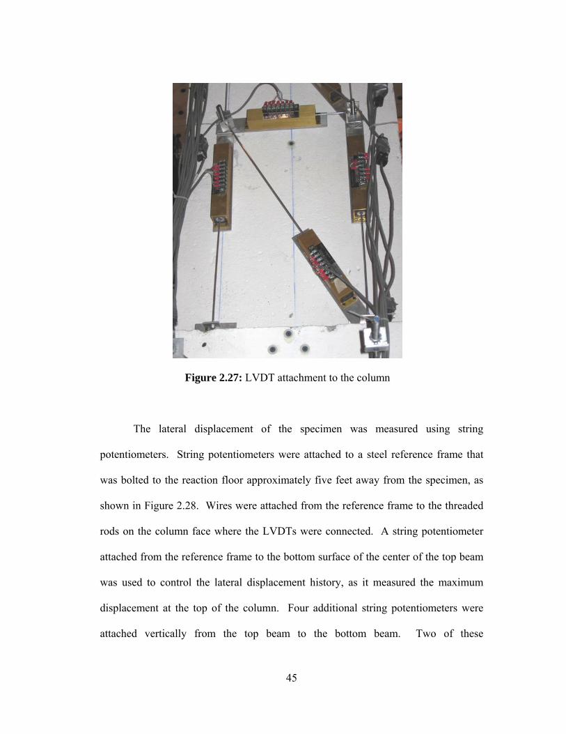
Figure 2.27: LVDT attachment to the column

The lateral displacement of the specimen was measured using string

potentiometers. String potentiometers were attached to a steel reference frame that

was bolted to the reaction floor approximately five feet away from the specimen, as

shown in Figure 2.28. Wires were attached from the reference frame to the threaded

rods on the column face where the LVDTs were connected. A string potentiometer

attached from the reference frame to the bottom surface of the center of the top beam

was used to control the lateral displacement history, as it measured the maximum

displacement at the top of the column. Four additional string potentiometers were

attached vertically from the top beam to the bottom beam. Two of these

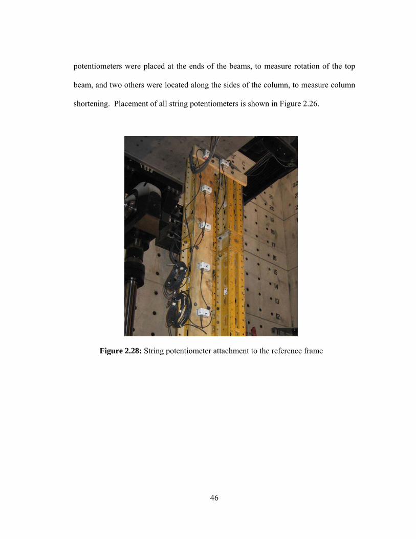
46

potentiometers were placed at the ends of the beams, to measure rotation of the top

beam, and two others were located along the sides of the column, to measure column

shortening. Placement of all string potentiometers is shown in Figure 2.26.

Figure 2.28: String potentiometer attachment to the reference frame

47

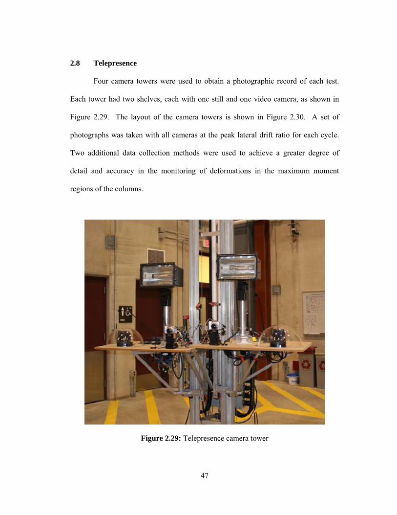
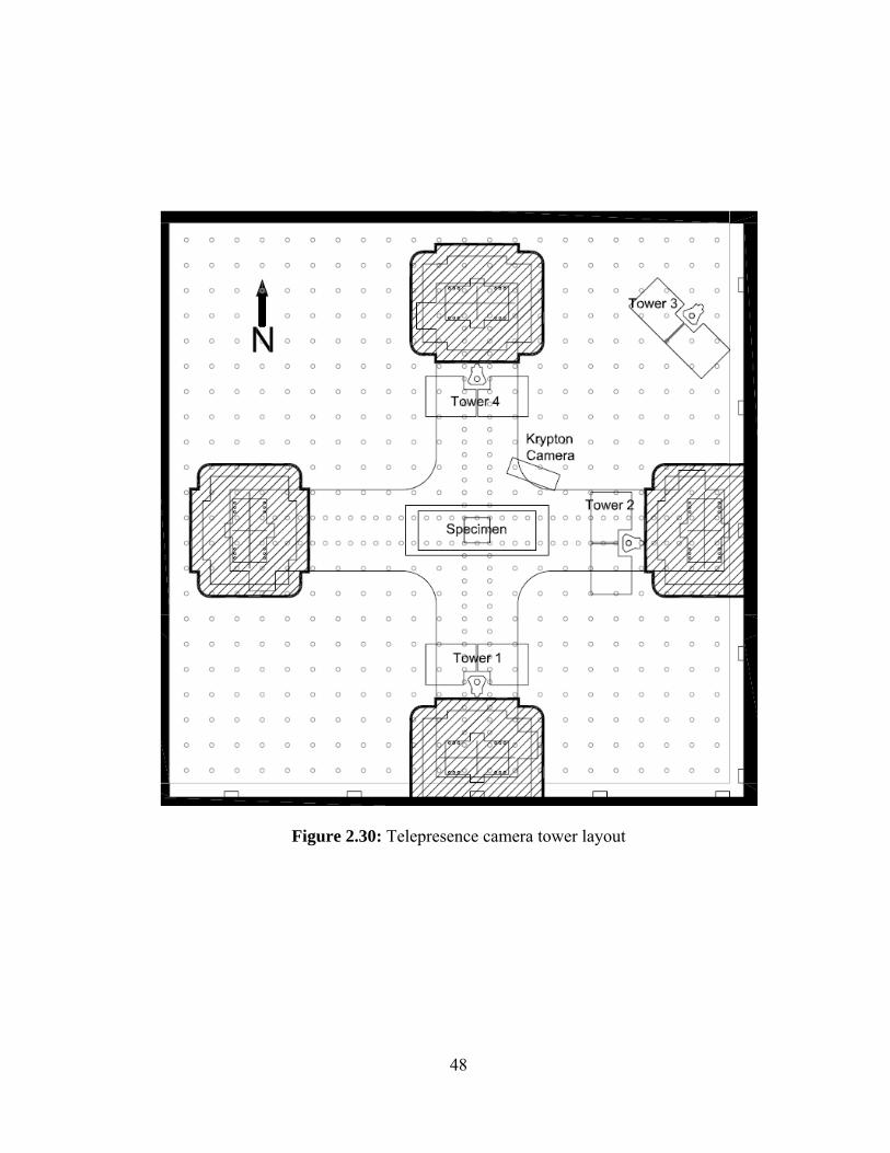
2.8 Telepresence

Four camera towers were used to obtain a photographic record of each test.

Each tower had two shelves, each with one still and one video camera, as shown in

Figure 2.29. The layout of the camera towers is shown in Figure 2.30. A set of

photographs was taken with all cameras at the peak lateral drift ratio for each cycle.

Two additional data collection methods were used to achieve a greater degree of

detail and accuracy in the monitoring of deformations in the maximum moment

regions of the columns.

Figure 2.29: Telepresence camera tower

48

Figure 2.30: Telepresence camera tower layout

49

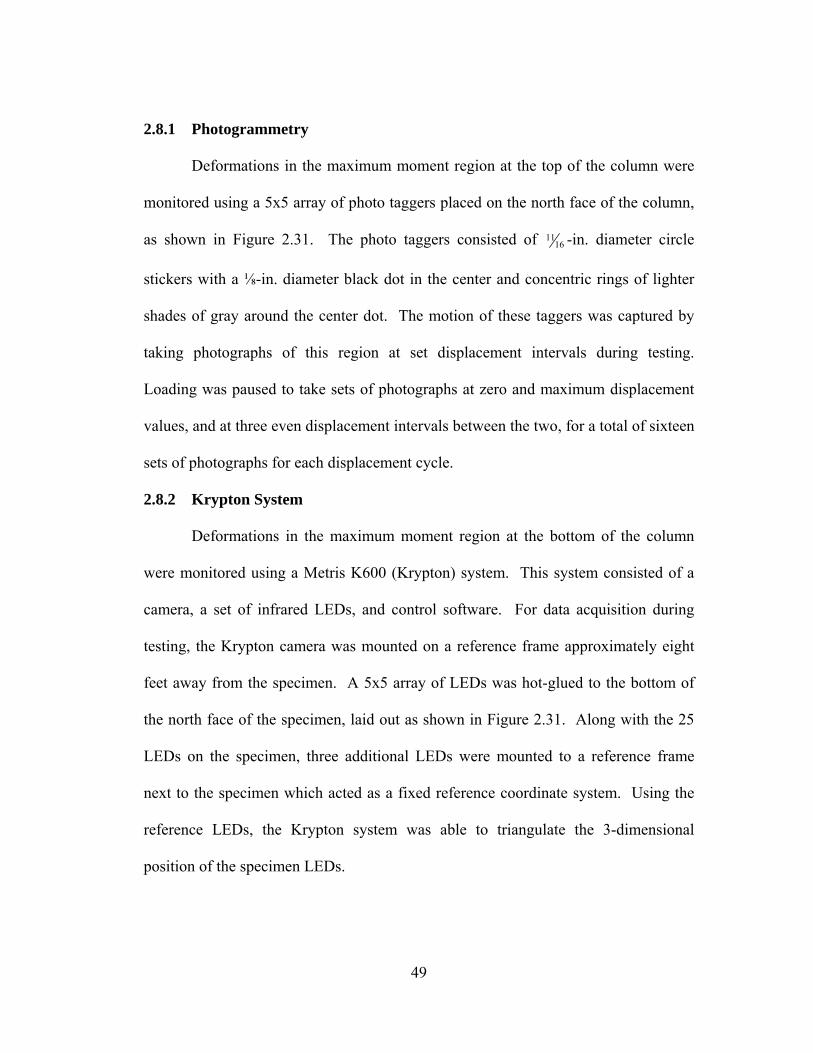
2.8.1 Photogrammetry

Deformations in the maximum moment region at the top of the column were

monitored using a 5x5 array of photo taggers placed on the north face of the column,

as shown in Figure 2.31. The photo taggers consisted of 1611 -in. diameter circle

stickers with a ⅛-in. diameter black dot in the center and concentric rings of lighter

shades of gray around the center dot. The motion of these taggers was captured by

taking photographs of this region at set displacement intervals during testing.

Loading was paused to take sets of photographs at zero and maximum displacement

values, and at three even displacement intervals between the two, for a total of sixteen

sets of photographs for each displacement cycle.

2.8.2 Krypton System

Deformations in the maximum moment region at the bottom of the column

were monitored using a Metris K600 (Krypton) system. This system consisted of a

camera, a set of infrared LEDs, and control software. For data acquisition during

testing, the Krypton camera was mounted on a reference frame approximately eight

feet away from the specimen. A 5x5 array of LEDs was hot-glued to the bottom of

the north face of the specimen, laid out as shown in Figure 2.31. Along with the 25

LEDs on the specimen, three additional LEDs were mounted to a reference frame

next to the specimen which acted as a fixed reference coordinate system. Using the

reference LEDs, the Krypton system was able to triangulate the 3-dimensional

position of the specimen LEDs.

50

Figure 2.31: Photo tagger and Krypton LED layout

51

CHAPTER 3: TEST RESULTS

3.1 Introduction

Two full-scale reinforced concrete building columns were tested to failure

under constant axial and cyclic lateral loading. Results from each of these tests

reported in this Chapter include a description of the progression of damage and a

summary of the measured data taken throughout each test. The following designation

is used throughout this Chapter; references to a 1.00% drift ratio cycle refer to a load

cycle with a maximum lateral displacement corresponding to a drift ratio of 1.00%,

and likewise for other drift ratios. Measured data presented in this Chapter includes

the lateral load-deflection and moment-curvature relationships for each specimen, as

well as the measured deflection components, bar strain, and shear capacity. Results

from predictive and behavioral models are also presented and compared with

measured and observed data from each test.

3.2 Damage Progression – Specimen 1

Specimen 1 was subjected to a constant axial load of 500 kips, or

approximately 0.50 cg fA ′ for the target concrete compressive strength of 3,000 psi.

The applied lateral displacement protocol is described in Section 2.6 and shown in

Figure 2.23.

Before loading began, hairline cracks were observed on the top and bottom

beams, as a result of post-tensioning the specimen to the crosshead and the reaction

floor. During the initial displacement cycles to a maximum drift ratio of 0.125%,

52

hairline cracks were observed at the interfaces between the column and the beams.

During these displacement cycles, no cracking was observed on any of the column

faces.

Beginning at cycles to a drift ratio of 0.25%, horizontal flexural cracks were

observed on the east and west faces of the column, perpendicular to the lateral

loading direction. At subsequent cycles to a 0.25% drift ratio, the horizontal cracks

propagated across the full width of the east and west faces of the column, extending

deeper into the column and becoming visible on the north and south faces. These

cracks opened and closed during each cycle. At this displacement level, all flexural

cracks in the maximum moment regions of the specimen remained essentially

horizontal in orientation, as shown in Figure 3.1.

During the first 0.50% drift ratio cycle, the horizontal flexural cracks observed

on the north and south column faces began to change in orientation, turning at an

angle indicative of shear cracking. Additional shear cracks formed and extended

deeper into the column as cycling continued, with cracks from opposite faces of the

column meeting in the center of the north and south faces, as displayed in Figure 3.2.

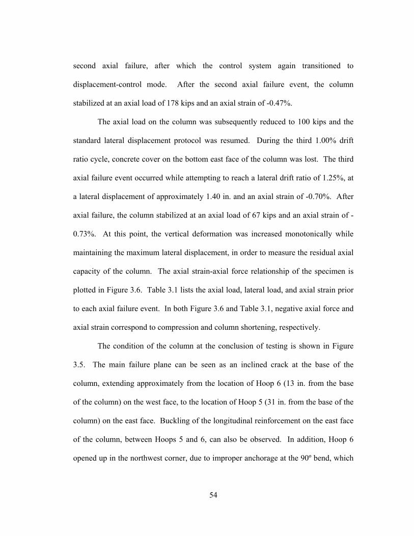
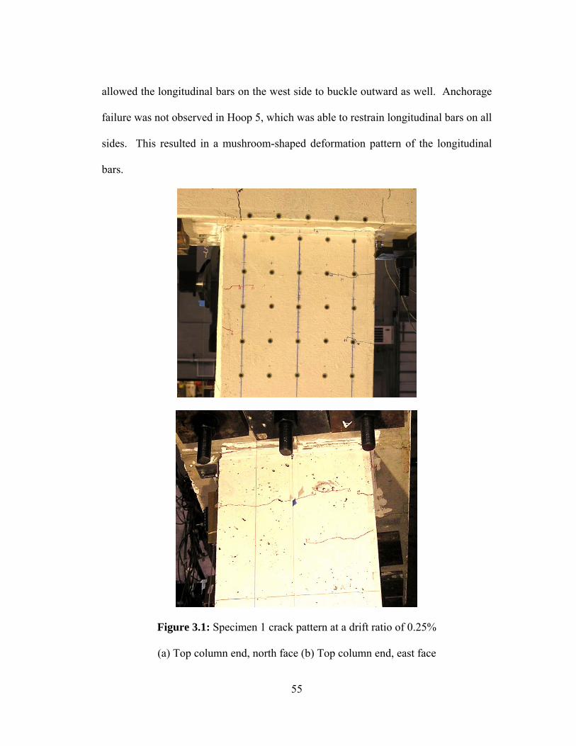
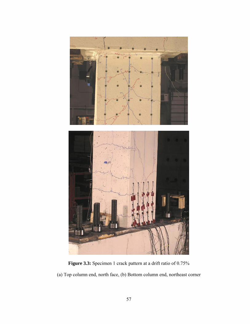
During the cycles to a drift ratio of 0.75%, there was significant growth in the

inclined cracks on the north and south faces of the column, with cracks from opposite

sides of the column crossing near the center of the north and south faces, as shown in

Figure 3.3. Additional horizontal cracks formed on the east and west faces, along

with several vertical cracks, indicating splitting of the concrete cover along the

53

longitudinal reinforcement. No cracking was observed in the middle third of the

column at this displacement level.

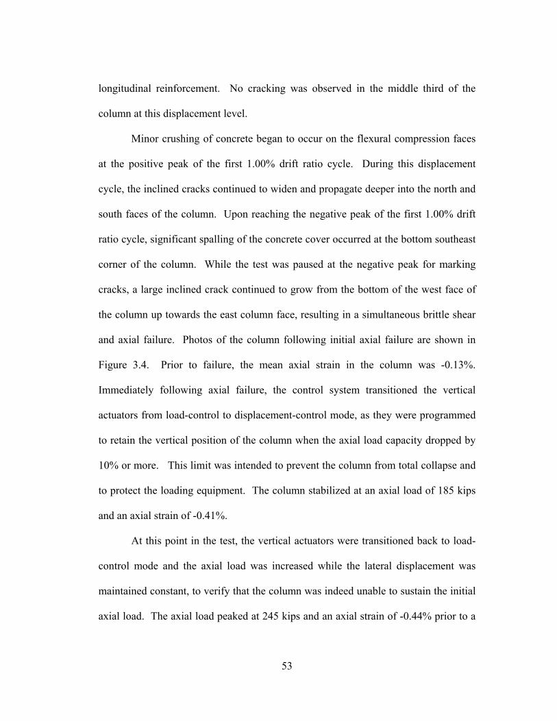
Minor crushing of concrete began to occur on the flexural compression faces

at the positive peak of the first 1.00% drift ratio cycle. During this displacement

cycle, the inclined cracks continued to widen and propagate deeper into the north and

south faces of the column. Upon reaching the negative peak of the first 1.00% drift

ratio cycle, significant spalling of the concrete cover occurred at the bottom southeast

corner of the column. While the test was paused at the negative peak for marking

cracks, a large inclined crack continued to grow from the bottom of the west face of

the column up towards the east column face, resulting in a simultaneous brittle shear

and axial failure. Photos of the column following initial axial failure are shown in

Figure 3.4. Prior to failure, the mean axial strain in the column was -0.13%.

Immediately following axial failure, the control system transitioned the vertical

actuators from load-control to displacement-control mode, as they were programmed

to retain the vertical position of the column when the axial load capacity dropped by

10% or more. This limit was intended to prevent the column from total collapse and

to protect the loading equipment. The column stabilized at an axial load of 185 kips

and an axial strain of -0.41%.

At this point in the test, the vertical actuators were transitioned back to load-

control mode and the axial load was increased while the lateral displacement was

maintained constant, to verify that the column was indeed unable to sustain the initial

axial load. The axial load peaked at 245 kips and an axial strain of -0.44% prior to a

54

second axial failure, after which the control system again transitioned to

displacement-control mode. After the second axial failure event, the column

stabilized at an axial load of 178 kips and an axial strain of -0.47%.

The axial load on the column was subsequently reduced to 100 kips and the

standard lateral displacement protocol was resumed. During the third 1.00% drift

ratio cycle, concrete cover on the bottom east face of the column was lost. The third

axial failure event occurred while attempting to reach a lateral drift ratio of 1.25%, at

a lateral displacement of approximately 1.40 in. and an axial strain of -0.70%. After

axial failure, the column stabilized at an axial load of 67 kips and an axial strain of -

0.73%. At this point, the vertical deformation was increased monotonically while

maintaining the maximum lateral displacement, in order to measure the residual axial

capacity of the column. The axial strain-axial force relationship of the specimen is

plotted in Figure 3.6. Table 3.1 lists the axial load, lateral load, and axial strain prior

to each axial failure event. In both Figure 3.6 and Table 3.1, negative axial force and

axial strain correspond to compression and column shortening, respectively.

The condition of the column at the conclusion of testing is shown in Figure

3.5. The main failure plane can be seen as an inclined crack at the base of the

column, extending approximately from the location of Hoop 6 (13 in. from the base

of the column) on the west face, to the location of Hoop 5 (31 in. from the base of the

column) on the east face. Buckling of the longitudinal reinforcement on the east face

of the column, between Hoops 5 and 6, can also be observed. In addition, Hoop 6

opened up in the northwest corner, due to improper anchorage at the 90º bend, which

55

allowed the longitudinal bars on the west side to buckle outward as well. Anchorage

failure was not observed in Hoop 5, which was able to restrain longitudinal bars on all

sides. This resulted in a mushroom-shaped deformation pattern of the longitudinal

bars.

Figure 3.1: Specimen 1 crack pattern at a drift ratio of 0.25%

(a) Top column end, north face (b) Top column end, east face

56

Figure 3.2: Specimen 1 crack pattern at a drift ratio of 0.50%

(a) Top column end, north face, (b) Bottom column end, south face

57

Figure 3.3: Specimen 1 crack pattern at a drift ratio of 0.75%

(a) Top column end, north face, (b) Bottom column end, northeast corner

58

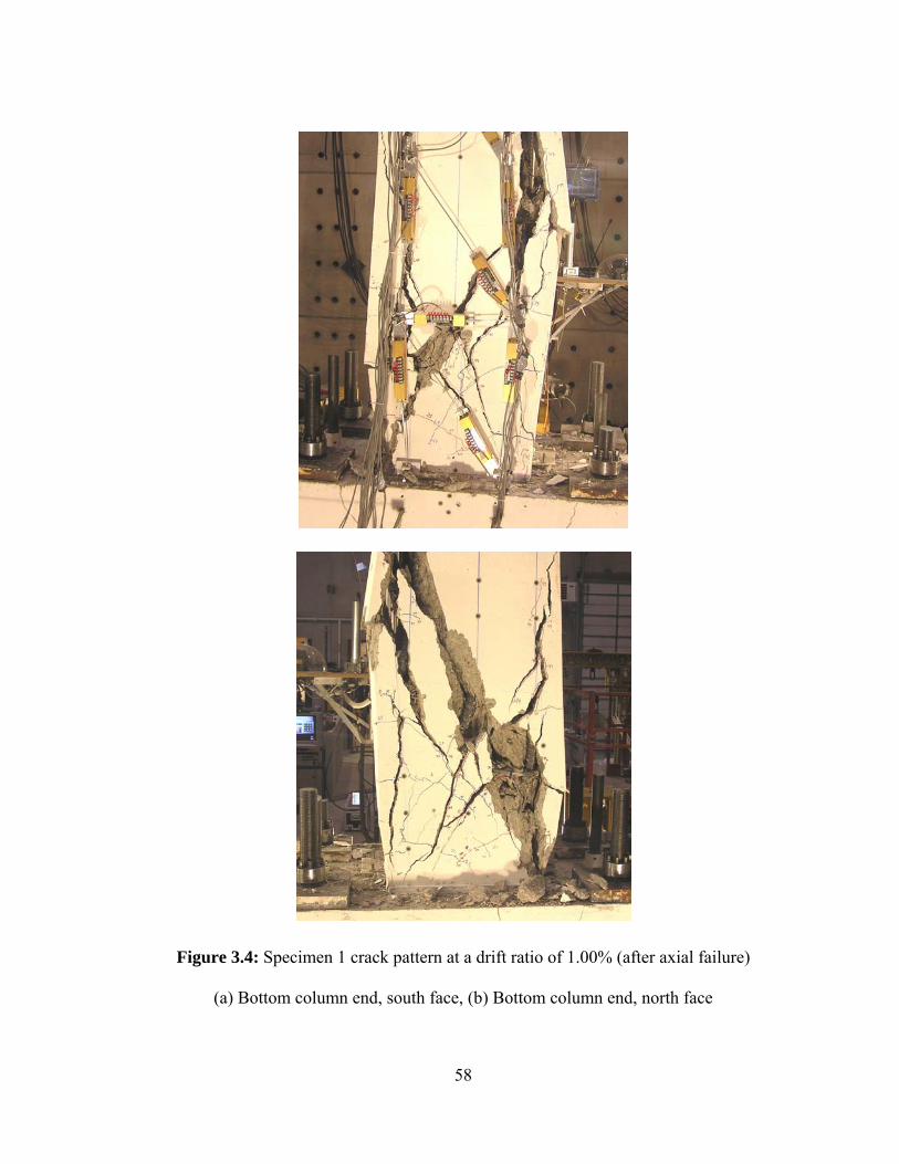
Figure 3.4: Specimen 1 crack pattern at a drift ratio of 1.00% (after axial failure)

(a) Bottom column end, south face, (b) Bottom column end, north face

59

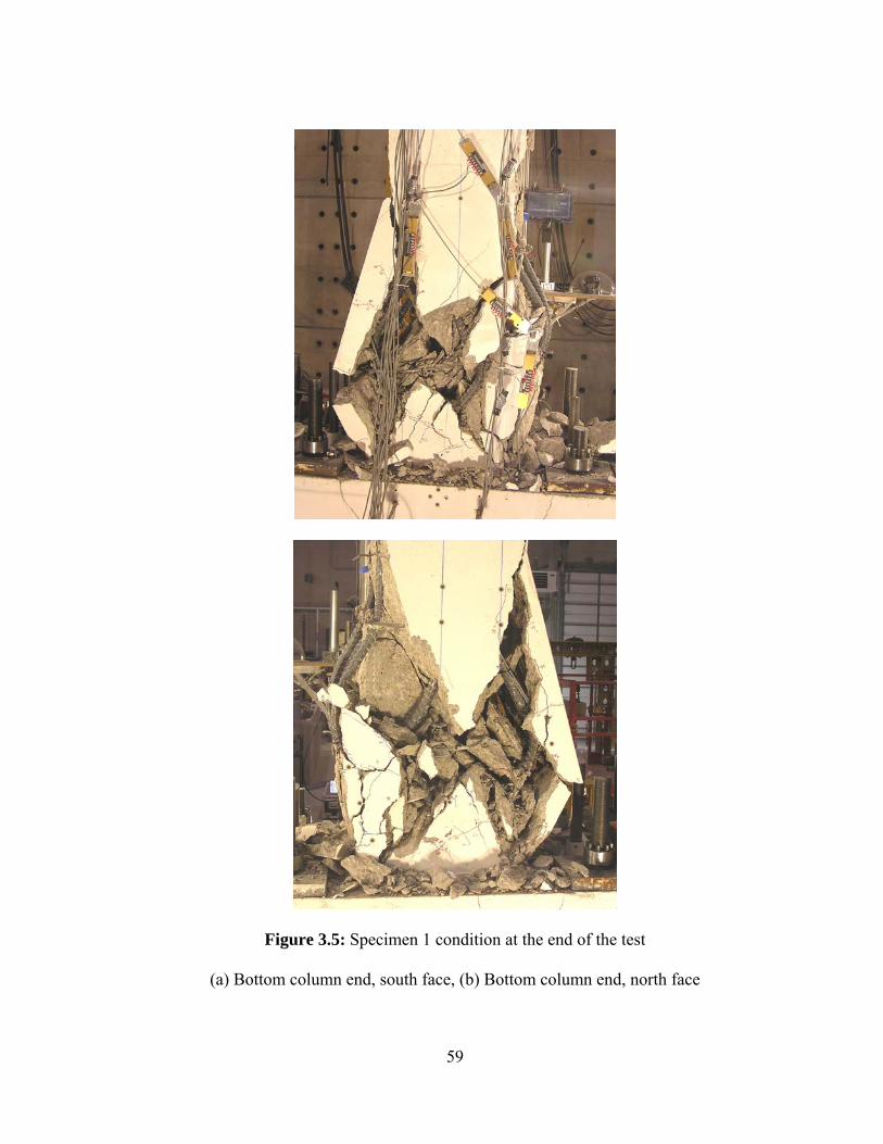
Figure 3.5: Specimen 1 condition at the end of the test

(a) Bottom column end, south face, (b) Bottom column end, north face

60

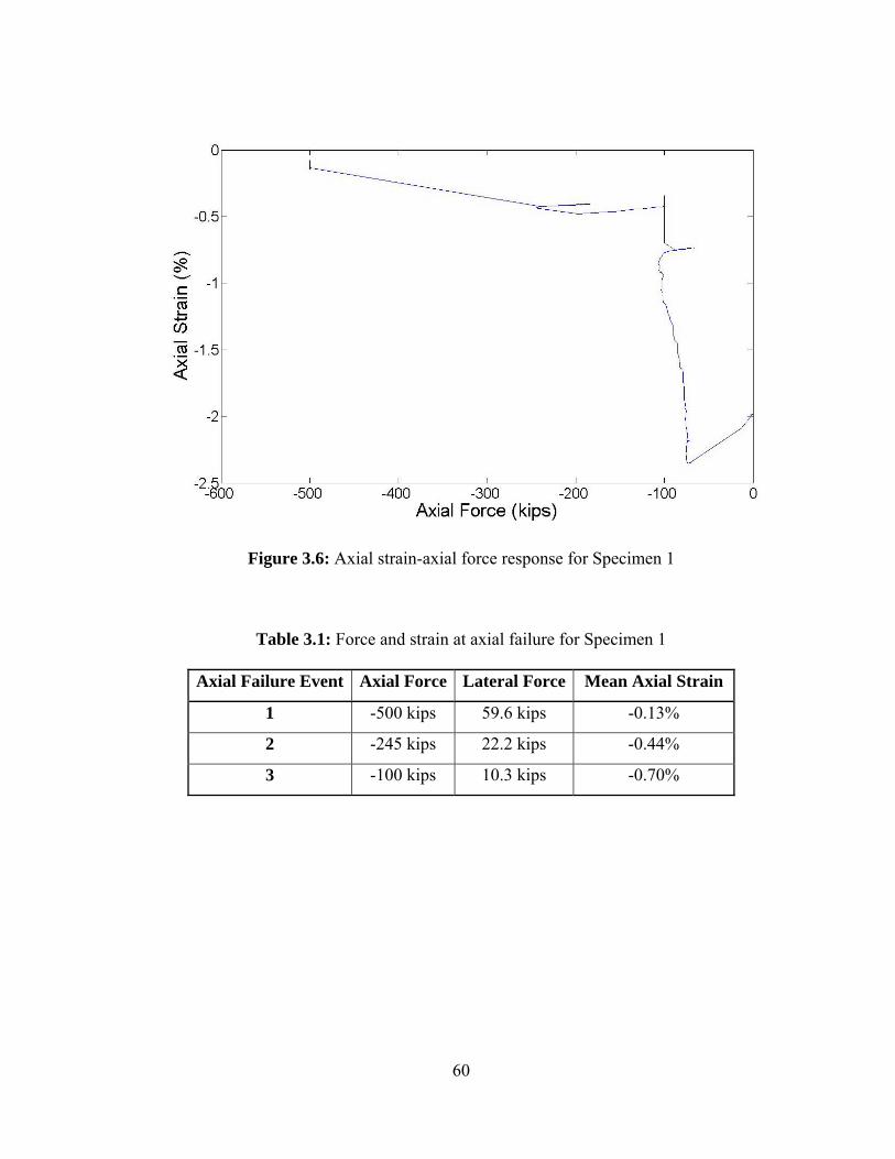
Figure 3.6: Axial strain-axial force response for Specimen 1

Table 3.1: Force and strain at axial failure for Specimen 1

Axial Failure Event Axial Force Lateral Force Mean Axial Strain

1 -500 kips 59.6 kips -0.13%

2 -245 kips 22.2 kips -0.44%

3 -100 kips 10.3 kips -0.70%

61

3.3 Damage Progression – Specimen 2

Specimen 2 was subjected to a constant axial load of 340 kips, or

approximately 0.35 cg fA ′ for the target concrete compressive strength of 3,000 psi.

The applied lateral displacement protocol was identical to that used for Specimen 1.

Similar to Specimen 1, hairline cracks were observed prior to lateral loading

along the top and bottom beams due to post-tensioning the specimen to the crosshead

and the reaction floor. During the 0.125% drift ratio cycles, hairline cracks were

observed at the interfaces between the column and the beams. At this displacement

level, no cracking was observed on any of the column faces.

During cycles to a drift ratio of 0.25%, horizontal flexural cracks were

observed on the east and west column faces, perpendicular to the direction of lateral

loading. At this displacement level, cracking was confined to the east and west faces

of the column.

The horizontal cracks observed on the east and west column faces continued

to grow during 0.50% drift ratio cycles, becoming visible on the north and south

column faces. These cracks opened and closed during each cycle. Figure 3.7

indicates that at this displacement level, the orientation of all cracks remained

essentially horizontal.

During 0.75% drift ratio cycles, the orientation of the cracks on the north and

south column faces began to change, growing at angles indicative of shear cracking,

as shown in Figure 3.8. These inclined cracks propagated deeper into the specimen as

cycling continued, with cracks from opposite sides of the column meeting and

62

crossing near the center of the north and south faces. Additional horizontal flexural

cracks were also observed on the east and west faces of the column.

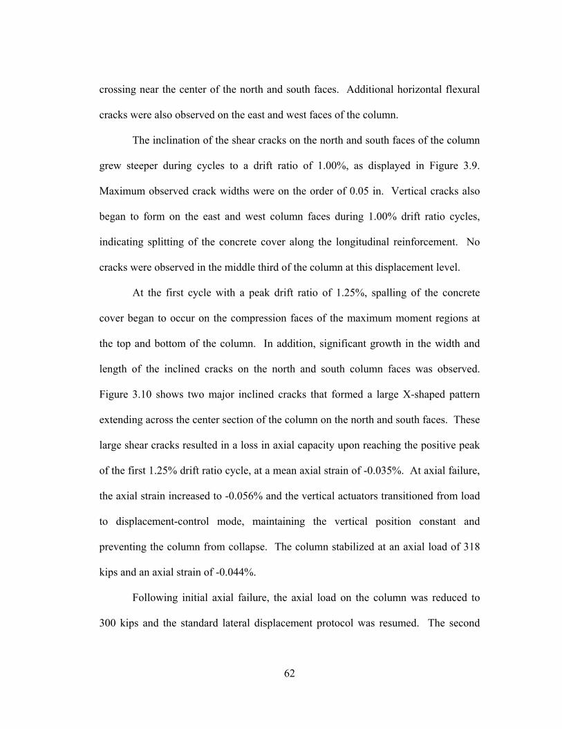
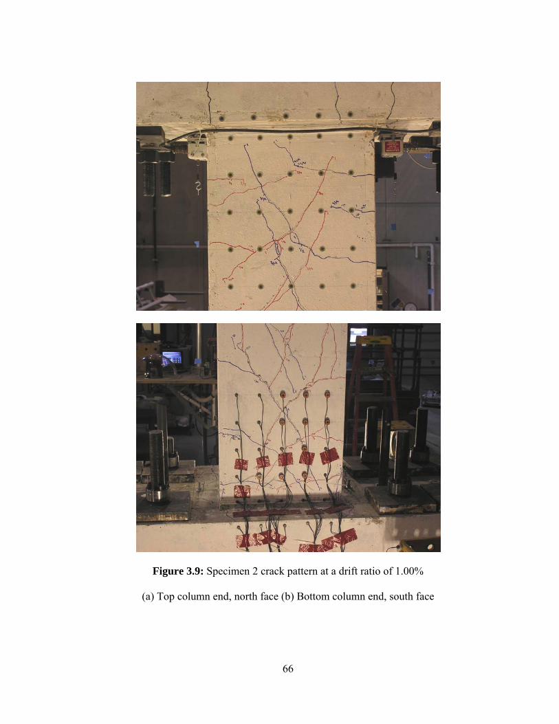
The inclination of the shear cracks on the north and south faces of the column

grew steeper during cycles to a drift ratio of 1.00%, as displayed in Figure 3.9.

Maximum observed crack widths were on the order of 0.05 in. Vertical cracks also

began to form on the east and west column faces during 1.00% drift ratio cycles,

indicating splitting of the concrete cover along the longitudinal reinforcement. No

cracks were observed in the middle third of the column at this displacement level.

At the first cycle with a peak drift ratio of 1.25%, spalling of the concrete

cover began to occur on the compression faces of the maximum moment regions at

the top and bottom of the column. In addition, significant growth in the width and

length of the inclined cracks on the north and south column faces was observed.

Figure 3.10 shows two major inclined cracks that formed a large X-shaped pattern

extending across the center section of the column on the north and south faces. These

large shear cracks resulted in a loss in axial capacity upon reaching the positive peak

of the first 1.25% drift ratio cycle, at a mean axial strain of -0.035%. At axial failure,

the axial strain increased to -0.056% and the vertical actuators transitioned from load

to displacement-control mode, maintaining the vertical position constant and

preventing the column from collapse. The column stabilized at an axial load of 318

kips and an axial strain of -0.044%.

Following initial axial failure, the axial load on the column was reduced to

300 kips and the standard lateral displacement protocol was resumed. The second

63

axial failure event occurred at a lateral drift ratio of 2.00%, and an axial strain of -

0.20%. The column stabilized at an axial load of 250 kips and an axial strain of -

0.26%. Axial loading was then resumed by increasing vertical deformation

monotonically while maintaining lateral displacement constant, in order to examine

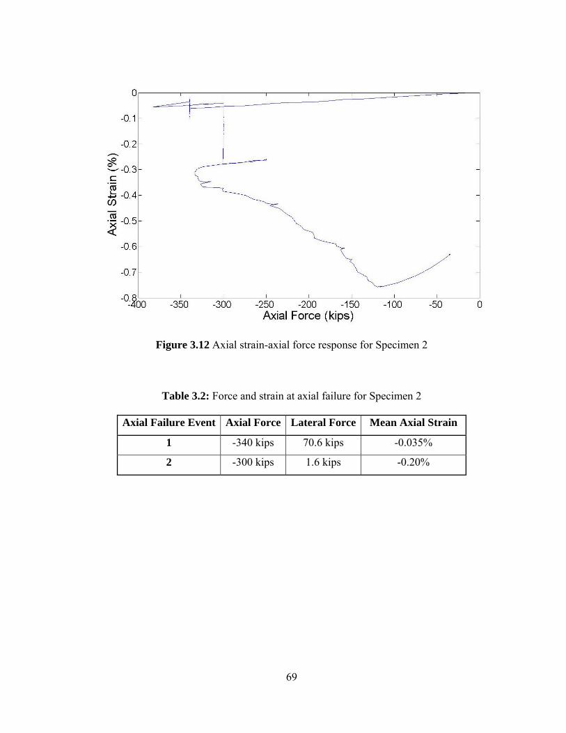
the residual axial capacity of the column. Figure 3.12 plots the axial strain-axial force

relationship for Specimen 2 throughout the test. Table 3.2 lists the axial load, lateral

load, and axial strain data prior to each axial failure event.

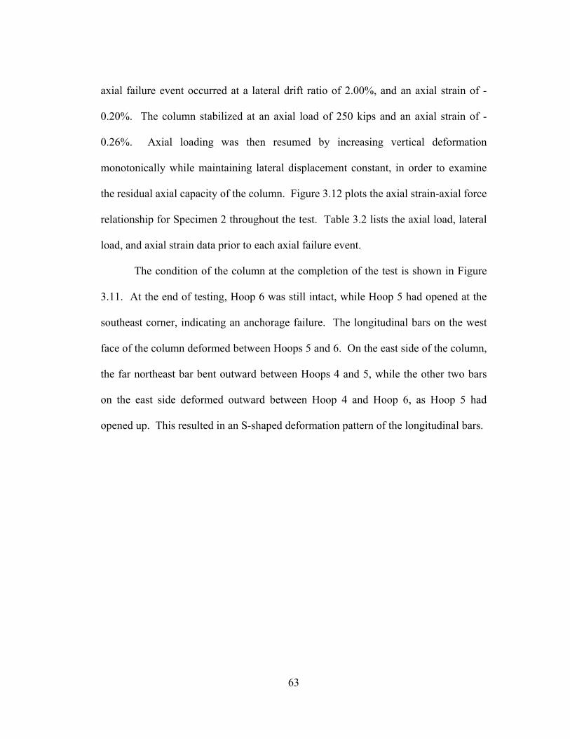
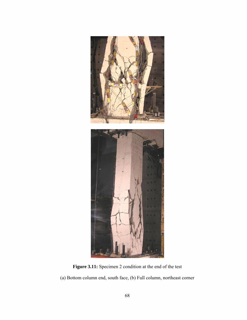
The condition of the column at the completion of the test is shown in Figure

3.11. At the end of testing, Hoop 6 was still intact, while Hoop 5 had opened at the

southeast corner, indicating an anchorage failure. The longitudinal bars on the west

face of the column deformed between Hoops 5 and 6. On the east side of the column,

the far northeast bar bent outward between Hoops 4 and 5, while the other two bars

on the east side deformed outward between Hoop 4 and Hoop 6, as Hoop 5 had

opened up. This resulted in an S-shaped deformation pattern of the longitudinal bars.

64

Figure 3.7: Specimen 2 crack pattern at a drift ratio of 0.50%

(a) Top column end, north face (b) Top column end, east face

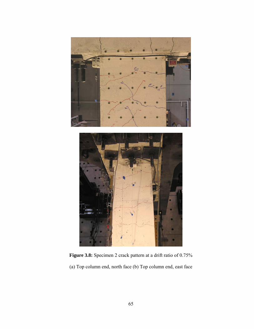
65

Figure 3.8: Specimen 2 crack pattern at a drift ratio of 0.75%

(a) Top column end, north face (b) Top column end, east face

66

Figure 3.9: Specimen 2 crack pattern at a drift ratio of 1.00%

(a) Top column end, north face (b) Bottom column end, south face

67

Figure 3.10: Specimen 2 crack pattern at a drift ratio of 1.25% (after axial failure)

(a) Center of column, north face

68

Figure 3.11: Specimen 2 condition at the end of the test

(a) Bottom column end, south face, (b) Full column, northeast corner

69

Figure 3.12 Axial strain-axial force response for Specimen 2

Table 3.2: Force and strain at axial failure for Specimen 2

Axial Failure Event Axial Force Lateral Force Mean Axial Strain

1 -340 kips 70.6 kips -0.035%

2 -300 kips 1.6 kips -0.20%

70

3.4 Load-Deflection Response

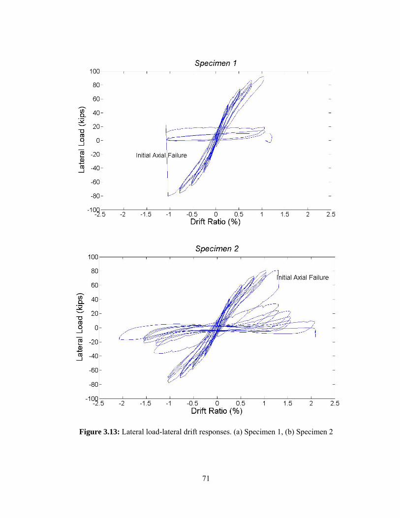
The lateral load-lateral drift response for each specimen is shown in Figure

3.13. Both graphs show minor reductions in strength due to repeated cycling at each

drift level. These hysteretic responses indicate that the behavior of both specimens

was very brittle in nature. Specimen 1 maintained axial and lateral load carrying

capacity up to a peak lateral load of 92.7 kips, and a lateral drift ratio of 1.00% prior

to initial axial failure. After failure, lateral load resistance was reduced to effectively

zero. Specimen 2 reached a peak lateral load and drift ratio of 81.5 kips and 1.25%,

respectively, prior to initial axial failure, after which lateral load resistance dropped

approximately 55% and continued to diminish until the end of the test.

Given the identical characteristics and applied lateral displacement protocol

for the two specimens, the difference in specimen response indicates that column

performance was significantly influenced by the magnitude of the applied axial load.

Specimen 1, which had the higher axial load, failed at a smaller lateral displacement

than Specimen 2. This is consistent with the relationship between axial load and

lateral displacement at axial failure previously documented in literature. In addition,

Specimen 1 experienced axial failure at a higher lateral load. This is also consistent

with the documented relationship between axial load and the resulting lateral strength

and stiffness.

71

Figure 3.13: Lateral load-lateral drift responses. (a) Specimen 1, (b) Specimen 2

72

The behavior of the two specimens at and past the point of axial failure was

also directly related to the difference in axial load. The failure of Specimen 1 was

very brittle, characterized by the sudden widening of an existing shear crack located

in the maximum moment region at the bottom of the specimen. Following initial

axial failure, the axial load carrying capacity dropped by 63% and nearly all residual

lateral load capacity was lost. The applied axial load was subsequently reduced to

100 kips and the lateral displacement protocol was resumed. The specimen was only

able to carry the reduced axial load up to the first peak of the next series of

displacement cycles, with a maximum lateral drift ratio of 1.25%. In Specimen 2,

failure resulted after the formation of two previously unobserved shear cracks across

the middle section of the column. As these cracks widened, column hoop 5 lost

anchorage, triggering axial failure of the longitudinal reinforcement. The initial

failure of Specimen 2 resulted in a reduction of only 6.5% of the axial load carrying

capacity and approximately 55% of the lateral load resistance. After initial failure,

cycling resumed at a reduced axial load of 300 kips and the specimen was able to

sustain the reduced axial load for several additional sets of displacement cycles, up to

a maximum lateral drift ratio of 2.00%. The post-failure behavior of the two

specimens indicates that a higher axial load results in a more rapid degradation of

both axial and lateral load carrying capacity, as well a reduction in the residual drift

capacity.

These relationships are further illustrated by examining the relationship

between mean axial strain and lateral drift for each of the specimens, as illustrated in

73

Figure 3.14. Increases in the mean axial strain for Specimens 1 and 2 following

initial axial failure were 215% and 26%, respectively. In addition, Figure 3.14 shows

that Specimen 2 was able to sustain the reduced axial load for a greater number of

cycles, and the increase in axial strain corresponding to each cycle was much smaller

than for Specimen 1.

Consideration should be given to the axial re-loading of Specimen 1 after

initial axial failure. This process ensured that the specimen was unable to sustain the

original axial load before the lateral displacement protocol was resumed under a

reduced axial load. This same process was not followed for Specimen 2, and may

have influenced the post-failure behavior of the second specimen. Upon resuming the

lateral displacement protocol, Specimen 1 had been subjected to two axial failure

events, while Specimen 2 had been subjected to only one. The additional damage

may have influenced the residual stiffness and load capacity of Specimen 1, although

as discussed, the relative behavior of the two specimens is consistent with the

expected behavior.

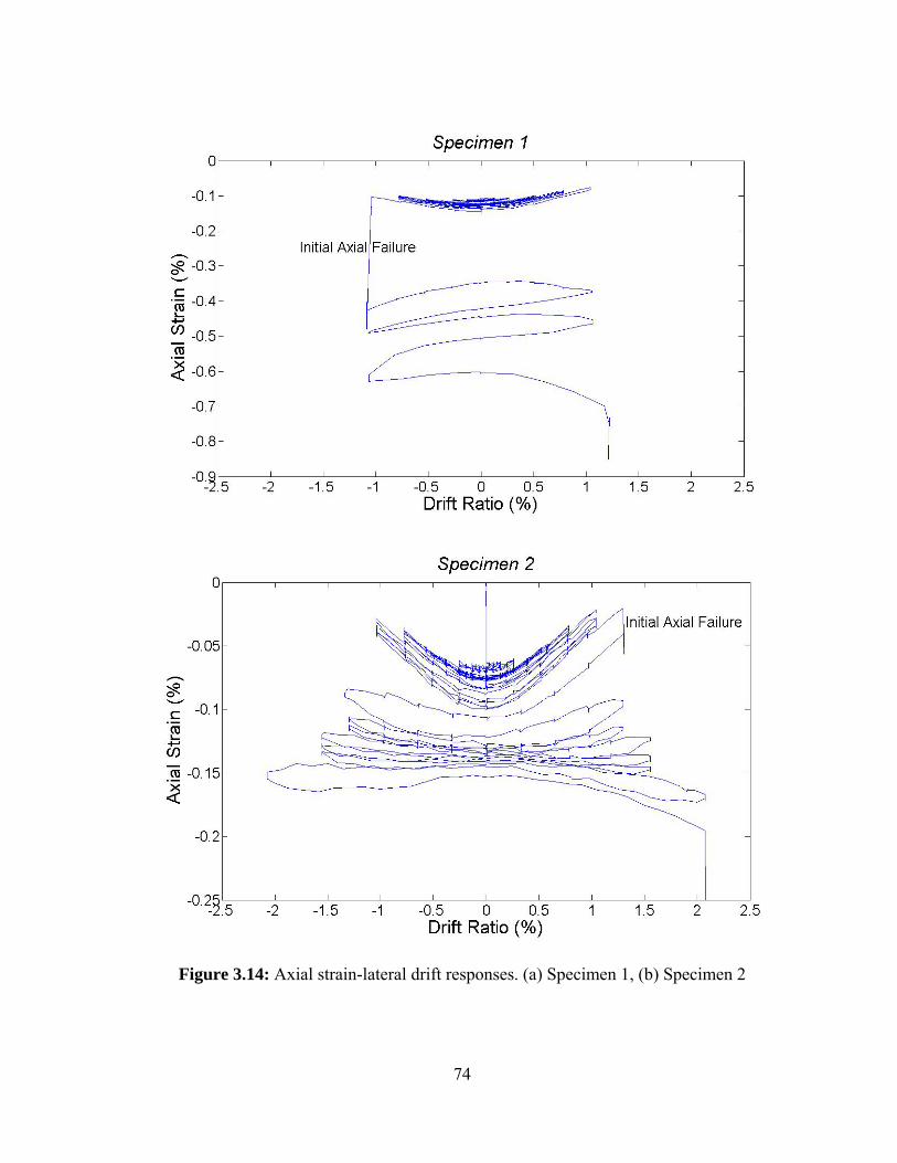
74

Figure 3.14: Axial strain-lateral drift responses. (a) Specimen 1, (b) Specimen 2

75

3.5 Moment-Curvature Analysis

The theoretical moment-curvature response of each specimen was calculated

under the assumptions that plane sections remain plane, and strain is distributed

linearly throughout the column cross-section. The stress in each layer of the cross-

section was calculated using the strain at the centroid of the layer. Concrete stress fc

was calculated using the stress-strain relationship developed by Hognestad (1951),

given by Eq. (3.1) through (3.3). Concrete was assumed to carry no tensile force.

oc

oc

ou

occ

o

c

o

cc

c

for

for

f

ff

εε

εε

εεεε

εε

εε

>

≤

⎪⎪

⎩

⎪⎪

⎨

⎧

⎥⎦

⎤⎢⎣

⎡⎟⎟⎠

⎞⎜⎜⎝

⎛−−

−′′

⎥⎥⎦

⎤

⎢⎢⎣

⎡⎟⎟⎠

⎞⎜⎜⎝

⎛−′′

=

15.01

22

(3.1)

cc ff ′=′′ 85.0 (3.2)

c

co E

f ′=

7.1ε (3.3)

Where:

cf = concrete stress (ksi)

cf ′′ = peak concrete stress (ksi)

cf ′ = concrete compressive strength (ksi)

cε = concrete strain

oε = concrete strain at peak stress

uε = ultimate concrete strain = 0.0038

cE = concrete modulus of elasticity (ksi)

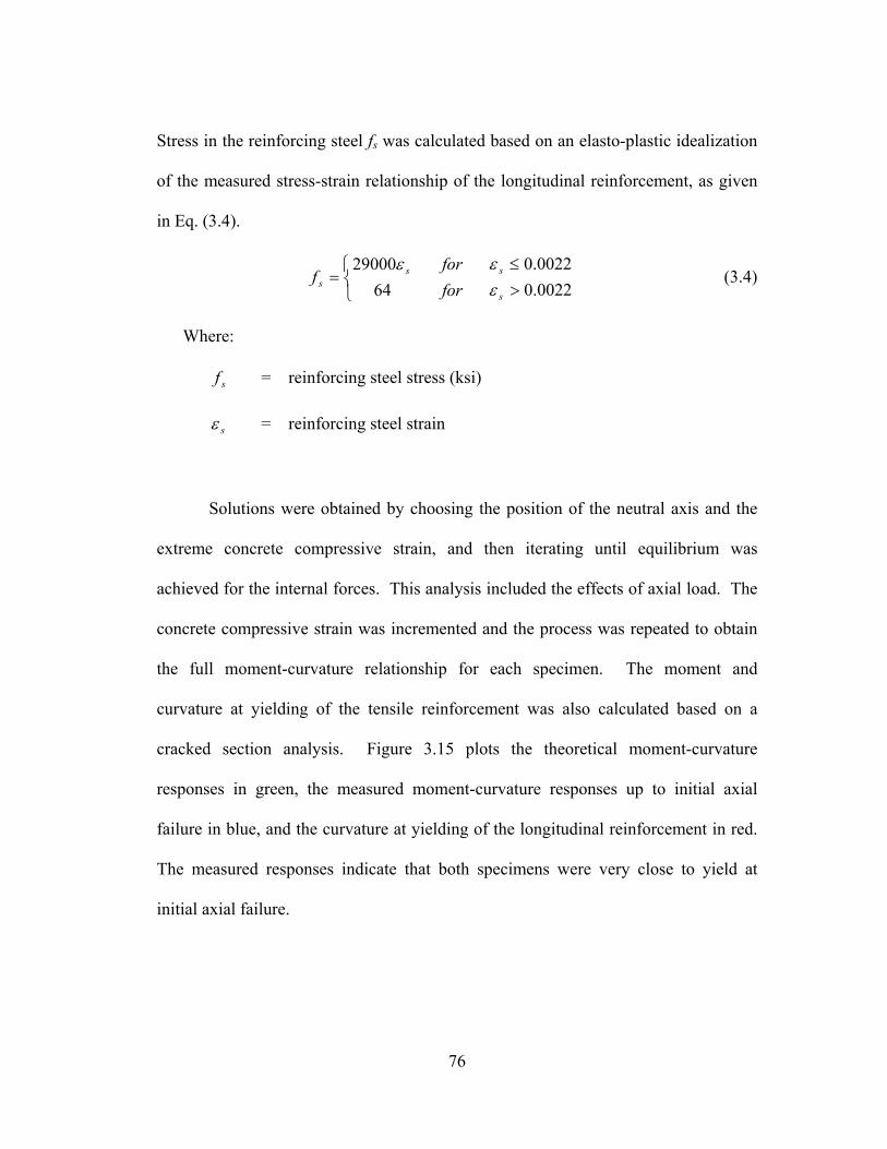
76

Stress in the reinforcing steel fs was calculated based on an elasto-plastic idealization

of the measured stress-strain relationship of the longitudinal reinforcement, as given

in Eq. (3.4).

⎩⎨⎧

>≤

=0022.00022.0

6429000

s

sss for

forf

εεε

(3.4)

Where:

sf = reinforcing steel stress (ksi)

sε = reinforcing steel strain

Solutions were obtained by choosing the position of the neutral axis and the

extreme concrete compressive strain, and then iterating until equilibrium was

achieved for the internal forces. This analysis included the effects of axial load. The

concrete compressive strain was incremented and the process was repeated to obtain

the full moment-curvature relationship for each specimen. The moment and

curvature at yielding of the tensile reinforcement was also calculated based on a

cracked section analysis. Figure 3.15 plots the theoretical moment-curvature

responses in green, the measured moment-curvature responses up to initial axial

failure in blue, and the curvature at yielding of the longitudinal reinforcement in red.

The measured responses indicate that both specimens were very close to yield at

initial axial failure.

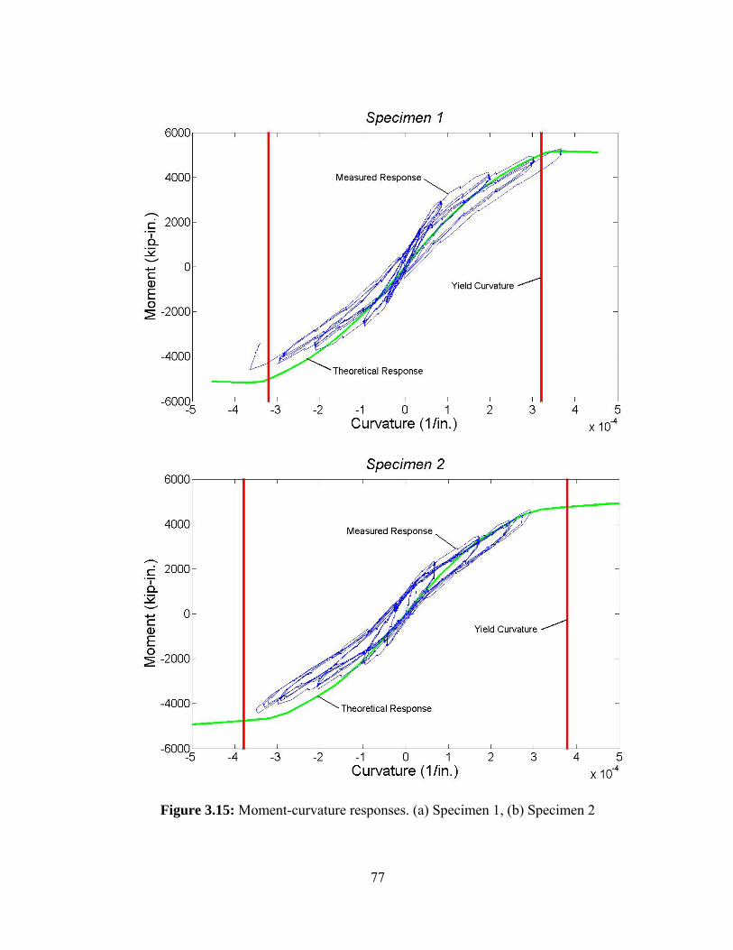
77

Figure 3.15: Moment-curvature responses. (a) Specimen 1, (b) Specimen 2

78

Moment and curvature values are reported under the assumption of equivalent

section properties at all locations along the column. No modifications or allowances

were made for column damage, and thus moment redistribution, due to cyclic

loading. This was considered an appropriate assumption, as is evidenced by the close

agreement between theoretical and measured responses.

Curvature profiles for the specimens up to initial axial failure are shown in

Figure 3.16. The vertical red lines in each graph represent the curvature at yield,

while the horizontal black lines represent the mid-height of the column. Both Figures

3.15 and 3.16 indicate that Specimen 1 reached yield curvature during the final cycle

prior to initial axial failure. According to the moment-curvature analysis, Specimen 2

did not reach yield prior to axial failure.

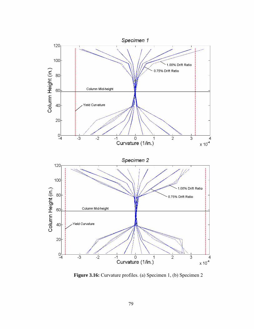
79

Figure 3.16: Curvature profiles. (a) Specimen 1, (b) Specimen 2

80

3.6 Deflection Components

Deflection profiles for displacement cycles prior to axial failure, created from

the horizontal string potentiometer data are shown in Figure 3.17. Both plots

illustrate the anticipated double curvature deflected shape typical of a fixed-fixed

column subjected to lateral loading. The interior green vertical lines on the graphs

correspond to theoretical values of deflection at the top of the column at first

cracking, while the exterior red vertical lines represent the theoretical deflection at the

top of the column at first yield of the longitudinal reinforcement. The calculated

cracking and yield deflections are 0.07 in. and 1.17 in., respectively, for Specimen 1,

and 0.09 in. and 1.29 in. for Specimen 2.

The theoretical cracking and yield deflections were determined by adding

components due to flexure, shear, and bar slip. The flexure component was

calculated using a moment-curvature analysis along with the moment-area method for

calculating deflections. To simplify the analysis, the moment-curvature relationship

was assumed to be linear up to the yield point. Thus, the flexure deflection ΔFlexure

was calculated as shown in Eq. (3.5).

2*6Flexure

LϕΔ = (3.5)

Where:

φ = maximum curvature in the column (in.-1)

L = height of column (in.)

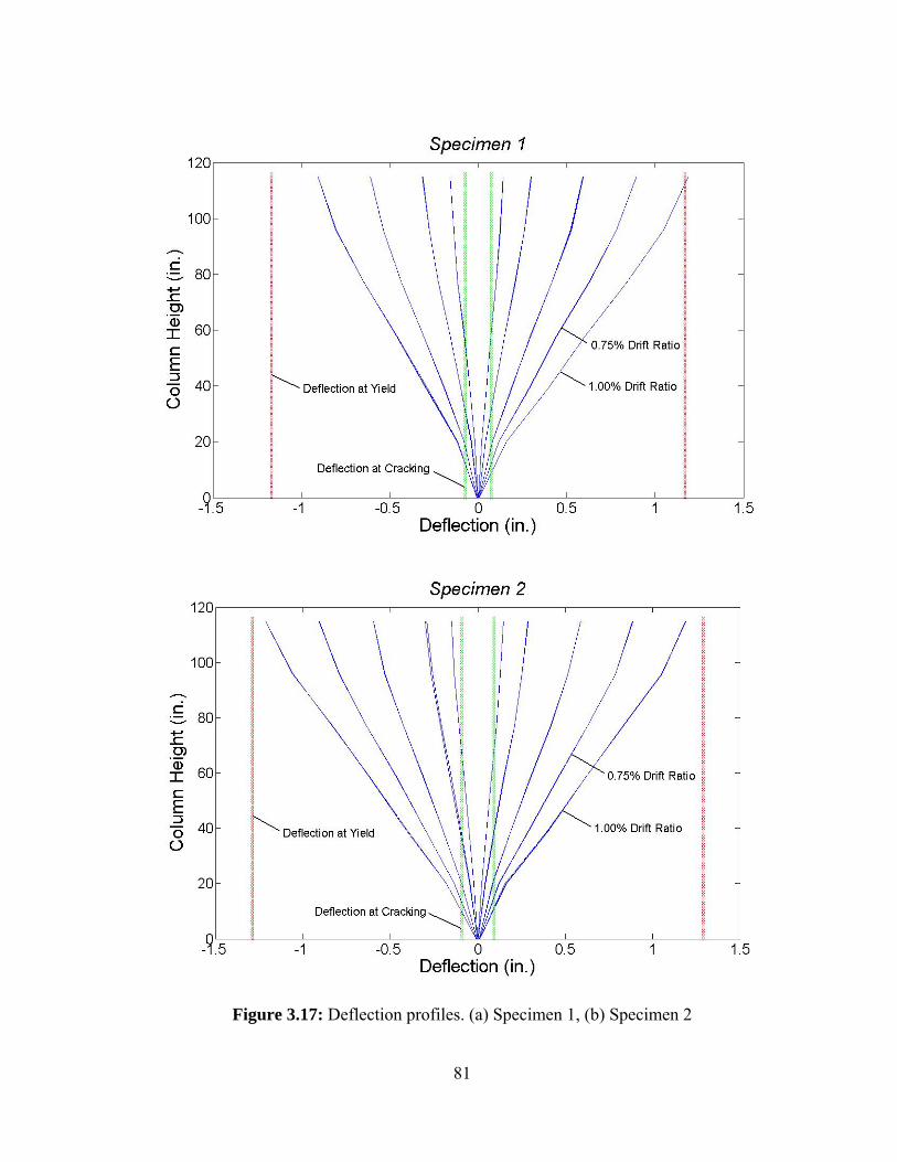
81

Figure 3.17: Deflection profiles. (a) Specimen 1, (b) Specimen 2

82

Shear deflection was calculated under the assumption of uniform shear strain

along the length of the column and linear-elastic material properties. The shear

component of deflection ΔShear was determined using Eq. (3.6) through (3.8).

65Shear

g

V LGA

Δ = (3.6)

2MVL

= (3.7)

2(1 )

cEGν

=+

(3.8)

Where:

V = shear force (kips)

G = concrete shear modulus (ksi)

Ag = cross-sectional area of the column (in2)

M = moment at column ends (kip-in.)

Ec = concrete modulus of elasticity (ksi)

ν = Poisson’s ratio = 0.20

The third component of deflection results from slip due to the extension of the

longitudinal reinforcement at the ends of the column, as well as slip from the

anchorage of the concrete. The slip deflection ΔSlip was calculated according to Eq.

(3.9), in which a uniform bond stress was assumed along the development length of

the bar within the beam (Matamoros 1999).

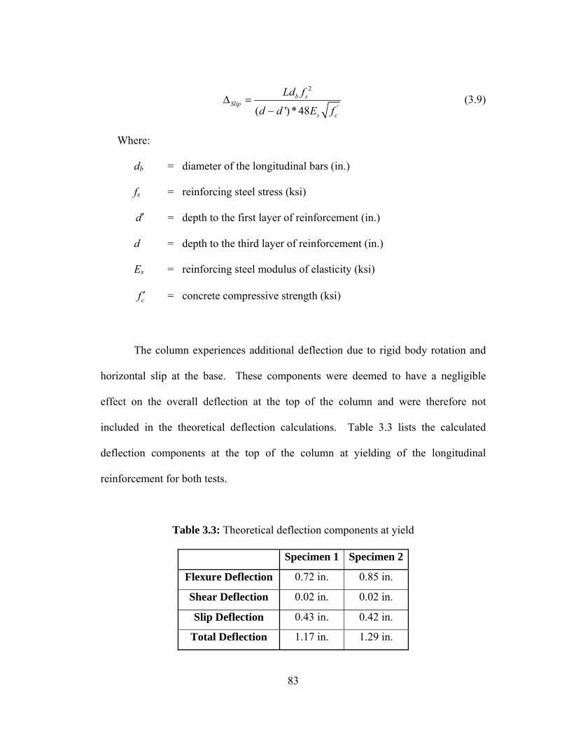
83

2

'( ') * 48b s

Slip

s c

Ld f

d d E fΔ =

− (3.9)

Where:

db = diameter of the longitudinal bars (in.)

fs = reinforcing steel stress (ksi)

d ′ = depth to the first layer of reinforcement (in.)

d = depth to the third layer of reinforcement (in.)

Es = reinforcing steel modulus of elasticity (ksi)

cf ′ = concrete compressive strength (ksi)

The column experiences additional deflection due to rigid body rotation and

horizontal slip at the base. These components were deemed to have a negligible

effect on the overall deflection at the top of the column and were therefore not

included in the theoretical deflection calculations. Table 3.3 lists the calculated

deflection components at the top of the column at yielding of the longitudinal

reinforcement for both tests.

Table 3.3: Theoretical deflection components at yield

Specimen 1 Specimen 2

Flexure Deflection 0.72 in. 0.85 in.

Shear Deflection 0.02 in. 0.02 in.

Slip Deflection 0.43 in. 0.42 in.

Total Deflection 1.17 in. 1.29 in.

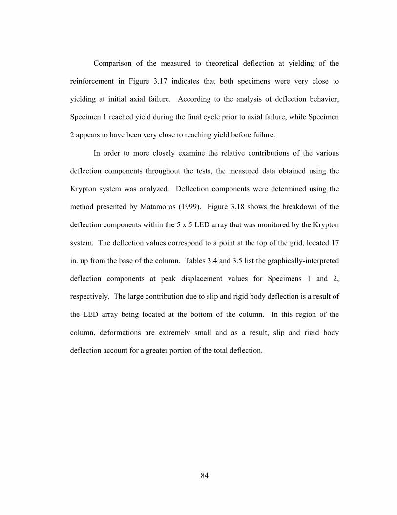
84

Comparison of the measured to theoretical deflection at yielding of the

reinforcement in Figure 3.17 indicates that both specimens were very close to

yielding at initial axial failure. According to the analysis of deflection behavior,

Specimen 1 reached yield during the final cycle prior to axial failure, while Specimen

2 appears to have been very close to reaching yield before failure.

In order to more closely examine the relative contributions of the various

deflection components throughout the tests, the measured data obtained using the

Krypton system was analyzed. Deflection components were determined using the

method presented by Matamoros (1999). Figure 3.18 shows the breakdown of the

deflection components within the 5 x 5 LED array that was monitored by the Krypton

system. The deflection values correspond to a point at the top of the grid, located 17

in. up from the base of the column. Tables 3.4 and 3.5 list the graphically-interpreted

deflection components at peak displacement values for Specimens 1 and 2,

respectively. The large contribution due to slip and rigid body deflection is a result of

the LED array being located at the bottom of the column. In this region of the

column, deformations are extremely small and as a result, slip and rigid body

deflection account for a greater portion of the total deflection.

85

Specimen 1

-0.20

-0.15

-0.10

-0.05

0.00

0.05

0.10

0.15

0.20D

efle

ctio

n (in

.)FlexureShearSlipRigid Body

Specimen 2

-0.20

-0.15

-0.10

-0.05

0.00

0.05

0.10

0.15

0.20

Def

lect

ion

(in.)

FlexureShearSlipRigid Body

Figure 3.18: Deflection components. (a) Specimen 1, (b) Specimen 2

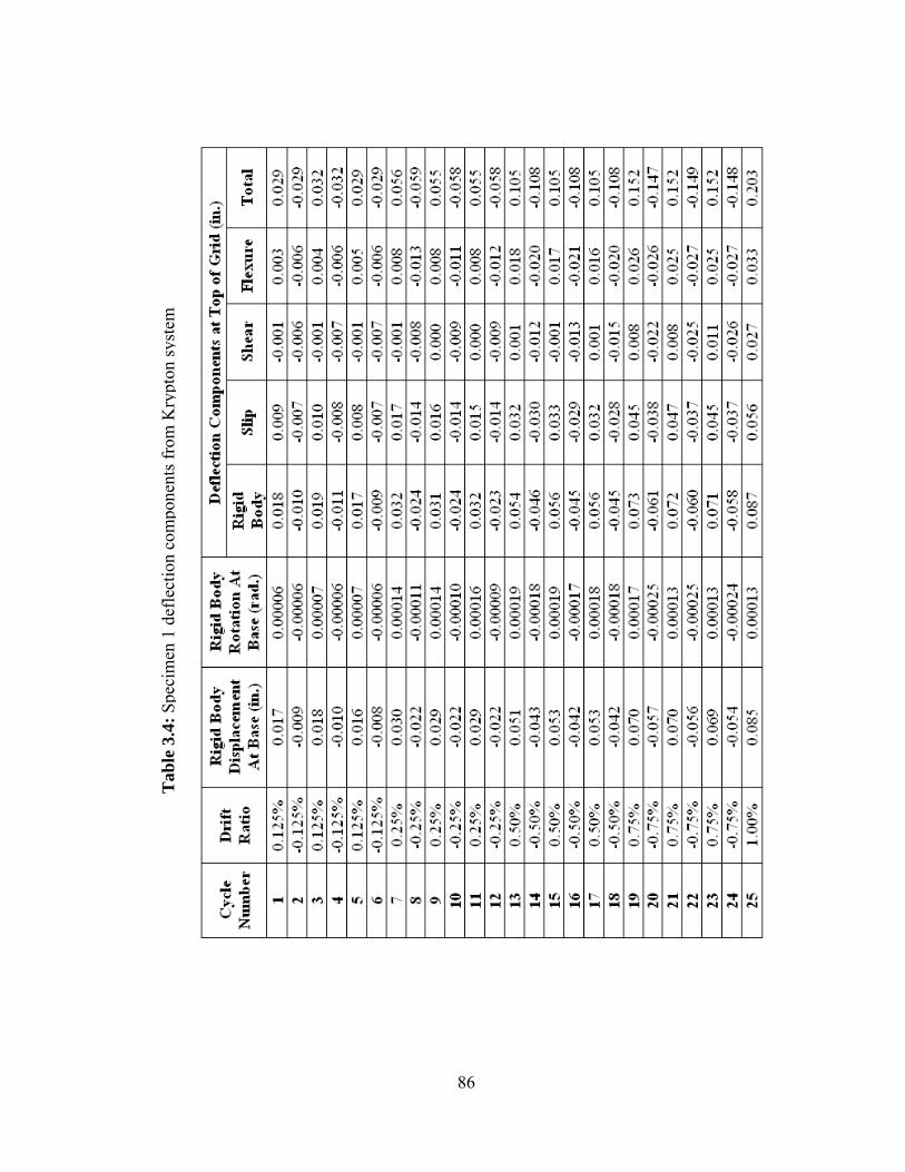
86

Tab

le 3

.4: S

peci

men

1 d

efle

ctio

n co

mpo

nent

s fro

m K

rypt

on sy

stem

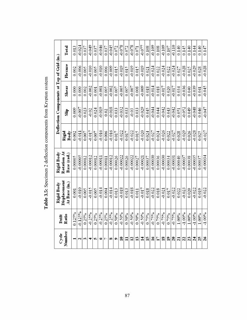
87

Tab

le 3

.5: S

peci

men

2 d

efle

ctio

n co

mpo

nent

s fro

m K

rypt

on sy

stem

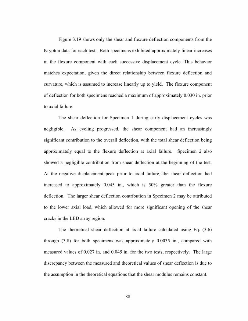
88

Figure 3.19 shows only the shear and flexure deflection components from the

Krypton data for each test. Both specimens exhibited approximately linear increases

in the flexure component with each successive displacement cycle. This behavior

matches expectation, given the direct relationship between flexure deflection and

curvature, which is assumed to increase linearly up to yield. The flexure component

of deflection for both specimens reached a maximum of approximately 0.030 in. prior

to axial failure.

The shear deflection for Specimen 1 during early displacement cycles was

negligible. As cycling progressed, the shear component had an increasingly

significant contribution to the overall deflection, with the total shear deflection being

approximately equal to the flexure deflection at axial failure. Specimen 2 also

showed a negligible contribution from shear deflection at the beginning of the test.

At the negative displacement peak prior to axial failure, the shear deflection had

increased to approximately 0.045 in., which is 50% greater than the flexure

deflection. The larger shear deflection contribution in Specimen 2 may be attributed

to the lower axial load, which allowed for more significant opening of the shear

cracks in the LED array region.

The theoretical shear deflection at axial failure calculated using Eq. (3.6)

through (3.8) for both specimens was approximately 0.0035 in., compared with

measured values of 0.027 in. and 0.045 in. for the two tests, respectively. The large

discrepancy between the measured and theoretical values of shear deflection is due to

the assumption in the theoretical equations that the shear modulus remains constant.

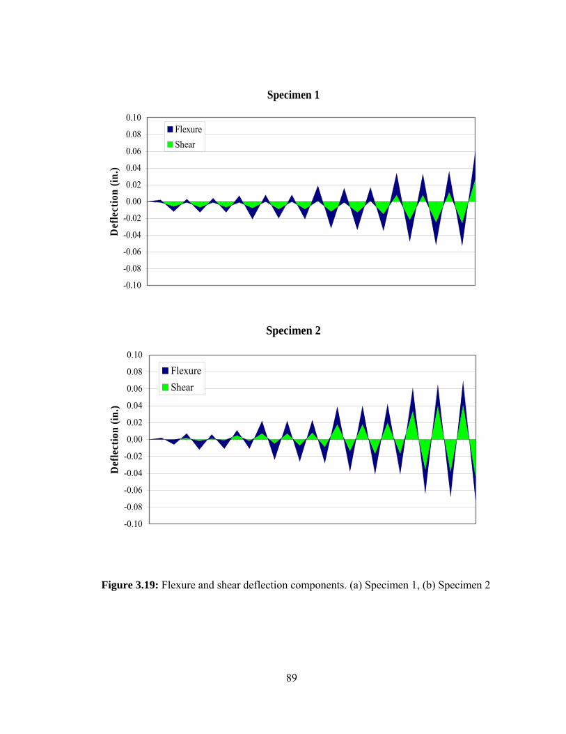
89

Specimen 1

-0.10

-0.08

-0.06

-0.04

-0.02

0.00

0.02

0.04

0.06

0.08

0.10D

efle

ctio

n (in

.)FlexureShear

Specimen 2

-0.10

-0.08

-0.06

-0.04

-0.02

0.00

0.02

0.04

0.06

0.08

0.10

Def

lect

ion

(in.)

FlexureShear

Figure 3.19: Flexure and shear deflection components. (a) Specimen 1, (b) Specimen 2

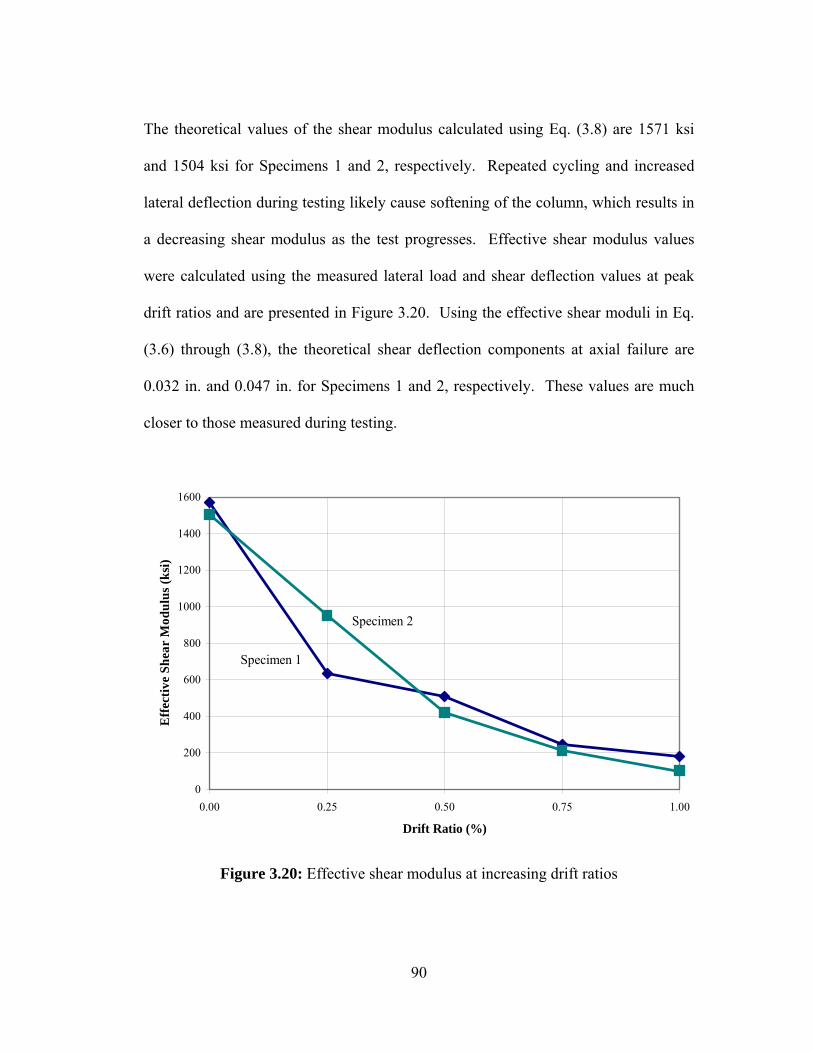
90

The theoretical values of the shear modulus calculated using Eq. (3.8) are 1571 ksi

and 1504 ksi for Specimens 1 and 2, respectively. Repeated cycling and increased

lateral deflection during testing likely cause softening of the column, which results in

a decreasing shear modulus as the test progresses. Effective shear modulus values

were calculated using the measured lateral load and shear deflection values at peak

drift ratios and are presented in Figure 3.20. Using the effective shear moduli in Eq.

(3.6) through (3.8), the theoretical shear deflection components at axial failure are

0.032 in. and 0.047 in. for Specimens 1 and 2, respectively. These values are much

closer to those measured during testing.

Specimen 1

Specimen 2

0

200

400

600

800

1000

1200

1400

1600

0.00 0.25 0.50 0.75 1.00

Drift Ratio (%)

Eff

ectiv

e Sh

ear

Mod

ulus

(ksi

)

Figure 3.20: Effective shear modulus at increasing drift ratios

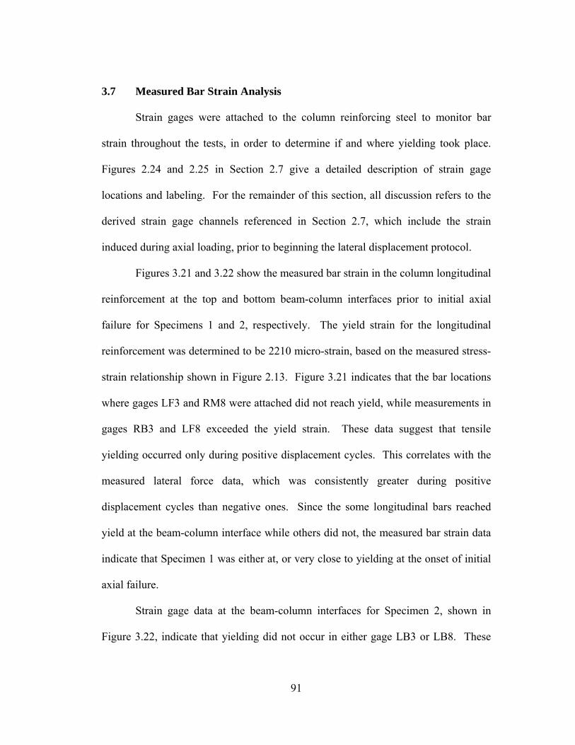
91

3.7 Measured Bar Strain Analysis

Strain gages were attached to the column reinforcing steel to monitor bar

strain throughout the tests, in order to determine if and where yielding took place.

Figures 2.24 and 2.25 in Section 2.7 give a detailed description of strain gage

locations and labeling. For the remainder of this section, all discussion refers to the

derived strain gage channels referenced in Section 2.7, which include the strain

induced during axial loading, prior to beginning the lateral displacement protocol.

Figures 3.21 and 3.22 show the measured bar strain in the column longitudinal

reinforcement at the top and bottom beam-column interfaces prior to initial axial

failure for Specimens 1 and 2, respectively. The yield strain for the longitudinal

reinforcement was determined to be 2210 micro-strain, based on the measured stress-

strain relationship shown in Figure 2.13. Figure 3.21 indicates that the bar locations

where gages LF3 and RM8 were attached did not reach yield, while measurements in

gages RB3 and LF8 exceeded the yield strain. These data suggest that tensile

yielding occurred only during positive displacement cycles. This correlates with the

measured lateral force data, which was consistently greater during positive

displacement cycles than negative ones. Since the some longitudinal bars reached

yield at the beam-column interface while others did not, the measured bar strain data

indicate that Specimen 1 was either at, or very close to yielding at the onset of initial

axial failure.

Strain gage data at the beam-column interfaces for Specimen 2, shown in

Figure 3.22, indicate that yielding did not occur in either gage LB3 or LB8. These

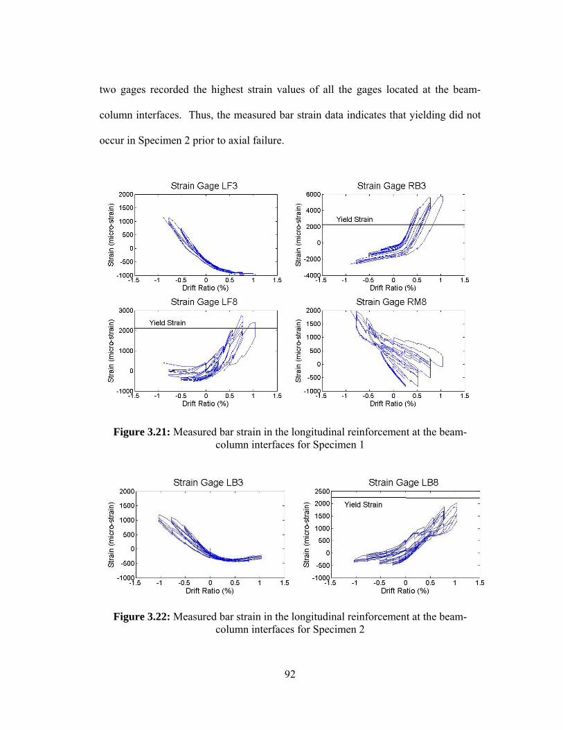
92

two gages recorded the highest strain values of all the gages located at the beam-

column interfaces. Thus, the measured bar strain data indicates that yielding did not

occur in Specimen 2 prior to axial failure.

Figure 3.21: Measured bar strain in the longitudinal reinforcement at the beam-column interfaces for Specimen 1

Figure 3.22: Measured bar strain in the longitudinal reinforcement at the beam-column interfaces for Specimen 2

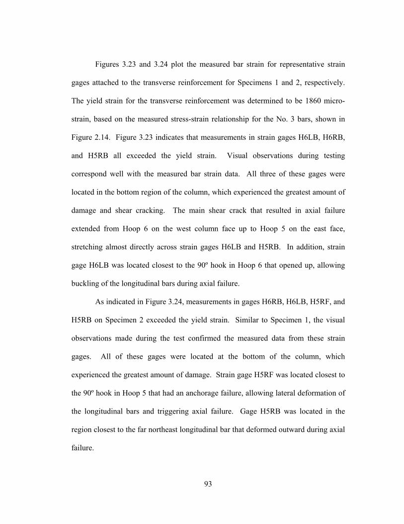
93

Figures 3.23 and 3.24 plot the measured bar strain for representative strain

gages attached to the transverse reinforcement for Specimens 1 and 2, respectively.

The yield strain for the transverse reinforcement was determined to be 1860 micro-

strain, based on the measured stress-strain relationship for the No. 3 bars, shown in

Figure 2.14. Figure 3.23 indicates that measurements in strain gages H6LB, H6RB,

and H5RB all exceeded the yield strain. Visual observations during testing

correspond well with the measured bar strain data. All three of these gages were

located in the bottom region of the column, which experienced the greatest amount of

damage and shear cracking. The main shear crack that resulted in axial failure

extended from Hoop 6 on the west column face up to Hoop 5 on the east face,

stretching almost directly across strain gages H6LB and H5RB. In addition, strain

gage H6LB was located closest to the 90º hook in Hoop 6 that opened up, allowing

buckling of the longitudinal bars during axial failure.

As indicated in Figure 3.24, measurements in gages H6RB, H6LB, H5RF, and

H5RB on Specimen 2 exceeded the yield strain. Similar to Specimen 1, the visual

observations made during the test confirmed the measured data from these strain

gages. All of these gages were located at the bottom of the column, which

experienced the greatest amount of damage. Strain gage H5RF was located closest to

the 90º hook in Hoop 5 that had an anchorage failure, allowing lateral deformation of

the longitudinal bars and triggering axial failure. Gage H5RB was located in the

region closest to the far northeast longitudinal bar that deformed outward during axial

failure.

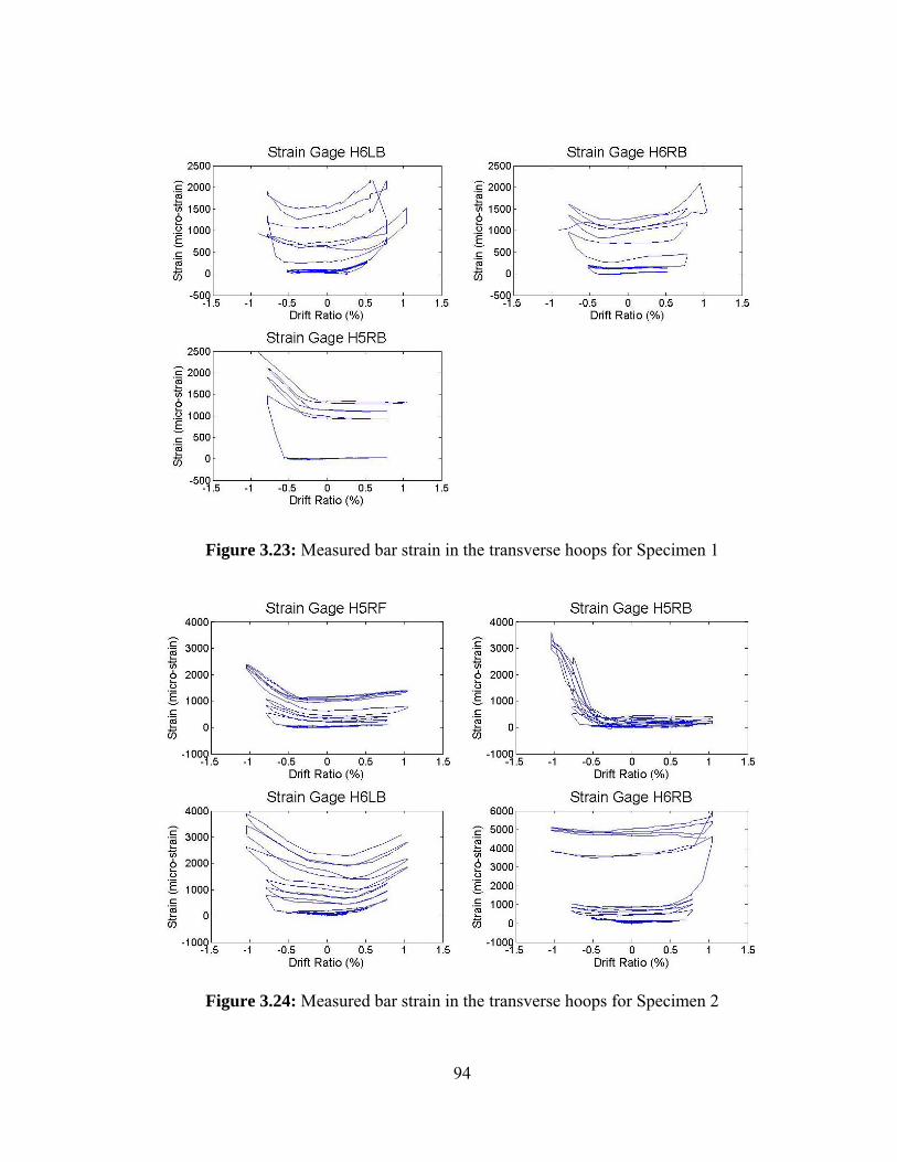
94

Figure 3.23: Measured bar strain in the transverse hoops for Specimen 1

Figure 3.24: Measured bar strain in the transverse hoops for Specimen 2

95

3.8 Shear Strength

For each specimen, Table 3.6 presents the maximum measured shear during

testing Vtest, the nominal shear strength Vn calculated using Eq. (3.10) through (3.12)

(ACI 318-08), and the shear force required to yield the longitudinal reinforcement Vp

based on the moment-curvature analysis reported in Section 3.5.

0.002 12000c c

g

PV f bdA

⎛ ⎞′= +⎜ ⎟⎜ ⎟

⎝ ⎠ (3.10)

st yts

A f dV

s= (3.11)

n c sV V V= + (3.12)

Where:

Vc = shear force carried by the concrete (kips)

P = axial load (lb)

Ag = cross-sectional area of the column (in2)

cf ′ = concrete compressive strength (psi)

b = column width (in.)

d = depth to tension reinforcement (in.)

Vs = shear force carried by the transverse steel (kips)

Ast = area of the transverse reinforcement (in2)

fyt = yield stress of the transverse reinforcement (ksi)

s = spacing of the transverse reinforcement (in.)

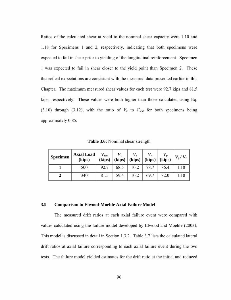
96

Ratios of the calculated shear at yield to the nominal shear capacity were 1.10 and

1.18 for Specimens 1 and 2, respectively, indicating that both specimens were

expected to fail in shear prior to yielding of the longitudinal reinforcement. Specimen

1 was expected to fail in shear closer to the yield point than Specimen 2. These

theoretical expectations are consistent with the measured data presented earlier in this

Chapter. The maximum measured shear values for each test were 92.7 kips and 81.5

kips, respectively. These values were both higher than those calculated using Eq.

(3.10) through (3.12), with the ratio of Vn to Vtest for both specimens being

approximately 0.85.

Table 3.6: Nominal shear strength

Specimen Axial Load(kips)

Vtest (kips)

Vc (kips)

Vs (kips)

Vn (kips)

Vp (kips) Vp / Vn

1 500 92.7 68.5 10.2 78.7 86.4 1.10

2 340 81.5 59.4 10.2 69.7 82.0 1.18

3.9 Comparison to Elwood-Moehle Axial Failure Model

The measured drift ratios at each axial failure event were compared with

values calculated using the failure model developed by Elwood and Moehle (2003).

This model is discussed in detail in Section 1.3.2. Table 3.7 lists the calculated lateral

drift ratios at axial failure corresponding to each axial failure event during the two

tests. The failure model yielded estimates for the drift ratio at the initial and reduced

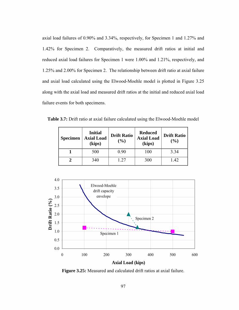
97

axial load failures of 0.90% and 3.34%, respectively, for Specimen 1 and 1.27% and

1.42% for Specimen 2. Comparatively, the measured drift ratios at initial and

reduced axial load failures for Specimen 1 were 1.00% and 1.21%, respectively, and

1.25% and 2.00% for Specimen 2. The relationship between drift ratio at axial failure

and axial load calculated using the Elwood-Moehle model is plotted in Figure 3.25

along with the axial load and measured drift ratios at the initial and reduced axial load

failure events for both specimens.

Table 3.7: Drift ratio at axial failure calculated using the Elwood-Moehle model

Specimen Initial

Axial Load(kips)

Drift Ratio(%)

Reduced Axial Load

(kips)

Drift Ratio (%)

1 500 0.90 100 3.34

2 340 1.27 300 1.42

Elwood-Moehle drift capacity

envelope

Specimen 1

Specimen 2

0.0

0.5

1.0

1.5

2.0

2.5

3.0

3.5

4.0

0 100 200 300 400 500 600

Axial Load (kips)

Dri

ft R

atio

(%)

Figure 3.25: Measured and calculated drift ratios at axial failure.

98

As depicted in Figure 3.25, the drift ratios calculated using the Elwood-

Moehle model matched actual drift ratios at axial failure very closely for the first

axial failure event for both specimens. The estimates of drift ratio at the reduced

axial load failure events were significantly less accurate. While the model

underestimated the drift ratio at the reduced axial load failure of Specimen 2, it

significantly overestimated the drift capacity at reduced axial load failure of

Specimen 1. Some of the inaccuracy in the estimation of drift ratio at reduced axial

load failure may be due to the inability of the Elwood-Moehle model to incorporate

the effects of damage and resulting losses in stiffness sustained during the initial axial

failures for both specimens. The amount of damage caused by the initial axial failure

event for Specimen 1 was far greater than that for Specimen 2, which is clearly shown

by the post-failure behavior of the two specimens. Additional research is necessary to

determine the residual axial load-drift capacity relationship beyond initial axial

failure.

3.10 Axial Capacity of Longitudinal Reinforcement

Reinforced concrete columns are assumed to distribute axial load throughout

their cross-section, with a portion of the load being carried by the longitudinal steel

Ps, and the remaining load carried by the concrete Pc. Based on observations from

tests performed by Lynn (2001) and Sezen (2000), the ability of columns to sustain

axial load after shear failure appears to be closely related to the portion of the load

carried by the longitudinal reinforcement. When Ps reaches a critical value the

99

reinforcement will fail, resulting in axial failure of the column. The maximum axial

capacity of the reinforcement may be limited by either the plastic or buckling

capacity of the bars, depending on the magnitude of the applied load and the buckling

characteristics of the longitudinal reinforcement.

Observations from tests performed by Lynn (2001) and Sezen (2000) indicate

that columns with an applied axial load greater than the gross axial capacity of the

bars Asfy exhibit a mushroom-shaped deformation pattern, indicating a failure

controlled by the buckling capacity of the longitudinal reinforcement Ps-buckle. The

observed behavior differed in columns with an applied axial load less than Asfy, which

tended to show an S-shaped deformation pattern in the longitudinal reinforcement.

These findings suggest that the plastic capacity of the bars under combined bending

and axial load Ps-plastic controlled the behavior of the column.

The deformed shape of the longitudinal reinforcement for Specimen 1

suggests that a buckling failure occurred, as can be observed in Figure 3.5. The

deformed shape for Specimen 2, shown in Figure 3.11, indicates that the column axial

capacity was limited by the plastic capacity of the reinforcing bars Ps-plastic. These

visual failure classifications match the observations from the Lynn and Sezen tests

relating the failure mode to the axial load level. The 500-kip axial load applied to

Specimen 1 was very close to the gross axial capacity of the longitudinal bars Asfy, at

which buckling is expected to control axial capacity. The 340-kip axial load applied

to Specimen 2 was significantly lower than Asfy, and was thus expected to fail due to

the plastic capacity of the longitudinal bars Ps-plastic.

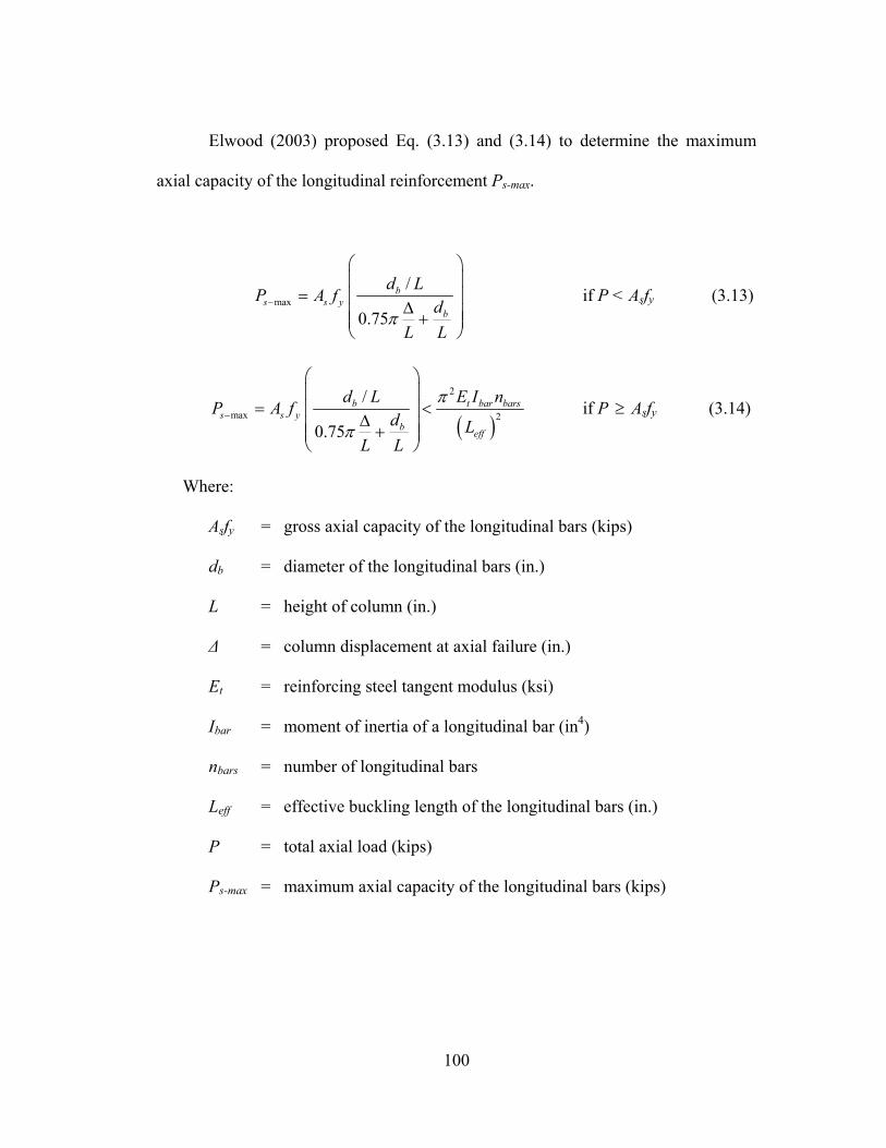
100

Elwood (2003) proposed Eq. (3.13) and (3.14) to determine the maximum

axial capacity of the longitudinal reinforcement Ps-max.

max/

0.75

bs s y

b

d LP A f

dL L

π−

⎛ ⎞⎜ ⎟

= ⎜ ⎟Δ⎜ ⎟+⎜ ⎟

⎝ ⎠

if P < Asfy (3.13)

( )

2

max 2

/

0.75

b t bar barss s y

beff

d L E I nP A f

d LL L

π

π−

⎛ ⎞⎜ ⎟

= <⎜ ⎟Δ⎜ ⎟+⎜ ⎟

⎝ ⎠

if P ≥ Asfy (3.14)

Where:

Asfy = gross axial capacity of the longitudinal bars (kips)

db = diameter of the longitudinal bars (in.)

L = height of column (in.)

Δ = column displacement at axial failure (in.)

Et = reinforcing steel tangent modulus (ksi)

Ibar = moment of inertia of a longitudinal bar (in4)

nbars = number of longitudinal bars

Leff = effective buckling length of the longitudinal bars (in.)

P = total axial load (kips)

Ps-max = maximum axial capacity of the longitudinal bars (kips)

101

Calculation of the limiting buckling load Ps-buckle in Eq. (3.14) requires the

determination of both the effective buckling length effL , and the tangent modulus Et .

Based on observations from previous tests, Elwood suggested that the effective

buckling length be assumed to be approximately 0.80s, which is between a fixed-

fixed and a pinned-pinned condition at the column hoops. The tangent modulus can

be graphically estimated from tensile coupon tests of the reinforcing bars. Elwood

suggested adopting a value for the tangent modulus of 7% of the elastic modulus,

which he considered representative of the properties of reinforcing bars.

In this study, ASTM A706 reinforcing steel was used, which had a post-yield

modulus of effectively zero up to a strain of 1.0%, as shown in Figure 2.13. As a

result, the tangent modulus could not accurately be calculated from the measured

stress-strain curve for the reinforcement. Since direct calculation of the tangent

modulus was not possible, bounding estimates of Et were established based on two

behavioral extremes, given the observed buckling failure behavior of Specimen 1.

The lower-bound value was determined using a transformed-section analysis and a

concentrically applied axial load of 500 kips. This yielded a load of 81 kips carried

by the longitudinal reinforcement, or 16% of the total axial load. Using this as the

minimum possible buckling load in the upper limit of Eq. (3.14) and solving for the

tangent modulus, yields a value that is 9% of the elastic modulus. The upper-bound

tangent modulus was calculated by assuming that the maximum value for the upper

limit of Eq. (3.14) was the plastic capacity of the reinforcing bars, given that buckling

was the observed failure mode. Solving for the plastic capacity yielded a maximum

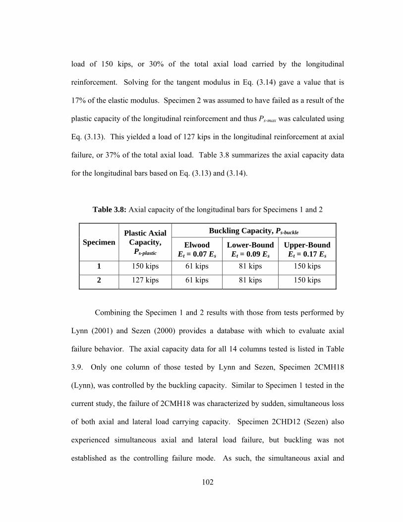
102

load of 150 kips, or 30% of the total axial load carried by the longitudinal

reinforcement. Solving for the tangent modulus in Eq. (3.14) gave a value that is

17% of the elastic modulus. Specimen 2 was assumed to have failed as a result of the

plastic capacity of the longitudinal reinforcement and thus Ps-max was calculated using

Eq. (3.13). This yielded a load of 127 kips in the longitudinal reinforcement at axial

failure, or 37% of the total axial load. Table 3.8 summarizes the axial capacity data

for the longitudinal bars based on Eq. (3.13) and (3.14).

Table 3.8: Axial capacity of the longitudinal bars for Specimens 1 and 2

Buckling Capacity, Ps-buckle Specimen

Plastic Axial Capacity,

Ps-plastic Elwood

Et = 0.07 Es Lower-Bound

Et = 0.09 Es Upper-Bound

Et = 0.17 Es 1 150 kips 61 kips 81 kips 150 kips

2 127 kips 61 kips 81 kips 150 kips

Combining the Specimen 1 and 2 results with those from tests performed by

Lynn (2001) and Sezen (2000) provides a database with which to evaluate axial

failure behavior. The axial capacity data for all 14 columns tested is listed in Table

3.9. Only one column of those tested by Lynn and Sezen, Specimen 2CMH18

(Lynn), was controlled by the buckling capacity. Similar to Specimen 1 tested in the

current study, the failure of 2CMH18 was characterized by sudden, simultaneous loss

of both axial and lateral load carrying capacity. Specimen 2CHD12 (Sezen) also

experienced simultaneous axial and lateral load failure, but buckling was not

established as the controlling failure mode. As such, the simultaneous axial and

103

lateral failure behavior for these three specimens cannot conclusively be attributed to

the controlling failure mode of the longitudinal reinforcement without additional

experimental evidence.

Inspection of the relationship between the applied axial load and the gross

axial capacity of the longitudinal reinforcement for the specimens exhibiting

simultaneous failure behavior reveals that each of these specimens had an axial load

very close to or greater than the gross axial capacity of the bars Asfy. All remaining

specimens in the database were subjected to axial loads much less than Asfy. Figure

3.26 presents the ratios of axial load P to gross axial capacity Asfy, and plastic

capacity Ps-plastic to buckling capacity Ps-buckle for all columns listed in Table 3.9.

Further study into the relationship between P and Asfy is warranted to establish the

validity of these observations.

104

Table 3.9: Axial capacity of the longitudinal bars for tests by Matchulat, Lynn,

and Sezen

Specimen Axial

Load, P (kips)

Gross Axial Capacity, Asfy

(kips)

Plastic Capacity, Ps-plastic

(kips)

Elwood BucklingCapacity, Ps-buckle

(kips)

Matchulat (2008)

1a,b 500 512 150 61

2 340 512 127 61

Lynn (2001)

3CLH18 120 488 59 99

2CLH18 120 303 33 38

3SLH18 120 488 59 99

2SLH18 120 303 27 38

2CMH18a,b 340 303 79 38

3CMH18 340 488 88 99

3CMD12 340 488 88 222

3SMD12 340 488 88 222

Sezen (2000)

2CLD12 150 512 41 137

2CHD12b 600 512 92 137

2CVD12 Variable 512 61 137

2CLD12M 150 512 41 137 a. Controlled by buckling capacity b. Simultaneous axial and lateral load failure

105

0.00

0.50

1.00

1.50

2.00

2.50

1

23C

LH182C

LH183S

LH182S

LH182C

MH183C

MH183C

MD123S

MD122C

LD122C

HD122C

VD12 2CLD12

M

Spec

imen

P / A

sfy

Ppla

stic

/ Pb

uckl

e

P /

Asf

y

Ppl

astic

/ P

buck

le

Figu

re 3

.26:

Rat

ios o

f axi

al lo

ad to

gro

ss a

xial

cap

acity

and

pla

stic

cap

acity

to b

uckl

ing

capa

city

106

CHAPTER 4: SUMMARY AND CONCLUSIONS

4.1 Summary

The objective of this study was to investigate the effect of axial load on the

behavior of two full-scale reinforced concrete columns subjected to cyclic lateral

loading. The two specimens had nominally identical material properties and

reinforcement details. Transverse reinforcement was widely spaced to simulate the

detailing found in columns most vulnerable to collapse. The specimens were

fabricated in the Structural Testing Laboratory at the University of Kansas and tested

at the NEES-MAST facility at the University of Minnesota. Construction materials

for the specimens included No. 3 ASTM A615 and No. 9 ASTM A706 reinforcing

steel, and normal-weight aggregate concrete with a target compressive strength of

3000 psi. The primary test variable was the magnitude of the applied axial load,

which was maintained constant at 500 kips for the first specimen, and 340 kips for the

second specimen.

The behavior of the specimens was monitored using an array of load,

displacement, and strain transducers. A detailed description of both the damage

progression in the specimens and their modes of failure is presented in Chapter 3.

Specimen 1, which was subjected to the higher axial load, experienced simultaneous

shear and axial failure at the negative peak of the first lateral displacement cycle to a

drift ratio of 1.00%. Specimen 2 experienced failure at the positive peak of the first

lateral displacement cycle to a drift ratio of 1.25%. Theoretical moment-curvature

responses, deflection components, shear strength, drift capacity, and axial capacity of

107

the longitudinal reinforcement were calculated and compared with measured values.

These data indicate that shear failure occurred very near yielding of the longitudinal

reinforcement for both specimens. Loss in axial load carrying capacity in both

specimens was precipitated by shear failure. The behavior of the two specimens after

the first axial failure event was markedly different, with the specimen subjected to the

higher axial load sustaining significantly greater damage.

A substantial reduction in lateral stiffness was observed after shear failure.

Although there was a sizeable amount of damage associated with each axial failure

event, the columns still maintained some residual axial capacity. The remaining axial

capacity after each failure event appeared to be significantly affected by the axial load

on the column, with the specimen subjected to the lower axial load having smaller

reductions in axial capacity after each failure event.

4.2 Conclusions

Test results indicate that column performance both before and following

initial axial failure was significantly impacted by the magnitude of the applied axial

load. The following conclusions are based on observations from the two column

tests:

1. The failure behavior of both specimens was very brittle in nature. Higher

axial load, however, resulted in a significantly more brittle shear failure.

108

2. As expected from theory and previous research, axial load was directly

proportional to the lateral strength and stiffness of the columns, and

inversely proportional to drift capacity at axial failure.

3. Axial load carrying capacity of the first specimen was reduced by 63%

following initial axial failure, while the second specimen only experienced a

6.5% reduction in axial capacity. Thus, a higher applied axial load

corresponded to a more rapid degradation of axial strength.

4. Lateral load resistance of the first specimen was reduced to effectively zero

following initial axial failure, while the second specimen only experienced a

55% reduction in lateral resistance. Thus, a higher applied axial load

corresponded to a more rapid degradation of lateral strength.

5. The second specimen was able to carry the reduced axial load for a greater

number of cycles beyond initial axial failure than the first specimen. Thus, a

higher axial load resulted in a lower residual drift capacity beyond initial

axial failure.

6. Neither specimen experienced significant yielding in flexure prior to axial

failure. The first specimen, however, appeared to have been very close to or

right at the yield point when axial failure occurred. This observation was

confirmed by the calculated and measured moment-curvature responses, as

well as deflection, bar strain, and shear strength data recorded during the

tests.

109

7. The measured drift values at initial axial failure for both specimens

correlated well with calculated values using the Elwood-Moehle axial

failure model. The calculated drift ratios at axial failure for the reduced

axial load values did not match those observed during the tests.

8. Both visual observations and measured load data indicate that the first

specimen experienced axial failure as a result of longitudinal bar buckling.

The second specimen, however, experienced axial failure due to the plastic

capacity of the longitudinal bars under combined bending and axial load.

These results are consistent with the longitudinal reinforcement axial

capacities calculated using the bar buckling model presented by Elwood.

Specimen behavior seems to indicate that simultaneous shear and axial

failure, with a drastic reduction in axial capacity and lateral stiffness, are to

be expected when the applied axial load is approximately equal to, or

exceeds the gross axial capacity of the longitudinal reinforcement Asfy.

110

REFERENCES

ACI Committee 318. (2008). Building Code Requirements for Structural Concrete and Commentary. American Concrete Institute, Farmington Hills, MI, 467 pp. ASTM C 39/C 39M – 05. (2005). “Standard Test Method for Compressive Strength of Cylindrical Concrete Specimens”. ASTM International, West Conshohocken, PA, 7 pp. ASTM C 78 – 08. (2008). “Standard Test Method for Flexural Strength of Concrete (Using Simple Beam with Third-Point Loading)”. ASTM International, West Conshohocken, PA, 4 pp. ASTM C 469 – 02. (2002). “Standard Test Method for Static Modulus of Elasticity and Poisson’s Ratio of Concrete in Compression”. ASTM International, West Conshohocken, PA, 5 pp. Elwood, Kenneth J. and Jack P. Meohle. (2003). “Shake Table Tests and Analytical Studies on the Gravity Load Collapse of Reinforced Concrete Frames”. PEER Report 2003/01, Pacific Earthquake Engineering Research Center, University of California, Berkeley, 346 pp. Elwood, Kenneth J. and Jack P. Moehle. (2005). “Axial Capacity Model for Shear-Damaged Columns”. ACI Structural Journal. Vol. 102, No. 4, July-Aug., pp. 578-587. Elwood, Kenneth J. and Jack P. Moehle. (2004). “Evaluation of Existing Reinforced Concrete Columns”. 13th World Conference on Earthquake Engineering. Vancouver, BC, Canada, August 1-6, No. 579. Elwood, Kenneth J., et al. (2007). “Update to ASCE/SEI 41 Concrete Provisions”. Earthquake Spectra. Vol. 23, No. 3, Aug., pp. 493-523. Hognestad, E. (1951). “A Study of Combined Bending and Axial Load in Reinforced Concrete Members”. Bulletin 399. University of Illinois Engineering Experiment Station, Urbana, IL, 128 pp. Lynn, Abraham C. (2001). “Seismic Evaluation of Existing Reinforced Concrete Building Columns”. PhD Dissertation, University of California, Berkeley. Lynn, Abraham C. et al. (1996). “Seismic Evaluation of Existing Reinforced Concrete Building Columns”. Earthquake Spectra. Vol. 12, No. 4, Nov., pp. 715-739.

111

Matamoros, Adolfo B., Lisa Matchulat, and Charles Woods. (2008). “Axial Load Failure of Shear Critical Columns Subjected to High Levels of Axial Load”. 14th World Conference on Earthquake Engineering. Beijing, China, October 12-17, 8 pp. Matamoros, Adolfo B. (2006). “Degrading Slope for Post-Peak Response of RC Columns Subjected to Load Reversals”. Proceedings, The Second NEES/E-Defense Workshop on Collapse Simulation of Reinforced Concrete Building Structures, October 31-November 1, E-Defense, Kobe, Japan, pp. 267-280. Matamoros, Adolfo B. (1999). “Study of Drift Limits for High-Strength Concrete Columns”. PhD Dissertation, University of Illinois at Urbana-Champaign. Nakamura, Takaya and Manabu Yoshimura. (2002). “Gravity Load Collapse of Reinforced Concrete Columns with Brittle Failure Modes”. Journal of Asian Architecture and Building Engineering. Vol. 1, No. 1, March, pp. 21-27. Saatcioglu, Murat and Guney Ozcebe. (1989). “Response of Reinforced Concrete Columns to Simulated Seismic Loading”. ACI Structural Journal. Vol. 86, No. 1, Jan.-Feb., pp. 3-12. Sezen, Halil. (2000). “Seismic Behavior and Modeling of Reinforced Concrete Building Columns”. PhD Dissertation, University of California, Berkeley. Sezen, Halil and Jack P. Moehle. (2006). “Seismic Tests of Concrete Columns with Light Transverse Reinforcement”. ACI Structural Journal. Vol. 103, No. 6, Nov.-Dec., pp. 842-849. University of Minnesota. (2008). Multi-axial Subassembly Testing Laboratory. http://nees.umn.edu.