Mitigating Power Fluctuations from Renewable Energy Sources

Sean LeaveySupervisor: Dr Stefan Hild

March 2012

Abstract

Government legislation, new technology and efforts to reduce carbon emissions will resultin renewable energy sources making up a higher proportion of the National Grid’s electricitysupply in the future. A grid using a higher proportion of renewable energy sources will sufferfrom larger supply fluctuations than presently experienced due to the unpredictable naturesof the underlying phenomena from which renewable sources derive their energy. Current mit-igation techniques are outlined, then a model is created to demonstrate a grid powered solelyfrom renewable energy sources. This model is used to predict the fluctuations that could beexperienced in such a grid. With this information in mind, a prototype of the world’s firstsmart charging laptop is built and demonstrated. This involves sensing the grid frequencyin real time and controlling the laptop’s charger accordingly. This system is tested with twodifferent laptop computers, and it is found that rates of charge and discharge and batterylife are the dominant factors in the computers’ performances. Further insight is gained fromsimulations of battery levels. Finally, the large scale effect of the smart charging technique ismodelled.

1

Contents

1 Introduction 41.1 Legislation . . . . . . . . . . . . . . . . . . . . . . . . . . . . . . . . . . . . . . . . 41.2 The National Grid . . . . . . . . . . . . . . . . . . . . . . . . . . . . . . . . . . . 41.3 Supply and Demand Pattern . . . . . . . . . . . . . . . . . . . . . . . . . . . . . 4

2 Power Fluctuations 42.1 Supply Fluctuations from Renewable Energy Sources . . . . . . . . . . . . . . . . 5

2.1.1 Periods of Low Wind . . . . . . . . . . . . . . . . . . . . . . . . . . . . . . 52.2 Demand Fluctuations . . . . . . . . . . . . . . . . . . . . . . . . . . . . . . . . . 62.3 Dealing with Power Fluctuations . . . . . . . . . . . . . . . . . . . . . . . . . . . 6

3 Characterising Supply/Demand Mismatch 63.1 Grid Frequency Mechanics . . . . . . . . . . . . . . . . . . . . . . . . . . . . . . . 7

4 Current Methods for Mitigating Power Fluctuations 74.1 Spinning Reserve . . . . . . . . . . . . . . . . . . . . . . . . . . . . . . . . . . . . 74.2 Short Term Operating Reserve . . . . . . . . . . . . . . . . . . . . . . . . . . . . 84.3 Frequency Response . . . . . . . . . . . . . . . . . . . . . . . . . . . . . . . . . . 8

5 Mitigating Power Fluctuations in the Future 85.1 A 100% Renewable Energy Grid . . . . . . . . . . . . . . . . . . . . . . . . . . . 85.2 Demand-Side Management . . . . . . . . . . . . . . . . . . . . . . . . . . . . . . 8

5.2.1 Smart Electric Cars . . . . . . . . . . . . . . . . . . . . . . . . . . . . . . 95.2.2 Smart Fridges . . . . . . . . . . . . . . . . . . . . . . . . . . . . . . . . . . 95.2.3 Consumer Incentives . . . . . . . . . . . . . . . . . . . . . . . . . . . . . . 9

6 Project Aims 10

7 Prototyping, Testing and Characterisation of a Smart Charging Laptop 107.1 Measuring the Grid Frequency . . . . . . . . . . . . . . . . . . . . . . . . . . . . 107.2 Frequency Measurement Technique . . . . . . . . . . . . . . . . . . . . . . . . . . 107.3 Verifying the Frequency Measurement Technique . . . . . . . . . . . . . . . . . . 117.4 Laptop Battery Performance . . . . . . . . . . . . . . . . . . . . . . . . . . . . . 127.5 Laptop Battery Simulations . . . . . . . . . . . . . . . . . . . . . . . . . . . . . . 13

8 Large Scale Impact of Smart Charging Laptop 158.1 Quantifying UK Grid Demand . . . . . . . . . . . . . . . . . . . . . . . . . . . . 158.2 Entirely Renewable Grid . . . . . . . . . . . . . . . . . . . . . . . . . . . . . . . . 15

8.2.1 Demand Model . . . . . . . . . . . . . . . . . . . . . . . . . . . . . . . . . 158.2.2 Wind Model . . . . . . . . . . . . . . . . . . . . . . . . . . . . . . . . . . 168.2.3 Solar Model . . . . . . . . . . . . . . . . . . . . . . . . . . . . . . . . . . . 168.2.4 The Combined Model . . . . . . . . . . . . . . . . . . . . . . . . . . . . . 17

8.3 Entirely Renewable Grid with Dynamic Demand Laptop Charging . . . . . . . . 188.3.1 Large Scale Laptop Model Assumptions . . . . . . . . . . . . . . . . . . . 198.3.2 Simulation Mechanism . . . . . . . . . . . . . . . . . . . . . . . . . . . . . 19

9 Discussion 209.1 Grid Models and Simulations . . . . . . . . . . . . . . . . . . . . . . . . . . . . . 20

9.1.1 Wind and Solar Models . . . . . . . . . . . . . . . . . . . . . . . . . . . . 209.2 Laptop Controller Experiment . . . . . . . . . . . . . . . . . . . . . . . . . . . . 21

9.2.1 Long Term Effect on Laptop Batteries . . . . . . . . . . . . . . . . . . . . 21

2

9.3 Project as a Whole . . . . . . . . . . . . . . . . . . . . . . . . . . . . . . . . . . . 229.4 Future Work . . . . . . . . . . . . . . . . . . . . . . . . . . . . . . . . . . . . . . 22

10 Conclusions 22

References 22

Appendices 25

A Interconnector Power Imports/Exports Sample 25

B National Grid Website Logger Program 25B.1 Initial Program . . . . . . . . . . . . . . . . . . . . . . . . . . . . . . . . . . . . . 25B.2 Refined Frequency Program . . . . . . . . . . . . . . . . . . . . . . . . . . . . . . 26

C Battery Logging Shell Scripts 26C.1 Ubuntu Linux . . . . . . . . . . . . . . . . . . . . . . . . . . . . . . . . . . . . . . 26C.2 Mac OS X . . . . . . . . . . . . . . . . . . . . . . . . . . . . . . . . . . . . . . . . 26

D Laptop Grid Model Assumptions 27

List of Figures

1 Average UK weekly demand 2011 . . . . . . . . . . . . . . . . . . . . . . . . . . . 42 Typical UK weekday demand pattern . . . . . . . . . . . . . . . . . . . . . . . . 53 Irish wind power fluctuations, Apr-May 2011 . . . . . . . . . . . . . . . . . . . . 54 Example of a future UK power production scenario . . . . . . . . . . . . . . . . . 55 A typical demand TV pickup . . . . . . . . . . . . . . . . . . . . . . . . . . . . . 66 Grid frequency spectrogram . . . . . . . . . . . . . . . . . . . . . . . . . . . . . . 77 A dynamic demand refrigerator . . . . . . . . . . . . . . . . . . . . . . . . . . . . 98 Control system output and grid frequency comparison . . . . . . . . . . . . . . . 109 Dynamic demand laptop system flowchart . . . . . . . . . . . . . . . . . . . . . . 1210 Control system input/output signal comparison . . . . . . . . . . . . . . . . . . . 1211 Dell laptop charge time series . . . . . . . . . . . . . . . . . . . . . . . . . . . . . 1313 Apple laptop charge time series . . . . . . . . . . . . . . . . . . . . . . . . . . . . 1312 Full Dell smart charging system . . . . . . . . . . . . . . . . . . . . . . . . . . . . 1414 Real and simulated laptop charge comparison . . . . . . . . . . . . . . . . . . . . 1416 Twenty-one day laptop charge simulation . . . . . . . . . . . . . . . . . . . . . . 1515 Laptop charge simulation histograms . . . . . . . . . . . . . . . . . . . . . . . . . 1617 Three day solar model simulation . . . . . . . . . . . . . . . . . . . . . . . . . . . 1718 Power surplus/deficit using renewable grid model . . . . . . . . . . . . . . . . . . 1819 Histogram of renewable grid model’s periods of deficit . . . . . . . . . . . . . . . 1820 A rare period of very long deficit . . . . . . . . . . . . . . . . . . . . . . . . . . . 1821 Power surplus/deficit using renewable grid model, with mitigation . . . . . . . . 1922 Example of power mitigation using 20 million laptops . . . . . . . . . . . . . . . 2023 Interconnector imports/exports sample . . . . . . . . . . . . . . . . . . . . . . . . 2524 Histograms of laptop grid model assumptions . . . . . . . . . . . . . . . . . . . . 27

3

1 Introduction

Increasing the use of renewable energy sourceswill bring about a reduction in the reliability ofelectricity generation being able to meet elec-tricity demand, due to the inherent variabilityof the physical phenomena renewable energysources derive their power from. It is thereforeimportant to find ways in which to mitigatethese fluctuations to prevent them from caus-ing shortcomings in supply during periods oflow prevalence of the underlying physical pro-cesses.

1.1 Legislation

The UK Government is working towards pro-viding a greater proportion of the NationalGrid’s electricity via renewable energy sourcesin order to reduce the UK’s greenhouse gasemissions from fossil fuel power plants. Un-der the Climate Change Act signed into lawin 2008, the government set out targets to cutCO2 equivalent emissions by 34% compared to1990 levels by 2020 [1]. In Scotland, the gov-ernment has been considering plans ”to meetan equivalent of 100% demand for electricityfrom renewable energy by 2020” [2]. The EUalso has a directive which legislates that theUK should increase production of electricityfrom renewable energy sources by 15% over thesame period [3].

1.2 The National Grid

Electricity is supplied to homes and businessesin the UK from the National Grid, a series ofinterconnected power stations, substations andother infrastructure connected to homes andbusinesses. Instantaneously, there is a specificdemand (typically of the order 35GW) cre-ated by the electrical devices connected to thegrid, and a specific power being supplied by thevarious interconnected generators from powerplants. Keeping these two factors in balanceis extremely important because the electricitygrid does not have the ability to store any en-ergy, so the demand must match the supplyto a high degree at all times otherwise devicesconnected to the grid across the country will re-ceive too little or too much electricity. NationalGrid PLC (Publicly Limited Company), the

independent body responsible for maintainingthe grid on the government’s behalf, are taskedwith keeping the supply and demand of elec-tricity in balance.

1.3 Supply and Demand Pattern

Electricity demand in the UK follows a rea-sonably predictable pattern. National GridPLC forecast demand using a number of mea-surements such as weather patterns, time ofyear, day of the week and time of day. Nat-urally, demand for electricity is greatest inthe colder months (see Figure 1) when peopleneed more heat, and particularly in the day-light hours when offices are lit and heated, andwhen people use productive equipment such ascomputers (see Figure 2). The whole coun-try’s demand throughout the day will tend tofluctuate only gradually, as localised occasionswhere power is required tend to be balancedby other simultaneous occasions where poweris no longer required, such as a kettle beingswitched on in one household as another house-hold’s kettle switches off having finished boilingsome water [4]. This is known as diversity of

demand.

Figure 1: Average weekly demand in the UK for2011 (data sourced from National Grid website).

2 Power Fluctuations

Power fluctuations, where the supply does notmatch the demand, need to be dealt with prop-erly to ensure that electrical devices connectedto the grid don’t receive too little or too muchpower. These fluctuations can arise from vari-ations in supply, such as when a power plantstops producing output, or from variations indemand, when consumers require more or lesspower than is being supplied.

4

Figure 2: Typical UK weekday demand pattern.Demand is greatest around dinner time, and lowestduring the night (data from demand on 23/10/11,sourced from National Grid website).

2.1 Supply Fluctuations from Renewable En-

ergy Sources

Renewable energy sources rely on highly com-plex physical processes which are hard to pre-dict to a high degree of accuracy. Electricitygeneration from wind, for instance, relies onphysical processes involving the interactions ofinnumerable air molecules, the Coriolis force,the Moon’s gravitational pull and thermody-namic quantities. As such, providing a pre-dictable power output from these sources is ex-tremely tricky (an example of the fluctuationscan be seen in Figure 3). Instead, it is neces-sary to evolve processes to cope with the nat-ural fluctuations from these renewable energysources.

Figure 3: Fluctuations of the power output of windfarms in Ireland in April and May 2011.

2.1.1 Periods of Low Wind

When wind power production takes placeacross a large area, localised instances of lowor high wind speeds somewhat average out.However, there can still occasionally be peri-ods of low average production when large scaleweather patterns have an impact.

Over the period of a week at the start ofJune 2011, wind turbines in the Republic ofIreland (for which there is information read-ily available) produced an average output of315 MW [5]. The average UK power demandover a typical week is about 35 GW [6]. If theUK were to use only wind turbines to powerthe grid, the power output of the wind tur-bines would need to match the power demand.In addition, there would have to be enough ofa buffer to cover periods where there is notenough wind power to match demand. Thisbuffer can be formed from energy storage fa-cilities and methods of reducing demand, asoutlined later in Section 4.

Figure 4: A simulation of UK power productionover the course of a day for a grid powered solelyfrom wind turbines, and a typical UK power de-mand profile for the same day (where the averagepower generation matches the average power de-mand). Unscaled data taken from Republic of Ire-land wind power production on 23/10/11.

Figure 4 shows a potential power productionprofile for the UK, using a grid powered solelyfrom wind turbines. Weather fluctuations re-sult in a varying power output, whereas powerdemand remains reasonably stable. In this in-stance, a buffer of about 15 GW (equivalent tothe output of about 30 typical large nuclearpower reactors1) would be required to cover forthe worst case scenario of the lowest wind pe-riod coinciding with the highest demand (oc-curring around 9am).

In reality, the buffer figure would need to beeven higher in order to cover longer periodswithout wind, higher winter demands, periodsof low wind coinciding with peak demand, andto allow for failures in wind farm transmission

1Nuclear power plants usually have two or more re-actors, meaning their output level is typically around1GW. Coal fired power plants, of which there are 18in the UK, have a typical output of about 1.5GW.

5

devices and other parts of the National Grid.UK demand is also likely to increase in the fu-ture as consumers move to using electric trans-port, heating and other uses of electricity asdwindling oil and gas reserves push these fuelprices higher.

Figure 5: A typical TV demand pickup on Thurs-day 20/10/11. The left bump occurred after East-

Enders finished at 8pm (a 400MW pickup) and theright bump occurred after Coronation Street fin-ished at 9pm (a 200 MW pickup).

2.2 Demand Fluctuations

Other than fluctuations in supply, there can befluctuations in demand in addition to the rea-sonably predictable day to day demand vari-ation. Occasionally, demand will undergo asudden change when the level of electricity con-sumption across the country is somewhat syn-chronised. So-called demand pickups can oc-cur after popular television programmes suchas soaps or football cup final matches finish,where demand increases by as much as 2.8 GW[7–9] as the viewers switch their kettles on for apost-programme cup of tea. The effect can beseen in Figure 5 for a typical Thursday evening.

2.3 Dealing with Power Fluctuations

In order to make effective use of renewable en-ergy sources, technologies must be developedwhich can mitigate their power fluctuations.

One of the main ways the National Grid con-trollers can directly deal with a power fluctua-tion is by changing output to meet the demand,but this can be costly and of limited use andeconomy for shorter periods of increased or de-creased demand. Power stations can raise orlower their electricity production temporarily,but this conflicts with their ideal output leveland production efficiencies can suffer [7]. For

a television demand pickup of the order 2 GW,the three large pumped storage hydroelectricfacilities in the UK have a combined outputjust large enough to cover this [9]. Occasionallyit is necessary to purchase power from Franceand the Netherlands during this period to coverthe gap in supply [10] (see Appendix A).

An indirect way of dealing with a demandspike from one part of the grid would be todecrease the demand in another part of thegrid to compensate. The National Grid havea program called Frequency Control Demand

Management which allows large consumers ofelectricity such as industrial works to take partin a system where they will scale back or halttheir electricity use by at least 3 MW for a pe-riod of 30 minutes during times of high de-mand [11]. The consumers are paid a pre-mium [12] for the time they spend on a reducedconsumption. In September 2011, the costto the National Grid in utilising commercialfrequency control demand management con-tracts amounted to £7.32M for a reduction of369 GWh (£19.82/ MWh) [13].

3 Characterising Supply/Demand

Mismatch

The mismatch between supply and demand onthe grid can be characterised by the frequencyof the AC (alternating current) voltage it pro-vides. In the UK and most of Europe the gridis designed to run at 50Hz [14,15]. When thereis too much power on the grid, the frequencywill be higher than this value, and when thereis too little power on the grid the frequency willbe lower [6, 12]. Typically, the frequency willdeviate within ±0.2 Hz of that value, which isa fluctuation limit deemed small enough so asto not damage electrical equipment plugged into the grid [6].

Dangers arise when the frequency dropslower than 49.5 Hz or increases above 50.5 Hz,as this suggests that substantially too muchor too little power is being transmitted overthe grid. National Grid PLC has statutoryobligations to maintain the frequency within50.0 ± 0.5 Hz [6, 14] in the absence of extrane-ous circumstances.

Figure 6 shows the grid frequency as a spec-trogram over a 10 hour period. The grid fre-

6

Figure 6: A spectrogram of the mains frequencyas measured at the University of Glasgow, between00:00 and 10:00 on 01/11/2011.

quency varies around the 50 Hz mark, keep-ing within the National Grid’s own target of50 ± 0.2 Hz for the large majority of the timein this instance.

3.1 Grid Frequency Mechanics

The mechanics of the voltage frequency pro-duced by a power plant arises from the angularvelocity at which its generator’s rotor is spin-ning [15]. When the demand is higher than thesupply, the deficit is met by extracting kineticenergy from the rotational inertia attributedto the generator [12]. Typically, for a powerplant class generator, the demand can be metin this way for a period of 2 to 8 seconds [16].After this period, additional power generatorswill have had to have been brought online tocover the demand, or the demand will have hadto have been reduced to compensate.

All of the power plants synchronised to thegrid at any given moment can been empiricallyrepresented as one generator with a flywheelwith output power and frequency equivalent tothat of the grid as a whole [17]. The flywheel’smoment of inertia can be described as I, andso if one knows a value for the inertia, one canestimate the electrical energy available on thegrid through the use of the highly generalisedEquation 1.

E =12Iω2 (1)

ω = 2πf (2)

From this we can see that the kinetic en-ergy is proportional to the square of the fre-quency f , for a flywheel with moment of iner-tia I. Therefore when the frequency is higher

than the ideal 50Hz, there is too much energyin the system, and when it is lower than 50Hz,there is too little energy in the system. It ison this basis that the frequency can be used asa guideline as to the current balance of supplyand demand on the grid.

The grid frequency is regulated by powerplants measuring the current grid frequencyand having their generators try to match thatfrequency. For a coal plant, this might involveregulating a steam inlet valve so as to convergeupon the current grid frequency; whereas fora hydroelectric plant this might involve regu-lating the flow of water through the turbines.In the event of a power plant going offline or alarge surge in demand creating a supply deficit,power plants will initially provide the extrapower required by using their flywheels’ kineticenergy. Once this is no longer sustainable, thepower plant’s frequency will drop unless mea-sures to compensate for the supply deficit havebeen put in place by grid controllers. An anal-ogy to this is with a car using cruise controlstarting to go up a hill: initially the car willmatch the speed it was travelling at before thehill, but eventually it will have to slow down ifits torque cannot match the force required tooppose gravity.

4 Current Methods for Mitigating

Power Fluctuations

Current methods for mitigating power fluctu-ations primarily involve the use of additionalso-called ’peaking’ power plants – fast start(typically gas turbine) generators which can beturned on to meet short term spikes in demand– and by increasing the output power providedby power plants already in operation. In addi-tion, the grid can purchase power from France,Northern Ireland and the Netherlands via un-derwater cables [18].

4.1 Spinning Reserve

A number of power plants generating electric-ity for the National Grid are running at onlya fraction of their total capacity. This extracapacity is kept available in order to use whenneeded, to cover supply shortages that the baseload cannot handle. However, running power

7

plants at less than 100% capacity typically re-sults in losses of efficiency, as generators areusually optimised to run at full load. A typi-cal coal plant might have a thermal efficiencyof 40% at full output, but only 35% at halfload [7]. The full efficiency is usually onlyachievable after a long period of warming up(around 8 hours), so this method is not idealfor handling shorter term fluctuations.

4.2 Short Term Operating Reserve

Certain types of electricity generators suchas gas turbine plants or hydroelectric dams(termed ’pumped storage’) are very quick toproduce electricity when needed. The Na-tional Grid keeps a selection of these plants onstandby for use at short notice. The use of gasturbine plants is expensive, as they substitutefuel efficiency for a quick reaction time, a bitlike a supercharger in a race car. A gas tur-bine plant may only have a thermal efficiencyof around 30% [7]. A hydroelectric dam has anoperation time limited to the amount of wateravailable to produce electricity from, and so isonly available after a suitable resupply periodafter its last use, and for a limited amount oftime.

4.3 Frequency Response

The National Grid has commercial agreementswith large electricity consumers to limit theiruse in times of high demand or low supplywhere spinning reserves are unable to cope [12].Consumers willing to take part in this are mostlikely to have electricity use patterns whicharen’t adversely affected by short periods ofloss of supply, such as steel works (where thefurnace can take days to heat up with an in-duction heater) or cold storage facilities.

5 Mitigating Power Fluctuations in

the Future

The use of fossil fuels for providing power isultimately unsustainable as increasing popula-tions and energy usage put more strain on nat-ural resources. This fact, along with govern-ment legislation, means that there might comea time when the National Grid must supply

electricity in its entirety from renewable energysources.

5.1 A 100% Renewable Energy Grid

If the UK were to move towards a state wherethe power supplied to the National Grid wassolely provided by renewable energy sourcessuch as wind, wave and solar, a great deal ofcare would need to be given towards handlingthe power fluctuations these renewable formswould produce.

The diversity of supply from renewable en-ergy in the UK might mean that a lack ofwind in Scotland might not necessarily im-pact greatly on the overall power supply fromwind in the UK, as the geographical diversityof other wind farms in the UK such as thosein Wales would ensure that adequate power issupplied from the wind [9]. However, there canbe periods where weather patterns contributeto low wind and low temperature across thewhole country, such as in winter. In this situa-tion, there can be little power generation fromwind farms and high energy consumption fromdomestic heating, which would create a prob-lem in a grid designed to maximise wind powergeneration. Using weather reports from Jan-uary 2005, a theoretical installed capacity of25 GW of wind turbines (just under half thepeak demand in the UK) would have placeddemand on other sources of power such as fossilfuel plants at between 6 and 56GW at variouspoints throughout the month [19].

Clearly, there is scope for a form of powerfluctuation mitigation which involves a reduc-tion in demand rather than an increase insupply from conventional power plants. Overshorter periods of time, this reduction can bemet through the use of smart household appli-ances and a temporary decrease in the powerconsumption of industrial consumers. Overlonger periods of time it would be necessaryfor behaviours to change with respect to powerconsumption when there is a lack of power fromrenewable energy. A study by Oswald et al [19]discusses these issues.

5.2 Demand-Side Management

Methods for reducing demand involve the useof buffers in order to temporarily prevent

8

devices that consume electricity from takingpower from the grid, instead continuing theiroperation by using its own internal supply ofenergy. Such buffers can take the form of fly-wheels (such as those used in kinetic energyrecovery systems in turbines), pumped stor-age using gravitational potential energy andalso even batteries in laptops – an applicationwhich will be investigated later. Devices withbuffers can be designed to use grid electricityonly when there is a supply surplus, and notwhen there is a deficit.

Managing demand in this way is calleddemand-side management. A number ofdemand-side management techniques exist,such as:

• Smart appliances, such as air condition-ers [20], which either monitor the grid fre-quency for an instantaneous measurementof the supply-demand balance or receiveinformation as to the current grid load viaradio, internet or other means. They usethis information to limit their power usein times of high demand or low supply.

• Flexible tariffs, smart electric carsand fridges, as outlined in the followingsections.

5.2.1 Smart Electric Cars

Various proposals exist for the charging of elec-tric cars using systems which sense the avail-ability of electricity on the grid [21]. Some sys-tems even propose using electric cars as elec-tricity supplies, releasing power back into thegrid when required, leaving enough stored forthe owner’s own usage [22].

5.2.2 Smart Fridges

Refrigerators with built-in controllers monitor-ing the grid frequency in order to decide whento initiate refrigeration have been tested andhave shown positive results [12]. Fridges typ-ically have two threshold temperatures: onetemperature above which the fridge will turnon its compressor to cool the contents, andanother temperature below which the fridgewill turn off its compressor to stop cooling thecontents too much. Smart fridges scale thesethreshold temperatures by the inverse of the

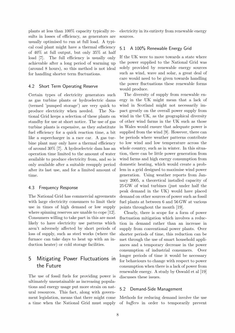
grid frequency, such that periods of grid deficitincrease the temperature at which they start tocool the contents. Typically, these fridges canmaintain the internal temperature within safelimits for up to an hour before being forced toswitch back on again regardless of the state ofthe grid. This window gives the National Gridcontrollers some time in which to get reservepower systems online. If every fridge in theUK (estimated to be around 40 million [23])were to use this kind of technology, savings ofbetween 500 MW [24] (roughly equivalent to ahydroelectric power plant) and 1200MW [23]could be achieved for up to an hour at shortnotice. Figure 7 shows the possible effect thisdeferral could have.

Figure 7: An example of the effect that dynamicdemand management in fridges could have on theelectricity demand over the course of a few hours.During a period of high demand, fridge energy con-sumption is deferred until a later time. Image takenfrom Stabilization of Grid Frequency Through Dy-

namic Demand Control (Short et al. [12]).

5.2.3 Consumer Incentives

A number of demand-based tariffs have beentrialled around the world, from a lower ’Econ-omy7’ tariff used in Europe for 7 hours duringthe night [25] to an hour-by-hour rate used inparts of Florida [26].

In France, the high proportion of nuclearpower plants, which are best utilised in pro-viding a constant output over long periods oftime, has led to incentives for consumers to usemore of their electricity during the night. Ahigher proportion of French homes are heatedwith electricity than gas, using night time stor-age heaters, due to the incentive created by

9

cheaper night time electricity [9]. This helpsto move some of the peak load during the dayinto the night.

A study conducted in a German town [22,27]showed that electricity tariffs which incentiviseuse of electricity outside of peak times can havean impact in reducing peak load during theday, but failed to fully mitigate large spikesin demand. In the study, a larger than nor-mal spike occurred around the border betweena low tariff and a medium tariff time, whichhad the opposite effect of mitigation in thatinstance; though the use of electricity duringthe day when demand is provided by the baseload was lower.

6 Project Aims

This project will focus on the development ofconcepts for mitigating power fluctuations us-ing demand-side techniques, to allow for a re-duction in the amount of standby fossil fuelpower plant capacity required.

To investigate methods for mitigation, a sys-tem to control the charging of a laptop which isresponsive to changes in grid frequency will beinvestigated, using mains frequency sensitivehardware and software methods. The reasonfor this is that laptops are widespread alreadyand so would not need major capital invest-ment, and the potential impact is significant.

To assist in quantifying the effect that sucha system might have on a future grid, a modelwill be developed to provide information aboutthe forms and magnitudes of the fluctuationsthat might be present in such an environment.

7 Prototyping, Testing and Char-

acterisation of a Smart Charging

Laptop

The simple case was considered of a laptopwhich charges when the grid frequency is above50 Hz and uses its battery when the grid fre-quency is below 50 Hz.

7.1 Measuring the Grid Frequency

In order for a laptop to effectively judge whento use power from the mains and when to use

its internal battery, it must know the state ofthe grid, as reflected in its frequency.

A real time digital control system running aLinux operating system was used to make thisdecision. The mains alternating current wasmeasured by using an AC transformer, whichstepped the voltage down from 230 V to 9 V.This allowed the mains input to be safely mea-sured by the control system.

A set of frequency time series values col-lected over the course of 24 hours using thesystem was compared against the correspond-ing 24 hours worth of frequency measurementsas reported by the National Grid website, us-ing data obtained by the Java program writtenprimarily to log the grid demand earlier. Thedata matched up well, meaning that the mainssignal received by the digital control systemwas unperturbed by other equipment nearbyand the data was being logged correctly andinstantaneously. The results can be seen inFigure 8.

Figure 8: A comparison between the frequency asmeasured by Fourier transforms conducted on datacollected by the digital control system and the fre-quency as reported by the National Grid website.The National Grid website reports frequency valueswhich may be up to three minutes out of date, so asystematic correction has been applied to this datain order for it to overlay the corresponding controlsystem measurements correctly.

7.2 Frequency Measurement Technique

The frequency of the input signal could havebeen measured directly using Fourier trans-forms (like that which has been done in Fig-ure 8). However, these operations are compu-tationally expensive and require a lot of mem-ory. For the purposes of this project, it isalso true that it is only necessary to knowwhether the input frequency is above or belowthe threshold in question, 50 Hz. Therefore, it

10

was more practical to use a differential bandpass filter method in order to obtain such in-formation.

The Method Used in order to Measure the Stateof the Signal

• The voltage signal from the National Gridis stepped down from 230 V to 9 V

• This signal is passed through an analogue-to-digital converter, then passed into thedigital control system, where the signal issampled a frequency of 4096 Hz

• The signal is passed through a band passfilter with range 45-55 Hz to eliminateany frequencies well outside the possiblerange2, such as higher frequency harmon-ics and background noise

• The signal is split into two copies, withthe first copy passing through a band passfilter with a range of 48-50 Hz, and the sec-ond copy passing through a band pass fil-ter with a range of 50-52Hz

• Both signals are saturated so as to becomesquare waves

• The signals undergo a half wave rectifica-tion and the absolute value is taken, so asto result in the signal being directly pro-portional to the signal the bandpass filterspick up

• The signals are passed through a low passfilter with corner frequency 1 Hz, so as toremove any fast transients

• The signal that passed through the higherbound band pass filter is then subtractedfrom the signal that passed through thelower bound band pass filter, thereby giv-ing a value which, if positive, representsan underlying frequency below 50 Hz, and,if negative, represents an underlying fre-quency above 50Hz

• The signal is passed through a low passfilter of 0.1 Hz to prevent the signal from

2The National Grid frequency very rarely falls belowthe 49.5Hz or rises above 50.5Hz, so this limit is verylenient.

changing sign too quickly when the gridfrequency is quickly fluctuating above andbelow 50 Hz

• The signal is input into a comparator,which outputs from the control system ahigh signal (in this case, 4 V) if the sig-nal from the previous step is negative, ora low signal (in this case, 0V) if the signalis positive

• This output control signal is amplified bya factor of 6

• The amplified signal is input into a FormA (’normally open’) relay requiring a con-trol signal potential difference of 20 V toswitch on, which drives the laptop chargercircuit

Notes: The frequency filters used are dig-ital versions; and the output signal from thecontrol system has to be amplified because ofconstraints on the ability of the control systemto output larger voltage signals.

The differential band pass filter method iseffectively comparing a signal with frequencycomponents below 50Hz with a signal withfrequency components above 50 Hz. At anygiven time, depending on the frequency of thegrid, one of these signals should be zero. Thismeans that, upon subtracting one signal fromthe other, the polarity of the resulting signalwill represent whether the frequency of the gridis above or below 50Hz.

A flowchart of the process can be seen inFigure 9. Characterisation measurements con-ducted with a calibrated frequency generatorshowed that this method has a resolution ofabout ±1 mHz.

7.3 Verifying the Frequency Measurement

Technique

In order to check that the frequency was be-ing correctly measured, the input signal andthe output control signal were measured for aperiod of 24 hours. A frequency spectrogramwas then produced using Fourier analysis per-formed on the input signal data, in order toshow the frequency components present in thesignal. In order to retrieve the underlying gridfrequency from this spectrogram, the frequency

11

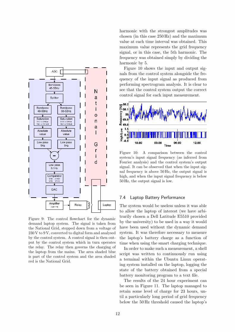
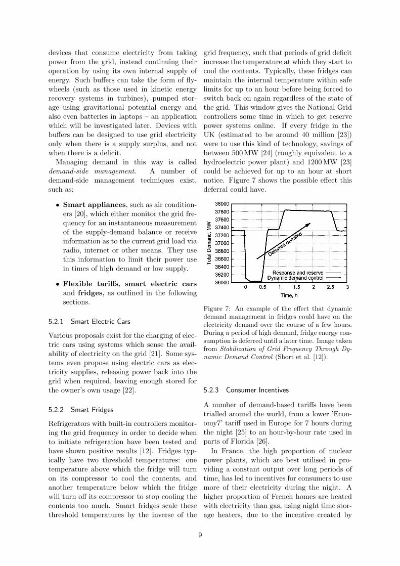
Figure 9: The control flowchart for the dynamicdemand laptop system. The signal is taken fromthe National Grid, stepped down from a voltage of230 V to 9 V, converted to digital form and analysedby the control system. A control signal is then out-put by the control system which in turn operatesthe relay. The relay then governs the charging ofthe laptop from the mains. The area shaded blueis part of the control system and the area shadedred is the National Grid.

harmonic with the strongest amplitudes waschosen (in this case 250Hz) and the maximumvalue at each time interval was obtained. Thismaximum value represents the grid frequencysignal, or in this case, the 5th harmonic. Thefrequency was obtained simply by dividing theharmonic by 5.

Figure 10 shows the input and output sig-nals from the control system alongside the fre-quency of the input signal as produced fromperforming spectrogram analysis. It is clear tosee that the control system output the correctcontrol signal for each input measurement.

Figure 10: A comparison between the controlsystem’s input signal frequency (as inferred fromFourier analysis) and the control system’s outputsignal. It can be observed that when the input sig-nal frequency is above 50 Hz, the output signal ishigh, and when the input signal frequency is below50 Hz, the output signal is low.

7.4 Laptop Battery Performance

The system would be useless unless it was ableto allow the laptop of interest (we have arbi-trarily chosen a Dell Latitude E5510 providedby the university) to be used in a way it wouldhave been used without the dynamic demandsystem. It was therefore necessary to measurethe laptop’s battery charge as a function oftime when using the smart charging technique.

In order to make such a measurement, a shellscript was written to continuously run usinga terminal within the Ubuntu Linux operat-ing system installed on the laptop, logging thestate of the battery obtained from a specialbattery monitoring program to a text file.

The results of the 24 hour experiment canbe seen in Figure 11. The laptop managed toretain some level of charge for 23 hours, un-til a particularly long period of grid frequencybelow the 50Hz threshold caused the laptop’s

12

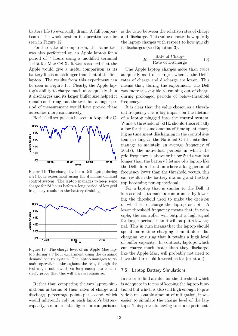
battery life to eventually drain. A full compar-ison of the whole system in operation can beseen in Figure 12.

For the sake of comparison, the same testwas also performed on an Apple laptop for aperiod of 7 hours using a modified terminalscript for Mac OS X. It was reasoned that theApple would give a useful comparison as itsbattery life is much longer than that of the firstlaptop. The results from this experiment canbe seen in Figure 13. Clearly, the Apple lap-top’s ability to charge much more quickly thanit discharges and its larger buffer size helped itremain on throughout the test, but a longer pe-riod of measurement would have proved theseoutcomes more conclusively.

Both shell scripts can be seen in Appendix C.

Figure 11: The charge level of a Dell laptop duringa 24 hour experiment using the dynamic demandcontrol system. The laptop manages to keep somecharge for 23 hours before a long period of low gridfrequency results in the battery draining.

Figure 13: The charge level of an Apple Mac lap-top during a 7 hour experiment using the dynamicdemand control system. The laptop manages to re-main operational throughout the test, though thetest might not have been long enough to conclu-sively prove that this will always remain so.

Rather than comparing the two laptop sim-ulations in terms of their rates of charge anddischarge percentage points per second, whichwould inherently rely on each laptop’s batterycapacity, a more reliable figure for comparisons

is the ratio between the relative rates of chargeand discharge. This value denotes how quicklythe laptop charges with respect to how quicklyit discharges (see Equation 3).

R =Rate of Charge

Rate of Discharge(3)

The Apple laptop charges more than twiceas quickly as it discharges, whereas the Dell’srates of charge and discharge are lower. Thismeans that, during the experiment, the Dellwas more susceptible to running out of chargeduring prolonged periods of below-thresholdfrequency.

It is clear that the value chosen as a thresh-old frequency has a big impact on the lifetimeof a laptop plugged into the control system.While a threshold of 50 Hz should theoreticallyallow for the same amount of time spent charg-ing as time spent discharging in the control sys-tem (so long as the National Grid controllersmanage to maintain an average frequency of50 Hz), the individual periods in which thegrid frequency is above or below 50 Hz can lastlonger than the battery lifetime of a laptop likethe Dell. In a situation where a long period offrequency lower than the threshold occurs, thiscan result in the battery draining and the lap-top becoming non-operational.

For a laptop that is similar to the Dell, itis reasonable to make a compromise by lower-ing the threshold used to make the decisionof whether to charge the laptop or not. Alower threshold frequency means that, in prin-ciple, the controller will output a high signalfor longer periods than it will output a low sig-nal. This in turn means that the laptop shouldspend more time charging than it does dis-charging, ensuring that it retains a high levelof buffer capacity. In contrast, laptops whichcan charge much faster than they discharge,like the Apple Mac, will probably not need tohave the threshold lowered as far (or at all).

7.5 Laptop Battery Simulations

In order to find a value for the threshold whichis adequate in terms of keeping the laptop func-tional but which is also still high enough to pro-vide a reasonable amount of mitigation, it waseasier to simulate the charge level of the lap-tops. This prevents having to run experiments

13

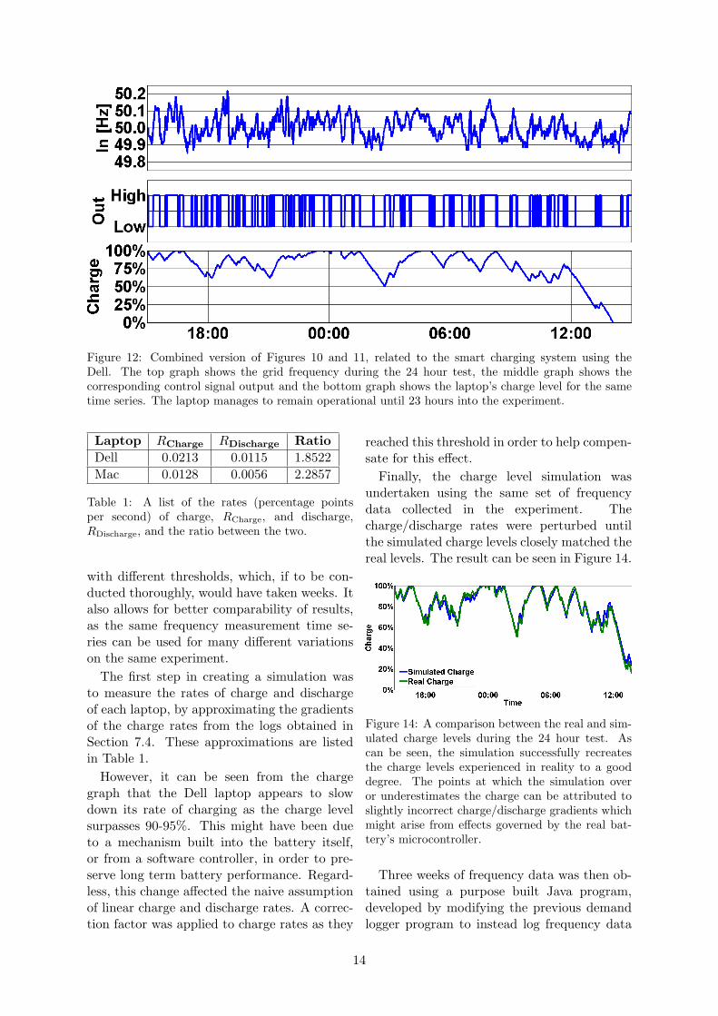
Figure 12: Combined version of Figures 10 and 11, related to the smart charging system using theDell. The top graph shows the grid frequency during the 24 hour test, the middle graph shows thecorresponding control signal output and the bottom graph shows the laptop’s charge level for the sametime series. The laptop manages to remain operational until 23 hours into the experiment.

Laptop RCharge RDischarge RatioDell 0.0213 0.0115 1.8522Mac 0.0128 0.0056 2.2857

Table 1: A list of the rates (percentage pointsper second) of charge, RCharge, and discharge,RDischarge, and the ratio between the two.

with different thresholds, which, if to be con-ducted thoroughly, would have taken weeks. Italso allows for better comparability of results,as the same frequency measurement time se-ries can be used for many different variationson the same experiment.

The first step in creating a simulation wasto measure the rates of charge and dischargeof each laptop, by approximating the gradientsof the charge rates from the logs obtained inSection 7.4. These approximations are listedin Table 1.

However, it can be seen from the chargegraph that the Dell laptop appears to slowdown its rate of charging as the charge levelsurpasses 90-95%. This might have been dueto a mechanism built into the battery itself,or from a software controller, in order to pre-serve long term battery performance. Regard-less, this change affected the naive assumptionof linear charge and discharge rates. A correc-tion factor was applied to charge rates as they

reached this threshold in order to help compen-sate for this effect.

Finally, the charge level simulation wasundertaken using the same set of frequencydata collected in the experiment. Thecharge/discharge rates were perturbed untilthe simulated charge levels closely matched thereal levels. The result can be seen in Figure 14.

Figure 14: A comparison between the real and sim-ulated charge levels during the 24 hour test. Ascan be seen, the simulation successfully recreatesthe charge levels experienced in reality to a gooddegree. The points at which the simulation overor underestimates the charge can be attributed toslightly incorrect charge/discharge gradients whichmight arise from effects governed by the real bat-tery’s microcontroller.

Three weeks of frequency data was then ob-tained using a purpose built Java program,developed by modifying the previous demandlogger program to instead log frequency data

14

to higher (15 second) resolution (see Ap-pendix B.2). This data was used in the simula-tions so as to provide a conclusive result as towhether or not a particular threshold frequencywould allow a laptop to stay operational at alltimes.

Simulations using different threshold fre-quencies below 50 Hz were then undertaken.Histograms of five of these thresholds areshown in Figure 15. From these histograms itis easy to see which threshold frequencies willallow the laptop to remain operational, and de-tails of the range of expected charge percent-ages are also readily apparent. For instance, athreshold frequency of 49.955 Hz always keepsthe laptop in the charge range 60-100%.

The best compromise with the Dell seemedto be to use a threshold of 49.975 Hz. Figure16 shows a time series of the charge level inthe laptop, simulated over a period of 21 daysusing this particular threshold. It is clear to seethat the laptop charge does not fall below 40%,and typically stays within the 70-100% chargelevel, allowing the user to disconnect from themains if required and still have an adequatecharge level for laptop use on the move.

Figure 16: A time series of the simulated chargelevels over a period of 21 days using a thresholdfrequency of 49.975 Hz. The charge level does notdrop below 40% and typically stays in the 70-100%region.

8 Large Scale Impact of Smart

Charging Laptop

8.1 Quantifying UK Grid Demand

Initially, in order to quantify the UK demand,a computer program was written which logsthe UK demand to five minute resolution (andUK grid frequency to 3 minute resolution) asreported by the National Grid website. The

data obtained using this method was useful forquantifying the demand on the scale of a week(the length of time the program was opera-tional), but it was not ideal for measuring theeffects of longer demand variations due to theneed to log data in real time. It was thereforefavourable to obtain historical data so as to beable to demonstrate the long term variationsin demand.

At the beginning of 2012, the National Gridmade available demand data to half-hour res-olution for all of 2011. A visualisation of thisdata can be seen in Figure 1. From this it waspossible to then obtain a figure for the aver-age power demand over the course of the year,which could be used to calibrate future models.

8.2 Entirely Renewable Grid

Due to the lack of substantial, high resolutiondata available regarding the fluctuations thatwould be present in a grid powered solely fromrenewable energy sources in the UK, such fluc-tuations can only be simulated.

In order to simulate this future grid, some as-sumptions must be made as to the form such agrid would take. The arbitrary assumption wasmade that the grid would be powered solelyfrom wind and solar energy sources, and thatthe split would be equal between the two, suchthat the average production from each sourceequalled half of the average demand.

8.2.1 Demand Model

A model of the demand in 2011 was producedusing the data obtained from the NationalGrid, with a resolution of 30 minutes. It waspossible to use 2011 data as long as it can beassumed that demand will not differ greatly in2020 from that in 2011.

From Figures 1 and 2 it is clear to see thatdemand is greatest during the day around din-ner time and lowest during the early hours ofthe morning. Throughout the year, the de-mand is greatest in winter and least in sum-mer.

On average, demand for 2011 was 35 GW.At its peak it was 55GW, and at its lowest itwas 19GW.

15

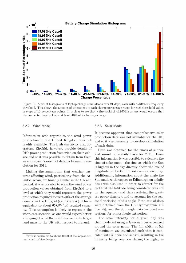
Figure 15: A set of histograms of laptop charge simulations over 21 days, each with a different frequencythreshold. This shows the amount of time spent in each charge percentage range for each threshold value,in steps of 10 percentage points. It is clear to see that a threshold of 49.975 Hz or less would ensure thatthe connected laptop keeps at least 40% of its battery charge.

8.2.2 Wind Model

Information with regards to the wind powerproduction in the United Kingdom was notreadily available. The Irish electricity grid op-erators, EirGrid, however, provide details ofIrish power production from wind on their web-site and so it was possible to obtain from theman entire year’s worth of data to 15 minute res-olution for 2011.

Making the assumption that weather pat-terns affecting wind, particularly from the At-lantic Ocean, are broadly similar in the UK andIreland, it was possible to scale the wind powerproduction values obtained from EirGrid to alevel at which they would represent the powerproduction required to meet 50% of the averagedemand in the UK grid (i.e. 17.5 GW). This isequivalent to about 65GW3 of installed capac-ity. This assumption is likely to represent theworst case scenario, as one would expect betteraveraging of wind fluctuations due to the largerland mass in the UK with respect to Ireland.

3This is equivalent to about 10000 of the largest cur-rent wind turbine designs.

8.2.3 Solar Model

It became apparent that comprehensive solarproduction data was not available for the UK,and so it was necessary to develop a simulationof such data.

Data was obtained for the times of sunriseand sunset on a daily basis for 2011. Fromthis information it was possible to calculate thetime of solar noon—the time at which the Sunis highest in the sky directly above the line oflongitude on Earth in question—for each day.Additionally, information about the angle theSun made with respect to Edinburgh on a dailybasis was also used in order to correct for thefact that the latitude being considered was noton the equator (and thus receiving the great-est power density), and to account for the sea-sonal variation of this angle. Both sets of datawere obtained from the UK Hydrographic Of-fice [28], and the Sun angle data included cor-rections for atmospheric extinction.

The solar intensity for a given day wasthen modelled using a Gaussian curve centredaround the solar noon. The full width at 5%of maximum was calculated such that it coin-cided with sunrise and sunset, resulting in theintensity being very low during the night, as

16

intended. It was assumed that sunset and sun-rise provide less than 5% of the maximum solarnoon value, with a small amount of light com-ing from atmospheric refraction, moonlight, ar-tificial light and other sources.

The effect of clouds was then modelled byintroducing ten intensity correction factors ofvarying frequency, which had the effect of re-ducing the intensity of light incident on theground on the scale of minutes, hours, days andweeks. Each ’cloud’ had an associated inten-sity correction factor between 0 and 1, which ismultiplied with the intensity value associatedwith the solar model for a given time step toproduce the actual intensity of light throughthe cloud. Each cloud had a different correc-tion factor, had an effect for different lengthsof time and recurred on a different frequency.The result was that it was clear to see signifi-cant drops in intensity throughout the day asthese ’clouds’ covered the Sun in the sky, whichallowed the model to better represent reality.

Finally, the actual power generated P froma square meter A of solar panels was calcu-lated using Equation 4. This used the model’scalculation for solar intensity for a given time,I, along with the power of sunlight incidenton the equator (�, the solar constant, roughly1.3×104 kW/m2) and the efficiency of the solarcells, η, which was assumed to be 40%4. Thearea of panels was scaled in the same way asthe wind model so that the average power pro-duced in a year was equal to half of the averagedemand for a year.

P = η�IA (4)

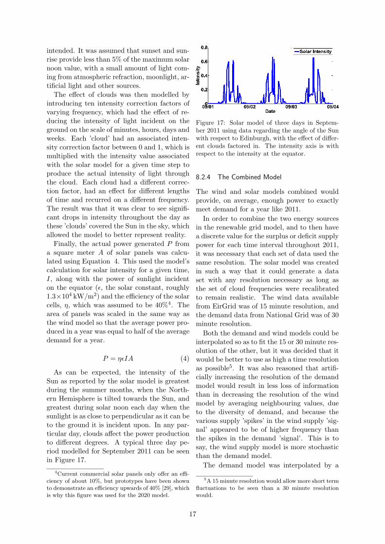
As can be expected, the intensity of theSun as reported by the solar model is greatestduring the summer months, when the North-ern Hemisphere is tilted towards the Sun, andgreatest during solar noon each day when thesunlight is as close to perpendicular as it can beto the ground it is incident upon. In any par-ticular day, clouds affect the power productionto different degrees. A typical three day pe-riod modelled for September 2011 can be seenin Figure 17.

4Current commercial solar panels only offer an effi-ciency of about 10%, but prototypes have been shownto demonstrate an efficiency upwards of 40% [29], whichis why this figure was used for the 2020 model.

Figure 17: Solar model of three days in Septem-ber 2011 using data regarding the angle of the Sunwith respect to Edinburgh, with the effect of differ-ent clouds factored in. The intensity axis is withrespect to the intensity at the equator.

8.2.4 The Combined Model

The wind and solar models combined wouldprovide, on average, enough power to exactlymeet demand for a year like 2011.

In order to combine the two energy sourcesin the renewable grid model, and to then havea discrete value for the surplus or deficit supplypower for each time interval throughout 2011,it was necessary that each set of data used thesame resolution. The solar model was createdin such a way that it could generate a dataset with any resolution necessary as long asthe set of cloud frequencies were recalibratedto remain realistic. The wind data availablefrom EirGrid was of 15 minute resolution, andthe demand data from National Grid was of 30minute resolution.

Both the demand and wind models could beinterpolated so as to fit the 15 or 30 minute res-olution of the other, but it was decided that itwould be better to use as high a time resolutionas possible5. It was also reasoned that artifi-cially increasing the resolution of the demandmodel would result in less loss of informationthan in decreasing the resolution of the windmodel by averaging neighbouring values, dueto the diversity of demand, and because thevarious supply ’spikes’ in the wind supply ’sig-nal’ appeared to be of higher frequency thanthe spikes in the demand ’signal’. This is tosay, the wind supply model is more stochasticthan the demand model.

The demand model was interpolated by a

5A 15 minute resolution would allow more short termfluctuations to be seen than a 30 minute resolutionwould.

17

factor of 2 in order to achieve the required res-olution. The time vector used to specify the30 minute intervals for the demand model hadextra time values inserted in between the ex-isting values. A linear interpolation was thenused to calculate the respective demand valuesfor the new time intervals.

The resulting set of wind, solar and demandmodels were then combined into one model,with the wind and solar supplies being sub-tracted from the demand for each time inter-val. This provided a new set of power valuesdenoting the deficit or surplus of power supplyfor each time interval. This new model can beseen for a particular day in Figure 18.

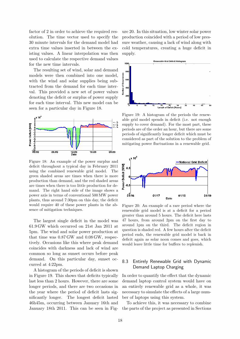
Figure 18: An example of the power surplus anddeficit throughout a typical day in February 2011using the combined renewable grid model. Thegreen shaded areas are times when there is moreproduction than demand, and the red shaded areasare times when there is too little production for de-mand. The right hand side of the image shows apower axis in terms of conventional 500MW powerplants, thus around 7:30pm on this day, the deficitwould require 40 of these power plants in the ab-sence of mitigation techniques.

The largest single deficit in the model was61.9 GW which occurred on 21st Jan 2011 at5pm. The wind and solar power production atthat time was 0.87 GW and 0.08 GW, respec-tively. Occasions like this where peak demandcoincides with darkness and lack of wind arecommon so long as sunset occurs before peakdemand. On this particular day, sunset oc-curred at 4:22pm.

A histogram of the periods of deficit is shownin Figure 19. This shows that deficits typicallylast less than 2 hours. However, there are somelonger periods, and there are two occasions inthe year where the period of deficit lasts sig-nificantly longer. The longest deficit lasted46h45m, occurring between January 16th andJanuary 18th 2011. This can be seen in Fig-

ure 20. In this situation, low winter solar powerproduction coincided with a period of low pres-sure weather, causing a lack of wind along withcold temperatures, creating a huge deficit insupply.

Figure 19: A histogram of the periods the renew-able grid model spends in deficit (i.e. not enoughsupply to cover demand). For the most part, theseperiods are of the order an hour, but there are someperiods of significantly longer deficit which must beconsidered as part of the solution to the problem ofmitigating power fluctuations in a renewable grid.

Figure 20: An example of a rare period where therenewable grid model is at a deficit for a periodgreater than around 5 hours. The deficit here lasts47 hours, from around 2pm on the first day toaround 1pm on the third. The deficit region inquestion is shaded red. A few hours after the deficitperiod ends, the renewable grid model is back indeficit again as solar noon comes and goes, whichwould leave little time for buffers to replenish.

8.3 Entirely Renewable Grid with Dynamic

Demand Laptop Charging

In order to quantify the effect that the dynamicdemand laptop control system would have onan entirely renewable grid as a whole, it wasnecessary to simulate the effects of a large num-ber of laptops using this system.

To achieve this, it was necessary to combinethe parts of the project as presented in Sections

18

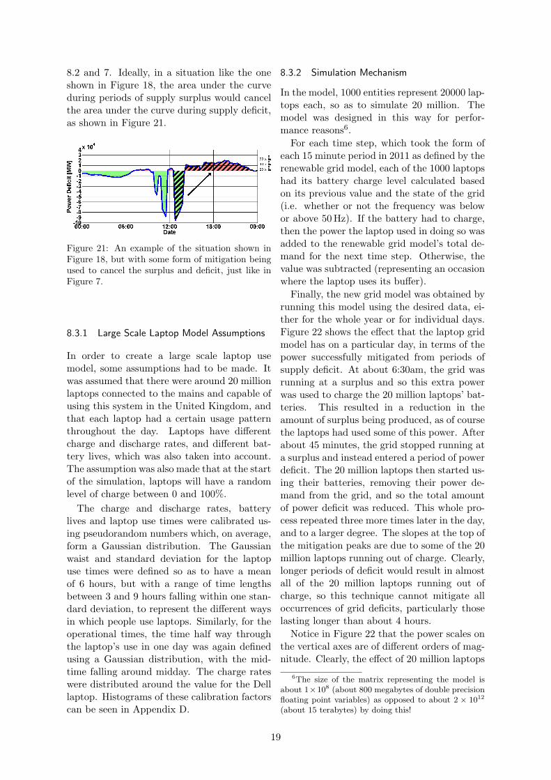
8.2 and 7. Ideally, in a situation like the oneshown in Figure 18, the area under the curveduring periods of supply surplus would cancelthe area under the curve during supply deficit,as shown in Figure 21.

Figure 21: An example of the situation shown inFigure 18, but with some form of mitigation beingused to cancel the surplus and deficit, just like inFigure 7.

8.3.1 Large Scale Laptop Model Assumptions

In order to create a large scale laptop usemodel, some assumptions had to be made. Itwas assumed that there were around 20 millionlaptops connected to the mains and capable ofusing this system in the United Kingdom, andthat each laptop had a certain usage patternthroughout the day. Laptops have differentcharge and discharge rates, and different bat-tery lives, which was also taken into account.The assumption was also made that at the startof the simulation, laptops will have a randomlevel of charge between 0 and 100%.

The charge and discharge rates, batterylives and laptop use times were calibrated us-ing pseudorandom numbers which, on average,form a Gaussian distribution. The Gaussianwaist and standard deviation for the laptopuse times were defined so as to have a meanof 6 hours, but with a range of time lengthsbetween 3 and 9 hours falling within one stan-dard deviation, to represent the different waysin which people use laptops. Similarly, for theoperational times, the time half way throughthe laptop’s use in one day was again definedusing a Gaussian distribution, with the mid-time falling around midday. The charge rateswere distributed around the value for the Delllaptop. Histograms of these calibration factorscan be seen in Appendix D.

8.3.2 Simulation Mechanism

In the model, 1000 entities represent 20000 lap-tops each, so as to simulate 20 million. Themodel was designed in this way for perfor-mance reasons6.

For each time step, which took the form ofeach 15 minute period in 2011 as defined by therenewable grid model, each of the 1000 laptopshad its battery charge level calculated basedon its previous value and the state of the grid(i.e. whether or not the frequency was belowor above 50 Hz). If the battery had to charge,then the power the laptop used in doing so wasadded to the renewable grid model’s total de-mand for the next time step. Otherwise, thevalue was subtracted (representing an occasionwhere the laptop uses its buffer).

Finally, the new grid model was obtained byrunning this model using the desired data, ei-ther for the whole year or for individual days.Figure 22 shows the effect that the laptop gridmodel has on a particular day, in terms of thepower successfully mitigated from periods ofsupply deficit. At about 6:30am, the grid wasrunning at a surplus and so this extra powerwas used to charge the 20 million laptops’ bat-teries. This resulted in a reduction in theamount of surplus being produced, as of coursethe laptops had used some of this power. Afterabout 45 minutes, the grid stopped running ata surplus and instead entered a period of powerdeficit. The 20 million laptops then started us-ing their batteries, removing their power de-mand from the grid, and so the total amountof power deficit was reduced. This whole pro-cess repeated three more times later in the day,and to a larger degree. The slopes at the top ofthe mitigation peaks are due to some of the 20million laptops running out of charge. Clearly,longer periods of deficit would result in almostall of the 20 million laptops running out ofcharge, so this technique cannot mitigate alloccurrences of grid deficits, particularly thoselasting longer than about 4 hours.

Notice in Figure 22 that the power scales onthe vertical axes are of different orders of mag-nitude. Clearly, the effect of 20 million laptops

6The size of the matrix representing the model isabout 1×108 (about 800 megabytes of double precisionfloating point variables) as opposed to about 2 × 1012

(about 15 terabytes) by doing this!

19

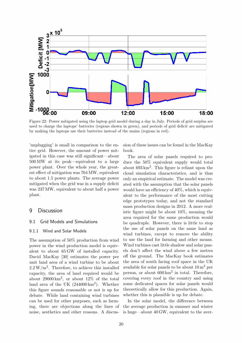
Figure 22: Power mitigated using the laptop grid model during a day in July. Periods of grid surplus areused to charge the laptops’ batteries (regions shown in green), and periods of grid deficit are mitigatedby making the laptops use their batteries instead of the mains (regions in red).

’unplugging’ is small in comparison to the en-tire grid. However, the amount of power mit-igated in this case was still significant—about500 MW at its peak—equivalent to a largepower plant. Over the whole year, the great-est effect of mitigation was 764 MW, equivalentto about 1.5 power plants. The average powermitigated when the grid was in a supply deficitwas 237MW, equivalent to about half a powerplant.

9 Discussion

9.1 Grid Models and Simulations

9.1.1 Wind and Solar Models

The assumption of 50% production from windpower in the wind production model is equiv-alent to about 65 GW of installed capacity.David MacKay [30] estimates the power perunit land area of a wind turbine to be about2.2 W/m2. Therefore, to achieve this installedcapacity, the area of land required would beabout 29000 km2, or about 12% of the totalland area of the UK (244000 km2). Whetherthis figure sounds reasonable or not is up fordebate. While land containing wind turbinescan be used for other purposes, such as farm-ing, there are objections along the lines ofnoise, aesthetics and other reasons. A discus-

sion of these issues can be found in the MacKaybook.

The area of solar panels required to pro-duce the 50% equivalent supply would totalabout 693 km2. This figure is reliant upon thecloud simulation characteristics, and is thusonly an empirical estimate. The model was cre-ated with the assumption that the solar panelswould have an efficiency of 40%, which is equiv-alent to the performance of the most cuttingedge prototypes today, and not the standardmass production designs in 2012. A more real-istic figure might be about 10%, meaning thearea required for the same production wouldbe quadruple. However, there is little to stopthe use of solar panels on the same land aswind turbines, except to remove the abilityto use the land for farming and other means.Wind turbines cast little shadow and solar pan-els don’t affect the wind above a few metresoff the ground. The MacKay book estimatesthe area of south facing roof space in the UKavailable for solar panels to be about 10 m2 perperson, or about 600 km2 in total. Therefore,covering every roof in the country and usingsome dedicated spaces for solar panels wouldtheoretically allow for this production. Again,whether this is plausible is up for debate.

In the solar model, the difference betweenthe average production in summer and winteris huge—about 40 GW, equivalent to the aver-

20

age demand in the year. The purpose of thisproject was to look at ways of mitigating powerfluctuations without having to resort to meth-ods such as those outlined in Section 4. If thelong term difference between summer and win-ter output from solar necessitates the use ofa set of standby power plants to make up thedifference, this would counteract the effect thatthe mitigation techniques would have in reduc-ing the need for these power plants. Clearly arenewable grid would need to be carefully de-signed in order to prevent the need to resort tousing the ’old ways’ for parts of the year, andrelying so much on solar power is probably notthe way forward.

The two renewable energy source models –the wind and solar models – were produced us-ing some assumptions as to how they wouldperform as an energy source. These assump-tions are accurate enough to obtain ’ball parkfigures’ for the kind of outputs these sourcesmight produce throughout a year, but they arenot accurate enough to be used for any sort ofprecision modelling. The models can be im-proved in many respects by using higher res-olution underlying data, more accurate cali-bration factors such as cloud effects by bas-ing them on real observations, and by factoringin regional geographical variations which affectthe ability to produce electricity.

9.2 Laptop Controller Experiment

The differential band pass filter method usedto obtain the state of the grid is very effective,with accuracy to within about 1mHz. Noisepresent in the signal is also suppressed in thestage which subtracts one copy from the other.Although the method provides information asto whether the frequency is above or below thechosen threshold, it does not give an estimateas to how far away the frequency is from thispoint. Such information would be useful fordifferentiating between slight and major short-falls in demand. If this information was avail-able, it would be possible to vary the thresholdat which the laptop system would stop tak-ing power from the grid. For instance, if thelaptop’s battery was below, say, 50% full, thecontrol system could decide to only stop thelaptop from taking power from the grid whenthe threshold fell below a lower threshold, ef-

fectively helping the grid only when the gridreally needs the help.

The results regarding the laptop controllerare proofs of concept. The best frequencythreshold for a particular laptop depends on anumber of variables, including the battery life,rates of charge and discharge, and whether ornot the laptop has a high CPU load when inuse. A desirable situation would be where theuser decides the threshold they wish to use,taking account of their personal needs. A lap-top that stays ’plugged in’ to a wall socket at alltimes can safely use a high threshold, whereas alaptop that is frequently used on the move willneed to retain a high level of battery chargelevel at all times for such circumstances. Sim-ilarly, a fail safe mechanism would need to bebuilt in to end user systems to prevent long pe-riods of frequency below threshold from drain-ing the laptop battery entirely, with the poten-tial for data corruption and loss of productiv-ity.

9.2.1 Long Term Effect on Laptop Batteries

An issue that has not been considered in thisstudy is the long term effect frequent chargeand discharge cycles can have on laptop bat-teries.

When a lithium-ion cell charges, typical ofthose used in modern laptops, deposits areformed inside the electrolyte, which increasesthe internal resistance of the battery and de-creases its ability to store energy over time.This means that frequent charging will limitthe life of the battery.

Tests of a lithium-ion cell showed that thebattery life is influenced mainly by the con-ditions in which the battery is charged, andnot so much the discharge conditions [31]. Inparticular, over-charging, where the battery ischarged beyond its design capacity, is a largefactor in the degradation [32]. This means thatit would be reasonable to build some logic intothe controller which takes into account the con-ditions in which the laptop would be charging.These conditions could be elements such as theambient temperature, current charge level (forinstance, whether or not to charge if the bat-tery is already almost full), or other factors.

21

9.3 Project as a Whole

For certain periods of power deficit of the ordera couple of hours long, it is not inconceivableto suggest that this kind of deficit could bedealt with through some forms of demand-sidemanagement such as the laptop control systemoutlined as part of this study. The particu-lar laptop system developed in this study wasable to mitigate an average of 237 MW of de-mand when used by 20 million devices, whichrepresents about 0.6% of the total average UKdemand. If all of our electronic devices, suchas lights, heating and cooling systems, electriccars, ovens, desktop computers, televisions andso on implemented a similar form of demand-side management, the power available for mit-igation at any one time would become evengreater. A combination of these devices shut-ting down in tandem might be enough to mit-igate some of the fluctuations that a grid pow-ered from renewable energy sources might cre-ate, and thus there would no longer be the needto build so many cost intensive ’peaking’ powerplants7.

However, demand-side management tech-niques are not quite so useful for longer periodsof supply deficit, and in a grid powered froma high proportion of volatile renewable energysources such as wind, such periods of supplydeficit will occasionally occur. Again, if thegrid is to involve a greater amount of energysources such as wind, models must be in placeto deal with the loss of production during pe-riods of low output. In particular, it is worthfocusing on the scenarios where long periods oflow wind coincide with high periods of demand,such as in winter and in the evening.

9.4 Future Work

In the future, it would be worth exploring waysin which to miniaturise the laptop control sys-tem. The system developed in this study in-volved the use of a large server class com-puter, which is obviously useless for this ap-plication in practice. The best method for lap-tops would likely be a microcontroller build into the charger’s transformer box. Such a mi-

7A typical new 500MW nuclear power plant costs ofthe order £1.5B to build [33].

crocontroller could also be used in other appli-cations.

The models developed as part of this studycan be improved as outlined in the discus-sion. With higher resolution data, it could bepossible to undertake different forms of anal-ysis, such as looking at the fluctuations froma frequency domain perspective. This methodwould have the potential to provide informa-tion about the magnitude and frequency ofdifferent fluctuations present in the renewablegrid model, which would be useful for bettercoordinating mitigation techniques.

10 Conclusions

The concept for power fluctuation mitigationusing laptops as outlined in this study showspromise. Although the simulations by nomeans fully represent reality, which is vastlymore complex than the basic assumptionsmade in the model allow, the concept has beenclearly demonstrated to have a positive effect.

This technique, along with some of the con-ventional methods of mitigation, could standthe National Grid in good stead to face thechallenges of the future, in terms of quality ofelectricity service, environmental impact (thepotential for a reduction in traditional gas andcoal fired plants) and cost (not having to payupwards of £7M a month for industries to tem-porarily cease electricity consumption).

In the future, the concepts developed as partof this study can be applied to other forms ofbuffers, which, working in tandem, can providea valuable means of demand reduction duringtimes of supply deficit.

References

[1] Parliament of the United Kingdom. Cli-mate Change Act, 2008.

[2] Scottish Government. 2020 Routemapfor Renewable Energy in Scot-land. http://www.scotland.gov.

uk/Publications/2011/08/04110353/2.

[3] The European Parliament. Directive2009/28/EC, April 2009.

22

[4] IEEE. IEEE Recommended Practice forElectric Power Distribution for IndustrialPlants. ANSI/IEEE Std 141-1986, 1986.

[5] EirGrid. Wind generation system perfor-mance data. http://www.eirgrid.com/

operations/systemperformancedata/

windgeneration/.

[6] National Grid. Electricity -Real Time Operational Data.http://www.nationalgrid.com/uk/

Electricity/Data/Realtime/, 2011.

[7] Janet Ramage Godfrey Boyle, Bob Ev-erett, editor. Energy Systems and Sustain-

ability: Power for the Sustainable Future.Oxford University Press, 2003.

[8] National Grid. Forecast-ing Demand. http://www.

nationalgrid.com/NR/rdonlyres/

1C4B1304-ED58-4631-8A84-3859FB8B4B38/

17136/demand.pdf.

[9] Godfrey Boyle. Renewable Energy. OxfordUniversity Press, 2004.

[10] I. Harrison and A. Marr. Britain from

Above. Pavilion, 2009.

[11] National Grid. Frequency Controlby Demand Management (FCDM).http://www.nationalgrid.com/uk/

Electricity/Balancing/services/

frequencyresponse/fcdm/, 2011.

[12] J.A. Short, D.G. Infield, and L.L. Freris.Stabilization of Grid Frequency ThroughDynamic Demand Control. Power Sys-

tems, IEEE Transactions on, 22(3):1284– 1293, August 2007.

[13] National Grid. Monthly BalancingServices Summary, September 2011.http://www.nationalgrid.com/uk/

Electricity/Balancing/Summary/,2011.

[14] Parliament of the United Kingdom. Elec-tricity Act, 1989.

[15] Nick Jelley John Andrews. Energy Science

- Principles, Technologies, and Impacts.Oxford University Press, 2007.

[16] P. Kundur, N.J. Balu, and M.G. Lauby.Power System Stability and Control. TheEPRI Power System Engineering Series.McGraw-Hill, 1994.

[17] O.I. Elgerd. Electric Energy Systems The-

ory: An Introduction. McGraw-Hill, 2007.

[18] National Grid. National Grid: Inter-connectors. http://www.nationalgrid.

com/uk/interconnectors/.

[19] James Oswald, Mike Raine, and HezlinAshraf-Ball. Will British weather pro-vide reliable electricity? Energy Policy,36(8):3212 – 3225, 2008.

[20] Tai-Lang Jong Chi-Min Chu. A NovelDirect Air-Conditioning Load ControlMethod. Power Systems, IEEE Transac-

tions on, 23(3):1356 – 1363, August 2008.

[21] Chang-Yu Huang, J.T. Boys, G.A. Covic,J.R. Lee, and R.V. Stebbing. Implemen-tation and Evaluation of an IPT Bat-tery Charging System in assisting GridFrequency Stabilisation through DynamicDemand Control. In Vehicle Power

and Propulsion Conference (VPPC), 2010

IEEE, pages 1 – 6, September 2010.

[22] M. Ifland, N. Exner, and D. Westermann.Appliance of Direct and Indirect DemandSide Management. In Energytech, 2011

IEEE, pages 1 – 6, May 2011.

[23] Department of Energy and ClimateChange. The Potential for Dynamic De-mand. Technical report, Department ofEnergy and Climate Change, November2008. URN 08/1453.

[24] National Grid. Operating the ElectricityTransmission Networks in 2020. Technicalreport, National Grid PLC, June 2009.

[25] J. Platts. Electrical Load Management:The British Experience. IEEE Spectrum,16(2), February 1979.

[26] M. A. Fischetti. Electric Utilities: PoistedFor Deregulation? IEEE Spectrum, 23(5),May 1986.

23

[27] Residens Project. http://www.

tu-ilmenau.de/fakmn/9999+

M54099f70862.0.html.

[28] UK Hydrographic Office. Her Majesty’sNautical Almanac Office. http://astro.ukho.gov.uk/.

[29] Martin A. Green, Keith Emery, YoshihiroHishikawa, Wilhelm Warta, and Ewan D.Dunlop. Solar cell efficiency tables (ver-sion 39). Progress in Photovoltaics:

Research and Applications, 20(1):12–20,2012.

[30] D.J.C. MacKay. Sustainable Energy -

Without the Hot Air. UIT, 2009.

[31] Soo Seok Choi and Hong S Lim. Factorsthat affect cycle-life and possible degra-dation mechanisms of a Li-ion cell basedon LiCoO2. Journal of Power Sources,111(1):130 – 136, 2002.

[32] L. S. Kanevskii and V. S. Dubasova.Degradation of Lithium-Ion batteries andhow to fight it: A review. Russian Journal

of Electrochemistry, 41:1–16, 2005.

[33] Nuclear Engineering International. Howmuch? http://www.neimagazine.com/

story.asp?storyCode=2047917.

24

Appendices

A Interconnector Power Imports/Exports Sample

The UK grid has interconnectors with neighbouring grid networks. Within the BritishIsles, there are interconnectors between Northern Ireland and Scotland, Northern Irelandand the Republic of Ireland, the Isle of Man and England, Scotland and England, andNorth England and South England. Outwith the UK, there are interconnectors betweenthe UK and France (2 GW), and the UK and the Netherlands (1 GW). There are alsopreliminary plans to create an interconnector between the UK and Norway (see http:

//en.wikipedia.org/wiki/Scotland-Norway_interconnector and http://en.wikipedia.

org/wiki/HVDC_Norway-Great_Britain) by 2020. Figure 23 shows the French and Dutchinterconnectors in use.

Figure 23: National Grid interconnector imports and exports on 24th October 2011. Throughout theday the UK buys power from France and the Netherlands, except for a period in the morning when theUK sells power in the other direction. Interestingly, there is a period during the day when the UK gridimports power from the Netherlands and exports power to France at the same time.

B National Grid Website Logger Program

B.1 Initial Program

Real time data is published on the National Grid’s website, on this page: http://www.

nationalgrid.com/ngrealtime/realtime/systemdata.aspx. The data available is demand,frequency, and system transfers (electricity export/import) between Scotland/England andNorth England to South England, and transfers from the interconnectors (Northern Ireland,France and the Netherlands). This data is of limited resolution.

The program8 developed uses regular expressions in order to extract the figures for demandand frequency from the HTML source code behind this web page.

8SVN Path: /trunk/GridAnalyticsProgram/

25

B.2 Refined Frequency Program

High resolution frequency data, along with a wealth of other information, is published by theNational Grid on their dedicated statistics website, BM Reports (http://www.bmreports.com/). The frequency data is published in both XML and CVS format, and can be found inthe ’Electricity Data Summary’ page within the ’General’ tab.

The program9 developed downloads an XML file periodically and adds the data it doesn’talready have to its logs.

C Battery Logging Shell Scripts

C.1 Ubuntu Linux

Install the battery-charge-graph package from the official Ubuntu repository, either using theSoftware Centre or by typing the following in a terminal:

sudo apt-get install battery-charge-graph

Then start the logging by typing the following in a terminal:

sudo battery-stats-collector -o batterylog.txt

Where batterylog.txt is the name of the file you wish to use for the log, in the current workingdirectory. Leave the terminal running the command open for as long as you wish to log thebattery charge level.

C.2 Mac OS X

Create a script file such as batterylog.sh and type the following into it:

#!/bin/bash

cd ~/Desktop/

date >> battery.txt;

while true; do

ioreg -w0 -l | grep Capacity >> battery.txt

sleep 15

done

Save the file and make sure it has execute permissions, either by altering its properties in theGUI or by running the following terminal command:

chmod +x batterylog.sh

Where batterylog.sh is the name of the script file you created.The script will log some information regarding battery state from the Mac OS X kernel to

a file called battery.txt. Dividing the value for ’current’ with the value for ’capacity’ willyield the current battery charge level between 0 and 1. Note that the program will sleep for15 seconds during each iteration. During subsequent analysis, it will be necessary to add acorrection factor to this 15 second interval due to the small but significant time it takes toexecute the program on each iteration. During the analysis in this experiment, the correctionfactor was found to be about 0.5 s.

9SVN Path: /trunk/FrequencyLoggerProgram/

26

D Laptop Grid Model Assumptions

(a) Charge Rates (b) Initial Charge Levels

(c) Times of Mid-Use (d) Operation Times

Figure 24: Histograms of laptop grid model assumptions

27