Mitchell Lecture - In situ testing services · ing are correlated to the in-situ test results to ... The tendency of a soil to either dilate or contract in shear often defines if

1 INTRODUCTION

The objective of this paper is not to provide a de-tailed summary on the interpretation of all in-situ tests, but to focus on some major tests and to present selected insights that the geotechnical engineering profession may find helpful.

The use and application of in-situ testing for the characterization of geomaterials have continued to expand over the past few decades, especially in ma-terials that are difficult to sample and test using con-ventional methods. Mayne et al (2009) summarized the key advantages of most in-situ tests as: improved efficiency and cost effectiveness com-

pared to sampling and laboratory testing, large amount of data, and, evaluation of both vertical and lateral variability.

Table 1 presents a summary of the current per-

ceived applicability of the major in-situ tests. It is fitting that this J.K. Mitchell lecture/paper should start with this table, since it was first published in 1978 by Professor Mitchell (Mitchell et al., 1978). Professor Mitchell carried out research and pub-lished on a wide range of topics ranging from fun-damentals of clay behavior to the use and interpreta-tion of in-situ tests, with the Apollo moon landing one of his first in-situ test experiments. In-situ test-ing was only a part of his extensive and impressive research record.

Table 1 illustrates that the Cone Penetration Test (CPT), and its recent variations (e.g. CPTu and SCPTu), have the widest application for estimating geotechnical parameters over a wide range of mate-rials from very soft soil to weak rock. This explains the continued growth in the use and application of the CPT worldwide. Hence, much of this paper will focus on the use and interpretation of the CPT. 2.0 ROLE OF IN-SITU TESTING

Before discussing in-situ tests, it is appropriate to briefly indentify the role of in-situ testing in geo-technical practice. Hight and Leroueil (2003) sug-gested that the appropriate level of sophistication for a site characterization program should be based on the following criteria:

Precedent and local experience Design objectives Level of geotechnical risk Potential cost savings

The evaluation of geotechnical risk was described

by Robertson (1998) and is dependent on the ha-zards (what can go wrong), probability of occur-rence (how likely is it to go wrong) and the conse-quences (what are the outcomes).

Traditional site investigation in many countries typically involves soil borings with intermittent standard penetration test (SPT) N-values at regular depth intervals (typically 1.5m) and occasional thin-

Interpretation of in-situ tests – some insights

P.K. Robertson Gregg Drilling & Testing Inc., Signal Hill, CA, USA

ABSTRACT: The use and application of in-situ testing has continued to expand in the past few decades. This paper focuses on some major in-situ tests (SPT, CPT and DMT) and presents selected insights that the geo-technical engineering profession may find helpful. Many of the recommendations contained in this paper are focused on low to moderate risk projects where empirical interpretation tends to dominate. For projects where more advanced methods are more appropriate, the recommendations provided in this paper can be used as a screening to evaluate critical regions/zones where selective additional in-situ testing and sampling may be appropriate.

Mitchell Lecture - ISC'4 Brazil, Sept., 2012

1

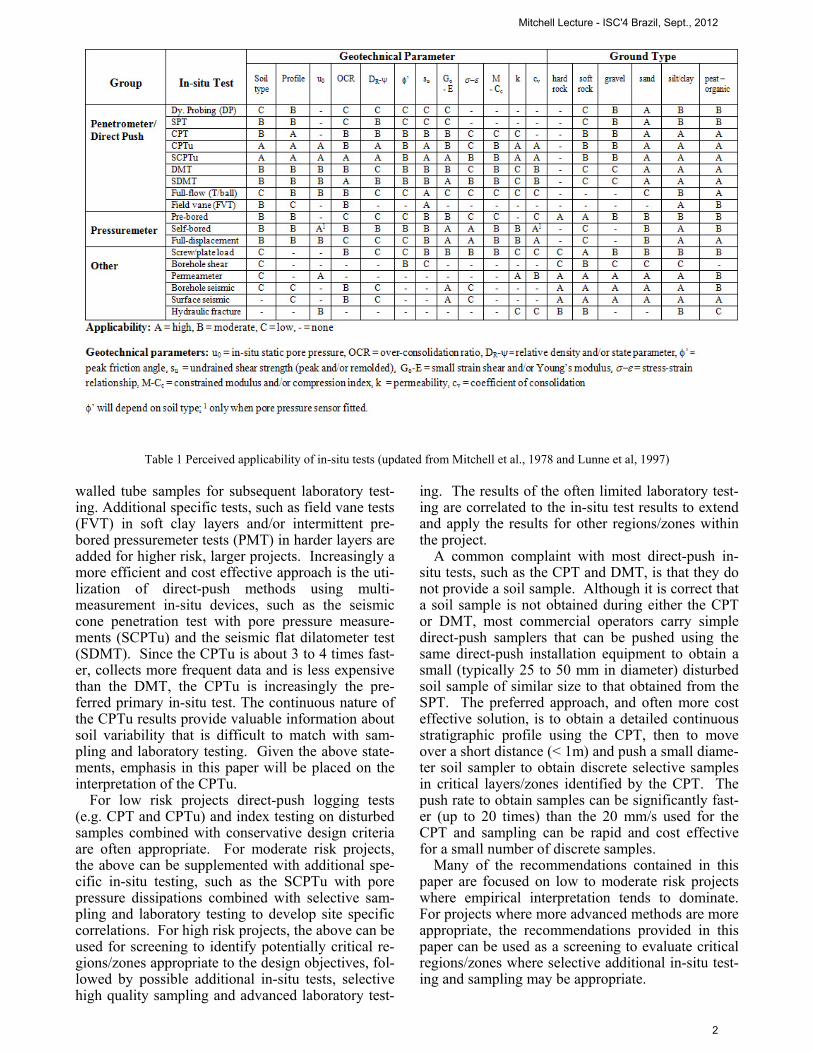
Table 1 Perceived applicability of in-situ tests (updated from Mitchell et al., 1978 and Lunne et al, 1997) walled tube samples for subsequent laboratory test-ing. Additional specific tests, such as field vane tests (FVT) in soft clay layers and/or intermittent pre-bored pressuremeter tests (PMT) in harder layers are added for higher risk, larger projects. Increasingly a more efficient and cost effective approach is the uti-lization of direct-push methods using multi-measurement in-situ devices, such as the seismic cone penetration test with pore pressure measure-ments (SCPTu) and the seismic flat dilatometer test (SDMT). Since the CPTu is about 3 to 4 times fast-er, collects more frequent data and is less expensive than the DMT, the CPTu is increasingly the pre-ferred primary in-situ test. The continuous nature of the CPTu results provide valuable information about soil variability that is difficult to match with sam-pling and laboratory testing. Given the above state-ments, emphasis in this paper will be placed on the interpretation of the CPTu.

For low risk projects direct-push logging tests (e.g. CPT and CPTu) and index testing on disturbed samples combined with conservative design criteria are often appropriate. For moderate risk projects, the above can be supplemented with additional spe-cific in-situ testing, such as the SCPTu with pore pressure dissipations combined with selective sam-pling and laboratory testing to develop site specific correlations. For high risk projects, the above can be used for screening to identify potentially critical re-gions/zones appropriate to the design objectives, fol-lowed by possible additional in-situ tests, selective high quality sampling and advanced laboratory test-

ing. The results of the often limited laboratory test-ing are correlated to the in-situ test results to extend and apply the results for other regions/zones within the project.

A common complaint with most direct-push in-situ tests, such as the CPT and DMT, is that they do not provide a soil sample. Although it is correct that a soil sample is not obtained during either the CPT or DMT, most commercial operators carry simple direct-push samplers that can be pushed using the same direct-push installation equipment to obtain a small (typically 25 to 50 mm in diameter) disturbed soil sample of similar size to that obtained from the SPT. The preferred approach, and often more cost effective solution, is to obtain a detailed continuous stratigraphic profile using the CPT, then to move over a short distance (< 1m) and push a small diame-ter soil sampler to obtain discrete selective samples in critical layers/zones identified by the CPT. The push rate to obtain samples can be significantly fast-er (up to 20 times) than the 20 mm/s used for the CPT and sampling can be rapid and cost effective for a small number of discrete samples.

Many of the recommendations contained in this paper are focused on low to moderate risk projects where empirical interpretation tends to dominate. For projects where more advanced methods are more appropriate, the recommendations provided in this paper can be used as a screening to evaluate critical regions/zones where selective additional in-situ test-ing and sampling may be appropriate.


2

3.0 BASIC SOIL BEHAVIOUR

Mayne et al (2009) and others have identified the need for an interpretative framework within which to assess the results of tests and assign parameters or properties based on the measured response. Increa-singly that framework is critical state soil mechanics (CSSM). Mayne et al (2009) presented a short summary of the main points in CSSM and showed that the basics of CSSM lie in the definition of only a few soil constants: effective friction angle ('cv), compression index (Cc) and selling index (Cs) as well as the initial state (eo, 'vo and either OCR or ).

Since most soils are essentially frictional in their behavior, they can be classified into either coarse-grained (e.g. sands) or fine-grained (e.g. silts and clays). The classification based on grain size is linked to drainage conditions during loading, where coarse-grained soils tend to respond drained during most static loading and fine-grained soils tend to re-spond undrained during most loading. Soils expe-rience volume change during shear that can be either dilative or contractive. Hence, in a general sense, soil behavior can be classified into four broad and general groups: drained-dilative, drained-contractive, undrained-dilative and undrained-contractive. Hence, it is helpful if any in-situ test can identify these broad behaviour types.

Although there are a large number of potential geotechnical parameters and properties, the major ones used most in practice are in general terms: in-situ state, strength, stiffness, compressibility and conductivity. In-situ state represents quantification of the density and compactness of the soil, as well as factors such as cementation. For most soils, in-situ state is captured in terms of either relative density (Dr) or state parameter () for coarse-grained soils and over-consolidation ratio (OCR) for fine-grained soils. These ‘state’ parameters essentially identify if soils will be either dilative or contractive in shear. Sands with a negative state parameter (-, i.e. ‘dense’) and clays with high OCR (OCR > 4) will generally dilate at large strains in shear, whereas sands with a positive state parameter (+, i.e. ‘loose’) and normally to lightly over-consolidated clays (OCR < 2) will generally contract in shear at large strains. The tendency of a soil to either dilate or contract in shear often defines if the key design parameters will be either the drained shear strength (') or the undrained shear strength (su). 4.0 STANDARD PENETRATION TEST (SPT)

Although in-situ testing has evolved and improved over the past 25 years, several old and inadequate tests remain in common use in many parts of the

world. One of the oldest in-situ tests is the standard penetration test (SPT), remaining a staple in many site investigations around the world. Mayne et al (2009) correctly questions the “false sense of reality in the geotechnical engineer’s ability to assess each and every soil parameter from the single N-value”. Geotechnical engineers in the 21st century should progressively abandon this crude, unreliable in-situ test.

Reasons frequently given as to why the SPT con-tinues to be used in some parts of the world are: (a) other better tests (e.g. CPT and DMT) are not locally available, (b) the SPT provides a soil sample for vis-ual identification, (c) the SPT is inexpensive, and, (d) direct-push tests are not possible in the local soils. The lack of local availability in some parts of the developed world is often a circular argument where local site investigation contractors do not of-fer better tests because engineers are not requesting the better tests and engineers are not requesting the better tests because local contractors are not offering these tests. This cycle needs to be broken by geo-technical engineers requiring (demanding) better in-situ testing. Local contractors will then make the capital investment to provide these tests if local geo-technical engineers require them. There are also many alternate, cost effective and efficient direct-push methods to obtain small disturbed samples for visual identification and for index testing, as de-scribed above. The inexpensive nature of the SPT is also incorrect. The SPT is very expensive based on a per data point basis. Typically the cost of the SPT in the USA is about $20 to $25 per N-value (data every 1.5m), compared to about $0.50 per data point for the CPT, because the CPT obtains more channels of data (typically 3) at more frequent intervals (typi-cally every 20 to 50mm). It is frequently less expen-sive to push the CPT followed by a small number of discrete direct-push samples at selective depths, than it is to do conventional drilling and the SPT.

The SPT N-value becomes meaningless when N > 50 due to the limitation in the hammer energy. Gen-erally, if direct-push reaction of at least 150 kN (15 tons) is available, the CPT can be pushed in soils with N > 50. With 200 kN (20 tons) reaction it is generally possible to push the CPT into most soils with N >100.

Although direct-push in-situ tests such as the CPT and DMT are more efficient using customized, large pushing equipment, it is also possible to carry out these direct-push methods using conventional drill-ing equipment. Treen et al (1992) showed how the CPT can be carried out in a cost effective manner in stiff glacial soils using a very simple down-hole CPT pushed with a drill-rig. It is very easy to push a cone (either wireless or with a cable) into the bottom of borehole for a stroke of about 1.5m or more, simi-lar to the way an SPT is performed but at a constant (non-dynamic) rate of penetration and recording


3

several channels of data, e.g. tip resistance (qc) and sleeve friction (fs). The 1.5m distance over which the CPT is pushed is then drilled (and sampled, if necessary) before repeating the procedure. This form of incremental down-hole CPT can provide a near continuous profile of CPT data in a cost effec-tive and more reliable manner, compared to the SPT. Additional measurements, such as pore pressure (penetration pore pressure, u, and rate of dissipation, t50) and shear wave velocity (Vs) can also be record-ed using either a down-hole CPTu or SCPTu. Hence, up to five (5) independent measurements can be made in a cost effective manner using conven-tional, well proven equipment and procedures, com-pared to the single crude N-value. The drill-rig can also be used to obtain either small diameter direct-push samples or larger diameter undisturbed (thin-walled tube) samples in the critical soils indentified by the CPT. The drill-rig can also be used to drill through hard layers (e.g. gravel) where direct-push methods may reach refusal. Hence, perceived low cost and the need for samples should no longer be used as an excuse for the continued use of the unre-liable SPT. Jefferies and Davies (1993) correctly suggested that the most reliable way to obtain SPT N values was to perform a CPT and convert the CPT to an equivalent SPT. Jefferies and Davies (1993) suggested a me-thod to convert the CPT cone resistance, qt, to an equivalent SPT N value at 60% energy, N60, using a soil behaviour type index, Ic,JD. The method was modified slightly by Lunne et al (1997), based on the simpler soil behaviour type index defined by Robertson and Wride (1998), as follows: (qt/pa)/N60 = 8.5 [1 - ( Ic/4.6)] (1)

Where qt is the corrected cone tip resistance and Ic is the soil behaviour type index defined by Robert-son and Wride (1998), that will be defined in detail later.

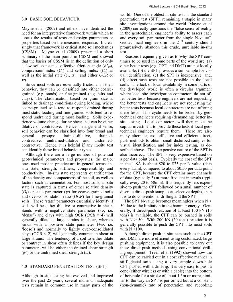
The above method has been shown to work effec-tively in a wide range of soils, although recent expe-rience in North America has shown that equation (1) tends to under predict the N60 values in some clays. Figure 1 compares various relationships of (qt/pa)/N60 as a function of Ic and presents a sug-gested updated relationship that can be defined by the following:

(qt/pa)/N60 = 10(1.1268 – 0.2817Ic) (2)

Equation 2 produces slightly larger N60 values in

fine-grained soils than the previous Jefferies and Davies (1993) method. In fine-grained soils with high sensitivity, equation 2 may over estimate the equivalent N60.

Figure 1. SPT-CPT correlations in terms of (qt/pa)/N60 and

CPT-based SBT index Ic

5.0 CONE PENETRATION TEST (CPT)

The electric cone penetration test (CPT) has been in use for over 40 years. The CPT has major advantag-es over traditional methods of field site investigation such as drilling and sampling since it is fast, repeat-able and economical. In addition, it provides near continuous data and has a strong theoretical back-ground. These advantages have produced a steady increase in the use and application of the CPT in many parts of the world.

Significant developments have occurred in both the theoretical and experimental understanding of the CPT penetration process and the influence of various soil parameters. These developments have illustrated that real soil behaviour is often complex and difficult to accurately capture in a simple soil model. Hence, semi-empirical correlations still tend to dominate in CPT practice although most are well supported by theory.

5.1 Equipment and Procedures

Lunne et al (1997) provided a detailed description on developments in CPT equipment, procedures, checks, corrections and standards, which will not be repeated here. Most CPT systems today include pore pressure measurements (i.e. CPTu) and provide CPT results in digital form. The addition of shear wave velocity (Robertson et al, 1986) is also becom-ing increasingly popular (i.e. SCPTu). If dissipation tests are also performed, the rate of dissipation can be captured by t50 (time to dissipate 50% of the excess pore pressures). Hence, it is now more com-mon to see the combination of cone resistance (qc), sleeve friction (fs), penetration pore pressure (u), rate of dissipation (t50) and, shear wave velocity (Vs), all measured in one profile. The addition of shear wave velocity has provided valuable insight into correla-


4

tions between cone resistance and soil modulus that will be discussed in a later section.

There are several major issues related to equip-ment design and procedure that are worth repeating and updating. It is now common that cone pore pressures are measured behind the cone tip in what is referred to as the u2 position (ASTM D5778, 2007; IRTP, 1999). In this paper, it will be assumed that the cone pore pressures are measured in the u2 position. Due to the inner geometry of the cone the ambient pore water pressure acts on the shoulder be-hind the cone and on the ends of the friction sleeve. This effect is often referred to as the unequal end area effect (Campanella et al, 1982). Many com-mercial cones now have equal-end area friction sleeves that essentially remove the need for any cor-rection to fs and, hence, provide more reliable sleeve friction values. However, the unequal end area ef-fect is always present for the cone resistance qc and there is a need to correct qc to the corrected total cone resistance, qt. This correction is insignificant in sands, since qc is large relative to the water pressure u2 and, hence, qt ~ qc in coarse-grained soils (i.e. sands). It is still common to see CPT results in terms of qc in coarse-grained soils. However, the unequal end area correction can be significant (10 - 30%) in soft fine-grained soil where qc is low rela-tive to the high water pressure around the cone due to the undrained CPT penetration process. It is now common to see CPT results corrected for unequal end area effects and presented in the form of qt fs

and u2, especially in softer soils. The correlations presented in this paper will be in terms of the cor-rected cone resistance, qt, although in sands qc can be used as a replacement.

Although pore pressure measurements are becom-ing more common with the CPT (i.e. CPTu), the ac-curacy and precision of the cone pore pressure mea-surements for on-shore testing are not always reliable and repeatable due to loss of saturation of the pore pressure element. At the start of each CPTu sounding the porous element and sensor are satu-rated with a viscous liquid such as silicon oil or gly-cerin (Campanella et al, 1982) and sometimes grease (slot element). However, for on-shore CPTu the cone is often required to penetrate several meters through unsaturated soil before reaching saturated soil. If the unsaturated soil is either clay or dense silty sand the suction in the unsaturated soil can be sufficient to de-saturate the cone pore pressure sen-sor. The use of viscous liquids, such as silicon oil and grease, has minimized the loss of saturation but has not completely removed the problem. Although it is possible to pre-punch or pre-drill the sounding and fill the hole with water, few commercial CPT operators carry out this procedure if the water table is more than a few meters below ground surface. A further complication is that when a cone is pushed

through saturated dense silty sand or very stiff over consolidated clay the pore pressure measured in the u2 position can become negative, due to the dilative nature of the soil in shear, resulting in small air bub-bles coming out of solution in the cone sensor pore fluid and loss of saturation in the sensor. If the cone is then pushed through a softer fine-grained soil where the penetration pore pressures are high, these air bubbles can go back into solution and the cone becomes saturated again. However, it takes time for these air bubbles to go into solution that can result in a somewhat sluggish pore pressure response for sev-eral meters of penetration. Hence, it is possible for a cone pore pressure sensor to alternate from saturated to unsaturated several times in one sounding. It can be difficult to evaluate when the cone is fully satu-rated, which adds uncertainty to the pore pressure measurements. Although this appears to be a major problem with the measurement of pore pressure dur-ing a CPTu, it is possible to obtain good pore pres-sure measurements in suitable ground conditions where the ground water level is close to the surface and the ground is predominately soft. In very soft, fine-grained soils, the CPTu pore pressures (u2) can be more reliable than qt, due to loss of accuracy in qt in very soft soils. It is interesting to note that when the cone is stopped and a pore pressure dissipation test preformed below the ground water level, any small air bubbles in the cone sensor tend to go back into solution (during the dissipation test) and the re-sulting equilibrium pore pressure can be accurate, even when the cone may not have been fully satu-rated during penetration before the dissipation test. CPTu pore pressure measurements are almost al-ways reliable in off-shore testing due to the high ambient water pressure that ensures full saturation.

Even though pore pressure measurements can be less reliable than cone resistance for on-shore test-ing, it is still recommended that pore pressure mea-surements be made for the following reasons: any correction to qt for unequal end area effects is better than no correction in soft fine-grained soils, dissipa-tion test results provide valuable information regard-ing equilibrium piezometric profile and penetration pore pressures provide a qualitative evaluation of drainage conditions during the CPT as well as assist-ing in evaluating soil behaviour type.

It has been documented (e.g. Lunne et al., 1986) that the CPT sleeve friction is less accurate than the cone tip resistance. The lack of accuracy in fs mea-surement is primarily due to the following factors (Lunne and Anderson, 2007); Pore pressure effects on the ends of the sleeve, Tolerance in dimensions between the cone and

sleeve, Surface roughness of the sleeve, and, Load cell design and calibration.


5

ASTM, D5778 (2007) specifies the use of equal end-area friction sleeve to minimize the pore pres-sure effects. Boggess and Robertson (2010) showed than cones that have unequal end-area friction sleeves can produce significant errors in fs measure-ment in soft fine-grained soils and during offshore testing. All standards have strict limits on dimen-sional tolerances. Some cones are manufactured to have sleeves that are slightly larger than the cone tip, but within standard tolerances, to increase the meas-ured values of fs. The IRTP (1999) has clear specifi-cations on surface roughness. In the early 1980’s subtraction cone designs became popular for im-proved robustness. In a subtraction cone design the sleeve friction is obtained by subtracting the cone tip load from the combined cone plus sleeve friction load. Any zero load instability (shifts) in each load cell results in a loss of accuracy in the calculated sleeve friction. Cone designs with separate tip and friction load cells are now equally as robust as sub-traction cones. Hence, it is recommended to use only cones with independent load cells that have im-proved accuracy in the measurement of fs. ASTM D5778 (2007) and the IRTP (1999) specify zero-load readings before and after each sounding for im-proved accuracy. With good quality control it is possible to obtain repeatable and accurate sleeve friction measurements, as illustrated by Robertson (2009a). However, fs measurements, in general, will be less accurate than tip resistance in most soft fine-grained soils.

The accuracy for most well designed, strain gauged load cells is 0.1% of the full scale output (FSO). Most commercial cones are designed to record a tip stress of around 100 MPa. Hence, they have accuracy for qt of around 0.1 MPa (100 kPa). In most sands, this represents an excellent accuracy of better than 1%. However, in soft, fine-grained soils, this may represent an accuracy of less than 10%. In very soft, fine-grained soils, low capacity cones (i.e. max. tip stress < 50 MPa) have better ac-curacy.

Throughout this paper use will be made of the normalized soil behaviour type (SBT) chart using normalized CPT parameters. Hence, accuracy in both qt and fs are important, particularly in soft fine-grained soil. Accuracy in fs measurements requires that the CPT be carried out according to the standard (e.g. ASTM D5778) with particular attention to cone design (separate load cells and equal-end area fric-tion sleeves), tolerances, and zero-load readings.

5.2 Soil Type

One of the major applications of the CPT has been the determination of soil stratigraphy and the identi-fication of soil type. This has been accomplished using charts that link cone parameters to soil type.

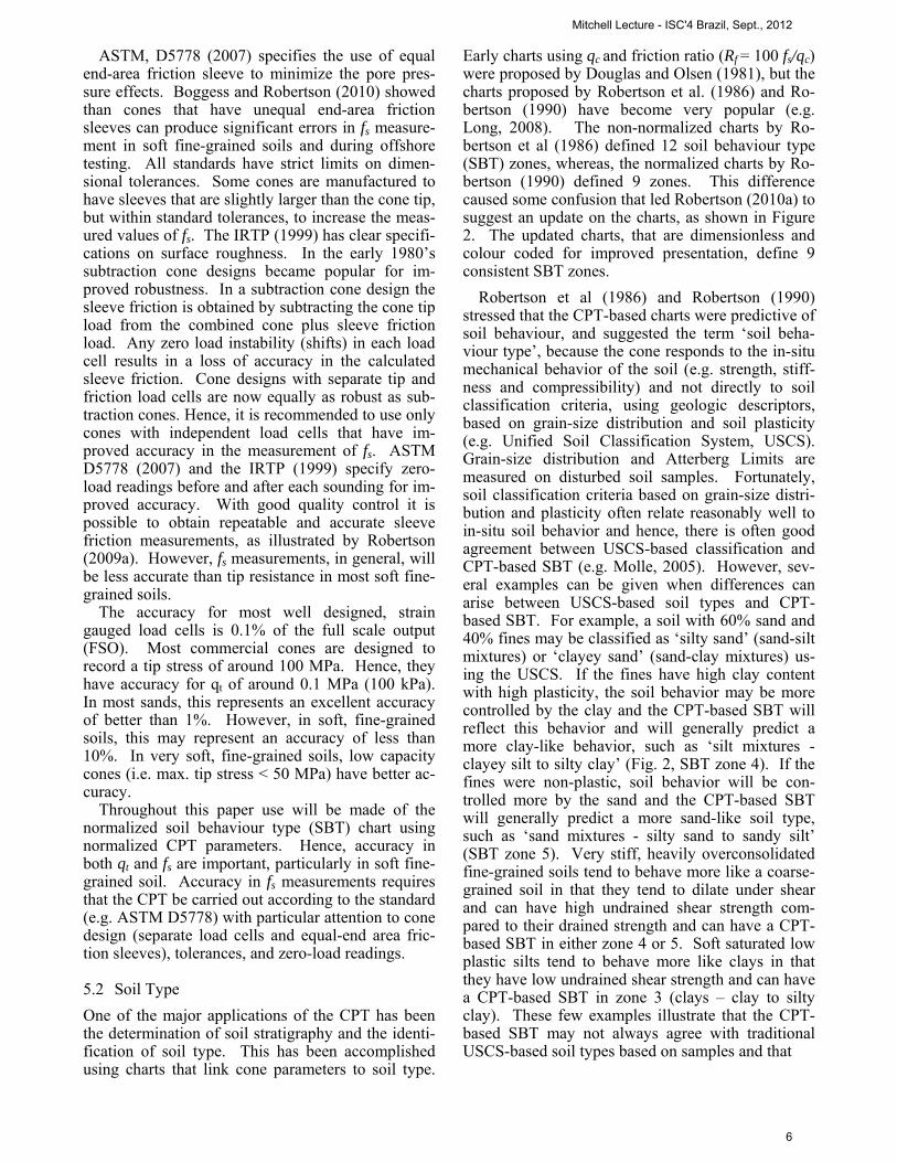
Early charts using qc and friction ratio (Rf = 100 fs/qc) were proposed by Douglas and Olsen (1981), but the charts proposed by Robertson et al. (1986) and Ro-bertson (1990) have become very popular (e.g. Long, 2008). The non-normalized charts by Ro-bertson et al (1986) defined 12 soil behaviour type (SBT) zones, whereas, the normalized charts by Ro-bertson (1990) defined 9 zones. This difference caused some confusion that led Robertson (2010a) to suggest an update on the charts, as shown in Figure 2. The updated charts, that are dimensionless and colour coded for improved presentation, define 9 consistent SBT zones.

Robertson et al (1986) and Robertson (1990) stressed that the CPT-based charts were predictive of soil behaviour, and suggested the term ‘soil beha-viour type’, because the cone responds to the in-situ mechanical behavior of the soil (e.g. strength, stiff-ness and compressibility) and not directly to soil classification criteria, using geologic descriptors, based on grain-size distribution and soil plasticity (e.g. Unified Soil Classification System, USCS). Grain-size distribution and Atterberg Limits are measured on disturbed soil samples. Fortunately, soil classification criteria based on grain-size distri-bution and plasticity often relate reasonably well to in-situ soil behavior and hence, there is often good agreement between USCS-based classification and CPT-based SBT (e.g. Molle, 2005). However, sev-eral examples can be given when differences can arise between USCS-based soil types and CPT-based SBT. For example, a soil with 60% sand and 40% fines may be classified as ‘silty sand’ (sand-silt mixtures) or ‘clayey sand’ (sand-clay mixtures) us-ing the USCS. If the fines have high clay content with high plasticity, the soil behavior may be more controlled by the clay and the CPT-based SBT will reflect this behavior and will generally predict a more clay-like behavior, such as ‘silt mixtures - clayey silt to silty clay’ (Fig. 2, SBT zone 4). If the fines were non-plastic, soil behavior will be con-trolled more by the sand and the CPT-based SBT will generally predict a more sand-like soil type, such as ‘sand mixtures - silty sand to sandy silt’ (SBT zone 5). Very stiff, heavily overconsolidated fine-grained soils tend to behave more like a coarse-grained soil in that they tend to dilate under shear and can have high undrained shear strength com-pared to their drained strength and can have a CPT-based SBT in either zone 4 or 5. Soft saturated low plastic silts tend to behave more like clays in that they have low undrained shear strength and can have a CPT-based SBT in zone 3 (clays – clay to silty clay). These few examples illustrate that the CPT-based SBT may not always agree with traditional USCS-based soil types based on samples and that


6

SBT zone Proposed common SBT description

1 Sensitive fine-grained 2 Clay - organic soil 3 Clays: clay to silty clay 4 Silt mixtures: clayey silt & silty clay 5 Sand mixtures: silty sand to sandy silt 6 Sands: clean sands to silty sands 7 Dense sand to gravelly sand 8 Stiff sand to clayey sand* 9 Stiff fine-grained*

* Overconsolidated or cemented

Figure 2: Updated Soil Behaviour Type (SBT) charts based on either non-normalized or normalized CPT (after Robertson, 2010a)

the biggest difference is likely to occur in the mixed soils region (i.e. sand-mixtures & silt-mixtures). Geotechnical engineers are often more interested in the in-situ soil behavior than a classification based only on grain-size distribution and plasticity carried out on disturbed samples, although knowledge of both is helpful. The geotechnical profession has a long history of using simplified classification sys-tems with geologic descriptors, and it will likely be some time before the profession fully accepts and adopts the more logical framework based on me-chanical response measurements directly from the in-situ tests.

Robertson (1990) proposed using normalized (and dimensionless) cone parameters, Qt1, Fr, Bq, to esti-mate soil behaviour type, where;

Qt1 = (qt – vo)/'vo (3) Fr = [(fs/(qt – vo)] 100% (4) Bq = (u2 – u0)/(qt – vo) = u/(qt – vo) (5)

Where: vo = in-situ total vertical stress 'vo = in-situ effective vertical stress u0 = in-situ equilibrium water pressure u = excess penetration pore pressure = (u2 – u0)

In the original paper by Robertson (1990) the

normalized cone resistance was defined using the term Qt1. The term Qt1 is used here to show that the cone resistance is the corrected cone resistance, qt and the stress exponent for stress normalization is 1.0 (further details are provide in a later section).

In general, the normalized charts provide more re-liable identification of SBT than the non-normalized charts, although when the in-situ vertical effective stress is between 50 kPa to 150 kPa there is often lit-tle difference between normalized and non-normalized SBT. The term SBTn will be used to distinguish between normalized and non-normalized SBT. The above normalization was based on theo-retical work by Wroth (1984). Robertson (1990)


7

suggested two charts based on either Qt1 – Fr or Qt1 - Bq but recommended that the Qt1 – Fr chart was gen-erally more reliable.

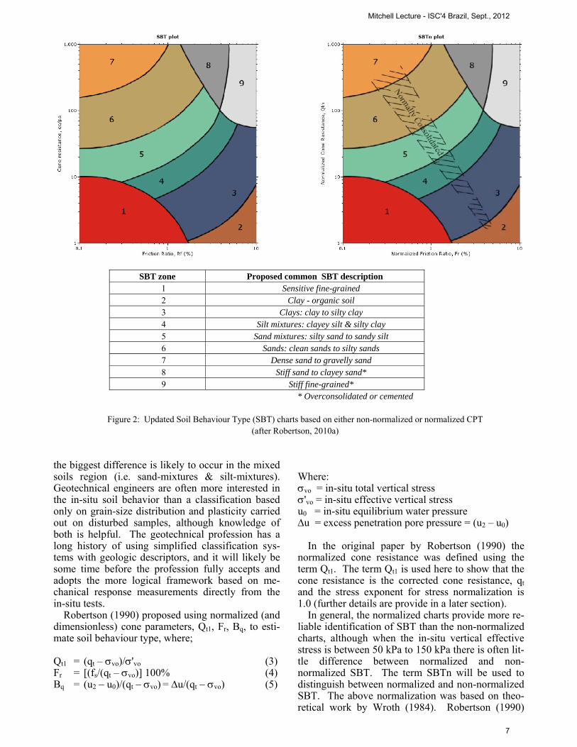
Schneider et al (2008) have shown that u/'vo is a better form for normalized pore pressure parameter than Bq. The chart by Schneider et al (2008) is shown in Figure 3. Superimposed on the Schneider et al chart are contours of Bq to illustrate the link with u/'vo. Also shown on the Schneider et al chart are approximate contours of OCR (dashed lines). Figure 3 shows that the use of u/'vo is not a good approach for estimating OCR. Application of the Schneider et al chart can be problematic for some onshore projects where the CPTu pore pres-sure results may not be reliable, due to loss of satu-ration. However, for offshore projects, where CPTu sensor saturation is more reliable, and onshore projects in soft fine-grained soils with high ground-water, the chart can be very helpful. In near surface very soft fine-grained soils, where the accuracy of the cone resistance (qt) may be limited, the Schneid-er et al chart can become a useful check on the data (e.g. if the cone resistance values are too low, the da-ta can plot below the limit of the chart, Bq > 1.0). Also the Schneider et al chart is focused primarily on fine-grained soils were excess pore pressures are recorded and Qt1 is small.

Figure 3: CPT classification chart from Schneider et al

(2008) based on (u2/’v) with contours of Bq and OCR Since 1990 there have been other CPT soil type

charts developed (e.g. Jefferies and Davies, 1991, Olsen and Mitchell, 1995, Eslami and Fellenius, 1997). The chart by Eslami and Fellenius (1997) is based on non-normalized parameters using effective cone resistance, qe and fs, where qe = (qt – u2). The

effective cone resistance, qe, suffers from lack of ac-curacy in soft fine-grained soils, as will be discussed in a later section. Zhang and Tumay (1999) devel-oped a CPT based soil classification system based on fuzzy logic where the results are presented in the form of percentage probability (e.g. percentage probability of either clay silt or sand). Although this approach is conceptually attractive (i.e. provides some estimate of uncertainty for each SBT zone) the results are often misinterpreted as a grain size distri-bution.

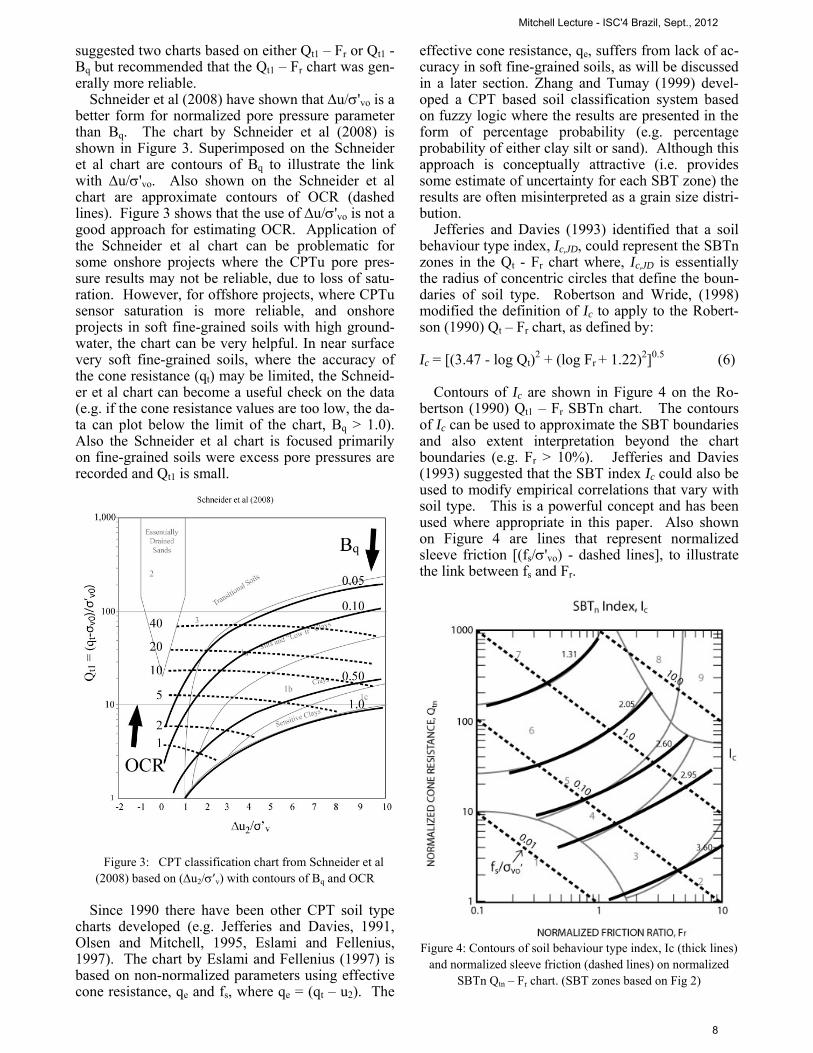
Jefferies and Davies (1993) identified that a soil behaviour type index, Ic,JD, could represent the SBTn zones in the Qt - Fr chart where, Ic,JD is essentially the radius of concentric circles that define the boun-daries of soil type. Robertson and Wride, (1998) modified the definition of Ic to apply to the Robert-son (1990) Qt – Fr chart, as defined by:

Ic = [(3.47 - log Qt)

2 + (log Fr + 1.22)2]0.5 (6)

Contours of Ic are shown in Figure 4 on the Ro-bertson (1990) Qt1 – Fr SBTn chart. The contours of Ic can be used to approximate the SBT boundaries and also extent interpretation beyond the chart boundaries (e.g. Fr > 10%). Jefferies and Davies (1993) suggested that the SBT index Ic could also be used to modify empirical correlations that vary with soil type. This is a powerful concept and has been used where appropriate in this paper. Also shown on Figure 4 are lines that represent normalized sleeve friction [(fs/'vo) - dashed lines], to illustrate the link between fs and Fr.

Figure 4: Contours of soil behaviour type index, Ic (thick lines) and normalized sleeve friction (dashed lines) on normalized

SBTn Qtn – Fr chart. (SBT zones based on Fig 2)


8

The form of equation 6 and the shape of the con-tours of Ic in Figure 4 illustrate that Ic is not overly sensitive to the potential lack of accuracy of the sleeve friction, fs, but is more controlled by the more accurate tip stress, qt. Research (e.g. Long, 2008) has sometimes questioned the reliability of the SBT based on sleeve friction values (e.g. Qt – Fr charts). However, numerous studies (e.g. Molle, 2005) have shown that the normalized charts based on Qt – Fr provide the best overall success rate for SBT com-pared to samples. It can be shown, using equation 6, that if fs vary by as much as +/- 50%, the resulting variation in Ic is generally less than +/- 10%. For soft soils that fall within the lower part of the Qt – Fr chart (e.g. Qt < 20), Ic is relatively insensitive to fs.

5.4 Stress normalization

Conceptually, any normalization to account for in-creasing stress should also account for the important influence of horizontal effective stresses, since pene-tration resistance is strongly influenced by the hori-zontal effective stresses (Jamiolkowski and Robert-son, 1988). However, this continues to have little practical benefit for most projects without a prior knowledge of in-situ horizontal stresses. Even normalization using only vertical effective stress re-quires some input of soil unit weight and groundwa-ter conditions. Fortunately, commercial software packages have increasingly made this easier and unit weights estimated from the non-normalized SBT charts appear to be reasonably effective for many applications (e.g. Robertson, 2010b).

Jefferies and Davies (1991) proposed a normaliza-tion that incorporates the pore pressure directly into a modified normalized cone resistance using: Qt1 (1-Bq). Recently, Jefferies and Been (2006) updated their modified chart using the parameter Qt1 (1-Bq) +1, to overcome the problem in soft sensitive soils where Bq > 1. Jefferies and Been (2006) noted that:

Qt1(1-Bq) +1 = (qt – u2)/ 'vo (7)

Hence, the parameter Qt1 (1-Bq) +1 is simply the effective cone resistance, (qt – u2), normalized by the vertical effective stress. Although incorporating pore pressure into the normalized cone resistance is conceptually attractive it has practical problems. In stiff fine-grained soils, the excess pore pressure also can be sensitive to the exact location of the porous sensor. Accuracy is a major concern in soft fine-grained soils where qt is small compared to u2. Hence, the difference (qt – u2) is very small and lacks accuracy and reliability in most soft soils. For most commercial cones the precision of Qt1 in soft fine-grained soils is about +/- 20%, whereas, the precision for Qt1 (1-Bq) +1 in the same soil is about +/- 40%, due to the combined lack of precision in (qt

– u2). Loss of saturation further complicates this parameter.

Robertson and Wride (1998), as updated by Zhang et al (2002), suggested a more generalized norma-lized cone parameter to evaluate soil liquefaction, using normalization with a variable stress exponent, n; where:

Qtn = [(qt – vo)/pa] (pa/'vo)

n (8)

Where: (qt – vo)/pa = dimensionless net cone resistance, (pa/'vo)

n = stress normalization factor n = stress exponent that varies with SBT pa = atmospheric pressure in same units as qt and v

Note that when n = 1, Qtn = Qt1. Zhang et al

(2002) suggested that the stress exponent, n, could be estimated using the SBT Index, Ic, and that Ic should be defined using Qtn.

In recent years there have been several publica-tions regarding the appropriate stress normalization (Olsen and Malone, 1988; Zhang et al., 2002; Idriss and Boulanger, 2004; Moss et al, 2006; Cetin and Isik, 2007). The contours of stress exponent sug-gested by Cetin and Isik (2007) are very similar to those by Zhang et al, (2002). The contours by Moss et al (2006) are similar to those first suggested by Olsen and Malone (1988). The normalization sug-gested by Idriss and Boulanger (2004) incorrectly used uncorrected chamber test results and the me-thod only applies to sands where the stress exponent varies with relative density with a value of around 0.8 in loose sands and 0.3 in dense sands. Robertson (2009a) provided a detailed discussion on stress normalization and suggested the following updated approach to allow for a variation of the stress expo-nent with both SBT Ic (soil type) and stress level us-ing:

n = 0.381 (Ic) + 0.05 ('vo/pa) – 0.15 (9)

where n ≤ 1.0

Robertson (2009a) suggested that the above stress

exponent would capture the correct in-situ state for soils at high stress level and that this would also avoid any additional stress level correction for lique-faction analyses in silica-based soils.

The approach used by Jefferies and Been (2006) (equation 7) is the only method that uses a stress ex-ponent n = 1.0 for all soils. This has significant im-plications at shallow depth (z < 3m) and great depth (z > 30m). Recent research (e.g. Boulanger, 2003) shows that the stress exponent is a function of soil state. Recent major projects that have applied the de-tailed approach suggested by Jefferies and Been (2006) also support the observation that the stress exponent is a function of soil state.


9

5.5 In-situ state and shear strength

For fine-grained soils, in-situ state is usually defined in terms of overconsolidation ratio (OCR), where OCR is defined as the ratio of the maximum past ef-fective consolidation stress ('p) and the present ef-fective overburden stress ('vo):

OCR = 'p/'vo (10)

For mechanically overconsolidated soils where the

only change has been the removal of overburden stress, this definition is appropriate. However, for cemented and/or aged soils the OCR may represent the ratio of the yield stress and the present effective overburden stress. The yield stress will also depend on the direction and type of loading.

The most common method to estimate OCR and yield stress in fine-grained soils was suggested by Kulhawy and Mayne (1990):

OCR = k (qt – v)/'vo = k Qt1 (11)

or 'p = k (qt – vo) (12)

Where k is the preconsolidation cone factor and 'p

is the preconsolidation or yield stress. Kulhawy and Mayne (1990) showed that an aver-

age value of k = 0.33 can be assumed, with an ex-pected range of 0.2 to 0.5. Although it is common to use the average value of 0.33, Been et al (2010) sug-gested that the selection of an appropriate value for ‘k’ should be consistent with other parameters, as discussed below.

In clays, the peak undrained shear strength, su and OCR are generally related. Ladd and Foott, (1974) empirically developed the following relationship based on SHANSEP concepts:

su/'vo = (su/'vo)OCR=1 (OCR)m = S (OCR)m (13)

The term S varies as a function of the failure

mode (testing method, strain rate). Ladd and De Groot (2003) recommended S = 0.25 with a standard deviation of 0.05 (for simple shear loading) and m = 0.8 for most soils. Equation 13 is also supported by Critical State Soil Mechanics (CSSM) where S = ½ sin' in direct simple shear (DSS) loading, and, m = 1 – Cs/Cc, where Cs is the swelling index and Cc is the compression index.

The peak undrained shear strength is estimated us-ing:

su =

(qt – vo)/Nkt (14)

Where Nkt is the cone factor that depends on soil stiffness, OCR and soil sensitivity, but experience has shown that soil sensitivity has the largest influ-

ence. Nkt can be linked to soil sensitivity via the normalized friction ratio, Fr, and can be represented approximately by:

Nkt = 10.5+7 log(Fr) (15)

Been et al (2010) showed that for consistency the

following should hold:

(Qt1)1-m = S Nkt (k)m (16)

Where: OCR = k (Qt1) (when Qt1 < 20) su/'vo = Qt1 / Nkt = S (OCR)m and, S = (su/'vo)OCR=1.

For most sedimentary clays, silts and organics

fine-grained soil, S = 0.25 for average direction of loading and ’ ~ 26, and, m = 0.8. Hence, the con-stant to estimate OCR can be automatically esti-mated based on CPT results using:

k = [(Qt1)

0.2 / (0.25 (10.5+7 log Fr))]1.25 (17)

Then,

OCR = (2.625+ 1.75 log Fr)

-1.25 (Qt1)1.25 (18)

This compares very closely to the form suggested

by Karlsrud et al (2005) based on high quality block samples from Norway (when soil sensitivity, St < 15) and that resulting from CSSM:

OCR = 0.25 (Qt1)

1.2 (19)

Equation 18 represents a method to automatically es-timate the in-situ state (OCR) in fine-grained soils based on measured CPT results, in a consistent man-ner.

The state parameter () is defined as the differ-ence between the current void ratio, e and the void ratio at critical state ecs, at the same mean effective stress for coarse-grained (sandy) soils. Based on critical state concepts, Jefferies and Been (2006) provide a detailed description of the evaluation of soil state using the CPT. They describe in detail that the problem of evaluating state from CPT response is complex and depends on several soil parameters. The main parameters are essentially the shear stiff-ness, shear strength, compressibility and plastic har-dening. Jefferies and Been (2006) provide a descrip-tion of how state can be evaluated using a combination of laboratory and in-situ tests. They stress the importance of determining the in-situ hori-zontal effective stress and shear modulus using in-situ tests and determining the shear strength, com-pressibility and plastic hardening parameters from laboratory testing on reconstituted samples. They also show how the problem can be assisted using


10

numerical modeling. For high risk projects a de-tailed interpretation of CPT results using laboratory results and numerical modeling can be appropriate (e.g. Shuttle and Cunning, 2007), although soil va-riability can complicate the interpretation procedure. Some unresolved concerns with the Jefferies and Been (2006) approach relate to the stress normaliza-tion using n = 1.0 for all soils, as discussed above, and the influence of soil fabric in sands with high fines content.

For low risk projects and in the initial screening for high risk projects there is a need for a simple es-timate of soil state. Plewes et al (1992) provided a means to estimate soil state using the normalized soil behavior type (SBT) chart suggested by Jefferies and Davies (1991). Jefferies and Been (2006) up-dated this approach using the normalized SBT chart based on the parameter Qt1(1-Bq) +1. Robertson (2009) expressed concerns about the accuracy and precision of the Jefferies and Been (2006) norma-lized parameter in soft soils. In sands, where Bq = 0, the normalization suggested by Jefferies and Been (2006) is the same as Robertson (1990). The con-tours of state parameter () suggested by Plewes et al (1992) and Jefferies and Been (2006) were based primarily on calibration chamber results for sands.

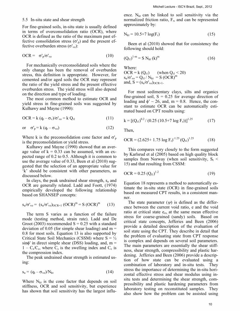
Based on the data presented by Jefferies and Been (2006) and Shuttle and Cunning (2007) as well the measurements from the CANLEX project (Wride et al, 2000) for predominantly coarse-grained unce-mented young soils, combined with the link between OCR and state parameter in fine-grained soil, Ro-bertson (2009a) developed contours of state parame-ter () on the updated SBTn Qtn – F chart for unce-mented Holocene age soils. The contours, that are shown on Figure 5, are approximate since stress state and plastic hardening will also influence the es-timate of in-situ soil state in the coarse-grained re-gion of the chart (i.e. when Ic < 2.60) and soil sensi-tivity for fine-grained soils. An area of uncertainty in the approach used by Jefferies and Been (2006) is the use of Qt1 rather than Qtn. Figure 5 uses Qtn since it is believed that this form of normalized parameter has wider application, although this issue may not be fully resolved for some time. The contours of shown in Figure 5 were developed primarily on la-boratory test results and validated with well docu-mented sites where undisturbed frozen samples were obtained (Wride et al., 2000). Jefferies and Been (2006) suggested that soils with a state parameter less than -0.05 (i.e. < -0.05) are dilative at large strains.

Over the past 40 years significant research has been carried out utilizing penetration test results (in-itially SPT and then CPT) to evaluate to resistance to cyclic loading (e.g. Seed et al., 1983, and Robertson & Wride, 1998). The most commonly accepted ap-proach (often referred to as the Berkeley approach) uses an equivalent clean sand penetration resistance

to correlate to the cyclic resistance of sandy soils. The approach is empirical based primarily on obser-vations from past earthquakes and supported by la-boratory observations.

Figure 5: Contours of estimated state parameter, (thick lines), on normalized SBTn Qtn – Fr chart for uncemented Ho-

locene-age sandy soils (after Robertson, 2009a)

Robertson and Wride (1998), based on a large da-tabase of liquefaction case histories, suggested a CPT-based correction factor to correct normalized cone resistance in silty sands to an equivalent clean sand value (Qtn,cs) using the following:

Qtn,cs = Kc Qtn (20)

Where Kc is a correction factor that is a function of grain characteristics (combined influence of fines content, mineralogy and plasticity) of the soil that can be estimated using Ic as follows:

if Ic 1.64 (21) Kc = 1.0

if Ic > 1.64 (22) Kc = 5.581Ic

3-0.403Ic4–21.63Ic

2+33.75Ic–17.88

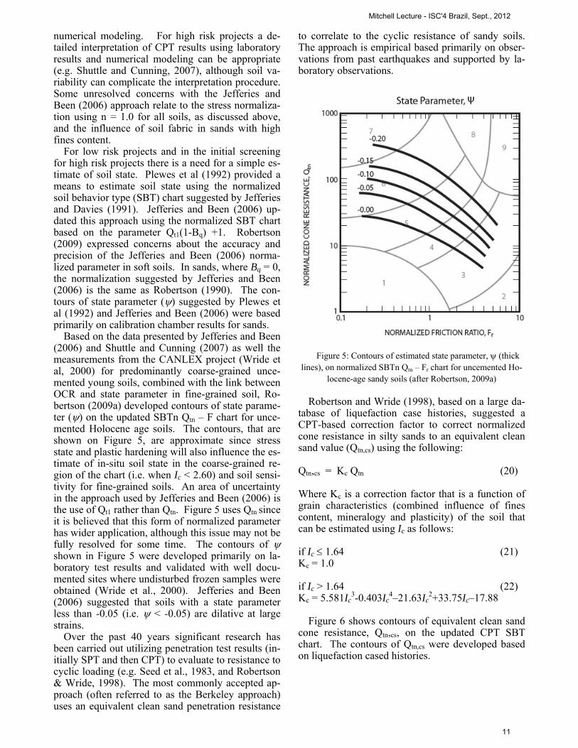
Figure 6 shows contours of equivalent clean sand cone resistance, Qtn,cs, on the updated CPT SBT chart. The contours of Qtn,cs were developed based on liquefaction cased histories.


11

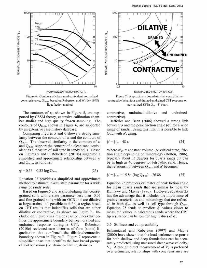
Figure 6: Contours of clean sand equivalent normalized cone resistance, Qtn,cs, based on Robertson and Wride (1998)

liquefaction method The contours of , shown in Figure 5, are sup-

ported by CSSM theory, extensive calibration cham-ber studies and high quality frozen sampling, The contours of Qtn,cs, shown in Figure 6, are supported by an extensive case history database.

Comparing Figures 5 and 6 shows a strong simi-larity between the contours of and the contours of Qtn,cs. The observed similarity in the contours of and Qtn,cs, support the concept of a clean sand equiv-alent as a measure of soil state in sandy soils. Based on Figures 5 and 6, Robertson (2010b) suggested a simplified and approximate relationship between and Qtn,cs, as follows:

= 0.56 – 0.33 log Qtn,cs (23)

Equation 23 provides a simplified and approximate method to estimate in-situ state parameter for a wide range of sandy soils.

Based on Figure 5 and acknowledging that coarse-grained soils with a state parameter less than -0.05 and fine-grained soils with an OCR > 4 are dilative at large strains, it is possible to define a region based on CPT results that indentifies soils that are either dilative or contractive, as shown on Figure 7. In-cluded on Figure 7 is a region (dashed lines) that de-fines the approximate boundary between drained and undrained response during a CPT. Robertson (2010c) reviewed case histories of flow (static) li-quefaction that confirmed the dilative/contractive boundary shown in Figure 7. Figure 7 represents a simplified chart that identifies the four broad groups of soil behaviour (i.e. drained-dilative, drained-

Figure 7: Approximate boundaries between dilative-contractive behaviour and drained-undrained CPT response on

normalized SBTn Qtn – Fr chart

contractive, undrained-dilative and undrained-contractive).

Jefferies and Been (2006) showed a strong link between and the peak friction angle (') for a wide range of sands. Using this link, it is possible to link Qtn,cs with ', using:

' = 'cv - 48

Where 'cv = constant volume (or critical state) fric-tion angle depending on mineralogy (Bolton, 1986), typically about 33 degrees for quartz sands but can be as high as 40 degrees for felspathic sand. Hence, the relationship between Qtn,cs and ' becomes:

' = 'cv + 15.84 [log Qtn,cs] – 26.88

Equation 25 produces estimates of peak fiction angle for clean quartz sands that are similar to those by Kulhawy and Mayne (1990). However, equation 25 has the advantage that it includes the importance of grain characteristics and mineralogy that are reflect-ed in both 'cvas well as soil type through Qtn,cs. Equation 25 tends to predicts ' values closer to measured values in calcareous sands where the CPT tip resistance can be low for high values of '.

5.6 Stiffness and compressibility

Eslaamizaad and Robertson (1997) and Mayne (2000) have shown that the load settlement response for both shallow and deep foundations can be accu-rately predicted using measured shear wave velocity, Vs. Although direct measurement of Vs is preferred over estimates, relationships with cone resistance are


12

useful for smaller, low risk projects where Vs mea-surements are not always taken. Schneider et al (2004) showed that Vs in sands is controlled by the number and area of grain-to-grain contacts, which in turn depend on relative density, effective stress state, rearrangement of particles with age and cementation. Penetration resistance in sands is also controlled by relative density, effective stress state and to a lesser degree by age and cementation. Thus, although strong relationships between Vs and penetration re-sistance exist, some variability should be expected due to age and cementation. There are many exist-ing relationships between cone resistance and Vs (or small strain shear modulus, G0), but most were de-veloped for either sands or clays and generally rela-tively young deposits. The accumulated 20 years of experience with SCPT results enables updated rela-tionships between cone resistance and Vs to be de-veloped for a wide range of soils, using the CPT SBTn chart (Qtn – F) as a base. Since Vs is a direct measure of the small strain shear modulus, G0, there can also be improved linkages between CPT results and soil modulus.

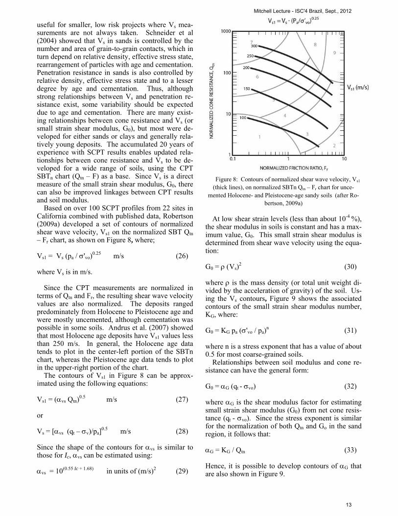
Based on over 100 SCPT profiles from 22 sites in California combined with published data, Robertson (2009a) developed a set of contours of normalized shear wave velocity, Vs1 on the normalized SBT Qtn – Fr chart, as shown on Figure 8, where;

Vs1 = Vs (pa /'vo)

0.25 m/s (26)

where Vs is in m/s. Since the CPT measurements are normalized in

terms of Qtn and Fr, the resulting shear wave velocity values are also normalized. The deposits ranged predominately from Holocene to Pleistocene age and were mostly uncemented, although cementation was possible in some soils. Andrus et al. (2007) showed that most Holocene age deposits have Vs1 values less than 250 m/s. In general, the Holocene age data tends to plot in the center-left portion of the SBTn chart, whereas the Pleistocene age data tends to plot in the upper-right portion of the chart.

The contours of Vs1 in Figure 8 can be approx-imated using the following equations:

Vs1 = (vs Qtn)

0.5 m/s (27)

or

Vs = [vs (qt – v)/pa]0.5

m/s (28)

Since the shape of the contours for vs is similar to those for Ic, vs can be estimated using:

vs = 10(0.55 Ic + 1.68) in units of (m/s)2 (29)

Figure 8: Contours of normalized shear wave velocity, Vs1 (thick lines), on normalized SBTn Qtn – Fr chart for unce-

mented Holocene- and Pleistocene-age sandy soils (after Ro-bertson, 2009a)

At low shear strain levels (less than about 10-4 %),

the shear modulus in soils is constant and has a max-imum value, G0. This small strain shear modulus is determined from shear wave velocity using the equa-tion:

G0 = Vs)

2 (30)

where is the mass density (or total unit weight di-vided by the acceleration of gravity) of the soil. Us-ing the Vs contours, Figure 9 shows the associated contours of the small strain shear modulus number, KG, where:

G0 = KG pa ('vo / pa)

n (31)

where n is a stress exponent that has a value of about 0.5 for most coarse-grained soils.

Relationships between soil modulus and cone re-sistance can have the general form:

G0 = G(qt - vo) (32)

where G is the shear modulus factor for estimating small strain shear modulus (G0) from net cone resis-tance (qt - vo). Since the stress exponent is similar for the normalization of both Qtn and Go in the sand region, it follows that:

G = KG / Qtn (33)

Hence, it is possible to develop contours of G that are also shown in Figure 9.


13

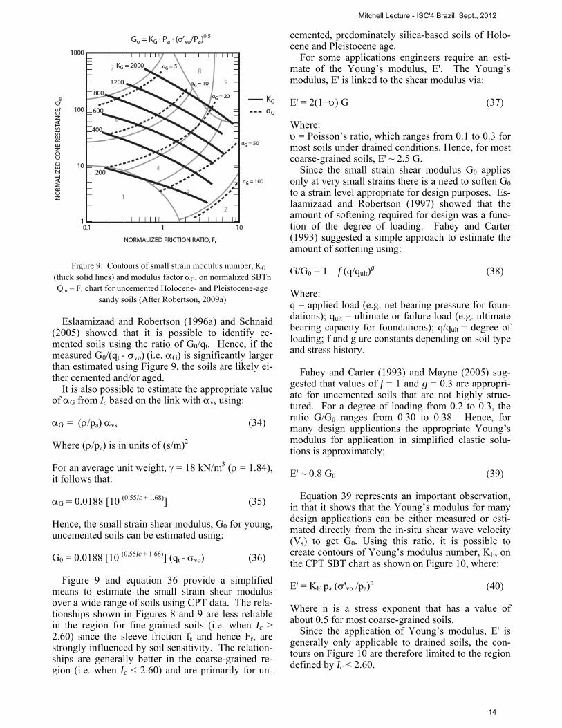
Figure 9: Contours of small strain modulus number, KG

(thick solid lines) and modulus factor G, on normalized SBTn Qtn – Fr chart for uncemented Holocene- and Pleistocene-age

sandy soils (After Robertson, 2009a) Eslaamizaad and Robertson (1996a) and Schnaid

(2005) showed that it is possible to identify ce-mented soils using the ratio of G0/qt. Hence, if the measured G0/(qt - vo) (i.e. G) is significantly larger than estimated using Figure 9, the soils are likely ei-ther cemented and/or aged.

It is also possible to estimate the appropriate value of G from Ic based on the link withvs using:

G = (pavs (34)

Where (pais in units of (s/m)2

For an average unit weight, = 18 kN/m3 ( = 1.84), it follows that:

G = 0.0188 [10 (0.55Ic + 1.68)] (35)

Hence, the small strain shear modulus, G0 for young, uncemented soils can be estimated using:

G0 = 0.0188 [10 (0.55Ic + 1.68)] (qt - vo) (36)

Figure 9 and equation 36 provide a simplified

means to estimate the small strain shear modulus over a wide range of soils using CPT data. The rela-tionships shown in Figures 8 and 9 are less reliable in the region for fine-grained soils (i.e. when Ic > 2.60) since the sleeve friction fs and hence Fr, are strongly influenced by soil sensitivity. The relation-ships are generally better in the coarse-grained re-gion (i.e. when Ic < 2.60) and are primarily for un-

cemented, predominately silica-based soils of Holo-cene and Pleistocene age.

For some applications engineers require an esti-mate of the Young’s modulus, E'. The Young’s modulus, E' is linked to the shear modulus via:

E' = 2(1+) G (37)

Where: = Poisson’s ratio, which ranges from 0.1 to 0.3 for most soils under drained conditions. Hence, for most coarse-grained soils, E' ~ 2.5 G.

Since the small strain shear modulus G0 applies only at very small strains there is a need to soften G0 to a strain level appropriate for design purposes. Es-laamizaad and Robertson (1997) showed that the amount of softening required for design was a func-tion of the degree of loading. Fahey and Carter (1993) suggested a simple approach to estimate the amount of softening using:

G/G0 = 1 – f (q/qult)

g (38)

Where: q = applied load (e.g. net bearing pressure for foun-dations); qult = ultimate or failure load (e.g. ultimate bearing capacity for foundations); q/qult = degree of loading; f and g are constants depending on soil type and stress history.

Fahey and Carter (1993) and Mayne (2005) sug-gested that values of f = 1 and g = 0.3 are appropri-ate for uncemented soils that are not highly struc-tured. For a degree of loading from 0.2 to 0.3, the ratio G/G0 ranges from 0.30 to 0.38. Hence, for many design applications the appropriate Young’s modulus for application in simplified elastic solu-tions is approximately;

E' ~ 0.8 G0 (39)

Equation 39 represents an important observation,

in that it shows that the Young’s modulus for many design applications can be either measured or esti-mated directly from the in-situ shear wave velocity (Vs) to get G0. Using this ratio, it is possible to create contours of Young’s modulus number, KE, on the CPT SBT chart as shown on Figure 10, where:

E' = KE pa ('vo /pa)

n (40)

Where n is a stress exponent that has a value of about 0.5 for most coarse-grained soils.

Since the application of Young’s modulus, E' is generally only applicable to drained soils, the con-tours on Figure 10 are therefore limited to the region defined by Ic < 2.60.


14

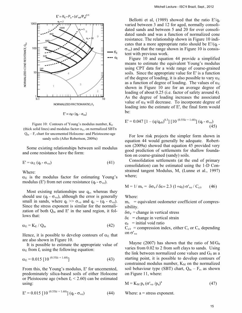
Figure 10: Contours of Young’s modulus number, KE

(thick solid lines) and modulus factor E, on normalized SBTn Qtn – Fr chart for uncemented Holocene- and Pleistocene-age

sandy soils (After Robertson, 2009a) Some existing relationships between soil modulus

and cone resistance have the form:

E' = E(qt - vo) (41)

Where: E is the modulus factor for estimating Young’s modulus (E') from net cone resistance (qt - vo).

Most existing relationships use qc, whereas they should use (qt - vo), although the error is generally small in sands, where qt >> vo and qc ~ (qt - vo). Since the stress exponent is similar for the normali-zation of both Qtn and E' in the sand region, it fol-lows that:

E = KE / Qtn (42)

Hence, it is possible to develop contours of E that are also shown in Figure 10.

It is possible to estimate the appropriate value of E from Ic using the following equation:

E = 0.015 [10 (0.55Ic + 1.68)] (43)

From this, the Young’s modulus, E' for uncemented, predominately silica-based soils of either Holocene or Pleistocene age (when Ic < 2.60) can be estimated using:

E' = 0.015 [10 (0.55Ic + 1.68)] (qt - vo) (44)

Bellotti et al, (1989) showed that the ratio E'/qc

varied between 3 and 12 for aged, normally consoli-dated sands and between 5 and 20 for over consoli-dated sands and was a function of normalized cone resistance. The relationship shown in Figure 10 indi-cates that a more appropriate ratio should be E'/(qt - vo) and that the range shown in Figure 10 is consis-tent with previous work.

Figure 10 and equation 44 provide a simplified means to estimate the equivalent Young’s modulus using CPT data for a wide range of coarse-grained soils. Since the appropriate value for E' is a function of the degree of loading, it is also possible to vary E as a function of degree of loading. The values of E shown in Figure 10 are for an average degree of loading of about 0.25 (i.e. factor of safety around 4). As the degree of loading increases the associated value of E will decrease. To incorporate degree of loading into the estimate of E', the final form would be:

E' = 0.047 [1 – (q/qult)

0.3] [10 (0.55Ic + 1.68)] (qt - vo) (45)

For low risk projects the simpler form shown in

equation 44 would generally be adequate. Robert-son (2009a) showed that equation 45 provided very good prediction of settlements for shallow founda-tion on coarse-grained (sandy) soils.

Consolidation settlements (at the end of primary consolidation) can be estimated using the 1-D Con-strained tangent Modulus, M, (Lunne et al., 1997) where; M = 1/ mv = v / e'voCc/r Where: mv = equivalent oedometer coefficient of compres-sibility. v = change in vertical stress = change in vertical straine0 = initial void ratio Cc/r = compression index, either Cc or Cr, depending on 'vo

Mayne (2007) has shown that the ratio of M/G0 varies from 0.02 to 2 from soft clays to sands. Using the link between normalized cone values and G0 as a starting point, it is possible to develop contours of constrained modulus number, KM on the normalized soil behaviour type (SBT) chart, Qtn – Fr, as shown on Figure 11, where:

M = KM pa ('vo /pa)

a (47)

Where: a = stress exponent.


15

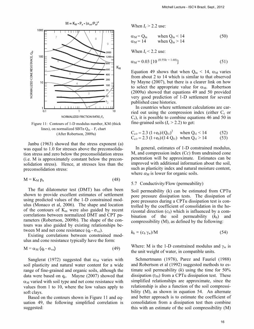
Figure 11: Contours of 1-D modulus number, KM (thick lines), on normalized SBTn Qtn – Fr chart

(After Robertson, 2009a) Janbu (1963) showed that the stress exponent (a)

was equal to 1.0 for stresses above the preconsolida-tion stress and zero below the preconsolidation stress (i.e. M is approximately constant below the precon-solidation stress). Hence, at stresses less than the preconsolidation stress:

M = KM pa (48)

The flat dilatometer test (DMT) has often been

shown to provide excellent estimates of settlement using predicted values of the 1-D constrained mod-ulus (Monaco et al, 2006). The shape and location of the contours of Km were also guided by recent correlations between normalized DMT and CPT pa-rameters (Robertson, 2009b). The shape of the con-tours was also guided by existing relationships be-tween M and net cone resistance (qt - vo).

Existing correlations between constrained mod-ulus and cone resistance typically have the form:

M = M (qt - vo) (49)

Sanglerat (1972) suggested that M varies with soil plasticity and natural water content for a wide range of fine-grained and organic soils, although the data were based on qc. Mayne (2007) showed that M varied with soil type and net cone resistance with values from 1 to 10, where the low values apply to soft clays.

Based on the contours shown in Figure 11 and eq-uation 49, the following simplified correlation is suggested:

When Ic > 2.2 use:

M = Qtn when Qtn < 14 (50) M = 14 when Qtn > 14

When Ic < 2.2 use:

M = 0.03 [10 (0.55Ic + 1.68)] (51)

Equation 49 shows that when Qtn < 14, M varies from about 2 to 14 which is similar to that observed by Mayne (2007), but there is a clearer link on how to select the appropriate value for M. Robertson (2009a) showed that equations 49 and 50 provided very good prediction of 1-D settlement for several published case histories.

In countries where settlement calculations are car-ried out using the compression index (either Cc or Cr), it is possible to combine equations 46 and 50 in fine-grained soils (Ic > 2.2) to get:

Cc/r eQt1)

2 when Qt1 < 14 (52) Cc/r eQt1) when Qt1 > 14 (53)

In general, estimates of 1-D constrained modulus,

M, and compression index (Cc) from undrained cone penetration will be approximate. Estimates can be improved with additional information about the soil, such as plasticity index and natural moisture content, where M is lower for organic soils.

5.7 Conductivity/Flow (permeability)

Soil permeability (k) can be estimated from CPTu pore pressure dissipation tests. The dissipation of pore pressures during a CPTu dissipation test is con-trolled by the coefficient of consolidation in the ho-rizontal direction (ch) which is influenced by a com-bination of the soil permeability (kh) and compressibility (M), as defined by the following:

kh = (ch w)/M (54)

Where: M is the 1-D constrained modulus and w is the unit weight of water, in compatible units.

Schmertmann (1978), Parez and Fauriel (1988) and Robertson et al (1992) suggested methods to es-timate soil permeability (k) using the time for 50% dissipation (t50) from a CPTu dissipation test. These simplified relationships are approximate, since the relationship is also a function of the soil compressi-bility (M), as shown in equation 54. An alternate and better approach is to estimate the coefficient of consolidation from a dissipation test then combine this with an estimate of the soil compressibility (M)


16

to obtain an improved estimate of the soil permeabil-ity (k).

The simplified relationship presented by Robert-son et al (1992), based on the work of Teh and Houlsby (1991), for the coefficient of consolidation in the horizontal direction (ch) as a function of the time for 50% dissipation (t50, in minutes) for a 10 cm2 cone can be approximated using:

ch = (1.67x10-6) 10(1 – log t50

) m2/s (55)

For a 15cm2 cone, the values of ch are increased by a factor of 1.5.

Combining the estimated 1-D constrained mod-ulus, given in equations 49 and 50, in compatible units (i.e. net cone resistance, (qt - vo) in kPa and w = 9.81 kN/m3) it is possible to develop contours of k versus t50 for various values of Qtn and '

vo, as shown on Figure 12.

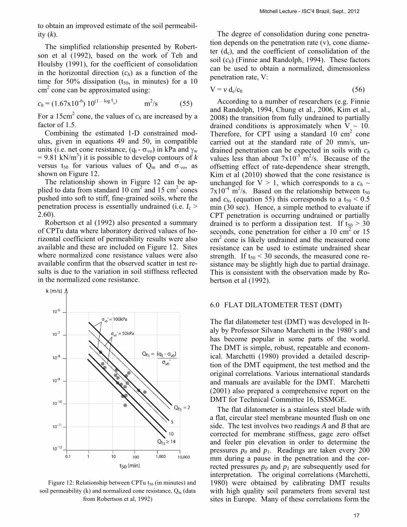
The relationship shown in Figure 12 can be ap-plied to data from standard 10 cm2 and 15 cm2 cones pushed into soft to stiff, fine-grained soils, where the penetration process is essentially undrained (i.e. Ic > 2.60).

Robertson et al (1992) also presented a summary of CPTu data where laboratory derived values of ho-rizontal coefficient of permeability results were also available and these are included on Figure 12. Sites where normalized cone resistance values were also available confirm that the observed scatter in test re-sults is due to the variation in soil stiffness reflected in the normalized cone resistance.

Figure 12: Relationship between CPTu t50 (in minutes) and

soil permeability (k) and normalized cone resistance, Qtn (data from Robertson et al, 1992)

The degree of consolidation during cone penetra-

tion depends on the penetration rate (v), cone diame-ter (dc), and the coefficient of consolidation of the soil (ch) (Finnie and Randolph, 1994). These factors can be used to obtain a normalized, dimensionless penetration rate, V:

V = v dc/ch (56)

According to a number of researchers (e.g. Finnie and Randolph, 1994, Chung et al., 2006, Kim et al., 2008) the transition from fully undrained to partially drained conditions is approximately when V ~ 10. Therefore, for CPT using a standard 10 cm2 cone carried out at the standard rate of 20 mm/s, un-drained penetration can be expected in soils with ch values less than about 7x10-5 m2/s. Because of the offsetting effect of rate-dependence shear strength, Kim et al (2010) showed that the cone resistance is unchanged for V > 1, which corresponds to a ch ~ 7x10-4 m2/s. Based on the relationship between t50 and ch, (equation 55) this corresponds to a t50 < 0.5 min (30 sec). Hence, a simple method to evaluate if CPT penetration is occurring undrained or partially drained is to perform a dissipation test. If t50 > 30 seconds, cone penetration for either a 10 cm2 or 15 cm2 cone is likely undrained and the measured cone resistance can be used to estimate undrained shear strength. If t50 < 30 seconds, the measured cone re-sistance may be slightly high due to partial drainage. This is consistent with the observation made by Ro-bertson et al (1992).

6.0 FLAT DILATOMETER TEST (DMT)

The flat dilatometer test (DMT) was developed in It-aly by Professor Silvano Marchetti in the 1980’s and has become popular in some parts of the world. The DMT is simple, robust, repeatable and econom-ical. Marchetti (1980) provided a detailed descrip-tion of the DMT equipment, the test method and the original correlations. Various international standards and manuals are available for the DMT. Marchetti (2001) also prepared a comprehensive report on the DMT for Technical Committee 16, ISSMGE.

The flat dilatometer is a stainless steel blade with a flat, circular steel membrane mounted flush on one side. The test involves two readings A and B that are corrected for membrane stiffness, gage zero offset and feeler pin elevation in order to determine the pressures p0 and p1. Readings are taken every 200 mm during a pause in the penetration and the cor-rected pressures p0 and p1 are subsequently used for interpretation. The original correlations (Marchetti, 1980) were obtained by calibrating DMT results with high quality soil parameters from several test sites in Europe. Many of these correlations form the


17

basis of current interpretation, having been generally confirmed by subsequent research.

The interpretation evolved by first identifying three "intermediate" DMT parameters (Marchetti 1980):

Material index, ID = (p1 - p0)/(p0 - u0) (57) Horizontal stress index, KD = (p0 - u0) /'vo (58) Dilatometer modulus, ED = 34.7(p1 - p0) (59)

Where:

u0 = pre-insertion in-situ equilibrium water pressure 'vo = pre-insertion in-situ vertical effective stress

The dilatometer modulus ED can also be expressed as a combination of ID and KD in the form: ED / 'vo = 34.7 ID KD (60)

The key DMT design parameters are ID and KD. Both parameters are normalized and dimensionless. ID is the difference between the corrected lift-off pressure (p0) and the corrected deflection pressure (p1) normalized by the effective lift-off pressure (p0 - u0). KD is the effective lift-off pressure normalized by the in situ vertical effective stress. Although al-ternate methods have been suggested to normalize KD, the original normalization suggested by Mar-chetti (1980) using the in-situ vertical effective stress is still the most common. It is likely that a more complex normalization for KD would be more appropriate, especially in sands, but most of the available published records of KD use the original normalization suggested by Marchetti (1980).

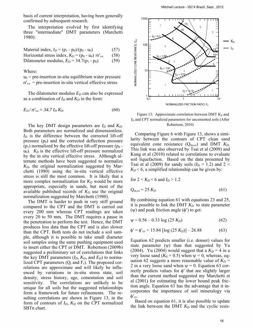
The DMT is harder to push in very stiff ground compared to the CPT and the DMT is carried out every 200 mm whereas CPT readings are taken every 20 to 50 mm. The DMT requires a pause in the penetration to perform the test. Hence, the DMT produces less data than the CPT and is also slower than the CPT. Both tests do not include a soil sam-ple, although it is possible to take small diameter soil samples using the same pushing equipment used to insert either the CPT or DMT. Robertson (2009b) suggested a preliminary set of correlations that links the key DMT parameters (ID, KD, and ED) to norma-lized CPT parameters (Qt and Fr). The proposed cor-relations are approximate and will likely be influ-enced by variations in in-situ stress state, soil density, stress history, age, cementation and soil sensitivity. The correlations are unlikely to be unique for all soils but the suggested relationships form a framework for future refinements. The re-sulting correlations are shown in Figure 13, in the form of contours of ID, KD on the CPT normalized SBTn chart.

Figure 13: Approximate correlation between DMT KD and

ID and CPT normalized parameters for uncemented soils (After Robertson, 2010)

Comparing Figure 6 with Figure 13, shows a simi-larity between the contours of CPT clean sand equivalent cone resistance (Qtn,cs) and DMT KD. This link was also observed by Tsai et al (2009) and Kung et al (2010) related to correlations to evaluate soil liquefaction. Based on the data presented by Tsai et al (2009) for sandy soils (ID > 1.2) and 2 < KD < 6, a simplified relationship can be given by:

for 2 < KD < 6 and ID > 1.2 Qtn,cs = 25 KD (61)

By combining equation 61 with equations 23 and 25, it is possible to link the DMT KD to state parameter () and peak friction angle (’) to get:

= 0.56 – 0.33 log (25 KD) (62)

' = 'cv + 15.84 [log (25 KD)] – 26.88 (63)

Equation 62 predicts smaller (i.e. denser) values for state parameter () than that suggested by Yu (2004). Yu (2004) would suggest that a KD = 4 in a very loose sand (K0 = 0.5) when = 0, whereas, eq-uation 62 suggests a more reasonable value of KD = 2 in a very loose sand when = 0. Equation 63 cor-rectly predicts values for ' that are slightly larger than the current method suggested my Marchetti et al (2001) for estimating the lower bound peak fric-tion angle. Equation 63 has the advantage that it in-corporates the importance of soil mineralogy via 'cv.

Based on equation 61, it is also possible to update the link between the DMT KD and the cyclic resis-


18

tance ratio (CRR7.5) for evaluating soil liquefaction in sandy soils. Using the CPT-based relationship be-tween CRR and Qtn,cs, suggested by Robertson and Wride (1998), and equation 61, an updated DMT re-lationship becomes:

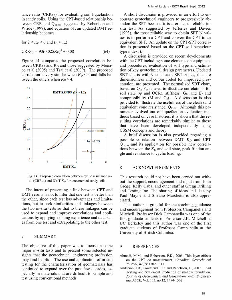
for 2 < KD < 6 and ID > 1.2 CRR7.5 = 93(0.025KD)3 + 0.08 (64) Figure 14 compares the proposed correlation be-tween CRR7.5 and KD and those suggested by Mona-co et al (2005) and Tsai et al (2009). The proposed correlation is very similar when KD < 4 and falls be-tween the others when KD > 4.

Fig. 14: Proposed correlation between cyclic resistance ra-tio (CRR7.5) and DMT KD for uncemented sandy soils

The intent of presenting a link between CPT and

DMT results is not to infer that one test is better than the other, since each test has advantages and limita-tions, but to seek similarities and linkages between the two in-situ tests so that to these linkages can be used to expand and improve correlations and appli-cations by applying existing experience and databas-es from one test and extrapolating to the other test.

7 SUMMARY

The objective of this paper was to focus on some major in-situ tests and to present some selected in-sights that the geotechnical engineering profession may find helpful. The use and application of in-situ testing for the characterization of geomaterials has continued to expand over the past few decades, es-pecially in materials that are difficult to sample and test using conventional methods.

A short discussion is provided in an effort to en-courage geotechnical engineers to progressively ab-andon the SPT because it is a crude, unreliable in-situ test. As suggested by Jefferies and Davies (1993), the most reliable way to obtain SPT N val-ues is to perform a CPT and convert the CPT to an equivalent SPT. An update on the CPT-SPT correla-tion is presented based on the CPT soil behaviour type index, Ic.

A discussion is provided on recent developments with the CPT including some elements on equipment and procedures, evaluation of soil type and estima-tion of key geotechnical design parameters. Updated SBT charts with 9 consistent SBT zones, that are dimensionless and colour coded for improved pres-entation, are presented. The normalized SBT chart, based on Qtn-Fr, is used to illustrate correlations for soil state ( and OCR), stiffness (G0, and E) and compressibility (M and Cc). A discussion is also provided to illustrate the usefulness of the clean sand equivalent cone resistance, Qtn,cs. Although this pa-rameter evolved out of liquefaction evaluation me-thods based on case histories, it is shown that the re-sulting correlations are remarkably similar to those that have been developed independently using CSSM concepts and theory.

A brief discussion is also provided regarding a possible correlation between DMT KD and CPT Qtn,cs, and its application for possible new correla-tions between the KD and soil state, peak friction an-gle and resistance to cyclic loading.

8 ACKNOWLEDGEMENTS

This research could not have been carried out with-out the support, encouragement and input from John Gregg, Kelly Cabal and other staff at Gregg Drilling and Testing Inc. The sharing of ideas and data by Paul Mayne and Silvano Marchetti is also appre-ciated.

This author is grateful for the teaching, guidance and encouragement from Professors Campanella and Mitchell. Professor Dick Campanella was one of the first graduate students of Professor J.K. Mitchell at UC Berkeley and this author was one of the first graduate students of Professor Campanella at the University of British Columbia.

9 REFERENCES

Ahmadi, M.M., and Robertson, P.K., 2005. Thin layer effects on the CPT qc measurement. Canadian Geotechnical Journal, 42(9): 1302-1317.

Anderson, J.B., Townsend, F.C. and Rahelison, L., 2007. Load Testing and Settlement Prediction of shallow foundation. Journal of Geotechnical and Geoenvironmental Engineer-ing, ASCE, Vol. 133, no.12, 1494-1502.


19

Andrus, R.D., Mohanan, N.P., Piratheepan, P., Ellis, B.S. and Holzer, T.L., 2007. Predicting shear-wave velocity from cone penetration resistance. Proceedings of Fourth Inter-national Conference on Earthquake Geotechnical Engi-neering, Thessaloniki, Greece.

ASTM D5778-95(2007). Standard Test Method for Performing Electronic Friction Cone and Piezocone Penetration Test-ing of Soils, ASTM International. www.astm.org.

Baldi, G., Bellotti, R., Ghionna, V.N., Jamiolkowski, M., and Lo Presti, D.F.C., 1989. Modulus of sands from CPTs and DMTs. In Proceedings of the 12th International Confe-rence on Soil Mechanics and Foundation Engineering. Rio de Janeiro. Balkema Pub., Rotterdam, Vol.1, pp. 165-170.

Bellotti, R., Ghionna, V.N., Jamiolkowski, M., and Robertson, P.K., 1989. Design parameters of cohesionless soils from in-situ tests. In Proceedings of Transportation Research Board Conference. Washington. January 1989.

Boggess, R. and Robertson, P.K., 2010. CPT for soft sediments and deepwater investigations. 2nd International Sympo-sium on Cone Penetration Testing, CPT’10. Huntington Beach, CA, USA. www.cpt10.com

Bolton, M.D., 1986. The strength and dilatancy of sands. Geo-technique, 36(1): 65-78.

Boulanger, R.W. and Idriss, I.M., 2004. State normalization of penetration resistance and the effect of overburden stress on liquefaction resistance. Proceedings 11th International Conference on Soil Dynamics and Earthquake Engineer-ing. Berkely, 484-491.

Boulanger, R.W., 2003. High overburden stress effects in li-quefaction analyses. Journal of Geotechnical and Geoen-vironmental Engineering, ASCE, December: 1071-1082.

Briaud, J.L., and Gibbens, R., 1999. Behavior of five large spread footings in sand. Journal of Geotechnical and Geoenvironmental Engineering, ASCE, 125(9): 787-796.

Campanella, R.G., and Robertson, P.K., 1982. State of the art in In-situ testing of soils: developments since 1978. In Proceedings of Engineering Foundation Conference on Updating Subsurface Sampling of Soils and Rocks and Their In-situ Testing. Santa Barbara, California. January 1982, pp. 245-267.

Campanella, R.G., Gillespie, D., and Robertson, P.K., 1982. Pore pressures during cone penetration testing. In Proceed-ings of the 2nd European Symposium on Penetration Test-ing, ESPOT II. Amsterdam. A.A. Balkema, pp. 507-512.

Cetin, K.O. and Isik, N.S., 2007. Probabilistic assessment of stress normalization for CPT data. Journal of Geotechnic-al and Geoenvironmental Engineering, ASCE, Vol. 133, no.7, 887-897.

Chung, S.F., Randolph, M.F., and Schneider, J. A., 2006. Ef-fect of penetration rate on penetrometer resistance in clay. J. of Geotech. Geoenviron. Eng, ASCE, 132(9): 1188-1196.

Douglas, B.J., and Olsen, R.S., 1981. Soil classification using electric cone penetrometer. In Proceedings of Symposium on Cone Penetration Testing and Experience, Geotechnic-al Engineering Division, ASCE. St. Louis, Missouri, Oc-tober 1981, pp. 209-227.

Eslaamizaad, S., and Robertson, P.K., 1996a. Seismic cone pe-netration test to identify cemented sands. In Proceedings of the 49th Canadian Geotechnical Conference. St. John’s, Newfoundland. September, pp. 352 – 360.

Eslaamizaad, S., and Robertson, P.K. 1996b. Cone penetration test to evaluate bearing capacity of foundation in sands. In Proceedings of the 49th Canadian Geotechnical Confe-rence. St. John’s, Newfoundland. September, pp. 429-438.

Eslaamizaad, S. and Robertson, P.K., 1997. Evaluation of set-tlement of footings on sand from seismic in-sity tests. In

Proceedings of the 50th Canadian Geotechnical Confe-rence, Ottawa, Ontario, October 1997, Vol.2, pp. 755-764.

Eslami, A., and Fellenius, B.H., 1997. Pile Capacity by direct CPT and CPTu methods applied to 102 case histories. Ca-nadian Geotechnical Journal, 34(6): 880-898.

Fahey, M. and Carter, J.P., 1993. A finite element study of the pressuremeter in sand using a nonlinear elastic plastic model. Canadian Geotechnical Journal, 30(2): 348-362.

Farrar, J.A., Torres, R., and Crutchfiedl, L.G., 2008. Cone Pe-netrometer Testing, Scoggins Dam, Tualatin Project, Ore-gon. Bureau of Reclamation, Technical Services Center, Denver, Engineering Geology Group, 86-68320.

Finnie, I.M.S. & Randolph, M.F. 1994. Punch-through and li-quefaction induced failure of shallow foundations on cal-careous sediments. Proc., 17th Int. Conf. on the Behavior of Offshore Structures, Boston, 1: 217-230.

Hardin, B.O., and Drnevich, V.P., 1972. Shear modulus and damping in soils: design equations and curves. ASCE, Journal of the Soil Mechanics and Foundation Division, Vol.98, SM7, pp. 667-692.

Hegazy, YA and Mayne, PW. “Statistical correlations between VS and cone penetration data for different soil types,” Proc., International Symposium on Cone Penetration Test-ing, CPT ’95, Linkoping, Sweden, 2, Swedish Geotechnic-al Society, 173-178, 1995.

Hight, D., and Leroueil, S., 2003. Characterization of soils for engineering purposes. Characterization and Engineering Properties of Natural Soils, Vol.1, Swets and Zeitlinger, Lisse, pp. 255-360.

Idriss, I.M. and Boulanger, R.W., 2004. Semi-empirical pro-cedures for evaluating liquefaction potential during earth-quakes. Proceedings 11th International Conference on Soil Dynamics and Earthquake Engineering. Berkeley, 32-56.

IRTP, 1999. International Reference Test Procedure for Cone Penetration Test (CPT). Report of the ISSMFE Technical Committee on Penetration Testing of Soils, TC 16, Swe-dish Geotechnical Institute, Linkoping, Information, 7, 6-16.

Janbu, N., 1963, Soil Compressibility as determined by oedo-meter and triaxial tests. Proceedings of the European Conference on Soil Mechanicxs and Foundation Engineer-ing, Wiesbaden, pp 19-25.

Jamiolkowski, M., Ladd, C.C., Germaine, J.T., and Lancellotta, R., 1985. New developments in field and laboratory testing of soils. In Proceedings of the 11th International Confe-rence on Soil Mechanics and Foundation Engineering. San Francisco, California, August 1985, Vol.1 pp. 57-153.

Jamiolkowski, M., and Robertson, P.K., 1988. Future trends for penetration testing. Penetration testing in the UK, Thomas Telford, London, pp. 321-342.

Jefferies, M.G., and Davies, M.O, 1991. Soil Classification by the cone penetration test: discussion. Canadian Geotech-nical Journal, 28(1): 173-176.

Jefferies, M.G., and Davies, M.P., 1993. Use of CPTU to esti-mate equivalent SPT N60. Geotechnical Testing Journal, ASTM, 16(4): 458-468.

Jefferies, M.G. and Been, K., 2006. Soil Liquefaction – A criti-cal state approach. Taylor & Francis, ISBN 0-419-16170-8 478 pages.

Karlsrud, K., Lunne, T., Kort, D.A. & Strandvik, S. 2005. CPTU correlations for Clays. Proc. 16th ICSMGE, Osaka, September 2005

Kim, K., Prezzi, M., Salgado, R., & Lee, W. 2008. Effect of penetration rate on cone penetration resistance in saturated clayey soils. J. of Geotech. Geoenviron. Eng., 134(8): 1142-1153.


20

Kulhawy, F.H., and Mayne, P.H., 1990. Manual on estimating soil properties for foundation design, Report EL-6800 Electric Power Research Institute, EPRI, August 1990.

Kung, G.T., Lee, D.H. and Tsai, P.H., 2010. Examination of existing DMT-based Liquefaction Evaluation methods by side-by-side DMT and CPT Tests. 5th International Confe-rence on Recent Advances in Geotechnical Earthquake Engineering and Soil Dynamics. San Diego, CA.

Ladd, C.C., and Foott, R. (1974). "New design procedure for stability of soft clays." J. of the Geotech. Eng. Div., 100(GT7), 763-786.

Ladd, C.C. & DeGroot, D.J. 2003. Recommended practice for soft ground site characterization. Soil and Rock America, Vol. 1 (Proc.12th PanAmerican Conf., MIT), Verlag Glückauf, Essen: 3-57.

Long, M., 2008. Design parameters from in situ tests in soft ground – recent developments. Proceedings of Geotech-nical and Geophysical Site Characterization. ISC’3, Tay-lor & Francis Group, 89-116

Lunne, T., Eidsmoen, T., Gillespie, D., and Howland, J.D., 1986. Laboratory and field evaluation on cone penetrome-ters. Proceedings of ASCE Specialty Conference In Si-tu’86: Use of In Situ Tests in Geotechnical Engineering. Blacksburg, ASCE, GSP 6 714-729

Lunne, T., Robertson, P.K., and Powell, J.J.M., 1997. Cone pe-netration testing in geotechnical practice. Blackie Aca-demic, EF Spon/Routledge Publ., New York, 1997, 312 pp.

Lunne, T., and Andersen, K.H., 2007. Soft clay shear strength parameters for deepwater geotechnical design. Proceed-ings 6th International Conference, Society for Underwater Technology, Offshore Site Investigation and Geomechan-ics, London, 151-176.

Marchetti, S. _1980_. “In-situ tests by flat dilatometer.” J. Geotech. Eng., 106_3_, 299–321.

Marchetti, S., Monaco, P., Totani, G., and Calabrese, M. 2001_. “The DMT in soil investigations. A report by the ISSMGE TC 16.” Proc., Int. Conf. on In Situ Measure-ment of Soil Properties and Case Histories, Bali, Indone-sia, Parahyangan Catholic Univ., Bandung, Indonesia, 95–132.

Marchetti, S., Monaco, P., Calabrese, M. and Totani, G., 2007. Comparison of moduli determined by DMT and backfi-gured from local strain measurements under a 40m diame-ter circular test load in the Venice Area. Proceedings Second International Conference on Flat Dilatometer, Washington, D.C., 220-230.

Mayne, P.W., 2000. Enhanced Geotechnical Site Characteriza-tion by Seismic Piezocone Penetration Test. Invited lec-ture, Fourth International Geotechnical Conference, Cairo University. pp 95-120.

Mayne, P.W., 2005. Integrated Ground Behavior: In-Situ and Lab Tests, Deformation Characteristics of Geomaterials, Vol. 2 (Proc. Lyon), Taylor & Francis, London, pp. 155-177.

Mayne, P.W., 2007. NCHRP Synthesis ‘Cone Penetration Testing State-of-Practice’. Transportation Research Board Report Project 20-05. 118 pages. www.trb.org

Mayne, P.W., 2008. Piezocone profiling of clays for maritime site investigations. 11th Baltic Sea Geotechnical Confe-rence. Gdansk, Poland., 151- 178.

Mayne, P.W., Coop, M.R., Springman, S.M., Huang, A.B, and Zornberg, J.G., 2009. Geomaterail behaviour and testing. State of the Art (SOA) paper, 17th ICSMGE Alexandria.

Mitchell, J.K., Guzikowski, F. and Villet, W.C.B., 1978. The Measurement of Soil Properties In-Situ, Report prepared for US Department of Energy Contract W-7405-ENG-48,

Lawrence Berkeley Laboratory, University of California, Berkeley, CA, 94720.

Monaco, P., Totani, G. and Calabrese, M., 2006. DMT-predicted vs observed settlements: a review of the availa-ble experience. Proc. 2nd Int. Conf. on the Flat Dilatome-ter, Washington D.C., 244-252.

Molle, J., 2005. The accuracy of the interpretation of CPT-based soil classification methods in soft soils. MSc Thesis, Section for Engineering Geology, Department of Applied Earth Sciences, Delf University of Technology, Report No. 242, Report AES/IG/05-25, December

Moss, R.E.S., Seed, R.B., and Olsen, R.S. 2006. Normalizing the CPT for overburden stress. Journal of Geotechnical and Geoenvironmental Engineering, 132(3): 378-387.

Ohta, H. Nishihara, A., and Morita, Y., 1985. Undrained stabil-ity of Ko-consolidated clays. Proceedings of 11th ICSMFE. Vol 2., San Fransico, pp 613-661.

Olsen, R.S., and Malone, P.G., 1988. Soil classification and site characterization using the cone penetrometer test. Pe-netration Testing 1988, ISOPT-1, Edited by De Ruiter, Balkema, Rotterdam, Vol.2, pp.887-893.

Olsen, R.S., and Mitchell, J.K., 1995. CPT stress normalization and prediction of soil classification. In Proceedings of the International Symposium on Cone Penetration Testing, Vol.2, Swedish Geotechnical Society, Linkoping, pp. 257-262.

Parez, L. and Faureil, R., 1988. Le piézocône. Améliorations apportées à la reconnaissance de sols. Revue Française de Géotech, Vol. 44, 13-27.

Plewes, H.D., Davies, M.P., and Jefferies, M.G., 1992. CPT based screening procedure for evaluating liquefaction sus-ceptibility. In Proceedings of the 45th Canadian Geotech-nical Conference, pp. 41-49.

Rad, N.S. and Lunne, T., 1986, Correlations between piezo-cone results and laboratory soil properties. Norwegian Geotechnical Institute, Oslo, Report 52155, 306-17.

Robertson, P.K., 1990. Soil classification using the cone pene-tration test. Canadian Geotechnical Journal, 27(1): 151-158.

Robertson, P.K., 1995. Penetrometer Testing - Session IV, Moderators Report. Conference on Advance in Site Inves-tigation Practice, London, U.K.

Robertson, P.K., 1998. Risk-based site investigation. Geotech-nical News: 45-47, September 1998.

Robertson, P.K., 2009a. Interpretation of cone penetration tests – a unified approach. Canadian Geotechnical Jour-nal, 46:1337-1355.

Robertson, P.K., 2009b. DMT – CPT correlations. Journal of Geotechnical and Geoenvironmental Engineering, ASCE, December: 135:1762-1771.

Robertson, P.K., 2010a. Soil behaviour type from the CPT: an update. 2nd International Symposium on Cone Penetration Testing, CPT’10, Huntington Beach, CA, USA. www.cpt10.com

Robertson, P.K., 2010b. Estimating in-situ state parameter and friction angle in sandy soils from the CPT. 2nd Interna-tional Symposium on Cone Penetration Testing, CPT’10, Huntington Beach, CA, USA. www.cpt10.com

Robertson, P.K., 2010c. Evaluation of Flow Liquefaction and Liquefied strength Using the Cone Penetration Test. Jour-nal of Geotechnical and Geoenvironmental Engineering, ASCE, 136(6): 842-853

Robertson, P.K. and Woeller, D.J. and Finn, W.D.L., 1992, Seismic Cone Penetration Test for Evaluating Liquefaction Potential, Canadian Geotechnical Journal, Vol. 29, No. 4, August, pp. 686-695.


21

Robertson, P.K., and R.G. Campanella, 1989. Design Manual for Use of CPT and CPTU, University of British Colum-bia, BC, 200p,

Robertson. P.K., Campanella, R.G., Gillespie, D., and Greig, J., 1986. Use of Piezometer Cone data. In-Situ’86 Use of Ins-itu testing in Geotechnical Engineering, GSP 6 , ASCE, Reston, VA, Specialty Publication, SM 92, pp 1263-1280.

Robertson, P.K., Sully, J.P., Woeller, D.J., Lunne, T., Powell, J.J.M. and Gillespie, D., 1992. Estimating coefficient of consolidation from piezocone tests. Canadian Geotechnic-al Journal, Ottawa, 29(4): 539-550.

Robertson, P.K., and Campanella, R.G., 1983a. Interpretation of cone penetration tests – Part I (sand). Canadian Geo-technical Journal, 20(4): 718-733.

Robertson, P.K., and Campanella, R.G. 1983b. Interpretation of cone penetration tests – Part II (clay). Canadian Geo-technical Journal, 20(4): 734-745.

Robertson, P.K. and Wride, C.E., 1998. Evaluating cyclic li-quefaction potential using the cone penetration test. Cana-dian Geotechnical Journal, Ottawa, 35(3): 442-459.

Robertson, P.K., Campanella, R.G., Gillespie, D., and Rice, A., 1986. Seismic CPT to measure in-situ shear wave velocity. Journal of Geotechnical Engineering Division, ASCE, 112(8): 791-803.

Sanglerat, G., 1972. The Penetrometer and Soil Exploration. Elsevier Pub., Amsterdam, 488pp.

Schnaid, F., 2005. Geocharacterization and Engineering prop-erties of natural soils by in-situ tests. In Proceedings of the 16th International Conference on Soil Mechanics and Geo-technical Engineering, Vol.1, Osaka, September, 2005, Millpress, Rotterdam, pp. 3-45.

Schneider, JA, McGillivray, AV and Mayne, PW. 2004. Eval-uation of SCPTU intra-correlations at sand sites in the Lower Mississippi River valley, USA, Geotechnical & Geophysical Site Characterization, Vol. 1, (Proc. ISC-2, Porto), Millpress, Rotterdam, 1003-1010.

Schneider, J.A., Randolph, M.F., Mayne, P.W. & Ramsey, N.R. 2008. Analysis of factors influencing soil classifica-tion using normalized piezocone tip resistance and pore pressure parameters. Journal Geotechnical and Geoenvi-ronmental Engrg. 134 (11): 1569-1586.

Schmertmann, J.H. 1978. Guidelines for cone penetration tests performance and design. Federal Highways Administra-tion, Washington, D.C., Report FHWA-TS-78-209.

Shuttle, D.A. and Cunning, J., 2007. Liquefaction potential of silts from CPTu. Canadian Geotechnical Journal: 44: 1-19

Seed, H.B., and Idriss, I.M., 1970. Soil moduli and damping factors for dynamics response analysis, Report No. EERC 70-10, University of California, Berkeley, December 1970.

Simonini, P., 2004, Characterization of Venice lagoon silts from in-situ tests and performance of a test embankment. Proceedings 2nd International Conference on Site Charac-terization, ISC’2, Geotechnical & Geophysical Site Cha-racterization, Porto, Vol. 1, 187-207.

Teh, C.I., and Houlsby, G.T. 1991. An analytical study of the cone penetration test in clay. Geotechnique, 41 (1): 17-34.

Treen, C. R., Robertson, P.K. and Woeller, D.J., 1992. Cone penetration testing in stiff glacial soils using a downhole cone penetrometer. Canadian Geotechnical Journal, 29:448-455.

Tsai, P.H., Lee, D.H., Kung, G.T.C., and Juang, C.H., 2009. Simplified DMT-based methods for evaluating liquefac-tion resistance of soils. Engineering Geology, Vol 103, No 1-2, pp 13-22.

Vesic, A.S, and Clough, G.W., 1968, Behaviour of granular materials under high stresses. Journal of Soil Mechanics and Foundations Div., ASCE, SM3, pp 313-326

Wride, C.E., Robertson, P.K., Biggar, K.W., Campanella, R.G., Hofmann, B.A., Hughes, J.M.O., Küpper, A., and Woeller, D.J. In-Situ testing program at the CANLEX test sites. Canadian Geotechnical Journal, 2000, Vol. 37, No. 3, June, pp. 505-529

Wroth, C.P., 1984. The interpretation of in-situ soil tests. Ran-kine Lecture, Geotechnique(4).

Yu, H-S. 2004. James K. Mitchell Lecture: In-situ soil testing: from mechanics to interpretation. Geotechnical & Geo-physical Site Characterization, Vol. 1 (Proc. ISC-2, Por-to), Millpress, Rotterdam: 3–38.

Zhang, Z., and Tumay, M.T., 1999. Statistical to fuzzy ap-proach toward CPT soil classification. Journal of Geo-technical and Geoenvironmental Engineering, 125(3): 179-186.

Zhang, G., Robertson, P.K. and Brachman, R.W.I., 2002, Esti-mating Liquefaction induced Ground Settlements From CPT for Level Ground, Canadian Geotechnical Journal, 39(5): 1168-1180


22

Documents

Mitchell Lecture - In situ testing services · ing are correlated to the in-situ test results to ... The tendency of a soil to either dilate or contract in shear often defines if