PART I

THE LORAN SYSTEM

CHAPTER 1

INTRODUCTION

BY B. W. SITTERLY AND D. DAVIDSON

The Loran system is a radio aid to navigation. It provides means,independent of all other aids (including even the compass and the log orair-speed meter), for locating a moving vehicle at a given moment andfor directing it to a predetermined point or along a predetermined path.There are many other radio aids by which ships or aircraft may belocated or guided; these operate in accordance with various principles,and as a background to the discussion of Loran it is profitable to considersome of these principles and to describe and compare some of these aidsbriefly.

NAVIGATION BY FIXING OF POSITION

In general, a navigator locates Klmself at the intersection of two linesof position on the surface of the earth. Each line is the locus of thepoints at which some observable quantity has a specific value. Forexample, the visual compass bearing of a recognized landmark places thenavigator upon a line that is the locus of all points from which the land-mark has the given bearing. This line is practically identical with arhumb line (line crossing successive meridians at a constant angle) onthe earth, laid off from the mark along the reverse bearing. A sextantaltitude of the sun places the navigator upon a line from all points of whichthe sun will be seen at that altitude. This line is a circle on the earth,centered at the subsolar point, of spherical radius equal to the complementof the altitude. It will be convenient to classify navigation aids accord-ing to the forms of the lines of position that they give.

1.1. Position from Measurement of Two Bearings (Lines Are Radii).Direction-jnding.-This is the familiar method used in visual piloting ofa ship, in which the navigator takes bearings of two known marks andplots on the chart the reverse bearings from the marks; the intersectionof the lines is his locatiou Conventional radio direction—finding is thesame geometrically; each mark is a transmitter sending out radio signals.In the simplest form of system the operator, instead of sighting over apeloms, hears the signals through a receiver connected to a loop antennathat he rotates around a vertical axis until an aural null is obtained. Thenormal to the plane of the loop then lies in the direction from which thesignals come. If the distance between the rereiver and the transmitter

3

4 IN TROD[:CTION [SEC. 11

is considerable, the line of position will not be quite straight on a chart,nor will its directional thetransmitter bequite thesarnea satthe receiver,but a simple correction can be applied to the readinzs toallow forthesedifferences. There are many more elaborate forms of radio direction-finder, employing more complex antennas, automatic null-seeking orscanning and visual instead of aural presentation, but all operating inaccordance with the same principles.

As a refinement to facilitate the operationof the direction-finder, theloop can be rotated automatically by a motor, with the indication elec-trically coupled so that it follows the rotation of the loop. Compensationfor quadrantal error can be made automatically, and all bearings can bepresented as true bearings.

An increase in precision may be gained by transferring the direction-finding function to receivers at fixed ground stations. The navigatoruses no equipment but his communications transmitter, with which heasks the stations for bearings. Their receiving antennas determine thedirections of his signals, and they communicate the bearings to him forplotting.

Orjordness Beacon .—The British “ Orfordness” beacon exemplifies aningenious technique by which the navigator obtains his bearing from aground station by a time measurement, using only his communicationsreceiver and transmitting no signals himself. The ground station orbeacon transmits a steady tone from a loop antenna that is rotating oncea minute about a vertical axis. The radiation pattern has two oppositenull lines that sweep around the beacon at the rate of 6° per sec., and asone of these passes the north direction, the signal is given a coded inter-ruption. The azimuth of a navigator from the station is therefore sixtimes the interval in seconds from the time when he hears the interruptionto the time when the null passes over him (or this amount plus 180°).

i5’onne.-The German “ Sonne” beacon (termed “ Consol” by theBritish) combines the principles of the Orfordness beacon and the com-mon radio range described in Sec. 15 but is much more elaborate andaccurate than either. The ground station has three fixed vertical anten-nas in line, so spaced, keyed, and phased that interference between theirsignals produces a radiation pattern of about a dozen sectors in whichsuccessions of dots are heard that alternate with sectors in which dashesare heard. Since the dots and dashes are interlocked, along the radiallines bounding the sectors they merge into a steady tone (equisignal).The dots and dashes are emitted, one a second, for a minute, duringwhich time the radiation pattern is slowly rotated by shifting the phasesof the two outside antennas, and hence at the end of the minute each dotsector has moved into the place of the adjacent dash sector, and viceversa. During the next minute a steady omnidirectional tone is emitted

SEC.1.1] POSITION FROM TWO BEARINGS 5

by the central antenna. Then the dots and dashes are repeated, startingat the initial configuration and going through the same rotation again, andso on. A navigator determines his radial line of position within hissector by measuring the time that elapses from the beginning of any dot-and-dash period to the instant at which the advancing equisignal bound-ary of the sector sweeps over him. He does this by simply counting thedots and dashes for these beat seconds, and one changes to the other asthe boundary passes. Which sector he is in must be determined by con-ventional direction finding on the signal during the steady-tone periodor by dead reckoning. The transmissions are received on an ordinaryradio receiver in the 250- to 500-kc/sec region, and fixes are plotted on aspecial chart giving the various zones and a key for each zone for inter-pretation of the received dot-and-dash cycle.

Omnidirectional Radio Range .—The so-called ‘( omnidirectional radiorange” operates still differently. It may be regarded as a developmentof the radio range of commercial air traffic (see Sec. 1.5) to which theSonne beacon is also akin. Four antennas mounted at the corners of asquare at a ground station send out a continuous signal, the differentantennas being phased so that a figure-eight radiation pattern results,and the phases are steadily and uniformly shifted so that the patternrotates around the station. At a distance, the received and rectified sig-nal has an audio modulation whose phase at any instant depends on theazimuth of the receiver from the station. In order to obtain a bearingfrom the phase of the audio modulation some reference direction must beestablished. This is done by exciting a center antenna in the square atthe carrier frequency, amplitude-modulating the signal at 10 kc/see andfrequency-modulating the 10-kc/sec modulation at the frequency (60cps) of rotation of the radiation pattern. This reference frequencymodulation is made to reach its maximum when the maximum of thedirectivity pattern passes through North. At any receiving point, thedifference in phase between the reference signal and the rotating signalis examined, and this phase difference in degrees is exactly equal to thebearing to the beacon in degrees. A 180° ambiguity occurs, but this isresolvable in the receiving apparatus.

The receiving equipment contains a receiver whose output is fed totwo separate channels. In one, a low-pass filter sorts out the 60-cpsmodulation of the carrier (the rotating phase signal), whereas in the othera high-pass filter presents the 10-kc/sec subcarrier to a discriminator that,in turn, removes the sub carrier and yields the 60-cps reference signal.By suitable comparing and indicating circuits, the phase of the referencevoltage is compared with that of the rotating phase voltage, and thebearing is shown on a meter.

For the long-range version of the system, the 10-kc/sec subcarrier

6 INTRODUCTION [SEC.1.2

would be replaced by a l-kc/see subcarrier, and large towers would beused instead of high-frequency arrays.

1.2. Position from Measurement of One Bearing and One Distance(Polar Coordinates) .-A compass bearing on a visible object plus asextant measurement of its apparent size or a radio bearing on a beaconplus a measurement of the interval between the receptions of synchro-nized radio and sound signals coming from it will provide a navigator withhis polar coordinates with respect to the object or beacon. (The bearingas observed must be reversed, of course, since it places the origin at theobserver.) The celestial altitude and observed azimuth of a heavenlybody will theoretically give similar information, but it is not useful prac-tically because the linear equivalent of the uncertainty of the compassreading may be a hundred miles as a consequence of the great distanceto the substellar point that is the origin of the coordinates.

Radar (Range and Bearing) .—Most radar systems give distance anddirection (range and bearing). A highly directional transmitting antennasends out a narrow beam of energy and rotates or fans over a sector, inorder to scan its field. The returning echoes are made to intensify thebeam of a cathode-ray tube. The range is commonly presented bydeflecting the electron stream of this cathode-ray tube away from a normalequilibrium track down the axis of the tube (where it produces a lightspot at the center of the circular screen) toward the edge of the screen,the range being approximately proportional to the deflection. Bysynchronizing the direction of the deflection with the scanning mechanismof the antenna, bearing on the earth’s surface is presented as bearing onthe screen. This displaying mechanism is the well-known plan positionindicator, PPI. It gives the observer, in effect, a map of the regionscanned, centered at his location. Because the distance measured bythe travel time of the signal is the airline distance (slant range) and notthe projection of this on the ground, the map is somewhat distorted.The measured ranges are accurate, being taken with reference to accuratecalibration markers provided by a precise high-frequency oscillator, buta correction that is a function of the range and the difference of elevationbetween the observer and the target must be applied to reduce theobsewed slant range to range from the point on the ground beneath theobserving aircraft.

The terrain in the vicinity of the aircraft is scanned by a narrow beamof energy produced by a suitable antenna and reflector. It is fannedvertically so as to irradiate all objects on the ground at different rangesbut at the given bearing. This fan beam is rotated or oscillated backand forth so as to cover either the full 3606 of azimuth or a selected sectorof it, w desired. Because of the differing reflectivity of the variousfeatures of the terrain, and because of the distinctive echoes returned by

sEC. 12] POSITION FROM BEARING AND DISTAiVCE 7

some geographically prominent ones such as cities and large bridges, aplot of the scanned terrain is presented on the radar oscilloscope or PPI.Although such systems are seldom used for navigation by actually plottingpositions of the aircraft on a chart, they have ‘been widely used for whatcan be thought of as extended visual piloting. In cloudy weather theradar information takes the place of visual information, and even in fairweather the radar data supplement visual observation in a useful way.

The properties of such radar systems and various applications of themare discussed at length in Vol. 2 of the Radiation Laboratory seriesentitled Radar Aids to Navigation.

Radar Beacons.—It sometimes happens that important places on theground are not unambiguously marked by characteristic radar patternson the PPI. This can be remedied by the use of radar beacons. Thebeacon acts to some extent as an amplifier of radar echoes. It has areceiver that detects the pulses sent out by a radar set and causes themto trigger the beacon’s transmitter to emit single reply pulses or groupsof pulses. Since the time required for the circuits of a beacon to act canbe made to be negligibly small, the reply is much like a radar echo. Itdiffers in that it can have any desired frequency and can be a pulse orgroup of pulses differing in duration from the original interrogating pulse.The replies can thus be coded for identifying the beacons. Since thefrequency of the reply is different from that of the interrogating radarpulse, the reply pulses can be received and displayed separately from theradar echoes, provided that the radar set has a receiver tuned for thesebeacon signals. Such radar-beacon systems are discussed further in Vol.2 mentioned above and more thoroughly in Vol. 3 entitled Radar Beacons.

Rebecca-Eureka. —One radar-beacon system that found considerableuse in the war is called the Rebecca-Eureka. In this system an aircraftcarries an interrogator (the Rebecca), which may transmit on any oneof a group of frequencies around 200 Me/see. Directional receivingantennas (dipole and director) are mounted on each side of the fuselagenear the nose, and by lobe switching these are made to receive repliesfrom a fixed ground beacon (the Eureka) alternately. Transmissions ofthe Rebecca are made from a stub mounted under the fuselage. Theindication provides two vertical deflection-modulated traces back to backin the center of the oscilloscope; range is measured upward from the base.Thus the vertical displacement of the signal gives the range, and thehorizontal deflection of the signal gives a left-right indication; a beaconto the left gives a greater deflection in the left half of the oscilloscopethan in the right. Since the screen has a grid superimposed on it, bear-ings can be estimated roughly. Homing to a Eureka beacon is accom-plished by flying a course such that the oscilloscope deflections to theright and left remain equal. The range of the system is about 25 to 50

8 INTRODL’CTION [SEC,13

miles, depending upon the Eureka beacon and the altitude of the aircraft.Some of the Eureka beacons weigh only about 20 lb complete and henceare readily portable.

Control oj Aircrajt by Ground Radar.-Use has also been made ofground radar stations for determining the azimuth and distance of air-craft, the location to be communicated to the navigator. This has beenemployed particularly in the surveillance and tactical control of militaryaircraft. Ships or aircraft may be detected at the station merely by theradar signals that are reflected from them, or they may carry radarbeacons, which will also identify them to the station. If separatereceivers are provided, the same transmitter may be used to handle atthe same time craft with radar beacons and those without. When asingle craft or group of craft is to be located or directed, increasedaccuracy in bearing may be obtained by using special transmittingantennas which project twe-lobed or alternating-lobed patterns nearly inthe same direction. The equisignal zone between the lobes is narrow,so that discrimination in angle is considerably improved. These systemsand methods are also discussed in Vol. 2 of this series.

It is to be noted that in general the bearing is much less accuratelydetermined than is the range, so that for the most precise determinationof position two ranges should be used rather than one range and onebearing.

1.3. Position from Measurement of Two Distances (Lines AreCircles) .—This form of position finding has many varieties. Threecommonly used methods that do not use radar technique may be men-tioned. The distance of a visible mark of known linear dimension maybe calculated if the apparent angular magnitude of this dimension ismeasured with a sextant; this distance is the radius of a circular line ofposition whose center is the mark. Distance from a point is also thequantity obtained in celestial navigation, as was mentioned above. Anavigational beacon that emits simultaneously a radio signal and a soundsignal in air or under water gives the navigator a measure of his distancefrom the beacon, for this is proportional to the time interval between theradio signal and the sound signal as they are received by him. Twoobservations of any of the above sorts establish two circular lines ofposition; their intersection gives the fix.

Radar and Radar-beacon Methods.-Since a radar set can readilymeasure range to an accuracy of a few hundred feet or better, a precisionmuch higher than it gives for measurements of bearing, it is peculiarlysuitable for getting fixes by measuring the distances to two objects atmown positions. In principle this can be done by using two naturaladar echoes. In practice this procedure is not so accurate as it mightI,ppear to be at first glance, since the connection between the observed

SEC.1.3] POSITION FROM TWO DISTANCES 9

range of an echo and the exact distance to some particular point of theextended object that produces the echo is not always well enough known.If the full potentialities of the method are to be realized, radar beaconsat accurately known locations must be used. Systems of this type inwhich apparatus in an aircraft measures the distances from it to twobeacons on the ground are known as H-systems.

In this type of system, in which ranges only are measured, there isnoneedfor using directional antennas inthe interrogating aircraft. Theparticular radio frequency used is of no consequence, provided that it ishigh enough to allow the use of the short pulses required for accuratemeasurement of distance. The principal H-systems used during the warand their frequencies are the following:

1. Gee-H. Gee-H operates at 80 to 100 Me/see for interrogation,20 to 40 Me/see for reply. The transmitters of the Gee systemwere modified so that they could operate as beacons in addition toemitting their regular pulses (see Sec. 1.4), and special interro-gating equipment wasaddedt othea ireraft.

2. Rebecca-H. The Rebecca-H operating in the 200-31 c/sec regionmade use of the airborne Rebecca equipment previously mentionedwith special high-powered Eureka beacons.

3. Micro-H. Micro-H operates in the 10,000-Mc/sec region. Theairborne AN/APS-15 bombing and navigational radar sets interro-gate AN/CPN-6 ground beacons.

4. Shoran. This system operates in the 300-h’Ic/sec region. It wasspecially designed for this purpose.

All of these H-systems except Shoran involved a somewhat makeshiftadaptation of existing equipment. Shoran was developed for this typeof navigation alone, with careful attention to appropriate instrumenta-tion. It has remarkable over-all accuracy, errors of fix of less than 75 ftbeing readily obtainable. It was just coming into widespread use inbombing of high precision as the war ended. It seems likely that it willbe of great usefulness for accurate mapping by aerial photography.

Although the H-system is simple enough in principle, the computa-tion of the location from the two observed ranges or the advance compu-tation of the two ranges to a desired location is laborious. During thewar much effort had to be spent on computations of this sort.

One advantage of the H-system is that numerous aircraft flying inde-pendently can get fixes by interrogating the same beacons. The numberthat can use the beacons at the same time varies in the different forms ofthe system because of differences in the design of the beacons and in theeffects on the airborne equipment of the beacons’ replies to the otheraircraft.

10 INTRODUCTION [SEC. 1.4

Oboe.—The Oboe system, much used during the war for accurateblind bombing of the Ruhr valley, is the converse of the H-system. Twoground stations measure the distance to a beacon-carrying airplane andgive it signals so that it can fly on a circle of predetermined radius aboutone station and release a bomb when it arrives at the proper distancefrom the other station. In this system the careful measuring can bedone in ground stations that are spacious compared with the cabins ofaircraft. The traffic capacity is low, however, and a high degree ofcoordination between the ground stations and the airplane is required.

In both the H-system and the Oboe system the distance from theground stations is limited to the radar-horizon range given roughly bythe formula

‘(.ik) = Z).

These systems are discussed in greater detail in Vol. 3 of the presentseries entitled Radar Beacons.

1s4. Position from Measurement of Two Differences of Distance(Lines Are Hyperbolas) .-During World War I a method was developedfor locating enemy guns by measuring the differences between the times atwhich their reports were heard at three different listening posts. Theposts were electrically connected so that the three detonations receivedfrom a shot from a given gun could be recorded on one chronograph.The time interval, from the arrival of the report at one post to its arrivalat another post, is a measure of the amount by which the gun’s distancefrom the latter post exceeds its distance from the former. This differ-ence is precisely the constant that defines a hyperbola with respect tothe two posts as foci. The time interval between the reception of thegun’s report at the middle listening post and its reception at one end postlocates the gun upon a hyperbolic line of position that passes betweenthe two posts and is concave toward the nearer one. The intervalbetween the received reports at the middle post and at the other end postlocates the gun upon another hyperbolic line of position. The twohyperbolas intersect at the gun.

This particular system has never been used in navigation. Employ-ing sound signals, it possesses no advantages over other short-rangelocating systems but is more complex. Systems similar in principle,however, using radio signals and radar time-measuring techniques, withreversal of the direction of travel of the signals (so that they are sent outby ground stations and received by the navigator), have been developedin Great Britain and the United States within the past five years and haveproved extremely valuable. The most widely used of these systems areGee (British) and Loran (American).

In Gee and Loran the fundamentals of operation are the same. Twoground transmitting stations define a family of lines of position by

smfL.1-4] POSITION FROM DISTANCE DIFFERENCES 11

emitting pulses in such 8 manner that the pulses from one are distinguish-able from those of the other. The int.eNal from the emission of a pulseby station A to the emission of the next pulse by station B has a fixed,known value. The interval between theee pulses as they are receivedby the navigator depends upon his location. It will be equal to the fixedvalue if the navigator is equally distant from the stations. It willbegreater than the fixed value if he is nearer to A (for then the pulse fromB, traveling farther than that from A, falls farther behind it in time) andless if he is nearer to B (for then the pulse from B gains by its shorterjourney). Every distinguishable interval characterizes a dtierent hyper-bola of position, which is a iixed line on the earth’s surface and may beprecomputed and drawn on a chart. Two pairs of stations (which maybe three stations in all) define two intersecting families of lines of positon,forming a Gee lattice or Loran grid; two observed time intervals, onefrom each family, define an intersection or point on this coordinate system.

The navigator is provided with a receiver having a cathode-ray tube,the face of which displays the successive incoming pulses as pips upon acalibrated time base, in the manner of radar. The time intervals areaccurate] y read by means of the calibrations (the latest Loran indicatorshows them directly on numbered dials). The navigator enters thechart with the numbers aa read and finds by inspection the correspondingpoint among the grid lines.

Gee.—In the Gee system the baselines are approximately 75 mileslong and are disposed with the master station in the center and two orthree slaves dispersed around it. Each of these groups of stations (chains)operates on a different radio frequency, and there are half a dozen fre-quencies available in each of four bands. This frequency flexibility isnecessary, since aa many as six chains have been operated in one region;it waa also convenient during World War II to have different frequenciesavailable in order to make the enemy’s problem of jamming the system amore formidable one. The frequencies commonly employed are between20 and 85 Me/see; hence the range is slightly more than optical, the bestresults being obsewed at high altitudes.

The navigator’s indicator presents visually a family of four or fivepulses, two being transmitted from the maater station and one from eachslave. A double slow-trace pattern having a total length of 4000 psecis employed. By the use of delay circuits, four fast traces can be initiatedat such times that the master-station pulses appear on two fast tracesand the inverted pulses from any two slave stations appear on the othertwo faat traces. Each of the slave pulses can be laterally adjusted to liewith its base coincident with the base of one of the maater pulses. Whenthis adjustment is completed, the two time differences (between each ofthe master pulses and its corresponding slave pulse) are read from the

i2 INTRODUCTION [Sw 1-4

relation between families of markers which can be mvitched onto theoscilloscope traces. The most closely spaced family of markers hasaunit separation of 6# psec and interpolation to tenths permits a readingto # psec. The received pulses are about 6 psec in length.

Gee is a free-running system (aa is Loran). The recurrence rate ofthe stations (250 pps) is based on the recurrence rate of the masterstation. The master may drift, and the slaves will follow this drift inrate without affecting their time clifference. To a navigator this drift isimmaterial, for his equipment is also freely running. As soon aa he hasreceived the signals from the ground stations, he adjusts his equipmentfor minimum drift during the time of measurement. Once he has madethe lateral adjustment of the pulses (in Loran it would be the match ofthe pulses), he no longer requires the signals and can make the actualreading at his leisure. In the meantime, the signals may have driftedwith respect to his equipment, but this will, of course, have no effect onhis reading or any subsequent readings.

Stundard Loran.—Loran is a pulsed medium-frequency long-rangesystem of hyperbolic navigation. Shore stations, synchronized in pairsby means of ground waves, provide lines of constant time difference ofarrival of the pulses from each pair. The navigator may select any twopairs to obtain a fix, reading tbe time difference of one pair at a time. Inthe daytime, only ground waves are available, and they are used overwater out to 700 nautical miles or more. At night, ground waves arereceived only to 500 nautical miles because of the higher noise level; butbecause of the stability of the lower ionospheric layer, fixes are availableout to 1400 nautical miles by, using single reflections from this layer.As many as eight station pairs can be operated on a single radio frequency,and four radio frequencies have been assigned. The pairs at a commonradio frequency are identified by means of the different recurrence ratesat which they operate.

A pair of received signals is displayed on a double-trace oscilloscopepattern whose total length is about 40,000 ~sec. By the use of delaycircuits two fast cathode-ray traces are initiated at such times that onetrace exhibits the master signal and the other exhibits the slave. Theleading edges of the pulses are superimposed, and the amplitudes are madeequal. When this final adjustment is complete, the time clifference isread by removing the signals and reading the relation between familiesof markers that are switched onto the traces. This time differenceestablishes one line of position, and it is necessary to repeat the procedurewith pulses from a second pair of stations to secure a second time differ-ence and line of position. The total time required to take and plot a fixunder average conditions is about three minutes.

SS Loran.-Sky-wave Synchronized Loran is a nighttime version ofLoran wherein a pair of ground stations are synchronized by the reflection

SEC. 14] POSITION FROM DISTANCE DIFFERENCES 13

from the lower ionospheric layer. Baselines are from 1000 to 1400nautical miles in length. Stations are usually disposed in a quadrilateralformed by two pairs. The navigator follows the same procedure as inStandard Loran except that sky waves only are used for reading. Cover-age over both land and sea is good, and signals are equally well receivedat all altitudes. Over most of the coverage area crossing angles aregreater than 70°, and the position lines of a pair are almost parallel.The system can be used for general navigation and has been used forarea bombing by the RAF.

Decca.-The British Decca system is similar in geometrical principleto Gee and Loran but very different in detail. The transmitting stationssend out c-w signals; their interference generates hyperbolic coordinatesthat are continuously and automatically presented by phase meters thatform part of the navigator’s receiver. Operation of these meters iswholly differential; the coordinates of the point of departure must beset into the instrument manually at the beginning of every continuousrun.

As in other hyperbolic systems, at least three stations (two pairs) arenecessary to establish a fix. The master station transmits at the basicfrequency of the system, and the slave in one pair radiates at a differentfrequency related to that of the master by some simple ratio such as3/2 or 4/3. The other slave in a triplet operates at still another simplyrelated frequency. Each slave monitors the master’s transmissions andmaintains its own emissions at its assigned frequency but with phaserigidly related to that of the master. The family of hyperbolic lines thatresult are thus lines of constant phase clifference.

The navigator’s equipment consists of a receiver channel for eachstation (three in all for fixing), suitable multiplying and phase-comparingcircuits, and two phase-indicating meters (similar to watt-hour meters).Maintenance of a constant-phase reading indicates that a hyperbolic lineis being followed, and changes in phase may be summed up when cuttingacross these “lanes.” The wavelengths used are of the order of a mile,and the reading precision has been variously quoted to be nln to + ofa wavelength.

Since interfering continuous waves can distort the readings in Deccaalmost without limit and without the navigator’s being immediatelyaware of it, the use of baselines more than 100 miles long is not satisfac-tory, because of the distorting effects of sky waves at greater distances,and the geometrical accuracy is therefore low. The useful service radiusis similarly limited to as little as 200 miles.

POP1.—The post office position indicator, POPI, embodies a differentapplication of hyperbolic navigation. It was advanced by the BritishPost Office as a general navigational system that when fully exploited inits principles might even provide blind+.pproach and glide-path facili-

14 INTRODUCTION [ace. 14

tiea. It has not been introduced to seMce or commercial usage, havingbeen carried through the trial stage only.

Two signals originate from two vertical antennas located a shortdistance apart, the operating frequency being alternately transmittedfrom each antenna at the rate of five times per second. Since the anten-nas are separated, the phase difference registered everywhere describesa family of confocal hyperbolas, with foci at the antennas. In POPI, theantennas are erected so closely together compared with the distances tothe receiver that the family of hyperbolas effectively degenerates intoa system of straight lines issuing from a point midway between the radia-tors. Thus, although POPI is technically a hyperbolic system, for allpractical purposes it must be considered a radial system.

The system of lines is mirrored with respect to the line joining theradiators. To avoid ambiguity, signals are also radiated from a thirdantenna located at the third comer of an equilateral triangle. UsuaUythe spacing is a half wavelength. The keying sequence is then “A, 1?,C, space, A, B, C, space,” etc., and the receiver compares the phases ofany two. The bearing is determined by selecting the signals from thetwo antennas that are most nearly equidistant, and the remaining signalis used to establish the sector. Six sectors are defined, and the purposeof selecting the signals from the two antennae most nearly equidistant isto obtain greater discrimination (near the perpendicular bisector thereare more lines per mile and therefore the geometrical accuracy is greater).This choice of signals from the two more nearly equidistant antennaa isalso advantageous from a propagational standpoint. For signals travel-ing equal distances errors arising from ionospheric reflections are smallerthan for signals traveling unequal distances. A navigator requires atleast two POPI stations to obtain a fix with his indicator.

The chief feature that distinguishes POPI from other systems is themethod of presenting the coordinate information in the navigator’sequipment. In what has been described above, the phase differencesthat occur over the radiation pattern are obviously those of radio fre-quencies, a typical frequency being 800 kc/see for the system. In orderto facilitate detection and measurement it is desirable to examine thephase difference at audio frequency. This audio frequency is suppliedby radiating a frequency that differs from the operating frequency by asmall amount of about 80 cps, from a fourth antenna placed at the centerof the triangle. Since this is mixed in the receiver with the transmissionsfrom the other antennas, an audio signal results. The original phasedifference between the r-f signals received from two antennas is equal tothe phase differtmce between the audio signals that result from the beat-ing of these two r-f signals with the signal from the central antenna.The receiver delivers an audio signal into a “ringing” circuit which con-

SEC 1.5] TRACKING 15

ti.nues to oscillate with a definite phase relationship to the incomingsignal even after the signal is no longer received. The output of thiscircuit is compared in phaae with the output of a similar circuit actuatedby the second signal (in the A, B, C sequence), and the difference isrecorded on a meter. An interval follows, and the comparison is made asecond time, the whole cycle recurring five times per second. Actually,there are three signals in the sequence, ~d the navigator can select anytwo of these for the phase comparison.

NAVIGATION BY TRACKING AND HOMING

1.6. Tracking.-A vehicle may be directed along a given path byany of the methods mentioned above, except by celestial observations.Celestial navigation is unique in that the lines of position which it fur-nishes move over the surface of the earth at a speed much greater (in lowand middle latitudes) than the cruising speed of any aircraft that is nowpracticable. All the other forms of visual and radio navigation may beused to guide a navigator along a track that may be a straight line, acircle, a hyperbola, or some other curve (a “true course” by compass,for instance, is a spherical equiangular spiral, or rhumb line). In thefollowing discussion, only radio and radar methods of tracking will beconsidered.

Radio Range.-The most widely used method of defining a path fortraffic is the radio range. In the commonest form of this, a groundstation has two crossed loop or Adcock antennas. The code letter A

(dotdash) is transmitted from one of the antennas, while the other aendsout the letter N (dash-dot), interlocked with the A. Since each antennapattern has two lobes separated by nulls and these patterns are crossed,the result is a combined pattern of four sectors, two where A predominatesand two where N predominates. Since the successions of A‘s and N’sare interlocked, a continuous tone is heard along the equisignal boundarybetween adjacent sectors. This tone, heard in the communicationsreceiver of the navigator, guides him along the boundary. If he departsfrom it, the tone breaks into A‘s or N’s, and the letter tells him the sideto which he has wandered. The four tracks defined by this system maybe directed as desired by suitably choosing the forms of the antennas,the angle between them, and the relative power of the A‘s and N’s.The tracks are straight, extending out from the station.

Circular Tracks by Radar.-If a navigator directs his craft so that theradar signal returned from an identified mark on the earth maintains aconstant delay, indicating a constant distance, the track followed is acircle around the mark with radius equal to the distance. The distancemay be chosen so that the circle passes through a desired dest inat ion.The navigator may use his indicated distance from a second mark as a

16 INTRODUCTION [SEC. 1.6

measure of his approach to the destination; when th~ distance coincideswith the known separation between mark and destination, he has arrived.The marks are generally radar beacons. Aa described, the method issimply a particular use of the H-system of position finding that has beendiscussed in Sec. 1.3.

Hyperbolic Tracks.-A constant reading, maintained on the Gee,Loran, or Decca indicator carried by a vehicle, guides the vehicle alongone member of the family of hyperbol= generated by the pair of trans-mitters whose signals are compared. Location along this track is shownby the changing reading on another pair of transmitters as the aircraft cutsacross its associated hyperbolic family. A hyperbolic track will also befollowed if a radar navigator maintains a constant difference between hisdistances from two marks or radar beacons, so that these increase ordecrease at the same rate. The constant difference maybe automaticallyadded to the nearer reading by introducing a corresponding time delayeither into the response of the radar beacon on the ground or into theaction of the receiver in the aircraft. This difference is then maintainedbetween the actual distances, and the apparent distances remain equal.The radar indicator displays this equality clearly, and the navigatorcan easily hold to it. The Micro-H bombing system used circularor hyperbolic tracks at will; along the latter, the bomb was releasedwhen both apparent distances together reached the precomputedvalue.

1,6. Homing.-A track defined in one of the ways just described maybe chosen so as to pass through any desired destination within range,but it will be a unique track, except in the special case that the destina-tion is the center from which a family of radial tracks proceed (as indirection finding). In that case only is a navigator in any arbitrarylocation able to travel directly to the destination along one line ofposition. In every other case he must follow the line of one family thatpasses through his location until it intersects the line of another familythat passes through the destination, or else he must cut across bothfamilies.

The obvious and most commonly used method of homing is to steerso that a radio signal emitted at the destination is always received fromdead ahead, according to the navigator’s direction-finder, or so that theimage of the destination on the PPI screen of his radar set always appearsdead ahead. This is the special case just mentioned. It is to be notedthat if this procedure is followed when there is any cross wind or current,the aircraft or vessel will not travel in the direction in which it is headedbut in a curve concave toward the direction from which the deflectingforce acts and increasing in curvature as the goal is approached. Thenavigator may maintain a straight approach by heading to windward of

SEC.17] GENERAL COMPARISON OF BASIC TECHNIQUES 17

the direction of the destination, but this requires accurate knowledge ofthe drift.

Homing may beaccomplished inthe general case, cutting across thetwo coordinate families, by steering so that the two instrument readings,which indicate the present position of the craft, approach their destina-tion values at rates approximately proportional to the amounts by whichthey respectively differ from those values. (For example, if the presentGee coordinates of an aircraft are 6.4 and 38.5 and the destination is at16.6, 35.1, the craft should be steered so that the first coordinate increasesabout three times as fast as the second diminishes. ) In a system likeGee, where both the destination readings can be set into the indicatorbeforehand, an almost direct homing track maybe held by eye estimationof the motion of the pips on the screen. Strict proportionality of changeof coordinates could be maintained by the use of rather simple auxiliaryequipment, which would direct the craft along a definite track to thedestination. Such equipment has not been developed as yet, but sug-gestions regarding its form and use in the Loran system are given inChap. 4. The technique might be adapted to any system in whichposition is referred to a coordinate grid based upon instrument readings.

1.7. General Comparison of Basic Techniques.—Some comparisonof the basic techniques can be made without entering into details ofinstrumentation or operation.

1. The direction-finding and hyperbolic systems, which do not use theecho or bounce-back principle of radar, have a great advantage inrange or coverage, both because they are not subject to the two-fold dispersal of a signal traveling over a return path and becausethey can operate with long waves, for which attenuation is muchless than it is for short waves and for which range maybe extendedby ionospheric reflection. Radar systems must use ultrahigh ormicrowave frequencies in order to get definition in the opticalsense.

2. Systems that measure distance by timing’ of signals give greaterline-of-position accuracy than direct angle-measuring systems.With radar systems, accuracy of the circular lines of position isindependent of distance or direction. With angle systems, accu-racy is inversely proportional to distance. With hyperbolic sys-tems (and the Sonne direction-finding beacon) accuracy dependson both distance and direction. At long distances the hyperbolicsystems effectively determine angle by distance-measuring tech-nique, with a considerable advantage in precision. Both angleand hyperbolic systems are affected at long ranges by errors dueto variations in the ionosphere, but these affect the direction of

18 INTRODUCTION [SEC.1.7

transmission more seriously than the time of transmission, againfavoring the hyperbolic systems.

3. Continuous-wave systems require much narrower transmissionbandwidths than pulsed systems, per transmission station. Butthis advantage is balanced by the fact that many pulse-emittingstations may operate in the same band, being distinguished bydifferent pulse recurrence frequencies or different forms of coding,whereas each c-w station requires a band to itself.

4. Pulsed systems can generally work through higher atmosphericnoise than can c-w systems and at long ranges are less seriouslyaffected by vagaries of the ionosphere.

CHAPTER 2

HISTORY OF LORAN

BY J. H. HALFORD, D. DAVIDSON,AND J. A. WALDSCHMITT

2.1. Origin of Pulsed Hyperbolic Navigation in the United States.The UHF Proposal.—The pulsed, hyperbolic, radio grid-laying system forlong-range navigation which finally evolved into the Loran system wasfirst proposed to the Microwave Committee in October 1940, by itschairman, Alfred L. Loomis. This proposal involved the use of synchro-nized pairs of high-power high-frequency pulse-transmitting stationsseparated by distances of the order of several hundred miles. Thefamilies of confocal hyperbolic lines of constant time difference generatedby these pairs of transmitting stations could then be interpreted as linesof position by observers equipped with electronic receiver-indicatorscapable of measuring the elapsed time between the arrival of correspond-ing pulses from the two members of each pair of stations. Ranges from300 to 500 miles for high-flying aircraft were anticipated.

The Army Signal Corps Technical Committee had set up the followingrequirements for a “ Precision ATavigational Equipment for GuidingAirplanes” at its meeting on Oct. 1, 1940:

a. General: it is desired to have precision navigational equipment forguiding airplanes to a predetermined point in space over or in anovercast by radio beams, detection apparatus, or direction-finders.

b. Distance: maximum possible. Five hundred miles desired.c. Altitude: the ceiling of present heavy bombers; about 35,000 ft.d. Accuracy: the greatest accuracy obtainable. One thousand feet at

200 miles is desired,

The Loomis navigation system proposal was quickly accepted by theMicrowave Committee and established as Project 3. A coordinationsubcommittee whose first recorded minutes are dated Dec. 20, 1940, wasformed to arrange for the procurement, installation, and field testing ofone pair of transmitting stations and suitable navigation equipment asoutlined in the original proposal. This committee was made up ofrepresentatives from several of the large electronic manufacturingcompanies.

Although the precise method of synchronizing the transmitters hadnot been determined, and no agreement had been reached concerning the

19

20 HISTORY OF LORAN [SEC.?.1

most practical method of constructing a suitable navigator’s receiver-indicator, the committee initiated the following orders for about $400,000worth of equipment during December 1940:

a. 2 receiver-indicators—RCA.b. 2 receiver-indicators (independent design) —Sperry.c. 2 crystal-controlled timers—Bell Laboratories.d. 1 1.5-megawatt transmitter—Westinghouse.e. 1 1.5-megawatt transmitter—General Electric.f. 6 high-frequency pulse triode transmitting tubes—RCA.

When the orders for equipment were placed, it was estimated that mostof the items would be available for test during the summer of 1941.

In addition to much discussion concerning the most practical methodsof synchronizing the stations and providing the navigator with time-dif-ference readings, there was considerable indecision concerning the bestplaces to locate the experimental stations. Several mountain peaks wereconsidered before it was finally decided to request permission to use twoabandoned Coast Guard lifeboat stations located at Montauk Point,Long Island, and Fenwick Island, Del. This provided a 209-nauticalmile baseline entirely over water and at the same time kept the stationswithin a reasonable distance of the Bell Telephone Laboratories in NewYork, from which Project 3 was coordinated.

Meetings of the Project 3 Committee and several subcommittees setup to coordinate transmitter, transmitting tube, and receiver-indicatordevelopment were held regularly throughout the winter and spring of1941. The minutes of these various meetings contain numerous discus-sions of possible methods of synchronization of the stations and of measur-ing the time difference between the received pulses in the field.

Several distinguished British visitors attended many of these meetings.E. G. Bowen of the British Mission was present at the Project 3 Commit-tee meeting on Dec. 20, 1940. I.ater, Squadron Leader G. Hignett of theBritish Embassy also participated. Although these British scientistswere aware that a somewhat similar navigational system of hyperbolicgrid-laying was under development in England, they were not completelyfamiliar with it and were, therefore, able to give only general advice tothe Project 3 Committee.

That the project, new in concept and untried experimentally, wasforedoomed to failure under control of a loose administrative committeebecame apparent. This weakness was recognized particularly by Mel-ville Eastham, who advised turning the central authority over to a full-time group at Massachusetts Institute of Technology that could maketrials, suggest changes, and guide the whole development as experimentindicated.

Experiments at Lower Frequencies.—As soon as a few personnel hadbeen hired, Eastham suggested to the Project 3 Committee that some of

SEC.2.1] ORIGIN OF PULSED HYPERBOLIC NAVIGATION 21

these people might be assigned the job of assisting RCA and Sperry in thedevelopment of a suitable indicator for the system. In the early springof 1941, a small navigation group (four or five men) was formed, there-fore, at Radiation Laboratory under the direction of Eastham and wasgradually augmented, until in 1943 there were about 30 staff members.This group was under the technical direction of J. C. Street, on leave fromHarvard University.

In addition to the receiver-indicator assignment, this group becameinterested in the basic concepts of the entire system. By early summerof 1941, the Radiation Laboratory Navigation Group, which had takenover the project from the microwave subcommittee, had come to theconclusion that far greater ranges might be attained from a medium-frequency system wherein sky-wave reflections could be utilized as incommunicate ens.

Accordingly, two portable pulse transmitters capable of tuning from8.5 down to 2.9 Me/see and generating pulses of about 5-kw peak powerwere hastily constructed during the early summer of 1941 for the investi-gation. These transmitters were set up at the Montauk Point andFenwick Island stations and pulsed at 33+ pps by impulses from the BellLaboratories timers that had been installed for use with the still unfinishedProject 3 high-frequency transmitters. No attempt was made at SyTI-chronization during these tests. When this system was first proposedto Eastham and Bowen, they got the mistaken idea that it was forlong-range direction-finding only, not grid-laying, as precision timemeasurements via the ionosphere were at that time unheard of. Thismisconception was not clarified until after the successful completion ofthe tests.

A set of receiving equipment was installed in a station wagon thatroved as far west as Springfield, Mo. As expected by the RadiationLaboratory group, the sky-wave signals from the E-layer of the iono-sphere were fairly strong and relatively stable. The stability of the firstreflection was particularly encouraging. The lower frequencies producedthe most stable signals at night, with the higher frequencies giving morestable sky-wave reflections by day.

These tests tended to show that the medium frequencies might beused for a tmly long-range navigation system although the potentialaccuracy could be only estimated. It also became obvious during thetests that the circular sweep form of indicator could not be used aatia-factorily for making timcdfference measurements to the order of 1 paecand, furthermore, that some form of two-trace indicator providing for a

dhct comparison of pulses by superposition of displaced sweeps wouldbe necessary.

Whiie these medhrn-frequency tests were underway, the first concreteinformation about the British Gee system was supplied to the Radiation

22 HISTORY OF LORAN [SEC.2.1

Laboratory during the late summer of 1941 by A. G. Touch of BAC.The visit of Touch was timely, since it came when all of the early Project3 ideas on indication had been found awkward, if not impractical.Touch described the Gee system in cursory fashion but left two veryimportant ideas in the minds of the navigation group:

1. Accurate measurements (to better than 1 ~sec) could be made withportable equipment.

2. A multiple-trace indicator providing a means of matching pulsesin time on delayed sweeps was a practical means of accomplishingthis.

Similar conclusions had been reached by the field party that was awaymaking observations at the time of Touch’s visit. It is a striking coinci-dence that this party returned with a strong recommendation for a two-trace indicator at the same time that the Laboratory group had reachedthe same conclusion from consideration of Touch’s report.

The evaluation of the circuits for a workable two-trace indicatorfollowed during the fall of 1941, although many essential refinementscame later.

During tests of the first two-trace indicator at Montauk, it was foundthat the 5-kw signals from Fenwick would be ample for direct synchroni-zation, especially on the lower frequencies. On the basis of this informa-tion the Radiation Laboratory group decided that the long-range featuresof the medium-frequency system were of such great value that this sys-tem should receive the full attention of the MIT group, since no greatadvantage in duplicating the efforts of the British on the high-frequencysystem could be seen. The work on the original Project 3 was abandoned.

In spite of many technical shortcomings, the medium-frequency sta-tions were synchronized during 1941, by means of the first experi-mental two-trace indicator located at an intermediate monitoringstation at hlanahawkin, N.J. (where the two signals had nearly equalamplitudes and could be more easily compared). Shortly thereafter,observers departed for Bermuda with slightly more carefully constmctedequipment incorporating the two-trace indicator technique. Because theoriginal low-power variable-frequency transmitters were stifl being used,the ground-wave signals were not expected to and did not reach Bermuda.Excellent sky-wave results were obtained, however, and the timdiffer-ence measurements made during January 1942 indicated an average errorin the line of position of only about 2} miles. Various frequencies(3.0, 4.8, and 7.7 Me/see) were wed for these tests in order to determinewhich would give the best sky waves by night and which by day. Manyexcellent quantitative data were obtained from these teats.

While the observers were in Bermuda, a scheme was devised for

SEC,2.1] ORIGIN OF PULSED HYPERBOLIC NAVIGATION 23

changing the recurrence rate of the timing chain by small amounts,thereby providing a simple and effective means for causing the distantsignal to appear to drift to a chosen position on the traces of the indicator.Further investigation of this method revealed the possibility of readilyproviding seven discrete increments in the recurrence rate in steps of1 part in 400. These various rates could be used to permit the oper-ation and identification of several pairs of stations at the same radiofrequency. This improvement applied equally well both to the ground-station timers and those incorporated in the observers’ portable indicators.

A few months before the official termination of Project 3, the entirefield organization, including its manager, W. L. Tierney of the BellLaboratories, was transferred to the Radiation Laboratory NavigationGroup at Massachusetts Institute of Technology. As this field organi-zation had worked out its own purchasing, receiving, and shipping pro-grams, authority was granted by the Division of Industrial Cooperationof Massachusetts Institute of Technology to continue with these activitiesindependent of the rest of the Radiation Laboratory. This arrangementcontinued throughout the life of the Loran group (later designated Divi-sion 11) and facilitated the carrying out of numerous critical field programsas well as the hasty procurement of much equipment for the Services.

Work that had been initiated during the latter part of 1941 on 100-kwpulse transmitters with plug-in tank circuits for operation on several fre-quencies was expedited during the spring of 1942 in order to provide afull-scale demonstration of the new medium-frequency system. Withthis power and frequency of 1.95 hfc/sec it was estimated that groundwaves could readily be used for direct synchronization and that ground-wave ranges of roughly 600 to 700 nautical miles over sea water andsky-wave ranges out to 1300 to 1400 nautical miles by night could beachieved. Daytime sky-wave service over similar ranges was to be pro-vided by transmitters operating simultaneously on about 7.5 Me/see.These secondary transmitters were actually never installed, partlybecause of doubt about the real utility of the additional service, butprimarily because new transmitters were always required as fast as theycould be produced for 2-Me/see service in new areas.

One of the most serious shortcomings of the Loran receiver-indicatorsused for the Bermuda tests was the difficulty of accurately measuring thetime difference between two signals of different amplitudes. A relativelysimple method of differential gain control was developed, thereby com-pleting the basic evolution of the Loran receiver-indicator as reproducedby the tens of thousands for use during the war.

The First Loran Trials.-B y June 1942, the first two high-power(100-kw peak power) transmitters had been installed and tested in theold Project 3 stations at Montauk Point, Long Island, and Fenwick

24 HISTORY OF LORAN [SEC.2.1

Island, Del. The first Radiation Laboratory timer (Model A) had beeninstalled at Fenwick, the slave station, and direct synchronism estab-lished. One of the Bell timers was used in the master station at Montauk.During the spring of 1942 the basic recurrence rate for the system wasreduced from 33+ to 25 pps in order to provide a larger recurrence intervalfor the accommodation of signals (with sky-wave reflections) from suchlong baseline installations as were already being planned for linkingLabrador and Greenland.

In the same month the first Naval Liaison Officer for Loran wasappointed. He was Lieut. Comdr. (now Captain) L. M. Harding, USCG.He and his successors in that office were invaluable in making arrange-ments for Naval cooperation in trials and in surveying the sites for newstations.

On June 13, 1942, an improved model of the receiver-indicator,incorporating multiple recurrence rates and clifferential gain cent rol, wastaken aloft in a Navy blimp from Lakehurst, N. J., for a full-scale demon-stration of the Loran system. Later that month arrangements werecompleted to send another receiver-indicator and observers out onan extended long-range observation trip on the USS Manasgyan, a CoastGuard weather ship. The frequencies used for these tests were 1.95 and7.5 Me/see, of which the former gave the better reception. Althoughonly one set of lines of position was available for both of these tests, theresults were so encouraging that immediate high-level Army and Navyaction was instituted to underwrite the procurement and installation of anumber of stations and shipborne receiver-indicators for an operationalservice test in the Northwest Atlantic, extending from Fenwick Islandto Cape Farewell, Greenland, with sky-wave signals extending as far eastas the Azores.

NDRC Procurernent.+everal joint Army-Navy-NDRC meetingswere held during the early summer of 1942 to discuss the progress of thesystem and to formulate plans for the most expeditious introduction ofLoran to service uee. As a result of these meetings, representatives ofthe Radiation Laboratory agreed to have four stations and three linesof position available for a full-scale service test on Oct. 1, 1942. Forfuture installations in the North Atlantic and Aleutian areaa, for oper-ational trials, the Navy requested that the foUowing equipment be pro-CUredby NDRC :

a. 250 model LRN-1 and model LRN-lA shipbome receiver-indicators.b. 62 KKkkw transmitters.c. 50 navigator trainer units.d. 80 transmitter timers.e. 50 special receivers for transmitter timers.

The total cost of these items amounted to about $1,250,000 for which the

SEC.2.1] ORIGIN OF PULSED HYPERBOLIC NAVIGATION 25

Navy agreed to reimburse NDRC. The question of airborne receivers,although the Radiation Laboratory had initiated development work underNDRC contract at General Electric Company in Bridgeport, Corm., wasturned over to the Aircraft Radio Laboratory of the Signal Corps atWright Field. The Army then requested the Radiation Laboratory tocancel all work being done by General Electric Company, even thoughthey had already finished one excellent model, and gave the job to Philco.This decision set the development and production of the AN/APN-4airborne receiver-indicator back about a year, although it may haveensured earlier large-scale production.

In anticipation of high-level service backing, negotiations had beenopened with the Royal Canadian Navy during the spring of 1942, andtwo suitable sites had been selected by Radiation Laboratory field engi-neers at Baccaro Point and Deming Island, Nova Scotia. The RCNarranged for the use of the sites chosen and assisted in the erection ofthe stations during the summer of 1942. While these stations werebeing erected, three additional sites were chosen by a joint USN, RCN,Radiation Laboratory flying survey.

During the summer of 1942 the closest possible coordination of theLoran effort with British work in the pulsed-hyperbolic-navigation fieldwas achieved. R. J. Dippy, the originator of the British Gee system,was sent to this country by the Telecommunications Research Establish-ment at the request of the Ministry of Aircraft Production. During his8-month stay at the Radiation Laboratory he succeeded in standardizingthe physical size of the airborne Loran equipment with its British counter-part so that the sets could be readily interchanged. Eighty-volt taps onthe power transformers were also specified for the Loran sets in orderthat they could be used in British planes that had 80-volt variable-frequency generators. By great perseverance Dippy managed to forcethese requirements through, with the result that Loran receiver-indicatorswere readily interchangeable with Gee sets. After getting the airborneprogram standardized, Dippy assisted in the design and development ofnew Loran ground-station timing equipment in which the British experi-ence was joined to that of the Radiation Laboratory. Although Dippywas called back to England before this timer could be completed, he con-tributed significantly to its design.

The summer and early fall of 1942 were spent producing equipmentfor the two stations in Nova Scotia and for the three northern stations inBonavista, Newfoundland; Battle Harbour, Labrador; and Narsak,Greenland. The final production design of the shipborne receiver-indicators was subcontracted to the RCA License Laboratory in NewYork. The RCA engineers also assisted in getting this equipment intoproduction at the Fada Radio and Electric Company. Incidentally, the

26 HIi3TOR Y OF LORAN [SEC.2.2

entire job of production engineering and design of the equipment byRCA, procurement of parts by Fada, and delivery of the first sets to theRadiation Laboratory in September 1942 took less than five months.This was made possible by the unusually good design work of the RCALicense Laboratory and by the willingness of the Radiation Laboratoryto accept good broadcast-receiver-type parts and construction.

At that time, it was assumed that the Navy would have their ownstandard type of receiver-indicators in production within a few months,at which time the Radiation Laboratory sets could be discarded. Actu-ally, many of these sets are still in service, and the Navy eventuallyreordered several thousand substantial copies of the original Fada equip-ment. It should be pointed out that one of the principal reasons for theexcellent results achieved with the Fada equipment was due to the radicalmethod of shock-mounting it. Early in the installation program, itbecame obvious that the sets would never survive under the extremeconditions of vibration and shock encountered on a fighting ship, and aproject was instituted to find a better type of shock-mount. The newmounts had a period of about 2 cps and were so soft that they appearedsloppy. However, they soon proved their ability to absorb the mostviolent shocks, and gratifying reports began to filter back to the RadiationLaboratory both from the USN and RCN concerning the remarkableability of the Loran receiver-indicator to stand up under battle conditions.

2.2. North Atlantic Standard Loran Chain. Establishment of GroundStations.—By Oct. 1, 1942, the two Canadian stations had been essentiallycompleted, although no standby equipment was available, and a sufficientnumber of Royal Canadian Navy personnel had been trained by theRadiation Laboratory to inaugurate regular service by the four-station(three-pair) chain for 16 hr daily. The remaining 8-hr period each daywas required for maintenance work and installation of various accessories,

Late in September, the first shipborne receiver-indicators began toarrive at the Radiation Laboratory for final inspection and alignmentbefore being turned over to the Atlantic fleet, whose Commander-in-Chief had stationed a number of noncommissioned personnel at theLaboratory to receive and install these sets on certain carefully chosenships. The first such installation was on the old battleship New York,on Oct. 18, 1942. Other installations followed during the fall until about45 sets had been put in service by the end of 1942. About 5 of theseearly sets were turned over to the RCN for use in navigator and main-tenance training programs that were set up in Halifax. These Canadiansets soon found their way onto certain key escort craft doing convoy dutyalong this coast.

In spite of every possible effort by the Radiation Laboratory, the usualprocurement and shipping difficulties made it impossible to complete the

SEC.2.2] NORTH ATLANTIC STANDARD LORAN CHAIN 27

three northern stations in Newfoundland, Labrador, and Greenlandduring 1942. Labrador managed to get on the air in November 1942, butfood, permanent housekeeping equipment, and personnel were lacking.Newfoundland was ready for synchronization trials in January 1943.Actual synchronization of this pair, however, was delayed due to anunannounced change in recurrence rates and lack of communicationbetween stations anti other Naval organizations. The Greenland stationwas delayed by several unfortunate difficulties, including a storm thatdestroyed the station buildings—fortunately, however, before the equip-ment had been installed. With the help of the local service people, theRadiation ,Laboratory engineers erected spare buildings which the Navyhad sent with the expedition. During February the station managed toget on the air, but synchronism was not established immediately owingto the very great distance to the Labrador station. After installing adirectional receiving antenna and rebuilding the receivers for greatersensitivity, the pair finally established synchronism in the spring of 1943.

On Jan. 1, 1943, the U.S. Coast Guard formally took over the fullresponsibility for the original two stations at Fenwick and MontaukPoint. At about the same time, the RCN took over the responsibilityfor the two stations in Nova Scotia. During the winter and spring of1943, the full effort of the Laboratory was devoted to the design andproduction of improved timing and transmitting equipment as well asmore reliable test equipment and other accessories for the ground stations.The Labrador, Newfoundland, and Greenland stations were turned overto the USCG, which had manned them from the start, during June 1943,and thereafter full 24-hr daily operation was maintained throughout thisoriginal seven-station system.

Thus by October 1942, four Standard I.oran stations had been estab-lished by Radiation Laboratory personnel and later had been operated ona 16-hr-a-day schedule by the RCN” and USN. The chain comprisedthe two test stations, Montauk and Fenwick, as well as the permanentinstallations at Baccaro and Deming, Nova Scotia. The Fenwick stationwas later moved to Bodie Island, North Carolina, and the MontaukPoint station was moved to Siasconset on Nantucket Island.

The I,oran systcm became fully opcrat ional in the spring of 1943 whencharts for the four-station Nnrth Atlantic chain were made avail ahlc, andabout 40 shim of the United States Atlantic fleet and a number ofCanadian corvettes had been equipped \vith I.oran receiver-indicators.In the early summer of the same year, the N’orth Atlantic chain Jvasextended northward and eastward to Newfoundland, I,abrador, andGreenland. These stations were established under the supervision ofRadiation laboratory personnel and were operated by the USN. I.aterthe chain was extended to Iceland, the Faeroes, and the Hebrides to give

‘2s HISTORY OF LORAN [sCc. 2.2

day and night navigational service over the North Atlantic shippinglanes. These stations were operated by the British Admiralty. At therequest of Royal Air Force Coastal Command for Loran service along thecoast of Norway, a station was installed in the Shetland Islands and wasoperated by the RAF. Another station was added to the North Atlanticchain at Port-aux-Basques in Newfoundland, in 1945, to serve the Gulfof St. Lawrence.

The Hatterar+Florida chain, consisting of Bo&e Island, N. C.,Folly Island, S.C. and Hobe Sound, Fla., waa established in 1945 toextend Loran service to the Caribbean. The Gulf of Mexico chain,consisting of Matagorda Island, Tex., Cameron, La., and P@ Isabel,Tex., is used chiefly for training.

Development of Lorart Na~gation at Sea.—The operational use ofLoran by the USN expanded rapidly after its introduction in the springof 1943. Installation, maintenance, and navigator-training facilitieswere set up in many ports on the mainland and in several extraterritorialbases. By the end of the war practically every surface vessel of destroyer-escort size or larger in the United States fleet waa equipped with Loran.

Installation of Loran receiver-indicators in surface vessels of the RCNwas initiated in the summer of 1943. A maintenance depot and a navi-gation school were established at Dartmouth, Nova Scotia. At the closeof the war approximately 120 corvettes, 40 frigates, 15 destroyer+ and2 cruisers were equipped with Loran receiver-indicators. The Loransystem was used extensively in convoy escort and submarine patrol.

Practically all ships of corvette size or larger in the Royal Navy wereequipped with Loran receiver-indicators, not only for operation in theNorth Atlantic, but also in the Indian and Pacific Oceans.

The Loran system was found to be useful not only for normal naviga-tion but for rendezvous between convoys and escorting aircraft andsurface vessels and for the accurate location of enemy shipping andU-boats. Few merchant ships were equipped with Loran, but the largefast troopships, which traveled without escort, relied on Loran fornavigation.

As reliable airborne receiver-indicators were not available until thesummer of 1944, little use was made of Loran by the American AirForces in antisubmarine operations along the Atlantic Coast. Manyvaluable Loran trial flights were carried out, however, and the system wasused extensively for the training of aerial navigation.

Development of Loran Navigation in the Air.—By the fall of 1944enemy submarine packs were driven from American coastal waters and,consequently, antisubmarine operations were extended far out to sea.The Royal Canadian Air Force took an active part in these submarinepatrol activities. Two very long range, VLR, squadrons of Liberators

SEC.2.2] NORTH ATLANTIC STANDARD LORAN CHAIN 29

were organized at Gander, Newfoundland. Because of the difficulty ofnavigating in bad weather, the pilots had to reserve at least an hour offlying time for searching for the airdrome. When these squadrons wereequipped with Loran, it was found that this search time could be almosteliminated, and the patrol range was correspondingly increased.

As mentioned in preceding sections the North Atlantic chain wasextended eastward to Iceland, the Faeroes, and the Hebrides in the fallof 1943. These stations were established and operated by the BritishAdmiralty. With the western stations they constitute a conventionalLoran chain.

When the French coast was liberated in the summer of 1944, sub-marine activity and the requirements for convoy protection shiftednorthward to the Murmansk route. To protect this route and also tofacilitate attacks on enemy shipping and installations along the coast ofNorway, it became evident that Loran coverage should be extended tothis coast. Because all eight of the specific recurrence rates were alreadyassigned to existing or projected stations of the North Atlantic chain,it was decided that a station should be constructed in the Shetlands totransmit on the same radio frequency and at the same recurrence rateas those in the Faeroes and the Hebrides. However, it was to be sophased that its signal would always appear on the lower trace of thenavigator’s receiver-indicator and to the right of the signal from theHebrides. It was further to be identified by a distinctive blink. Thestation was constructed and put into service by the RAF in November1944. Used extensively by surface vessels escorting convoys to Mur-mansk it also aided the RAF Coastal Command on such missions over thecoast of Norway as the attack on the !l’irpitz.

RAF Coastal Command took an active and continued interest inLoran from the time of its introduction in the European Theater. Atraining school for Loran navigators and maintenance men was estab-lished by Coastal Command at Mullaghmore in northern Iceland in thefall of 1944. The installation and training programs were carried outsmoothly and efficiently. Coastal Command made use of Gee for short-range missions and Loran for long-range missions. The installationswere so arranged that an aircraft could carry either Gee or Loran, thechoice depending on the type of navigation provided over the proposedroute. Navigation by Loran was confined primarily to the area coveredby the North Atlantic chain, although later, as described below, SS Lorancoverage was used for anti-U-boat patrol over the Bay of Biscay. Atthe end of the war in Europe, Coastal Command was operating ninesquadrons of Liberators, seven squadrons of Wellington, seven squadronsof Sunderlands, three squadrons of Catalinas, and four squadrons ofHalifaxes, or a total of approximately 450 aircraft. These were engaged

30 HISTORY OF LQRAN [SE.C 2.3

in meteorological, antishipping, anti-U-boat, convoy+xcort, and recon-naissance operation. Loran and Gee sets were available for all theseaircraft, and either Loran or Gee equipment was carried on almost everysortie. There were also four USN squadrons of Liberators engaged inanti-U-boat activities operating with Coastal Command. They werealso equipped with the alternative Loran or Gee installation.

2.3. European Sky-wave Synchronized Loran. Th ProposaZ.-Onreturning from loan to the Bureau of Ships where he assisted in gettingsome official Naval activity started on the production of Navy-approvedshipborne receiver-indicators, as well as preparing the complete operatingand maintenance instructions for the original NDRC receiver-indicators,J. A. Pierce assumed the leadership of the Loran Operational ResearchGroup. The principal interest of this group was in the analysis of sky-wave propagation of Loran signals in order to establish reliable sky-wavecorrection curves. As Pierce had suspected from the earliest days of themedium-f requenc y project, the probable errors of sky-wave observationsover distances greater than a few hundred miles were strikingly low, andtransmission was remarkably stable over the longer distances. This ledto the informal experimental test of a very important new concept onthe night of Apr. 10, 1943. The Fenwick Island station was requestedto attempt to maintain synchronism by means of the sky-wave signalreceived from Bonavista, Newfoundland, 1100 nautical miles away,during one of the regular off-schedule periods. The results of thisexperiment were observed at the Radiation Laboratory and revealed aline-of-position probable error of only 0.5 mile. And thus Sky-waveSynchronized Loran (usually referred to as SS Loran) was born.

Although SS Loran could be used only at night, it made possible1200- to 1300-nautical mile baselines, and it could be used nearly as wellover land as water. Here then was a method of providing fairly accuratenavigational coverage over most of central Europe, far deeper into enemyterritory than any other existing system. The first proposal was to haveone pair of stations in Scotland and near Leningrad and another betweenScotland and North Africa. It soon appeared, however, that it wouldnot be easy or expedient to try to arrange for a station in the U.S.S.R.at that time, and hence a plan was prepared that called for one station inScotland and three in h’orth Africa.

As these plans were being made and being introduced in England byD. G. Fink, who had become head of the Loran Division upon the retire-ment of Eastham, arrangements were made for extensive tests of theSS Loran concept in the United States. Equipment was assembled andmodified to provide four transmitting stations. The new RadiationLaboratory experimental station at East Brewster, Mass., and a newstation at Gooseberry Falls, Minn., were synchronized to provide an

SEC.2.3] EUROPEAN SKY-WA VE SYNCHRONIZED LORAN 31

East-West baseline, and stations at Key West, Fla., and Montauk Point,Long Island, gave a North-South baseline. This test system was readyfor full operation in the early fall of 1943. Night after night, Army,Navy, and Royal Air Force observation planes flew throughout the I?ast-central United States navigating entirely by SS Loran—the observersincluding high-ranking officers of all three services. At the conclusion

of the tests late in October 1943, a complete report covering ground-station performance, as well as the detailed results of the navigationaltests, was prepared by the RAF delegation in Washington. The averageerror of hundreds of navigational fixes proved to be between 1 and 2 milesover the entire service area.

At the conclusion of the SS Loran tests, a joint committee consistingof a representative of Chief of Naval Operations, one from Air Ministry,and one from the Army Air Forces decided that the system was of suchoperational value as to justify the diversion of much needed U.S. Navyground-station equipment to the European Theater for RAF use. Thetest system was immediately dismantled, and the equipment returned toRadiation Laboratory for reconditioning. Seven Radiation I,aboratoryengineers and a computer went to the European Theater to aid in puttingthe system in service.

Establishment of Ground Stations. —With the reluctant approval of theBritish Admiralty, after an extended study of possible interference withestablished communications, the 1900-kc/sec channel was chosen for theEuropean SS Loran system. Installation and testing of the four groundstations shown in Fig. 21 were completed in the spring of 1944.

Tactical use of the system was delayed by a scarcity of reliable air-borne equipment and by a lack of satisfactory charts. The early air-borne sets, AN/APN-4 Modifications I and II, were unsatisfactory forhigh-altitude service because of a tendency of the high-voltage trans-former to form corona. This weakness was corrected in the AN/APIi-4Modification 111, but sets of this type did not reach the European Theaterin sufficient numbers until late in the summer of 1944.

The early charts were inconvenient to use because the sky-wavecorrections were tabulated on a separate sheet and inaccurate because ofinsufficient knowledge of E-layer reflections in the European area, Thesky-wave corrections were based on relatively few measurements of theground-to-sky-wave interval made in the British Isles under conditionsthat were not entirely equivalent to those encountered in Loran oper-ations. These measurements indicated that the E-layer at the relativelyfar northern latitude was several kilometers higher than it had beenobserved in Loran tests in the United States. Subsequent observationsshowed that a sky-wave correction curve based on Loran measurementsaccumulated in the LTnited States from Loran transmitting and monitor

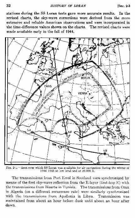
32 HISTORY OF LORAN [SEC.2.3

stations during the SS Loran tests gave more accurate results. In therevised charts, the sky-wave corrections were derived from the moreextensive and reliable American observations and were incorporated inthe time-difference values shown on the charts. The re,vised charts weremade available early in the fall of 1944.

FIG. 2.1.—Ai-ea over which SS Loran was available for air navigation during the winter of1944–1945 at low level md at 20,000ft.

The transmissions from Port Errol in Scotland were synchronized bymeans of the first sky-wave reflection from the E-layer (first-hop E) withthe transmissions from Bizerte in Tunisia. The transmissions from Ch-anin Algeria (on a different recurrence rate) were similarly synchronizedwith the transmissions from Apollonia in Libya. Transmission wasmaintained from about an hour before dusk until about an hour afterdawn.

SEC.23] EUROPEAN SKY- WAVE SYNCHRONIZED LORAN 33

Development of SS Loran Navigation.-The navigators were instructedto use only the first-hop E-reflections in making their time-differencemeasurements. The range of the first-hop E-reflection is limited by thecurvature of the earth and the height of the reflecting layer. It is foundto be approximately 1400 statute miles for low-flying aircraft and approxi-mately 1600 statute miles for planes flying above 20,000 ft. The coveragearea shown in Fig. 2“1 extends over a large portion of continental Europe.Over the Channel coast the signal from Apollonia was rather weak. Toimprove the signal in this area and to extend the coverage over theChannel and southern England, a station was eventually established atBrindisi on the heel of Italy to replace the one at Apollonia. However,it was never used tactically in operations against the enemy because thewar ended before the charts for the new system were available.

Trials made with the experimental SS Loran system in the UnitedStates and reports from the European SS ground transmitting andmonitoring stations indicated that the probable error in timing (the sumof errors due to variation of sky-wave transmission and equipment andpersonal errors in timing) amounted to about 8 psec, which correspondsto a probable positional error of 1 statute mile near the baseline and 1.6statute miles near the limit of the coverage area. Because of the timerequired to obtain a fix and the high speed of the planes, this accuracywas not realized in the air.

It was originally intended that a homing chain, consisting of threeStandard Loran stations should provide navigational information for air-craft returning to their home airfields and that Loran should be the onlynavigational system required. Unfortunately, the sites were chosen togive coverage over southeastern England at relatively high altitudes.The stations were too far apart to provide satisfactory signals at thealtitudes at which the planes were returning to their home fields (a fewthousand feet). Consequently, the homing chain was abandoned, andaircraft were equipped with both Gee and Loran. Gee was used forhoming and for short missions over the continent wherever Gee coverwas provided. Loran was used for night operations deep in enemyterritory beyond the range of the Gee stations.

The European SS Loran system was first used operationally by theRAF Bomber Command in October 1944. Because most of the opera-tions of this command were carried out at night and at rather long range,the SS Loran system was well suited to its needs. Ultimately all bombersin the command engaged in deep missions over enemy territory wereequipped with both Gee and Loran.

The largest group in Bomber Command was 5-Group, composed ofabout 350 Lancaster and 20 Mosquitoes. It was almost self-sufficient,as it had its own bomber force, flare force, pathfinders, and windfinders.

34 HISTORY OF LORAN [sm. 24

It had developed a method of vector bombing at night by the use oftarget-indicating flares. The main bomber force was preceded by ariumber of windfinding planes, a flare force, a “controller,” and one ormore of his deputies. The windfinding planes informed the rest of theforce of the direction and velocity of the winds along the route to aid themin their navigation and bombing. The controller directed the droppingof the target-indicating flares and, later on, the bombing of the target.Flying low and fast, usually in a Mosquito, he observed the location ofthe flares in relation to the target, selected one conveniently to windwardof the target (so that smoke of subsequent bombing would not obliteratethe flares), and directed the flare force to reinforce it. Then as the mainbomber force came in, he directed it to bomb the target-indicating flares,using a false wind vector such that the bombs would strike the targetrather than the target-indicating flares. He corrected any tendency ofthe bombing to drift away from the target by modifying the false-windvector. On nights of poor visibility, parachute flares were placed abovethe clouds and over the target by means of Gee, H2S, or Loran.

The Pathfinder Force, 8-Group, was composed of roughly 170 Lan-caster and 200 Mosquitoes. Its function was to lead the heavy bombersof other groups to the target and to mark the target by means of flares.The Mosquitoes also engaged in intruder operations and nuisance bomb-ing. All planes of this group were equipped with Loran and Gee. Seri-ous objection was raised to the use of a trailing antenna, especially withthe fast Mosquitoes, because it reduced the speed and maneuverability andhad a tendency to break off. A fixed antenna with coupling unit wasfinally developed that gave satisfactory results.

Early in February 1945, the Mosquitoes of 8-Group bombed Berlin.This nuisance bombing of Berlin continued almost every night until theend of the war. Loran was used for navigation and for bomb release.To obtain sufficient accuracy for bombing it was necessary to reduce thetime required to take a reading. The indicator was modified by theaddition of a second pair of time-difference controls in order to provideseparate controls for each of two recurrence rates. The pilot followed aLoran line passing over the target and released the bombs on crossing theproper Loran line on the other recurrence rate. Although no greataccuracy was claimed for the system, its users considered it highly effec-tive and a relatively simple, safe method of bombing.

2.4. Loran in the China-Burma-India Theater. Establishment ofthe Hump Triplets.—In the fall of 1943, a Loran system was proposed toprovide navigation over the Army Air Transport Command route fromIndia to China. The route at that time was a nonstop flight for anairline distance of less than 500 nautical miles over mountainous country

SEC. 2.4] LORAN IN THE CI?INA-BIJRMA-IN DIA TIIEA TER 35

with peaks up to 17,000 ft. The greater part of this distance was overenemy territory. In addition, the route wus plagued by seasons of veryhigh winds, monsoons with hmvy ruin, continual low overcast, numerousthunderstorms, and heavy prccipitut ion static.

This system, m originally conccivcd, consisted of a single pair ofstations at each end of the route, providing overlapping lines of positionnearly parallel to the line of flight. These were to guide the large numberof aircraft engaged in this operation without danger of collisions.

Lightweight, Air Tnmsportable equipment was designed rmd con-structed by Radiation Laboratory for four such stations. A prototypeinstallation was made in a mountainous section of California, flight-tested, and reported on by Headquarters, Army Air Forces, (.)ffice of theAir Communictitions Officer.

Eowever, theater operations did not permit straight-line routes butrather required a system providing navigational fixes. The plans were,therefore, amended to include a triplet on each side of the Hump.

Owing to the overland synchronism paths, the baseline lengths arelimited to roughly 50 to 75 nautical miles depending on the soil conduc-tivityy and the noise level.

Owing to poor coordination by the various AAF organizations in theUnited States the ground-station equipment did not reach the theateruntil August 1944.

Geographical coordinates for one station, Paya, as determined byaatro-observations were found to be in error by about 0.8 nautical miledue to the deflection from the vertical resulting from the near-by Himal-aya Mountains. The coordinates that proved to be correct were obtainedfrom the Survey of India charts. The need for highly accurate coor-dinates is especially great for short baseline systems. The ground-stationinstallations and operation were handled by the Fourth Army AirwaysCommunication System Wing, AAF.

The Assam Hump (India) triplet was tested and finally placed ino~eration in October 1944.

Flight tests and subsequent reports indicated a ground-wave rangeeaatward over the Hump of 280 to 300 statute miles during the daytimeand 200 to 250 miles at night. The daytime westward range over theflat lowland country is somewhat greater, with ranges of more than 400statute miles having been obtained. In this case the range was limitedonly by the receiver sensitivity and noise.

The system orientation fortunately provided coverage not only forthe northern direct Hump route in use when the system was conceivedbut also for the tactical areas of Myitkyina, Bhamo, etc., and the finalHump route via Myitkyina.

36 HISTORY OF LORAN [SEC.2.4

Approval of therequired air-hump tonnage (60 tons) for the tripleteast of the Hump was withheld by the China Theater Commander untilafter the successful testing of the Assam triplet.

The China triplet was placed on a 24-hr operating schedule on Mar.15, 1945.

Sky-wave Synchronized Pairs.—In addition to these two triplets com-prising the Hump system, the China and India-Burma Theaters’ Loranprogram quickly expanded to include the SS Inland China pair, the EastIndia Coast Standard triplet, the SS Burma pair, and the Chengtu triplet.A Radiation Laboratory representative was assigned as a technicalobserver to the Headquarters Fourth AACS Wing, AAF, India-BurmaTheater for the period June 1944 to March 1945, to assist in all phases ofthe Loran program.

An SS Loran pair was requested by the Twentieth Bomber Command,AAF, to provide line-of-position navigation over enemy-occupied Chinato the edge of the Japanese home island. Used in conjunction with theAPQ-15 high-altitude radar equipment, night navigation over this largearea was to be furnished.

As originally conceived, a station was to be located near Luchow,Kweichow, China, and the other near Paoning, Szechwan, Chha. Thkorientation placed the center line (perpendicular bisector of the baseline)directly through the southwestern Japanese home islands and gave abaseline length of about 480 nautical miles. It did not provide coverageover the home bases of the Twentieth Bomber Command near Chengtu,Szechwan, China, owing to the nearness of the northern station to thisarea. However, the loss of Luchow and all of the surrounding area to theJapanese forced a relocation of the system.

The slave station was combined with the southern slave station of theKunming Hump triplet chiefly to alleviate the Hump supply problem.The master station at Manchung, Szechwan, China, was sufficientlyremoved from the Chengtu area to provide homing coverage from thepair over this important area. This relocation of the pair provided auseful increase in the baseline length to about 605 nautical miles andplaced the center line toward Formosa, retracting the coverage towardJapan. Operation on this pair began Mar. 15, 1945, on a 24-hr-a-daybasis.

East India Coast System.—This system was requested by the RAF toprovide long-range navigation over the Bay of Bengal, the AndamanIslands, and Rangoon and by night to Bangkok and toward Singapore.The equipment was allotted by the Joint Chiefs of Staff to the AAF fromthe U.S. Navy. The siting, installation, and initial operation were theresponsibility of the Fourth AACS Wing, AAF. Operation was initiatedon Apr. 15, 1945.

This system was turned over to the Royal Air Force on July 1, 1945.

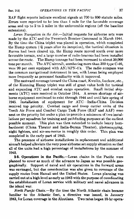
SEC.2.5] OPERA TIONS IN THE PACIFIC 37

RAF flight reports indicate excellent signals at 700 to 800 statute miles.Errors were reported to be less than 1 mile for the favorable coverageareas and up to 2 to 3 miles in the unfavorable regions (off the baselineextensions).

Loran Navigation in the Air. —Initial requests for airborne sets weremade by the ATC and the Twentieth Bomber Command in March 1944.By the time the China triplet was placed in operation, which completedthe Hump system (1+ years after its inception), the tactical situation inBurma had been cleared up, the Hump route moved south over morefavorable terrain, and a large number of radio beacons had been installedacross the route. The Hump tonnage had been increased to about 30,000tons per month. The ATC aircraft, numbering more than 300 type C-46,were 90 per cent equipped with AN/APN-4’s. The radio compass wasthe common navigational instrument in use, with Loran being employedmore frequently as personnel familiarity with it improved.

The eastward coverage toward the China coast, Kweilin, Luchow, etc.,of the Kunming Hump triplet was still of great value both for tacticaland expanding ATC and combat cargo operation. Small initial ship-ments (ATC) were received in October 1944. A severe shortage of air-borne equipment continued to exist through 1944 and until late spring of1945. Installation of equipment for ATC—India-China Divisionreceived top priority. Combat cargo and troop carrier units of theTenth Air Force and Combat Cargo Task Force (RAF and AAF) werenext on the priority list under a plan to provide a minimum of two instal-lations per squadron for training and pathfinding purposes at the earliestpossible moment. This plan was then extended to include heavy bom-bardment (China Theater and India-Burma Theater), photomapping,night fighters, and air-sea-rescue in roughly this order. This plan wascompleted in the early part of 1945.

The presence of airborne installations in replacement and additionalaircraft helped alleviate the very poor airborne set supply situation so thatall of the units had a high percentage of installations by the summer of1945.

2.6. Operations in the Pacific.-Loran chains in the Pacific wereplanned to cover as much of the advance to Japan as was possible geo-graphically. Support of naval and air operations in the forward areaswas envisaged, but due consideration was also given to coverage of thesupply routes from Hawaii and the United States. Loran planning wascarried out at a high level as early as 1943 with the purpose of coordinatingthe establishment of Loran service with military and naval advances inthe island war.

North PM”@ Chuin.-By the time the North Atlantic chain becamefamiliar to the Atlantic fleet, a directive was issued, in January1943, for Loran coverage in the Aleutians. Two rates began 104w opera-

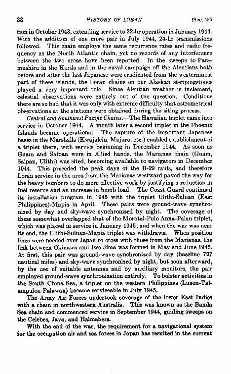
38 HISTORY OF LORAN [SEC.2.5

tion in October 1943, extending service to 22-hr operation in January 1944.With the addition of one more pair in July 1944, 24-hr transmissionsfollowed. This chain employs the same recurrence rates and radio fre-quency as the North Atlantic chain, yet no records of any interferencebetween the two areas have been reported. In the sweeps to Para-mushiru in the Kurils and in the naval campaign off the Aleutians bothbefore and after the last Japanese were eradicated from the westernmostpart of these islands, the Loran chairis on our Alaskan steppingstonesplayed a very important role. Since Aleutian weather is inclement,celestial observations were entirely out of the question. Conditionsthere are so bad that it was only with extreme difficulty that astrometricalobservations at the stations were obtained during the siting process.

Central and Southwest Pacijic Chains.—The Hawaiian triplet came intoservice in October 1944. A month later a second triplet in the PhoenixIslands became operational. The capture of the important Japanesebases in the Marshalls (Kwajalein, Majuro, etc.) enabled establishment ofa triplet there, with service beginning in December 1944. As soon asGuam and Saipan were in Allied hands, the Marianas chain (Guam,Saipan, Ulithi) was sited, becoming available to navigators in December1944. This preceded the peak days of the B-29 raids, and thereforeLoran service in the area from the Marianas westward paved the way forthe heavy bombers to do more effective work by justifying a reduction infuel reserve and an increase in bomb load. The Coast Guard continuedits installation program in 1945 with the triplet Ulithi-Suluan (EastPhilippines) -Mapia in April. These pairs were ground-wave synchro-nized by day and sky-wave synchronized by night. The coverage ofthese somewhat overlapped that of the Morotai-Pulo Anna-Palau triplet,which was placed in service in January 1945; and when the war was nearits end, the Ulithi-Suluan-Mapia triplet was withdrawn. When positionlines were needed over Japan to cross with those from the Marianas, thelink between Okinawa and Iwo Jima was formed in May and June 1945.At first, this pair was ground-wave synchronized by day (baseline 727nautical miles) and sky-wave synchronized by night, but soon afterward,by the use of suitable antennas and by auxiliary monitors, the pairemployed ground-wave synchronization entirely. To bolster activities inthe South China Sea, a triplet on the western Philippines (Luzon-Tal-ampulon-Palawan) became serviceable in July 1945.

The Army Air Forces undertook coverage of the lower Eaat Indieswith a chain in northwestern Australia. This waa known as the BandaSea chain and commenced service in September 1944, guiding sweeps onthe Celebes, Java, and Halmahera.

With the end of the war, the requirement for a navigational systemfor the occupation air and sea forces in Japan has resulted in the current

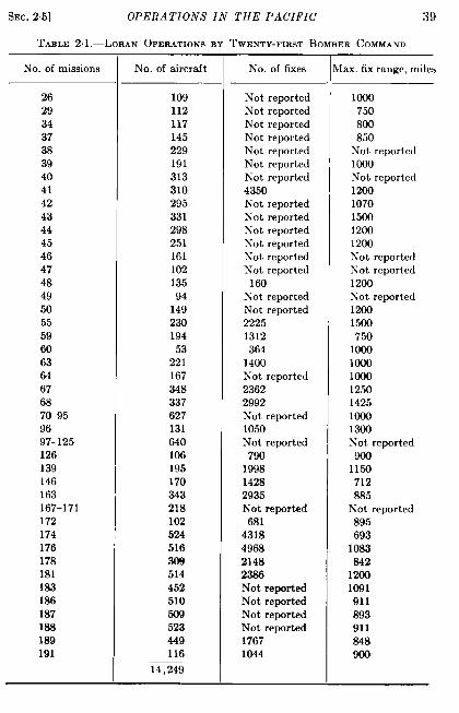
SEC.25] OPERATIONS IN THE PACIFIC 39

TABLE2.1.—LoRANOPERATIONSBY TWENTY-FIRSTBOMEERCOMMAND

No. of missions

2629343738394041424344454647484950555960636467687W959697-125126139146163167-171172174176178181183186187188189191

No. of aircraft

10911211714522919131331029533129825116110213594

14923019453

221167348337627131640106195170343218102524516309514452510m523449116

14,249

No. of fixes

Not reportedNot reportedNot reportedNot reportedNot reportedNot reportedN’otreported4350Not reportedh-et reportedh-et reportedNot reportedNot reportedNot reported160

Not reportedNTotreported22251312364

1400Not reported23622992Not reported1050Not reported790

199814282935h’ot reported681

4318496821482386Not reportedNot reportedNot reportedNot reported1767104-4

vlax.fixrange,miles

1000750800850

Not reported1000Not reported12001070150012001200h-et reportedNot reported1200Not reported12001500750

1000100010001250142510001300Sot reported900

1150712885

Not reported895693

1063842

12001091911893911848900

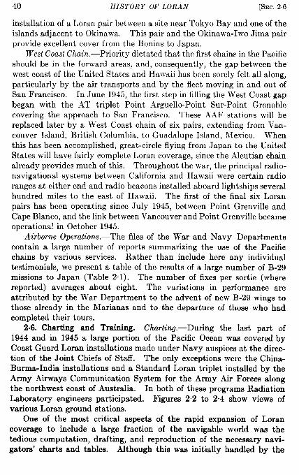
40 HISTORY OF LORAN [SEC,26

installation of a Loran pair between a site near Tokyo Bay and one of theislands adjacent to Okinawa. This pair and the Okinawa-Iwo Jima pairprovide excellent cover from the Bonins to Japan.

West Coast Chain. —Priority dictated that the first chains in the Pacificshould be in the forward areas, and, consequently, the gap between thewest coast of the United States and Hawaii has been sorely felt all along,particularly by the air transports and by the fleet moving in and out ofSan Francisco. In June 1945, the first step in filling the West Coast gapbegan with the AT triplet Point Arguello-Point Sur-Point Grenoblecovering the approach to San Francisco. These AAF stations will bereplaced later by a West Coast chain of six pairs, extending from Van-couver Island, British Columbia, to Guadalupe Island, Mexico. Whenthis has been accomplished, great-circle flying from Japan to the UnitedStates will have fairly complete Loran coverage, since the Aleutian chainalready provides much of this. Throughout the war, the principal radio-navigational systems between California and Hawaii were certain radioranges at either end and radio beacons installed aboard lightships severalhundred miles to the east of Hawaii. The first of the final six Loranpairs has been operating since July 1945, bet ween Point Grenville andCape Blanco, and the link between Vancouver and Point Grenville becameoperationa! in October 1945.

Airborne Operations.—The files of the War and Navy Departmentscontain a large number of reports summarizing the use of the Pacificchains by various services. Rather than include here any individualtestimonials, we present a table of the results of a large number of B-29missions to Japan (Table 2.1). The number of fixes per sortie (wherereported) averages about eight. The variations in performance areattributed by the War Department to the advent of new B-29 wings tothose already in the Marianas and to the departure of those who hadcompleted their tours.

2.6. Charting and Training. Chartz%g—During the last part of1944 and in 1945 a large portion of the Pacific Ocean was covered byCoast Guard Loran installations made under Navy auspices at the direc-tion of the Joint Chiefs of Staff. The only exceptions were the China-Burma-India installations and a Standard Loran triplet installed by theArmy Airways Communication System for the Army Air Forces alongthe northwest coast of Australia. In both of these programs RadiationLaboratory engineers participated. Figures 2.2 to 2.4 show views ofvarious Loran ground stationa.

One of the most critical aspects of the rapid expansion of Lorancoverage to include a large fraction of the navigable world was thetedious computation, drafting, and reproduction of the necessary navi-gators’ charts and tables. Although this was initially handled by the

SEC.2.6] CIIARTING AND 1’RAINING 41

Radiation Laboratory group, the Hydrographic Office of the Navy pre-pared to assume this responsibility during the latter part of 1942. Toensure minimum delay in this undertaking, F. G. Watson, who wasresponsible for the original work, resigned from the Radiation Labora-tory, accepted a Navy commission, and departed for Washington toassist in setting up a suitable Loran section. Since its inception, thatdepartment has produced a total of 2+ million copies of well ~ver a

FIG.2.2.—Atypicalgroundstation. Buildingto theleft containsequipment;thoseinthebackgroundarequartere. The Winchargertowerieat the right. (C’oI.WteqJo~U.S.CoautGuard.)

hundred different charts covering over 60 million square miles of theearth’s surface. During April 1945 alone, 230,482 Loran charts weredistributed to all services. These charts have been produced both inthis country and at certain forward bases where suitable facilities wereinstalled. The detailed history of the Hydrographic Office chartingactivity is given in Appendix A. The Royal Air Force and the Ml?also produced a number of Loran charts for inland areas in which theNavy had little interest.

Traini~ of Ground-station Operators.-During late September andearly October 1942, after the experience gained from putting the Canadianstations in operation, a series of talks was given at the Radiation Labowtory, summarizing for the technical staff of the Loran Division all theinformation then known and of value to the system. Up to this pointonly a few Royal Canadian Navy personnel had received a sketchy train-ing at the Montauk and Fenwick field stations and in the Laborato~

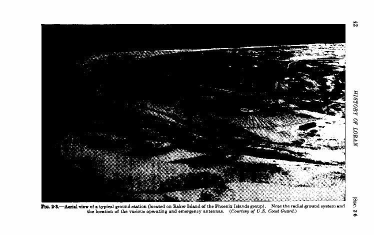
42H

ISTO

RY

OF

LO

RA

N[s1lC

.2.6

-ga‘i

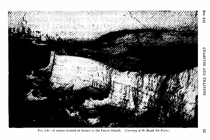
SEC

.2.6]

CH

AR

TIN

GA

ND

TR

AIN

ING

43

44 HISTORY OF LORAN [SEC.2.6

mth a view toward fitting them for their duties in operating and main-taining the Baccaro and Deming stations. The Laboratory instructionwas available to officers and enlisted men of the Navy who were attachedto the Loran Division as well as to an RCN group who had been sent fortraining. From the former group there evolved the Boston Loran Train-ing School, operated by the Coast Guard, which in turn prepared Navy,Army, and Allied officers and men for operation of equipment and theeventual establishment of other training centers. Close liaison was pos-sible between the Laboratory and the Coast Guard school until its laterremoval to Groton, Corm. Its debt to the Laboratory was repaid manytimes over by the pretraining of several groups, who were then sent toCambridge for special training. Part of the success of the Groton schoollay in the fact that a large number of its later instructors had actuallyoperated stations of the Atlantic chain and in the Aleutians.

Whenever possible, the men were given an opportunity to visit andoperate a field station employing equipment or techniques that they hadbeen studying. Occasionally, it was possible to operate prototype equip-ment in the Laboratory; and in a few instances men were allowed to helpbuild some of the gear that they later employed.

The Air Transportable Loran project involved the need for a quick,accurate means of charting the area to be served and the developmentof a rapid technique for printing many hundreds of maps in a short time.The charting requirement was finally solved so well that relativelyinexperienced men with high-schooi education could plot Loran coordi-nates on a tracing from a standard Army map. The process of deter-mining coordinates was considerably aided by the development of somestandard printed forms. The printing method best adapted to the par-ticular military requirements was the photostat process, although a silk-screen method or offset lithography might have served other requirementsmuch better.

The important task of producing instruction books and manuals wasnot undertaken until early in 1943 and even then on a rather informalbasis. Almost concurrent with the organization of a Sky-wave Synchro-mzed Loran school, the importance and magnitude of this branch ofinstruction became apparent, and a small subgroup was formed. ThisManual subgroup acted as a clearing house for information, maintainedactive liaison between the engineers and the Navy and Army, and fur-nished drawings and text to manufacturers under contract for Loranequipment developed by the Laboratory. All the earlier manuals wereissued through the Navy Liaison Officer for Loran, because the Navywas the principal user of the system. At a later date, when demandsfor printed material began to arrive from diversified sources, all material,except that printed at Navy request, was distributed through theDocument Office.

Ssc. 2.6] CHARTING AND TRAINING 45

Whereas Loran system operation wastheresponsibility of the Chiefof Naval Operations, training of Navy pemonnel in manipulation andmaintenance of shipboard Loran equipment was under the direction ofthe Bureau of Personnel. Airborne Loran training was kept within thejurisdiction of the Bureau of Aeronautics. Since construction and oper-ation of Navy Loran stations was delegated to the Coast Guard, thatagency conducted its own ground-station training program.

The Coast Guard, as operating agency for the U.S. Navy, constructed,installed, and ran the Loran stations that were under the cognizance ofthe Chief of Naval Operations. Its association with Loran began in1942, shortly after the Radiation Laboratory had conducted field trialson the first pair of synchronized stations. With the aid of the Labora-tory, the Coast Guard inaugurated a training program on ground-stationequipment at a naval Loran school in Boston. Enough men were trainedso that the stations referred to could be taken over by the Coast Guardin January 1943 and so that entire complements of personnel could beengaged in the erection of stations in the far north. When the Bostonschool was disbanded at a much later date, the Coast Guard removed itsground-training program to Groton, Corm., not far from the Academy atNew London. The basic electronics training at the Academy includedinstruction on many of the fundamental circuit arrangements found inLoran. Those completing the course who were going to work on Loranwere transferred to Grot on, Corm., to receive information on timers,transmitters, antennas, and monitors. Typical monitoring was demon-strated at Groton, and trainees were required to put in a short residenceat one of the near-by Loran stations. Officers and enlisted technicianswere given about five weeks of training, and operators received three-week %aining. The courses given were so comprehensive that otherservices such as the AACS, the RCN, and the Royal Navy sent traineesthrough this school rather than establishing formal schools of their own.

Training of Shipboard Navigators.—In the early days of Loran, allNavy and Coast Guard training was concentrated in the one school inBoston, Mass., which was organized by the Naval Liaison Officer forLoran at Radiation Laboratory, the Naval officer in charge at Massa-chusetts Institute of Technology, and the District Coast Guard Officer.During the introduction of Loran in the Aleutians in the latter part of1943, a school for navigators was established at Adak, Alaska. Progresswas slow at first, since the instructors were mainly self-taught and equip-ment was scarce. However, the Loran program expanded rapidly, andthis school became inadequate because of the geographical distributionof Loran chains and personnel. In February 1944, the Bureau of Per-sonnel established Loran schools at the following naval bases: Boston,New York, Philadelphia, Charleston, Norfolk, New Orleans, and CascoBay. Later schools were set up at Treasure Island (San Francisco),

46 HISTORY OF LORAN [SEC.2.6

Chicago, and Pearl Harbor. Here navigators and interested quarter-masters of the fleets were trained in shipboard Loran manipulation. Acomprehensive 4-day course was given, because the amount of shore timeavailable to personnel was seldom more than this. Liberal supplies ofmanuals and notes were made available to these men at the conclusionof the course so that they could continue to study while at sea. Althoughthe formal instruction was rather short, its quality was high, for the reli-ance placed on Loran by the members of the fleet is shown in the reportsthat are in the files of the Chief of Naval Operations and the HydrI+graphic Office.

Technicians also were trained at the bases listed above. In general,it waa the Navy policy to make all radar mechanics familiar with Loranship equipment and its circuits.

Navy Training of Air Navigators.-The Bureau of Aeronautics formedthe Airborne Coordinating Group, ACG, early in the war. Civilianradar technicians were sent into all theaters where naval aviation wasplaying its part, and they acted as trouble-shooters, instructors, andadvisers with respect to the many radar equipments in service. Thesemen made their reports to the Naval Research Laboratories, which inturn published their comments for general distribution. Loran was oneof the systems with which the ACG fieldmen were concerned. An officialjournal, the Digest, was published by the Bureau of Aeronautics andserved as a medium for passing the latest information concerning air-borne equipment to these men and to other interested services. Manyvaluable suggestions and advance information on airborne Loran werecontained in this journal.

The Hydrographic Office established an informal “ clinic” at the NewYork project office (where computations for Loran charts were per-formed). Navigators were invited there to discuss their results and toleave copies of their logs for analysis. Recommendations were thuseasily made on the spot for improved use of the equipment and thesystem.

The Bureau of Aeronautics combined a good deal of its Loran workwith Link trainer instruction at its Air Navigation training units, whichwere found at the major air-training bases. This bureau also issued somevery valuable booklets on Loran operation, and these were disseminatedwidely. In October 1944, the Bureau of Aeronautics sponsored a Loranresearch flight through the North Atlantic with participants from manybranches of the Naval Service and from the AAF. A thorough study ofthe service available from each Loran pair was made, and many usefulphotographs of “signals were included in the report.

The Navy issued several Loran films for the instruction of both shipand air navigators that were widely distributed to all the services using

SEC.2.6] CHARTING AND TRAINING 47

Loran. A helpful series of 35-mm slides supplemented the films and wereparticularly valuable for instmction of mechanics.

Traini~ in the RAF.—The introduction of Loran to the RAF actuallybegan in the United States in 1943 when a number of officers and enlistedmen were trained by the Radiation Laboratory in SS Loran and took partin the operation of the test system. Of this group, one officer and twoenlisted men later were instrumental in establishing a school in Loran formechanics of Bomber Command; another officer carried through theinitial instruction of navigators and mechanics at various Coastal Com-mand bases; still a third officer directed the ground-station operationsand training for 60-Group, the group primarily responsible for groundnavigational equipment. Ground-station training was carried out atthe station sites in the United Kingdom and Africa, and a large numberof mechanics and WAAF operators soon became proficient in the system.By the spring of 1944 the technical standards at the RAF stations werehigh.

Coastal Command, using the North Atlantic chain in its U-boatcampaign, relied on a traveling team of instructor and mechanic duringits installation program in early 1944. It also encouraged the exchangeof information among Loran-fitted squadrons. Later, a special Lorantraining unit was established by the Command in northern Ireland,offering a 2-weeks course in the subject and giving several training flightsin the ground- and sky-wave coverage. An advantage here was thatinstruction was carried out in the same area where the trainees were laterto use the system operationally. Coastal Command placed great empha-sis on Loran, for much of their flying was at low altitudes and at latitudeswhere the weather was generally inclement. Early training was given tothe meteorological squadrons so that the accuracy of their importantweather information could be improved.

When the Bomber Command fitting program began in the fall of1944, small groups of navigators were being trained by Bomber CommandDevelopment Unit, which conducted Service trials on equipment designedfor the Command. As this was insufficient to meet the initial demandsof one of the groups of the Command that was engaged in extensive nightraids on the Continent, hundreds of navigators, pilots, and bomb aimerswere introduced to Loran by lectures given by Loran experts of theBritish branch of the Radiation Laboratory. These lectures wereenhanced by USN films and slides. Later on, facilities of BomberDevelopment Unit were enlarged.

When SS Loran became operational, it was evident that the Serviceplan for training of navigators was seriously behind schedule, and inade-quate. Men of the British branch of the Radiation Laboratory wereinstrumental in conducting classes with small groups of navigators in one

18 HISTORY OF LORAN [SEC.2-6

of the Eighth U.S. Air Force bomb groups. These navigators becamefamiliar with Loran both in regard to the use of North Atlantic Loran formeteorological squadrons and in regard to SS Loran for night reconnais-sance over the Continent. The navigators of this bomb group served asa nucleus for U.S. Air Force navigator training on Loran in the UnitedKingdom, since Loran training was included as prerequisite for redeploy-ment of the Eighth Air Force to the Paci6c Theater.

As soon as the RAF 5-Group of Bomber Command made known theirintention of equipping the entire force of 250 to 300 planes for SS Loranoperation, and when it was apparent that any school established at thattime would be insufficient to meet demands of this group for immediateoperation, men of the. British branch of the Radiation Laboratory cir-culated among airdromes of 5-Group and instructed large classes of pilots,navigators, and bomb aimers. This instruction was necessarily abbre-viated because of the size of classes and was therefore augmented byspecial training films and slides. The British branch also produced somewritten material on SS Loran and its peculiarities that was widely dis-tributed among the groups of Bomber Command. Although this processwas hasty, it was fairly effective, for most of the RAF navigators werewell acquainted with hyperbolic navigation through their use of Gee.In the over-all training picture, a fair share of the burden of indoctrinationwas carried by members of the Telecommunications Research Establish-ment, TRE, the British organization responsible for radar and hyperbolicsystems. Most of the RAF navigators were very conscientious in theirinterest and took advantage of their frequent raids over the Continentto learn through using; as a result there was very soon a large number offairly skilled Loran navigators.

Army Air Force Training. —Navigators of the AAF relied at first uponfacilities offered by the USN and Coast Guard for training. AS Loranchains appeared in the theaters and as airborne equipment became avail-able, schools were established with varying degrees of success. Rarelywere these schools ahead of the actual operation of the neighboring Loranchain, and thus in many cases service to navigators was available beforethey had been adequately trained. The !~,ck of familiarity of the averageAAF navigator with hyperbolic-navigation systems or for that matteranything different from a homing beacon or radio range made it generallydifficult to introduce this new type of navigation with the degree ofsuccess attendant upon the introduction of Loran to the RAF navigators,who were already well versed in Gee.

It was not until the latter part of 1944 that the Air Transport Com-mand had an appreciable number of navigators availing themselves ofLoran service in the Atlantic or the Pacific. The ATC Loran Schoo] atWilmington, Del., organized early in 1944, had trained about 700 person-

SEC.2.7] SERVICE AREAS 49

nel in 1944 and a total of 1682 by August 1945. Of these, 235 werecommercial air-line navigators who were members of contract carriercrews, flying military aircraft. Two mobile training units were formedby ‘this school, one of which toured airfields in the United States, whereasthe other toured several theaters.

As the flow of B-29’s and B-24’s increased to the Pacific, the continen-tal air forces assumed a larger share of the burden of training air crews.Consequently, Loran instruction in the latter part of the war was includedin all the major air-navigation schools of the AAF. Training flightswere carried on in the area served by part of the North Atlantic chain,and in 1945 a Gulf Coast and a West Coast triplet simplified the trainingof B-29 navigators. Although no formal training ever took place atGuam and Saipan, a certain amount of spot-training and briefing byLoran officers did take place there.

2,7. Service Areas. -Loran operation began on the East Coast of theUnited States simply because the system was developed there and a pairof trial stations already existed. The expansion up the coast of NorthAmerica was natural and desirable, because the Atlantic convoy routewas subject to adverse weather and the rendezvous problem was acute.

Even before the completion of the Atlantic chain by the installationof stations north of the United Kingdom, the need for Loran service inthe Aleutian Islands was recognized and satisfied. At this time, early1944, a chart of the area served by Loran bore a striking resemblance to adiagram showing the parts of the world subject to mean annual cloudinessoi 0.7 or more. This was no coincidence.

The operation of the SS I.oran system in Europe and extensive instal-lations in the Pacific, China, and India extended the nighttime serviceover two great areas. With the installation of stations on the Gulf ofMexico and California coasts (primarily to provide actual signals forairborne training of navigators) the gap between these areas has beenclosed. At night the service area is, as shown in Fig. 2.5, a belt extending320° in longitude with a width varying from about 10° of latitude in thewestern United States to about 100° in tbe central Pacific Ocean. Thestations that providrn this service are listed in Appendix B. The totalarea served by Aug. 15, 1945, was about 63 million square miles, or 32 percent of the area of the earth.

In the daytime the service area is far smaller, about 15 million squaremiles. Although it is possible by day to fly the northern route betweenthe LTnited States and the United Kingdom without losing Loran cover,the areas in the Pacific are not contiguous and serve only as essentially“ local” approach systems of 700-mile radius centered in the variousisland groups. There is no significant daytime I,oran service over iand,except for the traffic guidance system over the Hump in Burma.

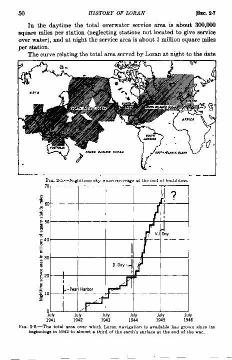
50 HISTORY OF LORAN -.2.7

In the daytime the total overwater service area is about 300,000square miles per station (neglecting stations not located to give serviceover water), and at night the service area is about 1 million square milesper station.

The curve relating the total area served by Loran at night to the date

-T-% k 71

-v) SOUr#●AOIFIO00#A# r -auancoc.am w

. . .

Fm. 25,-Nighttime sky-wave coverage at the end of hostilities.70

g f?“=60 1~~% I!?50 -

: -13 V-JDayg 40._9-.E I /:30 I

g D-Day$

I 1? 20% IE PearI Harborg 10z I a

/

o /July July July July July July1941 1942 1943 1944 1945 1946

Fro. 2.6.—Thetotal areaover whichLorannavigationis availablehas grownsinceitabeginningsin 1942to almoata thirdof theearth’ssurface at the end of the war.

$EC. 2,7] SERVICE AREAS al

is unusually interesting. It isshown in Fig. 2.6. The diagram beginsat July 1, 1941, because, as explained in Sec. 2.1, that may be regardedas the first date in the full scale development of Loran. For a year, testswere made and equipment was developed. Then, in July 1942, the firstdemonstrations were given, and NDRC agreed to begin the installationof operational stations. The program went forward for two years afterthat at the modest rate of 10 million square miles per year. This paceseems to have been determined primarily by the rate at which procure-ment of transmitting equipment was had through NDRC. Anotherlimiting factor was that installation of the system in each new area hadto be sold to the potential users who, of course, could not assess the poten-tial merit of the system because it was entirely new to them.

By July 1944, however, Naval procurement of transmitting equipmentwas in effect, and the system had won general acceptance. Thereafterinstallations proceeded at a rate commensurate with the enhanced pro-curement program, or about 40 million square miles per year. This ratepersisted to the end of the war.

The current (November 1945) area served at night is believed to beabout 70 million square miles. It is difficult to justify this figure, how-ever. A number of new installations are being pushed forward, as theyhave been since August 1945, but some pairs, which had only militarysignificance, have already been discontinued. The degree of acceptanceof the Loran system for peacetime military and civil use is not at allcertain. At this date, therefore, it is believed that the question markadequately expresses the current and future coverage.

&G. & & LIBRARYI-As VEGAS BRANCH

CHAPTER 3

PRINCIPLES OF LOWiN

BY B. W. SITTERLY

3.1. Time Differences and Lines of Position. Fundamental Relations.The primary fact upon which Loran is based is that the transmission timetaken by a radio pulse to travel over a distance measures the distance.The pulse travels 983.24 ft, or 0.18622 statute miles, or 0.16171 nauticalmiles, or 0.299692 km, in one microsecond (millionth of a second; abbre-viation, psec), The pulse takes 5.3700 psec to travel 1 statute mile,6.1838 psec to travel 1 nautical mile, 3.33676 /see to travel 1 km.Convenient approximations to these relations are 8 statute miles = 43psec; 5 nautical miles = 31 psec; 3 km = 10 psec. It is advantageous touse 983.24 ft as a unit of length in Loran computations; this unit may becalled a light-microsecond or simply a microsecond. In this unit, dis-tance is numerically equal to transmission time.

If a pair of Loran transmitters A and B were to emit pulses simul-taneously, a navigator eq~lally distant from A and B would receive themsimultaneously, but a navigator not equally distant from A and B wouldreceive the pulse from the farther station later than tl’at from the nearer.The time diflemnce measured by the na~-igator from one pulse to the otherwould be numerically equal to the difference between the distancestraveled by the pulses, measured in light-microseconds, or in form of anequation,

t= z!, (1)

where t is time difference and o is difference of light-microseconds. Ifstation B ~vere farther, its pulse would be received later than .4’s pulse;if nearer, earlier. The two cases may be distinguished formally by mak-ing f and Lpositive in the former case, negative in the latter. In observa-tion, however, it is not possible to determine the sign, for pulses fromdifferent Standard Loran stations are exactly alike.

In order to resolve the ambiguity in practice, the pulses are emitted,not simultaneously, but alternately, from the two stations. The intervalfrom the emission of a pulse from A to the emission of the next pulse fromB is called the absolute delay and denoted by D. As the pulses are receivedby the navigator, the time difference t is greater or less than D by thesame amount that B is farther or nearer than .4 (in light-microseconds).

52

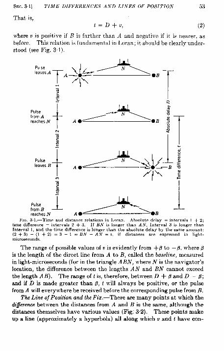
SEC.31] TIME DIFFERENCES AND LINES OF POSITION 53

That is,t= D+u, (2)

where v is positive if 1? is farther than A and negative if it is nearer, asbefore. This relation is fundamental in Loran; it should be clearly under-stood (see Fig. 3.1).

uPulseleavesA

~

A>!&/ N \● B

t p

z?~ T=

Pulsefrom Areaches N

+w-6z~=

Pukeleaves B

+

&~

Pulsefrom B 1reaches N

FIG, 3.1.—Time and distance relations in Loran, Absolute delay = intervals 1 + 2;time difference = interwds 2 + 3. If BN is longer than AN, Interval 3 is longer thanInterval 1, and the time difference is longer than the absolute delay by the same amount:(~ + 3) – (1 + 2) = 3 _ 1 = BN – A.v = ~, if distances are expressed in light.microseconds.

The range of possible values of u is evidently from +@ to – ~, where Bis the length of the direct line from A to B, called the baseline, measuredin light-microseconds (for in the triangle ABN, where N is the navigator’slocation, the difference between the lengths AN and BN cannot exceedthe length AB). The range oft is, therefore, between D + B and D – B;and if D is made greater than P, twill always be positive, or the pulsefrom A will everywhere be received before the corresponding pulse from B.

The Line oj Position and the Fiz.—There are many points at which thediffererwebetween the distances from A and B is the same, although thedistances themselves have various values (Fig: 3.2). These points makeup a line (approximately a hyperbola) all along which v and thave con-

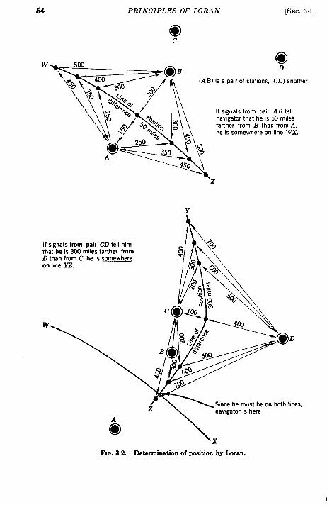
PRINCIPLES OF LORAN [SEC.3.1

c

,., .,-”1

.4”< “/“(AB) Is a pair of stations, (CD) another

o %e OF

~~

G+.@/-e

~ ~ce If signals from pair AB tell0 g nawgatorthat he ls50 miles

$+:, ~ farther from B thafi from A,

/a. D he!ssomewhere onllne WX.

Ifsignals from pair Clltell himthat heis300mlles farfher fromD than from C, he is somewhereonline YZ,

Fm.3.2.—Datemninationof position byhran.

SEC.3.1] TIME DIFFERENCES AND LINES OF POSITION 55

stant values. To every possible value of v or t there corresponds one ofthese lines of position, passing between A and B and slightly concavetoward the nearer of them. All the lines makeup a family, generated bythe two stations. An observer, measuring a certain value oft, can deducewhich of these lines he is on but not where he is on it.

To locate himself definitely, the observer must also measure the timedifference between the pulses emitted by a second pair of stations. Thispair generates a second family of lines of position, which intersect thefirst family. Every intersection represents a pair of measured timedifferences (one from each pair of stations) and defines a point that is thelocation or fix of the navigator who made the measurements. Conversely,two pairs of stations are required to provide a navigator with a fix. Thisdoes not necessarily mean four stations, for three stations may operateso that one of them forms a pair with each of the others. So arranged,the stations make up a Loran triplet. Four or more stations may similarlyform three or more pairs, every station except the end ones being commonto two adjacent pairs; this is called a Loran chain. In some situations,four stations operating as two pairs, with their baselines crossed nearlyat right angles, form an advantageous configuration; this is a Loranquadrilateral.

Since the locations of Loran lines of position depend only upon thepositions of the stations generating them, the lines are fixed on the surfaceof the earth. It is a task to calculate their course (see Chap. 6), but thecalculation may be made once for all, and the lines printed on charts andlabeled with the appropriate values of the tme difference. Any twointersecting families will then form a Loran coordinate system, as definiteas the geographical system of latitude and longitude and independent ofit. The navigator, having read two time differences, need find only theintersection of the two corresponding lines on his chart to locate his posi-tion without any computation. Three or more intersecting Loranfamilies will afford a check or double check on position, like three or morestar sights in celestial navigation.

Numerical Values of fl, D, and Other Quantities.—The value of L?,theelectrical length from A to B, is limited by the fact that the stations keepto their correct time relation by receiving each other’s pulses and bymaintaining constant time differences between the received and emittedpulses. To do this, the stations must be near enough together so thateach receives the other’s pulses clearly. The nature of the surface overwhich the pulses pass and the level of atmospheric electrical ‘‘ noise”prevalent in the region of operation, as well as the power and radio fre-quency of transmi~ion, are the factors controlling the practicable separa-tion of stations. At this writing (January 1946), all regularly operatingLoran transmitters employ radio frequencies between 1700 and 2000

56 PRINCIPLES OF LORAN [SEC,31

kclsec. This range of frequencies constitutes the Standard Loran band.The pulse power radiated at the transmitting antenna is normally about100 kw, and under average conditions the pulses will carry over water toa distance of 400 or 500 nautical miles with 24-hr reliability and sufficientstrength to enable two stations at that separation to hold to their timing.In fact, one pair (Labrador-Greenland) operates over a baseline of 590nautical miles. To obtain a wide area over which both stations of thepair can be received, however, the baseline should be considerably shorterthan the maximum range. Three hundred nautical miles (1855 ~sec)has been found to be about the optimum baseline length for effectivecoverage. Stations separated by land must be much closer togetherbecause with Standard Loran frequencies the low conductivity of soiland rock greatly reduces the range. An overland baseline of 100 nauticalmiles (618 psec) is about the longest practicable.

A Loran network operable only by night was employed in the strategicbombing of Germany, with baselines 1130 and 1300 nautical miles long(6980 and 8050 psec). These great separations were obtained by the useof sky-wave transmission of pulses (see Sec. 3 ‘2) between stations, atsome sacrifice of precision and reliability, and with complete interruptionof service during the day.

Trials of a Low Frequency Loran triplet, transmitting on 180 kc/seewith peak radiated power near 100 kw, are in progress. Data so farobtained indicate that reliable continuous operation can be maintainedeven in the tropics with 600 miles of water separating the stations. If thebaseline is principally over land, the distance should probably not exceed400 miles.

The value of D, the absolute delay, is dictated by the form of thereceiving and measuring apparatus (the Loran ~eceiver-indicator). Thisapparatus displays the received pulses as vertical deflections of a horizon-tal line or trace that appears on the face of an oscilloscope screen. Thistrace is the path of a light spot sweeping from left to right across thescreen, then snapping back and sweeping again. The spot sweeps acrossmany times in a second so that the trace is steadily visible and does notflicker.

During each sweep of the light spot across the screen, electricalimp&es from a crystal clock are impressed upon the moving light spot,producing time markers on the trace. The position of a received pulseamong these markers indicates the interval between the beginning of thesweep and the time at which the pulse arrived. If the pulse and thesweep are made to recur exactly the same number of times per second,successive pulses wilf always appear at the same place on the trace,persisting as a single stationary mark whose time maybe accurately read.To efiect this, each transmitting station aends out its pulses in a steady,

SEC.3.1] TIME DIFFERENCES AND LINES OF POSITIO:V 57

equally spaced succession; the number of pulses per second is called thepulse recurrence ra~e,PRR. The time interval between successive pulsesfrom the same station is called the recurrence period, L. The indicatorsweep is adjusted to recur at exactly the recurrence rate of the stations.In present Loran systems, t~vo basic recurrence rates are used; 25 persecond (low rate) and 33+ per second (high rate). Corresponding valuesof L are 40,000 and 30,000 psec.

The time sequence of pulses, as alternately erni~tedfrom a pair ofstations, is ABAB . The interval between successive A‘s or suc-cessive B’s is L. The transmission interval All is the absolute delayD, which must therefore be less than ],. The time sequence of pulses asreceived is also ABA B . . . , and the interval between successive A‘s orB’s is L, but the reception interval AB is the time difference t, whichvaries with the location of the navigator, between the values D + @ andD–/3.

In order that no ambiguity may occur in identifying pulses on thescreen of the indicator, D is made of such length that All as received willalways be greater than (L/2) and less than L, which }vill make All every-where longer than BA. This will be true if

where 6 is some arbitrary time interval, less than (L/2) — 2@. That is,

which is the equation defining the value of D for a particular pair ofstations. Then the fundamental relation t = D + v becomes

(3)

and t ranges from (L/2) + 6 to (L/2) + (2P + 6).With p usually 3000 psec or less, and L/2 15,000 or 20,000 ysec, there

is a wide choice of 6. In Standard Loran systems it has hitherto been1000 or 2000 psec, but other values may be used with installations nowbeing set up. For purposes of security in war time, 6 may be changedfrom time to time, and consequently only those having knowledge of thechanges can interpret Loran readings correctly. For this reason ~ iscalled the coding delay.

It is not difficult to visualize these relations spatially. All pointsthat are receiving a pulse at a given instant lie upon a circle, the centerof which is the station that emitted the pulse. This circle expands withthe speed of radio transmission, 0.16171 nautical mile per microsecond.

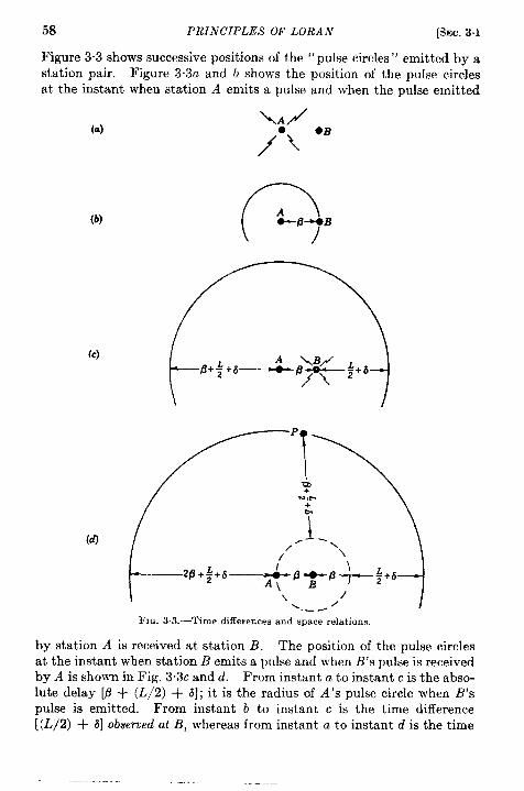
58 PRINCIPLES OF LORAN [SEC.3.1

lhgure3.3shows successive positions of the “pulsec ircles’’emittedbyastation pair. Figure 3.3a and b shows the position of the pulse circlesat the instant when station A emits a pulse and when the pulse emitted

\:/(a) ●B

//\

(b)

(c)

(d)

FIG. 33.-Time differences and space relations.

by station A is received at station B. The position of the pulse circlesat the instant when station B emits a pulse and when B’s pulse is receivedby A is shown in Fig. 3.3c and d. From instant a to instant c is the abso-lute delay [P + (L/2) + 6]; it is the radius of A’s pulse circle when B’spulse is emitted. From instant b to instant c is the time difference[(L/2) +6]obsemed at B,whereas from instant atoinstant disthe time

SEC.3.2] PROPAGATION AND RANGE 59

difference [26 + (L/2) + ~] observed at A. Note that the first of theseintervals is the shortest distance in light-microseconds between the twocircles and that the second is the greatest dist ante. Since the circlesexpand at the same rate, these distances will remain the same as thepulses move on. Note also that at any point over which the pulse circlefrom A is passing, the time that will elapse before the circle from B willarrive is the distance to the B-circle, measured along the radius to B fromthe point. This is the time difference at that point, and it is evidentthat the extreme values of this difference occur at points on the extendedbaselines and that at a point F’ equidistant from A and B the value is[P+ (-L/2) + 31.

The form of the display on the Loran indicator and the method ofreading the time difference are such that the actual number measured isnot t but t — (L/2). This reading is called the indicated time di~erenceand denoted by T. In practical operation, T k always used instead oft and referred to as the time difference. The Loran lines on the chartsare labeled, therefore. with values of T instead of t. From Eq. (3) it isevident that

T=(fl+6)+zi (4)

and that its extreme values are tiand (26 + 6). Along the continuationof the baseline beyond station B, T = 6; along the center line, T = @ + 6;and along the extended baseline beyond station A, T = 2/3+ ~. For atypical Standard Loran station pair, numerical quantities might be@ = 1855 psec (corresponding to 300 nautical miles), 6 = 1000 ~sec, andT would range from 1000 psec, at or behind station B, to 4710 Ksec, at orbehind station A.

In all the preceding relations, note that the stations are not denotedby the letters A or B indifferently. Station A is always that one of apair whose pulse begins the absolute delay (L/2) + (d + 8); station B isthe one whose pulse ends it. Station A is usually also the one whosecrystal oscillator defines the recurrence rate; station B must regulate thefrequency of its crystal oscillator to match A ‘s. In this case station A iscalled the master station of the pair, and station B is called the slavestation. Sometimes the initials M and S are used to represent them,instead of A and B.

3.2. Propagation and Range. Ground- and Sky-wa~~eTransmission.—Up to this point it has been assumed that the Loran radio pulses travelclose to the surface of the earth and consequently that their time delaysmeasure ground distances. This is true but not the whole truth. Loranpulses travel upward as well as outward; and, when they reach the iorzo-sphere (an electrically charged region in the upper atmosphere), they arerefk .ed back to earth in considerable strength, A transmitter at point

60 PRINCIPLES OF LORAN [SEC. 3.2

X (Fig. 3.4) will, therefore, send a pulse to a receiver at point R by two

paths, the direct path ~R and the indirect path ~, where I is a pointin the ionosphere. The pulse taking the direct path is said to be carriedby ground waves; that taking the indirect path is carried by sky waves.

FI~,3.4.—Ground wsves and sky waves,

The distance ~R is obviously greater than the distance ~. Thesky-wave transmission time is, therefore, longer than the ground-wavetransmission time, and a single pulse from the transmitter, arriving atthe receiver over the two different paths, will be received as two pulses,the sky-wave component coming after the ground-wave component byan interval eaual to the difference XIR — ~R in light-microseconds.This difference is called the sky-wave transmission ~elay; it may bedenoted by E.

Actually, there are several possible paths for sky waves. Theion~sphere contains two principal layers of electrified particles at differentheights above the earth’s surface; the lower (called the E-layer) is par-tially transparent to waves of the Standard Loran frequency band, withthe result that these waves are both reflected from it and transmittedthrough it to be reflected from the upper or F-layer. Moreover, multiplereflections between ionosphere and ground occur (see Chap. 5, Fig. 5.13).The various paths are of different length, producing a series or train ofsky waves following the ground wave. But only the sky wave travelingby the shortest path, the one singly reflected from the E-layer, is reliableenough in its persistence and timing to be used in Standard Loran, andall of the following discussion refers to it. In the special case of LowFrequency Loran, the pulse put out by the transmitters is so long thatthe ground wave and various sky waves are not resolved in reception.The behavior of this composite pulse is discussed in Chap. 5.

The greater the direct or ground-wave distance the less the indirect orsky-wave distance exceeds it. That is, if R (Fig. 35) is a receiver, X~ anear-by transmitter, and X, a distant transmitter, then (X= – X=),or E~, is less than (X= — X.Jt), or EA. This is evident from the

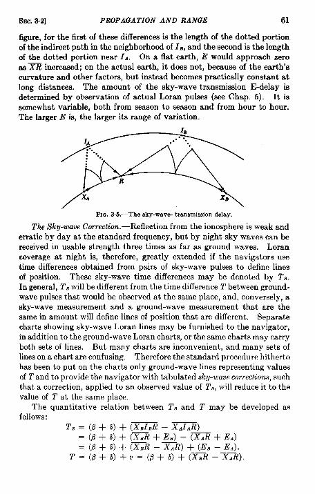
SEC. 3.2] PROPAGATION AND RANGE 61

figure, for the first of these differences is the length of the dotted portionof the indirect path in the neighborhood of 1,, and the second is the lengthof the dotted portion near I.. On a flat earth, E would approach zeroas ~ increased; on the actual earth, it does not, because of the earth’scurvature and other factors, but instead becomes practically constant atlong distances. The amount of the sky-wave transmission E-delay isdetermined by observation of actual Loran pulses (see Chap. 5). It issomewhat variable, both from season to season and from hour to hour.The larger E is, the larger its range of variation.

1A

:

Fm. 3.5.—Thesky-wav~transmissiondelay.

The Sky-wave Correction. -Reflection from the ionosphere is weak anderratic by day at the standard frequency, but by night sky waves can bereceived in usable strength three times as far as ground waves. Lorancoverage at night is, therefore, greatly extended if the navigators usetime differences obtained from pairs of sky-wave pulses to define linesof position. These sky-wave time differences may be denoted by Ts.In general, T. will be different from the time difference T between ground-wave pulses that would be observed at the same place, and, conversely, asky-wave measurement and a ground-wave measurement that are thesame in amount will define lines of position that are different. Separatecharts showing sky-wave Loran lines may be furnished to the navigator,in addition to the ground-wave Loran charts, or the same charts may carryboth sets of lines. But many charts are inconvenient, and many sets oflines on a chart are confusing. Therefore the standard procedure hithertohas been to put on the charts only ground-wave lines representing valuesof T and to provide the navigator with tabulated sky-wave corrections, suchthat a correction, applied to an observed value of T,, will reduce it to thevalue of T at the same place.

The quantitative relation between T, and T may be developed asfollows :

T. = (d + ~) + (XJ,R – x.~.~)= (P + o + (XBR + E,) – (XAR + E.4)——= (L7+ a) + (xl% – X.4R) + (ELI – E.).

T=(~+5) +v=(d+a)+(X,R –XJ?).

62 PRINCIPLES OF LURAN [SEC 3.2

Comparing the last two equations,

T= Tg–(E, –E.)=Ts+(E. –EE) =TE+C, (5)

where C, the sky-wave transmission delay from A minus that from B(note the order of subtraction), is the sky-wave correction. C always hasthe same sign as V, positive if station A is nearer than B, negative if it isfarther.

On the center line C is zero, as is U, for there E. = E,. Across thehyperbolas, away from the center line, C becomes positively or negativelygreater as the nearer station is approached. Along a hyperbola, itapproaches zero as the distance from the baseline increases, vanishingat great distances. Over the larger part of the region within which sky-wave time differences are reliable, C is less than 10 psec. It becomeslarger when the navigator is near both stations and largest when he isclose to one station and far from the other. For example:

Distancesof stations, nautical miles C, psecBoth > 6CMI < 12500 and 800 16400 and 700 26300 and 600 42300 and >1000 53

The transmission delay from a near station varies unpredictably, some-times by as much as 20 ~sec, making the corrections that involve thisstation correspondingly uncertain. As a general rule, 250 miles may beconsidered the shortest distance from a station at which reasonablyreliable lines of position may be obtained from its sky-wave pulses.

The Range of Loran Transmission.-The greatest distance at whichLoran pulses can be received in strength sufficient for measurement isdifferent at 1950 and 180 kc/see, different for ground waves and skywaves, different by day and by night, and different over water and overland. The ground wave at 1950 kc/secj by day, has a usable range of700 or 800 nautical miles over salt water, under low-noise conditions.At night the normal increase in natural noise cuts this down to approxi-mately 450 miles. Over land of average conductivity, the ranges areone-half to one-third of these, at considerable elevation above ground;on the surface, they are even less.

The one-hop E-layer sky wave at 1950 kc/see is not normally observ-able by day over the most generally navigated regions of the earth,except at extremely short ranges (at which its time delay is unreliable).Southeastern Asia in the dry season, however, seems to be an exceptionto this statement.

At night this sky wave carries pulses to a range of 1400 nautical milesover water and only slightly less over land (because the land attenuation

SEC. 3.3] PRINCIPLES OF OPERATION 63

is effective only in the regions near the transmitter and receiver, wherethe wave is near the ground).

At 180 kc/see, the rangee are much greater than at the standard frequency. Data obtained over several months of experimental trials indi-&te that by day the ground-wave range over sea is at least 1200 nauticalmiles and over land 1000 miles. As at the higher frequencies, the skywaves are largely absorbed by the ionosphere. At night, over land orsea, the sky-wave range usually exceeds 1500 nautical miles.

These ranges vary from day to day, seasonally, and with the !ocality,since they depend upon ionization in the upper atmosphere, severity ofnatural electrical disturbance, and surface conductivityy.

3.3. Principles of Operation. Time-difference Measurement .—As hasbeen mentioned, the time difference is presented to the observer visuallyas a length between marks on a line, which appears on the oscilloscopescreen of the Loran receiver-indicator (see Chap. 11). The Loran trans-mitter timer, which controls and regulates the emission of pulses by thetransmitting stations, is described in detail in Chap. 7. These twoinstruments embody the same principles, although they make differentuse of them. A brief and simplified description of a widely used form ofthe receiver-indicator is given here, followed by a statement of the addi-tional elements that the transmitter timer requires to perform its functions.

The Loran receiver is a conventional superheterodyne with fourrather broad fixed-tuned channels. The indicator contains a cathode-ray oscilloscope. The horizontal deflection of the beam and the graduat-ing vertical deflections are precisely controlled by a crystal clock; othervertical deflections are produced by the pulses from Loran stations com-municated to it through the receiver. The combination acts as a stopwatch with a graduated dial (the oscilloscope trace, graduated by pulsesfrom the crystal) and two independent hands (the delay circuits describedbelow) that may be set to mark the times of arrival of the two pulses, afterwhich the relative position of the hands measured by the graduationsshows the time interval between pulses.

The cathode-ray beam striking the oscilloscope screen produces aspot of light. Potential differences for deflecting the cathode-ray beamare regulated by the tryst al c1ock in such a manner that their variationswings the beam back and forth across the tube, sweeping the light spotover the screen in a regular pattern. This pattern is the slow-tracepattmn, and the period of its repetition is called the recurrence period L.A typical value of L is & see, or 40,000 psec. During this interval thenoving spot goes through this sequence:

1. It sweeps steadily from left to right across the upper part of thescreen. This upper trace is traversed in about 19,930 psec—almosthalf of L.

64 PRINCIPLES OF LORAN [SEC.3.3

2. It snaps downward and to the left. This retrace takes about 70psec.

3. It sweeps from left to right across the lower part of the screen,This lower tm.ce takes about 19,930 ~sec.

4. It snaps upward and to the left. This retrace takes about 70 ysec.

The sequence, repeated twenty-five times a second, is rapid enough tomake the path of the spot visible as a continuous line, 1 and 3 being brightand 2 and 4 almost invisible (Fig. 3.6). As the spot sweeps across thescreen, slight vertical displacements are imparted to it at 10-psec intervalsby the vibrating crystal, and greater displacements every 50 and 500

FIG. 3.6.—Indicator oscilloscope traces.

~sec. This action causes gradua-tions, or time markers, to appearalong the trace.

The pulses from the Lorantransmitters are passed to the oscil-loscope by the receiver and also ap-pear as vertical displacements ofthe moving spot. Since the dura-tion of a pulse, as distorted in thereceiver, is about 75 psec, a humpwith this length and with a heightdepending on the intensity of thepulse is seen on the trace in a posi-tion corresponding to the positionof the spot at the time of the recep-

tion of the pulse. The interval between pulses from the same station is L.During this time the light spot runs through its entire cycle and returns tothe same point. The hump, therefore, is repeated at this point in everycycle and appears as a stationary feature of the trace.

Between a pulse from station A and one from station B, the interval ist, or (L/2) + (P + 6) + U. During this time the spot traces a little morethan half its path on the screen; therefore, if the hump caused by thepulse from A appears on the upper trace, the hump caused by the pulsefrom B will appear on the lower trace, a little to the right of the other(Fig. 3.7). For example, if t is 23,250 psec, the pulse from B will appearto the right of that from A by the distance over which the spot moves in3250 psec. It is this displacement to the right which the observermeasures. The time difference that he reads from it is 2’.

The crystal of the indicator is in no way locked to the incoming pulses,When the indicator is turned on, the .4-pulse may appear at any point ofthe trace, and the recurrence period of the indicator may not exactlymatch that of the pulse, in which case the pulse will drift slowly along

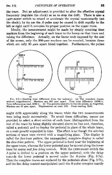
sEC. 3.3] PRINCIPLES OF OPERATION 65

the trace. But an adjustment is provided to alter the effective crystalfrequency (regulate the clock) so as to stop the drift. There is also aLEFT-RIGHTswitch to retard or accelerate the crystal momentarily (setthe clock); by its use the A-pulse may be caused to drift rapidly to theleft or right until it occupies its proper position on the upper trace.

Ideally, the measurement might be made by simply counting timemarkers from the beginning of each trace to the hump on that trace andtaking the difference. Actually, on the linear scale imposed by the sizeof the screen, only the 500-psec markers can be counted, because thosewhich are only 50 psec apart blend together. Furthermore, the pulses

/3qJo+

)(a) (b)

FIQ. 3.7.—Reading time difference from the indicator. (a) The complete traces,without magnification. Markers are 500 psec apart. True time difference 23000+.Time clifference as read, 3000+. (b) The sections adjacent to the two pulses, as magnified.Markers are 50 ~ec apart. Displacement as read, 250. Total reading, 3250.

might drift appreciably along the traces while the two measurementswere being made successively. To avoid these difficulties, means areprovided to select a short section of each trace (distinguished from therest of the trace by being slightly elevated above its line and, therefore,called a pedestal) and to display the pedestal in place of the whole trace,on a scale greatly expanded in time. The effect is as though the selectedsections of trace were viewed with a magnifying glass. This display iscalled the jast-b-ace pattern; the unmagnified, complete display is calledthe slow-trace pattern. The upper pedestal is fixed near the beginning ofthe upper trace, whereas the lower pedestal may be moved along the lowertrace by coarse and jine delay controls. With the LEFT-RIGHT switch theA-pulse is drifted to a position on the upper pedestal; with the delaycontrols the lower pedestal is moved under the B-pulse (Fig. 3.7a).Then the complete traces are replaced by the pedestals alone (Fig. 3“7b),and the fine delay control manipulated until the B-pulse occupies exactly

66 PRINCIPLES OF WRAN [SM. 8~

the same position on the lower pedestal that the A-pulse occupies on theupper pedestal. To make this adjustment precise, the lower pedestal israised and the upper brought down until they coincide; the pulses canthen be superposed with a normal reading error of less than 1 WWC,roughly 1 per cent of the apparent width of the pulse.

When this has been done, the relative horizontal displacementbetween the pedestals is exactly the same as that between the pulses.This displacement, therefore, measures the time difference T at themoment when the pulses are superposed. The stop-watch analogue tothis operation would be to set one stop-watch hand to the time of arrivalof one pulse and the other hand to the time of arrival of the other pulse,and to make the settings simultaneously. Drift of the pulses does notmat ter as long as superposition is effected (just as in a sextant observa-tion, where sun and horizon may swing back and forth together in thefield of view as long as they are brought to tangency). Once the settinghas been made, the displacement of the lower pedestal relative to theupper is read by counting the markers occurring after the start of thetop pedestal and before the start of the lower pedestal. The 500-~secmarkers are counted from the slow-trace display, and the 50- and 10-~secmarkers are counted from the fast-trace display (see Fig. 3“7, which issimplified and schematic, and Fig. 11.2 of Chap. 11, which shows thecomplete procedure of measurement).

Maintenance of Delay between Stations.—The two transmitting stationsthat make up a Loran pair are electrically independent. The pulsesemitted by a station are triggered by a free-running quartz-crystal oscil-lator, carefully controlled in temperature to maintain frequency within1 part in 300 million (1 psec in 5 rein). The vibration frequency of thecrystal is 50 kc/see and is reduced by divider circuits to the chosenrecurrence rate for the pair. The crystal-oscillator and divider circuitsare similar to those of the navigator’s indicator, but somewhat moreelaborate and stable. They actuate a display of traces, time markers,and pedestals on two oscilloscope screens (so as to present both slow andfast traces at the same time), and both pedestals are controlled by separatedelay circuits. At the master station, the circuit that controls the upperpedestal also triggers the transmitter. The pulse would be emittedexactly at the instant indicated by the left end of the pedestal if the trans-mitting system acted instantaneously. A receiver is connected to thetimer oscilloscope, as with the indicator; if the receiver also acted simul-taneously, the transmitter pulse that is received after traveling only a fewhundred feet would appear on the pedestal just at the beginning of thepedestal. Actually, transmission and reception take about 50 ~secbecause of lag in the circuits, and consequently the pulse is displaced tothe right on the pedestal by this ‘distance.

sEC. 3.3] PRINCIPLES OF OPERATION 67

At the slave station an exactly similar timer operates, but here thetransmitters triggered by the circuit that controls the lower pedestal,and hence the local pulse appears on it.

When the timers at the two stations are adjusted so that each pulseemitted from the slave transmitter follows the corresponding pulse emittedfrom the master transmitter by the absolute interval (L/2) + (P + 6),the stations are said to be in delayed synchronism. As has been explained,the indicated time difference observed at the slave station is then equalto $, whereas at the master station it is (2P + 6). Maintenance ofsynchronism is the duty of the operator at the slave station, who adjustshis timer to keep step with the pulse received from the master station.With the two timers and transmitters running independently, the oscillo-scope at either station will show the pulse emitted at that station (localpuke) at a fixed point on its pedestal, but the pulse received from theother station (remote pulse) will be drifting along the traces, for the crys-tals will not, in general, be vibrating at exactly the same frequency.The slave operator synchronizes his transmitter with the other in twosteps. First, he sets his lower pedestal (carrying his local pulse with it) toa position 6 psec to the right of his upper pedestal by means of the delaycontrols. Next, he varies the frequency of his oscillator in order to driftthe remote pulse onto the upper pedestal and to bring it to rest at thesame place on this pedestal at which the local pulse is fixed on the otherpedestal. He makes this adjustment by superposition, as does theobserver on a ship or airplane, but instead of bringing this about by vary-ing the delay to fit two remote pulses, he leaves the delay at its fixed settingand varies the oscillator phase, carrying the local pulse with it, until itfits the remote pulse. When this has been accomplished, the two pulseshave the same time relation as the two pedestals and are therefore indelayed synchronism. They will remain so as long as the two crystalshold the same frequency. Generally this will be of short duration, sinceneither oscillator is perfectly stable. For this reason the slave oscillatormust be made to follow the slight variations of the master. The slaveoperator may do this manually, watching the superposed pulses on thefast-trace display and advancing or retarding his oscillator slightly as theremote pulse begins to slide out from coincidence with the local. Coinci-dence may also be maintained by the Loran automutic synchronizer, an

electrical network linking the receiver input with the osc~ator control.This device “views” a portion of the rising slope of the remote pulse afterit has been manually set in its proper place on the upper trace and accel-erates the oscillator if the average elevation of this slope becomes greater(because the pulse has drifted to the left) or retards it if the elevationbecomes less (because of a drift to the right). In either case the effect isto counteract the drift. The synchronizer cannot set the pulses in

68 PRINCIPLES OF LORAN [SEC. 3.3

coincidenc~this must be done by visual inspection of the pulse images—but it will hold coincidence within 1 or 2 ~sec if there is not too muchelectrical noise. Under noisy conditions manual control is necessary,The stability of the oscillators is such, however, that synchronism maybemaintained by an experienced operator through long periods of electricaldisturbance if he can glimpse the remote pulse for a few seconds from timeto time.

While the slave operator maintains synchronism, the master operatorkeeps a continuous watch over the timing by means of his own oscillo-scope. He sets the delay controls so that the lower pedestal is at a dis-tance (26 + 5) to the right of the upper pedestal (on which his local pulseis fixed). If the slave transmitter is timed correctly, the remote pulsecoming from it will appear on the master’s lower pedestal, in position sothat the two pulses will coincide in the fast-trace display. If they do not,the master operator actuates a device that “blinks” his pulse (causes itto jump regularly back and forth), telling the slave to make a correctionand warning observers not to make readings. The master does not,however, change the frequency of his own oscillator.

Generally, the master is the station called -4 whose pulse initiates thedelay, and the slave is B whose pulse terminates it. In emergencies, Amay act as slave and B as master, with respect to dependence and inde-pendence of the frequency of the oscillators, but they do not exchangepositions in the sequence. If they should do so, the time order of theLoran lines around the stations would be reversed, making the chartsuseless.

At each station a switched electronic attenuator is inserted betweenthe receiving antenna and the receiver, which allows the remote pulse tocome through undiminished but cuts down the extreme intensity of thelocal pulse so that on the oscilloscope screen it can be matched in ampli-tude with the remote pulse. The attenuator is designed to act on thepulses without introducing any differential delay; but since it is the onecircuit in the timer that does not treat them exactly alike, such a differen-tial may well creep in, falsifying the timing at the two stations in oppositesenses. To detect such an effect and to check the operating personnel,the equipment, and propagation conditions, it is highly desirable that amonitor station, equipped with a standard indicator, be maintained in aknown position within good receiving distance of both ground stations andfar enough from both so that neither pulse has to be greatly attenuatedfor comparison with the other. The synchronism, pulse shapes, andsignal strengths should be observed, and routine reports should be sub-mitted to the operating authorities.

Distinction between Pairs oj Stations.—The navigator cannot determinehis position unless he can receive pulses from two pairs of stations. In

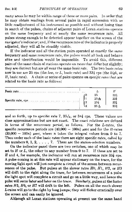
SEC.33] PRINCIPLES OF OPERATION 69

many areas he may be within range of three or more pairs. In order thathe may obtain readings from several pairs in rapid succession with aslittle readjustment of his instrument as possible and without losing timein search of the pulses, chains of adjacent pairs of Loran stations operateon the same frequency and at nearly the same recurrence rate. Allpulses strong enough to be detected appear together on the screen of thenavigator’s indicator; and, if the recurrence rate of the indicator is properlyadjusted, they will all be steadily visible.

If the indicator and all the station pairs operated at exactly the samefrequency and same recurrence rate, the pulses would all look and behavealike and identification would be impossible. To avoid this, differentpairs of the same chain of stations operate on rates that differ but slightly;they are distinct but are all near the same basic rate. The two basic ratesnow in use are 25 cps (the low, or L, basic rate) and 33* cps (the high, orH, basic rate). A chain or series of pairs operate on specijic rates that arerelated to the basic rate as follows:

Basicrate. . . . . . . . . . . . . . . ., ,., L 1[

{

o 25 33$

Specificrate, cps. . . . . . . . . . . . . . . . ; 257+. 33$25+ 33:

3 25& 33$

and so forth, up to specific rate 7, 25+s, or 34* cps. These values areclose approximations but are not exact. The exact relations are definedin terms of the recurrence period, as follows. For the L-rates, thespecific recurrence periods are (40,000 — 100n) psec and for the H-rates(30,000 – 10W) psec, where n takes the integral values from O to 7.Thus under each of the basic rates there are eight specific rates, called bythe numbers O, 1, 2, . . . , 7. These are the .stdiorz-selectzon numbers.

On the indicator panel there are two switches, one of which may beset to H or L, the other to any number from O to 7. If these are set toH and 4, for example, the indicator will run at recurrence rate 33; cps.A pulse coming in at this rate will appear stationary on the trace, for themoving light spot wifl just complete a circuit of the screen between recur-rences of the pulse. But pulses at the slower rates HO, HI, H2, or H3will drift to the right along the trace, for between recurrences of a pulsethe light spot will complete a circuit and go on a little way, and hence thepulse will recur later and later on the trace. Similarly, pulses at the fasterrates H5, H6, or H7 will drift to the left. Pulses on all the much slowerL-rates will go to the right by 1ong jumps; they wilf flicker erratically overthe screen and can easily be ignored.

Although all Loran stations operating at present use the same band

70 PRINCIPLES OF LORAN [SEC. 3.4

of radio frequencies, between 1700 and 2000 kc/see, they all do not use thesame frequency. Four different frequencies have been used—1750, 1850,1900, and 1950 kc/see. These radio frequencies are referred to aschannels, and they are numbered. Channel 1 is 1950 kc/see; Channel 2is 1850: Channel 3 is 1900; and Channel 4 is 1750. The Loran receivermay be tuned to any channel by turning a channel m“tch to the propernumber.

A pair of Loran stations bears a designation made up of the channelnumber, basic-rate letter, and station-selection number. The first twoof these characterize an entire group, or chain, of stations that are to beused by navigators in a particular area or in connection with particularoperations. Such a group of stations might include pairs designated2H0, 2H1, 2H2, 2H3. For all these the channel is 1850 kc/see and thebasic rate is 33+ cps; the specific rates are 33;, 33*, 333, and 33$ cps.The designation is prefixed to any value of T read by a navigator fromthe pulses of a pair and is part of the label of any charted Loran line.Such a line might be labeled 2H2-3380; the four-figure number being thevalue of T, the prefix the designation of the pair.

It has been mentioned that in a triplet of Loran stations, one stationacts as a member of two pairs and that in a chain of stations, all membersbut those at the ends act in this way. Sometimes the three stations of atriplet use the same recurrence rate (as explained in Sec. 3“5 in the dis-cussion of systems), but usually they use clifferent specific rates. In achain, adjacent pairs always use different rates. This means that astation which is a member of two pairs sends out two independentsequences of pulses, one slightly more closely spaced than the other.These pulses must be triggered by different timers but may be sent outfrom the same transmitter. Double pulsing, as this method of operationis called, decreases peak power somewhat by altering the duty cycle ofthe transmitter and slightly disturbs the timing of both pulses at themoment when the one of higher rate overtakes the other. It has beenwidely employed, however, in Loran operation because of its economy ofequipment, of which there was a critical shortage throughout the warperiod in which Loran grew up.

34. Loran Geometry: the Pair. The Loran Hyperbolas.—A hyper-bola is by definition the locus of points all of which are farther from onefied point than they are from another fixed point by the same distance.The two fixed points are the foci. A Loran line of position is thereforea hyperbola with its foci at the two transmitting stations A and B,

If. the surface of the earth were a plane, the lines generated by a pairof stations would form a family of conjocal plane hyperbolas (Fig. 3“8).The baseline, connecting the stations, would be a straight line. The lineT = IS+ 6 or v = Owould be a straight line called the centsr line, bisecting

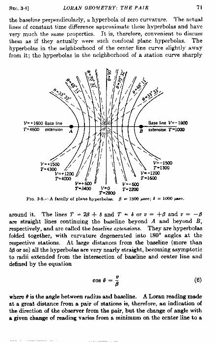
SEC. 3.4] LORAN GEOMETRY: THE PAIR 71

the baseline perpendicularly, a hyperbola of zero curvature. The actuallines of constant time difference approximate these hyperbolas and havevery much the same properties. It is, therefore, convenient to discussthem as if they actually were such confocal plane hyperbolas. Thehyperbolas in the neighborhood of the center line curve slightly awayfrom it; the hyperbolas in the neighborhood of a station curve sharply

FIQ.3.8.—A famify of plane hyperbolas. f3 = 1S00 J@c; J = 1~ -c.

around it. The lines T = 2@ + 6 and T = 6 or v = +@ and v = –@are straight lines continuing the baseline beyond A and beyond B,respectively, and are called the baseline eztenm”ons. They are hyperbolasfolded together, with curvature degenerated into 180° angles at therespective stations. At large distances from the baseline (more than56 or so) all the hyperbolas are very nearly straight, becoming asymptoticto radii extended from the intersection of baseline and center line anddefined by the equation

(6)

where o is the angle between radius and baseline. A Loran reading madeat a great distance from a pair of stations is, therefore, an indication ofthe direction of the observer from the pair, but the change of angle witha given change of reading varies from a minimum on the center line to a

72 PRINCIPLES OF LORAN [SEC. 3.4

maximum ona baseline extension, and two directions that are not oppo-site correspond to one reading.

If the earth were a true sphere, the baseline would be a great circle.The center line and extended baselines would also be great circles, andthe other Loran lines would form a family of confocal spherical hyperbolas.The earth is actually not quite spherical, so the Loran lines are slightly(but quite perceptibly) distorted from spherical hyperbolas to more com-plex curves. This distortion must be allowed for in precise chartingover large areas. The Loran hyperbolas are discussed further in Chap. 6.

The Factor of Geometm”calPrecim”on.—$5ince no observation is exact, anobserved reading will differ from the true value of the measured quantityby an amount that cannot be predicted for the individual observationbut may be estimated as an expected or “probable” value derived frommany comparisons between observed and “ true” values. This expectederror is usually taken as 0.67 ~W/n, where 2T2 signifies the sum ofthe squares of the deviations of a typical series of n observed values fromthe true values found by some more accurate method. If the distributionof deviations follows the gaussian normal law, the result thus derived isalso the median of the deviations. There are as many deviations thatare greater than the median as there are deviations that are less; thereforethe median is called the probable error.

If the probable error of a Loran measurement of time difference isz WWC,an observer who obtains the reading T from his indicator is aslikely to be actually located between the Loran lines T – z and T + zas to be outside this region. As far as he is concerned, the reading doesnot represent a sharp line but a strip at least 2X psec wide between twohyperbolas. The width of this strip in units of length is obviously amatter of importance to the observer, since he desires to obtain his loca-tion on the earth. The width is not 2Z times 0.1617 nautical miles, asmight be assumed without due thought. In fact, the conversion factorcannot be a constant, for it is obvious thai two hyperbolas of the samefamily are farther apart at a long distance from the baseline than theyare close to it. It is also true that hyperbolas which cross the baselinenear a focus diverge more sharply than those which cross near the centerline.

We may, therefore, write for y, the probable error in the position of theobserver’s Loran line corresponding to a probable error of z in the measure-ment of the time difference, y = lcwz. In this, k depends on the unit oflength and is, for example, unity if distance is measured in light-micro-seconds. The other factor, w, that depends on the observer’s positionmay be called the factor of geometrical prem”m”on. It equals ~ csc ~, inwhich $ is the angle between the two directions from the observer to thetratimitting stations. See Appendix Cl for the proof of this relation.

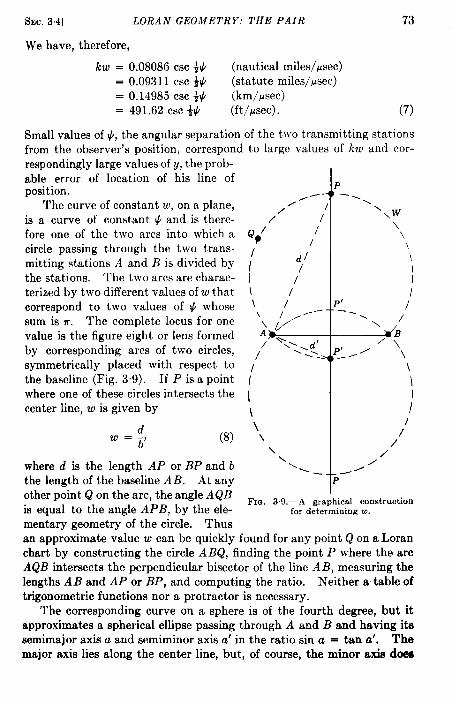
73SEC.3.4] LORAN GEOMETRY: THE PAIR

We have, therefore,

kw = 0.08086 CSC~+ (nautical miles/~sec)= 0.09311 Csc +# (statute miles/psec)= 0.14985 CSC~~ (km/psec)= 491.62 CSC~# (ft/psec). (7)

Small values of #, the angular separation of the tnw transmitting stationsfrom the observer’s position, correspond to large values of kw and cor-respondingly large values of y, the prob-able error of location of his line ofposition.

The curve of constant w, on a plane,is a curve of constant v and is there-fore one of the two arcs into which acircle passing through the two trans-mitting stations .4 and B is divided bythe stations. The two arcs are charac-terized by two different values of w thatcorrespond to two values of # whosesum is r. The complete locus for onevalue is the figure eight or lens formedby corresponding arcs of two circles,symmetrically placed with respect tothe baseline (Fig. 39). If P is a pointwhere one of these circles intersects thecenter line, w is given by

dw=_,b

(8)

where d is the length AP or BP and bthe length of the baseline AB. At anyother point Q on the arc, the angle A QBis equal to the angle APB, by the ele-mentary Keometry of the circle. Thus

q //

I d//

: /\ I

/I\\\

P

\

I

P’ /-. .\ /

‘:P:// \

/’//

.-P

FIG.. 3.9.—A graphical constructionfor determining w.

.-an approximate value w can be quickly found for any point Q on a Loranchart by constructing the circle ABQ, finding the point P where the arcAQB intersects the perpendicular bisector of the line AB, measuring thelengths AB and AP or BP, and computing the ratio. Neither a table oftrigonometric functions nor a protractor is necessary.

The corresponding curve on a sphere is of the fourth degree, but itapproximates a spherical ellipse passing through A and B and having itssemimajor axis a and semiminor axis a’ in the ratio sin a = tan a’. Themajor axis lies along the center line, but, of course, the minor axis does

74 PRINCIPLES OF LORAN [SEC.3.4

not lie along the baseline except in the special case # = 90°, w = ~~.In this case only is the approximation exact.

An approximate expression for w, in terms of the distance r and direc-tion O of the observer from the point midway between the stations, isoften useful. It is close to the truth if the distance is several times thebaseline length, but it breaks down at short distances. The expression is

()~=rG

Csc o, (9)

where r is the distance from the midpoint, b is the length of the baseline,and d is the angle that the line from midpoint to observer makes with thebaseline. This is the formula for the spacing of the asymptotes of theplane hyperbolas and is obtained by differentiating the equation of anasymptote, cos O = v/f3 (Sec. 3.4), and noting that in this case w = r dtl/dv.

Although w increases without upper limit as # decreases or i- increases,its lower limit is not zero but unity. This is its value along the baseline,where # = 180°. Here the conversion factor lcwis equal to the numericalcoefficient in Eq. (7). Over a considerable area near the baseline, w isnot much greater than unity and the precision is nearly constant. Theoptimum geometrical precision is therefore the same for all hyperboliccoordinate systems, whatever the length of baseline, and improvement inthe accuracy with which an observer may locate himself can be effectedonly by decreasing the probable error of a time-difference reading in micro-seconds. The precision falls off, however, with distance from the baselineless rapidly if the baseline is long than if it is short.

To recapitulate: Slight departures from synchronism at the stations,slight variations in time of travel of the pulses, and slight errors in pulse-matching by the observer combine to build up the probable error of ameasured Loran time difference. Let the measured value be T’ psec andthe probable error z psec. The probable error of the line of positiondesignated by T’ is represented geometrically by the strip on the earth,bounded by the hyperbolas T’ – z and T’ + z. The distance acrossthis strip in linear units is 21cwz. If the line of position on which theobserver is actually situated when the measurement is made is T, it isequally probable that T differs from T’ by less than z or by more than z,in either the positive or the negative direction, and equally probable thatthe observer’s actual line of position lies within or without the strip andthat it is distant from the hyperbola T’ by less or by more than kwz, inlinear units. The value of z must be determined experimentally or bystatistical analysis of large numbers of readings taken in actual Loranoperation.

The i3erwiw Area of a Pair.—The area within which an observer canreceive measurable pulses from both stations of a Loran pair is the area

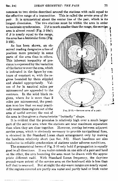
fhEc.3.4] LORAN GEOMETRY: THE PAIR 75

common to two circles described around the stations with radii equal tothe effective range of a transmitter. This is called the serwicearea of thepair. It is symmetrical about the center line of the pair, which is itslongest dimension. The two stations must be within the area in orderto maintain synchronism. If P is much smaller than the range, the servige ~area is almost round (Fig. 3.10a);if @ is nearly equal to the range,the area has a lenticular form (Fig.310b).

As has been shown, an ob-served reading designates a line ofposition more precisely in someparts of the area than in others.Thk inherent inequality of pre-cision is expressed by the variationof the factor w over the area, whichis indicated in the figure by con-tours of constant w, with the re-gions bounded by them stippledand shaded appropriately. Val-ues of kw in nautical miles permicrosecond are appended to thecontours. In the solid black re-gions, where kw is more than 2miles per microsecond, the preci-sion is so low that we may practi-cally count these regions out of thearea of useful service; the rest of

.. :7

Flo. 3,10.—Scrvice area of a pair.

the area is thus given a characteristic “ butterfly” shape.It is evident that the precision is relatively high over a much larger

part of the service area when the stations are near maximum separationthan when they are close together. However, overlap between adjacentservice areas, which is obviously necessary to provide navigational fixes,is obtained in the Standard I.oran chain arrangement only by makingthe baselines relatively short (SCCSec. 35). Short baselines are alsoconducive to reliable synchronism of stations under adverse conditions.

The symmetrical forms of Fig. 3.10 only hold if propagation is equallygood in all directions. If sca water extends on one side of a pair and landon the other, the arcs bounding the area must be drawn with the appro-priate different radii. With Standard I,oran frequency, the daytime~round-wave extent of the service area on the landward side is less thanhalf that to seawar{l. But at night the sky-wave ranges are nearly equal.[f the regions covcrcd arc partly sca water and partly land or fresh water

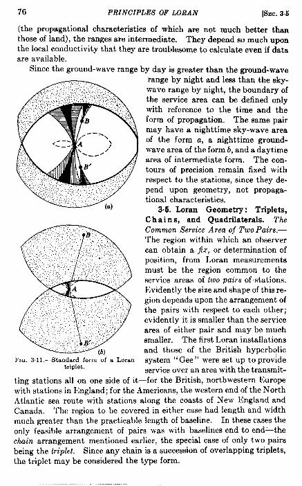
76 PRINCIPLES OF LORAN [SEC. 3.5

(the propagational characteristics of which are not much better thanthose of land), the ranges are intermediate. They depend so much uponthe local conductivity that they are troublesome to calculate even if dataare available.

Since the ground-wave range by day is greater than the ground-wave

.,FIU. 3.11 .—Standard form of a Loran

triplet.

range by night and less than the sky-wave range by night, the boundary ofthe service area can be defined onlywith reference to the time and theform of propagation. The same pairmay have a nighttime sky-wave areaof the form a, a nighttime ground-wave area of the form b, and a daytimearea of intermediate form. The con-tours of precision remain fixed withrespect to the stations, since they de-pend upon geometry, not propaga-tional characteristics.

3.5. Loran Geometry: Triplets,Chains, and Quadrilaterals. TheCommon service Area of Two Pairs.—The region within which an observercan obtain a jix, or determination ofposition, from Loran measurementsmust be the region common to theservice areas of two paiTs of. stations.Evidently the size and shape of this re-gion depends upon the arrangement ofthe pairs with respect to each other;evidently it is smaller than the servicearea of either pair and may be muchsmaller. The first Loran installationsand those of the British hyperbolicsystem “Gee” were set up to provideservice over an area with the transmit-

ting stations all on one side of it—for the British, northwestern Europewith stations in England; for the Americans, the western end of the NorthAtlantic sea route with stations along the coasts of New England andCanada. The region to be covered in either case had length and widthmuch greater than the practicable length of baseline. In these cases theonly feasible arrangement of pairs was with baselines end to end>thechain arrangement mentioned earlier, the special case of only two pairsbeing the triplet. Since any chain is a succession of overlapping triplets,the triplet may be considered the type form.

Slw. 3.5] LORAN GEOMETRY: TRIPLETS AND CHAINS 77

The typical service area of a triplet of this type is depicted in Fig.3“1la, where it is the area within the heavy boundary. In the stippledareas, the signals of only one pair are measurable. Within the commonservice area, the vertically shaded regions are those in which geometricalprecision for the pair AB is worse than 1 nautical mile per microsecond,the horizontally shaded regions those in which this is true of the pair AB’.In the solid black regions precision is worse than 2 nautical miles permicrosecond for one pair or the other. Only within the dashed boundaryis the precision better than ~ nautical mile per microsecond for both pairs.

Scak Statutemile0 lm2003m4m

Fm. 3.12.—A Standard Loran chain of three pairs

Figure 3.1 la would be symmetrical with respect to the baselines Alland A B’ if these formed a single straight line. As they are placed, withan angle between them, the common service area is larger and the preci-sion better on the side where the angle is less than 180°. A triplet ofstations placed along a coast line gives better service if the shore presentsa concave curve toward the sea over which the traffic passes. Note thatclose to the baselines on the convex side the precision is very low.

The manner in which the service areas of successive triplets overlapin a Loran chain is illustrated by Fig. 3“12. The chain here has threepairs forming two triplets, and over a considerable region the navigatorcan obtain three lines of position, which should concur in a point at his

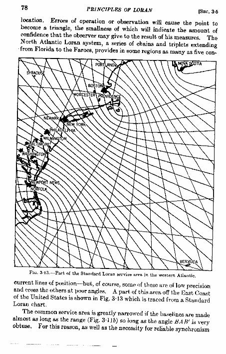
78 PRINCIPLES OF LORAN [sEC. 3,5

location. Errors of operation or observation will cause the point tobecome a triangle, the smalfnew of which will indicate the amount ofconfidence that the observer may give to the result of his measures.

TheNorth Atlantic Loran system, a series of chains and triplets extendingfrom Florida to the Faroes, provides in some regions as many as five con-

current lines of position—but, of course, some of these are of low precisionand cross the others at poor angles. A part of this area off the East Coastof the United States is shown in Fig. 3.13 which is traced from a StandardLoran chart.

The common service area is greatly narrowed if the baselines are madealmost as long as the range (Fig. 3,11 b) so long as the angle BA 31 is veryobtuse. For this reason, as well as the necessity for reliable synchronism

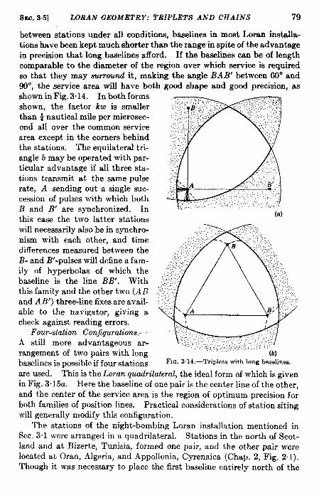
sEC. 3.5] LORAN GEOMETRY: TRIPLETS AND CHAINS 79

between stations under all conditions, baselines in most Loran installa-tions have been kept much shorter than the range in spite of the advantagein precision that long baselines afforal. If the baselines can be of lengthcomparable to the diameter of the region over which service is requiredso that they may surround it, making the angle BAB’ between 60° and90°, the service area will have both good shape and good precision, assho’w in Fig. 3.14. In both formsshown, the factor kw is smallerthan ~ nautical mile per microsec-ond all over the common servicearea except in the corners behindthe stations. The equilateral tri-angle b may be operated with par-ticular advantage if all three sta-tions transmit at the same pulserate, A sending out a single suc-cession of pulses with which bothB and B’ are synchronized. Inthis case the two latter stationswill necessarily also be in synchro-nism with each other, and timedifferences measured between theB- and B’-pulses will define a fam-ily of hyperbolas of which thebaseline is the line BB’. Withthis family and the other two (ABand AB’) three-line fixes are avail-able to the navigator, giving acheck against reading errors.

Four-station Con$gurations.—A still more advantageous ar-rangement of two pairs with longbaselines is possible if four stations

(a)

FIG. 3.14.—Triplets with long baselines.

are used. This is the Loran quadrilateral, the ideal form of which is givenin Fig. 3.15a. Here the baseline of one pair is the center line of the other,and the center of the service area is the region of optimum precision forboth families of position lines. Practical considerations of station sitingwill generally modify this configuration.

The stations of the night-bombing Loran installation mentioned inSec. 3.1 were arranged in a quadrilateral. Stations in the north of Scot-land and at Bizerte, Tunisia, formed one pair, and the other pair werelocated at Oran, Algeria, and Appollonia, Cyrenaica (Chap. 2, Fig. 2.1).Though it was necessary to place the first baseline entirely north of the

80 PRINCIPLES OF LORAN [SEC. 35

other, the geometry of the lines of position over Germany, where the twocenter lines intersected, was excellent. No other Loran system has beenset up to contain or span the area of operations by the baselines, but it isprobable that some future Low Frequency installations may take thisform.

FIG. 3.15.—Quadrilateral and star chain.

The British Gee system has frequently used a configuration of fourstations called a star chain. The master station is at the center, and threeslaves, all on the same pulse rate, are placed around it in directionsroughly 120° apart (Fig. 3.15b). This provides three triplets of theform of Fig. 3.1 la, “back to back,” so that good service is provided allaround the chain. Three-line fixes are theoretically provided, but theyare not practically worth while because the region of best fixes from anytriplet (two pairs) is crossed by the extended baseline of the third pair.The regions served by each triplet are labeled in Fig. 3. 15b by the lettersdenoting the two slave stations concerned (the master A being a memberof all pairs).

The Crossing Angle of Two Lines of Position.—The degree of precisionwith which a line of position is determined by an observation has beenrepresented by replacing the line by a strip of specified width. Similarly

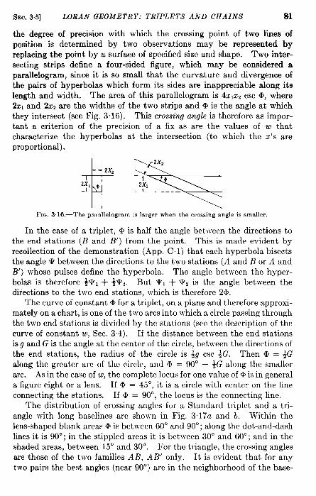
SEC.3.5] LORAN GEOMETRY: TRIPLETS AND CHAINS 81

the degree of precision with which the crossing point of two lines ofposition is determined by two observations may be represented byreplacing the point by a surface of specified size and shape. Two inter-secting strips define a four-sided figure, which may be considered aparallelogram, since it is so small that the curvature and divergence ofthe pairs of hyperbolas which form its sides are inappreciable along itslength and width. The area of this parallelogram is 4xIxZ csc Q, where2zI and 2x, are the widths of the two strips and @ is the angle at whichthey intersect (see Fig. 316). This crossing angle is therefore as impor-tant a criterion of the precision of a fix as are the values of w thatcharacterize the hyperbolas at the intersection (to which the x’s areproportional).

$%FIQ. 3.16.—The parallelogra,n is larger when the crossing angle is smaller.

In the case of a triplet, @ is half the angle between the directions tothe end stations (1? and B’) from the point. This is made evident byrecollection of the demonstration (App. C. 1) that each hyperbola bisectsthe angle w between the directions to the two stations (A and B or A andB’) whose pulses define the hyperbola. The angle between the hyper-bolas is therefore +Vl + ~Va. But T, + Vz is the angle between thedirections to the two end stations, ~vhich is therefore 20.

The curve of constant@ for a triplet, on a plane and therefore approxi-mately on a chart, is one of the two arcs into which a circle passing throughthe two end stations is divided by the stations (see the description of thecurve of constant w, Sec. 3-4). If the distance between the end stationsis g and G is the angle at the center of the circle, between the directions ofthe end stations, the radius of the circle is ~g csc +G. Then @ = #2along the greater arc of the circle, and @ = 90° — *G along the smallerarc. As in the case of w, the complctc locus for one value of @ is in generala figure eight or a lens. If @ = 45°, it is a circle with center on the lineconnecting the stations. If @ = 90°, the locus is the connecting line.

The distribution of crossing angles for a Standard triplet and a tri-angle with long baselines are showm in Fig. 3.17a and b. Within thelens-shaped blank areas @is between 60° and 90°; along the dot-and-dashlines it is 90°; in the stippled areas it is between 30° and 60°; and in theshaded areas, between 15° and 30°. For the triangle, the crossing anglesare those of the two families AB, AB’ only. It is evident that for anytwo pairs the best angles (near 90°) arc ,in the neighborhood of the base-

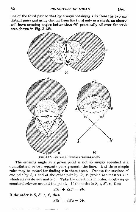
82 PRINCIPLES OF LORAN Bra,

line of the third pair so that by always obtaining a fix from the two modistant pairs and using the line from the third only as a check, an obsemwill have crossing angles better than 60° practically all over the wrvkarea shown in Fig. 3“13b.

(c)Fm. 3.17.—Curvesof constant crossing angle.

The crossing angle at a given point is not so simply specified if aquadrilateral or two separate pairs generate the lines. But three simplerules may be stated for finding @ in these cases. Denote the stations ofone pair by S, s and of the other pair by S’, s’ (which are masters andwhich slaves do not matter). Take the directions in order, clockwise orcounterclockwise around the point. If the order is S, s, S’, s’, then

LSs’ + As’ = 2+.

If the order is S, S’, s, s’, then

[ss’ – Ls’s = 2*.

SW. 35] LORAN GEOMETRY: TRIPLETS AND CHAINS 83

If the orcfcr is S, S’, s’, s then

[ss’ – Ls’s = 2*,

Tlw sign of @ is to IN disregarded in the last formula. These formulasgive VWIUCSof @ from 00 to 180° , whcrem the rule for drawing the circularloci of @ in the ca.sc of a triplvt always ~ivcs lCSSthrm 90”. But since thetrussing of ttvo Iirws results in four angles, two equal and less than 90°and two that arc supplements of these, we may always take @ as denotingthe first-quadrant wnglcs.

The curves of constant @ for four stations are not circles (except inthe special cmc of the four stations lying on the circle). They are thecurves obtained by connecting the appropriate intersections between thefamily of circles, ZI = constant; and the family of circles, LII = con-stant, where z I is the first fingle and LI I the second in any of the formulasof the last paragraph. l’igurc 3. 17c, depicting crossing angles for thequadrilateral, was constructed in this way. The contours for only onequarter of the area are shown, since they are the same in the other three.This symmetry is, of course, a consequence of the symmetry of arrmge-ment of stations.

In regions far enough from the two pairs so that the hyperbolas arevery close to their asymptotes (Sec. 3.4) the curves of constant crossingangle approximate closely the greater arcs of circles ptissing through themidpoints of the t~vo baselines and having radii ~m csc @, m being thedistance between the midpoints. The circle for 15° has the radius 1.93m.Fifteen degrees may be considered about the smallest crossing angle thatwill yield a usable fix. If the angle is smaller, the rectangle representingthe precision becomes so elongated that it practically degenerates into :isingle line of position (of high weight, of course, because it results fromthe concurrence of two measures).

Measures of the Precision oj a Fix.—Let T’ and T“ be measured timedifferences, obtained at the same place from different pairs of stations.Let the corresponding hyperbolas P and Q intersect at C, forming theacute angle @. If these measures were without error, the true location ofthe observer would be at C. In fact, the measures differ from the correctvalues T1 and Tz by unknown errors, and the true location is at a perpen-dicular distance ho,( T, – T’) from P and at a distance kw,( 2’, – T“)from Q, where kw has the same meaning as in Sec. 3.4. If we call thesedistances p’ and p“, the distance d of the true location from C is

d= V(P’)’ + (P”)2 * 2p’p” Cos 0,

where the plus sign is used if p’ and p“ have the same sign within theacute angles, the minus sign if their signs are different.

hsume that the errors affecting T’ are independent of those affecting2’” and that for a great number of measures both sets of errors have a

84 PRINCIPLES OF LORAN [SEC.3

statistically normal distribution. The measures will then have standarcdeviations u, = VZ(T’ – T,)’/n, and u, = v’z(T” – TJ2/n, andprobable errors c1 = 0.674%1 and cz = 0.6745uZ. The sums of thesquares of the residuals are determined from a 1arge number n of observa-tions made in actual operation of a Loran system. The distances p’ andp“will have standard deviations s1 = kwlul and s.i = kwzu2 and probableerrors pl = 0.6745s1 and pz = 0.6745sz.

Let Al? and DE in Fig. 3,18 represent the hyperbolas T’ + fc, andT’ – j,, and AD and BE the hyperbolas T“ + jcz and T“ – fez, respec-tively, j being an arbitrary factor. If j is given the value 1, then by the

Y

. . . . . . . . . .. .

Ha\\i

/ -- Por X

“.‘.

FIG. 3.18.—The error parallelogram, ellipse, and fide.

definition of the probable error, the chance that the observer’s actual lineof position TI lies between the lines A B and DE is i; the chance that theactual line T2 lies between AD and BE is also ~. Therefore the proba-bility that the observer’s true location is within the parallelogram ABCDis (~)’, or ~. If j is taken as 1.56, the probability that either hyperbolalies between the limits given is 0.707; consequently the chance that theirintersection is within the parallelogram is 0.7072, or i. This latterprobable parallelogram (by analo~ with probable error) rather simply andconveniently visualizes the accuracy of a fix and can easily be sketchedon a Loran chart, interpolating by inspection between the printed linesof position. The perpendicular distance between AB and DE in linearunits is 3. 12pl; that between AD and BE, 3. 12pz. The length of thesides of ABCD parallel to the hyperbola P is 3. 12p2 cm @; the length ofsides parallel to Q is 3. 12pl csc @; and the diago~.als have lengths 3.12Csc @ <P; + p; * 2p1p2 Cos *.

SEC.3.6] STANDARD LORAN 85

The probable parallelogram is convenient because for a given localityit may be sketched on a Loran chart without computation. It is nottheoretically very satisfactory, however, for its boundary is not a contourof constant probability. The chance that the true point is within asmall area of given size, situated in the middle of one side of the parallelo-gram, is greater than the chance that it is within an area of equal size ata corner. It may be shown (Appendix C.2) that contours of constantprobability are ellipses, and a probable ellipse, of such dimensions thatthe chance is even that the true point is within it, may be determined.This is the ellipse having conjugate axes along the hyperbolas P and Qand tangent to the four hyperbolas T’ & 1.74tl, T“ ~ 1.74cZ. Thelengths of the major and minor axes of this ellipse are functions of p,, p,,and 0. Expressions for them are given in Appendix C .2. The probableelhpse is drawn as a dashed curve in Fig. 3.18.

The probable error in distance may be denoted by P and defined asfollows: If d is the actual distance between the point corresponding to theobserved readings and the observer’s true location, the chance is eventhat d is less than P. The length of P is a function of p,, p,, and @. Itmay be expressed as an integral, but the integration can be performedonly numerically. Ho~vever, P is approximated closely enough forpractical purposes by the expression

(lo)

The dotted circle in Fig. 3.18 has the radius P. The derivation and thevalidity of Eq. (10) are discussed in Appendix C.3, which gives referencesto more detailed and comprehensive treatments of the precision of a fix.

3.6. Standard Loran. Localion oj Standard Loran Slations.—Loranwos originally de~-eloped m a wartime radio system of na~~igation for theU.S. and Canaciiin N’avies. It was intended to provide reliable serviceover sea water, by day or night, to distances of roughly 500 nauticalmiles and to gi~-e fixes as accllrately as good celestial navigation. Tomttaiuthe range desired 11-ithreasonable transmitter power, the frequencyhad to be much lower than those employed by radar; to provide pulsesthot could be matched with the requisite precision (l~ithin a few micro-seconds), the frequency had to be above the ordinary broadcast band.The choice of approximately 2 JIc/sec as the frequency to use ]\-asmadepartly on theoretical grounds and partly because experiment showed thata remarkably low level of noise at this frequency permitted reception ofground-wave pulses beyond 500 nautical miles by day ~vhereassteady andreliable E-layer sky-wave transmission at night multiplied the daytimeranges by two. In order to confine transmission to a narrow band thepulses had to be extremely long by radar standards, but their shape

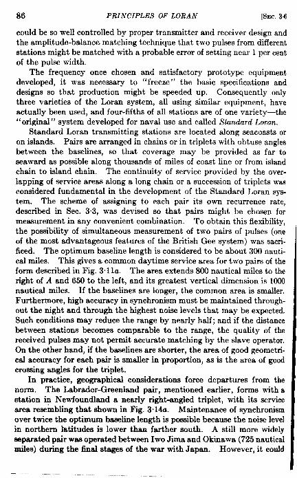
86 PRINCIPLES OF LORAN [SEC.3.6

could be so well controlled by proper transmitter and receiver design andthe amplitude-balance matching technique that two pulses from differentstations might be matched with a probable error of setting near 1 per centof the pulse width.

The frequency once chosen and satisfactory prototype equipmentdeveloped, it was necessary to “freeze” the basic specifications anddesigns so that production might be speeded up. Consequently onlythree varieties of the Loran system, all using similar equipment, haveactually been used, and four-fifths of all stations are of one variety—the“original” system developed for naval use and called S’tandani Loran.

Standard Loran transmitting stations are located along seacoasts oron islands. Pairs are arranged in chains or in triplets with obtuse anglesbetween the baselines, so that coverage may be provided as far toseaward as possible along thousands of miles of coast line or from islandchain to island chain. The continuity of service provided by the over-lapping of service areas along a long chain or a succession of triplets wasconsidered fundamental in the development of the Standard Loran sys-tem. The scheme of assigning to each pair its own recurrence rate,described in Sec. 3.3, was devised so that pairs might be chosen formeasurement in any convenient combination. To obtain this flexibility,the possibility of simultaneous measurement of two pairs of pulses (oneof the most advantageous features of the British Gee system) was sacri-ficed. The optimum baseline length is considered to be about 300 nauti-cal miles. This gives a common daytime service area for two pairs of theform described in Fig. 3.1 la. The area extends 800 nautical miles to theright of A and 650 to the left, and its greatest vertical dimension is 1000nauticaf miles. If the baselines are longer, the common area is smaller,Furthermore, high accuracy in synchronism must be maintained through-out the night and through the highest noise levels that may be expected.Such conditions may reduce the range by nearly half; and if the distancebetween stations becomes comparable to the range, the quality of thereceived pulses may not permit accurate matching by the slave operator.On the other hand, if the baselines are shorter, the area of good geometri-cal accuracy for each pair is smaller in proportion, as is the area of goodcrossing angles for the triplet.

In practice, geographical considerations force departures from thenorm. The Labrador-Greenland pair, mentioned earlier, forms with astation in Newfoundland a nearly right-angled triplet, with its servicearea resembling that shown in Fig. 3. 14u. Maintenance of synchronism

over twice the optimum baseline length is possible becauee the noise levelin northern tatitudes is lower than farther south. A still more widelyseparated pair was operated between Iwo Jima and Okinawa (725 nauticalmiles) during the final stages of the war with Japan. However, it could

SEC.3.6] STANDARD LORAN 87

not maintain a24-hr schedule, although advantage was taken of very lownoise andgood station sites. Theother extreme inseparation ofastand-ard pair is that between Guam and Saipan, with a baseline of only 130nautical miles.

To attain the maximum range, Loran transmitting stations must besited carefully. The imperfect electrical conductivity of rock and soilacts to attenuate the signal rapidly with distance traveled, and theattenuation is exponential in form, reducing signal amplitude to some-thing like ~ for each hundred miles traversed at standard frequency.Over salt water, the conductivity of which is good, the amplitude isreduced only to about i3mfor each hundred miles. Land close to a trans-mitting antenna, therefore, greatly decreases its range of transmission.Accordingly, a Loran station is placed as close to the actual water line aspossible, and an extensive ground system of copper wires or straps is laidon the ground around the antenna. No island or cape should lie acrossthe path of desired transmission, within a considerable distance. A saltmarsh, however, may intervene without serious effect, for its conductivityapproximates that of the sea.

The combined conditions imposed upon Loran station sites by geom-etry, geography, and conditions of terrain affecting transmission haveresulted in the location of many of these stations in extremely inaccessibleand uncomfortable places.

Equipment of a Standard Loran Station.—At a Standard Loran stationthat serves in two pairs, there are tw-o 100-kw transmitters, four trans-mitter timers, at least two gasoline or diesel po~ver generators, andauxiliary equipment. The transmitters and timers are housed in a singlebuilding, the timers being placed in an enclosure of wire netting to shieldthem from the field of the transmitters. In operation, two timers areconnected to one transmitter, which is fed by one power plant; the otherinstruments are stand-bys and are frequently alternated with the firstsetso that the equipment may be periodically overhauled and componentsreplaced without interrupting service. Transmitting and receivingantennas are separate and placed several hundred feet apart. Theformer is nondirectional, either a vertical wire or steel tower about 110ft in height or an inverted-L 55 ft or so along each arm. The receivingantenna is usually a single nondirectional vertical one about 50 ft long;but, if reception from the other member of one of the pairs is di5cult, along horizontal (Beverage) antenna, extended toward the distant station,is used to pick up its signals. Generally complete living and supply-storage quarters must also be provided, and therefore the whole stationoccupies several acres.

Equipment in a station that belongs to only one pair is the same,except that there are only two timers, one in use and one standing by.

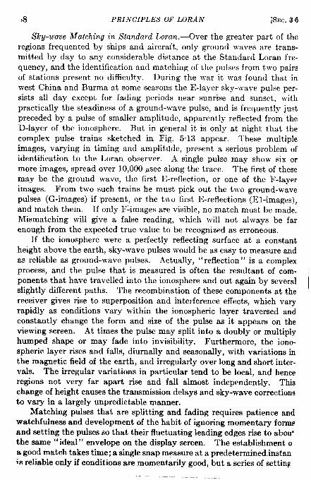
)8 PRINCIPLES OF LORAN [SEC. 36

Sky-wave Matching in Standard Loran.—Over the greater part of theregions frequented by ships and aircraft, only ground waves are trans-mitted by day to any considerable distance at the Standard Loran fre-quency, and the identification and matching of the pulses from two pairsof stations present no difficulty. During the war it was found that inwest China and Burma at some seasons the E-layer sky-wave pulse per-sists all day except for fading periods near sunrise and sunset, withpractically the steadiness of a ground-wave pulse, and is frequently justpreceded by a pulse of smaller amplitude, apparently reflected from theD-layer of the ionosphere. But in general it is only at night that thecomplex pulse trains sketched in Fig. 5.13 appear. These multipleimages, varying in timing and amplittide, present a serious problem ofidentification to the Loran observer. A single pulse may show six ormore images, spread over 10,000 ~sec along the trace. The first of thesemay be the ground wave, the first E-reflection, or one of the F-layerimages. From two such trains he must pick out the two ground-wavepulses (G-images) if present, or the two first E-reflections (El-images),and match them. If only F-images are visible, no match must be made.Mismatching will give a false reading, which will not always be farenough from the expected true value to be recognized as erroneous.

If the ionosphere were a perfectly reflecting surface at a constantheight above the earth, sky-wave pulses would be as easy to measure andas reliable as ground-wave pulses. Actually, [‘reflection “ is a complexprocess, and the pulse that is measured is often the resultant of com-ponents that have travelled into the ionosphere and out again by severalslightly different paths. The recombination of these components at thereceiver gives rise to superposition and interference effects, which varyrapidly as conditions vary within the ionospheric layer traversed andconstantly change the form and size of the pulse as it appears on theviewing screen. At times the pulse may split into a doubly or multiplyhumped shape or may fade into invisibility. Furthermore, the iono-spheric layer rises and falls, diurnally and seasonally, with variations inthe magnetic field of the earth, and irregularly over long and short inter-vals. The irregular variations in particular tend to be local, and henceregions not very far apart rise and fall almost independently. Thischange of height causes the transmission delays and sky-wave correctionsto vary in a largely unpredictable manner.

Matching pulses that are splitting and fading requires patience andwatchfulness and development of the habit of ignoring momentary formand setting the pulses so that their fluctuating leading edges rise to aboufthe same “ ideal” envelope on the display screen. The establishment o

a good match takes time; a single snap measure at a predetermined. instanis reliable only if conditions are momentarilyy good, but a series of setting

SEC.343] STANDARD LORAN 89

yields a much better average than appearances would lead the measurer

to expect. When the technique has IJccn mastered, matches made withsky-wave pulses arc unlikely to he more than 3 psec in error.

Some general precepts, for the identification of pulse images at night,maybe stated:

1. Within 500 or600statute miles of thestation emitting the pulses,the G-image is the first in order, the Ill-image next. From theground-lvave limit to 1500 or 1600 miles the E1-image is firs,t, fol-lowed by Ii20r Fl (the 132-image isoften imperceptible except atlong distances).

2. Normally the ground-wave image does not split or fade, thoughwhen it is not much stronger than the “noise,” it appears tofluctuate ina manner that sometimes resembles splittingj and theimage height will also vary with any oscillation of the receivingantenna owing to motion of the ship or aircraft. The El-imagesplits and fades, but less violently than do later images and overlonger cycles’. At times it is as steady as a ground-wave image.

3. The time interval in microseconds between the G- and El-images isrough] y

40 + q? d ~ 10,

where d is the distance of the emitting station in hundreds of nauti-cal miles. The interval between E 1 and E2 is roughly

that from E2 to Fl, a little more than this.

The limit of ground-wave reception varies with the amount of noiseabove which the pulse must rise and with the location of the station.Consequently a zone exists within which the first image maybe G or El,and it must be identified by its behavior and its interval from the nextimage. If both images appear, their separation is 75 to 100 psec in thiszone. An occasional extra El-image (“ sporadic E “), immediately afterthe regular one or overlapping its following side, may confuse the picture.Similarly, the outer boundary of the sky-wave service area takes the formof a similar zone, within which the first image may be El or E2; if bothappear, their separation is 75 to 100 psec in this zone. It is important toturn up the receiver to the highest practicable gain when identifying thefirst image of a train, to make sure that there is not another weak imageto the left of it. A steady scrutiny is necessary, for unusually high noisemay obscure a ground-wave image, or prolonged fading may obscure anEl-image for some time.

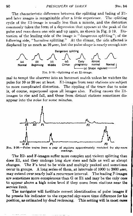
90 PRINCIPLES OF LORAN [$iEc.3.6

The chal acteristic difference between the splitting and fading of El-and later images is recognizable after a little experience. The splittingcycle of the l’; l-image is usually less than a minute, and the distortioncommonly takes the form of a depression that appears at the peak of thepulse and runs down one side and Up again, as shown in Fig. 3.19. Dis-tortion of the leading side of the image is “dangerous splitting”; of thefollowing side, “ harmless splitting.” At the climax, the side affected isdisplaced by as much as 10 ~sec, but the pulse shape is nearly enough nor-

Dangerous splitting

AYLAAA AA(a) (b) (c) Early Almost

Normal Beginning Wddle CIRX e normal‘5(e) Shape regained

FIG. 3.19.—Splitting of an El-image.

mal to tempt the observer into an incorrect match unless he watches thepulse for 10 or 20 sec at least. El-images from near stations are subjectto more complicated distortion. The rippling of the trace due to noiseis, of course, superposed upon all images also. Fading causes the El-images to rise and fall, and those from distant stations sometimes dis-appear into the noise for some minutes.

I

GEI F1 F2FIG. 3.20.—Pufae trains from a pair of stations approximately matched for sky-wave

readings.

The E2- and F-images suffer more complex and violent splitting thandoes El, and they undergo long slow rises and falls as well as abruptchanges. The F’s tend to be wide and multiply peaked and sometimesoccur in groupe. A long series of them, at intervals of 1000 to 2000 psec,may extend over nearly half a recurrence interval. The leading F-imagesare sometimes more conspicuous than G or El and may be the only onesto appear above a high noise level if they come from stations near theservice limit.

The navigator will facilitate correct identification of pulse images ifhe presets his indicator to the expected sky-wave time difference for hisposition, as estimated by dead reckoning. This setting will in most casa

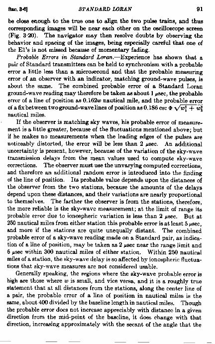
SW. 8.6] STANDARD LQRAN 91

be C1OSSenough to the true one to align the two pulse traina, and thuscorresponding images will be near each other on the oscilloscope screen(Fig. 3%). The navigator may then resolve doubts by observing thebehavior and spacing of the images, being especially careful that one ofthe El’s is not missed because of momentary fading.

Probable ETTOTS in Stun&rd Loran.-lZxperience haa shown that apair of Standard transmitters can be held to synchronism with a probableerror a little less than a micro~cond and that the probable measuringerror of an observer with an indicator, matching ground-wave pulses, isabout the same. The combined probable error of a Standard Loranground-wave reading may therefore be taken as about 1 psec, the probableerror of a line of position aa O.162w nautical mile, and the probable errorof a fix between two ground-wave lines of position as 0.186 csc @ ~’nautical miles.

If the observer is matching sky waves, his probable error of measure-ment is a little greater, because of the fluctuations mentioned above; butif he makes no measurements when the leading edges of the pulses arenoticeably distorted, the error will be less than 2 psec. An additionaluncertainty is present, however, because of the variation of the sky-wavetransmission delays from the mean values used to compute sky-wavecorrections. The observer must use the unvarying computed corrections,and therefore an additional random error is introduced into the findingof the line of position. Its probable value depends upon the distances ofthe observer from the two stations, because the amounts of the delaysdepend upon these distances, and their variations are nearly proportionalto themselves. The farther the observer is from the stations, therefore,the more reliable is the sky-wave measurement; at the limit of range itsprobable error due to ionospheric variation is less than 2 psec. But at250 nautical miles from either station this probable error is at least 5 ~sec,and more if the stations are quite unequally distant. The combinedprobable error of a sky-wave reading made on a Standard pair, as indica-tion of a line of position, maybe taken as 2 ~sec near the range limit and6 psex within 300 nautical miles of either station. Within 250 nauticalmiles of a station, the sky-wave delay is so affected by ionospheric fluctua-tions that sky-wave measures are not considered usable.

Generally speaking, the regions where the sky-wave probable error ishigh are those where w is small, and vice versa, and it is a roughly truestatement that at all distances from the stations, along the center line ofa pair, the probable error of a line of position in nautical miles is thesame, about 400 divided by the baseline length in nautical miles. Thoughthe probable error does not increase appreciably with distance in a givendirection from the mid-point of the baseline, it does change with thatdirection, incre~qing approximately with the secant of the angle that the

92 PRINCIPLES OF WRAN [tk!c. 3.6

line from midpoint to point of observation makes with the center line.This angle is the complement of O[sss Eq. (9)], and this rule is simply anapplication of that equation, the distance factor (r/b) dropping out becauseof the decrease of measuring error with distance.

If W denotes the probable error of a sky-wave line of position innautical miles, we may then write W = 400/b csc 8 and take 1.15 csc @tiW~ + m as a fair approximation to the probable error of a skywave fix.

A more precise evaluation of the probable errors of Standard Loran

FIG.3.21.—Useful &ice areneof a Stand-ard Loran pair. Solid line: ground-waveboundary; dashed line: sky-wave boundary.

sky-wave lines of position is ex-hibited in Fig. 522.

Se TV i c e Areaa in standard

Loran. —Although Loran readingson a pair of stativns may be madewherever both pulses can be re-ceived, they are of little value ifmade in regions where the prob-able error is large. It haa beencustomary to consider the usefulground-wave service area of aStandard pair to be those regionswhere kw is less than 2 nauticalmiles per microsecond. Theareas thus excluded are shown inblack in Fig, 3.10, Their bounda-ries are arcs of circles, with centerson the center line at a distance ofsix baseline lengths from thestations. From the useful sky-

wave service area are excluded the region within 250 nautical miles ofeach station (two circles which usually overlap) and also the regionadjacent to each extended baseline, bounded by the lines O = CSC-l(b/100),where b is in nautical miles. This angle is 30° if b is 200, 19.5° if b is 300,14.5° if b is 500. In these regions, according to the formula for W statedabove, the probable error of a sky-wave line of position exceeds 4 nauticalmiles. The two areas, delimited in this way, are shown in Fig. 321,

The useful common service area for a triplet or two pairs consistsof those regions which fall within the boundaries for both pairs, asdescribed above, and in addition are included inside the figure eight alongwhich @ for the two pairs is 15°. For a triplet, the two lobes of thiscontour are circles drawn through the end stations, with radii equal to thedistance bet ween these stations. For two separate pairs with the mid-

points of their baselines not too close together, the lobes are nearly enough

Sm. 3.6] STANDARD LORAN 93

circles drawn through the midpoints, with radii equal to twice the distancebetween these points. When these various boundaries have been laidout for two pairs, those areaa included tilde all of these will form anirregular figure such as that shown in Fig. 3“22.

Of course, these conventional limits are somewhat artificial, especiallythe crossing-angle limit. More correctly, this and the limit kw = 2

‘. / -j‘. -— ..”

FIG. 3.22.—Common ground-wave service area for two pairs.

nautical miles per microsecond should be replaced by the curve O.18~csc @ ~w? + w; = 2, for ground waves, or 1.15 csc @ v= = 4,for sky waves, a curve that would have to be plotted laboriously by points.But any hard-and-fast limit is artificial, and the conventional construc-tion gives a fair indication of the advantages and disadvantages of a givenor proposed station configuration. A more detailed exhibit of the varia-tion of W with position is given in the chapter on wave propagation(Chap. 5).

Air Transportable Loran.—A form of Standard Loran employingspecial lightweight equipment was developed at the Radiation Laboratoryfor the Army Air Forces. It was intended for use inland, in the ruggedterritory of northern Burma and southwestern China. Over land,Standard Loran has no advantage in range or geometrical precision overthe higher-frequency British Gee system and has some disadvantage inease and precision of time-difference measurement. In mountainous

94 PRINCIPLES OF WRAN [SEC. 3.7

country, however, ita signals can be received behind the mountains,whereas propagation at the Gee frequency is limited to the line of sight.

Timers and transmits were designed to be transportable by aircompletely aasembled, and tactical use of the system, advancing thestations with the advancing armies, wae envisaged. The timers wereadaptations of the navigator’s indicator. Their crystal oscillators anddivider circuits were less stable than those of the standard timer, butwhen properly handled they” gave reliable service with only a smalldecrease in timing precision. The light transmitters were somewhatdisappointing in power output and in other respects and were not actuallyused in the field; instead Standard transmitters were used. In operation,ground-wave ranges by day from 240 to 350 nautical miles were obtainedand 220 to 270 by night (for high-flying aircraft). Because all baselinelengths were less than 60 nautical miles, the geometrical precision at thedaytime ground-wave limit wae no better than 1 nautical mile per micro-second, and the crossing angles were small. Greatly increased rangegiven by sky waves at night was not useful practically, and therefore skywaves were used as substitutes for ground waves only when high noisemade the latter unusable.

3,7. Sky-wave Synchronized Loran.-The successful use of skywaves in extending the coverage of Standard Loran at night showed thata nighttime Loran systemj using sky-wave transmission for synchronizingthe pairs of stations as well as for position finding, was feasible. Thoughnecessarily inoperative by day except under special conditions, such asystem would permit long baselines to be set up across land, giving highgeometrical precision and good crossing angles to great distances, advan-tages that would offset the decrease in timing accuracy resulting from theuse of sky waves to link the stations. These advantages recommendedthe system for the guidance of night bombers over central Germany; andaa described in Chap. 2, such a system was tested in the eastern UnitedStates in the autumn of 1943 and operated over Europe during the lastyear of the war. A Standard Loran frequency and Standard Loranequipment were used. Two separate pairs of stations were arranged ina modified quadrilateral, the form of which (Fig. 2“1) gave the bestgeometrical characteristics obtainable while all western Europe was stillheld by the Central Powers. The system was called Sky-wave Syn-chronized, or SS, Loran. In the spring of 1945, two SS pairs beganoperation in southeast Asia. They were not arranged in a quadrilateralbut gave separate families of position lines, one over the region of easternChina held by the Japanese, the other over Burma and Malaya.

The variability of the ionosphere affects Loran measurements in twoways. The varying density of the layer and its departure from homo-geneity cause the total intensity of sky-wave signals to increase and

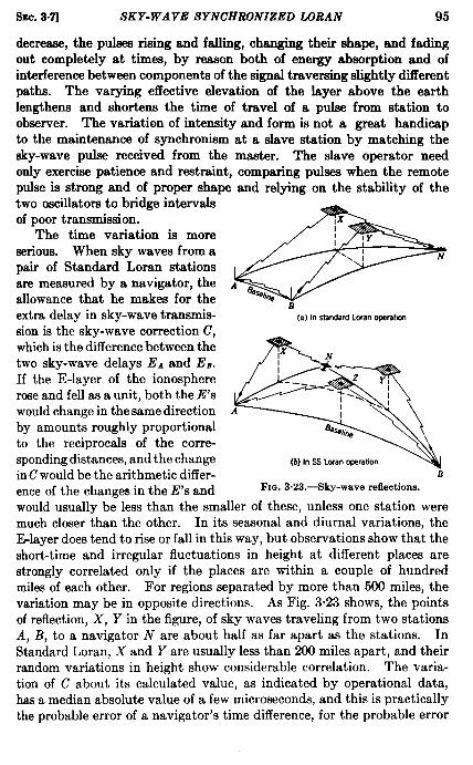
sm. 3q SKY-WAVE SYNCHRONIZED WRAN 95

decreaae, the pulaea rising and falling, changing their ahape, and fadiigout completely at times, by reason both of energy absorption and ofinterference between components of the signal traversing slightly ditTerentpaths. The varying effective elevation of the layer above the earthlengthens and shortens the time of travel of a pulse from station toobserver. The variation of intensity and form is not a great handicapto the maintenance of synchronism at a slave station by matching thesky-wave pulse received from the master. The slave operator needonly exercise patience and restraint, compting pulses when the remotepulse is strong and of proper shape and relying on the stability of thetwo oscillators to bridge intervalsof poor transmission.

The time variation is moreserious. When sky waves from apair of Standard Loran stationsare measured by a navigator, theallowance that he makes for theextra delay in sky-wave transmis-sion is the sky-wave correction C,which is the difference between thetwo sky-wave delays E. and En.If the E-layer of the ionosphererose and fell as a unit, both the E’swould change in the same directionby amounts roughly proportionalto the reciprocals of the corre-sponding distances, and the changein C would be the arithmetic differ-ence of the changes in the E’s and

B(a)InstandardLcfanopxahm

A

(b)InSSLoranoperatmnB

Fm. 3.23.-Sky-wave reflections.

would usually be less than the smaller of these, unless one station weremuch closer than the other. In its seasonal and diurnal variations, theE-layer does tend to rise or fall in this way, but observations show that theshort-time and irregular fluctuations in height at different places arestrongly correlated only if the places are within a couple of hundredmiles of each other. For regions separated by more than 500 miles, thevariation may be in opposite directions. As Fig. 3.23 shows, the pointsof reflection, X, Y in the figure, of sky waves traveling from two stationsA, 1?, to a navigator N are about half as far apart as the stations. InStandard Loran, X and Y are usually less than 200 miles apart, and theirrandom variations in height show considerable correlation. The varia-tion of C about its calculated value, as indicated by operational data,has a median absolute value of a few microseconds, and this is practicallythe probable error of a navigator’s time difference, for the probable error

96 PRINCIPLES OF LORAN [SEC.3.7

of synchronism between stations (maintained by ground-wave transmis-sion) is less than 1 Psec.

The absolute delay between a pair of SS Loran stations, as the slaveoperator holds his timer to a time difference ~, is

E. being the extra length of time taken by the sky-wave pulse from themaster transmitter to traverse the path AZB (Fig. 3“23) instead of AB.As the elevation of Z above ground fluctuates, EA varies, but the longerAB is the smaller is the variation (by reasoning similar to that used in theexplanation of Fig. 3“5, Sec. 3“2). For this reason, as well as to obtainthe most advantageous geometry, SS baselines are made as long aspossible. The longer baseline in the European quadrilateral was 1300nautical miles. Even with this length, the observed median absolutevariation of E. from its calculated amount, regarded as a probable error,is about 5 psec. This variation enters into the absolute delay D in itsfull amount, for there is no E, to balance ~. in the expression above,since the local pulse at the slave station is not reflected from the iono-sphere. The observed time difference at N varies with D as well as withC; moreover, C fluctuates more widely in SS observations than in Stand-ard ones, because if A B is 1300 nautical miles, X Y is 650, and the changesin the elevation of Y are to a large extent independent of those of X.The combined effects of the variations at Z, X, and Y give a probableerror of about 8 psec for a measured time difference in the SS Loransystem, according to observations made when the first experimental SSstations were operated in the eastern United States, in 1943.

When enough is known about the systematic variations in ionosphericelevation to predict its value to some extent, it may be possible to vary~ at the slave station so as to correct in part the changes in E. and holdD nearer to constancy. The data collected during the experimentaloperations in 1943 did not give much encouragement in this direction.Without any such correction, the probable timing error of 8 psec resultedin a median discrepancy of about l; nautical miles between SS Loranfixes and visual pinpoint locations. This very satisfactory accuracy wasdue to the low average value of the geometrical factor lcw within most ofthe area served by the quadrilateral, less than ~ nautical mile per micro-second, and the large crossing angles, between 60° and 90°, as well as torather expert handling of well-adjusted indicators and low speed of theaircraft. In actual use of the system over Germany, the accuracy of fixwas not quite so good.

The “blind spot” close to each, transmitting station, due to theunreliability and large delay variation of sky waves traveling short

SEC.3.8] LOW FREQUENCY LORAN 97

distances, is unimportant in Standard Loran because there is 24-hrground-wave service in this region. But in SS Loran, the neighborhoodof a station is beyond the ground-wave range of the other station of thepair. Itisquite possible, ho~vever, tomatch theground-~~,ave pulse fromthe near station and the sky-wave pulse from the distant one, just as theSS slave operator does in maintaining synchronism and the master opera-tor in monitoring.

Charts for SS Loran navigation do not carry ground-wave lines ofposition and numerical values of C as do Standard charts. Instead, thesky-wave corrections are incorporated in the calculations, and the givenlines of position represent sky-wave time differences, so that the navigatorneed make no correction to his reading. Ground-against-sky lines ofposition, appropriately distinguished from the others, are provided within250 miles of each station.

3,8. Low Frequency Loran.—When Standard Loran was first devel-oped, it was felt that precise measurement of time intervals betweenpulses would not be practical at frequencies much below 1 Me/see,because the pulses would have to be extremely slow in rise and fall inorder to avoid use of an excessive band}vidth. Furthermore, naturalnoise at low frequencies was known to be high. But the remarkableprecision with which the Standard pulses (themselves very long in com-parison with radar pulses) could be matched and the success of Loranoperators in measuring through noise of much greater amplitude than thepulses encouraged a reconsideration. A system with longer ranges andlonger baselines than Standard Loran was desired for covering the greatspaces of the Pacific, particularly near Japan and the Chinese ports, anda 24-hr overland service over eastern China, from stations either to sea-ward or in western and southern China, would have been of materialassistance in an East Asia land campaign against Japan. Equipment forsuch a system was designed and constructed during the winter and springof 1944–1945 on an emergency basis, using the Standard timer with somemodifications and incorporating some sections of the Standard trans-mitter into the LF transmitter. The transmitting antenna was a 1300-ftvertical wire supported by a barrage balloon, to be used temporarily andreplaced as soon as practicable by a 625-ft steel tower supporting a top-loaded umbrella-type antenna. A converter was provided for the navi-gator, by the use of which signals at the frequency chosen, 180 kc/see,would be received by the Standard Loran receiver-indicator. Low Fre-quency experimental transmitting stations were placed on Cape Cod,hlass,, Cape Fear, N. C., and Key Large, F1., and operated as a tripletduring the summer of 1945, with generally satisfactory results. Butbefore the equipment could be transferred from these stations to thePacific, the war ended.

98 PRINCIPLES OF LORAN [SEC.3.8

Data obtained from the experimental operations are discussed in detailin Chap. 5. Some general characteristics of the system are stated here.The peak power of the transmitters was about 100 kw, which gavesummer daytime ranges near 1200 and 1000 nautical miles over sea andland respective y and a summer nighttime range of 1500 or more. Thesefigures are subject to large variations with time of day and season becauseof the very great fluctuations in the natural electrical noise at 180 kc/seeand the variability of the sky-wave transmission also. The former maybe expected to decrease, and the latter to improve in winter, giving greaterranges.

The length of the pulses as received is more than 300 psec; require-ments of efficient antenna radiation and the need to keep the bandwidthnarrow to avoid interference with adj scent communication channels pre-clude a sharper pulse form. Pulse-matching accuracy is therefore lowerthan in Standard Loran; but, when ground waves are matched, theprobable error is only a few microseconds. With these long pulses anda sky wave that is apparently reflected from the E-layer only, the ground-wave and sky-wave pulse images, when both are present, overlap in asingle composite envelope. The long trains of pulses characteristic ofStandard Loran by night are not present at the low frequency—a greatadvantage, since a principal cause of large errors in Standard pulse-matching has been mistaking a sky wave for the ground wave or anF-image for an E.

The coalescence of ground wave and sky wave has a serious dis-advantage, however. At ranges between about 400 and 1200 nauticalmiles, the proportion of ground- and sky-wave components in the observedpulse varies with distance, with the momentary intensity of the sky wave,and with the r-f phase difference between the ground and sky waves.The rising slope of the pulse is composite or discontinuous (see Figs.5.31 and 532), and the time difference obtained by matching it withanother pulse is somewhere between the values for pure ground waveand pure sky wave, varying with the conditions and with the point onthe slope at which the match is made. Beyond 1200 nautical miles theground wave is absent, but the first- and second-hop sky waves combinein a similar fashion, and beyond 1800 miles the second and third combine.Measured time differences at all distances greater than a few hundredmiles must be considered as including a transmission delay increasingwith distance (contrary to the pure first-hop sky-wave delay of StandardLoran, which decreases). The curve of increase has a wavy or “step”form (Fig. 5.30), and the height and spacing of the steps differ by day andnight, over land and water (Fig. 5.46), and probably in summer andwinter. The short-time variation of the delay curve contributes tomeasured time differences a probable error of apparent delay similar to

SEC.38] LOW FREQUENCY LORAN 99

that given to Sky-wave Synchronized Loran measurements by changinglayer height, but somewhat greater, particularly where the delay curveis steep.

The baseline lengths of the experimental LF triplet were 535 and 606nautical miles. Over these distances, the ground wave received at theslave stations from the master was always strong enough to control thefirst 30 or 40 psec of the visible pulse form, even at night when the skywave dominated the top of the envelope. Therefore the slave operatorcould always hold synchronism by ground wave. A specially designedreceiver-indicator, displaying the pulses at the i-f heterodyne stage, with-out rectification, enabled him to superimpose the individual i-f cycles ofthe two pulses instead of their rectified envelopes. The cycles could bemat ched with a probable error of setting of about 0.1 psec when the signalstrength was well above the noise, so that synchronism could be main-tained with several times the precision of Standard Loran once an opera-ting technique had been devised for detecting and correcting occasionalmismatches of one or two whole cycles. Unfortunately, cycle matchingis not practicable at distances where the ground wave is too weak to risewell above the noise before the sky wave joins it, because in the compositepart of the pulse, interference between ground and sky wave introduces avariable and unpredictable r-f phase shift.

With synchronism accurately maintained by ground wave and trans-mitters arranged in line with double master station between the twoslaves, the LF system as operated resembled a Standard triplet on twicethe scale rather than a day and night SS system. The 24-hr service areaprovided over water was about twice that of a Standard triplet, and theland service area was roughly two-thirds of that over water. Ground-wave accuracy of fix by Low Frequency was at least equal to Standardaccuracy at equal distances from the baselines, for the greater timingerror with the long pulses was compensated by the more favorablegeometry provided by the long baselines. The accuracy might have beenincreased if time differences had been measured by cycle-matching, butno method was found to avoid errors of one or more whole cycles in thesemeasures (the navigator could not have the ground-station operator’sadvantage of knowing the true value in advance). Low Frequency sky.wave accuracy at long distances was less than that given by Standard orSS Loran. Accuracy figures obtained at some monitor stations are givenin Table 5.4.

The advantage of being able with equal facility to choose any two ofseveral families of position to obtain a fix is not very great in a systemwhere two pairs of stations command as large a common service area asdoes an LF Loran triplet or quadrilateral. On the other hand, a systemwith a large land coverage, extensively used by fast-moving aircraft,

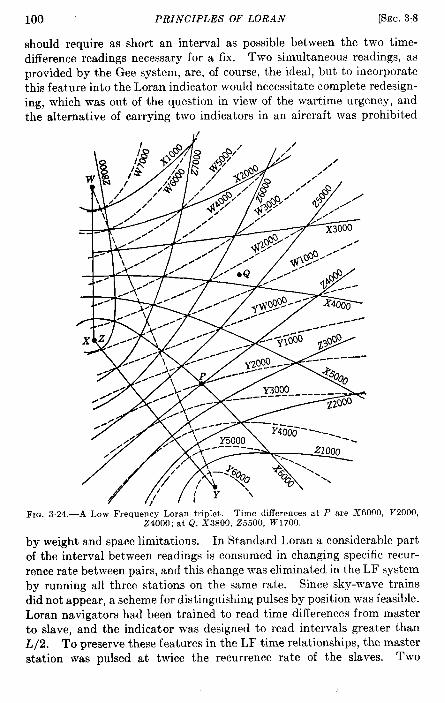
100 PRINCIPLES OF LORAN [SEC.3.8

should require as short an interval as possible between the two time-difference readings necessary for a fix. Two simultaneous readings, asprovided bythe Gee system, are, of course, the ideal, but to incorporatethis feature into the Loran indicator would necessitate complete redesign-ing, which was out of the question in view of the wartime urgency, andthe alternative of carrying two indicators in an aircraft was prohibited

,/

FIG. 3.24.—A Low Frequency Loran triplet. Time differences at P are X6000, Y2000,Z4000; at Q, X3800, Z5500, W1700.

by weight and space limitations. In Standard Loran a considerable part

of the interval between readings is consumed in changing specific recur-rence rate between pairs, and this change was eliminated in the LF systemby running all three stations on the same rate. Since sky-wave trainsdid not appear, a scheme for distinguishing pulses by position was feasible.Loran navigators had been trained to read time differences from masterto slave, and the indicator was designed to read intervals greater thanL/2. To preserve these features in the LF time relationships, the masterstation was pulsed at twice the recurrence rate of the slaves. Two

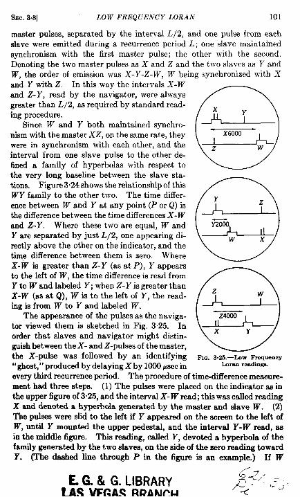
SEC.3.8] LOW FREQUENCY LORAN 101

master pulses, separated by the interval L/2, and one pulse from eachslave were emitted during a recurrence period L; one slave maintainedsynchronism with the first master pulse; the other with the second.Denoting the two master pulses as X and Z and the two slaves as Y andW, the order of emission was X-Y-Z-W, W being synchronized with Xand Y with Z. In this way the intervals X-Wand Z-Y, read by the navigator, were alwaysgreater than L/2, as required by standard read-

e

xing procedure. Y

Since W and Y both maintained synchro-nism with the master X2, on the same rate, they -

were in synchronism with each other, and the z winterval from one slave pulse to the other de-fined a family of hyperbolas with respect tothe very long baseline between the slave sta-tions. Figure 3.24 shows the relationship of thkWY family to the other two. The time differ-

0

Yence between W and Y at any point (P or Q) is z

the difference between the time differences X-Wand Z-Y. Where these two are equal, W and YTW

Y are separated by just L/2, one ap~earing di- W xrectly above the other on the indicator, and thetime difference between them is zero. WhereX-W is greater than Z-Y (as at P), Y appearsto the left of W, the time difference is read fromY to W and labeled Y; when Z-Y is greater thanX-W (as at Q), W is to the left of Y, the read-

0

z w

ing is from W to Y and labeled W.The appearance of the pulses as the naviga- z400a

tor viewed them is sketched in Fig. 325. In xorder that slaves and navigator might distin-

Y

Wish between the X- and Z-pulses of the master,the X-pulse was followed by an identifying F,O. 3.25.-IAw Frequency

“ghost,” produced by delaying X by 1000 p.wc in Loran readings.

every third recurrence period. The procedure of time-difference measure-ment had three steps. (1) The pulses were placed on the indicator as inthe upper figure of 3“25, and the interval X- W read; this was called readingX and denoted a hyperbola generated by the master and slave W. (2)The pulses were slid to the left if Y appeared on the screen to the left ofW, until Y mounted the upper pedestal, and the interval Y-W read, asin the middle figure. This reading, called Y, devoted a hyperbola of thefamily generated by the two slaves, on the side of the zero reading toward

y. (The d~ed line thugh P in the figure is an example.) If w

&G. & G. LIBRARY!AS VEGAS BRANCH

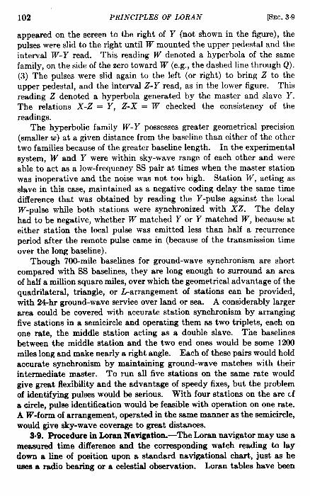
102 PRINCIPLES OF LORAN [SEC.3.9

appeared on the screen to the right of Y (not shown in the figure), thepulses were slid to the right until W mounted the upper pedestal and theinterval W-Y read. This reading W denoted a hyperbola of the samefamily, on the side of the zero toward W (e.g., the dashed line through Q).(3) The pulses were slid again to the left (or right) to bring Z to theupper pedestal, and the interval Z-Y read, as in the lower figure. Thisreading Z denoted a hyperbola generated by the master and slave Y.The relations X-Z = Y, Z-X = W checked the consistency of thereadings.

The hyperbolic family W-Y possesses greater geometrical precision(smaller w) at a given distance from the baseline than either of the othertwo families because of the greater baseline length. In the experimentalsystem, W and Y were within sky-wave range of each other and wereable to act as a low-frequency SS pair at times when the master stationwas inoperative and the noise was not too high. Station W, acting asslave in this case, maintained as a negative coding delay the same timedifference that was obtained by reading the Y-pulse against the localW-pulse while both stations were synchronized with X2. The delayhad to be negative, whether W matched Y or Y matched W, because ateither station the local pulse was emitted less than half a recurrenceperiod after the remote pulse came in (because of the transmission timeover the long baseline).

Though 70@mile baselines for ground-wave synchronism are shortcompared with SS baselines, they are long enough to surround an areaof half a million square miles, over which the geometrical advantage of thequadrilateral, triangle, or L-arrangement of stations can be provided,with 24-hr ground-wave service over land or sea. A considerably largerarea could be covered with accurate station synchronism by arrangingfive stations in a semicircle and operating them as two triplets, each onone rate, the middle station acting as a double slave. Tne baselinesbetween the middle station and the two end ones would be some 1200miles long and make nearly a right angle. Each of these pairs would holdaccurate synchronism by maintaining ground-wave matches with theirintermediate master. To run all five stations on the same rate wouldgive great flexibility and the advantage of speedy fixes, but the problemof identifying pulses would be serious. With four stations on the arc cfa circle, pulse identification would be feasible with operation on one rate.A W-form of arrangement, operated in the same manner as the semicircle,would give sky-wave coverage to great distances.

3.9. Procedure in Loran Navigation.-The Loran navigator may use ameasured time difference and the corresponding watch reading to laydown a line of position upon a standard navigational chart, just as heuses a radio bearing or a celestial observation. Loran tables have been

SEC.3.9] PROCEDURE IN LORAN NAVIGATION 103

prepared, giving the intersections of the Loran lines with the meridiansand parallels. By interpolating in these tables, three points of the linecorresponding to his reading may be plotted on the chart, and a curvedrawn through them and labeled with the reading, rate (to identify thefamily), and time of the observation. (Two points may serve in someregions and on some forms of chart, but in general the line is curved onthe chart.) If he uses a Loran chart, the tables are unnecessary. Linesat convenient intervals of time difference (every 20 or 50 ~sec is mostusual) are printed on the chart, and the line representing the reading isinterpolated by estimation between them.

A reading on another pair of stations gives the navigator a secondline of position intersecting the first line. It is similarly drawn andlabeled. If the navigator is on a slow ship, the change of position of theship is negligible during the interval between observations, and the pointwhere the lines intersect is the navigator’s location at both the recordedtimes. But a fast ship moves a considerable part of a mile in a minute,and an aircraft moves several miles. In these cases, the lines of positionmust be considered to move over the earth, and their intersection at thesarrwtime must be found.

One way to do this is to advance the first line of position to the timeof the second, according to standard plotting practice for all kinds oflines of position—lines obtained in piloting, radio bearings, or celestiallines. From any arbitrary point on the first line (conveniently near thenavigator’s estimated location) is measured a distance equal to theproduct of the speed of the craft and the time interval between observa-tions and taken in the direction of the motion. This distance and direc.tion locate a new point through which a new line of position is drawnparallel to the first line. The intersection of the new line with the linerepresenting the second observation is the position of the craft at the timeof the second observation.

Another way is to make observations in groups of thre~the first andlast on one pair of stations and the middle one on the other pair. Anexperienced observer can make the time intervals bet ween readingsnearly equal. Then the average of the first and last readings will bepractically equal to the reading that would be obtained if this pair hadbeen observed simultaneously with the other pair. The line representingthe average reading is drawn upon the chart and labeled with the averagewatch time. If the time intervals are decidedly unequal, an interpolatedreading is taken instead of the average. This method maybe used withany number of observations greater than two if they are taken in a sym-metrical order.

A graphical variant of this procedure is useful when a number ofobservations are taken under poor conditions so that accidental errora

104 PRINCIPLES OF LORAN [SEC.39

produce a considerable scatter. Observations on two pairs are takenalternately or in alternate groups and plotted directly against time oncross-section paper-both pairs on the same sheet or on different sheetsas convenient. Smooth curves are drawn to represent the series ofmeasures on each pair, and points on the two curves, for the same time,give the fix at that time.

All these methods tell the navigator where he was in the past, not inthe present. An experienced observer, using a Standard airborne indica-tor, can make two readings and plot the fix on a Loran chart in less than3 min if conditions are good. If the two pairs of pulses matched are onthe same recurrence rate, as in the Low Frequency triplet described above,the time is somewhat shortened. The recently produced direct-readingindicator for shipboard use exhibits the time difference numerically on adial as the observer matches the pulses. This eliminates the separateoperation of counting markers on a screen and further shortens the timerequired to make a reading, but the instrument as now produced is toobulky and heavy to use in an aircraft. The only really satisfactorymethod of observation in an aircraft is simultaneous matching of twopairs. If space can be spared for two airborne indicators, it is possiblefor one observer to do this. A lightweight double direct-reading indicatoris a technical problem that will undoubtedly be solved in the near future;by its use a continuous indication of the track followed would be givenas long as the observer held the pulses in coincidence by turning thecontrols. The further step from this to linkage of the delay controlsof the indicator with a tracer moving over a chart is a short one,which has already been successfully taken in trials with somewhat crudeinstrumentation.

The device was called the Loran plotting board. It consisted of a pen,moving over a board to which a Loran chart was clamped, and connectedto linkages by which linear motions of the pen, parallel to two guides,were made proportional to the rotary motions of the setting controls oftwo indicators. The guides were set parallel to Loran lines on the chart,and the linkages adjusted so that when either of the indicators was setupon a given reading in microseconds, the tracer waa set upon the cor-responding Loran line; and when the indicator setting was turned througha given interval in microseconds, the tracer, sliding along the appropriateguide, passed over a corresponding number of miles on the chart. Inbperation, once this correspondence between indicators and chart waaestablished, the observer simply picked up the proper pairs of pulses,matched them, and maintained the matches by turning the controls aathe pulses drifted with the progress of the craft. No numerical readingswere taken; the linkages continuously transferred the rea&ngs to thechart.

SEC.39] I’itOCEDUltE IN LO1tAN NAVIGATION 105

As used, the plotting board had a limited range; and since it translatedthe time differences mechanically into rectilinear coordinates, it wasaccurate only to the extent to which the Loran lines in the area approxi-mated families of straight parallel lines uniformly spaced on the chart.The approximation was fairly good in the experimental Sky-wave Syn-chronized system in connection with which the trials !vere made. Meansfor correcting these defects and lines of future development are discussedin ChaD. 4.

Sev&al automatic plotting boards have been developed, which tracethe path of a ship or aircraft by combining the velocity vector furnishedby the instruments with current or wind data, and integrate over theelapsed time. It is the distinctive feature of Loran plotting that noextrapolation from past to present occurs nor is any correction for motionof the medium involved. The instantaneous position with respect tofixed stations is constantly displayed; and with a proper chart projectionand a correctly designed linkage between delay circuit and tracer, theonly appreciable errors should be those of pulse timing and matchi%g.These are not cumulative, but on the contrary tend to average out overa period of time.

Loran may be used simply as an aid to conventional navigation bycompass and log or air-speed indicator, furnishing check points for deadreckoning. It may also be used as a complete system for guiding thevessel along a track defined by Loran readings to a destination locatedby Loran readings. The simplest way to do this is to seek that hyperbolawhich passes through the destination and to follow it in. The readingdefining this hyperbola is preset into the indicator, and the craft directedso that the pulses from the corresponding stations, widely separated wherethe craft is distant from the line, drift into coincidence and remain so.Progress along the line is determined by switching the indicator periodi-cally to another pair of pulses, while holding the course, and noting thetimes at which lines of that family are crossed, then returning the indicatorto the first setting and pair to continue tracking. This was the procedureused by the Royal Air Force in bombing Berlin by SS Loran. To facili-tate alternation between pairs, Standard indicators were modified by theaddition of a second pair of delay controls so that the controls could beset at two different readings and either switched into operation. With adouble indicator, displaying both pairs of pulses at once, no alternationwould be necessary. But, generally, this method strongly resembles theprocedure of the days before the chronometer, when a navigator, trustingonly his determination of latitude, might sail along the parallel that passedthrough his destination until he made his landfall. However, as lines ofvarious slopes may be defined in rectangular coordinates, track lines thatcut the hyperbolic families with various generalized slopes may be defined

106 PRINCIPLES OF LORAN [SEC.3.9

in Loran coordinates and directly tracked by the use of suitably modifiedLoran indicators. Suchlines, analogies of therhumb lines ofpresent-daynavigation, have been called Lorhumbs. ‘l’he required instrumentalmodifications, while conceptually simple, have not yet been embodied inworking models. Lorhumb navigation therefore belongs to the futureand is discussed in Sec. 4“4.

b

CHAPTER 4

FUTURE TRENDS

BY J. A. PIERCE

4.1. Potential Accuracy and Range.-The factors that control theaccuracy of timing with which two pulses can be compared do not, ingeneral, vary except with radio frequency. If the pulses are superimposedvisually and have their amplitudes made equal, and if the signal-to-noiseratio is really good, the precision of measurement is about 1 per cent ofthe length of the pulses. This accuracy can be realized in practicebecause in the hyperbolic systems, the two signals to be compared passthrough the same receiving networks and encounter exactly the sameartificial delays and distortions, and therefore their time difference is notat all affected by the circuit parameters, except to the extent that thepulses are lengthened beyond their proper duration.

A considerable number of experiments indicate that the length ofpulses which can be used effectively cannot easily be made less than some50 or 60 cycles of the radio frequency employed. Combination of thisestimate with that of the preceding paragraph indicates that a Loransystem should yield matches that are accurate to about half a wave-length, This accuracy corresponds to a minimum error in a line of posi-tion of a quarter wavelength, or 125 ft at the frequency used for StandardLoran. Actually the minimum error in Stand~rd Loran is about 500 ft,an increase due in part to the use of pulses about twice the length sug-gested above and in part to the use of reading techniques that are not soprecise as they might be.

The accuracy of Loran, in the ground-wave service area, could nodoubt be quadrupled by the use of shorter pulses and navigators’ indica-tors having more stable circuits and more closely spaced families of markerpips, but these improvements would not enhance the sky-wave service(which contributes a large part of the usefulness of the system) becausein that case the accuracy is controlled by propagational variations thatseldom permit an average error of less than 2 psec, which is twice the cur-rent reading error.

The Low Frequency I,oran system that was under development at theend of the war should, according to this argument, give average errors ofabout ~ mile in the best areas. Unfortunately, propagational factors aswell as geometrical ones will probably operate to increase the errors overa large part of the service area.

107

108 FUTURE TRENDS [SEC.4.2

Transmission ranges and service areas also depend primarily on fre-quency, but in this case the lower the frequency the better. Throughoutthe microwave region the reliable range is little more than the opticalrange. Even in the very high frequency band, ranges are not more than,say, one and a half times the optical range. This often results in goodcover for high-flying aircraft, but the distances usable at the surface of theearth are too small for the system to be of much use for navigation.

As the frequencies decrease through the high- and medium-frequencyregions, ground-wave ranges increase and the differential betweenbehavior at high and low altitudes grows smaller, especially over seawater, but the propagation of signals is no longer simple because of thecomplex structures of multiple sky-wave reflections that vary tremen-dously with the time of day and, at the higher frequencies, are extremelyunpredictable.

These sky-wave phenomena become simpler and more predictable inthe lower part of the medium-frequency range, but only at the low fre-quencies is there such a degree of stability that sky waves can be usedwithout some undesirable confusion of the navigator. At the very lowfrequencies propagation over thousands of miles is easy and reliable, butwideband antenna systems are not available (because the required size isprohibi hive) so long as current techniques prevail; therefore, the pulsemethods cannot be expected to operate there. It seems at present that100 to 150 kc/see is about the lowest limit at which pulse systems can beused. At these frequencies ranges of 1500 miles should be obtained byday or night, over land or sea, and at any altitude.

4.2. Automatic Data Analysis. -It requires only limited acquaintancewith a Loran receiver to realize that it will be simple to perform allmanipulations of the set automatically. That is, there is no technicalproblem in producing a receiver that will automatically present on a pairof dial counters, say, the Loran readings on two lines of position at twoselected rates. For military purposes there has been little or no require-ment for this sort of receiver, and it has been advisable so far to applythe available research and development efforts to standardization andrapid production of manually operated sets.

With the application of hyperbolic navigation to commercial trans-portation, however, there will be a demand for a position-determiningset that operates continuously, like the chronometer in the chart room,and at which the navigator may look when he wishes to know his position.There are many ways in which such machines can be built, but all ormost of them may be so complicated that the navigator would be properlyskeptical of their reliability.

The most common suggestion for a device of this kind is that themachine be made to read directly in latitude and longitude rather than in

SEC. 4.2] AUTOMATIC DATA ANALYSIS 109

Loran coordinates essentially by recording Loran charts or tables inmechanical form. This is a natural but misguided desire, as there islittle that is inherently more desirable or informative in latitude andlongitude than there is in the Loran coordinates themselves. The twofacts that a navigator always wants to know are the distance and direc-tion to one or to several points.

The next picture that comes to mind is that of a black box containinga number of push buttons and a pair of visible counter mechanisms. Anavigator might push the button marked BERMUDA, whereupon thecounters would spin and stop so that he could read “distance 342 miles;course 1140.” This device, however fine a toy it may be, fails because thenavigator should not be satisfied unless he is told his relation to a greatmany different places. To obtain this information he must, using eitherthe black box or the latitude-longitude indicator, proceed to plot hisposition on a chart before he can understand the interrelations betweenhis position and all other interesting points.

Obviously the only really effective automatic aid to navigation willplot the position of the vessel continuously and preferably leave a per-manent track on the chart so that the navigator can see at a glance hiscurrent position in its relation to all other points on the chart and alsocan have the history of his voyage presented before his eyes.

There are many ways to build a device of this sort, and most of themsuffer from a high degree of complexity. The desirability of such aninstrument, however, will be especially obvious to the sales managers ofour larger electronic corporations who, after the war as before it, may beexpected to be in a position to see that the necessary development timeis spent to reduce such a device to practice. The only prerequisites arethat ground stations must be in operation to provide the necessarycoverage and that the control of the ground stations be in responsiblehands.

It is worth while here to point out only a single concept, which,although it violates sea-going tradition, may have some influence becauseof its simplicity. In any Loran indicator there is sure to be a shaft whoserotation is more or less linearly proportional to the Loran reading. Thisshaft may be connected to a pen through a mechanism such that thelateral position of the pen also bears a linear relation to the Loran reading.A second shaft from the same or a second indicator may be connected sothat a rotation of that shaft in accordance with a second Loran readingproduces a linear motion of the pen at an angle to the first motion. Withthis arrangement any pair of Loran readings that define a point on thesurface of the earth also define a position of the pen point on a plane. Asheet of paper over which the pen moves is therefore a chart drawn inLoran coordinates. This simple system has the defect of considering all

110 FUTURE TRENDS [SEC.4.3

Loran lines in a family to be straight and parallel and also of consideringthat the angles of intersection between the lines of the two families areconstant all over the chart. These limitations, however, may not be toosevere, especially in the case of an area at some distance from the groundstations. The angle between the two directions of motion of the pen maybe set at the mean value of the crossing angle of the Loran lines in thearea, and the rates of motion in the two directions may be set to be pro-portional to the relative separations of the lines in each family.

This plotting-board concept has the immense advantage of mechanicaland electrical simplicity. In many cases, if the area on a chart is not toogreat and if the ground stations themselves are not in the charted area,the distortions encountered in drawing such a chart in Loran coordinatesare no greater than those involved in many other projections.

Figure 4.1 is a chart in these Loran coordinates that represents nearl ythe worst possible conditions. In this case, as seen in Fig. 313, both thefamilies of lines have a focus at a station on Nantucket Island so that thecurvature and divergence of the lines are both at a maximum. Eventhough the distortion of Cape Cod, Nantucket, and Martha’s Vineyard isextreme, the outline of southeastern New England is clearly recognizable,and the chart is useful for navigation.

4.3. Right-left Indicators.-It is mentally only a very short step andmechanically not a long one from automatic presentation of positionon a map to the making of a connection between the map and the rudderof a vessel so that a predetermined track may automatically be followed.The means are easy to visualize and are already at hand. Only a littleincentive and time are required, and hence, here again, commercial enter-prise may be relied upon to bring a family of such devices into being.

One variant from past experience with direction finding must bepointed out. When using a direction-finding system, any change ofcourse is immediately indicated and measured so that its correction, if itbe accidental, can be made instantaneously. When a hyperbolic systemm used, however, a change of course does not lead to any change of indica-tion until after the new course has been held for a finite time. That is,the hyperbolic system gives an indication of position, not of direction,and the indication does not at all depend upon the attitude of the vehicle.This is an important point and a valuable one. It makes navigationindependent of currents in sea or air because all courses and speeds directlyderived from hyperbolic systems are ground courses and ground speeds.

If a simple RIGHT-LEFTindicator is built to show an airplane pilotwhether he is to the right or left of a Loran line that he wishes to followand even how far to the right or left he is, it will not be very successful asa means for aiding him to follow the line. This is so because there is noappreciable relation between the indications on the meter and the course

SEC. 4.3] RIGHT-LEFT INDICA TOILS 111

FJQ, 4,1.—Rectilinear Loran projection of eastern Massachusetts.

112 FUTURE TRENDS [SEC.4.4

that the pilot should follow, andthus hetends toturn more and more tothe right if the meter shows him to be to the left of his desired track untilhe crosses the line at a large angle and has to repeat the process in reverse.The net result is a zigzag track which does, in fact, pass nearly over theobjective but which wastes unreasonable quantities of time, fuel, andpilot’s energy on the way.

This difficulty could theoretically be removed if the pilot would studythe behavior of the RIGHT-LE~ meter in enough detail to appreciate bothhis displacement from the line and his rate of progress toward or awayfrom it. With a knowledge of both these factors he could determine areasonable course change that would bring him gently to the desiredtrack and maintain him on it with only small excursions. The pilot is,however, too much occupied with his proper business to enter into sucha study; therefore it is necessary to advance the equipment another stageand to present to the pilot both his rate of approach and the distance tothe line that he wishes to follow. Thus he may be shown two meterreadings, one of which tells him, say, that he is 1000 ft to the left of theline while the other shows him that he is approaching the line at 50 ft/sec.It is immediately clear that if he continues on the same course that hehas been holding, he will reach the line in 20 sec and that if he wishes to-.come smoothly onto the line, he should begin to change course to the left.This conclusion is, of course, the opposite to that which would be derivedfrom the simple RIGHT-LEFTindicator and shows clearly the defect in thatpresentation.

Within certain limits it is possible to combine the factors of displace-ment and rate of change of displacement automatically so that instead oftwo meters mentioned in the preceding paragraph the pilot could bepresented with a single indicator calibrated in terms of the appropriatecourse correction such as “ 2° to the left. ” The only defect in this instru-ment would be the existence of a time constant dependent upon the timerequired to analyze the rate of approach to the track so that the pilotwould have to learn not to make a second correction too closely upon theheels of the first.

This difficulty would vanish if the meter indication, instead of beingpresented to a human pilot, were connected to a gyro-controlled automaticpilot, because in that case the linkage to the automatic pilot could easilybe given the appropriate time constant to prevent overcorrection.

4.4. The Lorhumb Line.—The mechanism suggested above is thesimple and natural way to build a device that will automatically follow aLoran line. This is worth while because there is always a line passingthrough any target in a Loran service area, but it falls far short of thereally desirable solution. The most important quality that the automaticequipment, like the human pilot-navigator combination, should have is

SEC. 4.4] THE LORHUMB LINE 113

the ability to proceed by a simple and reasonably direct course fromwherever the vessel happens to be to wherever it should go.

This ability can stem only from simultaneous examination of twofamilies of hyperbolas. There are many ways to make this examination,as there are many ways to make a plotting board, but one of them offerssuch great advantages of simplicity that it should be developed here.

Assume a Loran receiver capable of automatically following two Loranreadings in two families of hyperbolic lines. The shaft rotation corre-sponding to either of these readings could be connected through the dis-placement-and-rate device mentioned above to the rudder of the vesselso that any desired Loran line in the corresponding family could auto-matically be followed. A Loran line passing through the initial positionof the vessel could, for instance, be followed until it intersected a linepassing through the objective after which instant the second line couldbe followed. This would produce the desired end result, but it mightbe by a very indirect route indeed.

A much more direct path would be one cutting across both families oflines in such a way that the rates of change of the two Loran readingswould constantly bear the same ratio to each other as the total changesbetween initial and final readings. Along such a path, if the changes inone Loran reading were automatically followed while the delay betweenthe second pair of cathode-ray traces (corresponding to the second read-ing) were constrained to vary in the designated ratio to the variation inthe first reading, then the second pair of pulses, once set to coincidence,would remain so. The steering mechanism might be controlled by thesecond pair of pulses so as to maintain the coincidence, thus directing thevessel along the chosen path.

For example, if the readings were 3500 at the initial point and 27OOat the objective on the first Loran pair and 1400 and 1800 on the secondpair, the linkage between the indications would be set at – ~, Thevessel would then follow a course such that it would successively passthrough points whose Loran coordinates were (3400, 1450) (33oo, 1500). (2800, 1750) to the objective at (2700, 1800). The course wouldbe quite direct unless it passed very near one of the transmitting stations.In fact, the course would differ from a great circle only in proportion asthe Loran lines differed from being straight and parallel.

Figure 4.2 shows two lines of this sort drawn upon a I,oran chart ofpart of India. The great circle from Calcutta to Benares is shown as adashed line whereas the proposed curve, or “ Lorhumb line, ” which crossesthe East-West Loran lines at t!vo-thirds the rate that it crosses theNorth-South lines, is shown as a solid line. In this case the shortestdistance is 387 miles. The Lorhumb line is 1.9 miles, or 0.5 per cent,Iongel.

114 FUTURE TRENDS [SEC. 4.4

A second Lorhumb line is drawn between Benares and point Q whichis about halfway from Benares to Chabua. Here the geometry of theLoran lines is less favorable, and thus the proposed course is 2.o per cent,

— -.. .. . . . ..k13. 4.2.—lmrhumb hne m nortn lnala.

or 7.0 miles, longer than the great-circle distance of 358 miles. If anattempt were made to span the distance from Benares to Chabua with asingle Lorhumb line, the excess distance would be about 30 miles, or 4 per—cent of the total distance.

SEC. 4.5] RELAYED FIXES 115

This sort of path has been called the Lorhumb line because it is theexact parallel, in hyperbolic navigation, of the rhumb line in Mercatorsailing. Various Lorhumb lines might be connected bythe navigator asindicated in Fig. 4.2 to form an approximate great circle or any otherdesired path. Devices utilizing this principle will probably be adequatefor navigational purposes (as distinguished from problems of pilotage)and will presumably be more simple than others that, through morecomplete analysis of the exact forms of the hyperbolic lines, could followslightly more direct paths. The advantages of the design are so obviousthat devices which embody this principle may be expected to be ready forexperimental operation soon after the release of engineering talent frommore immediate military requirements.

4.5. Relayed Fixes.—A device for retransmitting the hyperbolicindications from the receiving point to a remote indicator may be appliedto Loran. Equipment of this sort may take the form of a pulse trans-mitter that is triggered by the various pulses in the output of a receivertuned for a hyperbolic system or may be essentially a superheterodynereceiver in which the intermediate frequency is sufficiently amplified andradiated, An indicator, of course, may or may not be used at the relaypoint.

The obvious uses for a system involving relayed fixes are those in whichit is more necessary or convenient for a distant controller to have knowl-edge of position than it is for the occupants, if any, of the vehicle undercontrol. Probably the only really military use might be in the control~f fighter aircraft (or pilotless aircraft), where it could be expedient torelay fixes to a carrier or other base for analysis and appreciation and thento retransmit the appropriate action information through a communica-tion circuit.

A somewhat similar use maybe for extensive study of ocean currents.In this case, a number of automatic drifting buoys could relay their fixesto one or more control stations, afloat or ashore, and thus permit thegathering of precise continuous data in any weather and over long periodsof time.

Probably the most important peacetime use of such a system, how-ever, would involve the standardized installation of relay equipment inlifeboats. The information received from them would be far more usefulfor rescue work than directional data because it would permit potentialrescuing vessels to determine at once not only the direction but the dis-tance to those in need of assistance. Such a program must await thegeneral use of Loran receivers on shipboard but could then easily beintegrated with an automatic distress-signal receiving mechanism, protided that a frequency channel entirely devoted to smch operation can bemade available.

116 FUTURE TRENDS [SEC.4.6

4.6. Guidance of Pilotless Aircraft. -Since hyperbolic navigationdoes not call for the transmission of any information from the vehicleunder control, it is a mechanism with vast potentialities for the two-dimensional guidance of automatic projectiles. If flying bombs are tobecome the all-weather air forces of the future, no other system offers suchimmediate possibilities for the mass control of very large numbers ofprojectiles.

Systems that require some contact between a projectile and groundoperators other than the launching crew may well have many tacticaluses in close support operations, but the possibility of maintaining stra-tegic bombardment by such methods is remote. A hyperbolically con-trolled flight of pilotless aircraft, on the other hand, could be operatedwithout any close coordination between launching crews and the controll-ing groups and without saturation of the guiding futilities.

The receivers for hyperbolic operations of this sort would differ greatlyfrom the present Loran receivers. In fact, their evolution should be innearly the opposite direction from that suggested in the last few pages.Instead of being adapted to more flexible and versatile methods for generalnavigation, the equipments for pilotless aircraft shouldb ereducedtothestage where they know only a single time difference but kno~v it well.The corresponding ground equipment, however, must have a degree offlexibility not now in use so that the hyperbolic lines recognized by theaircraft might be made to lie across any desired target. A pair of groundstations would establish a line of position extending from the launchingarea to the target, while a second pair would define the intersecting lineat which the projectiles would descend. Under gyroscopic control theprojectiles could be launched at any time and in any number and theaccuracy of their initial courses would need only to ensure an intersectionwith the first hyperbolic line before passing the target.

With a system of this sort, aircraft could be launched from manypoints in a large area. Dozens or hundreds of launching sites wouldindependently send off aircraft sensitive to a single line of position, with-out any requirements for coordination except that the control systemwould have to be in operation. These aircraft would follow their inde-pendent courses, perhaps for half the distance to the target, until theycame within the zone of influence of the hyperbolic line, whereupon eachwould change its course and come about exponentially to ride the line tothe objective. The effect would be that of raindrops falling into a giganticfunnel and being concentrated into a steady stream playing upon thetarget.

Such a stream of bombs would, of course, rapidly obliterate any objec-tive. In practice, therefore, the ground-station operators would steadilyalter their timing constants so that the line followed by the projectiles

SEC.4.7] HYPERBOLIC SURVEYING 117

would be caused to sweep back and forth over the target area, and theconstants of the release line would be altered, perhaps insteps, to providethe requisite variations in range. Thus the stream could be played backand forth across the target area like the stream of a fire hose or, moreexactly, like the stream of electrons scanning a television screen; allthis control could be exercised without any cooperation from the launch-ing crews who would, like the loaders on a battleship, simply maintainthe flow of projectiles without giving thought to their destination.

Similarly, the beam of pilotless aircraft could be swung from targetto target, to satisfy tactical requirements, without requiring any changein the launching technique or orders, provided only that the rate of sweepof the line be commensurate with the transverse acceleration available inthe aircraft.

This use of the hyperbolic principle differs from Loran in that manytypes of transmission should be made available for it. Although codingand other features may reduce the susceptibility to jamming, the bestdefense is unexpected variation of the operating frequency. If this sortof mass control of pilotless aircraft is to be developed, great attentionshould be given to all the timing elements to ensure that none of theboundary conditions of the system shall inhibit the free choice of radiofrequency. The indicating and control mechanisms should be standard-ized and reduced to practice in the simplest and most reliable form, butthe method of transmission and detection of the hyperbolic informationshould be capable of alteration at a moment’s notice so that, whereasLoran frequencies might be used for one tactical operation, microwavesor infrared might be used for the next.

In this respect, as in the additional flexibility of the ground stationsand the simplification of the airborne equipment, the development ofhyperbolic control of pilotless aircraft lies in a direction different fromthat in which commercial development of a general navigation systemmay be expected to go. It is, therefore, clear that although the exploita-tion of the new methods of navigation may be left to private enterprise,the development of a “hyperbolic air force” must, if it is desired, beobtained through direct and positive action by the Armed Services.

4.7. Hyperbolic Surveying.-A version of Low Frequency Loran thatmay become extremely important, at least for certain applications, iscalled “cycle matching” and consists of comparing the phase of r-f ori-f cycles of a pair of pulses rather than comparing the envelopes of thetwo pukes. Equipment for utilizing this technique is still in such anearly stage of laboratory development that an accurate appreciation isimpossible, but it seems reasonable to expect that meaaurementi may bemade to& psec over ground-wave ranges. The facility with which suchreadinga can be taken is as yet unknown, but it is probably safe to prdct

118 FUTURE TRENDS [SEC.4.7

that after a difficult development program, cycle matching can providea blind-bombing system with errors in the tens of yards and with a rangeof 600 or 800 miles.

Whatever the merits of cycle-matching LF Loran for navigation orblind bombing, it shows great promise for the precise measurement ofdistances of several hundred miles. Under “laboratory” conditions, itseems reasonable to expect an error of roughly 10 ft in a single measure-ment of the distance between two transmitting stations, and the averageof a number of observations made under good conditions in the fieldshould exhibit about the same precision in the hands of skilled crews.This is about the accuracy with which a good trigonometrical’ surveymeasures a distance of 100 miles.

It seems probable, therefore, that radio surveying can supplementthe ordinary methods for regions in which the basic triangulation systemcan be on a large scale. The procedure might be as follows. Threestations could be set up at the vertices of an equilateral triangle severalhundred miles ona side, and the lengths of the sides determined by repeatedmeasurements of the bounce-back time over a period of several weeks.During these measurements a number of “navigators’” receivers couldbe setup and operated for brief periods at points that could be identifiedon airplane photographs, thus providing a network of points of secondaryaccuracy based upon the original triangle. After thus surveying the areacontained in the triangle, one station could be removed to a new locationon the opposite side of the remaining baseline, and the process could berepeated. Thus a precise triangulation would be extended over immenseareas in a relatively short time, and as many points as desired could belocated with respect to the basic network. Neighboring secondary pointswould not be known, with respect to each other, with the precisionobtainable by optical survey, but the absolute errors should not be morethan a few yards and the speed of the whole operation should make iteconomically available in parts of the surface of the earth that could nototherwise be surveyed for many years to come. By this method, ofcoume, islands and shoals that camot be reached by optical means couldbe accurately charted.

Unfortunately, this is the sort of enterprise which cannot be under-taken on a small scale but must be attacked with vigor and with theexpenditure of considerable money and time. It appears, however, thatonce in motion, the method could produce surveys of an accuracy com-patible to that of any other method and produce them in a time farahortar than that now required. Good coordination of these methodswith airplane photography may permit the charting, within the next fewyears, of very large areas that are relatively inaccessible and thereforenot well known but that nevertheless may be of actual or potential mili-tary or economic importance.

SEC. 48] THE CURRENT PROBLEM 119

4.8. The Current Problem.-Hyperbolic navigation is no longer asecret. It maydevelop into a great aidto international commerce, butits availability for wartime navigation is at an end. If we are faced withanother war, one of the first steps taken at its onset will be to shut downall Loran stations exactly as the lighthouses were darkened at the begin-ning of the last war. Hyperbolic navigation must therefore be exploitedcommercially or reserved for occasional specialized and limited militarypurposes. It is obvious that the first course will lead to the greater good.

All of the equipment now in Loran operation is of 1942 design. Inevery category it was necessary, because of the wartime need for speedand for standardization, to adopt and build in quantity the first devicethat could be shown to be reasonably satisfactory. Although the presentequipment is obsolete, it cannot immediately be abandoned because of thefinancial investment that it represents and because nothing is availablewith which to replace it.

The major question of the moment is this: Who is to be responsible forthe development of new equipment, and, more especially, who shall con-trol its introduction?

During the war Loran was used internationally with good successbecause there was only a single source of transmitting equipment—the“Navy pool “-and therefore problems of technical and operationalstandardization were reduced nearly to zero. As we look forward intoan era of peace, this unifying force will no longer exist. Major decisionsmust be made on an international basis if Loran service over the oceansof the world is to be available to all. This can mean only that control ofLoran in the United States must be vested in an authority that can makethe necessary international commitments and enforce American compli-ance with them.

Even on a national basis unified control must be set up. At present,with the dissolution of the MIT Radiation Laboratory, there exists nocentral technical organization. The Naval Research Laboratory shouldaccept much of this responsibility but, so far, has_ had to confine itsactivities to routine testing of equipment after the fact of its manufacture.The Bureau of Ships and Bureau of Aeronautics of the Navy and theArmy’s Air Technical Service Command have all made efforts to assumetechnical control by writing specifications for production equipment and,to some extent, by writing development contracts with commercial manu-facturers. These steps, however successful, will not lead to the establish-ment of a single qualified technical group having cognizance of theoperational needs of all services. The system planning, which should besimilarly unified and based upon the knowledge of such a technical group,has hitherto been exercised by arbitration between the Chief of NavalOperationa Office and the Air Communications Office of the Army Air

120 FUTURE TRENDS [SEC.48

Forces, with some independent action by the Royal Air Force. TheU.S. Coast Guard, ~vhichhas done well asthe Navy' s operating agency,has made some attempts to conduct research leading to improved equip-ment but has been forced by circumstances to spend most of its availableenergy on dtiy-to-day operation, as have the Royal Navy and RoyalCanadian Navy. The latter service has dealt magnificently with thesimultaneous problems of Loran transmission, navigation, and trainingbut has had to follow the lead of the U.S. Navy in all technical matters.

The problem of integrating all the varied activities that have con-tributed to make up Loran as we know it and, we hope, of adding otheractivities in the future is complicated by the fact that most of the Armyand Navy officers who have been closely associated with the programare now returning to varied civilian activities. They must be replaced.Ways must be found for giving civil aviation and maritime groups a voicein the technical and administrative decisions of the future. The organ-izational problem is severe enough on a national basis. Internationallyit is acute.

CHAPTER 5

PROPAGATION

BY J. A. PIERCE

INTRODUCTION

5.1. Ground-wave Transmission at 2 Me/see. Field Strength andNoise Factors.—If no errors are made in the estimation of radiated power,the methods of calculation of ground-wave field intensity developed byB. van der Pol and H. Bremmerl and exhibited most simply by K. A.Nw-ton2 yield results that are in perfect agreement with observations at2 Me/see and 180 kc/see.

(a) Distancein nauticalmiles (b) DistanceinnauticalmilesFIct.&l.-The variation of field strength with distance: (a) at 2 Mc/aec; (b) at 180

kc/see. The inverse distance and ground-wave curves were computed by conventionalmethods, and the sky-wave curves were determined experimentally. Separate sky-wavecurves are shown for one- and twc-hop E-layer transmission at 2 Me/see because atthatfrequency Loran technique permits their resolution.

Figure 5.la shows computed field intensities for ground-wave trans-mission at 2 Me/see, and Fig. 5. lb the equivalent data for 180 kc/see.These curves are drawn for a power of 100 kw and for transmission oversea water and rocky ground. The same figures give experimental curvesof field intensity of sky waves at night.

1B. van der Pol and H. Bremmer, Phil. Mw., 24, 141–176,825-S64 (1937).1K. A. Norton, Proc. IRE, 29, 623-639 (1941).

121

122 PROPAGATION [SEC.5.1

The range of transmission is dependent upon the ambient noise level.At 2 Me/see the signal required for satisf act ory Loran operation is about5 ~v/meter in the middle latitudes in daytime. This corresponds to amaximum range of about 700 nautical miles, the nominal radius of theLoran service area. Table 5.1 shows the magnitudes of the requiredsignals and the usable ranges for Standard Loran ground waves over seawater.

TABLE 5.1,—REQUIEED SIGNALS AND USABLE GROUND-WAVERANGES STANDARDLORAN OVERSEA WATER

Day Night

Latitude

Equs,torial . . . . . . . . . . . .

Middle . . . . . . . . . .

Arctic . . . . . . .

Season Required Range, Required Range,signal, nautical signal, nautical

pv/meter miles pv/meter miles

. . . . . 25 550 250 400

{Summer 5 700 50 500Winter 1 850 10 650

{Summer 1 850 10 650Winter* 1 850 1 850

) I* Therangein winterin quietre.giomis limitedby thefinitesensitivityof theLoranreceivers.

These ranges are approximate. There are, of course, day-to-dayvariations of considerable magnitude. .4 thunderstorm, for instance, ifclose to the receiver, will produce an effect very similar to tropical nightconditions.

Velocity of Ground-wave Propagation. —From time to time, there havebeen tendencies to explain minor variations from expected Loran delayreadings as indicating departures from the expected velocity of propaga-tion. In most cases improvement in observing technique has dispelledthe first opinion. One attempt was made to examine the time differencecarefully at a point that involved 50-mile transmission over land fromone station of a pair while the path from the other station was over seawater. Although the results indicated an extra delay of about 2 ysec inthe overland transmission, there was no evidence that the probable errorof the results was significantly less than that figure. In the case of thebase-lines of 125 and 160 miles over land that were setup in England, thereadings at the master station were about 2 psec greater than expected,but these deviations are not greater than some that have been observedfor pairs operating over sea water.

Thus, there is as yet no real evidence that transmission over land is ata lower velocity than over sea water. In the latter case the velocity ofpropagation is equal to that assumed within the limits of current measur-ing techniques,

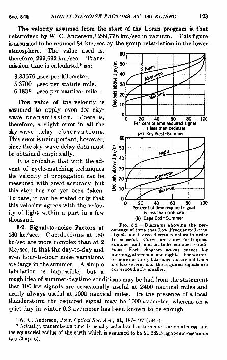
srsc. 6.2] SIGNAL-TO-NOISE FACTORS AT 180 KC/SEC 123

The velocity assumed from the start of the Loran program is thatdetermined by W. C. Anderson,l 299,776 km/see in vacuum. This figureis assumed to be reduced 84 km/see by the group retardation in the loweratmosphere. The value used is,therefore, 299,692 km/see. Trans-mission time is calculated* ae:

3.33676 Wsecper kilometer.5.3700 ysec per statute mile.6.1838 psec per nautical mile.

This value of the velocity isassumed to apply even for sky-wave transmission. There is,therefore, a slight error in all thesky-wave delay observations.This error is unimportant, however,since the sky-wave delay data mustbe obtained empirically.

It is probable that with the ad-vent of cycle-matching techniquesthe velocity of propagation can bemeasured with great accuracy, butthis step has not yet been taken.To date, it can be stated only thatthis velocity agrees with the veloc-ity of light within a part in a fewthousand.

6.2. Signal-to-noise Factors at130 kc/sec.—Conditions at 180kc~sec are more complex than at 2Me/see, in that the day-to-day andeven hour-to-hour noise variationsare large in the summer. A simpletabulation is impossible, but a

is less tharl o;dinate -(a) Key West-Summer

~~

islessthanordinate-(b) Cape Cod-Summer

FIG.S.2.—Diagr8ma showing the par-entage of time that Low Frequency Loransign.ah must exceed certain valuenin orderto be uwful. Curves are nhownfor tropicalsummer and mid-latitude summer condi-tions. Each diagram shows curves formorning, afternoon, and night. For winter,or more northerly latitudes, noise conditionsare less severe, and the required signals arecorrespondingly smaller.

rough idea of summer-daytime conditions may be had from the statementthat 100-kw signals are occasionally useful at 2400 nautical miles andnearly always useful at 1000 nautical miles. In the presence of a localthunderstorm the required signal may be 1000 pv/meter, whereas on aquiet day in winter 0.2 pv/meter has been known to be enough.

1W, C. Anderson,Jour. Optical Sot. Am., 91, 187–197(1941).● Actually, transmission time iu ueua]ly calculated in terms of the oblatenearsand

theequatorialradiuuof the earthwhich ia aauumedto be 21,282,5Iight-microeeconda(aceChap.6),

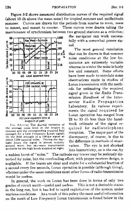
124 PROPAGATION [SEC.5.2

Figure 5“2 shows measured distribution curves of the required signal(about 10dbabove themean noise) fortropical summer and midlatitudesummer. Curves are drawn for the periods from sunrise to noon, noonto sunset, and sunset to sunrise. These curves were drawn taking themaintenance of synchronism between

60 1000

$50 316a.40 100%’~ 30 -E31.6>a a; 20 10

“g 10 3.16a

o020306091215182124

(c) Local apparent time

:70%

-60

$50

g 40

:305~ 20; 10zOO 0306091215182124

(b) Local apparent time atmldpomt of path

11’IG. 53.-(a) The diurnal variation ofthe average noise level in the tropice insummer and the corresponding required fieldstrength for a Low l’requcnry Loran signal;(b) the field strength of a 100-kw uignal atabcmt IZOOnautical miles. During the day-light hours the signal is almmt entirelyground wave, but sky-wave tmnsrnissionaccounts for the high Ievck attained at night.

two ground stations as a criterion;the navigator can work success-fully with a somewhat poorer sig-nal.

The most general conclusionthat can be drawn is that summernoise conditions at the low fre-quencies are extremely variablewhereas in winter the noise is fairlylow and constant. Some effortshave been made to correlate noiseobservations made in studies ofLoran transmission with the meth-ods for estimating the requiredsignal given in the Radio Tnms-rnission Handbook of the lnter-service Radio PropagationLaboratory. In various experi-ments the signal r e q u ire d forI,oran operation has ranged from23 to 33 db less than the hand-book estimate of the signal re-quired for radiotelephonereception. The major part of thediscrepancy, of course, is due tothe difference in methods of obser-vation. The eye is not shockedinto insensitivity, as is the ear, by

a sudden burst of’( noise. ” The cathode-ray traces may be seriously dis-turbed by noise, but the overloading effect, with proper receiver design, isnegligible. If the traces are clear and stable for a substantial fraction ofa second every few seconds, Loran operation is possible (although tiring),whereas under the same conditions most other forms of radio transmissionwould be useless.

In general, the work on Loran has been done in terms of only twogrades of circuit merit—useful and USCICSS,This is not a desirable status

in the long run, but it has Icd to rtipid cxploitaticm of the system underwartime conditions. As u result of this policy the most useful informationon the merit of Low Frequency 1.oran transmission is found below in the

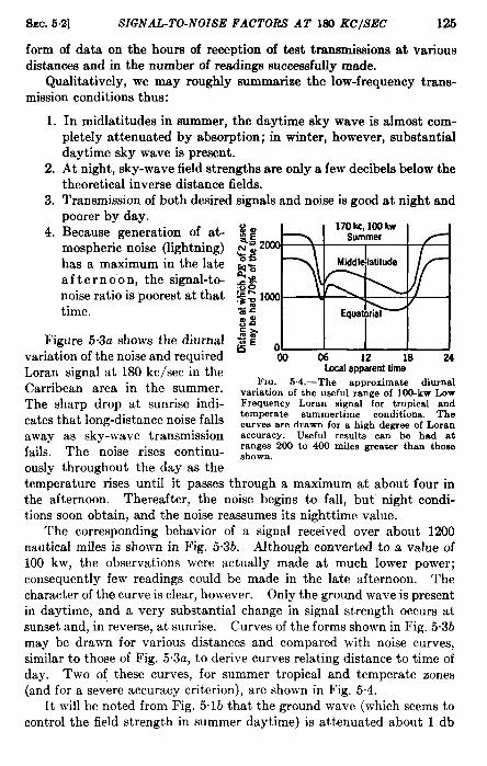
SEC.5.2] SIGNAL-TO-NOISE FACTORS AT MO KC/SEC 125

form of data on the hours of reception of test transmissions at variousdistances and in the number of readings successfully made.

Qualitatively, we may roughly summarize the low-frequency trans-mission conditions thus:

1.

2.

3.

4.

In midlatitudes in summer, the daytime sky wave is almost com-pletel y attenuated by absorption; in winter, however, substantialdaytime sky wave is present.At night, sky-wave field strengths are only a few decibels below thetheoretical inverse distance fields.Transmission of both desired signals and noise is good at night andpoorer by day.Because generation of at-mospheric noise (lightning)has a maximum in the lateafternoon, the signal-t~noise ratio is poorest at thattime.

Figure 5.3a shows the diurnalvariation of the noise and requiredLoran signal at 180 kc/see in theCarribean area in the summer.The sharp drop at sunrise indi-cates that long-distance noise fallsaway as sky-wave transmissionfails. The noise rises continu-ously throughout the day as the

170kc,100kwSummer

~~g; Middle-latitude

s$g~mloooX2 /

$%Equato>

S?J6E Om ~

12 18 24localapparenttime

FIG. 5.4.—The approximate diurnalvariation of the useful range of 100-kw LowFrequency Loran signal for tropical andtemperate 8ummertime conditions. Thecurves are drawn for a high degree of Loranaccuracy. Useful results can be had atranges200 to 400 milesgreaterthan thoseshown.

temperature rises until it passes through a maximum at about four inthe afternoon. Thereafter, the noise begins to fall, but night condi-tions soon obtain, and the noise reassumes its nighttime value.

The corresponding behavior of a signal received over about 1200nautical miles is shown in Fig. 5“3b. Although converted to a value of100 kw, the observations were actually made at much lower power;consequently few readings could be made in the late afternoon. Thecharacter of the curve is clear, however. Only the ground wave is presentin daytime, and a very substantial change in signal strength occurs atsunset and, in reverse, at sunrise. Curves of the forms shown in Fig. 5.3bmay be drawn for various distances and compared with noise curves,similar to those of Fig. 5.3a, to derive curves relating distance to time ofday. Two of these curves, for summer tropical and temperate zones(and for a severe accuracy criterion), are shown in Fig. 5“4.

It will be noted from Fig. 5 lb that the ground wave (which seems tocontrol the field strength in summer daytime) is attenuated about 1 db

126 PROPAGATION [sm. 53

for22 nautical miles and the night sky wave decreases, on the average,about 1 db for 60 miles. The curves of Fig. 5.4 may be adjusted forvarious power levels through the use of these constants. Variation withthe required accuracy is more difficult to estimate. It has, however,been found that a fair standard of practical operation is available atdistances 200 to 400 miles greater than those shown in Fig. 5“4.

LOIUN SKY-WAVE TIUNSMISSION AT 2 Me/see

6.3. The Ionosphere.—The ionosphere is usually defined as “ thatregion of the earth’s atmosphere which is ionized sufficiently to affect thepropagation of radio waves.” For practical purposes it may be thoughtof as all the atmosphere above the stratosphere, or, more specifically, theatmosphere between 30 and 300 miles above the surface of the earth.

The atmosphere at such heights consists primarily of the same con-stituents as at sea level, nitrogen and oxygen. Above 60 miles the oxygenpresumably exists in atomic rather than molecular form because theultraviolet light from the sun dissociates the atoms much faster than theyrecombine

There is little to indicate that the heavier elements settle out at thelower altitudes. Probably all the components of the atmosphere arewell mixed, except for the change from molecular to atomic oxygen at60 miles. It may be that hydrogen and helium escape into space; thereis no strong evidence that they exist at all in the upper air.

The atmospheric pressure decreases more or less exponentially withincreasing height to very small values. At 60 miles it is about one-millionth of the sea-level pressure; at 200 miles it is probably thousandsof times again as small. The mean free path, at 60 miles height, may betaken as 1 cm, and at 200 miles it may be as much as a mile or more.This mean free path is the average distance which a particl~molecule,atom, heavy ion, or electron—will travel before it collides with anotherparticle. It is a very important quantity.

The temperatures in the ionosphere are high. This does not meanthat there is much heat in the upper air, because there are very fewparticles to contain heat, but it does mean that the particles travelrapidly. At sea-level temperatures the air molecules travel at about0.5 km/see; at an altitude of 200 miles they move several times as fast.The temperature after falling to about – 70°F in the stratosphere increasesto nearly the sea-level value at about 30 miles. Then there may be asharp drop to about —140”F at 50 miles. Above that the temperature(velocity of particles) rises rapidly to somewhat more than 80”F at 60miles and to perhaps 1400°F at 200 miles.

If a certain wavelength of solar ultraviolet light excites one of theelectrons in an atom so that it breaks away from the atom and exists

SEC,5.3] THE IONOSPHERE 127

alone, the atom is ionized. The electron is usually called a negative ion,and the positively charged remnant of the atom is called a heavy or posi-tive ion. The electron is small and light. It will travel, independent ofthe heavy ion, at great speed until it finds another heavy ion with whichit can unite permanently or untilit finds an atom or molecule towhich it can stick temporarily.

Let us assume that ultravioletlight of some ionizing wavelengthis falling upon the atmosphere.There will be, in general, enoughenergy at this wavelength to pene-trate some distance into the airbut not enough to reach the sur-face of the earth before it has allbeen expended in ionization. Atseveral hundred miles above thesurface little ionization will be pro-duced because there are very fewatoms to absorb the energy. Theionization will therefore increaseas the height decreases becausethere is more and more materialthat can be ionized. As theheight decreases further, however,a substantial fraction of the origi-nal ultraviolet energy has beenused up; thus, although the num-ber of atoms continues to increasevery rapidly, the number of elec-trons set free does not increase sorapidly. At still lower heights thenumber of free electrons actually

Rate of productionof free electrons

FIca. 5.5.—The vertical distribution ofionization that would be moduced bv asingle ionizing agent acting upon a homo-geneous atmosphere. The actual ionospheremay be simulated by a number of curves ofthis form superimposed in various ways.

begins to diminish and, lower yet; decreases to zero when all of the suitableincoming energy has been used up.

This behavior can be calculated, under certain simplifying assump-tions, and gives a curve of the shape of Fig. 5.5 which is known as the“Chapman distribution.” The height at which the free electrons areproduced and the thickness of the layer of electrons depend upon the kindof ionizing energy, the kind of atoms that are ionized, and the tempera-ture of the air. The number of free electrons produced depends upon thesame things but especially upon the total energy available in the ionizingultraviolet light.

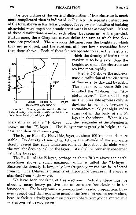
128 PROPAGATION [SEC.5.3

Thetrue picture of the vertical distribution of free electrons is muchmore complicated than is indicated in Fig. 5.5. A separate distributionof the form shown in Fig. 5.5isproduced forevery combination of ionizingultraviolet wavelength and atomit constituent in the atmosphere. Manyof these distributions overlap each other, but some are well separated.Furthermore, these Chapman curves define the rate at which free elec-trons are produced. There issome diffusion from the heightsat whichthey are produced, and the electrons at lower levels recombine fasterthan those above. Both of these factons operate tocause the heightsat

which the density of ionization is

EB

maximum to be greater than the300 F heights at which the electrons are

4 set free most rapidly.$:2WR Figure 5.6 shows the approxi-.-x 1 mate distribution of free electrons.E Day Night as they exist by day and by night.=

E E.% 100 The maximum at about 250 kmz

D is called the “ F-layer, ” or “Ap-pleton layer. ” The small bump

o0 5oo#cWlI,floo,mo 5XI,CQ0

on the lower side appears only in

FreeelectronsDercubiccm daytime in summer, because itFIG. 56.-The approximate distribution recombines quickly at night and is

of the density of ionization with height in theionosphere by day and by night. swamped in the body of the F-

layer in the winter. When it ap-pears it is called the “ F1-layer” and the remainder of the F-region isknown as the “ F*-layer. ” The F-layer varies greatly in height, ‘thick-ness, and density of ionization.

The E-, or Kennelly-Heaviside, layer, at about 100 km, is much morestable. Its density of ionization follows the altitude of the sun quiteclosely, except that some ionization remains throughout the night whenthe sunlight does not fall on the layer. We shall be primarily concernedwith the E-layer.

The “tail” of the E-layer, perhaps at about 70 km above the earth,sometimes shows a small maximum which is called the “D-layer.”Because the density is low, only low-frequency waves can be reflectedfrom it. The D-layer is primarily of importance because in it energy isabsorbed from radio waves.

We have been speaking of free electrons. Actually there must beabout as many heavy positive ions as there are free electrons in theionosphere. The heavy ions are unimportant in radio propagation, how-ever (except that their existence permits the free electrons to recombine),because their relatively great mass prevents them from giving appreciableinteraction with radio waves.

SEC.5.4] REFLECTION 129

5.4. Reflection.-A rough model forthe action of electroneinan r-ffield has been given by P. O. Pederson. 1 In a qualitative way it may bedescribed as follows.

Assume a small volume of the upper atmosphere to be equivalent to acapacitor with the space between its plates filled with air and a numberof free electrons. If an r-f voltage is applied across the capacitor, therewill be a displacement current proportional to the capacitance of theplates. In addition, the free electrons will be excited to vibrate back andforth along the lines of electrostatic force at the frequency of the appliedvoltage. Because of the inertia of the electrons, the phase of theiroscillation will lag the applied emf by 90°. The moving electrons there-fore constitute a current between the capacitor plates—a current inopposite phase to the displacement current. The magnitude of theelectron current depends upon the magnitude of the capacitance underconsideration and upon the applied emf, and it also varies directly as thenumber of free electrons.

The capacitor containing a volume of ionized air may now be thoughtof as a capacitance in parallel with an inductance that is inversely pro-portional to the number of free electrons. If the number of electrons issmall, the inductance shunting the capacitance is nearly infinite. As thenumber of electrons increases, the inductance decreases and the circuitbecomes more and more nearly antiresonant. The net effect is that of acapacitor whose net reactance increases as the number of electronsincreases. That is to say, the capacitance can decrease to zero if thedensity of free electrons is properly proportioned to the radio frequency.This means that the air-plus-electrons has a dielectric constant and anindex of refraction that are less than unity. If the electron currentexceeds the displacement current, the reactance does not become induc-tive; the index of refraction, however, becomes imaginary. These areconcepts which do not occur in simple optics.

The effect of the heavy ions that are, of course, present can beneglected because, although they are excited to oscillate (in the oppositephase to that of the electrons), their great mass limits the accelerationthat can be imparted to them. Thus the amplitude and velocity of theiroscillations are very small in comparison with those of the electrons.The current flow is, of course, proportional to the velocity; thus the neteffect of the positive ions is very small in comparison with that of theelectrons.

If a radio wave penetrates obliquely into the ionosphere, the phasevelocity, which determines the direction of the wavefront, increases as theindex of refraction decreases. At the same time the group velocity, which

1P. O. Pederson,The Propagation of Radio lVaoes along the Surface of the Earthandin the Atmosphere, “ DanmarksNaturvidenskabeligeSamfund,”Copenhagen,1927.

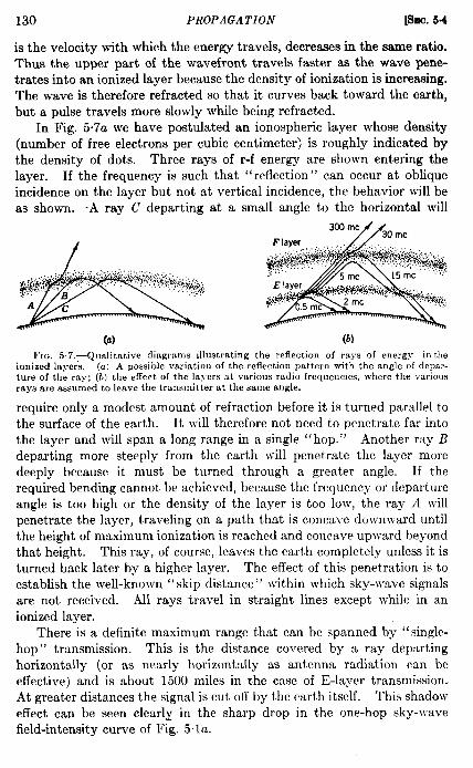
130 PROPAGATION [Snc. 5-4

is the velocity with which the energy travels, decreases in the same ratio.Thus the upper part of the wavefront travels faster as the wave pene-trates into an ionized layer because the density of ionization is increasing.The wave is therefore refracted so that it curves back toward the earth,but a pulse travels more slowly while being refracted.

In Fig. 5.7a we have postulated an ionospheric layer whose density(number of free electrons per cubic centimeter) is roughly indicated bythe density of dots. Three rays of r-f energy are shown entering thelayer. If the frequency is such that “reflection” can occur at obliqueincidence on the layer but not at vertical incidence, the behavior will beas shown. A ray C departing at a small angle to the horizontal will

(a) (b)

l:Iu, 5.7.—Qmditntive diagrams illustrating the reflection of rays of energy in theionized layc&. (a) A possible variation of the reflection pattern with the angle of depar-ture of the ray; (h) the effect of the layers at various radio frequencies, where the variousrays are assumed to leave the transmitter at the same angle.

require only a modest amount of refraction before it is turned parallel tothe surface of the earth. It will therefore not need to penetrate far intothe layer and will span a long range in a single “hop.” Another ray Bdeparting more steeply from the earth will penetrate the layer moredeeply because it must be turned through a greater angle. If therequired bending cannot be achieved, because the frequency or departureangle is too high or the density of the layer is too low, the ray A willpenetrate the layer, traveling on a path that is concave downward untilthe height of maximum ionization is reached and concave upward beyondthat height. This ray, of course, leaves the earth completely unless it isturned back later by a higher layer. The effect of this penetration is toestablish the well-known “skip distance” within which sky-wave signalsare not received. All rays travel in straight lines except w-hlle in anionized layer.

There is a definite maximum range that can be spanned by “single-hop” transmission. This is the distance covered by a ray departinghorizontally (or as nearly horizontally as antenna radiation can beeffective) and is about 1500 miles in the case of E-layer transmission.At greater distances the signal is cut off by the earth itself. This shadoweffect can be seen clearly in the sharp drop in the one-hop sky-wavefield-intensity curve of Fig. 5. la.

SEC. 5.5] ABSORPTION 131

A rough diagram indicating the typical action of both E- and F-layersis given in Fig. 5.7b. Here we have assumed a number of rays at differentradio frequencies, all departing from a transmitter along the same path.The medium frequencies shown, 500 kc/see and 2 Me/see, are bothreflected by the E-layer, but the 2-Me/see ray penetrates much moredeeply and travels somewhat farther. At 5 Me/see, the ray is refractedstrongly in the E-layer but does penetrate it and is easily reflected by theF-layer. The 15-Me/see ray is less affected by the E-layer and pene-trates more deeply into the F-layer, but the general behavior is muchthe same as at 5 Me/see. Under the conditions we have postulated, how-ever, 30 Me/see is too high a frequency to be returned. The ray passesthe E-layer with little refraction and is refracted strongly by the F-layerbut without being turned back toward the earth. The energy at thisand all higher frequencies, such as 300 Me/see, escapes into sp~ce. Asthe frequency increases, the deviation of the ray in the layers decreasesuntil at microwave or optical frequencies the effect of the ionization isnot at all perceptible.

The whole structure of Fig. 5“7b depends upon the density of ioniza-tion in the layers and upon the angle of departure of the orginal rays.At a lower angle the 5-Me/see ray might often be reflected from theE-layer and the 30-Mc/sec ray would be returned from the F-region.

5.5. Absorption.-The reflection of radio waves in the ionosphericlayers is only part of the process of radio transmission by sky waves.The absorption of energy from the waves is of at least the same importance.

Some mention was made above of the mean free path of an electron(or other particle) in the upper atmosphere. This quantity, or moreproperly the inversely varying frequency of collision, controls the energylost by a radio wave. Although there may be a million free electronsper cubic centimeter in a highly ionized layer, there are typically a milliontimes as many neutral atoms or molecules with one of which an electronmay coUide at any instant. Suppose, for example, that on the averagean electron can move freely only for a millionth of a second before collidingwith a heavy atom. If the electron is being vibrated by an r-f field at1 Me/see, there is ordy about one chance in two that the electron cancomplete a cycle of oscillation before a collision interferes with its motion.

Collisions are important for the following reason. Some ener~ isabstracted from the radio wave to provide the kinetic energy containedin the moving electrons. This energy is, in effect, lost to the radio waveonly for a half cycle because the moving electron, since it constitutes amoving charge, reradiates an electromagnetic field whose energy is equafto the energy absorbed by the electron. As the radio wave passes throughthe ionosphere, the energy reradiated by all the electrons adds in phaseto constitute a wave traveling in the same direction as the original wave.

132 PROP.4GA TION [SEC.55

If the electrons can move freely, tiny elements of the energy in the waveflow back and forth between electromagnetic and kinetic states, but thetotal energy in the wtivc remains the same. If, holvcver, an electronrebounds from an atom while temporarily carrying some of the energy,two things happen. The loss importfint is that the direction of motion ofthe electron is changed. The energy is then reradiated in a differentorientation, with the result that the phase relation ]vith the radiationfrom other electrons is damagrd. Even more serious is a real loss of r-fenergy because the atom is accclero,trd slightly and carries off part ofthe kinetic energy that had been loaned to the electron. This energy is

completely lost to the radio ]vfivc and remains in the atmosphere in theform of increased kinetic energy, or heat.

If the probability of collision mnd loss of energy is high enough, tberadio wave ~vill be completely nttenuatcd in the ionized layer. Thedegree of absorption is kws as the frequency is incremcd brcause the elec-trons are more likely to be able to complctc their half cycles of oscillationbefore a collision occurs. In the F-layer, there is little “ collisional fric-tion” because the mean free paths arc long rmd the collisional frequencyis low. In the E-layer, collisions arc so frequent that waves of frequencybelow 2 or 3 Me/see are completely absorbed in the daytime. At nightthe density of ionization in the E-layer decreases to perhaps a tenth ofthe daytime value. The absorption goes donm to low values because thechance of a collision between an electron and some other particle is simi-larly reduced.

We may summarize the situation thus: Ionization is needed to reflectradio waves, but ionization at low heights in the atmosphere absorbsenergy from the waves. The higher the frequency the stronger the ioni-zat ion required for reflection and the less the absorption.

Since most ionization in the atmosphere is produced by the action ofultraviolet light from the sun, there is little new ionization created atnight. The free electrons recombine, but so slowly that a substantialnumber of them remains throughout the night. Thus the maximumionization occurs at or soon after noon, and the minimum at sunrise.Similarly the ionization is more intense in summer than in winter becausethe incidence of the sunlight upon the atmosphere is more nearly perpen-dicular and the ionization increases as does the temperature.

Whether radio transmission is better by day or by night, in winter orin summer, is a question of frequency. At high frequencies, for example,20 Me/see, the weak ionization may prevent sky-wave transmission com-pletely in the winter or at night; in summer or daytime the strongerionization will support transmission and absorption is relatively unim-portant. At broadcast frequencies, absorption is complete in the day-time, with the result that only ground-wave ranges are useful. At night,

SEC. 5.6] E-LA YER TRANSMISSION 133

long-distance transmission is possible, and the decreased absorption inwinter makes communication better than in summer.

5.6. E-layer Transmission.—Figure 5.8 shows typical variations ofthe critical frequencies (which are proportional to the square roots of themaximum densities of ionization) in the E- and F-regions throughout theday. Recombination is so slow in the F-region that the maximum occurswell after noon, although all of the ionizing energy appears to come

~,-,-, \ I=-

G11 q I

0 I

00 04 08 12 16 20 00Local time

FIG. 5S.-A typical diurnal variationof the critical frequencies of the E- and F-layers of the ionosphere. This quantity isproportional to the square root of the maxi-mum density of ionization in a layer.

directly from the sun. The smoothdecrease throughout the night isanother manifestation of the factthat some free electrons have life-times of many hours in the F-layer.

---------------------------

A

FIG, 5.9,—A diagramillustratingthevariation of Penetrationinto an ionizedlayer as a function of the distance traversedby a ray.

The behavior of the E-layer at night is not understood. At the heightof the E-layer, complete recombination takes only a few minutes andconsequently, in daytime, the density of ionization adapts itself veryquickly to the amount of energy being received from the sun. TheElayer curve of Fig. 5.8, between sunrise and sunset, is nearly propor-tional to the fourth root of the cosine of the sun’s distance from thezenith. This is so exactly true that without question the ionization wouldgo almost to zero at night if direct ultraviolet light from the sun were itsonly source.

The energy brought into the earth’s atmosphere by meteoric bombard-ment may possibly be enough to sustain this nighttime ionization. 1 Inany case, meteoric effects are definitely perceptible and certairdy causemany of the variations in the density and distribution of free electronsin the E-layer even though they are probably not the major cause of theionization. The random variations in the density of the Elayer are ofthe first importance in the propagation of Loran signals by sky waves,because they determine the errors of the system.

The transmission time of a sky wave is greater than the transmissiontime of the ground wave, primarily because of the greater distance

1J. A. Pierce, “Abnormal Ioaiaationin the E Region of the Ionosphere,” ProcIRE, !26, 892-908 (1938).

134 PROPAGATION [SEC.5.6

traveled but also because the wave travels more slowly during the processof refraction. The difference between the two times is called the “sky-wave delay. ” Figure 5.9 shows that the sky-wave delay observed at apoint very near the transmitter (if penetration does not occur) is essen-tially equal to the transmission time of the sky wave. As the distanceincreases (rays B, C, and D), the transmission time of the sky waveincreases but the transmission time of the ground wave increases morerapidly. The sky-wave delay therefore decreases as the distance of trans-mission increases and, in fact, becomes very nearly constant at distancesof a thousand miles or more. Figure

150

i100

.E

i“ w

o02004U36(0 WXI1OOO12OO

DktanceinnauticalmilesFro, 5.10.—The Loran delay curve.

Delay is the amount that a sky wave lagsbehind a ground wave traveling from thesame transmitter to the same receiver. Theshaded mea shows the limits of variation ofthe delay.

5.10 shows the standard delay curvefor Loran, which is drawn for re-flecti on from the E-layer. Thecurve is a mean for night condi-tions at a frequent y just below 2hfc/see, and the shaded area indi-cates the limits of variation. Itis never drawn back to zero dis-tance because a 2-Me/see wavenearly always penetrates t h enighttime E-layer at short dis-tances, and because the delaybecomes more variable as thedistance decreases. At distancesless than 200 nautical miles thedelay is completely unreliable.

Fortunately for Loran the ground-wave ser~ice of the system is ordinarilyavailable at dist antes up to those at which the E-layer transmissionbecomes satisfactory.

The stability of the reflection becomes greater at longer distancespartly because grazing reflection is better than reflection at a steep ang’e,but primarily because a change in the height of reflection does not greatlychange the total distance traveled by the ray. At a distance of 1000miles the length of the sky-wave path increases only 1.78 miles for achange in the height of reflection of 5 miles. This is a change in the timeof transmission of less than 10 psec or about one-fifth of the correspondingchange at a short distance.

Variations of 5 miles in the height of reflection are rare but do occurat times. Their effect upon Standard Loran is not too large because suchan extreme variation is likely to exist over a large area. It will thereforeoperate to increase (or decresse) the transmission times from both stationsof a pair so that the time difference measured by the navigator does notvary as much as the individual delays.

The discussion in the last few paragraphs has been specifically applica-

SEC.5.6] E-LA YER TRANSMISSION 135

ble to the E-layer. Only this layer is used in Loran because the F-layeris too variable to permit prediction of the times of transmission with thenecessary accuracy. A comparison between the layers is shown in Fig.5.11, which shows the apparent variation of the line of position througha point in Bermuda. These observations were made as part of the firstexperiments on Loran. For ob-vious reasons, work involving theF-layer was discontinued afterthat time. The example shownis typical of the behavior cf bothlayers, although the time of daywas not favorable to maximumstability of either. The averagedeviations of the line of positionare 18 miles for the F-layer and 2

.E 305 20

=

Jan, 15, 1942:E Flayer7,7mcQ 10%“= 1)gi5= g.lo Jan. 17, 1942“-.~: -EXayer3.0 mcg c -20=.s -30ga -40

1800 1820 1840 1900 1920EST

miles for the E-layer. ‘The dis- F1~.5.11.—The variation with time of the

tance was 625 miles from the sta-Loran line-of-position error in Bermuda whenusing E- and F-layer reflection. The inata-

tions; consequently the equivalent bllity of the F-layer is so great aa to preclude

average errors in the bearing ofita uae for hyperbolic navigation.

Bermuda, as seen from near New York, were 1.7° for the F-1ayer experi-ment and 0.2° for the E-layer.

As will be seen from the notation on Fig. 5“11, the layer can be selectedby proper choice of frequency. At the time of these experiments, 7.7Me/see penetrated the Elayer and 3.0 Me/see did not. The Loran fre-quency is chosen as one that will be reflected by the E-layer at all times

Mostlypenetrationwithpm, if any, reflectionat short ranges God reflection with

i some penetrationof

Fm. 6.12.—Adiagram indicating variation with angle of the partial internal reflectionobtaining at 2 Mc/aec at night.

at all distances that will not be adequately served by ground waves.It is possible that frequencies sa high as 2.5 Me/see might satisfy thiscriterion, but both ground-wave range and sky-wave stability areimproved by using lower frequencies. (The lower limit of frequency,incidentally, is that at which it becomes too difficult to generati andradiate a sufficiently short pulse for bran purposes. With the criteriaadopted for Standard Loram, this frequeney is probably about 1 Me/see.)

136 PROPAGATION [SEC. 56

It should be noted that the last paragraph did not state that signalsat the Loran frequency would not penetrate the E-layer. They almost

always do penetrate at short distances, and part of the energy may pene-trate the layer at long distances. Thk seems to be possible because,contrary to what has been suggested above, the E-layer is not really asmooth homogeneous layer at night, although it is one in the daytime.At night the layer is porous. It seems to coilsist of many nuclei or cloudsof ionization chiefly at about the same height—a little below the heightof the daytime or normal E-layer—with either spaces or patches of sparse

(,) ~G lE 2E lF 2F

lime+FIG.5.13.—Adiagramindicatingat (a) a numberof the possibleray patbabetweenatransmitteranda receiver andat (b) the approximate pulse pattern received in this case.

ionization between them. The density of the ionization in the clouds isnot very great, so that 2-Me/see rays pass vertically through the “layer,”partly by penetrating the clouds and partly by passing between them.At angles closer to grazing incidence the probability of passing throughthe spaces becomes smaller and usually goes to zero for transmission overthe longer distances. 1 A diagram showing this effect is given in Fig. 5.12.

In general, some energy will be reflected by the porous nighttimeE-layer, and some will pass through it and be reflected from the F-layer.Multiple-hop transmission is possible in both cases, so that the pattern ofreceived pulses may therefore be very complex. The structure of someof these components of the received pattern is shown at A of Fig. 5.13.The way the corresponding signals look on a linear oscilloscope trace isindicated at B. This diagram is ideali zeal. A more accurate representa-tion of a pulse train in the presence of fading and noise has been given inChap. 3.

1This sameresultwouldbe producedby a homogeneouslayerif the layerwerenotthick comparedwith the wavelength. It is hard to believethat this is the case,how-ever,becausethe layerwouldhave to be only a fewhundredyardsthick at most.

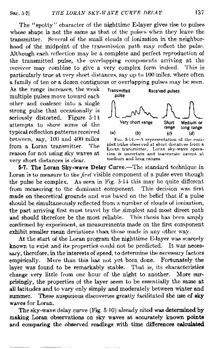
SEC. 57] THE LORAN SKY-WA VE CURVE DELAY 137

The ‘‘ spott y‘’ character of the nighttime E-layer gives rise to pulseswhose shape is not the same as that of the pulses when they leave thetransmitter. Several of the small clouds of ionization in the neighbor-hood of the midpoint of the transmission path may reflect the pulse.Although each reflection may be a complete and perfect reproduction ofthe transmitted pulse, the overlapping components arriving at thereceiver may combine to give a very complex form indeed. This isparticularly true at very short distances, say up to 100 miles, where oftena family of ten or a dozen contiguous or overlapping pulses may be seen.As the range increases, the weak Tf~”~rni~ed Rece!ved pulsesmultiple pulses move toward each pulse

other and coalesce into a singlestrong pulse that occasionally isseriously distorted. Figure 514 n~

Very short rangeattempts to show some of thetypical reflection patterns received (a) lb)

AnShort Medium orrange long range

(c) (dbetween, say, 100 and 400 miles FIU, 5.14.—A representation of the com-

from a Loran transmitter. The LO,,, ~,an,mitte, LO,=, ,~Y-WaVe~Pe,a-plex pulse observed at short distances from a

reason for not using sky waves at tion is uncertain and inaccurate except atvery short distances is clear. medium and long ranges.

6.7. The Loran Sky-wave Delay Curve.—The standard technique inLoran is to measure to the frost visible component of a pulse even thoughthe pulse be complex. As seen in Fig. 5.14 this may be quite differentfrom measuring to the dominant component. This decision was firstmade on theoretical grounds and was based on the belief that if a pulseshould be simultaneously reflected from a number of clouds of ionization,the part arriving first must travel by the simplest and most direct pathand should therefore be the most reliable. This thesis has been amplyconfirmed by experiment, as measurements made on the first componentexhibit smaller mean deviations than those made in any other way.

At the start of the Loran program the nighttime E-layer was scarcelyknown to exist and its properties could not be predicted. It was neces-sary, therefore, in the interests of speed, to determine the necessary factorsempirically. More than this has not yet been done. Fortunately thelayer was found to be remarkably stable. That is, its characteristicschange very little from one hour of the night to another. More sur-prisingly,theproperties of the layer seem to be essentially the same atall latitudes and to vary only simply and moderately between winter andsummer. These auspicious discoveries greatly facilitated the use of skywaves for Loran.

The sky-wave delay curve (Fig. 5.10) already cited was determined bymaking Loran observations on sky waves at accurately known pointsand comparing the observed readings with time differences calculati

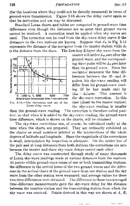
138 PROPAGATION [SEC.5.7

(for the locations where they could not be directly measured) in terms ofground-wave transmission. Figure 5.15 shows the delay curve again sothat its derivation and use may be discussed.

Standard Loran charts and tables are computed in ground-wave timedifferences even though the distances are so great that ground wavescannot be received. A correction must be applied when sky waves areused. The correction can be read from the sky-wave delay curve if thedistances to the two stations are known. Suppose that d,~ in Fig. 5“15represents the distance of the navigator from the master station while dsis the distance from the slave. The first-hop E-layer sky wave from the

g 160 Ii:

“; 80 l—~ I I

$ 40- I I3 I I# I I

o.0 1000~m~, 3000 60C0 7000

Groundwavetransmissiontime inmicrosecondsFIG. 5.15.—The derivation and use of the

Loran delay curve.

master will arrive AMpsec after theground wave, and the correspond-ing slave pulse will be AS~sec laterthan its ground wave. Since thenavigator measures the time dif-ferences between the M- and J!S-pulses, his sky-wave reading willdiffer from his ground-wave read-ing (if he has made one) by(A.M– As)@ec. This amount isthe sky-wave correction. In thiscase (closer to the master station)the skv-wave reading is smaller

than the ground-wave reading. The correction is therefore-called posi-tive, so that when it is added to the sky-wave reading, the ground-wavetime difference, which is shown on the charts, will be obtained.

The sky-wave corrections can, of course, be calculated easily at thetime when the charts are prepared. They are ordinarily exhibited onthe charts as small numbers printed at the intersections of the wholedegrees of latitude and longitude. Since the magnitude of the correctionsis small, interpolation by inspection is adequate. On the center line ofthe pair and at long distances from both stations the corrections are zerobecause the master and slave sky-wave delays cancel each other.

The delay curve was constructed through study of many thousandsof Loran sky-wave readings made at various distances from the stations.At pointswithin ground-wave range of one or both transmitting stations,the difference in the arrival times of the two ground waves and the differ-ence in the arrival times of the ground wave from one station and the skywave from the other station were measured, and average values for thesetwo time differences were obtained. The difference in these two averagedtime-difference measurements gave the sky-wave delay for the distancebetween the monitor station and the transmitting station from which thesky wave was received. Points derived in this way are shown at A, B,

8EC. 5.8] NORMAL VARIATIONS IN THE SKY-WAVE DELAY 139

and C of Fig. 5.15. For longer ranges, where ground waves could not beused, an inverse process had to be employed. The sky-wave readings ofa pair were averaged and compared with the calculated ground-wavereading at the monitor station. The discrepancy (e, or e, in the figure)was, of course, the sky-wave correction. Shce the two distances wereknown, the correction gave the slope of a chord of the delay curve, asshowrI at D1-DZ or El-E*. Many lines of this slope could be drawn in aneffort to find the vertical position of the line that would fit its end pointsinto a smooth curve with the end points of other similar lines at otherdistances. If enough observations are available, at enough distances,the curve can easily be constructed.

The curve that seems, after three years’ experience in various latitudes,to be the best average approximation to the true values is shown in Fig.5.10. This curve is represented by the following equation:

Sky-wave delay in ~sec = D + 0.3(’*Y f%%%

+0.18 X 1~’

where D is the minimum sky-wave delay which varies between 65 psecin winter and 75 ~sec in summer. The transmission time of the groundwave in microseconds is represented by t.

This formula applies for distances less than about 1130 nautical miles(where t = 7000). For greater distances the sky-wave delay equals D.This equation is purely empirical.

As shown by the variation of the quantity D, the layer height is some-what greater in summer. However, the delay curve, for all practicalpurposes, simply moves upward; thus the correction, which is always thedifference between two delays, is not affected. There is an error intro-duced by this change in two cases; the case when the navigator mayoccasionally wish to measure the time difference between a sky wave anda ground wave and the case of the synchronization path in sky-waveSynchronized Loran which will be discussed below.

The only important latitude effect is that the delay curve maybe usedat shorter distances at low latitudes. Near the equator fairly reliableoperation may be had at as little as 150 nautical miles, whereas at 45°latitude about 250 miles is the minimum safe distance. The curve itselfdoes not seem to vary appreciably over the latitude range from 25°N to63”N within which it has been carefully checked.

LORAN SKY-WAVE TRANSMISSION ERRORS AT 2 Mc/oec.

6.8. Normal Variations in the Sky-wave Delay.—Since we propose toexamine closely the averages and the mean deviations of the sky-wavedelay and sky-wave corrections, it is necessary to test, the accuracy withwhich transmitter synchronism can be maintained. An example, some-what better than normal, is given in Fig. 5.16. This figure shows the

140 PROPAGATION [SEC.5.8

number of the various ground-wave readings observed at a monitor sta-tion where the computed reading was 3510.6 -c. The mean, as is usual,agrees with the computation within 0.2 or 0.3 psec, and the averagedeviation is of the order of 0.6 psec. A series of sky-wave readings usuallyshows an average deviation at least

g lm0“%Sooz%~m

: 400:

E 200z

:506 350a 3510 3512 3514Reading in psec

FIG. 516.-A distribution curve showingthe normal scatter of Loran observationswhen ground-wave transmission is used,The average reading error is small comparedwith the random variations of sky-wavetransmission time.

four or five times as great as theaverage error in synchronism. Itis, therefore, nearly always satis-factory to assume that the syn-c h ro n is m of the transmittingstations is rigid and that any devi-ations observed are the result ofvariations in sky-wave propaga-tion. Exceptions to this assump-tion are usually obvious.

Three distribution curves ofobservations of the sky-wave de-lay are given in Fig. 5.17. Thecurves, which are drawn to havethe same area, exhibit clearly thetwo important facts of sky-wave

transmission for Loran. The average sky-wave delay diminishe~ as thedistance increases, as shown by the delay curve, and the spread of the read-ings also decreases in about the same proportion. The probable errors inthis set of observations are

9.9 ~sec at 240 nautical miles.9.0 ~sec at 290 nautical miles.5.8 psec at 450 nautical miles.

The first two are somewhat belowAt long distances it is impos-

sible to measure delay directly.Figure 5.18 sho}vs two distributioncurves of the sky-wave rcacfing(not delay) at distances of 87o and1350 nautical miles. The corre-sponding probable errors arc 2.1and 2.4 psec, although a smallererror would be expcctcd at thegreater distance. l’hcse are er-rors in the sky-wave correction.

As remarked above, major changesin the height of reflection of a sky

the normal scatter at these distances.

?.Q0.05%ZO134;’00.03zg 0.02

.20.01

;00 20 40 60 80 1001201401643180

Delay in microseconds

FIG, 517.-Thrce distribution curvesexhibiting the way both dclny and probableerror of dcluy decrcaw as the distance oftranrnulissionincrcascs.

wave may be expected to affect both transmksion paths in the same Jray

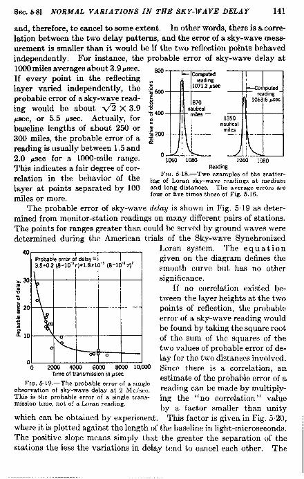
Sm. 5.8] NORMAL VARZA TIONS IN THE SKY-WAVE DELAY 141

and, therefore, to cancel to some extent. In other words, there is a corre-lation between the two delay patterns, and the error of a sky-wave meas-urement is smaUer than it would be if the two reflection points behavedindependently. For instance, the probable error of sky-wave delay at1000 miles averages about 3.9 psec.If every point in the reflectinglayer varied independently, theprobable error of a sky-wave read-ing would be about <2 X 3.9~sec, or 5.5 psec. Actually, forbaseline lengths of about 250 or300 miles, the probable error of areading is usually between 1.5 and2.0 psec for a 1000-mile range.This indicates a fair degree of cor-relation in the behavior of thelayer at points separated by 100miles or more.

SooComputed

reading2

- : r ;~

I 11071.2&c ‘$500 ,

omputedreading

i% ~ “:J:a, ‘ 1063.6/isecsz 400 miles—~ 1350

nautical;‘$ 200

males

&

o1060 loao 1060 10s0

ReadingFIQ. 5.18.—Two examples of the scatter-

ing of Loran sky-wave readings at mediumand long distances. The average errors arefour or five times those of Fig. 5.16,

The probable error of sky-wave delay is shown in Fig. 519 as deter-mined from monitor-station readings on many different pairs of stations.The points for ranges greater than could be served by ground waves weredetermined during the American trials of the Sky-wave Synchronized

40 I 1Probableerrorof delay=3.5+0.2 18-10”’r)+l.SXIO-$ (8-10-’ r)’

&m \=g

a~ 20

sg‘i?10

0UJ

o0 20CQ 40C0 6CO0 WOO 10,WO

Timeof transmissionin#see

Fto. 5.19.—The probable error of a singleobservation of sky-wave delay at 2 .Mc/see.This is the probable error of a single trans-mission time, not of a Loran reading.

Loran system. The equationgiven on the diagram defines thesmooth curve but has no othersignificance.

If no correlation existed be-tween the layer heights at the twopoints of reflection, the probableerror of a sky-wave reading wouldbe found by taking the square rootof the sum of the squares of thetwo values of probable error of de-lay for the two dktances involved.Since there is a correlation, anestimate of the probable error of areading can be made by multiply-ing the “no correlation” valuebv a factor smaller than unitv

which can be obtained by experiment. “This factor is given in Fig. 52;,where it is plotted against the length of the baseline in light-microseconds.The positive slope means simply that the greater the separation of thestations the less the variations in delay tend to cancel each other. The

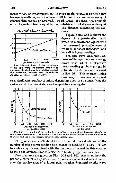
142 PROPAGATION psw. 5.9

factor “ P.E. of synchronization” ia given in the equation on the figurebecause sometimes, as in the case of SS Loran, the absolute accuracy ofsynchronism cannot be assumed. In SS Loran, of course, the probableerror of synchronism is equal to the probable error of sky-wave delay at

PEW. = K PE~M + PE&~ + PE:m1.0

0.s

m

.

0.6K

0.4K=O.21+o.0ooo75/3

02 H

~- Baselinein microseconds

FIG. 5.20.—A form of the correlationcoefficientdefiningthe relativebehavioroftwo pointsin the ionosphere, plotted againstthe separation between two transmittingstationa, M (master) and S (slave).

the distance separating the sta-tions.

Figure 5.21u and b shows thedegree of approximation withwhich this treatment agrees withthe measured probable error ofreadings, for short (Standard) andlong (SS) Loran baselines.

6.9. Sky-wave Accuracy Pat-tems.—The accuracy (or averageerror) with which a sky-waveLoran reading can be made can beestimated by the method discussedin Sec. 5.8. This average timingerror may or may not correspond

to a significant number of miles, depending upon the dktance from thestations and their orientation with respect to the navigator.

15 e 15 I

~“v 10 \.1%a

.E o coreputedcurve.sM f&5 25

\- no ,.w

o0

02OO4OO6GO8OO1OOO o 200400600 S001000

Dktancein nautical miles Distance in nautical miles(a) Standard Loran (b) SS Loran

FIG. 5.21.—Examples of the probable error of both Standard and Sky-wave Synchron-ised Loran observations. The smooth curves are computed by empirical methods given inthe text, and the circles indicate experimental observations.

The geometrical methods of Chap. 3 permit the calculation of thenumber of miles corresponding to a change in reading of 1 ysec. Theseformulas may be combined with the methods discussed in this chapterto yield the average error of a sky-wave reading expressed in miles.

Two diagrams are given, in Figs. 5.22 and 5.23, that show how theprobable error of a sky-wave line of position (in nautical miles) variesover the w-vice area of a Loran pair, whether Standard or Sky-wave

SEC. 5.9] SKY-WAVE ACCURACY PATTERNS 143

220 nauticalmiles

FIG. 522, -Acont.ourd iagrams hewing, as a function of the geographic position withrespect to the transmitting stations, the probable error of a Standard Loran line of positionwhen using sky waves.

-~ 970 nautical miles~-

FIG. 5.23.—A contour diagram showing, as a function of the geographic position withrespect to the transmitting stations, the probable error of a Sky-wave Synchronized Loranline of position.

144 PROPAGATION [SEC. 5.10

Synchronized. The Standard Loran diagram (Fig. 5“22) is drawn forthe relatively short baseline of 220 nautical miles. For modest changesin the baseline the errors would vary in inverse proportion, since thetiming errors would not change appreciably.

It is of special interest to note that the errors increase very slowlywith distance along the center line of the pair. This is because the tin&gerrors due to variation of the sky-wave delay are nearly inversely pro-portional to distance and almost cancel the increasing geometrical error.Beyond the 1400-mife limit or within 250 miles of the stations it is notsafe to use sky waves because of difficulty in sky-wave identification inthe first case and erratic behavior in the second.

The accuracy of SS Loran is greater than the sky-wave accuracy ofStandard Loran, as shown in Fig. 5“23, because the long baselines (in thiscase 970 nautical miles) greatly improve the geometrical accuracy, ormiles per microsecond of timing error. The timing error itself is not sogood as in Standard Loran, primarily because of sky-wave variations onthe synchronizing path, but the timing error is not increased so much asthe geometrical factors are improved. The total area served by an SSpair is not so great, but the errors are smaller and more constant exceptalong the baseline extensions.

6.10. Sporadic E-region Ionization.-One of the outstanding anoma-lies in the E-region is the existence of sporadic ionization. This takesthe form of clouds of free electrons, at a very constant height, that aresporadic in both time and space. They may appear at any time, day ornight, and last for a few minutes or for hours. Their size may be any-thing up to hundreds of miles across. They sometimes appear to movewith great velocities, and at other times they seem nearly stationary.The density of ionization is often low but occasionally is very great indeed-even greater than the greatest density ever observed in the F-layer.On at least one occasion the density has been observed to be enough toreflect signals up to 110 Me/see over a 1000-mile path.

These clouds are probably caused by corpuscular bombardment ofthe atmosphere by particles shot off by the sun, in much the same waythat northern lights are formed. Although sporadic E-region ionizationmay appear at any time, it is most likely in summer and at times ofsunspot maximum. It is most probable at high latitudes and is seldomobserved at the magnetic equator—again like the aurora borealis.

In the early days of Loran it was feared that signals from one stationof a pair might be reflected from a cloud of sporadic E-region ionizationwhile the signals from the other station would be transmitted by the‘normal” nighttime E-layer, thus leading to large and unpredictablerrors. Fortunately this is not the case, apparently because the normalelections occur at a height somewhat below that of the sporadic E;

SEC. 5.11] MAGNETIC ACTIVITY 145

consequently the signals normally are not propagated by the sporadicclouds. 1

The best evidence to this effect is given in Table 5.2 which exhibitsthe average value and probable error of sky-wave readings when sporadicE-region ionization is and is not present. These data were taken inOttawa, Canada, by the Canadian Navy in May, June, and July 1943,the season of maximum sporadic ionization. During this period thesporadic E-layer appeared about one-third of the time at Ottawa. Ofcourse there is no proof that sporadic ionization existed at the points ofreflection at the same time they were observed at Ottawa, but it is morelikely to have existed there at that time than when it was not observedat Ottawa. As the table shows, there was no significant change in theLoran reading at times when sporadic E-region ionization was observed.The probable errors (or average errors) of the readings were actuallysmaller at those times, but the difference was not large enough to besignificant.

TABLE5.2.—EFFEcTOFSPORADICE-EEGIONIONIZATIONONLORANREADINGS

Pair

MFMBDB

I Normal

Computedreading h-O.of ob-

servations

2932,4 5613814.7 4221342.4 368

1351

Meanreading

2932.13816.31342.5

Probableerror

3.24.43.7

During sporadic E

No. of ob-servations

305256206767

Mean Probablereading error

2932.6 2.93816.8 3.61341.8 3.1

I5.11. Magnetic Activity-Sudden or large variations in the earth’s

magnetic field are associated with changes in the ionosphere, althoughboth are probably secondary effects of some other phenomenon such ascorpuscular bombardment of the atmosphere. In the F-region the“magnetic effects” are extreme, presumably because of the relative easewith which the free electrons can move. There are no indications thatthe total number of free electrons is greatly changed in the F-layer. Thelayer heights increase and the densities decrease during magnetic activity,much as though the atmosphere (or at least the electrons in it) were beingpulled up by the top and stretched somewhat. In fact, during severemagnetic storms (extremes of activity) the F-layer is essentially “blownout of the atmosphere” and a new layer is formed underneath the rem-nants of the old one.

1At very shortdistancessporadicE-regionionization frequentlydoescausestrongsteady reflections. Since the height of reflectiondiffers from the normal, this con-tributesto the unreliabilityy of sky-wavetransmissionat shortdistancesat 2 Mc/sec.

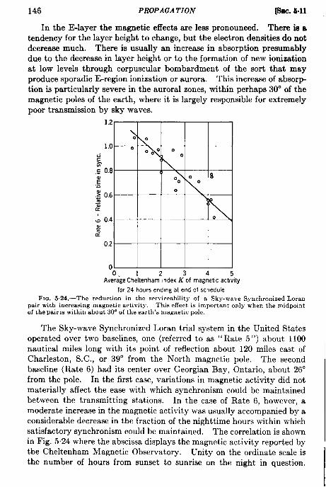
146 PROPAGATION plw. 5.11

In the E-layer the magnetic effects are less pronounced. There is atendency for the layer height to change, but the electron densities do notdecreaae much. There is usually an increase in absorption presumablydue to the decrease in layer height or to the formation of new ionizationat low levels through corpuscular bombardment of the sort that mayproduce sporadic Eregion ionization or aurora. This increase of absorp-tion is particularly severe in the auroral zones, within perhaps 30° of themagnetic poles of the earth, where it is largely responsible for extremelypoor transmission by sky waves.

1.2

\ 01.0 : ‘

~ 00° 00R (

.: 0.8 138

E.=0

.$ 0.6 \~$

)

la 0.4 0~2

0.2-

00. 1 2 3 4 5

AverageCheltenham Index K of magnetic actwity

for 24 hours ending at end of scheduleFm. 5.24.—The reduction in the scrviceabi]ity of a Sky-wave Synchronized Loran

pair with increasing magnetic activity. This effect is important only when the midpointof the pairis within about 30° of the earth’s magnetic pole.

The Sky-wave Synchronized Loran trial system in the United Statesoperated over two baselines, one (referred to as “ Rate 5”) about 1100nautical miles long with its point of reflection about 120 miles east ofCharleston, S.C., or 39° from the North magnetic pole. The secondbaseline (Rate 6) had its center over Georgian Bay, Ontario, about 26°from the pole. In the first case, variations in magnetic activity did notmaterially affect the ease with which synchronism could be maintainedbetween the transmitting stations. In the case of Rate 6, however, amoderate increase in the magnetic activity was usually accompanied by aconsiderable decrease in the fraction of the nighttime hours within whichsatisfactory synchronism could be maintained. The correlation is shownin Fig. 5.24 where the abscissa displays the magnetic activity reported bythe Cheltenham Magnetic Observatory. Unity on the ordinate scale isthe number of hours from sunset to sunrise on the night in question.

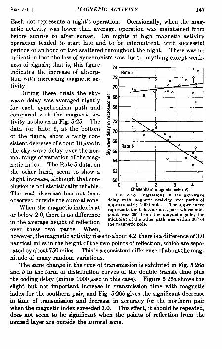
SEC.5.11] MAGNETIC ACTIVITY 147

Each dot represents a night’s operation. Occasionally, when the mag-netic activity was lower than average, operation was maintained frombefore sunrise to after sunset. On nights of high magnetic activityoperation tended to start late and to be intermittent, with successfulperiods of an hour or two scattered throughout the night. There was noindication that the loss of synchronism RWSdue to anything exce~t weak-ness of signals; that is, this figureindicates the increase of absorp-tion with increasing magnetic ac-tivity.

During these triafs the sky-wave delay was averaged nightlyfor each synchronism path andcompared with the magnetic ac-tivity as shown in Fig. 5.25. Thedata for Rate 6, at the bottomof the figure, show a fairly con-sistent decrease of about 10 psec inthe sky-wave delay over the nor-mal range of variation of the mag-netic index. The Rate 5 data, onthe other hand, seem to show aslight increase, although that con-clusion is not statistically reliable.The real decrease has not beenobserved outside the auroral zone.

When the magnetic index is ator below 2.0, there is no differencein the average height of reflectionover these two Daths. When,

.- .

74Rate5 0

72 0 {, 0 070 ~

w0 L00 0

#6s

p6

9

0’‘

{)

0

.-E,E 72 \ I

$70 ‘n \o 0:68s Rate 6 \ 0

0~~ 66 )-

64 0 0 <I,

62

600 1 2 3 4

CheltenhammameticindexKFIG. 5.25.—Variatio;s in the sky-wave

delay with magnetic activity over paths ofapproximately 1000 miles. The upper curverepresents the behavior on a path whose mid-point w= 39° from the magnetic pole; themidpoint of the other path was within 26° ofthe magnetic pole.

however, the magn~tic activity ris& to about 4.2, there is a difference of 3.onautical miles in the height of the two points of reflection, which are sepa-rated by about 750 miles. This is a consistent difference of about the mag-nitude of many random variations.

The same change in the time of transmission is exhibited in Fig. 5.26uand b in the form of distribution curves of the double transit time plusthe coding delay (minus 1000 psec in this case). Figure 5.26u shows theslight but not important increase in transmission time with magneticindex for the southern pair, and Fig. 5.26b gives the significant decreasein time of transmission and decrease in accuracy for the northern pairwhen the magnetic index exceeded 3.0. This effect, it should be repeated,does not seem to be significant when the points of reflection from thejonized layer are outside the auroral zone.

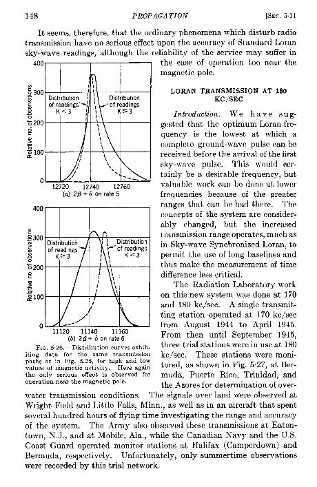
148 PROPAGATION [SEC,5.11

It seems, therefore, that the ordinary phenomena which disturb radiotransmission have no serious effect upon the accuracy of Standard Loransky-wave readings, although the reliability of the service may suffer in

400

2:300Distribution :I i Distribution

2 of readings>’ \ of readingsg K<3 ; ~ K5=30% 200 I 1

g

?.-5

012720 12740 12760

(a) 2f3+60nrate5

FIG. 526,-Distribution curves exbib-iting data for the same transmissionpaths as in Fig. 5.25, for high and lowvalues of magnetic activity. Here againthe only serious effect is observed foroperation near the magnetic pole.

the case of operation too near themagnetic pole.

LORAN TRANSMISSION AT 180KC/SEC

Introduction.—W e h a v e s u g-gested that the optimum Loran fre-quency is the lowest at which acomplete ground-wave pulse can bereceived before the arrival of the firstsky-wave pulse. This would cer-tainly be a desirable frequency, butvaluable work can be done at lowerfrequencies because of the greaterranges that can be had there. Theconcepts of the system are consider-ably changed, but the increasedtransmission range operates, much asin Sky-wave Synchronized Loran, topermit the use of long baselines andthus make the measurement of timedifference less critical.

The Radiation Laboratory workon this new system was done at 170and 180 kc/see. A single transmit-ting station operated at 170 kc/seefrom August 1944 to April 1945.From then until September 1945,three trial stations were in use at 180kc/see. These stations were moni-tored, as shown in Fig. 5.27, at Ber-muda, Puerto Rico, Trinidad, andthe Azores for determination of over-

water transmission conditions. The signals over land were observed atWright Field and Little Falls, Minn., as well as in an aircraft that spentseveral hundred hours of flying time investigating the range and accuracyof the system. The Army also observed these transmissions at Eaton-town, N. J., and at Mobile, Ala., while the Canadian Navy and the U.S.Coast Guard operated monitor stations at Halifax (Camperdown) andBermuda, respectively. Unfortunately, only summertime observationswere recorded by this trial network.

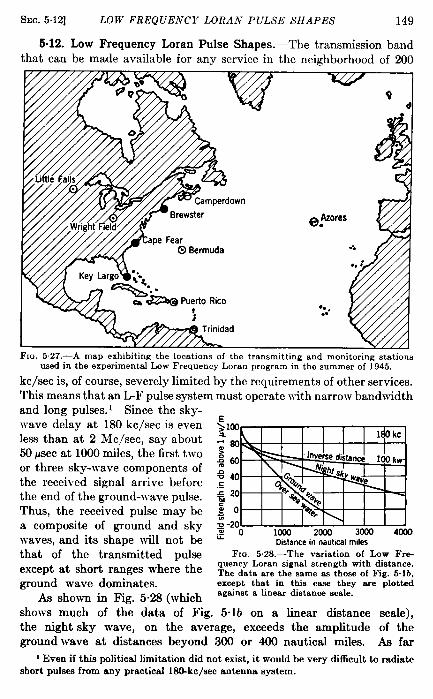
SEC. 5.12] LOW FREQUENCY LORAN PULSE SHAPES 149

5s12. Low Frequency Loran Pulse Shapes.—The transmission bandthat can be made available for any service in the neighborhood of 200

Flu. ,527.—A map exhibiting the locations of the transmitting and monitoring stationsussd in the experimental Low Frequency Loran program in the summer of 1945.

kc/see is, of course, severely limited by the requirements of other services.This means that an L.-F pulse system must operate with narrow bandwidthand long pulses.’ Since the sky-wave delay at 180 kc/see is even : lWless than at 2 Me/see, say about ~ao50 psec at 1000 miles, the first two ~ ~or three sky-wave components of m

~ 40the received signal arrive before c

L

(the end of the ground-~vave pulse. “&20 “Q* -Wb

%@ -$~Thus, the received pulse may be $ 0 ‘%’+pa composite of ground and sky :-200 ~m zm am ~waves, and its shape will not be C Distancein nauticalmiles

l&3kc

that of the transmitted pulse FtQ. 5.2S.—The variation of Lew Fr+

except at short ranges where the quency Loran signal strength with distance.The data are the same ss those of Fig. 5.lb,

ground wave dominates. except that in thk cass they are plotted

As shown in Fig. 5.28 (which againata linear distance scale.

shows much of the data of Fig. 5. lb on a linear distance scale),the night sky wave, on the average, exceeds the amplitude of theground wave at distances beyond 300 or 400 nautical miles. As far

1Even if this politicallimitationdid not exist, it wouldbe very difficultto radiateshort pulses from any practical 1W-kc/see antenna system.

150 PROPAGATION [SEC. 5.12

as is now known, the daytime sky wave may have nearly the value ofthe night sky wave in high latitudes in winter, but it is so completelyabsorbed as to be negligible at low latitudes in summer. Curves havenot been shown for the daytime sky wave because of insufficientinformation. The night sky wave is, of course, made up of manymultiple reflections. Its field strength vs. distance curve is probablymade up by the summation of a number of individual curves, those forthe higher multiples having lower field strengths at the short distancesand extending to longer ranges before dropping sharply when the shadow

“IA2fY)o

At 250naut.mi. 1

g= G~.m o 3W 0(

800

[

40CAt 500 naut. mi. At 750 naut. mi. At 1000 naut, mi.

AL&1

’23300

4!L014Q‘IlilJZi’i

o 300 00 3CSI00 3m o 300Time in microseconds

FIG. 529.-The way that Low Frequency Loran ground and sky waves may add atvarious distances. The ~ero of each horizontal scale marks the instant at which the firstpoint of the ground-wave Pukwarrivea. The relative amphtudes are given hy the changingordinate scale.

of the earth cuts them off. A more precise experimental determinationof the night sky-wave curve of Fig. 5.28 would probably show theseirregularities.

The exact shape of the received pulse at any distance depends uponthe length of the transmitted pulse, the amplitude of the sky-wave com-ponents relative to the ground-wave, and the sky-wave delays. Variousassumptions may be made about all of these factors, and most of themlead to very similar conclusions. The effect is demonstrated in Fig. 5“29where a pulse length of 200 Psec has been chosen. This figure has beendrawn on the assumption that the ground-wave and various sky-wavepulses are always in the wune r-f phase at the receiver, so that the individ-ual pulse envelopes can be added to give the composite envelope. Thisassumption is contrary to fact, as will be explained below, but it yieldaresults that are useful in understanding the problem. At 250 nauticalmiles the figure shows a nighttime condition where the flrat sky wave

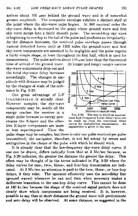
SEC. 5.12] LOW FREQUENCY LORAN PULSE SHAPES 151

arrives about 100 jtsec behind the ground wave and is of somewhatgreater amplitude. The composite envelope exhibits a distinct shelf atthe point where the sky-wave pulse begins. At 500 nautical miles thesky-wave delay is decreased to the point where ground wave and firstsky wave merge into a fairly smooth pulse. The second-hop sky waveis beginning to overlap at the tail of the pulse and produces an irregularity.As the distance increases, the received pulse envelope passes throughvarious distorted forms until at 1500 miles the ground-wave and firstsky-wave components are assumed to be negligible and the pulse regainsa fairly simple shape, at least throughout its first half, which is used formeasurement. The pulse arrives about 110 usec later than the theoreticaltime of arrival of the ground wave.sky-wave components drop out andthe total sky-wave delay increasesaccordingly. The changes in am-plitude with distance may be judgedby the changes of scale of the ordi-nates in Fig. 5.29.

One great advantage of L-Ftransmission is already clear.However complex the sky-wavecomponents may be, nearly all theenergy reaches the receiver in asingle pulse because no energy pen-etrates the E-layer and the effec-tive E-1ayer components are moreor less superimposed. Thus the

At longer and longer ranges various

300~g

E200s~E

“E 100s~s

o0 lCOO 2000 3000

Distance m nautical milesFIG.5.30,—The way in which an approxi-

mate Low Frequency Loran delay curve canbe made UP from the individual delaycurves for multiple-hop transmission. Anexplanation is given in the text.

pulse shape may be complex, but there is only one pulse received per pulsetransmitted; the navigator, therefore, is not led astray by errors andambiguities in the choice of the pulse with which he should work.

It is already clear that the low-frequency sky-wave delay curve, ifone can be drawn, differs radically from that at 2 Me/see because, asFig. 5.29 indicates, the greater the distance the greater the delay. Thiseffect may be thought of in the terms indicated in Fig. 5.30 where thedelay curves for one-, two-, three-, and four-hop transmission are indi-cated. At 2 Me/see no attention is paid to the two-, three-, or four-hopdelays, if they exist. The operator effectively uses the zero-delay line(ground waves) whenever he can and then when necessary makes adeliberate transition to the one-hop delay curve. This cannot be doneat 180 kc/see because the shape of the received signal pattesm does notclearly show which components are being received. It is, however,possible to say that at short distances the ground wave will predominateand zero delay will be observed. At some distance, as suggested in the

152 PROPAGATION [SEC.512

1000-mHe diagram of Fig. 5“29, the effective time of arrival of the receivedpulse is approximately that of the first-hop sky wave. At some greaterdktance, say 2000 miles, both the ground wave and the one-hop sky wavehave negligible amplitude and the time of arrival is essentially that of thetw~hop sky wave. Thus the equivalent low-frequency sky-wave delaycurve, as shown by the wavy line on Fig. 5.30, will find its way acrossthe figure with, in general, a positive slope. The tendency for this delaycurve to cling to each of the separate multiple-delay curves is affected by

Time ~FIG. 5.31.—A simplified diagram indi-

cating how Low Frequency Loran pulseshapes can vary with the phase relationbetween ground- and sky-wave components.

many factors including the pulselength and receiver bandwidth butdepends particularly upon the rela-tive amplitudes of the. v a r i o usmultiple reflections. Thus, if thet we-hop component should be veryweak compared with the one-hopc o m p o n e n t, the effective d~ymight tend to cling to the one-hop curve over a considerable dis-tance, perhaps almost to thedistance at which the one-hop sig-nal disappears. This effect can beunderstood easily by reference tothe night sky-wave curves of Fig.5.la.

We are thus led to the conclu-sion that over long distances thetime of transmission of a mdse in-

cludes a delay that increases with distance and that may, with minorinaccuracies, be considered as a small reduction in the velocity of propa-gation.

The assumption that the amplitudes of the various puke componentsmay be added to give the amplitude of the composite pulse is, of course,contrary to fact. The fibhop sky wave is in general delayed from 10to 25 cycles (at 180 kc/see) behind the ground-wave puke and is just aslikely to arrive out of phase as in phase. The height of reflection is notconstant but is usually alowly increasing or decreasing, so that the phaseof the one-hop sky-wave component may change through 2 or 3 cycleswith respect to the ground-wave pulse over a period of several hours.The effects of this phase change may be examined with the aid of Fig.5c31, which has been drawn assuming that no second- and higher-multiplereflections exist and that the ground wave has about half the amplitudeof the sky wave. If these components could be seen individually, theground wave would appear as shown by the dotted pulse between A and

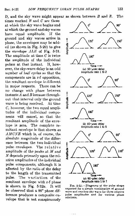
SEC. 5.12] LOW FREQUENCY LORAN PULSE SHAPES 153

Z), and the sky wave might appear as shown between B and E. Thetimes marked “B and C a~e thoseat which the sky wave begins andat which the ground and sky waveshave equal amplitude. If theground and sky waves arrive inphase, the envelopes may be add-ed (as shown in Fig. 5.29) to givethe envelope ALE of Fig. 5.31.The amplitude at time C is twicethe amplitude of the individualpukes at that instant. If, how-ever, the sky-wave delay is an oddnumber of half cycles so that thecomponents are in r-f opposition,the resultant envelope is differentin major respects. There can beno change with phase betweeninstants A and B because through-out that interval only the groundwave is being received. At timeC, however, the two equal ampli-tudes of the individual compo-nents will cancel, so that theresultant amplitude of the enve-lope is zero. The complete re-sultant envelope is that shown asA MCNE which is, of course, theabsolute magnitude of the differ-ence between the two individualpulse envelopes. The r e 1a t i v eamplitude of the peaks at M andN depends primarily upon the rel-ative amplitudes of the individualpulse components, although it isaffected by the ratio of the delayto the length of the transmittedpulse. The variation of theresultant envelope with r-f phaseis shown in Fig. 5.32a. It willbe observed that a 90° phase dif-

ference produces a composite en-velope that is not conspicuously

KY L!lY

~‘A w

——Time ~

(u) 90-#see delayAmplitude ratio 1 to 2

AlY._

ABA

‘A

180”

—.Time +

(b) 60-@3c delayAmplituderatio1to5

,A o

———Lx120”

L’K-L!&!

mT@ -

(c) 90-@ec delayAmplituderatio1to I

FIG. 5.32.—Diagrams of the puke shapeexpected for a simple combination of groundwave and one-hop sky wave for three relativepulse amplitudes and for various phaserelations.

154 PROPAGATION [SEC.5.12

different from that for zero degrees. Figure 5.32b and c shows the samesort of diagrams for relative ground-to-sky amplitude ratios of 1/5 andunity, respectively. In practice the patterns with plateaus or notchesin them are encountered infrequently, typically for 5 or 10 min. every2 hr. This low probability of occurrence stems from two causes: (1)With low ground-wave amplitudes, phase opposition must be attainedwithin 30° or 40° in order to produce any significant change in theappearance of the pulse. (2) Asecond reason stems from the fact thatthe shape and length of the received pulse is ordinarily determined by thebandwidth of the receiver. The distorted shapes represented in thesefigures require a wider bandwidth for their satisfactory reproduction thando the simple or in-phase shapes. This can be seen most clearly in Fig.5.32c where it is obvious that reproduction of the diagram for 180° willrequire approximately twice the bandwidth needed for the case of OO.There is, therefore, a tendency in the receiver to smooth out the moreeccentric pulse shapes, thus tending always to make the pulse look morelike the in-phase pulse than it really is.

The major timing errors in LF Loran arise from the condition shownin Fig. 5.32b where the ground wave is relatively weak compared withthe one-hop sky wave. In the 180° curves of Fig. 532a and c a largeerror is not ordinarily to be feared because the first rise of the ground-wave pulse has sufficient amplitude to permit the operator to make hisreading on the ground-wave component and to disregard any peculiarshapes introduced by the sky waves. In Fig. 5.32b, however, the groundwave contributes only the wedge-shaped beginning of the pulse. If thenoise is sufficiently low, the operator may be able to increase the gain ofthe receiver and make what amounts to a ground-wave match; but, if thenoise is high, the navigator may miss the snout of the pulse and make hismeasurement on the steeply rising portion. This can result in an errorof as much as 50 ~sec. It is practically impossible for the navigator toestimate corrections that would make his reading more truly representa-tive of his position, on the basis of the pulse shape that he sees. Ingeneral, the average value of the effective delay of the pulse must beincorporated in the construction of the navigator’s charts, and anydeviations from this average value must be accepted as errors. Thechart-producing agency cannot determine in advance whether or not thenavigator will identify the snout on the pukes in Fig. 5.32b. The chartsmust, therefore, be drawn in terms of the average reading made by theaverage operator under these conditions. This is equivalent to sayingthat larger errors must be expected at the distances at which the low-frequency delay curve of Fig. 5.30 is most steep. At distances where thedelay curve is essentially horizontal there is little opportunity forambiguity.

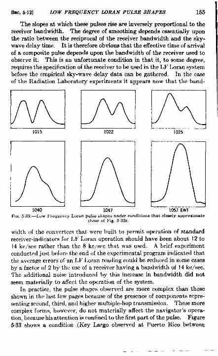
SEC.5.12] LOW FREQUENCY LORAN PULSE SHAPES 155

The slopes at which these pulses rise are inversely proportional to thereceiver bandwidth. The degree of smoothing depends essentially uponthe ratio between the reciprocal of the receiver bandwidth and the sky-wave delay time. It is therefore obvious that the effective time of arrivalof a composite pulse depends upon the bandwidth of the receiver used toobserve it. This is an unfortunate condition in that it, to some degree,requires the specification of the receiver to be used in the LF Loran systembefore the empirical sky-wave delay data can be gathered. In the caseof the Radiation Laboratory experiments it appears now that the band-

mbm1015 1022 1025

Ran1040 1047 1057 EWT

FIG.5.33.—Low Frcqucrwy Loran pulse sharmsunder conditions that cIoselYapproximatethose of Fig. 5.32c.

width of the converters that were built to permit operation of standardreceiver-indicators for LF Loran operation should have been about 12 to14 kc/see rather than the 8 kc/scc that was used. A brief experimentconducted just before the end of the experimental program indicated thatthe average errors of an LF Loran reading could be reduced in some casesby a factor of 2 by the use of a rcccivcr having a bandwidth of 14 kc/see.The additional noise introduced by thk increase in bandwidth did notseem materially to affect the operation of the system.

In practice, the pulse shapes observed are more complex than thoseshown in the last few pages because of the presence of components repre-senting second, third, and higher multiple-hop transmission. These morecomplex forms, however, do not materially affect the navigator’s opera-tion, because his attention is confined to the first part of the pulse. Figure5.33 shows a condition (Key Largo observed at Puerto Rico between

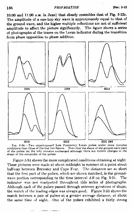
156 PROPAGATION [Sac. 5,12

10:00 and 11:00 A.M. in June) that closely resembles that of Fig. 5“32c.The amplitude of a one-hop sky wave is approximately equal to that ofthe ground wave, and the higher multiple reflections are not of sufficientamplitude to affect the picture significantly. The figure shows a seriesof photographs of the traces on the Loran indicator during the transitionfrom phase opposition to phase addition.

2355

0316

23591

C013

C031 EWTFIG, 5.34.—Two superimposed Low Frequency Loran pulae8 under more complex

conditiom than those of the Iafittwo fiuureu. Note that the shape of the ground-wave partof the pulses (at the icft) remaim unchanged although there me violent changc$ in theshape of the remainder of the pulnea.

Figure 5.34 shows the more complicated conditions obtaining at night.These pictures were made at about midnight in summer at a point abouthalfway between Brewster and Cape Fear. The distances are so shortthat the first part of the pulses, which arc shown matched, is the ground-wave portion corresponding to the time interval A B on Fig. 5.31. Theindicator was not readjusted throughout this series of photographs.Although each of the puhws passed through extreme gyrations of shape,the match of the leading edges was always good. Figure 5“35 shows thematch between a pair of pukws at a greater average distance, at aboutthe same time of night. One of the pulses exhibited a fairly strong

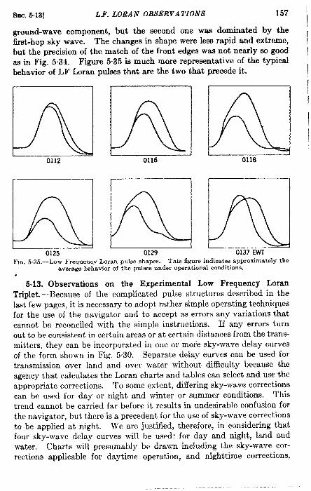
sac. 5.13] L.J’. LORAN OBSERVATIONS 157

ground-wave component, but the second one was dominated by thefirst-hop sky wave. The changes in shape were less rapid and extreme,but the precision of the match of the front edges was not nearly so goodas in Fig. 5.34. Figure 5.35 is much more representative of the typicalbehavior of LF Loran pulses that are the two that precede it.

Elbsl0112 0116

RIZII0125 0129

Kil0118

k0137Ewr

FIG. 5 35.—Low Frequency Loran pulse shapes. This figure indicates apPrOfimatelYtheaverage behavior of the pulses under operational conditions.

.

5.13. Observations on the Experimental Low Frequency LoranTriplet.-Because of the complicated pulse structures described in thelast few pages, it is necessary to adopt rather simple operating techniquesfor the use of the navigator and to accept as errors any variations thatcannot be reconciled with the simple instructions. If any errors turnout to be consistent in certain areas or at certain distances from the trans-mitters, they can be incorporated in one or more sky-wave delay curvesof the form shown in Fig, 5.30. Separate delay curves can be used fortransmission over land and over water without difficulty because theagency that calculates the Loran charts and tables can select and use theappropriate corrections. To some extent, differing sky-wave correctionscan be used for day or night and winter or summer conditions. Thistrend cannot be carried far before it results in undesirable confusion forthe navigator, but there is a precedent for the use of sky-wave correctionsto be applied at night. We are justified, therefore, in considering thatfour sky-wave delay curves will be used: for day and night, land andwater. Charts will presumably be drawn including the sky-wave cor-rections applicable for daytime operation, and nighttime corrections,

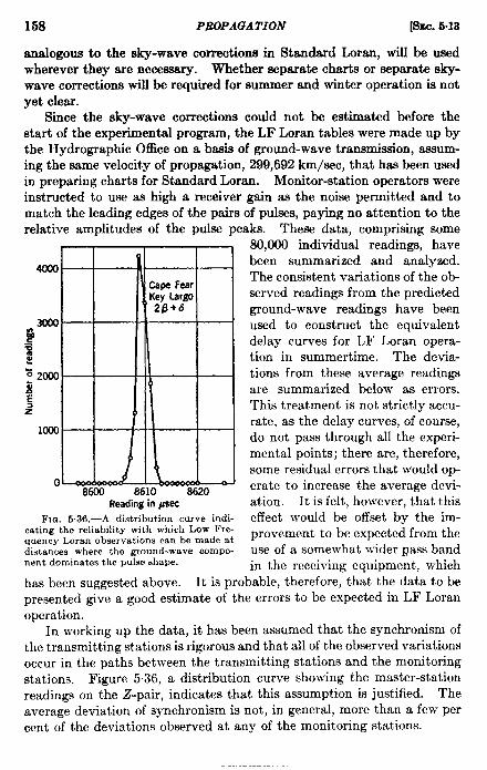
158 PROPAGATION [Saac. 6.13

analogous to the sky-wave corrections in Standard Loran, will be usedwherever they are necessary. Whether separate charts or separate sky-wave corrections will be required for summer and winter operation is notyet clear.

Since the sky-wave corrections could not be estimated before thestart of the experimental program, the LF Loran tables were made up bythe Hydrographic Office on a basis of ground-wave transmission, assum-ing the same velocity of propagation, 299,692 km/see, that has been usedin preparing charts for Standard Loran. Monitor-station operatore wereinstructed to use as high a receiver gain as the noise permitted and tomatch the leading edges of the pairs of pulses, paying no attention to therelative amplitudes of the pulse peaks. These data, comprising some

41xlo- 1CapeFearKeyUwgo2f3+6

Woa I.s~S’: 20W:

t

z

10QO 1

08600 8610 8620

Reading in @c

FICJ. 5.36.—A distribution curve indi-cating the reliability with which Low Fre-quency Loran observations can be made atdistances where the ground-wave compo-nent dominates the pulse shape.

80,000 individual readings, havebeen summarized and analyzed.The consistent variations of the ob-served readings from the predictedground-wave readings have beenused to construct the equivalentdelay curves for LF Loran opera-tion in summertime. The devia-tions from these average readingsare summarized below as errors.This treatment is not strictly accu-rate, as the delay curves, of course,do not pass through all the experi-mental points; there are, therefore,some residual errors that would op-erate to increase the average devi-ation. It is felt, however, that thiseffect would be offset by the im-provement to be expected from theuse of a somewhat wider pass bandin the receiving equipment, which

has been suggested above. It is probable, therefore, that the data to bepresented give a good estimate of the errors to be expected in LF Loranoperation.

In working up the data, it has been assumed that the synchronism ofthe transmitting stations is rigorous and that all of the observed variationsoccur in the paths between the transmitting stations and the monitoringstations. Figure 5.36, a distribution curve showing the master-stationreadings on the Z-pair, indicates that this assumption is justified. Theaverage deviation of synchronism is not, in general, more than a few percent of the deviations observed at any of the monitoring stations.

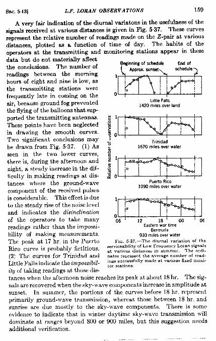
SEC. 5.13] L1’. LORAN OBSERVATIONS 159

A very fair indication of the diurnal variatons in the usefulness of thesignals received at various distances is given in Fig. 5“37. These curvesrepresent the relative number of readings made on the Z-pair at variousdistances, plotted as a function of time of day. The habits of theoperatom” at the transmitting anddata but do not matenafly aflectthe conclusions. The number ofreadings between the morninghours of eight and nine is low, asthe transmitting stations werefrequently late in coming on theair, because ground fog preventedthe flying of the balloons that sup-ported the transmitting antennas.These points have been neglectedin drawing the smooth curves.Two significant conclusions maybe drawn from Fig. 5.37. (1) Asseen in the two lower curves,there is, during the afternoon andnight, a steady increase in the ~lf-ficulty in making readings at dis-tances where the ground-wavecomponent of the received pulsesis considerable. This effect is dueto the steady rise of the noise leveland indicates the disinclinationof the operators to take manyreadings rather than the impossi-bility of making measurements.The peak at 17 hr. in the PuertoRICO curve is probably fictitious.(2) The curves for Trinidad andLittle Falls indicate the impossibil-ity of taking readings at those dis-

monitoring stations appear in these

Beginningof schedule End ofApprox. sunset schedule

1I I

I Io ) 1 r

Little Falls1420 malesover land

>...

i

Trinidad1670 miles over water

Puerto Rico1090 malesover water

1- 1 1

p

0

I0

06 ‘ 12 18 ‘ 00 ‘ 06Eastern war time

Bermuda930 malesoverwater

FIG. 5.37.—The diurnal variation of theserviceabdity of Low Frequency Loran signalsat various distances in summer. The ordi-nates represent the average number of read-ings successfully made at various fixed moni-tor stations.

tances when the afternoon noise reaches its peak at about 18 hr. The sig-nals are recovered when the sky-wave components increase in amplitude atsunset. In summer, the portions of the curves before 18 hr. representprimarily ground-wave transmission, whereas those between 18 hr. andsunrise are due mostly to the sky-wave components. There is someevidence to indicate that in winter daytime sky-wave transmission willdominate at ranges beyond 800 or 900 miles, but this suggestion needsadditional verification.

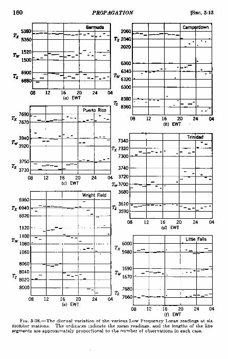
160 PROPAGATION [SEC.5.13

(b) EWl

5330Sefrmtda Csmperdown

T= -—- - — ___ L-- 2060 ___- .- -- — -- ---

5360 T= 2040 -- -.-- .2020

TW1520- - -—_ - -- -- -1500‘--

b360- . ---

T=6900 . —__ - --

~ - . ‘.

TW--

-—- _- ---6880 --– 6320 “

630008 12 16 24 04

(a) &o 8330 ---- --- - -G8364 — .

Puerto Rico7690.-

. .

T= ---7670 -- --– -- --- 08 12 16 20 24 04

3940.- --- --

TWTrinidad- -— -- 7340

3920 --Tx 7320 --- - . ---

7300--- -3750_ __ ___ --- -----

Tz3730 3740

- -08 12 16 24 04 3720

(c) E~--

TW37CQ -_ -. .-

Wright Field 36ao.-6960

3610---- ---- - -.Tx~940 -- .––– _- -_ Tz ---- ---

6920 -3590

08 12 16 20 24 041120 _ __ (d) w

1100 -- - -_-

Tw Little Falls1080“ 6000

,--- Tx1060 5980- -– “ -–_ - ‘-

8060- ___8040

1690Tw -- -—

Tz --- -8020--- 1670-- ---- - “-

8000 —- 7630Tz

08 12 16 7660-- -- -_—24 04

(e) EW’?08 12 16 20 24 04

W EWlFIG. 5,38.—The diurnal variation of the various Low Frequency Loran readings at six

monitor stations. The ordinates indicate the mean readings, and the lengths of the linesegments are approximately proportional to the number of observations in each case.

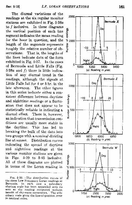
SEC. 5.13] L.F. LORAN OBSERVATIONS 161

The diurnal variations of thereadings at the six regular monitorstations are exhibited in Fig. 5.38ato j inclusive. In these diagramsthe vertical position of each linesegment indicates the mean readingfor the hour in question, and thelength of the segments representsroughly the relative number of ob-servations. That is, the lengths ofthe lines indicate data of the formexhibited in Fig. 5.37. In the casesof Bermuda and Little Falls (Fig.5.38a and j) there is little indica-tion of any diurnal trend in thereadings, although the signals atLittle Falls fail for 4 or 5 hr. in thelate afternoon. The other figuresin this series indicate either a con-sistent difference between daytimeand nighttime readings or a fluctu-ation that does not appear to bestatistically reliable in indicating adiurnal effect. There is, however,an indication that transmission con-ditions are usually more stable inthe daytime. This has led tobreaking the bulk of the data intotwo groups with a nominal dividingline at sunset. Distribution curvesindicating the spread of daytimeand nighttime readings at thevarious monitor stations are givenin Figs. 5.39 to 5.45 inclusive.All of these diagrams arc plottedin terms of the Loran reading in

FtcI, 539.-The distribution curves ofthe three Low Frequenry Loran readings atBermuda, In em-h cnsc n subsidiaryabscissa scale has been appended with itszero at the reading cotnputcd withoutbenefit of sky-wave corrections. The sub-sidiary sc@le glvcs the line-of-position errorin nautical mile.g.

,.-. -.. .—..-(a)weaalng In ,usec

1Ooc

(b) Reading in psec

z

L‘o

1000 ,I

Bermuda W

~.-:2% 500

-5 0gE2

1450 1500 1550 1600(c) Reading m flsec

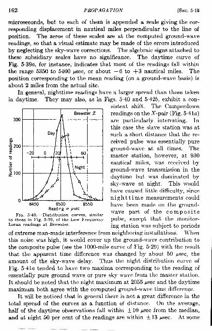
162 PROPAGATION [SEC.5.13

microseconds, but to each of them is appended a scale giving the cor-responding displacement in nautical miles perpendicular to the line ofposition. The zeros of these scales are at the computed ground-wavereadings, so that a visual estimate may be made of the errors introducedby neglecting the sky-wave corrections. The algebraic signs attached tothese subsidiary scales have no significance. The daytime curve ofFig. 5.39a, for instance, indicates that most of the readings fall withinthe range 5350 to 5400 psec, or about – 6 to +3 nautical miles. Theposition corresponding to the mean reading (on a ground-wave basis) isabout 2 miles from the actual site.

In general, nighttime readings have a larger spread than those takenin daytime. They may also, as in Figs. 5.40 and 5.42b, exhibit a con-“.

300 4Brews

Day

-20 0 20 ~ 60f .II I

\Night: h

S450 8500 8!

“z

S&Ji‘o

Reading In psec

Fm. 5.40.—Distribution curves, similarto those in Fig. 5.39, of the Low FrequencyLoran readings at Brewster.

sistent shift. The Camper downreadings on the X-pair (Fig. 5,41a)are particularly interesting. Inthis case the slave station was atsuch a short distance that the re-ceived pulse was essentially pureground-wave at all times. Themaster station, however, at 930nautical miles, was received byground-wave transmission in thedaytime but was dominated bysky-wave at night. This wouldhave caused little difficulty, sincenigh t t i me measurements couldhave been made on the ground-wave part of the compositepulse, except that the monitor-ing station was subject to periods

of extreme man-made interference from neighboring installations. -’henthis noise was high, it would cover up the ground-wave contribution tothe composite pulse (see the 1000-mile curve of Fig. 5.29) with the resultthat the apparent time difference was changed by about 50 psec, theamount of the sky-wave delay. Thus the night distribution curve ofFig. 5.41a tended to have two maxima corresponding to the reading ofessential y pure ground wave or pure sky wave from the master station.It should be noted that the night maximum at 2055 ~sec and the daytimemaximum both agree with the computed ground-wave time difference.

It will be noticed that in general there is not a great difference in thetotal spread of the curves as a function of distance. On the average,half of the daytime observations fall within t 10 psec from the median,and at night 50 per cent of the readings are within ~ 13 Psec. At some

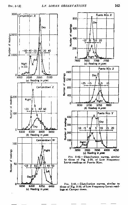
SEC,513] L.F. LORAN OBSERVATIONS 163

3000Camperdown X

I

Day

32000~~??z~Es 1000

(Xlo) ,:

0 41950 2000 2050 2100

(a) Reading m psec

ICamperdown Z

1:

i!i$200Night !:+5

;

z ~, ~ ~-20

j 1~ 100 II

4?

2

i’

o8300 8350 3-400 3450

(b) Reading in @c

100

g=~

z

; 50

s

0 6250 6300 6350 6400(c) Reading h Asac

Puerto Ri&oX800 9

Da~$~ 600~

z“ 400$ -1o’

z200

07600 7650 7700 7750

(a) Reading in #see

Puerto Rico z16(M

$ Dayem1200$’

-25 -15%~ 800 -

E

+ 400

03650 3700 3750 3800

(b) Reading inpac

400ge; 300

zJ 2(XIE

$100

03850 3900 3954 4W0 40!

(c) Reading in pc

FIO. 542.-Distribution curvee, similarto those of Fig. 5.39, of Low FrequencyLorunreadingsat PuertoRico.

FIG. 541 .—Distributioncurves,aimikr tothoeeof Fig. 5.39, of Low FrequencyLoranread-ingsat Camperdown.

164 PROPAGATION [SEC.5.13

distances such asin the Camperdown case quoted above or in the caseof the 890 miles over land represented in Fig. 5.44fI and c, there is con-

(6] Reading in #see

(c) Reading in&c

FIG. 5.43.—l3istribution curves, similarto those of Fig. 539, of Low FrequencyLoran readings at Trinidad.

siderable ambiguity in that theoperator may read essentially aground wave or a sky wave or acomposite value. It will be real-ized that this distance is that atwhich the estimated delay (Fig.5.30) is making its sharpest rise.

The discrepancies between theobserved readings and those com-puted for ground-wave transmis-sion are exhibited in Table 5.3.The discrepancy in Column 7 orColumn 9 is, with due regard forsign,a chord of the delay curve(see Fig. 5.30) between the twotransmission times given in Col-umns 3 and 4. By starting at theshorter distances, at which the de-lay may be assumed to be zero,points may be connected to defineapproximately the shape of thecurve, as was done to derive the2-Me/see delay curve. Fittingthese various data together callsfor the exercise of judgmentbecause the agreement betweenseparate sets of observations isnever so good as could be wished.In general, all of the observationsexcept those at Bermuda fit intothe delay pattern exhibited inFig. 5.46. The Bermuda obser-vations have been weighted verylightly in drawing these curvesbecause the anomalies there maybe attributed to a faulty amdi-

tude-balance circuit in the receiver used at that station. I. .

The shape of the overwater curves of Fig. 5.46 resembles the curve of

1A receiver that was known to be satisfactory was operated in Bermuda for a fewdays toward the end of the program. The observations with this receiver, althoughfew in number, werein good agreementwith the curvesof Fig, 5.46.

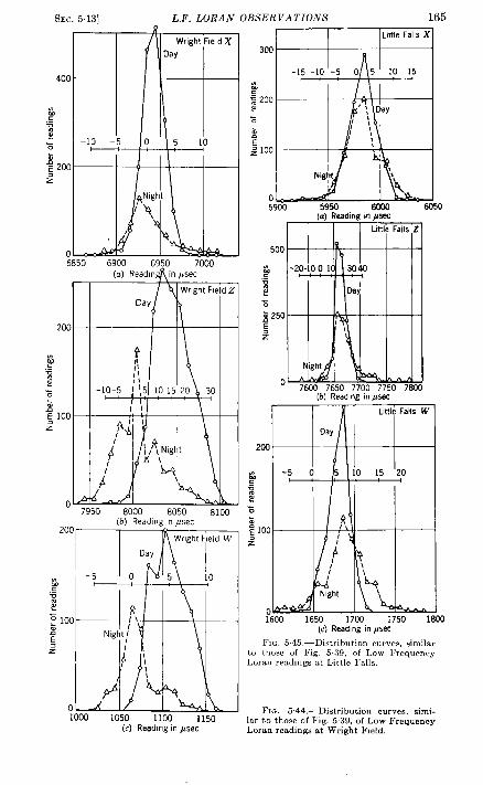
SEC.513] L.F. LORAN OBSERVATIONS 165R

/WrightFieldX

Day

400 -

%c5;

-lo – 50 5 10z~E 2002

,

06850 6900 6950 7002

(a) Readln inpsec

WrightFfeldZDay

\

f~1

-1o-5

I 1

A’[A

o 8000 8050 8100(b) Readingn psec

200

Day

-5 0Gg::

R: 100.f Nightj

s

o100Q 1050 1100 1150

(c) Read!ngin psec

LMe FallsX

300I

G~: 200!2Gz?g 100

h

o5900 5950 5ceo 6050

[.)Readingin #see

500

%c.-:2%~ 250E2

07600 7650 7700 7;

(b) Readingin p%

mb

Day

2W I

G -5 0 5 10 15 20~%tz5 $1f 100

2

Night

*+ N

!600 1650 17CQ 1750 1801(c) Readingin psec

FIG 545,-Distribution curves,~imilarto tbosc of Yig. 539, of Low I:requencyLoranreadingsat Little Falls,

FIG. 5.44.—Distributioncurves, simi-lar to thoseof Fig. 539, of Low FrequencyLoranreadingsat WrightField.

166 PROPAGATION [SEC.513

Fig. 5.30 except that the height of thesteps islessthan had been antici-pated. It is reasonable that the night curve should resemble the daycurve, displaced to the left, because any daytime ratio of first-hop sky-wavc amplitude to that of the ground wave can be found at night at someshorter distance. It is possible that the initial slope of the land curves

FIG.5.46.—The four experimental LowFrequency Loran delay curves for summeroperation.

represents a decrease in the veloc-ity of ground-wave propagationover land. The curves have beendrawn as they are because thereis no evidence that the “land curvesleave the origin along the abscissa.If the velocity is less over land, theshapes of the land curves may bevery nearly those of the watercurves superimposed upon a veloc-ity slope, which here seems to beabout 1 in 250. This hypothesisaccounts for the shape of thenight-land curve, but we should

expect that the slope of the day-land curve would begin to decrease atabout 7000 psec. More overland data should be taken to clarify thisquestion.

That the minor variations in the delay curves of Fig. 5.46 are not ofextreme importance is indicated in Columns 4 and 5 of Table 5.4. Thesecolumns give the displacements of the line of position (in nautical miles)corresponding to the discrepancies of the mean readings, from the cal-culated ground-wave values, which were given in Columns 7 and 9 ofTable 5,3. The entries for Brewster and Camperdown in Table 5-4,Columns 4 and 5, are nearly meaningless because the monitoring stationswere located almost upon the baseline extensions where the system is notexpected to provide navigation. The remaining figures in these columnsindicate the consistent discrepancies that the equivalent delay curvesare expected to correct. That is, the position lines at distances of theorder of 1000 miles are, in general, in error by less than 10 miles even ifthe delay curves are totally neglected.

Columns 6 and 7 of Table 5.4 give the average deviations from themean reading observed at the various monitor stations. Here again theentries for Brewster and Camperdown are not significant from the view-point of navigation. The figures in Columns 6 and 7, Table 5-4, do notform a very coherent pattern because the monitor stations lie at variousangles to the baselines. This effect has been removed in columns 8 and9 where the stations are assumed to lie on a great circle that intersectsthe center of the baseline at an angle of 45°. The geometrical factors

SEC. 5.13] L.F. LURAN OBSERVATIONS 167

have also been adjusted to apply to a baseline whose length is 600 nau-tical miles. The only assumption involved in this treatment is thatthe scattering of the observed time differences dces not depend upon theorientation of the baseline. This is not strictly true, but most of theadjustments are relatively minor.

Z.E10-6.+s:c.-;5&c:

s0300500 low lSCQ 300 m lWO 15W 2(

Mean distancein nautical miles Meandistance in nautical miles

(a) Summerday (b) Summernight

n

FIG. 5.47.—The median errors of the Low Frequency Loran experimental observationsP1Otted as a function of distance. The curves are corrected to simulate operation at anangle of 45° from a 600-mile baseline, The heads of the arrows appended to many of theexperimental points indicate the values before correction.

30 30 P

alSO /z: b=600 \ //g: 20 20-~ A~ .=:; 6=600 ,/g. o~ ,~

Lando

LandO*1O 10-Ee.=~ ‘b =12C9

o3005M 1O(XI 1500 1500 20W

Mean distancein nati~l mil~ Mean distancein natilcal miles

(a) Summerday (b) SummernightFIG.64S.—Emordiagrams for day and nightoperation,aimifmto thoseof IVg.5.47,but.

indicatingtheerrorsexceededleaathan10 percentof the time.

The median errors from Columns 8 and 9 are plotted in Fig. 5.47uand b. In these diagranm the solid lines represent the errors associatedwith a baseline length of 600 nautical miles, and the dashed lines representthe errors associated with Y- and W-readings which have a lZOO-rnile ‘baseline. The arrows attached to many of the points indicate the mag-nitude of the corrections that were made for the positions of the monitorstations. That is, the actual observed errors (Columns 6 and 7 of

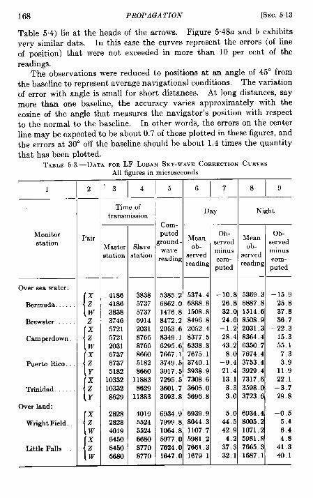
168 PROPAGATION [SEC.5.13

Table 5“4) lie at the heads of the arrows. Figure 5“48a and b exhibitsvery similar data. In this case the curves represent the errors (of lineof position) that were not exceeded in more than 10 per cent of thereadings.

The observations were reduced to positions at an angle of 45° fromthe baseline torepresent average navigational conditions. The variationof error with angle is small for short distances. At long distances, say

more than one baseline, the accuracy varies approximately with thecosine of the angle that measures the navigator’s position with respecttothenormal to the baseline. In other words, the errorson the centerline may be expected to be about 0.7 of those plotted in these figures, andthe errors at 30° off the baseline should be about 1.4 times the quantitythat has been plotted.

TABLE53.-DATA FOELF LORANSKY-WAVECORRECTIONCURVESAll tkures in microseconds

1

Monitorstation

Oversea water:

Bermuda..,

Brewster.

Camperdown.

PuertoRico.

Trinidad. . . . .

Over land:

WrightField.

Little Falls.

2

Pair

{

xzwz

{

xzw

{

xzY

{

xzY

{

xzw

{

xzw

3 I 4

Time oftransmission

&aster

tation

4186418638383746572157212031673767375182

1033210332

8629

28282828401964506450668J3

SlaveItation

3838573757376914203187668766866051828660

118838629

11883

401955245524668A)87708770

5

COm-putedround.wavereading

5385.26862.C1476.83472.22053.C8349.16295.f7667,13749,53917.:7295.53601.73693.8

6934.97999.fi1064.85977.c7624.C1647.C

6 I7 8 I9

Day Night

Ob- Ob-?tfean >fean

served servedob- ob-

minus minus]erved served

cOm- cOm-eading reading

puted putedI I I

5374.46888.81508.88496.82052.46377.56338.87675.13740.13938.97308.63605.03696.8

–10.8 5369.3 –15.926.8 6887.8 25.832.0 1514.6 37.824.6 8508.9 36.7

–1.2 2031.3 –22.328.4 8364.4 15.343.2 6350.7 55.18.0 7674.4 7.3

–9.4 3753.4 3.921.4 3929.4 11.913.1 7317.6 22.13.3 3598.0 –3.73.0 3723.6 29,8

6939.9 5.0 6934.4 –0.58044.3 44.5 8CU)5.2 5.41107.7 42.9 1071.2 6.45981.2 4.2 5981.8 4.87661.3 37.3 7665.3 41.31679 1 32.1 1687.1 40.1

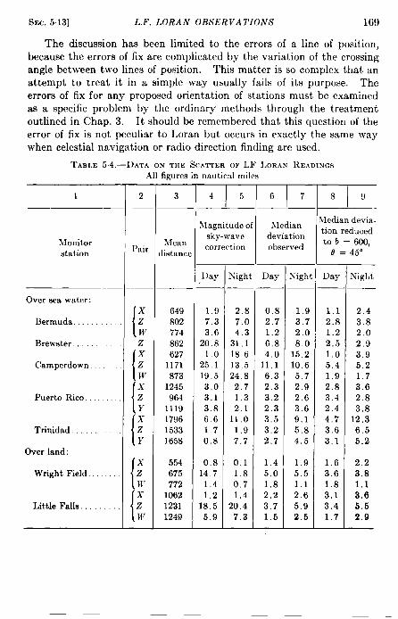
SEC. 513] L.F. LORAN OILYERVATIONS 169

The discussion has been limited to the errors of a line of position,because the errors of fix are complicated by the variation of the crossingangle between two lines of position. This matter is so complex that anattempt to treat it in a simple way usually fails of its purpose. Theerrors of fix for any proposed orientation of stations must be examinedas a specific problem by the ordinary methods through the treatmentoutlined in Chap. 3. It should be rcmcmbcrcd that this question of theerror of fix is not peculiar to I.oran but occurs in exactly the same waywhen celestial navigation or radio direction finding are used.

TABI.E 54.-DATA ON TME SCATTEROF LF I,ORA~ READINGSAll figures in nautical miles

1

Monitorstation

Over sea water:

Bermuda . . . . . . . . . .

Brewster, . . . . . . .

Camperdown.

Puerto Rico.

Trinidad. . . . . .

Over land:

Wright Field.

Little Falls,

2

I’air

{

xzwz

{

xzw’

{

xzY

(

xzY

{

xzU’

{

xzw

3

Meanlistanc

649802774862627

1171873

1245964

1119179615331658

554675772

106212311249

T}Iagnitude 0

sky-wavecorrection

1)ay

1.97.33.6

20.81.0

25,119.53.03.13,86.61.70.8

0.814,71.41.2

18.55.9

Nigh!

2.87.04.3

31.118 613.524.8

2.71.32.1

11.01.97.7

0,11.80.71,4

20,47.3

T_kledian

deviationobserved

Day

0.82.71.26.84.0

11.16.32,33.22.33.53.22.7

1,45,01,82,23.71.5

Sight

1.9

3,72,0

8.015.210.6

5.72.92.63,69.15.84,5

1.95.51.12.65.92.5

T\fedian devia-tion reducedto b = 600,

e = 45”

Day

1.12.81.22,51.05.41.92.83.42.44.73.63.1

1.63.61.83.13.41.7

Night

2.43.82.02.93.95.21.73,62.83.8

12,36.55.2

2,23.81.13.65.52.9

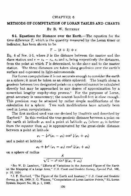
CHAPTER 6

METHODS OF COMPUTATION OF LORAN TABLES AND CHARTS

BY B. W. SI~ERLY

6.1. Equations for Distance over the Earth-The equation for thetime difference T, which is the quantity measured by the Loran timer orindicator, has been shown to be

T=((3+6)+LJ

Eq. 4 of Sec. 3.1, where @ is the distance between the master and theslave station and v = .s~ — s4, s~ and s~ being respectively the distances,from the point at which T is determined, to the slave and to the masterstation. The three distances are taken along geodesics over the earth’ssurface and expressed in light-microseconds.

For Loran computations it is not accurate enough to consider the earthas a sphere; it must be taken as an oblate spheroid. The length along ageodesic between two designated points on a spheroid cannot be calculateddirectly but may be approached to any degree of approximation by asomewhat lengthy step-by-step process. 1 For the purposes of Loran,great accuracy is unnecessary; the nearest hundred feet is close enough.This precision may be attained by rather simple modifications of thecalculation for a sphere. Two such modifications have actually beenused in Loran computations.

The first method used was one devised by Doolittle and described byHayford. 2 In this method the true geodesic distance between a point onthe earth at latitude pl and a point at latitude pz (where p, is fartherfrom the equator than pz) is approximated by the great-circle distancebetween a point at latitude

ql – +ez(pl – @z) cm2 *(PI + 92)

and a point at latitude

V2

on a sphere of radius

1See W. D. Lambert,

+ *e’ (P1 – p,) cos’ *(fol + p,)

E

<l – e’ sin’ *(PI + pz)’

“Effects of Variations in the .4ssumed Fizure of the Earthon the Mapping of a La~ge Area,” U.S. Coast and Geodetic Survey, >pecial Pub. 100,p,16, 1924.

‘ J. F. Hayford, “ The Figure of the Earth and Isostasy,” U.S. Coast and GeodeticSurvey, p. 88, 1909;F. G. Watson, “Computation of LoranLattice Points,” RL LoranSystemReport No. 23, p. 1, 1942.

170

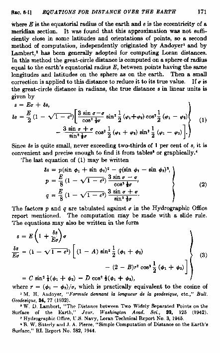
Smc.6.1] 17QUATIONS FOR DISTANCE OVER THE EARTH 171

where E is the equatorial radius of the earth and e is the eccentricity of ameridian section. It was found that this approximation was not suffi-ciently close in some latitudes and orientations of points, so a secondmethod of computation, independently originated by Andoyerl and byLambert,2 has been generally adopted for computing Loran distances.In this method the great-circle distance is computed on a sphere of radiusequal to the earth’s equatorial radius E, between points having the samelongitudes and latitudes on the sphere aa on the earth. Then a smallcorrection is applied to this distance to reduce it to its true value. If u isthe great-circle distance in radians, the true distance .s in linear units isgiven by

s= Eu+8s,

6s = ; (1 – VE’)[

3sin u-usinz ~ (w+P2) COS2; (n – 92)

COS* *U

1

(1)

_3sinu+usin2 +U 1

COS2~ (PI + 92) sinz ~ (Pl — P2) .

Since $s is quite small, never exceeding two-thirds of 1 per cent of s, it isconvenient and precise enough to find it from tablesa or graphically.’

The last equation of (1) may be titten

$s = p(sin @l + sin @2)2 – q(sin +1 – sin &)z,

P=~(l–<’2)3Sinu–u, COS2*V

I

(2)

q=~(l–<~)ssinv+v. sin2 *V

The factors p and q are tabulated against v in the Hydrographic Officereport mentioned. The computation may be made with a slide rule.The equations may also be written k the form

() 6s‘=El+ZU

g=(l–vl-[

~z) (1 – A) sinz ~ (@l + 02)(3)

– (2 – Ei)r’ Cos’ ; (41 + 02)1

= C sin’ 4(41 + 42) – D COS2~($, + @,),

where r = (@l — @/v, which is practically equivalent to the cosine of1M. H. Andoyer, “Formule dormant fo lqueur de b geodesique, etc.,” Bull.

Geodeeique, 34, 77 (1932).zW. D. Lambert, “The DistancebetweenTwo Widely SeparatedPoints on the

Surface of the Earth,” Jour. Washirwton Acad. Sci., S!4, 125 (1942).s HydrographicOffice,IJ.S.Navy, LoranTechnicalReport No. 3, 1945.t B, W. Sitterlyand J. A. Pierce,“Simple Computationof Distanceon the Earth’s

Surface,” RL Report No. 582, 1944.

172 COMPUTATION OF LORAN TABLES AND CHARTS [Srw. 6.1

the “average” true bearing along the great circle whose length is u, andA aud B are small quantities, functions of r and a. A rather simplenomogram may be constructed, for reading the coefficient Ii’[l + (ds/Eu)]directly, against the three arguments ~(qi + PZ), r, and u, to a precisionbetter than 1/100,000 of a, or against the two arguments 4(w i- d andr, to a precision of about 100 ft. at distances less than 1000 miles. Thenomogram is described and examples given in the Radiation Laboratoryreport mentioned. The quantity E[l + (6s/Eu)] may be regarded asthe “effective radius of curvature” of the arc u.

In all these methods, the great-circle distance u is calculated by oneof the standard formulas

cos u = sin VI sin 4V + cos ql cos P2 cos Ah, (4)hav u = hav (PI – p,) + cos p, cos p~ hav AA, (5)hav a = hav AA hav [180° – (m + p,)]

+ hav (180° – AA) hav (P1 – p,), (6)

where AX is the difference between the longitudes of the points and hav u(the haversine of u) is sinz *u. Since u is usually less than 20°, sevensignificant figures are required to determine it to 1“ (100 ft. ) from itscosine, five figures to determine it from its haversine. But, if a calculatingmachine is used, seven figures are not much more troublesome than five,while the five-place tables of haversines included in most collections ofnautical tablesl give only three or even two significant figures in thenatural values for small angles, since the first two or three decimals arezero. Five-figure tables giving one million times the haversine, between~ = 0°10” and ~ = z5”o0’, were prepared in 1944 at the Radiation Labora-

tory’ for the solution of Eq. (6). This form of solution has been foundconvenient and rapid. If u is less than 2°, the direct formulaa

s = v’[jI(qI – 92)]2 + (jz AA)2 (7)

is sufficiently accurate. Here jl = R sin 1’, jz = N cos +(VI + w) sin 1’,where R is the radius of curvature along the meridian and N the radius ofcurvature perpendicular to the meridian, at latitude i(pl + w2). Thedifferences (PI – P*) and AA are expressed in minutes of arc, and thelinear unit of s will be that of R and N. Tables of jl and fz are given inthe references the linear unit being the light-microsecond. Tables ofR and N appear in standard geodetic texts.

The small error in s which results from the use of the approximatecorrection 6s may be made still smaller by using the parametric or reducedlatitudes of the two end points, instead of the geographical latitudes, in

I For example, in the American Practiccat Naoigator, Hydrographic Office, U.S.Navy, PublicationNo. ‘J,revisedevery few years.

z I‘Manual of Proceduresfor Mobile Charting Units, Air TransportablebranSystem,” RL Report No. M-183, 1945.

sHydrographicOffice, U.S. Navy, Loran Technical Report No. 3, 1945.

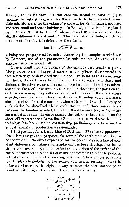
SEC. 6.2] EQUATIONS FOR A LORAN LINE OF POSITION 173

Eqs. (1) to (6) inclusive. In this caae the second equation of (1) ismodified by substituting sin u for 3 sin u in both the bracketed terms.This substitution alters the values of p and q in Eq. (2), making p negativeand very small and about halving q. In Eq. (3), 1 – A is to be replacedby – A’ and 2 – B by 1 – B’, where A’ and B’ are small quantitiesslightly different from A and B. The parametric latitude, which wemay denote here by 8, is defined by the relation

tan 0 = ~= tan @,

1#1being the geographical latitude. According to examples worked outby Lambert, use of the parametric latitude reduces the error of theapproximation by about half.

Over a small area the surface of the earth is very nearly a plane.Along a narrow strip it approximates closely a cylindrical or conical sur-face which may be developed into a plane. In so far as this approxima-tion holds, the earth may be represented truly to scale by a chart, anddistances directly measured between charted points. If one light-micro-second on the earth is equivalent to k mm. on the chart, the point on theearth where u = SB— SAwill correspond to the point on the chart wherea circle, described about the slave station with radius ksB, intersects acircle described about the master station with radius ks*. If a family ofsuch circles be described about each station and those intersectionsbetween the families selected, for which the difference (ks, – ks~ = kv)has a constant value, the curve passing through these intersections on thechart will represent the Loran line (T = v + /3+ 6) on the earth. Thistechnique has been used in constructing preliminary charts when theutmost rapidity in production was demanded.

6s2. Equations for a Loran Line of Position. The Plane Approxima-

tion.—For navigational purposes, the form of the earth may be taken tobe spheroidal. No direct expression for the coordinates of a line of con-stant difference of distance on a spheroid has been developed as far asthe writer is aware. But to the extent that a portion of the surface of theearth approximates a plane, a Loran line approximates a plane hyperbola,with its foci at the two transmitting stations. Three simple equationsfor the plane hyperbola are the central equation in rectangular and inpolar coordinates, with origin midway between the foci, and the polarequation with origin at a focus. These are, respectively,

~z = a2Y2 + az)~z — az

p = az(cz — az)

Cz COS2 e — a 2’

~2 — a2r=

Ccose+a’ I

(8)

174 COMPUTATION OF LORAN TABLES AND CHARTS [SEC.6.2

where 2C is the distance between the foci and c/a the eccentricity of ahyperbola, z is taken parallel to and y perpendicular to the line connectingthe foci (baseline), and o is zero when r coincides with this line. Wheny = O, z = a. To distinguish the two branches of the hyperbola ofeccentricity cia, which correspond to different values of T, z and a areconsidered positive on the side of the center line (y-axis) on which themaster station lies, negative on the other, co that a has the sign of U. Inthe denominator of the last equation the upper sign is applied to a if theorigin of polar coordinates is taken at the master station, the lower if it isat the slave station.

The constants a and c in Eq. (8) are related to the constants v and oof a Loran line by the relations

k~ kvc=—,2

a=—,2 (9)

where k is the length of a light-microsecond in the linear units in whichz, y, and r are expressed. By means of Eqs. (9) and (8) the lines of aLoran family may be plotted by points upon a chart on which the appro-priate coordinate grid, properly centered and oriented, has been con-structed. The rectangular equation is the best for this purpose, becauserectangular coordinates are easier to lay out than polar. The Hydro-graphic Office has published a tablel giving z with arguments a and y, fora ~ 0.75, and y with arguments a and x, for a ~ 0.70. The unit oflength is c; the interval in a is 0.001; and the tabulated coordinate is givento four decimal places. There are also instruments for tracing planehyperbolas mechanically, without calculation, tables, or constructedgrids; one of these is described in Sec. 6.6.

The plotted lines on the chart will depart from the course of the actuallines on the earth to the extent .to which the chart projection distorts theearth’s surface in representing it on a plane. This distortion is smallenough in the case of the azimuthal and conic projections, within certainlimits, so that corrections may be determined and applied to the planehyperbolas, “warping” them to fit the other features of the chart.Distortion in the Mercator projection is too great to be corrected in thisway, except in regions near the equator.

In theo~, it should be possible to express the coordinates of Eq. (8)in terms of latitude and longitude on the chart, by an algebraic trans-formation, since meridians and parallels on the chart form a planecoordinate grid. Such a transformation is practicable in the case ofprojections on which parallels and meridians are represented by a gridof straight lines, circles, or both; for others it is not. In all cases, graphi-

1HydrographicOffice,U.S. Navy, “Tables for the Constructionof Plane Hyper-bolas,” H.O. Misc. 11,486(1944).

SEC. 6.2] EQUATIONS FOR A LORAN LINE OF POSITION 175

cal construction is quicker and accurate enough for charting, whiledetermination of exact general formulas to correct the plane hyperbolasfor the terrestrial curvature and the form of the projection is not practica-ble. Approximate correction may be made by computing true Loranreadings at selected points on the earth and adjusting the hyperbolas sothat they will indicate these readings at the corresponding points on thechart.

The Spherical Approzimution.-A region of the terrestrial spheroid aslarge as the service area of a Low Frequency Lomn triplet departs farfrom a plane surface, but it may be rather closely represented by aspherical surface. Loran lines on this surface are spherical hyperbolas.The first two equations below are, respectively, the central equation of aspherical hyperbola in spherical rectangular and in spherical polar coor-dinates; the last two are different forms of the spherical polar equationwith origin at a focus.

sin2 a COS2c \sin~ z = sinz y + sinz a,sinz c — sinz atan2 ~ = tanz a (sin2 c – sin2 a)

sin2 c cosz O — sinz a ‘

tanr=sinz c — sinz a

sm c cos c cos 6 ~ sin a cos acos 2a — cos 2C——

sin 2%cos 0 + sin 2a’tanj ~ ~ = sin (c f a) sin [r – (c : a)]

2 sin (c T a) sin [7 + (c f a)]’

(lo)

where a, c, x, y, and T are spherical arcs. Here y is the spherical distanceof a point of the hyperbola from the baseline (which is the great circlepassing through the foci), that is, the arc intercepted bet]veen baselineand point, on a great circle that passes through the point and the poles ofthe baseline. Similarly, z is the spherical distance of the point from thecenter line (which is the great circle passing through the poles of thebaseline and midway between the foci). The origin for the first twoequations is the intersection of baseline and center line; for the third andfourth, one of the foci; and 0 is zero when T extends from this fecus towardthe other one, along the baseline. The first equation might have severalother forms, since ‘{spherical rectangular coordinates” may be chosen inseveral ways. The signs are taken in the same way as in ‘13q. (8).

Conversion from the coordinates of Eq. (10) to geographical longitudex and latitude p may be effected by standard transformation formulas ofspherical analytic geometry or trigonometry. Convenient forms of theseare given in Sec. 6.7 below [Eqs. (16) to (18)]. On a spherical earth ofradius E, a series of points X, p, computed by Eq. (10) and the trans-

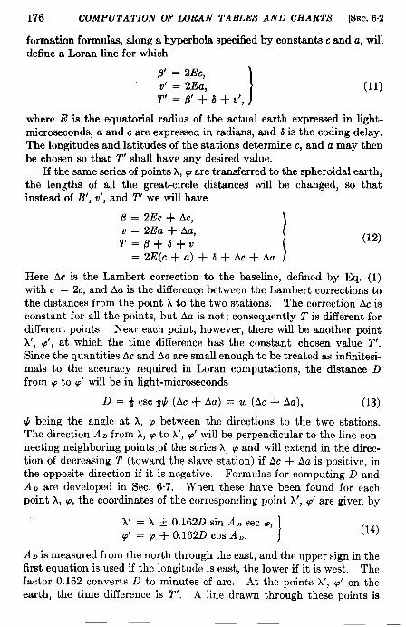
176 COMPUTATION OF LORAN TABLES AND CHARTS [SEC.6.2

formation formulas, along a hyperbola specified by constants c and a, willdefine a Loran line for which

where E is the equatorial radius of the actual earth expressed in Light-microseconds, a and c are expressed in radians, and 6 is the coding delay.The longitudes and latitudes of the stations determine c, and a may thenbe chosen so that T’ shall have any desired value.

If the same series of points A, p are transferred to the spheroidal earth,the lengths of all the great-circle distances will be changed, so thatinstead of B’, v’, and T’ we will have

P = 2Ec + Ac,

v = 2Ea + Aa,T=/?+d+v I (12)

=2E(c+a)+6+Ac+ Aa.

Here Ac is the Lambert correction to the baseline, defined by Eq. (1)with u = 2c, and Aa is the difference between the Lambert corrections tothe distances from the point X to the two stations. The correction ACisconstant for all the points, but Aa is not; consequently T is different fordifferent points. Near each point, however, there will be another pointk’, q’, at which the time difference has the constant chosen value T’.Since the quantities Ac and Aa are smaU enough to be treated as infinitesi-mals to the accuracy required in Loran computations, the distance Dfrom p to p’ will be in light-microseconds

D = ~ csc ~~ (Ac + Aa) = w (Ac + As), (13)

~ being the angle at A, p between the directions to the two stations.The direction AD from A, p to h’, p’ will be perpendicular to the line con-necting neighboring points of the series A, p and will extend in the direc-tion of decreasing T (toward the slave station) if Ac + Aa is positive, inthe opposite direction if it is negative. Formulas for computing D and

AD are developed in Sec. 6.7. When these have been found for eachpoint X, q, the coordinates of the corresponding point x’, q’ are given by

h’ = X ~ 0.162D sin AD sec p,

9’ = ~ + 0.162D cos AD. 1(14)

A. is measured from the north through the east, and the upper sign in thefirst equation is used if the longitude is east, the lower if it is west. Thefactor 0.162 converts D to minutes of arc. At the points A’, p’ on theearth, the time difference is T’. A line drawn through these points is

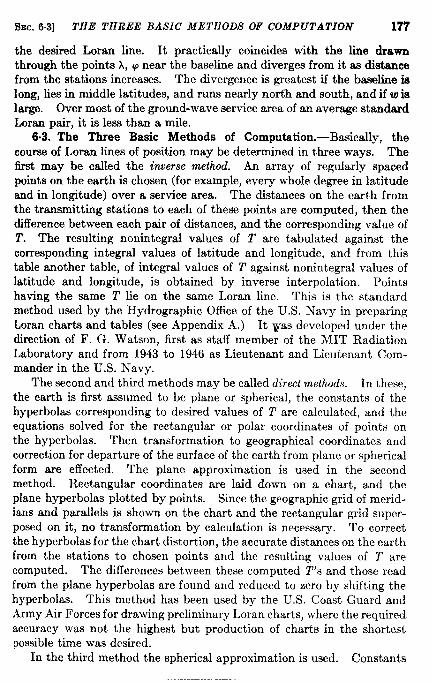
SEC. 6.3] THE THREE BASIC METHODS OF COMPUTATION 177

the desired Loran line. It practically coincides with the line drawnthrough the points A, p near the baseline and diverges from it as distancefrom the stations increases. The divergence is greatest if the baseline islong, lies in middle latitudes, and runs nearly north and south, and if w islarge. Over most of the ground-wave service area of an average standardLorsm pair, it is less than a mile.

6.3. The Three Basic Methods of Computation.-Basically, thecourse of Loran lines of position may be determined in three ways. Thefirst may be called the inverse method. An array of regularly spacedpoints on the earth is chosen (for example, every whole degree in latitudeand in longitude) over a service area. The distances on the earth fromthe transmitting stations to each of these points are computed, then thedifference between each pair of distances, and the corresponding value ofT. The resulting nonintegral values of T are tabulated against thecorresponding integral values of latitude and longitude, and from thistable another table, of integral values of T against nonintegral values oflatitude and longitude, is obtained by inverse interpolation. Pointshaving the same T lie on the same Loran line. This is the standardmethod used by the Hydrographic Office of the U.S. Navy in preparingLoran charts and tables (see Appendix A.) It was developed under thedirection of F. G. Watson, first as staff member of the MIT RadiationLaboratory and from 1943 to 1946 as Lieutenant and Lieutenant Com-mander in the U.S. Navy.

The second and third methods may be called direct methods. In these,the earth is first assumed to be plane or spherical, the constants of thehyperbolas corresponding to desired values of T are calculated, and theequations solved for the rectangular or polar coordinates of points onthe hyperbolas. Then transformation to geographical coordinates andcorrection for departure of the surface of the earth from plane or sphericalform are effected. The plane approximation is used in the secondmethod. Rectangular coordinates are laid down on a chart, and theplane hyperbolas plotted by points. Since the geographic grid of merid-ians and parallels is shown on the chart and the rectangular grid super-posed on it, no transformation by calculation is necessary. To correctthe hyperbolas for the chart distortion, the accurate distances on the earthfrom the stations to chosen points and the resulting values of T arecomputed. The differences between these computed T’s and those readfrom the plane hyperbolas are found and reduced to zero by shifting thehyperbolas. This method has been used by the LT.S. Coast Guard andArmy Air Forces for drawing preliminary Loran charts, where the requiredaccuracy was not the highest but production of charts in the shortestpossible time was desired.

In the third method the spherical approximation is used. Constants

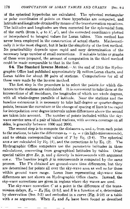
178 COMPUTA TIOiV OF LORAN TABLES AND CHARTS [SEC. 6.4

of the spherical hyperbolas are calculated. The spherical rectangularor polar coordinates of points on these hyperbolas are computed, andlatitude and longitude obtained by means of the transformation equations.The latitudes and longitudes are then corrected for the spheroidal formof the earth (from A, p to X’, p’), and the corrected coordinates plottedor interpolated to integral values for Loran tables. This method hasnever been employed in the construction of actual charts. Mathemati-cally it is the most elegant, but it lacks the simplicity of the first method.Its practicability depends upon rapid and easy determination of thenecessary large number of small corrections. If suitable tables or graphsof these were prepared, the amount of computation in the third methodcould be made comparable to that in the first.

6.4. The Standard Inverse Method. -At the end of 1945 the Hydro-graphic 05ce had published approximately 2* million Loran charts, andLoran tables for about 50 pairs of stations. Computations for all ofthese were made by the inverse method.

The first step in the procedure is to select the points for which dis-tances to the stations are calculated. It is convenient to take these at theintersections of all meridians, the longitudes of which are whole degrees,with all whole-degree parallels of latitude. N-ear the stations and thebaseline extensions it is necessary to take half-degree or quarter-degreepoints, because the curvature or the change of spacing of lines is too rapidfor interpolation over degree intervals unless differences above the secondare taken into account. The number of points included within the sky-wave service area of a pair of island stations, with oversea coverage on allsides, is generally between 1000 and 2000.

The second step is to compute the distances s, and s. from each pointto the stations, to take the differences SB– S* = o (in light-microseconds),and to obtain corresponding values of 7’ by Eq. (3.4). The sphericalarcs u are calculated by Eq. (4), and the corrections 6s by Eq. (2). TheHydrographic Office computers use the parametric latitudes in thesecalculations, converting from geographical latitudes by tables. Otherspecial tables give Em, p, and q directly in microseconds with argumentcos u. The baseline length @ in microseconds is computed by the sameprocess. The T’s obtained are ground-wave time differences, but theyare determined for points all over the sky-wave area as well as for thosewithin ground wave range. Loran lines representing sky-wave timedifferences are not shown on Hydrographic Office charts. Instead, thesky-wave corrections are given in regions where sky waves are used.

The sky-wave correction C at a point is the difference of the trans-mission delays, E* — EB [Eq. (3.5)], and E is a function of s, determinedby observation (Sec. 5.3) and embodied in a curve (Fig. 5.10) or a tablewith s as argument. When S~ and S, have been found as described

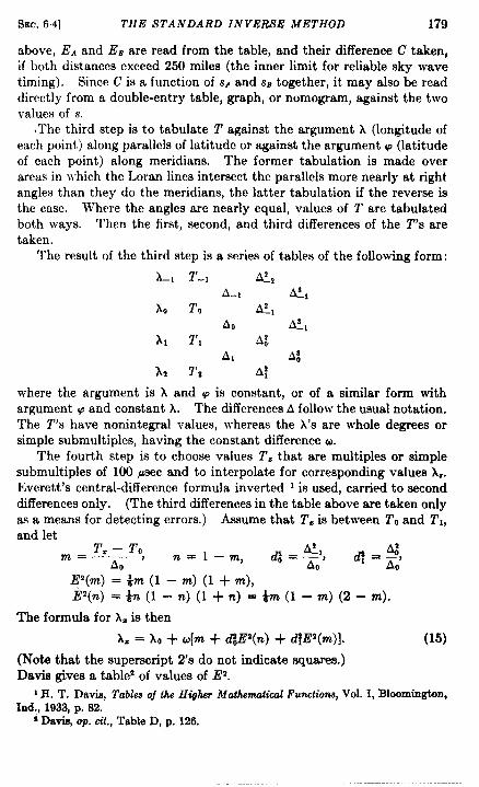
SEC.6.4] TIIE STANDARD INVERSE METHOD 179

above, EA and En are read from the table, and their difference C taken,if both distances exceed 250 miles (the inner limit for reliable sky wavetiming). Since C is a function of s. and SBtogether, it may also be readdirectly from a double-entry table, graph, or nomogram, against the twovalues of s.

,1’he third step is to tabulate T against the argument k (longitude ofeach point) along parallels of latitude or against the argument p (latitudeof each point) along meridians. The former tabulation is made overareas in which the Loran lines intersect the parallels more nearly at rightangles than they do the meridians, the latter tabulation if the reverse isthe case. Where the angles are nearly equal, values of T are tabulatedboth ways. Then the first, second, and third differences of the T’s aretaken.

The result of the third step is a series of tables of the following form:

where the argument is A and p is constant, or of a similar form withargument q and constant A. The differences A follow the usual notation.The T’s have nonintegral values, whereas the A’S are whole degrees orsimple submultiple, having the constant difference w

The fourth step is to choose values T= that are multiples or simplesubmultiple of 100 psec and to interpolate for corresponding values A,.Everett’s central-difference formula inverted ] is used, carried to seconddifferences only. (The third differences in the table above are taken onlyas a means for detecting errors. ) Assume that T. is between TOand T1,and let

T= – T, #_ g,, ~=1–m, ~-

A:m=—AO ‘ n A, 1 = &’

E’(m) = b (1 – m) (1 + m),i’(n) = % (1 –n)(l+7z) =*m(l-rn) (2- m).

The formula for A=is then

k= = XO+ w[m + @P(n) + ~E2(m)]. (15)

(Note that the superscript 2’s do not indicate squares.)Davis gives a table2 of values of Ez.

1H. T. Davis, Tables Ojth H~Asr itfdh.emdird Functions, Vol. I, Bloomington,Ind., 1933,p. 82.

; Davis, op. cit., Table D, p. 126.

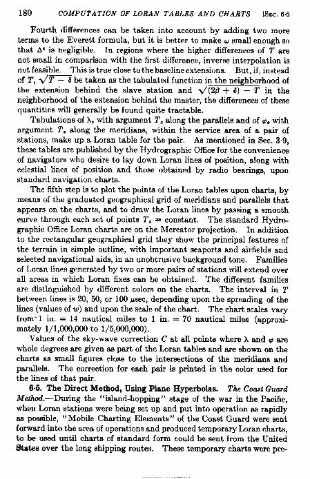
180 COMPUTATION OF LORAN TABLES AND CHARTS [SEC.6.5

Fourth differences can be taken into account by adding two moreterms to the Everett formula, but it is better to make u small enough sothat A4 is negligible. In regions where the higher differences of T arenot small in comparison with the first difference, inverse interpolation isnot feasible. This is true close to the baseline extensions. But, if, insteadof T, ~T – C!be taken as the tabulated function in the neighborhood ofthe extension behind the slave station and V(2P + 6) – T in theneighborhood of the extension behind the master, the differences of thesequantities will generally be found quite tractable.

Tabulations of h=with argument T. along the parallels and of ~= withargument T% along the meridians, within the service area of a pair ofstations, make up a Loran table for the pair. As mentioned in Sec. 3.9,these tables are published by the Hydrographic Office for the convenienceof navigators who desire to lay down Loran lines of position, along withcelestial lines of position and those obtained by radio bearings, uponstandard navigation charts.

The fifth step is to plot the points of the Loran tables upon charts, bymeans of the graduated geographical grid of meridians and parallels thatappears on the charts, and to draw the Loran lines by passing a smoothcurve through each set of points T= = constant. The standard Hydro-graphic Office Loran charts are on the Mercator projection. In additionto the rectangular geographical grid they show the principal features ofthe terrain in simple outline, with importmt seaports and airfields andselected navigational aids, in an unobtrusive background tone. Familiesof Loran lines generated by two or more pairs of stations will extend overall areas in which Loran fixes can be obtained. The different familiesare dktinguished by different colors on the charts. The interval in Tbetween lines is 20, 50, or 100 psec, depending upon the spreading of thelines (values of w) and upon the scale of the chart. The chart scales varyfrom’ 1 in. = 14 nautical miles to 1 in. = 70 nautical miles (approxi-mately 1/1,000,000 to 1/5,000,000).

Values of the sky-wave correction C at all points where x and p arewhole degrees are given aa part of the Loran tables and are shown on thecharts as small figures close to the intersections of the meridians andparallels. The correction for each pair is printed in the color used forthe lines of that pair.

6.6. The Direct Method, Using Plane Hyperbolas. The COaat Guard

Method.-During the “island-hopping” stage of the war in the Pacific,when Loran stations were being set up and put into operation as rapidlyas possible, “Mobile Charting Elements” of the Coast Guard were sentforward into the area of operations and produced temporary Loran charts,to be used until charts of standard form could be sent from the Unitedf3tates over the long shipping routes. These temporary charts were prc-

SEC.65] THE DIRECT METHOD, USING, PLANE HYPERBOLAS 181

pared by plotting plane hyperbolas on special geographical grids, correct-ing the hyperbolas for chart distortions, drawing in coast lines, locationof navigation aids, etc., and reproducing the grids photographically bythe Ozalid process. Details of procedure are given in a Coast GuardManual.’

The geographical grids were on transparent sheets of vinylite. Theseshowed meridians and parallels at intervals of 1°, on a scale of 1/2,000,000.The projection was the Lambert conformal conic with two standardparallels, the same that is used in the Civil Aeronautics Authority andU.S. Army aeronautical charts. In this projection the distortion is smallover regions between or near the standard parallels, so that Loran lines onthe chart have nearly the form of plane hyperbolas. The parallels areshown as concentric circles; the meridians as straight lines radiating fromthe common center of the parallels; directions around any point arerepresented truly; and great circles appear as nearly straight lines if notcarried too far from the standard ~arallels.

With the geographical grids was used another grid of rectangularcoordinates, also on vinylite. The stations of a Loran pair were plottedon the geographical grid, and this was placed over the rectangular grid,so that the z-axis of the latter passed through the stations and the y-axiswas midway between them. If the z-coordinates of the stations, in unitsof the grid, are f c (the positive sign being given to the master station),the inverse eccentricity a/c of the hyperbola representing time differenceT is given by

a z’-(fl+a)—=c P

[from Eqs. (3.4) and (6.9)], and the coordinates z, y of points on thehyperbola are defined by the first of Eq. (6.8). In practice, z and y wereobtained from the” Tables of Plane Hyperbola” (see footnote, page 174),the tables being entered with the argument: tabular a = [2’ – (B + t3)]/@(since c = 1 in the tables). The baseline distance B in microsecondswas calculated by the accurate formulas (4) and (2). The pairs of values

Z, Y given by the table were multiplied by c and then plotted, by means ofthe rectangular grid, on the vinylite sheet bearing the geographical grid.

If there were no distortion, the family of hyperbolas thus plottedwould be a Loran chart. It would only remain to remove the rectangulargrid, to draw in coast lines and other features of the terrain, and to makeprints from the vinylite sheet. But distortion is not negligible even onthe Lambert projection, except over smafl regions and nearly midwaybetween the standard parallels; and, even if it were, a procedure to checkthe plotted hyperbolas is desirable. The procedure devised for checking

1U.S. Chat Guard, “ Mobile Loran Monitor Charting Element,” Manual ofMeihodsandProcedure, with AddendaNos. 1, 2, 1944, 1945.

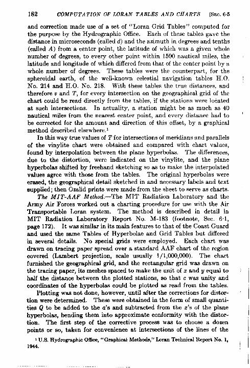
182 COMPUTATION OF LORAN TABLES AND CHARTS [SEC.6.5

and correction made use of a set of “Loran Grid Tables” computed forthe purpose by the Hydrographic Office. Each of these tables gave thedistance in microseconds (called d) and the azimuth in degrees and tenths(called A) from a center point, the latitude of which was a given wholenumber of degrees, to every other point within 1500 nautical miles, thelatitude and longitude of which differed from that of the center point by awhole number of degrees. These tables were the counterpart, for thespheroidal earth, of the well-known celestial navigation tables H.O.No. 214 and H.O. No. 218. With these tables the true distances, andtherefore v and T, for every intersection on the geographical grid of thechart could be read directly from the tables, if the stations were locatedat such intersections. In actuality, a station might be as much as 40nautical miles from the nearest center point, and every distance had tobe corrected for the amount and direction of this offset, by a graphicalmethod described elsewhere. *

In this way true values of T for intersections of meridians and parallelsof the vinylite chart were obtained and compared with chart values,found by interpolation between the plane hyperbolas. The differences,due to the distortion, were indicated on the vinylite, and the planehyperbolas shifted by freehand sketching so as to make the interpolatedv~ues agree with those from the tables. The original hyperbolas wereerased, the geographical detail sketched in and necessary labels and textsupplied; then Ozalid prints were made from the sheet to serve as charts.

The MI T-AAF Method.-The MIT Radiation Laboratory and theArmy Air Forces worked out a charting procedure for use wi~h the AirTransportable Loran system. The method is described in detail inMIT Radiation Laboratory Report No. M-183 (footnote, Sec. 6“1,page 172). It was similar in its main features to that of the Coast Guardand used the same Tables of Hyperbola and Grid Tables but differedin several details. No special grids were employed. Each chart wasdrawn on tracing paper spread over a standard AAF chart of the regioncovered (Lambert projection, wale usually 1/1,000,000). The chartfurnished the geographical grid, and the rectangular grid was drawn onthe tracing paper, its meshes spaced to make the unit of x and y equal tohalf the distance between the plotted stations, so that c was unity andcoordinates of the hyperbol~ could be plotted as read from the tab!es.

Plotting was not done, however, ,until after the corrections for distor-tion were determined. These were obtained in the form of small quanti-ties Q to be added to the a’s and subtracted from the Z’S of the planehyperbol~, bending them into approximate conformity with the distor-tion. The first step of the corrective process was to choose a dozenpoints or so, taken for convenience at int.emectiona of the lines of the

IU.S. HydrographicOffice,“Graphical Methods,” LaranTechnicalReport No. 1,1944. I

I

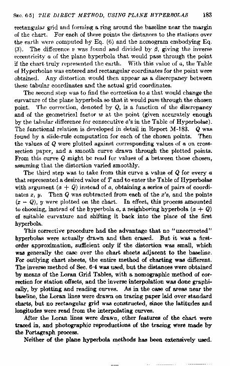
SEC.65] THE DIRECT METHOD, USING PLANE HYPERBOLAS 183

rectangular grid and forming a ring around the baseline near the marginof the chart. For each of these points the distances to the stations overthe earth were computed by Eq. (6) and the nomogram embodying Eq.(3). The difference v was found and divided by D, giving the inverseeccentricity a of the plane hyperbola that would pass through the pointif the chart truly represented the earth. With this value of a, the Tableof Hyperbola was entered and rectangular coordinates for the point wereobtained. Any distortion would then appear as a discrepancy betweenthese tabular coordinates and the actual grid coordinates.

The second step was to find the correction to a that would change thecurvature of the plane hyperbola so that it would pass through the chosenpoint. The correction, denoted by Q, is a function of the discrepancyand of the geometrical factor w at the point (given accurately enoughby the tabular difference for consecutive a’s in the Table of Hyperbola).The functional relation is developed in detail in Report M-183. Q wasfound by a slide-rule computation for each of the chosen points. Thenthe values of Q were plotted against corresponding values of a on crose-section paper, and a smooth curve drawn through the plotted points.From this curve Q might be read for values of a between those chosen,assuming that the distortion varied smoothly.

The third step was to take from this curve a value of Q for every uthat represented a desired value of T and to enter the Table of Hyperbolaswith argument (a + Q) instead of a, obtaining a series of pairs of coordi-nates x, y. Then Q was subtracted from each of the z’s, and the points(z – Q), y were plotted on the chart. In effect, this process amountedto choosing, instead of the hyperbola a, a neighboring hyperbola (a + Q)of suitable curvature and shifting it back into the place of the firsthyperbola.

This corrective procedure had the advantage that no “uncorrected”hyperbola were actually drawn and then erased. But it was a first-order approximation, sufficient ordy if the distortion was small, whichwm generally the case over the chart sheets adjacent to the baseline.For outlying chart sheets, the entire method of charting waa different.The inverse method of Sec. 6“4 was used, but the distances were obtainedby means of the Loran Grid Tables, with a nomographic method of cor-rection for station offsets, and the inverse interpolation wea done graphi-cally, by plotting and reading curves. As in the caae of mess near thebaseline, the Loran lines were drawn on tracing paper laid over standardcharts, but no rectangular grid was constructed, since the latitudes andlongitudes were read from the interpolating curves.

After the Loran lines were drawn, other features of the chart weretraced in, and photographic reproductions of the tracing were made bythe Portagraph proceea.

Neither of the plane hyperbola methods has been extensively used.

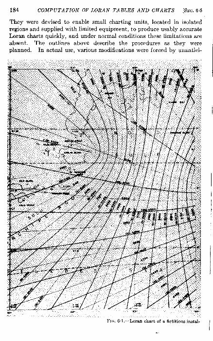
184 COMPUTATION OF LORAN TABLES AND CHARTS [SEC. 6.5

They were devised to enable small charting units, located in isolatedregions and supplied with limited equipment, to produce usably accurateLoran charts quickly, and under normal conditions these limitations areabsent. The outlines above describe the procedures as they wereplanned. In actual use, various modifications were forced by unantici-

1

~-IG.6 1.—Loran chart of a fictitious instal.

%3C.65] THE DIRECT METHOD, USING PLANE HYPERBOLAS 185

pated conditions or suggested by experience. For example, the entireAAF procedure was set up for use with charts on the Lambert conformalprojection, scale 1/1,000,000, covering areas about 4° by 6°. When theAAF charting units were required to produce single charts covering fourtimes this area, at half this scale, and charts on the Mercator projection,

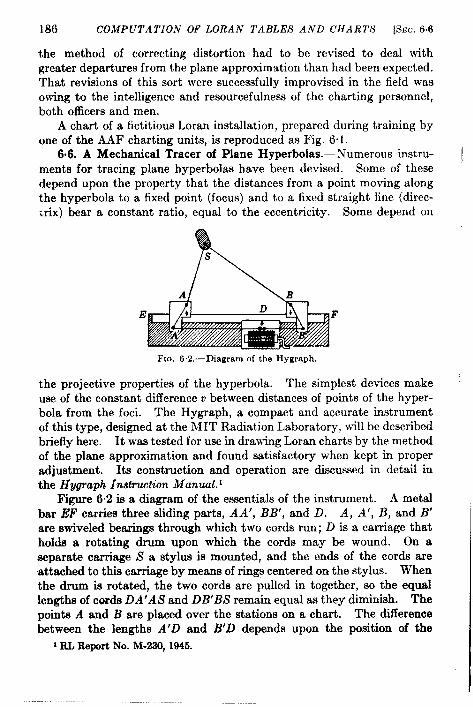
186 COMPUTATION OF LORAN TABLES AND CIfARTS [SEC. 66

the method of correcting distortion had to be revised to deal withgreater departures from the plane approximation than had been expected.That revisions of this sort were successfully improvised in the field wasowing to the intelligence and resourcefulness of the charting personnel,both officers and men.

A chart of a fictitious Loran installation, prepared during training byone of the AAF charting units, is reproduced as Fig, 6.1.

6.6. A Mechanical Tracer of Plane Hyperbolas. —Numerous instru-ments for tracing plane hyperbolas have been devised. Some of thesedepend upon the property that the distances from a point moving alongthe hyperbola to a fixed point (focus) and to a fixed straight line (direc-mix) bear a constant ratio, equal to the eccentricity. Some depend on

E

FIG. 62.-Diagram of the Hygraph,

the projective properties of the hyperbola. The simplest devices makeuse of the constant difference v between distances of points of the hyper-bola from the foci. The Hygraph, a compact and accurate instrumentof this type, designed at the MIT Radiation Laboratory, will be describedbriefly here. It was tested for use in drawing Loran charts by the methodof the plane approximation and found satisfactory when kept in properadjustment. Its construction and operation are discussed in detail inthe Hygraph 1n8t?Y4ZtiOn Manual. 1

F@re 6“2 is a diagram of the essentials of the instrument. A metalbar EF carries three sliding parts, AA’, BB’, and D. A, A’, B, and B’are swiveled bearings through which two cords run; D is a carriage thatholds a rotating drum upon which the cords may be wound. On aseparate carriage S a stylus is mounted, and the ends of the cords areattached to this carriage by means of rings centered on the stylus. Whenthe drum is rotated, the two cords are pulled in together, so the equallengths of cords DA’AS and DB’BS remain equal as they diminish. Thepoints A and B are placed over the stations on a chart. The differencebetween the lengths A’D and B’D depends upon the position of the

1RL F&portNo. M-220, 1945.

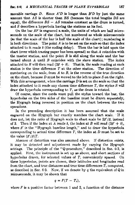
I

lb. 6.6] A MECHANICAL TRACER OF PLANE HYPERBOLAS 187

movable carriage D. Bince A’D is longer than B’D by just the sameamount that AS is shorter than BS (because the total lengths DS areequal), the tierence BS – AS remains constant as the drum is turned,and S describes a hyperbola having the stations as its foci.

On the bar EF is engraved a scale, the units of which are half micro-seconds on the scale of the chart, but numbered as whole microseconds(so that the scale of the bar is half the scale of the chart); numbering isin both directions. The point A is to be set on the scale so that the indexattached to it reads 8 (the coding delay). Then the bar is laid upon thechart (over which tracing paper has been spread) so that A coincides withthe master station, and the point B is slid along the ecale and the barturned about A until B coincides with the slave station. The indexattached to B will then read (20 + @. That is, the scale reading at eachstation is the time difference T at the other station. The direction ofnumbering on the scale, from A to B, is the reverse of the true directionon the chart, because D must be moved to the left to place Son the right.Wkh this arrangement, when the carriage D is set on the scale so that theindex attached to it reads any chosen time difference T, the stylus S willdraw the hyperbola corresponding to T, as the drum is rotated.

Of course, since the cords must pull the stylus toward the bar, thehyperbolas on the two sides of the baseline must be drawn separately,the Hygraph being reversed in position on the chart between the twooperations.

In the preceding description it has been assumed that the scaleengraved on the Hygraph bar exactly matches the chart scale. If itdoes not, let the ratio of Hygraph scale to chart scale be 213’/f?, insteadof 2. Then’if the index at A reads 6, the index at B will read (2j3’ + 6),where P’ is the “H ygraph baseline length,” and to draw the hyperbolacorresponding to actual time difference 2’, the index at D must be set tothe value (LY/0) l“.

Absence of distortion was also assumed above. If distortion exists,it may be detected and adjust mcnt made by varying the Hygraphsettings. The principle of the “Q-procedure,” described in Sec. 63, isapplied. First, the instrument is set up as above, and short sections ofhyperbolas drawn, for selected values of ?’, conveniently spaced. Onthese hyperbolas, points are chosen, their latitudes and longitudes readfrom the chart, and true distances and true time differences T. computed,as described in Sec. 6.3. Now, if we denote by q the equivalent of Q inmicroseconds, it may be shown that

q = F(T – TJ,

where F is a posit ivc fuct or bet wccn 1 und 2, u function of the distance

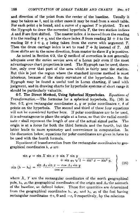
188 COMPUTATION OF LORAN TABLES AND CHARTS [SEC. 6.7

and direction of the point from the center of the baseline. Usually itmay be taken as 1, and in other cases it may be read from a small table.For each point q is found, and a curve of g against T is plotted. To setthe Hygraph to draw the corrected hyperbola T, the two station indicesA and i? are first shifted. The master index A is moved from the reading )6 to the reading 6 + q, and the slave index B from reading 2@ + 6 to thereading 2@ + 6 + q, q being taken from the curve with argument 7’.Then the drum carriage index is set to read T + 2q instead of T. Allthese shifts are in the same direction, from master to slave if q is positive.

As noted in Section 6:3, the Q method of correction is not generallyadequate over the entire service area of a Loran pair even if the mostadvantageous chart projection is used. The Hygraph can be used, there- ,fore, only over that part of the area which is fairly near the station. ,But this is just the region where the standard inverse method is mostlaborious, because of the sharp curvature of the hyperbolas. So theHygraph may be found a useful tool in Loran charting, if used withjudgment, and in drawing charts for hyperbolic systems of short range itshould be particularly valuable.

6,7. The Direct Method, Using Spherical Hyperbolas. Equations Of

Tnznsjommztion.-The formulas for a spherical hyperbola, Eq. ( 10) inSec. 6.2, give rectangular coordinates Z, y or polar coordinates ~, o ofpoints on the hyperbola. The second and third of these four equationswill not be considered further here. If polar coordinates are to be used,it is advantageous to place the origin at a focus, so that the radial coordi-nate r shall represent the length of one of the actual signal paths. Theorigin is at a focus for both the third formula and the fourth, but thelatter leads to more symmetry and convenience in computation. Inthe discussion below, equations for polar coordinates are given in form tobe used with the fourth formula.

Equations of transformation from the rectangular coordinates to geo-graphical coordinates A, p are

sinp=sin Xsinz+sin Y siny+ sin PO~ 1 – sin2 x – sin2 y,

1

(16) ‘sin Aosinz —cos AOsiny

sin (h – Ao) =Cos q

where X, Y are the rectangular coordinates of the north geographicalpole, ko, POthe geographical coordinates of the origin and A, the azimuthof the baseline, as defined below, These five quantities are determinedfrom the geographical coordinates k,, w,, and x,, p, of the foci havingrectangular coordinates + c, O and -c, O respectively, by the relations

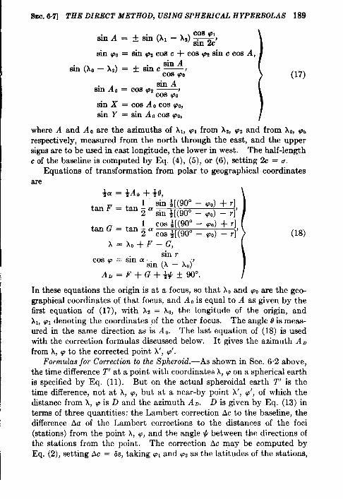
Sm. 6-71 THE DIRECT METHOD, USING SPHERICAL HYPERBOLAS 189

sin A = * sin (Al – A2)c~g)

sinpo=sin p2cosc+cos92 sinccos A,sin A

sin(xo-x2)=+sinc —Cos @o’ 1 (17)sin A

Sin AO = COS q7z —JCos po

sin X = cos AO cos PO,sin Y = sin AO cos qo,

where A and A Oare the azimuths of Al, WIfrom ~z, W2and from XO,ptirespectively, measured from the north through the east, and the uppersigns are to be used in east longitude, the lower in west. The half-length

c of the baseline is computed by Eq. (4), (5), or (6), setting % = u.Equations of transformation from polar to geographical coordinates

1 sin ~[(90° – 140)+ ~]tan F=tan–a .

2 am ~[(90° – PO) – T]’1 Cos +[(90° – Wo)+ r]

tan G = tan ~ a ~oa ~[(900 – PO) – ~1’

k=ho+F– G,sin r

Cos P = ‘ln a sin (X — Ao)’

(18)

In these equations the origin is at a focus, so that AOand woare the geo-graphical coordinates of that focus, and A o is equal to A as given by thefirst equation of (17), with h = Ao, the longitude of the origin, andAl, w denoting the coordinates .of the other focus. The angle 8 is meas-ured in the same direction as is A 0. The last equation of (18) is usedwith the correction formulas discussed below. It gives the azimuth AD

from A, p to the corrected point A’, p’.Formulas for Correction to the Spheroid.—As shown in Sec. 6.2 above,

the time difference T’ at a point with coordinates h, q on a spherical earthis specified by Eq. (11). But on the actual spheroidal earth T’ is thetime difference, not at h, p, but at a near-by point h’, p’, of which thedktance from h, p is D and the azimuth AD. D is given by Eq. (13) interms of three quantities: the Lambert correction Ac to the baseline, thedifference Aa of the Lambert corrections to the distances of the foci(stations) from the point X, p, and the angle # between the directions ofthe stations from the point. The correction Ac may be computed byEq. (2), setting Ac = h, taking PI and pj as the latitudes of the stations,

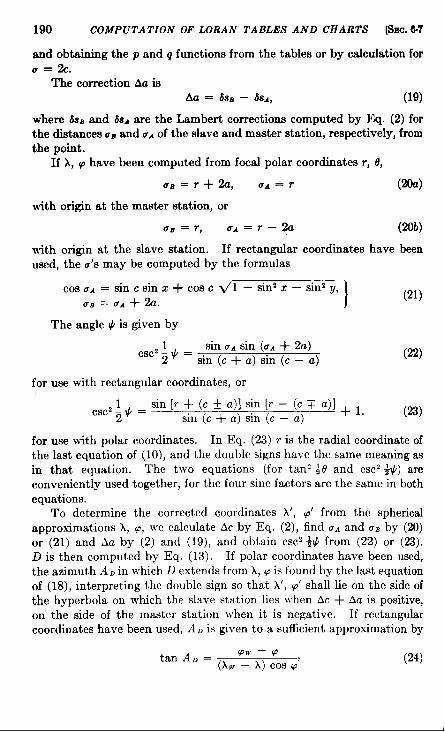
190 COMPUTATION OF LORAN TABLES AND CHARTS [SW. 6.7

and obtaining the p and q functions from the tables or by calculation foru=%.

The correction Aa isAa = & — ?&, (19)

where 6SBand 68.4are the Lambert corrections computed by Eq. (2) forthe distances u~ and aA of the slave and master station, respectively, fromthe point.

If A, p have been computed from focal polar coordinates r, 13,

uB=r+ 2a, flA=T

with origin at the master station, or

u.q = T, gA=r— P

with origin at the slave station. If rectangularused, the u’s may be computed by the formulas

(!Ma)

(20b)

coordinates have been

cos u.4 = sin c sin z + cos c <l – sinz z – sinz y, \ /01\UB=UA+2U. I

(Al)

The angle ~ is given by

sin u~ sin (UA+ 2a)CSC2; # =sin (c + a) sin (c – a)

for use with rectangular coordinates, or

(22)

~sc2~t= sin[r+(c*a)]sin[r –(c~a)]+l2 sin (c + a) sin (c – a)

(23)

for use with polar coordinates. In Eq. (23) r is the radial coordinate ofthe last equation of (10), and the double signs have the same meaning asin that equation. The two equations (for tan’ ~d and CSC’*v) areconveniently used together, for the four sine factors are the same in bothequations.

To determine the corrected coordinates h’, p’ from the sphericalapproximations A, q, we calculate Ac by Eq. (2), find UAand u. by (20)or (21) and Aa by (2) and (19), and obtain CSC2W from (22) or (23).D is then computed by Eq. (13). If polar coordinates have been used,the azimuth AD in which D extends from h, P is found by the last equationof (18), interpreting the double sign so that h’, p’ shall lie on the side ofthe hyperbola on which the slave station lies when Ac + Aa is positive,on the side of the master station when it is negative. If rectangularcoordinates have been used, A Dis given to a sufficient approximation by

tan AD =VW—V

(Aw – A) Cos q’(24)

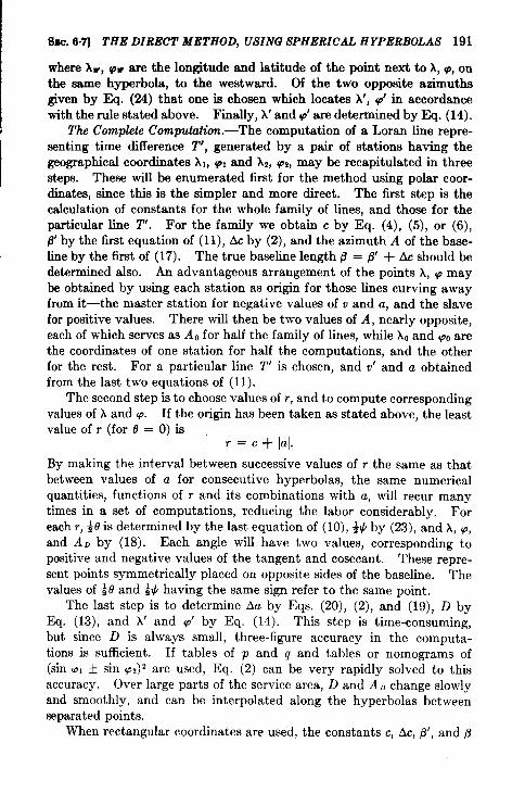
8m.z 6.7 THE DIRECT METHOD, USING SPHERICAL HYPERBOLAS 191

where AW, QW are the longitude and latitude of the point next to A, p, onthe same hyperbola, to the westward. Of the two opposite azimuthsgiven by Eq. (24) that one is chosen which locates X’, q’ in accordancewith the rule stated above. Finally, X’ and # are determined by Eq. (14).

The Complete G’omputution.-The computation of a Loran line repre-senting time difference Tt, generated by a pair of stations having thegeographical coordinates XI, PI and X2, W, may be recapitulated in threesteps. These will be enumerated first for the method using polar coor-dinates, since this is the simpler and more direct. The first step is thecalculation of constants for the whole family of lines, and those for theparticular line T’. For the family we obtain c by Eq. (4), (5), or (6),/3’ by the first equation of (11), Ac by (2), and the azimuth A of the base-line by the first of (17). The true baseline length 13= j3’ + Ac should bedetermined also. An advantageous arrangement of the points A, p maybe obtained by using each station as origin for those lines curving awayfrom it—the master station for negative values of u and a, and the slavefor positive values. There will then be two values of A, nearly opposite,each of which serves as A o for half the family of lines, while ko and p~ arethe coordinates of one station for half the computations, and the otherfor the rest. For a particular line T’ is chosen, and v’ and a obtainedfrom the last two equations of (11).

The second step is to choose values of r, and to compute correspondingvalues of k and p. If the origin has been taken as stated above, the leastvalue of r (for 0 = O) is

r=c+lal.

By making the interval between successive values of r the same as thatbetween values of a for consecutive hyperbolas, the same numericalquantities, functions of r and its combinations with a, will recur manytimes in a set of computations, reducing the labor considerably. Foreach r, ~0 is determined by the last equation of (10), ~~ by (23), and A, ~,and AD by (18). Each angle will have two values, corresponding topositive and negative values of the tangent and cosecant. These rePre-sent points symmetrically placed on opposite sides of the baseline. Thevalues of +9 and ~X having the same sign refer to the same point.

The last step is to determine Aa by Eqs. (20), (2), and (19), D byEq. (13), and A’ and p’ by Eq. (14). This step is time-consuming,but since D is always small, three-figure accuracy in the computa-tions is sufficient. If tables of p and q and tables or nomograms of(sin v, ~ sin PJ2 are used, Eq. (2) can be very rapidly solved to thisaccuracy. Over large parts of the service area, D and AD change slowlyand smoothly, and can be interpolated along the hyperbolas betweenseparated points.

When rectangular coordinates are used, the constants c, Ac, ~’, and @

192 COMPUTATION OF LORAN TABLES AND CHARTS [SEC. 6.8

axe found as above, and AO,PO,X, and Y by Eq. (17). The coordinatesof the master station are AI, V1in these equations. T’ is chosen, and v’and a determined as before. Then the quantities

sinz asinz a and sin2 ~ — s~2 a’

which are constant for a hyperbola, are computed to be used in the firstequation of (10). In the second step this equation gives values of zcorresponding to a and a series of chosen values of y. Two values of z,both having the same sign as a, are obtained in each computation, onefor +y and one for – y. If a is between f~c, the same fairly widelyspaced values of g may be used along all the hyperbolas, but as aapproaches ~ c, the interval between y’s must become smaller andsmaller. For each point Z, y Eqs. (16) give A and q. For determinationof the corrections, u~ and Uflare computed by Eq. (21), AD by Eq. (24),and ~# by Eq. (22). The last step is the same as for polar coordinates.

6.8. Factors Affecting the Correctness of Computed Loran TimeDifferences.-Correspondence between the time differences actuallyobserved over a Loran service area and those given by a Loran chart ortable depends upon the assumption of the correct velocity of signalpropagation, upon the holding of the correct coding delay by the slavestation, and upon the knowledge of the true latitudes and longitudes ofthe transmitting stations, as well as upon accurate computations of theLoran lines and accurate pulse matching. Analysis of Loran operationup to the present has given no evidence that the signal velocity over seadiffers from that stated in Chap. 5 and used in Hydrographic Officecomputations. Sufficient data have not yet been obtained to evaluatethe velocity over land. The land range of Standard Loran signals issmall, and there are no land baselines between permanent stations alongwhich velocity measurements could most readily be made. The effect ofa diminution of velocity upon the grid of Loran lines would be a shrinkingof the entire pattern, and a corresponding increase in the time differenceT at a fixed point on the earth, such that

T’–a=(T– 6):,c

where T increases to T’ as the velocity c decreases to c’, and 6 is the codingdelay. Existence of a proportionality of this sort between computedand observed time differences would reveal an abnormal signal velocityif this were uniform over the service area. But, if the velocity dependedon the local electrical characteristics of the surface (as it might moreplausibly do), the pattern of alteration of time differences might be verycomplex.

Szc. 6.8] COMPUTED LORAN TIME DIFFERENCES 193

The operator of a slave station maintains the coding delay by keepingthe time difference between the pulse from the remote master transmitterand that from his own adjacent antenna, as he observes them on hisoscilloscope, equal to & The powerful local signal is passed through theattenuator, in order that it may appear equal in amplitude to the weaksignal from the dktant master; and if there are maladjustments in theattenuating circuits, the local pulse may be deformed so that the apparentdelay may differ from the actual time between pulses by several micro-seconds. Such an error in timing will appear in all measured timedifferences, as a constant increment to 2’, independent of the observer’slocation, and as such it may be recognized.

The sites of Loran stations are often in places remote from accuratelydetermined geodetic reference points, so that they cannot be tied in tosuch points by triangulation. The positions must be found by astronom-ical observations. The instrument may be either the theodolite or theprismatic astrolabe (also called the equiangulator). Both are easilyportable, and either, in conjunction with a good timepiece and a radioreceiver, will give positions with an internal probable error of the order of1 sec of arc (100 ft) or better, from a few nights’ work. With the theo-dolite, latitude and longitude are determined separately by meridianobservations of stars, by the methods set forth in standard geodetictextbooks. With the astrolabe, stars in all azimuths are observed ataltitude 60° (or 45° in some forms of the instrument). The time atwhich each star passes this altitude is determined and the line of positioncomputed by formulas similar to those used by the celestial navigator,but with greater precision; the concurrence of lines of position from allthe stars gives the observer’s location.

Unfortunately, the internal probable error of a series of astronomicalobservations is not a reliable measure of the accuracy of the resultingposition. In all such observations, the fundamental reference directionis the direction of gravity, which ideally is normal to the spheroidal sur-face but actually may be inclined to the normal by a considerable fractionof a minute of arc. This “station error, “ if not allowed for, will appearin its full size as an error in the observed position and can be detected onlyby triangulation or some equivalent method of comparing the positionsof different points. Loran is such a method, and station errors will affectthe Loran time differences; conversely, the errors may bc determined fromthe deviations of observed time differences at accurately known positionsfrom their computed values.

At a given position of the observer, incorrect positions of the trans-mitting stations will affect three signal paths: that from each station tothe observer and that from the master M to slave S. These will allcombine to alter the observed time difference from its computed value.

194 COMPUTATION OF WRAN TABLES AND CHARTS [sm. 6.8

That is,AT = At, – Atm+ A@,

where AT is the change in time difference, At the change in time of trans-mission from station to observer, and A/3the change in time of transmis-sion from master to slave, all in the sense, observed minus computed, andtaken as positive or negative according as the transmission time isincreawd or diminished. Since an increase in tmdelays the beginning ofthe interval T, itdecreases T and must be subtracted.

If D. and D~ denote the distance in microseconds from the positionof each station, as determined by observation, to its true position, it isevident that At, is equal to the component of D, in the direction from Sopposite to the observer’s direction and similarly for At-, while A/3 isequal to the component of D, in the direction along the baseline awayfrom 11, minus the component of D~ in the direction along the baselinetoward S.

Since each D may be specified by two quantities, either amount anddirect ion or rectangular components, observations of A2’ at four knownpoints will determine the D’s. If D: and D: denote the components ofthe displacement of the slave station along and perpendicular to thebaseline respectively and D: and D: those of the master, the points ofobservation may be so chosen that D:, D:’, D: and D: are determined

separately. Let D: and Dj be counted positive in the direction frommaster to slave. At Point 1 on the baseline, between the stations, D:and D: do not enter into AT, At, = D;, At~ = –D~, A@ = D; – ~~;consequently, ATl = 2D~. At Point 2 on the extended baselinebehind the master station, D? and DC again have no effectAj3 = D: – D;, At. = D~, At~ = D~; consequently, AT, = 2(D: – D~)~or ATl – ATZ = 2D~. At Point 3 on the perpendicular through theslave station and near the station on the positive side, D: has no appreci-able effect on AT, but AL = –D;, Atm = – D;, A~ = D: – D;. HenceAT3 = D: – D:’, or ~ATl — ATS = D:. If the point is on the negativeside of the slave station, AT9 = D: + D~, or AT3 – ~ATl = D;’. simi-

larly, at Point 4 on the perpendicular through the master station and

near the station, AT4 = 2D~ — D~j ~ D:, where the upper and lowersigns apply respectively to points on the positive and negative sides of themaster station. on the positive side AT4 – 3(AT, + AT,) = D:; onthe negative, ~(ATl + AT2) – AT4 = D:. At Point 5 on the extendedbaseline behind the slave station, AT, is not affected by errors in the posi-tions at all. Neither does an incorrect assumption as to the velocity ofpropagation affect it. A discrepancy here, if not due to observationalerror, must represent an incorrect delay held at the slave station.

Of course, observations at any four or more points, properly dis-tributed, will determine the station displacements. The theory of thisdetermination is discussed in Appendix D.

I

I

i

PART II

LORAN EQUIPMENT

CHAPTER 7

TIMERS

BY R. H. WoonN’.41m ANII J. C. WIM.IAMS

7.1. General Requirements.—Thc function of the Standard I.orantimer is to control the synchronism of the pulsed transmissions of theground stations. AS explained in Sec. 3.3, a master station transmits aseries of pulses at an accurately constant recurrence rate. The timerequired for the signal to travel from the master station to the slavestation is designated as P. The transmission from the slave station is sosynchronized with that of the master station that the interval of time(as observed at the slave station) between the reception of the signalfrom the remote master station and the reception of the locally trans-mitted slave signal is equal to half the recurrence period L plus the codingdelay & The slave timer must be capable of measuring this interval oftime and maintaining this synchronism ~vith an error of less than 1 gsec.The interval of time (as observed at the master sttition) between thereception of the master signal and the reception of the slave signal is(L/2) + 2~ + & Although the operator of the master timer does notcontrol the synchronism of the signals, he must be able to measure thetime difference between the two signals with an error of less than 1 psec.If he observes that the synchronism is incorrect, he informs the slaveoperator and warns navigators of this fact by blinking the locally trans-mitted signal.

The function of the timer in the Sky-wave Synchronized Loran systemis similar to the function of the Standard Loran timer except that sincethe distance between master and slave stations in the SS system isgreater, the value of B is correspondingly greater. The same timingequipment is used for both systems. The function of the Low Frequencytimer is somewhat different and is dkcussed in Sec. 7.14. The StandardLoran timer must be modified for use in the LF system.

Experience has indicated that in order to measure with the requiredprecision time differences between the relatively slow-rising pulses ofStandard and SS Loran, the presentation on the cathode-ray oscilloscopeshould be such that one fast linear trace showing one pulse should appearduectly above another fast linear trace showing the other pulse. Thetiming of the traces must be adjustable so that the two pulses can be madeto appear on the fast traces and one pulse can be positioned directly

197

198 TIMBERS [SEC. 7.1

above the other. The vertical spacing between the traces must be adjust-able so that when the pulses are vertically aligned, the spacing can bereduced to zero and one pulse thereby superimposed upon the other.Furthermore, the relative amplitudes of the two pulses to be measured(one from the remote transmitter and the other from the local) must beadjustable so that they can be made equal. Under this condition ofsuperposition the time difference between the initiations of the two fasttraces is equal to the time difference between the arrivals of the two pulses.The time difference between the initiations of the fast traces is measuredby means of calibration markers derived from the blocking oscillators ofthe divider chain.

The general requirements for the timer are that it shall be capable ofproviding trigger pulses to the transmitter at any one of a number ofaccurately constant, predetermined recurrence rates and that the triggerpulses shall bear a precise, predetermined time relationship to the pulsedsignals received from a remote station. The equipment, supplementedby duplicate auxiliaries, must be capable of giving continuous service24 hr. a day with the exception of negligible switch-over time. Appro-priate monitoring facilities must be provided to permit operation as eithera master or a slave timer.

For satisfactory manual operation the slave timer must be capable ofprecise adjustment in frequent y in relation to the master timer so thatone series of pulses drifts with respect to the other less than 1 ~sec in5 to 10 min. For such precise adjustment, both master and slave timersmust have crystal oscillators that fluctuate in frequency less than 1 partin 109 over short periods of time.

The timing circuits required for initiating the fast traces and triggeringthe transmitter must be sufficiently flexible to cover continuously a widerange of possible time differences between the reception of the pulsefrom the remote station and the transmission of the local pulse. Thetiming circuits and associated sweep circuits must be stable. The cali-bration markers must be sufficiently clear to permit easy counting of timedifferences and su5ciently sharp to permit measurement with errors ofconsiderably less than 1 psec. It must be possible to check and adjustthese circuits during service without interfering with their operation.

The bandwidth of the receiver must be wide enough to allow thepulse to rise rapidly for accurate timing and yet narrow enough to givesatisfactory signal-to-noise ratios under severe conditions of noise. Ithas been found experimentafly that a 6-db bandwidth of 60 kc/see is agood compromise value and that bandwidths between 40 and 100 kc/aecare satisfactory.

The early models of the timer (Models A, B, and B-1) were composedof the following units:

SEC. 7.2] TIMER MODELS A, B, AND B-1 199

1. Oscillator unit, consisting of a highly stable crystal oscillator and aphase shifter.

2. Divider unit, consisting of divider circuits with feedback, lockeddelay multivibrators for initiating fast traces, sweep generators,calibration-marker circuits, an attenuator circuit of the relay type,and a transmitter-trigger circuit.

3. Oscilloscope.4. Receiver with amplitude-balance control.5. Regulated power supply.

The later models (Models C, C-1, and UJ) have been improved inseveral respects. The phase-shift capacitor of the oscillator is geared tothe frequency control in such a way that as it is rotated in maintainingsynchronism, the oscillator frequency is automatically adjusted to reducethe rate of drift of the slave timer with respect to the master timer. Thelocked delay multivibrators used to initiate the fast traces have beenreplaced by selector circuits, each consisting of a delay multivibrator,which generates a gate of adjustable delay, and a gate-pulse mixer thatpermits the selecting of the highly stable pulses from the dividers fortriggering other selector circuits and the fast-sweep generator. Thisselector circuit haa the advantage that its adjustment can be checked~~ithout interfering with the operation of the timer. The single oscillo-scope has been replaced by a dual oscilloscope, one cathode-ray tubedisplaying the two fast traces and the other displaying the completerecurrence cycle on two slow traces. An additional oscilloscope is usedfor checking the adjustment of the divider and selector circuits whilethe timer is in service. A synchronizer automatically controls the fre-quency of the oscillator of the slave timer to maintain the prescribed timedifference between the reception of the remote signaf and the transmissionof the local signal.

The most recent version of the timer (Model UE1) haa been morecarefully engineered than the earlier models, but it has few fundamentallynew features. Probably the most important innovation is a motor-driven phase-shift capacitor that is geared to the frequency control of theoscillator. The rotation of the phsse-shift capacitor is controlled bythe synchronizer. The advantages of the mechanical coupling betweenthe synchronizer and the oscillator over the earlier electronic coupfing arethat the high stability of the oscillator is retained and the rate of driftis reduced to a minimum by the operation of the geared frequency control.As the rate of drift is reduced, the rate of phase compensation can bereduced with the result that the synchronizer operates smoothly andreliably under severe conditions of noise.

7.2. Tmer Models A, B, end B-l.—Models A, B, and El are thefirst three series of timers that were designed for the bran system. A

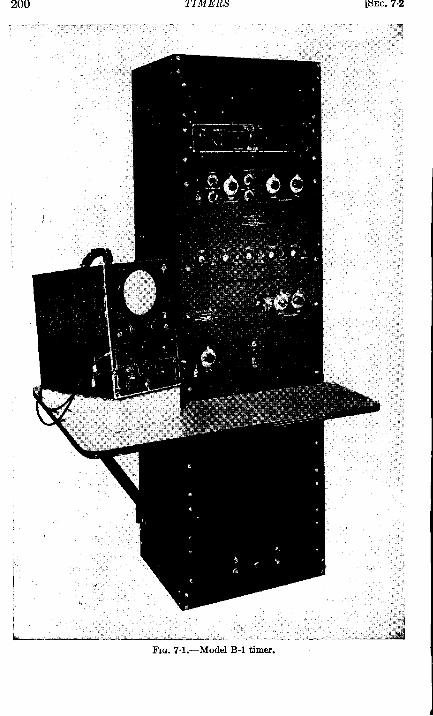
200 TIMERS [SEC.7.2

L

!

SEC.7.2] TIMER MODELS A, B, AND B-1 201

total of 56 timers of these types were constructed at the Radiation Labora-tory and at Research Construction Company. Since many of them arestill in active service in the North Atlantic chain, the Aleutians, andmany parts of the Pacific and probably will be for some time to come, itseems desirable to give a general description of the Model B-1 timer (seeFig. 7.1 ) in spite of its obsolescence.

Although the construction is somewhat crude, the fundamental designis similar to that of the modern timers. The block diagram of theModel B-1 timer and attenuator is shown in Fig. 7.2. As mentioned inSec. 7.1, one fast linear trace showing one pulse is presented on a cathode-ray tube directly below another such trace showing the other pulse.Since the local transmitter is triggered at the same instant that one fasttrace is initiated, the local pulse remains stationary. The remote pulseon the other fast trace drifts slowly to the right or to the left if the recur-rence rate of the local timer differs slightly from the recurrence rate ofthe remote timer. In operation, at a slave station, the time differencebetween the initiations of the two fast traces (one for the local pulse andone for the remote pulse) is adjusted to a predetermined value. Theremote pulse is placed on its fast trace below the local pulse on its fasttrace. The recurrence rate of the local timer is then adjusted to therecurrence rate of the remote master timer until the remote pulse ceasesto drift. By adjusting the phasing of the local timer, the remote pulseis moved directly below the local pulse. The amplitudes of the local andremote pulses are next equalized, and the vertical spacing between thetwo traces is eliminated so that one pulse is superimposed on the other.As long as they remain superimposed, the time difference between thereception of the remote pulse and the transmission of the local pulse isequal to the predetermined time difference between the initiations of thetwo fast traces. This time difference between the initiations of the fasttraces is adjustable and is measured precisely by means of calibrationmarkers.

A slow-trace presentation is provided to aid the operator in placingthe remote pulse on the fast trace. It consists of two slow linear traces,each of one-half the recurrence period, one placed below the other. Theduration and timing of the fast traces with respect to the slow-tracepattern are indicated by pedestals on the slow-trace pattern.

The Loran technique for measuring time difference requires timingequipment of high stability. The only device with the required stabilityis a crystal oscillator. Accordingly, a 50-kc/see, X-cut quartz bar,suspended in a thermostatically controlled oven, is used in the Model B-1timer to control the oscillator frequency. The circuit consists of anamplifier, a phase inverter, and a resistance and lamp bridge which servesas an automatic volume cent rol.

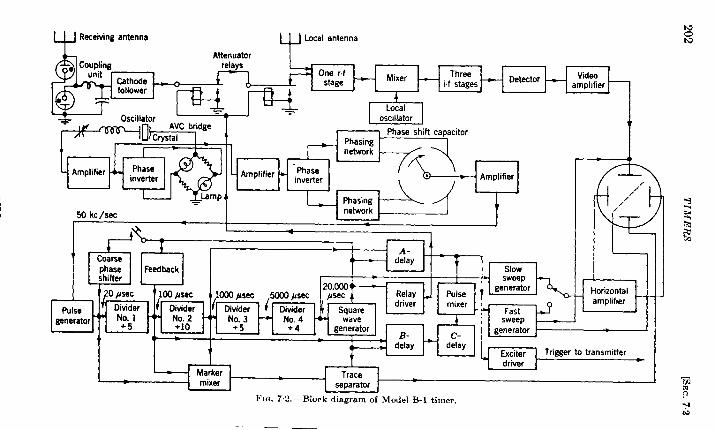
Y Receiving antenna

‘Y

Local antenna

Attenuator

I

—-t--i f?- H--rh=l

.

-7

Pulsegenerator

!t

Trigger to transmitter

Markermixer

FIC. 7.2,—Block diagram of Model B-1 timer.

k/’//

//

hHorizontalamplifier

t+oN

SEC. 7.2] TIMER MOD17L,’$ .4, Ii, AND B-1 203

The phase-shift capacitor is a convenient device for precise shiftingof the phase of the timer. The voltages impressed on its four sets ofstator plates are mutually 90° out of phase. The phase of the voltageinduced on the rotor plates varies uniformly as the rotor is turned fromone set of stator plates to another. One complete turn shifts the phaseof the output voltage one cycle (20 Ascc) with respect to the voltage fromthe oscillator. In operation this causes the remote pulse to move alongthe trace a distance corresponding to 20 psec. Fractions or whole num-bers of rotations produce proportional positive or negative shifts of phase.

The 50-kc/sec sine wave from the phase-shift capacitor must bereduced in frequency to a pulse recurrence rate of approximately 25 pps.Because of their greater precision, pulses of short duration are used insteadof sine waves. An amplifier that is rapidly driven from cutoff to satura-tion converts the 50-kc/sec sine waves to square waves which on differen-tiation become positive and negative pulses recurring every 20 .usec.The pulse recurrence rate is reduced from 50,000 to 50 pps by a series offour dividers. A divider is a device that produces a single output pulsefor a given whole number of input pukes. It consists of a capacitor thatis charged in steps by the input pulses acting through a double diode andof a blocking oscillator that discharges the capacitor and produces anoutput pulse when the voltage of the capacitor reaches a certain value.The four dividers are arranged to divide by 5, 10, 5, and 4, which producesseries of pulses with recurrence periods of 100, 1000, 5000, and 20,000 ~secrespectively. The recurrence period of the last divider is one-half therecurrence period required for Loran transmission.

The recurrence period is doubJed by a square-wave generator to givethe recurrence rate of 25 pps required for Loran transmission. Thesquare wave is impressed on the vertical plates of the cathode-ray tubeto give the vertical displacement of the slow-trace presentation. Theupper section of the square wave becomes the upper trace, and the lowersection becomes the lower trace. The spacing between the two traces isadjustable.

Since several pairs of Loran transmitters must operate on a single radiofrequency, it is necessary that they transmit at slightly different recur-rence rates to permit a navigator to distinguish the signals of one pair fromthose of another and to obtain time-difference measurements from anypair of transmitters. The timing of each recurrence rate must be precise;and, for the sake of economy, it is desirable that all recurrence rates bederived from a single crystal oscillator. Thk is accomplished by fee&ga pulse from the square-wave generator back into the second divider insuch a way that it charges the capacitor of the second divider. If thecharge from the square-wave generator is equivalent to a single chargefrom the first divider, the capacitor of the second divider is diachar@

204 TIMERS [SEC.72

after receiving 9 charges from the first divider instead of the normal 10(in 900 ~sec instead of the normal 1000 ysec), and the final recurrenceperiod becomes 39,900 Wsec instead of the 40,000 usec with no feedback.Similarly, if larger charges arc fed from the square-wave generator backinto the second divider, recurrence periods of 39,800, 39,700, 39,600,39,500,39,400, and 39,300 Ysec can be obtained. The corresponding eightrecurrence rates (numbered O to 7) are called “specific recurrence rates. ”A second set of eight recurrence rates is obtained by adjusting the lastdivider to divide by 3 instead of 4. The two different sets of recurrencerates, approximately 33* and 25 pps, obtained by adjusting the lastdivider are called the high and low, H and L, “basic recurrence rates.”

A coarse phase-shift control is required for quickly bringing the slavetimer into approximate synchronism with the remote master timer.For this purpose pulses from the last divider are fed back into the firstdivider through a push-button switch.

The oscillator, dividers, and square-wave generator produce therequired recurrence period, which is represented as two slow traces, onebelow the other, on a cathode-ray tube. The relative timing and durationof the fast traces are indicated by pedestals on the slow traces. Thereceiver-output signals produce vertical deflections on the two traces andshow the relative timing of the signal from the remote station with respectto the slow-trace pattern. The location of the remote signal on the slowtrace can be adjusted by means of the coarse (feedback) and fine (phase-shift capacitor) phase controls.

The time difference between the initiations of the fast traces is adjustedto equal the required time difference between the remote and local pulses.At the slave station the remote (master) pulse must precede the local(slave) pulse by half the recurrence period plus a small constant timedifference called the “coding delay.” If necessary this delay can bechanged, according to a predetermined schedule, to confuse the enemy.Thus the master pulse precedes the slave pulse over the entire coveragearea and so can be readily identified by the navigator. At the masterstation the local (master) pulse precedes the remote (slave) pulse by halfthe recurrence period plus the coding delay plus twice the time requiredfor a radio wave to travel from one station to the other.

The required time differences are obtained from the -4-, B-, andCdelay multivibrators. Since delay multivibrators are not sufficientlystable to give long delays with the required precision, the A- and B-delaymultivibrators are locked by pulses from the second and first dividersrespectively. The A-delay multivibrator gives delays that are multiplesof 1000 ysec and is adjustable from 1000 to 10,000 WRC. The B-delaymultivibrator gives delays that are multiples of 100 ~sec and is adjustablefrom 300 to 2500 psec. The C-delay multivibrator is unlocked and isvariable continuously from 30 to 170 ysec.

fhc. 781 TIMER MODELS C, C-1, AND UJ !z)5

At the slave station the multivibratore are arranged so that theA4elay multivibrator is triggered at the start of one slow trace. Tbiamultivibrator is adjusted to give a delay of 2000 -c after which it triggersthe fast-sweep generator and the local transmitter. The Bdelay multi-vibrator is triggered at the start of the other slow trace. It triggers theCdelay multivibrator which in turn triggera the fast-sweep generator.The B- and Cdelay multivibrators are adjusted to place the masterpedestrd to the left of the slawe pedestal by a distance corresponding tothe coding delay.

At the master station the fast-sweep generator and the local trans-mitter are triggered at the start of the upper trace. The three delaymultivibrators are a&nged in series so that the Adelay multivibrator,which is triggered at the start of the lower trace, tiiggers the Bdelaymultivibrator, which in turn triggers the Cdelay multivibrator. TheC-delay multivibrator initiates the fast trace. Thus the time differencebetween the initiations of the two fast traces is variable continuouslyfrom a little more than 1000 KC to a little more than 10,000 ysec(plus half the recurrence period). With the proper time difference(2P + 8 + L/2) between the initiations of the two fast traces, the opera-tor at the master station should find the remote signal directly below thelocal signal on the fast traces. If he does not, the signals are improperlysynchronized, and he notifies the slave operator of this condition byblinking his transmitter on and off.

For the precise measurement of the time difference between the initia-tions of the fast traces, calibration markers are displayed on the slow andfast traces. Pulses from the pulse generator, the first divider, and thesecond divider are mixed and impressed on the vertical plates of thecathode-ray tube to form 20-, 100-, and 1000-@ec calibration markers.By means of the 1000-Psec markers displayed on the slow traces, thehorizontal displacement of the lower pedestal to the right or left of theupper pedestal is estimated to the nearest thousand microseconds. Onf@ traces of approximately 1500-gsec duration, the displacement of the1000-~sec markers on the lower trace with respect to those on the uppertrace is estimated to the nearest hundred microseconds. Similarly, onfast traces of approximately 150-~sec duration the displacement of the20- and 100-~sec markers is estimated to the nearest microsecond.

MODEL C-1 TIMER

7.3. General Description of Timer Models C, C-1, and UJ.—The firstcompletely redesigned timer, the Model C, occupies twice the cabinetspace of the earlier models but is designed for ease of operation and forreliability in service. A dual oscilloscope gives a simultaneous displayof both the slow- and fast-trace pattern, and a test oscilloscope provides

206 TIMERS [SEC. 7.3

a convenient means of adjusting the timer while it is in service. Thelocked delay multivibrators of the earlier models are replaced by selectorcircuits that serve the same purpose but have the advantage that they

can be adjusted in service without interfering with their operation.Maintenance of synchronism at the slave station is simplified by gearingthe phase-shift capacitor to the frequency control. An automatic syn-chronizer further facilitates the operation of the Model C timer by cor-

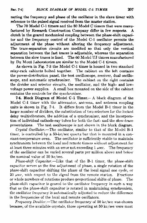
szc. 7.4] BLOCK DIAGRAM OF MODEL C-1 TIMER 207

recting the frequency and phase of the oscillator in the slave timer withreference to the puked signal received from the master station.

The 70 Model 01 timers and the 80 Model C timers that were manu-factured by Research Constmction Company differ in few respects. Aclutch in the geared mechanical coupling between the phaee-bift capaci-tor and the frequency control of the Model C-l oscillator permits theadjustment of the phase without altering the frequency adjustment.The trace-separation circuits are modified so that only the verticalseparation between the fast traces is adjustable, whereas the separationbetween the slow traces is fixed. The 60 Model UJ timers manufacturedby Du Mont Laboratories are similar to the Model C-1 timers.

As shown in Fig. 7.3 the Model G1 timer is housed in two standardrelay-rack cabinets bolted together. The cabinet on the left containsthe power-distribution panel, the test oscilloscope, receiver, dual oscillo-scope, and automatic synchronizer. The cabinet on the right containsthe divider and wlector circuits, the oscillator, and the high- and low-voltage power supplies. A small box mounted on the side of the cabinetcontains the controls for the synchronizer.

7.4. Block Diagram of Model C-1 Timer.—A block diagram of theModel C-1 timer with the attenuator, antenna, and antenna couplingunits is shown in Fig. 7.4. It differs from the Model B-1 timer in thelarger number of dividers, the substitution of two selectors for the lockeddelay multivibrators, the addition of a synchronizer, and the incorpora-tion of individual cathode-ray tubes for both the fast- and the slow-tracepresentations. The test oscilloscope is not shown in the block diagram.

Crystal Oscillator.-The oscillator, similar to that of the Model B-1timer, is controlled by a 50-kc/sec quartz bar that is mounted in a con-stant-temperature oven. The oscillator is sufficiently stable to maintainsynchronism bet ween the local and remote timers wit bout adjustment forat least three minutes with an error not exceeding 1 psec. The frequencyof the oscillator can be varied several parts per million above and belowthe nominal value of 50 kc/see.

Phase-shift Capucitor.-Like that of the B-1 timer, the phase-shiftcapacitor serves as the fine adjustment of phase, a single rotation of thephase-shift capacitor shifting the phase of the local signal one cycle, or20 ~sec, with respect to the signal from the remote station. Fractionsor whole numbers of rotations produce proportional shifts of phase. Thephase-shift capacitor is geared to the oscillator frequency in such a waythat as the phase-shift capacitor is rotated in maintaining synchronism,the oscillator frequency is automatically adjusted to reduce the differencein the frequencies of the local and remote oscillators.

Frequency Doubler.—The oscillator frequency of 50 kc/see was chosenbecause, of the available crystals, those operating at 50 kc/see were most

Synchronizerr-,I

Exc,terAB I,nk

\v[P.!,, A Sf0.!0.[

“’’”(’ ‘L

.. .._ ————-————.-__———____—______________1

Dcreferen’e

voltage A selector

A.tomalrfr:::~o:y

Odd h“fwdbmh I,,db,Ck

Starthere

,, (1 ,,!,2, /5;h:s7Frequ:n; :’;:,,”, /’0::: J,,, / ,,:,,, 7’;: /’:,::100psec

? H H H T--t ---i-l H ‘;

oscdlalor ml!,, doubler owllator N, 1-5d

No 2-2 No 3+5 NO A72

50 ),5.X~------- –-B- seleclor–––– ––—5~~+= --- .— -----1

Marker !

TE,c(terdr,ver

ToIransm,tter

I mtxer 11

Conl,nuous Gale pulseB delay

Coarsemm,

1

B delay 1

*

“C’”’’””’”’-cPT10,100 & 1000psec markers and

J

T,aceseparation Slow oscilloscope

Fast OSCl{lOSCOpe

FIG. 7.4.—Block diagram of Model C-1 timsr,

ocal andremotes,gnals

From tranwmttlngantenna co.pl,ng und

Rece,.,ngantenna

5

CO.phng.mt

Attenuator

+

?emoteSlg”al

~Rece,ver

k

Local gs,gnal

QSampl,ngnetwork

I

,,,,, ,, , ,. ,, ,.., .,,,., !,. ,,, ,. .,, !” .

SEC. 7.4] BLOCK DIAGRAM OF MODEL C-1 TIMER 209

stable. To provide 10-IJSRCcalibration markers and to simplify thedivider-feedback circuits, the 50-kc/sec signal from the phase-shiftcapacitor is doubled to 100 kc/see.

The blocking osdlator is controlled by the sinusoidal signal from thefrequency doubler and produces, at lo-psec intervals, sharp, preciselytimed pulses that drive the dividers and serve as calibration markers.

Ditiders.-A series of six dividers reduces the recurrence rate (100,000pps) of the blocking oscillator to that desired for the slow and fast traces.For operation at the low basic recurrence rate (50 sweeps per second or 25locally transmitted pulses per second), the six dividem are adjusted todivide by 5, 2, 5, 2, 5, and 4, respectively. For operation at the highbasic recurrence rate (33* pps), the last divider is adjusted to divide by 3.The last divider triggers the slow-sweep generator and the square-wavegenerator.

Eight specific recurrence rates (from zero through .wven) at each ofthe two basic recurrence rates are derived from a single crystal oscillatorby feeding pulses of adjustable amplitude from the last divider back intothe second and third dividers. The second divider receives pulses fromthe first divider at intervals of 50 psec and is adjusted to divide by 2.Therefore, if the amplitude of the pulse fed back from the last divider isequivalent to that received from the first divider, the recurrence periodof the second divider is reduced from 100 to 50 Psec once for every recur-rence period of the last divider. The recurrence period of the last divideris reduced therefore by 50 psec. The amplitude of the pulse fed backfrom the last divider into the second divider can be adjusted either toreduce the recurrence rate of the last divider by 50 psec or not to reduceit at all.

Similarly, the third divider receives pulses from the second divider atintervals of 100 psec and is adjusted to divide by 5. The amplitude ofthe pulse fed back from the last divider into the third divider, therefore,can be adjusted to reduce the recurrence period of the last divider by O,100, 200, or 300 psec. The combination of feedback into the second andthird dividers provides for reduction of the recurrence period of the lastdivider by O,50, 100, 150, 200, 250,300, or 350 ~sec. Since the recurrenceperiod of the square-wave generator and of the transmitted signal is twicethat of the last divider, the reduction of their recurrence period is O, 100,200, 300, 400, 500, 600, or 700 ~sec.

The square-wave generator (Eccles-Jordan circuit) is made up of twosymmetrically connected triodes, one of which conducts while the otheris nonconducting. Each pulse from the last divider reverses the conduct-ing and nonconducting states of the triodes. The plate circuits of thetriodes provide two square-wave output voltages that are mutally 180°out of phase. The square-wave generator divides the recurrence rate

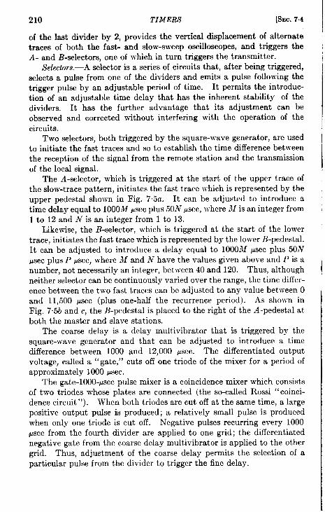
210 TIMERS IsEC. 7.4

of the last divider by 2, provides the vertical displacement of alternatetraces of both the fast- and slow-sweep oscilloscopes, and triggers theA- and B-selectors, one of which in turn triggers the transmitter.

Selectors.—A selector is a series of circuits that, after being triggered,selects a pulse from one of the dividers and emits a pulse following thetrigger pulse by an adjustable period of time. It permits the introduc-tion of an adjustable time delay that has the inherent stability of thedividers. It has the further advantage that its adjustment can beobserved and corrected without interfering with the operation of thecircuits.

Two selectors, both triggered by the square-wave generator, are usedto initiate the fast traces and so to establish the time difference betweenthe reception of the signal from the remote station and the transmissionof the local signal.

The A-selector, which is triggered at the start of the upper trace ofthe slow-trace pattern, initiates the fast trace which is represented by theupper pedestal shown in Fig. 7.5a. It can be adjusted to introduce atime delay equal to 1000M psec plus 50N psec, where M is an integer from1 to 12 and N is an integer from 1 to 13.

Likewise, the B-selector, which is triggered at the start of the lowertrace, initiates the fast trace which is represented by the lower B-pedestal.It can be adjusted to introduce a delay equal to 1000M psec plus 50Npsec plus P Psec, where M and N have the values given above and P is anumber, not necessarily an integer, between 40 and 120. Thus, althoughneither selector can be continuously varied over the range, the time differ-ence between the two fast traces can be adjusted to any value between Oand 11,500 psec (plus one-half the recurrence period). As shonm inFig. 7.5b and c, the B-pedestal is placed to the right of the A-pedestal atboth the master and slave stations.

The coarse delay is a delay multivibrator that is triggered by thesquare-wave generator and that can be adjusted to introduce a timedifference bet ween 1000 and 12,000 ~sec. The differentiated outputvoltage, called a “gate,” cuts off one triode of the mixer for a period ofapproximately 1000 Wsec.

The gate-1000-~sec pulse mixer is a coincidence mixer which consistsof two triodes whose plates are connected (the so-called Rossi “ coinci-dence circuit”). When both triodes are cut off at the same time, a largepositive output pulse is produced; a relatively small pulse is producedwhen only one triode is cut off. Negative pulses recurring every 1000psec from the fourth divider are applied to one grid; the differentiatednegative gate from the coarse delay multivibrator is applied to the othergrid. Thus, adjustment of the coarse delay permits the selection of aparticular pulse from the divider to trigger the fine delay.

Sac. 7-4] BLOCK DIAGRAM QF MODEL C-1 TIMER 211

The iine delay is a delay multivibrator that can be adjusted to in-duce a time difference of 50 to 650 psec. The output signal is dMeren-tiated to produce a gate approximately 50 *C long.

The gate-50-psec pulse mixer is simiiar to the coincidence mixerdescribed above. It selects a particular pulse from the first divider.

[a) Slow oscilloscope patternw!thout signals

Q---A-Signal (Local)

--B-Signal(Remote)

lb) Slowoscilloscope patternwith signals as it appears

at an A-station

(c) Slow oscilloscope pattern (d) Fast oscdloscope patternwith signals as d appears with markers and with A-

at a B-station and B-signals allgned

FIQ. 7.5.—Basic oscilloscope patterns.

The continuous delay is a multivibrator whose delay can be variedcontinuously from 40 to 120 psec.

Exciter Driver.-At a master station the pulse-output circuit is con-nected to the A-selector so that the local pulse appears on the upper orA-pedestal. At a slave station it is connected to the B-selector so thatthe local pulse appears on the lower or B-pedestal. The pulse-outputcircuit and exciter driver amplify and shape the pulse that drives thelocal transmitter.

212 TIMERS [Sllc. 74

Marker Mixer.-Calibration markers derived from the dividers aremixed and applied to the vertical plates of the fast and slow oscilloscopesfor the measurement of the time difference between the initiations of thetwo fast traces. The 10-~sec markers are derived from the 100-kc/secblocking oscillator; the 100-psec markers are derived from the seconddivider; and the 1000-psec markers are derived from the fourth divider.

Sweep Generators.—The output pulses from the A- and B-selectorsare mixed and applied to the fast-sweep generator to produce the upperand lower traces on the fast-sweep oscilloscope and the upper and lowerpedestals on the slow-sweep oscilloscope.

When the fast-sweep generator is triggered, it produces two equal andopposite voltage outputs that vary linearly with time and are applied tothe horizontal deflecting plates of the cathode-ray tube. The intensifyinggrid of the cathode-ray tube is so biased that the electron beam is blankedout except for the duration of the fast trace. In this way the shortintervals of time represented by the pedestals on the slow-trace patternare expanded to form the fast-trace pattern of Fig. 7.5d, which shows theremote and local signals and the calibration markers.

The slow-sweep generator is synchronized by pulses from the lastdivider and produces two voltage outputs that vary linearly with timeduring the interval bet\\-eenthe synchronizing pulses. These equal andopposite voltage outputs are impress~d on the horizontal plates of theslolv-sweep oscilloscope to produce the two linear traces of the slow-tracepattern shown in Fig. 7.5a.

Trace Scpurator.-The voltage output of the square-~rave generator isapplied to the vertical plates of both the slow- and fast-slveep oscilloscopesto produce the separation bct$vecn the upper and lo~rer traces. On thefast-s!veep oscilloscope the separation is vcwiable, whereas on the slow-sweep oscilloscope the separation is fixed.

An output voltage from the fast-sweep generator is mixed with thatfrom the tram scp:uutor and impressed on the vertical plates of the slow-sweep oscilloscope to produce the upper and lower traces and pedestalssho]vn in Fig. 7.5a.

Attenuator-bias Driwr.-Sincc the attenuator does not respond instan-taneously, it is nccess:wy to :LPPIY the attcnuat,ing bias some time beforethe transmission of the local signal. The attenuating bias is initiated,therefore, by a puisc from the coarse A- or B-delay multivibrator, thechoice depending on the operation of the timer as master or slave. Theoperfition of the attenuator is drscribml in Sec. 8.3.

Rccciuer.—Thc attenuated local signal from the sampling network andthe signals from the rccciving &ntcnn:L are amplified in the receiver andimpressed on the phitcs of the fast- and S1O}V-SWCCPoscilloscopes to pro-duce vertical Mfcctions.

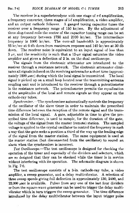
SEC.7.4] BLOCK DIAGRAM OF MODEL C-l TIMER 213

The receiver is a superheterodyne with one stage of r-f amplification,a frequency converter, three stages of i-f amplification, a video amplifier,and an output cathode follower. A ganged tuning capacitor tunes thereceiver over a frequency range of 150 kc/see. By the adjustment ofthree slug-tuned coils the center of the capacitor tuning range can be setat any frequency between 1750 and 2100 kc/see. The intermediatefrequency is 1600 kc/see. The over-all bandwidth is approximately65 kc/see at 6 db dew-n from maximum response and 140 kc/see at 30 dbdown. The receiver noise is equivalent to an input signal of less than3 ~v, and the sensitivity is such that a 15-w signal saturates the videoamplifier and gives a deflection of 2 in. on the dual oscilloscope.

The signals from the electronic attenuator are introduced to thereceiver through a resistance network. The electronic attenuator elimi-nates all signals induced on the receiving antenna for a short time (approxi-mately 1800 ~sec) during which the local signal is transmitted. The localsignal is picked up on a small loop located near the transmitting-antennacoupling unit and is introduced to the receiver through a potentiometerin the resistance network. The potentiometer permits the equalizationof the amplitudes of the local and remote signals as they appear on thecathode-ray tubes.

Synchronizer.—The synchronizer automatically controls the frequencyof the oscillator of the slave timer in order to maintain the prescribedtime difference between the reception of the remote signal and the trans-mission of the local signal. A gate, adjustable in time to give the pre-scribed time difference, is used to sample, for the duration of the gate,the voltage of the signal from the master (remote) station. The sampledvoltage is applied to the crystal oscillator to control the frequency in sucha way that the gate seeks a position a third of the way up the leading edgeof the signal from the master station. The same equipment is used atthe master station (but disconnected from the oscillator) to sound analarm when the synchronism is incorrect.

Test Oscilloscope.-The test oscilloscope is designed for checking theoperation of the timer and especially of the dividers and selectors, whichare so designed that they can be checked while the timer is in servicewithout interfering with its operation. The schematic diagram is shownin Fig. 7“6.

The test oscilloscope consists of a 3-in. cathode-ray tube, a videoamplifier, a sweep generator, and a delay multivibrator. A selection ofthree sweep speeds giving full deflection in approximately 130, 2400, and22,OOO~sec is available. Pulses from any one of the last four dividersor from the square-wave generator can be used to trigger the delay multi-vibrator which in turn triggers the sweep generator. The time differenceintroduced by the delay multivibrator between the input trigger pulse

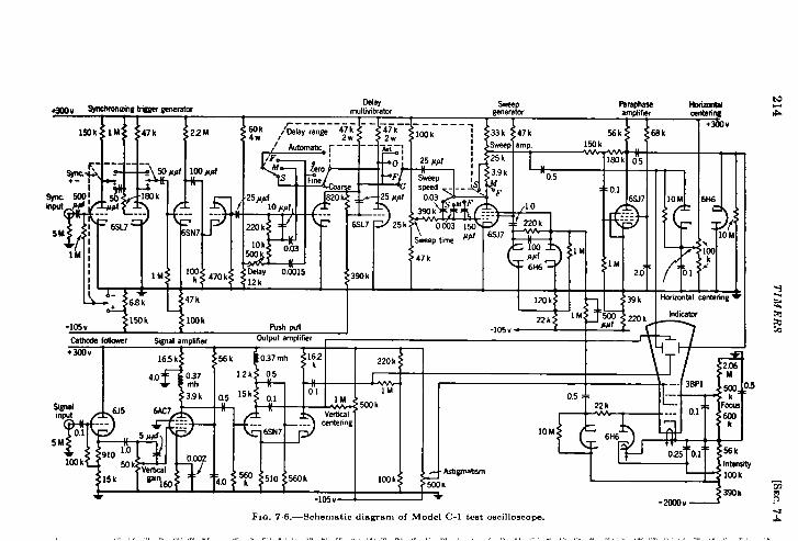
400V ~w hser mI@X

M

1..-r

470k

Celaymultivibrator *P

W@generaw ampk

--------- --,

“&;iE*, 1~.— ,.

H---------_=

47 k2W 10Uk

:{{33k 47k %k.

1 :------ ---- !3vemamo. 150k #150k lM

y ‘: : j_l

47k 2.2M

- --- -

y+, - >2 w ##f lof

* soo~ lSOkinpuf@ #f

.-. . . . -—

5M,~ ~ 6’7

SN7

1M ‘~:

\ J-. 6.8k 47h

-lc5b’150k lC41k

CathOdOfollmver 34gm31amplifier+Wov

16.5k %k 162k 220k

4,0 l,2k

0,5 15k 0.1u

6K7 * Vef-liral

5M

, 1 1 L 1 1 1 1

+

Mlk

22k W .39kM m ,?20k,.,

nnh pdl J -lo5v- r I P*, rOutputamplifer -

P

--- centenng

‘“3 Jhnfol 41 I .-.. I I I

AA5tigmbsm

5CQK3

k

!10M

L 01

HOIuonlal

b?ling=3&V

Indlcaim

7-. I

i!6H6

t10M

Y103Xk

entering

i

I-M+

2.0sM

-- 3BP1 ~,

L-- k.FW

. ..- 0.1 *

10M

-m”-f ’”’FIG. 7.6.—Schematic diagram of Model C-1 test oscilloscope.

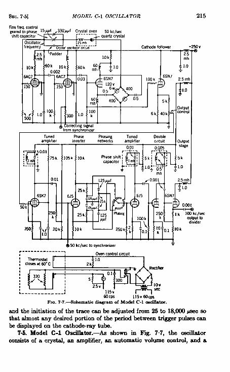
SEC.7.5] MODEL C-1 OSCILLATOR

Finefgeareshift

‘from syncilro;izer

amphfler

1

;----- Jo,ol

:Im:75k

,. .-. ~

0.01

6SK7,::

>k ‘--

1

~

3s0 20 I;.:

25ml

~.

Phase Phasing Tuned Ooubleinverter networks amphfler clrcult

m

Iltpulstage

5k

1.0

215

?50ve

WCtor

($50 kc/see to synchronizer*

- .-. -- . --------7

1 Ovencontrol circuit1

11111I,1L.-------_,_--J

60Cps llsvwccrsFIG. 7.7.-f3chematic diagram of Model C-1 oscillator.

and the initiation of the trace can be adjusted from 25 to 18,(MI psec sothat almost any desired portion of the period between trigger pulses canbe displayed on the cathode-ray tube.

7.6. Model C-1 Oscillator.-As shown in Fig. 7-7, the oscillatorconsists of a crystal, an ampliiier, an automatic volume control, and a

216 TIMERS [SEC. 75

series inductance, capacitance, and resistance circuit. A signal appliedto the amplifier is increased about one-hundred fifty times and applied tothe automatic volume control, which maintains a constant amplitude ofoscillation. The output of the automatic volume control drives thecrystal at its natural frequency of 50 kc/see. In series with the crystal,tuning coil, and resistor is a variable capacitor that controls the frequency.The signal generated across the resistor and applied to the amplifier com-pletes the oscillator circuit.

The oscillator must be stable to 1 part in 100 million for an hour ortwo at a time. This requirement means that the Q of the crystal mustbe high lest its frequency of oscillation be appreciably influenced byvariations in the electrical driving circuit. It must have a lo~v-tempera-ture coefficient; the oven temperature must be constant; and the electricaldriving circuit must be so designed that any phase shift Which it intro-duces \\-illbe small and stable.

The crystal is an X-cut quartz bar that oscillates at 50 kcisec. Thedimensions are 54 mm along the Y-, or mechanical, axis; 9+ mm alongthe X-, or electrical, axis; and 7* mm along the Z-, or optical axis. Theupper and loJver surfaces (7* by 54 mm) are electroplated, and electricalcontact is made to them through very fine wires that are soldered to themetallic plating at the center of each surface. The crystal is supportedbetween a cork pad and a felt pad of small cross section, which clamp theplated surfaces at the center points to ~vhich the vires are soldered.Since these points are nodes of vibration at the desired frequency, theclamping does not seriously affect the vibration of the crystal. Theclamping pressure is controlled by a scre]v adjustment on the crystalmount.

The dimensions of the c~stal are chosen to give a high Q and a lowtemperature coefficient. If the crystal is represented by its equivalentelectrical circuit of an inductance, capacitance, and resistance in series,Q is the ratio of A to R. The Q is approximately 65,000, and the resist-ance is approximately 3500 ohms. The temperature coefficient is nega-tive, about 1 part per million per degree centigrade at an operatingtemperature of 60”C.

Baffle plates are mounted at short distances from the ends of thecrystal to serve as sound reflectors. They reduce the amount of soundenergy uselessly radiated and so increase the Q of the crystal. Since atreflection the sound wave is re~.ersed in phase, the reflected wave at theend of the crystal should be in phase with the transmitted wave to rein-force the normal ~-ibration. The baffles are therefore adjusted for adistance of a quarter wavelength of 50-kc/sec sound in air.

The crystal oven consists of an outer aluminum case, an insulatinglayer of asbestos, and an intenor aluminum case that contains the crystal;

SEC.75] MODEL C-1 OSCILLATOR 217

its mount, and the inductor. The outer aluminum case is heated by sixheater cards, one attached to each side. A mercury thermostat, mountedon one side of the outer aluminum case, controls the temperature byopening and closing the circuit through the heater cards. A balsa-woodbox encloses and thermally isolates the whole assembly.

Heat is applied to the outer case for about 1 min out of a 4-rein cyclewhen the room temperature is 20”C. The heat “ripple” caused by theon-and-off heating cycle is smoothed by the filtering action of the alternateconducting and insulating layers. The aluminum cases can be consideredas having large thermal capacitance, and the insulating layer can be con-sidered as offering resistance to the flow of heat.

A mercury thermometer extending into the inner case indicatesexternally the temperature of the crystal. The absolute value undernormal stable conditions is not important as long as it is within a fewdegrees of 60”C. After the crystal temperature has reached equilibrium,it should be stable to within ~°C.

The oven temperature is raised when a relay allows current to flow inthe heater cards. This relay is actuated by the mercury thermostat thatconsists essentially of a glass tube of fine bore into which a pair of finecontact wires are sealed. The contacts are so placed that they completea circuit through the mercury column at about 60”C. Mounted on theouter aluminum case, the thermostat assumes the temperature of themetal. A rise in temperature of the outer oven closes the circuit throughthe relay coil, pulls up the armature of the relay, and opens the contactsof the heater circuit. Upon cooling, the circuit through the relay coilopens and allows the armature to fall back and close the heater circuitagain.

Because of its location, the thermostat has no immediate control overthe temperature of the inner oven, and at least three hours are requiredfor the crystal to reach a stable operating temperature.

Because of the small size of the mercury thermostat, the short-circuitcurrent must be limited to 10 ma and the voltage, when the circuit isopen, to 12 volts.

A selenium bridge rectifier converts lo-volt alternating current fromthe transformer to 8-volt direct current for the purpose of operating therelay. The transformer is protected by a fuse against short circuits inthe rectifier.

The amplifier, which furnishes the power to drive the oscillator, con-sists of two pentode tubes. Each tube operates under Class A conditionsand has a gain of about 13. Small inductances have been introduced inthe plate circuits to minimize the phase shift, and the unbypaaaed cathoderesistors provide degenerative feedback to reduce distortion.

The automatic volume control consists of a phase-inverting tube and

218 TIMERS [SEC.75

a bridge composed of two fixed resistors and two lamps whose resistancevaries with temperature. The phase inverter is a triode with equalimpedances in plate and cathode circuits. The cathode-output signal isin phase with the input signal on the grid; the plate-output signal is 180°out of phase with the grid signal. Since the same current is flowing inthe plate circuit as in the cathode circuit, and since the plate and cathodeimpedances are equal, the 50-kc/sec alternating voltages at the plate andcathode are equal.

When the oscillator is turned on, the lamps are cold, their resistanceis low, and the bridge is unbalanced; consequently a large signal isimpressed on the crystal. The mechanical vibration of the crystal andthe piezoelectric signal associated with it build up with a time constant(Q/j) of about 1 sec. As they increase, the amphfied signal and the out-put from the phase inverter also increase and cause the temperature andthe resistance of the lamps to rise. As the bridge approaches balance,the signal transmitted through it to the crystal decreases (the attenuationof the bridge increases) until a stable state is reached. In the stablestate, the bridge is slightly unbalanced. The gain of the amplifier is thenequal to the attenuation of the bridge plus the loss in the crystal and tun-ing circuit. The bridge is thus a variable attenuator that acts like anautomatic volume control without introducing the usual shift of phaseand associated shift of frequency.

The amplifier and automatic volume control are designed to minimizethe shift of phase between the amplifier input and output, especially theshift of phase that might depend on variable quantities such as linevoltage, temperature, or tube characteristics. Since the Q of the crystalis finite, the frequency at which it vibrates can be pulled slightly higheror lower by applying a driving voltage that either leads in phase or lagsbehind the crystal oscillation. (This is the principle by which the syn-chronizer controls the frequency of the oscillator. ) The variable capaci-tance in series with the crystal, inductance, and resistance provides sucha frequency control. This capacitance controls the phase of the signalapplied to the amplifier input with respect to that derived from the crys-tal. It therefore regulates the phase of the voltage from the automaticvolume control that drives the crystal and, hence, controls the frequencyat which the crystal vibrates.

Rotation of the oscillator frequency control through one division onthe dial varies the frequency by roughly 1 part in 3 million. Thisrepresents a change in rate of drift of 20 ~aec/min. These figures areonly approximate because the sensitivity of the oscillator to the frequencycontrol depends on the fixed capacitor and on the Q of the crystal. Thetine frequency control has a much smaller effect upon the circuit, itscomplete range corresponding to a little more than three divisions of the

SEC. 7.6] MODEL C-1 DIVIDER UNIT 219

coarse frequency dial. A clutch may be engaged so that the rotation ofthe phase-shift capacitor rotates the fine frequency capacitor, one com-plete rotation of the phase-shift capacitor corresponding to about sevendivisions of the dial of the fine frequency capacitor. In this way, thedifference between the frequencies of the local and remote oscillators isautomatically reduced in maintaining synchronism.

Since the oscillator is sensitive to loading, the output is taken from acathode follower that draws no current from the oscillator. A signal from ~, .3the grid of the phase inverter is impressed on the grid of the cathode ‘follower. T ‘1

)A potentiometer controls the amplitude of the signal applied to the 1~ ,,grid of the tuned amplifier and therefore controls the output of the oscil- ( Ilater unit. The tuned amplifier improves the waveform of the signal that ~ )is applied to the grid of the phase inverter.

‘he ‘urpo* ‘f The ‘base ( )inverter is to provide two output signals that are equal m amphtude and180° out of phase. These two signals are applied to four phasing net- ~ )

Iworks to produce four signals that are mutually 90° out of phase. If an J

alternating voltage is impressed across an impedance composed of a resist- ~ -Iante and a capacitance in series, the voltage across the resistor leads themvoltage across the capacitor by 90°. The voltage across the combination” ~is the vector sum of the voltage across the resistor and the voltage across .,the capacitor; in phase it lies between the two component volta~s. jSince the capacitive reactance l/%fC equals the resistance, the voltage Jacross the capacitor is equal to the voltage across the resistor. Uncjer ~thk condition the voltage across the resistor leads the voltage across the ~combination by 45°; the voltage across the capacitor lags behind @evoltage across the combination by 45°. Thus the four phasing networks ;

produce four voltages that are mutually 90° out of phase. These me ~impressed on the four stator plates of the phase-shift capacitor, which&-. .the same as that of the Model B-1 timer described in Sec. 7.2.

The tuned amplifier amplifies the signal from the rotor of the phase-shift capacitor and improves its waveform.

The frequency doubier differs from the tuned amplifier in that theplate antiremnant circuit is tuned to 100 kc/see, and the positive biasof the cathode is larger (because of the high cathode resistance). Thetube is nonconducting except for about a quarter of the 50-kc/sec period.The short pulse of current causes the tuned circuit to oscillate at itsresonant frequency of 100 kc/see. Since the amplitude of the oscillationdecreases slightly between pulses, it is neceeaary to improve the waveformin a 100-kc/sec tuned amplifier located in the divider unit.

The output stage is a cathode follower with cathode self-biae.706. Model C-1 Divider Unit.-In the divider schematic diagram

@lg. 7“8), the tuned amplifier, blooking oscillator, and six dividers with

220 TIMERS [SEC.76

feedback arc showm together ~vith the marker mixer, square-wave gener-ator, trace separator, and pedestal mixer.

The output of the frequency doubler is a 100-kc/scc sine ~vave withalternate cycles of dccrmscd amp]itudc. The tuned amplifier convertsthis output to a 100-kc/scc sine wfiw: of constant amplitude.

Since thr sine-~vavc output signal of the 100-kc/sec shaper is notsuitable for generating calibration markers or for driving the dividers, it

Tuned amplifier 10, 100 and 1000psecBlocking 10, 100 and 1000#see markers to twin scope

+250v oscdlator marker m!xer Marker output ? +250 vT T T -A

1 1 1 J I JI 1 1 11 1 1 1 I 1 I 1 1 I I D

–,”” I \Sq.-wave<“-” lSec pU15eS generator

‘A L‘loo~”f{ ““kc’’m@.

lUUUp100 psec pulses bias

A

C&&

6H6 .-L ,.J. .,

f!j-p.

0.5M Ok.6SN7

.6SN7

J

5W/.l/lf 10k

7)

. .

2~

T T:3kgL1.0 ~ 12k 1.0

I

%5

T1111\1 111L 11 K+0 No. 1 divider @ No. 2 dwider &

InspectionNo. 3 :Jider ~

adj, Inspection adi. Inspection Inspectiondwider No. 1 divider No, 2 “ divider No, 3 - divibr No. 4

FIO. 7.8.-SohemStio &

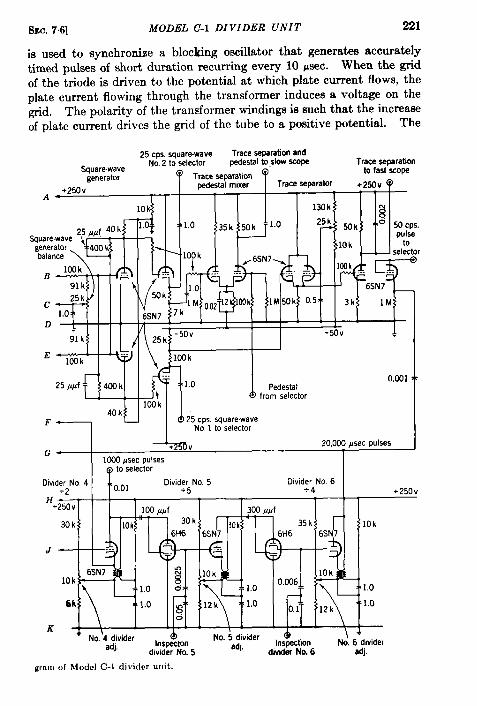
SEC.7.6] MODEL C-1 DIVIDER UNIT 221

is used to synchronize a blocking oscillator that generatis accuratelytimed pulses of short duration recurring every 10 Psec. When the gridof the triode is driven to the potential at which plate current flows, theplate current flowing through the transformer induces a voltage on thegrid. The polarity of the transformer windings is such that the increaseof plate current drives the grid of the tube to a positive potential. The

25 cps. square.wave Trace separationand

Square.waveNo.2 to selector pedestal toslow scope Trace sqarafion

generator @ Trace separation @ to fast S40PS

+250 V pedestalmixer Trace separator +250V @

A-10k 130k

g1.0 ~co 50qss.

pulse

“generator. ‘%3 k} I I }~ ! to... -+,,

F

C---$-WIN

I J-.. 20,000psec pulses

I

H+

J

6k 1.0 ~ 12;0

K \ 1 1 I 1 1 \+ \

No. 4 divider 0 & 4Inspecton

No. 5 divideradj. adj. Inspection No. 6 dwidet

dlwder No. 5 diwder No. 6 adj.

250V

gramof ModelC-1 dividerunit.

222 TIMERS [SEC. 75

grid-voltage rise brings about a further increase in plate current which,in turn, causes an additional increase in grid potential. This regenera-tion continuee until grid current is drawn and the grid capacitor is nega-tively charged. Its capacitance is small, and consequently it becomescharged very rapidly once the grid of the tube is driven into the highgrid-current region. When the rate of change of potential on thecapacitor caused by flow of grid current exceeds that caused by trans-former action, the grid voltage begins to decrease. This causes the platecurrent to decrease and hence reverses the polarity of the potentialinduced on the transformer secondary. The decreasing secondary volt-age augments the grid-voltage decrease until the cutoff voltage is exceededand the flow of plate current cesaes. The magnetic field that has beendeveloped in the transformer by plate current collapses and induces anovershoot voltage. Since the grid has been driven below, cutoff, addi-tional oscillations are prevented until the grid capacitor is discharged, atwhich time the cycle is repeated.

There are six dhiders with feedback which reduce the recurrence rate(100,000 pps) of the pulses from the blocking oscillator to the recurrencerate of the traces (which is twice the recurrence rate of the transmissionof the local A- or B-signal).

A typical divider circuit consists of a charging capacitor, a doublediode, a storage capacitor, and a blocking oscillator. The input pulses,through the action of the charging capacitor and the double diode, buildup a charge on the storage capacitor in steplike faahion, each input pulseraising the charge and the voltage one step. When the storage capacitor,which is connected to the grid of the blocking oscillator, reaches the poten-tial at which plate current flows, the cycle of the blocking oscillator istriggered, an output pulse is produced, and the storage capacitor is”dkcharged. This steplike accumulation of charge on the storage capaci-tor followed by its discharge is repeated indefinitely.

The number of steps between discharges, or the dividing factor of thecircuit, is inversely proportional to the input charge per step (which isproportional to the total positive input voltage applied to the chargingcapacitor and to the capacitance of the charging capacitor). It is directlyproportional to the capacitance of the storage capacitor and directly pr~portional to the difference between the discharged potential and thepotential at which the cycle of the blocking oscillator is triggered. Whenthe storage capacitor is discharged by the blocking owillator, it is firstdriven below ground potential but is immediately restored to groundpotential by the double diode. The potential at which the cycle of theblocking oscillator is triggered is determined by the cathode bias, whichis controlled by a potentiometer.

Feedback is applied from the lad divider to the second and third

SEC.7,6] MODEL C-1 DIVIDER UNIT 223

dividem. By means of a second double diode connected to the storagecapacitor of the third divider, for instance, every output puke from thelaat divider supplies a charge of adjustable amount to the storage capaci-tor. This feedback reduces the recurrence period between output pukesof the third divider once every recurrence period of the last divider andthereby reduces by the same amount the recurrence period of the lastdivider.

The functions of the square-wave generator are to divide the recur-rence rate of the last divider by 2 and to produce an output square wavefor the vertical displacement of the upper and lower traces of the fast-and slow-oscilloscope patterns. The square-wave generator is an Eccles-Jordan circuit similar to a multivibrator, and it consists of two triodeswhose plates are cross-coupled to the grids through resistors as well asthrough capacitors. It is a balanced circuit, each component associatedwith one triode corresponding to an identical component associated withthe other triode. There are two stable states of operation, in which allcurrents and voltages remain constant. In one state one tnode conductswhile the other is nonconducting; in the other state the conducting andnonconducting conditions of the triodes are reversed. The negativeportions of the output pulses from the last divider are applied througha diode to both grids of the square-wave generator. Each pulse causesthe states of operation of the triodes to reverse, producing at the twoplates square-wave outputs that are equal in amplitude but opposite inphase. Since the square-wave generator is sensitive to loading, the out-puts are taken from two cathode followers.

In the trace-separation pedestal mixer the square wave is mixed withthe flat-topped intensifier pulses from the fast-sweep generator (shownin Fig. 7.9). The output is applied to one of the vertical deflecting platesof the slow oscilloscope to produce the upper or A-trace with the .4-pedes-tal and the lower or B-trace with the B-pedestal. The vertical separationbetween the upper and lower traces of the slow oscilloscope is fixed.The square-wave and pedestal signals are applied to the grids of two triodeamplifiers that are cathode-coupled. The signals applied to the grids arerelatively small positive and negative voltages, and consequently bothtriodes operate over approximately linear portions of their characteristics.The current through the cathode resistor is controlled by the grid that ismomentarily more positive. The voltage waveforms that appear on theplates of the triodes are similar although unequal and opposite in phase.

The operation of the trace-separation circuit that gives adjustablevertical separation between the upper and lower traces of the fast oscillo-scope is similar to that of the trace-separation pedestal mixer. The cir-cuit consists of two cathode-coupled triodes that operate as cathodefollowers. An adjustable d-c potential is applied to one grid, and the

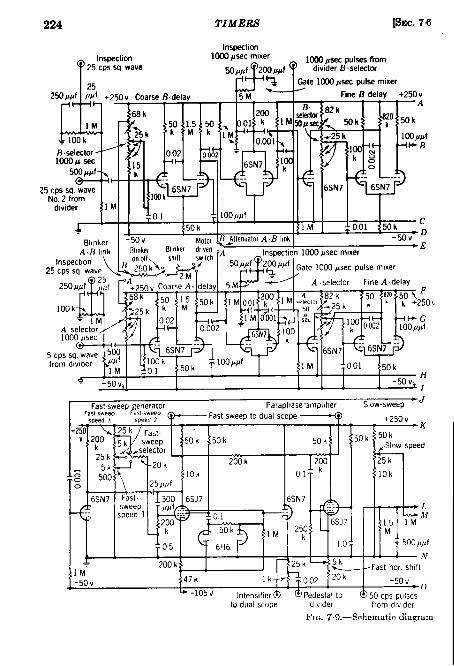
224 TIMERS @m. 76

Inspection

1,,,,, % :

Inspection l@30psec mixer25 ITS w wave

1000psec PUIS-SSfromW/J/Jf 2CllhWf dwlder B-selector

25 Gate 1000psec pulse mixer.

250ppf /I#f +2w V Coarw ~.delay 5M Fine B-delay +250 v

@h B. }Q,, I 1 1 A---

%. .. . .

‘f df:”r’””secm’xer EI *

50flflf 2~OP#f GaIe l~o psec pulse mixer

A. selector FmeAdelay

1,: ~o~ 82 k200 1 M .$flor _7& ~ ~IM 00) ~50 8;0 513~ F

k +250h

–J” .>, 1 [ 1 I -50vi;

0

6SN7 Fast

—.””r ‘1 1 1 1 I I ,

5kN

200k1M7 - Fast hor shift

—En,, 47 k 1k- - 20 k -50V ~L--105V Intenslflerd) @Pedestalto @50 CPSpulses

to dual scope dlvlder from divider

FIG. 7.’2.-Schematic diagram

sm. 7.6] MODEL C-1 DIVIDER UNIT

I dividerInspection 50/Jsecpulses

50 psac mixer fro

v

Qate 50 Paec(

+25a v pulse mixerA

lM 10 lWk lM

/bpf .001

B lfKIk. .

6SN7

D -50VE-

Inspection50 psec mixer

Gate 50 psec+250V

Fpulse mixer

100k lM

L@

lM 10G @#f 0.001

lOOk.

6SN7

IB-selector Co;t;e::ycontinuous

0.001 1P 50k {~ 50k

\ “WIk+

50k 500

6SN7

;:1 M

, =0.01

1 I 1 I

Trigger tosynchronizer

$-electormIxer +250 V

2001~5Z:0001 }k

6SJ7

I .IJ

1 I

‘ Paraphase ampllfier /

Attenuatordriver 250V

B

2.2M 40k0.1

6SN7 6s7

.5

.... ...

3 2M0

. -50VDrive to

attenuator

10/I/If

K

to

LM

N

oof Model C-1 selector unit,

226 TIMERS [SEC.7.7

square wave is applied to the other. The cathode potential cannot fallappreciably lower than the higher of the two grid potentials. When thed-c grid potential is low, the cathodes are free to follow the square waveimpressed on the other grid; when it is high, the cathode can follow onlythe positive portion of the square wave. The output from the cathodeis amplified and applied to one of the vertical deflecting plates of the fastoscilloscope.

The 10-, 100-, and 1000-paec marker mixer is a triple-coincidencemixer. The plates (with limiting reaistora) of three normally conductingtriodes are connected so that the combmed plate currents determine thepotential difference across the common plate resistor. The output posi-tive pulse is very small when one triode is cut off, somewhat larger whentwo are cut off, but very large when all are cut off. Negative pulses fromthe blocking oscillator recurring every 10 Psec are applied to the grid ofthe first triode and produce small positive output pulses. Once every100 *C a pulse from the second divider is rectified and applied to thegrid of the second mixing triode, which cuts it off for a period of approxi-mately 10 psec. A pedestal on the output waveform results, and one ofthe 111-psecpulses is effectively amplified. Similarly, a puke from thefourth divider produces a pedestal approximately 30 psec long andeffectively amplifies three of the 10-IERCpulses. The pedest+ds, whichare appreciably smaller in amplitude than the lo-psec markers, areeliminated by the limiting action of the msxker output amplifier. Thus,the output waveform is a series of marker pulses recurring accuratelyevery 10 psec. Every tenth puke is a 1OO-WWCmarker of increasedamplitude. Every tenth 100-~sec marker is identified as a 1000-~secmarker by a series of three pulses following the 100-Psec marker andspaced 10 psec apart.

7.7. Model C-1 Selector Unit.—As shown in Fig. 7.9, the selectorchassis contains the A- and B-selectors, the selector mixer, the fast- andslow-sweep generators and paraphsse amplifiers, the exciter driver, andthe attenuator driver.

The function of the selectors is to permit the introduction of an adjust-able and highly stable time difference between the initiations of the fastA- and B-sweeps (see Sec. 7.3). Mter being triggered by the square-wave generator, one selector circuit selects one of a series of pulses(recurring every 1000 psec) from one of the dividers. The selected1OOO-PWCpuke in turn triggers another selector circuit, which selects aparticular one of a series of 50-Psec pulses. The selected 50-PSCCpulse ofthe B-selector triggers a continuously adjustable multivibrator whoseoutput pulse initiates the fast sweep.

A typical selector circuit, such as the coarse A-delay and the associatedgate-1000-psec pulse mixer, consists of a delay multivibrator and a coin-cidence mixer. The delay multivibrator is a double-tnode cathode-

I

SEC.7.7] MODEL C-1 SELECTOR UNIT 227

coupled multivibrator that is inactive until it is triggered by a positivepulse on the first grid or a negative pulse on the second grid. In thenormal quiescent state the first triode is nonconducting while the secondtriode is conducting. The grid of the second triode is returned to theB-supply voltage through a high resistance so that the grid-to-cathodevoltage is essentially zero. Therefore, the cathode potential is determinedby the flow of current through the cathode and plate resistors and atriode operating at zero grid-to-cathode voltage. The bias of the firstgrid, which controls the time delay, must be negative with respect tothe quiescent cathode potential. A positive trigger pulse applied to thefirst grid or a negative trigger pulse applied to the second grid causes thefirst triode to conduct and the second to be cut off. The cathode poten-tial and also the change in the plate potential from the nonconductingto the conducting state are determined by the grid bias. The changein plate potential determines the amplitude of the negative pulse impressedon the second grid. The potential of the second grid, therefore, variesexponentially with time and returns toward the B-supply potential witha time constant equal to the product of the grid resistance and the cou-pling capacitance. When it approaches the cathode potential (as adjustedby the grid bias), the second triode again conducts and produces a nega-tive output pulse, the first triode is cut off, and the circuits assume theirnormal quiescent state. The time delay, therefore, is a function of thetime constant and the adjustable grid bias. Actually it is an approxi-mately linear function of the grid bias.

The gate-pulse mixer is a double-triode coincidence mixer of the typepreviously described. The negative output pulse of the delay multi-vibrator is differentiated to cut off the first triode for a time determinedby the product of the grid resistance and the coupling capacitance.Negative pulses from one of the dividers are impressed on the other grid.When both triodes are cut off, the resulting positive pulse is large enoughto cause current to flow through the biased amplifier and trigger thefollowing selector circuit.

The purpose of the selector mixer is to produce for each negativepulse from the A-selector and each negative pulse from the B-selector apositive output pulse to trigger the fast-sweep generator. It is a pentodeamplifier that is normally conducting. Positive and negative differen-tiated pulses from the A-selector are impressed on the suppressor grid,and positive and negative differentiated pulses from the B-selector areimpressed on the control grid. A positive pulse on either grid does notappreciably affect the flow of plate current; a negative pulse on eithergrid cuts off the plate current and produces a positive output pulse. Thispositive pulse is applied to a negatively biased amplifier that triggers thefazt-sweep generator.

The fast-sweep generator when triggered generates an output voltage

228 TIMERS [sac, 7.7

that varies linearly with time and deflects the cathode-ray beam hori-zontally to produce the A- and B-traces of the fast oscilloscope. Bymeans of a three-position switch and potentiometers the sweep speed canbe adjusted from a speed that gives full deflection in 60 psec to one thatgives full deflection in 1400 ~swc. The sweep generator also providespositive flat-topped intensifier pulses, which are applied to the intensifiergrid of the cathode-ray tube. The cathode-ray beam is cut off exceptfor the duration of the sweep.

The fast-sweep generator is a sharp cutoff pentode amplifier whoseplate is capacitance-coupled to the control grid. The potential of thesuppressor grid is limited by diodes to the region between ground and85 volts below ground potential. In the quiescent state, the suppressorgrid is held at – 85 volts, and the control grid is connected through ahigh resistance to a positive potential. Consequently, no plate currentflows, but there is a large flow of screen-grid current, and the screen-gridpotential is low.

A negative pulse applied to the plate and control grid momentarilycuts off the flow of screen-grid current, raises the screen-grid potential,and, through capacitance-coupling, raises the suppressor-grid potentialfrom – 85 volts to ground potential. The control grid immediatelyreturns to a potential at which space current flowTs. Since the suppressorgrid is at ground potential (where it remains for the duration of the sweep),less current flows to the screen grid, and the screen-grid potential remainshigher than in the original quiescent state. The plate potential tends todecrease from the quiescent nonconducting value; but, because of thecapacitance coupling of the plate to the control grid, the change in platepotential maintains the control grid at the potential (a few volts belowground) at which the plate current is controlled by the grid potential.Thus the plate potential is controlled by the potential difference acrossthe co~pling capacitor—a difference that is determined by the flow ofcharging current through the grid resistor. Since the grid potential andthe adjustable positive bias are practically constant, the flow of currentthrough the grid resistor is also constant, and the potential differenceacross the coupling capacitor (which is equal to the charge divided by thecapacitance) is a linear function of time. Consequently, the platepotential is a linear function of time, and the rate of change of potentialwhich determines the sweep speed is directly proportional to the differenceof potential between the adjustable positive bias and the grid potential(approximately ground) and inversely proportional to the grid resistanceand the coupling capacitance. As the plate potential approaches theknee of the characteristic curve of the tube, the screen-grid currentincreases and thereby reduces the screen-grid potential, drives the sup-pressor grid to negative potentials, and cuts off the plate current. As

SEC.7.8] MODEI, C-1 S YNCIIRONIZER 229

the plate current is cut off, the plate potential rises rapidly and causesgrid currcmt to flow in the coupling capacitor, thus further increasing thescreen-grid current and returning the circuit to its original quiescentstate.

The output of the sweep generator is applied to one horizontal deflect-ing plate of the fast cathode-ray tube, and the output of the paraphaseamplifier is applied to the other. The output waveform of a paraphaseamplifier is similar rmd equal to the input waveform (in this case the wavefrom the sweep gcrmrator), but it is inverted. The potential at a pointmidway between the deflecting plates of the cathode-ray tube remainspractically constant, therefore, and defocusing at the ends of the trace isminimized.

The slow-sweep generator and its associated paraphase amplifier arerather similar in operation to the fast-sweep generator and paraphaseamplifier. They arc triggered by pulses from the last divider und deflectthe beam of the slow oscilloscope horizontally to produce the upper andlower traces of the slow-trace pattern.

The exciter-driver circuit can be triggered by output pulses from eitherthe A- or B-selector, the choice depending on the function of the timer asa master or a slave. The pulse is amplified to trigger a gas-filled tube,the output pulse of which is shaped in ti resistance rmd capacitance net-work and transformer to drive the transmitter.

Similarly, a negative output pulse from either the coarse A-delaymulti vibrator or the coarse B-delay multi vibrator is chosen to controlthe bias of the electronic attenuator. The attenuator driver generatesa positive flat-topped pulse so timed that the transmission of the localsignal falls within its limits for all adjustments of the selectors. Theduration (approximately 1800 psec) of the flat-topped biasing pulse isdetermined by the differentiation of the negative output pulse from thecoarse A- or B-delay multi vibrator.

As a warning to Loran navigators, the transmitted signal is caused toblink if the synchronism is incorrect. This is done by a motor-drivenswitch (controlled from the panel of the dual oscilloscope) that changesthe bias of the coarse delay multivibrator and therefore changes (ordi-narily by 1000 psec) the time difference introduced by the selector for~ sec every second. Viewing the slow-trace pattern, a navigator seesthe signal shift periodically to the right or the left. The signal as viewedon the fast oscilloscope disappears for ~ sec every second.

7.8. Model C-1 Synchronizer.-The purpose of the synchronizer is tocontrol the frequency of the oscillator of the slave timer automatically sothat the prescribed time difference between the reception of the remotesignal and the transmission of the local signal is maintained. The infor-mation obtained from the sampling of the leading edge of the received

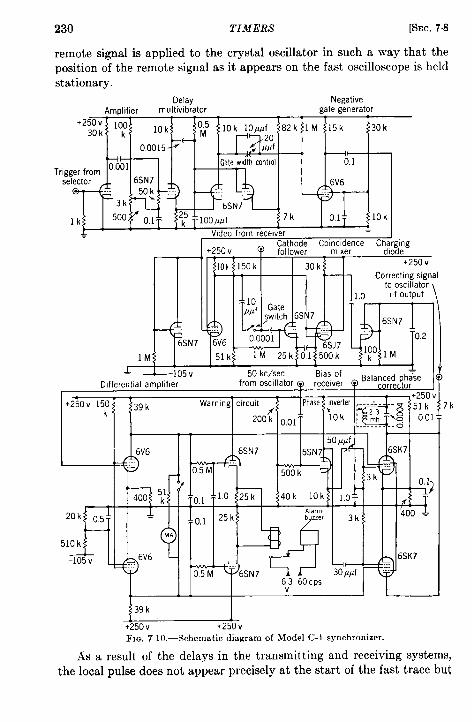
230 TIMERS [SEC. 7.8

remote signal is applied to the crystal oscillator in such a way that theposition of the remote signal as it appears on the fast oscilloscope is heldstationary.

Delav Negative

L_..25,/

I

Ampllfier multiwb;ator gate g;nerator

’25& 100 10 kk82k lM 15k 30 k

+0.0015

0001 GatewidthcontrolTrigger from

selector

6SN7

lk TIOOWf 7k H0.1

6V6

O.l T 10 k.t 1 1 L 1 n,, .,. , I

m.6SN7

lM

vlaeo Trom recewer J

@Cathode Coincidence Cha:~$g

+250 v+250 V

Correcting signal

> 1 ,L .-L-105V 50 kc/see 81as of

L

Differential amplifier from osclflator Q receiverBala:c:: phase

ctorI I I [+250 v

1250V

k150

k

1

39 k

6V6

400

Warmng clrcult,00{ $001 ye $::;’ [[~ :;g ~,~jl

50 J@6SN7 6SN7<– 6SK7

-~11 2–$ - k ~ ,1

0.5 M ““”.

500 k 3k 0.1)

Tr31 TIO 25 k 40k 10k ]oT < T1 I 1 . . .. I , I 1

L 11 T I I T r A1.rrn I I I 11. ,-,?. t

39 kI

+250 v +250 VFIG, 7 10.—Schematic diagram of Model C-1 synchronizer.

)

7k

As a result of the delays in the transmitting and receiving systems,the local pulse does not appear precisely at the start of the fast trace but

SEC.78] MODEL C-1 SYNCHRONIZER 231

is displaced to the right by a distance corresponding to a delay of approxi-mately 50 psec. When the signals at the slave station are properlysynchronized, the remote signal appears on the fast A-trace directlyabove the local signal on the fast B-trace. An adjustable time clifferenceof 50 psec or so, therefore, must be introduced between the start of thefast A-trace and the initiation of the gate that samples the voltage ofthe leading edge of the remote signal. The delay multivibrator shown inFig. 7.10 controls the position of the gate and of the remote signal on thefast A-trace. The delay multivibrator is a cathode-coupled double-tnode multivibrator similar in operation to those in the selector unit.

The positive flat-topped signal generated by the delay multivibratoris differentiated and applied to the grid of an amplifier. Since the gridof the amplifier is returned to the B-supply through a high resistance, thepositive pulse at the start of the delay (coincident with the start of the fastA-trace) does not appreciably affect the flow of current through theamplifier. However, the differentiated negative pulse following the delaycuts off the flow of current through the amplifier for a period of timedetermined by the product of the grid resistance and the coupling capaci-tance. The resulting pulse of approximately 20-psec duration is invertedand amplified to produce the negative gate that is applied to the cathodeof the coincidence mixer. The video signal from the receiver is appliedto the grid of the coincidence mixer. The amplitude of the negative out-put pulse from the coincidence mixer is determined by the averageamplitude of the video signal for the duration of the gate. In normaloperation the gate falls approximately a third of the way up the leadingedge of the remote signal. If it occurs a few microseconds early, the out-put is less than normal; if it occurs a few microseconds late, the outputpuke is greater than normal. The output pulse, which is applied througha diode to a capacitor, charges the capacitor negatively. The capacitoris sflowed to discharge to ground through a high resistance, the combina-tion having a time constant that is many times longer than the recurrenceperiod of the charging puke. Thus a sawtooth voltage is generated on thecapacitor, the amplitude of the teeth and afso the average negative poten-tial depending on the timing of the gate in relation to the remote signal.

The negative sawtooth voltage is applied to one control grid of thedifferential amplifier. The other control grid is maintained at a fixednegative reference potential. The two tetrodes are coupled through acommon cathode resistor and a common screen-grid resistor so that thetwo amplified output signals at the plates are sawtooth in form and oppo-site in phase. The relative average voltages at the plates depend on therelation between the average negative sawtooth bias and the negativereference bias and are applied directly to the two screen grida of thebalanced phase corrector. These average voltages are equal when, in nor-

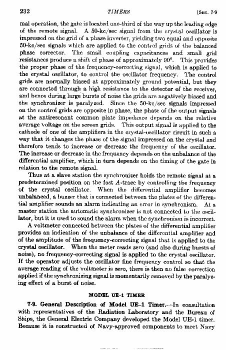
232 TIMERS [SEC. 7.9

mad operation, the gate is located one-third of the way up the leading edgeof the remote signal. A 50-kc/sec signal from the crystal oscillator isimpressed on the grid of a phase inverter, yielding two equal and opposite50-kc/sec signals which are applied to the control grids of the balancedphase corrector. The small coupling capacitances and small gridresistances produce a shift of phase of approximately 90°. This providesthe proper phase of the frequency-correcting signal, which is applied tothe crystal oscillator, to control the oscillator frequency. The controlgrids are normally biased at approximately ground potential, but theyare connected through a high resistance to the detector of the receiver,and hence during large bursts of noise the grids are negatively biatid andthe synchronizer is paralyzed. Since the 50-kc/sec signals impressedon the control grids are opposite in phase, the phase of the output signalsat the antiresonant common plate impedance depends on the relativeaverage voltage on the screen grids. This output signal is applied to thecathode of one of the amplifiers in the crystal-oscillator circuit in such away that it changes the phase of the signal impressed on the crystal andtherefore tends to increase or decrease the frequency of the oscillator.The increase or decrease in the frequency depends on the unbalance of thedifferential amplifier, which in turn depends on the timing of the gate inrelation to the remote signal.

Thus at a slave station the synchronizer holds the remote signal at apredetermined position on the fast A-trace by controlling the frequencyof the crystal oscillator. When the differential amplifier becomesunbalanced, a buzzer that is connected between the plates of the differen-tial amplifier sounds an alarm indicating an error in synchronism. At amaster station the automatic synchronizer is not connected to the oscil-lator, but it is used to sound the alarm when the synchronism is incorrect.

A voltmeter connected between the plates of the differential amplifierprovides an indication of the unbalance of the differential amplifier andof the amplitude of the frequency-correcting signal that is applied to thecrystal oscillator. When the meter reads zero (and also during bursts ofnoiw), no frequency-correcting signal is applied to the crystal oscillator.If the operator adjusts the oscillator fine frequency control so that theaverage reading of the voltmeter is zero, there is then no false correctionapplied if the synchronizing signal is momentarily removed by the paralyz-ing effect of a burst of noise.

MODEL lJE-1 TIMER

7.9. General Description of Model TIE-1 Timer.-In consultationwith representatives of the Radiation Laboratory and the Bureau ofShips, the General Electric Company developed the Model UE1 timer.Because it is constructed of Navy-approved components to meet Navy

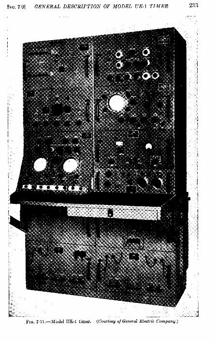
SEC.79] GENERAL DESCRIPTION OF MODEL UE-1 TIMER 233

k------- —- -FIG.7.1l.—Model UE-1timer. (Courtesyof Gened Eleciric Company.)

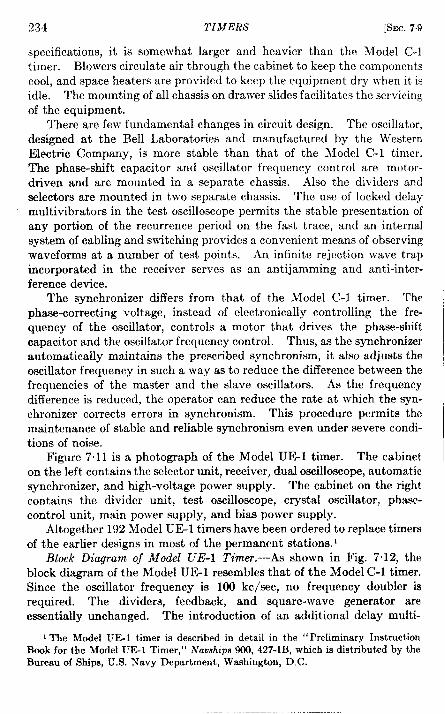
~~~ TIMERS [SEC.7-9

specifications, it is somewhat larger and heavier than the Model C-1timer. Blowers circulate air through the cabinet to keep the componentscool, andspace heaters areprovided tokeep the equipment dry whenit isidle. Themounting ofallchassis ondrawer slides facilitates the servicingof the equipment.

There are few fundamental changes in circuit design. The oscillator,designed at the Bell Laboratories and manufactured by the WesternElectric Company, is more stable than that of the Model C-1 timer.The phase-shift capacitor and oscillator frequency control are motor-driven and are mounted in a separate chassis. Also the dividers andselectors are mounted in two separate chassis. The use of locked delaymultivibrators in the test oscilloscope permits the stable presentation ofany portion of the recurrence period on the fast trace, and an internalsystem of cabling and switching provides a convenient means of observingwaveforms at a number of test points. An infinite rejection wave trapincorporated in the receiver serves as an antij amming and anti-inter-ference device.

The synchronizer differs from that of the Model C-1 timer. Thephase-correcting voltage, instead of electronically controlling the fre-quency of the oscillator, controls a motor that drives the phase-shiftcapacitor and the oscillator frequency control. Thus, as the synchronizerautomatically maintains the prescribed synchronism, it also adjusts theoscillator frequency in such a way as to reduce the difference between thefrequencies of the master and the slave oscillators. As the frequencydifference is reduced, the operator can reduce the rate at which the syn-chronizer corrects errors in synchronism. This procedure permits themaintenance of stable and reliable synchronism even under severe condi-tions of noise.

Figure 7.11 is a photograph of the Model UE1 timer. The cabineton the left contains the selector unit, receiver, duaf oscilloscope, automaticsynchronizer, and high-voltage power supply. The cabinet on the rightcontains the divider unit, test oscilloscope, tryst al oscillator, phasc-control unit, main power swpply, and bias power supply.

Altogether 192 Model UE1 timers have been ordered to replace timersof the earlier designs in most of the permanent stations. 1

Block Diagram of Model UE-1 Timer.-As shown in Fig. 7“12, theblock diagram of the Model UE-1 resembles that of the Model C-1 timer.Since the oscillator frequency is 100 kc/see, no frequency doubler isrequired. The dividers, feedback, and square-wave generator areessentially unchanged. The introduction of an additional delay multi-

1The Model UE 1 timer is described in detail in the “Preliminary InstructionBook for the Model UE-1 Timer,]’ NarJ9hips900, 427-IB, which is distributedby theBareauof Ships, U.S. h’avy Department,Washington,D.C.

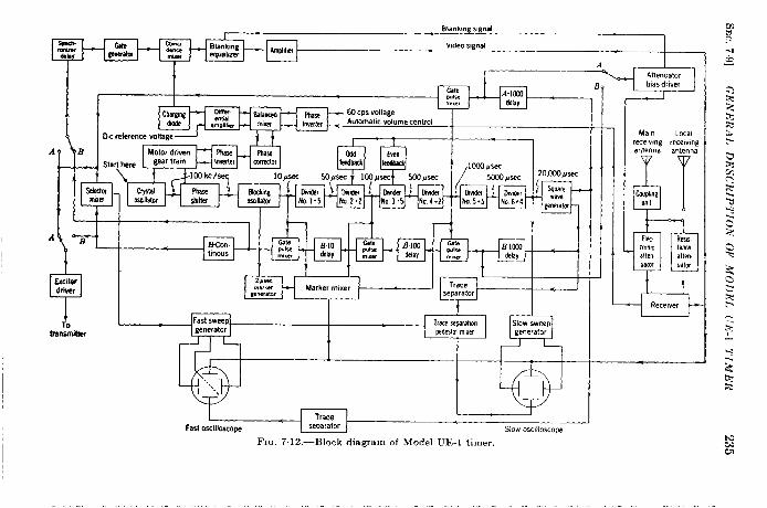
Blankms s,gnal

[

II Al

II,,,,

[EI

;;II

II,,,, In

V,deo s,gnal

1 ~.. r Anenuator I

A.tomahcvolume control

O.c reference voltage_ + i

-LB

1

m

I . ... t— B—

‘1

I‘Fast sweep\ generator

pcvFastoscillosco~ slow Oscilloscope

Ma,n Localrece, vl”g rece,v,,antenna antenn

H

W,nE““,1

!!Tm ResIstromc tamWen. atten.IMto, ua(CJ

FIG. 7.12.—Block dia~am of Model UE-1 timer.

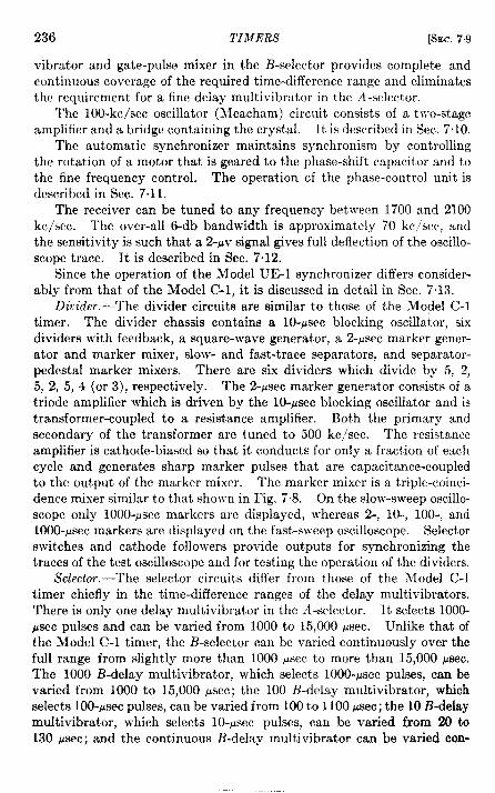
236 TIMERS [SEC. 79

vibrator and gate-pulse mixer in the B-selector provides complete andcent inuous coverage of the required time-di ffcrcnce range and eliminatesthe requirement for a fine delay multivibrator in the A-selector.

The 100-kc/sec oscillator (IVIeacharn) circuit consists of a two-stageamplifier and a bridge containing the crystal. It is described in Sec. 7,10.

The automatic synchronizer maintains synchronism by controllingthe rotation of a motor that is geared to the phase-shift capacitor and tothe fine frequency control. The operation of the phase-control unit isdescribed in Sec. 7.11.

The receiver can be tuned to any frequency between 1700 and 2100kc/see. The over-all 6-db bandwidth is approximately 70 kc/see, andthe sensitivityy is such that a 2-WVsignal gives full deflection of the oscillo-scope trace. It is described in Sec. 7.12.

Since the operation of the Model UE-1 synchronizer differs consider-ably from that of the Model C-1, it is discussed in detail in Sec. 7.13.

Divider.-The divider circuits are similar to those of the Model C-1timer. The divider chassis contains a 10-psec blocking oscillator, sixdividers with feedback, a square-wave generator, a 2-Psec marker gener-ator and marker mixer, slow- and fast-trace separators, and separator-pedestal marker mixers. There are six dividers which divide by 5, 2,5, 2, 5, 4 (or 3), respectively. The 2-~sec marker generator consists of atriode amplifier which is driven by the 10-Psec blocking oscillator and istransformer-coupled to a resistance amplifier. Both the primary andsecondary of the transformer are tuned to 500 kc/see. The resistanceamplifier is cathode-biased so that it conducts for only a fraction of eachcycle and generates sharp marker pulses that are capacitance-coupledto the output of the marker mixer. The marker mixer is a triple-coinci-dence mixer similar to that shown in Fig. 78. On the slow-sweep oscillo-scope only 1000-~sec markers are displayed, whereas 2-, 10-, 100-, and1000-~sec markers are displayed on the fast-sweep oscilloscope. Selectorswitches and cathode followers provide outputs for synchronizing thetraces of the test oscilloscope and for testing the operation of the dividers.

Selector.—The selector circuits differ from those of the Model C-1timer chiefly in the time-difference ranges of the delay multivibrators.There is only one delay multivibrator in the A-selector. It selects 1000-psec pulses and can be varied from 1000 to 15,000 psec. Unlike that ofthe Model C-1 timer, the B-selector can be varied continuously over thefull range from slightly more than 1000 ~sec to more than 15,000 psec.The 1000 B-delay multivibrator, which selects 1000-Psec pulses, can bevaried from 1000 to 15,000 psec; the 100 B-delay multivibrator, whichselects 100-Psec pulses, can be varied from 100 to 1100 ~sec; the 10 B-delaymultivibrator, which selects 10-Psec pulses, can be vaned from Xl to130 ,usec; and the continuous B-delay multi vibrator can be varied con-

SEC. 7.10] MODEL UE-1 OSCILLATOR 237

tinuously from 10 to 21 psec. The selector chassis also contains the biasgenerator for the electronic attenuator, the transmitter-exciter driver,sweep generators, and a selector switch and cathode follower for testing.

Test Oscilloscope.—The test oscilloscope is similar in function to thatof the Model C-1 timer. A system of internal cabling and selectorswitches provides a convenient means of observing the signals at a numberof test points in several chassis. The vertical-amplifier input circuit canbe connected to the oscillator, the dividers, selectors, man external probe.The sweep-synchronizing input circuit can be connected to the dividersor to an external probe.

The vertical deflecting circuits consist of an attenuator that can beswitched in or out, a cathode follower with a gain control, a video ampli-fier, a phase inverter, and a push-pull amplifier that is capacitance-coupled to the vertical deflecting plates and the centering circuits.

Either of two sets of pulses from the square-wave generator, differingin time by 20,000 psec and recurring every 40,000 psec, can be selected tosynchronize the sweep generator. The purpose of the sweep-synchroniz-ing circuits is to permit the observation on a fast trace of signals recurringduring any portion of the main recurrence period of 40,000 psec. This isaccomplished by introducing an adjustable time difference between theinput synchronizing pulse and the initiation of the fast trace. To providecomplete coverage of the whole recurrence period the time difference mustbe adjustable from a little more than 1000 Psec to a little more than21,000 psec. The synchronizing circuits consist of a pulse amplifier, acoarse delay multivibrator, and a fine delay multivibrator. To maintainthe required stability over its wide range, the coarse delay multivibratoris locked on 1000-psec pulses. It can be varied from 1000 to 20,000 psec.The fine delay multivibrator is unlocked and can be varied continuouslyfrom 300 to 1500 psec.

The sweep generator, which is triggered by the fine delay multivibra-tor, generates traces of any one of three speeds ~vhich is selected by aswitch on the panel. The three trace speeds correspond to durations of25,000, 3000, and 160 psec.

7.10. Model UE-1 Oscillator.—The most stable oscillator that hasever been built in quantity is the Model UE-1. The crystal is a GT-cutquartz plate with a low temperature coefficient (approximately 1 partin 107per degree centigrade). It is mounted in an evacuated glass bulbon wire supports that are soldered to its two silver-coated surfaces. Thissupport is rugged and enables the crystal to withstand severe mechanicalshocks without injury.

The crystal unit is contained in a heavy copper tube that is closed atboth ends to ensure uniformity of temperature distribution. The fineheater consists of four heating elements of the bridge which are associated

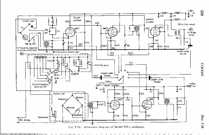
I T (

2/p.J<—

>1—1

+135v

T T05

Isolat,on

n nl ampl,f,er Tt!._AHcrystal

20k oscillator lW k

1006AC7

1k ZZ:##f _—-

c—~+ M,cmfrequency network oven

~_ ——— —— _____ —————— ———.

—115v 6

--$q 3-Coarse frequencyparts per 10° I

I.——. .—— —___

T Mt& k’I &o,5jo,5If’,,I

k

I 1 ! 1s..1 1 L 1 , , L J /

8.2 kCopper oxide

recttl,er

— F,ne frequency

CODH Ox,de

15k

I

d--L-~::~ ‘J 1.5h 0.5 470k 220Ill

SEC.7.10] MODEL UE-I OSCILLATOR 239

with the heater oscillator shown in Fig. 713 and are wrapped around thecopper tube. Although the resistances of two of them vary with tem-perature, the resistances of the other two are independent of temperature.The power supplied to these heating elements by the heater oscillator iscontrolled by the unbalance of the bridge, which in turn depends on thetemperature of the heating elements. Thus the heating power is a con-tinuoudy variable function of the temperature of the copper tube thatencloses the crystal and varies in such a way that it tends to maintain thetemperature at a constant value.

Surrounding the fine heater tube is a glass thermos cylinder closed atboth ends by glass thermos plugs. This insulation minimizes the loss ofheat from the fine heater. The thermos cylinder is enclosed in a coppertube with two end plates around which are wrapped the windings of thecoarse heater, The power supplied to the coarse heater is controlled bya thermal s~vitch mounted on one of the end plates. To minimize loss ofheat and to provide uniform thermal distribution, the coarse heater iswrapped in alternating layers of felt and aluminum foil. The outerhousing is a large chromium-plate brass cylinder.

The 100-kc/sec crystal-oscillator circuit (Fig. 7.13) consists of a two-stage amplifier and a bridge containing the crystal. The first stage is aresistance amplifier of moderately high gain. It is capacitance-coupledto the second stage which is transformer-coupled to the bridge circuit.The primary of the transformer is tuned to 100 kc/see. Negative feed-back is applied from the secondary of the transformer through a filter andthrough a parallel combination of a resistor and a capacitor to the cathodeof the first amplifier tube. The filter is a damped antiresonant circuittuned to 100 kc/see. This negative feedback reduces any tendency ofthe oscillator to oscillate at undesired frequencies.

The output of the amplifier is applied to one terminal of a bridge, theopposite terminal being grounded. The voltage between the other twoterminals is applied through a tuned transformer to the grid of the first~mplifier tube. Two opposite arms of the bridge are resistors whoseresistances are fixed and independent of temperature. Another arm is alamp whose resistance varies with temperature and therefore depends onthe amplitude of oscillation. The fourth arm contains the crystal inseries with a network whose reactance can be adjusted to control the fre -quency of oscillation. Any reactance unbalance of the bridge causes thevoltage impressed successively on the amplifier, on the bridge, andon the crystal to be phased in such a way that the frequency tends toincrease or decrease so that the reactance unbalance is reduced. Thus thereactance introduced in series with the crystal controls the frequency ofoscillation. Some of the power from the amplifier passes through thelamp and thereby heats it and controls its resistance. The resistance

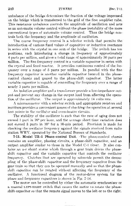
240 TIMERS [SEC.7.11

unbalance of the bridge determines the fraction of the voltage impressedon the bridge which is transferred to the grid of the first amplifier tube.This resistance unbalance controls the amplitude of oscillation and actsas an automatic volume control without the phase instability of the moreconventional types of automatic volume control. Thus the bridge con-trols both the frequency and the amplitude of oscillation.

The coarse frequency control is a selector switch that permits theintroduction of various fixed values of capacitive or inductive reactancein series with the crystal in one arm of the bridge. The switch has tenpositions, each introducing a change in frequency of approximately4parts per million, andgives atotal range of approximately 36 parts permillion. The fine frequency control is a variable capacitor in series withthe crystal and fixed reactor. It provides continuous control of the fre-quency over a range of 5 parts per million. In parallel with the finefrequency capacitor is another variable capacitor located in the phase-control chassis and geared to the phase-shift capacitor. The lattervariable capacitor is capable of controlling the frequency over a range ofnearly 5 parts per million.

An isolation amplifier and a transformer provide a low-impedance out-put and prevent any change in the outpllt load from affecting the opera-tion of the oscillator. The outpllt is approximately 14 volts rms.

A microammeter with a selector switch and appropriate resistors andrectifiers provides a con~-enient means of checking the operation at severaltest points in the oscillator and oven-beater circuits.

The stability of the oscillator is such that the rate of aging does notexceed 1 part in 109 per hour, and the a~-erage short time variation doesnot exceed 3 parts in 109 for a 10-min period. Provision is made forchecking the oscillator frequency against the signals received from radiostation WW, operated by the National Bureau of Standards.

7.11. Model UE-1 Phase-control Unit.—The phase-control chassiscontains an amplifier, phasing circuits, a phase-shift capacitor, and anoutput amplifier similar to those in the !Iodel C-1 timer. It also con-tains an a-c shunt motor which through a gear train drives the phase-shift capacitor and the variable capacitor that controls the oscillatorfrequency. Clutches that are operated by solenoids permit the decou-pling of the phase-shift capacitor and the frequency capacitor from thegear train so that they can be operated manually and so that the phase-shift capacitor can be rotated without affecting the frequency of theoscillator. .k functional diagram of the motor-drive system for thephase and frequency capacitors is shown in Fig. 7.14.

The motor can be. controlled by either the automatic synchronizer ora manual rmrr-mGrm switch that causes the motor to rotate the phase-shift capacitor so that the remote signal moves to the left or to the right.

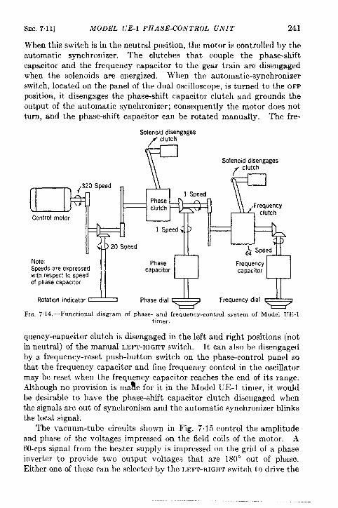
SEC.711] MODEL UE-1 PHASE-CONTROL UNIT 241

When this switch is in the neutral position, the motor is controlled by theautomatic synchronizer. The clutches that couple the phase-shiftcapacitor and the frequency capacitor to the gear train are disengagedwhen the solenoids are energized. When the automatic-synchronizerswitch, located on the panel of the dual oscilloscope, is turned to the OFFposition, it disengages the phase-shift capacitor clutch and grounds theoutput of the automatic synchronizer; consequently the motor does notturn, and the phase-shift capacitor can be rotated manually. The fre-

Solenoid disengages

Solenoid disengages

-,.,-! c. .--.! r Gi5

Note:Speeds are expressedwith respect to speedof phase capacitor

f

20 SpeedTclutch

1 Speed

Phasecapacitor

\\ iFrequency

& Speedr

Frequencycapacitor

TRotation indicator _ Phase dial

*Frequency dial

eFIG. 714.-Functional diagram of phase- and frequency-control system of Model UE-1

timer.

quency-capacitor clutch is disengaged in the left and right positions (notin neutral) of the manual LEFT-RIGHTswitch. It can also be disengagedby a frequency-reset push-button switch on the phase-control panel sothat the frequency capacitor and fine frequency control in the oscillatormay be reset when the frequency capacitor reaches the end of its range.Although no provision is ma!!!e for it in the NIodel UE-1 timer, it wouldbe desirable to have the phase-shift capacitor clutch disengaged whenthe signals are out of synchronism and the automatic synchronizer blinksthe local signal.

The vacuum-tube circuits shown in Fig. 7.15 control the amplitudeand phase of the voltages impressed on the field coils of the motor. AWcps signal from the heater supply is impressed on the grid of a phaseinverter to provide two output voltages that are 180° out of phase.Either one of these can be selected by the LEFT-RIGHT switch to drive the

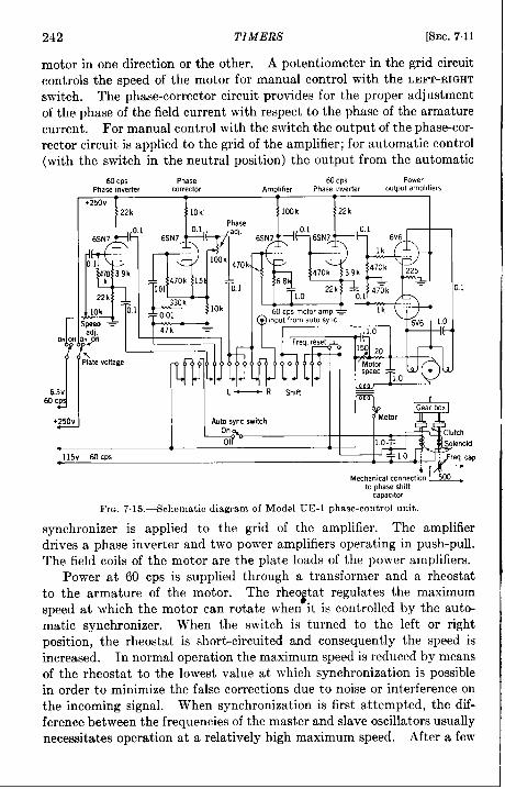
242 TIMERS [SEC.711

motor in one direction or the other. A potentiometer in the grid circuitcontrols the speed of the motor for manual control with the LE~-RIGHTswitch. The phase-corrector circuit provides for the proper adjustmentof the phase of the field current with respect to the phase of the armaturecurrent. For manual control with the switch the output of the phase-cor-rector circuit is applied to the grid of the amplifier; for automatic control(with the switch in the neutral position) the output from the automatic

!!!!0.1

6SN7—.

0.147o 39k

‘;: F’

I o.m6SN7r

!‘Wk470k

470k 1.5

L T]

0.01 0.1

330k10k

~o.ol

60 Cps Phase 60 CP5 PowerPhase ,nverter corrector Ampl#f,er Phase mvetier output ampl, f,ers

+250v22k 10k ; 100k

&?’p:;: 6S,7 ~~ 6SN &’ 6V6~

0.1

!,I

& --y:$+ *:;:7f~m

P Gear box

+250v A.to sync switch Motor

On*

off

115V 60CPS

to phase sh(ftca pac,tor

FIG. 7.15.—Schematic diagram of Model UE-1 phase-control unit.

synchronizer is applied to the grid of the amplifier. The amplifierdrives a phase inverter and two power amplifiers operating in push-pull.The field coils of the motor are the plate loads of the power amplifiers.

Power at 60 cps is supplied through a transformer and a rheostatto the armature of the motor. The rheo~tat regulates the maximumspeed at which the motor can rotate when it is controlled by the auto-matic synchronizer. When the switch is turned to the left or rightposition, the rheostat is short-circuited and consequently the speed isincreased. In normal operation the maximum speed is reduced by meansof the rheostat to the lowest value at which synchronization is possiblein order to minimize the false corrections due to noise or interference onthe incoming signal. When synchronization is first attempted, the dif-ference between the frequencies of the master and slave oscillators usuallynecessitates operation at a relatively high maximum speed. After a few

SEC.7.12] MODEL UE-1 RECEIVER 243

minutes of operation the maximum speed can be reduced. In this waythe advantages of the automatic synchronizer and also the high precisionof the crystal oscillator are retained.

7012. Model UE-1 Receiver.—The receiver, which is of the super-heterodyne type, is designed to operate at a single frequency. By meansof screwdriver controls, however, the tuning can be adjusted to any fre-quent y between 1700 and 2100 kc/see. The tuning dial provides front-panel adjustment of the tuning over a range of ~ 80 kc/see. The over-allbandwidth is approximately 70 kc/see as measured at 6 db below peakresponse. The sensitivity is such that a Z-p signal gives full deflectionof the trace on the cathode-ray tube.

As shown in the schematic diagram (Fig. 7.16) there are four tunedstages of preelection before the converter, providing an i-f and image-rejection ratio of more than 60 db and four stages of i-f amplificationoperating at 1100 kc/see.

The remote signal (along with other signals) from the electronicattenuator of the switching equipment (Sec. 84) is impressed on the gridof the final stage of electronic attenuation, which functions as an amplifierexcept for a short period of time during which the local signal is trans-mitted. The local signal from the resistance attenuator of the switchingequipment is passed through a resistance attenuator in the receiver andmixed with the signal from the electronic attenuator. The potentiometerin the resistance attenuator controls the amplitude of the local signal andis used to equalize the local and remote signals as they appear on the fastand slow oscilloscopes.

There are several devices for reducing the effect of interference causedby enemy jamming, undesired signals, and random noise. A wave trapof the infinite-rejection type in the plate circuit of the r-f amplifierintroduces an attenuation of 50 db or more over a narrow band of fre-quencies. A control mounted on the front panel permits the tuning ofthe wave trap to any frequency between 1700 and 2100 kc/see. It iseffective in reducing interference produced by jamming or by radiosignals of frequencies close to the frequency of the Loran signals. Therejected band is so narrow that the wave trap can be tuned to the Loranfrequency without distorting the shape of the signal beyond usability.A wave trap in the plate circuit of the first i-f amplifier serves a similarfunction in reducing interference from signals of the intermediatefrequency.

The r-f gain potentiometer controls the positive bias of the cathodesof the r-f amplifier and the first and second i-f amplifiers. The grids ofthe third and fourth i-f amplifiers are maintained at a positive potentialof approximately 120 volts, and the cathodes are connected to the plate ofa pentode that serves as a gain control and as an automatic volume con-

Remote ant Local ant,m Electronic attenuator ~ Tuner R.f ampl, her Converter 1s1 i f amphf,er 2nd I I ampl!f,er 3rd I f ampl,f,er 4th I f ampl,fter

T ,300 v ~ +300V1 T T

1.mtmuatormasOr,ver Local oscillator 10IIO!W, V,deoampl,f,er F(lter

+300 vDemod. tator Synchronizer AVC Rece,.er AVC

output .3(KIVI [ , . . .

I

~ 1 1 1 IIIL I 1 1

‘v’,“

~ ~’== 11/1.

loo/pf20

510#/lf ., ~F, n“. >W,,.!,

6Nme b,as control

Aller, uato,.b,a~ Phones V,deo to osc(lloscopcs AVC b,as tofm.m selector and synch mmzer synchronizer

FIG. 7.16.—Schematic diagram of Model UE-1 receiver.

SEC. 7.13] MODEL UE-1 SYNC II ItO,VIZIiR 245

trol. The cathode of the AVC pcntode is grolmdccl, and the potential ofthe screen grid is controlled by the i-f gain potentiometer. The .AVCselector switch hos four positions.” In the OFF position the grid of theAVC pentode is grounded; in the other thrrc positions negative signals,resulting from the rectification of the o{[tput of the final i-f amplifier, areapplied to the grid of the AV(; pcntode, and vurious capacitors are intro-duced in the plate circuit to provide three different AVC time constants.

When, in normal operation, the AVC switch is in the OFFposition, itgrounds the grid of the AVC pcntode, rind the cathodes of the i-f amplifierstend to follow the grids. The cathode-biasing resistance is dependentupon the d-c plate resistance of the Ai’C pentode thtit is controll~d bythe i-f gain potentiometer. With the AVC slritrh on one of the otherpositions, the d-c plate resistance of the AJ”[I pentodc is determined bythe negative rcctifkd signal. The plate resistonm is lolv cxrrpt dllringbursts of noise, Jvhen the pcntode current is cut o~~. The (!:Lthodcs of the

i-f amplifier then rise to the peak grid voltages and remain :~t :1 positivepotential with respect to the grids until the AJ”C pentodc again conductsand discharges the plate capacitor.

The video mnplificr p:wses signals of frcquenrirs Imtirmn 500 rps and40 kc/see. A high-pass filter, Jvhich xttcnlmtes vidro sign:lls of frc[j~len-cies below 2 kc/see, is helpful in reducing sonw types of intcrfcrcmce,

A portion of the video signal is rectitimt and mixed !rith tlw normalAVC voltage and is applied to the grids of the balanced mixer in theautomatic synchronizer to paralyze the automatic synchronizer duringbursts of noise.

7.13. Model UE-1 Synchronizer.—;kt the sh~~e station the rcvnotesignal on the A-trace precedes the local signal on thr B-trace i)y a pre-determined time difference (ordinarily 1000 pwc) pl(w hidf the recurrenceperiod. The operator adjusts the .4- and B-selwtors to give the pre-determined time difference between the initiations of the fost A- :mdB-traces and verifies the adjustment by means of calibration markers.Although the pulse that drives the local transmitter exciter occurs at thestart of the fast B-trace, the local signal as it appetirs on the f:~st B-traceis displaced to the right because of the time delays in the transmission

and receiving circuits. The remote signal on the i-trace is also delayedby the receiving circuits. When on the fast traces the remote signal issuperimposed on the local signal, the time difference between the initia-tion of the A-trace and the rise of the remote signal equals and cancelsthe time difference between the initiation of the B-trace and the rise ofthe local signal. Thus the measured time difference between the initia-tions of the fast .4- and B-traces accurately represents the time differencebetween the reception of the signal from the remote transmitter and thereception (not the initiation) of the signal from the local transmitter.

246 TIMERS [SEC. 7.13

Although the A- and B-selectors are sufficiently stable to maintain forseveral hours the proper time difference between initiations of the twofast traces, an infinitesimal difference in the frequencies of the local andremote crystal oscillators causes the remote signal on the A-trace todrift to the right or to the left of the local signal on the B-trace. Thepurpose of the automatic synchronizer at the slave station is to hold theremote signal in a position directly above the local signal.

As shown in the block diagram (Fig. 7.12) a delay multivibratorcontrols the position of a gate on the A-trace. The gate is mixed withthe video signal from the receiver, and the output charges a capacitorthrough a diode. The charge delivered once every recurrence period tothe capacitor is proportional to the average amplitude of the remote signalfor the duration of the gate. The resulting sawtooth voltage is appliedto the control grid of one pentode of the differential amplifier; a d-cvoltage is applied to the grid of the other pentode. The two outputs ofthe differential amplifier supply the screen voltages of the two” pentodesthat form the balanced mixer. Two 60-cps out-of-phase signals from aphase inverter are applied to the control grids of the balanced mixer.The output is applied through a phase corrector and through a phaseinverter to the field coils of the a-c motor in the phase-control chassis.The motor drives the phase-shift capacitor in such a way that the remotesignal appears to seek that position on the A-trace at which the gate liesa third of the way up the leading edge. hfore accurately, the timingof the fast traces and the transmission of the local signal with respect tothe remote signal are so controlled by the automatic synchronizer thatthe gate seeks a position a third of the way up the leading edge of theremote signal.

A milliammeter located on the panel of the dual oscilloscope indicatesthe degree of unbalance of the differential amplifier. When the unbalancecorresponding to the error in synchronism exceeds a certain limit, analarm buzzer sounds and the local transmission is blinked to indicate tousers of the signals that the signals are improperly synchronized.

At the master station, the local signal on the A-trace precedes theremote signal on the B-trace by a predetermined time difference ofhalf the recurrence period plus the coding delay plus twice the timerequired for a radio signal to travel from one station to the other. Thedelay circuit of the automatic synchronizer is initiated at the start of thefast B-trace and is so adjusted that the gate lies a third of the way up theleading edge of the remote signal when on the fast traces the local signalis superimposed on the remote signal. The automatic-synchronizerswitch is turned off; this grounds the synchronizer output and disengagesthe clutch between the motor and the phase-shift capacitor. In thiscondition, the automatic synchronizer sounds the warning buzzer and

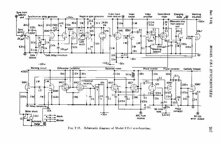
v

control

-105V -105I—

L 1 J12k -30v

-50 v— IWarmngcwculf Oifferentlal ampl,f,er Balancedmixer

~h,w+,e ,O,rectorCathodefollower

+254)v1

36k i! !10k 36k + 0.6 14hyll 48k 10k 10k n 1. T

10.8k 390

!1!1

L 390.5 k

= Relay sensmwtv, .m— d) ‘-le;ei”~ correctorv AvCfrom 6.3v a’c &

.5aCps.receiver error output

I L m@f*r?11FIG, 7.1 7.—Schematic diagram of Model UE-1 synchronizer. g

-1

248 TIMERS [SEC.713

blinks the local transmission when the signals are incorrectly synchron-ized, but it does not directly control the synchronization.

The schematic diagram of the automatic synchronizer is shown inFig. 7.17. At the slave station the synchronizer delay multivibrator isinitiated by the pulse from the gate-pulse mixer of the A-selector; at themaster station it is initiated by the pulse from the final gate-pulse mixerof the B-selector (because the pulse from the gate-pulse mixer is morestable than that from the continuous B-delay multivibrator). Thetrailing edge of the pulse from the delay multivibrator is differentiatedto cut off the current through an amplifier and produce a positive flat-topped pulse, or gate, of approximately 10-psec duration. This pulse 1sinverted in another amplifier whose plate is connected to the cathodeof the gate-video coincidence mixer. Thus, the cathode of the coinci-dence mixer, ~~'hichisnormally atthcpotential of the B-supply, isdri~~ento approximately ground potential for the duration of the gate. Thevideo signal is impressed on the control grid of the mixer. The plate ofthe video mixer, which is normally at the potential of the B-supply, isdriven toward g-round potential by the action of the gate on the cathodeand by the action of the video signal on the grid. The change of platepotential depends on the amplitude of the video signal.

To reduce the noise and increase the rate of rise, the lower third ofthe video signal is eliminated and the top is flattened in a negativelybiased amplifier that is driven to saturation. In normal operation thegate is located on the steep leading edge of the amplified and limitedremote signal. This signal is mixed in the blanking equalizer with asignal derived from the attenuator bias and is applied to the control gridof the gate-video coincidence mixer. .it a double-puked station theattenuator is controlled by two timers operating at two recurrence rates.Consequently the remote signal as observed at either recurrence rate (onthe oscilloscope of either timer) is periodically eliminated. Since thedifference in recurrence periods is 100 psec and at the low basic recurrencerate the recurrence period is approximately 40,000 psec, the difference inthe timing of the two signals is repeated every 400 periods, or every 16sec. As an observer watches the slow-trace pattern, he sees a section ofthe trace from which the video signals have been eliminated movearound the slow-trace pattern and then complete the circuit and eliminatethe remote signal once every 16 sec. A signal of adjustable amplitudederived from the attenuator bias is introduced during the blanking periodto compensate for the elimination of the remote signal and in this way tomaintain proper synchronism.

The negative output pulse from the coincidence mixer charges acapacitor through a diode. The charge leaks off with a time constant of7500 psec, considerably less than the recurrence period of the remote

SEC.7.14] GENERAL REQUIREMENTS 249

pulse, and the voltage resulting from the charge on the capacitor is appliedto the control grid of one pentode of the differential amplifier, The con-trol grid of the other pentode of the differential amplifier is maintainedat an adjustable d-c negative potential. When the local and remotetimers are in proper synchronism with no difference in the oscillator fre-quencies, the gate lies approximately a third of the way up the leadingedge of the remote pulse. The average potential on the charged capacitorand one control grid then equals the d-c potential on the other controlgrid, and the differential amplifier is balanced. A slight difference in theoscillator frequencies causes the remote signal to drift to the left or rightwith respect to the gate. Consequently the output of the coincidencemixer rises or falls with a corresponding change in the average potentialof the charged capacitor and with a corresponding unbalance of the differ-ential amplifier.

The two outputs of the differential amplifier supply the screen voltagesfor the two pentodes of the balanced mixer. Two equal 60-cps out-of-phase voltages from a phase inverter are impressed on the control gridsof the balanced mixer. The plates are connected in parallel to an anti-resonant plate load so that the phase and amplitude of the M)-cps outputsignal is controlled by the relative balance or unbalance of the screenvoltages of the balanced mixer. The screen voltages depend on the poten-tials of the control grids of the differential amplifier. During b{trsts ofnoise the outp~lt of the balanced mixer is reduced by the action of thereceiver automatic volume control on the bias of the balanced mixer,

By means of the phase corrector, the phase of the 60-cps output signalcan be adj~lsted in relation to the phase of the current in the armature ofthe synchronizing motor to give maximum torque. .1s described inSec. 7 11, the 60-cps output signal is applied to the field coils of the syn-chronizing motor and therefore controls the rotation of the phase-shiftcapacitor and the frequency capacitor.

LOW FREQUENCYTIMER

7.14. General Requirements.-.ks explained in Chaps. 3 and 5, a LowFrequency Loran system operating at 180 kc/see has several advantagesas compared with Standard Loran. The ground-wave ranges over bothland and sea are greatly increased, and the factor of geometrical precisionUIis better because of the greater length of the baseline over which it ispossible to synchronize the ground stations.

Simultaneous Fixing.—.4s explained in See. 3.8, the importance ofsimultaneous fixing (the measurement of two time differences simultane-ously) for air navigation, for homing to an airport, and especially foraerial bombing has been clearly demonstrated. Because of the rapidmotion of an airplane it is imperative that the navigator be able to obtain

250 TIMERS [SEC.7.14

a fix as rapidly as possible. In bombing by Loran it should be possiblefor the navigator or bombardier to set the delay controls to the pre-determined time differences of the target, fly along one line of position,and release the bombs when the signals corresponding to the other lineof position move into coincidence. In homing to an airport, especially incongested areas, it should be possible for the navigator to apply the sametechnique. This cannot easily be done with pairs at two recurrence ratesbecause the indicator would be too complex. Simultaneous fixingbecomes practical when three ground stations, a master and its twoslaves, operate at a single recurrence rate and the signals from any onestation are everywhere distinguishable from the signals from any otherstation.

The LF stations are now operated in accordance with these require-ments. The master station transmits signals at double the normal recur-rence rate. One slave station (operating at the normal recurrence rate)is synchronized with one series of alternate pulses from the master station,whereas the other slave station is synchronized with the other series ofalternate pulses. The sequence of pulses as observed at the master andslave stations is shown in Fig. 7.18. One series of alternate pulses Xtransmitted at the master station is distinguished from the other series ofpulses Z by an identifying “ ghost” series of pulses X’ which is shifted inphase by 1000 psec and appears fainter than the normal series of pulsesbecause its recurrence rate is only a third of the normal recurrence rate.The other two series of pulses W and Y are transmitted by the two slavestations at the normal recurrence rate and are therefore normal inappearance.

This system provides three families of time-difference readings andthree corresponding families of lines of position. With Standard Loranindicators, time differences can be measured between signals Z and Y,signals X and W, and signals W and Y. The intersection of any two ofthe corresponding lines of position establishes a fix.

Although the operation of the three ground stations on a single recur-rence rate necessitates little modification of the timers at the slave stations,it requires several modifications of the timers and operational procedureat the master station. Since the Z-pulse is required to follow the X-pulseby precisely one-half of the normal recurrence period, one timer, themaster timer, is used to trigger the transmitter at double the normalrecurrence rate and also to monitor the timing of the signal from one ofthe slave stations. Another timer, the monitor timer, is used to monitorthe timing of the signal from the other slave station. The oscillatorof the master timer provides the 50-kc/sec signal for the monitor timer;consequently both operate at the same frequency, and the locally trans-mitted signals observed on the monitor timer do not drif~.

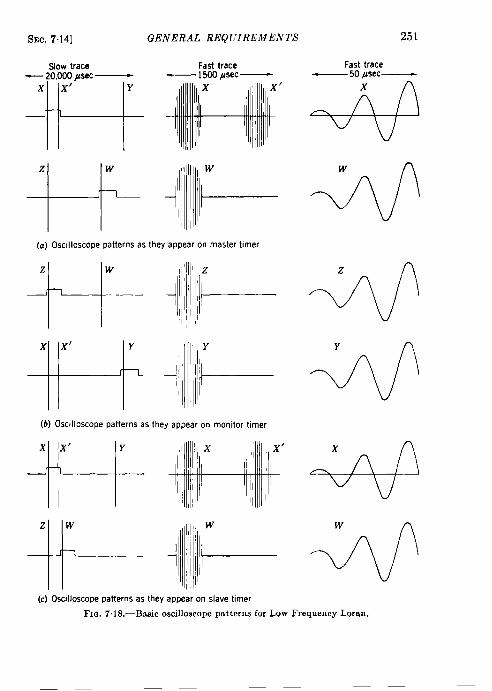
SEC. 7.14] GENERAL REQIJIREMENTS 251

Slow trace Fasttrace Fasttrace— 20,000psec— —1500psec— — 50~sec—

H

x x’ Y /

*

x

i-+

z w

–i L(a) Oscilloscopepatterns as they appear on master t,mer

w II

z w Iz

{ , “i~+

H

x x’ Y

- I I k

(b) Oscilloscope patterns as they appear on monitor timer

%1--1-

x x’ Y ,

+1----

Zw

; L

(c) OscdloscopePatternsastheyappearonslavetimerF1c+.7.18.—Basicoscilloscopepatternsfor LIJW

4z

4Y

-@

x

Nw

Frequency Loran.

252 TIMERS [SEC.7.14

Because of the low frequency and the relatively narrow bandwidthsof the transmitting and receiving equipment, there is a delay of 150 psecor so between the triggering of the transmitter and the rise of the receivedlocally transmitted signal. This delay necessitates the introduction of atime delay between the triggering of the transmitter and the initiationof the two fast traces. For the same reasons the received pulse risesS1OW1V. This makes the accurate measurement of time differences diffi-.cult. In an effort to improve the accuracy of time-difference measure-ments, the technique of matching i-f cycles of the remote and local signalshas been adopted.

Cycle-mutching Technique .—The unrectified i-f (50-kc/see) signal fromthe receiver is impressed on the vertical deflecting plate of the cathode-raytube so that the individual cycles of the local signal can be superimposedon those of the remote signal. Although there is some difficulty indetermining with certainty the proper cycle of one signal to be matchedwith a particular cycle of the other signal, the cycle-matching techniqueis capable of extremely accurate measurement of time differences whenthe proper correspondence of cycles has been established. With reason-able values of signal-to-noise ratio the cycle-matching technique seemsto be capable of time-difference measurements with probable errors ofapproximately =’T psec. The cycle-matching receiver is discussed indetail in Sec. 12.2. One-microsecond markers have been added to thetimers in order to take advantage of the improved timing accuracyoffered by the cycle-matching technique.

Communication by Blinking. —Because of the difficulty of establishingthe proper correspondence between the i-f cycles of the local and remotesignals, communication between the master and slave operators isrequired. In addition to the motor-operated blinking that is used toindicate incorrect synchronism, manual control of the blinking is providedfor communication bet ween the master and slave operators. A simpleblinking code permits the master operator to instruct the slave operatorto advance or retard the timing of the slave transmissions by the requiredinterval of time and also permits the slave operator to acknowledge themessage.

At the slave station the operator superimposes the cycles of theremote signal on those of the local signal, selecting with some uncer-tainty the appropriate correspondence between cycles. As explainedin Sec. 12.2, because of the irregular time difference (213+ 8 + L/2)between local and remote signals, the operator at the master stationcannot match cycles of the local and remote signals. Instead, he matchesthe envelopes. But, knowing the correct value of 2(3 + J + L/2 andcomparing it with the measured time difference between the local andremote signals, he can judge whether or not the synchronism is correct.

I

SEC. 7.15] BLOCK DIAGRAM OF LOW FREQUENCY TIMER 253

If necessary he advises the slave operator to advance or retard the timingat the slave station by 5.5 psec (one cycle at the radio frequency of180 kc/see). For the purpose of adjusting the synchronism at the slavestation and of adjusting the timing of the transmitter-trigger pulse inrelation to the r-f cycles, a variable time delay is introduced between theselector output pulse (which normally triggers the transmitter) and theoutput pulse from the exciter driver. At the master station this timedelay is maintained at a fixed value.

Because the phase of the i-f cycles of the receiver depends on thephase of the signal from the local oscillator as well as the phase of thereceived r-f signal, a highly stable local oscillator is required. For thispurpose a 50-kc/sec signal from the crystal oscillator of the timer isconverted in the receiver to produce a 130-kc/sec heterodyne signal.This beats with the r-f signal to produce an i-f signal of 50 kc/see.

Since the stability required for the cycle-matching technique cannotbe achieved with the type of pulsed transmitter used for Standard Loran,an oscillator-amplifier type of transmitter is used for LF Loran. A50-kc/sec c-w signal from the timer is required to control the phase andfrequency of the locally transmitted signal. It is converted in thetransmitter to the pulsed r-f signal.

The automatic synchronizer is not sufficiently stable for maintainingsynchronism in the LF Loran system. All synchronizing and monitoringoperations are, therefore, manually controlled.

7.15. Block Diagram of Low Frequency Timer.—A block diagramof the Model C-1 timer as modified for service at an LF Loran groundstation is shown in Fig. 7“19. The modified timer can be used at eithera master or a slave station. At a master station it can function as amaster timer to trigger the transmitter at double the normal recurrencerate and to monitor the timing of the signals from one of the slave sta-tions, or it can function as the monitor timer to monitor the timing of thesignals from the other slave station. The function of the slave timer isto trigger the local transmitter at the normal recurrence rate and inproper synchronism with the appropriate signal from the master station.

Crystal Oscillator.-The monitor timer does not control the transmis-sion of either of the two local signals X and Z. To prevent the driftingof the master and slave signals as they appear on the oscilloscope of themonitor timer, the master and monitor timers are driven by a singleoscillator, and therefore the phase shifter of the monitor timer, insteadof being connected to its oscillator, is connected through a switch to the50-kc/sec driver of the master timer.

50-kc/Sec Driver.—The phase-shifted 50-kc/sec signal from the timeroscillator must be supplied to the cycle-matching receiver in which it isconverted to the 13@kc/sec heterodyning signal. When the timer

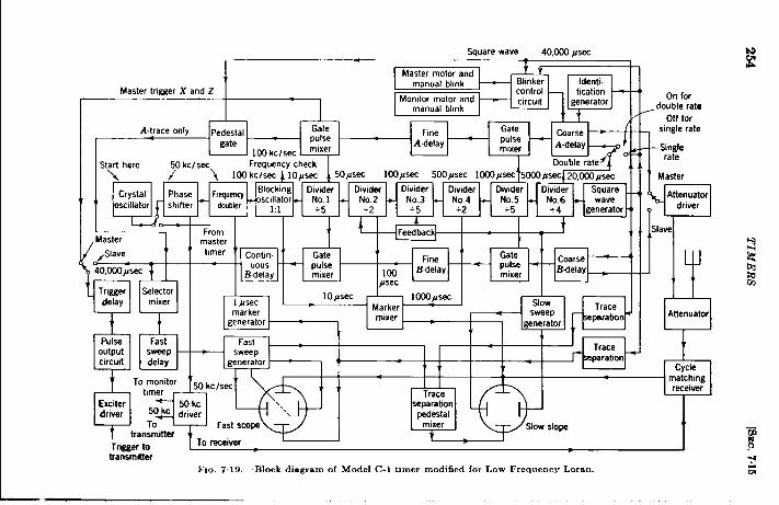
‘A /

LlqCrystal Phas~osmllator shlfte

laster

Squarewave 40,000psecsI

8+: &~~:“‘;:6’‘ ‘+-+Pulse

D

Fast Fastoutput sweep sweep

Trace

circuit delay generatorparation

To mondor

Cycle

50kc/seematching

timer Tracereceiver

Esciter 50 kc eparahon‘.driver 50 kc dfiver ‘.

Topadestal

Fast scope mixertransmitter

slow slope

Trigger to To receiver

transmitterFIG. 7.19.—Block diagram of Model C-1 timer modified for Low Frequency Loran.

sac?.7.15] BLOCK DIAGRAM OF mw FREQUENCY TIMER 255

operates as a master or a slave, the 50-kc/sec signal is also supplied tothe transmitter in which it is converted to the puked 180-kc/sec r-fsignal. When the timer operates as a master, the 5@kc/sec signal issupplied to the phase shifter of the monitor timer. A driver consistingof a tuned amplifier with a low-impedance output supplies the 50-kc/secsignal for these three purposes.

Because of the increased precision offered by the cycl~matchingtechnique, I-psec markers have been added to the calibration system.They provide a calibration scale with which it is possible to estimatetime differences with a probable error of approximately 0.1 psec.

Transmitter Trigger.-When the timer functions as a master, theoutput pulse from the A-selector triggers the transmitter. Consequentlythe A-selector of the master timer is triggered at double the normalrecurrence rate by the pulse from the last divider. The A-selector of themonitor timer is triggered at the normal recurrence rate by the pulsefrom the square-wave generator.

When the timer functions as a slave, the output pulse from the B-selector triggers the transmitter, and both the A- and B-selectors aretriggered at the normal rate by the pulse from the square-wave generator.

The master operator monitors the timing of the slave signal and, asnecessary, instructs the slave operator to advance Or retard by one r-fcycle the timing of the slave signal. On the slave oscilloscope the i-fcycles of the remote signal are superimposed on those of the local signal.Therefore the slave operator must be able to shift as instructed the timingof the transmitter-trigger pulse. For this purpose a calibrated delaymultivibrator is inserted ahead of the exciter driver. The slave operatornormally adjusts it to give a delay of 10 Ksec. On instruction from themaster operator, the slave operator can advance or retard the slave signalone r-f cycle with respect to the normal timing. At the master stationthe multivibrator is set and maintained at a fixed minimum delay.The calibrated delay multivibrator can also be used to adjust the timingof the transmitter-trigger pulse with respect to the r-f cycles.

Triggering of Fast-sweep Generator.—When the timer functions as amaster timer, the .4-selector is triggered at double the normal recurrencerate and the B-selector is triggered at the normal recurrence rate. How-ever a single fast A-trace and a single fast B-trace are required. Theoutput pulse from the A-selector (corresponding to the Z-signal) on thelower trace is therefore suppressed. This is accomplished by a pentodeamplifier (the pedestal-gate circuit) which passes the output pulse fromthe .4-selector to the selector mixer. The suppressor grid of the pentodeamplifier is controlled by a signal from the square-wave generator, andhence the pentode amplifier is nonconducting for the duration of thelower slow trace.

256 TIMERS [SEC. 715

Since there is a delay of approximately 150 psec between the triggeringof the transmitter and the rise of the local signal as it appears on thetimer oscilloscope, a corresponding delay must be introduced betweenthe triggering of the transmitter and the initiation of the fast A- or B-traceupon which the local signal appears. It is convenient to delay equallythe initiation of both the fast A- and B-traces with respect to the outputpulses of the A- and B-selectors. For this purpose the circuits have beenmodified by the addition of a delay multivibrator between the mixerand the fast-sweep generator. The delay multivibrator is continuouslyvariable from 50 to 300 psec.

lden~ijication Blinker.-.&s explained in Sec. 7.14, one series of alter-nate signals X transmitted by the master station must be distinguishablefrom the other series of alternate pukes Z. The distinguishing featl~reis an identifying ghost signal which is displaced slightly to the right ofand is less bright than the X-signal.

In order that this identification be achieved, e~-ery third X-pulse isdelayed by 1000 ~sec and appears on the slow tram in position X’ ofFig, 718. The identification is recognizable on the fast truce by thehorizontal line that passes through the base of the X-pulse (because everythird X-pulse is missing).

The identifying shift of timing is accomplished by means of a multi-vibrator that has a division ratio of 3/1 and a long cycle of operation(approximately 120,000 psec). The multivibrator is triggered by everythird positive pulse from the square-wave generator. The output signalis applied through a pentode amplifier to the bias of the coarse A-delaymultivibrator and is adjusted in amplitude to shift the delay by 1000psec once with every third recurrence of the X- (or X’-) pulse.

The identifying shift of timing is required only for the X- (and X’-)pulse on the upper trace, not for the Z-pulse on the lmver trace. There-fore the signal from the square-wave generator is applied to the suppressorgrid of the pentode amplifier so that the phase-shifting signal is eliminatedfor the duration of the lower trace,

Communication Blinker .—Pro~-ision must be made for two differentblinker functions. At the master station independent controls of themotor blinker (indicating incorrect synchronism) for both the master

X- and Z-pulses must be provided. .\lso, iudepen(lent controls of the

manual blinker (for communication between master and slave operators)

for both master pulses are required. iitthe sla~-r station the two blinkerfunctions are simpler (because only one pulse mllst be blinked) and thesame circuits are applicable.

The motor blinker shifts the timing of the local sigmd by 2000 ~secfor approximately ~ sec every second. .k cam, rotated by a synchronousmotor, operates a switch with a period of 1 sec. The switch controls

!EC.7.15] BLOCK DIAGRAM OF’ LOW FREQ UENCF TIMER 257

~he bias potential of the coarse A-delay multivibrator and by means ofthis controls the timing of the A’- and Z-pulses. The switched biaspotential is applied to the delay multivibrator through two pentodeamplifiers acting in parallel. One of the two signals (which are 180° outof phase) from the square-wave generator is applied to the suppressorgrid of one of the pentode amplifiers to permit the blinking of the X-pulsesonly. The other square-wave signal is applied to the suppressor grid ofthe other amplifier to permit the blinking of the Z-pulse only.

The manual blinker permits the independent keying of either of thelocal signals (by a shift in timing of 2000 psec) for the transmission ofsimple dot-dash messages to the slave operator. Two push-buttonswitches control the bias of the coarse A-delay mu]tivibrator, The sametwo pentode amplifiers that control the motor-switched blinker bias alsocontrol the manual blinker biw. These manual push-hlltton controlsare independent of each other and independent of the motor-blinkercontrols.

CHAPTER 8

SWITCHING EQUIPMENT

BY R. H. WOODWARD

8.1. General Requirements.-The Loran technique of measuring thetime difference between the arrivals of two pulsed signals requires anoscilloscope presentation in which a fast trace showing one pulsed signalappears directly above a similar fast trace showing the other pulsed sig-nal. It must be possible to time the fast traces so as to make one signalappear directly below the other. Both signals as they appear on theoscilloscope must be of the same amplitude. These requirements aresimple in principle, but it is difficult to comply with them at a Loranground station because the signals to be compared differ so greatly instrength. The local transmitter produces signals in the receiving antennathat may be some 140 db greater than the signals from the remote sta-tion, It is necessary, therefore, to attenuate the local signal and toamplify (or pass unattenuated) the remote signal so that the local andremote signals as they are impressed on the inputs of the receiver areapproximately equal; the final exact equalization is accomplished in avariable resistance network in the first stage of the receiver. Since thepurpose of comparing the two signals is to measure their time differenceaccurately, the attenuator must not produce any appreciable delay ordistortion of the local signal.

The local and remote signals that are induced on the receiving antennapass through a coupling unit and a transmission line to the attenuatorand receiver, The signals are delayed and their shapes are slightlyaltered by the action of the antenna, the coupling unit, and the trans-mission cable. The delay and distortion of the signals depend on the Qof these circuits. A local signal is also induced on the interconnectingcables and on the po~ver lines. This local signal and the remote signalare induced at different locations and (as they appear at the attenuatorinput) are delayed and distorted in different amounts. If the localsignal induced on the cables and po~ver lines reaches the receiver inputin sufficient strength to cause a deflection of the oscilloscope trace, itcauses an error in the time-difference measurement, and, therefore, itmust be eliminated.

The easiest ~vay of providing adequate shielding is to enclose theattenuator and the timers in a doubly shielded room. Power is supplied

258

sac. 8.1] GENERAL REQUIREMENTS 259

to the equipment in this room through an isolatlon transformer thateliminates any r-f signals picked up by the power lines. All cables thatenter the room pass through a metal box which serves as a commonground for both the inner and the outer shields of the room and for theshields of all the cables that enter the room.

It would be difficult to design an attenuator that would pass or amplifythe remote signal and attenuate the local signal from the receiving antennaby a large constant ratio without causing delay and distortion. Itis easier to attenuate the local signal from the main antenna so thoroughlythat the receiver’s output is negligible and simultaneously to introducea weak local signal of suitable strength from another local source. Thiscan be a short ineffic ent antenna or a dividing network of resistancesthat bypasses the attenuator and allows a suitable fraction of the localsignal to reach the receiver.

The i-eceiver has two inputs, one for the remote signal and one forthe local signal, and these signals travel through different channelsto the receiver. The remote signal is induced in the receiving antennaand passes through the coupling unit, the transmission cable, and theattenuator to the remote-signal input of the receiver. If the local signalis induced on a short antenna, it passes through a transmission cable tothe local-signal input of the receiver. If the local signal is obtained fromthe receiving antenna, the strong local signal induced on the receivingantenna passes through the coupling unit, the transmission cable, anda passive attenuating network to the local-signal input of the receiver.

If the receiving antenna is not used as the source of the local signal,it is convenient to limit the positive and negative r-f peaks of the localsignal at the receiving antenna by means of two gas-filled tubes associatedwith the coupling unit. When the local transmitter sends out a puise,a discharge takes place in these gas-filled tubes that results in attenua-tion of the local signal from the receiving antenna. Because such limit-ing tubes distort the local signal, a local signal from another sourcemust be provided for the measurement of the time difference. The useof two separate antennas for the remote and local signals, however, is asource of possible error in timing because of the different locations ofthe antennas and because of possible differences in the delays and dis-tortions introduced by the circuits of the two channels. The timinguncertainty is especially serious when a Beverage wave antenna (Sec.104) is used to receive the remote signal since a separate antenna mustbe used to receive the local signal. The use of a single vertical receivingantenna and a passive attenuating network to provide both the remoteand local signals is preferred, therefore, when possible, even though theproblem of attenuating an unlimited local signal is more difficult.

The attenuator is controlled by the timer and switches the remote-

260 SWITCHING EQUIPMENT [SEC. 8.1

s.gnal input of the receiver alternately to the receiving antenna and toground. In the early models the attenuator consists of two relays. Inthe later models it consists of two or more stages of amplification. Thebias of the amplifiers is driven to a large negative potential during thetransmission of the local signal.

At a station transmitting at a single recurrence rate, there are twotimers and two tmnsmitters. The duplication assures continuous serv-ice’ and facilitates maintenance of equipment. At a double-pulsedstation there are four timers and two transmitters. Each transmitterhas two exciter units and a pulse mixer, so that it can be controlled by~]-.-o timers ar -i transmit at two recurrence rates at the same time. Totake tG“ advantage of the duplication of equipment, provision must bemade for switching connections between the different transmitters andtimers. This additional switching equipment is also housed in theshielded room.

The switching equipment used with timer Models A, B, and B-1 isprimitive. The switching is accomplished by disconnecting cables fromone set of terminals and connecting them to another. The attenuatorconsists of two relays connected in series between the receiving antennaand the receiver and controlled by the timer. For attenuation the cir-cuit between the receiving antenna and the receiver is opened at eachrelay and the conductor is grounded. During the part of the recurrenceperiod when there is no attenuat~on, the receiving antenna is connecteddirectly to the receiver through the relay contacts. The attenuationprovided by this method is ample, but the operation of the relays isunreliable.

The switching equipment Models C, C-1, and UK provide twoselector switches for connecting each of two transmitter exciters with theexciter-driver circuits of any one of four timers. A tw~stage low-gainamplifier, whose grids are driven below cutoff during a portion of therecurrence period, attenuates the local signal.

The Model UM switching equipment for use with the Model UE-1timer provides complete switching between four transmitter excitersand four timers. Three discriminators, each consisting of an electronicattenuator with a bypassing resistance attenuator are provided. Eachof two timers may be connected through an independent discriminatorto a different antenna, and there is a third discriminator that may betaken out of service for maintenance. The use of a single antenna for thereception of both the local and remote signals is possible because of theresistance attenuators that bypass the electronic attenuators to provideundistorted local signals of the desired amplitude derived from the mainreceiving antenna, No gas-filled tubes are required to limit the localpulse.

SEC. &3] MODEL C-1 S WITCHING .EQUIPMENT 261

A laboratory model of a Low Frequency discriminator has been con-structed and tested. It consists of a four-stage triode electronic attenu-ator and a bypassing resistance attenuator. Special attention has beengiven to the shielding, the reduction of tube noise, and the eliminationof distortion and unequal phase shifts, with the result that local andremote signals differing by 160 db or more can be handled with negligibleerrors in timing.

8.2. The ‘Switching Equipment Used with Model A, B, and B-1Timers.—All of these timers are enclosed in a shielded room. Limitinggas-filled tubes are used in the antenna coupling unit, and the weaklocal signals are supplied by a special inefficient antenna. The attenu-ator consists of two relays between the antenna and receiver that areopen at the time of the local transmission. These relays are enclosedin individual insulated metal boxes, and the interconnecting leads passthrough copper tubing, which serves both to shield the leads and toground the boxes. The signals from the two antennas are both fed intoa variable resistance network in the input of the receiver, where thefinal equalization of the remote and local signals is accomplished.

The attenuation of the relays is sufficient, but their operation is toounreliable for ordinary service. Furthermore, since the time of theattenuated portion of the recurrence period cannot be accurately con-trolled, it must be made relatively long. At a double-pulsed station thetwo timers operating at different recurrence rates control a single setof attenuator relays. The relative phasing of the two sets of transmittedpulses runs through a complete cycle in about 15 sec. The signal fromeach of the two remote stations disappears for the part of the cycle inwhich it arrives simultaneously with the interval of attenuation corre-sponding to the transmission from the other remote station. The lengthof this time of disappearance is proportional to the length of the indi-vidual interval of attenuation. It is, therefore, desirable to make thisinterval of attenuation as short as possible. For these reasons the pairof relays of the early model are replaced by an electronic attenuator inthe later models of the switching equipment.

8.3. Model C-1 Switching Equipment.—Because the switching equip-ments designed for use with the Model C, C-1, and UJ timers are similar,only the Model C-1 switching equipment (Fig. 8.1) is discussed in thissection. It provides greater flexibility in switching than do the earlier

j,, models. It uses an electronic attenuator that is more reliable than therelays of the earlier models and operates with shorter intervals of attenua-tion, This type of switching equipment is used for Sky-wave Synchron-ized Loran as well as for Standard Loran. The block diagram of trans-mitting, timing, and hfodel C-1 switching equipment at a typical Loranstation is shown in Fig. 8.2. Provision is made for switching the exciter

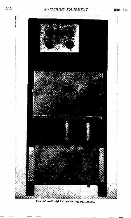
262 S WI TCIIING EQUIPMENT

.—. - ..- ._—..__ ..-_ ____

FIG. 8.1,—Model C-1 switching equipment.

[%c. 84

I

I

I

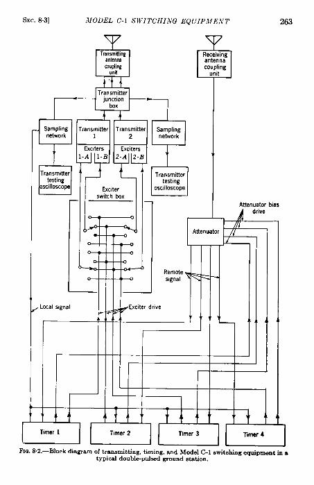
SEC.8.3]

1-

MODEL C-1 SWITCHING EQ UIP.&fEN T

w w

couplingumt

+’tl’Transmitter

junctionbox

4 4

Sampling Transmitter Transmitter Samplingnetwork 1 2 network

t

Transmittertesting

oscilloscope1 I

—

, Local signal

Exciterswitch box

—1

EL

Transmittertesting

oscilloscope

;

Remotesignal

263

Attenuator bias

l-iFdrive

Attenuator

Fm. 8.2.—Block diagram of transmitting, timing, and Model C-1 switching equipment in atypical double-puked ground station.

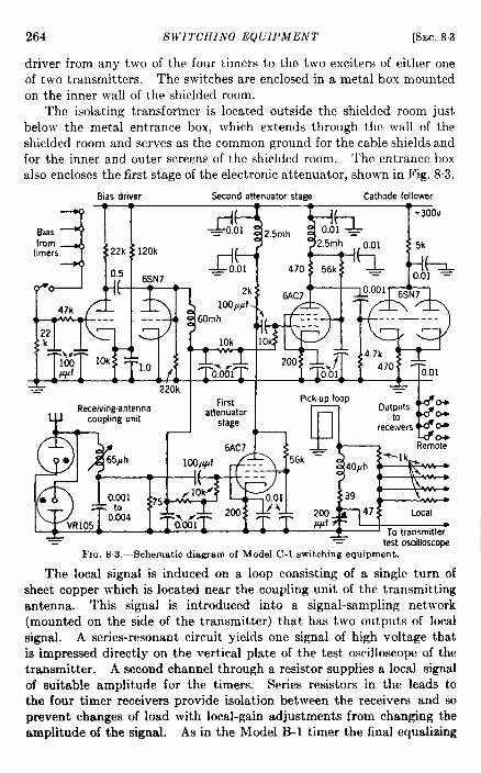
264 SVVITCHING EQUIPMENT [SEC.83

driver from any two of the four timers to the two exciters of either oneof two transmitters. The switches are enclosed in a metal box mountedon the inner wall of the shielded room.

The isolating transfer-mer is located outside the shielded room justbelow the metal entrance box, which extends through the wall of theshielded room and serves as the common ground for the cable shields andfor the inner and outer screens of the shielded room. The entrance boxalso encloses the first stage of the electronic attenuator, shown in Fig. 8.3.

Bias driver Second attenuator stage Cathode follower

FIG.S.3.4chematic diagram of Model C-1 switching equipment.

The local signal is induced on a loop consisting of a single turn ofsheet copper which is located near the coupling unit of the transmittingantenna. This signal is introduced into a signal-sampling network(mounted on the side of the transmitter) that has two outputs of localsignal. A series-resonant circuit yields one signal of high voltage thatis impressed directly on the vertical plate of the test oscilloscope of thetransmitter. A second channel through a resistor supplies a local signalof suitable amditude for the timers. Series resistors in the leads tothe four timer receivers provide isolation between the receivers and soprevent changes of load with local-gain adjustments from changing theamplitude of the signal. As in the Model B-1 timer the final equalizing

SEC.84] MODEL UM SWITCHING EQ UZPMENT 265

of the local and remote signals is accomplished in a variable resistancenetwork in the input of the receiver where the local and remote signalsare mixed.

The gas-filled tubes mentioned in Sec. 8.1 are used to help in theattenuation of the large local signal induced in the main receiving antenna.The coupling unit of the receiving antenna transforms the resistance ofthe antenna to that of the transmission line and neutralizes the antenna’sreactance at the required frequency. The remote signal induced onthe receiving antenna passes through the coupling unit, transmissionline, and attenuator to the receiver. The attenuator acts as an amplifierduring the time of reception of the remote signal. It consists of two6AC7 tubes connected as amplifiers in cascade.

In the interval of attenuation of about 1800 psec, the control gridsof the attenuator tubes are driven far enough beyond cutoff so that nosignals pass to the receiver. Since the local signal from the receivingantenna is then distorted by the limiting action of the gas-filled tubes, itmust be completely eliminated from the input of the receiver. Themaximum possible attenuation per stage is determined by the ratiobetween the grid-to-plate impedance and the plate-to-ground impedance.In practice this limit is not attained; the actual attenuation is limited bycirculating ground currents and by pickup between the grid and platecircuits. To reduce these effects, the two stages are enclosed in sepa-rate boxes connected by coaxial cable and the grid and plate circuits arefiltered.

The bias-driver circuits of the timers are all connected at the inputof the bias driver of the attenuator so that any one, two, or more timerscan control the attenuator. A single attenuator can serve a double-pulsed station operating at two recurrence rates. An attenuator foreach of two antennas is required, however, at the double-pulsed stationswhere long baselines and severe noise conditions necessitate the use ofBeverage antennas (see Sec. 10,4).

8.4. Model UM Switching Equipment.—The use of two differentantennas and coupling units for the reception of the local and remotesignals is a source of possible error in timing. Consequently, in thediscriminator of the Model UM switching equipment (Fig. 8.4) provisionis made for the use of a single antenna for the reception of both signals.The discriminator consists of an electronic attenuator and bypassingresistance attenuator. No ga.+filled limiting tubes are used. The elec-tronic attenuator is designed to handle the high voltages encounteredduring the transmission of the local signal.

Experience has shown that in operation over a long baseline or over

land, a Beverage or wave antenna at the ground station gives a higherratio of signal to atmospheric noise than does the standard vertical

266 SWITCHILVG liQ UIPMENT [SEC.8.4

I

FIG. 84.-} 1oc!cI ~11 s\\itclling equip,ne[~t. (Cuurtesyof General Electric Compang.)

SEC.8.4] MODEL UM SWITCHING EQUIPMEATT 267

antenna and accordingly facilitates the maintenance of synchronism.Although the use of the Beverage antenna is not recommended, becauseof the resulting uncertainty of timing of the remote signal with respectto the local signal, it issometimes necessary inrnaintaining synchronismover unusually long baselines. Since the Beverage antenna is directional,a separate antenna is required at a double-pulsed station for reception ofsignals from each of the two remote stations} and an individual discrimi-nator must be used with each antenna. Consequently, three independentdiscriminators are incorporated in the Model CM switching equipment,the third serving as a stand-by.

Normally in a single-pulsed station there are two timers and twotransmitters (four exciters); in a double-pulsed station there arc fourtimers and two transmitters (see Fig, 85).

The Lfodel UII switching equipment is constructed in a singlecabinet equipped with space heaters and a ventilating blower, Thecabinet is installed in the shielded room near one ~vall. All leads enter-ing the shielded room pass through the entrance box, which protrudesthrough the wall and is bolted to it. The uppermost chassis contains(1) a selector switch for connecting a line from the standard frequencyreceiver (for checking the crystal oscillators against the Bureau ofStandards time signals from station WWT) to the 100-kc/sec outputof any one of four timers, (2) four selector switches for connecting fromone to four transmitter exciters to any of four timers, (3) a line-frequencymeter, and (4) a line-voltage meter. The second chassis contains (1)four selector switches for connecting the local- and remote-signal inputsof one to four timers to the local and remote outputs of any of three dis-criminators and (2) a toggle switch for connecting the ventilating blowerof the cabinet to either of two power lines. The lowest panel containscircuit breakers, fuses, and switches for distributing power from eitherof two transformer-isolated sources to three discriminators in the cabinetand to the timers and lighting circuits in the shielded room.

Figure 86 is a block diagram of the Jlodel T-731switching equipment,.In each of three discrimirmtors two channels are provided. One is theelectronic attenuator whose output is conncctcd to the remote input ofthe timer receiver; the other is an adjustable resistance attenuator whoseoutput is connected to the local input of the timer receiver. Provisionis made for connecting a single antenna to the inputs of both channelsor for connecting individual antennas to the two inputs. A bandpassantenna filter is provided for the reduction of cross modulation causedby strong signals of frequencies outside the pass band. Its introductionin both channels causes no timing error because it delays and distortsboth remote and local signals equally. A ganged selector switch withthree positions makes it easy to change connections. The three com-

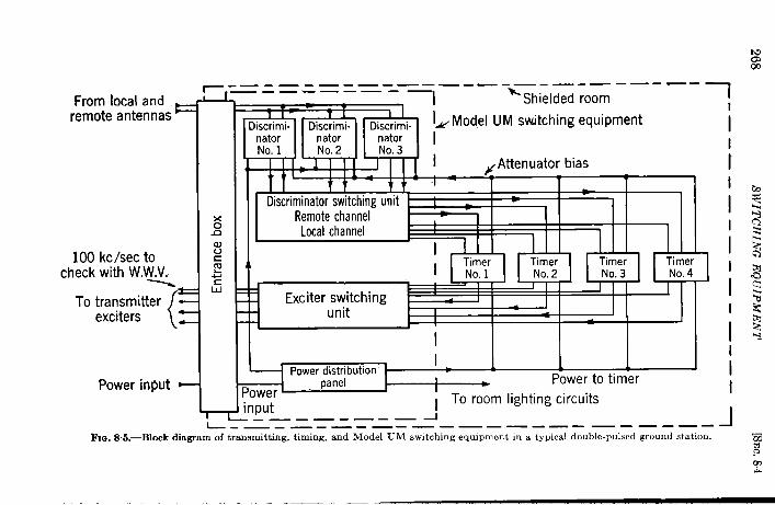
From local andremote antennas +

100check

kck.ec towith W.W.V.

--5=

{To transmitter --

exciters ~

Power input *

—.—- —-— ———— ——-— -—-— -——— -— --I r

x2wvcm.b&l

m

—.— ——. .

L --

mDiscrimi. Discrinator nator

u

nator INo.1 No.2 No.3 , . ..

‘ r biasH++#4—11 ‘ “Anenua’oDiscriminatorswitching unit 1

Remote channelLocal channel

+ I 1i,

ITimer Timer

1’

TimerNo. 1 No. 3 No. 4

1 1 I IExciter switching I I J

unit I

I

I1-

Power distribution 1 1 1 I

oanel I Power to timerPower’ r J

input; To room lighting circuits

—— —— — ——— J

I

iI

tI

II

I

I

II

II

II

——— ———— ——— ——— ——— ——— ——— J~G. 8.5.—Block diagram of transmitting, timing, and Model UM switching equipment in a typical double-pulsed ground station.

.— .—..

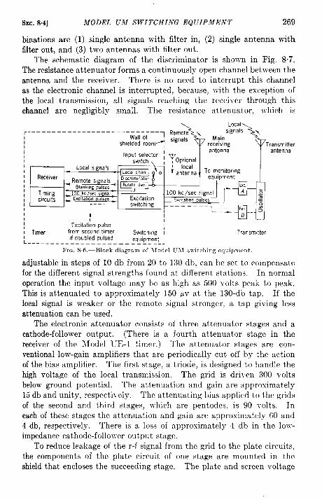
SEC. 84] MODEL Uhf SWITCHING EQUIPMENT 269

binations are (1) single antenna with filter in, (2) single antenna withfilter out, and (3) two antennas with filter out.

The schematic diagram of the discriminator is shown in Fig. 8.7.The resistance attenuator forms a continuously open channel between theantenna and the receiver. There is no need to interrupt this channelas the electronic channel is interruptecl, because, with the exception ofthe local transmission, all signals reaching the receiver through thischannel are negligibly small. The resistance attenuator, which is

I Transmitter

I antenna

1111 Receiver1111 Timing1 cwcults

I1

1 L.+i

Excttati~n pulse1

I Timer from second timer Switching / Transmitter

L--- –___ lYbHYbH E“Y_d___ :q:l!!e!!j

FIG. 86,-Block diagram of Model UiI switching equipment.

adjustable in steps of 10 db from 20 to 130 db, can be set to compensatefor the different signal strengths found at different stations. In normaloperation the input voltage may be as high as 500 volts peak to peak.This is attenuated to approximately 150 pv at the 130-db tap. If thelocal signal is weaker or the remote signal stronger, a tap giving lessattenuation can be used.

The electronic attenuator consists of three attenuator stages and acathode-follower output. (There is a fourth attenuator stage in thereceiver of the Model UE-1 timer.) The attenuator stages are con-ventional low-gain amplifiers that are periodically cut off by the actionof the bias amplifier. The first stage, a triode, is designed to handle thehigh voltage of the local transmission. The grid is driven 300 voltsbelow ground potential. The attenuation and gain are approximately15 db and unity, respectively. The attenuating bias applied to the gridsof the second and third stages, which are pentodes, is 90 volts. Ineach of these stages the attenuation and gain are approximately 6~ and4 db, respectively, There is a loss of approximately 1 db in the low-impedance cathode-follower output stage.

To reduce leakage of the r-f signal from the grid to the plate circuits,the components of the plate circuit of one stage are mounted in theshield that encloses the succeeding stage. The plate and screen voltage

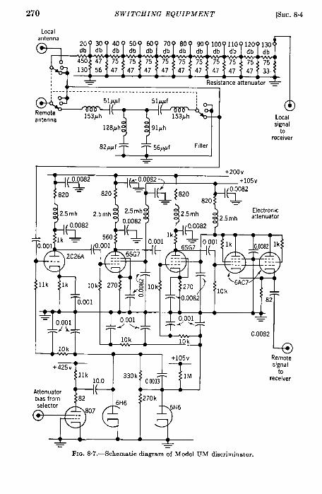
270 SWITCHING EQUIPMENT [SEC. 8.4

Localantenna

Resistance attenuator ~.. -. . ..- ------- ------ --------- .-- . . . ~ I

, ~-_ ......,. .5mh al[enua[or‘?i’~t!i“ec10

R.

.001 ,~~0.0082lk

--- ------ ------ ---

t 6AC7

10k

T82

A& A 1 L 1 1

‘ Ojo[l 0.001 =:2 L: :

10k0.0082

10k10k

(}%

Remote

+425v signalto

receiver

Attenuatorbias fromselector

L= =

FIG. 8.7.—Schematic diagram of Model UM discriminator.

SEC. 8.5] LOW FREQUENCY SWITCHING EQUIPMENT 271

and bias leads are filtered by single T-sections that are critically dampedto prevent oscillations. The filament transformers and plate-supplytransformers are provided with electrostatic shields. Each attenuatorstage, each section of the input selector switch, the bandpass antennafilter, and the resistance attenuator are enclosed in separate aluminumcastings insulated from the chassis.

The bias for cutting off the attenuator stages is obtained from a biasamplifier. The timing and duration of the attenuating bias are con-trolled by the timers. The duration is approximately 1800 ~sec. Itmust be long enough to provide adequate attenuation for the entireperiod during which local transmission may occur. This period dependsupon the adjustment of the timer.

The bias circuits of all the timers are connected to a common resistanceand to the bias-amplifier inputs of all the discriminators. Consequently,each operating timer controls all operating electronic attenuators unlessits bias circuit is switched off. At a double-pulsed station all signalsexcept the local transmissions are eliminated from two short sections ofthe slow-trace pattern. As observed on either of the two operatingtimers, one section remains stationary while the other moves around theslow-trace pattern, periodically eliminating the remote signal. Thedirection of motion is opposite for the two timers.

8.6. Low Frequency Switching Equipment.—The experimental LFLoran stations have been operated with slightly modified Model C-1switching equipment. Since the requirements for switching equip-ment at an LF Loran ground station are more severe than those forStandard or Sky-wave Synchronized Loran, an experimental model ofthe proposed equipment has been built and tested at the RadiationLaboratory.

Experiments in this country and experience with the European SSground stations that do not have shielded rooms have shown that undernormal conditions it is possible to design an attenuator capable of satis-factory operation without the protection of a shielded room. Theadvantages of elimination of the shielded room are increased convenienceand simplification of operation and more space in the timer building.The problem of providing sufficient attenuation without a shielded roomis greatly simplified if the electronic attenuator is incorporated in thetimer, closely associated with the r-f stage of the receiver. This, ofcourse, would call for a complete redesign of the timer, which has not beenfeasible. The laboratory model of the LF switching equipment has,however, been designed keeping in mind the possibility of eventualelimination of the shielded room.

The requirements for the attenuator for the permanent LF system aremore severe than those for the Standard and SS attenuator because the

272 SWITCHING EQUIPMENT [SEC.83

anticipated output power is 1 megawatt instead of 100 kw, and becauseof the continuous output of the 90-kc/sec c-w driver of the transmitter.This is about 20 watts and is present even during reception of the remotesignal. To avoid difficulty expected from the radiation of the secondharmonic from the 90-kc/sec driver and to alleviate the problem ofattenuating the local signal, it is planned that the transmitter buildingshall be located 1000 ft or so from the timer building and that the receiv-ing antenna shall be 1000 ft or more from the transmitting antenna.Furthermore, because the cycle-matching technique offers the possibilityof measuring time differences with an error of only about & psec, thedifference in phase shift (or distortion) introduced in the local-signalchannel (resistance attenuator) and the remote-signal channel (electronicattenuator) must be less than 6°. If it proves to be necessary, an ampli-fier can be used in the local-signal channel that is a duplicate of the elec-tronic attenuator when it is amplifying the remote signal.

As with the Model UM switching equipment a single receiving antennaand a resistance attenuator supply both the remote and local signals.With the exception of an additional switch for the 50-kc/sec signal tothe transmitter, the switching is similar to that of the Model UM.However, in the design of the LF attenuator, considerable effort hasbeen expended in reducing the thermal and “shot” noise in the electronicattenuator. The maximum over-all attenuation factor is determinedby the negative grid bias of the first stage, which limits the maximumlocal signal that the attenuator can handle, and the thermal and shotnoise of the attenuator (when acting as an amplifier), which limits theminimum remote signal that the attenuator can handle. In the designof the attenuator, the amplification when the attenuator is acting asan amplifier is limited by the cross modulation produced in the wide-bandpass amplifier by strong signals of unwanted frequencies. In aneffort to reduce the noise, low-noise triodes are substituted for the pen-todes of the earlier models. Although the maximum theoretical attenua-tion factor per stage of a pentode is greater than that of a triode, theattenuation factor attained in practice is limited by the coupling betweenthe grid and plate circuits rather than by the ratio of the grid-to-plateand plate-to-ground impedances. The triode has the advantages thattkle circuit is simpler, microphonics and internal tube noise are lower,and cross modulation is less. Four low-noise triode stages of attenua-tion are used, instead of the two or three pentode stages of the earliermodels.

Figure 8.8 is a schematic diagram of the LF attenuator. The fourstages of attenuation are enclosed in a long copper box, each stage beingseparated from the succeeding stage by a copper partition. As with theModel UM switching equipment, the plate circuit of one stage is mounted

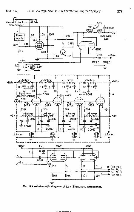
SEC. 8.5] LOW FREQUENCY SWITCHING EQUIPMENT

‘“””*

0.05

1 I r 1

273

ElQ “’fit”’_,v -L-J=vR’05~“ 3mh +150 v

‘i “9115”

+lT

r ------- ------ _________~–-1 ,___-__-_T____T

+105v +105v

-2 -2 v

L__________________________________-___J

+105vt

Rec.No. 1Rec.No,2Rec.No, 3Rec.No.4

*FICA8.8.dchematic diagram of “LowFrequency attenuator.

274 SWITCHING EQUIPMENT [SEC. 85

inside the compartment of the succeeding stage to minimize the couplingbetween the grid and the plate circuits. The routing of the leads isdesigned to minimize the coupling between the grid and plate circuits,and all bias and power leads are shielded and filtered. A separateelectrostatically shielded filament transformer supplies power to thefilament of each triode.

In an effort to reduce the phase shift through the attenuator, it isdesigned to pass all frequencies up to 10 Me/see. It is estimated thatit produces a phase shift not exceeding 6°.

Each stage of attenuation is capable of an attenuation factor of 40to 50 db. The over-all measured attenuation factor is greater than165 db; the over-all measured gain is 45 db. The noise level is ~ pv ascompared with 10 pv for the Model C-1 attenuator.

CHAPTER9

TRANSMITTERS

BY A. J. PoTfi, R. B. LAWRANCE, AND G. C. TR~LY

9.1. General Requirements.-The design characteristics of tlxtransmitter are based on the requirements of the system and on theaccuracy with which time differences caq be measured with the navi-gator’s receiver-indicator. The navigator’s instrument is designed to becapable of yielding readings to within 1 ~sec of the true value. Witha short baseline and normal signal-t~noise ratio, an average error in thesynchronism between two transmitters is approximately 0.5 ~sec. Sincethe period of a carrier cycle at the operating frequency is approximately0.5 psec, the maximum error assignable to the transmitter is a smallfraction of a cycle. Once started, the output pulse from the transmittermust rise smoothly and steadily to its maximum to prevent “ flutter”of the received pulse from impairing the accuracy of the navigator’stime-clifference reading.

To facilitate the accurate measurement of the time difference betweenpairs of received pulse signals, the leading edges of the signals shouldrise steeply. The reception of such pulses, however, necessitates wide-band receivers, with attendant increase in interference from noise andother signals. An experimental study has been made to determineoptimum conditions consistent with the desired reading accuracy. Theresults of this study have led to the adoption of an effective receiverbandwidth of about 75 lm/sec. Under the stimulus of a trapezoidaltransmitted pulse rising in approximately 10 usec, such a receiver yieldsan output pulse requiring 35 ~sec to reach its maximum. The trans-mitted pulse must therefore be at least 35 psec long. An upper limit tothe pulse length is set by the desirability of resolving sky-wave com-ponents which may follow at intervals as short as 65 psec. A transmittedpulse length of approximately 45 Psec has been adopted.

The rise time of the transmitted pulse is only broadly defined by therequired end result on the navigator’s instrument. From the standpointof apparatus the rise time is more strictly determined by such interrelatedfactors as the antenna Q, the Q of the transmitter tank circuits, and therequirement that the oscillations start consistently. In a trapezoidalpulse the sideband distribution is determined primarily by the pulsewidth and secondarily by the rise time; since lo-psec rise time is easily

275

276 TRANSMITTERS [SEC.9.1

achieved, this value has been adopted. The standard pulse has a risetime of 10 psec, flat top of 35 psec, and decay of 10 ysec, making the widthat half amplitude 45 ysec.

The technique of matching the envelope amplitudes and leadingedges of two pulses yields its highest precision when the shapes of thetwo transmitted pulses are exactly the same. If the two transmittersdiffer in frequency, the two pulse shapes aredistorted differently in thereceiver, and an error is introduced in the time-difference measurement.It is therefore necessary that the Loran transmitters have inherent fre-quency stability and that provision be made for simple and positivemeans of monitoring and maintaining frequency.

To conserve space in the limited frequency spectrum, pairs of Loranstations areidentified by different recurrence rates rather than by differ-ent radio frequencies. This scheme also simplifies thereceiver, althoughit requires a circuit complication in the indicator. Loran transmittersare accordingly designed in such awayastobe capable of emittingpulsesat two recurrence rates concurrently.

Pulsing the transmitter at two recurrence rates results in doublingthe duty cycle, increasing the average power output from 100 to 200watts. These are reasonable values and present no problem; the realdifficulties arise from the variable time interval between successivepulses. The starting and stopping characteristics of the transmittersand therefore the stability and shape of the emitted pulses are functionsnot only of the circuit constants but of the various voltages as well.Of practical necessity, these voltages perform some excursion duringand immediately following each pulse. The conditions that determinethe characteristics of a pulse, therefore, change with time; they dependon the variable time interval between successive pulses. The trans-mitters must perform so that the variation of pulse shape and amplitudeand the variation in timing, caused by the fluctuations of the voltages,are restricted to tolerable limits.

Originally the power capabilities of the transmitter were dictatedchiefly by existing tube types and their availability. Propagation studieshave predicted and experience has shown that a daytime ground-waverange of 700 nautical miles can be expected from a radiated power of100 kw. At the Loran frequency of 2 Me/see, a further increase inrange of 100 miles would require nearly ten times the power, an increasethat is not often worth while. A power of 100 kw gives ground-wavefields of about 500 pv/m at normal baseline distances over water, whichis adequate for synchronization in most latitudes.

In addition to the system requirements for the transmitters, otherimportant operating characteristics are required by the nature of theservice to be rendered. The equipment must be capable of continuous

SEC.9.2] STANDARD LORAN TRANSMITTERS 277

operation for long periods of time, in any climate fromthe Arctic to theequator. Itmustbe tolerant of power-soureev ariationsa swellasbeingrugged, simple to operate, and easy to maintain.

.

~I

~.,

;-!’

fI

I

~. . . .. . . ,_aa “FrG.9.1.—ModelTDP transmitter. (Court.svof Radio EngineeringLaboratoriesInc.)

9.2. Standard Loran Transmitters.—The major requirements of thetransmitter to be used in the 2-LIc/sec Loran system may be brieflyrecapitulated as follows:

1. Starting time variation less than 0.1 psec.2. Smooth, steady rise of output pulse.3. Pulse length of 45 psec at half amplitude.4. Consistent pulse rise time of 10 psec.5. Frequency stability and means for monitoring the frequency.6. Ability to transmit two trains of pulses at different rates.7. Peak power output of 100 kw.8. Continuous operation in all climates.9. Low harmonic radiation.

10. Simple operation and maintenance.

278 TRANSMITTERS [SEC. 9.2

Several transmitter models, differing in physical construction but similarin electrical design, have been produced. Atotalof 18 units of the earlyModel 108T have been manufactured by Harvey Radio Laboratories,Inc. The same manufacturer has produced 10 Model 125T and 12Model 170T transmitters. The Radio Engineering Laboratories, Inc.,have constructed 36 Model 575 transmitters and 70 Model TDP (Fig.91) transmitters. The General Electric Company has designed theModel TDP-1 (Fig. 9.2) transmitter to meet Navy specifications and hasmanufactured 66 units.

Model TDP Trarzsrnitter.-Electrically, Model TDP transmitter is apush-pull, tuned-plate, tuned-grid, self-excited oscillator with a modifiedform of cathode keying. Physically, it consists of two metal cabinetsabout 32 in. wide, 28 in. deep, and 72 in. high. One cabinet contains thepower oscillator, modulator bias and screen supplies, output couplingcircuits, and a dummy load. The second cabinet contains the controlcircuits, the high-voltage power supply, and the two exciter (“ pulser”)units.

In order to achieve timing stability each exciter is fed with recurrenttrigger pulses from one timer only. For double-pulsed operation theequipment is set up as shown in the diagram of Fig. 9.3, the two sequencesof pulses being mixed just before the modulator. For single-pulsedoperation one exciter is entirely disconnected and the other feeds the“ bias-and-pulse” modulator input line without first going through themixer.

The trigger pulses are short and have a steeply rising front edge.After voltage amplification they trigger a gas-filled tetrode in a pulse-forming stage, the output of which feeds a beam power output stage.Each positive-going output pulse is roughly rectangular, approximately45 psec long, and several hundred volts in amplitude. One sequence ofthese pulses, together with a bias voltage, is fed from each exciter to themixer, which in turn feeds the combined output and a resultant biasvoltage to the grid of the modulator. The modulator is a normally offtube which is turned on by these high-voltage, positive-going pulses andis so connected that it keys the high-power oscillator on and off. Thepulses of r-f energy are sent down a coaxial line to a tuning and matchingunit at the base of the Loran antenna and thence to the antenna itself.

Exciter Operation.—The operation of the exciter can best be under-stood by study of the simplified diagram (Fig. 9“4). The synchronizingtrigger from the timer is a positive pulse of either 3 or 20 volts’ amplitude,depending on the type of timer. This pulse is fed into a video preampli-fie~ which increases its amplitude to approximately 60 volts. Theamplified pulse is then fed through the diode to the grid of the gas tetrode.In some of the later models the preamplifier is replaced by a pulse trans-

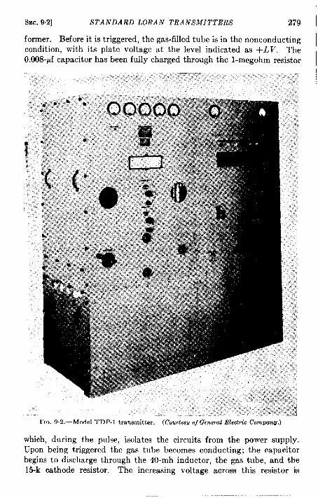
SEC.9.2] STANDARD LORAN TRANSMITTERS 279

former. Before it is triggered, the gas-filled tube is in the nonconductingcondition, with its plate voltage at the level indicated as +L V. The0.008-~f capacitor has been fully charged through the l-megohm resistor

FIG, 9.2.—Mode1 TDP-1 transmitter. (Courtesv of General Electric Company.)

which, during the pulse, isolates the circuits from the power supply.

Upon being triggered the gas tube becomes conducting; the capacitor

begins to discharge through the 40-mh inductor, the gas tube, and the15-k cathode resistor. The increasing voltage across this resistor is

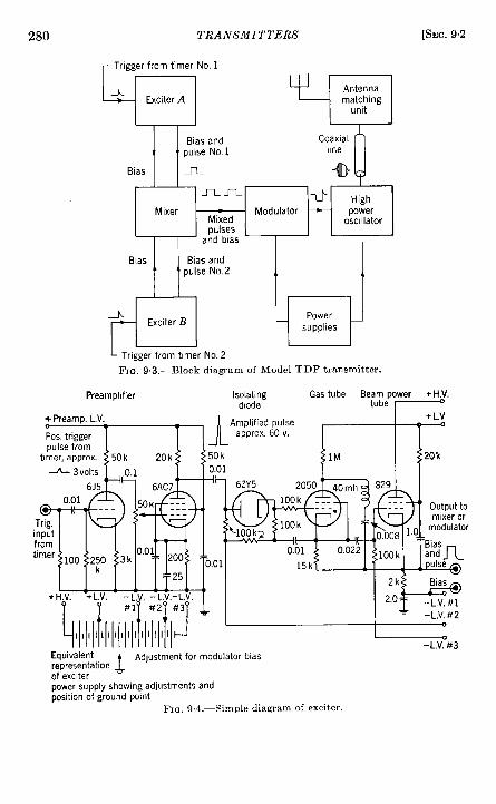
280 TRANSMITTERS

w“”’ w

IIBias and Coaxial

pulse No. 1 Ihne II

[SEC.9.2

Bias n *y

J1-n+ High

Mixer Modulator —Mixed

poweroscillator

pulsesand bias

Bias

H

Bias andpulse No.2 II

L Trigger from timer No. 2FIG. 9.3.—Block diagram of Model TDP transmitter.

Preamphf!er Isolatlng Gas tube Be:u~epy +H.),diode

+Preamp, L.V.

Tmi’’’’’d’” m

e?-+?fi”-- J Z1.L

‘“l Il-::f I“”o’l

+H++AH-tIUI

II

“,, *L, *J,

Equival~~~’~’I’I’I’’’”~ ~”~~representation ~ lA~j~~tm~nt~orof exciter -power supPly showing adjustmentsDosition of ground point

15kf l-f J 1P

modulator bias

and

4.—Simple diagram

I ‘UT -L,V, #l-L.V. #2

-I 0

-L.V. #3

FIG. 9 of exciter.

SEC, 92] STANDARD LORAN TRANSMITTERS 281

applied between the cathode and grid of the beam power tube and bringsits bias rapidly from beyond cutoff to a slightly positive voltage. Theplate current in the beam power tube and the output pulse voltagebuildup rapidly until the grid starts to draw current from the gas tubecircuit.

After this time the inductor, the two capacitors in series, and thegrid-cathode resistance of the beam power tube behave as an under-damped series circuit that executes a single half-cycle oscillation. Duringthe first 20 psec of this oscillation the grid swings slightly more positiveand an even larger grid current flows; after 45 psec, however, the gridvoltage becomes negative and grid current ceases. The circuits areproportioned in such a way that at precisely this time the 0.008-@f capac-

Outp.t to mod grid

Sias and pulseA (Singlepulseonly)r“ T

WHA[= ,mk

B5V4G

Sias A 40mh Ems, pulse A, pulse B10 mod gr,d

150k( 150ktoground)

Bim&/ l~k

ticiterB[

5V4G

Oias and PUI* B Alternative outputto mod gr,d

(S,ngle pulse only)

FIG. 9+-Simple diagram of mixer circuit,

itor is completely discharged; the gas tube again becomes nonconducting,

and the output pulse is terminated.

The output point carries direct bias voltage as well as the positive

pulse and is thus suitable for direct coupling to the modulator grid.

Both the gas tube and the beam power tube are connected as cathode

followers, and the “bootstrap” circuit allows a very large voltage outputto be obtained. The function of the isolating diode is to disconnect the

grid of the gas tetrode from its bias source during the pulse, thereby pre-venting positive-ion grid bombardment as the cathode potential iscarried toward +HV by the bootstrap action.

For double-pulsed operation the two exciters are used in conjunctionwith the diode mixer shown in the simplified diagram of Fig. 9.5. Thefunction of the mixer is to transmit the output pulses of the exciters tothe common modulator while isolating them from each other; it alsoprovides a connection for the modulator tube bias. Means are provided,by the 100-k resistors, to accommodate a small amount of unbalancebetween bias voltages furnished from the two supplies in the exciters. A40-mh inductance and shunting 150-k resistor are used to present a con-siderable impedance to the pulse output from the mixer, so that full vol-tage is applied to the modulator grid.

All transmitters are equipped with two exciters and a mixer. Simple

282 TRANSMITTEES [sEc. 9.2

switching operations permit either single-pulsed or double-pulsedoperation.

Operation oj Modulator and Power Oscillator.-The power oscillatorhas an essentially conventional tuned-plate, tuned-grid, push-pull cir-cuit. The modulator is connected between cathode and ground and isdesigned to provide a cathode bias considerably greater than cutoff,

Plate H.Vsupply

20,000V

1/ 1. 11 L

Scleent

Osc. cath. =supply currentcurrent

RF power oscillatorTo OSC. cathodes

‘:ii:h”eoi~’=’”=

Action of modulator

FIG, 9.6.—Simple diagram of modulator and oscillator.

so that no oscillations occur between pulses. At the instant when modu-lations applied, the cathode bias isreduced toalow value and oscilla-tions are started and sustained until the bias isagain returned to a highvalue. Thus the modulator may be regarded as a shorting switch inseries witha small resistance, asis shownat the bottom of the simplifieddiagram (Fig. 9.6).

A better understanding of the action may be had if some figures areassigned to the various voltages. The tubes used are VT98’S. Thecutoff bias at 25-kv plate voltage is —1000 volts. Most of the Lorantransmitters are operated at aplate voltage of 17.5kv, and the cathodevoltage above ground, sustained by the filter capacitor and oscillatorcathode resistance, is 2500 volts. This circuit has a long time constant,

SEC. 9.2] STANDARD LORAN TRANSMITTERS 283

so that to all intents and purposes the voltage is constant. At theinstant when the modulator is turned on, the oscillator cathode voltagedrops to a value of about 500 volts and the remaining 2000 volts appear

Voltagedropsstart of pulse

+ 500v

Pulsed

t

FIQ.9.7.—Cun

\ ~+

Voltagerisesatend of pulseto

+5000V+600

——— ~- .. --------

decreasingcurrent

PlatecapacitorVoltagegradually re.chargingcurrent

returns to+2500 v \

‘–-+ -------- --- .*-..,,=

Res!storcurrent~--- --- --->(c) After pulse

rent flow in transmitter. (a) During pulse; (b) end of pulse; (c) after pulse.

across the snuffing choke. The plate power for the oscillator is suppliedfrom the large storage capacitor connected between the cathodes and thecenter tap of the plate tank circuit. This capacitor is permitted to makethe same voltage excursion as the cathodes by the isolating impedancesbetween the center tap and the plate high-voltage supply.

Figure 9.7a shows the various current paths during the pulse. Themodulator grid has been driven positive by the exciter output, The

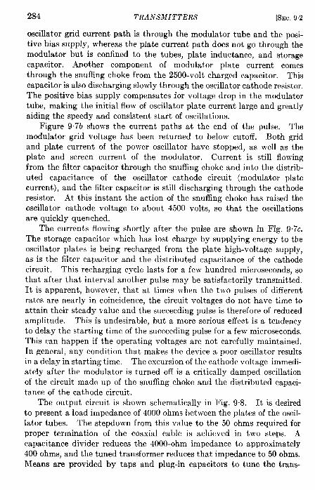
284 TRANSMITTERS [SEC.92

oscillator grid current path is through the modulator tube and the posi-tive bias supply, whereas the plate current path does not go through themodulator but is confined to the tubes, plate inductance, and storagecapacitor. Another component of modulator plate current comesthrough the snuffing choke from the 2500-volt charged capacitor. Thiscapacitor isalsodischarging slowlythroughthe oscillator cathode resistor.The positive bias supply compensates for voltage drop in the modulatortube, making theinitial flowof oscillator plate current large and greatlyaiding the speedy and consistent start of oscillations.

Figure 9.7b shows the current paths at the end of the pulse. Themodulator grid voltage has been returned to below cutoff. Both gridand plate current of the power oscillator have stopped, as well as theplate and screen current of the modulator. Current is still flowingfrom the filter capacitor through thesnuffing choke andintothedistrib-uted capacitance of the oscillator cathode circuit (modulator platecurrent), and the filter capacitors still discharging through the cathoderesistor. At this instant the action of the snuffing choke has raised theoscillator cathode voltage to about 4500 volts, so that the oscillationsare quickly quenched.

The currents flowing shortly after the pulse are shown in Fig. 9.7c.The storage capacitor which has lost charge by supplying energy to theoscillator plates is being recharged from the plate high-voltage supply,as is the filter capacitor and the distributed capacitance of the cathodecircuit. This recharging cycle lasts for a few hundred microseconds, sothat after that interval another pulse may be satisfactorily transmitted.It is apparent, however, that at times when the two pulses of differentrates are nearly in coincidence, the circuit voltages do not have time toattain their steady value and the succeeding pulse is therefore of reducedamplitude. This is undesirable, but a more serious effect is a tendencyto delay the starting time of the succeeding pulse for a few microseconds.This can happen if the operating voltages are not carefully maintained.In general, any condition that makes the device a poor oscillator resultsin a delay in starting time. The excursion of the cathode voltage immedi-ately after the modulator is turned off is a critically damped oscillationof the circuit made up of the snuffing choke and the distributed capaci-tance of the cathode circuit.

The output circuit is shown schematically in Fig. 9.8. It is desiredto present a load impedance of 4000 ohms between the plates of the oscil-later tubes. The stepdown from this value to the 50 ohms required forproper termination of the coaxial cable is achieved in two steps. Acapacitance divider reduces the 4000-ohm impedance to approximately400 ohms, and the tuned transformer reduces that impedance to 50 ohms.Means are provided by taps and plug-in capacitors to tune the trans-

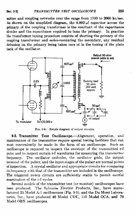
sac. 9q TRANSMITTER TEST OSCILLOSCOPE 285

mitter and coupling networks over the range from 1700 to 2000 kc/see.As shown on the simplified diagram, the 0.002-pf capacitor acrow theprimary of the coupling transformer is the resultant of the capacitancedivider and the capacitance required to tune the primary. In practicethe transformer tuning procedure consists of shorting the primary of thecoupling transformer and series-resonating the secondary, any residualdetuning on the primary being taken care oi in the tuning of the platetank of the oscillator.

1 ,

1820/#f

-1-

!zfHo.m2

T

Output 50 ohmcoaxial cable to ant

---

0.25

: ;, ] ‘~7-

Dummy load50 ohm.

y

300 watt,approx.

=

---

Y820)4J~ %j!~

6A

r.f outputTo modulator To+20,000 V

=

F1a. 9.8.—Simple diagram of outtmt circuits.

9.3. Transmitter Test Oscilloscope.-Alignment, operation, and

maintenance of the transmitter require special testing facilities that can

most conveniently be made in the form of an oscilloscope. ,Such anoscilloscope is required to inspect the envelope of the transmitted r-fpulse and to inspect certain r-f waveforms for measuring the transmitterfrequency. The oscillator cathodes, the oscillator grids, the outputterminal of the pulser, and the input stages of the pulser are normal pointsof inspection. A crystal oscillator and appropriate circuits for comparingits frequency with that of the transmitter are included in the oscilloscope.The triggered sweep circuits are sufficiently stable to permit carefulexamination of the r-f cycles.

Several models of the transmitter test (or monitor) oscilloscopes havebeen produced. The Sylvania Electric Products, Inc., have manu-facturwl 25 Model A-1 oscilloscopes (Fig. 9.9), and the Du Mont Labora-tories, Inc., have produced 40 Model CDU, 110 Model OCA, and 70Model (3BN oscilloscopes.

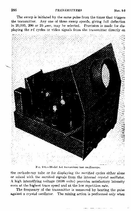
286 TRANSMITTERS [SEC.9.3

The sweep is initiated by the same pulse from the timer that triggersthe transmitter. Any one of three sweep speeds, giving full deflectionin 20,000, 200 or 25 ~sec, may be selected. Provision is made for di~playing the r-f cycles or video signals from the transmitter directly on

\

the cathode-ray tube or for displaying the rectified cycles either aloneor mixed with the rectified signals from the internal crystal oscillator.A high intensifying voltage (9oOO volts) provides satisfactory intensityeven at the highest trace speed and at the low repetition rate.

The frequency of the transmitter is measured by beating the pulseagainst a crystal oscillator. The mixing action isperformed only when

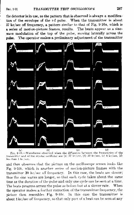
SEC. 9.3] TRANSMITTER TEST OSCILWSCOPE 287

the detector is in use, so the pattern that is observed is always a modifica-tion of the envelope of the r-f pulse. When the transmitter is about37 kc/see off frequency, a pattern similar to that of Fig. 9“10a, which isa series of motion-picture frames, results. The beats appear as a sine-.wave modulation of the top of the pulse, moving laterally across thepulse. The operator makes a preliminary adjustment of the transmitter

and then observes that the picture cm the oscilloscope screen looks likeFig. 9. 10b, ~~hich is another series of motion-picture frames ~vith thetransmitter 20 kc/see off frequency. In this case, the beats are slower;thus the sine waves are longer, so that each cycle takes about the sametime as the duration of the pulse and only one cycle can be seen at a time.The beats progress across the pulse as before but at a slower rate. Whenthe operator makes a further correction of the transmitter frequency, thepicture then resembles Fig. 9. 10c. In this case the transmitter isabout 4 kc/see off frequency, so that only part of a beat can be seen at any

288 TRANSMITTERS [SEC.9.4

one time. The top of the pulse displays a rocking motion, and the thick-ness of the trace at the top of the pulse varies at the same time. Theprogression of the beats continues, giving the series shown, and in thiscase is an aid to detection of the beat. In fact, if the progression is nottaking place, the operator must switch the crystal oscillator on and offin order to obtain random samples of the sequence shown, “a frame at atime,” and judge the transmitter setting from them by careful observa-tion of the thickness of the trace at the top of the pulse. Finally, whenthe transmitter is as nearly on the desired frequency as the operator canset it, the picture is as shown in Fig. 9.10d. No rocking or changing intrace thickness from side to side can be seen, but only the bobbing of thetop of the pulse and the uniform change in thickness of the trace. Thissetting is within 0.10 per cent of the frequency of the crystal oscillator,which is sufficiently accurate for the service required.

Assuming that the two signals are in phase at the beginning of eachpulse, the phase near the end of the pulse depends upon the differencein frequency of the two signals. For example, if the difference in fre-quency is 25 kc, the phase will have changed 360° in 40 psec. One com-plete cycle of beat action will have been completed so that the pulse willappear to have one cycle of sine wave superimposed on it. The ultimateaccuracy then depends on the minimum amount of phase change thatcan be detected during the pulse.

LOW FREQUENCYLORAN TRANSMITTERS

9.4. Low Frequency Transmitter Requirements. Introduction.—AnLF transmitter intended for Loran timing measurements must meetrather stringent requirements, since the period of one carrier-frequencycycle becomes comparable with or greater than the maximum tolerabletiming error. At a carrier frequency of 180 kc/see each cycle is 5.55~sec long, and much refinement of conventional Loran practice is neces-sary in order to keep synchronization errors down to about 1 psec. Theprincipal requirements are the following:

1. The carrier frequency must be established in such a way that it isaccurately the same at all stations. Any frequency difference intwo received pulses would lead to different pulse shapes at the out-put of the receiver, which has a fairly narrow bandwidth. Nosuch difference in pulse shapes can be tolerated when the sought-for timing accuracy is so high.

2. All stations must radiate pulses whose waveforms have preciselythe same characteristics, namely, the shape of the envelope andthe timing relationship between the envelope and the carrier-frequency cycles.

I

SEC.9.4] LOW FREQUENCY TRANSMITTER REQUIREMENTS 289

In addition to these two basic requirements it is desirable to incor-porate precautions for reducing aU spurious harmonic and adjacent-channel radiation to levels that will not cause excessive or unnecessaryinterference.

The transmitter to be described was developed as part of an emergencyprogram. It represents a valuable first step in the effort to meet therequirements just stated, and many of the techniques employed haveproved entirely satisfactory. AU of the individual circuits describedhave been in use for several months in the stations of the East Coastexperimental triplet.

The LF Station and Equipment .—As mentioned in Sec. 7.15, the timeris modified by the addition of a 50-kc/sec driver, one of whose functionsis to provide the transmitter with crystal-controlled signals of this fre-quency. The act of holding the two stations of a pair in synchronismmaintains their respective crystal oscillators at frequencies that differby less than 1 part in 100 million. Their transmitted carrier frequencies

can also be made equal, with this same accuracy, by designing the trans-

mitter as an oscillator amplifier whose frequency-determining device is

the continuously running crystal in the timer.

The carrier frequency of 180 kc/see must be obtained from the

50-kc/sec crystal v-ithout dependence on any other frequency source;

this is done by the use of circuits in which the crystal-controlled signal

is heterodyned with other signals derived from it by frequency multi-plication and division. The phase and frequency of the eventual

180-kc/sec output are thus rigidly determined by the phase and frequencyof the crystal oscillator.

Both the design of the frequency-changing and amplifying stagesand the layout of the station are influenced by the fact that the remote sig-nal must be received during the interval between local pulses. Althoughthe carrier frequency is to be derived from the 50-kc/sec crystal throughfrequency-changing stages that run continuously, the spurious signalpicked up by the receiver from these stages must be much weaker thanthe remote signal. Two precautions have been adopted to avoid troublefrom such interference. In planning the station layout the transmitterand the receiving equipment have been separated by about 1000 ft,the necessary interconnections being made with shielded cables. 1 Moreimportant, in designing the transmitter the carrier frequency of 180 kc/seeis made to appear only during the transmission of the local pulse; thelow-power continuously running stage operates at a frequency of 90kc/see, and the following doubler stage is inactive except when inten-tionally pulsed. The stages following the pulsed doubler are used to

1Experience indicates that interference is not severe even with the transmitterand timer in the same building.

Z9cl TRANSMITTERS [SEC. 94

shape the 180-kc/sec pulse and amplify it to its final level of approxi-mately 100 kw.

As shown in the block diagram of Fig. 9.11, the transmitter is suppliedwith two input waveforms: the ustial trigger and the continuous 50-kc/secwave. It is evident that the 50-kc/sec signal must be derived from apoint follw”ng the capacitor phase-shift circuit in the timer oscillator;doing so allows the relative timing of the trigger and the 50-kc/secwave to remain undkturbed when the timer phase shifter is manipu-

Timer /-50 kcfsec w ~ Future

PAddedoutputstage

Qcrystal

oscillator50 kclsec

Cw

b7!2Phase

control* ~“

50 kc/seeCw

Frequencyconversion

to 90 kc/see

4

5,filter

Poweramplifier

Driver(amplifies,

shapes top)

180 kcisecoulse

w-is!!%Transmission Transmitter components

&lCouplingunit

Imaa I I‘ Transmission

I I lines

FIG. 9.11.—Block diagram of Low Frequency transmitter.

lated. The cycle-envelope timing relationship of the emitted pulse is

hence independent of the setting of this control.

In Sec. 7.15 it was also mentioned that the trigger output of the

timer is passed through a calibrated delay multivibrator whose total

adjustment range is about 16 ~sec, or 8 ~sec each side of the normalcenter position. This trigger-delay control and the phase control in thetransmitter are intended for use in obtaining and maintaining the properrelationship of the envelope and the carrier cycles. Once the envelopeshape has been adjusted for proper rise rate and flat-top duration, thecycle-envelope relation may be adjusted by sliding the cycles relativeto the envelope, using the phase control for the purpose; alternativelythe envelope may be moved relative to the cycles by the trigger-delay

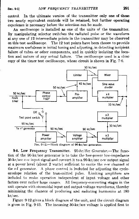
8Ec. 9.5] LOW FREQUENCY TRANSMITTER 291

control. In the ultimate version of the transmitter only one of thesetwo nearly equivalent controls will be retained, but further operatingexperience is necessary before the selection can be made.

An oscilloscope is installed as one of the units of the transmitter.By manipulating selector switches the radiated pulse or the waveformat anyone of 12 intermediate points in the transmitter maybe observedonthis test oscilloscope. The12test points have been chosen to providemaximum usefulness in initial tuning and adjusting, in detecting incipientfailure of tubes or other components, and in quickly isolating the loca-tion and nature of any actual failure. The oscilloscope used is a closecopy of the timer test oscilloscope, whose circuit is shown in Fig. 7.6.

50 kc/see

Limiter \ Mi~e~ —

40 kc/s.ec Sine wave50 kc/see= ,L divider

50 kc/see Phase‘1 Pre.

controlx4

From— t

~ 60” amplifler multipliertimer L /

I 10 kc/see’ Ioff A

Y 0

x3Test point switch multiplier

90 kc/see

To r.f generator, 30 kc/see

90 kc/see 90 kc/see

power ~ Voltage x3amplifier amplifier multiplier

FIG. 9.12.—Block diagrum of 90-kc/sec generator.

9.6. Low Frequency Transmitter. 90-kc/Scc Gmcrator.-The func-tion of the 90-kc/sec generator is to take the low-power low-impedance50-kc/sec c-w input signal and convert it to a 90-kc/sec c-w output signalat a power level (about 2 watts) sufficient to excite the c-w channel ofthe r-f generator. A phase control is included for adjusting the cycle-envelope relation of the transmitted pulse. Limiting amplifiers areincluded to make operation independent of input voltage and otherfactors over rather large ranges, All frequency-converting stages in theunit operate with sinusoidal input and output voltage waveforms, thereby

minimizing the chances of producing and radiating harmonics at 180

kc/see.

Figure 9.12gives ablockdiagram of theunit, andthe circuit diagram

is given in Fig. 9.13. The incoming 50-kc/sec voltage is applied first to

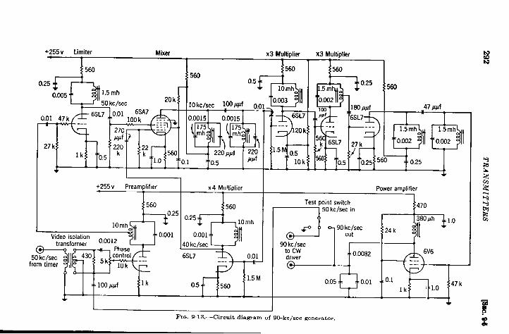
+255 V Limiter Mixer4

560

x3 Multiplier X3 Multiplier

A 560 I L560

[0 kc/see 10Qppf “,0

).0015 I 0.0015 I

0.5t

QI191

‘omh n :::1 ‘0”250003

?

ml 1s0/a#f6SL7 wf 6SL7_&

t, , , 1 L 1 1 1 1..- 1

+255 V

T

x4 Multiplier

T

110mh

$1 :=0.001 0.001 =.“i:r:n::y:e~ 0.0012

@50 kc/see

fro,m timer

=.100 ##f

—

60

47 ##f

m

1.5 mh

I

1.5 mh

0.002 0.CQ2 II

4---- 1.-.. ! u--- L--- )

tl%%!ii’i%+025 ,L 1 L 1 1 1 1 1 1 -14

Power amplifier!

Test point switch

z

50 kclsec in

e‘1

90 kclsecout +

470

380ph

1

1.024 k

90 kc/seeto Cw

1-6”’—‘%”: h%-

1 I d,1,047 k

lK

I

Fua. 9.1 3.—Circuit diagram of 90-kc/aec generator.

&

SEC. 951 LOW FREQUENCY TRANSMITTER 293

a passive network associated with the phase control; the phase differ-ence between input and output voltages of this circuit depends upon thesetting of the control. For adjusting the transmitter output cycle-envelopc relationship it is necessary to be able to vary the phase of the180-kc/sec carrier frequent y through slightly more than one cycle.This frequency of 180 kc/see is locked to that of the 50-kc/sec inputto the generator, rmd the phase variation introduced at 50 kc/see needtherefore be but ~~v of that required at 180 kc/see. By the same token,phase shift occurring at the 90-kc/sec output of the generator will be~~ the amount provided at 50 kc/see. The range of operation of thephase control has been made approximately 120°, providing 216° varia-

tion at 90 kc/see and 432° at 180 kc/see.The output voltage of the phasecontrol stage is not sufficient to

operate the sine-wave divider. Moreover, the voltage amplitude at theoutput of the phase-control circuit varies by 2 to 1 through the controlrange. The sine-wave divider, on the other hand, operates most satis-factorily when the 50-kc/sec input to the mixer tube is constant in ampli-tude and ceases to function entirely when this input fails to exceed acertain minimum. An adequate and constant signal level is obtainedby the use of preamplifier and limiter stages, which have sufficient gainto permit satisfactory operation even with abnormally low 50-kc/secinput voltage.

The transition from 50 to 90 kc/see is accomplished in three steps:(1) The input frequency of 50 kc/see is divided by 5 to produce 10 kc/see;(2) this is multiplied by 3 to obtain a frequency of 30 kc/see; and (3)this in turn is multiplied again by 3, resulting in the final frequency of90 kc/see. The factors by which frequencies in the generator are multi-plied and divided are small, leading to great stability of operation.

The sine-wave divider stage, which divides the 50-kc/sec input fre-quency by 5, consists of a pentagrid-mixer circuit and a conventionalfrequency-quadrupling stage. The two control grids of the mixer aredriven with 50 and 40 kc/see, respectively; the 10-kc/sec output fre-quency is multiplied by 4 in the quadruple to provide the necessarydriving voltage at 40 kc/see. Frequency-dividing operation startsspontaneously within a few tenths of a second after the 50-kc/sec inputsignal is applied and continues as long as the input signal is present.Biaa voltages and signal levels are arranged so that no output is obtainedfrom the 90-kc/sec generator if the crystal-controlled 50-kc/sec inputfrom the timer is missing; thus the transmitter operates at the correctcrystal-controlled frequency or not at all.

R-F Generator. The r-f generator may be considered the heart of thetransmitter. Its input voltages are the trigger from the timer, and thecontinuous 90-kc/sec sine wave from the 90-kc/aec generator. Its out-

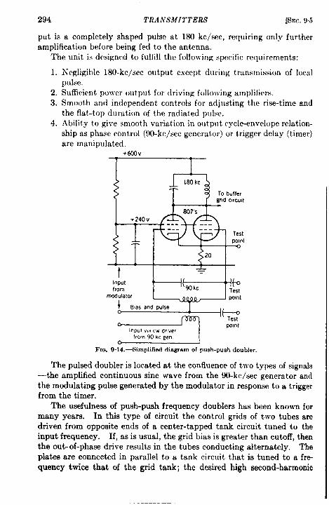
294 TRANSMITTERS [SEC. 9.5

put is a completely shaped pulse at 180 kc/see, requiring only furtheramplification before being fed to the antenna.

The unit isdcsigncd to fulfill the following specific requirements:

1. Negligible 180-kc/sec output except during transmission of localpulse.

2. S\lffi(,iriltpo]vcrolltpllt fordriving following amplifiers.3. Smooth and independent controls for adjusting the rise-time and

the flat-top duration of the radiated pulse.4. Ability to give smooth vcwiation inolltputc ycle-enveloper elation-

ship as phase ctmtrol (90-kc/scc generator) ortriggcr delay (timer)are manipulated,

+600V

1 T

[80 kc

807’s+240 V

t-1-—

Inputfrom

modulator

+ S,asancl pulse

Fm. 9.14.-Smplified diwamof push-push doubler.

The pulsed doubler is located at the confluence of two types of signals—the amplified continuous sine wave from the 90-kc/sec generator andthe modulating pulse generated by the modulator in response to a triggerfrom the timer.

The usefulness of push-push frequency doublers has been known formany years. In this type of circuit the control grids of two tubes aredriven from opposite ends of a center-tapped tank circuit tuned to theinput frequency. If, as is usual, the grid bias is greater than cutoff, thenthe out- of-phase drive results in the tubes conducting alternately. Theplates are connected in parallel to a tank circuit that is tuned to a fre-quency twice that of the grid tank; the desired high second-harmonic

SEC. 9.5] LOW FREQUENCY TRANSMITTER 295

output is produced by the equal and alternate surges of plate currentdrawn by the two tubes.

Figure 914 shows a simplified diagram of the push-push doubler usedin the r-f generator. As can be seen from this figure the c-w excitationat 90 kc/see is coupled inductively into the grid tank by a small link-type primary coil. The normal bias and the superimposed modulatingpulse are applied to the center tap of the grid circuit; and since the90-kc/sec coupling is inductive rather than capacitive, the speedy appli-cation and removal of the modulating pulse are not hindered by unwantedflow of modulator current in coupling impedances.

As used in the r-f generator the tube cutoff bias is approximately 00volts and the alternating grid voltage is somewhat greater than 100-voltpeak. The modulator pulse changes the bias to about 1.5 times cutoff,so that there are times when neither tube conducts. These operatingconditions result in high efficiency and in adequate protection againstunwanted continuous doubling.

The pulsed doubler, then, requires two inputs with the followingcharacteristics:

1. An inductively coupled 90-kc/sec continuous wave, obtained froma source that can supply grid driving power without appreciablechange in driving voltage.

2. A bias whose steady value of approximately – 200 volts can bepulsed, in response to a trigger from the timer, to a voltage in therange between – 150 and – 50 volts. This pulsed value is toremain constant for a controllable time and thereafter return to theinitial value of —200 volts.

The first requirement is met by the use of a c-w driver stage thatamplifies the out put of the 90-kc/sec generator to a level of about 20watts, nearly all of which is intentionally dissipated in fixed resistors.During the puke the grids of the pulsed doubler absorb energy at a rateof less than a watt, so the effect of their additional load is negligible.Figure 9.15 shows the complete circuit diagram of the r-f generator,including the c-w driver.

The mdulator is simply a delay multivibrator whose flat-toppedoutput pulse is passed through a cathode follower to the center tap ofthe doubler grid circuit. The need for a – 250-volt bh supply for thedoubler and the following buffer makes natural the use of this supplyfor the plate voltage of the multivibrator and cathode follower. Oper-ating these circuits from this negative supply makes the power-supplyproblem simpler and, by permitting directioupling, gives a flat-toppedmodulating pulse without the use of a large coupling capacitor. Themodulator output potentiometer is used to establish the operating condi-

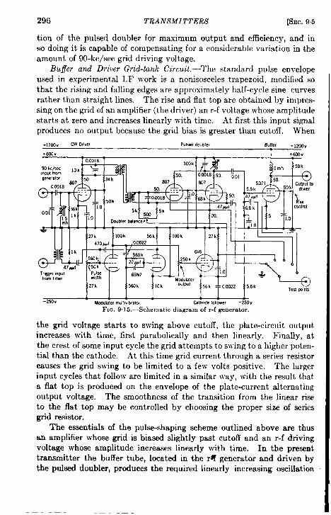
296 TRANSMITTERS [SEC.95

tion of the pulsed doubler for maximum output and efficiency, and inso doing it is capable of compensating for a considerable variation in theamount of 90-kc/sec grid driving voltage.

Buf)’er and Dri~jer Grid-tank Circuit.—The standard pulse envelopeused in experimental LF work is a nonisosceles trapezoid, modified sothat the rising and falling edges are approximately half-cycle sine curvesrather than straight lines. The rise and flat top are obtained by impres-sing on the grid of an amplifier (the driver) an r-f voltage whose amplitudestarts at zero and increases linearly with time. At first this input signalproduces no output because the grid bias is greater than cutoff. When

+12cil“ CWD,IW Pulsed doubler Buffer + 12CQV

FIG. 9.15.—Schematic diagram of r-f generator.

the grid voltage starts to swing above cutoff, the plate-circuit output

increases with time, first parabolically and then linearly. Finally, at

the crest of some input cycle the grid attempts to swing to a higher poten-

tial than the cathode. At this time grid current through a series resistor

causes the grid swing to be limited to a few volts positive. The largerinput cycles that follow are limited in a similar way, with the result that

a flat top is produced on the envelope of the plate-current alternating

output voltage. The smoothness of the transition from the linear rise

to the flat top may be controlled by choosing the proper size of series

grid resistor.

The essentials of the pulse-shaping scheme outlined above are thusan amplifier whose grid is biased slightly past cutoff and an r-f drivingvoltage whose amplitude increases linearly with time. In the presenttransmitter the buffer tube, located in the r~ generator and driven bythe pulsed doubler, produces the required linearly increasing oscillation

SEC.9.5] LOW FREQUENCY TRANSMITTER 297

inthedriver grid tank, Thecircuit isshownin Fig. 9.16. The elementsassociated with the buffer plate and driver grid function as a singleunified circuit, although for convenience some components are locatedin the exciter cabinet and some in the driver.

The grid of the buffer tube is operated Class C, with bias well pastcutoff and with a large 180-kc/sec driving voltage from the pulseddoubler. The flowof grid current inaseries resistor limits the positiveexcursion of the grid to a few volts above cathode potential, and plate

Exciter (buffer tube of r-f generator) Driver1 I

5mh 500+lzoov~

+600vC=y&--- 1 I=XK ~~~~

Rise <

From pulsed control <

doublerpla~Ool ~,6k .

F

6.8 k

T47ppf

-250VC--J I

’50k

1.0

:

6-600v lOOk

Test point Bias supply0 Driver test point/l

Test point

FIG. 9,16.—Simplified circuit of buffer.

current is accordingly drawn in definite-sized short pulses. The bufferplate tank circuit (driver grid tank) has unusually high capacitance, lowinductance, and high Q. When the trigger, modulator, and pulseddoubler have impressed 180-kc/sec driving voltage on the buffer grid,therefore, many cycles elapse before the plate-circuit oscillations reachtheir full amplitude. The initial portion of this buildup is sufficientlylong and linear to be useful in forming the desired leading edge.

The time to reach full amplitude (or the saturation that producesthe flat top on the output pulse) is controlled by varying the screen vol-tage of the buffer tetrode, thus adjusting the amount of charge drawnfrom the tank circuit by each pulse of plate current. The correct settingof the rise control is easily arrived at by observing the final radiatedpulse waveform on the test oscilloscope while the adjustment is made.As the rise control is vaned, the slope of the leading edge changes smoothlyand at an approximately u%form rate; the control exerted by the pulse-width adjustment is also inherently continuous and linear. Special

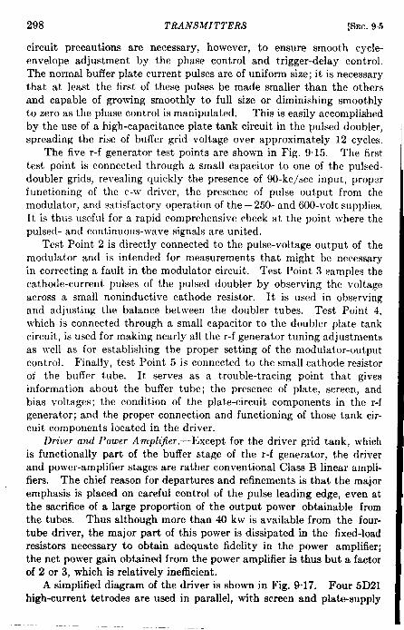
298 TRANSMITTERS [SEC.95

circuit precautions are necessary, however, to ensure smooth cycle-envelope adjustment by the phase control and trigger-delay control.The normal buffer plate current pulses are of uniform size; it is necessarythat at least the first of these pulses be made smaller than the othersand capable of growing smoothly to full size or diminishing smoothlyto zero as the phase control is manipulated. This is easily accomplishedby the use of a high-capacitance plate tank circuit in the pulsed doubler,spreading the rise of buffer grid voltage over approximately 12 cycles.

The five r-f generator test points are shown in Fig. 9.15. The firsttest point is connected through a small capacitor to one of the puked-doubler grids, revealing quickly the presence of 90-kc/sec input, properfunctioning of the c-w driver, the presence of pulse output from themodulator, and satisfactory operation of the —250-and 600-volt supplies.It isth~is usefulfor arapid comprehensive check at the point where thepulsed-and continuous-wave signals are united.

Test Point 2isdirectly connected tothepulse-voltage output of themodulator and is intended for measurements that might be necessaryin correcting a fault in the modulator circuit. Test Point 3 samples thecathode-current pulses of the pulsed doubler by observing the voltageacross a small noninductive cathode resistor. It is used in ohservingand adjusting the balance between the doubler tubes. Test Point 4,which is connected through a small capacitor to the doubler plate tankcircuit, is used for making nearly all the r-f generator tuning adjustmentsas well as for establishing the proper setting of the modulator-outputcontrol. Finally, test Point 5 is connected to the small cathode resistorof the buffer tube. It serves as a trouble-tracing point that givesinformation about the buffer tube; the presence of plate, screen, andbias voltages; the condition of the plate-circuit components in the r-fgenerator; and the proper connection and functioning of those tank cir-cuit components located in the driver.

Driver and Power Arnplijier-.-Except for the driver grid tank, whichis functionally part of the buffer stage of the r-f generator, the driverand power-amplifier stages are rather conventional Class B linear ampli-fiers. The chief reason for departures and refinements is that the majoremphasis is placed on careful control of the pulse leading edge, even atthe sacrifice of a large proportion of the output power obtainable fromthe tubes. Thus although more than 40 kw is available from the four-tube driver, the major part of this power is dissipated in the fixed-loadresistors necessary to obtain adequate fidelity in the power amplifier;the net power gain obtained from the power amplifier is thus but a factorof 2 or 3, which is relatively inefficient.

A simplified diagram of the driver is shown in Fig. 9.17. Four 5D21high-current tetrodes are used in parallel, with screen and plate-supply

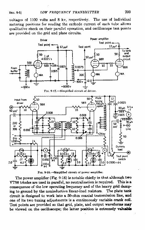
SEC.9.5] LOW FREQUENCY TRANSMITTER 299

voltages of 1100 volts and 8 kv, respectively. The use of individualmetering positions for reading the cathode current of each tube allowsqualitative check on their parallel operation, and oscilloscope test pointsare provided on the grid and plate circuits.

Driver Power amplifier

Test point

~ ‘es’rint I

,2=w

T To tank

Fromr--Ibuffer r+-’”-

501 of4-5D21’s

500 ..-..-

n 1

OJMA ~

LL.-_JJ50 50 ‘aid50#/Af output

98R circuit.-. -..

— 98R5V:P+%Y4Jc-J10‘f ‘-I‘i-+-+4--38ql2.F--

-@ov - +Etiv &

FIG. 9. 17.—Simplified circuit of driver.

&Swlich

15DCIVd.c

= =

FIG. 9.18,-Simplified circuit of power amplifier.

The power amplifier (Fig. 9-18) is notable chiefly in that although twoVT98 triodes are used in parallel, no neutralization is required. This is aconsequence of the low operating frequency and of the heavy grid damp-ing to ground by the noninductive linear-load resistors. The plate tankcircuit is designed to work into a 50-ohm coaxial transmission line, andone of its two tuning adjustments is a continuously variable crank coil.Test points are provided so that grid, plate, and output waveforms maybe viewed on the oscilloscope; the latter position is extremely valuabh

Dummyload

_~

300 TRANSMITTERS [SEC. 95

in that it allows the oscilloscope to be used as an accurate pulse volt-meter, for relative measurements.

Using the oscilloscope as a voltmeter makes it relatively simple toadjust the transmitting-antenna coupling unit without an r-f bridge orother measuring apparatus. This procedure recommends itself, sincethe adjustment for best transient performance, which can be obtainedwith the oscilloscope, is not necessarily identical with that for best c-wperformance as obtained from single-frequency impedance measurements.The technique consists of first measuring the r-f output current and oscil-loscope deflection when a 50-ohm noninductive resistor is used as a loadfor the transmitter. The transmission line, terminated with the couplingunit and antenna, is then connected in place of the resistor. Adjustmentsare systematically made to the coupling unit until the r-f line current andoscilloscope deflection regain their former values.

CHAPTER 10

ANTENNA SYSTEMS

BY R. B. LAWRANCE

101. Requirements for Ground-station Antennas. General Chara.c-

ter-istics: Pokmization.—Transrnitting and receiving antennaa f or Loranground stations are designed for vertical polarization, since the horizontalfield of a wave traveling along the earth’s surface is rapidly attenuated.All Loran synchronizing paths depend on propagation either by ground

I waves that foUow the curvature of the earth’a surface or by sky waves

I

that are emitted at low angles and are then reflected from the ionosphereto a distant receiving station. Efficient low-angle radiation and recep-tion are obtained by the use of extensive radial ground systems that alsominimize the variable effects of soil conductivity on transmission andreception.

Transmitting Antennas. —Four requirements determine the design ofLoran transmitting antennas, (1) The Q of the antenna must be low

I

enough to permit the radiation of a rapidly rising pulse. (2) The direc-tive pattern must be such as to irradiate the intended service area effec-tively, without substantial loss of energy in other directions. (3) Theinput impedance must be stable and present a suitable load for the trans-mitter, so that the radiated pulse shapes are the same for all stations.(4) The antenna must be capable of handling the required peak andaverage power.

The widespread use of modulated oscillators (whose frequencydepends on the impedance of the antenna) for the 2-Me/see ground-station transmitters has made the third requirement particularlyimportant. It has been almost universal practice to use a single verticaltransmitting antenna with no large potential y resonant metallic objectsin its vicinity, thereby avoiding interaction which might distort theall-important leading edge of the radiated pulse. This constructiongives an efficient and simple radiator with no inherent directivity in thehorizontal plane. This lack of horizontal directivity is not often serious.

Since none of the energy radiated at angles higher than about 20°above the horizontal is useful for Loran purposes, it is necessary to con-serve and if possible enhance the low-angle radiation. The use of anextensive radial ground system involving a half ton or more of copperwire has been found to give a worth-while increase in signal strength at

301

302 ANTENNA SYSTEMS [SEC. 10.1

extreme ranges, attributable to decreased loss of low-angle energy in theregion near the antenna.

All short vertical antennas operated against such a ground systemexhibit almost similar radiation patterns in elevation. As the antennalength is increased to a half wavelength or slightly more, however, theproportio~ of low-angle radiation increases significantly. A half-wave-length antenna at Standard Loran frequencies would be approximately260 ft high; although an antenna of this size would be beneficial in apeacetime Loran system, the wartime requirements have been bettermet with a length of the order of 110 ft, slightly less than a quarterwavelength. This gives an antenna that isrelatively easy to erect andthat meets the electrical requirements satisfactorily. Both the full-length vertical and the ‘‘ inverted-L” types have been used.

The Low Frequency Loran experiments have involved a carrier fre-quency of 180 kc/see, for which a quarter wavelength is of the order of1360 ft. A temporary solution of the mechanical and electrical problemshas been the use of a thin wire 1300 ft long, supported by a helium-filledbarrage balloon. A more permanent antenna has been designed but notyet erected; it consists of a 625-ft self-supporting top-loaded base-insulated steel tower.

Receiving Antennas.—The primary function of the receiving antennaat a ground station is to deliver to the receiving apparatus a remote-signalvoltage considerably in excess of the internal-noise voltage. The formof the received pulse at the receiver-input terminals should not be appre-ciabley distorted or delayed; hence the receiving-antenna system musthave adequate bandwidth.

If the baseline is not too long, the received signal is at all times use-fully stronger than the received atmospheric noise. Under these cir-cumstances a simple vertical receiving antenna is adequate even thoughit lacks directivity in the horizontal plane. The length of the antennais determined by the necessary bandwidth and is ordinarily between aneighth and a quarter wavelength. Such a nondirectional receivingantenna is particularly useful at a double station, where two remotesignals must be received usually from quite different directions.

When circumstances force the use of long baselines or a poor receivinglocation, the remote signal may no longer predominate over atmosphericnoise and other received interference. Since the interference generallyarrives from all directions and the desired signal arrives from but one,a directive antenna is helpful. The simplest nonresonant directiveantenna is the Beverage “wave” antenna, which has been used success-fully for 2-Me/see Loran. This type of antenna is simple to constructand works best when the soil conductivity is poor, but it requires consid-erable ground space.

6EC. 10.2] ANTENNA COUPLING UNITS 303

102. Antenna Couplfllg units. Gcrwrd Con.sideratimw.-There aretwo common schemes for coupling energy from the transmitter to thetransmitting antenna. In the simpler of these the transmitter is locatednear the input terminals of the antenna, and the connection is madewithout the use of a transmission line. The antenna input impedance isseldom suitable for use directly as a plate load, but an impedance matchcan be accomplished by the use of a reactive network. Such a networkmay or may not resemble a conventional tank circuit; its design requiresfairly accurate knowledge of both the desired plate-load impedance andthe antenna input impedance as well as of the nature of the signals tobe transmitted. This type of coupling between transmitter and antennahas not been used in any Standard Loran equipment.

In the more complex scheme the transmitter is located at a convenientdistance from the antenna and is connected to it by a transmission line.This gives more freedom in the layout of the transmitting station and,since the characteristic impedance of the transmission line is known inadvance, makes it possible to design the transmitter for a single standardvalue of load impedance. The input impedance of the transmissionline is a pure, constant resistance over the range of frequencies for whichthe terminating impedance equals the line characteristic impedance.Over the range of frequencies including the carrier and all significantsideband components, therefore, the coupling unit should be able totransform the frequency-varying resistance and reactance of the antennainto an impedance equal to that of the transmission line, primarilyresistive and practically constant.

In Low Frequency Loran the shape of the transmitted pulses must becontrolled with great care, and even with the faster-rising pulses of2-Me/see Loran the antenna and coupling unit must not produce appre-ciable lengthening of the pulse rise time. This requirement may bestated in terms of input impedance, as in the preceding paragraph, or inequivalent and alternative terms of energy storage.

Consider an antenna that is radiating energy at a constant power level;stored in the electric and magnetic fields surrounding the antenna is anamount of energy several times as great as that radiated per cycle. Thismeans that if the flow of energy to the antenna is suddenly stopped, theantenna will continue to radiate, with slowly decreasing amplitude, untilthis stored energy is exhausted. Conversely, if input power is suddenlyapplied to an antenna, several cycles will elapse before the stored energybuilds up and the antenna radiates at full power.

The presence of some stored energy is unavoidable, but for pulseI transmission the amount must be kept relatively low. For a given length

I of antenna, the stored energy may be reduced by increasing the effectivediameter of the antenna conductor. From an impedance standpoint,

I

304 ANTENNA SYSTEMS [SEC.10.2

this causes the input reactance to vary less rapidly with frequency;hence the bandwidth is increased. The effects of an antenna’s dimensionson its input impedance and bandwidth are discussed in Sec. IO*3; indesigning a coupling unit the bandwidth of the antenna is always thelimiting factor.

Simple Reudznce iVetwork8.-1n general the input resistance of aLoran transmitting antenna is different from the characteristic impedanceof the transmission line, and the input reactance ia not, except fortuitously,

Xm=xa-Xum equal to aero. Although ideallythe coupling unit should provide

‘mexact-tcfingoveracOF-

able range of frequencies, it hasbeen found that under certain con-ditions it is sufficient to design the

(a) unit for exact matching at the car-rier frequency only. If the Q of

,& =xmm-x. the antenna is not excessively

mhigh’andifthean’enna:pu’

resistance is not too greatly differ-ent from the line impedance sim-ple ladder networks of two or threereactance can be used. In order

(b) to keep to a minimum the energy

Xm=Xam-X. stored in the coupling unit, allA series impedances (which carry/- \

-3

high current) are made smallwhereas the shunt impedances are

‘A’;m ‘“’a ‘a%:t%s:sE&:::rnmOn-{c) ly used in Loran stations is a stand-

I?IQ. 10.1.—Simple L- and T-networks for ard solid-dielectric coaxial cablematching impedances at carrier frequency. with a nominal characteristic im-

pedance of 52 ohms. Since the antenna input resistance is usually between

IS and 45 ohms, a small impedance transformation is required. Figure

10! 1 shows three simple networks that are suitable for the purpose.

In all three circuits the symbols are defined as follows, values being taken

at the carrier frequency:

RA = antenna input resistance,X. = antenna input reactance,RX = source resistance to be matched (usually the characteristic

impedance of a transmission line: 52 ohms),XA~ = reactance of antenna arm of matching unit,Xl~ = reactance of input arm of matching unit,

SEC.10.2] ANTENNA COUPLING UNITS 305

XU = reactance of shunt arm of matching unit,XAA = net reactance of antenna and antenna arm of matching unit.

For the T-network, which is the more general form, the relations betweenthe quantities are given in the formulas below. In these formulas allreactance, capacitive and inductive, appear as positive numbers, theirnature being indicated by the note at the side of the equation and bythe symbols in the diagram.

x.. 2 mI (capacitive). (la)

dX.. = X,ga( – (X:w – RAR,) $ (inductive). (lb)

Xraf = XSM – J(x;M – R.R,) + (inductive for R.Alarge, (lC)capacitive for RA small).

X~~ changes sign when RJR1 = X&/(X& + R:).

A slight change in R. necessitates no readjustment of X.. (but doesrequire an adjustment in XI~) when Xs.M = 42RAR1.

The mathematical treatment yields two solutions each for XA~ andX,~, one having a positive sign before the radical and the other having anegative sign. However, the choice of the positive sign yields values ofreactance that are unnecessarily large (with excessive stored energy andconsequent reduction of bandwidth). The fact that two sets of adjust-ments exist which give proper matching at the carrier frequency is,of course, a consequence of the fact that the coupling unit has three inde-pendent elements. This is one more than the minimum number neces-sary for independent adjustment of input resistance and reactance; ifXSM were continuously variable, there would be an infinite number ofsuitable settings.

As in all reactive impedance-transforming circuits, conditions at thecarrier frequency remain unaltered if each inductive reactance is replacedby a corresponding capacitive reactance, and vice versa. Conditions atother frequencies are reversed; if for the original circuit a slightly higherfrequency gives an increased resistance and a capacitive reactance com-ponent, then for the revised circuit a slightly lower frequency gives asimilar increased resistance and a corresponding inductive reactance.This effect is discussed later, in connection with Fig. 10.4. In generalthe use of a capacitive shunt arm is preferable, since harmonic com-ponents are bypassed.

The T-network is most useful when R. is greater than about one-halfii,, although it may be used for values as low as one-fourth RJ if XSM ischanged or if a capacitor is inserted at a-a in the input arm. A T-net-work is used, in the form shown in Fig. 10. lc, for matching the Win-

306 ANTENNA SYSTEMS [SEC. 10.2

charger antenna (sea%. 10”4). Itcanalso beusedsatisfactorily withavertical wire antenna if the inductor X4~ is su5ciently large. In theLF application the T-network is used with both the balloon-supportedwire antenna and the permanent umbrella-loaded tower (see Sec. 10.5);for use with the tower the reactance of X3M is reduced and a series capaci-tor is inserted at a-a. With the baUoon antenna, XSX is proportioned sothat changes in antenna resistance, produced by varying angle of inclina-tion, cause relatively little error in coupling unit adjustment.

For the lower values of antenna resistance, as obtained with inverted-Land T-antennas, the L-network is satisfactory. The standard couplingunit, Navy type CG-47368, is normally used as a T-network but can bereconnected as an L-network; thus a single unit is adequate for use withall ZMc/sec Loran transmitting antennas. Since the step-up (lookingfrom antenna into transmission line) L-network may be regarded as aT-network with series input reactance X~~ equal to zero, the formulasfor its elements are the following:

Of the two forms of stepup L-network shown

(2a)

(2b)

(2C)

in Fix. 10.1 the first isthe more useful, since at Loran frequencies variable inductors of appropri-ate reactance are simpler and less expensive than corresponding variablecapacitors. In addition, since a low-resistance antenna usually hascapacitive input reactance, a smaller inductor may be used at X~.~f,making the over-all bandwidth appreciably greater than with the circuitof Fig. 10. lb. The suppression of harmonic radiation is the sole advan-tage of the latter circuit.

Finally, there is another form of the L-network that can be used tostep down antenna resistances that arc greater than twice the line charac-teristic impedance. This network may also be derived from the T-net-work formulas, by setting X~~ equal to zero. As yet, however, it has notbeen used as a Loran coupling unit.

Adjustment of 7’- and L-networks.—The adjustment of these couplingunits may be facilitated by the use of r-f impedance-measuring equip-ment, but this is not essential. In the absence of measuring equipmentthe transmitter is first tuned into a 50-ohm resistance load, and the out-put current, pulse shape, and operating conditions are carefully noted.The output connection is then transferred to the transmission line andantenna circuit, and the two coupling-unit tuning controls are adjusteduntil the previous conditions are closely simulated. Careful use is madeof the transmitter-testing oscilloscope during the tuning procedure,

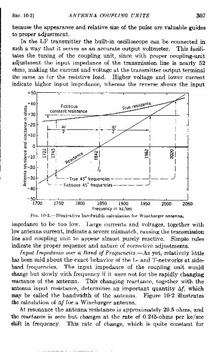
SEC. 10.2] ANTENNA COUPLING UNITS 307

because the appearance and relative size of the pulse are valuable guidesto proper adjustment.

In the LF transmitter the built-in oscilloscope can be connected insuch a way that it serves as an accurate output voltmeter. This facili-tates the tuning of the coupling unit, since with proper coupling-unitadjustment the input impedance of the transmission line is nearly 52ohms, making the current and voltage at the transmitter output terminalthe same as for the resistive load. Higher voltage and lower currentindicate higher input impedance, whereas the reverse shows the input

-50~1700 1750 1800 1850 1900 1950 2000 2050

Frequencyin kc/see

FIQ. 10.2.—Illustrative bandwidth calculation for Wincharger antenna.

impedance to be too low. Large currents and voltages, together withlow antenna current, indicate a severe mismatch, causing the transmissionline and coupling unit to appear almost purely reactive. Simple rulesindicate the proper sequence and nature of corrective adjustments.

Input Impedance over a Band of Frequencies.—As yet, relatively littlehas been said about the exact behavior of the L- and T-networks at side-band frequencies. The input impedance of the coupling unit wouldchange but slowly with frequency if it were not for the rapidly changingreactance of the antenna. This changing reactance, together with theantenna input resistance, determines an important quantity Aj, whichmay be called the bandwidth of the antenna. Figure 10.2 illustratesthe calculation of Af for a Wincharger antenna.

At resonance the antenna resistance is approximately 29.5 ohms, andthe reactance is zero but changes at the rate of 0.245-ohms per kc/seeshift in frequency. This rate of change, which is quite constant for

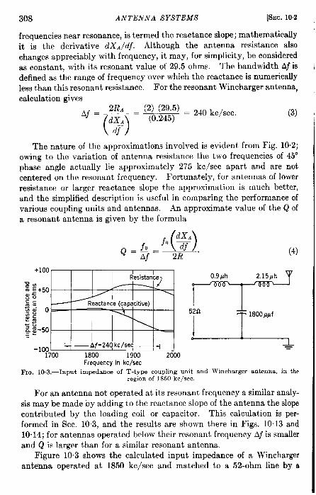
308 ANTENNA SYSTEMS [SEC. 10.2

frequencies near resonance, is termed the reactance slope; mathematicallyit is the derivative dXA/dj. Although the antenna resistance alsochanges appreciably with frequency, it may, for simplicity, be consideredas constant, with its resonant value of 29.5 ohms. The bandwidth Afisdefined as the range of frequency over which the reactance is numericallyless than this resonant resistance. For the resonant Wincharger antenna,calculation gives—

2RA (2) (29.5) = 240kc/sec.Aj=—

(-)

ciX~ = (0.245)(3)

dj

The nature of theapproximations involved isevident from Fig. 10.2;owing to the variation of antenna resistance the two frequencies of 45°phase angle actually lie approximately 275 kc/see apart and are notcentered on the resonant frequency. Fortunately, for antennas of lowerresistance or larger reactance slope the approximation is much better,and the simplified description is useful in comparing the performance ofvarious coupling units and antennas. An approximate value of the Q ofa resonant antenna is given by the formula

()dX,i

~=$=f” T.2R

(4)

+100 I IResistance

Z.m E+50WC~o~ .= —,g 0- ()2:.g: $.50:.

b-1oo =1700 1800 1900 2ocil

Frequency in kc/seeFIQ. 10.3.—Input impedance of T-type coupling unit and Wincharger antenna, in the

region of 1850 lcc/sec.

For an antenna not operated at its resonant frequency a similar analy-sis may be made by adding to the reactance slope of the antenna the slopecontributed by the loading coil or capacitor. This calculation is per-formed in Sec. 10.3, and the results are shown there in Figs. 1013 and10.14; for antennas operated below their resonant frequency A~is smallerand Q is larger than for a similar resonant antenna.

Figure 10.3 shows the calculated input impedance of a Winchargerantenna operated at 1850 kc/see and matched to a 52-ohm line by a

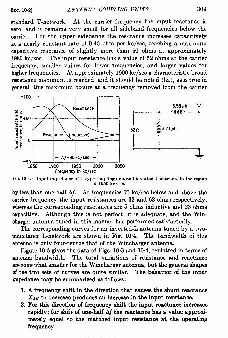
sac. 10.2] ANTENNA COUPLING UNITS 309

standard T-network. At the carrier frequency the input reactance is‘zero, and it remains very small for all sideband frequencies below thecarrier. For the upper sidebrmds the reactance increases capacitivelyat a nearly constant rate of 0.45 ohm per kc/see, reaching a maximumcapacitive reactance of slightly more than 50 ohms at approximately1980 kc/see. The input resistance has a value of 52 ohms at the carrierfrequency, smaller values for lower frequencies, and larger values forhigher frequencies. At approximately IWO kc/see a characteristic broadresistance maximum is reuched, and it should be noted that, as is true ingeneral, this maximum occurs at a frequency removed from the carrier

+100—

~mmEa 5+50.; ,E-V,al~:.~~kj 0~.

p--Af=95 kc/secy =-50

1850 1900 1950 2000 2050Frequency in kc/s.ec

Fm. 10.4.—Input impedance of L-type coupling unit and inverted-L antenna, in the regionof 1950 kc/sec.

by less than one-half A~. At frequencies 50 kc/see below and above thecarrier frequency the input resistances are 33 and 63 ohms respectively,whereas the corresponding reactance are 5 ohms inductive and 23 ohmscapacitive. Although this is not perfect, it is adequate, and the Win-chsrger antenna tuned in this manner has performed satisfactorily.

The corresponding curves for an inverted-L antenna tuned by a two-inductance L-network are shown in Fig. 10.4. The bandwidth of thisantenna is only four-tenths that of the Wincharger antenna.

Figure 10c5 gives the data of Figs. 10,3 and 10.4, replotted in terms ofantenna bandwidth. The total variations of resistance and reactanceare somewhat smaller for the Wincharger antenna, but the general shapesof the two sets of curves are quite similar. The behavior of the inputimpedance may be summarized as follows:

1.

2.

A frequency shift in the direction that causes the shunt reactanceXs~ to decrease produces an increase in the input resistance.

For this direction of frequency shift the input reactance increasesrapidly; for shift of one-half Af the reactance has a value approxi-mately equal to the matched input resistance at the operatingfrequency.

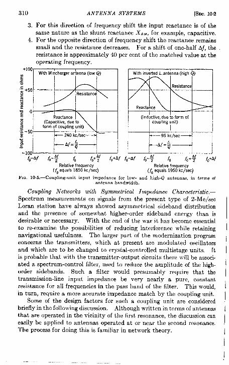
310

3.

4.

ANTENNA SYSTEMS [SEC. 10.2

For this direction of frequency shift the input reactance is of thesame nature as the shunt reactance XS~, for example, capacitive.For the opposite direction of frequency shift the reactance remainssmall and the resistance decreases. For a shift of one-half A~, theresistance is approximately 40 per cent of the matched value at theoperating frequency.

+100 ( 1With Wincharger antenna (low Q) With inverted L.antenna (high Q)

~%

‘: +50Resistance:~

: /

~o — IReactance (Inductive, due to form of

$c (Capacitive, due to coupling unit)

form of coupling unit)%‘~ -50

~ 240 Imlsec — —95 kc/see_~= _Af. $ _Af = $!

- 10Q I Ifo-Af &.$

Relativ!frequen[y+4°02 fo+Af fo-Af & f. fo+g fo+df

Relative frequency(f. equals 1850 kc/see) (~. equals 1950 kc/see)

Fm. 10.5.—Coupling-unit input impedance for low- and highQ antennas, in terms ofantenna bandwidth,

Coupling Networks with Symmetrical Impedance Characteristic.—Spectrum measurements on signals from the present type of 2-Me/seeLoran station have always showed asymmetrical sideband distributionand the presence of somewhat higher-order sideband energy than isdesirable or necessary. With the end of the war it has become essentialto m-examine the possibilities of reducing interference while retainingnavigational usefulness. The larger part of the modernization programconcerns the transmitters, which at present are modulated oscillatorsand which are to be changed to crystal-controlled multistage units. Itis probable that with the transmitter-output circuits there will be associ-ated a spectrum-control filter, used to reduce the amplitude of the high-order sidebands. Such a filter would presumably require that thetransmission-line input impedance be very nearly a pure, constantresistance for all frequencies in the pass band of the filter. This would,in turn, require a more accurate impedance match by the coupling unit.

Some of the design factors for such a coupling unit are consideredbriefly in the following discussion. Although written in terms of antennasthat are operated in the vicinity of the first resonance, the discussion caneasily be applied to antennas operated at or near the second resonance.The process for doing this is familiar in network theory.

I

SEC. 102] ANTENNA COUPLING UNITS 311

Impedance-changing circuits with symmetrical characteristics aremost easily obtained by the use of a transformer. Since a physicallyrealizable transformer has neither infinite inductance nor perfect couplingit can be represented in terms of an ideal transformer combined withfinite impedances. A simple equivalent circuit of this type, valid whenlosses and distributed capacitances may be neglected, is shown in Fig.10.6. The properties of the ideal transformer are that its open-circuitprimary and secondary impedances are infinite, that its short-circuitimpedances are zero, and that the primary voltage and current are ezxzctlyrelated to the secondary voltage and current by the turns ratio. Any

2$GL2

Coeff of coupling=k=*,

Ideal transformer - -

~“y

Pri. turns-[

1 L,— .——SW. turns b Lz

filF!!!$’AE(a) Circuit including practical transformer

W%)l!(!)?cn”(=;~ . .

(b) Allimpedances “transferred”to primaw side

Fm. 10.6.—Equivsdent circuit FIQ. 10.7.—Uae of transformer in matching ant.en~%for practical transformer, in terms to transmission line.of ideal transformer.

impedance appearing at one side of the transformer may thus be ‘‘ trans-ferred” to the other side by simply multiplying by the square of theappropriate turns ratio.

The simplest use of a practical transformer for matching an antennato a transmission line is shown in Fig. 10.7. Values of the equivalentseries inductance and capacitance of the antenna may be calculated bythe methods described in Sec. 10.3. If the antenna has a capacitiveinput reactance larger than the transformer leakage reactance, the capaci-tor Cl is replaced by an inductor. Tuning of the circuits is simple boththeoretically and practically: the primary circuit is tuned to resonancewhile the secondary is open-circuited, and the secondary is similarlytuned with the primary short~ircuited.

The transformed antenna resistance can be made equal to the lineimpedance, but at the input terminals it appears in series with a seriea-rwonant circuit, the combination being in parallel with the shunt-resonant primary circuit. The behavior at frequencies off resonancedepends on the relationship that the values of the resonant-circuitreaatances bear to the transformed resistance. Since the antenna con-

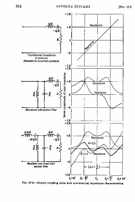
312 ANTENNA SYSTEMS [SEC. 10.2

R0

‘\

-QR

R

Transformed impedanceof antenna

(Resistance assumed constant)

QR

m

-QR

e -t R

Mld.shunt half.section filter

sectionfilter

+22?-

Resistante+R

0

-R

-2R+2R

al:+3E+RE.-3

.5

~og

zEg–R,

K?

i

-2R+2R

+R

o

-R

-( Af=$)——

-2Rfo-Af flJ- +’ f. fo+ +f fo+ At

Fm. 10.8.-Simple ooupling units with symmetrical impedance characteristiea

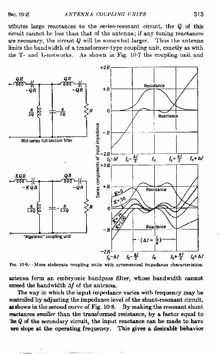
SEC.10.2] ANTENNA COUPLING UNITS 313

tributes large reactance to the series-resonant circuit, the Q of thiscircuit cannot be less than that of the antenna; if any tuning reactanceare necessary, the circuit Q will be somewhat larger. Thus the antennalimits the bandwidth of a transformer-type coupling unit, exactly as withthe T- and L-networks. As shown in Fig. 10.7 the coupling unit and

*( f QR

T k-QR -QR

& R2Q ‘-s

cMid.series full.section filter

R

‘Rw+—+—b++

-2R L I I 1 I

fO-Af fO-~ f, fO+$f fO+Af

Fm, 10.9.—More elaborate coupling units with symmetrical impedanee characteristics.

antenna form an embryonic bandpass filter, whose bandwidth cannotexceed the bandwidth Af of the antenna.

The way in which the input impedance varies with frequency maybecontrolled by adj usting the impedance level of the shun~resonant circuit,as shown in the second curve of Fig. 10.8. By making the resonant shuntreactance .wnuWr than the transformed resistance, by a factor equal to‘he Q of the secondary circuit, the input reactance can be made to havevxo slope at the operating frequency. This gives a desirablb bkhavior

314 ANTENNA SYSTEMS [SEC. 103

for frequencies in the immediate region of the carrier, but for frequenciesremoved by one-half Af the reactance and resistance are equal. Thethird set of curves in Fig. 10.8 shows a method of improving the inputimpedance at the higher sidebands, with some sacrifice of performancenear the carrier frequency.

Figure 108 shows the curves for a coupling unit treated as a midshunthalf-section filter; in Fig. 10.9 the characteristics of a midseries full-sectionfilter are shown. Theimproved resemblance tothefilter-theory behavioris evident, with thereactance very nearly zero throughout the pass bandand with the resistance decreasing smoothly to a small value at the edgeof the band. A modified circuit, with performance intermediate betweenthe two filter circuits, is also shown in Fig. 10.8. It is thought that inthe embodiment in which the factor K is equal to approximately 0.75 acircuit may be provided that will terminate the transmission line satis-factorily for all significant components transmitted through the filter atits input.

10,3. Prediction and Simulation of Antenna Characteristics.-In thedesign of Loran transmitting and receiving antennas it is obviouslydesirable to be able to predict the various characteristics in advance,with a fair degree of accuracy. Estimates of the bandJvidth arc necessaryfor reassurance that distortion of the pulse signals ~vill not be excessive,and predictions of antenna impedance furnish the starting basis forcoupling-unit design.

Furthermore, in experimental work with transmitters, it is desirableto have available dummy antennas that are capable of handling the fulltransmitter-output pon-er and that simulate closely the steady-state andtransient response of the antenna to be used ultimately. Both experi-mentation and the training of personnel are facilitated by the use of suchdummy antennas.

In recent years the accurate calculation of antenna input impedancehas been the subject of many published papers. The most comprehensiveand apparently the most accurate methods are those of Schelkunoff, andthe reader is referred to his papers. 1 The present section is concernedwith calculations in which some accuracy is sacrificed for simplicity; insome cases results are taken from Schelkunoff directly, and in othersapproximations are made from his formulae. In a few cases originalempirical results have been found useful and are given. The discussionsare confined to vertical antennas of uniform cross section operated at orbelow the first resonant frequency.

IS. A. Schelkunoff, “Theory of Antennas of Arbitrary Size and Shape,” Proc. IRE,29, No. 9, September1941; “Concerning Hallen’s Integral Equation for CylindricalAntemm,” Proc. IRE, 22, No. 12, December 1945; “Principal and ComplementaryWaveain AntennM,”Proc. IRE, S& No. 1, January1946.

SEC.10-3] PREDICTION AND SIMULATION OF ANTENNA 315

Characteristic Impedance and Electrical Length.—The concept ofcharacteristic impedance, much used in discussing transmission lines, isalso useful in antenna theory. Strictly speaking, a biconical antenna isthe only type possessing uniform characteristic impedance, since itsinductance and capacitance per unit length do not change with distancefrom the generator. The cylindrical antennas can, however, be con-sidered as having an average characteristic impedance, which is useful inboth the detailed and simplified theories. Schelkunoff gives a formulathat, for a cylindrical antenna operated against a perfectly conductingground plane, may be written as

20 = 138.2 log,, ~ + 23.2, (5)

where Zo = average characteristic impedance, ohms,1 = length of antenna conductor, any units,

d = diameter of antenna conductor, same units as 1.It is interesting to note that this is exactly the characteristic imped-

ance of a single-wire transmission line operated against ground, wherethe height is 1/2.718 times the length 1 of the antenna. Other authorshave given other formulas, differing in the additive constant by as muchas 40 ohms and sometimes including a term dependent on frequency.

The first, “quarter-wave,” resonance occurs at a frequency lowerthan that giving a free-space quarter wavelength equal to the length ofthe antenna. One of the many alternative ways of representing thiseffect is by defining an electrical length 0, such that

O=Ko~, (6)

where 0 = electrical length, degrees,Ko = a factor greater than 360°,

h = free-space wavelength, same units as 1.Inserting the wavelength-frequency relation and expressing the quantitiesin convenient units, we obtain

0 = (1.016) (K,) (L) (f~c) (1P). (7)

The factor Kg is a function of the proportions of the antenna and ishence a function of 20; it is plotted in Fig. 10”10. The reason for express-ing the electrical length in this manner is that in the region of the firstresonance the input reactance varies approximately as a cotangent func-tion. This relationship is not theoretically exact except for antennas ofinfinite characteristic impedance, but its simplicity is a great asset, andita accuracy is quite good for frequencies up to and slightly beyond the

316 ANTENNA SYSTEMS [SEC.103

first resonance.1 If subsequent discussions are confined to electricallengths not exceeding 90°, then the reactive component of the antennainput impedance is given by the approximate formula

x. = – Z. cot e, (8)

where XA = antenna input reactance, ohms.The input resistance of an antenna is customarily analyzed into three

components, one of which represents the useful radiation of a portion of

390

:$g 3s0.s*“~ 370

:b.

360 R1002OO3OO4OO5OO6OO

Averagecharacteristic impedance Z. in ohms

FIG. 10 10.—Effect of average characteristic impedance in lowering first resonant frequencyof vertical cylindr],calantennas. (Data from S.hdkunoff, Pro.. IRE, September,1941.)

35 ~z=34 / ‘g Experimental point / -

for 300-ft mastg 33

2/

.-; 32

E“~ 31v

g 30250 30Q 350 400 450, 500 550 600

Average characteristic Impedance in ohms

FIG. 10,11.—Radiation resistance at first resonance, as a function of characteristic imped-ance. (Data from Schelkunofl,Proc. IRE, September, 1941,)

the input power. The other two components represent dissipation in theimperfect conductors of the antenna and of the ground. For a goodradial ground system and a reasonably efficient antenna conductor thelatter two resistance components are usually of the order of 2 to 5 ohms;thus when the electrical length is greater than approximately 45°, theradiation resistance is the dominant component.

The radiation resistance may be represented as a function of theelectrical length and of the characteristic impedance. For a given lengthof antenna the radiation resistance increases slightly as the diameter is

1For example, reactance measurements on a uniform 300-ft tower with 20 = 264gave points evenly scattered about a cotangent curve, the average deviation being2 per cent. The measurements covered the region from 0 = 16° to 0 = 125”.

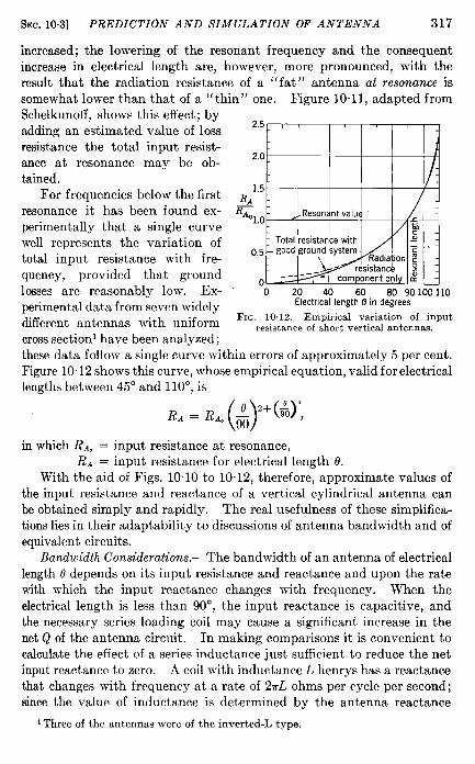
SEC. 10.3] PREDICTION AND SIMULATION OF ANTENNA 317

increased; the lowering of the resonant frequency and the consequentincrease in electrical length are, however, more pronounced, with theresult that the radiation resistance of a ‘(f at” antenna at resonance issomewhat lower than that of a “thin” one. Figure 10.11, adapted fromSchelkunoff, shows this effect; byadding an estimated value of lossresistance the total input resist-ance at resonance may be ob-tained.

For frequencies below the firstresonance it has been found ex-perimentally that a single curvewell represents the variation oftotal input resistance with fre-quency, provided that groundlosses are reasonably low. Ex-perimental data from seven widelydifferent antennas with uniformcross sectionl have been analyzed;

.

2,5 ,

2.0

1.5RA

R~‘1,0

- Total resistance with0,5 – good ground system.

o0 20 40 60 80 90100110

Electrical length O in degrees

FIG. 10.12.—Empirical variation of inputresistance of short vertical antennas.

these data follow a single curve within errors of approximately 5 per cent.Figure 10.12 shows this curve, whose empirical equation, valid for electricallengths between 45° and 110°, is

R.= l?..(;)’+($)’,in which RLO = input resistance at resonance,

RA = input resistance for electrical length 0.With the aid of Figs. 10.10 to 10.12, therefore, approximate values of

the input resistance and reactance of a vertical cylindrical antenna canbe obtained simply and rapidly. The real usefulness of these simplifica-tions lies in their adaptability to discussions of antenna bandwidth and ofequivalent circuits.

Bandwidth Considerations. -The bandwidth of an antenna of electricallength 8 depends on its input resistance and reactance and upon the ratewith which the input reactance changes with frequency. When theelectrical length is less than 90°, the input reactance is capacitive, andthe necessary series loading coil may cause a significant increase in thenet Q of the antenna circuit. In making comparisons it is convenient tocalculate the effect of a series inductance just sufficient to reduce the netinput reactance to zero. A coil with inductance L henrys has a reactancethat changes with frequency at a rate of 27rLohms per cycle per second;since the value of inductance is determined by the antenna reactance

tThreeof the antennas were of the inverted-L type.

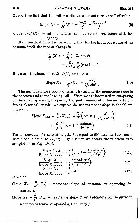
318 ANTENNA SYSTEMS [SEC.10$

Z. cot e we find that the coil contributes a “reactance slope” of value

d 2rfL z. cot o‘*ope “ = ~ ‘x’) = ~ = “ f

(9)

where d/d~ (XL) = rate of change of loading-coil reactance with fre-quency.

By a simple differentiation we find that for the input reactance of theantenna itself the rate of change is

$(x.) = $(–z. cot e)

Zo d= ~8 ~f (8 radians).

But since Oradians = (T/2) (~/jo), we obtain

d Uzo‘lOpe “ = ~ ‘x’) = 2f0 sin’ 0“

(lo)

The net reactance slope is obtained by adding the components due tothe antenna and to the loading coil. Since we are interested in comparingat the same operating frequency the performance of antennas with dif-ferent electrical lengths, we express the net reactance slope in the follow-ing form:

(11)

For an antenna of resonant length, 0 is equal to 90” and the total react-ance slope is equal to ifZO/2f.are plotted in Fig. 10’13:

Slope XtiZ!Slope X.OmP.~,.

Slope X.—.—slope Xo.mo.m,.

slope xc_— .—Slope Xwm)..-k

in which

By division we obtain the relations that

( 9 radians=. cot e +n’ )

sinZ o “

=:( )

2 0 radians7r sinz O

2=— cot e.lr

(12a)

(12b)

(12C)

slope XA = $(x’) =reactancedope of antenna at operating fr~

quency f.

Slope XL = ~ (XL) = reactance slope of series-loading coil required to

resonate antenna at operating frequency j.

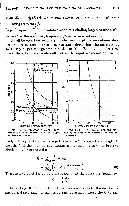
SEC. 10.3] PREDICTION AND SIMULATION OF ANTENNA

Slope xtiti = ~j (X4 + XL) = reactance slope of combination

sting frequency j.

319

at oper-

Slope Xu... ~. = ‘~ = reactance slope of a similar, larger, antenna self-

resonant at the operating frequent y (“comparison antenna”).It will be seen that reducing the electrical length of an antenna does

not produce extreme increases in reactance slope, since the net slope at45° is onlv 64 Der cent meater than that at 90°. Reduction in electricallength dies, h~wever, &ofoundly

3.0[SlopeX ,Ot,,

Slopex Compati,on2.5 antenna

/)

2.0.-Q \

; 1.5 \

t%

1.0-

0 -‘O 20 40 60 so 90

Electrical length 6 in degrees

Fra. 1013.-Reactance slopes withvertical antennas shorter than the lengthfor first re80nance,

the Q. If R~ is the antenna input

Meet the input resistance and hence

12

10 \

8

Kq

6

4\

2

———- ——. ___ __ \

00 20

ElectricalI$gth 13in%egrees80

FIG..1014.-Increase of antenna cir-cuit Q as length of vertical antenna isdecreased.

resistance for an electrical length 0,then‘the Q of the antenna and loading coil, considered as a simple ~eriescircuit, may be expressed as

Q = AA$ (x..,)

( e radians—— ~ cOte+—-2~. smz 0 )

(13)

This has a value Qo for an antenna resonant at the operating frequency

From Figs. 10.12 and 10.13, it can be seen that both the decreasinginput resistance and the increasing reactance slope cause the Q to rise

320 ANTENNA SYSTEMS pm. 103

rapidly as the electrical length is decreased; this result is ahown in Fig.10.14. The factor KQ is defined as follows:

&.:~ ( o radianscOt e + sinz ~

)(14)

= ratio of net Q to Q of comparison antenna (both at operating f~quency j)

. ratio of net Q to Q of the antenna at its resonant frequency.The net Q of a particular antenna can be obtained from the expression

(15)

It will be noted that the use of an antenna of electrical length 70°gives a Q that is double the resonant value whereas for an electrical lengthof 45° the factor is nearly 7. It is thus evident that for transmittingpurposes the electrical length should not be much less than 90°.

f=-4c+-$-v%-Simplest equivalent circuit

Moreelaboratecircu!tFJ~. 10 15.—Equivalent circuits for input impedance of a short vertical antenna.

It should be mentioned that the above values of Q are calculated onthe basis of negligible damping by the internal impedance of the sourcefeeding the transmitting antenna (or by the load impedance fed by thereceiving antenna.) If such a matched impedance is used and if theimpedance is essentially a pure resistance, the resulting Q will have half

of the value given. This is almost always true in the case of I,oran

ground-station receiving antennas, a fact that allows moderately short

antennas to be used without trouble from inadequate antenna-circuit

bandwidth. For transmitting antennas the situation is somewhat

complicated, since the impedances of both the t,ransrnit,t,er and the

antenna may be considered to change during the different portions of

the pulse. In general, however, the radiated pulse can he made to rise

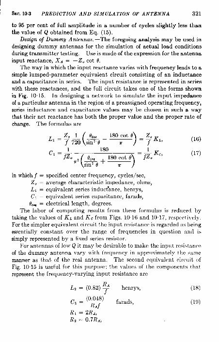
SEC. 103 PREDICTION AND SIMULATION OF ANTENNA 321

to 95 per cent of full amplitude in a number of cycles slightly less thanthe value of Q obtained from Eq. (15).

Design of Dummy Antennas.—The foregoing analysis may be used indesigning dummy antennas for the simulation of actual load conditionsduring transmitter testing. Use is made of the expression for the antennainput reactance, X4 = —Z. cot 0.

The way in which the input reactance varies with frequency leads to asimple lumped-parameter equivalent circuit consisting of an inductanceand a capacitance in series. The input resistance is represented in serieswith these reactance, and the full circuit takes one of the forms shownin Fig. 10.15. In designing a network to simulate the input impedanceof a particular antenna in the region of a preassigned operating frequency,series inductance and capacitance values may be chosen in such a waythat their net reactance has both the proper value and the proper rate ofchange. The formulas are

z. i

(–

180 cot 0

)~“ K.,

‘“Tin Si’%e– 7r ‘f(16)

1 180c’ = jzor,

(– )

~ Kc,ode. + 180 cot 0 = fzo

(17)

sin2 e ‘r

in which f = specified center frequency, cycles/see,Z. = average characteristic impedance, ohms,LI = equivalent series inductance, henrys,C, = equivalent series capacitance, farads,

0,= = electrical length, degrees.The labor of computing results from these formulas is reduced by

taking the values of KL and KC from Figs. 1016 and 10.17, respect i~-ely.For the simpler equivalent circuit the input resistance is regarded as beingessentially constant over the range of frequencies in question and issimply represented by a fixed series resistor.

For antennas of low Q it may be desirable to make the input rrsistanmof the dummy antenna vary with frequency in approximately the samemanner as that of the real antenna. The second equivalent circuit ofFig. 10.15 is useful for this purpose; the values of the components th~trepresent the frequency-varying input resistance are

L, = (0.82)+ henrys, (18)

~, = (0.048) -farads,

RA j(19)

RI = 2RA,

Rz = 0.7RA,

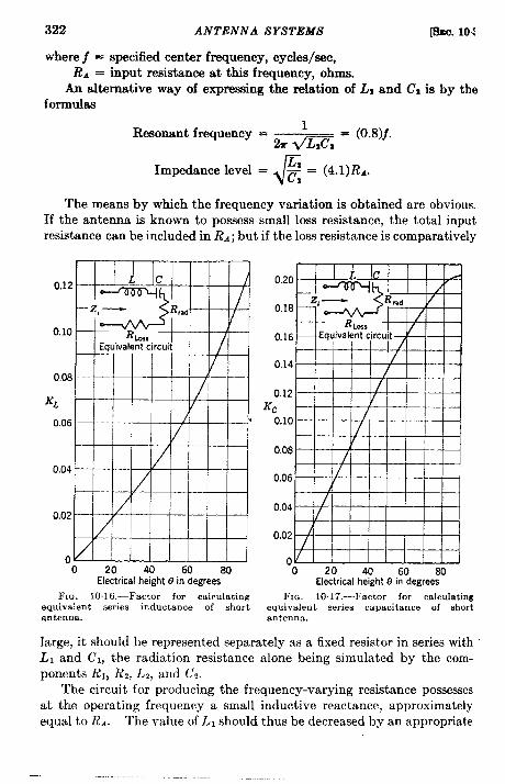
322 ANTENNA SYSTEMS llhw. 10<

where f = specified center frequent y, cycles/see,R. = input resistance at this frequency, ohms.

An alternative way of expressing the relation of L% and C, is by theforrmlhw

Resonant frequency =1

Zr m,= (0.8)f.

Impedance level =J

* = (4.l)R.4.

The means by which the frequency variation is obtained are obvious.If the antenna is known to possess small loss resistance, the total inputresistance can be included in R4; but if the loss resistance is comparatively

0.120.20

0.18

0,10 0.16

0,140.08

KL0.12

Kc

0.06 0.10

0.08

0.040.06

0.020,04

0.02

00

020 40 60 80 0 20 40

Electricalheight19in degrees Electrical height O i~%egree~”

FIG. 10.16.—Factor for calculating FIG. 10.17.—Factor for calcubtingequivalent series inductance of short equivalent series capacitance of shortantenna. antenna.

large, it should be represented separately as a fixed resistor in series withL, and (.71,the radiation resistance alone being simulated by the com-ponents RI, RZ, Lz, and Cz.

The circuit for producing the frequency-varying resistance possessesat the operating frequency a small inductive reactance, approximatelyequal to R.. The value of LI should thus be decreased by an appropriate

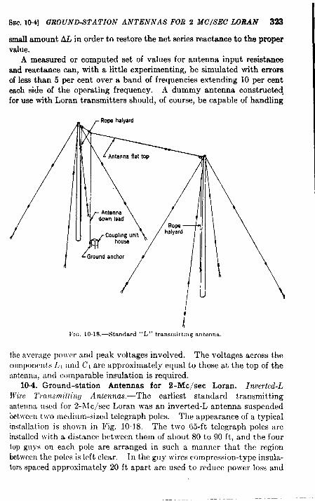
SEC.10.4] GROUND-STATION ANTENNAS FOR 2 MC/SEC LORAN ~~

small amount AL in order to restore the net series reactance to the propervalue.

A measured or computed set of values for antenna input resistanceand reactance can, with a little experimenting, be simulated with errorsof less than 5 per cent over a band of frequencies extending 10 per centeach side of the operating frequency. A dummy antenna constructedfor use with Loran transmitters should, of course, be capable of handling

/FIG, 10.18 .—Stmdard “L” transmitting antenna.

the mveragc po~vcr and peak voltages involved. The voltages across thecomponents 1.I :md Cl are approximately equal to those at the top of the:mtcnnu, and comparable insulation is required.

10.4. Ground-station Antemas for 2-Me/see Loran. lnoerted-LWire Tmusmi[(ing A nknna.s.—The earliest standard transmittingantenna used for 2-fife/see Loran was an inverted-L antenna suspendedbetween two medium-sized telegraph poles. The appearance of a typicalinstallation is showm in Fig. 10.18. The two 65-ft telegraph poles are

installed \vith a distance between them of about 80 to 90 ft, and the four

top gtlys on each pole are arranged in such a manner that the regionl)etween the poles is left clear. In the guy ~vires compression-type insula-tors spaced approximately 20 ft apart are used to i-educe power loss and

324 ANTENNA SYSTEMS [SEC. 10.4

pattern distortion. Figure 10.19 shows the input impedance of such atransmitting antenna.

In antennas of this type, the radiation resistance is of the order of15 ohms, or approximately half what it would be if the entire length ofantenna wire were suspended vertically. Good efficiency and good low-angle radiation require an adequate and well-bonded ground system,keeping the ground-loss resistance to the order of 2 ohms.

I I 40

c I 30 ~Resistance~–-‘S 20%

.5 I 10~m~ o 0:~ ~: 20 c

40m

~a I z::5 60 :~~80

cz

:8 100 / “ ;%a 120- 5& 140 gw

1601750 1800 1850 1900 1950

Frequencyin kc/seeFIG. 10.19.—Input resistance and reactance of 107-ft inverted-L antenna bent at 53 ft.

A typical ground system that has been used with the inverted-Lantenna consists of 120 AWG ATO.10 copper wires converging toward apoint beneath the antenna downlead. The radials have a minimumlength of 150 ft and are usually simply laid on top of the soil rather thanbeing plowed below its surface.

The weatherproof house containing the coupling unit is locatedwithin 2 or 3 ft of the ground-system center and the antenna downleadfor short connections. An effort is made to reduce to a minimum boththe resistance and the inductance of the connection from the couplingunit to the radial ground system and earth. The need for a low-induct-ance lead may be seen from the fact that with a pulse input of 100 kw thecurrent in this connection has a value of more than 100 amp peak. Evenwith a ground-lead inductance of only half a microhenry, the potentialclifference between “ground” points, supposedly at the same potential,would reach 600 volts peak. The use of ground rods, 6-in. -wide copperstrap, and careful bonding of the transmission-line sheath reduces suchpotential differences to a satisfactorily low value.

For a peak-power level of 100 kw, adequate insulation of the trans-mitting antenna is obtained with standard porcelain insulators havinganticorona bell-shaped metal end pieces. At the upper end of theantenna a single insulator 12 in. in length and 1$ in. in diameter is usually

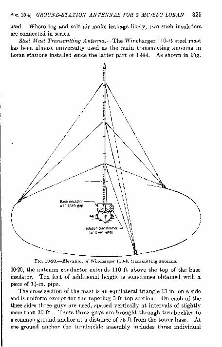
SEC. 10.4] GROUND-STATION ANTENNAS FOR 2 MC/SEC LORAN 325

used. Where fog and salt air make leakage likely, two such insulatorsare connected in series.

Steel Mast Transmitting Antenna.—The Wincharger 110-ft steel masthas been almost universally used as the main transmitting antenna inLoran stations installed since the latter part of 1944. As shown in Fig.

/

/

~4 ‘\

I

Isolahontransformerfor towerIhghts )

FIG. 10.20.—Elevation of Win charger 1lo-ft transmitting antenna.

1020, the antenna conductor extends 110 ft above the top of the baseinsulator. Ten feet of additional height is sometimes obtained with apiece of l+in. pipe.

The cross section of the mast is an equilateral triangle 13 in. on a sideand is uniform except for the tapering 5-ft top section. On each of thethree sides three guys are used, spaced vertically at intervals of slightlymore than 30 ft. These three guys are brought through turnbuckles toa common ground anchor at a distance of 75 ft from the tower base. Atone ground anchor the turnbuckle assembly includes three individual

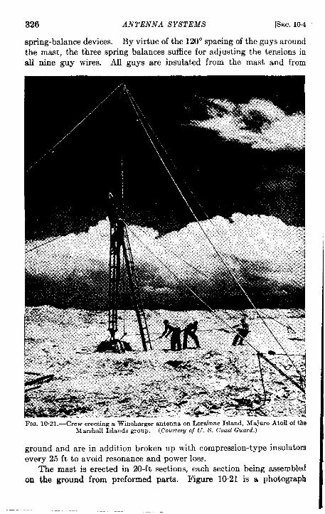
326 ANTENNA SYSTEMS [SEC. 10.4

spring-balance devices. By virtue of the 120° spacing of the guys aroundthe mast, the three spring balances suffice for adjusting the tensions inall nine guy wires. All guys are insulated from the mast and from

ground and are in addition broken up with compression-type insulatorsevery 25 ft to avoid resonance and power loss.

The mast is erected in 20-ft sections, each section being assembledon the ground from preformed parts. Figure 10.21 is a photograph

SEC. 104] GFtOUND-STA TION ANTENNAS FOR 2 MC/SEC LORAN 327

showing the second section ready for hoisting into place. Bolts are usedboth for the section assemblies and for holding the sections together.

The standard radial ground system with which this antenna is usedconsists of 120 radials of AWG No. 10 copper wire, each 300 ft long. Attheir outer extremities these radials are bonded to a piece of .4WG No. 8copper wire formed in a circle of 600-ft diameter. Twenty ground rodsare ordinarily used around this circle, spaced at 18° intervals. A 25-ftcircle of wire near the center of the system is similarly bonded to theradials, and at the center heavy copper strap and wire cable are used forbonding and connection. Ground rods are used at the antenna base andaround the 25-ft circle.

The input impedance of a Wincharger antenna in the 2-Me/see Loranrange is shown in Fig. 10.22. These data, taken from a Navy instrur-

~ ~+4rJ 1 40.$+30 lResiSkInce

jj 30:~ 2+20 / “ 20%: g,=+lo / Il):e

FE o - 0 g%; .5 0-10

&@ ~ ,5~ ~ -20

— yeag/

~= 8::,

~=

1750 lam 1s50 19CQ 1950Frequencyin kc/see

FIG. 10.22.—Input resistance and reactance of M“incharger 110-ft antenna. (DaiII fromC..!l. h’auy and Geuerui Eleclric Co.)

tion book, 1 are of interest in that the input reactance is given as zero at~8-12kc/see, corresponding to a free-space quarter wavelength of 133 ft.Since 110 ft is shorter than this value by 17 per cent, it is believed thatin making the measurements either the additional 10-ft top section or arather high-inductance connection }vas used.

Comparing the curves of Fig. 10.22 with those of Fig. 10.19, it canbe observed that the input resistance of the Wincharger antenna at1950 kc/see is 31.5 ohms as compared with 19 ohms for the inverted-Lantenna. In the region of this frequency, the input reactance of theformer changes at the rate of 0.25 ohm per kc/see, whereas that of thelatter has a slope of 0.35 ohm per kc/see. Although the difference inresistances is primarily a matter of vertical extension, the relatively largeequivalent diameter of the Wincharger mast makes its reactance varyless rapidly with frequency. In both of these respects the Winchargerantenna is a less frequency-selective device and consequently moresuitable for the radiation of pulses. Some slight additional benefit is

1c’Instruction Book for AotermaCouplingUnit Navy Type CG-47M3,” N~8hips100,751, June9, 1945.

328 ANTENNA SYSTEMS [SEC.104

derived from the fact that the coupling unit for the Wincharger antennasmay be made of greater bandwidth, since smaller impedance transforma-tion is required to match the 52-ohm transmission line.

Vertical Receiving Antennas.—The receiving antenna consists of avertical wire, No. 10 enameled copper, about 55 ft long suspended froma telephone pole with crossarm at the top. The lower end of the wire issecured by a deadman anchor. A ground system of 60 radials of No. 10copper wire approximately 125 ft long, placed on the ground, ensures alow resistance and, probably more important in this case, a more constantreal component of antenna impedance under varying weather conditions.

The impedance of the antenna is about 10 – j550 ohms in the vicinityof 2.o Me/see, and for a bandwidth of 100 kc/see the equivalent circuitis approximated by a series 10-ohm resistor and 150-p~f capacitor.

Beverage Receiving Antenna .—Because of its inherently circularpattern in the horizontal plane the vertical antenna may not provide asufficiently high signal-t~atmospheri c-noise ratio when the remotestation is unusually far away. Under these conditions, it is desirable touse an antenna that provides some directivity in order to raise the signal-to-noise ratio.

The Beverage or wave antenna has been used at some Loran stationsin order to raise the ratio of signal to atmospheric noise. This antennahas a marked directional characteristic and little sensitivity for horizon-tally polarized waves. A great reduction in precipitation static has beenreported at stations that experienced much trouble from this source whenusing the vertical antenna for reception.

The Beverage antenna as used in typical Loran installations consistsof a straight horizontal wire (hTo. 10 or A’o. 12 enameled copper) from oneto two wavelengths (500 to 1000 ft) long, supported 6 to 10 ft above theearth. The wire is located so that one end of it is several hundred feetfrom the timer building, the far end pointing toward the station to bereceived.

This far end is terminated in a noninductive resistance to ground equalto the characteristic resistance of the antenna (usually of the order of500 to 1000 ohms). The other end is terminated in a coupling unit thattransfers the energy from the antenna to the 50-ohm coaxial line leadingto the attenuator.

The antenna functions best over soil of poor conductivity. Thevoltage in the antenna is induced by a horizontal component whosedirection is the same as that of the wave propagation. This horizontalcomponent is the result of the forward tilt of the vertically polarized wavethat suffers progressive attenuation as it travela over the earth’s surface(Fig. 10.23). The effect of the earth’s conductivity and dielectric con-stant on the tilt angle are shown in Table 10.1. If the antenna is ter-

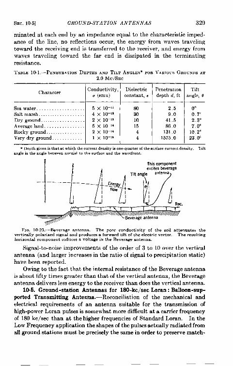
SEC. 10.5] GROUND-STATION ANTENNAS 329

minated at each end by an impedance equal to the characteristic imped-ance of the line, no reflections occur, the energy from waves travelingtoward the receiving end is transferred to the receiver, and energy fromwaves traveling toward the far end is dissipated in the terminatingresistance.

TABLE1O.1.—PENETEATIONDEPTHSANDTILTANGLES*FORVARIOCS GROUNDS AT2.0 Mc/SEc

CharacterConductivity,

a (emu)

Sea water . . . . . . . . . . . . . . . . . . . 5 x 10-”

Salt marsh, . . . . . . . . . . . . . . . . . . 4 x 113-lZ

Dry ground . . . . . . . . . . . . . . . . . . 2 x 1O-JJ

Average land . . . . . . . . . . . . . . . . 5 x 10-14

Rocky ground . . . . . . . . . . . . . . . . 2 x 1O-I4

Very dry ground . . . . . . . . . . . . 1 x 10-15 J-Dielectric Pcnetratioconstant, e depth d, f

80 2530 9.010 41.515 8604 131,04 1575.0

Tiltmgle, O

0°0.7°2.3°7.0°

10.2”23.0°

* Depth givenis that at which the current densityis one-quarterof the surface currentdensity. Tiltmgle is the angle between norm’alto the surface and the wavefront.

FIG. 10.23.—Beverage antenna. The poor conductivity of the soil attenuates thevertically polarized signal and produces a forward tilt of the electric vector. The resultinghorizontal component induces a voltage in the Beverage antenna.

Signal-t~noise improvements of the order of 3 to 10 over the verticalantenna (and larger increases in the ratio of signal to precipitation static)have been reported.

Owing to the fact that the internal resistance of the Beverage antennais about fifty times greater than that of the vertical antenna, the Beverageantenna delivers less energy to the receiver than does the vertical antenna.

10.6. Ground-station Antennas for 180-kc/sec Loran: Balloon-sup-ported Transmitting Anten~a.-Reconciliation of the mechanical andelectrical requirements of an antenna suitable for the transmission ofhigh-power Loran pulses is somewhat more difficult at a carrier frequencyof 180 kc/see than at the higher frequencies of Standard Loran. In theLow Frequency application the shapes of the pulses actually radiated fromall ground stations must be precisely the same in order to preserve match-

330 ANTENNA SYSTEMS [SEC.10.5

ing accuracy with the long rise times and pulse lengths. This impliesthat the antenna structures must behave identically or else that theirpulse-shaping effect must be made negligible compared with that of othercontrollable variables. Thus it is desirable for the bandwidths of theantenna and coupling unit to be at least as broad, relative to the fre-quency, as those of the Wincharger antenna and coupling unit in the2-Me/see Loran band.

Ascalemodcl of the Wincharger antenna wouldbe a base-insulatedtower approximately 1120 ft high, having a uniform cross section ofapproximately 10-ft equivalent diameter. Even with considerablesacrifice in electrical requirements the engineering and construction of a

FIG. 1024.-Barrage balloon used to support the experimental Low Frequency transmittingantenna.

permanent antenna structure would,it is clear, require considerable timeand effort. Since the LF Loran program aimed at a speedy test anddemonstration of the effectiveness of Loran techniques at 180 kc/see, acruder antenna was acceptable. The transmitting antenna used in thetests was a long thin wire supported by a lighter-than-air balloon.

The Copperweld antenna wire is 1300 ft in length and & in. indiameter. Its d-c conductivity is 30 per cent of that for a pure copperwire of the same diameter, because of the steel core. At 180 kctsec,

however, the effective conductivity is only a few per cent less than forpure copper, since the skin depth for copper at this frequency is onlyapproximately 0.006 in. The weight of the antenna wire is approximately38 lb; the insulators and other hardware weigh about 10 lb.

A small barrage balloon is used to lift the antenna. The type usedin the tests has a fully dilated volume of 3000 cu ft; its length isapproximately 36 ft, and it is 14 ft in diameter. The balloon has three

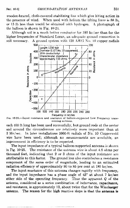
SEC.10.5] GROUND-STATION ANTENNAS 331

wooden-braced, cloth-covered stabilizing fins which give kiting action inthe presence of wind. When used with helium the lifting force is 58 lb,or 15 lb less than would be obttiined with hydrogen. .4 photograph ofthe balloon is shown in Fig. 1024.

Although soil is a much better comluctor for 180 kc/see than for thehigher frequencies of Stanchml I.oran, tin adcq{latc ground connection isstill necessary. A ground systcm with 120 .lWG No. 10 copper radials

500 IOQLength 1290 feet

~oo .Diameter O.1O’’(NO.10 cop ~erweld,_307. conductwity) I

80 ~

: Charactenstlc impedanceL,=

g 300 -approximately 73o ohms / $’1 60 ,;u=

200 40 g

: ~x0 100 20 :c- / ~

g 0 0r

0~~ -100a

~ -200

:3S3-300

0

‘-4(YJ

-50010Q 120 140 160 180 200 220 240 260

Frequency in kc/seeFIa. 10,25.—Input resistance and reactance of balloon-supported Low Frequency trans-

mitting antenna.

each 400 ft long has been used successfully, but ground rods at the centerand around the circumference are relatively more important than at2 Me/see. In later installations 1000-ft radials of No. 10 Copperweldwire have been used; although no measurements are available, animprovement in efficiency is to be expected.

The input impedance of a typical balloon-supported antenna is shownin Fig. 10.25. The resistance of the antenna wire is about 4.5 ohms perthousand feet, indicating that 2 or 3 ohms of the input resistance areattributable to this factor. The ground loss also contributes a resistancecomponent of the same order of magnitude, leading to an estimatedradiation efficiency of approximately 80 to 85 per cent at 180 kc/see.

The input reactance of this antenna changes rapidly with frequency,and the input impedance has a phase angle of 45° at about 7 kc/seeeither side of the operating frequency. Thus the apparent Q of theantenna, considered as a series combination of inductance, capacitance,and resistance, is approximately 13, about twice that for the Winchargermtenna. The reason for the high reactive slope is that the antenna is

332 ANTENNA SYSTEMS [SEC. 10.5

extremely thin compared with its length. This gives an unusually highcharacteristic impedance, of the order of 720 to 740 ohms.

The balloon-supported antenna has several disadvantages, some ofwhich significantly affect its usefulness for Loran purposes. Most ofthese stem from the varying position of the balloon with changing windsand temperatures. It is not abnormal for the balloon to drift laterallyas much as 450 ft from its ideal location directly over the base of theantenna; in this condition the antenna wire makes an angle of about 45°with the ground.

In maintaining synchronism it is desirable that several quantitiesremain constant, notably the radiated power, the cycle-and-envelopestructure of the radiated pulse, the amplitude and phase of the receivedlocal signal, and the amplitude and phase of the received remote signal.Changes in the attitude of the balloon-supported transmitting antennacause variations in each of these quantities.

As a vertical antenna is inclined, its radiation resistance decreases,changing both the radiation efficiency and the power delivered by thetransmitter. With some sacrifice in output power these changes can bemade to cancel; partial compensation is achieved if the coupling unit isinitially adjusted to match an inclined antenna. Another objectionableresult of variable antenna resistance is that the Q and bandwidth of theantenna are affected, with some effect on the shape of the radiated pulse.Compensation for this effect requires vigilance on the part of the trans-mitter operator.

In addition to influencing the radiated signals, changes in the attitudeof the transmitting antenna can affect both the remote and local signals,as obtained from the receiving antenna. This antenna, located about1000 ft from the transmitting antenna, is in a region where the inductionfield contributes as much to the local-signal pickup as does the radiationfield. If the effective distance to the transmitting antenna decreases by100 ft (a conservative estimate), then the amplitude of the local signalwill increase by about 15 per cent, giving a total range of variation of 30per cent. Under some circumstances this causes operational error.Even without this amplitude change a timing error is introduced that,although small, is greatest for the otherwise optirn~m orientation oftransmitting and receiving antennas. Finally there is the possibilitythat the rather closely coupled transmitting antenna may, by acting as atuned parasitic element, affect the directive pattern of the receivingantenna, JIovement of the transmitting antenna can thus affectremote-signal reception.

Tower ‘1’ransmitting A ntenna.-In designing the permanent trans-mitting antenna for an LF I.oran station the problem of reconciling elec-trical requirements with mechanical limitations of strength, weight, and

SEC.10.5] GROUND-STATION ANTENNAS 333

size becomes acute. It is vital for the antenna input impedance to havesufficient bandwidth so that the fast-rising pulses can be radiated withnegligible shaping. During each cycle the antenna must thus radiate afairly large percentage of the reactively stored energy present, in itsfields and in the coupling unit, at the beginning of the cycle. In otherwords, the antenna and coupling unit must have a suitably low value of Q.

As previously mentioned, satisfactory electrical characteristics couldbe obtained with a base-insulated tower of approximately 10-ft diameter

~lG. 10.26.—625-ft top-loaded tower antenna designed for Low Frequency Loran.

and 1120-ft height. Such a tower not only would be difficult and expen-sive to erect but would also require elaborate guying and an extremely

strong insulator at its base. Extensive tests made with model structures

have led to the design of a more practicable antenna m-hose main com-

ponent is a self-supporting tapered steel tower (?J25ft high. The cross

section of the tower is a square whose side tapers from 59 ft at the base

to 5 ft at the top. The four legs arc supported on push-pull porcelaininsulators with a 10-in. leakage path and an over-all height of nearly

5 ft. Since the insulators can withstand both tension and compression,

the tower requires no guying.

The distinctive feature of the antenna is its top-loading by 12 con-

ductors arranged like the ribs of an umbrella. .\s show-n in Fig. 10.26

these elements are held away from the tower by insulated guy ~vires which

are anchored 850 ft from the tower base; because of sag the angle between

the tower and the umbrella elements is approximately 45°. The small

tensions required in the umbrella-supporting guy wires and the sym-

metrical nature of their mechanical load make the umbrella lighter,

simpler, and safer than a comparable inverted-L or T-antenna. If

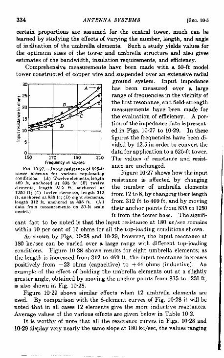
334 ANTENNA SYSTEMS [sm. 10.5

certain proportions are assumed for the central tower, much can belearned by studying the effects of varying the number, length, and angleof inclination of the umbrella elements. Such a study yields values forthe optimum sizes of the tower and umbrella structure and also givesestimates of the bandwidth, insulation requirements, and efficiency.

Comprehensive measurements have been made with a 50-ft modeltower constructed of copper wire and suspended over an extensive radial

o~150 170 190 210

Frequency m kc/see

FIG. 10.27.—Input resistance of 625-fttower antenna for various top-loadingconditions. (A) Twelve elements, length469 ft, anchored at 835 ft; (B) twelveelements, length 512 ft, anchored at1250 ft; (C) twelve elements, length 312ft, anchored at S35 ft; (D) eight elements,length 312 ft, anchored at 835 ft. (Alldata from meacmrementa on 50-ft ecalemodel.)

ground system. Input impedancehas been measured over a largerange of frequencies in the vicinity ofthe first resonance, and field-strengthmeasurements have been made forthe evaluation of efficiency. A por-tion of the impedance data is present-ed in Figs, 10”27 to 10.29. In thesefigures the frequencies have been di-vided by 12.5 in order to convert thedata for application to a 625-ft tower.The values of reactance and resistiante are unchanged.

Figure 1027 shows how the inputresistance is affected by changingthe number of umbrella elementsfrom 12 to 8, by changing their lengthfrom 312 ft to 469 ft, and by movingtheir anchor points from 835 to 1250ft from the tower bae.e. The signifi-

cant fact to be noted is that the input resistance at 180 kc/see remainswithin 10 per cent of 16 ohms for all the top-loading conditions shown.

As shown by Figs. 10.28 and 10.29, however, the input reactance at180 kc/see can be varied over a large range with different top-loadingconditions. Figure 1028 shows results for eight umbrella elements; asthe length is increased from 312 to 469 ft, the input reactance increasespositively from – 23 ohms (capacitive) to +44 ohms (inductive). Anexample of the effect of holding the umbrella elements out at a slightlygreater angle, obtained by moving the anchor points from 835 to 1250 ft,is also shown in Fig. 10.28.

Figure 10.29 shows similar effects when 12 umbrella elements areused. By comparison with the 8-element curves of Fig. 10”28 it will benoted that in all cases 12 elements give the more inductive reactance.Average values of the various effects are given below in Table 10”2.

It is worthy of note that all the reactance curves in Figs. 1028 and10.29 display very nearly the same slope at 180 kc/see, the values ranging

SW. 10.5] GROUND-STATION ANTENNAS 335

iFTzz12I

-40 Y A-l< D1 r

‘i50 160 170 180 190 200 210 220Frequency in kc/see

FIG, 1028.-Input reactance of 625-ft top-loaded tower antenna with eight umbreUaelements. (A) Length 469 It, anchored at 835 ft; (B) length 416 ft, anchored at 835 ft;(C’)length 365 ft, anchored at 835 ft; (D) length 312 ft, anchored at 835 ft; (E) length 312 ft.anchored at 1250 ft. (All data from measurements on 50-ft scale model.)

+120

‘i50 160 170 180 190 200 210 220Frequencyin kc/see

FIG. 10.29.—Input reactance of 625-ft top-loaded tower antenna with tvelve umbrellaelements. (.4) Length 469 ft, anchored at 1250 ft; (B) length 469 ft, anchored at 835 ft;(0 length 312 ft, anchored at 1250 ft; (D) length 312 ft, anchored at 835 ft. (AH data frommeasurements cm 50-ft scale model. )

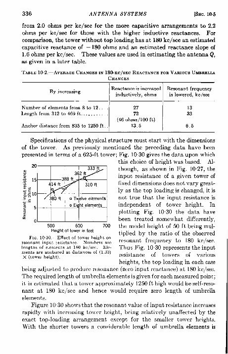
336 ANTENNA SYSTEMS [SEC. 10.5

from 2.0 ohms per kc/see for the more capacitive arrangements to 2.2ohms per kc/see for those with the higher inductive reactance. Forcomparison, the tower without top loading has at 180 kc/see an estimatedcapacitive reactance of – 180 ohms and an estimated reactance slope of1.6 ohms per kc/see. These values are used in estimating the antenna Q,as given in a later table.

TASLE102. -.4YEIIAGE CHANGES IN 180-KC/SEC REACTANCE FOR VAFUOUSUMBIiELLACHANGES

By increasingReactance is increased Resonant frequency

inductively, ohms is lowered, kc/see

Number of elements from 8 to 12 . . . . 27 13Length from 312t0469ft, . . . . . . . . . 33

(46 ohr&OO ft)Anchor distance from 835 to 1250 ft. 13.5 6.5

Specifications of the physical structure must start with the dimensionsof the tower. As previously mentioned the preceding data have beenpresented in terms of a 625-ft tower; Fig. 10.30 gives the data upon which

20

E333 ft

: 362 flg 15 388 ftz 414 ft 310 n::a% 10c 380 ft ❑ Twlelveel;ments“: .’s

o P ht elements:5;c

o500 600 700

Heightof towerin feetFKG. 10.30 .—EtTect of tower height on

resonant input resistanrc. Numbers arelengths of elen>ents at 180 kcisec. Ele-ments are anchored at d]stances of (1.33)X (tower height).

this choice of height was based. Al-though, as shown in Fig. 10.27, theinput resistance of a given tower offixed dimensions does not vary greakly as the top loading is changed, it isnot true that the input resistance isindependent of tower height. Inplotting Fig. 1030 the data havebeen treated somewhat differently,the model height of 50 ft being mul-tiplied by the ratio of the observedresonant frequency to 180 kc/see.Thus Fig, 1030 represents the inputresistance of towers of variousheights, the top loading in each case

being adjusted to produce resonance (zero input reactance) at 180 kc/see.The required length of umbrella elements is given for each measured point;it is estimated that a tower approximately 1250 ft high would be self-reso-nant at 180 kc/see and hence would require zero length of umbrellaelements.

Figure 10.30 shows that the resonant value of input resistance increasesrapidly with increasing tower height, being relatively unaffected by theexact top-loading arrangement except for the smaller tower heights.With the shorter towers a considerable length of umbrella elements is

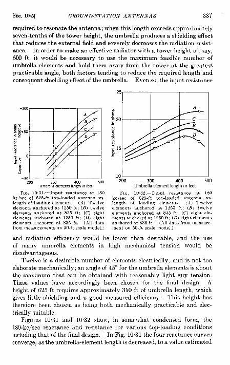
SEC. 10.5] GROUND-STATION ANTENNAS 337

required to resonate the antenna; when this length exceeds approximate yseven-tenths of the tower height, the umbrella produces a shielding effectthat reduces the external field and severely decreases the radiation resist-ance. In order to make an effective radiator with a tower height of, say,500 ft, it would be necessary to use the maximum feasible number ofumbrella elements and hold them away from the tower at the greatestpracticable angle, both factors tending to reduce the required length andconsequent shielding effect of the umbrella. Even so, the input resistance

FrG, 10.31.—Input reactance at 180kc/see of 625-ft top-loaded antenna vs.length of loading elements, (A) Twelveelements anchored at 1250 ft; (B) twelveelements anchored at S35 ft; (C) eightelements anchored at 1250 ft; (D) eightelements anchored at S35 ft. (.lfl datafrom measurements on 50-ft scale model.)

1(J~200 300 400 5(

Umbrellaelementlengthin feet10

FIG. 1032, - Input resistance at 1S0kc/see of t325-ft top-loaded antenna vs.length of load]ng elements. (.4) Twelveelements anchored at 1250 ft; (B) twelveelements anchored at S35 ft; (C) eight ele-ments anchored at 1250 ft; (D) eight elementsanchored at S35 ft. (.411data from measure-ment on 50-ft scale model. )

and radiation efficiency would be lower than desirable, and the useof many umbrella elements in high mechanical tension would bedisadvantageous.

Twelveis a desirable number of elements electrically, and is not tooelaborate mechanically; an angle of 45° for the umbrella elements is aboutthe maximum that can be obtained with reasonably light guy tension.These values have accordingly been chosen for the final design. Aheight of 625ft requires approximately 310ft of umbrella length, whichgives little shielding and a good measured efficiency. This height hastherefore been chosen as being both mechanically practicable and elec-trically suitable.

Figures 10.31 and 1032 show, in somewhat condensed form, the180-kc/sec reactance and resistance for various top-loading conditionsincluding that of the final design. In Fig. 10.31 the four reactance curvesconverge, astheumbrella-element length isdecreased, toavalue estimated

338 ANTENNA SYSTEMS [SEC. 10.5

as –180 ohms. It should be mentioned that all reactance data weremeasured with umbrella elements simulating six-wire cages 6 in. in diam-

“ ,o~140 150 160 170 180 190 200

Frequencyin kc/seeFIG. 10.33.—Estimated efficiency of

625-ft tower antenna with twelve umbrellaelements. Top-loading varied to controlresonant frequency, (a) Length 450 ft,anchored at S50 ft; (b) length 325 ft,anchored at S50 ft. (AU data from meas-urements on 50-ft scale model.)

from a properly top-loaded 625-ft

eter. Other measurements indi-cate that a reduction of umbrella-element diameter to 0.2 in. wouldmake the reactance on the average15 ohms more capacitive and theresonant frequencies 6 kc/seehigher.

The effect of shielding by theumbrella is clearly shown in thelower curve of Fig. 10.32 whereinthe input resistance reaches adefi-nite maximum for a,L umbrellalength of theorderof-120 ft. Fin-ally, Fig. 10.33 gives a rough esti-mate of the efficiency to be expected

tower antenna. At 180 kc/see the..- .expected efficiency is of the order of 80 per cent or better.

Table 10.3 summarizes the characteristics of various LF transmittingantennas.

TARLE103.-C•MFARISONOF 18&Kc/SECTRANSMITTING.i~T~~YAs

“ Win-charger” t

Vertical length, ft 1120 (est.)

Equivalent diameter 9.6ft (est.)18&kc reactance, ohms. ., 0React. slope, ohms perkc/sec. 2.5180-kc /secrcsistancc, ohms ., 2!3Q’withlowiing coil ., 8

“ Bal-“TO\rcr”$

oon”~

1340 625Olin, 4oft (cSt. )

o –180 (est. )6.5 1.6 (est. )39 10 (est. )15 23 (est. )

<<~m-

brc]la”l[

625

0“2.01611

* In calculating Q the effects of getwratm remstmcemd of coupling-unit reactance other thm thatof the loading cod have been nwlected. The effective bandwidtb is in ~eneralmeatcr thm ind,catedby this vrdue”ofQ.

TSwde model of Winchmger antenna, enlarged by a factor of approximately 10,2 for rcmnp.mxat180 kc/aec.

I Balbmn-supportedwire a“tenns., Iengthe”ed 4 per cent for resonanceat 180 kc/see.$Tower antenna w,th wuare cross section tapering from 59- to 5-ft side. Rcson.”t at approxi-

mately 360 kc/.sec.II%.me tower top-loade(i with 12 umbrella elementsapproxinmtely 310 fl long, anchored 835 ft from

hme. Resonant at 180 kc/see,

It will be noted that because of its extreme thinness, the balloon-supported wire has a reactance slope of 6.5 ohms per kc/see. At theother extreme, the 625-ft tower without top-loading has a reactance slopeestimated as 1.6 ohms per kcjsec. The capacitive input reactance, how-

SEC. 10.5] GRO l!,VD-STA TIO,V .41VTEN.VAS 339

ever, is estimated to be – 180 ohms or even somewhat more negative; thenecessary loading coil will hence contribute an additional slope of atleast 1.0 ohm per kc/see. The net Q of the tower without top loading istherefore approximately 23. By the use of top loading the Q of thetower antenna is made to approach that of the desirable but impracticableWkmharger scale model. With a balloon-supported antenna, pulsesrising in 10 or 12 cycles can be radiated satisfactorily; the umbrella-topped tower antenna should be capable of radiating pulses rising in 8cycles.

Experimental LF Loran stations have used pulse powers of the orderof 100 kw, but in order to allow eventual increases in transmitter powerthe tower antenna has been designed to handle pulses of 1 megawatt.With this poiver the input current will have a value of approximately250 amp rms, and the question of adequate insulation arises. Since theantenna is operated in the vicinity of resonance, the voltage across thebase insulators ~villnot be excessive, having a value of about 5.7-kv peakif the antenna is resonant and 8-kv peak if the antenna’s input reactanceis allowed to equal its input resistance.

The insulation of the guy wires has received much attention. At theends of the umbrella elements, in particular, the voltage to ground isexpected to be of the order of 50-kv peak. The qualitative argumentsleading to this conclusion are based on the concept, recently set forth bySchelkunoff,’ that it is valid to consider a straight vertical antenna ofreasonably uniform longitudinal cross section as a dissipationless trans-mission line, with radiation represented as a terminal impedance,

Consider that the 625-ft tower represents a portion of a transmissionline with characteristic impedance of the order of 200 ohms. We knowthat 625 ft is about one-eighth wavelength, and we know furthermorethat the addition of top-loading reduces the input reactance to zero.The umbrella can be considered as shunting the top of the tower to groundwith a lumped capacitive reactance, which must be of the order of 200ohms. The l-megawatt input current is estimated as 250 amp rms; thiswill be reduced to 175 amp rms at the top of the tower. By the flow ofthis current through a capacitive reactance of 200 ohms a potential toground of 35 kv rms (50-kv peak) will be produced. Since the umbrellaelements are each but 6 per cent of a wavelength long, little resonantincrease of this voltage is to be expected, and the potential to ground ofthe umbrella elements will be substantially that of the top of the tower.

As a check of this argument it is worth while calculating approximatelythe capacitance of the umbrella. .L single element has a capacitan~e toground of approximately 750 ~pf, and it appears reasonable for a com-

1S.A. Schelkunoff, “Theory of Antennas of .4rbitrary Size and Shape,” Proc, IRE,29, No. 9, 493-521, September 1941.

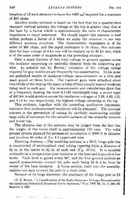
340 ANTENNA LSYS1’EMJ9 [sEC. 105

bination of 12 such elements to have the 44oO ppf required for a reactanceof 200 ohms.

Another cruder estimate is based on the fact that for a quarter-waveresonant vertical antenna the voltage at the top is greater than that atthe base by a factor which is approximately the ratio of characteristicimpedance to input resistance. We should expect this relation to holdwithin perhaps a factor of 2 when we apply the criterion to our verydifferent antenna structure. The characteristic impedance is of theorder of 200 ohms, and the input resistance is 16 ohms; this indicatesthat the base voltage of 4 kv rms will be stepped up to 50 kv rms, whichis of the same order of magnitude as the preceding estimate.

Only a small fraction of this total voltage to ground appears acrossthe insulator separating an umbrella element from its supporting guywire. As pointed out by Brown,’ estimates of the voltage ratingsrequired for guy insulators are frequently too conservative. In his paperare published results of insulator-voltage measurements on a thin steelmast guyed at three levels. The topmost guys were attached abouttwo-thirds of the way up the mast, a total of four equally spaced insulatorsbeing used in each guy. His measurements and calculations show thatat a frequency making the mast 0.1425 wavelength long, a power inputof 500 kw would produce across the insulators voltages of 3.38, 1.83, 1.21,and 1.14 kv rms respectively, the highest voltage occurring at the top.

This evidence, together with the preceding qualitative arguments,indicates that moderate-sized insulators will be adequate. The principalconcern is the prevention of corona by carefully maintaining suitablylarge radii of curvature for the metallic surfaces of the umbrella elementsand tower top.

The physical size of the antenna may be judged from the fact thatthe weight of the tower itself is approximately 170 tons. The radialground system planned for permanent installation is 2000 ft in diameterand involves 46 miles of N“o. 8 Copperweld wire.

Receiving Antenna.—The receiving antenna is a 59-ft Lingo pole thatis constructed of sectionalized steel tubing tapering from a diameter of3* in. in the center to 2* in. at each end (Fig. 103!). It is mountedvertically on a compression-type insulator at the base and is guyed at fourlevels. Each level is guyed every 90°, and the four ground anchors arespaced symmetrically around the pole, each being 33 ft 6 in. from thecenter of the base insulator. A boom section, built into the assembly,enables two men to erect the pole in a short time.

Because of its large diameter, the reactance of the Lingo pole at 2.0

1C,.H. Brown, “ .i consideration of the Radio-frequency J’oltages Encountered bythe Insulating Material of Broadcast Tower Antennas, “ Pror. IRE, 27, No. 9,566-578,Sept@ml ?r 1929

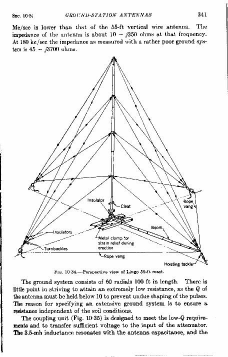
ISEC. 105] GIK)(JND-STA l’ION ANTENNAS 341

Me/see is lower than that of the 55-ft vertical wire antenna. The

impedance of the antenna is about 10 — ~350 ohms at that frequency.

At 180 kc/see the impcdtince as measured with a rather poor ground sys-

tem is 45 – ~3700 ohms.

FIG. 1034.-Perspective view of Lingo 59-ft m=t.

The ground system consists of 00 radials 100 ft in length. There is

little point in striving to attain an extremely low resistance, as the Q of

the antenna must be held below 10 to prevent undue shaping of the pulses.

The reason for specifying an extensive ground system is to ensure a

resistance independent of the soil conditions.The coupling unit (Fig. 10.35) is designed to meet the low-Q require-

ments and to transfer sufficient voltage to the input of the attenuator.The 3.5-mh inductance resonates with the antenna capacitance, and the

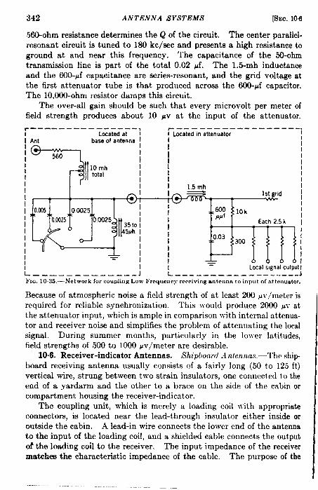
342 ANTENNA SYSTEMS [SEC. 10.6

5*ohmresistance determines the Qof the circuit. The center parallel-resonant circuit is tuned to 180 kc/see and presents a high resistance toground at and near this frequency. The capacitance of the 50-ohmtransmission line is part of the total 0.02 pf. The 1.5-mh inductanceand the 600-pf capacitance are series-resonant, and the grid voltage atthe first attenuator tube is that produced across the 600-~f capacitor.The 10,000-ohm resistor damps this circuit.

The over-all gain should be such that every microvolt per meter offield strength produces about 10 pv at the input of the attenuator.----- -.———— .— --- . -—-—————— --- —----- .i

!I

III

II

II

i

/IIL

Located at ; i LKated in attenuator I

Ant base of antenna I I

7

II

~ I560

II

I II I

i10 mh

I 1I

total II I

1.5 mh I

I0.005 0.0025 I

0.0025i1I

0.03

iT I =Local wgnal output I

.—__— ——— ————— —I t—–––– ———–-_–. _-–--. JFIG.. 1035.-Network for coupling Low Frequenry receiving antennn to input of nttcnuator.

Because of atmospheric noise a field strength of at least 200 ~v/meter isrequired for reliable synchronization. This would produce 2000 pv atthe attenuator input, which is ample in comparison with internal attenua-tor and receiver noise and simplifies the problem of attenuating the localsignal. During summer months, particularly in the lower lutitudes,field strengths of 500 to 1000 pv/meter are desirable.

10.6. Receiver-indicator Antennas. Shipl}omd .4nfcnnas.-Thr ship-board receiving antenna usually consists of a fairly long (50 to 125 ft)vertical wire, strung bet ween two strain insulators, one connected to theend of a yardarm and the other to a brace on the side of the cabin orcompartment housing the receiver-indi cat or.

The coupling unit, which is merely a loading coil with appropriateconnectors, is located near the lead-through insulator either inside oroutside the cabin. A lead-in wire connects the lower end of the antennato the input of the loading coil, and a shielded cable connects the outputof the loading coil to the receiver. The input impedance of the receivermatchea the characteristic impedance of the cable. The purpose of the

SEC, 106] RECE1 VER-INDICA TOR ANTENNAS 343

cable is to shield the receiver from noise generated in the cabin housingthe receiver-indicator.

The loading coil is adjusted approximately to balance the capacitivereactance of the antenna. Since the antenna is long enough to give strongsignals, the reception (signal-t&noise ratio) is limited by atmosphericnoise rather than by internal noise in the receiver. Therefore the tuningof the coupling unit is not critical.

Airborne Trailing Antenna. —.%ll airborne Loran equipment now inservice has been designed with the expectation that it is to be used with atrailing antenna. Because of the noise generated inside the aircraft, thelead from the antenna reel must be shielded, and the receiver inputimpedance is designed to match the impedance of the shielded cable.The wire cable with a weight of several pounds on the end is reeled outto a lengt h of 120 ft or so (approximate y a quarter wavelength), althoughsatisfactory results are obtained with considerably shorter lengths.Because of the length of the antenna, the received signals are so strongthat no coupling unit is required. The reel for the British trailingmtenna is manually operated and is usually mounted in the belly of theplane; the American reel is electrically operated and is usually mountednear the tail of the plane.

There are several serious objections to the use of a trailing antenna.‘l’here is danger, especially in fast planes, that the weight or the completesntenna may be broken off by the strong wind. Both the British andAmerican types of reel occasionally jam (this is especially serious in icingconditions), and the reeling of the antenna in and out are two moreinconvenient operations for the navigator. The trailing antenna is anintolerable hazard in flying in tight formation and during evasive action.

Fixed Airborne A ntenna.—Toward the end of the war an intensiveeffort was made to substitute a fixed antenna for the trailing antenna.In a fighter or light bomber it is usually possible to install a 30-ft fixedmtenna; in a heavy bomber it may be possible to install a 60-ft antenna,although usually a length of only 30 ft or so is available for Loran. It isestimated that the capacitance of the antenna lies between 50 and 300ppf. Wit bout the use of a coupling unit, the signal induced on such ashort antenna is too small for satisfactory reception; the signal-to-noiseratio is limited by the internal noise of the receiver.

Coupling units of several types have been tested. It has been foundthat the results obtained with a loading coil are as good as those obtainedwith coupling units that match the impedance of the antenna to theimpedance of the cable. The gain of the coupling unit (the ratio of thesignal with the coupling unit to the signal with direct connection tothe cable and receiver) is practically independent of the type of couplingunitprovided the antenna is tuned. The gain is between 6 and 10, depend..

344 ANTENNA SYSTEMS [SEC. 106

ing on the untuned impedance of the antenna. It has also been foundthat the effective capacitance of the antenna decreases when the plane isairborne. Therefore the coupling unit and the first r-f transformer shouldbe adjusted in the air.

The physical location of the coupling unit between the antenna andthe cable or between the cable and the receiver is of no consequenceelectrically. However, since it must be tuned in the air, a convenientlocation is near the receiver. The tuning of the coupling unit (since theQ is necessarily rather high) must be readjusted for each change of the r-fchannel (a different loading coil is required for the LOW Frequencychannel). Therefore, in the design of future equipment, individual load-ing coils should be incorporated in the receiver so that they are selectedby the r-f channel selector switch.

Pren”w”tation Static.—Loran reception like that of all airborne radiosystems, is seriously affected by precipitation static. No completelysatisfactory equipment for eliminating such static was available atthe end of the war. However the findings of the scientists of the Army-Navy Precipitation Static Project are reasonably promising.’

1 “ Precipitation Static, ” Air Forces Jfanual A’o, 40, December 1944; R. Gunn,

}V. C. Hall, and G. D. Kinzer, ‘‘ Precipitation-static Interference Problem andMethods for Its Investigation, ” Proc, IRE, 34, 15+160, April 1946; R. C. Waddel,R. ~. Drutowski, and W. X. Blatt, “ .\ircraft Instrumentation for Precipitation-staticResearch, ” Proc. IRE, 34, 161–166, .\pril 1946; R. G. Stirnmel, E. H. Rogers, F, E.Waterfall, and R. Gunn, “ Electrification of Aircraft Flying in Precipitation Areas,”Pror. IRE, 34, 167–177, April 1946; G. D. Kinzer and J. W. lIcGee, “ Investigations ofhfethods of Reducing Precipitation-static Radio Interference, ” Proc. IRE, 34, 234-240, May 1946; R. Gunn and J. P. Parker, “ The High-voltage ~haracteristics ofAircraft in Flight,” Proc. IRE, 34, 241-246, I lay 1!M6: 3f. Ne\vman and .t. O.Kemppainen, “ High-\-oltagr Installation of the Precipitation-static Project, ” Pror.IRE, 34, 247–253, May 1946.

CHAPTER 11

RECEIVER-INDICATORS

BY R. H. WOOD~VARD

SHIPBOARD RECEIVER-INDICATORS

11.1. Requirements and General Description.-The receiver-indi-cator is the instrument with which the Loran navigator measures the dif-ference in the times of arrival of pulsed signals. The navigator takesmeasurements of signals from two pairs of ground stations. Eachmeasurement determines a line of position, and the intersect on of twosuch lines establishes a fix, the navigator’s position.

Time-diJerence Mea.surement.—As explained in Sec. 33, the method ofmeasurement of the time difference is similar to that used at the groundstations (see Chap. 7). The signals of a particular recurrence rate fromtwo ground stations are displayed on an oscilloscope pattern of the samerecurrence rate. The pattern consists of two horizontal traces, oneabove the other and each having a duration of half the recurrence period.Since the recurrence rates of the signals and of the oscilloscope patternsare the same, the signals remain stationary on the pattern (whereassignalsof other recurrence rates drift to the right or to the left), If onepulse appears on the upper trace and the other on the lower trace, thepulse that appears to the left of the other is by definition the A-pulseand the one to the right is the B-pulse. The A- and B-pedestals aresmall rectangular deflections of the traces that indicate those portionsof the total recurrence period to be examined later in detail. TheA-pedestal is fixed in position near the beginning of the upper trace,whereas the B-pedestal can be continuously adjusted to any positionon the lower trace to the right of the A-pedestal. By momentarilyincreasing or decreasing the recurrence rate of the oscilloscope pattern,the pulses can be moved to the left or to the right on the traces and fromone trace to the other. In this way the navigator causes the A-pulse tomove onto the upper trace if originally on the lower one and then ontothe A-pedestal (see Fig. 11. la); the B-pulse then appears on the lowertrace to the right of the A-pulse. The initiation (which determines theposition) of the B-pedestal with respect to the slow-oscilloscope patternis adjustable, and the navigator so adjusts the initiation that the B-pedes-tal appeam under the B-pulse.

The time difference is taken aa the horizontal distance from a point345

346 RECEIVER-INDICATORS [SEC. 1I 1

II

I

(c) Fastest swaep

\ ‘30002 /

(dl Slow sweep. Each marker representing50ilm,croseconds Readmg!s 3,000+

x

\~

(e) Medlumfast sweep. Short markers represent50,long markers 5(M mlcmseconds. ReadingE 400+

~Fastestswaep. Markers represent 51X, 50, and10microseconds as shown. Reading ls24

Fm. 11.1.—OscilloBcope patterna of Model DAS-1 receiver-indicator. (a) Slow-trampattern with signals; (b) medium-trace pattern with signals; (c) faat-trace pattern withQ@I~S; (d) fdow-trace pattern with 50- and 50Qsac markers, showing time dif7erenceo(3000@c plus approximately 500ysec; (e) medium-trace pattern with 50- and 50&patamarkers, showing additional time difference of 400 paec plus approximately 30 paac; fj) fa&tiace pattern with 10-, 50-, smd50@aec markera, shotigtime di6erenceof Z4pe.ec. TotJltime difTerenca is 3424 *c.

SEC. 111] liE(JIJlltI<,\lblN7’S AND GENERAL DESCRII’TIO.V 347

on the lower trace, directly below the A-pulse to the B-pulse. Thisconvention cancels out one half of the rccurrcncc period. The time dif-ference can be estimated approximutcly by means of calibration markers.A method of greater precision is required, however. The upper andlower pedestals of Fig. 11~la are expanded and displayed as two full-Iength traces (Fig. 11”lb,) one above the other. The amplitudes of the,4- and B-pulses are equalized by means of the balance control. Therecurrence rate of the oscilloscope pattern is altcrccf slightly to move theA-pulse to a position near the left end of the trace, and the initiationof the B-pedmtul (lower trace) is adjusted to move the B-pulse into posi-tion directly below the A-pulse. On a third oscilloscope pattern (Fig.11.lc) consist ing of a faster pair of traces between which the verticalseparation is eliminated, the amplitudes are more accurately equalized,and the leading edge of one pulse is superimposed on that of the other.

When the signals have been so matched, the time difference betweenthem is exactly the same as that betlveen the initiations of the pedestals.This time difference is estimated to the nearest 500 ~sec by calibrationmarkers on the slow-trace pattern (Fig. 11. ld). The displacementbetween a 500-psec marker on the lo~ver fast trace and one on the upperfast trace gives the time difference to the nearest 50 psec (Fig. 11. le).Similarly, the displacement between 50-psec markers on two faster tracesgives the time difference to the nearest microsecond (Fig. 11. lj).

This method of presentation for measurement of time differences isemployed in all shipboard Loran receiver-indicators except the direct-reading receiver-indicator, hlodel DBE, described in Sec. 114. Themethod of presentation and the receiver-indicators described in thischapter can be used for all Loran systems—Standardj Sky-wave Syn-chronized, and Air Transportable-with the exception of Low Frequency.For LF Loran, a small low-frequency converter is required in conjunctionwith the receiver-indicator.

Requirermmts.-The transmissions from Loran ground stations areidentified by their radio frequencies and their pulse recurrence rates.The recei‘~er-indicator must be capable, therefore, of receiving signalsand measuring their time differences at several radio frequencies and at.wveralrecurrence rates. Four r-f channels have been assigned for Lorantransmission in various parts of the world: Channel 1, 1950 kc/see;Channel 2, 1850 kc/see; Channel 3, 1900 kc/see; Channel 4, 1750 kc/see.These signal frequencies are easily identified by a four-position switchthat selects any one of four fixed-tuned channels in the receiver. Eachchannel should be tunable from 1700 to 2000 kc/see.

Pairs of stations operating in a particular region on a single radiofrequency are distinguished by their pulse recurrence rates. Signalafrom all Loran stations operating at a single frequency and within receiv-

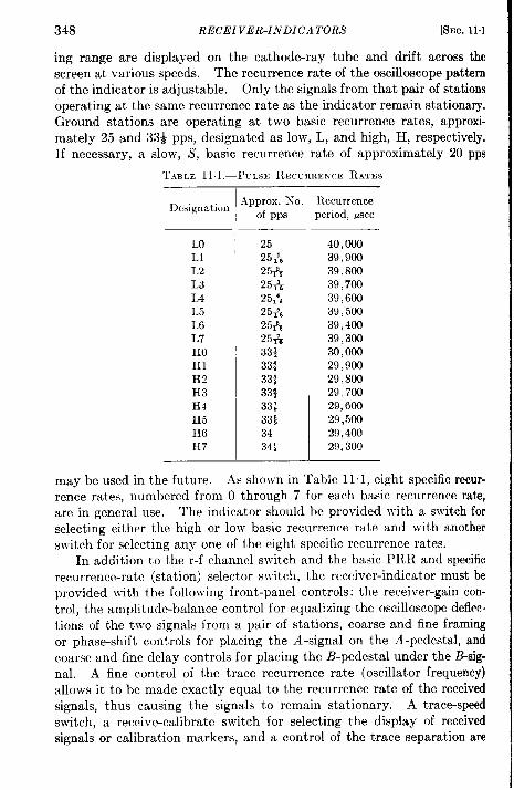
348 RECEIVER-INDICATORS [SEC. 11.1

ing range are displayed on the cathode-ray tube and drift across thescreen at various speeds. Therecurrence rate of the oscilloscope patternof the indicator is adjustable. Only the signals from that pair of stationsoperating at the same recurrence rate as the indicator remain stationary.Ground stations are operating at two basic recurrence rates, approxi-mately 25 and 33* pps, designated as low, L, and high, H, respectively.If necessary, a slow, S, basic recurrence rate of approximately 20 pps

‘r.4BLEll.l.—PITLSER~CI-RRENCERATES

Designation

LOL1L2L31AL51.6L7HOH1H2H3H4H5H6H7

Approx. No.of pps

Recurrenceperiod, psec

40,00039, 904)39,80039,70039,60039,50039,40039,30030,00029,90029,80029,70029,60029,50029,40029,300

may be used in the future. As shown in Table 11 1, eight specific recur-rence rates, numbered from O through 7 for each basic recurrence rate,are in general use, The indicator should be provided with a switch for

selecting either the high or low basic recurrence rate and with another

switch for selecting any one of the eight specific recurrence rates.

In addition to the r-f channel switch and the basic PRR and specific

recurrence-rate (station) selector switch, the receiver-indicator must beprovided with the following front-panel controls: the receiver-gain con-

trol, the amphtude-balance control for equalizing the oscilloscope deflec-

tions of the two signals from a pair of stations, coarse and fine framing

or phase-shift controls for placing the A-signal on the A-pedestal, and

coarse and fine delay controls for placing the ~-pedestal under the tig-

nal. A fine control of the trace recurrence rate (oscillator frequency)

allows it to be made exactly equal to the recurrence rate of the received

signals, thus causing the signals to remain stationary. A trace-speed

switch, a receive-calibrate switch for selecting the display of received

signals or calibration markers, and a control of the trace separation are

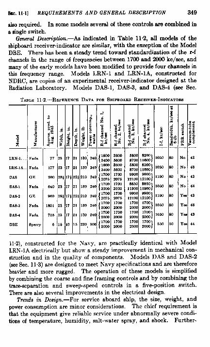
Em. 11.1] REQUIREMENTS AND GENERAL DESCRIPTION 349

also required. In some models several of these controls are combined ina single switch.

General Descr-iption.-As indicated in Table 11.2, dl models of theshipboard receiver-indcator are similar, with the exception of the ModelDBE. There has been a steady trend toward standardization of the r-fchannels in the range of frequencies between 1700 and 2000 kc/see, andmany of the early models have been modified to provide four charnels inthis frequency range. Models LRN-1 and LRN-lA, constructed forNDRC, are copies of an experimental receiver-indicator designed at theRa&ation Laboratory. Models DAS-1, DAS-3, and DAS-4 (WX Sec.

TABLE112.-REFEE~NCEDATAFOR SHIPZOAEDRECEIVER-INDICATORS

3xz

LRN-1,

LRN-lA,

DAS

DAS-1

DAS-2

DAa3

DAS-4

DBE

Fads

Fada

GE

Fada

GE

Fada

Fads

EIperry

6S00 S2LM ,Ow ~8700 11820}

}‘m 8200 1050 soS700lleQo9900 0000 ,*W ~

1210012100}

}‘w ’50 1050 so1190011’JOO

}- - 1100 so

12100 12100

}1700 17m 10.50 so2000 20001700 1700 ,050 ~2000 2000}1700 17002000 2000}

550 50

11.2), constructed for the Navy, are practically identical with ModelLRN-lA electrically but show a steady improvement in mechanical con-struction and in the quality of components. Models DAS and DAS-2

(we Sec. 11”3) are designed to meet Navy specifications and are thereforeheavier and more rugged. The operation of these models is simplifiedby combining the coarse and fine framing controls and by combining thetrac+separation and sweep-speed controls in a fiv~position switch.There are also several improvements in the electrical design.

Trends in Design.—For service aboard ship, the size, weight, andpower consumption are minor considerations. The chief requirement isthat the equipment give reliable service under abnormally severe condi-tions of temperature, humidity, salt-water spray, and shock. Further-

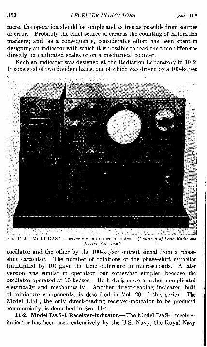
350 RECEIVER-INDIG’A TORS [SEC, 11.2

more, the operation should be simple and as free as possible from sourcesof error. Probably the chief source of error is the counting of calibrationmarkers; and, as a consequence, considerable effort has been spent indesigning an indicator with which it is possible to read the time differencedirectly on calibrated scales or on a mechanical counter,

Such an indicator was designed at the Radiation Laboratory in 1942.It consisted of two divider chains, one of which was driven by a 100-kc/sec

oscillator and the other by the 100-kc/sec output signal from a phass-shift capacitor. The number of rotations of the phase-shift capacitor(multiplied by 10) gave the time difference in microseconds. A laterversion was similar in operation but somewhat simpler, because theoscillator operated at 10 kc/see. Both designs were rather complicatedelectrical y and mechanical y. Another direct-reading indicator, builtof miniature components, is described in Vol. 20 of this series. TheModel DBE, the only direct-reading receiver-indicator to be producedcommercially, is described in Sec. 11.4.

11.2. Model DAS-1 Receiver-indicator.—The Model DAS-1 receiver-indicator has been used extensive y by the U.S. Navy, the P~oyal Navy

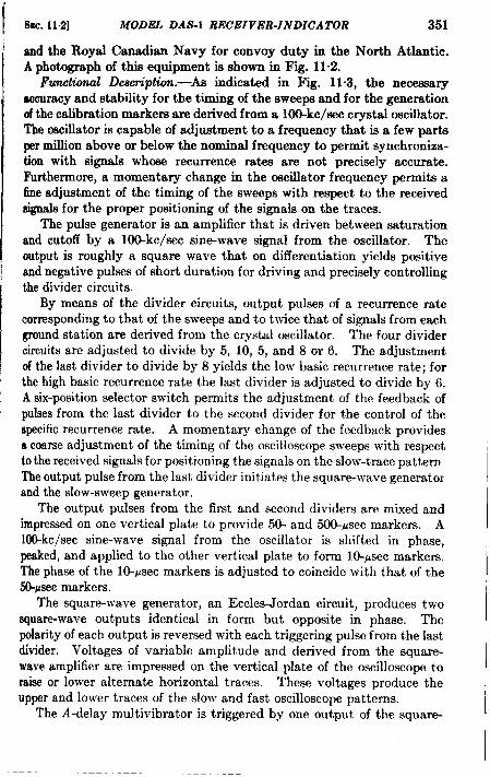
[SEC.11.2] MODEL DAS-I RECEIVER-INDICATOR 351

!and the Royal Canadian Navy for convoy duty in the North Atlantic.A photograph of this equipment is shown in Fig. 11“2.

Functional Desm”ption.-As indicated in Fig. 11-3, the necessaryaccuracy and stability for the timing of the sweepa and for the generationof the calibration markers are derived from a 10@kc/eec crystal oscillator.The oscillator is capable of adjustment to a frequency that is a few partsper million above or below the nominal frequency to permit synchroniza-tion with signals whose recurrence rates are not precisely accurate.Furthermore, a momentary change in the oscillator frequency permits aEneadjustment of the timing of the sweeps with respect to the receivedsignals for the proper positioning of the signals on the traces.

The pulse generator is an amplifier that is driven between saturationand cutoff by a 10@kc/sec sine-wave signal from the oscillator. Theoutput is roughly a square wave that on differentiation yielda positiveand negative pulses of short duration for driving and precisely controllingthe divider circuits.

By means of the divider circuits, output pulses of a recurrence ratecorresponding to that of the sweeps and to twice that of signals from eachground station are derived from the crystal oscillator. The four dividercircuits are adjusted to divide by 5, 10, 5, and 8 or 6. The adjustmentof the last divider to divide by 8 yields the low basic recurrence rate; forthe high basic recurrence rate the last divider is adjusted to divide by 6.A six-position selector switch permits the adjustment of the feedback ofpulsesfrom the last divider to the second divider for the control of thespecific recurrence rate. A momentary change of the feedback providesa coarse adjustment of the timing of the oscilloscope sweeps with respectto the received signals for positioning the signals on the slow-trace patternThe output pulse from the last divider initiates the square-wave generatoland the slow-sweep generator.

The output pulses from the first and second dividers are mixed andimpressed on one vertical plate to provide 50- and 500-~sec markers. A100-kc/sec sine-wave signal from the oscillator is shifted in phase,peaked, and applied to the other vertical plate to form 10-psec markers.The phase of the 10-psec markers is adjusted to coincide with that of theW-Psec markers.

The square-wave generator, an Eccles-Jordan cirmit, produces twosquare-wave outputs identical in form but opposite in phase. Thepolarity of each output is reversed with each triggering pulse from the lastdivider. Voltages of variable amplitude and derived from the square-wave amplifier are impressed on the vertical plate of the oscilloscope toraise or lower alternate horizontal traces. These voltages produce theupper and lower traces of the slow and fast oscilloscope patterns.

The A-delay multivibrator is triggered by one output of the square-

IIII

f # , 1 Ill

50flsec 500Nsec 2500psec I20,000psec I

I 1

E3-1F__7‘+ ‘-Jx - ,’+Mixer Pedestal

generator

+

Receiver

-m

1 1I )

Square.wave Amplitudegenerator balance ,

,bi1 4t

TraceAI I‘ 1hI1 separation Horizontal

1[

amplifier

Fine Fast-sweep &s4

B.delay generator F> I

wmNJ

SIX. 11.2] MODEL DAt3-1 RECEIVER-INDICATOR 353

wave generator at the beginning of the upper slow trace. It introduces afixed time delay of approximately 1000 psec. The coarse B-delay multi-vibrator is triggered by the other output of the square-wave generatorat the beginning of the lower slow trace. It introduces a time delay thatis variable in increments of 500 psec from approximately 1000 to approxi-mately 11,000 psec. Both the A-delay and the coarse B-delay multi-vibrators are stabilized by the introduction of 500+wc locking pulsesderived from the second divider. The coarse B-delay multivibratorinitiates the fine Bdelay multivibrator which introduces an additionaltime delay that is continuously variable from 200 to 700 psec. Thedelayed outputs of the A-delay and the fine B-delay multivibrators aremixed and used to trigger the pedestal generator.

The pedestal generator produces identical square-wave outputs whichare impressed on the vertical plate of the oscilloscope to produce the A-and B-pedestals of the slow trace pattern. Any one of three values of thepedestal length can be selected by means of the fast-sweep switch.

The fast-sweep generator is triggered by the pedestal generator andproduces a sweep voltage whose amplitude varies linearly with the timerepresented by the pedestal. When the horizontal plates of the oscillo-scope are switched from the slow to the fast sweeps, only that fraction ofthe recurrence interval represented by the tops of the pedestals is shownon the oscilloscope screen. The traces are expanded to the full width ofthe screen, and the trace of the A-pedestal appears directly above thetrace of the B-pedestal.

The transmitted pulses are received and amplified in a superheter~dyne receiver and are impressed on the vertical plate of the oscilloscope.The receiver consists of one stage of r-f preelection, a pentagrid converter,three i-f stages operating at 1050 kc/see, a diode detector, and one stageof video amplification. The bandwidth is approximately 80 kc/see at,6 db, and the sensitivity is such that a signal of less than 10 w gives full-scale deflection of the oscilloscope. Any one of four fixed-tuned r-fchannels can be selected by a switch. The frequency ranges of thechannelsare given in Table 112. The pulses as displayed on the OSC;llGecope are of approximately 75-psec duration.

The amplitude-balance circuit, driven by the square-wave generator,applies adjustable voltages of either polarity to one stage of i-f amplifica-tion. This provides a control of the relative gain of the receiver on alter-nate oscilloscope traces and permits the equalization of the amplitudesof the A- and B-pulses. Such equalization is required for the accuratemeasurement of time differences.

Manipulation.—In carrying out the time-cliff erence measurement asoutlined in Sec. 11”1, the operator of the Model DAS-1 receiver-inclicat ormust manipulate the following controls:

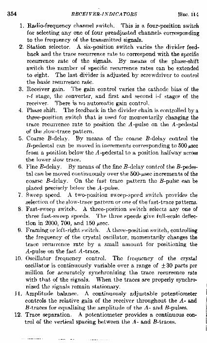
354

1.

2.

3.

4.

5.

6.

7.

8.

9.

10.

11.

12.

RECEIVER-INDICATORS [SEC. 11.:

Radio-frequency channel switch. This is a four-position switchfor selecting any one of four preadjusted channels correspondingto the frequency of the transmitted signals.Station selector. A six-position switch varies the divider feed-back and the trace recurrence rate to correspond with the specificrecurrence rate of the signals. By means of the phase-shiftswitch the number of specific recurrence rates can be extendedto eight. The last diiider is adjusted by screwdriver to controlthe basic recurrence rate.Receiver gain. The gain control varies the cathode bias of ther-f stage, the converter, and first and second i-f stages of thereceiver. There is no automatic gain control.Phase shift. The feedback in the divider chain is controlled by athree-position switch that is used for momentarily changing thetrace recurrence rate to position the A-pulse on the A-pedestalof the slow-trace patt em.Coame B-delay. By means of the coarse B-delay control theB-pedestal can be moved in increments corresponding to 500 psecfrom a position below the A-pedestal to a position halfway acrossthe lower slow trace.Fine B-delay. By means of the fine B-delay control the B-pedes-tal can be moved continuously over the 500-psec increments of thecoarse B-delay. On the fast trace pattern the B-pulse can beplaced precisely below the A-pulse.Sweep speed. A two-position sweep-speed switch provides theselection of the slow-trace pattern or one of the fast-trace patterns.Fast-sweep switch. A three-position switch selects any one ofthree fast-sweep speeds. The three speeds give full-scale deflec-tion in 2000, 700, and 150 psec.Framing or left-right switch. A three-position switch, controllingthe frequency of the crystal oscillator, momentarily changes thetrace recurrence rate by a small amount for positioning theA-pulse on the fast A-trace.Oscillator frequency control. The frequency of the crystaloscillator is continuously variable over a range of ~ 30 parts permillion for accurately synchronizing the trace recurrence ratewith that of the signals. When the traces are properly synchro-nized the signals remain stationary.Amplitude balance. A continuously adjustable potentiometercontrols the relative gain of the receiver throughout the A- andB-traces for equalizing the amplitude of the A- and B-pulses.Trace separation. A potentiometer provides a continuous con-trol of the vertical spacing between the A- and B-traces.

I

/

I

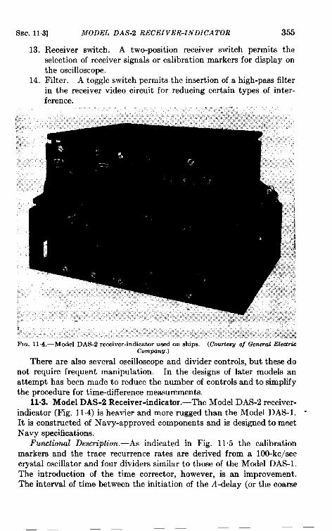
SEC. 11.3] MODEL DA S-2 RECEIVER-INDICATOR 355

13. Receiver switch. A two-position receiver switch permits theselection of receiver signals or calibration markers for display onthe oscilloscope.

14. Filter. A toggle switch permits the insertion of a high-pass filterin the receiver video circuit for reducing certain types of inter-ference.

FIG. 11 .4.—Model DAS-2 receiver-indicator used on ships. (Court.%u of General ElectricCompanu.)

There are also several oscilloscope and divider controls, but these donot require frequent manipulation. In the designs of later models anattempt has been made to reduce the number of controls and to simplifythe procedure for time-difference measurements.

11.3. Model DAS-2 Receiver-indicator. -The Model DAS-2 receiver-indicator (Fig. 11.4) is heavier and more rugged than the Model DAS-1.It is constructed of Navy-approved components and is designed to meetNavy specifications.

Functional Description. -As indicated in Fig. 11.5 the calibrationmarkers and the trace recurrence rates are derived from a 100-kc/seccrystal oscillator and four dividers similar to those of the Model DAS-1.The introduction of the time corrector, however, is an improvement.The interval of time between the initiation of the Adelay (or the coarse

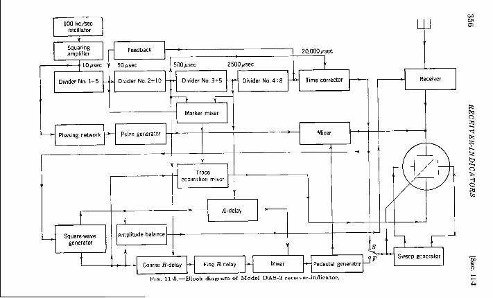
r++Squaringamplifier

10psec

Diwder No. 1+5

\, 50w3ec 500psec 2500psec

v

t Marker mixer

—

AI I I 1

QSquare-wavegenerator

J

I

—

+

s

I

d<

&~

sb2

, b

2ah

/

181

~F Sweep generator

FIG. 11 .5.—Block diagram of Model DAS-2 receiver-indicator.

SEC. 11.3] MODEL DA S-2 RECEIVER-INDICATOR 357

B-delay) multivibrator and the succeeding 500-psec locking pulse fromthe second divider varies with the position of the station selector switchthat controls the feedback. This interval of time is equal to 500 ~secminus 50N ,usec, where N is the feedback number and may be any integerfrom Oto 7. Because of the variation of this interval of time, the designof the Model DAS-1 A- and coarse B-delay multivibrator is more com-plicated than would otherwise be necessary. The purpose of the timecorrector is to eliminate the variable time interval between the initiationof the A-delay (or coarse B-delay) multivibrator and the succeeding500-psec locking pulse. The time correct or is a derivative of the Eccles-Jordan circuit that has two inputs. It generates a flat-topped signal thatis initiated by the pulse from the last divider and is terminated by thefirst succeeding 500-psec pulse from the second divider. The durationof the ffat-topped signal is 500 ~sec minus 50N .mec. The square-wavegenerator and the A- and coarse B-delay multivibrators are initiated atthe termination of the flat-topped signal. The time corrector alsosimplifies and improves the operation of the slow-sweep generator andsuppresses the retrace of the slow-trace pattern.

The A-delay multivibrator is locked by 2500-~sec pulses from thethkd divider and is adjusted to introduce a fixed time delay of 2000 ~secafter the initiation of the upper slow trace (2500 ~sec minus 50N psecafter the pulses from the last divider). The B-delay multivibrators,pedestal generator, sweep generator, and receiver are similar in functionto those of the Model DAS-1 receiver-indicator.

Manipulation.—The manipulation of the Model DAS-2 receiver-indicator is somewhat simpler than that of the Model DAS-1. A PRRtoggle switch provides a convenient selection of the two basic recurrencerates. The trace-separation control and the fast-sweep switch areeliminated, and their functions are performed by the sweep-speed switch.A single LEFT-RIGHTswitch shifts the positions of the .4- and B-signals onboth the slow and fast traces.

To measure a time difference, the operator must manipulate the fol-lowing controls:

1. R-f channel switch. A four-position switch selects any one of thepreadjusted channels listed for the Model DAS-2 receiver-indica-tor in Table 11.2.

2. PRR switch. A toggle switch with L (low) and H (high) positionsselects one of two adjustments of the last divider to provide therequired basic recurrence rate.

3. Station selector. An eight-position switch controls the specificpulse recurrence rate.

4. Gain control. This varies the amplitude of the received signals

as they appear on the oscilloscope.

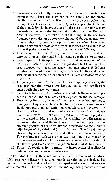
358

5.

6.

7.

8.

9.

10.

11.

12.

RECEIVER-INDICATORS [SEC. 11c4

LEFT-RIGHT switch. By means of the LEFT-RIGHT switch the

operator can adjust the positions of the signals on the traces.

On the first (slow trace) position of the sweep-speed switch, the

timing of the traces is shifted rapidly with respect to the timing

of the signals by the introiluction of pulses of either polarity from

the A-delay multivibrator tothe first divider. Ontheotherposi-

tions of the sweep-speed switch a slight change in the oscillator

frequency provides an appropriate change of the recurrence rate,

Coarse delay. By means of a potentiometer control the interval

of time between the start of the lower slow trace and the initiation

of the B-pedestal can be varied in increments of 500 ~sec.Fine delay. The fine B-delay control enables the operator to

vary continuously the totial B-delay time over the required range,

Sweep speed. A five-position switch provides selection of the

slow-trace pattern with wide trace separation, fast traces of 2300-psec duration with medium separation, fast traces of 650-psecduration with medium separation, fast traces of 160-~sec durationwith small separation, or fast traces of 160-w3ec duration with noseparation.Frequency control. A fine control of the frequency of the crystaloscillator permits precise synchronization of the oscilloscopetraces with the received signals.Amplitude balance. A potentiometer controls the relative ampli-tudes of the A- and B-pulses as they appear on the oscilloscope.Receiver switch. By means of a four-position switch any one offour types of signals can be selected for display on the oscilloscope.In the OFF position, calibration markers alone are displayed. In

the ON position, calibration markers are displayed with signals

from the receiver. In the CAL. 1 position, the stair-step pattern

of the second divider is displayed for checking the adjustment of

the second divider and the feedback. In the CAL. 2 position, the

stairstep pattern of the third divider is displayed for checking the

adjust ment of the third and fourth dividers. The first divider is

checked by means of the 10- and 50-gsec calibration markers.

For checking feedback on position CAL. 1 and on the third positionof the sweep-speed switch, the sweeps are initiated at the start ofthe flat-topped time-corrector signal instead of at its termination.Filter. A toggle switch permits the introduction of a filter for——reducing certain types of interference.

11.4. Model DBE Receiver-indicator.—The direct-reading ModelDBE receiver-indicator (Fig. 11.6) stands upright on the deck and issecured to the deck and bulkhead by S-shaped steel springs that serve asshock mounts. The oscilloscope screen and operating controls are on

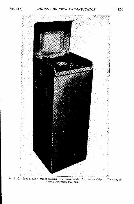
SEC. 11.4] MODEL DBE RECEIVER-INDICATOR 359

h. 11,6L. . ..- _.-— - ______ _ _.. -“..J

.—Model DBE direct-reading receiver-indicator for use on ships. (CcSpETrUGUroacope Co., Inc.)

Iurceqjof

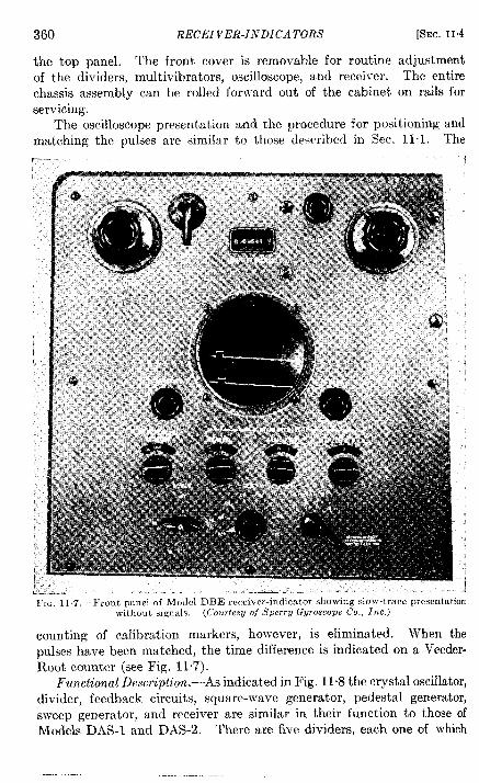
360 RECEIVER-INDICATORS [SEC. 11.4

the top panel. The front cover is removable for routine adjustment

of the dividers, multivibrators, oscilloscope, and receiver. The entire

chassis assembly can be rolled forward out of the cabinet on rails for

servicing.The oscilloscope presentation and the procedure for positioning and

matching the pulses are similar to those described in Sec. 11.1. The

.-- ...

LA.. ...JFIG. 11.7.—Front panel of Model DBErr.vwiver-indicator showing slow-trare presentation

without sigmds. (Cour/.sy of Sperry Gyroscope Co., Inc.)

counting of calibration markers, however, is eliminated. When the

pulses have been matched, the time difference is indicated on a Veeder-

Root counter (see Fig. 117).Functional Description.—As indicated in Fig. 11% the crystal oscillator,

divider, feedback circuits, square-wave generator, pedestal generator,sweep generator, and receiver are similar in their function to those ofModels DAS-I and DAS-2. There are five dividers, each one of wh~ch

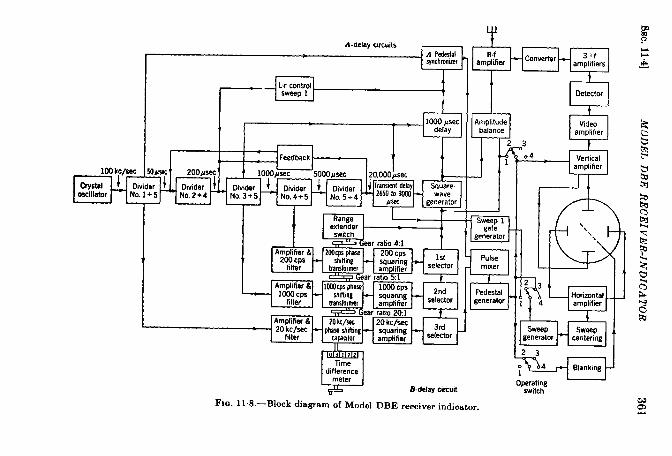
SE

C.11.4]

MO

DE

LD

BE

RE

CE

IVE

R-IN

DIC

AT

OR

361

— 7m

362 RECEIVER-INDICATORS [SEC, 11.4

divides the pulse recurrence rate by a ratio of 5/1 or less. Because ofthe lower dividing ratios the over-all operation is more reliable than thatof earlier models. The transient delay circuit is a locked delay multi-vibrator that serves the same purpose as the time corrector of ModelDAs-2. Italsoreduces the effect of thedistortion of thephase-stiftkgsine waves caused by feedback.

The rotations of the 200- and 1000-cps phase-shifting transformersand of the 20-kc/sec phase-shifting capacitor control the position of theB-pedestal and determine the measured time difference when the receivedsignals are matched. The sine waves of the three phase-shifted frequen-cies are derived through amplifiers and low-pass filters from the dividersof the appropriate recurrence rates. The three phase shifters are coupledthrough a gear train to the time-difference counter and to the coarse andfine delay controls. Since the gear ratios between the phase shifters areequal to the ratios of their frequencies, a rotation of the fine delay controlproduces the same change in time difference in all three frequencies.The three phase-shifted sine waves are squared and differentiated toyield the pulses that terminate the flat-topped output signals of threeselector circuits. Each selector circuit is a multivibrator of the Eccles-Jordan type with two inputs similar to the time-corrector circuit ofModel DAS-2. The first selector circuit is initiated at the start of thelower slow trace by a pulse from the square-wave generator. The outputsignal is terminated, depending on the bias selected by the extenderswitch, by the first, second, or third 5000-usec pulse derived from the200-cps phase-shifting transformer. By means of the fine delay controlthe time delay introduced by the first selector maybe varied continuouslyfrom less than 1000 to more than 18,000 #see. The time delay so intro-duced, however, is not itself sufficiently accurate for the time-differencemeasurement. To obtain the precision required for the time-differencemeasurement, the selecting process is repeated in two succeeding selectorsof greater precision whose output signals are terminated by pulses derivedfrom the phase-shifted 1000-cps and 20-kc/sec signals. The second selec-tor is triggered at the termination of the first selector output signal, and itsoutput signal is terminated by a pulse derived from the phase-shifted1000-cps sine wave. The third selector is triggered at the termination ofthe second selector signal. Its output signal is terminated by a pulsederived from the phase-shifted 20-kc/sec sine wave and having the pre-cision required for the time-cliff erence measurement. The pedestalgenerator and fast-sweep generator are triggered at the termination of thethird selector output signal.

By means of the coarse delay control the B-pedestal can be movedrapidly by increments of 1000 ~sec. The coarse delay control throughthe range-extender switch varies the bias of the first selector and shifts the

SEC. 11 .5] GENERAL DESCRIPTION AND TRENDS IN DESIGN 363

phase of the terminating pulse. Also, through a differential gearing anddetent system, it rotates the thousands and ten-thousands dials of the

time-difference counter.

Similarly the A-delay is obtained from the combination of a fixed

coarse selector (1000-~sec delay) and a fixed fine selector (A-pedestal

synchronizer). The output signal of the 1000-psec delay is terminated

by a 1000-Wsec pulse from the third divider, and the output signal of the

A-pedestal synchronizer is terminated by a 50-~sec pulse from the first

divider. The pedestal generator is triggered at the termination of the

output signal from the A-pedestal synchronizer.Manipulation.—As shown in Fig. 11.7 the manipulation is simplified

by the arrangement of the controls. The three station-selecting s’witches,r-f channel, basic PRR, and specific PRR, are grouped in a row. Thecoarse and fine delay controls are concentric, as are the gain and amplitudebalance controls. The LEFT-RIGHT switch and drift (oscillator frequency)control are a concentric lever and disk. The four-position operationsswitch provides selection of the normal slow-trace pattern, a pair ofvertically spaced 1300-psec traces, a pair of spaced 175-~sec traces, and hpair of 175-psec traces with no trace separation.

I AIREORNE RECEIVER-INDICATORS

11.6. General Description and Trends in Design.—The methods ofmeasurement, the oscilloscope presentation, the r-f channels, and recur-rence rates of the airborne receiver-indicator are similar to those of theshipboard instrument. For airborne equipment the requirements of lightweight and small size are severe. As indicated in Table 11.3, theserequirements are recognized, and an effort has been made to reduce theweight, size, and power consumption as far as practical. All airbornereceiver-indicator models have been designed for operation in bothAmerican and British aircraft, and most of them are physically inter-changeable with Gee sets. They can be operated on input power ofeither 80 or 115 volts and of any frequency between 400 and 2400 cps.

Genwal Description.—The Models SCR-722 and SCR-722A are light-weight modifications of the Model DAS-1 receiver-indicator with a powersupply designed for operation at 400 to 2400 cps instead of 60 cps. Theyare awkward for operation in the air but have been used for trainingpurposes.

The Model AN/APN-4 receiver-indicator, of which there are fivemodifications, was used most extensively during World War II. Modifi-cations I and II could not be used in normal service because of dividerinstability and high-voltage arcing at high altitudes. Modification 111has been used extensively and has performed well. There has been nolarge production of Modification IV, and Modification V reached the

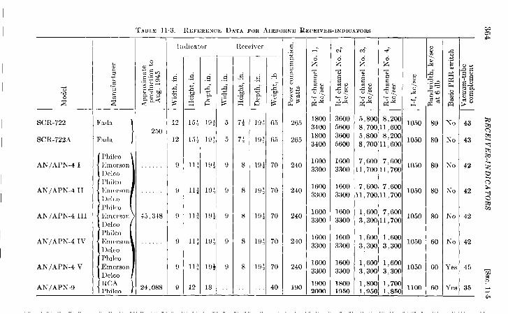
I SCR-722

I SCR-722.4

I AN/APX-4 I

IIAN/APK-4 II

AN/APN-4 III

AN/APh’-4 IV

I AN/APN-4 v

I AN/APN-9

.“

Fwhi

F:uia 1

‘ Philco \Ima-son1)(!ICOPhilcol~mrrsou1)(,IC()l’hilcolhncrsor.

;1)elcoPhilcoEmersonDelco

: Ph]lmEmersonDelco \

[RC.4Philco )——

‘rAB1.E 113.-RE~-ERENCE I)ATA FOR .41RSOKNE RECEIVIMt-IndiCatOrS

.“ . ,,,.,,, ...,,

Ind]cat,or

c.- .5

2 5-m Q

.5

E 6

15; 1!).

15+ 19

11$ 19

11$ 19

11+ 19

11; 19

11] 19

12 18

,“ .

---

z%cG;;\

22

180034001800

3400

16003300

16003300

1600

3300

1600

3300

1600

3300

19002000

.,, .

N-

E3cc

-8;\

y“

K~

3600560036005600

16003300

16003300

16003300

16003300

16003300

18001950

,,. .,,. ,. ,.,,

SEC. 115] GENER.4L DESCRIPTIOiV” AND TRENDS IN DESIG.V 365

European Theater too late for service. Modification V has a basic PRRswitch and six dividers instead of four; it is described in Sec. 11.6.

All the components of Model Ah-/APN-9 receiver-indicator (describedin Sec. 11.7) are contained in a single case that fits the same shock-mounted frame as the AhT/APAT-4 and Gee indicator. The set weighsonly 40 lb, and its power consumption is only 190 watts. Although itarrived too late for service in the European Theaterj it was used in thePacific. Its notable features are a 3-in. cathode-ray tube with a magnify-ing glass, nonlinear sweeps, and a rather complicated system of calibrationmarkers.

Trends in Design .—Because of the rapid motion of an aircraft, thetime required to make two readings and plot a fix is a most importantquantity, and, indeed, the reduction of this time should be the prime con-sideration in the future development of the Loran system and equipment.For example, a plane may travel at a speed of 5 miles per minute, and thenavigator may require 1 min for the measurement of each time differenceand another minute for p!otting the lines of position. Since the planetravels 5 miles while he makes the second measurement and 5 miles whilehe plots the lines of position, the intersection of the two lines does notrepresent the navigator’s true position. There are two methods for over-coming this difficulty, both of them awktvard. The navigator may cal-culate the distance that the plane has traveled in the interval betweenthe two measurements and advance the first line of position by the appro-priate distance. The intersection of the advanced first line of positionwith the second line is the true position at the time of the second measure-ment. As an alternative method, the navigator may make threemeasurements (with equal intervals of time between the first and secondmeasurements and between the second and third measurements) andcompute the mean of the first and third measurements. The intersectionof the second line of position with the line corresponding to the mean ofthe first and third measurements determines his position at the time ofthe second measurement.

To reduce the time required to make a reading, the airborne receiver-indicators are designed so that the operator can control the sweep speed,the trace separation, and the selection of received signals or calibrationmarkers by means of a single selector switch. This unification of thecontrols simplifies the operation slightly but leaves much to be desired.The Gee indicator, for instance (see Sec. 1.4), is much simpler to operatethan the Loran indicator because it permits the measurement of two timedifferences simultaneously and thus eliminates the necessity of advancinga line of position or of making three readings to determine a fix. For thisreason the Gee system is admirably adapted to a simple and useful typeof navigation, called the homing technique, that is described in Sec. 1.6.

366 RECEIVER-INDIC’A TORS [SEC. 11.5

This technique cannot easily be applied to navigation by Loran in itspresent form.

As mentioned in Sees. 3.8 and 77 the requirements for instantaneousfixing over a particular area are that it shall be possible to receive signalsfrom two pairs of ground stations transmitting at a single recurrence rateand that the navigator shall be able to adjust two sets of controls tomeasure the appropriate time differences simultaneously. The simplestsystem of synchronization of the ground stations is that used for the LowFrequency trials and described in Sec. 7.8. The same system can beapplied to Standard Loran with practically no modification of the ground-station equipment now in service, but long trains of sky waves may attimes make the presentation confusing.

The simplest type of receiver-indicator for instantaneous fixing is onesimilar to AN/APN-4, but it is provided with a second set of delay con-trols and a switch for simultaneously selecting either pair of B-delaycontrols, either of two gain-balance adjustments, and either of the out-puts from the square-wave generator for initiation of the A- and B-delaymult ivibrat ors and for the trace separation. Such a receiver-indicatorwould be little more complex than AN/APN-4. The only duplicationwould be in the potentiometers that control the biases of the delay multi-vibrators and the relative amplitudes of the signals.

A decimal system of calibration markers similar to that of the Geeindicator seems preferable to the common Loran display of 10-, 50-, 500-,and 2500-~sec markers on the slow, medium, and fast traces. The diwplay of 1000-psec markers on the slow traces, 1000- and 100-~sec markerson the medium traces, and 100- and lo-psec (and possibly 1- or 2-~sec)markers on the fast traces seems satisfactory. Furthermore, the 1OO-PWCmarkers should coincide in time with the corresponding 10-usec markenas do the markers displayed on the oscilloscope of the timer.

A much simplified form of the synchronizer (Sec. 7.3) has beendesigned to control the frequency of the crystal oscillator in such a waythat the signal from the master station remains stationaW on the upperpedestal. This feature, called “ top locking,” is believed to be a worth.while convenience for the operator of the receiver-indicator.

By the addition of a third delay multivibrator the advantage of thedirect-reading indicator can be incorporated in the instantaneous-fixingreceiver-indicator. In such a receiver-indicator, the first delay multi-vibrator would be variable in increments of 1000 psec and the second delaymult ivibrat or would be variable in increments of 100 psec. Calibratedselector switches would indicate the numbers of thousands and hundredsof microseconds of time clifference. The third delay multivibrator wouldbe variable continuously from 20 to 120 ~sec, and a calibrated dial on thepotentiometer would indicate the number of units of time difference,

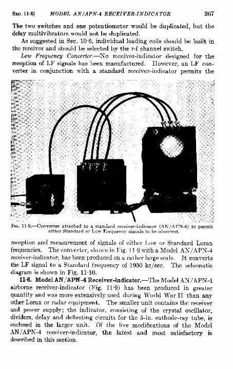
SEC. 116] MODEL AN/APN-4 RECEIVER-INDICATOR 367

The two switches and one potentiometer would be duplicated, but thedelay multivibrators would not be duplicated.

As suggested in Sec. 10.6, individual loading coils should be built inthe receiver and should be selected by the r-f channel switch.

Low Frequency Converter.—’NTo receiver-indicator designed for thereception of LF signals has been manufactured. However, an LF con-verter in conjunction with a standard receiver-indicator permits the

FIG. 11.9.—Converter attached to a standard receiver-indicator (AN/APN-4) to permiteither Standard or Low Frequency signals to be observed.

reception and measurement of signals of either Low or Standard Loranfrequencies. The converter, shown in Fig, 119 with a Model AN/APN-4receiver-indicator, has been produced on a rather large scale. It convertsthe LF signal to a Standard frequency of 1950 kc/see. The schematicdiagram is shown in Fig. 11.10.

11.6. Model AN/APN-4 Receiver-indicator.—The Model AN/APN-4airborne receiver-indicator (Fig. 11.9) has been produced in greaterquantity and was more extensively used during World War II than anyother Loran or radar equipment. The smaller unit contains the receiverand power supply; the indicator, consisting of the crystal oscillator,dividers, delay and deflecting circuits for the 5-in. cathode-ray tube, isenclosed in the larger unit. Of the five modifications of the Model.kN/APN-4 receiver-indicator, the latest and most satisfactory isdescribed in this section.

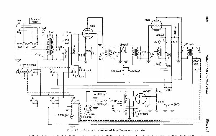
LOWn

Antenna

& ‘a’”

I From antenna\

-,:1

III

,~–—––

-i

h~?i!’dsta”t

Lt. local

6SA7

F

---------------

220p&f

22 k

150n 500

##f ppf

150/lpf

jllq’ql(~

— —— —

776800/I/If 3800p/Lf

——

180

b

10,0

——w----’ E-:--zL

h r10k

T < - E y-’~

6X5GT_T— —–—————– 10k‘, ‘>\ \ ‘, &“oo”’f—

I8 80v1 m- ,,

1

2.2M11, , , =6800g,f

, I1:, ,

BoA = ;3” Z“f?l 1°.— 1II , 115V — — —— — —, I

To receiver 1 ‘l10vor80v To heaters/ ~60-2400 CpS1 L———-—--—–__—_—— ————-=—-—____——— ————————--——- -—.L–––––—-–—––__-–— –--––-__–– –----— --__–-–––. –-–_.

,,.

L——

6800

&—1..Ic I I 10.—-Schematic diagram of Low Frequency converter.

.

;

Km; ~I/If , ;

&~–1 ,1

IIIIIIII;1,1IIII\l,1,1II11IIIIII11~1,1

--,1-— J

“.

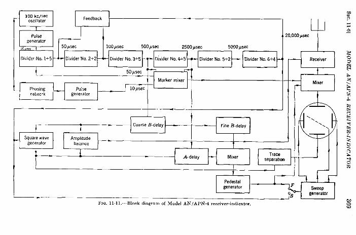
Pulsegenerator

10”,,. ! 50psec 100psec 500psec 2500psec 5@90Asec

Divider No. 1+5 — Diwder No. 2+2 ~ Divider No. 3+5 - Divider No. 4+5

t50 psec

1+I

,.,. ...-, ,,,,.G,

Phasing Pulse 10psec

network generator

I

1 I_Coarse E-delay Fine B-delay

I

Square-wave Amphtudegenerator balance I t t

I J I I I

L 1 A-delay Mixer

I Iu

Traceseparation

+5!0,000psec

Receiver

-QMixer

~FIG. 11.11.—Block diagram of Model AN/APN-4 receiver-indicator.

370 RECEIVER-INDIC’A TORS [SEC. 116

Functional Description.—The block diagram of the Modification VModel AN/APN-4 receiver-indicator, shown in Fig. 11.11, is similar tothat of the Model DAS-lreceiver-indicator (Fig. 113). Since there aresix dividers instead of four, themaximum dividing ratio is 5/l instead of10/1, and the operation is therefore more reliable. The output pulsefrom the last divider is fed back to the second and third dividers to controlthe specific recurrence rate.

Pulses derived from the crystal oscillator and from the first, third, andfourth dividers are mixed and applied to the vertical plate (along withthe trace separation and pedestals) of the cathode-ray tube as calibrationmarkers, at time intervals of 10, 50, 500, and 2500 psec.

The complete schematic diagrams of the receiver and the indicator areshown in Figs. 11.12 and 11.13. Circuits of these types are described insome detail in Chap. 7 and in other volumes of this series.

Manipulation.—In making a time-difference measurement, the opera-tor must manipulate the r-f channel; basic PRR and station selectorswitches; the gain, amplitude-balance and frequent y controls; the LE~-

RIGHT and sweep-speed switches; and the coarse and fine B-delay con-trols, as well as the usual oscilloscope controls. These controls aresimpler to operate than those of the Model DAS-1 receiver-indicator andare similar to those of Model DAS-2.

When the slow-trace oscilloscope pattern is displayed, the LEn-RIGHTswitch moves the signals rapidly along the trace by momentarily changingthe feedback; when one of the fast-trace patterns is displayed, the switchmoves the signals slowly by changing the oscillator frequency.

The eight-position sweep-speed switch is so designed that in making atime-difference measurement the operator rotates the switch in numericalsequence from Position 1 to Position 7. The first four positions show thereceived signals and are used for positioning and matching the signals.On the first position the normal slow-trace pattern is displayed. Thepatterns of the second and third positions are fast traces of 750 psec and200-psec respectively. For the final matching of the pulses, the separa-tion of the 200-psec traces is eliminated in Position 4. Positions 5, 6,and 7 are used for measuring the time difference between the initiationsof the fast traces corresponding to the time difference between the receivedsignals. For this purpose 10-, 50-, 500-, and 2500-psec calibrationmarkers are displayed on these three positions. The pattern on Position5 is two 200-psec traces with markers; on Position 6 it is two 750-~sectraces with markers; and on Position 7 it is two slow traces with pedestalsand markers. On Position 8 two 200-psec traces with the stair-steppattern of the third divider are presented for checking the adjustment ofthe feedback.

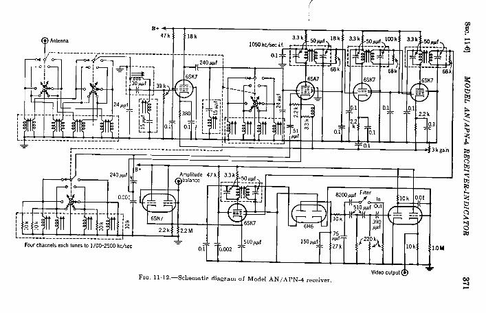
SE

C.

11.6]M

OD

EL

AN

/AP

N4

RE

CE

IVE

RIN

DIC

AT

OR

371

‘L_____

.

IiI

II

NH

%%

-11Ilr

!H--&

T---,,

,!,,,

“.

.I

.,.x

ill-

1

-11.----

L-------lL

--__;

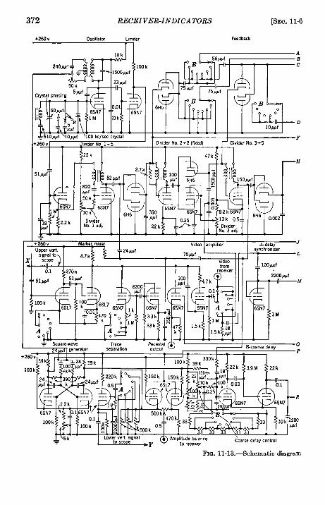
372 RECEIVER-INDICATORS [SEC. 116

+2Wv Oscillator Limiter Feedback

.

,.,. I I ABc

D

F

H

i’ 111/4

-- -- 33Amphtude balance

,6 ,...,,,., Coarse delay control

FIG. 11 .13.—Schematic diagram

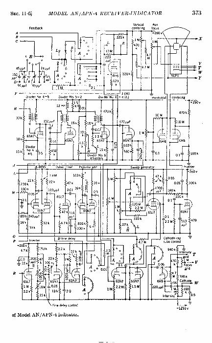
SEC. 11.6] MODEL AN/Al’N-4 liliL’EIVlili-I ~V1)1CA7’OR 373

V.”,,., A,,.. .. .

~centering

7’

d470h

10M

6H6

-d

01 102k

of Mvdel AN/APN-4 indicator.

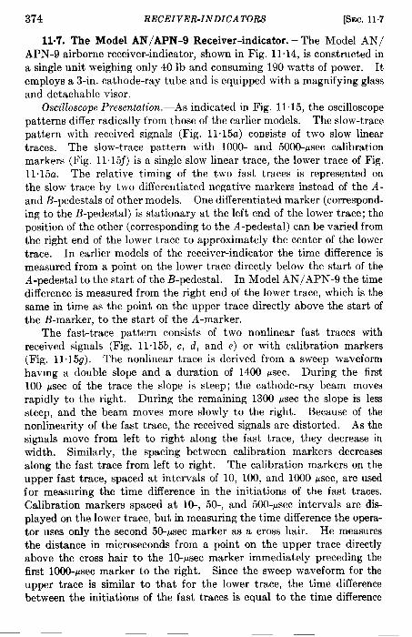
374 RECEIVER-INDICATORS [SEC. 117

11.7. The Model AN/APN-9 Receiver-indicator.-The Model AN/APN-9 airborne receiver-indicator, shown in Fig. 11~14, is constructed ina single unit weighing only 40 lb and consuming 190 watts of power. Itemploys a 3-in. cathode-ray tube and is equipped with a magnifying glassand detachable visor.

Oscilloscope Presentation.—As indicated in Fig. 11“15, the oscilloscopepatterns differ radically from those of the earlier models. The slow-tracepattern with received signals (Fig. 11~15a) consists of two slow lineartraces. The slow-trace pattern with 1000- and 5000-Wsec calibrationmarkers (Fig. 11. 15~) is a single slow linear trace, the lower trace of Fig.11.15a. The relative timing of the two fast traces is represented onthe slow trace by two clifferentiated negative markers instead of the A-

and B-pedestals of other models. One differentiated marker (correspond-ing to the B-pedestal) is stationary at the left end of the lower trace; theposition of the other (corresponding to the A-pedestal) can be varied fromthe right end of the lower trace to approximately the center of the lowertrace. In earlier models of the receiver-indicator the time difference ismeasured from a point on the lower trace directly below the start of theA-pedestal to the start of the B-pedestal. In Model AN/APN-9 the timedifference is measured from the right end of the lower trace, which is thesame in time as the point on the upper trace directly above the start ofthe B-marker, to the start of the A-marker.

The fast-trace pattern consists of two nonlinear fast traces withreceived signals (Fig. 11“15b, c, d, and e) or with calibration markers(Fig. 11. 15g). The nonlinear trace is derived from a sweep waveformhaving a double slope and a duration of 1400 psec. During the first100 psec of the trace the slope is steep; the cathode-ray beam movesrapidly to the right. During the remaining 1300 psec the slope is lesssteep, and the beam moves more slowly to the right. Because of thenonlinearity of the fast trace, the received signals are distorted. As thesignals move from left to right along the fast trace, they decrease inwidth. Similarly, the spacing between calibration markers decreasesalong the fast trace from left to right. The calibration markers on theupper fast trace, spaced at intervals of 10, 100, and 1000 psec, are usedfor measuring the time difference in the initiations of the fast traces.Calibration markers spaced at 10-, 50-, and 500-~sec intervals are dis-played on the lower trace, but in measuring the time difference the opera-tor uses only the second 50-~sec marker as a cross hair. He measuresthe distance in microseconds from a point on the upper trace directlyabove the cross hair to the lo-~sec marker immediately preceding thefirst 1000-psec marker to the right. Since the sweep waveform for theupper trace is similar to that for the lower trace, the time differencebetween the initiations of the fast traces is equal to the time difference

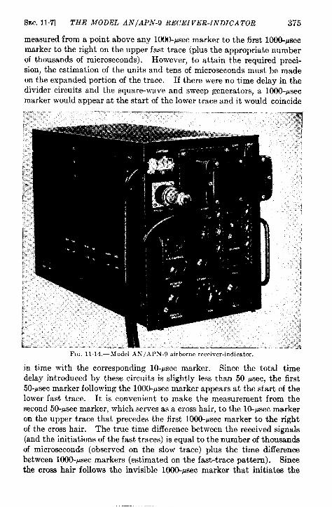
SEC. 11.7] THE MODEL AN/APN-9 RECEIVER-INDICATOR 375

measured from a point above any 1000-~sec marker to the first 100@psecmarker to the right on the upper fast trace (plus the appropriate numberof thousands of microseconds). However, to attain the required preci-sion, the estimation of the units and tens of microseconds must be madeon the expanded portion of the trace. If there were no time delay in thedivider circuits and the square-wave and sweep generators, a 1000-psecmarker would appear at the start of the lower trace and it would coincide

FIG. 1114.-Model AN/APN-9 airborne receiver-indicator.

in time with the corresponding lo-psec marker. Since the total t,irne

delay introduced by these circuits is slightly less than 50 ~sec, the first

50-gsec marker following the 1000-Psec marker appears at the start of the

lower fast trace. It is convenient to make the measurement from the

second 50-Psec marker, which serves as a cross hair, to the lo-~sec marker

on the upper trace that precedes the first 1000-psec marker to the right

of the cross hair. The true time difference between the received signals

(and the initiations of the fast traces) is equal to the number of thousands

of microseconds (observed on the slow trace) plus the time difference

between 1000-Psec markers (estimated on the fast-trace pattern). Since

the cross hair follows the invisible 1000-~sec marker that initiates the

376 RECEIVER-INDICATORS [SEC, 117

1

I ‘“’’’’ram,● Variable delay marker

(a) FUNCTION sw[tch Dosftlon 1

=

(b) FUNCTION switch posltlon2

I /-+Received signals

-J~(c) GAIN, BALANCE, DELAY controlsareadjusted

-4’=Received signals [superImposed)

L 1

(e) S,gnals are matc+ed

-0Received signals

(d) FUNCTION switch poslbon3

4-5000 ~sec [ntervals

11111111111111111111fVariable delay marker +

[~1FUNCTION switch poslllon4

I 500 psec Intervals.

100-j, sec marker

Reading po,nt of 100

u

I 10-,secntervals ~ 50-psec markers ~

10-psec markers Interval(This dlustrat[on showsa station

(The reading IS 6125 #see) rate count of 2- station-6j

k) FUNCTIONsw!tch posltlon 5

FIG. 11 15.—0M’IllowoIw pnttmw of Model .4X1.kf’ h--9 alrbor[le recel~,er-indicator.(a) Ful~rtlon sw]tvl~ on Poaitton 1; (b)func’tie!, sw]trh on position 2; (c) gain balance,del%>.ro!, tr[,lsad]tl?te<l; ((1) Iu,!rtiou switrbon Poslt~nn 3; (e) signals matched; U) funrt]onswitch ou Poslt]otl -I; (u) function smtch on Po~it ion 5.

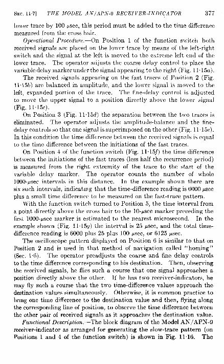
SEC. 11.7] TIIE il~ODEL A.V/.4P,V-9 RECEI VER-IiVDICA TOR 377

lower trace by 100 ~sec, this period must be added to the time differencemeasured from the cross hair.

Operational Procedure.—On Position 1 of the function switch bothreceived signals are placed on the lower trace by means of the left-rightswitch and the signal at the left is moved to the extreme left end of thelower trace. The operator adjusts the coarse delay control to place thevariable delay marker under the signal appearing to the right (Fig. 11.15a).

The received signals appearing on the fast traces of Position 2 (Fig.

11.15b) are balanced in amplitude, and the lower signal is moved to the

left, expanded portion of the trace. The fine-delay control is adjustedto move the upper signal to a position directly above the lolver signal(Fig. 1115c).

On Position 3 (Fig. 11.15d) the separation bet~veen the tlro traces iseliminated. The operator adjusts the amplitude-balance and the fine-

delay controls so that onc signal is superimposed on the other (Fig. 11 15e).

In this condition the time difference bet\veen the rcccived signals is equalto the time clitierence between the initiations of the fast traces.

On Position 4 of the function switch (Fig. 11.15j) the time differencebetween the initiations of the fast traces (less half the recurrence period)is measured from the right extremity of the trace to the start of thevariable delay marker. The operator counts the number of whole

looo-psec” intervals in this distance. In the example shown there are

six such intervals, indicating that the time-difference reading is 6000 psecplus a small time difference to be measured on the fast-trace pattern.

With the function switch turned to Position 5, the time interval froma point directly above the cross hair to the 10-ysec marker preceding thefirst 1000-psec marker is estimated to the nearest microsecond. In theexample shown (Fig. 11.15g) the interval is 25 ~sec, and the total time-difference reading is 6000 plus 25 plds 100 psec, or 6125 ~sec.

The oscilloscope pattern displayed on Position 6 is similar to that onPosition 2 and is used in that method of navigation called “ homing”(Sec. 16). The operator preadjusts the coarse and fine delay controlsto the time difference corresponding to his destination. Then, observingthe received signals, he flies such a course that one signal approaches aposition directly above the other. If he has two receiver-indicators, hemay fly such a course that the two time-difference values approach thedestination values simultaneously. Otherwise, it is common practice tobring one time difference to the destination value and then, flying alongthe corresponding line of position, to observe the time difference betweenthe other pair of received signals as it approaches the destination value.

Functional Description.-The block diagram of the Model AN/APN-9receiver-indicator as arranged for generating the slow-trace pattern (onpositions 1 and 4 of the function switch) is shown in Fig. 11“16. The

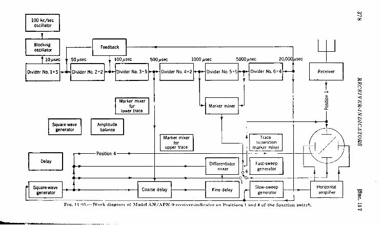
c1

100 kc/seeoscillator

CJ-4cc

r--l,Blockingoscillator [

Feedback

-~iderN04;00;‘;vider”o’+~‘iderNO‘m

EEH3EEI ?,

Marker rmxer J

I I Marker mixer I I ~~ Trace 1

LE!EK-1ET :

~ I_&E&.1Position 4 —–.–——

Delay

mixer

r

Scfuare.wavegenerator

ec 6Receiver

-4

+Horizontalamplifier

FIa. 11.1 c.—lllork dinxrnn, of \locfel .4NI.4PN-o rerei..cr-indic:ttor on Positions 1 and 4 of the function switch.+

SEC. 11 .7] THE MODEL AN/APN-9 REC.EIV17R-INDICA TOR 379

oscillator, clividcrs, feedback circuits, and sqnarc-wave generator aresimilar to those of Model AN/APN-4.

The coarse delay multivibrator, triggcrccf by positive pulses from thesquare-wave generator, is locked by 500-pscc pulses from the third divider.‘l’he delay introduced by this multivibrator cm Ix varied in incrementsof 500 ~sec from approximately 3000 pscc (to the right of the h:ft extremityof the lower trace) to 15,000”PSCC(the right cxtrcrnity of the lower trace)on the high recurrence rate and from 6000 to 20,()()() psec on the low recur-rence rate. Thus the time dif’fcrencc as metisured from the right extremityof the lower trticc can be varied from zwo to 12,()()0 ~scc on the highrecurrence rate and from zero to 14,000 pscc on the 10IVrecurrence rate.The fine delay multivibrator, ~vhich is tripped by the cowrsc clelay multi-

vibrator, is continuously vtiriahlc from approximately 400 to 1400 ~sec.The positive output pulses from the fine May multivibrator and fromthe square-wave generator arc diffwmtiatcd, mixed, and displayed on thecathode-ray tube to indicate the relative timing of the fast trace,

The slow-sweep generator is triggered by the output pulses from thelast divider and provides linear sweeps each of which has a duration equalto half the rrcurrcncc period. on Position 4 the upper trace is eliminatedby the action of a square wave on the grid of the cathode-ray tube, andcalibration markers arc displayed on the lower trace at 1000- and 5000-flsec intervals.

When the function switch is turned to Position 2, 3, 5, or 6 to displayone of the fast-trace patterns, the circuits are arranged as indicated in theblock diagram sho!vn in Fig. 11.17. on the slow trace both markersindicating the initiations of the fast traces appear on the same level,whereas for the accurate matching of signals, one fast trace must appeardirectly above the other. For the fast-trace presentation, therefore, thesquare wave that provides the trace separation (and the amplitude-balance) is delayed approximately 3000 ~sec with respect to the originalsquare wave that initiates the stationary fast trace. To accomplish thisthe original square wave is passed through a delay network and the result-ing differentiated waveform is applied at the appropriate level to the gridof a squaring amplifier.

In Position 5, output pulses from the first and third dividers are mixedin a circuit that is activated by the square wave. The output of thiscircuit is applied to one vertical deflection plate of the cathode-ray tubeto provide 50- and 500-psec calibration markers on the lower trace ordy.Similarly, 100- and 1000-jtsec markers from the second and fourth dividersare displayed on the upper trace. Pulses from the blocking oscillator areapplied to the other vertical deflecting plate to provide 1@~sec markerson both traces.

The fast-sweep generator, when triggered, produces a waveform that

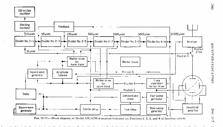
9100 kc/see

oscillator

Blockingoscillator

10psec

Divider No, 1<5

10 usec

----1 ‘eedback~I J

50ysec

. Dwider No. 2+2 Dlvlder No. 5-5 * Divider NO 6+4 *

4

I IMarkermixer

I

for +- - ,, !f

El

Marker m,xerlower trace

Squarewave

If

Amplltudegenerator balance

+ } ::;!; f +p~=posltlOn 5~

Delay

!~ _D’ff~~a’Or =

Square-wave

r 1--”

ILCoarse delay

generator Fine delay

n:

Slow-sweepgenerator

w

F‘0,000psec

Receiver

Pos[tlon

\

2,3,6

Position 5

&

//

//

/ E

r

--EIE1FIG. 11.17 .—B1ock diagram of Model AN/APN.9 receiver-i ndirator on Pusitions 2, 3, 5, and 6 of function switch.

4

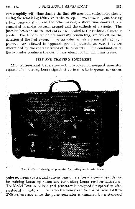
SEC. 118] PULSE-SIGNAL GENERA TORS 381

varies rapidly with time during the first 100 psec and varies more slowlyduring the remaining 1300 psec of the sweep. Two networks, one havinga long time constant and the other having a short time constant, areconnected in series between ground and the cathode of a triode. Thejunction between the two networks is connected to the cathode of anothertriode. The triodes, which are normally conducting, are cut off for theduration of the fast sweep. The cathodes, which are normally at highpotential, are allowed to approach ground potential at rates that aredetermined by the characteristics of the networks. The combination ofthe two rates produces the desired waveform for the nonlinear traces.

TEST AND TRAINING EQUIPMENT

11-8. Pulse-signal Generators.—.L low--power pulse-signal generator

capable of simulating Loran signals of various radio frequencies, various

FIG. 11.1 S.—Pulse-signal generator for testing receiver-indicator.

pulse recurrence rates, and various time differences is a convenient devicefor training Loran operators and for testing Loran receiver-indicators.The Model I-204-A pulse-signal generator is designed for operation withshipboard indicators. The radio frequency can be varied from 1700 to2000 kc/see; and since the pulse generator is triggered by a standard

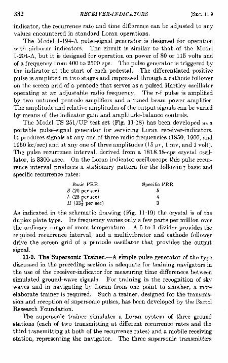
382 RECEIVER-INDICATORS [SEC. 119

indicator, the recurrence rate and time difference can be adjusted to any

values encountered in standw-d Loran operations.The Model I-194-A pulse-signal generator is designed for operation

with airborne indicators. The circuit is similar to that of the Model

1-204-A, but it isdesigned foroperation on powerof 800r 115 volts andof a frequency from 400 to 2500 cps. The pulse generator is triggered bythe indicator at the start of each pedestal. The differentiated positivepulse is amplified in two stages and impressed through a cathode followeron the screen grid of a pentode that serves as a pulsed Hartley oscillatoroperating at an adjustable radio frequency. The r-f pulse is amplifiedby two untuned pentode amplifiers and a tuned beam power amplifier.The amplitude and relative amplitudes of the output signals can be variedby means of the indicator gain and amplitude-balance controls.

The Model TS 251/UP test set (Fig. 11.18) has been developed as aportable pulse-signal generator for servicing Loran receiver-indicators.It produces signals at any one of three radio frequencies (1850, 1900, and1950 kc/see) and at any one of three amplitudes (15 AW,1 mv, and 1 volt).The pulse recurrence interval, derived from a 1818. 18-cps crystal oscil-lator, is 3300 ysec. On the Loran indicator oscilloscope this pulse recur-rence interval produces a stationary pattern for the followin~ basic andspecific recurrence rates:

Basic PRR Specific PRRS (20 per see) 5L (25 per see) 4H (33* per see) 3

As indicated in the schematic drawing (Fig. 11.19) the crystal is of theduplex plate type. Its frequency varies only a few parts per million overthe ordinary range of room temperature. A 6 to 1 divider provides therequired recurrence interval, and a multivibrator and cathode followerdrive the screen grid of a pentode oscillator that provides the outputsignal.

11.9. The Supersonic Trainer.-A simple pulse generator of the typediscussed in the preceding section is adequate for training navigators inthe use of the receiver-indicator for measuring time differences betweensimulated ground-wave signals. For training in the recognition of skywaves and in navigating by Loran from one point to another, a moreelaborate trainer is required. Such a trainer, designed for the transmis-sion and reception of supersonic pulses, has been developed by the BartolResearch Foundation.

The supersonic trainer simulates a Loran system of three groundstations (each of two transmitting at different recurrence rates and thethird t~ansmitting at both of the recurrence rates) and a mobile receivingstation, representing the navigator. The three supersonic transmitters

. — —

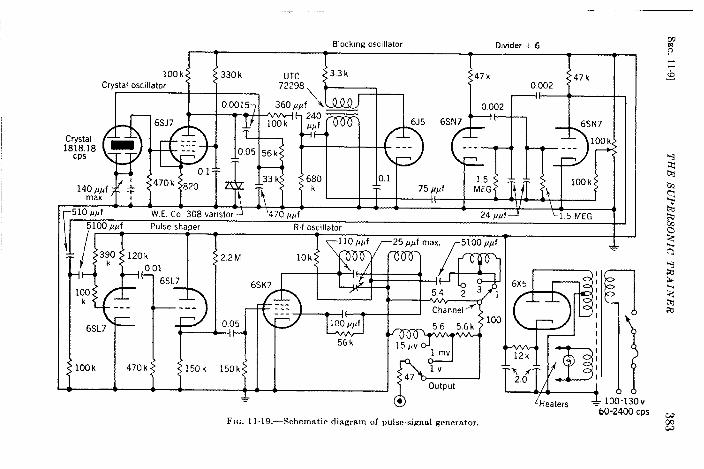
Blocklng oscillator D!~der + 6

I T T T T

t

]50k 150k

A wFr~. 11.19,—Schematic diagram of pulse-signal generator.

—

!ii?16X5

12k

B

I

>,.<

Heaters 100-I3OV‘60-2400 CPS

384 RECEIVER-INDICATORS [SEC. 119

are set up on a flat table on which a moving crab, whose motion maybecontrolled by the instructor or by the navigator, carries the receiver, apiezoelectric crystal transducer. The receiving transducer transformsthe supersonic (200-kc/see) pulse signals to pulses of electrical energywhich are converted to r-f (1950-kc/see) signals and are amplified andradiated as electromagnetic energy. By means of a standard receiver-indicator the navigator receives the radiated energy and measures thetime differences between the signals. A number of navigators, each

equipped with a receiver-indicator, can receive these signals at the sametime. Interference in the form of random noise, radar interference, c-wsignals, keyed c-w signals, or motor interference can be introduced at will.

Supersonic signals propagated over the surface of the table simulateground-wave Loran signals. A ground-glass plate, upon which a latitude-Iongitude grid is drawn and upon which cross hairs are optically projectedfrom the transmitters and from the mobile receiver, is supported severalinches above the surface of the table. Reflections of the supersonicsignals from the glass surface simulate reflections of Loran signals fromthe E-layer of the ionosphere. No attempt is made to simulate reflectionsfrom the F-layer. Splitting of sky-wave signals, caused by interferencebetween sky waves that travel different paths and therefore reach the

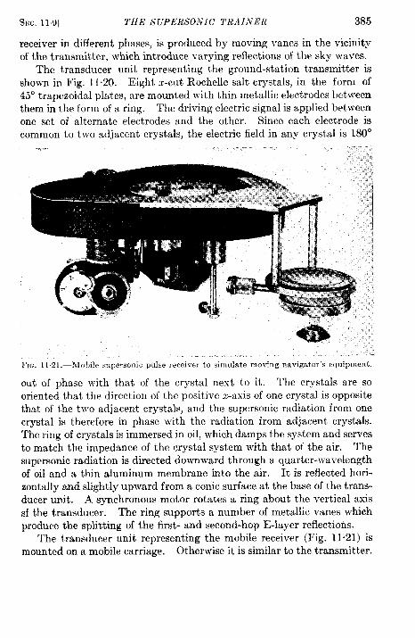
SEC, 119] THE SUPERSONIC TR.41NER 385

receiver in different phases, is produced by moving vanes in the vicinityof the transmitter, which introduce varying reflections of the sky waves.

The transducer unit representing the ground-station transmitter isshownin Fig. 11.20. Eight z-cut Rochelle salt crystals, in the form of45° trapezoidal plates, are mounted with thin metallic electrodes betweenthem in the form of a ring. The driving electric signal is applied betweenone set of alternate electrodes and the other. Since each electrode iscommon to two adj scent crystals, the electric field in any crystal is 180°

FIG. 11 .21. —Mohile supersonic pulse receiver tosimulate moving navigator’s equipment.

out of phase with that of the crystal next to it. The crystals are sooriented that the direction of the positive z-axis of one crystal is oppositethat of the two adjacent crystals, and the supersonic radiation from onetryst al is therefore in phase with the radiation from adj scent crystals.The ring of crystals is immersed in oil, which damps the system and servesto match the impedance of the crystal system with that of the air. Thesupersonic radiation is directed downward through a quarter-wavelengthof oil and a thin aluminum membrane into the air. It is reflected hori-zontally and slightly upward from a conic surface at the base of the trans-ducer unit. A synchronous motor rotates a ring about the vertical axissf the transducer. The ring supports a number of metallic vanes whichproduce the splitting of the first- and second-hop E-1ayer reflections.

The transducer unit representing the mobile receiver (Fig. 11.21) ismounted on a mobile carriage. Otherwise it is similar to the transmitter.

CHAPTER 12

SPECIAL TECHNIQUES AND MEASUREMENTS

BY G. H. MUSSELMAN

12.1. Receiver-design Notes. Introduction.—The circuits of I,oranreceivers in general use are similar in many respects to those in communi-cations types. They differ principally because of requirements for wide-band response and the need for a different amount of gain for alternatepulses. Aside from these restrictions and the modifications that theyimply, the usual design practices for good superheterodyne receivers canbe followed. The deviations from the normal will be discussed in some-what greater detail.

Most Loran receivers are provided with four identical r-f channelsthat are tuned to assigned frequency bands in the range of 1700 to 2000kc/see. A selector switch with positions numbered 1, 2, 3, and 4 allows achoice of 1950, 1850, 1900, and 1750 kc/see, respectively.

Early receivers ~’ere designed for high-impedance input with the idea

that a short antenna could be terminated directly at the receiver. This

arrangement proved to be undesirable, since better signal-to-noise ratios

are obtained with an antenna resonated at the operating frequency by a

loading coil, connected through a shielded coaxial cable to a receiver inputof 50 to 100 ohms. The antenna is thus kept farther from sources of

man-made noise.

One stage of amplification at radio frequency between the low-imped-

ance input and the mixer is mandatory to provide image rejection and a

signal well above the mixer noise. Successful receivers have been built

with only one tuned circuit between the plate of the r-f stage and thesignal grid of the mixer. This construction results in simplicity of

switching and some saving of space but lacks the improved bandpass

characteristics obtained with a double-tuned circuit that reduces cross

modulation and response at spurious frequencies. A remote cutoff tube

such as the type 6SK7 has been found superior in this stage to the type6AC7, despite the higher mutual conductance of the latter. Theinferior remote cutoff of the 6AC7 produces distortion of pulses of largeamplitude.

A gain of 30 or 40 per stage is reasonable; with a gain of about 7 for theinput transformer this gives a total gain of 210 to 280 from antenna ter-minal to the grid of the mixer.

386

SEC. 12.1] RECEIVER-DESIGN NOTES 387

A mixer stage employing a 6SA7 tube in either a Colpitts or Hartleyoscillator circuit designed to prevent frequency drift is customarily used.The oscillator frequency is higher than the signal frequency by the amountof the intermediate frequency. Optimum injection voltage should bealways used to secure the maximum conversion mutual conduct ante.A quartz crystal might be used in the oscillator circuit of each channel ifoperating extremes, such as temperature, required the additional expenseand slight inflexibilityy of a more stable circuit.

Intermediate frequencies used in different receivers have varied from500 to 1600 kc/see. The latter frequency was used in early receiversmainly because of easy procurement. The most used frequency has been1050 kc/see, although the second harmonic is close to the r-f value andmay produce undesirable effects with large signals. The 550-kc/secchannel does not suffer from this defect.

Double-tuned circuits, critically coupled with unit y-turns ratiobetween primary and secondary, have been used with various values oftuning capacitance, the lower capacitances allowing higher values ofdamping resistors for the same bandwidth. The response of each stageis designed to be down 1 db or less at 25 kc/see each side of the centerfrequency. By using a desirable type of tube such as the 6SK7, stagegains in the order of 30 to 40 are possible. Generally three stages areemployed follo}ved by a diode detector.

The problem of matching two pulses of generally unequal amplitudewas first solved by applying a voltage sauare wave to the cathode of thelast i-f amplifier and ~ary~g the g~in ~f this stage differentially. Thesquare wave is timed by the indicator circuits, the magnitude and relativepolarity being controlled by a potentiometer known as the gain- oramplitude-balance control. In later receivers the control is put on thefirst r-f tube to prevent overloading by strong signals. This typicalfeature of the Loran receiver is discussed in greater detail in Sec. 12.2.

A diode detector can be arranged in a conventional circuit to provideeither positive or negative swing corresponding to increased carrier.The polarity chosen depends both upon the number of phase reversalsencountered between detector and oscilloscope and upon which verticalplate of the oscilloscope is used for the video signal. It has been commonpractice to use the detector connected so that the output is negative andto follow this with one high-gain video stage. The video stage, usuallya 6AC7 with little bias and a 20,000-ohm plate load, is resistance-capacitance-coupled to that plate of the oscilloscope which gives anupward deflection for positive-going signals.

It is desirable to operate the detector at a carrier level of about 10volts peak. Receivers designed for operation at lower levels than thisshowed nonlinearity of the detector with small signals. Furthermore, if

388 SPECIAL TEG’HNIQ UES AND MEASUREMENTS [SEC. 12.1

the level at the detector is kept up, it is easier to design effective limitingcircuits that prevent large bursts of noise from overloading the videostage.

The main gain of the receiver is controlled by varying the cathodevoltage of all the remote cutoff tubes, bringing the cathodes to groundthrough a common gain potentiometer. Sufficient r-f filtering must beapplied at the individual cathodes to prevent undesired interstagecoupling through the control.

A high-pass filter section between the detector output and the inputto the video stage reduces certain types of interference (mainly that fromc-w stations) but should be normally switched out of the circuit, since itdegrades the desired pulses. The filter usually takes the form of a simple

resistance-capacitance network that cuts off at about 1000 cps. Nor-mallY, the Video response is uniform from 100 CpS to 50 kc/see.

The over-all bandwidth from the antenna terminal to the oscilloscope

should be 50 kc/see measured at points 6 db down from the maximum.

If, however, the r-f stage and the mixer stage are too broad, cross modula-

tion between Loran signals and broadcast or other strong signals in the

region of 2.0 hfc/sec will occur. Single-tuned parallel- or series-resonant

trap circuits tuned to the intermediate frequency can be inserted in the

antenna and r-f stages to reduce cross modulation. A parallel-tuned

circuit in series with the screen grid of the r-f amplifier tube is effective.

But because the screen is a nonlinear modulating element, when large

increments of screen voltage occur, a similar circuit placed in series with

the cathode of the same tube is even better.

General Requirements. Bandwidth .—Total receiver bandwidth should

be 50 kc/see at 6 db down and 150 kc/see at 60 db down. This over-all

measurement can be made by applying a 30 per cent modulated signal

from a calibrated signal generator to the antenna terminals. The output

is measured on the indicator oscilloscope or a d-c voltmeter connectedto the diode-load resistor. As the input frequency is varied by 5-kc/see

increments, the input level is adjusted to maintain constant output.

Plotting the required input level against frequency gives a selectivity

curve that contains most of the bandwidth information at a glance. A

second rough curve should be drawn for a greatly different input level; if

its shape departs widely from that of the first curve it indicates thepresence of regeneration in the i-f or r-f amplifier.

Image-rejection Ratio.—The receiver’s effectiveness in rejecting images,signals having a frequency numerically twice the intermediate frequencyplus the desired signal frequency, is expressed as the ratio between theimage, frequency signal applied to the input and the signal of the desiredfrequency that, when applied to the input, produces the same output.The ratio should be 60 db or better.

SEC. 12.1] RECEIVER-DESIGN NOTES 389

Spurious Response.—The ratio of undesired signal amplitude todesired signal amplitude giving the same output from the receiver ismeasured with one or more signal generators. All spurious responseshould be down 60 db or more.

I-f Rejection Ratio.—The i-f rejection ratio is the ratio between theamplitude of an i-f signal applied to the input of the receiver and theamplitude of the desired r-f signal that when applied to the input ofthe receiver, produces the same output. Although some Loran receiversdo not meet the figure, a ratio of 60 db is desirable,

Nm”seFactor.—The combination of r-f and i-f noise should not exceedthe equivalent of 0.5 pv. It can be measured by introducing an unmodu-lated signal from a calibrated signal generator to the antenna terminals.At full gain, the ratio between this signal voltage and the resulting d-cvoltage produced across the diode load resistor is determined. Thecalibrating voltage must be large compared with the residual-noise voltagebut small enough to ensure linear response from the diode. A second d-cvoltage reading is taken with the signal generator removed. (Thisvoltage is actually a combination of noise and diode emission. ) Theproduct of the second voltage and the ratio is the residual noise expressedas an equivalent voltage referred to the antenna circuit.

Maximum Sensitivity .—About l-in. peak-to-peak deflection on theindicator oscilloscope should be produced with a 5.O-pv signal (50 percent modulated at 400 cycles) applied to the input terminals. Muchgreater sensitivity than this is not necessary because atmospheric noiseat this frequency limits the usable over-all gain.

Sensitivity Range.—A receiver should be capable of reducing a200,000+v 50 per cent modulated signal applied at its input terminals toa 2-in. peak-to-peak deflection on the indicator oscilloscope, with thegain-balance control in the center position. The entire receiver shouldbe designed to amplify a signal of 600,000 pv linearly, even though itproduces more deflection than can be accommodated on the face of theindicator oscilloscope. If an iron-core choke is used as plate load forthe video stage, for the same plate-supply voltage considerably moreswing without overloading is possible than with resistance load. The fre-quency characteristic can be improved by introducing negative feedback.Several of the present receivers overload with a signal giving a little above3-in. deflection.

Gain-balance Range.—The amplitude- or gain-balance circuit shouldhave a maximum range of 1000 times with no more than 1 psec of intro-duced error. This range should allow a maximum signal of about 2.ovolts rms to be matched with one of 2000 ~v rms. Thus, a receiverembodying the specified sensitivity range should be capable of operatinganywhere in the service area and within 10 miles of one station, assuming

390 SPECIAL TECHNIQUES AND MEASUREMENTS [SEC. 122

an antenna system of about 5 meters effective height for the receiver anda radiated power of 100 kw for the transmitters.

This measurement must be made with a special generator capable ofemitting pulses similar to those of the Loran transmitters. The equip-

ment has a calibrated attenuator; and, although the recurrence rate is notcritical, it should have such a value that at least one pulse per trace isvisible when the output is applied to a Loran receiver. The timing ofthis generator should be locked in with the Loran indicator associatedwith the receiver under test. A reliable differential-gain system with nophase error incorporated in such equipment would enhance its value.If, instead, a standard attenuator is used, it is desirable to operate thesignal generator so that there is one pulse emitted per 40,000 psec. Asthe signal amplitude from the generator is varied, the range of the receiveramplitude-balance circuit can be determined from the amount of changeof the balance control required to maintain the pulse at constant heighton the indicator oscilloscope. The shape of the pulse is traced on thescreen with a crayon to facilitate the test. In checking the phase errorin the receiver, the signal generator should be locked to the indicatorrecurrence rate so that there is no drift of the pulse on the indicator screen.As the attenuator and gain-balance controls are varied over the extremerange, any shifting of the pulse in phase will be immediately evident.

Although the above specifications seem desirable in the light ofexperience consistent with present -day standards for Loran, it should benoted that many receivers in current use vary widely from these standards.

12.2. Differential-gain Principles. -Most pulse systems dependentirely on fast-rising pulses in order to achieve precision. The limita-tions imposed upon pulse shape through the use of medium radio fre-quencies for Loran service require a superposition technique to attain thedegree of precision necessary. Because each signal of a pair is usuallyreceived at a different amplitude, the time difference between two seriesof recurrent pulses is most accurately determined by amplifying eachseries by a proportionate amount; and thus when the two pulses areviewed on the oscilloscope trace, they are of equal amplitude.

Ground-station Requirement.-The average Loran ground-stationreceiving problem is one of matching two series of pulses that differ bybetween 20,000 and 200,000 to one in amplitude depending on stationand system layout. The problem is still more complex because thelarger of these two series of pulses (the local signal) has an amplitude ofseveral hundred peak volts.

The present method accomplishes the desired result in two steps. Anamplifier with negligible delay time passes the small remote signal but isbiased to cutoff during the local-signal time, The desired amount oflocal signal is paralleled with the inactive amplifier output to the receiver

SEC. 12.2] DIFFERENTIAL-GAIN PRINCIPLES 391

input. The timing of the biased-off interval is controlled by the timerthat also triggers the local transmitter. Leakage through the attenuatingamplifier is negligible in the biased-off condition compared with thesignal fed around by the resistance-attenuator network. It is desirableto have an even number of tubes in the amplifier so that a 180° phasedifference is not encountered between the signal from the amplifier andthat from the resistance network. This is particularly true when thecycle-matching system is used in the receiver.

The delay time through the biased amplifier is held to a low value byusing resistance-capacitance coupling between stages, with a plate-loadresistance small in comparison with the total shunt capacitance and theseries coupling capacitors large so that their reactance is small comparedwith the grid resistors.

The signal leakage through the biased amplifier in the off condition istheoretically a function of the ratio of plate-load resistance to the grid-plate capacitive reactance. In practice, it is almost impossible to achieveas low a degree of leakage, because couplings from input to output of theamplifier by way of chassis currents and stray capacitances determinethe lower limit. Vacuum-tube heater leads and plate-supply and biasleads must be equipped with adequate filter networks. It is possible toincrease the over-all ratio by adding more stages, which increases the gainduring the remote signal time without greatly increasing the leakageduring the local signal time. The transmission band of the amplifiermust, however, be kept extremely wide.

Navigator’s Equipment.-The difference in signal amplitude at thenavigator’s receiver depends on the location of the equipment with respectto the stations being received and can vary from zero when the locationis equidistant from the stations to a large number when the location isclose to one of the stations. The extreme ratios encountered in the opera-tion of ground-station equipment need not be considered in the designof mobile receivers. A large percentage of the service area can beutilized with a receiver capable of handling a ratio of 30/1, and all of theoriginal Loran receivers were so designed. Current practice tends towarda 1000/1 ratio, which includes more of the service area close to the stations.

The receiver must equalize the amplitude of pulses seen on a cathode-ray tube without adding any appreciable clifferential delay. In standard2.O-Mc/sec operation, circuits are designed so that no more than 1 psecof error is introduced by the gain-balance circuit at its extreme range.In general, a variable-~ pentode tube is used in the i-f or r-f amplifierchannel, the bias of which is controlled by a potentiometer to apply asquare wave of variable polarity and variable amplitude. The sourceof the square wave is the Eccles-Jordan circuit in the indicator, and thusthe gain of the receiver can be reduced during either the period of the

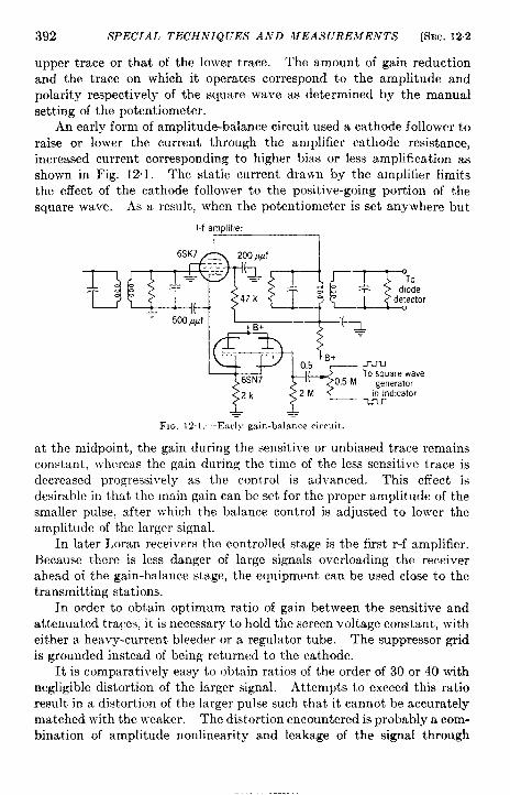
392 SPECIAL TECHNIQUES AND MEASUREMENTS [SEC. 12.2

upper trace or that of the lower trace. The amount of gain reduction

and the trace on which it operates correspond to the amplitude and

polarity respectively of the square wave as determined by the manualsetting of the potentiometer.

An early form of amplitude-balance circuit used a cathode follower toraise or lower the current through the amplifier cathode resistance,increased current corresponding to higher bias or less amplification asshown in Fig. 12.1. The static current drawn by the amplifier limitsthe effect of the cathode follower to the positive-going portion of thesquare wave. As a result, when the potentiometer is set anywhere but

l-f amplifler

16SK7

.500 ,u#f

~B+

in ind!cator

& &

FIG. 12.1.—Early gain-balance circuit.

at the midpoint, the gain during the sensitive or unbiased trace remains

constant, whereas the gain during the time of the less sensitive trace is

decreased progressively as the control is advanced. This effect is

desirable in that the main gain can be set for the proper amplitude of the

smaller pulse, after which the balance control is adjusted to lower the

amplitude of the larger signal.

In later I,oran receivers the controlled stage is the first r-f amplifier.

Because there is less danger of large signals overloading the receiver

ahead of the gain-balance stage, the equipment can be used close to the

transmitting stations.

In order to obtain optimum ratio of gain between the sensitive and

attenuated traces, it is necessary to hold the screen voltage constant, with

either a heavy-current bleeder or a regulator tube. The suppressor grid

is grounded instead of being returned to the cathode.

It is comparatively easy to obtain ratios of the order of 30 or 40 with

negligible distortion of the larger signal. Attempts to exceed this ratio

result in a distortion of the larger pulse such that it cannot be accurately

matched with the weaker. The distortion encountered is probably a com-

bination of amplitude nonlinearity and leakage of the signal through

SEC. 12.2] DIFFERENTIAL-GAIN PRINCIPLES 393

stray capacitances around the amplifier tube. Ratios in the order of100/ 1 have been accomplished by taking extreme care in circuit layout.For larger ratios it seems imperative to cascade two controlled amplifiers.

A system using two amplitude-balance stages separated by a con-ventional amplifier stage has been used in the portable cycle-matchingreceivers. Here each controlled stage consists of two cathode followersillustrated in Fig. 12.2. One tube, for example, is on by virtue of itsplate voltage being at about 200 volts during the upper-trace time,

J2-.u“

900 kR.f 6SN7

‘Mr =1 ---

500

From cathode

r F:

follower drivenby square wave

25#h 25&h generator m1000 1000 Indicator

d b2%ph 25fih-

d h Conventional=Cml 500 = pentode amphfier

00 k0.001

y ~’ P

-—.-—. -—.

Ii”

~1100 k 1~ k

— — —A;plitu~ebalancecontrol lSk .

—

FIG. 12.2.—Dual cathode-follower gain-balance circuit,

whereas the other tube is off owing to the fact that its plate voltage is onlyslightly positive. During the period of the lower trace, the operatingconditions of the tubes are interchanged so that a different tube is con-ducting for the duration of each trace. The Eccles-Jordan circuitprovides this timing, and each tube experiences the same operating volt-ages regardless of the degree of amplitude balance desired. The differ-ence in gain is obtained by varying the input signal applied to each tubeby means of a potentiometer and resistance network. Using resistorsand a potentiometer of about 500 and 1000 ohms respectively, it is possibleto obtain ratios of about 30 per stage with little distorting of the pulses.It is important that the grid-to-cathode capacitive reactance of eachtube be small compared with the effective resistance between cathodeand ground. When these values begin to approach equality, the pulseat the cathode becomes the resultant of that from the capacitive path andthe true pulse generated by the tube current through the cathode resistor.It is also important that the potentiometer resistance be small comparedwith the wiring and other shunt-capacitive reactance to avoid phase

394 SPECIAL TECHNIQUES AND MEASUREMENTS [SEC. 122

shift between the signal voltages applied to the two grids, resulting in thecreation of differential delay for large ratios.

The 180-kc/sec frequency at which cycle-matching receivers are usedis well suited for this type of gain-balance circuit because the reactanceare high enough to allow reasonable values for the potentiometer andresistance network. Since both the input and output of the amplitude-balance stage are low-impedance terminations, series-resonant circuitsare employed, the inductors and capacitors of which have such valuesthat the terminations of the stage serve as the damping components toprovide sufficient bandwidth.

The corresponding potentiometers in the two amplitude-balancestages are operated from common shafts. Radio-frequency filtering isemployed in the plate circuits of the cathode followers to prevent thesignal leakage between stages. A maximum range of 1000 to 1 is avail-able with less than 1 ~sec of introduced differential error, using the firststage in the receiver as an amplitude-balance stage.

All efforts toward perfecting amplitude-balance techniques have beenrestricted to the current use of Loran which requires matching only twopulses at a time. It may be desirable in an improved system to employ amaster and two easily identified slaves at the same recurrence rate, thethree matched simultaneously to provide the navigator with a fix fromone operation rather than two as now. This development would neces-sitate a three-trace indicator and a gain-balance circuit capable of hand-ling three different amplitudes instead of two, For this application, thevariable-p pentode controlled stage is more flexible than the cathode-follower type.

Some thought has been given to a receiver that would have automaticgain control for the pulses on the pedestals. Any simple refinement ofthe AVC principle seems doomed, because a large pulse would arriveat the oscilloscope electrodes before the gain of previous r-f amplifierscould be decreased. A rather elaborate modification would enable asampling network to measure, for example, the pulse on the A-pedestal,generate a bias sufficient to reduce the gain of a controlled stage by theproper amount, and store this bias until just before the A-pedestalappeared, before applying the bias to the controlled stage.

By this method each individual pulse on the A-pedestal would besampled, and the voltage created from it would control the gain of thenext individual pulse. For three pedestals it would require sampling eachsignal and storing the appropriate bias in three separate circuits, togetherwith a switching system, to apply the bias to the controlled tube at theproper time.

Another system would amplify all signals in several stages and thensample them for amplitude. A long delay line might be used to retard

SEC. 12.3] PULSE-SIGNAL GENERA TOR 395

the pulse appreciably so that the gain of succeeding stages could becontrolled and brought to the proper sensitivity by the time the pulseemerged from the delay line into the succeeding stages. It would, how-ever, require a line of approximately 100-psec minimum delay to providesufficient time for the controlled stage to reach equilibrium before apply-ing the actual pulse signal. Such a line would be prohibitive in size ifcomposed of ordinary lumped constants. It might be entirely possibleto construct an acoustic line employing supersonic frequencies for thispurpose. The design of the sampling voltmeter capable of handling thenecessary ratios is also interesting to contemplate.

The pressure of wartime Loran developments did not permit the expen-diture of etfort on operational refinements, but current progress in thisdirection is important, particularly since the use of automatic receiversfor automatic pilotage of various sorts hinges to a great extent on a simplebut foolproof automatic gain-balance system.

12.3. Pulse-signal Generator. General Description.—For the LowFrequency project a signal generator was built that proved to be exceed-ingly useful for general receiver and attenuator testing. The devicegenerates 180-kc/sec pulses of tbe same shape as those emanating fromthe Loran transmitters operating at that frequency, although the shapecan be varied somewhat from normal to suit individual test requirements.A crystal oscillator is used as the primary timing source, with a series ofblocking-oscillator dividers and one multivibrator-type divider to countdown to the desired recurrence rate. The nulse recurrence rate is 40, 50,,.or 66: pps, depending on a potentiometer adjustment in the last timingstage, which can divide by 10, 8, or 6.

The r-f pulse is generated by a Hartley LG oscillator circuit, which isscreen-grid-pulsed by the timer and shaping circuits. The radio fre-quency is adjustable over a range of about 10 kc/see each side of 180kc/see by means of a tuning capacitor controlled from the front panel.

The output amplitude of the pulses can be varied from 1 pv to 1 volt.A peak vacuum-tube voltmeter reads the input level to an attenuator;and when the level is properly set according to the meter, the outputamplitude is read directly from the attenuator and a calibrated poten-tiometer. Accuracy of calibration is good to about 10 per cent for longperiods of time.

Timer Circuit.—A triode oscillator controlled by a 100-kc/sec crystaldrives the counter chain. The first stage, dividing by 2, is a blocking-

oscillator divider with the time-constant circuit in the cathode, since itwas found that the cathode current is less affected by changes in filamentvoltage than is the grid current. The next three dividers are of the sametype, except that each divides by 5. The last divider stage is a cross-coupled multivibrator that favors even counts. The count can be

396 SPECIAL TECIINIQ iYES AND MEASUREMENTS [SEC. 124

adjusted for 6, 8, or 10 by varying the bias voltage applied to the controlgrids. If the d-c voltage is near ground potential, the count is long anddecreases as the voltage is made more positive. The output of this stageis essentially a square wave, but during the decreasing voltage time thereis sufficient undershoot so that a biased cathode follower is used to elimin-ate it. The output of the cathode follower is a clean square wave. Twoadditional tubes are used to shape and amplify the pulsing pip, and acathode follower raises the screen grid of the 61”6 oscillator tube to severalhundred volts during the pulse time. The cathode of the oscillator isheld at a sufficiently positive voltage to cut the tube off at all other times.

Radio-frequency energy is taken from the oscillator by means of asmall link coupled to the plate tank and fed through a concentric line toan L-pad. It is important that any setting of the pad present a constantresistance to the line so that there is no effect on the frequency of theoscillator, The output of the L-pad is connected to the vacuum-tubevoltmeter and to the calibrated potentiometer.

The vacuum-tube voltmeter consists of a diode rectifier with a timeconstant that is long compared with the period between successive pulses.

A d-c amplifier follows the diode and dri~-es a O- to 200-pa d-c meterused only as a reference indicator. The equipment is calibrated by com-paring the pulse (peak) output with the C-JVoutput of a htandard 180-kc/sec source using an oscilloscope as the indicator. N-ith the GeneralRadio attenuator dials set to the value of the knowm calibrating voltagethe carrier-set control (I.-pad) is adjusted until the two outputs are thesame in peak amplitude. The meter reading under these conditions isused for the standard oscillator output setting.

A selector switch and inspection jack permit checking the operationof each divider stage with a small oscilloscope. Each divider is providedwith an adjustable coupling capacitor to vary the count by one or moresteps.

The 10&kc/sec oscillator has a frequency adjustment in the form of avariable capacitor across the crystal to permit slight changes so that thepulse signal can be stopped on the traces of the indicator associated withthe receiver under test.

12.4. Pulse-bandwidth Measurements.—The action of tuned circuitson the shaping of pulses has been a subject of particl~lar interest in theLoran development. 31(~st other systems base their accuracy on theprinciple of using fast-rising pulses, so that a comparatively large per-centage of shaping can be tolerated. Bandwidth requircrncnts for suchpulses are easily satisfied in the microlv:l~-c region. .kt medium andparticularly at low radio frequencies the b:mdiri({th is appreciable com-pared with the carrier frequency, and the (lse (i slow-rising pukes ismandatory. In order to realize adequate precision at these frequencies

SEC. 125] SPECTRUM MEASC7REMENTS 397

it is necessary to match two pulses closely by brirqgingthem both to thesame amplitude and to superimpose them. The accuracy of measure-ment obtainable depends to a great extent on the shape of the pulses.

A square-wave-pulsed 180-kc/sec oscillator, triggered by a Loranindicator, was built as a part of the experimental program summarizedbelow. The pulse rises to full amplitude in two cycles, remains flat for150 psec, and then falls in several cycles. ~ cathode-follower type ofpulser applied across the oscillator tank coil starts the oscillator at almostfull amplitude, provided the static current drawn by the cathode followerthrough the inductance is carefully adjusted.

The output of the oscillator is taken through a cathode follower toobtain a low-impedance output. A wideband receiver (80 kc/see at 3 dbdown, 95 kc/see at 6 db down) operates into a conventional indicatorwith cathode-ray tube.

With the square-wave 180-kc/sec signal applied to the test receiver,the pulse rises in about 15 psec to 95 per cent of full amplitude. This iswithin 16.7 per cent of the calculated value of 12.5 ~sec which is givenby the reciprocal of the bandwidth (T = 1/80,000) at the 3-db points.A slight error in measuring the bandwidth or a small error in reading therise time of the pulse can account for the large apparent discrepancy.When a 20-kc/sec-wide circuit is placed between the generator and thereceiver, the pulse rises in 55 ~sec or within 9.1 per cent of the calculatedvalue. A 12-kc/sec-wide circuit produces a pulse that rises in 80 psec, ‘within 4 per cent of the calculated value.

Other experiments have be~n carried out, shaping the pulse from thegenerator so that its rise time is 65 ~sec. When this signal is applied tovarious tuned circuits, the resulting final pulse rise time may be expressedas follows: final rise time (in seconds) = /tz + (1/BW)’, in which t isthe rise time of the generator pulse in seconds and BW is the bandwidthof the receiver at the 3-db points in cycles.

1205. Spectrum Measurements. Field EqwipnwnL-Measurementshave been made of the distribution of energy with respect to frequency ofLoran transmissions at both 2 Me/see and 180 kc/see. Developmentwork associated with improving transmitting-antenna coupling systemsor limiting the width of sideband radiation requires a measuring setuplocated several miles from the antenna to indicate when progress is beingmade.

A h-ational HRO receiver with a General Radio ladder attenuator(identical with that used in the Model 605-B signal generator) connectedbetween the antenna and receiver served satisfactorily. The receiverwas operated with the selectivity controls set for narrow-band operation.Under these conditions the bandwidth is about 2 kc/see. The connectionbetween the attenuator and the input to the receiver must be well shielded,

398 SPECIAL TECHNIQUES AND MEASUREMENTS [SEC. 126

and the attenuator calibration must be checked with a reliable signalgenerator applied to the input of the attenuator before measurementsare made.

The audio output of the receiver is connected to the vertical plate ofthe oscilloscope in a Loran indicator. 4

The nonlinear relationship between input and audio output for pulseemission in the receiver iq such that it must be used at constant input.The voltage ratios between the various frequencies can be read from thecalibrated attenuator that is adjusted for constant output to the oscillo-scope. Readings are recorded against frequency and can later beconverted into decibels and then plotted to show the complete energy-frequency distribution curve.

It is imperative that the gain of the receiver be set so that the referenceoutput agreed upon does not overload any of the receiver circuits. usu-ally it requires a trial of several locations to determine a proper distancefrom the transmitting antenna that gives a high signal at the center fre-

.I

quency and still ensures reception from the antenna alone, well out of theinduction field.

12.6. Cycle-matching Receivers. Pulsed Injection. —JVith the devel-

opment of LOW Frequency Loran at 180 kc/see it became apparent that

matching longer pulses to the same accuracy as in the 2. O-Nlc/sec system

would be difficult in the presence of a finite signal-to-noise ratio. Accord-

ingly, the development of receivers for mat thing r-f cycles instead of the drectified-pulse envelopes was undertaken. The cycle-matching technique ‘had been considered almost from the beginning of Loran, but only the LF

system with its increased range but decreased accuracy of matching ~

provided sufficient incentive to investigate the possibilities of cycle-rnatching. The system may be considered one in which phase is meas-

ured, the cycles being shaped into a pulse for purposes of identification.The use of a tuned r-f receiver with no detector would necessitate a

gain of about 4 million, in order to amplify an input signal of 10 PV rms

to 120 volts peak to peak at the vertical plate of the oscilloscope. The

anticipated instability owing to so great a gain at one frequency was

discouraging.The present experimental receivers are the superheterodyne type.

The input signals are amplified through t~~o 180-kc/sec r-f amplifiers and

then heterodyned to 50 kc/see by a frequencvv of 130 kc/scc. The result-

ing pulses of 50 kc/see are amplified to about 200 volts peak to peak and

applied to the vertical plate of the oscilloscope in a modified ?Jodel DAS-1indicator. They are provided with l-psec markers and a superfine delay

adjustment. The stability is ample even with no particular shielding

precautions. A diode detector can be switched IN for making approxi-

mate measurements. After the pulse envelopes have been matched, the

SEC. 12.6] CYCLE-MATCH1!VG RECEIVERS 399

detector is switched OUT and the precision match of cycles is made.When the proper cycle is chosen, it is possible to match and read the timedifference with an error not greater than 0.1 psec.

The i-f cycles are phase sensitive to both the input signal and theheterodyning frequency. If the normal type of free-running oscillator

were used for the heterodyning source, the i-f cycles would appear in

constantly changing phase of a random nature related to the het erodyning

frequency. In order to overcome this difficulty, the local oscillator is

pulsed at the beginning of the fast-sweep trace, and thus there is no oscil-

lation except during the trace time. This results in a heterodyning source

that has no phase differential between upper and lower fast traces; and so

when two pulses are matched exactly, they each experience the same

effects from the heterodyne and, as a result, any differential effects are

canceled out. Because the oscillator is triggered by the fast trace, the

delay setting has no effect on the converting system.

The scheme of starting the local oscillator at the beginning of the fast-

sweep trace has one annoying defect. The circuit that initiates the fast

trace is the pedestal generator in the indicator. This generator is nor-

mally triggered from the output of a mixer, which combines the output of

the A-delay and the fine B-delay multivibrators. When the local oscil-

lator is turned on, there is a large transient produced in the plate currentof the mixer in the receiver. This transient results from the sudden

application of heterodyning voltage. In order to keep this transient

from interfering with the received signal, the indicator is arranged so thatthe delay mixer starts the local oscillator and a multivibrator with a fixeddelay of about 1000 ~sec. When the pulse from this multivibratorcollapses, it triggers the pedestal generator. The fast-sweep trace occurs,therefore, about 1000 psec after the local oscillator has been started, andthe transient has had plenty of time to degenerate by the time the signalarrives. Care must be taken to ensure that there is no differential phasingeflect as a result of these linkages. In the experimental receivers a push-button switch is incorporated that transfers a portion of the heterodyningvoltage to the vertical plate of the oscilloscope. When the switch isoperated, the heterodyning voltage is plotted on a trace, and the delaycontrols can be adjusted while looking for any phase clifferential. Theover-all operation of the circuits is such that time-difference readingsaccurate to 0.1 psec are obtained. If greater precision were needed, somedifficulty might be experienced using this particular technique becauseof the tie between the delay mixer, the start of the local oscillator, andthe initiation of the fast trace.

The indicator has been further modified so that when the slow traceis used, the heterodyning voltage runs continuously; otherwise, therewould be no signals observed until they were coincident with the pedestals.

400 SPECIAL TECHNIQUES AND MEASUREMENTS [SEC. 126

To realize the full potentialities of this scheme it is necessary to controlthe phase of the cycles of the r-f pulse at the Loran transmitting stations.This control has been established using a cycle-matching receiver formonitoring at the slave station.

The greatest problem associated with cycle-matching at present isthat of determining which cycles of the respective pulses should bematched. The long slow rise of the leading edge (100 to 150 psec) makesidentification of the initial cycle difficult. A preliminary investigationindicates that the pulse must rise within 10 or 12 cycles to remove thisambiguity completely. The shorter the rise time the easier it is for thenavigator to pick the right cycle, but the bandwidth of the system isgreater. This feature affects receiver design in that more noise is acceptedand the stages must be designed for larger bandwidth with decreased gainper stage. Using an intermediate frequency of 50 kc/see puts a very realand rapidly approached limitation on the amount of bandwidth possible;and even with narrow band~vidths, there is not much Q left in thesecircuits. Fortunately, the detector need not be used for the precisionmeasurement.

It is noteworthy that when cycles are being matched, considerablygreater amounts of impulse noise can be tolerated than when usingrectification. This seems to be the result of using a truly linear receivingsystem. In any detector system for pulse reception, noise charges up thediode-charging capacitor that can be drained only as rapidly as the timeconstant employed permits. With large bursts of noise there is con-siderable bouncing of the oscilloscope traces which makes matchingdesired pulse envelopes difficult. This effect can be only partiallyeliminated \vith the best diode-limiting and restoring devices. (h theother hand, the cycle-matching system allows noise to appear in thetruly a-c sense, so that immediately after a large noise burst or impulsethe trace is back in its neutral position on the oscilloscope, ready to handlethe desired Loran pulse. If too large a burst occurs, the video stageoverloads, with the resultant degrading effect of blocking and filteringcapacitors changing charge. Even so, this effect occurs at much highernoise levels than can be tolerated with a rectifier system. The overload-ing can be minimized somewhat by incorporating a balanced diodelimiter \vithout capacitors in the stage preceding the video-amplifierstage. At the ground stations, where the delay is fixed and the operatorconcentrates on the leading edge of one CJ-CIC,large bursts of noise can betolerated at the same time accuracy of synchronism is held to 0.1 ,asec.

A few navigators’ receivers bl~ilt for cycle-matching are 12 kc/seewide at 6 db down. The sensitivity is such that 10 PV applied to theantenna terminals produces a 2-in. deflection on the oscilloscope. Thegain-balance circuit is capable of handling a differential ratio of 60 db

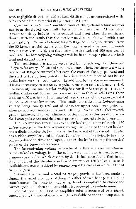
SEC. 12.6] CY(7LE-.I4ATCHIA’G RECEIVERS 401

with negligible distortion, and at least 40db can beaccomrnodate dwith-out exceeding a differential delay error of 0.1 Pscc.

Controlled lnj~ction.-.\m odifieclform of thecycle-matching receiverhas been developed specifically for ground-station use. At the slavestation the delay held is predetermined and fixed when the charts aredrawn, with the result that thereceiver need bemuehless ffexible thananavigator’s. When ahetcrodyning voltageof 130kc/sec dcri~-ed fromthe 50-kc/sec crystal oscillator in the timer is used at a timer (ground-station) receiver, any delays that are whole multiples of 100 psec can beheld, and the heterodyning voltages will be in the proper ph~se for bothlocal and distant pulses.

This relationship is simply visualized by considering that there are13 cycles for every 100 pscc of time; and hence whenever there is a wholenumber of 100-,usec intervals between the start of the top pedestal andthe start of the bottom pedestal, there is a whole number of 130-kc/seccycles bet ween these t~~-opoints. In addition to the above requirement,it is also necessary to use an even pulse recurrence rate, such as O, 2, 4, 6.The necessity for such a relationship is clear if it is recognized that thefeedback takes out 50 psec per trace per rate so that on odd rates, thereis an extra 50 psec in the total time betwren the start of the upper pedestaland the start of the lower one. This condition results in the heterodyningvoltage being exactly 180° out of phase for upper and lower pedestzdswhen an odd recurrence rate is used. It may pro~e upon further investi-gation, however, that the interlaced pattern of i-f cycles resulting whcuthe Loran pulses are matched may prove to be ncwptable in operation.

The receiver has two r-f stages at 180 kc, SCC,a nlixer tube ~rith 130kc/see injected as the heterodyning voltage, :Ln i-f amplifier at 50 kc see,and a diode detector that can be switched in or out of the circuit. It alsohas a video amplifier good to about 70 kc/see and of sufficiently low out-put impedance to drive the capacitance of the leads feeding the vertical

plates of the timer oscilloscopes.

The heterodyning voltage is produced within the receiver chassis.

Some 50-kc/sec voltage from the main crystal oscillator is used to excite

a sine-wave divider, which divides by 5. It has been found that in the

plate circuit of this divider a sufficient amount of 130-kc~sec current is

available and can be utilized by segregating it by means of a circuit tuned

to 130 kc/see.Between the first and second r-f stages, provision has been made to

change the selectivity by s~~-itching in either of two bandpass couplingtransformers. In operation, the wider band is employed to choose thecorrect cycle, and then the bandwidth is narrowed to exclude noise.

The cathode of the first r-f amplifier tube is connected to a high-Qtuned circuit. the inductance of which is variable so that the trap can be

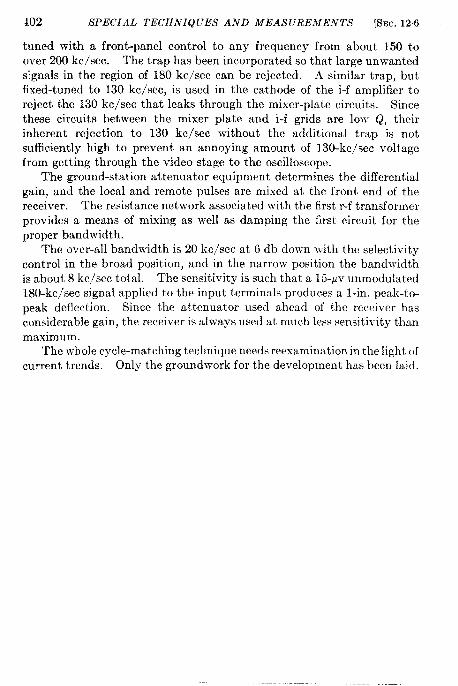
402 SPECIAL TECHNIQUES AND MEASUREMENTS [SEC. 126

tuned with a front-panel control to any frequency from about 150 toover 200kc/sec. Thetrap has been incorporated sothat large unwanteds~gnals in the region of 180 kc,/sec can be rejected. A similar trap, butfixed-tuned to 130 kc/see, is used in the cathode of the i-f amplifier toreject the 130 kc/see that leaks through the mixer-plate circuits. Sincethese circuits between the mixer plate and i-f grids are low Q, theirinherent rejection to 130 kc/see without the additional trap is notsufficient y high to prevent an annoying amount of 130-kc/sec voltagefrom getting through the video stage to the oscilloscope.

The ground-station attenuator equipment determines the differentialgain, and the local and remote pulses are mixed at the front end of thereceiver. The resistance network associated with the first r-f transformerprovides a means of mixing as well as damping the first circuit for theproper bandwidth.

The over-all bandwidth is 20 kc/see at 6 db down with the selectivityycontrol in the broad position, and in the narrow position the bandwidthis about 8 kc/see total. The sensitivity is such that a 15-w unmodulated180-kc/sec signal applied to the input terminals produces a l-in. peak-to-peak deflection. Since the attenuator used ahead of the receiver hasconsiderable gain, the receiver is always used at much less sensitivity thanmaximum.

The whole cycle-matching technique needs reexamination in the light ofcurrent trends. only the groundwork for the development has been laid.

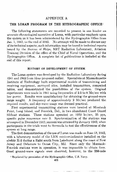
APPENDIX A

THE LORAN PROGWM IN THE HYDROGRAPHIC OFFICE’

The following statements are recorded to present in one binder anaccurate chronological narrative of Loran, with particular emphasis uponthe system as it has been administered by the Hydrographic Office fromJan. 1, 1943, to the end of 1945. No attempt will be made to discuss anyof its technical aspects; such information maybe found in technical reportsissued by the Bureau of Ships, MIT Radiation Laboratory, AviationTraining Division of the office of the Chief of Naval Operations, and theHydrographic Office. A complete list of publications is included at theend of this report.

HISTORY OF DEVELOPMENT OF SYSTEM

The Loran system was developed by the Radiation Laboratory during1941 and 1942 from ideas proposed earlier. Specialists at MassachusettsInstitute of Technology built experimental models of transmitting andreceiving equipment, surveyed sites, installed transmitters, computedtables, and demonstrated the possibilities of the system. Originalexperiments were made in 1941 using frequencies of 2.5 to 8 Me/see withlow power. Results were unsatisfactory for obtaining the ground-waverange sought. A frequency of approximately 2 Me/see produced therequired results, and sky-wave usage was deemed practical.

First experimental transmitting stations were located at MontaukPoint, Long Island, and Fenwick, Del., in two abandoned Coast Guardlifeboat stations. These stations operated on 1950 kc/see, 25 pps,specific pulse recurrence rate O. Synchronizat ion of the stations wasattempted in December 1941; success was attained b y January 1942, whenparticipants in the trials went to Bermuda to test the effectiveness of thesystem at long range.

The first demonstration of the use of Loran was made on June 13,1942,with a laboratory model of the LRN receiver-indicator installed on theairship K-2 during a flight south from Lakehurst along the coast of New,Jersey and Delaware to Ocean City, Md. Since only the Montauk-Fenwick stations were in operation, it was impossible to obtain fixes.Good ground-wave signals were observed, however, to the 250-mile

] Reprinted by permission of the Hydrographic Office, U.S. Navy.403

404 APPENDIX A

extremity of the trip. The procedure of homing on a Loran hyperbola

was used, and position-line accuracy of the system along the baseline was

verified.

On July 4, 1942, the first readings from a plane were made on a

laboratory receiver-indicator installed in a B-24 during a test flight from

Boston to Cape Sable, A’ova Scotia. Good signals ~vere received and

useful data obtained on signal range of stations .11 and F.

The first tests made aboard ship occurred on the CGC Manasguanduring a weather cruise off Newfoundland from June 17 to July 17, 1942.

Observations of both ground- and sky-wave signals during that period

indicated a total range of 1300 nautical miles and an overlap of ground

and sky coverage. The results were considered good enough to warrant

the expansion of the system and its recommendation to navigational

agencies.

Experimental service was extended by the construction of a slave

station at Baccaro, Nova Scotia, to operate with the double-pulsed master

at IMontauk Point on specific pulse recurrence rate 1, ancl the construction

of a second master at Dcming, X-ova Scotia, to operate \vith the slave at

Baccaro on specific pulse recurrence rate 2. These stations were con-

structed during the late summer and ~ventinto operation under the RoyalCanadian Navy on Ott. 1, 1942.

Preliminary tables for the three rates were computed at the RadiationLaboratory during August, September, and October 1942 and werereproduced by hectograph for temporary experimental use.

On Nov. 1, 1942, a test flight was made to Bermuda in a PBY for thepurpose of demonstrating the usc of Loran in obtaining fixes. Repre-sentatives of the Bureau of Aeronautics, Radiation Laboratory, ArmyAir Forces, and other interested activities ~vcre in the flight party. Thedemonstration v-as so successful that the observers ~rere convinced thatLoran could perform an important service in the war effort.

The Navy followed the development of the system with interestthrough the Office of Research and Inventions. The HydrographicOffice became involved because of the necessity for production of tablesand charts. On June 13, 1942, Cored. G. A. Patterson, USN (ret.),Officer in Charge of the Division of Research of the Hydrographic Office,and E. B. Collins, senior nautical scientist of the division, met withAdmiral Furer, Director of Research and In~-entions, to review progressof Loran. On July 29 a conference of all interested parties was held.Progress report given at this meeting included the following statements:Experimental stations at Montauk and Fenwick were in operation; theCanadians were building two stations in Nova Scotia (Baccaro andDeming) under the supervision of the Radiation Laboratory; sites had

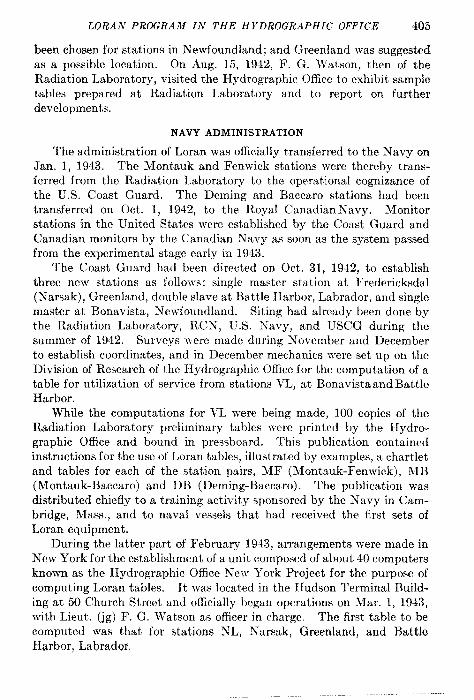
LORAN PROGRAM IN THE HYDROGRAPHIC OFFICE 405

been chosen for stations in Newfoundland; and Greenland was suggestedas a possible location. On Aug. 15, 1942, F. G. IJTatson, then of theRadiation Laboratory, visited the Hydrographic OffIce to exhibit sampletables prepared at Radiation Laboratory and to report on furtherdevelopments.

NAVY ADMINISTRATION

The administration of Loran was officially transferred to the Navy onJan. 1, 1943. The Montauk and Fenwick stations were thereby trans-ferred from the Radiation Laboratory to the operat~onal cognizance ofthe U.S. Coast Guard. The Deming and Baccaro stations had beentransferred on Oct. 1, 1942, to the Royal Canadian hTavy. Monitorstations in the United States were established by the Coast Guard andCanadian monitors by the Canadian Navy as soon as the system passedfrom the experimental stage early in 1943.

The Coast Guard had been directed on Oct. 31, 1942, to establishthree new stations as follows: single master station at Fredericksdal(Narsak), Greenland, double slave at Battle Harbor, Labrador, and singlemaster at Bonavista, A’ewfoundland. Siting had already been done bythe Radiation Laboratory, RCN, U.S. Navy, and USCG during thesummer of 1942. Surveys were made during NTovember and Decemberto establish coordinates, and in December mechanics were set up on theDivision of Research of the Hydrographic Office for the computation of atable for utilization of service from stations VL, at Bonavista and BattleHarbor.

While the computations for l“L were being made, 100 copies of theRadiation Laboratory preliminary tables were printed by the Hydro-graphic Office and bound in pressboard. This publication containedinstructions for the use of Loran tables, illustrated by examples, a chartletand tables for each of the station pairs, MF (~Montauk-Fenwick), MB(Montauk-Baccaro) and DB (Deming-13accaro). The publication wasdistributed chiefly to a training activity sponsored by the Navy in Cam-bridge, Mass., and to naval vessels that had received the first sets ofLoran equipment.

During the latter part of February 1943, arrangements were made inNew York for the establishment of a unit composed of about 40 computersknown as the Hydrographic Office N-ew York Project for the purpose ofcomputing Loran tables. It was located in the Hudson Terminal Build-ing at 50 Church Street and officially began operations on Mar. 1, 1943,with Lieut. (jg) F. G. Watson as officer in charge. The first table to becomputed was that for stations NTL) Narsak, Greenland, and BattleHarbor, Labrador.

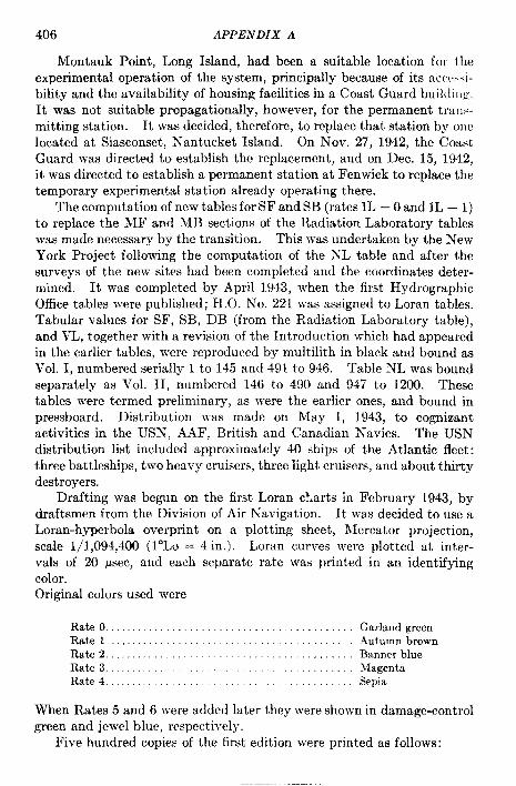
406 APPENDIX A

Montauk Point, Long Island, had been a suitable location for the

experimental operation of the system, principally because of its acct’.si-

bilit y and the availability y of housing facilities in a Coast Guard buil( IJ1)g.

It was not suitable propagationally, however, for the permanent tralls-mitting station. It~vasdecided, therefore, toreplace that station byo]lc

located at Siasconset, Nantucket Island. On Nov. 27, 1942, the Coast

Guard wasdirected toestablish the replacement, andon Dec. 15, 1942,

it was directed to establish a permanent station at Fenwick to replace the

temporary experimental station already operating there.

The computation of new tables for SF and SB (rates IL – O and IL – I)

to replace the MF and MB sections of the Radiation Laboratory tables

was made necessary by the transition. This was undertaken by the New

York Project following the computation of the iYL table and after the

surveys of the new sites had been completed and the coordinates deter-

mined. It was completed by April 1943, when the first H ydrographic

office tables were published; H.O. ATO. 221 was assigned to Loran tables.

Tabular values for SF, SB, DB (from the Radiation Laboratory table),

and VL, together with a revision of the Introduction which had appearedin the earlier tables, were reproduced by multilith in black and bound as

Vol. I, numbered serially 1 to 145 and 491 to 946. Table NL was bound

separately as Vol. 11, numbered 146 to 490 and 947 to 1200. These

tables were termed preliminary, as were the earlier ones, and bound in

pressboard. Distribution was made on May 1, 1943, to cognizant

activities in the USN’, AAF, British and Canadian Navies. The USN

distribution list included approximately 40 ships of the Atlantic fleet:

three battleships, two heavy cruisers, three light cruisers, and about thirty

destroyers.Drafting was begun on the first Loran c!.arts in February 1943, by

draftsmen from the Division of Air Navigation. It was decided to use a

Loran-hyperbola overprint on a plotting sheet, IMercator projection,

scale 1/1,094,400 (l”Lo = 4 in.). Loran curves were plotted at inter-

vals of 20 psec, and each separate rate was printed in an identifying

color.Original colors used were

Rate O. . . . . . . . . . . . . . . . . . . . . . . . . . . . . . . . . . . . . . . . . .. Garland greenRate . . . . . . . . . . . . . . . . . Autumn brownRate . . . . . . . . . . . . . . . . . . . . . . . . . . . . . . . . . . . . . . . . .. Banner blueRate . . . . . . . . . . . . . . . . . . . . . . . . . . . . . . . . ..hlagentaRate4 Sepia

When Rates 5 and 6 were added later they were shown in damage-controlgreen and jewel blue, respect ively.

Five hundred copies of the first edition were printed as follows:

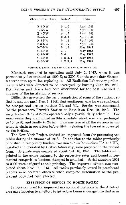
WRAN PROGRAM IN THE H YDROORAPHIC OFFICE 407

Short title of cha,rt

E-5-XWE-6NWE-7-XWF-4-X WF-5-NWF-6-N WF-7-iYWG-3-X WG-4N wG-5-NWG-O-NW

Rates*

o, 1, 20, 1, 20, 1, 22, 3, 40, 1, 20, 1, 20, 1, 23, 43, 41, 2, 3, 41, 2, 3, 4

Date

April 1943April 1943April 1943April 1943April 1943April 19$3May 1943May 1943May 1943May 1943klay 1943

* Rate O,SF; Rate 1, SB; Rate 2, DB; Rate 3, VL; Rate 4, NL.

Montauk remained in operation until July 1, 1943, when it waspermanently discontinued at 1800 Z; at 2200 Z on the same date Siascon-set went into operation replacing it. All Radiation Laboratory prelim-inary tables were directed to be destroyed by burning June 28, 1943.Both tables and charts had been distributed for the new rate well inadvance of the institution of service.

Difficulties prevented the early completion of some of the stations, sothat it was not until Dec. 1, 1943, that continuous service was confirmedfor navigational use on stations NL and VL. Service was announcedfor the permanent Fenwick Station on Rate O on Dec. 10, 1943. Theearly transmitting stations operated only a partial daily schedule. Forsome weeks they maintained an 8-hr schedule, which was later prolongedto 16, to 20, and finally to 24 hr. This was true of all the stations in theAtlantic chain in operation before 1944, including the two rates operatedby the British.

The New York Project devised an improved form for presenting thetables during the summer of 1943. In addition to the tables previouslypublished in temporary binders, two new tables for stations UA and UK,installed and operated by British Admiralty, were prepared in the revisedform. Originals were completed about Oct. 10, 1943. The tables wereprinted in the colors assigned to the respective rates and bound in per-manent composition binders, stamped in gold leaf. Serial numbers 1001to 2000 were assigned to this printing. The improved edition was com-pleted about Nov. 13, 1943. All tables previously issued in pressboardbinders were declared obsolete when complete distribution of the per-manent book had been eflected.

EXTENSION OF SERVICE TO NORTH PACIFIC

Imperative need for improved navigational methods in the Aleutianarea gave impetus to an effort to introduce Loran coverage into that area

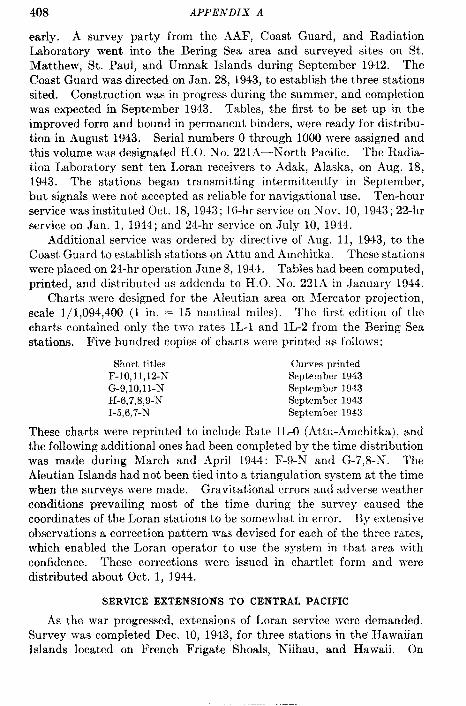
408 APPENDIX A

early. A survey party from the AAF, Coast Guard, and RadiationLaboratory went into the Bering Sea area and surveyed sites on St.Matthew, St. Paul, and Umnak Islands during September 1942. TheCoast Guard was directed on Jan. 28, 1943, to establish the three stationssited. Construction was in progress during the summer, and completionwas expected in September 1943. Tables, the first to be set up in theimproved form and bound in permanent binders, were ready for distribu-tion in August 1943. Serial numbers O through 1000 were assigned andthis volume was designated H.O. No. 221A—hTorth Pacific. The Radia-tion Laboratory sent ten Loran receivers to Adak, Alaska, on Aug. 18,1943. The stations began transmitting intermittently in September,but signals were not accepted as reliable for navigational use. Ten-hourservice was instituted Oct. 18, 1943; 16-hr service on hTov. 10, 1943; 22-hrservice on Jan. 1, 1944; and 24-hr service on July 10, 1944.

Additional service was ordered by directive of Aug. 11, 1943, to theCoast Guard to establish stations on Attu and Amchitka. These stationswere placed on 24-hr operation June 8, 194A. Tables had been computed,printed, and distributed as addenda to H.O. N’o. 221.k in January 1944.

Charts were designed for the Aleutian area on Mercator projection,scale 1/1,094,400 (1 in. = 15 nautical miles). The first edition of thecharts contained only the two rates IL-1 and lL-2 from the Bering Seastations. Five hundred copies of charts were printed as follows:

Short titlesF-10,11,12-NG-9,1 O,11-NH-6, 7, 8,9-NI-5,6,7-N

These charts were reprinted

Curves printedSeptember 1943September 1943September 1943September 1943

to include Rate 11,-0 (Attu-Amchitka), and

the following additional ones had been completed by the time distribution

was made during March and April 194zI: F-9-N and G-7,8-N. The

Aleutian Islands had not been tied into a triangulation system at the time

when the surveys were made. Gravitational errors and adverse weather

conditions prevailing most of the time during the survey caused the

coordinates of the Loran stations to be somewhat in error. By extensive

observations a correction pattern was devised for each of the three rates,

which enabled the Loran operator to use the system in that area with

confidence. These corrections were issued in chartlet form and were

distributed about Oct. 1, 1944.

SERVICE EXTENSIONS TO CENTRAL PACIFIC

As the war progressed, extensions of Loran service were demanded.

Survey was completed Dec. 10, 1943, for three stations in the Hawaiian

Islands located on French Frigate Shoals, Niihau, and Hawaii. On

LORAN PROGRAM IN THE H YDROORAPHIC OFFICE 409

Feb. 5, 1944, the Coast Guard was directed to establish three stations inthe Phoenix Islands on Baker, Gardner, and Atafu Islands. Surveys forstations in the Marshall Islands (Kwaj alein, Majuro, and Makin) weremade in February and March 1944. The Army Air Forces were author-ized on Feb. 10, 1944, to establish the Banda Sea chain, and coordinateswere furnished to the Hydrographer on Mar. 9, 1944.

Tables and charts were prepared for these stations during the springof 1944. A target date of July 1, 1944, was set for the completion ofVL-30 and VL-70 charts of the area. On Apr. 14 standard channeldesignations for the high and low channels were assigned. The methodof labeling Loran curves on charts was modified on the next printing toinclude the basic recurrence rate, the channel, and the specific rate inaddition to the T-value of the curve. For example, each curve containeda legend such as 2L0 or 1H-3 preceding the T-value on these and subse-quent charts. On earlier charts Loran curves had been labeled with theT-value preceded only by the specific recurrence rate.

Stations were completed for testing as follows:Niihau-Hawaii (Rate 2L-0) began testing July 11, 1944.Niihau-French Frigate (Rate 2L-1) began testing July 27, 1944.Majuro-Kwajalein (Rate 2L-2) began testing Sept. 28, 1944.Majur&Makin (Rate 2L-3) began testing Sept. 28, 1944.Gardner-Baker (Rate 2L-4) began testing Sept. 28, 1944.Gardner-Atafu (Rate 2L-5) began testing Sept. 28, 1944.Service was approved for navigation for the Hawaiian chain (Rates

2L-o and 2L-1) on Oct. 19, 1944, for the Phoenix chain (Rates 2L-4 and2L-5) on Nov. 21, 1944, and for the Marshall chain (Rates 2L-2 and 2L-3)on Dec. 1, 1944.

Tables, bound permanently, numbered 2001 through 3000, andidentified as H.O. No. 221B, Loran Tables, Central Pacific, were dis-tributed during July 1944, as were the following charts:

Chart No.

VL-30-30vL-3&31VIr3@42VL30-43VIr30-44VL-30-45VL-30-56VL-3057VL-30-58VL-30-70VL-30-71VRLF202

Rates

2L0, 1, 2, 32L-0, 12H-4, 52H-4, 5; 2L2, 32L-2, 32L0, 1, 2, 32H-4, 52H-4, 52L2, 3, 4, 52H-4, 52H-4, 52L-0, 1, 2, 3, 4, 5

Curves printed

June 1944May 1944June 1944June 1944June 1944June 1944May 1944May 1944June 1944May 1944May 1944June 1944

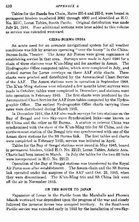
410 APPENDIX A

Tables for the Banda Sea Chain, Rates 2H-4 and 2H-5, were bound inpermanent binders numbered 3001 through 4000 and identified as H.O.No. 221C, Loran Tables, South Pacific. Original distribution was madeJuly 24, 1944. Four additional sections were later added to this volumeas service was extended westward.

CHINA-BURMA-INDIA

An acute need for an accurate navigational system for all weatherconditions was felt by aviators operating “over the hump” in the China-Burma-India Theater. The Army Air Forces were given cognizance ofestablishing service in that area. Surveys were made in April 1944 for achain of three stations near K’un-Ming and for another in Assam. TheHydrographic Office computed tables, which were completed in July, andplotted curves for Loran overlays on three AAF strip charts. Thesecharts were printed and distributed by the Aeronautical Chart Serviceof the AAF. The Assam stations were in operation in September 1944.The K’un-Ming stations were relocated a few months later; surveys weremade in October; tables were completed in December; and stations wentinto operation in February 1945. The first charts were produced by theAeronautical Chart Service for AAF from tables computed by the Hydro-graphic Office. The earliest Hydrographic Office charts carrying theserates were distributed during March 1945.

In December 1944, the AAF also made surveys for two stations on theBay of Bengal and two Sky-wave Synchronized links—one known asSS China and the other as SS Burma. A station in interior China wassynchronized with the slave of the K’un-Ming trio for SS China, and thenorthernmost station of the Bengal trio was synchronized with one of theAssam slave stations for the SS Burma link. The first tables and chartswere completed in February 1945; service was initiated in April.

Tables for the Bay of Bengal stations were issued in May 1945, boundin permanent binders, titled H.O. No. 221D, Loran Tables, Asiatic Area.Charts had been issued in March. In July the tables for the two SS linkswere incorporated in H.O. No. 221D.

Operation of the Bay of Bengal stations was transferred to the RoyalAir Force soon after establishment. The Assam chain and the SS Burmalink operated under the auspices of the AAF until Oct. 25, 1945, whenthey were discontinued. The K’un-Ming trio and SS China link wentoff the air in November 1945.

ON THE ROUTE TO JAPAN

Expansion of Loran in the Pacific from the Marshalls and Phoenix

Islands westward was dependent upon the progress of the war and closely

followed the invasion forces into occupied territory. In the Southwest

Pacific service was extended early in 1945 by the installation of two Sky-

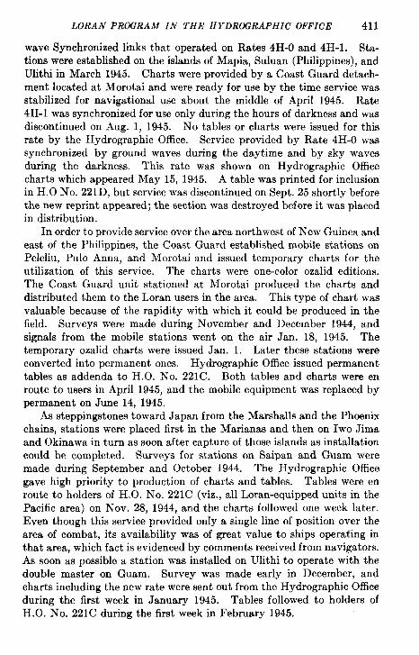
LORAN PROORAM IN THE HYDROORAPHIC OFFICE 411

wave Synchronized links that operated on Rates 4H-O and 4H-1. Sta-tions were established on the islands of Mapia, Suluan (Philippines), andUlithi in March 1945. Charts were provided by a Coast Guard detach-ment located at Morotai and were ready for use by the time service wasstabilized for navigational use about the middle of April 1945. Rate4H-1 was synchronized for use only during the hours of darkness and wasdkmontinued on Aug. 1, 1945. No tables or charts were issued for thisrate by the Hydrographic Office. Service provided by Rate 4H-O wassynchronized by ground waves during the daytime and by sky wavesduring the darkness. This rate was shown on Hydrographic Officecharts which appeared May 15, 1945. A table was printed for inclusionin H.O No. 221D, but service was discontinued on Sept. 25 shortly beforethe new reprint appeared; the section was destroyed before it was placedin distribution.

In order to provide service over the area northwest of New Guinea andeast of the Philippines, the Coast Guard established mobile stations onPeleliu, Pulo Anna, and Morotai and issued temporary charts for theutilization of this service. The charts were one-color ozalid editions.The Coast Guard unit stationed at Morotai produced the charts anddistributed them to the Loran users in the area. This type of chart wasvaluable because of the rapidity with which it could be produced in thefield. Surveys were made during November and December 1944, andsignals from the mobile stations went on the air Jan. 18, 1945. Thetemporary ozalid charts were issued Jan. 1. Later these stations wereconverted into permanent ones. Hydrographic Office issued permanenttables as addenda to H.O. NTO.221C. Both tables and charts were enroute to users in April 1945, and the mobile equipment was replaced bypermanent on June 14, 1945.

As steppingstones toward Japan from the Marshalls and the Phoenixchains, stations were placed first in the Marianas and then on Iwo Jimaand Okinawa in turn as soon after capture of those islands as installationcould be completed. Surveys for stations on Saipan and Guam weremade during September and October 1944. The Hydrographic Officegave high priority to production of charts and tables. Tables were enroute to holders of H.O. No. 221C (viz., all Loran-equipped units in thePacific area) on Nov. 28, 1944, and the charts followed one week later.Even though this service provided only a single line of position over thearea of combat, its availability was of great value to ships operating inthat area, which fact is evidenced by comments received from navigators.As soon as possible a station was installed on Ulithi to operate with thedouble master on Guam. Survey was made early in December, andcharts including the new rate were sent out from the Hydrographic Officeduring the first week in January 1945. Tables followed to holders ofH.O. No. 221C during the first week in February 1945.

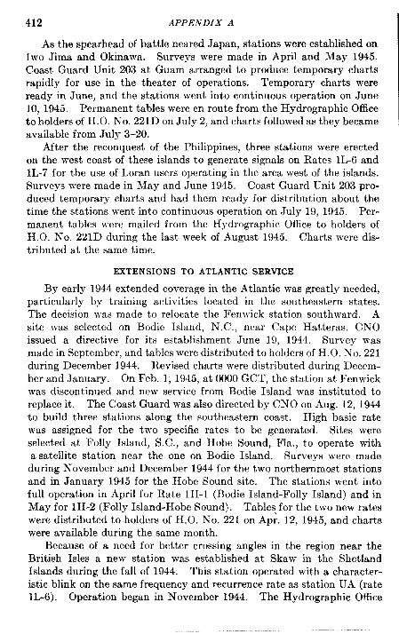
412 APPENDIX A

As the spearhead of battle neared Japan, stations were established onIwo Jima and Okinawa. Surveys were made in April and May 1945.Coast Guard Unit 203 at Guam arranged to produce temporary chartsrapidly for use in the theater of operations. Temporary charts wereready in June, and the stations went into continuous operation on June10, 1945. Permanent tables were en route from the Hydrographic Officeto holders of H.O. No. 221D on July 2, and charts followed as they becameavailable from July 3–20.

After the reconquest of the Philippines, three stations were erectedon the west coast of these islands to generate signals on Rates lL-6 and1P7 for the use of Loran users operating in the area west of the islands.Surveys were made in May and June 1945. Coast Guard Unit 203 pro-duced temporary charts and had them ready for distribution about thetime the stations went into continuous operation on July 19, 1945. Per-manent tables were mailed from the Hydrographic Office to holders ofH.O. No. 221D during the last week of August 1945. Charts were dis-tributed at the same time.

EXTENSIONS TO ATLANTIC SERVICE

By early 1944 extended coverage in the Atlantic was greatly needed,particularly by training activities located in the southeastern states.The decision was made to relocate the Fenwick station southward. Asite was selected on Bodie Island, NC., near Cape Hatteras. CNOissued a directive for its establishment June 19, 1944. Survey wasmade in September, and tables were distributed to holders of H.O. NTO.221during December 1944. Revised charts were distributed during Decem-ber and January. On Feb. 1, 1945, at 0000 GCT, the station at Fenwickwas discontinued and new service from Bodle Island was instituted toreplace it. The Coast Guard was also directed by CNO on Aug. 12, 1944to build three stations along the southeastern coast. High basic ratewas assigned for the two specific rates to be generated. Sites wereselected at Folly Island, S.C., and Hobe Sound, Fla., to operate witha satellite station near the one on Bodie Island. Surveys were madeduring N’ovember and December 1944 for the two northernmost stationsand in January 1945 for the Hobe Sound site. The stations went intofull operation in April for Rate lH-1 (Bodie Island-Folly Island) and inMay for 1H-2 (Folly Island-Hobe Sound). Table: for the two new rateswere distributed to holders of H.O. No. 221 on Apr. 12, 1945, and chartswere available during the same month.

Because of a need for better crossing angles in the region near theBritish Isles a new station was established at Skaw in the ShetlandIslands during the fall of 1944. This station operated with a character-istic blink on the same frequency and recurrence rate as station UA (rateIL-6). Operation began in November 1944. The Hydrographic Office

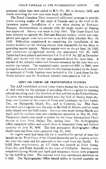
LORAN PROORAM IN THE H YDROORAPHIC OFFICE 413

prepared tables that were added to H.O. No. 221 in January 1945, andcharts including the new rate were ready in March.

The Royal Canadian Navy requested additional coverage to providebetter crossing angles off the coast of Canada and in the Gulf of St.Lawrence region. Installation of a new slave station at Port-aux-Basquesj Newfoundland, to operate with the single master at Demingwas approved. Survey was made in July 1944. The Coast Guard hadbeen directed to operate the Port-aux-Basques station, which was com-pleted and signals went into service on an 8-hr daily schedule Mar. 15,1945. Difficulties experienced in completing the installation of themaster facilities at the Deming station were responsible for the delay inproviding master signals. Master signals were on the air Sept. 10, 1945,and continuous navigational service was announced Oct. 26, 1945.Tables had been printed and issued as Vol. II of H.O. No. 221 in December1944, and charts with the new rate appeared about the same time, Areprint of the Atlantic tables had become necessary by the time this newsection was issued. The reprinted copies, numbered 6001 to 7000, werearranged in such manner that tables for the stations located on the Atlan-tic seaboard of N’orth America were included in Vol. I and those for theNorth Atlantic and the Northeast Atlantic were placed in Vol. II.

ARMY AIR FORCES AIR TRANSPORTABLE STATIONS

The AAF established several Loran chains during the first six months

of 1945 chiefly for the purpose of providing effective signals for training

schools operating under the direction of that activity in the United States.

To serve the training schools located near the Gulf of Mexico three sta-

tions were located on the coasts of Texas and Louisiana—at Port Isabel,

Tex., on LIatagorda Island, Tex., and at Cameron, La. This chain

provided useful signals over the area of the Gulf of NIexico and for some

miles inland over the Gulf states. Surveys were made during March andApril, and the stations went into continuous operation on kfay 23, 1945.

Temporary charts were made available by the Army Aeronautical Chart

Service at Love Field, Dallas, Tex., during June. The Hydrographic

Office computed tables and issued them in temporary form and limited

quantity on July 26, 1945. The first permanent Hydrographic Office

charts carrying these rates appeared Aug. 31, 1945.

An urgent need had been felt for a considerable period of time for

signals on the lVest Coast of the United States for use by aviation activi-

ties near the coast and for approach to the coast from the Pacific. Tofulfill these requirements, an AT chain was located at Point Arena,

Point Sur, and Point Arguello on the coast of California. Surveys were

completed during March and April and temporary charts were prepared

by the AACS in June. The stations went into continuous operation on1 July. The Hydrographic Office issued tables in limited quantity on

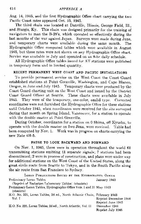
414 APPENDIX A

Aug. 14, 1945, and the first Hydrographic Office chart carrying the twoPacific Coast rates appeared Oct. 15, 1945.

The third chain was located at Danville, Illinois, George Field, Ill.,and Sturgis, Ky. This chain was designed primarily for the training ofnavigators to man the B-29’s, which operated so effectively during thelast months of the war against Japan. Surveys were made duringJune,

and temporary charts were available during the same month. TheHydrographic Office computed tables which were available in August1945, but these rates were not shown on any Hydrographic Office chart.Service was available in July and operated on an 8-hr daily schedule.

All Hydrographic Office tables issued for AT stations were publishedin temporary form and in limited quantity.

RECENT PERMANENT WEST COAST AND PACIFIC INSTALLATIONS

To provide permanent service on the West Coast the Coast Guard

established stations at Point Grenville, Washington, and Cape Blanco,

Oregon, in June and July 1945. Temporary charts were produced by the

Coast Guard charting unit on the West Coast and issued by the District

Coast Guard Officer at Seattle. These charts were available in July

1945. They were of the temporary, one-color, ozalid type, Corrected

coordinates were not furnished the Hydrographic Office for these stations

until October 1945, when coordinates were received for the site surveyedduring that month on Spring Island, l’ancouver, for a station to operatewith the double mast er at Point Grenville.

During October, coordinates for a station on O Shims, off Kyushu, to

operate with the double master on Iwo Jima, were received. Table had

been computed by Nov. 1. Work was in progress on charts carrying the

new Rate 4H-5.

PAUSE TO LOOK BACKWARD AND FORWARD

On Nov. 1, 1945, there were in operation throughout the world 61transmitting stations emitting 41 separate signals; 7 stations had beendiscontinued; 2 were in process of construction, and plans were under wayfor additional stations on the West Coast of the United States, along thegreat circle route from Seattle to Tokyo, and in the South Pacific alongthe air route from San Francisco to Sydney.

LORAN PUBLICATIONS ISSUED BY THE HYDROGRAPHIC OFFICE

Preliminary Loran Tables January 1943

(Reprint of Radiation Laboratory Tables) (obsolete)Preliminary Loran Tables, Hydrographic Office Vols. I and II May 1943

(obsolete)H.0, No. 221, Loran Tables, 2d cd., North Atlantic Chain, February 1943

Vol. I Reprint December 1944Reprint June 1945

H.O. No. 221. Loran Tables, 2d cd., North Atlantic, Vol. II December 1944Reprint July 1945

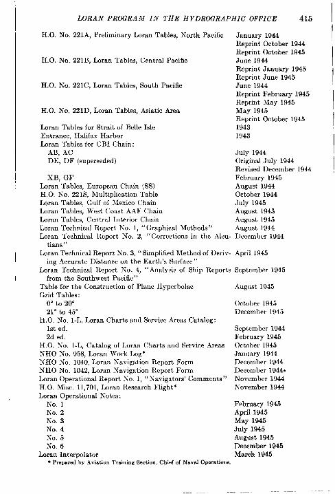
II

LORAN PROORAM IN THE HYDROGRAPHIC! OFFICE 415

H.O. No. 221A, Preliminary Loran Tables, North Pacific January 1944Reprint October 1944Reprint October 1945

H.O. No. 221B, Loran Tables, Central Pacific June 1944Reprint January 1945Reprint June 1945

H.O. No. 221C, Loran Tables, South Pacific June 1944Reprint February 1945Reprint May 1945

H.O. No. 221D, Loran Tables, Asiatic Area May 1945Reprint October 1945

Loran Tables for Strait of Belle Isle 1943Entrance, Halifax Harbor 1943Loran Tables for CBI Chain:

AB, AC July 1944DE, DF (superseded) Original July 1944

Revised December 1944XB, GF February 1945

Loran Tables, European Chain (SS) August 1944HO. No. 221S, Multiplication Table October 1944Loran Tables, Gulf of Mexico Chain July 1945Loran Tables, West Coast AAF Chain August 1945Loran Tables, Central Interior Chain August 1945Loran Technical Report No. 1, “ Graphical Methods” August 1944k-an Technical Report No. 2, “ Corrections in the Aleu- December 1944

tians”Loran Technical Report No. 3, “Simplified Method of Deriv- April 1945

ing Accurate Distance on the 13arth’s Surface”Loran Technical Report No. 4, “Analysis of Ship Reports September 1945

from the Southwest Pacific”Table for the Construction of Plane Hyperbola August 1945

Grid Tables:0° to 20° October 194521° to 45° December 1945

H.O. No. l-L, Loran Charts and Service Areas Catalog:1st ed. September 19442d ed, February 1945

H.O. No. l-L, Catalog of Leran Charts and Service Areas October 1945NHO No. 958, Loran Work Log* January 1944NHO No. 1040, Loran Navigation Report Form December 1944NHO No. 1042, Loran IVavigation Report Form December 1944*Loran Operational Report No. 1, “ Navigators’ Comments” November 1944HO, Misc. 11,701, Loran Research Flight * November 1944

Loran Operational Notes:No. 1 February 1945No. 2 April 1945No. 3 May 1945No. 4 July 1945No. 5 August 1945No. 6 December 1945

Loran Interpolator March 1945● Prepared by Aviation TrainingSsction, Chief of Naval Operation,

!I

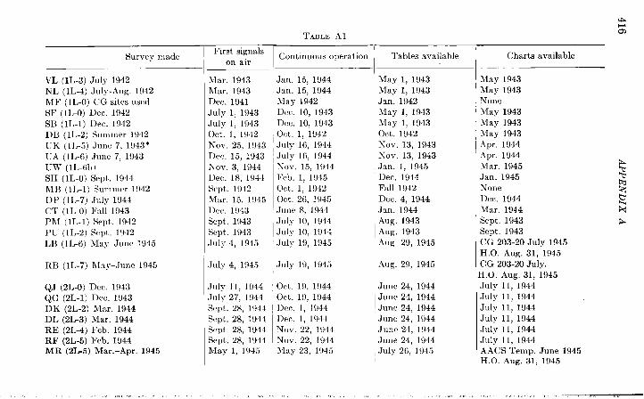
Survey xnaclc

VL (IL-3) July 1942NL (lL-4) July -Aug. 1942

hf F (11,-0) {;G sites usedSF (lL-O) D... 1942SB (lL-l) l)eC. 1942DB (11,-2) Summer 1942IJK (1 1.-5) June 7, 1943*UA (1L-6) .TUIIC 7, 1943UW (lL-ob)SH (lL-O) Sept. 1944kI B ( 11,-1) Summer 194211P ( 11,-7) July 1944CT (11,-0) Fall 1943PhI (lL-l) Sept. 1942Ptl ( 11,-2) Sept. 1942LB (11,-6) h@-JuIIc 1945

RB (IL-7) illay–.lune 1945

QJ (21,-0) Dec. 1!>43QG (2L-1) Ike. 1943DK (2L-2) Mar. 1!?44DL (2L-3) Mar. 1944RE (2L4) Feb. 1944RF (2L-5) Feb. 1944MR (2L-5) Mar.–Apr. 1945

,,, ,“

Frost signalson air

hlar. 1943illar. 1943Dec. 1!341

July 1, 1943July 1, 1943Oct. 1, 1!)42NOV. 25, 1!)43Dec. 15, 1943Nov. 3, 1944Dw. 18, 1!)44Sept. 1942Xlar. 15, 1945I)Cc. 1!)43S(!pt 1!)43Sq)t 1943July 4, 1945

July 4, 1!345

July 11,, 1944July 27, 1944SCpt. 28, 1944Sept. 28, 1944Sept. 28, 1944Sept. 28, 1944May 1, 1945

,W.

TABLE Al

Continuous operation

Jan. 15, 1944Jan. 15, 1944May 1942Dec. 10, 1943Dec. 10, 1943oct. 1, 1942

July 16, 1944

July 16, 1944Nov. 15, 1944F(t). 1, 1!)45

Oct. 1, 1942

Ort. 26, 194.5JUIK! 8, 1944July 10, 1944July 10, 1!)44,July 19, 1945

July 19, 1945

O(!t. 19, 1944Oct. 19, 1944Dec. 1, 1944Ilec. 1, 1944NOV. 22, 1944Nov. 22, 1944May 23, 1945

,. ”,,,., ,“

Tables available

May 1, 1943May 1, 1!443Jan. 1942May 1, 1943May 1, 1943Oct. 1942No>-. 13, 1943Nov. 13, 1943Jan. 1, 1945Dec. 1944Fall 1942Dec. 4, 1944Jan. 1944.kug. 1943Aug. 1943Aug. 29, 1945

Aug. 29, 1945

June 24, 1944June 24, 1944June 24, 1944June 24, 1944June 24, 1944June 24, 1944July 26, 1945

,,,

+m

Charts available

\fay 1943May 1943h’oneillay 1943May 1943May 1943Apr. 1944Apr. 1944hfar. 1945Jan. 1945NoneDec. 1944Lfar. 1944Scpt 1943Sept. 1943CC 203-20 July 1945H.O. Aug. 31, 1945CG 203-20 July,EI.O. Aug. 31, 1945July 11, 1944July 11, 1944July 11, 1944July 11, 1944July 11, 1944July 11, 1944AACS Temp. June 1945H.0, Aug. 31, 1945

,,, ,,, -,,

MT (2L-6) Mar. -Apr. 1945

GF (4L-0) Dec. 1944

DF (4L-1) Orig. Apr. 1944Rev. Oct. 1944

DE (4L-2) Orig. Apr. 1944Rev. Oct. 1944

AC (4L-3) Apr. 1944AB (4L-4) Apr. 1944XII (4L-5) Dec. 1944

XY (4L-6) Dec. 1944ZY (4L-7) Dec. 1944CH (lH-l) Nov.-Dee, 1944

CG (IH-2) Nov.–Jan. 19455A [lH-6) 51ar. –Apr. 1!145SG (1 11-7) hIar,–Apr, 1945WN (2H-4) Jan. 1944WA (2H-5) ,Jan. 1944

(2H-4) April-}lay 1945(2H-5) Oct. 1945

PD (2 EI-6) June 1945I% (2H-7) June 1945NP (4H-0) Feb. 1945

HP (4H-1) Feb. 1945

HV (4H-2) Dec. 1944SV (4H-3) Sept.–Ott. 1944

klay 1, 1945

Apr. 1945

Dec. 16, 1944

DeC. 16, 1944

Sqlt. 1944Scpt 1944klzr. 1945

Feb. 1945Feb. 1945Lftir, 25, 1945

Jan, 17, 1945June 15, 1945June 15, 1945July 1945July 1945.Junc 6, 1945

.July 1!)45July 194531ar. 24, 1945

}Iar. 24, 1945

Dec. 27, 1!?44X~OV. 28, 1944

May 23, 1945

Apr. 1945

Feb. 1945

Feb. 1945

Sept. 1!)44 *Sq)t, 1944*hI:Lr. 1945*

Feb. 1!345Feb. 1!)45Apr. 11, 1945(.Aug. 21, 1945)ilIay 15, 1945July 1, 1945July 1, 1945Aug. 1944Aug. 1944July 24, 1945

July 1945July 1!)45Apr. 7, 1945

Apr. 7, 1945

Jan. 12, 1945Ihw. 16, 1944

July 26, 1945

Temp. Feb. 6, 1945H.O. 221 July 2, 1945Orig. July 1944Itev. IXx. 1944Orig. July 1944Rev, Dec. 1944

July 1944July 1944~(X1lp. Feb. 6, 1945H.O. 221 July 2, 1945May 17, 1945Lfay 17, 1945Apr. 12, 1945

Apr. 12, 1945Aug. 14, 1945Aug. 14, 1945June 14, 1944June 14, 1944

Aug. 1!345Aug. 1945}Iar. 1!3, 1945

Jlar. 23, 1945

Feb. 5, 1946Nov. 2x, 1944

AACS Temp. June 1945H.O. ,%ug. 31, 1945Feb. 22, 1945Mar. 31, 1945Feb.-Mar. 1945

Feb.–Mar. 1945

Mar. 20, 1945Mar. 20, 1945Mar. 20, 1945

Mar, 31, 1945Mar. 31, 1945Apr. 19, 1945

Apr. 19, 1945Oct. 15, 1945Oct. 15, 1945Jun. 21, 1944June 21, 1944Temp. 0G13ND-July 1945

Temp. AACS-June 1945Temp. AACS-June 1945Temp. CG—Apr. 1945Pcrm. H. O.—May 15, 1945Temp. CG—April 16, 1945Not on H.O. chartsJan. 5, 1945Dec. 2, 1944

+%

● Date coordinates wmt from flritist, .kdmiralt~

TABLE Al .—(Continued)

Survey r?l:Lde

KJ (4H-4) Apr. -h[ay 1045KO (4H-5) Oct. 1945TU (4H-6) Nov. 1944 (mobile)

TM (4H-7) Nov. 1944 (mobile)

* Dimmntinued25 Oct. 1945

First signalson air

}fay 16, 1945

I)ec. 6, 1944

Dec. 6, 1944

!,, >,,, ,,, ,,, ,,, ,, ,,, ,

Continuous operation

June 10, 1945

June 14, 1945 (perm.)

June 14, 1945 (pcrm.)

Tables available I Charts available

July 2, 1945

Apr. 19, 1945

Apr. 1!1, 1945

Temp. CG 203—June 1945Perm. H.O. July 20, 1945Temp. CG—Jan. 1, 1945Perm, H. O. —Mar. 30, 1945Temp. CG—Jan. 1, 1945Perm. H. O, —Mar. 30, 1945

,,,, ,,, ,,, ,,, ,,, ,,,

APPENDIX B

LORAN GROUND STATIONS’

HATTERAS-FLORIDACHAINFrequency: 1950kc (channelNo. 1)Basic pulserate: 33* pps (high)

Recurrence M stationx

Location Coordinatesrate

l-H-l s H Bodie Island, N.C,{

35°49’ 04:’697N75°34’ OOV128W

l-H-l

}M c Folly Island, Charleston, S.C,

{32°41’ 02( ’787N

l-H-2 79°53’ 13:’131W

l-H-2 s G Hobe Sound, I%.{

27”04’ 41:’098N80°07’ 14~’574W

Recurrencerate

1-L-o

l-L-Ol-L-l }l-L-ll-L-2 }l-L-2l-L-7 }

l-L-7

l-L-3

l-L-3l-L-4 }

l-L-4

1-L-5

l-L-5l-L-6 )

I-L-6

l-L6b

—M. .s

s

M

s

M

s

M

s

M

s

M

s

s

—

h’ ORTH ATLANTIC CHAINFrequency: 1950 kc (channel hTo. 1)Basic pulse rate: 25 pps (1OIV)

Stat ion

H

s

B

D

P

v

L

h’

K

u

.4

w

Location Coordinates

Bodie Island, h’. C.

Siasconset, Nantucket

Baccaro, Nova Scotia

Deming, Nova Scotia

Port-aux-Basques, Ne\vfoundland

Bonavista, Nev,foundland

Battle Harbor, Labrador

Narsak, Greenland

Vik, Iceland

Skuvanes, Faeroes

{35°50’ 07:’96N75”33’ 32!’53W

{

41°14’ 59:’752N69°58’ 21?732W

{

’43°27’ 33! ’45hT65”28’ 16(’33W

{

45°12’ 53(’49N,61”10’ 32:’34W

{

47°33’ 53(’80N59°09’ 50(’69W

{48°41’ 45:’66N53°05’ 18~’24W

{52°14’ 51~3N55”36’ 43{’2W

{59”58’ 57(’oN44°39’ 51:’3W

{63°24’ 08!’N19°02’ 17(’W

{

61°27’ 22(’N6°49’ 21(’W

1 Revised to Oct. 15, 1945.

Mangersta, Hebrides{

58”11’ ll~N7°05’ 51!W

Skaw, Shetlands {60°49’ 47~’N0°46’ 41!’9W

419

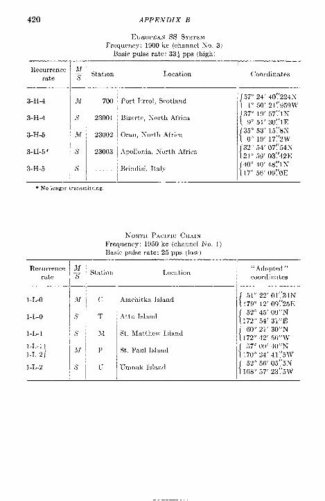
420 APPENDIX B

EUROPEAN SS SYSTEMFrequency: 1900kc (channel No. 3)

Basic pulse rate: 33+pps (high),,

‘ecurrenceI g ~S,s,,,.nrate

I I3-H-4 s 23001

3-H-5 .}f 23002

I,ocation

F’ort I.krol, Scotl:tnd

Bizcrtc, A-orth .+fric:l

Oran, >“orth .Africa

3-H-5 * s 23003 ~Apollonia, N“orth .~frics

3-H-5 s ;Brindisi, Italy~, ‘“”

* No 10W:I transmittir,g.

Coordinates

—

{

57°24’ 40! ’224X”1°50’ 21’.’959W

(

37° 19’57(’lN9“ 51’ 30!’IE

{

35” 53’ 15:’8N0°19’ 17:’2W’

{

32°54’ 07!’54N21059’ 03’.’42E

/ 40°40’ 48:’lN\17° .56’ 09:’OE

NORTH PACIFIC C;U.41NFrequency: 1950kc (c}lanuel No. 1)Basic pulse rate: 25 pps (lo\v)

l-L-O

l-L-o

l-L-l

l-L-ll-L-2 }

1-L-2

—\—

.}1 (’

,Y T

S 31

M P

s I L-

Location 1 “Adopted”cOOrdiImtes

—1Amchitka Island 1{51°22’ 01’.’34N

179° 12’ 09’.’25E

Attu Island{

52°45’ 09”LN172°54’ 31”E

St. kIatthev Island{

60°21’ 30”N172°42’ 56”W

St. Paul IS1;LUCI{

57’ 09’ 40”hT170°24’ 41”5W

Umnak Island 1{52°56’ 05{’5N168”57’ 23’.’5W

LORAN PROGRAM IN THE HYDROGRAPHIC OFFICE 421 !

CENTRAL PACIFIC CHAINFrequency: 1850 kc (channel No. 2)Basic pulse rate: 25 pps (low)

Recurrence M Stationrate x

2-L-O s J

2-L-o2-L-1}

M Q

2-L-1 s G

2-L-2 s K

2-L-22-L3 }

M D

2-L-3 s L

2-L-4 s I E

2-L-42-L-5 }

M R

2-L-5 s F

Location

Hawaii Island

N’iihau Island

French Frigate Shoals

Kwajalein Atoll

Majuro Atoll

Makin Atoll

Baker Island

Gardner Island

Atafu Island

Adoptedcoordinates I

I

/ 20°15’ 16!’5N~155°53’ 23!’3W Ij 21° 4S’ 16!’4N ‘i 160°14’ 13(’5W( 23” 47’04(’7N( 166°12’ 39:’5W

( 9°00’ 52’.’35N[ 167°43’ 52!’42E

1 7° 13’01’.’34N1171°04’ 29(’96E

~ 3°16’ 19:8N~172°40’ 35:9E/ 0° 11’46:23N1176°28’ 26’.’14W/ 4°41’ 41!’65S( 174°29’ 50’:61Wj 8°31’ 53’.’6S~172° 31’06!’OW

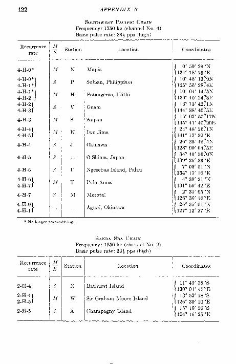
422

Recurrencerate

4-H-o *

4-H-o *4-H-1 * 14-H-1 *4-H-2 }4-H-24- H-3 }

4-H-3

4-H-44-H-5 }

4-H-4

4-H-5

4-H-6

4-H-64-H-7,

4-H-7

4-H-O4-H-1 }

APPENDIX B

SOUTHWEST PACIFIC CHAINFrequency: 1750kc (channel ISo,4)Basic pulse rate: 33~pps (high)

Station

N

P

H

J’

s

K

J

~

T

31

Location

\lapia

SLduaI1, Philippines

Potangeras, Llithi

Guam

Saipan

Iwo Jima

Okina\va

OShima, Japan

Xgesebus Island, Palau

PD1O .4nna

llorotai

Aguni, Okinawa

Coordinates

{0°50’ 29”N

134° 18’ 15”E

{

10°46’ 13!’9N125” 56’ 28:4E

{

10°04’ 14’.’5X139” 40’ 24’.’3E

{

13” 13’42’,’lN144°38’ 40(’5E

{

15” 07’ 50( ’17hT145°41’ 40!’20E

{

24°48’ 26(’lN141° 17’ 30” E

(

26” 23’ 49?4hT128°00’ 04!’5E

{

34” 40’ 36! ’ON139”26’ 33’%

{

7°03’ 51”N’134° 15’ 16”E

{

4°39’ 21”Ii131° 56’42”E

{

2“ 35’ 05”N128°36’ 16”E

{

26°35’ Ol”h’127° 12’ 27” E

* No longer trammiiting.

B.4NDA SEA C!H.41XFrequency: 1850 kc (channel Xo, 2)Basic pulse rate: 33 ~ pps (high)

Recurrence .Ifrate x

Station Location (’ordinates

2-H-4 /S x Bathurst Island{

11°45’ 38”S130”01’ 43”E

2-H-4

}.lr W Sir Graham Moore Island

{

13°52’ 18”S2-H-5 126°30’ 10”E

2-H-5 s A Champagny Island{

1.5°16’ 56”S124” 16’ 25”E

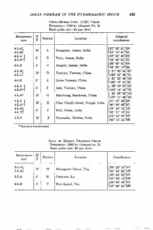
LORAN PROORAM IN THE H YDROGRAPHIC OFFICE 423

CHINA-BUrtMA-INDIA (CBI) CHAINFrequency: 1750 kc (channel No. 4)Basic pulse rate: 25 pps (low)

Recurrence ;Stat ion

rate

4-L-44-L-3 }

M A

4-L-44-L-5*}

s B

4-L-3 s c

4-L-24-L-1}

M D

4-L-2 s E

4-L-14-L-O*}

s F

4-L-o * M G

4-L-64-L-5 *}

M x

4-L-64-L-7 }

s Y

4-L-7 M z

* Sky-wave Synchronized.

Imcation

Hoogrijan, Assam, India

Paya, Assam, India

Amguri, Assam, India

Kunyan, Yunnan, China

Lutze Yunnan, China

Ami, Yunnan, China

Hanchung, Szechwan, China

Char Chapli Island, Bengal, India

Puri, Orissa, India

Coconada, Madras, India

GULF OF MEXICO TRAINING CHAINFrequency: 1850 kc (channel no. 2)Basic pulse rate: 25 pps (low)

Adoptedcoordinates

(27° 22’ 51’.’5N

[ 95° 14’41!’3E127°51’ 46’.’ON

~95° 59’05!’2E(26° 45’ 45!ON194”36’ 15!’OE( 24° 39’34~4N1102°37’ 56(’7E( 25” 22’49’.’5N

i 102°17’ 54:’2E( 23° 40’22!’4N

~103°14’ 56!’7E( 33° 09’02~5N1107”11’ 46~4E

[

21047’ 50;6N

90°09’ 08:9E

{

19°48’ 12(’4N85”51’ 10~’6E

{

16”55’ 06(’3N82°14’ 2/.’OE

Recurrence M Stationrate 3

Location I Coordinates

2-L-5)

A{ hf Matagorda Island, Tex{

28°20’ 18’.’6N2-L-6 96°25’ 22!’4W

2-L-5 s R Cameron, La.{

29°45’ 52!’9N93°22’ 19?OW

2-L-6 s T Port Isabel, Tex.{

26”04’ 48’.’ON97°09’ 55?8W

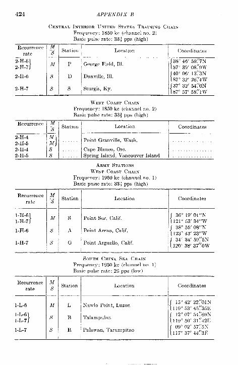
424

Recurrencerate

2-H-62-H-7 }

2-H-6

2-H-7

APPENDIX B

CENTRAL INTERIOR UNITED STATES TRAINING CHAINFrequency: 1850 kc (channel no. 2)Basic pulse rate: 33+ pps (high)

M—,A Station

IM

I

P

‘VD

Ss

Location I Coordinates

George Field, 111.{

38°46’ 59.’.’7S87°39’ 08V9W

Danville, Ill.{

40°06’ 13(’3N87”32’ 26’.’4W

Sturgis, Ky.{

37”32’ 54(’oN87”57’ 58!’1 W

WEST COAST CHAINFrequency: 18.50 kc (channel no, 2)Basic pulse rate: 33* pps (high)

Recurrence MI ~ / Station ~ Location Coordinates,

2-H-4 M2-H-5 )

Point Granville, Wash.M “’””’”

2-H-4 s Cape Blanco, Ore.2-H-5 s . Spring Island, Vancouver Island .

ARMY STATIONSWEST COAST CHAIN

Frequency: 1950kc (channel no. 1)Basic pulse rate: 33~pps (high)

Recurrence M~ Stationb

Location ICoordinatesrate

l-H-6

}M s POint Sur, Calif,

{

36° 19’01”NTl-H-7 121° 53’34”W

l-H-6 s A Point Arena, Calif,{

38° 55’08”IN123°43’ 23”W

l-H-7 s G ,POint.4rguel10, Calif.

I{

34”34’ 59:’5N120’38’ 37’.’OW

SOUTH CHINA S~.4 CHAINFrequency: 1950kc (chmmelno. 1)Basic pulse rate: 25pps (low)

Recurrence M~- Stat ion Location G30rdinates

rate— .

l-L-6 M L ~a~slo Point, Luzon15” 42’ 22(’OIN

I{ 119°53’ 45:’35El-L-6

}s B Talampulon

{

12“ 07’ 54! ’69>”l-L-7 11!) ’50’ 31!’421;

l-L-7 Palawan, Tarumpitao{

09”02’ 57:’5N7

Is R117°37’ 44:’3E

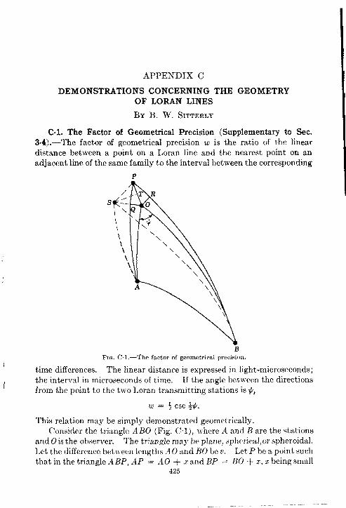
APPENDIX C

DEMONSTRATIONS CONCERNING THE GEOMETRYOF LORAN LINES

BY B. W. SITTERLY

Ccl. The Factor of Geometrical Precision (Supplementary to Sec.3.4) .—The factor of geometrical precision w is the ratio of the lineardistance between a point on a Loran line and the nearest point on anadjacent line of the same family to the interval between the corresponding

P

\\\ \

\\ \\\\\

A

BFIG. C, 1.—The factor of geometrical precision.

Itime differences. The linear distance is expressed in light-microseconds;

the interval in microseconds of time. If the angle between the directions(

from the point to the two Loran transmitting stations is ~,

u = ; Csc ++.

This relation may be simply demonstrated geometrically.

Consider the triangle ABO (Fig. C 1), where A and B are the stationsand O is the observer. The triangle maybe plane, spherical, or spheroidal.

Let the difference bet ween lengths A O and BO be v. Let P be a point suchthat in the triangle ABP, AP = AO + z and BP = BO + Z, z being small

425

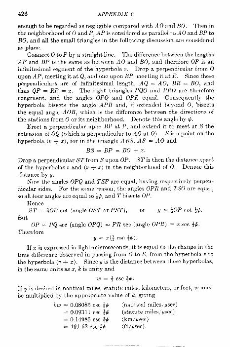
426 APPENDIX C

enough to be regarded as negligible compared with AO and BO. Then inthe neighborhood of O and P, .4P is considered as parallel to .40 and B1’ to130, and all the small triangles in the following discussion are considered

as plane.Connect O to P by a straight line. The difference between the lengths

AP and BP is the same as between A O and BO, and therefore 01’ is an

infinitesimal segment of the hyperbola v. Drop a perpendicular from O

upon AP, meeting it at Q, and one upon BP, meeting it at R. Since theseperpendiculars are of infinitesimal length, A Q = AO, BR = BO, andthus QP = RP = x. The right triangles PQO and PRO are thereforecongruent,and the angles OPQ and OPR equal. Consequently the

hyperbola bisects the angle APB and, if extended beyond O, bisectsthe equal angle AOB, which is the difference between the directions of

the stations from O or its neighborhood. Denote this angle by #.

Erect a perpendicular upon BP at P, and extend it to meet at S theextension of OQ (which is perpendicular to A O at O). S is a point on thehyperbola (u + z), for in the triangle ABS, AS = .40 and

BS=BP=BO +X.

Drop a perpendicular ST from S upon OP. ST is then the distance apartof the hyperbolas v and (v + z) in the neighborhood of O. Denote thisdistance by y.

h’ow the angles OPQ and TSP are equal, having respectively perpen-

dicular sides. For the same reason, the angles OPR and TSO are equal,so all four angles are equal to ~~, and T bisects OP.

HenceS2’ = ~OP cot (angle OST or PST), or y = +OP cot ++.

But

OP = PQ sec (angle OPQ) = PR see (angle OPR) = x sec ~~.Therefore

y = Z(* Csc **).

If z is expressed in light-microseconds, it is equal to the change in thetime difference observed in passing from O toA’,from the hyperbola v tothe hyperbola (u + x). Since y is the distance between these hyperbolas,in the same units as x, k is unity and

If y is desired in nautical miles, statute miles, kilometers, or feet, w mustbe multiplied by the appropriate value of k, giving

kw = 0.08086 CSC ++ (nautical miles~psec)

= 0.09311 Csc +4 (statute miles/psec)= 0.14985 CSC +4 (km/psec)= 491.62 CSC ++ (ft/Wsec).

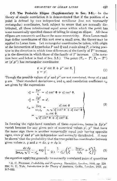
GEOA4ETR Y OF LORAN LINES 427

C02. The Probable Ellipse (Supplementary to Sec. 3.5).—In thetheory of simple correlation it is demonstrated that if the position of apoint is defined by two independent rectilinear (but not necessarilyrectangular) coordinates, both subject to errors that are normally dis-tributed, all these infinitesimal equal areas within which the point hassome numerical y specified chance of failing lie along an ellipse. All these

ellipses are concentric and have the same eccentricity. Since Loran read-ings define coordinates of this sort over a small area, the theory may beapplied to Loran fixes. Let rectangular coordinates be taken, with originat the intersection of hyperbolas P and Q and x-axis along P, z being posi-tive in the direction in which time differences of the family of Z’” increase,y in the direction in which those of the family of T“ increase. (The nota-tion here and below is that of Sec. 3.5.) The point (T’1 – T’, T, – T“)

or (p’,p”) has rectangular coordinates

z = p’ cot @ + p“ Csc 0,y = p’. 1

(1)

Though the possible values of p’ and p“ are not correlated, those of z andy are. Their standard deviations .s. and s,, and correlation coefficient rztiare given by the expressions

~Y2 #2=_ .% n 11

(2)

In forming the right-hand members of these equations, terms in zp’p”vanish because for any given pair of numerical values p’, p“ that havethe same sign there is another numerically equal pair having oppositesigns, since p’ and p“ are independent and normally distributed. It maybe shown’ that the probability that the true point has coordinates betweengiven values z, y and z + dz, y + dy is

the equation applying generally to normally correlated pairs of quantities

1 H. C. Plummer, Probability and FrPquenc~, hlacrnillan, Lonclon, 1940, pp. 224--231; G. U. Yule, Introduction to the Theory of Statistics,Griffin, London, 1927, pp.317-322.

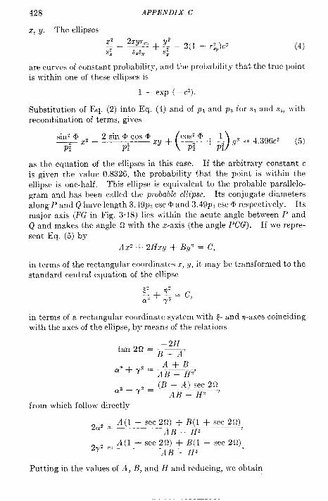
428 APPENDIX C

x, y. The ellipses

x’ 2zyr=4~— ~ + $ = 2(1 – ?.&)cz (4)z Y

are curves of constant probability, and the probability that the true pointis within one of these ellipses is

1 – exp (–c’).

Substitution of Eq. (2) into Eq. (4) and of p, and p, for s, and s,, ~~ithrecombination of terms, gives

sinz @ ~,_2sin@cos@—.

Pi P; “+t%+i)’’=’’g’c’ ‘5)

as the equation of the ellipses in this case. If the arbitrary constant c

is given the ~alue 0.8326, the probability that the point is within theellipse is one-half. This ellipse is equivalent to the probable parallelo-

gram and has been called the probable ellipse. Its conjugate diametersalong P and Q have length 3.49p~ csc @ and 3.49P1 csc @ respectively. Itsmajor axis (FG in Fig. 3.18) lies within the acute angle between P andQ and makes the angle Q with the z-axis (the angle PCG). If we repre-sent 12q. (5) by

.iX2 ~ 2Hxy ~ By’ = c,

in terms of the rectangular coordinates Z, Y, it may be transformed to thestandard central equation of the ellipse

in terms of a rectangular coordinate system w-ith f- and ~-axes coinciding

with the axes of the ellipse, by means of the relations

– 2H

‘an2Q=B–~’

.4+B~2 + 72 = ~~ _ @

(B – .4) sec 2Q~2—72=—AB–Hz ‘

from which follow directly

2a2 ~ A(I – sec 2Q) + B(I + mc 2fl).4B – H’

27, = A(l + sec 2Q) + B(I – sec 2cl)AB – H’

Putting in the values of A, B, and H and reducing, we obtain

GEOMETRY OF LORAN LINES 429

tan 2Q =2p; cot @ p? sin 2@

p;(cot’ @ – 1) + p;(cot’ @ + 1) = p; Cos 2* + p;’

1

(6)~ = /*(p; + p;) CSC2 t? + p? cot @ Csc 2Q,

-r = VW; + p;) CSC2 @ – p; cot @ Csc 2Q

The two axes of the ellipse (FG and HJ in Fig. 318) have lengths 3.49aand 3.49? respect ively, and these lengths, with the angle Q between the x-and saxes, give a definite picture of the theoretical distribution of errors offix around a point. The probabilityy that the true position is within anellipse similar to the probable ellipse and similarly placed, but with dimen-sions multiplied by 1.82, is nine-tenths.

C*3. The Probable Error of a FIX (Supplementary to Sec. 3%).-Theprobable error pl or pz is the “expected” distance between the hyperbolaP or Q specified by the observed time difference and the true line of posi-tion at the time of observation, in the sense that it is equally probable thatthe actual distance is greater or less. An expected or probable distance,in the same sense, between the intersection of P and Q and the true fixis for many purposes the most useful measure of the error of fix. Unfortu-nately, this distance cannot be simply specified. The quantity ~W,where d = <z 2 + g2, is the standard deviation of dist antes between theobserved fix and the true fix. It may be denotedadding, and summing the expressions in Eq. (1) andterms in Zp’p” vanish, we obtain

D2=~=?? +%2n n n

= +(cotj @ + 1) + s; CSC20.

D = CSC @ #S; + S;.

by D. Squaring,remembering that

Though values of z and y are normally distributed, d is not. The proba-bilityy that d is less than D varies with the shape of the error ellipses; whenthese are circular, the probabilityy is 0.632; and when they are extremelyeccentric, the probability approaches 0.683, the value for the standarddeviation of a single variable. The quantity 0.6745D is not the medianvalue of d, or probable error of a fix, for the probability that d is less than0.6745D is 0.366 if the error ellipses are circular and tends to 0.500 only astheir eccentricity approaches unity.

The distribution of the values of d is investigated’ by transforming Eq.(3) into polar coordinates r and o and integrating over all values of oand from r = O to r = R. The value of the integral is the probability

1Operational Research Staff, Office of the Chief Signal Officer, “The Range,Reliability, and Accuracy of a Low Frequency Loran System,” Report OR&P-23,

Appendix II, Washington, 1946, pp. 77–81. The discussion below is adapted from

that given in this reference.

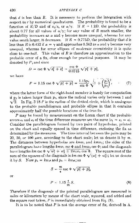
430 APPENDIX C

that d is less than R. It is necessary to perform the integration withrespect to r by numerical quadrature. The probability is found to be afunction of R/D and of sE/s, or a/y. If R = 1.2D, the probability isabout 0.77 for all values of a/y; for any value of R much smaller, theprobability increases as a and ~ become more unequal, whereas for anyvalue much larger, it decreases. If R = 0.775D, the probability that d isless than R is 0.452 if a = -yand approaches 0.562 as a and Y become veryunequal, whereas for error ellipses of moderate eccentricity it is quiteclose to one-half. This value of R is therefore an approximation to theprobable error of a fix, close enough for practical purposes. It may bedenoted by P; and since

(7)

where the latter form of the right-hand member is handy for computationif pz is taken larger than PI, since the radical varies only between 1 and~. In Fig. 318P is the radius of the dotted circle, which is analogousto the probable parallelogram and probable ellipse in that it containsapproximately half the possible locations of the true fix.

P may be found by measurement on the Loran chart if the probableerrors c1and C2of the time difference measures are the same (cl = CZ= c).Consider the parallelogram formed by two pairs of hyperbolas, printedon the chart and equally spaced in time difference, enclosing the fix asdetermined by the measures. The time interval between the pairs maybe20, 50, or 100 psec, according to the chart scale; let us denote it by m.The distances between hyperbolas are kmw, and ?cmwz; the sides of theparallelogram have lengths kmwl csc @ and kmwz csc @; and the diagonalshave lengths km csc @ V’ w: + w; f 2w1w2 cos @. The square root of thesum of the squares of the diagonals is km csc @ ~ (w! + w;); let us denoteit by S. Now PI = kwle and P2 = kwze; so

A’=; csc@dp; +p;,

or

P = 1.15:s. (8)

Therefore if the diagonals of the printed parallelogram are measured inmiles or kilometers by means of the chart scale, squared, and added andthe square root taken, P is immediately obtained from Eq. (8).

It is to be noted that P is not the average error of fix, derived in A.

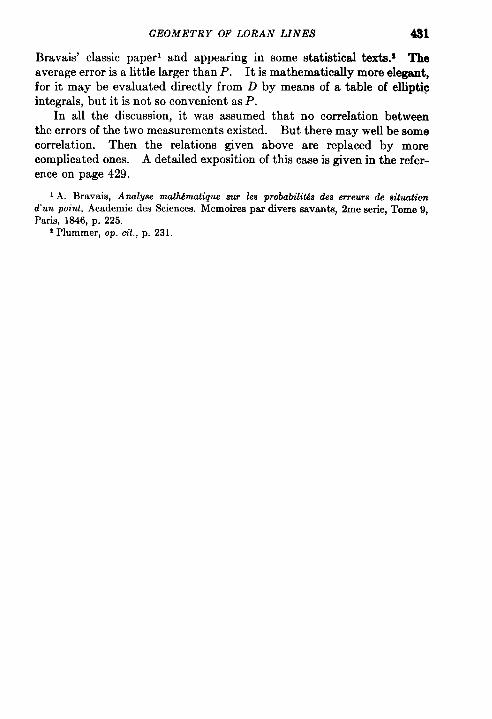
GEOMETRY OF LORAN LINES 491

Bravais’ classic paper’ and appearing in some statistical texts.s Theaverage error is a little larger than P. It is mathematically more elegant,for it may be evaluated directly from D by means of a table of ellipticintegrals, but it is not so convenient as P.

In all the discussion, it was assumed that no correlation betweenthe errors of the two measurements existed. But there may well be somecorrelation. Then the relations given above are replaced by morecomplicated ones. A detailed exposition of thk case is given in the refer-ence on page 429.

1A. 13ravaia, Anal yse mddmutique sur lee probabilitiesdes erreurede situatic.nd’un point, Academie des Sciences. Memoirea par divers savants, 2me serie, Tome 9,Paris, 1S46, p. 225.

t Plummer, op. cL, p. 231.

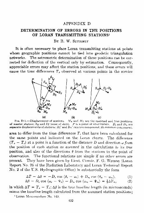
APPENDIX D

DETERMINATION OF ERRORS IN THE POSITIONSOF LORAN TIMNSMITTING STATIONS’

BY B. W. SITTERLY

It is often necessary to place Loran transmitting stations at pointswhose geographic positions cannot be tied into geodetic triangulationnetworks. The astrometric determination of these positions can be cor-rected for deflection of the vertical only by estimation. Consequently,appreciable errors may affect the station positions, and these errors willcause the time differences Z’o observed at various points in the service

(a) (b) (c)FIQ. D1 .—Displacement of stntions. .llA mid .U= me the assumed and true positic~l,s

of master station; ,5A nnd ST those of slax,c. P k a ]>oillt of ob.erwjtlon. L)b and D., ~rc

separate displacements of st:~tions; .9.’ und D,,,’ rclutivc componmlt; D. conlmon component,

area to differ from the time differences T. that have been calculated forthe same points and indicated on the Loran charts. The difference

(2’0 – 7’.) at a point is a function of the distance D and direction a from

the position of each stfition as assurncd in the calculations to its true

position, and also of the directions O from the stations to the point ofobservation. The functional relations arc simple if no other errors arepresent. They ]mvc been given by Licut. Comdr. F. G. l~atson (LoranReport No. 26 of the Radiation I.aboi-story and I.oran Technical ReportNo. 2 of the U.S. Hydrographic Officc) in substantially the form

AZ’ – A@ = –D, COS (8, – u,) + D,,+ ~OS (em – u~). (1)A/5’= D, COS (u, – ~,) – ~,,, COS (un – ~~) = +A?’m, (2)

in which AT = TO — T.; AD is the true baseline kmgth (in microseconds)minus the baseline length cdculatcd from the assumed station positions;

LLoran Ilcmorandmn .No. 14!).

432

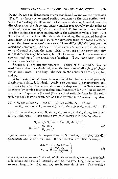
DETERMINATION OF ERRORS IN LORAN STATIONS 433

D, and D~ are the distances in microseconds and w and o~ the directions(Fig. D.la) from the assumed station positions to the true station posi-tions, s indicating the slave and m the master station; e, and emare thedirections from the slave and master station respectively to the point atwhich AT was obtained; AT~ is the value of T observed on the extendedbaseline behind the master station, minus the calculated value of (2B + 6);V, is the direction from the slave station along the extended baselineaway from the master; and ~~ is the direction from the master stationalong the baseline toward the slave (these differ slightly because themeridians converge). All the directions must be measured in the samesense of rotation from the same initial direction; either sense and anyinitial direction may be chosen, but clockwise and north are convenientchoices, making all the angles true bearings. They have been used inall the examples below.

Values of T. are directly observed. Values of T., 0, and v may be.read from a chart or calculated, since the locations of all points of obser,vation are known. The only unknowns in the equations are D., u., D~,and co~.

If four values of AT have been obtained by observation at properly

distributed points, it is ideally possible to compute the magnitudes and

directions by which the actual stations are displaced from their assumed

locations, by solving four equations simultaneously for the four unknown

quantities. Equations (1) and (2) are not of suitable form for the solu-

tion, but they may be combined and transformed into the single equation

AT = Da COSCJ,(COS~, – cos d,) + D, sin ti, (sin V, — sin 6$)

– D~ cos ti~(cos Vm – cos om) – Dm sin un(sin Vm – sin t?n), (3)

which is linear if D, cos co,, D, sin w,, Dm cos tire, and Dm sin OJmare takenas the unknowns. Wrhen these have been determined, the equations

(4)

together with two similar expressions in D., and u~, ;vill give the dis.

placements and their directions. If the directions are true bearings,

where O, is the assumed latitude of the slave station, A@, is its true lati-

tude minus its assumed latitude, and Al, its true longitude minus its

assumed longitude. A+, and Al, are in seconds of arc. The positive

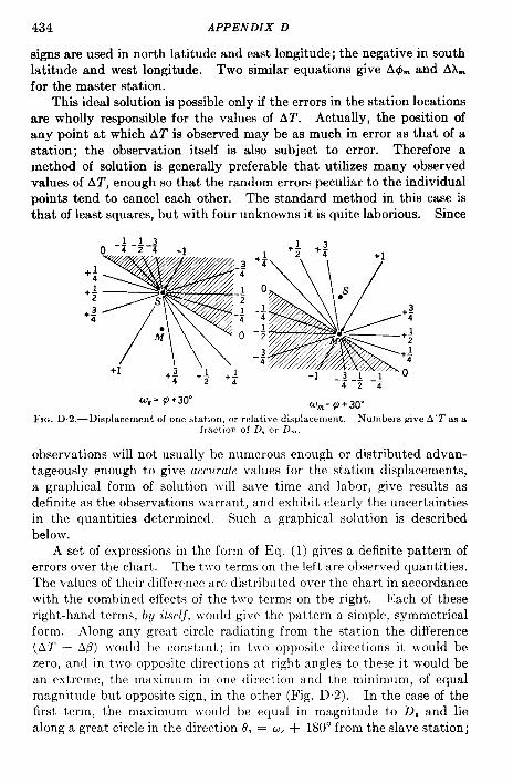
434 APPENDIX D

signs are used in north latitude and east longitude; the negative in southlatitude and west longitude. Two similar equations give AI#J~and ALfor the master station.

This ideal solution is possible only if the errors in the station locationsare wholly responsible for the values of AT. Actually, the position ofany point at which AT is observed may be as much in error as that of astation; the observation itself is also subject to error. Therefore amethod of solution is generally preferable that utilizes many observedvalues of AT, enough so that the random errors peculiar to the individualpoints tend to cancel each other. The standard method in this case isthat of least squares, but with four unknowns it is quite laborious. Since

F]Q. D,2.—Displacement of one station, or relatix.e displacement. Numbers give A’T as afraction of D, or D,,,.

observations will not usually be numerous enough or distributed advan-tageously enough to give accurate ~alues for the station displacements,a graphical form of solution ~rill save time and labor, give results asdefinite as the observations warrant, and exhibit clearly the uncertaintiesin the quantities determined. Such a graphical solution is describedbelow.

A set of expressions in the form of Eq. (1) gi~res a definite pattern of

errors over the chart. The two terms on the left are observed quantities.The values of their difference are distributed o~-er the chart in accordancewith the combined effects of the two terms on the right. Each of theseright-hand terms, by itscl~, would give the pattern a simple, symmetricalform. Along any grrat circle radiating from the station the difference(Al” – A~) would be constant; in t,vo opposite directions it would bezero, and in ttvo opposite directions at right angles to these it would be

an extreme, the maximum in one direction and the minimum, of equalmagnitude but opposite sign, in the other (Fig, 1),2). In the case of thefirst term, the maximum would be equal in magnitude to D, and liealong a great circle in the direction d. = u, + 180° from the slave station;

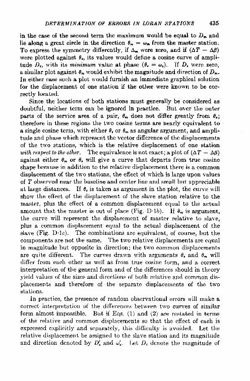
DETERMINATION OF ERRORS IN LORAN STATIONS 435

in the case of the second term the maximum would be equal to D. andlie along a great circle in the direction 0~ = ~~ from the master station.To express the symmetry differently, if A- were zero, and if (AT – A9)were plotted against 0., its values would define a cosine curve of ampli-tude D,, with its minimum value at phase (0, = u,). If D, were zero,a similar plot against 13~would exhibit the magnitude and direction of D~.In either case such a plot would furnish an immediate graphical solutionfor the displacement of one station if the other were known to be cor-rectly located.

Since the locations of both stations must generally be considered asdoubtful, neither term can be ignored in practice. But over the outerparts of the service area of a pair, 0~ does not differ greatly from 0,;therefore in these regions the two cosine terms are nearly equivalent toa single cosine term, with either O,or 6%as angular argument, and ampli-tude and phase which represent the vector difference of the displacementsof the two stations, which is the relative displacement of one stationwith respect to the other. The equivalence is not exact; a plot of (Al” – ALI)

against either 0~ or @, will give a curve that departs from true cosineshape because in addition to the relative displacement there is a commondisplacement of the two stations, the effect of which is large upon valuesof 2’ observed near the baseline and center line and small but appreciableat large distances. If 0, is taken as argument in the plot, the curve willshow the effect of the displacement of the slave station relative to themaster, plus the effect of a common displacement equal to the actualamount that the master is out of place (Fig. D.lb). If t?~is argument,the curve will represent the displacement of master relative to slave,plus a common displacement equal to the actual displacement of theslave (Fig. D. lc). The combinations are equivalent, of course, but thecomponents are not the same. The two relative displacements are equalin magnitude but opposite in direction; the two common displacementsare quite different. The curves drawn with arguments 0, and 0~ willdiffer from each other as well as from true cosine form, and a correctinterpretation of the general form and of the differences should in theoryyield values of the sizes and directions of both relative and common dis-placements and therefore of the separate displacements of the twostations.

In practice, the presence of random observational errors will make acorrect interpretation of the differences between two curves of similarform almost impossible. But if Eqs. (1) and (2) are restated in termsof the relative and common displacements so that the effect of each isexpressed explicitly and separately, this difficulty is avoided. Let therelative displacement be assigned to the slave station and its magnitudeand direction denoted by D, and u:. Let D. denote the magnitude of

436 APPENDIX D

thecommon displacement, and let (u, +~A’l?) denote itsdirection at theslave station and (co. — ~AV) its directional the master station, AV being(v, – v-). Then the equations

define the separate displacements in terms of the relative and Pommondisplacements. Equation (1) may be written as

A’T = –D, cos 08 cos a, – D, sin 0, sin u.+ D~ cos 0~ cos u~ + D,,, sin 0., sin u.,,

where A’T = AT — A~. Substituting the relations (6) gives

A’T = –0, cos 0. cos u; – D, COS8, COS(w, + *A*)– D: sin 0, sin u: – D, sin 0, sin (w. + ~A’Y)+ D. cos f3~cos (UC– ~AV) + DC sin 0., sin (UC– ~AT)

—— –D: COS(8, – u:)– D.{cos [8, – (u. + ~AV)] – COS [tJm – (Q – +AY)]},

which reduces to

A’T = –D; cos (19.– ti~) + 2D. sin h sin (H – w), (7)

where h = ~[(6, – (L) – AV], H = +(o, + 0~), Equation (2) may be

written as

A(3 = D, COS co, COS ~, — Dm COS u. COS ~.

+ D, sin W, sin V, – Dm sin UX sin T,,,,

and substitution of relations (6) leads to

The pattern of errors corresponding to a set of expressions in theform of Eq. (7) is, of course, the same as that corresponding to a set inthe form of Eq. (1). But the two right-hand terms of Eq. (7) contributeto the pattern very clifferently. The first term is similar to either right-hand term of Eq. (1) and gives by itself the same form of distribution(Fig. D2). The second term by itself gives a much more complicateddistribution (Fig. D.3) in which the skew shape is duc to the combinedeffects of the two sine factors, which vary in different ways with directionfrom the center of the baseline, whereas the confining of large values toregions not far from the center is due to the first sine factor. Thedistribution is symmetrical in the sense that the term has the same valuein amount and sign at any two points equally distant from the ccntcr inopposite directions. The pattern has different forms for different values

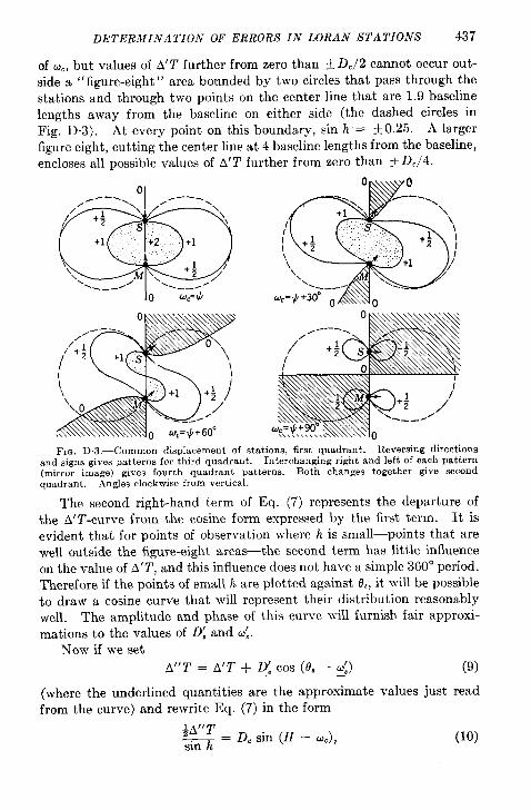
D.ETERMINA TION OF ERRORS IN LORAN STATIONS 437

of W, but values of A’ T further from zero than + D./2 cannot occur out-side a “ figure-eight” area bounded by two circles that pass through the

stat ions and through two points on the center line that are 1.9 baselinelengths away from the baseline on either side (the dashed circles inFig. D.3). At every point on this boundary, sin h = +0.25. A largerfigure eight,cuttingthecenterlineat4 baseline lengths from the baseline,

encloses all possible values of A’T further from zero than t D,/4.

10 UC= !J WC=*+30° 0 ANNYO

w“’ ‘u.~’.&~~%\i 0 w,=Y+60” \

NiNx\ ‘S“::.?:??. .k \\\wo

FIG. D ,3.—Common displacement of stations, first quadrant. Reversing directionsand signs gives patterns for third quadrant. Interchanging right and left of each pattern(mirror image) gives fourth quadrant patterns. Both changes together give secondquadrant. Angles clockwise from vertical.

The second right-hand term of Eq. (7) represents the departure of

the A’ T-curve from the cosine form expressed by the first term. It is

evident that for points of observation where h is small—points that are

well outside the figure-eight areas—the second term has little influence

on the value of A’T, and this influence does not have a simple 360° period.

Therefore if the points of small h are plotted against 0., it will be possible

to draw a cosine curve that will represent their distribution reasonably

well. The amplitude and phase of this curve will furnish fair approxi-

mations to the values of D: and u:.XOW if we set

A“T = A’T + D: COS (8, – u:) (9)—

(where the underlined quantities are the approximate values just read

from the curve) and rewrite Eq. (7) in the form

(lo)

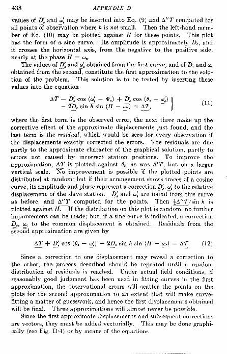
438 APPE.VDIX D

values of ~, and u; may be inserted into Eq. (9) and A(’T computed forall points of obse~ationwhereh isrzot small. Then the left-hand mem-ber of Eq. (10) may be plotted against H for these points. This plothas the form of a sine curve. Its amplitude is approximately D,, andit crosses the horizontal axis, from the negat i~-e to the posit i~-e side,nearly at the phase” H = u..

The values of ~j and ~~obtained from the first curve, and of D. and wobtained from the second, constitute the first approximation to~he solfi-tion of the problem. This solution is to be tested by inserting thesevalues into the equation

where the first term is the observed error, the next three make up thecorrective effect of the approximate displacements just found, and thelast term is the residual, which would be zero for every obsemation ifthe displacements exactly corrected the errors. The residuals are duepartly to the approximate character of the graphical solution, partly toerrors not caused by incorrect station positions. To improve theapproximation, AT is plotted against 8,, as was A’T, but on a largervertical scale. To improvement is possible if the plotted points are

distributed at random; but if their arrangement sho~vs traces of a cosinecurve, its amplitude and phase represent a correction D:, CJto the relativedisplacement of the sla}’e station. ~, and ~~ are found from this curyeas before, and A“T computed for—”the points. Then ~A’’T/sin h is

plotted against H. If the distribution on this plot is random, no furtherimprovement can be made; but, if a sine curve is indicated, a correction~., w to the common displacement is obtained. Residuals from thei~co~d approximation are given by

AT + Q; cos (0. – gj) – 2D. sin h sin (H – W) = AT. (12). ——

Since a correction to one displacement may reveal a correction tothe other, the process described should be repeated until a randomdistribution of residuals is reached. Under actual field conditions, if

reasonably good judgment has been used in fitting curves in the first

approximation, the observational errors w-ill scatter the points on the

plots for the second approximation to an extent that v-ill make curve-fitting a matter of guesswork, and hence the first displacements obtainedwill be final. Three approximations will almost never be possible.

Since the first approximate displacements and subsequent correctionsare vectors, they must be added vectorially. This may be done graphi-cally (see Fig. D.4) or by means of the equations

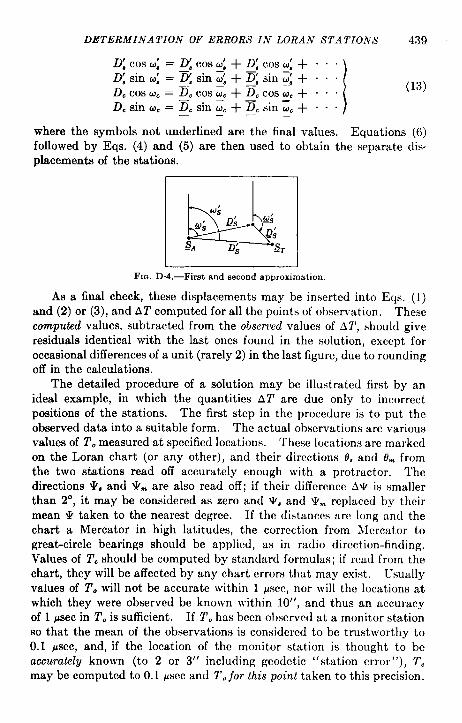
DETERMINATION OF ERRORS IN LORAN STATIONS 439

where the symbols not underlined are the final values. Equations (6)followed by Eqs. (4) and (5) are then used to obtain the separate dis-placements of the stations.

F1~. D.4.—Firat and second approximation.

As a final check, these displacements may be inserted into Eqs. (1)and (2) or (3), and AT computed for all the points of observation. Thesecomputed values, subt ratted from the obsen’ed values of AT, should giveresiduals identical with the last ones found in the solution, except foroccasional differences of a unit (rarely 2) in the last figure, due to roundingoff in the calculations.

The detailed procedure of a solution may be illustrated first by anideal example, in which the quantities AT are clue only to incorrect

positions of the stations. The first step in the procedure is to put the

observed data into a suitable form. The actual observations arc various

values of To measured at specified locations. These locations arc markedon the Loran chart (or any other), and their directions 8, and L fromthe two stations read off accurately enough with a protractor. Thedirections T, and V~ are also read off; if their difference AZ is smallerthan 2°, it may be considered as zero and V, and ~~ rcplaccd by theirmean * taken to the nearest degree. If the distances arc long and thechart a Mercator in high latitudes, the correction from Ifcrcator togreat-circle bearings should be applied, as in radio direction-finding.Values of Tc should be computed by standard formulas; if read from thechart, they will be affected by any chart errors that may exist. usuallyvalues of To will not be accurate within 1 psec, nor will the locations atwhich they were observed be known ~vithin 10”, and thus an accuracyof 1 psec in To is sufficient. If T. has been observed at a monitor stationso that the mean of the observations is considered to be trustworthy to0.1 Ysec, and, if the location of the monitor station is thought to beaccurately known (to 2 or 3“ including gcocfctic “station error”), T.may be computed to 0.1 pscc and T. jor this poin~ taken to this precision.

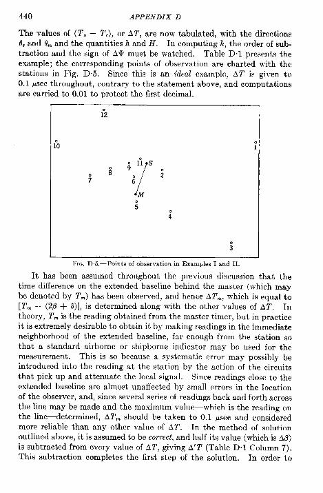
440 APPENDIX D

The values of (To – T.), or AT, are now tabulated, with the directions0, and t)~and the quantities h and H. In computing h, the order of sub-traction and the sign of AV must be watched. Table D.1 presents the

example; the corresponding points of observation are charted with the

stations in Fig. D.5. Since this’ is an ideal example, AT is given to0.1 ~sec throughout, contrary to the statement above, and computations

are carried to 0.01 to protect the first decimal.

FIG. D5.-Points of observation in Examples I and II.

It has been assumed throughout the previous discussion that the

time difference on the extended baseline behind the master (which may

be denoted by T~) has been observed, and hence AT~, -which is equal to

[T- – (26 + 6)], is determined along with the other values of AT. Intheory, Tn is the reading obtained from the master timer, but in practiceit is extremely desirable to obtain it by making readings in the immediate

neighborhood of the extended baseline, far enough from the station sothat a standard airborne or shipborne indicator may be used for themeasurement. This is so because a systematic error may possibly beintroduced into the reading at the station by the action of the circuitsthat pick up and attenuate the local signal. Since readings close to theextended baseline are almost unaffected by small errors in the locationof the observer, and, since several series of readings back and forth acrossthe line may be made and the maximum valu-which is the reading onthe line—determined, ATn should be taken to 0.1 ~sec and consideredmore reliable than any other value of AT. In the method of solutionoutlined above, it is assumed to be correct, and half its value (which is AD)is subtracted from every value of AT, giving A’ T (Table D. 1 Column 7).This subtraction completes the first step of the solution. In order to

DETERMINATION OF ERRORS IN LORAN STA TIONL~ 441

avoid introducing the small systematic error that would result fromrounding off 4AZ’~, all the values of A’T should be recorded to 0.1 vsec,though individually they have not this precision. Note that AT’~ istabulated with the rest (last line of Table D.1, with the label M); for it,

Oa = V. + 180°, 6’~ = ** + 180°, h = 0°,AT. – AD = A’T. = GAT.. )

(14)

The second step in the solution is the determination of approximatevalues of D, and ti~. For this purpose it is convenient to divide the data

10

—Ao

*1G+9+8

Scale for W’S

A

% lo~ aleos +790” 60° 30° 360°330”300”270° 9 .081 .012 .OtZ .012 .00t .OfC .09S +6

~ +G !

Horizontal plottlng scale v‘360°330° 300”270”240”210”180° 150” 120° 9=

FIG. D.6.—Family of curves.

+1 +

K)&o”

of observation into three classes, (Table D. 1, Column B), Class Aincluding values for which h is less than 15°, Class B including those forwhich it is between 15° and 30°, and Class C those for which it is 30°or more. These limits are arbitrary, simply cli~iding up the data accord-ing to the importance of the sine term in Eq. (7). As the classes arechosen here, Class A includes all points outside the dashed “figure eight”in Fig. 1).3. A rectangular graph is prepared, on which A’ T is plottedvertic:dly against 13Shorizontally. The different classes are identifiedby different symbols so that in fitting a cosine curve to the points, thoseof Class A may be given the greatest weight. Points of Class C, forwhich influence of the sine factor may predomirmte, should be practicallyignoredinfittingthecurveand may \vell be omitted from the graph.

.1 simple and ro.pid v-ay to fit a cosine curve to the points is to use af~mily of such curves of different amplitudes, dra]~-n on transparentmaterial. ?Figure D.(3 may be carefully copied on tracing cloth or paper

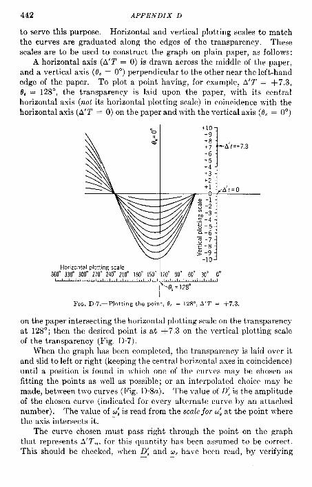
442 APPENDIX D

to serve this purpose. Horizontal and vertical plotting scales to matchthe curves are graduated along the edges of the transparency. Thesescales are to be used to construct the graph on plain paper, as follows:

A horizontal axis (A’Z’ = O) is drawn across the middle of the paper,

and a vertical axis (0. = 0°) perpendicular to the other near the left-handedge of the paper. To plot a point having, for example, A’T = +7.3,0, = 128°, the transparency is laid upon the paper, with its centralhorizontal axis (not itshorizontal plotting scale) incoincidence with thehorizontal axis (A’Z’ = O)onthe paper andw-it hthevertica laxis(6, = 0°)

Horizontal plotlng scale360”330”3tUl”270”240”210”180”150”120”90” 60” 30” O“

%,= 128°

FIc. D7.-Plottingt hepoint,0, = 128°,A’~ = +7.3.

on the paper intersecting the horizontal plotting scale on the transparencyat 128°; then the desired point is at +7.3 on the vertical plotting scaleof the transparency (Fig. D.7).

When the graph has been completed, thetransparency is laid overitand slid to left or right (keeping the central horizontal axes in coincidence)until a position is found in which one of the cur~-es may be chosen asfitting the points as well as possible; or an interpolated choice may be

made, between two curves (Fig. D.8a). The value of D: is the amplitudeof the chosen curve (indicated for every alternate curve by an attachednumber). The value of u: is read from the scale jor u: at the point where

the axis intersects it. –The curye chosen must pass right through the point on the graph

that represents A’T,,,, for this quantity has been assumed to be correct.This should be checked, when D: and W, have been read, by verifying—

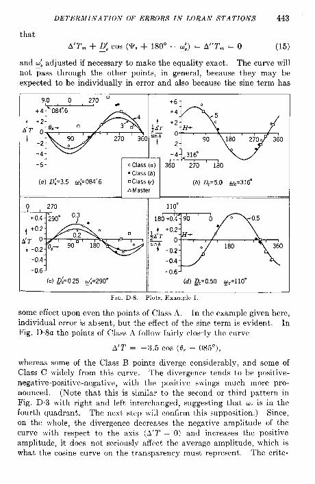
DE TERJ41NA TION OF ERRORS IN LORAN STATIONS 443

that

A’T~ + ~. COS (T, + 180° – c&) = A“T_ = O (15)—

and u: adjusted if necessary to make the equality exact, The curve will

not ~ass through the other points, in general, because they may be

expected to be individually in error and also because the sine term has

-~J o Class (a) 360 ‘ 2;0 ‘ lAO● Class (b)

(a) Q;=3.5 @~=084”.6 nClass (c) (b) Q=5.O gc=3160A Master

o 270 II 110”I , 1+o.4- 290”

, +02

A(T O

~‘*- ‘8%0

i -o.2- Os- 90

-0.4

-0.6

(C)Q;=O.25 g~=290” (d) QC=0.50 gc=l 10”

FIG. D. S.—Plots, Example I.

some effect upon even the points of (lass .A. In the example given here,

individual error is absent, but the effect of the sine term is evident. In

Fig. D.8a the points of Class A follow fairly clos-ly the curve

A’T = –3.5 COS (0, – 0850),

whereas some of the Class B points diverge considerably, and some ofClass C widely from this curve. The divergence tends to be positive-

negative-positive-negative, with the positive swings much more pro-nounced. (Note that this is similar to the second or third pattern inFig. D.3 with right and left interchanged, suggesting that u. is in the

fourth quadrant. The next step will confirm this supposition. ) Since,on the whole, the divergence decreases the negative amplitude of thecurve with respect to the axis (A’T = O) and increases the positiveamplitude, it does not seriously affect the average amplitude, which iswhat the cosine curve on the transparency must represent, The crite-

444 APPENDIX D

rion that D; cos (200° — @ must exactly equal —1.50 requires~’ = 084:6 if?, = 3.5o. The–tenthsof adegree have no real significance–abut are retained so that subsequent computations shall check out to0.01 ~sec. The phase (CO:= 084~6) is the horizontal interval from thevertical axis (0, = 0°) t–o the abscissa at which the curve attains itsextreme negative ordinate, but the scale forti~ gives this interval directlyat the point where the vertical axis intersects it.

The third step is the determination of approximate values of D, anda,. Adopting the values found above as first approximations to D:and w:, A“T and then (~A’’T/sin h) are computed for all points (first fivecolumns of Table D.2), and the latter quantity isplotted against H(Fig.D.8b). The computations may be performed very rapidly withasliderule having a sine scale. NTotethat A”Tn = O,asitshould be, and that

since sin h = O for the extended baselines, the quotient is indeterminateand therefore the point representing the master reading Z’- cannotappear on this plot. In fitting a curve to the plot, it must be borne in

mind that points of Class C should be given highest weight and pointsof Class A almost no weight. Ideally, they should all fit the curve, but

actual small divergences will be greatly magnified in the case of a Class Apoint by the small denominator of the quotient (iA’’T/sin h) so that alarge departure of the point from the curve will indicate only a smalldivergence in A“T. Class B points behave similarly, in less degree.The points are in effect weighted in proportion to h and should be treatedso.

The points of Class C in Fig. D.8b fit the curve of amplitude 5, onthe transparency, very well, in the position where the interval is about316° from the axis (H = 0°) to the rising intersection of the curve withthe axis (~A’’T/sin h = O). The scale jor w (just below the scale foru: on the transparency) reads 316° at the point where the axis (H = 0°)crosses it. Since no one point on the curve has to be exactly fitted,w is not determined to a fraction of a degree, as was co:. The departure~f points of Classes A and B from the curve defin;d by the Class Cpoints is very slight, considering the weighting effect just described, butit is systematically positive, indicating that the previous determina-tions of ~. and u: are slightly in error. The second approximation willtake care of this:

The first approximation to the solution of the example has been foundto be

D; = 3.5o psec, co; = 084°6,D. = 5,00 psec, ;. = 316~0.— —

The fourth step is to compute the residuals ~T, by Eq. (11), and plotthem against 0,. If the plot shows a systematic trend, a second approxi-

DETERMINATION OF ERRORS IN LORA.V STATIONS 445

mation is made. The first three terms of Eq. (11) add up to A“T’, for

D: COS(@:– T) was made exactly equal to A@. Consequently— —

A“Z’ – 10.00 sin h sin (H – 316°) = AT,

in this example. The sine term is computed for each observation (again

a rapid slide-rule process] and set down in (’olumn 7, Table D.2, andColumn 1 minus Column 7 gi~resAl’ in Column 8.

For the second approximation,

A~ = O,IT = –D; COS (0. – ~j) + 2DC sin h sin (H – cu.),

1

(16)AT,. = 0,-

— -.

corresponding to Eqs. (7) and (8), AD and AT- being the residuals to thebaseline length and to the master-extension reading. These are zerobecause AP was exactly fitted in the first approximation. When theresiduals of Table D.2 are plotted against 0, (Fig. D.8c), the periodicdistribution of the points of Classes A and B shows that D. is of appre-ciable size, and the separation of the Class C points fr~m the otherssuggests that D. is also appreciable.

We theref%e proceed to the second approximation. The point

representing the master extension reading (AT- = O, .9. = 200°), whichthe curve must again pass through, requires U: = 110° or 290° (expressingthe fact that D; must make right angles wit~the baseline if @ is not to becorrected further). Evidently the latter value is the right one, and thecurve D: = 0.25 fits the Class A and B points quite well. ~TOW thequantifies 0.25 cos (0. – 290°) are computed and added to ~, giving

A“ T, which is halved and divided by sin h (Table D.3, first five columns).These last quantities are plotted against H, on the large scale again.From this plot the values D, = 0.50, W. = 110° are obtained (Fig. D.8d).

To test the adequacy ~ the second approximation, new residuals ATare now obtained by computing the quantities 1.00 sin h sin (H – 100°)(Column 7 of Table D2) and subtracting this column from Column 4.Only two residuals exceed 0.05; and since the original errors were givenonlY to 0.1, this is a practically perfect agreement, and there is no need

to make another plot.The last step is to combine the first approximations with the correc-

tions to obtain the second approximations, which are taken as final, andto compute from these the separate station displacements. Equations(13) and then (6), (4), and (5) are solved by slide rule. The computationis given in Table D.+, the results being

Dm = 4.56 ~sec, w., = 317~8, A@~ = +33”, AL = –39”,D, = 3.91 psec, us = 00476, A@, = +38!’, AX, = +4”,

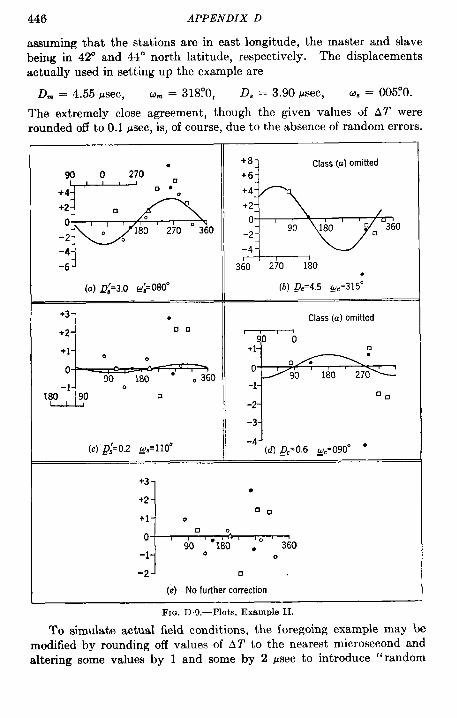
I446 APPENDIX D

assuming that the stations are in east longitude, the master and slavebeing in 42° and 44° north latitude, respectively. The displacementsactually used in setting up the example are

Dm = 4.55 psec, co~ =318Y0, D. = 3.90 psec, W, = 005:0.

The extremely close agreement, though the given values of AT wererounded off toO.1 gsec, is, of course, duetothe absence of random errors.

;p,ol;k;,,.

(a) Q:=3.O U:=wo” (b) Qc=4,5 @=315°

+3-

,8=’0 TF$

-3

(C)”Q;=0,2 gs=llo”-4

(d) Q=O.6 9=090° “—

+3

k

●

+200

+1 0

0❑ o

90 “180 .0 360-1 0 0

-2 0

(e) No further correction

F1~. D9,-Plots, Exampl.e IL

To simulate actual field conditions, the foregoing example may bemodified by rounding off values of AT” to the nearest microsecond andaltering some values by 1 and some by 2 ~sec to introduce “random

DETERMINATION OF ERRORS IN LORAN STATIONS 447

errors. ” One value of AT, to represent an accurately located monitorstation, is given correctly to 0.1 (this is observation 4). The modifiedvalues of AT appear in Table D.5, Column 2 (6., %, h, and H are thesame as in the first example), and the first approximation fills the remain-ing columns of the table, whereas the plots are shown in Fig. D.9a andb. The points of Class A are omitted from the second plot; their lowweight and their scatter make them practical y useless here. The curvefor ~. and ~ is made to fit the monitor station exactly. When theresiduals AT are plotted against 0, (Fig. D.9c), it is evident that the“errors” leave little meaning to a second approximation, but a slightimprovement in D: is suggested. When *A” T/sin h is plotted (Fig.D.9d), it appears that if a small error at the monitor station is admitted,the other Class C points can be satisfied a little better. The secondapproximation is detailed in Table D“6; and when AT (Column 6) isplotted (Fig D.9e), it is evident that no further approximation willmean anything. The residuals that are introduced into the example

(Table D5, Column 2, minus Table D 1, Column 2) are given in Column

7. They are not quite so small as those resulting from the solution.

This, of course, should be so, for the solution accommodates itself to theerroneous “observed readings,” not to the “true” values. The finalvalues are given in Table D.7.

The relative displacement of the slave with respect to the masterwas used in Eq. (7) instead of that of the master with respect to theslave, because Loran stations are commonly operated in triplets, onemaster working with two slaves. When this is the case, solution is madefor the displacements of the three stations. The relative displacementof each slave is determined from the observations on the pair of which itis a member, but the master displacement, which is D. for all three sta-

tions, is found by combining the observations on both pairs in a singlesine curve. Of course all directions for both pairs must be measuredfrom the same zero direction. If a triplet operates with two mastersand one double slave, the relative displacements must be assigned tothe masters and D. made equal to the slave displacement. The sub-scripts s and m must be interchanged in all the equations, and the signsof the cosine terms in Eqs. (7) to (12) and (15) and (16) must be reversed.

Example 111, which appears in Tables D“8, D“9, and D. 10 and Fig.D. 10, deals with an actual triplet. Evidently larger errors of observa-tion are present than in Example II. These errors appear to obscurethe common displacement altogether, though the relative displacementsare conspicuous. The curve in Fig. D 10c was made to fit the two moni-tor readings (observations 3 and 16). It represents the other pointsfor the first pair about as well as any curve (though not much betterthan a straight line), but the points for the second pair call for a larger

448 APPENDIX D

displacement in the opposite direction. In Fig. D. led, residuals fromthe first approximation are plotted against d, for the two pairs. Theseplots (which are not expanded in vertical scale) give no encouragementtoward a second approximation; so the first is taken as final. TableD 10 includes values of the displacements of these stations as obtainedfrom geodetic data, for comparison with the results of the solution. Ifthe geodetic values are inserted into Eq. (1 1), the sum of the squaresof the residuals obtained is 50 per cent larger than the sum of (AZ’)2 fromTable D.9, suggesting that the geodetic data are somewhat questionable.

o470

J “.-lo

(a) F,rst pair. ~~= 5.5 Q~=286~5

-$--=--

J .-10

A

(c) Both pairs. ~C=l.3 @c= 073°

+101

:W’”(b) Second pair. Q:= 6.5 M:= 148”

!+60(d) First

1

econd )pare. No corrections

+5~.

o090 A- 180

w.270 360

AA m–5 ■

FIG. DIO.-Plots, Example III.

As already mentioned, it has been assumed throughout that the time

difference Z’- on the extended baseline behind the master station has

been correctly observed. It has also been assumed that the correct

coding delay has been held at the slave station. The coding delay should

be checked by observation on the extended baseline behind the slave, for

the delay set on the timer may not be the actual delay in transmission.

A systematic error may occur here, as in monitoring at the master sta-

tion, and for the same reason. If the delay that actually occurs is

greater than that set for the pair, all observed readings will be greater

than corresponding computed readings by the amount of the excess,

and the quantity J (observed) minus 8 (computed), which may be denoted

by Ad, should be subtracted from all readings including Tm, before thevalues of AT are taken.

If for any reason trustworthy observed values of 6 and T~ have not

DETERMINATION OF ERRORS IN LORAN STATIONS 449

been obtained, it is possible, in theory at least, to obtain them in thecourse of the graphical solution. Considering A6 and A~ as unknowns,Eq, (7) is written in the form

AT = [Ad + 4A13– D: cos (e. – u;)] + 2D. sin h sin (H – u.). (17)

On the first plot, AT is plotted against d.. A vertical line is drawn onthe plot at (8. = + 180°). The central horizontal axis of the family ~of curves is not constrained to remain in coincidence with the axis

*

AT=A6+A6N ——— —.——----- - ~jA@AT=Ab+~ M3 *~A6

AT=A6~– - ‘–– – ‘- ;–– ‘–- &AT= O

d

O;=O”e:=IJ+18&’FrQ. D.1 l.—Graphlcal solution if A(3 and A& are unknown.

(AT = O) of the plot, but the curves are moved both vertically andhorizontally until the points of Class A are fitted. D: and u. are readas before, but now in addition (Fig. D. 11) the vertical—distanc~, from theaxis (AT = O) of the plot to the central horizontal axis of the curves, isequal to A5 + $&~, whereas the vertical distance, from the central hori-zontal axis of the curves to the point where the curve of amplitude D{crosses the line (8, = Y + 180°), is equal to ~AL?,the upward (downward)direction in either case indicating the positive (negative) sign. ThenEq. (9) becomes

A“T = AT – (A8 + ~A~) +2: cos (h – ~:), (18)—

and the rest of the first approximation is performed as before. In Eq.(11) defining the residuals, the term – A~ is added to the left-hand mem-ber. In the second approximation the process described above isrepeated, yielding corrections A6 and AD along with the other corrections.

In dealing with real observations, the introduction of two moreunknowns into the solution tends to make the convergence of the approxi-mate process slower, and thus an additional approximation may berequired to reduce residuals to minimum size and random distribution.A more serious effect is that the individual uncertainties of the quantitiesdetermined are increased, because A6, Afi, and the component of D.perpendicular to the baseline contribute to AT in very much the sameway, over a large part of the service area. So the solution in a givencase, obtained by any method of analysis, maybe quite misleading becauseof a few errors of observation if the extended baseline readings have notbeen obtained.

Of course, the displacements as determined will be affected by thecomputer’s judgment in giving relative weights to discordant observations.

450 APPENDIX D

Thk difficulty is unavoidable. No method except the laborious least-squares solution will apportion the influence of the several observationsautomatically or will assign separate probable errors to the quantitiesdetermined. The graphical treatment has the advantage of making theuncertainties evident and providing some basis for their estimation.For instance, in Example II it is clear from the plots that Observation7 is particularly discordant, and that the relative displacement of theslave station is determined much more definitely than the commondisplacement, which is very dependent upon the relative weights givenObservations 2, 6, and 9 and 11 (assuming that the “ monitor reading”No. 4 is of high weight). Actually, the first approximation, in whichObservations 9 and 11 were almost ignored and Observation 2 and themonitor were considered exactly correct, is nearer the “ truth” than thefinally adopted value, which distributes the discordances more evenly.In Example III, the directions of the relative displacements are verydefinite. Their magnitudes are more doubtful, but the true values areprobably not less than half or more than twice those adopted. How-ever, the individual locations of all the stations remain quite uncertainbecause even the quadrant in which the common displacement lies isnot sure. This situation is often to be expected if a solution is madefrom observations taken on routine missions, for there will usually be adeficiency and a poor distribution of Class C points, because of the smallarea within which they must lie. To locate the stations definitely,observations must be obtained in numbers sufficient to cancel out localerrors, in all four quadrants, both well within the figure-eight area (nearthe baseline) of each pair and well outside it. In this case a Ieast-sqtlaresolution may be worthwhile, using Eq. (3) with a constant term A6 addedto the right-hand member and treating the readings made on the baseline

extensions simply as single observations of very high weight.Although the solution of Example III gi~es geographic station posi-

tions that are uncertain in an absolute sense, a Loran chart calculatedfrom these positions will be in good accordance with observation overmost of the service area, for only near the baselines do the absolutepositions have much effect on the readings, and here the time-cliff erenceerrors in microseconds have the least equivalents in miles. In general,

‘ the final results Ad and AX are to be regarded as formal corrections bymeans of which a chart fitting the observations may be computed, not asaccurate station displacements. It may well be that the real principal

cause of observed discrepancies is systematic error in the survey databy which features of the terrain have been charted. In this case thesolution will bring the locations of the stations into the frame of referencedefined by the terrain, whatever that may be. But, after all, this iswhat the navigator wants.

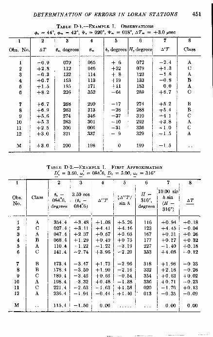
1

ohs. No

123456

789

101112

M

1

Ohs.No.

123456

789

101112

M.—

DETERMINATION OF ERRORS IN LORAN STATIONS 451

TABLE D. 1.—EXAMPLE 1. OBSERVATIONS~, = 44”, ~“ = 42”, ‘I?. = 020°, ‘Z~ = 018°, AT~ = +3.0 @ec

2

AT

–0.9+2.8–0.3+0.7+1.5+8,2

+6.7+6.9+5,6+5.3+2.5+3.0

+3.0

Class

AcA33Ac

BBcAcA

.

3 4

., degrees em

079 065112 046132 114153 113195 171226 352

258 290263 313274 346283 301306 006321 337

200 198

5

i, degrees

+6+32+8+19+11–64

–17–26–37–lo–31–9

o

6

{, degree

072079123133183289

274288310292336329

199

7

A(T

–2.4+1.3–1.8–0.8

0.0+6.7

+5.2+5.4+4 1+3.8+1.0+1,5

+1.5

TABLE D ,2.—EXAMPLE I. FIRST APPROXIMATIOND: = 3.50, W: = 084:6, D, = 5.00, u. = 316”— — — —

2

0, –034~6,

degrees

354.4027.4047.4068.4110.4141.4

173.4178.4189.4198.4221.4236.4

115.4

3

3,50 Cos

(6’, –

084~6)

+3.48+3,11+2.37+1.29–1.22–2,74

–3.47–3.50–345–3.32–2.63–1.94

–1.50

4

A“T

+1.08+4.41+0.57+0.49–1.22+3.96

+1.73+1.90+0.65+0.48–1.63–0.44

0,00

5

%A”TIsin h

+5,26+4. 16+2.05+0.75–3.19–2.20

–2 96–2.16–0.54–1.38+1.58+1.40

6

H–316°,

degrees

116123167177227333

318332354336020013

. .

7

0.00 Suh Sk(H –316”)

+0. 94+4.45+0.31+0.17–1.40+4.08

+1.96+2.16+0.63+0.71–1.76–0.35

0,00

8

class

AcABAc

BBcAcA

. .

8

AT—

+0.18–0.04+0. 26

+0.32+0.18–0.12

–0.23–0.26+0.02–0.23+013–0.09

0,00

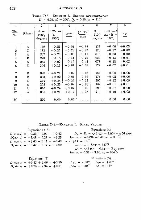
452

Ohs.No.

123456

789

101112

M

APPENDIX D

TABLE D.3.—EXAMFLE I. SECOND APPROXIMATION

[Class)

AcABAc

BBcAcA

D: = 0.25, :: = 290°, D. = 0.50, ~c = 110°— —-2

08 –290”,

degrees

149182202223265296

328333344353016031

270

-3

1,25 COS

(0, –

290°)

–0.21–0.25–0.23–0.18–0.02+0.11

+0.21+0.22+0.24+0.25+0.24+0.21

0.00

_4

A“T

–0.03–0.29+0.03+0. 14+0.16–0.01

–0.02+0.04+0 26+0. 02+0. 37+0.12

0.00

5

}A”T/

sinh

–0.14–O 27+011+021+0.42+0.01

+0 03–0.05–0.22–O 06–0.36–0.38

6

H–110°,

degrees

322329013023073179

164178200182226219

7

.00 sin Iin (H –

110°)

–0.06–0.27+0.03+0.13+0 18–0.02

–0.08–0.02+0.22+0.01+0.37+0.10

0,00

8

AT—

+0. 03–0.02

000+0.01–0.02+0. 01

+0.06+0.06+0.05+0.01

0.00+0.02

0.00

TABLE D4.-EXAMPLE I. FINAL VALUES

Equations (13) Equations (4)

D: COSQ: = +0.33 +0.09 = +0.42 D~ = D. = ti3.43z + 3.00’ = 4.56 @ec

D: sin u: = +3.48 – 0.23 = +3.25 tan u. = –3.00/+3.43, u. = 318’?8D, COSWC= +3.60 – 0.17 = +3.43 ~. + ~A~ = 319:8DC sin o. = –3.47 + 0.47 = –3.00 o,n = w —~AY = 317!8

D, = <3.902 + 0.312 = 3.91 ~sectan o. = 0.31/+3.90, u, = CK)4~6

Equations (6) Equations (5)

D, COSLO.= +0.42 + 3.48 = +3.90 A@~ = +33” A& = +38”

D. sin m = +3.25 – 2.94 = +0.31 AL = –39” AX, = +4”

DETERMINATION OF ERRORS IN LORAN STATIONS 453

TABLE D5.-EXAMPLE II. OSEERVATIONSAND FIRST APPROXIMAITONSStations, observation points, angles, and AT* same as in Exarnrde I

1

Ohs.No.

123456

789

101112

M

1

Ohs. No

12

3456

789

101112

M

(class)

AcABAc

BBcAcA

.

D; = 3.0, a; = 080°, De = 4.5, U. = 315°— — — —

2

AT

0.0+3.0–1.0

+0.7+2.0+6.0

+9.0+6,0+7.0+5.0+4.0+1.0

+3.0

3

A’T

–1.5+1.5–2.5–0.8+0.5+4.5

+7.5+4.5

+5.5+3.5+2.5–0.5

+1.5

4

3.0 Cos(Oa –084)0)

+3.0+2.5+1. s+0.9–1.3–2.5

–3.0–3.0–2.9–2.8–2.1–1.5

–1.5

5

AIIT

+1.5+4.0–0.7+0,1–0.8+2.0

+4.5+1.5+2.6+0.7+0.4–1.0

0.0

6

4A”T/sin h

+7.2+3.8–2,5+0.2–2.1–1,1

–7.7–1.7–2.2–2.0–0.4+3.2

. . . . .

7

).0 Sio hin (H –

315°)

+0.8+4.0

+0.3+0.1-1.3+3.5

+1.8+1.8+0.5+0.6–1.7–0.3

0.0

TABLE D6.-EXAMPLE IL SECOND APPROXIMATIOND, = 0.6, w -090”——

(Class)

AcABAc

BBcAcA

.

g = 0.’

2

0.2 Cos(08 –110°)

+0.2

+0.2+0.2

+0.10.0

–0.1

–0.2–0,2-0.2-0.2–0.2–0.2

0.0

>’ = Ilc.’

3

A,IT

+0.9+0.2–0.8+0.1

+0.5–1.6

+2.5–0.5+1.9–0.1+1,9–0.9

0.0

4

;A”T/—sin h

+4.3+0,2–2.9+0.2+1.3+0.9

–4.3+0.6–1.6

+0.3–1.8+2.9

. . . .

5

1.2sinhsin (H –

090”)

0.0-0.1-?-0,1+0.3+0.2+0.4

0.0+0.2+0.5+0.1+0,6+0.2

. . . . .

6

AT—

+0.9+0.3–0.9–0.2+0.3–2.0

+2.5–0.7+1.4–0.2+1.3–1,1

0.0

8

AT—

+0.70.0

–1.00.0

+0.5–1.5

+2.7–0.3+2.1+0.1+2,1–0.7

0.0

7

True AT—

+0.9

+0.2–0.7

0.0+0.5–2.2

+2,3–0.9+1,4–0,3+1,5–2.0

0.0

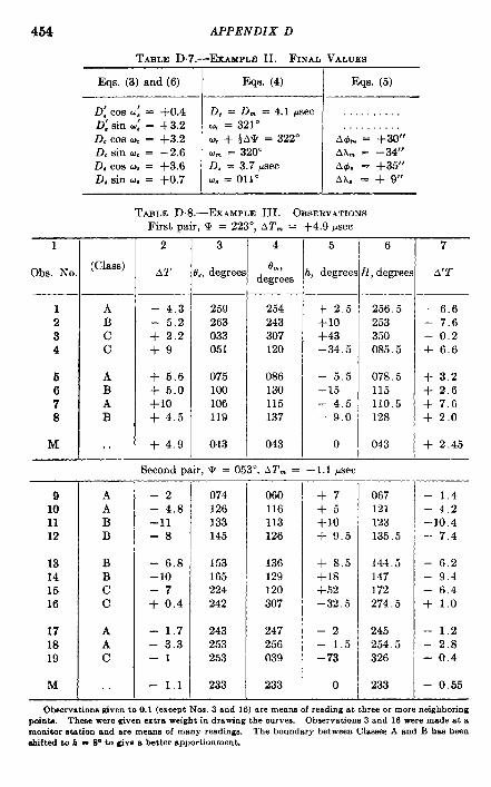
454 APPENDIX D

TABLE D.7.—EkAMPLE II. FINAL VALUES

Eqs. (3) and(6) Eq8. (4) Eqs. (5)

D:cosu: = +0.4 D, = D. = 4.1 Xec . . . .

D; sin Q: = +3.2 O. = 321° . . . .D. COSo. = +3.2 W. + 5A* = 322° A& = +30”D. sin cu. = –2.6 U. = 320” AA~ = —34”

D, cOSo. = +3.6 D, = 3.7 mec Ad, = +35”D, sin u, = +0,7 m, = 011° AA, = + 9“

TABLE D.8.—EXAMPLEIII. OBSERVATIONSFirst pair, ~ = 223°, AT~ = +4.9 Msec

1

Ohs. No. (Class)

1234

5678

ABcc

ABAB

M . .

9101112

13141516

171819

M

AABB

BBcc

AAc

2

AT

– 4.3– 5.2+ 2.2+9

+ 5.6+ 5.0+10+ 4.5

+ 4.9

3

,, degree

259263033051

075100106119

043

4

edeg~~es

254243307120

086130115137

043

5

i, degrees

+ 2.5+10+43–34.5

– 5.5–15– 4.5–90

o

Second pair, * = 053°, AT~ = – 1.1 @ec

–2– 4.8–11-8

– 6.8– 10–7+ 0.4

– 1.7– 3.3–1

- 1.1

074126133145

153165224242

243253253

233

060116113126

136129120307

247256039

233

+7+5+10+ 9.5

+ 8.5+18+52–32.5

–2– 1.5– 73

0

{, degrees A’T

—1256,5 – 6.6253 – 7.6350 – 0.2085.5 + 6.6

078.5 I + 3.2115110.5128

+ 2,6+ 7.6+ 2.0

043 I+2.45

067121123135.5

144.5147172274.5

245254.5326

233

– 1.4– 4.2–10.4– 7.4

– 6.2– 9.4– 6.4+ 10

– 1.2– 2.8-0.4

– 0.55

Observations given to 0.1 (except Nos. 3 and 16) are mea- of re.dw St three or more neighboringpoints. These were given extra weight in drawing the curves. Observations 3 and 16 were made at amonitor ntation and are means of many readinm. The boundary between Clamea A and B hm besn

sbiftsd to h - S“ to give a better apportionment.

R-,---- . . ...4... .-. .A - ------ ..-. .— .. --— .— ---- ---

TABLE D9.-EXAMPLE III. SOLUTION

1

Ohs, (Class)No.

1 A2 B3 c4 c

5 A6 B7 A

181BI M

I

I 910

II

1112

I 13141516

171819

M

AABB

BBcc

AAc

213.5 Cos (e, –

286;5)

+4.9

+5.0–1.6–3.1

–4.7–5.5–5.5–5.4

–2.45

A“T

–1.7–2.6–1.8

+3.5

–1.5–2.9+2.1–3.4

0.0

6.5 COS(08 – 148°)

+1.8+6 O+6.3+6.5

+6.5+6.2+1.6–0.5

–0.6–1.7–1.7

+0. 57

+0.4+1.8–4.1–0.9

+0.3–3.2–4.8+0.5

–1.8–4.5–2.1

0.0

4

~A’’T/sin h

–19.5– 7.5–13– 3.1

+ 7.8+ 5.6–13.4+10,9

+ 1.6+10.3–11.8– 2.7

+ 1.0– 5,2– 3.0– 0.5

+26.0+86.0+ 1.1

. . . .

2.6 sin h sin(H – 073°)

0.00.0

–1.8–0.3

0.0–0.4–0.1–0.3

0.0

0.0+0.2+0.3+0.4

+0.4+0.8+2.0+0.5

0.00,0

+2.4

0.0

6

AT

–1.7–2.6

0,0+3,8

–1.4–2.5+2.2–3.1

0.0

+0.4+1.6–4.4–1.3

–0.1–4.0–6.8

0.0

–1.8–4.5–4.5

0.0

TABLE D.1O.—EXAMPLE III. RESULTSValues from computations Values from geodetic data

First slave: D; = 5.5 psec W: = 286:5 D; = 5.4 ~sec ~~ = 295°

D, = 4,5 psec O. = 296° D, = 6.8 psec u, = 318°~ = 270 Aqh = +19” AA. = –44” A(JJ.= +44” AA. = —55”

Second slave: D: = 6.5 @ec ~; = 148° D: = 3.5 psec ~: = 1540D, = 7.0 ~sec u, = 138° D, = 1.6 ~sec u,, = 125°

,#. = 28° A#I, = –50” AA, = +51” A& = –9” AA, = +15”Master: D,

D. }= 1.3 gsec ““

}= 073° $

}= 2.3 psec *

a. }= 356°

u.@= +27:5 A& = +4” AAm = +14” mAqhn = +22” Ah = – 2“

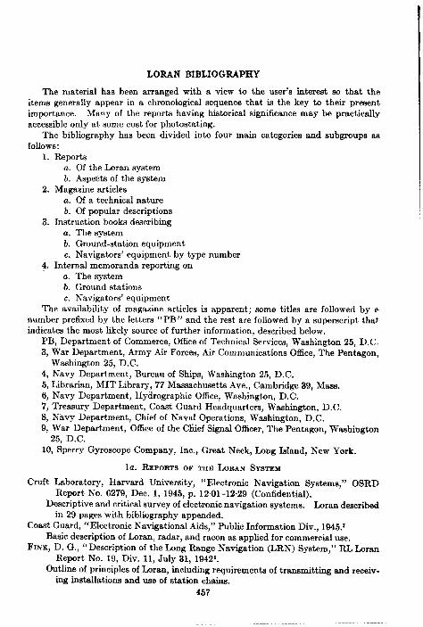
I

LORAN BIBLIOGRAPHY

The material has been arranged with a view to the user’s interest so that theitems generally appear in a chronological sequence that is the key to their presentimportance. MaIny of the reports having historical significance may be practicallyaccessible only at some cost for photostating.

The bibliography has been divided into four main categories and subgroups asfollows :

1. Reportsa. Of the Loran systemb. Aspects of the system

2. Magazine articlesa. Of a technical natureb. Of popular descriptions

3. Instruction books describinga. The systemb. Ground-station equipmentc. Navigators’ equipment by type number

4. Internal memoranda reporting ona. The systemb. Ground stationsc. Navigators’ equipment

The availability of magazine articles is apparent; some titles are followed by ~number prefixed by the letters “ PB” and the rest are followedby a superscriptthatindicatesthe most likely murceof furtherinformation,describedbelow.

PB, Departmentof Commerce, Office of Technical Services, Washington 25, D.C.3, War Department, Army Air Forces, Air Communications 05ce, The Pentagon,

Washington Z5, D.C.4, Navy Departmentj Bureau of Ships, Washington 25, D.C.5, Librarian, MIT Library, 77 Massachusetts Ave., Cambridge 39, Masa.6, Navy Department, Hydrographic Office, Washington, D.C.7, Treasury Department, Coast Guard Headquarters, Washington, D.C.8, Navy Department, Chief of Naval Operations, Washington, D.C.9, War Department, Office of the Chief Signal Officer, The Pentagon, Washington

25, D.C.10, Sperry Gyroscope Company, Inc., Great Neck, Long Island, New York.

la. REPORTS OF THE LOKAN SYSTEM

Cruft Laboratory, Harvard University, “Electronic Navigation Systems,” OSRDReport No. 6279, Dec. 1, 1945, p. 12.01–12.29 (Confidential).

Descriptive and critical survey of electronic navigation systems. Imran describedin 29 pages with bibliography appended.

Coast Guard, “Electronic Navigational Aids,” Public Information Div., 1945.7Basic description of Loran, radar, and racon as applied for commercial use.

FINK, D. G,, “ Description of the Long Range h’avigation (LRN) System,” RL Loran

Report No. 19, Div. 11, July 31, 19425.Outline of principles of Loran, including requirements of transmitting and receiv-

ing installations and use of station chains.

457

458 LORAN BIBLIOGRAPHY

HeadquartersArmy Airways CommunicationsSystem,“OperationsStandardLoran,Theory, Adjustment, Procedure,” AACS Marmat 1–16, July 15, 1944.3

Summary of Loran information and practice as affecting AACS personnel.Navy Department, “Loran Long Range Radio Navigational Aid,” OpNav 25-A-2,

PB-18603, 1945.’A brief description of the bran system and suggestions as to its peacetime use.

PIERCE, J. A., “ The Future of Hyperbolic Navigation,” RL Report No. 625, PB-25369,Aug. 18, 1945.

Three hyperbolic navigation systems are studied, Gee, Loran and Decca. Futuretrends are suggested, including automatic navigation and surveying.

SYITERLY, B. W., “Elements of Loranj” RL Report No. 499, Mar, 8, 1944,’

Complete handbook of Loran principles and some operating hints for navigators.Has been replaced by revised Navships 900,027.

—, “Elements of Loran,” Navships 900,027, Navy Dept., PB-25369, April 1944.A fundamental source book on the Loran system. RL Report No. 499 was revised

for the Navy Department.STREET,J. C., “Navigation,” Loran Memorandum No. 118, N’ov. 4, 1942.s

lb. ASPECTS OF THE SYSTEM

BATEMAN, R., “ Measurement of Factors Affecting Radio Communication and LoranNavigation in SWPA,” Signal Corps ORS Report No. 2-4, PB-27051, December1944.

Intensity of atmospheric noise level in Australia and New Guinea and its effect oncommunications and bran transmissions.

Carnegie Institution of Washington, “ Measurements of Oblique-incidence Propaga-tion,” Kensington Ionospheric Laboratory, January 1944, Apr. 12, 1944.4

CRICEiELOW, W. Q,, et al., “The Range, Reliability and Accuracy of a Lew FrequencyLoran System,” with supplement, “ Measurement Technique and Analysis of aLow Frequency Loran System,” Signal Corps ORS P-23, P-23-S, PB-28958,

January, May 1946.First part of the report duplicates PB-16236.

CBICHLOW, W. Q., and J. W. HEEBSTREIT, “ Radio iNavigational Accuracy Charts withApplication to Low Frequency lkran, ” PB-32229, June 1946.

Charts are described that give contours for several arrangements of transmittersto give good accuracy over greatest possible areas.

DAVIDSON, D., “Notes on the Ionosphere,” Loran Memorandum No. 124, June 4,

1943.s—, “Some Notes on 2-Mc Loran Propagation,” Loran Memorandum No. 134,

Jan. 1, 1944.sFINK, D. G., “Determination of Errors in the Loran System, ” Div. 11, RL Loran

Report No. 26, Apr. 6, 1943.’A consideration of the various types of errors in a Loran fix and means of deter-

mining their magnitude.— “Time and Distance Relationships in the Loran System, ” RL Loran Report

ko. 25, Div. 11, Oct. 15, 1942.6Report on time and distance factors in Loran, including choice of pulse rate and

U= of different rates for identification of station pairs.—, J. A. PIERCE, and F. G. WATSON, “Loran System-characteristics of the North

Atlantic Station Chain,” Loran Report No. 100, Aug. 28, 1942.’KELLY, M. J., “Interference of Loran Pulse Signals with Radio Telephone and Tele-

graph Reception,” NDRC Report No. 14-163, PB-32726, March 1943.Tests made by Bell Telephone Laboratories at Fenwick and Montauk.

LORAN BIBLIOGRAPHY 459

National Bureau of Standards, “Experimental Studies of Ionospheric Propagation asApplied to the Loran System, ” Report No. IRPL-R6, PB-13778, 1944.

Methods and results of a study of time-difference measurements from pulsetransmissions involving ground and sky waves.

—, “Second Report on Ilxperimental Studies of Ionospheric Propagation asApplied to the Loran System,” Report No. IRPL-R7, PB-13777, 1944.

Supplement to Report h“o. IRPL-R6 with particular reference to variations due toseasons of the year.

Navy Department, Loran Notes No. 2, Hydrographic Office Apr. 3, 1945.’Operations reports, bibliography.

—, Loran Operational Notes No. 3, Hydrographic Office, May 15, 1945.’Operational report summary, charts revisions.

—, Leran Operational Report No. 1, Hydrographic Office, 1944.’Summary of Navigators’ comments, Jan. 1, 1944, to Oct. 111944.

—, “ Graphical Methods, ” Loran Technical Report No. 1, Hydrographic Office, nodate,a

Evaluation of mechanical, optical and graphical methods for rapid location ofLoran lines.

—, “Loran Corrections in the Aleutians,” Loran Technical Report h-o. 2, Hydro-graphic Office, 1944.’

Analysis of system errors due to erroneous coordinates adopted for the trans-mitters.

— “Simplified kfethod of Deri~,ing Accurate Distances on the Earth’s Surface, ”~ran Technical Report N’o. 3, 1945.’

Complicated geodetic formulas for obtaining precise distances have been modifiedand a set of auxiliary tables compiled.

—, “The Loran Program in the Hydrographic Office, ” no date.’History and administration of Loran and the part played by the Hydrographic

Office (See Appendix A.).PIERCE, J. A., 1‘Factors Affecting E-Layer Propagation in the LRAT System, ” RL

Loran Report No. 21, Div. 11, l~ay 15, 1942.sA description of the use of the E-layer for Loran propagation. Use of delay

curves is given.—-----, “ Service Areas of Loran Pairs and Chains, ” RL Loran Report h-o. 28, Div. 11,

Mar. 6, 1943.’A summary of simple constructions to determine areas of satisfactory Loran

coverage.SITTERLY, B. W., “ Determination of J3rrors in the Positions of Loran Transmitting

Stations,” Loran Memorandum No. 149, RI. Report No. 11, July 21, 1945.sA method is suggested for correcting the considerable errors of time difference

encountered when Loran stations cannot be tied into geodetic triangulationnetworks (See Appendix D.).

—, “Manual of Procedures for Mobile Charting Units, Air Transportable LoranSystem,” RL Report No, M-183, Mar. 30, 1946.5

Rapid approximative methods for computing and plotting Imran lines of position,and for drawing and reproducing Loran charts, are described. Forms, tablesand graphs are included.

—, and J. A. PIERCE, “ Simple Computation of Distance on the Earth’s Surface,”RL Report No. 582, PB-6607, July 8, 1944.

The Andoyer-Lambert correction from a spherical to a tcrrest rial distance, ifexpressed as a fraction of the distance, is nearly independent of the distanceand so small it may be read from a nomogram. Examples are reproduced.

460 LORAN BIBLIOGRAPHY

STRAT-TON,J. A., “Factors Governing the Accuracy of a Pulse Navigation System, ”

RL Loran Report No. 20, Div. 11, May 23, 1942.5Study of system geometry, including probable accuracy to be expected, propaga-

tion factors, and prediction of range.WATSON, F. G., “A Report on Three-line Fixes,” Loran Memorandum A“o. 122, Dec.

15, 1942.s—, “ Computation of Loran Lattice Points, ” RL Loran Report No. 23, Div. 11,

Sept. 15, 1942.’A summary of methods used in preparation of Loran charts and tables.

2a. MAGAZINE ARTICLES OF A TECHNICAL ~7ATURE

DAVIDSON, D., “bran Indicator Circuit Operation,” Electronic Ind., March 1946,

p, S4.Brief discussion of 2-hfc propagation and complete circuit information of the

DAS-1 receiver-indicator.FINK, D. G., “Loran Receiver-indicator, ” Electronics, December, 1945, p, 110,

Circuit details and operational procedure of the navigator in obtaining a fix.—---, “Loran Transmitting Stations, ” Electronics, Lfarcb 1946, p. 109.

Circuits and operating functions of the timer, transmitter, and synchronizer.—, “ The I,oran System-Part I,” Electronics, November 1945, p. 94.

This section of a three-part story deals with the systcm in general.MCKENZIE, A. A., “Imran—the Latest in Navigational Aids,” Part I—Fundamental

Principles, QIST, December 1945, p. 12.An explanation in three parts written for amateurs. Issued hy Radiation Labora-

tory.—, “Loran—the Latest in Navigational Aids,” Part II—Ground Station Equip-

ment, QS’!7’, January 1946, p. 54.Station layout, timer, and transmitter are described.

—, “Loran-the Latest in Navigational Aids, ” Part lll—hTavigators’ Equipment

and Summary, QST, February 1946, p. 62.Receiver-indicators, with block diagram and typical chart.

PIERCE, J, A., “An Introduction to Hyperbolic h’avigation, with Particular Referenceto Loran,” Jour. IEE, July 1946, p. 243.

Abstract of a paper read before convention of the IRE, Jan. 24, 1946, and pres-ented simultaneously by recording in I,ondon. An interesting discussion is

recorded to which the author briefly replies.—, “An Introduction to Loran,” Proc. IRE, Lfay 1946, p. 216.

History of the Loran program, fundamental concepts of hyperbolic navigation,potential usefulness of the system, problems to be met.

—---, “ 2-Mc Sky-wave Transmission, “ Electronics, May 1946, p. 146.

An extremely clear summary of ionospheric knowledge together with results ofLoran operational findings concerning the E-layer.

ROCKE~, F. R., “An Evaluation of Hyperbolic Aviation,” Aviation, August 1946

p. 51.Comparisons of Loran, Shoran, Gee and Decca as to range and accuracy.

2b. MAGAZINE ARTICLES OF A POPULAR DESCRIPTION

DAVIDSON, D., “Loran Has Potential in Commercial Operations, ” Am. Aviation,Dec. 1, 1945, p. 79.

A one-page summary.KENYON, R. W., “Principles of Imran in Position hcation,” Electronic Ind., December

1945, p. 106.

LORAN BIBLIOGRAPHY 461

LEKASHMAN, R., “ Stars for Romance—Imran for Navigation,” Air Transport,February 1946, p. 57.

General discussion of the system with particular emphasis on its use for aircraftnavigation,

MANCHESTER, H,, “ Streets Painted on Air, ” Reader’s Digest, June 1946, p. 101.

Description of a flight in a Loran-equipped pla~e and resum6 of the system and itspotentialities. Condensed from Sci. American.

—, “ Successor to the Sextant,” Sci. A me~ican, June 1946, p, 36.Navy Department, “ Microsecond Navigation, ” Air Navigation Bull., Suppl. 1,

PB-17626, 1943.First of a series of articles illustrating use of Loran in air navigation. Sample logs

are shown.“Race on for Navigation Aids,” Business Week, June 29, 1946, p. 56,

Description of Decca navigation system with comments upon its competitiveposition with Loran.

WATSON, F. G., “ Part VI. bran, N“ew Long-range Aid to Navigation,” Ciuit Eng.,July 1946, p. 297.

Evaluation of the system with emphasis on its use for future marine surveyingand fathometry,

— and H, H, SWOPE, “Loran,” Sky and Telescope, V, A-OS.2 and 3, December1945 and January 1946.

General description of the system with particular emphasis on charting. Somereports from ships using the systcm. Both authors were formerly staff mem-

bers, Radiation Laboratory, later Navy Dept. Hydrographic Office.WOLFF, I., “Radar Aids to Navigat ion—Loran, Tcleran, Television, ” Princeton Eng.,

May 1946.

3a. INSTEUCTKO~ Boom DESCRIBING THE SYSTEM

Navy Department, Bureau of Ships, ‘( I,oran Handbook for Aircraft ,“ Air ForcesManuaZ No. 37, Training Aids Div., September 1944.1

Similar in content to Ships 278 but revised for aircraft use by ACO.— “Loran Handbook for Shipboard Operators, ” Ships 278, PB-13519, July I,

i944.The principles and practice of operation of Loran receiving equipment is described

for navigators and quartermasters, .kn appendix describes alignment andoperation of shipboard equipment,

Navy Department, “Lorzm Handbook for Shipboard Operators, ” A’aoships 278,PB-19961, January 1945.

The principles and practice of operation of Loran receiving equipment. SeePB-13519,

— “ Pocket Handbook of Airborne Loran Electronic Navigation, ” NauaerhO-80V-48, PB-17622, 1945.

Navigators’ Loran handbook describing the use of AN”/APN-4 equipment.

3b. INSTRUCTION BOOKS DESCRIBING GROUND-STATION IIQUIPME~T

Allen B. Du klont Laboratories, Inc., “ Instruction Book for Loran Switching Equip-ment h-avy Ilodel UK, ” lVauships 900,377 (.k), .4pril 19464.

Switching equipment suitable for use with Model L-J timer.Allen B. Du Ilont Laboratories, Inc., “ Preliminary Instruction Book for Navy Model

UJ Timer, ” Naoships 900,375-IB, no date. tFinal book ,Yavships 900,375A in preparation. The timing equipment described

is comparable to the Model C-1 Timer, Navships 900,221-IB.

462 LORAN BIBLIOGRAPHY

General Electric Company, “ Instruction Book for Loran Switching Equipment Navy

Model UM,” Naoships 900,745, Navy Dept., G131-19667, PB-17715, July 1945.The most modern type of switching equipment used in conjunction with Model

UE-1 Loran transmitter timer.—, “Instruction Sheet for Loran Isolation Transformer, Navy Type CG-301227,”

Navships 900,803, GEI-19666, PB-37922, September 1945.The isolation transformer was used at ground stations to isolate power lines enter-

ing the shielded timer room.—, “ Preliminary Instruction Book for Model UE-1 Timer, ” Naoships 900,427-IB,

Navy Dept.j GEI-19660, PB-17714, December 1944.This equipment is the largest and most modern of transmitter timers. This publi-

cation will be replaced by final book Nawhips 900,427A.GIFFORD, H., “ Modification of Loran Indicator ID-6 B/APN-4 for Use with Timer

Assembly ID-7/CPN in AT bran Ground Stations AN/CPN-l 1 and AN/-CPN-12,” AAF Radar Lab , TSJ3RR2D5-166, PB-9724, 1945

Adjustments and modifications to an indicator for use in master or slave stations.MCKENZIE, A. A., “ Harvey 170-T Loran Transmitter Manual, ” RL Report No.

M-162, May 10, 1944. sAn improved self-excited oscillator type of Lman transmitter designed to be inter-

changeable with the Navy’s type TDP. A limited number were manufactured.

— “Lightweight Imran Transmitter (LLTX),” RL Report No. M-158A, Apr.

i, 1944.’A lightweight, semiportable transmitter to be used with similar synchronizing

equipment in the China-Burma-India Theater is described.Navy Department, ‘‘ Instruction Book for N’avy Type CAQT-47438 Antenna Cou-

pling Assembly, ” A“avships 900,403A, no date.’—, “ Instruction Book for Navy Type CG-47368 Anterma Coupling Unit,”

Nauships 900, 751, no date.’“ Instruction Book for Navy Type CDU 60073 Transmitter Monitor Oscil-

~oscope, ” Navships 900,430-IB, no date.’

Supersedes preliminary Nauships 903-IB-1.“ Instruction Book for ISavy Model OBM Timer Monitor Oscilloscope,”

kawhips 900,222 A-IB, no date.4—, ‘(Instruction Book for Navy Model OBN Transmitter Monitor Oscilloscope, ”

Naoships 900, 429-IB, no date.’—, “ Instruction Book for Navy Model OCA Monitoring Oscilloscope,” Nawships

900,376A-IB, no date 4Replaces preliminary Naoships 900,376-IB.

“ Instructions for Navy Type CG-301227 Loran Isolation Transformer,”~’auships 900,803, no date. 4

—, Bureau of Ships, “Loran Transmitting Station Manual,” (text) Nauships900,060A and (drawings, Coast Guard) 900,060B, PB-16036, Mar. 1, 1945.

General, installation, maintenance information for Loran transmitting andreceiving equipment.

——, ‘1Synchronizer Modification Kit (for Model UJ Timing Equipment),” Nau-ships 900,371 -1-IB, PB-17712, August 1944.

Modification to Model UJ Timer synchronizer to permit automatic synchronismat double-pulsed stations. An addendum to Navships 900,375-IB.

Radiation Laboratory, Installation Notes, Parts List, and Drawings for Loran SystemTransmitter Timer Model C-1, D-1 1-12, NLO, Apr. 1, 1944.s

“ Instruction Book for Model C and C-1 Switching Equipment,” NavshipsiOO.294-IB, Navy Dept., July 1944.4

LORAN BIBLIOGRAPHY Y 463

Use of equipment usually employed to connect transmitter timers in a shieldedroom to a Loran transmitter and allow the synchronizing function of thetimers by blanking out the local transmitter pulse from the receiver.

— “ Instruction Book for Model C-1 Timer,” Nauships 900,221-IB, Navy Dept.,~ugust 1944. Includes Addendum 1, ~auships 900,221 -1-IB.

Complete information on the first major modification of the Loran transmittertimer and synchronizing equipment designed by Radiation Laboratory andmanufactured by Research Construction Co.

—, Instm.dion Manual for Loran System Transmitter Timer Model C, D-11-10,N-LOL, Div. 11, July 1, 1944.5

—, Loran Synchronizer Instruction Book, NLOL, Div. 11, September 1943.’The automatic synchronizing equipment to be used at slave stations employing

Model C timers is described.

—, Preliminary Handbook of Maintenance Instrudions for A T Loran StationsAN/CPNT-ll and AiY/CPN-12,” D-11-16, ALO, Nov. 10, 1944.5

Operation and maintenance of master and slave .4ir Transportable Loran sta-tions is described. In this equipment, the slave station is automaticallysynchronized by the master pulse received.

—, Supplement to Preliminary Handbook of Maintenance Instructions for- ATLoran Stations AN/CPN-11 and AN/CPhr-12, D-1 1-16A ALO, Feb. 15, 1945.6

Circuit changes, corrections, and additional operating information.Radio Engineering Laboratories, Inc., “ Instruction Book for N’avy Model TDP

Loran Transmitter,” Nauships 900,330, Navy Dept., PB-17999, Jan. 23, 1945.Self-excited oscillator transmitter used as standard ground-station equipment.

This publication replaces preliminary book, Nauships 925B-I.

Sylvania Electric Products, Inc., “ Preliminary Instruction Book for Navy hfodel

UK Loran Switching Equipment,” Nauships !Y30,377-IB, Navy Dept., PD.17713, October 1!344.

The equipment described was designed primarily as a necessary adiunct to theModel UJ Loran transmitter timer.

. .

3c. INSTRUCTION BOOKS DeSCribing NAVIG.ITORS’ llJUIPMENT BY TYPENUMBER

Fada Radio and Electric Company, IIIc., Equiprrrent Spare Parts List for ModelDAS4 Radio Navigation Equipment Receiver and Indicator, Navy Dept.,Bureau of Ships, PB-24916.

The spare parts list is for shipboard Loran equipment that is described inPB-24915.

—, “ Instruction Book for Radio Navigation Equipment Model DAS-4 (LoranSystem), ” Ships 322, Navy Dept., PB-24915, April 1945.

Information on a late model shipborne receiver-indicator.

MCKENZIE, A. A., “Handbook of Nlaintenance Instructions for Loran Low FrequencyConverter CV-27/UPN,” RL Report No. kf-225, PB-40630, July 6, 1945.

The converter described can be connected between the antenna and Standardreceiver to adapt the equipment for reception of either Standard or Low Fre-quency signals.

—, “ Handbook of Operating Instructions for Loran Low Frequency ConverterCV-27/UPN,” RL Report No. M-222, PB-40631, Apr. 27, 1945.

Use of a converter between antenna and Loran receiver-indicator allows operationon either Standard or Low Frequency Loran.

Navy Department, “ Catalog of Loran Charts and Service Areas, ” H ,0. h-o. I-L,Oct. 1, 1945.’

464 LORAN BIBLIOGRAPHY

A description of the Loran system and list of charts available covering the areasserved by the system. Indicator alignment information is given.

—, “Handbookof Maintenance Instructions for Test Set TS-251/UP,’’ Nauships900,652, no date.’

Same as publication AN 16-35TS251-2.—, “InstructionB ookforNavyT~pes CME-60069and -60069A Signal Genera-

tor,” Ships 369, no date. dOperator training equipment.

—, Bureau of Ships, “Supplement 1 to Model DAS-1, LRN-1, and LRN-lAShipboard Loran Instruction Books,” Oct. 1, 1943.4

Operating and alignment instructions.“Supplement 2 to Model DAS-1, LRN-1, and LRN-lA Shipboard Loran

Preliminary Instruction Books,” Navships 929-lB, PB-18107, Mar. 1, 1944.Instructions for use of basic recurrence rate 33* pps and errata.

Philco Corporation, Handbook of Maintenance Instructions for RadioSet *AN/APN-4,CO-AN 08-25CA-1, revised Mar. 10, 1944.3

The airborne Loran navigation equipment comprising *R-9/APN-4 receiver and*ID-6 /APN-4 indicator operating on either 80 or 115 volts, 400 to 2400 cycles,is described. See supplements for further modifications.

—, Handbook of Operating Instructions jor Radio Set *AN/APN-4, AN 08-10-184,June 24, 1943.3

Installation and operating instructions for airborne Loran receiver-indicators.“ Model *AN/APN-4, Bull. 1 and 2, Apr. 12, 1944.’

R~placement of glass tubes in receiver units and change of resistors.— “ Model *AN/APN-4,” Bull. 3, 4, and 5, May 22, 1944.’

R~placement of power transformer, parts changes, test procedure for ModificationIII.

“ Model *AN/APN-4,” Bull, 6 and 7, July 7, 1944.’Te’st procedures for hlodifications I, II, and III and addition of resistor in

second and fourth counters.“ Model *AN/APN-4,” Bull. 8 and 9, Aug. 25, 1944. s

A~dition of capacitors in square-wave generator and corrections to previousbulletins.

—, “ Model *AN/APN-4, ” Bull. 10, Sept. 20, 1944.’Description of the Modification V indicator.

“ Model *AN/APN-4,” Bull. 11 and 12, Sept. 9, 1944.’M~dification IV receiver and Modification V indicator.

— “ Model *AN/APN-4,” Bull. 13, Nov. 29, 1944.3T~st procedure Modification IV receiver.

Radiation Laboratory, “bran System Receiver-indicator LRN-I-A Operation andMaintenance Instructions,” NLOL, Div. 11, Feb. 2, 1943.’

Description of first large-production model of Loran navigation receiver andindicator.

—, ‘( Preliminary Instruction Book DAS-1 bran System Receiver-indicator,”Navships 929-1, Navy Dept., PB-17823, 1943.4

The shipborne navigation equipment described was manufactured by FadaRadio and Electric Co.

Radio Corporation of America, Handbook of Operating Instructions for Radar SetAN/APN-9, AN 08-30APN9-2, NOV. 15, 1944.3

Description, alignment, and use of airborne Loran navigation equipment.

Radiomarine Corporation of America, “Instruction Book for Loran Receiving Equip-

LORA,V BIBLIOGRAPHY 465

ment, Navy hlodel X-DBS,” iVavships 900,755, PB-17s87, PB-37923, June1945.

Theequipment described is a modified R-65/APA--9 receiver-indicator operatingfrom 60-cycle, 115-volt lines.

Sperry Gyroscope Company, Inc. ‘‘ Instruction Book for Loran Receiving EquipmentModels CXJDand XBf)E,’’Ships23l, PB-24940, November, 1944.

Shipboal-d units and their use are described.—— “LoranR eceivingEquipment, LIark I, Mod. 1,’’ Sperry Znstrtiction Book No.

;3-205, June 1946.10The equipment described is a direct-reading indicator for shipboard use. Itis

similar in most respects to the Navy type DBE.—, “1.oranR eceivingE quipnlent310delD BE,” ~Vavships 900,659, June 27, 1945,4

Equipment describcdis direct-reading shipboard receiver-indicator.War DepartlneIlt, Con~pleleCo?~rseof Instruction on.4h"/AP&"4 Operation and Service,

L-S.4.\F, .4ir Service Comrr,and, December 1943,7— and N’avy Department, .kir Council of the LTnited Kingdom, Handbook of

Muintena?we Instructions for Radio Set AY/APX-4. (.4A’16-30APN4-3),PB-14797, April 1945.

General description, operating instructions, diagrams of an airborne Loranreceiver-indicator.

—, Handbook of .Ifaintenance Instnwlions for Radar- Set .UJ/APX-9, AN 16-

30 APN9-3, PB-14878, September 1945.Description of an airborne receiver-indicator.

4a. INTERNAL hfE~ORANDA REFORTING ox TFII? SYSTEM

DAVIDSON, D., ``ACondensed Report of LRNObservations-June 17-July17, l942,''RL Loran Report 18, Div. 11, July 22, 1942,5

Preliminary appraisal of results uf Loran observations aboard LTSCG Manasquan.See I,oran Report 22.

———, “Report on Loran System Tests blade aboard the L-SCG Manasquan, ” RI,Loran Report N-o. 22, Div. llr.4ug. 15, 1942.5

Both gmundands kywavcxw ereusedfrom apairof experirncntal, synchronizedLorau transmitters to obtain navigational fixes that were compared with theresults of conventional navigation methods.

——, “Some Observations, Comments, Recommendations of the Operation ofProject C Equipment—USS Man.asquan,” Loran Memorandum iVo.106, July,1942.5

DOER, R., D. DAVIDSON, and F. G. WATSON, “Sky Wave Observations over theEastern Half of the United States” (describing a series of four flights calledthe ‘(AT-ll Reports 1, 2, 3, 4“), Div. 11, Radiation Laboratory, 1943, b

DUVALL, G, F., Lieut. USN (ret. ) “Conventional Navigation-USCG Manasquan”RL Loran Report No. 17, Div. 11, July 1942.6

A report of convention navigation methods during the period of Loran tests.See Loran Report No. 22.

EL~ORE, W, C., dal, “ThirdR eportonC rystalC lockProject,” NDRCReport h-o.14:145, PB-19646, hfay 1943.

Report of research on development of crystal oscillator for Loran system use,including special thermostat and hleacham-type circuits,

——-, “Fourth Report on the Crystal Clock Project and Preliminary Report on10-kc Oscillator,’’ NDRC Report No. 14:175, PB-19645, .4ugust 1943,

Report covers development of two types of oscillators, one crystal and one stable

466 LORAN BIBLIOGRAPHY

L-C, under development for use in Loran equipment. Work was done atBartol ResearchFoundation.

— “Fifth Report on the Crystal Clock Project and Report on 10-kcLC-oscil-~ator,” NDRC Report No. 14:193, PR-19644, October 1943.

The report deals with the performance of the General Radio thermostat and itsinfluence on oscillator stability as well as development of a lo-kc LC-oscillator.The work was done at the Bartol Research Foundation.

— “Crystal Clock Project: Final Report and Report on 10-kc LC-oscillator,”i’-TDRC Report No. 14:226, PB-19647, January 1944.

Summary of five earlier reports on stable crystal oscillator for use in Loran trans-mitting stations, and stable LC~scillator for use in a Loran receiver. A prejectof Bartol Reeearch Foundation, Swarthmore, Pa.

FINK, D. G., “The Lodar System of Pulse Direction Finding,” RL Lodar SystemReport No, 1, Div. 11, July 1, 1943,’

Discussion of a proposed system of pulse direction finding using a loop antenna.—————“The Lddar System of Pulse Direction Finding,” Div. 11, Radiation Labora-

~ory, July 1, 1943.6

—, J. A. PIERCE, and J. C. STREET, “Loran System—Definition of Terms andSymbols,” RL Loran Report No. 25, Div. 11, Aug. 28, 1942.’

Loran terminology and symbols.—, J. A. Pierce, and J. C. Street, “Proposal for a bran System Using Sky-wave

Synchronization,” RL bran Report No. SS-1, Div. 11, May 15, 1943.6MUSSELMAN, G. H., and E. J. STEPHENS ‘( Report on Aircraft Test, Boston to Nova

Scotia and Return, ” RL Loran Report h’o. 15, Div. 11, July 1942.6An observational flight to investigate field intensity of signals from the Montauk

Station at the proposed site for a station near Cape Sable, Nova Scotia. Thetrip was made July 4, 1942.

MUSSELMAN) G. H,, and J. K. TROLAN, “Low Frequency Noise at Key West,Florida, Feb. 1 to Feb. 10, 1944,” Loran Memorandum No. 139, RL ReportNo. 11, Feb. 23, 1944.’

Office of the Chief Signal Officer, “ Measurement Technique and Analysis of a LowFrequency Loran System,” Report No. ORS-P-23-S, May 1946.’

Supplement to Report No. ORS-P-23 and bound with it.— “The Range Reliability and Accuracy of a Law Frequency Leran System,”

~ith supplement, Report No. ORS-P-23, January 1946.gAn experimental and theoretical study of the RL Low Frequency Loran triplet

made by the Operational Research Staff of Office of the Chief Signal Officer.The supplement describes measurement and analysis techniques.

PIERCE, J. A., “ Group C Test Report, Jan. 2–Jan. 17, 1942,” RL Loran Report No.16, Div. 11, Jan. 22, 1942.’

A test of the hyperbolic navigation eystem using ionospheric reflection was madein Bermuda. E-layer signals at various frequencies indicated the usefulnessof such a system, but F-layer signals were judged to be too unstable.

—, ‘[ 170-kilocycle Noise and Pulse Transmission Measurements,” Loran Memo-randum No. 148, RL Report No. 11, Nov. 3, 1944. K

—, “LRN Tests at Lakehurst, June 13, 1942,” RL I.man Report No. 13, Div.11, June 17, 1942.’

First edition of a report on the use of Loran aboard a Navy blimp. Ground-wavesignals from the experimental, synchronized stations at Montauk and Fenwickwere used.

War Department, “Radio Navigational Accuracy Charts with Application to LawFrequency Loran,” Officeof the Chief Signal Officer, June 1946.’

LORAN BIBLIOGRAPHY 467

Prepared charts are used to plot contours for various arrangement-a of transmittersfor optimum coverage.

WATSON, F. G., “Flight Tests over Bermuda,” Loran Memorandum No. 116, Nov. 18,1942.’

4b. INTERNAL MEMORANDA REPORTING ON GROUND STATIONS

Dorm, R., `` High Frequency Supplementa~ Synchronization Unit, '' bran Memoran-dum No. 142, RL Report No. 11, Apr. 29, 1944.’

FINK, D. G., “Delaysi ntheMonitoringA ntennaS ystem,’’Luran Memorandum No.111, Oct. 21, 1942.6

JANSKY and BAILEY, In.structioa Book for Field Intensity Meter Type 43A, Washington,D. C., January 1945.’

LAWRENCE, R. B., and A. J. PoTfi, “Impedance Characteristics and EquivalentCircuits for Vertical Radiators,” RL Report No. 512, PB-32746, Apr. 15, 1944.

Discussion and set of curves for predicting input impedance of an antenna struc-ture over arangeof frequencies.

MCKENZIE, A. A., “Sites No. 1 and No. 2,” Lman Memorandum h’o. 108, Oct. 10,1942.’

MTJSSELMANN,G. H., “ Identification Blinker, Model A-1, ” Loran Memorandum No.147, RL Report No. 11, Aug. 31, 1944.5

— ‘[ Modification of Lightweight Loran Timing Equipment for Double Master~eration,” Loran Memorandum No. 145, RL Report No. 11, June 27, 1944. h

PIERCE, J. A., W. L. TIEENEY, and W. E. OWEN, “ .Memorandum on Proposed Loca-

tion for a Loran Station on Nantucket Island,” Loran Memorandum N“o. 110,Oct. 22, 1942.s

PoTri, A. J,, “Adjustment of Loran Antennas and Antenna Coupling Units at Fre-quencies between 1700 and 2000 Kilo cycles,” RL Report N’o, 511, PB-2466,Feb. 20, 1944.5

Characteristics of a standard Laran antenna and a method of tuning and cou-pling to it for any of the normal operating frequencies.

and R. B, LAWRANCE, <‘Y-oltage Patterns, ” Loran Memorandum No. 107,October, 1942.’

WALDSCHMITT, J. A., ‘1Average and Jfean (2P + ?) at Station h’ for L-NT Pair,”

Lors,n Memorandum No. 132, Nov. 22, 1943.6—, “ High Frequency Daytime Sky-wave Loran Project,” Loran Memorandum

No. 141, RL Report h-o. 11, Apr. 21, 1944.5—, “Loran Observations at Station h“, ” Loran h’Memorandum No. 133, Dec. 22,

1943.’— “Three-quarter Wavelength Cophase Transmitting Antenna,” Loran hfemo-

~andum No. 144, RL Report No. 11, hfay 15, 1944.6— “Transmitting Antennas, Radiated Pow-er, and Radiation Efficiency at the

~wo Standard SS Loran Stations, SS-1 and SS-3, ” Loran Memorandum No.131, Nov. 22, 1943.’

—, “United States Coast Guard 300-foot Tower,” Loran Memorandum No. 150,RL Report No. 11, Nov. 9, 1945.6

4c. INTERNAL MEMORANDA REYORTTNG ox NAVIGATORS’ EQUIPMENT

BISCHOFF, A. F., “ Report on NDRC Contract OEMsr-723 Airborne Loran Equip-ment,” General Electric Co., Bridgeport, Corm., Sept. 1, 1943, K

DAVIDSON, D., “Optimum Bandwidth for Loran Receivers,” Loran MemorandumNo. 137, Jan. 27, 1944.6

468 LORAN BIBLIOGRAPHY

Dom+ R., “Instructions for Using a Loop with Loran Receiver-indicator,” LoranMemorandum No. 136, Feb. 1, 1944.s

HALFORD, J. H., JR., “Receiving Installation Report No. l,” Loran MemorandumNo. 112, October, 1942.6

—, “Receiving Installation Report No. 2,” bran Memorandum No. 113,October, 1942.’

INGALLS, C. E,, “ Revision of General Radio Type 605-B Signal Generator for Pulsing,”

RL Report No. 575, PB-2872, 1944.Instructions for modifying the signal generator to produce pulsed r-f output.

Pulses can be at least from 0.5 to 100 Kec in duration.International Business Machines Corporation, “ Special Mechanical Counter for the

Mark HI or Phase Shtit Loran Indicator, ” NDRC Report No. 14-368, PB-32751, October 1944.

A mechanical device is described that can be used for a direct-reading indicator.LAWBANCE, R. B., “The Beverage Antenna as Applied to Loran, ” Loran Memorandum

No. 140, December, 1943.’MARSHALL, J. P., et al. “Supersonic Loran Trainer, ” NDRC Report No. 14:446,

PB-23329, June 1945.Report on general trainer problem and that of simulating actual flight conditions.

Design of Rochelle salt transducer and electronic circuits is included in descrip-tion of the complete trainer, Work was done at Bartol Research Foundation.

MOUNTJOY, G., and G. D. HULST, JR., “ Development of Loran Receiver Trainer, ”RCA License Div. Lab. Report No, 208, PB-23321, March 1943.

The unit is attached to an indicator and simulates transmitter signals for trainingpurposes.

MOUNTJOY, G., et al., “ Characteristics of Simplified Loran Receiving Equipment,”NDRC Report N’o. 14-206, PB-32735, November, 1943.

A field test of two test models leading to the type .4PX-9 receiver-indicator.MouNTJoY, G., E. SCHOENFELD, W. BROWN, and G. D. HGLST, JR., “A Portable

Signal Generator for Imran Receivers,” RCA Laboratories, NDRC Report No.14-297, PB-32734, June 27, 1944.

PHELAN, J. K., “Harvey-Wells Loran Receiver-Indicator, ” Loran Memorandum ATO.

103, Sept. 18, 1942.’Radiation Laboratory, “ Instructions for the Installation of Modification Kit M for

Model DAS and DAS-2 Equipments, ” D-11-18, February 1945.5Describes the installation of parts from a kit and modifications to existing cir-

cuits to obtain 2-@ec markers for precision monitoring with DAS and DAS-2receiver-indicators.

—, “Loran Beverage Antenna Installations” (from a report by RAF Hdq. 84thWing), Loran Memorandum No. 146, RL Report ATO,11, July 21, 1944.5

Radio Corporation of America, “Simplified Loran Receiving Equipment, ” LicenseDiv. Lab., NDRC Report No. 14-228, PB-32736, June 25, 1943.

Report of a study to simplify zirborne LOran equipment, leading tO the de~elOp-ment of the APN-9 type equipment.

‘( Development of Airborne Receiver Model LRN-1,” License Div. Lab.,~’DRC Report No. 14-207, PB-32732, September 1942.

The equipment was designed for marine use but can be mounted in aircraft andused for 400-cycle operation with passable results.

SCHOENFELD, E., G. D. HULST, JR., and W. BROWN, “A Converter for 170-kc LoranSignals,” RCA Laboratories, Oct. 20, 1944.’

Index

A

A-1 oscilloscope, 285A timer, 199Absolute delay, 5’2, 56, 96Absorption, 131, 146.4ccuracy. 107Aeronautics, Bureau of, 45Air navigators, 46Air Transportable equipment, 35Air Transportable Loran, 44, 93Air Transportable station, 413Airborne receivers, 25Aircraft, fighter, control of, 115

pilotless, guidance of, 116Aleutians, 37Amplifier, differential, 231, 246

paraphrase, 229power, 298

Amplitude-balance control, 387AN/APN-4 receiver-indicator, 25, 31,

363, 367AN/APN-9 receiver-indicator, 365, 374Angle, crossing, 80, 83

tilt, 328Angle systems, 17Antennas, 87

airborne trailing, 343bandwidth of, 307Beverage, 87, 267Beverage receiving, 328cylindrical, 315dummy, 314, 321fixed airborne, 343for 180-kc/see, 329ground-station, 301invcrtcxi-1,, 323net Q of, 320

Q of, 301receiver-indicator, 342receiving, 302, 340resonant, Q of, 308shipboard, 342

Antennas, transmitting (see Transmittingantenna)

for 2-llc/sec Loran, 323umbrella-type, 97vertical receiving, 328wave, 301

Antenna characteristics, 314Antijamming, 234.Apollonia, 32Area bombing, 13Army Air Force, 48Army .kir Transport Command, 34Army Airways Communication System,

40.&ssam Hump triplet, 35Atlantic fleet, 26Atlantic service, 412Attenuation, 63.kttenuator, 68, 207, 212, 213, 229, 258,

259, 265, 269, 271, 272Attenuator-bias driver, 212Attenuator driver, 229Aural null, 3Auroral zones, 146Automatic plotting boards, 105.4utomatic synchronizer, 67Automatic volume control, 217, 240

B

B timer, 199

B-1 timer, 199, 201

Baccaro, Nova Scotia, 27

Balloon, barrage, 330

Banda Sea chain, 38, 422

Bandwidth, 155, 198, 317, 388

of antenna, 307

Baseline, 13, 53, 56, 62, 70, 96, 99, 102

extended, 59

Baseline extensions, 71

Baseline length, 86

Beacon, Orfordness, 4

469

470 LORAN

Beacon, radar, 7

SOnne, 4Bearings, 3Bengal, Bay of, 36Bermuda, 22Beverage antenna, 87, 267Bizerte, 32Blind-approach facilities, 13Bli~k, 68

warning, 229Blinker, communication, 256

identification, 256Blinking, 197

communication by, 252Blocking oscillators, 209, 221, 222Bodie Island, 27Bombardment, corpuscular, 144

meteoric, 133Bootstrap, 281Boston Loran Training School, 44Bounce-back time, 118Bridge, 239British Admiralty, 28, 31British Mission, 20Buffer, 296Buoys, automatic, 115

c

C-1 switching equipment, 261C timer, 205C-1 timer, 205Calibration markers, 205Capacitor, phase-shift (see Phase-shift

capacitor)Cape Cod, 97(’ape Fear, 97CDL oscilloscope, 285Center line, 62, 70Central Pacific chain, 38, 408, 421Chain, 11, 70, 76

Banda, Sea, 38, 422Central Pacific, 38, 408, 421China-Burma-India (CBI), 423

Hatteras-Florida, 419Loran, 55North .ltlantic, 26, 78, 419North .\tlantic Standard Loran, 26Xorth Pacific, 37, 420Pacific, 37South China Sea, 424Southwest Pacific, 38, 422

Chain, star, 80training, Central Interior, 424

Gulf of Mexico, 423West Coast, 40, 424

Channels, 70r-f, 347

Chapman distribution, 127Charting, 40Charts, 31, 55, 104, 109, 154, 173, 180

for SS Loran, 97standard navigational, 102

China-Burma-India (CBI) chain, 423China-Burma-In&la (CBI) Theater, 34,

410China triplet, 36Choke, snuffing, 283Circuit merit, 124Clouds of ionization, 136

Coast Guard (see U. S. Coast Guard)Coding delay, 57, 102, 204Coincidence, 105Coincidence circuit, 210Communication by blinking, 252Communication blinker, 256Computation, direct methods of, 177,

180inverse method of, 1771 178methods of, 177

Conductivity, 56Constant-temperature oven, 207Continuous-wave systems, 18Converter, 97

Low Frequency, 367Coupling networks, 310Coupling units, 303, 324, 341, 342

adjustment of, 306gain of, 343

Crossing angle, 80, 83Crystal, 216, 237Crystal oscillator, 201, 207, 253Cycle matching, 99, 117, 2~2, 400

D

D-layer, 88, 128DAS receiver-indicator, 349DAS-1 receiver-indicator, 349-355

DAS-2 receiver-indicat4rr, 349, 355-358

DAS-3 receiver-indicator, 349DAS4 receiver-indicator, 349DBE receiver-indicator, 349, 358

INDEX 471

Decca, 13Delay, absolute (see Absolute delay)

coding (see Coding delay)differential, 391sky-wave (see Sky-vuwe delay)

Delay controls, 65fine, 65

Delay curve, 134

(See also Sky-wave delay curve)Delay multivibrators, 199, 204, 206,

210, 211, 226Delay patterns, correlation between, 141Delayed synchronism, 67Deming, Nova Scotia, 27Dielectric constant, 129Differential amplifier, 231, 246Differential delay, 391

Diode mixer, 281Direct-reading indicator, 104Direction-finding, 3, 17, 110Discriminator, 260, 261, 265, 269Dividers, 199, 203, 209, 219, 222, 236Double pulsing, 70Driver, 298

attenuator, 229attenuator-bias, 212exciter, 21150-kc/see, 253

E

F;-layer, 60, 95, 128, 135

one-hop, 62E-layer transmission, 133East India Coast system, 36Eccles-Jordan circuit, 209, 223Electrical length, 315Electrons, free, vertical distribution of,

128Ellipse, probable, 85, 427Envelope, composite, 151

resultant, 153Equisignal, 4Error, 157

determination of, 432geometrical, 144median, 167positional, 33probable (see Probable error)station, 193

European SS system, 420Exciter driver, 211Exciter units. 278

F

F-layer, 128, 135Fading, 88, 90, 95Faeroes, 27Families, 55, 99, 180

of hyperbolas, 113Fast-sweep generator, 199, 205, 212, 227,

228triggering of, 255

Fast-sweep oscilloscope, 212Fast-trace pattern, 65Feedback, 203, 209, 222Fenwick Island, Del. 20, 27Field equipment, 397Field intensity of sky waves, 121Field strength, 121

50-kc/sec driver, 2535-Group, 33575 transmitter, 278Fix, 53

errors of, 169precision of, 83probable error of, 429relayed, 115

Fixing, instantaneous, 366

simultaneous, 249Foci, 70Folly Island, 28Frequency of collision, 131

low, 108resonant, 317, 322

Frequency doubler, 207, 219

G

Gain, differential, 39oGain balance, 389, 393Gain control, automatic, 394

differential, 23Gate, 210, 231, 246Gate-pulse mixer, 199, 227Gee, 11, 17, 80, 100Gee-H, 9Gee lattice, 11Gee system, 22Generator, fast-sweep (see Fast-sweep

generator)9CLkc/see, 291pulse-signal, 395r-f, 293slow-sweep, 209, 212, 229

472 LORAN

Generator, square-wave, 203, 209, 223sweep, 212

Geodesic, 170Geodetic reference points, 193Geographical grids, 181Geometrical error, 144Geometrical precision, 72, 102

factor of, 425Ghost, 101Ghost pulses, 250Glide-path facilities, 13Graphical solution, 434Greenland, 27Groton school, 44Ground-station antennas, 301Ground-station operators, 41Ground stations, 31, 419Ground system, 87,301,324,340,341Ground-wave ranges, 23Ground waves, 60Group velocity, 129Guy insulators, 340Guy wires, 339

H

H-systems, 9Hatteras-Florida chain, 419Hawaiian triplet, 38Hebrides, 27Hobe Sound, 28Homing, 16Hop single, 130Hump triplets, 34Hydrographic Office, 41, 46, 403Hygraph, 186Hyperbolas, 11, 70

families of, 113spherical, 72, 175

Hyperbolic line of position, 10Hyperbolic navigation, 19Hyperbolic surveying, 117Hyperbolic systems, 17Hyperbolic track, 16

I

Iceland, 27Identification blinker, 256I-f rejection ratio, 389Image-rejection ratio, 388Impedance, characteristic, 315

input, 307, 324, 327, 331

Impedance level, 322Index of refraction, 129

Indicated time difference, 59Indicator, 11

direct-reading, 104Loran, 100right-left, 110two-trace, 21, 22

Injection, controlled, 401pulsed, 398

Input reactance, 318Input resistance, 317Instruction, 45Instruction books, 44

Loran, 457, 461–465Ionization, 127

clouds of, 136maximum, height of, 130sporadic E-region, 144

Ionosphere, 59, 88, 94, 126Isolation transformer, 259Iwo Jima, 38

K

Key Large, 97

L

L-network, 306Labrador, 27Lambert correction, 176Lambert projection, 181Latitude effect, 139Lifeboats, 115Light-microsecond, 52Line of position, 3, 52, 102

error in, 107hyperbolic, 10

Loran, Air Transportable, 44, 93internal memoranda on, 457, 465-468Low Frequency, 60, 97magazine articles on, 457sky-wave synchronized (see SS Loran)Standard, 12, 56, 85

Loran bibliography, 457-461Loran charts, 41, 406Loran computations, 170Loran coordinate system, 55Loran coordinates, 109

chart in, 110Loran distances, computing, 171

INDEX 473

Loran frequency, 135Imran grid, 11Loran indicator, 100Loran line, 173Loran network, 56Loran plotting board, 104Loran pulse shapes, low frequency, 149Loran quadrilateral, 55, 79Loran system, history of, 403Loran tables, 102, 180bran Training School, Boston, 44Loran transmitters, pair of, 52Loran trials, 23Lorhumb, 106Lorhumb line, 112Low Frequency Loran (see Loran, Low

Frequency)LRN-1 receiver-irdcator, 349LRN-lA receiver-indicator, 349

hf

Magnetic activity, 145Manuals, 44Marianas Islands, 38Marker mixer, 212, 226Markers, 12, 66, 104

calibration, 205Marshall Islands, 38Master station, 59, 68Mean free path, 131Measurement, precision of, 107Median errors, 167Memoranda, internal, on Loran, 457,

46$468Mercator projection, 174Meteoric bombardment, 133Micro-H, 9, 16

Microwave Committee, 19

Mixer, balanced, 246

coincidence, 231

gate-pulse, 199, 227

pulse, 210

Modulator, 278

operation of, 282

Monitor station, 68

Monitor timer, 250

Montauk Point, L. I., 20, 27

Multiple-hop transmission, 136

Multivibrators, delay (see Delay multi-

vibrators)

N

Naval Liaison, 24Navigation, hyperbolic, 19Navigators, air, 46

shipboard, 45Navy Administration, 405Network, coupling, 310

L, 306Loran, 56reactance, 304T-, 305, 306

New York Project, 405Newfoundland, 2790-kc/sec generator, 291Noise, 62

atmospheric, 125long-distance, 125

Noise factors, 121, 389North Africa station, 30North Atlantic chain, 26, 78, 419North Atlantic Standard Loran chain, 26North Pacific, service to, 407North Pacific chain, 37, 420Nova Scotia, 27

0

OBN oscilloscope, 285Oboe, 10OCA oscilloscope, 285Okinawa, 38Omnidirectional radio range, 5108T transmitter, 278125T transmitter, 278170T transmitter, 278Optical survey, 118Oran, 32Orfordness beacon, 4Oscillator, 215

blocking, 209, 221, 222crystal, 201, 207, 253power, operation of, 282self-excited, 278UE-1, 237

Oscilloscope, 199, 205A-1, 285CDU, 285fast-sweep, 212OBN, 285OCA, 285slow-sweep, 212test, 213, 237, 285, 291

474 LORAN

Oven, constant-temperature, 207crystal, 216

Oven temperature, 217

P

Pacific chain, 37Pacific installations, 414Pair designation, 70Pairs, of stations, 11

two, 76, 86Parallelogram, probable, 84Parametric latitude, 173Path6nders, 33Pedestal, 65Phase control, 240Phase corrector, 231Phase inverter, 218, 219Phase shift, coarse, 204Phase-shift capacitor, 199, 203, 207, 219Phase velocity, 129Phoenix Islands, 38Plan position indicator, 6Plotting board, 110

automatic, 105Loran, 104

Polarization, 301POPI, 13Port Errol, 32Position-determining set, 108Positional error, 33Power amplifier, 298Power plant, 87Preamplifier, 278Precipitation static, 328, 344Probable error, 72,84,91, 95,98, 140, 193

in distance, 85of fix, 429

Project, New York, 405Project 3, 20Propagation, velocity of, 122, 166Pulse, ambiguity in identifying, 57

composite, 60ghost, 250length of, 98local, 67overlapping, 137remote, 67shaping of, 396time sequence of, 57

pulse-bandwidth measurements, 396Pulse-matching accuracy, 98

Pulse mixer, 210Pulse power, radiation of, 56Pulse recurrence rate, 57, 348Pulse shapes, Low Frequency Loran, 149Pulse shapes, 155Pulse-signal generator, 395Pulsed doubler, 294Pulsed injection, 398Pulsed system, 18Pulsing, double, 70

Q

Q of resonant antenna, 308Q-procedure, 187Quadrilateral, 94

Loran, 55, 79

R

Radar, 6, 15Radar beacons, 7Radar systems, 17Radiation, low-angle, 301Radiation resistance, 316, 324Radio direction-finding, 3Radio frequencies, 55Radio range, 15

omnidirectional, 5RAF Bomber Command, 33RAF Coastal Command, 29Range, 62, 98, 107, 122

maximum, 130Rate, basic, 69

specific, 69Reactance networks, 304Reactance slope, 318Rebecca-Eureka, 7Rebecca-H, 9Receiver, 212

airborne, 25cycle-matching, 398UE-1, 243

Receiver, design, 386Receiver-indicator, 56, 63, 99, 345

airborne, 363direct-reading, 358shipboard, 345(See also various models of receiver-

indicator)Recurrence period, 57Recurrence rates, 12, 23

basic, 204, 348high, 57

INDEX 475

Recurrence rates, low, 57pulse, 57, 348specific 204, 348

Reflection, 88, 129multiple, 60stability of, 134

Refraction, 130Remote signal, 259Rendezvous, 28R-f generator, 293R-f receiver, tuned, 398Rhumb line, 3Royal Air Force, 47Royal Canadian Ak Force, 28Royal Canadian Navy, 25Royal Na.~y, 28

s

Scotland, 30SCR-722 receiver-iidicator, 363SCR-722A receiver-indicator, 363Selector circuits, 199, 206Selectors, 210, 226, 236Sensitivity, 389Service area, 49, 74, 92, 99Shetlands, 29Shipboard navigators, 45Shock-mounting, 26Shoran, 9Siasconset, 27,Sideband energy, 310Signal, local, 259

remote, 259required, 122, 124

Skip distance, 130Sky-wave accuracy patterns, 142Sky-wave components, 151Sky-wave corrections, 31, 61, 62, 138,

157, 180

Sky-wave delay, 134, 139, 147Sky-wave delay curve, 137

low-frequency, 152

Sky-wave phenomena, 108Sky-wave pulse, 8SSky-wave ranges, 23Sky-wave results, 22Sky-wave synchronized Loran (see SS

Loran)Sky-wave s~mchronized pairs, 36Sky-wave transmission, s9, 159Sky-wa~.e transmission delay, 60.62Sky-wave transmission errors, 139

Sky waves, 60, 91, 95field intensity of, 121train of, 60transmission time of, 133

Slant range, 6Slave station, 59, 68Slow-sweep generator (see Generator,

slow-sweep)Slow-sweep oscilloscope, 212Slow-trace pattern, 63Sonne beacon, 4kkmthwcst Pacific chain, 38, 422Spectrum-control filter, 310Spectrum measurements, 397Spheroid, oblate, 170Split, 88Splitting, 90Spurious response, 389Square-wave generator (see Generator,

square-wave)SS Loran, 12, 30, 94, 144

charts for, 97SS Loran navigation, 33SS Loran tests, 31SS system, European, 420Standard Loran, 12, 56, 85Standard Loran station, equipment of, 87Standardization, 119Star chain, 80Station error, 193Station positions, 432Station selection, 69Steering mechanism, 113Superposition, 67Sweep, 56Sweep generators, 212Switching equipment, 260, 261

C-l, 261low frequency, 271UM, 265

Synchronism, 101average deviation of, 158delayed, 67

Synchronizer, 199, 213, 229, 234automatic, 67UE1, 245

T

T-network, 305, 306TDP transmitter, 278TDP-I transmitter, 278

476 LORAN

Telecommunications Research Estab-lishment, 25

Test oscilloscope, 213, 237, 285,291Tilt angle, 328Time difference, 12, 52, 59, 63, 67, 101,

432indicated, 59

Time-difference measurement, 345Time markers, 56Time sequence of pulses, 57Timer, 67, 87, 197

A, 199B, 199B-1, 199, 201C, 205G-1, 205low-frequency, 249

block diagram of, 253monitor, 250UE-1, 232UJ, 205

Timing errors, 144Top loading, 334Top locking, 366Trace, 56Trace separation, 223Trace-separation circuits, 207Trace separator, 212Traces, nonlinear, 374Trainer, supersonic, 3S2Training, 40Trains, 9sTransformer, isolating, 264

isolation, 259Transmission, E-layer, 133

ground, 59ground-wave, 121multiple-hop, 136sky-wave, 59, 159

Transmission conditions, 161Transmission delay, 98

sky-wave, 60, 62Transmission line, 304Transmission time, 123

of sky wave, 133Transmitter timer, 63

Transmitter, 87, 275, 277, 278, 575Loran, pair of, 52Low Frequency, 288, 291

block diagram of, 290108T, 278125T, 278170T, 278Standard Loran, 277TDP, 278TDP-1, 278

Transmitting antenna, 97, 301balloon-supported, 329Low Frequency, 330, 338steel mast, 325tower, 332

Trap circuits, 388Trigger pulses, 198Triplet, 70, 92, 97, 102

Assam Hump, 35China, 36Hawaiian, 38Hump, 34Loran, 55

Two-trace indicator, 21, 22

u

UE-1oscillator, 237UE-1 receiver, 243UE-1 synchronizer, 245UE-1 timer, 232UHF proposal, 19UJ timer, 205

UM switching equipment, 265Umbrella, top-loading, 333U.S. Coast Guard, 27, 38, 40, 45U. S.. Fleet, 28

v

Vector bombing, 34Volume control, autimatic, 217, 240

w

West Coast chain, 40, 424West Chat installations, 414