Journal of Risk 8 (1), 2005, pp. 41-58

Misspecified Copulas in Credit Risk Models:

How Good is Gaussian?

Alfred Hamerle1 and Daniel Rösch2

University of Regensburg

Key Words: Credit Risk Models, Correlations, Copulas, Basel II

1 Professor Alfred Hamerle, Department of Statistics, Faculty of Business and Economics, University of Regensburg, 93040 Regensburg, Germany, Phone: +49-941-943-2588, Fax : +49-941-943-4936 Email: Alfred.Hamerle@wiwi.uni-regensburg.de

2 Daniel Rösch, Assistant Professor, Department of Statistics, Faculty of Business and Economics, Uni-versity of Regensburg, 93040 Regensburg, Germany, Phone: +49-941-943-2752, Fax : +49-941-943-4936 Email: Daniel.Roesch@wiwi.uni-regensburg.de

We would like to thank an anonymous referee for providing many helpful suggestions.

Misspecified Copulas in Credit Risk Models:

How Good is Gaussian?

Abstract

In addition to “classical” approaches, such as the Gaussian CreditMetrics or Basel II model, re-

cently the use of other copulas has been proposed in the area of credit risk for modeling loss distri-

butions, particularly T copulas which lead to fatter tails ceteris paribus. As an amendment to recent

research this paper shows some estimation results when the copula in a default-mode framework

using a latent variable distribution is misspecified. It turns out that parameter estimates may be bi-

ased, but that the resulting forecast for the loss distribution may still be adequate. We also compare

the performance of the true and misspecified models with respect to estimation risk. Finally, we

demonstrate the ideas using rating agencies data and show a simple way how to deal with estima-

tion risk in practice. Overall, our findings on the robustness of the Gaussian copula considerably

reduce model risk in practical applications

1

1 Introduction In the light of growing needs for more professional credit risk management, recent studies

have explored alternative specifications for credit risk models in a default-mode frame-

work. In most of these settings latent default triggering variables follow some factor model

or copula, see e.g. Li (2000), Frey/McNeil/Nyfeler (2001), or Bluhm/Overbeck/Wagner

(2003). The parameters of their asserted distributions are estimated from historical default

data.1

In practice, a crucial problem is the choice of the appropriate dependence structure for the

latent variables. Frey/McNeil/Nyfeler (2001) show that using the same parameter for the

correlation between the latent variables may result in by far different loss distributions us-

ing a Gaussian copula on the one hand (as in the Basel II model) and a T copula on the

other hand because the T copula has fatter tails. Thus, using the Gaussian assumption

Value-at-Risk (VaR) quantiles may be seriously understated.

The present paper addresses this problem from another point of view. While previous re-

search on copulas in default-mode models has analysed the performance of various estima-

tors using a known model specification, e.g. Gordy/Heitfield (2000) and Frey/McNeil

(2003), we extend their results by investigating the performance of the estimators when the

presumed copula is misspecified. As an example, we estimate parameters for a stylised

portfolio assuming a Gaussian copula, thereby neglecting that the true underlying data gen-

erating process is from a T copula. It turns out that the parameter estimate for the asset cor-

relation may exhibit a huge bias meaning that the expected value of the correlations under

the Gaussian specification differs from the true correlation.

Then, we examine the effect of the copula misspecification on the forecasted loss distribu-

tions, and their quantiles respectively. We find that the distribution forecasts, or the respec-

1 See Lucas (1995), Nagpal/Bahar (2001) and Servigny/Renault (2003) for results using a nonparametric

approach and Gordy (2000), Hamerle/Liebig/Rösch (2003a,b), and Frey/McNeil (2003) for methods of moments and maximum likelihood approaches.

2

tive quantiles, may still be adequate for practical risk management purposes even though

the copula was misspecified. This robustness result on the Gaussian copula may considera-

bly reduce model risk in practical credit risk model applications.

Another serious problem besides model risk is estimation risk2 due to the fact that small

sample estimates of correlations may differ from their expected values under either a Gaus-

sian or T assumption. Broadly speaking, estimation risk refers to potential errors which

result from the fact that parameter estimates are outcomes of random variables which may

realise far from their true parameter counterparts. We also compare true T copula models

with the misspecified Gaussian alternatives and find that both perform in a similar way

concerning the extent of estimation errors. In some cases the misspecified model may even

lead to more conservative estimates for the Value-at-Risk.

The rest of the paper is organised as follows. The next section provides the main result on

the misspecified copulas and model risk using Monte-Carlo simulation. Section three com-

pares true and misspecified copulas with respect to estimation risk. In section four a practi-

cal application example is provided using empirical rating data from Standard & Poors. We

compare various estimated copulas and show how estimation risk could be simply dealt

with in practice. Section five finishes with some concluding remarks.

2 Parameter Estimation

2.1 General Estimation Approach

The generating process for the asset return itR following a Gaussian copula can be written

as

ittit SFR ρρ −+= 1 (1).

2 See Jorion (1996) and Löffler (2003).

3

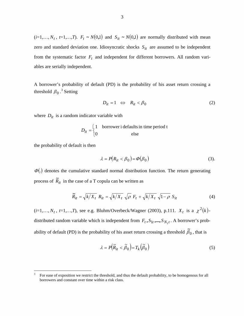
(i=1,…, tN , t=1,…,T). ( )10,~ NFt and ( )10,~ NSit are normally distributed with mean

zero and standard deviation one. Idiosyncratic shocks itS are assumed to be independent

from the systematic factor tF and independent for different borrowers. All random vari-

ables are serially independent.

A borrower’s probability of default (PD) is the probability of his asset return crossing a threshold 0β .3 Setting

01 β<⇔= itit RD (2)

where itD is a random indicator variable with

⎩⎨⎧

=else0

tperiod in time defaults iborrower 1itD

the probability of default is then

( ) ( )00 βΦβλ =<= itRP (3).

( ).Φ denotes the cumulative standard normal distribution function. The return generating

process of itR~ in the case of a T copula can be written as

ittttittit SXkFXkRXkR ρρ −+== 1~ (4)

(i=1,…, tN , t=1,…,T), see e.g. Bluhm/Overbeck/Wagner (2003), p.111. tX is a ( )k2χ -

distributed random variable which is independent from tNtt tSSF ,...,, 1 . A borrower’s prob-

ability of default (PD) is the probability of his asset return crossing a threshold 0β~ , that is

( ) ( )00~ ~~ ββλ kit TRP =<= (5)

3 For ease of exposition we restrict the threshold, and thus the default probability, to be homogenous for all

borrowers and constant over time within a risk class.

4

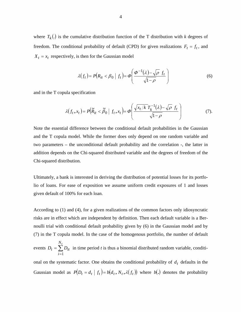
where ( ).kT is the cumulative distribution function of the T distribution with k degrees of

freedom. The conditional probability of default (CPD) for given realizations tt fF = , and

tt xX = respectively, is then for the Gaussian model

( ) ( ) ( )⎟⎟

⎠

⎞

⎜⎜

⎝

⎛

−

−=<=

−

ρρλΦ

Φβλ1

1

0t

tittf

fRPf (6)

and in the T copula specification

( ) ( ) ( )⎟⎟

⎠

⎞

⎜⎜

⎝

⎛

−

−=<=

−

ρ

ρλΦβλ

1

1

0tkt

ttitttfTkx

xfRPxf ,~~, (7).

Note the essential difference between the conditional default probabilities in the Gaussian

and the T copula model. While the former does only depend on one random variable and

two parameters – the unconditional default probability and the correlation -, the latter in

addition depends on the Chi-squared distributed variable and the degrees of freedom of the

Chi-squared distribution.

Ultimately, a bank is interested in deriving the distribution of potential losses for its portfo-

lio of loans. For ease of exposition we assume uniform credit exposures of 1 and losses

given default of 100% for each loan.

According to (1) and (4), for a given realizations of the common factors only idiosyncratic

risks are in effect which are independent by definition. Then each default variable is a Ber-

noulli trial with conditional default probability given by (6) in the Gaussian model and by

(7) in the T copula model. In the case of the homogenous portfolio, the number of default

events ∑=

=tN

iitt DD

1 in time period t is thus a binomial distributed random variable, conditi-

onal on the systematic factor. One obtains the conditional probability of td defaults in the

Gaussian model as ( ) ( )( )tttttt fNdbfdDP λ,,== where ( ).b denotes the probability

5

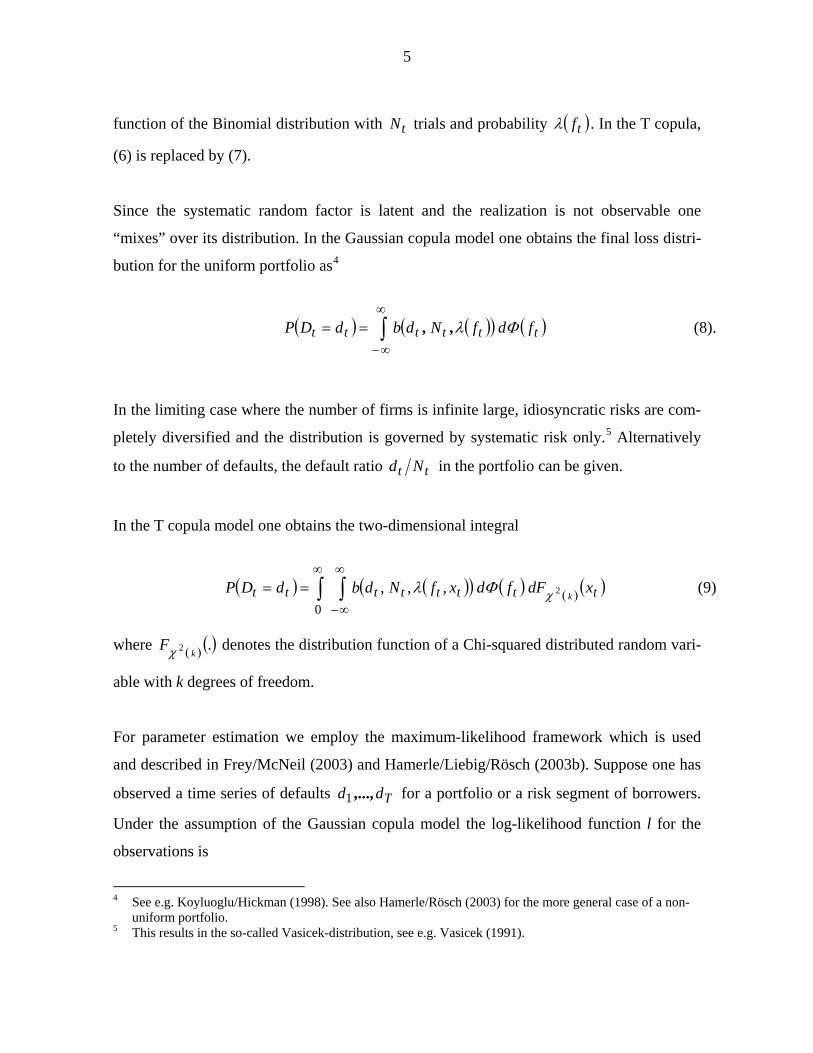
function of the Binomial distribution with tN trials and probability ( )tfλ . In the T copula,

(6) is replaced by (7).

Since the systematic random factor is latent and the realization is not observable one

“mixes” over its distribution. In the Gaussian copula model one obtains the final loss distri-

bution for the uniform portfolio as4

( ) ( )( ) ( )tttttt fdfNdbdDP Φλ,,∫∞

∞−

== (8).

In the limiting case where the number of firms is infinite large, idiosyncratic risks are com-

pletely diversified and the distribution is governed by systematic risk only.5 Alternatively

to the number of defaults, the default ratio tt Nd in the portfolio can be given.

In the T copula model one obtains the two-dimensional integral

( ) ( )( ) ( ) ( ) ( )tttttttt xdFfdxfNdbdDPk2,,,

0χΦλ∫∫

∞

∞−

∞== (9)

where ( ) ( ).2 kFχ denotes the distribution function of a Chi-squared distributed random vari-

able with k degrees of freedom.

For parameter estimation we employ the maximum-likelihood framework which is used

and described in Frey/McNeil (2003) and Hamerle/Liebig/Rösch (2003b). Suppose one has

observed a time series of defaults Tdd ,...,1 for a portfolio or a risk segment of borrowers.

Under the assumption of the Gaussian copula model the log-likelihood function l for the

observations is

4 See e.g. Koyluoglu/Hickman (1998). See also Hamerle/Rösch (2003) for the more general case of a non-

uniform portfolio. 5 This results in the so-called Vasicek-distribution, see e.g. Vasicek (1991).

6

( ) ( )( ) ( )⎪⎭

⎪⎬⎫

⎪⎩

⎪⎨⎧

= ∫∑∞

∞−=tttt

T

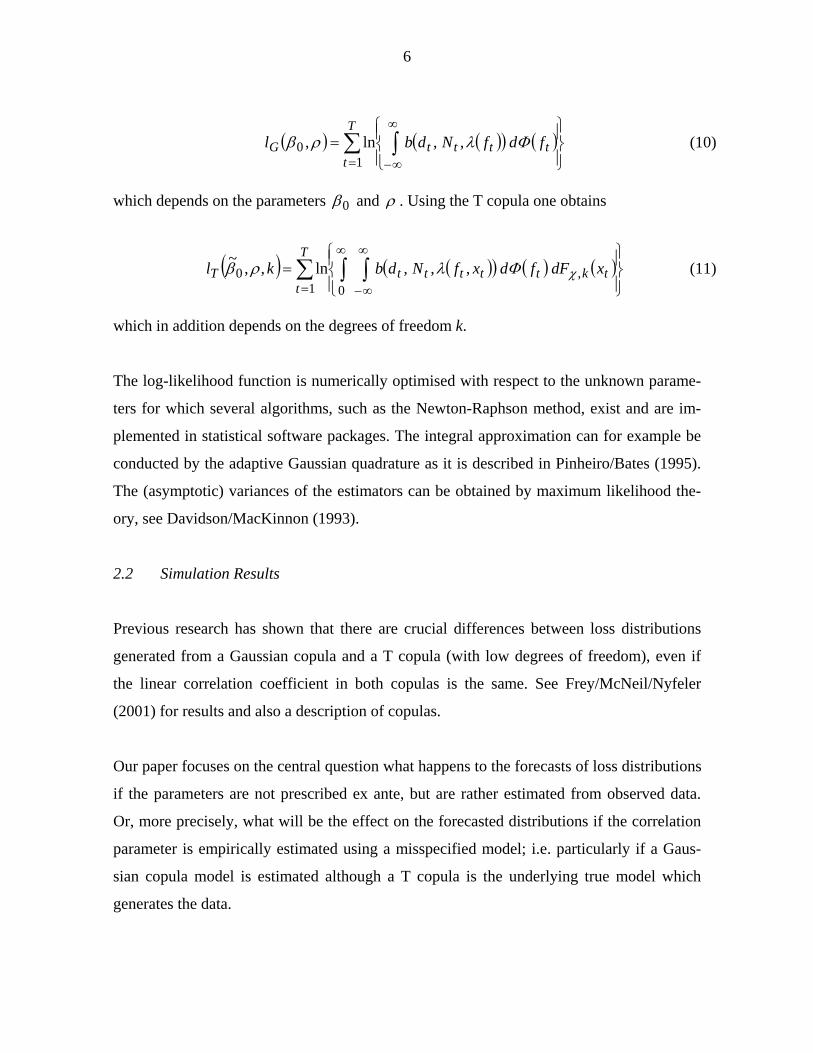
tG fdfNdbl Φλρβ ,,ln,

10 (10)

which depends on the parameters 0β and ρ . Using the T copula one obtains

( ) ( )( ) ( ) ( )⎪⎭

⎪⎬⎫

⎪⎩

⎪⎨⎧

= ∫∫∑∞

∞−

∞

=tkttttt

T

tT xdFfdxfNdbkl ,

010 ,,,ln,,~

χΦλρβ (11)

which in addition depends on the degrees of freedom k.

The log-likelihood function is numerically optimised with respect to the unknown parame-

ters for which several algorithms, such as the Newton-Raphson method, exist and are im-

plemented in statistical software packages. The integral approximation can for example be

conducted by the adaptive Gaussian quadrature as it is described in Pinheiro/Bates (1995).

The (asymptotic) variances of the estimators can be obtained by maximum likelihood the-

ory, see Davidson/MacKinnon (1993).

2.2 Simulation Results

Previous research has shown that there are crucial differences between loss distributions

generated from a Gaussian copula and a T copula (with low degrees of freedom), even if

the linear correlation coefficient in both copulas is the same. See Frey/McNeil/Nyfeler

(2001) for results and also a description of copulas.

Our paper focuses on the central question what happens to the forecasts of loss distributions

if the parameters are not prescribed ex ante, but are rather estimated from observed data.

Or, more precisely, what will be the effect on the forecasted distributions if the correlation

parameter is empirically estimated using a misspecified model; i.e. particularly if a Gaus-

sian copula model is estimated although a T copula is the underlying true model which

generates the data.

7

For the analysis we use Monte-Carlo simulations and generate a stylised portfolio of 1,000

borrowers in each scenario. Regarding the risk grades of borrowers we analyse two constel-

lations where a uniform medium-risk default probability of 1% is assumed on the one hand

and a low-risk default probability of 0.2% for each borrower on the other hand. The time-

series is set to length T=10. T copulas are generated with 5, 10 and 30 degrees of freedom

and the asset correlation parameter varies over 10%, 2% and 0% respectively.

Using these parameter constellations we randomly draw time series of default data gener-

ated from a T copula6 and estimate the parameters under the assumption of a Gaussian cop-

ula. For parameter estimation (default probability and asset correlation) we employ the

maximum-likelihood framework described above. Each constellation consists of 1,000

simulation runs. Table 1 shows the averages of the estimates obtained from the Monte-

Carlo simulations using the Gaussian copula.

6 Note that, although the distribution of the latent variables differs, the loss distribution for a T copula with

T margins and a T copula with Gaussian margins is the same.

8

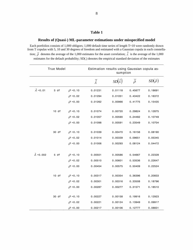
Table 1

Results of (Quasi-) ML-parameter estimations under misspecified model Each portfolios consists of 1,000 obligors; 1,000 default time series of length T=10 were randomly drawn

from T copulas with 5, 10 and 30 degrees of freedom and estimated with a Gaussian copula in each constella-tion; ρ̂ denotes the average of the 1,000 estimates for the asset correlation; λ̂ is the average of the 1,000

estimates for the default probability; SD(.) denotes the empirical standard deviation of the estimates

True Model Estimation results using Gaussian copula as-sumption

λ̂ ( )λ̂SD ρ̂ ( )ρ̂SD

λ =0.01 5 df ρ =0.10 0.01231 0.01118 0.45677 0.18691

ρ =0.02 0.01294 0.01051 0.43422 0.16372

ρ =0.00 0.01262 0.00966 0.41775 0.15435

10 df ρ =0.10 0.01074 0.00720 0.29824 0.12875

ρ =0.02 0.01057 0.00590 0.24482 0.10749

ρ =0.00 0.01098 0.00591 0.23549 0.10704

30 df ρ =0.10 0.01039 0.00470 0.16156 0.08190

ρ =0.02 0.01014 0.00339 0.09651 0.05345

ρ =0.00 0.01006 0.00293 0.08124 0.04472

λ =0.002 5 df ρ =0.10 0.00501 0.00586 0.54667 0.22328

ρ =0.02 0.00510 0.00601 0.53536 0.22647

ρ =0.00 0.00454 0.00575 0.50409 0.22524

10 df ρ =0.10 0.00317 0.00354 0.36396 0.20833

ρ =0.02 0.00301 0.00316 0.33508 0.18796

ρ =0.00 0.00287 0.00277 0.31571 0.18510

30 df ρ =0.10 0.00227 0.00158 0.19916 0.12923

ρ =0.02 0.00221 0.00124 0.13949 0.09917

ρ =0.00 0.00217 0.00106 0.12777 0.08831

9

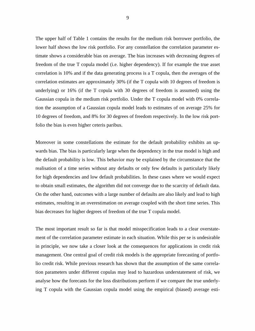
The upper half of Table 1 contains the results for the medium risk borrower portfolio, the

lower half shows the low risk portfolio. For any constellation the correlation parameter es-

timate shows a considerable bias on average. The bias increases with decreasing degrees of

freedom of the true T copula model (i.e. higher dependency). If for example the true asset

correlation is 10% and if the data generating process is a T copula, then the averages of the

correlation estimates are approximately 30% (if the T copula with 10 degrees of freedom is

underlying) or 16% (if the T copula with 30 degrees of freedom is assumed) using the

Gaussian copula in the medium risk portfolio. Under the T copula model with 0% correla-

tion the assumption of a Gaussian copula model leads to estimates of on average 25% for

10 degrees of freedom, and 8% for 30 degrees of freedom respectively. In the low risk port-

folio the bias is even higher ceteris paribus.

Moreover in some constellations the estimate for the default probability exhibits an up-

wards bias. The bias is particularly large when the dependency in the true model is high and

the default probability is low. This behavior may be explained by the circumstance that the

realisation of a time series without any defaults or only few defaults is particularly likely

for high dependencies and low default probabilities. In these cases where we would expect

to obtain small estimates, the algorithm did not converge due to the scarcity of default data.

On the other hand, outcomes with a large number of defaults are also likely and lead to high

estimates, resulting in an overestimation on average coupled with the short time series. This

bias decreases for higher degrees of freedom of the true T copula model.

The most important result so far is that model misspecification leads to a clear overstate-

ment of the correlation parameter estimate in each situation. While this per se is undesirable

in principle, we now take a closer look at the consequences for applications in credit risk

management. One central goal of credit risk models is the appropriate forecasting of portfo-

lio credit risk. While previous research has shown that the assumption of the same correla-

tion parameters under different copulas may lead to hazardous understatement of risk, we

analyse how the forecasts for the loss distributions perform if we compare the true underly-

ing T copula with the Gaussian copula model using the empirical (biased) average esti-

10

mates. That is, we model loss distributions under the true copula and under the assumption

of the misspecified Gaussian copula model for each constellation.

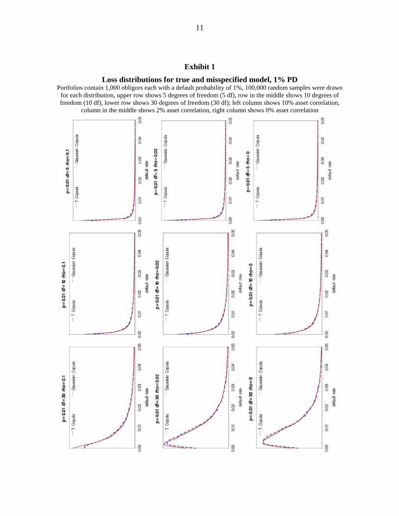
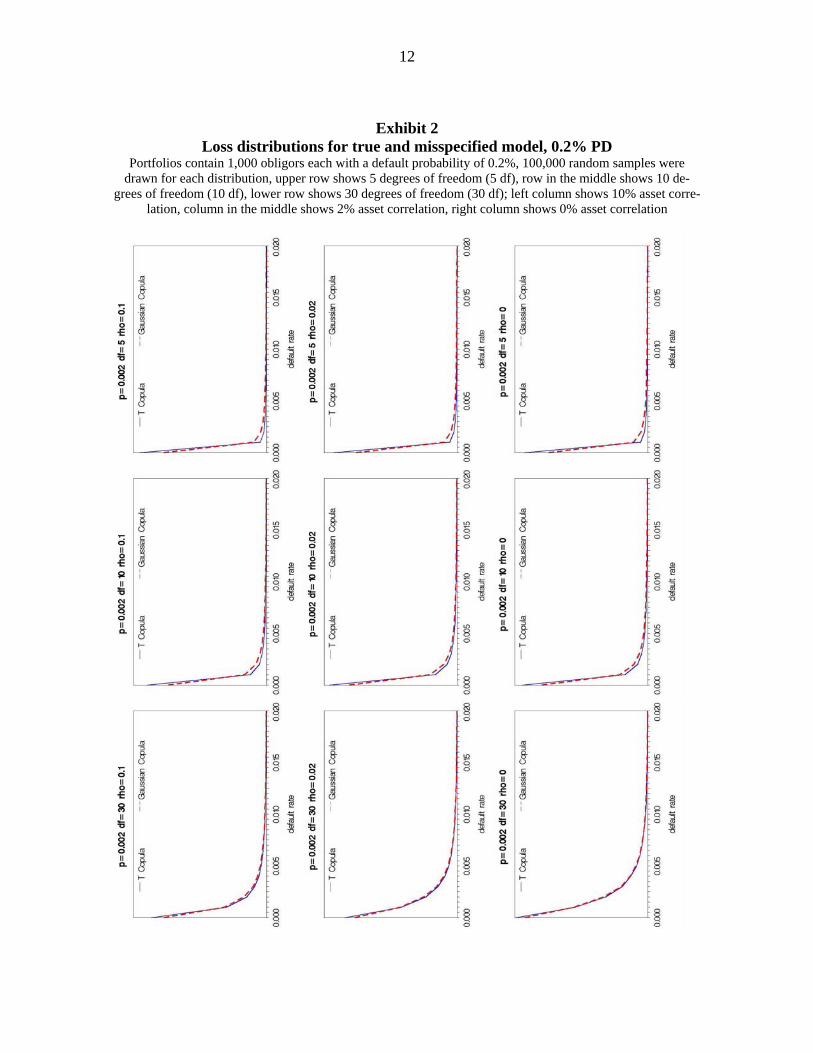
Exhibit 1 and Exhibit 2 contain the respective loss distributions for uniform portfolios with

1,000 borrowers under the assumption of 1% default probability each, and 0.2% default

probabilities respectively.

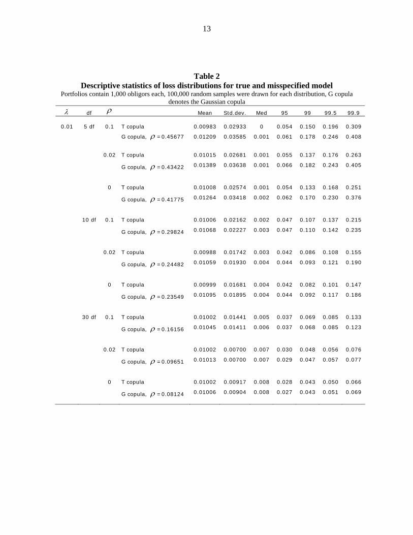
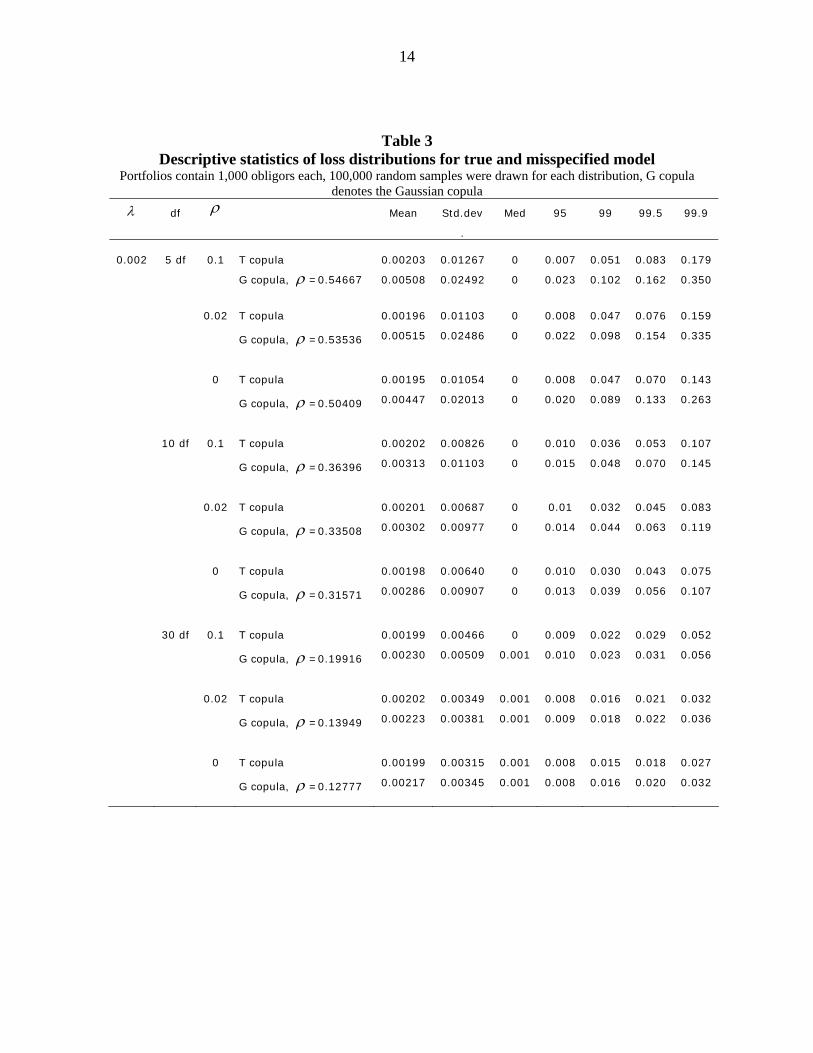
Table 2 and Table 3 show the appendant descriptive statistics: Mean, standard deviation,

and VaR quantiles. As can be seen, the distributions are of course not congruent, but in

most cases they are very similar. In particular, the VaR-quantiles using the misspecified

model no longer lead to an understatement of risk. Rather the picture is reversed: In each

but one scenario (where the default probability is 1%, the degrees of freedom are 30 and the

correlation is 10%) the VaR quantiles of the misspecified model are larger than those of the

true model. This is especially the case when the default probability is small since not only

the correlation parameter estimate but also the default probability estimate is upwards bi-

ased. Ceteris paribus the differences between the distributions decrease when dependence is

lower, i.e. the degrees of freedom are higher.

As a main result, we can record that despite of the misspecification of the underlying model

(i.e. the data generating process) in the estimation approach, the resulting forecast for the

loss distribution does no longer bear the danger of understating extreme risk.

11

Exhibit 1

Loss distributions for true and misspecified model, 1% PD Portfolios contain 1,000 obligors each with a default probability of 1%, 100,000 random samples were drawn

for each distribution, upper row shows 5 degrees of freedom (5 df), row in the middle shows 10 degrees of freedom (10 df), lower row shows 30 degrees of freedom (30 df); left column shows 10% asset correlation,

column in the middle shows 2% asset correlation, right column shows 0% asset correlation

12

Exhibit 2 Loss distributions for true and misspecified model, 0.2% PD

Portfolios contain 1,000 obligors each with a default probability of 0.2%, 100,000 random samples were drawn for each distribution, upper row shows 5 degrees of freedom (5 df), row in the middle shows 10 de-

grees of freedom (10 df), lower row shows 30 degrees of freedom (30 df); left column shows 10% asset corre-lation, column in the middle shows 2% asset correlation, right column shows 0% asset correlation

13

Table 2 Descriptive statistics of loss distributions for true and misspecified model

Portfolios contain 1,000 obligors each, 100,000 random samples were drawn for each distribution, G copula denotes the Gaussian copula

λ df ρ Mean Std.dev. Med 95 99 99.5 99.9

0.01 5 df 0.1 T copula 0.00983 0.02933 0 0.054 0.150 0.196 0.309

G copula, ρ =0.45677 0.01209 0.03585 0.001 0.061 0.178 0.246 0.408

0.02 T copula 0.01015 0.02681 0.001 0.055 0.137 0.176 0.263

G copula, ρ =0.43422 0.01389 0.03638 0.001 0.066 0.182 0.243 0.405

0 T copula 0.01008 0.02574 0.001 0.054 0.133 0.168 0.251

G copula, ρ =0.41775 0.01264 0.03418 0.002 0.062 0.170 0.230 0.376

10 df 0.1 T copula 0.01006 0.02162 0.002 0.047 0.107 0.137 0.215

G copula, ρ =0.29824 0.01068 0.02227 0.003 0.047 0.110 0.142 0.235

0.02 T copula 0.00988 0.01742 0.003 0.042 0.086 0.108 0.155

G copula, ρ =0.24482 0.01059 0.01930 0.004 0.044 0.093 0.121 0.190

0 T copula 0.00999 0.01681 0.004 0.042 0.082 0.101 0.147

G copula, ρ =0.23549 0.01095 0.01895 0.004 0.044 0.092 0.117 0.186

30 df 0.1 T copula 0.01002 0.01441 0.005 0.037 0.069 0.085 0.133

G copula, ρ =0.16156 0.01045 0.01411 0.006 0.037 0.068 0.085 0.123

0.02 T copula 0.01002 0.00700 0.007 0.030 0.048 0.056 0.076

G copula, ρ =0.09651 0.01013 0.00700 0.007 0.029 0.047 0.057 0.077

0 T copula 0.01002 0.00917 0.008 0.028 0.043 0.050 0.066

G copula, ρ =0.08124 0.01006 0.00904 0.008 0.027 0.043 0.051 0.069

14

Table 3

Descriptive statistics of loss distributions for true and misspecified model Portfolios contain 1,000 obligors each, 100,000 random samples were drawn for each distribution, G copula

denotes the Gaussian copula λ df ρ Mean Std.dev

.

Med 95 99 99.5 99.9

0.002 5 df 0.1 T copula 0.00203 0.01267 0 0.007 0.051 0.083 0.179

G copula, ρ =0.54667 0.00508 0.02492 0 0.023 0.102 0.162 0.350

0.02 T copula 0.00196 0.01103 0 0.008 0.047 0.076 0.159

G copula, ρ =0.53536 0.00515 0.02486 0 0.022 0.098 0.154 0.335

0 T copula 0.00195 0.01054 0 0.008 0.047 0.070 0.143

G copula, ρ =0.50409 0.00447 0.02013 0 0.020 0.089 0.133 0.263

10 df 0.1 T copula 0.00202 0.00826 0 0.010 0.036 0.053 0.107

G copula, ρ =0.36396 0.00313 0.01103 0 0.015 0.048 0.070 0.145

0.02 T copula 0.00201 0.00687 0 0.01 0.032 0.045 0.083

G copula, ρ =0.33508 0.00302 0.00977 0 0.014 0.044 0.063 0.119

0 T copula 0.00198 0.00640 0 0.010 0.030 0.043 0.075

G copula, ρ =0.31571 0.00286 0.00907 0 0.013 0.039 0.056 0.107

30 df 0.1 T copula 0.00199 0.00466 0 0.009 0.022 0.029 0.052

G copula, ρ =0.19916 0.00230 0.00509 0.001 0.010 0.023 0.031 0.056

0.02 T copula 0.00202 0.00349 0.001 0.008 0.016 0.021 0.032

G copula, ρ =0.13949 0.00223 0.00381 0.001 0.009 0.018 0.022 0.036

0 T copula 0.00199 0.00315 0.001 0.008 0.015 0.018 0.027

G copula, ρ =0.12777 0.00217 0.00345 0.001 0.008 0.016 0.020 0.032

15

3 Considering Estimation Risk

The previous section showed that parameter estimates under the misspecified model are

biased. If we forecast the loss distribution, however, this bias may lead to an even more

conservative VaR figure. We analysed this by using the averages of the estimates under the

misspecified copula in our simulations. In empirical applications in risk management, we

can hardly make use of average estimates resulting from a large number of simulated time

series. Rather we only face one single realisation of the default time series and have to

make do with that. Then we experience the problem that our parameter estimates are af-

fected by estimation errors and may realise far from their true parameter counterparts. Con-

sequently all risk figures generated from the estimates, such as for example the VaR, are

also affected by estimation risk. As one of the first to do so, Jorion (1996) assesses this

problem in the context of market risk. Löffler (2003) analyses estimation risk in the context

of credit risk. He generates measurement errors around given parameters via Monte-Carlo

simulation and finds that the effects of these errors on credit risk measures may be consid-

erable.

In the context of our problem in specifying copulas straightforwardly the question is raised,

not only which copula is more conservative on average, but also which specification pro-

vides the risk manager in practice with less uncertainty about the true parameter values. To

do this we again take a look at the T and the Gaussian copula, but instead of comparing the

average parameter estimates of the Gaussian copula with the true parameters, we use the

following proceeding:

• Step 1: We generate a time series of defaults from the true T copula model.

• Step 2: From this time series the (misspecified) Gaussian copula model parameters

are estimated.

• Step 3: From the same time series we estimate the T copula parameters. In order to

achieve a “fair” comparison we also estimate only two parameters for this copula

16

(the default probability and the degrees of freedom) and fix the third parameter (cor-

relation) at its true value.

• Step 4: For the resulting sets of parameter estimates from step 2 and step 3 we

model the loss distribution and calculate a Value at Risk quantile.

• Steps 1 to 4 are repeated many times.7

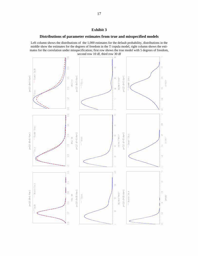
For exposition we use the portfolio where the default probability is 1% and the correlation

is zero. Firstly, Exhibit 3 shows the distributions of the parameter estimates from the true T

copula and the misspecified Gaussian model. For each parameter and model it turns out that

higher dependency leads to more uncertainty in the parameter estimates resulting in wider

empirical distributions. Also, for the small sample with 10 years of data under considera-

tion, the asymptotic normality property of the ML estimates is rather weak.

7 This proceeding is also chosen by Frey/McNeil (2003). These authors, however, only assess estimation

risk of the true model.

17

Exhibit 3

Distributions of parameter estimates from true and misspecified models Left column shows the distributions of the 1,000 estimates for the default probability, distributions in the middle show the estimates for the degrees of freedom in the T copula model, right column shows the esti-

mates for the correlation under misspecification; first row shows the true model with 5 degrees of freedom, second row 10 df, third row 30 df

18

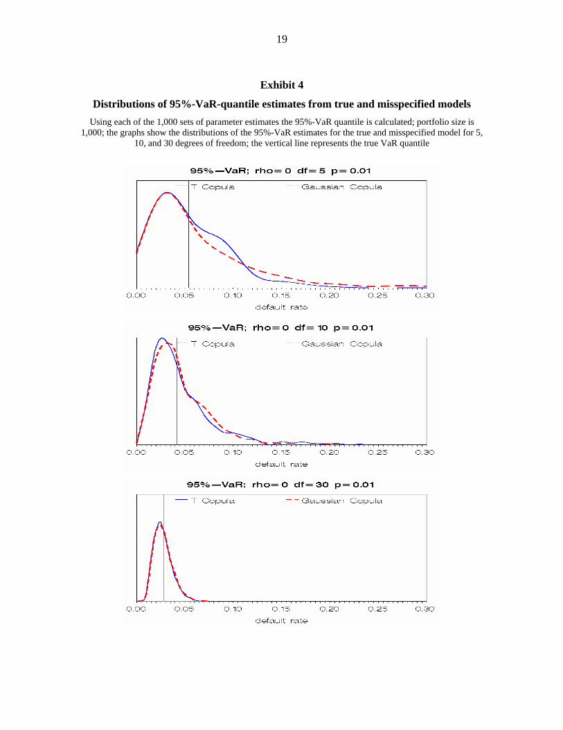
Exhibit 4 compares the distributions of the simulated 95%-VaR-quantiles under both copu-

las. As can be seen the estimation error with respect to the VaR is considerable for the true

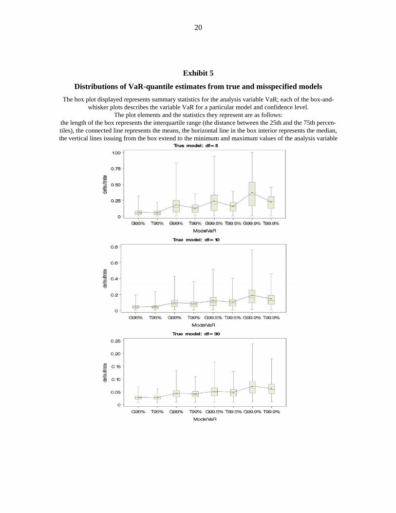
as well as the misspecified model and decreases with decreasing dependency. Exhibit 5

summarises the distributions of the VaRs calculated at 95%-, 99%, 99.5%, and 99.9% con-

fidence levels. Estimation risk increases with increasing confidence level for the true as

well as the misspecified model. Due to the fatter tails of the distributions under the mis-

specified model as shown before, the quantiles under the Gaussian copula are more far out-

side and exhibit larger dispersion, particularly for high dependence under the true model.

Hence, misspecification ceteris paribus may lead in our constellations to slightly higher

estimation errors, but on average VaR quantiles are more conservative. For lower depend-

ency the differences between the true and the misspecified model on average as well as

with respect to estimation risk vanish.

19

Exhibit 4

Distributions of 95%-VaR-quantile estimates from true and misspecified models Using each of the 1,000 sets of parameter estimates the 95%-VaR quantile is calculated; portfolio size is

1,000; the graphs show the distributions of the 95%-VaR estimates for the true and misspecified model for 5, 10, and 30 degrees of freedom; the vertical line represents the true VaR quantile

20

Exhibit 5

Distributions of VaR-quantile estimates from true and misspecified models The box plot displayed represents summary statistics for the analysis variable VaR; each of the box-and-

whisker plots describes the variable VaR for a particular model and confidence level. The plot elements and the statistics they represent are as follows:

the length of the box represents the interquartile range (the distance between the 25th and the 75th percen-tiles), the connected line represents the means, the horizontal line in the box interior represents the median, the vertical lines issuing from the box extend to the minimum and maximum values of the analysis variable

21

4 Empirical Example

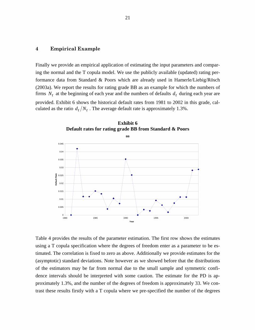
Finally we provide an empirical application of estimating the input parameters and compar-ing the normal and the T copula model. We use the publicly available (updated) rating per-formance data from Standard & Poors which are already used in Hamerle/Liebig/Rösch (2003a). We report the results for rating grade BB as an example for which the numbers of firms tN at the beginning of each year and the numbers of defaults td during each year are

provided. Exhibit 6 shows the historical default rates from 1981 to 2002 in this grade, cal-culated as the ratio tt Nd . The average default rate is approximately 1.3%.

Exhibit 6

Default rates for rating grade BB from Standard & Poors BB

0

0.005

0.01

0.015

0.02

0.025

0.03

0.035

0.04

0.045

1980 1985 1990 1995 2000

Year

Def

ault

Rat

e

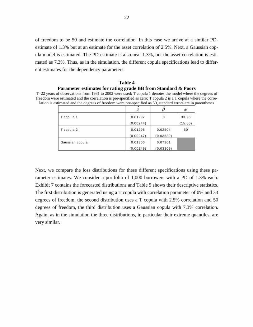
Table 4 provides the results of the parameter estimation. The first row shows the estimates using a T copula specification where the degrees of freedom enter as a parameter to be es-timated. The correlation is fixed to zero as above. Additionally we provide estimates for the (asymptotic) standard deviations. Note however as we showed before that the distributions of the estimators may be far from normal due to the small sample and symmetric confi-dence intervals should be interpreted with some caution. The estimate for the PD is ap-proximately 1.3%, and the number of the degrees of freedom is approximately 33. We con-trast these results firstly with a T copula where we pre-specified the number of the degrees

22

of freedom to be 50 and estimate the correlation. In this case we arrive at a similar PD-estimate of 1.3% but at an estimate for the asset correlation of 2.5%. Next, a Gaussian cop-ula model is estimated. The PD-estimate is also near 1.3%, but the asset correlation is esti-mated as 7.3%. Thus, as in the simulation, the different copula specifications lead to differ-ent estimates for the dependency parameters.

Table 4

Parameter estimates for rating grade BB from Standard & Poors T=22 years of observations from 1981 to 2002 were used; T copula 1 denotes the model where the degrees of freedom were estimated and the correlation is pre-specified as zero; T copula 2 is a T copula where the corre-

lation is estimated and the degrees of freedom were pre-specified as 50, standard errors are in parentheses λ̂ ρ̂ df

T copula 1 0.01297

(0.00244)

0

33.26

(15.60)

T copula 2 0.01298

(0.00247)

0.02504

(0.03539)

50

Gaussian copula 0.01300

(0.00249)

0.07301

(0.03309)

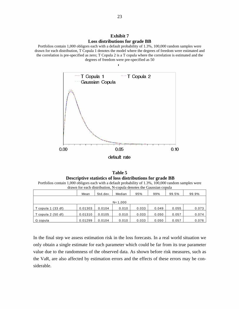
Next, we compare the loss distributions for these different specifications using these pa-rameter estimates. We consider a portfolio of 1,000 borrowers with a PD of 1.3% each. Exhibit 7 contains the forecasted distributions and Table 5 shows their descriptive statistics. The first distribution is generated using a T copula with correlation parameter of 0% and 33 degrees of freedom, the second distribution uses a T copula with 2.5% correlation and 50 degrees of freedom, the third distribution uses a Gaussian copula with 7.3% correlation. Again, as in the simulation the three distributions, in particular their extreme quantiles, are very similar.

23

Exhibit 7 Loss distributions for grade BB

Portfolios contain 1,000 obligors each with a default probability of 1.3%, 100,000 random samples were drawn for each distribution, T Copula 1 denotes the model where the degrees of freedom were estimated and the correlation is pre-specified as zero; T Copula 2 is a T copula where the correlation is estimated and the

degrees of freedom were pre-specified as 50

Table 5 Descriptive statistics of loss distributions for grade BB

Portfolios contain 1,000 obligors each with a default probability of 1.3%, 100,000 random samples were drawn for each distribution, N-copula denotes the Gaussian copula

Mean Std.dev. Median 95% 99% 99.5% 99.9%

N=1,000

T copula 1 (33 df) 0.01303 0.0104 0.010 0.033 0.049 0.055 0.073

T copula 2 (50 df) 0.01310 0.0105 0.010 0.033 0.050 0.057 0.074

G copula 0.01299 0.0104 0.010 0.033 0.050 0.057 0.076

In the final step we assess estimation risk in the loss forecasts. In a real world situation we only obtain a single estimate for each parameter which could be far from its true parameter value due to the randomness of the observed data. As shown before risk measures, such as the VaR, are also affected by estimation errors and the effects of these errors may be con-siderable.

24

To develop a simple strategy for implementing an assessment of estimation risk we assume asymptotic normal distributions for the estimators due to Maximum Likelihood theory, since the true small sample distribution is unknown. Under this approximation we derive a distribution of potential VaR measures in the following way:

• Step 1: For each of the three estimated copula models we generate a set of “pseudo-

parameters” from a joint normal distribution with mean vector equal to the point es-

timates of the parameters and the matrix of covariances equal to the estimated ma-

trix of covariances. By doing this we simulate one possible set of values for the

“true” unknown parameters.8

• Step 2: Using this set of pseudo-parameters we generate a loss distribution and cal-

culate a VaR quantile.

• Step 3: Steps 1 to 2 are repeated many times.

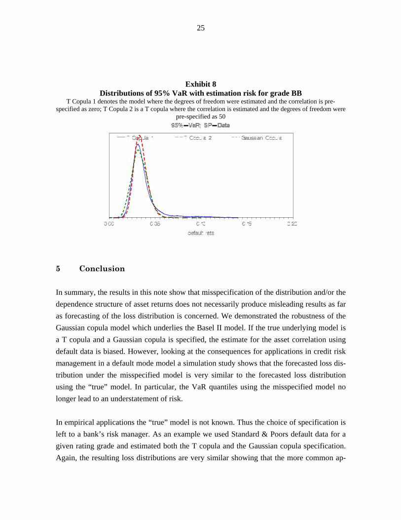
As a result we obtain a distribution of simulated VaR quantiles. Each of these values can be interpreted as the VaR derived under the assumptions that the underlying simulated poten-tial set of parameters is the true one. Exhibit 8 shows the resulting distribution for the three models. The Gaussian copula and T copula 2 behave rather similar with respect to the tails of the distributions, the T copula 1 VaR distribution is more skewed to the right. This result may stem from the assumed asymptotic normal distribution of the parameter estimates: As shown before, the small-sample distribution of the estimates is far from normal, particularly the distribution of the estimates for the degrees of freedom is skewed to the right, i.e. to lower dependence. Assuming normally distributed estimates, as it is done here, pulls more probability mass into the direction of higher dependence which results in higher VaR quan-tiles. If we choose this kind of proceeding for the assessment of estimation risk in practice, the T copula model may result in slightly more conservative VaR estimates. However, as exhibit 8 shows, the difference is still not very substantial.

8 It should be noted that negative asset correlations may result in the case of Gaussian copula. In these

cases we took the absolute value. In the case of the T copulas, simulated degrees of freedom of lower than two may be generated. Here we imposed the restriction for the degrees of freedom to be larger than two.

25

Exhibit 8 Distributions of 95% VaR with estimation risk for grade BB

T Copula 1 denotes the model where the degrees of freedom were estimated and the correlation is pre-specified as zero; T Copula 2 is a T copula where the correlation is estimated and the degrees of freedom were

pre-specified as 50

5 Conclusion In summary, the results in this note show that misspecification of the distribution and/or the dependence structure of asset returns does not necessarily produce misleading results as far as forecasting of the loss distribution is concerned. We demonstrated the robustness of the Gaussian copula model which underlies the Basel II model. If the true underlying model is a T copula and a Gaussian copula is specified, the estimate for the asset correlation using default data is biased. However, looking at the consequences for applications in credit risk management in a default mode model a simulation study shows that the forecasted loss dis-tribution under the misspecified model is very similar to the forecasted loss distribution using the “true” model. In particular, the VaR quantiles using the misspecified model no longer lead to an understatement of risk. In empirical applications the “true” model is not known. Thus the choice of specification is left to a bank’s risk manager. As an example we used Standard & Poors default data for a given rating grade and estimated both the T copula and the Gaussian copula specification. Again, the resulting loss distributions are very similar showing that the more common ap-

26

proach, also used in the Basel II capital framework, works for purposes of loss distribution forecasting in a satisfactory manner, provided that the parameters are estimated using de-fault data. Hence, model risk resulting from misspecification is therefore strongly reduced. In Jorion (1996) the problem of estimation errors in the context of Value-at-Risk in market risk is addressed. In most applications of credit risk models the parameter estimation risk is neglected. An exception is a study by Löffler (2003). Dealing with uncertainties in model inputs might be one important challenge for the future, not only for the New Basel Capital Accord but also for full internal credit models. Here, we find that a misspecified Gaussian copula performs similar with respect to estimation risk compared to the true T copula. However, estimation errors may be large for both models, and a lot of work has to be done into the direction of handling estimation risk. References

Bluhm, C., Overbeck, L., Wagner, C., 2003. An Introduction to Credit Risk Modeling, Lon-don.

Davidson, R., MacKinnon, J.D. (1993). Estimation and Inference in Econometrics, New York.

Frey, R., McNeil, A., 2003. Dependent Defaults in Models of Portfolio Credit Risk, Journal of Risk 6, 59-92.

Frey, R., McNeil, A., Nyfeler, M., 2001. Copulas and Credit Models, Risk 14, October, 111-114.

Gordy, M.B., 2000. A Comparative Anatomy of Credit Risk Models, Journal of Banking and Finance 24, 119-149.

Gordy, M.B., Heitfield, E. (2000): Estimating Factor Loadings When Ratings Performance Data Are Scarce, Board of Governors of the Federal Reserve System, Division of Research and Statistics, Working Paper.

Hamerle, A., Liebig, T., Rösch, D., 2003b. Benchmarking Asset Correlations, Risk 16, No-vember.

27

Hamerle, A., Liebig, T., Rösch, D., 2003a. Credit Risk Factor Modeling and the Basel II IRB Approach. Discussion Paper Series 2: Banking and Financial Supervision, No 02/2003, Deutsche Bundesbank.

Hamerle. A., Rösch, D., 2003. Parameterizing Credit Risk Models, Working Paper, Univer-sity of Regensburg.

Jorion, P., 1996. Risk2: Measuring the Risk in Value at Risk, Financial Analysts Journal, November/December, 47-56.

Li, D.X., 2000. On Default Correlation: A Copula Function Approach, Journal of Fixed Income 9, March, 43-54.

Lucas, D.J., 1995. Default Correlation and Credit Analysis. Journal of Fixed Income 4, 76-87.

Löffler, G., . The Effect of Estimation Risk on Measures of Portfolio Credit Risk, Journal of Banking and Finance 27, 1427-1453.

Nagpal, K., Bahar, R., 2001. Measuring Default Correlation. Risk, March, 129-132.

Servigny, A., Renault, O., 2003. Correlation Evidence, Risk 16, July, 90-94.

Vasicek, O.A., 1991. Limiting Loan Loss Probability Distribution. Working Paper, KMV Corporation, San Francisco.