Missing.... presumed at random: cost-analysis of incomplete data

HEALTH ECONOMICS

Health Econ. 12: 377–392 (2003)

Published online 10 December 2002 in Wiley InterScience (www.interscience.wiley.com). DOI:10.1002/hec.766

ECONOMIC EVALUATION

Missing.... presumed at random: cost-analysis of incompletedata

Andrew Briggsa,*, Taane Clarkb, Jane Wolstenholmea and Philip ClarkeaaHealth Economics Research Centre, University of Oxford, UKbCentre for Statistics in Medicine, University of Oxford, UK

Summary

When collecting patient-level resource use data for statistical analysis, for some patients and in some categories ofresource use, the required count will not be observed. Although this problem must arise in most reported economicevaluations containing patient-level data, it is rare for authors to detail how the problem was overcome. Statisticalpackages may default to handling missing data through a so-called ‘complete case analysis’, while some recent cost-analyses have appeared to favour an ‘available case’ approach. Both of these methods are problematic: completecase analysis is inefficient and is likely to be biased; available case analysis, by employing different numbers ofobservations for each resource use item, generates severe problems for standard statistical inference. Instead weexplore imputation methods for generating ‘replacement’ values for missing data that will permit complete caseanalysis using the whole data set and we illustrate these methods using two data sets that had incomplete resourceuse information. Copyright # 2002 John Wiley & Sons, Ltd.

Keywords economic evaluation; cost-analysis; missing data

Introduction

Clinical trials are increasingly including re-source use information in addition to healthoutcome data in order to allow economic evalua-tion of health care interventions. A recent reviewof cost assessment of healthcare technologiesin clinical trials has highlighted the handlingof missing data as an issue for such cost analyses[1]. Even in a most carefully designed study,data on resource use for all patients in a trialare unlikely to be complete. However, it is rareto find any discussion of how missing datawere handled in economic evaluations con-ducted alongside clinical trials. One exceptionto this is a recent evaluation of hospital at home

that acknowledged

. . . relatively few patients had a complete set of suchdata. Hence, mean costs for each item of resource usewere calculated and then aggregated to estimate thetotal cost per patient. Statistical testing was thereforenot possible at the level of total resource use perpatient. (p1804) [2]

While we applaud the clarity with which theauthors acknowledged the problem of missingdata, we will argue that the chosen solution(known as available case analysis) is not optimal,precisely because it is not clear that it allowsstatistical testing of the differences in total cost perpatient between alternatives under evaluation. Theuse of this method may also explain why anotherrecent economic evaluation conducted alongside a

Copyright # 2002 John Wiley & Sons, Ltd.Received 6 June 2001

Accepted 13 August 2002

*Correspondence to: Health Economics Research Centre, University of Oxford, Institute of Health Sciences, Headington,Oxford OX3 7LF, UK. E-mail: [email protected]

clinical trial failed to report any statistical analysisrelating to differences in total cost per patientbetween the two trial arms despite the availabilityof patient-level information, instead relying onsensitivity analysis to explore the implications ofuncertainty [3]. Indeed, we suspect that in mostcases, health economists when confronted withmissing data will use very simple methods (com-plete case, available case or unconditional meanimputation) to overcome the problem.

The problem of missing data is not new and hasreceived much attention in the statistical literatureas to the appropriate methods for handlingmissing data. While in principle missing economicdata alongside clinical trials is no different to otherforms of missing data, the distributional form ofcost data (it is commonly highly skewed) mayprovide challenges for the analyst. Furthermore,since economic evaluation is commonly ‘piggy-backed’ onto clinical trials, there is a danger thateconomic variables will be considered less impor-tant by researchers responsible for data collectionwhich could result in higher rates of missingness.

The purpose of this paper is to explore theavailable methods for handling missing data, witha view to highlighting the problems associatedwith the simplistic methods and to introduce moreappropriate approaches that maintain the statis-tical integrity of the analysis. The next sectionbegins with an overview of the problem of missingdata and of the methods available for handling theproblem. The following section then employs twoexamples of missing data problems. The firstinvolves a data set on hospitalisation where justone of the variables, length of stay in hospital,suffers from the missing data problem. The secondexample relates to a cost analysis of patientsrandomised to either transurethral resection of theprostate or contact-laser revapourisation of theprostate where data were missing for a number ofdifferent resource use variables. A final sectionoffers a discussion and an appendix is given listingsome popular software packages and algorithmsfor conducting the analyses reported in the paper.

Methods for handling missing data

Where data on resource use information has beencollected as part of a clinical trial, the cost data setwill be counts of resource use for each patient inthe costing part of the study. The problem of

missingness arises when data are not collected ormay not be available for some variables and/or forsome patients. This poses a problem for economicanalysis as standard statistical techniques havebeen designed to deal with rectangular data sets.

In this section, a general overview of the missingdata problem is given. First the patterns ofmissingness that can occur are identified. Nextthe commonly employed notation for the missing-ness mechanism is outlined. Finally, we review themethods available for handling missing dataproblem in a health economic context.

Patterns of missingness

Missing data can arise in a number of ways.Univariate missingness occurs when a singlevariable in a data set is causing a problem throughmissing values, while the rest of the variablescontain complete information. Unit non-responsedescribes the situation where for some people(observations) no data are recorded for any of thevariables. More common, however, is a situationof general or multivariate missingness where some,but not all of the variables will be missing for someof the subjects. Another common type of missing-ness is known as monotone missing data, whicharises in panel or longitudinal studies, and ischaracterised by information being available up toa certain time point/wave but not beyond thatpoint.

Missing data mechanisms

Little and Rubin [4] outline three missing datamechanisms:

1. Missing completely at random (MCAR). If dataare missing under this mechanism then it is as ifrandom cells from the rectangular data set arenot available such that the missing values bearno relation to the value of any of the variables.

2. Missing at random (MAR). Under this mechan-ism, missing values in the data set may dependon the value of other observed variables in thedata set, but that conditional on those valuesthe data are missing at random. The key is thatthe missing values do not depend on the valuesof unobserved variables.

Copyright # 2002 John Wiley & Sons, Ltd. Health Econ. 12: 377–392 (2003)

A. Briggs et al.378

3. Not missing at random (NMAR) describes thecase where missing values do depend onunobserved values.

The difference between these mechanisms is quitesubtle, particularly for the first two cases ofMCAR and MAR. For example, consider aquestionnaire distributed to patients, in order toascertain their use of health care resources follow-ing a particular treatment intervention, where notall the questionnaires are returned. The non-response is MCAR if the reason for failure tocomplete the questionnaire was unrelated to anyvariables under consideration. Of course, such asituation is unlikely. For example, retired patientsmay find more time to complete and return aquestionnaire than patients who have returned towork. Also, being older on average, the retiredpatients may make more use of health careresources. If having conditioned on the age andretirement status of the patients in the study non-response is at random then the missing dataproblem is MAR. However, consider that one ofthe reasons for non-response is that patients arenot at home, but have been taken into hospitalwith complications related to their original proce-dure. Now the missing data are NMAR since thevalue of the data that we do not observe is drivingthe reason for non-response. The methods fordealing with missingness outlined in the rest of thepaper are applicable to missing information that iseither MCAR or MAR.

Na.ııve methods for handling missing data

This section outlines the simple and ad hocapproaches to handling missing data that areoften used. The potential problems with theseapproaches are highlighted and the next sectionmoves on to a description of the more sophisti-cated imputation procedures.

Complete-case analysis. Complete-case analysis(CCA) or listwise deletion of cases is the defaultmethod in most statistical software packages. Itinvolves discarding cases where any variables aremissing. The advantages of using this method arethat it is easy to do and that the same set of data(albeit a reduced set) is used for all analyses.However, it is inefficient in that it excludes datathat are potentially informative for the analysis.Furthermore, CCA will be biased if the complete

cases systematically differ from the original sample(e.g. when the missing information is in factMAR). In practice, CCA may be an acceptablemethod with small amounts of missing informa-tion, but it is difficult to give definitive rules ofthumb as to how much missing data may beproblematic. In the case of general missingnesspatterns in multivariate data sets, relatively smallnumbers of missing data points can result in thelistwise deletion of a large number of cases for aCCA, and reduce the power of an analysis.

Available-case analysis. Available-case analysis(ACA) addresses the problem of inefficiency inCCA by estimating the mean for the completecases for each variable. The major disadvantage isthat different samples are used across the analysis,i.e. the sample base varies from one variable toanother since a different set of patients contributeto the estimation of different variables. This leadsto problems of comparability across variables, inparticular regarding the covariance structure in thedata set, and may explain why in some stochasticeconomic evaluations analysts have not reported astatistical analysis [2,3]. Since the primary purposeof cost analysis is to calculate total cost per patientacross the resource use variables, then it is clearthat available case analysis will lead to the sort ofproblems in undertaking statistical analysis of perpatient cost differences highlighted in the intro-duction. It should also be clear that available caseanalysis poses problems for standard regression-type methods that might be used when the focus ofcost-analysis is the marginal effect of importantcovariates on cost.

Imputation methods for missing data

Imputation is where the missing data can bereplaced with statistical estimates of the missingvalues. The goal of any imputation technique is toproduce a complete data set that can then beanalysed using statistical methods for completedata. The aim, therefore, is to simultaneouslyovercome the problems associated with both CCAand ACA. Several methods exist for imputingmissing values. These are described in more detailbelow.

Mean imputation (unconditional means). Meanimputation is a popular, though na.ııve, methodfor replacing missing data. The mean of the

Cost-Analysis of Incomplete Data 379


observed data for each variable is calculated andsubstituted into every case with a missing observa-tion for that variable. It is clear that the appeal ofunconditional mean imputation lies in its simpli-city. However, it is easy to see why this method isseriously flawed. Firstly, by imputing the meanvalue in a number of cases the estimated varianceor standard deviation for that variable will beunderestimated (since the imputed values do notdiffer from the mean or each other). Secondly,estimates of covariances and correlations are alsoadversely affected due to the fact that the imputedvalues for each of the variables are by definitionunconditional. Therefore the effect of this methodwill be to water down the observed correlationstructure of the data. Thus any further analysissuch as regression analysis is questionable.

Regression (conditional) imputation. A muchmore promising method is to use standard regres-sion analysis to provide estimates of the missingdata conditional on complete variables in theanalysis. For example, for the simple case ofunivariate missingness in a single continuousvariable Y , we fit a regression model to explainY by the remaining p variables represented by thevector X using the complete cases (subscripted by i):

Yi ¼ aþXpk¼1

bkXik þ ei ð1Þ

Predicted values for the expected values of themissing cases of Y (subscripted by j) can beobtained from

#YYj ¼ #aaþXpk¼1

#bbkXjk ð2Þ

It should be emphasised that the equations abovecould be generalised to include models for non-continuous data such as binomial or count data.Note that mean imputation from the previoussection is equivalent to the simplest form ofregression model with only an intercept term.

Missing data are usually multivariate and it ispossible to extend the procedure of regression-based imputation from the univariate case to dealwith multivariate missingness. For each missingvalue in the data set a model can be fitted for thatvariable employing the complete cases of all theother variables [5]. Where the number of variableswith missing values is large, the number of modelsto be fitted will also be large, however, efficientcomputational methods (such as Little & Rubin’s

sweep operator) can be employed [4]. Alterna-tively, an iterative regression approach can beadopted [6] whereby missing values in a givenvariable are predicted from a regression of thatvariable on the complete cases of all othervariables in the dataset. This process is repeatedfor all variables with missing values using completecases of the other variables including previouslyimputed values until a completed rectangular dataset has been generated. The imputation of missingvalues for each variable is then re-estimated in turnusing the complete set of data and the processcontinues until the imputed values stop changing.

Other straightforward approaches. In some otherapproaches, imputations are drawn from theactual values in the data set. For example, inpanel data, where data are subject to attrition, thelast observation for an individual may be carriedforward in time in order to complete the data set,and this approach is widely used. Little and Su [7]have suggested better methods for panel dataimputation based on simple row and column fits.Another imputation method is called the hot-deck,as used by the US Census Bureau [8]. This methodcompletes a missing observation by selecting atrandom, with replacement, a value from thoseindividuals who have matching observed valuesfor other variables (for matching purposes, con-tinuous variables may need to be categorised). Amore general approach to the hot-deck is to definea distance function on the basis of observedvariables. A missing value is imputed based onan observed value that is close in terms of distance.One such method is predictive mean matching [9].A similar approach, involves predicting propensityscores for values to be missing for individuals inthe data set and then imputing missing values fromcomplete cases with comparable propensity scores,and this method has been suggested for cost datasets with missing values due to attrition [10].

In practice, there are many methods that havebeen proposed for imputing missing values inorder to complete data sets and it is not ourintention to provide a comprehensive overview.Instead, we focus on methods that employ aformal statistical model for predicting missingvalues. The advantage of such methods is that theyretain the statistical integrity of the analysis,allowing appropriate inference that includes un-certainty in the prediction of the missing valuesthemselves (see the section on multiple imputationbelow).

A. Briggs et al.380


Maximum likelihood approaches. The maximumlikelihood (ML) approach involves formulating astatistical model and basing inference on thelikelihood function of the incomplete data. Wewill assume that the parameters of interestare the vector of means and the covariance matrixof the variables (or cell probabilities for a multi-nomial model in the case of strictly categoricaldata) [11]. In other contexts, these parametersmay be measures of effect, such as (log) oddsratios. If there were no missing data, it would bestraightforward to fit parameters of the model byML methods. If there were a univariate missingdata problem, then it would be possible tofactorise the likelihood in order to predict themissing data conditional only on the observeddata. For the problem of multivariate missingness,the likelihood does not factorise. However,use can be made of the Expectation-Maximi-sation (EM) algorithm [11], which is basedon a very simple premise. If we knew theparameters of the model we could estimatethe missing data and if we knew the missingvalues we could estimate the parameters.Therefore the following iterative procedure issuggested:

1. Choose starting values for missing data points2. Estimate the parameters3. Re-estimate the missing values, assuming that

the new parameter estimates are correct4. Repeat steps 2 & 3 until the results stop

changing.

Specifically, the EM algorithm involves iteratingbetween an Estimation-step and a Maximi-sation-step. The E-step involves averaging thecomplete-data likelihood over the predictivedistribution of the missing data given our para-meters in order to provide estimates of the missingdata. The M-step involves maximising the like-lihood given the complete data set in order toprovide updated estimates of the parameters. Afterconvergence [12], the parameters may then beused to generate predicted values for the missingdata directly. Starting values for the procedurecould easily be obtained from the conditional(or even unconditional) imputation methods de-scribed above for complete cases. However, itwould be prudent to run the EM algorithmwith alternative sets of starting values to ensurethat convergence has not occurred at a localmaxima.

The multiple imputation principle

It is important to recognise that when employingany imputation method we are estimating amissing value that is not observed. It is straight-forward to see that in the case of unconditionalmean imputation, the variance of the completedvariable will be too low, since the imputed meansdo not contribute to the variance. However, thesame is true with the other forms of imputation – ifthe expected value of the missing data point isimputed, although this is the ‘best’ prediction ofthe missing value (in the sense of mean squarederror), there will be no allowance for the un-certainty associated with the imputation process.For example, if imputations are based on aregression equation, as in Equation (2) for thesimple univariate missingness example, then therewill be no variation between predicted values forobservations with the same values for all of theother non-missing variables. Such ‘deterministic’imputation approaches [6] will therefore under-estimate the variance of any estimators in sub-sequent statistical analysis of the imputed data set.Therefore, imputed values of missing data shouldinclude a random component to reflect the factthat imputed values are estimated (using so-called‘stochastic’ imputation methods [6]) rather thantreating the imputed values as if they are knownwith certainty.

For the regression example, two components tothe uncertainty in the imputation process can bedistinguished. The first component is the meansquared error from the regression which representsthe between observation variability not explainedby the regression model. Two approaches toincluding this error term are either: to select avalue at random from a normal distribution withvariance equal to the mean squared error from theregression; or to compute the residuals from theregression and to add one of these residuals atrandom to each of the imputed values from theregression. Of these two approaches, the secondnon-parametric bootstrap approach is probablypreferred since it is straightforward to do and doesnot rely on the parametric assumption of normallydistributed errors. The second component ofuncertainty comes from the fact that the coeffi-cients of the regression model are themselvesestimated rather than known. The variance ofthe prediction error for each covariate patterncan be obtained from the variance–covariancematrix and, assuming multivariate normality, this



component of uncertainty can also be incorpo-rated into the stochastic imputation procedure.

Clearly, once missing values are imputed with arandom component, then a complete data set willno longer be unique and the results of any analysisof will be dependent on the particular imputedvalues. The principle of multiple imputation usesthis fact directly in order to allow estimation ofvariance in statistics of interest in an analysis thatinclude representation of uncertainty in the truevalues of the missing information.

With multiple imputation, an incomplete dataset will have the missing values imputed several(M) times, where the values to fill in are drawnfrom the predictive distribution of the missingdata, given the observed data. Each imputed dataset is then separately analysed with the desiredmethods for complete data. The variability in thestatistic of interest across the alternative data setsthen gives an explicit assessment of the increase invariance due to missing data. Thus this variance ofeach final parameter estimate is composed of twoparts: the estimated variance within each imputeddata set and the variance across the data sets.

Suppose that the statistic of interest in theanalysis is given by y. The steps in the multipleimputation procedure are then:

1. Generate M sets of imputed values for themissing data points, thus creating M completeddata sets.

2. For each completed data set, carry out thestandard complete data analysis, obtainingestimate #yyi of interest and its estimated variancev#aarð#yyiÞ for i ¼ 1 . . .M.

3. Combine the results from the different data sets.The multiple imputation estimate of y is

#yy ¼1

M

XMi¼1

#yyi

(i.e. the mean across the imputed data sets) andmultiple imputation estimate of variance is

v#aarð#yyÞ ¼1

M

XMi¼1

v#aarð#yyiÞ

þ 1þ1

M

� �1

M � 1

� �XMi¼1

ð#yyi � #yyÞ2

The first term on the right hand side of thisequation relates to the variance within the imputed

data sets, whereas the term on the far rightcaptures the uncertainty due to the variability inthe imputed values, i.e. between the imputed datasets. The term 1þ 1=M is a bias correction factor.

The approximate reference distribution forinterval estimates and significance tests is at distribution with degrees of freedom n ¼ðM � 1Þð1þ r�1Þ2; [13] where r is the estimatedratio of the between-imputation component ofvariance (numerator) to the within-imputationcomponent of variance (denominator).

Rubin [14] shows that the relative efficiency ofan estimate based on M complete data sets to onebased on an infinite number of them is approxi-mately ð1þ g=MÞ�I , where g is the rate of missingdata. With 50% missing data, an estimate basedon M ¼ 5 complete data sets has a standarddeviation that is only about 5% wider than onebased on infinite M. Unless rates of missing dataare very high, there is little advantage to usingmore than five complete data sets [15].

Note that while it is appropriate to averageacross multiple imputations for additive statis-tics like the mean and variance care shouldbe taken when generating multiple imputationestimates of other quantities. For example,standard deviations and correlation coefficientsshould not be estimated by averaging acrossmultiple imputations. Rather, multiple imputationestimates of such quantities should be derivedfrom the multiple imputation variances andcovariance.

Bayesian simulation methods

Markov chain Monte Carlo (MCMC) is a collec-tion of methods for simulating random drawsfrom non-standard distributions via Markovchains [16]. Data augmentation [17] is an iterativeMCMC method for simulating the posteriordistribution of the missing values in the data setgiven the observed values. It can be thought of as aBayesian equivalent of the EM algorithm usingsimulation, with the imputation step (correspond-ing to the E-step) being to generate predictedvalues for missing data, and the posterior step(corresponding to the M-step) being to estimatethe posterior distribution of the parameters giventhe complete data. Since data augmentation isbased on simulation, it does not converge to apoint estimate of the parameter of interest, rather

A. Briggs et al.382


the sequence of simulated values converges to theposterior distribution of the parameter.

Two methods, Schafer [11] and Van Buuren [18],use refinements of this methodology as discussedbelow and have freely available software (see theappendix).

Schafer algorithms. Schafer [11] has developedalgorithms that use Bayesian iterative simulationmethods to impute multiple rectangular data setswith arbitrary patterns of missing values assumingMAR. By assuming that the multivariate missingproblem is distributed either as a multivariatenormal for continuous variables, multinomial log-linear for categorical variables, or follows ageneral location model for a mixture of variables,it can be split into a series of univariate problems.MCMC methods are used to solve the multivariatecase by iteration. For example, suppose that thedata are multivariate normal, it is then possible togenerate imputations (i.e. completed data sets)from this distribution by applying an iterativealgorithm that draws samples from a sequence ofunivariate regressions. It is important to note thatthe predictors used to describe the missingnessshould be specified in the univariate regressions foreach variable with missing data.

Van Buuren algorithm. Van Buuren [18] hasapplied an alternative approach that is semi-parametric in nature. As for the parametricapproach above, each variable has a separateimputation model with a set of predictors thatexplain the missingness. In addition, an appro-priate form (e.g. linear, logistic) is specifieddepending on the type of variable. For example,binary variables will use a logistic model. UnlikeSchafer [11], this methodology does not explicitlyassume a particular form for the multivariatedistribution, but does assume a multivariatedistribution exists and that draws from it can begenerated by using MCMC (Gibbs sampling) tosample from the conditional distributions (basedon the models). Although, the semi-parametricnature of this approach is very attractive, MCMCmust converge to a distribution that exists and notsimply alternate between isolated conditionaldistributions. One way of checking convergenceis to observe whether the standard deviations andmeans of the imputed variables between iterationsare free of trend [18].

Examples of missing data imputation incost data sets

In this section, the methods of imputation formissing data outlined in the previous section areillustrated. Two data sets are employed. The firstis a data set of hospital episodes in the UKprospective diabetes study (UKPDS) where dataare missing on length of stay in hospital, i.e. thepattern of missingness is univariate. The second isan example of multivariate missingness in a costanalysis of either transurethral resection or con-tact-laser revascularisation of the prostate.

Missing length of stay in hospital

The UKPDS was a randomised controlled trial oftherapies for type 2 diabetes [19]. In all, 5102patients were recruited to the study of whom 3964were randomised to the main comparison ofconventional (n ¼ 1138) or intensive (n ¼ 2729)management of blood glucose. As part of thestudy, information on all hospitalisations wascollected. A total of 7684 separate hospitalisationswere recorded over the 10 year median follow-upof the trial, however, length of stay was notrecorded for 1262 (16%) of these. The aim of theanalysis is to be able to compare the hospitallength of stay between the conventional andintensive management arms of the trial.

Data available in the hospitalisations data setare summarised in Table 1, and shows thatcomplete data are available on the age, sex andbody mass index of the patients at entry into thestudy, as well as specialty codes for the stay andyear of study in which the hospitalisationoccurred.

Note that it is immediately apparent howcomplete case analysis can be biased. Since theaverage number of days in hospital is calculatedacross each arm of the study, but information onlength of stay is only missing for patients who hadhospitalisations, the resulting estimates of 13.14days length of stay in the conventional arm and10.93 days in the intensive arm (see Table 3), basedon complete cases only, are clearly biased down-wards. Of course, it could be argued that it isappropriate to base estimates of average length ofstay on complete cases from the hospitalisationdata only rather than the whole UKPDS patientpopulation. While this is true, note that such an



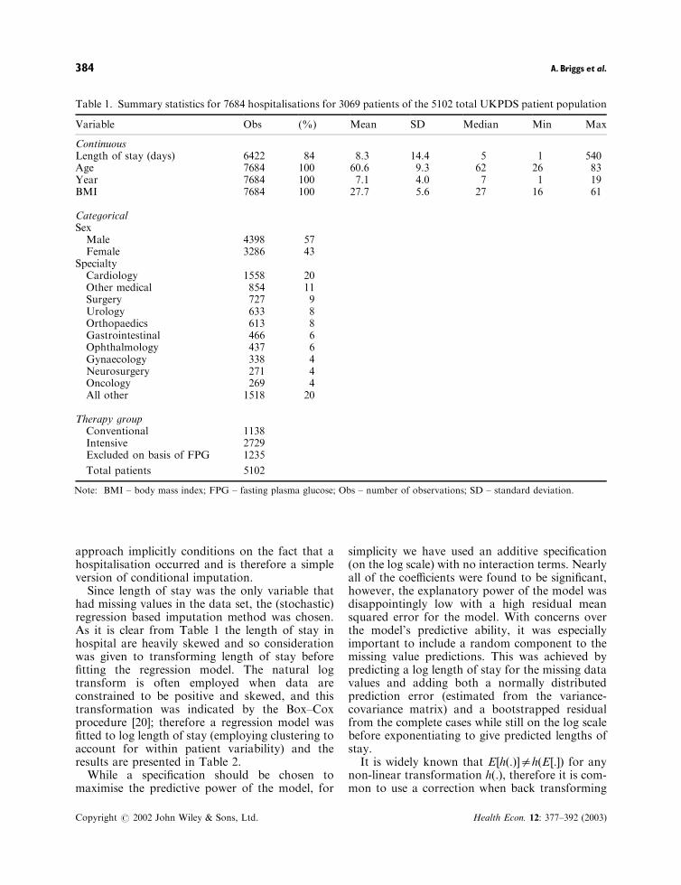
approach implicitly conditions on the fact that ahospitalisation occurred and is therefore a simpleversion of conditional imputation.

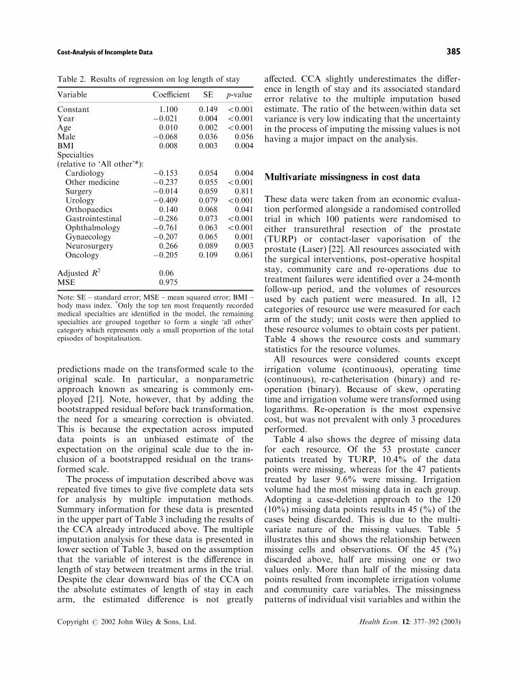
Since length of stay was the only variable thathad missing values in the data set, the (stochastic)regression based imputation method was chosen.As it is clear from Table 1 the length of stay inhospital are heavily skewed and so considerationwas given to transforming length of stay beforefitting the regression model. The natural logtransform is often employed when data areconstrained to be positive and skewed, and thistransformation was indicated by the Box–Coxprocedure [20]; therefore a regression model wasfitted to log length of stay (employing clustering toaccount for within patient variability) and theresults are presented in Table 2.

While a specification should be chosen tomaximise the predictive power of the model, for

simplicity we have used an additive specification(on the log scale) with no interaction terms. Nearlyall of the coefficients were found to be significant,however, the explanatory power of the model wasdisappointingly low with a high residual meansquared error for the model. With concerns overthe model’s predictive ability, it was especiallyimportant to include a random component to themissing value predictions. This was achieved bypredicting a log length of stay for the missing datavalues and adding both a normally distributedprediction error (estimated from the variance-covariance matrix) and a bootstrapped residualfrom the complete cases while still on the log scalebefore exponentiating to give predicted lengths ofstay.

It is widely known that E hð:Þ½ �=h E½:�ð Þ for anynon-linear transformation hð:Þ, therefore it is com-mon to use a correction when back transforming

Table 1. Summary statistics for 7684 hospitalisations for 3069 patients of the 5102 total UKPDS patient population

Variable Obs (%) Mean SD Median Min Max

ContinuousLength of stay (days) 6422 84 8.3 14.4 5 1 540Age 7684 100 60.6 9.3 62 26 83Year 7684 100 7.1 4.0 7 1 19BMI 7684 100 27.7 5.6 27 16 61

CategoricalSexMale 4398 57Female 3286 43

SpecialtyCardiology 1558 20Other medical 854 11Surgery 727 9Urology 633 8Orthopaedics 613 8Gastrointestinal 466 6Ophthalmology 437 6Gynaecology 338 4Neurosurgery 271 4Oncology 269 4All other 1518 20

Therapy groupConventional 1138Intensive 2729Excluded on basis of FPG 1235

Total patients 5102

Note: BMI – body mass index; FPG – fasting plasma glucose; Obs – number of observations; SD – standard deviation.

A. Briggs et al.384


predictions made on the transformed scale to theoriginal scale. In particular, a nonparametricapproach known as smearing is commonly em-ployed [21]. Note, however, that by adding thebootstrapped residual before back transformation,the need for a smearing correction is obviated.This is because the expectation across imputeddata points is an unbiased estimate of theexpectation on the original scale due to the in-clusion of a bootstrapped residual on the trans-formed scale.

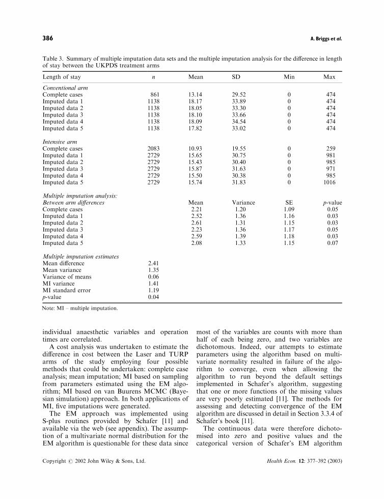
The process of imputation described above wasrepeated five times to give five complete data setsfor analysis by multiple imputation methods.Summary information for these data is presentedin the upper part of Table 3 including the results ofthe CCA already introduced above. The multipleimputation analysis for these data is presented inlower section of Table 3, based on the assumptionthat the variable of interest is the difference inlength of stay between treatment arms in the trial.Despite the clear downward bias of the CCA onthe absolute estimates of length of stay in eacharm, the estimated difference is not greatly

affected. CCA slightly underestimates the differ-ence in length of stay and its associated standarderror relative to the multiple imputation basedestimate. The ratio of the between/within data setvariance is very low indicating that the uncertaintyin the process of imputing the missing values is nothaving a major impact on the analysis.

Multivariate missingness in cost data

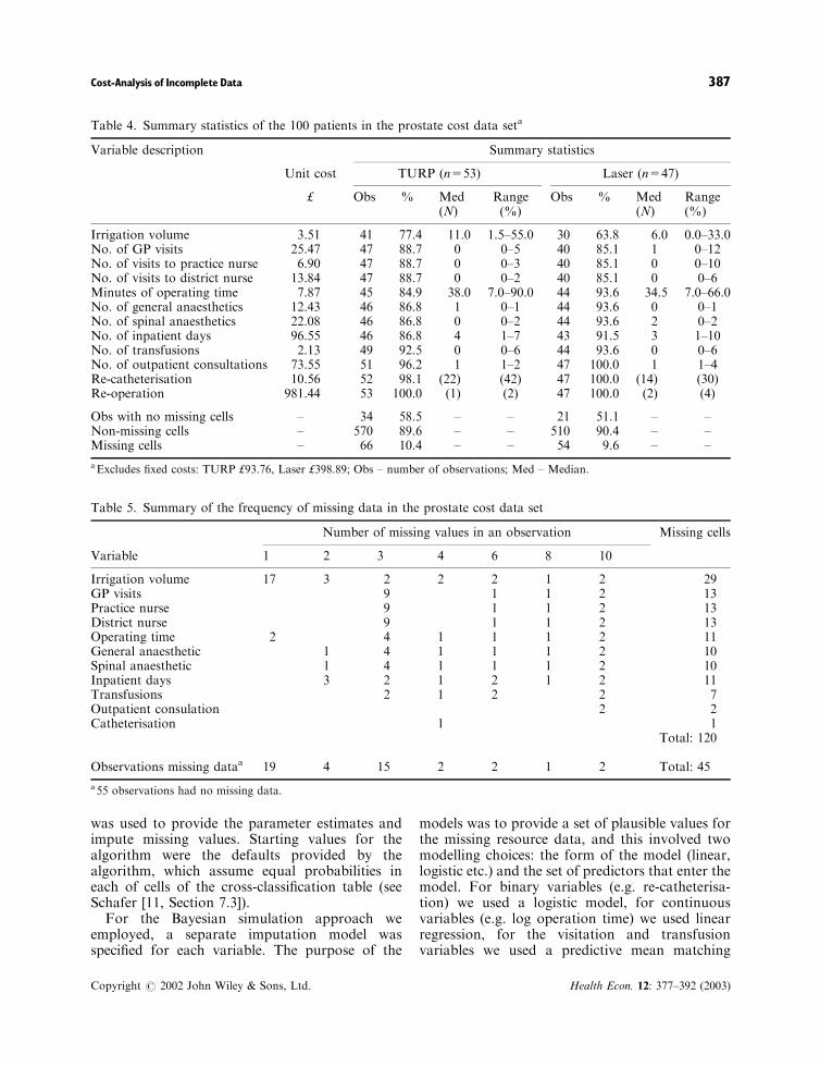
These data were taken from an economic evalua-tion performed alongside a randomised controlledtrial in which 100 patients were randomised toeither transurethral resection of the prostate(TURP) or contact-laser vaporisation of theprostate (Laser) [22]. All resources associated withthe surgical interventions, post-operative hospitalstay, community care and re-operations due totreatment failures were identified over a 24-monthfollow-up period, and the volumes of resourcesused by each patient were measured. In all, 12categories of resource use were measured for eacharm of the study; unit costs were then applied tothese resource volumes to obtain costs per patient.Table 4 shows the resource costs and summarystatistics for the resource volumes.

All resources were considered counts exceptirrigation volume (continuous), operating time(continuous), re-catheterisation (binary) and re-operation (binary). Because of skew, operatingtime and irrigation volume were transformed usinglogarithms. Re-operation is the most expensivecost, but was not prevalent with only 3 proceduresperformed.

Table 4 also shows the degree of missing datafor each resource. Of the 53 prostate cancerpatients treated by TURP, 10.4% of the datapoints were missing, whereas for the 47 patientstreated by laser 9.6% were missing. Irrigationvolume had the most missing data in each group.Adopting a case-deletion approach to the 120(10%) missing data points results in 45 (%) of thecases being discarded. This is due to the multi-variate nature of the missing values. Table 5illustrates this and shows the relationship betweenmissing cells and observations. Of the 45 (%)discarded above, half are missing one or twovalues only. More than half of the missing datapoints resulted from incomplete irrigation volumeand community care variables. The missingnesspatterns of individual visit variables and within the

Table 2. Results of regression on log length of stay

Variable Coefficient SE p-value

Constant 1.100 0.149 50.001Year �0.021 0.004 50.001Age 0.010 0.002 50.001Male �0.068 0.036 0.056BMI 0.008 0.003 0.004Specialties(relative to ‘All other’*):Cardiology �0.153 0.054 0.004Other medicine �0.237 0.055 50.001Surgery �0.014 0.059 0.811Urology �0.409 0.079 50.001Orthopaedics 0.140 0.068 0.041Gastrointestinal �0.286 0.073 50.001Ophthalmology �0.761 0.063 50.001Gynaecology �0.207 0.065 0.001Neurosurgery 0.266 0.089 0.003Oncology �0.205 0.109 0.061

Adjusted R2 0.06MSE 0.975

Note: SE – standard error; MSE – mean squared error; BMI –body mass index. *Only the top ten most frequently recordedmedical specialties are identified in the model, the remainingspecialties are grouped together to form a single ‘all other’category which represents only a small proportion of the totalepisodes of hospitalisation.



individual anaesthetic variables and operationtimes are correlated.

A cost analysis was undertaken to estimate thedifference in cost between the Laser and TURParms of the study employing four possiblemethods that could be undertaken: complete caseanalysis; mean imputation; MI based on samplingfrom parameters estimated using the EM algo-rithm; MI based on van Buurens MCMC (Baye-sian simulation) approach. In both applications ofMI, five imputations were generated.

The EM approach was implemented usingS-plus routines provided by Schafer [11] andavailable via the web (see appendix). The assump-tion of a multivariate normal distribution for theEM algorithm is questionable for these data since

most of the variables are counts with more thanhalf of each being zero, and two variables aredichotomous. Indeed, our attempts to estimateparameters using the algorithm based on multi-variate normality resulted in failure of the algo-rithm to converge, even when allowing thealgorithm to run beyond the default settingsimplemented in Schafer’s algorithm, suggestingthat one or more functions of the missing valuesare very poorly estimated [11]. The methods forassessing and detecting convergence of the EMalgorithm are discussed in detail in Section 3.3.4 ofSchafer’s book [11].

The continuous data were therefore dichoto-mised into zero and positive values and thecategorical version of Schafer’s EM algorithm

Table 3. Summary of multiple imputation data sets and the multiple imputation analysis for the difference in lengthof stay between the UKPDS treatment arms

Length of stay n Mean SD Min Max

Conventional armComplete cases 861 13.14 29.52 0 474Imputed data 1 1138 18.17 33.89 0 474Imputed data 2 1138 18.05 33.30 0 474Imputed data 3 1138 18.10 33.66 0 474Imputed data 4 1138 18.09 34.54 0 474Imputed data 5 1138 17.82 33.02 0 474

Intensive armComplete cases 2083 10.93 19.55 0 259Imputed data 1 2729 15.65 30.75 0 981Imputed data 2 2729 15.43 30.40 0 985Imputed data 3 2729 15.87 31.63 0 971Imputed data 4 2729 15.50 30.38 0 985Imputed data 5 2729 15.74 31.83 0 1016

Multiple imputation analysis:Between arm differences Mean Variance SE p-valueComplete cases 2.21 1.20 1.09 0.05Imputed data 1 2.52 1.36 1.16 0.03Imputed data 2 2.61 1.31 1.15 0.03Imputed data 3 2.23 1.36 1.17 0.05Imputed data 4 2.59 1.39 1.18 0.03Imputed data 5 2.08 1.33 1.15 0.07

Multiple imputation estimatesMean difference 2.41Mean variance 1.35Variance of means 0.06MI variance 1.41MI standard error 1.19p-value 0.04

Note: MI – multiple imputation.

A. Briggs et al.386


was used to provide the parameter estimates andimpute missing values. Starting values for thealgorithm were the defaults provided by thealgorithm, which assume equal probabilities ineach of cells of the cross-classification table (seeSchafer [11, Section 7.3]).

For the Bayesian simulation approach weemployed, a separate imputation model wasspecified for each variable. The purpose of the

models was to provide a set of plausible values forthe missing resource data, and this involved twomodelling choices: the form of the model (linear,logistic etc.) and the set of predictors that enter themodel. For binary variables (e.g. re-catheterisa-tion) we used a logistic model, for continuousvariables (e.g. log operation time) we used linearregression, for the visitation and transfusionvariables we used a predictive mean matching

Table 4. Summary statistics of the 100 patients in the prostate cost data seta

Variable description Summary statistics

Unit cost TURP (n=53) Laser (n=47)

£ Obs % Med(N)

Range(%)

Obs % Med(N)

Range(%)

Irrigation volume 3.51 41 77.4 11.0 1.5–55.0 30 63.8 6.0 0.0–33.0No. of GP visits 25.47 47 88.7 0 0–5 40 85.1 1 0–12No. of visits to practice nurse 6.90 47 88.7 0 0–3 40 85.1 0 0–10No. of visits to district nurse 13.84 47 88.7 0 0–2 40 85.1 0 0–6Minutes of operating time 7.87 45 84.9 38.0 7.0–90.0 44 93.6 34.5 7.0–66.0No. of general anaesthetics 12.43 46 86.8 1 0–1 44 93.6 0 0–1No. of spinal anaesthetics 22.08 46 86.8 0 0–2 44 93.6 2 0–2No. of inpatient days 96.55 46 86.8 4 1–7 43 91.5 3 1–10No. of transfusions 2.13 49 92.5 0 0–6 44 93.6 0 0–6No. of outpatient consultations 73.55 51 96.2 1 1–2 47 100.0 1 1–4Re-catheterisation 10.56 52 98.1 (22) (42) 47 100.0 (14) (30)Re-operation 981.44 53 100.0 (1) (2) 47 100.0 (2) (4)

Obs with no missing cells – 34 58.5 – – 21 51.1 – –Non-missing cells – 570 89.6 – – 510 90.4 – –Missing cells – 66 10.4 – – 54 9.6 – –

aExcludes fixed costs: TURP £93.76, Laser £398.89; Obs – number of observations; Med – Median.

Table 5. Summary of the frequency of missing data in the prostate cost data set

Number of missing values in an observation Missing cells

Variable 1 2 3 4 6 8 10

Irrigation volume 17 3 2 2 2 1 2 29GP visits 9 1 1 2 13Practice nurse 9 1 1 2 13District nurse 9 1 1 2 13Operating time 2 4 1 1 1 2 11General anaesthetic 1 4 1 1 1 2 10Spinal anaesthetic 1 4 1 1 1 2 10Inpatient days 3 2 1 2 1 2 11Transfusions 2 1 2 2 7Outpatient consulation 2 2Catheterisation 1 1

Total: 120

Observations missing dataa 19 4 15 2 2 1 2 Total: 45

a55 observations had no missing data.



model due to the multi-modal and skew nature ofthe observed data, but for other count variables(e.g. number of outpatient consultations) weapplied a multinomial (>2 levels) logistic model.We proposed to confine the imputation model foreach resource to include all other resource vari-ables. This is an explicit attempt to model theMAR process, because we assuming the missing-ness can be explained by observed data. In othercases, auxiliary variables may be available, and ithas been observed that including as many pre-dictors in the imputation model as possible tendsto make the MAR (and possibly NMAR) assump-tions more plausible [18].

The Gibbs sampling algorithm was run for 150iterations for each of 5 imputations. In general, inthe presence of large amounts of missing data,convergence can be obtained in as few as 10iterations [18]. Plots of the standard deviationsand means of the imputations by iteration werefree of trend, indicating that the imputation-variability had stabilised and there may beconvergence.

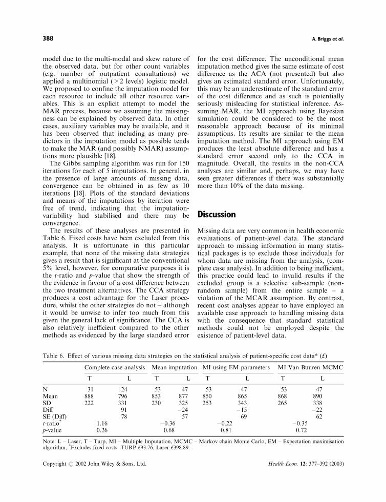
The results of these analyses are presented inTable 6. Fixed costs have been excluded from thisanalysis. It is unfortunate in this particularexample, that none of the missing data strategiesgives a result that is significant at the conventional5% level, however, for comparative purposes it isthe t-ratio and p-value that show the strength ofthe evidence in favour of a cost difference betweenthe two treatment alternatives. The CCA strategyproduces a cost advantage for the Laser proce-dure, whilst the other strategies do not – althoughit would be unwise to infer too much from thisgiven the general lack of significance. The CCA isalso relatively inefficient compared to the othermethods as evidenced by the large standard error

for the cost difference. The unconditional meanimputation method gives the same estimate of costdifference as the ACA (not presented) but alsogives an estimated standard error. Unfortunately,this may be an underestimate of the standard errorof the cost difference and as such is potentiallyseriously misleading for statistical inference. As-suming MAR, the MI approach using Bayesiansimulation could be considered to be the mostreasonable approach because of its minimalassumptions. Its results are similar to the meanimputation method. The MI approach using EMproduces the least absolute difference and has astandard error second only to the CCA inmagnitude. Overall, the results in the non-CCAanalyses are similar and, perhaps, we may haveseen greater differences if there was substantiallymore than 10% of the data missing.

Discussion

Missing data are very common in health economicevaluations of patient-level data. The standardapproach to missing information in many statis-tical packages is to exclude those individuals forwhom data are missing from the analysis, (com-plete case analysis). In addition to being inefficient,this practice could lead to invalid results if theexcluded group is a selective sub-sample (non-random sample) from the entire sample – aviolation of the MCAR assumption. By contrast,recent cost analyses appear to have employed anavailable case approach to handling missing datawith the consequence that standard statisticalmethods could not be employed despite theexistence of patient-level data.

Table 6. Effect of various missing data strategies on the statistical analysis of patient-specific cost data* (£)

Complete case analysis Mean imputation MI using EM parameters MI Van Buuren MCMC

T L T L T L T L

N 31 24 53 47 53 47 53 47Mean 888 796 853 877 850 865 868 890SD 222 331 230 325 253 343 265 338Diff 91 �24 �15 �22SE (Diff) 78 57 69 62t-ratio* 1.16 �0.36 �0.22 �0.35p-value 0.26 0.68 0.81 0.72

Note: L – Laser, T – Turp, MI – Multiple Imputation, MCMC – Markov chain Monte Carlo, EM – Expectation maximisationalgorithm, *Excludes fixed costs: TURP £93.76, Laser £398.89.

A. Briggs et al.388


This paper reviewed strategies for analysingdata in the presence of missing values andillustrated some of those strategies using twoexamples. Our goal was not to be exhaustive inreviewing this area, but to provide an introductionto more commonly applied methods and softwareroutines. In particular, we have focused on impu-tation methods that involve statistical modellingsuch that the uncertainty in the prediction processcan be captured through the principle of multipleimputation. Thus, traditionally popular singleimputation methods such as the hot deck thatinvolve identifying a nearest neighbour to serve asa surrogate missing value have not been employed

Most of the non-CCA methodologies discussedassume that the data are Missing at Random(MAR), that is, the missing values do not dependon the values of unobserved variables. This is amore realistic assumption than MCAR. Wedescribed three broad imputation approaches:regression imputation, the use of the EM algo-rithm to calculate maximum likelihood estimatesfor use in imputing the data, and Bayesiansimulation methods. Inferences associated withsingle imputations (i.e. single complete data sets)resulting from these methods tend to overstateprecision because they omit the between-imputa-tion component of variability. Multiple imputa-tion, an extension of single imputation, pools morethan one complete data set allowing for theuncertainty in the imputations to be appropriatelyreflected in the analysis.

Our examples demonstrated some fundamentalways of exploring and handling missing data. Theproportion of missing data is important. It may bereasonable to perform a CCA if a small percentageof patients are missing data, but as the percentageincreases there will be greater inefficiency andmore chance of bias. In general, it is advisable toinvestigate the missing data and, in most cases,attempt to impute or fill in the missing data. In thecase of univariate missingness, it may be accep-table to apply a regression imputation making ad-justments for the predictions (see the first examplebased on missing length of stay in the UKPDS).

Most missingness is multivariate and the ab-sence of a small percentage of data points canpotentially lead to a depleted CCA. In the secondexample of Laser versus TURP interventions, 10%of cells were missing, but 45% of patients wereremoved in a CCA. It seems sensible in this case toimpute 10% of the missing data in order toreinstate the extra 45% of patients. Imputation in

this setting requires allowances for the correlationbetween variables, and strictly univariate ap-proaches may be inappropriate. The EM algo-rithm was employed to estimate a covariancematrix for the variables, but only after making thevariables discrete due to the problem of largenumbers of zeros for individual parameters. Ourpreferred method was to use Bayesian simulationto create imputations, particularly the method ofVan Buuren [18]. This approach requires thespecification of imputation for each model andGibbs sampling is used to develop a multivariatedistribution for the data.

Bayesian methods are becoming increasinglypopular and Data augmentation (DA) [5], Gibbssampling (a particular type of DA) [16,18] andother Markov chain Monte Carlo methods arebecoming more widely applied in this area. ABayesian approach could have been used to handlemissing data in the first of our examples, using forexample, the WinBUGS [23] software package. Incommon with many other areas of statisticalanalysis in the absence of prior information toinform the values of missing data Bayesian andfrequentist approaches are not likely to generatesubstantially different results. Indeed, this wasprecisely what we discovered when implementing aBayesian WinBUGS regression model for theUKPDS length of stay data. This emphasises thefocus of this article on the importance of handlingmissing data using appropriate methods ratherthan on the philosophical discussion of Bayesianversus Frequentist methods. Often the EM algo-rithm is applied to estimate information that maybe used as a starting point for a Bayesiansimulation procedure [5].

The presumption of this paper has been on theestimation of missing values when data are MAR.In economic evaluation alongside clinical trials it iscommon for repeated measures to be taken suchthat a monotone pattern of missingness is ob-served with data points on individual beingobserved up to a certain time point within thestudy but not beyond. Where this has occurred dueto differential recruiting times to a study with afixed analysis end time then observations are saidto be censored. The analysis of censored cost datahas been popular area of research in recent years[24–29] and the assumption of uninformativecensoring underlying the method equates to theMCAR framework described in this paper.

Where data are missing due to attrition ratherthan due to censoring then it is unlikely that data



are MCAR. Although techniques such as mixedmodels and generalised estimating equations canbe used to make inference from data that aresubject to attrition [30] without the need forimputation of missing values, the implicit assump-tion underlying these methods is MAR. Inpractice, attrition will often be linked to specificreasons for patients leaving the study early thatmeans censoring is informative and missing valuesare NMAR. In such situations, these reasonsunderlying the attrition need to be fully explored.It may be appropriate to correct potential biasesusing techniques developed in econometrics sam-ple selection literature [31] that deal with non-random drop out in panel data [32]. Alternatively,methods for informative drop out have beendeveloped in the statistics literature for long-itudinal (or panel) data [30]. In general theadditional assumptions necessary for handlingmissing information that are NMAR can oftenbe quite limiting and may prove to be untestable –leading to a reliance on sensitivity analysis. Oneapproach to the problem of missing data, there-fore, is to collect additional information onmissing values. However, this solution only servesto emphasise that imputation methods are not acure for a poor study design and/or a poor datacollection processes. The true solution to theproblem of missing data is to efficiently captureall relevant information thereby assuring that theproblem does not arise.

Software

A review of software for imputing missing datamay be found at www.multiple-imputation.comand in Horton [33]. Below are some of the morewidely used programs:

SAS

* PROC MI (version 8.1) offers three methods forcreating the imputed data sets: the regressionmethod, the propensity score method, and theMarkov chain Monte Carlo (MCMC). PROCMIANALYZE (version 8.1) is used to combinethe results

* PROC MIXED (version 6 onwards) can takesubjects with incomplete data into its analysis.

* PRQEX3 (Sample program – version 6 on-wards) estimates multivariate missing data bysampling from a multivariate normal distribu-tion.

* IVEWARE is a SAS-based application forcreating multiple imputations.

(www.sas.com, www.multiple-imputation.com)

SOLAS 3.0 for Missing Data Analysis

* This is a commercial Windows standaloneprogram by Statistical Solutions Limited. Itprovides a comprehensive set of tools toperform both single and multiple imputation.

(www.statsol.ie)

S-PLUS

* The MICE program contains S-PLUS (versions4.5 onwards) routines for flexible generation ofmultivariate imputations using Gibbs Sam-pling. [add-on available from www.multiple-imputation.com]

* NORM, CAT, MIX and PAN is S-PLUSsoftware (version 3.4 onwards) for multipleimputation. NORM uses a multivariate normalmodel. CAT uses a log-linear model forcategorical data. MIX relies on the generallocation model for mixed categorical andcontinuous data. PAN is used in a panel datasetting. [add-on available from www.multiple-imputation.com]

* Missing data library for S-PLUS (version 6.0).This library supports model-based missing data,by use of the EM algorithm and data augmen-tation algorithms. The library incorporates theSchafer algorithms and provides some explora-tory missing data tools.

* Oswald is an S-plus library for the analysis oflongitudinal data. It includes informative drop-out modelling and GEE. [add-on available fromlib.stat.cmu.edu/S]

(www.insightful.com)

SPSS

* SPSS Missing Value Analysis1 is an additionalmodule for SPSS (version 10) that provides

A. Briggs et al.390


graphical tools to investigate missing data,and imputes missing data using the EM andregression algorithms.

(www.spss.com)

STATA

* Sg116(.1) performs hot-deck imputation formissing data.

* Sg156 performs a weighted logistic regressionfor data with missing values using the meanscore method.

* ‘Impute’ procedure provides imputed values bybest sub-set regression.

(www.stata.com)

Acknowledgements

A.B. holds a Public Health Career Scientist award fromthe UK Department of Health. T.C. is funded by anNHS Training Fellowship in Medical Statistics. Anearlier version of this paper was presented at the July1999 meeting of the UK Health Economists’ StudyGroup held in Aberdeen. We wish to thank twoanonymous referees for their constructive comments,although remaining errors are our own responsibility.

References1. Johnston KJ, Buxton MJ, Jones DR, Fitzpatrick R.

Assessing the costs of healthcare technologies inclinical trials. Health Technol Assess 1999; 3(6): 1–76.

2. Coast J, Richards SH, Peters TJ, Gunnell DJ,Darlow MA, Pounsford J. Hospital at home oracute hospital care? A cost minimisation analysis. BrMed J 1998; 316(7147): 1802–1806.

3. Roberts TE. Economic evaluation and randomisedcontrolled trial of extracorporeal membrane oxyge-nation: UK collaborative trial. The ExtracorporealMembrane Oxygenation Economics WorkingGroup. Br Med J 1998; 317(7163): 911–915.

4. Little RJA, Rubin DB. Statistical Analysis withMissing Data. John Wiley & Sons, New York, 1987.

5. Buck SF. A method of estimation of missing valuesin multivariate data suitable for use with anelectronic computer. J Roy Stat Soc Series B 1960;22(2): 302–306.

6. Brick JM, Kalton G. Handling missing data insurvey research. Stat Meth Med Res 1996; 5:215–238.

7. Little RJA, Su HL. Item non-response in panelsurveys. In Panel Surveys, Kasprzyk D, Duncan G,Kalton G (eds). Wiley: New York, 1989.

8. Hanson RH. US Bureau of the Census (ed.).The current population survey: design andmethodology. Technical paper No. 40. Washington:2001.

9. Rubin DB. Statistical matching, file concentrationwith adjusted weights and multiple imputations. JBusiness Econ Stat 1986; 4: 87–94.

10. Polsky D, Glick H. Estimating medical costs fromincomplete follow-up data [abstract]. Value Health1999; 2(3): 229

11. Schafer JL. Analysis of Incomplete MultivariateData. Chapman & Hall: London, 1997.

12. Wu CFJ. On the convergence properties of the EMalgorithm. Ann Stat 1983; 11: 95–103.

13. Rubin DB, Schenker N. Multiple imputation forinterval estimation from simple random sampleswith ignorable non-response. J Am Stat Assoc 1986;81: 366–374.

14. Rubin DB. Multiple Imputation for Nonresponse inSurveys. Wiley: New York, 1987.

15. Schafer JL. Multiple imputation: a primer. StatMeth Med Res 1999; 8: 3–16.

16. Gelfand AE, Smith AFM. Sampling-based ap-proaches to calculating marginal densities. J AmStat Assoc 1990; 85: 398–409.

17. Tanner MA, Wong WH. The calculation of poster-ior distributions by data augmentation. J Am StatAssoc 1987; 82: 528–550.

18. van Buuren S, Boshuizen HC, Knook DL.Multiple imputation of missing blood pressurecovariates in survival analysis. Stat Med 1999;18(6): 681–694.

19. UKPDS Study Group. Tight blood pressure con-trol, risk of macrovascular and microvascularcomplications in type 2 diabetes: UKPDS 38. UKprospective diabetes study group. BMJ 1998;317(7160): 703–713.

20. Box GEP, Cox DR. An analysis of transformations.J Roy Stat Soc Series B 1964; 2: 211–243.

21. Duan N. Smearing Estimate: A NonparametricRetransformation Method. J Am Stat Assoc 1983;78: 605–610.

22. Keoghane SR, Lawrence KC, Gray AM, ChappelDB, Hancock AM, Cranston DW. The OxfordLaser Prostate Trial: economic issues surroundingcontact laser prostatectomy. BJU Int 1996; 77(3):386–390.

23. WinBUGS 1.3 [computer program]. SpiegelhalterDJ, Thomas A, Best N et al. 1.3. CambridgeUniversity: MRC Biostatistics Unit; 2000.

24. Fenn P, McGuire A, Phillips V, Backhouse M,Jones D. The analysis of censored treatment costdata in economic evaluation. Med Care 1995; 33(8):851–863.

25. Etzioni RD, Feuer EJ, Sullivan SD, Lin D, Hu C,Ramsey SD. On the use of survival analysistechniques to estimate medical care costs. J HealthEcon 1999; 18(3): 365–380.



26. Lin DY, Feuer EJ, Etzioni R, Wax Y. Estimatingmedical costs from incomplete follow-up data.Biometrics 1997; 53(2): 419–434.

27. Bang H, Tsiatis AA. Estimating medical costs withcensored data. Biometrika 2000; 87(2): 329–343.

28. Carides GW, Heyse JF, Iglewicz B. A regression-based method for estimating mean treatment cost inthe presence of right-censoring. Biostatistics 2000;1(3): 299–313.

29. Willan AR, Lin DY. Incremental net benefit inrandomized clinical trials. Stat Med 2001; 20(11):1563–1574.

30. Diggle PJ, Liang KY, Zeger SL. Analysis of Long-itudinal Data. OUP: Oxford, 1994.

31. Greene WH. Econometric Analysis. (2nd Edn)Macmillan: New York, 1993.

32. Leigh JP, Ward MM, Fries JF. Reducing attritionbias with an instrumental variable in a regressionmodel: results from a panel of rheumatoid arthritispatients. Stat Med 1993; 12(11): 1005–1018.

33. Horton NJ, Lipsitz SR. Multiple imputation inpractice: comparison of software packages forregression models with missing variables. AmStatistician 2001; 55: 244–254.

A. Briggs et al.392


Documents

Missing.... presumed at random: cost-analysis of incomplete data