Embed Size (px)
Citation preview
Journal of Engineering Science and Technology Vol. 11, No. 2 (2016) 278 - 295 © School of Engineering, Taylor’s University
278
MISFIRE DETECTION IN A MULTI-CYLINDER DIESEL ENGINE: A MACHINE LEARNING APPROACH
AYYASAMY KRISHNAMOORTHY BABU1,*, V. ANTONY AROUL RAJ
2,
G. KUMARESAN3
1Department of Mechanical Engineering, PERI Institute of Technology, Chennai, India 2Department of Mechanical Engineering, Easwari Engineering College, Chennai, India
3Institute of Energy Studies, Anna University, Chennai, India *Corresponding Author: [email protected]
Abstract
Misfire is another type of abnormal combustion. When engine misfires,
cylinder (or cylinders) is not producing its normal amount of power. Engine
misfire also has negative effects on engine exhaust emissions such as HC, CO,
and NOx. Engine misfire should be detected and eliminated. Normal
combustion and misfire in the cylinder (if any) generates vibrations in the engine block. The vibration characters due to misfire are unique for a particular
cylinder. This can be diagnosed by processing the vibration signals acquired
from the engine cylinder block using a piezoelectric accelerometer. The
obtained signals were decoded using statistical parameters, like, Kurtosis,
standard deviation, mean, median, etc. Misfire identification algorithms such as
AdaBoost, LogitBoost, MultiClass Classifier, and J48 were used as tools for
feature selection and classification. The signals were trained and tested by the
selected classifiers. The classification accuracy of selected classifiers were
compared and presented in this paper. MultiClass Classifier was found to be
performing better with selected statistical features compared to other classifiers.
Keywords: Engine misfire, Feature extraction, Confusion matrix, AdaBoost,
LogitBoost, MultiClass Classifier.
1. Introduction
Misfiring can usually be caused by ignition or fuel system faults as well as engine
mechanical problems. The algorithms used for misfire detection proved to be
reliable, with neglectable detection error. Several methods of misfire detection
have been proposed [1, 2]: a. Monitoring catalyst temperature at exhaust. This
method is unacceptable since the catalyst temperature at exhaust does not rise
significantly in the case of low frequency misfire. b. Monitoring the oxygen
Misfire Detection in a Multi-Cylinder Diesel Engine: A Machine Learning Approach 279
Journal of Engineering Science and Technology February 2016, Vol. 11(2)
sensor signal in exhaust. This method is not encouraging since the momentary
increase in oxygen level for a single misfire might not evoke a good response
from the sensor and it is even more challenging at higher speeds. c. In-cylinder
pressure monitoring. This method is very reliable and accurate as individual
cylinder instantaneous mean effective pressure could be calculated in real time.
However, the cost of fitting each cylinder with a pressure transducer is
prohibitively high. d. Evaluation of crankshaft angular velocity fluctuations.
Extensive studies have been done using measurement of instantaneous crank
angle speed [3-7] and diverse techniques have been developed to predict misfire.
These methods call for a high resolution crank angle encoder and associated
infrastructure capable of identifying minor changes in angular velocity due to
misfire. The application of these techniques becomes more challenging due to
continuously varying operating conditions involving random variation in
acceleration coupled with the effect of flywheel, which tries to smoothen out
minor variations in angular velocity at higher speeds. Fluctuating load torque
applied to the crankshaft through the drive train poses additional hurdles in
decoding the misfire signals. Piotr and Jerky [8] reported their work using
vibroacoustic measurement at engine exhaust to model nonlinear methods for
misfire detection in locomotive engines. Although the idea of using vibroacoustic
signals is encouraging, the implementation of such a system requires the use of
multi sensor input escalating the cost and computational infrastructure. It also
offers more challenges when there is a need to integrate the system to an onboard
condition monitoring system for automobiles, with minimum infrastructure.
Ye [9] reported work on misfire detection using the Matter-element model,
which is built on diagnostics derived from specialists’ knowledge of practical
experience. In this model the misfire in the engine cylinder can be directly
identified using relation indices. The shortcoming observed here is that the
technique depends heavily on the knowledge of an expert and does not facilitate
automatic machine learning through a model built on an algorithm using
knowledge hidden in the data. The reliability of a system with automatic rule
based learning is more since it can be trained for the continuously changing
behavior of the engine, due to wear and tear.
Engine misfire detection done using sliding mode observer [10, 11] is
challenged with difficulty in modeling. Expressing a dynamic non-linear system
into a robust model will induce errors. The system becomes more complicated with
IC engines since it is a time varying system. Some studies have also been done
using linear approximation techniques using Kalman filter [12]. The inherent
problem in such systems is that there can be loss of valuable information due to
linear approximation and these signals cannot be used to extract other engine
information required for designing a vehicle condition monitoring system. The
linear approximation models using Kalman filter is found to be less efficient than
non-linear systems [13]. Chang, Kim, and Min [14] have reported their work using
a combination of engine block vibration and wavelet transform to detect engine
misfire and knock in a spark ignition engine. The use of engine block vibration is
appreciable because it requires minimum instrumentation but the use of wavelet
transforms increases the computational requirements. The present study proposes a
non-intrusive engine block acceleration measurement using a low cost mono axial
piezoelectric accelerometer connected to a computer through a signal processor.
The acquired analog vibration signals are converted to digital signals using an
280 A. K. Babu et al.
Journal of Engineering Science and Technology February 2016, Vol. 11(2)
analog to digital converter and the discrete data files are stored in the computer for
further processing. Feature extraction and feature selection techniques are employed
and their classification results obtained is presented in the ensuing discussion.
A good classifier should have the following properties:
• It should have good ‘predictive accuracy’; it is the ability of the model to
correctly predict the class label of new or previously unseen data.
• It should have good speed.
• The computational cost involved in generating and using the model
should be as low as possible.
• It should be ‘robust’; robustness is the ability of the model to make
correct predictions given the noisy data or data with missing values.
(Insensitive to noise in the data)
• The level of understanding and insight that is provided by classification
model should be high enough.
The selected classifiers have all the above properties and hence chosen for
the study.
The above review stimulated us to perform some statistical analysis on new
methods of misfire detection diagnostic such as adaboost, logitBoost, Simplelogic,
and Multiclass classifier, considering J48 decision tree as a reference tool on which
Babu Senapati et al. [2] have performed misfire detection from a multi-cylinder
gasoline engine. They obtained samples that were divided into training set to train
the classifier and testing set to validate the performance of the classifier. The
classification accuracy was evaluated by tenfold cross-validation which is found to
be around 95% for decision tree (J48) algorithm. The same authors [16] evaluated
the use of random forest (RF), as a tool for misfire detection using statistical
features, which is found to have a consistency high classification accuracy of
around 90%. From the favourable results obtained, the authors concluded that, the
combination of statistical features and random forest algorithm is well suited for the
detection of misfire in spark-ignition engines. However, the other statistical learning
approaches like AdaBoost, LogitBoost, SimpleLogistic, and MultiClass Classifier
have not been studied for misfire detection. Hence, in the present study, the above
classifiers were studied to find the classification accuracy for misfire detection in a
multi-cylinder gasoline engine.
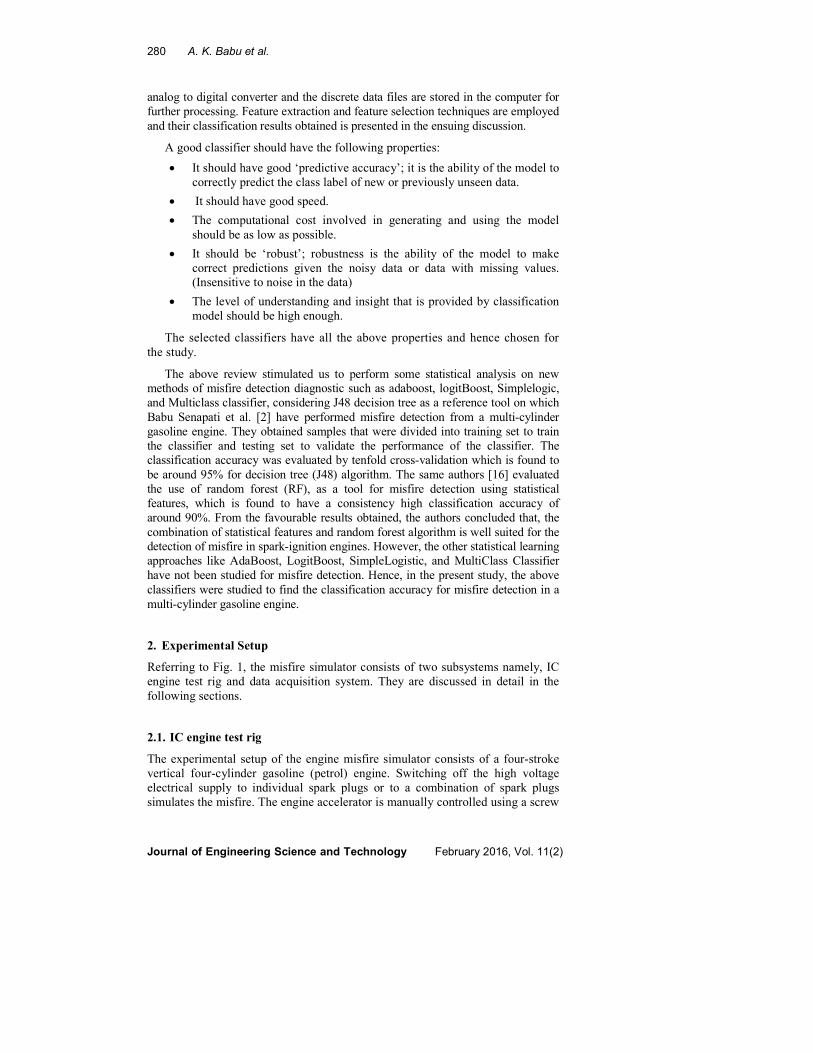
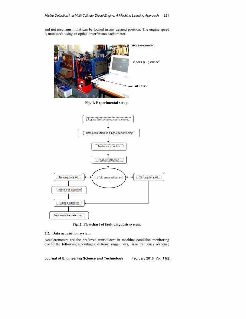
2. Experimental Setup
Referring to Fig. 1, the misfire simulator consists of two subsystems namely, IC
engine test rig and data acquisition system. They are discussed in detail in the
following sections.
2.1. IC engine test rig
The experimental setup of the engine misfire simulator consists of a four-stroke
vertical four-cylinder gasoline (petrol) engine. Switching off the high voltage
electrical supply to individual spark plugs or to a combination of spark plugs
simulates the misfire. The engine accelerator is manually controlled using a screw
Misfire Detection in a Multi-Cylinder Diesel Engine: A Machine Learning Approach 281
Journal of Engineering Science and Technology February 2016, Vol. 11(2)
and nut mechanism that can be locked in any desired position. The engine speed
is monitored using an optical interference tachometer.
Fig. 1. Experimental setup.
Fig. 2. Flowchart of fault diagnosis system.
2.2. Data acquisition system
Accelerometers are the preferred transducers in machine condition monitoring
due to the following advantages: extreme ruggedness, large frequency response
282 A. K. Babu et al.
Journal of Engineering Science and Technology February 2016, Vol. 11(2)
and large dynamic range. Accelerometers have a wide operating range enabling
them to detect very small and large vibrations. The vibration sensed can be taken
as a reflection of the internal engine condition. The voltage output of the
accelerometers is directly proportional to the vibration. A piezoelectric mono
axial accelerometer and its accessories form the core equipment for vibration
measurement and recording. The accelerometer is directly mounted on the center
of the engine head-using adhesive mounting as shown in Fig. 1.
The output of the accelerometer is connected to the signal-conditioning unit
through a DACTRON FFT analyzer that converts the signal from Analogue to
Digital (ADC). The digitized vibration signal (in time domain) is given as input
to the computer through the USB port. The data are stored in the secondary
memory of the computer using the accompanying software for data processing
and feature extraction.
3. Experimental Procedure
The engine is started by electrical cranking at no load and warmed up for 15
min. The FFT analyzer is switched on, the accelerometer is initialized and the
data are recorded after the engine speed stabilized. A sampling frequency of 24
kHz and sample length of 8192 is maintained for all conditions. The highest
frequency was found to be 10 kHz and since Nyquist sampling theorem says
that the sampling frequency must be at least twice that of the highest measured
frequency or higher. Hence the sampling frequency was chosen to be 24 kHz.
To strike a balance between computational load and data quality, the number of
samples is chosen as 1000.
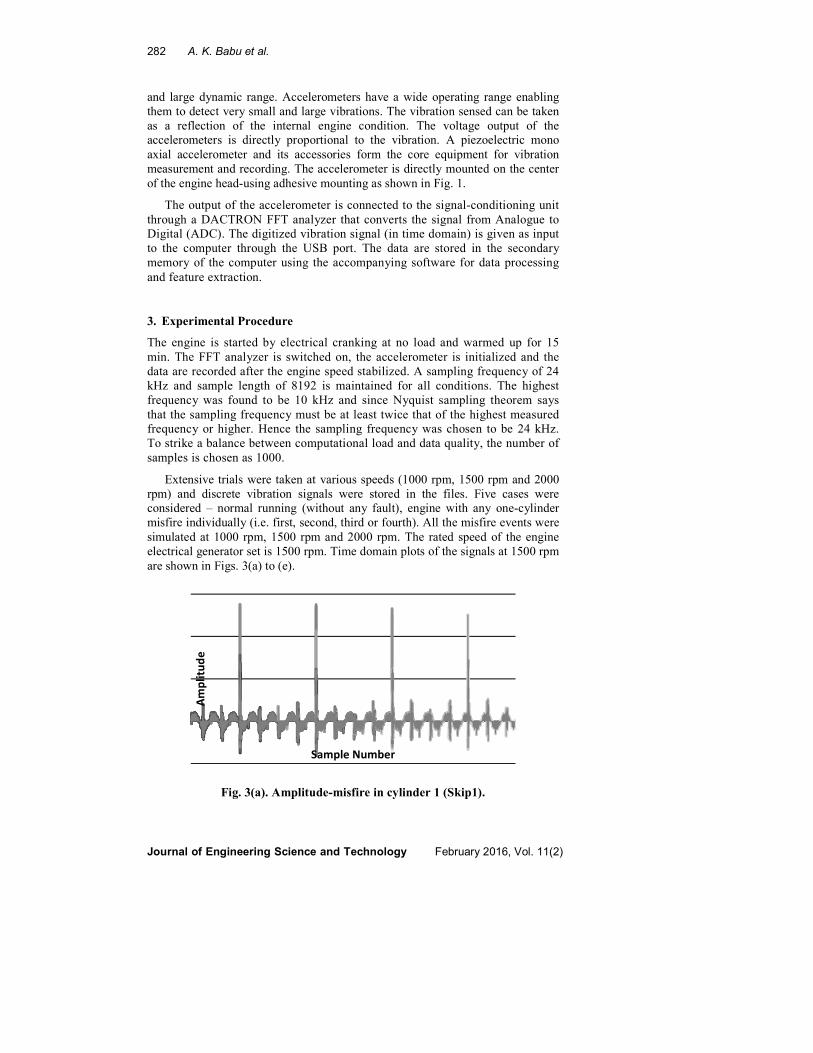
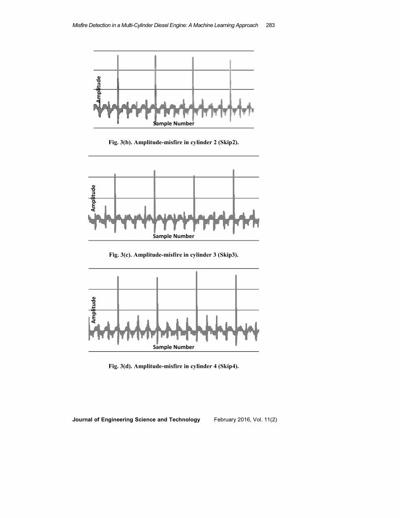
Extensive trials were taken at various speeds (1000 rpm, 1500 rpm and 2000
rpm) and discrete vibration signals were stored in the files. Five cases were
considered – normal running (without any fault), engine with any one-cylinder
misfire individually (i.e. first, second, third or fourth). All the misfire events were
simulated at 1000 rpm, 1500 rpm and 2000 rpm. The rated speed of the engine
electrical generator set is 1500 rpm. Time domain plots of the signals at 1500 rpm
are shown in Figs. 3(a) to (e).
Fig. 3(a). Amplitude-misfire in cylinder 1 (Skip1).
Am
pli
tud
e
Sample Number
Misfire Detection in a Multi-Cylinder Diesel Engine: A Machine Learning Approach 283
Journal of Engineering Science and Technology February 2016, Vol. 11(2)
Fig. 3(b). Amplitude-misfire in cylinder 2 (Skip2).
Fig. 3(c). Amplitude-misfire in cylinder 3 (Skip3).
Fig. 3(d). Amplitude-misfire in cylinder 4 (Skip4).
Am
pli
tud
e
Sample Number
Am
pli
tud
e
Sample Number
Am
pli
tud
e
Sample Number
284 A. K. Babu et al.
Journal of Engineering Science and Technology February 2016, Vol. 11(2)
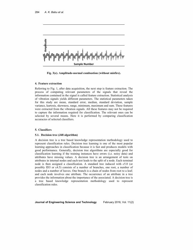
Fig. 3(e). Amplitude-normal combustion (without misfire).
4. Feature extraction
Referring to Fig. 1, after data acquisition, the next step is feature extraction. The
process of computing relevant parameters of the signals that reveal the
information contained in the signal is called feature extraction. Statistical analysis
of vibration signals yields different parameters. The statistical parameters taken
for this study are mean, standard error, median, standard deviation, sample
variance, kurtosis, skewness, range, minimum, maximum and sum. These features
were extracted from the vibration signals. All these features may not be required
to capture the information required for classification. The relevant ones can be
selected by several means. Here it is performed by comparing classification
accuracies of selected classifiers.
5. Classifiers
5.1. Decision tree (J48 algorithm)
A decision tree is a tree based knowledge representation methodology used to
represent classification rules. Decision tree learning is one of the most popular
learning approaches in classification because it is fast and produces models with
good performance. Generally, decision tree algorithms are especially good for
classification learning if the training instances have errors (i.e. noisy data) and
attributes have missing values. A decision tree is an arrangement of tests on
attributes in internal nodes and each test leads to the split of a node. Each terminal
node is then assigned a classification. A standard tree induced with c5.0 (or
possibly ID3 or c4.5) consists of a number of branches, one root, a number of
nodes and a number of leaves. One branch is a chain of nodes from root to a leaf;
and each node involves one attribute. The occurrence of an attribute in a tree
provides the information about the importance of the associated. A decision tree is
a tree based knowledge representation methodology used to represent
classification rules.
Am
pli
tud
e
Sample Number

Misfire Detection in a Multi-Cylinder Diesel Engine: A Machine Learning Approach 285
Journal of Engineering Science and Technology February 2016, Vol. 11(2)
The definition and process of extracting statistical features were described for
bearing fault diagnosis by Sugumaran et al., [15]. Following the footsteps of
Sugumaran et al., effect of number of features, feature selection and classification
accuracy for decision tree was carried out.
5.2. LogitBoost
A boosting procedure used in this study is implemented by LogitBoost. Boosting
is one of the most important recent developments in classification methodology.
Boosting is a way of combining the performance of many weak classifiers to
produce a powerful committee. It works by sequentially applying classification
algorithms to reweighted versions of the training data and then taking a weighted
majority vote of the sequence of classifiers thus produced. For many
classification algorithms, this simple strategy results in dramatic improvements in
performance. This is a specialized case of regression analysis over discrete or
ordinal values; but basic regression-based learning algorithms have inherent
disadvantages. Better algorithms that overcome these pitfalls have been
developed and are collectively known as Discriminant Analysis (DA) techniques
or simply Metal learning algorithms. One such algorithm that effectively
addresses these issues is the LogiBoost Meta classifier-based on the log of the
odds ratio for the dependent variable.
Friedman et al. [17] propose the LogitBoost algorithm for fitting additive
logistic regression models by maximum likelihood.
Start with weights wij=1/n. i=1, ……, n, j=1, ……, J, Fj (x) = 0 and pj
(x)=1/J ∀j
Repeat for m=1, ……, M :
(a) Repeat for j = 1, ……, J:
i. Compute working responses and weights in the jth
class
zij = ))x(p()x(p
)x(py
ijij
ijij*
−
−
wij = ))x(p()x(p ijij −
ii. Fit the function fmj(x) by a weighted least-squares
regression of zij to xi with weights wij.
(b) Set fmj (x) ←
)x(f)x(F)x(F)),x(fJ
1)x(f(
J
1Jmjjj
J
1k mkmj +←−−
∑ =
(c) Update pj(x) =
∑ =
J
1k
)x(F
)x(F
k
j
e
e
Output the classifier argmax Fj (x)
J
286 A. K. Babu et al.
Journal of Engineering Science and Technology February 2016, Vol. 11(2)
It is based on the concept of additive logistic regression. It can successfully
boost very simple learning schemes, (like DecisionStump), even in multiclass
situations. It differs from other boosting procedure such as AdaBoost.M1, in an
important way because it boosts schemes for numeric prediction in order to form
a combined classifier that predicts a categorical class.
5.3. AdaBoost (17)
AdaBoost, also known as ‘Adaptive Boosting’ is a machine learning algorithm. In
the present study, this boosting algorithm is used in conjunction with random
forest algorithm to improve its performance. The boosting algorithm takes as
input a training set of m examples S={(x1, y1), …., (xm, ym)} where xi is an
instance drawn from some space X and represented in some manner (typically, a
vector of attribute values), and yi∈Y is the class label associated with xi. In this
paper, it is assumed that the set of possible labels Y is of finite cardinality.
In addition, the boosting algorithm has access to another unspecified learning
algorithm called the weak learning algorithm, which is denoted generally as Weak
Learn. The boosting algorithm calls Weak Learn repeatedly in a series of rounds.
On round t, the booster provides Weak Learn with a distribution Dt over the
training set S. In response, Weak Learner computes a classified or hypothesis ht:
X→ Y which should misclassify a non traivial fraction of the training examples,
relative to Dt. That is the weak learner’s goal is to find a hypothesis ht which
minimizes the (training) error ∈t = Pri~Dt [ht(xi) ≠yi]. Note that this error is
measured with respect to the distribution Dt that was provided to the weak learner.
This process continues for T rounds, and at last, the booster combines the weak
hypotheses h1, …, hT into single final hypotheses hfin.
Still unspecified are (1) the manner in which Dt is computed on each round,
and (2) how hfin is computed. Different boosting schemes answer these two
questions in different ways. AdaBoost.M1 uses the simple rule shown in
algorithm. The initial distribution D1 is uniform over S so D1(i) = 1/m for all i. To
compute distribution DL+1 from Dt and the last weak hypothesis ht, we multiply
the weight of example I by some number βt∈[0,1] if left unchanged. The weights
are then renormalized by dividing by the normalization constant Zt. Effectively
‘easy’ examples that are correctly classified by many of the previous weak
hypothesis get lower weight, and ‘hard’ example which tend often to be
misclassified get higher weight. Thus, AdaBoost focuses the most weight on th
examples which seem to be hardest for WeakLearn.
Algorithm AdaBoostM1
Input: Sequence of m examples {(x1, y1), ….., (xm,ym)}
with labels yi ЄY = {1, ….., k}
weak learning algorithm WeakLearn
integer T specifying number of iterations
Initialize D1 (i) = 1/m for all i
Misfire Detection in a Multi-Cylinder Diesel Engine: A Machine Learning Approach 287
Journal of Engineering Science and Technology February 2016, Vol. 11(2)
Do for I = 1,2,….,T
Call WeakLearn, providing it with the distributor Dt.
Get back a hypothesis ht: X → Y.
Calculate the error of ht: Єt = ∑≠= iit y)x(hi
t ).i(D If Єt > ½, then set T =
t-1 and abort loop.
Set βt = Єt / (1-Єt).
Update distribution Dt = Dt+1(i)=
t
t
Z
)i(D×{
Where Zt is a normalization constant (chosen so that Dt+1 will
be a distribution.
Output the final hypothesis: hfin(x)=arg max ∑= βy)x(h:i tt
1log
The number βt is computed as shown in the figure as a function of ∈t. the final
hypothesis hfin is a weighted vote (i.e., a weighted linear threshold) of the weak
hypothesis. That is, for a given instance x, hfin outputs the label y that maximizes
the sum of the weights of the weak hypothesis predicting that label. The weight of
hypothesis ht is defined to be ln (1/βt) so that greater weight is given to hypothesis
with lower error.
5.4. Multiclass classifier
The extensions of boosting to classification with multiple classes were explored.
Some learning schemes can only be used in two-class situations such as SMO
class. To apply such schemes to multiclass datasets, the problem must be
transformed into several two-class ones and the results combined. This can be
done by MultiClass Classifier. It takes a base learner that can output a class
distribution or a numeric class, and applies it to a multiclass learning problem
using the simple one-per-class coding.
Among these strategies is the one-vs.-all strategy, where a single classifier is
trained per class to distinguish that class from all other classes. Prediction is then
performed by predicting using each binary classifier, and choosing the prediction
with the highest confidence score (e.g., the highest probability of a classifier such
as naive Bayes).
In pseudocode, the training algorithm for a one-vs.-all learner constructed
from a binary classification learner L is as follows:
Inputs:
• L, a learner (training algorithm for binary classifiers: Logistic)
• samples X
• labels y where yᵢ ∈ {1, … K} is the label for the sample Xᵢ
Output:
288 A. K. Babu et al.
Journal of Engineering Science and Technology February 2016, Vol. 11(2)
• a list of classifiers fk for k ∈ {1, … K}
Procedure:
• For each k in {1 … K}:
o Construct a new label vector yᵢ' = 1 where yᵢ = k, 0 (or -
1) elsewhere
o Apply L to X, y' to obtain fk
Making decisions proceeds by applying all classifiers to an unseen sample x
and predicting the label k for which the corresponding classifier reports the
highest confidence score:
6. Results and Discussion
The study of misfire classification using the selected classifiers is discussed in the
following phases:
1. Dimensionality reduction (Feature selection).
2. Validation of the classifiers.
From the experimental setup through data acquisition 200 signals were
acquired for each condition. The conditions are mentioned in section 3.
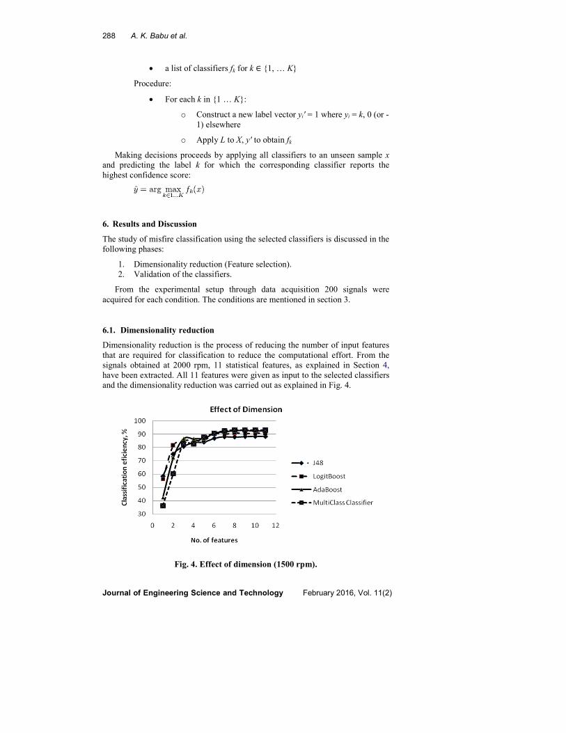
6.1. Dimensionality reduction
Dimensionality reduction is the process of reducing the number of input features
that are required for classification to reduce the computational effort. From the
signals obtained at 2000 rpm, 11 statistical features, as explained in Section 4,
have been extracted. All 11 features were given as input to the selected classifiers
and the dimensionality reduction was carried out as explained in Fig. 4.
Fig. 4. Effect of dimension (1500 rpm).
Misfire Detection in a Multi-Cylinder Diesel Engine: A Machine Learning Approach 289
Journal of Engineering Science and Technology February 2016, Vol. 11(2)
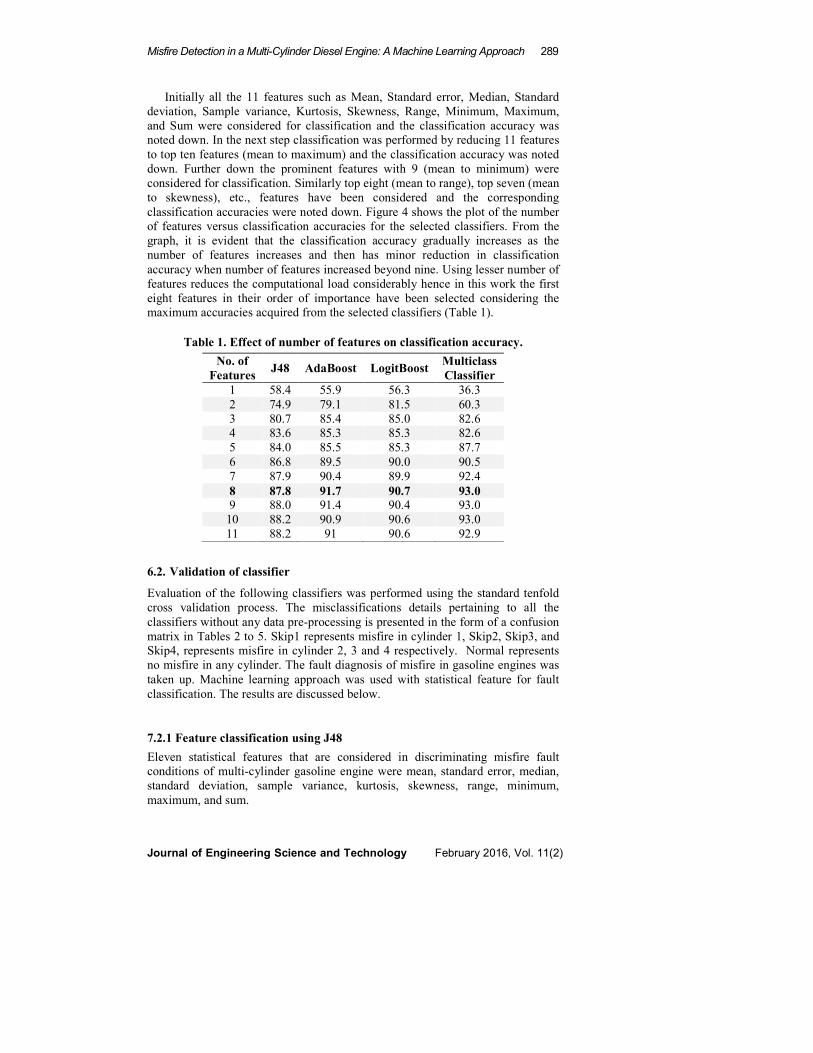
Initially all the 11 features such as Mean, Standard error, Median, Standard
deviation, Sample variance, Kurtosis, Skewness, Range, Minimum, Maximum,
and Sum were considered for classification and the classification accuracy was
noted down. In the next step classification was performed by reducing 11 features
to top ten features (mean to maximum) and the classification accuracy was noted
down. Further down the prominent features with 9 (mean to minimum) were
considered for classification. Similarly top eight (mean to range), top seven (mean
to skewness), etc., features have been considered and the corresponding
classification accuracies were noted down. Figure 4 shows the plot of the number
of features versus classification accuracies for the selected classifiers. From the
graph, it is evident that the classification accuracy gradually increases as the
number of features increases and then has minor reduction in classification
accuracy when number of features increased beyond nine. Using lesser number of
features reduces the computational load considerably hence in this work the first
eight features in their order of importance have been selected considering the
maximum accuracies acquired from the selected classifiers (Table 1).
Table 1. Effect of number of features on classification accuracy.
No. of
Features J48 AdaBoost LogitBoost
Multiclass
Classifier
1 58.4 55.9 56.3 36.3
2 74.9 79.1 81.5 60.3
3 80.7 85.4 85.0 82.6
4 83.6 85.3 85.3 82.6
5 84.0 85.5 85.3 87.7
6 86.8 89.5 90.0 90.5
7 87.9 90.4 89.9 92.4
8 87.8 91.7 90.7 93.0 9 88.0 91.4 90.4 93.0
10 88.2 90.9 90.6 93.0
11 88.2 91 90.6 92.9
6.2. Validation of classifier
Evaluation of the following classifiers was performed using the standard tenfold
cross validation process. The misclassifications details pertaining to all the
classifiers without any data pre-processing is presented in the form of a confusion
matrix in Tables 2 to 5. Skip1 represents misfire in cylinder 1, Skip2, Skip3, and
Skip4, represents misfire in cylinder 2, 3 and 4 respectively. Normal represents
no misfire in any cylinder. The fault diagnosis of misfire in gasoline engines was
taken up. Machine learning approach was used with statistical feature for fault
classification. The results are discussed below.
7.2.1 Feature classification using J48
Eleven statistical features that are considered in discriminating misfire fault
conditions of multi-cylinder gasoline engine were mean, standard error, median,
standard deviation, sample variance, kurtosis, skewness, range, minimum,
maximum, and sum.
290 A. K. Babu et al.
Journal of Engineering Science and Technology February 2016, Vol. 11(2)
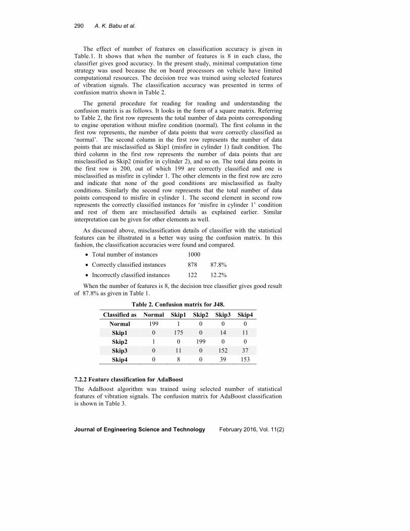
The effect of number of features on classification accuracy is given in
Table.1. It shows that when the number of features is 8 in each class, the
classifier gives good accuracy. In the present study, minimal computation time
strategy was used because the on board processors on vehicle have limited
computational resources. The decision tree was trained using selected features
of vibration signals. The classification accuracy was presented in terms of
confusion matrix shown in Table 2.
The general procedure for reading for reading and understanding the
confusion matrix is as follows. It looks in the form of a square matrix. Referring
to Table 2, the first row represents the total number of data points corresponding
to engine operation without misfire condition (normal). The first column in the
first row represents, the number of data points that were correctly classified as
‘normal’. The second column in the first row represents the number of data
points that are misclassified as Skip1 (misfire in cylinder 1) fault condition. The
third column in the first row represents the number of data points that are
misclassified as Skip2 (misfire in cylinder 2), and so on. The total data points in
the first row is 200, out of which 199 are correctly classified and one is
misclassified as misfire in cylinder 1. The other elements in the first row are zero
and indicate that none of the good conditions are misclassified as faulty
conditions. Similarly the second row represents that the total number of data
points correspond to misfire in cylinder 1. The second element in second row
represents the correctly classified instances for ‘misfire in cylinder 1’ condition
and rest of them are misclassified details as explained earlier. Similar
interpretation can be given for other elements as well.
As discussed above, misclassification details of classifier with the statistical
features can be illustrated in a better way using the confusion matrix. In this
fashion, the classification accuracies were found and compared.
• Total number of instances 1000
• Correctly classified instances 878 87.8%
• Incorrectly classified instances 122 12.2%
When the number of features is 8, the decision tree classifier gives good result
of 87.8% as given in Table 1.
Table 2. Confusion matrix for J48.
Classified as Normal Skip1 Skip2 Skip3 Skip4
Normal 199 1 0 0 0
Skip1 0 175 0 14 11
Skip2 1 0 199 0 0
Skip3 0 11 0 152 37
Skip4 0 8 0 39 153
7.2.2 Feature classification for AdaBoost
The AdaBoost algorithm was trained using selected number of statistical
features of vibration signals. The confusion matrix for AdaBoost classification
is shown in Table 3.
Misfire Detection in a Multi-Cylinder Diesel Engine: A Machine Learning Approach 291
Journal of Engineering Science and Technology February 2016, Vol. 11(2)
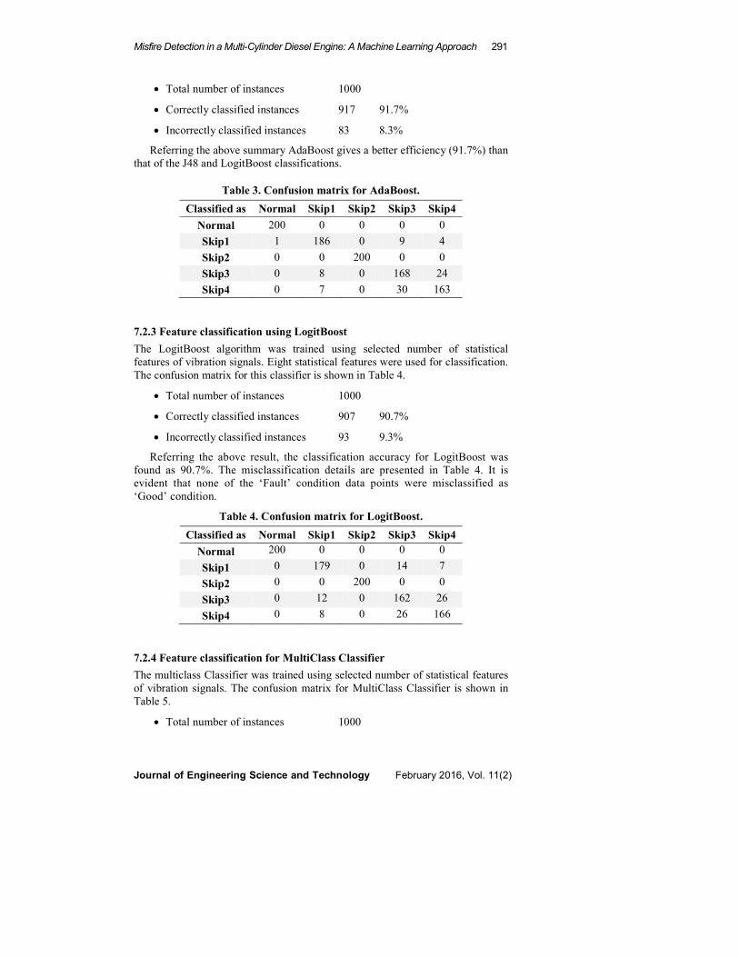
• Total number of instances 1000
• Correctly classified instances 917 91.7%
• Incorrectly classified instances 83 8.3%
Referring the above summary AdaBoost gives a better efficiency (91.7%) than
that of the J48 and LogitBoost classifications.
Table 3. Confusion matrix for AdaBoost.
Classified as Normal Skip1 Skip2 Skip3 Skip4
Normal 200 0 0 0 0
Skip1 1 186 0 9 4
Skip2 0 0 200 0 0
Skip3 0 8 0 168 24
Skip4 0 7 0 30 163
7.2.3 Feature classification using LogitBoost
The LogitBoost algorithm was trained using selected number of statistical
features of vibration signals. Eight statistical features were used for classification.
The confusion matrix for this classifier is shown in Table 4.
• Total number of instances 1000
• Correctly classified instances 907 90.7%
• Incorrectly classified instances 93 9.3%
Referring the above result, the classification accuracy for LogitBoost was
found as 90.7%. The misclassification details are presented in Table 4. It is
evident that none of the ‘Fault’ condition data points were misclassified as
‘Good’ condition.
Table 4. Confusion matrix for LogitBoost.
Classified as Normal Skip1 Skip2 Skip3 Skip4
Normal 200 0 0 0 0
Skip1 0 179 0 14 7
Skip2 0 0 200 0 0
Skip3 0 12 0 162 26
Skip4 0 8 0 26 166
7.2.4 Feature classification for MultiClass Classifier
The multiclass Classifier was trained using selected number of statistical features
of vibration signals. The confusion matrix for MultiClass Classifier is shown in
Table 5.
• Total number of instances 1000
292 A. K. Babu et al.
Journal of Engineering Science and Technology February 2016, Vol. 11(2)
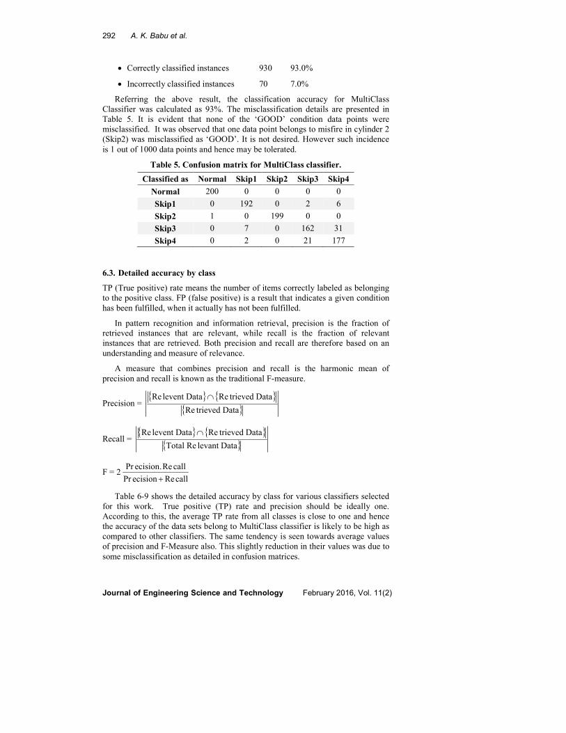
• Correctly classified instances 930 93.0%
• Incorrectly classified instances 70 7.0%
Referring the above result, the classification accuracy for MultiClass
Classifier was calculated as 93%. The misclassification details are presented in
Table 5. It is evident that none of the ‘GOOD’ condition data points were
misclassified. It was observed that one data point belongs to misfire in cylinder 2
(Skip2) was misclassified as ‘GOOD’. It is not desired. However such incidence
is 1 out of 1000 data points and hence may be tolerated.
Table 5. Confusion matrix for MultiClass classifier.
Classified as Normal Skip1 Skip2 Skip3 Skip4
Normal 200 0 0 0 0
Skip1 0 192 0 2 6
Skip2 1 0 199 0 0
Skip3 0 7 0 162 31
Skip4 0 2 0 21 177
6.3. Detailed accuracy by class
TP (True positive) rate means the number of items correctly labeled as belonging
to the positive class. FP (false positive) is a result that indicates a given condition
has been fulfilled, when it actually has not been fulfilled.
In pattern recognition and information retrieval, precision is the fraction of
retrieved instances that are relevant, while recall is the fraction of relevant
instances that are retrieved. Both precision and recall are therefore based on an
understanding and measure of relevance.
A measure that combines precision and recall is the harmonic mean of
precision and recall is known as the traditional F-measure.
Precision = { } { }
{ }DatatrievedRe
DatatrievedReDataleventRe ∩
Recall = { } { }
{ }DatalevantReTotal
DatatrievedReDataleventRe ∩
F = 2callReecisionPr
callRe.ecisionPr
+
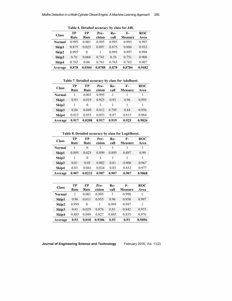
Table 6-9 shows the detailed accuracy by class for various classifiers selected
for this work. True positive (TP) rate and precision should be ideally one.
According to this, the average TP rate from all classes is close to one and hence
the accuracy of the data sets belong to MultiClass classifier is likely to be high as
compared to other classifiers. The same tendency is seen towards average values
of precision and F-Measure also. This slightly reduction in their values was due to
some misclassification as detailed in confusion matrices.
Misfire Detection in a Multi-Cylinder Diesel Engine: A Machine Learning Approach 293
Journal of Engineering Science and Technology February 2016, Vol. 11(2)
Table 6. Detailed accuracy by class for J48.
Class TP
Rate
FP
Rate
Pre-
cision
Re-
call
F-
Measure
ROC
Area
Normal 0.995 0.001 0.995 0.995 0.995 0.997
Skip1 0.875 0.025 0.897 0.875 0.886 0.933
Skip2 0.995 0 1 0.995 0.997 0.998
Skip3 0.76 0.066 0.741 0.76 0.751 0.906
Skip4 0.765 0.06 0.761 0.765 0.763 0.907
Average 0.878 0.0304 0.8788 0.878 0.8784 0.9482
Table 7. Detailed accuracy by class for AdaBoost.
Class TP
Rate
FP
Rate
Pre-
cision
Re-
call
F-
Measure
ROC
Area
Normal 1 0.001 0.995 1 1 1
Skip1 0.93 0.019 0.925 0.93 0.96 0.993
Skip2 1 0 1 1 1 1
Skip3 0.84 0.049 0.812 0.795 0.84 0.956
Skip4 0.815 0.035 0.853 0.87 0.815 0.964
Average 0.917 0.0208 0.917 0.919 0.925 0.9826
Table 8. Detailed accuracy by class for LogitBoost.
Class TP
Rate
FP
Rate
Pre-
cision
Re-
call
F-
Measure
ROC
Area
Normal 1 0 1 1 1 1
Skip1 0.895 0.025 0.899 0.895 0.897 0.99
Skip2 1 0 1 1 1 1
Skip3 0.81 0.05 0.802 0.81 0.806 0.967
Skip4 0.83 0.041 0.834 0.83 0.832 0.977
Average 0.907 0.0232 0.907 0.907 0.907 0.9868
Class TP
Rate
FP
Rate
Pre-
cision
Re-
call
F-
Measure
ROC
Area
Normal 1 0.001 0.995 1 0.998 1
Skip1 0.96 0.011 0.955 0.96 0.958 0.997
Skip2 0.995 0 1 0.995 0.997 1
Skip3 0.81 0.029 0.876 0.81 0.842 0.975
Skip4 0.885 0.049 0.827 0.885 0.855 0.976
Average 0.93 0.018 0.9306 0.93 0.93 0.9896
294 A. K. Babu et al.
Journal of Engineering Science and Technology February 2016, Vol. 11(2)
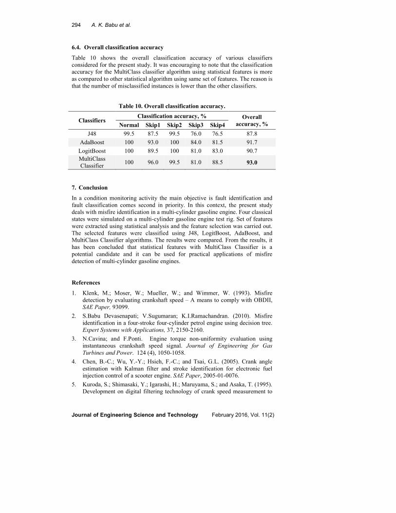
6.4. Overall classification accuracy
Table 10 shows the overall classification accuracy of various classifiers
considered for the present study. It was encouraging to note that the classification
accuracy for the MultiClass classifier algorithm using statistical features is more
as compared to other statistical algorithm using same set of features. The reason is
that the number of misclassified instances is lower than the other classifiers.
Table 10. Overall classification accuracy.
Classifiers Classification accuracy, % Overall
accuracy, % Normal Skip1 Skip2 Skip3 Skip4
J48 99.5 87.5 99.5 76.0 76.5 87.8
AdaBoost 100 93.0 100 84.0 81.5 91.7
LogitBoost 100 89.5 100 81.0 83.0 90.7
MultiClass
Classifier 100 96.0 99.5 81.0 88.5 93.0
7. Conclusion
In a condition monitoring activity the main objective is fault identification and
fault classification comes second in priority. In this context, the present study
deals with misfire identification in a multi-cylinder gasoline engine. Four classical
states were simulated on a multi-cylinder gasoline engine test rig. Set of features
were extracted using statistical analysis and the feature selection was carried out.
The selected features were classified using J48, LogitBoost, AdaBoost, and
MultiClass Classifier algorithms. The results were compared. From the results, it
has been concluded that statistical features with MultiClass Classifier is a
potential candidate and it can be used for practical applications of misfire
detection of multi-cylinder gasoline engines.
References
1. Klenk, M.; Moser, W.; Mueller, W.; and Wimmer, W. (1993). Misfire
detection by evaluating crankshaft speed – A means to comply with OBDII,
SAE Paper, 93099.
2. S.Babu Devasenapati; V.Sugumaran; K.I.Ramachandran. (2010). Misfire
identification in a four-stroke four-cylinder petrol engine using decision tree.
Expert Systems with Applications, 37, 2150-2160.
3. N.Cavina; and F.Ponti. Engine torque non-uniformity evaluation using
instantaneous crankshaft speed signal. Journal of Engineering for Gas
Turbines and Power. 124 (4), 1050-1058.
4. Chen, B.-C.; Wu, Y.-Y.; Hsieh, F.-C.; and Tsai, G.L. (2005). Crank angle
estimation with Kalman filter and stroke identification for electronic fuel
injection control of a scooter engine. SAE Paper, 2005-01-0076.
5. Kuroda, S.; Shimasaki, Y.; Igarashi, H.; Maruyama, S.; and Asaka, T. (1995).
Development on digital filtering technology of crank speed measurement to
Misfire Detection in a Multi-Cylinder Diesel Engine: A Machine Learning Approach 295
Journal of Engineering Science and Technology February 2016, Vol. 11(2)
detect misfire in internal combustion engine at high speed revolution. JSAE
Review. 16(4), 387–390.
6. Osburn, A. W.; Kostek, T. M.; and Franchek, M. A. (2006). Residual
generation and statistical pattern recognition for engine misfire diagnostics.
Mechanical Systems and Signal Processing. 20(8), 2232–2258.
7. Tinaut, F. V.; Melgar, A.; Laget, H.; and Dominguez, J. I. (2007). Misfire
and compression fault detection through the energy model. Mechanical
Systems and Signal Processing. 21(3), 1521–1535.
8. Piotr, B.; and Jerzy, M. (2005). Misfire detection of locomotive diesel engine
by nonlinear analysis. Mechanical Systems and Signal Processing. 19(4),
881–899.
9. Ye, J. (2009). Application of extension theory in misfire fault diagnosis of
gasoline engines. Expert Systems with Applications. 36(2), 1217–1221.
10. Shiao, Y.; and Moskwa, J. J. (1995). Cylinder pressure and combustion heat
release estimation for si engine diagnostics using nonlinear sliding observers.
IEEE Transactions on Control Systems Technology. 3.
11. Wang, Y.; and Chu, F. (2005). Real-time misfire detection via sliding mode
observer. Mechanical Systems and Signal Processing. 19(4), 900–912.
12. Kiencke, U. (1999). Engine misfire detection. Control Engineering Practice.
7(2), 203–208.
13. Ilkivova, M. R.; Ilkiv, B. R.; and Neuschl, T. (2002). Comparison of a linear
and nonlinear approach to engine misfires detection. Control Engineering
Practice. 10(10), 1141–1146.
14. Chang, J.; Kim, M.; and Min, K. (2002). Detection of misfire and knock in
spark ignition engines by wavelet transform of engine block vibration
signals. Measurement Science and Technology. 13(7), 1108–1114.
15. Sugumaran, V.; Muralidharan, V.; and Ramachandran, K.I. (2007). Feature
selection using decision tree and classification through proximal support
vector machine for fault diagnostics of roller bearing. Mechanical Systems
and Signal Processing. 21, 930-942.
16. Babu Devasenapati, S.; Ramachandran, K.I. (2012). Random forest based
misfire detection using Kononenko discretiser. ICTACT Journal on Soft
Computing.
17. Ferome Friedman; Trevor Hastie; and Robert Tibshirani. (2000). Additive
logistic regression: A statistical view of boosting. The Annals of Statistics.
28(2), 337-407.