Misc stuff - Memphis

Misc stuff

lookfor command – to look for commands based on “keyword”

(searches all m files in path, including your files, for the keyword).

what command – lists matlab related files (returns structure with fields for m, mat, mex, mdl, classes, and packages

files).,

Help window (pull down menu).

Helpdesk (internet)

http://www.mathworks.com/access/helpdesk/help/helpdesk.shtml

workspace >> help workspace WORKSPACE Open Workspace browser to manage workspace WORKSPACE Opens the Workspace browser with a view of the variables in the current Workspace. Displayed variables may be viewed, manipulated, saved, and cleared.

path >> help path PATH Get/set search path. PATH, by itself, prettyprints MATLAB's current search path. The initial search path list is set by PATHDEF, and is perhaps individualized by STARTUP. P = PATH returns a string containing the path in P. PATH(P) changes the path to P. PATH(PATH) refreshes MATLAB's view of the directories on the path, ensuring that any changes to non-toolbox directories are visible. PATH(P1,P2) changes the path to the concatenation of the two path strings P1 and P2. Thus PATH(PATH,P) appends a new directory to th current path and PATH(P,PATH) prepends a new directory. If P is already on the path, then PATH(PATH,P) moves P to the end of the path, and similarly, PATH(P,PATH) moves P to the beginning of the path. For example, the following statements add another directory to MATLAB’s search path on various operating systems: Unix: path(path,'/home/myfriend/goodstuff') Windows: path(path,'c:\tools\goodstuff’)

format command >> help format . . . FORMAT Set output format. . . . FORMAT does not affect how MATLAB computations are done.

To separate multiple commands on one line use “;” for no output, and ‘,’ for output

Cmd line editing

arrows: move cursor by character

ctrl arrows l and r: move cursor by word

ctrl a, e: move cursor to beginning, end line

ctrl u, d, h, k: clear line, delete char at cursor, delete char before cursor, delete to

end of line.

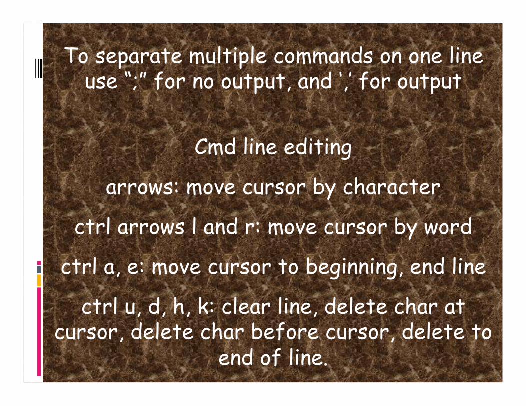
Running an m file from the command line (should not be interactive)

>> matlab < somefile.m

Don’t show output on terminal (send to bit bucket), run in background to not lock up

terminal matlab -nosplash < eig_mov.m > /nl &

Global variables

When you define a variable at the matlab prompt, it is defined inside of matlab's

"workspace.”

Running a script does not affect this, since a script is just a collection of commands, and

they're actually run from the same workspace.

If you define a variable in a script, it will stay defined in the workspace.

Global variables

Functions, on the other hand, do not share the same workspace.

A function won't know what a variable is unless

- the function gets the variable as an argument, or

- the variable is defined as a variable that is shared by the function and the matlab

workspace, i.e. a global variable.

Global variables

To use a global variable, every place (function, script, or at the matlab prompt)

that needs to share that variable must have a line near the top identifying it as a global

variable, ie:

global phi;

Then when the variable is assigned a value in one of those places, it will have a value in all

the other places that have the global statement.

Linear Algebra (a la Matlab) Review

>> a=[1 2 3;4 5 6;7 8 9] a = 1 2 3 4 5 6 7 8 9 >> c=trace(a) c = 15

>> a=[.96 -.28; .28 .96] a = 0.9600 -0.2800 0.2800 0.9600 >> inv(a) ans = 0.9600 0.2800 -0.2800 0.9600 >> a'*a ans = 1 0 0 1 >>

Block matrices >> b=[2 2;1 3] b =

2 2 1 3 c = 0 2 3 5 4 7 >> d=[1 0] d = 1 0 >> e=[-1 6 0] e = -1 6 0 >> a=[b c;d e] a = 2 2 0 2 3 1 3 5 4 7 1 0 -1 6 0

Linear Dependence

a b c

2a + 1b = c

Linear Independence

There is no simple, linear combination of a and b what will produce c.

a b c

Rank of a matrix

>> a=[1 2; 3 4] a = 1 2 3 4 >> rank(a) ans = 2 >> rref(a) ans = 1 0 0 1 >> >> a=[1 2 3;4 5 6;7 8 9] a = 1 2 3 4 5 6 7 8 9 >> rank(a) ans = 2 >> rref(a) ans = 1 0 -1 0 1 2 0 0 0

There are a lot of matrix math functions >> help matfun Matrix functions - numerical linear algebra.

Matrix analysis. norm - Matrix or vector norm. normest - Estimate the matrix 2-norm. rank - Matrix rank. det - Determinant. trace - Sum of diagonal elements. null - Null space. orth - Orthogonalization. rref - Reduced row echelon form. subspace - Angle between two subspaces.

Linear equations. / and / - Linear equation solution; use "help slash". linsolve - Linear equation solution with extra control. inv - Matrix inverse. rcond - LAPACK reciprocal condition estimator cond - Condition number with respect to inversion. condest - 1-norm condition number estimate. normest1 - 1-norm estimate.

cholinc - Incomplete Cholesky factorization. ldl - Block LDL' factorization. lu - LU factorization. luinc - Incomplete LU factorization. qr - Orthogonal-triangular decomposition. lsqnonneg - Linear least squares with nonnegativity constraints. pinv - Pseudoinverse. lscov - Least squares with known covariance.

Eigenvalues and singular values. eig - Eigenvalues and eigenvectors. svd - Singular value decomposition. gsvd - Generalized singular value decomposition. eigs - A few eigenvalues. svds - A few singular values. poly - Characteristic polynomial. polyeig - Polynomial eigenvalue problem. condeig - Condition number with respect to eigenvalues. hess - Hessenberg form. schur - Schur decomposition. qz - QZ factorization for generalized eigenvalues.

ordschur - Reordering of eigenvalues in Schur decomposition. ordqz - Reordering of eigenvalues in QZ factorization. ordeig - Eigenvalues of quasitriangular matrices.

Matrix functions. expm - Matrix exponential. logm - Matrix logarithm. sqrtm - Matrix square root. funm - Evaluate general matrix function.

Factorization utilities qrdelete - Delete a column or row from QR factorization. qrinsert - Insert a column or row into QR factorization. rsf2csf - Real block diagonal form to complex diagonal form. cdf2rdf - Complex diagonal form to real block diagonal form. balance - Diagonal scaling to improve eigenvalue accuracy. planerot - Givens plane rotation. cholupdate - rank 1 update to Cholesky factorization. qrupdate - rank 1 update to QR factorization.

>>

Data Analysis

Flow Charts

2 tasks

Understanding How a Process Works

Communicating How a Process Works (translating it into computer code, communicating to the computer.)

A flow chart can therefore be used to:

Define and analyze processes;

Build a step-by-step picture of the process for analysis, discussion, communication, and

coding;

and

Define, standardize or find areas for improvement in a process.

Also

by conveying the information or processes in a step-by-step flow, you can then

concentrate more intently on each individual step,

without feeling overwhelmed by the bigger picture.

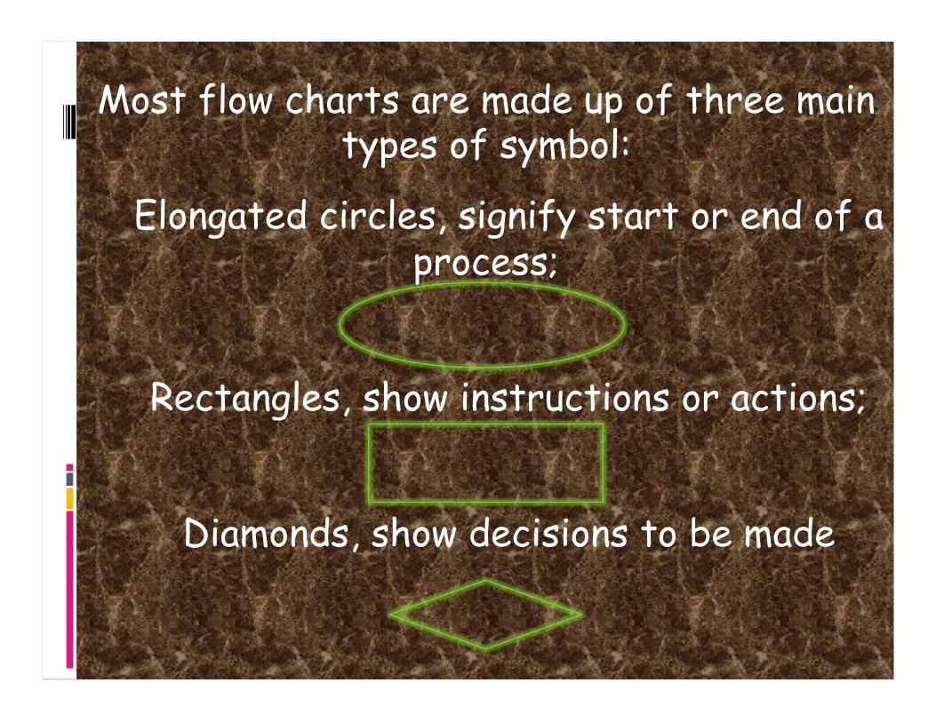
Most flow charts are made up of three main types of symbol:

Elongated circles, signify start or end of a process;

Rectangles, show instructions or actions;

Diamonds, show decisions to be made

Within each symbol, write down what the symbol represents. This could be the start or finish of the process, the action to be

taken, or the decision to be made.

Symbols are connected one to the other by arrows, showing the flow of the process.

Worlds most famous Flowchart: General Flowchart For Problem Resolution -

Don’t Fool with it!

YES NO

YES

YOU IDIOT! NO

Will it blow up in your hands?

NO

Look the other way

Anyone else know? You’re SCREWED!

YES YES

NO

Hide it Can you blame someone else?

NO

NO PROBLEM!

Yes

Is it working?

Did you fool with it?

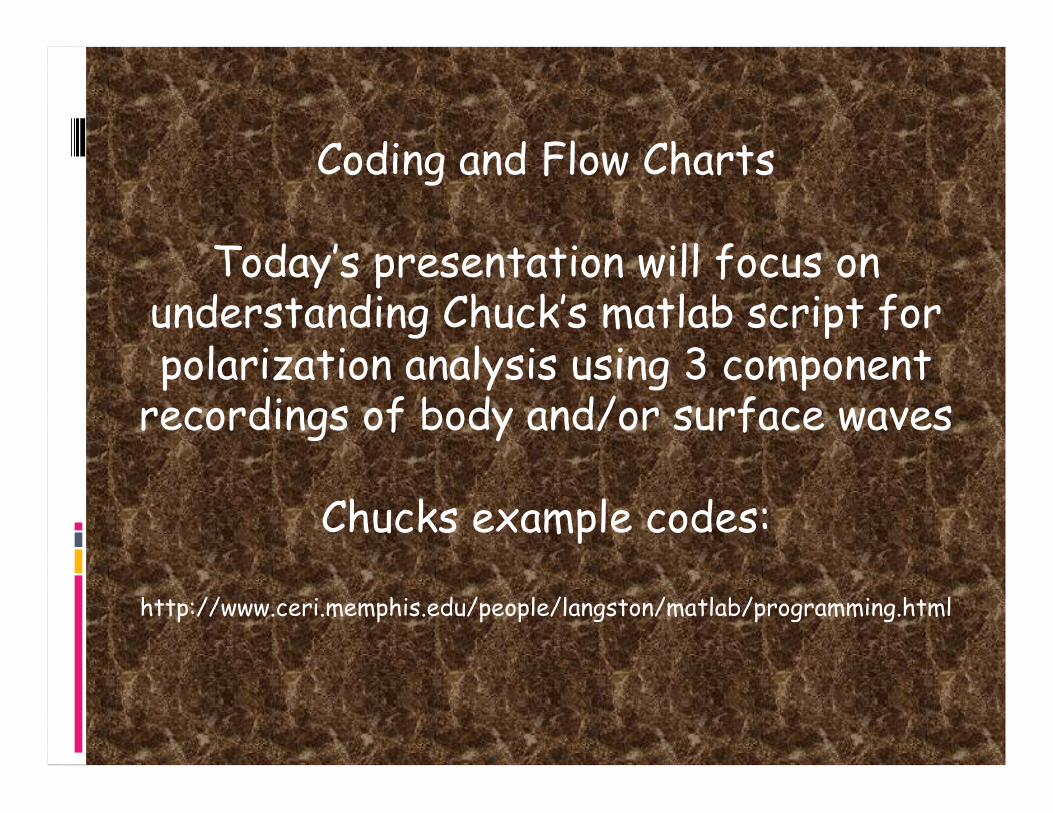
Coding and Flow Charts

Today’s presentation will focus on understanding Chuck’s matlab script for polarization analysis using 3 component

recordings of body and/or surface waves

Chucks example codes:

http://www.ceri.memphis.edu/people/langston/matlab/programming.html

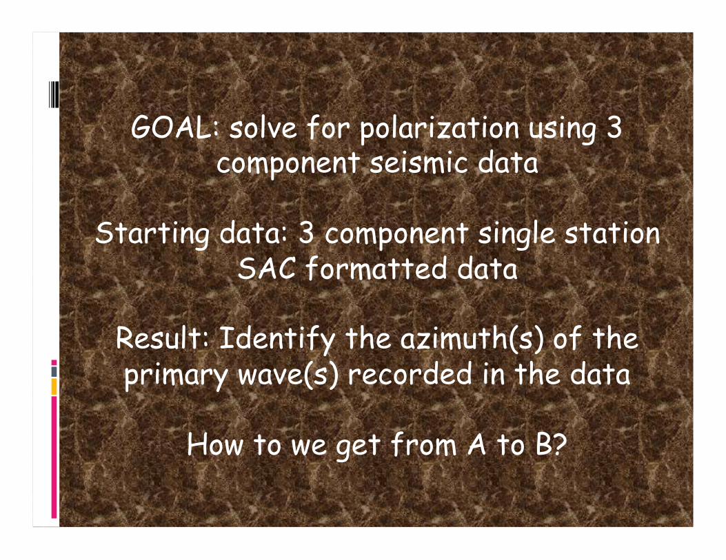
GOAL: solve for polarization using 3 component seismic data

Starting data: 3 component single station SAC formatted data

Result: Identify the azimuth(s) of the primary wave(s) recorded in the data

How to we get from A to B?

Principal Component Analysis

Principal component analysis (PCA) is a vector space transform often used to reduce

multidimensional data sets to lower dimensions for analysis.

Principal Component Analysis

PCA involves the calculation of the eigenvalue decomposition of a data covariance matrix or singular value

decomposition of a data matrix, usually after mean centering the data for each attribute.

Its operation can be thought of as revealing the internal structure of the data in a way

which best explains the variance in the data.

What we are looking for:

New set of axis (basis) that maximizes the correlation of HT(Z) with R, and minimizes the correlations between both HT(Z) and R

with T.

We are not using the full power of PCA, since we already have some model for the

result of the analysis (and have therefore preprocessed the data by taking the Hilbert transform of

the z component).

What is the idea?

Seismic waves are polarized

P wave longitudinal (V and R)

S wave transverse with SH and SV polarizations (T, V and R)

Rayleigh waves (V and R)

Love waves (T).

If we take a short time period we can think of each component as a vector of n terms.

If we take the dot product of each vector with itself and with the other two

components we can find the “angle” between tnem.

We can also make these dot products by making a 3xn arrary using each seismogram

as a row.

Multiplying this array with its transpose results in a 3x3 matrix with the various dot

products in the elements of the matrix.

Now find the eigenvectors and eigenvalues of this matrix.

From the eigenvectors we can make a rotation matrix that will rotate our matrix

to a diagonal matrix.

The off diagonal elements are now all zero and from the geometric interpretation of the dot product this means that the two

vectors used to make that dot product are perpendicular.

So we can rotate the original horizontal components into a new set of seismograms rotated to the principal directions defined

by the eigenvectors.

The dot products of the off diagonal terms will now be zero, indicating the vectors are

perpendicular.

• loadSACdata

• removemean

• plotwaveforms

• filterwaveformstohighlightwavesofinterest

• plotfilteredwaveforms

DataPreparation

• principalcomponentanalysisusing3‐componentdata

• note,thistechniquerequireszero‐meandata

MainCode• plotazimuthsofeigenvectors

• plotazimuthsexceeding50%ofmaximumvalue

Results

GOAL: Solve for polarization

Plotfilteredwaveforms

FilterwaveformstohighlightwavesofinterestDesignafilter;allowflexibleinputofcornerinfo Workon3files…suggestsasubroutine

Plotwaveformsvstime

Removethemean

LoadSACdata3files(Z,E,N)….suggestsusingasubroutine Providestationname

Step 1: Data Preparation

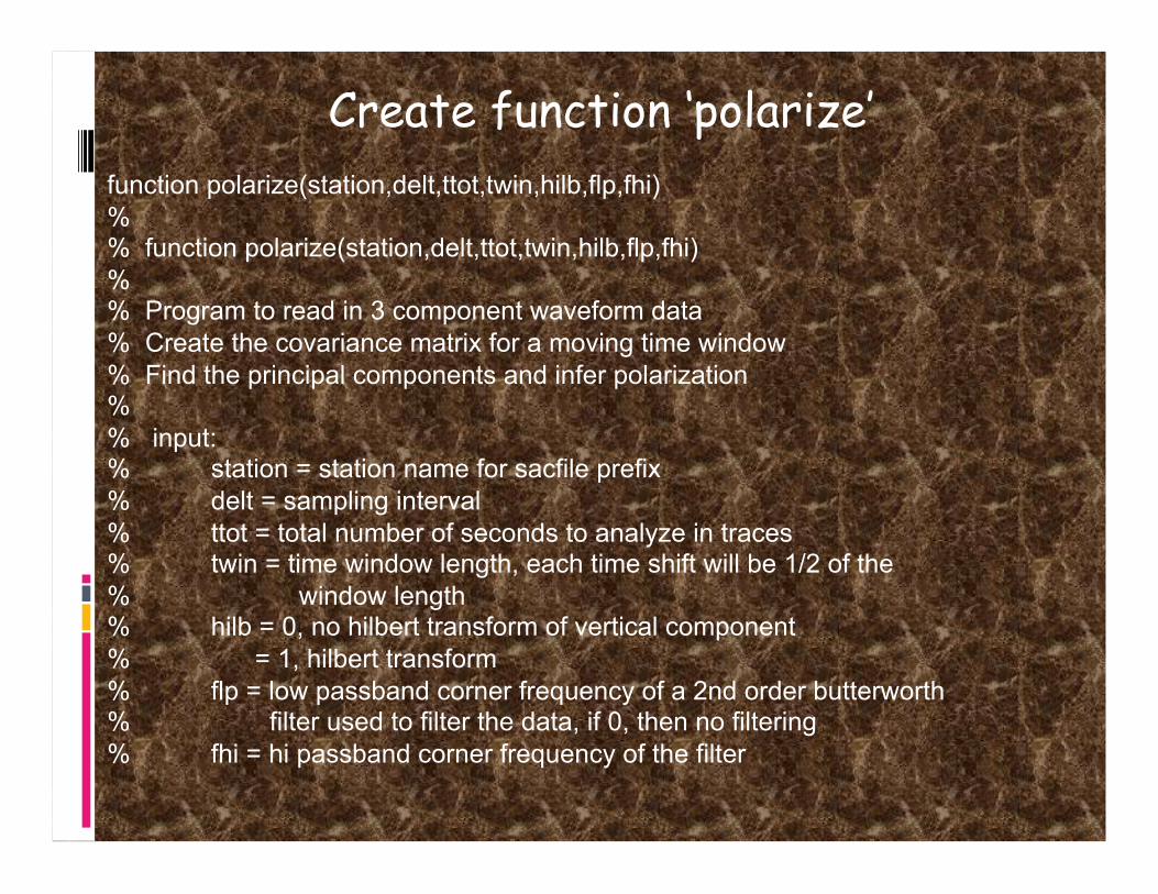
Create function ‘polarize’ function polarize(station,delt,ttot,twin,hilb,flp,fhi) % % function polarize(station,delt,ttot,twin,hilb,flp,fhi) % % Program to read in 3 component waveform data % Create the covariance matrix for a moving time window % Find the principal components and infer polarization % % input: % station = station name for sacfile prefix % delt = sampling interval % ttot = total number of seconds to analyze in traces % twin = time window length, each time shift will be 1/2 of the % window length % hilb = 0, no hilbert transform of vertical component % = 1, hilbert transform % flp = low passband corner frequency of a 2nd order butterworth % filter used to filter the data, if 0, then no filtering % fhi = hi passband corner frequency of the filter

Loading SAC data

Many matlab scripts exist to read in sac data.

I modified one so it is

- not sensitive to byte order - returns the data, plus: npts, delta, and

begin point of the SAC file

- data is a column vector

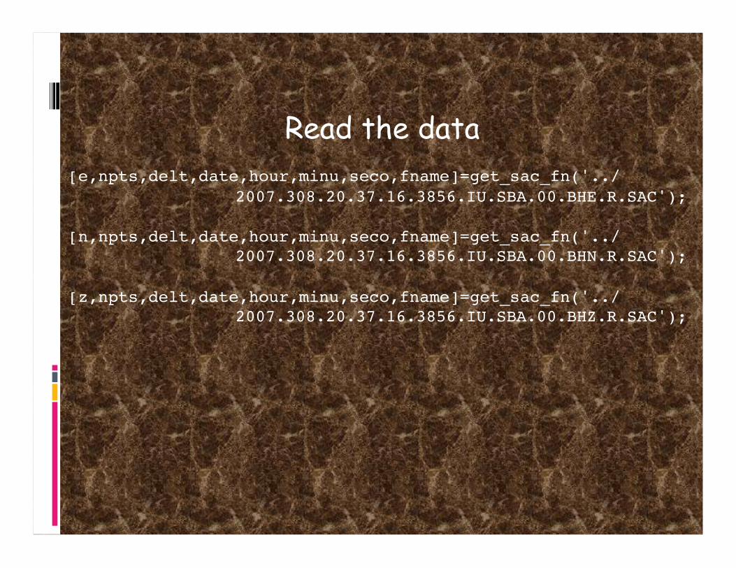
Read the data [e,npts,delt,date,hour,minu,seco,fname]=get_sac_fn('../

2007.308.20.37.16.3856.IU.SBA.00.BHE.R.SAC');

[n,npts,delt,date,hour,minu,seco,fname]=get_sac_fn('../ 2007.308.20.37.16.3856.IU.SBA.00.BHN.R.SAC');

[z,npts,delt,date,hour,minu,seco,fname]=get_sac_fn('../ 2007.308.20.37.16.3856.IU.SBA.00.BHZ.R.SAC');

Removing the data mean We need to remove the mean of the data for

principal component analysis (PCA).

We also need to transpose the column vector data into row vectors.

e=dmean(e’); % remove the mean from each n=dmean(n’); % and transpose the data z=dmean(z’);

subroutine: dmean function [a]=dmean(b) % % [a]=dmean(b) % % Remove the mean from a row vector m=mean(b); a=b-m; return;

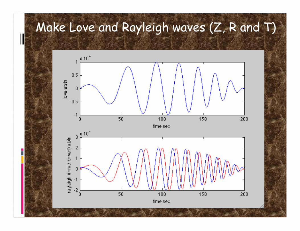
Make Love and Rayleigh waves (Z, R and T)

Rayleigh R and Z related by Hilbert X-form (90° phase shift, blue trace is Hilbert Transformed to green trace, then

overlays red trace.).

n=512; a=sin(2*pi*[0:(n-1)]/n); b=hilbert(a); clf plot(a) hold plot(-imag(b),'r') plot(real(b),'g--') grid

Hilbert Transform if hilb ==1; % hilbert transform the vertical component zh=hilbert(z); % to make Rayleigh wave in phase on vert

and horz z=-imag(zh); % if present (z constructed from HT, so

used +imag to make overlay for last figure)

else; end;

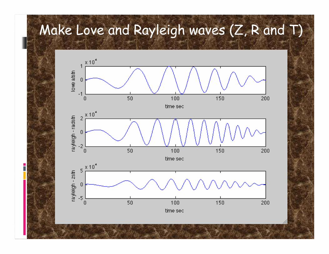
Make Love and Rayleigh waves (Z, R and T)

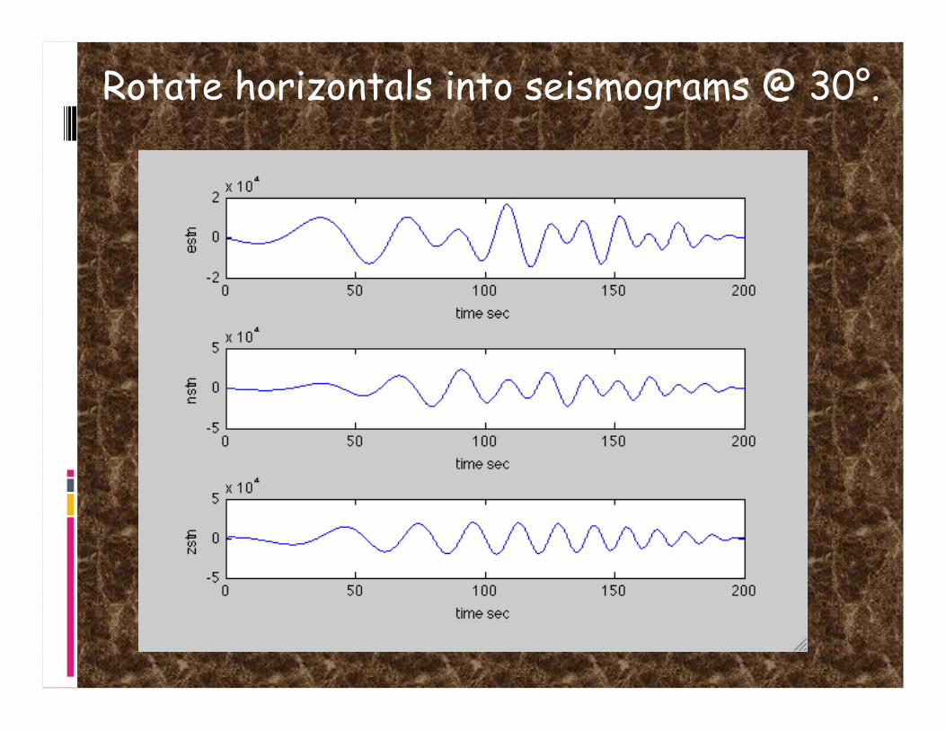
Rotate horizontals into seismograms @ 30°.

Plot the data

% plot the raw data

f1=figure('name','DATA SEISMOGRAMS');

subplot(3,1,1);

plot(t,e);

xlabel('time sec');

ylabel(strcat('EW Comp at ',station));

subplot(3,1,2);

plot(t,n);

xlabel('time sec');

ylabel(strcat('NS Comp at ',station));

subplot(3,1,3);

plot(t,z);

xlabel('time sec');

ylabel(strcat('Z comp at ',station));

Filtering

Filtering is a two step process in Matlab

Design the filter Apply the filter

There is a filter design GUI you can use to design the perfect filter called fdatool

Or you can design filters using pre-built filter types (Butterworth, Bessel, etc.)

function [d]=bandpass(c,flp,fhi,npts,delt) % % [d]=bandpass(c,flp) % % bandpass a time series with a 2nd order butterworth filter % % c = input time series % flp = lowpass corner frequency of filter % fhi = highpass corner frequency % npts = samples in data % delt = sampling interval of data % n=2; % 2nd order butterworth filter fnq=1/(2*delt); % Nyquist frequency Wn=[flp/fnq fhi/fnq]; % non-dimensionalize the corner frequencies [b,a]=butter(n,Wn); % butterworth bandpass non-dimensional frequency d=filtfilt(b,a,c); % apply the filter: use zero phase filter (p=2) return;

Filter & plot the filtered data

% filter the data

%

if flp > 0;

e1=bandpass(e,flp,fhi,npts,delt);

n1=bandpass(n,flp,fhi,npts,delt);

z1=bandpass(z,flp,fhi,npts,delt);

e=e1;

n=n1;

z=z1;

%

% plot the filtered data

f2=figure('name','FILTERED SEISMOGRAMS');

subplot(3,1,1);

…… removed for clarity

else;

end;

*The vertical channel has also had a Hilbert transform applied so that the Rayleigh wave is in phase on the NS and Z components

• Recognizethatincomingseismicphasesshouldrepresenttheprincipalcomponents,orthestrongestsignal,onthe3componentdata

• Theprincipalcomponents,inturn,areequaltotheeigenvectorsofthecovariancematrixofthe3componentmatrix.ThiscanbederivedusingPCAtechniques

• Eigenvectors/valuesrepresentaspatialtransformationwhichmaximizescovariancebetweenthe3components,andtheycontaininformationontheazimuthfromwhichtheprimarysignalisderived

• Sincemultiplephasesmaybepresent,wewouldprefertolookatshorttimewindowsofthe3componentdata,orinotherwords,performPCAonarunningwindowthroughthecontinuouswaveforms

MainCode

•  plotazimuthsofeigenvectors

•  plotazimuthsexceeding50%ofmaximumvalue

Results


Createarunningwindow

Createamatrixofthe3

componentdatainthewindow

Calculatethecorrelationmatrix

Findtheeigenvectors

andeigenvalues

Reordertheeigenvectors/eigenvalues

Calculatetheazimuthforeach

eigenvalue

Step 2: Main Code

npts1 nwin

npshift

Moving window using loops % Moving window loop % npts1=fix(ttot/delt) + 1; % total number of samples to analyze nwin=fix(twin/delt) + 1; % number of samples in a time window npshift=fix(twin/(2*delt))+1; % number of samples to shift over kfin=fix((npts1-nwin)/(npshift+1))+1; % number of time windows considered

mxde1=0.; mxde2=0.; mxde3=0.;

overlap

k=1

k=2

k=3

… k=kfin

for k=1:kfin; nwinst=(k-1)*(npshift-1)+1; % start of time window nwinfn=nwinst+nwin-1; % end of time window …….. missing code to be supplied later t2(k)=delt*(nwinst-1); % assign time for this window to the window start end;

Eigenvalues/Eigenvectors

Missing code from inside our loop a=csigm(e,n,z,nwinst,nwinfn); % signal matrix c=a'*a; % covariance matrix [v1,d1]=eig(c); % eigenvalue/eigenvectors [v,d]=order(v1,d1); % put eigenvalues & eigenvectors

in ascending order

% azimuth for each of the 3 eigenvalues ang1(k)=atan2(v(1,1),v(2,1)) * 180/pi; ang2(k)=atan2(v(1,2),v(2,2)) * 180/pi; ang3(k)=atan2(v(1,3),v(2,3)) * 180/pi;

% incidence angle of the 3 eigenvalues vang1(k)=acos(abs(v(3,1)))* 180/pi; %angle from the vertical vang2(k)=acos(abs(v(3,2)))* 180/pi; vang3(k)=acos(abs(v(3,3)))* 180/pi;

Still in loop de1(k)=d(1); de2(k)=d(2); de3(k)=d(3);

mxde1=max(mxde1,de1(k)); % find the maximum values mxde2=max(mxde2,de2(k)); mxde3=max(mxde3,de3(k));

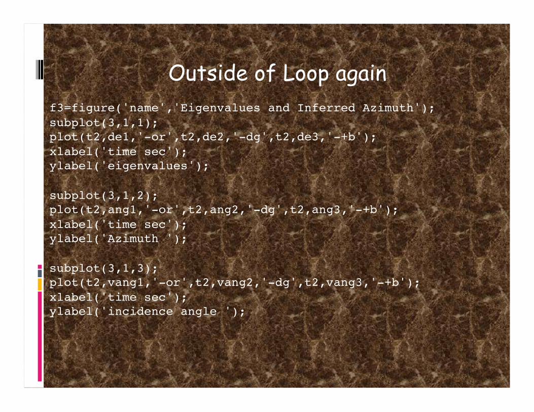
Outside of Loop again f3=figure('name','Eigenvalues and Inferred Azimuth'); subplot(3,1,1); plot(t2,de1,'-or',t2,de2,'-dg',t2,de3,'-+b'); xlabel('time sec'); ylabel('eigenvalues');

subplot(3,1,2); plot(t2,ang1,'-or',t2,ang2,'-dg',t2,ang3,'-+b'); xlabel('time sec'); ylabel('Azimuth ');

subplot(3,1,3); plot(t2,vang1,'-or',t2,vang2,'-dg',t2,vang3,'-+b'); xlabel('time sec'); ylabel('incidence angle ');

• 

MainCode

•  plotazimuthsofeigenvectors

•  plotazimuthsexceeding50%ofmaximumvalue

Results


Rose Diagrams % Rose plots f4=figure('name','Azimuth Distribution'); subplot(2,3,1); title('Azimuth - Largest Eigenvalue'); rose(ang1*pi/180,100);

subplot(2,3,2); title('Azimuth - Intermediate Eigenvalue'); rose(ang2*pi/180,100);

subplot(2,3,3); title('Azimuth - Smallest Eigenvalue'); rose(ang3*pi/180,100);

nskip=1;

ifnskip==1;

else;

neig1=0;

neig2=0;

neig3=0;

fork=1:kfin;

ifde1(k)>=0.5*mxde1;

neig1=neig1+1;

angm1(neig1)=ang1(k);

else;

end;


neig2=neig2+1;


else;

end;


neig3=neig3+1;


else;

end;

end;

subplot(2,3,4);

title('Azimuth‐LargestEigenvalue,50%Threshold');

rose(angm1*pi/180,100);

subplot(2,3,5);

title('Azimuth‐IntermediateEigenvalue,50%Threshold');


subplot(2,3,6);

title('Azimuth‐SmallestEigenvalue,50%Threshold');


end;

Documents

Misc stuff - Memphis