Mirror Symmetry And Loop Operators

Benjamin Assel,a Jaume Gomis b

aDepartment of Mathematics, King’s College London,

The Strand, London WC2R 2LS, United Kingdom

bPerimeter Institute for Theoretical Physics,

Waterloo, Ontario, N2L 2Y5, Canada

Abstract

Wilson loops in gauge theories pose a fundamental challenge for dualities. Wilson loops

are labeled by a representation of the gauge group and should map under duality to

loop operators labeled by the same data, yet generically, dual theories have completely

different gauge groups. In this paper we resolve this conundrum for three dimensional

mirror symmetry. We show that Wilson loops are exchanged under mirror symmetry

with Vortex loop operators, whose microscopic definition in terms of a supersymmetric

quantum mechanics coupled to the theory encode in a non-trivial way a representation of

the original gauge group, despite that the gauge groups of mirror theories can be radically

different. Our predictions for the mirror map, which we derive guided by branes in string

theory, are confirmed by the computation of the exact expectation value of Wilson and

Vortex loop operators on the three-sphere.

November 11, 2015

abenjamin.assel@gmail.combjgomis@perimeterinstitute.ca

arX

iv:1

506.

0171

8v2

[he

p-th

] 1

0 N

ov 2

015

Contents

1 Introduction 2

2 Loop Operators in 3d N = 4 Theories 6

2.1 Wilson Loop Operators . . . . . . . . . . . . . . . . . . . . . . . . . . . . . . . . . . . 9

2.2 Vortex Loop Operators . . . . . . . . . . . . . . . . . . . . . . . . . . . . . . . . . . . 10

3 Brane Realization Of Loop Operators and Mirror Map 13

3.1 Brane Realization Of Wilson Loop Operators . . . . . . . . . . . . . . . . . . . . . . 16

3.2 Mirror Of Wilson Loops From S-duality . . . . . . . . . . . . . . . . . . . . . . . . . 21

4 Mirror Symmetry and Loop Operators: Examples 28

4.1 T [SU(2)] . . . . . . . . . . . . . . . . . . . . . . . . . . . . . . . . . . . . . . . . . . . 28

4.2 Wilson Loops In The U(N − 1) Node Of T [SU(N)] . . . . . . . . . . . . . . . . . . . 32

4.3 The Other T [SU(N)] Loops . . . . . . . . . . . . . . . . . . . . . . . . . . . . . . . . 37

4.4 Loops And Mirror Map In Circular Quivers . . . . . . . . . . . . . . . . . . . . . . . 42

4.5 Loops In SQCD with 2N Quarks And Its Mirror . . . . . . . . . . . . . . . . . . . . . 45

5 Loop Operators In 3d N = 4 Theories On S3 48

5.1 Wilson Loops On S3 . . . . . . . . . . . . . . . . . . . . . . . . . . . . . . . . . . . . 50

5.2 Vortex Loops On S3 . . . . . . . . . . . . . . . . . . . . . . . . . . . . . . . . . . . . 52

5.3 Exact Partition Function Of 3d/1d Theories On S3 . . . . . . . . . . . . . . . . . . . 55

5.3.1 S3 Partition Function And Wilson loops . . . . . . . . . . . . . . . . . . . . . 55

5.3.2 1d N = 4 Supersymmetric Quantum Mechanics Partition Function . . . . . . 56

5.3.3 Matrix Model Computing Vortex Loops . . . . . . . . . . . . . . . . . . . . . 62

5.4 Loops in T [SU(N)] . . . . . . . . . . . . . . . . . . . . . . . . . . . . . . . . . . . . 64

5.4.1 T[SU(2)] loops . . . . . . . . . . . . . . . . . . . . . . . . . . . . . . . . . . . 65

5.4.2 Wilson loops in T[SU(N)] . . . . . . . . . . . . . . . . . . . . . . . . . . . . . 66

5.4.3 Vortex loops in T[SU(N)] . . . . . . . . . . . . . . . . . . . . . . . . . . . . . . 67

5.4.4 Mirror Map . . . . . . . . . . . . . . . . . . . . . . . . . . . . . . . . . . . . . 72

5.5 Loops In SQCD . . . . . . . . . . . . . . . . . . . . . . . . . . . . . . . . . . . . . . . 73

5.6 Hopping Duality . . . . . . . . . . . . . . . . . . . . . . . . . . . . . . . . . . . . . . 75

A Supersymmetry Transformations On S3 And SQM Embedding 81

B Evaluations of the SQM Index 83

B.1 U(k) Theory With N Fundamental And M Anti-fundamental Chirals . . . . . . . . . 84

B.2 U(k) Theory With N Fundamental, M Anti-fundamental Chirals And One Adjoint

Chiral . . . . . . . . . . . . . . . . . . . . . . . . . . . . . . . . . . . . . . . . . . . . 85

B.3 Two-Node Quiver . . . . . . . . . . . . . . . . . . . . . . . . . . . . . . . . . . . . . . 86

1

1 Introduction

Wilson loop operators [1] play a central role in our understanding of gauge theories. A Wilson loop

is specified by a curve γ in spacetime and by the choice of a representation R of the gauge group G

WR(γ) = TrRP exp

∮γ

iAµdxµ .

In a certain sense, they are the most fundamental observables in gauge theories.

Wilson loops raise an immediate challenge to any conjectured duality, be it a field theory duality

or a gauge/gravity duality: what is the dual description of Wilson loops? Even the more qualitative

question of how the choice of a representation R of the gauge group G labeling a Wilson is encoded

in the dual theory is challenging, and in general the answer is unknown. Indeed, the gauge groups

of theories participating in a field theory duality can be drastically different, and in gauge/gravity

dualities there is not even a Lie group G in sight in the dual bulk theory.

One may even argue that the existence of Wilson loops actually introduces a puzzle for dualities.

While global symmetries and ’t Hooft anomalies between dual theories must match, gauge symmetries

between dual theories need not. In a sharp sense, gauge symmetries are not symmetries, but rather

redundancies in our local description of particles of helicity one. Nevertheless, the gauge group G is

not void of important physical information about the theory: Wilson loop operators are labeled by

a representation R of G. And therefore, it is in this vain, that the gauge group is “physical” and its

elusive representations must be found in the dual.

In this paper we identify the dual description of half-supersymmetric Wilson loop operators in

gauge theories related by three dimensional mirror symmetry [2], an infrared (IR) duality whereby

two different ultraviolet (UV) 3d N = 4 gauge theories flow in the IR to the same superconformal

field theory (SCFT):

UV Theory A Theory B

IR SCFT

We find that there is a rather intricate “mirror map” relating Wilson loop operators in one theory

to Vortex loop operators in the mirror:

Theory A

W

V

Theory B

W

V

The mirror map in non-abelian gauge theories is rather subtle. In abelian gauge theories it follows

from the mapping of the abelian global symmetries of the mirror dual theories [3–5].1 We determine

1Vortex loop operators were previously studied in [6]. For Vortex loops in pure Chern-Simons theory see [7].

2

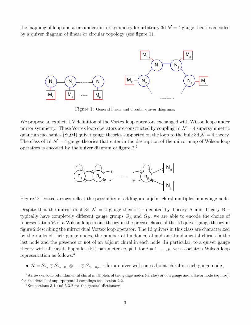
the mapping of loop operators under mirror symmetry for arbitrary 3d N = 4 gauge theories encoded

by a quiver diagram of linear or circular topology (see figure 1).

N1

M1

N2

NP

M2 M

P

N1

M1

N2

M2

MP N

3NP

M3

Figure 1: General linear and circular quiver diagrams.

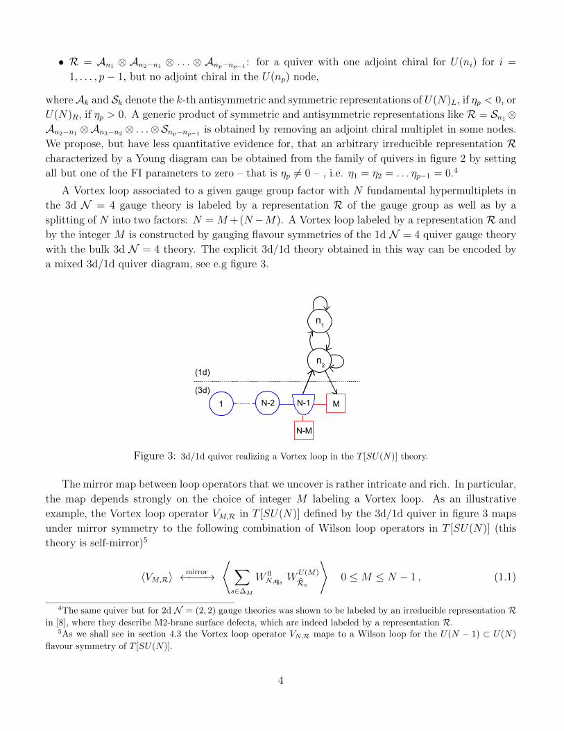
We propose an explicit UV definition of the Vortex loop operators exchanged with Wilson loops under

mirror symmetry. These Vortex loop operators are constructed by coupling 1dN = 4 supersymmetric

quantum mechanics (SQM) quiver gauge theories supported on the loop to the bulk 3d N = 4 theory.

The class of 1d N = 4 gauge theories that enter in the description of the mirror map of Wilson loop

operators is encoded by the quiver diagram of figure 2.2

n1

n2 n

P

NR

NL

Figure 2: Dotted arrows reflect the possibility of adding an adjoint chiral multiplet in a gauge node.

Despite that the mirror dual 3d N = 4 gauge theories – denoted by Theory A and Theory B –

typically have completely different gauge groups GA and GB, we are able to encode the choice of

representation R of a Wilson loop in one theory in the precise choice of the 1d quiver gauge theory in

figure 2 describing the mirror dual Vortex loop operator. The 1d quivers in this class are characterized

by the ranks of their gauge nodes, the number of fundamental and anti-fundamental chirals in the

last node and the presence or not of an adjoint chiral in each node. In particular, to a quiver gauge

theory with all Fayet-Iliopoulos (FI) parameters ηi 6= 0, for i = 1, . . . , p, we associate a Wilson loop

representation as follows:3

• R = Sn1 ⊗ Sn2−n1 ⊗ . . .⊗ Snp−np−1 : for a quiver with one adjoint chiral in each gauge node ,

2Arrows encode bifundamental chiral multiplets of two gauge nodes (circles) or of a gauge and a flavor node (square).

For the details of superpotential couplings see section 2.2.3See sections 3.1 and 5.3.2 for the general dictionary.

3

• R = An1 ⊗ An2−n1 ⊗ . . . ⊗ Anp−np−1 : for a quiver with one adjoint chiral for U(ni) for i =

1, . . . , p− 1, but no adjoint chiral in the U(np) node,

whereAk and Sk denote the k-th antisymmetric and symmetric representations of U(N)L, if ηp < 0, or

U(N)R, if ηp > 0. A generic product of symmetric and antisymmetric representations like R = Sn1⊗An2−n1 ⊗An3−n2 ⊗ . . .⊗Snp−np−1 is obtained by removing an adjoint chiral multiplet in some nodes.

We propose, but have less quantitative evidence for, that an arbitrary irreducible representation Rcharacterized by a Young diagram can be obtained from the family of quivers in figure 2 by setting

all but one of the FI parameters to zero – that is ηp 6= 0 – , i.e. η1 = η2 = . . . ηp−1 = 0.4

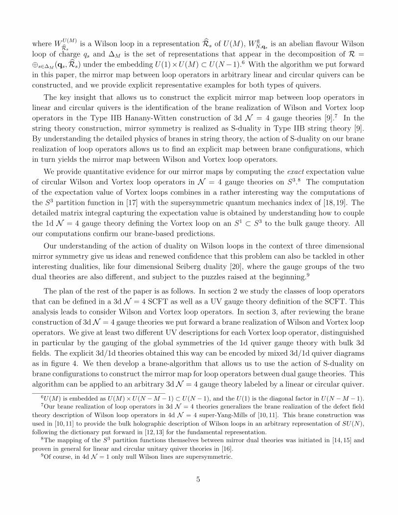
A Vortex loop associated to a given gauge group factor with N fundamental hypermultiplets in

the 3d N = 4 gauge theory is labeled by a representation R of the gauge group as well as by a

splitting of N into two factors: N = M+(N−M). A Vortex loop labeled by a representation R and

by the integer M is constructed by gauging flavour symmetries of the 1d N = 4 quiver gauge theory

with the bulk 3d N = 4 theory. The explicit 3d/1d theory obtained in this way can be encoded by

a mixed 3d/1d quiver diagram, see e.g figure 3.

N-M

(1d)

(3d)

MN-1N-21

n1

n2

Figure 3: 3d/1d quiver realizing a Vortex loop in the T [SU(N)] theory.

The mirror map between loop operators that we uncover is rather intricate and rich. In particular,

the map depends strongly on the choice of integer M labeling a Vortex loop. As an illustrative

example, the Vortex loop operator VM,R in T [SU(N)] defined by the 3d/1d quiver in figure 3 maps

under mirror symmetry to the following combination of Wilson loop operators in T [SU(N)] (this

theory is self-mirror)5

〈VM,R〉mirror←−−−→

⟨∑s∈∆M

W flN,qs W

U(M)

Rs

⟩0 ≤M ≤ N − 1 , (1.1)

4The same quiver but for 2d N = (2, 2) gauge theories was shown to be labeled by an irreducible representation Rin [8], where they describe M2-brane surface defects, which are indeed labeled by a representation R.

5As we shall see in section 4.3 the Vortex loop operator VN,R maps to a Wilson loop for the U(N − 1) ⊂ U(N)

flavour symmetry of T [SU(N)].

4

where WU(M)

Rsis a Wilson loop in a representation Rs of U(M), W fl

N,qsis an abelian flavour Wilson

loop of charge qs and ∆M is the set of representations that appear in the decomposition of R =

⊕s∈∆M(qs, Rs) under the embedding U(1)×U(M) ⊂ U(N−1).6 With the algorithm we put forward

in this paper, the mirror map between loop operators in arbitrary linear and circular quivers can be

constructed, and we provide explicit representative examples for both types of quivers.

The key insight that allows us to construct the explicit mirror map between loop operators in

linear and circular quivers is the identification of the brane realization of Wilson and Vortex loop

operators in the Type IIB Hanany-Witten construction of 3d N = 4 gauge theories [9].7 In the

string theory construction, mirror symmetry is realized as S-duality in Type IIB string theory [9].

By understanding the detailed physics of branes in string theory, the action of S-duality on our brane

realization of loop operators allows us to find an explicit map between brane configurations, which

in turn yields the mirror map between Wilson and Vortex loop operators.

We provide quantitative evidence for our mirror maps by computing the exact expectation value

of circular Wilson and Vortex loop operators in N = 4 gauge theories on S3.8 The computation

of the expectation value of Vortex loops combines in a rather interesting way the computations of

the S3 partition function in [17] with the supersymmetric quantum mechanics index of [18,19]. The

detailed matrix integral capturing the expectation value is obtained by understanding how to couple

the 1d N = 4 gauge theory defining the Vortex loop on an S1 ⊂ S3 to the bulk gauge theory. All

our computations confirm our brane-based predictions.

Our understanding of the action of duality on Wilson loops in the context of three dimensional

mirror symmetry give us ideas and renewed confidence that this problem can also be tackled in other

interesting dualities, like four dimensional Seiberg duality [20], where the gauge groups of the two

dual theories are also different, and subject to the puzzles raised at the beginning.9

The plan of the rest of the paper is as follows. In section 2 we study the classes of loop operators

that can be defined in a 3d N = 4 SCFT as well as a UV gauge theory definition of the SCFT. This

analysis leads to consider Wilson and Vortex loop operators. In section 3, after reviewing the brane

construction of 3dN = 4 gauge theories we put forward a brane realization of Wilson and Vortex loop

operators. We give at least two different UV descriptions for each Vortex loop operator, distinguished

in particular by the gauging of the global symmetries of the 1d quiver gauge theory with bulk 3d

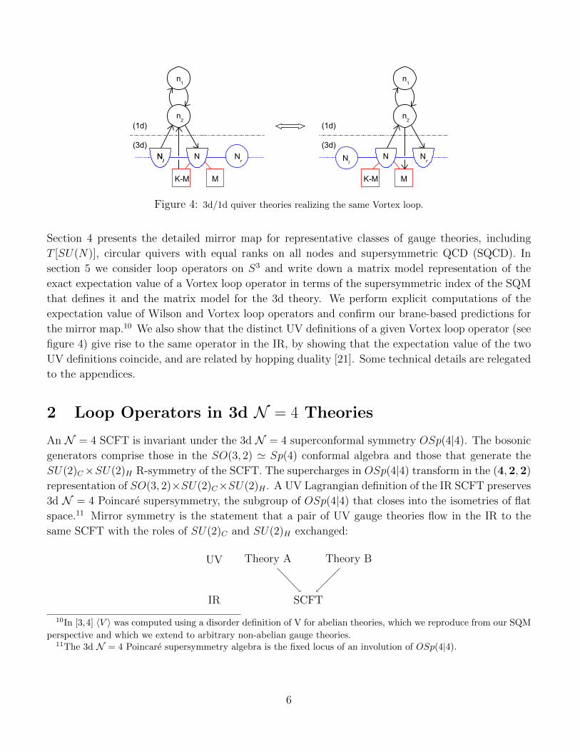
fields. The explicit 3d/1d theories obtained this way can be encoded by mixed 3d/1d quiver diagrams

as in figure 4. We then develop a brane-algorithm that allows us to use the action of S-duality on

brane configurations to construct the mirror map for loop operators between dual gauge theories. This

algorithm can be applied to an arbitrary 3d N = 4 gauge theory labeled by a linear or circular quiver.

6U(M) is embedded as U(M)×U(N −M − 1) ⊂ U(N − 1), and the U(1) is the diagonal factor in U(N −M − 1).7Our brane realization of loop operators in 3d N = 4 theories generalizes the brane realization of the defect field

theory description of Wilson loop operators in 4d N = 4 super-Yang-Mills of [10, 11]. This brane construction was

used in [10, 11] to provide the bulk holographic description of Wilson loops in an arbitrary representation of SU(N),

following the dictionary put forward in [12,13] for the fundamental representation.8The mapping of the S3 partition functions themselves between mirror dual theories was initiated in [14, 15] and

proven in general for linear and circular unitary quiver theories in [16].9Of course, in 4d N = 1 only null Wilson lines are supersymmetric.

5

K-M

(1d)

(3d)

M

NNl

Nr

K-M

(1d)

(3d)

M

NNl

Nr

Nl

n1

n2

n1

n2

Figure 4: 3d/1d quiver theories realizing the same Vortex loop.

Section 4 presents the detailed mirror map for representative classes of gauge theories, including

T [SU(N)], circular quivers with equal ranks on all nodes and supersymmetric QCD (SQCD). In

section 5 we consider loop operators on S3 and write down a matrix model representation of the

exact expectation value of a Vortex loop operator in terms of the supersymmetric index of the SQM

that defines it and the matrix model for the 3d theory. We perform explicit computations of the

expectation value of Wilson and Vortex loop operators and confirm our brane-based predictions for

the mirror map.10 We also show that the distinct UV definitions of a given Vortex loop operator (see

figure 4) give rise to the same operator in the IR, by showing that the expectation value of the two

UV definitions coincide, and are related by hopping duality [21]. Some technical details are relegated

to the appendices.

2 Loop Operators in 3d N = 4 Theories

An N = 4 SCFT is invariant under the 3d N = 4 superconformal symmetry OSp(4|4). The bosonic

generators comprise those in the SO(3, 2) ' Sp(4) conformal algebra and those that generate the

SU(2)C×SU(2)H R-symmetry of the SCFT. The supercharges in OSp(4|4) transform in the (4,2,2)

representation of SO(3, 2)×SU(2)C×SU(2)H . A UV Lagrangian definition of the IR SCFT preserves

3d N = 4 Poincare supersymmetry, the subgroup of OSp(4|4) that closes into the isometries of flat

space.11 Mirror symmetry is the statement that a pair of UV gauge theories flow in the IR to the

same SCFT with the roles of SU(2)C and SU(2)H exchanged:

UV Theory A Theory B

IR SCFT

10In [3,4] 〈V 〉 was computed using a disorder definition of V for abelian theories, which we reproduce from our SQM

perspective and which we extend to arbitrary non-abelian gauge theories.11The 3d N = 4 Poincare supersymmetry algebra is the fixed locus of an involution of OSp(4|4).

6

An N = 4 SCFT admits half-supersymmetric line operators/defects supported on a straight

line in flat space.12 There are two physically inequivalent classes of superconformal line defects

in an N = 4 SCFT, distinguished by their preserved symmetries. Superconformal line defects

supported on a time-like line are invariant either under an U(1, 1|2)W or U(1, 1|2)V subalgebra

of OSp(4|4).13 Let us exhibit this more explicitly.14 First, a straight time-like line in flat space

preserves SU(1, 1) × U(1)⊥ ⊂ SO(3, 2). The U(1, 1|2)W subalgebra is embedded as follows. Under

the embedding of SU(1, 1)×SU(2)H×U(1)⊥×U(1)C in SO(3, 2)×SU(2)C×SU(2)H , the supercharges

generating OSp(4|4) decompose as (2,2)++ ⊕ (2,2)+− ⊕ (2,2)−+ ⊕ (2,2)−−. The supercharges in

U(1, 1|2)W are (2,2)++⊕ (2,2)−−.15 For U(1, 1|2)V the analysis is identical with the roles of SU(2)Cand SU(2)H exchanged. A defect preserving U(1, 1|2)W is invariant under U(1)C × SU(2)H while a

defect preserving U(1, 1|2)V is invariant under SU(2)C × U(1)H . The main goal of this paper is to

give the UV description of these two classes of line operators/defects and to identity how the UV

descriptions are mapped under mirror symmetry.

A line defect in a UV Lagrangian description of a SCFT can be made invariant under four of the

supercharges in the 3d N = 4 Poincare supersymmetry algebra of the UV theory. The 3d N = 4

Poincare supercharges transform in the (2,2) representation of the SU(2)C × SU(2)H R-symmetry

of the UV theory and obey

{QαAA′ , QβBB′} = (γµC)αβ PµεABεA′B′ . (2.1)

We take the SO(2, 1) γ-matrices (γ0, γ1, γ2) = (iτ3, τ1, τ2), where τa are the Pauli matrices. The

charge conjugation matrix is C = τ2. In Lorentzian signature and in this basis the reality condition

on the supercharges is Q†αAA′ = (τ1) βα εABεA

′B′QβBB′ .

There are two inequivalent 1d N = 4 supersymmetric quantum mechanics (SQM) subalgebras

of the 3d N = 4 Poincare superalgebra of a UV theory that can be preserved by a line defect. We

denote them by SQMW and SQMV . SQMW preserves U(1)C × SU(2)H and the supercharges Q11A′

and Q22B′ , which anticommute to the generator of translations H along the defect

{Q11A′ , Q22B′} = εA′B′H . (2.2)

SQMV preserves SU(2)V × U(1)H and the preserved supercharges Q1A1 and Q2B2 obey

{Q1A1, Q2B2} = εABH . (2.3)

A 1d N = 4 SQM supersymmetry algebra can be brought to the canonical form

{Q+Q+} = H [J+, Q+] = −Q+ [J+, Q+] = Q+

{Q−, Q−} = H [J−, Q−] = −Q− [J−, Q−] = Q− (2.4)

12 Operators supported on curves obtained by acting on a straight line by broken conformal generators are also

half-supersymmetric and preserve an isomorphic symmetry algebra. Under a broken conformal symmetry a time-like

line becomes a rectangular time-like hyperbola, a space-like line becomes a space-like hyperbola (which includes a

circle) and a null line remains a null line.13U(1, 1|2)W and U(1, 1|2)V are the fixed locus of an involution of OSp(4|4)14A very similar analysis holds for a space-like line defect. For a null line defect, which we do not consider in this

paper, the preserved symmetries are larger.15The other choice (2,2)+− ⊕ (2,2)−+ corresponds to the same line defect but with opposite orientation.

7

with all other (anti)-commutators vanishing. For both SQMW and SQMV algebras Q+ = Q111 and

Q+ = Q222 = Q†111. For SQMW Q− = Q112, Q− = −Q221 = Q†112 while for SQMV Q− = Q212,

Q− = −Q121 = Q†212. The embedding of the SQMW and SQMV algebras in the 3d N = 4 Poincare

superalgebra has a U(1) commutant: RC − J12 for SQMW and RH − J12 for SQMV , where J12 is

the U(1)⊥ rotation generator transverse to the defect and RC and RH are the Cartan generators

of SU(2)C and SU(2)H respectively.16 Therefore, up to shifts by the “flavour” symmetry RC − J12

for SQMW and by RH − J12 for SQMV the Cartan R-symmetry generators can be taken to be

J+ = −RC −RH and J− = RH −RC .

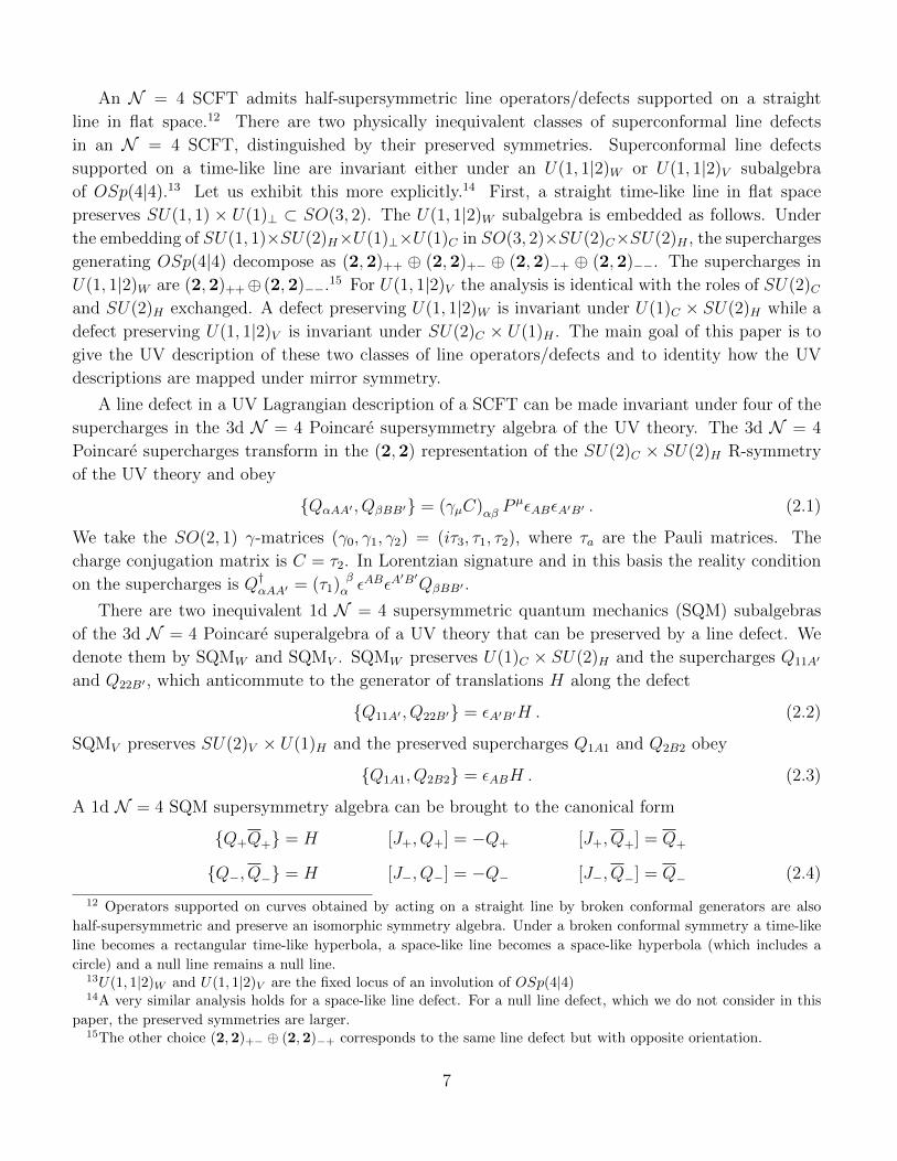
In summary, in a 3d N = 4 gauge theory there are two classes of line defects that can defined,

one preserving SQMW and the other SQMV . These line defects flow in the IR to superconformal line

defects preserving U(1, 1|2)W and U(1, 1|2)V respectively. Our analysis can be succinctly summarized

by the following diagram:

UV 3d N = 4 Poincare SQMW SQMV

IR OSp(4|4)

and

andU(1, 1|2)W U(1, 1|2)V

RG

defect

RG RG

defect

Both classes of UV supersymmetric line defects in a UV 3d N = 4 theory can be realized by

coupling different 1d N = 4 SQM theories with four supercharges to the bulk 3d N = 4 theory.

A canonical way of coupling a 1d N = 4 SQM theory to a 3d N = 4 theory is by gauging flavour

symmetries of the SQM theory with 3d N = 4 vector multiplets. The gauging of the defect flavour

symmetries with bulk vector multiplets is made supersymmetric by embedding the defect vector

multiplet of the supersymmetry algebra preserved by the defect into the bulk 3d N = 4 vector

multiplet at the position of the line defect. The embedding is found by identifying which combination

of fields in the higher dimensional vector multiplet transform as the fields of the defect vector multiplet

under the supersymmetry preserved by the defect. Replacing the defect vector multiplet fields in the

gauged 1d N = 4 SQM theory with the proper combination of bulk vector multiplet fields ensures

that the coupling of 1d fields to 3d fields is supersymmetric under the supersymmetry of the defect 1d

N = 4 SQM theory. Superpotential couplings between defect and bulk matter multiplets may also be

added when defect matter multiplets can be embedded in bulk hypermultiplets. Such couplings gauge

defect flavour symmetries with bulk flavour or gauge symmetries, depending on which symmetries of

the bulk matter multiplet are global and which are gauged.

We consider UV line defects invariant under SQMW and SQMV obtained by gauging global

symmetries of 1d N = 4 SQM theories obtained by dimensional reduction of 2d N = (0, 4) and 2d

N = (2, 2) theories with 3d N = 4 vector multiplets:

• SQMW : 2d N = (0, 4)→ 1d N = 4 SQM

16RC−J12 and RH−J12 is also the commutant of U(1, 1|2)W and U(1, 1|2)V in OSp(4|4). They appear respectively

in the anticommutator of the U(1, 1|2)W and U(1, 1|2)V supercharges preserved by the corresponding defect.

8

• SQMV : 2d N = (2, 2)→ 1d N = 4 SQM

Superpotential couplings between defect and bulk fields also play an important role in the construc-

tion of defects.

2.1 Wilson Loop Operators

A line defect in a UV 3d N = 4 gauge theory invariant under SQMW is the Wilson line operator,

which is labeled by a representation R of the gauge group. It is given by

WR = TrRP exp

∮i(Aµx

µ +√−x2 σ

)dτ , (2.5)

where σ ≡ σ3 is the scalar field in the N = 2 vector multiplet inside the N = 4 vector multiplet.

This operator manifestly breaks the SU(2)C symmetry acting on the three scalars ~σ = (σ1, σ2, σ3) in

the N = 4 vector multiplet down to U(1)C ,17 while preserving SU(2)H . If the operator is supported

on a straight line18, it preserves the 1d N = 4 SQM subalgebra SQMW of the 3d N = 4 theory and

its U(1)C×SU(2)H R-symmetry. In the IR a Wilson line operator flows to a conformal line operator

in the SCFT preserving U(1, 1|2)W .

The supersymmetric Wilson line operator (2.5) can be realized by coupling a 1d N = 4 SQM

theory living on the line with the bulk 3d N = 4 gauge theory. This coupling preserves the SQMW

supersymmetry algebra. The defect 1d N = 4 SQM that represents a Wilson loop operator is the

theory of a 1d N = 4 fermi multiplet, obtained by dimensional reduction of the 2d N = (0, 4)

fermi multiplet, which on-shell consists of a complex chiral fermion. The flavour symmetry of a 1d

N = (0, 4) fermi multiplet can be gauged preserving supersymmetry with a 1d N = (0, 4) vector

multiplet. The fields of the 1d N = (0, 4) vector multiplet that couple to the fermi multiplet can be

embedded in the 3d N = 4 vector multiplet as follows19

a0 = A0 (2.6)

σ1d = σ . (2.7)

This embedding makes manifest that the coupling of the fermi multiplet to the bulk N = 4 vector

multiplet preserves U(1)C × SU(2)H R-symmetry and the SQMW algebra.20

The 1dN = 4 SQM fermi multiplet on the defect can be integrated out exactly and it results in the

insertion of a supersymmetric Wilson loop (2.5) in the bulk 3d N = 4 theory. This representation

17The choice of scalar determines an embedding of U(1)C in SU(2)C .18When the scalar couples to the loop with constant charge a circular Wilson loop is not supersymmetric in the UV

theory. See, however, discussion at the end of this subsection and of circular Wilson loops on S3 in section 5.1.19The Fermi multiplet couples only to a subset of fields in the N = (0, 4) vector multiplet, and those do admit an

embedding into the 3d N = 4 vector multiplet. This observation can be applied to the study of supersymmetric surface

operators in 4d N = 2, which can preserve either 2d N = (2, 2) or N = (0, 4) supersymmetry. We can construct a

surface operator by gauging a N = (0, 4) fermi multiplet with a bulk vector multiplet. These surface operators were

studied in the context of N = 4 SYM in [22].20The purely 1d N = 4 theory of a gauged fermi multiplet is invariant under SO(4) R-symmetry. The coupling of

the fermi multiplet with the bulk through the embedding (2.7) breaks the R-symmetry down to U(1)C × SU(2)H .

9

of a supersymmetric Wilson loop in 4d N = 4 super-Yang-Mills (SYM) as a coupling of a fermi

multiplet with bulk fields appeared in [10, 11], where the defect field theory was derived from brane

intersections in string theory. Inspired by [10, 11], a brane realization of Wilson loop defects in 3d

N = 4 gauge theories will play a prominent role in section 3, where we will use S-duality of Type

IIB string theory to identify the mirror of Wilson loop operators.

As an aside, 1/4-supersymmetric Wilson loops supported on an arbitrary curve γ in R3 can be

defined mimicking the construction in [23] of 1/16-supersymmetric Wilson loops in 4d N = 4 SYM.

This requires tuning the coupling of the loop to the three scalars in the vector multiplet. Explicitly,

1/4-supersymmetric Wilson loops are given by

TrRP exp

∮γ

i (Aµ + iσµ) xµdτ (2.8)

and preserve two supercharges: QHA′ ≡ QαAA′ε

αA. These Wilson loop operators are in the cohomology

of the supercharges QHA′ of the Rozansky-Witten twisted theory [24]21 obtained by twisting spatial

rotations with SU(2)C . Half-supersymmetric Higgs branch operators are also in the cohomology of

this twisted theory.

2.2 Vortex Loop Operators

A supersymmetric line defect in a UV 3d N = 4 theory preserving SQMV can be constructed by

coupling the bulk theory to a 1d N = 4 SQM theory with SQMV symmetry. For line defects

preserving SQMV , the appropriate 1d N = 4 SQM theories are obtained by dimensionally reducing

4d N = 1 theories (or equivalently 2d N = (2, 2) theories). U(1)H is the R-symmetry already present

in 4d while SU(2)V emerges as an R-symmetry in the dimensional reduction down to 1d. Therefore

the SQMV invariant 1d N = 4 SQM theories we consider are supersymmetric gauge theories based

on the familiar 4d N = 1 vector multiplets and chiral multiplets. The same 4d N = 1 theories

dimensionally reduced to 2d define surface operators [26] in 4d N = 2 gauge theories.

We can construct a supersymmetric line defect in a 3d N = 4 gauge theory by gauging flavour

symmetries of a 1d N = 4 SQMV invariant theory with bulk vector multiplets. The embedding of

the bosonic fields in the 1d vector multiplet (a3, ~σ1d, d), where ~σ1d is a triplet of SU(2)V , in the 3d

N = 4 vector multiplet is (see appendix A)

a0 = A0 (2.9)

~σ1d = ~σ (2.10)

d = D + F12 . (2.11)

This embedding makes manifest that SU(2)V is preserved and that SU(2)H is broken down to U(1)H ,

as it selects one of the auxiliary fields transforming as a triplet of SU(2)H in the 3d N = 4 vector

multiplet, which we have denoted by D.22 The coupled theory preserves the SQMV algebra.

21This is the 3d counterpart of the statement in 4d N = 4 SYM that the 1/16-supersymmetric Wilson loop operators

in [23] are in the cohomology of a supercharge of the Langlands twist [25].22The choice of auxiliary field determines an embedding of U(1)H in SU(2)H .

10

We can gauge defect flavour symmetries either with 3d N = 4 fluctuating vector multiplets or

background vector multiplets. Background vector multiplets for flavour symmetries are associated

to canonical supersymmetric mass deformations in 3d N = 4 and 1d N = 4 theories.23 Gauging 1d

flavour symmetries with background 3d vector multiplets means that 1d and 3d flavour symmetries

are identified. 1d N = 4 and 3d N = 4 flavour symmetries are identified by SQMV -preserving defect

cubic superpotential couplings between defect chiral multiplets and bulk hypermultiplets24

W = qiIqIaQ

ai , (2.12)

where the index I is a 1d gauge index. The indices i, a are simultaneously indices for 1d flavour

symmetries and indices for either 3d flavour or gauge symmetries. When a (or i) is a 3d flavour index,

the superpotential breaks the (otherwise independent) flavour symmetries acting on chiral multiplets

qa (or qi) and hypermultiplets Qai to the diagonal flavour symmetry group.25 The background 3d

N = 4 vector multiplet gives the same mass to the 1d chiral multiplets and 3d hypermultiplets that

are acted on by the preserved diagonal flavour symmetry group.

The 1d N = 4 gauge theories that appear in the construction of the defects dual to Wilson loops

can be encoded in a standard quiver diagram shown in figure 2.26

An adjoint chiral multiplet may be added to any U(ni) gauge group factor, an option which we denote

by a dashed line. Each adjoint chiral multiplet is coupled to the neighbouring bifundamental chiral

multiplets through a cubic superpotential, while nodes without an adjoint chiral multiplet have an

associated quartic superpotential coupling the corresponding bifundamental chiral multiplets.

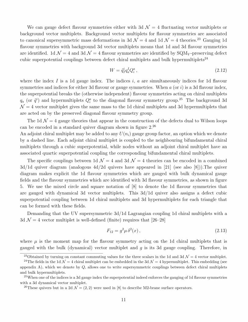
The specific couplings between 1d N = 4 and 3d N = 4 theories can be encoded in a combined

3d/1d quiver diagram (analogous 4d/2d quivers have appeared in [21] (see also [8])).The quiver

diagram makes explicit the 1d flavour symmetries which are gauged with bulk dynamical gauge

fields and the flavour symmetries which are identified with 3d flavour symmetries, as shown in figure

5. We use the mixed circle and square notation of [8] to denote the 1d flavour symmetries that

are gauged with dynamical 3d vector multiplets. This 3d/1d quiver also assigns a defect cubic

superpotential coupling between 1d chiral multiplets and 3d hypermultiplets for each triangle that

can be formed with these fields.

Demanding that the UV supersymmetric 3d/1d Lagrangian coupling 1d chiral multiplets with a

3d N = 4 vector multiplet is well-defined (finite) requires that [26–28]

F12 = g2µ δ2(x) , (2.13)

where µ is the moment map for the flavour symmetry acting on the 1d chiral multiplets that is

gauged with the bulk (dynamical) vector multiplet and g is its 3d gauge coupling. Therefore, in

23Obtained by turning on constant commuting values for the three scalars in the 1d and 3d N = 4 vector multiplet.24The fields in the 1d N = 4 chiral multiplet can be embedded in the 3d N = 4 hypermultiplet. This embedding (see

appendix A), which we denote by Q, allows one to write supersymmetric couplings between defect chiral multiplets

and bulk hypermultiplets.25When one of the indices is a 3d gauge index the superpotential indeed enforces the gauging of 1d flavour symmetries

with a 3d dynamical vector multiplet.26These quivers but in a 2d N = (2, 2) were used in [8] to describe M2-brane surface operators.

11

(1d) (3d)

n1

n2 n

P

N1

N2

M1

M2

Figure 5: 1d quiver theory coupled to 3d quiver theory by gauging 1d flavor symmetries with 3d vector mutiplets

(dynamical or weakly gauged).

the semiclassical UV description, defect fields induce a singular Vortex field configuration on the 3d

gauge fields. This justifies our use of the subscript V to describe this class of line defects, which we

refer as Vortex line defects/operators. These UV Vortex line defects flow in the IR to conformal line

operators in the SCFT preserving U(1, 1|2)V .

As another aside, we note that just as a 1/4-supersymmetric Wilson loop supported on an ar-

bitrary curve γ in R3 have been constructed in (2.8), it should be possible to construct a 1/4-

supersymmetric Vortex loop on an arbitrary curve in R3 by suitably adjusting the coupling of the

1d N = 4 SQM to the bulk 3d N = 4 theory. Such a Vortex loop would preserve two supercharges:

QCA ≡ QαAA′ε

αA′ . These Vortex loop operators are in the cohomology of the supercharges QCA of

the other version of the Rozansky-Witten twisted theory, obtained by twisting spatial rotations with

SU(2)H . Half-supersymmetric Coulomb branch operators, that is monopole operators, are also in

the cohomology of this twisted theory.

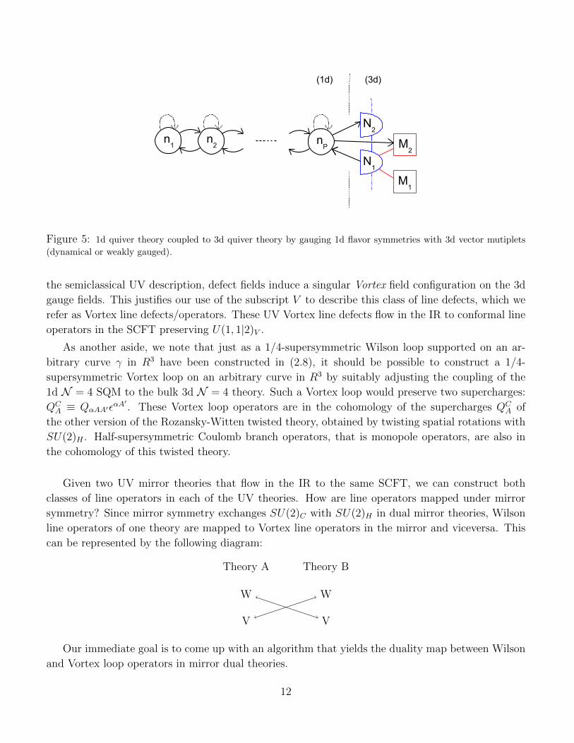
Given two UV mirror theories that flow in the IR to the same SCFT, we can construct both

classes of line operators in each of the UV theories. How are line operators mapped under mirror

symmetry? Since mirror symmetry exchanges SU(2)C with SU(2)H in dual mirror theories, Wilson

line operators of one theory are mapped to Vortex line operators in the mirror and viceversa. This

can be represented by the following diagram:

Theory A

W

V

Theory B

W

V

Our immediate goal is to come up with an algorithm that yields the duality map between Wilson

and Vortex loop operators in mirror dual theories.

12

3 Brane Realization Of Loop Operators and Mirror Map

In this section we first briefly introduce the Type IIB string theory realization of 3d N = 4 gauge

theories of [9] and recall how mirror symmetry gets realized as S-duality in string theory. Central

to the main goal of this paper is the brane realization of both types of line defects discussed in the

previous section that we put forward in this section. We then devise an explicit algorithm using

branes in string theory to identify the map between loop operators in mirror dual theories.

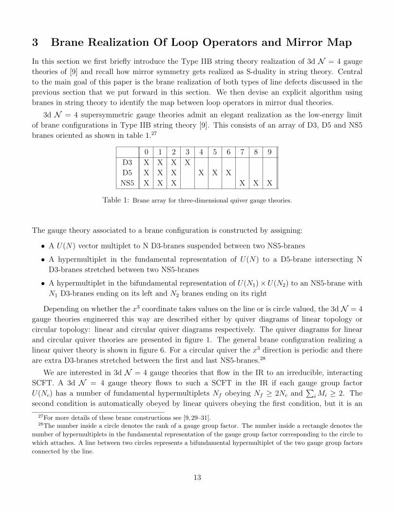
3d N = 4 supersymmetric gauge theories admit an elegant realization as the low-energy limit

of brane configurations in Type IIB string theory [9]. This consists of an array of D3, D5 and NS5

branes oriented as shown in table 1.27

0 1 2 3 4 5 6 7 8 9

D3 X X X X

D5 X X X X X X

NS5 X X X X X X

Table 1: Brane array for three-dimensional quiver gauge theories.

The gauge theory associated to a brane configuration is constructed by assigning:

• A U(N) vector multiplet to N D3-branes suspended between two NS5-branes

• A hypermultiplet in the fundamental representation of U(N) to a D5-brane intersecting N

D3-branes stretched between two NS5-branes

• A hypermultiplet in the bifundamental representation of U(N1)×U(N2) to an NS5-brane with

N1 D3-branes ending on its left and N2 branes ending on its right

Depending on whether the x3 coordinate takes values on the line or is circle valued, the 3d N = 4

gauge theories engineered this way are described either by quiver diagrams of linear topology or

circular topology: linear and circular quiver diagrams respectively. The quiver diagrams for linear

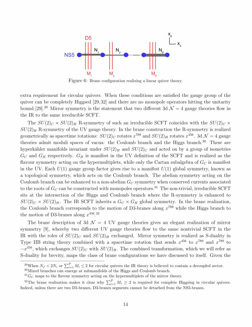
and circular quiver theories are presented in figure 1. The general brane configuration realizing a

linear quiver theory is shown in figure 6. For a circular quiver the x3 direction is periodic and there

are extra D3-branes stretched between the first and last NS5-branes.28

We are interested in 3d N = 4 gauge theories that flow in the IR to an irreducible, interacting

SCFT. A 3d N = 4 gauge theory flows to such a SCFT in the IR if each gauge group factor

U(Nc) has a number of fundamental hypermultiplets Nf obeying Nf ≥ 2Nc and∑

iMi ≥ 2. The

second condition is automatically obeyed by linear quivers obeying the first condition, but it is an

27For more details of these brane constructions see [9, 29–31].28The number inside a circle denotes the rank of a gauge group factor. The number inside a rectangle denotes the

number of hypermultiplets in the fundamental representation of the gauge group factor corresponding to the circle to

which attaches. A line between two circles represents a bifundamental hypermultiplet of the two gauge group factors

connected by the line.

13

NS5

D5 x

6

x3

N1

M1

N2

M2

NP

MP

Figure 6: Brane configuration realizing a linear quiver theory.

extra requirement for circular quivers. When these conditions are satisfied the gauge group of the

quiver can be completely Higgsed [29,32] and there are no monopole operators hitting the unitarity

bound [29].29 Mirror symmetry is the statement that two different 3d N = 4 gauge theories flow in

the IR to the same irreducible SCFT.

The SU(2)C × SU(2)H R-symmetry of such an irreducible SCFT coincides with the SU(2)C ×SU(2)H R-symmetry of the UV gauge theory. In the brane construction the R-symmetry is realized

geometrically as spacetime rotations: SU(2)C rotates x789 and SU(2)H rotates x456. 3d N = 4 gauge

theories admit moduli spaces of vacua: the Coulomb branch and the Higgs branch.30 These are

hyperkahler manifolds invariant under SU(2)H and SU(2)C and acted on by a group of isometries

GC and GH respectively. GH is manifest in the UV definition of the SCFT and is realized as the

flavour symmetry acting on the hypermultiplets, while only the Cartan subalgebra of GC is manifest

in the UV. Each U(1) gauge group factor gives rise to a manifest U(1) global symmetry, known as

a topological symmetry, which acts on the Coulomb branch. The abelian symmetry acting on the

Coulomb branch can be enhanced to a non-abelian GC symmetry when conserved currents associated

to the roots of GC can be constructed with monopoles operators.31 The non-trivial, irreducible SCFT

sits at the intersection of the Higgs and Coulomb branch where the R-symmetry is enhanced to

SU(2)C × SU(2)H . The IR SCFT inherits a GC × GH global symmetry. In the brane realization,

the Coulomb branch corresponds to the motion of D3-branes along x789 while the Higgs branch to

the motion of D3-branes along x456.32

The brane description of 3d N = 4 UV gauge theories gives an elegant realization of mirror

symmetry [9], whereby two different UV gauge theories flow to the same nontrivial SCFT in the

IR with the roles of SU(2)C and SU(2)H exchanged. Mirror symmetry is realized as S-duality in

Type IIB string theory combined with a spacetime rotation that sends x456 to x789 and x789 to

−x456, which exchanges SU(2)C with SU(2)H . The combined transformation, which we will refer as

S-duality for brevity, maps the class of brane configurations we have discussed to itself. Given the

29When Nf < 2Nc or∑Pi=1Mi ≤ 2 for circular quivers the IR theory is believed to contain a decoupled sector.

30Mixed branches can emerge at submanifolds of the Higgs and Coulomb branch.31GC maps to the flavour symmetry acting on the hypermultiplets of the mirror theory.32The brane realization makes it clear why

∑Pi=1Mi ≥ 2 is required for complete Higgsing in circular quivers.

Indeed, unless there are two D5-branes, D3-branes segments cannot be detached from the NS5-branes.

14

brane configuration corresponding to a UV 3d N = 4 gauge theory, the mirror dual gauge theory is

obtained by analyzing the low energy dynamics of the S-dual brane configuration. The mirror UV

gauge theory can be read by rearranging the branes along the x3 direction, possibly using Hanany-

Witten moves [9] involving the creation/annihilation of a D3-brane when an NS5-brane crosses a

D5-brane, to bring the S-dual brane configuration to a configuration where the low energy gauge

theory can be read using the rules summarized above. This transformation preserves the type of

quiver, and thus the mirror of a linear quiver is a linear quiver and the mirror of a circular quiver is

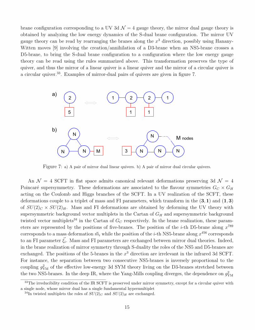
a circular quiver.33. Examples of mirror-dual pairs of quivers are given in figure 7.

N

3 N NNM

M nodes

N N

N

5

2 1

1

2

1

2 1a)

b)

Figure 7: a) A pair of mirror dual linear quivers. b) A pair of mirror dual circular quivers.

An N = 4 SCFT in flat space admits canonical relevant deformations preserving 3d N = 4

Poincare supersymmetry. These deformations are associated to the flavour symmetries GC × GH

acting on the Coulomb and Higgs branches of the SCFT. In a UV realization of the SCFT, these

deformations couple to a triplet of mass and FI parameters, which transform in the (3,1) and (1,3)

of SU(2)C × SU(2)H . Mass and FI deformations are obtained by deforming the UV theory with

supersymmetric background vector multiplets in the Cartan of GH and supersymmetric background

twisted vector multiplets34 in the Cartan of GC respectively. In the brane realization, these param-

eters are represented by the positions of five-branes. The position of the i-th D5-brane along x789

corresponds to a mass deformation ~mi while the position of the i-th NS5-brane along x456 corresponds

to an FI parameter ~ξi. Mass and FI parameters are exchanged between mirror dual theories. Indeed,

in the brane realization of mirror symmetry through S-duality the roles of the NS5 and D5-branes are

exchanged. The positions of the 5-branes in the x3 direction are irrelevant in the infrared 3d SCFT.

For instance, the separation between two consecutive NS5-branes is inversely proportional to the

coupling g2YM of the effective low-energy 3d SYM theory living on the D3-branes stretched between

the two NS5-branes. In the deep IR, where the Yang-Mills coupling diverges, the dependence on g2YM

33The irreducibility condition of the IR SCFT is preserved under mirror symmetry, except for a circular quiver with

a single node, whose mirror dual has a single fundamental hypermultiplet34In twisted multiplets the roles of SU(2)C and SU(2)H are exchanged.

15

disappears.

Linear quivers that flow to irreducible, interacting SCFT’s can be labeled by two partitions

of N – ρ and ρ – and are denoted by T ρρ [SU(N)] [29]. Circular quivers flowing to interacting

SCFT’s are labeled also by two partitions of N and a positive integer L, and can be denoted by

Cρρ [SU(N), L] [31].35 Under mirror symmetry

T ρρ [SU(N)]⇐⇒ T ρρ [SU(N)] (3.1)

and

Cρρ [SU(N), L]⇐⇒ C ρ

ρ [SU(N), L] , (3.2)

and the role of the two partitions are exchanged. The Coulomb branch of these theories, and by

mirror symmetry the Higgs branch, describe the moduli space of monopoles in the presence of Dirac

monopole singularities for linear quivers and the moduli space of instantons on a vector bundle over

an ALE space for circular quivers.

In this paper we give a brane realization of both classes of loop operators discussed in section 2

and put forward an algorithm that produces a map between loop operators of mirror dual theories.

3.1 Brane Realization Of Wilson Loop Operators

A key ingredient in our derivation of the mirror map of loop operators is identifying a brane realization

of Wilson loop operators, which are labeled by a representation R of the gauge group. Inserting a

supersymmetric Wilson loop operator in a 3d N = 4 linear or circular quiver gauge theory admits

a simple brane interpretation, obtained by enriching the setup in [9]. The construction we propose

extends to 3d N = 4 gauge theories the realization of Wilson loops by branes in 4d N = 4 SYM

in [10] [11] (see also [33] [34]).

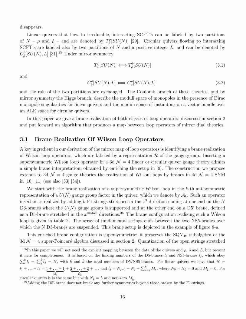
We start with the brane realization of a supersymmetric Wilson loop in the k-th antisymmetric

representation of a U(N) gauge group factor in the quiver, which we denote by Ak. Such an operator

insertion is realized by adding k F1 strings stretched in the x9 direction ending at one end on the N

D3-branes where the U(N) gauge group is supported and at the other end on a D5’ brane, defined

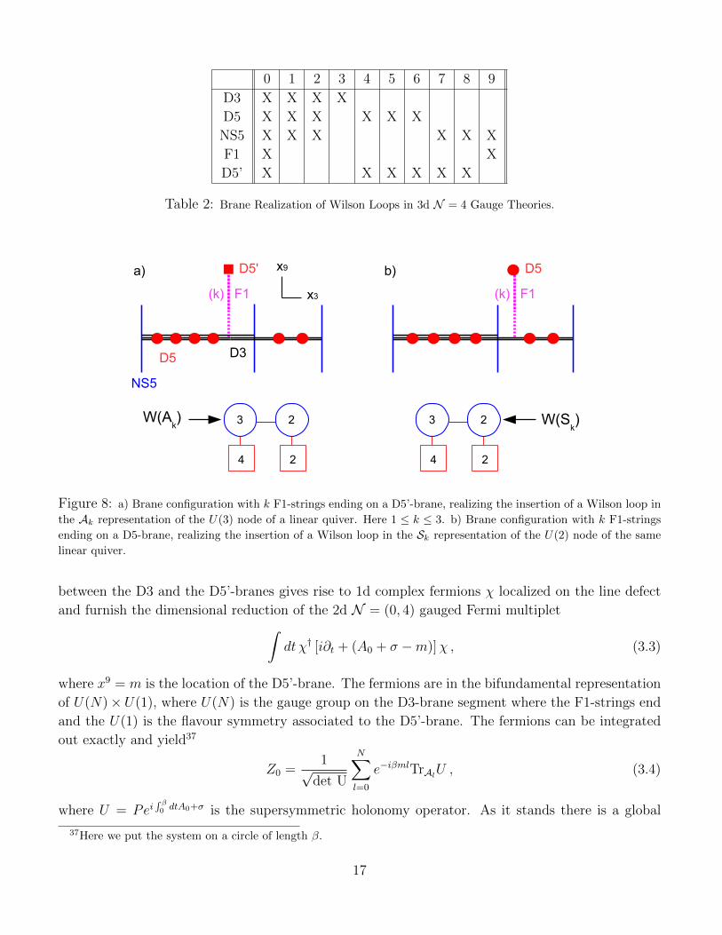
as a D5-brane stretched in the x045678 directions.36 The brane configuration realizing such a Wilson

loop is given in table 2. The array of fundamental strings ends between the two NS5-branes over

which the N D3-branes are suspended. This brane setup is depicted in the example of figure 8-a.

This enriched brane configuration is supersymmetric: it preserves the SQMW subalgebra of the

3d N = 4 super-Poincare algebra discussed in section 2. Quantization of the open strings stretched

35In this paper we will not need the explicit mapping between the data of the quivers and ρ, ρ and L, but present

it here for completeness. It is based on the linking numbers of the D5-branes li and NS5-branes lj , which obey∑ki li =

∑kj lj = N , with k and k the total numbers of D5/NS5-branes. For linear quivers we have that N =

l1 + . . .+ lk = 1 + . . .+ 1︸ ︷︷ ︸M1

+ 2 + . . .+ 2︸ ︷︷ ︸M2

+ . . . and lj = Nj−1 −Nj +∑ks=jMs, where N0 = Nk = 0 and Mk = 0. For

circular quivers it is the same but with Nk = L and non-zero Mk.36Adding the D5’-brane does not break any further symmetries beyond those broken by the F1-strings.

16

0 1 2 3 4 5 6 7 8 9

D3 X X X X

D5 X X X X X X

NS5 X X X X X X

F1 X X

D5’ X X X X X X

Table 2: Brane Realization of Wilson Loops in 3d N = 4 Gauge Theories.

(k)

x9

x3

NS5

D5

a) D5'

2

2

F1

4

3W(Ak)

b) D5

2

2

F1

4

3 W(Sk)

(k)

D3

Figure 8: a) Brane configuration with k F1-strings ending on a D5’-brane, realizing the insertion of a Wilson loop in

the Ak representation of the U(3) node of a linear quiver. Here 1 ≤ k ≤ 3. b) Brane configuration with k F1-strings

ending on a D5-brane, realizing the insertion of a Wilson loop in the Sk representation of the U(2) node of the same

linear quiver.

between the D3 and the D5’-branes gives rise to 1d complex fermions χ localized on the line defect

and furnish the dimensional reduction of the 2d N = (0, 4) gauged Fermi multiplet∫dt χ† [i∂t + (A0 + σ −m)]χ , (3.3)

where x9 = m is the location of the D5’-brane. The fermions are in the bifundamental representation

of U(N)×U(1), where U(N) is the gauge group on the D3-brane segment where the F1-strings end

and the U(1) is the flavour symmetry associated to the D5’-brane. The fermions can be integrated

out exactly and yield37

Z0 =1√

det U

N∑l=0

e−iβmlTrAlU , (3.4)

where U = Pei∫ β0 dtA0+σ is the supersymmetric holonomy operator. As it stands there is a global

37Here we put the system on a circle of length β.

17

anomaly for the U(1) ⊂ U(N), since under large gauge transformations Z0 → −Z0. Our brane

realization of the Wilson loop, however, engineers a bare supersymmetric Chern-Simons term at

level k = 1/2, that is 1/2∫

(A0 + σ), which precisely cancels the offending factor det(U)−1/2, and the

brane system is anomaly free.38 Integrating out the fermions in the presence of the Chern-Simons

term therefore yields

Z =N∑l=0

e−iβmlTrAlU . (3.5)

The presence of k F1-strings stretched between the D3 and D5’-branes is represented in the

gauge theory by the insertion of k creation operators for these fermions in the past and k annihi-

lation operators in the future. Physically, these operators insert a charged probe into the gauge

theory. Integrating out these fermions inserts a supersymmetric Wilson loop operator in the k-th

antisymmetric representation [10]⟨(χ†(0)

)kχk(β)

⟩Z

= e−iβmkTrAkU . (3.6)

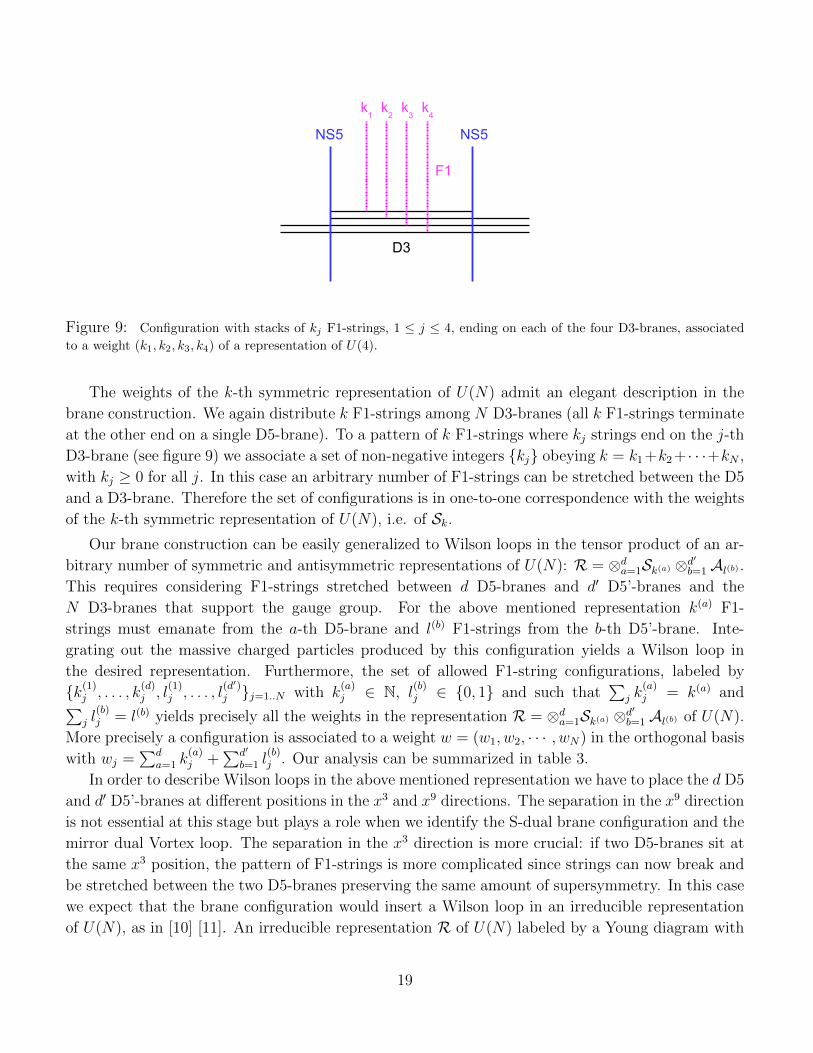
The weights of the k-th antisymmetric representation of U(N) admit an elegant description in

the brane construction. We must distribute k F1-strings among N D3-branes (all k F1-strings

terminate at the other end on a single D5’-brane). To a pattern of k F1-strings where kj strings

end on the j-th D3-brane (see figure 9) we associate a set of N non-negative integers {kj} obeying

k = k1 + k2 + · · · + kN , with kj ≥ 0 for all j. However, not all positive integers kj are allowed.

There can be at most one F1-string stretched between a D3-brane and a D5’-brane. This is the

so-called s-rule [9], and is a constraint that follows from Pauli’s exclusion principle [36]. Therefore,

the allowed configurations are described by a collection of N non-negative integers {kj} with the

constraint that kj ≤ 1. This set of configurations is in one-to-one correspondence with the weights

of the k-th antisymmetric representation of U(N), i.e. of Ak.We now turn to a Wilson loop in the k-th symmetric representation of U(N), which we denote by

Sk. Inserting a Wilson loop in the k-th symmetric representation is realized by adding k F1 strings

stretched in the x9 direction ending at one end on the N D3-branes where the U(N) gauge group

is supported and at the other end on a D5-brane stretched in the x012456 directions and localized in

the x9 direction. The array of fundamental strings ends between the two NS5-branes over which the

N D3-branes are suspended. This setup is illustrated in figure 8-b. In this case the charged probe

particle inserted by the Wilson loop can be though of as arising from a very heavy hypermultiplet,

represented by adding a D5-brane to the theory and then taking the D5-brane far away from the

stack, thus giving it a large mass and making the hypermultiplet fields nonrelativistic. Integrating

out the heavy hypermultiplet in the presence of k heavy insertions yields a supersymmetric Wilson

loop operator in the k-th symmetric representation [10,11].39

38This coupling is obtained by inserting the flux produced by the D5’-brane on the non-abelian Chern-Simons term

on the worldvolume of the D3-branes. This is T-dual to the haf-integral Chern-Simons term discussed in [35].39In [11] the heavy charged particle was obtained by going to the Coulomb branch while here by giving a large mass

to a hypermultiplet.

18

NS5

F1

D3

NS5

k1k2k3k4

Figure 9: Configuration with stacks of kj F1-strings, 1 ≤ j ≤ 4, ending on each of the four D3-branes, associated

to a weight (k1, k2, k3, k4) of a representation of U(4).

The weights of the k-th symmetric representation of U(N) admit an elegant description in the

brane construction. We again distribute k F1-strings among N D3-branes (all k F1-strings terminate

at the other end on a single D5-brane). To a pattern of k F1-strings where kj strings end on the j-th

D3-brane (see figure 9) we associate a set of non-negative integers {kj} obeying k = k1 +k2 + · · ·+kN ,

with kj ≥ 0 for all j. In this case an arbitrary number of F1-strings can be stretched between the D5

and a D3-brane. Therefore the set of configurations is in one-to-one correspondence with the weights

of the k-th symmetric representation of U(N), i.e. of Sk.Our brane construction can be easily generalized to Wilson loops in the tensor product of an ar-

bitrary number of symmetric and antisymmetric representations of U(N): R = ⊗da=1Sk(a) ⊗d′

b=1Al(b) .This requires considering F1-strings stretched between d D5-branes and d′ D5’-branes and the

N D3-branes that support the gauge group. For the above mentioned representation k(a) F1-

strings must emanate from the a-th D5-brane and l(b) F1-strings from the b-th D5’-brane. Inte-

grating out the massive charged particles produced by this configuration yields a Wilson loop in

the desired representation. Furthermore, the set of allowed F1-string configurations, labeled by

{k(1)j , . . . , k

(d)j , l

(1)j , . . . , l

(d′)j }j=1..N with k

(a)j ∈ N, l

(b)j ∈ {0, 1} and such that

∑j k

(a)j = k(a) and∑

j l(b)j = l(b) yields precisely all the weights in the representation R = ⊗da=1Sk(a) ⊗d

′

b=1 Al(b) of U(N).

More precisely a configuration is associated to a weight w = (w1, w2, · · · , wN) in the orthogonal basis

with wj =∑d

a=1 k(a)j +

∑d′

b=1 l(b)j . Our analysis can be summarized in table 3.

In order to describe Wilson loops in the above mentioned representation we have to place the d D5

and d′ D5’-branes at different positions in the x3 and x9 directions. The separation in the x9 direction

is not essential at this stage but plays a role when we identify the S-dual brane configuration and the

mirror dual Vortex loop. The separation in the x3 direction is more crucial: if two D5-branes sit at

the same x3 position, the pattern of F1-strings is more complicated since strings can now break and

be stretched between the two D5-branes preserving the same amount of supersymmetry. In this case

we expect that the brane configuration would insert a Wilson loop in an irreducible representation

of U(N), as in [10] [11]. An irreducible representation R of U(N) labeled by a Young diagram with

19

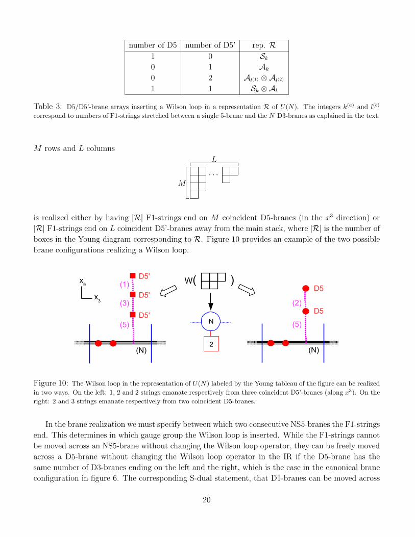
number of D5 number of D5’ rep. R1 0 Sk0 1 Ak0 2 Al(1) ⊗Al(2)1 1 Sk ⊗Al

Table 3: D5/D5’-brane arrays inserting a Wilson loop in a representation R of U(N). The integers k(a) and l(b)

correspond to numbers of F1-strings stretched between a single 5-brane and the N D3-branes as explained in the text.

M rows and L columns

· · ·

L

M

is realized either by having |R| F1-strings end on M coincident D5-branes (in the x3 direction) or

|R| F1-strings end on L coincident D5’-branes away from the main stack, where |R| is the number of

boxes in the Young diagram corresponding to R. Figure 10 provides an example of the two possible

brane configurations realizing a Wilson loop.

(1)D5'

2

N

W(

(3)

(5)

(N)

D5

(2)

(5)

(N)

D5'

D5'D5

)x9

x3

Figure 10: The Wilson loop in the representation of U(N) labeled by the Young tableau of the figure can be realized

in two ways. On the left: 1, 2 and 2 strings emanate respectively from three coincident D5’-branes (along x3). On the

right: 2 and 3 strings emanate respectively from two coincident D5-branes.

In the brane realization we must specify between which two consecutive NS5-branes the F1-strings

end. This determines in which gauge group the Wilson loop is inserted. While the F1-strings cannot

be moved across an NS5-brane without changing the Wilson loop operator, they can be freely moved

across a D5-brane without changing the Wilson loop operator in the IR if the D5-brane has the

same number of D3-branes ending on the left and the right, which is the case in the canonical brane

configuration in figure 6. The corresponding S-dual statement, that D1-branes can be moved across

20

an NS5-brane with the same number of D3-branes ending on the left and the right but that D1-branes

cannot be moved across a D5-brane without changing the IR dynamics, will play an important role

in unraveling the mirror map of loop operators.

3.2 Mirror Of Wilson Loops From S-duality

After having found a brane realization of Wilson loops, we now make use of the fact that mirror

symmetry corresponds to S-duality in the Type IIB brane realization to derive the mirror dual

of supersymmetric Wilson loop operators. Here we loosely call S-duality what is really S-duality

combined with the rotation that sends x456 to x789 and x789 to −x456, so that D5-branes and NS5-

branes get exchanged. We shall see that the information about the representation of the Wilson loop

is encoded in the discrete data of a 1d N = 4 SQM quiver quantum mechanics gauge theory.

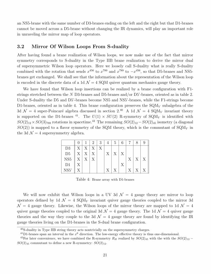
We have found that Wilson loop insertions can be realized by a brane configuration with F1-

strings stretched between the N D3-branes and D5-branes and/or D5’-branes, oriented as in table 2.

Under S-duality the D5 and D5’-branes become NS5 and NS5’-branes, while the F1-strings become

D1-branes, oriented as in table 4. This brane configuration preserves the SQMV subalgebra of the

3d N = 4 super-Poincare algebra discussed in section 2.40 A 1d N = 4 SQMV invariant theory

is supported on the D1-branes 41. The U(1) × SU(2) R-symmetry of SQMV is identified with

SO(2)12×SO(3)789 rotations in spacetime.42 The remaining SO(2)12−SO(2)45 isometry (a diagonal

SO(2)) is mapped to a flavor symmetry of the SQM theory, which is the commutant of SQMV in

the 3d N = 4 supersymmetry algebra.

0 1 2 3 4 5 6 7 8 9

D3 X X X X

D5 X X X X X X

NS5 X X X X X X

D1 X X

NS5’ X X X X X X

Table 4: Brane array with D1-branes

We will now exhibit that Wilson loops in a UV 3d N = 4 gauge theory are mirror to loop

operators defined by 1d N = 4 SQMV invariant quiver gauge theories coupled to the mirror 3d

N = 4 gauge theory. Likewise, the Wilson loops of the mirror theory are mapped to 1d N = 4

quiver gauge theories coupled to the original 3d N = 4 gauge theory. The 1d N = 4 quiver gauge

theories and the way they couple to the 3d N = 4 gauge theory are found by identifying the IR

gauge theories living on the D1-branes in the S-dual brane configuration.

40S-duality in Type IIB string theory acts nontrivially on the supersymmetry charges.41D1-branes span an interval in the x6 direction. The low-energy effective theory is thus one-dimensional.42For later convenience, we have combined the R-symmetry RH realized by SO(2)45 with the with the SO(2)12 −

SO(2)45 commutant to define a new R-symmetry: SO(2)12.

21

How can the mirror operator to a given Wilson loop be constructed? First we perform S-duality

on the brane configuration realizing a Wilson loop in a 3d N = 4 gauge theory. In the absence of

the F1-strings, the mirror 3d N = 4 theory is found by rearranging the S-dual brane configuration

so as to bring it to the canonical frame explained at the beginning of section 3, where the mirror

gauge theory can be easily read. After S-duality, the number of D3-branes on the left and on the

right of a D5-brane need not be the same while that number is the same for every NS5-brane, as

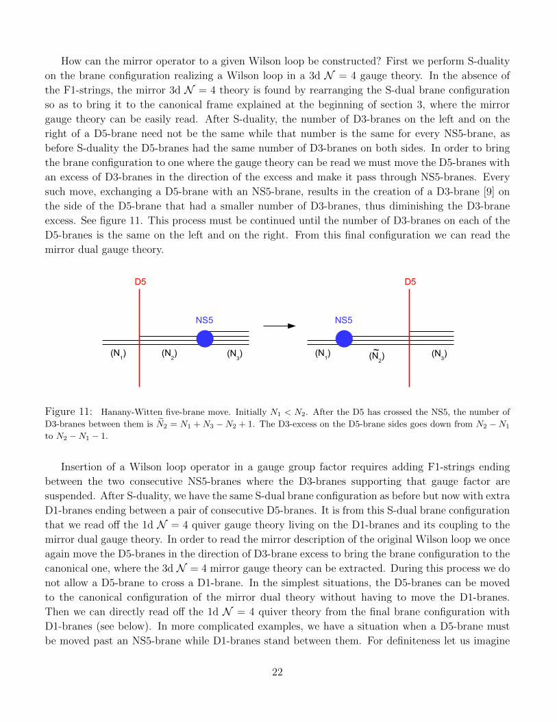
before S-duality the D5-branes had the same number of D3-branes on both sides. In order to bring

the brane configuration to one where the gauge theory can be read we must move the D5-branes with

an excess of D3-branes in the direction of the excess and make it pass through NS5-branes. Every

such move, exchanging a D5-brane with an NS5-brane, results in the creation of a D3-brane [9] on

the side of the D5-brane that had a smaller number of D3-branes, thus diminishing the D3-brane

excess. See figure 11. This process must be continued until the number of D3-branes on each of the

D5-branes is the same on the left and on the right. From this final configuration we can read the

mirror dual gauge theory.

D5

NS5

(N2)(N

1) (N

3)

D5

NS5

(N2)(N

1) (N

3)~

Figure 11: Hanany-Witten five-brane move. Initially N1 < N2. After the D5 has crossed the NS5, the number of

D3-branes between them is N2 = N1 +N3 −N2 + 1. The D3-excess on the D5-brane sides goes down from N2 −N1

to N2 −N1 − 1.

Insertion of a Wilson loop operator in a gauge group factor requires adding F1-strings ending

between the two consecutive NS5-branes where the D3-branes supporting that gauge factor are

suspended. After S-duality, we have the same S-dual brane configuration as before but now with extra

D1-branes ending between a pair of consecutive D5-branes. It is from this S-dual brane configuration

that we read off the 1d N = 4 quiver gauge theory living on the D1-branes and its coupling to the

mirror dual gauge theory. In order to read the mirror description of the original Wilson loop we once

again move the D5-branes in the direction of D3-brane excess to bring the brane configuration to the

canonical one, where the 3d N = 4 mirror gauge theory can be extracted. During this process we do

not allow a D5-brane to cross a D1-brane. In the simplest situations, the D5-branes can be moved

to the canonical configuration of the mirror dual theory without having to move the D1-branes.

Then we can directly read off the 1d N = 4 quiver theory from the final brane configuration with

D1-branes (see below). In more complicated examples, we have a situation when a D5-brane must

be moved past an NS5-brane while D1-branes stand between them. For definiteness let us imagine

22

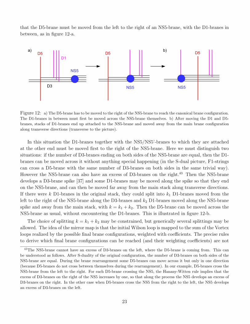
that the D5-brane must be moved from the left to the right of an NS5-brane, with the D1-branes in

between, as in figure 12-a.

D5

NS5

D1

D3

a) b)D5

NS5

D5

NS5

Figure 12: a) The D5-brane has to be moved to the right of the NS5-brane to reach the canonical brane configuration.

The D1-branes in between must first be moved across the NS5-brane themselves. b) After moving the D1 and D5-

branes, stacks of D1-branes end up attached to the NS5-brane and moved away from the main brane configuration

along transverse directions (transverse to the picture).

In this situation the D1-branes together with the NS5/NS5’-branes to which they are attached

at the other end must be moved first to the right of the NS5-brane. Here we must distinguish two

situations: if the number of D3-branes ending on both sides of the NS5-brane are equal, then the D1-

branes can be moved across it without anything special happening (in the S-dual picture, F1-strings

can cross a D5-brane with the same number of D3-branes on both sides in the same trivial way).

However the NS5-brane can also have an excess of D3-branes on the right.43 Then the NS5-brane

develops a D3-brane spike [37] and some D1-branes may be moved along the spike so that they end

on the NS5-brane, and can then be moved far away from the main stack along transverse directions.

If there were k D1-branes in the original stack, they could split into k1 D1-branes moved from the

left to the right of the NS5-brane along the D3-branes and k2 D1-branes moved along the NS5-brane

spike and away from the main stack, with k = k1 + k2. Then the D5-brane can be moved across the

NS5-brane as usual, without encountering the D1-branes. This is illustrated in figure 12-b.

The choice of splitting k = k1 + k2 may be constrained, but generically several splittings may be

allowed. The idea of the mirror map is that the initial Wilson loop is mapped to the sum of the Vortex

loops realized by the possible final brane configurations, weighted with coefficients. The precise rules

to derive which final brane configurations can be reached (and their weighting coefficients) are not

43The NS5-brane cannot have an excess of D3-branes on the left, where the D5-brane is coming from. This can

be understood as follows. After S-duality of the original configuration, the number of D3-branes on both sides of the

NS5-brane are equal. During the brane rearrangement some D5-branes can move across it but only in one direction

(because D5-branes do not cross between themselves during the rearrangement). In our example, D5-branes cross the

NS5-brane from the left to the right. For each D5-brane crossing the NS5, the Hanany-Witten rule implies that the

excess of D3-branes on the right of the NS5 increases by one, so that along the process the NS5 develops an excess of

D3-branes on the right. In the other case when D5-branes cross the NS5 from the right to the left, the NS5 develops

an excess of D3-branes on the left.

23

obvious. Intuitively the difficulty is related to the fact that the D3-spike is “on the wrong side” of

the NS5-branes, so that we cannot directly move the D1-branes along the spikes. We will see shortly

that the situation is under much better control starting from the D1-branes configurations realizing

Vortex loops and S-dualizing to configurations realizing the mirror Wilson loops.

What are the final brane configurations? In addition to the D3, D5, NS5 system realizing the

mirror dual theory, there are D1-branes ending on D3-branes on one side and on NS5 and/or NS5’-

branes situed far away from the main configuration. Moreover there are also D1-branes ending on

NS5-branes in the main stack. The physical interpretation of having q D1-branes ending on an

NS5-brane is as a background Wilson loop of charge q for a U(1) global symmetry associated to the

NS5-brane, which is a combination of the so-called topological symmetries of the 3d theory. These

flavor Wilson loops combine with the Vortex loop realized by the D1-branes ending on D3-branes,

which we describe now.

A final brane configuration with D1-branes ending on D3-branes in one end and on NS5 and/or

NS5’-branes on the other can be used to give at least two descriptions of the mirror of a Wilson loop.

This brane configuration can be thought of as a deformation of two other brane configurations, both

of which are conducive to reading off the 1d N = 4 quiver gauge theory living on the D1-branes and

its couplings to the bulk 3d N = 4 gauge theory. The D1-branes can be either moved to the nearest

NS5-brane to the left or to the nearest NS5-brane to the right. In order to reach this configuration,

from which the gauge theory description of the mirror loop operators can be read off, we must again

ensure that no D1-strings cross D5-branes. This means that we have to move the D5-branes between

the D1-branes and the nearest NS5-brane to the other side of that NS5-brane. In summary, we can

realize the mirror loop operator either as:

1. Deformation of the coupled 3d/1d theory realized by the D1-branes when they end on the

NS5-brane on the left.

2. Deformation of the coupled 3d/1d theory realized by the D1-branes when they end on the

NS5-brane on the right.

These yield two dual descriptions of the same operator.

Once we move the stack of D1-branes so that it ends on a neighbouring NS5-brane, we can read

off the 1d N = 4 quiver gauge theory and how it couples to the 3d N = 4 gauge theory. The 1d

N = 4 gauge theory associated to a brane configuration is constructed by assigning:

• A U(k) vector multiplet to k D1-branes suspended between an NS5-brane and an NS5’-brane.

• A U(k) vector multiplet and an adjoint chiral multiplet44 to k D1-branes suspended between

two NS5-branes or two NS5’-branes.

• Two chiral multiplets in the bifundamental and anti-bifundamental representations of U(k1)×U(k2) 45 to an NS5-brane or NS5’-brane with k1 D1-branes ending on its left and k2 D1-branes

ending on its right.

44The adjoint chiral multiplet describes the position of the D1-branes in the x12 directions (for NS5-branes), or in

the x45 directions (for NS5’-branes).45The bifundamental representation of U(k1)×U(k2) is (k1, k2) and the anti-bifundamental is its complex conjugate.

24

• A chiral multiplet in the bifundamental of U(NR)× U(k) and an chiral multiplet in the bifun-

damental of U(k) × U(NL) to k D1-branes ending on an NS5-brane which has NL D3-branes

ending on its left and NR D3-branes ending on its right.

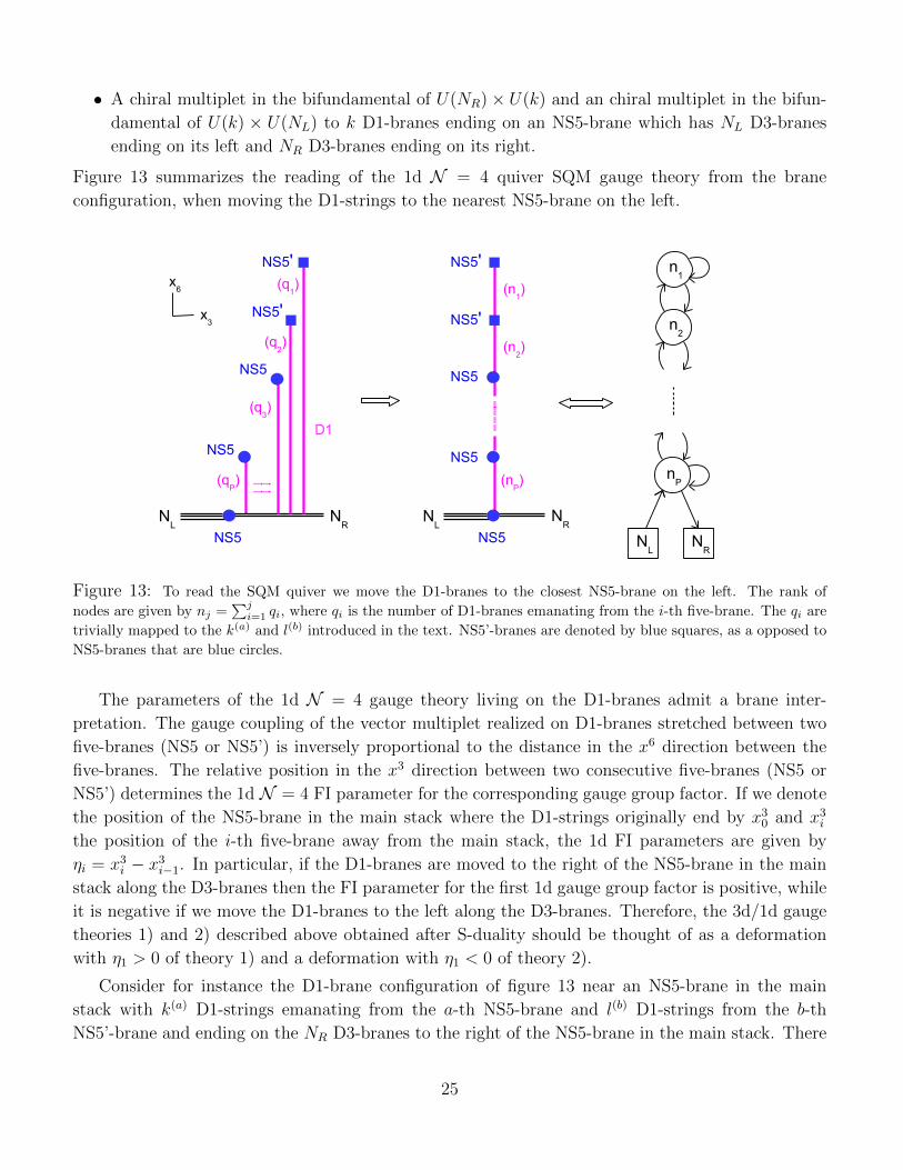
Figure 13 summarizes the reading of the 1d N = 4 quiver SQM gauge theory from the brane

configuration, when moving the D1-strings to the nearest NS5-brane on the left.

n1

n2

nP

NR

NL

NS5'

NS5

(nP)

NS5

NS5

x6

x3

(n2)

(n1)

NS5'

NL

NR

NS5'

NS5

NS5

NS5

NS5'

NL

NR

(qP)

(q1)

(q2)

(q3)

D1

Figure 13: To read the SQM quiver we move the D1-branes to the closest NS5-brane on the left. The rank of

nodes are given by nj =∑ji=1 qi, where qi is the number of D1-branes emanating from the i-th five-brane. The qi are

trivially mapped to the k(a) and l(b) introduced in the text. NS5’-branes are denoted by blue squares, as a opposed to

NS5-branes that are blue circles.

The parameters of the 1d N = 4 gauge theory living on the D1-branes admit a brane inter-

pretation. The gauge coupling of the vector multiplet realized on D1-branes stretched between two

five-branes (NS5 or NS5’) is inversely proportional to the distance in the x6 direction between the

five-branes. The relative position in the x3 direction between two consecutive five-branes (NS5 or

NS5’) determines the 1d N = 4 FI parameter for the corresponding gauge group factor. If we denote

the position of the NS5-brane in the main stack where the D1-strings originally end by x30 and x3

i

the position of the i-th five-brane away from the main stack, the 1d FI parameters are given by

ηi = x3i − x3

i−1. In particular, if the D1-branes are moved to the right of the NS5-brane in the main

stack along the D3-branes then the FI parameter for the first 1d gauge group factor is positive, while

it is negative if we move the D1-branes to the left along the D3-branes. Therefore, the 3d/1d gauge

theories 1) and 2) described above obtained after S-duality should be thought of as a deformation

with η1 > 0 of theory 1) and a deformation with η1 < 0 of theory 2).

Consider for instance the D1-brane configuration of figure 13 near an NS5-brane in the main

stack with k(a) D1-strings emanating from the a-th NS5-brane and l(b) D1-strings from the b-th

NS5’-brane and ending on the NR D3-branes to the right of the NS5-brane in the main stack. There

25

are also NL D3-branes to the left of this NS5-brane. To this brane configuration we can associate

the representation R = ⊗da=1Sk(a) ⊗d′

b=1 Al(b) of U(NR), where d and d′ denote the numbers of NS5

and NS5’-branes from which the D1-branes emanate. This brane configuration can be thought of

as a deformation of a 1d N = 4 quiver gauge theory in figure 13 with positive FI parameters.

There are actually different dual descriptions of the 1d N = 4 theories depending on the relative

order of the d NS5 and d′ NS5’-branes in the x6 direction. Different relative positions give rise to

different dual 1d N = 4 descriptions of the same Vortex loop operator labeled by the representation

R = ⊗da=1Sk(a) ⊗d′

b=1 Al(b) of U(NR). Roughly speaking, these dual descriptions are related by a 1d

N = 4 version of Seiberg duality [20] (see also [21,38]).

We have described the 1d N = 4 SQMV quiver theory living on the D1-branes. We must now

explain how it is coupled to the 3d N = 4 gauge theory. The idea is that the U(NL)×U(NR) flavor

symmetry of the 1d N = 4 theory is gauged with 3d bulk fields living on the D3-branes ending on the

NS5-brane on the main stack. We must, however, distinguish the D3-branes supporting dynamical

gauge fields from the non-dynamical D3-branes stretched between the NS5 and a D5-brane. To read

the SQM theory we had to move D1-branes to the closest NS5-brane to left (or to the right). Suppose

there are nD5 D5-branes standing between this NS5 and the D1-branes, then we have to move them

first to the left of the NS5 and, by the Hanany-Witten effect, one D3-brane per D5 is created ending

on the left of the NS5-brane. In this case the NL D3-branes ending on the left of the NS5 decompose

into NL = nD5 + nD3, where nD3 is the number of dynamical D3-branes, those supporting a U(nD3)

3d N = 4 vector multiplet. On the other side, the NR D3-branes ending on the right of the NS5

support a U(NR) 3d N = 4 vector multiplet. The 1d N = 4 theory is then coupled to the 3d N = 4

theory by gauging the U(NR) and U(nD3) ⊂ U(NL) flavor symmetries on the defect with dynamical

3d N = 4 vector multiplets.46 Furthermore, there is a cubic superpotential as in (2.12) which breaks

the U(nD5)3d × U(nD5)1d flavor symmetry to the diagonal U(nD5), where U(nD5)1d ⊂ U(NL) and

U(nD5)3d is the 3d flavor symmetry acting on the nD5 hypermultiplets associated to the D5-branes.

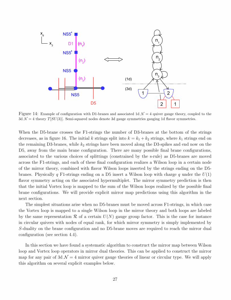
The 3d/1d coupling that can read from the brane picture is summarized in the example of figure 14.

The 3d/1d coupling for the SQMV theories read from moving the D1s to the nearest NS5 on the

right are found similarly, as shown in figure 15.

As mentioned above, it turns out to be simpler to derive the mirror map if we consider the inverse

problem of finding the combination of Wilson loops dual to a given Vortex loop. Starting with a

configuration of D1-branes realizing a Vortex loop, we can S-dualize to obtain a configuration with F1-

strings and move the D5-branes to reach the canonical brane configuration of the mirror-dual theory.

The crucial difference is that we do not need to move the F1-strings, instead we are allowed to move

the D5-branes across the stack of F1-strings if this is necessary to reach the canonical configuration.

When we have to move a D5 across the F1-strings the situation is always the same, namely the

D5-brane has an excess of D3-branes on the side toward which it is moving. This means that the

F1-strings are on the side of the D3-spikes, along which they can be moved without obstruction.

46More precisely the 3d N = 4 vector multiplet decomposes into multiplets of the subalgebra preserved by SQMV ,

each multiplet containing fields at a given position in the plane orthogonal to the defect. A 1d N = 4 SQMV vector

multiplet embedded in the 3d N = 4 vector multiplet lives at the position of the defect and gauges the corresponding

flavor symmetry.

26

x6

x3

D5

D1

NS5'

(n1)

NS5

2

2

(1d)

(3d)

1

NS5'

NS5

n1

1

n2

n3

(n2)

(n1)

(n3)

Figure 14: Example of configuration with D1-branes and associated 1d N = 4 quiver gauge theory, coupled to the

3d N = 4 theory T [SU(3)]. Semi-squared nodes denote 3d gauge symmetries gauging 1d flavor symmetries.

When the D5-brane crosses the F1-strings the number of D3-branes at the bottom of the strings

decreases, as in figure 16. The initial k strings split into k = k1 + k2 strings, where k1 strings end on

the remaining D3-branes, while k2 strings have been moved along the D3-spikes and end now on the

D5, away from the main brane configuration. There are many possible final brane configurations,

associated to the various choices of splittings (constrained by the s-rule) as D5-branes are moved

across the F1-strings, and each of these final configuration realizes a Wilson loop in a certain node

of the mirror theory, combined with flavor Wilson loops inserted by the strings ending on the D5-

branes. Physically q F1-strings ending on a D5 insert a Wilson loop with charge q under the U(1)

flavor symmetry acting on the associated hypermultiplet. The mirror symmetry prediction is then

that the initial Vortex loop is mapped to the sum of the Wilson loops realized by the possible final

brane configurations. We will provide explicit mirror map predictions using this algorithm in the

next section.

The simplest situations arise when no D5-branes must be moved across F1-strings, in which case

the Vortex loop is mapped to a single Wilson loop in the mirror theory and both loops are labeled

by the same representation R of a certain U(N) gauge group factor. This is the case for instance

in circular quivers with nodes of equal rank, for which mirror symmetry is simply implemented by

S-duality on the brane configuration and no D5-brane moves are required to reach the mirror dual

configuration (see section 4.4).

In this section we have found a systematic algorithm to construct the mirror map between Wilson

loop and Vortex loop operators in mirror dual theories. This can be applied to construct the mirror

map for any pair of 3d N = 4 mirror quiver gauge theories of linear or circular type. We will apply

this algorithm on several explicit examples below.

27

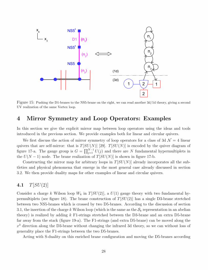
x6

x3 D1

NS5'

(n1)

2

2

(1d)

(3d)1

NS5'

NS5

n1

1

n2

n3

(n2)

(n1)

(n3)

Figure 15: Pushing the D1-branes to the NS5-brane on the right, we can read another 3d/1d theory, giving a second

UV realization of the same Vortex loop.

4 Mirror Symmetry and Loop Operators: Examples

In this section we give the explicit mirror map between loop operators using the ideas and tools

introduced in the previous section. We provide examples both for linear and circular quivers.

We first discuss the action of mirror symmetry of loop operators for a class of 3d N = 4 linear

quivers that are self-mirror: that is T [SU(N)] [29]. T [SU(N)] is encoded by the quiver diagram of

figure 17-a. The gauge group is G =∏N−1

j=1 U(j) and there are N fundamental hypermultiplets in

the U(N − 1) node. The brane realization of T [SU(N)] is shown in figure 17-b.

Constructing the mirror map for arbitrary loops in T [SU(N)] already incorporates all the sub-

tleties and physical phenomena that emerge in the most general case already discussed in section

3.2. We then provide duality maps for other examples of linear and circular quivers.

4.1 T [SU(2)]

Consider a charge k Wilson loop Wk in T [SU(2)], a U(1) gauge theory with two fundamental hy-

permultiplets (see figure 18). The brane construction of T [SU(2)] has a single D3-brane stretched

between two NS5-branes which is crossed by two D5-branes. According to the discussion of section

3.1, the insertion of the charge k Wilson loop (which is the same as the Sk representation in an abelian

theory) is realized by adding k F1-strings stretched between the D3-brane and an extra D5-brane

far away from the stack (figure 19-a). The F1-strings (and extra D5-brane) can be moved along the

x3 direction along the D3-brane without changing the infrared 3d theory, so we can without loss of

generality place the F1-strings between the two D5-branes.

Acting with S-duality on this enriched brane configuration and moving the D5-branes according

28

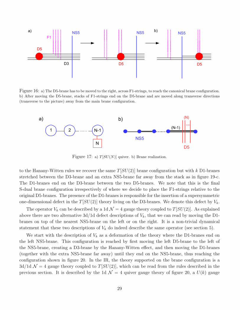
D5

NS5F1

D3 D5

NS5a) b)

D5

NS5

Figure 16: a) The D5-brane has to be moved to the right, across F1-strings, to reach the canonical brane configuration.

b) After moving the D5-brane, stacks of F1-strings end on the D5-brane and are moved along transverse directions

(transverse to the picture) away from the main brane configuration.

1 2 N-1

ND5

(N-1)

(N)

NS5

a) b)

Figure 17: a) T [SU(N)] quiver. b) Brane realization.

to the Hanany-Witten rules we recover the same T [SU(2)] brane configuration but with k D1-branes

stretched between the D3-brane and an extra NS5-brane far away from the stack as in figure 19-c.

The D1-branes end on the D3-brane between the two D5-branes. We note that this is the final

S-dual brane configuration irrespectively of where we decide to place the F1-strings relative to the

original D5-branes. The presence of the D1-branes is responsible for the insertion of a supersymmetric

one-dimensional defect in the T [SU(2)] theory living on the D3-branes. We denote this defect by Vk.

The operator Vk can be described by a 1d N = 4 gauge theory coupled to T [SU(2)]. As explained

above there are two alternative 3d/1d defect descriptions of Vk, that we can read by moving the D1-

branes on top of the nearest NS5-brane on the left or on the right. It is a non-trivial dynamical

statement that these two descriptions of Vk do indeed describe the same operator (see section 5).

We start with the description of Vk as a deformation of the theory where the D1-branes end on

the left NS5-brane. This configuration is reached by first moving the left D5-brane to the left of

the NS5-brane, creating a D3-brane by the Hanany-Witten effect, and then moving the D1-branes

(together with the extra NS5-brane far away) until they end on the NS5-brane, thus reaching the

configuration shown in figure 20. In the IR, the theory supported on the brane configuration is a

3d/1d N = 4 gauge theory coupled to T [SU(2)], which can be read from the rules described in the

previous section. It is described by the 1d N = 4 quiver gauge theory of figure 20, a U(k) gauge

29

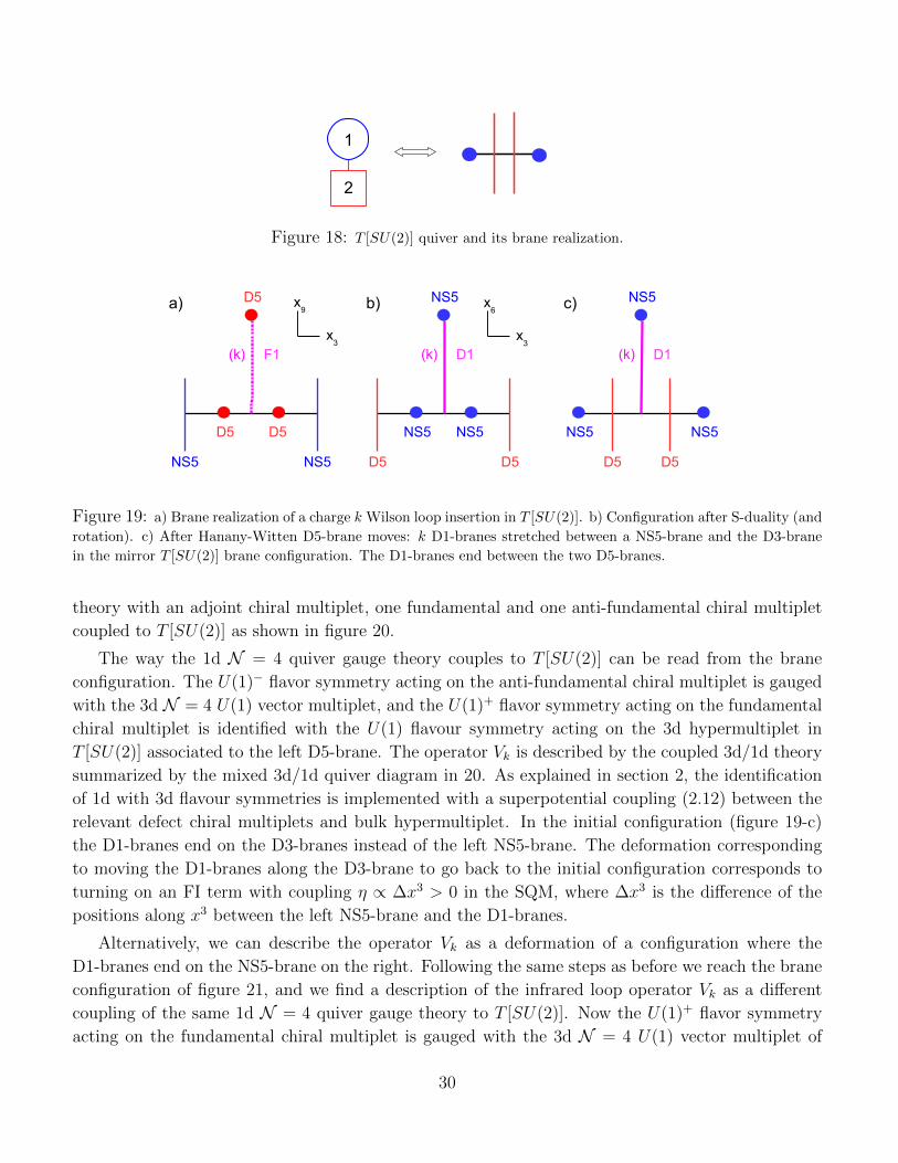
1

2

Figure 18: T [SU(2)] quiver and its brane realization.

D5

D1

NS5

D5

(k)

NS5NS5

D5

D1

NS5

D5

(k)

NS5NS5

x9

x3

D5

F1

D5

(k)

NS5NS5

x6

x3

D5 a) b) c)

Figure 19: a) Brane realization of a charge k Wilson loop insertion in T [SU(2)]. b) Configuration after S-duality (and

rotation). c) After Hanany-Witten D5-brane moves: k D1-branes stretched between a NS5-brane and the D3-brane

in the mirror T [SU(2)] brane configuration. The D1-branes end between the two D5-branes.

theory with an adjoint chiral multiplet, one fundamental and one anti-fundamental chiral multiplet

coupled to T [SU(2)] as shown in figure 20.

The way the 1d N = 4 quiver gauge theory couples to T [SU(2)] can be read from the brane

configuration. The U(1)− flavor symmetry acting on the anti-fundamental chiral multiplet is gauged

with the 3d N = 4 U(1) vector multiplet, and the U(1)+ flavor symmetry acting on the fundamental

chiral multiplet is identified with the U(1) flavour symmetry acting on the 3d hypermultiplet in

T [SU(2)] associated to the left D5-brane. The operator Vk is described by the coupled 3d/1d theory

summarized by the mixed 3d/1d quiver diagram in 20. As explained in section 2, the identification

of 1d with 3d flavour symmetries is implemented with a superpotential coupling (2.12) between the

relevant defect chiral multiplets and bulk hypermultiplet. In the initial configuration (figure 19-c)

the D1-branes end on the D3-branes instead of the left NS5-brane. The deformation corresponding

to moving the D1-branes along the D3-brane to go back to the initial configuration corresponds to

turning on an FI term with coupling η ∝ ∆x3 > 0 in the SQM, where ∆x3 is the difference of the

positions along x3 between the left NS5-brane and the D1-branes.

Alternatively, we can describe the operator Vk as a deformation of a configuration where the

D1-branes end on the NS5-brane on the right. Following the same steps as before we reach the brane

configuration of figure 21, and we find a description of the infrared loop operator Vk as a different

coupling of the same 1d N = 4 quiver gauge theory to T [SU(2)]. Now the U(1)+ flavor symmetry

acting on the fundamental chiral multiplet is gauged with the 3d N = 4 U(1) vector multiplet of

30

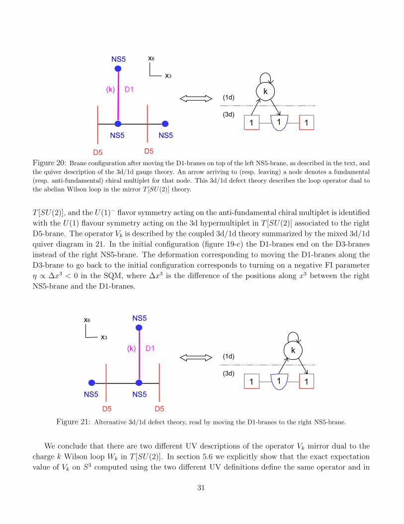
x6

x3

D5

D1

NS5

D5

(k)

NS5NS5

k

1 1

(1d)

(3d)1

Figure 20: Brane configuration after moving the D1-branes on top of the left NS5-brane, as described in the text, and

the quiver description of the 3d/1d gauge theory. An arrow arriving to (resp. leaving) a node denotes a fundamental

(resp. anti-fundamental) chiral multiplet for that node. This 3d/1d defect theory describes the loop operator dual to

the abelian Wilson loop in the mirror T [SU(2)] theory.

T [SU(2)], and the U(1)− flavor symmetry acting on the anti-fundamental chiral multiplet is identified

with the U(1) flavour symmetry acting on the 3d hypermultiplet in T [SU(2)] associated to the right

D5-brane. The operator Vk is described by the coupled 3d/1d theory summarized by the mixed 3d/1d

quiver diagram in 21. In the initial configuration (figure 19-c) the D1-branes end on the D3-branes

instead of the right NS5-brane. The deformation corresponding to moving the D1-branes along the

D3-brane to go back to the initial configuration corresponds to turning on a negative FI parameter

η ∝ ∆x3 < 0 in the SQM, where ∆x3 is the difference of the positions along x3 between the right

NS5-brane and the D1-branes.

x6

x3

D5

D1

NS5

D5

(k)

NS5NS5

k

1 1

(1d)

(3d)1

Figure 21: Alternative 3d/1d defect theory, read by moving the D1-branes to the right NS5-brane.

We conclude that there are two different UV descriptions of the operator Vk mirror dual to the

charge k Wilson loop Wk in T [SU(2)]. In section 5.6 we explicitly show that the exact expectation

value of Vk on S3 computed using the two different UV definitions define the same operator and in

31

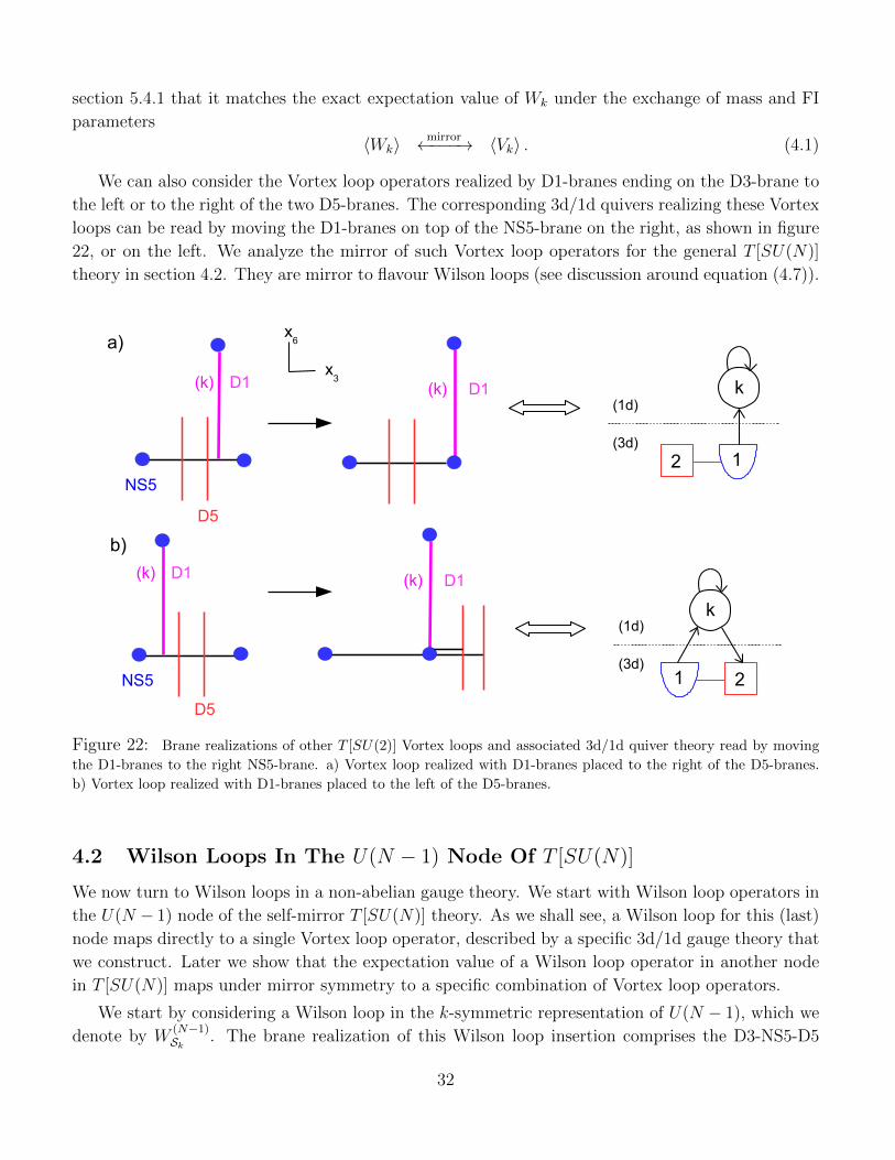
section 5.4.1 that it matches the exact expectation value of Wk under the exchange of mass and FI

parameters

〈Wk〉mirror←−−−→ 〈Vk〉 . (4.1)

We can also consider the Vortex loop operators realized by D1-branes ending on the D3-brane to

the left or to the right of the two D5-branes. The corresponding 3d/1d quivers realizing these Vortex

loops can be read by moving the D1-branes on top of the NS5-brane on the right, as shown in figure

22, or on the left. We analyze the mirror of such Vortex loop operators for the general T [SU(N)]

theory in section 4.2. They are mirror to flavour Wilson loops (see discussion around equation (4.7)).

D1(k) k

2 1

(1d)

(3d)

D1(k)

k

1

(1d)

(3d)2

x6

x3

D5

D1(k)

NS5

a)

b)

D5

D1(k)

NS5

Figure 22: Brane realizations of other T [SU(2)] Vortex loops and associated 3d/1d quiver theory read by moving

the D1-branes to the right NS5-brane. a) Vortex loop realized with D1-branes placed to the right of the D5-branes.

b) Vortex loop realized with D1-branes placed to the left of the D5-branes.

4.2 Wilson Loops In The U(N − 1) Node Of T [SU(N)]

We now turn to Wilson loops in a non-abelian gauge theory. We start with Wilson loop operators in

the U(N − 1) node of the self-mirror T [SU(N)] theory. As we shall see, a Wilson loop for this (last)

node maps directly to a single Vortex loop operator, described by a specific 3d/1d gauge theory that

we construct. Later we show that the expectation value of a Wilson loop operator in another node

in T [SU(N)] maps under mirror symmetry to a specific combination of Vortex loop operators.

We start by considering a Wilson loop in the k-symmetric representation of U(N − 1), which we

denote by W(N−1)Sk . The brane realization of this Wilson loop insertion comprises the D3-NS5-D5

32

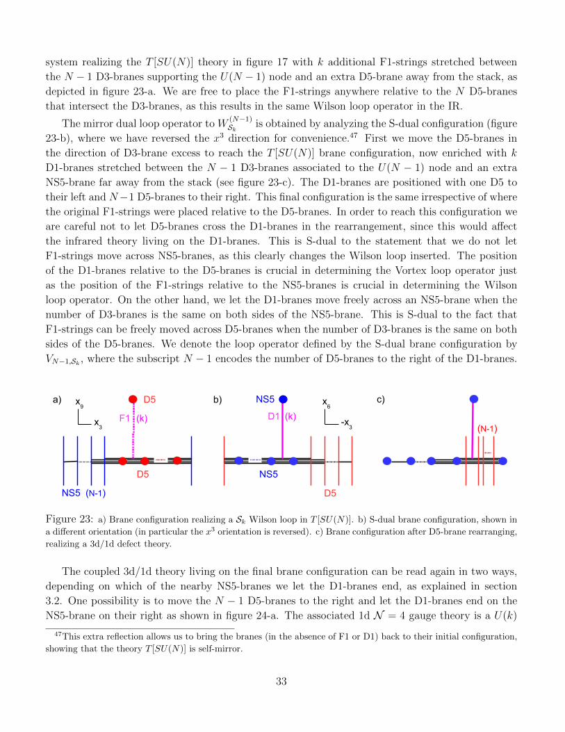
system realizing the T [SU(N)] theory in figure 17 with k additional F1-strings stretched between

the N − 1 D3-branes supporting the U(N − 1) node and an extra D5-brane away from the stack, as

depicted in figure 23-a. We are free to place the F1-strings anywhere relative to the N D5-branes

that intersect the D3-branes, as this results in the same Wilson loop operator in the IR.

The mirror dual loop operator to W(N−1)Sk is obtained by analyzing the S-dual configuration (figure

23-b), where we have reversed the x3 direction for convenience.47 First we move the D5-branes in

the direction of D3-brane excess to reach the T [SU(N)] brane configuration, now enriched with k

D1-branes stretched between the N − 1 D3-branes associated to the U(N − 1) node and an extra

NS5-brane far away from the stack (see figure 23-c). The D1-branes are positioned with one D5 to

their left and N−1 D5-branes to their right. This final configuration is the same irrespective of where

the original F1-strings were placed relative to the D5-branes. In order to reach this configuration we

are careful not to let D5-branes cross the D1-branes in the rearrangement, since this would affect

the infrared theory living on the D1-branes. This is S-dual to the statement that we do not let

F1-strings move across NS5-branes, as this clearly changes the Wilson loop inserted. The position

of the D1-branes relative to the D5-branes is crucial in determining the Vortex loop operator just

as the position of the F1-strings relative to the NS5-branes is crucial in determining the Wilson

loop operator. On the other hand, we let the D1-branes move freely across an NS5-brane when the

number of D3-branes is the same on both sides of the NS5-brane. This is S-dual to the fact that

F1-strings can be freely moved across D5-branes when the number of D3-branes is the same on both

sides of the D5-branes. We denote the loop operator defined by the S-dual brane configuration by

VN−1,Sk , where the subscript N − 1 encodes the number of D5-branes to the right of the D1-branes.

c)NS5

(k)

D5

b)

D1

NS5

NS5

(k)

D5 a)

F1

D5

(N-1)

(N-1)

x9

x3

x6

-x3

Figure 23: a) Brane configuration realizing a Sk Wilson loop in T [SU(N)]. b) S-dual brane configuration, shown in

a different orientation (in particular the x3 orientation is reversed). c) Brane configuration after D5-brane rearranging,

realizing a 3d/1d defect theory.

The coupled 3d/1d theory living on the final brane configuration can be read again in two ways,

depending on which of the nearby NS5-branes we let the D1-branes end, as explained in section

3.2. One possibility is to move the N − 1 D5-branes to the right and let the D1-branes end on the

NS5-brane on their right as shown in figure 24-a. The associated 1d N = 4 gauge theory is a U(k)

47This extra reflection allows us to bring the branes (in the absence of F1 or D1) back to their initial configuration,

showing that the theory T [SU(N)] is self-mirror.

33

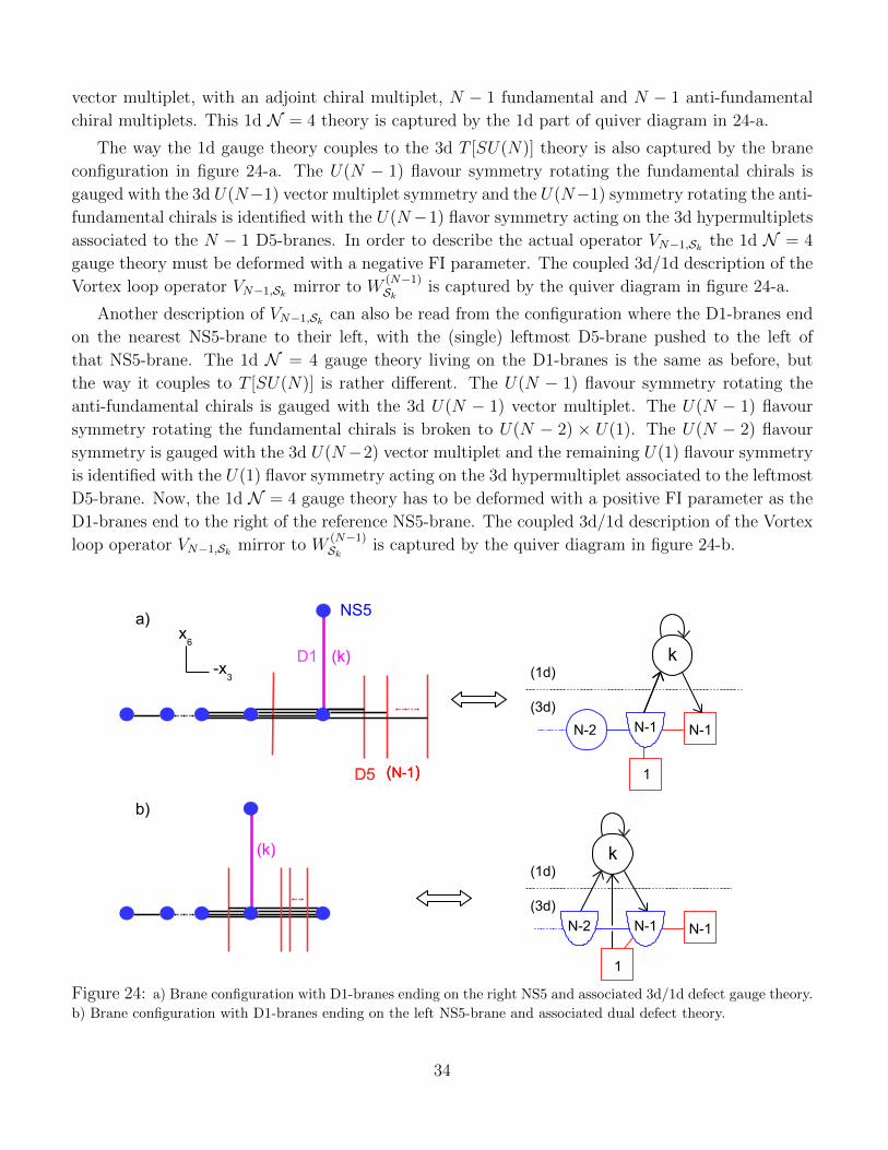
vector multiplet, with an adjoint chiral multiplet, N − 1 fundamental and N − 1 anti-fundamental

chiral multiplets. This 1d N = 4 theory is captured by the 1d part of quiver diagram in 24-a.

The way the 1d gauge theory couples to the 3d T [SU(N)] theory is also captured by the brane

configuration in figure 24-a. The U(N − 1) flavour symmetry rotating the fundamental chirals is

gauged with the 3d U(N−1) vector multiplet symmetry and the U(N−1) symmetry rotating the anti-

fundamental chirals is identified with the U(N−1) flavor symmetry acting on the 3d hypermultiplets

associated to the N − 1 D5-branes. In order to describe the actual operator VN−1,Sk the 1d N = 4

gauge theory must be deformed with a negative FI parameter. The coupled 3d/1d description of the

Vortex loop operator VN−1,Sk mirror to W(N−1)Sk is captured by the quiver diagram in figure 24-a.

Another description of VN−1,Sk can also be read from the configuration where the D1-branes end

on the nearest NS5-brane to their left, with the (single) leftmost D5-brane pushed to the left of

that NS5-brane. The 1d N = 4 gauge theory living on the D1-branes is the same as before, but

the way it couples to T [SU(N)] is rather different. The U(N − 1) flavour symmetry rotating the

anti-fundamental chirals is gauged with the 3d U(N − 1) vector multiplet. The U(N − 1) flavour

symmetry rotating the fundamental chirals is broken to U(N − 2) × U(1). The U(N − 2) flavour

symmetry is gauged with the 3d U(N−2) vector multiplet and the remaining U(1) flavour symmetry

is identified with the U(1) flavor symmetry acting on the 3d hypermultiplet associated to the leftmost

D5-brane. Now, the 1d N = 4 gauge theory has to be deformed with a positive FI parameter as the

D1-branes end to the right of the reference NS5-brane. The coupled 3d/1d description of the Vortex

loop operator VN−1,Sk mirror to W(N−1)Sk is captured by the quiver diagram in figure 24-b.

D5

D1

NS5

1

(1d)

(3d)

N-1

(k) k

(N-1)

N-1N-2

D5 (N-1)

x6

-x3

1

(1d)

(3d)

N-1

k

N-1N-2

(k)

a)

b)

Figure 24: a) Brane configuration with D1-branes ending on the right NS5 and associated 3d/1d defect gauge theory.

b) Brane configuration with D1-branes ending on the left NS5-brane and associated dual defect theory.

34

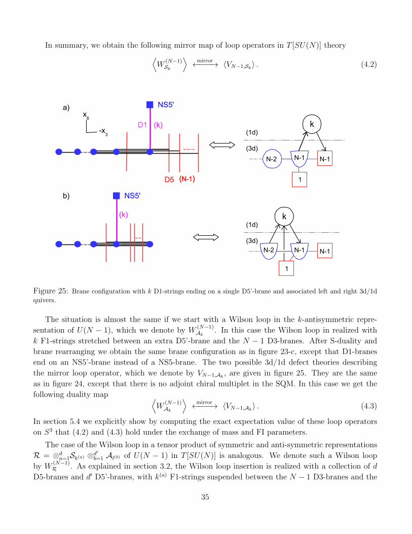
In summary, we obtain the following mirror map of loop operators in T [SU(N)] theory⟨W

(N−1)Sk

⟩mirror←−−−→ 〈VN−1,Sk〉 . (4.2)

D5

D1

NS5'

1

(1d)

(3d)

N-1

(k) k

(N-1)

N-1N-2

D5 (N-1)

x6

-x3

1

(1d)

(3d)

N-1

k

N-1N-2

(k)

a)

b) NS5'

Figure 25: Brane configuration with k D1-strings ending on a single D5’-brane and associated left and right 3d/1d

quivers.

The situation is almost the same if we start with a Wilson loop in the k-antisymmetric repre-

sentation of U(N − 1), which we denote by W(N−1)Ak . In this case the Wilson loop in realized with

k F1-strings stretched between an extra D5’-brane and the N − 1 D3-branes. After S-duality and

brane rearranging we obtain the same brane configuration as in figure 23-c, except that D1-branes

end on an NS5’-brane instead of a NS5-brane. The two possible 3d/1d defect theories describing

the mirror loop operator, which we denote by VN−1,Ak , are given in figure 25. They are the same

as in figure 24, except that there is no adjoint chiral multiplet in the SQM. In this case we get the

following duality map ⟨W

(N−1)Ak

⟩mirror←−−−→ 〈VN−1,Ak〉 . (4.3)

In section 5.4 we explicitly show by computing the exact expectation value of these loop operators

on S3 that (4.2) and (4.3) hold under the exchange of mass and FI parameters.

The case of the Wilson loop in a tensor product of symmetric and anti-symmetric representations

R = ⊗da=1Sk(a) ⊗d′

b=1 Al(b) of U(N − 1) in T [SU(N)] is analogous. We denote such a Wilson loop

by W(N−1)R . As explained in section 3.2, the Wilson loop insertion is realized with a collection of d

D5-branes and d′ D5’-branes, with k(a) F1-strings suspended between the N − 1 D3-branes and the

35

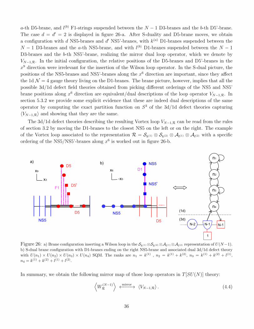
a-th D5-brane, and l(b) F1-strings suspended between the N − 1 D3-branes and the b-th D5’-brane.

The case d = d′ = 2 is displayed in figure 26-a. After S-duality and D5-brane moves, we obtain

a configuration with d NS5-branes and d′ NS5’-branes, with k(a) D1-branes suspended between the

N − 1 D3-branes and the a-th NS5-brane, and with l(b) D1-branes suspended between the N − 1

D3-branes and the b-th NS5’-brane, realizing the mirror dual loop operator, which we denote by

VN−1,R. In the initial configuration, the relative positions of the D5-branes and D5’-branes in the

x9 direction were irrelevant for the insertion of the Wilson loop operator. In the S-dual picture, the

positions of the NS5-branes and NS5’-branes along the x6 direction are important, since they affect

the 1d N = 4 gauge theory living on the D1-branes. The brane picture, however, implies that all the

possible 3d/1d defect field theories obtained from picking different orderings of the NS5 and NS5’

brane positions along x6 direction are equivalent/dual descriptions of the loop operator VN−1,R. In

section 5.3.2 we provide some explicit evidence that these are indeed dual descriptions of the same

operator by computing the exact partition function on S3 of the 3d/1d defect theories capturing

〈VN−1,R〉 and showing that they are the same.

The 3d/1d defect theories describing the resulting Vortex loop VN−1,R can be read from the rules

of section 3.2 by moving the D1-branes to the closest NS5 on the left or on the right. The example

of the Vortex loop associated to the representation R = Sk(1) ⊗ Sk(2) ⊗ Al(1) ⊗ Al(2) with a specific

ordering of the NS5/NS5’-branes along x6 is worked out in figure 26-b.

b)

NS5

D5 x9

x3

a)

F1

D5

D5'

D5

D1

NS5

1

(1d)

(3d)

N-1N-1N-2

x6

-x3

NS5

NS5'

n1

n2

n3

n4

Figure 26: a) Brane configuration inserting a Wilson loop in the Sk(1)⊗Sk(2)⊗Al(1)⊗Al(2) representation of U(N−1).

b) S-dual brane configuration with D1-branes ending on the right NS5-brane and associated dual 3d/1d defect theory

with U(n1) × U(n2) × U(n3) × U(n4) SQM. The ranks are n1 = k(1) , n2 = k(1) + k(2), n3 = k(1) + k(2) + l(1),

n4 = k(1) + k(2) + l(1) + l(2).

In summary, we obtain the following mirror map of those loop operators in T [SU(N)] theory:⟨W

(N−1)R

⟩mirror←−−−→ 〈VN−1,R〉 . (4.4)

36

We have found that the mirror of a Wilson loop labeled by a representation of the U(N −1) node

is a Vortex loop operator labeled by the same representation. We now turn to the more involved

case of a Wilson loop in a representation of another gauge group factor in T [SU(N)].

4.3 The Other T [SU(N)] Loops

We proceed now with constructing the mirror map for the remaining loop operators in T [SU(N)].

This includes the Wilson loop operators in the other nodes of T [SU(N)]. As explained in section

3.2 it is easier to describe the mirror map starting from the brane configuration realizing Vortex

loops and going to the S-dual picture with F1-strings realizing the mirror Wilson loops. In the brane

realization, defining a Wilson loop requires specifying the location of the F1-strings relative to the

NS5-branes and a representation R. Likewise, a Vortex loop is specified by the location of the D1-

branes relative to the D5-branes and by a choice of representation R of the gauge group supported

on the D3-branes where the D1-branes end.

In the T [SU(N)] theory we have Vortex loops labeled by a representation R of the U(N − 1)

gauge node, which are realized with D1-strings ending on the N − 1 D3-branes supporting that

gauge group factor. As just discussed, the relative position of the D1-branes along the x3 direction

relative to the D5-branes is important. In the brane realization of T [SU(N)], there are N D5-branes

crossing the N − 1 D3-branes, giving rise to the N fundamental hypermultiplets of the U(N − 1)

node. Each U(N − 1) Vortex loop is characterized by a splitting of the N hypermultiplets into

N = M + (N −M) and corresponds to the arrangement where the D1-branes have M D5-branes

to their right and N −M D5-branes to their left. Thus, the data characterizing a U(N − 1) Vortex

loop is a representation R of U(N − 1) and an integer 0 ≤ M ≤ N . We denote such a Vortex loop

by VM,R. These operators admit a description in terms of a 1d N = 4 quiver gauge theory coupled

to T [SU(N)], which is shown in figure (27-a) for the case when the the D1-branes are moved to be

on top of the closest NS5-brane to their right. As already explained in section 4.2 the Vortex loop

operator VN−1,R gets mapped under mirror symmetry to a Wilson loop W(N−1)R in a representation

R of U(N − 1).

This does not exhaust the Vortex loops that can be defined in T [SU(N)]. There are Vortex loop

operators in T [SU(N)] realized by D1-strings ending on the p D3-branes supporting the U(p) gauge

group factor, with 1 ≤ p ≤ N − 2. Since there are no fundamental hypermultiplets for this gauge

group factor, and correspondingly no D5-branes crossing the D3-branes supporting the U(p) gauge

group factor, Vortex loop operators in a U(p) node are simply labelled by a representation R of U(p).

We denote them by V(p)R , with 1 ≤ p ≤ N − 2. These operators admit a description in terms of a 1d

N = 4 quiver gauge theory coupled to T [SU(N)], which is shown in figure (27-b) for the case when

the D1-branes are moved to be on top of the closest NS5-brane to their left.

Let us start by considering a Vortex loop operators VM,R with 0 ≤ M ≤ N − 1. The case VN,Rwill be analyzed when discussing the Vortex loop operators V

(p)R , which whom they share a similar

physical mirror interpretation. An operator VM,R is realized by k D1-branes with N−M D5-branes on

their left and M D5-branes on their right and ending on the N−1 D3-branes supporting the U(N−1)

gauge node on one end and on a number of NS5 and NS5’-branes on the other end. k denotes the

37

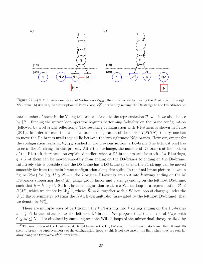
a)

N-M

(1d)

(3d)

MN-1N-2

n

1

b)

N

(1d)

(3d)

N-1p1

n

p-1

Figure 27: a) 3d/1d quiver description of Vortex loop VM,R. Here it is derived by moving the D1-strings to the right

NS5-brane. b) 3d/1d quiver description of Vortex loop V(p)R , derived by moving the D1-strings to the left NS5-brane.

total number of boxes in the Young tableau associated to the representation R, which we also denote

by |R|. Finding the mirror loop operator requires performing S-duality on the brane configuration

(followed by a left-right reflection). The resulting configuration with F1-strings is shown in figure

(28-b). In order to reach the canonical brane configuration of the mirror T [SU(N)] theory, one has

to move the D5-branes until they all lie between the two rightmost NS5-branes. However, except for

the configuration realizing VN−1,R studied in the previous section, a D5-brane (the leftmost one) has

to cross the F1-strings in this process. After this exchange, the number of D3-branes at the bottom

of the F1-stack decreases. As explained earlier, when a D5-brane crosses the stack of k F1-strings,

q ≤ k of them can be moved smoothly from ending on the D3-branes to ending on the D5-brane.

Intuitively this is possible since the D5-brane has a D3-brane spike and the F1-strings can be moved

smoothly far from the main brane configuration along this spike. In the final brane picture shown in

figure (28-c) for 0 ≤ M ≤ N − 1, the k original F1-strings are split into k strings ending on the M

D3-branes supporting the U(M) gauge group factor and q strings ending on the leftmost D5-brane,

such that k = k + q 48. Such a brane configuration realizes a Wilson loop in a representation R of

U(M), which we denote by W(M)

R, where |R| = k, together with a Wilson loop of charge q under the

U(1) flavor symmetry rotating the N -th hypermultiplet (associated to the leftmost D5-brane), that

we denote by W flN,q.

There are multiple ways of partitioning the k F1-strings into k strings ending on the D3-branes

and q F1-branes attached to the leftmost D5-brane. We propose that the mirror of VM,R with

0 ≤M ≤ N − 1 is obtained by summing over the Wilson loops of the mirror dual theory realized by

48The orientation of the F1-strings stretched between the D5/D5’ away from the main stack and the leftmost D5

seem to break the supersymmetry of the configuration, however this is not the case in the limit when they are sent far

away along the transverse x4,5,6 directions.

38

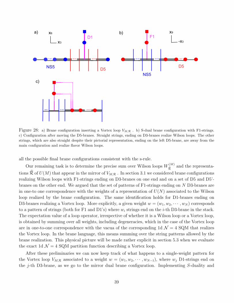
b)x6

x3

a)F1

D5

D1

NS5

x9

-x3

c)

NS5

D5

Figure 28: a) Brane configuration inserting a Vortex loop VM,R . b) S-dual brane configuration with F1-strings.

c) Configuration after moving the D5-branes. Straight strings, ending on D3-branes realize Wilson loops. The other

strings, which are also straight despite their pictorial representation, ending on the left D5-brane, are away from the

main configuration and realize flavor Wilson loops.

all the possible final brane configurations consistent with the s-rule.

Our remaining task is to determine the precise sum over Wilson loops W(M)

Rand the representa-

tions R of U(M) that appear in the mirror of VM,R . In section 3.1 we considered brane configurations

realizing Wilson loops with F1-strings ending on D3-branes on one end and on a set of D5 and D5’-

branes on the other end. We argued that the set of patterns of F1-strings ending on N D3-branes are

in one-to one correspondence with the weights of a representation of U(N) associated to the Wilson

loop realized by the brane configuration. The same identification holds for D1-branes ending on

D3-branes realizing a Vortex loop. More explicitly, a given weight w = (w1, w2, · · · , wN) corresponds

to a pattern of strings (both for F1 and D1’s) where wi strings end on the i-th D3-brane in the stack.

The expectation value of a loop operator, irrespective of whether it is a Wilson loop or a Vortex loop,

is obtained by summing over all weights, including degeneracies, which in the case of the Vortex loop

are in one-to-one correspondence with the vacua of the corresponding 1d N = 4 SQM that realizes

the Vortex loop. In the brane language, this means summing over the string patterns allowed by the

brane realization. This physical picture will be made rather explicit in section 5.3 when we evaluate

the exact 1d N = 4 SQM partition function describing a Vortex loop.

After these preliminaries we can now keep track of what happens to a single-weight pattern for

the Vortex loop VM,R associated to a weight w = (w1, w2, · · · , wN−1), where wj D1-strings end on

the j-th D3-brane, as we go to the mirror dual brane configuration. Implementing S-duality and

39

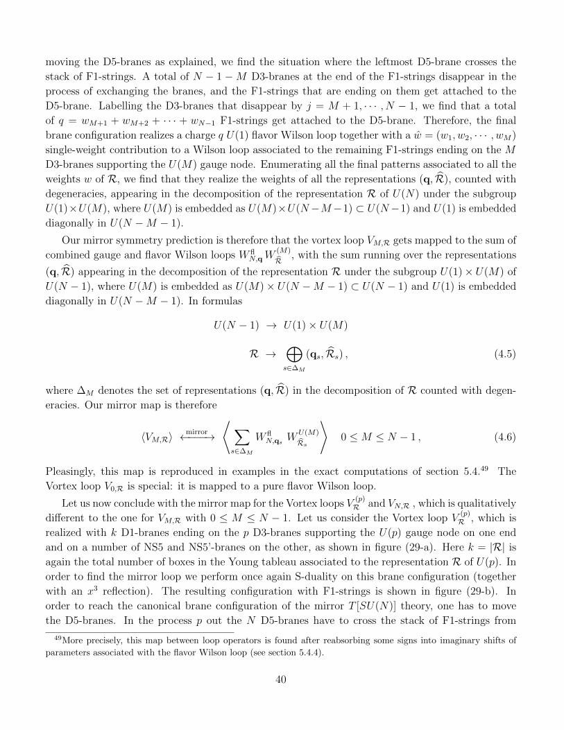
moving the D5-branes as explained, we find the situation where the leftmost D5-brane crosses the

stack of F1-strings. A total of N − 1 −M D3-branes at the end of the F1-strings disappear in the

process of exchanging the branes, and the F1-strings that are ending on them get attached to the

D5-brane. Labelling the D3-branes that disappear by j = M + 1, · · · , N − 1, we find that a total

of q = wM+1 + wM+2 + · · · + wN−1 F1-strings get attached to the D5-brane. Therefore, the final

brane configuration realizes a charge q U(1) flavor Wilson loop together with a w = (w1, w2, · · · , wM)

single-weight contribution to a Wilson loop associated to the remaining F1-strings ending on the M

D3-branes supporting the U(M) gauge node. Enumerating all the final patterns associated to all the

weights w of R, we find that they realize the weights of all the representations (q, R), counted with

degeneracies, appearing in the decomposition of the representation R of U(N) under the subgroup

U(1)×U(M), where U(M) is embedded as U(M)×U(N−M−1) ⊂ U(N−1) and U(1) is embedded

diagonally in U(N −M − 1).

Our mirror symmetry prediction is therefore that the vortex loop VM,R gets mapped to the sum of

combined gauge and flavor Wilson loops W flN,qW

(M)

R, with the sum running over the representations

(q, R) appearing in the decomposition of the representation R under the subgroup U(1)× U(M) of

U(N − 1), where U(M) is embedded as U(M)× U(N −M − 1) ⊂ U(N − 1) and U(1) is embedded

diagonally in U(N −M − 1). In formulas

U(N − 1) → U(1)× U(M)

R →⊕s∈∆M

(qs, Rs) , (4.5)

where ∆M denotes the set of representations (q, R) in the decomposition of R counted with degen-

eracies. Our mirror map is therefore

〈VM,R〉mirror←−−−→

⟨∑s∈∆M

W flN,qs W

U(M)

Rs

⟩0 ≤M ≤ N − 1 , (4.6)

Pleasingly, this map is reproduced in examples in the exact computations of section 5.4.49 The

Vortex loop V0,R is special: it is mapped to a pure flavor Wilson loop.

Let us now conclude with the mirror map for the Vortex loops V(p)R and VN,R , which is qualitatively

different to the one for VM,R with 0 ≤ M ≤ N − 1. Let us consider the Vortex loop V(p)R , which is

realized with k D1-branes ending on the p D3-branes supporting the U(p) gauge node on one end

and on a number of NS5 and NS5’-branes on the other, as shown in figure (29-a). Here k = |R| is

again the total number of boxes in the Young tableau associated to the representation R of U(p). In

order to find the mirror loop we perform once again S-duality on this brane configuration (together

with an x3 reflection). The resulting configuration with F1-strings is shown in figure (29-b). In

order to reach the canonical brane configuration of the mirror T [SU(N)] theory, one has to move

the D5-branes. In the process p out the N D5-branes have to cross the stack of F1-strings from

49More precisely, this map between loop operators is found after reabsorbing some signs into imaginary shifts of

parameters associated with the flavor Wilson loop (see section 5.4.4).

40

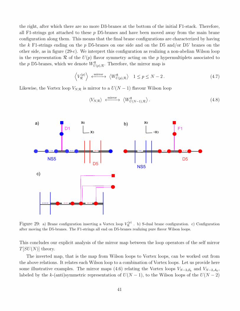
the right, after which there are no more D3-branes at the bottom of the initial F1-stack. Therefore,

all F1-strings got attached to these p D5-branes and have been moved away from the main brane

configuration along them. This means that the final brane configurations are characterized by having

the k F1-strings ending on the p D5-branes on one side and on the D5 and/or D5’ branes on the

other side, as in figure (29-c). We interpret this configuration as realizing a non-abelian Wilson loop

in the representation R of the U(p) flavor symmetry acting on the p hypermultiplets associated to

the p D5-branes, which we denote W flU(p),R. Therefore, the mirror map is⟨

V(p)R

⟩mirror←−−−→

⟨W flU(p),R

⟩1 ≤ p ≤ N − 2 . (4.7)

Likewise, the Vortex loop VN,R is mirror to a U(N − 1) flavour Wilson loop

〈VN,R〉mirror←−−−→

⟨W flU(N−1),R

⟩. (4.8)

b)x6

x3

a)F1

D5

D1

NS5

x9

-x3

c)

NS5

D5

Figure 29: a) Brane configuration inserting a Vortex loop V(p)R . b) S-dual brane configuration. c) Configuration

after moving the D5-branes. The F1-strings all end on D5-branes realizing pure flavor Wilson loops.

This concludes our explicit analysis of the mirror map between the loop operators of the self mirror

T [SU(N)] theory.

The inverted map, that is the map from Wilson loops to Vortex loops, can be worked out from

the above relations. It relates each Wilson loop to a combination of Vortex loops. Let us provide here

some illustrative examples. The mirror maps (4.6) relating the Vortex loops VN−2,Sk and VN−2,Ak ,

labeled by the k-(anti)symmetric representation of U(N − 1), to the Wilson loops of the U(N − 2)

41

node of the mirror T [SU(N)] theory, predicted from the brane picture, are

〈VN−2,Sk〉mirror←−−−→

⟨k∑k=0

W flN,k−k W

U(N−2)Sk

⟩, (4.9)

〈VN−2,Ak〉mirror←−−−→

⟨W

U(N−2)Ak +W fl

N,1 WU(N−2)Ak−1

⟩. (4.10)

Inverting these relations one obtain⟨W

U(N−2)Sk

⟩mirror←−−−→

⟨VN−2,Sk −W fl

N,1 VN−2,Sk−1

⟩, (4.11)

⟨W

U(N−2)Ak

⟩mirror←−−−→

⟨k∑k=0

(−1)k−k W flN,k−k VN−2,Ak

⟩. (4.12)

It is tempting to try to derive these relation directly from the brane picture. This would necessitate

new rules constraining the brane moves which are rather ad hoc. It could be interesting to pursue

this.

We have found an explicit map relating Vortex loop operators to gauge and flavor Wilson loop

operators. We will check these predictions by exact computations of the expectation value of the

loop operators on S3 in section 5.4.

4.4 Loops And Mirror Map In Circular Quivers

Our prescription to derive the mirror map of loop operators described in section 3 is used here to

find the mirror map for loop operators in 3d N = 4 gauge theories described by circular quivers with

equal ranks. The brane realization of this class of quivers is special: after performing S-duality, the

branes are already in the canonical brane configuration and no Hanany-Witten moves are required

to derive the mirror quiver gauge theory. This immediately implies that a Wilson loop labeled by a

representationR of the gauge group directly maps to a Vortex loop labeled by the same representation

R, and not to a sum of Vortex loop operators.

For concreteness, let us consider the circular quiver in figure 30-a, which has two U(N) gauge

group nodes U(N)a × U(N)b and L ≥ 2 fundamental hypermultiplets of U(N)b.50 The mirror dual

quiver is easily found by acting with S-duality and is shown in figure 30-b. It has gauge group∏Li=1 U(N)i and two fundamental hypermultiplets of U(N)L.

Let us first consider a Wilson loop labeled by a representation R of U(N)a, which we denote by

W(a)R . This is realized by the brane configuration in figure 31-a, where F1-strings emanate from extra

D5 and/or D5’-branes far away from the main stack and end on the N D3-branes supporting the

U(N)a gauge node. After S-duality the brane configuration is already in its canonical form to read

the mirror quiver theory. The F1-strings become D1-branes lying between the two D5-branes and

50L ≥ 2 is required for the UV gauge theory to flow to an irreducible SCFT in the IR.

42

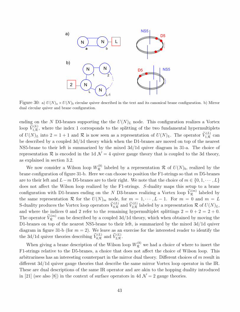
N

2N

N

N

LN N

NS5D5

NS5D5

a)

b)

a b

L

a

1

L-1

2

Figure 30: a) U(N)a ×U(N)b circular quiver described in the text and its canonical brane configuration. b) Mirror

dual circular quiver and brane configuration.

ending on the N D3-branes supporting the the U(N)L node. This configuration realizes a Vortex

loop V(L)

1,R , where the index 1 corresponds to the splitting of the two fundamental hypermultiplets

of U(N)L into 2 = 1 + 1 and R is now seen as a representation of U(N)L. The operator V(L)

1,R can

be described by a coupled 3d/1d theory which when the D1-branes are moved on top of the nearest

NS5-brane to their left is summarized by the mixed 3d/1d quiver diagram in 31-a. The choice of

representation R is encoded in the 1d N = 4 quiver gauge theory that is coupled to the 3d theory,

as explained in section 3.2.

We now consider a Wilson loop W(b)R labeled by a representation R of U(N)b, realized by the

brane configuration of figure 31-b. Here we can choose to position the F1-strings so that m D5-branes

are to their left and L−m D5-branes are to their right. We note that the choice of m ∈ {0, 1, · · · , L}does not affect the Wilson loop realized by the F1-strings. S-duality maps this setup to a brane

configuration with D1-branes ending on the N D3-branes realizing a Vortex loop V(m)R labeled by

the same representation R for the U(N)m node, for m = 1, · · · , L − 1. For m = 0 and m = L

S-duality produces the Vortex loop operators V(L)

0,R and V(L)

2,R labeled by a representation R of U(N)L,

and where the indices 0 and 2 refer to the remaining hypermultiplet splittings 2 = 0 + 2 = 2 + 0.

The operator V(m)R can be described by a coupled 3d/1d theory, which when obtained by moving the

D1-branes on top of the nearest NS5-brane to their left, is summarized by the mixed 3d/1d quiver

diagram in figure 31-b (for m = 2). We leave as an exercise for the interested reader to identify the

the 3d/1d quiver theories describing V(L)

0,R and V(L)

2,R .

When giving a brane description of the Wilson loop W(b)R we had a choice of where to insert the

F1-strings relative to the D5-branes, a choice that does not affect the choice of Wilson loop. This

arbitrariness has an interesting counterpart in the mirror dual theory. Different choices of m result in

different 3d/1d quiver gauge theories that describe the same mirror Vortex loop operator in the IR.

These are dual descriptions of the same IR operator and are akin to the hopping duality introduced

in [21] (see also [8]) in the context of surface operators in 4d N = 2 gauge theories.

43

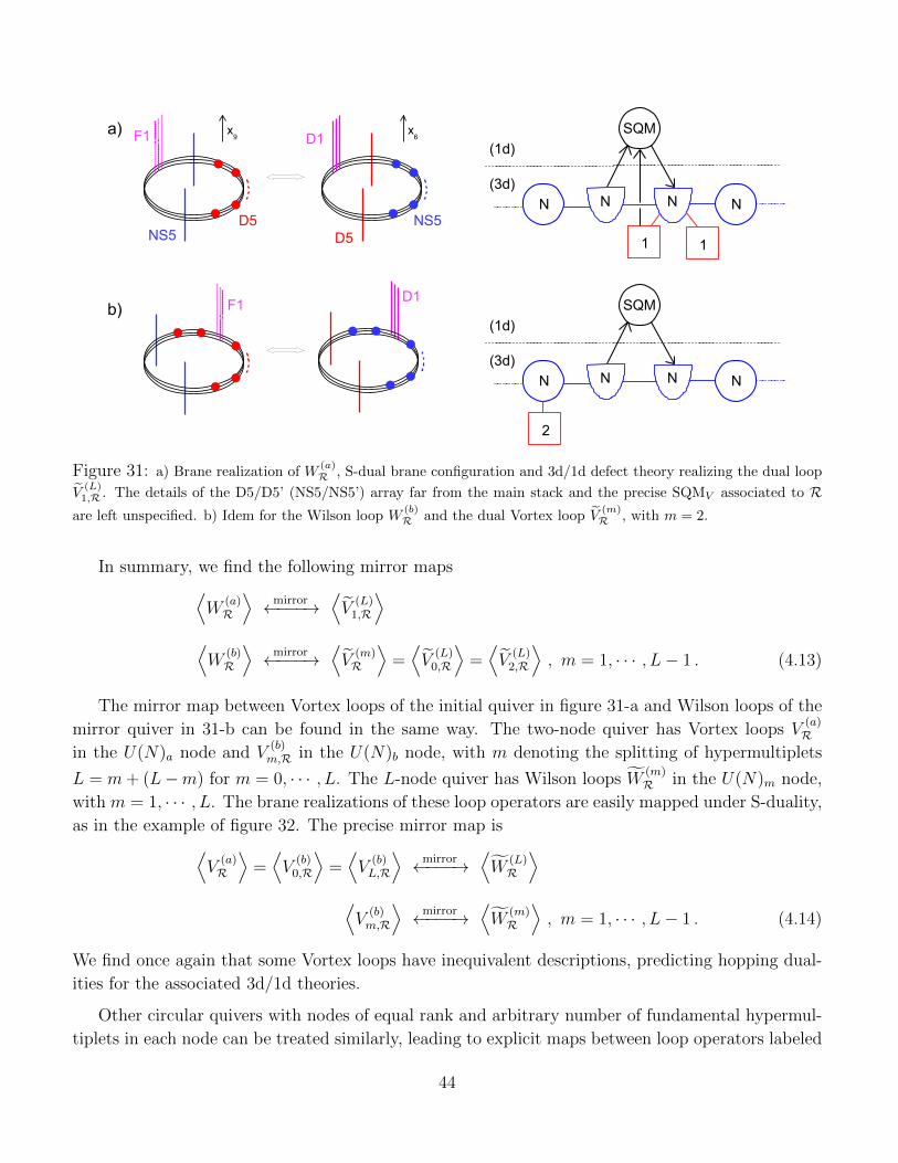
a)

b)

D1F1

D1F1

SQM

(1d)

(3d)

N

1

NN

1

N

SQM

(1d)

(3d)

N NN N

2

D5D5NS5

NS5

x9

x6

Figure 31: a) Brane realization of W(a)R , S-dual brane configuration and 3d/1d defect theory realizing the dual loop

V(L)1,R . The details of the D5/D5’ (NS5/NS5’) array far from the main stack and the precise SQMV associated to R

are left unspecified. b) Idem for the Wilson loop W(b)R and the dual Vortex loop V

(m)R , with m = 2.

In summary, we find the following mirror maps⟨W

(a)R

⟩mirror←−−−→

⟨V

(L)1,R

⟩⟨W

(b)R

⟩mirror←−−−→

⟨V

(m)R

⟩=⟨V

(L)0,R

⟩=⟨V

(L)2,R

⟩, m = 1, · · · , L− 1 . (4.13)

The mirror map between Vortex loops of the initial quiver in figure 31-a and Wilson loops of the

mirror quiver in 31-b can be found in the same way. The two-node quiver has Vortex loops V(a)R

in the U(N)a node and V(b)m,R in the U(N)b node, with m denoting the splitting of hypermultiplets

L = m+ (L−m) for m = 0, · · · , L. The L-node quiver has Wilson loops W(m)R in the U(N)m node,

with m = 1, · · · , L. The brane realizations of these loop operators are easily mapped under S-duality,

as in the example of figure 32. The precise mirror map is⟨V

(a)R

⟩=⟨V

(b)0,R

⟩=⟨V

(b)L,R

⟩mirror←−−−→

⟨W

(L)R

⟩⟨V

(b)m,R

⟩mirror←−−−→

⟨W

(m)R

⟩, m = 1, · · · , L− 1 . (4.14)

We find once again that some Vortex loops have inequivalent descriptions, predicting hopping dual-

ities for the associated 3d/1d theories.

Other circular quivers with nodes of equal rank and arbitrary number of fundamental hypermul-

tiplets in each node can be treated similarly, leading to explicit maps between loop operators labeled

44

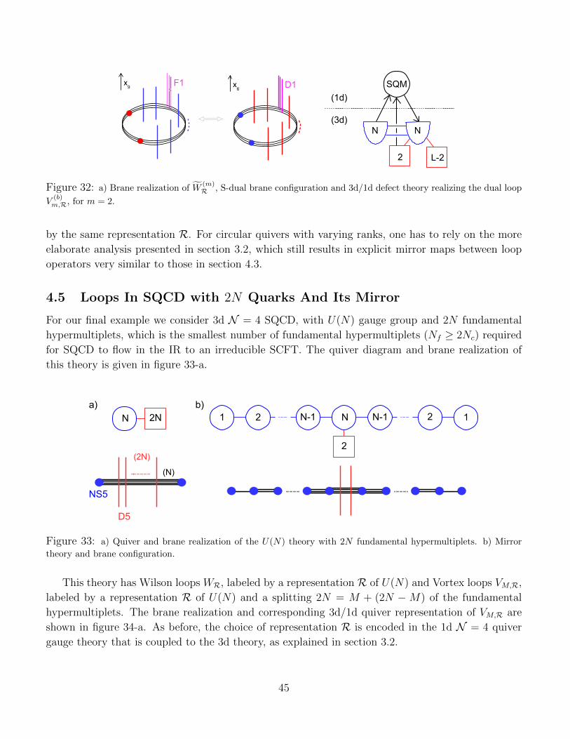
D1 SQM

(1d)

(3d)

2

NN

L-2

x9 x

6F1

Figure 32: a) Brane realization of W(m)R , S-dual brane configuration and 3d/1d defect theory realizing the dual loop

V(b)m,R, for m = 2.

by the same representation R. For circular quivers with varying ranks, one has to rely on the more

elaborate analysis presented in section 3.2, which still results in explicit mirror maps between loop

operators very similar to those in section 4.3.

4.5 Loops In SQCD with 2N Quarks And Its Mirror

For our final example we consider 3d N = 4 SQCD, with U(N) gauge group and 2N fundamental

hypermultiplets, which is the smallest number of fundamental hypermultiplets (Nf ≥ 2Nc) required

for SQCD to flow in the IR to an irreducible SCFT. The quiver diagram and brane realization of

this theory is given in figure 33-a.

2NN

a) b)

D5

NS5

(2N) 2

1 2 N-1 N 2N-1 1

(N)

Figure 33: a) Quiver and brane realization of the U(N) theory with 2N fundamental hypermultiplets. b) Mirror

theory and brane configuration.

This theory has Wilson loops WR, labeled by a representation R of U(N) and Vortex loops VM,R,

labeled by a representation R of U(N) and a splitting 2N = M + (2N −M) of the fundamental

hypermultiplets. The brane realization and corresponding 3d/1d quiver representation of VM,R are

shown in figure 34-a. As before, the choice of representation R is encoded in the 1d N = 4 quiver

gauge theory that is coupled to the 3d theory, as explained in section 3.2.

45

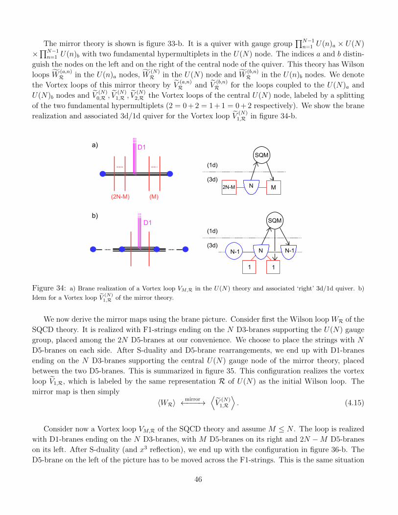
The mirror theory is shown is figure 33-b. It is a quiver with gauge group∏N−1

n=1 U(n)a × U(N)

×∏N−1

n=1 U(n)b with two fundamental hypermultiplets in the U(N) node. The indices a and b distin-

guish the nodes on the left and on the right of the central node of the quiver. This theory has Wilson

loops W(a,n)R in the U(n)a nodes, W

(N)R in the U(N) node and W

(b,n)R in the U(n)b nodes. We denote

the Vortex loops of this mirror theory by V(a,n)R and V

(b,n)R for the loops coupled to the U(N)a and

U(N)b nodes and V(N)

0,R , V(N)

1,R , V(N)

2,R the Vortex loops of the central U(N) node, labeled by a splitting

of the two fundamental hypermultiplets (2 = 0 + 2 = 1 + 1 = 0 + 2 respectively). We show the brane

realization and associated 3d/1d quiver for the Vortex loop V(N)

1,R in figure 34-b.

a)

b)

(2N-M) (M)

D1SQM

(1d)

(3d)2N-M N M

D1 SQM

(1d)

(3d)

1

N-1N

1

N-1

Figure 34: a) Brane realization of a Vortex loop VM,R in the U(N) theory and associated ‘right’ 3d/1d quiver. b)

Idem for a Vortex loop V(N)1,R of the mirror theory.

We now derive the mirror maps using the brane picture. Consider first the Wilson loop WR of the

SQCD theory. It is realized with F1-strings ending on the N D3-branes supporting the U(N) gauge

group, placed among the 2N D5-branes at our convenience. We choose to place the strings with N

D5-branes on each side. After S-duality and D5-brane rearrangements, we end up with D1-branes

ending on the N D3-branes supporting the central U(N) gauge node of the mirror theory, placed

between the two D5-branes. This is summarized in figure 35. This configuration realizes the vortex

loop V1,R, which is labeled by the same representation R of U(N) as the initial Wilson loop. The

mirror map is then simply

〈WR〉mirror←−−−→

⟨V

(N)1,R

⟩. (4.15)

Consider now a Vortex loop VM,R of the SQCD theory and assume M ≤ N . The loop is realized

with D1-branes ending on the N D3-branes, with M D5-branes on its right and 2N −M D5-branes

on its left. After S-duality (and x3 reflection), we end up with the configuration in figure 36-b. The

D5-brane on the left of the picture has to be moved across the F1-strings. This is the same situation

46

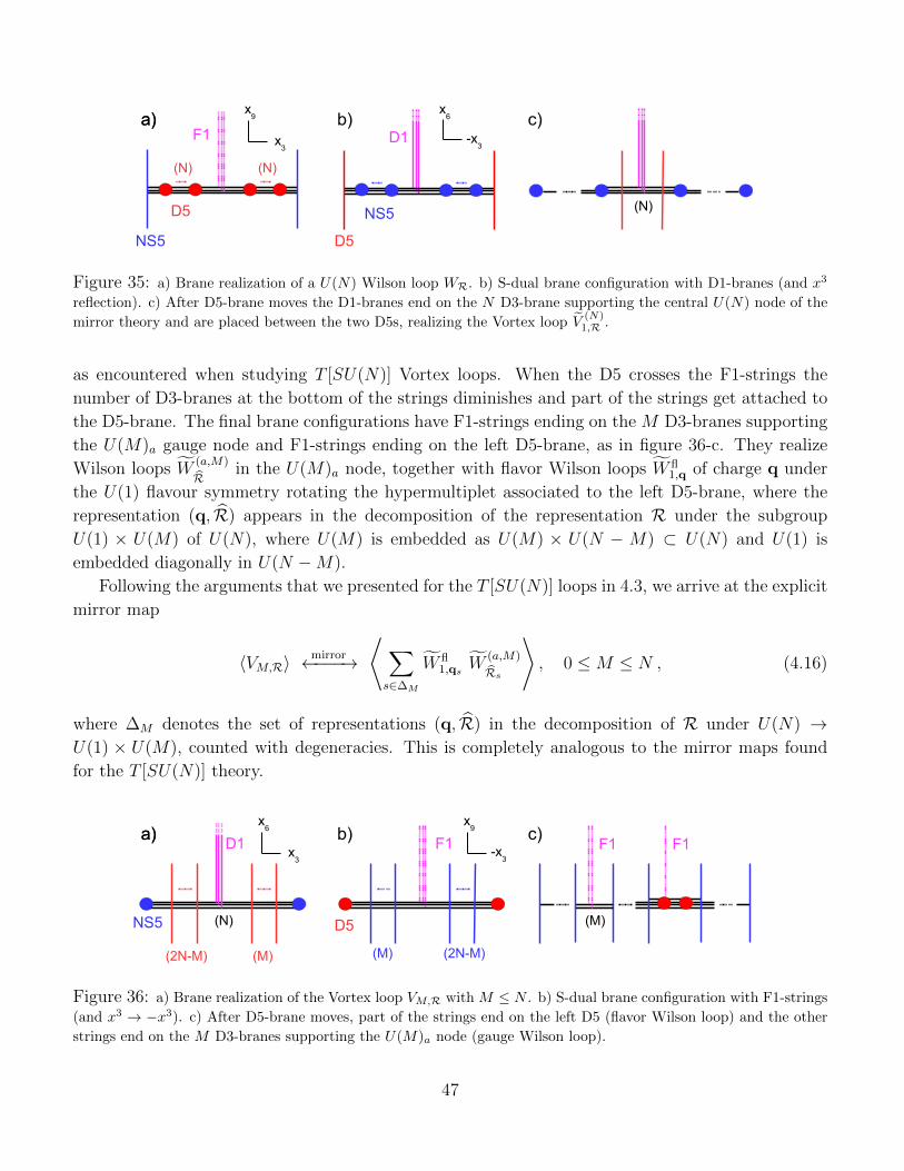
(N) (N)

F1 D1

D5

NS5

a) b)a) c)x

9

x3

x6

-x3

D5

NS5 (N)

Figure 35: a) Brane realization of a U(N) Wilson loop WR. b) S-dual brane configuration with D1-branes (and x3

reflection). c) After D5-brane moves the D1-branes end on the N D3-brane supporting the central U(N) node of the

mirror theory and are placed between the two D5s, realizing the Vortex loop V(N)1,R .

as encountered when studying T [SU(N)] Vortex loops. When the D5 crosses the F1-strings the

number of D3-branes at the bottom of the strings diminishes and part of the strings get attached to

the D5-brane. The final brane configurations have F1-strings ending on the M D3-branes supporting

the U(M)a gauge node and F1-strings ending on the left D5-brane, as in figure 36-c. They realize

Wilson loops W(a,M)

Rin the U(M)a node, together with flavor Wilson loops W fl

1,q of charge q under

the U(1) flavour symmetry rotating the hypermultiplet associated to the left D5-brane, where the

representation (q, R) appears in the decomposition of the representation R under the subgroup

U(1) × U(M) of U(N), where U(M) is embedded as U(M) × U(N − M) ⊂ U(N) and U(1) is

embedded diagonally in U(N −M).

Following the arguments that we presented for the T [SU(N)] loops in 4.3, we arrive at the explicit

mirror map

〈VM,R〉mirror←−−−→

⟨∑s∈∆M

W fl1,qs W

(a,M)

Rs

⟩, 0 ≤M ≤ N , (4.16)

where ∆M denotes the set of representations (q, R) in the decomposition of R under U(N) →U(1) × U(M), counted with degeneracies. This is completely analogous to the mirror maps found

for the T [SU(N)] theory.

(2N-M) (M)

D1 F1

(N) D5NS5 (M)

F1F1a) b)a) c)

x6

x3

x9

-x3

(2N-M) (M)

Figure 36: a) Brane realization of the Vortex loop VM,R with M ≤ N . b) S-dual brane configuration with F1-strings

(and x3 → −x3). c) After D5-brane moves, part of the strings end on the left D5 (flavor Wilson loop) and the other

strings end on the M D3-branes supporting the U(M)a node (gauge Wilson loop).

47

The map relating the Vortex loops VM,R with M ≥ N to combinations of Wilson loops W fl2,qW

b,M

Ris found similarly, with W fl

2,q denoting a flavor Wilson loop of charge q under the U(1) flavour

symmetry rotating the hypermultiplet associated to the right D5-brane this time. Note that the

‘central’ Vortex loop VN,R is directly mapped to the Wilson loop W(N)R of the central node of the

mirror theory:

〈VN,R〉mirror←−−−→

⟨W

(N)R

⟩. (4.17)

The only loops we did not discuss thus far are the Vortex loops V(a,n)R , V

(b,n)R of the U(n)a and

U(n)b nodes of the mirror theory, and the V(N)

0,R , V(N)

2,R Vortex loops of the central U(N) node, which

can be naturally renamed as V(a,N)R and V

(b,N)R respectively. The analysis of the brane realization of

these loops is the same as for the Vortex loops V(p)R of the T [SU(N)] theory (see section 4.3) and

lead to the conclusion that these loops are mapped to flavor Wilson loops. In particular⟨V

(a,n)R

⟩=⟨W flU(n)F ,R

⟩, n = 1, · · · , N , (4.18)⟨

V(b,n)R

⟩=⟨W flU(n)F ′ ,R

⟩, n = 1, · · · , N , (4.19)

where U(n)F is the flavor group acting on the n hypermultiplets associated to the n leftmost D5-

branes, U(n)F ′ is the flavor group acting on the n hypermultiplets associated to the n rightmost

D5-branes and W flU(n),R denotes a flavor Wilson loop in the representation R of U(n).

This completes the derivation of the mirror map between the loops of the U(N) theory with 2N

fundamental hypermultiplets and its mirror dual. The analysis generalizes easily to the U(N) theory

with Nf ≥ 2N fundamental hypermultiplets.

5 Loop Operators In 3d N = 4 Theories On S3

In this section we provide explicit quantitative evidence for our proposed action of mirror symmetry

on loop operators by computing the exact expectation value of supersymmetric loop operators on

S3 in 3d N = 4 gauge theories. We confirm our proposal for the action of mirror symmetry on loop

operators by showing that the expectation value of mirror loop operators match perfectly and indeed

give alternative UV descriptions of superconformal line defects in the IR SCFT.

Our first task is to define these observables in N = 4 theories on S3, where exact computations

can be performed by supersymmetric localization. Recall that in R3 the UV Lagrangian definition

of a 3d N = 4 SCFT is invariant under those supercharges in OSp(4|4) that close into the isometries

of flat space, which generate the 3d N = 4 super-Poincare algebra.51 While an N = 4 SCFT can

be placed canonically on the round S3 by stereographic projection, its UV Lagrangian description

likewise breaks OSp(4|4) to a subalgebra, which we now identify. On S3, the supersymmetries of a

generic UV (massive) 3d N = 4 theory are generated by the supercharges in OSp(4|4) that close into

51Super-Euclidean in R3.

48

the SU(2)l × SU(2)r isometries of S3 and project out the remaining SO(4, 1) conformal generators

on S3. Since we allow arbitrary massive deformations, and mass and FI parameters transform in

the (3,1) and (1,3) representations of SU(2)C × SU(2)H , the R-symmetry in OSp(4|4) is broken

down to its Cartan subalgebra on S3. Under the SU(2)l × SU(2)r × U(1)C × U(1)H embedding in

SO(4, 1)×SU(2)C×SU(2)H , the supercharges generating OSp(4|4), which transform in the (4,2,2),

decompose as (2,1)++ ⊕ (2,1)+− ⊕ (2,1)−+ ⊕ (2,1)−− ⊕ (1,2)++ ⊕ (1,2)−− ⊕ (1,2)−+ ⊕ (1,2)−−.

The supersymmetries preserved by a UV 3d N = 4 theory on S3 are (2,1)++⊕ (2,1)−−⊕ (1,2)+−⊕(1,2)−+. These supercharges generate the following supergroup52

SU(2|1)l × SU(2|1)r . (5.1)

The U(1)l generator in SU(2|1)l is RC +RH while the U(1)r generator in SU(2|1)l is RH−RC , where

RC and RH are the Cartan generators of SU(2)C and SU(2)H respectively. The isometries of S3 are

SU(2)l×SU(2)r. Explicitly, the anticommutators of the SU(2|1)l×SU(2|1)r supercharges on an S3

of radius L are

{Ql α, Ql β} =2

L

[(γaC−1

)αβJ la +

1

2εαβ (RC +RH)

](5.2)

{Qr α, Qr β} =2

L

[(γaC−1

)αβJra +

1

2εαβ (RC −RH)

], (5.3)

where J la and Jra generate SU(2)l and SU(2)r respectively.

In the flat space L → ∞ limit, the SU(2|1)l × SU(2|1)r symmetry on the S3 contracts to the

3d N = 4 super-Poincare symmetry. Indeed, writing J la = 12(Ja + LPa) and Jra = 1

2(Ja − LPa), and

taking the flat space limit we get

{Q∞l α, Q∞l β} =

(γaC−1

)αβPa (5.4)

{Q∞r α, Q∞r β} = −

(γaC−1

)αβPa , (5.5)

where Pa and Ja are the translation and rotation generators of R3. Comparing with the 3d N = 4

super-Poincare supercharges QαAA′ in (2.1) we find the identification: Q∞l α = Qα22, Q∞l α = Qα11,

Q∞r α = Qα21 and Q∞r α = Qα12.

The SU(2|1)l supersymmetry transformations are generated by Killing spinors εl and εl on S3

obeying [17]53

∇µεl =i

2Lγµεl ∇µεl =

i

2Lγµεl , (5.6)

while SU(2|1)r transformations are generated by Killing spinors εr and εr on S3 which satisfy [39]

∇µεr = − i

2Lγµεr ∇µεr = − i

2Lγµεr . (5.7)

52This supersymmetry is the fixed locus of an involution in OSp(4|4).53All these Killing spinors are the subset of conformal Killing spinors on S3, which obey ∇µεAA′ = 1

3γµ /∇εAA′ , that

project out the conformal generators on S3.

49

From the viewpoint of off-shell supersymmetric supergravity backgrounds [40], these Killing spinor

equations arise from 3d N = 4 supergravity in the presence of a background auxiliary field.54 The

superisometry of this supergravity background is SU(2|1)l × SU(2|1)r.

We take the left-invariant frame ea = Lµa, a = 1, 2, 3, where the left-invariant one-forms of SU(2)

are defined by g−1dg = iµaτa with g =

(z1 z2

−z2 z1

)so that det g = 1. In this frame εl and εl are

constant while εr and εr are given by εr = g−1ε0, εr = g−1ε0, with ε0, ε0 constant.55

The explicit 3dN = 4 supersymmetric Lagrangians on S3 can be written down using the formulae

for 3d N = 2 gauge theories on S3 in [17, 39, 42–44], which are invariant under SU(2|1)l × SU(2)r.

We first decompose the N = 4 vector multiplet and hypermultiplet into N = 2 vector and chiral

multiplets. By assigning U(1)l charge 1 and 1/2 to the chiral multiplets inside an N = 4 vector

multiplet and hypermultiplet respectively, the supersymmetry of such an N = 2 theory on S3 is

enhanced with extra four supercharges [39], which generate the remaining SU(2|1)r. Just as in flat

space, 3d N = 4 theories on S3 admit canonical relevant deformations associated to the GC × GH

symmetries of the IR SCFT. These are introduced by turning on SU(2|1)l × SU(2|1)r invariant

background vector and twisted vector multiplets on S3 for GH and GC respectively. Supersymmetric

backgrounds for 3d N = 4 vector and twisted vector multiples on S3 allow a single scalar in the

multiplet to be turned on, instead of the triplet of parameters in flat space. Therefore on S3 there is

a single mass parameter and a single FI for each Cartan generator in GH and GC respectively.

Following a similar analysis to the one in flat space in section 2, there are two inequivalent

classes of half-supersymmetric line operators that can be defined in a UV description of a 3d N = 4

SCFT on S3. They are characterised by two different embeddings of SU(1|1)l × SU(1|1)r inside

SU(2|1)l×SU(2|1)r. One class corresponds to supersymmetric Wilson loop operators and the other

to Vortex loop operators on S3.

5.1 Wilson Loops On S3

Consider a Wilson loop operator wrapping a curve γ ∈ S3

TrRP exp

∮γ

(iAµxµ − |x|σ) dτ (5.8)

in a 3d N = 4 gauge theory, where σ is the scalar field in the N = 2 vector multiplet inside the

N = 4 vector multiplet. This operator preserves the SU(2|1)l × SU(2|1)r Killing spinors that are

solutions to the following equations on S3 (see appendix A)56

(γµxµ − |x|) εl = 0 (γµx

µ + |x|) εl = 0 (5.9)

(γµxµ − |x|) εr = 0 (γµx

µ + |x|) εr = 0 . (5.10)

54The background fields in supergravity and conformal compensators are very similar to those required to put 4d

N = 2 theories on S4, see [41].55We note that all Killing spinors generating SU(2|1)l × SU(2|1)r are periodic along the Hopf circle.56These equations hold at the position of the loop.

50

By a choice of parametrization of the loop γ ∈ S3 we can always make |x| = 1. Since in the SU(2)lleft-invariant frame the Killing spinors εl and εl are constant, imposing that the Wilson loop preserves

half of the supercharges in SU(2|1)l requires that

xµ = naeµa , (5.11)

where na is a constant unit three-vector nana = 1. A Wilson loop wrapping the curve xµ = naeµa on

S3 preserves the following half of the SU(2|1)l supersymmetries

γanaεl = εl γan

aεl = −εl . (5.12)

The integral curves of the vector field xm = naema are great circles on S3. The choice of unit vector

na determines a Hopf fibration. Therefore, there is an S2 = SU(2)/U(1) worth of choices of Hopf

fibrations. Given a choice of Hopf fibration, there is another S2 = SU(2)/U(1) worth of Hopf circles,

labeled by the point on S2 where the Hopf fiber sits. This realizes the space of maximal circles on

S3 as SO(4)/U(1)×U(1) = S2 × S2. Note also that all circles in a choice of Hopf fibration preserve

the same supersymmetry in SU(2|1)l.

Without loss of generality we take na = (0, 0, 1). The Hopf circle preserves J l3 generating U(1)l ⊂SU(2)l and the SU(2|1)l supersymetries

γ3εl = εl γ3εl = −εl . (5.13)

The Hopf circle, which is labeled by a point on S2, also preserves U(1)r ⊂ SU(2)r. A Wilson loop

supported on this Hopf circle preserves the following supersymmetries in SU(2|1)r

γ3εr = εr γ3εr = −εr , (5.14)

where εr and εr are non-constant spinors in the left-invariant frame. We can without loss of generality

take the loop at the North or South pole of S2, in which case U(1)r is generated by Jr3 . For another

Hopf circle at a different point in S2, which can be obtained by the action of an isometry, the

preserved U(1)r and supersymmetry generators are obtained from those at the poles by conjugating

by the action of the isometry.

In summary, the Wilson loop (5.8) wrapping the Hopf circle at the North pole of S2 is half-

supersymmetric in a 3d N = 4 theory on S3. It preserves an SU(1|1)l × SU(1|1)r inside the

SU(2|1)l × SU(2|1)r supersymmetry of a 3d N = 4 theory on S3. The explicit supersymmetry

algebra of the Wilson loop is

{ql, ql} =2

L

[J l3 −

1

2(RC +RH)

](5.15)

{qr, qr} =2

L

[Jr3 −

1

2(RC −RH)

]. (5.16)

The insertion of this Wilson loop on S3 can be also realized by coupling the 1d N = 4 fermi multiplet

localized on the Hopf circle to the 3d N = 4 theory on S3. Putting the 1d gauged fermi multiplet

theory on S3 while preserving SU(1|1)l × SU(1|1)r is trivial as there are no 1/L modifications to

the 1d gauged fermi theory in flat space. Integrating out the fermi multiplet inserts the Wilson loop

operator (5.8).

51

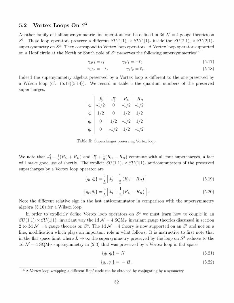
5.2 Vortex Loops On S3

Another family of half-supersymmetric line operators can be defined in 3d N = 4 gauge theories on

S3. These loop operators preserve a different SU(1|1)l × SU(1|1)r inside the SU(2|1)l × SU(2|1)rsupersymmetry on S3. They correspond to Vortex loop operators. A Vortex loop operator supported

on a Hopf circle at the North or South pole of S3 preserves the following supersymmetries57

γ3εl = εl γ3εl = −εl (5.17)

γ3εr = −εr γ3εr = εr , (5.18)

Indeed the supersymmetry algebra preserved by a Vortex loop is different to the one preserved by

a Wilson loop (cf. (5.13)(5.14)). We record in table 5 the quantum numbers of the preserved

supercharges.

J l3 Jr3 RC RH

ql -1/2 0 -1/2 -1/2

ql 1/2 0 1/2 1/2

qr 0 1/2 -1/2 1/2

qr 0 -1/2 1/2 -1/2

Table 5: Supercharges preserving Vortex loop.

We note that J l3 − 12(RC + RH) and Jr3 + 1

2(RC − RH) commute with all four supercharges, a fact

will make good use of shortly. The explicit SU(1|1)l × SU(1|1)r anticommutators of the preserved

supercharges by a Vortex loop operator are

{ql, ql} =2

L

[J l3 −

1

2(RC +RH)

](5.19)

{qr, qr} =2

L

[Jr3 +

1

2(RC −RH)

]. (5.20)

Note the different relative sign in the last anticommutator in comparison with the supersymmetry

algebra (5.16) for a Wilson loop.

In order to explicitly define Vortex loop operators on S3 we must learn how to couple in an

SU(1|1)l×SU(1|1)r invariant way the 1d N = 4 SQMV invariant gauge theories discussed in section

2 to 3d N = 4 gauge theories on S3. The 1d N = 4 theory is now supported on an S1 and not on a

line, modification which plays an important role in what follows. It is instructive to first note that

in the flat space limit where L→∞ the supersymmetry preserved by the loop on S3 reduces to the

1d N = 4 SQMV supersymmetry in (2.3) that was preserved by a Vortex loop in flat space

{ql, ql} = H (5.21)

{qr, qr} = −H , (5.22)

57A Vortex loop wrapping a different Hopf circle can be obtained by conjugating by a symmetry.

52

where the sphere generators J l3 = 12(J12+LH) and Jr3 = 1

2(J12−LH) become the translation generator

H and transverse rotation generator J12 in flat space.

Coupling a 1d N = 4 SQMV gauge theory on the loop to a 3d N = 4 theory on S3 requires

turning on background fields in the 1d N = 4 theory in order to make the 3d/1d theory invariant

under the SU(1|1)l × SU(1|1)r supersymmetry algebra of the Vortex loop. This is not surprising.

Placing a 3d N = 4 gauge theory on S3 deforms the flat space supersymmetry transformations and

action. Both modifications can be interpreted as arising from background 3d N = 4 supergravity

fields [40]. We now show that the 1d N = 4 supersymmetry transformations and action can be

deformed in such a way as to yield a supersymmetric Vortex loop operator on S3.

The starting point is the SQMV supersymmetry algebra discussed in section 2

{Q+, Q+} = H {Q−, Q−} = H . (5.23)

In order to couple the 1d N = 4 theory on S3 supersymmetrically we must deform the 1d N = 4

theory in such a way that the supersymmetry algebra becomes the SU(1|1)l × SU(1|1)r algebra of

the Vortex loop on S3

{ql, ql} =2

L

[J l3 −

1

2(RC +RH)

](5.24)

{qr, qr} =2

L

[Jr3 +

1

2(RC −RH)

]. (5.25)

This can be accomplished in two steps:

• Turning on a fixed background gauge field for the R-symmetry J− ≡ J l3 + Jr3 −RC

• Turning on a fixed imaginary mass parameter for the flavour symmetry GF ≡ J l3 + Jr3 −RH

GF does indeed commute with all four supercharges, as it is the sum of the bosonic generators in

(5.19) and (5.20), both of which are central elements. The charge J− commutes with ql and ql but

not with qr and qr. We also use in an important way that the 1d N = 4 theory lives on an S1 and

non-trivial Wilson lines can be turned on around the circle. Deforming the 1d N = 4 theory by these

backgrounds allows to couple a 1d N = 4 theory on a Hopf circle to a 3d N = 4 theory on S3 while

preserving SU(1|1)l × SU(1|1)r.

The SQMV supersymmetry algebra (5.23) gets deformed in the presence of a background 1d

N = 4 vector multiplet for a flavour symmetry G. We consider a background gauge field a on S1 and

a background scalar field in the vector multiplet corresponding to a real mass m.58 The deformed

SQMV algebra becomes59

{Q+, Q+} = H − (a+ im)G {Q−, Q−} = H − (a− im)G . (5.26)

H is the generator of translations on the circle, which we take to have length β = 2πL.

58Turning on a complex mass associated to the other two scalars in the vector multiplet deforms other commutators.59This can be easily understood by dimensional reduction of the 4d N = 1 supersymmetry algebra.

53

Turning on a background gauge field for the R-symmetry J− generically breaks the supersymme-

tries associated to the supercharged Q− and Q− charged under J−. However for quantized values of

the gauge field a− = nL

, n ∈ Z, supersymmetry remains unbroken with Q− and Q− generated by the

non-constant Killing spinors ε− = einτL and ε− = e−i

nτL , with τ ∈ [0, 2πL] parametrizing S1.60 For

these quantized holonomies, the supersymmetry algebra is deformed in the same way as if it were a

flavor symmetry. In conclusion, turning on the following background fields for J− and GF

J− : a = − 1

Lm = 0

GF : a = 0 m =i

L, (5.27)

the SQMV algebra (5.23) becomes the SU(1|1)l×SU(1|1)r supersymmetry preserved by a line defect

in a 3d N = 4 theory on S3. We can identify the generators as follows:61

Q+ = ql , Q+ = ql , Q− = qr , Q− = −qr (5.28)

H = − 2

LJ3r , J± = ∓(J3

l + J3r )−RC , GF = J3

l + J3r −RH (5.29)

Consistently with the deformation by the R-symmetry gauge field a− = − 1L

, we find that the Killing

spinors generating qr and qr behave at the position of the loop as ε− = eiτL and ε− = e−

iτL , respectively.

Note that these position dependent Killing spinors are nevertheless periodic along the Hopf circle.

The background fields (5.27) ensure that the 1d N = 4 theory living on a maximal circle of S3

can be coupled supersymmetrically to the bulk 3d N = 4 theory. This can also be understood by

looking at the 3d N = 4 supersymmetry transformations of the vector multiplet and hypermultiplet

on S3 generated by the four Killing spinors preserving the Vortex loop. These transformations

decompose into SQMV supersymmetry transformations deformed by the advertised background. To

couple the bulk theory to SQMV , preserving the four supercharges, it is then required to turn on this

background in the SQMV supersymmetry transformations and Lagrangian. The derivation of how

the supersymmetry transformations on S3 decompose is presented in appendix A.

The presence of these background fields can be recast, upon field redefinition, into twisted bound-

ary conditions for the fields in the 1d N = 4 theory around S1, thus affecting the partition function

(or supersymmetric index) of the 1d N = 4 theory. This will play a crucial role in the evaluation of

the expectation value of Vortex loop operators in section 5.3.

Having defined the half-supersymmetric Wilson and Vortex loop operators on S3, we now propose

to evaluate their expectation values exactly, using the results of supersymmetric localization and to

test the mirror symmetry predictions of section 4.

60This can be understood as follows. The constant gauge field a− can be absorbed into a redefinition of the fields

φ′ = e−ir−a−τφ, with r− the J−-charge of φ. The non-standard periodicity of the fields around S1 are then preserved

by the supersymmetry transformations generated with ε− = eia−τ and ε− = e−ia−τ . These spinors are globally defined

only for a− = nL , with n ∈ Z.

61In the flat space limit, the R-symmetry generators J± are identified with ∓J12 − RC . They are related to the

generators J± presented in section 2 by a shift by the flavor symmetry generator J12 − RH , which is the flat space

limit of GF .

54

5.3 Exact Partition Function Of 3d/1d Theories On S3

In this section we identify the matrix integral representation of the exact expectation value of a

half-supersymmetric Vortex (and Wilson) loop operator in an N = 4 theory on S3, which takes into

account the coupling of 1d N = 4 SQM on S1 to the N = 4 theory on S3 described in the previous

section. This matrix model model is obtained by combining in an interesting way the matrix integral

computing the S3 partition function of N = 4 theory on S3 [17] and the matrix model representation

of the supersymmetric index of 1d N = 4 SQM found in [18,19].

5.3.1 S3 Partition Function And Wilson loops

A powerful probe of the dynamics of a strongly coupled 3d N = 4 IR SCFT emerging at the endpoint

of an RG flow from a UV 3d N = 4 supersymmetric gauge theory is the partition function of the

gauge theory on S3. The S3 partition function is a renormalization group invariant observable, and

the computation performed in the UV exactly captures the partition function of the IR SCFT.

The S3 partition function of 3d N = 4 gauge theories can be localized to a finite dimensional

matrix integral [17]. The matrix integral is defined by integrating over the Cartan subalgebra of

the gauge group the product of the classical and one-loop contributions in the (exact) saddle point

analysis [17]

ZMM =1

|W|

∫C

dσ Zclass · Zvector · Zhyper , (5.30)

where W is the Weyl group and C is the contour of integration. The classical contribution depends

on the FI parameter η for each abelian gauge group factor

Zclass = e2πiηTrσ . (5.31)

The 3d N = 4 vector multiplet contribution is

Zvector =∏α>0

sh(α · σ)2 , (5.32)

while a hypermultiplet in a representation R of the gauge group with mass m yields

Zhyper =∏w∈R

1

ch(w · σ −m), (5.33)

where α are the roots of the Lie algebra and w the weights for the representation. Throughout we

use the following short-hand notation (borrowed from [15])

sh(x) ≡ 2 sinh(πx) ch(x) ≡ 2 cosh(πx) , th(x) ≡ tanh(πx) . (5.34)

In this paper we focus on gauge theories with unitary gauge groups. For a U(N) gauge group

the set of eigenvalues is {σi}1≤i≤N and |W| = N !. The vector multiplet and massive fundamental

hypermulptiplet factors are expressed in this case by

Zvector =∏i<j

sh(σi − σj)2 , Zhyper =N∏j=1

ch(σj −m)−1 (5.35)

55

By combining these building blocks the exact S3 partition function of an arbitrary 3d N = 4 gauge

theory acquires an elegant matrix model representation.

The contour of integration C of the matrix model that arises from the localization computation is

the real axis. The condition that the matrix integral over the real axis is convergent [14] is precisely

the same as the criterion for the quiver theory to be “good” or “ugly” [29], that is that for each

U(N) gauge group factor the number of fundamental hypermultiplets Nf obeys Nf ≥ 2N−1. In this

paper we have considered gauge theories that flow in the IR to an irreducible SCFT, so the matrix

models (in the absence of Wilson loops) are convergent.

The exact expectation value of the supersymmetric Wilson loop (5.8) is computed by inserting

into the matrix model of the theory (5.30) the factor

TrR

(e2πσ

)=∑w∈R

e2πw·σ , (5.36)

where R is the representation associated to the Wilson loop and w runs over the weights of R.

Wilson loops expectation values are in addition normalized by the partition function.

We note that the matrix integrals defined over the real contour capturing the expectation value

of Wilson loops can become divergent when the charge of the Wilson loop is sufficiently large. For

these superficially divergent matrix models we regulate the divergent integrals by deforming the

contour of integration C of the matrix model away from the real axis. The results that we find

using the deformed contours are completely consistent with our mirror symmetry predictions. It

may be possible to justify these deformed contours of integration for the divergent matrix integrals

by carefully performing the localization computation.

More precisely, for positive FI parameter η > 0, we deform the contour of integration of each

eigenvalue so that it encloses the poles of the matrix model integrand in the upper half-plane, as

in figure 37. This is then the same as closing the real line with a semi-circle going through +i∞.

Conversely if η < 0 we close the contour so that it encloses the poles in the lower half-plane. These

choices of contour lead to finite results for arbitrary large values of the Wilson loop charge, as long

as η 6= 0. For each matrix eigenvalue the Wilson loop charge q combines with the FI parameter η in

a complex parameter η + iq and the evaluation of the integral with our prescription coincides with

the analytic continuation to the complex value of the FI parameter.

5.3.2 1d N = 4 Supersymmetric Quantum Mechanics Partition Function

In this section we introduce and evaluate the partition function of the 1d N = 4 SQM quiver gauge

theories on a circle relevant for the description of Vortex loop operators in 3d N = 4 gauge theories.

The 1d N = 4 SQM partition function admits a Hilbert space interpretation as an index with

fugacities (or chemical potentials). It is defined as a trace over the Hilbert space of the theory [45]

I(z, µ) = TrH (−1)F e2πizJ− e2πiµΠ , (5.37)

where F is the fermion number, z is a chemical potential for the U(1)− R-symmetry with generator

J− and µ = {µj} is a collection of chemical potentials for flavor symmetries with Cartan generators

56

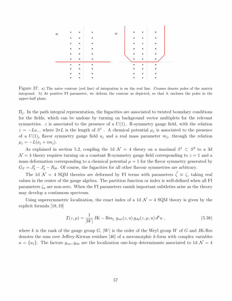
a) b)

Figure 37: a) The naive contour (red line) of integration is on the real line. Crosses denote poles of the matrix

integrand. b) At positive FI parameter, we deform the contour as depicted, so that it encloses the poles in the

upper-half plane.

Πj. In the path integral representation, the fugacities are associated to twisted boundary conditions

for the fields, which can be undone by turning on background vector multiplets for the relevant

symmetries. z is associated to the presence of a U(1)− R-symmetry gauge field, with the relation

z = −La−, where 2πL is the length of S1 . A chemical potential µj is associated to the presence

of a U(1)j flavor symmetry gauge field aj and a real mass parameter mj, through the relation

µj = −L(aj + imj).

As explained in section 5.2, coupling the 1d N = 4 theory on a maximal S1 ⊂ S3 to a 3d

N = 4 theory requires turning on a constant R-symmetry gauge field corresponding to z = 1 and a

mass deformation corresponding to a chemical potential µ = 1 for the flavor symmetry generated by

GF = J l3 − Jr3 −RH . Of course, the fugacities for all other flavour symmetries are arbitrary.

The 1d N = 4 SQM theories are deformed by FI terms with parameters ~ζ ≡ ζ, taking real

values in the center of the gauge algebra. The partition function or index is well-defined when all FI

parameters ζa are non-zero. When the FI parameters vanish important subtleties arise as the theory

may develop a continuous spectrum.

Using supersymmetric localization, the exact index of a 1d N = 4 SQM theory is given by the

explicit formula [18,19]

I(z, µ) =1

|W |JK− Resζ gvec(z, u) gchi(z, µ, u) dku , (5.38)

where k is the rank of the gauge group G, |W | is the order of the Weyl group W of G and JK-Res

denotes the sum over Jeffrey-Kirwan residues [46] of a meromorphic k-form with complex variables

u = {uI}. The factors gvec, gchi are the localization one-loop determinants associated to 1d N = 4

57

vector and chiral multiplets,

gvec(z, u) =

(π

sin(πz)

)k ∏α∈G

sin(−πα · u)

sin[π(α · u− z)](5.39)

gchi(z, µ, u) =∏w∈R

sin[−π(w · u+ q · µ+ (R2− 1)z)]

sin[π(w · u+ q · µ+ R2z)]

, (5.40)

where α runs over the roots of the gauge algebra, w runs over the weights of the chiral multiplet

representation, R is the chiral multiplet R-charge under 2J− and q = {qj} are the chiral multiplet

charges under the flavor symmetry generators Π = {Πj}.

We now explain briefly how to compute the Jeffrey-Kirwan residues of the meromorphic k-form

with simple poles and with FI parameters ζ. A given set pole u∗ = {u∗I} arises at the intersection of k

hyperplanes in Ck, defined by the equations w(I)·u∗+q(I)·µ+R(I)

2z = 0,62 with I = 1, · · · , k, appearing

in the denominator of the chiral multiplet one-loop determinant. In principle we should also consider

poles in the vector multiplet one-loop determinant but it happens that one cannot find a collection

of k hyperplanes intersecting at a point u∗ if one of the hyperplanes is described by α · u− z = 0.63

Thus each pole u∗ is associated with a set of k weights {w(I)}, each weight appearing in some chiral

multiplet factor. A set of weights {w(I)} defines a cone C(w(I)) = {∑k

I cIw(I) | cI > 0} ⊂ Rk. The

Jeffrey-Kirwan residue at u∗ is then given by

JK− Resζ [u∗] g(z, µ, u) dku =

{Res[u∗] g(z, µ, u) if − ζ ∈ C(w(I))

0 otherwise., (5.41)

where Res[u∗]g(z, µ, u) denotes the usual residue at the pole u = u∗ and ζ is understood as a k-

component vector.

The total index (5.38) is obtained by summing over all JK-residues at poles u∗

I(z, µ) =1

|W |∑u∗

JK− Resζ [u∗] gvec(z, u) gchi(z, µ, u) dku . (5.42)

We will give here the result of the evaluation of the index for the class of 1d N = 4 SQM quivers

entering our construction of Vortex loop operators mirror to Wilson loops, relegating part of the

details of the residue computations to appendix B.

The class of 1d N = 4 SQM quiver gauge theories we consider is described in figure 2. They are

linear quivers connected by pairs of bifundamental chiral multiplets, with NL fundamental and NR

anti-fundamental chiral multiplets in the terminating node, which we mean to be the node on the

right of the quiver in 2 (this is the one that is closest to the 3d quiver in the combined 3d/1d quiver).

The gauge group is then G =∏P

p=1 U(np), where U(nP ) denotes the terminating node. Moreover

62Strictly speaking the hyperplane equations are w(I) · u∗ + q(I) · µ + R(I)

2 z = n, with n ∈ Z, but in the index

computation only the hyperplane with n = 0 should be picked.63The pole from the vector multiplet is canceled by a corresponding zero from the chiral multiplet.

58

each node has either zero or one adjoint chiral multiplet and we denote cadjp ∈ {0, 1} the number of

adjoint chiral multiplets in the U(np) node. As explained in section 3.2, the 1d FI parameters of all

nodes in the quiver are taken negative if the 1d N = 4 theory is read from the brane configuration

with D1-strings moved to the closest NS5-brane on the right. Conversely they are all taken positive

if the 1d N = 4 theory is read from the brane configuration with D1-strings moved to the closest

NS5-brane on the left.64

Superpotentials: The 1d N = 4 SQM theories have superpotentials constraining the R-charges

of the chiral multiplets: cubic superpotential couplings between adjoint and bifundamental chiral

multiplets and quartic superpotential couplings between bifundamental chiral multiplets for the nodes

without adjoint chiral multiplet. The N fundamental and M anti-fundamental chiral multiplets in

the terminating U(NP ) node do not enter into such cubic and quartic superpotentials. Instead they

are coupled to a 3d hypermultiplet through a cubic superpotential as described in section 3.2. This

3d/1d coupling is responsible for the identification of bulk and defect flavor symmetries.

A cubic superpotential imposes the constraint Radj + Rbif1 + Rbif2 = 2 on the R-charges of

the fields with respect to the generator 2J−. A quartic superpotential imposes the constraint

Rbif1 + Rbif2 + Rbif3 + Rbif4 = 2. The cubic superpotential which couples the fundamental and

anti-fundamental chirals to the 3d hypermultiplet imposes the constraints Rfund +Ra−fund = 2, since

the bulk hypermultiplet is not charged under J− = J3l + J3

r −RC .

In order to perform the computation of the Jeffrey-Kirwan residues, we only impose that the

R-charges obey these superpotential constraints, but otherwise leave them arbitrary, to avoid having

to deal with higher order poles. It turns out that the final results depend only on the R-charges of

the adjoint chiral multiplets, which we need to specify at the end of the computation.

The R-charges for the adjoint chiral multiplets can be read from the flat space brane realization

of the quiver (see section 3.2). The complex scalar degrees of freedom of an adjoint chiral living on

D1-branes stretched between two NS5-branes correspond to displacements of the D1-branes along

the plane x1 − x2. The scalar transforms as a vector under SO(2)12 and is uncharged under J78.

The adjoint chiral then has charge 2 under 2(J12 − J78) which is identified with the 1d N = 4 SQM

generator 2J− in the flat space limit. On the other hand the complex scalar of adjoint chiral living

on D1-branes stretched between two NS5’-branes are associated with displacements of the D1-branes

along the plane x4 − x5. It transforms as a vector under SO(2)45 and is uncharged under J12 and

J78. The adjoint chiral is then uncharged under 2J−.

The R-charges (under 2J−) of the adjoint chiral multiplets are then fixed to be either 2 or 0,

depending on whether they arise from a brane construction with NS5 or NS5’ branes. In the 1d

64Less restrictive conditions could be imposed on the signs of the FI parameters in non-terminating nodes. For

instance in a two-node quiver with FI parameter ζ2 > 0 in the terminating node, we could allow for a FI parameter

ζ1 > −ζ2, with ζ1 6= 0, in the other node. This constraint follows from a careful analysis of the positions of the various

NS5-branes in the brane realization of the loop operator. We checked with a few explicit computations that the index

does not depend on ζ1 taking values in this range. At ζ1 = 0, corresponding to aligned NS5-branes, we do not know

how to evaluate the 1d partition function, but we expect a dramatic change in the result (see discussion around 3.1).

To simplify computations we require the FI parameters of all the nodes in a quiver to have the same sign (ζ1, ζ2 > 0

in the example).

59

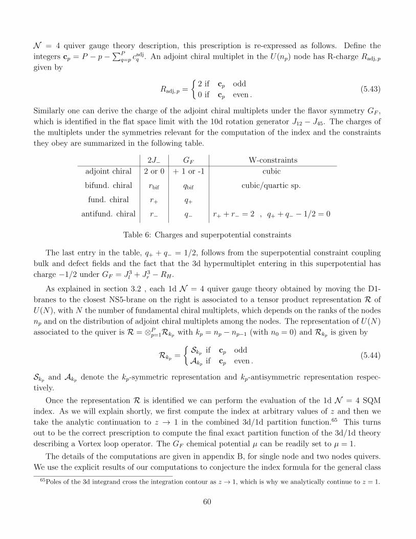
N = 4 quiver gauge theory description, this prescription is re-expressed as follows. Define the

integers cp = P − p −∑P

q=p cadjq . An adjoint chiral multiplet in the U(np) node has R-charge Radj, p

given by

Radj, p =

{2 if cp odd

0 if cp even .(5.43)

Similarly one can derive the charge of the adjoint chiral multiplets under the flavor symmetry GF ,

which is identified in the flat space limit with the 10d rotation generator J12 − J45. The charges of

the multiplets under the symmetries relevant for the computation of the index and the constraints

they obey are summarized in the following table.

2J− GF W-constraints

adjoint chiral 2 or 0 + 1 or -1 cubic

bifund. chiral rbif qbif cubic/quartic sp.

fund. chiral r+ q+

antifund. chiral r− q− r+ + r− = 2 , q+ + q− − 1/2 = 0

Table 6: Charges and superpotential constraints

The last entry in the table, q+ + q− = 1/2, follows from the superpotential constraint coupling

bulk and defect fields and the fact that the 3d hypermultiplet entering in this superpotential has

charge −1/2 under GF = J3l + J3

r −RH .

As explained in section 3.2 , each 1d N = 4 quiver gauge theory obtained by moving the D1-

branes to the closest NS5-brane on the right is associated to a tensor product representation R of

U(N), with N the number of fundamental chiral multiplets, which depends on the ranks of the nodes

np and on the distribution of adjoint chiral multiplets among the nodes. The representation of U(N)

associated to the quiver is R = ⊗Pp=1Rkp with kp = np − np−1 (with n0 = 0) and Rkp is given by

Rkp =

{Skp if cp odd

Akp if cp even .(5.44)

Skp and Akp denote the kp-symmetric representation and kp-antisymmetric representation respec-

tively.

Once the representation R is identified we can perform the evaluation of the 1d N = 4 SQM

index. As we will explain shortly, we first compute the index at arbitrary values of z and then we

take the analytic continuation to z → 1 in the combined 3d/1d partition function.65 This turns

out to be the correct prescription to compute the final exact partition function of the 3d/1d theory

describing a Vortex loop operator. The GF chemical potential µ can be readily set to µ = 1.

The details of the computations are given in appendix B, for single node and two nodes quivers.

We use the explicit results of our computations to conjecture the index formula for the general class

65Poles of the 3d integrand cross the integration contour as z → 1, which is why we analytically continue to z = 1.

60

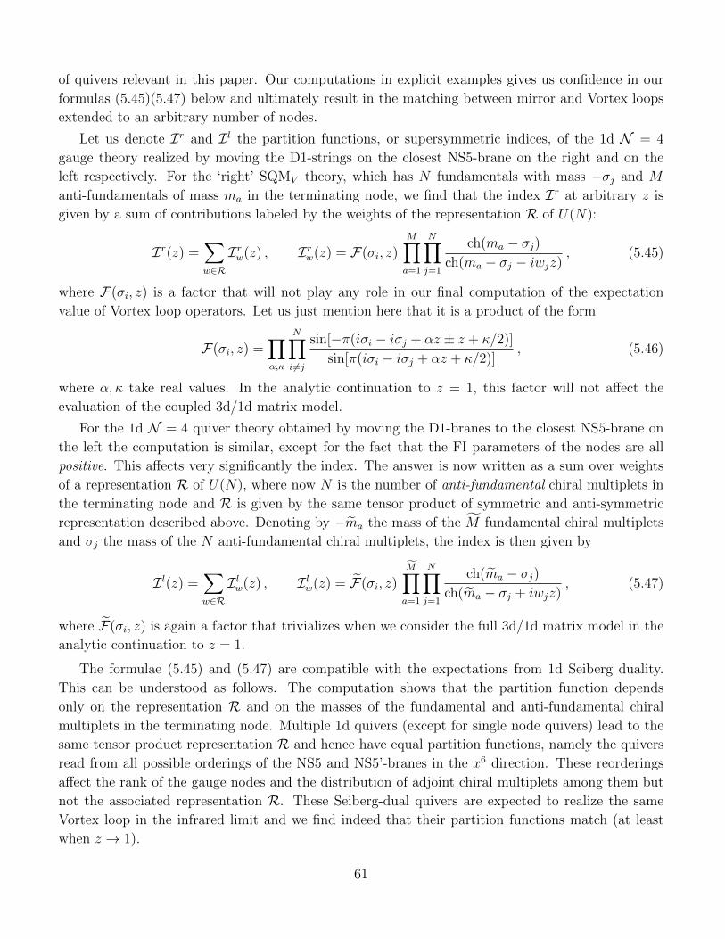
of quivers relevant in this paper. Our computations in explicit examples gives us confidence in our

formulas (5.45)(5.47) below and ultimately result in the matching between mirror and Vortex loops

extended to an arbitrary number of nodes.

Let us denote Ir and I l the partition functions, or supersymmetric indices, of the 1d N = 4

gauge theory realized by moving the D1-strings on the closest NS5-brane on the right and on the

left respectively. For the ‘right’ SQMV theory, which has N fundamentals with mass −σj and M

anti-fundamentals of mass ma in the terminating node, we find that the index Ir at arbitrary z is

given by a sum of contributions labeled by the weights of the representation R of U(N):

Ir(z) =∑w∈R

Irw(z) , Irw(z) = F(σi, z)M∏a=1

N∏j=1

ch(ma − σj)ch(ma − σj − iwjz)

, (5.45)

where F(σi, z) is a factor that will not play any role in our final computation of the expectation

value of Vortex loop operators. Let us just mention here that it is a product of the form

F(σi, z) =∏α,κ

N∏i 6=j

sin[−π(iσi − iσj + αz ± z + κ/2)]

sin[π(iσi − iσj + αz + κ/2)], (5.46)

where α, κ take real values. In the analytic continuation to z = 1, this factor will not affect the

evaluation of the coupled 3d/1d matrix model.

For the 1d N = 4 quiver theory obtained by moving the D1-branes to the closest NS5-brane on

the left the computation is similar, except for the fact that the FI parameters of the nodes are all

positive. This affects very significantly the index. The answer is now written as a sum over weights

of a representation R of U(N), where now N is the number of anti-fundamental chiral multiplets in

the terminating node and R is given by the same tensor product of symmetric and anti-symmetric

representation described above. Denoting by −ma the mass of the M fundamental chiral multiplets

and σj the mass of the N anti-fundamental chiral multiplets, the index is then given by

I l(z) =∑w∈R

I lw(z) , I lw(z) = F(σi, z)M∏a=1

N∏j=1

ch(ma − σj)ch(ma − σj + iwjz)

, (5.47)

where F(σi, z) is again a factor that trivializes when we consider the full 3d/1d matrix model in the

analytic continuation to z = 1.

The formulae (5.45) and (5.47) are compatible with the expectations from 1d Seiberg duality.

This can be understood as follows. The computation shows that the partition function depends

only on the representation R and on the masses of the fundamental and anti-fundamental chiral

multiplets in the terminating node. Multiple 1d quivers (except for single node quivers) lead to the

same tensor product representation R and hence have equal partition functions, namely the quivers

read from all possible orderings of the NS5 and NS5’-branes in the x6 direction. These reorderings

affect the rank of the gauge nodes and the distribution of adjoint chiral multiplets among them but

not the associated representation R. These Seiberg-dual quivers are expected to realize the same

Vortex loop in the infrared limit and we find indeed that their partition functions match (at least

when z → 1).

61

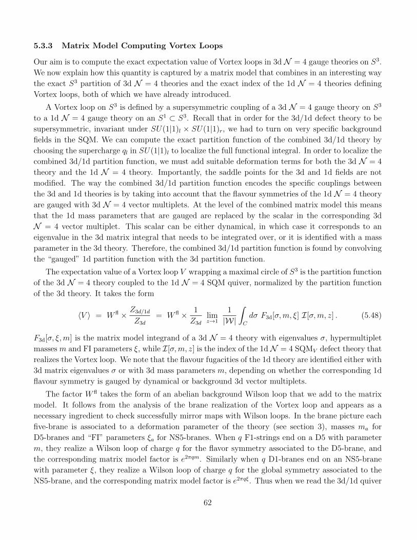
5.3.3 Matrix Model Computing Vortex Loops

Our aim is to compute the exact expectation value of Vortex loops in 3d N = 4 gauge theories on S3.

We now explain how this quantity is captured by a matrix model that combines in an interesting way

the exact S3 partition of 3d N = 4 theories and the exact index of the 1d N = 4 theories defining

Vortex loops, both of which we have already introduced.

A Vortex loop on S3 is defined by a supersymmetric coupling of a 3d N = 4 gauge theory on S3

to a 1d N = 4 gauge theory on an S1 ⊂ S3. Recall that in order for the 3d/1d defect theory to be

supersymmetric, invariant under SU(1|1)l × SU(1|1)r, we had to turn on very specific background

fields in the SQM. We can compute the exact partition function of the combined 3d/1d theory by

choosing the supercharge ql in SU(1|1)l to localize the full functional integral. In order to localize the

combined 3d/1d partition function, we must add suitable deformation terms for both the 3d N = 4

theory and the 1d N = 4 theory. Importantly, the saddle points for the 3d and 1d fields are not

modified. The way the combined 3d/1d partition function encodes the specific couplings between

the 3d and 1d theories is by taking into account that the flavour symmetries of the 1d N = 4 theory

are gauged with 3d N = 4 vector multiplets. At the level of the combined matrix model this means

that the 1d mass parameters that are gauged are replaced by the scalar in the corresponding 3d

N = 4 vector multiplet. This scalar can be either dynamical, in which case it corresponds to an

eigenvalue in the 3d matrix integral that needs to be integrated over, or it is identified with a mass

parameter in the 3d theory. Therefore, the combined 3d/1d partition function is found by convolving

the “gauged” 1d partition function with the 3d partition function.

The expectation value of a Vortex loop V wrapping a maximal circle of S3 is the partition function

of the 3d N = 4 theory coupled to the 1d N = 4 SQM quiver, normalized by the partition function

of the 3d theory. It takes the form

〈V 〉 = W fl ×Z3d/1d

Z3d

= W fl × 1

Z3d

limz→1

1

|W|

∫C

dσ F3d[σ,m, ξ] I[σ,m, z] . (5.48)

F3d[σ, ξ,m] is the matrix model integrand of a 3d N = 4 theory with eigenvalues σ, hypermultiplet

masses m and FI parameters ξ, while I[σ,m, z] is the index of the 1d N = 4 SQMV defect theory that

realizes the Vortex loop. We note that the flavour fugacities of the 1d theory are identified either with

3d matrix eigenvalues σ or with 3d mass parameters m, depending on whether the corresponding 1d

flavour symmetry is gauged by dynamical or background 3d vector multiplets.

The factor W fl takes the form of an abelian background Wilson loop that we add to the matrix

model. It follows from the analysis of the brane realization of the Vortex loop and appears as a

necessary ingredient to check successfully mirror maps with Wilson loops. In the brane picture each

five-brane is associated to a deformation parameter of the theory (see section 3), masses ma for

D5-branes and “FI” parameters ξa for NS5-branes. When q F1-strings end on a D5 with parameter

m, they realize a Wilson loop of charge q for the flavor symmetry associated to the D5-brane, and

the corresponding matrix model factor is e2πqm. Similarly when q D1-branes end on an NS5-brane

with parameter ξ, they realize a Wilson loop of charge q for the global symmetry associated to the

NS5-brane, and the corresponding matrix model factor is e2πqξ. Thus when we read the 3d/1d quiver

62

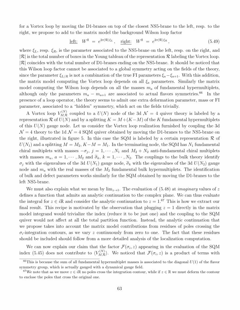
for a Vortex loop by moving the D1-branes on top of the closest NS5-brane to the left, resp. to the

right, we propose to add to the matrix model the background Wilson loop factor

left: W fl = e2π|R| ξL , right: W fl = e2π|R| ξR , (5.49)

where ξL, resp. ξR, is the parameter associated to the NS5-brane on the left, resp. on the right, and

|R| is the total number of boxes in the Young tableau of the representationR labeling the Vortex loop.

|R| coincides with the total number of D1-branes ending on the NS5-brane. It should be noticed that

this Wilson loop factor cannot be associated to a global symmetry acting on the fields of the theory,

since the parameter ξL/R is not a combination of the true FI parameters ξa−ξa+1. With this addition,

the matrix model computing the Vortex loop depends on all ξa parameters. Similarly the matrix

model computing the Wilson loop depends on all the masses ma of fundamental hypermultiplets,

although only the parameters ma − ma+1 are associated to actual flavors symmetries.66 In the

presence of a loop operator, the theory seems to admit one extra deformation parameter, mass or FI

parameter, associated to a “hidden” symmetry, which act on the fields trivially.

A Vortex loop V(N)M,R coupled to a U(N) node of the 3d N = 4 quiver theory is labeled by a

representationR of U(N) and by a splitting K = M+(K−M) of the K fundamental hypermultiplets

of this U(N) gauge node. Let us consider the Vortex loop realization furnished by coupling the 3d

N = 4 theory to the 1d N = 4 SQM quiver obtained by moving the D1-branes to the NS5-brane on

the right, illustrated in figure 5. In this case the SQM is labeled by a certain representation R of

U(N1) and a splitting M = M2, K−M = M1. In the terminating node, the SQM has N1 fundamental

chiral multiplets with masses −σj, j = 1, · · · , N1 and M2 + N2 anti-fundamental chiral multiplets

with masses ma, a = 1, · · · ,M2 and σk, k = 1, · · · , N2. The couplings to the bulk theory identify

σj with the eigenvalues of the 3d U(N1) gauge node, σk with the eigenvalues of the 3d U(N2) gauge

node and ma with the real masses of the M2 fundamental bulk hypermultiplets. The identification

of bulk and defect parameters works similarly for the SQM obtained by moving the D1-branes to the

left NS5-brane.

We must also explain what we mean by limz→1. The evaluation of (5.48) at imaginary values of z

defines a function that admits an analytic continuation to the complex plane. We can thus evaluate

the integral for z ∈ iR and consider the analytic continuation to z = 1.67 This is how we extract our

final result. This recipe is motivated by the observation that plugging z = 1 directly in the matrix

model integrand would trivialize the index (reduce it to be just one) and the coupling to the SQM

quiver would not affect at all the total partition function. Instead, the analytic continuation that

we propose takes into account the matrix model contributions from residues of poles crossing the

σi-integration contours, as we vary z continuously from zero to one. The fact that these residues

should be included should follow from a more detailed analysis of the localization computation.

We can now explain our claim that the factor F(σi, z) appearing in the evaluation of the SQM

index (5.45) does not contribute to 〈V (N)M,R〉. We noticed that F(σi, z) is a product of terms with

66This is because the sum of all fundamental hypermultiplet masses is associated to the diagonal U(1) of the flavor

symmetry group, which is actually gauged with a dynamical gauge field.67We note that as we move z ∈ iR no poles cross the integration contour, while if z ∈ R we must deform the contour

to enclose the poles that cross the original one.

63

the generic form (5.46). In taking the analytic continuation z → 1 these factors introduce residues

from poles crossing the integration contours proportional to sin(±πz). In the limit z = 1 these extra

residues all vanish, implying that the limit z = 1 can be taken directly in the integrand of (5.48)

for this factor F(σi, z). Noting that F(σi, z = 1) = ±1, we can simply drop this factor from our

computations. Our results will be valid only up to an overall sign.

The same argument would not work for the other factors in (5.45) because the numerators ch(ma−σj) are exactly canceled by inverse factors from the 3d hypermultiplets contributions! This means

that the residues of the poles crossing the integration contour as z → 1 due to these factors are

non-vanishing. The discussion is the same for the left index (5.47).

5.4 Loops in T [SU(N)]

In this section we perform the explicit computation of the exact expectation value of Wilson and

Vortex loop operators in the T [SU(N)] theory. We show precise agreement with all of our brane-

based predictions in section 4.3.

We will use the notationsa∏j

≡a∏j=1

,a∏j<k

≡∏

1≤j<k≤a

,

a,b∏j,k

≡a∏j=1

b∏k=1

. (5.50)

The T [SU(N)] theory has an U(N)J × U(N)F global symmetry group.68 SU(N)F is the flavor

symmetry rotating the fundamental hypermultiplets and SU(N)J is a global symmetry arising at

the infrared fixed point, enhancing the manifest U(1)N−1 topological symmetry acting on the dual

photons. These global symmetries can be weakly gauged to give masses m = (m1, . . . ,mN) to the

fundamental hypermultiplets and FI parameters ηi = ξi − ξi+1, with ξ = (ξ1, . . . , ξN), to the N − 1

nodes. The S3 partition function of the T [SU(N)] theory deformed by these massive parameters was

computed in [15,47] and is given by

ZT [SU(N)] = (−i)N(N−1)

2 e−2iπξN∑j mj

∑τ∈SN (−1)τ e2πi

∑Nj ξjmτ(j)∏N

j<k sh(ξj − ξk)sh(mj −mk), (5.51)

where SN is the group of permutations of N elements and (−1)τ is the signature of the permutation

τ . T [SU(N)] has the property of being self-mirror. This is realized by virtue of the partition

function (5.51) being invariant under the exchange mj ↔ ξj, except for the phase e−2iπξN∑j mj ,

which is unphysical, in the sense that it can be removed by a local counterterm constructed from

the background fields (namely mixed background Chern-Simons terms) defining the UV partition

function [48,49].

For the explicit mirror symmetry maps, it will prove useful to define the mirror symmetric quantity

ZT [SU(N)] ≡ e2iπξN∑j mj ZT [SU(N)] = (−i)

N(N−1)2

∑τ∈SN (−1)τ e2πi

∑Nj ξjmτ(j)∏N

j<k sh(ξj − ξk)sh(mj −mk), (5.52)

68Strictkly speaking the symmetry is SU(N)J × SU(N)F , but it is convenient to make the mapping of parameters

under mirror symmetry symmetric to add two extra U(1) symmetries, which act trivially.

64

which can be understood as the partition function expressed in another renormalization scheme and

which is manifestly invariant under the exchange of mass and FI parameters mj ↔ ξj.

All our results are nicely expressed in terms of two shift operators Sq and Sq acting on the

partition function Z ≡ ZT [SU(N)] of the theory. These operators act by shifting respectively the FI

parameters and the masses by imaginary terms,

SqZ ≡ Zξj→ξj−iqj , j = 1, · · · , N , (5.53)

SqZ ≡ Zmj→mj−iqj , j = 1, · · · , N , (5.54)

where q = (q1, · · · , qN) is a N -component vector.

5.4.1 T[SU(2)] loops

Let us start our analysis with the abelian theory T [SU(2)]. The partition function is given by the

matrix model

Z =

∫dσ

e2iπ(ξ1−ξ2)σ

ch(σ −m2)ch(σ −m1). (5.55)

One can evaluate this integral by closing the contour of integration by a semi-circle going through

i∞ (or −i∞) and summing over the residues inside the contour. This yields

Z = (−i)e−2iπξ2(m1+m2) e2iπ(ξ1m1+ξ2m2) − e2iπ(ξ1m2+ξ2m1)

sh(ξ1 − ξ2)sh(m1 −m2), (5.56)

which agrees with (5.51) for N = 2.

The matrix model computing the vev of a Wilson loop of charge q ∈ Z is given by

〈Wq〉 =1

Z

∫dσ

e2iπ(ξ1−ξ2)σ

ch(σ −m2)ch(σ −m1)e2πqσ =

S(q,0)Z

Z

= (−1)qe2πqm1e2iπ(ξ1m1+ξ2m2) − e2πqm2e2iπ(ξ1m2+ξ2m1)

e2iπ(ξ1m1+ξ2m2) − e2iπ(ξ1m2+ξ2m1), (5.57)

where we evaluated the integral at non-zero q by the analytical continuation ξ1 → ξ1 − iq, following

from our choice of deformed contour integral (see discussion after (5.36)).69

Let us turn now to the computation of Vortex loops. The T [SU(2)] theory has two fundamental

hypermultiplets, which give rise to three possible splitting 2 = i + (2− i), i = 0, 1, 2, defining three

possible Vortex loops Vi,q. Using the result for the Vortex loop factor (5.45), computed from its

right SQM quiver realization (and ignoring the factor F for the reasons mentioned before), inserted

in (5.48) and with extra Wilson line (5.49), the matrix models computing the Vortex loop vevs are

69As explained before, divergent Wilson loops are computed by deforming the contour of integration.

65

found to be70

〈V0,q〉 =1

Zlimz→1

∫dσ

e2iπ(ξ1−ξ2)σ

ch(σ −m2)ch(σ −m1)e2πqξ2 = e2πqξ2

Z

Z= e2πqξ2 (5.58)

〈V1,q〉 =1

Zlimz→1

∫dσ

e2iπ(ξ1−ξ2)σ

ch(σ −m2)ch(σ −m1 + iqz)e2πqξ2 = e2πqξ2

S(q,0)Z

Z

= (−1)qe2πqξ1e2iπ(ξ1m1+ξ2m2) − e2πqξ2e2iπ(ξ1m2+ξ2m1)

e2iπ(ξ1m1+ξ2m2) − e2iπ(ξ1m2+ξ2m1)(5.59)

〈V2,q〉 =1

Zlimz→1

∫dσ

e2iπ(ξ1−ξ2)σ

ch(σ −m2 + iqz)ch(σ −m1 + iqz)e2πqξ2 = e2πqξ2

S(q,q)Z

Z= e2πqξ1 . (5.60)

The mirror symmetry prediction (4.1) is recovered by our exact computations, namely

〈Wq〉mirror←−−−→ 〈V1,q〉 , (5.61)

wheremirror←−−−→ means that the operator vevs are equal under the exchange of masses mj and FI

parameters ξj, as required by mirror symmetry.

The explicit results also show that the other Vortex loops V0,q, V2,q are mapped to the flavor

Wilson loops of the mirror theory, as predicted in section 4.3.

5.4.2 Wilson loops in T[SU(N)]

We turn now to the non-abelian theories by considering Wilson loops in the T [SU(N)] theories. We

pick a Wilson loop in an arbirary representation R of a U(p) node, with 1 ≤ p ≤ N − 1. The matrix

model computing it decomposes into a sum of contributions labeled by the weights w of R

〈WU(p)R 〉 =

∑w∈R

WU(p)(w) . (5.62)

We compute now the matrix model WU(p)(w) associated to a single weight w = (w1, w2, ..., wp). To

simplify expressions we omit the factors depending on (and the integrals over) the eigenvalues σ(a)j

with a > p in the matrix model because they do not affect the computation. With this simplification

the matrix model is given by

WU(p)(w) =1

Z

∫ p∏a

[ daσ(a)

a!e2π

∑pj wjσ

(p)j

e2iπ(ξa−ξa+1)∑aj σ

(a)j∏a

j<k sh(σ(a)j − σ

(a)k )2∏a,a+1

j,k ch(σ(a)j − σ

(a+1)k )

]. (5.63)

The integration over the the eigenvalues σ(a)j with a = 1, ..., p−1 just reproduces the partition function

of ZT [SU(p)] with FI parameters ξ(p) = (ξ1, ξ2, · · · , ξp) and mass parameters σ(p) = (σ(p)1 , σ

(p)2 , · · · , σ(p)

p ).

70In section 4.1 we denoted for simplicity Vq ≡ V1,q.

66

We can use the formula (5.51) to integrate them out (and relabeling σ(p)j = σj)

WU(p)(w) =1

Z

∫dpσ(p)

p!ZT [SU(p)][ξ(p), σ(p)] e2π

∑pj wjσ

(p)j

e2iπ(ξp−ξp+1)∑pj σ

(p)j∏p

j<k sh(σ(p)j − σ

(p)k )2∏p,p+1

j,k ch(σ(p)j − σ

(p+1)k )

=1

Z

∑τ∈Sp

∫dpσ

p!

(−1)τ (−i)p(p−1)

2 e2iπ∑pj ξτ(j)σj∏p

j<k sh(ξj − ξk)e2π

∑pj wjσj

e−2iπξp+1∑pj σj∏p

j<k sh(σj − σk)∏p,p+1j,k ch(σj − σ(p+1)

k ). (5.64)

Relabeling the eigenvalues as σj → στ(j) in each integral brings the matrix model to the form

WU(p)(w) =1

Z

1

p!

∑τ∈Sp

∫dpσ

(−i)p(p−1)

2 e2iπ∑pj ξjσj∏p

j<k sh(ξj − ξk)e2π

∑pj wτ(j)σj

e−2iπξp+1∑pj σj∏p

j<k sh(σj − σk)∏p,p+1j,k ch(σj − σ(p+1)

k ).

(5.65)

For each term in the sum over Sp the factor e2π∑pj wτ(j)σj can be reabsorbed as a shift of the parameters

ξj by −iwτ(j), for j = 1, ..., p, at the cost of an extra factor (−1)(p−1)(w1+w2+...+wp). The matrix model

without these imaginary shifts is exactly Z (this can be seen by noticing that Z is the matrix

model obtained when w = 0). The evaluation of the integrals (with deformed integration contours as

explained after (5.36)) then coincides with an analytical continuation of Z to complex FI parameters.

We obtain

WU(p)(w) =(−1)(p−1)wtot

p!

1

Z

∑τ∈Sp

SwτZ , (5.66)

with wtot =∑p

j=1wj and wτ = (wτ(1), wτ(2), · · · , wτ(p), 0, · · · , 0︸ ︷︷ ︸N−p

). We need to sum over these single

weight contributions to get the final result (5.62). Recognizing Sp as the Weyl group W of U(p), we

can simplify the result using the property∑w∈R

( 1

p!

∑τ∈Sp

F [wτ ])

=∑w∈R

( 1

|W|∑τ∈W

F [τ.w])

=∑w∈R

F [w] . (5.67)

This leads to our final result

〈WU(p)R 〉 = (−1)(p−1)|R| 1

Z∑w∈R

S(w1,w2,··· ,wp,0,··· ,0)Z , (5.68)

where we also used the property that for any weight w,∑p

j wj = |R|, the number of boxes in the

Young tableau of R, and we replaced trivially Z by Z defined in (5.52) .

5.4.3 Vortex loops in T[SU(N)]

We now evaluate the matrix models computing the exact expectation value of Vortex loops in

T [SU(N)]. The Vortex loops are labeled by a representation R of a U(p) node and, for the U(N−1)

67

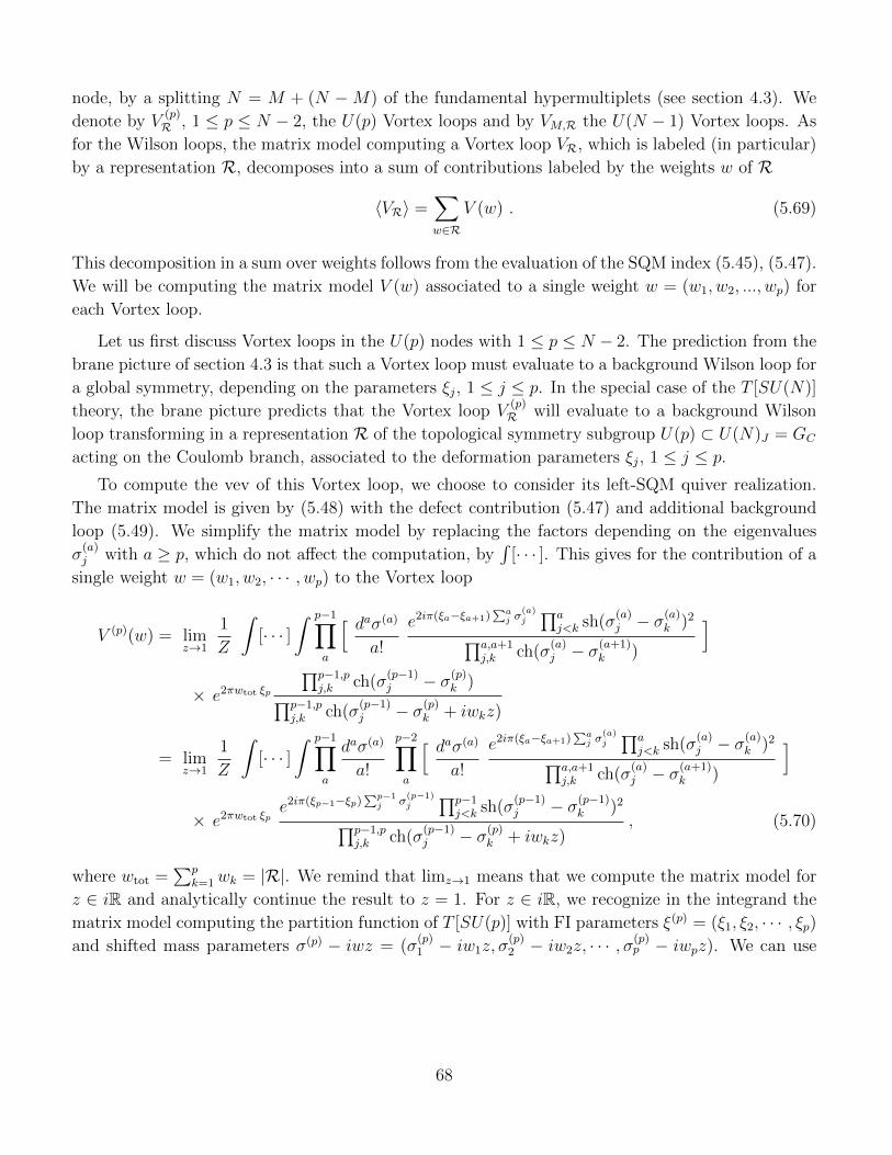
node, by a splitting N = M + (N −M) of the fundamental hypermultiplets (see section 4.3). We

denote by V(p)R , 1 ≤ p ≤ N − 2, the U(p) Vortex loops and by VM,R the U(N − 1) Vortex loops. As

for the Wilson loops, the matrix model computing a Vortex loop VR, which is labeled (in particular)

by a representation R, decomposes into a sum of contributions labeled by the weights w of R

〈VR〉 =∑w∈R

V (w) . (5.69)

This decomposition in a sum over weights follows from the evaluation of the SQM index (5.45), (5.47).

We will be computing the matrix model V (w) associated to a single weight w = (w1, w2, ..., wp) for

each Vortex loop.

Let us first discuss Vortex loops in the U(p) nodes with 1 ≤ p ≤ N − 2. The prediction from the

brane picture of section 4.3 is that such a Vortex loop must evaluate to a background Wilson loop for

a global symmetry, depending on the parameters ξj, 1 ≤ j ≤ p. In the special case of the T [SU(N)]

theory, the brane picture predicts that the Vortex loop V(p)R will evaluate to a background Wilson

loop transforming in a representation R of the topological symmetry subgroup U(p) ⊂ U(N)J = GC

acting on the Coulomb branch, associated to the deformation parameters ξj, 1 ≤ j ≤ p.

To compute the vev of this Vortex loop, we choose to consider its left-SQM quiver realization.

The matrix model is given by (5.48) with the defect contribution (5.47) and additional background

loop (5.49). We simplify the matrix model by replacing the factors depending on the eigenvalues

σ(a)j with a ≥ p, which do not affect the computation, by

∫[· · · ]. This gives for the contribution of a

single weight w = (w1, w2, · · · , wp) to the Vortex loop

V (p)(w) = limz→1

1

Z

∫[· · · ]

∫ p−1∏a

[ daσ(a)

a!

e2iπ(ξa−ξa+1)∑aj σ

(a)j∏a

j<k sh(σ(a)j − σ

(a)k )2∏a,a+1

j,k ch(σ(a)j − σ

(a+1)k )

]× e2πwtot ξp

∏p−1,pj,k ch(σ

(p−1)j − σ(p)

k )∏p−1,pj,k ch(σ

(p−1)j − σ(p)

k + iwkz)

= limz→1

1

Z

∫[· · · ]

∫ p−1∏a

daσ(a)

a!

p−2∏a

[ daσ(a)

a!

e2iπ(ξa−ξa+1)∑aj σ

(a)j∏a

j<k sh(σ(a)j − σ

(a)k )2∏a,a+1

j,k ch(σ(a)j − σ

(a+1)k )

]

× e2πwtot ξpe2iπ(ξp−1−ξp)

∑p−1j σ

(p−1)j

∏p−1j<k sh(σ

(p−1)j − σ(p−1)

k )2∏p−1,pj,k ch(σ

(p−1)j − σ(p)

k + iwkz), (5.70)

where wtot =∑p

k=1wk = |R|. We remind that limz→1 means that we compute the matrix model for

z ∈ iR and analytically continue the result to z = 1. For z ∈ iR, we recognize in the integrand the

matrix model computing the partition function of T [SU(p)] with FI parameters ξ(p) = (ξ1, ξ2, · · · , ξp)and shifted mass parameters σ(p) − iwz = (σ

(p)1 − iw1z, σ

(p)2 − iw2z, · · · , σ(p)

p − iwpz). We can use

68

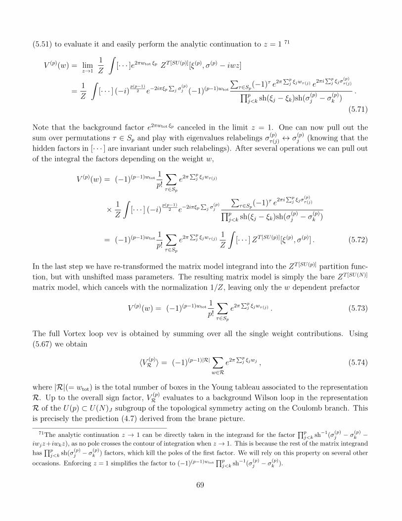
(5.51) to evaluate it and easily perform the analytic continuation to z = 1 71

V (p)(w) = limz→1

1

Z

∫[· · · ]e2πwtot ξp ZT [SU(p)][ξ(p), σ(p) − iwz]

=1

Z

∫[· · · ] (−i)

p(p−1)2 e−2iπξp

∑j σ

(p)j (−1)(p−1)wtot

∑τ∈Sp(−1)τ e2π

∑pj ξjwτ(j) e2πi

∑pj ξjσ

(p)τ(j)∏p

j<k sh(ξj − ξk)sh(σ(p)j − σ

(p)k )

.

(5.71)

Note that the background factor e2πwtot ξp canceled in the limit z = 1. One can now pull out the

sum over permutations τ ∈ Sp and play with eigenvalues relabelings σ(p)τ(j) ↔ σ

(p)j (knowing that the

hidden factors in [· · · ] are invariant under such relabelings). After several operations we can pull out

of the integral the factors depending on the weight w,

V (p)(w) = (−1)(p−1)wtot1

p!

∑τ∈Sp

e2π∑pj ξjwτ(j)

× 1

Z

∫[· · · ] (−i)

p(p−1)2 e−2iπξp

∑j σ

(p)j

∑τ∈Sp(−1)τ e2πi

∑pj ξjσ

(p)τ(j)∏p

j<k sh(ξj − ξk)sh(σ(p)j − σ

(p)k )

= (−1)(p−1)wtot1

p!

∑τ∈Sp

e2π∑pj ξjwτ(j)

1

Z

∫[· · · ]ZT [SU(p)][ξ(p), σ(p)] . (5.72)

In the last step we have re-transformed the matrix model integrand into the ZT [SU(p)] partition func-

tion, but with unshifted mass parameters. The resulting matrix model is simply the bare ZT [SU(N)]

matrix model, which cancels with the normalization 1/Z, leaving only the w dependent prefactor

V (p)(w) = (−1)(p−1)wtot1

p!

∑τ∈Sp

e2π∑pj ξjwτ(j) . (5.73)

The full Vortex loop vev is obtained by summing over all the single weight contributions. Using

(5.67) we obtain

〈V (p)R 〉 = (−1)(p−1)|R|

∑w∈R

e2π∑pj ξjwj , (5.74)

where |R|(= wtot) is the total number of boxes in the Young tableau associated to the representation

R. Up to the overall sign factor, V(p)R evaluates to a background Wilson loop in the representation

R of the U(p) ⊂ U(N)J subgroup of the topological symmetry acting on the Coulomb branch. This

is precisely the prediction (4.7) derived from the brane picture.

71The analytic continuation z → 1 can be directly taken in the integrand for the factor∏pj<k sh−1(σ

(p)j − σ(p)

k −iwjz+iwkz), as no pole crosses the contour of integration when z → 1. This is because the rest of the matrix integrand

has∏pj<k sh(σ

(p)j − σ

(p)k ) factors, which kill the poles of the first factor. We will rely on this property on several other

occasions. Enforcing z = 1 simplifies the factor to (−1)(p−1)wtot∏pj<k sh−1(σ

(p)j − σ

(p)k ).

69

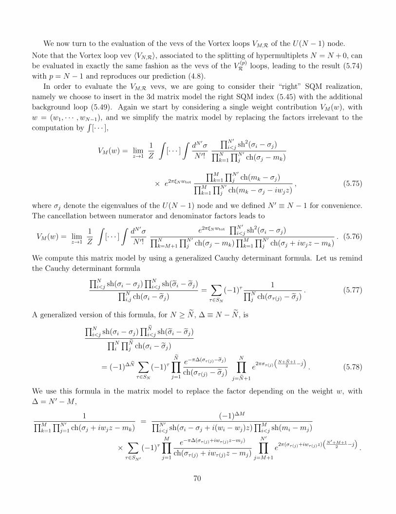
We now turn to the evaluation of the vevs of the Vortex loops VM,R of the U(N − 1) node.

Note that the Vortex loop vev 〈VN,R〉, associated to the splitting of hypermultiplets N = N + 0, can

be evaluated in exactly the same fashion as the vevs of the V(p)R loops, leading to the result (5.74)

with p = N − 1 and reproduces our prediction (4.8).

In order to evaluate the VM,R vevs, we are going to consider their “right” SQM realization,

namely we choose to insert in the 3d matrix model the right SQM index (5.45) with the additional

background loop (5.49). Again we start by considering a single weight contribution VM(w), with

w = (w1, · · · , wN−1), and we simplify the matrix model by replacing the factors irrelevant to the

computation by∫

[· · · ],

VM(w) = limz→1

1

Z

∫[· · · ]

∫dN′σ

N ′!

∏N ′

i<j sh2(σi − σj)∏Nk=1

∏N ′

j ch(σj −mk)

× e2πξNwtot

∏Mk=1

∏N ′

j ch(mk − σj)∏Mk=1

∏N ′

j ch(mk − σj − iwjz), (5.75)

where σj denote the eigenvalues of the U(N − 1) node and we defined N ′ ≡ N − 1 for convenience.

The cancellation between numerator and denominator factors leads to

VM(w) = limz→1

1

Z

∫[· · · ]

∫dN′σ

N ′!

e2πξNwtot∏N ′

i<j sh2(σi − σj)∏Nk=M+1

∏N ′

j ch(σj −mk)∏M

k=1

∏N ′

j ch(σj + iwjz −mk). (5.76)

We compute this matrix model by using a generalized Cauchy determinant formula. Let us remind

the Cauchy determinant formula∏Ni<j sh(σi − σj)

∏Ni<j sh(σi − σj)∏N

i,j ch(σi − σj)=∑τ∈SN

(−1)τ1∏N

j ch(στ(j) − σj). (5.77)

A generalized version of this formula, for N ≥ N , ∆ ≡ N − N , is∏Ni<j sh(σi − σj)

∏Ni<j sh(σi − σj)∏N

i

∏Nj ch(σi − σj)

= (−1)∆N∑τ∈SN

(−1)τN∏j=1

e−π∆(στ(j)−σj)

ch(στ(j) − σj)

N∏j=N+1

e2πστ(j)

(N+N+1

2−j). (5.78)

We use this formula in the matrix model to replace the factor depending on the weight w, with

∆ = N ′ −M ,

1∏Mk=1

∏N ′

j=1 ch(σj + iwjz −mk)=

(−1)∆M∏N ′

i<j sh(σi − σj + i(wi − wj)z)∏M

i<j sh(mi −mj)

×∑τ∈SN′

(−1)τM∏j=1

e−π∆(στ(j)+iwτ(j)z−mj)

ch(στ(j) + iwτ(j)z −mj)

N ′∏j=M+1

e2π(στ(j)+iwτ(j)z)

(N′+M+1

2−j).

70

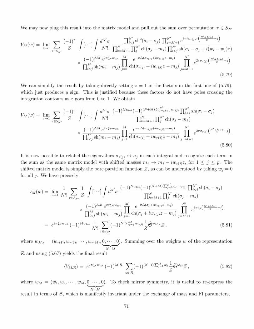
We may now plug this result into the matrix model and pull out the sum over permutation τ ∈ SN ′

VM(w) = limz→1

∑τ∈SN′

(−1)τ

Z

∫[· · · ]

∫dN′σ

N ′!

∏N ′

i<j sh2(σi − σj)∏N ′

j=M+1 e2πiwτ(j)z

(N′+M+1

2−j)

∏Nk=M+1

∏N ′

j ch(σj −mk)∏N ′

i<j sh(σi − σj + i(wi − wj)z)

× (−1)∆M e2πξNwtot∏Mi<j sh(mi −mj)

M∏j=1

e−π∆(στ(j)+iwτ(j)z−mj)

ch(στ(j) + iwτ(j)z −mj)

N ′∏j=M+1

e2πστ(j)

(N′+M+1

2−j).

(5.79)

We can simplify the result by taking directly setting z = 1 in the factors in the first line of (5.79),

which just produces a sign. This is justified because these factors do not have poles crossing the

integration contours as z goes from 0 to 1. We obtain

VM(w) = limz→1

∑τ∈SN′

(−1)τ

Z

∫[· · · ]

∫dN′σ

N ′!

(−1)Nwtot(−1)(N+M)∑N′j=M+1 wτ(j)

∏N ′

i<j sh(σi − σj)∏Nk=M+1

∏N ′

j ch(σj −mk)

× (−1)∆M e2πξNwtot∏Mi<j sh(mi −mj)

M∏j=1

e−π∆(στ(j)+iwτ(j)z−mj)

ch(στ(j) + iwτ(j)z −mj)

N ′∏j=M+1

e2πστ(j)

(N′+M+1

2−j).

(5.80)

It is now possible to relabel the eigenvalues στ(j) ↔ σj in each integral and recognize each term in

the sum as the same matrix model with shifted masses mj → mj − iwτ(j)z, for 1 ≤ j ≤ p. The

shifted matrix model is simply the bare partition function Z, as can be understood by taking wj = 0

for all j. We have precisely

VM(w) = limz→1

1

N ′!

∑τ∈SN′

1

Z

∫[· · · ]

∫dN′σ

(−1)Nwtot(−1)(N+M)∑N′j=M+1 wτ(j)

∏N ′

i<j sh(σi − σj)∏Nk=M+1

∏N ′

j ch(σj −mk)

× (−1)∆M e2πξNwtot∏Mi<j sh(mi −mj)

M∏j=1

e−π∆(σj+iwτ(j)z−mj)

ch(σj + iwτ(j)z −mj)

N ′∏j=M+1

e2πσj

(N′+M+1

2−j)

= e2πξNwtot (−1)Mwtot1

N ′!

∑τ∈SN′

(−1)N′∑M

j=1 wτ(j)1

ZSwM,τZ , (5.81)

where wM,τ = (wτ(1), wτ(2), · · · , wτ(M), 0, · · · , 0︸ ︷︷ ︸N−M

). Summing over the weights w of the representation

R and using (5.67) yields the final result

〈VM,R〉 = e2πξNwtot (−1)M |R|∑w∈R

(−1)(N−1)∑Mj=1 wj

1

ZSwMZ , (5.82)

where wM = (w1, w2, · · · , wM , 0, · · · , 0︸ ︷︷ ︸N−M

). To check mirror symmetry, it is useful to re-express the

result in terms of Z, which is manifestly invariant under the exchange of mass and FI parameters,

71

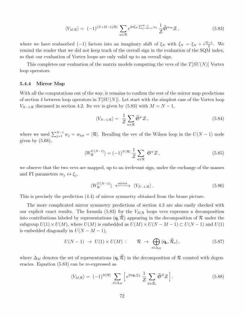
〈VM,R〉 = (−1)(N+M−1)|R|∑w∈R

e2πξN∑N−1j=M+1 wj

1

ZSwMZ , (5.83)

where we have reabsorbed (−1) factors into an imaginary shift of ξN with ξN = ξN + iN−12

. We

remind the reader that we did not keep track of the overall sign in the evaluation of the SQM index,

so that our evaluation of Vortex loops are only valid up to an overall sign.

This completes our evaluation of the matrix models computing the vevs of the T [SU(N)] Vortex

loop operators.

5.4.4 Mirror Map

With all the computations out of the way, it remains to confirm the rest of the mirror map predictions

of section 4 between loop operators in T [SU(N)]. Let start with the simplest case of the Vortex loop

VN−1,R discussed in section 4.2. Its vev is given by (5.83) with M = N − 1,

〈VN−1,R〉 =1

Z∑w∈R

SwZ , (5.84)

where we used∑N−1

j=1 wj = wtot = |R|. Recalling the vev of the Wilson loop in the U(N − 1) node

given by (5.68),

〈WU(N−1)R 〉 = (−1)N |R|

1

Z∑w∈R

SwZ , (5.85)

we observe that the two vevs are mapped, up to an irrelevant sign, under the exchange of the masses

and FI parameters mj ↔ ξj,

〈WU(N−1)R 〉 mirror←−−−→ 〈VN−1,R〉 . (5.86)

This is precisely the prediction (4.4) of mirror symmetry obtained from the brane picture.

The more complicated mirror symmetry predictions of section 4.3 are also easily checked with

our explicit exact results. The formula (5.83) for the VM,R loops vevs expresses a decomposition

into contributions labeled by representations (q, R) appearing in the decomposition of R under the

subgroup U(1)×U(M), where U(M) is embedded as U(M)×U(N −M − 1) ⊂ U(N − 1) and U(1)

is embedded diagonally in U(N −M − 1),

U(N − 1) → U(1)× U(M) : R →⊕s∈∆M

(qs, Rs) , (5.87)

where ∆M denotes the set of representations (q, R) in the decomposition of R counted with degen-

eracies. Equation (5.83) can be re-expressed as

〈VM,R〉 = (−1)M |R|∑s∈∆M

[e2πqs ξN

1

Z∑w∈Rs

SwZ]. (5.88)

72

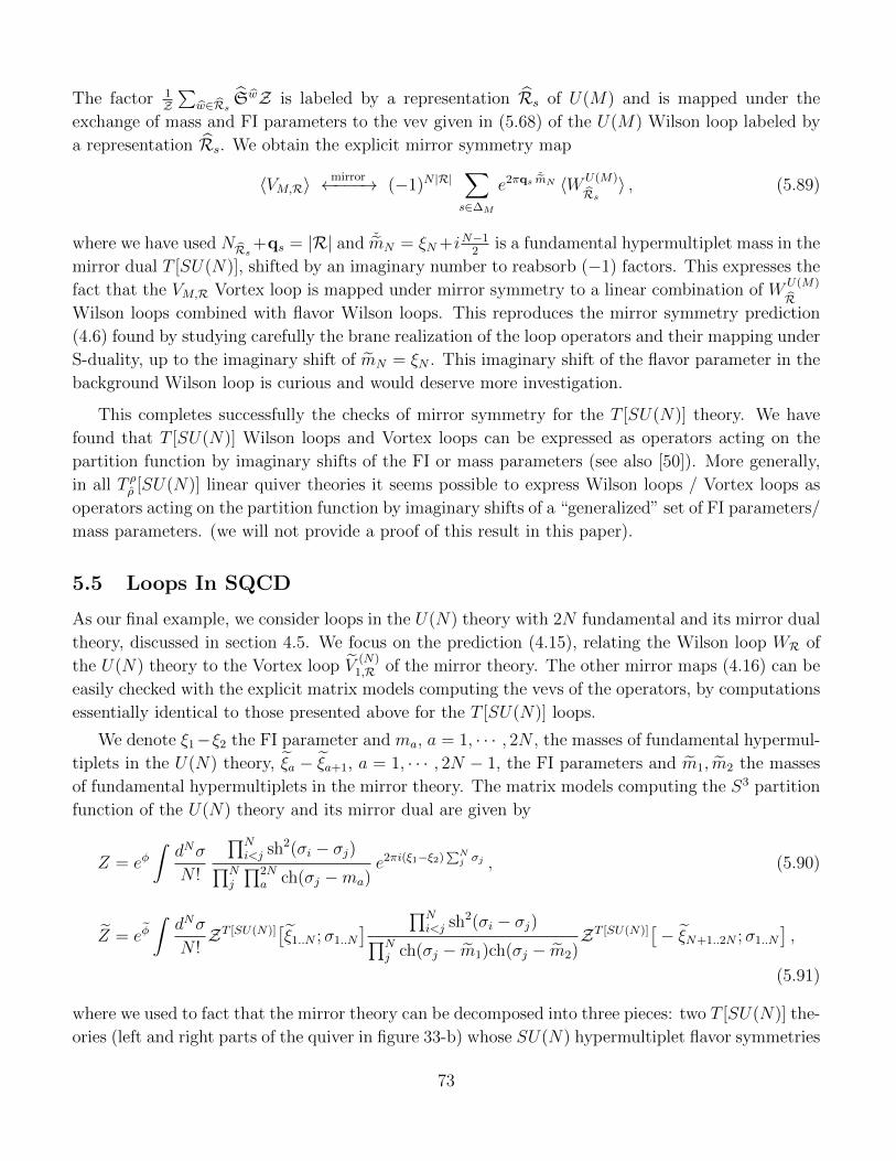
The factor 1Z∑

w∈Rs SwZ is labeled by a representation Rs of U(M) and is mapped under the

exchange of mass and FI parameters to the vev given in (5.68) of the U(M) Wilson loop labeled by

a representation Rs. We obtain the explicit mirror symmetry map

〈VM,R〉mirror←−−−→ (−1)N |R|

∑s∈∆M

e2πqs ˇmN 〈WU(M)

Rs〉 , (5.89)

where we have used NRs+qs = |R| and ˇmN = ξN +iN−12

is a fundamental hypermultiplet mass in the

mirror dual T [SU(N)], shifted by an imaginary number to reabsorb (−1) factors. This expresses the

fact that the VM,R Vortex loop is mapped under mirror symmetry to a linear combination of WU(M)

RWilson loops combined with flavor Wilson loops. This reproduces the mirror symmetry prediction

(4.6) found by studying carefully the brane realization of the loop operators and their mapping under

S-duality, up to the imaginary shift of mN = ξN . This imaginary shift of the flavor parameter in the

background Wilson loop is curious and would deserve more investigation.

This completes successfully the checks of mirror symmetry for the T [SU(N)] theory. We have

found that T [SU(N)] Wilson loops and Vortex loops can be expressed as operators acting on the

partition function by imaginary shifts of the FI or mass parameters (see also [50]). More generally,

in all T ρρ [SU(N)] linear quiver theories it seems possible to express Wilson loops / Vortex loops as

operators acting on the partition function by imaginary shifts of a “generalized” set of FI parameters/

mass parameters. (we will not provide a proof of this result in this paper).

5.5 Loops In SQCD

As our final example, we consider loops in the U(N) theory with 2N fundamental and its mirror dual

theory, discussed in section 4.5. We focus on the prediction (4.15), relating the Wilson loop WR of

the U(N) theory to the Vortex loop V(N)

1,R of the mirror theory. The other mirror maps (4.16) can be

easily checked with the explicit matrix models computing the vevs of the operators, by computations

essentially identical to those presented above for the T [SU(N)] loops.

We denote ξ1−ξ2 the FI parameter and ma, a = 1, · · · , 2N , the masses of fundamental hypermul-

tiplets in the U(N) theory, ξa − ξa+1, a = 1, · · · , 2N − 1, the FI parameters and m1, m2 the masses

of fundamental hypermultiplets in the mirror theory. The matrix models computing the S3 partition

function of the U(N) theory and its mirror dual are given by

Z = eφ∫dNσ

N !

∏Ni<j sh2(σi − σj)∏N

j

∏2Na ch(σj −ma)

e2πi(ξ1−ξ2)∑Nj σj , (5.90)

Z = eφ∫dNσ

N !ZT [SU(N)]

[ξ1..N ;σ1..N

] ∏Ni<j sh2(σi − σj)∏N

j ch(σj − m1)ch(σj − m2)ZT [SU(N)]

[− ξN+1..2N ;σ1..N

],

(5.91)

where we used to fact that the mirror theory can be decomposed into three pieces: two T [SU(N)] the-

ories (left and right parts of the quiver in figure 33-b) whose SU(N) hypermultiplet flavor symmetries

73

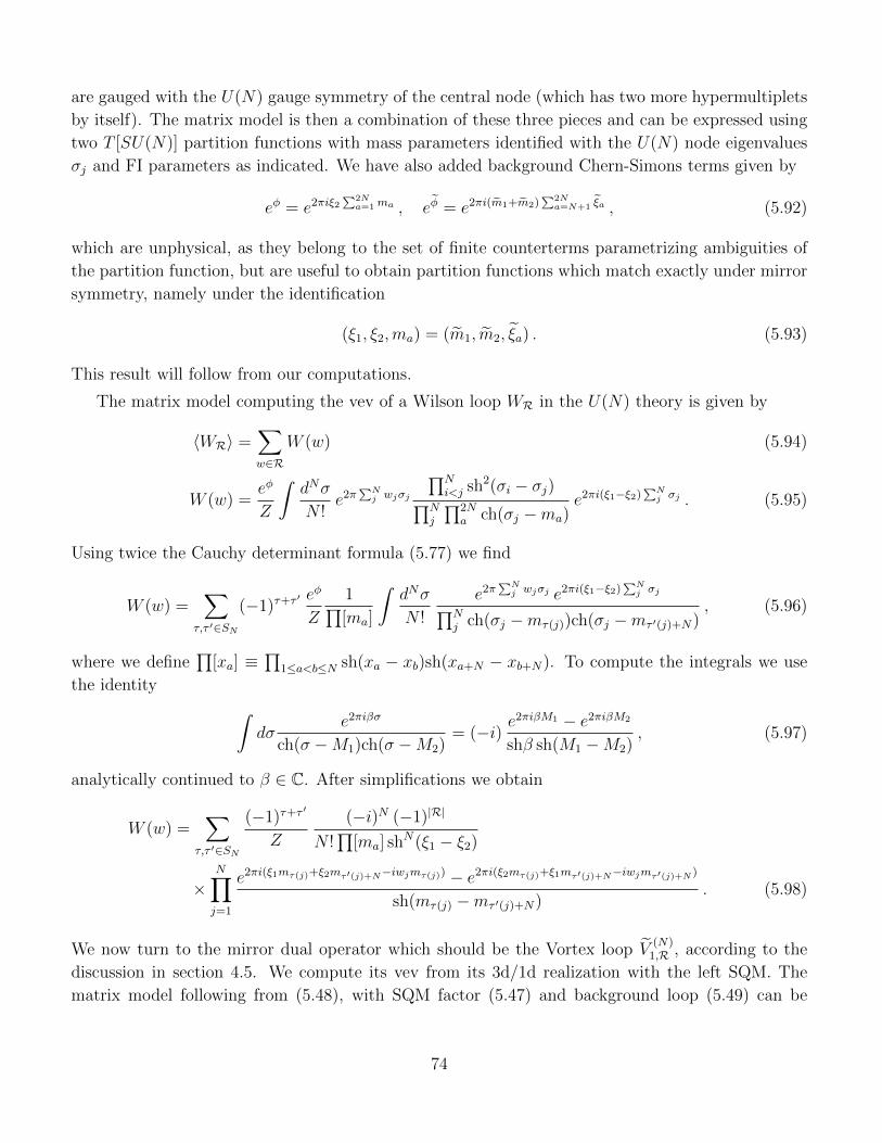
are gauged with the U(N) gauge symmetry of the central node (which has two more hypermultiplets

by itself). The matrix model is then a combination of these three pieces and can be expressed using

two T [SU(N)] partition functions with mass parameters identified with the U(N) node eigenvalues

σj and FI parameters as indicated. We have also added background Chern-Simons terms given by

eφ = e2πiξ2∑2Na=1ma , eφ = e2πi(m1+m2)

∑2Na=N+1 ξa , (5.92)

which are unphysical, as they belong to the set of finite counterterms parametrizing ambiguities of

the partition function, but are useful to obtain partition functions which match exactly under mirror

symmetry, namely under the identification

(ξ1, ξ2,ma) = (m1, m2, ξa) . (5.93)

This result will follow from our computations.

The matrix model computing the vev of a Wilson loop WR in the U(N) theory is given by

〈WR〉 =∑w∈R

W (w) (5.94)

W (w) =eφ

Z

∫dNσ

N !e2π

∑Nj wjσj

∏Ni<j sh2(σi − σj)∏N

j

∏2Na ch(σj −ma)

e2πi(ξ1−ξ2)∑Nj σj . (5.95)

Using twice the Cauchy determinant formula (5.77) we find

W (w) =∑

τ,τ ′∈SN

(−1)τ+τ ′ eφ

Z

1∏[ma]

∫dNσ

N !

e2π∑Nj wjσj e2πi(ξ1−ξ2)

∑Nj σj∏N

j ch(σj −mτ(j))ch(σj −mτ ′(j)+N), (5.96)

where we define∏

[xa] ≡∏

1≤a<b≤N sh(xa − xb)sh(xa+N − xb+N). To compute the integrals we use

the identity ∫dσ

e2πiβσ

ch(σ −M1)ch(σ −M2)= (−i) e

2πiβM1 − e2πiβM2

shβ sh(M1 −M2), (5.97)

analytically continued to β ∈ C. After simplifications we obtain

W (w) =∑

τ,τ ′∈SN

(−1)τ+τ ′

Z

(−i)N (−1)|R|

N !∏

[ma] shN(ξ1 − ξ2)

×N∏j=1

e2πi(ξ1mτ(j)+ξ2mτ ′(j)+N−iwjmτ(j)) − e2πi(ξ2mτ(j)+ξ1mτ ′(j)+N−iwjmτ ′(j)+N )

sh(mτ(j) −mτ ′(j)+N). (5.98)

We now turn to the mirror dual operator which should be the Vortex loop V(N)

1,R , according to the

discussion in section 4.5. We compute its vev from its 3d/1d realization with the left SQM. The

matrix model following from (5.48), with SQM factor (5.47) and background loop (5.49) can be

74

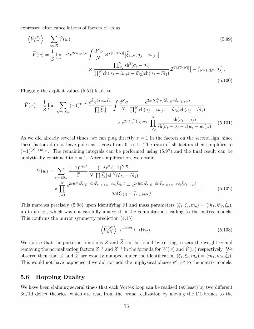
expressed after cancellations of factors of ch as⟨V

(N)1,R

⟩=∑w∈R

V (w) (5.99)

V (w) =1

Zlimz→1

eφ e2πwtotξN

∫dNσ

N !ZT [SU(N)]

[ξ1..N ;σj − iwjz

]×

∏Ni<j sh2(σi − σj)∏N

j ch(σj − iwjz − m2)ch(σj − m1)ZT [SU(N)]

[− ξN+1..2N ;σj

],

(5.100)

Plugging the explicit values (5.51) leads to

V (w) =1

Zlimz→1

∑τ,τ ′∈SN

(−1)τ+τ ′ eφ e2πwtotξN∏

[ξa]

∫dNσ

N !

e2πi∑Nj σj(ξτ(j)−ξτ ′(j)+N )∏N

j ch(σj − iwjz − m2)ch(σj − m1)

× e2π∑Nj ξτ(j)wjz

N∏i<j

sh(σi − σj)sh(σi − σj − i(wi − wj)z)

. (5.101)

As we did already several times, we can plug directly z = 1 in the factors on the second lign, since

these factors do not have poles as z goes from 0 to 1. The ratio of sh factors then simplifies to

(−1)(N−1)wtot . The remaining integrals can be performed using (5.97) and the final result can be

analytically continued to z = 1. After simplification, we obtain

V (w) =∑

τ,τ ′∈SN

(−1)τ+τ ′

Z

(−i)N (−1)N |R|

N !∏

[ξa] shN(m1 − m2)

×N∏j=1

e2πi(m1ξτ(j)+m2ξτ ′(j)+N−iwj ξτ(j)) − e2πi(m2ξτ(j)+m1ξτ ′(j)+N−iwj ξτ ′(j)+N )

sh(ξτ(j) − ξτ ′(j)+N). . (5.102)

This matches precisely (5.98) upon identifying FI and mass parameters (ξ1, ξ2,ma) = (m1, m2, ξa),

up to a sign, which was not carefully analyzed in the computations leading to the matrix models.

This confirms the mirror symmetry prediction (4.15)⟨V

(N)1,R

⟩mirror←−−−→ 〈WR〉 . (5.103)

We notice that the partition functions Z and Z can be found by setting to zero the weight w and

removing the normalization factors Z−1 and Z−1 in the formula for W (w) and V (w) respectively. We

observe then that Z and Z are exactly mapped under the identification (ξ1, ξ2,ma) = (m1, m2, ξa).

This would not have happened if we did not add the unphysical phases eφ, eφ to the matrix models.

5.6 Hopping Duality

We have been claiming several times that each Vortex loop can be realized (at least) by two different

3d/1d defect theories, which are read from the brane realization by moving the D1-branes to the

75

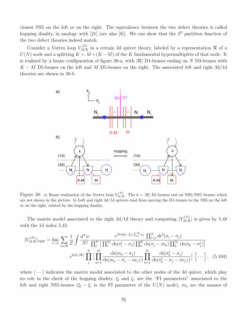
closest NS5 on the left or on the right. The equivalence between the two defect theories is called

hopping duality, in analogy with [21] (see also [8]). We can show that the S3 partition function of

the two defect theories indeed match.

Consider a Vortex loop V(N)M,R in a certain 3d quiver theory, labeled by a representation R of a

U(N) node and a splitting K = M+(K−M) of the K fundamental hypermultiplets of that node. It

is realized by a brane configuration of figure 38-a, with |R| D1-branes ending on N D3-branes with

K −M D5-branes on the left and M D5-branes on the right. The associated left and right 3d/1d

theories are shown in 38-b.

x6

x3

K-M

(1d)

(3d)

M

NNl

a)

b)K-M M

D1

Nl

Nr

N

Nr

(k)

K-M

(1d)

(3d)

M

NNl

Nr

Nl

k hopping k

Figure 38: a) Brane realization of the Vortex loop V(N)M,R. The k = |R| D1-branes end on NS5/NS5’-branes which

are not shown in the picture. b) Left and right 3d/1d quivers read from moving the D1-branes to the NS5 on the left

or on the right, related by the hopping duality.

The matrix model associated to the right 3d/1d theory and computing 〈V (N)M,R〉 is given by 5.48

with the 1d index 5.45:

〈V (N)M,R〉right = lim

z→1

∑w∈R

1

Z

∫dNσ

N !

e2πi(ξl−ξr)∑Nj σj

∏Ni<j sh2(σi − σj)∏N

j

[∏Nli ch(σli − σj)

∏Ka ch(σj −ma)

∏Nrk ch(σk − σrj )

]. e2πξr|R|

N∏j

[ M∏a=1

ch(ma − σj)ch(ma − σj − iwjz)

Nr∏k=1

ch(σrk − σj)ch(σrk − σj − iwjz)

] [· · ·], (5.104)

where [ · · · ] indicates the matrix model associated to the other nodes of the 3d quiver, which play

no role in the check of the hopping duality, ξl and ξr are the “FI parameters” associated to the

left and right NS5-branes (ξl − ξr is the FI parameter of the U(N) node), ma are the masses of

76

the fundamental hypermultiplets and σlj and σrk are the eigenvalues of the U(Nl) and U(Nr) nodes

standing respectively on the left and on the right of the U(N) node in the quiver diagram. This

simplifies to

〈V (N)M,R〉right = lim

z→1

∑w∈R

1

Z

∫dNσ

N !

e2πi(ξl−ξr)∑Nj σj

∏Ni<j sh2(σi − σj)∏N

j

[∏Nli ch(σli − σj)

∏Ka=M+1 ch(σj −ma)

].

e2πξr|R|∏Nj

[∏Ma=1 ch(ma − σj − iwjz)

∏Nrk=1 ch(σrk − σj − iwjz)

] [ · · · ] . (5.105)

The meaning of the z → 1 limit, as explained after equation 5.48, is to take the analytical continuation

of the matrix model computed with iz ∈ R. We can thus perform the change of variable σj →σj − iwjz, leading to

〈V (N)M,R〉right = lim

z→1

∑w∈R

1

Z

∫dNσ

N !

e2π(ξl−ξr)z|R| e2πi(ξl−ξr)∑Nj σj

∏Ni<j sh2(σi − σj − i(wi − wj)z)∏N

j

[∏Nli ch(σli − σj + iwjz)

∏Ka=M+1 ch(ma − σj + iwjz)

].

e2πξr|R|∏Nj

[∏Ma=1 ch(ma − σj)

∏Nrk=1 ch(σrk − σj)

] [ · · · ] . (5.106)

The analytical continuation z → 1 can be taken directly in the integrand for the factors in the

numerator, because they do not have poles for z ∈ C. The expression then simplifies again and

matches the matrix model computing 〈V (N)M,R〉 from the left 3d/1d theory realization:

〈V (N)M,R〉right = lim

z→1

∑w∈R

1

Z

∫dNσ

N !

e2πξl|R|∏Nj

[∏Nli ch(σli − σj + iwjz)

∏Ka=M+1 ch(ma − σj + iwjz)

].

e2πi(ξl−ξr)∑Nj σj

∏Ni<j sh2(σi − σj)∏N

j

[∏Ma=1 ch(ma − σj)

∏Nrk=1 ch(σrk − σj)

] [ · · · ]= 〈V (N)

M,R〉left , (5.107)

where we have used sh(x+ in) = (−1)nsh(x), for n ∈ Z. This is indeed the matrix model associated

to the left 3d/1d theory given by 5.48 with the 1d index 5.47, after simplification of some factors of

ch. Note that the additional background Wilson loop is important to get a precise match.

The hopping duality also explains the equivalence of Vortex loops labeled by representations of

different nodes. This occurs for instance for the Vortex loops of circular quivers with nodes of equal

ranks described in section 4.4 (see (4.13), (4.14)).

Consider the quiver in figure 39-a with two adjacent nodes U(N1) and U(N2), with K1 and K2

fundamental hypermultiplets respectively and assume N1 ≥ N2. The vortex loop V(N1)

0,R1, with R1

a representation of U(N1) and the subscript 0 indicating the splitting K1 = 0 + (K1 − 0), can be

77

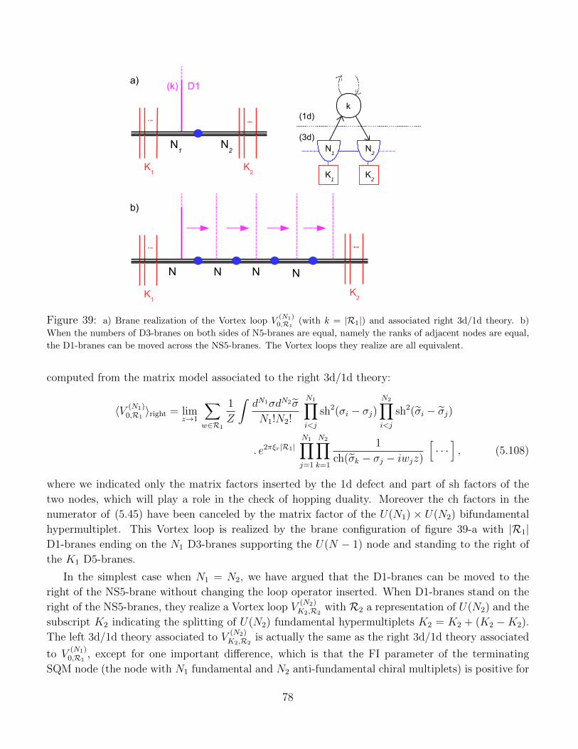
a)

K1

D1

N1

(k)

(1d)

(3d)N

1

k

K2

N2 N

2

K2

K1

b)

K1

N

K2

N N N

Figure 39: a) Brane realization of the Vortex loop V(N1)0,R1

(with k = |R1|) and associated right 3d/1d theory. b)

When the numbers of D3-branes on both sides of N5-branes are equal, namely the ranks of adjacent nodes are equal,

the D1-branes can be moved across the NS5-branes. The Vortex loops they realize are all equivalent.

computed from the matrix model associated to the right 3d/1d theory:

〈V (N1)0,R1〉right = lim

z→1

∑w∈R1

1

Z

∫dN1σdN2σ

N1!N2!

N1∏i<j

sh2(σi − σj)N2∏i<j

sh2(σi − σj)

. e2πξr|R1|N1∏j=1

N2∏k=1

1

ch(σk − σj − iwjz)

[· · ·], (5.108)

where we indicated only the matrix factors inserted by the 1d defect and part of sh factors of the

two nodes, which will play a role in the check of hopping duality. Moreover the ch factors in the

numerator of (5.45) have been canceled by the matrix factor of the U(N1) × U(N2) bifundamental

hypermultiplet. This Vortex loop is realized by the brane configuration of figure 39-a with |R1|D1-branes ending on the N1 D3-branes supporting the U(N − 1) node and standing to the right of

the K1 D5-branes.

In the simplest case when N1 = N2, we have argued that the D1-branes can be moved to the

right of the NS5-brane without changing the loop operator inserted. When D1-branes stand on the

right of the NS5-branes, they realize a Vortex loop V(N2)K2,R2

with R2 a representation of U(N2) and the

subscript K2 indicating the splitting of U(N2) fundamental hypermultiplets K2 = K2 + (K2 −K2).

The left 3d/1d theory associated to V(N2)K2,R2

is actually the same as the right 3d/1d theory associated

to V(N1)

0,R1, except for one important difference, which is that the FI parameter of the terminating

SQM node (the node with N1 fundamental and N2 anti-fundamental chiral multiplets) is positive for

78

V(N2)K2,R2

and negative for V(N1)

0,R1. The matrix model computing 〈V (N2)

K2,R2〉 from the left 3d/1d theory is

given by

〈V (N2)K2,R2

〉left = limz→1

∑w∈R2

1

Z

∫dN1σdN2σ

N1!N2!

N1∏i<j

sh2(σi − σj)N2∏i<j

sh2(σi − σj)

. e2πξr|R2|N1∏j=1

N2∏k=1

1

ch(σk − iwkz − σj)

[· · ·]. (5.109)

When N1 = N2 ≡ N we must find 〈V (N2)K2,R〉 = 〈V (N1)

0,R 〉, as the D1-branes realizing the loops can be

moved freely across the NS5. Let us consider this case first. Starting from the matrix model (5.108)

computing 〈V (N1)0,R 〉, with N1 = N , we can use the same trick as above and make the replacement∏N

i<j sh(σi − σj) → (−1)(N−1)|R|∏Ni<j sh(σi − σj + i(wi − wj)z) in the integrand. This allows us to

use the Cauchy determinant formula (5.77) with σj → σj + iwj, leading to

〈V (N1)0,R 〉right = lim

z→1

∑w∈R

∑τ∈SN

(−1)τ1

Z

∫dNσdN σ

N !2

N∏i<j

sh(σi − σj)N∏i<j

sh(σi − σj)

. (−1)(N−1)|R| e2πξr|R| 1∏Nj ch(στ(j) + iwτ(j) − σj)

[· · ·]. (5.110)

Relabeling σj → στ−1(j) and σj → στ(j), we obtain

〈V (N1)0,R 〉right = lim

z→1

∑w∈R

∑τ∈SN

(−1)τ1

Z

∫dNσdN σ

N !2

N∏i<j

sh(σi − σj)N∏i<j

sh(σi − σj)

. (−1)(N−1)|R| e2πξr|R| 1∏Nj ch(σj + iwτ(j) − στ(j))

[· · ·]

= limz→1

∑w∈R

1

Z

∫dNσdN σ

N !2

N∏i<j

sh2(σi − σj)N∏i<j

sh(σi − σj)sh(σi − σj − i(wi − wj)z)

. (−1)(N−1)|R| e2πξr|R|N1∏j=1

N2∏k=1

1

ch(σk − iwkz − σj)

[· · ·]

= 〈V (N2)K2,R〉left , (5.111)

where we have used the Cauchy identity to obtain the second equality and we have again enforced

z = 1 in the sh factors of the integrand to reach the matrix model (5.109) computing 〈V (N2)K2,R〉, with

N2 = N .

This shows that the Vortex loops realized by D1-branes ending on the left or on the right of

an NS5 with equal numbers of D3s on both sides are equivalent. Combining this property with

the hopping duality between the left and right 3d/1d quiver realization of a Vortex loop, we prove

the equivalence of Vortex loops in circular quivers with nodes of equal rank (4.13), (4.14). This is

illustrated in figure 39-b.

79

When N1 > N2 the map of Vortex loops is more complicated. It can be found from the brane

picture in the same way as we found mirror maps between loop operators. We consider the brane

realization of V(N1)

0,R1with |R1| D1-strings ending on the N1 D3-branes as in figure 39-a. As N1 > N2,

the NS5 has a D3-spike on its left side. We then move the D1-branes to the left, across the NS5-brane.

Some D1-branes can be moved along the D3-spike and get attached to the NS5-brane, realizing flavor

Wilson loops for the U(1) global symmetry associated to the NS5-brane. The other D1-branes end

on the N2 D3-branes on the right of the NS5 and realize a Vortex loop V(N2)K2,R2

. Recycling the ideas

of section 3.2, the precise prediction from the brane picture is found to be

⟨V

(N1)0,R1

⟩=

⟨∑s∈∆

W flNS5,qs V

(N2)

K2,Rs

⟩, (5.112)

where ∆ is the set of representations (qs, Rs) appearing in the decomposition of R1 under the

subgroup U(1) × U(N2) ⊂ U(N1 − N2) × U(N2) ⊂ U(N1), with U(1) embedded diagonally into

U(N1 − N2). W flNS5,q denotes the Wilson loop of charge q under the U(1) topological symmetry

associated to the NS5.

This map can be checked by explicit computations, using the generalized Cauchy formula (5.78).

It implies that the Vortex loops V(N1)

0,R1and V

(N2)K2,R2

are redundant and that in order to describe the

mirror map with Wilson loops of the mirror theory, it is sufficient to consider only the loops V(N1)

0,R1or

the loops V(N2)K2,R2

. In general for each pair of consecutive D5-branes in the brane picture, we need only

to consider the Vortex loops realized with D1-branes placed between the two D5-branes, with a fixed

number of NS5-branes on their left and on their right. This is the mirror statement to the fact that

between two consecutive NS5-branes, we need only consider Wilson loops realized with F1-strings

placed between the two NS5s, with a fixed number of D5-branes on their left and on their right.

Acknowledgements

We would like to thank Kevin Costello, Nadav Drukker, Davide Gaiotto, Heeyeon Kim, Hee-Cheol

Kim, Bruno Le Floch, Stefano Cremonesi, R. Santamaria and E. Witten for discussions. B.A.

thanks Perimeter Institute for its generous hospitality during several visits between 2013 and 2015.

JG is grateful to the KITP for its warm hospitality during the “New Methods in Nonperturbative

Quantum Field Theory” Program in early 2014, which was supported in part by the National Science

Foundation under Grant No. NSF PHY11-25915. This research was supported in part by Perimeter

Institute for Theoretical Physics. Research at Perimeter Institute is supported by the Government of

Canada through Industry Canada and by the Province of Ontario through the Ministry of Research

and Innovation. J.G. also acknowledges further support from an NSERC Discovery Grant and from

an ERA grant by the Province of Ontario. B.A. acknowledges support by the ERC Starting Grant

N. 304806, “The Gauge/Gravity Duality and Geometry in String Theory.”.

80

A Supersymmetry Transformations On S3 And SQM Em-

bedding

We provide here the 3d N = 4 supersymmetry transformations of the vector multiplet and hyper-

multiplet on S3. By restricting to the four supercharges preserved by the SQMV deformed algebra

SU(1|1)l × SU(1|1)R in (5.19)(5.20), we work out the embedding of the 1d N = 4 vector and chiral

multiplets inside the 3d N = 4 vector and hypermultiplets.

The 3d N = 4 supersymmetry transformations are generated by the four two-component Killing

spinors εAA′, with A = 1, 2 the index of the 2 of SU(2)C and A′ = 1, 2 the index of the 2 of SU(2)H .

The transformations of the 3d N = 4 abelian vector multiplet (Aµ,ΦI , λAA′ ,DI′) are72

δAµ = − i2λAA′γµε

AA′ δΦI = −1

2λAA′(τI)

ABε

BA′

δλAA′= −1

2Fµνγ

µνεAA′ − DI′(τI′)

A′B′ε

AB′ + iDµΦIγµ(τI)

ABε

BA′ +2i

3ΦIγ

µ(τI)ABDµε

BA′

δDI′ = − i2DµλAA′γµ(τI′)

A′B′ε

AB′ − i

6λAA′γµ(τI′)

A′B′Dµε

AB′ ,

where τI = τI′ are the Pauli matrices. I = 1, 2, 3 is the index of the 3 of SU(2)C while I ′ = 1, 2, 3

is the index of the 3 of SU(2)H . The Killing spinors ε11 = εL and ε22 = εL generate the 3d N = 2

supersymmetry transformations in SU(2|1)l, while ε12 = εR and ε21 = εR generate supersymmetry

transformations in SU(2|1)r.

The 3dN = 4 vector multiplet decomposes into a 3dN = 2 vector multiplet (Aµ,Φ3, λ11, λ22,D3) =

(Aµ, σ, λ, λ, D) and an adjoint chiral multiplet (Φ1 + iΦ2, λ12, λ21,D1 + iD2) = (φ, ψ, ψ, F ).

SQMV embedding

The four Killing spinors generating the deformed SQMV algebra are (see section 5.2)

εl =

(ε10

), εl =

(0

ε2

), εr =

(0

ε2

), εr =

(¯ε10

). (A.1)

In the left-invariant frame, εl and εl are constant, while εr and εr have a spatial dependent phase

eiτ/L and e−iτ/L respectively, where τ ∈ [0, 2πL] is the coordinate along the loop. We recall that the

equations solved by the Killing spinors are

∇µεl =i

2Lγµεl , ∇µεl =

i

2Lγµεl , (A.2)

∇µεr = − i

2Lγµεr , ∇µεr = − i

2Lγµεr , (A.3)

where L is the radius of S3. The supersymmetry transformations under the supercharges in deformed

72We derived these transformations by “covariantizing” the 3d N = 2 transformations of [4].

81

superalgebra SQMV reduce to73

δAτ = − i2

(λ1ε2 + λ2ε1 − ψ2

¯ε1 − ψ1ε2)

δΦ3 = −1

2

(−λ1ε2 − λ2ε1 − ψ2

¯ε1 − ψ1ε2)

δΦ = λ1ε2 + ψ2ε1 δΦ = −λ2¯ε1 − ψ1ε2

δλ1 =

(D3 −

i

2F12 +

Φ3

L

)ε1 − iDτΦ3ε1 + i

(DτΦ− i

Φ

L

)¯ε1

δλ2 = −(D3 −

i

2F12 +

Φ3

L

)ε2 − iDτΦ3ε2 − i

(Dτ Φ + i

Φ

L

)ε2

δψ1 =

(D3 −

i

2F12 +

Φ3

L

)¯ε1 + iDτΦ3

¯ε1 + i

(Dτ Φ + i

Φ

L

)ε1

δψ2 = −(D3 −

i

2F12 +

Φ3

L

)ε2 + iDτΦ3ε2 − i

(DτΦ− i

Φ

L

)ε2 , (A.4)

where Φ = Φ1 + iΦ2 and we have adopted 3d N = 2 notations λα, λα, ψα, ψα for the fermions, with

α = 1, 2.

These correspond to the supersymmetry transformations of a 1d N = 4 SQMV abelian vector

multiplet (see for instance [18]) but in the presence of a background gauge field a− = − 1L

for the

U(1)− R-symmetry, generated by J−. The presence of the background gauge field a− = − 1L

affects

the covariant derivative of Φ, Φ in the transformations above. The identification of the fields in the

3d N = 4 vector multiplet with the fields of the 1d N = 2 vector and adjoint chiral multiplet that

furnish a 1d N = 4 SQMV vector multiplet is

1d vector multiplet : (vτ , x3, λ−, λ−, D)1d ∼ (Aτ ,Φ3, λ2, λ1,D3 −i

2F12 +

Φ3

L) , r− = 0 (A.5)

1d chiral multiplet : (x1 + ix2, ψ, ψ)1d ∼ (Φ, ψ2, ψ1) , r− = −1 , (A.6)

where we have indicated the U(1)− charges of the 1d N = 2 multiplets:74 the 1d N = 2 vector

multiplet fields have vanishing U(1)− charge, while the fields x1 + ix2 and ψ in the 1d N = 2 SQM

adjoint chiral multiplet have U(1)− charge −1 and ψ charge 1.

We now turn to the 3d N = 4 hypermultiplet supersymmetry transformations. These do not

admit an off-shell formulation, so we provide the on-shell supersymmetry transformations:

δφA′= −ψAεAA

′(A.7)

δψA = iγµεAA′DµφA′ + iΦI(τI)

ABφA′ε

BA′ +i

3γµDµε

AA′φA′ . (A.8)

73We do not give the supersymmetry transformations of the auxiliary fields and transverse gauge fields, which

combine into another 1d N = 4 chiral multiplet.74U(1)− is a global symmetry from the point of view of the 1d N = 2 subalgebra, so that each N = 2 multiplet

comes with a U(1)− charge.

82

(φ1,−ψ2) and (φ2, ψ1) are two on-shell chiral multiplets of 3d N = 2 supersymmetry of R-charge

1/2 transforming under complex conjugate representations of the gauge group.

Restricting to the same four supercharges generating deformed SQMV as above, we obtain

δφ1 = (ψ1)1ε2 − (ψ2)1ε2

δ(ψ1)1 = i¯ε1Dτφ1 + i(Φ3 −

i

2L)φ1¯ε1 + iΦφ1ε1 − i(D1 − iD2)φ2ε2

δ(ψ2)1 = iε1Dτφ1 − i(Φ3 −

i

2L)φ1ε1 + iΦφ1¯ε1 − i(D1 − iD2)φ2ε2

δφ2 = (ψ1)2ε1 − (ψ2)2¯ε1

δ(ψ1)2 = −iε2Dτφ2 + i(Φ3 +

i

2L)φ2ε2 + iΦφ2ε2 − i(D1 + iD2)φ1¯ε1

δ(ψ2)2 = −iε2Dτφ2 − i(Φ3 +

i

2L)φ2ε2 + iΦφ2ε2 − i(D1 + iD2)φ1ε1 . (A.9)

This matches the on-shell deformed supersymmetry transformations of two 1d N = 4 chiral

multiplets (φ, ψ+, ψ−)qF ∼ (φ1, (ψ1)1, (ψ2)1)− 1

2and (φ2, (ψ1)2, (ψ

2)2) 12. The shift of Φ3 in the su-

persymmetry transformations is identified with a real mass deformation with complex parameter

mF = iL

for a flavor symmetry GF , such that the 1d N = 4 chiral multiplets have GF charge

qF = ∓12. The term (D1 + iD2)φ1 in the on-shell 1d N = 4 supersymmetry transformations arises

from a superpotential coupling. In the off-shell transformations it gets replaced with a complex

auxiliary field.

We note that the mass deformation obtained by giving a background to the GF flavour symmetry

is not visible anywhere in the transformations A.4, which means that the adjoint chiral multiplet

with bottom component Φ = Φ1 + iΦ2 is not charged under GF . This allows us to identify this flavor

symmetry with

GF = J l3 + Jr3 −RH . (A.10)

Moreover the background gauge field a− = − 1L

for J− is not visible in the transformations (A.9) of

the chiral multiplets with bottom components φ1 and φ2, which means that these multiplets are not

charged under J−. We then have the identification

J− = J l3 + Jr3 −RV . (A.11)

This identification of generators allows us to match the deformed SQMW supersymmetry algebra

with the SU(1|1)l × SU(1|1)r subalgebra preserved by the defect, as explained in section 5.2.

B Evaluations of the SQM Index

In this appendix we compute the 1d N = 4 SQM index, or partition function on S1, for some quiver

gauge theories with generic U(1)− R-symmetry background z and U(1)F flavor chemical potential

µ = 1, as defined in section 5.3.2. The R-symmetry and flavor symmetry charges are summarized in

table 6 and the specific adjoint R-charges are given in equation (5.43).

83

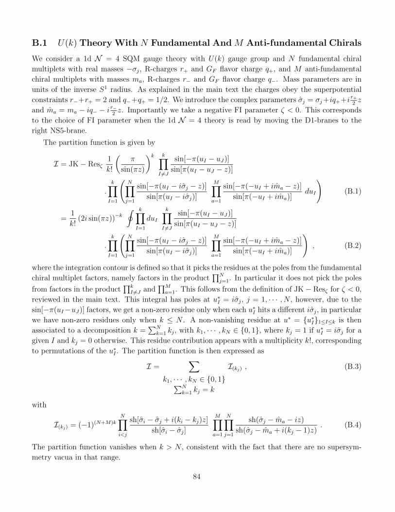
B.1 U(k) Theory With N Fundamental AndM Anti-fundamental Chirals

We consider a 1d N = 4 SQM gauge theory with U(k) gauge group and N fundamental chiral

multiplets with real masses −σj, R-charges r+ and GF flavor charge q+, and M anti-fundamental

chiral multiplets with masses ma, R-charges r− and GF flavor charge q−. Mass parameters are in

units of the inverse S1 radius. As explained in the main text the charges obey the superpotential

constraints r−+r+ = 2 and q−+q+ = 1/2. We introduce the complex parameters σj = σj+iq++i r+2z

and ma = ma − iq− − i r−2 z. Importantly we take a negative FI parameter ζ < 0. This corresponds

to the choice of FI parameter when the 1d N = 4 theory is read by moving the D1-branes to the

right NS5-brane.

The partition function is given by

I = JK− Resζ1

k!

(π

sin(πz)

)k k∏I 6=J

sin[−π(uI − uJ)]

sin[π(uI − uJ − z)]

.k∏I=1

(N∏j=1

sin[−π(uI − iσj − z)]

sin[π(uI − iσj)]

M∏a=1

sin[−π(−uI + ima − z)]

sin[π(−uI + ima)]duI

)(B.1)

=1

k!(2i sin(πz))−k

∮ k∏I=1

duI

k∏I 6=J

sin[−π(uI − uJ)]

sin[π(uI − uJ − z)]

.k∏I=1

(N∏j=1

sin[−π(uI − iσj − z)]

sin[π(uI − iσj)]

M∏a=1

sin[−π(−uI + ima − z)]

sin[π(−uI + ima)]

), (B.2)

where the integration contour is defined so that it picks the residues at the poles from the fundamental

chiral multiplet factors, namely factors in the product∏N

j=1. In particular it does not pick the poles

from factors in the product∏k

I 6=J and∏M

a=1. This follows from the definition of JK− Resζ for ζ < 0,

reviewed in the main text. This integral has poles at u∗I = iσj, j = 1, · · · , N , however, due to the

sin[−π(uI−uJ)] factors, we get a non-zero residue only when each u∗I hits a different iσj, in particular

we have non-zero residues only when k ≤ N . A non-vanishing residue at u∗ = {u∗I}1≤I≤k is then

associated to a decomposition k =∑N

k=1 kj, with k1, · · · , kN ∈ {0, 1}, where kj = 1 if u∗I = iσj for a

given I and kj = 0 otherwise. This residue contribution appears with a multiplicity k!, corresponding

to permutations of the u∗I . The partition function is then expressed as

I =∑

k1, · · · , kN ∈ {0, 1}∑Nk=1 kj = k

I(kj) , (B.3)

with

I(kj) = (−1)(N+M)k

N∏i<j

sh[σi − σj + i(ki − kj)z]

sh[σi − σj]

M∏a=1

N∏j=1

sh(σj − ma − iz)

sh(σj − ma + i(kj − 1)z). (B.4)

The partition function vanishes when k > N , consistent with the fact that there are no supersym-

metry vacua in that range.

84

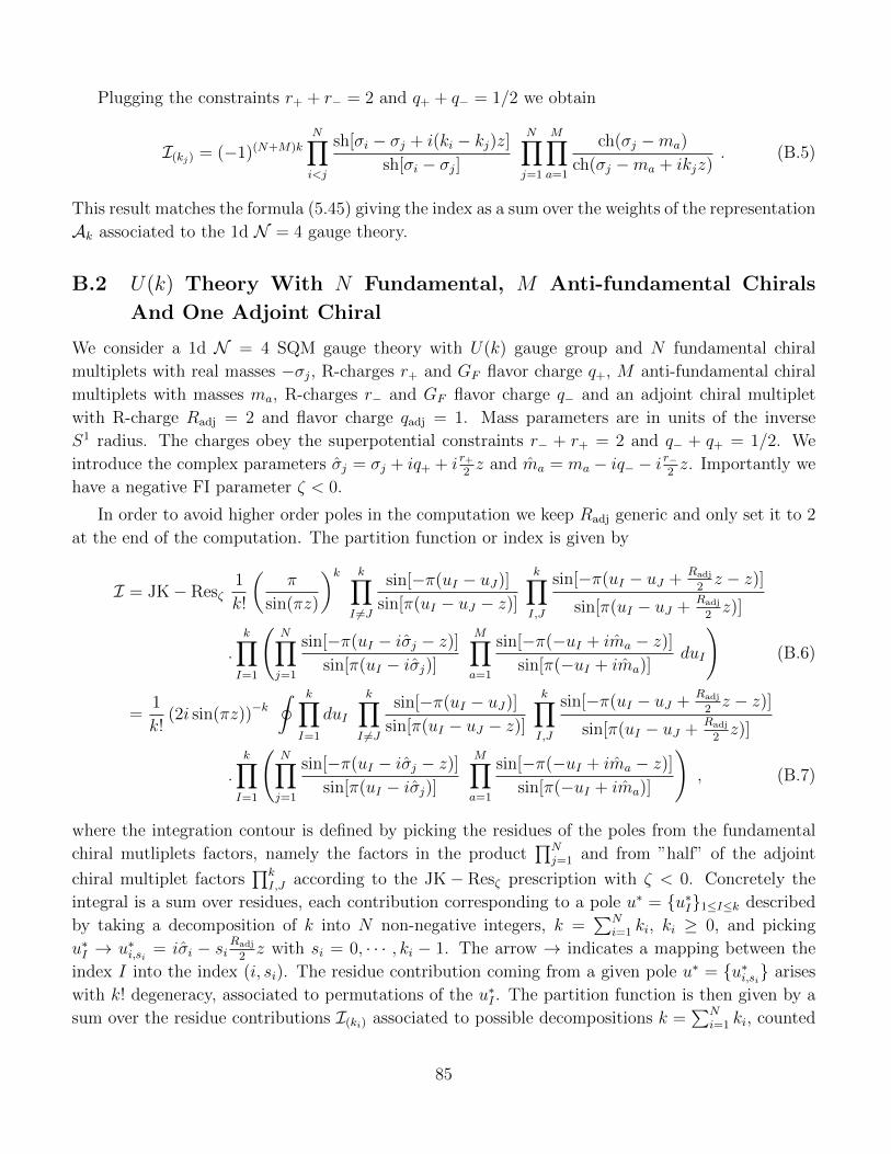
Plugging the constraints r+ + r− = 2 and q+ + q− = 1/2 we obtain

I(kj) = (−1)(N+M)k

N∏i<j

sh[σi − σj + i(ki − kj)z]

sh[σi − σj]

N∏j=1

M∏a=1

ch(σj −ma)

ch(σj −ma + ikjz). (B.5)

This result matches the formula (5.45) giving the index as a sum over the weights of the representation

Ak associated to the 1d N = 4 gauge theory.

B.2 U(k) Theory With N Fundamental, M Anti-fundamental Chirals

And One Adjoint Chiral

We consider a 1d N = 4 SQM gauge theory with U(k) gauge group and N fundamental chiral

multiplets with real masses −σj, R-charges r+ and GF flavor charge q+, M anti-fundamental chiral

multiplets with masses ma, R-charges r− and GF flavor charge q− and an adjoint chiral multiplet

with R-charge Radj = 2 and flavor charge qadj = 1. Mass parameters are in units of the inverse

S1 radius. The charges obey the superpotential constraints r− + r+ = 2 and q− + q+ = 1/2. We

introduce the complex parameters σj = σj + iq+ + i r+2z and ma = ma − iq− − i r−2 z. Importantly we

have a negative FI parameter ζ < 0.

In order to avoid higher order poles in the computation we keep Radj generic and only set it to 2

at the end of the computation. The partition function or index is given by

I = JK− Resζ1

k!

(π

sin(πz)

)k k∏I 6=J

sin[−π(uI − uJ)]

sin[π(uI − uJ − z)]

k∏I,J

sin[−π(uI − uJ +Radj

2z − z)]

sin[π(uI − uJ +Radj

2z)]

.k∏I=1

(N∏j=1

sin[−π(uI − iσj − z)]

sin[π(uI − iσj)]

M∏a=1

sin[−π(−uI + ima − z)]

sin[π(−uI + ima)]duI

)(B.6)

=1

k!(2i sin(πz))−k

∮ k∏I=1

duI

k∏I 6=J

sin[−π(uI − uJ)]

sin[π(uI − uJ − z)]

k∏I,J

sin[−π(uI − uJ +Radj

2z − z)]

sin[π(uI − uJ +Radj

2z)]

.k∏I=1

(N∏j=1

sin[−π(uI − iσj − z)]

sin[π(uI − iσj)]

M∏a=1

sin[−π(−uI + ima − z)]

sin[π(−uI + ima)]

), (B.7)

where the integration contour is defined by picking the residues of the poles from the fundamental

chiral mutliplets factors, namely the factors in the product∏N

j=1 and from ”half” of the adjoint

chiral multiplet factors∏k

I,J according to the JK− Resζ prescription with ζ < 0. Concretely the

integral is a sum over residues, each contribution corresponding to a pole u∗ = {u∗I}1≤I≤k described

by taking a decomposition of k into N non-negative integers, k =∑N

i=1 ki, ki ≥ 0, and picking

u∗I → u∗i,si = iσi − si Radj

2z with si = 0, · · · , ki − 1. The arrow → indicates a mapping between the

index I into the index (i, si). The residue contribution coming from a given pole u∗ = {u∗i,si} arises

with k! degeneracy, associated to permutations of the u∗I . The partition function is then given by a

sum over the residue contributions I(ki) associated to possible decompositions k =∑N

i=1 ki, counted

85

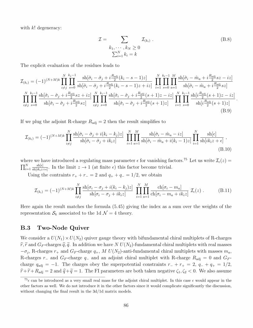
with k! degeneracy:

I =∑

k1, · · · , kN ≥ 0∑Ni=1 ki = k

I(ki) . (B.8)

The explicit evaluation of the residues leads to

I(ki) = (−1)(N+M)k

N∏i 6=j

kj−1∏s=0

sh[σi − σj + iRadj

2(ki − s− 1)z]

sh[σi − σj + iRadj

2(ki − s− 1)z + iz]

N∏i=1

ki−1∏s=0

M∏a=1

sh[σi − ma + iRadj

2sz − iz]

sh[σi − ma + iRadj

2sz]

N∏i 6=j

ki−1∏s=0

sh[σi − σj + iRadj

2sz + iz]

sh[σi − σj + iRadj

2sz]

N∏i 6=j

ki−1∏s=0

sh[σi − σj + iRadj

2(s+ 1)z − iz]

sh[σi − σj + iRadj

2(s+ 1)z]

N∏i=1

ki−1∏s=0

sh[iRadj

2(s+ 1)z − iz]

sh[iRadj

2(s+ 1)z]

.

(B.9)

If we plug the adjoint R-charge Radj = 2 then the result simplifies to

I(ki) = (−1)(N+M)k

N∏i 6=j

sh[σi − σj + i(ki − kj)z]

sh[σi − σj + ikiz]

N∏i=1

M∏a=1

sh[σi − ma − iz]

sh[σi − ma + i(ki − 1)z]

N∏i=1

sh[ε]

sh[ikiz + ε],

(B.10)

where we have introduced a regulating mass parameter ε for vanishing factors.75 Let us write Iε(z) =∏Ni=1

sh[ε]sh[ikiz+ε]

. In the limit z → 1 (at finite ε) this factor become trivial.

Using the contraints r+ + r− = 2 and q+ + q− = 1/2, we obtain

I(ki) = (−1)(N+M)k

N∏i 6=j

sh[σi − σj + i(ki − kj)z]

sh[σi − σj + ikiz]

N∏i=1

M∏a=1

ch[σi −ma]

ch[σi −ma + ikiz]Iε(z) . (B.11)

Here again the result matches the formula (5.45) giving the index as a sum over the weights of the

representation Sk associated to the 1d N = 4 theory.

B.3 Two-Node Quiver

We consider a U(N1)×U(N2) quiver gauge theory with bifundamental chiral multiplets of R-charges

r, r and GF -charges q, q. In addition we have N U(N2)-fundamental chiral multiplets with real masses

−σj, R-charges r+ and GF -charge q+, M U(N2)-anti-fundamental chiral multiplets with masses ma,

R-charges r− and GF -charge q− and an adjoint chiral multiplet with R-charge Radj = 0 and GF -

charge qadj = −1. The charges obey the superpotential constraints r− + r+ = 2, q− + q+ = 1/2,

r+ r+Radj = 2 and q+ q = 1. The FI parameters are both taken negative ζ1, ζ2 < 0. We also assume

75ε can be introduced as a very small real mass for the adjoint chiral multiplet. In this case ε would appear in the

other factors as well. We do not introduce it in the other factors since it would complicate significantly the discussion,

without changing the final result in the 3d/1d matrix models.

86

D1

NS5'

M

NS5'

NS5

N2

(k2)

(k1)

(N) (M)N

N1

Figure 40: Brane realization of a Vortex loop associated with the representation Ak1 ⊗ Ak2 and SQM two-node

quiver read by moving the D1-branes to the NS5-brane on the right. Here N1 = k1 and N2 = k1 + k2.

N2 > N1. This setup corresponds to the 1d N = 4 theory obtained by moving the D1-branes to right

NS5-brane, with k1 = N1 D1-branes ending on an extra NS5’-brane and k2 = N2 − N1 D1-branes

ending on a second extra NS5’-brane (see figure 40). The representation associated to this quiver is

R = Ak1 ⊗Ak2 .

We introduce the complex parameters σj = σj + iq+ + i r+2z and ma = ma − iq− − i r−2 z. in order

to avoid higher order poles in the computation we keep Radj generic and only set it to 0 at the end.

The partition function or index is given by

I =

∮ N1∏I=1

duI

N2∏J=1

dvJ1

N1!N2!

(π

sin(πz)

)N1+N2 N1∏I 6=J

sin[−π(uI − uJ)]

sin[π(uI − uJ − z)]

N2∏I 6=J

sin[−π(vI − vJ)]

sin[π(vI − vJ − z)]

N1∏I,J

sin[−π(uI − uJ +Radj

2z − z)]

sin[π(uI − uJ +Radj

2z)]

N1∏I=1

(N∏j=1

sin[−π(vI − iσj − z)]

sin[π(vI − iσj)]

M∏a=1

sin[−π(−vI + ima − z)]

sin[π(−vI + ima)]

)N1∏I

N2∏J

sin[−π(uI − vJ + q + r2z − z)]

sin[π(uI − vJ + q + r2z)]

sin[−π(vJ − uI + q + r2z − z)]

sin[π(vJ − uI + q + r2z)]

.

The integration contour picks the residues at the poles selected by the JK-recipe as explained in the

main text. The recipe allows to take poles from the the fundamental chiral mulitplet factors, as well

as from ”half” of the bifundamental and adjoint chiral multiplet factors. However one can realize, for

instance, that picking a pole u∗I = u∗J−Radj

2z from the adjoint factor and a pole u∗J = v∗K− q− r

2z from

the bifundamental factor, leads to u∗I = v∗K + q + r2z − z − 1, where we have used the superpotential

constraints, and in this case u∗I has an extra zero from the bifundamental factor, canceling the pole

from the adjoint factor. This kind of reasoning leads to the conclusion that we cannot take a pole

from the adjoint factor, as it yields a vanishing contribution.

A careful analysis along these lines leads to the following sets of poles (u∗, v∗) contributing to I:

87

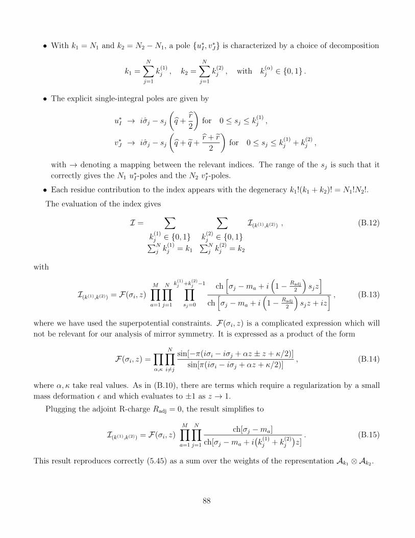
• With k1 = N1 and k2 = N2 −N1, a pole {u∗I , v∗J} is characterized by a choice of decomposition

k1 =N∑j=1

k(1)j , k2 =

N∑j=1

k(2)j , with k

(α)j ∈ {0, 1} .

• The explicit single-integral poles are given by

u∗I → iσj − sj(q +

r

2

)for 0 ≤ sj ≤ k

(1)j ,

v∗J → iσj − sj(q + q +

r + r

2

)for 0 ≤ sj ≤ k

(1)j + k

(2)j ,

with → denoting a mapping between the relevant indices. The range of the sj is such that it

correctly gives the N1 u∗I-poles and the N2 v

∗I -poles.

• Each residue contribution to the index appears with the degeneracy k1!(k1 + k2)! = N1!N2!.

The evaluation of the index gives

I =∑

k(1)j ∈ {0, 1}∑Nj k

(1)j = k1

∑k

(2)j ∈ {0, 1}∑Nj k

(2)j = k2

I(k(1),k(2)) , (B.12)

with

I(k(1),k(2)) = F(σi, z)M∏a=1

N∏j=1

k(1)j +k

(2)j −1∏

sj=0

ch[σj −ma + i

(1− Radj

2

)sjz]

ch[σj −ma + i

(1− Radj

2

)sjz + iz

] , (B.13)

where we have used the superpotential constraints. F(σi, z) is a complicated expression which will

not be relevant for our analysis of mirror symmetry. It is expressed as a product of the form

F(σi, z) =∏α,κ

N∏i 6=j

sin[−π(iσi − iσj + αz ± z + κ/2)]

sin[π(iσi − iσj + αz + κ/2)], (B.14)

where α, κ take real values. As in (B.10), there are terms which require a regularization by a small

mass deformation ε and which evaluates to ±1 as z → 1.

Plugging the adjoint R-charge Radj = 0, the result simplifies to

I(k(1),k(2)) = F(σi, z)M∏a=1

N∏j=1

ch[σj −ma]

ch[σj −ma + i(k

(1)j + k

(2)j

)z]. (B.15)

This result reproduces correctly (5.45) as a sum over the weights of the representation Ak1 ⊗Ak2 .

88

References

[1] K. G. Wilson, Confinement of Quarks, Phys.Rev. D10 (1974) 2445–2459.

[2] K. A. Intriligator and N. Seiberg, Mirror symmetry in three-dimensional gauge theories,

Phys.Lett. B387 (1996) 513–519, [hep-th/9607207].

[3] A. Kapustin, B. Willett, and I. Yaakov, Exact results for supersymmetric abelian vortex loops

in 2+1 dimensions, arXiv:1211.2861.

[4] N. Drukker, T. Okuda, and F. Passerini, Exact results for vortex loop operators in 3d

supersymmetric theories, arXiv:1211.3409.

[5] B. Assel, J. Gomis, and R. C. Santamaria. unpublished.

[6] N. Drukker, J. Gomis, and D. Young, Vortex Loop Operators, M2-branes and Holography,

JHEP 0903 (2009) 004, [arXiv:0810.4344].

[7] G. W. Moore and N. Seiberg, Taming the Conformal Zoo, Phys.Lett. B220 (1989) 422.

[8] J. Gomis and B. Le Floch, M2-brane surface operators and gauge theory dualities in Toda,

arXiv:1407.1852.

[9] A. Hanany and E. Witten, Type IIB superstrings, BPS monopoles, and three-dimensional

gauge dynamics, Nucl.Phys. B492 (1997) 152–190, [hep-th/9611230].

[10] J. Gomis and F. Passerini, Holographic Wilson Loops, JHEP 0608 (2006) 074,

[hep-th/0604007].

[11] J. Gomis and F. Passerini, Wilson Loops as D3-Branes, JHEP 0701 (2007) 097,

[hep-th/0612022].

[12] J. M. Maldacena, Wilson loops in large N field theories, Phys.Rev.Lett. 80 (1998) 4859–4862,

[hep-th/9803002].

[13] S.-J. Rey and J.-T. Yee, Macroscopic strings as heavy quarks in large N gauge theory and

anti-de Sitter supergravity, Eur.Phys.J. C22 (2001) 379–394, [hep-th/9803001].

[14] A. Kapustin, B. Willett, and I. Yaakov, Nonperturbative Tests of Three-Dimensional Dualities,

JHEP 1010 (2010) 013, [arXiv:1003.5694].

[15] S. Benvenuti and S. Pasquetti, 3D-partition functions on the sphere: exact evaluation and

mirror symmetry, arXiv:1105.2551.

[16] B. Assel, Hanany-Witten effect and SL(2, Z) dualities in matrix models, JHEP 1410 (2014)

117, [arXiv:1406.5194].

[17] A. Kapustin, B. Willett, and I. Yaakov, Exact Results for Wilson Loops in Superconformal

Chern-Simons Theories with Matter, JHEP 1003 (2010) 089, [arXiv:0909.4559].

[18] K. Hori, H. Kim, and P. Yi, Witten Index and Wall Crossing, JHEP 1501 (2015) 124,

[arXiv:1407.2567].

[19] C. Cordova and S.-H. Shao, An Index Formula for Supersymmetric Quantum Mechanics,

arXiv:1406.7853.

89

[20] N. Seiberg, Electric - magnetic duality in supersymmetric nonAbelian gauge theories,

Nucl.Phys. B435 (1995) 129–146, [hep-th/9411149].

[21] A. Gadde and S. Gukov, 2d Index and Surface operators, JHEP 1403 (2014) 080,

[arXiv:1305.0266].

[22] E. I. Buchbinder, J. Gomis, and F. Passerini, Holographic gauge theories in background fields

and surface operators, JHEP 0712 (2007) 101, [arXiv:0710.5170].

[23] K. Zarembo, Supersymmetric Wilson loops, Nucl.Phys. B643 (2002) 157–171,

[hep-th/0205160].

[24] L. Rozansky and E. Witten, HyperKahler geometry and invariants of three manifolds, Selecta

Math. 3 (1997) 401–458, [hep-th/9612216].

[25] A. Kapustin and E. Witten, Electric-Magnetic Duality And The Geometric Langlands

Program, Commun.Num.Theor.Phys. 1 (2007) 1–236, [hep-th/0604151].

[26] S. Gukov and E. Witten, Gauge Theory, Ramification, And The Geometric Langlands

Program, hep-th/0612073.

[27] N. R. Constable, J. Erdmenger, Z. Guralnik, and I. Kirsch, Intersecting D-3 branes and

holography, Phys.Rev. D68 (2003) 106007, [hep-th/0211222].

[28] D. Gaiotto, Surface Operators in N = 2 4d Gauge Theories, JHEP 1211 (2012) 090,

[arXiv:0911.1316].

[29] D. Gaiotto and E. Witten, S-Duality of Boundary Conditions In N=4 Super Yang-Mills

Theory, arXiv:0807.3720.

[30] B. Assel, C. Bachas, J. Estes, and J. Gomis, Holographic Duals of D=3 N=4 Superconformal

Field Theories, JHEP 1108 (2011) 087, [arXiv:1106.4253].

[31] B. Assel, C. Bachas, J. Estes, and J. Gomis, IIB Duals of D=3 N=4 Circular Quivers, JHEP

1212 (2012) 044, [arXiv:1210.2590].

[32] J. de Boer, K. Hori, H. Ooguri, and Y. Oz, Mirror symmetry in three-dimensional gauge

theories, quivers and D-branes, Nucl.Phys. B493 (1997) 101–147, [hep-th/9611063].

[33] N. Drukker and B. Fiol, All-genus calculation of Wilson loops using D-branes, JHEP 0502

(2005) 010, [hep-th/0501109].

[34] S. Yamaguchi, Wilson loops of anti-symmetric representation and D5-branes, JHEP 0605

(2006) 037, [hep-th/0603208].

[35] U. Danielsson, G. Ferretti, and I. R. Klebanov, Creation of fundamental strings by crossing

D-branes, Phys.Rev.Lett. 79 (1997) 1984–1987, [hep-th/9705084].

[36] C. P. Bachas, M. B. Green, and A. Schwimmer, (8,0) quantum mechanics and symmetry

enhancement in type I’ superstrings, JHEP 9801 (1998) 006, [hep-th/9712086].

[37] C. G. Callan and J. M. Maldacena, Brane death and dynamics from the Born-Infeld action,

Nucl.Phys. B513 (1998) 198–212, [hep-th/9708147].

90

[38] H. Kim, S.-J. Lee, and P. Yi, Mutation, Witten Index, and Quiver Invariant,

arXiv:1504.0006.

[39] I. Samsonov and D. Sorokin, Superfield theories on S3 and their localization, JHEP 1404

(2014) 102, [arXiv:1401.7952].

[40] G. Festuccia and N. Seiberg, Rigid Supersymmetric Theories in Curved Superspace, JHEP

1106 (2011) 114, [arXiv:1105.0689].

[41] J. Gomis and N. Ishtiaque, K?hler potential and ambiguities in 4d N = 2 SCFTs, JHEP 1504

(2015) 169, [arXiv:1409.5325].

[42] N. Hama, K. Hosomichi, and S. Lee, Notes on SUSY Gauge Theories on Three-Sphere, JHEP

1103 (2011) 127, [arXiv:1012.3512].

[43] D. L. Jafferis, The Exact Superconformal R-Symmetry Extremizes Z, JHEP 1205 (2012) 159,

[arXiv:1012.3210].

[44] N. Hama, K. Hosomichi, and S. Lee, SUSY Gauge Theories on Squashed Three-Spheres, JHEP

1105 (2011) 014, [arXiv:1102.4716].

[45] E. Witten, Constraints on Supersymmetry Breaking, Nucl.Phys. B202 (1982) 253.

[46] L. C. Jeffrey and F. C. Kirwan, Localization for nonabelian group actions, in Topology 34 no.

2, (1995) 291327. arXiv:alg-geom/9307001.

[47] T. Nishioka, Y. Tachikawa, and M. Yamazaki, 3d Partition Function as Overlap of

Wavefunctions, JHEP 1108 (2011) 003, [arXiv:1105.4390].

[48] C. Closset, T. T. Dumitrescu, G. Festuccia, Z. Komargodski, and N. Seiberg, Contact Terms,

Unitarity, and F-Maximization in Three-Dimensional Superconformal Theories, JHEP 1210

(2012) 053, [arXiv:1205.4142].

[49] C. Closset, T. T. Dumitrescu, G. Festuccia, Z. Komargodski, and N. Seiberg, Comments on

Chern-Simons Contact Terms in Three Dimensions, JHEP 1209 (2012) 091,

[arXiv:1206.5218].

[50] M. Bullimore, M. Fluder, L. Hollands, and P. Richmond, The superconformal index and an

elliptic algebra of surface defects, JHEP 1410 (2014) 62, [arXiv:1401.3379].

91