Embed Size (px)
Citation preview
Copyright MnDNR 2012 Page 1 of 87
Minnesota’s Sensitive Lakeshore Identification Manual: A Conservation Strategy for Minnesota’s Lakeshores January 2012 Version 3
STATE OF MINNESOTA
DEPARTMENT OF NATURAL RESOURCES
DIVISION OF ECOLOGICAL AND WATER RESOURCES
MN Sensitive Lakeshore ID Manual – Version 3
Copyright MNDNR 2012 Page 2 of 87
Minnesota’s Sensitive Lakeshore Identification Manual: A Conservation Strategy for Minnesota’s Lakeshores
Prepared by Donna Perleberg, Aquatic Plant Ecologist Kristin Carlson, Nongame Wildlife Biologist Paul Radomski, Project Manager Kevin Woizeschke, Nongame Wildlife Biologist Pam Perry, Nongame Wildlife Biologist Andrew Carlson, Fisheries Research Biologist Stephanie Simon, Aquatic Biologist
2012 COPYRIGHT, MINNESOTA DEPARTMENT OF NATURAL RESOURCES
Funding Support:
Development of this manual was supported by the State Wildlife Grant Program, Game and Fish Funds, Heritage
Enhancement Funds, and the Minnesota Environment and Natural Resources Trust Fund as recommended by the
Legislative-Citizen Commission on Minnesota Resources (LCCMR).
Metric and English Units
In Minnesota, most of the statewide lake hydrologic data
have been recorded in English units. Specifically, lake
depth contour data, lake area and shoreline length
measurements available from MnDNR are recorded in
feet. Where feasible, conversions have been made.
However, it would be difficult and time consuming to
convert these data to metric, particularly for GIS data. As
an example, standard lake depth data is available in five
or ten feet increments and these data would not convert
cleanly to metric (5, 10, 15, 20, 25 feet would be
converted to 1.5, 3.0, 4.6, 6.1, 7.6 meters). Conversely,
establishment of survey site locations in GIS and in-field
navigation with GPS is primarily done using UTM
(universal transverse mercator) coordinates (meters).
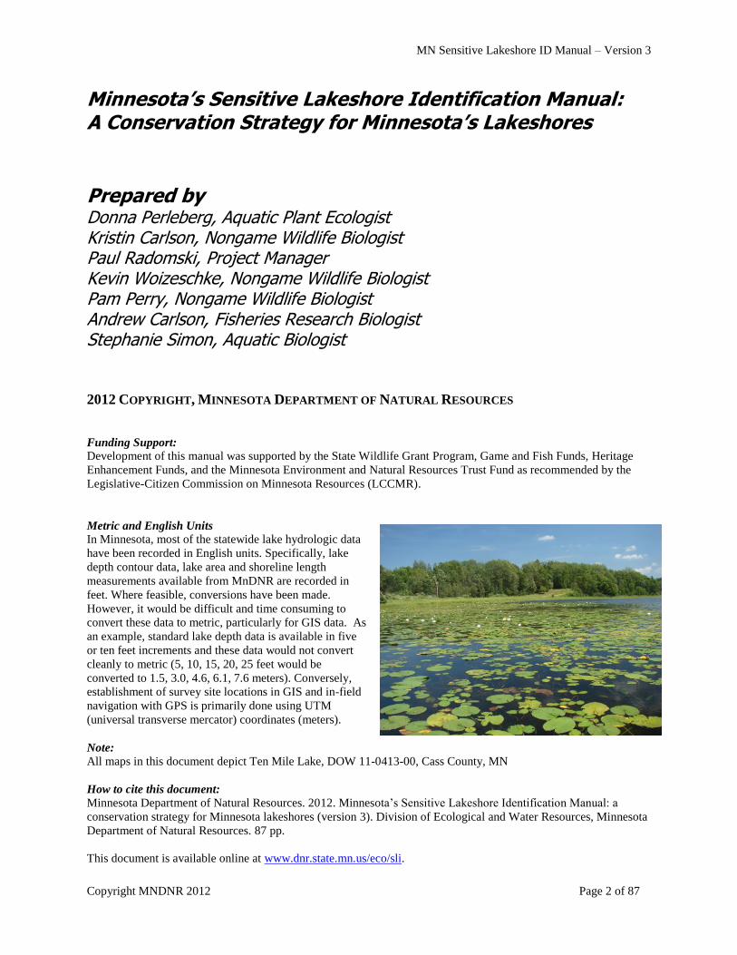
Note:
All maps in this document depict Ten Mile Lake, DOW 11-0413-00, Cass County, MN
How to cite this document:
Minnesota Department of Natural Resources. 2012. Minnesota‟s Sensitive Lakeshore Identification Manual: a
conservation strategy for Minnesota lakeshores (version 3). Division of Ecological and Water Resources, Minnesota
Department of Natural Resources. 87 pp.
This document is available online at www.dnr.state.mn.us/eco/sli.

MN Sensitive Lakeshore ID Manual – Version 3
Copyright MNDNR 2012 Page 3 of 87
SENSITIVE LAKESHORE IDENTIFICATION
MINNESOTA DEPARTMENT OF NATURAL RESOURCES
DIVISION OF ECOLOGICAL AND WATER RESOURCES
Chapter 1. An Introduction to Sensitive Lakeshores ...................................................................... 4 Chapter 2. Aquatic Habitat Survey and Mapping ........................................................................... 9
A. Lake-wide vegetation and near-shore substrate survey (grid point-intercept survey) ......... 10 B. Delineate and describe emergent and floating-leaf plant beds ............................................. 15 C. Identify areas of unique and rare aquatic plant species ........................................................ 17
Chapter 3. Aquatic Frog Calling Survey....................................................................................... 18 Chapter 4. Near-shore Fish and Other Aquatic Animals Survey .................................................. 20
Chapter 5. Bird Surveys ................................................................................................................ 22
Chapter 6. Wetlands, Hydric Soils, Rare Features, and Size and Shape of Natural Areas ........... 26 Chapter 7. Ecological Models to Delineate Sensitive Lakeshore ................................................. 28
A. Models based on habitat, plant and animal occurrences ...................................................... 28
B. Predictive models for prompt, timely delineations .............................................................. 42 C. Limitations of ecological model ........................................................................................... 46
References ..................................................................................................................................... 48
Appendices .................................................................................................................................... 54
MN Sensitive Lakeshore ID Manual – Version 3
Copyright MNDNR 2012 Page 4 of 87
Chapter 1. An Introduction to Sensitive Lakeshores
This manual explains the survey protocol used to identify and map sensitive fish and wildlife
shoreline habitat for Minnesota lakes. Sensitive areas are places that contain unique or critical
ecological habitat, and they provide important habitat for a variety of species, including species
of greatest conservation need. The protocols in this manual are science-based, and were
developed to be objective, fair, and commonly repeatable with basic due diligence. The purpose
of the survey protocol in this manual is to provide the framework for data collection and analysis
so that reliable advice can be given to local and state resource managers, who can use the
information to maintain environmental conditions and protect habitat for species in greatest
conservation need.
The shoreline and near-shore areas are critical to the health and well-being of fish, wildlife, and
native plants. Many fish and wildlife species, including many species of greatest conservation
need, are highly dependent on naturally vegetated shorelines as habitat for feeding, resting, and
mating and juvenile life stages. Development and land alteration in the immediate shoreland and
on the shoreline may have significant negative impacts on these species.
For the purpose of this manual the following definitions are used:
Shoreland is defined as Minnesota Rule 6120, which for lakes is that land located within 1000
feet of the ordinary high water level. Some local governments use a distance of 1320 feet. The
methods in this protocol use land located within 1320 feet of the ordinary high water level in
order to buffer the state-defined shoreland area.
Shoreline is the edge of a body of water and, alternatively, used here with regard to fish and
wildlife habitat to refer to the narrow band around the lake centered on the land-water interface.
Near-shore is the shallow aquatic areas of a lake within 680 feet of the shoreline.
Shore impact zone means land located between the ordinary high water level of a public water
and a line parallel to it at a setback of 50 percent of the structure setback, but not less than 50
feet. This area serves as the primary shoreline buffer, and for the General Development lakes
surveyed it is the first 50 feet landward.
Lakeshore is the area comprised of the shoreland, shoreline and the near-shore.
Need
Increases in shoreland development are changing lake ecosystems. Development pressure is
increasing with more dwellings per lake each year in Minnesota (Kelly and Stinchfield 1998).
Human habitation along the shore has a cumulative effect on fish and wildlife habitat, water
quality, and biota of lake ecosystems (Engel and Pederson 1998, Ramstack et al. 2004).
Christensen et al. (1996) found significantly less submerged woody habitat from fallen trees
along developed shorelines in Wisconsin and Michigan, and predicted that recent losses in
developed lakes will affect littoral communities for about two centuries. Meyer et al. (1997)

MN Sensitive Lakeshore ID Manual – Version 3
Copyright MNDNR 2012 Page 5 of 87
concluded that housing development along shores of northern Wisconsin lakes dramatically
altered native vegetation, especially shrubs, and reduced frog populations. Elias and Meyer
(2003) found that the mean number of plant species and the percent of native species were both
greater at undeveloped sites than along developed Wisconsin lakeshores for upland, shoreline,
and shallow water areas. Jennings et al. (1996) noted changes in near-shore substrate
composition in Wisconsin lakes due to human activity. In an Iowa lake, Byran and Scarnecchia
(1992) found significant reductions in aquatic macrophyte abundance in developed compared
with undeveloped shorelines. Jennings et al. (2003) also found that the amount of littoral wood
remains and emergent and floating-leaf vegetation was lower at developed sites and lakes with
greater development density. By comparing vegetation abundance along undeveloped and
developed shorelines for 44 lakes in Minnesota, Radomski and Goeman (2001) estimated that 20
to 28 percent of the near-shore emergent and floating-leaf coverage was lost. Radomski (2006)
determined that floating-leaf and emergent vegetative cover was significantly affected by
development for the period from 1939 to 2003 for Minnesota lakes.
Alteration of natural littoral zone habitats has negative consequences to fish and wildlife. Littoral
zone vegetation is important for amphibians, ducks, herons, and many species of greatest
conservation need (Meyer et al. 1997; Lindsay et al. 2002; Woodford and Meyer 2003).
Floating-leaf and emergent vegetation provides fish and wildlife with foraging areas and refuge
from predators (Killgore et al. 1993; Casselman and Lewis 1996; Valley et al. 2004). Many fish
depend on this habitat for some part or most of their life (Becker 1983). Emergent vegetation,
such as hardstem bulrush, provides spawning habitat, cover, and colonization sites for aquatic
invertebrates and protects shorelines from erosion by dampening wave energy. Numerous fish
species use protected embayments and vegetative cover disproportionately to their availability
(Wei et al. 2004). Human activities that change vegetative cover can alter ecological processes
and energy flow within lakes, thereby reducing their ability to support diverse and healthy fish
and wildlife populations (Schindler and Scheuerell 2002).
Lake shorelines often vary greatly with respect to their ecological characteristics and functions.
Additional work is needed to identify and protect high priority near-shore habitats. Protection of
these areas, either through conservation easements or more restrictive development standards, in
protected bays and areas where habitat exists for species of greatest conservation need seems
reasonable and warranted given the substantial near-shore habitat losses estimated to date and the
projected losses possible with further shoreland development. Greater protection of sensitive
shorelands and the valued ecosystem services requires identification, mapping and designation of
these places.
The Sensitive Lakeshore project originated in Cass County in 2005 as the Intra-Lake Land Use
Reclassification Project. The county led a technical team of federal, state, and local resource
managers to develop criteria for determining sensitive areas. The criteria were then incorporated
into a GIS (Geographic Information Systems) algorithm to identify sensitive lakeshores. The
county proposed specific development standards, including larger lot sizes and greater structure
setbacks for new lots, for these areas. The county held public hearings on this approach for
protecting significant fish and wildlife habitat. Cass County acknowledged that insufficient
resources existed for extensive field verification and validation of county designated sensitive
areas, and they asked the DNR for assistance before proceeding with any proposed zoning or

MN Sensitive Lakeshore ID Manual – Version 3
Copyright MNDNR 2012 Page 6 of 87
ordinance changes. This manual was the result of this Cass County/State collaboration. Since
then, the project has expanded to include Minnesota DNR collaboration with Crow Wing and
Itasca Counties as well as non-profit organizations such as the Leech Lake Area Watershed
Foundation and the Minnesota Land Trust.
Minnesota‟s Comprehensive Wildlife Conservation Strategy (CWCS) identifies the “significant
loss and degradation of habitat” as one of four major Management Challenges (DNR 2006).
Managing emerging issues affecting species of greatest conservation need is listed a Priority
Conservation Action, and the loss and degradation of Minnesota‟s lakeshore is clearly an
emerging issue. Species of greatest conservation need are animals whose populations are rare,
declining or vulnerable to decline. They are also species whose populations are below levels
desirable to ensure their long-term health and stability. Many species of greatest conservation
need depend on lakeshores.
The Minnesota State Demographic Center has projected growth in many of the lake-rich counties
to exceed 35 percent in the next 25 years. CWCS promotes habitat-based conservation, and there
is a need to assess the amount and quality of key near-shore habitats and to map their locations in
this subsection (Priority Conservation Actions for Surveys, subsection item 2a). Species of
greatest conservation need in this subsection that may benefit from this project include, but are
not limited to: American and least bitterns, red-necked grebe, black tern, common tern, common
loon, bald eagle, marsh and sedge wrens, swamp sparrow, Virginia and yellow rails, least darter,
pugnose shiner, longear sunfish and numerous invertebrate species. Other wildlife species of
interest that are associated with shoreline and lake communities include osprey, great blue heron,
and green and mink frogs.
Expected Results or Benefits
A sensitive area district concept and the allowance to reclassify isolated bay shorelands to a more
restrictive class was incorporated into Minnesota‟s Alternative Shoreland Management
Standards (version 1.0, December 12, 2005; a product of the Governor‟s Clean Water Initiative).
Local governments can now create sensitive area districts along sensitive shores and reclassify
bays on recreational development and general development-classed lakes to provide greater
protection to near-shore species of greatest conservation need. Assisting local governments on
potential districting and reclassification is a valuable service and benefit, and this manual is an
aid to provide those services and benefits.
Within the environmental review processes, determining where significant fish and wildlife
habitat occurs and delineating sensitive areas would be helpful in regulating shoreland and public
waters development including structures, bridges, culverts, water alterations, excavation, and
destruction of aquatic plants. Appropriate aquatic plant management and shoreland development
rules and regulations for sensitive areas may help promote healthy and balanced near-shore
communities and protect habitat for species of greatest conservation need.
In addition, landowners with property within sensitive lakeshore areas may be willing to donate
permanent conservation easements. Conservation easements are a long-term strategy to protect
critical lands and aquatic habitats, recreational opportunities, and water quality. This voluntary

MN Sensitive Lakeshore ID Manual – Version 3
Copyright MNDNR 2012 Page 7 of 87
approach allows for the protection of lakeshore ranging in size from hundreds to thousands of
feet. Thus, a program to delineate sensitive lakeshore areas is anticipated to be beneficial to DNR
processes, local government decision-making, and conservation-minded lakeshore property
owners.
Assessing the amount and quality of key near-shore habitats and mapping their locations
provides additional resources to support some of the Priority Conservation Actions outlined in
the CWCS for this ecological subsection.
Summary of Approach
The first work in identifying sensitive lakeshores requires the review and compilation of the
existing data. Sources of potential existing data on Minnesota lakes and lakeshore plant and
animal communities include, but are not limited to:
1. DNR Fisheries lake surveys
2. DNR Wildlife Shallow Lakes Program surveys
3. DNR Natural Heritage Information System
4. DNR Minnesota County Biological Survey Program
5. DNR Ecological and Water Resources lake surveys
6. DNR Invasive Species Program surveys
7. DNR Volunteer Loon Watcher surveys
8. DNR Bald Eagle and Osprey nest surveys
9. University of Minnesota/Bell Museum Herbarium
10. Published literature and agency reports
11. Aerial photography
12. National Wetland Inventory
13. National Cooperative Soil Survey
Available data are incorporated into a geographic information system (GIS), and these data are
used in survey design and determination of unique or critical ecological areas.
The sensitive lakeshore protocol consists of three components: field surveying lakeshore habitats
and their use by high priority animal species, identifying sensitive lakeshore habitats and
developing an ecological model, and compiling and delivering information on sensitive
lakeshores to various land and resource managers. This is the same general approach used by the
Minnesota County Biological Survey.
The first component involves field surveys of the lake aquatic plant communities and the
distribution of high priority animal species. The aquatic plant surveys are conducted lake-wide
and occur at a number of different scales. Submerged habitats and near-shore areas are also
sampled. High priority animal species include species of greatest conservation need as well as
other animals whose habitat use represent a good proxy for species of greatest conservation need.
The second component involves the development of ecological models that objectively and
consistently rank lakeshores for sensitive area designation. Objective methods deliver repeatable

MN Sensitive Lakeshore ID Manual – Version 3
Copyright MNDNR 2012 Page 8 of 87
results that are relatively insensitive to the subjective interpretations of the individuals doing the
ranking; in addition, consistent, fair rankings are more likely to stand up to scrutiny and can be
used as the basis for regulatory action.
The final component of identifying sensitive lakeshore is to deliver advice to local governments,
non-profit organizations, and other groups who could use the information to maintain high
quality environmental conditions and to protect habitat for species in greatest conservation need.

MN Sensitive Lakeshore ID Manual – Version 3
Copyright MNDNR 2012 Page 9 of 87
Figure 1. Lake zones included in the aquatic habitat survey (shoreline to maximum
rooting depth).
Shoreline
Ordinary High Waterline
Current waterline Shore-
land
Maximum rooting depth
Aquatic
Habitat Survey
Chapter 2. Aquatic Habitat Survey and Mapping
The Aquatic Habitat Survey describes the type, quantity and quality of the existing aquatic
habitat, from the shoreline to the maximum depth of aquatic plant growth (Figure 1).
The aquatic habitat surveys are conducted using a tiered survey approach. Survey components
include:
1. Assessment of lake-wide vegetation community using the grid point-intercept method.
2. Delineation and description of emergent and floating-leaf plant beds.
3. Delineation and description of other unique aquatic plant areas.
The grid point-intercept method is a useful tool for lake-wide assessment of aquatic plant
communities. However, it is not always adequate for assessment of near-shore vegetation,
including emergent and floating-leaf beds. One problem with the grid survey methodology is that
it may under sample near-shore, shallow sites where the habitat is often quite different from the
rest of the lake. To compensate for this shortcoming, sampling protocol includes methods to
delineate, map and describe emergent and floating-leaf habitat and other unique aquatic plant
communities.
Sampling Timeline
Most vegetation sampling is conducted during peak growth and before plants senesce – July
through early September. Lake-wide aquatic plant surveys are the first component and are
MN Sensitive Lakeshore ID Manual – Version 3
Copyright MNDNR 2012 Page 10 of 87
conducted after significant plant growth is noted in early summer through July. In lakes with
extensive wild rice (Zizania palustris) stands, surveys may be conducted earlier (June) to
minimize damage to wild rice. If curly-leaf pondweed (Potamogeton crispus) is an important
part of a lake plant community, surveys may be conducted in May or June, before this species
senesces. Surveys to delineate and describe emergent and floating-leaf plant stands and other
unique plant areas are conducted in August and early September, and they may be conducted the
year after the initial lake-wide aquatic plant assessment. Data management and analysis, which
will rely on GIS, are conducted during non-field survey times.
A. Lake-wide vegetation and near-shore substrate survey (grid point-intercept survey)
The goal of the lake-wide vegetation survey is to quantitatively assess the major plant species
within the lake basin. Objectives include:
1. Record the aquatic plant species that occur in the lake
2. Estimate frequencies of occurrence of individual species
3. Estimate the percent of the lake occupied by rooted vegetation
4. Develop GIS-based, lake-wide distribution maps for the common species
5. Estimate the maximum depth of rooted vegetation
6. Describe the shoal water substrate types
The grid point-intercept method used here records frequency of occurrence (presence/absence) as
the measure to estimate plant abundance and individual species abundance. The grid point-
intercept vegetation survey method estimates plant frequency by determining the proportion of
survey points that “hit” or intercept vegetation. Frequencies of individual species can also be
estimated by recording the plant species when intercepted by a point.
The grid point-intercept vegetation survey methodology follows that of Madsen (1999), and the
technique has been extensively used in Minnesota by the lead aquatic plant ecologist (Donna
Perleberg), the Minnesota DNR Wildlife Shallow Lakes Program, and has been adopted by the
Wisconsin DNR as their standard lake vegetation survey method (Jennifer Hauxwell, personal
communication). In comparisons of several boat-based aquatic vegetation survey methods, the
grid point-intercept method was found to provide the most rapid, repeatable, GIS-based method
to assess lake-wide plant species abundance and associated depth data (Perleberg 2001a,
Perleberg 2001b). Williams et al. (2008) recommended the point-intercept survey for whole- lake
assessments where statistical comparisons are needed. Other boat-based methods (Jesson and
Lound 1962, Yin et al. 2000) provide more site-specific detail, but require the boat to be
anchored at each sample site, thus reducing the total number of sites that can be sampled per
hour. Furthermore, because the grid point-intercept method collects frequency data only, other
advantages include consistency in data collection between different surveyors, ability to monitor
a variety of plant growth forms, opportunity to monitor at flexible times throughout the growing
season, and uncomplicated data analysis (Nichols 1984, Elzinga et al. 2001). In addition,
frequency data are recommended as an appropriate abundance estimate when studying long-term
changes in communities (Nichols 1999). It may not be appropriate to estimate aerial coverage
from these data because accuracy would be dependent on the resolution (spacing of points) of the
survey (Williams et al. 2008).

MN Sensitive Lakeshore ID Manual – Version 3
Copyright MNDNR 2012 Page 11 of 87
In the grid point-intercept
method, survey points are
established throughout the
littoral (or the vegetated)
zone on a grid using GIS.
While other aquatic
vegetation survey methods
may randomly assign survey
points within a stratified area
(Yin et al. 2000), a random
systematic placement of
survey points is more
appropriate because lake-
wide mapping is a primary
objective. If a current depth
contour map of the lake is
available, points may be
established within the littoral
zone only. However, on
many lakes, the exact area of
the littoral zone is unknown
and it is easier to establish
sample points across the entire basin and once in the field skip points that occur in deep water.
Once sampling has begun, surveyors may determine that little or no vegetation occurs beyond a
certain depth, and skip survey points that occur beyond that depth (Figure 2). In most Minnesota
lakes, it is recommended that surveyors sample to at least a depth of 20 feet (6 meters). If depth
contour lines are well documented, a stratified sampling approach may be appropriate where a
predetermined number of sample points are placed within a specific depth zone (ex. 200 points in
the shore to 5 feet zone, 200 points in the 6 to 15 feet zone). However, for most Minnesota lakes,
mapped depth contours only approximate the actual depths and a simple grid spacing of points is
easier. It is important that the maximum depth sampled and the total number of surveyed sites be
stated along with survey results.
Required sample size
The size of the littoral zone, the shape of the lake, and existing information about the plant
community will determine the number of points and the grid resolution (see Appendix 1 for more
information on the number of points necessary for appropriate sampling).
Within the littoral zone, a minimum of 250 points will be sampled on most lakes, to ensure that
commonly occurring species (species occurring at frequencies of at least 40%) are adequately
sampled with an error of 15% with 95% confidence. A two-person crew can generally survey
between 100 and 300 points per day (fewer points with high plant density or species richness).
Figure 2. Grid point-intercept survey. Example of sample site
locations, Ten Mile Lake, Cass County.

MN Sensitive Lakeshore ID Manual – Version 3
Copyright MNDNR 2012 Page 12 of 87
Equipment A checklist of required and recommended equipment is provided in Appendix 2, and the field
data collection form is given in Appendix 3. Survey point waypoints are uploaded to handheld
GPS units.
Field sampling Sampling is conducted primarily from a boat (Figure 3) and GPS units are used to navigate to
each sample point. The survey points are not intended to be permanent sampling locations and
are not marked with permanent markers. Rather, the goal is to navigate to the approximate
location of each sample point. Given the inherent inaccuracy of field-model GPS units, and the
shifting movement of the boat due to wave action, surveyors are not always able to stop precisely
on the survey point location. Surveyors are directed to navigate to within five meters of survey
point coordinates shown on the GPS unit. The boat operator maintains the position of the boat
without anchoring and sampling is conducted from a pre-designated side of the boat.
Survey points may be skipped under the following conditions:
1. Site location is on shore (sample station is permanently removed from database)
2. Site location is within a dense and/or shallow bed of emergent or floating-leaf vegetation and
motoring into the site would likely destroy vegetation (surveyors record general
observations about the site but do not include data in calculations)
3. Site location occurs in water depths greater than maximum rooting depth of vegetation
4. Access to site is prevented by dock, swim area, other boats
Water depth
At each sampling point, water depth is recorded in one-foot increments using an electronic depth
finder mounted at the stern of the boat or, in water depths less than eight feet (2.5 meters), with a
measured stick at the pre-designated sample side on the boat (Figure 3).
Figure 3. Sampling at each point-intercept location.
A B C
approx. 1 m square sample area,
Species A,B, C prsent in site
pre-designated
sample station on
boat
boat operator navigates to
within 5 m of GPS
coordinate depth
finder
Species D recorded as
“outside plot”
D
present in site
“outside plot”
MN Sensitive Lakeshore ID Manual – Version 3
Copyright MNDNR 2012 Page 13 of 87
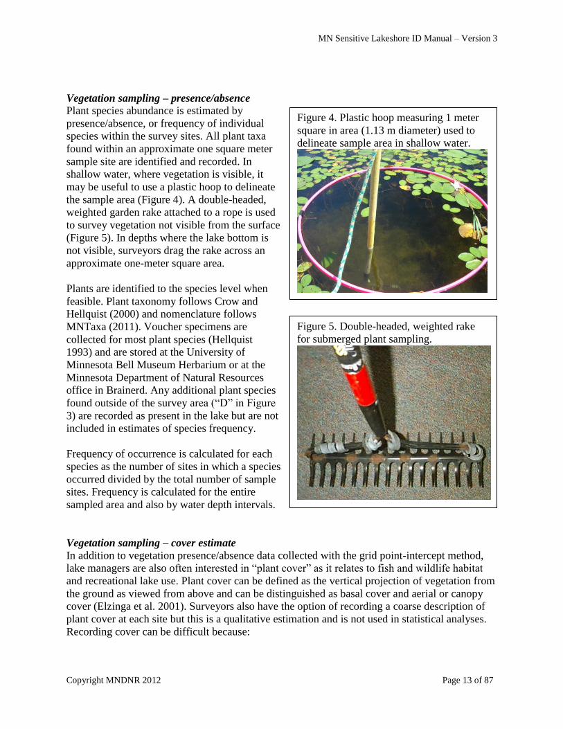
Vegetation sampling – presence/absence
Plant species abundance is estimated by
presence/absence, or frequency of individual
species within the survey sites. All plant taxa
found within an approximate one square meter
sample site are identified and recorded. In
shallow water, where vegetation is visible, it
may be useful to use a plastic hoop to delineate
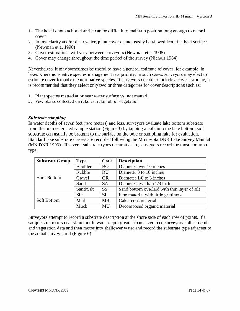
the sample area (Figure 4). A double-headed,
weighted garden rake attached to a rope is used
to survey vegetation not visible from the surface
(Figure 5). In depths where the lake bottom is
not visible, surveyors drag the rake across an
approximate one-meter square area.
Plants are identified to the species level when
feasible. Plant taxonomy follows Crow and
Hellquist (2000) and nomenclature follows
MNTaxa (2011). Voucher specimens are
collected for most plant species (Hellquist
1993) and are stored at the University of
Minnesota Bell Museum Herbarium or at the
Minnesota Department of Natural Resources
office in Brainerd. Any additional plant species
found outside of the survey area (“D” in Figure
3) are recorded as present in the lake but are not
included in estimates of species frequency.
Frequency of occurrence is calculated for each
species as the number of sites in which a species
occurred divided by the total number of sample
sites. Frequency is calculated for the entire
sampled area and also by water depth intervals.
Vegetation sampling – cover estimate
In addition to vegetation presence/absence data collected with the grid point-intercept method,
lake managers are also often interested in “plant cover” as it relates to fish and wildlife habitat
and recreational lake use. Plant cover can be defined as the vertical projection of vegetation from
the ground as viewed from above and can be distinguished as basal cover and aerial or canopy
cover (Elzinga et al. 2001). Surveyors also have the option of recording a coarse description of
plant cover at each site but this is a qualitative estimation and is not used in statistical analyses.
Recording cover can be difficult because:
Figure 4. Plastic hoop measuring 1 meter
square in area (1.13 m diameter) used to
delineate sample area in shallow water.
Figure 5. Double-headed, weighted rake
for submerged plant sampling.
MN Sensitive Lakeshore ID Manual – Version 3
Copyright MNDNR 2012 Page 14 of 87
1. The boat is not anchored and it can be difficult to maintain position long enough to record
cover
2. In low clarity and/or deep water, plant cover cannot easily be viewed from the boat surface
(Newman et a. 1998)
3. Cover estimations will vary between surveyors (Newman et a. 1998)
4. Cover may change throughout the time period of the survey (Nichols 1984)
Nevertheless, it may sometimes be useful to have a general estimate of cover, for example, in
lakes where non-native species management is a priority. In such cases, surveyors may elect to
estimate cover for only the non-native species. If surveyors decide to include a cover estimate, it
is recommended that they select only two or three categories for cover descriptions such as:
1. Plant species matted at or near water surface vs. not matted
2. Few plants collected on rake vs. rake full of vegetation
Substrate sampling
In water depths of seven feet (two meters) and less, surveyors evaluate lake bottom substrate
from the pre-designated sample station (Figure 3) by tapping a pole into the lake bottom; soft
substrate can usually be brought to the surface on the pole or sampling rake for evaluation.
Standard lake substrate classes are recorded following the Minnesota DNR Lake Survey Manual
(MN DNR 1993). If several substrate types occur at a site, surveyors record the most common
type.
Surveyors attempt to record a substrate description at the shore side of each row of points. If a
sample site occurs near shore but in water depth greater than seven feet, surveyors collect depth
and vegetation data and then motor into shallower water and record the substrate type adjacent to
the actual survey point (Figure 6).
Substrate Group Type Code Description
Hard Bottom
Boulder BO Diameter over 10 inches
Rubble RU Diameter 3 to 10 inches
Gravel GR Diameter 1/8 to 3 inches
Sand SA Diameter less than 1/8 inch
Sand/Silt SS Sand bottom overlaid with thin layer of silt
Soft Bottom
Silt SI Fine material with little grittiness
Marl MR Calcareous material
Muck MU Decomposed organic material

MN Sensitive Lakeshore ID Manual – Version 3
Copyright MNDNR 2012 Page 15 of 87
B. Delineate and describe emergent and floating-leaf plant beds
Protocols are based on the procedures documented in the DNR draft Aquatic Vegetation
Mapping Guidelines (DNR 2005) and may include a combination of aerial photo delineation and
interpretation, field delineation, ground-truthing and site specific surveys. Large stands of
emergent and floating-leaf vegetation are mapped. Mapping of small beds is resource intensive
and imprecise using available GIS tools. Plant beds are characterized by the dominant genera or
species and plant community descriptions may continue to be refined as more data are collected:
Survey Method Plant community Dominant plants
Field delineation Bulrush Schoenoplectus spp.
Spikerush Eleocharis spp.
Aerial photos
with field
verification;
descriptive detail
will vary with
survey effort
Giant cane Phragmites australis
Cattail Typha spp.
Wild rice Zizania palustris
Mixed emergent Various – Equisetum spp.,
Eleocharis spp., Sagittaria spp.,
Sparganium spp.
Waterlily Nymphaea odorata
Nuphar variegata
Brasenia schreberi
Figure 6. Sampling near-shore substrates. Red circle = substrate sample
recorded at sample site. Red-hatched circles = too deep for substrate sample,
off-site substrate recorded at X. Black circles = no substrate recorded.
SH
OR
E
6 fe
et
co
nto
ur
X
X
MN Sensitive Lakeshore ID Manual – Version 3
Copyright MNDNR 2012 Page 16 of 87
Aerial Photo Delineation
Existing aerial photographs are used to map floating-leaf vegetation. The photo source, scale,
and date are documented. Some issues associated with this method include difficulties in
identifying vegetation beds from photos. This may result in missing small or floating-leaf
vegetation beds altogether. Several photo sources are used, if possible, because different types of
vegetation may appear different on separate photos. The locations on the photo are only as
accurate as the photo rectification.
Aerial photo delineated maps are field-checked. Using field surveys, species compositions of
stands are verified. Changes in vegetation observed between different photo dates can also be
confirmed.
Field Delineation
Field mapping focuses on bulrush (Schoenoplectus spp.) beds, which are difficult to see on aerial
photos. Existing data are used along with a reconnaissance survey to identify extensive bulrush
stands for further quantification. Bulrush habitat is mapped and digitized using GPS (see
Appendix 4 for equipment checklist).
Stem density is an important factor in assessing the overall habitat quality of an emergent plant
stand. Emergent vegetation stem density in general, and bulrush stem density in particular, has
been used to describe several types of waterfowl and shorebird nesting habitat (Custer 1993,
Spautz and Nur 2002). Waterfowl studies may focus specifically on optimal ranges of bulrush
stem densities for a particular bird species (Custer 1993). Bulrush also serves as habitat for many
fish species (Becker 1983). Numerous factors may affect bulrush stem density including the
species of bulrush present, competition from other plant species, water depth (Hunter et al.
2000), substrate type, substrate nutrient levels, herbivory (Lentz and Cipollini 1998), and
disturbance by humans. Stem density varies within and among bulrush stands and the number of
stems per square meter may range from less than one to more than 800 (Hall and Freeman 1994).
Estimating bulrush stem density can be difficult and surveyors often rely on visual estimates to
describe stand density (MN DNR 2005). Bulrush stands have been described as “sparse”,
“moderately dense”, or “dense” (MN DNR 2005) with no association to stem density counts, or
with stem density counts that overlap (same mean count for sparse and moderate categories)
(Morris 1999). Kantrud (1996) suggests that a “healthy” stand of soft-stem bulrush
(Schoenoplectus tabernaemontani) would have a stem density range of 50 to 500. Field trials
were conducted in 2006 to determine the feasibility of estimating bulrush stem density using
plotless methods (Engeman et al. 1994). Survey methods were found to be labor intensive and
difficult to reliably repeat. Therefore, stem density estimates of bulrush is not included as a
standard method in this protocol.

MN Sensitive Lakeshore ID Manual – Version 3
Copyright MNDNR 2012 Page 17 of 87
C. Identify areas of unique and rare aquatic plant species
Surveyors use information collected during the grid point-intercept survey and emergent plant
bed mapping to locate unique aquatic plant species. These species may include:
1. Rare (endangered, threatened, special concern) plant species
2. Plant species that are not listed as rare but are uncommon in the state or locally. These may
include species that are proposed for rare listing.
3. Plants species with high coefficient of conservatism values. A coefficient of conservatism
value, or C value, may range from 0 to 10 and represents an estimated probability that a plant
is likely to occur in a landscape relatively unaltered from what is believed to be a pre-
settlement condition (Nichols 1999, Bourdaghs et al. 2006.). Because the amount of
information for each species differs, C values are subjectively assigned by biologists based
on existing information and professional judgment. Nichols (1999) developed tentative C
values for 128 Wisconsin lake plants based on their substrate preference, turbidity tolerance,
rooting strength, primary reproductive means, and tolerance to water drawdowns. C values
have now been established for most aquatic and wetland plant species native to Wisconsin
(WDNR 2011) and Minnesota (Milburn et al. 2007). C values may vary from region to
region (Swink and Wilhelm 1994, Herman et al. 1996) and values developed by Wisconsin
are mostly applicable in Minnesota. Plant species with assigned C values of 9 and 10 will be
included as “unique species.” C values could vary regionally within the state (Nichols 1999),
and it may be necessary to regionalize the selection process within Minnesota (e.g., for
southern Minnesota lakes, species with C values of 7 or higher will be included as “unique
species”). Terrestrial species are not included in the unique plant survey.
Partial list of rare (special concern, threatened, or endangered) and unique plant species most
likely to be found in Minnesota lakes or along lakeshores can be found in Appendix 5.
MN Sensitive Lakeshore ID Manual – Version 3
Copyright MNDNR 2012 Page 18 of 87
Chapter 3. Aquatic Frog Calling Survey
An aquatic frog survey is conducted from mid June to
mid July. The methodology follows the Minnesota Frog
and Toad Calling Survey (MFTCS) protocol, which was
an outgrowth of the North American Amphibian
Monitoring Program. Information on MFTCS can be
found at:
http://www.dnr.state.mn.us/volunteering/frogtoad_survey
/index.html
Several life-cycle characteristics make mink frogs (Rana
septentrionalis) and green frogs (Rana clamitans) ideal
indicator species of lakeshore habitats. First, mink and green frogs are shoreline-dependent
species that inhabit nearly all types of permanent water in this region. Adult male frogs are easily
surveyed by auditory detection. They establish and defend distinct territories, and tend to remain
along the periphery of lakes and ponds throughout the summer breeding season or in areas of
shallow water with emergent vegetation. Green frogs breed from late May to mid-August and
mink frogs begin their calling in late May with the breeding season extending from late June to
early August (Breckenridge 1944), so a summer calling survey is an effective technique to
determine presence and abundance.
Objectives of the aquatic frog calling survey include:
1. Determine index of abundance for all frogs and toads
2. Estimate actual abundance of mink frogs and green frogs
3. Develop distribution maps for mink frogs and green frogs
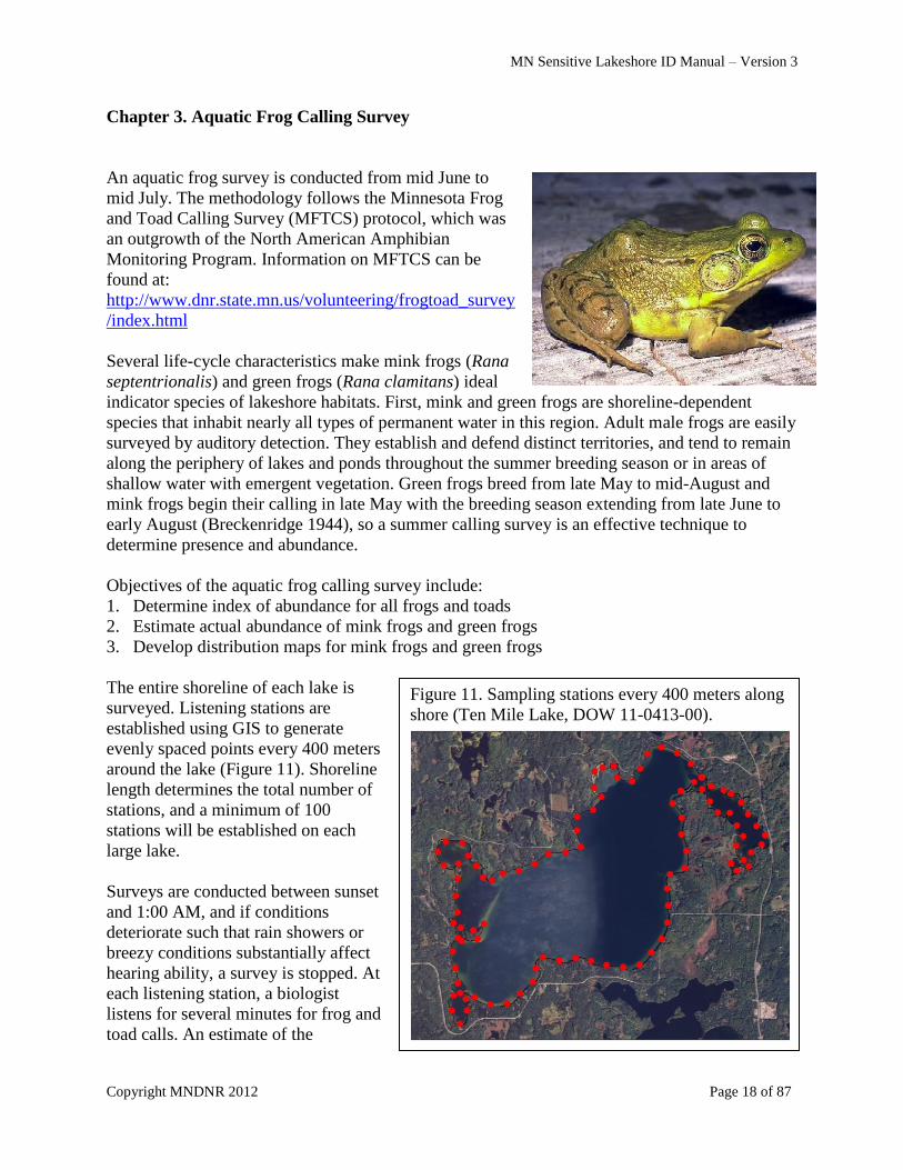
The entire shoreline of each lake is
surveyed. Listening stations are
established using GIS to generate
evenly spaced points every 400 meters
around the lake (Figure 11). Shoreline
length determines the total number of
stations, and a minimum of 100
stations will be established on each
large lake.
Surveys are conducted between sunset
and 1:00 AM, and if conditions
deteriorate such that rain showers or
breezy conditions substantially affect
hearing ability, a survey is stopped. At
each listening station, a biologist
listens for several minutes for frog and
toad calls. An estimate of the
Figure 11. Sampling stations every 400 meters along
shore (Ten Mile Lake, DOW 11-0413-00).
MN Sensitive Lakeshore ID Manual – Version 3
Copyright MNDNR 2012 Page 19 of 87
abundance of frogs and a calling index is recorded for both mink and green frogs. The calling
intensity of all other amphibian species heard is also recorded. The field datasheet used for the
survey is provided in Appendix 6.
The abundance of green and mink frogs at each station is classed as:
1. 1 – 9 individuals
2. 10 – 20 individuals
3. 20 – 100 individuals
4. >100 individuals
The call index value for each amphibian species heard is recorded according to the following:
1. Individuals can be counted (silence between calls)
2. Calls of individuals can be distinguished, but some overlap of calls
3. Full chorus (calls constant, continuous, and overlapping)
MN Sensitive Lakeshore ID Manual – Version 3
Copyright MNDNR 2012 Page 20 of 87
Chapter 4. Near-shore Fish and Other Aquatic Animals Survey
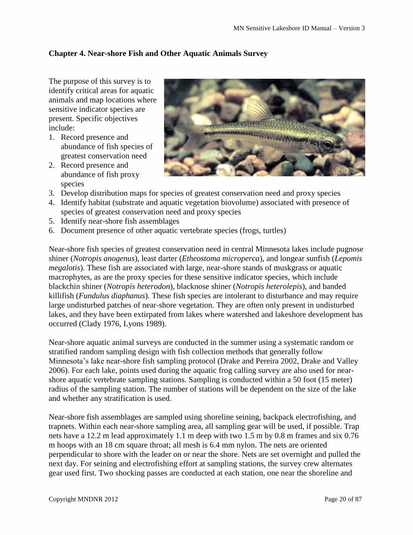
The purpose of this survey is to
identify critical areas for aquatic
animals and map locations where
sensitive indicator species are
present. Specific objectives
include:
1. Record presence and
abundance of fish species of
greatest conservation need
2. Record presence and
abundance of fish proxy
species
3. Develop distribution maps for species of greatest conservation need and proxy species
4. Identify habitat (substrate and aquatic vegetation biovolume) associated with presence of
species of greatest conservation need and proxy species
5. Identify near-shore fish assemblages
6. Document presence of other aquatic vertebrate species (frogs, turtles)
Near-shore fish species of greatest conservation need in central Minnesota lakes include pugnose
shiner (Notropis anogenus), least darter (Etheostoma microperca), and longear sunfish (Lepomis
megalotis). These fish are associated with large, near-shore stands of muskgrass or aquatic
macrophytes, as are the proxy species for these sensitive indicator species, which include
blackchin shiner (Notropis heterodon), blacknose shiner (Notropis heterolepis), and banded
killifish (Fundulus diaphanus). These fish species are intolerant to disturbance and may require
large undisturbed patches of near-shore vegetation. They are often only present in undisturbed
lakes, and they have been extirpated from lakes where watershed and lakeshore development has
occurred (Clady 1976, Lyons 1989).
Near-shore aquatic animal surveys are conducted in the summer using a systematic random or
stratified random sampling design with fish collection methods that generally follow
Minnesota‟s lake near-shore fish sampling protocol (Drake and Pereira 2002, Drake and Valley
2006). For each lake, points used during the aquatic frog calling survey are also used for near-
shore aquatic vertebrate sampling stations. Sampling is conducted within a 50 foot (15 meter)
radius of the sampling station. The number of stations will be dependent on the size of the lake
and whether any stratification is used.
Near-shore fish assemblages are sampled using shoreline seining, backpack electrofishing, and
trapnets. Within each near-shore sampling area, all sampling gear will be used, if possible. Trap
nets have a 12.2 m lead approximately 1.1 m deep with two 1.5 m by 0.8 m frames and six 0.76
m hoops with an 18 cm square throat; all mesh is 6.4 mm nylon. The nets are oriented
perpendicular to shore with the leader on or near the shore. Nets are set overnight and pulled the
next day. For seining and electrofishing effort at sampling stations, the survey crew alternates
gear used first. Two shocking passes are conducted at each station, one near the shoreline and
MN Sensitive Lakeshore ID Manual – Version 3
Copyright MNDNR 2012 Page 21 of 87
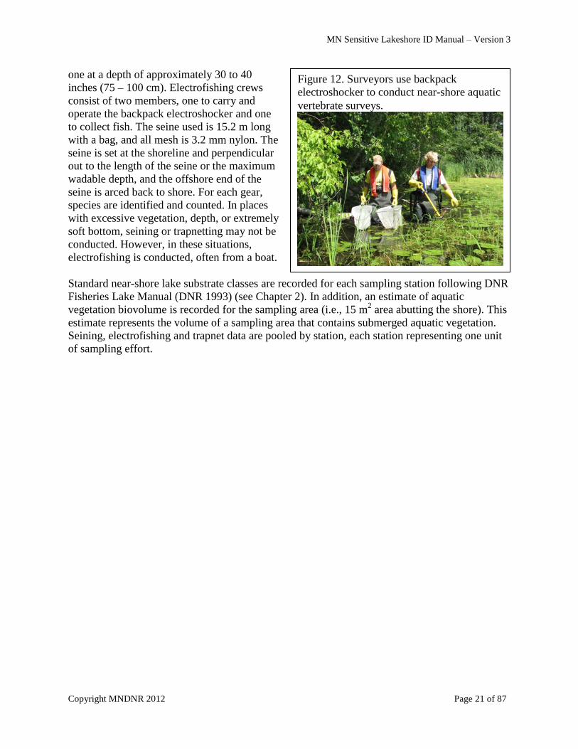
one at a depth of approximately 30 to 40
inches (75 – 100 cm). Electrofishing crews
consist of two members, one to carry and
operate the backpack electroshocker and one
to collect fish. The seine used is 15.2 m long
with a bag, and all mesh is 3.2 mm nylon. The
seine is set at the shoreline and perpendicular
out to the length of the seine or the maximum
wadable depth, and the offshore end of the
seine is arced back to shore. For each gear,
species are identified and counted. In places
with excessive vegetation, depth, or extremely
soft bottom, seining or trapnetting may not be
conducted. However, in these situations,
electrofishing is conducted, often from a boat.
Standard near-shore lake substrate classes are recorded for each sampling station following DNR
Fisheries Lake Manual (DNR 1993) (see Chapter 2). In addition, an estimate of aquatic
vegetation biovolume is recorded for the sampling area (i.e., 15 m2 area abutting the shore). This
estimate represents the volume of a sampling area that contains submerged aquatic vegetation.
Seining, electrofishing and trapnet data are pooled by station, each station representing one unit
of sampling effort.
Figure 12. Surveyors use backpack
electroshocker to conduct near-shore aquatic
vertebrate surveys.

MN Sensitive Lakeshore ID Manual – Version 3
Copyright MNDNR 2012 Page 22 of 87
Chapter 5. Bird Surveys
Birds use a wide variety of lakeshore habitats. Many birds
use specific habitat types or require a combination of
habitats for their life cycles; some of these habitats are
rare or limited in size and distribution, thus limiting the
range of the bird species. Lakeshore habitats used by
birds include trees and forested areas, shrub swamps,
aquatic emergent vegetation such as bulrush and cattail
marshes, rocky reefs and islands, mud flats, the
water/land interface of the shoreline, the water surface
and under the water.
Information on birds is collected in two phases. The first
phase is to search existing databases for historical records
of nesting and for occurrences of rare species. This data
collection takes place before the field season begins.
Special efforts are made to search during the field season
for species that had historical records. The second phase of the project is field surveys for all bird
species utilizing lake shorelines. Field surveys take place during the breeding season, when birds
are most vocal. Methods include point-counts, call-playback surveys for secretive marsh species,
and general observations of rare species observed.
Although all bird species are noted and recorded, surveyors focus on bird species of greatest
conservation need (SGCN). A second list of species is also given special note. These species are
dependent on specific aquatic habitats, represent SGCN proxy species, or are suffering declines
in Minnesota.
Bird Species of Greatest Conservation Need
These species have been found near north-central Minnesota lakeshores. Species are listed in
AOU order.
American Black Duck (Anas rubripes)
Common Loon (Gavia immer)
Red-necked Grebe (Podiceps grisegena)
American White Pelican (Pelecanus erythrorhynchos)
American Bittern (Botaurus lentiginosus)
Least Bittern (Ixobrychus exilis)
Bald Eagle (Haliaeetus leucocephalus)
Red-shouldered Hawk (Buteo lineatus)
Yellow Rail (Coturnicops noveboracensis)
Virginia Rail (Rallus limicola)
Common Tern (Sterna hirundo)
Forster‟s Tern (Sterna forsteri)
Black Tern (Chlidonias niger)
MN Sensitive Lakeshore ID Manual – Version 3
Copyright MNDNR 2012 Page 23 of 87
Common Nighthawk (Chordeiles minor)
Red-headed Woodpecker (Melanerpes erythrocephalus)
Yellow-bellied Sapsucker (Sphyrapicus varius)
Eastern Wood-Pewee (Contopus virens)
Least Flycatcher (Empidonax minimus)
Northern Rough-winged Swallow (Stelgidopteryx serripennis)
Sedge Wren (Cistothorus platensis)
Marsh Wren (Cistothorus palustris)
Veery (Catharus fuscescens)
Golden-winged Warbler (Vermivora chrysoptera)
Ovenbird (Seiurus aurocapilla)
Swamp Sparrow (Melospiza georgiana)
White-throated Sparrow (Zonotrichia albicollis)
Rose-breasted Grosbeak (Pheucticus ludovicianus)
Other Bird Species of Interest
Great Blue Heron (Ardea herodias)
Green Heron (Butorides virescens)
Osprey (Pandion haliaetus)
Sora (Porzana carolina)
Spotted Sandpiper (Actitis macularia)
Caspian Tern (Sterna caspia)
Alder Flycatcher (Empidonax alnorum)
Purple Martin (Progne subis)
Database Searches for Historical Information
This information search focuses on past records of species that have been entered in DNR
databases such as the DNR Natural Heritage Database Information System, DNR Volunteer
Loon Watcher Surveys, DNR Eagle Nest Records, and DNR Osprey Nest Records. Bird species
of focus include the common loon, red-necked grebe, bald eagle, osprey, black tern and other
colonial nesting waterbird species.
Field Surveys
Three methods are used to collect data on lakeshore birds – point counts, call-playback surveys
targeting marsh birds, and general field observations. All birds heard or seen while conducting
the surveys or while working on the lake or along the shoreline during the nesting season,
defined as the last week of May through the first week of July, are recorded.
Morning point counts for birds are conducted between sunrise and 10:00 AM at the same sample
stations used for frog surveys (see Chapter 5). The entire shoreline is surveyed by boat with
points at 400 m intervals. The boat is stopped when the GPS point is reached and the boat is
positioned 20 –50 m from shore (depending on water depth). A timer is set for 5 minutes and all
birds heard or seen are recorded. Relatively calm conditions are required in order to hear the
birds along the shoreline, so surveys require positioning the boat out of the wind (protected side
of lake or sheltered bay) or conducting surveys only when wind speeds are less than 6 mph. If
MN Sensitive Lakeshore ID Manual – Version 3
Copyright MNDNR 2012 Page 24 of 87
noise from sources such as waves along the shoreline, wind, or road construction negatively
affects the ability to hear birdsong, the survey is cancelled for that day. Birds seen or heard
within a 200 m radius of the sample point are recorded for that point. Birds seen or heard in the
distance are recorded as present at the lake but not associated with a specific sample point. Bird
flyovers (birds seen overhead but not utilizing any lake habitat) are not recorded.
Marsh birds are notoriously secretive and are not often recorded on passive-listening point
counts. Call-playback surveys done in the evening, before sunset, are a better method to discover
the presence of birds such as rails. The survey methodology used is modified from “Standardized
North American Marsh Bird Monitoring Protocols” (Conway 2005), and uses calls from species
expected to be found in the local lakeshore/marsh habitats. Surveys are not conducted from pre-
determined sampling stations, but at locations where there is significant marsh habitat. The
surveys are done from a boat and begin two hours before sunset. The survey begins with five
minutes of passive listening, which is followed by 30 seconds of call-playback, then a shorter
period of listening. This call-playback sequence is repeated three times. Species targeted with
this method include American bittern, least bittern, Virginia rail and sora. If suitable habitat for
yellow rails is found, surveys are conducted after dark using their distinctive call.
General field observations are also recorded while surveyors are in transit between points or
conducting other work on the lake. These observations include notes on feeding areas,
roosting/resting sites, and nest areas, especially for birds that are SGCN or other species of
interest. A bird checklist is kept to record all species observed on the lakeshore or in the water
for each study lake so that a species list can be compiled at the end of the field season. A sample
field data collection form is provided in Appendix 7.
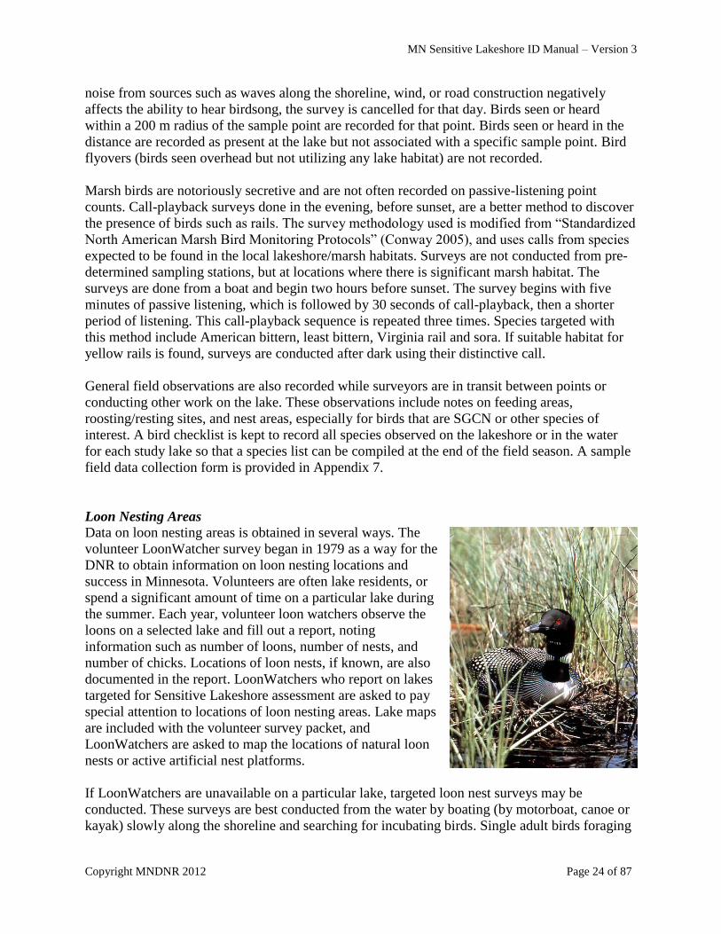
Loon Nesting Areas
Data on loon nesting areas is obtained in several ways. The
volunteer LoonWatcher survey began in 1979 as a way for the
DNR to obtain information on loon nesting locations and
success in Minnesota. Volunteers are often lake residents, or
spend a significant amount of time on a particular lake during
the summer. Each year, volunteer loon watchers observe the
loons on a selected lake and fill out a report, noting
information such as number of loons, number of nests, and
number of chicks. Locations of loon nests, if known, are also
documented in the report. LoonWatchers who report on lakes
targeted for Sensitive Lakeshore assessment are asked to pay
special attention to locations of loon nesting areas. Lake maps
are included with the volunteer survey packet, and
LoonWatchers are asked to map the locations of natural loon
nests or active artificial nest platforms.
If LoonWatchers are unavailable on a particular lake, targeted loon nest surveys may be
conducted. These surveys are best conducted from the water by boating (by motorboat, canoe or
kayak) slowly along the shoreline and searching for incubating birds. Single adult birds foraging

MN Sensitive Lakeshore ID Manual – Version 3
Copyright MNDNR 2012 Page 25 of 87
near shore may also indicate a nearby nest. Protected bays and areas of shoreline with abundant
emergent vegetation should be surveyed with particular care. Nest surveys should be conducted
during May and early June, when adults are still incubating eggs. Extreme care should be taken
not to disturb incubating loons. Disturbance can interfere with nesting and cause distractions that
make eggs more vulnerable to predators or extreme temperatures. Observation should be done
with binoculars when possible. If loons exhibit any threatened or defensive behavior, the
surveyor should quickly and quietly leave the area. Crews conducting bird and aquatic plant
surveys also record locations of loon nesting areas.
MN Sensitive Lakeshore ID Manual – Version 3
Copyright MNDNR 2012 Page 26 of 87
Chapter 6. Wetlands, Hydric Soils, Rare Features, and Size and Shape of Natural Areas
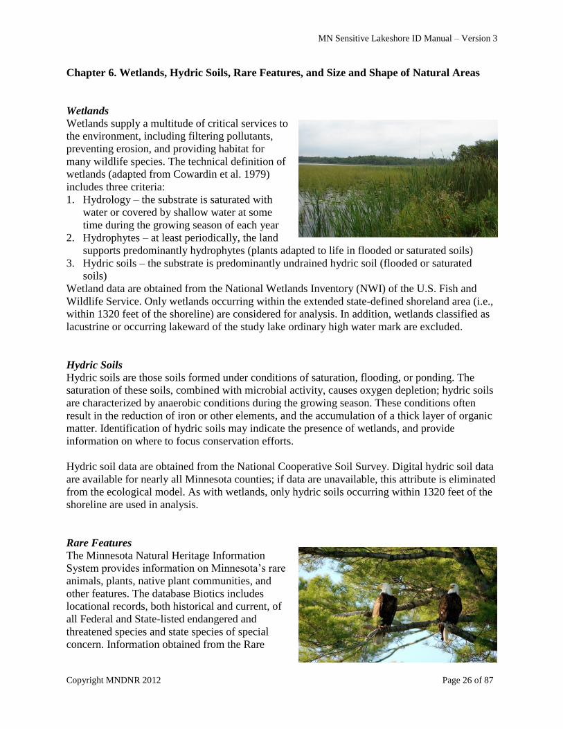
Wetlands
Wetlands supply a multitude of critical services to
the environment, including filtering pollutants,
preventing erosion, and providing habitat for
many wildlife species. The technical definition of
wetlands (adapted from Cowardin et al. 1979)
includes three criteria:
1. Hydrology – the substrate is saturated with
water or covered by shallow water at some
time during the growing season of each year
2. Hydrophytes – at least periodically, the land
supports predominantly hydrophytes (plants adapted to life in flooded or saturated soils)
3. Hydric soils – the substrate is predominantly undrained hydric soil (flooded or saturated
soils)
Wetland data are obtained from the National Wetlands Inventory (NWI) of the U.S. Fish and
Wildlife Service. Only wetlands occurring within the extended state-defined shoreland area (i.e.,
within 1320 feet of the shoreline) are considered for analysis. In addition, wetlands classified as
lacustrine or occurring lakeward of the study lake ordinary high water mark are excluded.
Hydric Soils
Hydric soils are those soils formed under conditions of saturation, flooding, or ponding. The
saturation of these soils, combined with microbial activity, causes oxygen depletion; hydric soils
are characterized by anaerobic conditions during the growing season. These conditions often
result in the reduction of iron or other elements, and the accumulation of a thick layer of organic
matter. Identification of hydric soils may indicate the presence of wetlands, and provide
information on where to focus conservation efforts.
Hydric soil data are obtained from the National Cooperative Soil Survey. Digital hydric soil data
are available for nearly all Minnesota counties; if data are unavailable, this attribute is eliminated
from the ecological model. As with wetlands, only hydric soils occurring within 1320 feet of the
shoreline are used in analysis.
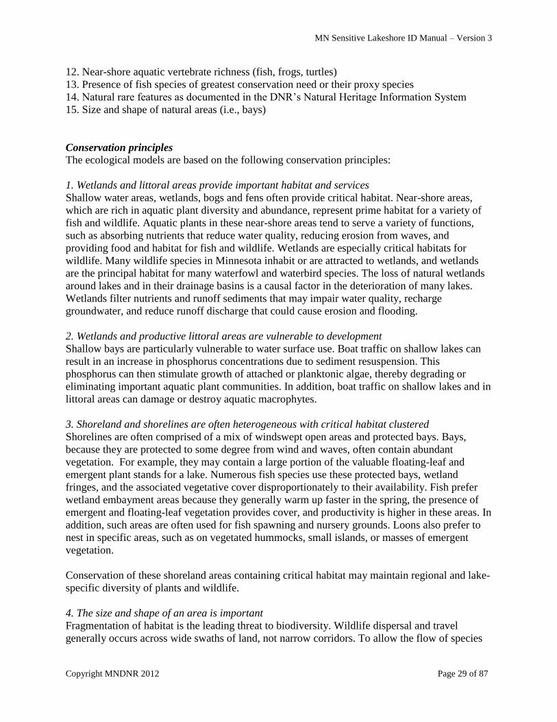
Rare Features
The Minnesota Natural Heritage Information
System provides information on Minnesota‟s rare
animals, plants, native plant communities, and
other features. The database Biotics includes
locational records, both historical and current, of
all Federal and State-listed endangered and
threatened species and state species of special
concern. Information obtained from the Rare

MN Sensitive Lakeshore ID Manual – Version 3
Copyright MNDNR 2012 Page 27 of 87
Heritage program has many uses, including in environmental review, land conservation,
management decisions, and education.
Locations of rare features within 1320 feet of the shoreline were obtained from the Biotics
database. Only listed plant and animal species (Federal or State endangered, threatened, or
special concern) were considered in the analysis. New rare feature locations recorded during
field surveys were submitted to the Natural Heritage program for inclusion in the database.
Size and shape of natural areas (i.e., bays)
Bays are defined as bodies of water partially enclosed by land. They offer some degree of
protection from the wind and waves, and therefore are frequently characterized by abundant
vegetation and wildlife. Protection of these areas will be beneficial to a variety of plant and
animal species.
Bays are delineated using lake maps and aerial photographs. Obvious bays (e.g., significant
indentations of shoreline, bodies of water set off from main body or nearly enclosed by land) are
mapped based on inspection of lake maps. Additional bays are identified using aerial
photographs. Underwater shoals or reefs that offset a body of water from the main body are often
visible only in these photographs. Bays are defined as either non-isolated or isolated. Non-
isolated bays are open to the main water body by a wide mouth (generally > 200 m). Isolated
bays have a narrower connection to the main water body (generally < 200 m) or are offshoots of
non-isolated bays. Maximum and minimum bay sizes are loosely set for each lake; these are
dependent upon the size of the lake. In general, separate lake basins are not defined as bays. Very
small indentations in the shoreline (i.e., coves) are also not classified as bays.
MN Sensitive Lakeshore ID Manual – Version 3
Copyright MNDNR 2012 Page 28 of 87
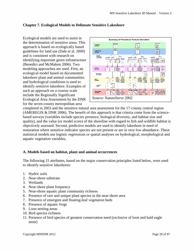
Chapter 7. Ecological Models to Delineate Sensitive Lakeshore
Ecological models are used to assist in
the determination of sensitive areas. This
approach is based on ecologically based
guidelines for land use (Dale et al. 2000)
and is consistent with research on
identifying important green infrastructure
(Benedict and McMahon 2006). Two
modeling approaches are used. First, an
ecological model based on documented
lakeshore plant and animal communities
and hydrological conditions is used to
identify sensitive lakeshore. Examples of
such an approach on a coarser scale
include the Regionally Significant
Ecological Area Assessment by the DNR
for the seven-county metropolitan area
completed in 2003 and the sensitive natural area assessment for the 17-county central region
(AMEREGIS & DNR 2006). The benefit of this approach is that criteria come from the science-
based surveys (variables include species presence, biological diversity, and habitat size and
quality), and the value (or model score) of the shoreline with regard to fish and wildlife habitat is
objectively assessed. Second, predictive models are used to identify lakeshore in need of
restoration where sensitive indicator species are not present or are in very low abundance. These
statistical models use logistic regressions or spatial analyses on hydrological, morphological and
aquatic vegetation variables.
A. Models based on habitat, plant and animal occurrences
The following 15 attributes, based on the major conservation principles listed below, were used
to identify sensitive lakeshores:
1. Hydric soils
2. Near-shore substrate
3. Wetlands
4. Near-shore plant frequency
5. Near-shore aquatic plant community richness
6. Presence of rare and unique plant species in the near-shore area
7. Presence of emergent and floating-leaf vegetation beds
8. Presence of aquatic frogs
9. Loon nesting areas
10. Bird species richness
11. Presence of bird species of greatest conservation need (exclusive of loon and bald eagle
nests)
Source: NatureServe 2002
MN Sensitive Lakeshore ID Manual – Version 3
Copyright MNDNR 2012 Page 29 of 87
12. Near-shore aquatic vertebrate richness (fish, frogs, turtles)
13. Presence of fish species of greatest conservation need or their proxy species
14. Natural rare features as documented in the DNR‟s Natural Heritage Information System
15. Size and shape of natural areas (i.e., bays)
Conservation principles
The ecological models are based on the following conservation principles:
1. Wetlands and littoral areas provide important habitat and services
Shallow water areas, wetlands, bogs and fens often provide critical habitat. Near-shore areas,
which are rich in aquatic plant diversity and abundance, represent prime habitat for a variety of
fish and wildlife. Aquatic plants in these near-shore areas tend to serve a variety of functions,
such as absorbing nutrients that reduce water quality, reducing erosion from waves, and
providing food and habitat for fish and wildlife. Wetlands are especially critical habitats for
wildlife. Many wildlife species in Minnesota inhabit or are attracted to wetlands, and wetlands
are the principal habitat for many waterfowl and waterbird species. The loss of natural wetlands
around lakes and in their drainage basins is a causal factor in the deterioration of many lakes.
Wetlands filter nutrients and runoff sediments that may impair water quality, recharge
groundwater, and reduce runoff discharge that could cause erosion and flooding.
2. Wetlands and productive littoral areas are vulnerable to development
Shallow bays are particularly vulnerable to water surface use. Boat traffic on shallow lakes can
result in an increase in phosphorus concentrations due to sediment resuspension. This
phosphorus can then stimulate growth of attached or planktonic algae, thereby degrading or
eliminating important aquatic plant communities. In addition, boat traffic on shallow lakes and in
littoral areas can damage or destroy aquatic macrophytes.
3. Shoreland and shorelines are often heterogeneous with critical habitat clustered
Shorelines are often comprised of a mix of windswept open areas and protected bays. Bays,
because they are protected to some degree from wind and waves, often contain abundant
vegetation. For example, they may contain a large portion of the valuable floating-leaf and
emergent plant stands for a lake. Numerous fish species use these protected bays, wetland
fringes, and the associated vegetative cover disproportionately to their availability. Fish prefer
wetland embayment areas because they generally warm up faster in the spring, the presence of
emergent and floating-leaf vegetation provides cover, and productivity is higher in these areas. In
addition, such areas are often used for fish spawning and nursery grounds. Loons also prefer to
nest in specific areas, such as on vegetated hummocks, small islands, or masses of emergent
vegetation.
Conservation of these shoreland areas containing critical habitat may maintain regional and lake-
specific diversity of plants and wildlife.
4. The size and shape of an area is important
Fragmentation of habitat is the leading threat to biodiversity. Wildlife dispersal and travel
generally occurs across wide swaths of land, not narrow corridors. To allow the flow of species

MN Sensitive Lakeshore ID Manual – Version 3
Copyright MNDNR 2012 Page 30 of 87
across wide areas, large natural areas are needed. When natural areas are fragmented into
numerous small and irregular shaped pieces (patches), the plants and animals found on the site,
and the interactions that take place between plants and animals (e.g., predator and prey
relationships) change. Habitat islands are vulnerable to loss of species.
The larger a natural area is, the more likely it will support populations of native plants and
animals. Fish species of greatest conservation need (pugnose shiner, least darter, and longear
sunfish) are intolerant to disturbance and may require large undisturbed patches of near-shore
vegetation. Fragmentation of vegetation often results in a reduction in the nest success of some
bird species. Small, irregularly shaped areas have a greater proportion of edge area than interior
area. Birds forced to nest in the edges may have a greater risk of losing offspring to predators
(crows, grackles, brown-headed cowbirds).
Edges do provide important habitat for many plants and animals and often have a high number of
species. This is in part because anthropogenic fragmentation of vegetation often increases the
occurrence of invasive, non-native plants and animals that inhabit edge habitats. Natural edges,
however, provide a mosaic of habitats that native plant and animal species utilize. Lakeshores
themselves are edges, as they represent the boundary between the lake habitat and the upland
habitat. Edges enable animals to access various habitats for nesting, foraging, or escape cover.
Several species of greatest conservation need, including the golden-winged warbler, are
frequently found within edge habitat.
5. Adjacent land use affects natural areas
Strategic conservation requires an integrated landscape approach that considers the influence of
neighboring areas. Local changes can have broad-scale impacts on lake and river ecosystems.
The introduction of non-native plant species into forests and lakeshores from urban gardens,
trampling of vegetation from heavy pedestrian or recreational use, and increased salinity of
wetlands from road salts are several ways that adjacent urban, suburban, and agricultural land
uses adversely impact natural areas.
Extensive development introduces new predators and may increase predator populations.
Wildlife impacts include increased mortality from cat predation, car kills, killing of wildlife
(snakes and bats) by landowners due to misperceptions/fear, and reduced reproductive success if
breeding is disrupted by human activities.
6. The connectivity of habitats and vegetation is important
Linkage is essential for natural systems to function properly. The loss of connectivity through the
addition of impervious surfaces such as roads and buildings often fragments landscapes.
Fragmentation changes how plants, animals, wind and water move across the landscape.
Habitat connectivity may allow an animal to relocate when habitat is lost or degraded due to
natural or human disturbance. Movement allows individuals from different populations to breed,
which maintains genetic diversity in the population. Some animals have different vegetation
requirements during different stages of their life cycle. For example, Blanding‟s turtles require
large wetland complexes for over-wintering and dry, sandy soil grasslands for breeding. An
animal‟s risk of being killed (increased predation, road strikes) during movement increases in

MN Sensitive Lakeshore ID Manual – Version 3
Copyright MNDNR 2012 Page 31 of 87
fragmented landscapes. Lake, stream and wetland habitat quality is dependent on maintaining
vegetated riparian and lakeshore zones, and connectivity to upland vegetation.
7. Species diversity is important
Diversity of both plant and animal species is critical to maintaining the health of an ecosystem.
Diversity allows an ecosystem to adapt to varying conditions. Recent ecological research shows
that a plot of land with many plant species is more productive and resistant to drought, pests, and
other stresses than a plot with only a few species. Diverse habitats are fundamental in allowing
an area to have high plant and animal diversity.
Many human activities cause changes in the environment that lead to lower species diversity and
decreased ecological resiliency. Examples include excess nitrogen from pollutants, the
introduction of invasive non-native species, and the disruption of natural processes such as
natural water flow. These disruptions often lead to the elimination of many native species and the
promotion of just a few species. These disturbed areas then are less able to tolerate outbreaks of
pests and diseases and large-scale changes such as climate change.
Ecological Model Details
A GIS ecological model is used to identify sensitive lakeshore. The goal is to recognize potential
shoreland and near-shore areas that contain important environmental features. The ability to
identify sensitive areas is dependent on field surveys, which provide reliable information on the
elements of biodiversity, how natural resource elements are connected, and their condition.
There are several shortcomings with this general approach to identify sensitive lakeshore. For
example, the minimum required size of a habitat patch needed for a given organism is quite
variable. In addition, habitat variation exists over a range of spatial scales, and the size of the
sampling unit used in the various surveys may not be optimal for ecological considerations.
However, spatial dependence of neighboring points or nearby sample points is often a reasonable
assumption in lakes, and the shoreland development policies necessitate that GIS analytical units
constitute groupings of adjacent sampling points.
Environmental decision-making is complex and often based on multiple lines of evidence.
Integrating the information from these multiple lines of evidence is rarely a simple process. The
identification of sensitive lakeshore used here is an objective, repeatable and quantitative
approach to the combination of multiple lines of evidence through calculation of weight of
evidence (weight of evidence as used in this manual relates to an interpretative methodology).
The model has several components. First, spatial data layers of soils, wetlands, rare features,
plant communities, and fish and wildlife habitat are overlaid with a spatial layer of shoreland
areas. Priority rankings for shoreland segments or plots are based on an overlapping moving
window that follows the shoreline. An overlapping window technique allows the value of
connectivity to be automatically included in the rankings. The size of the window used in the
analysis is dependent on the lake size since the optimal window size varies by survey designs
(e.g., for moderately sized lakes, a 2000 feet long (1320 feet landward, 680 feet lakeward) by
500 feet wide window, with 250 feet overlap is used, whereas for large lakes this window size is
MN Sensitive Lakeshore ID Manual – Version 3
Copyright MNDNR 2012 Page 32 of 87
increased). In this framework, shorelands are rated based on the cumulative score of the spatial
data layers to provide resource conservation priorities.
Attributes from field surveys are summarized by polygons according to the elements occurrence
(EO) data standard (NatureServe 2002). Substrate and aquatic plant data are given a negligible
locational uncertainty type (areal estimated type with a 25 m radius). Unique plant communities
and emergent and floating-leaf stands are of the areal delimited type (assuming negligible
uncertainty). Frog and bird survey locations and loon nesting area polygons are of the areal
estimated type with a 200 m radius. Fish and other aquatic vertebrate survey polygons are of the
areal estimated type with a 50 m radius. The Natural Heritage Information System also uses this
EO data standard.
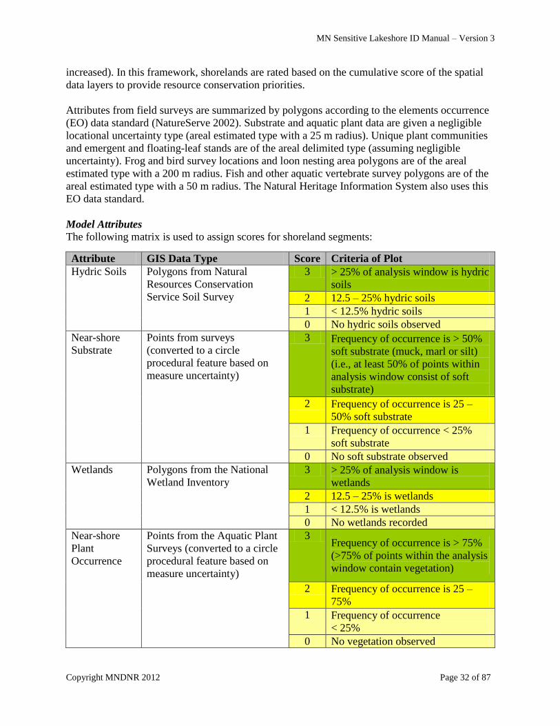
Model Attributes The following matrix is used to assign scores for shoreland segments:
Attribute GIS Data Type Score Criteria of Plot
Hydric Soils Polygons from Natural
Resources Conservation
Service Soil Survey
3 > 25% of analysis window is hydric
soils
2 12.5 – 25% hydric soils
1 < 12.5% hydric soils
0 No hydric soils observed
Near-shore
Substrate
Points from surveys
(converted to a circle
procedural feature based on
measure uncertainty)
3 Frequency of occurrence is > 50%
soft substrate (muck, marl or silt)
(i.e., at least 50% of points within
analysis window consist of soft
substrate)
2 Frequency of occurrence is 25 –
50% soft substrate
1 Frequency of occurrence < 25%
soft substrate
0 No soft substrate observed
Wetlands Polygons from the National
Wetland Inventory
3 > 25% of analysis window is
wetlands
2 12.5 – 25% is wetlands
1 < 12.5% is wetlands
0 No wetlands recorded
Near-shore
Plant
Occurrence
Points from the Aquatic Plant
Surveys (converted to a circle
procedural feature based on
measure uncertainty)
3 Frequency of occurrence is > 75%
(>75% of points within the analysis
window contain vegetation)
2 Frequency of occurrence is 25 –
75%
1 Frequency of occurrence
< 25%
0 No vegetation observed
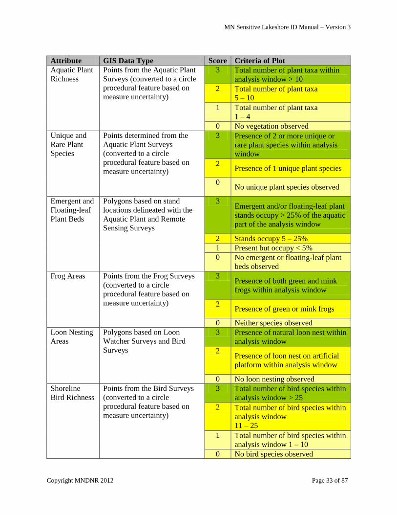
MN Sensitive Lakeshore ID Manual – Version 3
Copyright MNDNR 2012 Page 33 of 87
Attribute GIS Data Type Score Criteria of Plot
Aquatic Plant
Richness
Points from the Aquatic Plant
Surveys (converted to a circle
procedural feature based on
measure uncertainty)
3 Total number of plant taxa within
analysis window > 10
2 Total number of plant taxa
5 – 10
1 Total number of plant taxa
1 – 4
0 No vegetation observed
Unique and
Rare Plant
Species
Points determined from the
Aquatic Plant Surveys
(converted to a circle
procedural feature based on
measure uncertainty)
3 Presence of 2 or more unique or
rare plant species within analysis
window
2 Presence of 1 unique plant species
0 No unique plant species observed
Emergent and
Floating-leaf
Plant Beds
Polygons based on stand
locations delineated with the
Aquatic Plant and Remote
Sensing Surveys
3 Emergent and/or floating-leaf plant
stands occupy > 25% of the aquatic
part of the analysis window
2 Stands occupy 5 – 25%
1 Present but occupy < 5%
0 No emergent or floating-leaf plant
beds observed
Frog Areas Points from the Frog Surveys
(converted to a circle
procedural feature based on
measure uncertainty)
3 Presence of both green and mink
frogs within analysis window
2 Presence of green or mink frogs
0 Neither species observed
Loon Nesting
Areas
Polygons based on Loon
Watcher Surveys and Bird
Surveys
3 Presence of natural loon nest within
analysis window
2 Presence of loon nest on artificial
platform within analysis window
0 No loon nesting observed
Shoreline
Bird Richness
Points from the Bird Surveys
(converted to a circle
procedural feature based on
measure uncertainty)
3 Total number of bird species within
analysis window > 25
2 Total number of bird species within
analysis window
11 – 25
1 Total number of bird species within
analysis window 1 – 10
0 No bird species observed
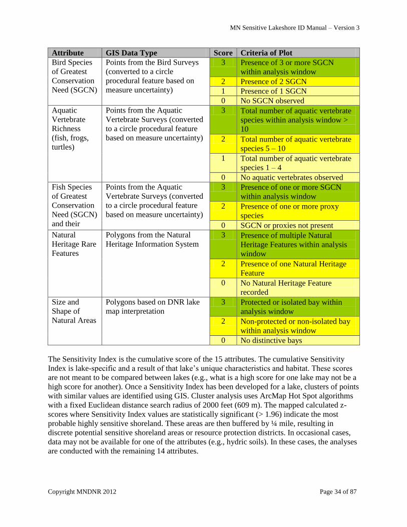
MN Sensitive Lakeshore ID Manual – Version 3
Copyright MNDNR 2012 Page 34 of 87
Attribute GIS Data Type Score Criteria of Plot
Bird Species
of Greatest
Conservation
Need (SGCN)
Points from the Bird Surveys
(converted to a circle
procedural feature based on
measure uncertainty)
3 Presence of 3 or more SGCN
within analysis window
2 Presence of 2 SGCN
1 Presence of 1 SGCN
0 No SGCN observed
Aquatic
Vertebrate
Richness
(fish, frogs,
turtles)
Points from the Aquatic
Vertebrate Surveys (converted
to a circle procedural feature
based on measure uncertainty)
3 Total number of aquatic vertebrate
species within analysis window >
10
2 Total number of aquatic vertebrate
species 5 – 10
1 Total number of aquatic vertebrate
species 1 – 4
0 No aquatic vertebrates observed
Fish Species
of Greatest
Conservation
Need (SGCN)
and their
proxies
Points from the Aquatic
Vertebrate Surveys (converted
to a circle procedural feature
based on measure uncertainty)
3 Presence of one or more SGCN
within analysis window
2 Presence of one or more proxy
species
0 SGCN or proxies not present
Natural
Heritage Rare
Features
Polygons from the Natural
Heritage Information System
3 Presence of multiple Natural
Heritage Features within analysis
window
2 Presence of one Natural Heritage
Feature
0 No Natural Heritage Feature
recorded
Size and
Shape of
Natural Areas
Polygons based on DNR lake
map interpretation
3 Protected or isolated bay within
analysis window
2 Non-protected or non-isolated bay
within analysis window
0 No distinctive bays
The Sensitivity Index is the cumulative score of the 15 attributes. The cumulative Sensitivity
Index is lake-specific and a result of that lake‟s unique characteristics and habitat. These scores
are not meant to be compared between lakes (e.g., what is a high score for one lake may not be a
high score for another). Once a Sensitivity Index has been developed for a lake, clusters of points
with similar values are identified using GIS. Cluster analysis uses ArcMap Hot Spot algorithms
with a fixed Euclidean distance search radius of 2000 feet (609 m). The mapped calculated z-
scores where Sensitivity Index values are statistically significant (> 1.96) indicate the most
probable highly sensitive shoreland. These areas are then buffered by ¼ mile, resulting in
discrete potential sensitive shoreland areas or resource protection districts. In occasional cases,
data may not be available for one of the attributes (e.g., hydric soils). In these cases, the analyses
are conducted with the remaining 14 attributes.

MN Sensitive Lakeshore ID Manual – Version 3
Copyright MNDNR 2012 Page 35 of 87
The intentions of the user will help determine which product will be most valuable. Those
organizations looking to change zoning ordinances and rezone properties may focus on the
potential resource protection districts. Those entities looking to prioritize shorelands for
conservation easements may find the Sensitivity Indices provide a more detailed view of
lakeshore sensitivity.
It is expected that the conservation principles and this ecological model will have a greater
propensity to identify the most highly sensitive lakeshores to be shorelands associated with bays
or sheltered areas of the lake characterized by quiet water and abundant vegetation. However,
sections of the shoreline with high wind and wave exposure (i.e., high-energy shorelines) may
also be sensitive. Although many of the animal species surveyed (e.g., frogs, bird and fish
species of greatest conservation need) prefer the protected, vegetation-rich areas such as bays,
other species inhabit the windswept shorelines. These high-energy shorelines often have
vegetation communities and substrates that differ significantly from the bays. Waves may uproot
or fragment plants, or affect plant growth and reproduction (Doyle 2001). Waves can also
transport sediments, altering the substrate composition. Silt may be suspended and removed from
an area, leaving a sandy or gravelly bottom. Because walleye typically require silt-free substrates
for spawning (Newburg 1975), they may inhabit these shores during spawning. There is a
positive association between wind-wave power and walleye, and walleye may be also attracted to
high-energy areas where smaller prey species are vulnerable due to wave action (Cross and
McInerny 2006). Certain shorebirds, such as sandpipers and plovers, use the sandy beaches of
high-energy shorelines for feeding and even nesting. Because these high-energy shorelines
provide habitat for several animal species, they may have sufficient diversity to receive a high
species richness score. The presence of rare features, wetlands, and hydric soils around these
sections of shoreline may also enable these areas to obtain high scores in the ecological model.
Habitat Connectivity
In addition to the sensitive lakeshore areas identified through the ecological model, adjacent
rivers and streams that provide connectivity should also be considered for protection. Aquatic
habitat connectivity allows for the movement of organisms within a watershed. Organisms can
move between existing habitats, colonize new areas, or recolonize former habitat in the wake of
local extinctions. Aquatic habitat connections, also known as ecological connections, allow
movement of animals from various populations, increasing diversity. They also allow animals
with different habitat requirements during different life stages to access these habitats. For the
purposes of this project, ecological connections are defined by three criteria:
1. The lake is connected, networked, or linked to existing good habitat
a. The presence of an impassable dam eliminates a connection
b. A stream/river that enters/exits the lake but does not connect up/downstream to
another waterbody is not considered an ecological connection
2. The connection itself is good habitat
a. Although a ditch or canal may provide connectivity, these channels are not high
quality habitat and, as such, are not considered ecological connections
3. Higher land use development standards would benefit the designated ecological connection

MN Sensitive Lakeshore ID Manual – Version 3
Copyright MNDNR 2012 Page 36 of 87
Often, lake inlets and outlets are designated ecological connections. Other non-river habitats,
such as a wetland that connects two nearby lakes, could also be considered ecological
connections.
Depending on the existing classification of rivers and streams, the local government may use the
ecological connection recommendation to consider reclassifying to a more protective river class.
Shorelands of ecological connections could also be designated as priority conservation
acquisitions.
Other Areas of Ecological Significance
Additional areas of ecological significance that are not associated with priority shoreland
features may also occur within a lake. These may be sites that are not typically associated with
aquatic plants or rare fish because they occur along less protected/high energy shorelines and are
dominated by hard substrates. Or, they may be sites that are too small to warrant inclusion as part
of a shoreline resource protection district – but the small size of these sites is a defining feature
that adds to their importance within the lake. Identifying these sites is important, although exact
delineation of their boundaries may be difficult because they occur in the water and can be
patchy in distribution.
GIS Steps of Ecological Model The following nine steps are used to create a sensitive lakeshore map (see Appendix 8 for
details):
1. Create points every 250 ft along the shoreline.
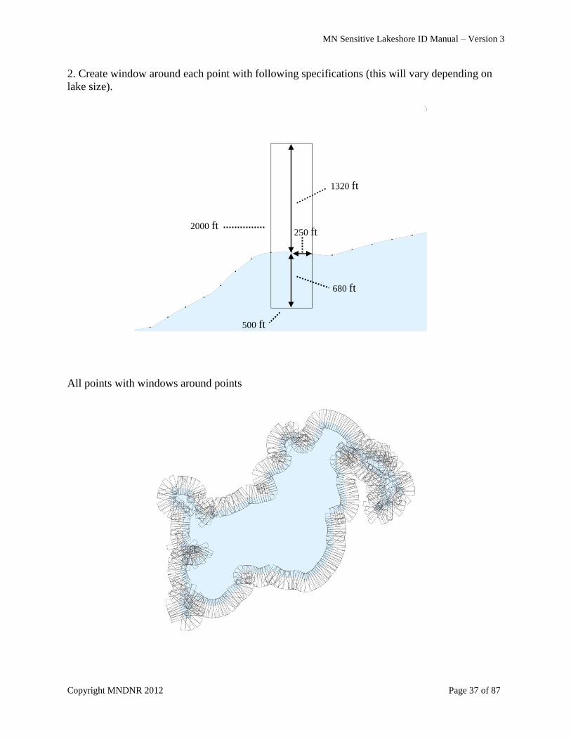
MN Sensitive Lakeshore ID Manual – Version 3
Copyright MNDNR 2012 Page 37 of 87
2. Create window around each point with following specifications (this will vary depending on
lake size).
All points with windows around points
1320 ft
680 ft
2000 ft
500 ft
250 ft
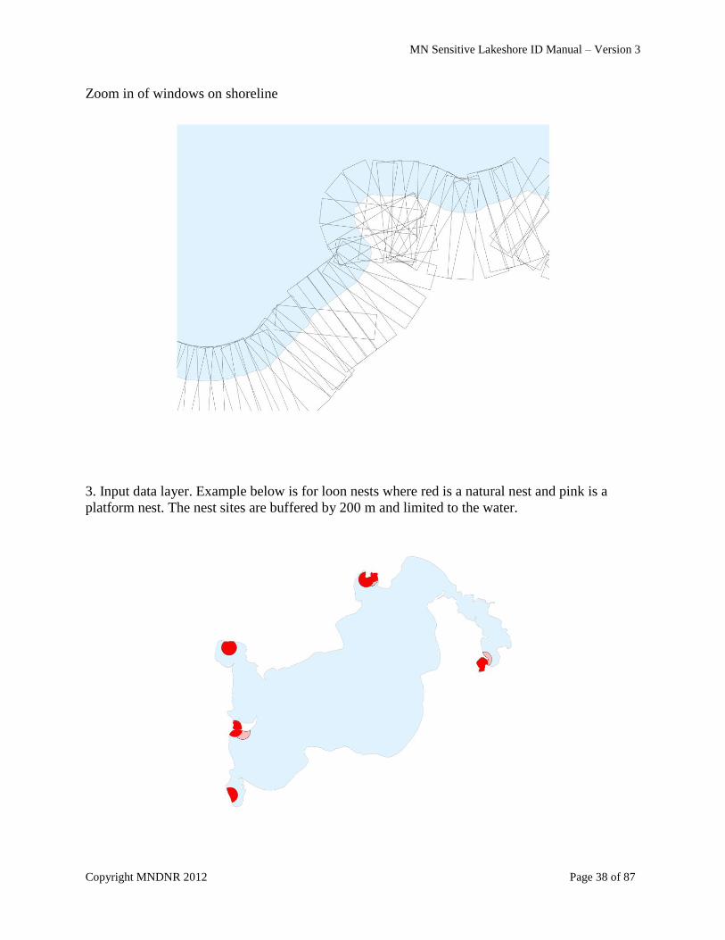
MN Sensitive Lakeshore ID Manual – Version 3
Copyright MNDNR 2012 Page 38 of 87
Zoom in of windows on shoreline
3. Input data layer. Example below is for loon nests where red is a natural nest and pink is a
platform nest. The nest sites are buffered by 200 m and limited to the water.
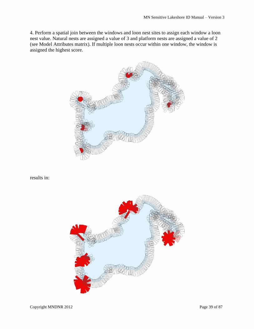
MN Sensitive Lakeshore ID Manual – Version 3
Copyright MNDNR 2012 Page 39 of 87
4. Perform a spatial join between the windows and loon nest sites to assign each window a loon
nest value. Natural nests are assigned a value of 3 and platform nests are assigned a value of 2
(see Model Attributes matrix). If multiple loon nests occur within one window, the window is
assigned the highest score.
results in:
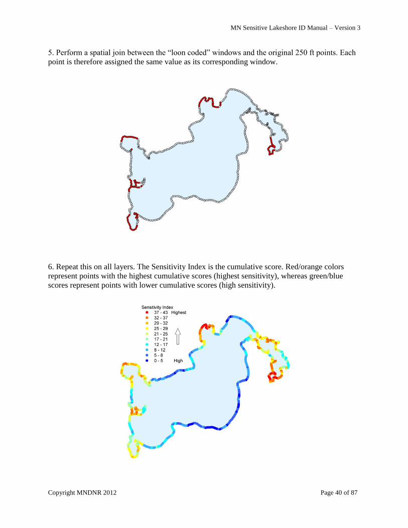
MN Sensitive Lakeshore ID Manual – Version 3
Copyright MNDNR 2012 Page 40 of 87
5. Perform a spatial join between the “loon coded” windows and the original 250 ft points. Each
point is therefore assigned the same value as its corresponding window.
6. Repeat this on all layers. The Sensitivity Index is the cumulative score. Red/orange colors
represent points with the highest cumulative scores (highest sensitivity), whereas green/blue
scores represent points with lower cumulative scores (high sensitivity).
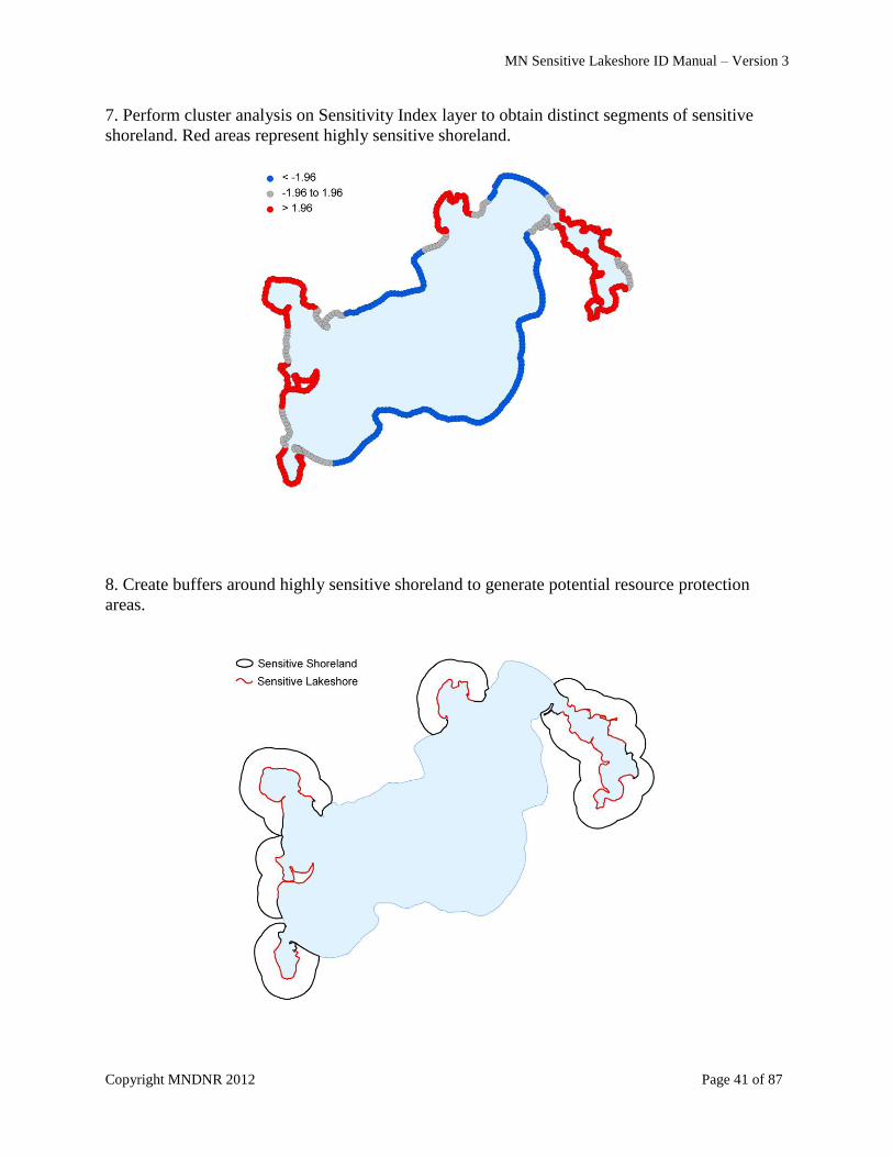
MN Sensitive Lakeshore ID Manual – Version 3
Copyright MNDNR 2012 Page 41 of 87
7. Perform cluster analysis on Sensitivity Index layer to obtain distinct segments of sensitive
shoreland. Red areas represent highly sensitive shoreland.
8. Create buffers around highly sensitive shoreland to generate potential resource protection
areas.
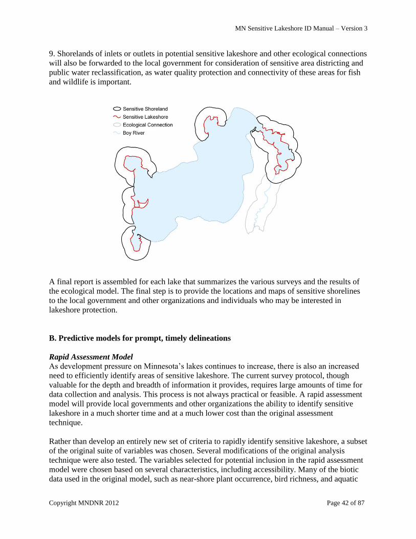
MN Sensitive Lakeshore ID Manual – Version 3
Copyright MNDNR 2012 Page 42 of 87
9. Shorelands of inlets or outlets in potential sensitive lakeshore and other ecological connections
will also be forwarded to the local government for consideration of sensitive area districting and
public water reclassification, as water quality protection and connectivity of these areas for fish
and wildlife is important.
A final report is assembled for each lake that summarizes the various surveys and the results of
the ecological model. The final step is to provide the locations and maps of sensitive shorelines
to the local government and other organizations and individuals who may be interested in
lakeshore protection.
B. Predictive models for prompt, timely delineations
Rapid Assessment Model
As development pressure on Minnesota‟s lakes continues to increase, there is also an increased
need to efficiently identify areas of sensitive lakeshore. The current survey protocol, though
valuable for the depth and breadth of information it provides, requires large amounts of time for
data collection and analysis. This process is not always practical or feasible. A rapid assessment
model will provide local governments and other organizations the ability to identify sensitive
lakeshore in a much shorter time and at a much lower cost than the original assessment
technique.
Rather than develop an entirely new set of criteria to rapidly identify sensitive lakeshore, a subset
of the original suite of variables was chosen. Several modifications of the original analysis
technique were also tested. The variables selected for potential inclusion in the rapid assessment
model were chosen based on several characteristics, including accessibility. Many of the biotic
data used in the original model, such as near-shore plant occurrence, bird richness, and aquatic
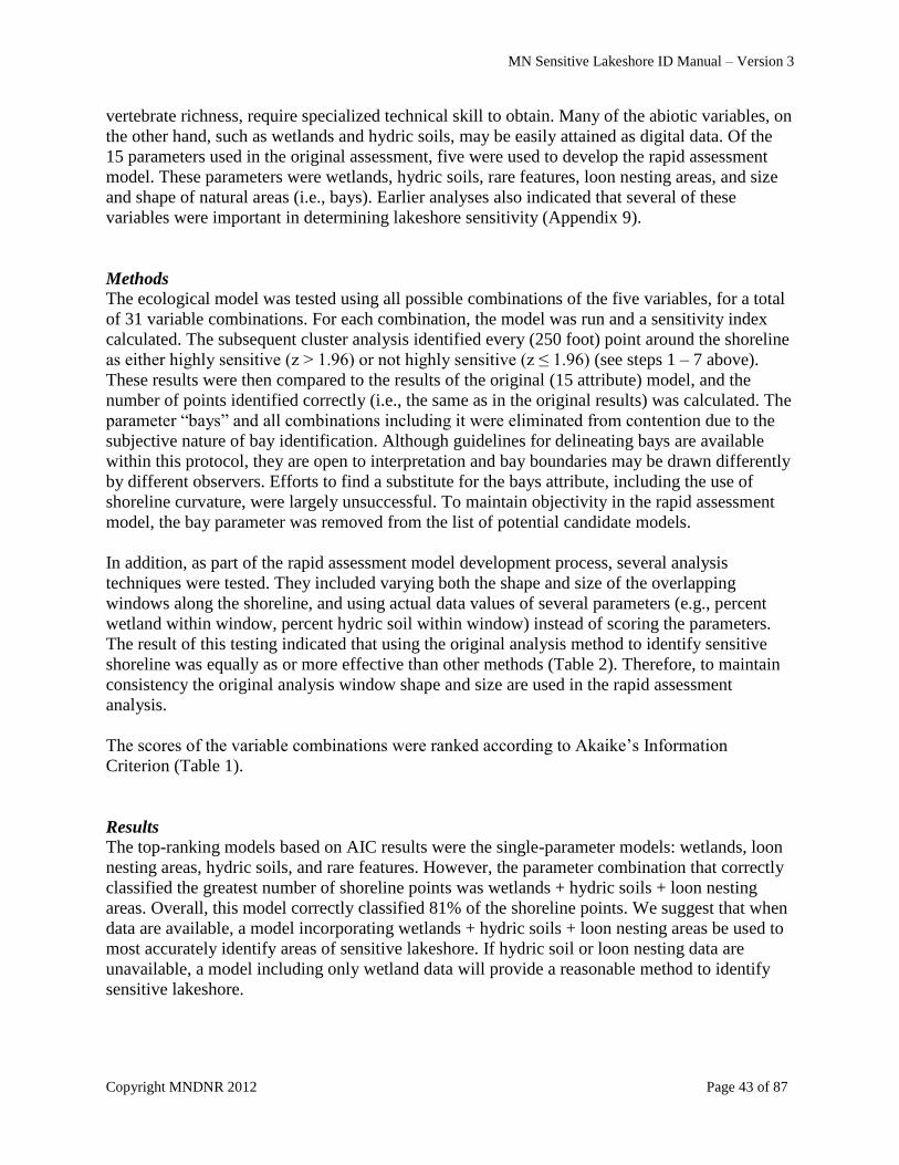
MN Sensitive Lakeshore ID Manual – Version 3
Copyright MNDNR 2012 Page 43 of 87
vertebrate richness, require specialized technical skill to obtain. Many of the abiotic variables, on
the other hand, such as wetlands and hydric soils, may be easily attained as digital data. Of the
15 parameters used in the original assessment, five were used to develop the rapid assessment
model. These parameters were wetlands, hydric soils, rare features, loon nesting areas, and size
and shape of natural areas (i.e., bays). Earlier analyses also indicated that several of these
variables were important in determining lakeshore sensitivity (Appendix 9).
Methods
The ecological model was tested using all possible combinations of the five variables, for a total
of 31 variable combinations. For each combination, the model was run and a sensitivity index
calculated. The subsequent cluster analysis identified every (250 foot) point around the shoreline
as either highly sensitive (z > 1.96) or not highly sensitive (z ≤ 1.96) (see steps 1 – 7 above).
These results were then compared to the results of the original (15 attribute) model, and the
number of points identified correctly (i.e., the same as in the original results) was calculated. The
parameter “bays” and all combinations including it were eliminated from contention due to the
subjective nature of bay identification. Although guidelines for delineating bays are available
within this protocol, they are open to interpretation and bay boundaries may be drawn differently
by different observers. Efforts to find a substitute for the bays attribute, including the use of
shoreline curvature, were largely unsuccessful. To maintain objectivity in the rapid assessment
model, the bay parameter was removed from the list of potential candidate models.
In addition, as part of the rapid assessment model development process, several analysis
techniques were tested. They included varying both the shape and size of the overlapping
windows along the shoreline, and using actual data values of several parameters (e.g., percent
wetland within window, percent hydric soil within window) instead of scoring the parameters.
The result of this testing indicated that using the original analysis method to identify sensitive
shoreline was equally as or more effective than other methods (Table 2). Therefore, to maintain
consistency the original analysis window shape and size are used in the rapid assessment
analysis.
The scores of the variable combinations were ranked according to Akaike‟s Information
Criterion (Table 1).
Results
The top-ranking models based on AIC results were the single-parameter models: wetlands, loon
nesting areas, hydric soils, and rare features. However, the parameter combination that correctly
classified the greatest number of shoreline points was wetlands + hydric soils + loon nesting
areas. Overall, this model correctly classified 81% of the shoreline points. We suggest that when
data are available, a model incorporating wetlands + hydric soils + loon nesting areas be used to
most accurately identify areas of sensitive lakeshore. If hydric soil or loon nesting data are
unavailable, a model including only wetland data will provide a reasonable method to identify
sensitive lakeshore.
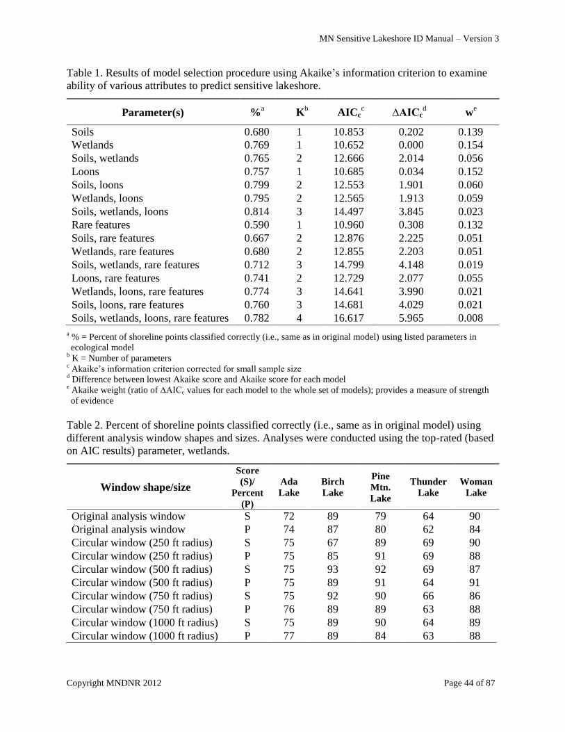
MN Sensitive Lakeshore ID Manual – Version 3
Copyright MNDNR 2012 Page 44 of 87
Table 1. Results of model selection procedure using Akaike‟s information criterion to examine
ability of various attributes to predict sensitive lakeshore.
Parameter(s) %a K
b AICc
c ∆AICc
d w
e
Soils 0.680 1 10.853 0.202 0.13900
Wetlands 0.769 1 10.652 0.000 0.15400
Soils, wetlands 0.765 2 12.666 2.014 0.05600
Loons 0.757 1 10.685 0.034 0.15200
Soils, loons 0.799 2 12.553 1.901 0.06000
Wetlands, loons 0.795 2 12.565 1.913 0.05900
Soils, wetlands, loons 0.814 3 14.497 3.845 0.02300
Rare features 0.590 1 10.960 0.308 0.13200
Soils, rare features 0.667 2 12.876 2.225 0.05100
Wetlands, rare features 0.680 2 12.855 2.203 0.05100
Soils, wetlands, rare features 0.712 3 14.799 4.148 0.01900
Loons, rare features 0.741 2 12.729 2.077 0.05500
Wetlands, loons, rare features 0.774 3 14.641 3.990 0.02100
Soils, loons, rare features 0.760 3 14.681 4.029 0.02100
Soils, wetlands, loons, rare features 0.782 4 16.617 5.965 0.00800 a % = Percent of shoreline points classified correctly (i.e., same as in original model) using listed parameters in
ecological model b K = Number of parameters
c Akaike‟s information criterion corrected for small sample size
d Difference between lowest Akaike score and Akaike score for each model
e Akaike weight (ratio of ∆AICc values for each model to the whole set of models); provides a measure of strength
of evidence
Table 2. Percent of shoreline points classified correctly (i.e., same as in original model) using
different analysis window shapes and sizes. Analyses were conducted using the top-rated (based
on AIC results) parameter, wetlands.
Window shape/size
Score
(S)/
Percent
(P)
Ada
Lake
Birch
Lake
Pine
Mtn.
Lake
Thunder
Lake
Woman
Lake
Original analysis window S 72 89 79
80
64 90
Original analysis window P 74 87 80 62 84
Circular window (250 ft radius) S 75 67 89 69 90
Circular window (250 ft radius) P 75 85 91 69 88
Circular window (500 ft radius) S 75 93 92 69 87
Circular window (500 ft radius) P 75 89 91 64 91
Circular window (750 ft radius) S 75 92 90 66 86
Circular window (750 ft radius) P 76 89 89 63 88
Circular window (1000 ft radius) S 75 89 90 64 89
Circular window (1000 ft radius) P 77 89 84 63 88
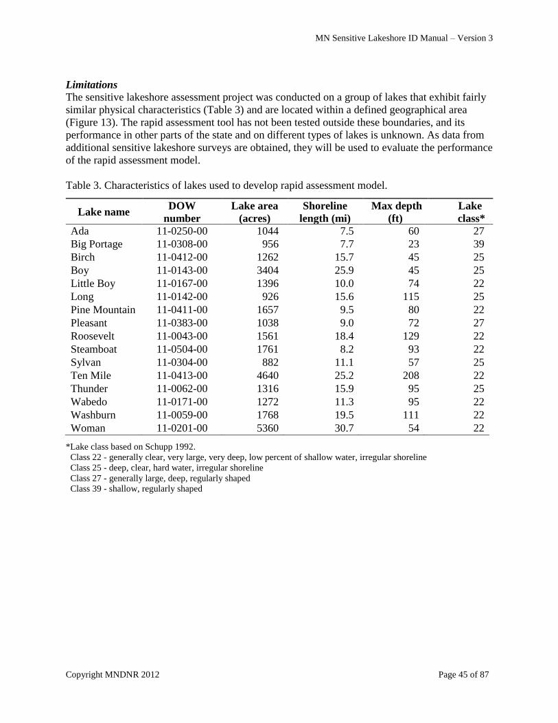
MN Sensitive Lakeshore ID Manual – Version 3
Copyright MNDNR 2012 Page 45 of 87
Limitations
The sensitive lakeshore assessment project was conducted on a group of lakes that exhibit fairly
similar physical characteristics (Table 3) and are located within a defined geographical area
(Figure 13). The rapid assessment tool has not been tested outside these boundaries, and its
performance in other parts of the state and on different types of lakes is unknown. As data from
additional sensitive lakeshore surveys are obtained, they will be used to evaluate the performance
of the rapid assessment model.
Table 3. Characteristics of lakes used to develop rapid assessment model.
Lake name DOW
number
Lake area
(acres)
Shoreline
length (mi)
Max depth
(ft)
Lake
class*
Ada 11-0250-00 1044 7.5 60 27
Big Portage 11-0308-00 956 7.7 23 39
Birch 11-0412-00 1262 15.7 45 25
Boy 11-0143-00 3404 25.9 45 25
Little Boy 11-0167-00 1396 10.0 74 22
Long 11-0142-00 926 15.6 115 25
Pine Mountain 11-0411-00 1657 9.5 80 22
Pleasant 11-0383-00 1038 9.0 72 27
Roosevelt 11-0043-00 1561 18.4 129 22
Steamboat 11-0504-00 1761 8.2 93 22
Sylvan 11-0304-00 882 11.1 57 25
Ten Mile 11-0413-00 4640 25.2 208 22
Thunder 11-0062-00 1316 15.9 95 25
Wabedo 11-0171-00 1272 11.3 95 22
Washburn 11-0059-00 1768 19.5 111 22
Woman 11-0201-00 5360 30.7 54 22
*Lake class based on Schupp 1992.
Class 22 - generally clear, very large, very deep, low percent of shallow water, irregular shoreline
Class 25 - deep, clear, hard water, irregular shoreline
Class 27 - generally large, deep, regularly shaped
Class 39 - shallow, regularly shaped
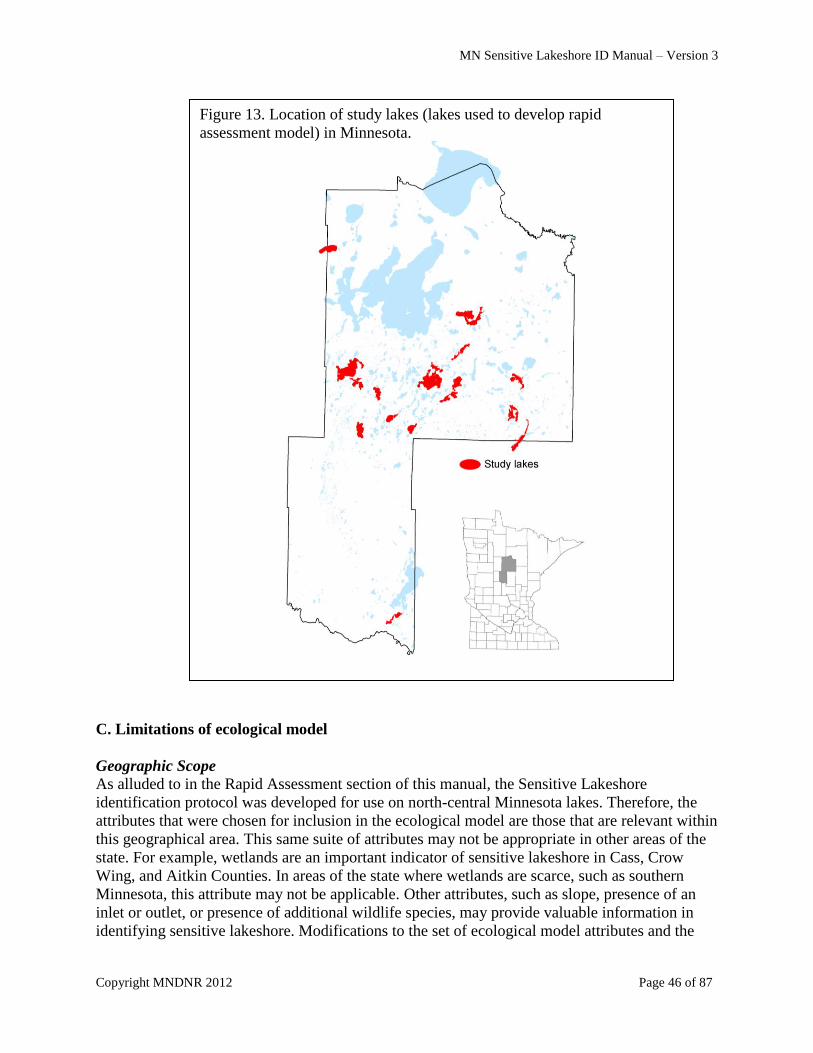
MN Sensitive Lakeshore ID Manual – Version 3
Copyright MNDNR 2012 Page 46 of 87
C. Limitations of ecological model
Geographic Scope
As alluded to in the Rapid Assessment section of this manual, the Sensitive Lakeshore
identification protocol was developed for use on north-central Minnesota lakes. Therefore, the
attributes that were chosen for inclusion in the ecological model are those that are relevant within
this geographical area. This same suite of attributes may not be appropriate in other areas of the
state. For example, wetlands are an important indicator of sensitive lakeshore in Cass, Crow
Wing, and Aitkin Counties. In areas of the state where wetlands are scarce, such as southern
Minnesota, this attribute may not be applicable. Other attributes, such as slope, presence of an
inlet or outlet, or presence of additional wildlife species, may provide valuable information in
identifying sensitive lakeshore. Modifications to the set of ecological model attributes and the
Figure 13. Location of study lakes (lakes used to develop rapid
assessment model) in Minnesota.
MN Sensitive Lakeshore ID Manual – Version 3
Copyright MNDNR 2012 Page 47 of 87
attribute scoring criteria may be necessary if implementing sensitive lakeshore identification
outside of central Minnesota.
Lake Size
The ecological model for sensitive lakeshore delineation is most appropriate for use on lakes 500
acres or larger in size. On smaller lakes, cluster analysis may lead to very small or fragmented
sections of shoreline being identified as sensitive; one goal of this protocol is to avoid “spot
zoning” of shorelines by local governments. Alternatively, once the 1320 foot buffer is created
around sections of sensitive shoreline, nearly the entire lake may fall within the potential
resource protection district. Therefore, for smaller lakes, use of other lake classification
techniques may be more appropriate. Lakes designated as natural environment lakes, Fisheries
cisco lakes, Wildlife special shallow lakes, or MCBS high biological quality lakes would all
benefit from additional lakeshore protection.

MN Sensitive Lakeshore ID Manual – Version 3
Copyright MNDNR 2012 Page 48 of 87
References
AMEREGIS and Minnesota Department of Natural Resources. 2006. Growth pressures on
sensitive natural areas in the DNR‟s Central Region. MN DNR, St. Paul.
Becker, G.C. 1983. Fishes of Wisconsin. University of Wisconsin Press, Madison.
Benedict, M.A., and E.T. McMahon. 2006. Green Infrastructure: linking landscapes and
communities. Island Press, Washington, D.C
Bourdaghs, M., C.A. Johnston and R.R. Regal. 2006. Properties and performance of the floristic
quality index in Great Lakes coastal wetlands. Wetlands 26(3):718–735
Breckenridge, W.J. 1944. Reptiles and Amphibians of Minnesota. University of Minnesota
Press, Minneapolis. 202 pp.
Byran, M.D., and D.L. Scarnecchia. 1992. Species richness, composition, and abundance of fish
larvae and juveniles inhabiting natural and developed shorelines of a glacial Iowa lake.
Environmental Biology of Fishes 35:329–341.
Casselman, J.M., and C.A. Lewis. 1996. Habitat requirements of northern pike (Esox lucius).
Canadian Journal of Fisheries and Aquatic Sciences 53(Supplement 1):161–174.
Christensen, D.L., B.R. Herwig, D.E. Schindler, and S.R. Carpenter. 1996. Impacts of lakeshore
residential development on coarse woody debris in north temperate lakes. Ecological
Applications 6:1143–1149.
Clady, M.D. 1976. Change in abundance of inshore fishes in Oneida Lake, 1916–1970. New
York Fish and Game Journal 23:73–81.
Conway, C.J. 2005. Standardized North American marsh bird monitoring protocols. Wildlife
Research Report #2005-04. U.S. Geological Survey, Arizona Cooperative Fish and Wildlife
Research Unit, Tucson, AZ.
Cross, T., and M. McInerny. 2006. Relationships between aquatic plant cover and fish
populations based on Minnesota lake survey data. Minnesota Department of Natural Resources,
Investigational Report 537, St. Paul.
Crow, G.E., and C.B. Hellquist. 2000. Aquatic and wetland plants of Northeastern North
America. 2 volumes. The University of Wisconsin Press, Madison.
Custer, C.M. 1993. Waterfowl Management Handbook. Fish and Wildlife Leaflet 13.1.11. Life
history traits and habitat needs of the redhead. U.S. Fish and Wildlife Service, Northern Prairie
Wildlife Research Center, LaCrosse, WI. 7 pp.
http://www.nwrc.usgs.gov/wdb/pub/wmh/13_1_11.pdf
MN Sensitive Lakeshore ID Manual – Version 3
Copyright MNDNR 2012 Page 49 of 87
Dale, V.H., and 8 co-authors. 2000. Ecological principles and guidelines for managing the use of
land. Ecological Applications 10(3):639–670.
Doyle, R.D. 2001. Effects of waves on the early growth of Vallisneria americana. Freshwater
Biology 46(3):389–397.
Drake, M.T., and D.L. Pereira. 2002. Development of a fish-based index of biotic integrity for
small inland lakes in central Minnesota. North American Journal of Fisheries Management
22:1105–1123.
Drake, M.T., and R.D. Valley. 2006. Validation and application of a fish-based index of biotic
integrity for small central Minnesota lakes. North American Journal of Fisheries Management
25:1095–1111.
Elias, J.E., and M.W. Meyer. 2003. Comparisons of undeveloped and developed shorelands,
northern Wisconsin, and recommendations for restoration. Wetlands 23:800–816.
Elzinga, C.L., D.W. Salzer, J.W. Willoughby, and J.P. Gibbs. 2001. Monitoring plant and
animal populations. Blackwell Science, MA. 360 pp.
Engel, S., and J.L. Pederson, Jr. 1998. The construction, aesthetics, and effects of lakeshore
development: a literature review. Wisconsin Department of Natural Resources, Research Report
177, Madison.
Engeman, R.M., R.T. Sugihara, L.F. Pank, and W.E. Dusenberry. 1994. A comparison of
plotless density estimators using Monte Carlo simulations. Ecology 75:1769–1779
Hall, B.R., and G.E. Freeman. 1994. Effects of vegetation on hydraulic roughness and
sedimentation in wetlands. WRP Technical note SD-CP-2.2. U.S. Army Engineer Waterways
Experiment Station, Vicksburg, MS. 10 pp.
http://el.erdc.usace.army.mil/elpubs/pdf/sdcp2-2.pdf
Hellquist, C.B. 1993. Taxonomic considerations in aquatic vegetation assessments. Lake and
Reservoir Management 7(2):175–183.
Herman, K.D., L.A. Masters, M.R. Penskar, A.A. Reznicek, G.S. Wilhelm and W.W.
Brodowicz. 1996. Floristic quality assessment with wetland categories and computer application
programs for the State of Michigan. Michigan Department of Natural Resources, Wildlife
Division, Natural Heritage Program, Lansing. 21 pp.
Hunter, R.G., D.L. Combs and D.B. George. 2000. Growth of softstem bulrush (Scirpus validus)
in microcosms with different hydrologic regimes and media depths. Wetlands 20(1):15–22.
Jennings, M., K. Johnson, and M. Staggs. 1996. Shoreline protection study: a report to the
Wisconsin state legislature. Wisconsin Department of Natural Resources, Publication PUBL-RS-
921–96, Madison.

MN Sensitive Lakeshore ID Manual – Version 3
Copyright MNDNR 2012 Page 50 of 87
Jennings, M.J., E.E. Emmons, G.R. Hatzenbeler, C. Edwards, and M.A. Bozek. 2003. Is littoral
habitat affected by residential development and land use in watersheds of Wisconsin lakes? Lake
and Reservoir Management 19:272–279.
Jesson, R., and R. Lound. 1962. An evaluation of a survey technique for submerged aquatic
plants. Game Investigational Report No. 6. Minnesota Department of Conservation, Division of
Game and Fish, Section of Research and Planning, Fish and Wildlife Surveys Unit, St. Paul. 10
pp.
Kantrud, H.A. 1996. The alkali (Scirpus maritimus L.) and saltmarsh (S. robustus Pursh)
bulrushes: a literature review. U.S. Dept. of Interior. National Biological Service. Information
and Technology Report 6. Northern Prairie Science Center, Jamestown, ND.
http://www.npwrc.usgs.gov/resource/plants/bulrush
Kelly, T., and J. Stinchfield. 1998. Lakeshore development patterns in northeast Minnesota:
status and trends. Minnesota Department of Natural Resources, Office of Management and
Budget Services, St. Paul.
Killgore, K.J., E.D. Dibble, and J.J. Hoover. 1993. Relationships between fish and aquatic plants:
a plan of study. U.S. Army Corps of Engineers, Miscellaneous Paper A-93-1, Vicksburg, MS.
Lentz, K.A., and D.F. Cipollini Jr. 1998. Effect of light and simulated herbivory on growth of
endangered northeastern bulrush, shape Scirpus ancistrochaetus Schuyler. Plant Ecology
139(1):125–131.
Lindsay, A.R., S.S. Gillum, and M.W. Meyer. 2002. Influence of lakeshore development on
breeding bird communities in a mixed northern forest. Biological Conservation 107:1–11.
Lyons, J. 1989. Changes in the abundance of small littoral-zone fishes in Lake Mendota,
Wisconsin. Canadian Journal of Zoology 67:2910–2916.
Madsen, J.D. 1999. Point intercept and line intercept methods for aquatic plant management.
APCRP Technical Notes Collection (TN APCRP-M1-02). U.S. Army Engineer Research and
Development Center, Vicksburg, MS. http://el.erdc.usace.army.mil/elpubs/pdf/apcmi-02.pdf
Meyer, M., J. Woodford, S. Gillum, and T. Daulton. 1997. Shoreland zoning regulations do not
adequately protect wildlife habitat in northern Wisconsin. U.S. Fish and Wildlife Service, State
Partnership Grant P-1-W, Segment 17, Final Report, Madison.
Milburn, S.A., M. Bourdaghs, and J.J. Husveth. 2007. Floristic quality assessment for Minnesota
wetlands. Minnesota Pollution Control Agency. St. Paul.
Minnesota Department of Natural Resources. 1993. Lake Survey Manual. Section of Fisheries,
St. Paul.
MN Sensitive Lakeshore ID Manual – Version 3
Copyright MNDNR 2012 Page 51 of 87
Minnesota Department of Natural Resources. 2003. Field Guide to the native plant communities
of Minnesota: The Laurentian Mixed Forest Province. Ecological Land Classification Program,
Minnesota County Biological Survey, and Natural Heritage and Nongame Research Program, St.
Paul.
Minnesota Department of Natural Resources. 2005. Aquatic vegetation mapping guidelines.
Working version, May 2005. Section of Fisheries, St. Paul. 91 pp.
Minnesota Department of Natural Resources. 2006. Tomorrow‟s habitat for the wild and rare: an
action plan for Minnesota wildlife, Comprehensive Wildlife Conservation Strategy. St. Paul.
MNTaxa. 2011. Minnesota State checklist of vascular plants. Minnesota Department of Natural
Resources, Division of Ecological and Water Resources. St. Paul. Updated April 2011.
http://www.dnr.state.mn.us/eco/mcbs/plant_lists.html
Morris, E.R. 1999. Attenuation of surface water waves in stands of hardstem bulrush (Scirpus
acutus). Master of Science Thesis. Laurentian University, Sudbury, Ontario. 111 pp.
NatureServe. 2002. Element occurrence data standard. Arlington, VA.
http://www.natureserve.org/prodServices/eodraft/all.pdf
Newburg, H.J. 1975. Evaluation of an improved walleye (Stizostedion vitreum) spawning shoal
with criteria for design and placement. Minnesota Department of Natural Resources,
Investigational Report 340, St. Paul.
Newman, R.M. and K. Holmberg, J. Foley, D. Middleton. 1998. Assessing macrophytes in
Minnesota's game lakes. Final Report to the Minnesota Dept. of Natural Resources, Wetland
Wildlife Populations and Research Group, Bemidji. 69 pp.
Nichols, S.A. 1984. Quantitative methods for assessing macrophyte vegetation. In: Ecological
assessment of macrophyton: collection, use, and meaning of data. ASTM STP 843. W.M. Dennis
and B.G. Isom, eds. American Society for Testing and Materials. pp. 7–15.
Nichols, S.A. 1999. Floristic quality assessment of Wisconsin lake plant communities with
example applications. Lake and Reservoir Management 15(2):133–141.
Perleberg, D.J. 2001a. Evaluation of DNR Fisheries Lake Vegetation Survey Method.
Unpublished report. Minnesota Department of Natural Resources, Ecological Services Division,
Brainerd. 32 pp.
Perleberg, D.J. 2001b. Estimating species abundance and distribution: a comparison of three
quantitative survey methods for lakewide assessment of submerged macrophyte communities.
Unpublished report. Minnesota Department of Natural Resources, Ecological Services Division,
Brainerd. 13 pp.
MN Sensitive Lakeshore ID Manual – Version 3
Copyright MNDNR 2012 Page 52 of 87
Radomski, P. 2006. Historical changes in abundance of floating-leaf and emergent vegetation in
Minnesota lakes. North American Journal of Fisheries Management 26:932–940.
Radomski, P., and T.J. Goeman. 2001. Consequences of human lakeshore development on
emergent and floating-leaf vegetation abundance. North American Journal of Fisheries
Management 21:46-61.
Ramstack, J.M., S.C. Fritz, and D.R. Engstrom. 2004. Twentieth century water quality trends in
Minnesota lakes compared with presettlement variability. Canadian Journal of Fisheries and
Aquatic Sciences 61:561-576.
Rowan, J.S., R.W. Duck, J. Carwardine, O.M. Bragg, A.R. Black, and M.E.J. Cutler. 2004.
Development of a technique for lake habitat survey 9LHS: Phase 1. Produced by Environmental
Systems Research Group, Univ. of Dundee. For Scotland and Northern Ireland Forum for
Environmental Research (Sniffer) Project WFD40. http://www.sniffer.org.uk
Schindler, D.E., and M.D. Scheuerell. 2002. Habitat coupling in lake ecosystems. Oikos 98:177–
189.
Schupp, D.H. 1992. An ecological classification of Minnesota lakes with associated fish
communities. Minnesota Department of Natural Resources, Investigational Report 417, St. Paul.
Spautz, H., and N. Nur. 2002. Distribution and abundance in relation to habitat and landscape
features and nest site characteristics of California black rail (Laterallus jamaicensis coturniculus)
in the San Francisco Bay Estuary. Final report to the U.S. Fish and Wildlife Service. March
2002. 36 pp. http://www.prbo.org/cms/docs/wetlands/BLRA_PRBO_Mar2002.pdf
Swink, F., and G. Wilhelm. 1994. Plants of the Chicago region (4th
ed.). Indiana Academy of
Science, Indianapolis. 921 pp.
Titus, J.E. 1993. Submersed macrophyte vegetation and distribution within lakes: line transect
sampling. Lake and Reservoir Management 7:155–164.
Valley, R.D., T.K. Cross, and P. Radomski. 2004. The role of submersed aquatic vegetation as
habitat for fish in Minnesota lakes, including the implications of non-native plant invasions and
their management. Minnesota Department of Natural Resources, Special Publication 160, St.
Paul.
Wei, A., P. Chow-Fraser, and D. Albert. 2004. Influence of shoreline features on fish distribution
in the Laurentian Great Lakes. Canadian Journal of Fisheries and Aquatic Sciences 61:1113–
1123.
Williams, L.D., G.O. Dick, R.M. Smart, and C.S. Owens. 2008. Point-intercept and surface
observation GPS (SOG): A comparison of survey methods-Lake Gaston, NC/NV. ERDC/TN
APCRP-EA-019. U.S Army Engineer Research and Development Center, Vicksburg, MS.
MN Sensitive Lakeshore ID Manual – Version 3
Copyright MNDNR 2012 Page 53 of 87
Wisconsin DNR. 2007. Wisconsin Floristic Quality Assessment Project. Accessed December
2011. http://www.botany.wisc.edu/WFQA.asp
Woodford, J.E., and M.W. Meyer. 2003. Impact of lakeshore development on green frog
abundance. Biological Conservation 110:277–284.
Yin, Y., J.S. Winkelman, and H.A. Langrehr. 2000. Long Term Resource Monitoring Program
procedures: Aquatic vegetation monitoring. U.S. Geological Survey, Upper Midwest
Environmental Sciences Center, La Crosse, WI. April 2000. LTRMP 95-P002-7. 8 pp. +
Appendixes A–C.
MN Sensitive Lakeshore ID Manual – Version 3
Copyright MNDNR 2012 Page 54 of 87
Appendices
1. Grid point-intercept vegetation survey – required sample size
2. Grid point-intercept vegetation survey – equipment checklist
3. Grid point-intercept vegetation survey – field data collection form
4. Aquatic plant bed (e.g., bulrush) field delineation – equipment checklist
5. Partial list of rare (SPC-special concern, THR-threatened, END-endangered) and unique
plant species most likely to be found in lakes or along lakeshores
6. Aquatic frog calling survey – field data collection form
7. Bird survey – field data collection form
8. Evaluation of GIS ecological model attributes
9. GIS methods for sensitive lakeshore analysis
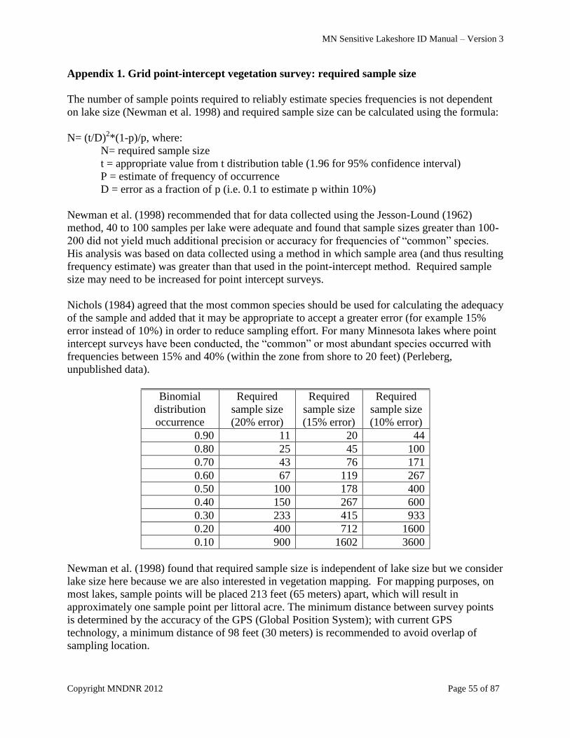
MN Sensitive Lakeshore ID Manual – Version 3
Copyright MNDNR 2012 Page 55 of 87
Appendix 1. Grid point-intercept vegetation survey: required sample size
The number of sample points required to reliably estimate species frequencies is not dependent
on lake size (Newman et al. 1998) and required sample size can be calculated using the formula:
N= (t/D)2*(1-p)/p, where:
N= required sample size
t = appropriate value from t distribution table (1.96 for 95% confidence interval)
P = estimate of frequency of occurrence
D = error as a fraction of p (i.e. 0.1 to estimate p within 10%)
Newman et al. (1998) recommended that for data collected using the Jesson-Lound (1962)
method, 40 to 100 samples per lake were adequate and found that sample sizes greater than 100-
200 did not yield much additional precision or accuracy for frequencies of “common” species.
His analysis was based on data collected using a method in which sample area (and thus resulting
frequency estimate) was greater than that used in the point-intercept method. Required sample
size may need to be increased for point intercept surveys.
Nichols (1984) agreed that the most common species should be used for calculating the adequacy
of the sample and added that it may be appropriate to accept a greater error (for example 15%
error instead of 10%) in order to reduce sampling effort. For many Minnesota lakes where point
intercept surveys have been conducted, the “common” or most abundant species occurred with
frequencies between 15% and 40% (within the zone from shore to 20 feet) (Perleberg,
unpublished data).
Binomial
distribution
occurrence
Required
sample size
(20% error)
Required
sample size
(15% error)
Required
sample size
(10% error)
0.90 11 20 44
0.80 25 45 100
0.70 43 76 171
0.60 67 119 267
0.50 100 178 400
0.40 150 267 600
0.30 233 415 933
0.20 400 712 1600
0.10 900 1602 3600
Newman et al. (1998) found that required sample size is independent of lake size but we consider
lake size here because we are also interested in vegetation mapping. For mapping purposes, on
most lakes, sample points will be placed 213 feet (65 meters) apart, which will result in
approximately one sample point per littoral acre. The minimum distance between survey points
is determined by the accuracy of the GPS (Global Position System); with current GPS
technology, a minimum distance of 98 feet (30 meters) is recommended to avoid overlap of
sampling location.
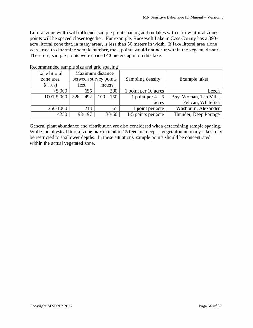
MN Sensitive Lakeshore ID Manual – Version 3
Copyright MNDNR 2012 Page 56 of 87
Littoral zone width will influence sample point spacing and on lakes with narrow littoral zones
points will be spaced closer together. For example, Roosevelt Lake in Cass County has a 390-
acre littoral zone that, in many areas, is less than 50 meters in width. If lake littoral area alone
were used to determine sample number, most points would not occur within the vegetated zone.
Therefore, sample points were spaced 40 meters apart on this lake.
Recommended sample size and grid spacing
Lake littoral
zone area
(acres)
Maximum distance
between survey points Sampling density Example lakes
feet meters
>5,000 656 200 1 point per 10 acres Leech
1001-5,000 328 – 492 100 – 150 1 point per 4 – 6
acres
Boy, Woman, Ten Mile,
Pelican, Whitefish
250-1000 213 65 1 point per acre Washburn, Alexander
<250 98-197 30-60 1-5 points per acre Thunder, Deep Portage
General plant abundance and distribution are also considered when determining sample spacing.
While the physical littoral zone may extend to 15 feet and deeper, vegetation on many lakes may
be restricted to shallower depths. In these situations, sample points should be concentrated
within the actual vegetated zone.
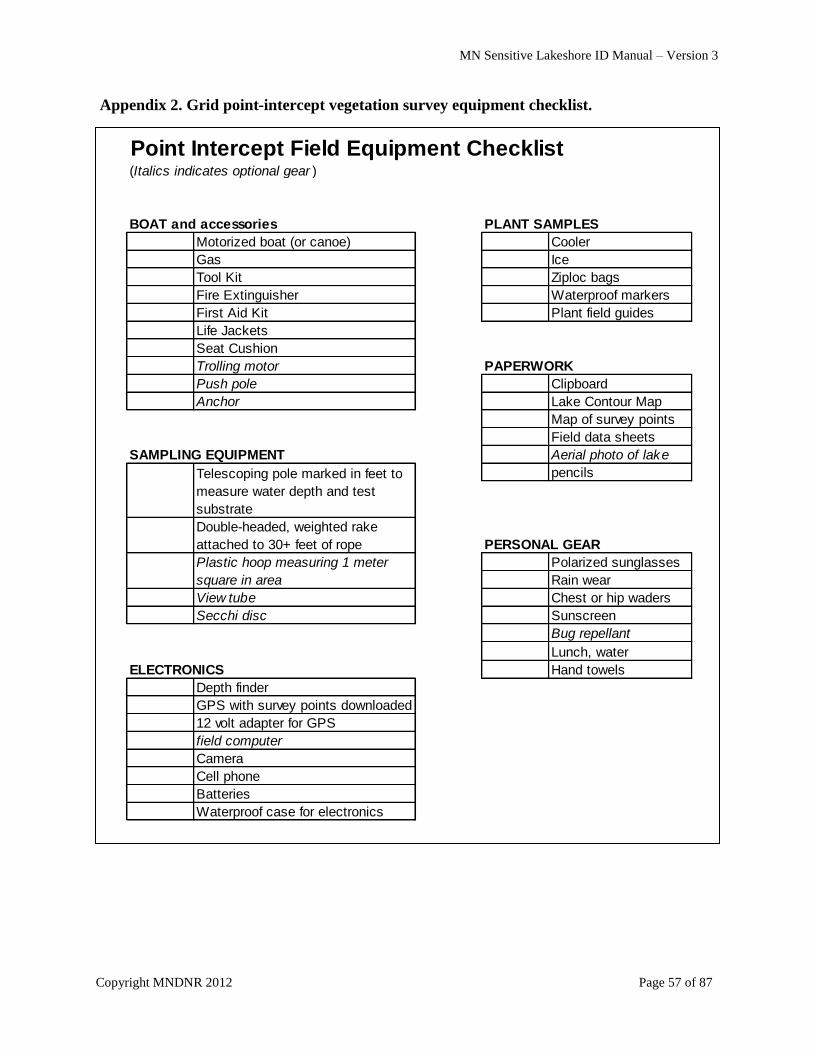
MN Sensitive Lakeshore ID Manual – Version 3
Copyright MNDNR 2012 Page 57 of 87
Appendix 2. Grid point-intercept vegetation survey equipment checklist.
Point Intercept Field Equipment Checklist(Italics indicates optional gear )
BOAT and accessories PLANT SAMPLES
Motorized boat (or canoe) Cooler
Gas Ice
Tool Kit Ziploc bags
Fire Extinguisher Waterproof markers
First Aid Kit Plant field guides
Life Jackets
Seat Cushion
Trolling motor PAPERWORK
Push pole Clipboard
Anchor Lake Contour Map
Map of survey points
Field data sheets
SAMPLING EQUIPMENT Aerial photo of lake
pencils
Double-headed, weighted rake
attached to 30+ feet of rope PERSONAL GEAR
Polarized sunglasses
Rain wear
View tube Chest or hip waders
Secchi disc Sunscreen
Bug repellant
Lunch, water
ELECTRONICS Hand towels
Depth finder
GPS with survey points downloaded
12 volt adapter for GPS
field computer
Camera
Cell phone
Batteries
Waterproof case for electronics
Telescoping pole marked in feet to
measure water depth and test
substrate
Plastic hoop measuring 1 meter
square in area
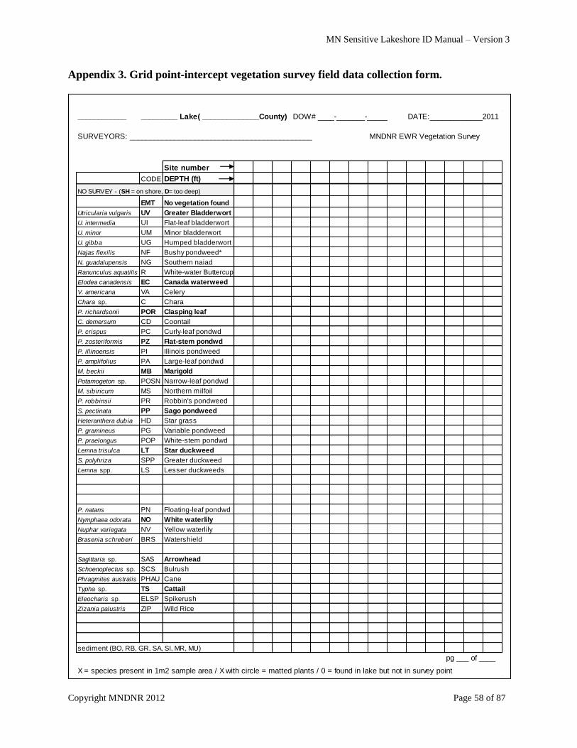
MN Sensitive Lakeshore ID Manual – Version 3
Copyright MNDNR 2012 Page 58 of 87
Appendix 3. Grid point-intercept vegetation survey field data collection form.
____________ _________ Lake( ______________County) DOW# ____-_______-_____ DATE:_____________2011
SURVEYORS: _____________________________________________ MNDNR EWR Vegetation Survey
Site number
CODE DEPTH (ft)
NO SURVEY - (SH = on shore, D= too deep)
EMT No vegetation found
Utricularia vulgaris UV Greater Bladderwort
U. intermedia UI Flat-leaf bladderwort
U. minor UM Minor bladderwort
U. gibba UG Humped bladderwort
Najas flexilis NF Bushy pondweed*
N. guadalupensis NG Southern naiad
Ranunculus aquatilis R White-water Buttercup
Elodea canadensis EC Canada waterweed
V. americana VA Celery
Chara sp. C Chara
P. richardsonii POR Clasping leaf
C. demersum CD Coontail
P. crispus PC Curly-leaf pondwd
P. zosteriformis PZ Flat-stem pondwd
P. illinoensis PI Illinois pondweed
P. amplifolius PA Large-leaf pondwd
M. beckii MB Marigold
Potamogeton sp. POSN Narrow-leaf pondwd
M. sibiricum MS Northern milfoil
P. robbinsii PR Robbin's pondweed
S. pectinata PP Sago pondweed
Heteranthera dubia HD Star grass
P. gramineus PG Variable pondweed
P. praelongus POP White-stem pondwd
Lemna trisulca LT Star duckweed
S. polyhriza SPP Greater duckweed
Lemna spp. LS Lesser duckweeds
P. natans PN Floating-leaf pondwd
Nymphaea odorata NO White waterlily
Nuphar variegata NV Yellow waterlily
Brasenia schreberi BRS Watershield
Sagittaria sp. SAS Arrowhead
Schoenoplectus sp. SCS Bulrush
Phragmites australis PHAU Cane
Typha sp. TS Cattail
Eleocharis sp. ELSP Spikerush
Zizania palustris ZIP Wild Rice
sediment (BO, RB, GR, SA, SI, MR, MU)
pg ___ of ____
X = species present in 1m2 sample area / X with circle = matted plants / 0 = found in lake but not in survey point
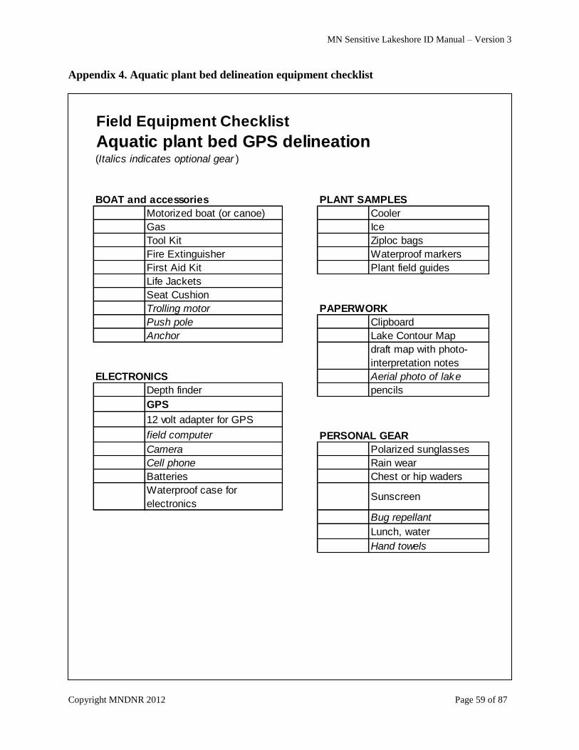
MN Sensitive Lakeshore ID Manual – Version 3
Copyright MNDNR 2012 Page 59 of 87
Appendix 4. Aquatic plant bed delineation equipment checklist
Field Equipment Checklist
Aquatic plant bed GPS delineation (Italics indicates optional gear )
BOAT and accessories PLANT SAMPLES
Motorized boat (or canoe) Cooler
Gas Ice
Tool Kit Ziploc bags
Fire Extinguisher Waterproof markers
First Aid Kit Plant field guides
Life Jackets
Seat Cushion
Trolling motor PAPERWORK
Push pole Clipboard
Anchor Lake Contour Map
draft map with photo-
interpretation notes
ELECTRONICS Aerial photo of lake
Depth finder pencils
GPS
12 volt adapter for GPS
field computer PERSONAL GEAR
Camera Polarized sunglasses
Cell phone Rain wear
Batteries Chest or hip waders
Waterproof case for
electronicsSunscreen
Bug repellant
Lunch, water
Hand towels
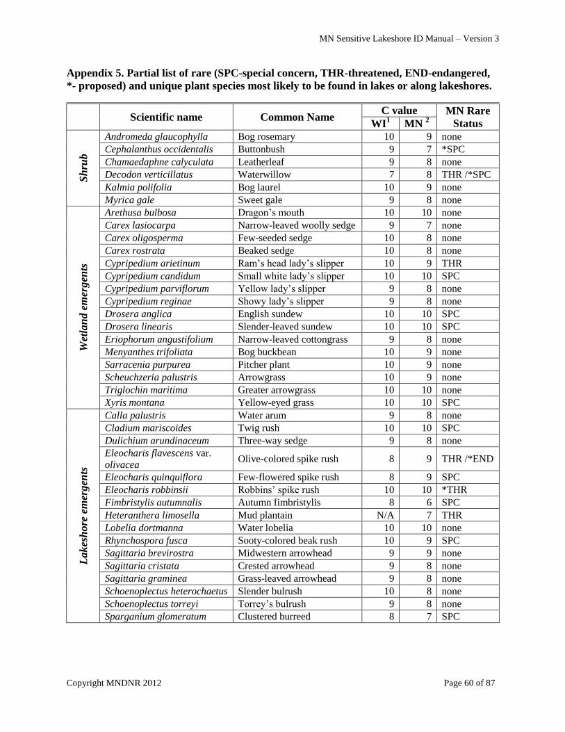
MN Sensitive Lakeshore ID Manual – Version 3
Copyright MNDNR 2012 Page 60 of 87
Appendix 5. Partial list of rare (SPC-special concern, THR-threatened, END-endangered,
*- proposed) and unique plant species most likely to be found in lakes or along lakeshores.
Scientific name Common Name C value MN Rare
Status WI1 MN
2
Sh
rub
Andromeda glaucophylla Bog rosemary 10 9 none
Cephalanthus occidentalis Buttonbush 9 7 *SPC
Chamaedaphne calyculata Leatherleaf 9 8 none
Decodon verticillatus Waterwillow 7 8 THR /*SPC
Kalmia polifolia Bog laurel 10 9 none
Myrica gale Sweet gale 9 8 none
Wet
lan
d e
mer
gen
ts
Arethusa bulbosa Dragon‟s mouth 10 10 none
Carex lasiocarpa Narrow-leaved woolly sedge 9 7 none
Carex oligosperma Few-seeded sedge 10 8 none
Carex rostrata Beaked sedge 10 8 none
Cypripedium arietinum Ram‟s head lady‟s slipper 10 9 THR
Cypripedium candidum Small white lady‟s slipper 10 10 SPC
Cypripedium parviflorum Yellow lady‟s slipper 9 8 none
Cypripedium reginae Showy lady‟s slipper 9 8 none
Drosera anglica English sundew 10 10 SPC
Drosera linearis Slender-leaved sundew 10 10 SPC
Eriophorum angustifolium Narrow-leaved cottongrass 9 8 none
Menyanthes trifoliata Bog buckbean 10 9 none
Sarracenia purpurea Pitcher plant 10 9 none
Scheuchzeria palustris Arrowgrass 10 9 none
Triglochin maritima Greater arrowgrass 10 10 none
Xyris montana Yellow-eyed grass 10 10 SPC
Lakes
hore
em
ergen
ts
Calla palustris Water arum 9 8 none
Cladium mariscoides Twig rush 10 10 SPC
Dulichium arundinaceum Three-way sedge 9 8 none
Eleocharis flavescens var.
olivacea Olive-colored spike rush 8 9 THR /*END
Eleocharis quinquiflora Few-flowered spike rush 8 9 SPC
Eleocharis robbinsii Robbins‟ spike rush 10 10 *THR
Fimbristylis autumnalis Autumn fimbristylis 8 6 SPC
Heteranthera limosella Mud plantain N/A 7 THR
Lobelia dortmanna Water lobelia 10 10 none
Rhynchospora fusca Sooty-colored beak rush 10 9 SPC
Sagittaria brevirostra Midwestern arrowhead 9 9 none
Sagittaria cristata Crested arrowhead 9 8 none
Sagittaria graminea Grass-leaved arrowhead 9 8 none
Schoenoplectus heterochaetus Slender bulrush 10 8 none
Schoenoplectus torreyi Torrey‟s bulrush 9 8 none
Sparganium glomeratum Clustered burreed 8 7 SPC
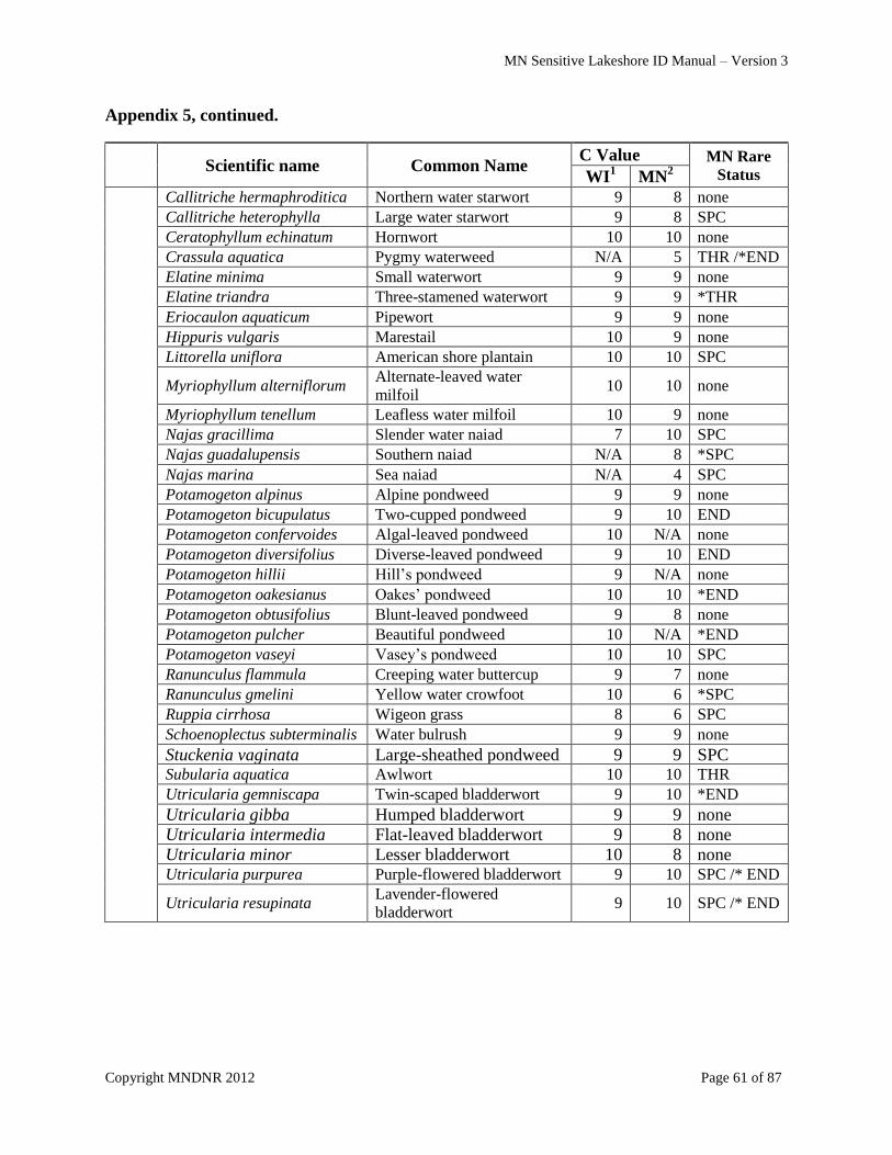
MN Sensitive Lakeshore ID Manual – Version 3
Copyright MNDNR 2012 Page 61 of 87
Appendix 5, continued.
Scientific name Common Name C Value MN Rare
Status WI1 MN
2
Su
bm
erged
Callitriche hermaphroditica Northern water starwort 9 8 none
Callitriche heterophylla Large water starwort 9 8 SPC
Ceratophyllum echinatum Hornwort 10 10 none
Crassula aquatica Pygmy waterweed N/A 5 THR /*END
Elatine minima Small waterwort 9 9 none
Elatine triandra Three-stamened waterwort 9 9 *THR
Eriocaulon aquaticum Pipewort 9 9 none
Hippuris vulgaris Marestail 10 9 none
Littorella uniflora American shore plantain 10 10 SPC
Myriophyllum alterniflorum Alternate-leaved water
milfoil 10 10 none
Myriophyllum tenellum Leafless water milfoil 10 9 none
Najas gracillima Slender water naiad 7 10 SPC
Najas guadalupensis Southern naiad N/A 8 *SPC
Najas marina Sea naiad N/A 4 SPC
Potamogeton alpinus Alpine pondweed 9 9 none
Potamogeton bicupulatus Two-cupped pondweed 9 10 END
Potamogeton confervoides Algal-leaved pondweed 10 N/A none
Potamogeton diversifolius Diverse-leaved pondweed 9 10 END
Potamogeton hillii Hill‟s pondweed 9 N/A none
Potamogeton oakesianus Oakes‟ pondweed 10 10 *END
Potamogeton obtusifolius Blunt-leaved pondweed 9 8 none
Potamogeton pulcher Beautiful pondweed 10 N/A *END
Potamogeton vaseyi Vasey‟s pondweed 10 10 SPC
Ranunculus flammula Creeping water buttercup 9 7 none
Ranunculus gmelini Yellow water crowfoot 10 6 *SPC
Ruppia cirrhosa Wigeon grass 8 6 SPC
Schoenoplectus subterminalis Water bulrush 9 9 none
Stuckenia vaginata Large-sheathed pondweed 9 9 SPC
/*END Subularia aquatica Awlwort 10 10 THR
Utricularia gemniscapa Twin-scaped bladderwort 9 10 *END
Utricularia gibba Humped bladderwort 9 9 none
Utricularia intermedia Flat-leaved bladderwort 9 8 none
Utricularia minor Lesser bladderwort 10 8 none Utricularia purpurea Purple-flowered bladderwort 9 10 SPC /* END
Utricularia resupinata Lavender-flowered
bladderwort 9 10 SPC /* END
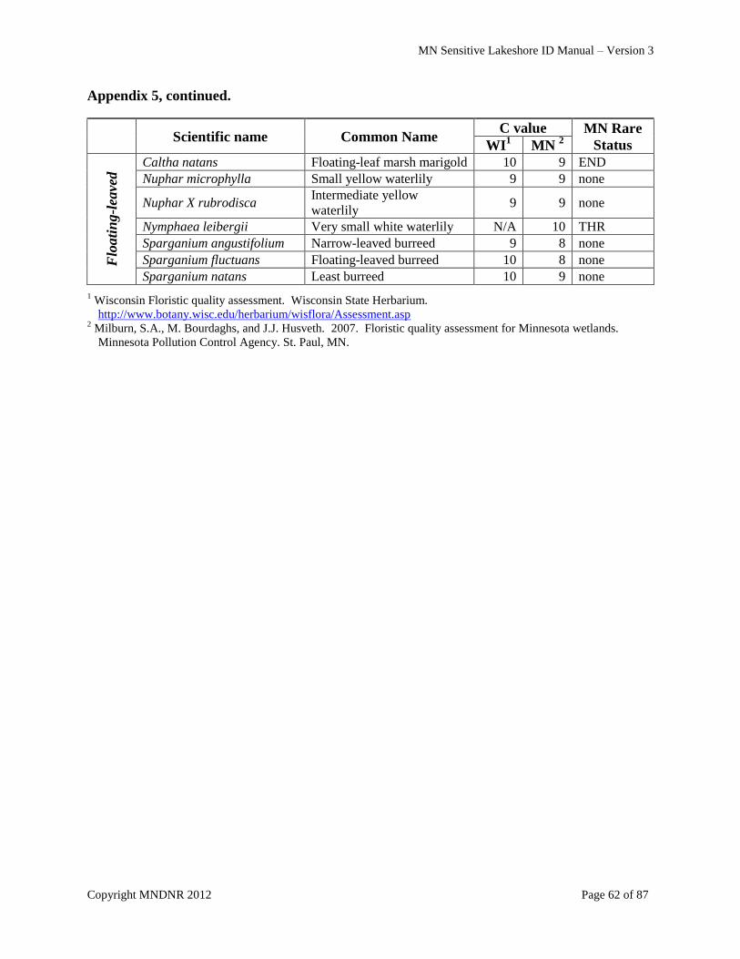
MN Sensitive Lakeshore ID Manual – Version 3
Copyright MNDNR 2012 Page 62 of 87
Appendix 5, continued.
Scientific name Common Name C value MN Rare
Status WI1 MN
2
Flo
ati
ng
-lea
ved Caltha natans Floating-leaf marsh marigold 10 9 END
Nuphar microphylla Small yellow waterlily 9 9 none
Nuphar X rubrodisca Intermediate yellow
waterlily 9 9 none
Nymphaea leibergii Very small white waterlily N/A 10 THR
Sparganium angustifolium Narrow-leaved burreed 9 8 none
Sparganium fluctuans Floating-leaved burreed 10 8 none
Sparganium natans Least burreed 10 9 none 1 Wisconsin Floristic quality assessment. Wisconsin State Herbarium.
http://www.botany.wisc.edu/herbarium/wisflora/Assessment.asp 2 Milburn, S.A., M. Bourdaghs, and J.J. Husveth. 2007. Floristic quality assessment for Minnesota wetlands.
Minnesota Pollution Control Agency. St. Paul, MN.
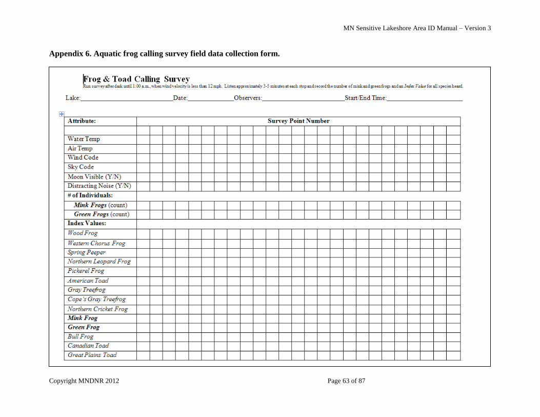
MN Sensitive Lakeshore Area ID Manual – Version 3
Copyright MNDNR 2012 Page 63 of 87
Appendix 6. Aquatic frog calling survey field data collection form.

MN Sensitive Lakeshore Area ID Manual – Version 3
Copyright MNDNR 2012 Page 64 of 87
Appendix 6, continued.
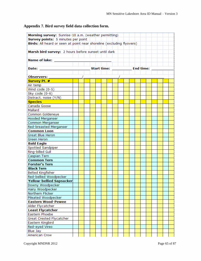
MN Sensitive Lakeshore Area ID Manual – Version 3
Copyright MNDNR 2012 Page 65 of 87
Appendix 7. Bird survey field data collection form.
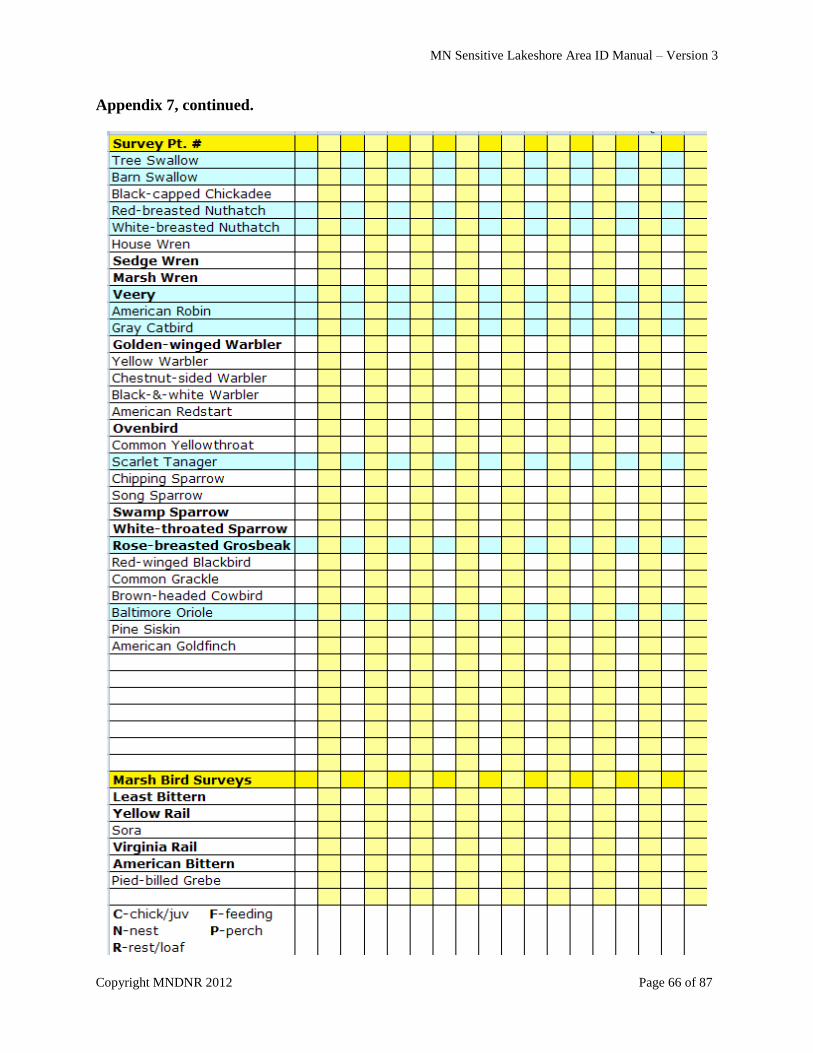
MN Sensitive Lakeshore Area ID Manual – Version 3
Copyright MNDNR 2012 Page 66 of 87
Appendix 7, continued.

MN Sensitive Lakeshore Area ID Manual – Version 3
Copyright MNDNR 2012 Page 67 of 87
Appendix 7, continued.
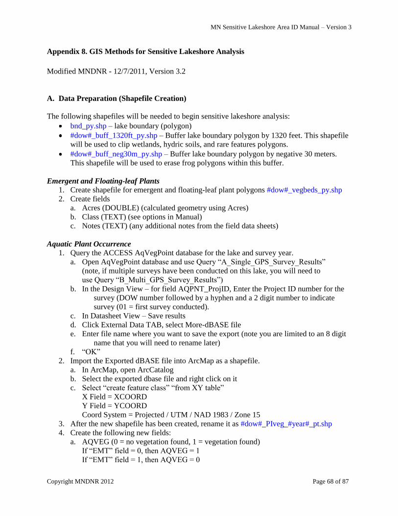
MN Sensitive Lakeshore Area ID Manual – Version 3
Copyright MNDNR 2012 Page 68 of 87
Appendix 8. GIS Methods for Sensitive Lakeshore Analysis
Modified MNDNR - 12/7/2011, Version 3.2
A. Data Preparation (Shapefile Creation)
The following shapefiles will be needed to begin sensitive lakeshore analysis:
bnd_py.shp – lake boundary (polygon)
#dow#_buff_1320ft_py.shp – Buffer lake boundary polygon by 1320 feet. This shapefile
will be used to clip wetlands, hydric soils, and rare features polygons.
#dow#_buff_neg30m_py.shp – Buffer lake boundary polygon by negative 30 meters.
This shapefile will be used to erase frog polygons within this buffer.
Emergent and Floating-leaf Plants
1. Create shapefile for emergent and floating-leaf plant polygons #dow#_vegbeds_py.shp
2. Create fields
a. Acres (DOUBLE) (calculated geometry using Acres)
b. Class (TEXT) (see options in Manual)
c. Notes (TEXT) (any additional notes from the field data sheets)
Aquatic Plant Occurrence
1. Query the ACCESS AqVegPoint database for the lake and survey year.
a. Open AqVegPoint database and use Query “A_Single_GPS_Survey_Results”
(note, if multiple surveys have been conducted on this lake, you will need to
use Query “B_Multi_GPS_Survey_Results”)
b. In the Design View – for field AQPNT_ProjID, Enter the Project ID number for the
survey (DOW number followed by a hyphen and a 2 digit number to indicate
survey (01 = first survey conducted).
c. In Datasheet View – Save results
d. Click External Data TAB, select More-dBASE file
e. Enter file name where you want to save the export (note you are limited to an 8 digit
name that you will need to rename later)
f. “OK”
2. Import the Exported dBASE file into ArcMap as a shapefile.
a. In ArcMap, open ArcCatalog
b. Select the exported dbase file and right click on it
c. Select “create feature class” “from XY table”
X Field = XCOORD
Y Field = YCOORD
Coord System = Projected / UTM / NAD 1983 / Zone 15
3. After the new shapefile has been created, rename it as #dow#_PIveg_#year#_pt.shp
4. Create the following new fields:
a. AQVEG (0 = no vegetation found, 1 = vegetation found)
If “EMT” field = 0, then AQVEG = 1
If “EMT” field = 1, then AQVEG = 0
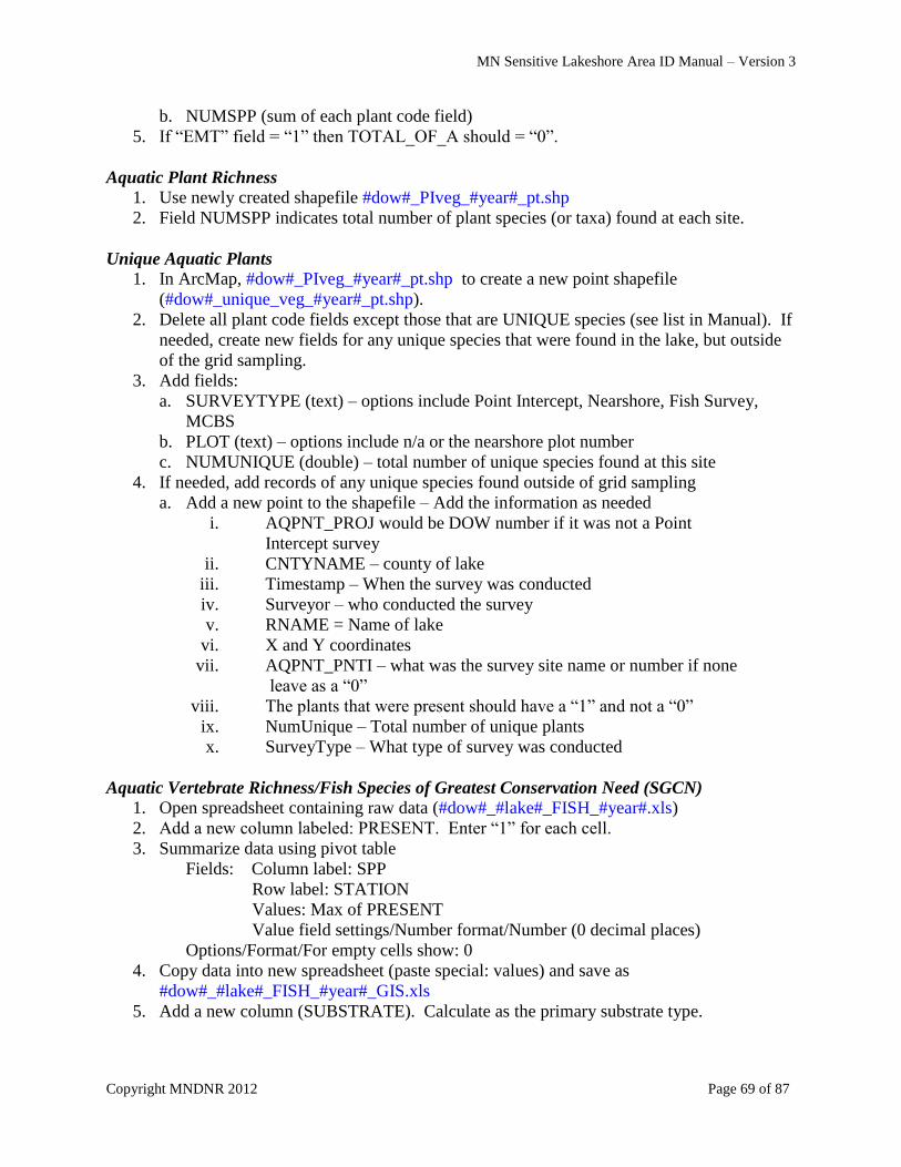
MN Sensitive Lakeshore Area ID Manual – Version 3
Copyright MNDNR 2012 Page 69 of 87
b. NUMSPP (sum of each plant code field)
5. If “EMT” field = “1” then TOTAL_OF_A should = “0”.
Aquatic Plant Richness
1. Use newly created shapefile #dow#_PIveg_#year#_pt.shp
2. Field NUMSPP indicates total number of plant species (or taxa) found at each site.
Unique Aquatic Plants
1. In ArcMap, #dow#_PIveg_#year#_pt.shp to create a new point shapefile
(#dow#_unique_veg_#year#_pt.shp).
2. Delete all plant code fields except those that are UNIQUE species (see list in Manual). If
needed, create new fields for any unique species that were found in the lake, but outside
of the grid sampling.
3. Add fields:
a. SURVEYTYPE (text) – options include Point Intercept, Nearshore, Fish Survey,
MCBS
b. PLOT (text) – options include n/a or the nearshore plot number
c. NUMUNIQUE (double) – total number of unique species found at this site
4. If needed, add records of any unique species found outside of grid sampling
a. Add a new point to the shapefile – Add the information as needed
i. AQPNT_PROJ would be DOW number if it was not a Point
Intercept survey
ii. CNTYNAME – county of lake
iii. Timestamp – When the survey was conducted
iv. Surveyor – who conducted the survey
v. RNAME = Name of lake
vi. X and Y coordinates
vii. AQPNT_PNTI – what was the survey site name or number if none
leave as a “0”
viii. The plants that were present should have a “1” and not a “0”
ix. NumUnique – Total number of unique plants
x. SurveyType – What type of survey was conducted
Aquatic Vertebrate Richness/Fish Species of Greatest Conservation Need (SGCN)
1. Open spreadsheet containing raw data (#dow#_#lake#_FISH_#year#.xls)
2. Add a new column labeled: PRESENT. Enter “1” for each cell.
3. Summarize data using pivot table
Fields: Column label: SPP
Row label: STATION
Values: Max of PRESENT
Value field settings/Number format/Number (0 decimal places)
Options/Format/For empty cells show: 0
4. Copy data into new spreadsheet (paste special: values) and save as
#dow#_#lake#_FISH_#year#_GIS.xls
5. Add a new column (SUBSTRATE). Calculate as the primary substrate type.
MN Sensitive Lakeshore Area ID Manual – Version 3
Copyright MNDNR 2012 Page 70 of 87
6. In ArcMap, open the fish data ( #dow#_#lake#_FISH_#year#_GIS.xls) and 400m survey
points (#dow#_400m_survpts_pt.shp). Join the fish data (STATION) to the survey
points (ID) and export as #dow#_fish_#year#_pt.shp. Delete all fields except FID,
SHAPE, STATION, #SPECIES CODES#, and SUBSTRATE
Size and Shape of Natural Areas (Bays)
1. Export lake boundary polygon (#dow#_bnd_py.shp) and save as
#dow#_bay_delineation_py.shp
2. Create bays by editing the bay delineation polygon shapefile
Task: Cut Polygon Features
Snap to Edge
Save Edits
3. Add new field (TYPE) and label as Isolated, Non-isolated, or Not
Bird Richness/Bird Species of Greatest Conservation Need (SGCN)
1. Open spreadsheet containing raw data (#dow#_#lake#_BIRDS_#year#.xls)
2. Add a new column labeled: PRESENT. Enter “1” for each cell.
3. Summarize data using pivot table
Fields: Column label: SPECIES_ID
Row label: STATION
Values: Max of PRESENT
Value field settings/Number format/Number (0 decimal places)
Options/Format/For empty cells show: 0
4. Copy data into new spreadsheet (paste special: values) and save as
#dow#_#lake#_BIRDS_#year#_GIS.xls
5. In ArcMap, open the bird data ( #dow#_#lake#_BIRDS_#year#_GIS.xls) and 400m
survey points (#dow#_400m_survpts_pt.shp). Join the bird data (STATION) to the
survey points (ID) and export as #dow#_bird_#year#_pt.shp. Delete all fields except FID,
SHAPE, STATION, and #SPECIES CODES#
Frog Areas
1. Open FileMaker and query lake of interest. Save records as Excel file
(#dow#_lake_FROG_#year#_GIS.xls).
2. Delete all fields except DOWLKNUM, STATION, MINK_PRES, MINK_ABUND,
GREEN_PRES, and GREEN_ABUND
3. In ArcMap, open the frog data ( #dow#_#lake#_FROG_#year#_GIS.xls) and 400m
survey points (#dow#_400m_survpts_pt.shp). Join the frog data to the survey points and
export as #dow#_frog_#year#_pt.shp.
Loon Nesting Areas
1. Obtain loon nesting areas shapefile from MN DNR Sensitive Lakeshore project team
Rare Features
1. Obtain rare features polygons
a. MN DNR employees may access data through Quick Layers (Events and
Sightings/Rare Natural Features Shapefile – polygons)

MN Sensitive Lakeshore Area ID Manual – Version 3
Copyright MNDNR 2012 Page 71 of 87
*MN DNR employees need to have completed Natural Heritage training and have
a password to access the Rare Features data.
b. Non-DNR employees may request data from the Natural Heritage program
2. Select all features that fall within (or partially within) the 1320 foot shoreland zone;
export these data as #dow#_nhis_1320ft_py.shp
Hydric Soils:
1. Obtain soils shapefile
a. Soils data are available at: http://soildatamart.nrcs.usda.gov/ Select state and
county of interest for download.
2. Clip soils layer to within 1320 feet of shoreline and save as #dow#_soils_1320ft_py.shp
Near-shore Substrate: 2. In ArcMap, open the point-intercept substrate data shapefile
(#dow#_pisub_#year#_pt.shp) and the fish data shapefile (#dow#_fish_#year#_pt.shp).
Make sure that each shapefile has a field named “SUBSTRATE”
3. Merge these two shapefiles and save resulting shapefile as
#dow#_substrate_combined_pt.shp
4. Delete all fields except FID, SHAPE, STATION, and SUBSTRATE. Make sure that the
only substrate codes in the field are BO (boulder), GR (gravel), RU (rubble), SA (sand),
SI (silt), MU (muck), and MA (marl). If there are additional codes or combined codes,
recode to one of the above. Delete records with no substrate recorded.
Wetlands:
1. Obtain wetlands polygons
a. MN DNR employees may obtain these data through Quick Layers (National
Wetlands Inventory/Cowardin Class or Circular 39 classification-Polygons)
b. Non-DNR employees may obtain the data at:
http://107.20.228.18/Wetlands/WetlandsMapper.html#
2. Clip wetlands layer to within 1320 feet of shoreline. Save final shapefile as
#dow#_nwi_1320ft_py.shp
B. GIS Ecological Model Analysis
The following shapefiles are needed for GIS ecological model sensitive lakeshore analysis (most
will have been created with the previous steps):
bnd_py.shp – lake boundary (polygon)
#dow#_plantbeds_#year#_py.shp – emergent and floating-leaf vegetation beds (polygon)
#dow#_PIveg_#year#_pt.shp – point-intercept aquatic vegetation data (point)
#dow#_unique_veg_#year#_pt.shp – unique/rare aquatic vegetation locations (point)
#dow#_fish_#year#_pt.shp – locations of fish and other aquatic vertebrate species (point)
#dow#_bay_delineation_py.shp – bay delineation (both isolated and non-isolated)
(polygon)
#dow#_bird_#year#_pt.shp – locations of birds (point)
MN Sensitive Lakeshore Area ID Manual – Version 3
Copyright MNDNR 2012 Page 72 of 87
#dow#_frog_#year#_pt.shp – locations of frogs (point)
#dow#_loon_nest_pt.shp – locations of loon nesting areas (point)
#dow#_nhis_1320ft_py.shp/#dow#_new_rare_1320ft_py.shp/
#dow#rare_veg_1320ft_py.shp – locations of Natural Heritage rare features (from NHIS
database)/locations of newly located rare wildlife features/locations of newly located rare
aquatic vegetation features (point)
#dow#_soils_1320ft_py.shp – soils clipped to within 1320 feet of shoreline (polygon)
#dow#_substrate_combined_pt.shp – substrate (from both aquatic vegetation and fish
surveys) (point)
#dow#_nwi_1320ft_py.shp – NWI wetlands clipped to within 1320 feet of shoreline
(polygon)
Create points along shoreline:
1. Convert lake polygon into polyline
a. In ArcMap, add the polygon shapefile (bnd_py.shp)
b. Create a new polyline shapefile in ArcCatalog. (bnd_ln.shp)
c. Select the Start Editing option in the Editor toolbar.
d. Set the Task to Create New Feature and the Target to the polyline shapefile
(bnd_ln.shp).
e. Click Select All on the Context menu of the polygon shapefile (bnd_py.shp).
f. Select Copy from the ArcMap Edit menu or type Ctrl+C.
g. Select Paste from the ArcMap Edit menu or type Ctrl+V.
h. Save your edits.
2. Open the attribute table and select the record that contains the shoreline
3. In ArcCatalog, create a new point shapefile that will contain the points around the
lakeshore (250ft_pt.shp)
4. Open Visual basic editor (ALT- F11 or Tool/Macros/Visual Basic Editor)
a. Under the normal template; right click on the modules and select new module.
b. Paste the code (points_along_curve.doc)
5. Run the macro
6. Enter distance between points (250 feet = 76.2 meters)
7. Add field POINT_ID (double) and calculate as FID
Create perpendicular transects at each point along the shoreline:
1. Buffer shoreline 1000 meters (bnd_1000m_buff_py.shp)
2. In ArcCatalog, create a new polyline shapefile that will contain the transects for each
point along the lakeshore with the same coordinate system that is being used in the other
files (transect_ln.shp)
3. In the Table of Contents have four shapefiles in this order;
a. The Station Layer, which contains the set of regularly occurring points along the
centerline - 250 foot points along lakeshore (250ft_pt.shp)
b. The Centerline Layer, which contains a single centerline polyline - shoreline as
polyline (bnd_ln.shp)
c. The Editable Station Line Layer, which will contain the created set of polylines
representing the station lines - polyline created in step 2 that will hold the new
transects (transect_ln.shp)
MN Sensitive Lakeshore Area ID Manual – Version 3
Copyright MNDNR 2012 Page 73 of 87
d. The Channel Layer, which contains a single channel polygon - buffered shoreline
1000m either side (bnd_1000m_buff_py.shp)
4. In addition, ArcMap must be in edit mode with the Station Line Layer selected for editing
- the polyline file that will hold the transects (transect_ln.shp)
5. Open Visual basic editor (ALT-F11 or Tools/Macros/Visual Basic Editor)
a. Under the normal template - right click on the modules and select new module.
b. Paste the code (transect_code.doc)
c. Select from bottom of code up to, and including, 1st line of code reading: “Private
Sub ConstructStationLines_Click()”
d. Click the run code button (see step 5 above in creation of points along shoreline)
e. Save edits
f. Add field LINE_ID and calculate as FID.
Create analysis windows:
1. Open project and create buffer on transect_ln.shp (arctoolbox: analyis tools/proximity/
buffer; specify input as transects_ln.shp; output as window_py.shp; enter distance in
linear units (for 250 feet it is 76.2 meters); full style; flat end type; none on dissolve - OK
2. Open attribute table for window_py.shp
3. Add field POINT_ID and calculate as FID. Delete all fields except FID, SHAPE, and
POINT_ID
4. Commence individual layer analysis.
Analyze Distribution of Emergent and Floating-leaf Plants:
Use following files:
1. 250ft_pt.shp (250ft shoreline points)
2. window_py.shp (analysis window polygons)
3. aquatic_plant_emergent_floating_py.shp (combined emergent and floating-leaf
vegetation bed polygons)
1. Make copy of emergent and floating-leaf vegetation shapefile
(#dow#_plantbeds_#year#_py.shp) and save resulting shapefile as
aquatic_plant_emergent_floating_py.shp
2. Clip all emergent and floating-leaf plant beds to within the lake boundary. Add a new
field named TYPE (text, 20). Use the field calculator to calculate TYPE (bulrush,
waterlilies, etc…) appropriately for each record
3. Delete all fields except FID, SHAPE, AREA, and TYPE.
4. Union window_py.shp with aquatic_plant_emergent_floating_py.shp; save resulting
shapefile as aquatic_plant_emergent_floating_union.shp
5. Select all records that have a FID_WINDOW value of –1; switch selection and export
records as aquatic_plant_emergent_floating_union_2.shp
6. Right-click to recalculate geometry for field AREA (square meters)
7. Add field ID_ID (text, 15) and calculate as [POINT_ID]&" "& [TYPE]
8. Select all records with emergent/floating vegetation (TYPE is not null) and summarize by
ID_ID; Minimum of POINT_ID, Sum of AREA, First of TYPE (Sum_Output.dbf)
9. Add new field; PERCENT (double); calculate PERCENT by dividing SUM_AREA by
92812
MN Sensitive Lakeshore Area ID Manual – Version 3
Copyright MNDNR 2012 Page 74 of 87
10. Summarize MIN_POINT_ by Sum of PERCENT (Sum_Output_2.dbf)
11. Add new field; EFLP_IDX (double)
12. Sort by SUM_PERCENT and select records for calculating EFLP_IDX; select all records
>0 and <1.7% and calculate as 1; select all records 1.7-8.5% and calculate as 2; select all
records >8.5% and calculate as 3
13. Join 250ft_pt.shp by POINT_ID with Sum_Output_2.dbf by MIN_POINT_ and export to
new shapefile (aquatic_plant_emergent_floating_index.shp)
Analyze Aquatic Plant Occurrence:
Use following files:
1. 250ft_pt.shp (250ft shoreline points)
2. window_py.shp (analysis window polygons)
3. aquatic_plant_occurrence_py.shp (buffered vegetation survey point data)
1. Buffer vegetation survey point data (#dow#_PIveg_#year#_pt.shp) with 25 meter buffer;
save resulting shapefile as aquatic_plant_occurrence_py.shp
2. Delete all fields except FID, SHAPE, and AQVEG
3. Union window_py.shp with aquatic_plant_occurrence_py.shp; save resulting shapefile as
aquatic_plant_occurrence_union.shp
4. Select all records that have a FID_WINDOW value of –1; switch selection and export
records as aquatic_plant_occurrence_union_2.shp
5. Add new field ID_ID (text,15); calculate as [POINT_ID]& " "& [FID_AQUATI]
6. Summarize ID_ID by Minimum of POINT_ID; Minimum of FID_AQUATI and
Minimum of AQVEG (Sum_Output.dbf)
7. Summarize MIN_POINT_ by Sum of MIN_AQVEG (Sum_Output_2.dbf)
8. Add 3 new fields NUM_PTS ; FREQ_OCC ; and APO_IDX (double)
9. Calculate NUM_PTS by subtracting 1 from CNT_MIN_PO (to eliminate the –1 records
counted as polygons)
10. Select all records where NUM_PTS equal 0, then switch selection (to avoid VBA error);
calculate FREQ_OCC by dividing SUM_MIN_AQ by NUM_PTS
11. Sort by FREQ_OCC and select records for calculating APO_IDX; select all records >0
and <25% and calculate as 1; select all records 25– 75% and calculate as 2; select all
records >75% and calculate as 3
12. Join 250ft_pt.shp by POINT_ID with Sum_Output_2.dbf by MIN_POINT_ and export to
new shapefile (aquatic_plant_occurrence_index.shp)
Analyze Aquatic Plant Richness:
Use following files:
1. 250ft_pt.shp (250ft shoreline points)
2. window_py.shp (analysis window polygons)
3. aquatic_plant_richness_py.shp (buffered vegetation survey point data)
1. Buffer vegetation survey point data (#dow#_PIveg_#year#_pt.shp) with 25 meter buffer;
save resulting shapefile as aquatic_plant_richness_py.shp
2. Delete all fields except FID, SHAPE, and #SPECIES_CODES#; also delete EMT
(emergents) and UNK (unknown species) if they are present within species codes.
MN Sensitive Lakeshore Area ID Manual – Version 3
Copyright MNDNR 2012 Page 75 of 87
3. Union window_py.shp with aquatic_plant_richness_py.shp; save resulting shapefile as
aquatic_plant_richness_union.shp
4. Select all records that have a FID_WINDOW value of –1; switch selection and export
records as aquatic_plant_richness_union_2.shp
5. Summarize POINT_ID by Maximum of #SPECIES_CODES# (Sum_Output.dbf)
6. Add new field; SUM_SPP (double); using field calculator, calculate as Sum of
MAX_#SPECIES_CODES#
7. Add new field; APR_IDX (double)
8. Sort by SUM_SPP and select records for calculating APR_IDX; select all records 1-4 and
calculate as 1; select all records 5-10 and calculate as 2; select all records >10 and
calculate as 3
9. Join 250ft_pt.shp by POINT_ID with Sum_Output.dbf by POINT_ID and export to new
shapefile (aquatic_plant_richness_index.shp)
Analyze Unique Aquatic Plants
*This shapefile should not included listed (END, THR, or SPC) plant species. Those are
included in the Natural Heritage Rare Features layer.
Use following files:
1. 250ft_pt.shp (250ft shoreline points)
2. window_py.shp (analysis window polygons)
3. aquatic_plant_unique_py.shp (buffered unique vegetation point data)
1. Buffer vegetation survey point data (#dow#_unique_veg_#year#_pt.shp) with 25 meter
buffer; save resulting shapefile as aquatic_plant_unique_py.shp
2. Delete all fields except FID, SHAPE, and #SPECIES_CODES#
3. Union window_py.shp with aquatic_plant_unique_py.shp; save resulting shapefile as
aquatic_plant_unique_union.shp
4. Select all records that have a FID_WINDOW value of –1; switch selection and export
records as aquatic_plant_unique_union_2.shp
5. Summarize POINT_ID by Maximum of #SPECIES_CODES# (Sum_Output.dbf)
6. Add new field; SUM_SPP (double); using field calculator, calculate as Sum of
MAX_#SPECIES_CODES#
7. Add new field; APU_IDX (double)
8. Sort by SUM_SPP and select records for calculating APU_IDX; select all records equal
to 1 and calculate as 2; select all records >1 and calculate as 3
9. Join 250ft_pt.shp by POINT_ID with Sum_Output.dbf by POINT_ID and export to new
shapefile (aquatic_plant_unique_index.shp)
Analyze Aquatic Vertebrate Richness
Use following files:
1. 250ft_pt.shp (250ft shoreline points)
2. window_py.shp (analysis window polygons)
3. aquatic_vertebrate_richness_py.shp (buffered vertebrate survey point data)
1. Buffer aquatic vertebrate survey point data (#dow#_fish_#year#_pt.shp) with 50 meter
buffer; save resulting shapefile as aquatic_vertebrate_richness_py.shp
MN Sensitive Lakeshore Area ID Manual – Version 3
Copyright MNDNR 2012 Page 76 of 87
2. Delete all fields except FID, SHAPE, and #SPECIES_CODES#; also delete
unknown/undefined species (UNK, YOY, JUV, SUN, BLH), hybrids (HSF), or
invertebrates (crayfish) if they are present within species codes.
3. Union window_py.shp with aquatic_vertebrate_richness_py.shp; save resulting shapefile
as aquatic_vertebrate_richness_union.shp
4. Select all records that have a FID_WINDOW value of –1; switch selection and export
records as aquatic_vertebrate_richness_union_2.shp
5. Summarize POINT_ID by Maximum of #SPECIES_CODES# (Sum_Output.dbf)
6. Add new field; SUM_SPP (double); using field calculator, calculate as Sum of
MAX_#SPECIES_CODES#S
7. Add new field; AVR_IDX (double)
8. Sort by SUM_SPP and select records for calculating AVR_IDX; select all records 1-4
and calculate as 1; select all records 5-10 and calculate as 2; select all records >10 and
calculate as 3
9. Join 250ft_pt.shp by POINT_ID with Sum_Output.dbf by POINT_ID and export to new
shapefile (aquatic_vertebrate_richness_index.shp)
Analyze Size and Shape of Natural Areas (Bays)
Use following files:
1. 250ft_pt.shp (250ft shoreline points)
2. window_py.shp (analysis window polygons)
3. bays_py.shp (bay delineation polygons)
1. Make copy of bay delineation shapefile and save as bays_py.shp
2. Delete all fields except FID, SHAPE, and TYPE
3. Add new field; SCORE (double); select records and calculate Isolated as 3; Non-isolated
as 2; Not as 0
4. Union window_py.shp with bays_py.shp; save resulting shapefile as bays_union.shp
5. Select all records that have a FID_WINDOW value of –1; switch selection and export
records as bays_union_2.shp
6. Summarize POINT_ID by Maximum of SCORE (Sum_Output.dbf)
7. Add new field; BAY_IDX (double); calculate as MAX_SCORE
8. Join 250ft_pt.shp by POINT_ID with Sum_Output.dbf by POINT_ID and export to new
shapefile (bays_index.shp)
Analyze Bird Richness
Use following files:
1. 250ft_pt.shp (250ft shoreline points)
2. window_py.shp (analysis window polygons)
3. bird_richness_py.shp (buffered bird survey point data)
1. Buffer bird survey point data (#dow#_bird_#year#_pt.shp) with 200 meter buffer; save
resulting shapefile as bird_richness_py.shp
2. Delete all fields except FID, SHAPE, and #SPECIES_CODES#; also delete
unknown/undefined species if they are present within #SPECIES_CODES#.
MN Sensitive Lakeshore Area ID Manual – Version 3
Copyright MNDNR 2012 Page 77 of 87
3. Union window_py.shp with bird_richness_py.shp; save resulting shapefile as
bird_richness_union.shp
4. Select all records that have a FID_WINDOW value of –1; switch selection and export
records as bird_richness_union_2.shp
5. Summarize POINT_ID by Maximum of #SPECIES_CODES# (Sum_Output.dbf)
6. Add new field; SUM_SPP (double); using field calculator, calculate as Sum of
MAX_#SPECIES_CODES#
7. Add new field; BIRD_IDX (double)
8. Sort by SUM_SPP and select records for calculating BIRD_IDX; select all records 1-10
and calculate as 1; select all records 11-25 and calculate as 2; select all records >25 and
calculate as 3
9. Join 250ft_pt.shp by POINT_ID with Sum_Output.dbf by POINT_ID and export to new
shapefile (bird_richness_index.shp)
Analyze Bird Species of Greatest Conservation Need (SGCN)
Use following files:
1. 250ft_pt.shp (250ft shoreline points)
2. window_py.shp (analysis window polygons)
3. bird_sgcns_py.shp (buffered bird survey point data)
1. Buffer bird survey point data (#dow#_bird_#year#_pt.shp) with 200 meter buffer; save
resulting shapefile as bird_sgcns_py.shp
2. Delete all fields except FID, SHAPE, and #SPECIES_CODES#; also delete all
#SPECIES_CODES# fields that are not SGCNs and delete unknown/undefined species if
they are present within #SPECIES_CODES#
3. Union window_py.shp with bird_sgcns_py.shp; save resulting shapefile as
bird_sgcns_union.shp
4. Select all records that have a FID_WINDOW value of –1; switch selection and export
records as bird_sgcns_union_2.shp
5. Summarize POINT_ID by Maximum of #SPECIES_CODES# (Sum_Output.dbf)
6. Add new field; SUM_SGCN (double); using field calculator, calculate as Sum of
MAX_#SPECIES_CODES#
7. Add new field; BGCN_IDX (double)
8. Sort by SUM_SGCN and select records for calculating BGCN_IDX; select all records
equal to 1 and calculate as 1; select all records equal to 2 and calculate as 2; select all
records equal to 3 or more and calculate as 3
9. Join 250ft_pt.shp by POINT_ID with Sum_Output.dbf by POINT_ID and export to new
shapefile (bird_sgcn_index.shp)
Analyze Fish Species of Greatest Conservation Need (SGCN)
Use following files:
1. 250ft_pt.shp (250ft shoreline points)
2. window_py.shp (analysis window polygons)
3. fish_sgcns_py.shp (buffered fish survey point data)
MN Sensitive Lakeshore Area ID Manual – Version 3
Copyright MNDNR 2012 Page 78 of 87
1. Buffer fish survey point data (#dow#_fish_#year#_pt.shp) with 50 meter buffer; save
resulting shapefile as fish_sgcns_py.shp
2. Delete all fields except FID, SHAPE, and #SPECIES_CODES#
3. Add two new fields, SUM_PROXY and SUM_SGCNS (double); using field calculator,
calculate each appropriately for nearshore fish species
4. Add new field, SCORE (double); sort by SUM_PROXY, select all records greater than 0
and calculate as 2; sort by SUM_SGCNS, select all records greater than 0 and calculate
as 3
5. Union window_py.shp with fish_sgcns_py.shp; save resulting shapefile as
fish_sgcns_union.shp
6. Select all records that have a FID_WINDOW value of –1; switch selection and export
records as fish_sgcns_union_2.shp
7. Summarize POINT_ID by Maximum of SCORE (Sum_Output.dbf)
8. Add new field FGCN_IDX (double) and calculate as MAX_SCORE
9. Join 250ft_pt.shp by POINT_ID with Sum_Output.dbf by POINT_ID and export to new
shapefile (fish_sgcn_index.shp)
Analyze Frog Areas
Use following files:
1. 250ft_pt.shp (250ft shoreline points)
2. window_py.shp (analysis window polygons)
3. frogs_py.shp (buffered frog survey point data)
1. Buffer frog survey point data (#dow#_frog_#year#_pt.shp) with 200 meter buffer.
Erase lake-side portion of buffered polygons with 30 meter inside buffer around shoreline
(#dow#_buff_neg30m_py.shp).
2. Delete all fields except FID, SHAPE, MINK_PRES, and GREEN_PRES
3. Add three new fields, MINK_PA, GREEN_PA, and SCORE (double)
4. Sort by MINK_PRES, select all Y records and calculate MINK_PA as 1; sort by
GREEN_PRES, select all Y records and calculate GREEN_PA as 1; calculate SCORE as
sum of MINK_PA and GREEN_PA
5. Union window_py.shp with frogs_py.shp; save resulting shapefile as frogs_union.shp
6. Select all records that have a FID_WINDOW value of –1; switch selection and export
records as frogs_union_2.shp
7. Summarize POINT_ID by Maximum of SCORE (Sum_Output.dbf)
8. Add new field FROG_IDX (double)
9. Sort by MAX_SCORE and select records for calculating FROG_IDX; select all records
equal to 1 and calculate as 2; select records equal to 2 and calculate as 3
10. Join 250ft_pt.shp by POINT_ID with Sum_Output.dbf by POINT_ID and export to new
shapefile (frog_index.shp)
Analyze Loon Nesting Areas
Use following files:
1. 250ft_pt.shp (250ft shoreline points)
2. window_py.shp (analysis window polygons)
3. loons_py.shp (buffered loon nest point data)

MN Sensitive Lakeshore Area ID Manual – Version 3
Copyright MNDNR 2012 Page 79 of 87
1. Buffer loon nest point data (#dow#_loon_nest_pt.shp) with 200 meter buffer. Erase non-
lake portion of polygons. Save resulting shapefile as loons_py.shp
2. Delete all fields except FID, SHAPE, and NATURAL
3. Add new field SCORE (double); sort by NATURAL; select all N records and calculate as
2; select all Y records and calculate as 3
4. Union window_py.shp with loons_py.shp; save resulting shapefile as loons_union.shp
5. Select all records that have a FID_WINDOW value of –1; switch selection and export
records as loons_union_2.shp
6. Summarize POINT_ID by Maximum of SCORE (Sum_Output.dbf)
7. Add new field LOON_IDX (double) and calculate as MAX_SCORE
8. Join 250ft_pt.shp by POINT_ID with Sum_Output.dbf by POINT_ID and export to new
shapefile (loon_index.shp)
Analyze Rare Features
Use following files:
1. 250ft_pt.shp (250ft shoreline points)
2. window_py.shp (analysis window polygons)
3. rare_features_py.shp (rare features polygons from the Natural Heritage Information
System combined with new rare features [excluding fish] found during field surveys)
1. Import rare vegetation shapefile (#dow#rare_veg_#year#_pt.shp), if it exists. Buffer
point files by appropriate distance using NHIS guidelines and save resulting shapefile as
#dow#rare_veg_1320ft_py.shp
2. Merge NHIS rare features polygons (#dow#_nhis_1320ft_py.shp) with new [excluding
fish] rare feature polygons found during field surveys (#dow#_new_rare_1320ft_py.shp
and #dow#rare_veg_1320ft_py.shp) and save resulting shapefile as rare_features_py.shp
3. Delete all fields except FID, SHAPE, SCI_NAME, and S_PROTSTAT; also delete all
records except those with S_PROTSTAT equal to END, THR, or SPC
4. Add new field SCORE (double) and calculate as 1
5. Union window_py.shp with rare_features_py.shp; save resulting shapefile as
rare_features_union.shp
6. Select all records that have a FID_WINDOW value of –1; switch selection and export
records as rare_features_union_2.shp
7. Add new field ID_ID (text,15); calculate as [POINT_ID]& " "& [FID_RARE_F]
8. Summarize ID_ID by Minimum of POINT_ID and Minimum of SCORE
(Sum_Output.dbf)
9. Summarize MIN_POINT_ by Sum of MIN_SCORE (Sum_Output_2.dbf)
10. Add new field RARE_IDX (double)
11. Sort by SUM_MIN_SCORE and select records for calculating RARE_IDX; select all
records equal to 1 and calculate as 2; select all records >1 and calculate as 3
12. Join 250ft_pt.shp by POINT_ID with Sum_Output_2.dbf by MIN_POINT_ and export to
new shapefile (rare_feature_index.shp)
Analyze Distribution of Hydric Soils:
Use following files:
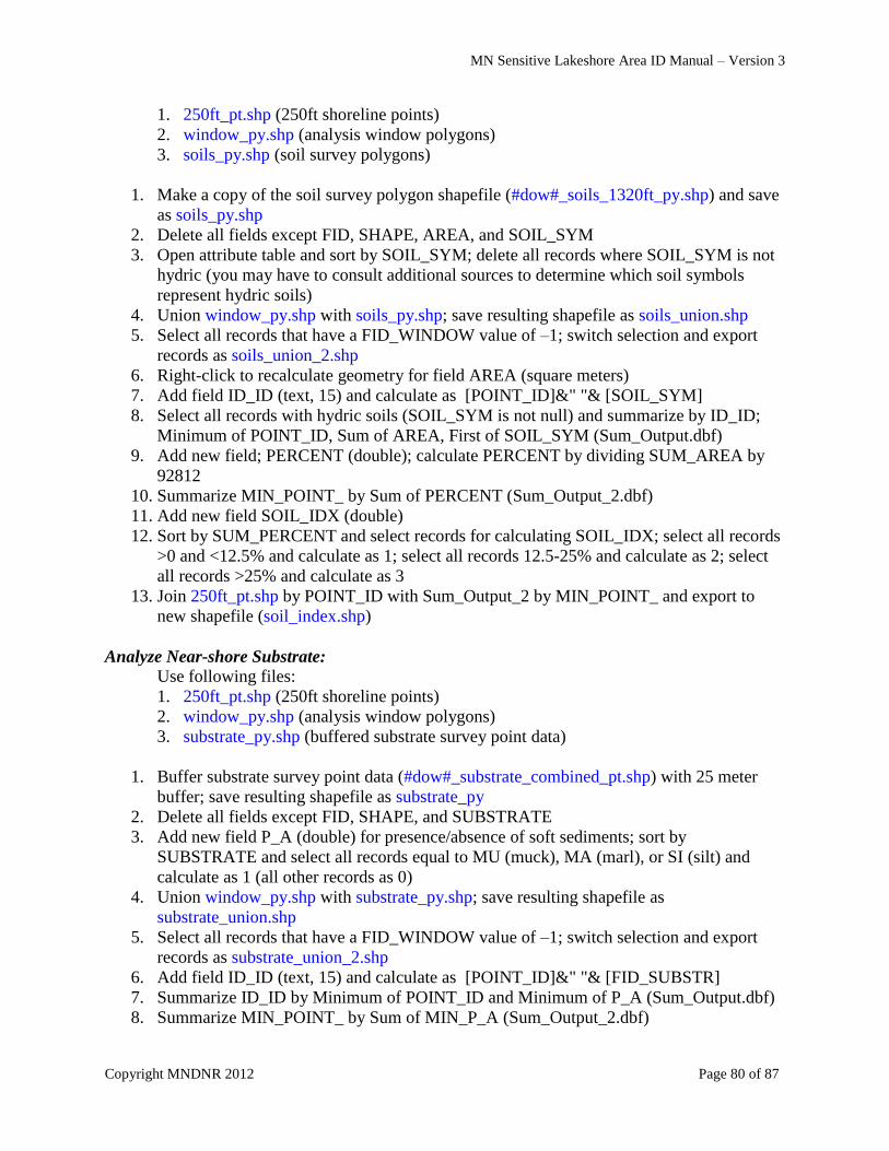
MN Sensitive Lakeshore Area ID Manual – Version 3
Copyright MNDNR 2012 Page 80 of 87
1. 250ft_pt.shp (250ft shoreline points)
2. window_py.shp (analysis window polygons)
3. soils_py.shp (soil survey polygons)
1. Make a copy of the soil survey polygon shapefile (#dow#_soils_1320ft_py.shp) and save
as soils_py.shp
2. Delete all fields except FID, SHAPE, AREA, and SOIL_SYM
3. Open attribute table and sort by SOIL_SYM; delete all records where SOIL_SYM is not
hydric (you may have to consult additional sources to determine which soil symbols
represent hydric soils)
4. Union window_py.shp with soils_py.shp; save resulting shapefile as soils_union.shp
5. Select all records that have a FID_WINDOW value of –1; switch selection and export
records as soils_union_2.shp
6. Right-click to recalculate geometry for field AREA (square meters)
7. Add field ID_ID (text, 15) and calculate as [POINT_ID]&" "& [SOIL_SYM]
8. Select all records with hydric soils (SOIL_SYM is not null) and summarize by ID_ID;
Minimum of POINT_ID, Sum of AREA, First of SOIL_SYM (Sum_Output.dbf)
9. Add new field; PERCENT (double); calculate PERCENT by dividing SUM_AREA by
92812
10. Summarize MIN_POINT_ by Sum of PERCENT (Sum_Output_2.dbf)
11. Add new field SOIL_IDX (double)
12. Sort by SUM_PERCENT and select records for calculating SOIL_IDX; select all records
>0 and <12.5% and calculate as 1; select all records 12.5-25% and calculate as 2; select
all records >25% and calculate as 3
13. Join 250ft_pt.shp by POINT_ID with Sum_Output_2 by MIN_POINT_ and export to
new shapefile (soil_index.shp)
Analyze Near-shore Substrate:
Use following files:
1. 250ft_pt.shp (250ft shoreline points)
2. window_py.shp (analysis window polygons)
3. substrate_py.shp (buffered substrate survey point data)
1. Buffer substrate survey point data (#dow#_substrate_combined_pt.shp) with 25 meter
buffer; save resulting shapefile as substrate_py
2. Delete all fields except FID, SHAPE, and SUBSTRATE
3. Add new field P_A (double) for presence/absence of soft sediments; sort by
SUBSTRATE and select all records equal to MU (muck), MA (marl), or SI (silt) and
calculate as 1 (all other records as 0)
4. Union window_py.shp with substrate_py.shp; save resulting shapefile as
substrate_union.shp
5. Select all records that have a FID_WINDOW value of –1; switch selection and export
records as substrate_union_2.shp
6. Add field ID_ID (text, 15) and calculate as [POINT_ID]&" "& [FID_SUBSTR]
7. Summarize ID_ID by Minimum of POINT_ID and Minimum of P_A (Sum_Output.dbf)
8. Summarize MIN_POINT_ by Sum of MIN_P_A (Sum_Output_2.dbf)
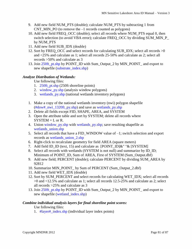
MN Sensitive Lakeshore Area ID Manual – Version 3
Copyright MNDNR 2012 Page 81 of 87
9. Add new field NUM_PTS (double); calculate NUM_PTS by subtracting 1 from
CNT_MIN_PO (to remove the –1 records counted as polygons)
10. Add new field FREQ_OCC (double); select all records where NUM_PTS equal 0, then
switch selection (to avoid VBA error); calculate FREQ_OCC by dividing SUM_MIN_P_
by NUM_PTS
11. Add new field SUB_IDX (double)
12. Sort by FREQ_OCC and select records for calculating SUB_IDX; select all records >0
and <25% and calculate as 1; select all records 25-50% and calculate as 2; select all
records >50% and calculate as 3
13. Join 250ft_pt.shp by POINT_ID with Sum_Output_2 by MIN_POINT_ and export to
new shapefile (substrate_index.shp)
Analyze Distribution of Wetlands:
Use following files:
1. 250ft_pt.shp (250ft shoreline points)
2. window_py.shp (analysis window polygons)
3. wetlands_py.shp (national wetlands inventory polygons)
1. Make a copy of the national wetlands inventory (nwi) polygon shapefile
(#dow#_nwi_1320ft_py.shp) and save as wetlands_py.shp
2. Delete all fields except FID, SHAPE, AREA, and SYSTEM
3. Open the attribute table and sort by SYSTEM; delete all records where
SYSTEM = L or R.
4. Union window_py.shp with wetlands_py.shp; save resulting shapefile as
wetlands_union.shp
5. Select all records that have a FID_WINDOW value of –1; switch selection and export
records as wetlands_union_2.shp
6. Right-click to recalculate geometry for field AREA (square meters)
7. Add field ID_ID (text, 15) and calculate as [POINT_ID]&" "& [SYSTEM]
8. Select all records with wetlands (SYSTEM is not null) and summarize by ID_ID;
Minimum of POINT_ID, Sum of AREA, First of SYSTEM (Sum_Output.dbf)
9. Add new field; PERCENT (double); calculate PERCENT by dividing SUM_AREA by
92812
10. Summarize MIN_POINT_ by Sum of PERCENT (Sum_Output_2.dbf)
11. Add new field WET_IDX (double)
12. Sort by SUM_PERCENT and select records for calculating WET_IDX; select all records
>0 and <12.5% and calculate as 1; select all records 12.5-25% and calculate as 2; select
all records >25% and calculate as 3
13. Join 250ft_pt.shp by POINT_ID with Sum_Output_2 by MIN_POINT_ and export to
new shapefile (wetland_index.shp)
Combine individual analysis layers for final shoreline point scores:
Use following files:
1. #layer#_index.shp (individual layer index points)
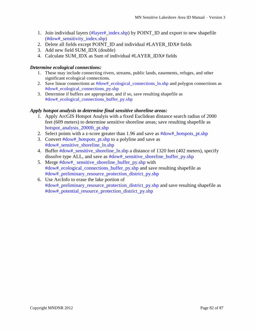
MN Sensitive Lakeshore Area ID Manual – Version 3
Copyright MNDNR 2012 Page 82 of 87
1. Join individual layers (#layer#_index.shp) by POINT_ID and export to new shapefile
(#dow#_sensitivity_index.shp)
2. Delete all fields except POINT_ID and individual #LAYER_IDX# fields
3. Add new field SUM_IDX (double)
4. Calculate SUM_IDX as Sum of individual #LAYER_IDX# fields
Determine ecological connections: 1. These may include connecting rivers, streams, public lands, easements, refuges, and other
significant ecological connections.
2. Save linear connections as #dow#_ecological_connections_ln.shp and polygon connections as
#dow#_ecological_connections_py.shp
3. Determine if buffers are appropriate, and if so, save resulting shapefile as
#dow#_ecological_connections_buffer_py.shp
Apply hotspot analysis to determine final sensitive shoreline areas:
1. Apply ArcGIS Hotspot Analyis with a fixed Euclidean distance search radius of 2000
feet (609 meters) to determine sensitive shoreline areas; save resulting shapefile as
hotspot_analysis_2000ft_pt.shp
2. Select points with a z-score greater than 1.96 and save as #dow#_hotspots_pt.shp
3. Convert #dow#_hotspots_pt.shp to a polyline and save as
#dow#_sensitive_shoreline_ln.shp
4. Buffer #dow#_sensitive_shoreline_ln.shp a distance of 1320 feet (402 meters), specify
dissolve type ALL, and save as #dow#_sensitive_shoreline_buffer_py.shp
5. Merge #dow#_ sensitive_shoreline_buffer_py.shp with
#dow#_ecological_connections_buffer_py.shp and save resulting shapefile as
#dow#_preliminary_resource_protection_district_py.shp
6. Use ArcInfo to erase the lake portion of
#dow#_preliminary_resource_protection_district_py.shp and save resulting shapefile as
#dow#_potential_resource_protection_district_py.shp
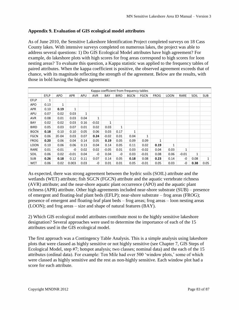
MN Sensitive Lakeshore Area ID Manual – Version 3
Copyright MNDNR 2012 Page 83 of 87
Appendix 9. Evaluation of GIS ecological model attributes
As of June 2010, the Sensitive Lakeshore Identification Project completed surveys on 18 Cass
County lakes. With intensive surveys completed on numerous lakes, the project was able to
address several questions: 1) Do GIS Ecological Model attributes have high agreement? For
example, do lakeshore plots with high scores for frog areas correspond to high scores for loon
nesting areas? To evaluate this question, a Kappa statistic was applied to the frequency tables of
paired attributes. When the kappa coefficient is positive, the observed agreement exceeds that of
chance, with its magnitude reflecting the strength of the agreement. Below are the results, with
those in bold having the highest agreement:
Kappa coefficient from frequency tables
EFLP APO APR APU AVR BAY BIRD BGCN FGCN FROG LOON RARE SOIL SUB
EFLP 1
APO 0.13 1
APR 0.10 0.19 1
APU 0.07 0.02 0.03 1
AVR 0.08 0.01 0.03 0.04 1
BAY 0.02 0.02 0.03 0.16 -0.02 1
BIRD 0.05 0.03 0.07 0.01 0.02 0.03 1
BGCN 0.18 0.10 0.10 0.05 0.06 0.03 0.17 1
FGCN 0.06 2E-04 0.03 0.07 0.24 -0.02 0.01 0.04 1
FROG 0.20 0.06 0.04 0.14 0.05 0.19 0.05 0.09 0.09 1
LOON 0.10 0.06 0.06 0.13 0.04 0.14 0.05 0.11 0.02 0.19 1
RARE 0.01 -0.01 -0 0.02 0.02 -0.05 0.01 0.03 -0.02 0.04 0.03 1
SOIL 0.06 0.02 -0.01 0.04 -0 0.04 -0 0.03 -0.01 0.08 0.06 -0.01 1
SUB 0.26 0.18 0.12 0.11 0.07 0.14 0.05 0.18 0.08 0.23 0.14 -0 0.08 1
WET 0.06 0.02 0.003 0.03 -0 0.01 0.01 0.05 -0.01 0.05 0.03 -0 0.38 0.05
As expected, there was strong agreement between the hydric soils (SOIL) attribute and the
wetlands (WET) attribute; fish SGCN (FGCN) attribute and the aquatic vertebrate richness
(AVR) attribute; and the near-shore aquatic plant occurrence (APO) and the aquatic plant
richness (APR) attribute. Other high agreements included near-shore substrate (SUB) – presence
of emergent and floating-leaf plant beds (EFLP); near-shore substrate – frog areas (FROG);
presence of emergent and floating-leaf plant beds – frog areas; frog areas – loon nesting areas
(LOON); and frog areas – size and shape of natural features (BAY).
2) Which GIS ecological model attributes contribute most to the highly sensitive lakeshore
designation? Several approaches were used to determine the importance of each of the 15
attributes used in the GIS ecological model.
The first approach was a Contingency Table Analysis. This is a simple analysis using lakeshore
plots that were classed as highly sensitive or not highly sensitive (see Chapter 7, GIS Steps of
Ecological Model, step #7; hotspot analysis; two classes; nominal data) and the each of the 15
attributes (ordinal data). For example: Ten Mile had over 500 „window plots,‟ some of which
were classed as highly sensitive and the rest as non-highly sensitive. Each window plot had a
score for each attribute.
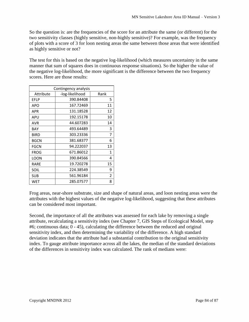
MN Sensitive Lakeshore Area ID Manual – Version 3
Copyright MNDNR 2012 Page 84 of 87
So the question is: are the frequencies of the score for an attribute the same (or different) for the
two sensitivity classes (highly sensitive, non-highly sensitive)? For example, was the frequency
of plots with a score of 3 for loon nesting areas the same between those areas that were identified
as highly sensitive or not?
The test for this is based on the negative log-likelihood (which measures uncertainty in the same
manner that sum of squares does in continuous response situations). So the higher the value of
the negative log-likelihood, the more significant is the difference between the two frequency
scores. Here are those results:
Contingency analysis
Attribute -log-likelihood Rank
EFLP 390.84408 5
APO 167.72469 11
APR 131.18528 12
APU 192.15178 10
AVR 44.607283 14
BAY 493.64489 3
BIRD 303.23336 7
BGCN 381.68377 6
FGCN 94.222037 13
FROG 671.86012 1
LOON 390.84566 4
RARE 19.720278 15
SOIL 224.38549 9
SUB 561.96184 2
WET 285.07577 8
Frog areas, near-shore substrate, size and shape of natural areas, and loon nesting areas were the
attributes with the highest values of the negative log-likelihood, suggesting that these attributes
can be considered most important.
Second, the importance of all the attributes was assessed for each lake by removing a single
attribute, recalculating a sensitivity index (see Chapter 7, GIS Steps of Ecological Model, step
#6; continuous data; 0 - 45), calculating the difference between the reduced and original
sensitivity index, and then determining the variability of the difference. A high standard
deviation indicates that the attribute had a substantial contribution to the original sensitivity
index. To gauge attribute importance across all the lakes, the median of the standard deviations
of the differences in sensitivity index was calculated. The rank of medians were:
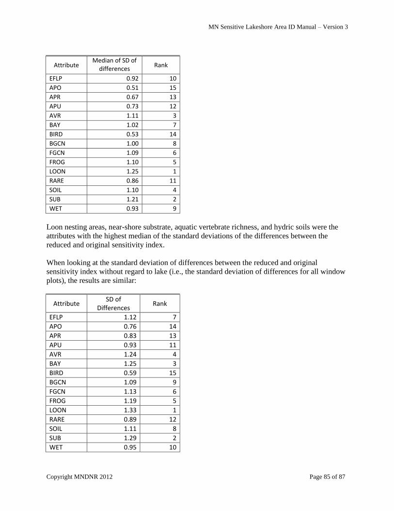
MN Sensitive Lakeshore Area ID Manual – Version 3
Copyright MNDNR 2012 Page 85 of 87
Attribute Median of SD of
differences Rank
EFLP 0.92 10
APO 0.51 15
APR 0.67 13
APU 0.73 12
AVR 1.11 3
BAY 1.02 7
BIRD 0.53 14
BGCN 1.00 8
FGCN 1.09 6
FROG 1.10 5
LOON 1.25 1
RARE 0.86 11
SOIL 1.10 4
SUB 1.21 2
WET 0.93 9
Loon nesting areas, near-shore substrate, aquatic vertebrate richness, and hydric soils were the
attributes with the highest median of the standard deviations of the differences between the
reduced and original sensitivity index.
When looking at the standard deviation of differences between the reduced and original
sensitivity index without regard to lake (i.e., the standard deviation of differences for all window
plots), the results are similar:
Attribute SD of
Differences Rank
EFLP 1.12 7
APO 0.76 14
APR 0.83 13
APU 0.93 11
AVR 1.24 4
BAY 1.25 3
BIRD 0.59 15
BGCN 1.09 9
FGCN 1.13 6
FROG 1.19 5
LOON 1.33 1
RARE 0.89 12
SOIL 1.11 8
SUB 1.29 2
WET 0.95 10
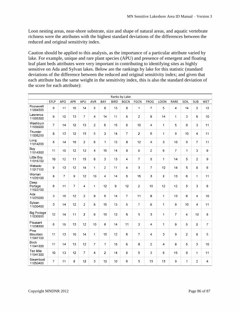
MN Sensitive Lakeshore Area ID Manual – Version 3
Copyright MNDNR 2012 Page 86 of 87
Loon nesting areas, near-shore substrate, size and shape of natural areas, and aquatic vertebrate
richness were the attributes with the highest standard deviations of the differences between the
reduced and original sensitivity index.
Caution should be applied to this analysis, as the importance of a particular attribute varied by
lake. For example, unique and rare plant species (APU) and presence of emergent and floating
leaf plant beds attributes were very important in contributing to identifying sites as highly
sensitive on Ada and Sylvan lakes. Below are the rankings by lake for this statistic (standard
deviations of the difference between the reduced and original sensitivity index; and given that
each attribute has the same weight in the sensitivity index, this is also the standard deviation of
the score for each attribute):
Ranks by Lake
EFLP APO APR APU AVR BAY BIRD BGCN FGCN FROG LOON RARE SOIL SUB WET
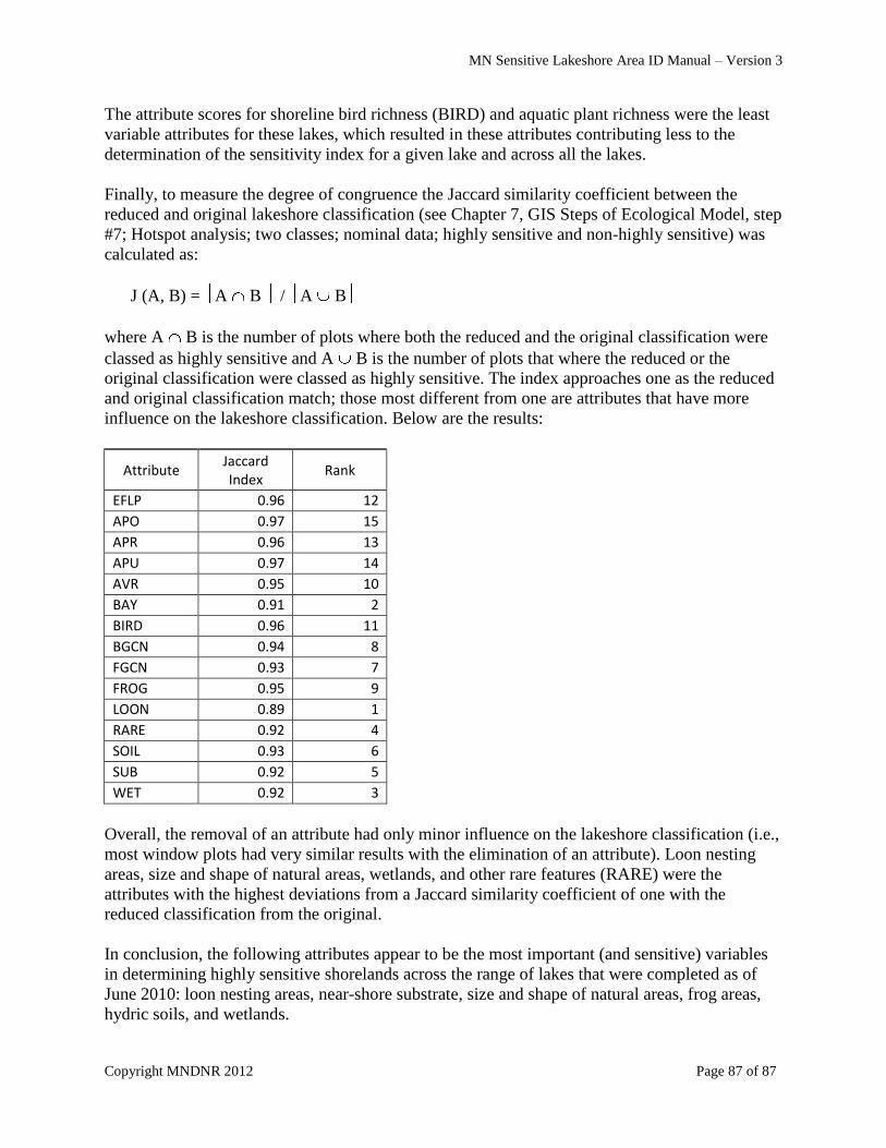
MN Sensitive Lakeshore Area ID Manual – Version 3
Copyright MNDNR 2012 Page 87 of 87
The attribute scores for shoreline bird richness (BIRD) and aquatic plant richness were the least
variable attributes for these lakes, which resulted in these attributes contributing less to the
determination of the sensitivity index for a given lake and across all the lakes.
Finally, to measure the degree of congruence the Jaccard similarity coefficient between the
reduced and original lakeshore classification (see Chapter 7, GIS Steps of Ecological Model, step
#7; Hotspot analysis; two classes; nominal data; highly sensitive and non-highly sensitive) was
calculated as:
J (A, B) = A B / A B
where A B is the number of plots where both the reduced and the original classification were
classed as highly sensitive and A B is the number of plots that where the reduced or the
original classification were classed as highly sensitive. The index approaches one as the reduced
and original classification match; those most different from one are attributes that have more
influence on the lakeshore classification. Below are the results:
Attribute Jaccard Index
Rank
EFLP 0.96 12
APO 0.97 15
APR 0.96 13
APU 0.97 14
AVR 0.95 10
BAY 0.91 2
BIRD 0.96 11
BGCN 0.94 8
FGCN 0.93 7
FROG 0.95 9
LOON 0.89 1
RARE 0.92 4
SOIL 0.93 6
SUB 0.92 5
WET 0.92 3
Overall, the removal of an attribute had only minor influence on the lakeshore classification (i.e.,
most window plots had very similar results with the elimination of an attribute). Loon nesting
areas, size and shape of natural areas, wetlands, and other rare features (RARE) were the
attributes with the highest deviations from a Jaccard similarity coefficient of one with the
reduced classification from the original.
In conclusion, the following attributes appear to be the most important (and sensitive) variables
in determining highly sensitive shorelands across the range of lakes that were completed as of
June 2010: loon nesting areas, near-shore substrate, size and shape of natural areas, frog areas,
hydric soils, and wetlands.


![[Engberg-Pederson, Troels Engberg-Pedersen] Aristo(BookZa.org)](https://img.pdfslide.us/doc/110x75/55cf98ea550346d0339a6e12/engberg-pederson-troels-engberg-pedersen-aristobookzaorg.jpg)