February 2021

Minneapolis Rent Stabilization Study

Edward G. Goetz Patrick Alcorn

Peter Hendee Brown Anthony Damiano

Jeff Matson

i

Minneapolis Rent Stabilization Study

SUMMARY

The form of programs. There are approximately 200 municipalities and two states across the United States that currently have a form of rent regulation. Rent regulation programs have taken on many forms in cities across the U.S. The variation in laws occurs across five dimensions:

• Choice of cap. Programs vary by how they cap rent increases. Most programs tie the cap to the Consumer Price Index (CPI), a widely used measure of inflation. The most restrictive programs set the cap at a percentage of the CPI, while more lenient programs set the cap at the CPI plus an additional percentage point increase. The range is illustrated by Berkeley, California which caps rents at 65% of the CPI and the State of Oregon which allows rent increases at the CPI plus 7%.

• Exceptions to the cap. Many programs allow owners to pass through costs for a range of items. Most common are allowances for major capital improvements, utilities increases, and property tax hikes. Some programs allow for owners to appeal on the basis of a “right to reasonable return” that allow the owner a base return from the property. Some jurisdictions allow owners to bank increases and then convert the banked increases at a later date. Even when exceptions such as these are allowed, many programs nevertheless limit the total increase that an owner is allowed.

• Exemptions. Various exemptions to rent caps exist. The most common is an exemption for new construction. Some programs also exempt small buildings, either across the board or when owner-occupied.

• Decontrol. Vacancy decontrol which allows a landlord to return the rent to market level when a tenant vacates the unit is used widely. A vacancy bonus is allowed in some jurisdictions that allow for a higher-than-cap increase, but that is not unlimited (as in total vacancy decontrol).

• Compliance and education. Programs vary by how compliance is monitored and how disputes are handled. Generally, some programs require tenants to initiate complaints and challenges while other programs aim for more proactive implementation.

ii

The impact of programs. Many studies have been done of existing rent stabilization programs. These studies have produced a variety of findings related to affordability and housing costs, impacts on new construction, housing stability, conversions, tear downs, and other impacts on the rental stock, maintenance and capital improvements, and on the distribution of benefits from rent control. Outcomes in individual cities are dependent on the unique features of not only the rent regulations themselves, but also the characteristics of the local housing market.

• The empirical research indicates that rent regulations have been effective at achieving two of its primary goals, maintaining below-market rent levels and moderating price appreciation. Generally, places with stronger rent control programs have had more success preventing large prices appreciation than weaker programs.

• There is widespread agreement in the empirical literature that rent regulation increases housing stability for tenants who live in regulated units.

• There is little empirical evidence to show that rent control policies negatively impact new construction. Construction rates are highly dependent on localized economic cycles and credit markets. Additionally, most jurisdictions with rent stabilization specifically exclude new construction from controls, either in perpetuity or for a set period of time.

• Rent regulations have been shown to be related to an overall reduction in rental units as owners have commonly responded to rent regulation by removing units from the rental market via condominium conversion, demolition, or other means.

• There is little evidence that rent regulations cause a reduction in housing quality. There is some evidence that major capital improvements keep pace with need but that more aesthetic upkeep may suffer. Most programs allow for the pass-through of capital improvement costs.

• There is considerable debate in the empirical literature about whether the majority of benefits from rent stabilization go to the neediest households.

The Minneapolis rental market.

• Rent trends in Minneapolis since 2000 have shown three distinct patterns. In the years 2000

to 2007 there was a steady but modest increase in rents annually. The housing crisis of 2008 to 2012 saw a stagnation of rents at the median. The third pattern emerged after the housing crisis – the years 2013 through 2018 saw steeper rent increases and a wider variation in rent increases across the market.

• Over the entire period from 2000 to 2019 incomes increased faster than rents for renter households at the median and above. However, tenants in the bottom quartile saw steep

iii

rent increases (44% increases from 2006 to 2019) and almost no growth in income (2.9% increase in the same period).

• BIPOC renters generally, and Black renter households in particular saw a worsening of affordability for most of the study period. Black households saw rent increases in this period while incomes fell in real dollars. White households fared best, with incomes steadily and consistently rising more rapidly than rents.

• We used rent trends in Minneapolis to model what might have happened to rents had various rent caps been in place. A rent cap set at 75% of CPI and a rent cap at the CPI would have had a consistent but relatively small impact on the middle of the Minneapolis rental market. Rent caps at higher levels (CPI+3% and CPI+7%) would not have constrained rent increases in Minneapolis until the post-crash period. These caps would have limited the most aggressive rent increases in the City but would not have affected median increases.

Building-level Economics We also investigated the potential impact of rent control from the perspective of building owners and the housing industry more generally. We interview 30 industry people to collect their thoughts and concerns about a rent stabilization program. We also modeled the impact of various rent caps by creating an example apartment proforma based on actual Minneapolis rents in the study period illustrating how those rents and the economic measures that apartment owners consider would change under different rent caps. Industry perspectives. The informants we spoke with expressed a range of concerns about the potential impact of rent stabilization.

• Many of the owners said that their rents would not actually be impacted by any of the example rent caps we shared with them, as they say they charge below market rents and raise rents gently. They questioned the need for rent regulation.

• Nevertheless, almost all informants expressed as their greatest concern the potential for a rent stabilization program to constrict rent growth while operating expenses continue to rise. Some noted that they would be incentivized to increase rents prior to enactment of a program of rent regulation.

• Informants expressed a range of additional concerns that ranged from a negative impact on new housing development, reduced maintenance and decline in housing quality, to changes in lending terms and the withdrawal of units and investors from the Minneapolis market.

• Most informants felt that the actual impact of rent stabilization would depend on the specific features of the program and market factors.

iv

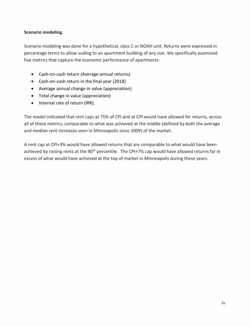
Scenario modeling. Scenario modeling was done for a hypothetical, class C or NOAH unit. Returns were expressed in percentage terms to allow scaling to an apartment building of any size. We specifically examined five metrics that capture the economic performance of apartments:

• Cash-on-cash return (Average annual returns) • Cash-on-cash return in the final year (2018) • Average annual change in value (appreciation) • Total change in value (appreciation) • Internal rate of return (IRR).

The model indicated that rent caps at 75% of CPI and at CPI would have allowed for returns, across all of these metrics, comparable to what was achieved at the middle (defined by both the average and median rent increases seen in Minneapolis since 2009) of the market. A rent cap at CPI+3% would have allowed returns that are comparable to what would have been achieved by raising rents at the 90th percentile. The CPI+7% cap would have allowed returns far in excess of what would have achieved at the top of market in Minneapolis during these years.

Table of Contents Summary . . . . . . . . . i Part 1: Rent Regulation in Other Cities . . . . . 1 History of Rent Control in the United States . . . . . 2 Components of Rent Stabilization Legislation . . . . 4 Rent Regulation . . . . . . . 5 Definition of Controlled Stock . . . . . 7 Mechanisms to Decontrol Units . . . . . 8 Protections Against Evictions . . . . . . 11 Cost Pass-throughs . . . . . . . 12 Preferential Rent and “Banking” Increases . . . . 15 Infrastructure, Implementation, and Enforcement . . . 15 Outreach and Education . . . . . . 17 Peer Cities Analysis . . . . . . . . 17 Oakland, California . . . . . . . 18 Portland, Oregon . . . . . . . 23 Newark, New Jersey . . . . . . . 25 Sacramento, California . . . . . . 28 Impact of Rent Regulations . . . . . . . 30 Affordability and Housing Costs . . . . . 30 Impact on Controlled and Non-controlled Stock . . . 33 Housing Stability / Tenure Length . . . . . 34 Housing Construction . . . . . . . 36 Conversions, Tear Downs, and Owner Move-ins . . . 36 Maintenance and Capital Improvements . . . . 37 Distribution of Benefits . . . . . . 39 Part 2: The Minneapolis Rental Market . . . . . 41 Minneapolis Rental Housing Stock . . . . . . 41

Composition of the Rental Housing Stock . . . . 41 Age of the Rental Housing Stock . . . . . 44 Ownership Characteristics . . . . . . 45

Rental Safety and Habitability . . . . . . 48 Rental Tiers . . . . . . . . 48 Tenant Complaints . . . . . . . 49 Code Violations . . . . . . . 50 Potential Growth in Housing Market . . . . . . 51 Predicted Growth in Housing . . . . . . 51 Rent Trends . . . . . . . . . 54 Rent Trends, 2001-2019 . . . . . . 54 Rent Trends in Small-building Rentals . . . . 59 Advertised Rents . . . . . . . 60

Affordability Analysis . . . . . . . . 61 Rent and Income Trends for Minneapolis Renters . . . 62 Cost-burden . . . . . . . . 66 Tenant Focus Groups . . . . . . . . 67 Rents . . . . . . . . . 67 Upkeep . . . . . . . . 69 Homelessness . . . . . . . . . 69 Hypothetical Rent Changes Under Different Rent-Increase Caps . . 71 Methods . . . . . . . . 71 Rent Caps . . . . . . . . 71 Impact of Rent Caps – A Retrospective Analysis, 2001-2019 . . 73 Part 3: Economic Analysis . . . . . . . 77 Industry Perspectives . . . . . . . . 77 Method . . . . . . . . 77 Summary of Responses . . . . . . 78 Detailed Responses . . . . . . . 79 Scenario Modeling . . . . . . . . 85 Rent Increases Under Different Rent Caps . . . . 87 Rent Caps and Investment Metrics . . . . . 88 Sources . . . . . . . . . 94 Appendix . . . . . . . . . 98

1

Part 1: Rent Regulation in Other Cities

In this section, we review the experience of rent stabilization in other cities in the U.S. We provide a brief and high-level history of rent regulations in the United States, and the describe the most common policy options found in most US rent regulations. We take a more in-depth look at what rent stabilization looks like in four peer cities, focusing both on program design and also on implementation issues. Finally, we review the literature regarding the policy and economic impacts of rent regulations. Many make the distinction between rent control and rent stabilization as two distinct forms of rent regulations. Under this view, the differences between rent control and stabilization have to do with the strength and sometimes the scope of regulations. However, these terms usually serve as a stand-in for the historical distinction between first-generation and second-generation regulations. The first generation of rent regulations in the U.S. contained long term price ceilings on rent. The second generation of rent regulations emerged in the 1970s and contained a series of more moderate regulations. This more moderate form is the most common form of rent regulation today, and typically incorporates approved rates of increase, exempts certain properties, and sometimes contains provisions such as vacancy decontrol that allow rents to rise to market levels when a tenant moves out. The only remaining first-generation rent control program is in New York City, which also has a more moderate rent stabilization program. Much of the early work on rent control was generated by economists who focused on first-generation rent control programs that placed a hard ceiling on rents. This literature also frequently assesses the potential impact of rent control from a theoretical perspective rather than from an empirical assessment of how rent regulation has worked out. The early work in economics led to a widely held set of views that rent control would, in fact, produce a set of adverse impacts in local housing markets, including a decline in maintenance of housing, a decline in the production of new housing, and rent increases in the portion of the housing stock not controlled. These views approach the status of orthodoxy among economists and real estate professionals. The literature reviewed below, however, paints a different picture of the actual track record of rent regulation. First, as already noted, rent regulations have taken on many different forms and include provisions that deviate in many ways from the strict model of rent control invoked by economists. Second, studies have shown a mix of outcomes that are largely determined by the specific provisions of the regulations being studied. Third, the literature shows that rent regulations can be effective tools to achieve the goals of stability and affordability. Fourth, the

2

literature indicates that some jurisdictions couple rent regulations with additional policies to address the negative market outcomes feared by its skeptics.

1.A History of Rent Control in the United States Rent regulations in the United States originated in World War I when local jurisdictions, such as New York City and Washington D.C., imposed emergency controls to prevent profiteering. However, during this time rent control was not promoted at the federal level and local laws were invalidated in the 1920s as housing emergencies came to an end (Keating, 1998). Policies in the United States are primarily associated with the federal controls that emerged during World War II. The wartime economy put significant stress on local housing markets and rent control programs were introduced to guarantee affordable housing and prevent rent gouging (Arnott, 1995). The Office of Price Administration (OPA) was established in 1942 as a federal independent agency with a broad authority to ration goods, set prices, and control rents. Under this authority, the OPA designated localities as “defense rental areas”, and imposed a rent ceiling on the designated area. In addition to freezing rents, the OPA also rolled back the allowable rent to the level it had been at before any appreciation due to the wartime production economy. At the height of the wartime rent control, almost 80% of all dwelling units were located in areas under federal rent control (Fetter, 2013). These regulations continued until well past the end of war, only being terminated en masse in the late 1940s, with some continuing into the 1950s. By the end of the 1950s, rent controls largely disappeared and did not reemerge until the 1970s (Arnott, 1995). The second generation of rent control policies, often called rent stabilization or “moderate rent control”, emerged in the 1970s due to rampant inflation, social upheaval, and mass tenant organizing. This generation of rent stabilization programs were predominantly local in origin. From 1970 to 1983, median rents in the United States grew twice as fast as renter incomes (Appelbaum and Gilderbloom, 1989). Major cities such as Boston, Washington D.C., Los Angeles, and San Francisco adopted rent stabilization policies during this time, as well as smaller cities throughout New York, New Jersey, Massachusetts, Connecticut, and California (Arnott, 1995). In contrast to earlier programs which established strict price ceilings, the second generation of programs was more moderate, instead capping the amount rent could be increased year-to-year. Additionally, they included various provisions that allowed landlords to increase rents beyond the fixed cap, such as increases for capital improvements, maintenance, a guaranteed “reasonable rate of return”, and hardship provisions. Until recently, almost all of the contemporary rent regulations in the United States originated during this time period.

3

New York deserves its own treatment, due to the unique nature of the interaction between its rent control and rent stabilization programs. New York was the only city to continue the rent controls of the World War II era, enacting the New York Emergency Housing Act of 1950 when the federal legislation expired. The law only covers buildings built before 1947 where a tenant has continuously occupied the building since 1971. These units are subject to a maximum base rent system, which places a hard cap on the nominal rent that can be charged for the unit. However, the number of rent controlled units has continuously declined, from about 2 million in the 1950s to approximately 22,000 currently. This is because once a unit becomes vacant, it is typically permanently deregulated, except for certain conditions in which a family member is allowed to subsume a lease. Rent stabilized apartments are much more prevalent in the New York rental housing stock, about 50% of the total rental units. Rent stabilization covers most buildings that have six or more units and were constructed before 1974. Rents in these units can be increased yearly, subject to the cap determined by the Rent Guidelines Board. While the specifics of regulations have changed throughout the history of the program, the most recent update was the 2019 Housing Stability and Tenant Protection Act. The 1990s saw a backlash against rent regulation led by the real estate industry. In 1994, Massachusetts residents voted to ban rent control statewide after a landlord-backed initiative was placed on the ballot. Regulations in California were curtailed by the 1995 Costa Hawkins Act. Dozens of states moved to preempt all forms of rent regulation at the municipal level. These policies were often championed by the American Legislative Exchange Council (ALEC). On its website, ALEC provides template legislation for state lawmakers to adopt the preemption model.1 Currently, 38 states prevent local jurisdictions from enacting rent control laws—including seven states that use Dillon’s Rule that restricts cities from acting where they are not given specific consent from the state government. The rapid appreciation in rents in metropolitan areas across the country during the post-recession period has created renewed interest in rent control policies. In 2018, a proposition to substantially expand rent stabilization in California qualified for the ballot though it ultimately failed. In 2019, Oregon became the first state in the nation to pass statewide rent control legislation. Soon after, California passed AB1482 which established a statewide rent cap. In New York, tenant advocates successfully strengthened the existing law by passing the Housing Stability and Tenant Protection Act of 2019. The bill removed a sunset provision and made the law permanent, enabled any locality to opt-in to rent stabilization, and closed loopholes which

1 ALEC Rent Control Preemption Act Template

4

allowed units to be deregulated. Action has also occurred at the local level. Several cities in California, such as Richmond and Sacramento, have also adopted rent control programs in recent years. Currently, there are ongoing campaigns to either pass rent control legislation or repeal preemption laws in Illinois, Massachusetts, and Washington state. There are approximately 200 municipalities across California, New York, New Jersey, Washington D.C. and Maryland that currently have a form of rent regulation program, in addition to the statewide programs in California and Oregon.

1.B Components of Rent Stabilization Legislation The details and implementation of rent regulations vary based on jurisdictions’ goals. Broadly, these goals include protecting tenants from excessive rent increases, alleviating the affordable housing crisis, preserving existing affordable housing, providing housing habitability and security of tenure for renters, maintaining economic and racial diversity, and preventing real estate speculation (Been et al, 2019). Rent stabilization comes in many varieties in the U.S. Local governments have fashioned programs to fit local concerns and to respond to local political factors. The variations in rent stabilization approaches occurs across five different dimensions; the rent cap and its operation; exceptions to the cap, exemptions of building or unit-type that are allowed, provisions for decontrol, and program monitoring and implementation. Figure 1.1 depicts these major choices. Figure 1: Program Design Choices

Both political and policy considerations impact the details of rent stabilization programs. Some design components reflect direct tradeoffs. For example, legal mechanisms that enable landlords to return rents to market levels upon vacancy may alleviate opposition from the real

5

estate industry, but they also limit the program’s efficacy in providing stability and affordability. Exemptions can also create incentives that are contradictory to the spirit of the regulations. Jurisdictions that allow for stabilized units to be easily converted to condominiums risk incentivizing property owners to withdraw their units from the rental market. In this section we summarize the common components of rent regulations as they exist in the United States, and the range of options available to policymakers in drafting a potential program. Rent regulation Rent caps, the rate that landlords are allowed to increase rents year-to-year, are the definitional component of modern rent control programs. Policy options here include not just the magnitude of the allowable increase, but the mechanism for establishing a cap. While first-generation rent control policies placed a hard ceiling on rents, contemporary programs allow limited annual increases. Caps enable rents to rise with inflation and help internalize a portion of the appreciation related to other costs, like property taxes, utilities, and labor. The cap thus limits landlord’s ability to generate revenue from rents from beyond increases in the cost of living and operating costs. There are a variety of ways in determining the magnitude and form of caps. Many rent-regulated jurisdictions utilize the Consumer Price Index (CPI) to determine each year’s allowed increase. Some, like Los Angeles, Richmond, and Newark set the allowable increase at the full amount of the yearly regional CPI. In Newark, the rent board publishes the monthly CPI percentage, and the allowed rent increase is equal to the CPI for the month that a tenant’s new lease began. For example, if a tenant’s prior lease ended on December 31st, 2020 and the new lease began on January 1st, 2021 the allowable increase would be 1.7%—the CPI for January 2021. Some programs determine increases as a percentage of the annual CPI. For example, West Hollywood’s program allows an increase equal to 75% of the CPI, Berkeley’s allowable increase is 65% of the CPI, and the cap in Cambridge was typically 85% of CPI. Since 2005, the allowed increase in Berkeley has ranged from a low of 0.1% in 2010 to a high of 2.7% in 2007, with an average increase of approximately 1.7%. Other jurisdictions have a cap that is equivalent to the CPI, plus an additional set base percentage. For example, the state law in Oregon caps rent increases at 7% each year, in addition to the full amount of the CPI. In 2020, this was equal to an allowed increase of 9.9%. Units covered under California’s statewide law are subject to a statewide rent cap of either 5% plus the CPI, or 10%, whichever amount is less. In Jersey City, the allowable increase is directly

6

tied to the change in cost of living during a lease (Been et al., 2019). The increase is limited to 4% or the percentage difference between the CPI three months prior to the end of the lease and three months prior to the start of the lease, whichever is less. There can be variation in the specific CPI subsection used to determine the increase (Flaming et al, 2009). Most jurisdictions use the CPI for All Urban Consumers: All Items as the standard for determining rent increases. One alternative index is the Urban Wage Earners and Clerical Workers: All Items index. A potential benefit of using this index is that it more accurately reflects the change in cost of living for renters, as renters are more likely to work in those types of jobs. Another potential index is the All Items Less Shelter index. The CPI for All Urban Consumers: All Items measures the cost of the typical household basket of goods, including housing costs. However, the index uses rent as the measure for the cost of housing, creating a circular logic where large increases in rent are used to determine the level of rent increase allowed. While the cumulative change from 1978 to 2007 for the All Items index increased 233%, the All Items Less Shelter Index increased only 197% for the same time frame. These examples highlight the importance of the index used in determining allowable rent increases. Finally, nominal rent increases have occasionally been used in controlled jurisdictions. In some years, the Berkeley and Santa Monica Rent Boards have authorized nominal dollar increases based on average rents multiplied by a percentage increase (Flaming et al, 2009). Arguments for using a nominal increase instead of a percentage

Glossary of Terms Rent Control/First-Generation Rent Regulations: Policies that strictly regulate rent increases, usually in the form of a rent ceiling. Most commonly found in World War I and World War II-era programs. Rent Stabilization/Second-Generation Rent Regulations: The most common form of modern regulations, allowing for yearly capped rent increases— usually in the form of a percentage of the previous year’s rent. Additionally, these policies often allow for some costs to be passed on to tenants. Rent Cap: The limit placed on the amount rent can be raised each year. Most often, in the form of a percentage coupled with the inflation rate. Vacancy Decontrol: A provision of rent regulation policies that allow for rents to be raised any amount when a unit becomes vacant. Just-Cause Eviction Protections: A policy often implemented in coordination with rent regulations to protect tenants from without-cause evictions. Usually limits evictions to failure to pay rent, serious breach of lease, and a small number of landlord-based causes. Rent Banking: A provision that would allow landlords to not increase rents in some years in order to “bank” them and use several stored increases in one year. Preferential Rents: A practice where landlords offer a lower rent they are legally allowed to, often with the expectation that they will be able to return it to the legal market level when a tenant renews their lease. Fair Return: A provision in almost all rent regulations that entitles a landlord to a “fair return” on their investment. When a landlord is able to prove they meet the criteria for not receiving a fair return, they can be granted rent increases above the allowable yearly increase.

7

is that percentage increases allow the largest increases for the most expensive units, but changes in operating costs for apartments are largely uniform. However, this practice appears to be seldomly used by jurisdictions with rent regulations. Definition of controlled stock Another component of rent stabilization programs is the universe of properties that are subject to the regulations. Many considerations affect whether a unit is covered by the program, including the age and size of the property, the unit’s price, the tenant’s income, and among others. For example, many cities attempt to address fears of dampening new development by exempting newly built properties either indefinitely or for a set period of time. Others attempt to protect “mom and pop” landlords by exempting owner-occupied duplexes and other small properties. Policymakers often attempt to maximize the breadth of the program by applying it to a wide range of units. However, this can complicate the political feasibility as the real estate industry typically fights to include as many exemptions as possible. There is a potential tradeoff here between alleviating industry opposition and ensuring the effectiveness of a program.

New Construction One of the most common exemptions in rent stabilization legislation is for new buildings. In order to minimize the impact of regulations on new construction, most cities exempt buildings constructed after a certain date, or allow a grace period of a number of years before regulations come into effect. Statewide legislation in New Jersey excludes new construction for 30 years, while Oregon and California preclude newly constructed units for 15 years after completion. In California, the Costa-Hawkins Act prohibits cities from extending rent controls to dwellings constructed after 1995. Similarly, all the cities in Massachusetts that formerly had rent control exempted newly constructed buildings from regulations (Sims, 2007). In New York City, rent stabilization typically only applies to buildings that were constructed before July 1st, 1974.

Small Building Exemptions Exemptions also exist depending on the size and type of a building. While many programs apply to all rental units, some cities exclude smaller buildings, such as single-family homes, duplexes, and triplexes. New York City exempts all buildings with six or fewer units. In New Jersey, the law excludes buildings with four or fewer units. In California, the Costa-Hawkins Act prevents any

8

local rent control program from regulating single-family homes. However, those properties are now regulated by the new statewide law, which covers all rental units that are over 15 years old. Mechanisms to Decontrol Units Another common feature of rent stabilization programs is a mechanism to decontrol units, both permanently and temporarily. The most common form of decontrol occurs when a unit is vacated, but units can also be removed from rent regulations when an owner moves into a controlled property, when the property is converted to a condominium or removed from the market, or if a tenant’s income surpasses a certain threshold.

Vacancy Decontrols and Vacancy Bonuses Vacancy decontrols are a common feature of modern programs. Vacancy decontrol allows a landlord to raise rent without restriction when a unit becomes vacant. Once the unit is re-inhabited, controls enter into effect for the duration of the new tenancy. Policies differ in the level of decontrol allowed. Under the Costa-Hawkins Act in California, there is no restriction on rent increases when a unit becomes vacant. Once a tenant vacates the unit, rent can be set at any amount, setting a new base rent for the next tenant. When the new tenant begins their lease, yearly caps on rent increases go into effect for the duration of the new tenant’s lease. In Washington D.C. only partial decontrol is allowed, known as a vacancy bonus. The level of bonus is dependent on the duration of the prior tenant’s residency in the unit. The rent can be increased by 10% when a unit becomes vacant if the tenant occupied the unit less than ten years and 20% if the length was over 10 years. In the past, New York rent stabilization previously allowed landlords to increase rents up to 20% upon vacancy, with additional bonuses if the landlord had not claimed a vacancy increase in over 8 years. However, the Housing Stability and Tenant Protection Act of 2019 fully eliminated vacancy increases in New York, meaning rent caps stay in place even when a unit becomes vacant. Before the statewide ban on rent control in Massachusetts, both Boston and Brookline had their own versions of vacancy decontrol (Sims, 2007). Boston allowed units to enter “passive control” once a unit became completely vacated by its prior tenants. At that point, the landlord could raise rents on a year-to-year basis, but tenants were able to appeal unfair increases to the rent control board. Brookline had a more traditional system, in which vacant apartments were exempt from all controls upon vacancy. Cities in New Jersey also have a range of regulations regarding what happens when a unit becomes vacant. Of the 120 cities with rent stabilization

9

legislation, about three quarters have some form of vacancy decontrol. In some New Jersey cities, decontrols are permanent, meaning that once a unit becomes vacant it is permanently exempt from new restrictions. Other cities in the state only allow vacancy bonuses ranging from 15% to 35%. Finally, some restrict the frequency in which vacancy increases can be implemented (Baar, 1998). The regulation of vacancies can have critical impacts upon the outcomes of rent stabilization programs. Vacancy decontrol may ease anxieties from property owners as it allows them to recoup some of their foregone profits. However, it also severely undermines the long-term effectiveness of rent control programs. The experience of Berkeley is a useful example of how decontrols impact affordability. From the passage of the city’s rent stabilization ordinance until the passage of Costa-Hawkins in 1995, Berkeley had full vacancy control, meaning rent caps stayed in effect even when a unit became vacant. However, the passage of the Costa-Hawkins Act banned vacancy control, creating a three year transition period of partial decontrol and then full decontrol. By 2013, 85% of all rent stabilized apartments in the city had turned over at least once and rents increased to the higher levels typical of the Bay Area’s unrestricted market. Additionally, in 2010 the Berkeley Rent Stabilization Board found that tenants were paying an aggregate amount of $100 million more annually in rent than if vacancy-related increases had not occurred (Kelekian and Barton, 2013). In 2013 there were approximately 3,000 long-term tenants whose apartments had not yet gone through a cycle of decontrol. In those apartments the average rent was approximately $780 per month, compared to the average of $1,436 for the other 16,000 stabilized units that had undergone at least one cycle of decontrol (Kelekian and Barton, 2013). The Berkeley Rent Board further found that the difference in monthly rent paid between a renter who began their lease in 2010 versus 2017 was approximately $1,500 (Cash, Zuk, and Federico, 2018).

Owner Move-in, Condo Conversions, and Withdrawal from the Market A common critique of rent regulations is that it incentivizes landlords to withdraw properties from the rental market by converting them into condominiums. Because of this, some jurisdictions include provisions that prevent or limit the ability to convert controlled units to condos. Without protections, condominium conversions potentially undermine the foundational goals of rent control programs (Baar, 1983). If property owners are easily able to withdraw their properties from the market through conversions, there is a risk of losing affordable rental housing.

10

In Massachusetts, restrictions on conversions were included in each city’s program before the statewide rent control ban (Sims, 2007). Landlords in Cambridge were required to submit an application to the city’s rent control board in order for a conversion to proceed. In Boston, written notice had to be given to tenants three years before a conversion, in addition to providing assistance in finding new housing and the payment of a severance fee. In effect, the regulations made it very difficult to remove controlled units from the market (Sims, 2007). In New Jersey, local jurisdictions are preempted by state law from enacting their own regulation of condominium conversions. However, state law specifies that a landlord must also give a three year notice before pursuing an eviction related to a condo conversion. If the landlord is not able to find comparable replacement housing for the tenant, the tenant is entitled to up to five one-year stay-of-eviction actions. After the first stay action, a landlord is able to compensate the tenant with a cash payment equal to five months rent and legally obtain possession of the unit (Baar, 1983). Conversions in California are typically subject to local laws, though a minimal layer of protection is guaranteed through state law. Landlords must go through the Subdivision Map Act process which includes providing tenants with 180 day notice if they will be evicted, and providing them with the first opportunity to purchase (Gorska and Crispell, 2016). Ordinances regarding condo conversions in California vary from place to place, but many share common features. Most only allow for conversions if the vacancy rate is above a certain threshold (3-5% generally). Others prevent conversions if it would cause the proportion of rental units to the city’s total housing stock to drop below a certain percentage. In Alameda and Santa Clara counties, this is 40%, while others have adopted lower thresholds. Other restrictions include caps on the number of units that can be converted each year, and the prohibition of the conversion of smaller buildings. However, a common way property owners avoid local and state regulations is through the Ellis Act—which allows landlords to evict all tenants in a building if they plan to remove the building from the rental market completely. This can result in converting the building to condos or tearing it down and rebuilding in its place (Pastor et al, 2018). New York updated its regulations related to condominium conversions in the 2019 rent control expansion. Previously, in order to legally convert a rental property into a condominium, 15% of the property’s tenants had to be willing to purchase their unit (Rosen, 2018). Additionally, the 15% required to move forward could be made up of both current tenants and non-tenants who wanted to purchase a unit. The updated regulations increase the threshold to 51% of the building's tenants and no longer allow for non-tenants to be included in meeting the requirement.

11

Luxury Decontrol New York City is the only jurisdiction in the United States that implemented a mechanism to bring units out of controlled status based on rent level and tenants’ incomes (Been et al, 2019), referred to as luxury decontrol. However, this provision of the program was fully repealed with the 2019 expansion of the state’s rent control laws. In the past, units could be decontrolled under a high rent, high income provision if they met two conditions. First, the income of the tenant currently occupying the unit had to exceed $200,000 for the two prior years. Second, the unit’s rent had to meet the Deregulation Rent and Income Threshold (DRT), which in recent years was between $2700-2800 per month. Protection Against Evictions Many of the program features discussed so far, such as vacancy decontrol, condominium conversion, and owner-move in exemptions, can incentivize landlords to evict tenants. Thus, many rent stabilization programs are accompanied by tenant protections to guard against evictions. Programs without eviction protections risk unwarranted evictions where a landlord evicts a tenant to increase rent without restriction, and eviction protections without rent regulations risk landlords increasing rents to an unaffordable level in order to evict a tenant. A common way to protect tenants from this practice is called “just-cause eviction.” Just-cause eviction limits the legal reasons that an eviction can be filed against a tenant, usually to non-payment of rent, breach of lease, illegal activity, or nuisance, in addition to a few landlord-based reasons, as well. In Oregon, the statewide rent stabilization law contains a just-cause eviction provision that limits the reasons that a tenant can be evicted. The only valid reasons for eviction are criminal activity, serious breaches of tenant’s lease, and failure to pay rent. Additionally, there are a few landlord-based cases in which evictions can take place—if the unit is being significantly renovated or demolished, if the owner or an immediate family member is moving into the unit, or if the unit is sold to a new owner who plans to move in. In these cases, the landlord must provide a 90-day notice of eviction and compensate the tenants with the equivalent of one month’s rent in relocation assistance. However, eviction protections do not come into effect in Oregon until after the first year of a tenancy. Therefore, a no-cause eviction can legally occur at the end of the first year of a lease. Additionally, after the first year, a landlord may evict a tenant if they have violated the terms of the lease three times in the preceding twelve months. This has caused significant concern from tenant advocates who are fearful the provision will incentivize landlords to evict tenants for minor breaches of their lease (Chew and Treuhaft, 2019).

12

Under California's 2019 statewide rent control expansion, tenants are covered by just-cause protections after the first 12 months of residing in the unit. However, the protections only apply to buildings that are older than 15 years, and single-family homes and most owner-occupied properties are exempt. Similar to Oregon, the law recognizes two categories of evictions, at-fault and no-fault evictions. Allowed reasons for at-fault evictions are failure to pay rent, breach of a material term of the lease, unpermitted sublet of the unit, or criminal activity, among others. The law also requires the landlord to provide a written notice with a three-day window for the tenant to remedy any violation. After that, the owner may file for a legal eviction. There are also only four no-fault evictions allowed in California, intent to withdraw a property from the rental market, occupation of the unit by the owner or an immediate family member, a substantial renovation that will last longer than 30 days, and a vacancy of the property ordered by a court of law. In the case of a no-fault eviction, the landlord must provide the tenant with one of two options—relocation assistance equal to one month’s rent or a waiver for the rent of the final month of the lease. Cost pass-throughs

Maintenance and Capital Improvements Cost pass-throughs are individualized increases granted to landlords to recover some of their costs related to maintenance and capital improvement. Rent regulations are critiqued on the basis of inhibiting the maintenance of rental units. The argument is that as revenue is capped, costs continue to increase. Instead of accepting lower profit margins, landlords are expected to minimize costs where available. Cost pass-throughs are included to incentivize maintenance and capital investment. However, without safeguards, they risk allowing unnecessary rent increases for trivial maintenance and renovation activities. Jurisdictions vary in the amount of maintenance and capital improvement costs that can be passed through to tenants and what maintenance and capital improvement actions are eligible under cost pass-through provisions. Capital improvement pass-throughs in Los Angeles County are designed to incentivize compliance with the county’s rent stabilization ordinance and allow landlords to only recover costs directly related to capital investments. In order to pass through costs, landlords are required to annually register the county and complete an application to pass through any costs. If approved, a landlord is allowed to collect up to 50% of the total cost of a capital

13

improvement2 or primary renovation.3 The approved pass-through is not considered rent and is included as a separate line item on a tenant’s monthly housing payment. Once the approved costs have been recovered, the landlord can no longer collect the additional amount. Further, the county can decline a pass-through that would, when added to any rent increase for the year, increase a tenant’s rent by more than 8%. In New York, landlords are able to recover the full cost of their investment (Been et al., 2019). The law distinguishes two separate processes for major capital improvements (MCI) and individual apartment improvements (IAI). MCIs include investments like new windows, roofs, or heating systems and are subject to approval from the State Department of Housing and Community Renewal. IAIs—upgrades to individual units such as new carpeting or a new kitchen appliance—require no approval. Under the previous law, pass-throughs for buildings over 35 units were amortized over 9 years and buildings under 35 units were amortized over 8 years. However, the rent stabilization expansion passed in 2019 expanded the amortization period to 12.5 years and 12 years, respectively. Additionally, the previous law capped the MCI increases at 6%, but they are now capped at 2%. The MCI rental increases must be removed from the rent after 30 years following the date of the increase. Finally, landlords are no longer able to increase rents for stabilized apartments for an MCI if the building has less than 35% rent stabilized units.4 Landlords in Berkeley are required to petition the rent control board to recover costs related to major capital improvements. In order to qualify for a capital improvement increase the improvement must materially add value to the property, prolong its useful life, have a useful life over more than one year, and a minimum direct cost of either $200 per unit or $1500 per property, whichever is less. The types of improvements that qualify must either 1) bring the property into compliance with a new code, 2) significantly improve the property’s seismic safety, 3) be provided to the tenant in good faith to primarily benefit the tenant, or 4) be a major repair. The allowable increase per unit for capital improvements ranges from 0.927% to 1.187% of the project’s total cost.

2 The County ordinance defines a capital improvement as including, but not limited to, the complete exterior painting of the building, landscaping, flooring, fixtures, doors, windows, fences, security items, meter conversions, major appliances, or window screens and coverings. All capital improvements must have a useful life of at least five years, and can not include regular maintenance or from the failure of the landlord to conduct regular maintenance. (Ord. 2019-0063 § 2, 2019) 3 A primary renovation must include either or both: 1) Replacement or substantial modification of any structural, electrical, plumbing, or mechanical system that requires a permit pursuant to State or local law. 2) Abatement of hazardous materials, such as lead-based paint or asbestos, in accordance with applicable federal, State, and local laws. 4 https://hcr.ny.gov/system/files/documents/2020/11/fact-sheet-24-10-2019.pdf

14

Utilities and property taxes Some jurisdictions allow landlords to apply for individualized rent increases that are due to property tax increases. Many of the rent control jurisdictions in New Jersey allow this type of pass-through (Baar 1983). For example, Newark allows landlords an increase equal to one twelfth of the proportion of the current year’s property tax increase. Some programs also allow individual adjustments to cover increases in utility costs. Landlords in San Francisco, for example, can apply to the rent board for an individual adjustment if the landlord pays for gas, electricity, or steam, and the cost paid by the landlord increases from one calendar year to the next. In such cases, landlords are eligible for an increase equivalent to 100% of the increase in utility cost.

Right to Fair Return Most rent stabilization programs include provisions that allow for landlords to apply for rent increases above the allowable limit under hardship provisions that enable landlords to increase rent to ensure they do not have problems related to cash-flow. Additionally, almost every program provides for a fair return on investment, usually by guaranteeing a certain “reasonable” rate of return (Arnott 1995). Such provisions are, according to some, necessary to prevent legal challenges (Been et al, 2019; PolicyLink, 2001). A study of New Jersey cities found that while a rent control board only received about 3 or 4 applications for a hardship increase on average each year, over 70% of applications were approved (Baar and Keating, 1981). There is a great deal of variation within how jurisdictions define a fair return. Typically, the standard is determined by weighing the income a landlord receives from their property against their approved operating costs relative to the property’s valuation (Been et al, 2019). Another standard uses the landlord's net operating income (NOI). NOI is the difference between the total income earned from a property and the expenses required for operating costs. Rent regulations potentially limit the income earned by a landlord on a property, while their operating expenses increase year to year. The city of Richmond, California guarantees landlords a right to earn an amount equal to their NOI in the base rent year of the law, 2015, plus 100% of the increase in CPI. However, if this amount is greater than a 15% increase, the portion that is in excess of the 15% must be deferred to the following year or later. As with many of the provisions in rent stabilization programs, hardship increases and right to fair return provisions are balanced against the goals of most programs to limit rent increases.

15

Regulations that are too generous incentivize landlords to apply for unneeded rent increases, adding administrative cost to the program and undermining affordability goals (Been et al, 2019; Appelbaum and Gilderbloom, 1989). Preferential Rent and “Banking” Increases Preferential rent refers to the practice of landlords offering a rent increase that is lower than the amount they are legally allowed to make. Banking refers to the ability of the landlord to recover the foregone rent increase in subsequent years. This program feature, in effect, allows landlords to offer rent increases below the cap in some years and above the cap in other years to make up for it. Some programs put limits on banked increases. For example, Oakland, California allows banking but does not allow banked increases to exceed an amount three times the CPI. The program also does not allow the banking of increases for a period greater than 10 years. In New York, the rent stabilization expansion of 2019 locks in the preferential rents for the duration of the tenancy. Following the end of the tenancy, the landlord can claim the banked amount and return the rent to its legal regulated amount (NY Office of Rent Administration, 2020). Infrastructure, Implementation, and Enforcement There are a variety of ways in which rent stabilization programs are implemented. One of the most common is through an elected or appointed rent control board. Generally, the board is governed by a mixture of landlords, tenants, and additional members that don’t represent the interests of either group. Rent boards vary in function across jurisdictions. The primary purpose of most is to establish the base rent and allowable rent increase each year. Other primary responsibilities of these boards is to mediate conflicts between landlords and tenants, hear and decide upon landlord applications for additional increases based on hardship, capital investment, and vacancy, and to hear and adjudicate appeals from both landlords and tenants. For example, the Berkeley Rent Stabilization Board has nine members and is responsible for enacting regulations, hearing petition appeals, and general administration of the program (City of Berkeley, 2020). The board’s responsibilities include providing information to landlords and tenants, determining annual rent increases, conducting administrative hearings, and issuing petitions on applications to adjust rents. Additionally, the board collects data on rent increases, evictions, and owner move-ins, publishing periodic reports on program outcomes. Another function of rent boards is to maintain and enforce a registry of all rental properties that are subject to rent stabilization policies. In these jurisdictions, landlords are required to

16

register their property with the rent board in order to legally increase rents on their properties. They additionally pay a registration fee, which is usually used to cover the administrative expenses of the boards. Registration fees allow the rent boards in Berkeley and Santa Monica to operate cost neutral for the local government (Montojo et al, 2018). In Berkeley, any unit covered by the rent stabilization ordinance must be registered yearly with the rent board, and the owner is required to pay a registration fee of $250 per unit. The cost of the registration fee may be passed through to the tenant only if the tenant has occupied the unit since before 1999, and the pass-through must be approved by the rent board. In the 2021 fiscal year, the Berkeley Rent Board will have an authorized expenditure amount of about $6.1 million. In other jurisdictions, there is not an elected or appointed body that administers the program, but instead responsibilities are delegated to a new or existing department of the government. The Tenant Protection Program in Sacramento is housed within the city’s Business Compliance Unit of the Community Development Department and is administered by city staff and one “hearing examiner” who is appointed by the city council. The Tenant Protection Program is responsible for the implementation and administrative enforcement of the program—including maintaining a registry of regulated rental units, publishing the yearly cap, hearing petitions from landlords and tenants, and publishing annual reports on program outcomes. Other jurisdictions do not have a specific body that enforces their rent control programs. For example, the statewide rent stabilization program in Oregon does not have its own administrative body. Instead, rent increases are determined by a set percentage of 7% per year plus the annual CPI. A pre-existing state agency, the Oregon Department of Administrative Services, is responsible for announcing the annual increase, which is predetermined by the most recent regional CPI report.5 While this program has less administrative overhead and is simpler to implement, it can lead to difficulties in enforcing compliance with the law. In Oregon, tenants are required to take a landlord to court to enforce provisions of the law. If found guilty, the landlord is required to pay the tenant an amount equal to three months rent plus any damages suffered. Additionally, the landlord would likely be required to pay the tenant’s legal fees and any administrative fees incurred. While this method provides tenants with an opportunity for remediation, it requires a significant amount of time and resources for a tenant to pursue. Moreover, tenant-based compliance programs like this require that tenants be aware of the program and its provisions and puts the entire burden of implementation on tenants.

5 SB 608

17

Another service that is provided in some cities is an on-line calculator that computes allowable rent increases. A tenant or a landlord can simply enter the current rent and the calculator applies the rent increase cap to produce the maximum allowable rent increase.6 The City of Berkeley provides an on-line search tool in which a user can enter an address and see the rent ceiling that applies to that unit.7 Outreach & Education Efforts to ensure compliance with rent stabilization programs are critical policy decisions for cities. While remedies are often available when a landlord violates the law, many cities create programs to educate both landlords and tenants on their rights and responsibilities in order to prevent infractions. The city of Oakland hosts frequent workshops on a variety of topics related to rental housing in the city. The workshops cover a variety of issues, including sessions geared towards teaching landlords about specific components of the rental stabilization program, sessions specifically designed for small property owners. The city also provides regular workshops in multiple languages for tenants. Most jurisdictions with rent stabilization programs maintain a website with information regarding the rights and responsibilities of tenants and landlords. The New York Office of Homes and Community Renewal has over 40 one-page fact sheets that provide overviews of different details of the state rent stabilization legislation. Some programs require that yearly notices are sent to landlords notifying them of their responsibility to register their properties and pay the registration fee. In 2019-2020 the city of Newark piloted a program that sent letters to 7,800 landlords reminding them to register their property by the deadline. The program increased the number of registered landlords from 520 in 2018 to an all-time high of over 2,800 in 2020. The city of Sacramento is in the process of designing a similar outreach program for 2021, only the second year of the city’s program. Additionally, administrators of rent programs often coordinate with local organizations to conduct outreach to tenants. The city of Sacramento is partnering with a local housing nonprofit, Sacramento Self Help Housing, in implementation and outreach around the program.

1.C Peer Cities Analysis To provide a deeper understanding of how programs operate, four peer cities with some form of rent stabilization were chosen in conjunction with city staff using the criteria of city size, size

6 https://hcidla2.lacity.org/rso-rent-increase-calculator 7 https://www.cityofberkeley.info/RentBoardUnitSearch.aspx

18

of the city’s rental market, and the size of the city’s operating budget. Because of the small sample size of cities with rent stabilization, many of the traditional peer cities of Minneapolis were eliminated. Additionally, almost all of the potential peer cities are located in New York, New Jersey, or California. The unique characteristics of those housing markets present difficulties in drawing firm conclusions from an analysis. Our focus in this section is on how the programs are implemented. The cities chosen were Oakland, CA; Portland, OR; Newark, NJ; and Sacramento, CA. While Newark and Oakland have programs that have been active for decades, both Sacramento and Portland (via Oregon’s statewide law) enacted rent stabilization policies in 2019. We hope that the latter two cities are able to provide specific insight for the city of Minneapolis to the administrative and operational procedures of a new rent stabilization program. Oakland, California

The ordinance The City of Oakland passed rent control in 1983. The ordinance was for many years considered one of the weakest rent control programs in the Bay Area. The policy, which is known as the Rent Adjustment Program (RAP), limits the amount of rent increases to the Consumer Price Index (CPI) for the region. The program has vacancy decontrol, and rental units constructed after January 1, 1983 are exempt. Other exemptions apply to single family homes, condominium units that are rented, and government-subsidized units. The program allows banking, in which the owner is allowed to make up in subsequent years for lower-than-allowed rent increases in previous years. Such banking increases, however, are limited to no more than three-times the current year’s CPI. Owners are not allowed to bank increases more than 10 years. Though there are various exceptions to the allowable rent increase cap, property owners must petition the Rent Board for any increase in excess of the CPI. Thus, all exceptions are not ‘as of right’ and require notification to the Board and the Board’s approval. Owners can petition for the following exceptions to the rent cap:

● up to 70% of allowable capital improvements costs made in the previous 24 months, ● costs to cover repairs from fire, earthquake, or natural disaster to the extent that these

costs are not insured,

19

● increased housing service costs including insurance, utilities, heat, water, and other services, and

● “fair return” increases that allow the owner to maintain a base net operating income. Though these various pass-throughs are allowed in the law, there is also an overall 10% limit in the Oakland ordinance for any 12-month period, and a 30% limit for any five-year period. Tenants may petition the Rent Board to contest illegally high rent increases, a lack of required notice for additional increases (as specified in the ordinance), the expiration of a capital improvement amortization period, and an improper service of the annual rent increase notice. Some elements of the Oakland law are governed, as all rent stabilization programs in California, by the State “Costa-Hawkins” Rental Housing Act which prescribes vacancy decontrol, new construction exemptions, and exemptions for single family homes.

Program evolution The program has evolved considerably over time. Most of the modifications in the program have been made to strengthen it. One change was to eliminate an exemption for capital. Originally, “substantially rehabilitated units” were exempted from further rent controls under the program. The concept behind this exemption was that if a unit was thoroughly rehabilitated and updated it was essentially like new construction and therefore should be treated as new construction is in the program. The provision was thought to be an important incentive for upgrading and improving the housing stock. In practice, the threshold for what was considered “substantially rehabilitated” was a rehab cost that was greater than 50% of the cost of building an equivalent number of new units. This exemption was eliminated in recent years after tenant organizations complained that it was being abused by owners. Tenant organizations complained in 2017 that landlords were adding up the costs of routine maintenance and capital improvements from many previous years to apply for certificates of exemption. 8 Oakland was one of the few cities in California to allow this type of exemption. San Francisco is another, but requires the rehabilitation investment to exceed 75% of the cost of newly constructed units. Between 1997 and 2017, SF granted only 19 exemptions of this sort.9 Though Oakland eliminated the substantial rehabilitation exemption, the Rental Adjustment Program retains a provision under which owners may petition to pass through capital improvement costs.

8 BondGraham, Darwin. 2017. “Some Oakland Landlords are Using a Legal Loophole to Exempt Housing from Rent Control.” East Bay Express, September 13. https://www.eastbayexpress.com/oakland/some-oakland-landlords-are-using-a-legal-loophole-to-exempt-housing-from-rent-control/Content?oid=9074126. 9 BondGraham 2017.

20

Another recent (2019) change in Oakland’s program is the elimination of an exemption for two- and three-unit buildings in which one of the units is occupied by the owner. This provision also induced some abusive practices by owners and realtors. Realtors began, in essence, marketing this exemption by describing it to potential investors. Realtors were pushing a business model in which an investor would purchase a duplex or triplex and evict the tenants on the basis of an intention to move in and/or petition for exemption from rent control on the same basis. In exchange for eliminating this exemption, the law was also adjusted to give the owners of duplexes and triplexes an expedited hearing for “fair return” petitions. A fair return petition is a request for larger-than-cap rent increases in order to provide the owner with a fair return on their investment. Though purchase and evictions in two- and three-unit buildings had become common, once the law changed there were very few fair return petitions made.10

Complementary initiatives The rent stabilization policy regime in Oakland goes beyond the rent increase caps in the RAP. The City has added substantial tenants’ rights in other forms. The Oakland law includes “substantial” tenants’ rights. In 2003, Oakland initiated a “Just Cause Eviction” policy. The ordinance (Oakland Municipal Code Section 8.22.300 et seq.) was passed by voters in 2002 and amended in 2016 and 2018. The most recent amendment was to extend the just cause requirements to tenants in duplex and triplex buildings. The city also has a tenant harassment ordinance (O.M.C. Section 8.22.610 E) modeled after similar ordinances in San Francisco, Santa Monica, West Hollywood, and East Palo Alto. Enacted in November 2014, it is called the “Tenant Protection Ordinance” (TPO). The ordinance cites the high and rising market demand throughout the Bay Area as creating “an incentive for some landlords to engage in harassing behaviors or fail to make repairs to pressure existing tenants in rent-controlled units to move so that rents can be raised.” The City Council decided that the existing remedies of the Just Cause Eviction law, the provisions of the Rent Adjustment Program, and the tenant option of pursuing a legal recourse were insufficient deterrents to this type of landlord behavior. Prior to enactment of the TPO, the City was receiving 100 to 200 complaints per month. Many of the cases were outside the jurisdiction of the Rent Adjustment Program. The ordinance defines harassment as the failure to fully provide housing services or a threat to do so, the failure to perform repairs and maintenance or a threat to do so, abusing the

10 Interview with Leah Simon-Weisberg and Jackie Zaneri, February 2, 2021.

21

owner’s right of access to a rental unit, removal of personal property from a rental unit, attempts to influence a tenant to vacate through fraud, intimidation or coercion (including threats to report the tenant to Immigration and Customs Enforcement), and any of 10 additional specified actions. The TPO prohibits retaliation against the tenant, as well. Tenant/landlord relations in Oakland are also governed by a Tenant Move Out Agreement ordinance (O.M.C. Section 8.22.700 et seq.) that regulates the rights and responsibilities of each party at the stage of tenant turnover. The City’s Uniform Residential Tenant Relocation ordinance (O.M.C. Section 8.22.800 et seq.) requires a relocation payment from owners to tenants in the case of owner move-ins and for other “no tenant fault” evictions.

Implementing the ordinance

The Oakland program is implemented by the City’s Department of Housing and Community Development. The City follows an ‘active-enforcement’ model that “uses extensive outreach to inform tenants and owners about their rights and obligations under the law and program regulations, maintains full and accurate records through reporting requirements for initial rents and eviction proceedings, provides mediation and dispute resolution services, and actively enforces the law and program regulations when it finds violations.”11 To implement this enforcement model, RAP has 26 full-time equivalent (FTE) staff members. RAP staff are divided into three units, Administration and Policy (7 FTE), Community Engagement and Enforcement (8 FTEs), and Hearings (11 FTE). The Administration and Policy unit includes the Program Manager and Assistant Program Manager who lead the entire RAP effort. This unit is also responsible for supporting the Rent Board, conducting research and analysis, and producing reports. The Community Engagement and Enforcement unit is responsible for tenant and property owner outreach, conducting workshops and other public education efforts. The Hearings unit includes six Hearing Examiners, case analysts, and support staff. The hearing officers hear and rule on petitions made by landlords and tenants. Appeal of the hearing officers’ rulings are heard by the full Rent Board. The Rent Board is made up of seven individuals, including two residential rental property owners, two tenants, and three persons who are neither owners nor tenants. There are six alternate members of the Board, two in each category. Board members are nominated by the Mayor and confirmed by the City Council and serve three-year staggered terms. Service on the Rent Board is not compensated. The Board meets weekly and hears appeals of decisions of the hearing officers.

11 RAP Annual Report 2018-19 and 2019-20. Report to City Administrator from Director of City of Oakland Housing and Community Development Department, February 1, 2021.

22

According to the most recent annual report of the RAP unit, the City expanded its housing counseling hours from 12 hours per week to 35, and counselors provided assistance to approximately 8,000 residents over two years. In the past two years, RAP staff held hearings on 1,531 petitions from tenants and landlords. In the same period, City staff facilitated 14 workshops, including one in Spanish. In 2019, the City offered the following:

● Small property owner’s workshop, on RAP issues related to owner-occupied duplex/triplexes,

● Landlord 101 workshop, ● Tenants’ rights workshop, ● “Evictions in Oakland – A workshop for Oakland property owners,” ● “Landlord and tenant rights and responsibilities – security deposits.”

The RAP office offers an on-line Property Owners packet, in multiple languages, outlining the law and the responsibilities of tenants and landlords under the City’s rent regime, as well as resources available to them. A Tenants packet offers the same information for tenants. The City also lists on its website local organizations that provide assistance to tenants and a list of other organizations providing assistance to property owners, with full contact information for all. Finally, the staff also offers a mediation program that tenants and landlords can utilize. Owners of rental property covered either by the Rent Adjustment Ordinance or the Just Cause for Eviction Ordinance must file with the City and pay an annual fee of $101 for each unit. Fees are due by January 1 of each year. Owners who pay the fee on time are allowed to pass half of the fee to the tenant as a one-time charge. For this fee, tenants and landlords receive significant support in terms of explaining rights and responsibilities according to the law. Our informants noted that most property owners want to follow the law and thus are interested in knowing and understanding what it requires. Rather than needing to hire costly legal advice, owners can access the information and resources made available by the City for the cost of the per-unit fee. In FY 2019-20, the RAP fees produced $7,994,654 in revenues to the City. Various other fees and investment interest supported a total RAP budget of $8.2 million.

23

Portland, Oregon Rent control in Portland, Oregon is governed by a state law. The State of Oregon has preempted local governments from enacting rent control. The State’s largest city, Portland, has suffered from high housing prices for years. In 2017, the City had one of the largest median rent increases in the country. In the five years from 2014 to 2019, rent in Portland rose by more than 30%. There was an unsuccessful effort in 2017 to lift the local ban on rent control. Advocates came back the next year and switched their strategy to enacting a state law that would regulate rents, while keeping the local ban in place. Senate Bill 608, enacted in 2019 was the result.

The law The law contains two parts, a rent-increase cap and a tightening of the rules for evictions. Both the cap and the eviction protections apply only to multi-unit buildings. The law exempts units in buildings constructed in the previous 15 years, a rolling exemption that adds new units to the controlled stock each year. The 15-year exemption was a conscious attempt to avoid what the law’s framers felt was the negative impacts of the Costa-Hawkins approach in California. The California law sets the new construction exemption at a specific date, 1995. This results in an ever-shrinking stock of controlled housing and a growing stock of uncontrolled housing that leads to significant disparities in outcomes and a kind of dual housing market. Though private sector sources sometimes indicate that investors have 10 to 15 year time horizons for the investments they make, the framers of the Oregon law settled on 15 years purely as a political compromise that was amenable to both the tenant faction and the landlord groups. Government subsidized units are exempted. The bill limits rent increases to the CPI plus 7%. The program has vacancy decontrol, allowing owners to increase rents without limit when a vacancy occurs. The tenant protection measures in the law require a just cause for evictions. If tenants are evicted due to “landlord-based” causes (such as intent to demolish or repurpose the building, intent of owner to move in, or sale to new buyer who intends to move in) landlords must provide 90-day notice and one month of paid rent to the tenant as relocation assistance. This provision does not apply to small landlords who own four or fewer rentals. The just cause provision applies to renters after a year of tenancy in their apartment. Although tenants may be evicted without just-cause protections in the first year of their tenancy, vacancy

24

decontrol does not apply in this case. Eliminating vacancy decontrol for such cases is an attempt to discourage short-term evictions. Landlords found guilty of violating the provisions of the rent cap or just-cause protections must pay tenants for damages plus three months rent.

Implementation The state rent control law in Oregon does not establish any state level administration or enforcement responsibilities. The sole act of the government in implementing the law is the publication of the official rent increase cap. This is done by the Department of Administrative Services. Every September state economists will establish the acceptable rent increase for the upcoming year using the CPI for Western States. For 2020 the cap was 9.9% Enforcement of the law happens at the individual level. It is incumbent upon tenants to use the courts to enforce the compliance of landlords. The entirely laissez-faire approach of the state was a consequence of a lack of appetite for an enforcement infrastructure among state legislators, according to the legislative aide who designed the bill. Rent control advocates wanted active state enforcement but such provisions were not written into the law. There is nothing to prevent local governments from enforcing the law by establishing a rental registry system and collecting rent increase data. Nor is there anything preventing local governments from providing information and public education support for the program. But, such efforts are unlikely at best.

Impact The Oregon rent control program is best understood as an anti-rent gouging law. With the vacancy decontrol and the high rent cap, which allows rent increases of close to 10%, the law only constrains the highest rent increases. The Speaker of the House acknowledged that the main goal of the legislation was to “end the practice of rent gouging.”12 In 2018 when the bill was introduced, some estimates of the Portland rental market indicated that up to one-quarter of rent increases in the city exceeded 10%. Thus, the bill’s proponents felt that it would have an important impact despite the high cap and the vacancy decontrol.

12 Lauren Dake, 2019. “Rent Control is not the law in Oregon.” February 28. Oregon Public Broadcasting, https://www.opb.org/news/article/oregon-rent-control-law-signed/.

25

Nevertheless, there is evidence that some landlords in Oregon rushed to increase rents on current tenants before the law took effect.13 When California enacted its statewide law, it set base rent at what applied in March of the previous year, to avoid last minute increases. According to real estate investment services firm CBRE “investors remain interested in Portland-area multifamily properties.” The firm’s analysis indicates that the rent control program has not had “an appreciable impact on apartment markets in the state, especially metro Portland.” The firm also found“no evidence of lower property values in the market yet, with cap rates for multifamily generally stable.”14

Newark, New Jersey

The Ordinance Rent control in Newark dates to 1973 when it was enacted by the city’s municipal council. However, it has been updated throughout the course of its history, most recently in 2019. The law has been significantly strengthened over the years. Originally the ordinance capped rent increases at 4% for buildings of 50 units or more and 5% for buildings less than 50 units. In 2014, the ordinance was amended to cap rent increases at an amount equivalent to the percentage change in the Consumer Price Index from 15 months before the date of the proposed increase to 3 months before the date of the proposed increase.15 Only buildings that are in compliance with city ordinances and are registered with the rent board are eligible for rent increases. The primary categories of buildings exempt from the rent control ordinance are all public housing units and owner-occupied properties with one to four units. Additionally, newly constructed buildings with four or more units are exempt from the ordinance for thirty years. Buildings that were substantially rehabilitated can be exempt for five years if the building was vacant for 18 months prior, and one year if the building was not exempt. Substantial rehabilitation is defined in the ordinance as exceeding 50% of the building’s value. Landlords must apply for the exemptions for newly constructed properties and rehabilitated vacant properties prior to occupancy in the building.

13 Ibid. 14 Dees Stribling, 2019. “No evidence yet of impact from Oregon rent control law.” Bisnow National, December 4. https://www.bisnow.com/national/news/multifamily/no-evidence-yet-of-impact-by-oregon-rent-control-law-102074. 15 Newark Ordinance §19:2-3.1

26

Implementation

Newark’s program is administered by the Office of Rent Control and the Newark Rent Control Board. The Office of Rent Control’s main purpose is to provide educational and technical assistance to both landlords and tenants. According to the office’s website, it provides technical assistance on, “which apartments are subject to local rent control laws; what is the legal base rent; what rent increases the law permits; tax surcharges;water/sewer surcharges; major new improvement surcharges; hardship increases;and annual registration requirements.”16 It additionally keeps files on all registered properties, available for inquiries related to specific properties. The Rent Control Board is responsible for “conduct[ing] hearings and mediation of tenant and landlord petitions regarding the adjustment of rents under the City’s rent control laws.”17 This includes granting rent increases, decreases, surcharges; imposing monetary penalties for violation of the law; holding public hearings; collecting and maintaining the necessary information to implement the program. In order to carry out these tasks, the board is imbued with the power to request hiring of staff as necessary, and adopting rules and regulations to further the provisions of the ordinance. Finally, it can recommend ordinance and bylaw changes to the municipal council. The board consists of five members, all appointed by the mayor and approved by the council—two tenants, two landlords, and one member who is a homeowner and neither a tenant or landlord. Members serve two-year terms and are paid an annual stipend of up to $3,500 dependent on how many meetings they attend throughout the year. The primary petitions that the board hears are related to individualized increases—tax surcharges, capital improvements, and hardship increases. Both tenants and landlords have the option to appeal any decision of the Rent Control Board to the Law Division of the Superior Court within 45 days of a judgement being issued.

Adjustments to the Program The program has undergone reforms in recent years as both tenant groups and real estate groups have tried to influence the ordinance. In 2014, a number of changes were made to the rent control ordinance. The first, mentioned above, reformed the annual rent cap from a 5%

16 City of Newark Office of Economic and Housing Development: Office of Rent Control. https://www.newarknj.gov/departments/rentcontrol 17 ibid.

27

cap for buildings of less than 50 units and 4% for buildings of 50 or more units to an annual cap tied to the Consumer Price Index.18 The new ordinance also initiated an ongoing debate in the city regarding the renovation of rental units. Until 2014, landlords were able to increase rents by up to 25% if they could prove they spent $100 or more per room to renovate the unit. With the purpose of restricting rent increases related to minor improvements, the 2014 ordinance increased the threshold to increase rents to $5,000 per room and decreased the cap to 20%.19 After backlash from landlords, the council took up the issue again in 2017. The city kept the increase at 20%, but changed the formula used to calculate the amount spent to qualify for the increase. The 2017 ordinance allowed a 20% increase if A landlord spent an equivalent amount to eight months of rent. Previously, a $1,000/month unit was required to receive $15,000 in renovation to receive a $200 increase in rent. Under the new ordinance, the same unit only required $8,000 in renovation (eight months multiplied by $1,000 rent).20 However, just a few months later tenants successfully pressured the council to dial back the new ordinance. The most recent update now requires landlords to spend an equivalent to 12 months of rent, and the allowed increase was lowered to 10%. 21 In recent years the city has increased efforts at unit registration and compliance. Historically the city less than half of the eligible rental units have been registered. In 2018, only 584 properties were registered with the city. However, the city conducted a pilot program in 2019 to increase enforcement. Over 7,900 letters were mailed to landlords notifying them of their obligation to register their units. The city reported a 454% increase in registered properties, a total of 2,885.22 Additionally, increased enforcement led to a total over $65,000 in rebates being issued to tenants who were overcharged rent, an increase of 323% from 2018.23

18 Nix, Naomi. “Newark City Council Passes New Rent Control Ordinance.” NJ.com, May 21, 2014. https://www.nj.com/essex/2014/05/newark_city_council_votes_on_rent_control_ordinance.html. 19 ibid. 20 Yi, Karen. “New Rule ‘deconstruction of Rent Control’ in Newark, Advocates Say.” NJ.com, March 8, 2017. https://www.nj.com/essex/2017/03/newark_rent_control_ordinance.html. 21 Rouse, Karen. “Newark Tenants Try to Tighten Rent Control as Downtown Booms.” New York Public Radio, WNYC, August 2, 2017. https://www.wnyc.org/story/newark-tenants-turn-voters-control-rising-rents/. 22 Office of Mayor Ras J. Baraka. “Press Release: Mayor Baraka Says Rent Control Registration by Landlords at All-Time High,” November 20, 2020. https://www.newarknj.gov/news/mayor-baraka-says-rent-control-registration-by-landlords-at-an-all-time-high. 23 Barker, Cyril Josh. “Newark Steps up Rent Control Enforcement in Response to Growing Demand for Housing.” New York Amsterdam News, February 13, 2020. http://amsterdamnews.com/news/2020/feb/13/newark-steps-rent-control-enforcement-response-gro/.

28

Sacramento, California

The Ordinance The city council adopted the Sacramento Tenant Protection Act on August 13, 2019, establishing the Tenant Protection Program. Under the program, rent increases are capped at 5% plus the percentage of the annual increase of the California Consumer Price Index for All Urban Consumers for All Items, with a maximum total increase of 10%.24 In order to legally increase rent, a landlord is also required to provide written notice to the tenant. The ordinance also establishes eviction protections for tenants. After a tenant has occupied a unit pursuant to a lease for 12 months, they are entitled to a renewal of lease unless at least one of the following conditions apply:

● Failure to pay rent, ● Breach of rental agreement, ● Criminal and nuisance activity, ● Failure to give access, ● The unit requires necessary and substantial repairs, ● The owner or an immediate family member plans to use the unit as a primary residence

for at least 12 months, ● Withdrawal of the unit from the rental market

Advocates have raised concerns about the one-year period in which no-cause evictions are still legal, fearing that landlords will use the period to displace tenants.25 Instead, they preferred the eviction protections to immediately go into effect when a lease is signed. Another option was presented by a City Councilmember Katie Valanzuela, which would reduce the period from one year to three months.26 Like all local rent stabilization programs in California, the Tenant Protection Program is subject to the Costa-Hawkins Act. This exempts all units constructed after 1995 and single-family homes from the program. Additionally, under Costa-Hawkins vacancy decontrol is mandatory. Other exempted units are:

● short-term rentals (less than 30 days), ● rental units in institutional care facilities,

24 Sacramento City Code Chapter 5.156: Tenant Protection 25 Interview with Sacramento Tenant Organizer, February 19th, 2021. 26 Sacramento City Council Meeting, January 5th, 2021.

29

● units owned, operated, or subsidized by a government entity, ● units where the tenant shares a kitchen or bathroom with the property owner, ● units that the landlord or an immediate relative of the landlord use as their primary

residence. In total, there are 42,000 units across 8,100 parcels in the city that are subject to the Tenant Protection Program.

Implementation The details of the program itself are dictated by the ordinance, but the administrative and operational procedures of the new program were not immediately designed. Instead the city manager was tasked with, “adopt[ing] administrative procedures to implement the provisions of this chapter, including, but not limited to, preparing a rental housing registry in conjunction with the Rental Housing Inspection Code…”27 The program is organizationationally situated in the Business Compliance Unit of the Community Development Department. On September 24, 2019 the City Council approved the Tenant Protection Program’s operating and revenue budget, including 3.0 full-time equivalent employees—2.0 Customer Service Specialists and 1.0 Program Specialist.28 However, tenant advocates have raised concerns with the size and structure of the program.29 First, there is skepticism that 3 FTE positions will be able to handle the volume of requests from tenants and landlords. Second, tenant advocates preferred an independent elected Rent Board, such as those that exist in other cities, with the power to make binding decisions. Like local governments across the country, city staff in Sacramento shifted their focus to COVID-19 response in 2020. Because of this, the construction of administrative procedures is still taking place. According to a timeline provided by the city, staff resumed program development and implementation in September of 2020 and planned to carry out that process through the end of 2020. This process has included the development of a rental registry of all properties covered by the Tenant Protection Program. Additionally, staff set the program fee at a yearly rate of $20 per rental unit. As of February 2021, administrative and operational practices for the Tenant Protection Program have not been implemented. However, according to the timeline set by the city, the

27 Sacramento Tenant Protection Program Website: https://www.cityofsacramento.org/Community-Development/Code-Compliance/Tenant-Protection-Program 28 Sacramento City Council Meeting, January 5th, 2021. 29 Interview with Sacramento Tenant Organizer, February 19th, 2021.

30

first round of registration of units will occur in early 2021. At the end of January, the city began their initial outreach to landlords, notifying them of the requirement to register their rental units and sending billing notices. Additionally, the city began outreach to tenants to notify them of their rights under the Tenant Protection Program. From mid-January to March, registration forms will be mailed to the 8,100 parcels covered by the program, and invoices for registration fees will be sent from April 2021 to May 2021. In the first full calendar year of the program, concerns have emerged from tenants and advocates about the effectiveness of the city’s outreach and educational efforts. During a January 5th City Council meeting, several residents testified during the public comment period to several instances of landlords ignoring the city ordinance governing the Tenant Protection Program. Additionally, several mentioned receiving incorrect information from city staff regarding the program. According to city staff, no formal administrative hearings have occurred under the program yet., but they eventually will be overseen by an appointed “hearing examiner”.30 The hearing examiner will be responsible for hearing and adjudicating complaints, appeals, and petitions. However, staff noted that the City Attorney’s office had issued several letters to landlords in violation of the Tenant Protection Program, resulting in the rescinding of unlawful rent increases or evictions.

1.D Impact of Rent Regulations Affordability and Housing Costs Empirical research indicates that rent regulations have been effective at achieving two of its primary goals, maintaining below-market rent levels and moderating price appreciation (Autor et al, 2014; Early, 2000; Heskin et al, 2000; Sims, 2007; Clark and Heskin, 1982; Levine et al, 2007). However, there is disagreement regarding the size of the impact. Outcomes in individual cities are dependent on the unique features of not only the rent regulations themselves, but also the characteristics of the local housing market. Generally, places with stronger rent control programs, like Berkeley and Santa Monica, have had more success preventing large price appreciation than weaker programs, such as those in cities across New Jersey.

30 Sacramento City Council Meeting, January 5th, 2021.

31

A study from California analyzed the impact of vacancy control policies on median rent levels. Prior to the Costa-Hawkins Act of 1995 which phased out all vacancy controls in the state, the cities of Berkeley, East Palo Alto, Santa Monica, West Hollywood, and Cotati had policies which restricted the ability of landlords to raise rents when a unit became vacant. The study found that vacancy controls had been effective in keeping rents lower. Cities with controls on average had lower rent levels than cities with vacancy decontrol or no rent control at all (Heskin et al, 2000). Similarly, in Santa Monica, a study found that the city’s program was effective in preventing large increases in rent (Levine et al, 2007). The authors constructed a hypothetical timeline of rental increase in the city from 1979-80 to 1987 based on the Consumer Price Index, providing a baseline comparison for rents in the city before and after regulations were implemented. They found that the average difference between the expected and actual rents was $159 per month. Schulman (1980) found similar results analyzing Santa Monica. Under the stronger rent control program that existed in Berkeley before 1995, rents increased at a lower rate than the rental component of the Bay Area’s Consumer Price Index. While the rent component of the CPI for the Bay Area increased by 106% from 1980 to 1990, the total rent increases of rental units in Berkeley increased by only 54%. Further, the loss of low-income rental units was half that of the total Bay Area. However, Berkeley still lost a significant portion of its low-income housing during this time, pointing to the need for further policies to complement any rental regulations (Barton, 1998). The experience of Los Angeles in the 1980s illustrates how differences in the details of rent control programs can produce varied results. The initial program enacted in 1979 was fairly moderate, guaranteeing a yearly increase of 7%. In a 1984 report the city found that while regulations were successful in stabilizing rents and giving more stability to tenants, rents in controlled apartments rose at approximately the same rate as non-controlled areas outside Los Angeles. This was most likely due to the combined effect of the relatively high permissible increases and vacancy decontrol (Teitz, 1998). In 1985 the city adjusted the increase mechanism to a system based upon the annual CPI increase—with a guaranteed minimum increase of 3% and a maximum of 8%. The change led to an estimated net benefit increase of 29% for tenants, approximately $138 million in 1987. The shift to the CPI-based system was a major factor in the increased benefits, holding rent increases significantly below prior levels (Teitz, 1998). There is evidence that the end of rent control in Cambridge, Massachusetts led to large rent increases for decontrolled units. A survey from the city of Cambridge in 1998 found that

32

nominal rents for tenants in formerly controlled units had risen 40% between 1994 and 1997 (Autor et al, 2014). Prior to the program’s termination, rent controlled-units were valued at a 45% to 50% discount compared to never-controlled units. After the termination of the program, those properties’ values rose 18% to 25% relative to never-controlled properties with similar characteristics. Overall, the end of rent control accounted for $2 billion of $7.7 billion in property appreciation from 1994 to 2004 . Sims (2007) found that after the termination of rent controls, rent increased approximately $84 per month, leading to a wealth transfer of $17 million per month from tenants to landlords. In Washington D.C., rent regulations likely had a significant impact on moderating rent increases (Turner, 1998). The Urban Institute estimated that monthly rents likely would have been anywhere from $50 to $200 higher in 1987 absent controls, with the best estimate ranging from $95 to $100 in monthly rent. However, some studies have found that rent control did not significantly curb rising rents. A study of rent control jurisdiction in New Jersey did not find a significant reduction in controlled rents relative to the uncontrolled stock (Ambrosius et al, 2015). While they found that rents in uncontrolled cities were higher than in controlled cities, the results were not statistically significant. Gilderbloom and Ye (2007) also found that rents in rent regulated cities in New Jersey were only slightly lower than in cities without rent control. Multiple authors argue that programs in New Jersey have failed to provide significant relief to tenants because of their moderate nature, primarily only preventing exorbitant rent increases (Ambrosius et al 2015; Appelbaum and Gilderbloom 1989; Gilderbloom and Ye, 2007). Gilderbloom and Ye (2007) go as far to call the programs in New Jersey as “symbolic rather than distributional reform.” While the research indicates that moderate rent control is associated with less significant impacts on rents, these programs are able to protect tenants from extreme rent increases and price gouging (Ambrosius et al, 2015; Appelbaum and Gilderbloom, 1989; Gilderbloom and Ye, 2007). Finally, some have argued that by reducing the supply of housing, rent regulations actually cause rents to increase. Diamond et al. (2018) found in their study of San Francisco evidence that a 1994 rent control expansion in the city increased overall rents by 5.1%. They find that the higher rents are due to the overall reduction in housing supply, which they calculate to be a 6% reduction in total rental supply. Further, they found that the landlord response to the 1994 expansion of rent controls was to remove up to 15% of total units from the rental supply. This happened through owners moving into their properties or demolishing them and constructing new buildings that would then be exempt from regulations.

33

However, despite overall increases in the cost of rent in San Francisco, tenants in rent-controlled apartments significantly benefited from rent control laws. Rent control provided an average benefit between $2300 and $6600 each year from 1995-2012, for a total of $214 annually and $2.9 billion in aggregate (Diamond et al, 2018). On the other side, rent control created a cost of $2.9 billion, with an incidence of 58% to current tenants and 42% to future tenants. The authors conclude that the costs of rent control essentially counteracted the benefits. However, the study does not account for renters who moved into newly controlled apartments following the expansion of the law in 1994 and might understate the aggregate tenant benefits. Many studies document the negative impacts of vacancy decontrol on preventing rent increases. In his study of San Francisco, Goetz (1995) found that advertised rents continuously increased prior to and following the adoption of rent control in 1979. The City’s vacancy decontrol allowed a steady increase in advertised rents, and in fact, led to an accelerated rate of increase after adoption of the policy. Appelbaum and Gilderbloom (1989) cite several studies in their literature review that show rents in decontrolled units rising at a faster rate than units that were not decontrolled. In Los Angeles during the 1980s, rents for decontrolled units were “substantially higher” for decontrolled units, with an average rent that was 29% higher than non-decontrolled units. Impact on controlled and non-controlled stock Diamond et al. (2018) found that the San Francisco program drove rents upward in both the controlled- and non-controlled stock, in an aggregate amount that matched the savings it produced for tenants in controlled units. Fallis and Smith (1984) created a model that compared predicted rents to actual rents in Los Angeles two years after the implementation of its rent stabilization ordinance. They found that while the expected increase in rents during the two years was 23.9%, rent stabilized units only increased by 13.7%. However, non-stabilized units increased at a rate higher than the expected increase in absence of controls. In the absence of rent controls, uncontrolled rents were forecasted to increase by 23.9%. However, uncontrolled rents increased by 46.2% in the two-year period. Evidence from other locations, however, indicates that rents were reduced for all rental units, regardless of whether they were controlled or not (Autor et al, 2014; Sims, 2007; Gyourko and Linneman, 1989). Further, there is evidence that the end of rent control in Massachusetts led to an increase in assessed value for both decontrolled and never-controlled units in Cambridge (Autor et al., 2014). They estimate that approximately half of the $1.7 billion increase in assessed property value for units decontrolled following the Massachusetts rent control ban

34

was due to the effects of rent decontrol. Furthermore, the removal of rent control impacted rental units that were never subject to regulations. The authors estimate that 13%, or approximately $1.1 billion, of the property value increase for never-controlled units was due to the indirect effects of ending rent control. These increases are due to both direct and indirect effects. First, following the end of rent control landlords were able to charge market rents. The indirect effects consider the mechanisms that properties increase in value due to changes in neighborhood desirability—landlords renovate and modernize their units, new higher-income tenants who value these amenities move into the neighborhood, moving into higher rent never-controlled properties (Autor et al, 2014). Housing Stability/Tenure Length There is widespread agreement in the empirical literature that rent regulation increases housing stability for tenants who live in regulated units (Ambrosius et al, 2015; Diamond et al, 2018; Glaeser and Luttmer 2003; Gyourko and Linneman 1989; Heskin et al, 2000; Sims, 2007; Levine et al, 2007). Some of the economic literature treats lengthened housing tenure as a market distortion, evidence that renters are being forced to stay in housing that they would not prefer under a perfectly competitive market (Gyourko and Linneman, 1989). Others note the impact lengthened tenure has on a landlord’s ability to realize the full market-potential of their properties (Basu and Emerson, 2001). They argue that when rents can be returned to market-levels upon vacancy, landlords prefer short-staying tenants. However, a tenant’s type is not known to the landlord, leading to asymmetric information between the two parties. However, housing research overwhelmingly stresses the importance of housing stability for economic well-being, and physical, emotional, and mental health (Harkness and Newman, 2005; Smith et al, 2003; Welch and Lewis, 1998; Guzman et al, 2005; Bartlett, 1997). Housing stability has been associated with greater educational achievement among children (Scanlon and Devine, 2001; Kerbow, 1986; Brennan, 2011; Newman and Holupka, 2014). Diamond et al. (2018) find that in San Francisco, tenants in rent-controlled apartments were significantly more likely to be able to stay in their home relative to those in non-controlled housing. Tenants who lived in rent-controlled housing were 10% to 20% more likely to stay at the same address. The effects were particularly prevalent for older households. However, they also found that the effect of the program was less for neighborhoods with greater turnover and more rapidly rising rents. They hypothesize that several features of the San Francisco program interfere with tenant stability in some neighborhoods. These features are, 1) no-fault evictions if the landlord is planning to move into the property themselves, 2) the Ellis Act provision that allows landlords to evict tenants if they plan to tear down a property or convert it into a condo,

35

and 3) the ability of landlords and tenants to negotiate cash payment from landlords to tenants in exchange for the tenants early move out. Research in Santa Monica found that the city’s program was successful in increasing the tenure length of renters (Levine et al, 2007). Comparing survey data from before the program was adopted in 1979 and in 1987, they found that the average tenant stayed in their unit 2.3 years longer after the program than before. Sims (2007) found that the end of rent control in Massachusetts cities was negatively correlated with the length of time a renter stayed in a unit. The elimination of rent control in the 1990s was associated with a decrease in tenure of 1.84 years, a 30% reduction from the mean of 6 years. A study of four California cities also points to increased housing stability due to the presence of vacancy controls (Heskin et al, 2000). The authors found that tenant turnover was about 10.1% lower from 1985 to 1990 in cities with controls than those without. They also found that cities with vacancy controls became more diverse in the time period studied, with specific increases in the percentage of Latinx residents in block groups with vacancy controls. Barton (2011) found that in 1990, 33% of Berkeley tenants had been in the same unit for six or more years—an increase from 20% in 1980. Similarly, the percent of tenants who had been in place for less than 15 months fell from 44% in 1980 to 31% in 1990. While factors apart from rent control could impact the changes in duration of tenancy, Berkeley's experience is consistent with the proposition that rent control programs help create stability for tenants. While Gyourko and Linneman (1989) found that rent control is not an effective redistributional tool for tenants, their findings show that it is an effective mechanism to provide housing stability. Their analysis is furthered by a study of New York City rent control in 1968, which found that 80% of the difference in expected length of tenure between tenants in rent-controlled and non-rent controlled apartments is due to the policy itself (Ault et al, 1992). However, both studies view reduced tenant mobility as a negative consequence, arguing that rent control creates inefficiencies in the housing market but artificially prolonging tenure length and reducing tenant mobility. Analyzing gentrification in New York, Freeman and Braconi (2004) found that while living in rent stabilized housing did not significantly decrease the odds of a poor household moving from their dwelling, non-college educated household heads were significantly more likely to stay in their unit if they lived in rent stabilized housing.

36

Also related to tenant stability, rent regulations provide transparency and predictability to the rent increases that tenants face. Without rental regulations, tenants likely do not know in advance if, and by how much their rent will be increased, creating uncertainty in a renter’s budgeting. As Gilderbloom and Ye (2007) point out, rent control provides tenants with a baseline understanding of how their rent will be changed year to year facilitating a greater level of budget planning that can increase residential stability. Housing Construction Many economists have theorized that rent control or stabilization will significantly dampen housing production. According to this view, developers are discouraged from building new units because rent regulations hinder the profitability of new units (Appelbaum and Gilderbloom, 1989, Sturtevant, 2018). Thus, new housing development may shift to a different, nearby city or simply not occur at all. However, there is little empirical evidence to show that rent control policies negatively impact new construction (Gilderbloom and Ye 2007; Turner 1998; Sims 2007; Arnott 1995; Goetz, 1995; Appelbaum and Gilderbloom, 1989). Construction is more dependent on localized economic cycles and other factors, especially in moderate programs that allow for various exemptions. Additionally, most jurisdictions with rent stabilization specifically exclude new construction from controls, either in perpetuity or for a set period of time. Nevertheless, some economists have argued that even with exemptions, new construction will decrease if there is uncertainty about future market conditions (Sturtevant, 2018). Studying the end of rent control in Boston, Brookline, and Cambridge, Sims (2007) found that the end of rent control had no statistically significant impact in the short-term on the construction of new housing. Similarly, Gilderbloom and Ye (2007) compared municipalities in New Jersey that had rent control to those without and found no statistically significant difference in construction activity during the period studied. Conversions, Tear Downs, and Owner Move Ins While there is little evidence that rent control has a negative impact on the construction of new housing, empirical research is clearer that rent regulations can incentivize property owners to withdraw rental units from the market through condominium conversions, owner move ins, or tear downs (Barton, 1998; DMQ, 2018; Sims, 2007; Gyourko and Linneman, 1989; Olsen, 1991). Most notably, a 2018 study from San Francisco found that the 1994 expansion of rent control laws created significant incentives for landlords to remove their properties from the market (Diamond et al, 20018). They find a 15% total reduction in rental units available because of a

37

combination of owners moving into their properties, tearing down and reconstructing properties, or significantly renovating them, or converting them into condominiums. The significant property investment led to a decrease in rental units available, and in the number of renters per building. Also looking at San Francisco, Asquith (2019) found that the housing market poorly absorbed demand shocks. Landlords, unable to realize large price gains from the surge in demand, are more likely to withdraw some or all of their units from the market under San Francisco’s owner-move in provision or Ellis Act evictions. Sims (2007) also finds evidence that rent control may have incentivized property owners to convert their units to owner-occupied. Following the end of rent control, units in decontrolled areas were approximately seven percentage points more likely to be converted to a rental or condominium than in areas that never had rent controlled units. The removal of rent-controlled units from the market could be a result of a combination of vacancy decontrol and the exemption of new construction that pushes landlords to utilize these avenues to maximize profits from their properties. This has led many to recommend additional regulations to protect the existing stock against conversion, preventing property owners from easily being able to withdraw their units from the rental market (Baar, 1983; Arnott, 1995). Where conversion is easy, rent stabilization can lead to the loss of units. Rosen (2018), for example, argues that the increase from 109,000 co-operative units in 1974 to 255,000 in 1999 in New York City was due to the ease in which property owners could sell off their rental properties and convert them into co-operative housing. Maintenance and Capital Improvements Economic theory suggests that maintenance will decrease as a result of rent regulations. Housing quality is theorized as a function of the landlord’s ability to earn revenue on their properties at market-rate rents. When rent increases are capped, landlords will respond by lowering their operating costs and reducing maintenance. However, others have argued that the impact is theoretically ambiguous (Olsen, 1988; Kutty, 1996; Moon and Stotsky, 1993; Frankena, 1975). Additionally, Arnott (2013) notes that maintenance failure is an issue in all long-term rental contracts where the owner is responsible for maintenance, regardless of if the unit is subject to rent regulations. Olsen (1988, pg. 295) states that “the effects of rent control on maintenance of the controlled stock are based on incredibly simple models of housing markets and rent control ordinances and on casual empiricism.” However, all contemporary rent control programs allow for yearly rent increases and many programs reward landlords for maintenance and capital improvement.

38

For example, some only approve rent increases if a unit is in compliance with building codes, and others grant larger rent increases in order to cover costs for significant maintenance projects. Kutty (1996) finds that the impact of rent control on housing maintenance is largely dependent on the features of the program itself. Programs with features allowing for responses to changes in the quality of housing services, either incentives or penalties, largely prevent declines in maintenance. Olsen (1988) presents a theoretical model that, in fact, shows apartments could be better maintained under rent control if the rewards for maintenance and penalties for downgrading are large enough. Gyourko and Linneman (1987) find that a higher percentage of controlled units in New York City were classified as “deteriorating” or “dilapidated” compared to uncontrolled units. Importantly, however, their study only considers New York City’s rent-controlled units, which are subject to hard caps and significantly older, having been built prior to 1947. As a result, they make no causal claim between housing quality and the presence of rent control because of the possibility that structural differences between the controlled-stock and uncontrolled-stock are unrelated to the effects of rent control. One study of Massachusetts cities found that while there was not evidence that rent control was associated with major maintenance problems—plumbing, heating, and electrical failures—rent control was associated with “chronic aesthetic problems” (Sims, 2007). These include peeling paint, holes in the wall, and loose railings. Using plumbing deficiencies as a proxy for housing maintenance, Gilderbloom and Ye (2007) found that rent control in New Jersey cities had no significant impact on housing quality outcomes. In Los Angeles, a city-conducted study found that while housing quality did decrease in rent-controlled units, the decline was modest and occurred at a slower rate than in surrounding non-controlled cities (Teitz, 1998). In Washington D.C., a study found that about one in five rental units in the district were physically deficient (Turner, 1998). Absent rent controls, landlords’ revenues would have increased 33%, and many reported they would invest increased revenues into deferred maintenance. However, the number of buildings that were physically deteriorated decreased overall in the decade following the adoption of rent control, making it difficult to draw any conclusion about the impact of regulations on maintenance. Furthermore, 80% of tenants in rent-controlled buildings believed that maintenance was good or better than it would be without regulations (Turner, 1998).

39

Distribution of Benefits The question of who benefits is important in evaluating the effectiveness of rent regulations. Some have argued that the benefits of rent regulations are unevenly distributed and poorly targeted (Glaeser and Luttmer, 2003; Olsen, 1991; Gyourko and Linneman, 1987; Grebler, 1952; Kristoff, 1970). Glaeser and Luttmer (2003) argue, for example, that not only does restricting rents decrease the number of units available, it also leads to an inefficient allocation of housing. Rental units become available to a greater number of potential renters, who value a rental unit at a lower level than other renters. Because there is no sorting mechanism, the units are randomly distributed to prospective renters, causing a misallocation. Grebler (1952) argued that landlords would engage in highly selective behavior of more affluent tenants. While limited in raising rents, they will protect their interests by only renting to more economically stable tenants. Others concluded that because wealthier households spend more money on housing, a percentage reduction in their rent will create more benefit for them than it would for a poorer household (Olsen, 1991). The empirical evidence on this subject, however, is mixed. Sims (2007) finds that rent control in Massachusetts did not adequately serve the populations targeted by the program, predominantly low-income and BIPOC renters. Of renters in controlled units, only 26% were in the bottom quintile of the household income distribution, and while Latinx and Black residents were 25% of the related cities' populations, they were only 12% of the population in rent-controlled units. Gyourko and Linneman (1989) found New York City’s rent control program to be poorly targeted. While many poor families received benefits, so too did many higher income families. While many low-income families benefited from rent controls, other equally poor families received no benefits. Although Black renters received less benefit from occupying a rent-controlled apartment than their white counterparts, they were more likely to reside in a rent-controlled apartment. Turner (1998) also found the distribution of benefits in Washington D.C. unevenly distributed. One quarter of D.C. renters paid rents as high, or higher, than market-rate levels in 1987. Of those who paid less than market-level, one third paid within $100 less than market-level, another third between $100 and $200 less, and the final third more than $200 below market levels. The most likely beneficiaries were those who stayed in their units for a prolonged period of time. This is not surprising, given the bonuses available to landlords when a unit became vacant. Low-income households moved more frequently and thus rented apartments that had returned to market-level rents through vacancy-bonus increases.

40

On the other hand, several studies have shown programs to be well-targeted. Clark and Heskin (1982) found that low-income, Black, and Latinx tenants overwhelmingly benefited from rent control programs in Los Angeles. The city of Los Angeles completed its own studies in both 1984 and 1988 and found while older white renters benefited the most, there were positive benefits across the board for all renters (Teitz, 1998). Similarly, Gilderbloom and Ye (2007) found that Black residents and low-income residents of New Jersey cities were more likely to live in rent-controlled housing. Barton (1998) provides survey data showing low-income and non-student tenants as the largest share of residents in Berkeley’s rent controlled housing. One study looking at the impacts of rent control in Santa Monica analyzed the program's impacts on meeting its stated goal of specifically providing assistance to “the poor, minorities, students, young families and senior citizens” (Levine et al, 2000). They found that the program was successful in meeting several of its goals. While length of tenure increased and average rents decreased, the income composition of tenants remained unchanged. The program also appeared effective in stemming a decline of families with children and providing stability and access to housing for elderly residents. However, they found that the program was ineffective in stopping the pricing out of Black and Latinx residents. During the period studied, both groups experienced decreases in the percentage of the population in the city. However, the authors note that because Santa Monica is a predominantly white city, the margin of error for race was large.

41

Part 2: The Minneapolis Rental Market In this section we report on the existing rental housing stock in the City of Minneapolis. We focus on the characteristics of rental housing in the city, including size, age, condition, cost, and location. In order to provide the most updated and fine-grained information, and because no single dataset has all of the necessary information, we use several different sources in this section.1

2.A Market Conditions in Minneapolis Rental Housing Stock Composition of the rental housing stock

In 2020, according to the data contained in the City of Minneapolis’ parcel database, the city had 208,653 housing units (see figure 2.1). The largest percentage of these units (43.7%) were apartments in buildings with four or more units. Another 11.1% of the units were in duplex and triplex buildings. Multi-family buildings thus account for 54.8% of housing units in the City. The rest of the stock is single-family housing, either detached (36.1%) or attached (9.1%). Condominium units are included in the single-family attached category and make up the bulk of that category.

Figure 2.1: Minneapolis Housing Stock, 2020 Property Type Units Pct. Buildings Pct.

Single Family Detached 75,333 36.1 75,329 81.0

Single Family Attached 18,914 9.1 3,181 3.4

Duplex/Triplex 23,156 11.1 11,148 12.0

Apartment (4 or More Units) 91,112 43.7 3,291 3.5

NA 138 0.1 41 0

Total 208,653 92,990 - Source: City of Minneapolis parcel data

For details of the rental housing stock in Minneapolis we primarily rely upon the City’s rental licensing data.2 Figure 2.2 presents data on the tenure status of residential buildings and housing units in the city. According to the rental licensing data, there are just fewer than 20,000 rental

1 In the analyses to follow we rely upon the most recently available data to describe current conditions. Because we use multiple data sources, however, the definition of “current” may change from one analysis to the next. All tables will identify dates and data sources. 2 There are 260 multi-family buildings with four or more units that do not have a rental license Of these, 53 are tax exempt, but there is no clear indication as to why these buildings have no rental licenses.

42

buildings in the city and over 90,000 rental units.3 Single-family detached homes account for 37.2% of residential buildings with rental licenses in the city, and 7.9 of rental units. This is in all likelihood an undercount since compliance with rental licensing is likely to be lower among owners of single-family homes. Figure 2.2: Rental Housing Stock, 2020

Property Type Buildings with Rental License

Pct Units with Rental License

Pct

Single Family Detached 7,404 37.2 7,406 7.9

Single Family Attached 716 3.6 3,218 3.4

Duplex/Triplex 8,701 43.8 18,174 19.5

Apartment 4 or More Units 2,999 15.1 64,339 70.0

NA 33 0.2 113 0.1

Total 19,853 93,250 Source: City of Minneapolis Rental Licensing Data. Small-building rentals, defined as rentals in buildings with fewer than four units, make up 30% of the city’s rental units, but 85% of the city’s rental buildings. The prevalence of small-building rentals varies by community area, however, as shown in figure 2.3. Figure 2.3: Small-Building Rentals by Community Area

Total Rental Small Building*

Rentals Community N Pct Calhoun-Isle 13,125 2,967 22.6 Camden 3,266 2,680 82.1 Central 14,273 1,604 11.2 Longfellow 5,137 1,963 38.2 Near North 6,152 3,360 54.6 Nokomis 2,766 1,948 70.4 Northeast 7,753 5,101 65.8 Phillips 5,653 1,715 30.3 Powderhorn 13,544 5,730 42.3 Southwest 6,118 3,056 50.0 University 15,463 2,679 17.3

* One to four-unit buildings Source: Rental Licensing Data

3 Some buildings are mixed-tenure buildings. These are counted among the category “buildings with rental license.”

43

In three of the City’s community areas with the largest number of rental units, Central, University, and Calhoun-Isles, there are relatively few small-building rentals. Just 11% of rental in Central are in small-buildings, 17% in University, and 23% in Calhoun-Isles. In contrast, in the Camden community more than 80% of the rental units are located in small buildings. Near North, Nokomis, Northeast communities also all have a majority of their respective rental units located in smaller buildings. The largest number of small-building rentals are located in Powderhorn (5,730), Northeast (5101), and Near North (3,360). As noted in Part 1 of this study, some rent stabilization programs exempt some or all small-building rentals. Such an exemption in Minneapolis would have a very definite spatial pattern and impact.

One- and two-bedroom units are the most common rental units in Minneapolis. Together they account for 70% of all rentals in the city. Thirteen percent of the rental stock is studio apartments, and 17% of rental units have three or more bedrooms (see figure 2.4) Figure 2.4: Rental housing stock by # of bedrooms

Bedrooms Pct 0 Bedroom 13.1 1 Bedroom 39.7 2 Bedrooms 30.5 3 Bedrooms 12.0 4 Bedrooms 3.1 5 Or More Bedrooms 1.6

Source: 2019 One-year American Community Survey

Figure 2.5: 2+ Bedroom Units by Community

Source: 2019 ACS

Community Pct 2BR+

Calhoun Isle 34.8

Camden 72.0

Central 19.4

Longfellow 39.1

Near North 69.5

Nokomis 57.8

Northeast 57.7

Phillips 43.6

Powderhorn 44.4

Southwest 66.0

University 57.3

Total 45.5

44

The distribution of small units is also quite varied. Figure 2.5 below divides the rental stock into studios and one-bedrooms (small units) and units with two or more bedrooms. This roughly divides the Minneapolis rental stock into two equal parts. But the table shows significant variation in the location of units by size. The Central community rental stock is overwhelmingly studio and one-bedroom units; larger units only make up 19.4% of rentals in Central. Larger units are one-third (34.8%) of rentals in Calhoun-Isles and 39% of rentals in Longfellow. On the other end of the spectrum, the rental stock in Camden is 72% larger units, Near North is 69.5% two-bedroom units or larger, and Southwest is two-thirds large units.

Age of Rental Housing Stock Figures 2.6 and 2.7 show the average age of buildings with rental licenses in Minneapolis. Several patterns emerge. First, the rental stock is old, an average of 94 years old. As figure 2.6 shows, the oldest rentals, on average are in duplex and triplex buildings, and in single-family detached dwellings. Condominiums and townhouses are an average of 62 years old. Figure 2.7 shows the average age of rentals by community area.

Figure 2.6: Average Building Age by Type Type N Average

Age

Single Family Detached 7,404 93.3

Single Family Attached 716 62.2

Duplex/Triplex 8,701 101.8

Apartment 5 or More Units 2,999 81.1

NA 33 -

Total 19,853 94.1

The oldest rental stock is in the communities of Phillips, Powderhorn, Northeast, Calhoun-Isles, and Near North. Each of these community areas has an average age for rental units that are above the citywide figure. Nokomis and Central have the youngest rental stock on average.

The following figures breakdown the rental stock by whether it was constructed before or after 1980. More than 90% of rental units and 75% of buildings with rental licenses were built prior to 1980 (see figure 2.8). Small-building rentals are the oldest in the city. Almost 100% of duplex and triplex rental buildings were built before 1980, and 95% of single-family detached rentals are at least that old.

Figure 2.7: Average Building Age by Community

Community Average Age Calhoun-Isle 97.7 Camden 89.9 Central 81.8 Longfellow 92.2 Near North 95 Nokomis 80.7 Northeast 100.4 Phillips 103.4 Powderhorn 100.9 Southwest 86.2 University 90.5 Total 94.1

45

Figure 2.8: Rental Housing Stock by Type by Age Type Total

Buildings Buildings Pre-1980

Pct. Pre-1980

Total Units

Units Pre-1980

Pct. Built Pre-1980

Single Family Detached 7,398 7,036 95.1 7,400 7,038 95.1

Single Family Attached 715 418 58.5 3,218 1,662 51.6 Duplex / Triplex 8,698 8,526 98.0 18,168 17,785 97.9

Apartment (4 or More Units) 2999 2731 91.1 64,339 43,803 68.1

NA 33 28 - 113 88 -

Total 19,843 18,739 94.4 93,238 70,376 75.5 Source: City of Minneapolis Rental Licensing Data

Figure 2.9: Rental Housing Stock by Age by Community Community Total

Buildings Buildings Pre-1980

Pct. Built Pre-1980 Total Units

Units Pre-1980

Pct. Built Pre-1980

Calhoun-Isle 1,721 1,646 95.6 13,122 10,018 76.3

Camden 2,266 2,182 96.3 3,266 3,043 93.2

Central 429 321 74.8 14,273 7,520 52.7

Longfellow 1,184 1,140 96.3 5,137 4,244 82.6

Near North 2,345 2,129 90.8 6,148 4,920 80.0

Nokomis 1,360 1,334 98.1 2,766 2,555 92.4

Northeast 2,810 2,680 95.4 7,750 6,380 82.3

Phillips 941 862 91.6 5,651 4,847 85.8

Powderhorn 3,167 3,060 96.6 13,544 12,712 93.9

Southwest 1,894 1,862 98.3 6,118 5,963 97.5

University 1,726 1,523 88.2 15,463 8,174 52.9

Total 19,843 18,739 94.4 93,238 70,376 75.5

Source: City of Minneapolis Rental Licensing Data

Figure 2.9 presents the same data by community area. Consistent with the previous tables, the data show that the youngest rental housing stock in the Central community and University. In these two community areas almost have of the rental units have been built since 1980.

Ownership Characteristics

Most rental units in Minneapolis are owned by corporate (LLC) entities. These groups operate more than 59,000 units, 63% of the rental stock in Minneapolis. One-third of rental units are owned by individuals and small percentages are owned by government and nonprofit organizations according to the rental licensing dataset.4 Figure 2.10 shows the breakdown.

4 Owner type was classified using a keyword search on multiple fields in the parcel database, including owner name, taxpayer name and rental license applicant name.

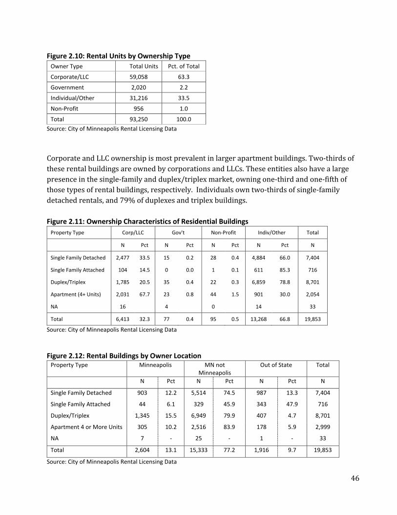
46

Figure 2.10: Rental Units by Ownership Type Owner Type Total Units Pct. of Total

Corporate/LLC 59,058 63.3

Government 2,020 2.2

Individual/Other 31,216 33.5

Non-Profit 956 1.0

Total 93,250 100.0 Source: City of Minneapolis Rental Licensing Data

Corporate and LLC ownership is most prevalent in larger apartment buildings. Two-thirds of these rental buildings are owned by corporations and LLCs. These entities also have a large presence in the single-family and duplex/triplex market, owning one-third and one-fifth of those types of rental buildings, respectively. Individuals own two-thirds of single-family detached rentals, and 79% of duplexes and triplex buildings. Figure 2.11: Ownership Characteristics of Residential Buildings

Property Type Corp/LLC Gov't Non-Profit Indiv/Other Total

N Pct N Pct N Pct N Pct N

Single Family Detached 2,477 33.5 15 0.2 28 0.4 4,884 66.0 7,404

Single Family Attached 104 14.5 0 0.0 1 0.1 611 85.3 716

Duplex/Triplex 1,785 20.5 35 0.4 22 0.3 6,859 78.8 8,701

Apartment (4+ Units) 2,031 67.7 23 0.8 44 1.5 901 30.0 2,054

NA 16 4 0 14 33

Total 6,413 32.3 77 0.4 95 0.5 13,268 66.8 19,853

Source: City of Minneapolis Rental Licensing Data

Figure 2.12: Rental Buildings by Owner Location Property Type Minneapolis MN not

Minneapolis Out of State Total

N Pct N Pct N Pct N

Single Family Detached 903 12.2 5,514 74.5 987 13.3 7,404

Single Family Attached 44 6.1 329 45.9 343 47.9 716

Duplex/Triplex 1,345 15.5 6,949 79.9 407 4.7 8,701

Apartment 4 or More Units 305 10.2 2,516 83.9 178 5.9 2,999

NA 7 - 25 - 1 - 33

Total 2,604 13.1 15,333 77.2 1,916 9.7 19,853

Source: City of Minneapolis Rental Licensing Data

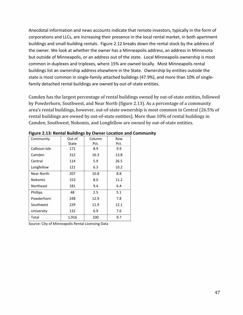
47

Anecdotal information and news accounts indicate that remote investors, typically in the form of corporations and LLCs, are increasing their presence in the local rental market, in both apartment buildings and small-building rentals. Figure 2.12 breaks down the rental stock by the address of the owner. We look at whether the owner has a Minneapolis address, an address in Minnesota but outside of Minneapolis, or an address out of the state. Local Minneapolis ownership is most common in duplexes and triplexes, where 15% are owned locally. Most Minneapolis rental buildings list an ownership address elsewhere in the State. Ownership by entities outside the state is most common in single-family attached buildings (47.9%), and more than 10% of single-family detached rental buildings are owned by out-of-state entities. Camden has the largest percentage of rental buildings owned by out-of-state entities, followed by Powderhorn, Southwest, and Near North (figure 2.13). As a percentage of a community area’s rental buildings, however, out-of-state ownership is most common in Central (26.5% of rental buildings are owned by out-of-state entities). More than 10% of rental buildings in Camden, Southwest, Nokomis, and Longfellow are owned by out-of-state entities.

Figure 2.13: Rental Buildings by Owner Location and Community Community Out of

State Column

Pct. Row Pct.

Calhoun-Isle 171 8.9 9.9 Camden 312 16.3 13.8 Central 114 5.9 26.5 Longfellow 121 6.3 10.2

Near North 207 10.8 8.8 Nokomis 153 8.0 11.2 Northeast 181 9.4 6.4

Phillips 48 2.5 5.1 Powderhorn 248 12.9 7.8 Southwest 229 11.9 12.1 University 132 6.9 7.6

Total 1,916 100 9.7

Source: City of Minneapolis Rental Licensing Data

48

2.B Rental Safety and Habitability Our examination of current housing conditions in Minneapolis’ rental market includes multiple measures of livability found in various city databases relating to rental licenses, the 311 system, and housing code violations found by inspectors. One argument made by opponents of rent stabilization measures is that they will have an unintended effect on lower quality housing much in need of repair as limits on rents will prevent landlords from making improvements. Deferred maintenance could have a disparate impact on low-income communities in Minneapolis or force renters to choose between higher costs and worse living conditions as the following analysis shows.

Rental Tiers

The City of Minneapolis utilizes a tiered system for inspection of rental properties that ensures buildings in worse condition (Tier 3) are inspected more frequently than those largely free from housing code violations or complaints (Tier1.) Closely tied to the building's physical condition, properties are scored primarily on life safety and quality of life variables, with active code violations, nuisance violations, and condemnation letters also taken into account. Tier properties 1 are only inspected every eight years. These properties meet current building codes and have incurred no violations in the last two years. Tier 2 properties are inspected every 5 years and Tier 3 buildings are those thought to be in the worst condition, with the most code violations, and are inspected annually. The data is provided as part of the rental license database found on the City’s Open Data portal, which is updated weekly. The existence of a property ID in this dataset means the data can be combined with other information (e.g. parcels) to show how value or ownership type (individual, LLC, etc.) may be correlated with inspections tier.

Figure 2.14 Rental Inspections in Tier 2 and Tier 3 Buildings, by Community Area

0%2%4%6%8%

10%12%14%16%18%

Pct of Rental Units Tier 2 or 3

Pct_Tier2 Pct_Tier3

49

Figure 2.14 shows each community’s percentage of rental units that are Tier 2 or 3 (table A1 in the appendix contains the number of inspections by tier by Community Area). Camden and Near North have the largest percentage of rentals in these categories, but significant numbers are also found in Phillips, Calhoun Isles (the Uptown area), and the University. These communities make up the majority of low-income areas found in the city, and as such, the neighborhoods with the largest percentage of properties in need of improvements.

Tenant Complaints

Data found in the Public 311 database can also be used to highlight areas of concern as this data contains tenant complaints regarding housing conditions, safety and livability. This data is available in annual snapshots dating back to 2012 and includes the geographic location of the complaint as well as the complaint type. Similar to the code violation data, the overall trend in tenant complaints has decreased in most if not all communities since this data was first made available.

Figure 2.15: 311 Complaint by Community Area, 2012-2017

The communities of Camden and Near North again have consistently seen the highest percentage of rental units with a tenant complaint, with rates two to three times higher than surrounding neighborhoods. Tenant complaints are another difficult dataset to make sense of as there are a variety of reasons a tenant will or will not make a complaint. Fear of retaliation in the form of eviction, rent increases, or even deportation of individuals and households in questionable legal status all have an impact on tenant complaints. However, looking in their

0.00

0.05

0.10

0.15

0.20

0.25

0.30

0.35

0.40

2012 2013 2014 2015 2016 2017

Pct of Licensed Units with 311 Complaint

Calhoun-Isles Camden Central (CBD) LongfellowNear North Nokomis Northeast PhillipsPowderhorn Southwest University

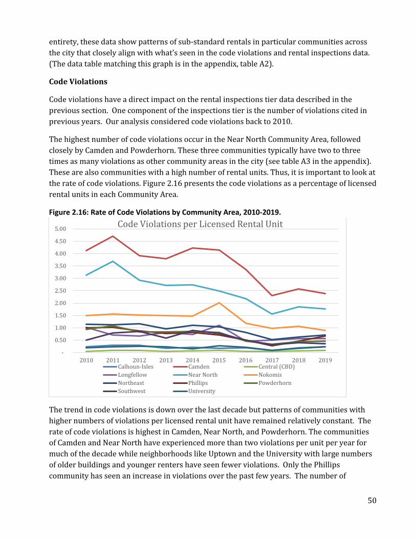
50

entirety, these data show patterns of sub-standard rentals in particular communities across the city that closely align with what’s seen in the code violations and rental inspections data. (The data table matching this graph is in the appendix, table A2).

Code Violations

Code violations have a direct impact on the rental inspections tier data described in the previous section. One component of the inspections tier is the number of violations cited in previous years. Our analysis considered code violations back to 2010.

The highest number of code violations occur in the Near North Community Area, followed closely by Camden and Powderhorn. These three communities typically have two to three times as many violations as other community areas in the city (see table A3 in the appendix). These are also communities with a high number of rental units. Thus, it is important to look at the rate of code violations. Figure 2.16 presents the code violations as a percentage of licensed rental units in each Community Area.

Figure 2.16: Rate of Code Violations by Community Area, 2010-2019.

The trend in code violations is down over the last decade but patterns of communities with higher numbers of violations per licensed rental unit have remained relatively constant. The rate of code violations is highest in Camden, Near North, and Powderhorn. The communities of Camden and Near North have experienced more than two violations per unit per year for much of the decade while neighborhoods like Uptown and the University with large numbers of older buildings and younger renters have seen fewer violations. Only the Phillips community has seen an increase in violations over the past few years. The number of

-

0.50

1.00

1.50

2.00

2.50

3.00

3.50

4.00

4.50

5.00

2010 2011 2012 2013 2014 2015 2016 2017 2018 2019

Code Violations per Licensed Rental Unit

Calhoun-Isles Camden Central (CBD)Longfellow Near North NokomisNortheast Phillips PowderhornSouthwest University

51

reported code violations is likely to be sensitive to the rate of inspection and the implementation of the rental tier system in which some properties are inspected more often than others. (The data table matching this graph is in the appendix, table A4).

2.C Potential Growth in Housing Market Predicted Growth in Housing

An analysis of recent City assessor’s data as well as conversations with CPED long-range planners were used to inform our efforts to predict growth in the housing market both by geography and by the type of housing constructed. While the Met Council estimates that the City will add approximately 10,000 new housing units by 2030, we can see from recent production that this may be a conservative estimate. In the last 20 years the number of housing units increased by roughly 25,000 with the majority of these being multi-family rentals. Development during most of this period has also been concentrated in three areas of the City: the Downtown CBD, the area surrounding University of Minnesota, and the Calhoun-Isles (Uptown) community (see figure A1 in the appendix). Looking at the trends in figure 2.5 we the increase in new construction of multi-family housing over the past two decades and an increase in the number of units per building. From 2012 to 2017 the City saw a spike (with the exception of 2015) in construction of larger apartment buildings. That trend has declined since 2017 (see figure 2.17).

Figure 2.17: New Multi-Family Residential Construction, 2000-2019.

Figure 2.18 shows that over the past decade a larger percentage of new multi-family buildings are being constructed outside the three main areas of apartment construction, the CBD, Uptown, and University, and are dispersing to other parts of the City. This confirms what we heard from CPED staff, that much of the “low-hanging fruit” (e.g. vacant lots in high land value

52

areas) has been developed leading housing developers to seek opportunities elsewhere. This along with the 2040 development plan which allows higher densities along transit corridors in neighborhoods that are currently primarily single-family residential, leads us to assume that this dispersal pattern will continue.

Figure 2.18: Percent New Multi-Family Residential Buildings in

CBD, Uptown, University areas, 2010-2019

Figure 2.19: Multi-family Buildings by Community Area, 2012-2019.

Figure 2.19 shows where multi-family housing has been built in the City since 2012. We see that construction has especially increased in the Powderhorn Community Area and in Northeast. In fact, for the past decade, Powderhorn has replaced Calhoun-Isles as the third

53

most common location for new multi-family buildings in the City (see figure A2 in the appendix). A smaller increase in the number of buildings built occurred in Near North in this time period. While most rent stabilization ordinances exempt new construction from rent increase limits, the effects of new market rate rentals has been shown to have an effect on older properties in the surrounding neighborhood. Prior CURA research (Damiano and Frenier, 2020) shows that new construction of large multifamily buildings affects the bottom end of the market, inducing rent increases in nearby buildings. As new constructions fan out to more parts of the city we could expect rents to rise in more places. Another phenomenon that has occurred since the start of the last housing bubble (2006-2008) has been the shift from condo construction to rentals among new units (figure 2.20 below). Condominium construction peaked in 2006, but since that time apartments have dominated multi-family housing construction.

Figure 2.20: Condominium Construction, 2000-2019.

There are several factors that have contributed to this shift. During the period of 2000-2006 the easy availability of credit and mortgages (many of them subprime ARMs) led to a condominium building boom and numerous conversions of existing apartment units to condominiums. Following the housing crisis which began in 2008 credit and mortgage lending tightened, the growing wealth of younger professionals, changes in housing preference, and a MN law regarding warranties on condominium construction all led to a precipitous decline in new condo units.5 Finally, as figure 2.21 shows for the U.S. as a whole,

5 https://streets.mn/2015/08/09/are-minnesotas-construction-defect-laws-causing-a-condo-shortage/

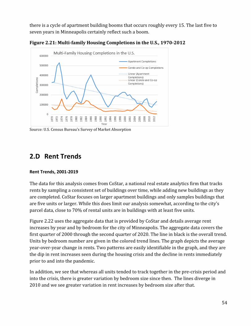
54

there is a cycle of apartment building booms that occurs roughly every 15. The last five to seven years in Minneapolis certainly reflect such a boom.

Figure 2.21: Multi-family Housing Completions in the U.S., 1970-2012

Source: U.S. Census Bureau’s Survey of Market Absorption

2.D Rent Trends Rent Trends, 2001-2019 The data for this analysis comes from CoStar, a national real estate analytics firm that tracks rents by sampling a consistent set of buildings over time, while adding new buildings as they are completed. CoStar focuses on larger apartment buildings and only samples buildings that are five units or larger. While this does limit our analysis somewhat, according to the city’s parcel data, close to 70% of rental units are in buildings with at least five units.

Figure 2.22 uses the aggregate data that is provided by CoStar and details average rent increases by year and by bedroom for the city of Minneapolis. The aggregate data covers the first quarter of 2000 through the second quarter of 2020. The line in black is the overall trend. Units by bedroom number are given in the colored trend lines. The graph depicts the average year-over-year change in rents. Two patterns are easily identifiable in the graph, and they are the dip in rent increases seen during the housing crisis and the decline in rents immediately prior to and into the pandemic.

In addition, we see that whereas all units tended to track together in the pre-crisis period and into the crisis, there is greater variation by bedroom size since then. The lines diverge in 2010 and we see greater variation in rent increases by bedroom size after that.

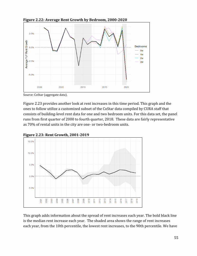
55

Figure 2.22: Average Rent Growth by Bedroom, 2000-2020

Source: CoStar (aggregate data).

Figure 2.23 provides another look at rent increases in this time period. This graph and the ones to follow utilize a customized subset of the CoStar data compiled by CURA staff that consists of building-level rent data for one and two bedroom units. For this data set, the panel runs from first quarter of 2000 to fourth quarter, 2018. These data are fairly representative as 70% of rental units in the city are one- or two-bedroom units. Figure 2.23: Rent Growth, 2001-2019

This graph adds information about the spread of rent increases each year. The bold black line is the median rent increase each year. The shaded area shows the range of rent increases each year, from the 10th percentile, the lowest rent increases, to the 90th percentile. We have

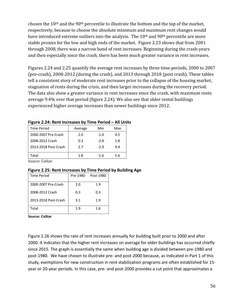
56

chosen the 10th and the 90th percentile to illustrate the bottom and the top of the market, respectively, because to choose the absolute minimum and maximum rent changes would have introduced extreme outliers into the analysis. The 10th and 90th percentile are more stable proxies for the low and high ends of the market. Figure 2.23 shows that from 2001 through 2008, there was a narrow band of rent increases. Beginning during the crash-years and then especially since the crash, there has been much greater variance in rent increases. Figures 2.24 and 2.25 quantify the average rent increases by three time-periods, 2000 to 2007 (pre-crash), 2008-2012 (during the crash), and 2013 through 2018 (post crash). These tables tell a consistent story of moderate rent increases prior to the collapse of the housing market, stagnation of rents during the crisis, and then larger increases during the recovery period. The data also show a greater variance in rent increases since the crash, with maximum rents average 9.4% over that period (figure 2.24). We also see that older rental buildings experienced higher average increases than newer buildings since 2012.

Figure 2.24: Rent Increases by Time Period – All Units Time Period Average Min Max

2000-2007 Pre-Crash 2.0 -1.0 4.5

2008-2012 Crash 0.3 -2.8 1.8 2013-2018 Post-Crash 2.7 -2.9 9.4

Total 1.8 -1.6 5.6 Source: CoStar

Figure 2.25: Rent Increases by Time Period by Building Age Time Period Pre-1980 Post-1980

2000-2007 Pre-Crash 2.0 1.9

2008-2012 Crash 0.3 0.3

2013-2018 Post-Crash 3.1 1.9

Total 1.9 1.6

Source: CoStar

Figure 2.26 shows the rate of rent increases annually for building built prior to 2000 and after 2000. It indicates that the higher rent increases on average for older buildings has occurred chiefly since 2015. The graph is essentially the same when building age is divided between pre-1980 and post-1980. We have chosen to illustrate pre- and post-2000 because, as indicated in Part 1 of this study, exemptions for new construction in rent stabilization programs are often established for 15-year or 20-year periods. In this case, pre- and post-2000 provides a cut point that approximates a

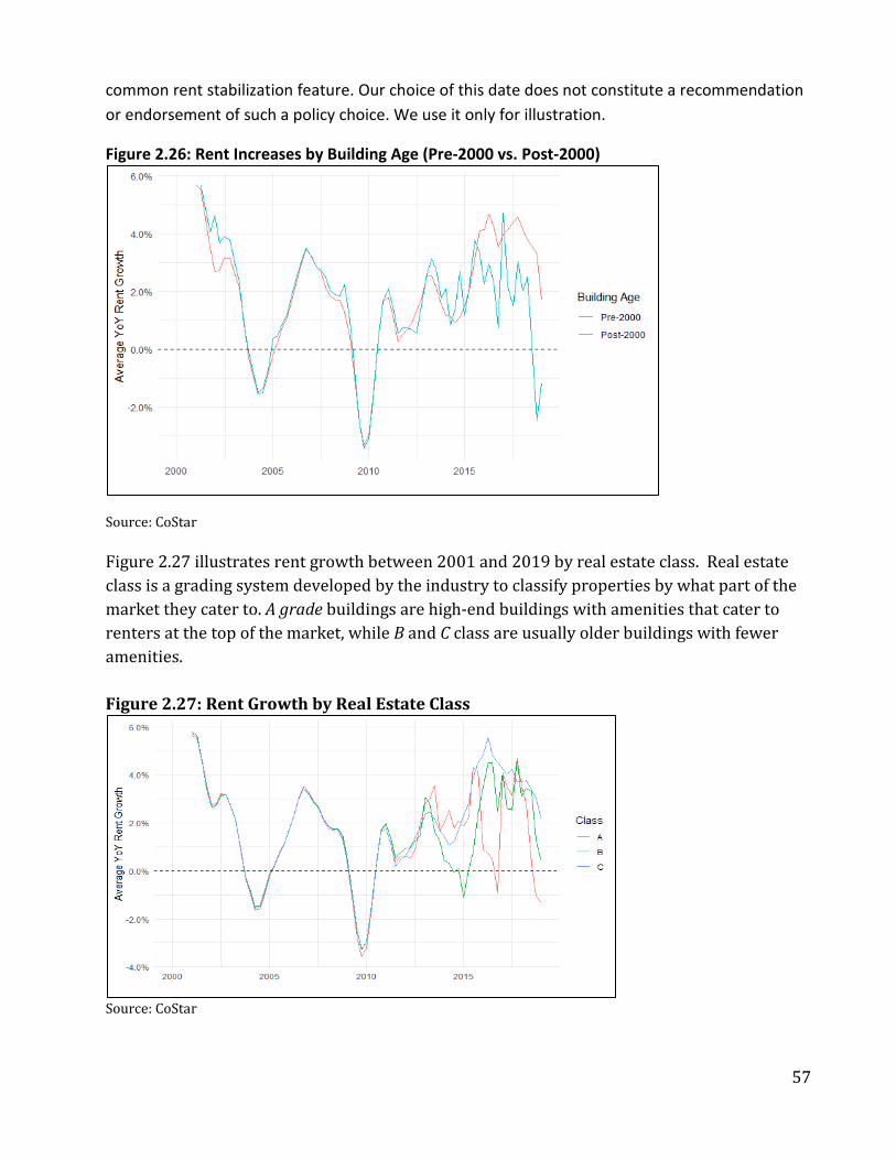
57

common rent stabilization feature. Our choice of this date does not constitute a recommendation or endorsement of such a policy choice. We use it only for illustration.

Figure 2.26: Rent Increases by Building Age (Pre-2000 vs. Post-2000)

Source: CoStar Figure 2.27 illustrates rent growth between 2001 and 2019 by real estate class. Real estate class is a grading system developed by the industry to classify properties by what part of the market they cater to. A grade buildings are high-end buildings with amenities that cater to renters at the top of the market, while B and C class are usually older buildings with fewer amenities. Figure 2.27: Rent Growth by Real Estate Class

Source: CoStar

58

Again, we see these different market segments performing as one during the pre-crash and crash years. Since the crash, there is much greater variation in the marketplace, with A grade buildings recording lower rates of rent increase in recent years than Class B and Class C units. There is a very strong correlation between building age and quality rating. A full 98% of C class buildings were built before 1980. Conversely 93% of A class buildings were built post-1980. We highlight this to show how both older and lower quality buildings have, on average, seen higher rent growth in recent years. This is the housing stock that is more likely to be occupied by lower-income renters. CoStar breaks down its sample by building size and type, generally by number of floors (low-, mid-, and high-rise). They also classify some buildings as “garden” apartments. These are usually low-rise buildings that can be u-shaped with a garden or green space in the middle. The patterns we see in figure 2.28 echo patterns that we have seen already. Rents for all types of buildings tracked each other from 2000 through the end of the crisis in 2012. Since the crash there is great variation in rent increases across building type. Rents in hi-rise buildings, for example, have spiked higher and lower than for any other building. Garden apartment buildings and low-rise buildings have seen the greatest rent growth since the crash.

Figure 2.28: Rent Growth by Building Type

Source: CoStar

Rent changes since 2000 have not varied greatly by community area. Figure 2.29 reports the average year-over-year rent increases by community area, for the entire study period and for the three sub-periods (pre-crash, crash, and post-crash). There are very minor differences across community areas prior to and during the crash. Since 2013, however, there is more

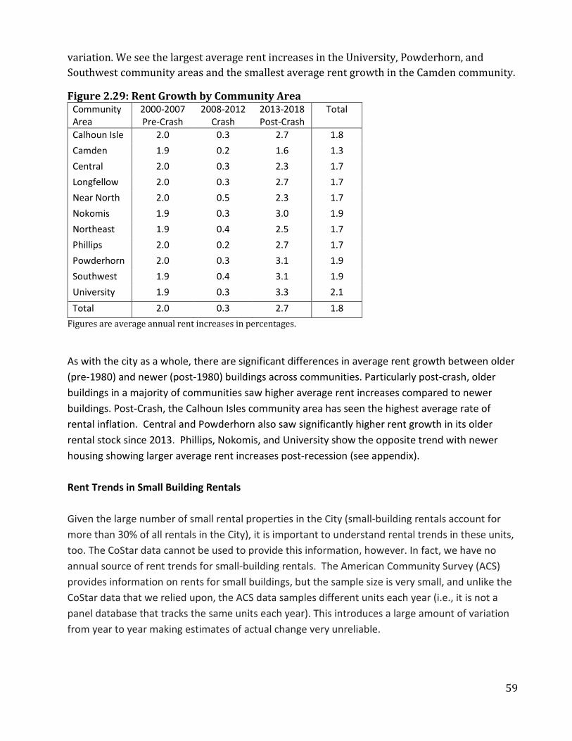
59

variation. We see the largest average rent increases in the University, Powderhorn, and Southwest community areas and the smallest average rent growth in the Camden community.

Figure 2.29: Rent Growth by Community Area Community Area

2000-2007 Pre-Crash

2008-2012 Crash

2013-2018 Post-Crash

Total

Calhoun Isle 2.0 0.3 2.7 1.8 Camden 1.9 0.2 1.6 1.3 Central 2.0 0.3 2.3 1.7 Longfellow 2.0 0.3 2.7 1.7 Near North 2.0 0.5 2.3 1.7 Nokomis 1.9 0.3 3.0 1.9 Northeast 1.9 0.4 2.5 1.7 Phillips 2.0 0.2 2.7 1.7 Powderhorn 2.0 0.3 3.1 1.9 Southwest 1.9 0.4 3.1 1.9 University 1.9 0.3 3.3 2.1 Total 2.0 0.3 2.7 1.8

Figures are average annual rent increases in percentages.

As with the city as a whole, there are significant differences in average rent growth between older (pre-1980) and newer (post-1980) buildings across communities. Particularly post-crash, older buildings in a majority of communities saw higher average rent increases compared to newer buildings. Post-Crash, the Calhoun Isles community area has seen the highest average rate of rental inflation. Central and Powderhorn also saw significantly higher rent growth in its older rental stock since 2013. Phillips, Nokomis, and University show the opposite trend with newer housing showing larger average rent increases post-recession (see appendix). Rent Trends in Small Building Rentals Given the large number of small rental properties in the City (small-building rentals account for more than 30% of all rentals in the City), it is important to understand rental trends in these units, too. The CoStar data cannot be used to provide this information, however. In fact, we have no annual source of rent trends for small-building rentals. The American Community Survey (ACS) provides information on rents for small buildings, but the sample size is very small, and unlike the CoStar data that we relied upon, the ACS data samples different units each year (i.e., it is not a panel database that tracks the same units each year). This introduces a large amount of variation from year to year making estimates of actual change very unreliable.

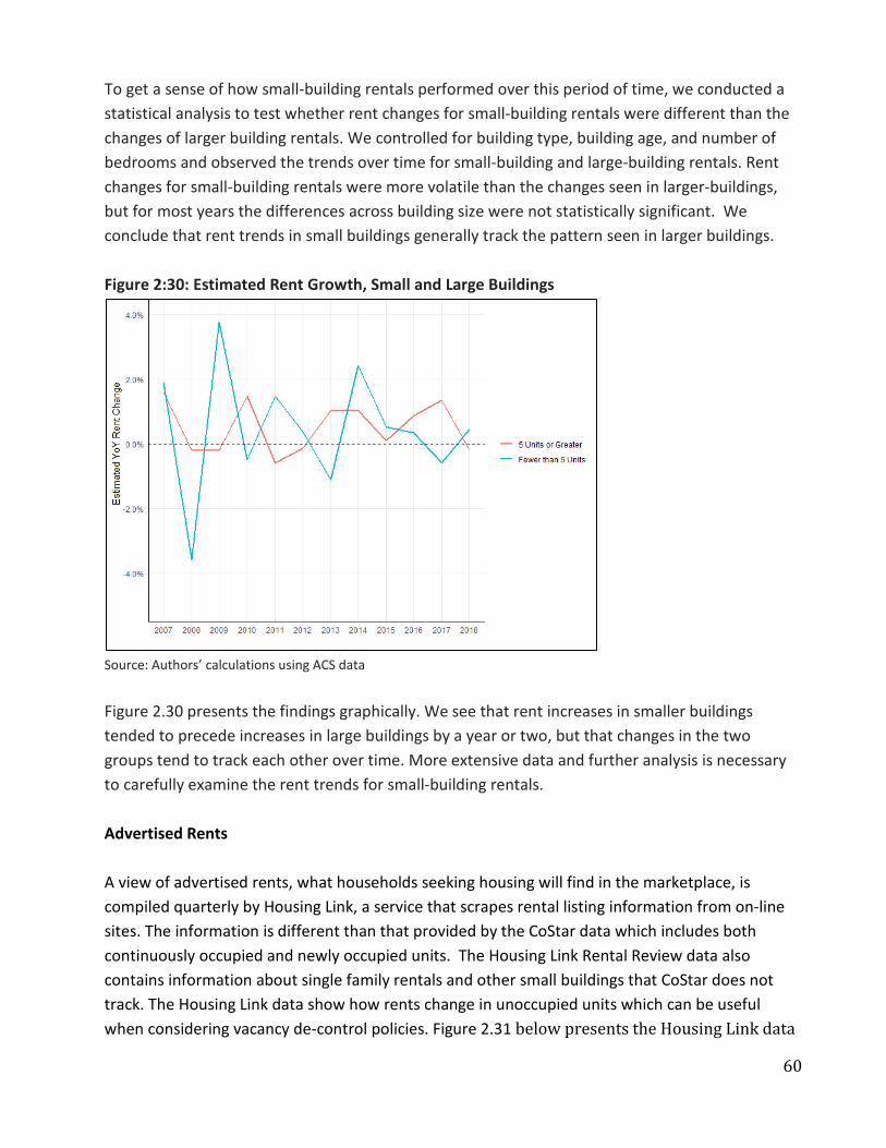
60

To get a sense of how small-building rentals performed over this period of time, we conducted a statistical analysis to test whether rent changes for small-building rentals were different than the changes of larger building rentals. We controlled for building type, building age, and number of bedrooms and observed the trends over time for small-building and large-building rentals. Rent changes for small-building rentals were more volatile than the changes seen in larger-buildings, but for most years the differences across building size were not statistically significant. We conclude that rent trends in small buildings generally track the pattern seen in larger buildings. Figure 2:30: Estimated Rent Growth, Small and Large Buildings

Source: Authors’ calculations using ACS data Figure 2.30 presents the findings graphically. We see that rent increases in smaller buildings tended to precede increases in large buildings by a year or two, but that changes in the two groups tend to track each other over time. More extensive data and further analysis is necessary to carefully examine the rent trends for small-building rentals. Advertised Rents A view of advertised rents, what households seeking housing will find in the marketplace, is compiled quarterly by Housing Link, a service that scrapes rental listing information from on-line sites. The information is different than that provided by the CoStar data which includes both continuously occupied and newly occupied units. The Housing Link Rental Review data also contains information about single family rentals and other small buildings that CoStar does not track. The Housing Link data show how rents change in unoccupied units which can be useful when considering vacancy de-control policies. Figure 2.31 below presents the Housing Link data

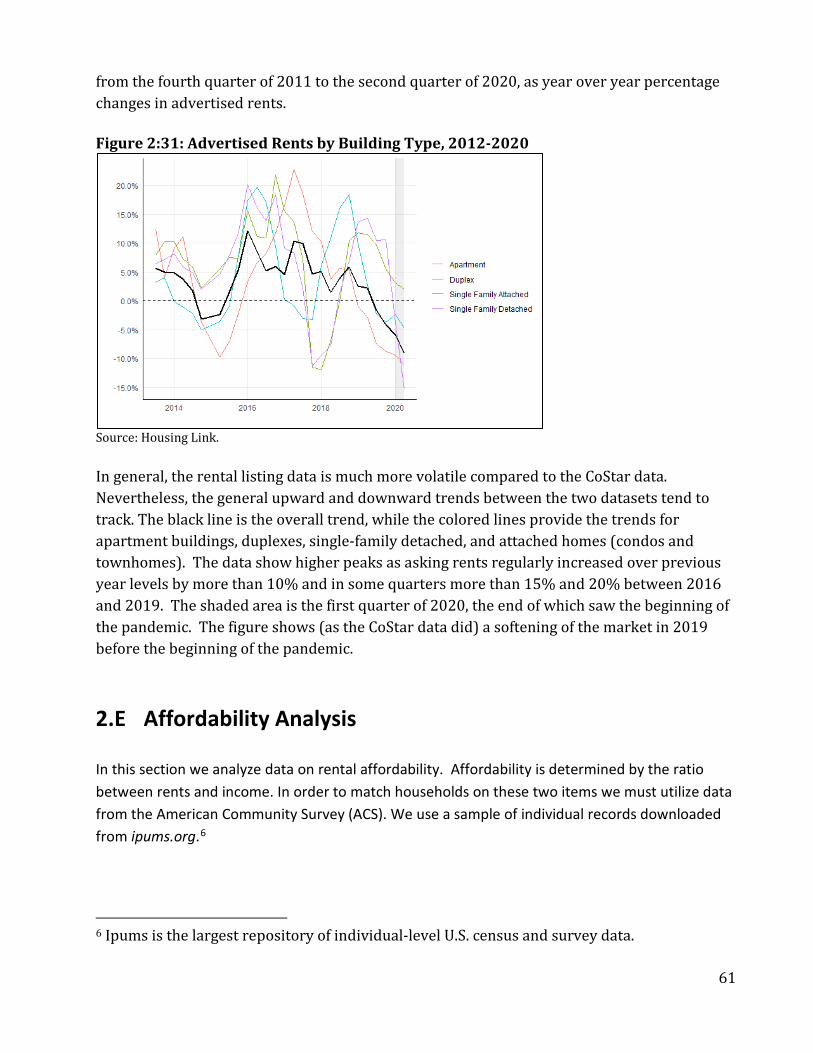
61

from the fourth quarter of 2011 to the second quarter of 2020, as year over year percentage changes in advertised rents. Figure 2:31: Advertised Rents by Building Type, 2012-2020

Source: Housing Link. In general, the rental listing data is much more volatile compared to the CoStar data. Nevertheless, the general upward and downward trends between the two datasets tend to track. The black line is the overall trend, while the colored lines provide the trends for apartment buildings, duplexes, single-family detached, and attached homes (condos and townhomes). The data show higher peaks as asking rents regularly increased over previous year levels by more than 10% and in some quarters more than 15% and 20% between 2016 and 2019. The shaded area is the first quarter of 2020, the end of which saw the beginning of the pandemic. The figure shows (as the CoStar data did) a softening of the market in 2019 before the beginning of the pandemic.

2.E Affordability Analysis In this section we analyze data on rental affordability. Affordability is determined by the ratio between rents and income. In order to match households on these two items we must utilize data from the American Community Survey (ACS). We use a sample of individual records downloaded from ipums.org.6

6 Ipums is the largest repository of individual-level U.S. census and survey data.

62

Rent and Income Trends for Minneapolis Renters

The ACS data we report are adjusted for inflation using the Minneapolis-St. Paul Metro CPI for All Items, and amounts are reported in 2019 dollars unless otherwise noted. All of the income data relates to renter households only. Because the ACS is a small sample and not panel data, the data can be ‘noisy’ (exhibiting large increases or decreases in a single year due to the out-sized influence of outliers). In order to produce more legible graphs and provide a clearer sense of the trends in Minneapolis during this time period, we present the data as five-year moving averages. The first year of the ACS panel data is 2006 and that year serves as the baseline for this analysis. All changes depicted in the following graphs represent cumulative percent changes since 2006. Figure 2.32 presents the data for changes in rent and income for the median renter in Minneapolis since 2006. By 2010 (the first year for which a five-year average could be computed) both incomes and rents were below the 2006 level, likely as a result of the housing crash and resulting recession that began in 2008. For the median renter in Minneapolis, rents and incomes did not return to 2006 levels until 2014. From that point onward incomes rose against their 2006 value at a higher rate than rents rose from their 2006 value. At the end of the study period, income for the median renter in Minneapolis had increased by just more than 25% since 2006 while rent had increased just over 10% during that time period. Figure 2.32 shows an improving affordability picture for the median renter in Minneapolis. Figure 2.32: Change in Rent and Household Income for Median Renter, 2006-2019

Source: ACS

The pattern shown in figure 2.32 hides, however, starkly different stories for renters at the top and the bottom of the rental market in Minneapolis over these years. Figure 2.33 shows the trends in income and rent for renters in the bottom quartile and for those in the top quartile. Renters in the bottom quartile saw increases in rents throughout the study period. By 2010 rents

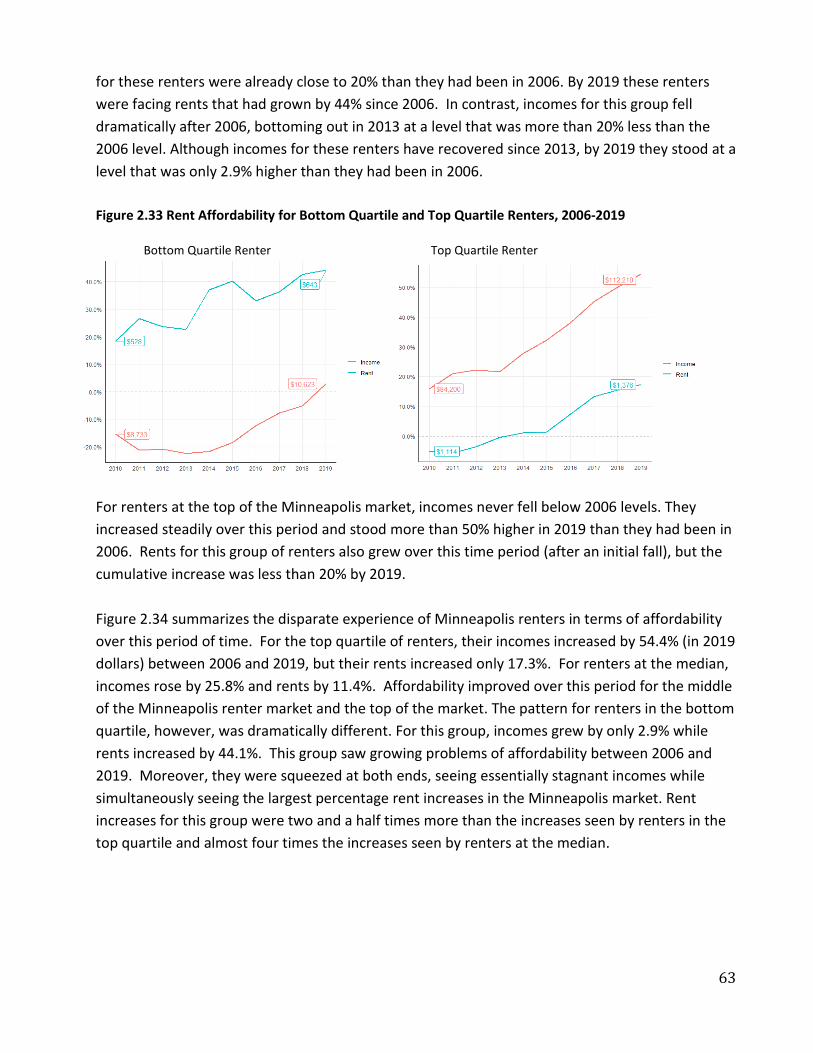
63

for these renters were already close to 20% than they had been in 2006. By 2019 these renters were facing rents that had grown by 44% since 2006. In contrast, incomes for this group fell dramatically after 2006, bottoming out in 2013 at a level that was more than 20% less than the 2006 level. Although incomes for these renters have recovered since 2013, by 2019 they stood at a level that was only 2.9% higher than they had been in 2006. Figure 2.33 Rent Affordability for Bottom Quartile and Top Quartile Renters, 2006-2019

Bottom Quartile Renter Top Quartile Renter

For renters at the top of the Minneapolis market, incomes never fell below 2006 levels. They increased steadily over this period and stood more than 50% higher in 2019 than they had been in 2006. Rents for this group of renters also grew over this time period (after an initial fall), but the cumulative increase was less than 20% by 2019. Figure 2.34 summarizes the disparate experience of Minneapolis renters in terms of affordability over this period of time. For the top quartile of renters, their incomes increased by 54.4% (in 2019 dollars) between 2006 and 2019, but their rents increased only 17.3%. For renters at the median, incomes rose by 25.8% and rents by 11.4%. Affordability improved over this period for the middle of the Minneapolis renter market and the top of the market. The pattern for renters in the bottom quartile, however, was dramatically different. For this group, incomes grew by only 2.9% while rents increased by 44.1%. This group saw growing problems of affordability between 2006 and 2019. Moreover, they were squeezed at both ends, seeing essentially stagnant incomes while simultaneously seeing the largest percentage rent increases in the Minneapolis market. Rent increases for this group were two and a half times more than the increases seen by renters in the top quartile and almost four times the increases seen by renters at the median.

64

Figure 2.34: Growth in income and rent by income percentile, 2006-2019.

There are also large differences by racial group. Figure 2.35 presents the income and rent changes between 2006 and 2019 for different racial/ethnic groups. The racial/ethnic data for some groups should be considered with caution as small group sizes may produce unreliable sample values. The larger the group the greater the confidence in the values. The graphs in figure 2.34, for example, show some extreme volatility for some groups (most prominently American Indian/Alaskan Native), despite the fact that we are computing running averages over a five-year period. The patterns show that the most favorable affordability changes over these years were experienced by white renters, who saw an income increase of over 30% and a cumulative rent increase of less than 20%. BIPOC populations ended the period with slightly higher income increases than rent increases, but this hides significant variation. While affordability improved for Latinx and Asian groups, it declined for Black renters and American Indian renters. Even for the Latinx and Asian groups, rent increases were above income increases for much of the study period. These two groups saw a significant jump in income in the last three years to turn around their affordability pattern. Black renters and American Indian renters, however, saw rents increase in excess of income increases during this period. The pattern for Black renters is especially stark. This group saw significant income declines over the entire period. by 2019, the income of the median Black renter was close to 10% lower than it had been in 2006. Rents, on the other hand, were more than five percent higher over the study period.

65

Fig 2.35 – Cumulative Change in Rent and Household Income for Median Renter by Race/Ethnicity White BIPOC

Black Latinx

Asian American Indian/Alaskan Native

66

Cost-burden

A direct way to measure affordability is to compute the ratio of rent to income, or what is referred to as “rent burden.” Rents that constitute more than 30% of a household’s income is considered a burden. Figure 2.36 shows the percentage of renter households with a housing cost burden, broken down by household income.

Figure 2.36: Rent Burden by Household Income

Source: ACS The graph shows, as would be expected, the prevalence of cost-burden is much higher for the lowest-income households. Households with incomes less than 30% of the area median income (30% of AMI = $30,000) have experienced a steady rate of rent burden since 2010. About 50% of these households are rent burdened, a figure that does not change much over the 10-year period. The group of households with incomes between 30% and 60% of the AMI (incomes between $30,000 and $60,000) saw a growing prevalence of rent-burden in the past 10 years. In 2010, about 27% of these households were rent burdened. By 2019, just over 35% of these households were rent burdened. Rent burden was a relatively rare problem for households with incomes above 60% of AMI (incomes greater than $60,000). The rate of rent burden for this group was less than five percent for most of the years since 2010. The prevalence of rent burden did not vary significantly by the citizenship status of the household. For most years since 2010, the prevalence of rent burden was higher for households with children compared to those without, was higher for single person households compared to larger

67

households, and was higher for multi-generational households (i.e., with grandparents) than for other households (see appendix).

2.F Tenant focus groups

We conducted two focus groups with Minneapolis tenants. We cooperated with Inquilinxs Unidxs por Justicia, a renter’s rights and organizing group, to recruit tenants for the focus groups. The first focus group was conducted on December 8, 2020 and the second on January 19, 2021. The December focus group was conducted in Spanish. Staff members at Inquilinxs Unidxs por Justicia translated and transcribed the meeting. The second focus group was conducted and transcribed by a member of the CURA research team. Tenant concerns that emerged during the focus group focused broadly on two issues, rising rents (the cost of housing), and property upkeep and the responsiveness of landlords on maintenance issues. Rents In the first focus group, participants expressed concern about rents. Some of the participants have larger households, occupying larger units, and therefore paying relatively higher rents. For these participants rent increases in the 3% to 5% range were problematic because of the absolute dollar increase that they represented. These tenants did not think of their rent increases in terms of percentage increases, but rather reported them, and spoke about them in absolute dollar terms. Thus, a $1500 rent would increase by $75 per month at a 5% increase. This was seen by the participants as producing a great strain on their incomes and budgets which could not easily absorb such increases. Even a 3% raise in this scenario would mean $45 extra each month, an amount that participants felt was beyond their ability to absorb. Of course, as rents rise, so do the absolute values of 3% or 5% increases. So that the same rate of increase in the next year will mean even a higher absolute rent increase. Some of the Spanish-speaking participants (focus group 1) reported multiple rent increases in a single year. One referred to rent increases every 3 or 6 months, another said, “in March we paid $750, in July we paid $850, and in February we will pay $950.” Another reported rent increases every six months. One participant reported exorbitant annual rent increases. David (focus group 2) reported that his rent for a studio bedroom in Uptown almost doubled in rent over a three-year period. He endured average annual rent increases of 28% for those years. More common were rent increases

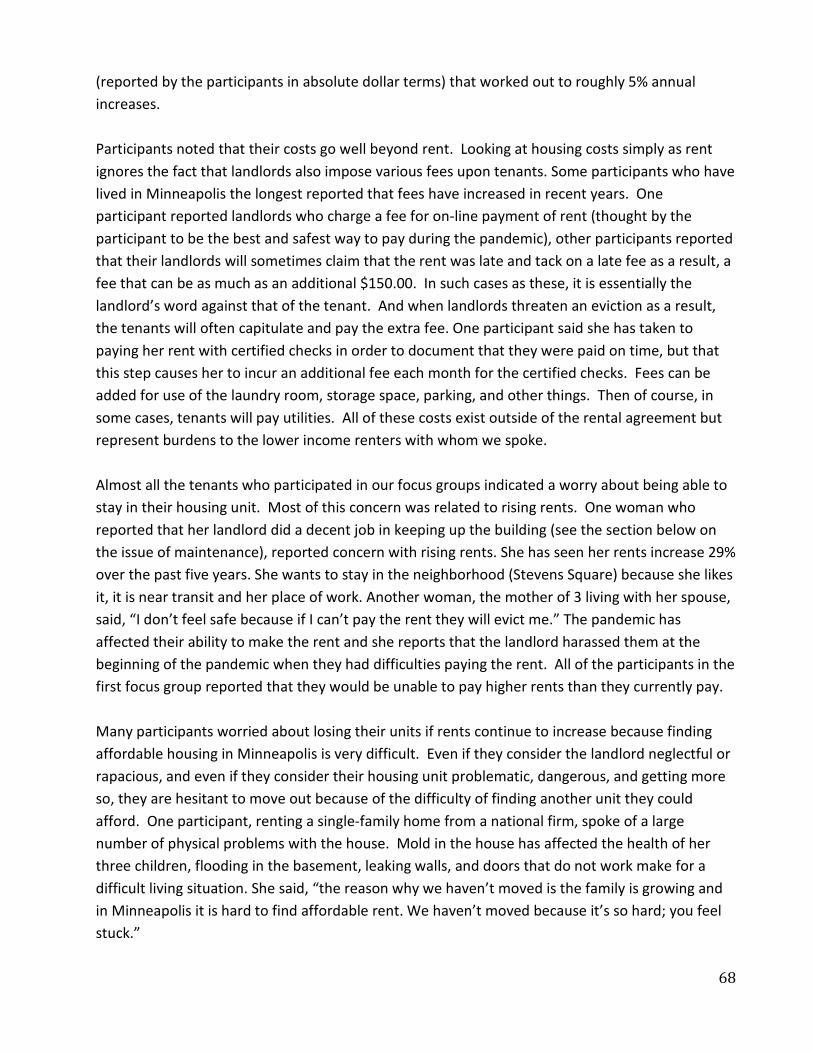
68

(reported by the participants in absolute dollar terms) that worked out to roughly 5% annual increases. Participants noted that their costs go well beyond rent. Looking at housing costs simply as rent ignores the fact that landlords also impose various fees upon tenants. Some participants who have lived in Minneapolis the longest reported that fees have increased in recent years. One participant reported landlords who charge a fee for on-line payment of rent (thought by the participant to be the best and safest way to pay during the pandemic), other participants reported that their landlords will sometimes claim that the rent was late and tack on a late fee as a result, a fee that can be as much as an additional $150.00. In such cases as these, it is essentially the landlord’s word against that of the tenant. And when landlords threaten an eviction as a result, the tenants will often capitulate and pay the extra fee. One participant said she has taken to paying her rent with certified checks in order to document that they were paid on time, but that this step causes her to incur an additional fee each month for the certified checks. Fees can be added for use of the laundry room, storage space, parking, and other things. Then of course, in some cases, tenants will pay utilities. All of these costs exist outside of the rental agreement but represent burdens to the lower income renters with whom we spoke. Almost all the tenants who participated in our focus groups indicated a worry about being able to stay in their housing unit. Most of this concern was related to rising rents. One woman who reported that her landlord did a decent job in keeping up the building (see the section below on the issue of maintenance), reported concern with rising rents. She has seen her rents increase 29% over the past five years. She wants to stay in the neighborhood (Stevens Square) because she likes it, it is near transit and her place of work. Another woman, the mother of 3 living with her spouse, said, “I don’t feel safe because if I can’t pay the rent they will evict me.” The pandemic has affected their ability to make the rent and she reports that the landlord harassed them at the beginning of the pandemic when they had difficulties paying the rent. All of the participants in the first focus group reported that they would be unable to pay higher rents than they currently pay. Many participants worried about losing their units if rents continue to increase because finding affordable housing in Minneapolis is very difficult. Even if they consider the landlord neglectful or rapacious, and even if they consider their housing unit problematic, dangerous, and getting more so, they are hesitant to move out because of the difficulty of finding another unit they could afford. One participant, renting a single-family home from a national firm, spoke of a large number of physical problems with the house. Mold in the house has affected the health of her three children, flooding in the basement, leaking walls, and doors that do not work make for a difficult living situation. She said, “the reason why we haven’t moved is the family is growing and in Minneapolis it is hard to find affordable rent. We haven’t moved because it’s so hard; you feel stuck.”

69

Upkeep Some of the residents reported significant problems with property upkeep and the responsiveness of their landlords. in some cases, these concerns were the first they voiced, taking precedence over the issue of rent. Two of the participants in the second focus group had rented from Steve Frenz, and reported significant maintenance issues that went uncorrected while he owned the building. Two other participants, who rent from a national firm that owns and rents out single family homes in Minneapolis and other markets across the country, spoke of their difficulties getting any response to the deteriorating conditions in their units. Even contacting the landlord was difficult in their case, said one participant: “Even though we’re renters they want us to keep up the property like we were the owner. They have an office in Roseville and when you go there, no one is there. They have Atlanta-area phone numbers and local numbers, but no one answers the local numbers. They have a 800 number for maintenance or neighbor issues, and when you call that number they just say they don’t do that kind of work.” The other tenant who was renting from this company spoke of inadequate electrical systems in the house. “The landlord sent somebody out to fix it, but it still blows out. They said we did it. My TV blew out too. I can’t put a small air conditioner in the front of the house so we put it in the kitchen. They said we need a new line, but nothing was ever done.”

2.G Homelessness Homelessness in the region has increased over the last two decades according to several agencies and organizations who study and provide support for this population. According to Hennepin County, homelessness has increased by 20% from 2009-2018 with a 50% increase in the unsheltered population. Wilder Research, which conducts a statewide point-in-time survey every three years that attempts to count every sheltered and unsheltered homeless person also reports homelessness rates up 33% between 2000 and 2018. Figure 2.37: Hennepin County Homeless Population, 2009-2018

70

Hennepin County - St. Stephen's Human Services latest report and survey found an overall increase in the unsheltered homeless population from 404 in Jan 2018 to 732 in July 2019, an increase of 81% (see figure 2.38). A portion of this increase is likely due to seasonal variation. Figure 2.38: Unsheltered Homeless Population

In recent years, Minneapolis has seen a significant increase in homeless encampments. In the summer of 2018, a homeless encampment emerged on the City’s southside, along Franklin Avenue near Hiawatha. The area had more than 300 tents by the fall, making it one of the largest homeless encampments ever in the state.7 The site was cleared by December 2018 as many persons moved to the temporary “Navigation Center” that had been built in response. The site was reoccupied by homeless families in 2019 and again in 2020. 2020 saw the emergence of several homeless encampments in City parks. The Minneapolis Parks and Recreation Board provided some supports to these encampments in the form of restrooms, portable toilets, trash/recycling containers. St. Stephen’s Human Services, who partners with Hennepin County in providing shelter services and research around the causes of homelessness states in a 2019 report that “homelessness is a complicated issue with many societal causes including large deficits in affordable housing.”8 Housing instability including evictions for failure to pay rent play a large role in homelessness. According to a survey of unsheltered homeless individuals conducted in Jan 2018 and again in July 2019 the number of homeless persons who had been evicted fell from 45% to 28% but was still the third largest contributing factor towards the lack of shelter. The primary reasons stated for homelessness continue to be mental illness and drug/alcohol addiction. Survey respondents were also asked if they had ever been on a lease, with 75% of those responding saying “yes”. However, survey respondents were not asked about the cost of housing, the reasons for an eviction, or whether either of these affected their homeless situation.

7 https://nextcity.org/daily/entry/how-minneapolis-managed-a-massive-homeless-encampment.

8 https://www.hennepin.us/-/media/hennepinus/your-government/projects-initiatives/end-homelessness/unsheltered-report-jul-2019.pdf.

71

2.H Hypothetical Rent Changes Under Different Rent-Increase Caps This section uses building level CoStar data from previous analyses in this report and presents a series of hypothetical counterfactual situations. Specifically, we ask, “How would a variety of rent stabilization scenarios have affected rents over the past 19 years?” The following estimates should be understood as rough calculations based on available data and in many ways represent an upper bound for both the modeled effect on overall rents as well as the reduction in rents that individual units in the sample would receive. Methods As we layout in previous sections, while the CoStar data provides unique insights into the rental market, it is limited in several ways. First it only samples buildings that are 5 units or larger. Second, we only are only able to directly sample one- and two-bedroom units. Additionally, rents in our sample include only buildings that contain 100% market rate units meaning that they do not receive any outside subsidy and have no income restrictions on who can occupy particular units. For the purposes of the following analysis, we make several important assumptions:

1) We assume landlords and property owners in the sample would not have changed their behavior as far as how they adjusted rents over time with an annual rent cap. Such changes in behavior would include but not be limited to increasing rents to cap if/when they would otherwise have been lower than the cap and taking units off the market in the form of condo conversion or other building-use change.

2) We assume no vacancy decontrol. That is, we assume either rent increase limits are binding on all units regardless of whether the unit becomes vacant and/or the unit remains occupied by the same household throughout the study period.

3) We assume no allowances for utility or capital improvement pass-throughs. 4) We assume 100% compliance by landlords.

Rent Caps As shown in our literature review, it is common for rent stabilization programs to limit rent increases to a factor related to overall inflation. In practice, this means using the Consumer Price Index (CPI) for the Minneapolis-Saint Paul Metropolitan Area. At the low end of rent increases we model a rent cap of 75% of CPI. We also model a rent cap set at the regional CPI. At the least

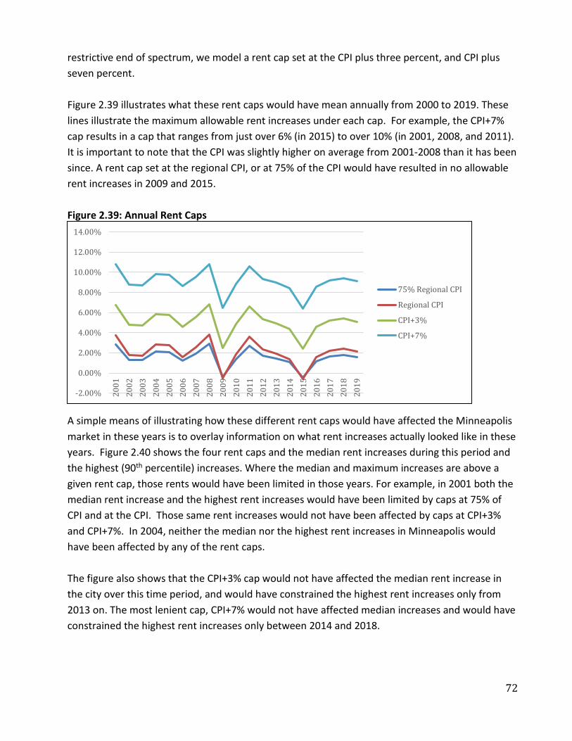
72

restrictive end of spectrum, we model a rent cap set at the CPI plus three percent, and CPI plus seven percent. Figure 2.39 illustrates what these rent caps would have mean annually from 2000 to 2019. These lines illustrate the maximum allowable rent increases under each cap. For example, the CPI+7% cap results in a cap that ranges from just over 6% (in 2015) to over 10% (in 2001, 2008, and 2011). It is important to note that the CPI was slightly higher on average from 2001-2008 than it has been since. A rent cap set at the regional CPI, or at 75% of the CPI would have resulted in no allowable rent increases in 2009 and 2015. Figure 2.39: Annual Rent Caps

A simple means of illustrating how these different rent caps would have affected the Minneapolis market in these years is to overlay information on what rent increases actually looked like in these years. Figure 2.40 shows the four rent caps and the median rent increases during this period and the highest (90th percentile) increases. Where the median and maximum increases are above a given rent cap, those rents would have been limited in those years. For example, in 2001 both the median rent increase and the highest rent increases would have been limited by caps at 75% of CPI and at the CPI. Those same rent increases would not have been affected by caps at CPI+3% and CPI+7%. In 2004, neither the median nor the highest rent increases in Minneapolis would have been affected by any of the rent caps. The figure also shows that the CPI+3% cap would not have affected the median rent increase in the city over this time period, and would have constrained the highest rent increases only from 2013 on. The most lenient cap, CPI+7% would not have affected median increases and would have constrained the highest rent increases only between 2014 and 2018.

-2.00%

0.00%

2.00%

4.00%

6.00%

8.00%

10.00%

12.00%

14.00%

2001

2002

2003

2004

2005

2006

2007

2008

2009

2010

2011

2012

2013

2014

2015

2016

2017

2018

2019

75% Regional CPI

Regional CPI

CPI+3%

CPI+7%

73

Figure 2.40: Rent Caps and Actual Rent Increases, 2001-2019

As the review of other programs demonstrated, rent stabilization programs in the US typically exempt new construction from rent restrictions. As a result, in the following pages we present the analysis only for units in buildings that are more than 20-years old. We chose this threshold not as an endorsement of a new construction exemption, or as an endorsement for a 20-year limit, but rather to simply provide an example of how rents would be affected under such circumstances. In the appendix we provide a duplicative analysis assuming that rent caps would apply to all units in the city, regardless of age. Impact of Rent Caps – A Retrospective Analysis, 2001-2019 These figures show the share of units in the sample that would have been affected by a cap in each given year at each given cap level. Figure 2.41 shows tremendous swings from one year to the next in terms of the share of units that would be affected by the rent caps. In 2001 and 2002, over 95% of units would have been affected by caps set at 75% of CPI and at the CPI level. These numbers drop precipitously to zero in 2004 and 2005 and then shoot back up again in 2006 and 2007. This pattern emerges because during these years most rent increases in Minneapolis were right at the CPI or just under it. Minor variations in the CPI itself, then, led to significant changes in the percent of units affected. This is a common pattern with threshold-based phenomena. Figure 2.40 illustrates the breadth of impact, but not the depth. That is to say, although almost 100% of the rent changes would have been affected by the caps in 2001 and 2002, they would not have been affected much.

-2.00%

0.00%

2.00%

4.00%

6.00%

8.00%

10.00%

12.00%

14.00%

2001

2002

2003

2004

2005

2006

2007

2008

2009

2010

2011

2012

2013

2014

2015

2016

2017

2018

2019

75% Regional CPI

Regional CPI

CPI+3%

CPI+7%

Mpls Max (90%)

Mpls Median

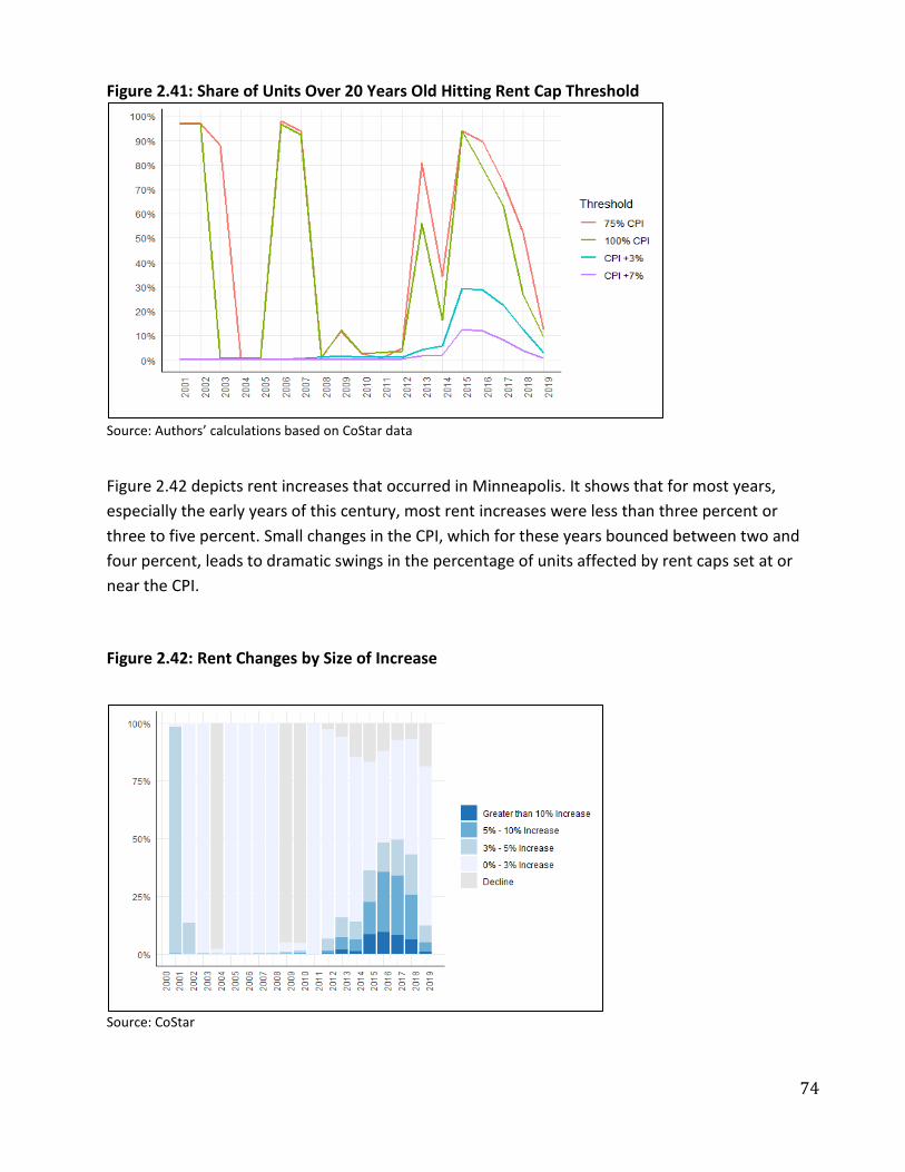
74

Figure 2.41: Share of Units Over 20 Years Old Hitting Rent Cap Threshold

Source: Authors’ calculations based on CoStar data

Figure 2.42 depicts rent increases that occurred in Minneapolis. It shows that for most years, especially the early years of this century, most rent increases were less than three percent or three to five percent. Small changes in the CPI, which for these years bounced between two and four percent, leads to dramatic swings in the percentage of units affected by rent caps set at or near the CPI.

Figure 2.42: Rent Changes by Size of Increase

Source: CoStar

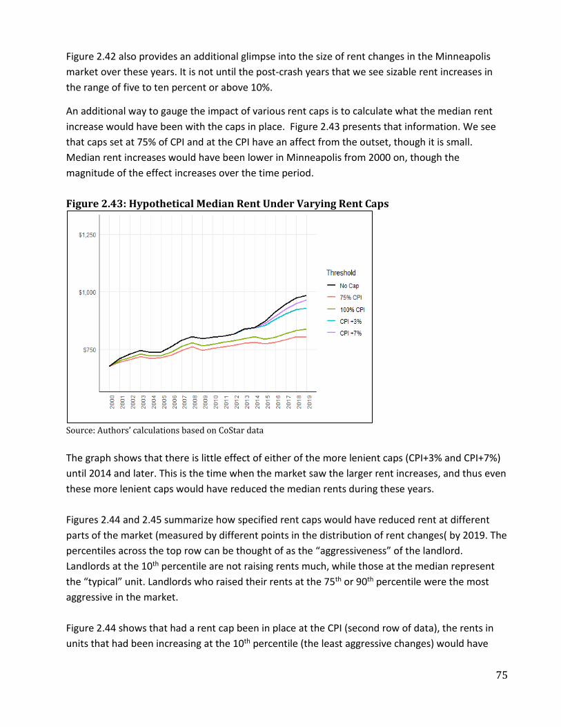
75

Figure 2.42 also provides an additional glimpse into the size of rent changes in the Minneapolis market over these years. It is not until the post-crash years that we see sizable rent increases in the range of five to ten percent or above 10%.

An additional way to gauge the impact of various rent caps is to calculate what the median rent increase would have been with the caps in place. Figure 2.43 presents that information. We see that caps set at 75% of CPI and at the CPI have an affect from the outset, though it is small. Median rent increases would have been lower in Minneapolis from 2000 on, though the magnitude of the effect increases over the time period. Figure 2.43: Hypothetical Median Rent Under Varying Rent Caps

Source: Authors’ calculations based on CoStar data The graph shows that there is little effect of either of the more lenient caps (CPI+3% and CPI+7%) until 2014 and later. This is the time when the market saw the larger rent increases, and thus even these more lenient caps would have reduced the median rents during these years. Figures 2.44 and 2.45 summarize how specified rent caps would have reduced rent at different parts of the market (measured by different points in the distribution of rent changes( by 2019. The percentiles across the top row can be thought of as the “aggressiveness” of the landlord. Landlords at the 10th percentile are not raising rents much, while those at the median represent the “typical” unit. Landlords who raised their rents at the 75th or 90th percentile were the most aggressive in the market. Figure 2.44 shows that had a rent cap been in place at the CPI (second row of data), the rents in units that had been increasing at the 10th percentile (the least aggressive changes) would have

76

been 5.3% less in 2019 than if the cap had not been in place. Moving to the right on that row, we see that rents for units that had been changing at the median would have been 13.8% less in 2019 than if the CPI cap were not in place. Finally, for buildings in which the landlords were most aggressive, where rents had been increased at the 90th percentile, a cap at the CPI would have meant a 2019 rent 25.7% lower than without the cap. Figure 2.45 presents the same information but expressed at the annual change in rent over the entire period.

Figure 2.44: Percent Difference in Rent in 2019 Between Baseline and with Cap Cap 10th 25th 50th Median 75th 90th 75% CPI 8.1 10.4 17.3 23.7 28.7 CPI 5.3 7.0 13.8 20.4 25.7 CPI +3% 0.0 0.0 3.8 8.9 13.9 CPI +7% 0.0 0.0 0.0 2.3 7.2

Source: Authors’ calculations based on CoStar data

Figure 2.45: Differences in Rent Expressed as Annual Income Changes

Cap 10th 25th 50th Median 75th 90th 75% CPI $536 $680 $885 $1,216 $1,684 CPI $339 $442 $615 $916 $1,244 CPI +3% $0 $0 $87 $258 $548 CPI +7% $0 $0 $0 $69 $239

Source: Authors’ calculations based on CoStar data Note that these estimates assume either continuous occupation by the same tenant over the entire period, or it assumes no vacancy decontrol. It also assumes no other pass-throughs or exceptions over the entire period. The tables show that the more lenient caps would have had no effect or a negligible effect over the study period on rents that were increasing at the ‘less aggressive’ levels, and also up to the median. These more lenient caps generated sizable effects only for landlords raising rents at the 75th percentile and higher.

77

PART 3: ECONOMIC ANALYSIS The building-economics analysis consists of two parts. The first part is a summary list of potential issues and impacts of a rent stabilization program gathered from interviews with 30 participants in the Minneapolis apartment market. The second part is a scenario modeling exercise where we created an example apartment proforma based on actual Minneapolis rents in the study period and then modified that model to illustrate how those rents and the economic measures that apartment owners consider would change under different rent caps. We used information gleaned from the interviews to inform our models.

3.A INDUSTRY PERSPECTIVES Method We interviewed 30 people involved in Minneapolis apartments, ranging from for profit developers, non-profit developers, owners, landlords, investors, and lenders, to experts in real estate law, market research, appraisal/valuation, and construction. We selected a broad range of participants so as to obtain perspectives from both owners/landlords and developers as well as knowledgeable experts in the industry who had less direct economic interests in apartments but who understood the perspective of those who did. These disinterested informants in some cases validated and in other cases questioned the responses of the more self-interested informants and gave us the ability to triangulate between different perspectives. The following table shows the breakdown of interviewees, a number of whom represented more than one perspective. For example, owners and developers are also typically investors, and some developers have worked in both for-profit and non-profit development. Figure 3.1: Interviewees by Role

Role/Perspective No. Owner/Landlord 15 Developer (Market Rate, Affordable) 8 Non-Profit Developer/Owner 5 Lender 6 Industry Expert 7 Investor (Owners and Developers) 18 Total 40

We sent a ten-question questionnaire to each interviewee in advance. We held structured, open-ended interviews that lasted between one and two hours, during which we reviewed the

78

questionnaire and took notes. The following is a summary of the feedback we received from the industry informants we spoke to. Most of these items refer to potential economic impacts, while others are related to possible strategic and tactical changes in industry behavior that the informants felt might be induced by RS. These perspectives reflect the consensus of the people we spoke to and, where opinions were divided, we included all viewpoints. When an informant’s words captured an idea better than our words, we included their direct quotes in italics. Summary of Responses

Many of the owners said that their rents would not actually be impacted by any of the example rent caps we shared with them, as they say they charge below market rents and raise rents gently. That said, almost all informants expressed as their greatest concern the potential for a rent stabilization program to constrict rent growth while operating expenses continue to rise. This would potentially reduce not just profits but the amount of income available for capital reinvestment in apartment properties over the long run. Apartment owners rely on both income growth and the ability to refinance and use gains from appreciation to reinvest in their properties periodically, and most informants expressed concern that reinvestment could decline and with it, the quality of housing.

More generally, informants expressed concerns that a rent stabilization program could lead to a slowing or decline in the rate of growth of property values (which would potentially affect reinvestment, values, returns, sales prices, and the City's tax base); could lead to stricter lending terms (making it more difficult to buy or refinance); and could add new costs of administration (City) and compliance (owners). Many informants expressed concern that rent stabilization, along with other recent new regulations, could have (or already has had) a chilling effect on the apartment market in Minneapolis that could reduce access to capital for new projects and reinvestment in older properties; lead to a constricting of the new production pipeline and a reduction in new supply; lead to condo conversions and replacement of older buildings with new, higher density buildings; lead to higher rents and values in the long run; and lead owners to divest, potentially causing a shift in housing ownership away from smaller local owners towards large national owners. Many informants expressed concern about the timing of this idea as 2020 has led to declining rents and increasing vacancy and an apparent market correction already appears to be underway. Informants commented that the design and implementation of a rent stabilization program would require collaboration amongst all parties – owners, developers, tenants, and the City – if it is to succeed.

All of the responses we detail below are speculative. Without knowing the details of a rent stabilization program, it is difficult to predict what might happen and to what degree, and even

79

if the details were known, it would still be difficult to predict long-term impacts. As one of our respondents said in their reply to every single question on the questionnaire and in the interview, “it depends.”

Detailed Responses

The informants we spoke with identified a range of potential impacts of a rent stabilization program on the practices and strategies of participants in the Minneapolis apartment market. The concerns focused on 1) potential impacts on rents and revenues; 2) capital investment and reinvestment; 3) changes in the rental housing stock related to new construction and removal of units from the market; 4) rental housing financing; and, 5) the profile of rental housing owners/operators. Informants also suggested the need to consider both short- and long-term implications of RS, and widely questioned the need for such a program in Minneapolis at this time.

The need to think short- and long-term

Several of the informants we spoke with regarded RS as different from other regulations that have the effect of one-time, up-front costs (e.g., inclusionary zoning and park dedication fees). There was a general concern that RS may produce less of an immediate impact to tenants and landlords related to changing rents, but more significant effects in the longer term, affecting property values, capital reinvestment, housing quality, housing supply, and the City’s tax base. Informants mentioned potential impacts to apartment economics that ranged from reduced income available for capital improvements to declining rates of growth for property values and deterioration of housing stock. These effects may be more difficult to predict or plan for as they involve numerous variables and forces over many years.

Questioning the need for RS in Minneapolis

A number of informants commented that the Minneapolis market is unusual because it is a “rent to occupancy” market rather than a “rent to vacancy market,” which means Minneapolis landlords and owners focus on keeping occupancy high at slightly lower rents rather than on maximizing rents at the cost of higher vacancy. Rent stabilization may incent current and future owners to prioritize rent growth over occupancy. These owners also said that they prioritize maximum occupancy and minimum turnover of tenants as turnover costs are greater than the value of the rent increases they might receive if they turned units over more often. Most informants, including nonprofit developers, lenders, investors and other industry experts, suggested that there is not a rent problem in Minneapolis, that rents are not

80

overpriced, and that rates of increase are not overly high when considered across longer time frames (for example from the 2000s to present rather than the past five years).

Many informants expressed concern that as the City’s regulatory framework becomes

increasingly more restrictive, uncertainty grows for owners, investors, and lenders, who may choose to deploy their resources elsewhere. Informants noted that since 2019, the City has implemented or considered: Inclusionary Zoning (2019), Resident Protection Act (2019), Advance Notice of Sale, Tenant Option to Purchase, and Rent Stabilization. Many informants asked why rent stabilization is being considered now, as rents are not overpriced and rent increases have not been high when considered over a longer time frame, and now rents are falling, vacancy is climbing, and fear and uncertainty are very high. One nonprofit leader said, “There have been more changes in the past three years than in the past 20 years.” An owner said, “Markets hate uncertainty, and there are two responses to uncertainty: Raise rents or sell.” One lender said, “now is not the time.”

Potential impacts on rents, revenues, and housing costs

Potentially limited impact on rents. Despite their concerns about a rent stabilization

program, most owners and informants said that the rent cap examples from other cities and states that we shared with them would not actually apply to their properties. Most owners claimed that they already charge below market rents and raise them gently rather than aggressively (the example rent caps on rates of increase that we shared are all higher than the rent increases these owners claim to typically make). Informants pointed to this as support for their belief that RS is unnecessary.

Our own analysis of the data presented in Part 2 confirms the expectation that a rent

cap might have a limited impact on rents. The data indicated that from 2000 until 2013, the median and average rent increases in Minneapolis would have been affected only by a cap as low as the CPI or 75% of CPI.

The imminent passage of a Rent Stabilization ordinance may cause some owners to raise rents in advance. The expectation of limited impact notwithstanding, several owners commented that if they thought RS was imminent, they would immediately and aggressively raise rents from current below market rates to market rates. The purpose of such increases would be to minimize the reduction in future income and property value, which together affect an owner’s profits and their ability to reinvest in a property. One owner said, “All tenants would get letters. We would raise rents to market levels. All of the gains from the next ten years, I would need to collect them all now. Everyone else would do it, too.”

81

Rent stabilization may cause some owners to increase non-rent fees and charges.

Some owners indicated that they would be incentivized to seek ways to increase non-rent income from fees and charges for parking, storage lockers, laundry, lost keys, late fees, etc.

Our focus group sessions with tenants indicate that this already occurs in the market.

Tenants reported that a portion of their increased housing costs are the result of fees and charges that are separate from the contract rent.

Rent stabilization may add costs to the City for administration and to Owners for compliance, some of which would be passed on to tenants through higher rents. Owners anticipated incurring new costs related to compliance requirements and indicated that they will be incented to pass some or all of these costs along to tenants through increased rents.

Our peer-city study of Oakland, California noted that the City charges $100 per unit

annually to fund their policy infrastructure and allows owners to pass along half of that in a one-time fee to tenants.

Potential impacts on capital reinvestment, both short- and long-term The impact on capital reinvestment was the greatest concern expressed by nearly all of the market informants we spoke to and stemmed from the expectation that RS would constrict income to property owners while expenses continued to rise, reducing net operating income (NOI) for capital expenditures, debt service, and profit. This concern had both short-term and long-term dimensions.

Rent stabilization may cause some owners to reduce spending on operations and maintenance. Owners indicated that in the immediate term, they would be inclined to maintain their profit levels and may therefore reduce spending in other areas such as maintenance and upkeep, and this, in turn, could reduce housing quality. This might include, for example, less effort spent on snow and ice removal, landscaping, etc. One nonprofit housing leader said, “If you do something to limit my rents, then all costs downstream will be affected. And If you think developers and owners would proceed with a lower return on investment, you would be wrong. They would proceed with the same ROI, and lower operating costs to make the pro forma work.”

Rent stabilization has the potential to reduce Capital Reinvestment in apartments over

the long run. Many owners refinance periodically (for example every 10 years) and use the

82

gain from appreciation to fund major capital expenditures and to distribute profits. Informants suggested that if income were to decline, property values would then grow at a slower rate, and the amount of money available from refinancing for capital expenditures would be reduced as well. Over time, a decline in capital expenditures could lead to declining housing quality and could also further reduce property values. “This is the real pressure point – you will hold off, delay another year, and instead of replacing the roof you will patch the roof.” Another owner said, “Old NOAH needs ongoing capital reinvestment but if there is no return, why invest in the building?" And one industry expert said, “There will be no carpet replacement. The quality of housing will go down because there is no incentive to maintain it and the tenants are going to have to live with what they get.”

Potential impacts on new construction and the apartment housing stock

The market participants we interviewed pointed to a number of changes in the apartment housing market that could be triggered by rent stabilization.

Rent stabilization may constrict the production of new apartments. Many informants

commented that RS would at least temporarily constrict the housing production pipeline, required to keep pace or to catch up with demand. This constraint on supply would increase scarcity, and cause rents and values to rise at steeper rates over the long run. Many of the developers we spoke to commented that they have either stopped activity in Minneapolis or are in the process of doing so because of the passage of the inclusionary zoning ordinance in 2020 and other new regulations. Developers and other informants suggested that apartment production might slow down, at least temporarily, as developers take a “wait and see” approach, while several informants commented that while some developers may exit the market, others will come in and find new ways to develop in Minneapolis.

Our review of program experiences elsewhere indicates that new development is

typically not affected by rent stabilization programs, at least in part because most programs exempt new construction.

Rent stabilization may result in loss of existing apartment units through

conversion/demolition. Several informants thought a small number of apartments would be converted to condominiums to avoid rent regulations, and that some older buildings might be replaced with new construction at higher density so as to avoid a rent cap through a possible new construction exemption.

83

Our review of the experience of other cities indicated that condominium conversion and demolition or removal of building by other means is a concern after RS is enacted and is often addressed by additional regulations.

Potential impacts on apartment financing Rent stabilization may cause capital flight from the Twin Cities. Informants –

particularly developers – expressed concern that rent stabilization may cause risk-averse capital to seek other markets. Respondents argued that a large share of the capital – equity and debt – invested in Minneapolis housing comes from outside of the state. RS and the City’s regulatory framework may be perceived to increase risk and uncertainty, causing capital to look elsewhere for lower risk and more favorable yields. Capital flight may constrict the production of new housing and as well as reinvestment in older buildings in Minneapolis. According to one local developer, “Lending and investing decisions are made in board rooms in big cities by people who care only about risk-adjusted returns. It is all about margin and risk. The announcement will have a chilling effect on capital.” Another developer said, “This policy will chase people out of town. Capital comes from big life insurance companies and pension funds and that takes 80% of developers off the table – All of the local fee developers will be unable to source capital for Minneapolis projects.”

Rent stabilization has the potential to lead to stricter lending terms. Opinions were divided (among all informants and among members of the lending community) on the impact of RS on lending. Some people thought little, if anything, would change, other than smaller loan sizes to reflect changes in value (if values grow more slowly or decline). Others, including several commercial lenders, thought lending terms could become stricter, including higher interest rates, lower loan to value (LTV) ratios, and stricter capital reserve requirements. Banks make loans based on an LTV ratio and the lower the LTV, the smaller the loan amount as a share of the total cost of the property. This means that with a lower LTV, a buyer must provide more equity – cash – if they are to purchase a property. This would raise the barrier to entry and make it more difficult for first time buyers, individuals, and smaller “mom- and pop” property owners to enter the apartment market or to refinance in the future.

Potential local market impacts

Rent stabilization may cause some owners of older apartments to exit the Minneapolis market. A number of informants commented that rent stabilization may cause both larger owners and small mom-and-pop companies to consider divesting of their properties. Several informants commented that they knew of portfolios that were quietly being offered for sale

84

off-market. Several other owners with properties in Minneapolis and elsewhere in the Twin Cities said they were exiting or considering exiting the Minneapolis market and reinvesting in other surrounding cities. In all cases, informants commented that it was not just rent stabilization but all of the recent new regulations that were creating uncertainty in the marketplace.

Rent stabilization could accelerate the transition of apartment ownership in

Minneapolis from local to non-local owners. According to our informants, a large share of Minneapolis apartments is locally owned as compared to other markets where apartments are predominantly owned by big national firms. If RS were to cause local owners to divest, the new buyers would not necessarily be other local owners. One developer said, “New properties are owned by REITs and guys in New York who are sophisticated and run huge portfolios. Lots of these older properties in Minneapolis are smaller mom and pop deals.” One NFP leader said, “we are speeding towards transferring ownership towards disinterested, investor-driven owners from out of town. I get a call every day from one coast or the other saying, ‘we have seen your property and we are interested in it and in other parts of your portfolio too.’”

Many informants who were not owners and landlords went out of their way to say that

Minneapolis has good landlords and owners who try to do the right thing and who are assets to the community. One non-profit development leader said, “Minneapolis has assets in local owners who really do give a damn. It is not like on the coasts, where that type of owner is gone. There are now only national entities on the coasts – and no local connection. By ignoring the value of these local assets, you are forcing those people out.” Disagreement about the potential impact of RS on property values. Many informants believed that RS would cause property values to grow at slower rates or to decline. Property values are based on income growth over time, and if that growth is constricted while costs continue to rise, then property values, and tax revenues would be negatively impacted. One owner said, “RS would increase cap rates and cut the value of our portfolio. It would make Minneapolis a less attractive place to attract capital. And theoretically, if assessed values go down, so do property taxes, so the City should be cautious.” The City’s “2018 Assessment for Taxes Collected in 2019” shows that apartments represented 17.5% of the City’s estimated tax base. Should values decline or rise more slowly as a result of RS, it would affect this portion of the City’s tax base.

Several owners took the opposite view, however, suggesting that RS would cause rents and values to increase in the long term. These owners believe that RS will have a chilling effect on production and may incent some owners to convert apartments to condos or replace old

85

buildings with new, higher density apartments that would likely be excluded from RS because of their age. In this scenario, RS would reduce growth in apartment supply and even cause supply to shrink. One developer said, “We are done doing development in MPLS because of inclusionary zoning [and rising costs] but I am holding onto my apartments. I’m bullish on Minneapolis and I think rents are going to skyrocket.”

The CPI is an unreliable proxy for all of the costs associated with operating rental

housing. A number of owners expressed concern that the CPI is an inadequate proxy for rates of increase on expenses because some costs do not track with the CPI. Some expenses grow faster than the CPI (labor and materials) and other expenses, such as property taxes and insurance are unrelated to the CPI and are unpredictable. Owners say that property taxes have been increasing at steeper rates in recent years (reflecting increased property values) and that this is the largest and most unpredictable line on their expense budget. Insurance is another large cost that is based on variables unrelated to the CPI and insurance costs in 2020 increased for some owners because of public safety concerns. Utilities, too, do not rise at predictable rates. Our review of program designs in other cities indicated that some incorporate cost pass-throughs for taxes and utilities.

A rent stabilization RS program should be a product of collaboration if it is to succeed.

A number of informants said that collaboration would be key to the design of a workable and successful rent stabilization program. “It has got to make sense for everybody: owners, tenants, developers, and the City’s coffers.”

3.B Scenario Modeling One objective of this study is to consider how the interview responses from the previous section can help to illuminate what has happened in the Minneapolis apartment market and what might have happened (or could happen in the future) if a rent stabilization program had been (or were to be) implemented. The purpose of this part of the study is to explore how different rent caps would affect a) rents for tenants and b) the economics of apartment properties. We model these outcomes for the 10 most recent years. We model a 10-year ownership period because that this is the typical investment horizon used by many investors. The appendix also models a slightly longer, 15-year investment period. The models were based on the following:

86

• The pro forma model is of a single typical market rate, class C or “NOAH” type

apartment unit. It can be scaled to any number of units (a fourplex, 20 units, 50, 100, etc.).

• Informants suggested that rents for class C apartment unit in 2019 may range between $900 and $1,050, for an average of $975.

• Median rent for a Minneapolis apartment in 2019 was $984, which is close to $975, so we used Minneapolis median rents as a proxy for class C rents. (The average apartment rent in 2019 was higher, $1,097, a figure driven up by outliers at the top of the market.)

• We then used median rents in starting years (2004/2009) and increased them at the rates of example rent caps (75% CPI, CPI, CPI+3%, and CPI+7%)

• We included assumptions for vacancy, miscellaneous income, and expense rate of growth, capital reserve, and debt service. The model delivers typical returns when run at the historic rental increase rates for an average Minneapolis apartment (minimum annual cash-on-cash returns of 7% to 10% and an IRR of at least 15%).

A full description of the model specifications and assumptions is located in the appendix. After modeling rents from 2009-2018 for our profile apartment, we then consider the economic performance of the apartment in terms of model five different metrics that investors use to assess the attractiveness of investment options:

• Cash-on-cash return (Average annual returns) • Cash-on-cash return in the final year (2018) • Average annual change in value (appreciation) • Total change in value (appreciation) • Internal rate of return (IRR).

Our model provides measures of return to owners/investors in percentages that can be compared across different scales of properties. For example, this model can be scaled to any number of units. The returns as percentages would not change. Many owners commented that, while they had concerns about how a rent stabilization program might impact income, profits, and capital reinvestment over time, they also do not raise rents at rates that would be subject to most of the example caps we shared with them. This part of the study supports those comments, illustrating that, based on historic rent data, the average apartment owner would not be affected by any other than the most restrictive rent caps (75% of CPI and CPI) that we considered and that the average property earns profits that

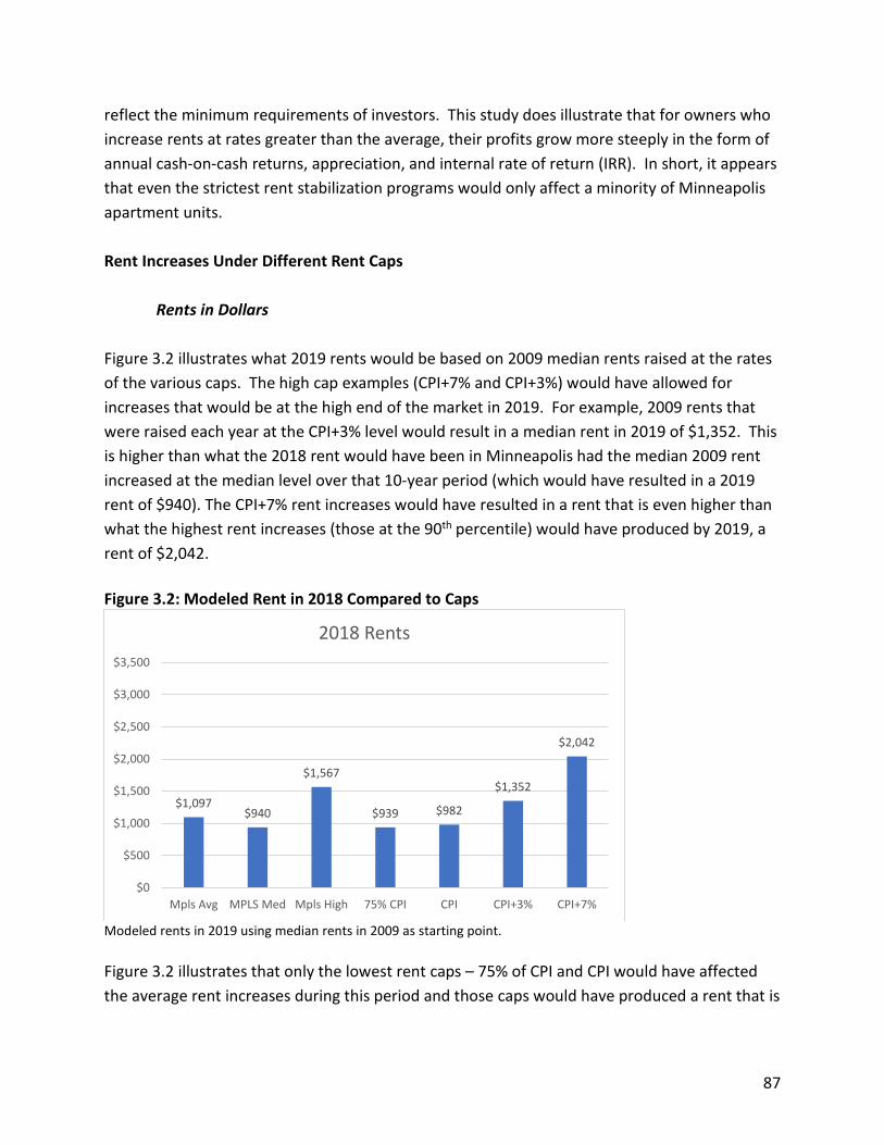
87

reflect the minimum requirements of investors. This study does illustrate that for owners who increase rents at rates greater than the average, their profits grow more steeply in the form of annual cash-on-cash returns, appreciation, and internal rate of return (IRR). In short, it appears that even the strictest rent stabilization programs would only affect a minority of Minneapolis apartment units. Rent Increases Under Different Rent Caps

Rents in Dollars Figure 3.2 illustrates what 2019 rents would be based on 2009 median rents raised at the rates of the various caps. The high cap examples (CPI+7% and CPI+3%) would have allowed for increases that would be at the high end of the market in 2019. For example, 2009 rents that were raised each year at the CPI+3% level would result in a median rent in 2019 of $1,352. This is higher than what the 2018 rent would have been in Minneapolis had the median 2009 rent increased at the median level over that 10-year period (which would have resulted in a 2019 rent of $940). The CPI+7% rent increases would have resulted in a rent that is even higher than what the highest rent increases (those at the 90th percentile) would have produced by 2019, a rent of $2,042. Figure 3.2: Modeled Rent in 2018 Compared to Caps

Modeled rents in 2019 using median rents in 2009 as starting point. Figure 3.2 illustrates that only the lowest rent caps – 75% of CPI and CPI would have affected the average rent increases during this period and those caps would have produced a rent that is

$1,097$940

$1,567

$939 $982

$1,352

$2,042

$0

$500

$1,000

$1,500

$2,000

$2,500

$3,000

$3,500

Mpls Avg MPLS Med Mpls High 75% CPI CPI CPI+3% CPI+7%

2018 Rents

88

at or above what the median rent increases would have produced. Owners affected by the higher caps would have been those who raised rents at rates far greater than the market norm. Rent Caps and Investment Metrics Rents are only one variable in apartment economics. As described in the summary of the interviews, Rent Stabilization has the potential to affect a number of apartment economic variables over time. In this section we combine 2001-19 rent data and example rent caps with a model proforma to create a series of scenarios that illustrate how apartment investment metrics could be affected by rent caps. In general, our analysis in this section indicates that these apartment metrics are only affected in cases where owners raise rents above the average level, duplicating the findings for rents that were shown in the previous section.

Qualifications The model assumes continued occupancy by a tenant over the entire study period, and thus does not contemplate the potential impact of vacancy decontrol. Moreover, the model does not incorporate any provisions for cost pass-throughs (for property taxes or utilities, for example) that are sometimes part of rent stabilization programs. An industry standard for a real estate proforma is used to model discounted cash flows over an assumed 10-year ownership period, based on the assumptions that one buys in year 0, owns for 10 full years (1-10), and sells in year 10 for a sale price based on estimated year 11 rents. Some apartment owners, however, are long term owners and rather than selling, they refinance on a schedule (for example every ten years). When they refinance, the new financing is based on a higher property value due to appreciation and the owner can use the gain to invest in major capital improvements and/or distribute profits (similar to a home equity loan). The models we constructed assumed one owner buying in year 0 (end of 2003 or 2008), owning from year 1 (2004 or 2009), through years 10 or 15 (2018), and selling in 2018 for a price based on estimated 2019 rents, and we did not include refinancing in either scenario. We used similar levels of debt for the 10-year model as we did for the 15-year model to make them easier to compare. In reality, the market was different in those two years and financing would have been different too, but we applied an average level of debt service to both.

89

In summary, these models are examples that serve as a representation by which to compare different scenarios. Their greatest utility is in demonstrating differences across the scenarios, and they should not be considered predictions of actual outcomes.

Annual return as a percentage of equity invested or “cash-on-cash return”

The buyer of a property must provide equity based on the lender’s requirements for Loan to Value. For example, for a $400,000 property, if the lender is willing to lend at 75% LTV, then the loan will be for $300,000 and the buyer must provide $100,000 in equity to close. Annual cash returns or cash flows after financing (CFAF) are the cash remaining after all operating expenses, capital reserve, and debt service have been subtracted from income. Owners divide annual cash returns by the amount of their equity investment to determine cash-on-cash return, expressed as a percentage. An annual return of $10,000 in cash divided by equity of $100,000 = a 10% cash-on-cash return. Cash-on-cash returns typically start lower and grow over time, as income grows while debt service payments remain flat. Cash-on-cash returns do not reflect increasing property value due to appreciation. Our interviews with market actors indicated that investors expect minimum returns of 7%-10% and that “double digit” returns (returns that equal or exceed 10%) are preferred. Figure 3.3: Cash-on-Cash Return: Average Return 2009-2018.

Figure 3.3 illustrates how the average cash-on-cash return would have grown for building owners under different caps. Our informants indicated that an average annual return of 7% to 10% is the minimum of what is desired by investors. The figure shows that landlords who increased rents at the average and the median of all units in Minneapolis over this 10-year

7.2% 7.1%

12.6%

7.5% 8.0%

12.0%

18.6%

0.0%

5.0%

10.0%

15.0%

20.0%

25.0%

30.0%

35.0%

Mpls Avg MPLS Med Mpls High 75% CPI CPI CPI+3% CPI+7%

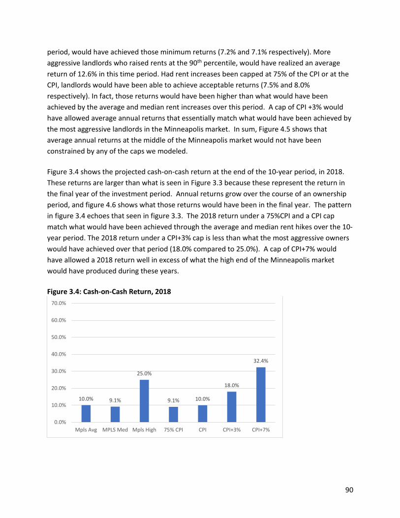
90

period, would have achieved those minimum returns (7.2% and 7.1% respectively). More aggressive landlords who raised rents at the 90th percentile, would have realized an average return of 12.6% in this time period. Had rent increases been capped at 75% of the CPI or at the CPI, landlords would have been able to achieve acceptable returns (7.5% and 8.0% respectively). In fact, those returns would have been higher than what would have been achieved by the average and median rent increases over this period. A cap of CPI +3% would have allowed average annual returns that essentially match what would have been achieved by the most aggressive landlords in the Minneapolis market. In sum, Figure 4.5 shows that average annual returns at the middle of the Minneapolis market would not have been constrained by any of the caps we modeled. Figure 3.4 shows the projected cash-on-cash return at the end of the 10-year period, in 2018. These returns are larger than what is seen in Figure 3.3 because these represent the return in the final year of the investment period. Annual returns grow over the course of an ownership period, and figure 4.6 shows what those returns would have been in the final year. The pattern in figure 3.4 echoes that seen in figure 3.3. The 2018 return under a 75%CPI and a CPI cap match what would have been achieved through the average and median rent hikes over the 10-year period. The 2018 return under a CPI+3% cap is less than what the most aggressive owners would have achieved over that period (18.0% compared to 25.0%). A cap of CPI+7% would have allowed a 2018 return well in excess of what the high end of the Minneapolis market would have produced during these years. Figure 3.4: Cash-on-Cash Return, 2018

10.0% 9.1%

25.0%

9.1% 10.0%

18.0%

32.4%

0.0%

10.0%

20.0%

30.0%

40.0%

50.0%

60.0%

70.0%

Mpls Avg MPLS Med Mpls High 75% CPI CPI CPI+3% CPI+7%

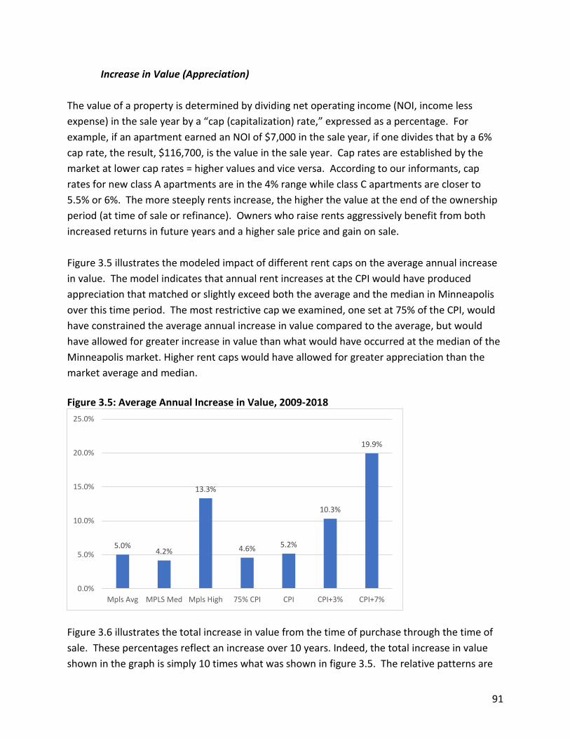
91

Increase in Value (Appreciation) The value of a property is determined by dividing net operating income (NOI, income less expense) in the sale year by a “cap (capitalization) rate,” expressed as a percentage. For example, if an apartment earned an NOI of $7,000 in the sale year, if one divides that by a 6% cap rate, the result, $116,700, is the value in the sale year. Cap rates are established by the market at lower cap rates = higher values and vice versa. According to our informants, cap rates for new class A apartments are in the 4% range while class C apartments are closer to 5.5% or 6%. The more steeply rents increase, the higher the value at the end of the ownership period (at time of sale or refinance). Owners who raise rents aggressively benefit from both increased returns in future years and a higher sale price and gain on sale. Figure 3.5 illustrates the modeled impact of different rent caps on the average annual increase in value. The model indicates that annual rent increases at the CPI would have produced appreciation that matched or slightly exceed both the average and the median in Minneapolis over this time period. The most restrictive cap we examined, one set at 75% of the CPI, would have constrained the average annual increase in value compared to the average, but would have allowed for greater increase in value than what would have occurred at the median of the Minneapolis market. Higher rent caps would have allowed for greater appreciation than the market average and median. Figure 3.5: Average Annual Increase in Value, 2009-2018

Figure 3.6 illustrates the total increase in value from the time of purchase through the time of sale. These percentages reflect an increase over 10 years. Indeed, the total increase in value shown in the graph is simply 10 times what was shown in figure 3.5. The relative patterns are

5.0%4.2%

13.3%

4.6% 5.2%

10.3%

19.9%

0.0%

5.0%

10.0%

15.0%

20.0%

25.0%

Mpls Avg MPLS Med Mpls High 75% CPI CPI CPI+3% CPI+7%

92

the same. The two most restrictive caps would have allowed for total increases in value that matched the middle of the Minneapolis market, while the more lenient caps would have allowed for appreciation well above those levels. Figure 3.6: Total Increase in Value, 2009-2018

Internal Rate of Return (IRR) In addition to annual returns (cash flows and cash-on-cash return as a percentage) and appreciation over the ownership period, owners also consider a property’s Internal Rate of Return (IRR). IRR is an algebraic calculation that takes into account the initial equity invested, annual returns to that equity (above), and appreciation (also above) to determine an average rate of return over the entire ownership period. Because it considers both annual cash flows and long-term appreciation, IRR is typically higher than annual rates of return. So, for example, a project may earn annual returns of 7%-10% and have an IRR of 15% or more.1 According to respondents, investors expect to earn a minimum IRR of 15% or higher. Figure 3.7 shows that the 15% threshold for IRR is achieved under all of the rent cap scenarios. The 75%CPI and the CPI caps would allow IRR that matches or slightly exceeds what would have been achieved at the average and the median of the Minneapolis market from 2009 to 2018. A cap of CPI+3% would have allowed IRR that matches what the most aggressive owners would

1 IRR is affected by the rates of growth in income, because it integrates a property’s value at the time of sale. That value is based on the last year of income divided by a cap rate. The higher the rate of increase over the ownership period, the higher the income in the last year, the higher the sale value, and the higher the IRR.

50.2% 45.9%

133.2%

45.7% 51.7%

103.2%

199.4%

0.0%

50.0%

100.0%

150.0%

200.0%

250.0%

300.0%

350.0%

Mpls Avg MPLS Med Mpls High 75% CPI CPI CPI+3% CPI+7%

93

have achieved over this period. The most lenient cap (CPI+7%) would have allowed IRR far in excess of what would have been achieved at the top of the market. Figure 3.7: Internal Rate of Return, 2009-2018.

16.3% 15.9%

22.3%

16.3% 17.0%

22.4%

29.1%

0.0%

5.0%

10.0%

15.0%

20.0%

25.0%

30.0%

35.0%

Mpls Avg MPLS Med Mpls High 75% CPI CPI CPI+3% CPI+7%

94

Sources Ambrosius, J., Gilderbloom, J., Steele, W., Meares, W., Keating, D. (2015). “Forty years of rent

control: Reexamining New Jersey’s moderate local policies after the great recession.” Cities 49: 121-133.

Appelbaum, R., Gilderbloom, J. (1990). “The Redistributional Impact of Modern Rent Control.”

Environment and Planning A: Economy and Space 22 (5): 601-614. Arnott, R., (1995). “Time for Revisionism on Rent Control.” Journal of Economic Perspectives 9 (1):

99-120. Arnott, R., Shevyakhova, E., (2014). “Tenancy rent control and credible commitment in

maintenance.” Regional Science and Urban Economics 47: 72-85. Asquith, B. (2019). “Do Rent Increases Reduce the Housing Supply Under Rent Control? Evidence

from Evictions in San Francisco.” https://ssrn.com/abstract=3165599. Ault, R., Jackson, J., Saba, R. (1992). “Effect of Long-Term Rent Control on Tenant Mobility.” Journal

of Urban Economics 35: 140-158. Autor, D., Palmer, C., Pathak, P. (2014). “Housing Market Spillovers: Evidence from the End of Rent

Control in Cambridge, Massachusetts.” Journal of Political Economy 122 (3): 661-717. Baar, K. (1983). “Guidelines for Drafting Rent Control Laws: Lessons of a Decade.” Rutgers Law

Review 35: 723-885. Baar, K. (1998). “New Jersey's Rent Control Movement.” In M. Teitz and others, eds.,Rent Control:

Regulation and the Rental Housing Market. New Brunswick, NJ: Center for Urban Policy Research, Rutgers.

Barton, S. (2011). “Land Rent and Housing Policy.” American Journal of Economics and Sociology 70

(4): 845-873. Been, V., Gould Ellen, I., & House, S. (2019). Laboratories of regulation: Understanding the diversity

of rent regulation laws. Fordham Urban Law Journal, 46(5), 1041-1080. Bartlett, S. (1997). “The Significance of Relocationfor Chronically Poor Families in the USA.”

Environment and Urbanization 9 (1): 121-132. Basu, K., Emerson, P. (2000). “The Economics of Tenancy Rent Control.” The Economic Journal 110

(466): 939-962.

Brennan, M. (2011). “The Impacts of Affordable Housing on Education: A Research Summary.” Washington, D.C.: The Center for Housing Policy.

95

Cash, A., Zuk, M., Federico, A., (2018). “Proposition 10: Estimating the Scale of Expanded Rent Control in the Bay Area. A Policy Brief.” Urban Displacement Project, University of California, Berkeley.

Chew, A., Treuhaft, S. (2019). “Our Homes, Our Future: How Rent Control Can Build Stable, Healthy Communities.” Right to the City Alliance, PolicyLink, The Center for Popular Democracy.

Clark, W., Heskin, A. (1982). “The Impact of Rent Control on Tenure Discounts and Residential Mobility.” Land Economics, 58 (1): 109-117.

Cohen, R. (2011). “The Impacts of Affordable Housing on Health: A Research Summary.” Washington, D.C.: The Center for Housing Policy.

Damiano, A. & C. Frenier. (Updated Oct. 2020) "Build Baby Build?: Housing Submarkets and the Effects of New Construction on Existing Rents.” Center for Urban and Regional Affairs (CURA) Working Paper.

Diamond, R., McQuade, T., Qian, F. (2019). "The Effects of Rent Control Expansion on Tenants, Landlords, and Inequality: Evidence from San Francisco." American Economic Review, 109 (9): 3365-94.

Guzman, C., Bhatia, R., and Durazo, C. (2005). Anticipated Effects of Residential Displacement on Health: Results from Qualitative Research. San Francisco Department of Public Health and South of Market Community Action Network;

Fallis, G., Smith, L. (1984). “Uncontrolled Prices in a Controlled Market: The Case of Rent Controls.”

American Economic Review, 74 (1): 193-200. Fetter, D. (2016). “The Home Front: Rent Control and the Rapid Wartime Increase in Home

Ownership.” The Journal of Economic History, 76 (4): 1001-1043. Flaming, D., Burns, P., Matsunaga, M., Ponce, M., Baar, K., Bostic, R., Bennet, M. (2009). Economic

Study of the Rent Stabilization Ordinance (RSO) and the Los Angeles Housing Market. City of Los Angeles Housing Department.

Frankena, M. (1975). “Alternative Models of Rent Control.” Urban Studies, 12 (3): 303-308. Freeman, L., Braconi, F. (2004). “Gentrification and Displacement: New York City in the 1990s.”

Journal of the American Planning Association 70 (1): 39-52. Gilderbloom, J., Ye, L. (2007). “Thirty Years of Rent Control: A Survey of New Jersey Cities.” Journal

of Urban Affairs 29 (2): 207-220. Glaeser, E. (2002). “Does Rent Control Reduce Segregation?” Harvard Institute of Economic

Research, Discussion, Paper Number 1985. Cambridge, MA: Harvard Institute of Economic Research.

96

Goetz, E. (1995). “A Little Pregnant: the Impact of Rent Control in San Francisco.” Urban Affairs Review, 30 (4): 604-612.

Gorska, K., Crispell, M. (2016). “Condominium Conversion Policy Brief.” Urban Displacement Project,

University of California, Berkeley. Gyourko, J., Linneman, P. (1989). “Equity and Efficiency Aspects of Rent Control: an Empirical Study

of New York City.”

Harkness, J., Newman, S. (2005). Housing affordability and children’s well-being: Evidence from the National Survey of America’s Families. Housing Policy Debate 16 (2): 223-255.

Harvard Law Review. (1988). “Reassessing Rent Control: Its Economic Impact in a Gentrifying Housing Market.” Harvard Law Review 101 (8): 1835-1855.

Heskin, C., Levine, N., Garrett, M. (2000). “The Effects of Vacancy Decontrol: A Spatial Analysis of Four California Cities.” Journal of the American Planning Association 66 (2): 162-176.

Kelekian, J., Barton, S. (2013). “Rent Stabilization and the Berkeley Rental Housing Market 15 Years after Vacancy Decontrol.” City of Berkeley Rent Stabilization Board.

Kerbow, D. (1996). Patterns of Urban Student Mobility and Local School Reform. Technical Report. Chicago, IL: University of Chicago Center for Research on the Education of Students Placed At Risk, Report No. 5.

Kutty, NK. (1996). “The Impact of Rent Control on Housing Maintenance: A Dynamic Analysis Incorporating European and North American Rent Regulations.” Housing Studies, 11 (1): 69-88.

Levine, N., Grigsby III, E., Heskin, A. (1990). “Who Benefits from Rent Control? Effects on Tenants in Santa Monica, California.” Journal of the American Planning Association, 56 (2): 140-152.

Lubell, J., and M. Brennan. (2007). The positive impact of affordable housing on education: A research summary. Washington, D.C.: Center for Housing Policy and Enterprise Community Partners.

Moon, C., Stotsky, J. (1993). “The effect of rent control on housing quality change: A longitudinal analysis.” Journal of Political Economy 101 (6): 1114-1148.

Montojo, N., Barton, S., Moore, E. (2018). Opening the Door for Rent Control: Toward a Comprehensive Approach to Protecting California's Renters. Berkeley, CA: Haas Institute for a Fair and Inclusive Society.

Newman, S., Holupka, C. (2014). “Housing Affordability and Investments in Children.” Journal of Housing Economics 24: 89-100.

Olsen, E. (1988). “What do economists know about the effect of rent control on housing maintenance?” Journal of Real Estate Finance and Economics, 1: 295-307.

97

Olsen, E. (1972). “An Econometric Analysis of Rent Control.” Journal of Political Economy 80 (6): 1081-1100.

Olsen, E. (1991). “Is Rent Control Good Social Policy.” Chicago-Kent Law Review 67 (3): 931-945.

Pastor, M., Carter, V., Abood, M. (2018). “Rent Matters: What are the Impacts of Rent Stabilization Measures?” USC Dornsife Program for Environmental and Regional Equity.

PolicyLink. (2001). “Equitable Development Toolkit: Rent Control.” PolicyLink.

Scanlon, E., and K. Devine. (2001). “Residential Mobility and Youth Well-Being: Research, Policy, and Practice Issues.” Journal of Sociology and Social Welfare 28 (1): 119-138.

Schulman, D. (1981). “Real Estate Valuation Under Rent Control: The Case of Santa Monica.” Real Estate Economics 9 (1): 38-53.

Sims, D. (2007). “Out of Control: What Can We Learn From the End of Massachusetts Rent Control?” Journal of Urban Economics 61 (1): 129-151.

Smith, S.J., Easterlow, D., Munro, M., and Turner, K.M. (2003). “Housing as Health Capital: How Health Trajectories and Housing Paths are Linked.” Journal of Social Issues 59 (3): 501-525.

Sturtevant, L. (2018). “The Impact of Rent Control: A Research Review and Synthesis.” National Multifamily Housing Council Research Foundation.

Teitz, M. (1998). “Rent Stabilization in Los Angeles: A Moderate Approach to Regulation” In M. Teitz and others, eds. Rent Control: Regulation and the Rental Housing Market. New Brunswick, NJ: Center for Urban Policy Research, Rutgers.

Turner, M. (1998). “Moderating Market Pressures for Washington, D.C., Rental Housing.” In M. Teitz

and others, eds. Rent Control: Regulation and the Rental Housing Market. New Brunswick, NJ: Center for Urban Policy Research, Rutgers.

Weich, S., and Lewis, G. (1998). “Poverty, Unemployment, and Common Mental Disorders: Population Based Cohort Study.” British Medical Journal 317: 115-119.

98

Appendix Figure A1: Rental Inspections by Tier by Community Area

Rental Inspections Tier

Community Rental

Licenses Licensed

Units Tier1 Tier1 units

Pct* Tier1 Tier2

Tier2 units

Pct Tier2 Tier3

Tier3 units

Pct Tier3

Calhoun-Isles 2,185 13,452 2,053 12,225 91% 116 1140 8% 16 67 0%

Camden 2,304 3,236 1,807 2,498 77% 378 504 16% 119 229 7%

Central (CBD) 1,882 20,626 1,818 19,698 96% 62 914 4% 2 5 0%

Longfellow 1,258 5,466 1,151 5,174 95% 86 196 4% 21 80 1%

Near North 2,481 5,323 1,954 4,402 83% 352 551 10% 175 360 7%

Nokomis 1,430 2,759 1,337 2,538 92% 75 143 5% 18 60 2%

Northeast 2,933 7,259 2,721 6,807 94% 170 301 4% 42 134 2%

Phillips 1,088 5,045 915 4,398 87% 119 422 8% 54 217 4%

Powderhorn 3,584 14,215 3,279 13,174 93% 228 665 5% 77 359 3%

Southwest 2,075 5,832 1,997 5,660 97% 71 130 2% 7 19 0%

University 2,093 15,732 1,938 14,782 94% 133 833 5% 22 116 1% * Percentages are based on unit totals. Figure A2: Rental Complaints by Community Area, 2012-2017

tenant complaints total and per licensed unit

Community 2012 p/u 2013 p/u 2014 p/u 2015 p/u 2016 p/u 2017 p/u

Calhoun-Isles 213 0.02 222 0.02 256 0.02 241 0.02 214 0.02 72 0.01

Camden 1,122 0.35 978 0.30 954 0.29 817 0.25 751 0.23 764 0.24

Central (CBD) 153 0.01 185 0.01 294 0.01 267 0.01 211 0.01 12 0.00

Longfellow 269 0.05 280 0.05 373 0.07 285 0.05 293 0.05 195 0.04

Near North 1,152 0.22 952 0.18 994 0.19 853 0.16 855 0.16 640 0.12

Nokomis 326 0.12 307 0.11 299 0.11 304 0.11 280 0.10 218 0.08

Northeast 525 0.07 457 0.06 549 0.08 434 0.06 453 0.06 312 0.04

Phillips 315 0.06 282 0.06 360 0.07 270 0.05 275 0.05 118 0.02

Powderhorn 857 0.06 881 0.06 984 0.07 801 0.06 659 0.05 411 0.03

Southwest 309 0.05 326 0.06 307 0.05 294 0.05 243 0.04 164 0.03

University 225 0.01 233 0.01 258 0.02 240 0.02 289 0.02 130 0.01 No location data for complaints after 2017.

99

FIgure A3: Code Violations by Community Area, 2010-2019

Code Violations

Community 2010 2011 2012 2013 2014 2015 2016 2017 2018 2019

Calhoun-Isles 3,081 3,851 4,040 2,291 2,828 2,355 2,603 1,202 2,619 3,131 Camden 13,358 15,203 12,640 12,287 13,705 13,372 10,877 7,438 8,342 7,719 Central (CBD) 1,124 1,675 1,837 883 1,214 1,865 1,062 1,016 1,406 1,678 Longfellow 5,573 3,846 3,600 4,402 3,967 6,055 2,473 2,759 3,144 3,081 Near North 16,676 19,597 15,594 14,484 14,591 13,258 11,572 8,284 9,848 9,399 Nokomis 4,135 4,312 4,167 4,130 4,056 5,558 3,242 2,705 2,948 2,496 Northeast 8,345 8,108 8,460 7,002 7,944 7,462 5,850 3,798 4,548 5,121 Phillips 5,036 5,153 4,436 3,869 4,119 3,604 2,521 1,421 2,319 3,398 Powderhorn 13,428 15,323 11,976 11,706 12,009 11,688 6,584 4,804 6,376 6,479 Southwest 2,959 4,653 4,919 3,387 5,214 4,447 2,892 1,825 2,358 2,038 University 2,955 3,658 3,826 3,706 2,473 4,155 3,309 1,324 2,564 3,685

Figure A4: Rate of code violations by community, 2010-2019

code violations per licensed rental unit

Community 2010 2011 2012 2013 2014 2015 2016 2017 2018 2019

Calhoun-Isles 0.23 0.29 0.30 0.17 0.21 0.18 0.19 0.09 0.19 0.23 Camden 4.13 4.70 3.91 3.80 4.24 4.13 3.36 2.30 2.58 2.39 Central (CBD) 0.05 0.08 0.09 0.04 0.06 0.09 0.05 0.05 0.07 0.08 Longfellow 1.02 0.70 0.66 0.81 0.73 1.11 0.45 0.50 0.58 0.56 Near North 3.13 3.68 2.93 2.72 2.74 2.49 2.17 1.56 1.85 1.77 Nokomis 1.50 1.56 1.51 1.50 1.47 2.01 1.18 0.98 1.07 0.90 Northeast 1.15 1.12 1.17 0.96 1.09 1.03 0.81 0.52 0.63 0.71 Phillips 1.00 1.02 0.88 0.77 0.82 0.71 0.50 0.28 0.46 0.67 Powderhorn 0.94 1.08 0.84 0.82 0.84 0.82 0.46 0.34 0.45 0.46 Southwest 0.51 0.80 0.84 0.58 0.89 0.76 0.50 0.31 0.40 0.35 University 0.19 0.23 0.24 0.24 0.16 0.26 0.21 0.08 0.16 0.23

Figure A5: Rent Increases by Time Period for One Bedroom Units

Time Period Average Min Max 2000-2007 Pre-Crash 2.0 -1.0 4.5 2008-2012 Crash 0.3 -2.8 1.8 2013-2018 Post-Crash 2.8 -2.3 9.3

Total 1.8 -1.6 5.6

100

Figure A6: Rent Increases by Time Period for Two-Bedroom Units

Time Period Average Min Max

2000-2007 Pre-Crash 1.9 -1.0 4.5

2008-2012 Crash 0.3 -2.8 1.8

2013-2018 Post-Crash 2.6 -4.4 9.8

Total 1.8 -1.7 5.6

Figure A7: New Multi-family Units by Community, 2000-2019

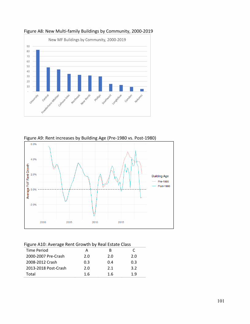
101

Figure A8: New Multi-family Buildings by Community, 2000-2019

Figure A9: Rent increases by Building Age (Pre-1980 vs. Post-1980)

Figure A10: Average Rent Growth by Real Estate Class

Time Period A B C 2000-2007 Pre-Crash 2.0 2.0 2.0 2008-2012 Crash 0.3 0.4 0.3 2013-2018 Post-Crash 2.0 2.1 3.2 Total 1.6 1.6 1.9

102

Figure A11: Rent Growth by Building Age by Community Area

Community Area Pre-Crash (2000-2007) Post-Crash (2013-2018)

Pre-1980 Post-1980 Pre-1980 Post-1980 Calhoun Isle 2.0 1.7 3.5 0.6 Camden 1.9 - 1.6 - Central 2.0 1.9 2.8 1.9 Longfellow 1.9 2.6 2.7 2.7 Near North 2.0 - 2.3 - Nokomis 1.9 - 2.7 4.0 Northeast 1.9 2.0 2.7 2.0 Phillips 1.9 2.6 2.5 3.6 Powderhorn 2.0 - 3.2 2.1 Southwest 1.9 - 3.2 2.4 University 1.9 1.9 3.2 3.4 All 2.0 1.9 3.1 1.9

Figure A12: Rent Burden by Citizenship Status of Head of Household

103

Figure A13: Rent Burden by Presence of Children in Household

Figure A14: Rent Burden by Single Person Household

Figure A15: Rent Burden by Multi-Generational Household

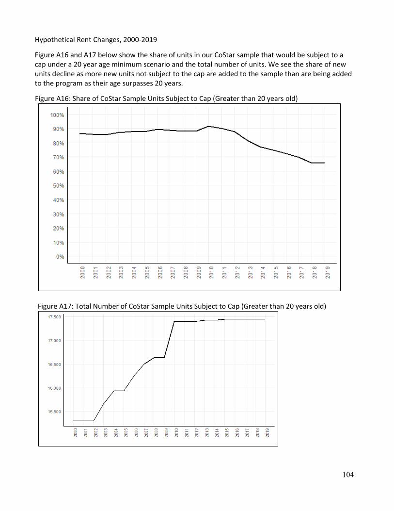
104

Hypothetical Rent Changes, 2000-2019

Figure A16 and A17 below show the share of units in our CoStar sample that would be subject to a cap under a 20 year age minimum scenario and the total number of units. We see the share of new units decline as more new units not subject to the cap are added to the sample than are being added to the program as their age surpasses 20 years.

Figure A16: Share of CoStar Sample Units Subject to Cap (Greater than 20 years old)

Figure A17: Total Number of CoStar Sample Units Subject to Cap (Greater than 20 years old)

105

Figure A18: Share of All Sample Units Hitting Rent Cap Threshold, 2001-2019

Figure A19: Hypothetical Median Rent Under Rent Caps – All Sample Units

Figure A19 shows big differences between the actual median rents and any of the rent cap scenarios by the end of the study period, as the median without a cap is pushed consistently upwards by the high median rent of new buildings.

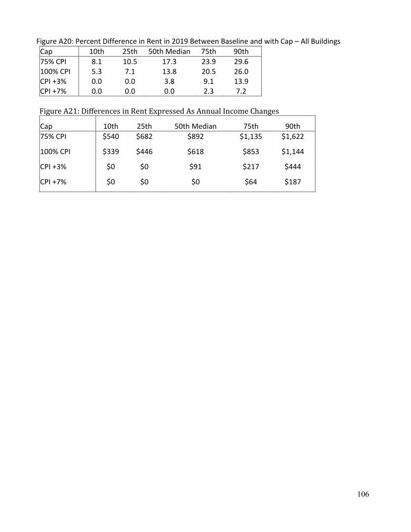
106

Figure A20: Percent Difference in Rent in 2019 Between Baseline and with Cap – All Buildings Cap 10th 25th 50th Median 75th 90th 75% CPI 8.1 10.5 17.3 23.9 29.6 100% CPI 5.3 7.1 13.8 20.5 26.0 CPI +3% 0.0 0.0 3.8 9.1 13.9 CPI +7% 0.0 0.0 0.0 2.3 7.2 Figure A21: Differences in Rent Expressed As Annual Income Changes

Cap 10th 25th 50th Median 75th 90th 75% CPI $540 $682 $892 $1,135 $1,622

100% CPI $339 $446 $618 $853 $1,144

CPI +3% $0 $0 $91 $217 $444

CPI +7% $0 $0 $0 $64 $187

107

Building Economics Model Specification and Assumptions One Apartment

• The model is based on a discounted cash flow analysis proforma for a single apartment unit. • The model apartment is based on the actual Minneapolis median rent in the sale year of

2018, which reflects a Class C market rate or NOAH apartment at approximately $975/month.

• Rent increases over the ownership period are based on actual Minneapolis Median rents in 2004 and 2009, increased at the actual median, average, and 90th percentile (representing the very highest), rates of increase for Minneapolis apartments.

• Rather than focusing on dollars, this model provides measures of return to owners/investors in percentages that can be compared across different scales of properties. For example, this model can be scaled to any number of units, for example, from 1 to 20 to 200 units (the returns as percentages would not change).

• We created two versions of this model, analyzing 10- and 15-year ownership periods with purchase in 2009 (10 years) and 2004 (15 years) and sale in 2018 at values based on 2019 rents.

• Although income and expense may vary depending upon size and age of building and numbers of units, unit prices, rents, and expenses are a common form of measurement in the apartment industry.

• We applied a variety of rent cap scenarios (based on those used in other cities and states) to the model to determine how rent caps would affect returns to owners/investors at the median, average, and high rates of rent increases. We modeled the following rent caps, based on the Minneapolis Regional Consumer Price Index: 75% of CPI, CPI, CPI+3%, CPI+5%, and CPI+7%.

Purchase Price and Financing in 2004 and 2009

• The original purchase price of the apartment is based on an approximation of market value, or slightly discounted market value, derived from actual rents in 2004 and 2009. (Net Operating Income divided by a conservative cap rate of 8.5%.)

• The financing for the purchase of the apartment in 2004 and 2009 was based on 65% Loan-to-value ratio (LTV), 6% interest rate, and a 20-year term. These financing terms assume that the lender loaned 65% of the sale price and the buyer provided 35% in equity at the time of purchase in 2004 and 2009. The loan was based on a 6% interest rate and a 20-year amortization term, which means that the loan would be fully repaid after 20 years. (Amortization can also be 25 or 30 years, for example.)

• This financing reflects a buyer who has enough capital to finance with less leverage (2004) and/or a more restrictive lending environment and lower leverage during the recession (2009). This loan results in higher debt service than a higher-leveraged loan for a longer term. For example, a 75% loan with a 30-year amortization term would require more, smaller payments (as a share of annual income) spread over a longer, term.

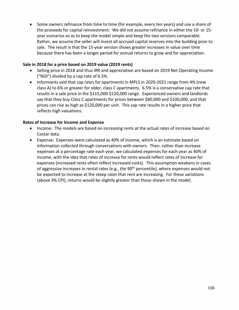
108

• Some owners refinance from time to time (for example, every ten years) and use a share of the proceeds for capital reinvestment. We did not assume refinance in either the 10- or 15-year scenarios so as to keep the model simple and keep the two versions comparable. Rather, we assume the seller will invest all accrued capital reserves into the building prior to sale. The result is that the 15-year version shows greater increases in value over time because there has been a longer period for annual returns to grow and for appreciation.

Sale in 2018 for a price based on 2019 value (2019 rents)

• Selling price in 2018 and thus IRR and appreciation are based on 2019 Net Operating Income (“NOI”) divided by a cap rate of 6.5%.

• Informants said that cap rates for apartments in MPLS in 2020-2021 range from 4% (new class A) to 6% or greater for older, class C apartments. 6.5% is a conservative cap rate that results in a sale price in the $115,000-$120,000 range. Experienced owners and landlords say that they buy Class C apartments for prices between $80,000 and $100,000, and that prices can rise as high as $120,000 per unit. This cap rate results in a higher price that reflects high valuations.

Rates of Increase for Income and Expense

• Income: The models are based on increasing rents at the actual rates of increase based on Costar data.

• Expense: Expenses were calculated as 40% of income, which is an estimate based on information collected through conversations with owners. Then. rather than increase expenses at a percentage rate each year, we calculated expenses for each year as 40% of income, with the idea that rates of increase for rents would reflect rates of increase for expenses (increased rents often reflect increased costs). This assumption weakens in cases of aggressive increases in rental rates (e.g., the 90th percentile), where expenses would not be expected to increase at the steep rates that rent are increasing. For these variations (above 3% CPI), returns would be slightly greater than those shown in the model.

109

Figure A.22

Figure A.23

$1,097 $984

$1,608

$977 $1,056

$1,679

$3,054

$0

$500

$1,000

$1,500

$2,000

$2,500

$3,000

$3,500

Mpls Avg MPLS Med Mpls High 75% CPI CPI CPI+3% CPI+7%

2019 Rents (2004-2018)

10.6%7.7%

11.1%8.7% 9.7%

16.4%

28.8%

0.0%

5.0%

10.0%

15.0%

20.0%

25.0%

30.0%

35.0%

Mpls Avg MPLS Med Mpls High 75% CPI CPI CPI+3% CPI+7%

Cash-on-Cash Return:Average Annual Returns, 2004-2018

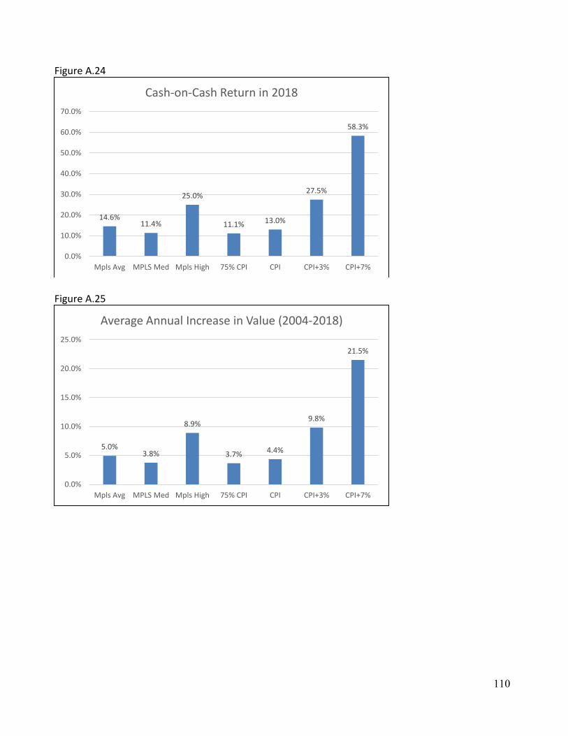
110

Figure A.24

Figure A.25

14.6%11.4%

25.0%

11.1% 13.0%

27.5%

58.3%

0.0%

10.0%

20.0%

30.0%

40.0%

50.0%

60.0%

70.0%

Mpls Avg MPLS Med Mpls High 75% CPI CPI CPI+3% CPI+7%

Cash-on-Cash Return in 2018

5.0%3.8%

8.9%

3.7% 4.4%

9.8%

21.5%

0.0%

5.0%

10.0%

15.0%

20.0%

25.0%

Mpls Avg MPLS Med Mpls High 75% CPI CPI CPI+3% CPI+7%

Average Annual Increase in Value (2004-2018)

111

Figure A.26

Figure A.27

74.4%56.3%

133.4%

54.8% 65.3%

147.4%

322.4%

0.0%

50.0%

100.0%

150.0%

200.0%

250.0%

300.0%

350.0%

Mpls Avg MPLS Med Mpls High 75% CPI CPI CPI+3% CPI+7%

Total Increase in Value, 2004-2018

16.0%13.5%

17.1%14.1% 15.0%

19.7%

25.7%

0.0%

5.0%

10.0%

15.0%

20.0%

25.0%

30.0%

35.0%

Mpls Avg MPLS Med Mpls High 75% CPI CPI CPI+3% CPI+7%

Internal Rate of Return, 2004-2018