Embed Size (px)
Citation preview


MINITAB 17 Essential contents
DAY 1: • Background
• Hypothesis test
• ANOVA
DAY 1 • Regression
• Design of Experiments (DOE)
• Taguchi Method


Eg.: Tools’ Flow
Rozzeta Dolah, Zenichi Miyagi, Kazuo Tatebayashi, Management and Production Engineering Review. Volume 3, Issue 4, Pages 26–34, ISSN (Online), DOI: 10.2478/v10270-012-0031-z, January 2013

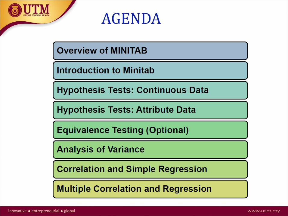
AGENDA

Opening a New Project


Open & Save


INTRODUCTION TO
MINITAB

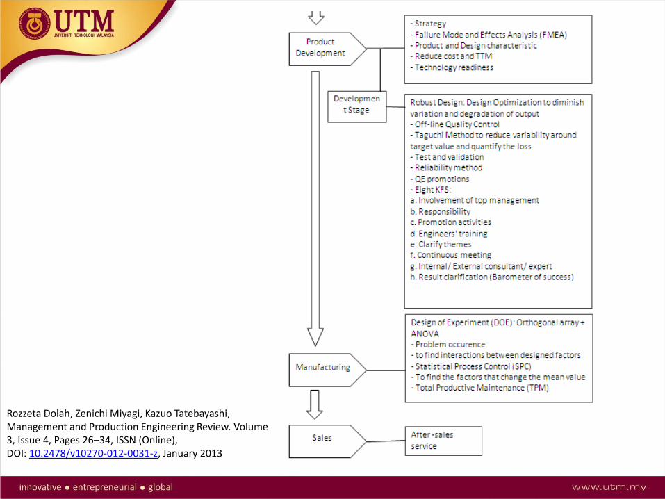
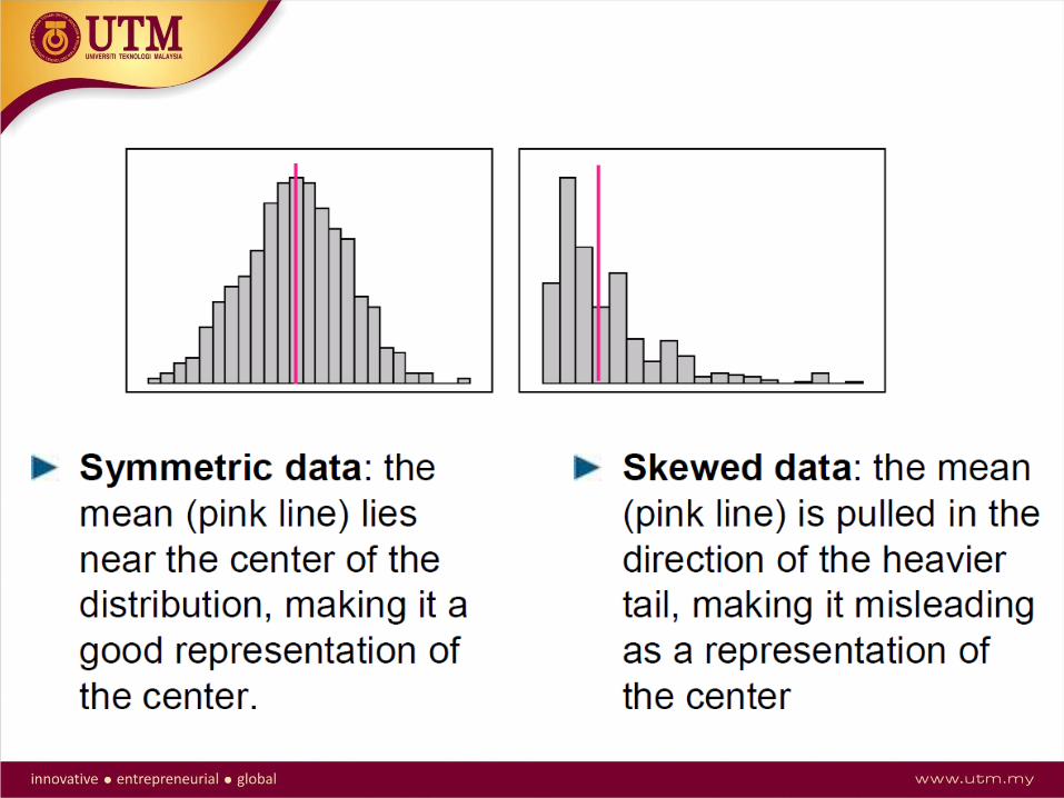
Central Tendency & Dispersion

Dispersion

STDEV


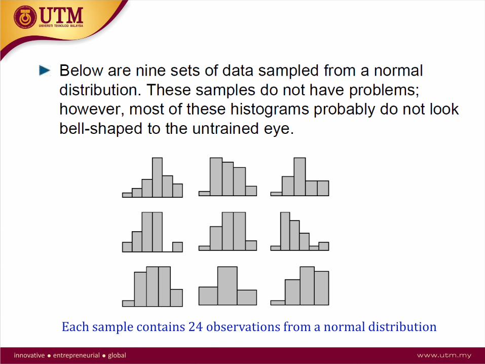
Each sample contains 24 observations from a normal distribution

Box Plot
Bike Trip 2.MTW

50% of the data falls within the box
Whiskers extend the whole data

Pareto.MTW
Pareto Chart: Quality tools / Pareto Chart X axis: Categorical Y axis: Continous
Fishbone.MTW
IntSPC.MTW

SPC: Determine the control limit:
• Calculate Central line
• X = R =
• X = avg. of subgroup avg.
• xi = avg. of its subgroup
• g = no. of subgroups
• R = avg. of subgroup ranges
• Ri = range of its subgroup
• Where A2, D4, D3 are factors - vary according to different n
RAxσ3xUCL 2xx
RAxσ3xLCL 2xx
RDσ3RUCL 4xR
RDσ3RLCL 3xR
AGENDA
Hypotheses Tests: Continuous Data
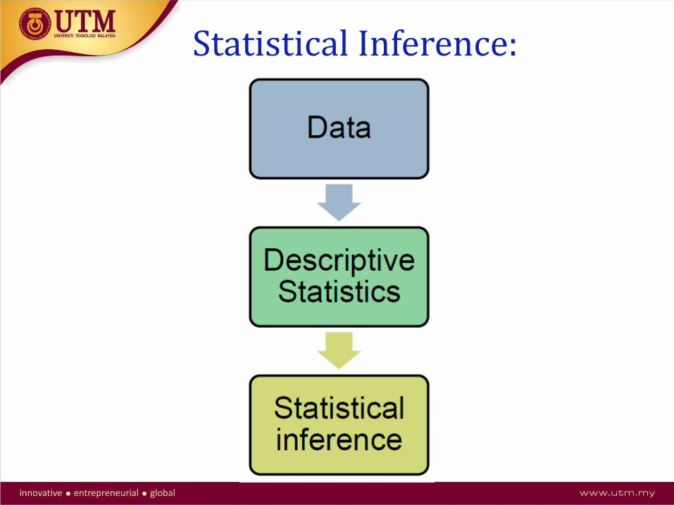
Statistical Inference:


Denotations:
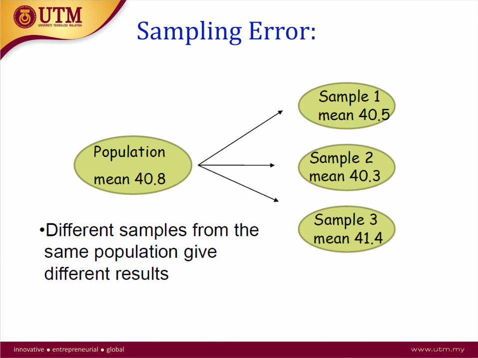
Sampling Error:


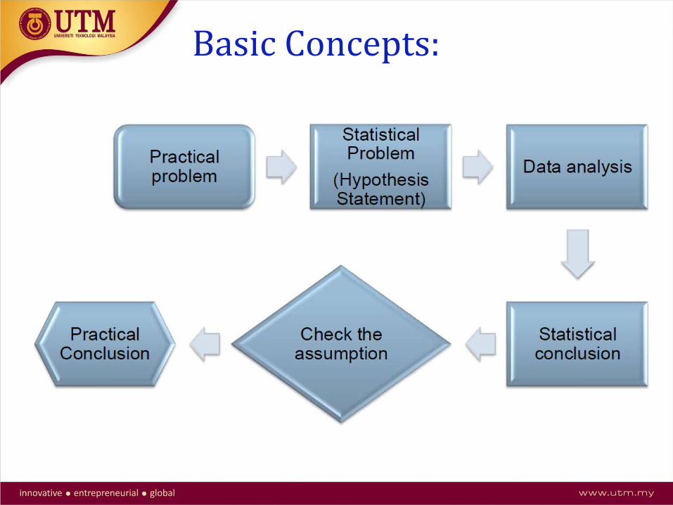
Basic Concepts:

Basic Testing:


Directional & Non-Directional

Directional & Non-Directional

Directional & Non-Directional

Directional & Non-Directional

Basic Testing:

population
Random Sample

Basic Testing:


Statistic Conclusion:


Alpha & p-value:


Confidence Interval:

Basic Concepts:

Basic Concepts:

Power Analysis:
= chance of detecting a shift


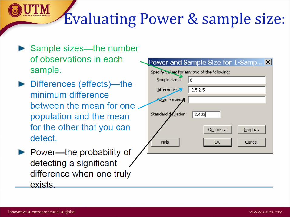
Evaluating Power & sample size:

Stat / Power and sample size / 1-sample t From the cereal data, stdev is 2.403 from t-test results. CerealBx.MPJ = with 6 observations, stdev of 2.403 and alpha 0.05, the power is only 0.5377. Thus, if mean is off target by 2.5grams, the chance of detecting it with a sample size of 6 is 53.77% Therefore, if the process mean is off target by 2.5 grams, there is a 46% chance that you will not detect it with a sample size of 6
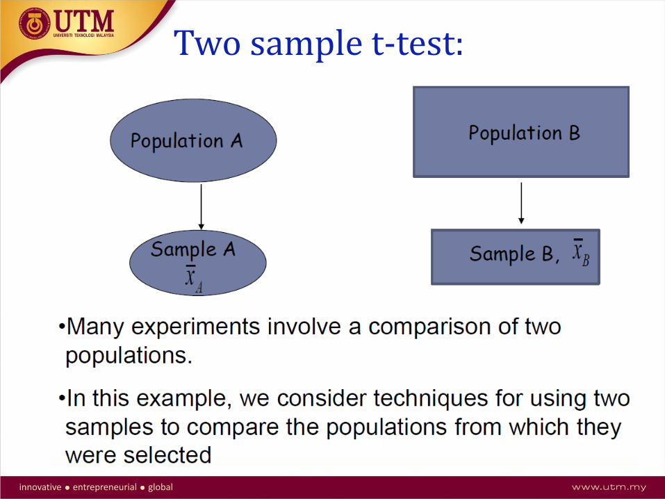
Two sample t-test:

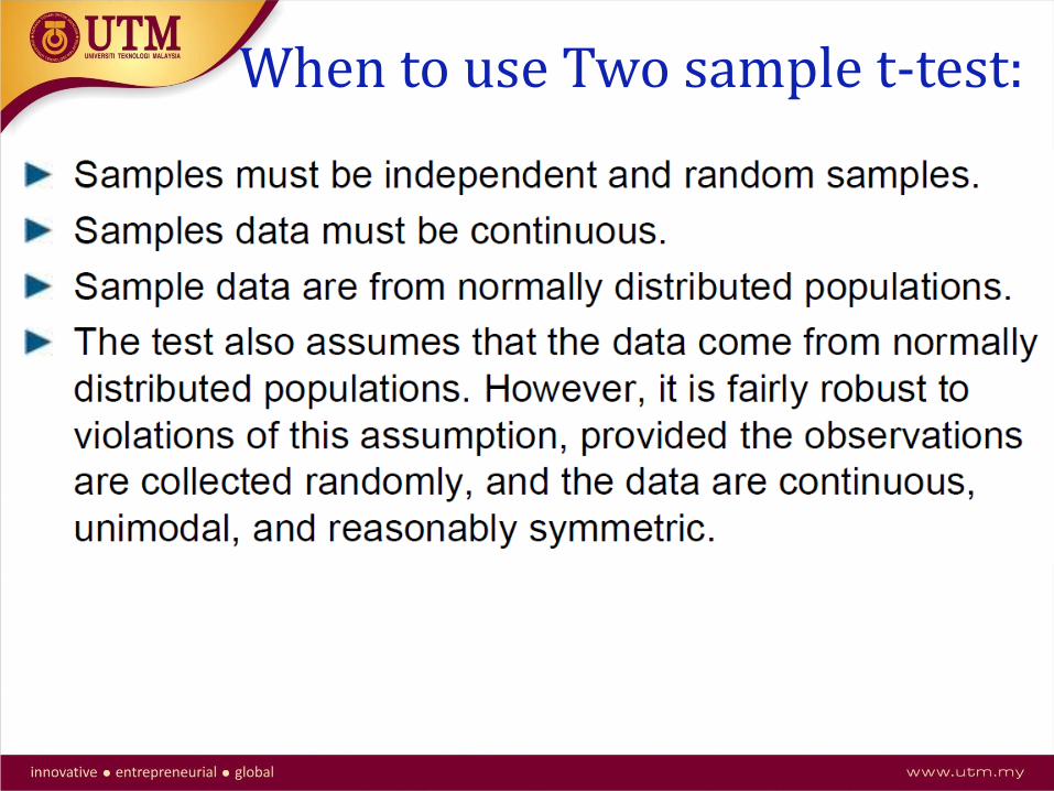
When to use Two sample t-test:

Why use Two sample t-test:

Comparing Variences : 2-variances:

Eg.: Plastic Strength
A calculator manufacturer is selecting a plastic supplier. Based on the result of power & sample size, he decided to use a sample size of 20 from each supplier to compare the strength of the supplier of plastic pellets. Plastic.MPJ - Stat/ Basic/ 2-simple t / each sample is in its own column -Graph / Dot plot / Multiple Y’s / Simple / ok - Stat / Basic Statistics / Graphical summary Two-Sample T-Test and CI: SupplrA, SupplrB Two-sample T for SupplrA vs Supplr N Mean StDev SE Mean SupplrA 20 163.82 5.66 1.3 SupplrB 19 160.14 3.26 0.75 Difference = μ (SupplrA) - μ (SupplrB) Estimate for difference: 3.67 95% CI for difference: (0.67, 6.68) T-Test of difference = 0 (vs ≠): T-Value = 2.50 P-Value = 0.018 DF = 30
Ho = A - B = 0 H1 = A - B 0 P value < 0.05 Reject the null. Accept H1. Conclusion: The mean strengths are different. Next: compare variance.

Ho = A / B = 1 H1 = A / B 1 P value < 0.10 Reject the null. Accept H1.
Compare variances:

Double click x-axis, Go to Binning Tab

Next, check for Normality: Stat / Basic statistics / Graphical summary
P-value 0.718 & 0 164 > 1.0. Conclusion: Data are from Normal distribution.
Summary Layout: Editor / Layout tool Click Finish.

E.g Anode .MPJ
An electronic manufacturer must ensure that the electrical anode in each capacitor is a certain distance above the surface of the capacitor’s ceramic body. Recently, the manufacturer has produced many capacitors with anode heights that violate the lower specification limit. A change has been implemented which they believe will increase anode height. The engineers must determine how much data to collect, and then compare the height measurements before and after the process change Process name: Anode insertion process
Hint: 1. Determine the required sample size in enabling to detect the process has
improved by at least 0.4mm with a power of 0.80. Stdev: 0.55mm. 2. Normality ? (graphical summary) 3. Equal variance? Use alpha 0.10 4. 2-sample t-test to check improvement on After the process change. Use alpha
0.05.

Paired T-Test:
e.g: 20 drivers; Each driver drives Car A and Car B
Parking.xlsx -Export to MPJ -Assistant / Hypothesis Tests Paired t

When to use Paired T-Test:
Why:

2-sample t-test: Ho : A - B = 0 H1 : A - B 0 2-variance test: Ho : A / B = 1 H1 : A / B 1
1-sample t-test: Ho : = # H1 : #
Paired t-test: Ho : Diff A-B = 0 H1 : Diff A 0

Outlier test:


* Another way to check the data through Editor/ Brush

ANOVA Analysis of Variance

Important terms:

• Analysis of Variance = ANOVA
• Developed by Sir R.A Fisher
• Variance in variable is decomposed into different section of variations
• One way ANOVA
• Two way ANOVA
• Factorial ANOVA
• Repeated measures ANOVA

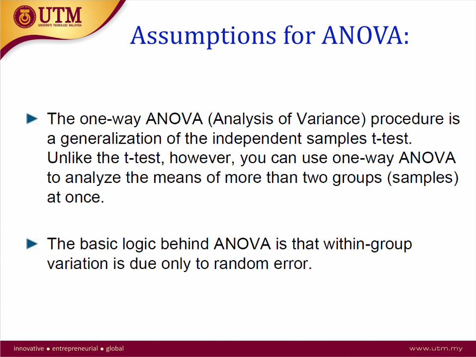
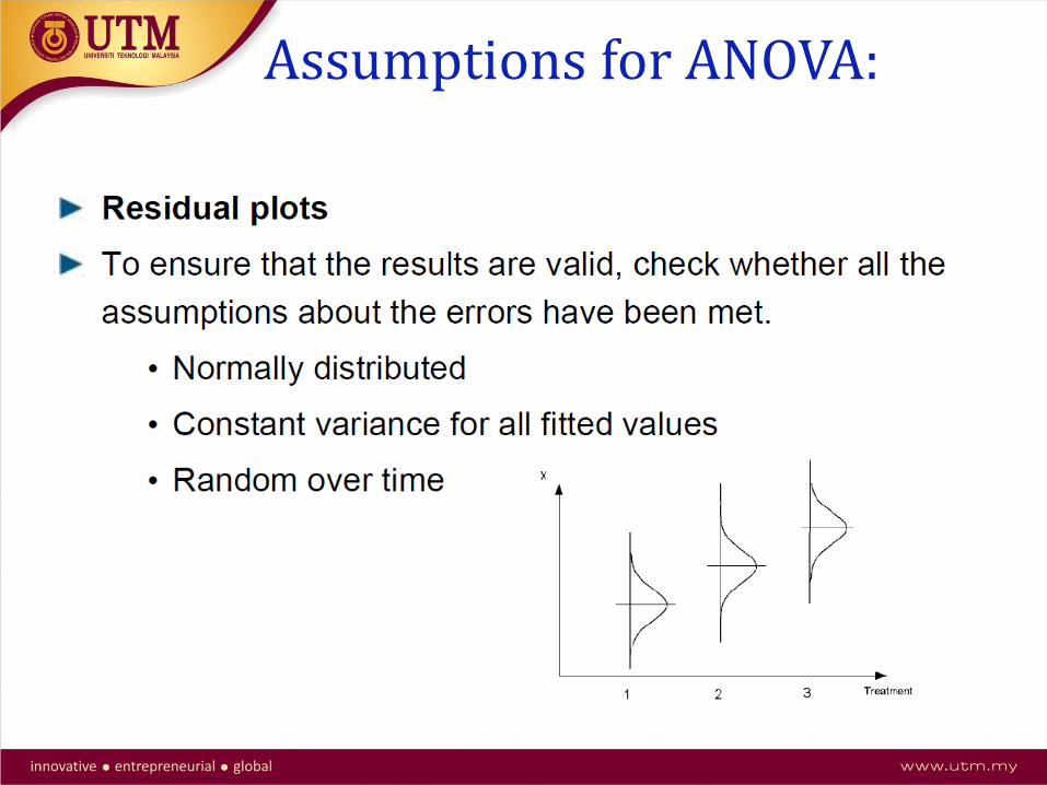
Assumptions for ANOVA:
Assumptions for ANOVA:

Assumptions for ANOVA:

Eg: Car Seat thread strength

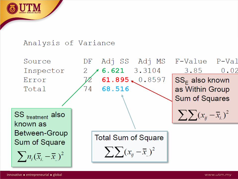
One Way ANOVA: between-inspector differences

Results:

Probability

Two way ANOVA
• We have identified 2 product characteristics (factors) that are thought to influence the amount of vibration of running motors. Factor A = brand of bearing used in motors & Factor B = the material used for motor casing. A is 5 brands and B is three types of material: steel, aluminum, plastic. Two motors (r = 2) were constructed and tested for each of the a.b = 5x3= 15 combination with 2 repetitions = 30 runs of experiments.

Two way ANOVA
SSA = b.r ( average A – Ybar)2
SSA = 3.2[ (14.07 – 14.353)2+(16.35-14.353)2+ (13.48-14.353)2+(14.62-14.353)2+(13.25-14.353)2] = 6[6.118125] = 36.709 SSB = a.r ( average B – Ybar)2
=5.2[(14.39 – 14.353)2+(14.52 – 14.353)2+(14.15 – 14.353)2] = 10 [ 0.070467 ] = 0.705
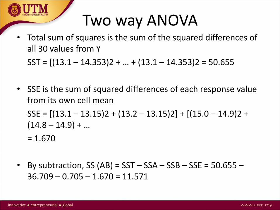
• Total sum of squares is the sum of the squared differences of all 30 values from Y
SST = [(13.1 – 14.353)2 + … + (13.1 – 14.353)2 = 50.655
• SSE is the sum of squared differences of each response value from its own cell mean
SSE = [(13.1 – 13.15)2 + (13.2 – 13.15)2] + [(15.0 – 14.9)2 + (14.8 – 14.9) + …
= 1.670
• By subtraction, SS (AB) = SST – SSA – SSB – SSE = 50.655 – 36.709 – 0.705 – 1.670 = 11.571
Two way ANOVA

Two Way ANOVA
• At a significant level level of 0.05, main effect for A and
interaction AB are significant. B is not significant factor.
• Meaning: the brand of bearing is very important. Although the casing material does not have significant effect, it does influence the effect of A becaue the interaction AB is significant

Interpreting Results:

Assumptions for ANOVA:

Residual:

Normal Probability Plot:


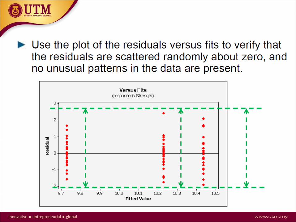
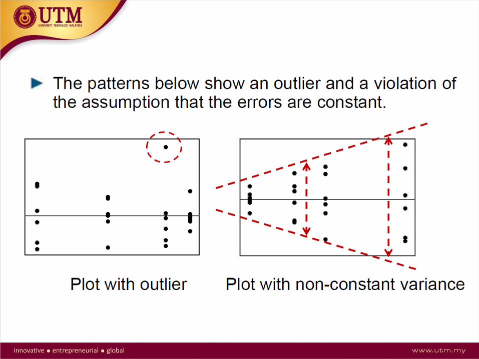
Residuals vs. Fit:


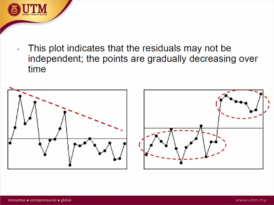
Residuals vs. Order:

Correlation & Regression
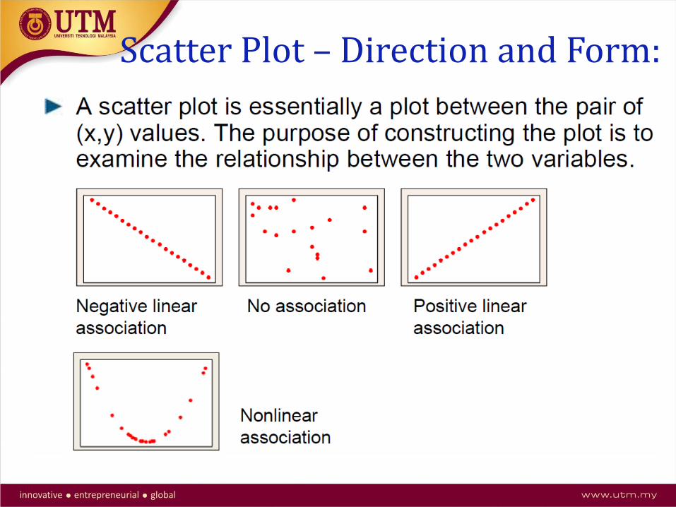
Scatter Plot – Direction and Form:

Scatter Plot –Strength:

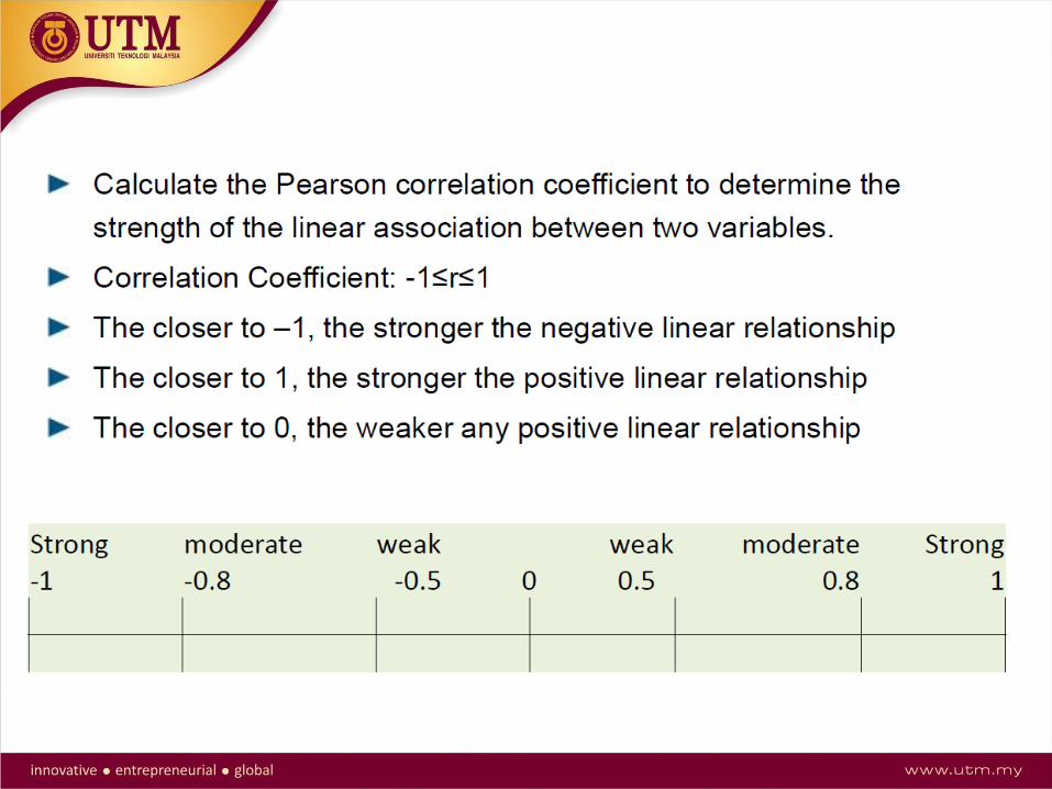
Correlation:


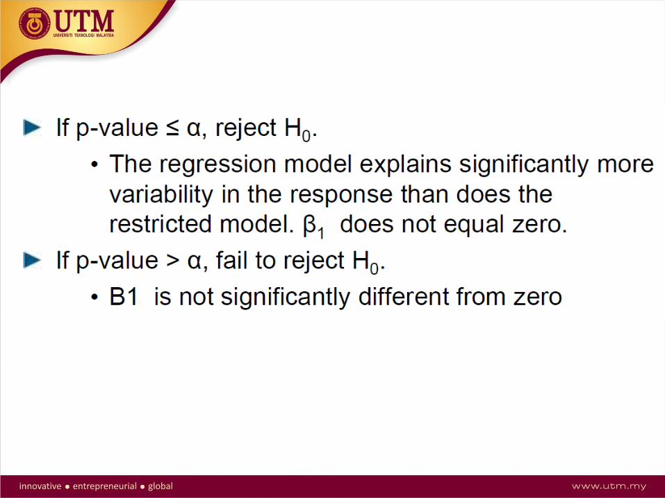
Hypothesis Test:

Simple Regression:


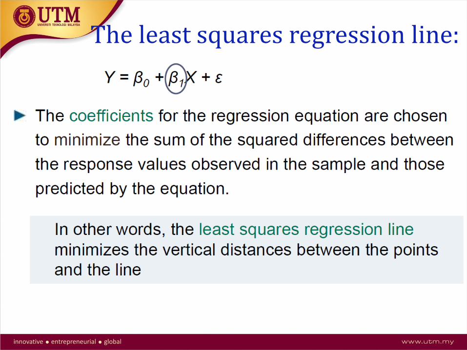
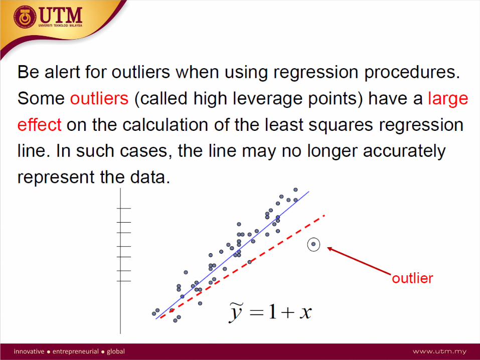
The least squares regression line:

Why use regression? :
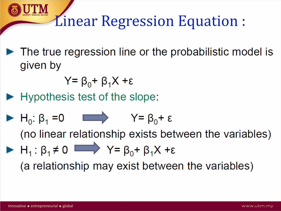
Linear Regression Equation :

Common Mistake:

Common Mistake:

Multiple Regression:


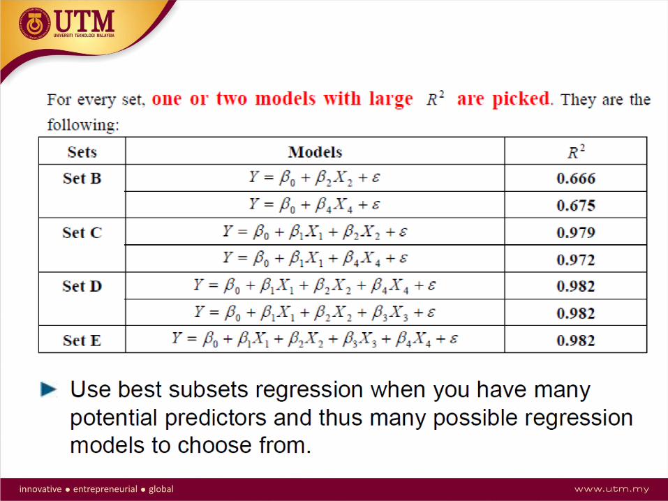
Best subsets regression:


Design of Experiments DOE
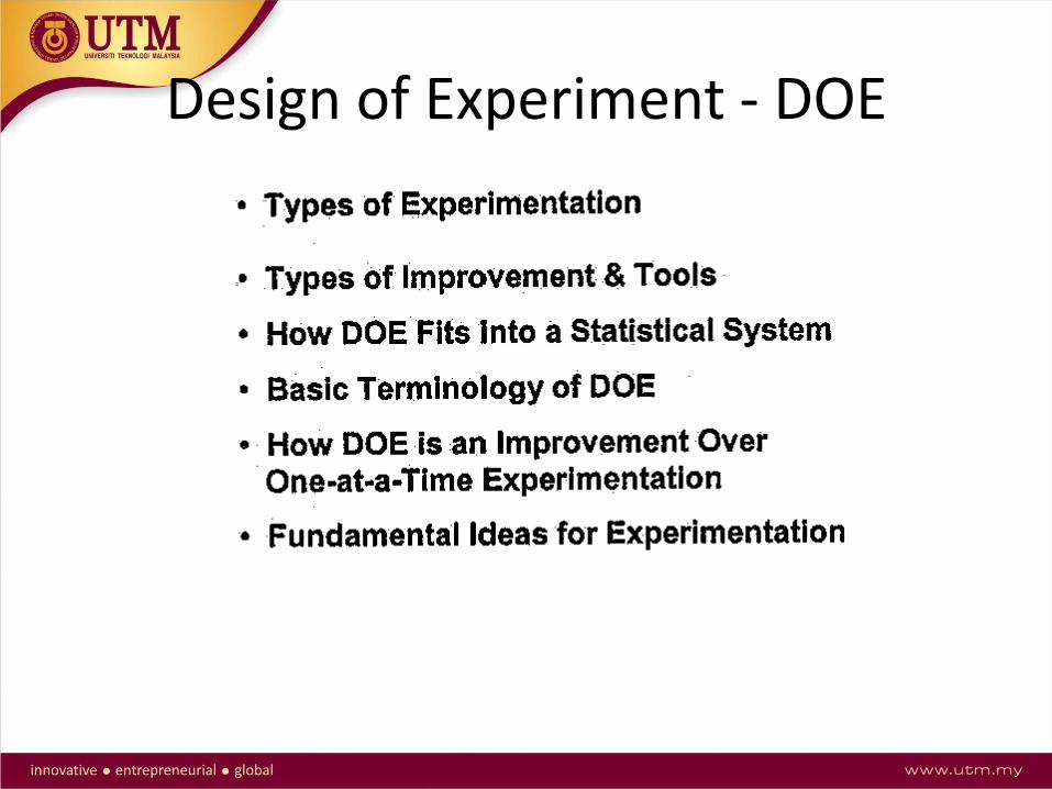
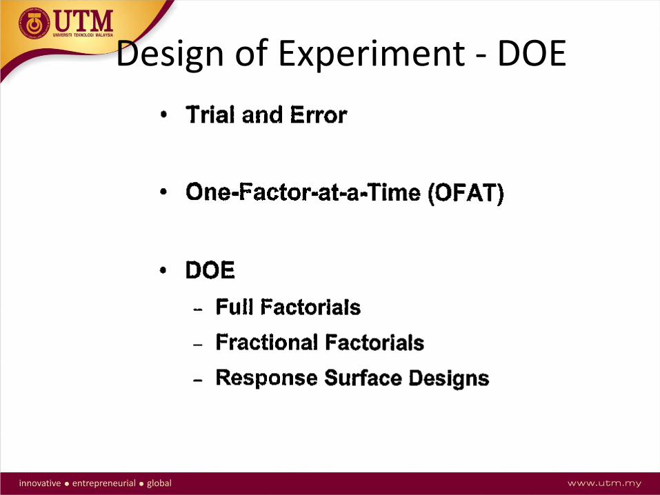
Design of Experiment - DOE
Design of Experiment - DOE

Design of Experiment - DOE

Design of Experiment - DOE

Design of Experiment - DOE


Design of Experiment - DOE

Design of Experiment - DOE

Design of Experiment - DOE

Design of Experiment - DOE


Design of Experiment - DOE

Design of Experiment - DOE


Eg. Etching stain defect
• Three etching factors are varied to observe the three responses, namely total thickness variations (TTV), etching removal, and wafer brightness after etching.
• The target for TTV is to achieve the lowest value as possible. Etching removal is aimed at 38 + 2 um and finally the brightness is approximately 75 + 2 %.

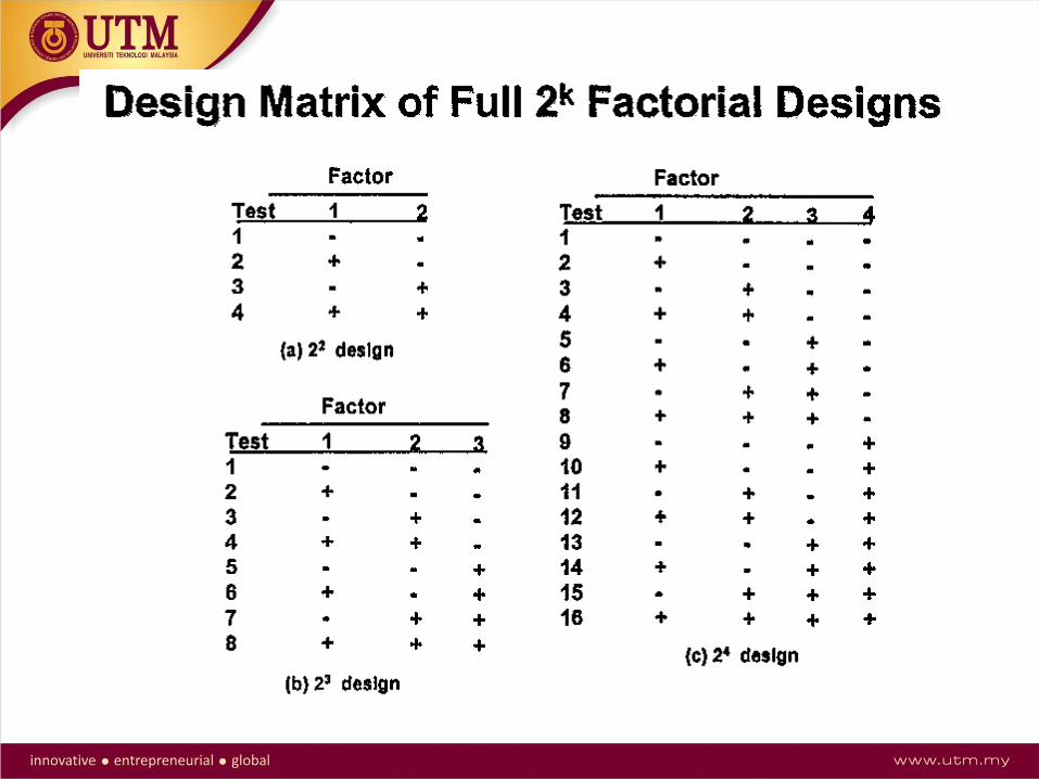
Analyze using DOE 2^3 with cp
RUN Wafer Rotation
at Etching (rpm)
Acid
Temperature
(oC)
Etching Bubling
Flowrate (l/min) TTV
Removal
(um) Brightness (%)
1 43 38 350 3.31 35.46 72.47
2 53 33 450 2.28 41.99 80.47
3 33 43 250 5.64 41.58 84.40
4 53 43 450 4.68 36.22 71.50
5 53 43 250 5.45 39.06 84.99
6 43 38 350 3.16 35.52 71.25
7 33 33 450 3.11 40.28 86.50
8 33 33 250 2.44 34.05 68.90
9 43 38 350 3.28 35.10 71.56
10 33 43 450 4.24 35.34 64.30
11 53 33 250 2.57 38.48 76.54

Analyze the responses:

Process Robustness