10. Automated algorithm selection

AEA 2019/2020

1/44

2/44

Content

Motivation

Meta-learning

Algorithm runtime prediction (for SAT)

Generalizations to other domains

3/44

No Free Lunch theorems

The performance of a system can be improved by always pickingthe best algorithm?

I ”No Free Lunch” theorems: no algorithm can be the bestacross all possible problems and, on average, all algorithmsperform the same.

Motivation for Algorithm Selection: if, on average, differentalgorithms are the best for different parts of the problem space,selecting them based on the features of the problem can improveperformance.

Identify a portfolio of complementary algorithms and a strategy forchoosing between them.

Debate: if the NFL theorems would apply to Algorithm Selectionsystems, the ramifications in practice may not be significant.

4/44

Algorithm selection

I The algorithm selection problem: select the most suitablealgorithm for a particular problem

Which algorithm is likely to perform best for my problem?I a learning task → the field of meta-learning : learning about

learning algorithm performance on classification problems.

I Methods based on algorithm selection began to outperformstandalone solvers in SAT competitions;Other problems addressed: CSP, planning, Max-SAT, QBF,ASP.

5/44

Algorithm selection

The winner-take-all approach: measure algorithms’ performance ona given problem distribution, and use the algorithm with the lowestaverage runtime.

I the neglect of algorithms that, while uncompetitive onaverage, have good performance on particular instances.

6/44

The algorithm selection problem

A formal abstract model:

I the problem space P: the set of instances of a problem class

I the feature space F : measurable characteristics of theinstances (generated by a computational feature extractionprocess applied to P)

I the algorithm space A: the set of considered algorithms fortackling the problem

I the performance space: the mapping of each algorithm to aset of performance metrics

The problem: for a problem instance x ∈ P, with featuresf (x) ∈ F , find the selection mapping S(f (x)) into algorithm spaceA s.t. the selected algorithm A ∈ A maximizes the performancemapping p(A, x).

7/44

The algorithm selection problem

Figure: Schematic diagram of Rice’s algorithm selection problem model.The objective is to determine the selection mapping S so as to have highalgorithm performance.

8/44

Algorithm Selection

ML techniques to learn the performance mapping (from problemsto algorithms) using features extracted from the problems.

I a training phase: candidate algorithms are run on a sample ofthe problem space to experimentally evaluate theirperformance

I the training data are used to create a performance modelused to predict the performance on new problems

Key Components of an Algorithm Selection System:

I feature extraction

I performance model

I prediction-based selector/scheduler

Optional: presolver, secondary/hierarchical models and predictors

9/44

Content

Motivation

Meta-learning

Algorithm runtime prediction (for SAT)

Generalizations to other domains

10/44

Meta-learning

In machine learning, Algorithm Selection is referred to asmeta-learning 1.

I Select the best learning algorithm to solve a classificationproblem using different performance measures (classificationaccuracy).

I Characterize a classification problem and examine the impactof it on algorithm behavior.Use rule-based learning algorithms to develop rules:

If the dataset has characteristics C1, C2, ..., Cn

Then use algorithm A1 and don’t use algorithm A2.

1Aha, D. Generalizing from case studies: A case study, 1992

11/44

Meta-learning for classification problems

The study of Aha (’92) 1: an empirical method for generalizingresults from case studies

I A nearest-neighbor classifier (IB1), a set covering rule learner(CN2), a decision tree (C4)

I Instances: training datasets from the letter recognitiondatabase

I Features: #instances, #classes, #prototypes per class,#relevant and irrelevant attributes, the distribution range ofthe instances and prototypes

IF (#training instances < 737) AND

(#prototypes per class > 5.5) AND

(#relevants > 8.5) AND

(#irrelevants < 5.5)

THEN IB1 will be better than CN2.

12/44

Meta-learning for classification problems

StatLog (Comparative Testing of Statistical and Logical Learning)project: the comparison of machine learning, neural, and statisticalapproaches to classification

I the goal: to relate performance of algorithms tocharacteristics of classification datasets

I a broader range of datasets, algorithms and featuresI simple measures (size of datasets)I statistical measures (mean and variance of instance attributes)I information theoretical measures (entropy): can capture the

randomness of an instance, which correlates with complexity

13/44

StatLog project

Figure: Features used to characterize classification datasets

14/44

Covariance and correlation

Association of two variables

I Covariance summarizes interrelation of two random variables.

σXY = Cov(X ,Y ) = E (X−E (X ))(Y−E (Y )) = E (XY )−E (X )E (Y )

If Cov(X ,Y ) > 0, X and Y are positively correlated.If Cov(X ,Y ) < 0 (large X correspond to small Y ), thevariables are negatively correlated.If Cov(X ,Y ) = 0, X and Y are uncorrelated.

15/44

Covariance and correlation

Association of two variables

I Correlation coefficient is a rescaled, normalized covariance.

ρ =Cov(X ,Y )

(StdX )(StdY )

Values of ρ near 1 - strong positive correlation, values near(-1) - strong negative correlation, values near 0 - weak/nocorrelation.

16/44

Skewness and Kurtosis

Population skewness of a distribution is a measure of asymmetry(zero is symmetric).

γ1 = E [(X − µ)3]/σ3

17/44

Skewness and Kurtosis

Population kurtosis characterizes symmetric deviations fromNormality; is a measure of peakedness or flatness compared to aGaussian distribution.

γ2 = E [(X − µ)4]/σ4 − 3

A large kurtosis shows a distribution with large tails (there arecategories far from the average), while a small kurtosis shows adistribution in which fewer categories far from the average arepresent.

18/44

StatLog project

In the notation of Rice’s model:

I P: 22 classification datasets

I A: 23 machine learning, neural, statistical learning algorithms

I F : 16 features of the datasets

I performance: classification accuracy

No single algorithm performed best for all problems (supported bythe NFL theorem). Use a decision tree algorithm C4.5 to learnrules for each algorithm (the mapping S).

Example: rules generated for the classification and regression tree(CART) algorithm

CART recommended IF (N ≤ 6435 AND skew > 0.57)CART not recommended IF (N > 6435 OR (N < 6435 AND skew < 0.57 ) )

Valuable meta-data widely used by meta-learning researchers(extend to use regression, case-based reasoning, etc.)

19/44

Other developments

A large collection of meta-data for classification 2:

I P: 112 classification datasets from the UCI repository

I A: 3 rule-based, 1 neural, 4 statistical learning algorithms (SVMsfor the 1st time)

I performance: rank based on an F-measure that combines aweighting of cost-sensitive accuracy and computational time

I F : 31 features (derived from the StatLog characteristics, statisticalfeatures: index of dispersion, center of gravity, max and mineigenvalues of the covariance matrix)

I A decision tree C4.5 to learn the mapping S , producing rules foreach algorithm. Average accuracy of 10-fold cross-validation testingexceeds 80% accuracy in predicting the best algorithm.

2Ali, S., Smith, K. On learning algorithm selection for classification, ’06

20/44

Automated Machine Learning

Automated machine learning (AutoML): automatically choose agood algorithm and feature preprocessing steps for a new dataset,and set their hyperparameters.

AUTO-SKLEARN 3, 4 improves the AutoML methods by:

I automatically take into account past performance on similardatasets

I construct ensembles from the models evaluated during theoptimization

AUTO-SKLEARN won on the ChaLearn AutoML challenge.

3M. Feurer et al. Efficient and Robust Automated Machine Learning, 20154http://www.ml4aad.org/automl/

21/44

AUTO-SKLEARN

Improvements of the AutoML approach:

I a meta-learning step for initializing the Bayesian optimizer

I an automated ensemble construction step (use classifiersfound by optimization)

Figure: Improved AutoML approach 3

22/44

Automated ensemble construction

Bayesian hyperparameter optimization is

I data-efficient in finding the best-performing hyperparametersetting, but

I is a very wasteful procedure: all the models it trains duringthe course of the search are lost.

Rather than discarding these models, store them and use anefficient post-processing method to construct an ensemble.

Ensemble selection: start from an empty ensemble and iterativelyadd the model that maximizes ensemble validation performance(with uniform weight, but allowing for repetitions).

23/44

AUTO-SKLEARN’s components 3

I Classification algs: linear models, SVMs, nearest neighbors,naive Bayes, decision trees, ensemble, etc.

I Feature preprocessing methods: feature selection, kernelapproximation, matrix decomposition, embeddings, featureclustering, polynomial feature expansion, etc

I Data preprocessing methods: rescaling of the inputs,imputation of missing values, one-hot encoding, balancing ofthe target classes

24/44

Content

Motivation

Meta-learning

Algorithm runtime prediction (for SAT)

Generalizations to other domains

25/44

Algorithm runtime prediction

I Predict how long an algorithm will take to run on an unseeninput, using ML techniques to build a model of the algorithm’sruntime as a function of problem-specific instance features.

I Empirical performance models (EPM)5: used for algorithmselection, parameter tuning and algorithm configuration,generate hard benchmarks, gain insights into instancehardness and algorithm performance

5F. Hutter et al. Algorithm runtime prediction: Methods & evaluation, 2014

26/44

Empirical performance models

A problem instance: a list of features z = [z1, ..., zm]T , drawn froma feature space F ; the features are computable by a piece ofproblem-specific code that extracts characteristics for an instance.

The configuration space of a parameterized algorithm withparameters θ1, ..., θk with domains Θ1, ...,Θk : a subset of thecross-product of parameter domains: Θ ⊆ Θ1x ...xΘk ; the elementsof Θ: complete instantiations of the algorithm’s parameters(configurations). The input space: I = ΘxF .

∆(R) the space of probability distributions over the real no.; Given

I an algorithm A with configuration space Θ and

I a distribution of instances with feature space F ,

an empirical performance model (EPM) is a stochastic processf : I → ∆(R) that defines a probability distribution overperformance measures, for each combination of a parameterconfiguration θ ∈ Θ of A and a problem instance with z ∈ F .

27/44

Empirical performance models

To construct an EPM for algorithm A with configuration space Θon an instance set Π

I run A on various combinations of configurations θi ∈ Θ andinstances πi ∈ Π, and record the performance values yi

I record a p = k + m-dimensional vector of predictor variablesxi = [θTi , z

Ti ]T , θi the k-dimensional parameter configuration,

zi the m-dimensional feature vector of the instance used inthe ith run

I the training data for the regression models: {(x1, y1), ...,(xn, yn)}; X the nxp matrix containing [x1, ..., xn]T (designmatrix), y the vector of performance values [y1, ..., yn]T .

Use a log-transformation (predicting log runtime) - useful for largevariation in runtimes for hard combinatorial problems. Discard the inputdimensions constant across all training data points and normalize theremaining ones. Disregard missing values for normalization.

28/44

Problem-specific instance features for SAT 5

29/44

Problem-specific instance features

I Probing features: execute a cheap algorithm for the probleminstance and keep track of several statistics (e.g. counting theno. of clauses a DPLL SAT solver learns in 2 seconds)

Probing features based on one type of algorithm (e.g, localsearch) are often useful for predicting the performance ofanother type of algorithm (e.g., tree search).

I Timing features: measure the time the computation of variousfeatures take

30/44

Performance predictions

I For each algorithm-distribution pair, execute the algorithm onall instances of the distribution, measure its runtimes, andcollect the results.

I Complementary quantitative metrics to evaluate meanpredictions µ1, . . . , µn and predictive variances σ2

1, . . . , σ2n

given true performance values y1, . . . , yn.

I Root mean squared error (RMSE):√

1/n∑n

i=1(yi − µi )2

I Pearson’s correlation coefficient (CC):∑n

i=1(µiyi )−n·µ·y(n−1)·sµ·sy , x

sample mean and sx standard deviation of x

31/44

Performance predictions

I 10-fold cross-validation, report means of the measures acrossthe 10 folds; statistical significance using a Wilcoxonsigned-rank test (cross-validation folds are correlated)

I data and software:http://www.cs.ubc.ca/labs/beta/Projects/EPMs/

32/44

Quantitative comparison of models for runtime predictionson previously unseen instances 5

33/44

Visual comparison of models for runtime predictions 5

34/44

Content

Motivation

Meta-learning

Algorithm runtime prediction (for SAT)

Generalizations to other domains

35/44

Generalizations to other domains

Sorting

I Use dynamic programming to estimate the mapping S via aMarkov decision process 6;

I feature: the length of the sequenceI generate rules/optimal policies showing which of the

algorithms (InsertionSort, MergeSort, Quick-Sort) should beused depending on the length of sequence.

6Lagoudakis, M., Litman, M., Parr, R. 2001. Selecting the right algorithm

36/44

Sorting

I 7 More sorting algorithms, additional features to characterizea sequence (the degree of presortedness), a learning approachfor the mapping S ; 4 classes of random sequences of varyingsize and degree of presortedness.

I P: 43195 instances of random sequences of different sizes andcomplexities

I A: InsertionSort, ShellSort, HeapSort, MergeSort, QuickSortI performance: algorithm rank based on CPU timeI F : measures of presortedness (#inversions, the length of the

longest ascending subsequence, etc.) and length of sequenceI C4.5 to produce rules, and two classifiers (naiveBayes, a

Bayesian network learner). A dynamic approach to algorithmselection was also adopted for the recursive sorting algorithms.

Over 90% accuracy in selecting the fastest sorting algorithm.

7Guo, H. 2003. Algorithm selection for sorting and probabilistic inference: Amachine learning-based approach

37/44

Learning to select/switch between algorithms online

Learning to select a sorting algorithm at each node

I Keep track of a state (e.g., length of sequence left to besorted recursively)

I Choose algorithm to use for subtree based on state using RL- e.g., QuickSort for long sequences, InsertionSort for shortones

38/44

Constraint Satisfaction

I The empirical hardness of SAT instances: the existence ofalgorithm-independent phase transitions for random 3-SATproblems: when the ratio of the no. of clauses to variables isapproximately 4.26, the instance becomes hard (longer tosolve for all algorithms).

I Identify features that correlate with the empirical hardness ofproblem instances.

39/44

Constraint Satisfaction

I 8 the relationship between the features of an instance and thetime taken by an algorithm to solve CSPs

I P: 8544 instances of the winner determination problem,generated randomly across 3 instance sizes;

I A: CPLEX 7.1I performance: computation time to solution of the problemI F : 25 features: statistical characteristics of the graph

representations of the instance (degree statistics, edge density,average minimum path length, etc.), features derived fromsolving a linear programming relaxation of the problem (normsof the integer slack variables), statistics of the prices in theauction problem.

I The mapping S was learned using a linear regression model, aswell as second-degree polynomial and spline models, to predictthe logarithm of CPLEX CPU time.

8Leyton-Brown, K., et al. 2002. Learning the empirical hardness ofoptimization problems: The case of combinatorial auctions.

40/44

Algorithm portfolios

Combine algorithms with high average running times to form analgorithm portfolio.

Approach for the construction of algorithm portfolios:

I Train a model for each algorithmI Given an instance:

I Compute feature valuesI Predict each algorithm’s running time using runtime modelsI Run the algorithm predicted to be fastest

41/44

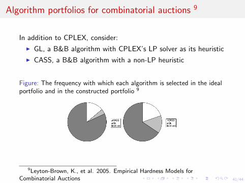
Algorithm portfolios for combinatorial auctions 9

In addition to CPLEX, consider:

I GL, a B&B algorithm with CPLEX’s LP solver as its heuristic

I CASS, a B&B algorithm with a non-LP heuristic

Figure: The frequency with which each algorithm is selected in the idealportfolio and in the constructed portfolio 9

9Leyton-Brown, K., et al. 2005. Empirical Hardness Models forCombinatorial Auctions

42/44

Portfolio-based Algorithm Selection for SAT

I No single ”dominant” SAT solver; different solvers performbest on different instances

I Traditional approach: choose the best solver for a given classof instances

I Make this decision online on a per-instance basis;SATzilla: an automated approach for constructingper-instance algorithm portfolios for SAT that use empiricalhardness models to choose among their constituent solvers

I SAT algorithms: tree-search algorithms, local searchalgorithms, resolution-based approaches

43/44

Algorithm selection and algorithm configuration

I Algorithm selection operates on finite (small) sets ofalgorithms; algorithm configuration operates on thecombinatorial space of an algorithm’s parameter settings.

I AClib a benchmark library for instances of the algorithmconfiguration problem http://aclib.net

ASlib a Benchmark Library for Algorithm Selectionhttp://www.coseal.net/aslib/; Experiments on AClib -more costly than experiments on ASlib

I ASlib and AClib can be combined: generate actualperformance data based on the resources in AClib and thencreate an ASlib scenario which selects between different solverconfigurations on a per-instance basis

44/44

Bibliography

I F. Hutter et al. Algorithm runtime prediction: Methods &evaluation, Artificial Intelligence 206, 79-111, 2014

I M. Feurer et al. Efficient and Robust Automated Machine Learning,NIPS 28, 2962-2970, 2015

I K. Smith-Miles. Cross-Disciplinary Perspectives on Meta-Learningfor Algorithm Selection, ACM Computing Surveys 41(1), 2009

I L. Kotthoff. Algorithm Selection for Combinatorial Search Problems:A survey, Data Mining and Constraint Programming, 149-190, 2016

I K. Leyton-Brown et al. Empirical Hardness Models forCombinatorial Auctions, ch. 19, 2005