Embed Size (px)
Citation preview
CMU SCS
Mining Large Graphs and Fraud Detection
Christos Faloutsos CMU
CMU SCS
Thank you! Dr. Dragos Margineantu
Dr. Mohammed Zaki
Kimberly Mathern
Lawrence Tingson
MLDAS, Doha 2015 (c) 2015, C. Faloutsos 2
CMU SCS
(c) 2015, C. Faloutsos 3
Roadmap
• Introduction – Motivation – Why study (big) graphs?
• Part#1: Patterns in graphs • Part#2: time-evolving graphs; tensors • Conclusions
MLDAS, Doha 2015
CMU SCS
(c) 2015, C. Faloutsos 4
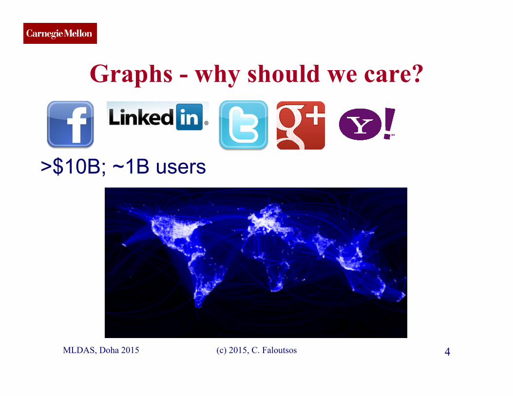
Graphs - why should we care?
>$10B; ~1B users
MLDAS, Doha 2015

CMU SCS
(c) 2015, C. Faloutsos 5
Graphs - why should we care?
Internet Map [lumeta.com]
Food Web [Martinez ’91]
MLDAS, Doha 2015
CMU SCS
(c) 2015, C. Faloutsos 6
Graphs - why should we care? • web-log (‘blog’) news propagation • computer network security: email/IP traffic and
anomaly detection • Recommendation systems • ....
• Many-to-many db relationship -> graph
MLDAS, Doha 2015
CMU SCS
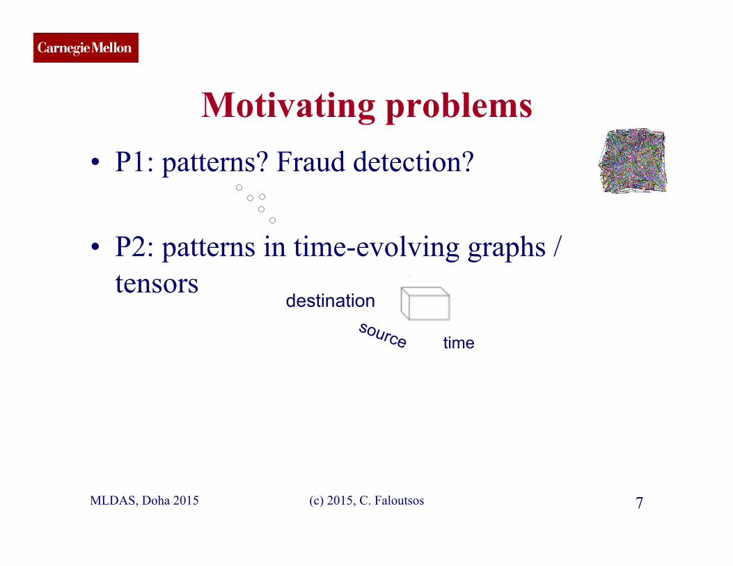
Motivating problems • P1: patterns? Fraud detection?
• P2: patterns in time-evolving graphs / tensors
MLDAS, Doha 2015 (c) 2015, C. Faloutsos 7
time
destination
CMU SCS
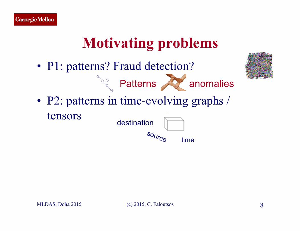
Motivating problems • P1: patterns? Fraud detection?
• P2: patterns in time-evolving graphs / tensors
MLDAS, Doha 2015 (c) 2015, C. Faloutsos 8
time
destination
Patterns anomalies

CMU SCS
(c) 2015, C. Faloutsos 9
Roadmap
• Introduction – Motivation – Why study (big) graphs?
• Part#1: Patterns & fraud detection • Part#2: time-evolving graphs; tensors • Conclusions
MLDAS, Doha 2015

CMU SCS
MLDAS, Doha 2015 (c) 2015, C. Faloutsos 10
Part 1: Patterns, &
fraud detection
CMU SCS
(c) 2015, C. Faloutsos 11
Laws and patterns • Q1: Are real graphs random?
MLDAS, Doha 2015
CMU SCS
(c) 2015, C. Faloutsos 12
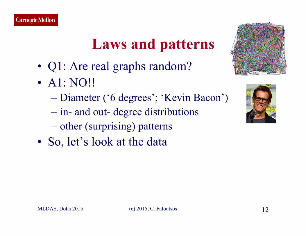
Laws and patterns • Q1: Are real graphs random? • A1: NO!!
– Diameter (‘6 degrees’; ‘Kevin Bacon’) – in- and out- degree distributions – other (surprising) patterns
• So, let’s look at the data
MLDAS, Doha 2015
CMU SCS
(c) 2015, C. Faloutsos 13
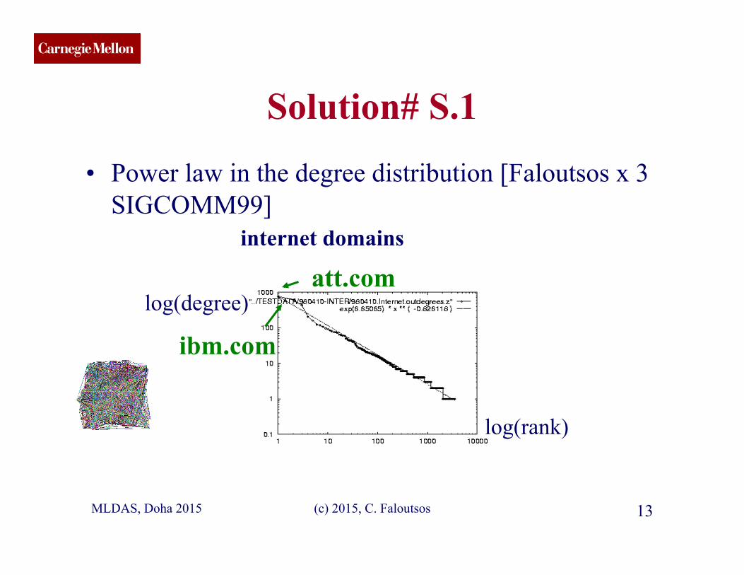
Solution# S.1 • Power law in the degree distribution [Faloutsos x 3
SIGCOMM99]
log(rank)
log(degree)
internet domains
att.com
ibm.com
MLDAS, Doha 2015
CMU SCS
(c) 2015, C. Faloutsos 14
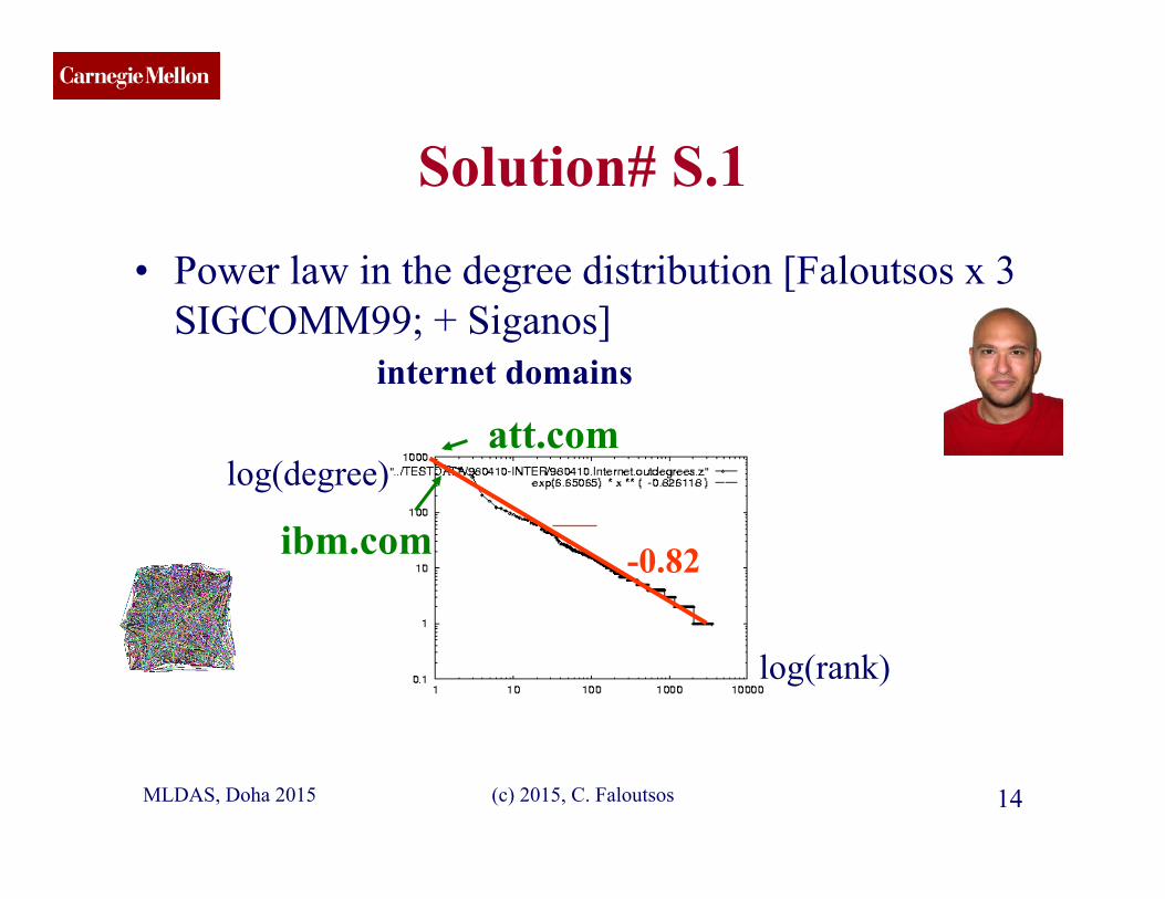
Solution# S.1 • Power law in the degree distribution [Faloutsos x 3
SIGCOMM99; + Siganos]
log(rank)
log(degree)
-0.82
internet domains
att.com
ibm.com
MLDAS, Doha 2015

CMU SCS
(c) 2015, C. Faloutsos 15
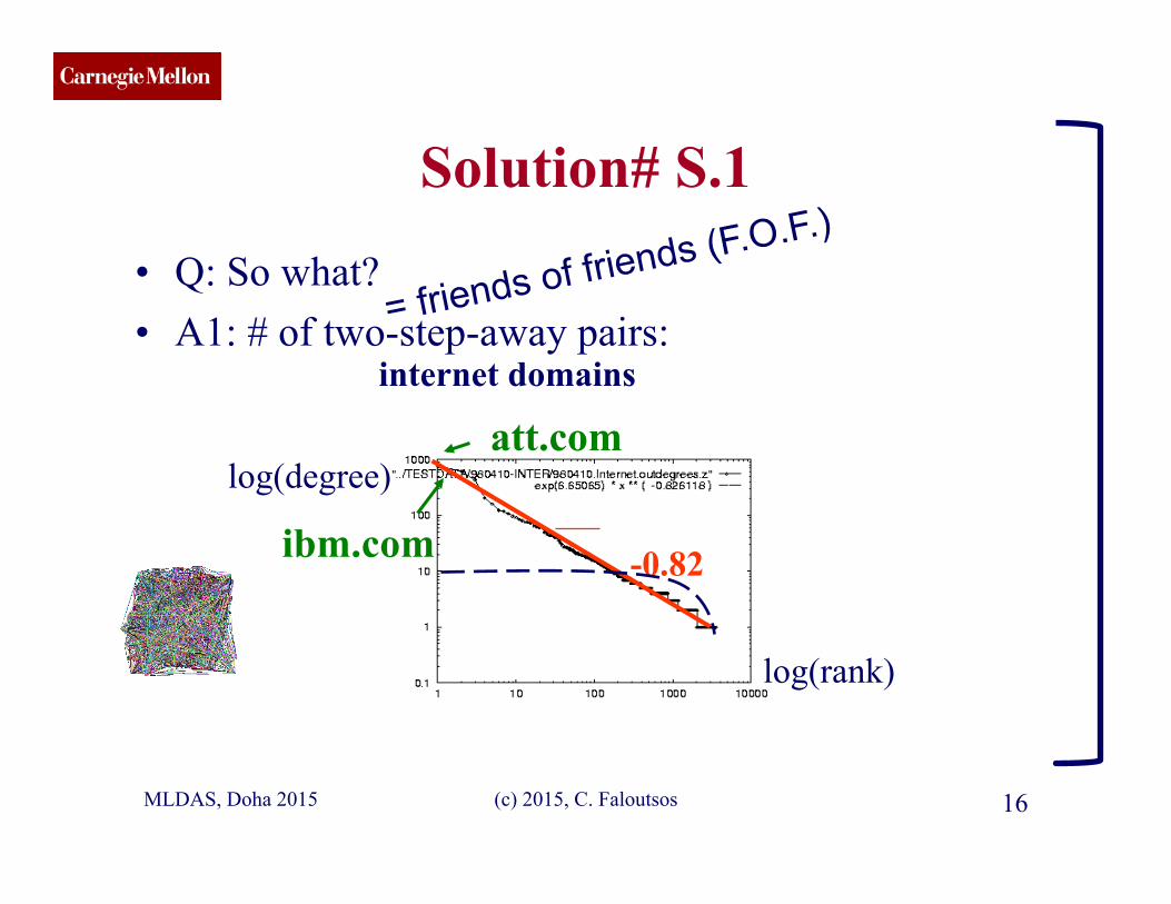
Solution# S.1 • Q: So what?
log(rank)
log(degree)
-0.82
internet domains
att.com
ibm.com
MLDAS, Doha 2015
CMU SCS
(c) 2015, C. Faloutsos 16
Solution# S.1 • Q: So what? • A1: # of two-step-away pairs:
log(rank)
log(degree)
-0.82
internet domains
att.com
ibm.com
MLDAS, Doha 2015
= friends of friends (F.O.F.)

CMU SCS
(c) 2015, C. Faloutsos 17
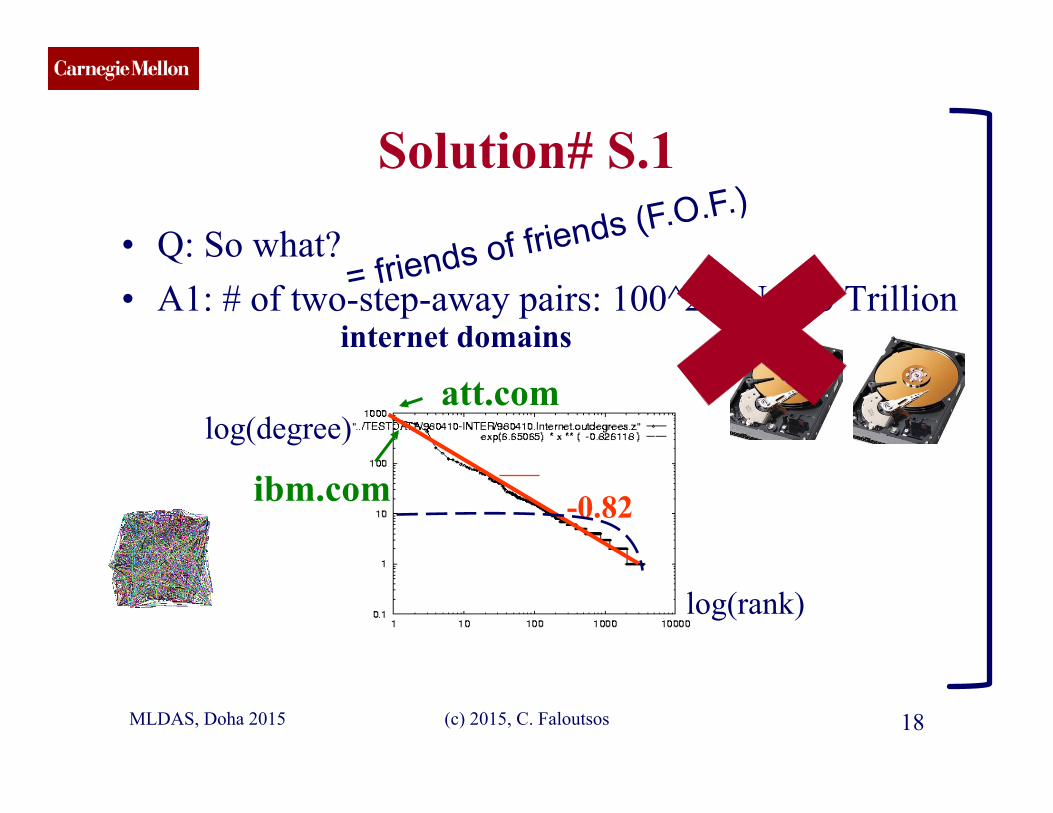
Solution# S.1 • Q: So what? • A1: # of two-step-away pairs: 100^2 * N= 10 Trillion
log(rank)
log(degree)
-0.82
internet domains
att.com
ibm.com
MLDAS, Doha 2015
= friends of friends (F.O.F.)
CMU SCS
(c) 2015, C. Faloutsos 18
Solution# S.1 • Q: So what? • A1: # of two-step-away pairs: 100^2 * N= 10 Trillion
log(rank)
log(degree)
-0.82
internet domains
att.com
ibm.com
MLDAS, Doha 2015
= friends of friends (F.O.F.)
CMU SCS
(c) 2015, C. Faloutsos 19
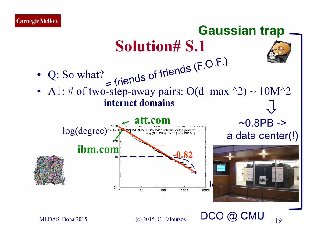
Solution# S.1 • Q: So what? • A1: # of two-step-away pairs: O(d_max ^2) ~ 10M^2
log(rank)
log(degree)
-0.82
internet domains
att.com
ibm.com
MLDAS, Doha 2015
~0.8PB -> a data center(!)
DCO @ CMU
Gaussian trap
= friends of friends (F.O.F.)

CMU SCS
(c) 2015, C. Faloutsos 20
Solution# S.1 • Q: So what? • A1: # of two-step-away pairs: O(d_max ^2) ~ 10M^2
log(rank)
log(degree)
-0.82
internet domains
att.com
ibm.com
MLDAS, Doha 2015
~0.8PB -> a data center(!)
Gaussian trap
CMU SCS
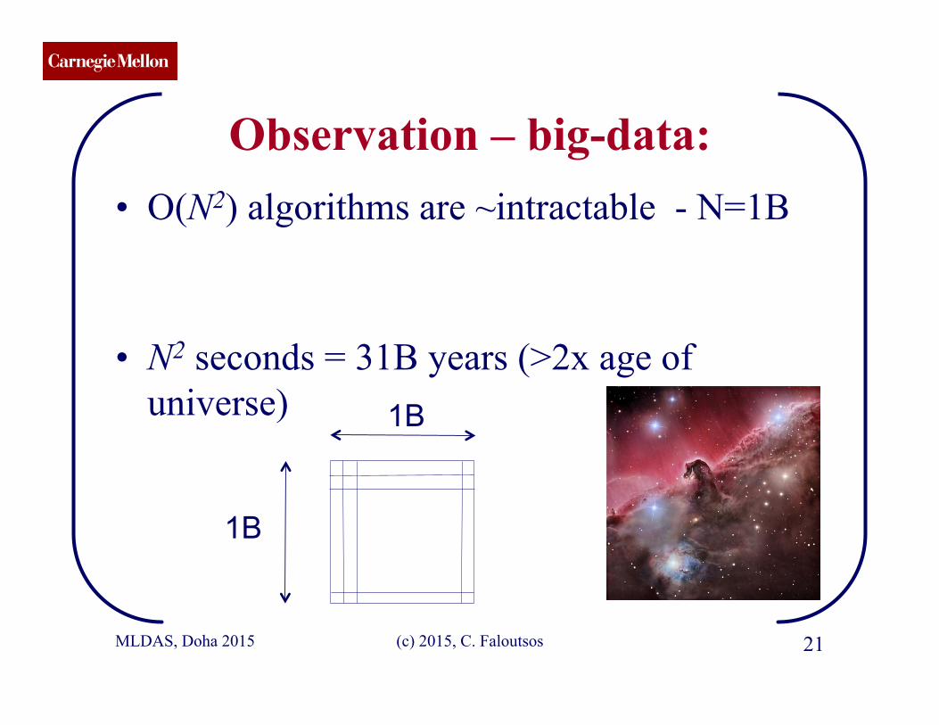
Observation – big-data: • O(N2) algorithms are ~intractable - N=1B
• N2 seconds = 31B years (>2x age of universe)
MLDAS, Doha 2015 (c) 2015, C. Faloutsos 21
1B
1B
CMU SCS
(c) 2015, C. Faloutsos 22
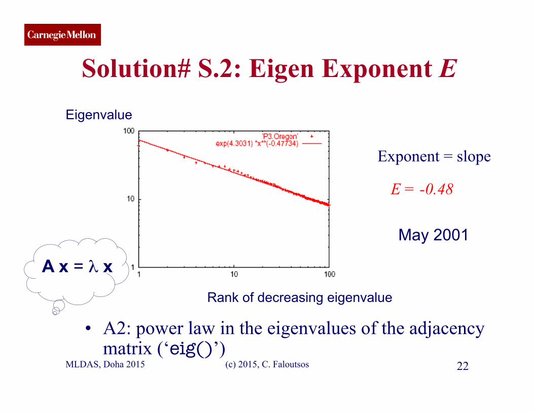
Solution# S.2: Eigen Exponent E
• A2: power law in the eigenvalues of the adjacency matrix (‘eig()’)
E = -0.48
Exponent = slope
Eigenvalue
Rank of decreasing eigenvalue
May 2001
MLDAS, Doha 2015
A x = λ x

CMU SCS
(c) 2015, C. Faloutsos 23
Roadmap
• Introduction – Motivation • Part#1: Patterns in graphs
– Patterns: Degree; Triangles – Anomaly/fraud detection – Graph understanding
• Part#2: time-evolving graphs; tensors • Conclusions
MLDAS, Doha 2015

CMU SCS
(c) 2015, C. Faloutsos 24
Solution# S.3: Triangle ‘Laws’
• Real social networks have a lot of triangles
MLDAS, Doha 2015

CMU SCS
(c) 2015, C. Faloutsos 25
Solution# S.3: Triangle ‘Laws’
• Real social networks have a lot of triangles – Friends of friends are friends
• Any patterns? – 2x the friends, 2x the triangles ?
MLDAS, Doha 2015
CMU SCS
(c) 2015, C. Faloutsos 26
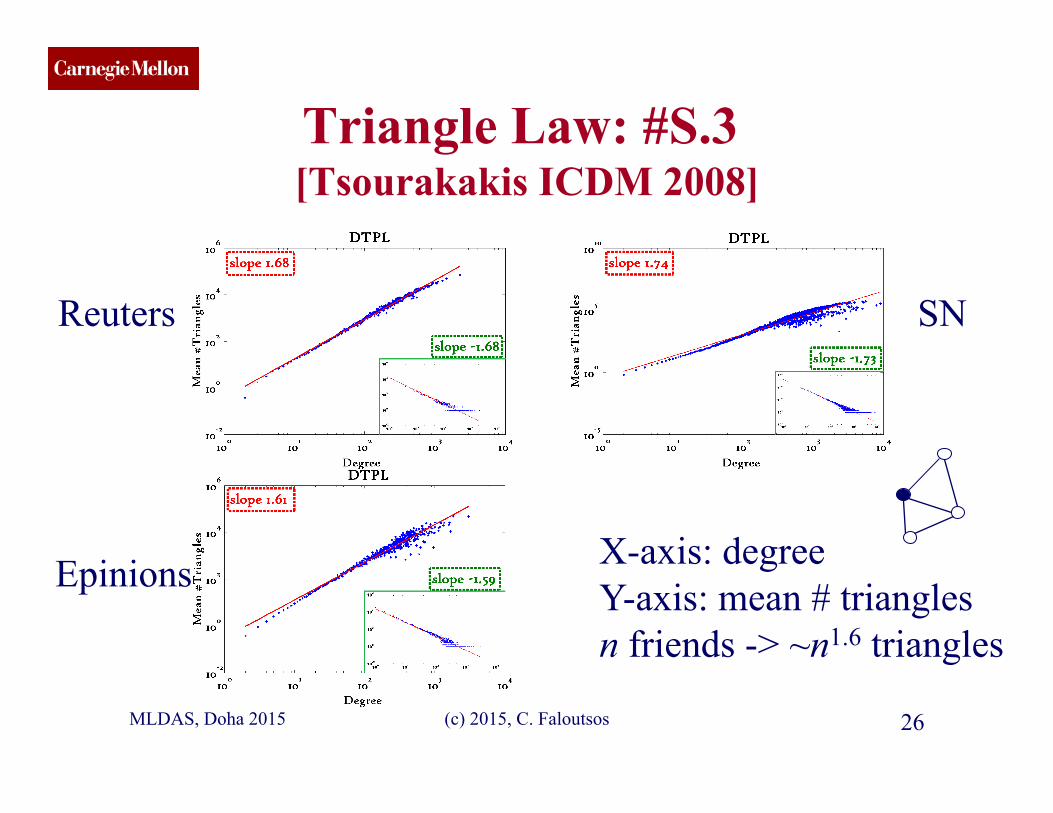
Triangle Law: #S.3 [Tsourakakis ICDM 2008]
SN Reuters
Epinions X-axis: degree Y-axis: mean # triangles n friends -> ~n1.6 triangles
MLDAS, Doha 2015
CMU SCS
(c) 2015, C. Faloutsos 27
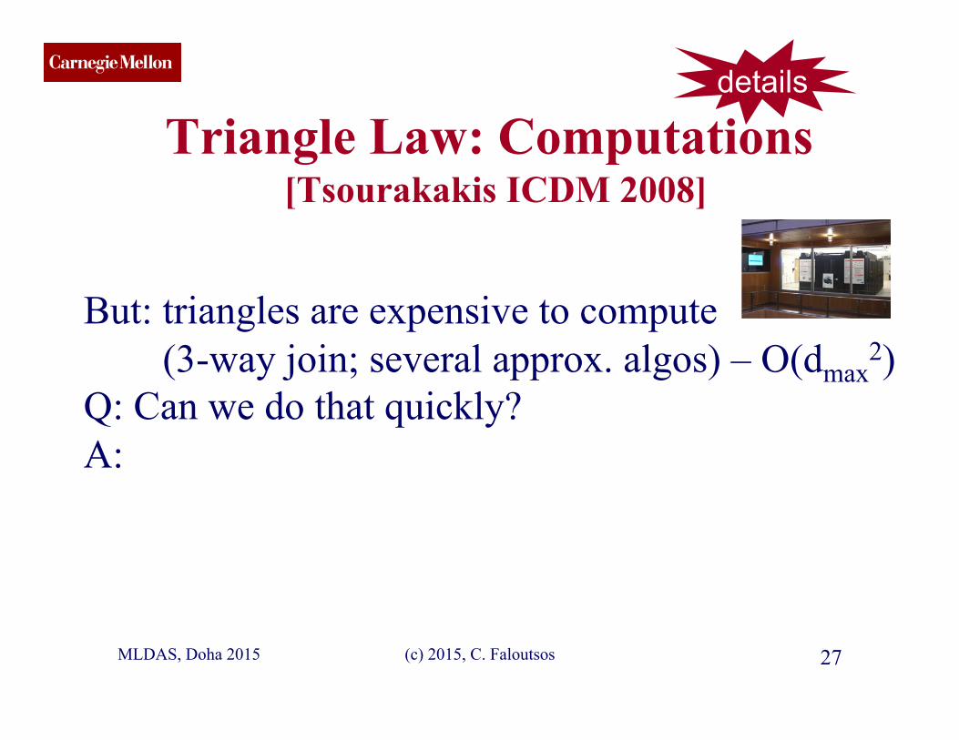
Triangle Law: Computations [Tsourakakis ICDM 2008]
But: triangles are expensive to compute (3-way join; several approx. algos) – O(dmax
2) Q: Can we do that quickly? A:
details
MLDAS, Doha 2015

CMU SCS
(c) 2015, C. Faloutsos 28
Triangle Law: Computations [Tsourakakis ICDM 2008]
But: triangles are expensive to compute (3-way join; several approx. algos) – O(dmax
2) Q: Can we do that quickly? A: Yes!
#triangles = 1/6 Sum ( λi3 )
(and, because of skewness (S2) , we only need the top few eigenvalues! - O(E)
MLDAS, Doha 2015
A x = λ x
details
CMU SCS
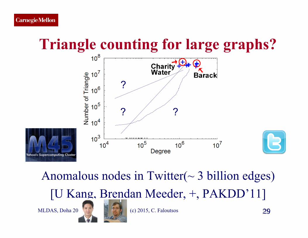
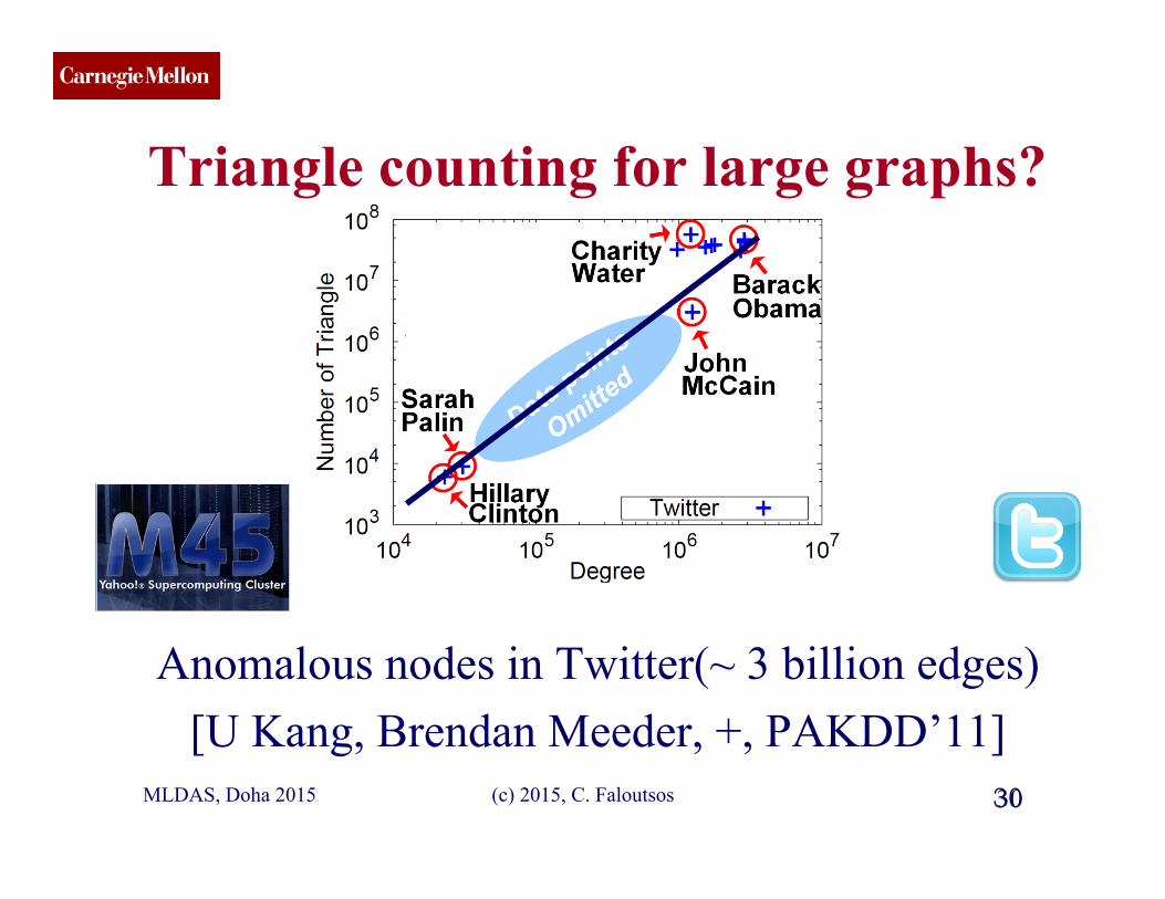
Triangle counting for large graphs?
Anomalous nodes in Twitter(~ 3 billion edges) [U Kang, Brendan Meeder, +, PAKDD’11]
29 MLDAS, Doha 2015 29 (c) 2015, C. Faloutsos
? ?
?
CMU SCS
Triangle counting for large graphs?
Anomalous nodes in Twitter(~ 3 billion edges) [U Kang, Brendan Meeder, +, PAKDD’11]
30 MLDAS, Doha 2015 30 (c) 2015, C. Faloutsos
CMU SCS
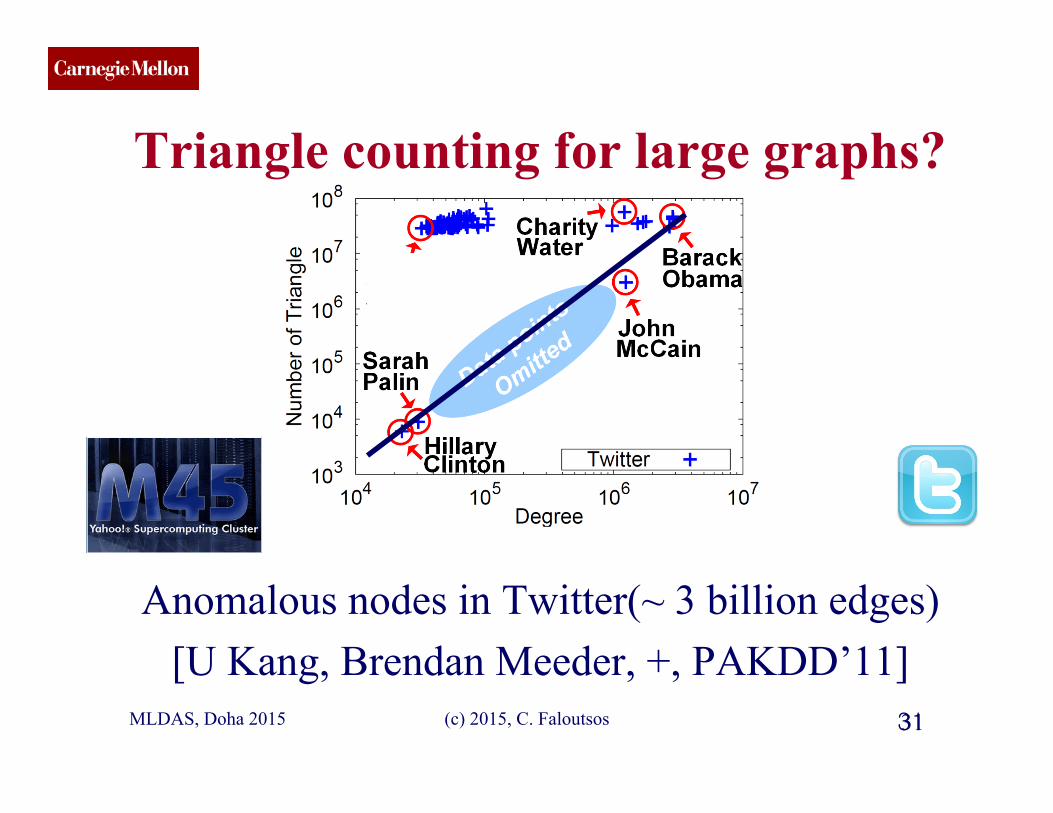
Triangle counting for large graphs?
Anomalous nodes in Twitter(~ 3 billion edges) [U Kang, Brendan Meeder, +, PAKDD’11]
31 MLDAS, Doha 2015 31 (c) 2015, C. Faloutsos
CMU SCS
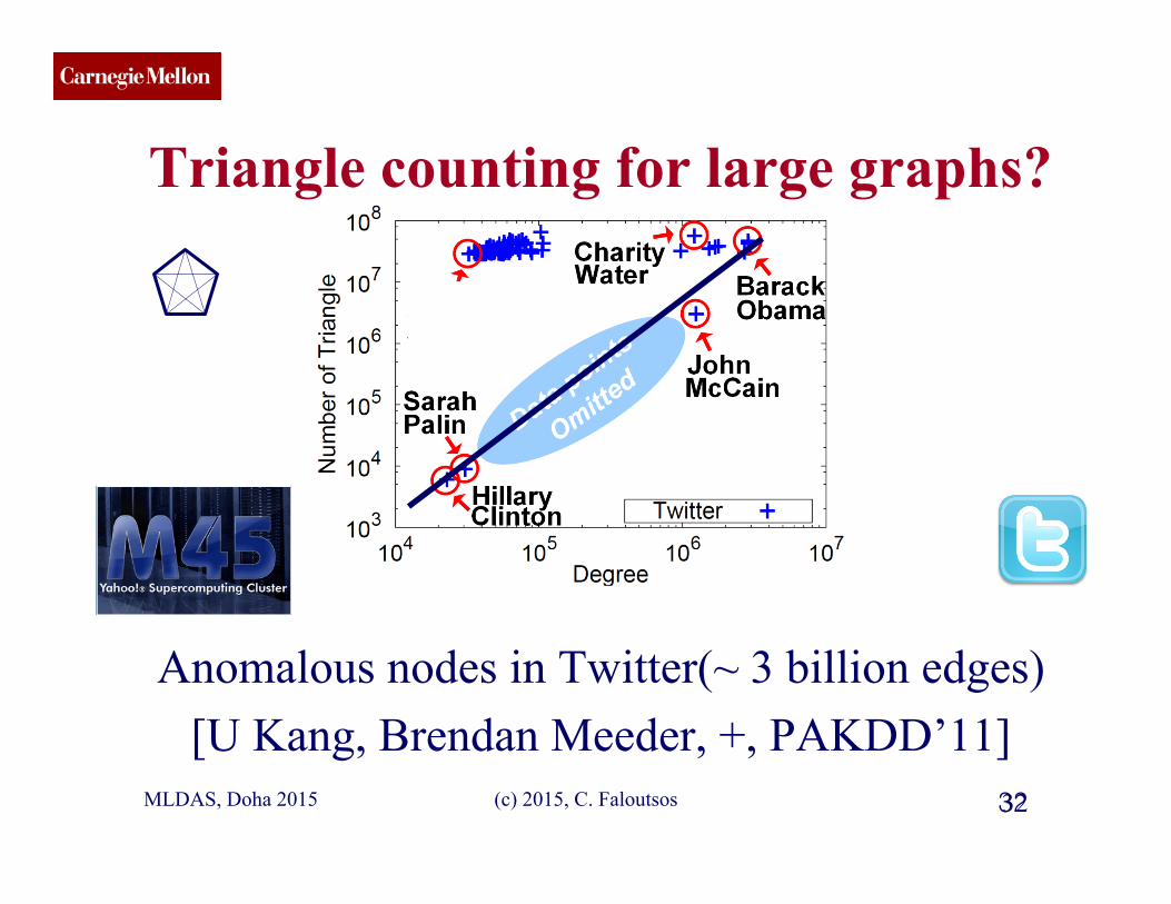
Triangle counting for large graphs?
Anomalous nodes in Twitter(~ 3 billion edges) [U Kang, Brendan Meeder, +, PAKDD’11]
32 MLDAS, Doha 2015 32 (c) 2015, C. Faloutsos
CMU SCS
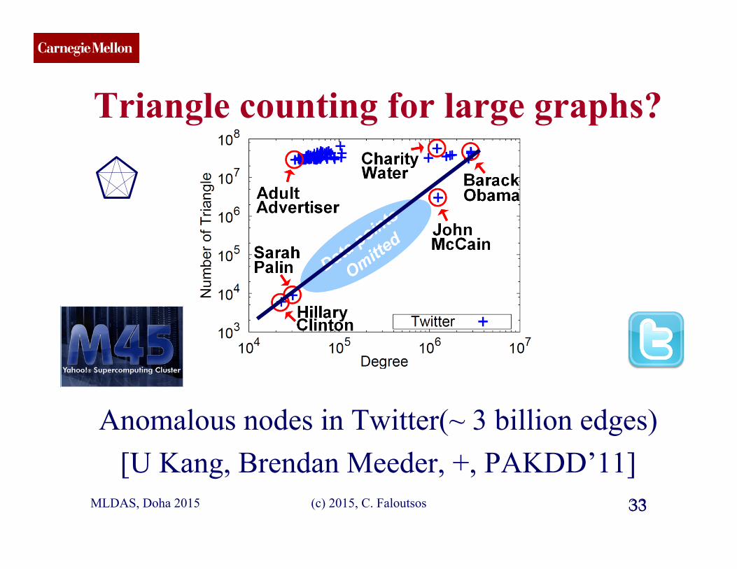
Triangle counting for large graphs?
Anomalous nodes in Twitter(~ 3 billion edges) [U Kang, Brendan Meeder, +, PAKDD’11]
33 MLDAS, Doha 2015 33 (c) 2015, C. Faloutsos
CMU SCS
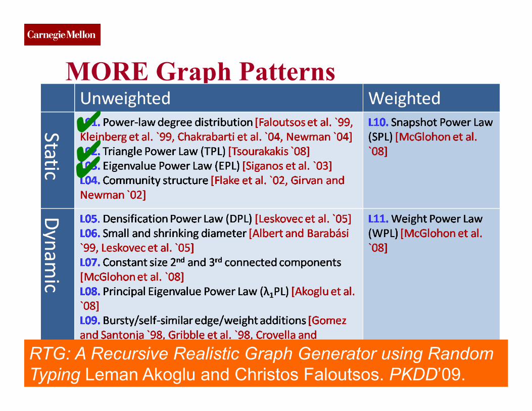
MORE Graph Patterns
MLDAS, Doha 2015 (c) 2015, C. Faloutsos 34
✔ ✔ ✔
RTG: A Recursive Realistic Graph Generator using Random Typing Leman Akoglu and Christos Faloutsos. PKDD’09.
CMU SCS
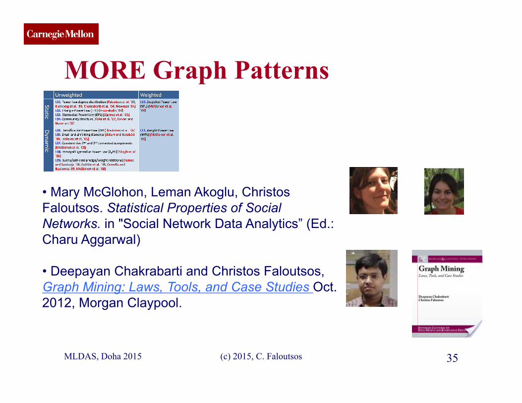
MORE Graph Patterns
MLDAS, Doha 2015 (c) 2015, C. Faloutsos 35
• Mary McGlohon, Leman Akoglu, Christos Faloutsos. Statistical Properties of Social Networks. in "Social Network Data Analytics” (Ed.: Charu Aggarwal)
• Deepayan Chakrabarti and Christos Faloutsos, Graph Mining: Laws, Tools, and Case Studies Oct. 2012, Morgan Claypool.
CMU SCS
(c) 2015, C. Faloutsos 36
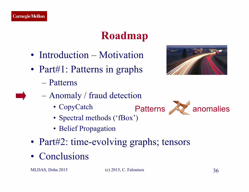
Roadmap
• Introduction – Motivation • Part#1: Patterns in graphs
– Patterns – Anomaly / fraud detection
• CopyCatch • Spectral methods (‘fBox’) • Belief Propagation
• Part#2: time-evolving graphs; tensors • Conclusions MLDAS, Doha 2015
Patterns anomalies
CMU SCS
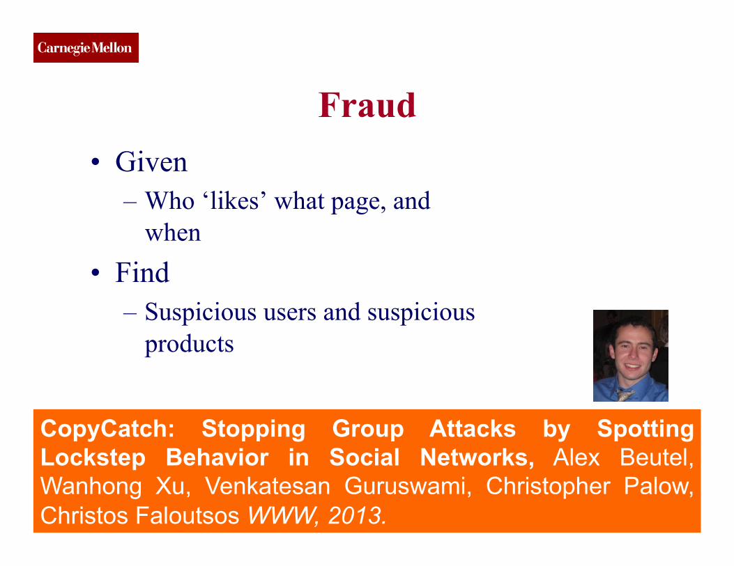
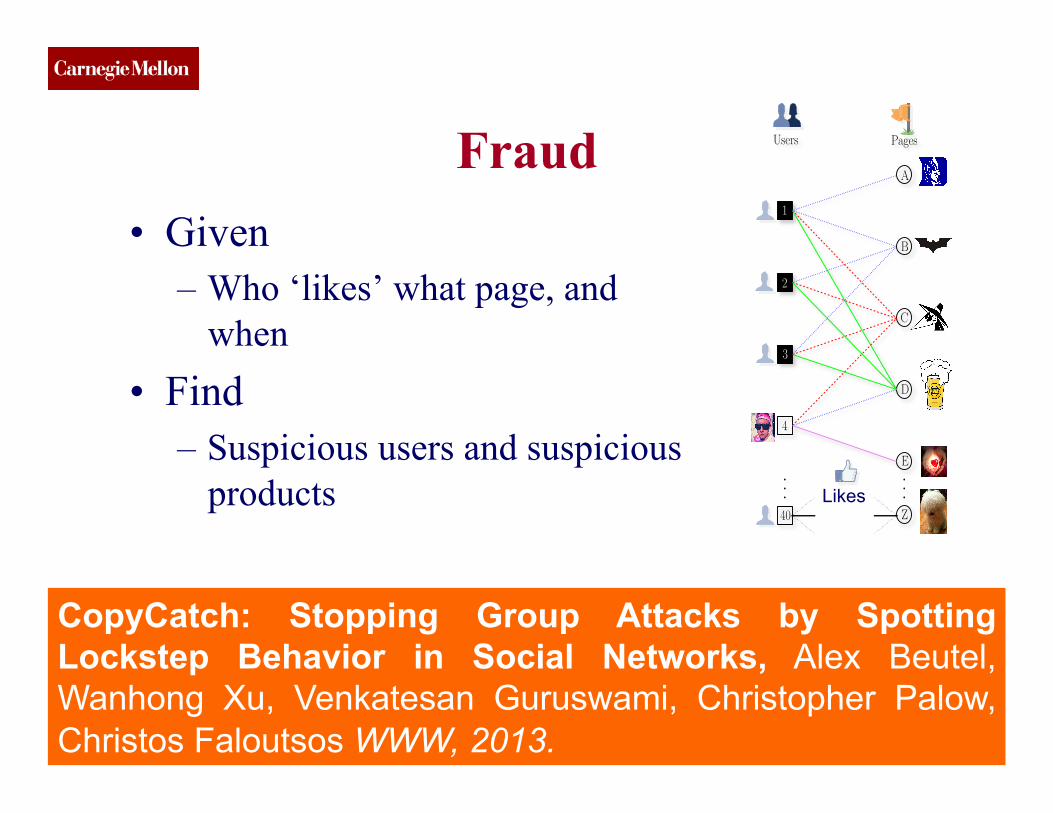
Fraud • Given
– Who ‘likes’ what page, and when
• Find – Suspicious users and suspicious
products
MLDAS, Doha 2015 (c) 2015, C. Faloutsos 37
CopyCatch: Stopping Group Attacks by Spotting Lockstep Behavior in Social Networks, Alex Beutel, Wanhong Xu, Venkatesan Guruswami, Christopher Palow, Christos Faloutsos WWW, 2013.
CMU SCS
Fraud • Given
– Who ‘likes’ what page, and when
• Find – Suspicious users and suspicious
products
MLDAS, Doha 2015 (c) 2015, C. Faloutsos 38
CopyCatch: Stopping Group Attacks by Spotting Lockstep Behavior in Social Networks, Alex Beutel, Wanhong Xu, Venkatesan Guruswami, Christopher Palow, Christos Faloutsos WWW, 2013.
Users Pages
A
B
C
D
E
1
2
3
4
40 Z
Likes
CMU SCS
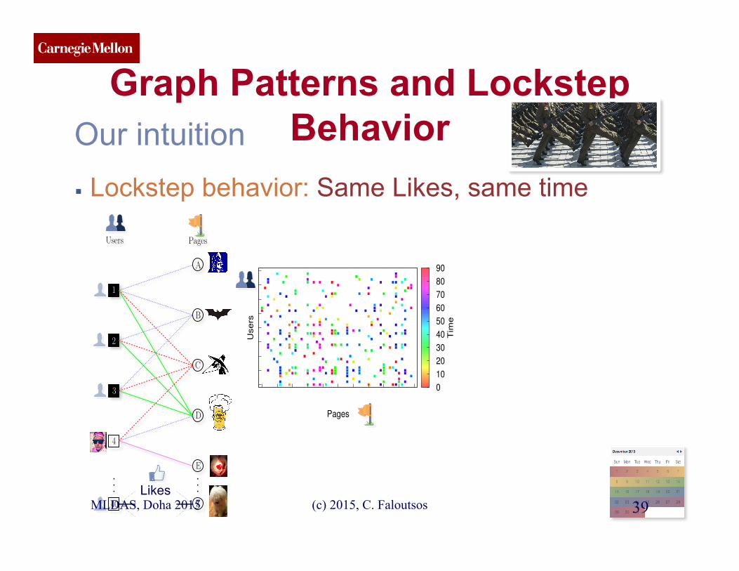
Our intuition ▪ Lockstep behavior: Same Likes, same time
Graph Patterns and Lockstep Behavior
Pages
Users
0
10
20
30
40
50
60
70
80
90
Tim
e
Users Pages
A
B
C
D
E
1
2
3
4
40 Z
Likes MLDAS, Doha 2015 39 (c) 2015, C. Faloutsos
CMU SCS
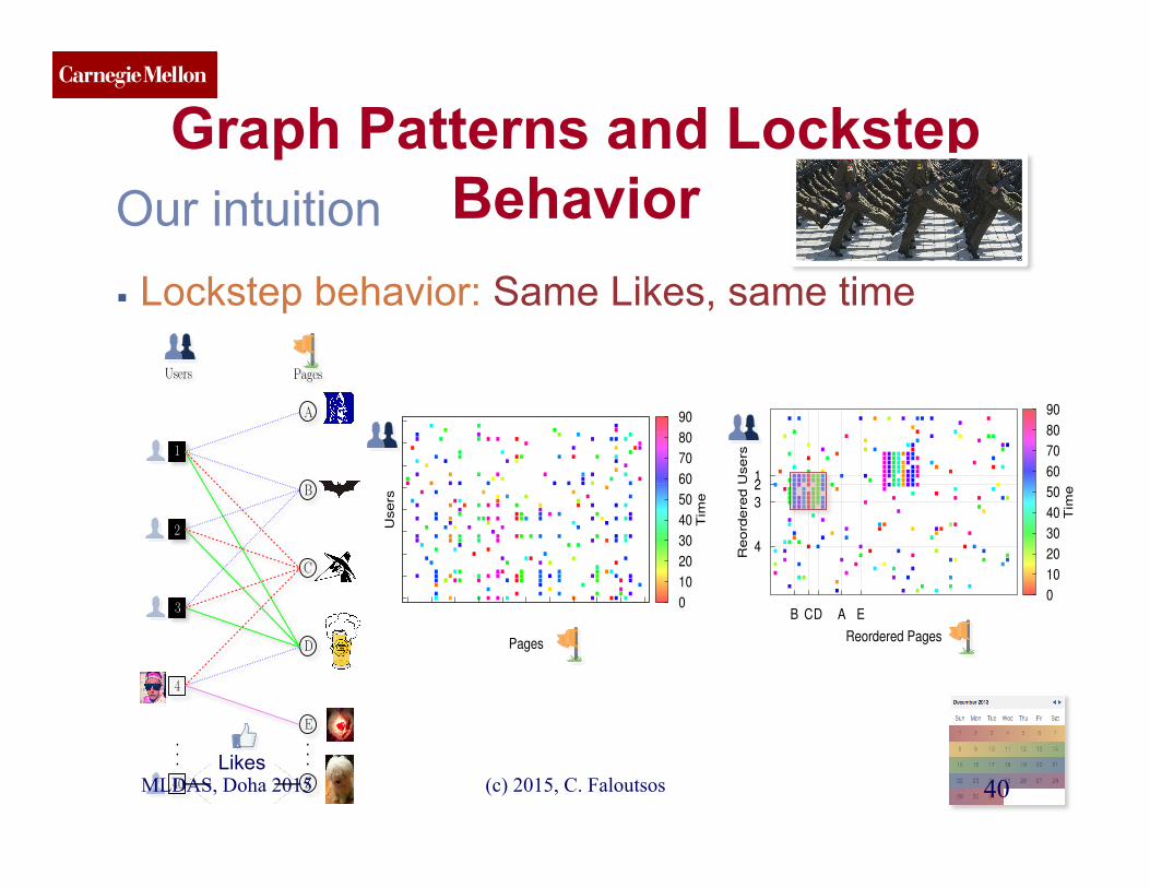
Our intuition ▪ Lockstep behavior: Same Likes, same time
Graph Patterns and Lockstep Behavior
Users Pages
A
B
C
D
E
1
2
3
4
40 Z
Pages
Users
0
10
20
30
40
50
60
70
80
90
Tim
e
B CD A E
Reordered Pages
4
3 2 1
Reord
ere
d U
sers
0
10
20
30
40
50
60
70
80
90
Tim
e
Likes MLDAS, Doha 2015 40 (c) 2015, C. Faloutsos
CMU SCS
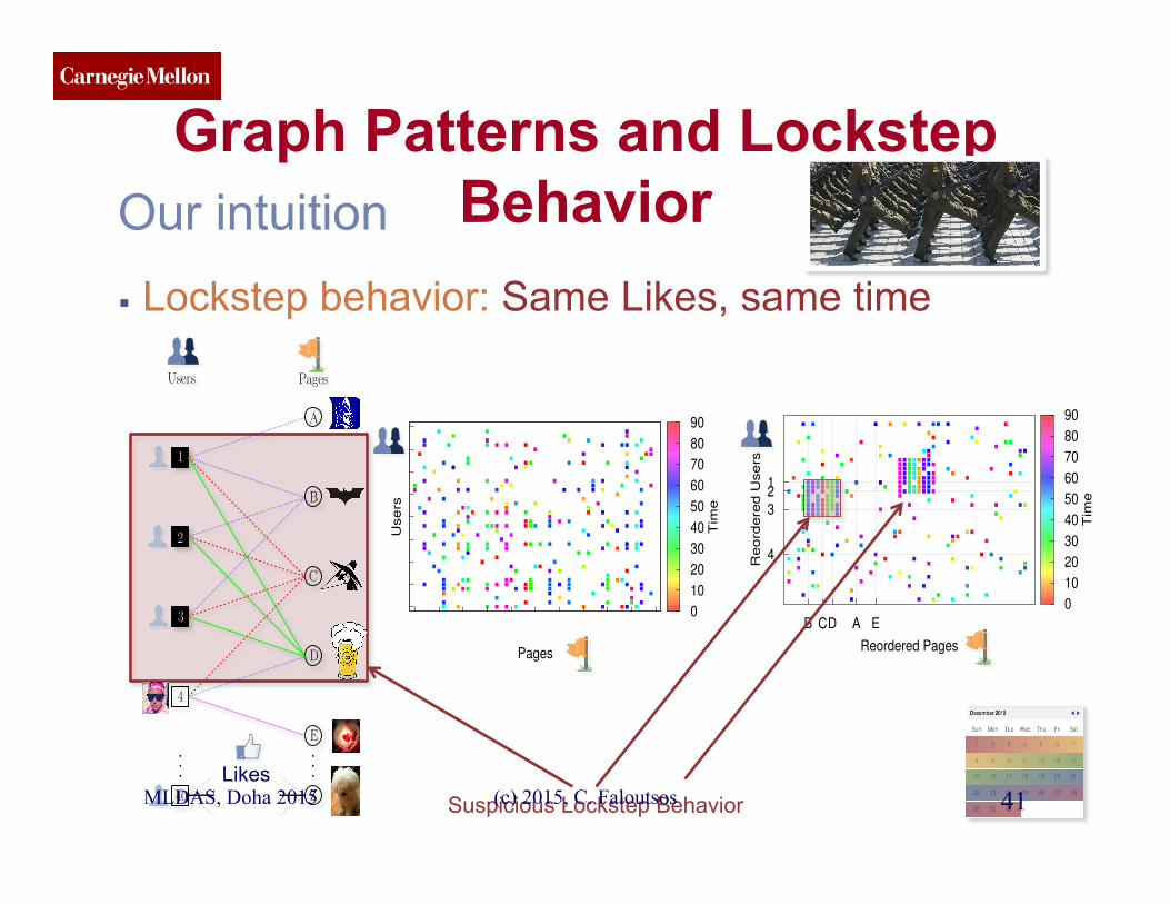
Our intuition ▪ Lockstep behavior: Same Likes, same time
Graph Patterns and Lockstep Behavior
Users Pages
A
B
C
D
E
1
2
3
4
40 Z
Pages
Users
0
10
20
30
40
50
60
70
80
90
Tim
e
B CD A E
Reordered Pages
4
3 2 1
Reord
ere
d U
sers
0
10
20
30
40
50
60
70
80
90
Tim
e
Suspicious Lockstep Behavior Likes
MLDAS, Doha 2015 41 (c) 2015, C. Faloutsos
CMU SCS
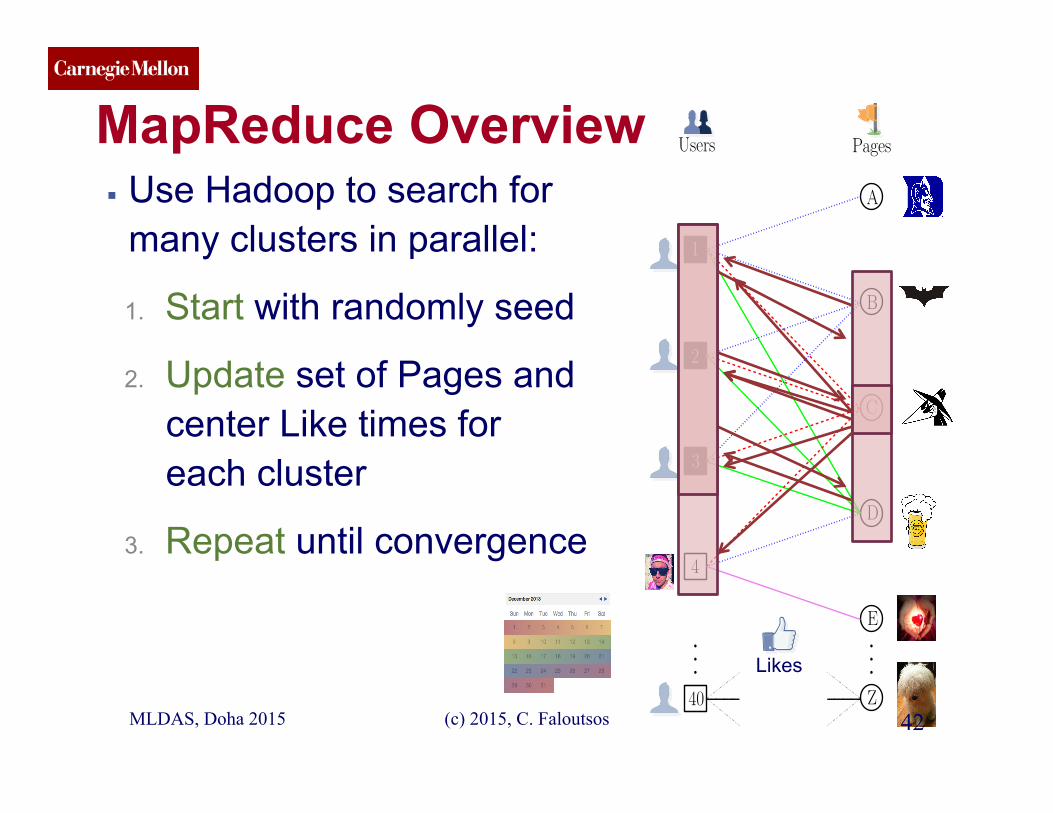
MapReduce Overview ▪ Use Hadoop to search for
many clusters in parallel:
1. Start with randomly seed
2. Update set of Pages and center Like times for each cluster
3. Repeat until convergence
Users Pages
A
B
C
D
E
1
2
3
4
40 Z
Likes
MLDAS, Doha 2015 42 (c) 2015, C. Faloutsos
CMU SCS
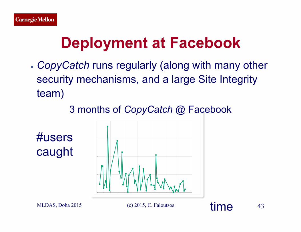
Deployment at Facebook ▪ CopyCatch runs regularly (along with many other
security mechanisms, and a large Site Integrity team)
08/25 09/08 09/22 10/06 10/20 11/03 11/17 12/01
Num
ber
of u
sers
cau
ght
Date of CopyCatch run
3 months of CopyCatch @ Facebook
#users caught
time MLDAS, Doha 2015 43 (c) 2015, C. Faloutsos
CMU SCS
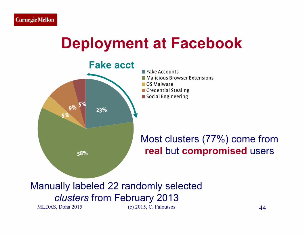
Deployment at Facebook
23%
58%
5%9%
5%
Fake AccountsMalicious Browser ExtensionsOS MalwareCredential StealingSocial Engineering
Manually labeled 22 randomly selected clusters from February 2013
Most clusters (77%) come from real but compromised users
Fake acct
MLDAS, Doha 2015 44 (c) 2015, C. Faloutsos
CMU SCS
(c) 2015, C. Faloutsos 45
Roadmap
• Introduction – Motivation • Part#1: Patterns in graphs
– Patterns – Anomaly / fraud detection
• CopyCatch • Spectral methods (‘fBox’) • Belief Propagation
• Part#2: time-evolving graphs; tensors • Conclusions MLDAS, Doha 2015
CMU SCS
(c) 2015, C. Faloutsos 46
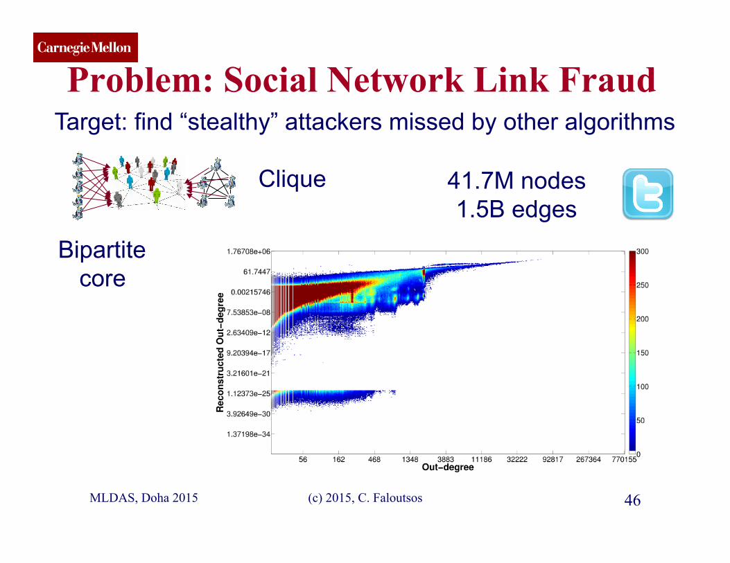
Problem: Social Network Link Fraud
MLDAS, Doha 2015
Target: find “stealthy” attackers missed by other algorithms
Clique
Bipartite core
41.7M nodes 1.5B edges

CMU SCS
(c) 2015, C. Faloutsos 47
Problem: Social Network Link Fraud
MLDAS, Doha 2015
Neil Shah, Alex Beutel, Brian Gallagher and Christos Faloutsos. Spotting Suspicious Link Behavior with fBox: An Adversarial Perspective. ICDM 2014, Shenzhen, China.
Target: find “stealthy” attackers missed by other algorithms
Takeaway: use reconstruction error between true/latent representation!

CMU SCS
(c) 2015, C. Faloutsos 48
Roadmap
• Introduction – Motivation • Part#1: Patterns in graphs
– Patterns – Anomaly / fraud detection
• CopyCatch • Spectral methods (‘fBox’) • Belief Propagation
• Part#2: time-evolving graphs; tensors • Conclusions MLDAS, Doha 2015
CMU SCS
MLDAS, Doha 2015 (c) 2015, C. Faloutsos 49
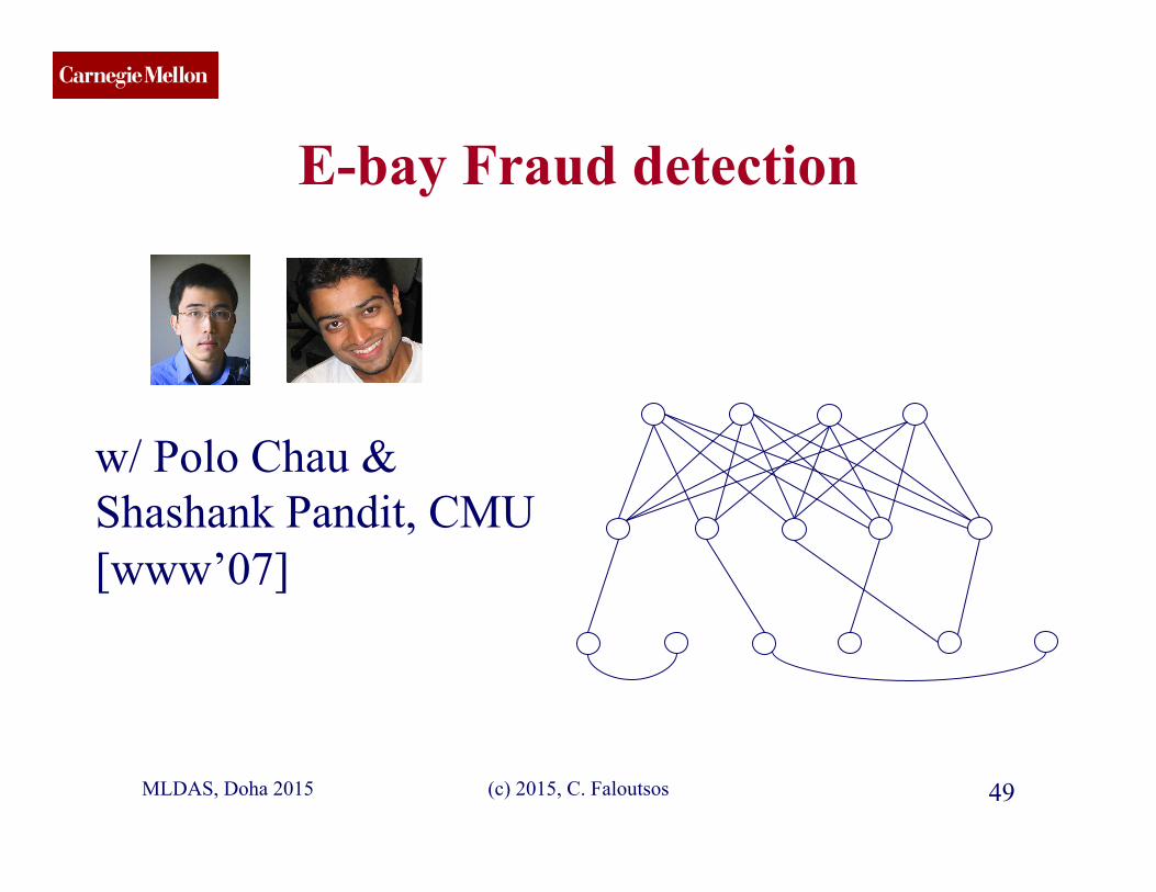
E-bay Fraud detection
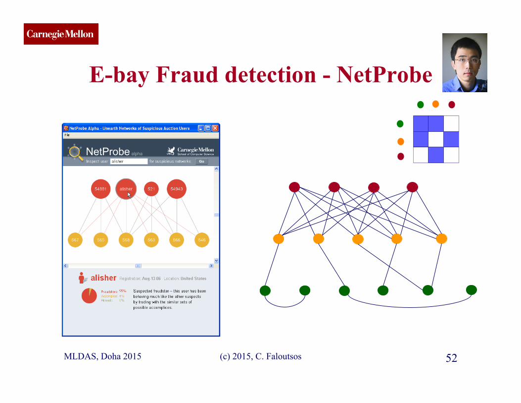
w/ Polo Chau & Shashank Pandit, CMU [www’07]
CMU SCS
MLDAS, Doha 2015 (c) 2015, C. Faloutsos 50
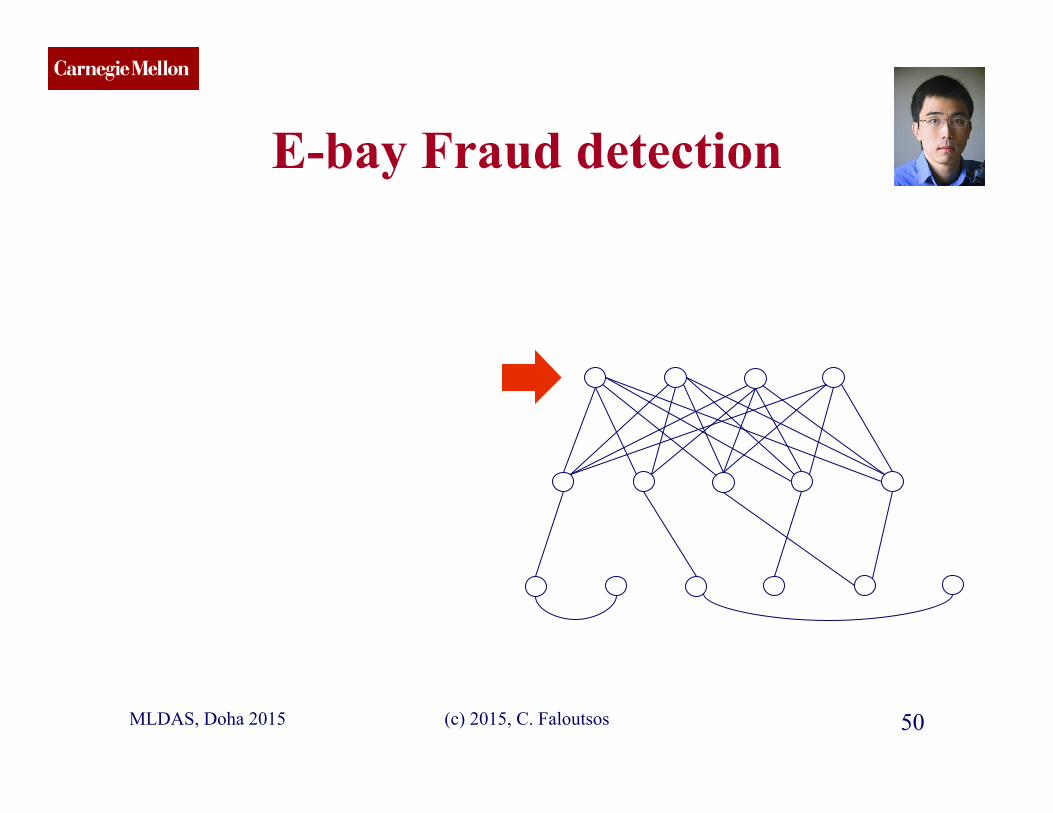
E-bay Fraud detection
CMU SCS
MLDAS, Doha 2015 (c) 2015, C. Faloutsos 51
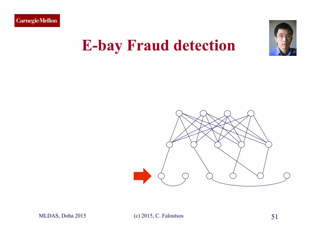
E-bay Fraud detection
CMU SCS
MLDAS, Doha 2015 (c) 2015, C. Faloutsos 52
E-bay Fraud detection - NetProbe

CMU SCS
Popular press
And less desirable attention: • E-mail from ‘Belgium police’ (‘copy of
your code?’) MLDAS, Doha 2015 (c) 2015, C. Faloutsos 53

CMU SCS
(c) 2015, C. Faloutsos 54
Roadmap
• Introduction – Motivation • Part#1: Patterns in graphs
– Patterns – Anomaly / fraud detection
• CopyCatch • Spectral methods (‘fBox’) • Belief Propagation; antivirus app
• Part#2: time-evolving graphs; tensors • Conclusions MLDAS, Doha 2015
CMU SCS
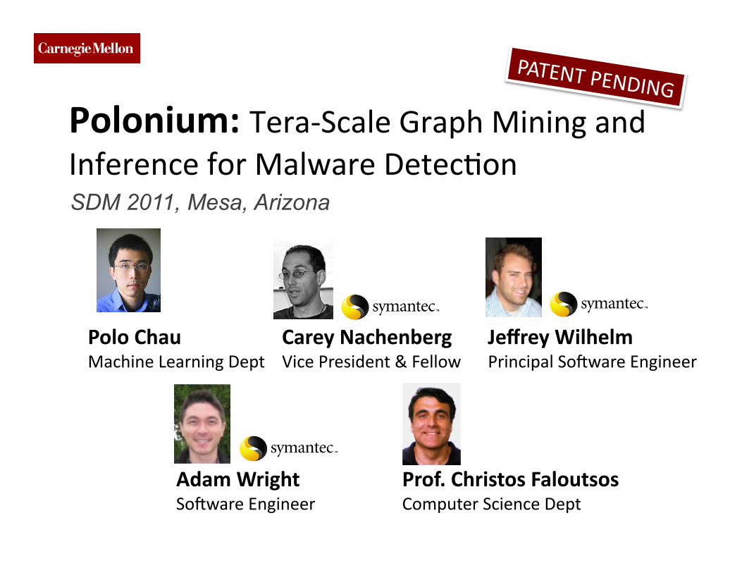
Polo Chau Machine Learning Dept
Carey Nachenberg Vice President & Fellow
Jeffrey Wilhelm Principal So9ware Engineer
Adam Wright So9ware Engineer
Prof. Christos Faloutsos Computer Science Dept
Polonium: Tera-‐Scale Graph Mining and Inference for Malware DetecCon
PATENT PENDING
SDM 2011, Mesa, Arizona
CMU SCS
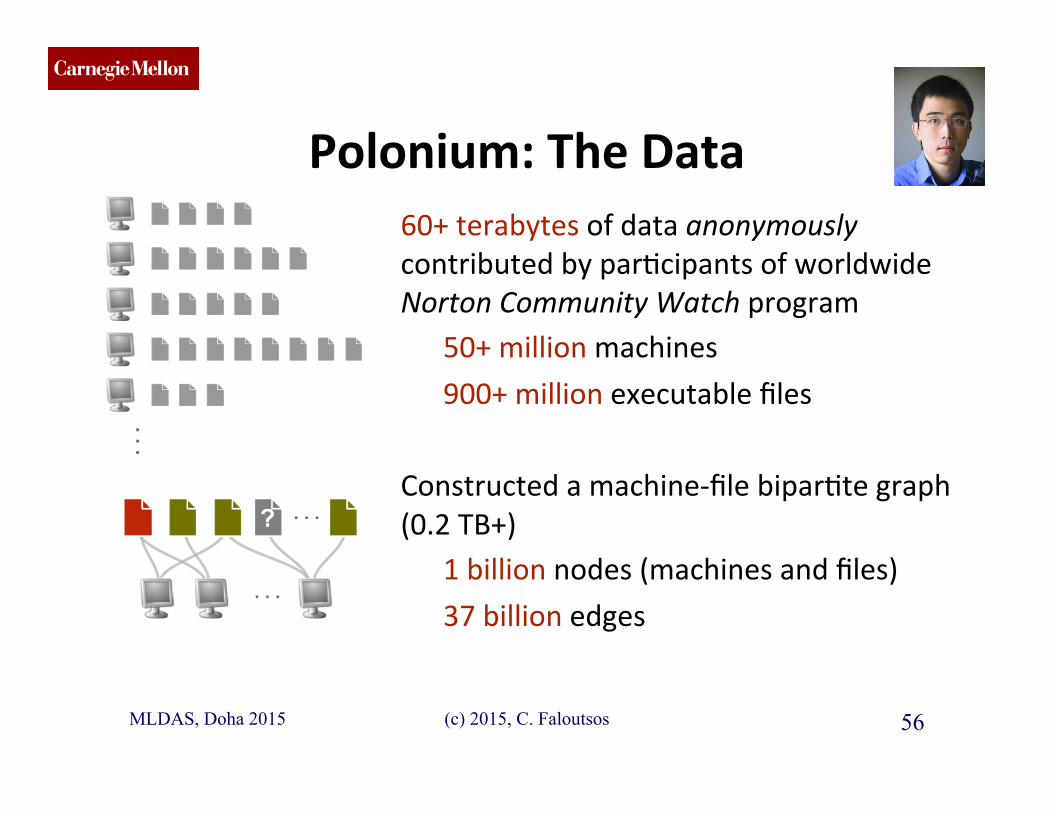
Polonium: The Data 60+ terabytes of data anonymously contributed by parCcipants of worldwide Norton Community Watch program
50+ million machines
900+ million executable files
Constructed a machine-‐file biparCte graph (0.2 TB+)
1 billion nodes (machines and files)
37 billion edges
MLDAS, Doha 2015 56 (c) 2015, C. Faloutsos
CMU SCS
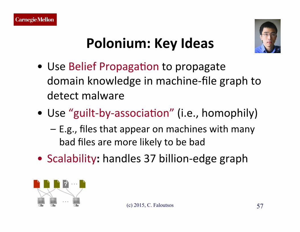
Polonium: Key Ideas
• Use Belief PropagaCon to propagate domain knowledge in machine-‐file graph to detect malware
• Use “guilt-‐by-‐associaCon” (i.e., homophily) – E.g., files that appear on machines with many bad files are more likely to be bad
• Scalability: handles 37 billion-‐edge graph
MLDAS, Doha 2015 57 (c) 2015, C. Faloutsos
CMU SCS
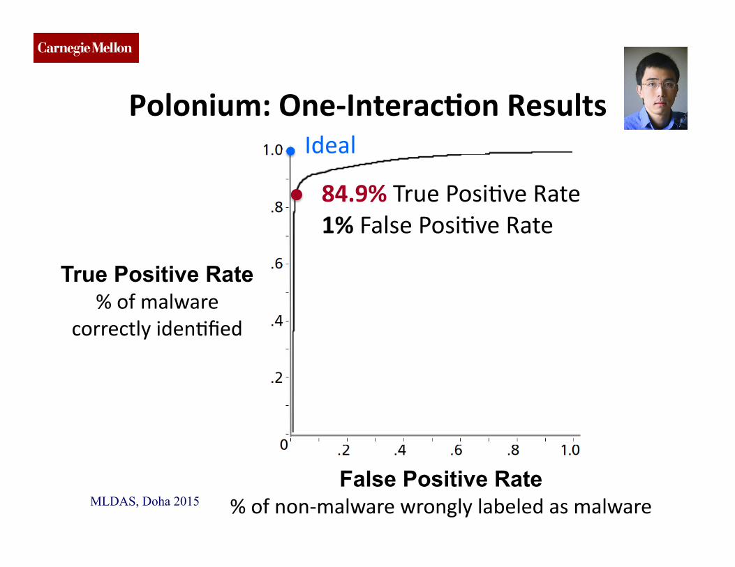
Polonium: One-‐InteracDon Results
84.9% True PosiCve Rate 1% False PosiCve Rate
True Positive Rate % of malware
correctly idenCfied
58
Ideal
MLDAS, Doha 2015 (c) 2015, C. Faloutsos False Positive Rate
% of non-‐malware wrongly labeled as malware

CMU SCS
(c) 2015, C. Faloutsos 59
Roadmap
• Introduction – Motivation • Part#1: Patterns in graphs
– Patterns – Anomaly / fraud detection
• CopyCatch • Spectral methods (‘fBox’) • Belief Propagation; financial fraud
• Part#2: time-evolving graphs; tensors • Conclusions MLDAS, Doha 2015
CMU SCS
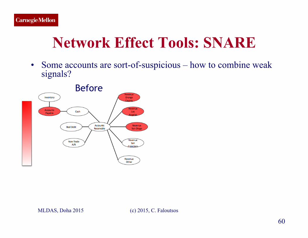
Network Effect Tools: SNARE
60
• Some accounts are sort-of-suspicious – how to combine weak signals?
Before
MLDAS, Doha 2015 (c) 2015, C. Faloutsos
CMU SCS
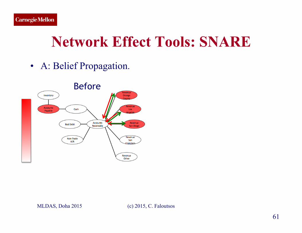
Network Effect Tools: SNARE
61
• A: Belief Propagation.
Before
MLDAS, Doha 2015 (c) 2015, C. Faloutsos
CMU SCS
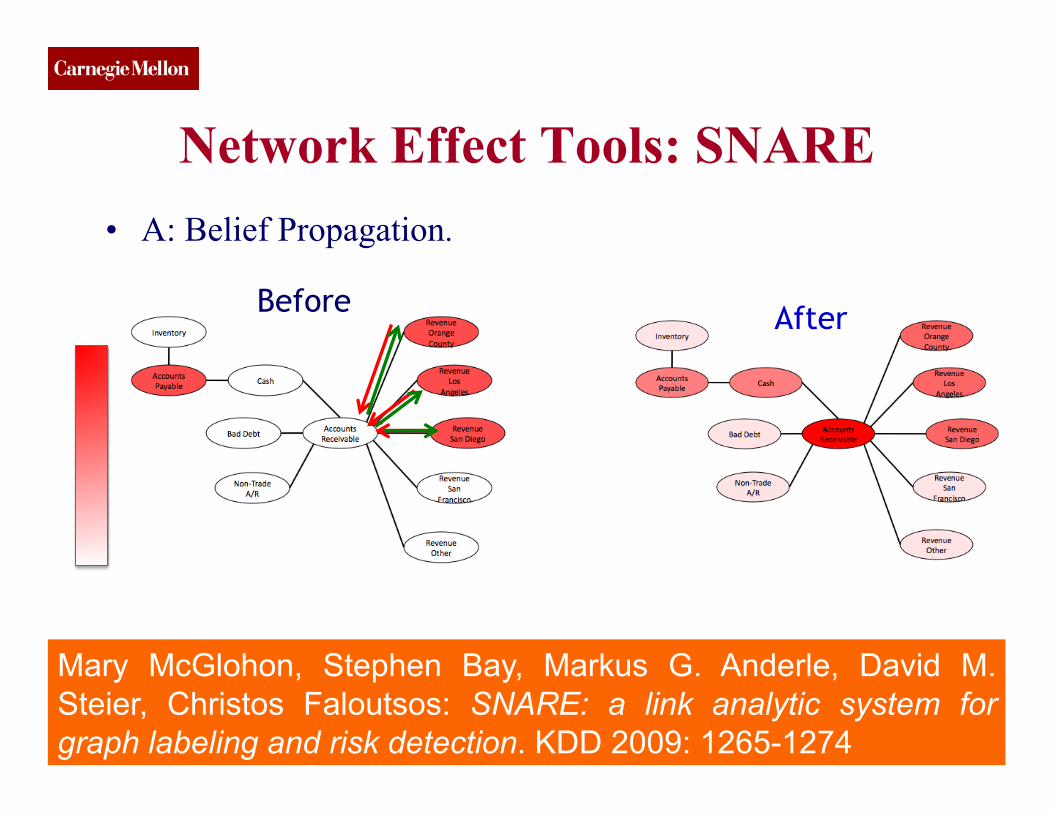
Network Effect Tools: SNARE
62
• A: Belief Propagation.
After Before
MLDAS, Doha 2015 (c) 2015, C. Faloutsos
Mary McGlohon, Stephen Bay, Markus G. Anderle, David M. Steier, Christos Faloutsos: SNARE: a link analytic system for graph labeling and risk detection. KDD 2009: 1265-1274
CMU SCS
Network Effect Tools: SNARE
63
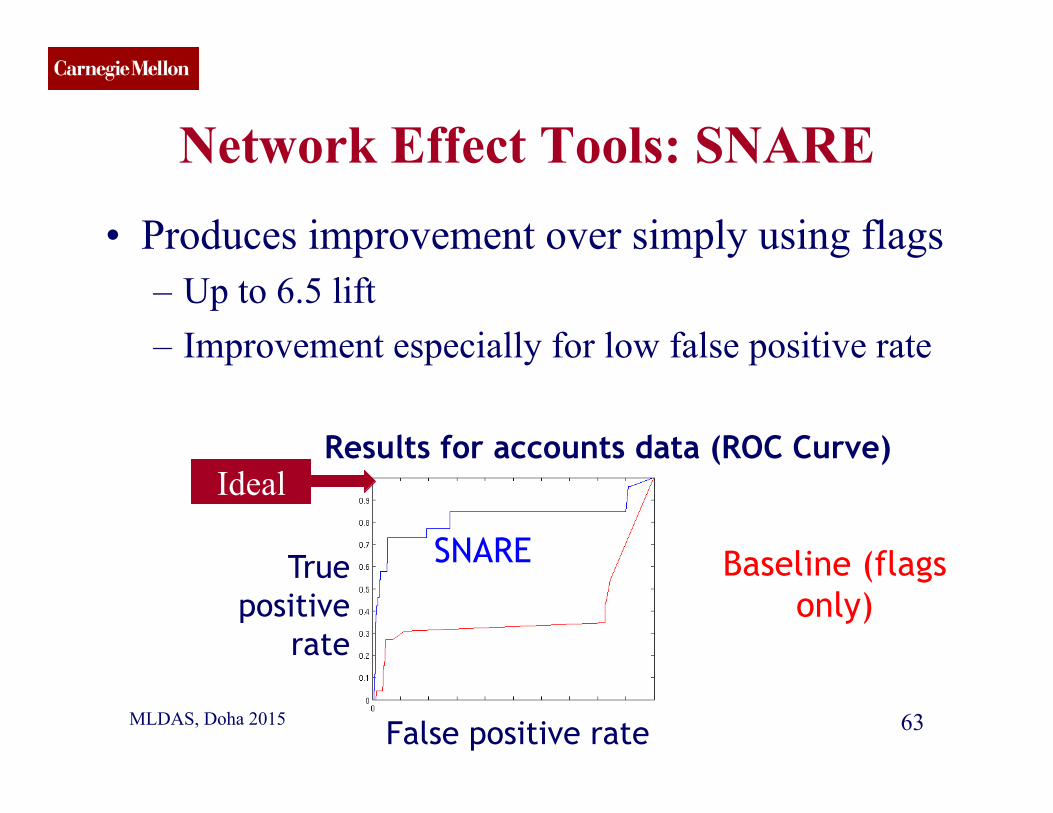
• Produces improvement over simply using flags – Up to 6.5 lift – Improvement especially for low false positive rate
True positive
rate
Results for accounts data (ROC Curve) Ideal
SNARE Baseline (flags only)
MLDAS, Doha 2015 (c) 2015, C. Faloutsos False positive rate

CMU SCS
Network Effect Tools: SNARE
64
• Accurate- Produces large improvement over simply using flags
• Flexible- Can be applied to other domains • Scalable- One iteration BP runs in linear time
(# edges) • Robust- Works on large range of parameters
MLDAS, Doha 2015 (c) 2015, C. Faloutsos

CMU SCS
(c) 2015, C. Faloutsos 65
Roadmap
• Introduction – Motivation • Part#1: Patterns in graphs
– Patterns – Anomaly / fraud detection
• CopyCatch • Spectral methods (‘fBox’) • Belief Propagation; fast computation & unification
• Part#2: time-evolving graphs; tensors • Conclusions MLDAS, Doha 2015

CMU SCS
Unifying Guilt-by-Association Approaches: Theorems and Fast Algorithms
Danai Koutra U Kang
Hsing-Kuo Kenneth Pao
Tai-You Ke Duen Horng (Polo) Chau
Christos Faloutsos
ECML PKDD, 5-9 September 2011, Athens, Greece
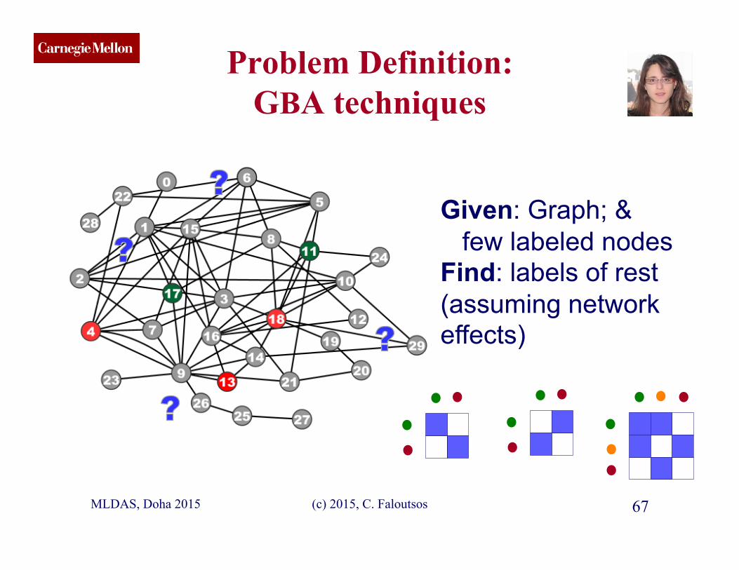
CMU SCS Problem Definition:
GBA techniques
(c) 2015, C. Faloutsos 67
Given: Graph; & few labeled nodes Find: labels of rest (assuming network effects)
MLDAS, Doha 2015
CMU SCS
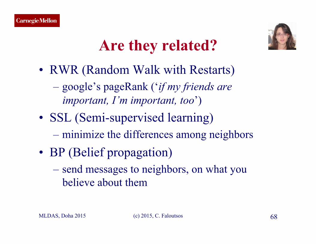
Are they related? • RWR (Random Walk with Restarts)
– google’s pageRank (‘if my friends are important, I’m important, too’)
• SSL (Semi-supervised learning) – minimize the differences among neighbors
• BP (Belief propagation) – send messages to neighbors, on what you
believe about them
MLDAS, Doha 2015 (c) 2015, C. Faloutsos 68
CMU SCS
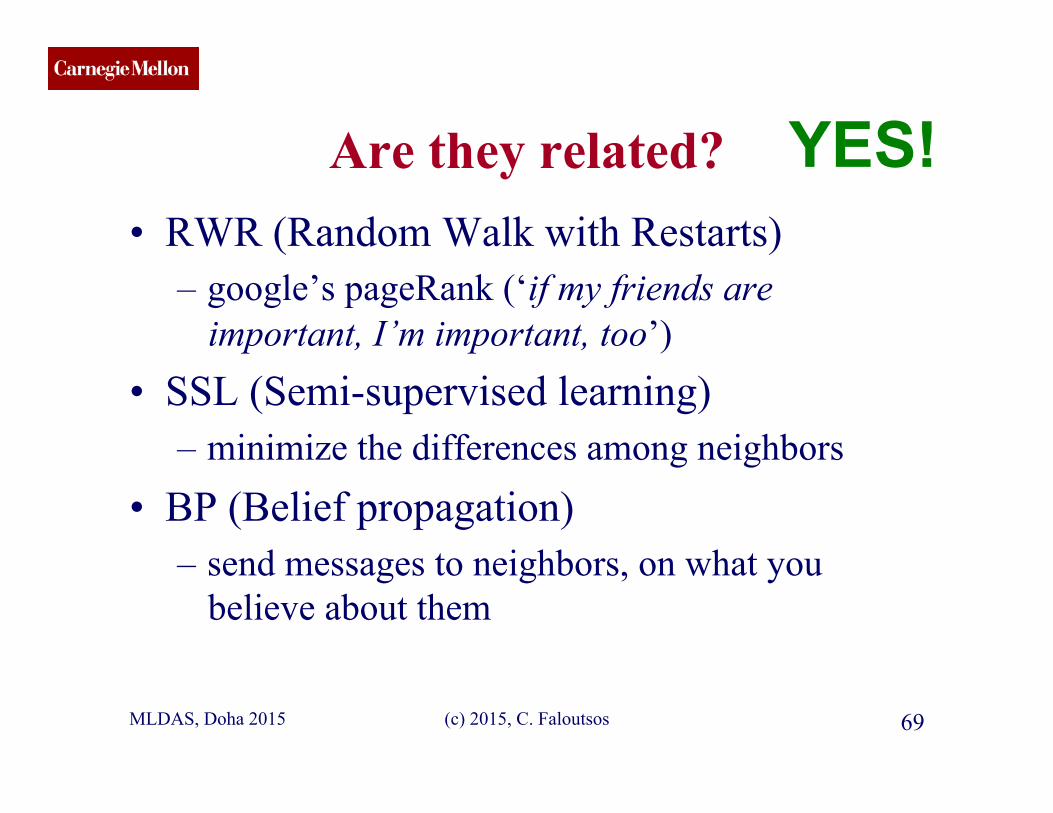
Are they related? • RWR (Random Walk with Restarts)
– google’s pageRank (‘if my friends are important, I’m important, too’)
• SSL (Semi-supervised learning) – minimize the differences among neighbors
• BP (Belief propagation) – send messages to neighbors, on what you
believe about them
MLDAS, Doha 2015 (c) 2015, C. Faloutsos 69
YES!
CMU SCS
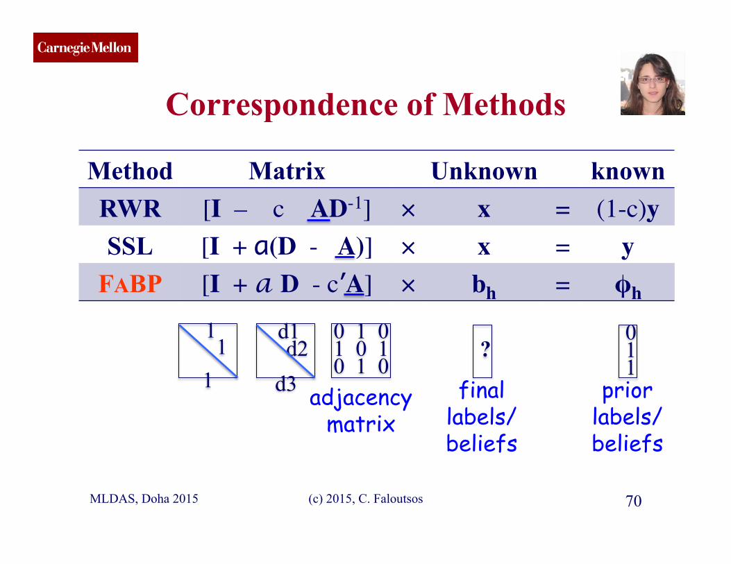
Correspondence of Methods
(c) 2015, C. Faloutsos 70
Method Matrix Unknown known RWR [I – c AD-1] × x = (1-c)y SSL [I + a(D - A)] × x = y
FABP [I + a D - c’A] × bh = φh
0 1 0 1 0 1 0 1 0
? 0 1 1
1 1
1
d1 d2 d3 final
labels/ beliefs
prior labels/ beliefs
adjacency matrix
MLDAS, Doha 2015
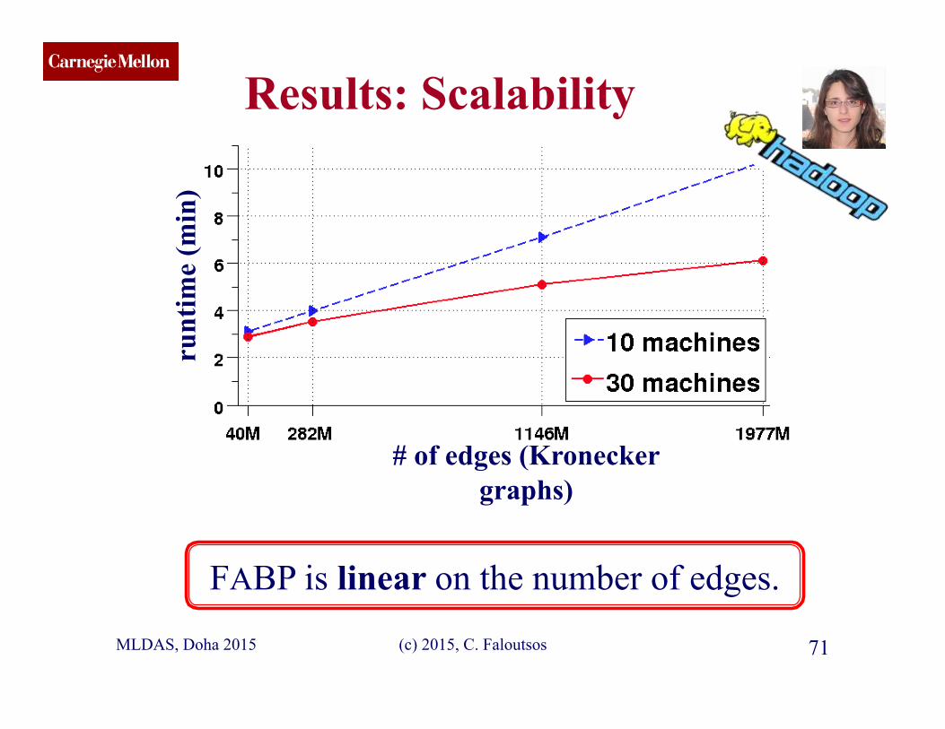
CMU SCS Results: Scalability
(c) 2015, C. Faloutsos 71
FABP is linear on the number of edges.
# of edges (Kronecker graphs)
runt
ime
(min
)
MLDAS, Doha 2015
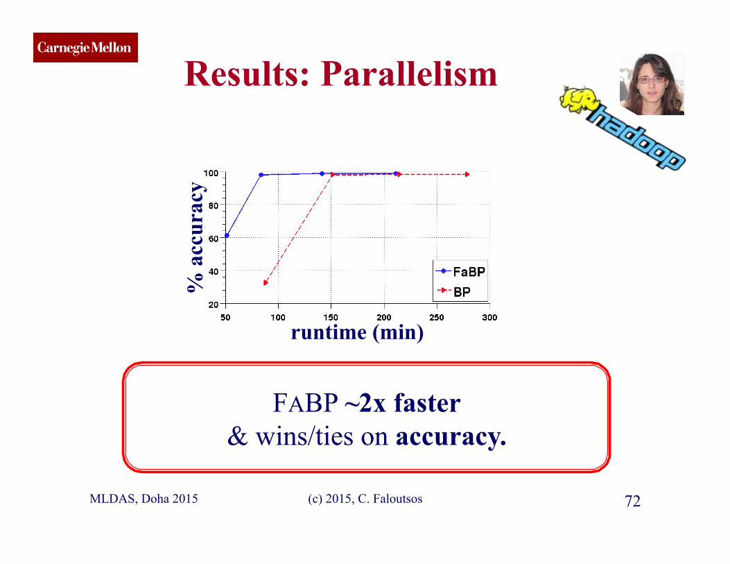
CMU SCS Results: Parallelism
(c) 2015, C. Faloutsos 72
FABP ~2x faster & wins/ties on accuracy.
runtime (min)
% a
ccur
acy
MLDAS, Doha 2015
CMU SCS
Summary of Part#1 • *many* patterns in real graphs
– Power-laws everywhere – Gaussian trap
• Avg << Max
– Long (and growing) list of tools for anomaly/fraud detection
MLDAS, Doha 2015 (c) 2015, C. Faloutsos 73
Patterns anomalies

CMU SCS
(c) 2015, C. Faloutsos 74
Roadmap
• Introduction – Motivation • Part#1: Patterns in graphs • Part#2: time-evolving graphs; tensors • Conclusions
MLDAS, Doha 2015
CMU SCS
MLDAS, Doha 2015 (c) 2015, C. Faloutsos 75
Part 2: Time evolving
graphs; tensors

CMU SCS
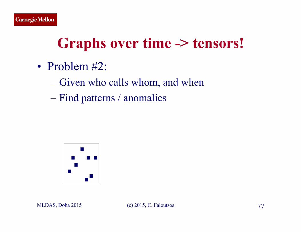
Graphs over time -> tensors! • Problem #2:
– Given who calls whom, and when – Find patterns / anomalies
MLDAS, Doha 2015 (c) 2015, C. Faloutsos 76
smith
CMU SCS
Graphs over time -> tensors! • Problem #2:
– Given who calls whom, and when – Find patterns / anomalies
MLDAS, Doha 2015 (c) 2015, C. Faloutsos 77
CMU SCS
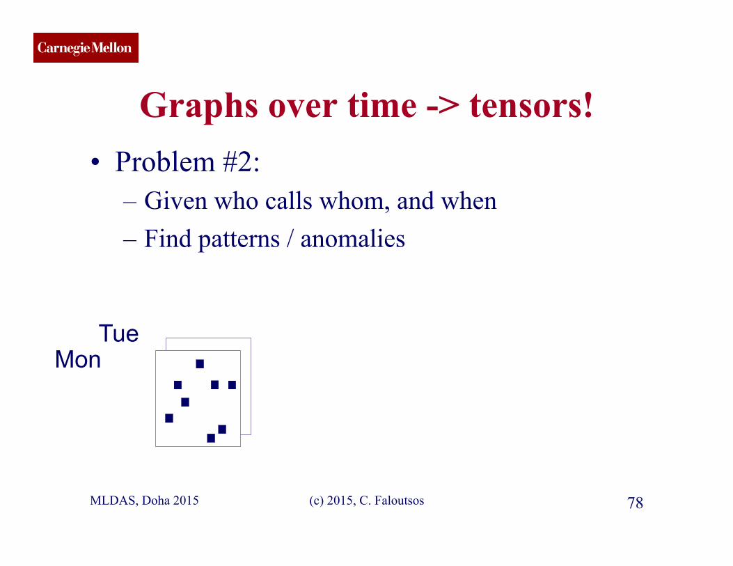
Graphs over time -> tensors! • Problem #2:
– Given who calls whom, and when – Find patterns / anomalies
MLDAS, Doha 2015 (c) 2015, C. Faloutsos 78
Mon Tue
CMU SCS
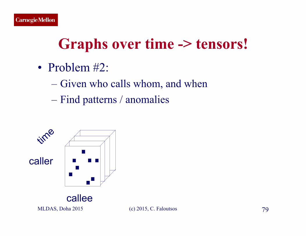
Graphs over time -> tensors! • Problem #2:
– Given who calls whom, and when – Find patterns / anomalies
MLDAS, Doha 2015 (c) 2015, C. Faloutsos 79 callee
caller
CMU SCS
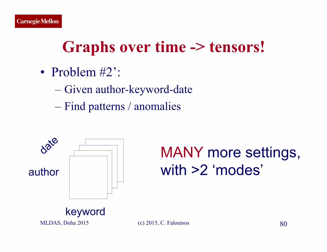
Graphs over time -> tensors! • Problem #2’:
– Given author-keyword-date – Find patterns / anomalies
MLDAS, Doha 2015 (c) 2015, C. Faloutsos 80 keyword
author
MANY more settings, with >2 ‘modes’
CMU SCS
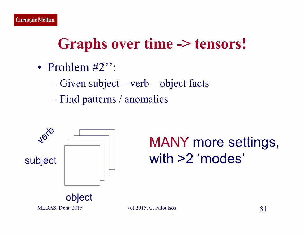
Graphs over time -> tensors! • Problem #2’’:
– Given subject – verb – object facts – Find patterns / anomalies
MLDAS, Doha 2015 (c) 2015, C. Faloutsos 81 object
subject
MANY more settings, with >2 ‘modes’
CMU SCS
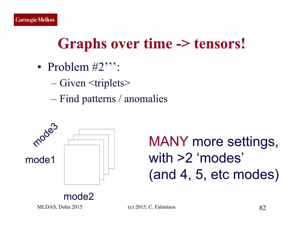
Graphs over time -> tensors! • Problem #2’’’:
– Given <triplets> – Find patterns / anomalies
MLDAS, Doha 2015 (c) 2015, C. Faloutsos 82 mode2
mode1
MANY more settings, with >2 ‘modes’ (and 4, 5, etc modes)

CMU SCS
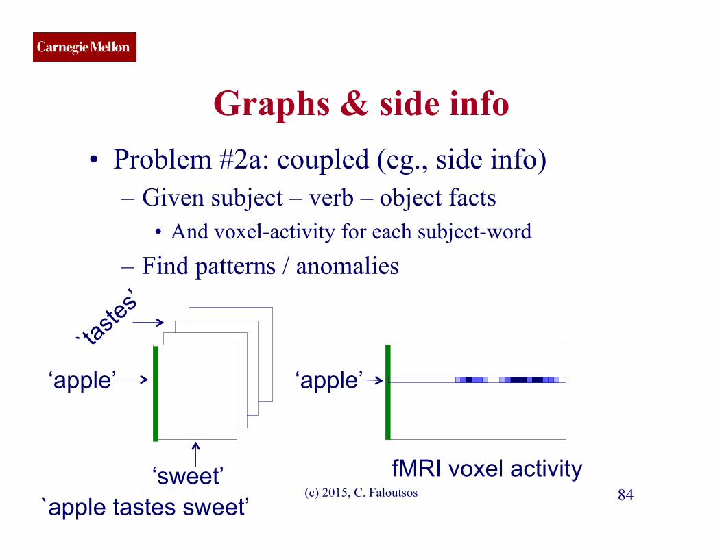
Graphs & side info • Problem #2a: coupled (eg., side info)
– Given subject – verb – object facts • And voxel-activity for each subject-word
– Find patterns / anomalies
MLDAS, Doha 2015 (c) 2015, C. Faloutsos 83 object
subject
fMRI voxel activity `apple tastes sweet’
CMU SCS
Graphs & side info • Problem #2a: coupled (eg., side info)
– Given subject – verb – object facts • And voxel-activity for each subject-word
– Find patterns / anomalies
MLDAS, Doha 2015 (c) 2015, C. Faloutsos 84 ‘sweet’
‘apple’
fMRI voxel activity `apple tastes sweet’
‘apple’
CMU SCS
(c) 2015, C. Faloutsos 85
Roadmap
• Introduction – Motivation • Part#1: Patterns in graphs • Part#2: time-evolving graphs; tensors
– Intro to tensors – Results – Speed
• Conclusions
MLDAS, Doha 2015
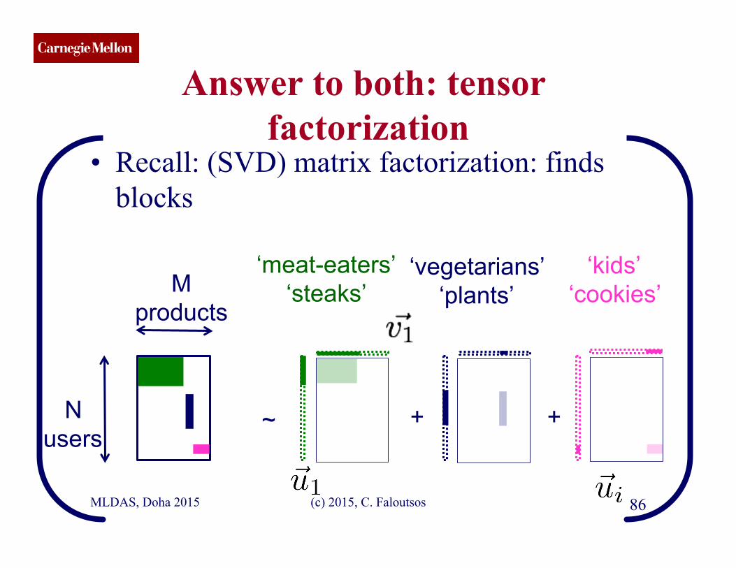
CMU SCS Answer to both: tensor
factorization • Recall: (SVD) matrix factorization: finds
blocks
MLDAS, Doha 2015 (c) 2015, C. Faloutsos 86
N users
M products
‘meat-eaters’ ‘steaks’
‘vegetarians’ ‘plants’
‘kids’ ‘cookies’
~ + +
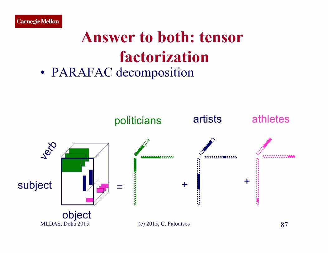
CMU SCS Answer to both: tensor
factorization • PARAFAC decomposition
MLDAS, Doha 2015 (c) 2015, C. Faloutsos 87
= + + subject
object
politicians artists athletes

CMU SCS
Answer: tensor factorization • PARAFAC decomposition • Results for who-calls-whom-when
– 4M x 15 days
MLDAS, Doha 2015 (c) 2015, C. Faloutsos 88
= + + caller
callee
?? ?? ??
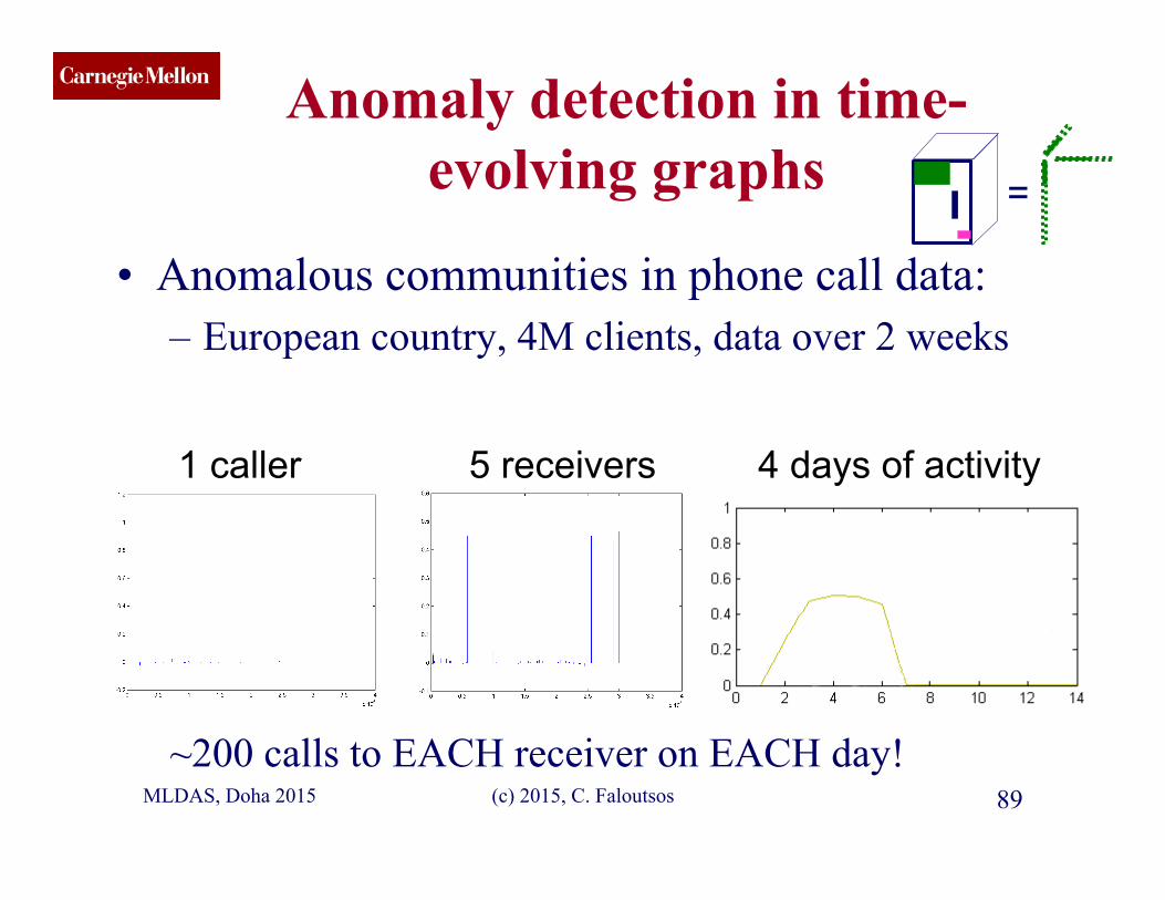
CMU SCS Anomaly detection in time-
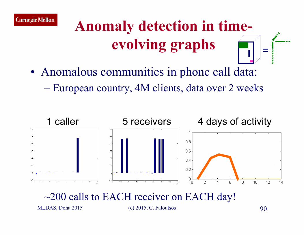
evolving graphs
• Anomalous communities in phone call data: – European country, 4M clients, data over 2 weeks
~200 calls to EACH receiver on EACH day!
1 caller 5 receivers 4 days of activity
MLDAS, Doha 2015 89 (c) 2015, C. Faloutsos
=
CMU SCS Anomaly detection in time-
evolving graphs
• Anomalous communities in phone call data: – European country, 4M clients, data over 2 weeks
~200 calls to EACH receiver on EACH day!
1 caller 5 receivers 4 days of activity
MLDAS, Doha 2015 90 (c) 2015, C. Faloutsos
=

CMU SCS Anomaly detection in time-
evolving graphs
• Anomalous communities in phone call data: – European country, 4M clients, data over 2 weeks
~200 calls to EACH receiver on EACH day! MLDAS, Doha 2015 91 (c) 2015, C. Faloutsos
=
Miguel Araujo, Spiros Papadimitriou, Stephan Günnemann, Christos Faloutsos, Prithwish Basu, Ananthram Swami, Evangelos Papalexakis, Danai Koutra. Com2: Fast Automatic Discovery of Temporal (Comet) Communities. PAKDD 2014, Tainan, Taiwan.

CMU SCS
(c) 2015, C. Faloutsos 92
Roadmap
• Introduction – Motivation • Part#1: Patterns in graphs • Part#2: time-evolving graphs; tensors
– Intro to tensors – Results – Speed
• Conclusions
MLDAS, Doha 2015
CMU SCS
Neuro-semantics
13�
�
3.�Additional�Figures�and�legends��
Figure�S1.�Presentation�and�set�of�exemplars�used�in�the�experiment. Participants were presented 60 distinct word-picture pairs describing common concrete nouns. These consisted of 5 exemplars from each of 12 categories, as shown above. A slow event-related paradigm was employed, in which the stimulus was presented for 3s, followed by a 7s fixation period during which an X was presented in the center of the screen. Images were presented as white lines and characters on a dark background, but are inverted here to improve readability. The entire set of 60 exemplars was presented six times, randomly permuting the sequence on each presentation.
To fully specify a model within this com-putational modeling framework, one must firstdefine a set of intermediate semantic featuresf1(w) f2(w)…fn(w) to be extracted from the textcorpus. In this paper, each intermediate semanticfeature is defined in terms of the co-occurrencestatistics of the input stimulus word w with aparticular other word (e.g., “taste”) or set of words(e.g., “taste,” “tastes,” or “tasted”) within the textcorpus. The model is trained by the application ofmultiple regression to these features fi(w) and theobserved fMRI images, so as to obtain maximum-likelihood estimates for the model parameters cvi(26). Once trained, the computational model can beevaluated by giving it words outside the trainingset and comparing its predicted fMRI images forthese words with observed fMRI data.
This computational modeling framework isbased on two key theoretical assumptions. First, itassumes the semantic features that distinguish themeanings of arbitrary concrete nouns are reflected
in the statistics of their use within a very large textcorpus. This assumption is drawn from the field ofcomputational linguistics, where statistical worddistributions are frequently used to approximatethe meaning of documents and words (14–17).Second, it assumes that the brain activity observedwhen thinking about any concrete noun can bederived as a weighted linear sum of contributionsfrom each of its semantic features. Although thecorrectness of this linearity assumption is debat-able, it is consistent with the widespread use oflinear models in fMRI analysis (27) and with theassumption that fMRI activation often reflects alinear superposition of contributions from differentsources. Our theoretical framework does not take aposition on whether the neural activation encodingmeaning is localized in particular cortical re-gions. Instead, it considers all cortical voxels andallows the training data to determine which loca-tions are systematically modulated by which as-pects of word meanings.
Results. We evaluated this computational mod-el using fMRI data from nine healthy, college-ageparticipants who viewed 60 different word-picturepairs presented six times each. Anatomically de-fined regions of interest were automatically labeledaccording to the methodology in (28). The 60 ran-domly ordered stimuli included five items fromeach of 12 semantic categories (animals, body parts,buildings, building parts, clothing, furniture, insects,kitchen items, tools, vegetables, vehicles, and otherman-made items). A representative fMRI image foreach stimulus was created by computing the meanfMRI response over its six presentations, and themean of all 60 of these representative images wasthen subtracted from each [for details, see (26)].
To instantiate our modeling framework, we firstchose a set of intermediate semantic features. To beeffective, the intermediate semantic features mustsimultaneously encode thewide variety of semanticcontent of the input stimulus words and factor theobserved fMRI activation intomore primitive com-
Predicted“celery” = 0.84
“celery” “airplane”
Predicted:
Observed:
A B
+.. .
high
average
belowaverage
Predicted “celery”:
+ 0.35 + 0.32
“eat” “taste” “fill”
Fig. 2. Predicting fMRI imagesfor given stimulus words. (A)Forming a prediction for par-ticipant P1 for the stimulusword “celery” after training on58 other words. Learned cvi co-efficients for 3 of the 25 se-mantic features (“eat,” “taste,”and “fill”) are depicted by thevoxel colors in the three imagesat the top of the panel. The co-occurrence value for each of these features for the stimulus word “celery” isshown to the left of their respective images [e.g., the value for “eat (celery)” is0.84]. The predicted activation for the stimulus word [shown at the bottom of(A)] is a linear combination of the 25 semantic fMRI signatures, weighted bytheir co-occurrence values. This figure shows just one horizontal slice [z =
–12 mm in Montreal Neurological Institute (MNI) space] of the predictedthree-dimensional image. (B) Predicted and observed fMRI images for“celery” and “airplane” after training that uses 58 other words. The two longred and blue vertical streaks near the top (posterior region) of the predictedand observed images are the left and right fusiform gyri.
A
B
C
Mean over
participants
Participant P
5
Fig. 3. Locations ofmost accurately pre-dicted voxels. Surface(A) and glass brain (B)rendering of the correla-tion between predictedand actual voxel activa-tions for words outsidethe training set for par-
ticipant P5. These panels show clusters containing at least 10 contiguous voxels, each of whosepredicted-actual correlation is at least 0.28. These voxel clusters are distributed throughout thecortex and located in the left and right occipital and parietal lobes; left and right fusiform,postcentral, and middle frontal gyri; left inferior frontal gyrus; medial frontal gyrus; and anteriorcingulate. (C) Surface rendering of the predicted-actual correlation averaged over all nineparticipants. This panel represents clusters containing at least 10 contiguous voxels, each withaverage correlation of at least 0.14.
30 MAY 2008 VOL 320 SCIENCE www.sciencemag.org1192
RESEARCH ARTICLES
on
May
30,
200
8 w
ww
.sci
ence
mag
.org
Dow
nloa
ded
from
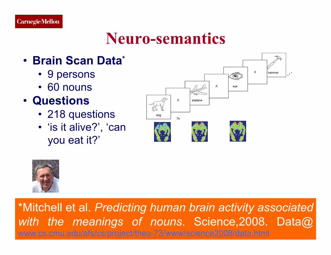
• Brain Scan Data*
• 9 persons • 60 nouns
• Questions • 218 questions • ‘is it alive?’, ‘can
you eat it?’
To fully specify a model within this com-putational modeling framework, one must firstdefine a set of intermediate semantic featuresf1(w) f2(w)…fn(w) to be extracted from the textcorpus. In this paper, each intermediate semanticfeature is defined in terms of the co-occurrencestatistics of the input stimulus word w with aparticular other word (e.g., “taste”) or set of words(e.g., “taste,” “tastes,” or “tasted”) within the textcorpus. The model is trained by the application ofmultiple regression to these features fi(w) and theobserved fMRI images, so as to obtain maximum-likelihood estimates for the model parameters cvi(26). Once trained, the computational model can beevaluated by giving it words outside the trainingset and comparing its predicted fMRI images forthese words with observed fMRI data.
This computational modeling framework isbased on two key theoretical assumptions. First, itassumes the semantic features that distinguish themeanings of arbitrary concrete nouns are reflected
in the statistics of their use within a very large textcorpus. This assumption is drawn from the field ofcomputational linguistics, where statistical worddistributions are frequently used to approximatethe meaning of documents and words (14–17).Second, it assumes that the brain activity observedwhen thinking about any concrete noun can bederived as a weighted linear sum of contributionsfrom each of its semantic features. Although thecorrectness of this linearity assumption is debat-able, it is consistent with the widespread use oflinear models in fMRI analysis (27) and with theassumption that fMRI activation often reflects alinear superposition of contributions from differentsources. Our theoretical framework does not take aposition on whether the neural activation encodingmeaning is localized in particular cortical re-gions. Instead, it considers all cortical voxels andallows the training data to determine which loca-tions are systematically modulated by which as-pects of word meanings.
Results. We evaluated this computational mod-el using fMRI data from nine healthy, college-ageparticipants who viewed 60 different word-picturepairs presented six times each. Anatomically de-fined regions of interest were automatically labeledaccording to the methodology in (28). The 60 ran-domly ordered stimuli included five items fromeach of 12 semantic categories (animals, body parts,buildings, building parts, clothing, furniture, insects,kitchen items, tools, vegetables, vehicles, and otherman-made items). A representative fMRI image foreach stimulus was created by computing the meanfMRI response over its six presentations, and themean of all 60 of these representative images wasthen subtracted from each [for details, see (26)].
To instantiate our modeling framework, we firstchose a set of intermediate semantic features. To beeffective, the intermediate semantic features mustsimultaneously encode thewide variety of semanticcontent of the input stimulus words and factor theobserved fMRI activation intomore primitive com-
Predicted“celery” = 0.84
“celery” “airplane”
Predicted:
Observed:
A B
+.. .
high
average
belowaverage
Predicted “celery”:
+ 0.35 + 0.32
“eat” “taste” “fill”
Fig. 2. Predicting fMRI imagesfor given stimulus words. (A)Forming a prediction for par-ticipant P1 for the stimulusword “celery” after training on58 other words. Learned cvi co-efficients for 3 of the 25 se-mantic features (“eat,” “taste,”and “fill”) are depicted by thevoxel colors in the three imagesat the top of the panel. The co-occurrence value for each of these features for the stimulus word “celery” isshown to the left of their respective images [e.g., the value for “eat (celery)” is0.84]. The predicted activation for the stimulus word [shown at the bottom of(A)] is a linear combination of the 25 semantic fMRI signatures, weighted bytheir co-occurrence values. This figure shows just one horizontal slice [z =
–12 mm in Montreal Neurological Institute (MNI) space] of the predictedthree-dimensional image. (B) Predicted and observed fMRI images for“celery” and “airplane” after training that uses 58 other words. The two longred and blue vertical streaks near the top (posterior region) of the predictedand observed images are the left and right fusiform gyri.
A
B
C
Mean over
participants
Participant P
5
Fig. 3. Locations ofmost accurately pre-dicted voxels. Surface(A) and glass brain (B)rendering of the correla-tion between predictedand actual voxel activa-tions for words outsidethe training set for par-
ticipant P5. These panels show clusters containing at least 10 contiguous voxels, each of whosepredicted-actual correlation is at least 0.28. These voxel clusters are distributed throughout thecortex and located in the left and right occipital and parietal lobes; left and right fusiform,postcentral, and middle frontal gyri; left inferior frontal gyrus; medial frontal gyrus; and anteriorcingulate. (C) Surface rendering of the predicted-actual correlation averaged over all nineparticipants. This panel represents clusters containing at least 10 contiguous voxels, each withaverage correlation of at least 0.14.
30 MAY 2008 VOL 320 SCIENCE www.sciencemag.org1192
RESEARCH ARTICLES
on
May
30,
200
8 w
ww
.sci
ence
mag
.org
Dow
nloa
ded
from
MLDAS, Doha 2015 94 (c) 2015, C. Faloutsos
*Mitchell et al. Predicting human brain activity associated with the meanings of nouns. Science,2008. Data@ www.cs.cmu.edu/afs/cs/project/theo-73/www/science2008/data.html
CMU SCS
Neuro-semantics
13�
�
3.�Additional�Figures�and�legends��
Figure�S1.�Presentation�and�set�of�exemplars�used�in�the�experiment. Participants were presented 60 distinct word-picture pairs describing common concrete nouns. These consisted of 5 exemplars from each of 12 categories, as shown above. A slow event-related paradigm was employed, in which the stimulus was presented for 3s, followed by a 7s fixation period during which an X was presented in the center of the screen. Images were presented as white lines and characters on a dark background, but are inverted here to improve readability. The entire set of 60 exemplars was presented six times, randomly permuting the sequence on each presentation.
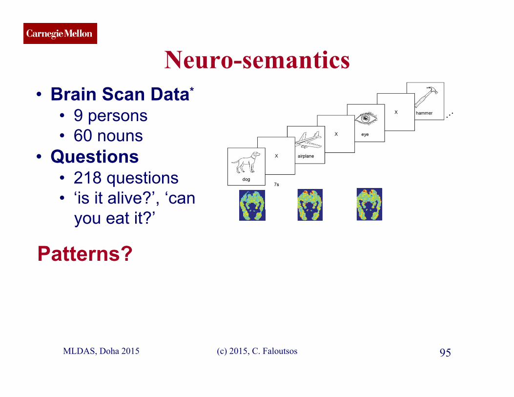
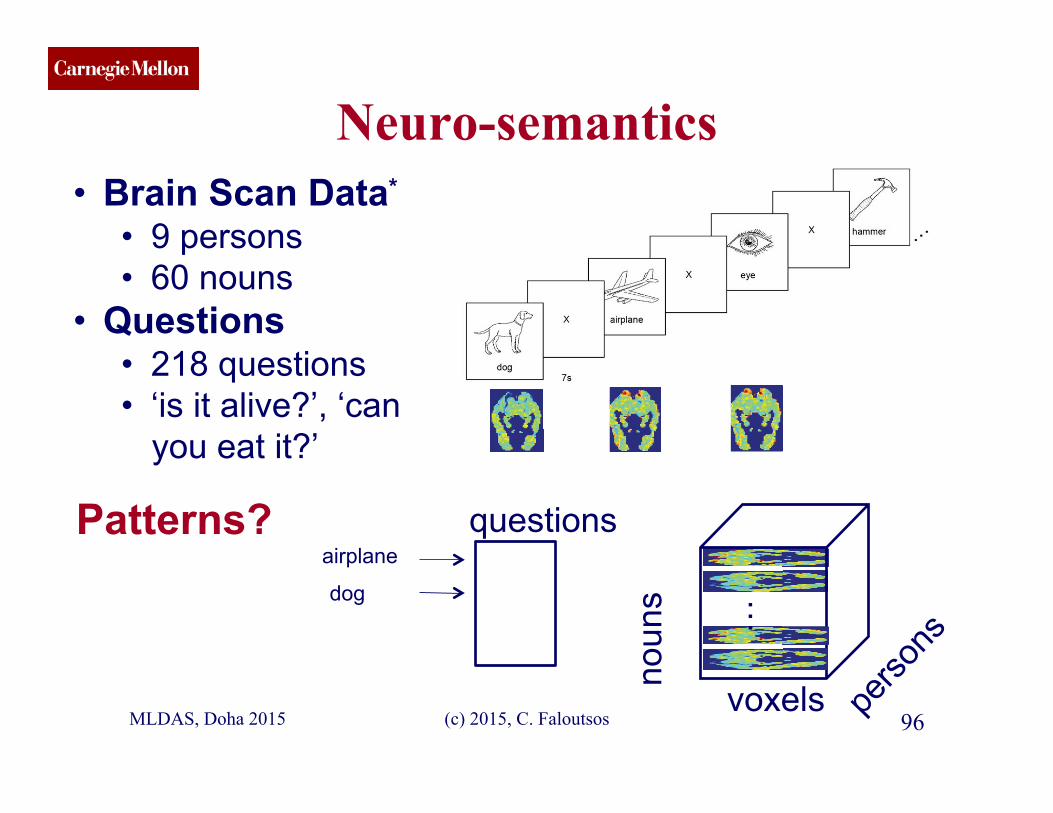
• Brain Scan Data*
• 9 persons • 60 nouns
• Questions • 218 questions • ‘is it alive?’, ‘can
you eat it?’
MLDAS, Doha 2015 95 (c) 2015, C. Faloutsos
Patterns?
To fully specify a model within this com-putational modeling framework, one must firstdefine a set of intermediate semantic featuresf1(w) f2(w)…fn(w) to be extracted from the textcorpus. In this paper, each intermediate semanticfeature is defined in terms of the co-occurrencestatistics of the input stimulus word w with aparticular other word (e.g., “taste”) or set of words(e.g., “taste,” “tastes,” or “tasted”) within the textcorpus. The model is trained by the application ofmultiple regression to these features fi(w) and theobserved fMRI images, so as to obtain maximum-likelihood estimates for the model parameters cvi(26). Once trained, the computational model can beevaluated by giving it words outside the trainingset and comparing its predicted fMRI images forthese words with observed fMRI data.
This computational modeling framework isbased on two key theoretical assumptions. First, itassumes the semantic features that distinguish themeanings of arbitrary concrete nouns are reflected
in the statistics of their use within a very large textcorpus. This assumption is drawn from the field ofcomputational linguistics, where statistical worddistributions are frequently used to approximatethe meaning of documents and words (14–17).Second, it assumes that the brain activity observedwhen thinking about any concrete noun can bederived as a weighted linear sum of contributionsfrom each of its semantic features. Although thecorrectness of this linearity assumption is debat-able, it is consistent with the widespread use oflinear models in fMRI analysis (27) and with theassumption that fMRI activation often reflects alinear superposition of contributions from differentsources. Our theoretical framework does not take aposition on whether the neural activation encodingmeaning is localized in particular cortical re-gions. Instead, it considers all cortical voxels andallows the training data to determine which loca-tions are systematically modulated by which as-pects of word meanings.
Results. We evaluated this computational mod-el using fMRI data from nine healthy, college-ageparticipants who viewed 60 different word-picturepairs presented six times each. Anatomically de-fined regions of interest were automatically labeledaccording to the methodology in (28). The 60 ran-domly ordered stimuli included five items fromeach of 12 semantic categories (animals, body parts,buildings, building parts, clothing, furniture, insects,kitchen items, tools, vegetables, vehicles, and otherman-made items). A representative fMRI image foreach stimulus was created by computing the meanfMRI response over its six presentations, and themean of all 60 of these representative images wasthen subtracted from each [for details, see (26)].
To instantiate our modeling framework, we firstchose a set of intermediate semantic features. To beeffective, the intermediate semantic features mustsimultaneously encode thewide variety of semanticcontent of the input stimulus words and factor theobserved fMRI activation intomore primitive com-
Predicted“celery” = 0.84
“celery” “airplane”
Predicted:
Observed:
A B
+.. .
high
average
belowaverage
Predicted “celery”:
+ 0.35 + 0.32
“eat” “taste” “fill”
Fig. 2. Predicting fMRI imagesfor given stimulus words. (A)Forming a prediction for par-ticipant P1 for the stimulusword “celery” after training on58 other words. Learned cvi co-efficients for 3 of the 25 se-mantic features (“eat,” “taste,”and “fill”) are depicted by thevoxel colors in the three imagesat the top of the panel. The co-occurrence value for each of these features for the stimulus word “celery” isshown to the left of their respective images [e.g., the value for “eat (celery)” is0.84]. The predicted activation for the stimulus word [shown at the bottom of(A)] is a linear combination of the 25 semantic fMRI signatures, weighted bytheir co-occurrence values. This figure shows just one horizontal slice [z =
–12 mm in Montreal Neurological Institute (MNI) space] of the predictedthree-dimensional image. (B) Predicted and observed fMRI images for“celery” and “airplane” after training that uses 58 other words. The two longred and blue vertical streaks near the top (posterior region) of the predictedand observed images are the left and right fusiform gyri.
A
B
C
Mean over
participants
Participant P
5
Fig. 3. Locations ofmost accurately pre-dicted voxels. Surface(A) and glass brain (B)rendering of the correla-tion between predictedand actual voxel activa-tions for words outsidethe training set for par-
ticipant P5. These panels show clusters containing at least 10 contiguous voxels, each of whosepredicted-actual correlation is at least 0.28. These voxel clusters are distributed throughout thecortex and located in the left and right occipital and parietal lobes; left and right fusiform,postcentral, and middle frontal gyri; left inferior frontal gyrus; medial frontal gyrus; and anteriorcingulate. (C) Surface rendering of the predicted-actual correlation averaged over all nineparticipants. This panel represents clusters containing at least 10 contiguous voxels, each withaverage correlation of at least 0.14.
30 MAY 2008 VOL 320 SCIENCE www.sciencemag.org1192
RESEARCH ARTICLES
on
May
30,
200
8 w
ww
.sci
ence
mag
.org
Dow
nloa
ded
from
CMU SCS
Neuro-semantics
13�
�
3.�Additional�Figures�and�legends��
Figure�S1.�Presentation�and�set�of�exemplars�used�in�the�experiment. Participants were presented 60 distinct word-picture pairs describing common concrete nouns. These consisted of 5 exemplars from each of 12 categories, as shown above. A slow event-related paradigm was employed, in which the stimulus was presented for 3s, followed by a 7s fixation period during which an X was presented in the center of the screen. Images were presented as white lines and characters on a dark background, but are inverted here to improve readability. The entire set of 60 exemplars was presented six times, randomly permuting the sequence on each presentation.
• Brain Scan Data*
• 9 persons • 60 nouns
• Questions • 218 questions • ‘is it alive?’, ‘can
you eat it?’
Tofullyspecify
amodelwithint
hiscom-
putationalmode
lingframework,o
nemustfirst
defineasetofin
termediateseman
ticfeatures
f 1(w)f 2(w)…f n(w)tobeextract
edfromthetext
corpus.Inthispa
per,eachintermed
iatesemantic
featureisdefined
intermsoftheco
-occurrence
statisticsofthein
putstimuluswo
rdwwitha
particularotherwo
rd(e.g.,“taste”)or
setofwords
(e.g.,“taste,”“tas
tes,”or“tasted”)w
ithinthetext
corpus.Themode
listrainedbythe
applicationof
multipleregressio
ntothesefeature
sf i(w)andthe
observedfMRIim
ages,soastoobt
ainmaximum-
likelihoodestima
tesforthemodel
parametersc vi
(26).Oncetrained,
thecomputational
modelcanbe
evaluatedbygivin
gitwordsoutside
thetraining
setandcomparin
gitspredictedfM
RIimagesfor
thesewordswith
observedfMRIda
ta.Thiscom
putationalmodeli
ngframeworkis
basedontwokey
theoreticalassump
tions.First,it
assumesthesema
nticfeaturesthatd
istinguishthe
meaningsofarbit
raryconcretenoun
sarereflected
inthestatisticsof
theirusewithina
verylargetext
corpus.Thisassum
ptionisdrawnfro
mthefieldof
computationallin
guistics,wherest
atisticalword
distributionsare
frequentlyusedt
oapproximate
themeaningofd
ocumentsandw
ords(14–17).
Second,itassume
sthatthebrainact
ivityobserved
whenthinkinga
boutanyconcrete
nouncanbe
derivedasaweig
htedlinearsumo
fcontributions
fromeachofits
semanticfeatures.
Althoughthe
correctnessofthis
linearityassumpt
ionisdebat-
able,itisconsist
entwiththewide
spreaduseof
linearmodelsin
fMRIanalysis(2
7)andwiththe
assumptionthatf
MRIactivationo
ftenreflectsa
linearsuperpositio
nofcontributions
fromdifferent
sources.Ourtheore
ticalframeworkdo
esnottakea
positiononwheth
ertheneuralactiv
ationencoding
meaningislocali
zedinparticular
corticalre-
gions.Instead,it
considersallcort
icalvoxelsand
allowsthetrainin
gdatatodetermin
ewhichloca-
tionsaresystemat
icallymodulated
bywhichas-
pectsofwordme
anings.
Results.Weevaluated
thiscomputational
mod-elusing
fMRIdatafromn
inehealthy,college
-ageparticipan
tswhoviewed60
differentword-pic
turepairspre
sentedsixtimes
each.Anatomicall
yde-finedreg
ionsofinterestwe
reautomaticallyla
beledaccording
tothemethodolog
yin(28).The60
ran-domlyo
rderedstimuliinc
ludedfiveitems
fromeachof1
2semanticcatego
ries(animals,body
parts,buildings
,buildingparts,clo
thing,furniture,in
sects,kitcheni
tems,tools,vegeta
bles,vehicles,and
otherman-mad
eitems).Areprese
ntativefMRIimage
foreachstim
uluswascreatedb
ycomputingthem
eanfMRIre
sponseoveritssi
xpresentations,a
ndthemeanof
all60oftheserep
resentativeimages
wasthensub
tractedfromeach
[fordetails,see(
26)].Toinstan
tiateourmodeling
framework,wefir
stchoseas
etofintermediate
semanticfeatures.
Tobeeffective,
theintermediatese
manticfeaturesm
ustsimultane
ouslyencodethew
idevarietyofsema
nticcontento
ftheinputstimul
uswordsandfacto
rtheobserved
fMRIactivationin
tomoreprimitivec
om-
Predicted
“celery” = 0.84
“celery”“airplan
e”
Predicted:
Observed:
AB
+...
high
average below average
Predicted “celer
y”:+ 0.35+ 0.32
“eat”“taste”
“fill”
Fig.2.Predicting
fMRIimages
forgivenstimulus
words.(A)
Formingapredict
ionforpar-
ticipantP1fort
hestimulus
word“celery”afte
rtrainingon
58otherwords.Le
arnedc vico-efficients
for3ofthe25s
e-manticfe
atures(“eat,”“tast
e,”and“fill”
)aredepictedby
thevoxelcolo
rsinthethreeima
gesatthetop
ofthepanel.Thec
o-occurrenc
evalueforeacho
fthesefeaturesfor
thestimulusword
“celery”is
showntothelefto
ftheirrespectiveim
ages[e.g.,thevalu
efor“eat(celery)”i
s0.84].The
predictedactivation
forthestimuluswo
rd[shownatthebo
ttomof(A)]isal
inearcombinationo
fthe25semantic
fMRIsignatures,w
eightedby
theirco-occurrence
values.Thisfigure
showsjustonehor
izontalslice[z=
–12mminMontr
ealNeurological
Institute(MNI)spa
ce]ofthepredict
edthree-dim
ensionalimage.(
B)Predictedand
observedfMRIima
gesfor“celery”a
nd“airplane”after
trainingthatuses5
8otherwords.The
twolongredandb
lueverticalstreaks
nearthetop(post
eriorregion)ofthe
predictedandobse
rvedimagesaret
heleftandrightfu
siformgyri.
A B
C
Mean overparticipants
Participant P5
Fig.3.Locations
ofmostac
curatelypre-
dictedvoxels.Sur
face(A)andg
lassbrain(B)
renderingofthecor
rela-tionbetw
eenpredicted
andactualvoxelac
tiva-tionsfor
wordsoutside
thetrainingsetfor
par-ticipantP
5.Thesepanelssho
wclusterscontaining
atleast10contigu
ousvoxels,eachof
whosepredicted-
actualcorrelationis
atleast0.28.These
voxelclustersared
istributedthroughou
tthecortexan
dlocatedinthelef
tandrightoccipit
alandparietallobe
s;leftandrightfu
siform,postcentra
l,andmiddlefronta
lgyri;leftinferiorfr
ontalgyrus;medial
frontalgyrus;anda
nteriorcingulate.
(C)Surfacerenderi
ngofthepredicted-
actualcorrelation
averagedoveralln
ineparticipan
ts.Thispanelrepres
entsclusterscontai
ningatleast10co
ntiguousvoxels,ea
chwithaveragec
orrelationofatleast
0.14.
30MAY2008V
OL320SCIENC
Ewww.science
mag.org1192RESEAR
CHARTICLES
on May 30, 2008 www.sciencemag.org Downloaded from
Tofullyspecify
amodelwithin
thiscom-
putationalmode
lingframework
,onemustfirst
defineasetof
intermediatese
manticfeatures
f 1(w)f 2(w)…f n(w)tobeextrac
tedfromthetext
corpus.Inthisp
aper,eachinter
mediatesemanti
cfeature
isdefinedinte
rmsoftheco-o
ccurrence
statisticsofthe
inputstimulus
wordwwitha
particularotherw
ord(e.g.,“taste”
)orsetofword
s(e.g.,“ta
ste,”“tastes,”or
“tasted”)within
thetextcorpus.
Themodelistra
inedbytheappl
icationof
multipleregressio
ntothesefeatu
resf i(w)andthe
observedfMRI
images,soasto
obtainmaximum
-likelihoo
destimatesfor
themodelparam
etersc vi
(26).Oncetraine
d,thecomputatio
nalmodelcanbe
evaluatedbygiv
ingitwordsou
tsidethetrainin
gsetand
comparingitsp
redictedfMRIim
agesforthesew
ordswithobser
vedfMRIdata.
Thiscomputatio
nalmodeling
frameworkis
basedontwok
eytheoreticalas
sumptions.First
,itassumes
thesemanticfea
turesthatdisting
uishthemeaning
sofarbitraryco
ncretenounsare
reflected
inthestatisticso
ftheirusewithi
naverylargetex
tcorpus.
Thisassumption
isdrawnfromthe
fieldofcomputa
tionallinguistic
s,wherestatist
icalword
distributionsare
frequentlyused
toapproximate
themeaningof
documentsand
words(14–17).
Second,itassum
esthatthebrain
activityobserve
dwhenth
inkingaboutan
yconcretenou
ncanbe
derivedasawe
ightedlinearsu
mofcontributio
nsfromea
chofitsseman
ticfeatures.Alth
oughthe
correctnessofth
islinearityassu
mptionisdebat
-able,it
isconsistentw
iththewidesprea
duseof
linearmodelsin
fMRIanalysis(2
7)andwiththe
assumptiontha
tfMRIactivatio
noftenreflects
alinearsu
perpositionofc
ontributionsfrom
differentsources.
Ourtheoreticalfr
ameworkdoesn
ottakeaposition
onwhetherthen
euralactivation
encoding
meaningisloc
alizedinpartic
ularcorticalre
-gions.I
nstead,itconsid
ersallcorticalv
oxelsand
allowsthetrain
ingdatatodeterm
inewhichloca-
tionsaresystem
aticallymodulat
edbywhichas-
pectsofwordm
eanings.
Results.Weevaluate
dthiscomputatio
nalmod-
elusingfMRId
atafromninehea
lthy,college-age
participantswho
viewed60diffe
rentword-pictur
epairspr
esentedsixtime
seach.Anatom
icallyde-
finedregionsofi
nterestwereauto
maticallylabele
daccordin
gtothemethodo
logyin(28).Th
e60ran-
domlyordered
stimuliincluded
fiveitemsfrom
eachof12sema
nticcategories(a
nimals,bodypart
s,building
s,buildingparts
,clothing,furnit
ure,insects,
kitchenitems,to
ols,vegetables,
vehicles,andoth
erman-ma
deitems).Arepr
esentativefMRI
imagefor
eachstimuluswa
screatedbycomp
utingthemean
fMRIresponse
overitssixpres
entations,andth
emeanof
all60oftheser
epresentativeim
ageswas
thensubtractedf
romeach[ford
etails,see(26)]
.Toinsta
ntiateourmodeli
ngframework,w
efirstchosea
setofintermedia
tesemanticfeatu
res.Tobe
effective,theint
ermediatesema
nticfeaturesmu
stsimultan
eouslyencodeth
ewidevarietyof
semanticcontent
oftheinputstim
uluswordsand
factorthe
observedfMRIa
ctivationintomor
eprimitivecom-
Predicted
“celery” = 0.84
“celery”
“airplane”
Predicted:
Observed:
AB
+...
high
average below averag
e
Predicted “cele
ry”:+ 0.35+ 0.32
“eat”“taste”
“fill”
Fig.2.Predictin
gfMRIimages
forgivenstimu
luswords.(A)
Formingapredic
tionforpar-
ticipantP1for
thestimulus
word“celery”aft
ertrainingon
58otherwords.L
earnedcvico-
efficientsfor3of
the25se-
manticfeatures
(“eat,”“taste,”
and“fill”)ared
epictedbythe
voxelcolorsinth
ethreeimages
atthetopofthe
panel.Theco-
occurrencevalue
foreachofthese
featuresforthes
timulusword“ce
lery”isshownto
theleftoftheirre
spectiveimages[
e.g.,thevaluefor
“eat(celery)”is
0.84].Thepredict
edactivationfor
thestimulusword
[shownatthebo
ttomof(A)]isa
linearcombinatio
nofthe25sema
nticfMRIsignatu
res,weightedby
theirco-occurren
cevalues.Thisf
igureshowsjust
onehorizontals
lice[z=
–12mminMont
realNeurologica
lInstitute(MNI)
space]ofthepr
edictedthree-dim
ensionalimage.
(B)Predictedan
dobservedfMR
Iimagesfor
“celery”and“air
plane”aftertrain
ingthatuses58
otherwords.The
twolongredand
blueverticalstre
aksnearthetop
(posteriorregion
)ofthepredicte
dandobs
ervedimagesare
theleftandrigh
tfusiformgyri.
A B
C
Mean overparticipants
Participant P5
Fig.3.Location
sofmostac
curatelypre-
dictedvoxels.S
urface(A)and
glassbrain(B)
renderingofthe
correla-tionbet
weenpredicted
andactualvoxel
activa-tionsfor
wordsoutside
thetrainingsetf
orpar-ticipantP
5.Thesepanelssh
owclusterscontai
ningatleast10c
ontiguousvoxels,
eachofwhose
predicted-actualc
orrelationisatleas
t0.28.Thesevox
elclustersaredis
tributedthrougho
utthecortexan
dlocatedinthele
ftandrightoccip
italandparietal
lobes;leftandri
ghtfusiform,
postcentral,andm
iddlefrontalgyri;
leftinferiorfronta
lgyrus;medialfron
talgyrus;andant
eriorcingulate
.(C)Surfaceren
deringofthepr
edicted-actualcor
relationaveraged
overallnine
participants.This
panelrepresents
clusterscontaining
atleast10contig
uousvoxels,each
withaverage
correlationofatle
ast0.14.
30MAY2008
VOL320SCI
ENCEwww.sc
iencemag.org
1192RESEARCHART
ICLES
on May 30, 2008 www.sciencemag.org Downloaded from
Tofullyspecify
amodelwithint
hiscom-
putationalmode
lingframework,o
nemustfirst
defineasetofin
termediateseman
ticfeatures
f 1(w)f 2(w)…f n(w)tobeextract
edfromthetext
corpus.Inthispa
per,eachintermed
iatesemantic
featureisdefined
intermsoftheco
-occurrence
statisticsofthein
putstimuluswo
rdwwitha
particularotherwo
rd(e.g.,“taste”)or
setofwords
(e.g.,“taste,”“tas
tes,”or“tasted”)w
ithinthetext
corpus.Themode
listrainedbythe
applicationof
multipleregressio
ntothesefeature
sf i(w)andthe
observedfMRIim
ages,soastoobt
ainmaximum-
likelihoodestima
tesforthemodel
parametersc vi
(26).Oncetrained,
thecomputational
modelcanbe
evaluatedbygivin
gitwordsoutside
thetraining
setandcomparin
gitspredictedfM
RIimagesfor
thesewordswith
observedfMRIda
ta.Thiscom
putationalmodeli
ngframeworkis
basedontwokey
theoreticalassump
tions.First,it
assumesthesema
nticfeaturesthatd
istinguishthe
meaningsofarbit
raryconcretenoun
sarereflected
inthestatisticsof
theirusewithina
verylargetext
corpus.Thisassum
ptionisdrawnfro
mthefieldof
computationallin
guistics,wherest
atisticalword
distributionsare
frequentlyusedt
oapproximate
themeaningofd
ocumentsandw
ords(14–17).
Second,itassume
sthatthebrainact
ivityobserved
whenthinkinga
boutanyconcrete
nouncanbe
derivedasaweig
htedlinearsumo
fcontributions
fromeachofits
semanticfeatures.
Althoughthe
correctnessofthis
linearityassumpt
ionisdebat-
able,itisconsist
entwiththewide
spreaduseof
linearmodelsin
fMRIanalysis(2
7)andwiththe
assumptionthatf
MRIactivationo
ftenreflectsa
linearsuperpositio
nofcontributions
fromdifferent
sources.Ourtheore
ticalframeworkdo
esnottakea
positiononwheth
ertheneuralactiv
ationencoding
meaningislocali
zedinparticular
corticalre-
gions.Instead,it
considersallcort
icalvoxelsand
allowsthetrainin
gdatatodetermin
ewhichloca-
tionsaresystemat
icallymodulated
bywhichas-
pectsofwordme
anings.
Results.Weevaluated
thiscomputational
mod-elusing
fMRIdatafromn
inehealthy,college
-ageparticipan
tswhoviewed60
differentword-pic
turepairspre
sentedsixtimes
each.Anatomicall
yde-finedreg
ionsofinterestwe
reautomaticallyla
beledaccording
tothemethodolog
yin(28).The60
ran-domlyo
rderedstimuliinc
ludedfiveitems
fromeachof1
2semanticcatego
ries(animals,body
parts,buildings
,buildingparts,clo
thing,furniture,in
sects,kitcheni
tems,tools,vegeta
bles,vehicles,and
otherman-mad
eitems).Areprese
ntativefMRIimage
foreachstim
uluswascreatedb
ycomputingthem
eanfMRIre
sponseoveritssi
xpresentations,a
ndthemeanof
all60oftheserep
resentativeimages
wasthensub
tractedfromeach
[fordetails,see(
26)].Toinstan
tiateourmodeling
framework,wefir
stchoseas
etofintermediate
semanticfeatures.
Tobeeffective,
theintermediatese
manticfeaturesm
ustsimultane
ouslyencodethew
idevarietyofsema
nticcontento
ftheinputstimul
uswordsandfacto
rtheobserved
fMRIactivationin
tomoreprimitivec
om-
Predicted
“celery” = 0.84
“celery”“airplan
e”
Predicted:
Observed:
AB
+...
high
average below average
Predicted “celer
y”:+ 0.35+ 0.32
“eat”“taste”
“fill”
Fig.2.Predicting
fMRIimages
forgivenstimulus
words.(A)
Formingapredict
ionforpar-
ticipantP1fort
hestimulus
word“celery”afte
rtrainingon
58otherwords.Le
arnedc vico-efficients
for3ofthe25s
e-manticfe
atures(“eat,”“tast
e,”and“fill”
)aredepictedby
thevoxelcolo
rsinthethreeima
gesatthetop
ofthepanel.Thec
o-occurrenc
evalueforeacho
fthesefeaturesfor
thestimulusword
“celery”is
showntothelefto
ftheirrespectiveim
ages[e.g.,thevalu
efor“eat(celery)”i
s0.84].The
predictedactivation
forthestimuluswo
rd[shownatthebo
ttomof(A)]isal
inearcombinationo
fthe25semantic
fMRIsignatures,w
eightedby
theirco-occurrence
values.Thisfigure
showsjustonehor
izontalslice[z=
–12mminMontr
ealNeurological
Institute(MNI)spa
ce]ofthepredict
edthree-dim
ensionalimage.(
B)Predictedand
observedfMRIima
gesfor“celery”a
nd“airplane”after
trainingthatuses5
8otherwords.The
twolongredandb
lueverticalstreaks
nearthetop(post
eriorregion)ofthe
predictedandobse
rvedimagesaret
heleftandrightfu
siformgyri.
A B
C
Mean overparticipants
Participant P5
Fig.3.Locations
ofmostac
curatelypre-
dictedvoxels.Sur
face(A)andg
lassbrain(B)
renderingofthecor
rela-tionbetw
eenpredicted
andactualvoxelac
tiva-tionsfor
wordsoutside
thetrainingsetfor
par-ticipantP
5.Thesepanelssho
wclusterscontaining
atleast10contigu
ousvoxels,eachof
whosepredicted-
actualcorrelationis
atleast0.28.These
voxelclustersared
istributedthroughou
tthecortexan
dlocatedinthelef
tandrightoccipit
alandparietallobe
s;leftandrightfu
siform,postcentra
l,andmiddlefronta
lgyri;leftinferiorfr
ontalgyrus;medial
frontalgyrus;anda
nteriorcingulate.
(C)Surfacerenderi
ngofthepredicted-
actualcorrelation
averagedoveralln
ineparticipan
ts.Thispanelrepres
entsclusterscontai
ningatleast10co
ntiguousvoxels,ea
chwithaveragec
orrelationofatleast
0.14.
30MAY2008V
OL320SCIENC
Ewww.science
mag.org1192RESEAR
CHARTICLES
on May 30, 2008 www.sciencemag.org Downloaded from
Tofullyspecify
amodelwithin
thiscom-
putationalmode
lingframework
,onemustfirst
defineasetof
intermediatese
manticfeatures
f 1(w)f 2(w)…f n(w)tobeextrac
tedfromthetext
corpus.Inthisp
aper,eachinter
mediatesemanti
cfeature
isdefinedinte
rmsoftheco-o
ccurrence
statisticsofthe
inputstimulus
wordwwitha
particularotherw
ord(e.g.,“taste”
)orsetofword
s(e.g.,“ta
ste,”“tastes,”or
“tasted”)within
thetextcorpus.
Themodelistra
inedbytheappl
icationof
multipleregressio
ntothesefeatu
resf i(w)andthe
observedfMRI
images,soasto
obtainmaximum
-likelihoo
destimatesfor
themodelparam
etersc vi
(26).Oncetraine
d,thecomputatio
nalmodelcanbe
evaluatedbygiv
ingitwordsou
tsidethetrainin
gsetand
comparingitsp
redictedfMRIim
agesforthesew
ordswithobser
vedfMRIdata.
Thiscomputatio
nalmodeling
frameworkis
basedontwok
eytheoreticalas
sumptions.First
,itassumes
thesemanticfea
turesthatdisting
uishthemeaning
sofarbitraryco
ncretenounsare
reflected
inthestatisticso
ftheirusewithi
naverylargetex
tcorpus.
Thisassumption
isdrawnfromthe
fieldofcomputa
tionallinguistic
s,wherestatist
icalword
distributionsare
frequentlyused
toapproximate
themeaningof
documentsand
words(14–17).
Second,itassum
esthatthebrain
activityobserve
dwhenth
inkingaboutan
yconcretenou
ncanbe
derivedasawe
ightedlinearsu
mofcontributio
nsfromea
chofitsseman
ticfeatures.Alth
oughthe
correctnessofth
islinearityassu
mptionisdebat
-able,it
isconsistentw
iththewidesprea
duseof
linearmodelsin
fMRIanalysis(2
7)andwiththe
assumptiontha
tfMRIactivatio
noftenreflects
alinearsu
perpositionofc
ontributionsfrom
differentsources.
Ourtheoreticalfr
ameworkdoesn
ottakeaposition
onwhetherthen
euralactivation
encoding
meaningisloc
alizedinpartic
ularcorticalre
-gions.I
nstead,itconsid
ersallcorticalv
oxelsand
allowsthetrain
ingdatatodeterm
inewhichloca-
tionsaresystem
aticallymodulat
edbywhichas-
pectsofwordm
eanings.
Results.Weevaluate
dthiscomputatio
nalmod-
elusingfMRId
atafromninehea
lthy,college-age
participantswho
viewed60diffe
rentword-pictur
epairspr
esentedsixtime
seach.Anatom
icallyde-
finedregionsofi
nterestwereauto
maticallylabele
daccordin
gtothemethodo
logyin(28).Th
e60ran-
domlyordered
stimuliincluded
fiveitemsfrom
eachof12sema
nticcategories(a
nimals,bodypart
s,building
s,buildingparts
,clothing,furnit
ure,insects,
kitchenitems,to
ols,vegetables,
vehicles,andoth
erman-ma
deitems).Arepr
esentativefMRI
imagefor
eachstimuluswa
screatedbycomp
utingthemean
fMRIresponse
overitssixpres
entations,andth
emeanof
all60oftheser
epresentativeim
ageswas
thensubtractedf
romeach[ford
etails,see(26)]
.Toinsta
ntiateourmodeli
ngframework,w
efirstchosea
setofintermedia
tesemanticfeatu
res.Tobe
effective,theint
ermediatesema
nticfeaturesmu
stsimultan
eouslyencodeth
ewidevarietyof
semanticcontent
oftheinputstim
uluswordsand
factorthe
observedfMRIa
ctivationintomor
eprimitivecom-
Predicted
“celery” = 0.84
“celery”
“airplane”
Predicted:
Observed:
AB
+...
high
average below averag
e
Predicted “cele
ry”:+ 0.35+ 0.32
“eat”“taste”
“fill”
Fig.2.Predictin
gfMRIimages
forgivenstimu
luswords.(A)
Formingapredic
tionforpar-
ticipantP1for
thestimulus
word“celery”aft
ertrainingon
58otherwords.L
earnedcvico-
efficientsfor3of
the25se-
manticfeatures
(“eat,”“taste,”
and“fill”)ared
epictedbythe
voxelcolorsinth
ethreeimages
atthetopofthe
panel.Theco-
occurrencevalue
foreachofthese
featuresforthes
timulusword“ce
lery”isshownto
theleftoftheirre
spectiveimages[
e.g.,thevaluefor
“eat(celery)”is
0.84].Thepredict
edactivationfor
thestimulusword
[shownatthebo
ttomof(A)]isa
linearcombinatio
nofthe25sema
nticfMRIsignatu
res,weightedby
theirco-occurren
cevalues.Thisf
igureshowsjust
onehorizontals
lice[z=
–12mminMont
realNeurologica
lInstitute(MNI)
space]ofthepr
edictedthree-dim
ensionalimage.
(B)Predictedan
dobservedfMR
Iimagesfor
“celery”and“air
plane”aftertrain
ingthatuses58
otherwords.The
twolongredand
blueverticalstre
aksnearthetop
(posteriorregion
)ofthepredicte
dandobs
ervedimagesare
theleftandrigh
tfusiformgyri.
A B
C
Mean overparticipants
Participant P5
Fig.3.Location
sofmostac
curatelypre-
dictedvoxels.S
urface(A)and
glassbrain(B)
renderingofthe
correla-tionbet
weenpredicted
andactualvoxel
activa-tionsfor
wordsoutside
thetrainingsetf
orpar-ticipantP
5.Thesepanelssh
owclusterscontai
ningatleast10c
ontiguousvoxels,
eachofwhose
predicted-actualc
orrelationisatleas
t0.28.Thesevox
elclustersaredis
tributedthrougho
utthecortexan
dlocatedinthele
ftandrightoccip
italandparietal
lobes;leftandri
ghtfusiform,
postcentral,andm
iddlefrontalgyri;
leftinferiorfronta
lgyrus;medialfron
talgyrus;andant
eriorcingulate
.(C)Surfaceren
deringofthepr
edicted-actualcor
relationaveraged
overallnine
participants.This
panelrepresents
clusterscontaining
atleast10contig
uousvoxels,each
withaverage
correlationofatle
ast0.14.
30MAY2008
VOL320SCI
ENCEwww.sc
iencemag.org
1192RESEARCHART
ICLES
on May 30, 2008 www.sciencemag.org Downloaded from
…
airplane
dog
noun
s
questions
voxels MLDAS, Doha 2015 96 (c) 2015, C. Faloutsos
Patterns?
To fully specify a model within this com-putational modeling framework, one must firstdefine a set of intermediate semantic featuresf1(w) f2(w)…fn(w) to be extracted from the textcorpus. In this paper, each intermediate semanticfeature is defined in terms of the co-occurrencestatistics of the input stimulus word w with aparticular other word (e.g., “taste”) or set of words(e.g., “taste,” “tastes,” or “tasted”) within the textcorpus. The model is trained by the application ofmultiple regression to these features fi(w) and theobserved fMRI images, so as to obtain maximum-likelihood estimates for the model parameters cvi(26). Once trained, the computational model can beevaluated by giving it words outside the trainingset and comparing its predicted fMRI images forthese words with observed fMRI data.
This computational modeling framework isbased on two key theoretical assumptions. First, itassumes the semantic features that distinguish themeanings of arbitrary concrete nouns are reflected
in the statistics of their use within a very large textcorpus. This assumption is drawn from the field ofcomputational linguistics, where statistical worddistributions are frequently used to approximatethe meaning of documents and words (14–17).Second, it assumes that the brain activity observedwhen thinking about any concrete noun can bederived as a weighted linear sum of contributionsfrom each of its semantic features. Although thecorrectness of this linearity assumption is debat-able, it is consistent with the widespread use oflinear models in fMRI analysis (27) and with theassumption that fMRI activation often reflects alinear superposition of contributions from differentsources. Our theoretical framework does not take aposition on whether the neural activation encodingmeaning is localized in particular cortical re-gions. Instead, it considers all cortical voxels andallows the training data to determine which loca-tions are systematically modulated by which as-pects of word meanings.
Results. We evaluated this computational mod-el using fMRI data from nine healthy, college-ageparticipants who viewed 60 different word-picturepairs presented six times each. Anatomically de-fined regions of interest were automatically labeledaccording to the methodology in (28). The 60 ran-domly ordered stimuli included five items fromeach of 12 semantic categories (animals, body parts,buildings, building parts, clothing, furniture, insects,kitchen items, tools, vegetables, vehicles, and otherman-made items). A representative fMRI image foreach stimulus was created by computing the meanfMRI response over its six presentations, and themean of all 60 of these representative images wasthen subtracted from each [for details, see (26)].
To instantiate our modeling framework, we firstchose a set of intermediate semantic features. To beeffective, the intermediate semantic features mustsimultaneously encode thewide variety of semanticcontent of the input stimulus words and factor theobserved fMRI activation intomore primitive com-
Predicted“celery” = 0.84
“celery” “airplane”
Predicted:
Observed:
A B
+.. .
high
average
belowaverage
Predicted “celery”:
+ 0.35 + 0.32
“eat” “taste” “fill”
Fig. 2. Predicting fMRI imagesfor given stimulus words. (A)Forming a prediction for par-ticipant P1 for the stimulusword “celery” after training on58 other words. Learned cvi co-efficients for 3 of the 25 se-mantic features (“eat,” “taste,”and “fill”) are depicted by thevoxel colors in the three imagesat the top of the panel. The co-occurrence value for each of these features for the stimulus word “celery” isshown to the left of their respective images [e.g., the value for “eat (celery)” is0.84]. The predicted activation for the stimulus word [shown at the bottom of(A)] is a linear combination of the 25 semantic fMRI signatures, weighted bytheir co-occurrence values. This figure shows just one horizontal slice [z =
–12 mm in Montreal Neurological Institute (MNI) space] of the predictedthree-dimensional image. (B) Predicted and observed fMRI images for“celery” and “airplane” after training that uses 58 other words. The two longred and blue vertical streaks near the top (posterior region) of the predictedand observed images are the left and right fusiform gyri.
A
B
C
Mean over
participants
Participant P
5
Fig. 3. Locations ofmost accurately pre-dicted voxels. Surface(A) and glass brain (B)rendering of the correla-tion between predictedand actual voxel activa-tions for words outsidethe training set for par-
ticipant P5. These panels show clusters containing at least 10 contiguous voxels, each of whosepredicted-actual correlation is at least 0.28. These voxel clusters are distributed throughout thecortex and located in the left and right occipital and parietal lobes; left and right fusiform,postcentral, and middle frontal gyri; left inferior frontal gyrus; medial frontal gyrus; and anteriorcingulate. (C) Surface rendering of the predicted-actual correlation averaged over all nineparticipants. This panel represents clusters containing at least 10 contiguous voxels, each withaverage correlation of at least 0.14.
30 MAY 2008 VOL 320 SCIENCE www.sciencemag.org1192
RESEARCH ARTICLES
on
May
30,
200
8 w
ww
.sci
ence
mag
.org
Dow
nloa
ded
from
To fully specify a model within this com-putational modeling framework, one must firstdefine a set of intermediate semantic featuresf1(w) f2(w)…fn(w) to be extracted from the textcorpus. In this paper, each intermediate semanticfeature is defined in terms of the co-occurrencestatistics of the input stimulus word w with aparticular other word (e.g., “taste”) or set of words(e.g., “taste,” “tastes,” or “tasted”) within the textcorpus. The model is trained by the application ofmultiple regression to these features fi(w) and theobserved fMRI images, so as to obtain maximum-likelihood estimates for the model parameters cvi(26). Once trained, the computational model can beevaluated by giving it words outside the trainingset and comparing its predicted fMRI images forthese words with observed fMRI data.
This computational modeling framework isbased on two key theoretical assumptions. First, itassumes the semantic features that distinguish themeanings of arbitrary concrete nouns are reflected
in the statistics of their use within a very large textcorpus. This assumption is drawn from the field ofcomputational linguistics, where statistical worddistributions are frequently used to approximatethe meaning of documents and words (14–17).Second, it assumes that the brain activity observedwhen thinking about any concrete noun can bederived as a weighted linear sum of contributionsfrom each of its semantic features. Although thecorrectness of this linearity assumption is debat-able, it is consistent with the widespread use oflinear models in fMRI analysis (27) and with theassumption that fMRI activation often reflects alinear superposition of contributions from differentsources. Our theoretical framework does not take aposition on whether the neural activation encodingmeaning is localized in particular cortical re-gions. Instead, it considers all cortical voxels andallows the training data to determine which loca-tions are systematically modulated by which as-pects of word meanings.
Results. We evaluated this computational mod-el using fMRI data from nine healthy, college-ageparticipants who viewed 60 different word-picturepairs presented six times each. Anatomically de-fined regions of interest were automatically labeledaccording to the methodology in (28). The 60 ran-domly ordered stimuli included five items fromeach of 12 semantic categories (animals, body parts,buildings, building parts, clothing, furniture, insects,kitchen items, tools, vegetables, vehicles, and otherman-made items). A representative fMRI image foreach stimulus was created by computing the meanfMRI response over its six presentations, and themean of all 60 of these representative images wasthen subtracted from each [for details, see (26)].
To instantiate our modeling framework, we firstchose a set of intermediate semantic features. To beeffective, the intermediate semantic features mustsimultaneously encode thewide variety of semanticcontent of the input stimulus words and factor theobserved fMRI activation intomore primitive com-
Predicted“celery” = 0.84
“celery” “airplane”
Predicted:
Observed:
A B
+.. .
high
average
belowaverage
Predicted “celery”:
+ 0.35 + 0.32
“eat” “taste” “fill”
Fig. 2. Predicting fMRI imagesfor given stimulus words. (A)Forming a prediction for par-ticipant P1 for the stimulusword “celery” after training on58 other words. Learned cvi co-efficients for 3 of the 25 se-mantic features (“eat,” “taste,”and “fill”) are depicted by thevoxel colors in the three imagesat the top of the panel. The co-occurrence value for each of these features for the stimulus word “celery” isshown to the left of their respective images [e.g., the value for “eat (celery)” is0.84]. The predicted activation for the stimulus word [shown at the bottom of(A)] is a linear combination of the 25 semantic fMRI signatures, weighted bytheir co-occurrence values. This figure shows just one horizontal slice [z =
–12 mm in Montreal Neurological Institute (MNI) space] of the predictedthree-dimensional image. (B) Predicted and observed fMRI images for“celery” and “airplane” after training that uses 58 other words. The two longred and blue vertical streaks near the top (posterior region) of the predictedand observed images are the left and right fusiform gyri.
A
B
C
Mean over
participants
Participant P
5
Fig. 3. Locations ofmost accurately pre-dicted voxels. Surface(A) and glass brain (B)rendering of the correla-tion between predictedand actual voxel activa-tions for words outsidethe training set for par-
ticipant P5. These panels show clusters containing at least 10 contiguous voxels, each of whosepredicted-actual correlation is at least 0.28. These voxel clusters are distributed throughout thecortex and located in the left and right occipital and parietal lobes; left and right fusiform,postcentral, and middle frontal gyri; left inferior frontal gyrus; medial frontal gyrus; and anteriorcingulate. (C) Surface rendering of the predicted-actual correlation averaged over all nineparticipants. This panel represents clusters containing at least 10 contiguous voxels, each withaverage correlation of at least 0.14.
30 MAY 2008 VOL 320 SCIENCE www.sciencemag.org1192
RESEARCH ARTICLES
on
May
30,
200
8 w
ww
.sci
ence
mag
.org
Dow
nloa
ded
from
To fully specify a model within this com-putational modeling framework, one must firstdefine a set of intermediate semantic featuresf1(w) f2(w)…fn(w) to be extracted from the textcorpus. In this paper, each intermediate semanticfeature is defined in terms of the co-occurrencestatistics of the input stimulus word w with aparticular other word (e.g., “taste”) or set of words(e.g., “taste,” “tastes,” or “tasted”) within the textcorpus. The model is trained by the application ofmultiple regression to these features fi(w) and theobserved fMRI images, so as to obtain maximum-likelihood estimates for the model parameters cvi(26). Once trained, the computational model can beevaluated by giving it words outside the trainingset and comparing its predicted fMRI images forthese words with observed fMRI data.
This computational modeling framework isbased on two key theoretical assumptions. First, itassumes the semantic features that distinguish themeanings of arbitrary concrete nouns are reflected
in the statistics of their use within a very large textcorpus. This assumption is drawn from the field ofcomputational linguistics, where statistical worddistributions are frequently used to approximatethe meaning of documents and words (14–17).Second, it assumes that the brain activity observedwhen thinking about any concrete noun can bederived as a weighted linear sum of contributionsfrom each of its semantic features. Although thecorrectness of this linearity assumption is debat-able, it is consistent with the widespread use oflinear models in fMRI analysis (27) and with theassumption that fMRI activation often reflects alinear superposition of contributions from differentsources. Our theoretical framework does not take aposition on whether the neural activation encodingmeaning is localized in particular cortical re-gions. Instead, it considers all cortical voxels andallows the training data to determine which loca-tions are systematically modulated by which as-pects of word meanings.
Results. We evaluated this computational mod-el using fMRI data from nine healthy, college-ageparticipants who viewed 60 different word-picturepairs presented six times each. Anatomically de-fined regions of interest were automatically labeledaccording to the methodology in (28). The 60 ran-domly ordered stimuli included five items fromeach of 12 semantic categories (animals, body parts,buildings, building parts, clothing, furniture, insects,kitchen items, tools, vegetables, vehicles, and otherman-made items). A representative fMRI image foreach stimulus was created by computing the meanfMRI response over its six presentations, and themean of all 60 of these representative images wasthen subtracted from each [for details, see (26)].
To instantiate our modeling framework, we firstchose a set of intermediate semantic features. To beeffective, the intermediate semantic features mustsimultaneously encode thewide variety of semanticcontent of the input stimulus words and factor theobserved fMRI activation intomore primitive com-
Predicted“celery” = 0.84
“celery” “airplane”
Predicted:
Observed:
A B
+.. .
high
average
belowaverage
Predicted “celery”:
+ 0.35 + 0.32
“eat” “taste” “fill”
Fig. 2. Predicting fMRI imagesfor given stimulus words. (A)Forming a prediction for par-ticipant P1 for the stimulusword “celery” after training on58 other words. Learned cvi co-efficients for 3 of the 25 se-mantic features (“eat,” “taste,”and “fill”) are depicted by thevoxel colors in the three imagesat the top of the panel. The co-occurrence value for each of these features for the stimulus word “celery” isshown to the left of their respective images [e.g., the value for “eat (celery)” is0.84]. The predicted activation for the stimulus word [shown at the bottom of(A)] is a linear combination of the 25 semantic fMRI signatures, weighted bytheir co-occurrence values. This figure shows just one horizontal slice [z =
–12 mm in Montreal Neurological Institute (MNI) space] of the predictedthree-dimensional image. (B) Predicted and observed fMRI images for“celery” and “airplane” after training that uses 58 other words. The two longred and blue vertical streaks near the top (posterior region) of the predictedand observed images are the left and right fusiform gyri.
A
B
C
Mean over
participants
Participant P
5
Fig. 3. Locations ofmost accurately pre-dicted voxels. Surface(A) and glass brain (B)rendering of the correla-tion between predictedand actual voxel activa-tions for words outsidethe training set for par-
ticipant P5. These panels show clusters containing at least 10 contiguous voxels, each of whosepredicted-actual correlation is at least 0.28. These voxel clusters are distributed throughout thecortex and located in the left and right occipital and parietal lobes; left and right fusiform,postcentral, and middle frontal gyri; left inferior frontal gyrus; medial frontal gyrus; and anteriorcingulate. (C) Surface rendering of the predicted-actual correlation averaged over all nineparticipants. This panel represents clusters containing at least 10 contiguous voxels, each withaverage correlation of at least 0.14.
30 MAY 2008 VOL 320 SCIENCE www.sciencemag.org1192
RESEARCH ARTICLES
on
May
30,
200
8 w
ww
.sci
ence
mag
.org
Dow
nloa
ded
from
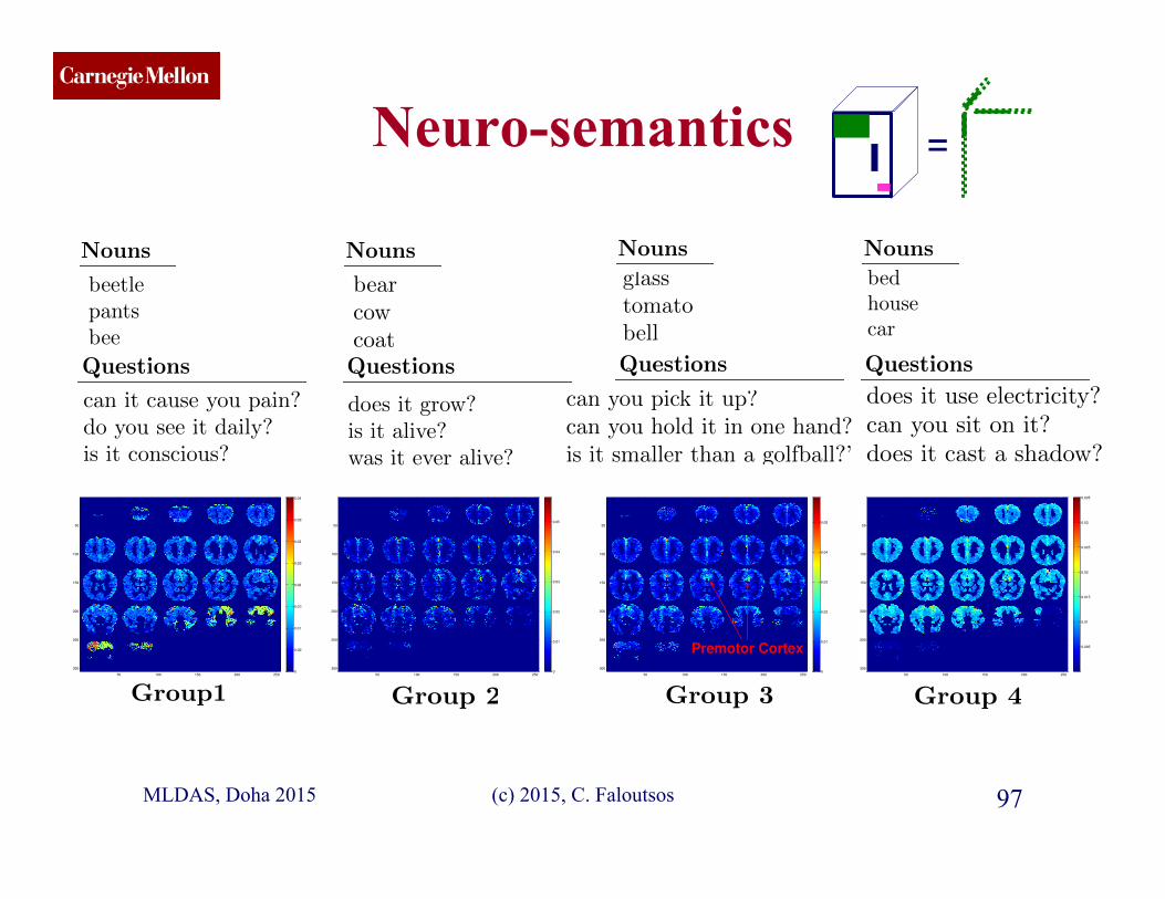
CMU SCS Neuro-semantics
50 100 150 200 250
50
100
150
200
250
3000
0.005
0.01
0.015
0.02
0.025
0.03
0.035
0.04
50 100 150 200 250
50
100
150
200
250
3000
0.01
0.02
0.03
0.04
0.05
50 100 150 200 250
50
100
150
200
250
3000
0.01
0.02
0.03
0.04
0.05
Premotor Cortex
50 100 150 200 250
50
100
150
200
250
300
0.005
0.01
0.015
0.02
0.025
0.03
0.035
Group1
Group 2 Group 4
Group 3
beetle can it cause you pain?pants do you see it daily?bee is it conscious?
beetle can it cause you pain?pants do you see it daily?bee is it conscious?
Nouns Questions Nouns Questions
Nouns Questions
beetle can it cause you pain?
Nouns Questions Nouns Questions
Nouns Questions
beetle can it cause you pain?
Nouns Questions Nouns Questions
Nouns Questions
beetle can it cause you pain?
Nouns Questions Nouns Questions
Nouns Questions
beetle can it cause you pain?bear does it grow?cow is it alive?coat was it ever alive?
bear does it grow?cow is it alive?coat was it ever alive?
glass can you pick it up?tomato can you hold it in one hand?bell is it smaller than a golfball?’
glass can you pick it up?tomato can you hold it in one hand?bell is it smaller than a golfball?’
bed does it use electricity?house can you sit on it?car does it cast a shadow?
bed does it use electricity?house can you sit on it?car does it cast a shadow?
Figure 4: Turbo-SMT finds meaningful groups of words, questions, and brain regions that are (both negativelyand positively) correlated, as obtained using Turbo-SMT. For instance, Group 3 refers to small items that canbe held in one hand,such as a tomato or a glass, and the activation pattern is very di↵erent from the one ofGroup 1, which mostly refers to insects, such as bee or beetle. Additionally, Group 3 shows high activation in thepremotor cortex which is associated with the concepts of that group.
v
1
and v
2
which were withheld from the training data,the leave-two-out scheme measures prediction accuracyby the ability to choose which of the observed brainimages corresponds to which of the two words. Aftermean-centering the vectors, this classification decisionis made according to the following rule:
kv1 � v̂1k2 + kv2 � v̂2k2 < kv1 � v̂2k2 + kv2 � v̂1k2
Although our approach is not designed to make predic-tions, preliminary results are very encouraging: Usingonly F=2 components, for the noun pair closet/watch
we obtained mean accuracy of about 0.82 for 5 out of the9 human subjects. Similarly, for the pair knife/beetle,we achieved accuracy of about 0.8 for a somewhat dif-ferent group of 5 subjects. For the rest of the humansubjects, the accuracy is considerably lower, however, itmay be the case that brain activity predictability variesbetween subjects, a fact that requires further investiga-tion.
5 Experiments
We implemented Turbo-SMT in Matlab. Our imple-mentation of the code is publicly available.5 For the par-allelization of the algorithm, we used Matlab’s ParallelComputing Toolbox. For tensor manipulation, we used
5http://www.cs.cmu.edu/
~
epapalex/src/turbo_smt.zip
the Tensor Toolbox for Matlab [7] which is optimizedespecially for sparse tensors (but works very well fordense ones too). We use the ALS and the CMTF-OPT[5] algorithms as baselines, i.e. we compare Turbo-
SMT when using one of those algorithms as their coreCMTF implementation, against the plain execution ofthose algorithms. We implemented our version of theALS algorithm, and we used the CMTF Toobox6 im-plementation of CMTF-OPT. We use CMTF-OPT forhigher ranks, since that particular algorithm is moreaccurate than ALS, and is the state of the art. All ex-periments were carried out on a machine with 4 IntelXeon E74850 2.00GHz, and 512Gb of RAM. Wheneverwe conducted multiple iterations of an experiment (dueto the randomized nature of Turbo-SMT), we reporterror-bars along the plots. For all the following experi-ments we used either portions of the BrainQ dataset,or the whole dataset.
5.1 Speedup As we have already discussed in the In-troduction and shown in Fig. 1, Turbo-SMT achievesa speedup of 50-200 on the BrainQ dataset; For allcases, the approximation cost is either same as the base-lines, or is larger by a small factor, indicating thatTurbo-SMT is both fast and accurate. Key facts that
6http://www.models.life.ku.dk/joda/CMTF_Toolbox
97 MLDAS, Doha 2015 (c) 2015, C. Faloutsos
=

CMU SCS Neuro-semantics
98 MLDAS, Doha 2015 (c) 2015, C. Faloutsos
50 100 150 200 250
50
100
150
200
250
3000
0.005
0.01
0.015
0.02
0.025
0.03
0.035
0.04
50 100 150 200 250
50
100
150
200
250
3000
0.01
0.02
0.03
0.04
0.05
50 100 150 200 250
50
100
150
200
250
3000
0.01
0.02
0.03
0.04
0.05
Premotor Cortex
50 100 150 200 250
50
100
150
200
250
300
0.005
0.01
0.015
0.02
0.025
0.03
0.035
Group1
Group 2 Group 4
Group 3
beetle can it cause you pain?pants do you see it daily?bee is it conscious?
beetle can it cause you pain?pants do you see it daily?bee is it conscious?
Nouns Questions Nouns Questions
Nouns Questions
beetle can it cause you pain?
Nouns Questions Nouns Questions
Nouns Questions
beetle can it cause you pain?
Nouns Questions Nouns Questions
Nouns Questions
beetle can it cause you pain?
Nouns Questions Nouns Questions
Nouns Questions
beetle can it cause you pain?bear does it grow?cow is it alive?coat was it ever alive?
bear does it grow?cow is it alive?coat was it ever alive?
glass can you pick it up?tomato can you hold it in one hand?bell is it smaller than a golfball?’
glass can you pick it up?tomato can you hold it in one hand?bell is it smaller than a golfball?’
bed does it use electricity?house can you sit on it?car does it cast a shadow?
bed does it use electricity?house can you sit on it?car does it cast a shadow?
Figure 4: Turbo-SMT finds meaningful groups of words, questions, and brain regions that are (both negativelyand positively) correlated, as obtained using Turbo-SMT. For instance, Group 3 refers to small items that canbe held in one hand,such as a tomato or a glass, and the activation pattern is very di↵erent from the one ofGroup 1, which mostly refers to insects, such as bee or beetle. Additionally, Group 3 shows high activation in thepremotor cortex which is associated with the concepts of that group.
v
1
and v
2
which were withheld from the training data,the leave-two-out scheme measures prediction accuracyby the ability to choose which of the observed brainimages corresponds to which of the two words. Aftermean-centering the vectors, this classification decisionis made according to the following rule:
kv1 � v̂1k2 + kv2 � v̂2k2 < kv1 � v̂2k2 + kv2 � v̂1k2
Although our approach is not designed to make predic-tions, preliminary results are very encouraging: Usingonly F=2 components, for the noun pair closet/watch
we obtained mean accuracy of about 0.82 for 5 out of the9 human subjects. Similarly, for the pair knife/beetle,we achieved accuracy of about 0.8 for a somewhat dif-ferent group of 5 subjects. For the rest of the humansubjects, the accuracy is considerably lower, however, itmay be the case that brain activity predictability variesbetween subjects, a fact that requires further investiga-tion.
5 Experiments
We implemented Turbo-SMT in Matlab. Our imple-mentation of the code is publicly available.5 For the par-allelization of the algorithm, we used Matlab’s ParallelComputing Toolbox. For tensor manipulation, we used
5http://www.cs.cmu.edu/
~
epapalex/src/turbo_smt.zip
the Tensor Toolbox for Matlab [7] which is optimizedespecially for sparse tensors (but works very well fordense ones too). We use the ALS and the CMTF-OPT[5] algorithms as baselines, i.e. we compare Turbo-
SMT when using one of those algorithms as their coreCMTF implementation, against the plain execution ofthose algorithms. We implemented our version of theALS algorithm, and we used the CMTF Toobox6 im-plementation of CMTF-OPT. We use CMTF-OPT forhigher ranks, since that particular algorithm is moreaccurate than ALS, and is the state of the art. All ex-periments were carried out on a machine with 4 IntelXeon E74850 2.00GHz, and 512Gb of RAM. Wheneverwe conducted multiple iterations of an experiment (dueto the randomized nature of Turbo-SMT), we reporterror-bars along the plots. For all the following experi-ments we used either portions of the BrainQ dataset,or the whole dataset.
5.1 Speedup As we have already discussed in the In-troduction and shown in Fig. 1, Turbo-SMT achievesa speedup of 50-200 on the BrainQ dataset; For allcases, the approximation cost is either same as the base-lines, or is larger by a small factor, indicating thatTurbo-SMT is both fast and accurate. Key facts that
6http://www.models.life.ku.dk/joda/CMTF_Toolbox
Small items -> Premotor cortex
=
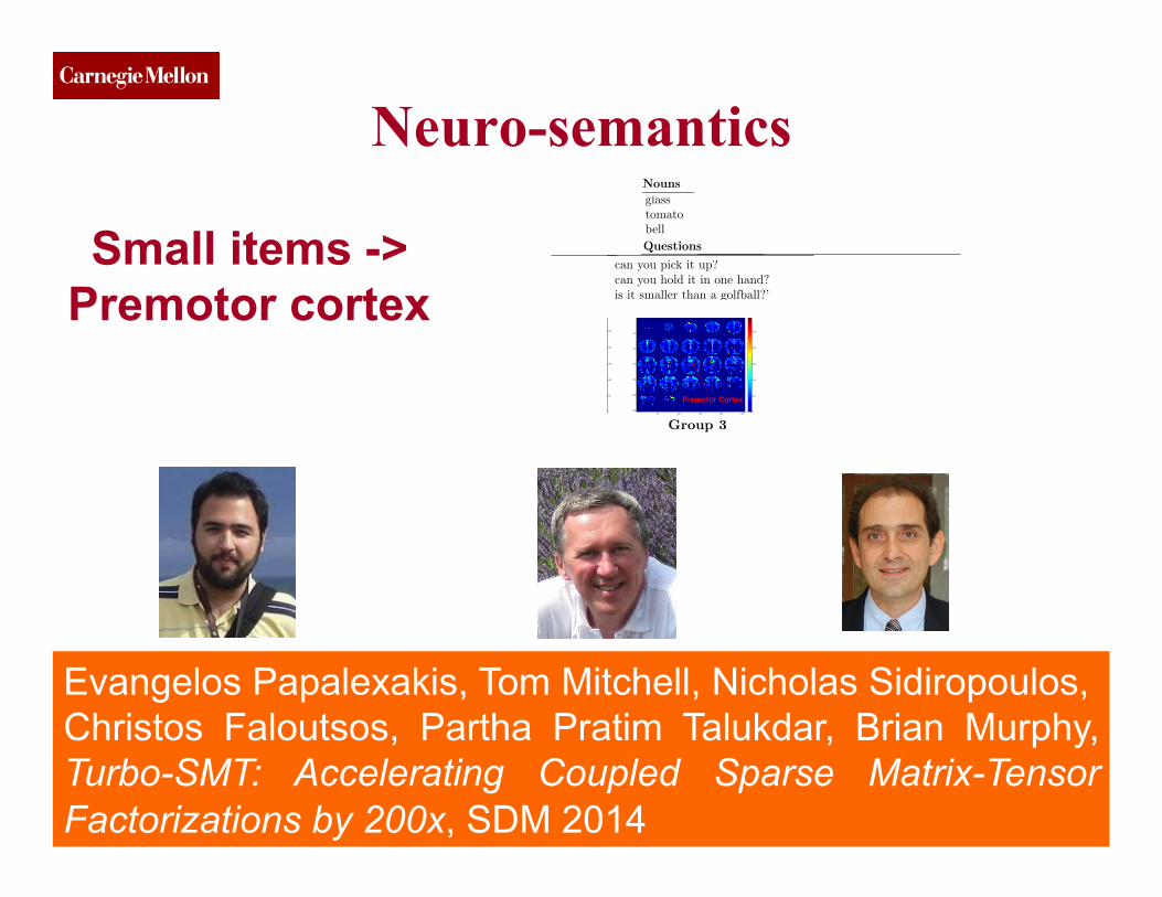
CMU SCS Neuro-semantics
99 MLDAS, Doha 2015 (c) 2015, C. Faloutsos
50 100 150 200 250
50
100
150
200
250
3000
0.005
0.01
0.015
0.02
0.025
0.03
0.035
0.04
50 100 150 200 250
50
100
150
200
250
3000
0.01
0.02
0.03
0.04
0.05
50 100 150 200 250
50
100
150
200
250
3000
0.01
0.02
0.03
0.04
0.05
Premotor Cortex
50 100 150 200 250
50
100
150
200
250
300
0.005
0.01
0.015
0.02
0.025
0.03
0.035
Group1
Group 2 Group 4
Group 3
beetle can it cause you pain?pants do you see it daily?bee is it conscious?
beetle can it cause you pain?pants do you see it daily?bee is it conscious?
Nouns Questions Nouns Questions
Nouns Questions
beetle can it cause you pain?
Nouns Questions Nouns Questions
Nouns Questions
beetle can it cause you pain?
Nouns Questions Nouns Questions
Nouns Questions
beetle can it cause you pain?
Nouns Questions Nouns Questions
Nouns Questions
beetle can it cause you pain?bear does it grow?cow is it alive?coat was it ever alive?
bear does it grow?cow is it alive?coat was it ever alive?
glass can you pick it up?tomato can you hold it in one hand?bell is it smaller than a golfball?’
glass can you pick it up?tomato can you hold it in one hand?bell is it smaller than a golfball?’
bed does it use electricity?house can you sit on it?car does it cast a shadow?
bed does it use electricity?house can you sit on it?car does it cast a shadow?
Figure 4: Turbo-SMT finds meaningful groups of words, questions, and brain regions that are (both negativelyand positively) correlated, as obtained using Turbo-SMT. For instance, Group 3 refers to small items that canbe held in one hand,such as a tomato or a glass, and the activation pattern is very di↵erent from the one ofGroup 1, which mostly refers to insects, such as bee or beetle. Additionally, Group 3 shows high activation in thepremotor cortex which is associated with the concepts of that group.
v
1
and v
2
which were withheld from the training data,the leave-two-out scheme measures prediction accuracyby the ability to choose which of the observed brainimages corresponds to which of the two words. Aftermean-centering the vectors, this classification decisionis made according to the following rule:
kv1 � v̂1k2 + kv2 � v̂2k2 < kv1 � v̂2k2 + kv2 � v̂1k2
Although our approach is not designed to make predic-tions, preliminary results are very encouraging: Usingonly F=2 components, for the noun pair closet/watch
we obtained mean accuracy of about 0.82 for 5 out of the9 human subjects. Similarly, for the pair knife/beetle,we achieved accuracy of about 0.8 for a somewhat dif-ferent group of 5 subjects. For the rest of the humansubjects, the accuracy is considerably lower, however, itmay be the case that brain activity predictability variesbetween subjects, a fact that requires further investiga-tion.
5 Experiments
We implemented Turbo-SMT in Matlab. Our imple-mentation of the code is publicly available.5 For the par-allelization of the algorithm, we used Matlab’s ParallelComputing Toolbox. For tensor manipulation, we used
5http://www.cs.cmu.edu/
~
epapalex/src/turbo_smt.zip
the Tensor Toolbox for Matlab [7] which is optimizedespecially for sparse tensors (but works very well fordense ones too). We use the ALS and the CMTF-OPT[5] algorithms as baselines, i.e. we compare Turbo-
SMT when using one of those algorithms as their coreCMTF implementation, against the plain execution ofthose algorithms. We implemented our version of theALS algorithm, and we used the CMTF Toobox6 im-plementation of CMTF-OPT. We use CMTF-OPT forhigher ranks, since that particular algorithm is moreaccurate than ALS, and is the state of the art. All ex-periments were carried out on a machine with 4 IntelXeon E74850 2.00GHz, and 512Gb of RAM. Wheneverwe conducted multiple iterations of an experiment (dueto the randomized nature of Turbo-SMT), we reporterror-bars along the plots. For all the following experi-ments we used either portions of the BrainQ dataset,or the whole dataset.
5.1 Speedup As we have already discussed in the In-troduction and shown in Fig. 1, Turbo-SMT achievesa speedup of 50-200 on the BrainQ dataset; For allcases, the approximation cost is either same as the base-lines, or is larger by a small factor, indicating thatTurbo-SMT is both fast and accurate. Key facts that
6http://www.models.life.ku.dk/joda/CMTF_Toolbox
Evangelos Papalexakis, Tom Mitchell, Nicholas Sidiropoulos, Christos Faloutsos, Partha Pratim Talukdar, Brian Murphy, Turbo-SMT: Accelerating Coupled Sparse Matrix-Tensor Factorizations by 200x, SDM 2014
Small items -> Premotor cortex
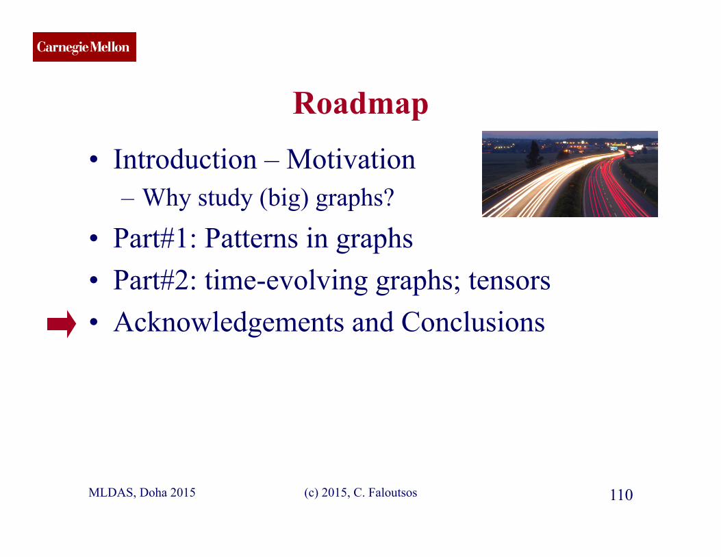
CMU SCS
(c) 2015, C. Faloutsos 110
Roadmap
• Introduction – Motivation – Why study (big) graphs?
• Part#1: Patterns in graphs • Part#2: time-evolving graphs; tensors • Acknowledgements and Conclusions
MLDAS, Doha 2015

CMU SCS
(c) 2015, C. Faloutsos 111
Thanks
MLDAS, Doha 2015
Thanks to: NSF IIS-0705359, IIS-0534205, CTA-INARC; Yahoo (M45), LLNL, IBM, SPRINT, Google, INTEL, HP, iLab
Disclaimer: All opinions are mine; not necessarily reflecting the opinions of the funding agencies
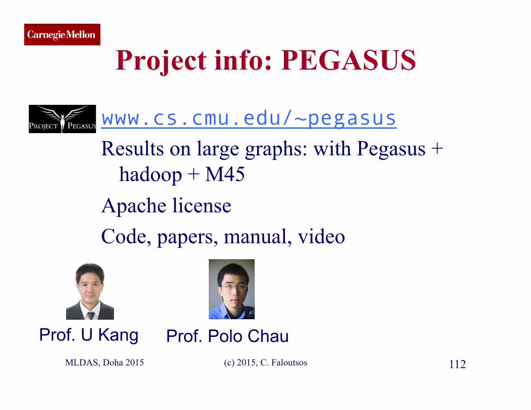
CMU SCS
(c) 2015, C. Faloutsos 112
Project info: PEGASUS
MLDAS, Doha 2015
www.cs.cmu.edu/~pegasus Results on large graphs: with Pegasus +
hadoop + M45 Apache license Code, papers, manual, video
Prof. U Kang Prof. Polo Chau
CMU SCS
(c) 2015, C. Faloutsos 113
Cast
Akoglu, Leman
Chau, Polo
Kang, U
Prakash, Aditya
MLDAS, Doha 2015
Koutra, Danai
Beutel, Alex
Papalexakis, Vagelis
Shah, Neil
Lee, Jay Yoon
Araujo, Miguel
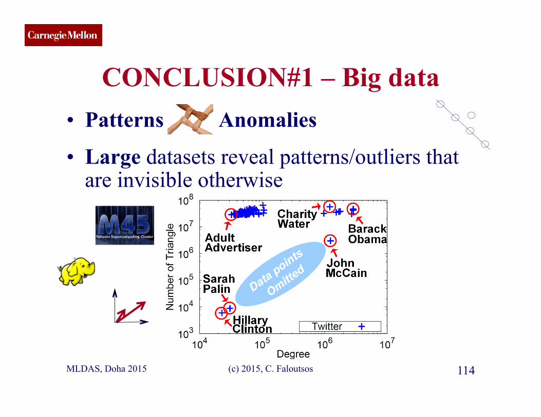
CMU SCS
(c) 2015, C. Faloutsos 114
CONCLUSION#1 – Big data • Patterns Anomalies
• Large datasets reveal patterns/outliers that are invisible otherwise
MLDAS, Doha 2015
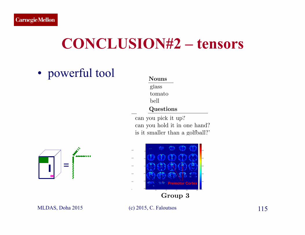
CMU SCS
(c) 2015, C. Faloutsos 115
CONCLUSION#2 – tensors
• powerful tool
MLDAS, Doha 2015
50 100 150 200 250
50
100
150
200
250
3000
0.005
0.01
0.015
0.02
0.025
0.03
0.035
0.04
50 100 150 200 250
50
100
150
200
250
3000
0.01
0.02
0.03
0.04
0.05
50 100 150 200 250
50
100
150
200
250
3000
0.01
0.02
0.03
0.04
0.05
Premotor Cortex
50 100 150 200 250
50
100
150
200
250
300
0.005
0.01
0.015
0.02
0.025
0.03
0.035
Group1
Group 2 Group 4
Group 3
beetle can it cause you pain?pants do you see it daily?bee is it conscious?
beetle can it cause you pain?pants do you see it daily?bee is it conscious?
Nouns Questions Nouns Questions
Nouns Questions
beetle can it cause you pain?
Nouns Questions Nouns Questions
Nouns Questions
beetle can it cause you pain?
Nouns Questions Nouns Questions
Nouns Questions
beetle can it cause you pain?
Nouns Questions Nouns Questions
Nouns Questions
beetle can it cause you pain?bear does it grow?cow is it alive?coat was it ever alive?
bear does it grow?cow is it alive?coat was it ever alive?
glass can you pick it up?tomato can you hold it in one hand?bell is it smaller than a golfball?’
glass can you pick it up?tomato can you hold it in one hand?bell is it smaller than a golfball?’
bed does it use electricity?house can you sit on it?car does it cast a shadow?
bed does it use electricity?house can you sit on it?car does it cast a shadow?
Figure 4: Turbo-SMT finds meaningful groups of words, questions, and brain regions that are (both negativelyand positively) correlated, as obtained using Turbo-SMT. For instance, Group 3 refers to small items that canbe held in one hand,such as a tomato or a glass, and the activation pattern is very di↵erent from the one ofGroup 1, which mostly refers to insects, such as bee or beetle. Additionally, Group 3 shows high activation in thepremotor cortex which is associated with the concepts of that group.
v
1
and v
2
which were withheld from the training data,the leave-two-out scheme measures prediction accuracyby the ability to choose which of the observed brainimages corresponds to which of the two words. Aftermean-centering the vectors, this classification decisionis made according to the following rule:
kv1 � v̂1k2 + kv2 � v̂2k2 < kv1 � v̂2k2 + kv2 � v̂1k2
Although our approach is not designed to make predic-tions, preliminary results are very encouraging: Usingonly F=2 components, for the noun pair closet/watch
we obtained mean accuracy of about 0.82 for 5 out of the9 human subjects. Similarly, for the pair knife/beetle,we achieved accuracy of about 0.8 for a somewhat dif-ferent group of 5 subjects. For the rest of the humansubjects, the accuracy is considerably lower, however, itmay be the case that brain activity predictability variesbetween subjects, a fact that requires further investiga-tion.
5 Experiments
We implemented Turbo-SMT in Matlab. Our imple-mentation of the code is publicly available.5 For the par-allelization of the algorithm, we used Matlab’s ParallelComputing Toolbox. For tensor manipulation, we used
5http://www.cs.cmu.edu/
~
epapalex/src/turbo_smt.zip
the Tensor Toolbox for Matlab [7] which is optimizedespecially for sparse tensors (but works very well fordense ones too). We use the ALS and the CMTF-OPT[5] algorithms as baselines, i.e. we compare Turbo-
SMT when using one of those algorithms as their coreCMTF implementation, against the plain execution ofthose algorithms. We implemented our version of theALS algorithm, and we used the CMTF Toobox6 im-plementation of CMTF-OPT. We use CMTF-OPT forhigher ranks, since that particular algorithm is moreaccurate than ALS, and is the state of the art. All ex-periments were carried out on a machine with 4 IntelXeon E74850 2.00GHz, and 512Gb of RAM. Wheneverwe conducted multiple iterations of an experiment (dueto the randomized nature of Turbo-SMT), we reporterror-bars along the plots. For all the following experi-ments we used either portions of the BrainQ dataset,or the whole dataset.
5.1 Speedup As we have already discussed in the In-troduction and shown in Fig. 1, Turbo-SMT achievesa speedup of 50-200 on the BrainQ dataset; For allcases, the approximation cost is either same as the base-lines, or is larger by a small factor, indicating thatTurbo-SMT is both fast and accurate. Key facts that
6http://www.models.life.ku.dk/joda/CMTF_Toolbox
=
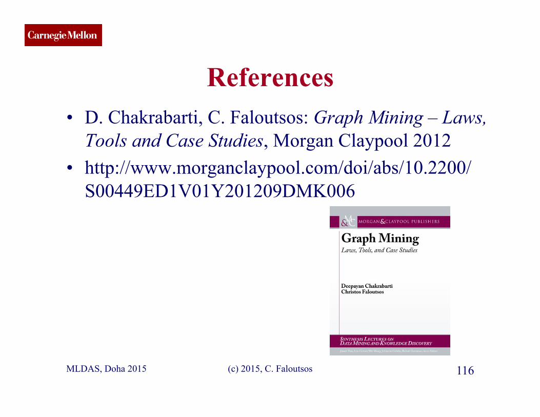
CMU SCS
(c) 2015, C. Faloutsos 116
References • D. Chakrabarti, C. Faloutsos: Graph Mining – Laws,
Tools and Case Studies, Morgan Claypool 2012 • http://www.morganclaypool.com/doi/abs/10.2200/
S00449ED1V01Y201209DMK006
MLDAS, Doha 2015
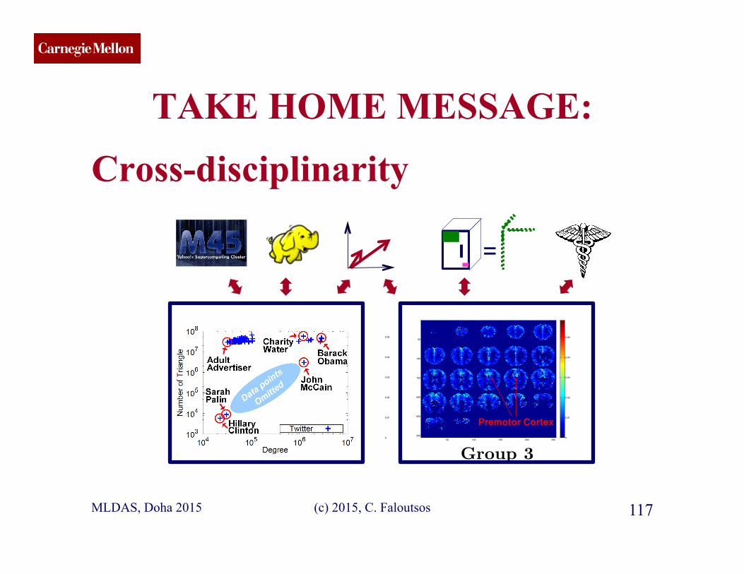
CMU SCS
TAKE HOME MESSAGE: Cross-disciplinarity
MLDAS, Doha 2015 (c) 2015, C. Faloutsos 117
50 100 150 200 250
50
100
150
200
250
3000
0.005
0.01
0.015
0.02
0.025
0.03
0.035
0.04
50 100 150 200 250
50
100
150
200
250
3000
0.01
0.02
0.03
0.04
0.05
50 100 150 200 250
50
100
150
200
250
3000
0.01
0.02
0.03
0.04
0.05
Premotor Cortex
50 100 150 200 250
50
100
150
200
250
300
0.005
0.01
0.015
0.02
0.025
0.03
0.035
Group1
Group 2 Group 4
Group 3
beetle can it cause you pain?pants do you see it daily?bee is it conscious?
beetle can it cause you pain?pants do you see it daily?bee is it conscious?
Nouns Questions Nouns Questions
Nouns Questions
beetle can it cause you pain?
Nouns Questions Nouns Questions
Nouns Questions
beetle can it cause you pain?
Nouns Questions Nouns Questions
Nouns Questions
beetle can it cause you pain?
Nouns Questions Nouns Questions
Nouns Questions
beetle can it cause you pain?bear does it grow?cow is it alive?coat was it ever alive?
bear does it grow?cow is it alive?coat was it ever alive?
glass can you pick it up?tomato can you hold it in one hand?bell is it smaller than a golfball?’
glass can you pick it up?tomato can you hold it in one hand?bell is it smaller than a golfball?’
bed does it use electricity?house can you sit on it?car does it cast a shadow?
bed does it use electricity?house can you sit on it?car does it cast a shadow?
Figure 4: Turbo-SMT finds meaningful groups of words, questions, and brain regions that are (both negativelyand positively) correlated, as obtained using Turbo-SMT. For instance, Group 3 refers to small items that canbe held in one hand,such as a tomato or a glass, and the activation pattern is very di↵erent from the one ofGroup 1, which mostly refers to insects, such as bee or beetle. Additionally, Group 3 shows high activation in thepremotor cortex which is associated with the concepts of that group.
v
1
and v
2
which were withheld from the training data,the leave-two-out scheme measures prediction accuracyby the ability to choose which of the observed brainimages corresponds to which of the two words. Aftermean-centering the vectors, this classification decisionis made according to the following rule:
kv1 � v̂1k2 + kv2 � v̂2k2 < kv1 � v̂2k2 + kv2 � v̂1k2
Although our approach is not designed to make predic-tions, preliminary results are very encouraging: Usingonly F=2 components, for the noun pair closet/watch
we obtained mean accuracy of about 0.82 for 5 out of the9 human subjects. Similarly, for the pair knife/beetle,we achieved accuracy of about 0.8 for a somewhat dif-ferent group of 5 subjects. For the rest of the humansubjects, the accuracy is considerably lower, however, itmay be the case that brain activity predictability variesbetween subjects, a fact that requires further investiga-tion.
5 Experiments
We implemented Turbo-SMT in Matlab. Our imple-mentation of the code is publicly available.5 For the par-allelization of the algorithm, we used Matlab’s ParallelComputing Toolbox. For tensor manipulation, we used
5http://www.cs.cmu.edu/
~
epapalex/src/turbo_smt.zip
the Tensor Toolbox for Matlab [7] which is optimizedespecially for sparse tensors (but works very well fordense ones too). We use the ALS and the CMTF-OPT[5] algorithms as baselines, i.e. we compare Turbo-
SMT when using one of those algorithms as their coreCMTF implementation, against the plain execution ofthose algorithms. We implemented our version of theALS algorithm, and we used the CMTF Toobox6 im-plementation of CMTF-OPT. We use CMTF-OPT forhigher ranks, since that particular algorithm is moreaccurate than ALS, and is the state of the art. All ex-periments were carried out on a machine with 4 IntelXeon E74850 2.00GHz, and 512Gb of RAM. Wheneverwe conducted multiple iterations of an experiment (dueto the randomized nature of Turbo-SMT), we reporterror-bars along the plots. For all the following experi-ments we used either portions of the BrainQ dataset,or the whole dataset.
5.1 Speedup As we have already discussed in the In-troduction and shown in Fig. 1, Turbo-SMT achievesa speedup of 50-200 on the BrainQ dataset; For allcases, the approximation cost is either same as the base-lines, or is larger by a small factor, indicating thatTurbo-SMT is both fast and accurate. Key facts that
6http://www.models.life.ku.dk/joda/CMTF_Toolbox
=

CMU SCS
TAKE HOME MESSAGE: Cross-disciplinarity
MLDAS, Doha 2015 (c) 2015, C. Faloutsos 118
Thank you!
50 100 150 200 250
50
100
150
200
250
3000
0.005
0.01
0.015
0.02
0.025
0.03
0.035
0.04
50 100 150 200 250
50
100
150
200
250
3000
0.01
0.02
0.03
0.04
0.05
50 100 150 200 250
50
100
150
200
250
3000
0.01
0.02
0.03
0.04
0.05
Premotor Cortex
50 100 150 200 250
50
100
150
200
250
300
0.005
0.01
0.015
0.02
0.025
0.03
0.035
Group1
Group 2 Group 4
Group 3
beetle can it cause you pain?pants do you see it daily?bee is it conscious?
beetle can it cause you pain?pants do you see it daily?bee is it conscious?
Nouns Questions Nouns Questions
Nouns Questions
beetle can it cause you pain?
Nouns Questions Nouns Questions
Nouns Questions
beetle can it cause you pain?
Nouns Questions Nouns Questions
Nouns Questions
beetle can it cause you pain?
Nouns Questions Nouns Questions
Nouns Questions
beetle can it cause you pain?bear does it grow?cow is it alive?coat was it ever alive?
bear does it grow?cow is it alive?coat was it ever alive?
glass can you pick it up?tomato can you hold it in one hand?bell is it smaller than a golfball?’
glass can you pick it up?tomato can you hold it in one hand?bell is it smaller than a golfball?’
bed does it use electricity?house can you sit on it?car does it cast a shadow?
bed does it use electricity?house can you sit on it?car does it cast a shadow?
Figure 4: Turbo-SMT finds meaningful groups of words, questions, and brain regions that are (both negativelyand positively) correlated, as obtained using Turbo-SMT. For instance, Group 3 refers to small items that canbe held in one hand,such as a tomato or a glass, and the activation pattern is very di↵erent from the one ofGroup 1, which mostly refers to insects, such as bee or beetle. Additionally, Group 3 shows high activation in thepremotor cortex which is associated with the concepts of that group.
v
1
and v
2
which were withheld from the training data,the leave-two-out scheme measures prediction accuracyby the ability to choose which of the observed brainimages corresponds to which of the two words. Aftermean-centering the vectors, this classification decisionis made according to the following rule:
kv1 � v̂1k2 + kv2 � v̂2k2 < kv1 � v̂2k2 + kv2 � v̂1k2
Although our approach is not designed to make predic-tions, preliminary results are very encouraging: Usingonly F=2 components, for the noun pair closet/watch
we obtained mean accuracy of about 0.82 for 5 out of the9 human subjects. Similarly, for the pair knife/beetle,we achieved accuracy of about 0.8 for a somewhat dif-ferent group of 5 subjects. For the rest of the humansubjects, the accuracy is considerably lower, however, itmay be the case that brain activity predictability variesbetween subjects, a fact that requires further investiga-tion.
5 Experiments
We implemented Turbo-SMT in Matlab. Our imple-mentation of the code is publicly available.5 For the par-allelization of the algorithm, we used Matlab’s ParallelComputing Toolbox. For tensor manipulation, we used
5http://www.cs.cmu.edu/
~
epapalex/src/turbo_smt.zip
the Tensor Toolbox for Matlab [7] which is optimizedespecially for sparse tensors (but works very well fordense ones too). We use the ALS and the CMTF-OPT[5] algorithms as baselines, i.e. we compare Turbo-
SMT when using one of those algorithms as their coreCMTF implementation, against the plain execution ofthose algorithms. We implemented our version of theALS algorithm, and we used the CMTF Toobox6 im-plementation of CMTF-OPT. We use CMTF-OPT forhigher ranks, since that particular algorithm is moreaccurate than ALS, and is the state of the art. All ex-periments were carried out on a machine with 4 IntelXeon E74850 2.00GHz, and 512Gb of RAM. Wheneverwe conducted multiple iterations of an experiment (dueto the randomized nature of Turbo-SMT), we reporterror-bars along the plots. For all the following experi-ments we used either portions of the BrainQ dataset,or the whole dataset.
5.1 Speedup As we have already discussed in the In-troduction and shown in Fig. 1, Turbo-SMT achievesa speedup of 50-200 on the BrainQ dataset; For allcases, the approximation cost is either same as the base-lines, or is larger by a small factor, indicating thatTurbo-SMT is both fast and accurate. Key facts that
6http://www.models.life.ku.dk/joda/CMTF_Toolbox
=