Embed Size (px)
Citation preview

Mining for MeaningThe Extraction of Lexico-Semantic Knowledge from Text
Tim Van de Cruys
draft
1
Contents
Contents 2
Introduction 5
I Theory 9
1 The Nature of Meaning 111.1 Theories of meaning . . . . . . . . . . . . . . . . . . . . . . . . . . 111.2 Context . . . . . . . . . . . . . . . . . . . . . . . . . . . . . . . . . 161.3 Tight vs. topical similarity . . . . . . . . . . . . . . . . . . . . . . . 22
2 The Computation of Meaning 232.1 Formal model . . . . . . . . . . . . . . . . . . . . . . . . . . . . . . 232.2 Similarity calculations: geometry vs. probability . . . . . . . . . . . 242.3 Weighting schemes . . . . . . . . . . . . . . . . . . . . . . . . . . . 29
3 Dimensionality Reduction 333.1 Introduction . . . . . . . . . . . . . . . . . . . . . . . . . . . . . . . 333.2 Latent semantic analysis . . . . . . . . . . . . . . . . . . . . . . . . 343.3 Non-negative matrix factorization . . . . . . . . . . . . . . . . . . . 42
4 Three-way Methods 474.1 Introduction . . . . . . . . . . . . . . . . . . . . . . . . . . . . . . . 474.2 Tensor algebra . . . . . . . . . . . . . . . . . . . . . . . . . . . . . . 514.3 Three-way factorization algorithms . . . . . . . . . . . . . . . . . . . 52
2

3
II Evaluation 57
5 Evaluation of Wordnet-based Similarity 595.1 Introduction . . . . . . . . . . . . . . . . . . . . . . . . . . . . . . . 595.2 Methodological remarks . . . . . . . . . . . . . . . . . . . . . . . . 605.3 Evaluation framework . . . . . . . . . . . . . . . . . . . . . . . . . . 615.4 Results . . . . . . . . . . . . . . . . . . . . . . . . . . . . . . . . . . 68
6 Evaluation of Cluster Quality 836.1 Introduction . . . . . . . . . . . . . . . . . . . . . . . . . . . . . . . 836.2 Methodology . . . . . . . . . . . . . . . . . . . . . . . . . . . . . . 836.3 Evaluation framework . . . . . . . . . . . . . . . . . . . . . . . . . . 856.4 Results . . . . . . . . . . . . . . . . . . . . . . . . . . . . . . . . . . 866.5 Comparison of the different models . . . . . . . . . . . . . . . . . . 95
7 Evaluation of Domain Coherence 977.1 Introduction . . . . . . . . . . . . . . . . . . . . . . . . . . . . . . . 977.2 Evaluation framework . . . . . . . . . . . . . . . . . . . . . . . . . . 977.3 Results . . . . . . . . . . . . . . . . . . . . . . . . . . . . . . . . . . 1007.4 Discussion & comparison . . . . . . . . . . . . . . . . . . . . . . . . 106
III Applications 109
8 Lexico-Semantic Multiword Expression Extraction 1118.1 Introduction . . . . . . . . . . . . . . . . . . . . . . . . . . . . . . . 1118.2 Previous work . . . . . . . . . . . . . . . . . . . . . . . . . . . . . . 1128.3 Methodology . . . . . . . . . . . . . . . . . . . . . . . . . . . . . . 1148.4 Results and evaluation . . . . . . . . . . . . . . . . . . . . . . . . . 1198.5 Conclusions and further work . . . . . . . . . . . . . . . . . . . . . . 125
9 Noun Sense Discrimination 1279.1 Introduction . . . . . . . . . . . . . . . . . . . . . . . . . . . . . . . 1279.2 Previous Work . . . . . . . . . . . . . . . . . . . . . . . . . . . . . . 1299.3 Methodology . . . . . . . . . . . . . . . . . . . . . . . . . . . . . . 1309.4 Examples . . . . . . . . . . . . . . . . . . . . . . . . . . . . . . . . 1349.5 Evaluation . . . . . . . . . . . . . . . . . . . . . . . . . . . . . . . . 1369.6 Conclusion & Future Work . . . . . . . . . . . . . . . . . . . . . . . 139

4 CONTENTS
10 Selectional Preferences 14110.1 Introduction . . . . . . . . . . . . . . . . . . . . . . . . . . . . . . . 14110.2 Previous Work . . . . . . . . . . . . . . . . . . . . . . . . . . . . . . 14210.3 Methodology . . . . . . . . . . . . . . . . . . . . . . . . . . . . . . 14410.4 Results . . . . . . . . . . . . . . . . . . . . . . . . . . . . . . . . . . 14710.5 Conclusion and Future Work . . . . . . . . . . . . . . . . . . . . . . 152
Conclusion 155
A Clustering Tasks 159A.1 Concrete noun categorization . . . . . . . . . . . . . . . . . . . . . . 159A.2 Abstract/concrete noun discrimination . . . . . . . . . . . . . . . . . 161
List of Abbreviations 163
Bibliography 165

Introduction
Human readers have the extraordinary capability to infer the meaning of a word fromtext, even if they have never heard of the word before, and there are no visual cuespresent to support its interpretation. Take for example sentences (1) – (3):
(1) FomalhautFomalhaut
staatstands
opon
2424
lichtjarenlight years
vanof
dethe
zon,sun
enand
isis
1515
keertimes
zoas
helder.bright
Fomalhaut is 24 light years away from the sun, and is 15 times as bright.
(2) ZelfsEven
eena
rijperipe
kumquatkumquat
smaakttastes
nogstill
tamelijkrather
zuur.sour
Even a ripe kumquat still tastes rather sour.
(3) OpOn
eena
statigstately
deuntjetune
danstedanced
menone
dethe
pavane.pavane
On a stately tune, they danced the pavane.
Even if we have never heard of words like Fomalhaut, kumquat and pavane before, wecan still make reasonable assumptions about their meaning. The surrounding wordsallow us to assume that Fomalhaut is probably a star, that kumquat is some kind ofedible organic object – most likely a fruit – and that a pavane is some kind of dance.We are able to infer the meaning of words because the context gives us cues about theirsemantic content. Likewise, we might be able to use the context of unknown words toinfer their meaning automatically.
Of course, we can only get at the meaning of Fomalhaut because we are alreadyfamiliar with the other words in the sentence, such as lichtjaar ‘light year’ and zon‘sun’. Likewise, we know what kind of objects might be ripe and taste sour, and wehave a general idea of what it is that can be danced. The situation becomes morecomplicated if we want to use a computer to automatically infer the meaning of words:unlike humans, a computer does not have any a priori knowledge of words whatsoever.For this reason, most work on the acquisition of semantics from text has focused on
5

6 INTRODUCTION
semantic similarity. Determining how similar a word is to other known words is mucheasier than determining what its actual meaning is. It is hard to extract the meaning ofFomalhaut from scratch, but it is much easier to determine that Fomalhaut appears inthe same contexts as words like Sirius and Betelgeuse. Likewise, the word kumquatwill appear in similar contexts as words like orange, lemon and apple, and pavane willbe found in locations similar to words like bourree, gigue or polka.
The semantic similarity of a word can thus be determined by accumulating itsdifferent contexts in a large corpus, and comparing those contexts to the contexts ofother words. If two words have similar contexts, they are likely to be semanticallyrelated. Likewise, if two words share only few or no contexts at all, they are probablysemantically unrelated. This process of determining a word’s semantics by looking atthe way it is distributed in texts is called DISTRIBUTIONAL SIMILARITY, and it will bethe main foundation of this dissertation.
The extraction of semantics from text is a very broad and extensive subject. Ittherefore makes sense to clearly demarcate what will be our object of research, and alsomention what this dissertation will not be about. The main subject of this dissertationis the lexico-semantic extraction of nouns from large-scale written corpora. The threeitalicized words are important here. By lexico-semantic extraction, we mean that werestrict ourselves to the extraction of semantic information on the lexical level: we areinterested in extracting the semantics of single words, as they might be described in adictionary. Of course, the lexical level is only a part of the vast domain that is semantics.Humans combine words into sentences to form complex meanings. Moreover, thecombination of words has an influence on the meaning of the combined parts. Thesephenomena belong to the domain of compositional semantics, and they are beyond thescope of this dissertation.
Secondly, this dissertation mainly investigates the extraction of nouns. It goeswithout saying that there are many more word classes – adjectives, verbs and evenfunction words – that deserve our attention with regard to the determination of theirsemantics. Verbs, in particular, make up an interesting word class with complexsemantic behaviour. This dissertation, however, is limited to the extraction of nouns,and the lexico-semantic extraction of other word classes is again largely beyond itsscope.1
Thirdly, we will investigate the lexical semantics of nouns by looking at theirdistribution in large written text corpora of newspaper texts. It is very well possiblethat the semantics present in these corpora is very different from the semantics to befound in spoken corpora, or in sources that go beyond the realm of linguistics. The
1Note, however, that we will touch upon the extraction of verb semantics in the last chapter, where wediscuss the extraction of selectional preferences.

7
semantics that we investigate in this dissertation, however, will be the semantics ofwords as they appear in written newspaper texts.
With these reservations set aside, we can introduce the three main research questionsthat will be investigated in this dissertation. First of all, we want to determine whatkind of semantic similarity is captured by different context models. We will presentthree different groups of models (each based on a different notion of context), and wewill quantitatively investigate what kind of semantic similarity is captured by them.At the same time, we will investigate the usefulness of the models (and the resultinglexico-semantic resources) in a number of applications, notably multi-word expressionextraction and word sense discrimination.
Secondly, we want to investigate the applicability of dimensionality reduction meth-ods for semantic similarity extraction. Dimensionality reduction – or factorization – isthe collective name for mathematical techniques that try to reduce an abundant numberof overlapping features to a limited number of independent, informative dimensions.We will discuss a number of dimensionality reduction methods, and quantitativelyevaluate whether they are beneficial for semantic similarity extraction. Again, theirusefulness is also investigated in two applications: word sense discrimination andselectional preference induction.
Thirdly, we will investigate the use of three-way methods for lexico-semanticinformation extraction. Up till now, most research on the extraction of lexical semanticsfrom text has focused on two-way methods, in which two-way co-occurrences (e.g.terms× documents) are used. Co-occurrences need not be limited to two ways, though;it is easy to think of entities that occur in three (or more) ways (e.g. verbs × subjects× direct objects). We will present the mathematical machinery to deal with multi-wayco-occurrences, and test the usefulness of three-way methods in an application, namelythe induction of selectional preferences.
The outline of this dissertation is as follows. The first part provides a theoreticframework – grounding the distributional similarity theorem and setting up a formalframework for a computational implementation. This includes a thorough overviewof two dimensionality reduction algorithms – singular value decomposition and non-negative matrix factorization – and a discussion of three-way methods. The second partinvestigates the three different groups of models and their various model parameters,and provides a quantitative evaluation of their ability to extract semantic similarity. Thefinal part of this dissertation provides a number of applications, in which the differentmodels and techniques presented in the first part are applied.


Part I
Theory
9

Chapter 1
The Nature of Meaning
If we want to extract meaning automatically from text, we first need to investigate what‘meaning’ actually is. What does it mean for a word to mean something? How is aparticular word able to convey a particular content? And how is this content built up?What is, in short, the nature of meaning?
1.1 Theories of meaning
In the course of history, the nature of meaning has been one of the major issues in thephilosophical debate. The issue was first raised in the ancient Greek world, and wassubsequently tackled by numerous philosophers. In the 19th century, meaning alsoentered the realm of linguistics – first in the context of diachronic linguistics,1 lateralso as a synchronic study. In the following paragraphs, we briefly discuss the differenttheories of meaning (and their relation to reality) that have been proposed both inphilosophy and linguistics, and assess their potential to serve within computationallyimplemented procedures of meaning extraction.
1.1.1 Referential theory of meaning
In a referential theory of meaning, the meaning of a particular word is regarded as apointer to the designated object in the real world. The meaning of a word is what itrefers to. If we utter a word like apple, we refer to an actual apple (or the set of allapples) in reality. Intuitively, a referential theory of meaning seems very appealing.
1Christian Karl Reisig proposed the study of ‘Semasiologie’ in 1825, Michel Breal coined the term‘semantique’ in 1883.
11

12 CHAPTER 1. THE NATURE OF MEANING
If parents want to teach their children the meaning of a word like apple, chances arepretty high that they will point to an actual apple – or a picture of one. At first sightwords indeed seem no more than references to things (entities, actions or relations)existing in the outside world. There are, however, a number of problems with such areferential theory of meaning. The theory is able to account for what is generally calledthe denotation or extension of words, but fails to describe other semantic characteristics,generally referred to as connotation or intension. The German philosopher GottlobFrege (1848–1925) illustrated this deficiency with a by now well-known example.Compare the following sentences:
(1) The morning star is the morning star.
(2) The morning star is the evening star.
Both morning star and evening star refer to the same entity, viz. the planet Venus,which might be visible either in the morning or in the evening (depending on therelative position of Venus and the earth). Sentences (1) and (2), however, significantlydiffer in meaning. Sentence (1) expresses a simple tautology, whereas sentence (2)expresses a new and important astronomical truth. Sentences (1) and (2) do not meanthe same thing, but a referential theory of meaning does not account for the differencebetween them.
Frege’s solution to the morning/evening star paradox was to make a distinctionbetween Sinn (sense) and Bedeutung (reference). Bedeutung is the object that the wordrefers to, whereas Sinn is the cognitive representation of the object. By making thisdistinction, it is possible for words to have a different sense but the same referent (as inthe paradox above).
The referential theory of meaning has been popular with logicians (e.g. the youngWittgenstein and Bertrand Russell). It provides a parsimonious and straightforwardmodel of meaning, but the previous examples have shown that it is incapable of captur-ing all aspects of meaning. Moreover, it is unclear how we ought to proceed in order toextract these ‘meaning references’ in a computational way. The theoretical problemsas well as the practical drawbacks make the referential theory rather unattractive forthe computational extraction of meaning.
1.1.2 Mentalist theory of meaning
Another solution – one that has been very popular throughout the history of philosophy,starting with the Greek philosopher Plato – is to represent meaning exclusively as ideas.A mentalist theory of meaning associates the meaning of a particular word with aparticular idea in the human mind. This theory effectively solves the morning/evening

1.1. THEORIES OF MEANING 13
star paradox: The morning star might be the same thing as the evening star in reality,but the idea of the morning star and the evening star may very well differ. The questionthat immediately follows is what this notion of idea actually entails. Surely, it cannotbe the mental representations that are present in each individual person. These mentalrepresentations differ a lot among different persons. If one person hears the wordstrawberry, an image of an appetizing dessert plate – possibly covered with lots ofwhipped cream – might pop up. Another person might prefer them with powder sugar,and another one without any topping at all. Or one might even be disgusted by theidea of strawberries, because of a severe allergic reaction in the past. To be practicallyusable, the ideas need to have some generality, exceeding the individual level. But itis difficult to achieve this generalization without resorting to the notion of idea in theplatonic sense, that is somehow mysteriously present in people’s minds. This is not thedirection we want to venture into, especially if we want to implement semantics in acomputational way. If we want a sound theory of semantics that can be implementedcomputationally, we will need a theory that is not dependent on reference or ideas.
1.1.3 Behavioural theory of meaning
The vagueness and non-generality that inevitably seems to surround the mentalistview has led people to abandon the mentalist theory of meaning in favour of a theorythat sticks to ‘observable’ facts. Inspired by the behaviourist movement that becamepopular within the field of psychology, the American linguist Leonard Bloomfielddefines meaning of a linguistic form as ‘the situation in which the speaker utters itand the response which it calls forth in the hearer’. (Bloomfield, 1933, p. 139). Themeaning of a word is thus reduced to the speaker’s stimulus that elicits its use, and/orthe hearer’s response to that word.
Although the behavioural theory of meaning claims to overcome the vagueness ofideas in the mentalist view, it seems almost as problematic as the theory it opposes.There is a plethora of different stimuli that elicit the same word, and the number ofdifferent responses evoked by that word is equally high. Take, for example, a word likejazz. In some situations, a person might utter the word to indicate they would like tohear some jazz tunes. In other situations, they might utter the word to approve – ordisapprove – of the music they are listening to at that moment. And one odd person –not particularly familiar with different music styles – might even utter jazz when in factthey are listening to hip hop. Similarly, people’s reactions to the word jazz may differquite a lot. One person might turn on the radio and look for a suitable radio station,another one might start nodding their head whistling a Duke Ellington tune, whileyet another might make an unhappy face and stick out their tongue. Every languageutterance has a similar abundance of stimuli eliciting it, and a similar abundance of

14 CHAPTER 1. THE NATURE OF MEANING
responses following it. This makes it practically impossible to describe the meaning ofa particular word in terms of the utterance’s stimuli and responses.
Moreover, behaviourists have a rather vague and untenable view of what thisbehaviourist meaning description practically should look like. In his main textbook onlinguistics, Language, Bloomfield notes:
The situations which prompt people to utter speech, include every objectand happening in their universe. In order to give a scientifically accuratedefinition of meaning for every form of a language, we should have tohave a scientifically accurate knowledge of everything in the speaker’sworld. (Bloomfield, 1933, p. 139)
Bloomfield himself acknowledges that
. . . the statement of meanings is therefore the weak point in [behavioural]language-study, and will remain so until human knowledge advances veryfar beyond its present state. (Bloomfield, 1933, p. 140)
Bloomfield also deems it necessary to ‘resort to makeshift theories’ whenever scientificdescription is impossible – one of those theories being a referential theory of meaning.
In addition to the theoretical and practical drawbacks associated with a behaviour-ist’s description of meaning, the theory obviously doesn’t stand a chance to functionwithin a computational framework. In order to implement meaning in a behavourial,computational framework, a computer should be able to observe, interpret and classifyhuman stimuli and responses. The current state of artificial intelligence does not allowsuch complex cognitive computations just yet.
1.1.4 Use theory of meaning
A radically different theory of meaning qualifies the meaning of an expression as itsuse in a language system. A use theory of meaning does not refer to an external entity(a referent, an idea, or stimuli and responses) to qualify a word’s meaning, but insteadqualifies the meaning of a word as the value it gets through the (linguistic) system inwhich it is used. It was Wittgenstein who famously noted that ‘the meaning of a wordis its use in the language’ (Wittgenstein, 1953).
The use theory of meaning differs radically from the previous theories of meaning.In the previous theories, there is an existing order of things (a ‘meaning’) outside of thelanguage system; the words of a language are used to talk about existing entities, butentities and words belong to two different classes, and there is no influence between

1.1. THEORIES OF MEANING 15
the two classes. A use theory of meaning, on the other hand, advances a system inwhich meaning is defined and constructed within the language itself.
The first person to explore this radically different view in the context of linguistictheory was the Swiss linguist Ferdinand de Saussure (1857–1913), who is the foundingfather of the linguistic movement nowadays known as structuralism. In his mostimportant work, the Cours de Linguistique Generale (Course in General Linguistics),Saussure lays out the foundations for a differential view on language. Saussure definesa linguistic sign as a combination of the signifiant (‘signifier’) – representing the soundform of the sign – and the signifie (‘signified’) – representing the linguistic meaning ofthe sign.
According to Saussure,
. . . la langue est un systeme dont tous les termes sont solidaires et ou lavaleur de l’un ne resulte que de la presence simultanee des autres . . .[language is a system in which all terms are equal, and in which thevalue of one is only the result of the simultaneous presence of the others](Saussure, 1916)
This quote represents Saussure’s structuralist view on language: the linguisticmeaning of a sign is not a given, existing truth in the outside world, but it is defined interms of its use in particular contexts (and its non-use in other contexts). The meaningof a particular word is not an independent or transcendental fact, but it is defined withina network of different embedded meanings, which in turn get their values from theirposition in the network of meanings.
The structuralist view on language has been further developed by a number oflinguists, one of the most notable being Zellig Harris. Harris advocated a distributionalmethod for linguistic research: linguistic elements (words, but also morphemes orphonemes) can be investigated by looking at the way they are distributed in language.As such, the distributional method is also able to discover the semantic properties of aword. Harris notes:
The fact that, for example, not every adjective occurs with every nouncan be used as a measure of meaning difference. For it is not merely thatdifferent members of the one class have different selections of members ofthe other class with which they are actually found. More than that: if weconsider words or morphemes A and B to be more different in meaningthan A and C, then we will often find that the distributions of A and B aremore different than the distributions of A and C. In other words, differenceof meaning correlates with difference of distribution. (Harris, 1954, p.156)

16 CHAPTER 1. THE NATURE OF MEANING
The hypothesis that semantically similar words tend to occur in similar contextshas been coined the DISTRIBUTIONAL HYPOTHESIS in subsequent work, and Harris’work is often cited as the main source of inspiration. The distributional hypothesisnot only turns out to provide a sound basis for meaning description, it also provides asuitable starting point for an implementation in a computational framework, as will beshown in chapter 2.
1.2 Context
In the first part of this chapter, we have shown that a use theory of meaning is a soundbasis for the computational extraction of lexico-semantic meaning: the sum of a word’scontexts is a good indicator of the word’s use, and hence its ‘meaning’. In the secondpart of this chapter, we focus on the notion of context. The context of a particularword can be interpreted in a number of ways: the context might be the document theword appears in, it might be a window of words around a particular word, or it mightbe the syntactic context in which the word takes part. In this section, we will havea look at these different kinds of context, investigate which parameters are involved,and examine how different contexts might be useful for lexico-semantic knowledgeextraction. The next chapter will then investigate how these various contexts can beformalized and implemented in a computational way.
1.2.1 Document-based context
First of all, a particular word always appears in a particular document. This gives riseto our first instantiation of the distributional hypothesis:
Hypothesis 1. Words are semantically similar if they appear in similar documents.
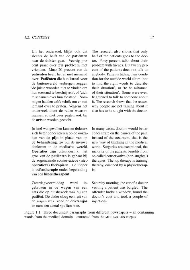
Words that appear in the same documents tend to be thematically related: textsusually focus on one particular topic (or a few topics), so that the majority of contentwords is related to these topics. Take for example the three newspaper paragraphs infigure 1.1, taken from the MEDIARGUS newspaper corpus, a 1.4 billion word corpus of(Belgian) Dutch newspaper texts.
The three paragraphs all contain words related to the medical domain (printedin boldface). Note that a word like patient ‘patient’ appears in all three documents.Likewise, words like dokter ‘doctor’ and arts ‘doctor’ appear in the same documents.In a similar vein, words related to another topic – say economics, soccer, or rock music– appear together in the same documents. If such related words appear in the samedocuments sufficiently frequently, a computer algorithm might be able to infer thatthey are indeed semantically related.
1.2. CONTEXT 17
Uit het onderzoek blijkt ook datslechts de helft van de patientennaar de dokter gaat. Veertig pro-cent praat over z’n probleem metvrienden. Maar 20 procent van depatienten heeft het er met niemandover. Patienten die hun kwaal voorde buitenwereld verbergen zeggen‘de juiste woorden niet te vinden omhun toestand te beschrijven’, of ‘zichte schamen over hun toestand’. Som-migen hadden zelfs schrik om er metiemand over te praten. Volgens hetonderzoek dient de reden waarommensen er niet over praten ook bijde arts te worden gezocht.
The research also shows that onlyhalf of the patients goes to the doc-tor. Forty percent talks about theirproblem with friends. But twenty per-cent of the patients does not talk toanybody. Patients hiding their condi-tion for the outside world claim ‘notto find the right words to describetheir situation’, or ‘to be ashamedof their situation’. Some were evenfrightened to talk to someone aboutit. The research shows that the reasonwhy people are not talking about italso has to be sought with the doctor.
In heel wat gevallen kunnen dokterszich beter concentreren op de oorza-ken van de pijn in plaats van opde behandeling, zo wil de nieuwedenktrant in de medische wereld.Operaties zijn uitzonderlijk, hetgros van de patienten is gebaat bijde zogenaamde conservatieve (niet-operatieve) therapieen. De topperis oefentherapie onder begeleidingvan een kinesitherapeut.
In many cases, doctors would betterconcentrate on the causes of the paininstead of the treatment, that is thenew way of thinking in the medicalworld. Surgeries are exceptional, themajority of the patients benefits fromso-called conservative (non-surgical)therapies. The top therapy is trainingtherapy, coached by a physiotherap-ist.
Zaterdagvoormiddag werd in-gebroken in de wagen van eenarts die op huisbezoek was bij eenpatient. De dader sloeg een ruit vande wagen stuk, vond de doktersjasen nam een aantal spuiten mee.
Saturday morning, the car of a doctorvisiting a patient was burgled. Theoffender broke a window, found thedoctor’s coat and took a couple ofinjections.
Figure 1.1: Three document paragraphs from different newspapers – all containingwords from the medical domain – extracted from the MEDIARGUS corpus
18 CHAPTER 1. THE NATURE OF MEANING
The main parameter to be set is the size of the document context. This will dependon the corpus used and the application in mind. In a newspaper corpus, the unit mightbe an article, or a paragraph. When using a web corpus, one might consider a particularweb page as document context.
1.2.2 Window-based context
Secondly, a particular word appears within the context of other words in its vicinity,which brings us to our second instantiation of the distributional hypothesis:
Hypothesis 2. Words are semantically similar if they appear within similar contextwindows.
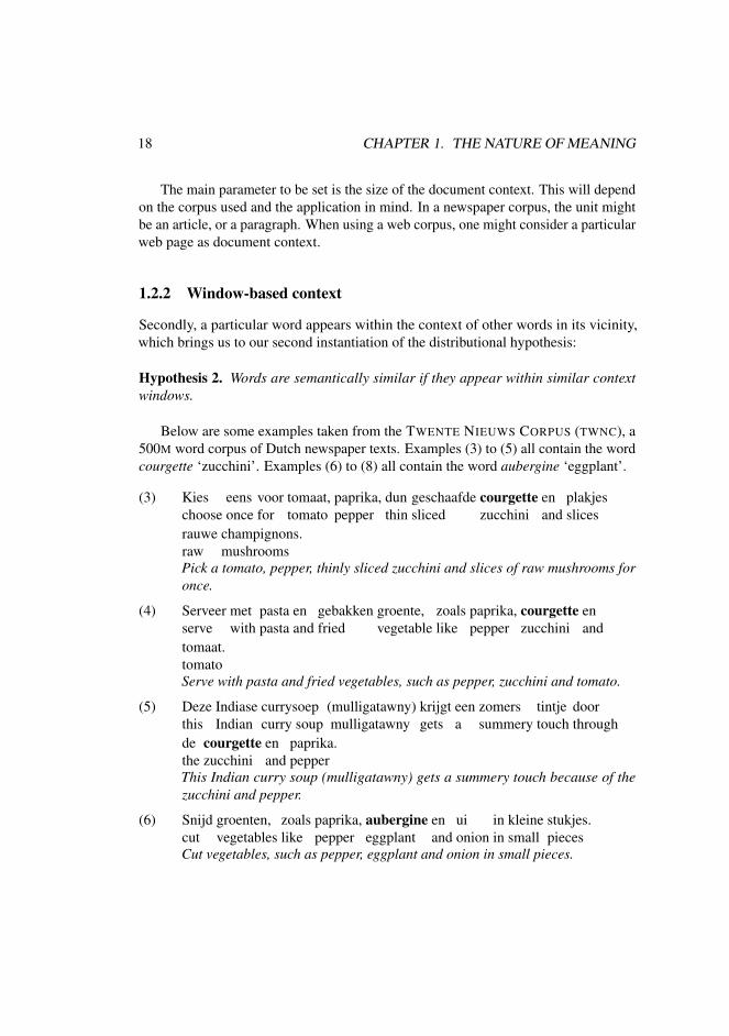
Below are some examples taken from the TWENTE NIEUWS CORPUS (TWNC), a500M word corpus of Dutch newspaper texts. Examples (3) to (5) all contain the wordcourgette ‘zucchini’. Examples (6) to (8) all contain the word aubergine ‘eggplant’.
(3) Kieschoose
eensonce
voorfor
tomaat,tomato
paprika,pepper
dunthin
geschaafdesliced
courgettezucchini
enand
plakjesslices
rauweraw
champignons.mushrooms
Pick a tomato, pepper, thinly sliced zucchini and slices of raw mushrooms foronce.
(4) Serveerserve
metwith
pastapasta
enand
gebakkenfried
groente,vegetable
zoalslike
paprika,pepper
courgettezucchini
enand
tomaat.tomatoServe with pasta and fried vegetables, such as pepper, zucchini and tomato.
(5) Dezethis
IndiaseIndian
currysoepcurry soup
(mulligatawny)mulligatawny
krijgtgets
eena
zomerssummery
tintjetouch
doorthrough
dethe
courgettezucchini
enand
paprika.pepper
This Indian curry soup (mulligatawny) gets a summery touch because of thezucchini and pepper.
(6) Snijdcut
groenten,vegetables
zoalslike
paprika,pepper
aubergineeggplant
enand
uionion
inin
kleinesmall
stukjes.pieces
Cut vegetables, such as pepper, eggplant and onion in small pieces.

1.2. CONTEXT 19
(7) Natuurlijk,of course
inin
PurmerendPurmerend
verkopensell
zethey
ookalso
tomaten,tomatoes
enand
aubergine,eggplant
enand
paprika.pepperOf course, tomatoes, eggplants and peppers are also sold in Purmerend.
(8) Voegaddverb
aubergine,eggplant
aardappelen,potatoes
bataatbataat
(zoetesweet
aardappel)potato
enand
paprikapepper
toe.addparticleAdd eggplant, potatoes, bataat (sweet potato) and peppers.
Note that courgette and aubergine in the examples above have a tendency to occur withthe same words, such as paprika ‘pepper’, tomaat ‘tomato’, and groente ‘vegetable’.Again, if such related words (like courgette and aubergine) occur with the same words(like paprika and tomaat) sufficiently frequently, a computer algorithm might be ableto infer that they are indeed semantically related. Note that courgette and aubergineeven do not have to occur together (although they might). It is their co-occurrence withother words that is indicative of their semantic relatedness.
A simple context window as described above is often called a BAG OF WORDScontext. This expression is used to indicate the fact that no order (or syntax) is takeninto account; the ordered words are mixed together (‘put together in one bag’) so thattheir internal order is lost.
The main parameter to be set is the size of the window in which a word’s contextwords occur. One might take into account a small window, in which only the left andright co-occurring word are used as context. A medium-sized window might use twoor five words to the left and right of the word in question. A large window might takeinto account all context words that occur in the same sentence, or even in the sameparagraph.
One can imagine that different context window sizes will lead to different kinds ofsemantic similarity. When using a small context window, an algorithm might be ableto find tight semantic relationships: in a small context window, more closely relatedcontext words might appear in the word’s vicinity, and the algorithm might even beable to discover some basic syntactic facts (e.g. the fact that a particular word appearswith an article). When using a larger context window, more loosely related wordsmight show up, and all order gets lost in the bag of words. Using larger windows, thealgorithm might be more likely to discover topically similar words again. In the secondpart of this thesis, we will investigate whether this hypothesis is true.

20 CHAPTER 1. THE NATURE OF MEANING
1.2.3 Syntax-based context
Thirdly, a particular word always takes part in particular syntactic relations. This givesrise to our third and final instantiation of the distributional hypothesis:
Hypothesis 3. Words are semantically similar if they appear in similar syntacticcontexts.
In this research, syntactic context will be instantiated in the form of dependencygraphs; dependency graphs provide a theory-neutral instantiation of a sentence’s syntax,since no particular grammatical framework is assumed. More specifically, this researchwill use dependency structures that conform to the guidelines for the Corpus SpokenDutch (CGN, Hoekstra et al. (2001)). The dependency structures used in the CGNsyntactic annotation have developed into a de facto standard for the computationalanalysis of Dutch (Bouma, van Noord, and Malouf, 2001) and they are used as outputformat of the Dutch dependency parser ALPINO (van Noord, 2006). Formally, aCGN dependency structure D = 〈V,E〉 is a labeled directed acyclic graph, with nodelabels V representing the categories (phrasal labels and POS labels) and edge labels Erepresenting the dependency relations.
topsmain
modmwu
mwpadv’s0
mwpadv
avonds1
hdverb
drink2
supronwe3
objnp
detdet
een4
hdnoun
bierDIM5
Figure 1.2: Dependency structure for the sentence ’s avonds drinken we een biertje(‘in the evening we’ll drink a beer’)
Figures 1.2 and 1.3 show dependency structures for two sentences from the ME-DIARGUS corpus, parsed with ALPINO. Table 1.1 shows the set of dependencies thatcan be deduced from the structures. In our syntax-based models of semantic similarity(discussed in the next chapter), we will use these dependency triples as the input data.

1.2. CONTEXT 21
topsmain
su1
nounwijn0
hdverb
word1
vcppart
obj11
modadv
weer2
modadj
veel3
hdverb
drink4
modadj
tegenwoordig5
Figure 1.3: Dependency structure for the sentence wijn wordt weer veel gedronkentegenwoordig (‘wine is drunk a lot again today’)
〈drink mod ’s avonds 〉〈drink su we 〉〈drink obj1 bierDIM 〉〈word su wijn 〉〈drink obj1 wijn 〉〈drink mod weer 〉〈drink mod veel 〉〈drink mod tegenwoordig〉
Table 1.1: The set of dependency triples extracted from the two parses in figures 1.2and 1.3
Note that both biertje2 and wijn appear as direct object of the verb drink. Again, ifwe look at a large number of sentences, we might notice that biertje and wijn appear insimilar syntactic contexts.
One important parameter in syntax-based models is the set of dependency relationsthat will be incorporated into the model. A number of dependency relations that mightbe useful in distributional similarity models are given in table 1.2. These are thedependency relations that will be used in the syntax-based models presented in thisthesis.
2DIM indicates the word is a diminutive form.

22 CHAPTER 1. THE NATURE OF MEANING
abbr. relation example
SU subject 〈author, SU, write〉OBJ1 direct object 〈wine, OBJ1, drink〉OBJ2 indirect object 〈him, OBJ2, give〉PC prepositional complement 〈dog, PC, look after〉MOD modifier 〈red, MOD, apple〉PREDC predicative complement 〈apple, PREDC, tasty〉COO coordination 〈apple, COO, pear〉APP apposition 〈London, APP, city〉
Table 1.2: Dependency relations used as contexts
1.3 Tight vs. topical similarity
We already briefly mentioned the difference between tight, synonym-like semanticsimilarity and more loosely related, topical similarity. With tight similarity, we indicatethe fact that two words are very similar, i.e. there is a (near-)synonymous or (co-)hyponymous relationship between the two words. With topically similar words, wemean words that belong to the same semantic domain.
The example below makes clear the difference between both kind of similarities.Two sets of words are given that are semantically similar to the word arts ‘doctor’.The first set contains words that are tightly similar to arts, containing synonyms (e.g.dokter ‘doctor’) and hyponyms (e.g. chirurg ‘surgeon’). The second set of words istopically related to arts, containing words that all belong to the medical domain. Thetopically related words are related to the target word by more loose relationships, suchas association and meronymy (part-whole relationships).
1. dokter ‘doctor’, medicus ‘doctor’, huisarts ‘family doctor’, chirurg ‘surgeon’,specialist ‘specialist’, gynaecoloog ‘gynaecologist’
2. patient ‘patient’, ziekte ‘disease’, diagnose ‘diagnosis, behandeling ‘treatment,ziekenhuis ‘hospital’, stethoscoop ‘stethoscope’
In the evaluation part (the second part of this thesis), we will not only try to evaluatethe performance of the various models for the extraction of semantic similarity; we willalso try to determine the nature of the similarity, i.e. whether the models are extractingtight, synonym-like similarity or more loosely related, topical similarity.

Chapter 2
The Computation of Meaning
In the last chapter, we made clear that the context of a particular word is able to suitablyinform us about its semantics, and we looked at the various contexts that might beuseful for the induction of semantic similarity. In this chapter, we will investigate howthis notion of context can be formally implemented in a computational framework.
2.1 Formal model
The last chapter provides an intuitive idea of how the context of a word might be usedto calculate its semantic similarity to other words. Now, in order to implement this ideain a computational framework, it needs to be expressed in more formal terms. In thissection, we will have a look at some existing literature that stipulates semantic spacemodels and the notion of context in more formal terms.
Lowe (2001) provides a formal definition of a semantic space model; he defines themodel as a quadruple 〈A,B,S,M〉. B is a set of basic elements (b1. . . bD) determiningthe dimensionality D of the vector space and the interpretation of each dimension. Bmight be a set of documents, words, or dependency relations, depending on the contextthat is used. A specifies the function that maps the standard co-occurrence frequenciesof basis elements and words to their final value, so that each word is represented bya vector v = [A(b1, t),A(b2, t), . . . ,A(bD, t)]. A may be the identity function (so thatthe final vector contains simple co-occurrence counts), but often a more advancedmapping is used. A is called the lexical association function or weighting function. Theweighting function is discussed in section 2.3. S is a similarity measure that maps pairsof vectors onto a real number that represents semantic similarity. Different similaritymeasures are discussed in 2.2. Finally, M is a mathematical transformation that takes
23

24 CHAPTER 2. THE COMPUTATION OF MEANING
one semantic space and maps it onto another, e.g. by reducing its dimensionality. Mmay be an identity mapping, so that the original space remains unchanged, but oftena mathematical transformation proves beneficial for countering data sparseness andreducing noise. Various dimensionality reductions are discussed in chapter 3.
Pado & Lapata (2007) extend Lowe’s framework for constructing semantic spacemodels based on syntax (dependency parses). Dependency parses are interpreted asdirected graph structures of nodes and labeled edges. A particular dependency pathπ for a particular target word t can then be represented as an ordered set of tuplesaccording to the dependency graph (ensuring connectedness and cycle-freeness).
In their framework, a semantic space is a tuple 〈B,T,M,S,A,cont,µ,v〉. B is theset of basis elements, T is the set of target words, M is the matrix M = B×T , A is thelexical association function, and S is the similarity measure. These parameters do notdiffer significantly from Lowe’s model. The additional parameters used are the contentselection function cont : T → 2π , the basis mapping function µ : π → B, and the pathvalue function v : π → R.
The context selection function cont allows us to select certain paths in the graphthat contribute to the context of a particular target word. This function allows us toselect only paths with a particular length, or paths that are labeled with a particulardependency relation. The basis mapping function µ maps paths onto basis elements.This way, the dependency paths are decoupled from their representation in the finalsemantic space. Such decoupling allows, for example, to use words instead of syntacticfeatures in the final representation. The path value function v is used to assign weightsto particular paths. E.g., longer dependency paths might be given less weight; anotherpossibility is to give more weight to particular dependency relations.
2.2 Similarity calculations: geometry vs. probability
Semantic similarity can be implemented in two different – albeit related – ways: in a(geometrically oriented) vector space model or in a (statistically oriented) probabilitydistribution model. Both models are instantiations of the formal model described above.We will discuss the former in section 2.2.1 and the latter in section 2.2.2. Differentsimilarity measures S are presented for both models.
2.2.1 Vector space model
In a semantic vector space model, each word in a language is mapped to a point in areal finite dimensional vector space. The vector space model is one of the most widelyused models for the acquisition of semantic similarity. The model makes it possible to

2.2. SIMILARITY CALCULATIONS: GEOMETRY VS. PROBABILITY 25
express ‘semantic proximity’ between entities in terms of spatial distance. In a vectorspace model, particular entities (words, for example) are represented as vectors offeatures (the word’s different contexts) in a multi-dimensional Euclidean space. Byapplying a suitable similarity measure (cfr. infra), one can straightforwardly calculatethe similarity between the different entities.
The vector space model was first developed in the context of information retrieval(Salton, Wong, and Yang, 1975), representing documents and queries as vectors of thewords they contain. The documents that are the closest to a particular query in thisvector space (i.e. the documents that are using the same words as in the query) willmost likely represent the documents that the user was looking for.
This model can straightforwardly be applied to similarity calculations betweenwords. The two words for which the semantic similarity is to be calculated, arerepresented as vectors of the words’ various contexts. Figure 2.1 shows an examplematrix M containing vectors for four different target words (using dependency relationsas features). In this example the set of target words is
T = {apple,banana,car, truck}
and the set of basic elements is
B = {redad j,yellowad j, tastyad j, f astad j,eatob j,driveob j}
redad j yellowad j tastyad j fastad j eatob j driveob j
apple 200 24 129 0 289 0banana 1 152 87 1 214 1car 120 74 0 98 1 386truck 67 44 0 37 0 175
Figure 2.1: A noun-by-features matrix
The value in matrix cell (i, j) is the co-occurrence frequency of word i with value j.In the example above, the adjective red appears 200 times with the word apple, and theword car appears 386 times as the object of drive.
To facilitate computations, vectors are often normalized to vector length of 1. Thevector length or norm of a vector −→v with length k is calculated with equation 2.1.
|−→v |=
√√√√ k
∑i=1
v2i (2.1)

26 CHAPTER 2. THE COMPUTATION OF MEANING
Dividing a vector by its vector length normalizes it to a vector length of 1. Whennormalizing the vectors in figure 2.1, the resulting matrix looks like the one in figure 2.2.
redad j yellowad j tastyad j fastad j eatob j driveo b j
apple .533 .064 .344 .000 .770 .000banana .004 .550 .315 .004 .774 .004car .284 .175 .000 .232 .002 .914truck .342 .224 .000 .189 .000 .893
Figure 2.2: A noun-by-features matrix normalized by vector length
In order to calculate the contextual overlap between two vectors −→v and −→w (which– as has been described in the previous chapter – we think of as a good predictor forsemantic similarity), we need a proper vector similarity measure S = sim(−→v ,−→w ).
The two simplest measures for vector similarity are the Manhattan distance and theEuclidean distance. The Manhattan distance or L1 norm is defined as
distMANHATTAN(−→v ,−→w ) =k
∑i=1|vi−wi| (2.2)
and the Euclidean distance, or L2 norm, is defined as
distEUCLIDEAN(−→v ,−→w ) =
√√√√ k
∑i=1
(vi−wi)2 (2.3)
Both distance measures are intuitively easy to understand, and provide a straight-forward extension of semantic similarity calculations in terms of spatial distance. Inpractice, though, neither the Manhattan distance nor the Euclidean distance are fre-quently used as word similarity measures. Both measures are very sensitive to extremevalues – which often occur with frequency counts – even after normalization.
Two other similarity measures that do show up in word similarity calculations –Jaccard and Dice – are derived from set theory. Originally, they were designed forbinary vectors, but they can easily be extended in order to deal with frequency data.
The Jaccard similarity measure is defined as
simJACCARD(−→v ,−→w ) = ∑ki=1 min(vi,wi)
∑ki=1 max(vi,wi)
(2.4)
and the Dice similarity measure is defined as

2.2. SIMILARITY CALCULATIONS: GEOMETRY VS. PROBABILITY 27
simDICE(−→v ,−→w ) =2×∑
ki=1 min(vi,wi)
∑ki=1(vi +wi)
(2.5)
Intuitively, both measures calculate the weight of overlapping features (the numer-ator with the min function) compared to the total feature weight (the denominator,either using the max function for the Jaccard measure or the sum of both vectors’feature values for the Dice measure).
The best known and most widely used similarity measure, however, is the cosinesimilarity measure. The cosine similarity is easy to compute, and it often achieves thebest results. It has therefore become the best known and most widely used vector spacesimilarity measure. The cosine similarity measure is calculated as
cos(−→v ,−→w ) =−→v ·−→w|−→v | |−→w |
(2.6)
where −→v ·−→w is the dot product between vector −→v and −→w , both of length k
−→v ·−→w =k
∑i=1
viwi (2.7)
Note that, when both vectors −→v and −→w are normalized to unit length, the denomin-ator is redundant, so that the cosine similarity amounts to a simple dot product betweentwo vectors.
Once we have defined the similarity measure S, we can calculate the similaritybetween the different word vectors. The resulting calculation yields the similaritymatrix Ssim of size n× n, where n is the number of target words T . The similaritymatrix is represented in figure 2.3.
apple banana car truck
apple 1.000 .741 .164 .197banana .741 1.000 .103 .129car .164 .103 1.000 .996truck .197 .129 .996 1.000
Figure 2.3: A word by word similarity matrix
28 CHAPTER 2. THE COMPUTATION OF MEANING
2.2.2 Probabilistic model
The vector space model is the oldest, best known and most widely used model forsemantic similarity, but it is not the only one. A word’s contextual information canalso be captured in a statistically oriented probability distribution model. Probabilitydistribution models allow for the use of well-known information-theoretic measuresof similarity, and they offer the possibility of implementing semantic similarity in aBayesian framework.
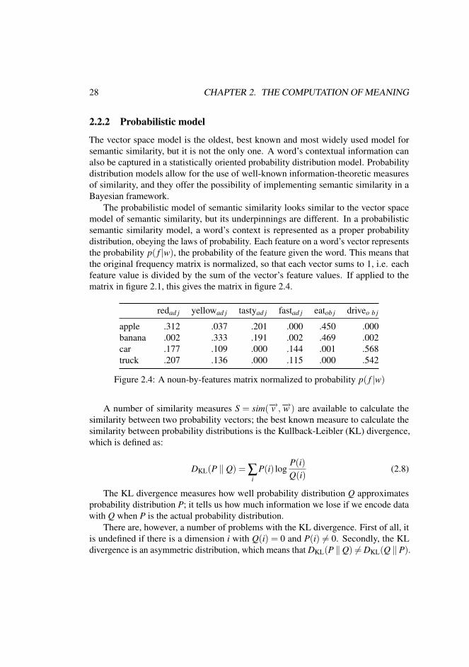
The probabilistic model of semantic similarity looks similar to the vector spacemodel of semantic similarity, but its underpinnings are different. In a probabilisticsemantic similarity model, a word’s context is represented as a proper probabilitydistribution, obeying the laws of probability. Each feature on a word’s vector representsthe probability p( f |w), the probability of the feature given the word. This means thatthe original frequency matrix is normalized, so that each vector sums to 1, i.e. eachfeature value is divided by the sum of the vector’s feature values. If applied to thematrix in figure 2.1, this gives the matrix in figure 2.4.
redad j yellowad j tastyad j fastad j eatob j driveo b j
apple .312 .037 .201 .000 .450 .000banana .002 .333 .191 .002 .469 .002car .177 .109 .000 .144 .001 .568truck .207 .136 .000 .115 .000 .542
Figure 2.4: A noun-by-features matrix normalized to probability p( f |w)
A number of similarity measures S = sim(−→v ,−→w ) are available to calculate thesimilarity between two probability vectors; the best known measure to calculate thesimilarity between probability distributions is the Kullback-Leibler (KL) divergence,which is defined as:
DKL(P ‖ Q) = ∑i
P(i) logP(i)Q(i)
(2.8)
The KL divergence measures how well probability distribution Q approximatesprobability distribution P; it tells us how much information we lose if we encode datawith Q when P is the actual probability distribution.
There are, however, a number of problems with the KL divergence. First of all, itis undefined if there is a dimension i with Q(i) = 0 and P(i) 6= 0. Secondly, the KLdivergence is an asymmetric distribution, which means that DKL(P ‖Q) 6= DKL(Q ‖ P).

2.3. WEIGHTING SCHEMES 29
There are other similarity measures that overcome these problems. The first one isthe Jensen-Shannon (JS) divergence. The JS divergence is defined as:
DJS(P ‖ Q) =12
DKL(P ‖ P+Q2
)+12
DKL(Q ‖ P+Q2
) (2.9)
Intuitively, the JS divergence tells us how much information is lost if the twoprobability distributions P and Q are replaced by the average of both distributions. TheJS divergence does not have any problems with infinite values, and it is symmetric.
Another possibility is to approximate the KL divergence as close as possible bymixing it to a small degree with the other distribution. This is what the skew divergencedoes. The skew divergence is defined as:
Dskew(α)(P,Q) = DKL(P ‖ αQ+(1−α)P) (2.10)
The skew divergence constant α is a number between 0 and 1, usually set close to1 to approximate the KL divergence as close as possible; a normal value of α = 0.99.The measure remains asymmetric, but mixing in the other probability distribution to asmall degree, effectively solves the infinity problem with zero values.
2.3 Weighting schemes
The methods described above can be applied to raw frequency counts. Often, though,an extra weighting step is applied in order to adapt the feature value according to itsactual importance. In our formal model, this is the lexical association function orweighting function A. Many different weighting functions have been applied to theproblem of semantic similarity. In the following paragraphs, we will have a look at theintuition behind them, and investigate the different possibilities.
2.3.1 Introduction: Zipf’s law
Zipf’s law states that the frequency of a word in any particular corpus is inverselyproportional to its rank in a frequency list. As a result, word distributions are extremelyskewed: the majority of words occur very infrequently, whereas the top few mostfrequent words take up the largest part of the corpus. This fact brings about a frequencybias: words with similar frequencies will be considered more similar than they actuallyare.
Intuitively, it is more significant for a word’s semantics to appear with an infrequentbut highly specific, ‘meaningful’ feature than to appear with a very frequent, broad,‘meaningless’ feature. As an example, compare denim skirt with nice skirt. It seems
30 CHAPTER 2. THE COMPUTATION OF MEANING
reasonable to attach more weight to the first feature denim than to the second featurenice. The former feature is highly specific and appears with a small subset of words(like denim pants, denim jeans, a denim jacket), whereas the latter is more broad andunspecific, and appears with a much larger set of words (a nice girl, a nice feeling, anice zebra, . . . ). Moreover, a co-occurrence like denim skirt is much more informativethan e.g. a skirt, although the latter one will have a much higher frequency. By applyinga suitable weighting, we can neutralize the skewed frequencies arising from the Zipfiandistribution.
Weighting functions can be divided into local and global weighting functions,according to the information they use in order to calculate the weighted value; localweighting functions only use a particular co-occurrence frequency count on its ownto calculate the weighted value, whereas global weighting functions make use ofglobal word and feature distribution statistics calculated over the corpus as a whole.In the following paragraphs, we will have a look at both types, and discuss their mostimportant instantiations in the scope of semantic similarity.
2.3.2 Local weighting
A local weighting function is a function that is applied to a particular co-occurrence fre-quency without any knowledge about the corpus frequencies as a whole. In the simplestcase, this amounts to applying the identity function to a particular co-occurrence fre-quency. Another simple local weighting is the application of a binary function, whichassigns a value of one if the co-occurrence frequency is larger than zero (i.e. thecombination occurs at least once in the corpus) and zero otherwise.
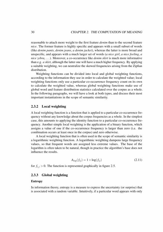
A local weighting function that is often used in the scope of semantic similarity isa logarithmic weighting function. A logarithmic weighting dampens large frequencyvalues, so that frequent words are assigned less extreme values. The base of thelogarithm is often taken to be natural, though in practice the algorithm’s base does notinfluence the results.
Alog( fi j) = 1+ log( fi j) (2.11)
for fi, j > 0. The function is represented graphically in figure 2.5.
2.3.3 Global weighting
Entropy
In information theory, entropy is a measure to express the uncertainty (or surprise) thatis associated with a random variable. Intuitively, if a particular word appears with only

2.3. WEIGHTING SCHEMES 31
0
2
4
6
8
10
0 200 400 600 800 1000 1200 1400 1600 1800 2000
(log(x) + 1)
Figure 2.5: A logarithmic function is used to smooth extreme frequency values
a few features (documents), it will be much more informative than a word that appearswith lots of features (documents). Words that appear in many documents (i.e. wordsthat are more uniformly distributed) will have a high entropy value. Words that appearin only a limited number of documents, on the other hand, will have a low entropyvalue.
Formally, entropy weighting is usually calculated according to the formula in 2.12.
Aent(i, j) = fi j(1+n
∑k=1
pik log(pik)log(n)
), pik =fik
∑nl=1 fil
(2.12)
with fi j being the original co-occurrence frequency and n the total number of features(documents). This formula actually calculates an entropy ratio G(i) = 1− H(d|i)
H(d) , whereH(d) is the entropy of the uniform distribution of the documents, and H(d | i) is theentropy of the conditional distribution given that the noun i appeared. The originalco-occurrence frequency is then multiplied by this ratio.
We will evaluate entropy as a weighting function in the document-based models.

32 CHAPTER 2. THE COMPUTATION OF MEANING
Pointwise mutual information
Another popular weighting function is called pointwise mutual information (PMI). PMIwas first proposed by Church and Hanks (1990), and is based on the information-theoretic notion of mutual information. Mutual information measures the mutualdependence between to random variables X and Y. It is defined as
I(X ,Y ) = ∑x
∑y
p(x,y) logp(x,y)
p(x)p(y)(2.13)
Pointwise mutual information – i.e. the mutual information for particular events –is defined as
I(i, j) = logp(i, j)
p(i)p( j)(2.14)
Intuitively, PMI tells us how much information a particular feature contains abouta target word (and vice versa). PMI measures how often two events i and j occur,compared to the expected value if they were independent. The numerator gives theactual probability of the target word and feature occurring together, whereas the denom-inator contains the probability of the target word and feature occurring independently(multiplying the marginal probabilities). Thus, the ratio indicates how much more thetarget word and feature co-occur than we would expect by chance.
Although PMI is used a lot as weighting function, it is problematic for low fre-quency counts: the score will depend on the frequency of individual words. Thus,low-frequency co-occurrences will receive a higher score than high-frequency co-occurrences (all other things being equal). One solution to this problem is to use aparticular cut-off (e.g. a co-occurrence frequency of at least 3). Another solution is theuse of an extra weighting factor dependent on the frequency (Pantel and Lin, 2002).
We will evaluate PMI as a weighting function in the window-based and syntax-basedmodels.

Chapter 3
Dimensionality Reduction
3.1 Introduction
In the previous chapters, semantic similarity calculations have been carried out usingthe words’ original feature space, which usually contains a large number of highlycorrelated features. The goal of a dimensionality reduction – also called factorization –is to find a smaller number of uncorrelated or lowly correlated dimensions (factors).There are two reasons for applying such a transformation to the data:
• When the feature space is large, similarity calculations often become computa-tionally expensive or even impossible. A dimensionality reduction reduces thefeature space to a much smaller number of dimensions, so that computationsbecome tractable again.
• A dimensionality reduction is able to discover latent structure present in thedata. This way, a dimensionality reduction is able to generalize over individualdata samples. By classifying the data according to the latent structure andnot according to the individual features, a dimensionality reduction is able toovercome data sparseness and noise.
One of the most famous dimensionality reduction methods for text processingis latent semantic analysis (LSA). LSA allegedly finds ‘latent semantic dimensions’,according to which nouns and documents can be represented more efficiently. In thesubsequent section, we will first have a look at LSA and its underlying singular valuedecomposition. Next, we will examine non-negative matrix factorization, an algorithmthat overcomes some of the problems linked to LSA.
33

34 CHAPTER 3. DIMENSIONALITY REDUCTION
3.2 Latent semantic analysis
3.2.1 Introduction
Latent semantic analysis (Landauer and Dumais, 1997; Landauer, Foltz, and La-ham, 1998) models the meaning of words and documents by projecting them into avector space of reduced dimensionality; the reduced vector space is built up by applyingsingular value decomposition (SVD) – a well known linear algebraic method – to asimple term-by-document frequency matrix A. The resulting lower dimensional matrixA is the best possible fit in a least squares sense (minimization of the Frobenius norm;equation 3.1).
argminA‖ A− A ‖F (3.1)
By enforcing a lower number of dimensions, the algorithm is forced to make general-izations over the simple frequency data. Co-occurring terms are mapped to the samedimensions; terms that do not co-occur are mapped to different dimensions.
In the next section, we have a closer look at the principles and mathematics behindSVD. Next, some example SVD’s are provided in order to exemplify their generalizationcapacity. We conclude with a discussion of the drawbacks linked to LSA.
3.2.2 Singular value decomposition
While rooted in linear algebra, singular value decomposition has proven to be auseful tool in statistical applications. It is closely akin to statistical methods suchas principal components analysis, and has been used as a versatile dimensionalityreduction technique in different scientific fields, such as image recognition, signalprocessing (Deprettere, 1988), and information retrieval. SVD stems from a well knowntheorem in linear algebra: a rectangular matrix can be decomposed into three othermatrices of specific forms, so that the product of these three matrices is equal to theoriginal matrix:1
Am×n = Um×z Σz×z (Vn×z)T (3.2)
where z = min(m,n). A graphical representation of SVD (with z = n) is given infigure 3.1.
1The singular value decomposition that is presented here is called the ‘thin’ or ‘reduced’ SVD. Inapplications such as LSA, it is unusual to compute the full SVD; the reduced version is faster to compute andmore economical in storage, and it provides sufficient information for statistical applications.

3.2. LATENT SEMANTIC ANALYSIS 35
Figure 3.1: Graphical representation of SVD
Matrix A is the original matrix of size m× n. Matrix U is an m× z matrix thatcontains newly derived vectors called left-singular vectors. Matrix VT denotes thetranspose of matrix V, an n× z matrix of derived vectors called right-singular vectors.The third matrix Σ is a z× z square diagonal matrix (i.e. a square matrix with non-zeroentries only along the diagonal); Σ contains derived constants called singular values. Akey property of the derived vectors is that all dimensions are orthogonal (i.e. linearlyindependent) to each other, so that each dimension is uncorrelated to the others.
The singular value decomposition can be interpreted as a method that rotates theaxes of the n-dimensional space in such a way that the largest variation is capturedby the leading dimensions. The diagonal matrix Σ contains the singular values sortedin descending order. Each singular value represents the amount of variance that iscaptured by a particular dimension. The left-singular and right-singular vector linked tothe highest singular value represent the most important dimension in the data (i.e. thedimension that explains the most variance of the matrix); the singular vectors linked tothe second highest value represent the second most important dimension (orthogonal tothe first one), and so on. Typically, one uses only the first k� z dimensions, strippingoff the remaining singular values and singular vectors. If one or more of the leastsignificant singular values are omitted, then the reconstructed matrix will be the bestpossible least-squares approximation of the original matrix in the lower dimensionalspace. Intuitively, SVD is able to transform the original matrix – with an abundance ofoverlapping dimensions – into a new, many times smaller matrix that is able to describethe data in terms of its principal components. Due to this dimension reduction, a moresuccinct and more general representation of the data is obtained. Redundancy is filteredout, and data sparseness is reduced.
The calculation of SVD involves iteratively solving a number of eigenvalue prob-lems. A thorough understanding of the algorithm’s computational details requires afirm background in linear algebra, and explaining all the mathematical nuts and boltsis well beyond the scope of this thesis. Suffice it to say that there are a number of

36 CHAPTER 3. DIMENSIONALITY REDUCTION
programs available that can handle the kind of large-scale singular value decomposi-tions necessary for linguistic data sets. In this research, SVDPACK (Berry, 1992) hasbeen used. SVDPACK is a program that is able to handle sparse matrices quickly andefficiently (depending on the number of singular values one wants to retain).
3.2.3 Examples
Consider two documents, one about Belgium (B) and one about the Netherlands (NL).
• Belgium is a kingdom in the middle of Europe, and Brussels is its capital.Brussels has a Dutch-speaking and a French-speaking university, but the largeststudent city is Leuven. Leuven has 31,000 students.
• The Netherlands is a country in Western Europe, located next to the North Sea.The Netherlands’s capital is Amsterdam. Amsterdam has two universities.Groningen is another important student city. In Groningen, there are 37,000students.
As we have seen in the previous chapter, these documents can easily be transformedinto a term-document matrix, in which each document is represented by a columnvector. Each element in the column vector corresponds to the frequency of a particularterm (in this case cities) in the document. Similarly, each element on the row vectorindicates how often a term appears in a particular document. The resulting matrix,together with its singular value decomposition, is given in figure 3.2.
A
B NL
Groningen 0 2Leuven 2 0
Amsterdam 0 2Brussel 2 0
=
U
0.00 0.71−0.71 0.000.00 0.71−0.71 0.00
Σ
[2.83 0
0 2.83
]VT
[−1 00 1
]
Figure 3.2: Singular value decomposition of a term-document matrix
The original matrix A is decomposed into three other matrices U, Σ and VT . Thesingular values in Σ show that two equally important dimensions are found; furthermore,

3.2. LATENT SEMANTIC ANALYSIS 37
the left- and right-singular vectors show that the frequencies are evenly divided amongterms as well as among documents.
Figure 3.3 shows what happens when we add another document about Belgium,with a slightly different frequency distribution of terms: the Belgian dimension becomesthe most important (i.e. captures the most variation, 2.92), while the Dutch dimensionremains the same (2.83). The third dimension (0.68) captures the remaining variation(the fact that the third document only talks about Brussels).
A
B NL B
Groningen 0 2 0Leuven 2 0 0
Amsterdam 0 2 0Brussel 2 0 1
=
U
0.00 −0.71 0.00−0.66 0.00 0.750.00 −0.71 0.00−0.75 0.00 –0.66
Σ
2.92 0.00 0.000.00 2.83 0.000.00 0.00 0.68
V T
−0.97 0.00 0.260.00 −1.00 0.00–0.26 0.00 –0.97
∼= A
0.00 2.00 0.001.87 0.00 0.500.00 2.00 0.002.12 0.00 0.56
Figure 3.3: Truncated singular value decomposition
If we now truncate the SVD by keeping only the two most important dimensions,and then reconstruct our original matrix, we get matrix A, which is the best possiblereconstruction from only two dimensions. Note that matrix A resembles matrix A,except for the numbers of the third document: instead of assigning all frequency massto the term Brussel, the mass is almost evenly divided among the Belgian terms Brusseland Leuven. When keeping only two dimensions, the SVD ‘guesses’ the best possibledistribution. This is an example of how the technique is used to obtain a more succinctmodel that is able to generalize among the data.
Below, we describe a more elaborate example, illustrating once again the gener-alization capacity of a singular value decomposition. Figure 3.4 represents anotherterm-by-document matrix, containing Dutch nouns that are related to two distinctsemantic topics. The nouns tulp ‘tulip’, tuin ‘garden’, and park ‘park’ are related tothe topic of gardening. The nouns ei ‘egg’, kaas ‘cheese’, and boter ‘butter’ all relate

38 CHAPTER 3. DIMENSIONALITY REDUCTION
to the topic of food. The noun bloem is an ambiguous word in Dutch, meaning ‘flower’(related to the gardening topic) as well as ‘flour’ (related to the food topic). Figure 3.4represents the distribution of the seven nouns across five different documents. Thecomplete SVD (matrices U, Σ and VT ) is given in figures 3.5 to 3.7.
A =
d1 d2 d3 d4 d5tulp 1 0 1 0 0tuin 1 1 0 0 0park 0 1 0 0 0ei 0 0 0 1 1kaas 0 0 0 1 0boter 0 0 0 1 1bloem 1 0 0 0 1
Figure 3.4: Term-by-document matrix A
U =
dim1 dim2 dim3 dim4 dim5tulp −0.21 0.52 −0.48 −0.58 0.35tuin −0.22 0.60 0.46 0 −0.40park −0.05 0.22 0.65 0 0.55ei −0.56 −0.30 0.06 0 0.20kaas −0.26 −0.22 0.17 −0.58 −0.55boter −0.56 −0.30 0.06 0 0.20bloem −0.47 0.30 −0.31 0.58 −0.20
Figure 3.5: The left-singular matrix U
Σ =
2.30 0 0 0 0
0 1.93 0 0 00 0 1.30 0 00 0 0 1.00 00 0 0 0 0.52
Figure 3.6: The square diagonal matrix Σ

3.2. LATENT SEMANTIC ANALYSIS 39
VT =
d1 d2 d3 d4 d5
dim1 −0.39 −0.12 −0.09 −0.60 −0.69dim2 0.74 0.43 0.27 −0.43 −0.16dim3 −0.26 0.85 −0.37 0.22 −0.15dim4 0 0 −0.58 −0.58 0.58dim5 −0.49 0.28 0.67 −0.28 0.39
Figure 3.7: The right-singular matrix VT
We can now easily project the terms and documents of the original matrix intoa space of reduced dimensionality; in the following example, we will retain twodimensions. Matrix B gives the terms after a reduction to two dimensions, scaled withthe singular values. The matrix is obtained by multiplying a slice of matrix U (U7×2)with a slice of matrix Σ (Σ2×2). Matrix B is given in figure 3.8. The term vectors –normalized to vector length – are represented graphically in figure 3.9.
B =
dim1 dim2tulp −0.48 1.01tuin −0.51 1.16park −0.12 0.43ei −1.28 −0.58kaas −0.60 −0.43boter −1.28 −0.58bloem −1.08 0.58
Figure 3.8: Matrix B, the multiplication of U7×2 and Σ2×2
In figure 3.9, we can clearly distinguish the two different topics: the ‘garden’ topic(with tulp, tuin and park) in the second quadrant, and the ‘food’ topic (with ei, kaas andboter) in the third quadrant. Note that the terms tulp and park do not appear together inthe same document in the original matrix; in the reduced two-dimensional SVD space,however, they are clearly closely related. This is again an example of the generalizationcapability of the SVD. Also note that the ambiguous word bloem, related to both the‘garden’ topic and the ‘food’ topic, ends up in between them.
Similarly, we obtain matrix C – the projection of the documents into the two-dimensional reduced vector space – by multiplying Σ2×2 with VT
2×5. Matrix C isgiven in figure 3.10. The document vectors – again normalized to vector length – are

40 CHAPTER 3. DIMENSIONALITY REDUCTION
dim 1
dim 2
tulptuinpark
ei
kaasboter
bloem 0.5
1.0
−0.5
−0.5−1.0
Figure 3.9: A graphical representation of the term vectors in the reduced dimensionalspace
represented graphically in figure 3.11.
C =
d1 d2 d3 d4 d5dim1 −0.89 −0.27 −0.21 −1.37 −1.58dim2 1.42 0.82 0.52 −0.82 −0.30
Figure 3.10: Matrix C, the multiplication of Σ2×2 and VT
2×5
Again, we see the same topic division among the document vectors. Documentsd1, d2 and d3 are grouped together in the second quadrant, and documents d4 and d5appear together in the third quadrant. Note again that documents d2 and d3 appearclosely together, although they do not share any terms in the original term-documentmatrix.

3.2. LATENT SEMANTIC ANALYSIS 41
dim 1
dim 2
d1
d2d3
d4
d5
0.5
1.0
−0.5
−0.5−1.0
Figure 3.11: A graphical representation of the document vectors in the reduced dimen-sional space
3.2.4 Drawbacks
LSA suffers from a number of drawbacks, that have been regularly noted in the literature.(Manning and Schutze, 2000, p. 565)
The first major drawback is that a singular value decomposition assumes normallydistributed data. A normal distribution is inappropriate for frequency count data,such as textual co-occurrence data. There are other distributions – such as a Poissondistribution – that are better suited for modeling count data. As a consequence ofthe normality assumption, the reconstruction A′ of the original matrix A may containnegative numbers, which clearly is a bad approximation for frequency counts.
A second drawback – related to the first one – is the presence of negative values inthe derived dimensions themselves. The derived dimensions are said to represent actual‘latent semantic’ dimensions. A particular term or document can have a positive ornegative value on those dimensions. It is not clear what negative values on a semanticscale should designate. A particular term or document either is related (positive value)or is not related (zero value) to a particular topic; it seems counterintuitive to say that aparticular word is negatively related to a particular topic. This intuition is confirmed by

42 CHAPTER 3. DIMENSIONALITY REDUCTION
experiments. In the following section, we will present an algorithm that only allowsnon-negative data in its dimensionality reduction. By enforcing this constraint, thealgorithm is able to find much more distinct and clear-cut semantic dimensions.
3.3 Non-negative matrix factorization
3.3.1 Introduction
In this section, we describe a dimensionality reduction technique called non-negativematrix factorization (NMF) that does not suffer from the drawbacks of LSA and itsunderlying singular value decomposition. Non-negative matrix factorization is adimensionality reduction technique that has become popular in fields such as imagerecognition, speech recognition and machine learning. Its key idea is to impose a non-negativity constraint on the factorization. This constraint brings about a parts-basedrepresentation, because only additive and no subtractive combinations are allowed.In many cases, this constraint proves beneficial for the inductive capabilities of thedimensionality reduction: the algorithm is able to extract more clear and distinctcharacteristics from the data.
The difference between the parts-based induction of NMF and the holistic inductionof non-constrained methods such as PCA (and the related singular value decomposition)can be illustrated with an example from facial image recognition (Lee and Seung, 1999).A famous method in facial image recognition uses so-called ‘eigenfaces’ (Turk andPentland, 1991). These are a small number of prototypical faces represented by theeigenvectors that are found by applying PCA to a database of facial images. Eigenfacesmay contain positive as well as negative values. A key characteristic is that theyare ‘holistic’: an eigenface contains all kinds of facial traits, and thus represents aprototypical face. By taking a linear combination of various ‘eigenfaces’, a particularinstance of a face may be reconstructed.
The representation that is found by NMF looks quite different: instead of findingholistic, prototypical faces, the algorithm induces particular facial traits (different kindsof eyes, noses, mouths, . . . ). By enforcing a non-negative constraint, the algorithm isable to build up a parts-based representation of facial images. A particular instance ofa face may then be reconstructed by taking a linear combination of the different parts.The very same characteristic will also prove to be beneficial for building up semanticrepresentations from text.

3.3. NON-NEGATIVE MATRIX FACTORIZATION 43
3.3.2 Theory
Non-negative matrix factorization (NMF) (Lee and Seung, 2000) is the name for agroup of algorithms in which a matrix V is factorized into two other matrices, W andH.
Vn×m ≈Wn×rHr×m (3.3)
Figure 3.12 gives a graphical representation of non-negative matrix factorization.
Figure 3.12: A graphical representation of non-negative matrix factorization
Typically r is much smaller than n,m so that both instances and features areexpressed in terms of a few components. As mentioned above, non-negative matrixfactorization enforces the constraint that all three matrices must be non-negative, so allelements must be greater than or equal to zero.
There are two objective functions that may be used in order to quantify the qualityof the approximation of the original matrix. One objective function minimizes the sumof squares (equation 3.4).
min ‖ V−WH ‖F = min ∑i
∑j(Vi j− (WH)i j)2 (3.4)
The other one minimizes the Kullback-Leibler divergence (equation 3.5).
min DKL(V ‖WH) = min ∑i
∑j
(Vi j log
Vi j
(WH)i j−Vi j +(WH)i j
)(3.5)
Practically, the factorization can be efficiently carried out through the iterativeapplication of multiplicative update rules. The set of update rules that minimize theEuclidean distance are given in 3.6 and 3.7.
Haµ ←Haµ
(WT V)aµ
(WT WH)aµ
(3.6)

44 CHAPTER 3. DIMENSIONALITY REDUCTION
Wia←Wia(VHT )ia
(WHHT )ia(3.7)
The set of update rules that minimize the Kullback-Leibler divergence are givenin 3.8 and 3.9.
Haµ ←Haµ
∑i WiaViµ
(WH)iµ
∑k Wka(3.8)
Wia←Wia∑µ Haµ
Viµ(WH)iµ
∑v Hav(3.9)
Matrices W and H are randomly initialized, and the update rules are iterativelyapplied – alternating between them. In each iteration, the matrices W and H are suitablynormalized, so that the rows of the matrices sum to 1. The algorithm stops after afixed number of iterations, or according to some stopping criterion (the change of theobjective function drops below a certain threshold). The update rules are guaranteedto converge to a local optimum. In practice, it is usually sufficient to run the NMFalgorithm repeatedly in order to find the global optimum.
3.3.3 Example
In the following example, we take matrix V in figure 3.13 (reproduced from matrixA used in the SVD example on page 38), and factorize it to two dimensions usingnon-negative matrix factorization. As objective function, we take the Kullback-Leiblerdivergence (which implies the use of the update rules in 3.8 and 3.9). The globallyoptimal matrices W and H are represented in figures 3.14 and 3.15.2
Matrices W and H can be interpreted as conditional probabilities. Matrix Wrepresents the probability of a word given a particular topical, ‘semantic’ dimension.
Matrix H gives the probability of a dimension given a document (in the example,each document contains one particular topic).
By multiplying matrices W and H, we get matrix V′, containing the probabilitiesof a word given a document.
Note that the values of (tulp, d2), (tuin, d3), and (park, d1,3) – that have zeros inthe original co-occurrence matrix – have received appropriate probability values in thereconstructed matrix V′. The factorization model has made correct inferences about
2Note once again that the update rules are guaranteed to converge to a local optimum; it might take anumber of tries to find the globally optimal solution.

3.3. NON-NEGATIVE MATRIX FACTORIZATION 45
V =
d1 d2 d3 d4 d5tulp 1 0 1 0 0tuin 1 1 0 0 0park 0 1 0 0 0ei 0 0 0 1 1kaas 0 0 0 1 0boter 0 0 0 1 1bloem 1 0 0 0 1
Figure 3.13: Term-by-document matrix V
W =
dim1 dim2tulp 0 1
3tuin 0 1
3park 0 1
6ei 1
3 0kaas 1
6 0boter 1
3 0bloem 1
616
Figure 3.14: Matrix W, containing the original nouns and a reduced number of dimen-sions
H =
d1 d2 d3 d4 d5dim1 0 0 0 1 1dim2 1 1 1 0 0
Figure 3.15: Matrix H, containing the original documents and a reduced number ofdimensions
words related to the gardening topic appearing in sentences related to the gardeningtopic. Likewise, (kaas, d5) has received an appropriate probability value. The am-biguous word bloem – related to the two topics – has received appropriate probabilityvalues across the whole document range.

46 CHAPTER 3. DIMENSIONALITY REDUCTION
V′ =
d1 d2 d3 d4 d5tulp 1
313
13 0 0
tuin 13
13
13 0 0
park 16
16
16 0 0
ei 0 0 0 13
13
kaas 0 0 0 16
16
boter 0 0 0 13
13
bloem 16
16
16
16
16
Figure 3.16: The reconstructed matrix V′, the multiplication of W and H
Chapter 4
Three-way Methods
4.1 Introduction
In the former chapters, language data has been treated as two-way co-occurrences; wehave shown that the semantic similarity of words can be investigated by looking atthe contextual features with which those words appear. The two-way co-occurrencedata has been represented in the form of a matrix. It is the form that is best suited forrepresenting two-way co-occurrence frequencies. The matrix representation allowsfor the application of algebraic and statistical methods, which in turn allows for theinduction of semantic generalizations.
Reducing language to two-way co-occurrence frequencies is of course a vastoversimplification. Language is a complex system of interrelated words, driven bygrammar rules and subcategorization frames. By keeping track of multi-way co-oc-currences, we can attempt to do some more justice to this complexity (although theframework represented here remains a major simplification). Compare the followingsentences:
(1) DeThe
voetbalclubsusoccer team
speeltplays
eena
goedegood
wedstrijdob j.game
The soccer team is playing a good game.
(2) DeThe
acteursuactor
speeltplays
Hamletob j.Hamlet
The actor is playing Hamlet.
47

48 CHAPTER 4. THREE-WAY METHODS
〈speel su voetbalclub〉〈speel obj wedstrijd 〉〈speel su acteur 〉〈speel obj Hamlet 〉
Table 4.1: Extracted dependency relations
The dependency relations (subject-verb and verb-object) for examples (1) and (2) aregiven in table 4.1.
Say we now want to investigate the semantics of Dutch verbs (like spelen ‘toplay’). In our standard two-way framework, we would then take the verbs to be onemode, and combine the syntactic dependencies that the verbs appear with (subjects anddirect objects in this case) together in the other mode, yielding a matrix like the one infigure 4.1.
V =
voetbalclubsu acteursu wedstri jdob j Hamletob j . . .
speel 1 1 1 1. . . . . . . . . . . . . . . . . .. . . . . . . . . . . . . . . . . .
Figure 4.1: Two-way co-occurrence matrix
This is a genuine, appropriate way of investigating a verb’s semantics, but wedo lose some more complex and interesting relations between a verb and its objects.By capturing a verb’s co-occurrences in a matrix form, we are able to investigate itsco-occurrence with particular subjects and direct objects separately, but we are not ableto investigate a verb’s co-occurrence with subjects and direct objects at the same time:we lose the three-way relationship that exists between verb, subject and direct object.
It is possible, however, to capture in a matrix the relationship between subjectsand direct objects for one particular verb. For the examples with spelen above, thisyields the matrix given in figure 4.2. The rows of the matrix represent the subjects, thecolumns represent the direct objects. A graphical representation of this matrix is givenin figure 4.3.
We can now construct similar matrices for each verb we want to investigate. Saywe want two include two more verbs, winnen ‘to win’, and bewerken ‘to adapt’. Thematrices for these verbs are given in figures 4.4 and 4.5. Note that the two matrices

4.1. INTRODUCTION 49
Vspeel =
wedstrijd Hamlet . . .
voetbalclub 1 0 . . .acteur 0 1 . . .. . . . . . . . . . . .
Figure 4.2: Two-way co-occurrence matrix of subjects and direct objects for the verbspelen ‘to play’
. . .acteur voet-bal-club
wed-
strijd
Ham-
let
. . .
. . .0
1
. . .1
0
. . .. . .
. . .
Figure 4.3: Graphical representation of the co-occurrence matrix for the verb spelen‘to play’
Vwin and Vbewerk contain the same instances and features (subjects and direct objects)in their rows and columns as the first matrix Vspeel .
Vwin =
wedstrijd Hamlet . . .
voetbalclub 1 0 . . .acteur 1 0 . . .. . . . . . . . . . . .
Figure 4.4: Two-way co-occurrence matrix of subjects and direct objects for the verbwinnen ‘to win’
As a last step, we can now stack the three matrices together, which yields a three-dimensional cube like the one in figure 4.6.
It will have become clear by now that we are leaving the familiar domain of two-dimensional matrices. As we have noted before, a matrix is not a suitable form forthe representation of multi-way data. For co-occurrence data beyond two modes, we

50 CHAPTER 4. THREE-WAY METHODS
Vbewerk =
wedstrijd Hamlet . . .
voetbalclub 0 0 . . .acteur 0 1 . . .. . . . . . . . . . . .
Figure 4.5: Two-way co-occurrence matrix of subjects and direct objects for the verbbewerken ‘to adapt’
. . .acteur voet-bal-club
. . .acteur voet-bal-club
. . .acteur voet-bal-club
wed-
strijd
Ham-
let
. . .
wed-
strijd
Ham-
let
. . .
wed-
strijd
Ham-
let
. . .
. . .0
1
. . .1
0
. . .. . .
. . .
speel←
win←
bewerk←
Figure 4.6: Graphical representation tensor
need a more general representation. The generalization of a matrix is called a tensor.A tensor is able to encode co-occurrence data of any n modes. Figure 4.7 shows agraphical comparison of a matrix and a tensor with three modes – although a tensorcan easily be generalized to more than three modes.1
We are now leaving the familiar domain of two-dimensional matrix algebra, andenter the realm of higher-dimensional tensor algebra. Tensor algebra involves somenovel mathematical machinery. The goal of the next section is to provide a succinctintroduction.
1We will stick to examples that use no more than three modes; it is easy to construct higher order tensorsmathematically, but it is impossible – or at least very difficult – to represent them visually.

4.2. TENSOR ALGEBRA 51
Figure 4.7: Matrix representation vs. tensor representation
4.2 Tensor algebra
In this overview of tensor algebra, we will review some conceptual and notationalpreliminaries (based on Kiers (2000) and Kolda and Bader (2009)), and focus on somevital tensor operations required for the tensor-based dimensionality reductions that areexplained in the subsequent sections.
The order of a tensor is the number of ‘dimensions’.2 Vectors (tensors of orderone) are denoted by boldface lowercase letters (x). Matrices (tensors of order two) aredenoted by boldface capital letters (X). Higher-order tensors (order three or higher) aredenoted by boldface calligraphic letters (X). Scalars are denoted by lowercase letters(x).
The ith entry of a vector x is written as xi, element (i, j) of a matrix X is writtenas xi j, and element (i, j,k) of a third-order tensor X is written as xi jk. Indices rangefrom 1 to D, so i = 1, . . . ,D. The nth element in a sequence is written as a superscriptin parentheses, so A(n) denotes the nth matrix in a sequence.
The norm of a tensor X ∈ RD1×D2×D3 – analogous to the Frobenius norm formatrices – is the square root of the sum of squares of all its elements (equation 4.1).
‖X ‖=
√√√√ D1
∑i1=1
D2
∑i2=1
. . .DN
∑iN=1
x2i1i2...iN (4.1)
An N-order tensor X ∈ RD1×D2×...×DN is of rank one if it can be written as theouter product of N vectors.
X = a(1) ◦a(2) ◦ . . .◦a(N) (4.2)
2The term dimension is ambiguous, because it is also used to denote the cardinality of vectors and vectorspaces. Therefore, the dimensions of a tensor are usually referred to as modes or ways.

52 CHAPTER 4. THREE-WAY METHODS
The small circle (◦) denotes the outer product, and it is calculated by multiplyingfor each element of the tensor the corresponding vector elements.
xi1i2...iN = a(1)i1
a(2)i2
. . .a(N)iN for all 1≤ in ≤ In (4.3)
A third order rank one tensor is given in figure 4.8.
X a
b
c
Figure 4.8: A third order rank one tensor, which can be written as the outer product ofthree vectors
Finally, the rank of a tensor X is defined as the smallest number of rank one tensorswhose sum is equal to X. Figure 4.9 shows a tensor that can be generated with the sumof three rank one tensors (the sum of three outer products). Therefore, rank(X) = 3.
Figure 4.9: A third order tensor of rank three, which can be written as the sum of threeouter products
4.3 Three-way factorization algorithms
To be able to cope with multi-way data, several algorithms have been developed as mul-tilinear generalizations of the SVD. In statistics, three-way component analysis has beenextensively investigated (for an overview, see Kiers and van Mechelen (2001)). The twomost popular methods are parallel factor analysis (PARAFAC, Harshman (1970), Carrolland Chang (1970)) and three-mode principal component analysis (3MPCA, Tucker(1966)), also called higher order singular value decomposition (HOSVD, De Lathauwer

4.3. THREE-WAY FACTORIZATION ALGORITHMS 53
et al. (2000)). Three-way factorizations have been applied in various domains, such aspsychometry and image recognition (Vasilescu and Terzopoulos, 2002). In informationretrieval, three-way factorizations have been applied to the problem of link analysis(Kolda and Bader, 2006).
One last important method dealing with multi-way data is non-negative tensorfactorization (NTF, Shashua and Hazan (2005)). NTF is a generalization of non-negativematrix factorization, and can be considered an extension of the PARAFAC model withthe constraint of non-negativity.
In the next sections, we will look in some more detail at two different factorizationalgorithms: parallel factor analysis and non-negative tensor factorization.
4.3.1 Parallel factor analysis
Parallel factor analysis (PARAFAC) is a multilinear analogue of the singular valuedecomposition (SVD) used in latent semantic analysis. The key idea is to minimize thesum of squares between the original tensor and the factorized model of the tensor. Forthe three mode case of a tensor T ∈ RD1×D2×D3 this gives equation 4.4, where k is thenumber of dimensions in the factorized model (recall that ◦ denotes the outer product).
minxi∈RD1,yi∈RD2,zi∈RD3
‖ T−k
∑i=1
xi ◦ yi ◦ zi ‖ (4.4)
The factorization algorithm finds a tensor (as a sum of rank one tensors) that is assimilar as possible to the original tensor in the least squares sense, but has a fixed lowerrank k: it is the best possible low rank approximation of the original tensor for rank k.
The algorithm results in three matrices, indicating the loadings of each mode on thefactorized dimensions. The model is represented graphically in figure 4.10, visualizingthe fact that the PARAFAC decomposition consists of the summation over the outerproducts of n (in this case three) vectors.
Figure 4.10: Graphical representation of PARAFAC as the sum of outer products

54 CHAPTER 4. THREE-WAY METHODS
Figure 4.11 represents the factorization as three loadings matrices, containing theloadings on each factor for the three different modes. The representation is equivalentto the representation with the sum of outer products – it differs only conceptually.
X AB
C
Figure 4.11: Graphical representation of PARAFAC as three loadings matrices
There are a number of algorithms available to calculate the PARAFAC decomposition.The most popular one is the alternating least squares method (ALS), that was proposedin the original papers by Harshman (1970), and Carroll and Chang (1970). In eachiteration, two of the modes are fixed and the third one is fitted in a least squaressense. This calculation is done for each mode in turn, and the process is repeated untilconvergence.
4.3.2 Non-negative Tensor Factorization
Our second multi-way factorization is called non-negative tensor factorization (NTF; itis the generalization of non-negative matrix factorization for multi-way data. The NTFmodel is similar to the PARAFAC analysis, with the constraint that all data needs to benon-negative (i.e. ≥ 0).
With non-negative tensor factorization, the non-negativity constraint is enforced,yielding a model like the one in equation 4.5:
minxi∈RD1
≥0,yi∈RD2≥0,zi∈RD3
≥0
‖ T−k
∑i=1
xi ◦ yi ◦ zi ‖2F (4.5)
As with the PARAFAC model, the algorithm results in three matrices, indicating theloadings of each mode on the factorized dimensions.
There are again a number of ways to compute the factorization. Bro and DeJong (1997) use again an alternating least squares algorithm (similar to the ALS

4.3. THREE-WAY FACTORIZATION ALGORITHMS 55
algorithm for PARAFAC, but with some adaptations to enforce non-negativity; the non-negativity can be enforced by using a non-negative least squares computation, basedon Lawson and Hanson (1974). Another possibility is to use multiplicative updaterules – similar to the update rules for non-negative matrix factorization, explained insection 3.3.2 (Welling and Weber, 2001).


Part II
Evaluation
57


Chapter 5
Evaluation of Wordnet-basedSimilarity
5.1 Introduction
In this chapter – and the next two – we provide a quantitative evaluation of differ-ent word space models and their parameters. More specifically, we investigate threedifferent groups of models that have been built up according to the three hypotheses for-mulated in chapter 1 (viz. document-based, window-based and syntax-based models),using the formal framework presented in chapter 2. With this quantitative evaluation,we want to determine which models are best suited for the extraction of lexico-semanticinformation. Also, we want to find out whether there are differences in the kind oflexico-semantic information that is captured by the different models. Special attentionis devoted to models applying some form of dimensionality reduction; we want toinvestigate whether the use of dimensionality reduction algorithms proves beneficialfor particular models.
In this chapter, the models are evaluated by comparing them to CORNETTO, ahandcrafted lexico-semantic hierarchy for Dutch, similar to WordNet. If two wordsare close to each other in the hierarchy, they are semantically similar. By comparing amodel’s output to the CORNETTO database, we can determine how good a particularmodel is at extracting semantic similarity. More specifically, we are able to determinethe different models’ ability to induce tight, synonym-like similarity (cfr. section 1.3).By nature, words that are close to each other in an IS-A hierarchy tend to be tightlyrelated. The results presented in this chapter thus evaluate the models’ ability to extracttight, synonym-like similarity. In chapter 6, we will evaluate the same synonym-
59

60 CHAPTER 5. EVALUATION OF WORDNET-BASED SIMILARITY
like similarity extraction by comparing the output of a clustering algorithm to a goldstandard classification. In chapter 7, we will then evaluate the models’ ability to inducesemantically related, i.e. topically similar words.
We start out with a description of the different resources and tools that have beenused for the construction of the models and their evaluation. Next, we describe theevaluation framework employed for the calculation of wordnet-based similarity. Thenext part – the main section of this chapter – presents the evaluation results for thethree different models (document-based, window-based and syntax-based) and theirvarious parameters. In the last section, we compare the different models, and drawsome conclusions about their ability to extract semantic similarity – and their aptnessfor particular applications.
5.2 Methodological remarks
5.2.1 Corpus
All contextual co-occurrence information that has been used for building the modelshas been extracted from the Twente Nieuws Corpus (TWNC), a 500M word corpus ofDutch newspaper texts from the period 1999-2005.1 The corpus has been consistentlydivided into articles and paragraphs, which can be used as document sizes in thedocument-based models. Additionally, the corpus has been parsed with ALPINO (vanNoord, 2006) – a dependency-parser for Dutch – so that dependency-relations areavailable for use in the syntax-based models.
5.2.2 Lexico-semantic database
The models are evaluated by comparing the results to the Dutch lexico-semantic data-base CORNETTO (Horak, Vossen, and Rambousek, 2008). CORNETTO is a recentlydeveloped database that combines information from the Dutch part of EuroWordNet(Vossen, 1998) and Referentiebestand Nederlands (Maks, Martin, and de Meerse-man, 1999). The database contains hierarchically structured IS-A relations, similarto the original WordNet (Fellbaum, 1998). CORNETTO contains about 70K synsets,2
which altogether contain about 100K words. About 50K of all synsets are noun synsets,accounting for about 75K nouns in total. A sample extract of CORNETTO’s nounhierarchy is given in figure 5.1 on page 63.
1The corpus contains articles from four different Dutch newspapers, viz. Algemeen Dagblad, NRCHandelsblad, Parool, Trouw and Volkskrant.
2A synset is a set of synonymous words within the semantic IS-A hierarchy.

5.3. EVALUATION FRAMEWORK 61
5.2.3 Tools & implementation
All models and corresponding similarity calculations have been implemented in PY-THON, partially using the NUMPY module for scientific computations (which is usefulfor a number of linear algebraic operations). SVD calculations have been carried outusing the SVDPACKC library (Berry, 1992), which allows fast sparse truncated singularvalue decompositions, depending on the number of singular values one wants to retain.NMF calculations have been carried out in MATLAB, using a sparse implementation ofthe NMF algorithm. The evaluation framework itself has been implemented in PYTHONas well, making extensive use of the PYCORNETTO interface developed by ErwinMarsi.
5.3 Evaluation framework
5.3.1 Introduction
The models are automatically evaluated by comparing them to the lexico-semanticdatabase CORNETTO. By looking up the distance between two words in the database,we can determine how similar they are. A number of similarity measures have beendeveloped in order to formalize this distance measurement in WordNet-like hierarchies.First, we provide a description of the two wordnet similarity measures used in thesubsequent evaluations. Next, we describe the actual evaluation framework and thedesign of the test set.
5.3.2 Similarity measures
In this section, we describe two wordnet similarity measures that will be used formeasuring the similarity between words in a wordnet taxonomy. We will use thefollowing definitions and notation, largely following Budanitsky and Hirst (2006):3
• The length of the shortest path from synset ci to synset c j (measured by countingthe edges between nodes) is denoted by len(ci,c j). A top root node ensures theexistence of a path between any two nodes.
• The depth of a node is the length of the path from the global root to the node,i.e., depth(ci) = len(root,ci).
• the least common subsumer – lcs(c1,c2) – is the common subsumer for whichthe path length len(c1,c2) is minimal, i.e. the most specific common superclass.
3An extensive overview of different similarity measures is provided in this paper as well.

62 CHAPTER 5. EVALUATION OF WORDNET-BASED SIMILARITY
• Given any formula simx(c1,c2) for semantic similarity between two conceptsc1 and c2, the similarity simx(w1,w2) between two words w1 and w2 can becalculated as
simx(w1,w2) = maxc1∈s(w1),c2∈s(w2)
simx(c1,c2) (5.1)
where s(wi) is ‘the set of concepts in the taxonomy that are senses of wordwi’ (Resnik, 1995), and simx(c1,c2) is either of the two similarity measuresdescribed below. So we make the assumption that the similarity of two words isequal to the similarity of the words’ most related senses.
Similarity by path length
Wu and Palmer (1994) propose a measure that computes the similarity between two con-cepts by looking at the path length between them in the wordnet taxonomy. Intuitively,it seems reasonable to take the path length into account when determining semanticsimilarity: the closer two nodes are together in a taxonomy, the more semanticallysimilar they are. Some precaution needs to be taken, however. If we only consider pathlength, then all links need to represent a uniform ‘semantic distance’. Usually, this isnot the case. Particular subtaxonomies might be much denser than others,4 and thedistance that one particular link represents may therefore differ a lot. Wu and Palmerpropose the following measure to measure the path length – while at the same timescaling the outcome to the relative position of the words in the taxonomy:
simwp(c1,c2) =2C
A+B+2C(5.2)
where A = len(c1, lcs(c1,c2)), B = len(c2, lcs(c1,c2)), and C = depth(lcs(c1,c2)). Notethat len(c1, lcs(c1,c2))+ len(c2, lcs(c1,c2)) denotes the path length from c1 to c2, anddepth(lcs(c1,c2)) denotes the global depth of the path in the taxonomy. If a particularpath has a large depth, it will be given more weight compared to a path that is high upin the taxonomy.
Let us illustrate the Wu and Palmer similarity measure with an example. Infigure 5.1, an extract of the CORNETTO database is given.
4Some taxonomies might concentrate on technical topics, or have a detailed subtaxonomy for particularscientific fields such as biology.

5.3. EVALUATION FRAMEWORK 63
iets:noun:2‘entity’
p = 4,03×10⁻¹
object:noun:1‘object’
p = 8,77×10⁻²
wezen:noun:1‘being’
p = 5,38×10⁻²
organisme:noun:2‘organism’
p = 4,73×10⁻²
dier:noun:1‘animal’
p = 4,62×10⁻²
zoogdier:noun:1‘mammal’
p = 4,44×10⁻²
beer:noun:1‘bear’
p = 1,11×10⁻⁵
ijsbeer:noun:1‘polar bear’
p = 6,27×10⁻⁷
vis:noun:1‘fish’
p = 2,59×10⁻⁴
riviervis:noun:1‘freshwater fish’p = 1,38×10⁻⁵
goudvis:noun:1‘goldfish’
p = 1,12×10⁻⁶
Figure 5.1: CORNETTO extract

64 CHAPTER 5. EVALUATION OF WORDNET-BASED SIMILARITY
Say we want to calculate the Wu and Palmer similarity between ijsbeer ‘polar bear’and haai ‘shark’, i.e. simwp(ijsbeer,haai).5 To do so, we first determine the least com-mon subsumer lcs(ijsbeer:noun:1, goudvis:noun:1) = dier:noun:1. Next, we determinethat len(ijsbeer:noun:1, dier:noun:1) = 3, that len(goudvis:noun:1, dier:noun:1) =3, and that depth(dier:noun:1) = 4.6 It is now straightforward to determine thatsimwp = 2×4
3+3+(2×4) = 0.571.Wu and Palmer’s similarity measure is not the only similarity measure based on
path length in a taxonomy. A similar measure has been proposed by Leacock andChodorow (1998).
The Wu and Palmer similarity measure is able to mend the problem of varying linkdistances, and in practice proves to correlate well with human judgments of semanticsimilarity. However, the measure still depends on the actual taxonomic structure. In thenext section, an alternative method for measuring semantic similarity in a taxonomy ispresented, based on information theory. It takes into account the taxonomic structure,but does not depend directly on the link distances.
Information-theoretic similarity
Intuitively, the more information two particular concepts share, the more similar theyare. This information is captured indirectly by edge-counting methods. If two conceptsare subsumed by a common subsumer low in the taxonomy, they are likely to sharemany characteristics; if two concepts only have a subsumer higher up in the taxonomy,they probably do not share many characteristics.
If we associate probabilities with concepts in the taxonomy, we are able to capturethe same information without being dependent on the (varying and unreliable) linkdistances. For every concept c in the taxonomy, we calculate the probability p(c), theprobability of encountering an instance of concept c.7 We can then straightforwardlycalculate the information content of a concept c as the self-information of p(c):
I(p(c)) =− log p(c) (5.3)
5Note that this means looking up the different concepts that are designated by ijsbeer and goudvis. Inthis case, there is only a single concept for each word, ijsbeer:noun:1 and goudvis:noun:1. If there weremore concepts for the words we want to look up, we would calculate the similarity between each pair ofconcepts, and take the maximum of these similarity scores.
6Note that we determine the path length by counting the edges between nodes. Another option isto count the number of nodes themselves, which is the option that Wu and Palmer take in their originalimplementation. Other researchers (Resnik, 1999) have opted for the edge-counting method in order todetermine the path length, which is the approach we adopt here.
7Note that this means that the probability function p is monotonically nondecreasing when moving upin the taxonomy: if c1 subsumes c2, then p(c1)≥ p(c2).

5.3. EVALUATION FRAMEWORK 65
Note that, as the probability increases, informativeness decreases. So the moreabstract a concept, the lower its information content. This quantitative characteriza-tion of the information content of a concept provides an alternative way to computethe semantic similarity of concepts. “The more information two different conceptsshare, the more similar they are, and the information shared by two concepts is indic-ated by the information content of the concepts that subsume them in the taxonomy.”(Resnik, 1999)
Formally, this can be defined as:
simIC = maxc∈S(c1,c2)
−logp(c) (5.4)
where S(c1,c2) is the set of concepts which subsume both c1 and c2. The synset thatachieves the maximum value in equation 5.4. In practice, this will always be the leastcommon subsumer of c1 and c2, because no subordinate synset is less informative thanits superordinates:8
simIC =−logp(lcs(c1,c2)) (5.5)
Information content in itself is a suitable measure of semantic similarity (see Resnik(1999)), but in our evaluation framework we will make use of Lin’s (1998b) measureas an information-theoretic measure of semantic similarity. Lin’s measure for semanticsimilarity can be seen as a normalized version of information content. It is defined as:
simlin(c1,c2) =2× log p(lcs(c1,c2))log p(c1)+ log p(c2)
(5.6)
Note that – except for the multiplicative constant 2 – the measure is the same asthe information content similarity measure in equation 5.5, but normalized by thecombined information content of the two concepts assuming they are independent.Lin’s measure thus not only takes the commonality of the two concepts into account,but also the differences (both expressed in terms of their information content).
To be able to implement the measure, we need to estimate the probabilities of allconcepts in the taxonomy. To do so, we look at the frequencies of the words in alarge corpus. Each word in the corpus is counted as an occurrence of the concept thatsubsumes it. In the example in figure 5.1, an occurrence of the word ijsbeer counts asan occurrence of all the superordinate classes (beer, zoogdier, dier, organisme, and soon). Formally,
8The formula was designed this way to be able to cope with multiple inheritance. In this case, two nodesmight both be least common subsumers, but they will have different information content values.

66 CHAPTER 5. EVALUATION OF WORDNET-BASED SIMILARITY
f req(c) = ∑n∈words(c)
f req(n) (5.7)
where words(c) is the set of words subsumed by concept c. The probabilities then justamount to the relative frequencies:
p(c) =f req(c)
N(5.8)
where N is the total number of words in the corpus (that are present in the taxonomy).To be able to precisely estimate the probabilities of all concepts, we would need a
sense-tagged corpus. But large sense-tagged corpora are not readily available, espe-cially for Dutch. Therefore, upon encountering a particular word in the corpus, thefrequency of all senses of the word will be increased. This method makes the frequencyestimation weaker but more generally applicable. In practice, it is the only method thatallows the use of a large corpus.
Let us illustrate the Lin similarity measure again with the example in figure 5.1. Tocalculate the Lin’s similarity between ijsbeer ‘polar bear’ and haai ‘shark’, we firstextract the probabilities of the two words and their least common subsumer:
p(ijsbeer:noun:1) = 6,27×10⁻⁷ p(goudvis:noun:1) = 1,12×10⁻⁶
p(dier:noun:1)9 = 4,62×10⁻²
It is now straightforward to calculate Lin’s similarity according to equation 5.6:
simlin(ijsbeer,haai) =2× log(4,62×10⁻²)
log(6,27×10⁻⁷)+ log(1,12×10⁻⁶)= 0.220
5.3.3 Evaluation of pairwise similarity
In order to evaluate a model’s performance for a particular word, we calculate thepairwise similarity between that word and its top k similar words. For each target word,the top k similar words are extracted. We then calculate the similarity between thetarget word and each of its top k nouns (using one of the similarity measures describedabove). The pairwise similarity value for a particular word at k is then the average ofthe pairwise similarity values. Formally,

5.3. EVALUATION FRAMEWORK 67
simx,k(w0) = ∑ki=1 simx(w0,wi)
k(5.9)
where w0, . . . ,wk is a list of top similar words (the first word w0 being the target wordfor which the similar words are calculated), simx is either simwp or simlin, and k is thenumber of similar words over which the average pairwise similarity is calculated. Thesimilarity score for a particular model is then again the average of the average pairwisesimilarity for all target words in the test set.
Let us illustrate this procedure with an example target word. In (1), the 5 mostsimilar words for the target word wedstrijd ‘game’ are given (using a syntax-basedmodel):
(1) wedstrijd ‘game’: duel ‘duel’, toernooi ‘tournament’, race ‘race’, finale ‘final’,ronde, ‘round’
It is now straightforward to calculate the average pairwise similarity using a particularsimilarity measure and a particular value of k, e.g. simlin,3(wedstri jd)
=simlin(wedstri jd,duel)+ simlin(wedstri jd, toernooi)+ simlin(wedstri jd,race)
3
=.796+ .799+ .793
3= .796
As mentioned before, the score for the whole test set is then the average of theseindividual average pairwise similarities for all target words in the test.
5.3.4 Test set
For the construction of the evaluation’s test set, we extracted the 10K most frequentnouns from the TWNC. From those nouns, we selected the ones that also appeared inthe CORNETTO database. This amounts to a total test set of 5478 nouns.
A random baseline for the evaluation is provided in table 5.1. The baseline has beencreated by combining each of the 5478 nouns with 5 other nouns randomly selectedfrom the same test set. The table provides means and standard deviations calculatedover 5 different random runs.

68 CHAPTER 5. EVALUATION OF WORDNET-BASED SIMILARITY
similarity k = 1 k = 3 k = 5
1 simwp .128±2.60×10⁻³ .126±1.53×10⁻³ .126±8.08×10⁻⁴
2 simlin .164±9.62×10⁻⁴ .163±6.02×10⁻⁴ .163±7.17×10⁻⁴
Table 5.1: CORNETTO similarity scores for the random baseline
wu & palmer’s similarity lin’s similaritymodel k = 1 k = 3 k = 5 k = 1 k = 3 k = 5
1 wpar .337 .302 .284 .330 .302 .2872 wart .379 .331 .309 .354 .320 .304
Table 5.2: Evaluation results for different document sizes in the document-based model
5.4 Results
5.4.1 Document-based model
In this section, we investigate the aptness of document-based models for the inductionof semantic similarity. First, the influence of different document sizes is examined. Inthe second part, we inspect the influence of different weighting parameters. The thirdpart then looks at the influence of dimensionality reduction algorithms.
For the construction of document-based models, a smaller subset of the TwenteNieuws Corpus has been used, amounting to ± 3-6 years of newspaper text (dependenton the document size). When more data is used, the models become too large, sothat computations become prohibitively expensive. All models have been constructedusing 30K nouns as target words, and 500K documents as features. No cut-offs havebeen applied, so all frequency data is taken into account. Cosine has been used as asimilarity measure (this holds for all evaluations performed in this chapter).
Document size
Table 5.2 gives the result for two different document sizes – paragraph (wpar) andarticle (wart). The models both use a combination of local logarithmic weighting andglobal entropy weighting, and an SVD dimensionality reduction to 300 dimensions.These are the best scoring parameters for both document sizes in the document basedmodel (cfr. table 5.5 and 5.6).
The results indicate that a model using a larger document size is able to achievebetter results. This is most likely due to data sparseness in the model with small

5.4. RESULTS 69
wu & palmer’s similarity lin’s similaritymodel k = 1 k = 3 k = 5 k = 1 k = 3 k = 5
1 A f req .315 .272 .259 .318 .284 .2722 Alog f req .323 .285 .267 .325 .294 .2793 Aent .315 .271 .259 .318 .284 .2724 Alogent .323 .285 .267 .325 .294 .279
Table 5.3: Evaluation results for different weighting parameters in the document-basedmodel with paragraph size
document size: the model uses a (rather small) paragraph size, and is not able to encodeas many collocations as the model with a larger document size. Also, the model with asmall document size uses less corpus data due to the feature limit of 500K documents.
Weighting
Table 5.3 and 5.4 give the results for the document-based model with regard to differentweighting parameters; the former table makes use of paragraphs as document size,whereas the latter uses articles. Four different weighting options are considered. Thefirst model uses no weighting whatsoever (i.e. the identity function is applied as aweighting function). The second model uses local logarithmic weighting, and no globalweighting. The third model uses global entropy weighting, and no local weighting.And the fourth model uses a combination of a local logarithmic weighting and a globalentropy weighting. The four different models can be formalized as follows:
A f req(i, j) = fi jAlog f req(i, j) = 1+ log( fi j)
Aent(i, j) = fi j(1+∑nk=1
pik log(pik)log(n) ), pik = fik
∑nl=1 fil
Alogent(i, j) = fi j(1+∑nk=1
pik log(pik)log(n) ), pik = 1+log( fik)
∑nl=1 1+log( fil)
(5.10)
For both document sizes, we see that logarithmic weighting improves the results alittle. The application of global entropy weighting does not improve the results – neitherwith the bare frequency counts nor with the logarithmically weighted frequency counts.This is probably due to the vast sparseness of the document-based feature vectors.The entropy weighting is able to adapt the frequency value according to a word’simportance in the document, but similar words simply do not co-occur sufficientlyfrequently to be able to make proper similarity calculations.

70 CHAPTER 5. EVALUATION OF WORDNET-BASED SIMILARITY
wu & palmer’s similarity lin’s similaritymodel k = 1 k = 3 k = 5 k = 1 k = 3 k = 5
1 A f req .331 .298 .280 .335 .310 .2962 Alog f req .348 .302 .285 .350 .317 .3043 Aent .331 .298 .280 .335 .310 .2964 Alogent .348 .302 .285 .350 .317 .304
Table 5.4: Evaluation results for different weighting parameters in the document-basedmodel with article size
wu & palmer’s similarity lin’s similarityA M d k = 1 k = 3 k = 5 k = 1 k = 3 k = 5
Afreq Msvd 50 .283 .257 .243 .292 .270 .259100 .302 .275 .261 .308 .285 .274300 .327 .287 .274 .324 .292 .282
Alogfreq Msvd 50 .282 .260 .248 .291 .273 .263100 .310 .282 .269 .312 .290 .279300 .331 .295 .279 .327 .297 .284
Alogent Msvd 50 .303 .279 .263 .306 .283 .272100 .325 .293 .276 .324 .297 .284300 .337 .302 .284 .330 .302 .287
Table 5.5: Evaluation results for different dimensionality reduction parameters in thedocument-based model with paragraph size
Dimensionality reduction
Table 5.5 gives the results for the document-based model with paragraph size (weight-ed according to three different weighting functions) combined with singular valuedecomposition. Table 5.6 gives the same result for the document-based model witharticle size. Non-negative matrix factorization has not been applied, because thecomputation of those factorizations was computationally too expensive.10
The results indicate that the models using singular value decomposition are able toimprove upon the original models (with d = 300), albeit only to a small extent. Theimprovement is visible for all different weighting parameters and for both document
10Computationally too expensive in this case means that the factorization could not be carried out withinthe memory limit of 4GB.

5.4. RESULTS 71
wu & palmer’s similarity lin’s similarityA M d k = 1 k = 3 k = 5 k = 1 k = 3 k = 5
Afreq Msvd 50 .311 .278 .264 .307 .279 .269100 .323 .288 .273 .318 .289 .277300 .349 .304 .285 .338 .303 .288
Alogfreq Msvd 50 .322 .291 .274 .313 .288 .275100 .341 .305 .286 .330 .301 .286300 .357 .317 .298 .341 .311 .296
Alogent Msvd 50 .320 .289 .274 .312 .286 .275100 .344 .308 .289 .333 .304 .290300 .379 .331 .309 .354 .320 .304
Table 5.6: Evaluation results for different dimensionality reduction parameters in thedocument-based model with article size
sizes, although some parameters bring about a larger improvement. In general, themodels using articles as a document size get a better improvement. Also, the modelusing logarithmic weighting combined with entropy weighting is improving more thanthe other models. This makes the model using log-entropy weighting combined withSVD the best scoring model for the document-based approach.11
Summary
The performance of the document-based model for the extraction of semantic similarityis rather low. The use of larger document sizes seems to make the model more robustwith respect to data sparseness. Dimensionality reduction (SVD) improves the resultsa little, but the results remain rather low. Log-entropy weighting achieves the bestperformance.
5.4.2 Window-based models
Introduction
In this section, we will investigate the performance of different window-based modelson the task of extracting semantic similarity.12 In the first part, we investigate the
11Note that these are the parameters that are commonly used in latent semantic analysis, though latentsemantic analysis takes all words into consideration. In the results above, we only consider nouns.
12Recall that in these models, we use the words that appear within a certain window size around thetarget word. These models are also known as bag of words models.
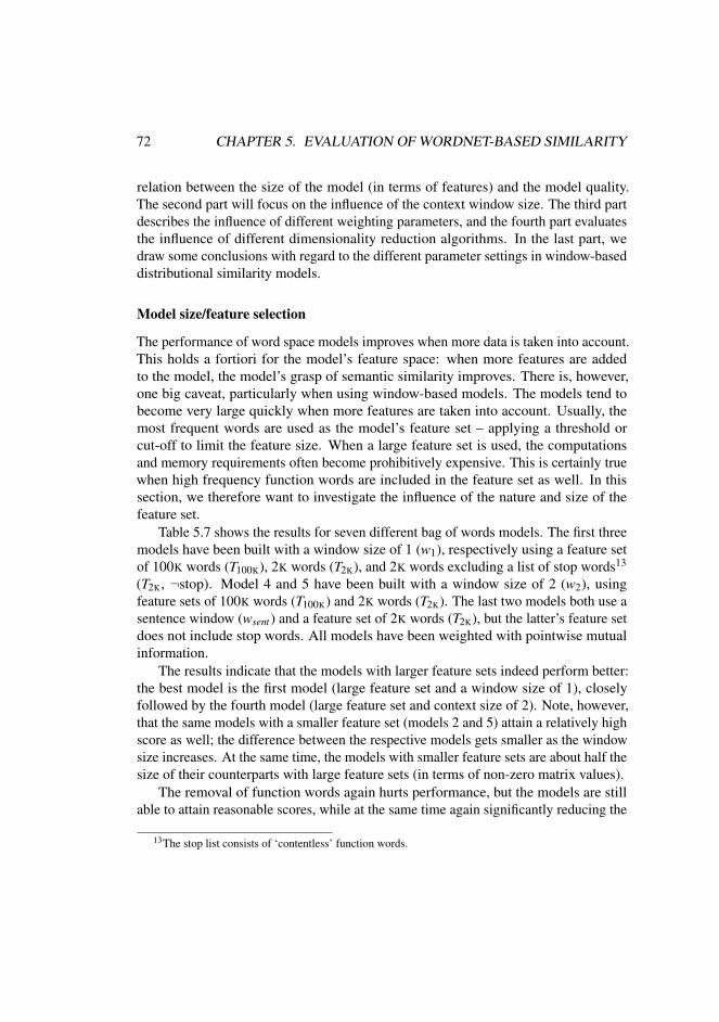
72 CHAPTER 5. EVALUATION OF WORDNET-BASED SIMILARITY
relation between the size of the model (in terms of features) and the model quality.The second part will focus on the influence of the context window size. The third partdescribes the influence of different weighting parameters, and the fourth part evaluatesthe influence of different dimensionality reduction algorithms. In the last part, wedraw some conclusions with regard to the different parameter settings in window-baseddistributional similarity models.
Model size/feature selection
The performance of word space models improves when more data is taken into account.This holds a fortiori for the model’s feature space: when more features are addedto the model, the model’s grasp of semantic similarity improves. There is, however,one big caveat, particularly when using window-based models. The models tend tobecome very large quickly when more features are taken into account. Usually, themost frequent words are used as the model’s feature set – applying a threshold orcut-off to limit the feature size. When a large feature set is used, the computationsand memory requirements often become prohibitively expensive. This is certainly truewhen high frequency function words are included in the feature set as well. In thissection, we therefore want to investigate the influence of the nature and size of thefeature set.
Table 5.7 shows the results for seven different bag of words models. The first threemodels have been built with a window size of 1 (w1), respectively using a feature setof 100K words (T100K), 2K words (T2K), and 2K words excluding a list of stop words13
(T2K, ¬stop). Model 4 and 5 have been built with a window size of 2 (w2), usingfeature sets of 100K words (T100K) and 2K words (T2K). The last two models both use asentence window (wsent ) and a feature set of 2K words (T2K), but the latter’s feature setdoes not include stop words. All models have been weighted with pointwise mutualinformation.
The results indicate that the models with larger feature sets indeed perform better:the best model is the first model (large feature set and a window size of 1), closelyfollowed by the fourth model (large feature set and context size of 2). Note, however,that the same models with a smaller feature set (models 2 and 5) attain a relatively highscore as well; the difference between the respective models gets smaller as the windowsize increases. At the same time, the models with smaller feature sets are about half thesize of their counterparts with large feature sets (in terms of non-zero matrix values).
The removal of function words again hurts performance, but the models are stillable to attain reasonable scores, while at the same time again significantly reducing the
13The stop list consists of ‘contentless’ function words.

5.4. RESULTS 73
wu & palmer’s similarity lin’s similaritydescription k = 1 k = 3 k = 5 k = 1 k = 3 k = 5
1 w1, T100K .633 .561 .526 .541 .485 .4562 w1, T2K .607 .540 .507 .514 .463 .4363 w1, T2K, ¬stop .589 .521 .487 .510 .457 .4284 w2, T100K .627 .551 .516 .541 .483 .4555 w2, T2K .620 .546 .511 .535 .477 .4506 wsent , T2K .547 .465 .428 .477 .420 .3917 wsent , T2K, ¬stop .528 .447 .411 .465 .406 .378
Table 5.7: Evaluation results for different model size parameters in the bag of wordsmodel
size of the model: the models that filter out stop words are again about half the size oftheir non-filtered counterparts.
From the results in table 5.7, we conclude that it is best to use as many featuresas possible; when the use of many features is computationally too expensive, modelswith smaller feature sizes still perform well compared to their counterparts with largerfeature size. The same goes for the removal of high frequency function words: functionwords should be included if possible, but if the model size grows too large, they maybe removed without severely hurting the model’s performance.
Window size
In the next paragraphs, we will look at the influence of window size on the model’sperformance. We will use window sizes of 1, 2, 5, and 10 (both left and right aroundthe target word, but not crossing sentence boundaries), as well as the sentence andthe paragraph in which the target word appears. All models use a feature set of size2K without stop word removal, and all have been weighted with pointwise mutualinformation. Table 5.8 gives the results for the varying window sizes.
The model that uses a window size of 2 (w2) scores best. In general, smallerwindow sizes perform better for the induction of semantic similarity. The model witha window size of 1 (w1) performs worse than w2, but this is probably due to datasparseness: the small window combined with the small feature set does not allow themodel to be sufficiently informative. The results in table 5.7 indicate that a model witha window size of 1 performs better when more features are taken into account.14
14A window size of 2K has been used to keep all parameters but the window size equal. Using a larger

74 CHAPTER 5. EVALUATION OF WORDNET-BASED SIMILARITY
wu & palmer’s similarity lin’s similaritywindow size k = 1 k = 3 k = 5 k = 1 k = 3 k = 5
1 w1 .607 .540 .507 .514 .463 .4362 w2 .620 .546 .511 .535 .477 .4503 w5 .620 .541 .500 .532 .474 .4424 w10 .578 .497 .457 .502 .445 .4135 wsent .547 .465 .428 .477 .420 .3916 wpar .442 .377 .349 .404 .357 .336
Table 5.8: Evaluation results for different window sizes in the bag of words model
Weighting
The results below show the influence of different weighting options. Four differentweighting options are considered. The first model uses no weighting whatsoever (i.e.the identity function is applied as a weighting function). The second model uses locallogarithmic weighting, and no global weighting. The third model uses global pointwisemutual information weighting, and no local weighting. And the fourth model uses acombination of a logarithmic weighting and pointwise mutual information. The fourdifferent models can be formalized as follows:
A f req(i, j) = fi j Alog f req(i, j) = 1+ log fi j
Apmi(i, j) = log p( fi j)p( fi)p( f j)
Alogpmi(i, j) = log p(1+log fi j)p(∑ j 1+log fi j)p(∑i 1+log fi j)
(5.11)
In order to examine the influence of different weighting options on different windowsizes, results are given for a small window size (w2, table 5.9) and a large window size(wpar, table 5.10).
For a window size of 2, pointwise mutual information (Apmi) clearly achieves thebest result. Both logarithmic weighting (Alog f req) and the combination of logarithmicweighting and PMI (Alogpmi) improve upon the bare frequency counts, but both methodsperform worse than Apmi.
For the models using a paragraph as context window, the results look different.Apmi still achieves the best result, but the improvement on the bare frequency countsis smaller. Furthermore, Alog f req and Alogpmi do not improve upon the bare frequencycounts.
feature set would have made the models with larger windows prohibitively expensive.
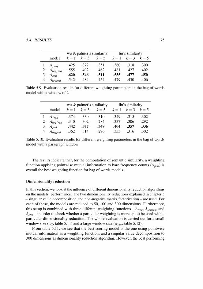
5.4. RESULTS 75
wu & palmer’s similarity lin’s similaritymodel k = 1 k = 3 k = 5 k = 1 k = 3 k = 5
1 A f req .425 .372 .351 .360 .318 .3002 Alog f req .555 .492 .462 .481 .427 .4023 Apmi .620 .546 .511 .535 .477 .4504 Alogpmi .542 .484 .454 .479 .430 .406
Table 5.9: Evaluation results for different weighting parameters in the bag of wordsmodel with a window of 2
wu & palmer’s similarity lin’s similaritymodel k = 1 k = 3 k = 5 k = 1 k = 3 k = 5
1 A f req .374 .330 .310 .349 .315 .3022 Alog f req .340 .302 .284 .337 .306 .2923 Apmi .442 .377 .349 .404 .357 .3364 Alogpmi .362 .314 .296 .353 .316 .302
Table 5.10: Evaluation results for different weighting parameters in the bag of wordsmodel with a paragraph window
The results indicate that, for the computation of semantic similarity, a weightingfunction applying pointwise mutual information to bare frequency counts (Apmi) isoverall the best weighting function for bag of words models.
Dimensionality reduction
In this section, we look at the influence of different dimensionality reduction algorithmson the models’ performance. The two dimensionality reductions explained in chapter 3– singular value decomposition and non-negative matrix factorization – are used. Foreach of these, the models are reduced to 50, 100 and 300 dimensions. Furthermore,this setup is combined with three different weighting functions – Afreq, Alogfreq, andApmi – in order to check whether a particular weighting is more apt to be used with aparticular dimensionality reduction. The whole evaluation is carried out for a smallwindow size (w2, table 5.11) and a large window size (wpar, table 5.12).
From table 5.11, we see that the best scoring model is the one using pointwisemutual information as a weighting function, and a singular value decomposition to300 dimensions as dimensionality reduction algorithm. However, the best performing

76 CHAPTER 5. EVALUATION OF WORDNET-BASED SIMILARITY
wu & palmer’s similarity lin’s similarityA M d k = 1 k = 3 k = 5 k = 1 k = 3 k = 5
Afreq Msvd 50 .395 .350 .329 .333 .299 .282100 .411 .361 .339 .347 .307 .291300 .421 .369 .347 .355 .316 .297
Mnmf 50 .443 .404 .388 .372 .340 .327100 .481 .435 .411 .406 .367 .347300 .497 .435 .410 .421 .370 .350
Alogfreq Msvd 50 .481 .438 .421 .414 .375 .360100 .506 .464 .439 .435 .397 .376300 .533 .483 .455 .461 .417 .392
Mnmf 50 .434 .400 .385 .377 .346 .333100 .451 .414 .397 .395 .361 .346300 .442 .407 .391 .387 .355 .341
Apmi Msvd 50 .540 .489 .465 .461 .420 .401100 .574 .513 .487 .490 .442 .420300 .606 .539 .507 .518 .466 .440
Mnmf 50 .423 .398 .385 .369 .347 .336100 .459 .417 .398 .397 .364 .349300 .473 .426 .405 .418 .378 .360
Apmi – – .620 .546 .511 .535 .477 .450
Table 5.11: Evaluation results for different dimensionality reduction parameters in thebag of words based model with a window of 2
factorized model does not improve on its non-factorized counterpart (shown in the lastline for reasons of comparison). For small windows, semantic similarity calculationsdo not benefit from dimensionality reduction algorithms.
Table 5.11 shows a number of additional striking characteristics that require ourattention. With regard to SVD, the models that perform best are the ones that usePMI as a weighting function. Using logarithmic weighting also improves on the barefrequency data; the use of bare frequency data yields the worst performing models.With regard to NMF, the situation is quite different. The best performing models are theones that do not apply weighting; using logarithmic weighting or PMI yields modelsthat perform worse. The use of the Kullback-Leibler divergence as the NMF’s objectivefunction makes weighted models perform worse than their non-weighted counterparts.In general, though, models using SVD reach better results than models using NMF.

5.4. RESULTS 77
wu & palmer’s similarity lin’s similarityA M d k = 1 k = 3 k = 5 k = 1 k = 3 k = 5
Afreq Msvd 50 .331 .288 .273 .317 .285 .273100 .352 .311 .290 .333 .302 .286300 .371 .328 .305 .345 .315 .297
Mnmf 50 .337 .304 .284 .315 .290 .277100 .360 .316 .291 .338 .304 .285300 .377 .324 .304 .350 .310 .295
Alogfreq Msvd 50 .323 .289 .272 .316 .289 .276100 .336 .297 .281 .327 .298 .284300 .337 .304 .285 .331 .304 .289
Mnmf 50 .313 .288 .271 .309 .288 .276100 .333 .295 .277 .327 .295 .281300 .332 .296 .281 .327 .299 .286
Apmi Msvd 50 .389 .333 .313 .354 .313 .298100 .418 .357 .332 .379 .333 .314300 .443 .376 .351 .402 .351 .331
Mnmf 50 .320 .284 .270 .303 .275 .263100 .356 .314 .297 .328 .298 .285300 .391 .335 .312 .360 .319 .301
Apmi – – .442 .377 .349 .404 .357 .336
Table 5.12: Evaluation results for different dimensionality reduction parameters in thebag of words based model with a paragraph window
Table 5.12 shows results that are similar to the ones given in table 5.12. The bestscoring model is again the one using PMI as a weighting function, and an SVD to 300dimensions. Again it does not improve on its non-factorized counterpart; in the bestcase it is able to achieve a similar score. Bag of words models using a large contextwindow do not provide good models for semantic similarity calculations, and theapplication of dimensionality reduction algorithms does not improve on those results.
The tendencies for SVD are again the same, the only difference being that logar-ithmic weighting does not bring about an improvement. With regard to NMF, simplefrequencies again yield the best models.

78 CHAPTER 5. EVALUATION OF WORDNET-BASED SIMILARITY
Summary
For the extraction of tight semantic similarity, smaller context windows provide themost informative features. The more features that are taken into account, the betterperformance the models reach. Still, the models are able to attain a reasonable per-formance when a smaller number of features is taken into account. When the goalis to extract tight semantic similarity, it is better not to exclude a stop list (thoughit is a possibility that does not severely decrease performance when the models gettoo large). With regard to dimensionality reduction algorithms, no model improvesupon its non-reduced counterpart, but the SVD models combined with Apmi are ableto approximate their non-reduced counterparts very closely within a highly reducedvector space.
5.4.3 Syntax-based models
Introduction
In this section, we look at the performance of syntax-based models for the calculation ofsemantic similarity. All syntax-based models have been constructed using dependencyrelations extracted from the Twente Nieuws Corpus (parsed with the Dutch dependencyparser ALPINO).15 The dependency relations that are used to construct the models arelisted in table 1.2 on page 22.
In the next paragraphs, we extensively examine the influence of different weightingfunctions models. In all subsequent evaluations, we use a syntax-based model with anoun cutoff of 20 (a noun has to appear with 20 different features) and a triple cutoff of2 (a particular noun-feature combination has to appear twice). This amounts to a modelthat contains 30K nouns cross-classified by 170K features. In practice, this gives agood balance between model size and model quality. As a similarity measure, cosine isused.
Weighting
We have tested the syntactic model with the same weighting functions that have beenapplied to the window-based model: no weighting (Afreq), local logarithmic weighting(Alogfreq), pointwise mutual information (Apmi) and a combination of a logarithmicfunction and pointwise mutual information (Alogpmi). A formal overview of the differentfunctions is given on page 74.
15An example feature for the noun apple might be ‘eatob j’.

5.4. RESULTS 79
wu & palmer’s similarity lin’s similaritymodel k = 1 k = 3 k = 5 k = 1 k = 3 k = 5
1 Afreq .480 .415 .385 .414 .364 .3392 Alogfreq .648 .578 .546 .555 .502 .4743 Apmi .640 .584 .554 .546 .504 .4804 Alogpmi .631 .576 .546 .540 .499 .474
Table 5.13: Evaluation results for different weighting parameters in the syntax-basedmodel
The results are presented in table 5.13; they indicate that the performance of thedifferent weighting models is mixed. For k = 1, simple logarithmic weighting scoresbest (simwp = .648 and simlin = .555). For the other values of k, the model that usesonly pointwise mutual information is the most successful. All weighting modelsperform better than the model using simple frequency counts, but a combination oflogarithmic weighting and PMI does not improve over the models that use either ofthose.
Dimensionality reduction
To evaluate the influence of dimensionality reduction algorithms on the syntax-basedmodel, we use a setup that is similar to the one used with the window-based model.Again, the two dimensionality reductions explained in chapter 3 – singular valuedecomposition and non-negative matrix factorization – have been applied. For each ofthese, the models are reduced to 50, 100 and 300 dimensions. This setup is combinedwith three different weighting functions – Afreq, Alogfreq, and Apmi – to check whether aparticular weighting is more apt to be used with a particular dimensionality reduction.
No dimensionality reduction model is able to improve upon the score of its non-reduced counterpart, so dimensionality reduction does not help in getting better sim-ilarity models with regard to CORNETTO similarity. We do notice that some models(notably the SVD models reduced to 300 dimensions using local logarithmic weightingand global pointwise mutual information) are able to closely approach their non-reduced counterparts (for k = 1, simwp = .610 (↔ .648), simlin = .520 (↔ .555) withAlogfreq, and simwp = .604 (↔ .640), simlin = .510 (↔ .546) with Apmi). The last lineof the table shows the non-reduced PMI model for comparison.
With regard to the differences between both dimensionality reduction algorithms,the tendencies are similar to the window-based model. For SVD, the best performing

80 CHAPTER 5. EVALUATION OF WORDNET-BASED SIMILARITY
wu & palmer’s similarity lin’s similarityA M d k = 1 k = 3 k = 5 k = 1 k = 3 k = 5
Afreq Msvd 50 .373 .339 .325 .320 .294 .283100 .416 .374 .355 .355 .322 .305300 .466 .408 .384 .396 .351 .332
Mnmf 50 .409 .393 .385 .338 .322 .315100 .454 .430 .417 .376 .356 .347300 .502 .455 .433 .423 .388 .369
Alogfreq Msvd 50 .552 .503 .482 .468 .425 .408100 .576 .527 .499 .487 .448 .426300 .610 .553 .524 .520 .474 .449
Mnmf 50 .407 .392 .388 .342 .327 .322100 .463 .441 .427 .389 .367 .355300 .508 .468 .452 .432 .400 .385
Apmi Msvd 50 .548 .500 .482 .459 .422 .406100 .572 .525 .505 .483 .446 .427300 .604 .560 .535 .510 .476 .453
Mnmf 50 .368 .359 .353 .318 .304 .298100 .413 .393 .383 .350 .331 .322300 .443 .414 .405 .382 .356 .347
Apmi – – .640 .584 .554 .546 .504 .480
Table 5.14: Evaluation results for different dimensionality reduction parameters in thesyntax-based model
model is Apmi, together with Alogfreq. For NMF, the best scoring models are the Afreqand Alogfreq models; the Apmi models scores considerably worse.
Summary
The class of syntax-based models gives the best performance for the extraction ofsemantic similarity. Pointwise mutual information seems to provide the best weighting,although simple logarithmic weighting yields quite good results as well. Dimensionalityreduction algorithms do not improve upon the results, but singular value decompositionis able to approximate the original model.

5.4. RESULTS 81
wu & palmer’s similarity lin’s similaritymodel k = 1 k = 3 k = 5 k = 1 k = 3 k = 5
document-based .379 .331 .309 .354 .320 .304window-based .633 .561 .526 .541 .485 .456syntax-based .648 .584 .554 .555 .504 .480
Table 5.15: Comparison of the best scoring models for each class
5.4.4 Conclusion
Table 5.15 compares the best results of the three different classes that have beenevaluated in this chapter.
The syntax-based models yield the best results (with Alogfreq for k = 1 and Apmifor k = 3,5) closely followed by the window-based models (using a small window ofw = 1 and Apmi weighting). The best performing document-based model (using SVDreduced to 300 dimensions with article size and Alogent weighting) scores worse thanthe other two models.
Dimensionality reduction algorithms are - to a small extent - beneficial for document-based models. Singular value decomposition (in combination with logentropy-weighting)is able to improve upon the original data. The window-based and syntax-based modelsdo not benefit from dimensionality reduction algorithms; the window-based modelwith dimensionality reduction achieves results similar to its non-factorized counter-part, while the application of dimensionality reduction is detrimental when using asyntax-based model. The results of the models using non-negative matrix factorizationare disappointing: in all cases, either SVD or the non-factorized models reach betterresults.
For the extraction of tight, synonym-like similarity, we conclude that a syntax-basedmodel is the preferred model.


Chapter 6
Evaluation of Cluster Quality
6.1 Introduction
In this chapter, we evaluate the quality of a word space model by comparing the outputof a clustering algorithm (that calculates the similarity between words through the wordspace model) to a gold standard categorization. For this purpose, we will make useof the lexical categorization tasks that have been defined for the workshop ‘Bridgingthe gap between semantic theory and computational simulations’, organized at ESSLLI2008 in Hamburg.1
6.2 Methodology
6.2.1 Clustering tasks
The workshop provides two different noun categorization (clustering) tasks:
1. CONCRETE NOUN CATEGORIZATION – In the concrete noun categorization task,the goal is to cluster 44 concrete nouns in a number of classes on various levelsof generality:
• 2-WAY CLUSTERING – cluster nouns in two top classes natural and arte-fact;
• 3-WAY CLUSTERING – cluster nouns in three classes animal, vegetable andartefact;
1http://wordspace.collocations.de/doku.php/esslli:start
83

84 CHAPTER 6. EVALUATION OF CLUSTER QUALITY
• 6-WAY CLUSTERING – cluster nouns in six classes bird, groundAnimal,fruitTree, green, tool and vehicle.
2. ABSTRACT/CONCRETE NOUN DISCRIMINATION – The evaluation of algorithmsdiscriminating between abstract and concrete nouns consists of three parts:
• In the first part, 30 nouns (15 with high concreteness value and 15 with lowconcreteness value) are clustered in two clusters, HI and LO;
• in the second part, 10 nouns with average concreteness value are addedto the two-way clustering, to see whether they end up in the HI or the LOcluster;
• in the third part, a three-way clustering of the 40 nouns (15 HI, 10 ME, 15LO) is performed.
We will investigate the performance of the different models with regard to thesetasks. With regard to the second task, we will only assess the first part (the ability ofthe models to discriminate between concrete and abstract nouns). Part 2 and 3 will notbe considered here.2
The test sets provided by the workshop are in English. They have been translatedinto Dutch by three translators, and – when multiple translations were found – themajority translation has been taken as the final one. The frequencies of the Dutchwords are by and large comparable to the frequencies of their English counterparts.The gold standard categorization for both tasks is given in appendix A (page 159).
6.2.2 Clustering algorithm
The clustering solutions have been computed with the clustering program CLUTO(Karypis, 2003). The k-way solution is computed by performing a sequence of k−1repeated bisections. This means that the matrix is first clustered into two groups, andthen one of the groups is selected and bisected further. This process continues untilthe desired number of clusters is found. In each step, the cluster is bisected so thatthe resulting 2-way clustering solution maximizes the clustering optimization functiongiven in equation 6.1.
I2 =i=1
∑k
√∑
v,u∈Si
cos(v,u) (6.1)
2The interested reader is referred to Van de Cruys (2008a).

6.3. EVALUATION FRAMEWORK 85
where k is the number of clusters, Si is the set of nouns assigned to the ith cluster, v andu are two nouns, and cos(v,u) is the cosine similarity of those nouns. After computingthe initial clustering, the overall solution is globally optimized. In practice, this ensuresthe algorithm computes the same clustering solution for the same set of objects.3
6.3 Evaluation framework
For the evaluation of cluster quality, we use two different measures: ENTROPY andPURITY (Zhao and Karypis, 2001). These are the standard measures of cluster qualityavailable in CLUTO. Entropy measures how the various semantic classes are distributedwithin each cluster. Given a particular cluster Sr of size nr, the entropy of this clusteris defined to be
E(Sr) =− 1logq
q
∑i=1
nir
nrlog
nir
nr(6.2)
where q is the number of classes in the dataset, and nir is the number of documents of
the ith class that were assigned to the rth cluster. The entropy of the entire clustering isthen the sum of the individual cluster entropies weighted according to the cluster size:
entropy =k
∑r=1
nr
nE(Sr) (6.3)
The clustering solution is perfect if clusters only contain words from one singleclass; in that case the entropy of the clustering solution is zero. Smaller entropy valuesindicate better clustering solutions.
Using the same mathematical definitions, the purity of a cluster is defined as:
Pu(Sr) =1nr
maxi
nir (6.4)
The purity gives the fraction of the overall cluster size that the largest class of wordsassigned to that cluster represents. The purity of the clustering solution is then againthe weighted sum of the individual cluster purities:
purity =k
∑r=1
nr
nPu(Sr) (6.5)
Larger purity values indicate better clustering solutions.
3The algorithm is selected by choosing the ‘rbr’ clustering method option in CLUTO.

86 CHAPTER 6. EVALUATION OF CLUSTER QUALITY
6.4 Results
The models in this chapter are built in exactly the same way as the models presented inchapter 5, in which the semantic similarity is evaluated. After building the models, thefeature vectors of the nouns involved in the categorization tasks have been extractedfrom the models, and fed to the clustering algorithm.
6.4.1 Concrete noun categorization
Document based
Table 6.1 shows the clustering results for the document-based model with regard todifferent weighting parameters. Results are given for smaller paragraph (wpar) andlarger article (wart ) document sizes.
2-way 3-way 6-waymethod docsize entropy purity entropy purity entropy purity
Afreq wpar .970 .591 .739 .591 .548 .523wart .505 .886 .587 .727 .318 .750
Alogfreq wpar .562 .864 .757 .614 .408 .659wart .611 .841 .685 .614 .392 .659
Aent wpar .970 .591 .739 .591 .548 .523wart .505 .886 .587 .727 .318 .750
Alogent wpar .562 .864 .757 .614 .408 .659wart .611 .841 .685 .614 .392 .659
Table 6.1: Clustering results for concrete noun categorization: bag of words approachwith different weighting parameters
The best results are reached with simple frequency information (using articles asdocument size); none of the weightings is able to improve upon the simple frequencyvalues. Still, the best scoring model does not yield a very good clustering solution.
Table 6.2 gives the results for the document-based model combined with dimen-sionality reduction (SVD). Results are given for three different weighting functions(Afreq, Alogfreq and Alogent), using both paragraphs and articles as document sizes.
The results for the document-based model in combination with dimensionalityreduction are mixed. On the one hand, the models are able to attain better results for the3-way and 6-way clustering. The model using a combination of logarithmic smoothing
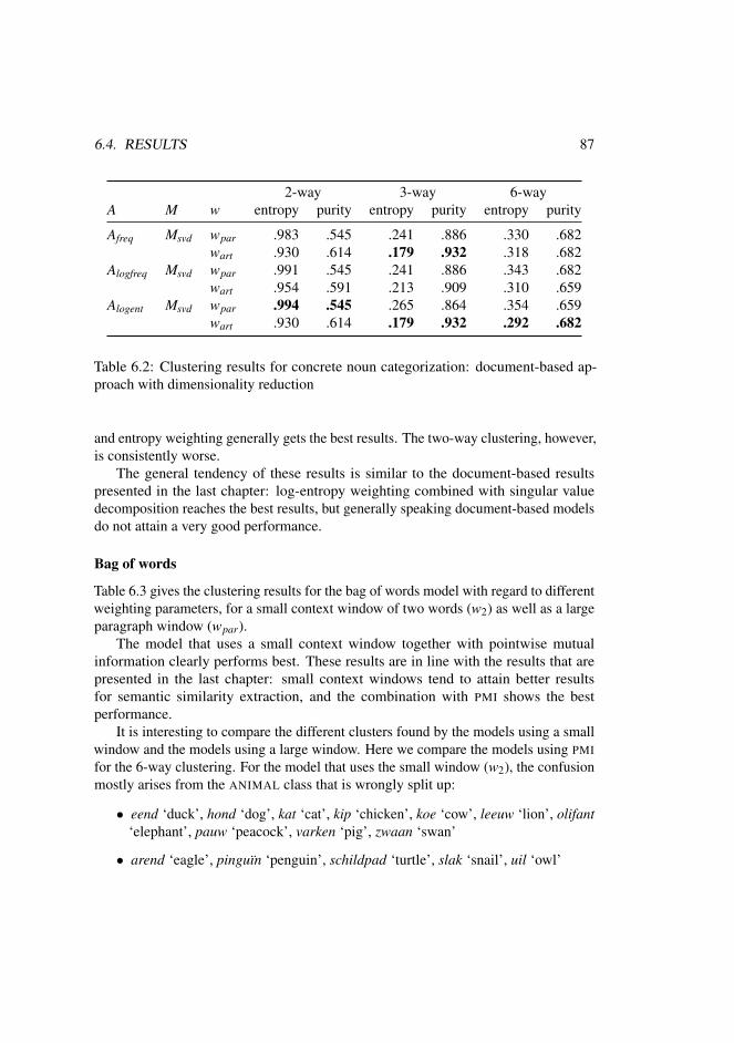
6.4. RESULTS 87
2-way 3-way 6-wayA M w entropy purity entropy purity entropy purity
Afreq Msvd wpar .983 .545 .241 .886 .330 .682wart .930 .614 .179 .932 .318 .682
Alogfreq Msvd wpar .991 .545 .241 .886 .343 .682wart .954 .591 .213 .909 .310 .659
Alogent Msvd wpar .994 .545 .265 .864 .354 .659wart .930 .614 .179 .932 .292 .682
Table 6.2: Clustering results for concrete noun categorization: document-based ap-proach with dimensionality reduction
and entropy weighting generally gets the best results. The two-way clustering, however,is consistently worse.
The general tendency of these results is similar to the document-based resultspresented in the last chapter: log-entropy weighting combined with singular valuedecomposition reaches the best results, but generally speaking document-based modelsdo not attain a very good performance.
Bag of words
Table 6.3 gives the clustering results for the bag of words model with regard to differentweighting parameters, for a small context window of two words (w2) as well as a largeparagraph window (wpar).
The model that uses a small context window together with pointwise mutualinformation clearly performs best. These results are in line with the results that arepresented in the last chapter: small context windows tend to attain better resultsfor semantic similarity extraction, and the combination with PMI shows the bestperformance.
It is interesting to compare the different clusters found by the models using a smallwindow and the models using a large window. Here we compare the models using PMIfor the 6-way clustering. For the model that uses the small window (w2), the confusionmostly arises from the ANIMAL class that is wrongly split up:
• eend ‘duck’, hond ‘dog’, kat ‘cat’, kip ‘chicken’, koe ‘cow’, leeuw ‘lion’, olifant‘elephant’, pauw ‘peacock’, varken ‘pig’, zwaan ‘swan’
• arend ‘eagle’, pinguın ‘penguin’, schildpad ‘turtle’, slak ‘snail’, uil ‘owl’

88 CHAPTER 6. EVALUATION OF CLUSTER QUALITY
2-way 3-way 6-waymethod window entropy purity entropy purity entropy purity
Afreq w2 .714 .715 .422 .727 .556 .477wpar .966 .544 .638 .659 .380 .659
Alogfreq w2 .924 .659 .887 .477 .375 .659wpar .922 .636 .866 .523 .729 .409
Apmi w2 .000 1.000 .213 .909 .206 .773wpar .911 .659 .541 .705 .377 .591
Alogpmi w2 .924 .659 .648 .614 .277 .727wpar .871 .705 .650 .659 .472 .568
Table 6.3: Clustering results for concrete noun categorization: bag of words approachwith different weighting parameters
The model using the large window (wpar), on the other hand, seems to find moretopically related clusters:
• koe ‘cow’, maıs ‘corn’, varken ‘pig’
• aardappel ‘potato’, ananas ‘pineapple’, banaan ‘banana’, champignon ‘mush-room’, fles ‘bottle’, kers ‘cherry’, ketel ‘kettle’, kip ‘chicken’, kom ‘bowl’, lepel‘spoon’, peer ‘pear’, sla ‘lettuce’, ui ‘onion’
The first cluster seems related to stock breeding, containing stock animals (koe ‘cow’and varken ‘pig’) and a crop often used as feed (maıs ‘corn’). The second cluster lookslike a food-related cluster, containing fruit and vegetables, but also an animal oftenconsumed as meat (kip ‘chicken’) and a number of kitchen utensils (fles ‘bottle’, ketel‘kettle’, kom ‘bowl’, lepel ‘spoon’).
Table 6.4 gives the results for the bag of words model combined with dimensionalityreduction algorithms (SVD and NMF). Results are given for three different weightingfunctions (Afreq, Alogfreq and Apmi), both for a small context window (w2) and a largecontext window (wpar).
Again, the model using a small context window and PMI (in combination with SVD)generally seems to give the best performance. The result, however, does not exceed itsnon-factorized counterpart.
Another remarkable result is that the NMF model – in combination with simplefrequency counts and a large window – is able to reach the best specific result for

6.4. RESULTS 89
2-way 3-way 6-wayA M w entropy purity entropy purity entropy purity
Afreq Msvd w2 .714 .750 .422 .727 .549 .477wpar .966 .545 .271 .886 .337 .682
Mnmf w2 .492 .864 .431 .773 .329 .750wpar .930 .614 .179 .932 .310 .705
Alogfreq Msvd w2 .924 .659 .887 .477 .440 .614wpar .922 .636 .719 .659 .607 .432
Mnmf w2 .944 .636 .679 .591 .492 .591wpar .896 .682 .617 .659 .617 .432
Apmi Msvd w2 .000 1.000 .223 .909 .233 .818wpar .972 .568 .541 .705 .334 .682
Mnmf w2 .881 .682 .550 .705 .414 .659wpar .964 .591 .513 .727 .384 .614
Table 6.4: Clustering results for concrete noun categorization: bag of words approachwith dimensionality reduction
the three-way clustering. Clearly, NMF is able to induce general semantic traits fromthe data, yielding a good clustering result. Upon inspection of the data, we see thatgood ANIMAL and ARTEFACT clusters are formed. A third clustering contains mostlyVEGETABLEs, but again also food related ARTEFACT nouns such as kom ‘bowl’ andlepel ‘spoon’, and the food related ANIMAL noun kip ‘chicken’.
Syntax-based
Table 6.5 gives the clustering results for the syntax-based model, again according tofour different weighting parameters.
The results indicate that the models using PMI and LOGPMI perform best – thoughit should be noted that all syntax-based models attain quite good results. Remarkably,the model that uses only logarithmic weighting performs not so well (particularly withregard to the two-way clustering). This result is different compared to the semanticsimilarity results presented in the last chapter. Overall, using PMI seems to provide themost stable performance for the induction of semantic similarity using the syntax-basedmodel.
Figure 6.1 shows the confusion matrix of the 6-way clustering for the models usingPMI and LOGPMI; the matrix is the same for both models.

90 CHAPTER 6. EVALUATION OF CLUSTER QUALITY
2-way 3-way 6-waymethod entropy purity entropy purity entropy purity
Afreq .000 1.000 .067 .977 .264 .750Alogfreq .784 .659 .000 1.000 .245 .750Apmi .000 1.000 .000 1.000 .153 .864Alogpmi .000 1.000 .000 1.000 .153 .864
Table 6.5: Clustering results for concrete noun categorization: syntactic approach withdifferent weighting parameters
cluster bird grou frui gree tool vehi
1 0 0 4 5 0 02 0 0 0 0 7 03 6 0 0 0 0 04 0 0 0 0 0 75 0 0 0 0 6 06 1 8 0 0 0 0
Figure 6.1: Confusion matrix of the 6-way clustering for the syntax-based model (PMIand LOGPMI).
Upon examining the results, the decisions made by the algorithm look quite reason-able:
• One bird (‘chicken’) is classified as groundAnimal;
• fruits and vegetables are assigned to one single cluster;
• the tools class is split up into two different clusters, so that a division is madebetween ‘active’ and ‘passive’ tools:
– beitel ‘chisel’, hamer ‘hammer’, mes ‘knife’, pen ‘pen’, potlood ‘pencil’,schaar ‘scissors’, schroevendraaier ‘screwdriver’;
– beker ‘cup’, fles ‘bottle’, ketel ‘kettle’, kom, ‘bowl’, lepel ‘spoon’, telefoon‘telephone’.

6.4. RESULTS 91
The only noun that may be considered wrongly classified is slak ‘snail’, which isclassified as a bird.
It is interesting to note that the difference between fruit and vegetables nonethelessis present in the data. When clustering the words from the subsets fruitTree and greeninto two classes, they are properly split up:
• kers ‘cherry’, banaan ‘banana’, peer ‘pear’, ananas ‘pineapple’;
• champignon ‘mushroom’, maıs ‘corn’, sla ‘lettuce’, aardappel ‘potatoe’, ui‘oignon’.
In table 6.6, the results for the syntax-based model combined with dimensionalityreduction algorithms (SVD and NMF) are shown. Again, three different weightingfunctions (Afreq, Alogfreq and Apmi) are evaluated.
2-way 3-way 6-wayA M entropy purity entropy purity entropy purity
Afreq Msvd .902 .682 .457 .795 .430 .636Mnmf .917 .659 .260 .864 .244 .750
Alogfreq Msvd .784 .659 .000 1.000 .238 .773Mnmf .589 .795 .000 1.000 .235 .750
Apmi Msvd .000 1.000 .000 1.000 .206 .773Mnmf .589 .795 .067 .977 .266 .727
Table 6.6: Clustering results for concrete noun categorization: syntactic approach withdimensionality reduction
Again, we see the same tendencies that became apparent in the former chapter:SVD in combination with PMI gives the best performance, but the results are not asgood as the PMI model that does not use any dimensionality reduction (notably, the6-way clustering performs worse).
6.4.2 Abstract/concrete noun discrimination
In the abstract/concrete noun discrimination task, we try to separate 15 abstract nounsand 15 concrete nouns into two different clusters.

92 CHAPTER 6. EVALUATION OF CLUSTER QUALITY
Document-based model
Table 6.7 presents the clustering results for the document-based model. Four differentweighting functions have been applied, each with two different document sizes.
method docsize entropy purity
Afreq wpar .362 .931wart .296 .933
Alogfreq wpar .579 .862wart .463 .900
Aent wpar .362 .931wart .296 .933
Alogent wpar .579 .862wart .463 .900
Table 6.7: Clustering results for abstract/concrete noun discrimination: document-basedapproach with different weighting parameters
The document-based model is not able to make a good division between abstractand concrete nouns. Using a large document size (wart) yields slightly better results.No particular weighting function gets better results than the simple frequency data.
Table 6.8 presents the results for the document-based model in combination withsingular value decomposition. Using a singular value decomposition yields worseresults than the use of the original models.
A M w entropy purity
Afreq Msvd wpar .739 .724wart .470 .867
Alogfreq Msvd wpar .739 .724wart .662 .767
Alogent Msvd wpar .625 .793wart .604 .800
Table 6.8: Clustering results for abstract/concrete noun discrimination: document-basedapproach with dimensionality reduction
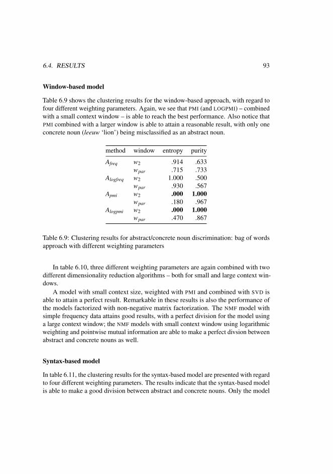
6.4. RESULTS 93
Window-based model
Table 6.9 shows the clustering results for the window-based approach, with regard tofour different weighting parameters. Again, we see that PMI (and LOGPMI) – combinedwith a small context window – is able to reach the best performance. Also notice thatPMI combined with a larger window is able to attain a reasonable result, with only oneconcrete noun (leeuw ‘lion’) being misclassified as an abstract noun.
method window entropy purity
Afreq w2 .914 .633wpar .715 .733
Alogfreq w2 1.000 .500wpar .930 .567
Apmi w2 .000 1.000wpar .180 .967
Alogpmi w2 .000 1.000wpar .470 .867
Table 6.9: Clustering results for abstract/concrete noun discrimination: bag of wordsapproach with different weighting parameters
In table 6.10, three different weighting parameters are again combined with twodifferent dimensionality reduction algorithms – both for small and large context win-dows.
A model with small context size, weighted with PMI and combined with SVD isable to attain a perfect result. Remarkable in these results is also the performance ofthe models factorized with non-negative matrix factorization. The NMF model withsimple frequency data attains good results, with a perfect division for the model usinga large context window; the NMF models with small context window using logarithmicweighting and pointwise mutual information are able to make a perfect divsion betweenabstract and concrete nouns as well.
Syntax-based model
In table 6.11, the clustering results for the syntax-based model are presented with regardto four different weighting parameters. The results indicate that the syntax-based modelis able to make a good division between abstract and concrete nouns. Only the model

94 CHAPTER 6. EVALUATION OF CLUSTER QUALITY
A M w entropy purity
Afreq Msvd w2 .914 .633wpar .604 .800
Mnmf w2 .180 .967wpar .000 1.000
Alogfreq Msvd w2 1.000 .500wpar .930 .567
Mnmf w2 .000 1.000wpar .715 .733
Apmi Msvd w2 .000 1.000wpar .180 .967
Mnmf w2 .000 1.000wpar .296 .933
Table 6.10: Clustering results for abstract/concrete noun discrimination: bag of wordsapproach with dimensionality reduction
based on simple frequencies is not able to make a decent division; the other models areable to induce a perfect clustering.
method entropy purity
Afreq .985 .567Alogfreq .000 1.000Apmi .000 1.000Alogpmi .000 1.000
Table 6.11: Clustering results for abstract/concrete noun discrimination: syntax-basedapproach with different weighting parameters
In table 6.12, the syntax-based model (weighted with three different weightingfunctions) is again combined with two different dimensionality reduction algorithms.The results of the factorized models reflect the performance of their non-factorizedcounterparts. The models that make a perfect cut without dimensionality reductionsalso make a perfect cut with the use of dimensionality reduction. Notice again, however,that NMF is able to strongly improve the results of the model using simple frequency

6.5. COMPARISON OF THE DIFFERENT MODELS 95
data.
A M entropy purity
Afreq Msvd 1.000 .500Mnmf .180 .967
Alogfreq Msvd .000 1.000Mnmf .000 1.000
Apmi Msvd .000 1.000Mnmf .000 1.000
Table 6.12: Clustering results for abstract/concrete noun discrimination: syntax-basedapproach with dimensionality reduction
6.5 Comparison of the different models
Examining the differences in cluster quality between the different models, we can drawsome conclusions with regard to their ability to extract semantic similarity. Clearly, thedocument-based models are do not perform well. The models are not able to correctlycategorize concrete nouns, nor are they able to make a proper division between abstractand concrete nouns. The window-based model performs better than the document-based model. The window size plays a significant role: models using a small windowtend to perform better than the ones using a large window (using PMI as weightingfunction).4 But the model that performs best is the syntax-based model. Differentweighting functions perform well, but PMI consistently seems to yield good results.In general, the application of dimensionality reduction models does not yield bettercluster quality.
4Notice however that the models with a large window size seem to grasp a kind of ‘topical’ similarity.


Chapter 7
Evaluation of Domain Coherence
7.1 Introduction
In this chapter, we will evaluate the ability of the various models to induce moreloosely related, topically similar words. This will be done by evaluating the ability ofthe models to extract similar words that belong to the same semantic domains. TheCORNETTO database has been augmented with semantic domain tags. By evaluatingthe models’ ability to extract similar words that belong to the same semantic domain asthe target word, we are able to evaluate a model’s ability to induce topical similarity.
7.2 Evaluation framework
7.2.1 Semantic domains
Semantic domains are particular areas of human knowledge (such as POLITICS, MEDI-CINE or SPORTS) according to which words and senses can be classified. Words thatbelong to the same semantic domain (e.g. doctor and hospital are both in the MEDI-CINE domain) are topically related. This makes semantic domains perfectly suitable toinvestigate topical similarity or domain coherence.
Semantic domains are a part of the original English WordNet: it has been augmentedwith Wordnet Domain labels – a collection of 200 domain labels (tags) organized ina hierarchical structure (Magnini and Cavagli, 2000; Bentivogli et al., 2004). Eachsynset in WordNet is labeled with one or more labels. When there are no suitable labelsfor a particular synset, the label ‘factotum’ is assigned.
97

98 CHAPTER 7. EVALUATION OF DOMAIN COHERENCE
The CORNETTO database, used in our evaluation framework, has been augmentedwith domain labels as well. Domain labels from the English WordNet have auto-matically been added.1 Moreover, domain labels from the VLIS database2 have beenautomatically converted to WordNet domain labels. The CORNETTO domain labels areconsulted with the PYCORNETTO interface.
7.2.2 Similarity measure
For each target word in the test set, the 10 most similar words according to a particularmodel are extracted. All possible domain labels for the target word are extracted fromthe CORNETTO database, and compared to all possible domain tags for the extractedsimilar words. The most frequent domain tag – that is also present in the tagset ofthe target word – is taken as the correct domain tag. The number of words that istopically coherent to the target word is then the number of words that have the correcttag, divided by all words for which a domain tag has been extracted. Formally,
simtopic =maxt∈tags(s0) ∑i
{ 1 if t in tags(si)0 otherwise
i(7.1)
where s0 is the target word, s1...i is the list of similar words present in CORNETTO withat least one domain tag, and tags(si) is the set of domain tags for word si. We ignorewords that are not found in the CORNETTO database.
Let us illustrate the topical similarity measure with an example. In table 7.1, 10words are given that are topically related to the target word zebrapad ‘pedestriancrossing’, together with the domain tags extracted from CORNETTO. The target wordzebrapad has one possible tag: TRANSPORT. We look up which of the similar wordsalso has this tag as one of its domain tags, and divide the number of correctly taggedwords by the total number of similar words. This gives us a topic similarity simtopic of8
10 = .80.Note that, among the similar words of zebrapad, there are many words that are
only loosely, topically related (e.g. voetganger ‘pedestrian’ and fietser ‘cyclist’). Still,those words belong to the same TRANSPORT domain, so that a high simtopic value isattributed to the set of words.
Another important fact to note is that words that are tightly similar are usually alsotopically related. In table 7.2, 10 words are given that are tightly similar (synonymous
1CORNETTO’s synsets are aligned with the English WordNet synsets, which makes the mappingstraightforward.
2Van Dale Lexical Information System; a database developed by Van Dale lexicographers.

7.2. EVALUATION FRAMEWORK 99
word translation domain tags
0 zebrapad ‘pedestrian crossing’ TRANSPORT1 voetganger ‘pedestrian’ TRANSPORT2 fietser ‘cyclist’ CYCLING, TRANSPORT3 stoplicht ‘traffic light’ TOWN PLANNING, TRANSPORT4 trottoir ‘pavement’ TRANSPORT5 stoep ‘pavement’ BUILDING INDUSTRY, TRANSPORT6 kruispunt ‘crossing’ TRANSPORT7 fietspad ‘cycle track’ TRANSPORT8 rotonde ‘roundabout’ BUILDING INDUSTRY, TRANSPORT9 lantaarnpaal ‘lamppost’ BUILDING INDUSTRY, TOWN PLANNING10 berm ‘verge’ TOWN PLANNING
Table 7.1: Domain tags for the similar words of zebrapad, ‘pedestrian crossing’
word translation domain tags
0 huis ‘house’ BUILDING INDUSTRY1 woning ‘house’ BUILDING INDUSTRY2 pand ‘building’ BUILDING INDUSTRY, TOWN PLANNING, . . .3 gebouw ‘building’ BUILDING INDUSTRY, TOWN PLANNING4 villa ‘villa’ BUILDING INDUSTRY5 kamer ‘room’ ADMINISTRATION, BUILDING INDUSTRY, . . .6 huisje ‘small house’ –7 boerderij ‘farm’ AGRICULTURE8 appartement ‘appartment’ BUILDING INDUSTRY, TOWN PLANNING9 flat ‘flat FASHION, BUILDING INDUSTRY10 schuur ‘shed’ BUILDING INDUSTRY
Table 7.2: Domain tags for the similar words of huis, ‘house’
or hyponymous) to the target word huis ‘house’. Most of those words also belong tothe same semantic domain BUILDING INDUSTRY, yielding a high simtopic score of89 = .89.3
One last important fact to be considered is that – due to the automatic procedure – asignificant number of words in CORNETTO is erroneously tagged, or has an incomplete
3huisje ‘small house’ is not present in the CORNETTO database, so only 9 words are taken into account.

100 CHAPTER 7. EVALUATION OF DOMAIN COHERENCE
word translation domain tags
0 film ‘movie’ CINEMA, PHOTOGRAPHY, TV, . . .1 regisseur ‘director’ MUSIC2 speelfilm ‘movie’ PAINTING3 filmmaker ‘filmmaker’ PERSON4 hoofdrolspeler ‘main actor’ THEATRE5 acteur ‘actor’ PERSON6 hoofdrol main part THEATRE7 script script THEATRE8 hoofdrolspeelster main actress –9 cinema cinema BUILDING INDUSTRY, THEATRE, . . .10 scenarioschrijver scriptwriter LITERATURE
Table 7.3: Domain tags for the words topically related to film, ‘movie’
tagset. Take, for example, the topically related words to the target word film ‘movie’,presented in table 7.3. All words clearly seem topically related to the CINEMA domain.Yet, none of the similar words is tagged with the actual CINEMA tag, so that a topicalsimilarity score simtopic of .00 is attributed. As a result, many sets may in reality bemore topically related than the evaluation score suggests.
7.3 Results
The models in this chapter are built in exactly the same way as the models presented inchapters 5 and 6, in which the wordnet-based similarity and cluster quality are evaluated.The baseline topical similarity score (using the same random models that were used forthe creation of the CORNETTO baseline in chapter 5) amounts to .0482±1.09×10⁻³
(mean and standard deviation).
7.3.1 Document-based models
Weighting
In table 7.4 the topical similarity scores for the document-based model are given,according to different weighting functions. The results indicate that the model using alarge document size performs better. Also, using logarithmic weighting improves theresults. Entropy weighting does not improve the results. The different weighting scores

7.3. RESULTS 101
simtopicmodel wpar wart
1 A f req .315 .3492 Alog f req .329 .3593 Aent .315 .3494 Alogent .329 .359
Table 7.4: Topical similarity results for different weighting parameters in the document-based model with two different document sizes
presented here show the same tendencies as the weighting scores for the document-based model presented in chapter 5.
Dimensionality reduction
Table 7.5 gives the results for the document-based model in combination with singularvalue decomposition. The results show that SVD as a dimensionality reduction isable to improve the results. All models tend to improve with SVD (reduced to 300dimensions); in combination with log-entropy weighting, the similarity scores improvemost. These results are again similar to the results for dimensionality reductionpresented in chapter 5: SVD improves the results, and the improvement is the largestwith log-entropy weighting.
7.3.2 Bag of words models
Window size
In table 7.6, the topical similarity scores for different window sizes are given. If wecompare the results to those in table 5.8 on page 74, we notice some striking differences.Whereas the CORNETTO similarity is clearly best with smaller context windows – andheavily deteriorates with larger context windows – this is not the case for the topicalsimilarity score. The models with a smaller context window (w2, w5) still get a goodscore, but the results for the models with large context window (w10, wsent and to alesser extent wpar) are clearly within the same range. The results indicate that thewindow-based models are able to extract topical similarity with small windows as wellas with large windows.

102 CHAPTER 7. EVALUATION OF DOMAIN COHERENCE
simtopicA M d wpar wart
Afreq Msvd 50 .262 .320100 .300 .347300 .340 .370
Alogfreq Msvd 50 .263 .335100 .306 .359300 .343 .379
Alogent Msvd 50 .302 .346100 .329 .372300 .357 .394
Alogent – – .329 .359
Table 7.5: Evaluation results for different dimensionality reduction parameters in thedocument-based model with two different document sizes
window size simtopic
1 w1 .3802 w2 .4143 w5 .4234 w10 .4225 wsent .4186 wpar .399
Table 7.6: Evaluation results for different window sizes in the bag of words model
Weighting
In table 7.7, the topical similarity scores for the four different weighting functions arepresented, both for a context window of 2 and a paragraph window. One striking factto notice is that a simple frequency model in combination with a paragraph windowperforms quite well. The other scores are in line with the semantic similarity scorespresented in chapter 5: weighting with pointwise mutual information scores best forboth window sizes, and the other weighting parameters Alog f req and Alogpmi performworse than Apmi with a small window (w2) and even perform worse with a largeparagraph window (wpar).

7.3. RESULTS 103
simtopicmodel w2 wpar
1 A f req .209 .3492 Alog f req .350 .3093 Apmi .414 .3994 Alogpmi .370 .325
Table 7.7: Evaluation results for different weighting parameters in the bag of wordsmodel with two different context windows
Dimensionality reduction
In table 7.8, the topical similarity score for different dimensionality reduction al-gorithms is given, with regard to two different context window sizes (w2 and wpar).The tendencies with regard to dimensionality reduction for bag of words models againdo not differ tremendously from the tendencies we have seen in chapter 5. The bestscoring models are the ones using pointwise mutual information with a singular valuedecomposition. For small windows (w2), the best scoring model does not improveupon its non-reduced counterpart. This is different, however, for large windows (wpar):pointwise mutual information combined with singular value decomposition to 100 and300 dimensions brings about an improvement compared to its non-reduced counterpart.Note that this improvement is larger for the topical similarity presented here, comparedto the wordnet-based similarity (table 5.12 on page 77).
Note that, for non-negative matrix factorization, the best scoring models are also theones using pointwise mutual information. In chapter 5, the best scoring NMF modelswere the ones using simple frequency information.
7.3.3 Syntax-based models
Weighting
Table 7.9 gives the topical similarity scores for different weighting functions for syntax-based models. The model using only pointwise mutual information again performsbest, followed by the model using a combination of logarithmic weighting and PMI,and the model using only logarithmic weighting. Simple frequency information againperforms worst.
Compared to the wordnet-based similarity results, the topical similarity scoresare a little bit different. Whereas with the wordnet-based similarity, both PMI and

104 CHAPTER 7. EVALUATION OF DOMAIN COHERENCE
simtopicA M d w2 wpar
Afreq Msvd 50 .190 .302100 .200 .328300 .207 .349
Mnmf 50 .260 .341100 .284 .367300 .285 .371
Alogfreq Msvd 50 .301 .295100 .320 .305300 .339 .311
Mnmf 50 .283 .293100 .300 .305300 .296 .308
Apmi Msvd 50 .380 .384100 .404 .400300 .416 .409
Mnmf 50 .306 .339100 .316 .373300 .329 .388
Apmi – – .442 .399
Table 7.8: Evaluation results for different dimensionality reduction parameters in thebag of words based model with two different context windows
logarithmic weighting perform quite well, PMI is clearly the winner with regard totopical similarity.
Dimensionality reduction
Table 7.10 gives the results for different dimensionality reduction algorithms in thesyntax-based models. Singular value decomposition combined with PMI again performsbest, but dimensionality reduction algorithms do not bring about any improvement,compared to the models without dimensionality reduction.

7.3. RESULTS 105
model simtopic
1 A f req .2592 Alog f req .4043 Apmi .4414 Alogpmi .432
Table 7.9: Evaluation results for different weighting parameters in the syntax-basedmodel
A M d simtopic
Afreq Msvd 50 .185100 .214300 .253
Mnmf 50 .266100 .310300 .342
Alogfreq Msvd 50 .345100 .370300 .391
Mnmf 50 .270100 .340300 .379
Apmi Msvd 50 .377100 .405300 .434
Mnmf 50 .256100 .303300 .337
Apmi – – .441
Table 7.10: Topical similarity for different dimensionality reduction parameters in thesyntax-based model

106 CHAPTER 7. EVALUATION OF DOMAIN COHERENCE
7.4 Discussion & comparison
The results presented in this chapter provide mixed results. On the one hand, modelsthat score well in the two former tasks (semantic similarity in chapter 5 and clusterquality in chapter 6) also perform well on the task of extracting topically similar words.This is in particular the case for the syntax-based approach, and to a lesser extent forthe window-based approach with small window size.
On the other hand, we notice that models that do not perform well on the two formerevaluation tasks (the document-based model and the window-based model with largewindow) still perform reasonably well with regard to the extraction of topical similarity.We may therefore conclude that those models are not extracting tight, synonym-likesemantic similarity, but are still extracting semantically related, topically similar words.
Let us illustrate this fact with a number of examples. In the examples below, wecompare the 10 most similar words according to:
a. the syntax-based model, using PMI weighting: this model performs best both withregard to wordnet-based similarity/cluster quality and topical similarity;
b. the window-based model, using PMI weighting and paragraph window: this modelperforms worse with regard to wordnet-based similarity/cluster quality, but performsreasonably well in the topical similarity evaluation.
(1) a. krant ‘newspaper’: dagblad ‘newspaper’, zakenkrant ‘business paper’,kwaliteitskrant ‘quality newspaper’, blad ‘paper’, tabloid ‘tabloid’, zon-dagskrant ‘sunday newspaper’, weekblad ‘magazine’, ochtendblad ‘morn-ing paper’, boulevardblad ‘tabloid, sportkrant ‘sports paper’
b. krant ‘newspaper’: dagblad ‘newspaper’, voorpagina ‘front page’, hoofd-redacteur ‘chief editor’, redactie ‘editors’, weekblad ‘magazine’, kwali-teitskrant ‘quality newspaper’, redacteur ‘editor’, berichtgeving ‘cover-age’, hoofdredactie ‘chief editors’, journalist ‘journalist’
(2) a. film ‘movie’: speelfilm ‘movie’, thriller ‘thriller’, komedie ‘comedy’,documentaire ‘documentary’, musical ‘musical’, drama ‘tragedy’, boek‘book’, roman ‘novel’, muziek ‘music’, video ‘video’
b. film ‘movie’: regisseur ‘director’, speelfilm ‘movie’, filmmaker ‘film-maker’, hoofdrolspeler ‘main actor’, acteur ‘actor’, hoofdrol ‘main part’,script ‘script’, hoofdrolspeelster ‘main actress’, cinema ‘cinema’, scenari-oschrijver ‘script writer’
(3) a. politie ‘police’: brandweer ‘fire brigade’, justitie ‘justice’, douane ‘cus-toms’, leger ‘army’, politiekorps ‘police force’, Politie ‘Police’, agent

7.4. DISCUSSION & COMPARISON 107
‘officer’, autoriteit ‘authority’, recherche ‘criminal investigation depart-ment’, marechaussee ‘military police’
b. politie ‘police’: politiewoordvoerder ‘police spokesman’, agent ‘officer’,politiebureau ‘police station’, politiemens ‘police person’, aanhouding ‘ar-rest’, politieagente ‘police woman’, vuurwapen ‘firearm’, arrestant ‘arrestperson’, arrestatieteam ‘special squad’, recherche ‘criminal investigationdepartment
Clearly, both approaches capture a different kind of semantic similarity. The firstapproach captures a tight, synonym-like similarity, whereas the second approach cap-tures a broader, topical relatedness. In example (1), the syntax-based model (a) yieldssynonyms (dagblad ‘newspaper’) and hyponyms (tabloid ‘tabloid’) as semanticallysimilar words for krant ‘newspaper’. The window-based model (b), on the other hand,also yields more loosely related words, such as meronyms (voorpagina ‘front page’)and associations (redacteur ‘editor’, journalist ‘journalist’). The same tendency ispresent in the two other examples. In example (2), the syntax-based model yieldssynonyms and hyponyms, and a number of co-hyponyms (boek ‘book’, muziek ‘music’)as different kinds of media/art expressions. The window-based model again also yieldsmore loosely, topically related words such as acteur ‘actor’ and script ‘script’. Andin example (3), the similar words in (a) consists mostly of co-hyponyms designatingauthoritative organizations similar to politie ‘police’, whereas in (b), more topicallyrelated words such as aanhouding ‘arrest’ and vuurwapen ‘firearm’ show up again.
Changing the context also changes the semantic characteristics captured by themodels. Syntax-based models and window-based models with small window sizeare particularly apt for the extraction of tight, synonym-like similarity, as has beenshown in chapter 5, in which the wordnet-based similarity was evaluated by comparingthem to the semantic hierarchical database CORNETTO, and in chapter 6, in whichthe models’ cluster quality was compared to a gold standard. In this chapter, we haveshown that those models also perform well with regard to the extraction of topicalsimilarity: words that are tightly similar (such as synonyms and hyponyms) are usuallyalso topically related.
Document-based models and window-based models with large window size, onthe other hand, are not suitable for the extraction of tight, synonym-like similarity.As we have shown in chapters 5 and 6, these models perform far worse with regardto wordnet-based similarity evaluation and the evaluation of cluster quality. Still, themodels perform reasonably well in the extraction of topical similarity, as we haveshown in this chapter. The examples shown above are also exemplary for the differentsemantics extracted by the different models. Clearly, a tight context (syntax-based orsmall window-based) leads to tight, synonym-like similarity, whereas a broad context

108 CHAPTER 7. EVALUATION OF DOMAIN COHERENCE
(document-based or large window-based captures topically similar words that are oftenmore loosely related to the target word.

Part III
Applications
109


Chapter 8
Lexico-Semantic MultiwordExpression Extraction1
8.1 Introduction
In the previous chapters, we have shown that it is possible to automatically extract adatabase of semantically similar words. More specifically, we have shown that we areable to extract a high quality semantic clustering of nouns, using a syntax-based wordspace model. In this chapter, we will explain how the extracted semantic similaritydatabase can in turn be used to automatically extract multi-word expressions (MWEs)from text.
MWEs are expressions whose linguistic behaviour is not predictable from thelinguistic behaviour of their component words. Baldwin (2006) characterizes theidiosyncratic behavior of MWEs as ‘a lack of compositionality manifest at differentlevels of analysis, namely, lexical, morphological, syntactic, semantic, pragmatic andstatistical’. One property that seems to affect MWEs the most is semantic non-composi-tionality. MWEs are typically non-compositional. As a consequence, it is not possible toreplace the content words of a MWE by semantically similar words. Take for examplethe expressions in (1) and (2):
(1) a. break the vaseb. break the cupc. break the dish
1This chapter presents joint work with Begona Villada Moiron. The research presented in this chapter hasbeen published as Van de Cruys and Villada Moiron (2007a) and Van de Cruys and Villada Moiron (2007b).
111

112 CHAPTER 8.
(2) a. break the iceb. *break the snowc. *break the hail
Expression (1) is fully compositional. Therefore, vase can easily be replaced withsemantically similar nouns such as cup and dish. Expression (2), on the contrary, isnon-compositional; it is impossible to replace ice with semantically related words,such as snow and hail. Note that we assume a dual classification of expressionsinto compositional and non-compositional instances; we ignore the possibility thatexpressions fall in a continuum between compositionality and non-compositionalitywith many fuzzy cases in between. By ‘fuzzy cases’ we refer to expressions that areneither fully compositional nor fully non-compositional; such expressions may involvemetaphoricity or figurative language.
Due to their non-compositionality, current proposals argue that MWEs need tobe described in the lexicon (Sag et al., 2002). In most languages, electronic lexicalresources (such as dictionaries, thesauri, ontologies) suffer from a limited coverageof MWEs. To facilitate the update and expansion of language resources, the NLPcommunity would clearly benefit from automated methods that extract MWEs fromlarge text collections. This is the main motivation to pursue an automated and fullyunsupervised MWE extraction method.
8.2 Previous work
Recent proposals that attempt to capture semantic compositionality (or lack thereof)employ various strategies. Approaches evaluated so far make use of dictionarieswith semantic annotation (Piao et al., 2006), WordNet (Pearce, 2001), automaticallygenerated thesauri (Lin, 1999; Fazly and Stevenson, 2006; McCarthy, Keller, andCarroll, 2003), vector-based methods that measure semantic distance (Baldwin etal., 2003; Katz and Giesbrecht, 2006), translations extracted from parallel corpora(Villada Moiron and Tiedemann, 2006) or hybrid methods that use machine learningtechniques informed by features coded using some of the above methods (Venkatapathyand Joshi, 2005).
Pearce (2001) describes a method to extract collocations from corpora by measur-ing semantic compositionality. The underlying assumption is that a fully compositionalexpression allows synonym replacement of its component words, whereas a collocationdoes not. Pearce measures to what degree a collocation candidate allows synonymreplacement. The measurement is used to rank candidates relative to their composition-ality.

8.2. PREVIOUS WORK 113
Building on Lin (1998a), McCarthy, Keller, and Carroll (2003) measure the se-mantic similarity between expressions (phrasal verbs) as a whole and their componentwords. They exploit contextual features and frequency information in order to assessmeaning overlap. They established that human compositionality judgements correlatewell with those measures that take into account the semantics of the particle. Contraryto these measures, multiword extraction statistics (log-likelihood, mutual information)correlate poorly with human judgements.
A different approach proposed by Villada Moiron and Tiedemann (2006) measurestranslational entropy as a sign of meaning predictability, and therefore non-composition-ality. The entropy observed among word alignments of a potential MWE varies: highlypredictable alignments show less entropy and probably correspond to compositionalexpressions. Data sparseness and polysemy pose problems because the translationalentropy cannot be accurately calculated.
Fazly and Stevenson (2006) use lexical and syntactic fixedness as partial indicatorsof non-compositionality. Their method uses Lin’s (1998) automatically generatedthesaurus to compute a metric of lexical fixedness. Lexical fixedness measures thedeviation between the pointwise mutual information of a verb-object phrase and theaverage pointwise mutual information of the expressions resulting from substitutingthe noun by its synonyms in the original phrase. This measure is similar to Lin’s (1999)proposal for finding non-compositional phrases. Separately, a syntactic flexibility scoremeasures the probability of seeing a candidate in a set of pre-selected syntactic patterns.The assumption is that non-compositional expressions score high in idiomaticity, thatis, a score resulting from the combination of lexical fixedness and syntactic flexibility.The authors report an 80% accuracy in distinguishing literal from idiomatic expressionsin a test set of 200 expressions. The performance of both metrics is stable across allfrequency ranges.
In this study, we are interested in establishing whether a fully unsupervised methodcan capture the (partial or) non-compositionality of MWEs. The method should notdepend on the existence of large (open domain) parallel corpora or sense taggedcorpora. Also, the method should not require numerous adjustments when appliedto new subclasses of MWEs, for instance, when coding empirical attributes of thecandidates. Similar to Lin (1999), McCarthy, Keller, and Carroll (2003) and Fazlyand Stevenson (2006), our method makes use of automatically generated thesauri; thetechnique used to compile the thesauri differs from previous work. Aiming at finding amethod of general applicability, the measures to capture non-compositionality differfrom those employed in earlier work.

114 CHAPTER 8.
8.3 Methodology
In the description and evaluation of our algorithm, we focus on the extraction of verbalMWEs that contain prepositional complements, although the method could easily begeneralized to other kinds of MWEs.
In our semantics-based approach, we want to formalize the intuition of non-compo-sitionality, so that MWE extraction can be done in a fully automated way. A numberof statistical measures are developed that try to capture the MWE’s non-compositionalbond between a verb-preposition combination and its noun by comparing the particularnoun of an MWE candidate to other semantically related nouns.
8.3.1 Data extraction
The MWE candidates (verb + prepositional phrase) are automatically extracted fromthe Twente Nieuws Corpus (Ordelman, 2002), a large corpus of Dutch newspaper texts(500 million words), which has been automatically parsed by the Dutch dependencyparser Alpino (van Noord, 2006). Next, a matrix is created of the 5,000 most frequentverb-preposition combinations by the 10,000 most frequent nouns, containing thefrequency of each MWE candidate.2 To this matrix, a number of statistical measures areapplied to determine the non-compositionality of the candidate MWEs. These statisticalmeasures are explained in §8.3.3.
8.3.2 Clustering
In order to compare a noun to its semantically related nouns, a noun clustering iscreated. These clusters are automatically extracted using standard distributional sim-ilarity techniques.3 First, dependency triples are extracted from the Twente NieuwsCorpus. Next, feature vectors are created for each noun, containing the frequency ofthe dependency relations in which the noun occurs. A frequency matrix of 10K nounsby 100K dependency relations is constructed. The cell frequencies are weighted withpointwise mutual information. clusters using a K-means clustering algorithm (Mac-Queen, 1967) using cosine similarity. During development, several other clusteringalgorithms and parameters have been tested, but the settings described above gave usthe best EuroWordNet similarity score (using Wu and Palmer (1994)).
Note that our clustering algorithm is a hard clustering algorithm, which meansthat a certain noun can only be assigned to one cluster. This may pose a problem for
2The lowest frequency verb-preposition combination (with regard to the 10,000 nouns) appears 3 times3A detailed description of distributional similarity techniques is given in chapter 2.

8.3. METHODOLOGY 115
polysemous nouns. On the other hand, this makes the computation of our metricsstraightforward, since we do not have to decide among various senses of a word.
8.3.3 Measures
The measures used to find MWEs are inspired by Resnik’s method to find selectionalpreferences (Resnik, 1993; Resnik, 1996). Resnik uses a number of measures basedon the Kullback-Leibler divergence, to measure the difference between the priorprobability of a noun class p(c) and the probability of the class given a verb p(c|v).We adopt the method for particular nouns, and add a measure for determining the‘unique preference’ of a noun given other nouns in the cluster, which, we claim, yieldsa measure of non-compositionality. In total, four measures are used, the latter twobeing the symmetric counterpart of the former two.
Verb preference
The first two measures, Av→n (equation 8.2) and Rv→n (equation 8.3), formalize theunique preference of the verb4 for the noun. Equation 8.1 gives the Kullback-Leiblerdivergence between the overall probability distribution of the nouns and the probab-ility distribution of the nouns given a verb; it is used as a normalization constant inequation 8.2. Equation 8.2 models the actual preference of the verb for the noun.
Sv = ∑n
p(n | v) logp(n | v)
p(n)(8.1)
Av→n =p(n | v) log p(n|v)
p(n)
Sv(8.2)
When p(n|v) is 0, Av→n is undefined. In this case, we assign a score of 0.Equation 8.3 gives the ratio of the verb preference for a particular noun, compared
to the other nouns that are present in the cluster.
Rv→n =Av→n
∑n′εC Av→n′(8.3)
where C is the cluster in which the noun n appears. When Rv→n is more or less equallydivided among the different nouns in the cluster, there is no preference of the verb for aparticular noun in the cluster, whereas scores close to 1 indicate a ‘unique’ preference ofthe verb for a particular noun in the cluster. Candidates whose Rv→n value approaches 1
4We will use ‘verb’ to designate a prepositional verb, i.e. a combination of a verb and a preposition.

116 CHAPTER 8.
are likely to be non-compositional expressions, since the noun of the expression cannotbe substituted with a semantically similar noun.
Noun preference
In the latter two measures, An→v and Rn→v, the direction of preference is changed:they model the unique preference of the noun for the verb. Equation 8.4 models theKullback-Leibler divergence between the overall probability distribution of verbs, andthe distribution of the verbs given a certain noun. It is used again as a normalizationconstant in equation 8.5, which models the preference of the noun for the verb.
Sn = ∑v
p(v | n) logp(v | n)
p(v)(8.4)
An→v =p(v | n) log p(v|n)
p(v)
Sn(8.5)
When p(v|n) is 0, An→v is undefined. In this case, we again assign a score of 0.Equation 8.6 gives the ratio of noun preference for a particular verb, compared to
the other nouns that are present in the cluster.
Rn→v =An→v
∑n′εC An′→v(8.6)
Both measures have the same characteristics as the ones that model verb preference.If a noun shows a much higher preference for a verb than the other nouns in the cluster,we expect that the candidate expression tends towards non-compositionality.
Note that the measures for verb preference and the measures for noun preferenceare different in nature. It is possible that a certain verb only selects a restricted set ofnouns, while the nouns themselves can co-occur with many different verbs. This bringsabout different probability distributions. In our evaluation, we want to investigate theimpact of both preferences.
Lexical fixedness measure
For reasons of comparison, we also evaluated the lexical fixedness measure – based onpointwise mutual information – proposed by Fazly and Stevenson (2006).5 The lexicalfixedness is computed following equation 8.7
5Fazly and Stevenson (2006) combine the lexical fixedness measure with a measure of syntacticflexibility. Here, we only compare our method to the former measure, concentrating on non-compositionalityrather than syntactic rigidity.

8.3. METHODOLOGY 117
Fixednesslex(v,n) =PMI(v,n)−PMI
s(8.7)
where PMI stands for the mean given the cluster, and s for the standard deviation. Notethat Fazly and Stevenson (2006) use the m most similar nouns given a certain noun,while we use all nouns in a cluster. This means that our value for m varies.
8.3.4 Example
In this section, an elaborated example is presented, to show how our method works.Take for example the two MWE candidates in (3):
(3) a. inin
dethe
smaaktaste
vallenfall
to be appreciatedb. in
indethe
putwell
vallenfall
to fall down the well
In the first expression, smaak cannot be replaced with other semantically similar nouns,such as geur ‘smell’ and zicht ‘sight’, whereas in the second expression, put caneasily be replaced with other semantically similar words, such as kuil ‘hole’ and krater‘crater’.
The first step in the formalization of this intuition, is the extraction of the clustersin which the words smaak and put appear from our clustering database. This gives usthe clusters in (4).
(4) a. smaak: aroma ‘aroma’, gehoor ‘hearing’, geur ‘smell’, gezichtsvermogen‘sight’, reuk ‘smell’, spraak ‘speech’, zicht ‘sight’
b. put: afgrond ‘abyss’, bouwput ‘building excavation’, gaatje ‘hole’, gat‘hole’, hiaat ‘gap’, hol ‘cave’, kloof ‘gap’, krater ‘crater’, kuil ‘hole’,lacune ‘lacuna’, leemte ‘gap’, valkuil ‘pitfall’
Next, the various measures described in §8.3.3 are applied. Resulting scores are givenin tables 8.1 and 8.2.
Table 8.1 gives the scores for the MWE in de smaak vallen, together with some othernouns that are present in the same cluster. Av→n shows that there is a clear preference(.12) of the verb val in for the noun smaak. Rv→n shows that there is a unique preferenceof the verb for the particular noun smaak. For the other nouns (geur, zicht, . . . ), the

118 CHAPTER 8.
MWE candidate Av→n Rv→n An→v Rn→v
val#in smaak .12 1.00 .04 1.00val#in geur .00 .00 .00 .00val#in zicht .00 .00 .00 .00
Table 8.1: Scores for MWE candidate in de smaak vallen and other nouns in the samecluster
verb has no preference whatsoever. Therefore, the ratio of verb preference for smaakcompared to the other nouns in the cluster is 1.00.
An→v and Rn→v show similar behaviour. There is a preference (.04) of the nounsmaak for the verb val in, and this preference is unique (1.00).
MWE candidate Av→n Rv→n An→v Rn→v
val#in put .00 .05 .00 .05val#in kuil .01 .11 .02 .37val#in kloof .00 .02 .00 .03val#in gat .04 .71 .01 .24
Table 8.2: Scores for MWE candidate in de put vallen and other nouns in the samecluster
Table 8.2 gives the scores for the instance in de put vallen – which is not a MWE –together with other nouns from the same cluster. The results are quite different from theones in table 8.1. Av→n – the preference of the verb for the noun – is quite low in mostcases, the highest score being a score of .04 for gat. Furthermore, Rv→n does not showa unique preference of val in for put (a low ratio score of .05). Instead, the preferencemass is divided among the various nouns in the cluster, the highest preference of val inbeing assigned to the noun gat (.71).6
The other two scores show again a similar tendency; An→v – the preference of thenoun for the verb – is low in all cases, and when all nouns in the cluster are considered(Rn→v), there is no ‘unique’ preference of one noun for the verb val in. Instead, thepreference mass is divided among all nouns in the cluster.
6Note that this expression is ambiguous: it can be used in a literal sense (in een gat vallen, ‘to fall downa hole’) and in a metaphorical sense (in een zwart gat vallen, ‘to get depressed after a joyful or busy period’).

8.4. RESULTS AND EVALUATION 119
After assessing the values of the four different measures, our method would proposein de smaak vallen as a non-compositional expression and therefore, MWE; on the otherhand, the method would consider in de put vallen as compositional, thus a non-MWE.
8.4 Results and evaluation
In this section, our automatic method is extensively evaluated. In the first part, wepresent the results of our quantitative evaluation – including both an automatic evalu-ation (using Dutch lexical resources) and a manual evaluation (carried out by humanjudges). The second part is a qualitative evaluation, indicating the advantages and thedrawbacks of our method.
8.4.1 Quantitative evaluation
Automatic evaluation
The MWEs that are extracted with the fully unsupervised method described above areautomatically evaluated by comparing them to handcrafted lexical databases. Sincewe have extracted Dutch MWEs, we are using the two Dutch resources available:the Referentie Bestand Nederlands (RBN, (Martin and Maks, 2005)) and the VanDale Lexicographical Information System (VLIS) database. Precision and recall arecalculated with regard to the MWEs that are present in our evaluation resources. Amongthe MWEs in our reference data, we consider only those expressions that are presentin our frequency matrix: if the verb is not among the 5,000 most frequent verbs, orthe noun is not among the 10,000 most frequent nouns, the frequency information isnot present in our input data. Consequently, our algorithm would never be able to findthose MWEs.
The first six rows of table 8.3 show precision, recall and f-measure for variousparameter thresholds with regard to the measures Av→n, Rv→n, An→v and Rn→v, togetherwith the number of candidates found (n). The last line shows the highest values wewere able to reach by using the lexical fixedness score.
Using only two parameters – Av→n and Rv→n – gives the highest f-measure (±14%), with a precision and recall of about 17% and about 12% respectively. Addingparameter Rn→v increases precision but degrades recall, and this tendency continueswhen adding both parameters An→v and Rn→v. In all cases, a higher threshold increasesprecision but degrades recall. When using a high threshold for all parameters, thealgorithm is able to reach a precision of ± 38%, but recall is low (± 4%).

120 CHAPTER 8.
parameters precision recall f-measureAv→n Rv→n An→v Rn→v n (%) (%) (%)
.10 .80 – – 3175 16.09 13.11 14.45
.10 .90 – – 2655 17.59 11.98 14.25
.10 .80 – .80 2225 19.19 10.95 13.95
.10 .90 – .90 1870 20.70 9.93 13.42
.10 .80 .01 .80 1859 20.33 9.69 13.13
.20 .99 .05 .99 404 38.12 3.95 7.16
Fixednesslex(v,n) 3.00 3899 15.14 9.92 11.99
Table 8.3: Evaluation results compared to RBN & VLIS
The lexical fixedness score is able to reach an f-measure of ± 12% (using athreshold of 3.00). These scores show the best performance that we have reached usinglexical fixedness.
Human evaluation
The evaluation procedure described above was applied fully automatically by compar-ing the output of our method to two existing Dutch lexical databases. We are awareof the fact that the automated annotation process may introduce some errors. Theremay be extracted expressions wrongly labeled as true MWEs, as well as extractedexpressions erroneously labeled as false MWEs. Furthermore, it is known that thelexical databases used are static resources that are likely to miss actual MWEs found inlarge corpora. This is either because the lexical resources are incomplete, or becausethe MWEs were not included due to a different understanding of the concept of MWE.With this motivation, we set up a human evaluation experiment. From the datasetthat produced the best f-measure (Av→n = .10 and Rv→n = .80), 200 expressions wererandomly selected. To assess the performance of our method across different frequencyranges, we selected 100 highly frequent MWE candidates (frequency ≥ 100) and 100less frequent ones (frequency < 100).
Three human judges were asked to label the expressions as MWE or as non-MWE.The judges were asked to always provide an answer. To investigate if the rankings fromthe 3 judges agreed, we employed the Kappa statistic (Cohen, 1960). We obtained anaverage pairwise interannotator agreement of κ = .60, showing a reasonable correlationbetween the judges.
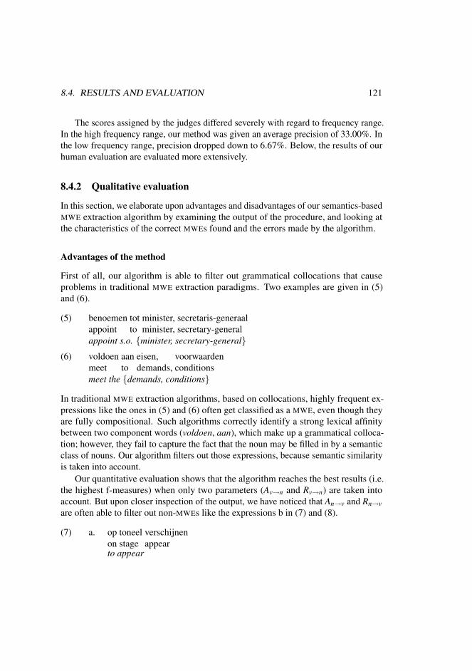
8.4. RESULTS AND EVALUATION 121
The scores assigned by the judges differed severely with regard to frequency range.In the high frequency range, our method was given an average precision of 33.00%. Inthe low frequency range, precision dropped down to 6.67%. Below, the results of ourhuman evaluation are evaluated more extensively.
8.4.2 Qualitative evaluation
In this section, we elaborate upon advantages and disadvantages of our semantics-basedMWE extraction algorithm by examining the output of the procedure, and looking atthe characteristics of the correct MWEs found and the errors made by the algorithm.
Advantages of the method
First of all, our algorithm is able to filter out grammatical collocations that causeproblems in traditional MWE extraction paradigms. Two examples are given in (5)and (6).
(5) benoemenappoint
totto
minister,minister,
secretaris-generaalsecretary-general
appoint s.o. {minister, secretary-general}(6) voldoen
meetaanto
eisen,demands,
voorwaardenconditions
meet the {demands, conditions}
In traditional MWE extraction algorithms, based on collocations, highly frequent ex-pressions like the ones in (5) and (6) often get classified as a MWE, even though theyare fully compositional. Such algorithms correctly identify a strong lexical affinitybetween two component words (voldoen, aan), which make up a grammatical colloca-tion; however, they fail to capture the fact that the noun may be filled in by a semanticclass of nouns. Our algorithm filters out those expressions, because semantic similarityis taken into account.
Our quantitative evaluation shows that the algorithm reaches the best results (i.e.the highest f-measures) when only two parameters (Av→n and Rv→n) are taken intoaccount. But upon closer inspection of the output, we have noticed that An→v and Rn→vare often able to filter out non-MWEs like the expressions b in (7) and (8).
(7) a. opon
toneelstage
verschijnenappear
to appear

122 CHAPTER 8.
b. opon
toneelstage
zingensing
to sing on the stage
(8) a. inin
geheugenmemory
liggenlie
be in memoryb. in
inziekenhuishospital
liggenlie
lie in the hospital
When only taking into account the first two measures (a unique preference of the verbfor the noun), the expressions in b do not get filtered out. It is only when the two othermeasures (a unique preference of the noun for the verb) are taken into account that theyare filtered out – either because the preference of the noun for the verb is very low, orthe noun preference for the verb is more evenly distributed among the cluster. The bexpressions, which are non-MWEs, result from the combination of a verb with a highlyfrequent PP. These PPs are typically locative, directional or predicative PPs, that maycombine with numerous verbs.
Also, expressions like the ones in (9), where the fixedness of the expression liesnot so much in the verb-noun combination, but more in the PP part (naar school, naarhuis) are filtered out by the latter two measures. These preposition-noun combinationsseem to be institutionalized PPs, so-called determinerless PPs (Baldwin et al., 2006).
(9) a. naarto
schoolschool
willenwant
want to go to schoolb. naar
tohuishome
willenwant
want to go home
Errors of the method
In this section, we give an exhaustive list of the errors made by our algorithm, andquantitatively evaluate the importance of each error category.
1. First of all, our algorithm highly depends on the quality of the noun clustering.If a noun appears in a cluster with unrelated words, the measures will overratethe semantic uniqueness of the expressions in which the noun appears.
2. Syntax might play an important role. Sometimes, there are syntactic restrictionsbetween the preposition and the noun. A noun like pagina ‘page’ can only

8.4. RESULTS AND EVALUATION 123
appear with the preposition op ‘on’, as in lees op pagina ‘read on page’. Other,semantically related nouns, such as hoofdstuk ‘chapter’, prefer in ‘in’. Due tothese restrictions, the measures will again overrate the semantic uniqueness ofthe expression.
3. We found many expressions in which the fixedness of the expression lies notso much in the combination of the verb and the prepositional phrase, but ratherin the prepositional phrase itself (naar school, naar huis). Note, however, thatour two latter measures were able to filter out many of those expressions (asexplained above). But in our error evaluation, we used the result that yields thehighest f-measure (and does not take the latter measures into account).
4. Our hard clustering method does not take polysemous nouns into account. Anoun can only occur in one cluster, ignoring other possible meanings. Schaal,for example, means ‘dish’ as well as ‘scale’. In our clustering, it only appearsin a cluster of dish-related nouns. Therefore, expressions like maak gebruik op[grote] schaal ‘make use of [sth.] on a [large] scale’, receive again overratedmeasures of semantic uniqueness, because the ‘scale’ sense of the noun iscompared to nouns related to the ‘dish’ sense.
5. Related to the previous error category is the fact that certain nouns – althoughoccurring in a perfectly sound cluster – possess a semantic feature or charac-teristic that distinguishes them from the other nouns in the cluster, and causesthe verb to uniquely prefer that particular noun. An example of this kind oferror is the expression eet in restaurant ‘eat in a restaurant’, which is perfectlycompositional. But due to the fact that the noun restaurant ends up in a clusterwith nouns such as bar ‘bar’, cafe ‘bar’, kroeg ‘pub’, winkel ‘shop’, hotel ‘hotel’– which are places where one is less likely to eat – the fixedness of the expressionis overestimated.
6. The effectiveness of our method is highly dependent on the corpus distribution.Sometimes, expressions that would be effective counterweights for the erroneousclassification of compositional expressions as MWE just are not found in thecorpus. This might be either due to sparseness of the data, or due to the specificnature of the corpus itself. Examples are sluit wegens verbouwing ‘close due toalteration’, with cluster members such as restauratie ‘restoration’ and renovatie‘renovation’, and uit van emotie ‘express emotion’, with cluster members such asagressie ‘agression’, irritatie ‘irritation’, ongeduld ‘impatience’. Expressionssuch as sluit wegens renovatie or uit van irritatie are perfectly possible, but arenot (sufficiently) attested in the corpus. Therefore, the compositional formswhich are attested in the corpus are overestimated as MWE.

124 CHAPTER 8.
7. Finally, misclassifications may be caused by parsing errors or other technicalissues.
In order to get a better view of the errors of the method, we manually classifiedthe expressions that were evaluated as non-MWE by our judges. Each expression wasassigned to one of the error categories described above. Overall results, and results forhigh and low frequency expressions are given.
overall (%) high freq. (%) low freq. (%)
1 erroneous clustering 3.6 3.8 3.42 specific preposition 6.4 15.4 1.13 PP fixedness 26.4 21.2 29.54 polysemous word 15.7 13.5 17.05 specific semantic feature 22.9 30.8 18.26 corpus distribution 21.4 13.5 26.17 parsing/other 3.6 1.9 4.5
Table 8.4: Quantitative error evaluation
Misclassifications due to erroneous clustering or parsing errors only constitute asmall part of the errors. Also, misclassifications due to syntactic restrictions (specificprepositions) are responsible for only a small part of the errors. More important aremisclassifications due to fixedness in the PP, or due to polysemy or specific semanticfeatures of the nouns. The former might be remedied by a more effective use of ourmeasures An→v and Rn→v, the latter by taking on a soft clustering approach. Finally,there are quite some errors due to the specific distribution of MWEs in the corpus. Theseerrors are more common in the low frequency range. Clearly, our method is highlydependent on the corpus that is used, and it should be sufficiently large in order toadequately classify less frequent MWEs.
MWE fuzziness
A last observation to mention is that the status of certain expressions extracted withour method is unclear. Expressions such as vraag met klem ‘ask with emphasis’ or gaover tot orde [van de dag] ‘pass to the order [of the day]’ seem to be on the borderof compositionality vs. non-compositionality, and therefore cannot be adequatelyqualified as MWE or non-MWE. This observation is confirmed by the conflicting viewsthe three judges showed when assessing these kind of expressions.

8.5. CONCLUSIONS AND FURTHER WORK 125
8.5 Conclusions and further work
Our algorithm based on non-compositionality explores a new approach aimed at large-scale MWE extraction. Using only two parameters, Av→n and Rv→n, yields the highestf-measure. Using the two other parameters, An→v and Rn→v, increases precision butdegrades recall. Due to the formalization of the intuition of non-compositionality (usingan automatic noun clustering), our algorithm is able to rule out various expressions thatare coined MWEs by traditional algorithms.
Note that our algorithm has taken on a purely semantics-based approach. ‘Syntacticfixedness’ of the expressions is not taken into account. Combining our semantics-basedapproach with other MWE extraction methods that take into account different featuresmight improve the results significantly.
We believe that our method provides a genuine and successful approach to get agrasp of the non-compositionality of MWEs in a fully automated way. We also believethat it is one of the first methods able to extract MWEs based on non-compositionalityon a large scale, and that traditional MWE extraction algorithms will benefit from takingthis non-compositionality into account.


Chapter 9
Noun Sense Discrimination1
9.1 Introduction
The computation of semantic similarity relies on the distributional hypothesis (Har-ris, 1985), which states that words that occur in similar contexts tend to be similar. Inchapter 1, we have seen that there are three different definitions of the notion context: adocument-based context, a window-based context, and a syntax-based context. The firstapproach takes the documents in which the word appears as features. The documentcontext might be the sentence, paragraph or actual document that a word appears in.One of the dominant methods using this method is LATENT SEMANTIC ANALYSIS(LSA). The second approach makes use of the bag of words co-occurrence data; inthis approach, a certain window around a word is used for gathering co-occurrenceinformation. The window may either be a fixed number of words, or the paragraph ordocument that a word appears in. Thus, words are considered similar if they appearin similar windows. The document-based approach is very much related to the bagof words approach. The third approach uses a more fine grained distributional model,focusing on the syntactic relations in which words appear. Typically, a large text corpusis parsed, and dependency triples are extracted.2 Words are considered similar if theyappear in similar syntactic relations. Note that the former approach does not need anykind of linguistic annotation, whereas for the latter, some form of syntactic annotationis needed.
1The research presented in this chapter has been published as Van de Cruys (2007) and Van deCruys (2008c).
2e.g. dependency relations that qualify apple might be ‘object of eat’ and ‘adjective red’. This gives usdependency triples like < apple,ob j,eat >.
127

128 CHAPTER 9.
In this chapter, we will combine the window-based approach with the syntax-based approach. The results yielded by these two approaches are typically quitedifferent in nature: the first approach typically puts its finger on a broad, thematickind of similarity,3 while the latter typically grasps a tighter, synonym-like similarity.Example (1) shows the difference between the two kinds of similarity; for each kind,the top ten most similar nouns to the Dutch noun muziek ‘music’ are given. In (a), thewindow-based approach is used, while (b) uses the syntax-based approach. (a) showsindeed more thematic similarity, whereas (b) shows tighter similarity.
(1) a. muziek ‘music’: gitaar ‘guitar’, jazz ‘jazz’, cd ‘cd’, rock ‘rock’, bas‘bass’, song ‘song’, muzikant ‘musician’, musicus ‘musician’, drum‘drum’, slagwerker ‘drummer’
b. muziek ‘music’: dans ‘dance’, kunst ‘art’, klank ‘sound’, liedje ‘song’,geluid ‘sound’, poezie ‘poetry’, literatuur ‘literature’, popmuziek ‘popmusic’, lied ‘song’, melodie ‘melody’
Especially the syntax-based method has been adopted by many researchers in orderto find semantically similar words. There is, however, one important problem withthis kind of approach: the method is not able to cope with ambiguous words. Take theexamples:
(2) eena
onevenodd
nummernumber
an odd number
(3) eena
steengoedgreat
nummernumber
‘a great song’
The word nummer does not have the same meaning in these examples. In ex-ample (2), nummer is used in the sense of ‘designator of quantity’. In example (3), itis used in the sense of ‘musical performance’. Accordingly, we would like the wordnummer to be disambiguated into two senses, the first sense being similar to words likegetal ‘number’, cijfer ‘digit’ and the second to words like liedje ‘song’, song ‘song’.
While it is relatively easy for a human language user to distinguish between thetwo senses, this is a difficult task for a computer. Even worse: the results get blurredbecause the attributes of both senses (in this example oneven and steengoed) aregrouped together into one sense. This is the main drawback of the syntax-basedmethod. On the other hand, methods that capture semantic dimensions are known to
3This is true in particular when using a large context window, cfr. chapter 7.
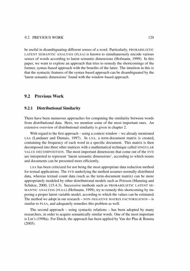
9.2. PREVIOUS WORK 129
be useful in disambiguating different senses of a word. Particularly, PROBABILISTICLATENT SEMANTIC ANALYSIS (PLSA) is known to simultaneously encode varioussenses of words according to latent semantic dimensions (Hofmann, 1999). In thispaper, we want to explore an approach that tries to remedy the shortcomings of theformer, syntax-based approach with the benefits of the latter. The intuition in this isthat the syntactic features of the syntax-based approach can be disambiguated by the‘latent semantic dimensions’ found with the window-based approach.
9.2 Previous Work
9.2.1 Distributional Similarity
There have been numerous approaches for computing the similarity between wordsfrom distributional data. Here, we mention some of the most important ones. Anextensive overview of distributional similarity is given in chapter 2.
With regard to the first approach – using a context window – we already mentionedLSA (Landauer and Dumais, 1997). In LSA, a term-document matrix is created,containing the frequency of each word in a specific document. This matrix is thendecomposed into three other matrices with a mathematical technique called SINGULARVALUE DECOMPOSITION. The most important dimensions that come out of the SVDare interpreted to represent ‘latent semantic dimensions’, according to which nounsand documents can be presented more efficiently.
LSA has been criticized for not being the most appropriate data reduction methodfor textual applications. The SVD underlying the method assumes normally-distributeddata, whereas textual count data (such as the term-document matrix) can be moreappropriately modeled by other distributional models such as Poisson (Manning andSchutze, 2000, §15.4.3). Successive methods such as PROBABILISTIC LATENT SE-MANTIC ANALYSIS (PLSA) (Hofmann, 1999), try to remedy this shortcoming by im-posing a proper latent variable model, according to which the values can be estimated.The method we adopt in our research – NON-NEGATIVE MATRIX FACTORIZATION – issimilar to PLSA, and adequately remedies this problem as well.
The second approach – using syntactic relations – has been adopted by manyresearchers, in order to acquire semantically similar words. One of the most importantis Lin’s (1998a). For Dutch, the approach has been applied by Van der Plas & Bouma(2005).

130 CHAPTER 9.
9.2.2 Discriminating senses
Schutze (1998) uses a disambiguation algorithm – called context-group discrimination– based on the clustering of the context of ambiguous words. The clustering is basedon second-order co-occurrence: the contexts of the ambiguous word are similar if thewords they in turn co-occur with are similar.
Pantel and Lin (2002) present a clustering algorithm – coined CLUSTERING BYCOMMITTEE (CBC) – that automatically discovers word senses from text. The key ideais to first discover a set of tight, unambiguous clusters, to which possibly ambiguouswords can be assigned. Once a word has been assigned to a cluster, the featuresassociated with that particular cluster are stripped off the word’s vector. This way, lessfrequent senses of the word can be discovered.
The former approach uses a window-based method; the latter uses syntactic data.But none of the algorithms developed so far have combined both sources in order todiscriminate among different senses of a word.
9.3 Methodology
9.3.1 Non-negative Matrix Factorization
In this framework, we will adopt non-negative matrix factorization (NMF) (Lee andSeung, 2000) as a dimensionality reduction algorithm. In NMF, a matrix V is factorizedinto two other matrices, W and H, with r� n,m.
Vn×m ≈Wn×rHr×m (9.1)
An extensive overview of NMF and its computational details is given in section 3.3 onpage 42.
In this framework, we will adopt the NMF algorithm that minimizes the Kullback-Leibler divergence as objective function. In our experience, entropy-based measurestend to work well for natural language. Thus, we want to find the matrices W and Hfor which the Kullback-Leibler divergence between V and WH (the matrix product ofW and H) is the smallest.
We can now straightforwardly apply NMF to create semantic word models. NMFis applied to a frequency matrix, containing bags of words co-occurrence data. Theadditive property of NMF ensures that semantic dimensions emerge according to whichthe various words can be classified. Two sample dimensions are shown in example (4).For each dimension, the words with the largest value on that dimension are given.Dimension (a) can be qualified as a ‘transport’ dimension, and dimension (b) as a‘cooking’ dimension.

9.3. METHODOLOGY 131
(4) a. bus ‘bus’, taxi ‘taxi’, trein ‘train’, halte ‘stop’, reiziger ‘traveler’, perron‘platform’, tram ‘tram’, station ‘station’, chauffeur ‘driver’, passagier‘passenger’
b. bouillon ‘broth’, slagroom ‘cream’, ui ‘onion’, eierdooier ‘egg yolk’,laurierblad ‘bay leaf’, zout ‘salt’, deciliter ‘decilitre’, boter ‘butter’, bleek-selderij ‘celery’, saus ‘sauce’
9.3.2 Extending Non-negative Matrix Factorization
We now propose an extension of NMF that combines both the bag of words approachand the syntactic approach. The algorithm finds again latent semantic dimensions,according to which nouns, bag of words contexts and syntactic relations are classified.
Since we are interested in the classification of nouns according to both ‘bag-of-words’ context and syntactic context, we first construct three matrices that capturethe co-occurrence frequency information for each mode. The first matrix contains co-occurrence frequencies of nouns cross-classified by dependency relations, the secondmatrix contains co-occurrence frequencies of nouns cross-classified by words thatappear in the noun’s context window, and the third matrix contains co-occurrencefrequencies of dependency relations cross-classified by co-occurring context words.
We then apply NMF to the three matrices, but we interleave the separate factoriza-tions: the result of the preceding factorization is used to initialize the factorization ofthe next matrix. This implies that we need to initialize only three matrices at random;the other three are initialized by calculations of the previous step. The process isrepresented graphically in figure 9.1.
In the example in figure 9.1, matrix H is initialized at random, and the update ofmatrix W is calculated. The result of update W is then used to initialize matrix V , andthe update of matrix G is calculated. This matrix is used again to initialize matrix U ,and the update of matrix F is calculated. This matrix can be used to initialize matrixH, and the process is repeated until convergence.
In (5), an example is given of the kind of semantic dimensions found. Thisdimension may be coined the ‘transport’ dimension, as is shown by the top 10 nouns(a), context words (b) and syntactic relations (c).
(5) a. auto ‘car’, wagen ‘car’, tram ‘tram’, motor ‘motorbike’, bus ‘bus’, metro ‘subway’, auto-mobilist ‘driver’, trein ‘trein’, stuur ‘steering wheel’, chauffeur ‘driver’
b. auto ‘car’, trein ‘train’, motor ‘motorbike’, bus ‘bus’, rij ‘drive’, chauffeur ‘driver’, fiets‘bike’, reiziger ‘reiziger’, passagier ‘passenger’, vervoer ‘transport’
c. viertrapsad j ‘four-stage’, verplaats metob j ‘move with’, toeterad j ‘honk’, tank in houdob j[parsing error], tanksub j ‘refuel’, tankob j ‘refuel’, rij voorbijsub j ‘pass by’, rij voorbijad j ‘passby’, rij afsub j ‘drive off’, peperduurad j ‘very expensive’

132 CHAPTER 9.
Figure 9.1: A graphical representation of the extended NMF
9.3.3 Sense Subtraction
Next, we want to use the factorization that has been created in the former step forword sense discrimination. The intuition is that we ‘switch off’ one dimension of anambiguous word, to reveal possible other senses of the word. From matrix H, we knowthe importance of each syntactic relation given a dimension. With this knowledge, wecan ‘subtract’ the syntactic relations that are responsible for a certain dimension fromthe original noun vector:
−→v new =−→v orig(−→v1 −−→h dim) (9.2)
Equation 9.2 is an element-wise multiplication that multiplies each feature (syn-tactic relation) of the original noun vector (−→v orig) with a scaling factor, according tothe load of the feature on the subtracted dimension (
−→h dim – the vector of matrix H
containing the dimension we want to subtract). −→v1 is a vector of ones, the size of−→h dim.
9.3.4 A Clustering Framework
The last step is to determine which dimension(s) are responsible for a certain sense ofthe word. In order to do so, we embed our method in a clustering approach. First, aspecific word is assigned to its predominant sense (i.e. the most similar cluster). Next,

9.3. METHODOLOGY 133
the dominant semantic dimension(s) for this cluster are subtracted from the word vector(equation 9.2), and the resulting vector is fed to the clustering algorithm again, to seeif other word senses emerge. The dominant semantic dimension(s) can be identifiedby ‘folding in’ the cluster centroid into our factorization (so we get a vector −→w ofdimension size r), and applying a threshold to the result (in our experiments a thresholdof δ = .05 — so dimensions responsible for > 5% of the centroid are subtracted).
We used two kinds of clustering algorithms to determine our initial centroids. Thefirst algorithm is a standard K-means algorithm. The second one is the CBC algorithmby Pantel and Lin (2002). The initial vectors to be clustered are weighted usingpointwise mutual information (Church and Hanks, 1990).
K-means
First, a standard K-means algorithm is applied to the nouns we want to cluster. Thisyields a hard clustering, in which each noun is assigned to exactly one (dominant)cluster. In the second step, we try to determine for each noun whether it can beassigned to other, less dominant clusters. First, the salient dimension(s) of the centroidto which the noun is assigned are determined. We compute the centroid of the clusterby averaging the frequencies of all cluster elements except for the target element wewant to reassign, and adapt the centroid with pointwise mutual information. Aftersubtracting the salient dimensions from the noun vector, we check whether the vectoris reassigned to another cluster centroid (i.e. whether it is more similar to a differentcentroid). If this is the case, (another instance of) the noun is assigned to the cluster,and we repeat the second step. If there is no reassignment, we continue with the nextword. The target element is removed from the centroid to make sure that we onlysubtract the dimensions associated with the sense of the cluster.
Note that K-means requires setting the number of clusters beforehand, so k is aparameter to be set.
CBC
The second clustering algorithm operates in a similar vein, but instead of using simpleK-means, we use Pantel and Lin’s CBC algorithm to find the initial centroids (coinedCOMMITTEES).
In order to find committees, the top k nouns for each noun in the database areclustered with average-link clustering. The clusters are scored and sorted in such a waythat preference is given to tight, representative clusters. If the committees do not coverall elements sufficiently, the algorithm recursively tries to find more committees. Anelaborate description of the algorithm can be found in Pantel and Lin (2002).

134 CHAPTER 9.
In the second step, we start assigning elements to committees. Once an elementis assigned, the salient dimensions are subtracted from the noun vector in the sameway as in 9.3.4 (only do we not have to remove any target word from the centroid;committees are supposed to represent tight, unambiguous clusters).
CBC attempts to find the number of committees automatically from the data, so kdoes not have to be set.
9.4 Examples
9.4.1 Sense Subtraction
In what follows, we will talk about semantic dimensions as, e.g., the ‘music’ dimensionor the ‘city’ dimension. In the vast majority of the cases, the dimensions are indeedas clear-cut as the transport dimension shown above, so that the dimensions can berightfully labeled this way.
Two examples are given of how the semantic dimensions that have been found canbe used for word sense discrimination. We will consider two ambiguous nouns: pop,which can mean ‘pop music’ as well as ‘doll’, and Barcelona, which can designateeither the Spanish city or the Spanish football club.
First, we look up the top dimensions for each noun. Next, we successively subtractthe dimensions dealing with a particular sense of the noun, as described in 9.3.3. Thisgives us three vectors for each noun: the original vector, and two vectors with one ofthe dimensions eliminated. For each of these vectors, the top ten similar nouns aregiven, in order to compare the changes brought about.
(6) a. pop, rock, jazz, meubilair ‘furniture’, popmuziek ‘pop music’, heks ‘witch’, speelgoed ‘toy’,kast ‘cupboard’, servies ‘[tea] service’, vraagteken ‘question mark’
b. pop, meubilair ‘furniture’, speelgoed ‘toy’, kast ‘cupboard’, servies ‘[tea] service’, heks‘witch’, vraagteken ‘question mark’ sieraad ‘jewel’, sculptuur ‘sculpture’, schoen ‘shoe’
c. pop, rock, jazz, popmuziek ‘pop music’, heks ‘witch’, danseres ‘dancer’, servies ‘[tea] service’,kopje ‘cup’, house ‘house music’, aap ‘monkey’
Example (6) shows the top similar words for the three vectors of pop. In (a),the most similar words to the original vector are shown. In (b), the top dimension(the ‘music dimension’) has been subtracted from (a), and in (c), the second highestdimension (a ‘domestic items’ dimension) has been subtracted from (a).
The differences between the three vectors are clear: in vector (a), both senses aremixed together, with ‘pop music’ and ‘doll’ items interleaved. In (b), no more musicitems are present. Only items related to the doll sense are among the top similar words.In (c), the music sense emerges much more clearly, with rock, jazz and popmuziekbeing the most similar, and a new music term (house) showing up among the top ten.

9.4. EXAMPLES 135
Admittedly, in vector (c), not all items related to the ‘doll’ sense are filtered out.We believe this is due to the fact that this sense cannot be adequately filtered out by onedimension (in this case, a dimension of ‘domestic items’ alone), whereas it is mucheasier to filter out the ‘music’ sense with only one ‘music’ dimension. We will try toremedy this in our clustering framework, in which it is possible to subtract multipledimensions related to one sense.
A second example, the ambiguous proper name Barcelona, is given in (7).
(7) a. Barcelona, Arsenal, Inter, Juventus, Vitesse, Milaan ‘Milan’, Madrid, Parijs ‘Paris’, Wenen‘Vienna’, Munchen ‘Munich’
b. Barcelona, Milaan ‘Milan’, Munchen ‘Munich’, Wenen ‘Vienna’, Madrid, Parijs ‘Paris’,Bonn, Praag ‘Prague’, Berlijn ‘Berlin’, Londen ‘London’
c. Barcelona, Arsenal, Inter, Juventus, Vitesse, Parma, Anderlecht, PSV, Feyenoord, Ajax
In (a), the two senses of Barcelona are clearly mixed up, showing cities as well asfootball clubs among the most similar nouns. In (b), where the ‘football dimension’has been subtracted, only cities show up. In (c), where the ‘city dimension’ has beensubtracted, only football clubs remain.
9.4.2 Clustering Output
In (8), an example of our clustering algorithm with initial K-means clusters is given.
(8) a. werk ‘work’ beeld ‘image’ foto ‘photo’ schilderij ‘painting’ tekening ‘drawing’ doek ‘canvas’installatie ‘installation’ afbeelding ‘picture’ sculptuur ‘sculpture’ prent ‘picture’ illustratie‘illustration’ handschrift ‘manuscript’ grafiek ‘print’ aquarel ‘aquarelle’ maquette ‘scale-model’ collage ‘collage’ ets ‘etching’
b. werk ‘work’ boek ‘book’ titel ‘title’ roman ‘novel’ boekje ‘booklet’ debuut ‘debut’ biografie‘biography’ bundel ‘collection’ toneelstuk ‘play’ bestseller ‘bestseller’ kinderboek ‘childbook’ autobiografie ‘autobiography’ novelle ‘short story’
c. werk ‘work’ voorziening ‘service’ arbeid ‘labour’ opvoeding ‘education’ kinderopvang ‘childcare’ scholing ‘education’ huisvesting ‘housing’ faciliteit ‘facility’ accommodatie ‘acommod-ation’ arbeidsomstandigheid ‘working condition’
The example shows three different clusters to which the noun werk ‘work’ isassigned. In (a), werk refers to a work of art. In (b), it refers to a written work. In (c),the ‘labour’ sense of werk emerges.

136 CHAPTER 9.
9.5 Evaluation
9.5.1 Methodology
The clustering results have been evaluated according to Dutch EuroWordNet (Vossen, 1998).Precision and recall are calculated by comparing the results to EuroWordNet synsets.The precision is the number of clusters found that correspond to an actual sense ofthe word. Recall is the number of word senses in EuroWordNet that are found by thealgorithm. Our evaluation method is largely the same as the one used by Pantel andLin (2002).
Both precision and recall are based on wordnet similarity. A number of similaritymeasures have been developed to calculate semantic similarity in a hierarchical wordnet.Two of those measures – Wu & Palmer’s and Lin’s – have been presented earlierin chapter 5. In this evaluation, Wu & Palmer’s (1994) measure will be adopted.A detailed description of this Wu & Palmer’s similarity measure can be found insection 5.3.2 on page 61.
To calculate precision, we apply the same methodology as Pantel and Lin (2002).4
Let S(w) be the set of EuroWordNet senses. simW (s,u), the similarity between a synsets and a word u is then defined as the maximum similarity between s and a sense of u:
simW (s,u) = maxtεS(u)
sim(s, t) (9.3)
Let ck be the top k-members of a cluster c, where these are the k most similar membersto the centroid of c. simC(c,s), the similarity between s and c, is then defined as theaverage similarity between s and the top-k members of c:
simC(s,c) =∑
uεck
simW (s,u)
k(9.4)
An assigment of a word w to a cluster c can now be classified as correct if
maxsεS(w)
simC(s,c) > θ (9.5)
and the EuroWordNet sense of w that corresponds to c is
argmaxsεS(w)
simC(s,c) (9.6)
4Note, however, that our similarity measure is different. Where Pantel and Lin use Lin’s (1998a)measure, we use Wu and Palmer’s (1994) measure.
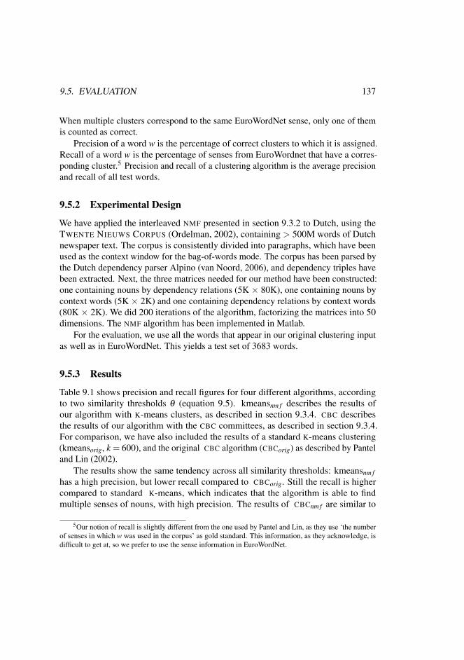
9.5. EVALUATION 137
When multiple clusters correspond to the same EuroWordNet sense, only one of themis counted as correct.
Precision of a word w is the percentage of correct clusters to which it is assigned.Recall of a word w is the percentage of senses from EuroWordnet that have a corres-ponding cluster.5 Precision and recall of a clustering algorithm is the average precisionand recall of all test words.
9.5.2 Experimental Design
We have applied the interleaved NMF presented in section 9.3.2 to Dutch, using theTWENTE NIEUWS CORPUS (Ordelman, 2002), containing > 500M words of Dutchnewspaper text. The corpus is consistently divided into paragraphs, which have beenused as the context window for the bag-of-words mode. The corpus has been parsed bythe Dutch dependency parser Alpino (van Noord, 2006), and dependency triples havebeen extracted. Next, the three matrices needed for our method have been constructed:one containing nouns by dependency relations (5K × 80K), one containing nouns bycontext words (5K × 2K) and one containing dependency relations by context words(80K × 2K). We did 200 iterations of the algorithm, factorizing the matrices into 50dimensions. The NMF algorithm has been implemented in Matlab.
For the evaluation, we use all the words that appear in our original clustering inputas well as in EuroWordNet. This yields a test set of 3683 words.
9.5.3 Results
Table 9.1 shows precision and recall figures for four different algorithms, accordingto two similarity thresholds θ (equation 9.5). kmeansnm f describes the results ofour algorithm with K-means clusters, as described in section 9.3.4. CBC describesthe results of our algorithm with the CBC committees, as described in section 9.3.4.For comparison, we have also included the results of a standard K-means clustering(kmeansorig, k = 600), and the original CBC algorithm (CBCorig) as described by Panteland Lin (2002).
The results show the same tendency across all similarity thresholds: kmeansnm fhas a high precision, but lower recall compared to CBCorig. Still the recall is highercompared to standard K-means, which indicates that the algorithm is able to findmultiple senses of nouns, with high precision. The results of CBCnm f are similar to
5Our notion of recall is slightly different from the one used by Pantel and Lin, as they use ‘the numberof senses in which w was used in the corpus’ as gold standard. This information, as they acknowledge, isdifficult to get at, so we prefer to use the sense information in EuroWordNet.

138 CHAPTER 9.
threshold θ
.40 (%) .60 (%)
kmeansnm f prec. 78.97 55.16rec. 63.90 44.77
CBCnm f prec. 82.70 54.87rec. 60.27 40.51
kmeansorig prec. 86.13 58.97rec. 60.23 41.80
CBCorig prec. 44.94 29.74rec. 69.61 48.00
Table 9.1: Precision and recall percentages for four different algorithms according totwo similarity thresholds
the results of kmeansorig, indicating that few words are reassigned to multiple clusterswhen using CBC committees with our method.
Obviously, kmeansorig scores best with regard to precision, but worst with regard torecall. CBCorig finds most senses (highest recall), but precision is considerably worse.
The fact that recall is already quite high with standard K-means clustering indicatesthat the evaluation is skewed towards nouns with only one sense, possibly due to alack of coverage in EuroWordNet. In future work, we specifically want to evaluatethe discrimination of ambiguous words. Also, we want to make use of the newCornetto Database6, a successor of EuroWordNet for Dutch which is currently underdevelopment.
Still, the evaluation shows that our method provides a genuine way of findingmultiple senses of words, while retaining high precision. Especially the method usinga simple K-means clustering performs particularly well. The three way data allows thealgorithm to put its finger on the particular sense of a centroid, and adapt the featurevector of a possibly ambiguous noun accordingly.
6http://www.let.vu.nl/onderzoek/projectsites/cornetto/index.html

9.6. CONCLUSION & FUTURE WORK 139
9.6 Conclusion & Future Work
In this paper, an extension of NMF has been presented that combines both bag of wordsdata and syntactic data in order to find latent semantic dimensions according to whichboth words and syntactic relations can be classified. The use of three-way data allowsone to determine which dimension(s) are responsible for a certain sense of a word, andadapt the corresponding feature vector accordingly, ‘subtracting’ one sense to discoveranother one. When embedded in a clustering framework, the method provides a fullyautomatic way to discriminate the various senses of words. The evaluation againstEuroWordNet shows that the algorithm is genuinely able to disambiguate the featuresof a given word, and accordingly its word senses.
We conclude with some issues for future work. First of all, we would like to testthe method that has been explored in this paper with other evaluation frameworks. Wealready mentioned the focus on ambiguous nouns, and the use of the new Cornettodatabase for Dutch. Next, we would like to work out a proper probabilistic frameworkfor the ‘subtraction’ of dimensions. At this moment, the subtraction (using a cut-off) is somewhat ad hoc. A probabilistic modeling of this intuition might lead to animprovement.
And finally, we would like to use the results of our method to learn selectionalpreferences. Our method is able to discriminate the syntactic features that are linked toa particular word sense. If we can use the results to improve a parser’s performance,this will also provide an external evaluation of the algorithm.


Chapter 10
Selectional Preferences1
10.1 Introduction
Distributional similarity methods have proven to be a valuable tool for the inductionof semantic similarity. The aggregate of a word’s contexts generally provides enoughinformation to compute its meaning, viz. its semantic similarity or relatedness to otherwords.
Up till now, most algorithms use two-way co-occurrence data to compute themeaning of words. A word’s meaning might for example be computed by looking at:
• the various documents that the word appears in (words × documents);
• a bag of words context window around the word (words × context words);
• the dependency relations that the word appears with (words × dependencyrelations).
The extracted data – representing the co-occurrence frequencies of two differententities – is encoded in a matrix. Co-occurrence frequencies, however, need not bepairwise. One can easily imagine situations where it is desirable to investigate co-occurrence frequencies of three modes and beyond. In an information retrieval context,one such situation might be the investigation of words × documents × authors. In anNLP context, one might want to investigate words × dependency relations × bag ofword context words, or verbs × subjects × direct objects.
1The research presented in this chapter has been published as Van de Cruys (2009).
141

142 CHAPTER 10.
Note that it is not possible to investigate the three-way co-occurrences in a matrixrepresentation form. It is possible to capture the co-occurrence frequencies of averb with its subjects and its direct objects, but one cannot capture the co-occurrencefrequencies of the verb appearing with the subject and the direct object at the same time.When the actual three-way co-occurrence data is ‘matricized’, valuable information isthrown-away. To be able to capture the mutual dependencies among the three modes,we will make use of a generalized tensor representation.
Two-way co-occurrence models (such as latent semantic analysis) have often beenaugmented with some form of dimensionality reduction in order to counter noiseand overcome data sparseness. We will also make use of a dimensionality reductionalgorithm appropriate for tensor representations.
10.2 Previous Work
10.2.1 Selectional Preferences & Verb Clustering
Selectional preferences have been a popular research subject in the NLP community.One of the first to automatically induce selectional preferences from corpora wasResnik Resnik (1996). Resnik generalizes among nouns by using WordNet nounsynsets as clusters. He then calculates the selectional preference strength of a specificverb in a particular relation by computing the Kullback-Leibler divergence between thecluster distribution of the verb and the aggregate cluster distribution:
Sv = ∑c
p(c | v) logp(c | v)
p(c)(10.1)
The selectional association is then the contribution of a particular cluster to the verb’spreference strength:
Av,c =p(c | v) log p(c|v)
p(c)
Sv(10.2)
The model’s generalization relies entirely on WordNet; there is no generalizationamong the verbs.2
The research in this paper is related to previous work on clustering. Pereira etal. (1993) use an information-theoretic based clustering approach, clustering nounsaccording to their distribution as direct objects among verbs, conditioned on a set oflatent semantic classes.
2Other notable approaches using WordNet for selectional preference induction are Abe and Li’s (1996)and Clark and Weir’s (2001).
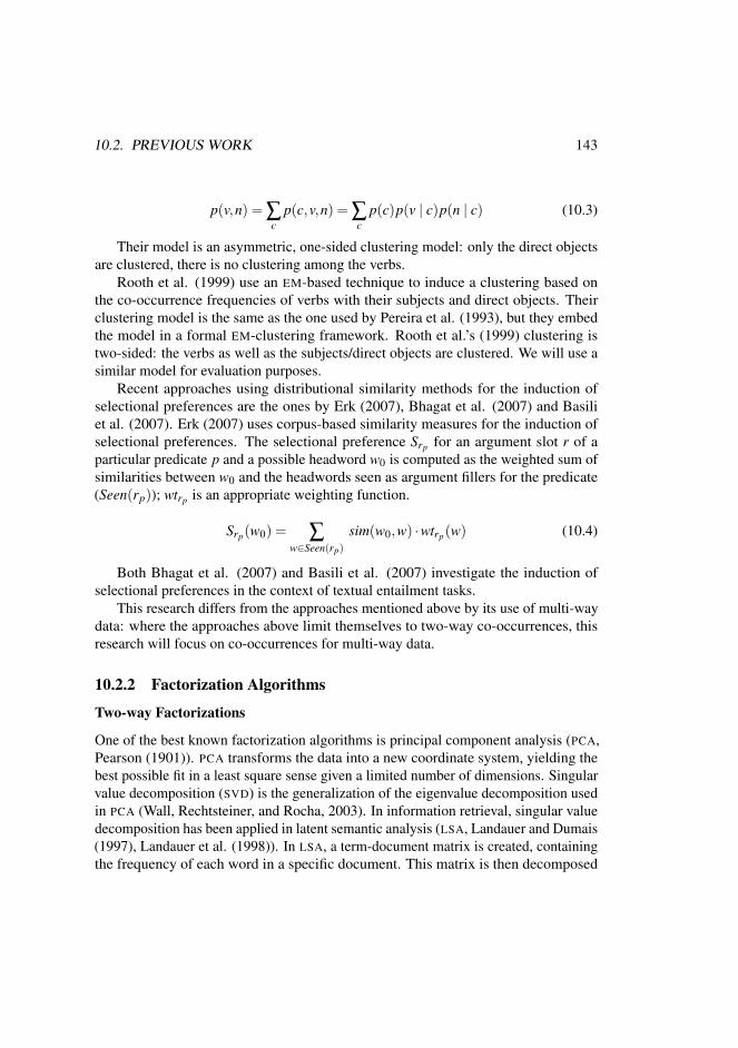
10.2. PREVIOUS WORK 143
p(v,n) = ∑c
p(c,v,n) = ∑c
p(c)p(v | c)p(n | c) (10.3)
Their model is an asymmetric, one-sided clustering model: only the direct objectsare clustered, there is no clustering among the verbs.
Rooth et al. (1999) use an EM-based technique to induce a clustering based onthe co-occurrence frequencies of verbs with their subjects and direct objects. Theirclustering model is the same as the one used by Pereira et al. (1993), but they embedthe model in a formal EM-clustering framework. Rooth et al.’s (1999) clustering istwo-sided: the verbs as well as the subjects/direct objects are clustered. We will use asimilar model for evaluation purposes.
Recent approaches using distributional similarity methods for the induction ofselectional preferences are the ones by Erk (2007), Bhagat et al. (2007) and Basiliet al. (2007). Erk (2007) uses corpus-based similarity measures for the induction ofselectional preferences. The selectional preference Srp for an argument slot r of aparticular predicate p and a possible headword w0 is computed as the weighted sum ofsimilarities between w0 and the headwords seen as argument fillers for the predicate(Seen(rp)); wtrp is an appropriate weighting function.
Srp(w0) = ∑w∈Seen(rp)
sim(w0,w) ·wtrp(w) (10.4)
Both Bhagat et al. (2007) and Basili et al. (2007) investigate the induction ofselectional preferences in the context of textual entailment tasks.
This research differs from the approaches mentioned above by its use of multi-waydata: where the approaches above limit themselves to two-way co-occurrences, thisresearch will focus on co-occurrences for multi-way data.
10.2.2 Factorization Algorithms
Two-way Factorizations
One of the best known factorization algorithms is principal component analysis (PCA,Pearson (1901)). PCA transforms the data into a new coordinate system, yielding thebest possible fit in a least square sense given a limited number of dimensions. Singularvalue decomposition (SVD) is the generalization of the eigenvalue decomposition usedin PCA (Wall, Rechtsteiner, and Rocha, 2003). In information retrieval, singular valuedecomposition has been applied in latent semantic analysis (LSA, Landauer and Dumais(1997), Landauer et al. (1998)). In LSA, a term-document matrix is created, containingthe frequency of each word in a specific document. This matrix is then decomposed

144 CHAPTER 10.
into three other matrices with SVD. The most important dimensions that come out ofthe SVD allegedly represent ‘latent semantic dimensions’, according to which nounsand documents can be represented more efficiently.
LSA has been criticized for a number of reasons, one of them being the fact that thefactorization contains negative numbers. It is not clear what negativity on a semanticscale should designate. Subsequent methods such as probabilistic latent semanticanalysis (PLSA, Hofmann (1999)) and non-negative matrix factorization (NMF, Lee andSeung (2000)) remedy these problems, and indeed get much more clear-cut semanticdimensions.
Three-way Factorizations
To be able to cope with three-way data, several algorithms have been developed as mul-tilinear generalizations of the SVD. In statistics, three-way component analysis has beenextensively investigated (for an overview, see Kiers and van Mechelen (2001)). The twomost popular methods are parallel factor analysis (PARAFAC, Harshman (1970), Carrolland Chang (1970)) and three-mode principal component analysis (3MPCA, Tucker(1966)), also called higher order singular value decomposition (HOSVD, De Lathauweret al. (2000)). Three-way factorizations have been applied in various domains, such aspsychometry and image recognition (Vasilescu and Terzopoulos, 2002). In informationretrieval, three-way factorizations have been applied to the problem of link analysis(Kolda and Bader, 2006).
One last important method dealing with multi-way data is non-negative tensorfactorization (NTF, Shashua and Hazan (2005)). NTF is a generalization of non-negativematrix factorization, and can be considered an extension of the PARAFAC model withthe constraint of non-negativity (cfr. infra).
One of the few papers that has investigated the application of tensor factorizationfor NLP is Turney (2007), in which a three-mode tensor is used to compute the semanticsimilarity of words. The method achieves 83.75% accuracy on the TOEFL synonymquestions.
10.3 Methodology
10.3.1 Tensors
Distributional similarity methods usually represent co-occurrence data in the form of amatrix. This form is perfectly suited to represent two-way co-occurrence data, but forco-occurrence data beyond two modes, we need a more general representation. Thegeneralization of a matrix is called a tensor. A tensor is able to encode co-occurrence
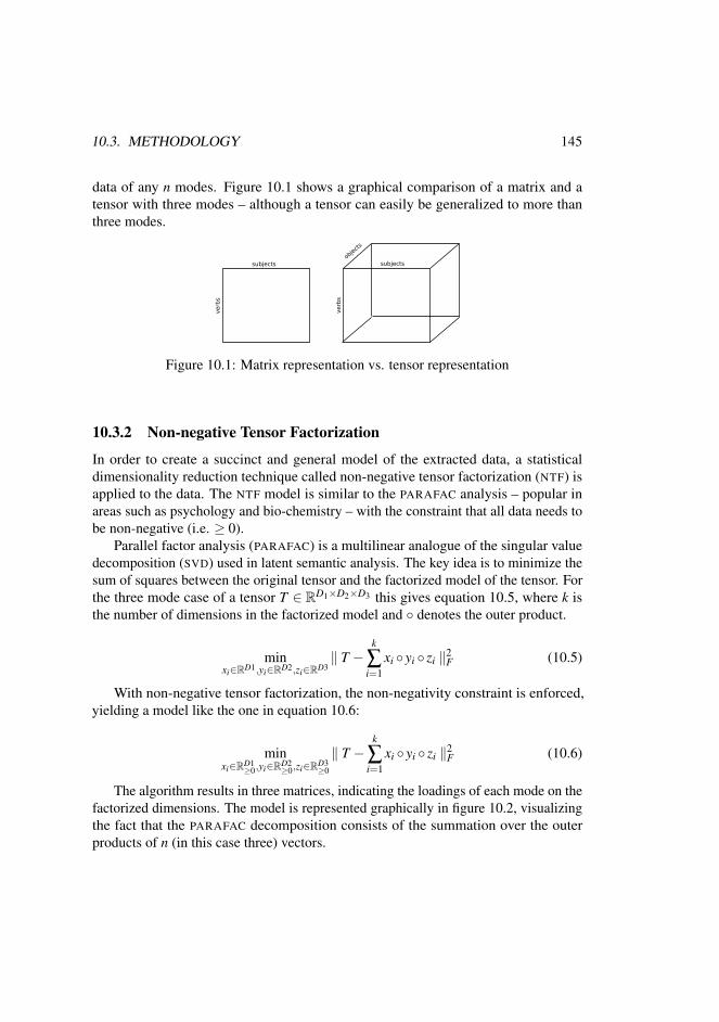
10.3. METHODOLOGY 145
data of any n modes. Figure 10.1 shows a graphical comparison of a matrix and atensor with three modes – although a tensor can easily be generalized to more thanthree modes.
Figure 10.1: Matrix representation vs. tensor representation
10.3.2 Non-negative Tensor Factorization
In order to create a succinct and general model of the extracted data, a statisticaldimensionality reduction technique called non-negative tensor factorization (NTF) isapplied to the data. The NTF model is similar to the PARAFAC analysis – popular inareas such as psychology and bio-chemistry – with the constraint that all data needs tobe non-negative (i.e. ≥ 0).
Parallel factor analysis (PARAFAC) is a multilinear analogue of the singular valuedecomposition (SVD) used in latent semantic analysis. The key idea is to minimize thesum of squares between the original tensor and the factorized model of the tensor. Forthe three mode case of a tensor T ∈ RD1×D2×D3 this gives equation 10.5, where k isthe number of dimensions in the factorized model and ◦ denotes the outer product.
minxi∈RD1,yi∈RD2,zi∈RD3
‖ T −k
∑i=1
xi ◦ yi ◦ zi ‖2F (10.5)
With non-negative tensor factorization, the non-negativity constraint is enforced,yielding a model like the one in equation 10.6:
minxi∈RD1
≥0,yi∈RD2≥0,zi∈RD3
≥0
‖ T −k
∑i=1
xi ◦ yi ◦ zi ‖2F (10.6)
The algorithm results in three matrices, indicating the loadings of each mode on thefactorized dimensions. The model is represented graphically in figure 10.2, visualizingthe fact that the PARAFAC decomposition consists of the summation over the outerproducts of n (in this case three) vectors.

146 CHAPTER 10.
Figure 10.2: Graphical representation of the NTF as the sum of outer products
Computationally, the non-negative tensor factorization model is fitted by applyingan alternating least-squares algorithm. In each iteration, two of the modes are fixedand the third one is fitted in a least squares sense. This process is repeated untilconvergence.3
10.3.3 Applied to Language Data
The model can straightforwardly be applied to language data. In this part, we describethe factorization of verbs × subjects × direct objects co-occurrences, but the examplecan easily be substituted with other co-occurrence information. Moreover, the modelneed not be restricted to 3 modes; it is very well possible to go to 4 modes and beyond— as long as the computations remain feasible.
The NTF decomposition for the verbs × subjects × direct objects co-occurrencesinto the three loadings matrices is represented graphically in figure 10.3.4 By applyingthe NTF model to three-way (s,v,o) co-occurrences, we want to extract a generalizedselectional preference model, and eventually even induce some kind of frame semantics(in the broad sense of the word).
In the resulting factorization, each verb, subject and direct object gets a loadingvalue for each factor dimension in the corresponding loadings matrix. The originalvalue for a particular (s,v,o) triple xsvo can then be reconstructed with equation 10.7.
xsvo =k
∑i=1
ssivviooi (10.7)
To reconstruct the selectional preference value for the triple (man,bite,dog), forexample, we look up the subject vector for man, the verb vector for bite and the direct
3The algorithm has been implemented in MATLAB, using the Tensor Toolbox for sparse tensor calcula-tions (Bader and Kolda, 2009).
4Note that the representation of NTF as three loadings matrices (presented in this figure) is equivalent tothe representation as the sum of outer products (presented in figure 10.2).

10.4. RESULTS 147
Figure 10.3: Graphical representation of the NTF for language data
object vector for dog. Then, for each dimension i in the model, we multiply the ithvalue of the three vectors. The sum of these values is the final preference value.
10.4 Results
10.4.1 Setup
The approach described in the previous section has been applied to Dutch, using theTwente Nieuws Corpus (Ordelman, 2002), a 500M word corpus of Dutch newspapertexts. The corpus has been parsed with the Dutch dependency parser Alpino (vanNoord, 2006), and three-way co-occurrences of verbs with their respective subject anddirect object relations have been extracted. As dimension sizes, the 1K most frequentverbs were used, together with the 10K most frequent subjects and 10K most frequentdirect objects, yielding a tensor of 1K × 10K × 10K. The resulting tensor is verysparse, with only 0.0002% ( 1
5000 th) of the values being non-zero.The tensor has been adapted with a straightforward extension of pointwise mu-
tual information (Church and Hanks, 1990) for three-way co-occurrences, followingequation 10.8. Negative values are set to zero.5
MI3(x,y,z) = logp(x,y,z)
p(x)p(y)p(z)(10.8)
The resulting matrix has been factorized into k dimensions (varying between 50and 300) with the NTF algorithm described in section 10.3.2.
5This is not just an ad hoc conversion to enforce non-negativity. Negative values indicate a smallerco-occurrence probability than the expected number of co-occurrences. Setting those values to zero provesbeneficial for similarity calculations (see e.g. Bullinaria and Levy (2007)).

148 CHAPTER 10.
10.4.2 Examples
Tables 10.1 to 10.5 show example dimensions that have been found by the algorithmwith k = 100. Each example gives the top 10 subjects, verbs and direct objects for aparticular dimension, together with the score for that particular dimension.
Table 10.1 shows the induction of a ‘police action’ frame, with police authoritiesas subjects, police actions as verbs and patients of the police actions as direct objects.
subjects sus verbs vs objects ob js
politie ‘police’ .99 houd aan ‘arrest’ .64 verdachte ‘suspect’ .16agent ‘policeman’ .07 arresteer ‘arrest’ .63 man ‘man’ .16autoriteit ‘authority’ .05 pak op ‘run in’ .41 betoger ‘demonstrator’ .14Justitie ’Justice’ .05 schiet dood ‘shoot’ .08 relschopper ‘rioter’ .13recherche ‘detective force’ .04 verdenk ‘suspect’ .07 raddraaiers ‘instigator’ .13marechaussee ‘militarypolice’
.04 tref aan ‘find’ .06 overvaller ‘raider’ .13
justitie ‘justice’ .04 achterhaal ‘overtake’ .05 Roemeen ‘Romanian’ .13arrestatieteam ‘specialsquad’
.03 verwijder ‘remove’ .05 actievoerder ‘campaigner’ .13
leger ‘army’ .03 zoek ‘search’ .04 hooligan ‘hooligan’ .13douane ‘customs’ .02 spoor op ‘track’ .03 Algerijn ‘Algerian’ .13
Table 10.1: Top 10 subjects, verbs and direct objects for the ‘police action’ dimension
In table 10.2, a legislation dimension is induced, with legislative bodies as subjects,6
legislative actions as verbs, and mostly law (proposals) as direct objects. Note thatsome direct objects (e.g. ‘minister’) also designate persons that can be the object of alegislative act.
Table 10.3 depicts a dimension of ‘war deployment’. The dimension containsmilitary powers (countries, military organizations and leaders) that deploy (or remove)particular military forces.
Table 10.4 shows a ‘publishing’ dimension. The subjects contain writers (personsand bodies), which publish (in a broad sense) textual works.
Table 10.5, finally, is clearly an exhibition dimension, with verbs describing actionsof display and trade that art institutions (subjects) can perform on works of art (objects).
These are not the only sensible dimensions that have been found by the algorithm.A quick qualitative evaluation indicates that about 44 dimensions contain similar,framelike semantics. In another 43 dimensions, the semantics are less clear-cut (singleverbs or expressions account for one dimension, or different senses of a verb get mixed
6Note that VVD, D66, PvdA and CDA are Dutch political parties.

10.4. RESULTS 149
subjects sus verbs vs objects ob js
meerderheid ‘majority’ .33 steun ‘support’ .83 motie ‘motion’ .63VVD .28 dien in ‘submit’ .44 voorstel ‘proposal’ .53D66 .25 neem aan ‘pass’ .23 plan ‘plan’ .28Kamermeerderheid‘Chamber majority’
.25 wijs af ‘reject’ .17 wetsvoorstel ‘bill’ .19
fractie ‘party’ .24 verwerp ‘reject’ .14 hem ‘him’ .18PvdA .23 vind ‘think’ .08 kabinet ‘cabinet’ .16CDA .23 aanvaard ‘accepts’ .05 minister ‘minister’ .16Tweede Kamer ‘SecondChamber’
.21 behandel ‘treat’ .05 beleid ‘policy’ .13
partij ‘party’ .20 doe ‘do’ .04 kandidatuur ‘candidature’ .11Kamer ‘Chamber’ .20 keur goed ‘pass’ .03 amendement ‘amendment’ .09
Table 10.2: Top 10 subjects, verbs and direct objects for the ‘legislation’ dimension
subjects sus verbs vs objects ob js
regering ‘government’ .26 stuur ‘send’ .72 troep ‘troop’ .82VS ‘US’ .26 trek terug ‘withdraw’ .67 militair ‘soldier’ .42Nederland ‘Netherlands’ .25 zet in ‘deploy’ .14 soldaat ‘soldier’ .21president ‘president’ .23 lever ‘supply’ .07 delegatie ‘delegation’ .12leger ‘army’ .22 heb ‘have’ .06 leger ‘army’ .12land ‘country’ .20 haal weg ‘remove’ .03 waarnemer ‘observer’ .08NAVO ‘NATO’ .20 beschikbaar stel ‘make
available’.03 marinier ‘marine’ .08
Indonesie ‘Indonesia’ .19 zeg toe ‘promise’ .03 grondtroepen ‘groundforces’
.08
Verenigde Staten ‘UnitedStates’
.19 ruim op ‘clear’ .02 gezant ‘envoy’ .07
Groot-Brittannie ‘GreatBritain’
.18 bied aan ‘offer’ .02 versterking‘reinforcement’
.07
Table 10.3: Top 10 subjects, verbs and direct objects for the ‘war movement’ dimension
up). 13 dimensions are not so much based on semantic characteristics, but rather onsyntax (e.g. fixed expressions and pronomina).
The qualitative evaluation indicates that quite some dimensions indeed do notcontain framelike semantics, but those dimensions do contain information that may beuseful for selectional preference induction. Such a dimension is shown in table 10.6.It shows an example dimension in which practically all of the dimension’s mass isattributed to one particular expression: een rol spelen ‘to play a role’. The subject slotis more spread out: different kind of things might play a role – each with a fairly low

150 CHAPTER 10.
subjects sus verbs vs objects ob js
hij ‘he’ .62 schrijf ‘write’ .87 boek ‘book’ .30die ‘who’ .41 publiceer ‘publish’ .33 roman ‘novel’ .21ze ‘she’ .32 zing ‘sing’ .14 brief ‘letter’ .20ik ‘I’ .30 lees voor ‘read aloud’ .09 gedicht ‘poem’ .18zij ‘she’ .19 wijd ‘devote’ .09 tekst ‘text’ .17auteur ‘author’ .16 vertaal ‘translate’ .09 essay ‘essay’ .17je ‘you’ .14 bewerk ‘adapt’ .08 stuk ‘piece’ .16journalist ‘journalist’ .13 voltooi ‘finish’ .07 artikel ‘article’ .16schrijver ‘writer’ .13 componeer ‘compose’ .06 biografie ‘biography’ .15krant ‘newspaper’ .09 presenteer ‘present’ .06 verhaal ‘story’ .14
Table 10.4: Top 10 subjects, verbs and direct objects for the ‘publishing’ dimension
subjects sus verbs vs objects ob js
tentoonstelling ‘exhibition’ .50 toon ‘display’ .72 schilderij ‘painting’ .47expositie ‘exposition’ .49 omvat ‘cover’ .63 werk ‘work’ .46galerie ‘gallery’ .36 bevat ‘contain’ .18 tekening ‘drawing’ .36collectie ‘collection’ .29 presenteer ‘present’ .17 foto ‘picture’ .33museum ‘museum’ .27 laat ‘let’ .07 sculptuur ‘sculpture’ .25oeuvre ‘oeuvre’ .22 koop ‘buy’ .07 aquarel ‘aquarelle’ .20Kunsthal .19 bezit ‘own’ .06 object ‘object’ .19kunstenaar ‘artist’ .15 zie ‘see’ .05 beeld ‘statue’ .12dat ‘that’ .12 koop aan ‘acquire’ .05 overzicht ‘overview’ .12hij ‘he’ .10 in huis heb ‘own’ .04 portret ‘portrait’ .11
Table 10.5: Top 10 subjects, verbs and direct objects for the ‘exhibition’ dimension
probability.
10.4.3 Evaluation
The results of the NTF model have been quantitatively evaluated in a pseudo-disambiguationtask, similar to the one used by Rooth et al. (1999). It is used to evaluate the generaliza-tion capabilities of the algorithm. The task is to judge which subject (s or s′) and directobject (o or o′) are more likely for a particular verb v, where (s,v,o) is a combinationdrawn from the corpus, and s′ and o′ are a subject and direct object randomly drawnfrom the corpus. A triple is considered correct if the algorithm prefers both s and oover their counterparts s′ and o′ (so the (s,v,o) triple – that appears in the test corpus– is preferred over the triples (s′,v,o′), (s′,v,o) and (s,v,o′)). Table 10.7 shows threeexamples from the pseudo-disambiguation task.

10.4. RESULTS 151
subjects sus verbs vs objects ob js
naamsbekendheid ‘fame’ .04 speel ‘play’ 1.00 rol ‘role’ 1.00aard ‘nature’ .04 lever op ‘yield’ .00 hoofdrol ‘leading part’ .03nut ‘use’ .04 onderzoek ‘research’ .00 die ‘who’ .00hygiene ‘hygiene’ .04 zie ‘see’ .00 stroming ‘movement’ .00eer wraak ‘revenge’ .04 neem ‘take’ .00 hoofd ‘head’ .00schaamte ‘shame’ .04 vertolk ‘express’ .00 religie ‘religion’ .00institutie ‘institution’ .04 dring terug ‘push back’ .00 werk ‘work’ .00Cultuur ‘Culture’ .04 hekel ‘aversion’ .00 traditie ‘tradition’ .00verdeling ‘division’ .04 krijg ‘get’ .00 overheid ‘government’ .00verbinding ‘connection’ .04 onderstreep ‘underline’ .00 iedereen ‘everyone’ .00
Table 10.6: Top 10 subjects, verbs and direct objects for the ‘play a role’ dimension
s v o s′ o′
jongere drink bier coalitie aandeel‘youngster’ ‘drink’ ‘beer’ ‘coalition’ ‘share’werkgever riskeer boete doel kopzorg‘employer’ ‘risk’ ‘fine’ ‘goal’ ‘worry’directeur zwaai scepter informateur vodka‘manager’ ‘sway’ ‘sceptre’ ‘informer’ ‘wodka’
Table 10.7: Three examples from the pseudo-disambiguation evaluation task’s test set
Four different models have been evaluated. The first two models are tensor factor-ization models. The first model is the NTF model, as described in section 10.3.2. Thesecond model is the original PARAFAC model, without the non-negativity constraints.
The other two models are matrix factorization models. The third model is thenon-negative matrix factorization (NMF) model, and the fourth model is the singularvalue decomposition (SVD). For these models, a matrix has been constructed thatcontains the pairwise co-occurrence frequencies of verbs by subjects as well as directobjects. This gives a matrix of 1K verbs by 10K subjects + 10K direct objects (1K ×20K). The matrix has been transformed using pointwise mutual information.
The models have been evaluated with 10-fold cross-validation. The corpus contains298,540 different (s,v,o) co-occurrences. Those have been randomly divided into 10equal parts. So in each fold, 268,686 co-occurrences have been used for training, and29,854 have been used for testing. The accuracy results of the evaluation are given intable 10.8.
The results clearly indicate that the NTF model outperforms all the other models.
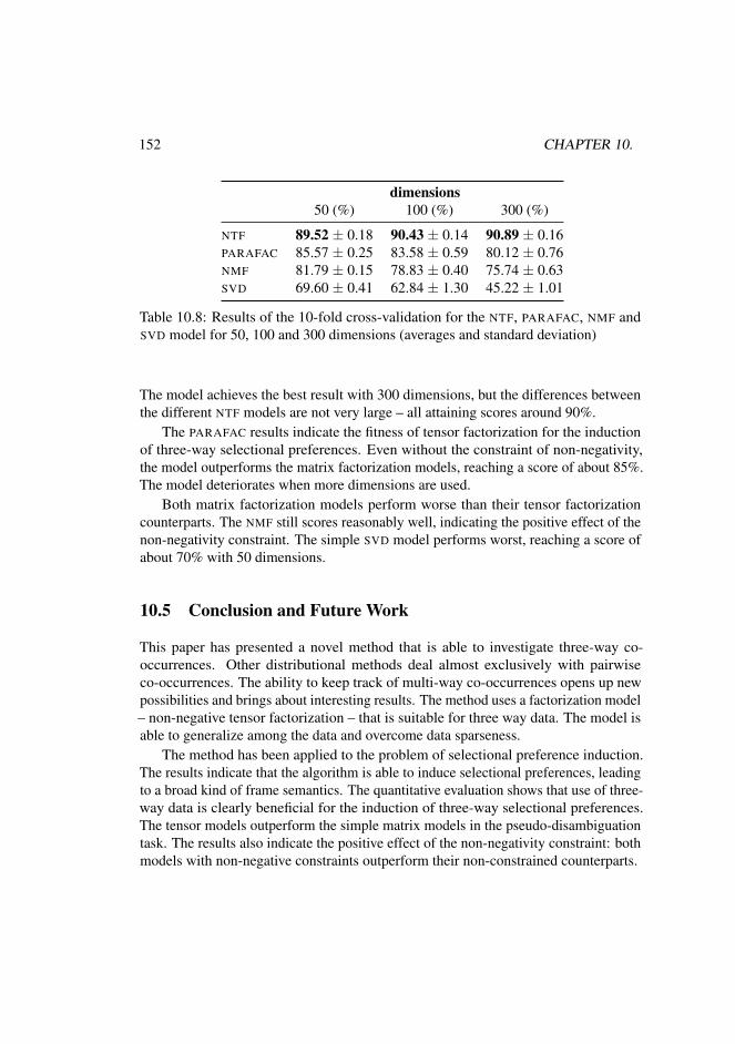
152 CHAPTER 10.
dimensions50 (%) 100 (%) 300 (%)
NTF 89.52 ± 0.18 90.43 ± 0.14 90.89 ± 0.16PARAFAC 85.57 ± 0.25 83.58 ± 0.59 80.12 ± 0.76NMF 81.79 ± 0.15 78.83 ± 0.40 75.74 ± 0.63SVD 69.60 ± 0.41 62.84 ± 1.30 45.22 ± 1.01
Table 10.8: Results of the 10-fold cross-validation for the NTF, PARAFAC, NMF andSVD model for 50, 100 and 300 dimensions (averages and standard deviation)
The model achieves the best result with 300 dimensions, but the differences betweenthe different NTF models are not very large – all attaining scores around 90%.
The PARAFAC results indicate the fitness of tensor factorization for the inductionof three-way selectional preferences. Even without the constraint of non-negativity,the model outperforms the matrix factorization models, reaching a score of about 85%.The model deteriorates when more dimensions are used.
Both matrix factorization models perform worse than their tensor factorizationcounterparts. The NMF still scores reasonably well, indicating the positive effect of thenon-negativity constraint. The simple SVD model performs worst, reaching a score ofabout 70% with 50 dimensions.
10.5 Conclusion and Future Work
This paper has presented a novel method that is able to investigate three-way co-occurrences. Other distributional methods deal almost exclusively with pairwiseco-occurrences. The ability to keep track of multi-way co-occurrences opens up newpossibilities and brings about interesting results. The method uses a factorization model– non-negative tensor factorization – that is suitable for three way data. The model isable to generalize among the data and overcome data sparseness.
The method has been applied to the problem of selectional preference induction.The results indicate that the algorithm is able to induce selectional preferences, leadingto a broad kind of frame semantics. The quantitative evaluation shows that use of three-way data is clearly beneficial for the induction of three-way selectional preferences.The tensor models outperform the simple matrix models in the pseudo-disambiguationtask. The results also indicate the positive effect of the non-negativity constraint: bothmodels with non-negative constraints outperform their non-constrained counterparts.

10.5. CONCLUSION AND FUTURE WORK 153
The results as well as the evaluation indicate that the method presented here is apromising tool for the investigation of NLP topics, although more research and a morethorough evaluation would be desirable.
There is quite some room for future work. First of all, we want to further investigatethe usefulness of the method for selectional preference induction. One of the mostimportant extensions is the inclusion of other dependency relations in our model, apartfrom subjects and direct objects (thus making use of tensors with more than 3 modes).
Secondly, there is room for improvement and further research with regard to thetensor factorization model. The model presented here minimizes the sum of squareddistance. This is, however, not the only objective function possible. Another possibilityis the minimization of the Kullback-Leibler divergence. Minimizing the sum ofsquared distance assumes normally distributed data, and language phenomena arerarely normally distributed. Other objective functions – such as the minimization of theKullback-Leibler divergence – might be able to capture the language structures muchmore adequately. We specifically want to stress this second line of future research asone of the most promising and exciting ones.
Finally, the model presented here is not only suitable for selectional preferenceinduction. There are many problems in NLP that involve three-way co-occurrences. Infuture work, we want to apply the NTF model presented here to other problems in NLP,the most important one being word sense discrimination.


Conclusion
In this dissertation, we have investigated the extraction of semantic similarity usingdistributional similarity techniques. In the first part, we investigated what kind ofinformation might be able to provide cues about the semantics of words, and wedetermined that the context of a word is able to inform us about its semantics. Weestablished three different kinds of context – a document-based context, a window-based context, and a syntax-based context – and we provided a formalization of thenotion of context, so that the semantics of a word can be formally computed. Next,we gave an overview of two dimensionality reduction algorithms – singular valuedecomposition and non-negative matrix factorization – two algorithms that reduce thevast number of overlapping feature dimensions to a limited number of generalizeddimensions that might be able to capture inherent semantics characteristics presentin the data. We also provided an overview of tensor algebra and the multilineargeneralization of non-negative matrix factorization in tensor space – non-negativetensor factorization. Using tensor algebra, we are not limited to using co-occurrencesin two modes; three-way methods allow us to analyze multi-way co-occurrences, whichallow us to capture the semantic information present in the data in a more informedand thorough way.
In the second part of this dissertation, we provided a quantitative overview ofthree different groups of models of semantic similarity, constructed according to thethree different notions of context. We experimented with different parameters, anddetermined what models and parameters yield the best results according to threedifferent evaluation schemes. In the first two evaluation schemes – the evaluationof wordnet-based similarity and the evaluation of cluster quality – we evaluated themodels’ ability to extract tight, synonym-like similarity. In the third evaluation scheme– the evaluation of domain coherence – we evaluated the models’ ability to extract moreloosely related, topical similarity. In all evaluations, we paid special attention to theeffects of dimensionality reduction algorithms.
In the third part, we developed a number of applications that make use of the
155

156 CONCLUSION
techniques (and the resulting semantic resources) presented in the first part. In the firstapplication, we used an automatically induced lexico-semantic clustering to extractmulti-word expressions based on their non-compositionality. In the second application,we described a technique that combines a syntactic context and a large window-basedcontext in a factorization framework, in order to discriminate among the differentsenses of nouns. And in the third application, we explored three-way methods in com-bination with non-negative tensor factorization in order to induce three-way selectionalpreferences.
We are now able to answer the three research questions that were formulated inthe introduction of this dissertation. In the evaluation part of this dissertation, wehave shown that different notions of context lead to different kinds of similarity. Weconcluded that syntax-based models and window-based models with a small windoware best suited for the extraction of tight, synonym-like similarity. This was indicatedby their performance on the wordnet-based similarity evaluation and the evaluation ofcluster quality. By nature, words that are tightly similar are also topically coherent,which was indicated by the good performance of these models on the third evaluationtask. On the other hand, the document-based models and window-based modelswith large windows size – the models that did not perform well on the extraction oftight similarity – still performed reasonably well on the third evaluation task. Weconcluded that a tight context (syntax-based or small window-based) leads to tight,synonym-like similarity, whereas a broad context (document-based or large window-based) captures more loosely related topically similar words. We also showed thatan automatically induced clustering based on syntactic context allows us to extractmulti-word expressions based on their non-compositionality, and that a tight, syntacticcontext and a broad window-based context can be combined in a non-negative matrixfactorization framework in order to discriminate the different senses of a noun.
The answer to our second research question is mixed. On the one hand, ourquantitative evaluation indicated that dimensionality reduction algorithms do not bringabout a large improvement in the extraction of semantic similarity. Dimensionalityreduction was only beneficial for the document-based model. In the other models,dimensionality reduction did not improve or even hurt the performance of the models.The performance of the non-negative matrix factorization models in the quantitativeevaluation was particularly disappointing.
On the other hand, dimensionality reduction algorithms did prove beneficial in anumber of applications. Non-negative matrix factorization allowed us to induce a num-ber of semantic dimensions according to which context words and syntactic relationscould be classified. These dimensions in turn allowed us to subtract dimensions relatedto a specific sense of a noun, so that other senses of the word become apparent. Themultilinear generalization of non-negative matrix factorization – non-negative tensor

157
factorization – was also beneficial for the induction of selectional preferences.Which brings us to our third research question: we have demonstrated the useful-
ness of three-way methods for the induction of selectional preferences. The quantitativeevaluation shows that the use of three-way data is beneficial for the induction of three-way selectional preferences. The tensor models outperform the simple matrix modelsin the pseudo-disambiguation task. The results also indicate the positive effect ofthe non-negativity constraint: both models with non-negative constraints outperformtheir non-constrained counterparts. The results indicate that three-way methods are apromising tool for the investigation of NLP topics.


Appendix A
Clustering Tasks
A.1 Concrete noun categorization
noun translation class6 class3 class2
kip chicken bird animal naturalarend eagle bird animal naturaleend duck bird animal naturalzwaan swan bird animal naturaluil owl bird animal naturalpinguın penguin bird animal naturalpauw peacock bird animal natural
hond dog groundAnimal animal naturalolifant elephant groundAnimal animal naturalkoe cow groundAnimal animal naturalkat cat groundAnimal animal naturalleeuw lion groundAnimal animal naturalvarken pig groundAnimal animal naturalslak snail groundAnimal animal naturalschildpad turtle groundAnimal animal natural
kers cherry fruitTree vegetable naturalbanaan banana fruitTree vegetable naturalpeer pear fruitTree vegetable naturalananas pineapple fruitTree vegetable natural
champignon mushroom green vegetable naturalmaıs corn green vegetable natural
159

160 APPENDIX A. CLUSTERING TASKS
sla lettuce green vegetable naturalaardappel potato green vegetable naturalui onion green vegetable natural
fles bottle tool artifact artifactpotlood pencil tool artifact artifactpen pen tool artifact artifactbeker cup tool artifact artifactkom bowl tool artifact artifactschaar scissors tool artifact artifactketel kettle tool artifact artifactmes knife tool artifact artifactschroevendraaier screwdriver tool artifact artifacthamer hammer tool artifact artifactlepel spoon tool artifact artifactbeitel chisel tool artifact artifacttelefoon telephone tool artifact artifact
boot boat vehicle artifact artifactauto car vehicle artifact artifactschip ship vehicle artifact artifactvrachtwagen truck vehicle artifact artifactraket rocket vehicle artifact artifactmotor motorcycle vehicle artifact artifacthelikopter helicopter vehicle artifact artifact

A.2. ABSTRACT/CONCRETE NOUN DISCRIMINATION 161
A.2 Abstract/concrete noun discrimination
noun translation class2
kip chicken HIarend eagle HIleeuw lion HIschildpad turtle HIbanaan banana HIui onion HIaardappel potato HIkom bowl HIpotlood pencil HItelefoon telephone HIvrachtwagen truck HIschip ship HIauto car HIfles bottle HIhamer hammer HI
jaloezie jealousy LOwaarheid truth LOhypothese hypothesis LOhoop hope LOgenade mercy LOmysterie mystery LOdankbaarheid gratitude LOconcept concept LOverleiding temptation LOtrots pride LOgeloof belief LOinzicht insight LOwijsheid wisdom LOgeluk luck LOafleiding distraction LO


List of Abbreviations
CBC clustering by committee
CGN Corpus Gesproken Nederlands
JS Jensen-Shannon
KL Kullback-Leibler
LSA latent semantic analysis
MWE multi-word expression
NMF non-negative matrix factorization
NTF non-negative tensor factorization
PARAFAC parallel factor analysis
PCA principal component analysis
PLSA probabilistic latent semantic analysis
PMI pointwise mutual information
SVD singular value decomposition
TWNC Twente Nieuws Corpus
163


Bibliography
[Abe and Li1996] Abe, Naoke and Hang Li. 1996. Learning word association normsusing tree cut pair models. In Proceedings of the Thirteenth International Confer-ence on Machine Learning.
[Bader and Kolda2006a] Bader, Brett W. and Tamara G. Kolda. 2006a. Algorithm862: Matlab tensor classes for fast algorithm prototyping, acm transactions onmathematical software. 32(4), December.
[Bader and Kolda2006b] Bader, Brett W. and Tamara G. Kolda. 2006b. Efficient MAT-LAB computations with sparse and factored tensors. Technical Report SAND2006-7592, Sandia National Laboratories, Albuquerque, NM and Livermore, CA, Decem-ber.
[Bader and Kolda2009] Bader, Brett W. and Tamara G. Kolda. 2009. Mat-lab tensor toolbox version 2.3. http://csmr.ca.sandia.gov/∼tgkolda/TensorToolbox/, July.
[Baldwin et al.2003] Baldwin, T., C. Bannard, T. Tanaka, and D. Widdows. 2003. AnEmpirical Model of Multiword Expressions Decomposability. In Proc. of the ACL-2003 Workshop on Multiword Expressions: Analysis, Acquisition and Treatment,pages 89–96, Sapporo, Japan.
[Baldwin et al.2006] Baldwin, T., J. Beavers, L. van der Beek, F. Bond, D. Flickinger,and I.A. Sag, 2006. In search of a systematic treatment of Determinerless PPs,pages 163–180. Computational Linguistics Dimensions of Syntax and Semanticsof Prepositions. Kluwer Academic.
[Baldwin2006] Baldwin, Tim. 2006. Compositionality and Multiword Expressions:Six of One, Half a Dozen of the Other? Invited talk given at the COLING/ACL’06Workshop on Multiword Expressions: Identifying and Exploiting UnderlyingProperties, July.
165

166 BIBLIOGRAPHY
[Basili et al.2007] Basili, Roberto, Diego De Cao, Paolo Marocco, and Marco Pennac-chiotti. 2007. Learning selectional preferences for entailment or paraphrasingrules. In Proceedings of RANLP 2007, Borovets, Bulgaria.
[Bentivogli et al.2004] Bentivogli, Luisa, Pamela Forner, Bernardo Magnini, andEmanuele Pianta. 2004. Revising wordnet domains hierarchy: Semantics, cover-age, and balancing. In Proceedings of COLING 2004 Workshop on MultilingualLinguistic Resources, pages 101–108, Geneva, Switzerland.
[Berry1992] Berry, Michael. 1992. Large scale singular value computations. Interna-tional Journal of Supercomputer Applications, 6(3):13–49.
[Bhagat, Pantel, and Hovy2007] Bhagat, Rahul, Patrick Pantel, and Eduard Hovy. 2007.Ledir: An unsupervised algorithm for learning directionality of inference rules. InProceedings of Conference on Empirical Methods in Natural Language Processing(EMNLP-07), pages 161–170, Prague, Czech Republic.
[Bloomfield1933] Bloomfield, Leonard. 1933. Language. Henry Holt, New York.[Bouma, van Noord, and Malouf2001] Bouma, Gosse, Gertjan van Noord, and Robert
Malouf. 2001. Alpino: Wide-coverage computational analysis of dutch. In WalterDaelemans, Khalil Sima’an, J. Veenstra, and J. Zavrel, editors, ComputationalLinguistics in the Netherlands 2000. Rodopi, Amsterdam, New York, pages 45–59.
[Bro and Jong1997] Bro, R. and S. De Jong. 1997. A fast non-negativity-constrainedleast squares algorithm. Journal of Chemometrics, 11:393–401.
[Budanitsky and Hirst2006] Budanitsky, Alexander and Graeme Hirst. 2006. Eval-uating wordnet-based measures of lexical semantic relatedness. ComputationalLinguistics, 32(1):13–47.
[Bullinaria and Levy2007] Bullinaria, John A. and Joseph P. Levy. 2007. Extractingsemantic representations from word co-occurrence statistics: A computationalstudy. Behavior Research Methods, 39:510–526.
[Carroll and Chang1970] Carroll, J. D. and J.-J. Chang. 1970. Analysis of individualdifferences in multidimensional scaling via an n-way generalization of ”eckart-young” decomposition. Psychometrika, 35:283–319.
[Church and Hanks1990] Church, Kenneth Ward and Patrick Hanks. 1990. Wordassociation norms, mutual information & lexicography. Computational Linguistics,16(1):22–29.
[Clark and Weir2001] Clark, Stephen and David Weir. 2001. Class-based probabilityestimation using a semantic hierarchy. In Proceedings of NAACL 2001, Pittsburgh,USA.
[Cohen1960] Cohen, Jacob. 1960. A coefficient of agreement for nominal scales.Educational and Psychological Measurement, 20:37–46.

167
[De Lathauwer, Moor, and Vandewalle2000] De Lathauwer, Lieven, Bart De Moor,and Joos Vandewalle. 2000. A multilinear singular value decomposition. SIAMJournal on Matrix Analysis and Applications, 21(4):1253–1278.
[Deprettere1988] Deprettere, F., editor. 1988. SVD and signal processing: algorithms,applications and architectures. North-Holland Publishing Co., Amsterdam, TheNetherlands.
[Erk2007] Erk, Katrin. 2007. A simple, similarity-based model for selectional prefer-ences. In Proceedings of ACL 2007, Prague, Czech Republic.
[Fazly and Stevenson2006] Fazly, A. and S. Stevenson. 2006. Automatically con-structing a lexicon of verb phrase idiomatic combinations. In Proceedings of the11th Conference of the European Chapter of the Association for ComputationalLinguistics (EACL-2006), Trento, Italy.
[Fellbaum1998] Fellbaum, C., editor. 1998. WordNet: An Electronic Lexical Database.MIT Press, Cambridge, Massachusetts.
[Harris1985] Harris, Z. 1985. Distributional structure. In Jerrold J. Katz, editor, ThePhilosophy of Linguistics. Oxford University Press, pages 26–47.
[Harris1954] Harris, Zellig S. 1954. Distributional structure. Word, 10(23):146–162.[Harshman1970] Harshman, R.A. 1970. Foundations of the parafac procedure: models
and conditions for an ”explanatory” multi-mode factor analysis. In UCLA WorkingPapers in Phonetics, volume 16, pages 1–84, Los Angeles. University of California.
[Hoekstra et al.2001] Hoekstra, Heleen, Michael Moortgat, Bram Renmans, InekeSchuurman, and Ton van der Wouden. 2001. Syntactic annotation for the spokendutch corpus project (cgn). In Walter Daelemans, Khalil Sima’an, J. Veenstra, andJ. Zavrel, editors, Computational Linguistics in the Netherlands 2000, pages 73–87,Amsterdam, New York. Rodopi.
[Hofmann1999] Hofmann, Thomas. 1999. Probabilistic latent semantic analysis. InProc. of Uncertainty in Artificial Intelligence, UAI’99, Stockholm.
[Horak, Vossen, and Rambousek2008] Horak, A., P. Vossen, and A. Rambousek. 2008.The development of a complex-structured lexicon based on wordnet. In Proceed-ings of the Fourth International GlobalWordNet Conference – GWC 2008, Szeged,Hungary.
[Karypis2003] Karypis, George. 2003. CLUTO - a clustering toolkit. Technical Report#02-017, nov.
[Katz and Giesbrecht2006] Katz, G. and E. Giesbrecht. 2006. Automatic identificationof non-compositional multi-word expressions using Latent Semantic Analysis. InProc. of the COLING/ACL’06 Workshop on Multiword Expressions: Identifyingand Exploiting Underlying Properties, pages 12–19, Sydney, Australia.
168 BIBLIOGRAPHY
[Kiers2000] Kiers, H.A.L. 2000. Towards a standardized notation and terminology inmultiway analysis. Journal of Chemometrics, 14:105–122.
[Kiers and van Mechelen2001] Kiers, H.A.L and I. van Mechelen. 2001. Three-waycomponent analysis: Principles and illustrative application. Psychological Methods,6:84–110.
[Kolda and Bader2006] Kolda, Tamara and Brett Bader. 2006. The TOPHITS modelfor higher-order web link analysis. In Workshop on Link Analysis, Counterterrorismand Security.
[Kolda and Bader2009] Kolda, Tamara G. and Brett W. Bader. 2009. Tensor decom-positions and applications. SIAM Review, 51(3), September. In press.
[Landauer, Foltz, and Laham1998] Landauer, Thomas, Peter Foltz, and Darrell Laham.1998. An Introduction to Latent Semantic Analysis. Discourse Processes, 25:295–284.
[Landauer and Dumais1997] Landauer, Thomas K. and Susan T. Dumais. 1997. Asolution to Plato’s problem: The Latent Semantic Analysis theory of the acquisition,induction, and representation of knowledge. Psychology Review, 104:211–240.
[Lawson and Hanson1974] Lawson, C.L. and B.J. Hanson. 1974. Solving LeastSquares Problems. Prentice-Hall, Englewood Cliffs, NJ.
[Leacock and Chodorow1998] Leacock, Claudia and Martin Chodorow. 1998. Com-bining local context with wordnet similarity for word sense identification. InChristiane Fellbaum, editor, WordNet: An Electronic Database. MIT press, Cam-bridge, MA, pages 265–283.
[Lee and Seung1999] Lee, Daniel D. and H. Sebastian Seung. 1999. Learning the partsof objects by non-negative matrix factorization. Nature, 401:788–791.
[Lee and Seung2000] Lee, Daniel D. and H. Sebastian Seung. 2000. Algorithms fornon-negative matrix factorization. In NIPS, pages 556–562.
[Lin1998a] Lin, D. 1998a. Automatic retrieval and clustering of similar words. InProceedings of COLING/ACL 98, Montreal, Canada.
[Lin1998b] Lin, Dekang. 1998b. An information-theoretic definition of similarity. InProceedings of the 15th International Conference on Machine Learning, pages296–304. Morgan Kaufmann.
[Lin1999] Lin, Dekang. 1999. Automatic identification of non-compositional phrases.In Proceedings of ACL-99, pages 317–324. University of Maryland.
[Lowe2001] Lowe, Will. 2001. Towards a theory of semantic space. In Proceedingsof the 23rd Annual Conference of the Cognitive Science Society, pages 576–581,Edinburgh, UK.

169
[MacQueen1967] MacQueen, J. B. 1967. Some methods for classification and analysisof multivariate observations. In Proceedings of 5-th Berkeley Symposium onMathematical Statistics and Probability, volume 1, pages 281–297, Berkeley.University of California Press.
[Magnini and Cavagli2000] Magnini, Bernardo and Gabriela Cavagli. 2000. Integ-rating subject field codes into wordnet. In Proceedings of LREC-2000, SecondInternational Conference on Language Resources and Evaluation, pages 1413–1418, Athens, Greece.
[Maks, Martin, and de Meerseman1999] Maks, I., W. Martin, and H. de Meerseman,1999. Referentie Bestand Nederlands. Manual.
[Manning and Schutze2000] Manning, Christopher and Hinrich Schutze. 2000. Found-ations of Statistical Natural Language Processing. MIT Press, Cambridge, Mas-sachussets.
[Martin and Maks2005] Martin, W. and I. Maks, 2005. Referentie Bestand Nederlands.Documentatie, April.
[McCarthy, Keller, and Carroll2003] McCarthy, Diana, Bill Keller, and John Carroll.2003. Detecting a Continuum of Compositionality in Phrasal Verbs. In Proc. ofthe ACL-2003 Workshop on Multiword Expressions: Analysis, Acquisition andTreatment, Sapporo, Japan.
[Nerbonne and Van de Cruys2009] Nerbonne, John and Tim Van de Cruys. 2009. De-tecting aspectual relations quantitatively. In Erhard Hinrichs and John Nerbonne,editors, Theory and Evidence in Semantics(Proceedings of a Symposium in honorof David Dowty), pages 159–182, Stanford. CSLI.
[van Noord2006] van Noord, Gertjan. 2006. At Last Parsing Is Now Operational. InPiet Mertens, Cedrick Fairon, Anne Dister, and Patrick Watrin, editors, TALN06.Verbum Ex Machina. Actes de la 13e conference sur le traitement automatique deslangues naturelles, pages 20–42, Leuven.
[Ordelman2002] Ordelman, R.J.F. 2002. Twente Nieuws Corpus (TwNC), August.Parlevink Language Techonology Group. University of Twente.
[Pado and Lapata2007] Pado, Sebastian and Mirella Lapata. 2007. Dependency-basedconstruction of semantic space models. Computational Linguistics, 33(2):161–199.
[Pantel and Lin2002] Pantel, Patrick and Dekang Lin. 2002. Discovering word sensesfrom text. In Proceedings of ACM Conference on Knowledge Discovery and DataMining (KDD-02), pages 613–619, Edmonton, Canada.
[Pearce2001] Pearce, Darren. 2001. Synonymy in collocation extraction. In WordNetand Other lexical resources: applications, extensions & customizations (NAACL2001), pages 41–46, Pittsburgh. Carnegie Mellon University.

170 BIBLIOGRAPHY
[Pearson1901] Pearson, K. 1901. On lines and planes of closest fit to systems of pointsin space. Philosophical Magazine, 2(6):559–572.
[Pereira, Tishby, and Lee1993] Pereira, Fernando, Naftali Tishby, and Lillian Lee.1993. Distributional clustering of English words. In 31st Annual Meeting ofthe ACL, pages 183–190.
[Piao et al.2006] Piao, S., P. Rayson, O. Mudraya, A. Wilson, and R. Garside. 2006.Measuring MWE compositionality using semantic annotation. In Proceedingsof the Workshop on Multiword Expressions: Identifying and Exploiting Under-lying Properties, pages 2–11, Sydney, Australia. Association for ComputationalLinguistics.
[van der Plas and Bouma2005] van der Plas, Lonneke and Gosse Bouma. 2005. Syn-tactic contexts for finding semantically similar words. Computational Linguisticsin the Netherlands 2004. Selected Papers from the Fifteenth CLIN Meeting, pages173–184.
[Resnik1993] Resnik, Philip. 1993. Selection and Information: A Class-Based Ap-proach to Lexical Relationships. PhD Thesis, University of Pennsylvania.
[Resnik1995] Resnik, Philip. 1995. Using information content to evaluate semanticsimilarity in a taxonomy. In Proceedings of the 14th International Joint Conferenceon Artificial Intelligence, pages 448–453, Montreal, Canada.
[Resnik1996] Resnik, Philip. 1996. Selectional constraints: An information-theoreticmodel and its computational realization. Cognition, 61:127–159.
[Resnik1999] Resnik, Philip. 1999. Semantic similarity in a taxonomy: Aninformation-based measure and its application to problems of ambiguity in naturallanguage. Journal of Artificial Intelligence Research, 11:95–130.
[Rooth et al.1999] Rooth, Mats, Stefan Riezler, Detlef Prescher, Glenn Carroll, andFranz Beil. 1999. Inducing a semantically annotated lexicon via em-based cluster-ing. In 37th Annual Meeting of the ACL.
[Sag et al.2002] Sag, Ivan, T. Baldwin, F. Bond, A. Copestake, and D. Flickinger.2002. Multiword Expressions: a pain in the neck for NLP. In Proceedings of theThird International Conference on Intelligent Text Processing and ComputationalLinguistics, pages 1–15, Mexico City, Mexico.
[Salton, Wong, and Yang1975] Salton, Gerard, A. Wong, and C. S. Yang. 1975. A vec-tor space model for automatic indexing. Communications of the ACM, 18(11):613–620.
[Saussure1916] Saussure, Ferdinand De. 1916. Cours de Linguistique Generale. InCharles Bally, Albert Sechehaye, and Albert Riedlinger, editors, . Payot, Lausanneand Paris.

171
[Schutze1998] Schutze, Hinrich. 1998. Automatic word sense discrimination. Compu-tational Linguistics, 24(1):97–123.
[Shashua and Hazan2005] Shashua, Amnon and Tamir Hazan. 2005. Non-negativetensor factorization with applications to statistics and computer vision. In ICML
’05: Proceedings of the 22nd international conference on Machine learning, pages792–799, New York, NY, USA. ACM.
[Tucker1966] Tucker, L.R. 1966. Some mathematical notes on three-mode factoranalysis. Psychometrika, 31:279–311.
[Turk and Pentland1991] Turk, Matthew and Alex Pentland. 1991. Eigenfaces forrecognition. J. Cognitive Neuroscience, 3(1):71–86.
[Turney2007] Turney, Peter D. 2007. Empirical evaluation of four tensor decomposi-tion algorithms. Technical Report ERB-1152, National Research Council, Institutefor Information Technology.
[Van de Cruys2006a] Van de Cruys, Tim. 2006a. The application of singular valuedecomposition to dutch noun-adjective matrices. In Piet Mertens et al., editors,Verbum Ex Machina. Actes de RECITAL (TALN), pages 767–772, Leuven UniversityPress, Leuven, Belgium.
[Van de Cruys2006b] Van de Cruys, Tim. 2006b. Semantic clustering in dutch. InKhalil Sima’an et al., editors, Proceedings of the Sixteenth Computational Linguist-ics in the Netherlands (CLIN), pages 17–32, University of Amsterdam, Amsterdam,The Netherlands.
[Van de Cruys2007] Van de Cruys, Tim. 2007. Exploring three way contexts for wordsense discrimination. In Marco Baroni, Allesandro Lenci, and Magnus Sahlgren,editors, Proceedings of the Workshop on Contextual Information in SemanticSpace Models: Beyond Words and Documents (COSMO), pages 33–41, Roskilde,Denmark.
[Van de Cruys2008a] Van de Cruys, Tim. 2008a. A comparison of bag of words andsyntax-based approaches for word categorization. In Marco Baroni, Stefan Evert,and Allesandro Lenci, editors, Proceedings of the Lexical Semantics Workshop:Bridging the gap between semantic theory and computational simulations, pages47–54, ESSLLI 2008, Hamburg, Germany.
[Van de Cruys2008b] Van de Cruys, Tim. 2008b. A simple extension of non-negativematrix factorization for three-way data. In Workshop on Mining MultidimensionalData (MMD ’08) at ECML PKDD 2008, Antwerp, Belgium.
[Van de Cruys2008c] Van de Cruys, Tim. 2008c. Using three way data for wordsense discrimination. In Proceedings of the 22nd International Conference onComputational Linguistics (Coling 2008), pages 929–936, Manchester, UnitedKingdom.

172 BIBLIOGRAPHY
[Van de Cruys2009] Van de Cruys, Tim. 2009. A non-negative tensor factorizationmodel for selectional preference induction. In Proceedings of the workshop onGeometric Models for Natural Language Semantics (GEMS), pages 83–90, Athens,Greece.
[Van de CruysTo appear] Van de Cruys, Tim. To appear. A non-negative tensor factor-ization model for selectional preference induction. Journal of Natural LanguageEngineering. Special Issue on Geometrical Models of Natural Language Semantics.
[Van de Cruys and Villada Moiron2007a] Van de Cruys, Tim and Begona VilladaMoiron. 2007a. Lexico-semantic multiword expression extraction. In Peter Dirixet al., editor, Proceedings of the 17th Meeting of Computational Linguistics in theNetherlands (CLIN), pages 175–190, University of Leuven, Leuven, Belgium.
[Van de Cruys and Villada Moiron2007b] Van de Cruys, Tim and Begona VilladaMoiron. 2007b. Semantics-based multiword expression extraction. In Proceedingsof the Workshop on A Broader Perspective on Multiword Expressions, pages 25–32,ACL, Prague, Czech Republic.
[Vasilescu and Terzopoulos2002] Vasilescu, M. Alex O. and Demetri Terzopoulos.2002. Multilinear analysis of image ensembles: Tensorfaces. In ECCV, pages447–460.
[Venkatapathy and Joshi2005] Venkatapathy, S. and A. Joshi. 2005. Measuring therelative compositionality of verb-noun collocations by integrating features. InProceedings of the Human Language Technology Conference and Conference onEmpirical Methods in Natural Language Processing, pages 899–906, Vancouver.
[Villada Moiron and Tiedemann2006] Villada Moiron, Begona and Jorg Tiedemann.2006. Identifying idiomatic expressions using automatic word-alignment. In Pro-ceedings of the EACL 2006 Workshop on Multi-word-expressions in a multilingualcontext”, pages 33–40, Trento, Italy.
[Vossen1998] Vossen, P., editor. 1998. EuroWordNet: a multilingual database withlexical semantic networks for European Languages. Kluwer, Dordrecht.
[Wall, Rechtsteiner, and Rocha2003] Wall, Michael E., Andreas Rechtsteiner, andLuis M. Rocha, 2003. Singular Value Decomposition and Principal Compon-ent Analysis, chapter 5, pages 91–109. Kluwel, Norwell, MA, Mar.
[Weeds2003] Weeds, Julie. 2003. Measures and Applications of Lexical DistributionalSimilarity. PhD Thesis, University of Sussex.
[Welling and Weber2001] Welling, M. and M. Weber. 2001. Positive tensor factoriza-tion. Pattern Recognition Letters, 22:1255–1261.
[Wittgenstein1953] Wittgenstein, Ludwig. 1953. Philosophical Investigations. Philo-sophische Untersuchungen. Basil Blackwell, Oxford. Translated by G.E.M.Anscombe.

173
[Wu and Palmer1994] Wu, Zhibiao and Martha Palmer. 1994. Verb semantics andlexical selection. In 32nd. Annual Meeting of the Association for ComputationalLinguistics, pages 133–138, New Mexico State University, Las Cruces, New Mex-ico.
[Zhao and Karypis2001] Zhao, Ying and George Karypis. 2001. Criterion functionsfor document clustering: Experiments and analysis. Technical Report #01-40.