Embed Size (px)
Citation preview

Mining for Co-occurring Motion Trajectories
– Sport Analysis - by
Maja Dimitrijevic
B.Sc. (Computer Science) University of Novi Sad, 1998
A THESIS SUBMITTED IN PARTIAL FULFILLMENT OF THE REQUIREMENTS FOR THE DEGREE OF
Master of Science
in
THE FACULTY OF GRADUATE STUDIES
(Department of Computer Science)
We accept this thesis as conforming
to the required standards
______________________________________
______________________________________
THE UNIVERSITY OF BRITISH COLUMBIA
December 2001
Maja Dimitrijevic, 2001
ii
Abstract
This thesis investigates the applicability of a data mining algorithm for automatic pattern
discovery widely used for conventional databases, called Apriori, to a new domain – 2D
motion trajectory data. This is one the first attempts to analyze motion trajectory data, in
the data mining style, i.e., to develop methods for automatic finding of interesting
patterns or rules in the object motion trajectories. While our focus is on the application to
the hockey game analysis, similar methods could also be used in the area of video
surveillance, for sport game strategies, or more generally in geographic applications.
More specifically, our focus is on the discovery of the hockey game patterns that contain
frequent motion trajectories of the hockey players, where the frequency is defined with
respect to a motion trajectory similarity measure. Furthermore, the patterns relate motion
of the players of the same or opposing teams, which should be correlated according to
their roles in the game. We design and implement a system that discovers such patterns,
and test its effectiveness and efficiency on a real life and semi-randomly generated data
set. Our effectiveness tests tend to prove the right choice of the motion trajectory
similarity measure, and the validity of the algorithm. Our tests also include a comparison
of using the Apriori algorithm, with a semi-naïve algorithm, proving the importance of
using Apriori, which outperforms the semi-naïve algorithm for various choices of
parameters and data sizes.

iii
Contents Abstract ii
Contents iii
List of Figures vi
List of Tables vii
Acknowledgements viii
Chapter 1 Introduction 1
1.1 Background and Motivation 1
1.2 Related Work 3
1.3 Problem Challenges and Contribution 5
1.4 Thesis Outline 8
Chapter 2 Background and Related Work 10
2.1 Mining for the Patterns in Conventional Databases 10
2.2 Time Series - Notion of Similarity 12
2.3 Finding Patterns and Rules in Time Series 14
2.4 Fuzzy Association Rules 15
2.5 Motion Trajectory Models 16
Chapter 3 Pattern Finding Method 18
3.1 Hockey Game Patterns 18
3.2 Data Acquisition 19
3.3 Data Preprocessing - Feature Point Extraction 20
3.4 Trajectory Representation 21
3.5 Trajectory Similarity Measure 22
3.5.1 Similarity Measure we use 24

iv
3.6 Introduction to Our Pattern Finding Method 28
3.7 Phase1 – Continuous Trajectory Segments 29
3.7.1 Pattern Support in Phase1 29
3.7.2 Suffix/Prefix Monotonicity 30
3.8 Pattern Finding Algorithm 32
3.8.1 Starting Itemset 32
3.8.2 Apriori Prefix/Suffix Pruning Algorithm 33
3.9 Phase2 – Final Patterns 36
3.9.1 Candidate Pattern Support in Phase2 37
3.9.2 Monotonicity in Phase2 40
3.10 Apriori Pruning Algorithm in Phase2 41
Chapter 4 Implementation 42
4.1 The Trajectory and the Primary Data Structures 42
4.2 Candidate Pattern Representation 46
4.3 Candidate Pattern Generation 48
4.4 Counting Support of Phase2 Candidate Patterns 55
4.4.1 Complexity of Counting Support in Phase2 55
4.4.2 Item Occurrence Table 57
4.4.3 Counting Pattern Support Using ItemOccurrenceTable
61
4.5 Summary 64
Chapter 5 Experimental Results 65
5.1 Experimental Environment 65
5.2 Testing Effectiveness 66
5.3 Efficiency Evaluation 71
5.3.1 Phase1 Efficiency 73
5.3.2 Phase2 Efficiency 81

v
5.4 Summary 90
Chapter 6 Conclusion 91
6.1 Summary and Conclusions 91
6.2 Future Work 93
6.2.1 More Sophisticated Similarity Measures 93
6.2.2 Further Experiments 94
6.2.3 Integration with a Database System 94
6.2.4 Association Rules 95
Bibliography 96

vi
List of Figures
Figure 3.1: The player trajectories after processing one 10-second video clip
20
Figure 3.2: The result of feature point extraction on a set of player trajectories from one video clip
21
Figure 3.3: Phase2 Pattern and its Occurrence 38
Figure 4.1: A Part of a Sample Index Table 51
Figure 4.2: A Part of an Item Occurrence Table 61
Figure 5.1: Occurrences of a Phase1 Pattern 67
Figure 5.2: Sample Phase1 Patterns with their Support 68
Figure 5.3: Sample Occurrences of a Phase2 Pattern 70
Figure 5.4: The Efficiency of Phase1 Candidate Pattern Finding wrt. Similarity Threshold
75
Figure 5.5: The Efficiency of Phase1 Candidate Pattern Finding with respect to Support Threshold
78
Figure 5.6: Phase1 Efficiency wrt. Data Size 80
Figure 5.7: Efficiency of Phase2 Candidate Pattern Finding wrt. Similarity Threshold
84
Figure 5.8: Efficiency of Phase2 Candidate Pattern Finding wrt. Support Threshold
87
Figure 5.9: Efficiency of Phase2 Candidate Pattern Finding wrt. Data Size
88

vii
List of Tables
Table 3.1: Sample Similarity Values 28
Table 5.1: The parameter values used in the tests 71
Table 5.2: Level Sizes and the efficiency of Phase1 Candidate Pattern Finding wrt. Similarity Threshold
74
Table 5.3: Level Sizes and the Efficiency of Phase1 Candidate Pattern Finding wrt. Support Threshold
77
Table 5.4: Level Sizes and the Efficiency of Phase2 Candidate Pattern Finding wrt. Similarity Threshold
83
Table 5.5: Level Sizes and the Efficiency of Phase2 Candidate Pattern Finding wrt. Support Threshold
86
Table 5.6: Level Sizes and the Efficiency of Phase2 Candidate Pattern Finding wrt. the Number of Items
89

viii
Acknowledgements
I would like to express my sincere appreciation to my supervisor Raymond Ng, who has
patiently directed and lead my research. I thank him for inspiration, fruitful ideas, and
many effective meetings, as well as for providing me constant and strong financial
support.
I extend sincere appreciation to Jim Little, who has offered me explanations and
references crucial for my work, as well as some valuable comments on writing and style.
Many thanks for being the second reader of my thesis.
I also wish to express my gratitude to Alan Mackworth, who was my advisor in
the beginning of my studies. I thank him for his understanding and support in the first
days, when I needed it most, as well as for his help with financial support.
Many thanks go to Valerie, Joyce and Holly, for their kindness and help, and
making all administrative procedures so smooth and easy for me.
Finally, I wish to thank to my family for their understanding and love. Foremost
thanks go to my husband for his ideas and technical help, but most importantly, for his
deep love and care.
Maja Dimitrijevic
The University of British Columbia
December 2001

1
Chapter 1
Introduction
1.1 Background and Motivation
According to one of the definitions [FPSM92], data mining is a process of
“nontrivial extraction of implicit, previously unknown, and potentially useful
information from data". An obvious reason for the growing popularity of this
area lies in the fact that there are massive amounts of data collected and stored in
computers in the past years, by various businesses and organizations. It is a
challenging task to process this data, in order to find interesting rules and
regularities, which can be used to understand or predict future behavior of the
data.
Recently, the development of technology for capturing and encoding
digital images resulted in large amounts of video data stored on computer
systems. The popularity of video is obvious considering its essential role in
broadcast, entertainment and advertising industries, as well as the growing
popularity of multimedia applications.

2
Naturally, one of the main characteristics of a video is the object motion.
Many techniques for storage and retrieval of video data recently developed aim
to capture the object motion in the video [ACCES96, CCMSZ98, LG01, Gu99,
CC00]. However, to our knowledge, there has been no attempt as yet to analyze
object motion data, in the data mining style, i.e., to develop methods for
automatic finding of interesting patterns and rules in the object motion
trajectories. Such analysis could be used in the area of video surveillance, for
sport game strategies, or more generally in geographic applications where the
analysis of spatio-temporal trajectories has an important role.
The focus of this work is to employ data mining technique, in order to
automatically discover patterns in object motion trajectories. More specifically,
we are interested in the application to sport analysis – finding patterns in the
motion trajectories of sport players, particularly hockey. We are using an
automatic hockey player tracking vision system to collect real life data, which is
of essential importance, since it gives us an insight to real life data, and makes
experiments on real life data possible.
The patterns we are looking for should contain frequent motion
trajectories of the hockey players, where the frequency is defined with respect to
a motion trajectory similarity measure. Furthermore, the patterns should relate
motion of the players of the same or opposing teams, which should be correlated
according to their roles in the game.
Automatic discovery of frequent patterns is an inherent part of the
problem of association rule discovery in databases, which has been widely
explored in the recent years [AIS93, BMS97, RMS98, NLHP98, HGN00]. An
association rule is a relationship among objects, such as “occur together” or “one
3
implies the other”. There has been a lot of work in this area, and effective and
efficient algorithms have been developed, applicable to the massive amounts of
data. However, as opposed to classical data mining in conventional transaction
databases, our focus is on more complex, continuous, time-dependent data – 2D
motion trajectories of objects from videos. One key notion that distinguishes this
domain is the notion of similarity between trajectory segments based on which
the patterns are defined, as opposed to boolean membership function from the
classical transaction databases. Our aim is to explore applicability of the
algorithm used for classical association rule mining, to this new domain.
1.2 Related Work
In the area of video databases, there is a significant amount of research that
concentrates on indexing and search mechanisms of video databases that
incorporate dynamic content of the video data. For example [CC00] and [LG01,
Gu99] propose spatio-temporal representations of object motion trajectories,
employing feature vector representation. They also utilize similarity measures
between motion trajectories, for the task of content-based retrieval according to
an example query. However, their work does not consider automatic frequent
pattern discovery based on trajectory segment similarity, which involves a huge
number of trajectory segment comparisons.
The problem of pattern discovery in the context of classical “market
basket” applications is explored in [AIS93, AS95, BMS97, RMS98, NLHP98,
HGN00]. A “market basket” is a transaction that consists of a set of items, where
there is a boolean membership function to determine if an item belongs to a
basket. In the market-basket-like applications, the patterns consist of items,

4
which can either belong to a basket, or not. An item in the market-basket-like
applications can be equivalent to a trajectory segment in the context of motion
trajectory pattern mining. When talking about finding patterns in raw trajectory
data, an item can be equivalent to a unit-length segment, a transaction to a
segment of a trajectory and a pattern to a set of unit length segments. When
talking about finding patterns that relate different trajectories, an item can be
equivalent to a segment in one trajectory, a transaction to a set of trajectories
occurring in one game, and a pattern to a set of such segments that occur
frequently together in the same game. That gives a link between the market
basket pattern mining and trajectory pattern mining. However, in the market
basket context, there is no notion of similarity between items, which is essential
in the trajectory pattern mining.
The notion of similarity arises in the area of research focused on mining
time series, the simplest form of spatio-temporal data [ALS95, DGM97,
BDGM98, DG00, KPC01]. An interesting work on mining time series is
[DLMRS98], where an Apriori-like algorithm for finding frequent patterns and
rules in time series is proposed. In this work, a time series is discretized by
clustering the segments of a certain length, before applying the rule finding
algorithm. Although a similarity measure is used in the first stage of the
algorithm, when primitive segments of a certain length are clustered, the notion
of similarity is lost after that. Although the work in [DLMRS98] is relevant for
the problem we focus on, since it involves finding patterns on a curve like data,
and uses a similarity measure between the segments of the curve, our problem is
more general and complex. Namely, as opposed to a time series curve, which is a
1D function, we analyze 2D motion trajectories. Furthermore, we aim to keep the
notion of trajectory segment similarity throughout the pattern finding algorithm.
That will make it possible to compare segments of any length using the similarity

5
measure, which considers the segments as a whole. On the other hand, in
[DLMRS98] due to discretizing the time series curve, segments of higher length
can only be compared as a series of primitive segments.
1.3 Problem Challenges and Contribution
We are analyzing and proposing a solution to a new, yet significant problem of
automatic pattern discovery from a set of 2D motion trajectories, using data
mining techniques.
We are particularly interested in the application of 2D motion trajectory
analysis of sport player teams. The data set we have been working with is
comprised of digitized hockey game videos, collected by using a semi-automatic
state-of-the-art tracking system [JLTrack]. The system processes a video
sequence to obtain paths of the hockey player on the ice rink map diagram.
The patterns we are interested in should relate trajectories of different
players in order to show how the players collaborate or are related. More
precisely, the pattern should contain a set of different players’ trajectory
segments, occurring frequently in the same game, satisfying some time
constraints among the segments. An example of a pattern we are looking for
could be: “Player A starts making a zig-zag trajectory turning right with a 20
degree angle and then left with a 60 degree angle, after which within a time
interval of 1 second, player B turns left with a 120 degree angle, after which,
within a time interval of 2 seconds, player C shoots”.
The following are major issues and challenges we have faced when
designing the system that discovers the patterns of such kind.

6
1. Defining Pattern Frequency
The pattern frequency in the conventional transaction databases is defined
with respect to the total number of transactions containing the set of items
comprising the pattern. However, in our domain of motion trajectories,
instead of a membership function of an item in a transaction, there is a notion
of the degree of support of an item in a transaction, based on a similarity
measure. Moreover, there is a notion of the degree of support of the whole
pattern in a transaction, also based on similarity measure. It is of essential
importance to choose the appropriate similarity measure, natural for the
motion trajectories, yet convenient for the task of the pattern finding. We
have reviewed some of the existing similarity measures and proposed and
used a rotation and translation insensitive, scaling sensitive similarity
measure, which is appropriate for our task [DG00, Gu99, LG01, CC00]. We
have defined the frequency of a pattern with respect to the similarity measure
between the pattern and transactions. This is discussed in more detail in
Chapter X.
2. Organizing the Process of Pattern Discovery
To efficiently discover all frequent patterns in a data set of hockey player
trajectories, we have decided to apply a level-wise pattern-length-growing
algorithm, based on the principle of the Apriori algorithm used for pattern
finding in the conventional “market basket” domain [AIS93, AIS95].
To increase efficiency, we have divided the process of pattern finding
into two phases. In the Phase1 we discover frequent trajectory segments,
neglecting the players, and the time aspect. In Phase2 we start from the
frequent segments discovered in Phase1, and proceed to discover the final

7
patterns, i.e., the sets of frequent segments, satisfying time constraints, and
occurring in different players’ trajectories. We use very similar pattern
finding algorithms in both phases, as will be discussed in Chapter 3.
Applicability of the Apriori Framework
One of the main issues is whether, and under which conditions, is the Apriori
framework applicable for our problem. There is a necessary condition for the
applicability of the Apriori framework, called downclosure property, or the
support monotonicity. In Chapters 3 we discuss this in more detail, and state
the conditions that similarity measure has to satisfy in order for the
downclosure property to hold. For both Phases 1 and 2 we have used such
similarity measures that do not violate this condition, which allowed us to
utilize the Apriori based algorithm for both phases.
Huge number of items to start the algorithm
The Apriori algorithm starts with a set of items, from which the patterns are
built level-wise. Unlike in the conventional Apriori settings, in our case the
number of items was much larger compared to the number of transactions,
since the items take continuous values. This causes the algorithm complexity
to explode. We alleviate this problem by clustering the total set of items in
both Phases 1 and 2.
3. Transforming the original dataset which can help in different ways
For three different reasons, we have decided to apply a common
transformation of the motion trajectories – feature point extraction, such as in
[LG01, Gu99]. Firstly, it reduces the error in the original dataset (which is
due to the measurement error of the players’ positions in the rink). At the

8
same time it makes the application of similarity measure more meaningful,
since the feature points in a trajectory are given more significance, than the
unimportant points. Finally, extracting feature points reduces the dataset size,
which speeds up the counting of pattern candidates.
We have designed and implemented efficient data structures and algorithms for
the pattern finding method we propose. We test the effectiveness of our pattern
finding method by applying it to a sample real life data set. In order to test the
efficiency, we generate semi-random dataset, and show that the program is
applicable even on the datasets of significant size, since the efficiency drops only
linearly with the increase of the number of transactions (i.e., hockey games) in
the data set. However, according to our tests, the algorithm efficiency is very
sensitive to the change of various parameters in the algorithm. To show the
importance of using Apriori framework for the pattern generation algorithm, we
implement a semi-naïve algorithm, and compare its performance to the original
one, proving that the efficiency always significantly drops, for various parameter
values and data sizes.
1.4 Thesis Outline
The rest of the thesis is organized as follows. In Chapter 2 we give a detailed
problem formulation, and present an overview of some of the existing work
related to our problem. In this chapter we define the problem we focus on, and
discuss the challenges and our solutions. In the same chapter we also describe the
process of data acquisition, data preprocessing, and talk about trajectory
similarity measure, based on which the motion trajectory patterns are defined. In
Chapter 4 we discuss implementation issues and challenges, and describe the

9
main data structures we used, as well as the algorithm implementation. The
experimental results are given in Chapter 5, where we show how the algorithm
behaves as the data set increases and the algorithm’s sensitivity to the change of
various parameters, and compare our algorithm to a semi-naive one. Finally, in
Chapter 6 we draw the conclusions and propose some directions of future work
to further enhance the effectiveness of motion trajectory pattern finding.

10
Chapter 2
Background and Related Work
In this chapter we give an overview of the research in the areas related to the
problem we focus on. We also introduce some terminology, which we use in the
later chapters when talking about our method for pattern finding in motion
trajectories of sport players.
2.1 Mining for the Patterns in Conventional Databases
One branch of research in the area of data mining concentrates on finding
patterns and association rules among them, in the massive amounts of data
collected by the retail industry businesses, called market basket data [AIS93,
HGN00]. We introduce some terminology used in the problem of finding
patterns and rules in the context of market baskets, which will also be used in
later chapters of the thesis.
In the market basket problem, there is a finite set of items I and a set of
transactions {T}, where a transaction T is T ⊆ I. A transaction T corresponds to a
set of items in a customer’s basket. We say that a transaction T contains/supports

11
an item set F ⊆ I if F ⊆ T. The support of an item set F, s(F), is defined as the
ratio of the number of transactions that contain F to the total number of
transactions. An item set F is said to be frequent if s(F) is higher than a specified
support threshold.
An efficient algorithm for finding all frequent item sets in the market
basket data is presented in [AIS93]. Finding all frequent item sets is the first and
most essential step in the process of finding association rules in the market
basket domain. An association rule relates two frequent item sets X and Y, and
can be written in the form X⇒Y. The definition of an association rule between X
and Y is based on the frequency of X, Y and X∪ Y. There has been a lot of
research work on proposing various versions of association rule definitions, to
make the rules more meaningful, or to enhance predictive components to the
rules [BMS97, RMS98, NLHP98].
Finding frequent item sets is computationally the most demanding part in
the process of association rule discovery. After frequent item sets are found, the
association rules among them can be easily determined, since the frequency of
each item set is known. Analogously to finding frequent item sets in the market
basket context, our work concentrates on finding frequent patterns in the context
of motion trajectory data of the sport players. After frequent patterns are found, it
should not be difficult to determine association rules among them.
There is a certain analogy between our task of pattern finding in motion
trajectories of sport players and finding frequent market basket item sets. A
market basket item can be analogous to a trajectory segment, and a market basket
item set to a set of trajectory segments. A market basket transaction can be
analogous to a set of different players’ motion trajectories occurring within some

12
time frame. Instead of a boolean function determining a market basket item
support in a transaction, we can say that a transaction supports a pattern with a
certain degree based on a trajectory similarity measure. Similarly to the support
of a market basket item set, we have a pattern support, defined as a summation of
the degrees of the pattern support in each transaction.
Our definition of a pattern in the context of motion trajectory data of the
sport players is a lot different, and more general than the definition of a frequent
market basket item set. In the market basket context, there is a boolean function
determining whether an item set belongs to a transaction or not. However, in the
context of motion trajectory data, the patterns contain motion trajectory
segments, and there is a notion of motion trajectory similarity, determining a
degree of the pattern belonging to a trajectory, or to a set of trajectories.
Moreover, while a transaction in the market basket context refers to a set or a
sequence [AS95] of items, our transaction has more structure. It contains motion
trajectories belonging to different players, and includes the time component.
2.2 Time Series - Notion of Similarity
The notion of similarity between patterns and their occurrences is used in the
problem of mining for the patterns and association rules in time series data. Time
series is the simplest form of spatio-temporal data, applied in financial, medical,
or geographical applications.
One branch of research concentrates on using clustering and classification
to analyze time series data, such as in [O99] where the focus is on identifying
distinctive subsequences, from a set of sequences obtained from some source,
using clustering. Another branch emphasizes the temporal relationship between

13
items, such as [BBJ98, VHTM99] where the problem is mining interval time
series. An area of research on the time series data, especially related to our
problem is finding similarity measures between two time series. A survey of
various time series similarity measures is given in [DG00]. Many of the proposed
similarity measures allow transformations such as scaling, y-axis translation,
outliers (small x-axis gaps), [ALS95, DGM97, BDGM98], time warping
[KPC01]. For example, [ALS95] uses a longest common subsequence based
similarity measure, and the concept of sliding window, and defines the similarity
as the number of similar windows. Mannila and others in [DGM97] propose a
time series representation based on the approximation by a linear function, within
the sliding window. This work is expanded in [BDGM98], where the properties
of well separated geometric sets, a concept from computational geometry, is used
for designing algorithms for computing time series similarity. Another approach
is to use the techniques from the theory of probability for the representation and
similarity measures [KP98].
Most of the proposed time series similarity measures are based on
sophisticated and computationally complex techniques. They are mostly applied
for the tasks of finding sequences that match a given query sequence [AFS93,
HZ96]. They are also applied for the problems involving clustering and
classification [KP98], where higher computational complexity is more acceptable
than in the task of finding patterns and association rules. Furthermore, all time
series representation techniques and proposed similarity measures are designed
for the time series data, which is a simple 1D function, while we focus on 2D
motion trajectories. An analogy between those two contexts, is that both time
series and a motion trajectory is a curve, and the pattern finding in both is based
on comparing the segments of the curves with respect to a similarity measure
between the segments. However, when dealing with the motion trajectories, we

14
may also want to capture the attributes of motion, such as the speed and velocity.
Furthermore, unlike time series, which is a 1D function, we have 2D trajectories,
which can have different location in space. We may want to consider two motion
trajectory segments similar, if they are of similar shape, but have different
location in space. That would mean that the 2D motion trajectory similarity
measure should be to some extent insensitive to rotation and translation.
However, while there is some limited notion of translation in time series (with
respect to the time-axis or y-axis), there can be no notion of rotation.
To summarize, for the problem we focus on, using a similarity measure
specifically designed for the motion trajectories should be more appropriate than
the one designed for the time series. For our task of pattern finding we need a
similarity measure simple and efficient, yet applicable on 2D motion trajectories.
2.3 Finding Patterns and Rules in Time Series
Another piece of research most relevant for the problem we focus on, and
involving time series data, is the work from Das, Mannila and others on the rule
discovery from time series [DLMRS98]. They use the efficient pattern finding
algorithm called Apriori, often used for finding frequent item sets in the market
basket problem. They focus on the patterns of the time series segment shapes, in
order to detect common behavior of the time series function.
However, in their approach, they discretize the time-series curve, by pre-
clustering small, constant length primitive segments of the curve, according to a
similarity measure between them. Each cluster is represented alphanumerically,
and a time series is represented as an alphanumerical string. An item is
equivalent to a cluster representative, and an item set to an alphanumerical

15
sequence. In this way, pattern finding in curve-like data is reduced to pattern
finding in discrete market-basket-like data, where there are no similarity issues.
A gain of the pre-clustering method is in the efficiency after the
clustering is completed. On the other hand, there are several drawbacks of this
method. Firstly, they only cluster primitive segments of a certain length, after
which the notion of similarity between the segments is lost. Furthermore, the
notion of the similarity between the longer segments as a whole is not considered
at all.
2.4 Fuzzy Association Rules
An extension to classical pattern finding in the market basket data, is the
concept of fuzzy association rules [KFW98, Fu98, AC99]. The motivation of
fuzzy association rule mining is to allow the attributes or items to take numerical
values, instead of only categorical. Therefore, in the fuzzy association rule
framework a non-boolean fuzzy membership function of an item to a transaction
is incorporated. The pattern support is defined with respect to the fuzzy
membership function of the pattern to each transaction. Kuok, Fu and others
introduce fuzzy association rules, where the attributes can take numerical values
[KFW98]. They assume that fuzzy sets are given, while in the next paper [Fu98]
they extend that approach by proposing a way to determine fuzzy sets
automatically by clustering.
Mining fuzzy association rules alleviates the problem of having only a
deterministic membership function of the items in a transaction. However, there
is still a notion of an item belonging to a transaction, instead of an item being
similar to another item in a transaction. Furthermore, to find the degree of an

16
item set (or a pattern) belonging to a transaction, all items are considered
independently of each other. For our task of finding patterns in the motion
trajectory data, we need a similarity measure, which would be natural to use for
comparing motion trajectory segments, while considering them more as a whole
than as a set of their attributes.
2.5 Motion Trajectory Models
Although our task is somewhat similar to discovering patterns in time series,
motion trajectory data has its specificity – a naturally embedded notion of the
motion, which implies trajectories in 2D or 3D space, speed and acceleration.
There are various representations of the motion trajectories, such as [LG01,
CC00], which capture the notion of the object motion. These representations are
primarily devised for the purpose of the content-based retrieval from video
databases, such as the system presented in [CCMSZ98].
In [LG01] object motion is represented using trajectory and speed curves.
The curves are represented by extracting high curvature points. The result is a list
of pairs, each depending on 3 adjacent high curvature points, which makes the
segments globally independent. Such representation is insensitive to translation,
rotation and scaling. Similarity between two lists of feature points (trajectories) is
calculated using the Euclidean distance, and also incorporating dynamic warping.
Dynamic warping gives more robustness to comparing two motion trajectories,
by making it able to accurately compare two similar trajectories with different
number of feature points, and decreasing outlier sensitivity.
In [CC00] an object trajectory is first smoothed, then segmented, and
finally modeled as a feature vector. The trajectory is segmented so that the

17
acceleration of the object is constant on one segment. An element of the feature
vector represents one segment and includes acceleration, initial velocity, spatial
distance between the edge points, and temporal position of the segment within
the entire trajectory. This object trajectory model supports translation invariance,
and does not support scale invariance. Similarity between two feature vectors is
calculated using Mahalanobis metric.
In both [LG01] and [CC00] approaches, the object motion is represented
as a list of attribute values. Additionally, they both devise a similarity metric for
comparing motion trajectory segments. Due to convenience of the motion
representation, rotation and translation invariance, we will use a motion
trajectory representation and similarity measure similar as in [LG01] for the task
of pattern mining.
We are interested in automatic pattern discovery in 2D motion trajectories
in the data mining style. One of the most important issues for this task is to
design efficient pattern finding algorithms, to deal with large amounts of data.
The difficulty comes from the fact that the process of pattern discovery should be
automatic, without too much user involvement. To our knowledge, there has
been no work on automatic pattern discovery in 2D motion trajectories.

18
Chapter 3
Pattern Finding Method
In this chapter we define the problem we focus on, and describe the method for
motion trajectory pattern finding, which we have proposed and implemented.
Firstly, we describe the process of data acquisition, data preprocessing, and talk
about trajectory similarity measure, based on which the motion trajectory
patterns are defined. Our pattern finding process is organized in two phases. In
this chapter we give key definitions and the algorithm outlines for both Phase1
and Phase2. In the next chapter we will talk about the implementation in more
detail, while Chapter 5 will present some experimental results.
3.1 Hockey Game Patterns
The application of the pattern finding we focus on is sport game analysis,
particularly hockey. We are interested in the patterns that contain trajectory
shape description, relate motion of different players and include time constraints.
An example of a pattern we are looking for could be: “Player A starts
making a circular trajectory turning left with the radius of approximately 2m,

19
after which within a time interval of 1 second, player B starts making a zig-zag
trajectory, turning right and then left, with an angle of approximately 30 and 60
degrees respectively, after which, within a time interval of 2 seconds, player C
shoots”.
There are several properties of this pattern interesting to note:
1) The description of the player trajectories in the pattern is based on
trajectory shape.
2) The pattern involves different players, whose motion should be
correlated, since they play in the same or opposing teams, at
approximately the same time periods.
3) The pattern involves time constraints on the moments when different
players motion trajectories start.
4) At the end of the pattern there is an event – a goal shot.
Our goal is to devise an efficient method for finding patterns that occur
frequently in the hockey games, and include these properties.
3.2 Data Acquisition
In order to test the effectiveness of the pattern finding method, we use a real life
data set. The data set consists of a collection of hockey game video clips,
including the interval of about 10 seconds before a shot is made. Each video
contains motion trajectories of several players within the 10 second interval.
We use a state-of-the-art semi-automatic vision tracking system,
developed in LCI, Computer Science Department at UBC [ref]. The system

20
processes a video sequence to obtain a path of each player on the ice rink map
diagram.
The system includes semi-automatic tracking of the players in the original
video, a homographical transformation for calculating the camera movements,
and geometrical transformation from the image to the rink coordinate system.
One of the problems for tracking the player position is their moving in and out of
camera zoom. In future this problem may be overcome by combining different
camera views together. Currently, the resulting player trajectories may contain
gaps, when the players are lost from the camera view.
Figure 3.1: The player trajectories after processing one 10-second video clip.
3.3 Data Preprocessing - Feature Point Extraction
After obtaining a collection of hockey games, we apply a common maximum
curvature feature point extraction method on the players’ motion trajectories as in
[Jenny]. The user can choose the number of points to be pruned away by
adjusting the parameters of the feature point extraction algorithm.

21
There are several factors motivating the use of feature point extraction.
Firstly, feature points are most relevant for trajectory shape. It makes sense to
preprocess player trajectories in order to extract feature points, as a preparation to
applying pattern finding algorithm that invokes trajectory similarity measure
which considers trajectory shapes. Secondly, data size is reduced. Feature point
extraction reduces data size, by pruning away less relevant points, which
enhances pattern finding algorithm efficiency. Thirdly, data measurement error is
alleviated. In the process of our data acquirement, there is some measurement
error in the precision of the resulting player positions. Since feature point
extraction transforms trajectories retaining only more global trajectory features,
small measurement errors are alleviated.
Figure 3.2: The result of feature point extraction on a set of player trajectories from one video clip.
3.4 Trajectory Representation
After feature point extraction, each trajectory is represented by a list of feature
points in (x,y) coordinate system. We transform this trajectory representation into
a list of (l,θ) pairs. In each pair l represents the distance between two adjacent
feature points, while θ represents the angle between two adjacent lines. The

22
angle θ is oriented, and its sign depends on the direction of the player’s
movement. If the player turns right the angle is positive, if he turns left the angle
is negative.
This trajectory representation is rotation and translation insensitive, while
scaling sensitive. It preserves local information, since each (l,θ) pair depends
only on 3 adjacent points. That allows us to easily extract trajectory segments of
any length, without any information loss.
There is a certain “discrepancy” in this (l,θ) trajectory representation,
which will also reflect to the similarity measure between the segments. Namely,
a segment containing k+1 (x,y) points is represented by k-1 (l,θ) pairs. In fact,
there are k l-values corresponding to the segment, but only k-1 θ-values. Because
the l-value corresponds to a line in the segment, and θ-value corresponds to the
angle between 2 adjacent lines, there are k lines, and k-1 angles corresponding to
the segment. As a consequence, the similarity measure that compares two
segments will take into account only the angle between the last and the second
last segment lines. It will not take into account the length of the last line.
Currently we ignore this problem and neglect the length of the last segment line
when we calculate similarity between two segments.
3.5 Trajectory Similarity Measure
One of the most important issues for the motion trajectory pattern finding is to
choose an appropriate trajectory similarity measure. The trajectory similarity
measure should satisfy the following requirements:

23
1. Matches human perception.
The value of similarity measure between two trajectory segments should
reflect human judgment of their similarity.
2. Rotation/translation insensitive, scaling sensitive.
If we are interested in the trajectory shape only, the similarity measure should
be insensitive to the rotation or translation of the segments. However, for the
application to hockey game trajectories, the position of trajectories in the
rink, or even relative position of different player trajectories may be
important. Therefore, it may be desirable to devise similarity measures that
would capture that information. We do not experiment with such similarity
measures, leaving that for the future work. We use a similarity measure that
is rotation and translation insensitive, but scaling sensitive which is also
important for the hockey game trajectory analysis.
3. Efficient to compute.
In the task of automatic pattern finding there has to be a huge number of
trajectory segment similarity computations. Therefore it is essential that the
similarity measure is efficient to compute.
4. Satisfies the conditions for soundness and completeness of the pattern finding
algorithm.
There are certain conditions that the similarity measure has to satisfy in order
for our pattern finding algorithm to be sound and complete. We will discuss
more about that in the following chapters.

24
<
<=
121
2
212
1
,
,
iii
i
iii
i
i
llll
llll
r
We adopt, with some adaptations, trajectory representation and similarity
measure as defined in [Jenny], since it satisfies our requirements.
3.5.1 Similarity Measure we use
The following is the definition of the similarity measure we use to compare
motion trajectory segments of the same length.
Let s1 and s2 be two trajectory segments s1 and s2, of the same length n:
( )),(),...,,(1 1111
11 nnlls θθ= , ( )),(),...,,(2 222
12
1 nnlls θθ=
We use the following similarity measure between s1 and s2:
>−−
=otherwise
simthreshssdistDssdistDsssim
,0)2,1(),2,1(
)2,1(
|)|)2,1( 21
1ii
n
iirssdist θθα −+⋅=∑
=
,
where ,
D is some chosen maximal distance, simthresh is a similarity threshold, and α is
a weight to adjust the significance of the angle and length distance.

25
In our experiments in Chapter X, we assign the value of α = 1.0, and D =
10, which means that maximal similarity equals 10. We usually vary the
similarity threshold in the range from 7.0 to 9.0.
Choosing a Similarity Measure (a Distance Function)
Choosing an appropriate similarity measure, or the distance function, which in
fact defines the similarity measure, is the key for effectiveness of the pattern
finding method. At first, our choice for the distance function was simply
Euclidean distance of s1 and s2, as the 2n-dimensional points. However, in that
case, as our experiments confirmed, the distance (similarity) of s1 and s2 would
disproportionately depend on the absolute line lengths (i.e., l-values) of the
segments. We illustrate this on an example below.
Figure 3.1: Sample Segments to Illustrate Behavior of the Distance Measure with respect to the Line Length.
There are 4 sample trajectory segments in the Figure 3.1. The only difference
between them is the length of one line, which is marked in the figure. The ratio

26
of that line length in segment a) to the line length in segment a’) is 2:3, the same
as the ratio of the line length in segment b) to the line length in segment b’). That
is the reason that according to human perception, the similarity of segment a) to
the segment a’) should be approximately the same as the similarity of segment b)
to the segment b’).
The distance function, and hence similarity measure that we use, matches
human perception in this respect. The exact similarity measure values, with two
different options for α are as follows:
sim(a,a’) = sim(b,b’) = 9.83 , if α = 0.5
sim(a,a’) = sim(b,b’) = 9.96 , if α = 0.1
However, when simply using the Euclidean distance of s1 and s2, as the
2n-dimensional points, the similarity of the segment a) to the segment a’) is less
than the similarity of the segment b) to the segment b’). Exact values are as
follows:
sim(a,a’) = 5.00 sim(b,b’) = 7.50 , if α = 0.5 sim(a,a’) = 9.00 sim(b,b’) = 9.50 , if α = 0.1
The reason for this “nice behavior” of our similarity measure is in the fact
that it does not depend on the absolute line lengths, but on the ratio of the
corresponding line lengths in the two segments (ri). Furthermore, we keep the
ratio ri within the range [0,1] (according to the formula for ri given above).
Knowing that the value of the angle θi is within the range [-π, π], and the value
of ri is within the range [0,1], we can control the significance of the angle and
length distance in the distance measure by adjusting parameter α.

27
Similarity Measure Tests on the Sample Trajectory Segments
The purpose of this test is to test the similarity measure, and illustrate how it
depends on the change in the angles, and line lengths of the trajectory segments.
Figure 3.2: Sample Segments
In Figure 3.2, the segments a) and b) differ in the length of one line, segments a)
and c) differ in one angle, and the segments b) and c) differ in both the angle and
line length. Table 3.1 shows the similarities of those pairs of segments, according
to our similarity measure, for two choices of parameter α.

28
αααα = 1.0 αααα = 1.5
sim(a,b) 9.18 8.78
sim(a,c) 8.42 8.42
sim(b,c) 7.61 7.21
Table 3.1: Sample Similarity Values
The significance of the line length distance changes with parameter α. For α =
1.0 similarity between the segments a) and b) is higher than between a) and c).
As α is increased, the significance of the length distance increases, and the
similarity between a) and b) drops. For the segment b) and c), which differ both
in the angle and the line length, the line length and angle distances add up, giving
a lower similarity value.
3.6 Introduction to Our Pattern Finding Method
We design the pattern finding method, based on the notion of trajectory segment
similarity. The aim is to discover patterns that contain frequent trajectory
segments, relate different player trajectories and include time constraints. We
generalize a conventional pattern finding algorithm framework called Apriori,
designed for the conventional market basket problem.
Our method is divided in two phases, which will be discussed in the
following sections. The goal of Phase1 is to find frequent continuous trajectory
segments, where the frequency of a segment is defined with respect to the
segment trajectory shape. Phase2 takes the output of Phase1 on input, and
combines frequent trajectory segments discovered in Phase1 into the final
patterns.

29
3.7 Phase1 – Continuous Trajectory Segments
The goal of the Phase1 of our pattern finding algorithm is to discover continuous
trajectory segments which occur frequently in raw trajectory data. The frequency
of one trajectory segment in the trajectory dataset is based on the similarity of the
segment to all other segments of the dataset.
Phase1 considers the whole dataset as unorganized trajectory data, where
the player, video clip, or game to which trajectory belongs are neglected. A
pattern in Phase1 is a frequent continuous trajectory segment, where the
frequency of a segment is defined with respect to the trajectory similarity
measure. Only later, in Phase2 of the algorithm, the frequent segments
discovered in Phase1 will be combined into patterns of frequent sets of segments,
relating different players, and including time constraints between the segments.
3.7.1 Pattern Support in Phase1
Support is a measure of the frequency of a pattern. It refers to the degree of the
pattern support in the given dataset. A candidate pattern in Phase1 is a
continuous motion trajectory segment.
Definition 3.1 A candidate pattern p is frequent if sup(p) > supthresh, where
supthresh is a given threshold parameter. A candidate pattern p is a pattern iff it
is frequent.
We define the support of a candidate pattern p as the sum of similarities to all
segments o, from all trajectories from the given set of player trajectories, which
have the same length as the candidate pattern p. If the similarity of the candidate

30
pattern p to any segment o from a player trajectory is above zero according to the
similarity measure defined in 3.5.1, we say that o is an occurrence of candidate
pattern p.
Definition 3.2 Support of a trajectory segment p is defined as follows:
∑∈
=TBo
opsimp ),()sup( , length(p) = length(o), TB = ∪ T, where T is any
trajectory, of any player, from the given set of player trajectories.
3.7.2 Suffix/Prefix Monotonicity
An essential property that the pattern support has to satisfy for the efficient
“Apriori-like” pattern finding algorithm to be used, is called monotonicity.
Basically, monotonicity says that if the length of a pattern is prolonged, the
support of the pattern cannot increase.
In the Phase1 of our pattern finding process, where the patterns are
continuous segments, we find that a somewhat restricted monotonicity property
holds. Namely, if we prolong a pattern by concatenating a prefix/suffix to it, the
support of a new pattern cannot increase. More formally, we have the following
definition.
Definition 3.3 Let a, p, p’ be trajectory segments, such that p’ = pa (p’ is a
concatenation of p and a). The suffix monotonicity holds if:
(∀ p, a) sup(p) ≥ sup(p’) .
The prefix monotonicity can be defined accordingly.
We will show that the suffix (prefix) monotonicity holds for any similarity
measure that satisfies the following condition (C1).

31
C1: For any trajectory segments p, o, p’, o’, a, b
p’=pa and o’=ob ⇒ sim( p,o) ≥ sim(p’,o’)
Proposition: For the Phase1 candidate patterns and the similarity measure
defined in 3.5.2, suffix monotonicity holds.
Proof:
Let p and a be Phase1 candidate patterns (i.e., continuous trajectory
segments), and p’ a Phase1 candidate pattern such that p’=pa. We have
∑=o
opsimp ),()sup( and ∑='
)','()'sup(o
opsimp , where o and o’
are all occurences of segments p and p’ respectively, in all trajectories
and length(o)=length(p) , length(o’)=length(p’).
For each o1’ from the sum representing sup(p’), there is an o1 from the
sum representing sup(p), such that o1’=o1b. Since the similarity measure
satisfies condition C1, it hold that sim( p,o1) ≥ sim(p’,o1’)
It follows that sup(p) ≥ sup(p’).
A similar proof holds for prefix monotonicity.
The condition C1 is somewhat restrictive over all similarity measures. One
problem may arise from the fact that similarity measures satisfying this condition
favor shorter segments. For our task of pattern finding, that means that the
algorithm may fail to determine longer segments as the patterns. One way to
alleviate this limitation is by adjusting the parameters for the feature point
extraction. Namely, if we are interested in longer trajectory segments,

32
representing more global player’s movements, the parameters for feature point
extraction should be more selective, yielding more rough trajectory
representation, with less number of feature points. Consequently, fewer feature
points stand for a longer trajectory segment, which represents a more global
player’s movement. Since the length of the pattern is equal to the number of
feature points, the discovered patterns will stand for the longer trajectory
segments.
It would still be desirable to be able to use various sophisticated similarity
measures, while the support monotonicity would still hold. However, we will not
discuss that in this thesis, leaving it for the future work.
3.8 Pattern Finding Algorithm
For both Phase1 and Phase2, we use an algorithm framework developed for
pattern and association rule finding in conventional databases, called “Apriori”.
3.8.1 Starting Itemset
In the Apriori framework, patterns are generated from a set of items that a pattern
consists of. In Phase1 an item is a 1-length segment, i.e. an (l,θ) pair. We create
the set of all items by clustering all (l,θ) pairs from all trajectories, after the
trajectory feature points have been extracted and the trajectories represented by
lists of (l,θ) pairs. A Phase1 candidate pattern is a list of (l,θ) pairs, which
represents one continuous trajectory segment. In Phase2 an item is a frequent
continuous trajectory segment found to be a pattern in Phase1.

33
To generate all candidate patterns of length k in a naive way, we could
join all the items in all possible ways, which would yield |I|k candidate patterns,
where |I| is the number of items. Considering that for each candidate pattern we
need to count support, which is a very computationally expensive operation, the
naive way of pattern generation would be unfeasible.
However, using the monotonicity property, it is possible to a priori prune
out candidate patterns, before their support needs to be counted. Also, the pattern
generation can be organized level-wise, where each level k contains all patterns
of the length k. Moreover, during the generation of the next level, only one
previous level needs to be kept in memory.
The Apriori pattern finding algorithm is such that it finds all maximal
length patterns, i.e., the patterns that are not contained in any other pattern. The
following is the algorithm outline.
3.8.2 Apriori Prefix/Suffix Pruning Algorithm
We give an outline of the Apriori pattern finding algorithm that uses prefix/suffix
apriori pruning of the candidate patterns.
Notation:
Ck - Candidate set k. Ck contains all canidate patterns of length k.
Lk - Level k. Lk contains all patterns of length k.
Result – List of maximal patterns.
pk - Pattern of length k.
suffixk(p) - Length k suffix of the pattern p.
prefixk(p) - Length k prefix of the pattern p.

34
Input:
1. Set of motion trajectories.
2. Itemset (set of the clustered (l,θ) pairs).
3. Support threshold.
4. Similarity threshold.
Algorithm Outline:
1. Add all items (1-length segments) to C1.
2. Count the support of each candidate pattern from C1, and add frequent
patterns to L1.
3. k = k+1
4. Generate Ck from Lk-1 in the following way:
Join each pair of patterns p1 and p2 from Lk-1, such that suffixk-2(p1) =
prefixk-2(p2), into a new candidate pattern pk of length k. Add the new
candidate pattern pk to Ck.
5. Count the support of each candidate pattern pk from Ck. If pk is frequent,
add it to Lk.
6. For all patterns pk-1 from Lk-1, which are not either a prefix or a suffix of
any pattern from Lk, add pk-1 to Result.
7. Proceed from step 3. until Lk is empty.
Since the pattern support satisfies suffix/prefix monotonicity, this algorithm is
sound and complete. It generates all maximal length frequent continuous
segments whose elements are from the starting itemset.
35
Semi-Naive Algorithm without Suffix Pruning
We have implemented a semi-naïve version of the pattern finding algorithm, to
show the importance of apriori candidate pattern pruning. We switch off pruning
according to the suffix subpattern, while still using pruning according to the
prefix supbapttern. In Step 4 of the algorithm, we generate candidate patterns by
adding each item to the end of each pattern p from Lk-1. In that way, each
candidate pattern is such that its prefix of length k-1 is frequent, but not
necessarily its suffix. According to our experiments (Chapter 6.3.), the efficiency
of the preffix/suffix pruning algorithm is about 4 times higher than of this semi-
naive algorithm.
Pruning in Sequential Pattern Finding
We observe that in the problem of sequential pattern mining [Agr Seq], where
the candidate patterns are not continuous, a stronger monotonicity property
holds. It allows a priori pruning not only with respect to the prefix and suffix of
the pattern of length k, but with respect to every sequential subpattern of length
k-1. However, in our Phase1, since the patterns are continuous, we can only
exploit prefix/suffix pruning. In our Phase2, as it will be discussed in the
following sections, it may happen that the patterns are sequential, but not
continuous. In that case pruning with respect to every sequential subpattern of
length k-1 can be exploited, similarly to the classical sequential pattern mining.

36
3.9 Phase2 – Final Patterns
The goal of Phase2 in our pattern finding algorithm is to find patterns that relate
motion trajectories of different players, and include time constraints among the
player trajectories. The process of pattern finding in Phase2 starts from the
frequent trajectory segments generated in Phase1, and generates candidate
patterns as the sets of frequent trajectory segments, each segment belonging to a
different player, and satisfying time constraints.
A candidate pattern in Phase2 is a list of the frequent segments
discovered in Phase1 p = <s1, s2 … sk>, that occur frequently together, in the
same video clip. We say that a Phase2 pattern occurs in a video clip if each
segment si occurs in some trajectory of the video clip with the same similarity
measure and threshold similarity as defined in Phase1.
Some constraints that a Phase2 pattern can include are:
1) No segments si and sj occur in the trajectories of the same players.
2) All segments occur in the trajectories of the players from the same
team.
3) Segment si occurs in a trajectory of a particular player, for example
Gretzky.
4) Segments start sequentially one after the other, but all start within a
certain time interval.
5) There is a certain time interval (for example between 0 and 1
seconds) between the start of any two adjacent segments si and si+1.

37
Currently our implementation includes a combination of constraints 1) and 4),
but it can be easily upgraded to allow the choice of other constraints too.
3.9.1 Candidate Pattern Support in Phase2
We will first define the support of Phase2 candidate patterns, and then talk about
the monotonicity property of the pattern support in Phase2.
Firstly, we define the occurrence of a Phase2 candidate pattern in one
video clip, as follows.
Definition 3.4 Let {oi} be all occurrences of a segment si in a particular video
clip V. An occurrence of a candidate pattern p = <s1, s2 … sk> is defined as
follows: o = < o1, o2 … ok >, where oi is an occurrence of si in a trajectory of V,
and the list of occurrences o satisfies the conditions included in the pattern p. The
occurrence oi of si is defined in 3.7.1.
For example, suppose that we have a candidate pattern p = <s1, s2>
(Figure 3.3). Let the condition that the pattern has to satisfy be the combination
of constraints 4) and 1) from the previous section, i.e. that the occurrence
segments belong to different player trajectories, and that they start sequentially
one after another, within the time period of 10 sec. An occurrence of p can be o =
<o1, o2>, where o1 is a segment of the trajectory belonging to player Gretzky, o2
is a segment of the trajectory belonging to a player Milich, as shown in the
Figure 3.3. Both segments o1 and o2 take place within a certain 10 sec interval of
one video clip, and the start time of the segment o2 is t = 3 sec, and of the
segment o2 t = 5 sec, relative to the beginning of the video clip.

38
Figure 3.3: Phase2 Pattern and its Occurrence.
We define the degree of an occurrence support of the Phase2 pattern with
respect to the similarities of the segments si to their occurrences oi as follows.
Definition 3.5 The degree of occurrence support o= < o1, o2 … ok >, of a pattern
p = <s1, s2 … sk> is defined as follows:
iii ossim )},(min{ o)degsupp(p, =

39
For example, for a candidate pattern p = <s1, s2> and its occurrence o = <o1, o2>,
with corresponding similarities sim(s1, o1) = 8.53 , sim(s1, o1) = 9.02, the degree
of support is degsupp(p,o) = 9.02.
In order to define the pattern’s support, we choose one occurrence of the
pattern in the video clip, which has the highest degree of support. In other words,
the support of the candidate pattern in the video clip is defined as the maximal
degree support of the pattern over all pattern’s occurrences in the video clip.
Definition 3.6 The support of candidate pattern p in a video clip V is:
o)},{degsupp(pmax V)supp(p,o
= , where o is any occurrence in V of pattern p.
It is important to note that our approach for defining the pattern support is
valid for our particular application, where all video clips are relatively short (only
about 10 sec long). If video clips are longer, we could divide them into the
shorter intervals, and talk about the pattern support within one interval.
The pattern support is defined as the sum of the pattern support over the
set of video clips. We will note that the set of video clips can be restricted to
contain only the clips of the games that happened in a certain date interval, or
that include specific players.
Definition 3.7 The total support of candidate pattern p is defined as follows:
∑=V
Vpp ),sup()sup(
Finally, we say that a Phase2 candidate pattern is a pattern it its support is
above some given support threshold, as defined below.

40
Definition 3.8 A candidate pattern p is frequent if sup(p) > supthresh, where
supthresh is a given threshold parameter. A candidate pattern p is a pattern iff it
is frequent.
3.9.2 Monotonicity in Phase2
Monotonicity of the Phase2 pattern support depends on the time conditions
included in the pattern.
For example, in the patterns with the constraint 4) in Section 3.9, the
segments start sequentially, and the time condition refers to the total time frame
for all the segments. For such kind of patterns the monotonicity property holds
with respect to any sequential subpattern of the pattern. Therefore, the pruning
power is higher than for patterns where only suffix/prefix monotonicity holds.
However, for patterns with the constraint 5) in Section 3.9, the segments start
sequentially, but there is a certain interval of time gap between the segments. For
that kind of pattern, only suffix/prefix monotonicity holds.
Therefore, there are two versions of the algorithm, one that involves only
suffix/prefix pruning, and another that involves any sequential subpattern
pruning. Which version is going to be invoked depends on the kind of time
condition the user has specified. However, in both versions the algorithm
framework is the same, and the only difference is in the pruning power.
Proof for the proposition that monotonicity property holds in Phase2
follows from the definition of the support of the Phase2 patterns, and is
analogous to the proof for the monotonicity property in Phase1 given in
paragraph 4.2.1.

41
3.10 Apriori Pruning Algorithm in Phase2
The algorithm outline for the pattern generation in Phase2 is similar to the
Phase1, which is presented in section 3.8.2, considering that instead of Phase1
candidate patterns, we have Phase2 candidate patterns throughout the algorithm.
One difference is in the version of Phase2 pattern generation algorithm
that allows pruning with respect to all sequential subpatterns. In this version,
steps 4 and 6 of the algorithm, are modified into steps 4.a) and 6.a) as follows.
4a. Generate Ck from Lk-1 in the following way:
Join each pair of patterns p1 and p2 from Lk-1, such that suffixk-2(p1) =
prefixk-2(p2), into a new candidate pattern pk of the length k. If all pk’s
subpatterns of the length k-1, are in Lk-1, add the new candidate pattern
pk to Ck.
6a. For all patterns pk-1 from Lk-1, which are not a subpattern of any
pattern from Lk, add pk-1 to Result.
Finally, Phase2 algorithm is as follows:
I. Check the pattern condition.
II. For a pattern condition that allows only suffix/prefix pruning, do steps
1 to 7.
III. For a pattern condition that allows any sequential subpattern pruning,
do the steps 1 to 3, 4a, 5, 6a, 7.

42
Chapter 4
Implementation
This chapter describes implementation of our trajectory pattern finding
algorithm, addressing some efficiency issues and our solutions. It describes basic
data types used in the implementation and outlines the algorithms for candidate
pattern generation and candidate pattern support counting.
4.1 The Trajectory and the Primary Data Structures
The trajectory is the basic entity used throughout the pattern finding program. Its
representation has to be simple and efficient, since comparing two trajectories to
find their similarity is a highly frequent and computationally demanding
operation. We represent a trajectory as a static array of points, where each point
contains time (the number of video frame) assigned to the point, and two fields
for either (x,y) or (l, θ) point coordinates.
typedef struct tagPoint {
int dFrame; // frame (time) double fX; // L or X coordinate double fY; // θ or Y coordinate
} Point;

43
typedef struct tagTraj { int dNumPoints; Point *oatPoints; // array of points } Traj;
Some important operations on the trajectory data type that we have implemented
are:
- Finding similarity between two trajectory segments.
- Extracting feature points from the trajectory.
- Converting a trajectory representation from (x,y) coordinates into the list
of (l,θ) pairs.
- Converting a trajectory representation from the list of (l,θ) pairs back to
the (x,y) coordinate representation.
Each trajectory of any video clip belongs to one player, and is stored in a record
called Player. A player's trajectory can be non-continuous due to the player
moving in and out of camera field of view. Therefore, for each player we hold a
list of all continuous segments of his trajectory. Other possibly important
information for the player in a video clip is the team to which the player belongs,
his role, and whether this player shot and scored in this video clip. Therefore, the
record holding the information relevant for a player is as follows.
typedef struct tagPlayer {
int dPlId; // player ID bool bScorer; // true if the player scored in the game
char cTeam; // 'A' or 'B' char cRole; // 'F'-forward 'D'-defense 'U'-unknown Traj *oatTrajArr; // The array of continuous trajectory segments
int dNumberOfTrajs; } Player;

44
The trajectories of all players of one video clip are stored in the structure called
Game. The maximal number of players is hard coded to 12, since the number of
players in any video clip we encountered was in the range between 2 and 12.
Each game also holds the number of the first and last video frames, and the step
between the frames, which are the same for all trajectories of all players in one
video clip. They are defined during the process of digitizing the trajectories of
the video clip. Additionally, Game entity holds the size of the hockey rink.
typedef struct tagGame { int dNumPlayers; Player catPlayers[MAX_NUM_PLAYERS]; int dStart, dStop, dStep; // start, stop frames, step between them double dXsize, dYsize; // size of the rink } Game;
At the time when this program was implemented there was not a large amount of
real life video clips collected and digitized, so we hold in memory all trajectories,
from all video clips. GameDB is the name of the array of video clip records
(Games). typedef struct tagGameDB { int dNumGames; Game catGames[MAX_NUM_GAMES]; } GameDB;
Loading and Preprocessing Trajectories
The whole GameDB structure is filled in by loading data about the games,
players and trajectories from a file, which was created by the video clip digitizing
process. Additionally, out of all video clips, the user can choose to load only

45
those that satisfy some conditions such as to have happened at a certain time, or
to contain a certain team.
In order to prepare the trajectories for further steps of the trajectory
pattern finding program, the first step is to extract feature points from all
trajectories, and convert them from (x,y) to (l,θ) representation. Therefore, we
implement a procedure on the GameDB data type for transforming all trajectories
from all video clips in this way.
Counting Phase1 Candidate Pattern Support
Counting the total support of a Phase1 candidate pattern (which is a continuous
trajectory segment) is one of the essential operations on a trajectory, involving
the whole GameDB, and is a procedure on the GameDB data type. The method
for counting total support of Phase1 candidate pattern is straightforward. It
involves a pass through all trajectories of all players in all games, and comparing
each trajectory segment against the candidate pattern trajectory. If the similarity
of a segment of any player trajectory is above the similarity threshold, we say
that the segment is an occurrence of the candidate pattern. The time associated to
the first point in the segment is called the start time of the occurrence. The degree
of similarity between the occurrence and the candidate pattern trajectory is added
to the candidate pattern total support. Similarity measure and the way of counting
Phase1 pattern support are described in detail in Chapter 3.5 and 3.7.
A variation in counting Phase1 candidate pattern support could be to
consider only non-overlapping segments in the trajectories as possible pattern
occurrences. A simple way to avoid counting overlapping occurrences is to fix
possible occurrence starting points in the trajectories. However, this way of

46
counting would weaken the total completeness of the algorithm, because the
monotonicity property of the pattern support will not necessarily hold. Therefore
we count the support without avoiding overlapping.
Counting support for Phase2 candidate patterns is trickier and more
computationally demanding. To improve the efficiency of counting support of a
Phase2 candidate pattern, we create a table of all occurrences of the trajectory
segments (items of Phase2 candidate patterns) that can be contained in a pattern.
This will be discussed in Chapter 4.4.
4.2 Candidate Pattern Representation
For efficiency reasons, it is essential to have a simple and efficient candidate
pattern representation in both Phase1 and Phase2, since a large number of
candidate patterns will be stored in memory and accessed many times during the
pattern finding algorithm.
Item Mapping Table
The main component of the candidate pattern is an item. Both Phase1 and Phase2
of the pattern finding algorithm start from a set of items, from which the
candidate patterns are being built. An item in Phase1 is one (l,θ) pair,
representing a unit-length trajectory segment. An item in Phase2 is a k-length list
of (l,θ) pairs, representing a k-length trajectory segment. To store and easily
access the items either in Phase1 or Phase2, it is convenient to map all the items
to integer numbers. Since the items in both phases are trajectory segments (of
different lengths), the same structure for the mapping table is used in both

47
phases. It is implemented as an array of trajectories and is called
MapItemIDTable.
typedef struct tagMapItemID {
int ItemID; // Trajectories of the table should be ordered wrt ItemID, // so that the access to the trajectory (the item) // according to the item ID is fast.
Traj tSeg; } MapItemID; typedef struct tagMapItemIDTable {
MapItemID *oatMapItemID; int dNumItems;
} MapItemIDTable;
The set of items in Phase1 is the set of all (l,θ) pairs from all trajectories of all
players in GameDB. The set of items in Phase2 is the set of maximal candidate
patterns found in Phase1, in other words the set of maximal frequent continuous
trajectory segments.
Because the number of items in both phases can be huge, before starting
the pattern finding algorithm, all items are clustered. Only item representatives
are stored in the resulting MapItemIDTable. Clustering is based on the similarity
measure between trajectory segments described in Chapter 3.5. The radius of a
cluster is a clustering algorithm parameter. The item clustering procedure is a
part of MapItemIDTable data type.
Candidate Pattern
A candidate pattern is represented as an array of the numbers to which items of
the candidate pattern are mapped. For example < 0 1 5 2 > represents a 4-length
pattern. This candidate pattern representation is used throughout the pattern

48
finding algorithm. The candidate patterns are stored in buffers that are contained
in data structure implementing a level, as will be explained below, in the
following sections.
The general description of the Phase2 pattern involves restrictions on the
trajectory segment occurrence time, and on the players in which the segments can
occur (Chapter 3.1). However, those restrictions are the same for all candidate
patterns during one whole pattern finding procedure. Therefore in our
implementation those conditions are not explicitly included into the candidate
pattern representation. They are taken into account during counting of the
candidate pattern support, and are included in the way of counting support
procedure is implemented.
4.3 Candidate Pattern Generation
Pattern finding in both Phase1 and Phase2 is organized level-wise, where each
level k holds all patterns of the length k. Each level k+1 is generated by joining
elements from the level k. The algorithm for generation of the level k+1 consists
of 2 steps:
1. Generate candidate patterns of length k+1.
2. Count support of candidate patterns of length k+1 and add them to level
k+1 if the support is above a given support threshold.
This section talks about the fist step, the candidate pattern generation, which is
similar in both Phase1 and Phase2 of our pattern finding method. Counting
candidate support in Phase1 was addressed in section 4.1, and counting candidate
support in Phase2 will be discussed in section 4.4.

49
Suffix/Prefix Joining Method
As discussed in Chapter 4, suffix/prefix joining of the k length patterns is the
efficient way to generate k+1 length candidate patterns. Depending on the
conditions involved in the pattern (Chapter 4.5.1), either prefix/suffix
monotonicity, or full monotonicity of the pattern support may hold.
In case that only prefix/suffix monotonicity holds, it is sufficient to apply
suffix/prefix joining of the elements from level k in order to generate level k+1 to
secure generation of all candidate patterns for the level k+1, without any over-
generation. Over-generation would mean to unnecessarily count support of some
patterns that could have been apriori pruned away.
In case that full monotonicity holds, in order to prevent over-generation,
after suffix/prefix joining, we would have to additionally prune away those
candidate patterns that contain any non-frequent subset. For example, we would
prune away < 5 4 3 1 > if < 5 3 1 > is not a pattern.
Candidate pattern generation is a very computationally expensive
operation, even when using suffix/prefix joining method. The naive way of k+1
length candidate pattern generation by suffix/prefix joining would involve a pass
through all elements of level k, and for each level element e1, another pass
through all elements in order to find elements joinable with e1. The complexity
of this naive algorithm would be O(M2), where M is the number of elements in
the level k. The number of elements in the level k is exponential in the number of
items, and can be up to ik in the worst case, where i is the number of items. That
means that if we start with 50 items, even on the level 3 we have up to 125,000
possible elements. Even if their number is more than 2 times less due to support
threshold pruning, we may have around 50,000 elements. The efficiency of the

50
algorithm with the complexity of around 50,0002 could be unacceptable. We
have tried candidate pattern generation in this naïve way, and confirmed that it is
so inefficient that the candidate pattern generation can take even more time than
counting support of the candidate patterns.
Therefore, an indexing of the patterns on the level k is essential for the
generation of k+1 length candidate patterns. Since our algorithm uses
suffix/prefix joining, the best indexing of the patterns in the level k would be
according to their k-1 length prefix or suffix. However, if the number of items is
i, the index size would be ik-1. Even for only 50 items this can be too large
number even for small k. Therefore, the elements are indexed according to their
prefix of length j, where j <= k-1, depending on the memory availability. Each
index table entry contains all elements that have the same prefix of length j.
Figure 4.1 shows a part of a sample index table. The table belongs to
level 4, and the index length is 2. In this example, there are only 6 items (i.e.,
frequent continuous segments), mapped to the numbers from 0 to 5. Generally,
the index of an n-length pattern p = <s1,s2,..,sn> in this table is s1 * 6 + s2. Each
table entry is marked Table[K], where K is the entry index. An ordinal number is
assigned to each pattern of the table entry, and the pattern is called “FSn” where
FS stands for “frequent set”, and n is its ordinal number in the entry. Each pattern
is represented by the list of the item numbers to which the items of the pattern are
mapped, which is placed in brackets. For example, table entry Table[15] contains
all patterns whose index is 15, i.e., the first item of the pattern is mapped to
number 2, and the second one to number 3 (according to the equation 15 = 2 * 6
+ 3). As we can see in the figure, there are only 3 such patterns: FS0{2,3,1,5}
FS1{2,3,5,1} FS2{2,3,5,5). Some table entries (such as Table[0]) are empty, meaning
that there are no patterns whose prefix < s1,s2> corresponds to them.

51
Table[0] Table[1] FS0{0,1,1,5} FS1{0,1,2,5} FS2{0,1,3,0} FS3{0,1,3,5} FS4{0,1,5,1} FS5{0,1,5,2} FS6{0,1,5,5} # Table[2] FS0{0,2,1,5} FS1{0,2,5,1} FS2{0,2,5,5} # Table[3] FS0{0,3,1,5} # Table[4] Table[5] FS0{0,5,1,1} FS1{0,5,1,2} FS2{0,5,1,5} FS3{0,5,2,1} FS4{0,5,2,5} FS5{0,5,3,0} FS6{0,5,3,5} # Table[6] FS0{1,0,1,5} FS1{1,0,2,5} FS2{1,0,5,1} FS3{1,0,5,2} FS4{1,0,5,5} # Table[7] FS0{1,1,3,5} FS1{1,1,5,3} FS2{1,1,5,5} # Table[8] FS0{1,2,3,5} FS1{1,2,5,3} FS2{1,2,5,5} # Table[9] FS0{1,3,1,0} FS1{1,3,1,5} FS2{1,3,2,5} FS3{1,3,5,1} FS4{1,3,5,2} # Table[10] Table[11] FS0{1,5,1,3} FS1{1,5,1,5} FS2{1,5,2,3} FS3{1,5,2,5} FS4{1,5,3,1} FS5{1,5,3,2} FS6{1,5,3,5} # Table[12] Table[13] FS0{2,1,3,5} FS1{2,1,5,3} FS2{2,1,5,5} # Table[14] Table[15] FS0{2,3,1,5} FS1{2,3,5,1} FS2{2,3,5,5} # Table[16] Table[17] FS0{2,5,1,3} FS1{2,5,1,5} FS2{2,5,3,1} FS3{2,5,3,5} # Table[18] Table[19] FS0{3,1,1,5} FS1{3,1,2,5} FS2{3,1,5,1} FS3{3,1,5,2} FS4{3,1,5,5} # Table[20] FS0{3,2,1,5} FS1{3,2,5,1} FS2{3,2,5,5} # Table[21] Table[22] Table[23] FS0{3,5,1,1} FS1{3,5,1,2} FS2{3,5,1,5} FS3{3,5,2,1} FS4{3,5,2,5} # …..
Figure 4.1: A Part of a Sample Index Table.

52
Index Table Implementation
An index table entry can contain a large number of elements. To ensure that
searching for elements of one index table entry is fast, and yet memory efficient,
an index table entry is implemented as a linked array of buffers. A buffer stores
candidate patterns, which are represented as integer number arrays. All buffers of
one entry are linked in a list. The implementation of the index table, and the
whole level is as follows.
typedef struct tagBuffer {
ItemID elems[BUFFER_LEN]; // the buffer int dfslen; // lentgh of candidate patterns stored in the buffer int dmaxNumSegments; // BUFFER_LEN / dfslen int dcurrNumSegments; // number of segments currently
// held in the buffer } Buffer; typedef struct tagLinkedArray {
Buffer buff; struct tagLinkedArray *pnext; struct tagLinkedArray *pprevious;
} LinkedArray; typedef struct tagFSList // Index table entry {
int dfslen; LinkedArray *pfirstLA; LinkedArray *plastLA;
} FSList; typedef struct tagFSIndexTable {
FSList arfslist[MAX_TABLE_LEN]; int dNumItems; int dtablelen; // dtablelen < NUMITEMS^(indexlen) int dindexlen; // the length of the indexed prefix (usually between 1 and 5) int dfslen; // length of a frequent set
// (frequent set is an element of the table)

53
} FSIndexTable; typedef struct tagLevel { int dLevNum; //length of elements of this level FSIndexTable tFSIndexTable; }Level;
This way of storing elements is highly efficient since buffers are static arrays
with fast access. It is also memory saving, since the buffer size does not need to
be very large, and new buffers are allocated only when needed.
To make a pass through the elements of one whole index table entry most
efficient, we implement iterators for each of the listed data structures
(FSIndexTable, FSList, LinkedArray, Buffer). The iterators contain a pointer to
the structure it iterates, and the current position in it.
typedef struct tagBufferIterator {
Buffer *pbuff; FreqSet fs; // Item* int dfsInd; // Buff_GetFS(pbuff, fsInd, pfs);
} BufferIterator; typedef struct tagLAIterator {
LinkedArray *pla; // pointer to linked array to which iterator is associated BufferIterator *pbuffIt;
} LAIterator; typedef struct tagFSListIterator // Dummy type {
FSList *pfslist; LAIterator *plaIterator; // iterator of the array (in which fs is located)
} FSListIterator; typedef struct tagFSIndexTableIterator {
FSIndexTable *ptable; // table to which the iterator is associated FSListIterator *pentryIterator; int dtableEntryInd; // table entry to which the entry
// iterator currently points. } FSIndexTableIterator;

54
Suffix/Prefix Joining Algorithm Outline
Our algorithm for candidate pattern generation through suffix/prefix joining
method relies on the index table representation of the level, and uses iterators
over the index table elements. One iterator iterates all elements of the current
level. Another iterates all elements of one table entry, searching for the elements
joinable with the current level element of the first iterator. The algorithm is
briefly outlined below; the length of the table index, i.e., of the indexed candidate
pattern prefix is denoted j; a pattern (an element of the level k) is called e, and
the new candidate pattern derived from two patterns from the previous level as
e⊕ q.
Algorithm 4.1: Suffix/Prefix Joining
1. Start a global iterator over the whole index table.
2. Find the next element e using the global iterator. Let ek-1 be k-1-length
suffix of e. Let e’ be j-length prefix of ek-1. The index of the table
containing elements that are joinable with e is e’.
3. Start the table entry iterator over the table entry whose index is e’.
4. Find the next element q using the table entry iterator.
5. If the k-1-length suffix of e is equal to k-1-prefix of q , join e and q into
the new candidate pattern e ⊕ q.
6. Return to step 4. until the whole table entry is iterated.
7. Return to step 2. until the whole table is iterated.

55
As an example to illustrate this, let e = < a b c d > and index length j = 2. That
means that e’= < b c > . The second index iterator searches index table entry
containing patterns with prefix < b c > , such as { < b c g f > , < b c d d >, < b c
d g > , … }. New candidate patterns will be { < a b c d d > , < a b c d g > , … }.
4.4 Counting Support of Phase2 Candidate Patterns
Counting candidate support is the main efficiency bottleneck in data mining
pattern finding algorithms. It involves a pass through the whole original dataset,
which is often huge in datamining applications. To improve counting efficiency,
it is possible to keep track of some useful information collected during a pass
through the data. That certainly requires a significant amount of available
memory. Thus, there is always a tradeoff between computational efficiency and
memory requirement.
4.4.1 Complexity of Counting Support in Phase2
Complexity of counting support of each candidate pattern in Phase2 is much
higher than in for Phase1 candidate patterns. It grows exponentially extremely
fast with the pattern length. In Phase1 complexity of counting candidate support
is constant as the pattern length grows. It only depends on the size of the dataset,
i.e., the total number of all player trajectories in all game video clips. In Phase2,
counting a candidate pattern support in one video clip means trying all possible
combinations of finding occurrences of each trajectory of the candidate pattern in
different video clip trajectories, and all possible ways to satisfy the time
condition of the pattern. (Note: See Chapter 3.9 for the definition of Phase2
candidate pattern occurrence support).

56
For example, suppose that a candidate pattern consists of 3 trajectories,
with a condition that each trajectory has to occur in different players’ trajectory
in a video clip, and that the time of the occurrence of first trajectory follows the
occurrence of second which follows the occurrence of third. Suppose that a video
clip contains 10 player trajectories, each of which contains 10 points. In order to
find the support of the pattern in the video clip, we have to find the best possible
occurrence, i.e., the one with the highest similarity degree. There are 103 possible
combinations of the player trajectories in which trajectories of the candidate
pattern occur. Furthermore, when one player trajectory combination is fixed to
contain the candidate pattern occurrence, within each of the player trajectories,
there is up to 10-3 =7 possible starting times for the candidate trajectory
occurrence. That yields 73 = 147 possible combinations for the candidate pattern
occurrence. All in all, there can be up to 103 * 147 = 147,000 possible candidate
pattern occurrences in one video clip.
In order to find the candidate pattern support in one video clip, we have to
check whether each of the possible candidate pattern occurrences is indeed an
occurrence, i.e., whether its degree of support is above the threshold. That would
involve finding similarity of all candidate pattern trajectory segments to their
corresponding segments in the occurrence. But, finding similarity between two
trajectory segments is an expensive operation. Therefore, a logical way to
improve efficiency of counting support is to store some similarities, so that we do
not have to find them all over again for each new candidate pattern.
One idea was to store all occurrences and their similarities, of each
pattern on the level k, to be able to reuse them when generating k+1 length
candidate patterns. Due to the monotonicity of the degree of support of a
candidate pattern occurrence in a video clip (Chapter 3.9.2), an occurrence of a

57
k+1 length candidate pattern has to contain an occurrence of its k length
prefix/suffix sub-pattern. Therefore, this bookkeeping would mean that we do not
have to even search for the occurrences of k+1 length candidate patterns, but just
to try to extend the occurrences of its k-length suffix or prefix sub-pattern, whose
location we had already stored.
However, the problem is that this would be too much bookkeeping.
Namely, there can be too many (up to ik, where i is the number of items and k the
level number) patterns on the level k, and for each of them we would have to
store all their occurrences, in all video clips, where each occurrence would
contain the information about the position of all k segments (in which player’s
trajectory, and at which time it occurs) and the occurrence support degree.
4.4.2 Item Occurrence Table
Instead of bookkeeping occurrences of the whole candidate patterns, we decided
to store in a table only occurrences of the items (the segments the patterns can
contain). In that way, the size of the book-kept data does not increase
exponentially. In order to find the occurrences of a pattern, we have to combine
the occurrences of the items contained in the pattern. This is more work than if
the whole sub-pattern occurrences had been kept, but the bookkeeping data
amount is acceptable.
Therefore, before the candidate pattern support counting begins, we
create a table called Item Occurrence Table. It stores occurrences of all items,
keeping track of the video clip in which the item occurs, the player in whose
trajectory the item occurs, the occurrence time, and the similarity degree between
the item and its occurrence.

58
The item occurrence table stores only those item occurrences that have
the similarity degree above the given threshold. Those are the only item
occurrences that can be contained in any pattern occurrence. Therefore, the
number of possible candidate pattern occurrences when we use the item
occurrence table is now only a fraction of the original number of possible
candidate pattern occurrences in a video clip.
The item occurrence table also keeps the similarities of the items to their
occurrences. That is the only information we need to find the degree of the
occurrence support, which is needed for counting candidate pattern support.
Therefore, the expensive operation of finding similarity between trajectory
segments of the candidate pattern and its occurrence is avoided.
Data structures that implement ItemOccurrenceTable are listed below.
The following is a record that stores an item occurrence in a trajectory.
typedef struct tagIOccur {
int dTime; // time of the occurence start point. int dEndTime; // time of the occurence end point. int dOccurLen; // the number of feature points
// contained in the occurrence. double fSimm; // similarity of the occurrence to the corresponding item.
} IOccur;
In order to be able to check whether the time condition is satisfied for an
occurrence of a Phase2 pattern, for each item occurrence we store the time of its
beginning and end. Also, we store the similarity of the item occurrence (fSimm),
which will be used for finding the support of the candidate pattern (the whole
trajectory set) occurrence in the video clip. As defined in Chapter 3.9, this
support is defined as the minimal similarity over all similarities of the
occurrences and corresponding trajectories from the pattern.

59
Each trajectory in a game belongs to a certain player. The condition of the
Phase2 pattern can also contain some restrictions on the players of the pattern
occurrence. Therefore, we have a record called ItemPlayer, which holds an array
of the occurrences of one item in one trajectory of one player, as well as the
player’s ID.
typedef struct tagIPlayer // ItemPlayer {
int dPlayerID; IOccurArray tOccArr; // the array of item occurrences.
} IPlayer; typedef struct tagIOccurArray {
IOccur *oatOc; // open array of item occurrences. int dLen; // number of item occurrences.
} IOccurArray; The item occurrences for each player of a game where the item occurs are
stored in the following records. typedef struct tagIGame {
int dGameID; IPlayerArray tPlArr; // array of players in which the
// item occurs in this game. } IGame; typedef struct tagIPlayerArray { IPlayer *oatPl; int dLen; } IPlayerArray;

60
Finally, ItemOccurTable stores all occurrences of all items in all games.
typedef struct tagItemOccurTable { IGameArray caIGameAr[NUM_ITEMS]; // array of
// ItemOccurTable entries int dLen; // length of the table (the number of items) } ItemOccurTable; typedef struct tagIGameArray {
IGame *oatIGame; // array of IGame occurences. int dNumGames; //length of the array.
} IGameArray;
To generate Item Occurrence Table, for each item we find all its occurrences, in
every game, in every player trajectory and store them in the table. Figure 4.2
shows a part of a sample item occurrence table.
*** I T E M (SEGMENT) No. 0 - GAME - 0 Player_ID <11> Occur[0]: time=100 endTime=130 length=3 simm=8.842333 | - GAME - 1 Player_ID <11> Occur[0]: time=190 endTime=230 length=3 simm=8.829966 | Player_ID <21> Occur[0]: time=90 endTime=120 length=3 simm=8.614173 | - GAME - 5 Player_ID <12> Occur[0]: time=200 endTime=220 length=3 simm=8.526532 | Player_ID <22> Occur[0]: time=0 endTime=50 length=3 simm=8.547879 | - GAME - 14 Player_ID <23> Occur[0]: time=32 endTime=62 length=3 simm=8.973197 | *** I T E M (SEGMENT) No. 1 - GAME - 4 Player_ID <22> Occur[0]: time=0 endTime=40 length=3 simm=8.502787 | - GAME - 5 Player_ID <13> Occur[0]: time=30 endTime=60 length=3 simm=8.662586 | Player_ID <22> Occur[0]: time=140 endTime=170 length=3 simm=8.517602 | - GAME - 6 Player_ID <12> Occur[0]: time=10 endTime=40 length=3 simm=8.540689 |

61
Occur[1]: time=20 endTime=70 length=3 simm=8.641144 | Occur[2]: time=160 endTime=200 length=3 simm=8.801800 |
Player_ID <13> Occur[0]: time=40 endTime=70 length=3 simm=8.671706 | *** I T E M (SEGMENT) No. 2 - GAME - 10 Player_ID <25> Occur[0]: time=100 endTime=160 length=3 simm=8.669413 | - GAME - 15 Player_ID <11> Occur[0]: time=113 endTime=143 length=3 simm=9.102736 | - GAME - 17 Player_ID <12> Occur[0]: time=1 endTime=61 length=3 simm=8.678275 | Player_ID <13> Occur[0]: time=21 endTime=61 length=3 simm=8.664496 | - GAME - 19 Player_ID <23> Occur[0]: time=0 endTime=30 length=3 simm=8.508089 | Occur[1]: time=120 endTime=150 length=3 simm=8.799586 |
Figure 4.2: A Part of an Item Occurrence Table.
4.4.3 Counting Pattern Support Using ItemOccurrenceTable
To count the candidate pattern support, we need to find all candidate pattern
occurrences, using the item occurrence table. The algorithm for counting
candidate pattern support uses iterators of the array of item occurrences in one
trajectory (IOccurArray), and of the array of item occurrences in different players
(IPlayerArray).
typedef struct tagIOccurArrayIt { IOccurArray *ptOcAr; // occurrence array associated to the iterator. int dOcInd; // index of the current occurrence. } IOccurArrayIt; typedef struct tagIPlayerArrayIt { IPlayerArray *ptPlAr; // player array associated to the iterator. int dPlInd; // index of the current player. } IPlayerArrayIt;
The following is the algorithm outline.

62
Algorithm 4.2: Counting Phase2 Candidate Pattern Support
Let <s1 … sn> denote a candidate pattern.
1. Find the next video clip v in which all items (trajectory segments) s1 … sn
occur.
( Method: Search the lists of video clips stored in the record IGame
associated to each item si )
2. Within the video clip v find next combination of players p1 … pn, such
that si occurs in the trajectory of pi , and any additional restriction on
which items belonging to which players holds.
( The condition can be: “i # j ⇒ pi # pj” )
( Method: Iterate the lists of players stored in IPlayerArray from each si‘s
IGame )
3. Within the trajectories of the players p1 … pn find next combination of
occurrences o1 … on of s1 … sn , such that the time restriction is satisfied.
(The time restriction may be: “each occurrence of si+1 follows the
occurrence of si“)
( Method: Iterate the lists of occurrences in the player trajectories stored
in IOccurArray stored in each IPlayer record of each item s1 … sn )
4. Find the minimum similarity over all o1 … on . Add the similarity to the
total support of the candidate pattern <s1 … sn>.
5. Return to step 3. until all possible combinations of occurrences s1 … sn
are exhausted.

63
( Method: Use IOccurArray iterator for each OccurArray of the of the
game v of the players p1 … pn of the items s1 … sn )
6. Return to step 2. until all possible combinations of p1 … pn are exhausted.
( Method: Use IPlayerArray iterator for each PlayerArray of the game v
of the items s1 … sn )
7. Return to step 1. until all video clips are exhausted.
Even when using item occurrence table, which allows fast search through the
candidate pattern occurrences, the complexity of finding the best occurrence in
the video clip is still high. Therefore, our experiments use a greedy approach
version of the algorithm. Instead of the best occurrence, we find any occurrence
in the video clip that has the degree of support to the candidate pattern above the
degree of support threshold. This somewhat weakens the completeness of the
pattern finding algorithm. However, intuitively we can say that the error in
calculating support in the greedy way is very small. One reason is the nature of
the minimum function. As a new trajectory (Phase2 item) is added to the
candidate pattern, the support of the new candidate pattern occurrence in the
video clip, tends to drop.

64
4.5 Summary
This chapter explained how the candidate patterns of the next level are generated,
and how their support is counted, in both Phase1 and Phase2. The global pattern
finding algorithm level-wise, which also includes pruning away non-maximal
patterns is outlined in Chapter 4.3.2.
The result of the pattern generation process is a list of all maximal length
patterns. All resulting patterns are printed in a file. A user can choose patterns
from the file to be represented graphically, using drawing applications
implemented in Java. The following chapter will provide some experimental
results, including the examples of the generated patterns.

65
Chapter 5
Experimental Results
In this chapter we show effectiveness of the pattern finding method, through
some sample patterns discovered in real life hockey video data. We evaluate
performance of our algorithm with respect to the change of various parameters
and the data size, and compare it to a semi-naïve algorithm. We use semi-
randomly generated data for the performance tests.
5.1 Experimental Environment
We have conducted our experiments on a Celeron CPU at 500 MHz, running
WindowsNT, with the memory size of 256 MB. The process has been assigned
the highest priority so that the system scheduling does not influence the outcome.
To test effectiveness of the pattern finding method, we used the real life
data collected from real life hockey video clips. We had 22 digitized and
processed video clips of the last 12 seconds before a score has been made.

66
To test the efficiency of the algorithm on a larger amount of data, we use
semi-randomly generated data. We generate new trajectories, maintaining the
distribution of the l and θ values from the real trajectories, in the following way.
After the feature points have been extracted and the real trajectories converted to
(l,θ) representation, we collect all l and θ values occuring in all trajectories, and
create cumulative histograms of l and θ values. Using these histograms, we
implement a random data generator, which generates new l or θ values according
to the probability that the value exists in the real data. In the semi-randomly
generated data, we keep the length of all trajectories fixed to a certain TrajLen,
and for each video clip we generate 12 player trajectories.
In all our experiments, Phase2 patterns contain the following two conditions:
1. All segments occur in the trajectories of different players in the same 10
second video clip.
2. The occurrence of each segment si+1 follows the occurrence of segment si.
5.2 Testing Effectiveness
In order to test effectiveness of the pattern finding method, we implement small
Java applications to show the resulting patterns graphically. All player
trajectories are represented in the hockey rink coordinate system.
Phase1 Segment Occurrences
Figure 5.1 shows player trajectories of one video clip, and the occurrences of one
Phase1 pattern (i.e. frequent trajectory segment) in this video clip.

67
Figure 5.1: Occurrences of a Phase1 Pattern
Blue and yellow curves represent player trajectories of the two different teams.
All player trajectories of team A are colored blue, and of team B yellow. The
trajectories contain only the feature points, which are marked by black dots. The
red lines represent occurrences of the frequent segment. The numbers next to
each occurrence in the figure stand for the time of the occurrence start. The
length of the segment is 3, which means it contains 3 feature points. Each
occurrence ends with a gray line, which stands for the last line in the segment.
The last line is colored gray instead of red to remind us that the last line length
does not count in the similarity measure, as is explained in Chapter 3.4. The
starting time of each segment occurrence is denoted by the time frame number,
which is listed close to the first segment point in the figure.
The similarity threshold for the occurrences of the segment in Figure 5.1
is 8.55. We can see that different segments, especially with different line lengths
satisfy this threshold. However, corresponding angles of the segments seem more

68
similar than the line lengths. That is due to the way we defined the similarity
measure, assigning a higher weight to the angles than to the line lengths.
Sample Phase1 Patterns
Our experiments show that the shape of the segment often influences the support
of the segment in the way we would expect. Usually the segments with zig-zag
shapes, where the angle direction changes, have lower support than circular
shape segments. Also, as expected, the segments containing lines much longer
than the average tend to have lower support. Figure 5.2 shows some sample
segments with their support values.
supp1 = 449.3 supp2 = 374.3 supp3 = 243.7
supp4 = 172.0 supp5 = 179.1
Figure 5.2: Sample Phase1 Patterns with their Support

69
The supports of each segment in Figure 5.2 are listed in the figure. They are
defined as the total sum of similarities of all segment occurrences, while the
occurrence threshold value was set to 8.55.
The segment support values, and hence the found patterns are influenced
by the nature of the data, particularly how the feature points have been extracted.
In future, it would be desirable to repeat the tests of the algorithm effectiveness
on a larger amount of real life data, while trying different trajectory smoothing
and feature point extraction techniques.
Phase2 Pattern Occurrences
Figure 5.3 shows player trajectories of two video clips, and the occurrences of
one Phase2 pattern in the two clips.

70
Figure 5.3: Sample Occurrences of a Phase2 Pattern
Blue and yellow lines in Figure 5.3 stand for the player trajectories of two
different teams. The pattern consists of three 3-length segments. Each segment
occurs in a trajectory of a different player, and the time of the occurrence of each
segment follows the time of the occurrence of the previous segment of the
pattern. The first segment of the pattern is marked red, and occurs at time 0 in the
first video clip, and at time 120 in the second clip. The second segment is marked
light blue, and occurs at time 150 in the first video clip, and at time 120 in the
second clip. The third segment is marked green, and occurs at time 140 in the
first video clip, and at time 200 in the second clip.

71
It seems meaningful to experiment with changing the condition on the
time frame of the segment occurrences to a shorter time period. It seems that the
time condition should be different for different segment lengths in terms of the
time the segment covers. However, experimenting with different time conditions
in Phase2 patterns is out of the scope of this thesis. It will be more meaningful to
make experiments on this when much more real life data is acquired, which will
allow much more comprehensive and accurate tests.
5.3 Efficiency Evaluation
To test the efficiency of our pattern finding method, we apply experiments on a
semi-randomly generated data set, for both Phase1 and Phase2 of the pattern
finding algorithm. We test algorithm efficiency with respect to the following
parameters: support threshold, similarity threshold, data size (number of games
and trajectory length) and number of items. In each test we vary one parameter
value and fix all other parameters to the values listed in Table5.1.
Support threshold = 3% Similarity threshold = 8.55 Number of video clips = 800 Trajectory length = 8 Number of items in Phase1 = 49 Number of items in Phase2 = 53
Table 5.1: The parameter values used in the tests.

72
Semi-Naïve Algorithm
We compare the efficiency of our suffix/prefix pruning algorithm with a semi-
naïve algorithm. The semi-naïve version of the algorithm does not exploit the
suffix monotonicity property, while still exploiting prefix monotonicity. The
candidate patterns of length k+1 are still generated from the length k patterns.
However, instead of joining the patterns with the same suffix and prefix, we
simply add all possible items to the length k patterns. For example, if we had
only two items, and two 2-length patterns P={< a b >, < b b >}, the 3-length
candidate patterns would be (< a b a >, < a b b >, < b b a >, < b b b >}. While no
new candidate pattern can contain a non-pattern prefix, it is possible that they
contain a non-pattern suffix. Obviously, the number of new candidate patterns
depends only on the item number and the size of the previous level.
The aim of comparing efficiency to this semi-naïve algorithm is to show
importance of the apriori pruning. We tested both algorithms on different values
of support threshold, similarity threshold, and different data sizes, and showed
that the efficiency of the semi-naïve algorithm is lower, because apriori pruning
is not utilized to the full extent.
The graphs in Figure 5.8 and Figure 5.9 compare the efficiency of the
Phase2 pattern finding using the prefix/suffix pruning and the semi-naïve
algorithm. At the same time, in Figure 5.8 and Figure 5.9 we show the
performance of both algorithms while the support threshold and the data size are
varied.

73
Counting Support vs. Candidate Generation
One of the results of our experiments is that the efficiency of the whole pattern
finding process time depends on the time needed for counting candidate pattern
support. In all experiments, counting candidate pattern support took almost 99%
of the level generation time, while candidate pattern generation took only about
1%. That is an expected result, as it is the case in most association rule finding
applications. Therefore, it is an encouraging result, proving that the candidate
pattern generation was designed and implemented correctly and efficiently.
5.3.1 Phase1 Efficiency
The following experiments test the efficiency of Phase1 pattern generation. As
the starting set of items in Phase1 we took the set of all points existing in all
player trajectories in the real data set. We cluster this set of points before the
algorithm starts, with the similarity between two points as the clustering
parameter. All tests of the Phase1 efficiency are based on using 49 cluster
representative points as the starting items.
Similarity Threshold Sensitivity
The similarity threshold is a parameter of the similarity measure, which
influences strongly the outcome of the pattern finding process. When the support
threshold is fixed, a lower similarity threshold will allow more segments to be
frequent, which will mean the level size and hence the time of the pattern
generation increases.

74
According to our definition of the trajectory similarity measure, similarity
can take values between 0 and 10. Table 5.2 shows an experiment where all
parameters except for the similarity threshold were fixed to the reference values.
Figure 5.4 is the graph showing the time with respect to changes of similarity
threshold.
SIM.THRESH. 8.55 8.45 8.25 7.85
Time (sec) 40.0 52.6 100.5 378.4
Level 2 365 454 686 1213
Level 3 48 101 466 3162
Level 4 0 0 0 21
Table 5.2: Level Sizes and the Efficiency of Phase1 Candidate Pattern Finding wrt. Similarity Threshold.
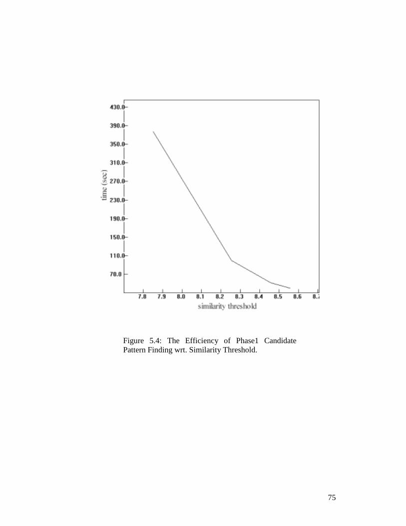
75
Figure 5.4: The Efficiency of Phase1 Candidate Pattern Finding wrt. Similarity Threshold.

76
Support Threshold Sensitivity
Our experiments on the sensitivity of the Phase1 pattern finding to the support
threshold are based on changing the value of support threshold in such way to
influence the ratio of the number of pattern occurrences counted for the pattern
support, to the number of all possible pattern occurrences. This will be explained
below.
Total number of all player trajectories in the semi-random data is:
TotalTraj = NumClips * 12 ,
where NumClips is the number of semi-random video clips.
The number of all possible occurrences of the candidate segment in one
trajectory TotalOccInTraj is:
TotalOccInTraj = TrajLen – k +1 .
Thus, the number of all possible occurrences of a k-length segment is:
TotalOcc = TotalTraj * TotalOccInTraj .
We define a “ratio support parameter” SuppRatio which is related to the total
support threshold with the following formula:
SuppThresh = SuppRatio * TotalOcc * SimThresh .
If we suppose that each occurrence counted for the segment support had the
smallest possible similarity, we could say that with the SuppThresh as the total
support threshold, we can find all segments that occur in at least SuppRatio of all

77
possible occurrence places. For example, if SuppRatio = 3%, we could say that a
frequent segment occurs in at least 3% of all the possible places where it could
possibly occurr. However, since we supposed that each occurrence counted for
the segment support had the smallest possible similarity, we cannot take this
statement literally. But the error caused by higher occurrence similarity is small,
and we disregard it.
Table 5.3 and Figure 5.5 show an experiment where we vary ratio support
threshold.
SUPPORT 3% 2% 1% 0.5% 0.3%
Time (sec) 40.0 52.0 92.0 162.0 232.3
Level 2 365 442 598 767 897
Level 3 48 163 600 1347 2048
Level 4 0 0 0 42 269
Table 5.3: Level Sizes and the Efficiency of Phase1 Candidate Pattern Finding wrt. Support Threshold.

78
Figure 5.5: The Efficiency of Phase1 Candidate Pattern Finding wrt. Support Threshold.

79
Phase1 Efficiency wrt. Data Size
In this experiment, while all parameters are fixed, we change the number of
video clips in the data set. Figure 5.6 shows that the efficiency drops linearly
with the increase of the number of video clips, as we had expected. Since the
ratio support threshold, and all other parameters are fixed, the number of
segments satisfying support threshold remained the same as the number of video
clips was increased. The only change in the efficiency is due to the change in the
efficiency of counting support for each candidate pattern. Therefore, we can
conclude that counting a Phase1 candidate pattern support efficiency drops
linearly with the increase of the number of video clips.

80
Figure 5.6: Phase1 Efficiency wrt. Data Size

81
5.3.2 Phase2 Efficiency
The starting set of items in Phase2 is the set of frequent trajectory segments
found to be patterns in Phase1. We cluster this itemset before the algorithm
starts, with the similarity between two trajectory segments as the clustering
parameter. In Phase2 efficiency tests we use an itemset consisting of 53 cluster
representative segments, 49 of which are of length 3, and 4 of which are of the
length 4.
Item Occurrence Table
Counting candidate pattern support in Phase2 is performed using the Item
Occurrence Table (Chapter 4.4). Before the level generation process starts, we
generate the Item Occurrence Table. The experiments showed that the time
required for the Item Occurrence Table generation is almost constant, for various
data sizes and various support and similarity threshold parameters, as is shown in
Table 5.4 and 5.7. This result is encouraging, proving that the Item Occurrence
Table generation is not too expensive, i.e. it does not explode when changing
parameters.
We have not performed experiments to directly prove and evaluate how
important the Item Occurrence Table is for improving the efficiency of counting
candidate pattern support. However, we can compare the time needed for Phase1
pattern generation, where counting is done directly on trajectory data, with
Phase2 pattern generation, where we use the Item Occurrence Table. We can see
that in various tests, the time needed for the generation of the levels with almost
the same number of elements, is often even higher in Phase1, than in Phase2.
Had we applied the same method for counting candidate support in both phases,

82
we would surely expect Phase2 level generation to be more time consuming,
since its complexity is much higher.
Similarity Threshold Sensitivity
Similarly to the experiments of similarity threshold efficiency in Phase1, we
perform an experiment to test the Phase2 algorithm behavior with respect to the
similarity threshold. Phase2 efficiency proves to be especially sensitive to the
similarity threshold, as it was expected. Namely, as the similarity threshold is
decreased, the number of occurrences for each segment that can be the item in
Phase2 becomes higher. The number of possible occurrences of a pattern, which
have to be searched when finding the pattern support increases with the number
of segment occurrences. Therefore, counting support of each candidate pattern
takes much more time.
The actual results are given in Table 5.4 and Figure 5.7. The table shows
the number of candidate patterns on each level, preprocessing time, and the time
for the pattern generation, while similarity threshold takes different values.

83
SIMILARITY 8.65 8.60 8.55 8.52 8.50 8.45
Time without preprocessing (sec) 2.9 7.2 21.0 39.4 67.9 376.0
Preprocessing time (sec) (IOccurTable generation)
15.9 15.9 16.0 16.2 16.1 16.4
Level 2 144 213 280 327 364 478
Level 3 141 447 1231 1949 2507 4230
Level 4 0 0 15 200 844 6961
Level 5 0 0 0 0 0 3
Table 5.4: Level Sizes and the Efficiency of Phase2 Candidate Pattern Finding wrt. Similarity Threshold.
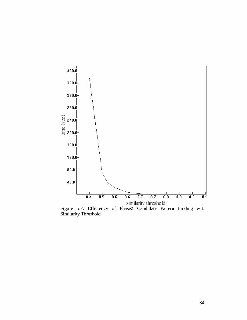
84
Figure 5.7: Efficiency of Phase2 Candidate Pattern Finding wrt. Similarity Threshold.

85
Support Threshold Sensitivity
We define the ratio support threshold parameter in Phase2 as the ratio of the
number of video clips where the pattern occurs to the total number of video clips.
The actual support threshold will be as follows:
SuppThresh = SuppRatio * VideoClipNum * SimThresh
SimThresh is the similarity threshold of a segment (an item) occurrence. In our
experiments it is the same as the occurrence degree support.
Table 5.5 and Figure 5.8 show the level sizes and the efficiency of the
pattern finding in Phase2 as the support threshold changes. It also shows that
preprocessing time, which depends on the generation of the Item Occurrence
Table is constant. The efficiency only depends on the number of elements on
each level (which is equivalent to the number of candidate patterns whose
support needs to be counted). Figure 5.8 also shows the performance of the semi-
naïve algorithm, while all algorithm parameters are the same.
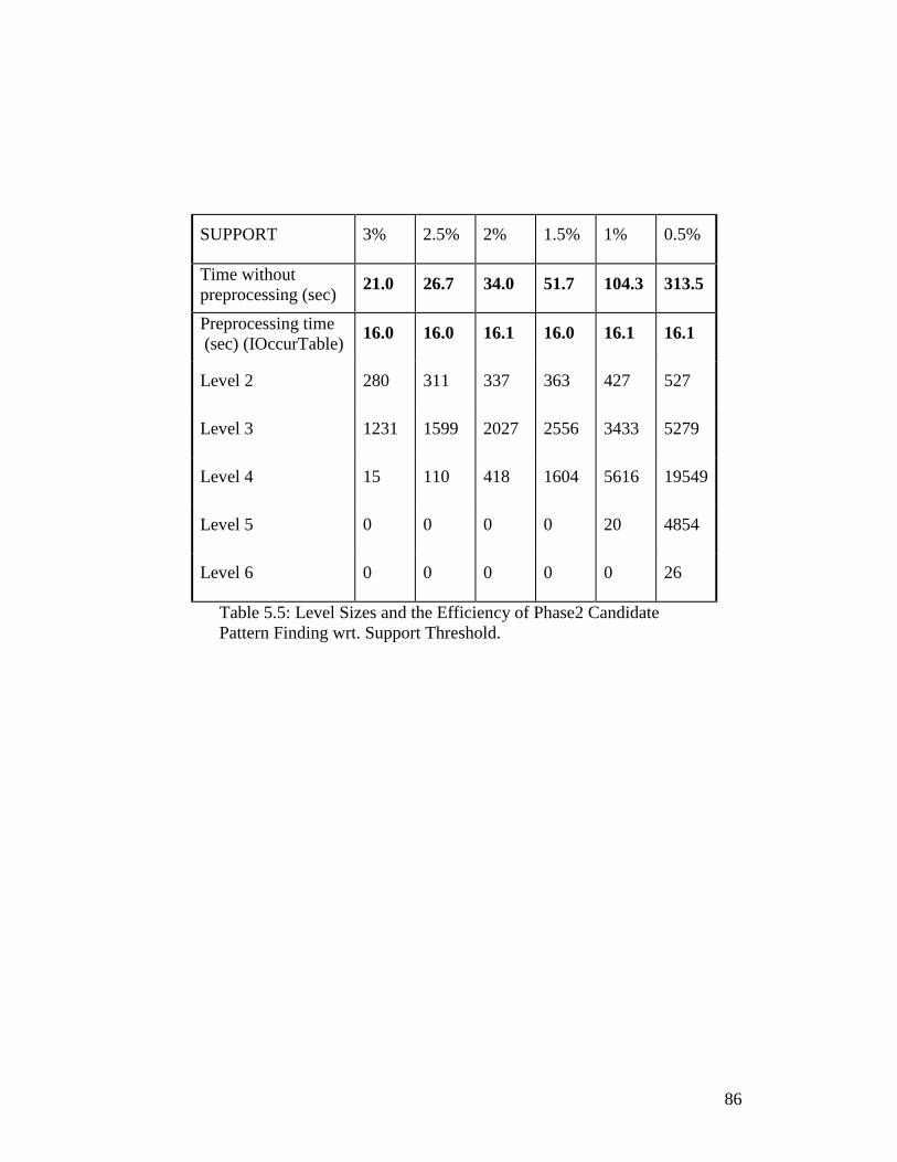
86
SUPPORT 3% 2.5% 2% 1.5% 1% 0.5%
Time without preprocessing (sec) 21.0 26.7 34.0 51.7 104.3 313.5
Preprocessing time (sec) (IOccurTable) 16.0 16.0 16.1 16.0 16.1 16.1
Level 2 280 311 337 363 427 527
Level 3 1231 1599 2027 2556 3433 5279
Level 4 15 110 418 1604 5616 19549
Level 5 0 0 0 0 20 4854
Level 6 0 0 0 0 0 26
Table 5.5: Level Sizes and the Efficiency of Phase2 Candidate Pattern Finding wrt. Support Threshold.

87
Figure 5.8: Efficiency of Phase2 Candidate Pattern Finding wrt. Support Threshold.
Algorithm Performance with respect to Data Size
Similarly to the experiments for the Phase1 efficiency with respect to data size,
we fix all parameters except for the number of video clips in the data set. As in
the Phase1, the efficiency changes linearly as the number of video clip increases,

88
which is shown in Figure 5.9. All parameters are fixed, and the level sizes are
almost the same for all numbers of video clips. The only change in the efficiency
is due to the change in the efficiency of counting support for each candidate
pattern. Therefore, we can conclude that counting a Phase2 candidate pattern
support efficiency drops linearly with the increase of the number of video clips.
Figure 5.9 also shows the efficiency performance of the semi-naïve algorithm,
while the algorithm parameters are the same.
Figure 5.9: Efficiency of Phase2 Candidate Pattern Finding wrt. Data Size.
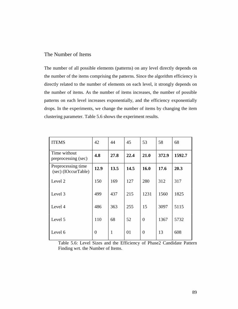
89
The Number of Items
The number of all possible elements (patterns) on any level directly depends on
the number of the items comprising the patterns. Since the algorithm efficiency is
directly related to the number of elements on each level, it strongly depends on
the number of items. As the number of items increases, the number of possible
patterns on each level increases exponentially, and the efficiency exponentially
drops. In the experiments, we change the number of items by changing the item
clustering parameter. Table 5.6 shows the experiment results.
ITEMS 42 44 45 53 58 68
Time without preprocessing (sec) 4.8 27.8 22.4 21.0 372.9 1592.7
Preprocessing time (sec) (IOccurTable) 12.9 13.5 14.5 16.0 17.6 20.3
Level 2 150 169 127 280 312 317
Level 3 499 437 215 1231 1560 1825
Level 4 486 363 255 15 3097 5115
Level 5 110 68 52 0 1367 5732
Level 6 0 1 01 0 13 608
Table 5.6: Level Sizes and the Efficiency of Phase2 Candidate Pattern Finding wrt. the Number of Items.
90
5.4 Summary
We have shown the effectiveness of the frequent trajectory segment (Phase1
pattern) finding method, and at the same time proved the appropriateness of the
trajectory similarity measure we used. The Phase2 pattern finding algorithm
successfully finds the frequently co-occurring segments, whose occurrences
satisfy additional constraints. However, in order to check how meaningful the
found Phase2 patterns are, a larger amount of real life data is required, and it will
be left for the future work.
We performed the tests to compare the efficiency of the apriori pruning
pattern finding algorithm we used, to a semi naïve algorithm, and hence show the
importance of the apriori pruning. For various data size, and support threshold
parameters, the original algorithm always outperforms the semi-naïve one. In our
tests where the number of items was fixed, the efficiency of the semi-naïve
algorithm was 4 times less than of the original one.
In the tests on the algorithm sensitivity to changing similarity and support
threshold, the performance of the algorithm in both phases drops with the
increase of similarity threshold, and with the decrease of support threshold. As
we had expected, Phase2 algorithm proves to be much more sensitive to the
similarity threshold than to the support threshold, and its efficiency drops
exponentially with small decrease of the similarity threshold.
When we change data size (the number of clips), while keeping the same
values for all parameter, the algorithm efficiency in both Phase1 and Phase2
drops only linearly. However, when we increase the number of possible items
that the patterns can contain, the efficiency drops exponentially, because the
number of possible candidate patterns exponentially increases with the number of
items.
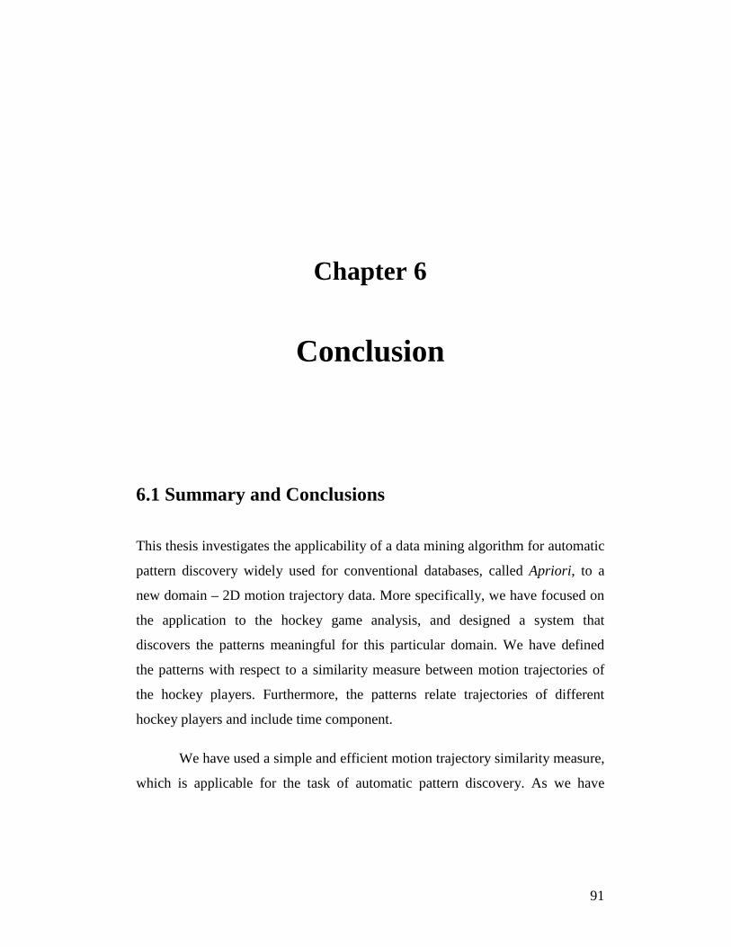
91
Chapter 6
Conclusion
6.1 Summary and Conclusions
This thesis investigates the applicability of a data mining algorithm for automatic
pattern discovery widely used for conventional databases, called Apriori, to a
new domain – 2D motion trajectory data. More specifically, we have focused on
the application to the hockey game analysis, and designed a system that
discovers the patterns meaningful for this particular domain. We have defined
the patterns with respect to a similarity measure between motion trajectories of
the hockey players. Furthermore, the patterns relate trajectories of different
hockey players and include time component.
We have used a simple and efficient motion trajectory similarity measure,
which is applicable for the task of automatic pattern discovery. As we have

92
proved, when the patterns are defined using the chosen similarity measure, the
proposed Apriori-like pattern finding algorithm is sound and complete.
We have implemented the pattern finding algorithm, using efficient data
structures, index tables and iterators. Our experiments showed that pattern
generation takes insignificant time comparing to counting of the pattern support,
which is expected for the algorithms based on the Apriori framework, and proves
that our implementation is optimized.
In order to test the effectiveness and efficiency of the proposed hockey
player trajectory pattern finding method, we have performed a series of
experiments. The effectiveness tests were performed on a real life data set
consisting of a collection of hockey video clips. Continuous trajectory segments,
which the algorithm determined to be frequent, and to be the part of the patterns
we are looking for, were usually in accordance with our expectation according to
the knowledge about hockey player movement. That proves the right choice of
the motion trajectory similarity measure, and the validity of the algorithm.
However, some more profound tests, which would possibly confirm that the final
patterns are indeed meaningful, i.e., in accordance with the actual hockey game
strategy, are left for the future work, since they require a much larger real life
data set.
We have tested the efficiency of the algorithm on a semi-randomly
generated data set. The experiments proved that the efficiency heavily depends
on similarity and support threshold parameters, and on the starting number of
items from which the patterns are built, which can cause the algorithm
performance to drop exponentially. However, the algorithm behaves very well
with the increase of the data size. Namely, the algorithm efficiency drops only

93
linearly with the increase of the number of video clips in the data collection. We
have also illustrated the importance of using the Apriori algorithm, by comparing
it to a semi-naïve algorithm, which was outperformed by the original algorithm
for various choices of parameters and data sizes.
6.2 Future Work
The work presented in this thesis is the first attempt to use the Apriori framework
as the data mining algorithm for the pattern finding in the domain of 2D motion
trajectories. There is a wide choice of directions to which the future work can go,
which we will briefly discuss below.
6.2.1 More Sophisticated Similarity Measures
There are many possibilities to improve the effectiveness of the pattern finding
method by choosing more sophisticated similarity measures.
One obvious improvement may be to employ a motion trajectory
representation and possibly a more sophisticated similarity measure that also
takes into account another important attribute of motion - the trajectory speed.
Furthermore, it may not be desirable for the similarity measure used for
the particular domain of the hockey player game analysis to be absolutely
insensitive to translation and rotation. For example, it may depend on the
position in the rink where the trajectories are located, such as the proximity to the
goal, or to the edges of the rink. It may even take into account the direction of
motion, such as if it is towards or away from the goal. Furthermore, similarity
between two sets of player trajectories could take into account the players’

94
position with respect to each other, such as their distance to each other, or if their
direction of motion is towards or away from each other.
Additionally, it may prove successful to use a more sophisticated
technique for smoothing trajectories, and for the feature point extraction. The
way feature points are extracted from the trajectories strongly influences the
performance of the similarity function, and hence the meaningfulness of the
resulting patterns.
6.2.2 Further Experiments
One step of the future work would be to experiment on a larger real life data set.
That would be especially important for testing the meaningfulness of Phase2
patterns, which relate different players. The resulting patterns should be in
accordance with the game strategy, the role of the players, and should reflect
some frequent actions, collaboration of the players of one team, or correlation of
the players in opposing teams. We expect that in the future the automatic
tracking system will be enhanced and possibly will enable tracking of the
position of the puck, distinguishing the player names, and allow even more
efficient data processing. That would give us possibility for testing on a larger
data set, as well as discovering pattern with more content, such as including the
player possession of the puck, player roles, or names.
6.2.3 Integration with a Database System
There is an ongoing work on integrating the hockey tracking system, pattern
discovery process and a database system for storing and retrieving video clip
collection. The idea is to integrate the whole hockey game analysis process,

95
starting from the data acquirement (digitizing and processing video clips to
extract the player trajectories), through selecting a certain subset of the video
collection according to the user query, and finding the patterns within the
selected collection. Since the hockey tracking system is semi-automatic, user
involvement is required, and there is a user-friendly graphical interface for using
the tracking system. After the video clips are processed, and the player
trajectories in the rink coordinates found, they are stored in the database. From
the database, a user can select video clips that satisfy certain conditions, such as
containing a certain player, a certain hockey team, or have been shot at a certain
date interval. Finally, the pattern finding algorithm is applied to the chosen
subset, and the resulting patterns are output.
6.2.4 Association Rules
After the patterns are identified, the next step is to find association rules
pertaining to the patterns. While the meaning of the patterns is “co-occurrence”,
association rules may also have a predictive component. For example, an
association rule may be: “When player P1 does an action A1, there is 10%
chance that player P2 will do an action A2”. There are various measures for the
association, or correlation between the first and second part of the rule, some of
them having a stronger predictive component, or pertaining to a causal
relationship. It would be interesting to employ some of them, and extend the
patterns we detect to association rules. In that way a predictive component would
be added to our hockey game pattern discovery.

96
Bibliography
[ACCES96] S. Adali, K.S. Candan, S. Chen, K. Erol. and Subrahmanian, V. (1996). The
Advanced Video Information System: data structures and query processing. Multimedia
Systems, 4:172 -- 186.
[AC99] Wai-Ho Au, K.C.C Chan, FARM: a data mining system for discovering fuzzy
association rules, Fuzzy Systems Conference Proceedings, FUZZ-IEEE '99. IEEE
International Volume: 3 , 1999 , Page(s): 1217 –1222.
[AFS93] R. Agrawal, C. Faloutsos, and A. Swami, Efficient similarity search in sequence
databases. In The fourth International Conference on Foundations of Data Organization
and Algorithms, Evanston, Illinois, October 1993.
[AIS93] R. Agrawal, T. Imielinski, and A. Swami. Mining association rules between sets
of items in large databases. In Proceedings of ACM SIGMOD Conference on
Management of Data (SIGMOD'93), pages 207 216, May 1993.
[ALS95] R.Agrawal, K.Lin, H.S.Sawhney, K.Shim, Fast similarity search in the presence
of noise, scaling and translation in time-series databases, VLDB 1995.
[AS95] R. Agrawal and R. Srikant. Mining sequential patterns. In ICDE, Taipei, Taiwan,
Mar. 1995.
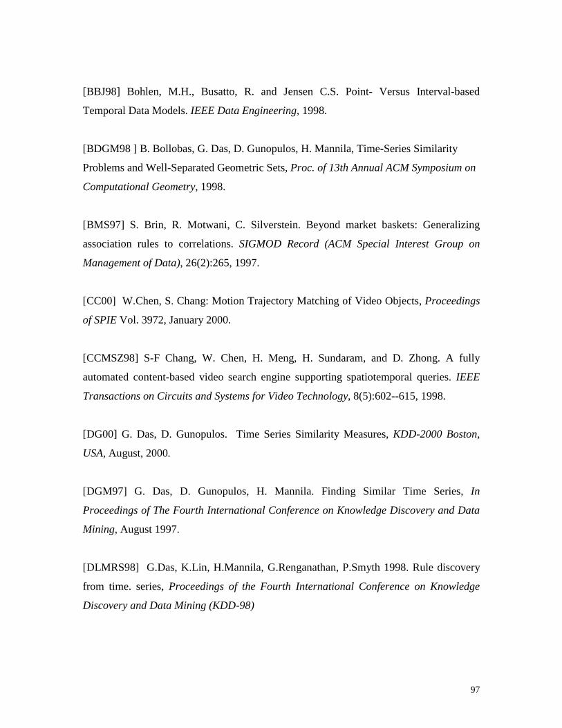
97
[BBJ98] Bohlen, M.H., Busatto, R. and Jensen C.S. Point- Versus Interval-based
Temporal Data Models. IEEE Data Engineering, 1998.
[BDGM98 ] B. Bollobas, G. Das, D. Gunopulos, H. Mannila, Time-Series Similarity
Problems and Well-Separated Geometric Sets, Proc. of 13th Annual ACM Symposium on
Computational Geometry, 1998.
[BMS97] S. Brin, R. Motwani, C. Silverstein. Beyond market baskets: Generalizing
association rules to correlations. SIGMOD Record (ACM Special Interest Group on
Management of Data), 26(2):265, 1997.
[CC00] W.Chen, S. Chang: Motion Trajectory Matching of Video Objects, Proceedings
of SPIE Vol. 3972, January 2000.
[CCMSZ98] S-F Chang, W. Chen, H. Meng, H. Sundaram, and D. Zhong. A fully
automated content-based video search engine supporting spatiotemporal queries. IEEE
Transactions on Circuits and Systems for Video Technology, 8(5):602--615, 1998.
[DG00] G. Das, D. Gunopulos. Time Series Similarity Measures, KDD-2000 Boston,
USA, August, 2000.
[DGM97] G. Das, D. Gunopulos, H. Mannila. Finding Similar Time Series, In
Proceedings of The Fourth International Conference on Knowledge Discovery and Data
Mining, August 1997.
[DLMRS98] G.Das, K.Lin, H.Mannila, G.Renganathan, P.Smyth 1998. Rule discovery
from time. series, Proceedings of the Fourth International Conference on Knowledge
Discovery and Data Mining (KDD-98)

98
[FPSM92] W. Frawley and G. Piatetsky-Shapiro and C. Matheus, Knowledge Discovery
in Databases: An Overview. AI Magazine, Fall 1992, pg 213-228.
[Fu98] Ada Wai-Chee Fu, Man Hong Wong, Siu Chun Sze, Wai Chiu Wong, Wai Lun
Wong, and Wing Kwan Yu. Finding fuzzy sets for the mining of fuzzy association rules
for numerical attributes. In Proceedings of 1 st Intl. Symposium on Intelligent Data
Engineering and Learning (IDEAL'98), pages 263--268, October 1998.
[Gu99] Zhe Gu, Video Database Retrieval based on Trajectory Analysis, Master Thesis,
1999.
[HGN00] J. Hipp, U. Guntzer, and G. Nakaeizadeh. Algorithms for Association Rule
Mining - A General Survey and Comparison. In Proc. ACM SIGKDD International
Conference on Knowledge Discovery and Data Mining, 2000.
[HZ96] S. Hagit, S. Zdonik. Approximate queries and representations for large data
sequences. Proc. 12th IEEE International Conference on Data Engineering. pp 546-553,
New Orleans, Lousiana, February 1996.
[JLTrack] Rafal Jaroskiewicz, Jim Little, The Hockey Tracking System, developed at
Department of Computer Science, University of British Columbia, 2000.
[KFW98] C.M.Kuok, A.Fu and M.H.Wong. Fuzzy association rules in large dabases with
quantitative attributes. In ACM SIGMOID Records, March, 1998.
[KPC01] Kim S.W., Park, S., Chu, W.W., An Index-Based Approach for Similarity
Search Supporting Time Warping in Large Sequence Databases, ICDE, 2001.
[KP98] E. Keogh, M. Pazzani, An enhanced representation of time series which allows
fast and accurate classification, clustering and relevance feedback, Knowledge Discovery
and Data Mining, 1998.

99
[LG01] James J. Little, Zhe Gu, Video Retrieval by Spatial and Temporal Structure of
Trajectories, SPIE Storage and Retrieval for Media Databases 2001, San Jose.
[NLHP98] R. Ng, L.V. Lakshmanan, J. Han, A. Pang. Exploratory Mining and Pruning
Optimizations of Constrained Association Rules, Proc. 1998 ACMSIGMOD Int. Conf.
Management of Data, pages 13--24, Seattle, Washington, June 1998.
[O99] T. Oates. Identifying Distinctive Subsequences in Multivariate Time Series by
Clustering, Knowledge Discovery and Data Mining, 1999.
[RMS98] S. Ramaswamy, S. Mahajan, and A. Silberschatz. On the discovery of
interesting patterns in association rules. In Proc. 1998 Int. Conf. Very Large Data Bases,
pages 368--379, New York, NY, August 1998.
[VHTM99] R.Villafane, K.A.Hua, D.Tram, B.Maulik. Mining Interval Time Series, Data
Warehousing and Knowledge Discovery, 1999.