Minimum-Phase & All-Pass Filters - Multimedia Signal · PDF file · 2017-01-20Minimum-Phase & All-Pass Filters ... =Gz −n0 M ∏ k=1 (1−z kz ... The area under the group delay

Minimum-Phase & All-Pass Filters

Peter Kabal

Department of Electrical & Computer EngineeringMcGill UniversityMontreal, Canada

Version 2.1 March 2011

c© 2011 Peter Kabal

2011/03/11

You are free:

to Share – to copy, distribute and transmit this work

to Remix – to adapt this work

Subject to conditions outlined in the license.

This work is licensed under the Creative Commons Attribution 3.0 UnportedLicense. To view a copy of this license, visit http://creativecommons.org/licenses/by/3.0/ or send a letter to Creative Commons, 171 SecondStreet, Suite 300, San Francisco, California, 94105, USA.

Revision History:

• 2011-03 v2.1: Creative Commons licence, minor updates (simplifications)

• 2010-01 v2.0: New material on min-phase & all-pass filters

• 2007-11 v1.6: Initial release

Minimum-Phase & All-Pass Filters 1

1 Introduction

This report examines the properties of minimum-phase and all-pass filters. The analysis deals

with the case of complex filter coefficients. This strategy simplifies the analysis since we will be

able to express general filters as the cascade of first order filters sections. We will be interested

in the amplitude, phase, and group delay responses of these filters. Of particular interest will be

filters which have a response described by a rational z-transform,

H(z) =B(z)

A(z)

= Gz−n0

M

∏k=1

(1 − zkz−1)

N

∏k=1

(1 − pkz−1)

= Gz−n0

M

∏k=1

(1 − rkejθk z−1)

N

∏k=1

(1 − ρkejφk z−1)

,

(1)

where in the last part of the equation the zeros have been expressed as zk = rkejθk and the poles as

pk = ρkejφk .

1.1 Amplitude Response

The magnitude-squared response of a filter H(z) can be evaluated from the z-transform as

|H(ω)|2 = H(ω)H∗(ω)

= H(z)H∗(1/z∗)|z=e jω .(2)

The z-transform relationship for the second term can be seen to result in

H∗(1/z∗) =∞

∑n=−∞

h∗nzn. (3)

The double conjugation (once on z and again on H(·)) has the effect of leaving the zn terms uncon-

jugated. Only the coefficients are conjugated. The response H∗(1/z∗) has an expansion in positive

powers of z, i.e. the time response is flipped about n = 0.


For the rational transform of Eq. (1), the magnitude-squared response is

|H(ω)|2 = |G|2

M

∏k=1

(1 − zkz−1)(1 − z∗k z)

N

∏k=1

(1 − pkz−1)(1 − p∗k z)

∣∣∣∣∣∣∣∣∣∣z=e jω

= |G|2

M

∏k=1

(1 − 2Re[zke−jω] + |zk|2)

N

∏k=1

(1 − 2Re[pke−jω] + |pk|2)

= |G|2

M

∏k=1

(1 − 2rk cos(ω − θk) + r2k)

N

∏k=1

(1 − 2ρk cos(ω − φk) + ρ2k)

.

(4)

The frequency dependent terms in the magnitude-squared response are sin ω and cos ω. For a

system with real coefficients, the magnitude-squared response is symmetrical about ω = 0 and

can be expressed as a ratio of polynomials in cos ω.

1.2 Phase Response

The phase response of a filter with frequency response H(ω) is1

arg[H(ω)] = tan−1

(HI(ω)

HR(ω)

), (5)

where HR(ω) and HI(ω) are the real and imaginary parts of the frequency response, respectively.

For the rational response given by Eq. (1), the phase response is

arg[H(ω)] = arg[G]− n0ω +M

∑k=1

tan−1

(−Im[zke−jω]

1 − Re[zke−jω]

)−

N

∑k=1

tan−1

(−Im[pke−jω]

1 − Re[pke−jω ]

)

= arg[G]− n0ω +M

∑k=1

tan−1

(rk sin(ω − θk)

1 − rk cos(ω − θk)

)−

N

∑k=1

tan−1

(ρk sin(ω − φk)

1 − ρk cos(ω − φk)

).

(6)

For a system with real coefficients, the phase response is anti-symmetrical about ω = 0.

1Some authors define the phase with a negative sign. Here, we will refer to the negative of the phase as the phase lag.


1.3 Group Delay Response

The group delay response is the negative derivative of the phase response2

τg(ω) = −d arg[H(ω)]

dω

=HI(ω)

dHR(ω)

dω− HR(ω)

dHI(ω)

dωH2

R(ω) + H2I (ω)

.

(7)

A more compact form of the same result is

τg(ω) = −Im

[dH(ω)/dω

H(ω)

]. (8)

Since the group delay is the derivative of the phase lag, the area under the group delay curve over

a frequency interval of 2π is equal to the change in the phase lag over the same interval.

Consider the group delay for just one of the terms in the numerator of the rational response

given in Eq. (1),3

τ(zk)g (ω) =

|zk|2 − Re[zke−jω]

1 − 2Re[zke−jω] + |zk|2

=r2

k − rk cos(ω − θk)

1 − 2rk cos(ω − θk) + r2k

.

(9)

The overall group delay for the rational transfer function is

τg(ω) = no +M

∑k=1

|zk|2 − Re[zke−jω]

1 − 2Re[zke−jω] + |zk|2−

N

∑k=1

|pk|2 − Re[pke−jω ]

1 − 2Re[pke−jω ] + |pk|2

= no +M

∑k=1

r2k − rk cos(ω − θk)


−N

∑k=1

ρ2k − ρk cos(ω − φk)

1 − 2ρk cos(ω − φk) + ρ2k

.

(10)

The group delay response has terms in sin ω and cos ω. For a system with real coefficients, the

group delay response is symmetrical about ω = 0 and can be expressed as a ratio of polynomials in

cos ω. As a ratio of polynomials, the group delay is often better behaved than the phase response

– the phase response can have phase jumps and ambiguities of multiples of 2π. Thus it may be

preferable to characterize a system or filter by the group delay response rather than the phase

2The derivation of the expression for the group delay response uses the identity d tan−1(y/x)/du = (x dy/du −y dx/du)/(x2 + y2).

3The result uses the relations dRe[zke−jω]/dω = Im[zke−jω] and dIm[zke−jω]/dω = −Re[zke−jω].


response.

1.4 Example

As an example, consider the filter H(z) = 1 − z−1. This is just the case in which there is a single

zero in Eq. (1),

H(ω) = 1 − e−jω

= 2je−jω/2 sin(ω/2).(11)

The amplitude response is 2| sin(ω/2)|, which has a discontinuous derivative at ω = 0. From

Eq. (4), the magnitude-squared response is

|H(ω)|2 = 2(1 − cos ω). (12)

This is a polynomial in cos ω.

The phase response of this filter is (from Eq. (6))

arg[H(ω)] = tan−1

(sin ω

1 − cos ω

). (13)

The phase response is π/2 for ω = 0+ and is −π/2 for ω = 0−. There is a phase jump of size π at

ω = 0. Directly from Eq. (11), we can see that the phase can also be written as

arg[H(ω)] = π/2 − ω/2 + arg[sin(ω/2)]. (14)

In this form, the linear trend in the phase is clear. The last term gives a phase jump of ±π at ω = 0.

For this same example, the group delay evaluates to

τg(ω) =1

2

1 − cos ω

1 − cos ω. (15)

The group delay is well behaved and is equal to 1/2 sample everywhere, including at ω = 0 (as

shown by invoking L’Hopital’s rule twice). The area under the group delay curve (over 2π) is

equal to π.

2 Causal Stable Filters

For the sequel, we consider causal stable filters with rational z-transforms. The poles of these

filters must lie inside the unit circle. The positions of the zeros, however, can lie inside or outside

the unit circle.


We will work with a simplified version of the rational function H(z) in Eq. (1),

H(z) =B(z)

A(z)

=

b0

M

∏k=1

(1 − zkz−1)

A(z).

(16)

We have set the delay factor n0 which appeared in Eq. (1) to zero.4

2.1 Systems with the Same Magnitude Response

Consider the zero at zk corresponding to a root factor (1− zkz−1) in the expansion of the numerator

polynomial B(z). Then H∗(1/z∗) which appears in the expression Eq. (2) for the magnitude-

squared response has a root factor (1 − z∗k z) in its numerator corresponding to a zero at 1/z∗k , i.e.

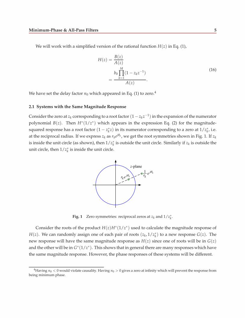
at the reciprocal radius. If we express zk as rkejθk , we get the root symmetries shown in Fig. 1. If zk

is inside the unit circle (as shown), then 1/z∗k is outside the unit circle. Similarly if zk is outside the

unit circle, then 1/z∗k is inside the unit circle.

kjkr e

1 kj

ker

Fig. 1 Zero symmetries: reciprocal zeros at zk and 1/z∗k .

Consider the roots of the product H(z)H∗(1/z∗) used to calculate the magnitude response of

H(z). We can randomly assign one of each pair of roots (zk, 1/z∗k ) to a new response G(z). The

new response will have the same magnitude response as H(z) since one of roots will be in G(z)

and the other will be in G∗(1/z∗). This shows that in general there are many responses which have

the same magnitude response. However, the phase responses of these systems will be different.

4Having n0 < 0 would violate causality. Having n0 > 0 gives a zero at infinity which will prevent the response frombeing minimum phase.


3 Minimum-Phase Systems

A causal stable filter is said to minimum-phase if all of its zeros are inside the unit circle. A maximum-

phase system has all of its zeros outside the unit circle. A system with a zero on the unit circle is

not strictly minimum-phase.

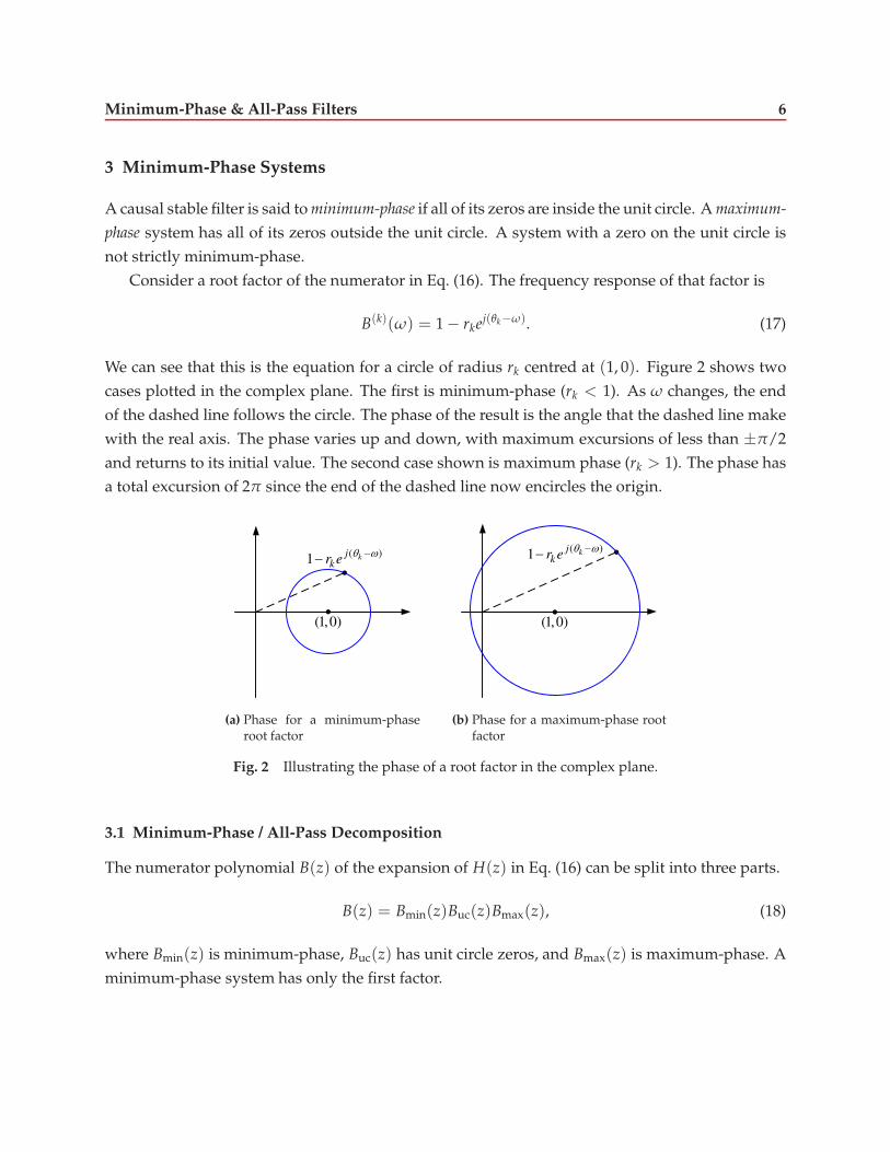
Consider a root factor of the numerator in Eq. (16). The frequency response of that factor is

B(k)(ω) = 1 − rkej(θk−ω). (17)

We can see that this is the equation for a circle of radius rk centred at (1, 0). Figure 2 shows two

cases plotted in the complex plane. The first is minimum-phase (rk < 1). As ω changes, the end

of the dashed line follows the circle. The phase of the result is the angle that the dashed line make

with the real axis. The phase varies up and down, with maximum excursions of less than ±π/2

and returns to its initial value. The second case shown is maximum phase (rk > 1). The phase has

a total excursion of 2π since the end of the dashed line now encircles the origin.

( )1 kj

kr e

(1,0)

(a) Phase for a minimum-phaseroot factor

( )1 kj

kr e

(1,0)

(b) Phase for a maximum-phase rootfactor

Fig. 2 Illustrating the phase of a root factor in the complex plane.

3.1 Minimum-Phase / All-Pass Decomposition

The numerator polynomial B(z) of the expansion of H(z) in Eq. (16) can be split into three parts.

B(z) = Bmin(z)Buc(z)Bmax(z), (18)

where Bmin(z) is minimum-phase, Buc(z) has unit circle zeros, and Bmax(z) is maximum-phase. A

minimum-phase system has only the first factor.


Let the maximum-phase term be written as

Bmax(z) = β0

K

∏k=1

(1 − βkz−1). (19)

Since this term is maximum phase, |βk| > 1 for k = 1, . . . , K. Now write Bmax(z) as

Bmax(z) = z−KB∗max(1/z∗)

Bmax(z)

z−KB∗max(1/z∗)

= Gmin(z)Gall(z).

(20)

The first term Gmin(z) is minimum-phase. The delay factor z−K shifts this term to make the corre-

sponding time response causal. The second term Gall(z) is all-pass. It has a constant magnitude

response equal to unity. This can be seen from Eq. (2) by evaluating

Gall(z)G∗all(1/z∗) = 1 for all z. (21)

The all-pass filter can be written as

Gall(z) =β0

β∗0

K

∏k=1

1 − βkz−1

z−1(1 − β∗k z)

. (22)

This is a stable causal IIR filter – the denominator has roots inside the unit circle. The all-pass filter

is maximum phase.

Based on the decomposition of Eq. (18), we can express any causal stable filter H(z) as the

product of a minimum-phase filter, a filter with unit circle zeros, and an all-pass filter,

H(z) = Hmin(z)Buc(z)Gall(z). (23)

By this construction Hmin(z) can be written as

Hmin(z) =Bmin(z) z−K B∗

max(1/z∗)

A(z). (24)

4 All-Pass Filters

An all-pass filter is a filter for which the magnitude of the frequency response is constant. All-

pass filters, except for trivial filters, are IIR. For the sequel, we set the magnitude of the frequency

response to unity. Start with the simplest non-trivial all-pass filter, which can form one section of


a causal, stable all-pass filter,

H(k)all (z) =

z−1 − α∗k

1 − αkz−1. (25)

Here we have expressed the all-pass filter in terms of its pole location αk. In this form, |αk| < 1.

A general all-pass filter can be formed as the cascade of all-pass sections

Hall(z) =K

∏k=1

z−1 − α∗k

1 − αkz−1. (26)

If the all-pass filter has real coefficients, then for each complex root αk, there must be a correspond-

ing conjugate root α∗k .

From Eq. (26) we can see that an all-pass filter is characterized by having a numerator polyno-

mial which has the coefficients of the denominator polynomial, conjugated and in reverse order,

Hall(z) =z−KD∗(1/z∗)

D(z). (27)

Then from Eq. (2), we see that any filter of this form has constant magnitude

|Hall(ω)|2 = 1. (28)

4.1 Phase Response of an All-Pass Filter

If αk is expressed as rkejθk , the phase response for an all-pass section is

arg[H(k)all (ω)] = arg[e−jω − α∗

k ]− arg[1 − αke−jω)]

= arg[e−jω ] + arg[1 − α∗k ejω]− arg[1 − αke−jω]

= −ω − 2 tan−1

(rk sin(ω − θk)


) (29)

The denominator inside the tan−1(·) function is positive for rk < 1 (corresponding to a stable,

causal all-pass filter). The numerator can change sign, and so the phase contribution due to the

tan−1(·) function is limited to ±π/2 (and 2 tan−1(·) is limited to ±π). The tan−1(·) function

contributes an oscillation around the linear phase term – the phase is monotonic downward (as

shown in the discussion of the group delay response which follows). The phase response for each

all-pass section decreases by 2π as ω increases by 2π.

The phase response for the overall filter is the sum of the phases for each section. Thus the


overall phase is monotonic downward and decreases by 2πK as ω increases by 2π.

arg[Hall(ω)] = −Kω − 2K

∑k=1

tan−1

(rk sin(ω − θk)


)(30)

For an all-pass section, real roots have θk = 0, or θk = ±π. For an overall all-pass filter with

real coefficients, for each section with a complex root, there is another section with the conjugate

root. These complex conjugate pairs of roots conspire to make the phase anti-symmetrical about

ω = 0 and result in an overall filter with real coefficients.

4.2 Group Delay Response of an All-Pass Filter

The group delay of the all-pass filter can be determined from Eq. (30),

τg(ω) = K + 2K

∑k=1

rk cos(ω − θk)− r2k


=K

∑k=1

1 − r2k


(31)

In the second expression, we see that for rk < 1, the group delay for an all-pass filter is the ratio

of positive quantities and hence is always positive. The denominator of the group delay response

for a filter section has a minimum at ω = θk, contributing a peak in the group delay response of

that section at that frequency.

Positivity of the group delay means that the phase is monotonically moving downward as a

function of frequency. Since the phase decreases by 2πK as ω advances by 2π, the area under the

group delay curve for a frequency interval spanning 2π is 2πK. This same result can be stated as:

the average group delay of an all-pass filter is K samples. Noting this, each term in the sum in the

first line of Eq. (31) must have an average value of zero.

4.3 Magnitude System Response of an All-Pass Filter

We already know that an all-pass filter has a frequency response which is constant in magnitude.

As a generalization of this result, consider the magnitude of Hall(z) where z is not necessarily on

the unit circle. This response is the product of first order responses as shown in Eq. (26). The


magnitude-squared of each first-order section is

|H(k)all (z)|

2 =1 − 2Re[α∗

k z] + |αk|2|z|2

|z|2 − 2Re[α∗k z] + |αk|

2

=

> 1, |z| > 1,

1, |z| = 1,

< 1, |z| < 1.

(32)

The overall filter then also obeys these inequalities,

|Hall(z)|2 =

> 1, |z| > 1,

1, |z| = 1,

< 1, |z| < 1.

(33)

We note that the magnitude system response is constant for z on the unit circle. The magnitude

system response is not constant for z on a circle with non-unity radius.

The magnitude calculated above is that of Hall(z)H∗all(z). Earlier in Eq. (21) we found that for

an all-pass filter Hall(z)H∗all(1/z∗) = 1 for all z. The two expressions agree for |z| = 1.

4.4 Impulse Response of an All-Pass Filter

From Eq. (26), we can use the initial value theorem5 to find the first term in the impulse response

of an all-pass filter,

hall[0] =K

∏k=1

(−α∗k ). (34)

Since the roots αk are all less than one in magnitude, |hall[0]| < 1.

4.5 All-Pass Filter Structure

We have seen in Eq. (27) that an all-pass filter has a numerator polynomial that has conjugate

reversed coefficients from the denominator polynomial. An example of a second order all-pass

section using the minimum number of multiplies is shown in Fig. 3. This filter structure uses only

two coefficients and two delays. For any c1 and c2 resulting in a stable filter, the structure gives an

5For a causal system, h[0] = limz→∞

H(z).


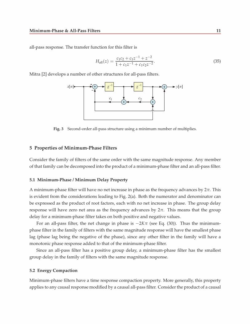
all-pass response. The transfer function for this filter is

Hall(z) =c1c2 + c1z−1 + z−2

1 + c1z−1 + c1c2z−2. (35)

Mitra [2] develops a number of other structures for all-pass filters.

1z

1z

1c 2c

[ ]x n [ ]y n

Fig. 3 Second-order all-pass structure using a minimum number of multiplies.

5 Properties of Minimum-Phase Filters

Consider the family of filters of the same order with the same magnitude response. Any member

of that family can be decomposed into the product of a minimum-phase filter and an all-pass filter.

5.1 Minimum-Phase / Minimum Delay Property

A minimum-phase filter will have no net increase in phase as the frequency advances by 2π. This

is evident from the considerations leading to Fig. 2(a). Both the numerator and denominator can

be expressed as the product of root factors, each with no net increase in phase. The group delay

response will have zero net area as the frequency advances by 2π. This means that the group

delay for a minimum-phase filter takes on both positive and negative values.

For an all-pass filter, the net change in phase is −2Kπ (see Eq. (30)). Thus the minimum-

phase filter in the family of filters with the same magnitude response will have the smallest phase

lag (phase lag being the negative of the phase), since any other filter in the family will have a

monotonic phase response added to that of the minimum-phase filter.

Since an all-pass filter has a positive group delay, a minimum-phase filter has the smallest

group delay in the family of filters with the same magnitude response.

5.2 Energy Compaction

Minimum-phase filters have a time response compaction property. More generally, this property

applies to any causal response modified by a causal all-pass filter. Consider the product of a causal


filter P(z) and a causal all-pass filter Gall(z),

H(z) = P(z)Gall(z), (36)

where P(z) has impulse response p[n] and Gall(z) has impulse response gall[n]. We will assume

that the gain of the all-pass filter is unity, i.e. G = 1.

Parseval’s relationship shows that the total energy of the output signal can be calculated in

either the time domain or the frequency domain,

ε =∞

∑n=0

|h[n]|2 =1

2π

∫ π

−π|H(ω)|2 dω. (37)

The frequency domain expression can be expanded as

ε =1

2π

∫ π

−π|P(ω)|2|Gall(ω)|2 dω

=1

2π

∫ π

−π|P(ω)|2 dω.

(38)

This shows that the total energy of the product filter is the same as the total energy of the filter

P(z),∞

∑n=0

|h[n]|2 =∞

∑n=0

|p[n]|2. (39)

Now consider a truncated version of p[n],

pN [n] =

p[n], 0 ≤ n < N

0, otherwise.(40)

Let the corresponding response for the product filter be hN [n]. Since both pN [n] and gall[n] are

causal, we can show that the output signal for the truncated input matches the output signal for

the original input signal for the first N samples,

hN [n] =∞

∑k=0

pN [k]gall [n − k]

=min(n,N−1)

∑k=0

p[k]gall [n − k].

(41)

Then hN [n] = h[n] for 0 ≤ n < N.


From Parseval’s relationship,

N−1

∑n=0

|p[n]|2 =∞

∑n=0

|pN [n]|2

=∞

∑n=0

|hN [n]|2

=N−1

∑n=0

|h[n]|2 +∞

∑n=N

|hN [n]|2.

(42)

ThusN−1

∑n=0

|p[n]|2 ≥N−1

∑n=0

|h[n]|2. (43)

For the minimum-phase / all-pass filter case, we can identify p[n] with hmin[n], giving the

partial energy relationshipN−1

∑n=0

|hmin[n]|2 ≥

N−1

∑n=0

|h[n]|2. (44)

For N = 1, we get |hmin[0]| ≥ |h[0]|. This last result can also be seen from the fact that h[0] =

hmin[0]gall[0] and that |gall[0]| ≤ 1 (see Eq. (34)).

5.3 Log-Magnitude Frequency Response of a Minimum-Phase Filter

Consider a causal stable minimum phase filter with real coefficients,

H(z) =B(z)

A(z). (45)

Both B(z) and A(z) are minimum-phase. The log-magnitude-squared response is

log(|H(ω)|2

)= log

(|B(ω)|2

)− log

(|A(ω)|2

). (46)

The average log-spectrum of, say, |B(ω)|2 is

B2L =1

2π

∫ π

−πlog(|B(ω)|2

)dω. (47)

We will write this integral as a contour integral with z = exp(ω) and the contour being the unit


circle traversed in the counter clockwise direction as ω goes from −π to π.

B2L =1

2πj

∮

Clog(|B(z)|2

)1

zdz

=1

2πj

∮

Clog(

B(z))1

zdz +

1

2πj

∮

Clog(

B∗(1/z∗))1

zdz

=1

2πj

∮

Clog(

B(1/z))1

zdz +

1

2πj

∮

Clog(

B∗(1/z∗))1

zdz.

(48)

We have used Eq. (2) to express the magnitude squared as a product of B(z) and B∗(1/z∗). This

product becomes a sum after taking the log. From the second line to the third, we have replaced

B(z) by B(1/z) since on the unit circle, the integral of log(

B(ω))

is the same as the integral of

log(

B(−ω)).

Consider the first contour integral in the last line of Eq. (48). The singularities of log(B(z)

)are

the poles of B(z) (at the origin) and the zeros of B(z) (inside the unit circle). Then the singularities

of log(

B(1/z))

are all outside the unit circle. The contour in the integral “encloses” the region

inside the circle and this region is analytic. We can now apply the Cauchy integral formula [1],

f (zo) =1

2πj

∮

C

f (z)

z − zodz. (49)

In our case, f (z) = log(

B(1/z))

and zo = 0. Then with B(1/z) = b0 + b1z + b2z2, . . ., the integral

evaluates to log(b0). A similar argument can be applied to the second contour integral in Eq. (48)

resulting in the value log(b∗o ). Then

B2L = log(b0) + log(b∗0)

= 2 log(|b0|).

(50)

Finally applying the same reasoning to the integral of log(|A(ω)|2

), the mean of the log-

magnitude-squared spectrum is

1

2π

∫ π

−πlog(|H(ω)|2

)dω = 2 log(|b0/a0|). (51)

For an integral involving log(|H(ω)|n

), the mean is scaled by n/2,

1

2π

∫ π

−πlog(|H(ω)|n

)dω = n log

(|b0/a0|

). (52)

This expression is valid for all integer n. For a magnitude curve in dB, the mean value is

HdB = 20 log10

(|b0/a0|

). (53)


5.4 Minimum-Phase and Maximum-Phase FIR Filters

Let Hmin(z) be a minimum-phase FIR filter,

Hmin(z) =N−1

∑n=0

h[n]z−n . (54)

The corresponding maximum-phase filter is given by

Hmax(z) = z−K H∗min(1/z∗). (55)

The maximum-phase filter is obtained as the conjugated time-reversal of the minimum-phase filter

Hmax(z) =N−1

∑n=0

h[N − 1 − n]∗z−n. (56)

6 Example: Minimum-Phase / All-Pass Decomposition

We consider the filter with the pole/zero configuration shown in the first part of Fig. 4. This

filter is not minimum-phase – it is actually maximum-phase. The filter can be decomposed as the

product of a minimum-phase filter and and all-pass filter (see the pole/zero plots in Fig. 4). The

gain of the minimum-phase filter has been set to give unity for the first impulse response value.

(a) Non-minimum-phase filter (b) Minimum-phase filter (c) All-pass filter

Fig. 4 Pole/zero plots for the decomposition of a non-minimum-phase filter.

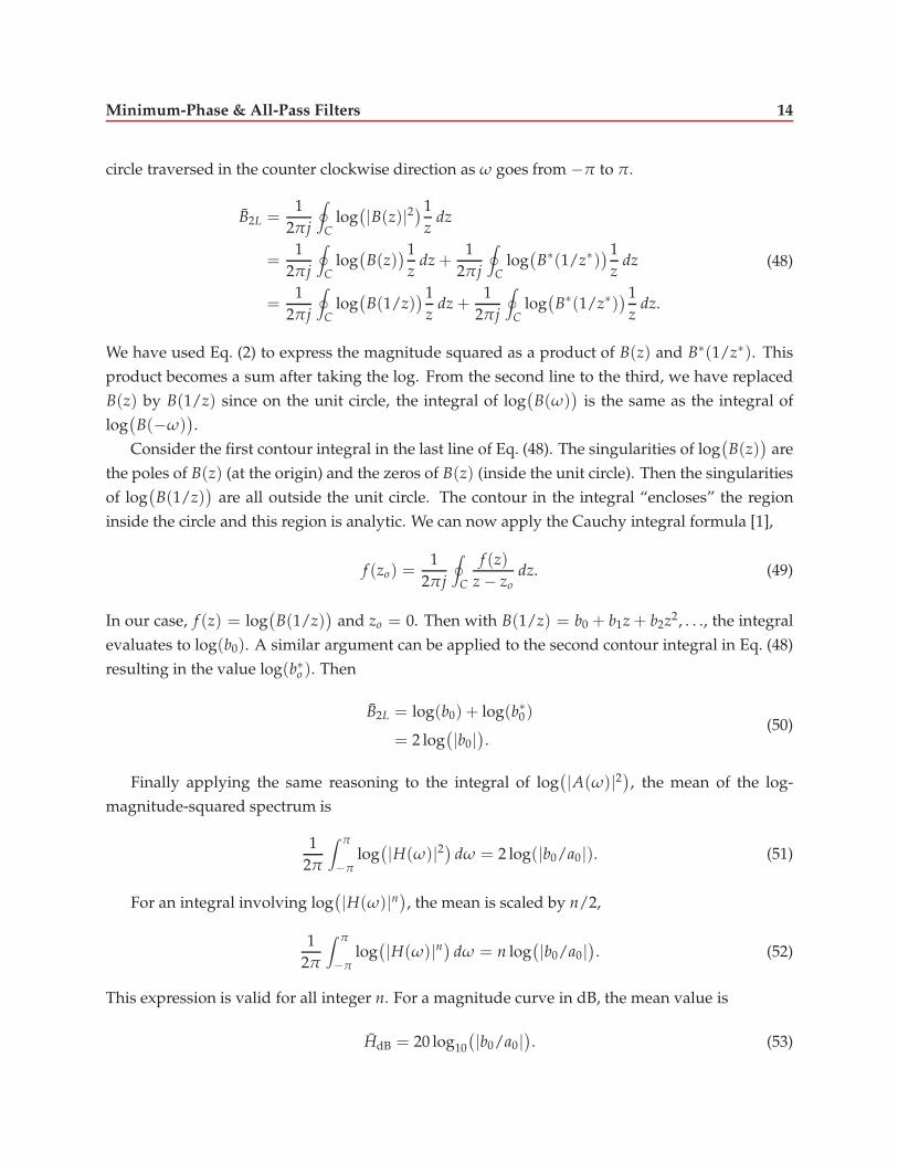
The frequency responses and the impulse response of the minimum-phase filter are shown in

Fig. 5. The magnitude curve has a mean of 3.88 dB (see Eq. (53)). The phase response has no net

increase across frequency, i.e., the phase returns to zero at ω = π. The group delay response has

both positive and negative values since the phase has both positive and negative slopes. The net

area under group delay curve is zero.

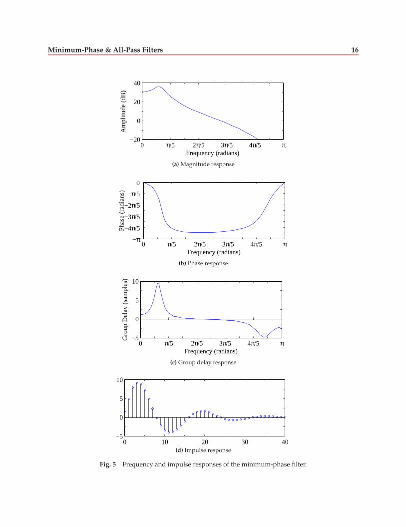
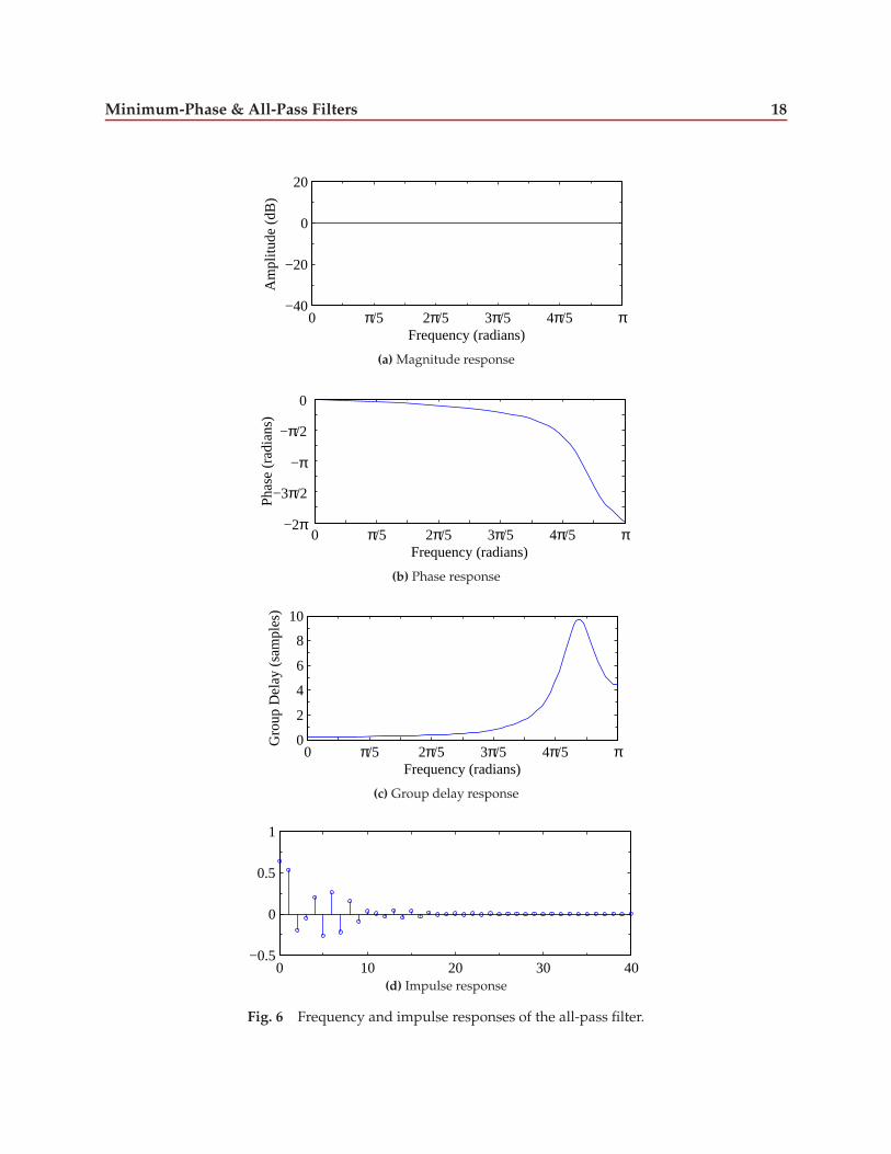
The frequency responses and the impulse response of the all-pass filter are plotted in Fig. 6.


−20

0

20

40

0 π/5 2π/5 3π/5 4π/5 πFrequency (radians)

Am

plitu

de (

dB)

(a) Magnitude response

−π

−4π/5

−3π/5

−2π/5

−π/5

0


Pha

se (

radi

ans)

(b) Phase response

−5

0

5

10


Gro

up D

elay

(sa

mpl

es)

(c) Group delay response

0 10 20 30 40−5

0

5

10

(d) Impulse response

Fig. 5 Frequency and impulse responses of the minimum-phase filter.


The magnitude response is constant as expected. The phase response is monotonic downward

and changes by π as ω goes from 0 to π. The group delay is positive (since the phase response

is monotonic) and has an area of π for ω between 0 and π. The impulse response has a first

coefficient which is less than unity (note the difference in the vertical scale relative to Fig. 5).

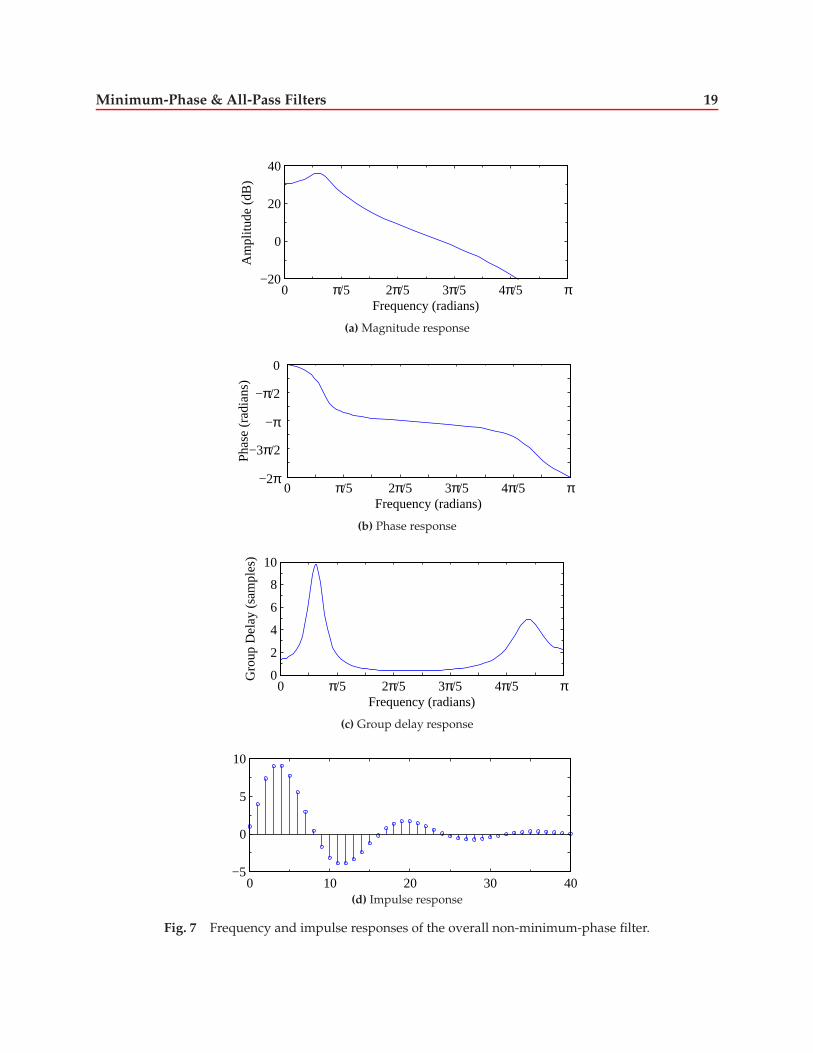
The frequency responses and the impulse response of the overall non-minimum-phase filter

are plotted in Fig. 7. The magnitude response is the same as for the minimum-phase filter. The

phase response is the sum of the phase responses of the minimum-phase filter and the all-pass

filter. The overall phase changes by π degrees as ω goes from 0 to π. The group delay response is

the sum of the group delay responses for the minimum-phase filter and the all-pass filter. The area

under the group delay curve is π for ω between 0 and π. The impulse response is the convolution

of the impulse responses of the minimum-phase filter and the all-pass filter. The all-pass filter

has the effect of smearing the impulse response without changing the total energy. The impulse

response of the non-minimum-phase filter has a first coefficient which is the product of the first

coefficients of the constituent responses.

7 Additional Notes

Further information on minimum-phase filters and all-pass filters can be found in a number of

standard digital signal processing texts [2][3][4]. Here we summarize some other properties and

uses of minimum-phase and all-pass filters.

7.1 Group Delay Equalization

Traditionally, frequency selective filters have been designed without explicit regard to their group

delay response. A multi-section all-pass filter can be used to equalize the delay response without

altering the magnitude response. The all-pass filter adds group delay to bring the overall group

delay closer to being constant. Mitra [2] gives a design example for an all-pass delay equalizer.

7.2 Stable Inverse Filter

The minimum-phase property is important if the inverse response is to be stable. This consid-

eration shows up in the design of linear prediction systems in, for example, speech processing

systems (see Proakis [4]).

7.3 Unit Circle Zeros

A system with unit circle zeros, by our definition, is not minimum-phase. Note also that the

inverse response is not strictly stable if unit circle zeros are present. The root factors for the unit

circle zeros contribute a constant group delay of one-half sample for each unit circle zero.


−40

−20

0

20


Am

plitu

de (

dB)


−2π

−3π/2

−π

−π/2

0


Pha

se (

radi

ans)

(b) Phase response

0

2

4

6

8

10


Gro

up D

elay

(sa

mpl

es)


0 10 20 30 40−0.5

0

0.5

1


Fig. 6 Frequency and impulse responses of the all-pass filter.


−20

0

20

40


Am

plitu

de (

dB)


−2π

−3π/2

−π

−π/2

0


Pha

se (

radi

ans)

(b) Phase response

0

2

4

6

8

10


Gro

up D

elay

(sa

mpl

es)


0 10 20 30 40−5

0

5

10


Fig. 7 Frequency and impulse responses of the overall non-minimum-phase filter.


It has been suggested that unit circle zeros can be moved inside the unit circle by a small

amount to make the response minimum-phase without major “practical” effect. Returning to our

initial example of the response in Section 1.3, we will move the zero from on the unit circle to just

inside the unit circle,

H(z) = 1 − (1 − ǫ)z−1. (57)

The amplitude response at ω = 0 is |H(0)| = ǫ. For instance, for ǫ = 10−3, the response at ω = 0

is 66 dB below the value at ω = π.

For a small positive ǫ, the phase response is continuous and makes an excursion from −π/2

to π/2 as ω increases through zero. The group delay is

τg(ω) =(1 − ǫ)(1 − ǫ − cos ω)

2(1 − ǫ)(1 − cos ω) + ǫ2. (58)

For a small positive ǫ, the group delay has a downward spike at ω = 0. Away from ω = 0, the

group delay approaches the 1/2 sample value we found earlier when the zero was on the unit

circle. For instance if ǫ = 10−3, then τg(0) = −103 samples. This downward spike has a negative

area which cancels the area under the the group delay curve.

If instead we had moved the zero to just outside the unit circle, the phase goes from −π/2

to −π as ω approaches zero from below. The phase then jumps to +π and falls to +π/2 at ω

increases from zero. This results in a total phase change of 2π (compared to a phase change of π

for a zero on the unit circle and a phase change of zero for a zero inside the unit circle.).

In this example, moving the unit circle zero inside by a small amount has a major effect on the

group delay, albeit at a frequency at which the amplitude response is small.

7.4 Decomposition of Linear Phase FIR Filters

For FIR filters, design strategies which result in linear phase filters are popular. For a linear phase

FIR filter with N coefficients, the group delay is (N − 1)/2 samples. The resulting filters can be

factored into a minimum-phase filter, a filter with unit circle zeros, and a maximum-phase filter.

The design procedures can be modified to ensure double-order unit circle zeros [5]. For N odd,

the overall filter can then be factored into four terms,

H(z) = Hmin(z)Huc(z)Huc(z)Hmax(z), (59)

where the double-order zeros have been separated and one zero from each pair has been assigned

to Huc(z). Consider forming two filters, each with M = (N + 1)/2 coefficients,

HA(z) = Hmin(z)Huc(z), HB(z) = Hmax(z)Huc(z). (60)


Each of these filters inherits the frequency selective properties of the original filter – each filter will

have a magnitude response equal to the square root of the magnitude response of the overall filter,

|HA(ω)| = |HB(ω)|, |HA(ω)|2 = |H(ω)|2. (61)

Each unit circle zero adds a group delay of 1/2 sample.6 These delays add to the delay con-

tributed by the minimum-phase zeros in HA(z). Since the group delay for the minimum-phase

zeros is negative at some frequencies, the overall group delay over this part of the frequency

range is smaller than the contribution due to the unit circle zeros. For HB(z), the group delay of

the unit circle zeros adds to the delay contributed by the maximum-phase zeros. The group delays

of the two filters add up to the delay of the linear phase filter,

τAg (ω) + τB

g (ω) =N − 1

2. (62)

Since the group delay of the filter employing the minimum-phase zeros is less than the group

delay of filter employing the maximum-phase zeros,

τAg (ω) ≤

M − 1

2. (63)

The filter employing the minimum-phase zeros will have a group delay that is less than the delay

of a linear phase filter of the same length.

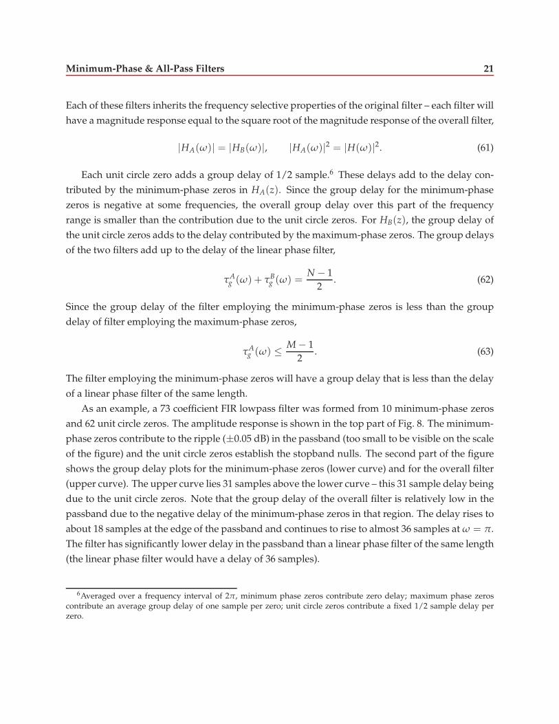
As an example, a 73 coefficient FIR lowpass filter was formed from 10 minimum-phase zeros

and 62 unit circle zeros. The amplitude response is shown in the top part of Fig. 8. The minimum-

phase zeros contribute to the ripple (±0.05 dB) in the passband (too small to be visible on the scale

of the figure) and the unit circle zeros establish the stopband nulls. The second part of the figure

shows the group delay plots for the minimum-phase zeros (lower curve) and for the overall filter

(upper curve). The upper curve lies 31 samples above the lower curve – this 31 sample delay being

due to the unit circle zeros. Note that the group delay of the overall filter is relatively low in the

passband due to the negative delay of the minimum-phase zeros in that region. The delay rises to

about 18 samples at the edge of the passband and continues to rise to almost 36 samples at ω = π.

The filter has significantly lower delay in the passband than a linear phase filter of the same length

(the linear phase filter would have a delay of 36 samples).

6Averaged over a frequency interval of 2π, minimum phase zeros contribute zero delay; maximum phase zeroscontribute an average group delay of one sample per zero; unit circle zeros contribute a fixed 1/2 sample delay perzero.


−60

−40

−20

0


Am

plitu

de (

dB)

(a) Amplitude response

−20

0

20

40


Gro

up D

elay

(b) Group delay response

Fig. 8 Frequency response for an FIR filter using minimum-phase zeros and unitcircle zeros. The group delay curve shows two curves: the upper curve is for theoverall filter; the lower curve is for the minimum-phase zeros alone.


7.5 Uniqueness of the Phase of a Minimum-Phase Filter

Earlier, we saw that for a filter of a given order, there were generally several filters with the

same magnitude response, differing only in their phase responses. However, for causal stable

minimum-phase filters with a given magnitude response, the matching phase response can be

found. We summarize the analysis given in [3].

1. The real part of the frequency response corresponds to a symmetric time response. We can

find the anti-symmetric time response which must be added to the symmetric time response

to make the overall response causal. This anti-symmetric time response gives the imaginary

part of the frequency response for the causal filter.

2. We can convert an amplitude/phase representation to a real/imaginary representation by

taking the logarithm of the frequency response,

X(ω) = log |X(ω)|+ j arg[X(ω)]. (64)

For the frequency response of the log-spectrum to be well-defined, X(z) must converge on

the unit circle. Note that the log |X(z)| has singularities at both the poles and zeros of X(z).

Hence, log |X(ω)| converges if X(z) is minimum-phase.

3. Denote the inverse transform of X(ω) as x[n]. This sequence is known as the complex cep-

strum. The complex cepstrum will be causal if and only if X(z) is minimum-phase.

Based on this analysis, we can calculate the cepstral component corresponding to the log-mag-

nitude alone. This will be symmetric. Then we find the anti-symmetric part which makes the

cepstrum causal. The transform of the anti-symmetric part gives the phase response.

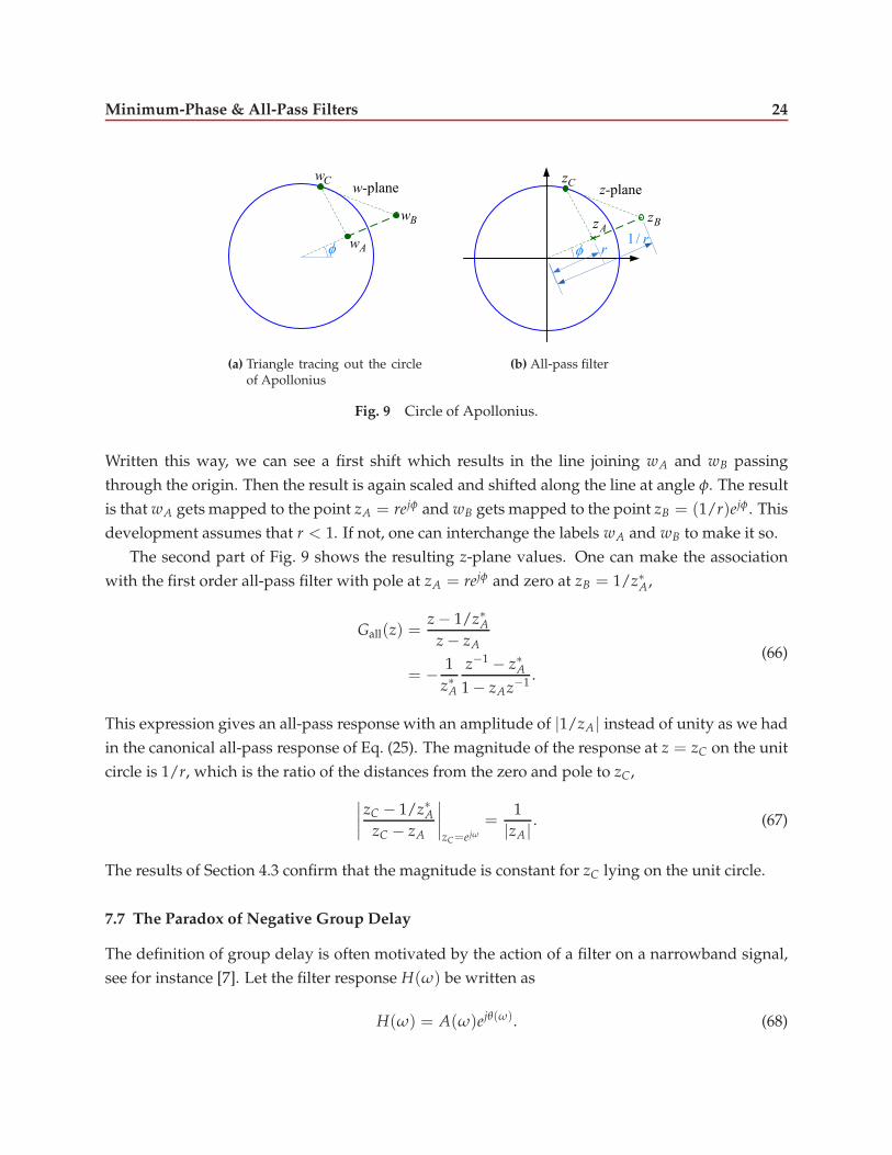
7.6 Circle of Apollonius

Consider two fixed points wA and wB in the plane. Now consider a third point wC forming a

triangle. If the ratio of the lengths |wC − wB| to |wC − wA| is kept constant, then wC traces a circle

– the circle of Apollonius [6]. The first part of Fig. 9 shows an example of the configuration of the

triangle and the resulting circle of Apollonius.

The circle of Apollonius is closely related to the property that the magnitude response of an

all-pass filter is constant. To see this, consider a shift and scaling operation from the w-plane to

the z-plane. Let the ratio of the two sides of the triangle be 1/r, where r < 1. Let the angle formed

by the line joining the points be φ = arg[wB − wA]. We scale and shift the w-plane values to the

z-plane,

z =1 − r2

r

w − wA

|wB − wA|+ rejφ . (65)


Aw

Bw

Cw

(a) Triangle tracing out the circleof Apollonius

Az Bz

Cz

r1/ r

(b) All-pass filter

Fig. 9 Circle of Apollonius.

Written this way, we can see a first shift which results in the line joining wA and wB passing

through the origin. Then the result is again scaled and shifted along the line at angle φ. The result

is that wA gets mapped to the point zA = rejφ and wB gets mapped to the point zB = (1/r)ejφ . This

development assumes that r < 1. If not, one can interchange the labels wA and wB to make it so.

The second part of Fig. 9 shows the resulting z-plane values. One can make the association

with the first order all-pass filter with pole at zA = rejφ and zero at zB = 1/z∗A,

Gall(z) =z − 1/z∗A

z − zA

= −1

z∗A

z−1 − z∗A1 − zAz−1

.

(66)

This expression gives an all-pass response with an amplitude of |1/zA | instead of unity as we had

in the canonical all-pass response of Eq. (25). The magnitude of the response at z = zC on the unit

circle is 1/r, which is the ratio of the distances from the zero and pole to zC,

∣∣∣∣zC − 1/z∗A

zC − zA

∣∣∣∣zC=e jω

=1

|zA|. (67)

The results of Section 4.3 confirm that the magnitude is constant for zC lying on the unit circle.

7.7 The Paradox of Negative Group Delay

The definition of group delay is often motivated by the action of a filter on a narrowband signal,

see for instance [7]. Let the filter response H(ω) be written as

H(ω) = A(ω)ejθ(ω). (68)


In the vicinity of a frequency ωc, we will assume that the amplitude is constant and the phase is

linear,

A(ω) = A(ωc), θ(ω) = θ(ωc) + (ω − ωc)dθ(ω)

dω

∣∣∣∣ω=ωc

, for ω near ωc. (69)

We have expanded the phase response as the first two terms of a Taylor series about ω = ωc. We

can write the phase response in the neighbourhood of ωc as

θ(ω) = −ωcτp(ωc)− (ω − ωc)τg(ωc), for ω near ωc. (70)

where τp(ω) = −θ(ω)/ω is the phase delay and where the second term has been expressed in

terms of the group delay τg(ω).

Consider a signal m[n] modulating a carrier at frequency ωc.

x[n] = m[n]ejωcn. (71)

The corresponding frequency response is

X(ω) = M(ω − ωc). (72)

We will assume that M(ω) is lowpass such that the response of M(ω − ωc) is non-zero only near

ω = ωc. Let this signal be input to the filter H(ω). With the narrowband assumption, the output

of the filter can be written as

Y(ω) = H(ω)X(ω)

= A(ωc)e−jωcτp(ωc)e−j(ω−ωc)τg(ωc)M(ω − ωc)

= A(ωc)e−jωτp(ωc)M(ω − ωc).

(73)

where we have defined M(ω) = e−jωτg(ωc)M(ω). The inverse transform of M(ω) is m[n− τg(ωc)],

where we have to interpret the non-integer shift as an interpolation operation. The output signal

can then be written as

y[n] = A(ωc)m[n − τg(ωc)]ejωc(n−τp(ωc)). (74)

We see that the group delay shifts the envelope7 and the phase delay shifts the carrier.

If the filter has a negative group delay in a frequency band, can the envelope of a narrowband

signal in that band actually undergo a time advance? The envelope is the information-bearing part

7Group delay is also known as envelope delay.


of the narrowband signal. The paradox is that a time advance of the envelope is counter-intuitive,

yet the mathematics suggests it might be possible. We will explore some of the considerations

which prevent the time advance from happening for practical (causal) systems. First we note that

no time limited signal can be strictly bandlimited. But, can we create a modulated signal that is

sufficiently narrowband to demonstrate the effect of a negative group delay?

When does negative group delay occur? It certainly occurs for minimum-phase filters since

the area under the group delay curve must integrate to zero. For these filters, the fastest change

in phase occurs when singularities lie near the unit circle. Poles near the unit circle will give a

positive spike in the group delay, while zeros near the unit circle will give a negative spike in the

group delay. For zeros, the negative values of group delay occur near a dip in the response, i.e. any

signal in the region of the dip is is much attenuated. Any practical narrowband signal has energy

concentrated at one frequency, but exhibits a falling off of energy away from the peak value. The

relative gain at frequencies away from the null will bring up the skirts of the narrowband signal

to effectively mask the effect of the signal components in the region of the negative group delay.

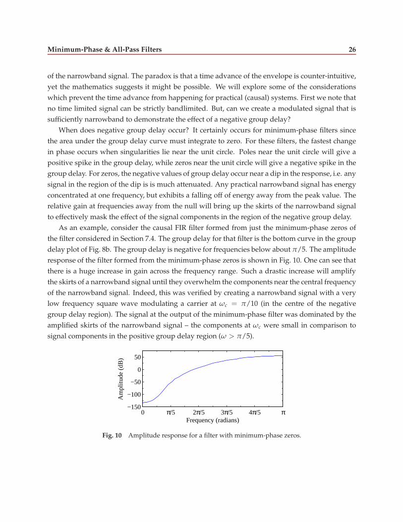
As an example, consider the causal FIR filter formed from just the minimum-phase zeros of

the filter considered in Section 7.4. The group delay for that filter is the bottom curve in the group

delay plot of Fig. 8b. The group delay is negative for frequencies below about π/5. The amplitude

response of the filter formed from the minimum-phase zeros is shown in Fig. 10. One can see that

there is a huge increase in gain across the frequency range. Such a drastic increase will amplify

the skirts of a narrowband signal until they overwhelm the components near the central frequency

of the narrowband signal. Indeed, this was verified by creating a narrowband signal with a very

low frequency square wave modulating a carrier at ωc = π/10 (in the centre of the negative

group delay region). The signal at the output of the minimum-phase filter was dominated by the

amplified skirts of the narrowband signal – the components at ωc were small in comparison to

signal components in the positive group delay region (ω > π/5).

−150

−100

−50

0

50


Am

plitu

de (

dB)

Fig. 10 Amplitude response for a filter with minimum-phase zeros.


8 Summary

The analysis of minimum-phase filters and the factorization of general filters is a rich topic. In this

report, we have been careful to analyze filters where the coefficients are allowed to be complex.

This leads to a straightforward formulas which, of course, subsume the case of real filter coeffi-

cients. The results given here on the constraints on the log-magnitude of a minimum-phase filter

are not often cited in the generality developed here.8

8The result specialized for an optimal linear predictor (which is minimum phase), is given in [8].


References

[1] R. V. Churchhill and J. W. Brown, Complex Variables and Applications, 5th ed., McGraw-Hill,1990 (ISBN 978-0-07-010905-6).

[2] S. K. Mitra, Digital Signal Processing, 3rd ed., McGraw-Hill, 2006 (ISBN 978-0-07-286546-2).

[3] A. V. Oppenheim and R. W. Schafer, Discrete-Time Signal Processing, 3rd ed., Prentice-Hall, 2010(ISBN 978-0-13-198842-2).

[4] J. G. Proakis and D. G. Manolakis, Digital Signal Processing, 4th ed., Prentice-Hall, 2007 (ISBN978-0-13-187374-2).

[5] P. Kabal, FIR Filters: Frequency-Weighted and Minimum-Phase Designs, Technical Report, Electri-cal & Computer Engineering, McGill University, Nov. 2007 (on-line at www-mmsp.ece.mcgill.ca/Documents/Reports).

[6] A. Papoulis, Signal Analysis, McGraw-Hill, 1977 (ISBN 978-0-07-048460-3).

[7] J. O. Smith, Introduction to Digital Filters with Audio Applications, on-line book, http://ccrma.stanford.edu/~jos/filters, accessed Nov. 2007.

[8] J. D. Markel and A. H. Gray, Jr., Linear Prediction of Speech, Springer, 1976 (ISBN 978-387-07563-1).