Embed Size (px)
Citation preview
General rights Copyright and moral rights for the publications made accessible in the public portal are retained by the authors and/or other copyright owners and it is a condition of accessing publications that users recognise and abide by the legal requirements associated with these rights.
Users may download and print one copy of any publication from the public portal for the purpose of private study or research.
You may not further distribute the material or use it for any profit-making activity or commercial gain
You may freely distribute the URL identifying the publication in the public portal If you believe that this document breaches copyright please contact us providing details, and we will remove access to the work immediately and investigate your claim.
Downloaded from orbit.dtu.dk on: Jun 09, 2019
Minimum Mean-Square Error Single-Channel Signal Estimation
Beierholm, Thomas
Publication date:2008
Document VersionPublisher's PDF, also known as Version of record
Link back to DTU Orbit
Citation (APA):Beierholm, T. (2008). Minimum Mean-Square Error Single-Channel Signal Estimation. IMM-PHD-2007-185

Minimum Mean-Square ErrorSingle-Channel Signal Estimation
Thomas Beierholm
Kongens Lyngby 2007IMM-PHD-2007-185

Technical University of DenmarkInformatics and Mathematical ModellingBuilding 321, DK-2800 Kongens Lyngby, DenmarkPhone +45 45253351, Fax +45 [email protected]
IMM-PHD: ISSN 0909-3192
Summary
This topic of this thesis is MMSE signal estimation for hearing aids when onlyone microphone is available. The research is relevant for noise reduction systemsin hearing aids. To fully benefit from the amplification provided by a hearing aid,noise reduction functionality is important as hearing-impaired persons in somenoisy situations need a higher signal to noise ratio for speech to be intelligiblewhen compared to normal-hearing persons.
In this thesis two different methods to approach the MMSE signal estimationproblem is examined. The methods differ in the way that models for the signaland noise are expressed and in the way the estimator is approximated. Thestarting point of the first method is prior probability density functions for bothsignal and noise and it is assumed that their Laplace transforms (moment gen-erating functions) are available. The corresponding posterior mean integral thatdefines the MMSE estimator is rewritten into an inverse Laplace transform inte-gral over an integrand involving the moment generating functions. This integralis approximated using saddlepoint approximation. It is found that the saddle-point approximation becomes inaccurate when two saddlepoints coalesce and asaddlepoint approximation based on two coalescing saddlepoints is derived. Forpractical reasons the method is limited to low dimensional problems and theresults are not easily extended to the multivariate case.
In the second approach signal and noise are specified by generative models andapproximate inference is performed by particle filtering. The speech model isa time-varying auto-regressive model reparameterized by formant frequenciesand bandwidths. The noise is assumed non-stationary and white. Comparedto the case of using the AR coefficients directly then it is found very beneficial

ii
to perform particle filtering using the reparameterized speech model because itis relative straightforward to exploit prior information about formant features.A modified MMSE estimator is introduced and performance of the particle fil-tering algorithm is compared to a state of the art hearing aid noise reductionalgorithm. Although performance of the two algorithms is found comparablethen the particle filter algorithm is doing a much better job tracking the noise.
Resume
Emnet for denne PhD rapport er MMSE signal estimering til brug i høreapparatersom kun har en mikrofon. Emnet er relevant for støjreduktionssystemer tilhøreapparater. For fuldt ud at kunne drage nytte af forstærkningen i et høreapparater det vigtigt med støjreduktionsfunktionalitet da hørehæmmede personer inogle støjfyldte situationer har brug for et højere signal-støj forhold for at kunneforsta tale nar der sammenlignes med normalthørende personer.
I denne rapport undersøges to forskellige metoder til MMSE signal estimer-ingsproblemet. Metoderne benytter forskellige repræsentationer af signal og støjog de benytter forskellige metoder til at approksimation af MMSE estimatoren.Udgangspunktet for den første tilgang er prior sandsynlighedstæthedsfunktionerfor bade signal og støj og det antages at deres Laplace transform (momentgenererende funktion) er tilgængelig. Det tilhørende posterior middelværdi inte-gral som definerer MMSE estimatoren omskrives til et invers Laplace tranformintegral over en integrand som bestar at afledede af de moment genererendefunktioner. Dette integral approksimeres ved hjælp af saddelpunktsapproksi-mation. Det fremgar at saddelpunktsapproksimationen bliver upræcis nar tosaddelpunkter er tæt pa hinanden og en saddelpunktsapproksimation baseretpa to saddelpunkter tæt pa hinanden udledes. Af praktiske grunde er metodenbegrænset til problemer af lav dimensionalitet og resultaterne kan ikke umid-delbart generaliseres til det flervariable tilfælde.
I den anden metode er signal og støj specificerede ved generative modellerog inferens approksimeres ved hjælp af partikelfiltrering. Tale modellen er entidsvarierende autoregressiv model reparameteriseret ved formant frekvenser ogbandbredder. Støjen antages ustationær og hvid. Sammenlignet med tilfældethvor AR koefficienter benyttes direkte sa er det fundet fordelagtigt at lave par-

iv
tikelfiltrering i den reparameteriserede talemodel fordi det er relativt simpelt atbenytte forhandsviden omkring formant frekvenser og bandbredder. En mod-ificeret MMSE estimator introduceres og performance af partikelfilteralgorit-men sammenlignes med en støjreduktionsalgoritme some bruges i høreapparater.Selvom performance af de to algoritmer er sammenlignelig sa er partikelfilteral-goritmen meget bedre til at tracke støjen.

Preface
The work presented in this thesis was carried out at Informatics and Mathemat-ical Modelling, Technical University of Denmark and at GN ReSound A/S inpartial fulfillment of the requirements for acquiring the Ph.D. degree in electricalengineering.
The goal of this thesis is to provide a unifying framework of the research carriedout in the Ph.D. study during the period Jun. 2004 - Oct. 2007, excluding aleave of absence in July 2007.

vi

Contributions
Two conference papers were written just prior to the official start of the projectand mentioned here as they to some degree have had an impact on the workdone in the official project period.
• Thomas Beierholm, Brian Dam Pedersen and Ole Winther, Low Complex-ity Bayesian Single Channel Source Separation, In Proceedings ICASSP-04, May 2004, Vol. 5, pp. 529− 532, Montreal, Canada.
• Thomas Beierholm and Paul M. Baggenstoss, Speech Music Discrimina-tion Using Class-Specific Features, Proceedings of 17th International Con-ference on (ICPR’04), Vol. 2, pp. 379 − 382, August 2004, Cambridge,UK.
This project has produced three papers with the following contributions
• Thomas Beierholm, Albert H. Nuttall and Lars K. Hansen, Use and Sub-tleties of Saddlepoint Approximation for Minimum Mean-Square Error Es-timation, Submitted to IEEE Transactions on Information Theory June2006.
– Derivation of an integral representation for the minimum mean-squareerror estimator involving the moment-generating functions of the ran-dom variables in an observation model consisting of a linear combi-nation of two independent random variables.

viii
– demonstrates that for the case of two coalescing saddlepoints, thesaddlepoint approximation based on isolated saddlepoints is very in-accurate.
– Derivation of a saddlepoint approximation based on two coalescingsaddlepoints with two correction terms.
– Demonstrates that the saddlepoint approximation based on two coa-lescing saddlepoints makes an excellent approximation when in facttwo saddlepoints are coalescing.
• Thomas Beierholm and Ole Winther, Particle Filter Inference in an Ar-ticulatory Based Speech Model, Accepted for publication in IEEE Journalof Signal Processing Letters.
– Demonstration of particle filter inference in a parallel formant synthe-sizer model parameterized by formant frequencies, bandwidths andgains for the application of speech enhancement.
– Experiments show that performance of the proposed speech modelprovides higher SNR improvements than a speech model parameter-ized by auto-regressive coefficients.
• Thomas Beierholm, Ole Winther and Bert de Vries, Non-Stationary NoiseReduction by Particle Filtering in a Cascade Formant Synthesizer Model,Submitted to IEEE Transactions on Speech and Language Processing June2007.
– It is demonstrated that reducing noise in speech by particle filterinference in a time-varying auto-regressive model is more beneficialif prior knowledge of formants is exploited which is achieved by pa-rameterizing the AR coefficients by formant frequencies and formantbandwidths
– Adapting the gains (variances) of the speech and noise models di-rectly instead of the log-gains produced results with less fluctuationsand more importantly it eliminated a stability issue experienced whenusing the log-gains.
– It is found that noise tracking capabilities of the proposed particlefilter algorithm are superior to that of a hearing instrument noisereduction algorithm, especially for low SNR levels.

Acknowledgements
First of all, I would like to thank GN ReSound A/S and in particular the Al-gorithm R&D group for funding, financial support and commitment to settingup the project despite difficulties in doing so. I also thank the Algorithm R&Dgroup for letting me roam around freely and members of the group for pleas-ant company. I would like to thank Sten Frostholm for IT support and ShawnPerman for being full of surprises.
Special thanks goes to my supervisors, Dr. Bert de Vries and Dr. Ole Winther,for guidance and support. Their contributions to the PhD project are hard tooverestimate. I would also like to thank Prof. Lars Kai Hansen for always beingopen and available for discussing ideas and the MISP department at Aalborguniversity for housing me in the final stages of the project.
I would like to thank Dr. Philip Ainsleigh for bringing up the idea of pursuinga PhD project, Dr. Paul Baggenstoss for explaining basic and subtle matterson the class-specific approach, Prof. Peter Willett who made my (unfortunatelytoo short) visit at UConn possible in the first place but also very warm and inparticular Albert Nuttall whom I feel very privileged to have worked togetherwith.
I also thank Line for understanding and support during the time of the project.

x

Contents
Summary i
Resume iii
Preface v
Contributions vii
Acknowledgements ix
1 Introduction 1
1.1 Saddlepoint Approximation . . . . . . . . . . . . . . . . . . . . . 3
1.2 Particle Filtering . . . . . . . . . . . . . . . . . . . . . . . . . . . 4
1.3 Reading Guideline . . . . . . . . . . . . . . . . . . . . . . . . . . 5
2 Saddlepoint Approximation for MMSE Estimation 7
2.1 Introduction to the model and the estimator . . . . . . . . . . . . 8
xii CONTENTS
2.2 SPA . . . . . . . . . . . . . . . . . . . . . . . . . . . . . . . . . . 10
2.3 Laplace-Gauss Example . . . . . . . . . . . . . . . . . . . . . . . 19
2.4 Discussion . . . . . . . . . . . . . . . . . . . . . . . . . . . . . . . 21
3 Particle Filtering for MMSE Estimation 23
3.1 Introduction to the models . . . . . . . . . . . . . . . . . . . . . 24
3.2 Monte Carlo . . . . . . . . . . . . . . . . . . . . . . . . . . . . . . 31
3.3 Importance Sampling . . . . . . . . . . . . . . . . . . . . . . . . . 32
3.4 Sequential Importance Sampling . . . . . . . . . . . . . . . . . . 37
3.5 Importance Distribution and Resampling . . . . . . . . . . . . . 40
3.6 Bayesian Adaptive FIR Filtering . . . . . . . . . . . . . . . . . . 46
3.7 Bayesian Adaptive IIR Filtering . . . . . . . . . . . . . . . . . . . 47
3.8 Bayesian Periodic Signal Modeling . . . . . . . . . . . . . . . . . 48
3.9 Discussion . . . . . . . . . . . . . . . . . . . . . . . . . . . . . . . 51
4 Results & Outlook 53
4.1 Saddlepoint Approximation . . . . . . . . . . . . . . . . . . . . . 53
4.2 Particle Filtering . . . . . . . . . . . . . . . . . . . . . . . . . . . 54
A Conditional Mean of Signal in Single-Channel Additive NoiseObservation Model 59
B SPA for Single Isolated Saddlepoint 61
C MGF M-variate Laplace Distribution 63
CONTENTS xiii
D Brief Introduction to Excitation Models 65
D.1 The Rosenberg-Klatt Model . . . . . . . . . . . . . . . . . . . . . 65
D.2 The LF model . . . . . . . . . . . . . . . . . . . . . . . . . . . . . 66
D.3 The Rosenberg++ model . . . . . . . . . . . . . . . . . . . . . . 68
E Use and Subtleties of Saddlepoint Approximation for MinimumMean-Square Error Estimation 69
F Particle Filter Inference in an Articulatory Based Speech Model 79
G Non-Stationary Noise Reduction by Particle Filtering in a Cas-cade Formant Synthesizer Model 85

xiv CONTENTS

Chapter 1
Introduction
A modern digital hearing aid provides DSP solutions to several challengingproblems that are of high importance in trying to help persons who suffer froma hearing loss. One of these problems consists of reducing noise in the inputsignal to the hearing aid. If there is noise in the input then the amplificationprovided by the hearing aid may not help the user because persons with ahearing loss tend to be more sensitive to noise than normal hearing persons[10]. Therefore a user of a hearing aid can experience a situation where speechis entirely audible but at the same time impossible to understand. This meansthat for a given noisy situation where speech is understandable for a normal-hearing person the speech may not be understandable for a hearing aid userbecause a higher Signal to Noise Ratio (SNR) is necessary before the noisyspeech is intelligible. Conversely, in situations where the amplified noisy speechis intelligible for a hearing aid user, suppressing noise is also important in orderto reduce listener fatigue and thus make it more comfortable for the user towear the hearing aid.
There are a number of constraints a developer faces when designing a noise re-duction system for a hearing aid. Since the very beginning of digital hearing aidsthe constraint that stands out the most is the fact the resources are very scarceand a noise reduction algorithm therefore must be of very low complexity to bea serious candidate for implementation. Furthermore, the noise reduction algo-rithm must introduce a small delay in the signal path and introduce virtually

2 Introduction
no audible distortions or artifacts in the processed speech signal. Additionally,the noise reduction algorithm should preferably operate in the frequency do-main and work for all types of speech and noise. These constraints makes itchallenging to develop a useful noise reduction algorithm for hearing aids.
If a hearing aid has two or more microphones available then spatial informationcan be used to suppress noise. The principle behind such a multi-microphonenoise reduction algorithm is to place a beam in the direction of the desiredspeaker to let speech pass undisturbed and nulls in the directions of the noisesources. Currently such algorithms tend to be more effective and useful thansingle-microphone noise reduction algorithms for suppressing noise [10]. How-ever, not all hearing aids have two or more microphones but only one micro-phone. Hence, there is an interest in single-microphone noise reduction algo-rithms for hearing aids.
A single-channel noise reduction algorithm can not rely on spatial informationand is thus less informed than multi-microphone approaches. In this report it isassumed that the input to the hearing aid, x, is a sum of a signal, s, and noise,v, which leads to the following observation model
xn = sn + vn (1.1)
where n denotes a sample/time index. The signal can for instance be thoughtof as speech and the noise can be thought as ambient (broad or narrow band)noise or a competing speaker. The nature of the problem in single-channel signalestimation is thus that in order to estimate the signal sn, or for that matter thenoise vn, the nth input sample xn must be split into two numbers/samplessuch that (1.1) is obeyed. If only xn is available (blind approach) there are aninfinite number of ways to split xn into sn and vn, such that (1.1) is obeyed.Mathematically such a problem is called under-determined meaning that moreinformation is required in order to compute a unique solution.
Ways to approach a solution to the single-channel signal estimation problemtend to be quite dependent on the situation at hand. If for instance it is knownthat both signal and noise are stationary, that the signal is a sinusoid, the noiseis pink and the SNR is between 10 and 15 dB then the situation is quite differ-ent from a competing speaker situation where both signal and noise representspeech. In the former situation the signal can be recovered by estimating onlythree parameters, the frequency, phase and amplitude of the sinusoid, whereas inthe latter situation a Computational Auditory Scene Analysis (CASA) approachmay be considered.
A systematic approach to the single-channel estimation problem can be per-formed using Bayesian methodology. Knowledge about the signal and noise isencapsulated in statistical models also called prior distributions (or just priors).
1.1 Saddlepoint Approximation 3
Using data available, Bayes’ theorem converts the priors to posteriors. Theposteriors are attractive because they encompass all available information; boththe prior knowledge provided by the developer in the priors and the informationconveyed in the acquired data. For instance, assuming that the signal and noiseare independent then by Bayes theorem
p(sn|D)p(vn|D) =p(D|sn, vn)ps(sn)pv(vn)
p(D)(1.2)
where D denotes all available acquired data, D={..., xn−1, xn}. In the Bayesianmethodology inference and estimation are centered around posterior distribu-tions. The MMSE estimator of the signal is defined as the mean of the signalposterior and is computed by the following integral
sn =∫
dsn sn p(sn|D) (1.3)
As mentioned in [15], the MMSE estimator is optimal for a large class of differ-ence distortion measures and it tends to be the most used estimator for noisereduction, therefore MMSE estimation is adopted in this report.
The overall problem statement for this report is: To perform MMSE estimationof speech in a single-channel setup.
1.1 Saddlepoint Approximation
Inserting (1.2) in (1.3) and enforcing (1.1) yields
sn =1
p(D)
∫dsn sn ps(sn) pv(xn − sn) (1.4)
The MMSE estimator is thus expressed directly in terms of the priors by aweighted convolution integral. It is thus clear that the choice of priors is whatultimately determines the performance of the corresponding MMSE estimatorand they are parameters under control of the developer. In principle, (1.4) rep-resents an attractive ’plug-and-play’ framework in which signal and noise modelscan be inserted and (1.4) provides the MMSE estimator for the signal. For adeveloper of noise reduction algorithms such a setup could be very beneficial.Choose models (priors) for the signal and noise, choose a noisy signal and (1.4)provides the MMSE estimate of the signal for listening. In this way a devel-oper can spend most of the time extending and enhancing models for the signal
4 Introduction
and noise and thus increase the chance of developing an improved noise reduc-tion algorithm. However, in reality a developer is quite limited in the choice ofmodels because of inferential difficulties. There is no straightforward way to dothe integral in (1.4) for all but the simplest models. The integral in (1.4) thusrepresents a bottleneck for a developer who will spend most of the time dealingwith the integration instead of concentrating on improving the signal and noisemodels.
The topic of chapter 2 is approximation of the integral in (1.4) by the methodof Saddlepoint Approximation (SPA). The idea has been motivated by workdone by Albert H. Nuttall in obtaining accurate approximations to tail prob-abilities for a number of useful statistics (see e.g. [29, 30]) which has been animportant method in developing the class-specific approach [3, 4]. A number ofobservations made SPA an interesting topic for further investigation; the SPAprovided excellent tail probability approximations, the SPA was developed forstatistics consisting of a linear combination of independent random variables(note that the observation model in (1.1) is a linear combination of two in-dependent random variables) and the SPA was computed by searching for aunique real saddlepoint. Thus the prospect was an accurate approximation ofthe integral in (1.4) where the problem of evaluating the integral in (1.4) couldbe replaced by the simpler problem of searching for a unique real saddlepoint,hence closing in on a ’plug-and-play’ setup.
Problem statement 1: Approximate the integral in (1.4) by means of saddlepointapproximation for general priors.
1.2 Particle Filtering
As mentioned in section 1.1 the choice of priors for the signal and noise is crucialfor the resulting performance of the corresponding MMSE estimator. The start-ing point of the approach described in section 1.1 is the availability of the modelsin terms of the prior PDFs, ps(sn) and pv(vn) or their Laplace transforms asit will appear in chapter 2. Alternatively, priors can be specified by genera-tive models which explicitly states how the data (observations) are assumed tohave been generated. For instance, speech is often modeled as a time-varyingauto-regressive process driven by white Gaussian noise where AR coefficientsand innovation noise variance can change from sample to sample. Using sucha model for speech it may be cumbersome and difficult to try and derive anexpression for ps(sn) because parameters are unknown and must be integrated
1.3 Reading Guideline 5
out. If instead the noisy speech is formulated as a state-space model whereclean speech enters as a hidden variable a number of methods for approximateinference can be used. One such method is particle filtering.
The idea of investigating particle filter inference in a time-varying auto-regressivemodel for speech was initially inspired by work done by Hermansen et al. in[22, 20] where the model based speech spectrum (the speech spectrum envelope)was parameterized by formant features; frequencies, bandwidths and gains. Theprospect of using such features instead of AR coefficients directly is to facilitateincorporation of prior knowledge of the formant features in the MMSE esti-mation. Inference by particle filtering in a time-varying auto-regressive speechmodel was performed by Vermaak et al. in [39] and has been adopted in thisreport and modified to work with formant features.
Problem statement 2: Perform particle filter inference in a time-varying auto-regressive generative model for speech parameterized by formant features.
1.3 Reading Guideline
The main body of this report consists of two self-contained independent chap-ters, one chapter on MMSE estimation using saddlepoint approximation andthe other chapter on MMSE estimation using particle filtering. The purpose ofthese two chapters is primarily to introduce the basic ideas behind the methodsof saddlepoint approximation and particle filtering but the intent is also thatthey can serve as background reading for the three papers found in appendicesE-G. Although the two main chapters in this report are self-contained the pa-pers should be read together with the chapters as it has been an aim to minimizethe overlap between the chapters and the papers. As such the papers constitutean important part of this report. Also the results in the papers will be referredto in chapter 4.

6 Introduction

Chapter 2
Saddlepoint Approximationfor MMSE Estimation
This chapter describes work done on Minimum Mean-Square Error (MMSE) es-timator approximation using SaddlePoint Approximation (SPA). Deriving theMMSE estimator for a signal using observations from a single channel whenthe mixing coefficients are known can be intractable for non-standard distribu-tions. The derivation involves a weighted convolution between the ProbabilityDensity Functions (PDFs) of the involved Random Variables (RVs). The ideapresented in this chapter is to make use of integral transforms of the involvedrandom variables instead of the PDFs and reformulate the original integral intoan inverse transform integral. The applied integral transform is the Laplacetransform. The inverse transform integral will in general also be intractable,however, by transforming the path of integration to go through a SaddlePoint(SP) of the integrand, the inverse integral transform can be approximated byusing information only at the SP.
The work described in this chapter was motivated by a desire to extend the workin [5] where separation of two speakers was performed in a two-step procedure:Maximum Likelihood (ML) estimation of mixing coefficients and MMSE esti-mation of the sources conditional on the mixing coefficients. As a result of thiswork the question arose as to what kind of source PDFs would result in excellentseparation performance given that the mixing coefficients are known and thatMMSE estimation is performed. One obstacle in extending the work in [5] is

8 Saddlepoint Approximation for MMSE Estimation
the derivation of the MMSE estimator. Considering for example Class-specificPDFs or multivariate sparse distributions the derivation of an exact analyticexpression for the MMSE estimator looks like a daunting task.
The work described in this chapter is inspired by work done by Albert H. Nuttallin obtaining accurate tail probability evaluations using SPA for a number ofuseful statistics see e.g. [29][30]. The author is indebted to Albert H. Nuttallwithout whom this work would not have been possible. He has acted as both amentor and a collaborator.
The purpose of this chapter is to explain or describe background theory thatmay be useful when reading the paper ”Use and Subtleties of Saddlepoint Ap-proximation for Minimum Mean-Square Error Estimation” in appendix. Espe-cially section 2.2.4 may be helpful. Perhaps ”theory” is not the correct wordto use because the chapter emphasizes intuitive explanations/descriptions overmathematical rigor. The contributions of the work done on MMSE estimatorapproximation are the derivation and use of the inverse transform integral for-mulation based on Moment Generating Functions (MGFs) and the derivation ofthe SPA for two close or coalesced SPs. The formulation based on MGFs seemsnew. When two SPs are close or coalesce the normal SPA based on a single SPdoes not work which motivated the derivation of the SPA for two close or coa-lesced SPs. This chapter also extends some of the ideas to the M-dimensionalcase and finally points out some problems in applying SPA for MMSE signalestimation.
2.1 Introduction to the model and the estimator
The mixing model under consideration is
y = ax1 + bx2 , a > 0, b > 0 (2.1)
where the scalars a and b are referred to as mixing coefficients. The observationsare contained in y and x1 and x2 denote the two sources which are mixedtogether. The model is a linear underdetermined noise-free two-in-one model.In the following it is assumed that the mixing coefficients are known. It’s theestimation of the sources that is under consideration. To be specific, it is theMMSE estimator of the sources that is under consideration. Let the M-variateRV xk = [xk,1, . . . , xk,M ]T have PDF pk(x) then the MMSE estimator for x1 isgiven by the following weighted convolution integral
E{x1|y} =1
p(y)1b
∫dx x p1(x) p2
(y − ax
b
)(2.2)
2.1 Introduction to the model and the estimator 9
or alternatively by
E{x1|y} =[
∂
∂hln
∫dx p1(x) p2
(y − ax
b
)exp(hT x)
1b
]∣∣∣∣h=0
(2.3)
These integrals are in general intractable except for a few special cases. Forunivariate RVs the integrals can be computed for various sparse distributionssuch as the Laplace and Cauchy distributions. For multivariate distributions theintegrals can be computed analytically to obtain closed form expressions for e.g.Gaussian RVs or RVs having Gaussian mixture distributions. The integral in(2.2) can be reformulated into a complex contour integral where the integrandis derived from the Laplace transforms of p1(x) and p2(x). Let multivariateRV xk = [xk,1, . . . , xk,M ]T have MGF µk(λ) where the Region Of Analyticity(ROA) of the MGF is Rk in the multidimensional complex λ-space and k = 1, 2.Let contour Ck lie in ROA Rk for k = 1, 2. The estimator is then given by
E{x1|y} =1
(i 2π)Mp(y)
∫
C
dz exp(−yT z) µ′1(az)µ2 (bz) (2.4)
The derivation is found in appendix A. One benefit of rewriting (2.2) into (2.4)is connected to properties of integral transforms of RVs. As argued in [37], thenalgebraic operations on RVs are many times most conveniently handled by theuse of integral transforms. For instance, if the RV xk can be written as a linearcombination of independent RVs then the Laplace transform of the PDF of xk
is the product of the Laplace transforms of the PDFs of the RVs in the linearcombination. Another potential extension is for the case that the sources havemodels on the form xk = gksk, where gk is a univariate positive RV independentof sk. For models of this form the mixing model in (2.1) turns into a sum ofproducts of RVs. Products between RVs are conveniently handled using Mellintransforms if they are available, however two issues limit the usefulness of usingMellin transforms. The Mellin transform is defined for non-negative RVs. It ispossible to work with RVs not everywhere positive but that gets quite involvedrather quickly (example of computing the Mellin transform of a bivariate RVnot everywhere positive is given in [37] page 153). For use in (2.4) the resultantMellin transforms will have to be transformed to Laplace transforms whichin the univariate case involves a complex contour integral (details are foundin Appendix C in [37]). The relation between the Mellin transform and thebilaterial Laplace transform for the multidimensional case is given in [8] page197.
The situation is thus that two different integrals for the MMSE estimator are athand, one via PDFs and the other via MGFs. SPAs can be developed in eitherdomain. As will be explained in sections 2.2.3 and 2.2.4 then close SPs haveimplications when applying the SPA. Maybe the PDF integral won’t have closeSPs, or maybe close SPs will happen at different values of the parameters [31].
10 Saddlepoint Approximation for MMSE Estimation
Although the PDF integral starts out along the real axis, that contour can bemodified and extended into another complex plane, if found fruitful. There isa chance that one would get two different SPAs, in general. This idea is notpursued in this chapter.
2.2 SPA
The history of SPA goes back almost two centuries. The SPA was used for thefirst time in statistics in a 1954 paper by Daniels [9] but [9] ascribes the physicistPeter Debye for first having used the method of steepest descent systematicallyin 1909 for studying Bessel functions. However, the authors in [33] point out thatDebye himself borrowed the idea of the method from a 1863 unpublished paperof Bernhard Riemann. The paper further shows that elements of the methodwas used even earlier in 1827 by Cauchy and that a Russian Mathematician P.A. Nekrasov had given a very general and detailed exposition of the method 25years before the work of Debye.
In [9] it is shown how the SPA represents the leading term in a proper asymptoticexpansion by using the method of steepest descent in which the path of integra-tion is the curve of steepest descent through an appropriate saddlepoint. Themethod of steepest descent, also known as the saddle-point method, is a naturaldevelopment of Laplace’s method applied to the asymptotic estimate of integralsof analytic functions [33]. As such, this section begins by briefly reviewing theprinciples in Laplace’s method (Laplace approximation). Thereafter some im-portant fundamental properties of analytic functions are enumerated and brieflyexplained. Next, the concepts of SPs and Monkey saddles will be explained andfinally in section 2.2.4 an explanation of the SPA is given.
2.2.1 Laplace approximation
Let’s say that the following (real) integral poses a problem
F =∫
f(x)dx (2.5)
where f(x) is a positive function, f(x) > 0. One approach would be to expandthe integrand in a Taylor series truncated to the first few terms and integrate.A slightly different approach will be used here. The integral is written in thefollowing way
F =∫
eφ(x)dx (2.6)
2.2 SPA 11
where φ(x) = ln f(x). The point is to expand the exponent, φ(x), in a truncatedTaylor series. The Taylor expansion of φ(x) around a point x0 is
φ(x) ≈ φ(x0) + φ′(x0)(x− x0) +12φ′′(x0)(x− x0)2 (2.7)
A key point now is to choose x0 wisely. The point x0 is chosen such thatφ′(x0) = 0 (it is assumed that φ′′(x0) 6= 0). This means that (2.7) reduces to
φ(x) ≈ φ(x0) +12φ′′(x0)(x− x0)2 (2.8)
Inserting (2.8) into (2.6) it is clear that the integral is over a gaussian kernelwith mean x0 and variance −1/φ′′(x0) provided that x0 is a maximum of thefunction so that the second derivative evaluated in x0 is negative. Thus,
F =∫
eφ(x)dx (2.9)
'∫
eφ(x0)+12 φ′′(x0)(x−x0)
2dx (2.10)
= eφ(x0)
(− 2π
φ′′(x0)
)1/2
(2.11)
This approximation is for instance useful for normalizing a PDF [25]. There is atwo-page chapter about this approximation in [25] called ’Laplace’s Method’.There it is written ”Physicists also call this widely-used approximation thesaddle-point approximation.”. In the view of this chapter it may be misleadingto call Laplace’s Method for saddlepoint approximation. In [25] the generaliza-tion of (2.11) to a function of many variables is shown. As an aside, [33] notesthat originally Laplace estimated an integral on the form
Fn =∫ b
a
fn(x)g(x)dx =∫ b
a
enu(x)g(x)dx, f(x) > 0, (2.12)
as n → ∞. Even though this integrand is different from the integrand in (2.5)then the approximation principle is the same.
The same type of approximation can also be used for approximating a functionthat is written as an integral [19]
f(x) =∫
m(x, t)dt =∫
ek(x,t)dt (2.13)
where k(x, t) = ln m(x, t). Expanding k(x, t) around a stationary point, t(x),
12 Saddlepoint Approximation for MMSE Estimation
gives
f(x) '∫
ek(x,t(x))+
(t−t(x))2
2∂2k(x,t)
∂t2
����t(x)dt (2.14)
= ek(x,t(x))
− 2π
∂2k(x,t)∂t2
∣∣∣t(x)
1/2
(2.15)
The key thing to note about this approximation is that the stationary point t(x)depends on x so that for each x there is a new integrated Taylor series expansion.The stationary point t(x) is a maximum and the second-order partial derivativesatisfies ∂2k(x, t)/∂t2 < 0. As also noted in [19] then because the integral isbeing centralized there is hope that the approximation is ’accurate’ and theprice to pay is that for each x the stationary point t(x) must be found and thefunctions k(x, t) and ∂2k(x, t)/∂t2 must be evaluated at that point.
2.2.2 Results from Calculus of Complex Variables
The concept of an analytic function is important for the understanding andapplication of the SPA. This section briefly summarizes a few of the most centralproperties of analytic functions and explains the role of the properties in thecontext of SPA. It will appear that analyticity of a function imposes some quitestrong restrictions on the function. Two quick definitions taken from [7] are ”Anentire function is a function that is analytic at each point in the entire finiteplane. Since the derivative of a polynomial exists everywhere, it follows thatevery polynomial is an analytic function.” and ”A Singular point of a functionf is a point where f fails to be analytic.”
• An analytic function obeys the Cauchy-Riemann equations
Let f be a function of a complex variable z = x + iy such that f(x + iy) =u(x, y) + iv(x, y). Also let ux and uy denote the first-order derivatives withrespect to x and y of the function u. Then the Cauchy-Riemann equations canbe written as
ux = vy, uy = −vx (2.16)
• If a function f(z) is analytic in a Domain D, then its component functionsu and v are harmonic in D.
2.2 SPA 13
That the component functions are harmonic means that they obey Laplace’sequation, that is,
uxx + uyy = 0 and vxx + vyy = 0 (2.17)
This property of analytic functions can be derived directly from the Cauchy-Riemann equations and implies that stationary points (points where f(z)/dz =0) where the second-order partial derivatives are non-zero are SPs of u and vbecause the second-order partial derivatives have opposite signs.
• For an analytic function the level curves of u and v are orthogonal
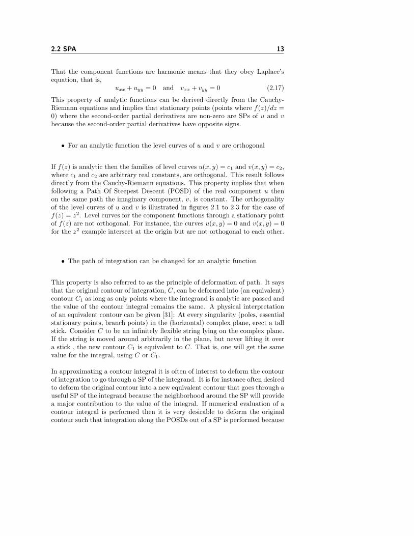
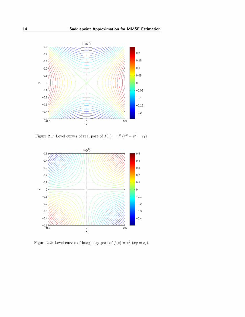
If f(z) is analytic then the families of level curves u(x, y) = c1 and v(x, y) = c2,where c1 and c2 are arbitrary real constants, are orthogonal. This result followsdirectly from the Cauchy-Riemann equations. This property implies that whenfollowing a Path Of Steepest Descent (POSD) of the real component u thenon the same path the imaginary component, v, is constant. The orthogonalityof the level curves of u and v is illustrated in figures 2.1 to 2.3 for the case off(z) = z2. Level curves for the component functions through a stationary pointof f(z) are not orthogonal. For instance, the curves u(x, y) = 0 and v(x, y) = 0for the z2 example intersect at the origin but are not orthogonal to each other.
• The path of integration can be changed for an analytic function
This property is also referred to as the principle of deformation of path. It saysthat the original contour of integration, C, can be deformed into (an equivalent)contour C1 as long as only points where the integrand is analytic are passed andthe value of the contour integral remains the same. A physical interpretationof an equivalent contour can be given [31]: At every singularity (poles, essentialstationary points, branch points) in the (horizontal) complex plane, erect a tallstick. Consider C to be an infinitely flexible string lying on the complex plane.If the string is moved around arbitrarily in the plane, but never lifting it overa stick , the new contour C1 is equivalent to C. That is, one will get the samevalue for the integral, using C or C1.
In approximating a contour integral it is often of interest to deform the contourof integration to go through a SP of the integrand. It is for instance often desiredto deform the original contour into a new equivalent contour that goes through auseful SP of the integrand because the neighborhood around the SP will providea major contribution to the value of the integral. If numerical evaluation of acontour integral is performed then it is very desirable to deform the originalcontour such that integration along the POSDs out of a SP is performed because
14 Saddlepoint Approximation for MMSE Estimation
x
y
Re(z2)
−0.5 0 0.5−0.5
−0.4
−0.3
−0.2
−0.1
0
0.1
0.2
0.3
0.4
0.5
−0.2
−0.15
−0.1
−0.05
0
0.05
0.1
0.15
0.2
Figure 2.1: Level curves of real part of f(z) = z2 (x2 − y2 = c1).
x
y
Im(z2)
−0.5 0 0.5−0.5
−0.4
−0.3
−0.2
−0.1
0
0.1
0.2
0.3
0.4
0.5
−0.4
−0.3
−0.2
−0.1
0
0.1
0.2
0.3
0.4
0.5
Figure 2.2: Level curves of imaginary part of f(z) = z2 (xy = c2).

2.2 SPA 15
x
yRe(z2) and Im(z2)
−0.5 0 0.5−0.5
−0.4
−0.3
−0.2
−0.1
0
0.1
0.2
0.3
0.4
0.5
−0.4
−0.3
−0.2
−0.1
0
0.1
0.2
0.3
0.4
0.5
Figure 2.3: Level curves of both real and imaginary part of f(z) = z2.
the magnitude of the integrand rapidly goes to zero along this path (there areno oscillations) and will give the most accurate answer for the integral.
• An analytic function may be subjected to analytic continuation therebyextending the domain of definition of the analytic function
Generally, even if an integrand does not have a SP in a desired region, it may bepossible to use analytic continuation to extend the integrand outside its ROA,where there could very well be a SP. Complexities can arise with multivaluedfunctions and the presence of zeros of the function f(z), which, unfortunately,act like ”black holes” to paths of steepest descent [31].
2.2.3 Saddlepoints
Consider a general contour integral
I =∫
C
f(z) dz =∫
C
exp ( φ(z) ) dz (2.18)
16 Saddlepoint Approximation for MMSE Estimation
x
y
Monkey SP
0.5 1 1.5 2−0.5
−0.4
−0.3
−0.2
−0.1
0
0.1
0.2
0.3
0.4
0.5
0.21
0.215
0.22
0.225
0.23
0.235
0.24
0.245
0.25
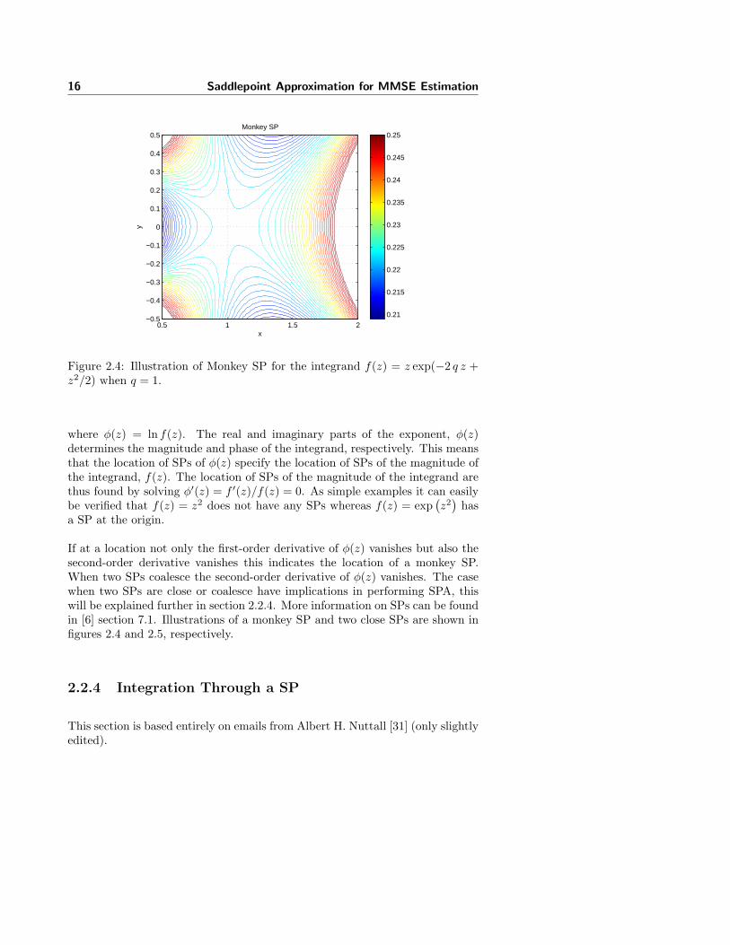
Figure 2.4: Illustration of Monkey SP for the integrand f(z) = z exp(−2 q z +z2/2) when q = 1.
where φ(z) = ln f(z). The real and imaginary parts of the exponent, φ(z)determines the magnitude and phase of the integrand, respectively. This meansthat the location of SPs of φ(z) specify the location of SPs of the magnitude ofthe integrand, f(z). The location of SPs of the magnitude of the integrand arethus found by solving φ′(z) = f ′(z)/f(z) = 0. As simple examples it can easilybe verified that f(z) = z2 does not have any SPs whereas f(z) = exp
(z2
)has
a SP at the origin.
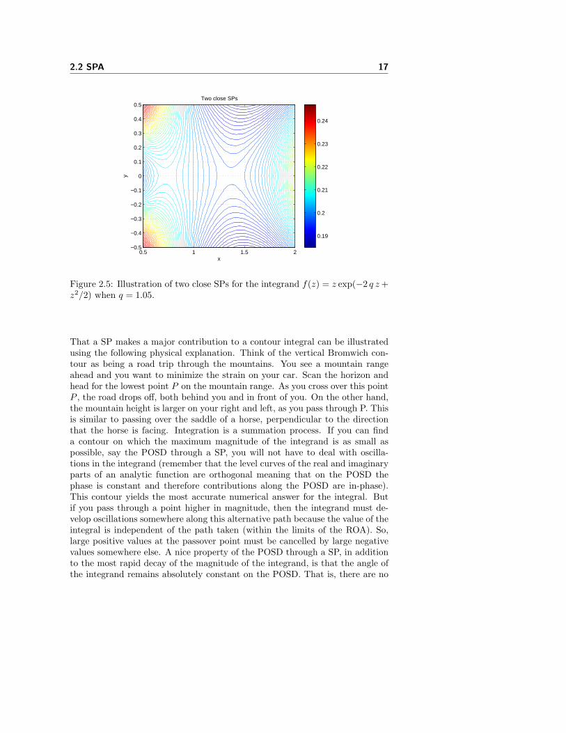
If at a location not only the first-order derivative of φ(z) vanishes but also thesecond-order derivative vanishes this indicates the location of a monkey SP.When two SPs coalesce the second-order derivative of φ(z) vanishes. The casewhen two SPs are close or coalesce have implications in performing SPA, thiswill be explained further in section 2.2.4. More information on SPs can be foundin [6] section 7.1. Illustrations of a monkey SP and two close SPs are shown infigures 2.4 and 2.5, respectively.
2.2.4 Integration Through a SP
This section is based entirely on emails from Albert H. Nuttall [31] (only slightlyedited).
2.2 SPA 17
x
y
Two close SPs
0.5 1 1.5 2−0.5
−0.4
−0.3
−0.2
−0.1
0
0.1
0.2
0.3
0.4
0.5
0.19
0.2
0.21
0.22
0.23
0.24
Figure 2.5: Illustration of two close SPs for the integrand f(z) = z exp(−2 q z +z2/2) when q = 1.05.
That a SP makes a major contribution to a contour integral can be illustratedusing the following physical explanation. Think of the vertical Bromwich con-tour as being a road trip through the mountains. You see a mountain rangeahead and you want to minimize the strain on your car. Scan the horizon andhead for the lowest point P on the mountain range. As you cross over this pointP , the road drops off, both behind you and in front of you. On the other hand,the mountain height is larger on your right and left, as you pass through P. Thisis similar to passing over the saddle of a horse, perpendicular to the directionthat the horse is facing. Integration is a summation process. If you can finda contour on which the maximum magnitude of the integrand is as small aspossible, say the POSD through a SP, you will not have to deal with oscilla-tions in the integrand (remember that the level curves of the real and imaginaryparts of an analytic function are orthogonal meaning that on the POSD thephase is constant and therefore contributions along the POSD are in-phase).This contour yields the most accurate numerical answer for the integral. Butif you pass through a point higher in magnitude, then the integrand must de-velop oscillations somewhere along this alternative path because the value of theintegral is independent of the path taken (within the limits of the ROA). So,large positive values at the passover point must be cancelled by large negativevalues somewhere else. A nice property of the POSD through a SP, in additionto the most rapid decay of the magnitude of the integrand, is that the angle ofthe integrand remains absolutely constant on the POSD. That is, there are no
18 Saddlepoint Approximation for MMSE Estimation
oscillations in the complex values of the integrand. It is therefore of interest tomove the contour of integration to go through a SP of the integrand.
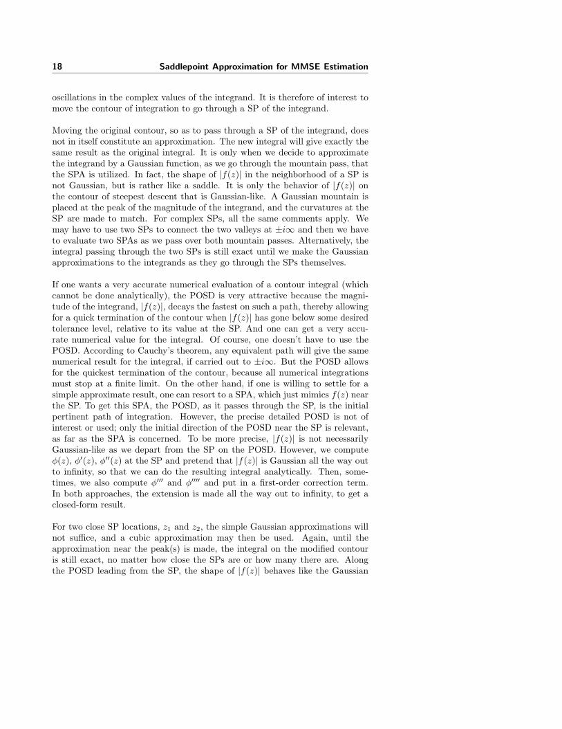
Moving the original contour, so as to pass through a SP of the integrand, doesnot in itself constitute an approximation. The new integral will give exactly thesame result as the original integral. It is only when we decide to approximatethe integrand by a Gaussian function, as we go through the mountain pass, thatthe SPA is utilized. In fact, the shape of |f(z)| in the neighborhood of a SP isnot Gaussian, but is rather like a saddle. It is only the behavior of |f(z)| onthe contour of steepest descent that is Gaussian-like. A Gaussian mountain isplaced at the peak of the magnitude of the integrand, and the curvatures at theSP are made to match. For complex SPs, all the same comments apply. Wemay have to use two SPs to connect the two valleys at ±i∞ and then we haveto evaluate two SPAs as we pass over both mountain passes. Alternatively, theintegral passing through the two SPs is still exact until we make the Gaussianapproximations to the integrands as they go through the SPs themselves.
If one wants a very accurate numerical evaluation of a contour integral (whichcannot be done analytically), the POSD is very attractive because the magni-tude of the integrand, |f(z)|, decays the fastest on such a path, thereby allowingfor a quick termination of the contour when |f(z)| has gone below some desiredtolerance level, relative to its value at the SP. And one can get a very accu-rate numerical value for the integral. Of course, one doesn’t have to use thePOSD. According to Cauchy’s theorem, any equivalent path will give the samenumerical result for the integral, if carried out to ±i∞. But the POSD allowsfor the quickest termination of the contour, because all numerical integrationsmust stop at a finite limit. On the other hand, if one is willing to settle for asimple approximate result, one can resort to a SPA, which just mimics f(z) nearthe SP. To get this SPA, the POSD, as it passes through the SP, is the initialpertinent path of integration. However, the precise detailed POSD is not ofinterest or used; only the initial direction of the POSD near the SP is relevant,as far as the SPA is concerned. To be more precise, |f(z)| is not necessarilyGaussian-like as we depart from the SP on the POSD. However, we computeφ(z), φ′(z), φ′′(z) at the SP and pretend that |f(z)| is Gaussian all the way outto infinity, so that we can do the resulting integral analytically. Then, some-times, we also compute φ′′′ and φ′′′′ and put in a first-order correction term.In both approaches, the extension is made all the way out to infinity, to get aclosed-form result.
For two close SP locations, z1 and z2, the simple Gaussian approximations willnot suffice, and a cubic approximation may then be used. Again, until theapproximation near the peak(s) is made, the integral on the modified contouris still exact, no matter how close the SPs are or how many there are. Alongthe POSD leading from the SP, the shape of |f(z)| behaves like the Gaussian

2.3 Laplace-Gauss Example 19
function exp(−b d2), where d is the distance away from the SP. With that inmind, and with a contour that passes through 2 SPs, if the Gaussian functionapproximation about SP1 has decayed significantly by the distance that SP2 isreached, then a decent approximation can be expected from the two SPAs. Butif the Gaussian function approximation about SP1 has not decayed significantlyby the distance to SP2, then one have to switch to a cubic approximation forthe argument of the exponential approximation near the two close SPs. On thePOSD out of one SP at z1, a Gaussian approximation based on the behaviorright at the peak location z1 is made. Then, when we start integrating alongthat POSD out of z1, before we can get to a region of small magnitude of theintegrand, |f(z)|, we run into another POSD coming from another close SP atz2, and we then have to ascend up that path toward the other SP at z2. A Gaus-sian mountain is placed at the peak of the magnitude of the integrand, and thecurvatures at the SP are made to match. These two mountains intersect andinterfere with each other, and a different function of z must be used near thesetwo close peaks, to approximate their interacting behavior. A quadratic approx-imation to φ′(z) does just that, by being zero at the two SPs; that behavior isperfect near the two close SPs. The integral of the quadratic function gives acubic function of z that does a good job of approximating the true behavior ofφ(z) in the neighborhood of the two close SPs, which are the major points andregion of interest. We will then integrate on this approximate function to getour SPA.
When the two close SPs z1, z2 are complex conjugates, they are both locationsof peaks of the magnitude of integrand f(z). The contour C could be moved topass through both of these points. But when the two close SPs are both real(and still close), C can pass through only one of these SPs, namely, the onewhich has a minimum of f(z) as z is varied along the real axis (The other closereal SP has a local maximum along the real axis). In the direction perpendicularto the real axis (i.e., along the Bromwich contour), the function f(z) then has amaximum at the SP used. Once the replacement of φ(z) by the approximatingcubic function of z is made, the exact crossing point of the real axis in thecomplex plane is irrelevant because the new function of z is entire and has nosingularities anywhere. This allows for considerable freedom of path movement,the real important thing is which valleys do the ends of the contours end up inas the new path must end up in the same valley(s) as beforehand.
2.3 Laplace-Gauss Example
The intent of including this example is to give an impression of the difficulties inapplying SPA for a multivariate example where both variables are not Gaussian.

20 Saddlepoint Approximation for MMSE Estimation
The example could represent a speech enhancement scenario (see [17][18]) wherespeech is modeled by a multivariate Laplace distribution and noise is modeledby multivariate Gaussian distribution. In the end of this section a number ofpoints will be mentioned that have to be understood before this example canbe completed.
The zero-mean multivariate Laplace distribution, as computed from a multi-variate scale mixture of Gaussians [14], is
p(x) =1
(2π)d/2
2λ
K(d/2)−1
(√q(x) 2/λ
)
(√q(x) 2/λ
)(d/2)−1(2.19)
where d denotes the dimensionality of the RV x, Km(x) denotes the modifiedBessel function of the second kind and order m, λ denotes a positive scalar andq(x) = xT Γ x, where Γ is a positive definite matrix with detΓ = 1. Thecovariance matrix of RV x is Σx = λΓ. In (2.1), let RV x1 be Laplacian andRV x2 be Gaussian. The MGF of the multivariate Laplace distribution and itsfirst-order derivative (see appendix C), is
µx(ω) =1
1− λ2 ωT Γω
, µ′x(ω) =λΓω(
1− λ2 ωT Γω
)2 (2.20)
Inserting (2.20) into (2.4) then
E{x1|y} =1
(i 2π)Mp(y)
∫
C
dz e−yT z aλ1Γ1z(1− a2λ1
2 zT Γ1z)2 e
12 b2zT Σz (2.21)
Substituting z = bΣ1/2z in (2.21) yields
E{x1|y} =aλ1Γ1
b2 (i 2π)Mp(y)
∫
C
dz e−pT z+ 12 zT z z
(1− zT Az)2(2.22)
where
pT = yT Σ−1/2 1b
, A =a2λ1
b2 2
(Σ−1/2
)T
Γ1Σ−1/2 (2.23)
The fundamental integral is then
I =1
(i 2π)M
∫
C
dz e−pT z+ 12zT z z
(1− zT Az)2(2.24)
It may not be possible to evaluate the integral for M > 2. For the particularcase M = 2, we have
I1 =1
(i 2π)2
∫
C1
∫
C2
dz1dz2 z1 e−p1z1−p2z2+12 z2
1+ 12 z2
21
(1− a11z21 − a22z2
2 − 2a12z1z2)2
(2.25)
2.4 Discussion 21
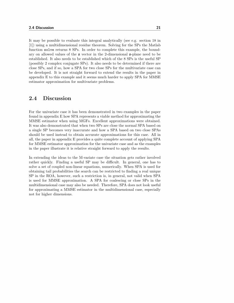
It may be possible to evaluate this integral analytically (see e.g. section 18 in[1]) using a multidimensional residue theorem. Solving for the SPs the Matlabfunction solve returns 8 SPs. In order to complete this example, the bound-ary on allowed values of the z vector in the 2-dimensional z-plane need to beestablished. It also needs to be established which of the 8 SPs is the useful SP(possibly 2 complex conjugate SPs). It also needs to be determined if there areclose SPs, and if so, how a SPA for two close SPs for the multivariate case canbe developed. It is not straight forward to extend the results in the paper inappendix E to this example and it seems much harder to apply SPA for MMSEestimator approximation for multivariate problems.
2.4 Discussion
For the univariate case it has been demonstrated in two examples in the paperfound in appendix E how SPA represents a viable method for approximating theMMSE estimator when using MGFs. Excellent approximations were obtained.It was also demonstrated that when two SPs are close the normal SPA based ona single SP becomes very inaccurate and how a SPA based on two close SPAsshould be used instead to obtain accurate approximations for this case. All inall, the paper in appendix E provides a quite complete account of applying SPAfor MMSE estimator approximation for the univariate case and as the examplesin the paper illustrate it is relative straight forward to apply the results.
In extending the ideas to the M-variate case the situation gets rather involvedrather quickly. Finding a useful SP may be difficult. In general, one has tosolve a set of coupled non-linear equations, numerically. When SPA is used forobtaining tail probabilities the search can be restricted to finding a real uniqueSP in the ROA, however, such a restriction is, in general, not valid when SPAis used for MMSE approximation. A SPA for coalescing or close SPs in themultidimensional case may also be needed. Therefore, SPA does not look usefulfor approximating a MMSE estimator in the multidimensional case, especiallynot for higher dimensions.

22 Saddlepoint Approximation for MMSE Estimation
Chapter 3
Particle Filtering for MMSEEstimation
The purpose of this chapter is to demystify particle filtering (PF) and demon-strate in a couple of examples how PF can be used. This chapter also servesas an introduction to the two papers applying PF found in appendices F andG. The intent is to describe the fundamental ideas behind PF and not focus ontheoretical aspects.
PF is a technique used for approximate inference that is suitable for onlineapplications. In the literature PF is also referred to as Sequential Monte Carlo.From a Bayesian point of view a fundamental idea of PF is that of representing aposterior PDF of interest by a number of samples where we can think of a sampleas a number that is returned by a Random Number Generator (RNG) with adistribution equal to that of the posterior PDF. Herein lies an approximationbut the more samples that are used to represent the posterior PDF the betterthe approximation becomes and in the limit the representation becomes exact(see e.g. [12] ch. 2). Given a number of samples from a posterior PDF ofinterest it is possible to estimate properties of the posterior PDF such as forinstance the location of a maximum or the mean value. The mean value is themain quantity of interest in Minimum Mean-Square Error (MMSE) estimationwhich will be considered later in the examples. The idea is thus to replace thefunctional representation of the posterior PDF by samples. In [36], it is written”..we note the essential duality between a sample and the density (distribution)

24 Particle Filtering for MMSE Estimation
from which it is generated. Clearly, the density generates the sample; conversely,given a sample we can approximately recreate the density (as a histogram, akernel density estimate, an empirical cdf, or whatever).”
Another key idea in PF is to obtain samples from a posterior PDF that are”important” such that useful approximations can be made by a manageablenumber of samples. This is done by attaching a weight to each sample whichtells how important a particular sample is. Samples with low weight can then bediscarded and replaced by samples with higher weight in a process referred to asresampling. A particle consists of a sample and its weight. It is described laterhow the weights are computed. The weights are needed because samples willbe produced by a RNG which is considerably simpler than the desired targetRNG. By attaching weights to the samples generated by the simpler RNG theseweighted samples constitutes a representation of the posterior PDF that is justas valid as samples drawn from the complex target RNG. The combination ofusing a simple RNG and weighted samples is the concept behind ImportanceSampling (IS) which plays a fundamental role in PF.
A crucial idea behind PF is that of propagating the particles sequentially intime making PF suitable for online applications. PF processes a sequence onesample at a time by propagating particles (samples and weights) recursively.The process of propagating particles recursively in time is called SequentialImportance Sampling (SIS). The combination of SIS and the above mentionedresampling constitutes the main body of a particle filter.
In section 3.1 a class of useful models will be introduced and it will appear thatPF in this class of models is very convenient. The following sections go intodetails of PF by first briefly explaining the principle behind the Monte Carlomethod in section 3.2, then describing the idea of IS in section 3.3 and outliningthe procedure of SIS in section 3.4. Next, the purpose of resampling is describedin section 3.5, followed by three examples in sections 3.6-3.8 that all have somerelevance to signal processing for hearing aids. Finally this chapter is concludedwith a discussion in section 3.9.
3.1 Introduction to the models
The starting point of a class of useful and convenient discrete system modelsis the assumption that the z-transform representation of the model, the systemfunction H(z), is a rational function of polynomials in z;
H(z) =Y (z)X(z)
, (3.1)
3.1 Introduction to the models 25
where Y (z) and X(z) are polynomials in z. Most often, however, H(z) is ex-pressed as a ratio of polynomials in z−1, see e.g. [32] ch. 6; i.e.,
H(z) =∑M
k=0 bk z−k
1−∑Nk=1 ak z−k
, (3.2)
with the corresponding difference equation
yn =N∑
k=1
ak yn−k +M∑
k=0
bk xn−k . (3.3)
If zero-mean white Gaussian noise with variance σ2 is added to the right handside of (3.3) the difference equation can be written in a direct form II matrixformulation with the following state and observation equations
wn = Awn−1 + Bxn (3.4)
yn = Cwn + D dn , dniid∼ N (0, 1) , (3.5)
where wn = [ wn, · · · , wn−N+1 ]T is a state vector, xn = [ xn, · · · , xn−N+1 ]T
the input vector and
A =[
aT
I(N−1) 0(N−1)×1
](3.6)
B =[
10(N−1)×1
](3.7)
C =[
bT]
(3.8)
D =[
σ]
(3.9)
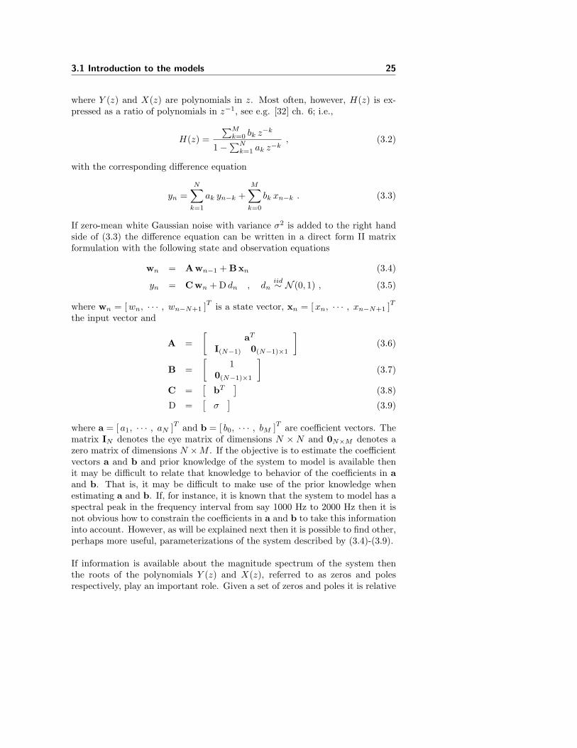
where a = [ a1, · · · , aN ]T and b = [ b0, · · · , bM ]T are coefficient vectors. Thematrix IN denotes the eye matrix of dimensions N × N and 0N×M denotes azero matrix of dimensions N ×M . If the objective is to estimate the coefficientvectors a and b and prior knowledge of the system to model is available thenit may be difficult to relate that knowledge to behavior of the coefficients in aand b. That is, it may be difficult to make use of the prior knowledge whenestimating a and b. If, for instance, it is known that the system to model has aspectral peak in the frequency interval from say 1000 Hz to 2000 Hz then it isnot obvious how to constrain the coefficients in a and b to take this informationinto account. However, as will be explained next then it is possible to find other,perhaps more useful, parameterizations of the system described by (3.4)-(3.9).
If information is available about the magnitude spectrum of the system thenthe roots of the polynomials Y (z) and X(z), referred to as zeros and polesrespectively, play an important role. Given a set of zeros and poles it is relative

26 Particle Filtering for MMSE Estimation
straightforward to visualize the shape of the magnitude spectrum, see e.g. [32]section 5.3 and [28]. It is also possible to roughly determine locations of zerosand poles from a sketch of a magnitude response. This will be illustrated with anexample using babble noise (fs = 16 kHz). A babble noise sound is analyzed inframes using a Hamming window of 25 ms duration and shifted in time in stepsof 1.5 ms. For each frame a power spectrum is computed. The power spectraare averaged in intervals of 500 ms and a 10th order LPC analysis is performedon each of the averaged power spectra. Finally, roots (poles) are computedfrom the denominator polynomial in the system function. The poles computedfrom one of the averaged power spectra are seen in the plot in figure 3.1. Themagnitude and phase response of the corresponding all-pole system function areshown in figure 3.2. As can be seen in figure 3.1 then the poles occur in complex
−1 −0.5 0 0.5 1
−1
−0.8
−0.6
−0.4
−0.2
0
0.2
0.4
0.6
0.8
1
Real Part
Imag
inar
y P
art
Figure 3.1: Figure shows unit circle in the complex z-plane and the locationof poles obtained by a 10th order LPC analysis of a smoothed babble powerspectrum.
conjugate pairs, 5 in total, all inside the unit circle. Each complex conjugatepole pair forms a resonance whose frequency is determined by the angles of thepoles and whose sharpness (bandwidth) is determined by the distance of thepoles to the unit circle. There is 500 Hz between each of the concentric greencircles and 500 Hz between each of the red lines coming radially out of theorigin. Each peak in the magnitude spectrum in the upper plot in figure 3.2
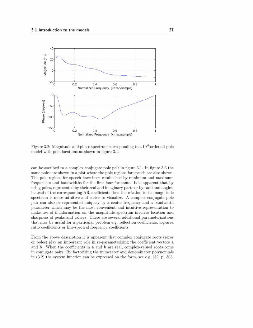
3.1 Introduction to the models 27
0 0.2 0.4 0.6 0.8 1−150
−100
−50
0
Normalized Frequency (×π rad/sample)
Pha
se (
degr
ees)
0 0.2 0.4 0.6 0.8 1−20
0
20
40
Normalized Frequency (×π rad/sample)
Mag
nitu
de (
dB)
Figure 3.2: Magnitude and phase spectrum corresponding to a 10thorder all-polemodel with pole locations as shown in figure 3.1.
can be ascribed to a complex conjugate pole pair in figure 3.1. In figure 3.3 thesame poles are shown in a plot where the pole regions for speech are also shown.The pole regions for speech have been established by minimum and maximumfrequencies and bandwidths for the first four formants. It is apparent that byusing poles, represented by their real and imaginary parts or by radii and angles,instead of the corresponding AR coefficients then the relation to the magnitudespectrum is more intuitive and easier to visualize. A complex conjugate polepair can also be represented uniquely by a center frequency and a bandwidthparameter which may be the most convenient and intuitive representation tomake use of if information on the magnitude spectrum involves location andsharpness of peaks and valleys. There are several additional parameterizationsthat may be useful for a particular problem e.g. reflection coefficients, log-arearatio coefficients or line-spectral frequency coefficients.
From the above description it is apparent that complex conjugate roots (zerosor poles) play an important role in re-parameterizing the coefficient vectors aand b. When the coefficients in a and b are real, complex-valued roots comein conjugate pairs. By factorizing the numerator and denominator polynomialsin (3.2) the system function can be expressed on the form, see e.g. [32] p. 303,

28 Particle Filtering for MMSE Estimation
−1 −0.5 0 0.5 1
−1
−0.8
−0.6
−0.4
−0.2
0
0.2
0.4
0.6
0.8
1
Real Part
Imag
inar
y P
art
Figure 3.3: Figure shows the unit circle and the poles from figure 3.1. The figurealso shows the pole regions for speech corresponding to the first four formants.
(by a theorem known as the fundamental theorem of algebra [28] p. 24)
H(z) = A
∏M1k=1(1− gk z−1)
∏M2k=1(1− hk z−1)(1− h∗k z−1)∏N1
k=1(1− ck z−1)∏N2
k=1(1− dk z−1)(1− d∗k z−1)(3.10)
where M = M1 + 2M2 and N = N1 + 2N2. In this factorization there are M2
pairs of complex conjugate zeros and N2 pairs of complex conjugate poles. Apair of complex conjugate roots corresponds to a Second-Order Section (SOS)on the form
HSOS(z) = 1− a1z−1 − a2z
−2 (3.11)
where a1 and a2 are real coefficients. As an example, consider a pair of complexconjugate roots, z1 and z∗1 . They can be related directly to the coefficients in(3.11) in the following way
HSOS(z) = (1− z1z−1)(1− z∗1z−1) = 1− (z1 + z∗1)z−1 + z1z
∗1z−2 (3.12)
Thus,a1 = z1 + z∗1 , a2 = −z1z
∗1 . (3.13)
Given the zeros and poles of a system function it is now possible to compute thecorresponding coefficients in a and b by first mapping the complex conjugate

3.1 Introduction to the models 29
roots to coefficients in a SOS on the form given by (3.11). Note that realroots correspond directly to the coefficient in a first-order section. Finally, thecoefficient vectors corresponding to first and second-order sections are convolved.If the complex conjugate roots are represented in polar form as z1 = Rejω andz∗1 = Re−jω and inserted in equation (3.12) one obtains
HSOS(z) = 1− (Rejω + Re−jω)z−1 + RejωRe−jωz−2 (3.14)= 1− 2R cos(ω)z−1 + R2z−2 . (3.15)
The SOS coefficients expressed in terms of the radius and angle of a complexconjugate root pair are thus
a1 = 2R cos(ω) , a2 = −R2 . (3.16)
Given a formant frequency, f , and formant bandwidth, b, (both in Hz) then thecorresponding complex root is given by
z1 = e−π bfs
+j2π ffs . (3.17)
This relation is explained in [26] and [35] and is based on transforming froms-plane to z-plane. The mapping from f and b to the coefficients in (3.11) arethus given by
a1 = 2e−π bfs cos
(2π
f
fs
), a2 = −e−2π b
fs (3.18)
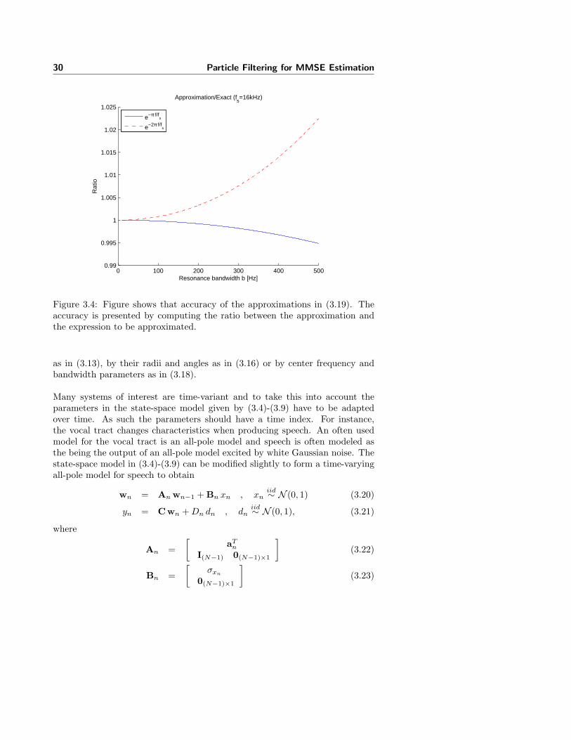
The mappings in (3.18) are non-linear. Reasonable approximations can be foundfor the mappings in (3.18) when modeling speech because the bandwidth of theresonances created in the vocal tract typically will be less than say 500 Hz. Thismeans that e−π b
fs and e−2π bfs may be approximated by first-order Taylor series
expansions. That is
e−π bfs ≈ 1− π
b
fs, e−2π b
fs ≈ 1− 2πb
fs. (3.19)
In figure 3.4 the accuracy of the approximations are shown for fs = 16 kHz
To summarize, motivated by the usefulness of discrete linear time-invariant sys-tems a linear state-space model has been introduced in (3.4)-(3.9). The modelis parameterized by the coefficient vectors a and b and an observation noisevariance. When estimating the coefficients in the a and b vectors it has beenargued that different parameterizations may be more advantageous. The basisof these representations is the factorization of the corresponding numerator anddenominator polynomials in terms of first and second-order sections. The co-efficients in the second-order sections can be represented by a pair of complexconjugate roots. The roots can be specified by their real and imaginary parts
30 Particle Filtering for MMSE Estimation
0 100 200 300 400 5000.99
0.995
1
1.005
1.01
1.015
1.02
1.025
Approximation/Exact (fs=16kHz)
Resonance bandwidth b [Hz]
Rat
io
e−π f/fs
e−2π f/fs
Figure 3.4: Figure shows that accuracy of the approximations in (3.19). Theaccuracy is presented by computing the ratio between the approximation andthe expression to be approximated.
as in (3.13), by their radii and angles as in (3.16) or by center frequency andbandwidth parameters as in (3.18).
Many systems of interest are time-variant and to take this into account theparameters in the state-space model given by (3.4)-(3.9) have to be adaptedover time. As such the parameters should have a time index. For instance,the vocal tract changes characteristics when producing speech. An often usedmodel for the vocal tract is an all-pole model and speech is often modeled asthe being the output of an all-pole model excited by white Gaussian noise. Thestate-space model in (3.4)-(3.9) can be modified slightly to form a time-varyingall-pole model for speech to obtain
wn = An wn−1 + Bn xn , xniid∼ N (0, 1) (3.20)
yn = Cwn + Dn dn , dniid∼ N (0, 1), (3.21)
where
An =[
aTn
I(N−1) 0(N−1)×1
](3.22)
Bn =[
σxn
0(N−1)×1
](3.23)

3.2 Monte Carlo 31
C =[
1 01×(N−1)
](3.24)
Dn =[
σdn
](3.25)
Noise reduction can be performed by MMSE estimation of the state-vector wn.MMSE estimates of the model parameters are also of interest. In the followingsections, a method is described that can be used for approximate inference inthe models specified by (3.4)-(3.9) and (3.20)-(3.25).
3.2 Monte Carlo
The basic idea behind the Monte Carlo method is to repeat an experiment anumber of times and use the outcomes of the experiments to estimate a quantityof interest. For instance, the task of computing the probability that a givensolitaire game will succeed may be very difficult. The Monte Carlo approach toestimate this probability is to play (simulate) a number of games (say 1, 000, 000)and take the ratio between the number of successful games and the total numberof games as the probability estimate. The same way probabilities of interest inpoker or blackjack may be approximated; simulate many games and computean estimate of the probability of winning given a particular setup.
The history of the Monte Carlo method is quite fascinating. It began in 1945when physicists at Los Alamos were studying the feasibility of a thermonuclearweapon. It’s beginning is also closely connected to the development of thefirst electrical computers. In [27] it is written ”The spirit of Monte Carlo isbest conveyed by an example discussed in von Neumann’s letter to Richtmeyer.Consider a spherical core of fissionable material surrounded by a shell of tampermaterial. Assume some initial distribution of neutrons in space and in velocitybut ignore radiative and hydrodynamic effects. The idea is to now follow thedevelopment of a large number of individual neutron chains as a consequenceof scattering, absorption, fission, and escape....Thus, a genealogical history ofan individual neutron is developed. The process is repeated for other neutronsuntil a statistically valid picture is generated.”
For the case of performing MMSE estimation the Monte Carlo approach is togenerate samples from the posterior PDF and average the value of the samples.However, although it sounds simple it is typically not realistic to draw samplesdirectly from the posterior PDF. It is not as easy as simulating a game of poker.There are several ways to generate samples from a given distribution see e.g. [23]pp. 23− 31. Some of these methods are not very practical for high-dimensionalproblems or suitable for on-line applications. IS, however, is a promising methodand is explained in the next section.

32 Particle Filtering for MMSE Estimation
3.3 Importance Sampling
Importance sampling is a method for generating samples from a distribution. Itworks by generating samples from a simpler proposal or importance distributionand correcting the bias by attaching importance weights to the drawn samples.To motivate the use of IS we will introduce an example adapted from [23] p.31− 34. The goal is to evaluate the integral
I =∫ 1
−1
∫ 1
−1
dx dy f(x, y) , (3.26)
where
f(x, y) = 0.5e−90(x−0.5)2−45(y+0.1)4 + e−45(x+0.4)2−60(y−0.5)2 . (3.27)
The function f(x, y) is shown to the left in figure 3.5. The integral in (3.26)
−1
0
1
−1
0
10
0.2
0.4
0.6
0.8
1
x
f(x,y)
y −1
0
1
−1
0
10
0.2
0.4
0.6
0.8
1
x
g(x,y)
y
Figure 3.5: Plot to the left shows the function f(x, y) and the plot to the rightshows the importance distribution g(x, y).
can be approximated using a Riemann sum by discretizing the domain [−1, 1]×[−1, 1] on a regular grid. Thus, the integral can be approximated as
IRiemann = ∆x∆y∑
i
∑
j
f(xi, yj) , (3.28)
where ∆x and ∆y are the spacings in the x and y directions, respectively. If aregular grid with a spacing of 0.02 is used in both the x and y directions thenapproximately 16 percent of the points are above the threshold 0.01. If onlypoints above this threshold are used then it produces a 1% relative difference
3.3 Importance Sampling 33
in the result. A regular grid thus uses many computations on points wheref(x, y) is negligible. Another disadvantage of the regular grid approach is thatthe complexity of evaluating an integral scales exponentially with the number ofdimensions. For instance, in the regular grid example 101 points is used on theinterval [−1, 1] on both the x and y-axis giving a total of 1012 = 10201 points.However, if the example is extended with a third z-axis (using same interval andgrid spacing) we would have to use 1013 = 1030301 points. It is thus obviousthat the regular grid approach becomes rather involved rather quickly as thenumber of dimensions increase.
A different approach is to uniformly sample the domain [−1, 1] × [−1, 1]. Theintegral in (3.26) can be written
I =∫ 1
−1
∫ 1
−1
dx dy f(x, y)p(x, y)p(x, y)
(3.29)
=1P
∫ 1
−1
∫ 1
−1
dx dy f(x, y)p(x, y) (3.30)
=1P
Ep(x,y){f(x, y)} , (3.31)
where P = p(x, y) = 1/4 and it is understood that f(x, y) is zero outside thedomain [−1, 1] × [−1, 1]. Because p(x, y) is a PDF, an approximation to theexpectation in (3.31) and thus the integral in (3.26) can be obtained by drawingN samples from p(x, y) and approximate p(x, y) by a sum of delta functions(with equal weighting 1/N). The approximation based on uniform samplingthus becomes
IUniform =1
N P
∑n
f(xn, yn) . (3.32)
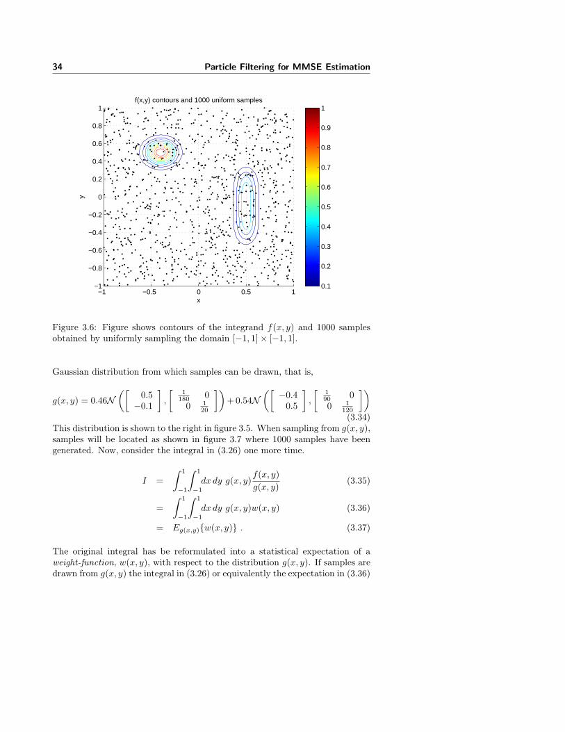
Figure 3.6 shows drawn samples for the case N = 1000. Because the approxi-mation is based on a sample of random samples then a new value of Iuniform
is obtained for each new experiment. That is, accuracy of the approximationhas to be measured statistically. One way to measure the accuracy of the ap-proximation is to perform K experiments and compute the mean and standarddeviation of the K results. As is evident from figure 3.6 then uniform samplingis also very inefficient because many samples are placed in regions where f(x, y)is negligible. The idea in IS is that instead of sampling the domain uniformly wecould find a different distribution to sample from that is more likely to producesamples in the areas where f(x, y) is non-negligible and thus improve efficiencyof the samples significantly. Samples could be generated from a distribution onthe form
g(x, y) ∝ 0.5e−90(x−0.5)2−45(y+0.1)2 + e−45(x+0.4)2−60(y−0.5)2 , (3.33)
with (x, y) ∈ [−1, 1] × [−1, 1]. This corresponds to a truncated mixture of
34 Particle Filtering for MMSE Estimation
−1 −0.5 0 0.5 1−1
−0.8
−0.6
−0.4
−0.2
0
0.2
0.4
0.6
0.8
1
x
y
f(x,y) contours and 1000 uniform samples
0.1
0.2
0.3
0.4
0.5
0.6
0.7
0.8
0.9
1
Figure 3.6: Figure shows contours of the integrand f(x, y) and 1000 samplesobtained by uniformly sampling the domain [−1, 1]× [−1, 1].
Gaussian distribution from which samples can be drawn, that is,
g(x, y) = 0.46N([
0.5−0.1
],
[1
180 00 1
20
])+0.54N
([ −0.40.5
],
[190 00 1
120
])
(3.34)This distribution is shown to the right in figure 3.5. When sampling from g(x, y),samples will be located as shown in figure 3.7 where 1000 samples have beengenerated. Now, consider the integral in (3.26) one more time.
I =∫ 1
−1
∫ 1
−1
dx dy g(x, y)f(x, y)g(x, y)
(3.35)
=∫ 1
−1
∫ 1
−1
dx dy g(x, y)w(x, y) (3.36)
= Eg(x,y){w(x, y)} . (3.37)
The original integral has be reformulated into a statistical expectation of aweight-function, w(x, y), with respect to the distribution g(x, y). If samples aredrawn from g(x, y) the integral in (3.26) or equivalently the expectation in (3.36)
3.3 Importance Sampling 35
−1 −0.5 0 0.5 1−1
−0.8
−0.6
−0.4
−0.2
0
0.2
0.4
0.6
0.8
1
x
yf(x,y) contours and 1000 samples from proposal distribution
0.1
0.2
0.3
0.4
0.5
0.6
0.7
0.8
0.9
1
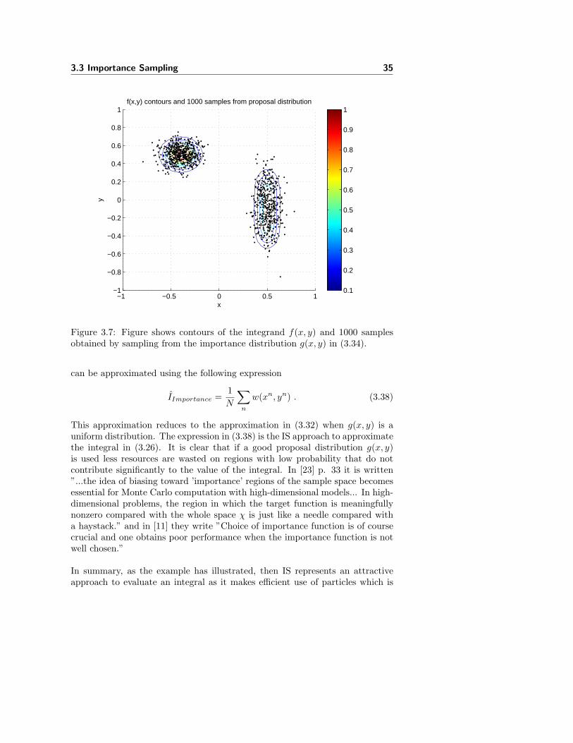
Figure 3.7: Figure shows contours of the integrand f(x, y) and 1000 samplesobtained by sampling from the importance distribution g(x, y) in (3.34).
can be approximated using the following expression
IImportance =1N
∑n
w(xn, yn) . (3.38)
This approximation reduces to the approximation in (3.32) when g(x, y) is auniform distribution. The expression in (3.38) is the IS approach to approximatethe integral in (3.26). It is clear that if a good proposal distribution g(x, y)is used less resources are wasted on regions with low probability that do notcontribute significantly to the value of the integral. In [23] p. 33 it is written”...the idea of biasing toward ’importance’ regions of the sample space becomesessential for Monte Carlo computation with high-dimensional models... In high-dimensional problems, the region in which the target function is meaningfullynonzero compared with the whole space χ is just like a needle compared witha haystack.” and in [11] they write ”Choice of importance function is of coursecrucial and one obtains poor performance when the importance function is notwell chosen.”
In summary, as the example has illustrated, then IS represents an attractiveapproach to evaluate an integral as it makes efficient use of particles which is
36 Particle Filtering for MMSE Estimation
important for practical use. It has also been indicated that IS is a method thatcan work for high-dimensional problems. The example also demonstrated howIS works by drawing samples from a simpler importance distribution and howa weight for each sample is computed.
As this chapter is about MMSE estimation the IS procedure is now repeated fora general MMSE-type integral. The pertinent integral is
IMMSE =∫
dx x p(x) . (3.39)
If N independent samples are drawn from p(x) then the integral in (3.39) canbe approximated by
IMMSE =1N
∑
i
xi . (3.40)
Generally, it is impossible to draw independent samples directly from the pos-terior distribution of interest. However, the integral in (3.39) can be written
IMMSE =∫
dx xp(x)π(x)
π(x) , (3.41)
and if N independent samples are generated from the importance distribution,π(x), then the integral can be approximated by
IMMSE =1N
N∑
i=1
xi p(xi)π(xi)
=1N
∑
i
xi w(xi) . (3.42)
The approximation in (3.42) is dependent on the choice of importance distribu-tion π(x). If the vector x can be divided into two parts x = [x1,x2]T such thatintegration over x1 conditional on x2 can be performed analytically the integralin (3.41) can be subjected to the principle of Rao-Blackwellization. Rewritingthe integral in (3.41) into
IMMSE =∫
dx1
∫dx2 [x1,x2] p(x1|x2)
p(x2)π(x2)
π(x2) (3.43)
=∫
dx2 Ep(x1|x2) {[x1,x2]} w(x2)π(x2) (3.44)
then if N independent samples are drawn from the importance distributionπ(x2), the integral in (3.39) can be approximated by
IRao−MMSE =1N
N∑
i=1
Ep(x1|x2)
{[x1,xi
2
]}w(xi
2) . (3.45)
In [23] p.27 it says ”Rao-Blackwellization. This method reflects a basic principle(or rule of thumb) in Monte Carlo computation: One should carry out analyticalcomputation as much as possible.” This principle will be used in section 3.4.

3.4 Sequential Importance Sampling 37
Finally, another important issue in IS is weight normalization. In MMSE es-timation the density p(x) in (3.39) represents a posterior PDF which may beknown up to a constant, that is, p(x) = p(x)/c where c =
∫dx p(x). The integral
in (3.41) can thus be written
IMMSE =∫
dx xp(x)π(x)
π(x)/ ∫
dxp(x)π(x)
π(x) . (3.46)
If N independent samples are generated from the importance distribution, π(x),then the integral can be approximated by
INorm−MMSE =∑
i xi w(xi)∑
i w(xi)=
∑
i
xi w(xi) , w(xi) =w(xi)∑i w(xi)
. (3.47)
Weight normalization is used in all subsequent examples.
3.4 Sequential Importance Sampling
Sequential Importance Sampling (SIS) refers to the task of sequentially gener-ating samples from the importance distribution and recursively computing theaccompanying weights. This idea is e.g. important for practical use of IS tostate estimation in dynamical systems as can be understood from the followingexcerpt from [2] ”For many problems an estimate is required every time that ameasurement is received. In this case a recursive filter is a convenient solution.A recursive filtering approach means that the received data can be processedsequentially rather than as a batch, so that it is not necessary to store thecomplete data set nor to reprocess existing data if a new measurement becomesavailable.”
A common way to introduce SIS is to the problem of state estimation in anonlinear state-space model with known parameters. Because the model is non-linear direct Kalman filtering is not possible. However, in this chapter a slightlydifferent approach is taken because SIS is introduced for inference in the models(3.4)-(3.9) and (3.20)-(3.25) which are both linear given the parameters in themodels and parameters are assumed unknown. For the model (3.4)-(3.9) param-eter estimation is of interest and for the model (3.4)-(3.9) joint estimation ofthe state and the parameters are of interest. Because the model in (3.20)-(3.25)is linear given the parameters the principle of Rao-Blackwellization (see section3.3) can be used whereby the problem of MMSE estimator approximation isreduced to the problem of sampling from the posterior PDF of the parameters.
Now a general derivation of the recursive weight-update equation is given. Thederivation largely follows the derivation provided in [11]. The starting point of
38 Particle Filtering for MMSE Estimation
the derivation is a sequence of PDFs {p(x1:n)} where n represents a time index.The goal is to derive a method for sampling sequentially from {p(x1:n)}; that is,first obtain samples and their weights from p(x1), then p(x1:2) and so on. Theimportance weights at time n are given by
wn =p(x1:n)π(x1:n)
, (3.48)
where π(x1:n) denotes the importance distribution. The importance distributionis decomposed into π(x1:n) = π(xn|x1:n−1)π(x1:n−1). This decomposition iscrucial because it means that if a path x(i)
0:n−1 is available (superscript i denotesan index into a set of paths) at time n this path can be augmented with asample, x(i)
n , drawn from π(xn|x(i)1:n−1) to obtain the path x(i)
0:n, thus the pathx(i)
0:n−1 is not modified. Inserting the decomposed importance distribution into(3.48), yields
wn =p(x1:n−1)π(x1:n−1)
· p(x1:n)p(x1:n−1)π(xn|x1:n−1)
(3.49)
= wn−1 · p(x1:n)p(x1:n−1)π(xn|x1:n−1)
(3.50)
= wn−1 · p(xn|x1:n−1)π(xn|x1:n−1)︸ ︷︷ ︸
wupdate
. (3.51)
In going from (3.50) to (3.51) an implicit assumption has been made thatPDF p(x1:n−1) at times n−1 and n are equal. As noted in [11], the densities{π(xn|x1:n−1)} are parameters to be selected by the user. At each time-stepthe SIS procedure consists of propagating the particles at the previous time-step by a sampling step and a weight-update step performed for each particle.That is, at time n the SIS procedure completes, for each particle indexed by asuperscript i, the steps
1. Sample x(i)n ∼ π(xn|x(i)
1:n−1)
2. Update weight using (3.51) to get w(i)n .
3. Normalize weights.
To summarize SIS, when the objective is to apply IS for state-estimation in a dy-namical system or for parameter estimation in a model whose parameters changeover time we have to draw samples from a sequence of posterior PDFs denotedby e.g. {p(x1:n)} and compute weights given by the ratio p(x1:n)/π(x1:n). The

3.4 Sequential Importance Sampling 39
problem is that the raw IS procedure requires us to draw paths whose lengthincrease over time which means that the number of computations and memoryconsumption increase with time. The key idea in arriving at the SIS procedurewas that of decomposing the importance distribution in such a way that samplesfrom the sequence of PDFs of interest, {p(x1:n)}, could be generated recursively.The decomposition could also be used to derive an expression for the weightssuch that they can be recursively propagated in time. Thus, SIS eliminates theincrease in the number of computations and memory consumption over time.
Considering the speech model in (3.20)-(3.25) the sequence of PDFs of interestis the sequence of posterior PDFs {p(w0:n,a0:n, σx0:n , σd0:n |y1:n)}. Now a no-tational context switch is made in order to comply with the notation commonto SIS literature. The state vector is renamed from w to x and all parame-ters are stacked in the parameter vector θ. That is, the sequence of posteriorPDFs is denoted {p(x0:n,θ0:n|y1:n)}. The nth element in the sequence can bedecomposed into p(x0:n, θ0:n|y1:n) = p(x0:n|θ0:n, y1:n)p(θ0:n|y1:n). The point isto realize that p(x0:n|θ0:n, y1:n) is Gaussian because the model in (3.20)-(3.25)reduces to a linear Gaussian state-space model (see also [39]). Integration overthe state vector can thus be performed analytically. This process is referred toas Rao-Blackwellization as explained in section 3.3. The MMSE estimator forthe state vector and parameter vector is given by the following expression
< xn, θn >=∫
dx0:n
∫dθ0:n [xn, θn] p(x0:n, θ0:n|y1:n) . (3.52)
As a consequence of the Rao-Blackwellization, approximating this MMSE es-timator is depending on generating samples from the sequence {p(θ0:n|y1:n)}.If N independent samples are drawn from the importance distribution π(θ0:n)then (3.52) can be approximated by
< xn, θn > =1N
N∑
i=1
Ep(x0:n|θi0:n,y1:n){[xn,θi
n]} w(θi0:n|y1:n) (3.53)
The factor wupdate in (3.51) is given by
wupdate =p(θn|θ0:n−1, y1:n)π(θn|θ0:n−1, y1:n)
(3.54)
∝ p(yn|θ0:n, y1:n−1)p(θn|θ1:n−1)π(θn|θ0:n−1, y1:n)
(3.55)
At time n the SIS procedure for MMSE estimation of state and parameter vectorcompletes, for each particle indexed by a superscript i, the steps
1. Sample θ(i)n ∼ π(θn|θ(i)
1:n−1) .

40 Particle Filtering for MMSE Estimation
2. Perform Rao-Blackwellization to get x(i)n .
3. Update weight using (3.55) to get w(i)n .
4. Normalize weights to get w(i)n .
5. Estimate state and parameter vector by∑
i[x(i)n ,θ(i)
n ]w(i)n .
For the model in (3.4)-(3.9) the SIS procedure is very similar. However, when theinput is not assumed stochastic which is the case for the model (3.4)-(3.9) usedin the examples in sections 3.6-3.8, only the parameters need to be estimatedand the Rao-Blackwellization step disappears.
In the examples in sections 3.6-3.8 it is assumed that the parameters evolveaccording to first-order Markov processes such that p(θn|θ1:n−1) = p(θn|θn−1).Furthermore the importance distribution is set equal to p(θn|θn−1) which meansthat drawing samples is simple and that the weight update factor in (3.55)reduces to wupdate ∝ p(yn|θ0:n, y1:n−1). This choice of importance distributionis discussed in the next section.
3.5 Importance Distribution and Resampling
Now the SIS procedure is applied to the example of estimating the mean ofthe un-normalized PDF given by (3.27). That is, the mean value of the PDFp(x, y) = f(x, y)/c where c is a constant will be approximated by applying theSIS procedure outlined in section 3.4. This example is a little different in thatp(x, y) is ’static’ and does not necessarily represent a posterior PDF. Particlesare adapted by choosing independent and equal first-order Markov processes,also called Random Walks (RWs), as the importance distributions for x andy. The RW variance (reminiscent of a step-size parameter) is set to 0.01 andinitially particles are distributed uniformly in the region [−1, 1]× [−1, 1]. Thatis, if θn = [xn, yn]T then
p(θ0) = U ([−1,−1], [1, 1]) (3.56)p(θn|θn−1) = N (02×1, 0.01I2×2) (3.57)
where U (a,b) denotes the uniform distribution on the interval given by [a,b]and N (µ,Σ) denotes a Gaussian distribution with mean µ and covariance ma-trix Σ that in this case is truncated to the region [−1, 1]× [−1, 1].
Figure 3.8 and 3.9 show particle paths and weights, respectively, after one it-eration. For this example thirty particles are used. Figure 3.10 and 3.11 show

3.5 Importance Distribution and Resampling 41
particle paths and weights after six iterations. From this example it is clearthat only few particles contribute to the mean estimation because many par-ticle weights are insignificant. The whole idea of IS is to make efficient useof particles. For this example it is clear that inefficient use of the particles isthe result of a non-optimal importance distribution which places particles in re-gions where f(x, y) is negligible. This leads to the question of what the optimalimportance distribution for SIS is?
−1 −0.5 0 0.5 1−1
−0.8
−0.6
−0.4
−0.2
0
0.2
0.4
0.6
0.8
1
x
y
f(x,y) contours and 30 particles
1
23
4
5
6
7
8
9
1011
12
13
14
15
16
17
18
19
20
21
22
23
24
25
26
27
28
29
30
Figure 3.8: Figure shows contours of f(x, y) and the 30 particle paths after oneiteration of SIS.
In [13] the optimal importance function is found under the criterion of minimumvariance of the importance weights. However, use of the optimal importancefunction is made difficult by two issues 1) sampling from it and 2) evaluationof the importance weights. As mentioned in both [13] and [11] then the SISprocedure is not guaranteed to be efficient even though the optimal importancefunction can be used. Furthermore, it can even be shown that the variance ofthe importance weights increases over time even though the optimal importancefunction is used. In [13] it says ”Thus, it is impossible to avoid a degeneracyphenomenon. In practice, after a few iterations of the algorithm, all but one ofthe normalized importance weights are very close to zero and a large computa-

42 Particle Filtering for MMSE Estimation
5 10 15 20 25 300
0.2
0.4
0.6
0.8
1
Particle index
Wei
ght
Importance weights
Figure 3.9: Figure shows particle weights after one iteration of SIS.
tional effort is devoted to updating trajectories whose distribution to the finalestimate is almost zero.” This phenomenon is referred to as degeneration of theparticles.
In order to reduce the effect of the degeneracy, particle filters adds a resam-pling step (also called selection step in some literature) to the SIS procedure.The fundamental idea behind the resampling is to eliminate particles with lowimportance weights and move them to regions with higher importance weights.The way this is done is to duplicate some particles a number of times. In [34]it is written ”A selection scheme associates to each particle x(i)
0:t a number of’children’, say Ni ∈ N, such that
∑Ni=1 Ni = N” where N denotes the number
of particles. After resampling all particles (original and duplicated) have equalweights 1/N . The example is now continued to demonstrate how this works.
The example is repeated but now with a resampling step in each iteration. Infigure 3.12 those particles after first iteration (see figure 3.8) to be deleted aremarked by a red cross. In figure 3.13 those particles marked by a cross infigure 3.12 have been removed and the four particles left after the deletion havebeen duplicated a number of times and adapted with one step of a GaussianRW. In figure 3.14 this procedure has been repeated six times and we see thatall thirty particles are more or less placed in ’important’ regions and therebyincreasing efficiency of the particles. However, the example also do illustratethat in this particular case the particle filter is not ’capturing’ the presence ofthe weaker second mode of the PDF which makes the estimate of the mean valuequite inaccurate. Eventually, even when using thousands of particles then afterenough iterations the particles will all be placed around the ’stronger’ mode.

3.5 Importance Distribution and Resampling 43
−1 −0.5 0 0.5 1−1
−0.8
−0.6
−0.4
−0.2
0
0.2
0.4
0.6
0.8
1
x
y
f(x,y) contours and 30 particles
1
2
3
4
5
6
7
8
910
11 12
1314
15
16
17
18
19
20
21
22
23
24
25
26
27
28
29
30
Figure 3.10: Figure shows contours of f(x, y) and particle paths after six itera-tions of SIS.
The resampling procedure used in this example is called residual resampling.This resampling procedure is used in the ReBEL (Recursive Bayesian EstimationLibrary) toolbox and is described in [34].

44 Particle Filtering for MMSE Estimation
5 10 15 20 25 300
0.2
0.4
0.6
0.8
1
Particle index
Wei
ght
Importance weights
Figure 3.11: Figure shows particle weights after six iterations of SIS.
−1 −0.5 0 0.5 1−1
−0.8
−0.6
−0.4
−0.2
0
0.2
0.4
0.6
0.8
1
x
y
f(x,y) contours and 30 particles
1
23
4
5
6
7
8
9
1011
12
13
14
15
16
17
18
19
20
21
22
23
24
25
26
27
28
29
30
Figure 3.12: The figure shows which particles are deleted after a resampling stepin first iteration. Se figure 3.8 for comparison. After resampling four particlesare retained (number 6, 11, 16, 22)

3.5 Importance Distribution and Resampling 45
−1 −0.5 0 0.5 1−1
−0.8
−0.6
−0.4
−0.2
0
0.2
0.4
0.6
0.8
1
x
yf(x,y) contours and 30 particles
Figure 3.13: The four particles left after the deletion have been duplicated anumber of times and adapted with one step of a Gaussian RW.
−1 −0.5 0 0.5 1−1
−0.8
−0.6
−0.4
−0.2
0
0.2
0.4
0.6
0.8
1
x
y
f(x,y) contours and 30 particles
Figure 3.14: This figure shows particles paths after six iterations of SIS withresampling.
46 Particle Filtering for MMSE Estimation
3.6 Bayesian Adaptive FIR Filtering
In this section a PF approach to the adaptive FIR filtering problem is presented.Generally, the FIR model is
yn =M∑
k=0
bk xn−k + σunun = bT
n xn + σunun , un ∼ N (0, 1) (3.58)
where M denotes the order of the filter. The model in (3.58) is a special caseof the model in (3.4)-(3.9). In adaptive filtering the goal is to estimate thecoefficient vector bn given input and output data. In addition to the coefficientvector the noise variance is also assumed unknown. The parameters are assumedto evolve according to the following first-order Markov processes
b0 = ν , ν ∼ N (0(M+1)×1, δ
2b0
I(M+1)
)bn = bn−1 + ςn , ςn ∼ N (
0(M+1)×1, δ2bI(M+1)
)σ2
u0= γ , γ ∼ U (
0, δ2u0
)σ2
un= σ2
un−1+ ψn , ψn ∼ N (
0, δ2u
)(3.59)
where the hyper-parameters δ2b0
, δ2b, δ2
u0, δ2
u need to be tuned for the particularproblem at hand. Because samples are generated by the prior the weights aregiven by
ωn ∝ p(yn|xn,bn, σ2) , p(yn|xn,bn, σ2) = N (yn − bT
n xn, σ2)
(3.60)
As a demonstration one thousand samples are generated using (3.58) whereM = 3, b = [0.7,−0.4, 0.2,−0.9]T and σ2
un= 0.1. In figure 3.15 is shown the
result of using the NLMS algorithm to estimate the coefficients for two differentstep-sizes. Figure 3.15 indicates that the step-size parameter can be varied toadjust the magnitude of the fluctuations and the rate of convergence. In thePF method the RW variances have a similar role. Furthermore, the numberof particles to use also needs to be determined. Figure 3.16 shows the resultsof applying the PF method to estimate the coefficients and the noise variance.The setting of the hyperparameters is δ2
b0=1, δ2
u0=1, δ2
u=5e−5 and the numberof particles used is 30. In figure 3.16a δ2
b=1e−4 and in figure 3.16b δ2b=5e−4.
The PF method is also used to estimate the noise variance which is also shownin figure 3.16. Computational-wise the PF method is more expensive than theNLMS algorithm, approximately the number of particles times more expensive.Maybe the most interesting aspect of using a PF based adaptive filter is theopportunity to incorporate knowledge of the system into the adaptation. It isfor instance straightforward to reparameterize the model in (3.58) using one ofthe parameterizations discussed in section 3.1.
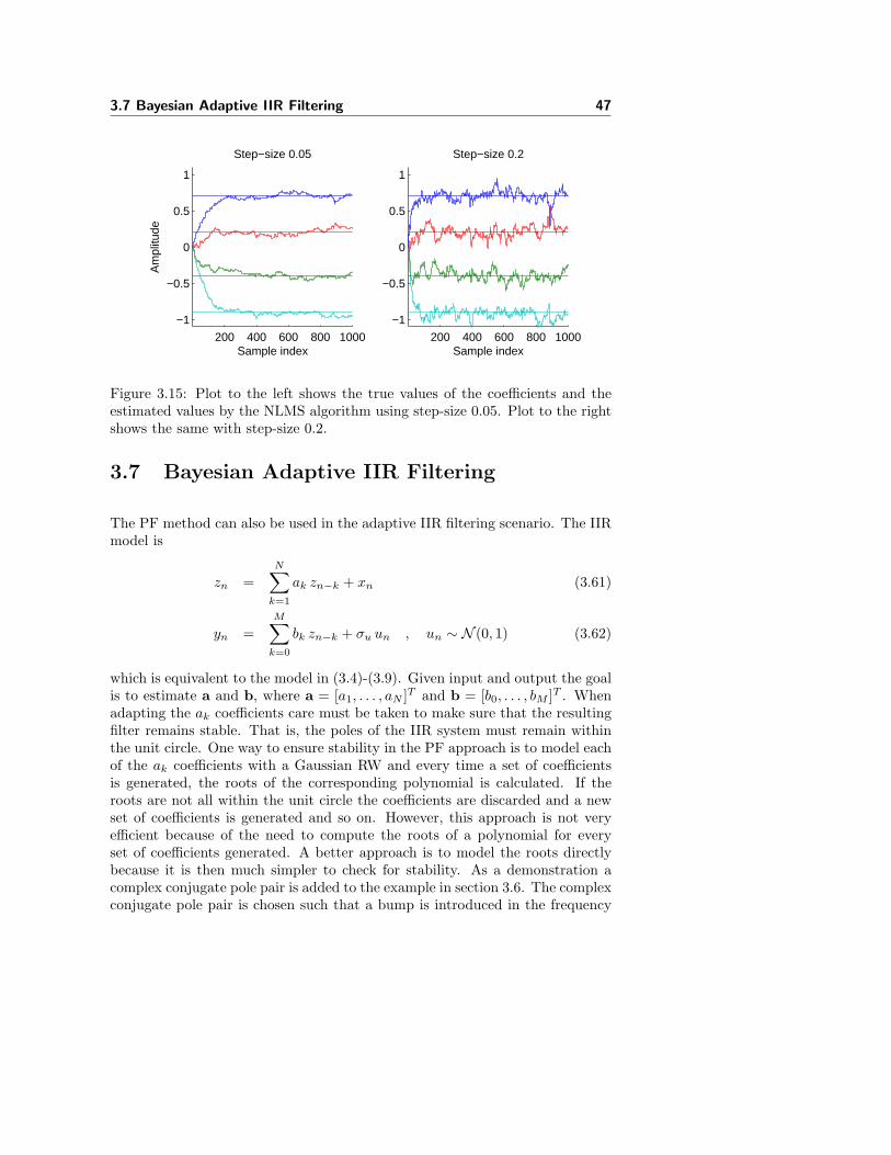
3.7 Bayesian Adaptive IIR Filtering 47
200 400 600 800 1000
−1
−0.5
0
0.5
1
Sample index
Am
plitu
deStep−size 0.05
200 400 600 800 1000
−1
−0.5
0
0.5
1
Sample index
Step−size 0.2
Figure 3.15: Plot to the left shows the true values of the coefficients and theestimated values by the NLMS algorithm using step-size 0.05. Plot to the rightshows the same with step-size 0.2.
3.7 Bayesian Adaptive IIR Filtering
The PF method can also be used in the adaptive IIR filtering scenario. The IIRmodel is
zn =N∑
k=1
ak zn−k + xn (3.61)
yn =M∑
k=0
bk zn−k + σu un , un ∼ N (0, 1) (3.62)
which is equivalent to the model in (3.4)-(3.9). Given input and output the goalis to estimate a and b, where a = [a1, . . . , aN ]T and b = [b0, . . . , bM ]T . Whenadapting the ak coefficients care must be taken to make sure that the resultingfilter remains stable. That is, the poles of the IIR system must remain withinthe unit circle. One way to ensure stability in the PF approach is to model eachof the ak coefficients with a Gaussian RW and every time a set of coefficientsis generated, the roots of the corresponding polynomial is calculated. If theroots are not all within the unit circle the coefficients are discarded and a newset of coefficients is generated and so on. However, this approach is not veryefficient because of the need to compute the roots of a polynomial for everyset of coefficients generated. A better approach is to model the roots directlybecause it is then much simpler to check for stability. As a demonstration acomplex conjugate pole pair is added to the example in section 3.6. The complexconjugate pole pair is chosen such that a bump is introduced in the frequency
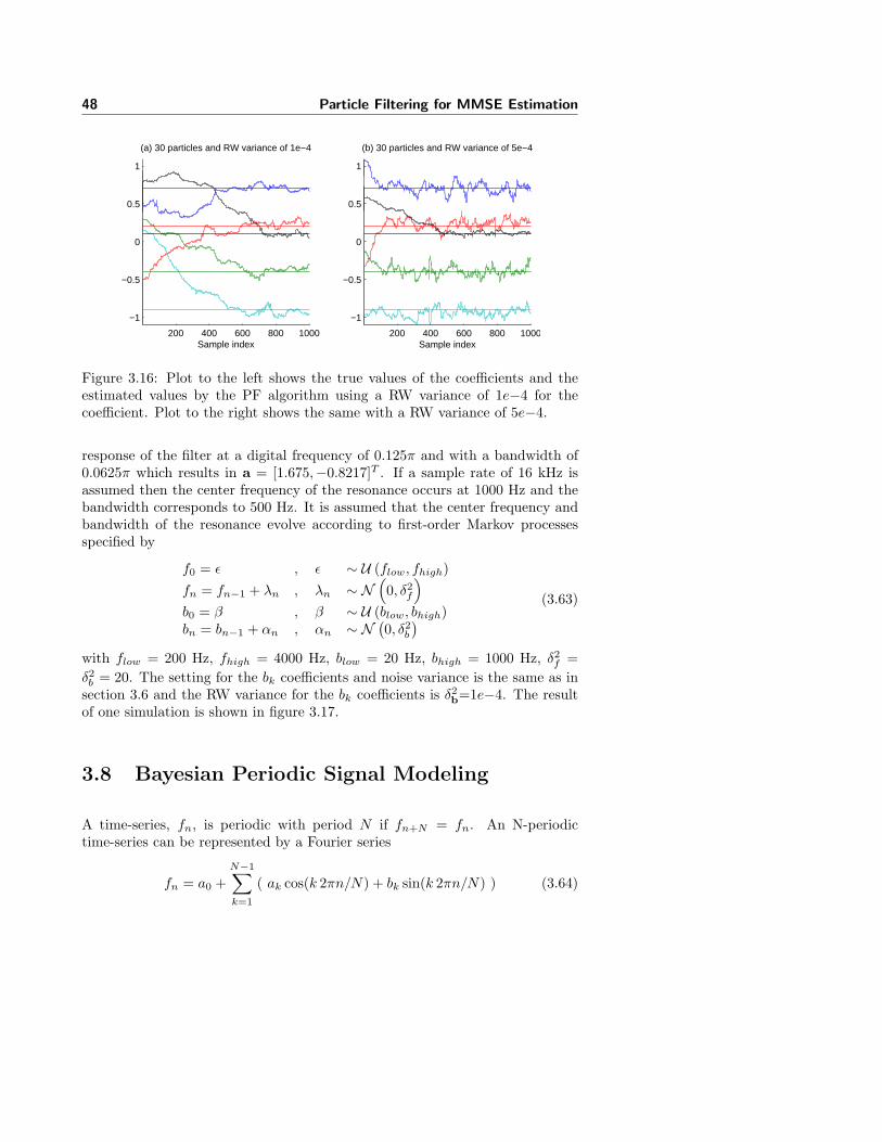
48 Particle Filtering for MMSE Estimation
200 400 600 800 1000
−1
−0.5
0
0.5
1
Sample index
(a) 30 particles and RW variance of 1e−4
200 400 600 800 1000
−1
−0.5
0
0.5
1
Sample index
(b) 30 particles and RW variance of 5e−4
Figure 3.16: Plot to the left shows the true values of the coefficients and theestimated values by the PF algorithm using a RW variance of 1e−4 for thecoefficient. Plot to the right shows the same with a RW variance of 5e−4.
response of the filter at a digital frequency of 0.125π and with a bandwidth of0.0625π which results in a = [1.675,−0.8217]T . If a sample rate of 16 kHz isassumed then the center frequency of the resonance occurs at 1000 Hz and thebandwidth corresponds to 500 Hz. It is assumed that the center frequency andbandwidth of the resonance evolve according to first-order Markov processesspecified by
f0 = ε , ε ∼ U (flow, fhigh)fn = fn−1 + λn , λn ∼ N
(0, δ2
f
)
b0 = β , β ∼ U (blow, bhigh)bn = bn−1 + αn , αn ∼ N (
0, δ2b
)(3.63)
with flow = 200 Hz, fhigh = 4000 Hz, blow = 20 Hz, bhigh = 1000 Hz, δ2f =
δ2b = 20. The setting for the bk coefficients and noise variance is the same as in
section 3.6 and the RW variance for the bk coefficients is δ2b=1e−4. The result
of one simulation is shown in figure 3.17.
3.8 Bayesian Periodic Signal Modeling
A time-series, fn, is periodic with period N if fn+N = fn. An N-periodictime-series can be represented by a Fourier series
fn = a0 +N−1∑
k=1
( ak cos(k 2πn/N) + bk sin(k 2πn/N) ) (3.64)

3.8 Bayesian Periodic Signal Modeling 49
500 1000 1500 2000 2500 3000 3500 4000−1.5
−1
−0.5
0
0.5
1(a) Tracking coefficients in b vector
500 1000 1500 2000 2500 3000 3500 4000
0
0.5
1
1.5
2
2.5(b) Noise variance tracking
500 1000 1500 2000 2500 3000 3500 4000400
600
800
1000
1200
1400
1600
1800
2000
Sample index
(c) Tracking resonance parameters
500 1000 1500 2000 2500 3000 3500 4000−1
−0.5
0
0.5
1
1.5
2
Sample index
(d) Estimated coefficients in a vector
Figure 3.17: (a) True and estimated bk coefficients (b) true and estimated noisevariance (c) true and estimated resonance frequency and bandwidth (d) pathsfrom (c) converted to ak coefficients.
For the example in this section a zero-mean signal will be modeled which meansthat a0=0 and the Fourier series is truncated to L components (the fundamentaland L− 1 harmonics) such that the following model is used
fn =L∑
k=1
( ak cos(k 2πn/N) + bk sin(k 2πn/N) ) (3.65)
A model for a noisy periodic signal is thus
yn = cTnxn + σu un , un ∼ N (0, 1) (3.66)
where (omitting time index) cT = [a1, b1, . . . , aL, bL]T and
xn = [cos(2πn/N), sin(2πn/N), . . . , cos(L 2πn/N), sin(L 2πn/N)]T (3.67)
Here, (3.65) is used to model a synthetic periodic signal. The periodic sig-nal is generated using the Liljencrants-Fant (LF) model which models the har-monic component present in the signal exciting the vocal tract when producingvoiced speech. The waveform was generated using the settings t0=99ts, te =0.7t0, tp=0.6t0, ta=0.05t0, Ee=3, where ts denotes the sampling period. See

50 Particle Filtering for MMSE Estimation
Appendix D for an introduction to the LF model and its parameters. Figure3.18 shows one period of the generated excitation signal. The figure also showsthe Fourier series coefficients of the waveform and the waveform which resultswhen retaining only six components in the Fourier series. The waveform shown
0 1 2 3 4 5 6
x 10−3
−3
−2
−1
0
1
time [s]
g’(t
)
One period of a glottal derivative waveform from LF model
5 10 15 20 25 30 35 40 45 50−0.5
0
0.5
1
Coefficient index
Mag
nitu
de
Fourier series coefficients
ab
Figure 3.18: Upper plot shows one period of the derivative glottal flow waveformgenerated using the LF model. The period is 100 samples and fs = 16 kHz. Theplot also shows the approximation to this periodic signal (black dashed line) byretaining the first L components in the Fourier series of the waveform, that is,L = 6 in (3.65). Lower plot shows the Fourier series coefficients of the periodicwaveform (blue: ak coefficients, red: bk coefficients).
in the upper plot of figure 3.18 was repeated 80 times such that an 8000-samplessequence was obtained. White Gaussian noise with variance 3.7e−2 was addedto the periodic signal which resulted in a SNR of approximately 12 dB. EachFourier coefficient was adapted using a Gaussian RW with variance 1e−3. Thepitch period is adapted using a discrete uniform RW. If N denotes the pitchperiod then,
N0 = δ , δ ∼ UD (70, 130)
Nn ={
Nn−1 , , if mod(n,Nn−1) == 0Nn−1 + φn , φn ∼ UD (−4, 4) , else
(3.68)
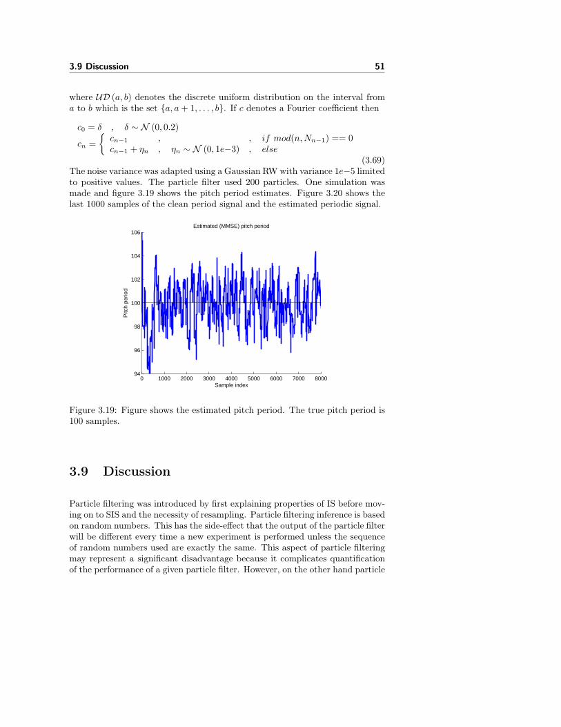
3.9 Discussion 51
where UD (a, b) denotes the discrete uniform distribution on the interval froma to b which is the set {a, a + 1, . . . , b}. If c denotes a Fourier coefficient then
c0 = δ , δ ∼ N (0, 0.2)
cn ={
cn−1 , , if mod(n,Nn−1) == 0cn−1 + ηn , ηn ∼ N (0, 1e−3) , else
(3.69)The noise variance was adapted using a Gaussian RW with variance 1e−5 limitedto positive values. The particle filter used 200 particles. One simulation wasmade and figure 3.19 shows the pitch period estimates. Figure 3.20 shows thelast 1000 samples of the clean period signal and the estimated periodic signal.
0 1000 2000 3000 4000 5000 6000 7000 800094
96
98
100
102
104
106Estimated (MMSE) pitch period
Pitc
h pe
riod
Sample index
Figure 3.19: Figure shows the estimated pitch period. The true pitch period is100 samples.
3.9 Discussion
Particle filtering was introduced by first explaining properties of IS before mov-ing on to SIS and the necessity of resampling. Particle filtering inference is basedon random numbers. This has the side-effect that the output of the particle filterwill be different every time a new experiment is performed unless the sequenceof random numbers used are exactly the same. This aspect of particle filteringmay represent a significant disadvantage because it complicates quantificationof the performance of a given particle filter. However, on the other hand particle
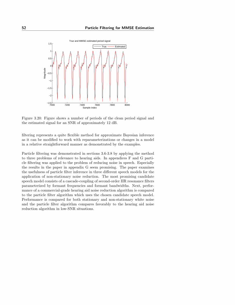
52 Particle Filtering for MMSE Estimation
7000 7200 7400 7600 7800 8000−2.5
−2
−1.5
−1
−0.5
0
0.5
1
1.5True and MMSE estimated period signal
Sample index
Mag
nitu
de
True Estimated
Figure 3.20: Figure shows a number of periods of the clean period signal andthe estimated signal for an SNR of approximately 12 dB.
filtering represents a quite flexible method for approximate Bayesian inferenceas it can be modified to work with reparameterizations or changes in a modelin a relative straightforward manner as demonstrated by the examples.
Particle filtering was demonstrated in sections 3.6-3.8 by applying the methodto three problems of relevance to hearing aids. In appendices F and G parti-cle filtering was applied to the problem of reducing noise in speech. Especiallythe results in the paper in appendix G seem promising. The paper examinesthe usefulness of particle filter inference in three different speech models for theapplication of non-stationary noise reduction. The most promising candidatespeech model consists of a cascade-coupling of second-order IIR resonance filtersparameterized by formant frequencies and formant bandwidths. Next, perfor-mance of a commercial-grade hearing aid noise reduction algorithm is comparedto the particle filter algorithm which uses the chosen candidate speech model.Performance is compared for both stationary and non-stationary white noiseand the particle filter algorithm compares favorably to the hearing aid noisereduction algorithm in low-SNR situations.

Chapter 4
Results & Outlook
This report has considered MMSE signal estimation in a single-channel setupwhere the signal is contaminated by additive noise. This problem has beenapproached in two different ways. One way in which priors for the signal andnoise have been expressed by their PDFs and the MMSE estimator is approx-imated using saddlepoint approximation and another way in which the priorshave been provided in terms of generative models and the MMSE estimator isapproximated by particle filtering. Conclusions and recommendations for fur-ther research will be given for both approaches.
4.1 Saddlepoint Approximation
The integral defining the MMSE estimator when expressed directly in terms ofprior PDFs consists of a weighted convolution integral between the prior PDFs,see e.g. (1.4) or (2.2). However as has been shown in this report then for theunivariate case considered in the paper in appendix E and for the multivariatecase considered in chapter 2 then this integral can be rewritten into an inverseLaplace transform integral with an integrand that is the product between theMoment Generating Function (MGF) of the noise and the first-order derivativeof the MGF of the signal. The presence of the derivative of the MGF changes
54 Results & Outlook
everything compared to the situation of using SPA for approximating tail prob-abilities where there is no derivative of MGFs involved. The consequence of thederivative is that the search for a useful saddlepoint becomes significantly morecomplex as the search problem is not confined to locating a unique and real sad-dlepoint as in the case of approximating a tail probability. Furthermore, there isthe added issue of nearby or coalescing saddlepoints as has been demonstratedin the paper in appendix E. This means that applying SPA to approximate theMMSE integral is far from ’plug-n-play’. It is not straightforward to extend andapply the results of the paper in appendix E to the multivariate case. Even ifthe results in appendix E is (or can be) extended to the multivariate case thenapplying the results gets rather involved and will be limited to low dimensionalproblems. As such,
MMSE estimation by SPA appears not as promising as we thought before westarted and we do not consider it a priority to further investigate this method.
4.2 Particle Filtering
The use of particle filtering for MMSE estimation of speech has been examinedin detail. A reparameterized time-varying auto-regressive model for speech wasused. It has been found very beneficial to reparameterize the speech model interms of formant feature parameters to exploit prior knowledge of these featuresin the estimation task. Even though the proposed reparameterization introducednon-linearities into the model then particle filtering turned out to be a quiteflexible and easy-to-use method for such reparameterizations. The versatilityof particle filtering for parameter estimation has also been demonstrated in thethree examples in sections 3.6-3.8, where especially the example in section 3.8could be used to improve the speech model.
The performance of the particle filtering algorithm was compared to a stateof the art hearing aid noise reduction algorithm in the paper in appendix G.Both stationary and non-stationary white noise were used. In order to makea meaningful comparison a modified MMSE estimator was introduced. It al-lowed trading off SNR improvement for increased speech intelligibility by ad-justing one parameter. Performance of the two algorithms were measured bytwo complementary objective measures, segmental SNR improvement and a sig-nal distortion measure. The measurements indicated that the particle filteringalgorithm performs better than the hearing aid algorithm for SNR levels below10 dB. However, informal listening tests indicated that performance of the twoalgorithms was very similar. It is believed that short-comings of the used speechmodel is the main reason that listening tests did not favor the particle filtering

4.2 Particle Filtering 55
Time [s]
Fre
quen
cy [H
z]
Wide−band spectrogram of TIMIT sound
0 0.5 1 1.5 2 2.5 30
1000
2000
3000
4000
5000
6000
7000
8000
Figure 4.1: Wide-band spectrogram of TIMIT sound SA1 downsampled to 16kHz.
algorithm over the hearing aid algorithm.
It was also found that the particle filtering algorithm was able to track thenoise variance better than the hearing aid algorithm for SNR levels below 10dB. However, for SNR levels above 10 dB the noise tracking of the particle filteralgorithm became inaccurate during intervals of speech with most of the energyconcentrated at high frequencies. The used speech model does not model suchhigh frequency energy. To illustrate this point, figure 4.1 shows a wide-bandspectrogram of the TIMIT sound SA1 (’She had your dark suit in greasy wash-water all year’). It is observed that at the time points 1.0 s, 1.7 s and 2.1 s burstswith significant energy at high frequencies are present in the speech signal. Ifthis spectrogram is correlated with figure 11b in the paper in appendix G it isseen that these intervals cause inaccurate estimates of the noise variance.
It is believed that performance of the particle filter algorithm can be improvedsignificantly by extending the speech model. Both noise tracking as well asnoise reduction capabilities and also for SNR levels above 10 dB. One short-coming of the speech model is that it does not model speech energy above 5000Hz because formants do not appear above approximately this frequency andfor a sampling frequency of 16 kHz it gives a high-frequency interval wherepresent speech energy is not modeled. The speech model could for instance beextended such that the output is given as a mixing of the non-extended speech
56 Results & Outlook
model and high-pass filtered noise. Another short-coming of the speech modelis a missing harmonic component in the excitation signal which occurs duringvoiced speech. Such a harmonic component can for instance be modeled by aFourier series which was also used in the example in section 3.8 but even betterit could be modeled by for instance the Rosenberg-Klatt++ model described inappendix D.
The noise tracking capabilities of the particle filtering algorithm looks inter-esting from a hearing aid point of view. Excellent noise tracking capabilitiesis important for the success of a non-stationary noise reduction algorithm andtraditional approaches to obtain a noise estimate have limited noise trackingcapabilities during periods of speech. Therefore it may be worth investigatinghow the noise estimate from a particle filter algorithm can be integrated into ahearing aid.
The approximate inference performed by the particle filtering algorithm canalso be improved by introducing more sophisticated proposal distributions suchas for instance the method developed in [11]. Such approaches will increaseefficiency of particles at the expense of increased computational complexity.
There are two primary issues that will have to be investigated further beforenoise reduction by particle filtering can be considered a serious candidate for usein hearing aids. Firstly, performance must be improved by extending the speechmodel such that high-frequency speech components are modeled and such thata harmonic excitation signal is also modeled. This should make the particlefiltering algorithm more robust in the sense that performance is not varying toomuch dependent of what speech sounds are being processed and it should alsoimprove performance for higher SNRs. Secondly, validation and quantification ofperformance is relative tedious because many experiments have to be conductedbefore a solid statistical picture of the workings of the particle filtering algorithmcan been obtained. The particle filtering algorithm is reliant on random numbersand hence performance should be measured statistically. It must be determinedwhether the increased overhead of doing many experiments is not a practicalnightmare. There is also the possibility lurking that for a particular situation theparticle filter algorithm will be highly sensitive to some sets of random numberssuch that on average in one out of say thousand experiments the particle filteringalgorithm performs poorly due to for instance local maxima.
Computational complexity is not considered a primary issue. It is consideredpossible to implement small particle filters with say ten to twenty particleson next generation digital hearing aid platforms. Another point is that manyhearing aid companies are now focusing on wireless links between hearing aidsin binaural settings and at some point it is considered likely that communicationbetween a hearing aid and for instance a cell phones will be possible hence the

4.2 Particle Filtering 57
hearing aid will have access to much more powerful processing units. Anotherissue that should be investigated further on is that of extending the noise model.In this report emphasis has been focused on developing a useful speech modelbut the usefulness of the particle filtering algorithm will also be dependent onhow accurate the noise model is.
As such,
it is recommended to consider particle inference in the proposed generative modelfor speech as an alternative approach to the single-channel speech estimationproblem and further work should focus on extending the speech model and onissues related to validation and quantification as mentioned above.

58 Results & Outlook
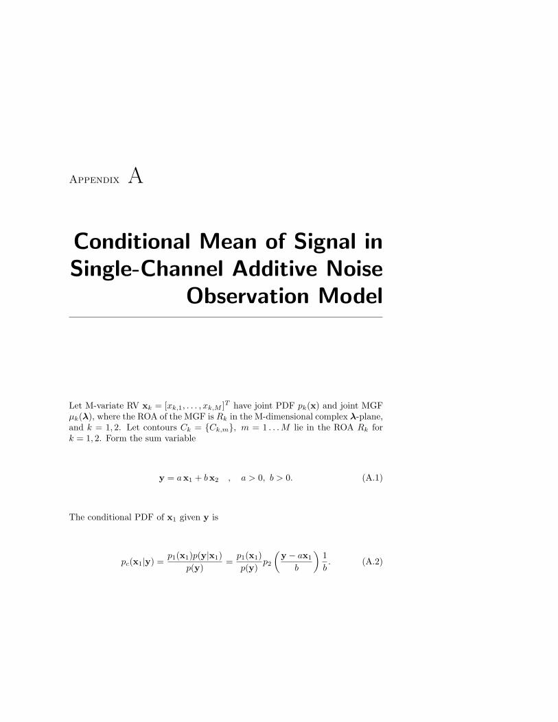
Appendix A
Conditional Mean of Signal inSingle-Channel Additive Noise
Observation Model
Let M-variate RV xk = [xk,1, . . . , xk,M ]T have joint PDF pk(x) and joint MGFµk(λ), where the ROA of the MGF is Rk in the M-dimensional complex λ-plane,and k = 1, 2. Let contours Ck = {Ck,m}, m = 1 . . . M lie in the ROA Rk fork = 1, 2. Form the sum variable
y = ax1 + bx2 , a > 0, b > 0. (A.1)
The conditional PDF of x1 given y is
pc(x1|y) =p1(x1)p(y|x1)
p(y)=
p1(x1)p(y)
p2
(y − ax1
b
)1b. (A.2)
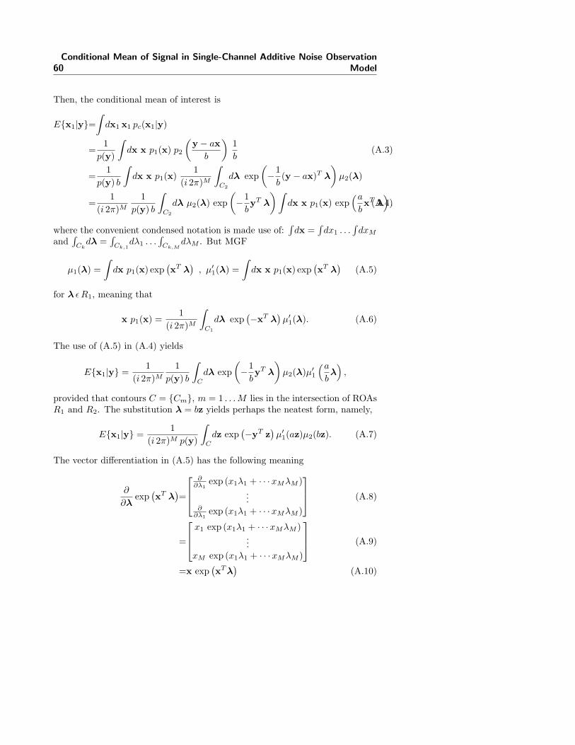
60Conditional Mean of Signal in Single-Channel Additive Noise Observation
Model
Then, the conditional mean of interest is
E{x1|y}=∫
dx1 x1 pc(x1|y)
=1
p(y)
∫dx x p1(x) p2
(y − ax
b
)1b
(A.3)
=1
p(y) b
∫dx x p1(x)
1(i 2π)M
∫
C2
dλ exp(−1
b(y − ax)T λ
)µ2(λ)
=1
(i 2π)M
1p(y) b
∫
C2
dλ µ2(λ) exp(−1
byT λ
) ∫dx x p1(x) exp
(a
bxT λ
).(A.4)
where the convenient condensed notation is made use of:∫
dx =∫
dx1 . . .∫
dxM
and∫
Ckdλ =
∫Ck,1
dλ1 . . .∫
Ck,MdλM . But MGF
µ1(λ) =∫
dx p1(x) exp(xT λ
), µ′1(λ) =
∫dx x p1(x) exp
(xT λ
)(A.5)
for λ εR1, meaning that
x p1(x) =1
(i 2π)M
∫
C1
dλ exp(−xT λ
)µ′1(λ). (A.6)
The use of (A.5) in (A.4) yields
E{x1|y} =1
(i 2π)M
1p(y) b
∫
C
dλ exp(−1
byT λ
)µ2(λ)µ′1
(a
bλ
),
provided that contours C = {Cm}, m = 1 . . .M lies in the intersection of ROAsR1 and R2. The substitution λ = bz yields perhaps the neatest form, namely,
E{x1|y} =1
(i 2π)M p(y)
∫
C
dz exp(−yT z
)µ′1(az)µ2(bz). (A.7)
The vector differentiation in (A.5) has the following meaning
∂
∂λexp
(xT λ
)=
∂∂λ1
exp (x1λ1 + · · ·xMλM )...
∂∂λ1
exp (x1λ1 + · · ·xMλM )
(A.8)
=
x1 exp (x1λ1 + · · ·xMλM )...
xM exp (x1λ1 + · · ·xMλM )
(A.9)
=x exp(xT λ
)(A.10)

Appendix B
SPA for Single IsolatedSaddlepoint
Consider the integral
I =1
(i 2π)M
∫
C
dz exp [φ(z)] , (B.1)
where C = {Cm}, m = 1 . . . M are Bromwich contours. Suppose that
∂φ(z)∂zm
∣∣∣∣zs
= 0 for m = 1 . . . M, (B.2)
meaning that zs is the location of a saddlepoint of the integrand. Then,
φ(z) ∼= φ(zs) +12(z− zs)T Λ(zs)(z− zs) (B.3)
for z near zs. Substitution in (B.1) yields
I ∼= exp [φ(zs)](i 2π)M
∫
C1
dz exp(
12(z− zs)T Λ(zs)(z− zs)
)(B.4)
where it is presumed that contours C1 are equivalent Bromwich contours to Cthat passes through the point zs. Substituting z = zs + it in (B.4) then
I ∼= exp [φ(zs)](2π)M
∫ ∞
−∞dt exp
(−1
2tT Λ(zs) t
)=
exp [φ(zs)](2π)M/2|Λ(zs)|1/2
(B.5)

62 SPA for Single Isolated Saddlepoint
where the Jacobian of the variable substitution is J = iM . This is the SPA foran isolated saddlepoint, at which Λ(zs)6=0. Correction terms can be derived byextending the expansion in (B.3) to higher-order terms.
Appendix C
MGF M-variate LaplaceDistribution
Let x be a zero-mean M-variate Laplace distributed RV with dimensionality M ,then the corresponding MGF is computed from
µx(z)=∫
dx exp(zT x
)px(x) (C.1)
=∫
dx exp(zT x
) ∫ ∞
0
ds pX|S(x|S = s)pS(s) (C.2)
where pX|S(x|S = s) is Gaussian with covariance matrix sΓ (detΓ = 1), thus
pX|S(x|S = s) =1
(2π s)M/2exp
(− 1
2sxT Γ−1x
)(C.3)
and s is exponentially distributed,
pS(s) =1λ
exp(− s
λ
), s > 0, λ > 0. (C.4)
Interchanging the order of integration and inserting (C.4) into (C.2) yields,
µx(z) =1λ
∫ ∞
0
ds exp(− s
λ
) ∫dx exp
(zT x
)pX|S(x|S = s) (C.5)
64 MGF M-variate Laplace Distribution
The MD integral over x is recognized as the MGF of a Gaussian RV with PDFas in (C.3). Hence,
µx(z)=1λ
∫ ∞
0
ds exp(−s
(1λ− 1
2zT Γz
))(C.6)
=1λ
∫ ∞
0
ds exp(
s
(λzT Γz− 2
2λ
))(C.7)
=− 1λ
2λ
λzT Γz− 2(C.8)
=1
1− λ2 zT Γz
(C.9)
The integral in (C.7) converges when zT Γz < 2λ .

Appendix D
Brief Introduction toExcitation Models
D.1 The Rosenberg-Klatt Model
The continuous-time Rosenberg-Klatt model (RK model) is given by (see e.g.[24][21])
g(t) ={
2at− 3bt2, 0 ≤ t ≤ OQ · T0
0 , OQ · T0 < t ≤ T0(D.1)
where
a =27 ·AV
4 ·OQ2 · T0, b =
27 ·AV
4 ·OQ3 · T 20
, a = OQ · T0 · b. (D.2)
Here, g(t) models one period of the harmonic excitation. The upper equationin (D.1) models the open phase of the period and the lower equation modelsthe closed phase of the period. T0 is the period in seconds, AV is an amplitudeparameter and OQ is called the open quotient. OQ is 0 if the there is no openphase (always closed) and it is 1 if there is no closed phase (always open). Aplot of two periods of the model waveform is plotted in figure D.1 for the settingFs = 16 kHz, OQ = 0.6, AV = 2.4 and T0 = 0.01 s (pitch 100 Hz). This modelis also referred to as the KLGLOTT88 model.
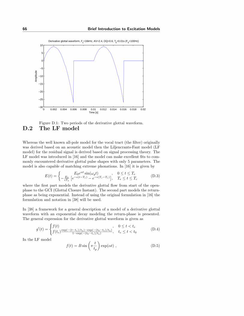
66 Brief Introduction to Excitation Models
0 0.002 0.004 0.006 0.008 0.01 0.012 0.014 0.016 0.018 0.02−30
−25
−20
−15
−10
−5
0
5
10
Time [s]
Am
plitu
de
Derivative glottal waveform, Fs=16kHz, AV=2.4, OQ=0.6, T
0=0.01s (F
0=100Hz)
Figure D.1: Two periods of the derivative glottal waveform.D.2 The LF model
Whereas the well known all-pole model for the vocal tract (the filter) originallywas derived based on an acoustic model then the Liljencrants-Fant model (LFmodel) for the residual signal is derived based on signal processing theory. TheLF model was introduced in [16] and the model can make excellent fits to com-monly encountered derivative glottal pulse shapes with only 5 parameters. Themodel is also capable of matching extreme phonations. In [16] it is given by
E(t) ={
E0eαt sin(ωgt) , 0 ≤ t ≤ Te
− E0εTa
[e−ε(t−Te) − e−ε(Tc−Te)
], Te ≤ t ≤ Tc
(D.3)
where the first part models the derivative glottal flow from start of the open-phase to the GCI (Glottal Closure Instant). The second part models the return-phase as being exponential. Instead of using the original formulation in [16] theformulation and notation in [38] will be used.
In [38] a framework for a general description of a model of a derivative glottalwaveform with an exponential decay modeling the return-phase is presented.The general expression for the derivative glottal waveform is given as
g′(t) =
{f(t) , 0 ≤ t < tef(te)
exp(−(t−te)/ta)−exp(−(t0−te)/ta)1−exp(−(t0−te)/ta) , te ≤ t < t0
(D.4)
In the LF model
f(t) = B sin(
πt
tp
)exp(αt) , (D.5)

D.2 The LF model 67
and by direct integration
g(t) =
∫ t
0f(τ)dτ , 0 ≤ t < te∫ te
0f(τ)dτ + taf(te)
1−exp(−(t−te)/ta)−((t−te)/ta) exp(−(t0−te)/ta)1−exp(−(t0−te)/ta)
, te ≤ t < t0
=
B tp
[π+exp(αt)
�αtp sin(π t
tp)−π cos(π t
tp)�
(αtp)2+π2
], 0 ≤ t < te
∫ te
0f(τ)dτ + taf(te)
1−exp(−(t−te)/ta)−((t−te)/ta) exp(−(t0−te)/ta)1−exp(−(t0−te)/ta)
, te ≤ t < t0
(D.6)
There are 5 parameters in the model, 4 timing parameters and one amplitudeparameter. The timing parameters are {tp,te,ta,t0} and the amplitude param-eter is denoted Ee. The parameters are illustrated in figure D.2. The timingparameter tp denotes the instant of the peak of the glottal flow which also corre-sponds to when the derivative glottal flow, g′(t), crosses zero. Timing parameterte denotes the instant when the derivative glottal flow reaches its negative peak,Ee. This instant is also referred to as the Glottal Closure Instant (GCI). Timingparameter t0 designates the time it takes to complete one period of the glottalpulse, which is also the pitch period. The timing parameter ta is the time con-stant of the exponential decay but it also designates the duration of the returnphase. After te + ta the vocal folds have reached maximum closure and theairflow has reduced to its minimum [38]. In order to generate or synthesize aperiod of the glottal-pulse the synthesis parameters {B, α} must be determined.Especially α is not straightforward to determine. In order to determine α a con-tinuity condition must be fulfilled. The continuity condition must be satisfiedin order to have zero leakage. To obey the continuity condition the followingmust be fulfilled
∫ te
0
f(τ)dτ + taf(te)D(t0, te, ta) = 0 (D.7)
where
D(t0, te, ta) = 1− (t0 − te)/taexp((t0 − te)/ta)− 1
(D.8)
which is found by inserting t = t0 into (D.6). If all 4 timing parameters areknown then α is determined by solving the continuity condition in (D.7). Thiscan be done for instance by using Matlab’s fzero function. In [38] an iterativeprocedure for computing α more suitable for implementation on a DSP is de-scribed. After α has been determined the amplitude parameter B can be foundby inserting the point (te, Ee) into (D.5).

68 Brief Introduction to Excitation Models
0 1 2 3 4 5 6 7 8 9
x 10−3
−400
−200
0
200
tp
te
t0
EeOpen−Phase Closed−Phase
ta − Return−Phase
time [s]
g’(t
)
0 1 2 3 4 5 6 7 8 9
x 10−3
−0.1
0
0.1
0.2
0.3
g(t)
Figure D.2: Glottal pulse (top) and its time derivative (bottom).
D.3 The Rosenberg++ model
The motivation for using the LF model over the Rosenberg-Klatt model is theenhanced flexibility of the LF model and because it also models the return-phase. In particle filtering samples will be drawn from priors of the timingparameters and these samples will then be used to generate one period of thederivative glottal pulse period. This can get quite complex computationallybecause for every particle the continuity condition has be to solved for α everytime new values of the timing parameters are obtained. The Rosenberg++model (R++ model) is an upgraded Rosenberg-Klatt model which makes agood approximation to the LF model and for which the complexity of solvingthe continuity condition is significantly decreased. For the R++ model
f(t) = 4At(tp − t)(tx − t) (D.9)
The continuity condition can be solved for tx analytically
tx = te
(1−
12 t2e − tetp
2t2e − 3tetp + 6ta(te − tp)D(t0, te, ta)
)(D.10)
Appendix E
Use and Subtleties ofSaddlepoint Approximationfor Minimum Mean-Square
Error Estimation
Submitted to IEEE Transactions on Information Theory June 2006.

70 Appendix E
1
Use and Subtleties of Saddlepoint Approximationfor Minimum Mean-Square Error Estimation
Thomas Beierholm,Student Member, IEEE, Albert H. Nuttall, and Lars K. Hansen
Abstract— An integral representation for the minimum mean-square error estimator for a random variable in an observationmodel consisting of a linear combination of two random variablesis derived. The derivation is based on the moment-generatingfunctions for the random variables in the observation model. Themethod generalizes so that integral representations for higher-order moments of the posterior of interest can be easily obtained.Two examples are presented that demonstrate how saddlepointapproximation can be used to obtain accurate approximationsfor a minimum mean-square error estimator using the derivedintegral representation. However, the examples also demonstratethat when two saddlepoints are close or coalesce, then saddlepointapproximation based on isolated saddlepoints is not valid.Asaddlepoint approximation based on two close or coalescedsaddlepoints is derived and in the examples, the validity andaccuracy of the derivation is demonstrated.
Index Terms— Minimum mean-square error estimation(MMSE), saddlepoint approximation, coalescing saddlepoints,monkey saddlepoint, moment-generating functions.
I. I NTRODUCTION
T HE possibility of using SaddlePoint Approximation(SPA) to evaluate the conditional mean for a Random
Variable (RV) in a linear combination with constant coef-ficients of two RVs is examined. The integral defining theconditional mean contains a weighted convolution integralofthe corresponding Probability Density Functions (PDFs). Thisintegral is in general intractable, ruling out analytic evaluationof the conditional mean and therefore necessitating the useof approximations. The conditional mean is also referred toasthe Minimum Mean-Square Error (MMSE) estimator. The ideadescribed in this paper is based on two observations 1) that theweighted convolution integral defining the desired estimatorcan be rewritten as a complex inversion integral involving theMoment-Generating Functions (MGFs) of the RVs; 2) that thecomplex inversion integral can be approximated by SPA.
The SPA was introduced into statistics in [2] where itwas used for approximating the mean ofn independent andidentically distributed RVs. More recently, in [3] and [4] theSPA has proven very useful in obtaining tail probabilitiesfor a number of statistics. Using the SPA to obtain accurateevaluations of a PDF, a unique real SaddlePoint (SP) in theRegion Of Analyticity (ROA) is used. In contrast, in orderfor the SPA to be useful for the approximation of an MMSEestimator, two SPs, as a complex conjugate pair, will in generalhave to be made use of. This brings on the subtlety that whenthe two SPs are close, a SPA based on an isolated SP becomes
T. Beierholm is with GN ReSound A/S, 2630 Taastrup, Denmark.A. H. Nuttall, P. O. Box 401, Old Lyme, CT 06371, USA.L. K. Hansen is with Informatics and Mathematcal Modeling, Technical
University of Denmark, DK-2800 Kgs. Lyngby, Denmark.
very inaccurate or even worse, when the two SPs coalesce, theusual SPA becomes invalid. In two examples, it has been foundthat two SPs moved towards each other on the real line asthe domain of the conditional RV in the MMSE estimator wastraversed. The two SPs finally coalesced into a monkey SP andthen moved vertically in opposite directions into the complexplane. A SPA based on close or coalesced SPs is derived, andthe accuracy and validity of this SPA, when the two SPs areclose or coalesce, is demonstrated in two examples.
The main contributions of the paper are the derivation ofthe integral representation for the MMSE estimator and thederivation of a SPA based on two close or coalesced SPs.
In section II-A the derivation of an integral representationfor the MMSE estimator is presented. Section II-B reviewsthe SPA based on an isolated SP, while section II-C derivesthe SPA based on two close or coalesced SPs. Two examplesare presented in section III that demonstrate the subtlety ofcoalescing SPs and the accuracy of the SPA based on twoclose or coalesced SPs. Finally, in section IV a summary ispresented.
II. T HEORY
A. Conditional Mean
Let RV xk have PDFpk(x) and MGF µk(λ), where theROA of the MGF isRk in the complexλ-plane, andk = 1, 2.Let contourCk lie in ROA Rk for k = 1, 2. Form the sumvariable
y = ax1 + bx2 , a > 0 , b > 0
The conditional PDF ofx1 given y is
pc(x1|y) =p1(x1)p(y|x1)
p(y)=
p1(x1)
p(y)p2
(
y − ax1
b
)
1
b(1)
Then, the conditional mean of interest is
E{x1|y}=
∫
dx1 x1pc(x1|y)
=1
p(y)
∫
dxxp1(x)p2
(
y − ax
b
)
1
b(2)
=1
p(y)b
∫
dxxp1(x)1
i2π
∫
C2
dλ e(−y−ax
bλ)µ2(λ)
=1
i2πp(y)b
∫
C2
dλµ2(λ)e−y
bλ
∫
dxxp1(x)eaλb
x(3)
But MGF
µ1(λ) =
∫
dx p1(x)eλx , µ′
1(λ) =
∫
dx xp1(x)eλx (4)

Use and Subtleties of Saddlepoint Approximation for MinimumMean-Square Error Estimation 71
2
for λǫR1, meaning that
xp1(x) =1
i2π
∫
C1
dλ e−xλµ′
1(λ) (5)
The use of (4) in (3) yields
E{x1|y} =1
i2πp(y)b
∫
C
dλ e−y
bλµ2(λ)µ′
1
(a
bλ)
provided that contourC lies in the intersection of ROAsR1
and R2. The substitutionλ = bz yields perhaps the neatestform, which is also the form used in the examples, namely,
E{x1|y} =1
i2πp(y)
∫
C
dz e−yzµ′
1(az)µ2(bz) (6)
Alternatively, if p(y) is not given in closed form
E{x1|y} =1
a
∫
Cdz e−yzµ′
1(az)µ2(bz)∫
Cdz e−yzµ1(az)µ2(bz)
An alternative route uses (5) in (2) to get
E{x1|y}=1
p(y)b
∫
dxxp2
(
y − ax
b
)
1
i2π
∫
C1
dλ e−xλµ′
1(λ)
=1
i2πp(y)b
∫
C1
dλ µ′
1(λ)
∫
dx p2
(
y − ax
b
)
e−xλ
=1
i2πp(y)a
∫
C
dλ µ′
1(λ)µ2
(
b
aλ
)
e−y
aλ
where the same condition as above is required of contourC.The substitutionλ = az leads to (6). Finally, it is straightforward to consider higher-order moments of the conditionalPDF in (1) e.g.
E{x21|y} =
1
a
∫
Cdz e−yzµ′′
1(az)µ2(bz)∫
Cdz e−yzµ1(az)µ2(bz)
B. SPA for Single Isolated Saddlepoint
Consider the integral
I =1
i2π
∫
C
dz eφ(z) (7)
whereC is a Bromwich contour. Suppose thatφ′(zs) = 0,meaning thatzs is the location of a SP of the integrand. Then,
φ(z) ∼= φ(zs) +1
2φ′′(zs)(z − zs)
2 (8)
for z nearzs. Substitution in (7) yields
I ∼=eφ(zs)
i2π
∫
C1
dz e1
2φ′′(zs)(z−zs)2 (9)
where it is presumed that contourC1 is an equivalentBromwich contour toC that passes through the pointzs. Let
z = zs + r i/√
φ′′(zs) , dz = dr i/√
φ′′(zs)
Then, (9) becomes
I ∼=eφ(zs)
2π√
φ′′(zs)
∫
∞
−∞
dr e−1
2r2
=eφ(zs)
√
2πφ′′(zs)(10)
This is the SPA for an isolated SP, at whichφ′′(zs)6=0.Correction terms can be derived by extending the expansion
in (8) to higher-order terms. In particular, the first-ordercorrection to the SPA is
I ∼=eφ(zs)
√
2πφ′′(zs)
(
1 +1
8
φ′′′′(zs)
[φ′′(zs)]2−
5
24
[φ′′′(zs)]2
[φ′′(zs)]3
)
(11)
C. SPA for Two Close Saddlepoints
Consider the integral
I =1
i2π
∫
C
dz eφ(z) (12)
where C is a Bromwich contour in the original strip ofanalyticity of the integrand, and
φ′(z1) = 0 , φ′(z2) = 0
wherez1 is near (or equal to)z2. That is, there are two close(or coalesced) saddlepoints of the integrand of (12). Then,itfollows that
φ′(z) ∼= g (z − z1)(z − z2) = g (z2 − 2zmz + z1z2) (13)
for z nearz1 andz2, whereg is a constant to be determined,and a midpoint is defined as
zm =z1 + z2
2
From (13),
φ′′(z) ∼= 2g(z − zm) , φ′′′(z) ∼= 2g (14)
for z nearzm. Substitutingz = zm in the first relation yieldsφ′′(zm) ∼= 0 which is useless. However, the same substitutionin the second relation leads to the selection
g ≡1
2φ′′′(zm)
which is well behaved, even as the two SPs approach andcoalesce with each other. It is presumed thatφ′′′(zm) 6= 0.Integration of (13) now yields
φ(z) ∼= g
(
1
3z3 − zmz2 + z1z2z
)
+ h (15)
for z nearz1 andz2. The constanth is determined by forcingequality in (15) at the midpointzm, with the result that
h ≡ φ(zm) +1
6g zm (z2
1 − 4z1z2 + z22)
Integral (12) now takes the form
I ∼=eh
i2π
∫
C1
dz e1
3gz3
−gzmz2+gz1z2z (16)
where it is presumed thatC1 is an equivalent Bromwichcontour toC. Let
A = g1/3 = [φ′′′(zm)/2]1/3 , z = −t/A (17)
α = zmA , β = z1z2A2
to get
I ∼=eh
i2πA
∫
C2
dt e−1
3t3−αt2+βt (18)
The minus sign indz = −dt/A has been absorbed into thisexpression, by switching the direction of integration along

72 Appendix E
3
contourC2. C2 must take account of the possible complexityof φ′′′(zm), the three possible roots forA in (17), and thez = −t/A change of variables.
Now let t = u−α in (18) in order to eliminate the quadraticterm and get
I ∼=eh+α(β− 2
3α2)
i2πA
∫
C3
du e−1
3u3+(α2
−β)u
ContourC3 is simply a shift of contourC2. Finally, using allthe definitions above, along with some algebra, there follows
I ∼=eφ(zm)
i2πA
∫
C3
du e−1
3u3+ρu (19)
where
A =
(
1
2φ′′′(zm)
)1/3
, ρ =1
4A2(z1 − z2)
2 (20)
As z1 approachesz2, ρ tends to zero; however, the integral in(19) is well-defined for all values ofρ, real or complex. Finally,if contour C3 is arranged to start at infinity anywhere in theangular sector of widthπ/3 centered about angle−2π/3 andend at infinity anywhere in the angular sector of widthπ/3centered about angle2π/3, then (19) takes the special form
I ∼=eφ(zm)
AAi(ρ)
whereAi(z) is an Airy function. This is the SPA for two closeSPs under the conditions cited above.
In order to get correction terms to the SPA in (19), itis necessary to consider additional terms in expansion (14),namely,
φ′′′(z) ∼= 2g + φ′′′′(zm)(z − zm) +1
2φ′′′′′(zm)(z − zm)2
for z nearzm. Then, (15) is modified to read
φ(z) ∼=g
(
1
3z3
− zmz2 + z1z2z
)
+ h +
1
24φ′′′′(zm)(z − zm)4 +
1
120φ′′′′′(zm)(z − zm)5
for z nearzm. This adds a multiplicative factor of
e1
24φ′′′′(zm)(z−zm)4 ∼=1 +
1
24φ′′′′(zm)(z − zm)4 +
1
120φ′′′′′(zm)(z − zm)5
to (16). This results in a multiplicative factor
1 +1
24
φ′′′′(zm)
A4(t + α)4 −
1
120
φ′′′′′(zm)
A5(t + α)5
in (18) and the factor
1 +1
24
φ′′′′(zm)
A4u4
−1
120
φ′′′′′(zm)
A5u5
in (19), namely,
I ∼= (21)eφ(zm)
i2πA
∫
C3
du e−1
3u3+ρu
(
1 +φ′′′′(zm)
24 A4u4
−φ′′′′′(zm)
120 A5u5
)
Again, if contourC3 is arranged to start at infinity anywhere inthe angular sector of widthπ/3 centered about angle−2π/3and end at infinity anywhere in the angular sector of widthπ/3 centered about angle2π/3, then (21) takes the specialform
I ∼= (22)eφ(zm)
A
(
Ai(ρ) +φ′′′′(zm)
24 A4Ai′′′′(ρ) −
φ′′′′′(zm)
120 A5Ai′′′′′(ρ)
)
This is the SPA with correction terms for two close SPs.Contour C3 is exactly the contour that describes the Airyfunction Ai(z), see [5, p.52]. The Airy functions are namedafter the Royal Astronomer, Sir George Biddell Airy. Theairy functions are obtained as solutions to Airy’s differentialequation [5, p.50]
d2f
dz2− zf = 0
They are
fn(z) =1
i2π
∫
Ln
dt exp(
−t3/3 + zt)
, n = 1, 2, 3
When contourL1 is arranged to start at infinity anywhere inthe angular sector of widthπ/3 centered about angle−2π/3and end at infinity anywhere in the angular sector of widthπ/3 centered about angle2π/3, the solution is called the Airyfunction of the first kind and is denoted byAi(z).
III. E XAMPLES
Two examples are described. The examples demonstratehow the SPA based on isolated SPs becomes very inaccuratein the region where two SPs coalesce. The examples alsodemonstrate how the SPA based on nearby or coalesced SPsimproves accuracy significantly in this region. It should benoted that for both examples, the conditional mean estimatorof interest can be derived analytically in closed form.
A. Example 1: Gaussian RVs
The MGF of a zero-mean gaussian RV with varianceσ2x
and its first-order derivative with respect toλ is
µ(λ) = exp(
σ2xλ2/2
)
, µ′(λ) = σ2xλ exp
(
σ2xλ2/2
)
Using (6) the conditional mean for Gaussian RVs is given by
mx =aσ2
1
i2πp(y)
∫
Cx
dz z exp(
−yz + σ2z2/2)
(23)
where
σ2 = a2σ21 + b2σ2
2 , p(y) =1
√2πσ
exp
(
−1
2
y2
σ2
)
, for all y
The Bromwich contourCx can be anywhere in thez-planebecause the integrand is entire. After substitutingz = σz, theintegral in (23) becomes
I =1
σ
1
i2π
∫
Cx
dzz
σexp(−y
z
σ+
z2
2) , with mx =
aσ21
p(y)I
Defineq = y/(2σ) and letz = z; then

Use and Subtleties of Saddlepoint Approximation for MinimumMean-Square Error Estimation 73
4
I =1
σ
1
i2π
∫
Cx
dz z exp(−2qz +z2
2)
The fundamental integral is then
I =1
i2π
∫
C
dz z exp(−2qz +z2
2) (24)
which depends on only one parameter, namely,q = y/(2σ).The integral in (24) can be calculated analytically. Makingthesubstitutionsz = ir anddz = idr, then
I=−1
i2π
∫
∞
−∞
dr r exp(−2qir −r2
2)
=
√
2
πq exp(−2q2) (25)
Continuing with the SPA to the integral in (24), the integrand,f(z), is
f(z) = exp (φ(z)) = exp
(
−2qz +z2
2+ log z
)
The following functions are needed in the SPA, the correctionterm or in finding the SPs
φ(z) = −2qz + log(z) + z2/2 (26)
φ′(z) = −2q +1
z+ z , φ′′(z) = 1 −
1
z2(27)
φ′′′(z) =2
z3, φ′′′′(z) = −
6
z4, φ′′′′′(z) =
24
z5(28)
The SPs are found by solvingφ′(z) = 0. The integrand in(24) will go to −∞ for negativez and will go to +∞ forz positive. As the integrand goes through zero atz = 0 thismeans that the integrand may not have real SPs. It is knownthat there must be two SPs and they are found as solutions tothe equation
z2− 2qz + 1 = 0
namely,zs = q ±
√
q2 − 1 (29)
This means that forq2 < 1, the pair of SPs are complexconjugate; otherwise, there are two real SPs. Forq2 < 1, thetwo complex conjugate SPs are
z1 = q + i√
1 − q2 , z2 = q − i√
1 − q2 (30)
For q2 ≥ 1, the two real SPs are
z1 = q +√
q2 − 1 , z2 = q −√
q2 − 1 (31)
Figure 1 shows a trace of the SPs forq varying from−1.2to 1.2. Initially the SPs start out on the negative real axisand move towards each other. Whenq = −1 the two SPshave coalesced atz = −1 into a monkey SP, an SP oforder 2, whereφ′′(zs) = 0. The SPs then move verticallyin opposite directions into the complexz-plane because theSPs are a complex conjugate pair. Whenq = 0 the SPs arepure imaginary. Forq becoming more positive, the SPs startto approach each other and become nearly real. Whenq = 1the SPs are real and have coalesced atz = 1; then they movein opposite directions on the positive real axis.
−1.5 −1 −0.5 0 0.5 1 1.5
−1
−0.8
−0.6
−0.4
−0.2
0
0.2
0.4
0.6
0.8
1
Trace of SPs
Real part of SPs
Imag
inar
y pa
rt o
f SP
s
z
1
z2
Fig. 1. Plot showing trace of SPs forq going from−1.2 to 1.2. The initiallocations of the SPs whenq = −1.2 are also indicated in the figure by asmall circle and cross.
For the caseq2 < 1, the SPA can be computed by summingup the contributions to the integral for each of the two SPs.However, because the two SPs are complex conjugates, thecontributions will be complex conjugates as well. This meansthat the SPA can be computed by taking the real part of thecontribution for one of the two SPs and multiply this valueby two. So in essence, the functionsφ(z) andφ′′(z) need tobe evaluated only once. Using the SP,z1, the total SPA to theintegral in (24) is
I ∼= 2 · Re
{
exp(φ(z1)√
2πφ′′(z1)
}
(32)
Inserting the expression forz1 in (30) into (26) and (27)
φ(z1)=−1
2− q2
− iq√
1 − q2 + log(
q + i√
1 − q2
)
φ′′(z1)=2(q2 + iq
√
1 − q2 − 1)
(q + i√
1 − q2)2
It is not possible to obtain a simple analytic expression forthe SPA to the integral in (24). The ratio between the SPA in(32) and the exact analytic expression for the integral in (24)doesn’t lead to a simple expression either.
For the caseq2 ≥ 1, the real SP, wheref(z) is minimum onthe realz-axis, is used. The useful SP in (31) isz1. Insertingthe expression forz1 into (26) and (27)
φ(z1)=−1
2− q2
− q√
q2 − 1 + log(
q +√
q2 − 1)
φ′′(z1)=2q2
√
q2 − 1 + q4 − 1
q2(1 +√
q2 − 1)2
Using these expressions in the SPA based on isolated SPs andin the ratio between SPA and the exact value of the integral,simple analytical expressions are not obtained. The same istrue for the SPA with a correction term.
In figure 2, the accuraces of the SPA and the SPA with acorrection term are illustrated. This is done by computing theratios between the SPAs using (10) and (11) and the exact
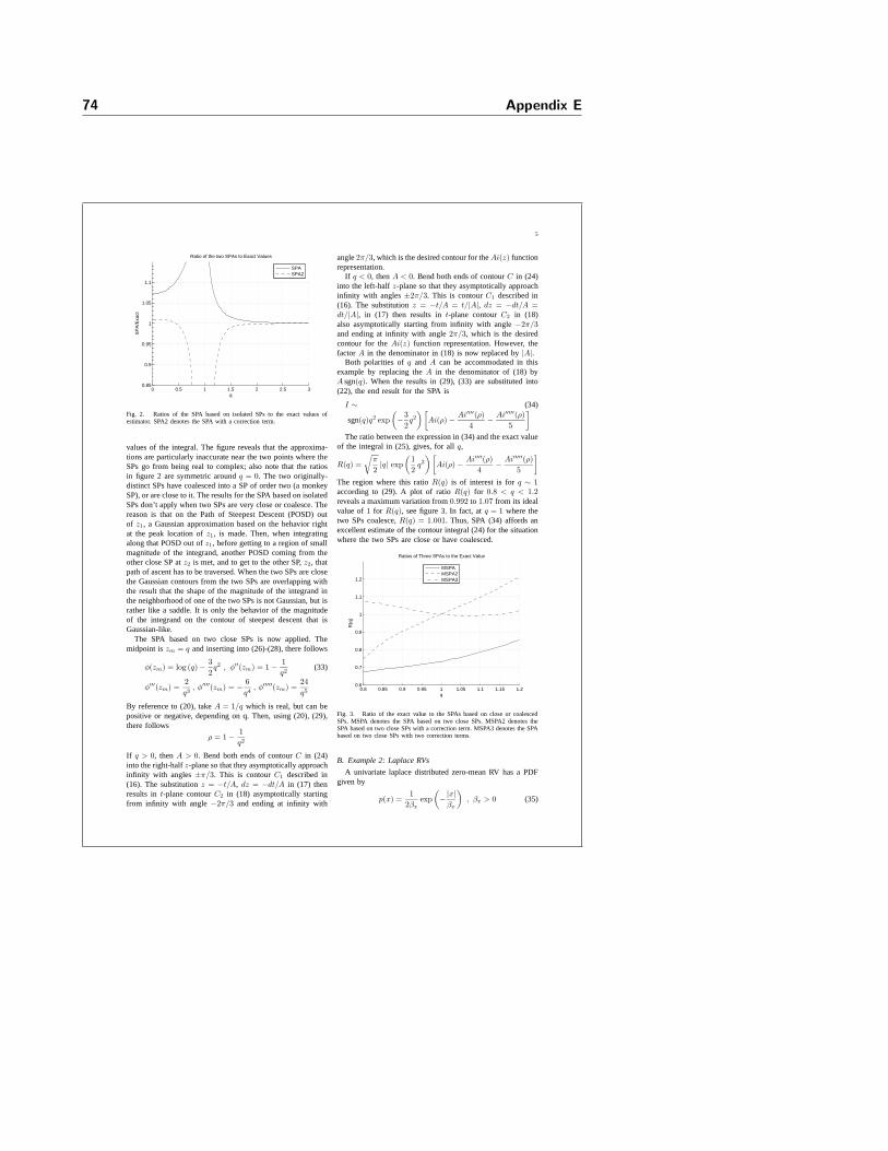
74 Appendix E
5
0 0.5 1 1.5 2 2.5 30.85
0.9
0.95
1
1.05
1.1
q
SP
A/E
xact
Ratio of the two SPAs to Exact Values
SPASPA2
Fig. 2. Ratios of the SPA based on isolated SPs to the exact values ofestimator. SPA2 denotes the SPA with a correction term.
values of the integral. The figure reveals that the approxima-tions are particularly inaccurate near the two points wheretheSPs go from being real to complex; also note that the ratiosin figure 2 are symmetric aroundq = 0. The two originally-distinct SPs have coalesced into a SP of order two (a monkeySP), or are close to it. The results for the SPA based on isolatedSPs don’t apply when two SPs are very close or coalesce. Thereason is that on the Path of Steepest Descent (POSD) outof z1, a Gaussian approximation based on the behavior rightat the peak location ofz1, is made. Then, when integratingalong that POSD out ofz1, before getting to a region of smallmagnitude of the integrand, another POSD coming from theother close SP atz2 is met, and to get to the other SP,z2, thatpath of ascent has to be traversed. When the two SPs are closethe Gaussian contours from the two SPs are overlapping withthe result that the shape of the magnitude of the integrand inthe neighborhood of one of the two SPs is not Gaussian, but israther like a saddle. It is only the behavior of the magnitudeof the integrand on the contour of steepest descent that isGaussian-like.
The SPA based on two close SPs is now applied. Themidpoint iszm = q and inserting into (26)-(28), there follows
φ(zm) = log (q) −3
2q2 , φ′′(zm) = 1 −
1
q2(33)
φ′′′(zm) =2
q3, φ′′′′(zm) = −
6
q4, φ′′′′′(zm) =
24
q5
By reference to (20), takeA = 1/q which is real, but can bepositive or negative, depending on q. Then, using (20), (29),there follows
ρ = 1 −1
q2
If q > 0, thenA > 0. Bend both ends of contourC in (24)into the right-halfz-plane so that they asymptotically approachinfinity with angles±π/3. This is contourC1 described in(16). The substitutionz = −t/A, dz = −dt/A in (17) thenresults int-plane contourC2 in (18) asymptotically startingfrom infinity with angle−2π/3 and ending at infinity with
angle2π/3, which is the desired contour for theAi(z) functionrepresentation.
If q < 0, thenA < 0. Bend both ends of contourC in (24)into the left-halfz-plane so that they asymptotically approachinfinity with angles±2π/3. This is contourC1 described in(16). The substitutionz = −t/A = t/|A|, dz = −dt/A =dt/|A|, in (17) then results int-plane contourC2 in (18)also asymptotically starting from infinity with angle−2π/3and ending at infinity with angle2π/3, which is the desiredcontour for theAi(z) function representation. However, thefactor A in the denominator in (18) is now replaced by|A|.
Both polarities ofq and A can be accommodated in thisexample by replacing theA in the denominator of (18) byA sgn(q). When the results in (29), (33) are substituted into(22), the end result for the SPA is
I ∼ (34)
sgn(q)q2 exp
(
−3
2q2
) [
Ai(ρ) −Ai′′′′(ρ)
4−
Ai′′′′′(ρ)
5
]
The ratio between the expression in (34) and the exact valueof the integral in (25), gives, for allq,
R(q) =
√
π
2|q| exp
(
1
2q2
) [
Ai(ρ) −Ai′′′′(ρ)
4−
Ai′′′′′(ρ)
5
]
The region where this ratioR(q) is of interest is forq ∼ 1according to (29). A plot of ratioR(q) for 0.8 < q < 1.2reveals a maximum variation from0.992 to 1.07 from its idealvalue of1 for R(q), see figure 3. In fact, atq = 1 where thetwo SPs coalesce,R(q) = 1.001. Thus, SPA (34) affords anexcellent estimate of the contour integral (24) for the situationwhere the two SPs are close or have coalesced.
0.8 0.85 0.9 0.95 1 1.05 1.1 1.15 1.20.6
0.7
0.8
0.9
1
1.1
1.2
q
R(q
)
Ratios of Three SPAs to the Exact Value
MSPAMSPA2MSPA3
Fig. 3. Ratio of the exact value to the SPAs based on close or coalescedSPs. MSPA denotes the SPA based on two close SPs. MSPA2 denotes theSPA based on two close SPs with a correction term. MSPA3 denotes the SPAbased on two close SPs with two correction terms.
B. Example 2: Laplace RVs
A univariate laplace distributed zero-mean RV has a PDFgiven by
p(x) =1
2βx
exp
(
−|x|
βx
)
, βx > 0 (35)

Use and Subtleties of Saddlepoint Approximation for MinimumMean-Square Error Estimation 75
6
For this Laplace-distributed RV, the MGF is
µx(λ) = E{exp(λx)} =1
1 − β2xλ2
, |Re(λ)| < 1/βx
and the first-order derivative with respect toλ is
µ′
x(λ) =2β2
xλ
(1 − β2xλ2)2
Inserting into (6), the integrand is
f(z) = exp (φ(z)) =2aβ2
1z exp(−yz)
(1 − b2β2
2z2)(1 − a2β2
1z2)2
The conditional mean is then given by
mx =2aβ2
1
i2πp(y)
∫
Cx
dz exp(−yz)z
(1 − z2
c2 )(1 − z2
d2 )2(36)
wherey, c andd are real positive constants,c = 1/(bβ2) andd = 1/(aβ1) and
p(y) =β1β2
(
eβ1y
a β1b − eβ2y
b β2a)
e−y(β1b+β2a)
ab
2(β21b2 − β2
2a2)
, y > 0
After substitutingz = cz, the integral in (36) becomes
I =1
i2π
∫
Cx
dz exp(−ycz)c2z
(1 − z2)(1 − c2z2
d2 )2(37)
After making the substitutionsA = yc andB = c/d in (37),the fundamental integral to approximate is
I =1
i2π
∫
C
dz exp(−Az)z
(1 − z2)(1 − B2z2)2(38)
The exact value of this integral will depend on the twofundamental parametersA and B. Therefore, the ratio ofthe SPA to the exact value will depend only onA and B:R(A, B). The integral in (38) can be evaluated analyticallyusing residues. For the polez = 1 the residue is
res1 = −exp(−A)
2(B2 − 1)2
and for the double pole atz = 1/B the residue is
res2 =exp(−A/B)
(
A + 2B − AB2)
4B(B2 − 1)2
and the exact value for the integral is then
I = −res1 − res2 (39)
Bromwich contourC in (38) crosses the real axis of thez-plane in the original strip of analyticity between the points±x0, x0 = min(1, 1/B). This integrand has simple poles at±1 and double poles at±1/B. The integrand in (38) is thenextended to the rest of thez-plane by analytic continuation(AC). Since parameterA is positive, the two ends of contourC can be bent to the right in thez-plane, so that the newcontour,C1, starts at infinity with angle−π/3 and ends up atinfinity with angleπ/3, still passing between the points±x0.ContourC1 is equivalent toC.
The exp(−Az) function dominates the behavior of theintegrand for largez. For B < 1 the original contourC isin the interior of (−1, 1) which is the original ROA. Forz
real and positive the integrand starts at a value0 for z = 0and increases to+∞ as z → 1 from the left. Forz real andnegative, the integrand starts at a value0 and decreases to−∞for z → −1 from the right. This means that there is no realSP inside the ROA unlessA is large enough for the functionexp(−Az) to dominate inside the ROA so that a real andpositive SP is created inside the ROA. One way to deal with amissing SP inside the ROA is to extend the integrand to allzby means of AC and move the contour of integration outsidethe original ROA towards+∞ in the complexz-plane becausethe functionexp(−Az) decays rapidly to zero there. However,this contour is not equivalent to the original contour becausea pole has been crossed. Another possibility is to make use ofcomplex SPs in the complexz-plane to obtain a SPA.
The SPA makes use of the following functions
φ(z)=−Az+log(z) − log(1 − z2) − 2 log(1 − B2z2)
φ′(z)=−A +1
z+
2z
1 − z2+
4B2z
1 − B2z2
φ′′(z)=−1
z2+
2(1 + z2)
(z2 − 1)2+
4B2(B2z2 + 1)
(B2z2 − 1)2
φ′′′(z)=2
z3−
4z(3 + z2)
(z2 − 1)3−
8B4z(3 + B2z2)
(B2z2 − 1)3
φ′′′′(z)=−6
z4+
12(z4 + 6z2 + 1)
(z2 − 1)4
+24B4(B4z4 + 6B2z2 + 1)
(B2z2 − 1)4
φ′′′′′(z)=24
z5−
48z(z4 + 10z2 + 5)
(z2 − 1)5
−96B6z(B4z4 + 10B2z2 + 5)
(B2z2 − 1)5
The SPs are found by solving forz in the equation
AB2z5 + 5B2z4 −A(B2 + 1)z3 − (3B2 + 1)z2 + Az − 1=0
This polynomial of degree5 in z cannot be factored (by theMatlab symbolic toolbox). So, analytic expressions for thelocations of the SPs in the complexz-plane cannot be found,although we know there must be5 of them. The SPs canbe found numerically by assigning numerical values to theparametersA and B and using Matlab’s roots routine. ForB < 1 and a large value ofA in exp(−Az), there is1 SP in(−∞,−1/B), 1 SP in(−1/B,−1), 2 SPs in(0, 1), and1 SPin (1, 1/B). These are all on the realz-axis. AsA decreases,the two real SPs in(0, 1) coalesce and then separate verticallyinto the complexz-plane. It is not known if their real partsremain in(−1, 1). For B > 1 and largeA, there is1 SP in(−∞,−1), 1 SP in(−1,−1/B), 2 SPs in(0, 1/B), and1 SPin (1/B, 1). All are real. Again, asA decreases, they coalesceand separate vertically and it is not known if they remain inthe original ROA. However, this analysis suggests that a SPAcan be applied by using SPs in the complexz-plane whena real SP in the original ROA doesn’t exist. We must makesure that the corresponding POSD through the two complexconjugate SPs is equivalent to the Bromwich contour confinedto the original ROA.

76 Appendix E
7
Figure 4 shows the POSD for the example with two complexconjugate SPs in the ROA (see [6] for how to find POSDs).The two crosses are the locations of the two complex conjugateSPs in the ROA. The circles show the POSDs out of the SPsaway from the origin and the stars show the POSDs out of theSPs towards the origin. Notice how both POSDs out of the SPsin the first and second quadrants head directly into the zero atthe origin. This two-pieced path is an equivalent contour totheoriginal Bromwich contour, and SPA or numerical integrationcan be used.
0 2 4 6 8 10 12−5
−4
−3
−2
−1
0
1
2
3
4
5
Real part
Imag
inar
y pa
rt
POSDs out from SPs
POSDs toward infinityPOSDs toward originSPs
0 0.5 1 1.5−2
−1
0
1
2
Fig. 4. POSDs out of the SPs in the complexz-plane.
The SPA is computed as in example I where two complexconjugate SPs are used when there is no real SP in the ROA.Plots illustrating the ratioR(A, B) for the SPA and the SPAwith a correction term (SPA2) are seen in figure 5. It is seenthat throughout theAB-plane, the ratios are close to1 asexpected, except for a ridge that identifies the values ofA andB where two close or coalesced SPs make the SPA based onisolated SPs inaccurate. In figure 6, the ratio is illustrated forthe caseB = 0.38.
B
A
SPA/Exact
1 2 31
2
3
4
5
6
7
8
9
10
0 1 2 3
B
A
SPA2/Exact
1 2 31
2
3
4
5
6
7
8
9
10
0 1 2 3
Fig. 5. RatioR(A, B) for the SPA and the SPA with a correction term(SPA2.
1 2 3 4 5 6 7 8 9 100.75
0.8
0.85
0.9
0.95
1
1.05
1.1
1.15
1.2
1.25
A
Rat
io
SPA/Exact
SPASPA2monkey SP
Fig. 6. Comparison of ratios for the SPA and the SPA with a correctionterm (SPA2) for the caseB = 0.38.
With the same setting,B = 0.38, the SPA based on twoclose or coalesced SPs is computed in the interval ofA wherethe SPA based on isolated SPs is particular inaccurate. Theresults are seen in figure 7. From the figure it is clear that theSPA based on two close or coalesced SPs with two correctionterms results in an excellent approximation in the region wherethe SPA based on isolated SPs is particularly inaccurate.
2.5 3 3.5 4 4.5 5 5.50.8
0.85
0.9
0.95
1
1.05
1.1
1.15
1.2
1.25
1.3
A
Rat
io
MSPA/Exact
MSPAMSPA2MSPA3monkey SP
Fig. 7. Ratio of the exact values of the estimator to the SPAs based on closeor coalesced SPs. MSPA denotes the SPA based on two close SPs.MSPA2denotes the SPA based on two close SPs with a correction term.MSPA3denotes the SPA based on two close SPs with two correction terms..
IV. SUMMARY
Given a linear combination of two random variables, thepossibility of using a saddlepoint approximation for minimummean-square error estimation of either of the two randomvariables in the linear combination, has been demonstrated.The approach was based on a derived integral representationfor the minimum mean-square error estimator involving the

Use and Subtleties of Saddlepoint Approximation for MinimumMean-Square Error Estimation 77
8
moment-generating functions of the random variables. Further-more, it was demonstrated that for the case of two coalescingsaddlepoints, the saddlepoint approximation based on isolatedsaddlepoints became very inaccurate and if a saddlepointapproximation based on two coalescing saddlepoints with twocorrection terms was used instead, this saddlepoint approxi-mation makes an excellent approximation.
ACKNOWLEDGMENTS
The first author would like to thank Professor Peter Willettfor providing the author the opportunity to make a stay atthe University of Connecticut (UConn) and thereby makethis work possible. The first author would also like to thankTod E. Luginbuhl, Phillip L. Ainsleigh, Paul M. Baggenstossand Peter Willett for making the stay at UConn a warm andinsightful experience.
REFERENCES
[1] L. Benaroya, F. Bimbot, and R. Gribonval, “Audio source separation witha single sensor,”IEEE Trans. Speech Audio Processing, vol. 14, pp. 191–199, Jan. 2006.
[2] H. E. Daniels, “Saddlepoint approximations in statistics,” The Annals ofMathematical Statistics, vol. 25, no. 4, pp. 631–650, Dec 1954.
[3] A. H. Nuttall, “Saddlepoint approximation and first-order correction termto the joint probability density function of m quadratic andlinear formsin k gaussian random variables with arbitrary means and covariances,”NUWC, Technical Report 11262, December 2000.
[4] ——, “Saddlepoint approximations for the combined probability and jointprobability density function of selected order statisticsand the sum of theremainder,” NUWC, Technical Report 11509, February 2004.
[5] N. Bleistein and R. A. Handelsman,Asymptotic Expansions of Integrals.Dover Publications, 1986.
[6] A. H. Nuttall, “Evaluation of the generalized qm function for complexarguments,” NUWC, Technical Report 11708, August 2005.
Thomas Beierholm was born in Aalborg, Denmark, in September 1976.He received the M.Sc. degree from the Department of CommunicationTechnology, Aalborg University, Aalborg, Denmark, in 2001. From 2001 to2004 he worked as a DSP software developer in the company GN ReSoundA/S.
He is currently employed in GN ReSound A/S as an Industrial PhD student.His research interests include digital signal processing theory and methodswith application to speech and audio, in particular signal separation and noisereduction.
Albert H. Nuttall received the B.Sc., M.Sc., and Ph.D. degrees in electricalengineering from the Massachusetts Institute of Technology (MIT), Cam-bridge, in 1954, 1955, and 1958, respectively.
He was with MIT as an Assistant Professor until 1959. From 1957 to 1960,he was with Melpar, and from 1960 to 1968, he was with Litton Industries.He was with the Naval Underwater Systems Center (NUSC), New London,CT, where his interest was in statistical communication theory. He is nowwith the Naval Undersea Warfare Center, Newport, RI.
Dr. Nuttall received the NUSC Distinguished Chair in SignalProcessingfrom the Navy in April 1987.
Lars K. Hansen received the M.Sc. and Ph.D. degrees in physics fromthe University of Copenhagen, Copenhagen, Denmark, in 1984and 1986,respectively.
He was with Andrex Radiation Products A/S, from 1987 to 1990.Since1990, he has been with the Technical University of Denmark, Lyngby, andsince 2000 as a Full Professor of signal processing. He is theDirector ofthe THOR Center for Neuroinformatics and Head of the Copenhagen Imageand Signal Processing Graduate School (CISP). His current research interestsinclude modeling of adaptive systems, meta-analysis, and applications inneuroimaging.

78 Appendix E

Appendix F
Particle Filter Inference in anArticulatory Based Speech
Model
Accepted for publication in IEEE Journal of Signal Processing Letters.
80 Appendix F
JOURNAL OF SIGNAL PROCESSING LETTERS, VOL. X, NO. XX, NOVEMBER 2006 1
Particle Filter Inference in an Articulatory BasedSpeech Model
Thomas Beierholm (*),Student Member, IEEE, and Ole Winther
Abstract— A speech model parameterized by formant fre-quencies, formant bandwidths and formant gains is proposed.Inference in the model is made by particle filtering for the ap-plication of speech enhancement. The advantage of the proposedparameterization over existing parameterizations based on ARcoefficients or reflection coefficients is the smooth time-varyingbehavior of the parameters and their loose coupling. Experimentsconfirm this advantage both in terms of parameter estimationandSNR improvement.
Index Terms— Particle filtering, time-varying auto-regressivespeech model, formant frequency.
I. I NTRODUCTION
I N the application of speech enhancement, the speechsignal is commonly modeled as a time-varying Auto-
Regressive (AR) Gaussian process. In block-processing sys-tems the speech signal is assumed quasi-stationary meaningthat the parameters of the AR process describing the speechsignal are assumed fixed in the duration of the block. Asdescribed in Ref. [1] the articulators of speech, such as thevocal tract, are continually moving, hence the assumptionof quasi-stationarity of speech can be improved upon. TheTime-Varying Auto-Regressive (TVAR) model used in Refs.[1], [2] lets the parameters of the AR process describing thespeech signal vary from sample to sample and thus avoids theassumption of quasi-stationarity of the speech signal.
The TVAR model facilitates a state-space formulation ofthe observed noisy signal in which the problem of jointestimation of the unknown parameters of the model andthe state sequence becomes a challenge. One approach is toperform ML estimation using the EM algorithm. A differentapproach was used in Refs. [1], [2], where sequential Bayesianestimation of the unknown parameters and state sequencewas performed by particle filtering. Instead of using the ARcoefficients directly, then, in Ref. [2] the TVAR model wasreparameterized in terms of reflections coefficients as thisleadto a stronger physical interpretation of the model and stabilityof the model could easily be verified.
In this paper a model similar to the TVAR model but withan even stronger physical interpretation is used [3]. The modelis parameterized in terms of formant frequencies, formantbandwidths and formant gains, called the fbg parameters inthe following. It is intended that this new parameterizationcan lead to improved particle filtering by way of exploitingknown properties of the fbg parameters and thereby eventually
Manuscript received July xx, 2006; revised December xx, 2006.T. Beierholm is with GN ReSound A/S, Lautrupbjerg 7, P.O. Box99, 2750
Ballerup, Denmark, email [email protected]. Winther is with IMM, Danish Technical University, 2800 Lyngby,
Denmark.
improve quality of the estimated speech signal. As stressedin Ref. [3] the new parameters have a slow time variationdue to the inertia of the speech producing system in contrastto the reflection coefficients which can have a rapid timevariation. The new parameters are also loosely coupled, exhibitsmooth trajectories and the stability of the model is thus easilyensured.
A common feature of the TVAR model [1] and the fbgparameterized model introduced in this work is that condi-tional on the unknown parameters of the model, the modelreduces to a linear Gaussian state-space system. In Ref. [1]this feature was made use of in a variance reduction (Rao-Blackwellization) step whereby the problem of sampling fromthe joint posterior distribution of the states and the unknownparameters of the model is reduced to that of sampling fromthe posterior distribution of the unknown parameters only.
In short, the contributon of this paper is to introduce aspeech model with an even stronger physical interpretationthan the reflection coefficients [2] and obtain filtered estimatesof the clean speech signal with Rao-Blackwellized particlefiltering [1].
II. T IME-VARYING AUTO-REGRESSIVEMODEL
In the Time-Varying Auto-Regressive (TVAR) model aspeech signal is modeled as a non-stationary AR(p) process,wherep denotes the order of the AR process which is assumedfixed in the following. The coefficients of the AR(p) processand the variance of the process noise are allowed to changefrom sample to sample, i.e.
x[n] =
p∑
i=1
ai[n]x[n − i] + σe[n]e[n] , e[n] ∼ N (0, 1) ,
whereσ2e [n] is the variance of the innovation sequence and
N (µ,Σ) denotes a Gaussian distribution with meanµ andcovariance matrixΣ. It is assumed that the speech signal iscontaminated by non-stationary Gaussian noise
y[n] = x[n] + σd[n]d[n] , d[n] ∼ N (0, 1) ,
where σ2d[n] denotes the variance of the observation noise.
The TVAR model is conveniently formulated as a state-spacemodel with the following state and observation equations
x[n] = A[n]x[n − 1] + B[n]v[n] , v[n] ∼ N (0p×1, Ip) (1)
y[n] = Cx[n] + D[n]w[n] , w[n] ∼ N (0, 1) , (2)
wherea[n] = ( a1[n], · · · , ap[n] )T is the coefficient vector,
x[n] = (x[n], · · · , x[n − p + 1] )T the state vector and
A[n] =
(
aT [n]
I(p−1) 0(p−1)×1
)
, B[n] =
(
σe[n]0(p−1)×1
)
(3)
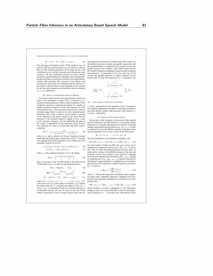
Particle Filter Inference in an Articulatory Based Speech Model 81
JOURNAL OF SIGNAL PROCESSING LETTERS, VOL. X, NO. XX, NOVEMBER 2006 2
C =(
1 0 · · · 0)
, D[n] = ( σd[n] ) . (4)
The state-space formulation of the TVAR model in eqs. (1)and (2), with the parameterization eqs. (3) and (4), is used inRef. [1]. The unknown parameters of the model are thep ARcoefficients ina[n] and the innovation and observation noisevariances. The AR coefficients and the two noise varianceparameters represented by their logarithms were assumed inde-pendent and taken as evolving according to first-order Markovrandom walk processes. The variance of the random walkprocesses for each of the AR coefficients and the variances ofthe random walk processes for the logarithms to the varianceof the innovation sequence and observation noise are denotedδa, δe, δd, respectively.
III. A RTICULATORY-BASED SPEECHMODEL
The speech model based on the fbg parameters (which areclose to the articulators of speech [3]), is referred to as aParallel Formant Synthesizer(PFS) in speech synthesis. A PFSsynthesizes speech by summing the outputs of a number ofparallel connected resonance circuits. The structure of a PFSis illustrated in Fig. 1. The resonators are driven by a commonexcitation signal which is taken to be white standard normaldistributed noise. Each resonance circuit models a formantin the spectrum of the speech signal, in the sense that thespectrum of the excitation signal is shaped to have a peakat the resonance frequency and the bandwidth and gain ofthe ‘bump’ is determined by the resonance circuit as well.The resonators are taken as second-order IIR filters with z-transforms
Hk(z) =gk
1 − ak,1(fk, bk)z−1 − ak,2(bk)z−2, (5)
wherefk, bk andgk denotes the formant frequency, formantbandwidth and formant gain, respectively, of thekth formant.The mapping from these parameters to the coefficients of theresonators is given by [4], [5]
ak,1(fk, bk) = 2 exp(−πbk/fs) cos(2πfk/fs) (6)
ak,2(bk) =− exp(−2πbk/fs) , (7)
wherefs is the sampling frequency inHz. By letting
Ak[n] =
(
ak,1(fk, bk) ak,2(bk)1 0
)
(8)
then in state-space form, the PFS model is described by theTVAR model in eqs. (1) and (2) with parameterization
A[n] = diag(A1, · · · ,AK) (9)
B[n] =
(
01×2K
g1[n] 0 · · · gK [n] 0
)T
(10)
C =(
1 0 1 0 · · · 1 0)
, D[n] = ( σd[n] ) , (11)
wherex[n] = (x1[n], x1[n − 1], · · · , xK [n], xK [n − 1])T
is the state vector,K is the number of formants,xk[n] denotesthe output from thekth resonator (see figure 1) andv[n] ∼N (02×1, I2). A formulation based on a cascade structure ofsecond-order sections can also be used. In fact the TVARmodel is equivalent to such a cascade structure hence the two
main differences between the TVAR and the PFS models arethe different structures, cascade and parallel respectively, andthe parameterization. As opposed to the cascade structure theparallel structure also contains a zero which means that thePFS model can improve modeling of speech sounds containinganti-resonances. A description of the pros and cons of thecascade and parallel structures in speech synthesis can befound in Ref. [5]. The PFS model has3K+1 parameters. The
Formant #1x
+
+
+
f1 b1g1
Formant #Kx
fK bKgK
White noise gen.
e[n]
x1[n]
xK[n]
x[n]
Fig. 1. Block diagram of Parallel Formant Synthesizer.
fk andbk parameters and the logarithm to thegk parametersare assumed independent and taken as evolving according tofirst-order Markov random walk processes with variancesδf ,δb andδg, respectively.
IV. PARTICLE FILTER INFERENCE
We provide a brief summary of the particle filter methodused for inference in the PFS model as it is described in detailelsewhere [1]. Generally, filtering refers to the task of drawingsamples from thefiltering distributionp(xn, θn |y1:n) in orderto estimate the mean (the MMSE estimate) of the state vectorand the parameter vector. In the context of the PFS model
θ = (f1, b1, g1, · · · , fK , bK , gK , σd).
The joint distribution is decomposed using Bayes rule:
p(xn, θ0:n |y1:n) = p(xn |θ0:n,y1:n) p(θ0:n |y1:n) . (12)
For both models (TVAR and PFS) the state vector can beintegrated out analytically becausep(xn |θ0:n,y1:n) is Gaus-sian. This so-called Rao-Blackwellization has the effect ofreducing the variance of the MMSE estimate of the state andparameter vectors. The problem is then reduced to samplingfrom the lower dimensional distributionp(θ0:n |y1:n) insteadof sampling fromp(x0:n, θ0:n |y1:n). In particle filtering thisdistribution is approximated by a weighted sum ofδ-functions(the particles). The importance weight of particle with historyθ0:n is given by
w(θ0:n) ∝p(θ0:n | y1:n)
π(θ0:n | y1:n), (13)
whereπ(.) denotes the importance distribution where samplesare drawn from. Sequential importance sampling can be per-formed if the importance distribution is restricted to be ofthegeneral form
π(θ0:n | y1:n) = π(θ0:n−1 | y1:n−1)π(θn |θ0:n−1, y1:n) (14)
which facilitates recursive propagation of the importanceweights in time. The crucial restriction is that the time depen-dence only goes ton−1 in the first term. Inserting eq. (14) in

82 Appendix F
JOURNAL OF SIGNAL PROCESSING LETTERS, VOL. X, NO. XX, NOVEMBER 2006 3
eq. (13) and expanding the numerator using Bayes’ rule andusing the assumption that the parameters evolve according toa first-order Markov process, i.e.p(θn|θ0:n−1)=p(θn|θn−1),then the weights obeyw(θ0:n) ∝ w(θ0:n−1)wn with
wn ∝p(yn|θ0:n, y1:n−1)p(θn|θn−1)
π(θn |θ0:n−1, y1:n). (15)
This way sequential importance sampling avoids the need forstoring the pathsθ0:n−1 of the particles. Using (15) directly,then for each time step the procedure of the particle filter isto draw N samples from the chosen importance distribution(the denominator in (15)) and then compute the weightsby direct evaluation of (15). However, the complexity ofcomputing the weights can be simplified if the importancedistribution at timen is set equal to the prior distribution,i.e. π(θn |θ0:n−1, y1:n) = p(θn|θn−1) so that (15) reducesto wn ∝ p(yn|θ0:n, y1:n−1). This way the procedure of theparticle filter is to drawN samples from the prior distribution(second factor in numerator in (15)) which is relative simplebecause of the first-order Markov process assumption.
Setting the importance distribution equal to the prior dis-tribution contributes to a degeneracy whereby all weightsexcept one after a few time steps are very close to zero.This happens because the importance distribution is differentfrom the true posterior distribution. As a remedy, a resamplingstep is introduced. The resampling step duplicates particles inproportion to their importance weights in such a way thatall particles have approximately the same weight after theresampling step.
V. EXPERIMENTS
The performance of the PFS model is examined and com-pared to the TVAR model examined by Vermaak et al. in[1]. The starting point is the TIMIT speech sentences “Insimpler terms, it amounts to pointing the platform in theproper direction.” (si1466) and “His sudden departure shockedthe cast.” (sx111) both downsampled to16 kHz. From eachsentence a0.38s (6000 samples) speech sound is extracted.The waveforms of the extracted sounds are seen in Fig. 2.From the wide-band spectrogram of the waveform shown inthe upper plot of Fig. 2 it was evident that by low-passfiltering F1 (the first formant) could be separated from theother formants. A modified speech sound was created wherefrequencies above1100 Hz were suppressed and onlyF1existed in the modified speech sound. In the same mannera speech sound with onlyF1 andF2 was created. Those twomodified sounds were contaminated by zero-mean stationarywhite Gaussian noise at0 dB SNR and subsequently usedto manually tune the random walk parameters for both thePFS and the TVAR model so that the particle filtering gaveas high SNR improvements as possible. The particle filteringused by Ref. [1] was modified in two respects; 1) so thatit exploited that the variance of the observation noise wasknown and constant and 2) it was initialized using f and bparameters that were then mapped to AR coefficients usingeqs. (6) and (7). In this way the initializations in the TVARmodel and the PFS model were alike. The first800 sampleswere not used in the computation of the SNR improvements
0 0.05 0.1 0.15 0.2 0.25 0.3 0.35−0.4
−0.2
0
0.2
0.4
0.6
"In simpler terms, it amounts to pointing the platform in the proper direction."
ih
dxax
m
aw
n
0 0.05 0.1 0.15 0.2 0.25 0.3 0.35
0
0.2
0.4
0.6
−0.2
−0.4
"His sudden departure shocked the cast."
Time [s]
ch axrsh aa
Fig. 2. Plot of the waveforms for extracted sounds from two TIMITsentences. Phonetic information is also shown in the plots.
in order to minimize initialization effects. The manual tuningof the random walk parameters lead to the following settingδa=2.5×10⁻⁵ and δe=5×10⁻³ in the TVAR model and thesettingδf=20, δb=7 andδg=5×10⁻³ in the PFS model. Boththe performance of the TVAR model and the PFS model wasfound to be relative insensitive to the setting of the randomwalk parameters.
With these settings and using100 particles the particlefilter was run on the sound where onlyF1 exists. As alsoobserved in Ref. [1] using more than100 particles producedonly small performance improvements. The experiment wasrepeated7 times. The TVAR model was specified to use2 AR coefficients and in the PFS modelK=1. The meanSNR improvement measured for the TVAR model was6.27dB and the SNR improvement measured for the PFS modelwas 7.21 dB. The PFS model provided slightly higher butconsistent SNR improvements for this setup. Halving the valueof the random walk parametersδf and δb produced a meanSNR improvement of7.12 dB and doubling them produced7.16 dB. The value of these parameters could be changedat least an order of magnitude and still produce higher SNRimprovements than that of the TVAR model which favors thePFS model as being a better speech model than the TVARmodel.
In the particle filter the unknown parameters are augmentedto the state vector. In this way the particle filter provides esti-mates of the unknown parameters. UsingPraat [6] the formantfrequency tracks were extracted from the clean speech. The‘true‘ F1 formant frequency is illustrated in the upper plot ofFig. 3 together with the estimatedF1 formant frequency tracksusing the TVAR model and the PFS model. The estimatedformant frequency tracks were obtained by averaging theestimates from7 repeated experiments. By using the inversemapping in eqs. (6) and (7) the formant frequency track forthe TVAR model was computed from the estimated AR coef-ficients. As is evident from Fig. 3a the PFS model provides amuch better estimate of the formant frequency than the TVARmodel. It is also seen from Fig. 3b that the PFS model providesa more smooth and accurate estimate of the AR coefficients.Next, performance was measured for the sound withF1 and

Particle Filter Inference in an Articulatory Based Speech Model 83
JOURNAL OF SIGNAL PROCESSING LETTERS, VOL. X, NO. XX, NOVEMBER 2006 4
0 1000 2000 3000 4000 5000 6000400
500
600
700
800
900
1000
1100
For
man
t fre
quen
cy [H
z]
(a)
F1TVAR
F1PFS
F1True
0 1000 2000 3000 4000 5000 6000−1
−0.95
−0.9
−0.85
−0.8
Sample index
a 2 mag
nitu
de
(b)
a
TVAR
aPFS
aTrue
Fig. 3. (a) EstimatedF1 formant frequency track using the TVAR and PFSmodels and the ‘true‘ formant frequency extracted from clean speech. (b)Estimated tracks of thea2 AR coefficient together with the ‘true‘ values.
F2 using the same conditions as for the sound withF1 only.The PFS model and the TVAR model gave6.24 dB and5.41
dB mean SNR improvements, respectively. The PFS modelprovided slightly higher and consistent SNR improvements forthis setup also. The estimated formant frequency tracks usingthe models are seen in Fig. 4. This experiment illustrated evenmore the convenience of the PFS model over the TVAR modelin that it’s much more straight forward to use the propertiesofthe PFS model to ensure reasonable behavior of particle paths.It is for instance more cumbersome to initialize the TVARmodel so that the formant frequencies of the particle paths getin range with the formants of the sound. It is also significantlymore cumbersome to ensure that the particle paths of theTVAR model remain within the limits of the range ofF1 andF2. If this is not ensured the estimated spectrum of the soundusing the TVAR model can have a low-pass characteristic ora single peak instead of two peaks. Performance was then
0 1000 2000 3000 4000 5000 6000
400
600
800
1000
1200
1400
1600
1800
2000
2200
Sample index
For
man
t fre
quen
cy [H
z]
F
TVARF
PFSF
PraatF
True
Fig. 4. EstimatedF1 andF2 formant frequency tracks using the TVAR andPFS models and the ‘true‘ formant frequencies extracted from clean speech.On the figure are also shown the formant frequency tracks extracted usingPraat on the noisy signal.
measured for the two fullband waveforms shown in Fig. 2.
TABLE I
MEASURED DB SNR IMPROVEMENTS FOR THETVAR AND PFSMODELS
FOR4 DIFFERENTSNRS USING THE SI1466AND SX111 TIMIT SOUNDS.
si1466 sx111Model 0 5 10 20 0 5 10 20
TVAR 5.20 3.06 1.03 0.24 3.80 1.59 0.92 −0.02
PFS 5.69 4.54 3.07 1.43 4.82 2.92 1.62 0.42
SNR improvements were measured for4 different SNRs usingboth models and same conditions as in previous experiments.The results are seen in Table I. The PFS model producedhigher SNR improvements for both sounds and all4 SNRs. It’salso seen that there is a negative correlation between measureddB SNR improvement and SNR. As a last experiment particlefiltering was performed on the full length TIMIT waveformsin order to test the quality of the enhanced speech signals. Thesignals were degraded by non-stationary noise at0 dB SNR.Only one run on each sound was made and the variance of thenoise was made time-varying and the particle filtering changedaccordingly. The listening tests revealed a significant reductionof the noise with only minor noticeable artifacts introduced tothe speech.
VI. CONCLUSION
We have proposed a new parameterization of a time-varyingauto-regressive speech model and used particle filtering forinference in a noise reduction set-up. The performance of theproposed speech model was compared to that of a speechmodel parameterized by auto-regressive coefficients for theapplication of speech enhancement [1]. The results froma number of experiments showed that the proposed modelprovided higher SNR estimates of the speech over a largeinterval of the random walk parameters of the particle filterandmore accurate and smooth estimates of the model parameterswere obtained as well which favors the proposed model as abetter model for speech.
ACKNOWLEDGMENT
The authors would like to thank Jaco Vermaak for makingthe code used in [1] available to us.
REFERENCES
[1] J. Vermaak, C. Andrieu, A. Doucet, and S. J. Godsill, “Particle methodsfor bayesian modeling and enhancement of speech signals,”IEEE Trans.Speech Audio Processing, vol. 10, pp. 173–185, 2002.
[2] A. Doucet, S. Godsill, and M. West, “Monte carlo filteringand smoothingwith application to time-varying spectral estimation,” inIn Proc. ICASSP,Istanbul, Turkey, June 2000, pp. 701–704.
[3] K. Hermansen and U. Hartmann, “Fbg model based low rate coding ofspeech,” inProceedings of NORSIG 2002 : The 5th IEEE Nordic SignalProcessing Symposium, Norway, Oct. 2002.
[4] J. D. Markel and A. H. Gray,Linear Prediction of Speech. New York,USA: Springer-Verlag, New York, 1976.
[5] D. H. Klatt, “Software for a cascade/parallel formant synthesizer,” J.Acoust. Soc. Am., vol. 67, pp. 971–995, 1980.
[6] P. Boersma and D. Weening. (2006) Praat: doing phoneticsbycomputer (version 4.4.24). Compter program. [Online]. Available:http://www.praat.org/

84 Appendix F
Appendix G
Non-Stationary NoiseReduction by ParticleFiltering in a Cascade
Formant Synthesizer Model
Submitted to IEEE Transactions on Speech and Language Processing June 2007.

86 Appendix G
IEEE TRANSACTIONS ON AUDIO, SPEECH AND LANGUAGE PROCESSING, VOL. X, NO. XX, NOVEMBER 2007 1
Non-Stationary Noise Reduction by ParticleFiltering in a Cascade Formant Synthesizer Model
Thomas Beierholm (*),Student Member, IEEE, Ole Winther and Bert de Vries
Abstract— This paper examines the usefulness of particle filterinference in three different speech models for the application ofnon-stationary noise reduction. The most promising candidatespeech model consists of a cascade-coupling of second-orderIIR resonance filters parameterized by formant frequenciesand formant bandwidths. Next, performance of a commercial-grade hearing aid noise reduction algorithm is compared to theparticle filter algorithm which uses the chosen candidate speechmodel. Performance is compared for both stationary and non-stationary white noise and the particle filter algorithm comparesfavorably to the hearing aid noise reduction algorithm in low-SNR situations.
Index Terms— Bayesian signal processing, particle filtering,time-varying auto-regressive speech model, formant frequencies,noise reduction, MMSE estimation, formant synthesis.
EDICS Category: SPE-ENHA
I. I NTRODUCTION
T HE field of single-channel noise reduction (also referredto as speech enhancement) has received much attention
and, still today, remains an active field of research. Oneapplication of single-channel Noise Reduction (NR) is forHearing Instruments (HI) where potentially such an algorithmcan make a tremendous difference for the user. Typically, NRin a HI is performed by time-varying linear filtering either inthe frequency domain or directly in the time domain based onthe concept of spectral subtraction. No matter what domainis used for processing the noisy signal, the most commonapproach is to start the analysis of the noisy signal in thefrequency domain. This is most natural as a frequency domainrepresentation is already available for performing the actualamplification in an HI. The focus of the frequency analysisis centered around obtaining a noise power estimate which isthen used for computing gains using some objective functionderived from e.g. Wiener filter theory or statistical estimationtheory. A basic limitation of this approach is to obtain anaccurate noise power estimate. During speech activity it isdifficult to obtain an accurate estimate of the noise, especiallyif the noise is non-stationary. Therefore it is often assumed thatthe noise is stationary or its spectrum changes slowly duringspeech intervals. The dilemma is typically that if the noiseistracked slowly, then inaccurate noise estimates result when thenoise is non-stationary, whereas if fast tracking of the noise isperformed there is a high risk of canceling speech.
Manuscript received June xx, 2007; revised Month xx, 2007.T. Beierholm is with GN ReSound A/S, Lautrupbjerg 7, P.O. Box99, 2750
Ballerup, Denmark, email [email protected]. Winther is with IMM, Danish Technical University, 2800 Lyngby,
Denmark.B. de Vries is with GN ReSound A/S, Algorithm R&D, Eindhoven,The
Netherlands (email: [email protected]).
In this work a rather different single-channel NR is pro-posed. The approach is based on a generative model for thenoisy speech and Bayesian inference of the clean speech andthe parameters in the generative model. An important featureof the used generative model is that speech features and thenoise variance are allowed to change from sample to sampleand hence fluctuating or non-stationary noise is built into themodel. The degree of non-stationarity of the noise is controlledby a single scalar hyperparameter that determines how fast thevariance of the noise can change.
Three different candidate speech models are examined. Onespeech model is parameterized by AR coefficients and iscalled a Time-Varying Auto-Regressive (TVAR) model [1].The other two speech models are parameterized by formantfrequencies, formant bandwidths and formant gains. Thesemodels are called Cascade Formant Synthesizer (CFS) andParallel Formant Synthesizer (PFS) models in speech synthesis[2]. All three speech models facilitate a state-space formulationof the observed noisy signal in which the problem of jointestimation of the unknown parameters of the model andthe state sequence becomes a challenge. One approach is toperform ML estimation using the EM algorithm. A differentapproach was used in [3], [4], where sequential Bayesianestimation of the unknown parameters and state sequence wasperformed by particle filtering. Particle filtering is suitable foronline processing and will be used for inference in this work.
Representing speech using AR coefficients was used in [3].However, we demonstrate that by representing speech usingformant features instead will appear to be very beneficialif known properties of the formant feature parameters areexploited. By parameterizing the AR coefficients in terms offormant features instead of parameterizing directly in termsof the AR coefficients, more realistic dynamics of the ARcoefficients are ensured.
A common feature of the generative models introduced inour work is that, conditional on the unknown parameters ofthe models, the state space model becomes Gaussian. In [3],this feature is made use of in a variance reduction step (Rao-Blackwellization) whereby the problem of sampling from thejoint posterior distribution of the states and the unknownparameters of the model is reduced to that of sampling fromthe posterior distribution of the unknown parameters only.
Based on initial tests the CFS model is chosen for furtherevaluation and comparison with a HI NR algorithm which isbased on the principle of spectral subtraction. The objective ofthe HI NR algorithm is to suppress noise as much as possiblewithout introducing any audible speech distortion. To performa meaningful comparison between the particle filtering algo-rithm and the HI NR algorithm, a modified Minimum Mean
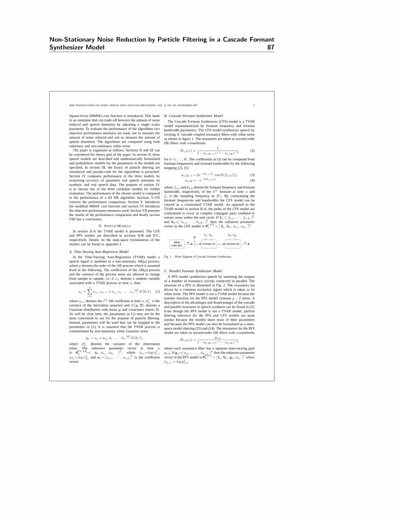
Non-Stationary Noise Reduction by Particle Filtering in a Cascade FormantSynthesizer Model 87
IEEE TRANSACTIONS ON AUDIO, SPEECH AND LANGUAGE PROCESSING, VOL. X, NO. XX, NOVEMBER 2007 2
Square-Error (MMSE) cost function is introduced. This leadsto an estimator that can trade-off between the amount of noisereduced and speech distortion by adjusting a single scalarparameter. To evaluate the performance of the algorithms twoobjective performance measures are used, one to measure theamount of noise reduced and one to measure the amount ofspeech distortion. The algorithms are compared using bothstationary and non-stationary white noise.
The paper is organized as follows. Sections II and III canbe considered the theory part of the paper. In section II, threespeech models are described and mathematically formulatedand probabilistic models for the parameters in the models arespecified. In section III, the basics of particle filtering areintroduced and pseudo-code for the algorithms is presented.Section IV compares performance of the three models byexamining accuracy of parameter and speech estimates onsynthetic and real speech data. The purpose of section IVis to choose one of the three candidate models for furtherevaluation. The performance of the chosen model is comparedto the performance of a HI NR algorithm. Sections V-VIIconcern the performance comparison. Section V introducesthe modified MMSE cost function and section VI introducesthe objective performance measures used. Section VII presentsthe results of the performance comparison and finally sectionVIII has a conclusion.
II. SPEECHMODELS
In section II-A the TVAR model is presented. The CFSand PFS models are described in sections II-B and II-C,respectively. Details on the state-space formulations of themodels can be found in appendix I.
A. Time-Varying Auto-Regressive Model
In the Time-Varying Auto-Regressive (TVAR) model aspeech signal is modeled as a non-stationary AR(p) process,wherep denotes the order of the AR process which is assumedfixed in the following. The coefficients of the AR(p) processand the variance of the process noise are allowed to changefrom sample to sample, i.e. ifxn denotes a random variableassociated with a TVAR process at timen, then
xn =
p∑
i=1
an,i xn−i + σenen , en
iid∼ N (0, 1) (1)
wherean,i denotes theith AR coefficient at timen, σ2
enis the
variance of the innovation sequence andN (µ,Σ) denotes aGaussian distribution with meanµ and covariance matrixΣ.As will be clear later, the parameters in (1) may not be themost convenient to use for the purpose of particle filtering.Instead, parameters will be used that can be mapped to theparameters in (1). It is assumed that the TVAR process iscontaminated by non-stationary white Gaussian noise
yn = xn + σdndn , dn
iid∼ N (0, 1),
where σ2
dndenotes the variance of the observation
noise. The unknown parameter vector at timenis θTV AR
n =[ an, φen, φdn
]T , where φen= log σ2
en,
φdn= log σ2
dnand an= [ an,1, · · · , an,p ]
T is the coefficientvector.
B. Cascade Formant Synthesizer Model
The Cascade Formant Synthesizer (CFS) model is a TVARmodel reparameterized by formant frequency and formantbandwidth parameters. The CFS model synthesizes speech byexcitingK cascade-coupled resonance filters with white noiseas shown in figure 1. The resonators are taken as second-orderIIR filters with z-transforms
Hn,k(z) =1
1 − an,2k−1z−1 − an,2kz−2(2)
for k=1, . . . , K. The coefficients in (2) can be computed fromformant frequencies and formant bandwidths by the followingmapping [2], [5]
an,2k−1 = 2e−πbn,k/fs cos(2πfn,k/fs) (3)
an,2k = −e−2πbn,k/fs , (4)
wherefn,k andbn,k denote the formant frequency and formantbandwidth, respectively, of thekth formant at timen andfs is the sampling frequency inHz. By constraining theformant frequencies and bandwidths the CFS model can beviewed as a constrained TVAR model. As opposed to theTVAR model in section II-A, the poles of the CFS model areconstrained to occur in complex conjugate pairs confined tocertain areas within the unit circle. Iffn=[ fn,1, . . . , fn,K ]T
and bn=[ bn,1, . . . , bn,K ]T then the unknown parametervector in the CFS model isθCFS
n = [ fn, bn, φen, φdn
]T .
Formant #1x
fn,1 bn,1gn
Formant #K
fn,K bn,K
White noise gen.
en xn
Fig. 1. Block diagram of Cascade Formant Synthesizer.
C. Parallel Formant Synthesizer Model
A PFS model synthesizes speech by summing the outputsof a number of resonance circuits connected in parallel. Thestructure of a PFS is illustrated in Fig. 2. The resonators aredriven by a common excitation signal which is taken to bewhite noise. The PFS model is not a TVAR model because thetransfer function for the PFS model containsp − 2 zeros. Adescription of the advantages and disadvantages of the cascadeand parallel structures in speech synthesis can be found in [2].Even though the PFS model is not a TVAR model, particlefiltering inference for the PFS and CFS models are quitesimilar because the models share most of their parametersand because the PFS model can also be formulated as a state-space model obeying (23) and (24). The resonators for the PFSmodel are taken as second-order IIR filters with z-transforms
Hn,k(z) =gn,k
1 − an,2k−1z−1 − an,2kz−2
where each resonance filter has a separate time-varying gaingn,k. If gn=[ φgn,1
, . . . , φgn,K]T then the unknown parameter
vector in the PFS model isθPFSn = [ fn, bn, gn, φdn
]T whereφgn,k
= log g2
n,k.

88 Appendix G
IEEE TRANSACTIONS ON AUDIO, SPEECH AND LANGUAGE PROCESSING, VOL. X, NO. XX, NOVEMBER 2007 3
Formant #1x
+
+
+
fn,1 bn,1gn,1
Formant #Kx
fn,K bn,Kgn,K
White noise gen.
en
xn,1
xn,K
xn
Fig. 2. Block diagram of Parallel Formant Synthesizer.
D. Probabilistic Models for Parameters
As will be evident in section III, particle filtering dependsonstatistical models for the parameters contained in the parametervector θ. It is important that samples can be drawn fromthe parameter models, specifically because, as section III willdemonstrate particle filtering relies on samples being drawnfrom the initial state distributionp(θ0) and the state-transitiondistribution p(θn |θn−1). A specification of the parametermodels can be found in appendix II.
III. PARTICLE FILTER INFERENCE
Generally, filtering refers to the task of computing thefiltering distributionp(xn, θn |y1:n) and the MMSE estimateof the state vector and the parameter vector at timen usingobservationsy1:n = [y1, · · · , yn]T up to and including timen. In the ideal case it is possible to compute a closed-form analytic expression for the MMSE estimator of theparameter vector and the state vector. For non-ideal cases thisis not possible, making approximations necessary. GivenN
independent samples from the filtering distribution at timen,an approximation to the MMSE estimator can be computed as
[xn , θn] =1
N
N∑
i=1
[xin , θ
in] (5)
where the superscript denotes the sample index. It is generallynot possible to draw samples directly from the filtering distri-bution but samples can be drawn usingimportance sampling.In this case samples are drawn from an importance distribu-tion, π(xn, θn |y1:n), (also called a proposal distribution) andimportance weights are formed
w(xn , θn) =p(xn, θn |y1:n)
π(xn, θn |y1:n)(6)
Using the importance distribution the MMSE estimator can bewritten
< xn , θn >= Eπ(xn,θn |y1:n) {[xn , θn] w(xn , θn)} (7)
However, the expression in (7) is just as intractable as theoriginal integral defining the MMSE estimator. IfN indepen-dent samples are drawn from the importance distribution andthe weights given by (6) are evaluated for each drawn samplethen the expression for the MMSE estimator in (7) can beapproximated as
[xn , θn] =
N∑
i=1
[xin , θ
in] w(xi
n , θin) (8)
where
w(xin , θ
in) =
w(xin , θ
in)
∑N
i=1 w(xin , θ
in)
are the normalized importance weights. The above rea-soning can be generalized to consider full trajectoriesp(x0:n, θ0:n |y1:n) .
The posterior distribution over the full trajectories can bedecomposed into
p(x0:n, θ0:n |y1:n) = p(x0:n |θ0:n,y1:n) p(θ0:n |y1:n) (9)
Because the state variables given the parameters are Gaussian,the state variables can be marginalized out with Kalman (Rao-Blackwellization) leaving us with a filtering model for theparameters. So,p(x0:n |θ0:n,y1:n) can be marginalized andthe marginalized posteriorp(xn |θ0:n,y1:n) admits a Gaussiandistribution whose mean and covariance can be computed byKalman filtering. Introducing a new importance distribution,π(θ0:n|y1:n), the MMSE estimator approximation can becomputed as
[xn, θn] =
N∑
i=1
Ep(xn| θ0:n,y1:n)
{
[xn, θi0:n]
}
w(θi0:n) (10)
where
w(θ0:n) =p(θ0:n |y1:n)
π(θ0:n |y1:n), w(θi
0:n) =w(θi
0:n)∑N
i=1 w(θi0:n)
(11)
A very undesirable feature of the importance samplingmethod in the general case is the need to store the trajectories(the history) of the samples drawn from the importancedistribution and the observations. This means that storagerequirements and the computational load will grow over time.This makes the importance sampling method impractical forreal-time applications. Fortunately, there is a way to formulatea recursive version of the importance sampling method whichalleviates the undesirable features. This method is known asSequential Importance Sampling(SIS). The important step todevelop a recursive version of the approximation in (10) isto obtain a recursion formula for the weights in (11) whichcan then be used in (10). This can be done if the importancedistribution is restricted to the general form
π(θ0:n |y1:n) = π(θ0:n−1 |y1:n−1) · π(θn |θ0:n−1,y1:n)(12)
The crucial restriction is that the time dependence only goesto n− 1 in the first term. It can then be shown (see appendixIII) that the weights obey the recursion
w(θ0:n) ∝ w(θ0:n−1) · w(θn) (13)
with
w(θn) ∝p(yn|y1:n−1, θ0:n) p(θn|θn−1)
π(θn|θ0:n−1,y1:n). (14)
In this way sequential importance sampling avoids the needto store the pathsθ0:n−1 of the particles. The complexity ofcomputing the weights can be simplified if the importancedistribution at timen is set equal to the prior distribution, i.e.π(θn |θ0:n−1, y1:n) = p(θn|θn−1) so that (14) reduces to
wn ∝ p(yn|θ0:n,y1:n−1). (15)

Non-Stationary Noise Reduction by Particle Filtering in a Cascade FormantSynthesizer Model 89
IEEE TRANSACTIONS ON AUDIO, SPEECH AND LANGUAGE PROCESSING, VOL. X, NO. XX, NOVEMBER 2007 4
However, setting the importance distribution equal to the priordistribution contributes to a degeneracy whereby all weightsexcept one after a few time steps are very close to zero.This happens because the importance distribution is differentfrom the true posterior distribution. As a remedy, a resamplingstep is introduced. The resampling step duplicates particles inproportion to their importance weights in such a way thatall particles have approximately the same weight after theresampling step. Incorporating the selection step, the weightsw(θ0:n−1) will all be equal to1 andw(θ0:n) ∝ w(θn).
Putting it all together, the procedure of the particle filteris illustrated with pseudo-code in Algorithm 1. The mainreferences for this summary of particle filtering are [3], [6].
Algorithm 1 Particle filter pseudo-code1: Draw samples from initial distributions (35), (37) or (39)2: for t = 1 to T do3: for i = 1 to N do4: Draw sample from state-transition distributions (36),
(38) or (40)5: Form system matrices (25)-(28) or (30)-(33)6: Perform a Kalman filter step according to state-space
eqns (23)-(24) (Rao-Blackwellization)7: Compute weight using (15)8: end for9: Resampling
10: Compute estimates using (5)11: end for
IV. EXPERIMENTS& D ISCUSSION OFSPEECHMODELS
In section IV-A the data used to examine and compareperformance of the three models is described. Also in sectionIV-A, the setting of the hyper-parameters for the modelsis specified and the measured dB SNR improvements arepresented. In sections IV-B to IV-D separate discussions ofthe workings of each of the models are presented. Finally, insection IV-E a summary of the experiments is given and oneof the three models is chosen for further evaluation.
A. Data Generation & Measured SNR Improvements
To investigate the behavior of the three models, both syn-thetic and real speech data are used. The synthetic data isgenerated from the TVAR model but the parameter valuesare extracted from real speech. Formant frequencies, formantbandwidths and formant gains are extracted from the TIMITsentence,sa2, containing a female speaker saying ”Don’task me to carry an oily rag like that.” down-sampled to16 kHz. Formant frequencies are extracted by finding thelocation of peaks in a14th order model-based spectrum, theformant bandwidths are extracted by computing the3 dBdown points from the location of the peaks and the formantgains are taken as the values of the peaks in the spectrum.The parameters are extracted from a25ms window and thewindow is shifted in steps of1.25ms duration. After the rawextraction of the parameters, the formant frequency tracksaremanually prepared by first sorting out the first four formants
and then cubic interpolation is performed on the parametertracks such that the rate of the parameter values is equal to thesampling rate. The upper plot in figure 3 shows a wide-band
Fre
quen
cy [H
z]
Wide−band spectrogram of TIMIT sound
0 0.5 1 1.5 20
1000
2000
3000
4000
5000
Time [s]
Fre
quen
cy [H
z]Real speech f, b and g parameters used for synthetic data
0 0.5 1 1.5 20
1000
2000
3000
4000
5000
Fig. 3. Upper plot shows a wide band spectrogram of the TIMIT sentence,sa2, and the lower plot illustrates the extracted fbg parameters. The thicknessof the tracks in the lower plot indicates the estimated formant bandwidths andthe strength of the formants are indicated so that dark intervals represent strongformants.
spectrogram of the original TIMIT speech sentence and thelower plot illustrates the formant-bandwidth-gain parametersextracted from the TIMIT sentence. The synthetic data usedfor experiments in this section is generated using the parametervalues illustrated in the lower plot by first mapping formantfrequencies and bandwidths to AR coefficients using (3) and(4). The noise variance was made known and constant atunity, that is Dn(θ) = 1 for all n. The standard deviationof the innovation noise was taken to be proportional to thegain of the first formantσen
∝ gn,1. The standard deviationof the innovation noise was scaled such that the SNR ofthe generated noisy data was approximately5 dB. Finally,data was generated using (23) and (24). The real speech dataconsists of the TIMIT sentence with white Gaussian noiseadded at an SNR of5 dB.
The number of particles used in all experiments is100.Using more particles provides only minor changes in SNRimprovement. All experiments are repeated seven times andthe measured SNR improvements and the parameter estimatesrepresent an average over the seven repeated experiments. Allhyper parameters were manually tuned to provide highest SNRimprovements. This resulted in the settings shown in table I(see appendix II for a specification of the hyper parameters).The measured dB SNR improvements are seen in table II.
B. TVAR
To better understand how the TVAR particle filter works,model-based spectrograms were made using the true and esti-mated AR coefficients and gains. The plot in figure 4a showsthe model-based spectrogram using the true AR coefficientsand gains and the plot in figure 4b shows the corresponding
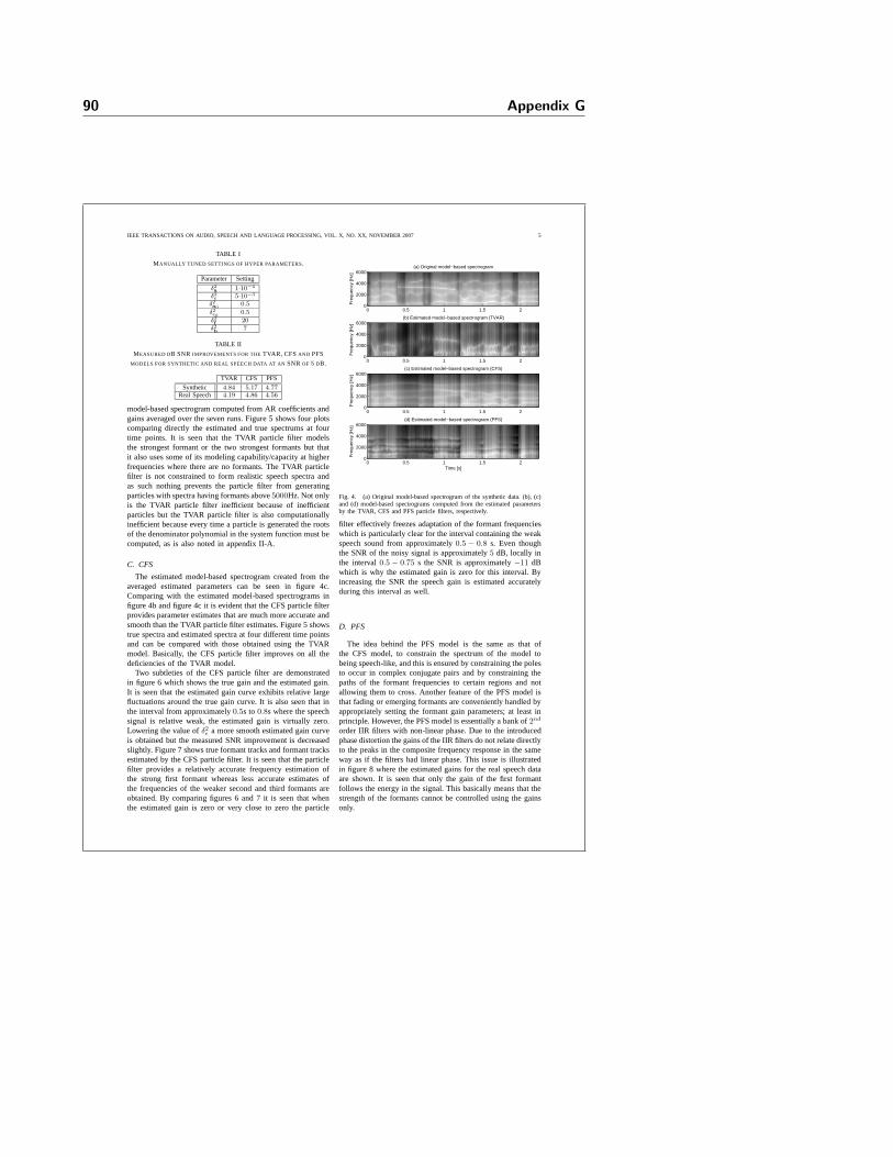
90 Appendix G
IEEE TRANSACTIONS ON AUDIO, SPEECH AND LANGUAGE PROCESSING, VOL. X, NO. XX, NOVEMBER 2007 5
TABLE I
MANUALLY TUNED SETTINGS OF HYPER PARAMETERS.
Parameter Setting
δ2a 1·10
−4
δ2e
5·10−3
δ2a0
0.5
δ2e0
0.5
δ2
f20
δ2
b7
TABLE II
MEASURED DB SNR IMPROVEMENTS FOR THETVAR, CFSAND PFS
MODELS FOR SYNTHETIC AND REAL SPEECH DATA AT ANSNROF 5 DB.
TVAR CFS PFS
Synthetic 4.84 5.17 4.77
Real Speech 4.19 4.86 4.56
model-based spectrogram computed from AR coefficients andgains averaged over the seven runs. Figure 5 shows four plotscomparing directly the estimated and true spectrums at fourtime points. It is seen that the TVAR particle filter modelsthe strongest formant or the two strongest formants but thatit also uses some of its modeling capability/capacity at higherfrequencies where there are no formants. The TVAR particlefilter is not constrained to form realistic speech spectra andas such nothing prevents the particle filter from generatingparticles with spectra having formants above5000Hz. Not onlyis the TVAR particle filter inefficient because of inefficientparticles but the TVAR particle filter is also computationallyinefficient because every time a particle is generated the rootsof the denominator polynomial in the system function must becomputed, as is also noted in appendix II-A.
C. CFS
The estimated model-based spectrogram created from theaveraged estimated parameters can be seen in figure 4c.Comparing with the estimated model-based spectrograms infigure 4b and figure 4c it is evident that the CFS particle filterprovides parameter estimates that are much more accurate andsmooth than the TVAR particle filter estimates. Figure 5 showstrue spectra and estimated spectra at four different time pointsand can be compared with those obtained using the TVARmodel. Basically, the CFS particle filter improves on all thedeficiencies of the TVAR model.
Two subtleties of the CFS particle filter are demonstratedin figure 6 which shows the true gain and the estimated gain.It is seen that the estimated gain curve exhibits relative largefluctuations around the true gain curve. It is also seen that inthe interval from approximately0.5s to0.8s where the speechsignal is relative weak, the estimated gain is virtually zero.Lowering the value ofδ2
ea more smooth estimated gain curve
is obtained but the measured SNR improvement is decreasedslightly. Figure 7 shows true formant tracks and formant tracksestimated by the CFS particle filter. It is seen that the particlefilter provides a relatively accurate frequency estimationofthe strong first formant whereas less accurate estimates ofthe frequencies of the weaker second and third formants areobtained. By comparing figures 6 and 7 it is seen that whenthe estimated gain is zero or very close to zero the particle
Fre
quen
cy [H
z]
(a) Original model−based spectrogram
0 0.5 1 1.5 20
2000
4000
6000
Fre
quen
cy [H
z]
(b) Estimated model−based spectrogram (TVAR)
0 0.5 1 1.5 20
2000
4000
6000
Fre
quen
cy [H
z]
(c) Estimated model−based spectrogram (CFS)
0 0.5 1 1.5 20
2000
4000
6000
Time [s]
Fre
quen
cy [H
z]
(d) Estimated model−based spectrogram (PFS)
0 0.5 1 1.5 20
2000
4000
6000
Fig. 4. (a) Original model-based spectrogram of the synthetic data. (b), (c)and (d) model-based spectrograms computed from the estimated parametersby the TVAR, CFS and PFS particle filters, respectively.
filter effectively freezes adaptation of the formant frequencieswhich is particularly clear for the interval containing theweakspeech sound from approximately0.5 − 0.8 s. Even thoughthe SNR of the noisy signal is approximately5 dB, locally inthe interval0.5 − 0.75 s the SNR is approximately−11 dBwhich is why the estimated gain is zero for this interval. Byincreasing the SNR the speech gain is estimated accuratelyduring this interval as well.
D. PFS
The idea behind the PFS model is the same as that ofthe CFS model, to constrain the spectrum of the model tobeing speech-like, and this is ensured by constraining the polesto occur in complex conjugate pairs and by constraining thepaths of the formant frequencies to certain regions and notallowing them to cross. Another feature of the PFS model isthat fading or emerging formants are conveniently handled byappropriately setting the formant gain parameters; at least inprinciple. However, the PFS model is essentially a bank of2
nd
order IIR filters with non-linear phase. Due to the introducedphase distortion the gains of the IIR filters do not relate directlyto the peaks in the composite frequency response in the sameway as if the filters had linear phase. This issue is illustratedin figure 8 where the estimated gains for the real speech dataare shown. It is seen that only the gain of the first formantfollows the energy in the signal. This basically means that thestrength of the formants cannot be controlled using the gainsonly.
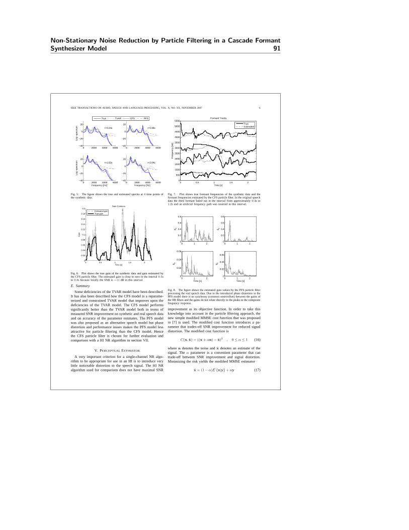
Non-Stationary Noise Reduction by Particle Filtering in a Cascade FormantSynthesizer Model 91
IEEE TRANSACTIONS ON AUDIO, SPEECH AND LANGUAGE PROCESSING, VOL. X, NO. XX, NOVEMBER 2007 6
0 2000 4000 6000−40
−20
0
20
Log−
spec
trum
t=0.24s
True TVAR CFS PFS
0 2000 4000 6000−40
−20
0
20
t=0.99s
0 2000 4000 6000−40
−20
0
20
t=1.62s
Frequency [Hz]
Log−
spec
trum
0 2000 4000 6000−40
−20
0
20
t=2.04s
Frequency [Hz]
Fig. 5. The figure shows the true and estimated spectra at4 time points ofthe synthetic data.
0 0.5 1 1.5 20
0.02
0.04
0.06
0.08
0.1
0.12
0.14
0.16
0.18
0.2
Time [s]
Gai
n
Gain Contours
Estimated gainTrue gain
Fig. 6. Plot shows the true gain of the synthetic data and gainestimated bythe CFS particle filter. The estimated gain is close to zero inthe interval0.5sto 0.8s because locally the SNR is−11 dB in this interval.
E. Summary
Some deficiencies of the TVAR model have been described.It has also been described how the CFS model is a reparame-terized and constrained TVAR model that improves upon thedeficiencies of the TVAR model. The CFS model performssignificantly better than the TVAR model both in terms ofmeasured SNR improvement on synthetic and real speech dataand on accuracy of the parameter estimates. The PFS modelwas also proposed as an alternative speech model but phasedistortion and performance issues makes the PFS model lessattractive for particle filtering than the CFS model. Hencethe CFS particle filter is chosen for further evaluation andcomparison with a HI NR algorithm in section VII.
V. PERCEPTUAL ESTIMATOR
A very important criterion for a single-channel NR algo-rithm to be appropriate for use in an HI is to introduce verylittle noticeable distortion to the speech signal. The HI NRalgorithm used for comparison does not have maximal SNR
0 0.5 1 1.5 20
500
1000
1500
2000
2500
3000
3500
4000
4500
5000
5500
Time [s]
Fre
quen
cy [H
z]
Formant Tracks
TrueEstimated
Fig. 7. Plot shows true formant frequencies of the syntheticdata and theformant frequencies estimated by the CFS particle filter. Inthe original speechdata the third formant faded out in the interval from approximately 0.4s to1.2s and an artificial frequency path was inserted in this interval.
0 1 20
0.2
0.4
0.6
0.8
g 1
0 1 20
0.2
0.4
0.6
0.8g 2
0 1 20
0.02
0.04
0.06
g 3
Time [s]0 1 2
0
0.02
0.04
0.06
g 4
Time [s]
Fig. 8. The figure shows the estimated gain values by the PFS particle filterprocessing the real speech data. Due to the introduced phasedistortion in thePFS model there is no synchrony (common onset/offset) between the gains ofthe IIR filters and the gains do not relate directly to the peaks in the compositefrequency response.
improvement as its objective function. In order to take thisknowledge into account in the particle filtering approach, thenew simple modified MMSE cost function that was proposedin [7] is used. The modified cost function introduces a pa-rameter that trades-off SNR improvement for reduced signaldistortion. The modified cost function is
C(x, x) = ((x + αn) − x)2 , 0 ≤ α ≤ 1 (16)
wheren denotes the noise andx denotes an estimate of thesignal. Theα parameter is a convenient parameter that cantrade-off between SNR improvement and signal distortion.Minimizing the risk yields the modified MMSE estimator
x = (1 − α)E {x|y} + αy (17)

92 Appendix G
IEEE TRANSACTIONS ON AUDIO, SPEECH AND LANGUAGE PROCESSING, VOL. X, NO. XX, NOVEMBER 2007 7
where the following observation modely = x + n has beenassumed. The modified estimator is thus expressed as a linearinterpolation between the MMSE estimator and the observednoisy speech signal and therefore can be used directly in theparticle filtering framework.
VI. OBJECTIVE PERFORMANCEMEASURES
There is not a clear winner when it comes to objectivelyevaluating speech enhancement algorithms but several studies,see [8]–[11], indicate that separate measures for residualnoisesuppression and speech distortion provide a reasonable indica-tion of performance. We chose to evaluate noise suppressionby the segmental-SNR metric and speech distortion by thefrequency-weighted log-spectral distance, see [8]–[11].
The HI NR algorithm processes the noisy speech block-wiseby convolving the noisy speech with a slowly time-varyinglinear filter whereas the CFS particle filter processes the noisyspeech sample-wise by evaluation of a statistical estimatorfunction. The group delay introduced by the HI NR algorithmmust be taken into account when computing the performancemeasures. Otherwise a simple delay of the input could givesubstantial SNR improvement measurements even though nonoise has been removed. The same issue does not exist withthe CFS particle filter. For the CFS particle filter the segmentalSNR improvement is computed from
segSNRI =1
M
M∑
m=1
[10 log10
∑t n2
in,m(t)∑
t n2out,m(t)
]+35
−20
(18)
wherem is the block index and the SNR is restricted to valuesbetween−25 and+35 dB to avoid bias. For the CFS particlefilter, the output noise is given bynout = y − x. For the HINR algorithm, the segmental SNR improvement is computedfrom
segSNRI = segSNRout − segSNRin (19)
where
segSNRout =1
M
M∑
m=1
[10 log10
∑t x2
out,m(t)∑
t n2out,m(t)
]+35
−20
(20)
segSNRin =1
M
M∑
m=1
[10 log10
∑t x2
in,m(t)∑
t n2in,m(t)
]+35
−20
(21)
In order to compute the segmental SNR at the output, the HINR algorithm is modified such that the clean speech and thenoise signals are separately filtered in the same way as thenoisy speech is filtered. The clean speech and noise filtered inthis way are used in (20).
The frequency-weighted log-spectral signal distortion mea-sure indicates an Euclidian distance between short-time spectra(in dB) of the clean speech component and the processedspeech component and is computed from
SD =1
M
M∑
m=1
√√√√ 1
K
K∑
k=1
(waud(k)10 log10
X(k, m)
X(k, m)
)2
(22)
where X(k, m) denotes the estimated speech-frequencypower-density spectrum in blockm, k denotes frequencybin index andwaud(k) denotes a frequency weighting factorgiving approximately equal weight to each auditory criticalband.
VII. PERFORMANCE
The performance of the HI NR and the CFS algorithms aretested using stationary and non-stationary white noise createdby performing a Gaussian Random Walk (RW) on the varianceof the noise using an RW variance of1e−6 truncated topositive values. Performance is measured for four differentSNRs,0, 5, 10 and 20 dB, and six different speakers takenfrom the TIMIT database, three male (SA1, SX333, SX451)and three female (SX206, SX312, SX402) speakers.
We compared two approaches to the state transition for thegain: Gaussian distributed in the gain and the log gain, respec-tively. The latter has the advantage that the gain is guaranteedto stay non-negative. However, we observed stability problemswith it because it takes unrealistically large steps for large gainand excruciatingly small steps for small gain. We thereforeapplied a Gaussian RW truncated to positive values to thegain directly, guaranteeing a fixed step size, independent ofthe value of the gain. Hence, instead of adapting the log-variances it was chosen to adapt the standard deviations ofthe noise and speech. The CFS parameter vector used is thusθ
CFSn = [ fn, bn, σen
, σdn]T and δ2
d′=5e−7, δ2e′=1e−6,
whereδd′ andδe′ denotes the RW variances forσdnandσen
,respectively.
We compare the performance of our algorithm to acommercial-grade algorithm from the hearing aids industry.GN ReSound supplied us with a version of their spectralsubtraction based noise reduction algorithm. In this algorithm,the noise spectrum is tracked through time-varying low-passfiltering of the signal+noise spectrum. Exact details of thealgorithm are not disclosed, but we find it important to com-pare our method to commercial standards rather than choosingone of the many proposed methods in the literature. We areparticularly interested in evaluating the performance of oursystem for estimating the signal under low-SNR conditions,because this is the situation that is notoriously difficult forsingle-microphone systems, including our reference algorithmthat was supplied by GN ReSound.
Figures 9 and 10 show objective performance measuresobtained for stationary noise and non-stationary noise, respec-tively. The figures show how performance vary dependingof the value of theα parameter in (17) for four differentSNR levels. Each curve represents an average performancecomputed from the average performance for each of the sixspeakers. As expected thesegSNRI measure decreases withincreasingα, however, at an SNR level of20 dB thesegSNRI
measure increases withα because the raw MMSE estimategives a negativesegSNRI score. It is also seen that the SDmeasure increases with increasingα except whenα is small.At an SNR level of20 dB the SD curve is relative flat though.The corresponding objective measures for the HI NR are alsoindicated. The grey horizontal lines in the figure show the

Non-Stationary Noise Reduction by Particle Filtering in a Cascade FormantSynthesizer Model 93
IEEE TRANSACTIONS ON AUDIO, SPEECH AND LANGUAGE PROCESSING, VOL. X, NO. XX, NOVEMBER 2007 8
corresponding segSNRI and SD values for the HI NR. Basedon figures 9 and 10 and informal listening tests a suitablesetting of theα parameter was found to be0.25. The objectiveperformance measurements indicate that the CFS algorithmperforms better compared to the HI NR algorithm for low SNRlevels. When the SNR level is high enough the measurementsindicate that the HI NR algorithm performs better than theCFS algorithm. Informal listening tests indicate that there isa slight difference in quality of the enhanced speech for thetwo algorithms where the enhanced speech produced by theHI NR algorithm is preferable. It was found that the distortionintroduced by the CFS algorithm is more noticeable than forthe HI NR algorithm. This observation can explain why theCFS algorithm is not performing much better than the HI NRalgorithm for non-stationary noise relative to the stationarynoise case.
0 0.1 0.2 0.3 0.4 0.5−1
0
1
2
3
4
5
6
7
8
9
α
segS
NR
I [dB
]
segSNRI curves as a function of α
0 0.1 0.2 0.3 0.4 0.57
8
9
10
11
12
13
14
15
α
SD
SD curves as a function of α
0 dB5 dB10 dB20 dB
Fig. 9. Plots illustrating the variation in segSNRI and SD measurements asa function ofα at four different SNR levels for stationary white noise. Themeasurements have been made by averaging performance for the six speakers.The grey horizontal lines show the corresponding segSNRI and SD values forthe HI NR. Error bars are not shown because they were found to be visibleon the20 dB level curves only.
By converting the sub-band noise power estimates in theHI NR algorithm to a noise variance estimate, it is possibleto compare the noise variance estimates of the CFS and HINR algorithms. Figure 11 shows three examples for the caseof speaker SA1 and non-stationary noise. In figure 11(a) and(b) the non-stationary noise with RW variance is used at 0 dBSNR and 5 dB SNR, respectively and in (c) noise where thevariance changes abruptly every500 ms and otherwise keptconstant is used. In figure 11a the CFS algorithm tracks thenoise variance much better than the HI NR algorithm whichseems to not only react slowly but also seems to underestimatethe noise variance. In figure 11b the HI NR algorithm is betterat tracking the noise, mostly because the increased SNR makesit easier for the HI NR to track the noise. Figure 11b makesvisible some intervals where the noise variance estimatedby the CFS algorithm deviates significantly from the truenoise variance. This is caused by a short-coming of the CFSmodel. The deviations occur during intervals corresponding to
0 0.1 0.2 0.3 0.4 0.5−1
0
1
2
3
4
5
6
7
8
9
α
segS
NR
I [dB
]
segSNRI curves as a function of α
0 0.1 0.2 0.3 0.4 0.57
8
9
10
11
12
13
14
15
α
SD
SD curves as a function of α
0 dB5 dB10 dB20 dB
Fig. 10. Figure legend as in figure 9 but now with non-stationary whitenoise.
unvoiced speech sounds where most of the speech energy isconcentrated at higher frequencies. Figure 11c demonstratesthe difference between the two algorithms reacting to suddenchanges in the noise variance. The CFS algorithms is trackingthe noise variance much faster than the HI NR algorithm forthis case.
0 0.5 1 1.5 2 2.5 3
0.5
1
1.5
(a) Noise variance estimate at 0 dB SNR
Var
ianc
e
True CFS HI NR
0 0.5 1 1.5 2 2.5 3
0.2
0.4
0.6
0.8(b) Noise variance estimate at 5 dB SNR
Var
ianc
e
True CFS HI NR
0 0.5 1 1.5 2 2.5 3
0.5
1
1.5
(c) Noise variance estimate at 0 dB SNR
Time [s]
Var
ianc
e
True CFS HI NR
Fig. 11. (a) shows the true variance of the non-stationary noise with RWvariance and the noise variance estimated by the CFS and HI NRalgorithmsat an SNR level of0 dB (using speaker SA1). (b) show the noise varianceestimates for the same setup but at an SNR level of5 dB. (c) illustrates howthe two algorithms react to sudden changes in the noise variance.
VIII. C ONCLUSION
It has been found that reducing noise in speech by particlefilter inference in a TVAR model is more beneficial if priorknowledge of the formants is exploited. This was achievedby parameterizing the AR coefficients by formant frequencies

94 Appendix G
IEEE TRANSACTIONS ON AUDIO, SPEECH AND LANGUAGE PROCESSING, VOL. X, NO. XX, NOVEMBER 2007 9
and formant bandwidths instead of using the AR coefficientsdirectly. It was also found that conditional on the resonancefilter used to model the formants, the cascade formant synthe-sizer model was found more useful than the parallel formantsynthesizer model. The performance of a hearing instrumentnoise reduction algorithm was compared to the particle filteralgorithm for stationary and non-stationary white noise. Itwas found that noise tracking capabilities of the particle filteralgorithm were superior to that of the hearing instrument noisereduction algorithm, especially for low SNR levels. We planto further develop the particle filtering approach for high-SNR situations and consider boosting low-SNR performancefor our hearing instrument set-up through integration of theparticle filter algorithm with the hearing instrument noisereduction algorithm. We will develop the particle filteringapproach by extending the speech model to take into accounthigh-frequency speech components and to include a harmonicexcitation term.
APPENDIX ISTATE-SPACE FORMULATION
A. TVAR
The TVAR model is conveniently formulated as a state-space model with the following state and observation equations
xn = An xn−1 + Bn en (23)
yn = Cxn + Dn dn, (24)
wherexn = [ xn, · · · , xn−p+1 ]T is the state vector and
An =
[
aTn
I(p−1) 0(p−1)×1
]
(25)
Bn =
[
σen
0(p−1)×1
]
(26)
C =[
1 01×(p−1)
]
(27)
Dn = [ σdn] , (28)
wherean = [ an,1, · · · , an,p ]T is the coefficient vector. The
state-space formulation of the TVAR model in eqs. (23) and(24), with the parameterization in (25), (26), (27) and (28), isused in [3].
B. PFS
By letting
An,k =
[
an,2k−1 an,2k
1 0
]
(29)
then in state-space form, the PFS model is described by (23)and (24) with system matrices
An = diag(An,1, · · · ,An,K) (30)
Bn =
[
01×2K
gn,1 0 · · · gn,K 0
]T
(31)
C =[
1 0 1 0 · · · 1 0]
(32)
Dn = [ σdn] , (33)
where the state vector changes form to
xn = [xn,1, xn−1,1, · · · , xn,K , xn−1,K ]T (34)
and the process noise becomes bivariateen ∼ N (02×1, I2).In (34) xn,k denotes the output from thekth resonator (seefigure 2) .
APPENDIX IIPROBABILISTIC MODELS FORPARAMETERS
The initial state and state-transition distributions for theTVAR model are factorized as in [3], that is
p(θTV AR0 ) = p(a0)p(φe0
)p(φd0) (35)
p(θTV ARn |θTV AR
n−1 ) = p(an|an−1)p(φen|φen−1
)
×p(φdn|φdn−1
) , n > 1 . (36)
The initial state and state-transition distributions for theparameters in the CFS model are factorized as
p(θCFS0 ) = p(f0)p(b0)p(φe0
)p(φd0) (37)
p(θCFSn |θCFS
n−1 ) = p(fn|fn−1)p(bn|bn−1)p(φen|φen−1
)
×p(φdn|φdn−1
) , n > 1 . (38)
The initial state and state-transition distributions for theparameters in the PFS model are factorized as
p(θPFS0 ) = p(f0)p(b0)p(g0)p(φd0
) (39)
p(θPFSn |θPFS
n−1 ) = p(fn|fn−1)p(bn|bn−1)p(gn|gn−1)
×p(φdn|φdn−1
) , n > 1 . (40)
A. TVAR
The initial state distributions are taken to be Gaussian andthe parameters are assumed to evolve according to first-orderGaussian Markov processes. As such, samples from the initialstate and state-transition distributions are generated using thefollowing generative expressions
a0 = v , v ∼ N(
0p×1, δ2a0
Ip
)
an = an−1 + wn , wn ∼ N(
0p×1, δ2aIp
)
φe0= α , α ∼ N (−2, 0.25)
φen= φen−1
+ βn , βn ∼ N(
0, δ2e
)
φd0= γ , γ ∼ N
(
0, δ2d0
)
φdn= φdn−1
+ ǫn , ǫn ∼ N(
0, δ2d
)
(41)
Samples drawn from the chosen initial state and state-transition distributions for the AR coefficients in (41) thatproduce poles of the system function that reside on or outsidethe unit circle are discarded. This step is a sufficient conditionto ensure stability of the TVAR process.
B. CFS
For the CFS model, samples are drawn from the initial andstate-transition distribution in the following way
f0 = ω , ω ∼ U (fl, fh)fn = fn−1 +ψn , ψn ∼ N
(
0K×1, δ2fIK
)
b0 = ν , ν ∼ U (bl,bh)bn = bn−1 + ςn , ςn ∼ N
(
0K×1, δ2bIK
)
(42)
The models for the process noise and the observation noisevariances are equivalent to those in (41). In order to exploitknown properties of the formant frequencies in the particle

Non-Stationary Noise Reduction by Particle Filtering in a Cascade FormantSynthesizer Model 95
IEEE TRANSACTIONS ON AUDIO, SPEECH AND LANGUAGE PROCESSING, VOL. X, NO. XX, NOVEMBER 2007 10
filtering the formant frequencies are constrained to the fre-quencies rangesfn,1 ∈ [200, 1500]Hz, fn,2 ∈ [800, 2700]Hz,fn,3 ∈ [2000, 3800]Hz and fn,4 ∈ [2800, 5600]Hz. Further-more, the formant frequencies are constrained to be at least200Hz apart, that is,fn,k−fn,k−1>200Hz for 1 < k ≤ K.These constraints are similar to what was used in [12]. Theformant bandwidths are constrained to the frequency intervalbn,k ∈ [30, 500]Hz. In (42), U(a,b) denotes a multivariateuniform distribution on the domain[a,b]. The setting usedin the following is fl = [300, 1000, 2000, 3000]T, fh =[1000, 2000, 3000, 4000]T, bl = [30, 30, 30, 30]T and bh =[500, 500, 500, 500]T.
C. PFS
The parameter models for the formant frequencies andformant bandwidths in the PFS model are equivalent to thosein (42) and the observation noise model equivalent to that in(41). The model for the formant gains are
g0 = κ , κ ∼ N (−2IK×1, 0.25IK)gn = gn−1 + ξn , ξn ∼ N
(
0K×1, δ2gIK
) (43)
APPENDIX IIIDERIVATION OF (13) AND (14)
The numerator in (11) can be expanded as follows usingBayes’ rule
p(θ0:n |y1:n) =p(y1:n |θ0:n)p(θ0:n)
p(y1:n)
=p(yn |y1:n−1, θ0:n)p(y1:n−1 |θ0:n)p(θn|θ0:n−1)p(θ0:n−1)
p(yn |y1:n−1)p(y1:n−1)
=p(yn |y1:n−1, θ0:n)p(y1:n−1 |θ0:n−1)
p(yn |y1:n−1)p(y1:n−1)(44)
×p(θn|θn−1)p(θ0:n−1)
where it has been assumed that the parametersevolve according to a first-order Markov process, i.e.p(θn |θ0:n−1)=p(θn |θn−1) and where the conditionalindependencep(y1:n−1|θ0:n)=p(y1:n−1|θ0:n−1) has beenused. Inserting (12) and (44) into (11) then the weights obey
w(θ0:n)
∝p(yn|y1:n−1, θ0:n)p(y1:n−1|θ0:n−1)p(θn|θn−1)p(θ0:n−1)
p(yn|y1:n−1)p(y1:n−1)π(θ0:n−1|y1:n−1)π(θn|θ0:n−1,y1:n)
∝p(y1:n−1|θ0:n−1)p(θ0:n−1)
p(y1:n−1)π(θ0:n−1|y1:n−1)
×p(yn|y1:n−1, θ0:n)p(θn|θn−1)
p(yn|y1:n−1)π(θn|θ0:n−1,y1:n)
∝w(θ0:n−1) ·p(yn|y1:n−1, θ0:n) p(θn|θn−1)
p(yn|y1:n−1) π(θn|θ0:n−1,y1:n)
∝w(θ0:n−1) ·p(yn|y1:n−1, θ0:n) p(θn|θn−1)
π(θn|θ0:n−1,y1:n)
∝w(θ0:n−1) · w(θn)
with
w(θn) ∝p(yn|y1:n−1, θ0:n) p(θn|θn−1)
π(θn|θ0:n−1,y1:n).
REFERENCES
[1] Y. Grenier, “Time-dependent ARMA modeling of nonstationary signals,”IEEE Transactions on Acoustics, Speech and Signal Processing, vol. 31,pp. 899–911, Aug 1983.
[2] D. H. Klatt, “Software for a cascade/parallel formant synthesizer,”J.Acoust. Soc. Am., vol. 67, pp. 971–995, 1980.
[3] J. Vermaak, C. Andrieu, A. Doucet, and S. J. Godsill, “Particle methodsfor bayesian modeling and enhancement of speech signals,”IEEE Trans.Speech Audio Processing, vol. 10, pp. 173–185, Mar. 2002.
[4] A. Doucet, S. Godsill, and M. West, “Monte carlo filteringand smooth-ing with application to time-varying spectral estimation,” in In Proc.ICASSP, Istanbul, Turkey, June 2000, pp. 701–704.
[5] J. D. Markel and A. H. Gray,Linear Prediction of Speech. New York,USA: Springer-Verlag, New York, 1976.
[6] A. Doucet, N. de Freitas, and N. Gordon, Eds.,Sequential Monte Carloin Practice. Springer Verlag, 2001, ch. 1.
[7] D. Zhao and W. B. Kleijn, “HMM-based speech enhancement usingexplicit gain modeling,” inProc. ICASSP 2006, Toulouse, France, 2006.
[8] J. Hansen and B. Pellom, “An effective quality evaluation protocol forspeech enhancement algorithms,” 1998.
[9] Y. Hu and P. Loizou, “Evaluation of objective measures for speechenhancement,” inProceedings of INTERSPEECH-2006, Philadelphia,PA, 2006.
[10] R. Huber, “Objective assessment of audio quality usingan auditoryprocessing model,” Dissertation, Oldenburg, University.
[11] T. Rohdenburg, V. Hohmann, and B. Kollmeier, “Objective perceptualquality measures for the evaluation of noise reduction schemes,” inProc. International Workshop on Acoustic Echo and Noise Control,Eindhoven, The Netherlands, September 2005.
[12] Y. Zheng and M. Hasegawa-Johnson, “Formant tracking bymixture stateparticle filter,” in IEEE ICASSP, vol. 5, Quebec, Canada, May 2004.

96 Appendix G
Bibliography
[1] I. A. Aızenberg and A. P. Yuzhakov. Integral representations and residuesin multidimensional complex analysis, volume 58 of Translations of Math-ematical Monographs. American Mathematical Society, Providence, RI,1983. Translated from the Russian by H. H. McFaden, Translation editedby Lev J. Leifman.
[2] M. Sanjeev Arulampalam, Simon Maskell, Neil Gordon, and Tim Clapp.A tutorial on particle filters for online nonlinear/non-gaussian bayesiantracking. IEEE Trans. Signal Processing, 50(2):174–188, February 2002.
[3] Paul M. Baggenstoss. The pdf projection theorem and the class-specificmethod. IEEE Trans. Signal Processing, 51(3):672–685, March 2003.
[4] Thomas Beierholm and Paul M. Baggenstoss. Speech music discriminationusing class-specific features. International Conference on Pattern Recogni-tion (ICPR), August 2004.
[5] Thomas Beierholm, Brian Dam Pedersen, and Ole Winther. Low complex-ity bayesian single channel source separation. Montreal, Canada, May 2004.Proc. IEEE Int. Conf. Acoust., Speech, Signal Processing.
[6] Norman Bleistein and Richard A. Handelsman. Asymptotic Expansions ofIntegrals. Dover Publications, Inc., New York, 1986.
[7] James Ward Brown and Ruel V. Churchill. Complex Variables and Appli-cations. McGraw-Hill, 7 edition, 2004.
[8] Yu A. Brychkov, H.-J. Glaeske, A. P. Prudnikov, and Vu Kim Tuan. Mul-tidimensional Integral Transformations. Gordon and Breach Science Pub-lishers, 1992.
98 BIBLIOGRAPHY
[9] H. E. Daniels. Saddlepoint approximations in statistics. The Annals ofMathematical Statistics, 25(4):631–650, December 1954.
[10] Bert de Vries and Rob A.J. de Vries. An integrated approach to hearing aidalgorithm design or enhancement of audibility, intelligibility and comfort.IEEE Benelux Signal Processing Symposium, April 2004.
[11] Arnaud Doucet, Mark Briers, and Stephane Senecal. Efficient block sam-pling strategies for sequential monte carlo. J. Comp. Graph. Statist.,15(3):693–711, 2006.
[12] Arnaud Doucet, Nando de Freitas, and Neil Gordon. Sequential MonteCarlo Methods in Practice. Springer-Verlag, 3 edition, 2001.
[13] Arnaud Doucet, Simon Godsill, and Christophe Andrieu. On sequentialmonte carlo sampling methods for bayesian filtering. Statistics and Com-puting, 10:197–208, 2000.
[14] T. Eltoft, Kim Tasesu, and Te-Won Lee. On the multivariate laplace dis-tribution. IEEE Signal Processing Lett., 13:300–303, May 2006.
[15] Yariv Ephraim. A bayesian estimation approach for speech enhancementusing hidden markov models. IEEE Trans. Signal Processing, 40(4):725–735, April 1992.
[16] G. Fant, J. Liljencrants, and Q. Lin. A four-parameter model of glottalflow. STL-QPSR, 26(4):1–13, 1985.
[17] Saeed Gazor and Wei Zhang. Speech probability distribution. IEEE SignalProcessing Lett., 10:204–207, July 2003.
[18] Saeed Gazor and Wei Zhang. Speech enhancement employing laplacian-gaussian mixture. IEEE Trans. Speech Audio Processing, 13:896–904,September 2005.
[19] Constantino Goutis and George Casella. Explaining the saddlepoint ap-proximation. The American Statistician, 53(3):216–224, August 1999.
[20] U. Hartmann and K. Hermansen. Model based spectral subtraction usedfor noise suppression in speech with low SNR. In Nordic Signal ProcessingSymposium (NORSIG), June 2000.
[21] Pamornpol Jinachitra and Julius O. Smith III. Joint estimation of glottalsource and vocal tract for vocal synthesis using kalman smoothing and emalgorithm. In Proc. IEEE Workshop on Applications of Signal Processingto Audio and Acoustics, New Paltz, New York, 2005.

BIBLIOGRAPHY 99
[22] U. Hartmann K. Hermansen, F. Fink and V. Moss Hansen. Hearing aids forprofoundly deaf people based on a new parametric concept. In Proc. IEEEWorkshop on Applications of Signal Processing to Audio and Acoustics,New Paltz, New York, June 1993.
[23] Jun S. Liu. Monte Carlo Strategies in Scientific Computing. Springer-Verlag, 2001.
[24] Hui-Ling Lu and Julius O. Smith III. Glottal source modeling for singingvoice. In Proceedings of the International Computer Music Conference(ICMC-00, Berlin), pages 90–97, Berlin, 2000.
[25] David J. C. MacKay. Information Theory, Inference, and Learn-ing Algorithms. Cambridge University Press, 2003. available fromhttp://www.inference.phy.cam.ac.uk/mackay/itila/.
[26] J. D. Markel and Jr. A. H. Gray. Linear Prediction of Speech. Springer-Verlag, 3 edition, 1982.
[27] N. Metropolis. The beginning of the monte carlo method. Los AlamosScience, Special Issue dedicated to Stanislaw Ulam, pages 125–130, 1987.
[28] Tristan Needham. Visual Complex Analysis. Oxford University Press, 1997.
[29] Albert H. Nuttall. Saddlepoint approximation and first-order correctionterm to the joint probability density function of M quadratic and linearforms in K gaussian random variables with arbitrary means and covariances.NUWC Technical Report 11262, December 2000.
[30] Albert H. Nuttall. Saddlepoint approximations for the combined probabil-ity and joint probability density function of selected order statistics andthe sum of the remainder. NUWC Technical Report 11509, February 2004.
[31] Albert H. Nuttall. private communication, 2005.
[32] Alan V. Oppenheim and Ronald W. Schafer. Discrete-Time Signal Pro-cessing. Prentice-Hall, 1989.
[33] Svetlana S. Petrova and Alexander D. Solov’ev. The origin of the methodof steepest descent. Historia Mathematica, 24:361–375, 1997.
[34] A. Doucet R. van der Merwe, N. de Freitas and E. A. Wan. The unscentedparticle filter. Technical Report CUED/F-INFENG/TR 380, CambridgeUniversity Engineering Department, Cambridge, England, August 2000.
[35] Lawrence R. Rabiner and Ronald W. Schafer. Digital Processing of SpeechSignals. Prentice-Hall, 1978.

100 BIBLIOGRAPHY
[36] A. F. M. Smith and A. E. Gelfand. Bayesian statistics without tears: Asampling-resampling perspective. The American Statistician, 46(2):84–88,May 1992.
[37] Melvin D. Springer. The Algebra of Random Variables. John Wiley & Sons,1979.
[38] Raymond Veldhuis. A computationally efficient alternative for theliljencrants-fant model and its perceptual evaluation. Journal of the Acous-tical Society of America, 103:556–571, January 1998.
[39] Jaco Vermaak, Christophe Andrieu, Arnaud Doucet, and Simon John God-sill. Particle methods for bayesian modeling and enhancement of speechsignals. IEEE Trans. Speech Audio Processing, 10:173–185, March 2002.