Embed Size (px)
Citation preview

Minimum Cycle Basis
Algorithms & Applications
Dimitrios Michail
Thesis
for obtaining the degree of a
Doctor of the Engineering Sciences (Dr.-Ing.)
of the natural-technical faculties of
Saarland University
Saarbrucken
July, 2006

Tag des Kolloquiums: 16 November, 2006
Dekan: Prof. Dr.-Ing. Thorsten Herfet
Prufungsausschuss: Prof. Dr.-Ing. Gerhard Weikum (Vorsitzender)
Prof. Dr. Markus Blaser (Berichterstatter)
Prof. Dr. Kurt Mehlhorn (Berichterstatter)
Prof. Dr. Martin Skutella (Berichterstatter)
Dr. Rene Beier

στην Κανέλα


Abstract
We consider the problem of computing a minimum cycle basis of an undi-
rected edge-weighted graph G with m edges and n vertices. In this problem,
a 0, 1 incidence vector is associated with each cycle and the vector space
over F2 generated by these vectors is the cycle space of G. A set of cy-
cles is called a cycle basis of G if it forms a basis of its cycle space. A
cycle basis where the sum of the weights of its cycles is minimum is called
a minimum cycle basis of G. Minimum cycle bases are useful in a number
of contexts, e.g., the analysis of electrical networks, structural engineering,
and chemistry.
We present an O(m2n + mn2 log n) algorithm to compute a minimum
cycle basis. The previously best known running time to compute a minimum
cycle basis was O(mωn), where ω is the exponent of matrix multiplication.
It is presently known that ω < 2.376. When the edge weights are integers,
we give an O(m2n) algorithm. For unweighted graphs which are reasonably
dense, our algorithm runs in O(mω) time.
Additionally, we design approximation algorithms for the minimum cycle
basis problem. For any ε > 0 we design a fast (1 + ε)-approximation algo-
rithm by using approximate shortest cycles computations. Moreover, for
any integer k ≥ 1 we present two constant factor approximate algorithms
with approximation factor 2k − 1. One of them has an expected running
time of O(kmn1+2/k + mn(1+1/k)(ω−1)) while the other has a deterministic
O(n3+2/k) running time. For sufficiently dense graphs these running times
are o(mω). For special cases of graphs like geometric or planar graphs we
present even faster approximation algorithms. Our techniques extend to the
directed minimum cycle basis problem.
We also study the minimum cycle basis problem from a practical perspec-
tive. We describe how to efficiently implement de Pina’s O(m3 +mn2 log n)
algorithm. We develop several heuristics which decrease the running time

vi Abstract
considerably. We also present an O(m2n2) algorithm which is obtained by
combining the two fundamentally different approaches which have been used
so far to compute a minimum cycle basis. Furthermore, an experimental
comparison between several algorithms is presented.
Finally, we study the minimum cycle basis of a nearest neighbor graph
which is defined on a point sample of a surface in R3. We show that, under
certain sampling conditions, the minimum cycle basis encodes topological
information about the surface and yields bases for the trivial and non-trivial
loops of the surface. We validate our results by experiments.

Kurzzusammenfassung
Wir betrachten das Problem, eine minimale Kreisbasis eines ungerichteten,
Kanten-gewichteten Graphen G mit m Kanten und n Knoten zu berechnen.
Wir prasentieren einen Algorithmus mit Laufzeit O(m2n + mn2 log n) um
eine solche minimale Kreisbasis zu berechnen. Weiterhin entwickeln wir Ap-
proximationsalgorithmen fur das Minimale Kreisbasen Problem. Fur jedes
ε > 0 entwickeln wir einen schnellen (1 + ε)-Approximations Algorithmus.
Außerdem, prasentieren wir fur jede ganze Zahl k ≥ 1 zwei Approximation-
salgorithmen, die beide einen Approximationsfaktor von 2k − 1 haben. Der
eine hat erwartete Laufzeit O(kmn1+2/k + mn(1+1/k)(ω−1)) und der andere
Laufzeit O(n3+2/k). Unsere Methoden sind auch auf gerichtete Graphen an-
wendbar.
Wir untersuchen das Minimale Kreisbasis Problem ebenfalls aus einer
praktischen Perspektive. Wir entwickeln verschiedene Heuristiken, die die
Laufzeit betrachtlich verbessern. Weiterhin vergleichen wir verschiedene Al-
gorithmen anhand von Experimenten.
Schließlich untersuchen wir die minimale Kreisbasis eines”nearest neigh-
bor“ Graphen, der auf eine Stichprobenmenge einer Oberflache im R3 definiert
wird.


Acknowledgements
First of all I would like to thank my supervisor, Kurt Mehlhorn, for his
help and support during the completion of this thesis. It is my belief that
doing research is something I learned from him. I would also like to thank
Markus Blaser and Martin Skutella for agreeing to co-referee this thesis and
Craig Gotsman, Kanela Kaligosi, Telikepalli Kavitha, Katarzyna Paluch,
and Evangelia Pyrga for collaborating with me in various results of this
thesis.
Special thanks go to my parents, my brother and sister and to all my
friends.

Contents
List of Figures xiv
List of Tables xv
List of Algorithms xvi
1 Introduction 1
2 Preliminaries 7
2.1 Graph Theory . . . . . . . . . . . . . . . . . . . . . . . . . . . 7
2.2 Graphs and Linear Algebra . . . . . . . . . . . . . . . . . . . 9
2.3 Topology . . . . . . . . . . . . . . . . . . . . . . . . . . . . . 12
2.3.1 Simplicial Complexes . . . . . . . . . . . . . . . . . . . 12
2.3.2 Manifolds and Simplicial Homology . . . . . . . . . . 13
3 Exact Minimum Cycle Basis 15
3.1 Introduction . . . . . . . . . . . . . . . . . . . . . . . . . . . . 15
3.1.1 Algorithmic History . . . . . . . . . . . . . . . . . . . 17
3.2 An Algebraic Framework . . . . . . . . . . . . . . . . . . . . . 17
3.3 Computing the Cycles . . . . . . . . . . . . . . . . . . . . . . 20
3.4 Computing the Witnesses . . . . . . . . . . . . . . . . . . . . 23
3.5 A New Algorithm . . . . . . . . . . . . . . . . . . . . . . . . . 24
3.5.1 Running Time . . . . . . . . . . . . . . . . . . . . . . 29
3.6 Computing a Certificate of Optimality . . . . . . . . . . . . . 30
3.7 Concluding Remarks . . . . . . . . . . . . . . . . . . . . . . . 32
4 Approximate Minimum Cycle Basis 33
4.1 Introduction . . . . . . . . . . . . . . . . . . . . . . . . . . . . 33
4.2 An α-approximate Algorithm . . . . . . . . . . . . . . . . . . 34

xii Contents
4.2.1 Running Time . . . . . . . . . . . . . . . . . . . . . . 36
4.3 Most of the Cycles . . . . . . . . . . . . . . . . . . . . . . . . 38
4.4 The Remaining Cycles . . . . . . . . . . . . . . . . . . . . . . 40
4.4.1 1st Approach . . . . . . . . . . . . . . . . . . . . . . . 40
4.4.2 2nd Approach . . . . . . . . . . . . . . . . . . . . . . . 44
4.4.3 More Approximation . . . . . . . . . . . . . . . . . . . 46
4.5 Planar and Euclidean Graphs . . . . . . . . . . . . . . . . . . 47
4.6 Directed Graphs . . . . . . . . . . . . . . . . . . . . . . . . . 49
4.7 Concluding Remarks . . . . . . . . . . . . . . . . . . . . . . . 50
5 Minimum Cycle Basis Algorithms in Practice 51
5.1 Introduction . . . . . . . . . . . . . . . . . . . . . . . . . . . . 51
5.1.1 Experimental Setup . . . . . . . . . . . . . . . . . . . 52
5.2 Heuristics . . . . . . . . . . . . . . . . . . . . . . . . . . . . . 53
5.2.1 Compressed and/or Sparse Representation . . . . . . . 53
5.2.2 Upper Bounding the Shortest Path . . . . . . . . . . . 54
5.2.3 Reducing the Shortest Path Computations . . . . . . 54
5.2.4 Basis Reordering . . . . . . . . . . . . . . . . . . . . . 55
5.3 Updating the Witnesses, Si’s . . . . . . . . . . . . . . . . . . 55
5.4 Number of Shortest Path Computations . . . . . . . . . . . . 56
5.5 Combining the Two Approaches . . . . . . . . . . . . . . . . 59
5.5.1 Horton’s Algorithm . . . . . . . . . . . . . . . . . . . 60
5.5.2 A Hybrid Algorithm . . . . . . . . . . . . . . . . . . . 61
5.6 Running Times Comparison . . . . . . . . . . . . . . . . . . . 63
5.6.1 Dense Unweighted Graphs . . . . . . . . . . . . . . . . 66
5.7 Approximation Algorithms . . . . . . . . . . . . . . . . . . . 66
5.8 Concluding Remarks . . . . . . . . . . . . . . . . . . . . . . . 69
6 Sampled Manifolds 71
6.1 Introduction . . . . . . . . . . . . . . . . . . . . . . . . . . . . 71
6.1.1 Other Approaches and Remarks . . . . . . . . . . . . 72
6.2 Structure of Cycles . . . . . . . . . . . . . . . . . . . . . . . . 73
6.2.1 The Basic Idea . . . . . . . . . . . . . . . . . . . . . . 73
6.2.2 Sampling and Restricted Delaunay Triangulations . . 75
6.2.3 Short Cycles . . . . . . . . . . . . . . . . . . . . . . . 76
6.2.4 Long Cycles . . . . . . . . . . . . . . . . . . . . . . . . 82
6.2.5 Putting It All Together . . . . . . . . . . . . . . . . . 84
6.3 Experimental Validation . . . . . . . . . . . . . . . . . . . . . 85
6.3.1 Genus Determination . . . . . . . . . . . . . . . . . . 85
6.4 Application to Surface Reconstruction . . . . . . . . . . . . . 89

Contents xiii
6.5 Concluding Remarks . . . . . . . . . . . . . . . . . . . . . . . 92
7 Conclusions 93
Bibliography 95
Notation 103
Index 107

List of Figures
3.1 A graph and its cycle bases . . . . . . . . . . . . . . . . . . . 16
3.2 Example of the signed graph, Gi . . . . . . . . . . . . . . . . 21
5.1 Candidate cycle for the MCB . . . . . . . . . . . . . . . . . . 61
5.2 Comparison for random unweighted graphs . . . . . . . . . . 64
5.3 Comparison for random weighted graphs . . . . . . . . . . . . 65
5.4 Statistics about the Horton set . . . . . . . . . . . . . . . . . 67
5.5 2k − 1 approximate algorithm’s performance . . . . . . . . . . 68
6.1 Induced path from a to b with edges of the triangulation . . . 77
6.2 Bounding ||p(t)− q(t)|| in terms of ||a− b|| . . . . . . . . . . 81
6.3 Proving Theorem 6.16 . . . . . . . . . . . . . . . . . . . . . . 83
6.4 The “double” and “bumpy” torus models . . . . . . . . . . . 86
6.5 The “homer” torus model . . . . . . . . . . . . . . . . . . . . 88
6.6 A non-smooth model . . . . . . . . . . . . . . . . . . . . . . . 89
6.7 Several difficult situations . . . . . . . . . . . . . . . . . . . . 90

List of Tables
5.1 Updating the witnesses versus calculating the cycles . . . . . 56
5.2 Statistics about sets S sizes on random graphs . . . . . . . . 57
5.3 Effect of the H3 heuristic . . . . . . . . . . . . . . . . . . . . 58
5.4 Statistics about sets Si sizes on random graphs . . . . . . . . 59
6.1 Conditions for cycle separation of the MCB . . . . . . . . . . 84

List of Algorithms
3.1 De Pina’s combinatorial algorithm for computing an MCB . . 18
3.2 An algebraic framework for computing an MCB . . . . . . . . 19
3.3 A faster MCB algorithm . . . . . . . . . . . . . . . . . . . . . 25
3.4 An algorithm which computes an MCB certificate . . . . . . . 31
4.1 An α-approximation MCB algorithm . . . . . . . . . . . . . . 34
4.2 The first 2k − 1 approximation algorithm . . . . . . . . . . . . 40
4.3 The second 2k − 1 approximation algorithm . . . . . . . . . . 44
4.4 A (2k − 1)(2q − 1) approximation algorithm . . . . . . . . . . 46
5.1 Hybrid MCB algorithm . . . . . . . . . . . . . . . . . . . . . . 62
Chapter 1Introduction
It is well known that Euler [31], with his solution of the Konigsberg bridge
problem, laid the foundation for the theory of graphs. However, the first
fundamental application of graph theory to a problem in physical science
did not arise till 1847, when Kirchhoff [60] developed the theory of trees
for its application in the study of electrical networks. In the study of such
networks, Kirchhoff’s laws play a fundamental role. These laws specify the
relationships among the voltage variables as well as those among the current
variables of a network. For a given electrical network, these relationships
do not depend on the nature of the elements used; rather, they depend
only on the way the various elements are connected or, in other words, on
the graph of the network. In fact, the cycles and cutsets of the graph of a
network completely specify the equations describing Kirchhoff’s voltage and
current laws. The question then arises whether every cycle and every cutset
of a network are necessary to specify these equations. Answering this and
other related questions require a thorough study of the properties of cycles,
cutsets, and trees of a graph. This explains the role of graph theory as an
important analytical tool in the study of electrical networks [74].
It does not take long to discover that a connection can be built between
graph theory and algebra. Viewing graphs in an algebraic fashion, we can
define several vector spaces on a graph. Since edges carry most of the
structure of a graph, we are mostly concerned with the edge space, the
vector space formed by the edge sets of a graph. One of the most important
subspaces of the edge space is the cycle space, our main concern in this
thesis. The cycle space is the vector space generated by all cycles of a
graph. For undirected graphs this vector space is defined over the 2-element
field F2 = 0, 1.

2 Chapter 1. Introduction
The cycle space reveals useful structural information about a graph.
Thus, understanding the structure and the properties of the cycle space is
essential in order to understand the properties of the underlying graph. A
basis of the cycle space is a maximal set of linearly independent cycles which
can generate any other cycle of the graph. It is rather common in computer
science to associate combinatorial objects with weight functions. Given a
graph G = (V,E), call w : E 7→ R≥0 a non-negative weight function on the
edges of G. If such a weight function is not explicitly mentioned it can be
safely assumed that it is the uniform weight function. Such a weight function
provides an ordering on several combinatorial structures of a graph. Given
a cycle basis, its weight is defined as the sum of the weights of its cycles.
The weight of a cycle is the sum of the weights of its edges. Thus, an edge
weight function defines an ordering on the cycle bases of a graph.
Constructing a cycle basis of a graph is a rather easy combinatorial
problem. Given any spanning tree T of a graph G = (V,E) consider the
following set of cycles. For each edge e = (u, v) ∈ E \ T the cycle formed
by e and the unique path from u to v in T . All these cycles form a cycle
basis, called a fundamental cycle basis. Thus, constructing a cycle basis is
a linear time process assuming that we encode it appropriately and do not
explicitly output the cycles1. Imposing extra conditions, however, on the
particular cycle basis makes the problem considerably harder. Consider the
question of finding the spanning tree T of a graph such that the induced
fundamental cycle basis has minimum weight. This problem is called the
fundamental minimum cycle basis problem. Deo et al. [21] proved that it is
NP-complete.
Fortunately, if we do not restrict ourselves to fundamental cycle bases
the problem becomes easier and polynomial time algorithms can be derived.
The problem of finding a cycle basis with minimum weight is denoted as the
minimum cycle basis problem. Since any fundamental cycle basis is a cycle
basis but not vice-versa, a minimum cycle basis can have less weight than a
minimum fundamental cycle basis.
The problem of finding low-cost cycle bases, or in other words sparse
cycle bases, has been considered in the literature multiple times, see for
example [73, 82, 54, 61]. Horton [52] was the first to present a polyno-
mial time algorithm for finding a minimum cycle basis in a non-negative
edge weighted graph. Later, Hartvigsen and Mardon [47] studied the struc-
ture of minimum cycle bases and characterized graphs whose short cycles2
form a minimum cycle basis. They essentially characterized those graphs
1The size of a cycle basis can be superlinear on the size of a graph.2A cycle C is considered a short cycle if it is the shortest cycle through one of its edges.

3
for which an algorithm of Stepanec [73] always produces a minimum cy-
cle basis. Hartvigsen [46] also introduced another vector space associated
with the paths and the cycles of a graph, the U -space. Hartvigsen extended
Horton’s approach to compute a minimum weight basis for this space as
well. Hartvigsen and Mardon [48] also studied the minimum cycle basis
problem when restricted to planar graphs and designed an O(n2 log n) time
algorithm.
The first improvement over Horton’s algorithm was obtained by de Pina
in his PhD thesis [20], where an O(m3 +mn2 log n) algorithm is presented.
The approach used by de Pina was fundamentally different by the one of
Horton. Recently, Golynski and Horton [40] observed that the original ap-
proach from Horton could be improved by using fast matrix multiplication,
obtaining an O(mωn) algorithm. It is presently known [17] that ω < 2.376.
Finally, Berger et al. [8] presented another O(m3 + mn2 log n) algorithm
using similar techniques as de Pina.
The applicability and importance of minimum cycle bases is not re-
stricted to solving or understanding problems in electrical networks. The
problem has many more applications in many diverse areas of science. One
such application is for example structural engineering [14], while chemistry
and biochemistry [39] is another. Recently, Tewari et al. [75] used a cycle
basis to do surface reconstruction from a point cloud sampled from a genus
one smooth manifold. In many of the above algorithms, the amount of work
is dependent on the cycle basis chosen. A basis with shorter cycles may
speed up the algorithm.
The minimum cycle basis problem can also be considered in the case of
directed graphs. A cycle in a directed graph is a cycle in the underlying
undirected graph with edges traversed in both directions. A −1, 0, 1 edge
incidence vector is associated with each cycle: edges traversed by the cycle
in the right direction get 1 and edges traversed in the opposite direction get
−1. The main difference here is that the cycle space is generated over Qby the cycle vectors. In the case of directed graphs polynomial algorithms
were also developed. The first polynomial time algorithm had running time
O(m4n) [56]. Liebchen and Rizzi [64] gave an O(mω+1n) deterministic algo-
rithm. This has already been improved to O(m3n+m2n2 log n) [45]. How-
ever, faster randomized algorithms are known like the O(m2n log n) Monte
Carlo algorithm in [55]. The fastest algorithms for finding a minimum cycle
basis in directed graphs are based on the techniques used in de Pina’s the-
sis [20] and the ones presented in this thesis. However, several extra ideas
are required in order to compensate for the extra cost of arithmetic that
arises when changing the base field from F2 to Q. See for example [56, 45].

4 Chapter 1. Introduction
For a more extensive treatment of different classes of cycle bases which
can be defined on graphs we refer the interested reader to Liebchen and
Rizzi [63].
Organization and Contributions
Chapter 2 contains some very basic definitions and notation about the math-
ematical machinery used in this thesis. This includes some graph theory,
the connection of algebra and graphs, and some basic topology theory. A
reader familiar with these subjects can safely skip this chapter.
Chapter 3 describes how to compute a minimum cycle basis of a weighted
undirected graph in O(m2n + mn2 log n) time. We achieve such a running
time by considering an older approach and casting it into an algebraic frame-
work. This algebraic framework has two main parts, (a) maintaining linear
independence, and (b) computing short cycles (paths). Given the algebraic
framework, we design a recursive algorithm which uses fast matrix multipli-
cation to speedup the linear independence step. The idea here is to relax an
invariant of de Pina’s algorithm [20], while at the same time maintain cor-
rectness. The relaxation allows us to group several steps into one bulk step
which can then be performed by using some fast matrix multiplication algo-
rithm. The dominating factor of the running time is now the shortest cycles
computation. For special cases like unweighted graphs or integer weights we
present faster algorithms, by using better shortest paths algorithms.
Chapter 4 goes one step further and presents approximation algorithms
for the minimum cycle basis problem. Our first result is an α-approximation
algorithm, for any α > 1, obtained by using approximate shortest paths com-
putations. We also present constant factor approximation algorithms which
for sufficiently dense graphs have an o(mω) running time. In order to obtain
such a running time we divide the cycles computation in two parts based
on a (2k − 1)-spanner computation, for any integer k ≥ 1. In the first part
we compute, very fast, a large number of cycles of a (2k − 1)-approximate
minimum cycle basis. The second part is a slower computation of the re-
maining cycles. The improvement in the running time is due to the fact
that the remaining cycles are O(n1+1/k). Our techniques are also applicable
to the directed minimum cycle basis problem. Finally, one of our (2k − 1)-
approximation algorithms is very efficient even when implemented without
fast matrix multiplication. We elaborate on this further in Chapter 5.
Our interest in the minimum cycle basis problem is not purely theoret-
ical. Chapter 5 studies the minimum cycle basis problem from a practical
viewpoint. Our first concern is to examine the applicability of the fast

5
matrix multiplication techniques. To this end we implemented de Pina’s
O(m3 + mn2 log n) algorithm, and developed several heuristics which im-
prove the best case while maintaining its asymptotic behavior. One of these
heuristics, by reducing the number of shortest paths computations, improves
the running time dramatically. Experiments with our implementation on
random graphs suggest that the dominating factor of the running time is
the shortest paths computation. Note that for sparse graphs (m ∈ O(n))
the algorithm presented in Chapter 3 is also an O(n3 log n) algorithm. Thus,
our theoretical improvement for the exact minimum cycle basis computa-
tion is not useful in practice for random graphs. On the other hand, there
are instances of the problem where the dominating part is the linear in-
dependence. In such cases our improvement should also have a practical
importance. One such instance is studied in more detail in Chapter 6.
The observation that for certain graphs the dominating part of the run-
ning time is the shortest paths computations, naturally leads to the question
of whether we can compute a minimum cycle basis with fewer shortest paths
computations. All known minimum cycle basis algorithms can be divided
into two main categories. The ones that follow Horton’s approach and the
ones that follow de Pina’s approach. While Horton’s approach, even when
used with fast matrix multiplication, is slower than the approach in Chap-
ter 3, there is one important property which seems rather helpful. Horton’s
approach performs fewer shortest path computations and spends more time
ensuring linear independence. In Chapter 5 we combine the two approaches
to reach a “hybrid” algorithm which performs the shortest paths compu-
tations of Horton’s algorithm and ensures linear independence by using de
Pina’s approach. The resulting algorithm has running time O(m2n2). Ex-
periments suggest that the hybrid algorithm is very efficient when applied
on random dense unweighted graphs. Finally, Chapter 5 contains a compar-
ison between several existing minimum cycle basis implementations and an
experimental view of our constant factor approximation algorithms.
Chapter 6 treats the minimum cycle basis of a particular instance of
graphs. Consider a compact manifold S in R3 and a finite set of points
P in S. A common approach into treating such point samples is to first
construct some neighboring graph. One such popular graph is the k-nearest
neighbor graph; an undirected graph with vertex set P and an edge between
two sample points a and b if b is one of the k points closest to a and a is
one of the k points closest to b. Chapter 6 studies the minimum cycle basis
of the k-nearest neighbor graph when S is a compact smooth manifold and
P is a sufficiently dense sample.
We show that for suitably nice samples of smooth manifolds of genus g

6 Chapter 1. Introduction
and sufficiently large k, the k-nearest neighbor graph Gk has a cycle basis
consisting only of short (= length at most 2(k + 3)) and long (= length at
least 4(k + 3)) cycles. Moreover, the minimum cycle basis is such a basis
and contains exactly m− (n− 1)− 2g short cycles and 2g long cycles. The
short cycles span the subspace of trivial loops and the long cycles form a
homology basis; see Chapter 2 for a definition. Thus, the MCB of Gk reveals
the genus of S and also provides a basis for the set of trivial cycles and a
set of generators for the non-trivial cycles of S. We also validate our results
with experiments.
We offer conclusions and some open problems in Chapter 7.
LEDA Extension Package
As a result of this thesis we have developed a LEDA [67] extension package
for computing exact and approximate minimum cycle bases [65].
Publication Notes and Collaboration
The results presented in Chapter 3 are joint work with Telikepalli Kavitha,
Kurt Mehlhorn, and Katarzyna Paluch. This work was published in the
Conference Proceedings of the 31st International Colloquium on Automata,
Languages and Programming (ICALP 2004) [58]. Chapter 4 is joint work
with Telikepalli Kavitha and Kurt Mehlhorn. It has been accepted in the
Conference Proceedings of the 24th International Symposium on Theoretical
Aspects of Computer Science (STACS 2007) [57]. Chapter 5 is joint work
with Kurt Mehlhorn. A preliminary version was published in the Confer-
ence Proceedings of the 4th International Workshop on Experimental and
Efficient Algorithms (WEA 2005) [66]. A full version has been accepted
for publication in the ACM Journal of Experimental Algorithmics: Selected
papers from WEA’05. Finally, the results of Chapter 6 are joint work with
Craig Gotsman, Kanela Kaligosi, Kurt Mehlhorn, and Evangelia Pyrga [42]
and have been accepted for publication in the Computer Aided Geometric
Design journal.

Chapter 2Preliminaries
In this chapter we review several basic facts concerning the problems studied
in this thesis. Reading this chapter is not necessary, in order to understand
the remaining part of the thesis, as long as the reader has a basic familiarity
with graph theory, the various vector spaces that can be associated with
graphs, and basic topology. Throughout this thesis we assume familiarity
with basic algebra. An excellent reference to the subject is [49].
2.1 Graph Theory
We use standard terminology from graph theory. In this thesis we consider
finite graphs which in most of the cases are undirected. Thus, we only
provide definitions for undirected graphs. For directed graphs see [18].
An undirected graph G is a pair (V,E), where V is a finite set, and E
is a family of unordered pairs of elements of V . The elements of V are
called vertices, and the elements of E are called edges of G. Sometimes the
notation V (G) and E(G) is used, to emphasize the graph that these two
sets belong to. Given an edge between two vertices v, u ∈ V , v 6= u we
denote this edge by (v, u) or (u, v). For an edge e = (u, v) ∈ E, u and v are
called its end-vertices or endpoints. We also say that edge e is incident to
vertices u and v. Similarly we say that vertex v is adjacent to vertex u. Since
we assume an undirected graph, the adjacency relation is symmetric. The
degree of a vertex in an undirected graph is the number of edges incident to
it. We use the notation deg(v) to denote the degree of a vertex v.
A path p of length k from a vertex u to a vertex u′ in a graph G(V,E)
is a sequence 〈v0, v1, . . . , vk〉 of vertices such that u = v0, u′ = vk and
(vi−1, vi) ∈ E for i = 1, 2, . . . , k. The length of the path is the number of

8 Chapter 2. Preliminaries
edges in the path. If there is a path p from u to u′, we say that u′ is reachable
from u via p. A path is simple if all its vertices are distinct. In an undirected
graph, a path 〈v0, v1, . . . , vk〉 forms a cycle if v0 = vk and v1, v2, . . . , vk are
distinct. A graph with no cycles is acyclic.
An undirected graph is connected if every pair of vertices is connected by
a path. The connected components of a graph are the equivalence classes of
vertices under the “is reachable from” relation. Thus, an undirected graph
is connected if it has exactly one connected component. We will denote the
number of connected components of graph G as κ(G).
A graph G′ = (V ′, E′) is a subgraph of G = (V,E) if V ′ ⊆ V and
E′ ⊆ E. Given a set V ′ ⊆ V , the subgraph of G induced by V ′ is the graph
G′ = (V ′, E′) where E′ = (u, v) ∈ E : u, v ∈ V ′.
The Shortest Path Problem
Let a graph G = (V,E) and a weight function w : E 7→ R mapping edges to
real-valued weights. Such a graph is called a weighted graph. The weight1
of a path p = 〈v0, v1, . . . , vk〉 is the sum of the weights of its edges, w(p) =∑ki=1w(vi−1, vi). Define the shortest path weight from u to v as
δ(u, v) =
minw(p) : p is a path from u to v if there is a path
from u to v,
∞ otherwise.
A shortest path from u to v is defined as any path p such that w(p) = δ(u, v).
Problem 2.1 (single source shortest paths). Given a graph G = (V,E)
together with an edge weight function w : E 7→ R find a shortest path from
a given source vertex s ∈ V to every vertex v ∈ V .
In the single source shortest paths problem some edges may have negative
weights. If G contains no negative-weight cycles reachable from the source s,
then for all v ∈ V the shortest path weight δ(s, v) is well defined. Otherwise,
if there is a negative-weight cycle on some path from s to v, define δ(s, v) =
−∞.
If we are interested in knowing the shortest paths distances between all
pair of vertices we have the all pairs shortest paths problem.
Problem 2.2 (all pairs shortest paths). Given a graph G = (V,E) and an
edge weight function w : E 7→ R find a shortest path between each pair of
vertices v, u ∈ V .
1The term length is also used to denote the weight of a path.

2.2. Graphs and Linear Algebra 9
Dijkstra’s Algorithm
One of the most famous algorithms in computer science is Dijkstra’s algo-
rithm [26] for solving the single source shortest paths problem on a weighted
graph G = (V,E) for the case in which all weights are non-negative, that is
w(e) ≥ 0 for each edge e = (u, v) ∈ E.
Dijkstra’s algorithm maintains a set S of vertices whose final shortest
path weights from source s ∈ V have already been determined. The algo-
rithm repeatedly selects the vertex u ∈ V \ S with the minimum shortest
path estimate from S. Vertex u is added into S and the shortest path esti-
mate of all vertices in V \S which are adjacent to u is updated to incorporate
that u now belongs in S.
Let n = |V | and m = |E| be the cardinalities of the vertex and the edge
set of G. The fastest implementation [34] of Dijkstra’s algorithm requires
O(m+ n log n) time and linear space.
2.2 Graphs and Linear Algebra
Let G = (V,E) be a graph with n vertices and m edges, say V = v1, . . . , vnand E = e1, . . . , em. The vertex space V(G) of G is the vector space over
the 2 element field F2 of all functions V 7→ F2. Every element of V(G)
corresponds naturally to a subset of V , the set of those vertices to which
it assigns a 1, and every subset of V is uniquely determined in V(G) by its
indicator function. The sum U + U ′ of two vertex sets U,U ′ ⊆ V is their
symmetric difference, and U = −U for all U ⊆ V . The zero in V(G) is the
empty (vertex) set. Since v1, . . . , vn is a basis of V(G), its standard
basis, the dimension of V(G) is dimV(G) = n.
In the same way as above, the functions E 7→ F2 form the edge space
E(G) of G: its elements are the subsets of E, vector addition amounts to
symmetric difference, ∅ ⊆ E is the zero, and F = −F for all F ⊆ E. As
before, e1, . . . , em is the standard basis of E(G), and dim E(G) = m.
The edges of a graph carry most of its structure and thus we will be
concerned only with its edge space. Given two edge sets F, F ′ ∈ E(G) and
their coefficients λ1, . . . , λm and λ′1, . . . , λ′m with respect to the standard
basis, we have their inner product as
〈F, F ′〉 := λ1λ′1 + . . .+ λmλ
′m ∈ F2 .
Note that 〈F, F ′〉 = 0 may hold even when F = F ′ 6= 0, more precisely
〈F, F ′〉 = 0 if and only if F and F ′ have an even number of edges in common.

10 Chapter 2. Preliminaries
When 〈a, b〉 = 0 we say that a and b are orthogonal.
Given a subspace F of E(G), we write
F⊥ := D ∈ E(G) | 〈F,D〉 = 0 for all F ∈ F .
This is again a subspace and we call it the orthogonal subspace. The dimen-
sions of these two subspaces are related by
dimF + dimF⊥ = m .
The cycle space C(G) is the subspace of E(G) spanned by all the cycles
in G, more precisely, by their edge sets2. The dimension of C(G) is the cy-
clomatic number. The elements of C(G) are easily recognized by the degrees
of the subgraphs they form.
Proposition 2.1. The following are equivalent for an edge set F ⊆ E:
(i) F ∈ C(G),
(ii) F is an edge disjoint union of cycles of G,
(iii) All vertex degrees of the graph G(V, F ) are even.
Proof. Cycles have even degrees and symmetric difference preserves this.
Thus, (i)→(iii) follows by induction on the number of cycles used to generate
F . The implication (iii)→(ii) follows by induction on |F |: if F 6= ∅ then
(V, F ) contains a cycle C, whose edges we delete for the induction step. The
implication (ii) →(i) follows from the definition of C(G).
Consider a connected graph G = (V,E) and let T be a spanning tree of
G. Let c1, c2, . . . , cm−n+1 denote all the edges in E \ T . We call these edges
the chords of T . For each such chord ci there is a unique cycle Ci which is
formed by ci and the unique path on T between the endpoints of ci. Such
cycles are the fundamental cycles of G with respect to T .
By definition each fundamental cycle Ci contains exactly one chord,
namely ci, which is not contained in any other fundamental cycle. Thus,
no fundamental cycle can be expressed as a linear combination of other
fundamental cycles. Hence, the fundamental cycles C1, C2, . . . , Cm−n+1 are
linearly independent. We will also show that every subgraph in the cycle
2For simplicity we do not normally distinguish between cycles and edge sets w.r.t thecycle space. Similarly, we view edge sets also as vectors. Since we are working over F2,where addition of vectors representing edge sets is the same as the symmetric differenceof the edge sets, we use either + or ⊕ to denote the addition operator.

2.2. Graphs and Linear Algebra 11
space of G can be expressed as a linear combination of the fundamental cy-
cles. This immediately implies that the set C1, C2, . . . , Cm−n+1 is a basis
of the cycle space of G.
Consider any subgraph C in the cycle space of G. Let C contain the
chords ci1 , ci2 , . . . , cir . Let also C ′ be equal to Ci1 ⊕ Ci2 ⊕ . . . ⊕ Cir . C ′ by
definition contains the chords ci1 , ci2 , . . . , cir and no other chords of T . Since
C also contains these chords and no others, C ⊕ C ′ contains no chords.
We now claim that C ⊕ C ′ is empty. If not, then by the preceding
discussion C ⊕ C ′ contains only edges of T and thus contains no cycles.
This contradicts that C ⊕ C ′ is in the cycle space. Hence, C = C ′ =
Ci1 ⊕ Ci2 ⊕ . . . ⊕ Cir . In other words, every subgraph in the cycle space
of G can be expressed as a linear combination of Ci’s. Thus, we have the
following theorem.
Theorem 2.1. Let a connected graph G = (V,E) with n vertices and m
edges. The fundamental cycles w.r.t a spanning tree of G constitute a basis
for the cycle space of G. Thus, the dimension of the cycle space of G is
equal to m− n+ 1.
It is rather easy to see that in the case of a graph G which is not con-
nected, the set of all fundamental cycles with respect to the chords of a
spanning forest of G is a basis of the cycle space of G.
Corollary 2.2. The dimension of the cycle space of a graph G = (V,E)
with n vertices, m edges, and κ connected components is equal to m−n+κ.
The next theorem will prove to be particularly useful, especially com-
bined with the fact that the minimum cycle basis problem can be solved by
the greedy algorithm.
Theorem 2.3. Assume B is a cycle basis of a graph G, C is a cycle in B,
and C = C1⊕C2. Then, either B \ C ∪ C1 or B \ C ∪ C2 is a cycle
basis.
Proof. Assume otherwise. Then, both C1 and C2 can be expressed as a
linear combination of B \ C. But C = C1 ⊕ C2, and thus C can also be
expressed as a linear combination of B \ C. A contradiction to the fact
that B is a basis.
For a more detailed treatment of such topics we refer the reader to [11,
74, 25].

12 Chapter 2. Preliminaries
2.3 Topology
This section contains some basic definitions from topology; for a more thor-
ough introduction we refer the interested reader to [68]. An introduction to
homology theory can be found in [37].
2.3.1 Simplicial Complexes
Definition 2.1 (affinely independent). Let v0, . . . , vn be n + 1 vectors in
Rd, n ≥ 1. They are called affinely independent (a-independent) if v1 −v0, . . . , vn − v0 are linearly independent. By convention if n = 0 then the
vector v0 is always a-independent.
The definition of a-independence does not in reality depend on the or-
dering of the vi’s. As an example consider three vectors v0,v1, and v2. They
are a-independent if and only if they are not collinear.
Definition 2.1 can be reformulated in the following useful form.
Definition 2.2 (affinely dependent). Let v0, . . . , vn be vectors in Rd. A
vector v is said to be affinely dependent (a-dependent) on them if there exist
real numbers λ0, . . . , λn such that λ0+· · ·+λn = 1 and v = λ0v0+· · ·+λnvn.
Proposition 2.2. Let v0, . . . , vn be a-independent and let v be a-dependent
on them. Then, there exist unique real numbers λ0, . . . , λn s.t.∑n
i=0 λi = 1
and v =∑n
i=0 λivi.
The λ’s are called the barycentric coordinates of v w.r.t v0, . . . , vn. We
next define what a simplex is.
Definition 2.3 (simplex). Let v0, . . . , vn be a-independent. The (closed)
simplex with vertices v0, . . . , vn is the set of points a-dependent on v0, . . . , vnand with every barycentric coordinate ≥ 0.
Let sn = (v0 . . . vn) be a simplex. A face of sn is a simplex whose vertices
form a (nonempty) subset of v0, . . . , vn. If the subset is proper we say that
the face is a proper face. If sp is a face of sn we write sp < sn or sn > sp.
The boundary of sn is the union of the proper faces of sn.
Definition 2.4 (simplicial complex). A simplicial complex is a finite set K
of simplexes in Rd with the following two properties: (a) if s ∈ K and t < s
then t ∈ K, (b) if s ∈ K and t ∈ K then s ∩ t is either empty or else a face
both of s and of t.
Depending on our needs we can define oriented and unoriented simplexes
and simplicial complexes. See for example [37].

2.3. Topology 13
2.3.2 Manifolds and Simplicial Homology
A 2-manifold is a topological space in which every point has a neighborhood
homeomorphic to R2. In this thesis only connected, compact, orientable 2-
manifolds without boundary will be considered. The genus of a 2-manifold
is the number of disjoint cycles that can be removed without disconnect-
ing the manifold. Two connected, compact, orientable 2-manifolds without
boundary are homeomorphic if and only if they have the same genus.
Let R be an arbitrary ring and M be a 2-manifold as described above.
A k-chain is a formal linear combination of oriented k-simplices3 with coeffi-
cients in the ring R. The set of k-chains forms a chain group Ck(M ;R) under
addition. The boundary operator ∂k : Ck 7→ Ck−1 is a linear map taking any
oriented simplex to the chain consisting of its oriented boundary facets. A
k-chain is called a k-cycle if its boundary is empty and a k-boundary if it
is the boundary of a (k + 1)-cycle. Every k-boundary is a k-cycle. Let Zkand Bk denote the subgroups of k-cycles and k-boundaries in Ck. The k-th
homology group Hk(M ;R) is the quotient group Zk/Bk. If M is an oriented
2-manifold of genus g, then H1(M ;R) ∼= R2g.
More intuitively, a homology cycle is a formal linear combination of ori-
ented cycles with coefficients in R. The identity element of the homology
group is the equivalence class of separating cycles, that is, cycles whose
removal disconnects the surface. Two homology cycles are in the same ho-
mology class if one can be continuously deformed into the other via a defor-
mation that may include splitting cycles at self-intersection points, merging
intersecting pairs of cycles, or adding or deleting separating cycles. We de-
fine a homology basis for M to be any set of 2g cycles whose homology classes
generate H1(M ;R).
When we are dealing with unoriented simplicial complexes, we can re-
place the ring R by the field F2.
3 In simplicial homology, we assume that M is a simplicial complex and build chainsfrom its component simplices. In singular homology, continuous maps from the canonicalk-simplex to M play the role of ’k-simplices’. These two definitions yield isomorphichomology groups for manifolds.


Chapter 3Exact Minimum Cycle Basis
Summary
In this chapter we consider the problem of computing a minimum cycle basis inan undirected graph G with m edges and n vertices. The input is an undirectedgraph whose edges have non-negative weights. Graph cycles are associated witha 0, 1 incidence vector and the vector space over F2 generated by these vectorsis the cycle space of G. A set of cycles is called a cycle basis of G if it forms abasis for its cycle space. A cycle basis where the sum of the weights of its cyclesis minimum is called a minimum cycle basis of G.
We present an algebraic framework and an O(m2n + mn2 logn) algorithmfor solving the minimum cycle basis problem. Using specialized shortest pathswe also present improved time bounds for special cases like integer weights orunweighted graphs.
3.1 Introduction
Let G = (V,E) be an undirected graph with m edges and n vertices. A cycle†
of G is any subgraph of G where each vertex has even degree. Associated
with each cycle C is an incidence vector x, indexed on E, where for any
e ∈ E
xe =
1 if e is an edge of C,
0 otherwise.
The vector space over F2 generated by the incidence vectors of cycles is
called the cycle space of G. It is well known (see Corollary 2.2) that this
vector space has dimension m− n+ κ(G), where m is the number of edges
of G, n is the number of vertices, and κ(G) is the number of connected
† From now on we use the term cycle to denote either a cycle or a disjoint union ofcycles (see Proposition 2.1) in the graph. The exact meaning should be clear from thecontext.

16 Chapter 3. Exact Minimum Cycle Basis
Figure 3.1: A graph with 4 vertices and 5 edges and its three possiblecycle bases. Assuming uniform edge weights, two of the cycle baseshave cost 7 and the minimum cycle basis has cost 6.
components of G. A maximal set of linearly independent cycles is called a
cycle basis.
The edges ofG have non-negative weights assigned to them. A cycle basis
where the sum of the weights of the cycles is minimum is called a minimum
cycle basis of G. We consider the problem of computing a minimum cycle
basis of G. We also use the abbreviation MCB to refer to a minimum cycle
basis. We will assume that G is connected since the minimum cycle basis of a
graph is the union of the minimum cycle bases of its connected components.
Thus, we will denote the dimension of the cycle space as N = m− n+ 1.
See Figure 3.1 for an example of a graph with 4 vertices and 5 edges and
the possible cycle bases. The graph has 3 cycle bases. Assuming uniform
weights on the edges, two of them have cost 7 and one, the minimum cycle
basis, has cost 6.
The problem of computing a minimum cycle basis has been extensively
studied, both in its general setting and in special classes of graphs. Its
importance lies in understanding the cyclic structure of graphs and its use
as a preprocessing step in several algorithms. That is, a cycle basis is used
as input for some algorithms, and using a minimum cycle basis instead of
any arbitrary cycle basis usually reduces the amount of work that has to
be done. Such algorithms include algorithms from diverse applications like
electrical engineering [15], structural engineering [14], chemistry [39], and
surface reconstruction [75]. Chapter 6 is originally motivated by such an
application.

3.2. An Algebraic Framework 17
3.1.1 Algorithmic History
The first polynomial time algorithm for the minimum cycle basis problem
was given by Horton [52] and had running time O(m3n). Horton’s approach
was to create a set M of O(mn) cycles which he proved was a superset
of an MCB and then extract the MCB as the shortest m − n + 1 linearly
independent cycles from M using Gaussian elimination. De Pina [20] gave
an O(m3+mn2 log n) algorithm to compute an MCB. The approach in [20] is
different from that of Horton; de Pina’s algorithm is similar to the algorithm
of Padberg and Rao [69] to solve the minimum weighted T -odd cut problem.
Later on Golynski and Horton [40] observed that the shortest m−n+ 1
linearly independent cycles could be obtained from M in O(mωn) time using
fast matrix multiplication algorithms, where ω is the exponent for matrix
multiplication. It is presently known [17] that ω < 2.376. The O(mωn)
algorithm was the fastest known algorithm for the MCB problem.
For planar graphs, Hartvigsen and Mardon [48] showed that an MCB
can be computed in O(n2 log n) time. In [47] Hartvigsen and Mardon study
the structure of minimum cycle bases and characterize graphs whose short
cycles1 form an MCB.
Closely related to the problem of computing an MCB is the problem
of finding a minimum fundamental cycle basis. In this problem, given a
connected graph G, we are required to find a spanning tree T of G such that
the fundamental cycle basis (where each cycle is of the form: one edge from
E \T and a path in T ) is as small as possible. This problem has been shown
to be NP-complete [21].
Applications and history of the problem are surveyed in Deo et al. [21],
Horton [52], and de Pina [20].
3.2 An Algebraic Framework
Let T be any spanning tree in G(V,E) and let e1, . . . , eN be the edges of
E \T in some arbitrary but fixed order. De Pina [20] gave the combinatorial
algorithm in Algorithm 3.1 to compute a minimum cycle basis in G. Before
we show the correctness of de Pina’s algorithm, we will cast the algorithm
into an algebraic framework. The intuition behind the Algorithm 3.1 and
the idea as to why it works is not clear from its combinatorial version.
A cycle in G can be viewed in terms of its incidence vector, meaning
that each cycle is a vector (with 0’s and 1’s in its coordinates) in the space
1A cycle C is considered a short cycle if it is the shortest cycle through one of its edges.

18 Chapter 3. Exact Minimum Cycle Basis
Algorithm 3.1: De Pina’s combinatorial algorithm.
Initialize S1,i = ei for i = 1, . . . , N .for k = 1, . . . , N do
Find a minimum weight cycle Ck with an odd number of edges inSk,k.for i = k + 1, . . . , N do
if Ck has an even number of edges in Sk,i thendefine Sk+1,i = Sk,i
elsedefine Sk+1,i = Sk,i ⊕ Sk,k
end
end
endReturn C1, . . . , CN.
spanned by all the edges. Here we will look such vectors restricted2 to the
coordinates indexed by e1, . . . , eN. That is, each cycle can be represented
as a vector in 0, 1N .
Algorithm 3.2 computes the cycles of a minimum cycle basis and their
witnesses. A witness S of a cycle C is a subset of e1, . . . , eN which will
prove that C belongs to the minimum cycle basis. We will view these wit-
nesses or subsets in terms of their incidence vectors over e1, . . . , eN. Hence,
both cycles and their witnesses are vectors in the space 0, 1N .
〈C, S〉 stands for the standard inner product of the vectors C and S. We
say that a vector S is orthogonal to C if 〈C, S〉 = 0. Since we are in the
field F2, observe that 〈C, S〉 = 1 if and only if C contains an odd number of
edges of S.
The Algorithm 3.2 performs N main steps. In each step i, 1 ≤ i ≤ N
a new cycle Ci is computed. In order for this new cycle Ci to be linearly
independent of the set of cycles C1, . . . , Ci−1 previously computed, the
algorithm first computes a non-zero vector Si which is orthogonal to the
cycles C1, . . . , Ci−1. Given such an Si, the algorithm then computes a cycle
Ci which is the shortest cycle in G such that 〈Ci, Si〉 = 1.
We first prove some simple properties of Algorithm 3.2.
2 For a cycle C, use C to denote its incidence vector in 0, 1N and C∗ to denote itsincidence vector in 0, 1m. Consider a set of cycles C1, . . . , Ck. Clearly, if the vectorsC∗1 , . . . , C
∗k are dependent, then so are the vectors C1, . . . , Ck. Conversely, assume that∑
i λiCi = 0 for some λi ∈ 0, 1. Then, C =∑i λiC
∗i contains only edges in T . Moreover,
since C is a sum of cycles, each vertex has even degree with respect to C. Thus, C = 0and hence linear dependence of the restricted incidence vectors implies linear dependenceof the full incidence vectors. For this reason, we may restrict attention to the restrictedincidence vectors when discussing questions of linear independence.

3.2. An Algebraic Framework 19
Algorithm 3.2: An algebraic framework for computing an MCB.
for i = 1, . . . , N doLet Si denote an arbitrary non-zero vector in the subspace orthog-onal to C1, C2, . . . , Ci−1.That is, Si 6= ~0 satisfies: 〈Ck, Si〉 = 0 for 1 ≤ k ≤ i− 1.[Initially, S1 is any arbitrary non-zero vector in the space 0, 1N .]
Compute a minimum weight cycle Ci such that 〈Ci, Si〉 = 1.end
Lemma 3.1. For each i, 1 ≤ i ≤ N there is at least one cycle C that
satisfies 〈C, Si〉 = 1.
Proof. Observe that each Si is non-zero and thus it has to contain at least
one edge e = (u, v) ∈ E \ T . The cycle Ce formed by the unique path on
T from u to v and edge e has intersection of size exactly 1 with Si. Thus,
there is always at least one cycle that satisfies 〈Ce, Si〉 = 1.
Lemma 3.2 shows that the set C1, . . . , CN returned by Algorithm 3.2
is a basis.
Lemma 3.2. For each i, 1 ≤ i ≤ N cycle Ci is linearly independent of
cycles C1, . . . , Ci−1.
Proof. Any vector v in the span of C1, . . . , Ci−1 satisfies 〈v, Si〉 = 0 since
〈Cj , Si〉 = 0 for all 1 ≤ j ≤ i − 1. But Ci satisfies 〈Ci, Si〉 = 1. Thus, Cicannot lie in the span of C1, . . . , Ci−1 or we get a contradiction.
We next show that it is also a minimum cycle basis.
Theorem 3.3 (de Pina [20]). The set of cycles C1, . . . , CN computed by
Algorithm 3.2 is a minimum cycle basis.
Proof. Suppose not. Then, there exists some 0 ≤ i < N such that there is a
minimum cycle basis B that contains C1, . . . , Ci but there is no minimum
cycle basis that contains C1, . . . , Ci, Ci+1. Since the cycles in B form a
spanning set, there exist cycles B1, . . . , Bk in B such that
Ci+1 = B1 +B2 + · · ·+Bk . (3.1)
Since 〈Ci+1, Si+1〉 = 1, there exists some Bj in the above sum such that
〈Bj , Si+1〉 = 1. But Ci+1 is a minimum weight cycle such that 〈Ci+1, Si+1〉 =
1. So the weight of Ci+1 ≤ the weight of Bj .

20 Chapter 3. Exact Minimum Cycle Basis
Let B′ = B ∪ Ci+1 \ Bj. Since Bj is equal to the sum of Ci+1 and
B1, . . . , Bk \ Bj (refer Equation (3.1)), B′ is also a basis. Moreover, B′
has weight at most the weight of B which is a minimum cycle basis. So B′
is also a minimum cycle basis.
We have C1, C2, . . . , Ci+1 ⊆ B′ because by assumption C1, . . . , Ci ⊆B and the cycle Bj that was omitted from B cannot be equal to any one of
C1, . . . , Ci since 〈Bj , Si+1〉 = 1 whereas 〈Cl, Si+1〉 = 0 for all l ≤ i. The exis-
tence of the minimum cycle basis B′ that contains the cycles C1, . . . , Ci+1contradicts our assumption that there is no minimum cycle basis containing
C1, . . . , Ci, Ci+1. Hence, the cycles C1, C2, . . . , CN are indeed a mini-
mum cycle basis.
There are two main subroutines in Algorithm 3.2:
(a) computing a non-zero vector Si in the subspace orthogonal to the cycles
C1, . . . , Ci−1,
(b) computing a minimum weight cycle Ci such that 〈Ci, Si〉 = 1.
Depending on how we implement these two steps we can obtain algorithms
with different running time complexities. Especially for the computation of
Si, depending on the amount of information that we are reusing from phases
1, . . . , i− 1, we can obtain better and better running times.
3.3 Computing the Cycles
Given Si we can compute a minimum weight cycle Ci such that 〈Ci, Si〉 = 1
by reducing it to n shortest paths computations in an appropriate graph
Gi. The following construction is well known [6, 43]. The signed graph Giis defined from G = (V,E) and Si ⊆ E in the following manner.
Gi has two copies of each vertex v ∈ V . Call them v+ and v−.
for every edge e = (v, u) ∈ E do
if e /∈ Si then
Add edges (v+, u+) and (v−, u−) to the edge set of Gi.
Assign their weights to be the same as e.else
Add edges (v+, u−) and (v−, u+) to the edge set of Gi.
Assign their weights to be the same as e.end if
end for

3.3. Computing the Cycles 21
1
4
3
2
4+
3+
3−
1+
1−
2+
2−
4−
Figure 3.2: An example of the graph Gi, where Si = (1, 2). Since theedge (1, 2) belongs to Si we have the edges (1−, 2+) and (1+, 2−) goingacross the − and + levels. The edges not in Si, i.e., (1, 4), (2, 4), and(3, 4) have copies inside the + level and the − level.
Gi can be visualized as 2 levels of G, the + level and the − level. Within
each level we have edges of E \ Si. Between the levels we have the edges of
Si. See Figure 3.2 for an example of Gi.
Given any v+ to v− path in Gi, we can correspond to it a cycle in G by
identifying the vertices and edges in Gi with their corresponding vertices and
edges in G. Because we identify both v+ and v− with v, any v+ to v− path
p in Gi corresponds to a cycle C in G. More formally, take the incidence
vector of the path p (over the edges of Gi) and obtain an incidence vector
over the edges of G by identifying (v∗, u†) with (v, u) where ∗ and † are +
or −. Suppose the path p contains more than one copy of the same edge
(it could for example contain both (v+, u−) and (v−, u+) for some (v, u)).
Then, add the number of occurrences of that edge modulo 2 to obtain an
incidence vector over the edges of G. As an example, consider Figure 3.2.
The path 〈4+, 1+, 2−, 4−〉 corresponds to the cycle 〈4, 1, 2, 4〉 in G.
Lemma 3.4. The path p = minv∈V
shortest (v+, v−) path in Gi corresponds to
a minimum weight cycle C in G that has odd intersection with Si.
Proof. Since the endpoints of the path p are v+ and v−, p has to contain
an odd number of edges of Si. This is because only edges of Si provide a
change of sign and p goes from a + vertex to a − vertex. We might have
deleted some edges of Si while forming C since those edges occurred with
a multiplicity of 2. But this means that we always delete an even number
of edges from Si. Hence, C has an odd number of edges of Si present in

22 Chapter 3. Exact Minimum Cycle Basis
it. Also, the weight of C ≤ the weight (or length) of p since edges have
non-negative weights.
We should now prove that C is a minimum weight cycle among such
cycles. Let C ′ be any other cycle in G with an odd number of edges of Siin it. If C ′ is not a simple cycle, then C ′ is a union of simple cycles (with
disjoint edges) and at least one of those simple cycles C0 should have an odd
number of edges of Si present in it. Note also that the weight of C0 ≤ the
weight of C ′.
Let u be a vertex in C0. We will identify C0 with a path in Gi by
traversing C0 starting at the vertex u and identifying it with u+. If we
traverse an edge e of Si, then we identify the vertices incident on e with
opposite signs. If we traverse an edge outside Si, then we identify the vertices
incident on e with the same sign. Since C0 is a cycle, we come back to the
vertex u. Also, C0 has an odd number of edges of Si present in it. So the
sign of the final vertex is of the opposite sign to the sign of the starting
vertex. Hence, C0 translates to a u+ to u− path p′ in Gi and the weight of
p′ = the weight of C0.
But p was the minimum weight path among all shortest (v+, v−) paths
in Gi for all v ∈ V . Hence, the weight of p ≤ the weight of p′. So we finally
get that the weight of C ≤ the weight of p ≤ the weight of p′ ≤ the weight of
C ′. This proves that C is a minimum weight cycle that has odd intersection
with Si.
The computation of the path p can be performed:
(a) by computing n shortest (v+, v−) paths, one for each vertex v ∈ V , each
by Dijkstra’s algorithm in Gi and taking their minimum, or
(b) by one invocation of an all pairs shortest paths algorithm in Gi.
This computation takes O(n(m + n log n)). Note that depending on the
relation between m and n, the algorithm can choose which shortest paths
algorithm to use. For example, in the case when the edge weights are integers
or the unweighted case it is better to use faster all pairs shortest paths
algorithms than run Dijkstra’s algorithm n times.
In the general case of weighted undirected graphs, since we have to com-
pute in total N such cycles C1, C2, . . . , CN , we spend O(mn(m + n log n))
time, since N = m− n+ 1.

3.4. Computing the Witnesses 23
3.4 Computing the Witnesses
We now consider the problem of computing the subsets Si, for 1 ≤ i ≤N . We want Si to be a non-zero vector in the subspace orthogonal to
C1, . . . , Ci−1. The trivial way would be to solve one linear system in each
of the N iterations. This would cost O(mω) in each iteration and thus a
total of O(mω+1).
One way to improve upon the trivial way is to maintain a whole basis of
the subspace. Any vector in that basis will then be a non-zero vector in the
subspace. The intuition behind such an approach is that in each iteration
we have only one new cycle, and thus computing a basis of the orthogonal
subspace should be relatively easy since we know the basis from the previous
iteration. This is the approach chosen by de Pina [20] in Algorithm 3.1. We
now cast this approach to our algebraic framework and prove its correctness.
Initially, Sj = ej for all j, 1 ≤ j ≤ N . This corresponds to the
standard basis of the space 0, 1N . At the beginning of phase i, we have
Si, Si+1, . . . , SN which is a basis of the space C⊥ orthogonal to the space
C spanned by C1, . . . , Ci−1. We use Si to compute Ci and update vec-
tors Si+1, . . . , SN to a basis S′i+1, . . . , S′N of the subspace of C⊥ that is
orthogonal to Ci. The update step of phase i is as follows:
For i+ 1 ≤ j ≤ N , let
S′j =
Sj if 〈Ci, Sj〉 = 0 ,
Sj + Si if 〈Ci, Sj〉 = 1 .
The following lemma proves that this step does indeed what we claim.
Lemma 3.5. The set S′i+1, . . . , S′N forms a basis of the subspace orthog-
onal to C1, . . . , Ci.
Proof. We will first show that S′i+1, . . . , S′N belong to the subspace orthogo-
nal to C1, . . . , Ci. We know that Si, Si+1, . . . , SN form a basis of the subspace
orthogonal to C1, . . . , Ci−1. Since each S′j , i+ 1 ≤ j ≤ N is a linear combi-
nation of Sj and Si, it follows that S′j is orthogonal to C1, . . . , Ci−1. If an Sjis already orthogonal to Ci, then we leave it as it is, i.e., S′j = Sj . Otherwise
〈Ci, Sj〉 = 1 and we update Sj as S′j = Sj + Si. Since both 〈Ci, Sj〉 and
〈Ci, Si〉 are equal to 1, it follows that each S′j is now orthogonal to Ci also.
Hence, S′i+1, . . . , S′N belong to the subspace orthogonal to C1, . . . , Ci.
Now we will show that S′i+1, . . . , S′N are linearly independent. Suppose
there is a linear dependence among them. Substitute S′j ’s in terms of Sj ’s
and Si in the linear dependence relation. Si is the only vector that might

24 Chapter 3. Exact Minimum Cycle Basis
occur more than once in this relation. So either Si occurs an even num-
ber of times and gets cancelled and we get a linear dependence among
Si+1, . . . , SN or Si occurs an odd number of times, in which case we get
a linear dependence among Si, Si+1, . . . , SN . Either case contradicts the
linear independence of Si, Si+1, . . . , SN . We conclude that S′i+1, . . . , S′N are
linearly independent.
This completes the description of the algebraic framework (see Algo-
rithm 3.2) and one of its possible implementations (see Algorithm 3.1). Let
us now bound the running time of Algorithm 3.1. During the update step of
the i-th iteration, the cost of updating each Sj , j > i is O(N) and hence it
is O(N(N − i)) for updating Si+1, . . . , SN . There are N iterations in total,
thus, the total cost of maintaining this basis is O(N3) which is O(m3).
The total running time of the Algorithm 3.1 is O(m3 + mn2 log n) by
summing up the costs of computing the cycles and witnesses. For dense
graphs the bottleneck of Algorithm 3.1 is the O(m3) term, meaning that
the choice of the shortest paths method is not crucial for the worst case
running time.
3.5 A New Algorithm
In this section we are going to realize Algorithm 3.2 in such a manner such
that the cost of updating the witnesses is O(mω). This also implies that
different shortest paths routines will give us different running time bounds.
Recall our approach to compute the vectors Si. We maintained a basis
of C⊥ in each iteration and that required O(m2) in each iteration. Note
that we need just one vector from the subspace orthogonal to C1, . . . , Ci.
But the algorithm maintains N − i such vectors: Si+1, . . . , SN . This is the
limiting factor in the running time of the algorithm. In order to improve
the running time of Algorithm 3.2, we relax the invariant that Si+1, . . . , SNform a basis of the subspace orthogonal to C1, . . . , Ci. Since we need just one
vector in this subspace, we can afford to relax this invariant and maintain
the correctness of the algorithm.
In Algorithm 3.2, as realized in Section 3.4, in the i-th iteration we up-
date Si+1, . . . , SN . The idea now is to update only those Sj ’s where j is
close to i and postpone the update of the later Sj ’s. During the postponed
update, many Sj ’s can be updated simultaneously. This simultaneous up-
date is implemented as a matrix multiplication step and the use of a fast
algorithm for matrix multiplication causes the speedup.

3.5. A New Algorithm 25
Algorithm 3.3: A faster MCB algorithm.
Initialize the cycle basis with the empty set and initialize Sj = ejfor 1 ≤ j ≤ N .
Call the procedure extend cb(, S1, . . . , SN, N).
A call to extend cb(C1, . . . , Ci, Si+1, . . . , Si+k, k) extends thecycle basis by k cycles. Let C denote the current partial cycle basiswhich is C1, . . . , Ci.
Procedure extend cb(C, Si+1, . . . , Si+k, k):if k = 1 then
compute a minimum weight cycle Ci+1 such that 〈Ci+1, Si+1〉 = 1.else
call extend cb(C, Si+1, . . . , Si+bk/2c, bk/2c) to extend the currentcycle basis by bk/2c elements. That is, we compute the cyclesCi+1, . . . , Ci+bk/2c in a recursive manner.
During the above recursive call, Si+1, . . . , Si+bk/2c get up-dated. Denote their final versions (at the end of this step) asS′i+1, . . . , S
′i+bk/2c.
call update(S′i+1, . . . , S′i+bk/2c, Si+bk/2c+1, . . . , Si+k) to update
Si+bk/2c+1, . . . , Si+k. Let Ti+bk/2c+1, . . . , Ti+k be the output re-turned by update.
call extend cb(C ∪ Ci+1, . . . , Ci+bk/2c, Ti+bk/2c+1, . . . , Ti+k,dk/2e) to extend the current cycle basis by dk/2e cycles. That is,the cycles Ci+bk/2c+1, . . . , Ci+k will be computed recursively.
end
Our main procedure is called extend cb and works in a recursive manner.
Algorithm 3.3 contains a succinct description.
Procedure extend cb(C1, . . . , Ci, Si+1, . . . , Si+k, k) computes k new
cycles Ci+1, . . . , Ci+k of the MCB using the subsets Si+1, . . . , Si+k. We main-
tain the invariant that these subsets are all orthogonal to C1, . . . , Ci. It
first computes Ci+1, . . . , Ci+bk/2c using Si+1, . . . , Si+bk/2c. At this point, the
remaining subsets Si+bk/2c+1, . . . , Si+k need not be orthogonal to the new
cycles Ci+1, . . . , Ci+bk/2c. Our algorithm then updates Si+bk/2c+1, . . . , Si+kso that they are orthogonal to cycles Ci+1, . . . , Ci+bk/2c and they continue
to be orthogonal to C1, . . . , Ci. Then, it computes the remaining cycles
Ci+bk/2c+1, . . . , Ci+k.

26 Chapter 3. Exact Minimum Cycle Basis
Let us see a small example as to how this works. Suppose N = 4.
We initialize the subsets Si, i = 1, . . . , 4 and call extend cb, which then
calls itself with only S1 and S2 and then only with S1 and so computes
C1. Then, it updates S2 so that 〈C1, S2〉 = 0 and computes C2. Then, it
simultaneously updates S3 and S4 which were still at their initial values so
that the updated S3 and S4 (which we call T3 and T4) are both orthogonal to
C1 and C2. Next it computes C3 using T3 and updates T4 to be orthogonal to
C3. T4 was already orthogonal to C1 and C2 and the update step maintains
this. Finally, it computes C4.
Observe that whenever we compute Ci+1 using Si+1, we have the prop-
erty that Si+1 is orthogonal to C1, . . . , Ci. The difference is the function
update which allows us to update many Sj ’s simultaneously to be orthogo-
nal to many Ci’s. As mentioned earlier, this simultaneous update enables
us to use the fast matrix multiplication algorithm which is crucial to the
speedup. We next describe the update step in detail.
The function update
When we call function update(S′i+1, . . . , S′i+bk/2c, Si+bk/2c+1, . . . , Si+k),
the sets Si+bk/2c+1, . . . , Si+k need not all be orthogonal to the space spanned
by C ∪ Ci+1, . . . , Ci+bk/2c. We already know that Si+bk/2c+1, . . . , Si+kare all orthogonal to C and now we need to ensure that the updated sets
Si+bk/2c+1, . . . , Si+k (call them Ti+bk/2c+1, . . . , Ti+k) are all orthogonal to C∪Ci+1, . . . , Ci+bk/2c. We now want to update the sets Si+bk/2c+1, . . . , Si+k,
i.e., we want to determine Ti+bk/2c+1, . . . , Ti+k such that for each j in the
range for i+ bk/2c+ 1 ≤ j ≤ i+ k we have
(i) Tj is orthogonal to Ci+1, . . . , Ci+bk/2c, and
(ii) Tj remains orthogonal to C1, . . . , Ci.
So, we define Tj (for each i+ bk/2c+ 1 ≤ j ≤ i+ k) as follows:
Tj = Sj + a linear combination of S′i+1, . . . , S′i+bk/2c . (3.2)
This makes sure that Tj is orthogonal to the cycles C1, . . . , Ci because Sjand all of S′i+1, . . . , S
′i+bk/2c are orthogonal to C1, . . . , Ci. Hence, Tj which
is a linear combination of them will also be orthogonal to C1, . . . , Ci. The
coefficients of the linear combination will be chosen such that Tj will be
orthogonal to Ci+1, . . . , Ci+bk/2c. Rewriting Equation (3.2) we get
Tj = Sj + aj1S′i+1 + aj2S
′i+2 + · · ·+ ajbk/2cS
′i+bk/2c .

3.5. A New Algorithm 27
We will determine the coefficients aj1, . . . , ajbk/2c for all i+ bk/2c+ 1 ≤ j ≤i+ k simultaneously. Writing all these equations in matrix form, we have
Ti+bk/2c+1
...
...
Ti+k
= (A I) ·
S′i+1...
S′i+bk/2cSi+bk/2c+1
...
Si+k
(3.3)
where A is the dk/2e × bk/2c matrix whose `-th row has the unknowns
aj1, . . . , ajbk/2c, where j = i+ bk/2c+ `. Here Tj represents a row with the
coefficients of Tj as its row elements.
Let
(X
Y
)=
S′i+1...
S′i+bk/2cSi+bk/2c+1
...
Si+k
·(CTi+1 . . . C
Ti+bk/2c
)(3.4)
where
X =
S′i+1...
S′i+bk/2c
· (CTi+1 . . . CTi+bk/2c
)(3.5)
and
Y =
Si+bk/2c+1...
Si+k
· (CTi+1 . . . CTi+bk/2c
). (3.6)
Let us multiply both sides of Equation (3.3) with an N × bk/2c matrix
whose columns are the cycles Ci+1, . . . , Ci+bk/2c. Using Equation (3.4) we
get Ti+bk/2c+1
...
...
Ti+k
·(CTi+1 . . . C
Ti+bk/2c
)= (A I) ·
(X
Y
). (3.7)

28 Chapter 3. Exact Minimum Cycle Basis
The left hand side of Equation (3.7) is the 0 matrix since each of the vectors
Ti+bk/2c+1, . . . , Ti+k has to be orthogonal to each of Ci+1, . . . , Ci+bk/2c.
The following lemma shows that X is invertible, or in other words that
the coefficients we are looking for do indeed exist.
Lemma 3.6. The matrix X in Equation (3.5) is invertible.
Proof. The matrix
X =
〈Ci+1, S
′i+1〉 . . . 〈Ci+bk/2c, S′i+1〉
〈Ci+1, S′i+2〉 . . . 〈Ci+bk/2c, S′i+2〉
......
...
〈Ci+1, S′i+bk/2c〉 . . . 〈Ci+bk/2c, S′i+bk/2c〉
=
1 ∗ ∗ . . . ∗0 1 ∗ . . . ∗0 0 1 . . . ∗...
......
......
0 0 0 . . . 1
is an upper triangular matrix with 1’s on the diagonal, since each S′j is the
final version of the subset Sj using which Cj is computed, which means that
〈Cj , S′j〉 = 1 and 〈C`, S′j〉 = 0 for all ` < j. Hence, X is invertible.
We are thus given an invertible bk/2c × bk/2c matrix X and a dk/2e ×bk/2c matrix Y and we want to find a dk/2e × bk/2c matrix A such that:
(A I) ·(X
Y
)= 0 .
Here 0 stands for the dk/2e×bk/2c zero-matrix and I stands for the dk/2e×dk/2e identity matrix.
We need AX + Y = 0 or A = −Y X−1 = Y X−1 since we are in the field
F2. We can determine A in time O(kω) using fast matrix multiplication and
inverse algorithms since the matrix X is invertible (Lemma 3.6). Hence, we
can compute all the coefficients aj1, . . . , ajbk/2c for all i+bk/2c+1 ≤ j ≤ i+ksimultaneously using matrix multiplication and matrix inversion algorithms.
By the implementation of the function update, Lemma 3.7 follows.
Lemma 3.7. In the case k = 1, i.e., whenever procedure extend cb is called
like extend cb(C1, . . . , Ci, Si+1, 1), the vector Si+1 is orthogonal to the cy-
cles C1, . . . , Ci. Moreover, Si+1 always contains the edge ei+1.

3.5. A New Algorithm 29
Corollary 3.8. At the end of Algorithm 3.3 the N ×N matrix whose i-th
row is Si for 1 ≤ i ≤ N is lower triangular with 1 in its diagonal.
Proof. By the implementation of update we know that the final version of
the vector Si contains edge ei. Moreover, the final version of the vector Si is
a linear combination of Si and Sj for j < i. It is easy to show by induction
that the final version of Si does not contain any of the edges ei+1, . . . , eN .
Hence, just before we compute Ci+1 we always have a non-zero vector
Si+1 orthogonal to C1, . . . , Ci. Moreover, Ci+1 is a minimum weight cycle
such that 〈Ci+1, Si+1〉 = 1. The correctness of Algorithm 3.3 follows from
Theorem 3.3.
Theorem 3.9. The set of cycles C1, . . . , CN computed by Algorithm 3.3
is a minimum cycle basis.
3.5.1 Running Time
Let us analyze the running time of Algorithm 3.3. The recurrence of the
algorithm is as follows:
T (k) =
cost of computing a minimum weight cycle Cisuch that 〈Ci, Si〉 = 1
if k = 1,
2T (k/2) + cost of update if k > 1.
The computation of matrices X and Y takes time O(mkω−1) using the
fast matrix multiplication algorithm. To compute X (respectively Y ) we are
multiplying bk/2c×N by N ×bk/2c (respectively dk/2e×N by N ×bk/2c)matrices. We split the matrices into 2N/k square blocks and use fast ma-
trix multiplication to multiply the blocks. Thus, multiplication takes time
O((2N/k)(k/2)ω) = O(mkω−1). We can also invert X in O(kω) time and
we also multiply Y and X−1 using fast matrix multiplication in order to
get the matrix A. Finally, we use the fast matrix multiplication algo-
rithm again, to multiply the matrix (A I) with the matrix whose rows are
S′i+1, . . . , S′i+bk/2c, Si+bk/2c+1, . . . , Si+k. This way we get the updated subsets
Ti+bk/2c+1, . . . , Ti+k (refer to Equation (3.3)). As before this multiplication
can be performed in time O(mkω−1).
Using the algorithm described in Section 3.3 to compute a shortest cycle
Ci that has odd intersection with Si, the recurrence turns into

30 Chapter 3. Exact Minimum Cycle Basis
T (k) =
O(mn+ n2 log n) if k = 1,
2T (k/2) +O(kω−1m) if k > 1.
This solves to T (k) = O(k(mn+n2 log n)+kω−1m). Thus, T (m) = O(mω+
m2n + mn2 log n). Since mω < m2n, this reduces to T (m) = O(m2n +
mn2 log n).
For m > n log n, this is T (m) = O(m2n). For m ≤ n log n, this is
T (m) = O(mn2 log n). We have shown the following theorem.
Theorem 3.10. A minimum cycle basis in an undirected weighted graph
can be computed in time O(m2n+mn2 log n).
Our algorithm has a running time of O(mω +m · n(m+ n log n)), where
the n(m+ n log n) term is the cost to compute all pairs shortest paths. We
can also formulate a more general theorem.
Theorem 3.11. A minimum cycle basis in an undirected weighted graph
with m edges and n vertices can be computed in time O(mω+m·APSP(m,n))
where APSP(m,n) denotes the time to compute all pairs shortest paths.
When the edges of G have integer weights, we can compute all pairs
shortest paths in time O(mn) [76, 77], that is, we can bound T (1) by O(mn).
When the graph is unweighted or the edge weights are small integers, we can
compute all pairs shortest paths in time O(nω) [72, 36]. When such graphs
are reasonably dense, say m ≥ n1+1/(ω−1) poly (log n), then the O(mω) term
dominates the running time of our algorithm. We conclude with the follow-
ing corollary.
Corollary 3.12. A minimum cycle basis in an undirected graph with integer
edge weights can be computed in time O(m2n). For unweighted graphs which
satisfy m ≥ n1+1/(ω−1) poly (log n), for some fixed polynomial, we have an
O(mω) algorithm to compute a minimum cycle basis.
3.6 Computing a Certificate of Optimality
In this section we address the problem of constructing a certificate to verify
a claim that a given set of cycles C = C1, . . . , CN forms an MCB. A
certificate is an “easy to verify” witness of the optimality of our answer.
The sets Si for 1 ≤ i ≤ N in our algorithm, from which we calculate
the cycles C = C1, . . . , CN of the minimum cycle basis, are a certificate
of the optimality of C. The verification algorithm would consist of verifying

3.6. Computing a Certificate of Optimality 31
that the cycles in C are linearly independent and that each Ci is a minimum
weight cycle such that 〈Ci, Si〉 = 1.
Asymptotically the verification algorithm and Algorithm 3.3 have the
same running time. However, the verification algorithm is conceptually
much simpler and the constants involved much smaller. Thus, given a set of
cycles C1, . . . , CN we would like to compute its certificate. Algorithm 3.4
computes witnesses S1, . . . , SN given C1, . . . , CN .
Algorithm 3.4: Given a set of cycles, compute its certificate.
Compute a spanning tree T . Let e1, . . . , eN be the edges of E \ T .Form the 0-1 N ×N matrix C =
(CT1 . . . C
TN
), where the i-th column
of C is the incidence vector of Ci over e1, . . . , eN.Compute C−1.if the matrix inversion algorithm returns an error thenC is singular. Thus, C1, . . . , CN are linearly dependent. Return anerror since they cannot form a cycle basis.
elseReturn the rows of C−1 as our witnesses or certificate.
end
The rows of C−1 form our witnesses S1, S2, . . . , SN . The property that
we want from S1, . . . , SN is that for each 1 ≤ i ≤ N , 〈Ci, Si〉 = 1. Since
C−1C is the identity matrix, this property is obeyed by the rows of C−1.Suppose each Ci is a minimum weight cycle such that 〈Ci, Si〉 = 1.
Then, by Lemma 4.1 we have that∑N
i=1 |Ci| ≤ weight of an MCB. Since
C1, . . . , CN are linearly independent (by the existence of C−1), it means
that C1, . . . , CN forms a minimum cycle basis.
On the other hand, if for some i, Ci is not a minimum weight cycle such
that 〈Ci, Si〉 = 1, then by replacing Ci with a minimum weight cycle that
has odd intersection with Si (as in the proof of Theorem 3.3) we get a cycle
basis with smaller weight.
Hence, the cycles C1, . . . , CN form an MCB if and only if each Ci is a
minimum weight cycle such that 〈Ci, Si〉 = 1. Since the inverse of an N ×Nmatrix can be computed in O(Nω) time, we have the following theorem.
Theorem 3.13. Given a set of cycles C = C1, . . . , CN we can construct
a certificate S1, . . . , SN in O(mω) time.

32 Chapter 3. Exact Minimum Cycle Basis
3.7 Concluding Remarks
In this chapter we have presented an algorithm to solve the minimum cycle
basis problem in undirected weighted graphs in O(m2n + mn2 log n) time.
The algorithm is a result of presenting an algebraic framework based on the
work of de Pina [20] and then implementing the linear independence step
faster using fast matrix multiplication. Using specialized shortest paths for
the shortest path step of the algebraic framework, we also provide algorithms
with improved running times for special cases like integer edge weights or
when the graph is unweighted.
The main remaining open problem is whether the running time of algo-
rithms based on this algebraic framework can be improved and reach the
O(mω) upper bound even for sparse graphs.

Chapter 4Approximate Minimum Cycle Basis
Summary
Most algorithms that use cycle bases build and solve some linear system based onsuch a basis. The use of a minimum cycle basis is not required but provides thesparsest such linear system and thus results in faster running times. However, thebest running time required to compute a minimum cycle basis is still not reallypractical.
In this chapter we compute approximate minimum cycle bases. Such bases arestill considered sparse and moreover can be computed much faster. We present anα-approximate algorithm for any α > 1. Although faster than the exact approachthis algorithm does not drop below the Θ(mω) bound. On the other hand, for anyinteger k ≥ 1 we present two constant factor 2k−1 approximate algorithms whichfor sufficiently dense graphs are o(mω). The first algorithm which is faster forsparser graphs has an expected running time of O(kmn1+2/k + mn(1+1/k)(ω−1))while the second has deterministic running time O(n3+2/k).
Our techniques are based on spanner constructions. For graphs which admitbetter spanners we provide even faster algorithms. These techniques extend alsoto the directed minimum cycle basis problem. We give very fast approximatealgorithms for this version as well.
4.1 Introduction
The most obvious application of the minimum cycle basis problem is to con-
struct sparse systems when solving problems in electrical networks [74, 20].
The recent work of Berger et al. [8] is directly motivated by this applica-
tion. Furthermore, the problem has many applications in many diverse areas
of science. One such application is for example structural engineering [14],
while chemistry and biochemistry [39] is another. Recently, Tewari et al. [75]
used a minimum cycle basis to do surface reconstruction from a point cloud
sampled from a genus one smooth manifold.
In most cases the use of minimum cycle bases is done as a preprocessing

34 Chapter 4. Approximate Minimum Cycle Basis
step. The use of an MCB ensures sparseness and therefore results into
faster running times since the amount of work is dependent on the cycle
basis chosen. Because MCB algorithms are mostly used as preprocessing,
their running time should not dominate the whole algorithm’s running time.
Unfortunately this is not always the case. Algorithm 3.3 has a running time
of O(m2n+mn2 log n). In some special cases of graphs this becomes Θ(mω)
but not lower.
This chapter presents several approximation algorithms for computing
approximate minimum cycle bases in undirected graphs. The running times
are significant improvements over the exact approach. In the case of constant
factor approximation we present algorithms which are o(mω) for sufficiently
dense graphs.
4.2 An α-approximate† Algorithm
The bottleneck in the running time of our exact minimum cycle basis algo-
rithm is the computation of a minimum weight cycle Ci such that 〈Ci, Si〉 =
1. Suppose we relax our constraint that our cycle basis should have mini-
mum weight and ask for a cycle basis whose weight is at most α times the
weight of an MCB.
Algorithm 4.1: An α-approximation MCB algorithm.
for i = 1 to N doLet Si be any arbitrary non-zero vector in the subspace orthogonalto D1, D2, . . . , Di−1, i.e., Si satisfies: 〈Dk, Si〉 = 0 for 1 ≤ k ≤i− 1.
Compute a cycle Di such that 〈Di, Si〉 = 1 and the weight of Di ≤α · the weight of a minimum weight cycle that has odd intersectionwith Si.
end
For any parameter α > 1, we present an approximation algorithm which
computes a cycle basis whose weight is at most α times the weight of a
minimum cycle basis. To the best of our knowledge, this is the first time
that an approximation algorithm for the MCB problem is being given.
†Formally, an α-approximation algorithm for a minimization problem Π is a polynomialtime algorithm, that for any instance I of problem Π always computes a feasible solutionto I, whose value is at most a factor α of the value of the optimum solution to I. We callα the approximation ratio, or an approximation (or performance) guarantee.

4.2. An α-approximate Algorithm 35
This algorithm is obtained by relaxing the base step (k = 1) in proce-
dure extend cb of Algorithm 3.3. In the original algorithm we computed a
minimum weight cycle Ci+1 such that 〈Ci+1, Si+1〉 = 1. Here, we relax it to
compute a cycle Di+1 such that 〈Di+1, Si+1〉 = 1 and the weight of Di+1 is
at most α times the weight of a minimum weight cycle that has odd inter-
section with Si+1 (call such a cycle, α-stretch). The method of updating the
subsets Si is identical to the way the update step is done in Algorithm 3.3.
Algorithm 4.1 describes the general framework of our approximation
algorithm in order to compute a set of cycles D1, . . . , DN.The linear independence of the Di’s follows from the existence of the
Si’s. That is, 〈Di, Si〉 = 1 while 〈Dk, Si〉 = 0 for all 1 ≤ k ≤ i − 1 shows
that Di is linearly independent of D1, . . . , Di−1. Similarly, note that the
subsets S1, . . . , SN are linearly independent since each Si is independent of
Si+1, . . . , SN because 〈Di, Si〉 = 1 whereas 〈Di, Sj〉 = 0 for each j > i.
It remains to prove the correctness of Algorithm 4.1. Let |C| denote the
weight of cycle C. We need to show that∑N
i=1 |Di| ≤ α · weight of MCB.
Let Ai be a shortest cycle that has odd intersection with Si. The set
A1, . . . , AN need not be linearly independent since the subsets Si’s were
not updated according to the Ai’s. The following lemma was originally
shown in [20] in order to give an equivalent characterization of the MCB
problem as a maximization problem. We present a simple proof of the
lemma here.
Lemma 4.1 (de Pina [20]). Let S1, . . . , SN be linearly independent vectors
in 0, 1N and let Ai be the shortest cycle in G such that 〈Ai, Si〉 = 1. Then,∑Ni=1 |Ai| ≤ w(MCB).
Proof. We will look at the Ai’s in sorted order, i.e., let π be a permutation
on [N ] such that |Aπ(1)| ≤ |Aπ(2)| ≤ . . . ≤ |Aπ(N)|. Let C1, . . . , CN be the
cycles of an MCB and let |C1| ≤ |C2| ≤ . . . ≤ |CN |. We will show that for
each i, |Aπ(i)| ≤ |Ci|. That will prove the lemma.
We will first show that 〈Ck, Sπ(`)〉 = 1 for some k and ` with 1 ≤k ≤ i ≤ ` ≤ N . Otherwise, the N − i + 1 linearly independent vectors
Sπ(i), Sπ(i+1), . . . , Sπ(N) belong to the subspace orthogonal to C1, . . . , Ci;
however, this subspace has dimension only N − i.Thus, |Aπ(`)| ≤ |Ck| since Aπ(`) is a shortest cycle s.t. 〈Aπ(`), Sπ(`)〉 = 1.
But by the sorted order, |Aπ(i)| ≤ |Aπ(`)| and |Ck| ≤ |Ci|. This implies that
|Aπ(i)| ≤ |Ci|.
Theorem 4.2. The linearly independent cycles D1, . . . , DN computed in
Algorithm 4.1 have weight at most α times the weight of a minimum cycle
basis.

36 Chapter 4. Approximate Minimum Cycle Basis
Proof. By construction for each 1 ≤ i ≤ N we know that |Di| ≤ α · |Ai|.Using Lemma 4.1 we get that
N∑i=1
|Di| ≤ αN∑i=1
|Ai| ≤ α · weight of MCB .
4.2.1 Running Time
Since all the steps of Algorithm 4.1 except the base step corresponding to
computing a cycle are identical to Algorithm 3.3, we have the following
recurrence for Algorithm 4.1:
T (k) =
cost of computing an α-stretch cycle Di such
that 〈Di, Si〉 = 1if k = 1,
2T (k/2) +O(kω−1m) if k > 1.
So the running time of Algorithm 4.1 depends on which parameter α is
used in the algorithm. We will compute an α-stretch cycle Di that is odd
in Si by using the same method as in Section 3.3. But instead of a shortest
(v+, v−) path in Gi, here we compute an α-stretch (v+, v−) path. We next
show that the minimum of such paths corresponds to an α-stretch cycle in
G that has odd intersection with Si. The proof is very similar to the proof
of Lemma 3.4.
Lemma 4.3. The path p = minv∈V
α-stretch (v+, v−) path in Gi corresponds
to an α-stretch cycle C in G that has odd intersection with Si.
Proof. Since the endpoints of the path p are v+ and v−, p has to contain
an odd number of edges of Si. This is because only edges of Si provide a
change of sign and p goes from a + vertex to a − vertex. We might have
deleted some edges of Si while forming C since those edges occurred with
a multiplicity of 2. But this means that we always delete an even number
of edges from Si. Hence, C has an odd number of edges of Si present in
it. Also, the weight of C ≤ the weight (or length) of p since edges have
non-negative weights.
We should now prove that C is an α-stretch cycle among such cycles.
Let C ′ be any other cycle in G with an odd number of edges of Si in it. If
C ′ is not a simple cycle, then C ′ is a union of simple cycles (with disjoint
edges) and at least one of those simple cycles C0 should have an odd number
of edges of Si present in it. Note also that the weight of C0 ≤ the weight of
C ′.

4.2. An α-approximate Algorithm 37
Let u be a vertex in C0. We will identify C0 with a path in Gi by
traversing C0 starting at the vertex u and identifying it with u+. If we
traverse an edge e of Si, then we identify the vertices incident on e with
opposite signs. If we traverse an edge outside Si, then we identify the vertices
incident on e with the same sign. Since C0 is a cycle, we come back to the
vertex u. Also, C0 has an odd number of edges of Si present in it. So the
sign of the final vertex is of the opposite sign to the sign of the starting
vertex. Hence, C0 translates to a u+ to u− path p′ in Gi and the weight of
p′ = the weight of C0.
But p is the minimum weight path among α-stretch (v+, v−) paths in
Gi for all v ∈ V . Hence, the weight of p ≤ α times the weight of p′. So we
finally get that the weight of C ≤ the weight of p ≤ α times the weight of
p′ ≤ α times the weight of C ′. This proves that C is an α-stretch cycle that
has odd intersection with Si.
We formulate our theorem in its general form.
Theorem 4.4. An α-approximate minimum cycle basis in an undirected
weighted graph with m edges and n vertices can be computed in time O(mω+
m ·APASP(α,m, n)) where APASP(α,m, n) denotes the time to compute all
pairs α-approximate shortest paths.
When α = 2, we use the result in [16] to compute 2-stretch paths
which would result in 2-stretch cycles. Then, Algorithm 4.1 runs in time
O(m3/2n3/2) + O(mω). For reasonably dense graphs (for example, m ≥n(1.5+δ)/(ω−1.5) for a constant δ > 0), this is an O(mω) algorithm.
At this point we should make the following remark. In each phase we
need to find the minimum among n approximate paths but we need to
actually construct at most one of these paths. We would like to avoid the
complication of traversing all n paths in order to select the minimum, as
this could potentially dominate the running time. This could be the case
for example if the approximate shortest paths algorithm returns non-simple
paths. For α = 2 the result by Cohen and Zwick computes distances between
all pairs of vertices which are 2-stretch. In this case we first find the pair
(v+, v−) which achieves the minimum that we are looking for and then
simply perform an exact shortest path computation only between this pair.
This results in time O(m1/2n3/2) +O(m+ n log n) which is O(m1/2n3/2) in
each phase. Summing over all the N phases we get the following.
Corollary 4.5. A cycle basis which is a 2-approximate minimum cycle basis
in an undirected weighted graph can be computed in O(m3/2n3/2) + O(mω)
time.

38 Chapter 4. Approximate Minimum Cycle Basis
For (1 + ε)-approximation we use the all pairs (1 + ε)-stretch paths algo-
rithm [81]. Then, we have an O(mnω
ε log Wε ) +O(mω) algorithm to compute
a cycle basis which is at most 1 + ε times the weight of an MCB, where W
is the largest edge weight in the graph. If m ≥ n1+1/(ω−1) poly (log n) and
all edge weights are polynomial in n, then Algorithm 4.1 is an O(mω
ε log 1ε )
algorithm.
As before in each phase we use the approximate shortest paths algorithm
by Zwick in order to select the (v+, v−) pair which achieves the minimum
approximate path. Then, we only construct this path by doing an exact
shortest path computation. Thus, outputting the cycle basis takes O(m +
n log n) in each phase or O(m2 +mn log n) in total.
Corollary 4.6. A (1+ε)-approximate minimum cycle basis in an undirected
weighted graph, for any ε > 0, can be computed in time O(mnω
ε log Wε ) +
O(mω) where W is the largest edge weight in the graph. The time to output
the approximate minimum cycle basis is at most O(m2 +mn log n).
The previous approximation algorithm can approximate arbitrarily close
to the optimum but its running time is not lower than Θ(mω). Next we
present algorithms which for sufficiently dense graphs are o(mω). The idea
is simple. We divide the computation in two phases. In the first phase
we compute, very fast, a large number of cycles. In the second phase we
compute the remaining cycles using the techniques that we have developed
so far.
4.3 Most of the Cycles
The lower bound in Lemma 4.1 is quite powerful. It also provides us with the
following corollary which triggers the development of faster approximation
algorithms.
Lemma 4.7. Consider a weighted undirected graph G(V,E) and let T be an
arbitrary spanning tree of G. Let Ci for 1 ≤ i ≤ N be the cycle formed by
edge ei = (ui, vi) ∈ E \ T and the shortest path in G \ ei between ui and
vi. Then,∑N
i=1 |Ci| ≤ w(MCB).
Proof. Set Ri = ei for 1 ≤ i ≤ N in Lemma 4.1.
We call the above set of cycles the short cycles multi-set. The fact that
the minimum cycle basis is lower bounded by the short cycles multi-set
leads to the observation that a large subset of an approximate minimum
cycle basis can be computed efficiently if we are given a sparse t-spanner
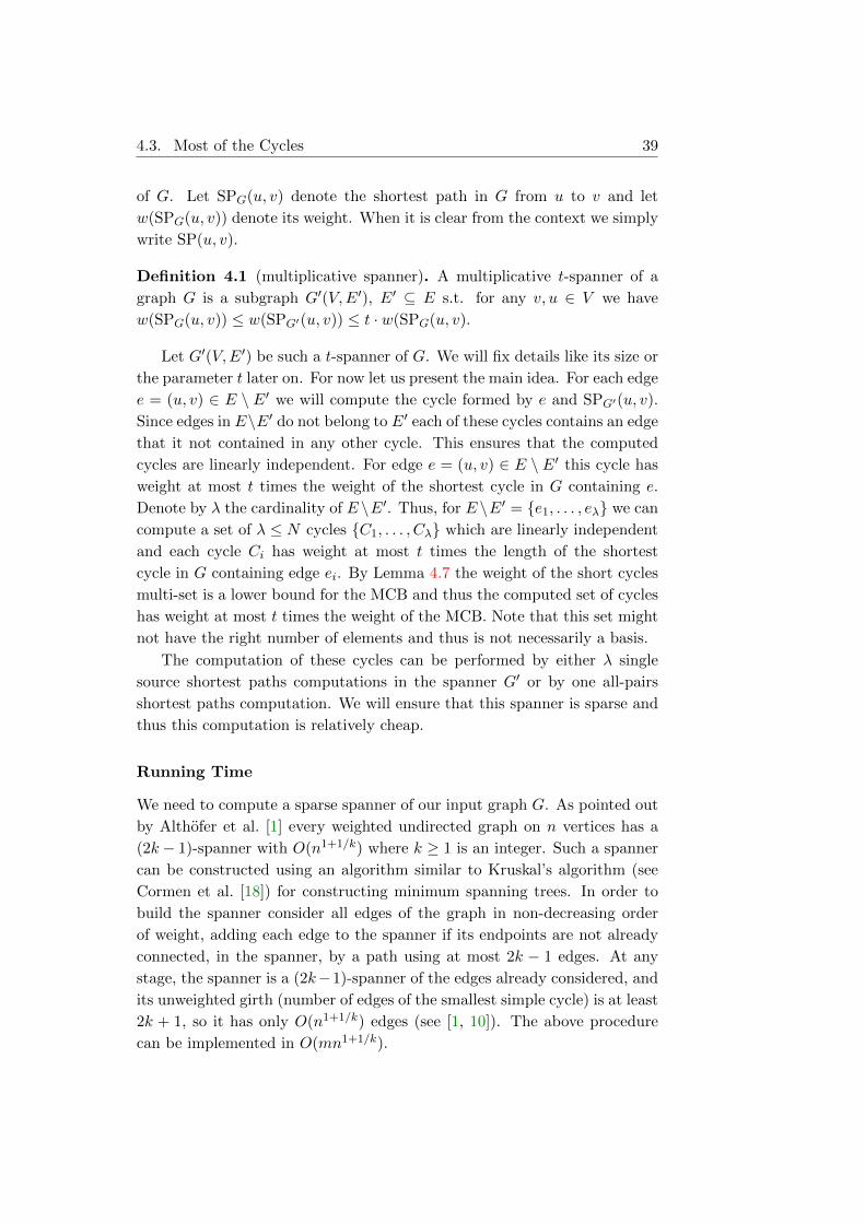
4.3. Most of the Cycles 39
of G. Let SPG(u, v) denote the shortest path in G from u to v and let
w(SPG(u, v)) denote its weight. When it is clear from the context we simply
write SP(u, v).
Definition 4.1 (multiplicative spanner). A multiplicative t-spanner of a
graph G is a subgraph G′(V,E′), E′ ⊆ E s.t. for any v, u ∈ V we have
w(SPG(u, v)) ≤ w(SPG′(u, v)) ≤ t · w(SPG(u, v).
Let G′(V,E′) be such a t-spanner of G. We will fix details like its size or
the parameter t later on. For now let us present the main idea. For each edge
e = (u, v) ∈ E \ E′ we will compute the cycle formed by e and SPG′(u, v).
Since edges in E\E′ do not belong to E′ each of these cycles contains an edge
that it not contained in any other cycle. This ensures that the computed
cycles are linearly independent. For edge e = (u, v) ∈ E \ E′ this cycle has
weight at most t times the weight of the shortest cycle in G containing e.
Denote by λ the cardinality of E \E′. Thus, for E \E′ = e1, . . . , eλ we can
compute a set of λ ≤ N cycles C1, . . . , Cλ which are linearly independent
and each cycle Ci has weight at most t times the length of the shortest
cycle in G containing edge ei. By Lemma 4.7 the weight of the short cycles
multi-set is a lower bound for the MCB and thus the computed set of cycles
has weight at most t times the weight of the MCB. Note that this set might
not have the right number of elements and thus is not necessarily a basis.
The computation of these cycles can be performed by either λ single
source shortest paths computations in the spanner G′ or by one all-pairs
shortest paths computation. We will ensure that this spanner is sparse and
thus this computation is relatively cheap.
Running Time
We need to compute a sparse spanner of our input graph G. As pointed out
by Althofer et al. [1] every weighted undirected graph on n vertices has a
(2k − 1)-spanner with O(n1+1/k) where k ≥ 1 is an integer. Such a spanner
can be constructed using an algorithm similar to Kruskal’s algorithm (see
Cormen et al. [18]) for constructing minimum spanning trees. In order to
build the spanner consider all edges of the graph in non-decreasing order
of weight, adding each edge to the spanner if its endpoints are not already
connected, in the spanner, by a path using at most 2k − 1 edges. At any
stage, the spanner is a (2k−1)-spanner of the edges already considered, and
its unweighted girth (number of edges of the smallest simple cycle) is at least
2k + 1, so it has only O(n1+1/k) edges (see [1, 10]). The above procedure
can be implemented in O(mn1+1/k).

40 Chapter 4. Approximate Minimum Cycle Basis
Algorithm 4.2: The first (2k − 1)-approximation algorithm.
input : Graph G(V,E) and integer k ≥ 1.output: A (2k − 1)-approximate MCB.
Construct a (2k − 1)-spanner G′ with O(n1+1/k) edges. Let e1, . . . , eλbe the edges of G \G′.For each 1 ≤ i ≤ λ construct Ci as ei = (ui, vi) and the shortest pathin G′ from ui to vi.
Find linearly independent Sλ+1, . . . , SN in the subspace orthogonal tocycles C1, . . . , Cλ.
Call Algorithm 3.3 as extend cb(C1, . . . , Cλ, Sλ+1, . . . , SN, N − λ)to compute (2k − 1)-approximate cycles Cλ+1, . . . , CN , i.e., the basisof the recursion uses (2k − 1)-approximate distance oracles.
Return C1, . . . , Cλ ∪ Cλ+1, . . . , CN.
In the above spanner we are going to perform λ shortest paths compu-
tations, one for each edge of G that is not in the spanner. Using Dijkstra’s
algorithm we need O(λ ·(n1+1/k+n log n)) and since λ ≤ m we can compute
both the spanner and the λ linearly independent cycles in time O(mn1+1/k).
At this point we should mention that there are faster algorithms to construct
similar spanners, see for example [78, 71]. Nevertheless, at this phase the
above solution is satisfactory since it is not the dominating factor of the
running time.
4.4 The Remaining Cycles
In Section 4.3 we computed most of the cycles of an approximate minimum
cycle basis. We are left with computing the remaining cycles. Note that
the number of the remaining cycles is exactly the dimension of the cycle
space of the spanner G′. By ensuring that the spanner G′ is sparse the
remaining cycles will be close to linear. We present three algorithms which
are based on two different approaches. Each of them is faster for different
graph densities. The main difference between the two approaches is whether
we are going to use the edges e1, . . . , eλ in the remaining cycles.
4.4.1 1st Approach
Our first approach computes the remaining cycles by performing approxi-
mate cycles computations in G.
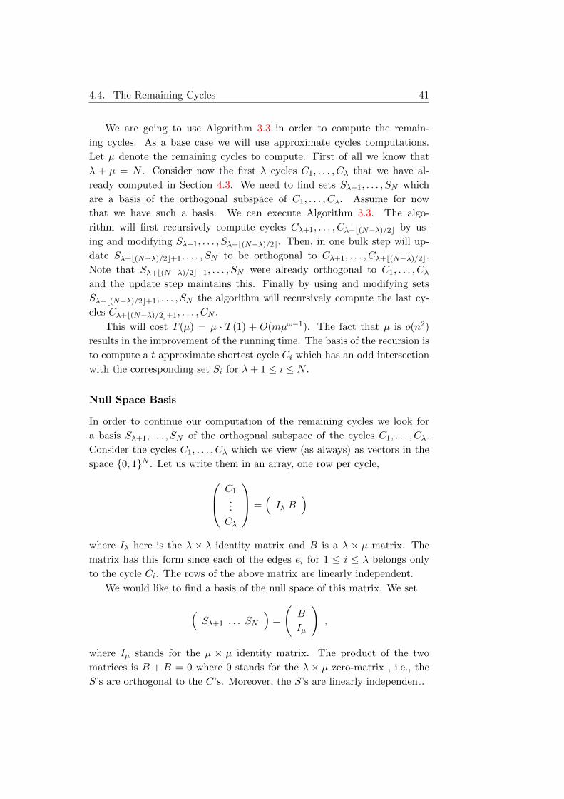
4.4. The Remaining Cycles 41
We are going to use Algorithm 3.3 in order to compute the remain-
ing cycles. As a base case we will use approximate cycles computations.
Let µ denote the remaining cycles to compute. First of all we know that
λ + µ = N . Consider now the first λ cycles C1, . . . , Cλ that we have al-
ready computed in Section 4.3. We need to find sets Sλ+1, . . . , SN which
are a basis of the orthogonal subspace of C1, . . . , Cλ. Assume for now
that we have such a basis. We can execute Algorithm 3.3. The algo-
rithm will first recursively compute cycles Cλ+1, . . . , Cλ+b(N−λ)/2c by us-
ing and modifying Sλ+1, . . . , Sλ+b(N−λ)/2c. Then, in one bulk step will up-
date Sλ+b(N−λ)/2c+1, . . . , SN to be orthogonal to Cλ+1, . . . , Cλ+b(N−λ)/2c.
Note that Sλ+b(N−λ)/2c+1, . . . , SN were already orthogonal to C1, . . . , Cλand the update step maintains this. Finally by using and modifying sets
Sλ+b(N−λ)/2c+1, . . . , SN the algorithm will recursively compute the last cy-
cles Cλ+b(N−λ)/2c+1, . . . , CN .
This will cost T (µ) = µ · T (1) + O(mµω−1). The fact that µ is o(n2)
results in the improvement of the running time. The basis of the recursion is
to compute a t-approximate shortest cycle Ci which has an odd intersection
with the corresponding set Si for λ+ 1 ≤ i ≤ N .
Null Space Basis
In order to continue our computation of the remaining cycles we look for
a basis Sλ+1, . . . , SN of the orthogonal subspace of the cycles C1, . . . , Cλ.
Consider the cycles C1, . . . , Cλ which we view (as always) as vectors in the
space 0, 1N . Let us write them in an array, one row per cycle, C1
...
Cλ
=(Iλ B
)
where Iλ here is the λ × λ identity matrix and B is a λ × µ matrix. The
matrix has this form since each of the edges ei for 1 ≤ i ≤ λ belongs only
to the cycle Ci. The rows of the above matrix are linearly independent.
We would like to find a basis of the null space of this matrix. We set
(Sλ+1 . . . SN
)=
(B
Iµ
),
where Iµ stands for the µ × µ identity matrix. The product of the two
matrices is B + B = 0 where 0 stands for the λ × µ zero-matrix , i.e., the
S’s are orthogonal to the C’s. Moreover, the S’s are linearly independent.

42 Chapter 4. Approximate Minimum Cycle Basis
By this definition, the Sλ+1, . . . , SN have the following property: they
contain some edges from e1, . . . , eλ and eλ+i ∈ Sλ+i for 1 ≤ i ≤ µ. This
property is important for the existence of the cycles with odd intersection
with the witnesses while running Algorithm 3.3.
The running time required to compute this null space basis is the time
required to output the already known matrix B. By using some sparse
representation of the vectors we need at most O(λ · µ). In the general case
λ ≤ m and µ = N−λ ∈ O(n1+1/k). Thus, this step needs O(mn1+1/k) time.
Remaining Cycles
The final step is to execute Algorithm 3.3 in order to compute the re-
maining cycles. The input to this algorithm is cycles C1, . . . , Cλ and sets
Sλ+1, . . . , SN . As mentioned earlier this requires time T (µ) = µ · T (1) +
O(mµω−1). Here T (1) is the time to perform t-approximate single source
shortest paths between at most n pairs of vertices in the signed graph Gi.
The shortest paths computation is going to be performed µ = N − λtimes. Therefore, we require a faster algorithm than constructing a spanner.
We are going to use an approximate distance oracle. Thorup and Zwick [78]
constructed a structure which answers (2k−1)-approximate shortest paths in
time O(k). This structure requires space O(kn1+1/k) and can be constructed
in expected time O(kmn1/k). In the case of unweighted graphs Baswana and
Sen [7] showed that a (2k−1)-approximate distance oracle can be computed
in expected O(min(n2, kmn1/k)) time. In the unweighted case the same can
also be done deterministically [70].
We use such a construction. The cost of computing cycles Cλ+1, . . . , CNin the last part is µ · T (1) + O(mµω−1). We bound T (1) by the cost of
computing an approximate distance oracle of Gi (the graph introduced in
Section 3.3) which is O(kmn1/k) expected time and the cost of performing
n queries in the approximate distance oracle. Each query costs O(k) and
thus a total of O(nk).
Note that although we perform n queries to this oracle we only need
to build one path. Given a query (u, v) the approximate distance oracle
of Thorup and Zwick finds a tree, constructed during preprocessing, which
contains both u and v and the path in this tree between u and v is a 2k− 1
stretch path. Thus, the returned path is simple and it has at most O(n)
edges. We can construct it explicitly in amortized constant time per edge or
by some preprocessing in constant time per edge. Thus, forming the actual
cycle can be done in O(n) time.
Therefore, the total cost is O(µ(kn + kmn1/k) + mµω−1). Since µ ∈

4.4. The Remaining Cycles 43
O(n1+1/k) we get a bound of O(kn2+1/k+kmn1+2/k+mn(1+1/k)(ω−1)) which
is O(kmn1+2/k +mn(1+1/k)(ω−1)) assuming that m ≥ n.
Approximation Guarantee
Let us now prove that the computed set of cycles is a t-approximation of
the MCB. Let Sλ+1, . . . , SN be the witnesses at the end of the algorithm.
At this point we should emphasize that the sets Sλ+1, . . . , SN change during
the execution of Algorithm 3.3. Each computed cycle Cλ+1, . . . , CN is a
t-approximation of the shortest cycle in G with an odd intersection with the
corresponding witness. Moreover, when the algorithm computes a cycle Cifor λ + 1 ≤ i ≤ N the set Si has acquired its final value and is orthogonal
with all cycles C1, . . . , Ci−1. Let also Si = ei for 1 ≤ i ≤ λ. Then, each
Ci for 1 ≤ i ≤ λ is also a t-approximation of the shortest cycle in G with an
odd intersection with Si.
Lemma 4.8. The sets S1, . . . , SN are linearly independent.
Proof. Consider Si. We know that 〈Ci, Si〉 = 1 for all 1 ≤ i ≤ N . We claim
that 〈Ci, Sj〉 = 0 for all i+ 1 ≤ j ≤ N . In this case each Si is independent
of the Si+1, . . . , SN and the lemma follows.
Assume a partition of the set Si+1, . . . , SN into two sets Si+1, . . . , Sλand Sλ+1, . . . , SN. The claim follows for the first set from the definition
of the sets Si+1, . . . , Sλ. For 1 ≤ i ≤ λ the cycle Ci contains edge ei and
a path in the spanner. The spanner has edges ej only for j > λ and sets
Si+1, . . . , Sλ by definition contain only edges from ei+1, . . . , eλ. For the
second set the claim follows by the invariants of Algorithm 3.3 since we
initialize Sλ+1, . . . , SN to be orthogonal to Ci and the update step maintains
this.
It is now straightforward to show that the computed set of cycles is a t-
approximation of a minimum cycle basis. Combine Lemma 4.8, Lemma 4.1
and the fact that for each 1 ≤ i ≤ N we compute a cycle Ci which t-
approximates the shortest cycle with an odd intersection with Si. We set
t = 2k − 1 and obtain the following theorem.
Theorem 4.9. A (2k−1)-approximate minimum cycle basis, for any integer
k ≥ 1, in an undirected weighted graph can be computed in expected time
O(kmn1+2/k +mn(1+1/k)(ω−1)).
We also obtain the following corollary.
Corollary 4.10. An O(log n)-approximate minimum cycle basis in an undi-
rected weighted graph can be computed in expected time O(mnω−1+mn log n).

44 Chapter 4. Approximate Minimum Cycle Basis
Algorithm 4.3: The second (2k − 1)-approximation algorithm.
input : Graph G(V,E) and integer k ≥ 1.output: A (2k − 1)-approximate MCB.
Construct a (2k − 1)-spanner G′ with O(n1+1/k) edges. Let e1, . . . , eλbe the edges of G \G′.For each 1 ≤ i ≤ λ construct Ci as ei = (ui, vi) and the shortest pathin G′ from ui to vi.
Call Algorithm 3.3 with exact shortest paths to find an MCBCλ+1, . . . , CN of G′.
Return C1, . . . , Cλ ∪ Cλ+1, . . . , CN.
4.4.2 2nd Approach
Our second algorithm just computes a minimum cycle basis of the t-spanner
G′. The dimension of the cycle space of G′ is µ = N−λ and thus we have the
right number of cycles. Let C1, . . . , Cλ be the cycles computed in Section 4.3
and Cλ+1, . . . , CN be the MCB of G′. Cycles C1, . . . , Cλ∪Cλ+1, . . . , CNare by definition linearly independent and we are also going to prove that
they form a t-approximation of the MCB of G.
For 1 ≤ i ≤ λ, let pi denote the shortest path in G′ between ui and viwhere ei = (ui, vi). Recall that for 1 ≤ i ≤ λ we have Ci = ei + pi. We
assume that the edges in E are indexed s.t. e1, . . . , eλ are the edges in E\E′,edges eλ+1, . . . , eN belong to E′ and edges eN+1, . . . , em are the edges of a
fixed but arbitrary spanning tree T of G′ and thus also of G.
In order to show that cycles C1, . . . , CN are a t-approximation of the
MCB we again define appropriate linearly independent vectors S1, . . . , SN ∈0, 1N and use Lemma 4.1. Consider Algorithm 3.3 executing with input
the t-spanner G′. Except from cycles Cλ+1, . . . , CN it returns also vectors
(edge sets in G′) Rλ+1, . . . , RN ∈ 0, 1N−λ s.t. for each λ + 1 ≤ i ≤ N
and i < j ≤ N we have 〈Ci, Rj〉 = 0 and moreover Ci is the shortest cycle
in G′ s.t. 〈Ci, Ri〉 = 1 for λ + 1 ≤ i ≤ N . Also, the N − λ × N − λ
matrix whose j-th row is Rj is lower triangular with 1 in its diagonal (see
Corollary 3.8). This implies that the Rj ’s are linearly independent. Given
any vector S ∈ 0, 1N let S† be the projection of S onto its last N − λcoordinates. In other words if S is an edge set of G let S† be the edge set
restricted only to the edges of G′.
We define vectors Sj ∈ 0, 1N for 1 ≤ j ≤ N as follows. For 1 ≤ j ≤ λ
let Sj be the vector with 0 everywhere except the j coordinate which is 1.

4.4. The Remaining Cycles 45
For λ+ 1 ≤ j ≤ N let
Sj = (−〈C†1, Rj〉, . . . ,−〈C†λ, Rj〉, Rj1, Rj2, . . . , Rj(N−λ)) .
Note that the above defined sets Sj for 1 ≤ j ≤ N are linearly independent.
This follows by construction since the N × N matrix whose j-th row is Sjis lower triangular with 1’s in its diagonal. The above definition of Sj ’s is
motivated by the property that for each 1 ≤ i ≤ λ, we have 〈Ci, Sj〉 =
−〈C†i , Rj〉+ 〈C†i , Rj〉 = 0, since the cycle Ci has 0 in all first λ coordinates
except the i-th coordinate which is 1.
We are now in the position to show the following which together with
Lemma 4.1 implies the correctness of our approach.
Lemma 4.11. Consider the above defined sets Sj for 1 ≤ j ≤ N and let
Dj be the shortest cycle in G s.t. 〈Dj , Sj〉 = 1. Cycle Cj returned by
Algorithm 4.3 has weight at most t times the weight of Dj.
Proof. This is trivial for 1 ≤ j ≤ λ since Dj is the shortest cycle in G which
uses edge ej and Cj = ej + pj . Consider now Dj for λ + 1 ≤ j ≤ N . If Dj
uses any edge ei for 1 ≤ i ≤ λ we replace it with the corresponding shortest
path in the spanner. This is as saying consider the cycle Dj +Ci instead of
Dj . Let
D′j = Dj +∑
1≤i≤λ(ei ∈ Dj)Ci
where (ei ∈ Dj) is 1 if ei ∈ Dj and 0 if ei /∈ Dj . Then,
〈D′j , Sj〉 = 〈Dj , Sj〉+∑
1≤i≤λ(ei ∈ Dj)〈Ci, Sj〉 .
But for 1 ≤ i ≤ λ the cycle Ci has 0 in all first λ coordinates except
the i-th one which is 1. Thus, by the definition of Sj we have 〈Ci, Sj〉 =
−〈C†i , Rj〉 + 〈C†i , Rj〉 = 0. We conclude that 〈D′j , Sj〉 = 〈Dj , Sj〉 = 1. But
D′j by definition has 0 in the first λ coordinates and S†j = Rj , which in turn
implies that 〈D′†j , Rj〉 = 1.
Cj is the shortest cycle in G′ s.t. 〈Cj , Rj〉 = 1. Thus, Cj has weight at
most the weight of D′†j (which is the same cycle as D′j) and by construction
D′j has weight at most t times the weight of Dj .
Altogether, we have shown that the cost of our approximate basis is at
most t times the cost of an optimal basis. As a t-spanner we again use a
(2k − 1)-spanner. The best time bound in order to compute an MCB is

46 Chapter 4. Approximate Minimum Cycle Basis
Algorithm 4.4: A (2k − 1)(2q − 1)-approximation algorithm.
input : Graph G(V,E) and integers k, q ≥ 1.output: A (2q − 1)(2k − 1)-approximate MCB.
Construct a (2k−1)-spanner G′ with O(kn1+1/k) edges. Let e1, . . . , eλbe the edges of G \G′.For each 1 ≤ i ≤ λ construct Ci as ei = (ui, vi) and a (2k − 1)-stretchpath from ui to vi obtained by the spanner G′.
Call Algorithm 4.2 to compute a (2q − 1)-approximate MCB of G′.Denote these cycles as Cλ+1, . . . , CN
Return C1, . . . , Cλ ∪ Cλ+1, . . . , CN.
O(m2n + mn2 log n) and since a (2k − 1)-spanner has at most O(n1+1/k)
edges the total running time becomes O(n3+2/k).
Theorem 4.12. A (2k−1)-approximate minimum cycle basis, for any inte-
ger k ≥ 1, in a weighted undirected graph can be computed in time O(n3+2/k).
Since any graph has an O(log n)-spanner of linear size we also obtain the
following corollary.
Corollary 4.13. An O(log n)-approximate MCB in a weighted undirected
graph can be computed in time O(n3 log n).
Algorithm 4.2 is faster for sparser graphs and Algorithm 4.3 for denser
graphs. More precisely, Algorithm 4.3 is faster if m > n4−ω+3−ωk which
with the current upper bound on ω is m > n1.624+0.624k . Both algorithms
are faster than O(mω), Algorithm 4.3 for m > n(3+2/k)/ω = n1.26+0.84k and
Algorithm 4.2 for m > max(n1+1/k,ω−1√kn1+2/k).
4.4.3 More Approximation
Consider now Algorithm 4.3. After computing the first λ cycles we use an
exact MCB algorithm to compute the MCB of the t-spanner G′. We can
instead use our approximate Algorithm 4.2 which is fast for sparse graphs.
We begin by computing a (2k−1)-spanner G′ of G and the first λ cycles.
Then, we call Algorithm 4.2 to compute a (2q−1)-approximate MCB of G′.
The result will be a (2k − 1)(2q − 1)-approximate MCB of G. This follows
by the fact that our first λ cycles combined with the MCB of G′ form a
(2k − 1)-approximate MCB.
Note that in this case it is not sufficient to use the O(mn1+1/k) approach
of Althofer et al. [1] in order to compute the initial (2k − 1)-spanner G′.

4.5. Planar and Euclidean Graphs 47
Thorup and Zwick [78] have shown how to construct a (2k − 1)-spanner
G′ with size O(kn1+1/k) in expected time O(kmn1/k). Such a spanner is
a collection of shortest path trees T (w) for w ∈ V and given two vertices
u, v ∈ V there is a tree in this collection that contains a path between u and
v that is of stretch at most 2k− 1. Furthermore, the corresponding tree can
be obtained in O(k) time. We can also preprocess these trees in order to be
able to output the path in amortized or worst case constant time per edge.
Consider running Algorithm 4.2 in the subgraph G′. The algorithm
will first compute a (2q − 1)-spanner G′′ of the (2k − 1)-spanner G′ and
some of the cycles. Then, it will compute the remaining cycles by do-
ing (2q − 1)-approximate shortest cycles computations in G′. We there-
fore get an algorithm with expected running time O(qk · n1+1/kn1+2/q +
kn1+1/kn(1+1/q)(ω−1)). Note that this upper bound does not include the
time to output the initial cycles using the (2k − 1)-spanner.
Theorem 4.14. A (2k − 1)(2q − 1)-approximate MCB of an undirected
graph with non-negative edge weights, for any two integers k, q ≥ 1, can be
computed in expected time O(qk ·n2+1/k+1/q · (n1/q +n(1+1/q)(ω−2))) plus the
time to output the MCB.
Corollary 4.15. An O(log2 n) approximate MCB of an undirected weighted
graph can be computed in expected time O(nω) plus the time to output the
MCB.
4.5 Planar and Euclidean Graphs
Some types of graphs are much easier to handle than others w.r.t the mini-
mum cycle basis. Consider a planar graph G. In linear time we can find an
embedding of G in the plane. Then, the approximate cycle basis algorithm
just returns the set of bounded faces of G. It is easy to see that all these
cycles are linearly independent and due to Euler’s formula they are also the
right number, N = m− n+ 1 = f − 1, where f is the number of faces of G.
For the approximation factor let E∗ ⊆ E be the set of edges of G which
belong to at least one cycle. Since each edge is incident with at most two
faces, this cycle basis has weight at most
2 ·∑e∈E∗
w(e) ≤ 2 · w(MCB) ,
since a minimum cycle basis has to use each edge that belongs to at least
one cycle.

48 Chapter 4. Approximate Minimum Cycle Basis
The embedding can be found in linear time [50]. The bounded faces can
also be enumerated in linear time and the size of the output is also linear.
Theorem 4.16. A 2-approximate minimum cycle basis of a planar graph
can be computed in linear time using linear space.
Let P be a set of points in the Euclidean plane. The Euclidean graph
G(P ) on P has vertices corresponding to points in P . The graph is complete
and the weight of an edge is the Euclidean distance between the points
corresponding to the vertices. In order to find an approximate MCB of
G(P ) we use the result that the Delaunay triangulation of the points P is
a ≈ 2.42 [59] spanner of G(P ). Let DT denote the Delaunay triangulation
of P . DT is a planar graph. The approximate MCB algorithm returns the
following set of cycles: (a) For each edge e = (u, v) ∈ G(P ) \ DT the cycle
Ce formed by edge e and the shortest path in DT from u to v, and (b) a
minimum cycle basis of DT.
Theorem 4.17. A 2.42 approximation of the MCB in a complete Euclidean
graph in the plane can be constructed in O(n3) time.
Proof. The proof of the approximation ratio follows exactly the proof in
Section 4.4.2. For the running time we note that computing the Delaunay
triangulation requires O(n log n) time. The shortest paths computations on
the planar spanner require O(λn) which is O(n3). Computing an MCB of
a planar graph can be done in O(n2 log n) by the algorithm of Hartvigsen
and Mardon [48].
In the case we want to handle higher (but fixed) dimensions we can
use the fact that the well-separated pair decomposition [13] (s-WSPD) for
separation factor s = 4(t+ 1)/(t− 1) is a t-spanner of G(P ) for t > 1. The
algorithm begins by computing an s-WSPD decomposition. The time to
compute an s-WSPD is O(n log n+sdn) where d is the dimension. Since the
size of the WSPD is O(sdn) we know that λ ≤ m and µ = N − λ ∈ O(sdn).
Thus, the time to compute the first λ cycles is O(m(sdn+ n log n)).
For the remaining cycles we use the approach in Algorithm 4.3. Comput-
ing exactly the MCB of the spanner we get a running time of O(sdn3 log n).
Theorem 4.18. A t-approximate MCB for t > 1 of a complete Euclidean
graph can be computed in time O(sdn3 log n) where s = 4(t+ 1)/(t− 1) and
d the fixed dimension.

4.6. Directed Graphs 49
4.6 Directed Graphs
Our techniques can also be applied to the minimum cycle basis problem in
directed graphs. A cycle in a directed graph is a cycle in the underlying
undirected graph with edges traversed in both directions. A −1, 0, 1 edge
incidence vector is associated with each cycle: edges traversed by the cycle
in the right direction get 1 and edges traversed in the opposite direction get
−1. The main difference here is that the cycle space is generated over Q by
the cycle vectors. Note that the weight of a cycle is simply the sum of the
weight of its edges independent of the orientation of these edges.
The algorithms for finding an MCB in directed graphs are based on the
techniques used in [20] and the ones developed in this thesis. Several extra
ideas are required in order to compensate for the extra cost of arithmetic
that arises when changing the base field from F2 to Q. Lemma 4.1 can
be generalized, see for example [56]. Algorithm 4.3 can also be directly
generalized. For the spanner computation we view our directed graph G
as undirected and we compute a (2k − 1)-spanner G′. We then give to the
edges of G′ the orientation that they have in G.
As in Section 4.4.2 we return two sets of cycles. The first set is con-
structed as follows. For each edge ei ∈ E \E′ for 1 ≤ i ≤ λ we compute the
cycle ei + pi where pi is the shortest path in G′ between the endpoints of
ei when G′ is viewed as an undirected graph. Then, we traverse each such
cycle in an arbitrary orientation and form our directed cycles based on the
direction of the edges in G. The second set is simply the set of cycles of a
directed MCB of G′. The proof of correctness of this approach is similar to
the one presented in Section 4.4.2 if we replace the base field with Q.
The time to compute our spanner is again O(mn1+1/k). The fastest
deterministic algorithm [45] to compute an MCB of a directed graph has
a running time of O(m2Nω−1 + N3) + O(N(m2n + mn2 log n)). We exe-
cute this algorithm on our spanner and G′ has at most O(n1+1/k) edges.
Thus, N ≤ m ∈ O(n1+1/k) and the running time becomes O(mn1+1/k) +
O(n(1+1/k)(ω+1)) +O(n4+3/k). For k ≥ 1 this is O(n4+3/k).
Theorem 4.19. A (2k−1)-approximate minimum cycle basis, for any inte-
ger k ≥ 1, in a weighted directed graph can be computed in time O(n4+3/k).
If we allow the use of randomization then we can compute approximate
directed MCB even faster. The Monte Carlo algorithm in [55] computes an
MCB of a directed graph with positive weights in time O(m2n log n) with
high probability. Using this algorithm we get the following theorem.

50 Chapter 4. Approximate Minimum Cycle Basis
Theorem 4.20. A (2k−1)-approximate minimum cycle basis, for any inte-
ger k ≥ 1, in a positively weighted directed graph can be computed with high
probability in time O(n3+2/k log n).
4.7 Concluding Remarks
In this chapter we have obtained fast algorithms which compute approximate
minimum cycle bases of graphs. We presented an α-approximate algorithm
for any α > 1 and several constant factor approximate algorithms. These al-
gorithms are considerably faster than any current approach which computes
exactly a minimum cycle basis.
The minimum cycle basis problem is used mostly as preprocessing and
usually any sparse cycle basis suffices. Thus, our constant factor algorithms
have high practical value. Moreover, one of our algorithms even when im-
plemented without fast matrix multiplication runs in time O(n3+3/k). We
elaborate on this further in Section 5.7.
For sufficiently dense graphs our algorithms are o(mω). Furthermore, we
developed fast approximation algorithms for special classes of graphs. Our
techniques extend to the directed minimum cycle basis problem.

Chapter 5Minimum Cycle Basis Algorithms
in Practice
Summary
In this chapter we consider the practical problem of computing a minimum cyclebasis of an undirected graph G = (V,E) with n vertices and m edges. We describean efficient implementation of an O(m3 +mn2 logn) algorithm presented in [20].For sparse graphs this is the currently fastest known algorithm. This algorithm’srunning time can be partitioned into two parts with time O(m3) and O(m2n +mn2 logn) respectively. Our experimental findings imply that in random graphsthe true bottleneck of a sophisticated implementation is the O(m2n+mn2 logn)part. A straightforward implementation would require N ·n single source shortestpaths computations, thus we develop several heuristics in order to get a practicalalgorithm. Our experiments show that in random graphs our techniques result ina significant speedup.
Based on our experimental observations we combine the two fundamentallydifferent approaches, which have been used so far to compute a minimum cyclebasis, to obtain a new hybrid algorithm with running time O(m2n2). The hybridalgorithm is very efficient in practice for random dense unweighted graphs.
We also compare these two algorithms with a number of previous implemen-tations for finding a minimum cycle basis of an undirected graph. Finally, wediscuss the performance of our approximation algorithms in practice.
5.1 Introduction
In this chapter we consider the practical problem of computing a minimum
cycle basis of an undirected graph G = (V,E) with n vertices and m edges.
We describe an efficient implementation of Algorithm 3.1, using LEDA [67].
For sparse graphs this is the currently fastest known algorithm. As dis-
cussed in Chapter 3, this algorithm’s running time can be partitioned into
two parts with time O(m3) and O(m2n + mn2 log n) respectively. Our ex-

52 Chapter 5. Minimum Cycle Basis Algorithms in Practice
perimental findings imply that in random graphs the true bottleneck of a
sophisticated implementation is the O(m2n + mn2 log n) part. A straight-
forward implementation would require N · n single source shortest paths
computations, thus we develop several heuristics in order to get a practical
algorithm. Our experiments show that in random graphs our techniques
result in a significant speedup.
Based on these experimental observations, we combine the two funda-
mentally different approaches to compute a minimum cycle basis, to obtain
a new hybrid algorithm with running time O(m2n2). This new hybrid algo-
rithm is very efficient in practice for random dense unweighted graphs.
We also compare these two algorithms with a number of previous im-
plementations [53, 19] for finding a minimum cycle basis of an undirected
graph. These implementations were developed in order to analyze complex
electrical networks, more precisely to compute a sparse cycle basis to de-
scribe the ‘voltage law’ part of a system. Both contain algorithms which
compute optimal or sub-optimal cycle bases. For our comparisons we used
only the implementations which compute optimal cycle bases.
Finally, we discuss our approximation algorithms and their applicability
in practice.
5.1.1 Experimental Setup
This chapter contains some experimental results and comparisons. All ex-
periments are done using random sparse and dense graphs.
Random Graphs
The G(n; p) model is due to Erdos and Renyi [29]. Let G(n) be the set of all
undirected graphs (without self-loops) on n vertices and define M :=(n2
);
M is the number of edges in a complete graph on n vertices. G(n) has
precisely 2M elements. In the G(n; p) model each of the M potential edges
is present with probability p, independently of the other edges. That is, the
sample space of G(n; p) is the entire set G(n), and the probability of a graph
G ∈ G(n) with m edges is pm(1 − p)M−m. If p = 12 all graphs in G(n) are
equiprobable.
All graphs, which we use in our experiments, were constructed using the
G(n; p) model for p = 4/n, 0.3, and 0.5.

5.2. Heuristics 53
Platform†
Our implementation uses LEDA [67]. All experiments were performed on
a Pentium M 1.7GHz machine with 1GB of memory and 1MB L2 cache,
running GNU/Linux. We used the GNU g++ 3.3 compiler with the -O
optimization flag. All other implementations considered use the boost C++
libraries [12].
5.2 Heuristics
In this section we present several heuristics which can improve the running
time substantially. All heuristics preserve the worst-case time and space
bounds.
5.2.1 Compressed and/or Sparse Representation (H1)
All vectors (sets S and cycles C) which are handled by the algorithm are
in 0, 1m or 0, 1N . Moreover, any operations performed are normal set
operations. This allows us to use a compressed representation where each
entry of these vectors is represented by a bit of an integer. This allows us to
save up space and at the same time to perform 32 or 64 bitwise operations
in parallel.
Except from a compressed representation we can also use a sparse rep-
resentation. Every cycle C or set S is simply a collection of edges. Thus, we
can represent such sets by a sorted list of integers. Each integer uniquely
represents an edge. The only operation required is performing symmetric
difference and this can be done in time proportional to the sizes of the
vectors involved.
Which of the two above representations to use, seems to be relevant to
the particular instances of the problem that we need to solve. For example if
we know that the minimum cycle basis contains only cycles of small length,
then a sparse representation seems more relevant. We believe that when
solving small instances a compressed representation should be preferable
but on larger instances a sparse one would provide better performance and
less space consumption.
†The various implementations in this chapter use different graph libraries, eitherLEDA [67] or boost [12]. This could be the reason, for some additional constant fac-tor performance differences between the algorithms.

54 Chapter 5. Minimum Cycle Basis Algorithms in Practice
5.2.2 Upper Bounding the Shortest Path (H2)
During phase i we might perform up to n shortest paths computations in
order to compute the shortest cycle Ci with an odd intersection with the set
Si. We can thus use the shortest path found so far as an upper bound on
the shortest path. This is implemented as follows; a node is only added in
the priority queue of Dijkstra’s implementation if its current distance is not
more than our current upper bound.
5.2.3 Reducing the Shortest Path Computations (H3)
We come to the most important heuristic. In each of the N phases we are
performing single source shortest paths computations between at most n
pairs of vertices or one all pairs shortest paths computation. In the general
case this can be accomplished by n single source shortest paths computa-
tions. This results in total to N ·n single source shortest paths computations.
Let S = e1, e2, . . . , ek be a witness at some point of the execution.
We need to compute the shortest cycle C such that 〈C, S〉 = 1. We can
reduce the number of shortest paths computations based on the following
observation. Let C≥i be the shortest cycle in G such that:
(i) 〈C≥i, S〉 = 1 ,
(ii) C≥i ∩ e1, . . . , ei−1 = ∅ , and
(iii) ei ∈ C≥i .
Then, cycle C can be expressed as
C = mini=1,...,k
C≥i . (5.1)
Note that at least one of the C≥i for 1 ≤ i ≤ k exists, since we make sure
that there is always at least one cycle with an odd intersection with S.
We can compute C≥i in the following way. We delete edges e1, . . . , eifrom the graph G and the corresponding edges from the signed graph Gi.
Let ei = (v, u) ∈ G. Then, we compute a shortest path in Gi from v+ to
u+. The path computed will have an even number of edges from the set S
and together with ei an odd number. Since we deleted edges e1, . . . , ei the
resulting cycle does not contain any edges from e1, . . . , ei−1.Using the above observation we can compute each cycle in O(k·SP(n,m))
time when |S| = k < n and in O(n · SP(n,m)) when |S| ≥ n. Thus, the

5.3. Updating the Witnesses, Si’s 55
running time for the cycles computations is equal to
SP(n,m) ·N∑i=1
minn, |Si| (5.2)
where SP(n,m) denotes the time to compute single source shortest paths in
an undirected non-negative weighted graph with n vertices and m edges.
5.2.4 Basis Reordering (H4)
The main invariant of all algorithms based on the algebraic framework (Al-
gorithm 3.2) which was presented in Section 3.2, is that for 1 ≤ i ≤ N , Simust be a vector in the subspace orthogonal to the cycles C1, . . . , Ci−1.Several vectors in this subspace suffice for the correctness of the MCB algo-
rithm.
In Algorithm 3.1 at the beginning of phase 1 ≤ i ≤ N we have a set of
vectors Si, . . . , SN which form a basis of the subspace orthogonal to the
cycles C1, . . . , Ci−1. Heuristic H3 implies that computing cycle Ci can be
performed with a different number of shortest paths computations, based
on the sparseness of the vector from the orthogonal subspace that is chosen.
The basis reordering heuristic swaps Si with Sj such that i ≤ j ≤ N and
|Sj | is minimized.
The goal of this heuristic is to make a significant progress at the begin-
ning of the algorithm. As the computation reaches its final stages, most of
the orthogonal basis vectors will be relative dense and thus the heuristic will
not have a big effect. Moreover, the dimension of the subspace orthogonal
to C1, . . . , Ci−1 decreases during the algorithm. Thus, at the final stages we
do not have a wide choice on which basis vector to choose. At early stages
however, only a few shortest paths computations will be necessary in order
to compute each MCB cycle.
This heuristic is less applicable to Algorithm 3.3 since in each phase
we have much fewer Si’s in the subspace orthogonal to the set of cycles
C1, . . . , Ci−1 that in Algorithm 3.1.
5.3 Updating the Witnesses, Si’s
In this section we present experimental results which suggest that the dom-
inating factor of the running time of Algorithm 3.1 (at least for random
graphs) is not the time needed to update the witnesses but the time to
compute the cycles.

56 Chapter 5. Minimum Cycle Basis Algorithms in Practice
sparse (m ≈ 2n)
n S’s C’s
77 0.01 0.02154 0.0100013 0.250001303 0.0300028 0.770003541 0.0500085 4.35001795 0.230037 13.41060 0.519957 28.85991412 1.07985 59.27982070 2.97977 267.092505 4.46042 377.2813336 9.84878 795.548
G(n; 0.3) G(n; 0.5)
n S’s C’s S’s C’s
50 0.0100001 0.33 0.100001 0.6670 0.0900026 1.44 0.339982 2.92998100 0.529994 5.75 1.75995 15.0799150 3.55005 37.6801 9.66977 114.75200 12.5297 145.8 35.8403 421.82250 34.578 508.309 99.888 1556.64
Table 5.1: Comparison of the time (in seconds) taken to update thesets Si, 1 ≤ i ≤ N and the time taken to calculate the cycles Ci,1 ≤ i ≤ N in random weighted graphs, by Algorithm 3.1.
Recall that the time to update the witnesses is O(m3) and the time to
compute the cycles is O(m2n + mn2 log n). Thus, on sparse graphs Algo-
rithm 3.1 has the same running time O(n3 log n) as Algorithm 3.3. Algo-
rithm 3.3 has a running time of O(m2n+mn2 log n+mω); the mω factor is
dominated by the m2n but we present it here in order to understand what
type of operations the algorithm performs. Recall that Algorithm 3.3 im-
proves upon Algorithm 3.1 with respect to the time needed to update the
sets S by using fast matrix multiplication.
Although fast matrix multiplication can be practical for medium and
large sized matrices, our experiments show that in random graphs the time
needed to update the Si’s is a small fraction of the time needed to compute
the cycles. Table 5.1 presents a comparison of the required time to update
the Si’s and to calculate the cycles Ci’s by using the signed graph Gi for
random weighted graphs.
In order to get a better understanding of this fact, we performed several
experiments. As it turns out, in practice, the average cardinality of the Si’s
is much less than N and moreover the number of times we actually perform
set updates (if 〈Ci, Sj〉 = 1) is much less than N(N − 1)/2. Moreover,
heuristic H1 helps to further decrease the time required to perform these
updates. Table 5.2 summarizes our results.
5.4 Number of Shortest Path Computations
Heuristic H3 dramatically improves the best case of the Algorithm 3.1, while
maintaining at the same time the worst case. Instead of N · n single source
shortest paths computations, we perform much less. In Table 5.4 we study

5.4. Number of Shortest Path Computations 57
n m N N(N − 1)/2 max(|S|) davg(|S|)e # 〈S,C〉 = 1
sparse (m ≈ 2n)
10 19 10 45 4 2 851 102 52 1326 25 3 113104 208 108 5778 44 4 258206 412 212 22366 108 5 760491 981 500 124750 226 7 2604596 1192 609 185136 315 6 2813963 1925 985 484620 425 7 54691060 2120 1084 586986 498 7 59801554 3107 1581 1248990 537 8 95402070 4139 2105 2214460 1051 13 206453032 6064 3092 4778686 1500 13 313564441 8882 4525 10235550 2218 17 58186
G(n; 0.3)
10 13 4 6 2 2 225 90 66 2145 27 3 13750 367 318 50403 133 5 113675 832 758 286903 370 6 3707100 1485 1386 959805 613 7 8103150 3352 3203 5128003 1535 9 22239200 5970 5771 16649335 2849 10 49066300 13455 13156 86533590 6398 10 116084500 37425 36926 681746275 18688 14 455620
G(n; 0.5)
10 22 13 78 7 2 1425 150 126 7875 57 4 36350 612 563 158203 298 6 252775 1387 1313 861328 654 6 6282100 2475 2376 2821500 1168 8 15771150 5587 5438 14783203 2729 9 39292200 9950 9751 47536125 4769 11 86386300 22425 22126 244768875 10992 13 227548500 62375 61876 1914288750 30983 15 837864
Table 5.2: Statistics about sets S sizes on sparse random graphs withp = 4/n and dense random graphs for p = 0.3 and 0.5. Sets are consid-ered during the whole execution of Algorithm 3.1. Column #〈S,C〉 = 1denotes the number of updates performed on the Si’s. An upper boundon this is N(N − 1)/2, which we actually use when bounding the algo-rithm’s running time. Note that the average cardinality of the Si’s isvery small compared to N although the maximum cardinality of someSi’s is in O(N).

58 Chapter 5. Minimum Cycle Basis Algorithms in Practice
G(n; 0.3)
n H3 Heur. NO Heur.
35 0.06 0.4750 0.32 2.3960 0.85 6.1180 2.41 23.2100 6.55 68.34120 14.82 169.41150 41.6 604.07
G(n; 0.5)
n H3 Heur. NO Heur.
25 0.06 0.2540 0.31 2.0850 0.82 6.3860 1.95 14.7875 4.7 42.685 7.41 78.28100 17.77 210.69120 39.78 521.93150 122.2 1954.24
sparse (m ≈ 2n)
n H3 Heur. NO Heur.
51 0.01 0.19104 0.07 1.48206 0.52 11.85491 3.3 154.31656 7.61003 392.29
Table 5.3: Running times in seconds of Algorithm 3.1 with and with-out the H3 heuristic on random graphs. Without the heuristic thealgorithm performs Θ(nm) single source shortest paths computations.
the sizes of the sets Si (Si,i in the terminology of Algorithm 3.1) for i =
1, . . . , N used to calculate the cycles for sparse and dense graphs respectively.
The main observation here is that in both sparse and dense graphs al-
though the maximum set can have quite large cardinality (something like
O(N)) the average set size is much less than n. Moreover, in sparse graphs
every set used has cardinality less than n. On dense graphs the sets with
cardinality less than n are more than 95% percent. Thus, heuristic H3 is
almost always in effect which in turn implies a significant speedup. Ta-
ble 5.3 compares the running times of Algorithm 3.1 with and without the
H3 heuristic.
The heuristic for reducing the number of shortest paths computation has
a dramatic effect on the performance of Algorithm 3.1. Nevertheless, the
observation that for random graphs the shortest paths are the dominating
factor of the algorithm remains valid. This fact is motivating enough, in
order to try to design an algorithm which performs fewer shortest paths
computations.

5.5. Combining the Two Approaches 59
n m N max(|Si|) davg(|Si|)e |Si : |Si| < n|sparse (m ≈ 2n)
10 19 10 4 2 1051 102 52 16 5 52104 208 108 39 5 108206 412 212 106 10 212491 981 498 246 13 498596 1192 609 220 11 609963 1925 980 414 11 9801060 2120 1076 496 17 10761554 3107 1573 795 21 15732070 4139 2108 1036 27 21083032 6064 3092 1468 33 30924441 8882 4522 1781 33 4522
G(n; 0.3)
10 13 4 2 2 425 90 66 20 4 6650 367 318 153 10 30275 832 758 357 15 721100 1485 1386 638 15 1343150 3352 3203 1534 18 3133200 5970 5771 2822 29 5635300 13455 13156 6607 32 12968500 37425 36926 15965 39 36580
G(n; 0.5)
10 22 13 7 3 1325 150 126 66 5 12150 612 563 222 12 53275 1387 1313 456 10 1276100 2475 2376 1094 15 2314150 5587 5438 2454 19 5338200 9950 9751 4828 28 9601300 22425 22126 10803 33 21875500 62375 61876 30877 38 61483
Table 5.4: Statistics about sets Si sizes on sparse random graphs withp = 4/n and dense random graphs for p = 0.3 and 0.5, at the mo-ment we calculate cycle Ci with Algorithm 3.1. Compare the averagecardinality of Si with n.
5.5 Combining the Two Approaches
In this section we develop a new algorithm for the minimum cycle basis
problem with running time O(m2n2). The algorithm is a combination of the
two main approaches that have been used to compute a minimum cycle basis.
Its main motivation is to reduce the number of shortest paths computations.
We begin by describing Horton’s algorithm [52] in more detail.

60 Chapter 5. Minimum Cycle Basis Algorithms in Practice
5.5.1 Horton’s Algorithm
Unlike the algorithms that we have seen so far, Horton’s algorithm does not
compute the cycles one by one but instead computes a superset of the MCB
and then greedily extracts the MCB by Gaussian elimination. This superset
contains O(mn) cycles which are constructed in the following way.
For each vertex w ∈ V and edge e = (u, v) ∈ E construct the candidate
cycle C = SP(w, u) + SP(w, v) + (u, v) where SP(a, b) is the shortest path
from a to b (see Figure 5.1). If these two shortest paths do not contain a
vertex other than w in common then keep the cycle otherwise discard it.
Let us call this set of cycles the Horton set and denote it with HS. We next
show that HS always contains an MCB.
For simplicity we will make the following assumption. We refer the
interested reader to [52] for the treatment of the more general case.
Assumption 5.1. All shortest paths in graph G are unique.
The proof consists of a series of simple lemmata.
Theorem 5.1 (Horton [52]). Let u and v be two vertices in G, and let B be
a cycle basis of G. Let P denote a path from u to v. Any cycle C ∈ B that
contains u and v can be exchanged for either a cycle that includes the path
P , or a cycle that excludes one of u and v.
Proof. Let P1 and P2 be the two paths in C joining u and v. Assume
P 6= P1 and P 6= P2, for otherwise C does not need to be exchanged. Define
C1 = P+P1 and C2 = P+P2. Then, C1 and C2 are cycles and C = C1+C2.
By Theorem 2.3, C can be exchanged for either C1 or C2. If the exchanged
cycle Ci is not a simple cycle, then Ci can be exchanged for one of its simple
cycles and that simple cycle cannot include both u and v.
Corollary 5.2 (Horton [52]). If B is a minimum cycle basis and P is the
unique shortest path from x to y, then every cycle in B that contains x and
y must contain the path P .
Proof. In the proof of Theorem 5.1, w(Ci) ≤ w(P ) + w(Pi) < w(P1) +
w(P2) = w(C). Hence, if C does not contain P , it can be exchanged for a
shorter cycle, a contradiction to the fact that B is a minimum cycle basis.
Theorem 5.3 (Horton [52]). Let w be any vertex of any cycle C in a mini-
mum cycle basis of G. Then, there is an edge (v, u) ∈ C such that C consists
of a shortest path from w to v, a shortest path from w to u, and the edge
(v, u).

5.5. Combining the Two Approaches 61
w
u
v
e = (v, u)
SP(w, v)
SP(w, u)
Figure 5.1: Candidate cycle for the MCB.
Proof. Let C = (w0, w1, . . . , wn−1, wn), where w = w0 = wn. Define
Pi = (w,w1, w2, . . . , wi) and Qi = (w,wn−1, . . . , wi). By Corollary 5.2
and Assumption 5.1, d(w,wi) = w(Pi) or w(Qi). Let v = wi, where i is
the largest subscript such that d(w,wi) = w(Pi). Let u = wi+1. Then,
C = Pi + (wi, wi+1) +Qi+1.
However, not every MCB is contained in the Horton set. If we assume
uniqueness of the MCB then it is immediately clear that the only MCB is
contained in this set. Horton actually proved that if all edges have positive
weights then it does not matter which shortest path is chosen between each
pair of vertices.
Extracting an MCB from the Horton set is straightforward by using
Gaussian elimination and the greedy algorithm. We first sort the cycles
by length. The i-th cycle of the Horton set is in the MCB if it is linearly
independent from the cycles which we have already selected among the first
i−1 cycles of the Horton set. We continue this process until we have selected
N such cycles. Note that this greedy step is really necessary.
5.5.2 A Hybrid Algorithm
The two approaches that we have seen so far for computing an MCB can be
combined, and this is the purpose of this section. Both Algorithm 3.1 and
Algorithm 3.3 requireO(mn(m+n log n)) time for the shortest paths queries.
Our experimental observation was (recall Table 5.1) that for random graphs
this is the dominating factor. Thus, it seems only natural to try to reduce
this factor.
The main idea here is to exchange the shortest paths computations per-
formed by Algorithm 3.1 and Algorithm 3.3 by the computation of HS. The
resulting algorithm has again N phases, one for each cycle of the MCB.
During these phases we maintain the invariant that in phase i, Si is a vector

62 Chapter 5. Minimum Cycle Basis Algorithms in Practice
Algorithm 5.1: Hybrid MCB algorithm
Ensure uniqueness of the shortest path distances of G (lexicographi-cally or by perturbation)Construct superset (Horton set) HS of MCBLet Si = ei for all i = 1, . . . , Nfor i = 1 to N do
Find Ci as the shortest cycle in HS s.t 〈Ci, Si〉 = 1for j = i+ 1 to N do
if 〈Ci, Sj〉 = 1 thenSj = Sj + Si
end
end
end
in the subspace orthogonal to the cycles C1, . . . , Ci−1. To compute the cycle
Ci in phase i, we search for the shortest cycle C ∈ HS such that 〈C, Si〉 = 1.
The Horton set contains an MCB but not necessarily all the cycles that
belong to any MCB. We resolve this difficulty by ensuring uniqueness of the
MCB. We ensure uniqueness by ensuring uniqueness of the shortest path
distances on the graph (either by perturbation or by lexicographic ordering).
After the preprocessing step, every cycle of the MCB will be contained in the
Horton set. This proves the correctness of the new algorithm. A succinct
description can be found in Algorithm 5.1.
Running Time
Theorem 5.4. Algorithm 5.1 solves the minimum cycle basis problem in
time O(m2n2).
Proof. The time to compute the cycles is only O(n2m). To see this note
that it is enough to build one shortest path tree for each node v ∈ V . This
takes time O(n(m+n log n)). Then, we can construct the O(mn) candidate
cycles in O(n2m) since each cycle might contain at most O(n) edges.
Querying the Horton set takes time O(m2n2) since the Horton set con-
tains at most mn cycles, we need to search for at most m cycles and each
cycle contains at most n edges.
The space requirement is O(mn2), a factor of n more than O(mn) which
is the space required to represent the cycles of the MCB. The important
property of this algorithm is that the time to actually compute the cycles is
only O(n2m). This is a factor of mn better than the O(m2n) time required by

5.6. Running Times Comparison 63
Algorithm 3.1 or Algorithm 3.3. Together with the experimental observation
that in general the linear independence step is not the bottleneck, we actually
hope to have developed an efficient algorithm.
5.6 Running Times Comparison
In this section we compare various implementations for computing a mini-
mum cycle basis. We include in our comparison the following algorithms:
(i) our implementation [65] of Algorithm 3.1 denoted as DP or DP U in the
case of unweighted graphs,
(ii) our implementation of Algorithm 5.1 denoted as HYB or HYB U in the
case of unweighted graphs,
(iii) an implementation [19] of Horton’s algorithm denoted as HOR in case
of weighted and as HOR U1 in case of unweighted graphs,
(iv) another implementation [53] of Horton’s algorithm, for unweighted
graphs, denoted as HOR U2, and
(v) an implementation [19] of another O(m3 + mn2 log n) algorithm due
to Berger et al. [8], which is similar to de Pina’s algorithm, denoted as
FEAS for weighted and FEAS U for unweighted graphs.
Implementations (iii) and (iv) contain some common codes. We include
both in the comparison because there seems to be a constant factor difference
in the running times. Fast matrix multiplication can nicely improve many
parts of these implementations with respect to the worst case complexity.
We did not experiment with these versions of the algorithms.
The comparison of the running times is performed for three different
type of undirected graphs:
(a) random sparse graphs, where m ≈ 2n,
(b) random graphs from G(n; p) with different density p = 0.3, 0.5, and
(c) hypercubes.
Tests are performed for both weighted and unweighted graphs. In the case
of weighted graphs the weight of an edge is an integer chosen independently
at random from the uniform distribution in the range [0 . . . 216].
Figure 5.2 and Figure 5.3 contain the results of the comparisons for
unweighted and weighted graphs respectively. In the case of weighted graphs

64 Chapter 5. Minimum Cycle Basis Algorithms in Practice
0.001
0.01
0.1
1
10
100
50 100 150 200 250 300 350
tim
e(s
ec)
nodes
Sparse Graphs (m ≈ 2n)
0.01
0.1
1
10
100
30 40 50 60 70 80 90 100
tim
e(s
ec)
G(n; 0.3)
0.01
0.1
1
10
100
20 30 40 50 60 70 80
tim
e(s
ec)
G(n; 0.5)
0.01
0.1
1
10
5 5.5 6 6.5 7 7.5 8
tim
e(s
ec)
dimension
hypercubes
AlgorithmsDP UHYB UFEAS UHOR U1HOR U2
Figure 5.2:Comparisonof various al-gorithms forrandom un-weighted graphs.Algorithm 3.1is denoted asDP U and Al-gorithm 5.1 asHYB U. HOR U1
and HOR U2 aretwo differentimplementationsof Horton’s al-gorithm. FEAS U
is an imple-mentation ofanother O(m3)algorithm. SeeSection 5.6 fordetails.

5.6. Running Times Comparison 65
0.001
0.01
0.1
1
10
100
100 200 300 400 500 600 700
tim
e(s
ec)
nodes
Sparse Graphs (m ≈ 2n)
0.001
0.01
0.1
1
10
100
20 30 40 50 60 70 80 90 100
tim
e(s
ec)
G(n; 0.3)
0.01
0.1
1
10
100
20 30 40 50 60 70 80 90
tim
e(s
ec)
G(n; 0.5)
0.01
0.1
1
10
100
1000
5 5.5 6 6.5 7 7.5 8 8.5 9
tim
e(s
ec)
dimension
hypercubes
AlgorithmsDP
HYBFEASHOR
Figure 5.3:Comparisonof variousalgorithmsfor randomweighted graphs.Algorithm 3.1is denoted asDP and Algo-rithm 5.1 asHYB. HOR is Hor-ton’s algorithmand FEAS isanother O(m3 +mn2 log n) al-gorithm. SeeSection 5.6 fordetails.

66 Chapter 5. Minimum Cycle Basis Algorithms in Practice
Algorithm 3.1 outperforms all the other algorithms. It is also worth noting
that the hybrid algorithm (Algorithm 5.1) outperforms Horton’s algorithm
in the case of sparse graphs but it is slower in all other cases. On the
other hand in the case of unweighted graphs, except for sparse graphs and
hypercubes where Algorithm 3.1 is superior, for dense graphs Algorithm 5.1
outperforms all the remaining algorithms. As can be easily observed the
differences on the running time of the implementations are rather small for
sparse graphs. For dense graphs however, we observe a substantial difference
in performance.
5.6.1 Dense Unweighted Graphs
In the case of dense unweighted graphs, the hybrid algorithm performs better
than the other algorithms. However, even on the exact same graph, the
addition of weights changes the performance substantially. This change in
performance is not due to the difference in size of the produced Horton set
between the unweighted and the weighted case, but due to the total number
of queries that have to be performed in this set.
In the hybrid algorithm before computing the MCB, we sort the cycles
of the Horton set. Then, for each of the N phases we query the Horton
set, from the least costly cycle to the most, until we find a cycle with an
odd intersection with our current witness S. Figure 5.4 presents for dense
graphs the number of cycles in the Horton set (the size of the Horton set
is considered with duplicate cycles) and the number of queries required in
order to extract the MCB from this set. In the case of unweighted graphs,
the number of queries is substantially smaller than in the case of weighted
graphs. This is exactly the reason why the hybrid algorithm outperforms
the others in unweighted dense graphs.
5.7 Approximation Algorithms
In this section we consider the approximation algorithms, Algorithm 4.2 and
Algorithm 4.3. Both algorithms use fast matrix multiplication. However,
they are also efficient even when used without fast matrix multiplication.
This fact has high practical value since high performance fast matrix multi-
plication libraries are difficult to implement.
Concerning Algorithm 4.3, the fastest algorithm to compute exactly
an MCB without fast matrix multiplication is Algorithm 3.1 and requires
O(m3 + mn2 log n) time. Since we only execute the exact algorithm in the
spanner where m ∈ O(n1+1/k) we get the following theorem.

5.7. Approximation Algorithms 67
16
64
256
1024
4096
16384
65536
262144
10 20 30 40 50 60 70
unweighted G(n; 0.3)
64
256
1024
4096
16384
65536
262144
1.04858e+ 06
10 20 30 40 50 60 70
unweighted G(n; 0.5)
1664
25610244096
1638465536
2621441.04858e+ 064.1943e+ 06
1.67772e+ 07
10 20 30 40 50 60 70
weights [1, 256] G(n; 0.3)
64256
10244096
1638465536
2621441.04858e+ 064.1943e+ 06
1.67772e+ 076.71089e+ 07
10 20 30 40 50 60 70
weights [1, 256] G(n; 0.5)
1664
25610244096
1638465536
2621441.04858e+ 064.1943e+ 06
1.67772e+ 07
10 20 30 40 50 60 70
nodes
weights [1, 65536] G(n; 0.3)
64256
10244096
1638465536
2621441.04858e+ 064.1943e+ 06
1.67772e+ 076.71089e+ 07
10 20 30 40 50 60 70
nodes
weights [1, 65536] G(n; 0.5)
cyclesqueries
cyclesqueries
cyclesqueries
cyclesqueries
cyclesqueries
cyclesqueries
Figure 5.4: Number of cycles in the Horton set (set with duplicates)and number of queries required in this set (set sorted by cycle weight)in order to extract the MCB for random dense graphs with randomweights of different ranges. Each random graph is considered with threedifferent edge weight ranges: (a) unweighted, (b) weights in [1, 28], (c)weights in [1, 216].
Theorem 5.5. Algorithm 4.3 computes a (2k − 1)-approximate minimum
cycle basis, for any integer k ≥ 1, in an undirected weighted graph without
fast matrix multiplication in time O(n3+3/k).
Algorithm 4.2 can also be implemented without fast matrix multipli-
cation. The last phase is the only part which depends on fast matrix
multiplication techniques. Instead of using Algorithm 3.3 we use Algo-
rithm 3.1. The running time of this approach is O(mµ2) = O(mn2+2/k)

68 Chapter 5. Minimum Cycle Basis Algorithms in Practice
0.00390625
0.015625
0.0625
0.25
1
4
16
50 100 150 200 250 300 350 400 450 500
tim
e(s
ec)
nodes
Sparse Graphs (m ≈ 2n)
0.00390625
0.015625
0.0625
0.25
1
4
16
64
256
1024
4096
16384
50 100 150 200 250 300 350 400 450 500
tim
e(s
ec)
G(n; 0.3)
AlgorithmsExact
3-approxMST
Figure 5.5:Performance ofthe (2k − 1)-approximationAlgorithm 4.3without fastmatrix multi-plication (seeTheorem 5.5) inrandom weightedgraphs. Threevariants areused k = 1(exact computa-tion), k = 2 (3-approximation)and k = ∞(minimumspanning treefundamentalbasis).
plus O(µ(kn+ kmn1/k)) for the shortest paths. We have shown the follow-
ing theorem.
Theorem 5.6. Algorithm 4.2 computes a (2k − 1)-approximate minimum
cycle basis, for any integer k ≥ 1, in an undirected weighted graph without
fast matrix multiplication in expected time O(kmn1+2/k +mn2+2/k).
Both algorithms are o(mω) for sufficiently dense graphs and appropriate
values of k. Moreover, they are easy to implement efficiently.
Figure 5.5 presents the performance of Algorithm 4.3 without fast matrix
multiplication. We again use random weighted graphs (weights in [1, 216])
in our experiments and use three variants of the algorithm. The first is an
exact computation using k = 1. The second is a 3-approximation algorithm
using k = 2 and the last is using k = n (same behavior as k =∞). When k
equals the number of nodes of the graph the spanner computation returns the
minimum spanning tree and thus the cycle basis returned is the fundamental

5.8. Concluding Remarks 69
cycle basis induced by the minimum spanning tree. The algorithm in this
case needs time O(mn) but the approximation factor is O(n). We present
it in the figure for comparison.
As we expected, the running time of the 3 approximation algorithm is
always better than the running of the exact algorithm. For sparse graphs
there is a small improvement. On the other hand for dense graphs the
performance of the 3 approximation algorithm is significantly better than the
exact approach. Recall that the goal of Algorithm 4.3 is to reduce the MCB
computation of a dense graph to a computation in a sparser graph. As we
increase k the performance is getting better until it reaches the time bound
of the algorithm which constructs the fundamental minimum spanning tree
basis.
5.8 Concluding Remarks
The purpose of this chapter was to study the minimum cycle basis problem
from a practical point of view. To discover whether algorithms for the MCB
problem can be implemented efficiently and whether any heuristic can be
used to speed up these algorithms.
All algorithms for computing an MCB use some shortest paths subrou-
tine. Our main observation, about random sparse and dense graphs, is that
the shortest paths routines are the bottleneck of the algorithms. Thus, in
this case any theoretical improvement using fast matrix multiplication (like
the one presented in Chapter 3) in order to ensure linear independence is
not necessary. Of course there are other graphs where this is not necessarily
the case. One such example will be examined in more detail in Chapter 6.
The number of shortest paths computations seems to be rather impor-
tant for the running time of MCB algorithms. We were unable however to
prove some better upper bound on the number of shortest path computa-
tions necessary to compute an MCB. Currently the algorithm in Chapter 3
requires O(mn) single source shortest paths or O(m) all pairs shortest paths
computations. We leave it as an open problem whether the method in Sec-
tion 3.3 can be improved. Any improvement will immediately give a faster
algorithm for the MCB problem. Such an improvement could be obtained
with respect to the properties of the witnesses (for example the density of
the Si’s) or completely independent of them.
A first step in this direction has been obtained in Chapter 4 but in the
expense of returning an approximate solution.

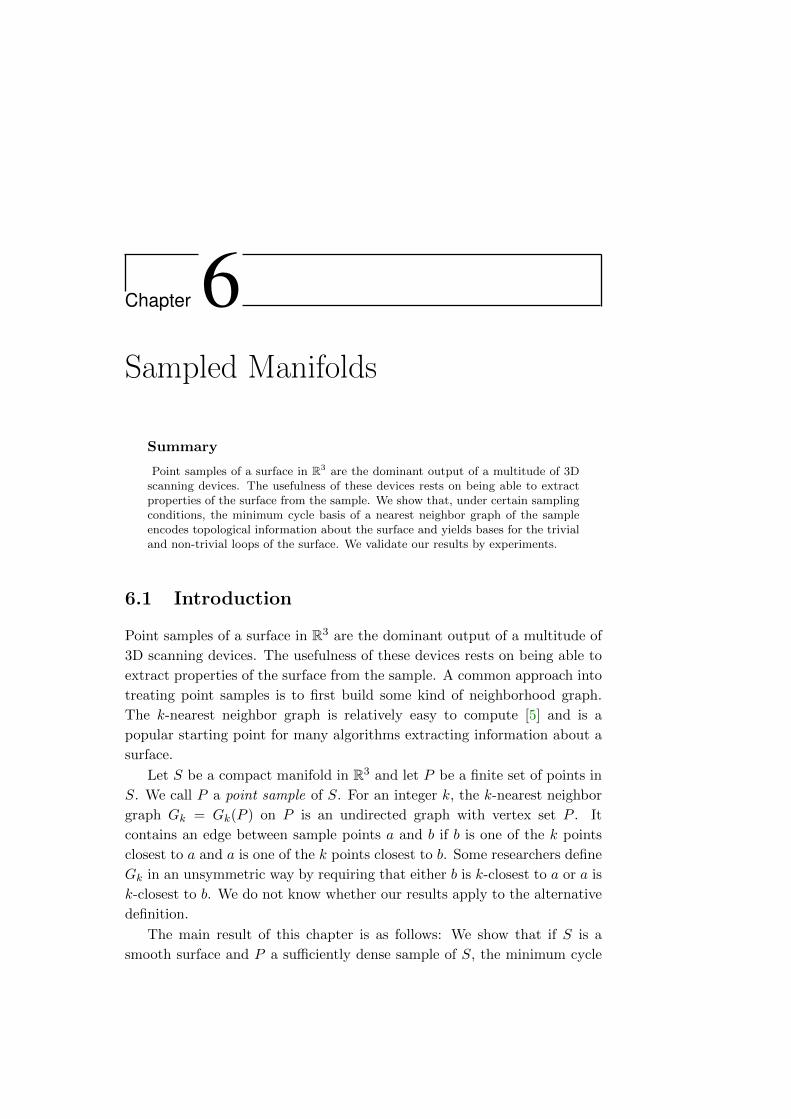
Chapter 6Sampled Manifolds
Summary
Point samples of a surface in R3 are the dominant output of a multitude of 3Dscanning devices. The usefulness of these devices rests on being able to extractproperties of the surface from the sample. We show that, under certain samplingconditions, the minimum cycle basis of a nearest neighbor graph of the sampleencodes topological information about the surface and yields bases for the trivialand non-trivial loops of the surface. We validate our results by experiments.
6.1 Introduction
Point samples of a surface in R3 are the dominant output of a multitude of
3D scanning devices. The usefulness of these devices rests on being able to
extract properties of the surface from the sample. A common approach into
treating point samples is to first build some kind of neighborhood graph.
The k-nearest neighbor graph is relatively easy to compute [5] and is a
popular starting point for many algorithms extracting information about a
surface.
Let S be a compact manifold in R3 and let P be a finite set of points in
S. We call P a point sample of S. For an integer k, the k-nearest neighbor
graph Gk = Gk(P ) on P is an undirected graph with vertex set P . It
contains an edge between sample points a and b if b is one of the k points
closest to a and a is one of the k points closest to b. Some researchers define
Gk in an unsymmetric way by requiring that either b is k-closest to a or a is
k-closest to b. We do not know whether our results apply to the alternative
definition.
The main result of this chapter is as follows: We show that if S is a
smooth surface and P a sufficiently dense sample of S, the minimum cycle

72 Chapter 6. Sampled Manifolds
basis of the nearest neighbor graph of P gives information about the genus
of S and yields bases for the set of trivial and non-trivial loops. Our
experiments suggest that this is true also for some non-smooth surfaces.
More formally, we show that for suitably nice samples of smooth man-
ifolds of genus g and sufficiently large k, the k-nearest neighbor graph Gkhas a cycle basis consisting only of short (= length at most 2(k + 3)) and
long (= length at least 4(k+ 3)) cycles. Moreover, the MCB is such a basis
and contains exactly m− (n− 1)− 2g short cycles and 2g long cycles. The
short cycles span the subspace of trivial loops and the long cycles form a
homology basis; see next section or Section 2.3 for a definition. Thus, the
MCB of Gk reveals the genus of S and also provides a basis for the set of
trivial cycles and a set of generators for the non-trivial cycles of S.
We prove the statement for smooth manifolds, sufficiently dense samples,
and sufficiently large k. A dense sample is defined in a manner similar to
that of Amenta and Bern [2], as follows: The medial axis of a manifold S
embedded in R3 is the closure of the set of points in R3 with more than one
nearest neighbor on S. The local feature size f : S 7→ R assigns to every
point in S its least distance to the medial axis of S. The point sample P is
called an ε-sample of S, if every point x ∈ S has a point in P at distance
at most εf(x). If in addition ||p − q|| ≥ δf(p) for all distinct p, q ∈ P
the sample P is called an (ε, δ)-sample. This definition requires the sample
to be dense with respect to the local feature size, but at the same time
samples cannot be arbitrarily close. Our main result is now as follows: If
P is an (ε, δ)-sample of a smooth manifold for sufficiently small ε and k is
sufficiently large (the meaning of sufficiently large depends on ε and δ), the
claim of the preceding paragraph is true. The claim is also true if we use a
weaker sampling assumption, namely locally uniform ε-samples [35].
6.1.1 Other Approaches and Remarks
Given a point sample, undoubtedly, the ultimate application is to form a
geometric approximation of the surface based on the sample. The objective
is typically to form a piecewise linear surface (i.e. triangle mesh) whose
geometry and topology are as similar to the original as possible. For smooth
surfaces and sufficiently dense samples, good and efficient reconstruction
algorithms are available, see e.g., the papers [9, 51, 2, 3, 35, 24, 62] and the
survey by Dey [22]. For non-smooth surfaces or sparse samples the problem
is open.
The best asymptotic running time in order to do smooth surface recon-
struction is O(n log n) [35] and efficient implementations are available [24,

6.2. Structure of Cycles 73
23]. Certainly, once this is done, it is relatively easy to extract less detailed
information such as the genus of the surface or a homology basis. For ex-
ample, a homology basis of a manifold 3D mesh may be computed in O(n)
time by an algorithm of Vegter and Yap [80], and a shortest homology basis
may be computed in O(n2 log n + n2g + ng3) by an algorithm of Erickson
and Whittlesey [30].
Thus, in the case of smooth manifolds computing an MCB in order to
compute less detailed information is an overkill. The purpose of this chapter
is not to compete algorithmically with the previously mentioned approaches,
but instead to study the properties and the combinatorial structure that
the minimum (and some sparse) cycle bases of certain neighborhood graphs
possess.
6.2 Structure of Cycles
6.2.1 The Basic Idea
Let S be a compact 2-manifold of genus g with no boundary embedded in
R3. For the sequel we will need to define a number of topological concepts.
Rather than give a complete formal exposition, which may be found in most
algebraic topology textbooks (e.g. [68]), we provide a more intuitive informal
set of definitions. See also Chapter 2.
A closed simple curve on S is called a loop. The elements of the first
homology group of S are equivalence classes of loops. The identity element
of this homology group is the equivalence class of separating loops, namely,
loops whose removal disconnects the surface. Two homology loops are in the
same homology class if one can be continuously deformed into the other via
a deformation that may include splitting loops at self-intersection points,
merging intersecting pairs of loops, or adding and deleting separating loops.
A loop is trivial if it is a separating loop and is non-trivial otherwise. A
homology basis of S is any set of 2g loops whose homology classes span all
non-trivial loops.
Let P be a sample of S andGk its k-nearest neighbor graph. For any edge
(a, b) of Gk we define a curve in S connecting a and b. Let us parameterize
the segment ab by length. Let p(t) = a+t(b−a) be the point with parameter
value t, 0 ≤ t ≤ 1 and let q(t) be a point on S nearest to p(t). We assume
that q(t) is unique. Then, q(t) traces a continuous curve on S connecting
a and b, which we denote by γab. In this way, we obtain a drawing of Gkon S and cycles in Gk induce loops in S. In particular, cycles can induce
trivial or non-trivial loops, in which case we call them trivial or non-trivial

74 Chapter 6. Sampled Manifolds
cycles, respectively. The assumption that q(t) is unique is not very stringent.
Observe that if q(t) is not unique, p(t) is a point on the medial axis and hence
max(f(a), f(b)) ≤ ||a− b||/2.
We next give general conditions under which every minimum cycle basis
of Gk contains exactly 2g long cycles, the long cycles induce a homology
basis of S over the reals, and all short (= non-long) cycles are trivial.
1. L(γab) ≤ c1||a− b|| where c1 is a constant, i.e., the length of the curve
γab is not much larger than the length of the segment ab.
2. There is a subgraph M of Gk (all vertices and a subset of the edges)
such that
• the drawing restricted to M is an embedding,
• M is a mesh of genus g for S,
• the faces of M have bounded size, say at most c2 edges, and
• for every edge e ∈ Gk \M the shortest path in M connecting a
and b has bounded length, say bounded by c3.
3. The minimal length of a non-trivial loop of S is Lmin and for every
edge (a, b) of the graph Gk the distance between its endpoints is at
most Lmin/(2 max(c2, c3 + 1)).
Theorem 6.1. If the conditions above hold, every MCB of Gk contains
exactly m− (n− 1)− 2g short (length less than max(c2, c3 + 1)) and exactly
2g long (length at least 2 max(c2, c3 + 1)) cycles. Moreover, the long cycles
induce a basis of the first homology group of S over the reals.
Proof. The embedding of M has mM edges and f faces where f−mM +n =
2 − 2g. Consider the following set B of cycles: all face cycles of M but
one and for each edge e = (a, b) ∈ Gk \M the cycle consisting of e plus
the shortest path in M connecting a and b. Any cycle in B has length
at most max(c2, c3 + 1) and the cycles in B are independent. There are
f − 1 + m −mM = mM − n + 2 − 2g − 1 + m −mM = m − (n − 1) − 2g
cycles in B.
Any cycle basis of Gk must contain at least 2g non-trivial cycles and
these cycles induce loops which span the homology group of S. Consider
any non-trivial cycle. It has length at least Lmin. For any edge (a, b) of
Gk the length of γab is at most Lmin/(2 max(c2, c3 + 1)) and hence any
non-trivial cycle must contain at least 2 max(c2, c3 + 1) edges.
We have now shown that there are m− (n− 1)− 2g independent cycles
of length at most max(c2, c3 + 1) and that every non-trivial cycle consists

6.2. Structure of Cycles 75
of at least 2 max(c2, c3 + 1) edges. Consider now any MCB B∗ of Gk. It
must contain at least 2g long cycles. Assume that it contains less than
m− (n− 1)− 2g short cycles. Then, at least one cycle in B, call it C, is not
spanned by the short cycles in B∗, i.e., the representation of C as a sum of
cycles in B∗ contains a cycle D which is not short. Thus, we can improve
the total length of B∗ by replacing D by C.
In Sections 6.2.3 and 6.2.4 we substantiate the theorem for smooth sur-
faces. We will actually prove a stronger result. Note that in the previous
theorem we did not use the first condition. This condition will be useful later
on when we will also replace the global condition of maximal edge length
(see the third condition) by a local condition depending on the local feature
size.
6.2.2 Sampling and Restricted Delaunay Triangulations
The local feature size is 1-Lipschitz continuous, i.e.,
Lemma 6.2 (Amenta and Bern [2]). For any two points p and q on S,
|f(p)− f(q)| ≤ ||p− q||.
Let DP and VP denote the Delaunay and the Voronoi diagram of P .
The Voronoi cell Vp ⊂ VP for a point p ∈ P is defined as the set of points
x ∈ R3 such that ||x−p|| ≤ ||q−x|| for any q ∈ P and q 6= p. The Delaunay
triangulation of P is the dual of VP . It has an edge pq if and only if Vp, Vqshare a face, has a triangle pqr if and only if Vp, Vq, Vr share an edge, and
a tetrahedron pqrs if and only if Vp, Vq, Vr, and Vs share a Voronoi vertex.
We assume that the input sample P ∈ R3 is in general position and that no
vertex of VP lies on S.
Consider the restriction of the Voronoi diagram VP to the surface S.
This defines the restricted Voronoi diagram VP |S , with restricted Voronoi
cells Vp|S = Vp ∩ S. It is said to satisfy the ball property if each Vp|S is
a topological 2-ball, each nonempty pairwise intersection Vp|S ∩ Vq|S is a
topological 1-ball, and each nonempty triple intersection Vp|S ∩ Vq|S ∩ Vr|Sis a single point.
The dual of the restricted Voronoi diagram defines the restricted De-
launay triangulation DP |S . In more detail, an edge pq is in DP |S if and
only if Vp|S ∩ Vq|S is nonempty and a triangle pqr is in DP |S if and only
if Vp|S ∩ Vq|S ∩ Vr|S is nonempty. Our general position assumption guaran-
tees that there is no tetrahedron in DP |S . It is known that the restricted
Delaunay edges for an ε-sample are short.

76 Chapter 6. Sampled Manifolds
Lemma 6.3 (Amenta and Bern [2], see also Giesen and Wagner [38]). Let
P be an ε-sample of S with ε < 1. If pq is an edge of the restricted Delaunay
triangulation, then ||p− q|| ≤ 2ε1−εminf(p), f(q).
For ε ≤ 0.08, the restricted Voronoi diagram is known to have the ball
property [2]. In this case the restricted Delaunay triangulation is a simplicial
surface homeomorphic to S [28]. The k-neighborhood graph Gk contains the
restricted Delaunay triangulation if P is a sufficiently nice sample of S.
Lemma 6.4 (Andersson et al.[4]). Let P be an (ε, δ)-sample of S, let w =2ε1−ε and k ≥ (δ(1+w)+w)2
δ2(1−w)2−w4 . Then, the restricted Delaunay triangulation DP |Sis a subgraph of Gk.
Funke and Ramos [35] have shown how to turn any ε-sample into a locally
uniform ε-sample by using decimation. Locally uniform samples are related
to (ε, δ)-samples, but technically more involved. Both types of sample have
the property that each sample point has only a constant number of restricted
Delaunay neighbors. This is the only property that we require and thus, our
results are valid for both cases. We have chosen to state our results in terms
of (ε, δ)-samples, for ease of exposition.
We also state one more useful fact which we need later on. At each point
p ∈ S, there are two tangent medial balls centered at points of the medial
axis. The vectors from p to the centers of its medial balls are normal to S,
and S does not intersect the interiors of the medial balls. Since f(p) is at
most the radius of the smaller medial ball, S is also confined between the
two tangent balls of radius f(p).
6.2.3 Short Cycles
In this section we show that for an appropriate sampling density there exists
a linearly independent set of m− (n− 1)− 2g short cycles.
Warm-Up: The Planar Case
Consider a finite set P of points in the plane, its nearest neighbor graph Gk,
its Delaunay triangulation DP , and assume that DP is contained in Gk. We
describe a cycle basis consisting only of short cycles. In the next section, we
will generalize the approach of this section to manifolds in R3.
Consider the following set B of cycles. It contains (a) the face cycles
of all bounded faces of the Delaunay triangulation and (b) for each edge
e = (a, b) ∈ Gk \DP the cycle formed by e and the shortest path from a to
b in DP .
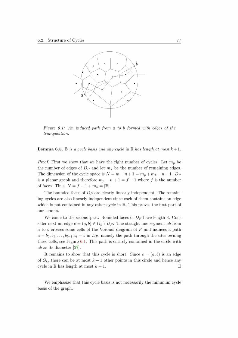
6.2. Structure of Cycles 77
a
b
Figure 6.1: An induced path from a to b formed with edges of thetriangulation.
Lemma 6.5. B is a cycle basis and any cycle in B has length at most k+1.
Proof. First we show that we have the right number of cycles. Let mp be
the number of edges of DP and let mk be the number of remaining edges.
The dimension of the cycle space is N = m− n+ 1 = mp +mk − n+ 1. DP
is a planar graph and therefore mp − n+ 1 = f − 1 where f is the number
of faces. Thus, N = f − 1 +mk = |B|.The bounded faces of DP are clearly linearly independent. The remain-
ing cycles are also linearly independent since each of them contains an edge
which is not contained in any other cycle in B. This proves the first part of
our lemma.
We come to the second part. Bounded faces of DP have length 3. Con-
sider next an edge e = (a, b) ∈ Gk \DP . The straight line segment ab from
a to b crosses some cells of the Voronoi diagram of P and induces a path
a = b0, b1, . . . , bl−1, bl = b in DP , namely the path through the sites owning
these cells, see Figure 6.1. This path is entirely contained in the circle with
ab as its diameter [27].
It remains to show that this cycle is short. Since e = (a, b) is an edge
of Gk, there can be at most k − 1 other points in this circle and hence any
cycle in B has length at most k + 1.
We emphasize that this cycle basis is not necessarily the minimum cycle
basis of the graph.

78 Chapter 6. Sampled Manifolds
The 3-dimensional Case
We consider essentially the same set of cycles as in the preceding section:
(a) all but one faces of the restricted Delaunay triangulation, and (b) for
each remaining edge e = (a, b) ∈ Gk \DP |S the cycle consisting of e plus the
shortest path from a to b in the restricted Delaunay triangulation. As in
the planar case, these cycles are linearly independent. It remains to prove
that they are short. In this section we will prove the following theorem.
Theorem 6.6. Let P be an ε-sample of S, let k < log 1+ε1−ε
32 , and assume
that DP |S ⊆ Gk. Let (a, b) ∈ Gk \DP |S. Then, there is a path from a to b
in DP |S of length at most 2k + 5.
Consider the edge e = (a, b) ∈ Gk \ DP |S , then the curve γab crosses
some cells of the restricted Voronoi diagram and induces a path pab = (a =
b0, b1, . . . , bl−1, bl = b) in the restricted Delaunay triangulation, namely the
path through the sites owning these cells. Since Gk contains the restricted
Delaunay triangulation, pab exists in Gk.
Lemma 6.7. Let e = (a, b) ∈ Gk \DP |S and let B be the ball with ab as its
diameter. If the induced path pab is contained in B, then the cycle consisting
of e plus pab has length at most k + 1.
Proof. Since e ∈ Gk, the ball B contains at most k − 1 other points apart
from a and b.
The above lemma generalizes the planar case. Unfortunately, we are
unable to prove that pab runs within B. We therefore argue somewhat
differently. We first show that either there is a very short path in DP |S from
a to b or both a and b are far away from the medial axis. In the latter case
we show that pab is contained in a slightly bigger ball but still sufficiently
small for our purposes. We begin with the following auxiliary lemma.
Lemma 6.8. Let a and b be two points in P and assume that there is a
path of length l in DP |S from a to b. Let α = (1 + ε)/(1 − ε). Then,
α− 1 = 2ε/(1− ε) and
||a− b|| ≤ (αl − 1) min(f(a), f(b)) .
Proof. We use induction on the length of the path. Let the path from a to
b in DP |S be a = q0, q1, . . . , ql = b. Then, ||a− b|| = ||a− ql||.

6.2. Structure of Cycles 79
For the base case l = 1 we have that ||a−q1|| ≤ (α−1)f(a) by Lemma 6.3.
Assume that the statement holds for paths of length l − 1, then
||a− b|| = ||a− ql||≤ ||a− ql−1||+ ||ql−1 − ql||≤ ||a− ql−1||+ (α− 1)f(ql−1) by Lemma 6.3
≤ ||a− ql−1||+ (α− 1)(f(a) + ||a− ql−1||) by Lemma 6.2
= (α− 1)f(a) + α||a− ql−1||≤ (α− 1)f(a) + α(αl−1 − 1)f(a) by induction
= (αl − 1)f(a) .
The same argument applies to b instead of a.
Lemma 6.9. Let (a, b) ∈ Gk, λ ≥ 1 and assume that
k < log 1+ε1−ε
1 + λ
λ. (6.1)
Then, either there is a path of length at most k from a to b in the restricted
Delaunay triangulation or
f(a), f(b) > λ||a− b|| . (6.2)
Proof. Recall that α = 1+ε1−ε . Thus, inequality (6.1) implies αk − 1 < 1/λ.
Consider the shortest path in the restricted Delaunay triangulation a =
q0, q1, . . . , ql−1, ql = b from a to b. Furthermore, assume l > k and f(a) ≤λ||a− b||. Lemma 6.8 implies that
||a− qi|| ≤ (αi − 1)f(a) ≤ (αk − 1)f(a) < f(a)/λ ≤ ||a− b|| for 1 ≤ i ≤ k,
and hence there are k points closer to a than b is, a contradiction. The
argument works symmetrically for b.
The above lemma states that it is enough to prove Theorem 6.6 when
f(a), f(b) > λ||a − b||. From now on, we proceed under this assumption
for some λ ≥ 1. Let us parameterize the segment ab by length. Let p(t) =
a+t(b−a) be the point with parameter value t, 0 ≤ t ≤ 1 and let q(t) be the
point on S nearest to p(t). Note that q(t) is unique, because otherwise p(t)
would be a point of the medial axis contradicting the fact that f(a) > ||a−b||.Finally, let c denote the mid-point of the segment ab and s(t) denote the
site of the Voronoi cell containing q(t).

80 Chapter 6. Sampled Manifolds
Our goal is to prove that s(t) belongs to a ball of radius√32 ||a − b||
centered at c (Lemma 6.13) and that this ball contains at most 2(k + 3)
sample points. We begin with the latter.
Lemma 6.10. For (a, b) ∈ Gk and c as defined above, the ball B′ of radius√32 ||a− b|| centered at c contains at most 2(k + 3) sample points.
Proof. Consider the ball Ba with center a and radius ||a− b||. Every sample
point in the interior of this ball is closer to a than b is. Thus, Ba has at most
k points in its interior. Also Ba has at most four points in its boundary by
our non-degeneracy assumption. Similarly, the ball Bb with center b and
radius ||a− b|| also contains at most k + 4 points.
The ball B′ is completely contained in the union of Ba and Bb and thus
it contains at most 2(k + 4) − 2 points. The −2 accounts for the fact that
a and b are contained in both balls.
Next we estimate the distance from c to s(t).
Lemma 6.11. ||c− s(t)|| ≤ ||a− b||/2 + 2||p(t)− q(t)||
Proof. Assume w.l.o.g that ||a − p(t)|| ≤ ||b − p(t)||, otherwise we do the
computation with b. By the triangle inequality, ||c − s(t)|| ≤ ||c − p(t)|| +||p(t)−q(t)||+||q(t)−s(t)||. Since q(t) is closer to s(t) than any other sample
point, ||q(t) − s(t)|| ≤ ||q(t) − a||. Moreover, ||q(t) − a|| ≤ ||q(t) − p(t)|| +||p(t)− a||. Finally, ||a− p(t)||+ ||p(t)− c|| = ||a− b||/2.
It remains to bound ||p(t) − q(t)|| as a function of ||a − b||. We first
estimate the distance of q(t) from the medial axis.
Lemma 6.12. f(q(t)) > (λ− 1)||a− b||
Proof. Assume w.l.o.g that ||a − p(t)|| ≤ ||b − p(t)||, otherwise we do the
computation with b. Since q(t) is the point in S closest to p(t), we have
||a − q(t)|| ≤ ||a − p(t)|| + ||p(t) − q(t)|| ≤ 2||a − p(t)|| ≤ ||a − b||. By
Lemma 6.2 f(q(t)) ≥ f(a)−||a−q(t)|| and hence f(q(t)) ≥ f(a)−||a−b|| >(λ− 1)||a− b||.
Lemma 6.13. For λ ≥ 2, ||p(t) − q(t)|| ≤√3−14 ||a − b|| and ||c − s(t)|| ≤
√32 ||a− b|| .
Proof. Consider the point q(t). By Lemma 6.12 there are two medial balls
with radius at least (λ−1)||a−b|| tangent to q(t). The surface passes between
these balls and does not intersect their interior, in particular, a and b do not
lie in the interior of these balls. Thus, the worst case (when the distance

6.2. Structure of Cycles 81
m
Bm
q(t)
a
b
p(t)c
v
Figure 6.2: Bounding ||p(t)− q(t)|| in terms of ||a− b||.
||p(t) − q(t)|| compared to ||a − b|| is maximized) occurs, when both lie on
the boundary of one of these balls (see Figure 6.2). Let m be the center of
this ball and use Bm to denote the ball. Consider the perpendicular bisector
of segment ab passing through m. It intersects segment ab at c and ball Bmat v. Also, p(t) is on the segment q(t)m.
Distance ||p(t)− q(t)|| is upper bounded by ||c− v|| and thus we are left
with bounding ||c−v||. Referring to Figure 6.2 we see that the triangle acm
is right. Thus, ||c−m||2 = ||a−m||2 − ||a− c||2. Moreover,
||a−m|| = ||v −m|| = ζ||a− b|| for some ζ ≥ λ− 1 ,
and ||a− c|| = ||a− b||/2. Combining all these,
||c−m|| =√ζ2 − 1
4· ||a− b|| .
Finally, ||c− v|| = ζ||a− b|| − ||c−m|| and hence
||p(t)− q(t)|| ≤ ||c− v|| =(ζ −
√ζ2 − 1
4
)||a− b||
≤ (1−√
3
4)||a− b||
<
√3− 1
4||a− b|| .
This proves the first part of the lemma. The second part follows now from

82 Chapter 6. Sampled Manifolds
Lemma 6.11 since,
||c− s(t)|| ≤ 1
2||a− b||+ 2||p(t)− q(t)|| ≤
√3
2||a− b|| .
It is now easy to complete the proof of Theorem 6.6. Set λ = 2. Then,
pab is contained in the ball B′ and B′ contains at most 2(k + 3) sample
points. Thus, pab has length at most 2k + 5. Together with the edge e we
get a cycle of length at most 2(k + 3).
Recall that our goal is to satisfy the assumptions of Section 6.2.1. If we
combine Theorem 6.6 and Lemma 6.8 we get that the edges of Gk are small
in length.
Corollary 6.14. Let α = (1 + ε)/(1− ε). For any edge e = (a, b) ∈ Gk,
||a− b|| ≤ (α2k+5 − 1) min(f(a), f(b)) . (6.3)
Moreover, we will need the following lemma which can be easily derived
from [38, Lemma 10 and Theorem 4].
Lemma 6.15 (Giesen and Wagner [38]). Let a and b be two points of S such
that ||a − b|| ≤ η · min(f(a), f(b)) with η ≤ 1/4. Then, L(γab) ≤ 4||a − b||where L(γab) denotes the length of γab.
Using Lemma 6.15 we set c1 to 4 in Section 6.2.1.
6.2.4 Long Cycles
In this section we make precise how non-trivial cycles are long. The idea is
simple; non-trivial cycles have a certain minimum length and edges of Gk are
short. We will actually prove a stronger result. The length of a non-trivial
loop is bounded from below by the maximum feature size of any point on
the loop. Combined with Lemma 6.15, we will obtain the desired result.
Assume that η = α2k+5 − 1 ≤ 14 . Let C be any non-trivial cycle of Gk.
Substituting each edge (a, b) ∈ C by the curve γab gives us a non-trivial loop
γ on S. By Lemma 6.15 and Corollary 6.14 we get
L(γ) ≤ 4∑
(a,b)∈C
||a− b|| ≤ 4∑
(a,b)∈C
ηmin(f(a), f(b)) ,
and if |C| denotes the number of edges of C,
L(γ) ≤ 4η|C| maxa∈C
f(a) . (6.4)

6.2. Structure of Cycles 83
p
v
v′
β
Bγ
Bp
Bm
Bm
γ
12L(γ)
13L(γ)
Figure 6.3: Proving Theorem 6.16.
In order to get a lower bound on |C| we need to relate γ to its distance to
the medial axis. More precisely, we are going to show the following theorem
which might be of independent interest.
Theorem 6.16. Let γ be any non-trivial loop on S, then L(γ) ≥ maxp∈γ
f(p).
Proof. Let p be a point on γ with maximum distance from the medial axis
and assume L(γ) < f(p) for the sake of contradiction. Let β be a non-
trivial loop of different homology class going through p (see Figure 6.3). At
each point x ∈ β there are two tangent balls with radius f(x) which do not
contain any point of S in their interior. One of these tangent balls when
moving it along β (and adjusting its size accordingly) produces an object
T , topologically equivalent to a torus, around which γ loops non-trivially.
Let Bp be the ball with center p and radius 5L(γ)/6. For all x ∈ Bp ∩β,
the local feature size is large, namely, f(x) ≥ f(p) − ||p − x|| > L(γ) −5L(γ)/6 = L(γ)/6 and hence for x ∈ Bp ∩ β the ball defining T has radius
at least L(γ)/6.
The loop γ stays inside a ball of radius L(γ)/2 centered at p and hence
well inside Bp. Since γ loops around T its length it least 2πL(γ)/6 > L(γ),
a contradiction.
We can now establish that non-trivial cycles in Gk are long.
Theorem 6.17. For appropriate values of ε, δ, and k any non-trivial cycle
C ∈ Gk has length |C| ≥ 14η where η = α2k+5 − 1 ≤ 1
4 .

84 Chapter 6. Sampled Manifolds
ε valid k chosen k η short-cycles long-cyclesupper bound lower bound
10−2 [15, 20] 15 1.014 36 -5× 10⁻³ [14, 40] 14 0.391 34 -
10−3 [14, 202] 14 0.068 34 45× 10−4 [14, 405] 14 0.033 34 8
10−4 [14, 2027] 14 0.0066 34 385× 10−5 [14, 4054] 14 0.0033 34 76
Table 6.1: Evaluation of the various conditions for the separation ofthe MCB for different values of the sampling density ε.
Proof. Using inequality (6.4) and Theorem 6.16 we obtain
L(γ) ≤ 4η|C| maxa∈C
f(a) ≤ 4η|C|L(γ) ,
and the theorem follows.
Corollary 6.18. If η = α2k+5 − 1 < 116(k+3) then all non-trivial cycles in
Gk have length larger than 4(k + 3).
Proof. We fix k and ε to some constants according (a) to our assumptions
in Section 6.2.3 and (b) such that η < 116(k+3) . Then, by Theorem 6.17
|C| ≥ 14η > 4(k + 3).
Putting everything together establishes Theorem 6.1.
Corollary 6.19. If the conditions in Section 6.2.1 hold, the sampling den-
sity is high enough and k is large enough: every MCB of Gk contains exactly
m− (n−1)−2g short (length less than 2(k+3)) and exactly 2g long (length
at least 4(k + 3)) cycles.
Proof. Use DP |S as M in the assumptions of Section 6.2.1. By Lemma 6.15
we can set c1 = 4. Theorem 6.6, Corollary 6.14 and Theorem 6.17 prove the
remaining assumptions. The corollary follows by the proof of Theorem 6.1
for c2 = 3 and c3 = 2k + 5.
6.2.5 Putting It All Together
Our assumptions so far suggest that given an (ε, δ)-sample and w = α−1 =2ε1−ε , we should choose k such that:
(δ(1 + w) + w)2
δ2(1− w)2 − w4≤ k < log 1+ε
1−ε
3
2. (6.5)

6.3. Experimental Validation 85
There are values of ε such that inequality (6.5) cannot be satisfied. However,
as ε decreases the right hand side increases while the left hand side decreases.
Thus, both conditions can always be simultaneously satisfied for some dense
enough sample. The above conditions are what is required for the trivial
cycles of the MCB to have length at most 2(k + 3).
For the lower bound on the length of the non-trivial cycles of the MCB,
we also require that η = α2k+5 − 1 ≤ 14 , and in order for the length of the
non-trivial cycles to reach the desired number |C| ≥ 14η > 4(k+3) we require
that η = α2k+5 − 1 < 116(k+3) .
We fix δ to 3w/8 ≈ 3ε/4 and evaluate, in Table 6.1, the bounds for
different values of ε.
Remark The lower and upper bounds presented in Table 6.1 are not tight.
Somewhat large constants appear due to the proof technique used. Perhaps,
by using some other proximity graph instead of the k-neighborhood or by
performing a different analysis the bounds can be improved. This is espe-
cially true for the value of ε required by the theory in order for the non-trivial
cycles to be longer than the trivial ones. In practice this is true for smaller
values of k and sampling densities. The next section presents experimental
data which confirm this.
6.3 Experimental Validation
6.3.1 Genus Determination
This section presents experimental data on the size of trivial and non-trivial
cycles in the MCBs of point clouds sampled from compact manifolds. The
main observation is that the MCB cycles are separated into the two cate-
gories, short trivial and long non-trivial, for rather small values of k and
sampling density. Moreover, the upper bound on the length of the triv-
ial cycles is much less than 2(k + 3) and the method also works for some
non-smooth samples.
We study four different examples:
(a) the “double torus”, a genus 2 double torus (Figure 6.4a) with a sparse
point cloud (Figure 6.4b),
(b) the “bumpy torus”, a genus 1 surface (Figure 6.4c) with a dense point
cloud (Figure 6.4d),
(c) the “homer torus”, a genus 1 surface (Figure 6.5a) with a sparse point
cloud (Figure 6.5b), and

86 Chapter 6. Sampled Manifolds
(a) Double torus (b) 767 points cloud
(c) Bumpy torus (d) 5044 points cloud
1
4
16
64
256
1024
4096
2 4 6 8 10 12 14
1+#cycles
length
double torus
1
4
16
64
256
1024
4096
16384
65536
5 10 15 20 25 30
length
bumpy torus
k = 10 k = 10
(e) Distribution of the lengths of the MCB cycles of Gk of the double andbumpy torus models for k = 10.
Figure 6.4: The “double” and “bumpy” torus models. The red cyclesare the long non-trivial cycles extracted from the MCB of Gk for k =10.

6.3. Experimental Validation 87
(d) the “wedge torus”, a genus 1 non-smooth surface (Figure 6.6a) with a
sparse point cloud (Figure 6.6b).
Double torus
Since the model has genus 2 we expect the MCB to reveal exactly 4 non-
trivial cycles. The minimum value of k for this event to happen is 6. All
cycles but four of the MCB have length at most 8, two cycles have length 13
and two 24. As k increases this gap grows, for k = 8 two cycles have length
11, two others have length 24 and all the rest at most 5. For k = 10 two
cycles have length 8, two 13 and the rest at most 4. This continues to be
true as we increase k as long as the edges of the k-nearest neighbor graph
do not shortcut a handle.
Although the proof of Lemma 6.10 fails in the case of the unsymmetric k-
nearest neighbor graph, where an edge is added even if only one endpoint is
a k-nearest neighbor of the other, in practice we observe the same behavior.
The values of k are even smaller for this case. For minimum k = 5 there are
two cycles of length 11, two of length 24 and the rest at most 6. For k = 9
all MCB cycles are triangles except two with length 9 and two with length
14.
Bumpy torus
The situation improves if the sampling is dense. The “bumpy torus” model
has genus one and thus we expect the MCB to reveal two non-trivial cycles.
For k = 6 the two non-trivial cycles have length 35 and 42 and the rest at
most 27. Due to the density of the sample as we increase k this difference
becomes more noticeable. For k = 10 the non-trivial cycles have length 22
and 30 and the rest at most 12. For k = 12 the two non-trivial have length
20 and 26 and the rest at most 9. Note also that in all these examples almost
all trivial cycles have length 3 or 4. For example, when k = 12 about 99% of
the trivial cycles are triangles. See Figure 6.4e for a histogram of the cycles
lengths when k = 10.
Homer torus
This model has again genus 1 and thus we expect the MCB to reveal two
non-trivial cycles. For k = 7 the MCB contains one cycle of length 252, one
of length 8 and all the remaining have length at most 5. Our point cloud
however is considerably sparse and thus it is quite easy for the MCB to fail

88 Chapter 6. Sampled Manifolds
(a) Homer torus (b) 3486 points cloud
Figure 6.5: The “homer” torus model and the two non-trivial cyclesrevealed by the MCB for k = 7. The two non-trivial cycles have length8 and 252 respectively.
to detect the two non-trivial cycles for other values of k. We elaborate more
on this at the end of this section.
Wedge torus
The non-smooth surface has genus one. We expect that as long as k is
not too large, our method should reveal two non-trivial cycles. Figure 6.6b
shows the two non-trivial cycles of the MCB for k = 22. Note that this is a
difficult instance for surface reconstruction.
Discussion
In the examples above, the MCB was able to reveal the genus. There were
exactly 2g long cycles and long and short cycles are clearly discernible by
length. However, in practice, if g is unknown and the sampling density
not as high as it should be, how can g be determined from the MCB? We
suggest the following heuristic. Let l be the minimal integer such that the
MCB contains no cycle of length between l and 2l inclusive. Then, 2g is the
number of cycles of length larger than l. If this number is odd, this is an
indication of insufficient sampling density or a wrong value of k.
What can go wrong when the sample is not sufficiently dense or the value
of k is not chosen properly? When k is too small, the MCB might contain
long trivial cycles. When k is too large, Gk may contain edges between

6.4. Application to Surface Reconstruction 89
(a) Wedge torus (b) 6078 points cloud
1
4
16
64
256
1024
4096
16384
65536
2 4 6 8 10 12 14 16 18 20
1+#cycles
length
non-smooth wedge-torus
k = 22
(c) Distribution of the lengths of the MCBcycles for k = 22.
Figure 6.6: The “wedge” torus model and the two non-trivial cyclesrevealed by the MCB for k = 22.
points distant from each other in S and hence spurious long cycles may
enter the basis, see Figure 6.7. The figure also shows that non-smoothness
by itself is not an obstacle.
6.4 Application to Surface Reconstruction
In this section we outline the approach of Tewari et al. [75] for surface
reconstruction. The interested reader is referred to their paper for more
details.
Tewari et al. [75] show that if a basis for the trivial loops of the manifold
may be computed from the sample of a 2-manifold of genus 1, it is possi-
ble to parameterize the sample set, and then construct a piecewise-linear
approximation to the surface. They use the MCB of the k-nearest neigh-
bor graph to extract this basis, assuming that the non-trivial cycles are the
two longest ones. They observed that this is correct if the sample is dense

90 Chapter 6. Sampled Manifolds
too small klong trivial cycles
too large kspurious edge
edges are ok
Figure 6.7: Several difficult situations. In the left figure due to sym-metry a small choice for k (k = 4) leads to long trivial cycles. Inthe upper right figure a large value of k results in an edge which con-nects two parts of the surface which are distant from each other. Thelower right figure shows that edges near non-smooth features are not aproblem as long as k is not too large.
enough, but did not prove anything in this respect. Theorem 6.1 shows
under which conditions this reconstruction algorithm provably constructs a
triangulation homeomorphic to the surface.
The parameterization based approach has its origins in Tutte’s “spring
embedder” for planar graphs [79]. Tutte introduced a simple, yet powerful
method for producing straight-line drawings of planar graphs. The vertices
of the outer face are mapped to the vertices of a convex polygon and all
other vertices are placed at the centroid of their neighbors. Algorithmically,
this amounts to solving a linear system of equations. If we use pv to denote
the location of vertex v and Nv to denote the set of neighbors of v, this
means
pv =∑w∈Nv
λvwpw and λvw = 1/|Nv| (6.6)
for every interior vertex v. Tutte proved that the coordinates computed
in this way define a non-degenerate embedding for any 3-connected planar
graph. Floater [32] showed that the result stays true if vertices are placed

6.4. Application to Surface Reconstruction 91
at arbitrary convex combinations of their neighbors, i.e.,∑w∈Nv
λvw = 1 and λvw ≥ 0 .
For the sequel, it is convenient to rewrite Equation (6.6) as∑w∈Nv
λvw(pw − pv) = 0
and to introduce xvw for the vector from v to w in the embedding. Gortler
et al. [41] extended the method to embeddings onto the torus. Given a
3-connected map (= graph + cyclic ordering on the edges incident to any
vertex) of genus one, they viewed undirected edges v, w as pairs of directed
edges and associated a variable xvw with every directed edge. They used
the equations:
xvw + xwv = 0 for all edges (v, w) (symmetry)∑w∈Nv
λvwxvw = 0 for all vertices v (center of gravity)
∑(w,v)∈∂f
xwv = 0 for all faces f (face sums)
The first class of equations ensures that the vector from w to v is the same
as the vector from v to w, the second class ensures that v is a convex
combination of its neighbors, and the third class ensures that the vectors
along any face boundary sum to zero. There are 2m unknowns and m+n+f
equations. Two equations are redundant (one center of gravity constraint
and one face sum constraint) and hence the rank of the system is m+ n +
f−2 = 2m−2 (this uses the Euler theorem f−m+n = 2−2g = 0). Gortler
et al., extending results of Gu and Yau [44], proved that two independent
solutions can be used as the x and y-coordinates of an embedding onto a
torus.
Floater and Reimers [33] observed that Tutte’s method can also be used
to reconstruct surfaces with boundary of genus zero and Tewari et al. [75]
extended the observation to closed surfaces of genus one, as follows. Con-
struct the k-nearest neighbor graph Gk of P and then set up the equations
introduced above. Face sum constraints are needed for a basis of the trivial
cycles and this is exactly what an MCB yields. The solution of the system
defines an embedding of P onto the torus. A triangulation, say the Delau-
nay triangulation, of the embedded point set is computed and then lifted

92 Chapter 6. Sampled Manifolds
back to the original point set. In this way a genus 1 surface interpolating P
is obtained. The surface may have self-intersections. Postprocessing can be
used to improve the quality of the mesh.
6.5 Concluding Remarks
In this chapter we have shown that given a suitably nice sample of a smooth
manifold of genus g and sufficiently large k, the k-nearest neighbor graph
of the sample has a cycle basis consisting only of short (= length at most
2(k + 3)) and long (= length at least 4(k + 3)) cycles. Moreover, the MCB
is such a basis and contains exactly m − (n − 1) − 2g short cycles and 2g
long cycles. The short cycles span the subspace of trivial loops and the long
cycles form a homology basis. Thus, the MCB reveals the genus of S and
also provides a basis for the set of trivial cycles and a set of generators for
the non-trivial cycles of S. These cycles may then be used to parameterize P
and ultimately generate a piecewise linear manifold surface approximating
S.
In our experiments we observe that the length separation of trivial and
non-trivial cycles happens already for relatively sparse samples. In addition,
this threshold is less than 2(k + 3). Furthermore, our experiments suggest
that the method also works for some non-smooth surfaces.
As a final remark we note that a constant factor approximate MCB has
similar properties as the MCB for sufficiently dense samples.

Chapter 7Conclusions
This thesis studies the minimum cycle basis problem in undirected graphs.
Our work can be logically divided into four parts. The nature of the first
three is algorithmic while the fourth is structural. In the first part we im-
prove existing algorithms with respect to the running time, reaching an
O(m2n + mn2 log n) bound in the general case. For special cases of undi-
rected graphs we improve the bounds even further. In the second part we
approximate the minimum cycle basis problem and provide time bounds
which for sufficiently dense graphs are o(mω). In the third part we experi-
ment with various implementations of MCB algorithms. We design several
heuristics, from simple to more complex, which improve the running times
dramatically. In the fourth part of this thesis, we study properties of the
minimum cycle bases of neighborhood graphs of point clouds sampled from
compact smooth 2-manifolds. Such MCBs encode topological and geomet-
rical information about the underlying manifold. We note that most of the
techniques developed in this thesis are extendible in the directed minimum
cycle basis problem where the base field is no longer F2 but Q.
There are still quite a few remaining questions regarding minimum cycle
bases in undirected graphs. First of all, we only presented improved upper
bounds for finding an MCB. An interesting open problem is to derive a lower
bound on the running time of any MCB algorithm for an undirected graph.
The approach that we used in Chapter 3 is very unlikely to be improved to
something better that Θ(mω). Is therefore something like an Ω(mω) lower
bound for the MCB problem?
The second main question is whether Algorithm 3.3 can be further im-
proved and reach an O(mω) upper bound even for sparse graphs. In order
to accomplish this we need to reduce the time taken by the shortest paths

94 Chapter 7. Conclusions
computations. One way to accomplish this is to find the shortest cycle with
an odd number of edges from some subset of the edges S ⊆ E in time
o(APSP(n,m)) where APSP(n,m) is the time to perform all pairs shortest
paths in an undirected graph with n vertices and m edges.
From a practical perspective we are interested in computing sparse cycle
bases very fast. A constant factor approximate cycle basis is such a sparse
cycle basis. One of the most important open question in this area is to
decouple the cycle basis computation from the null space basis. We have
partially solved this by computing all but O(n1+1/k) cycles without using a
null space basis.

Bibliography
[1] Althofer, I., Das, G., Dobkin, D., Joseph, D., and Soares, J.
On sparse spanners of weighted graphs. Discrete Comput. Geom. 9, 1
(1993), 81–100.
[2] Amenta, N., and Bern, M. Surface reconstruction by voronoi fil-
tering. In SCG ’98: Proceedings of the fourteenth annual symposium
on Computational geometry (New York, NY, USA, 1998), ACM Press,
pp. 39–48.
[3] Amenta, N., Choi, S., and Kolluri, R. The power crust. In
Proceedings of 6th ACM Symposium on Solid Modeling (2001), pp. 249–
260.
[4] Andersson, M., Giesen, J., Pauly, M., and Speckmann, B.
Bounds on the k-neighborhood for locally uniformly sampled surfaces.
In Symposium on Point-Based Graphics (2004).
[5] Arya, S., Mount, D. M., Netanyahu, N. S., Silverman, R., and
Wu, A. Y. An optimal algorithm for approximate nearest neighbor
searching fixed dimensions. J. ACM 45, 6 (1998), 891–923.
[6] Barahona, F., and Mahjoub, A. R. On the cut polytope. Math.
Programming 36 (1986), 157–173.
[7] Baswana, S., and Sen, S. Approximate distance oracles for un-
weighted graphs in expected o(n2) time. ACM Transactions on Algo-
rithms. to appear.
[8] Berger, F., Gritzmann, P., and de Vries, S. Minimum cycle
basis for network graphs. Algorithmica 40, 1 (2004), 51–62.

96 Bibliography
[9] Boissonnat, J.-D., and Cazals, F. Smooth surface reconstruction
via natural neighbour interpolation of distance functions. In Proc. 16th
Annual ACM Sympos. Comput. Geom. (2000), pp. 223–232.
[10] Bollobas, B. Extremal Graph Theory. Academic Press, New York,
1978.
[11] Bollobas, B. Modern Graph Theory. Springer-Verlag, 1998.
[12] Boost C++ Libraries. http://www.boost.org, 2001.
[13] Callahan, P., and Kosaraju, R. A decomposition of multidimen-
sional point sets with applications to k-nearest-neighbors and n-body
potential field. Journal of the ACM 42, 1 (1995), 67–90.
[14] Cassell, A. C., Henderson, J. C., and Ramachandran, K. Cycle
bases of minimal measure for the structural analysis of skeletal struc-
tures by the flexibility method. In Proc. Royal Society of London Series
A (1976), vol. 350, pp. 61–70.
[15] Chua, L. O., and Chen, L. On optimally sparse cycle and cobound-
ary basis for a linear graph. IEEE Trans. Circuit Theory CT-20 (1973),
495–503.
[16] Cohen, E., and Zwick, U. All-pairs small-stretch paths. Journal of
Algorithms 38 (2001), 335–353.
[17] Coppersmith, D., and Winograd, S. Matrix multiplications via
arithmetic progressions. Journal of Symb. Comput. 9 (1990), 251–280.
[18] Cormen, T. H., Leiserson, C. E., and Rivest, R. L. Introduction
to Algorithms. The MIT Press and McGraw-Hill Book Company, 1989.
[19] Kreisbasenbibliothek CyBaL. http://www-m9.ma.tum.de/dm/cycles/
cybal, 2004.
[20] de Pina, J. Applications of Shortest Path Methods. PhD thesis, Uni-
versity of Amsterdam, Netherlands, 1995.
[21] Deo, N., Prabhu, G. M., and Krishnamoorthy, M. S. Algo-
rithms for generating fundamental cycles in a graph. ACM Trans. Math.
Software 8 (1982), 26–42.
[22] Dey, T. K. Curve and surface reconstruction. In Handbook of Discrete
and Computational Geometry, J. E. Goodman and J. O’Rourke, Eds.
CRC Press, 2004.

Bibliography 97
[23] Dey, T. K., Giesen, J., and Hudson, J. Delaunay based shape
reconstruction from large data. In Proc. IEEE Symposium in Parallel
and Large Data Visualization and Graphics (2001), pp. 19–27.
[24] Dey, T. K., and Goswami, S. Tight cocone: A water-tight sur-
face reconstructor. Journal of Computing and Information Science in
Engineering 3 (2003), 302–307.
[25] Diestel, R. Graph Theory. Springer-Verlag, Heidelberg, 2005.
[26] Dijkstra, E. W. A note on two problems in connection with graphs.
Numerische Mathematik 1 (1959), 269–271.
[27] Dobkin, D. P., Friedman, S. J., and Supowit, K. J. Delaunay
graphs are almost as good as complete graphs. Discrete Comput. Geom.
5, 4 (1990), 399–407.
[28] Edelsbrunner, H., and Shah, N. Triangulating topological spaces.
In Proc. 10th ACM Symposium on Computational Geometry (1994),
pp. 285–292.
[29] Erdos, P., and Renyi, A. On random graphs I. Publ. Math. Debrecen
6 (1959), 290–297.
[30] Erickson, J., and Whittlesey, K. Greedy optimal homotopy and
homology generators. In Proceedings of the Sixteenth Annual ACM-
SIAM Symposium on Discrete Algorithms (2005), pp. 1038–1046.
[31] Euler, L. Solutio problematis ad geometriam situs pertinentis. Comm.
Acad. Sci. Imp. Petropol. 8 (1736), 128–140. (Latin).
[32] Floater, M. S. Parametrization and smooth approximation of surface
triangulations. Computer Aided Geometric Design 14, 3 (1997), 231–
250.
[33] Floater, M. S., and Reimers, M. Meshless parameterization and
surface reconstruction. Computer Aided Geometric Design 18, 2 (2001),
77–92.
[34] Fredman, M. L., and Tarjan, R. E. Fibonacci heaps and their uses
in improved network optimization algorithms. J. ACM 34, 3 (1987),
596–615.
[35] Funke, S., and Ramos, E. A. Smooth-surface reconstruction in
near-linear time. In Proceedings of the thirteenth annual ACM-SIAM
symposium on Discrete algorithms (2002), pp. 781–790.

98 Bibliography
[36] Galil, Z., and Margalit, O. All pairs shortest paths for graphs
with small integer length edges. Journal of Computing Systems and
Sciences 54 (1997), 243–254.
[37] Giblin, P. J. Graphs, Surfaces and Homology. An Introduction to
Algebraic Topology. Chapman and Hall, 1981. Second Edition.
[38] Giesen, J., and Wagner, U. Shape dimension and intrinsic met-
ric from samples of manifolds with high co-dimension. In SCG ’03:
Proceedings of the nineteenth annual symposium on Computational ge-
ometry (New York, NY, USA, 2003), ACM Press, pp. 329–337.
[39] Gleiss, P. M. Short Cycles, Minimum Cycle Bases of Graphs from
Chemistry and Biochemistry. PhD thesis, Fakultat Fur Naturwis-
senschaften und Mathematik der Universitat Wien, 2001.
[40] Golynski, A., and Horton, J. D. A polynomial time algorithm to
find the minimum cycle basis of a regular matroid. In 8th Scandinavian
Workshop on Algorithm Theory (2002).
[41] Gortler, S., Gotsman, C., and Thurston, D. One-forms on
meshes and applications to 3D mesh parameterization. Computer Aided
Geometric Design (To Appear, 2005).
[42] Gotsman, C., Kaligosi, K., Mehlhorn, K., Michail, D., and
Pyrga, E. Cycle bases of graphs and sampled manifolds. Tech. Rep.
MPI-I-2005-1-2008, Max-Planck-Institut fur Informatik, Stuhlsatzen-
hausweg 85, 66123 Saarbrucken, Germany, December 2005. Accepted
for publication in Computer Aided Geometric Design.
[43] Grotschel, M., Lovasz, L., and Schrijver, A. Geometric Algo-
rithms and Combinatorial Optimization. Springer-Verlag, 1988.
[44] Gu, X., and Yau, S.-T. Computing conformal structures of surfaces.
Communications in Information and Systems 2, 2 (2002), 121–146.
[45] Hariharan, R., Kavitha, T., and Mehlhorn, K. A faster de-
terministic algorithm for minimum cycle basis in directed graphs. In
Proceedings of ICALP (2006). to appear.
[46] Hartvigsen, D. Minimum path bases. J. Algorithms 15, 1 (1993),
125–142.

Bibliography 99
[47] Hartvigsen, D., and Mardon, R. When do short cycles generate
the cycle space? Journal of Combinatorial Theory, Series B 57 (1993),
88–99.
[48] Hartvigsen, D., and Mardon, R. The all-pairs min cut problem
and the minimum cycle basis problem on planar graphs. Journal of
Discrete Mathematics 7, 3 (1994), 403–418.
[49] Herstein, I. N. Topics in Algebra. John Wiley & Sons, New York,
1975.
[50] Hopcroft, J., and Tarjan, R. Efficient planarity testing. Journal
of the ACM 21 (1974), 549–568.
[51] Hoppe, H., DeRose, T., Duchamp, T., McDonald, J., and
Stuetzle, W. Surface reconstruction from unorganized points. In
Proceedings of SIGGRAPH (1992), pp. 71–78.
[52] Horton, J. D. A polynomial-time algorithm to find a shortest cycle
basis of a graph. SIAM Journal of Computing 16 (1987), 359–366.
[53] Huber, M. Implementation of algorithms for sparse cycle bases of
graphs. Tech. rep., Technische Universitat Munchen, 2002. http://
www-m9.ma.tum.de/dm/cycles/mhuber.
[54] Hubicka, E., and Syslo, M. M. Minimal bases of cycles of a graph.
Recent Advances in Graph Theory (1975), 283–293.
[55] Kavitha, T. An O(m2n) randomized algorithm to compute a mini-
mum cycle basis of a directed graph. In Proceedings of ICALP, LNCS
3580 (2005), pp. 273–284.
[56] Kavitha, T., and Mehlhorn, K. A polynomial time algorithm
for minimum cycle basis in directed graphs. In STACS 2005, 22nd
Annual Symposium on Theoretical Aspects of Computer Science (2005),
vol. 3404 of LNCS, pp. 654–665. Full version available at http://www.
mpi-inf.mpg.de/~mehlhorn.
[57] Kavitha, T., Mehlhorn, K., and Michail, D. New approximation
algorithms for minimum cycle bases of graphs. In Proceedings of 24th
International Symposium on Theoretical Aspects of Computer Science
(2007). to appear.

100 Bibliography
[58] Kavitha, T., Mehlhorn, K., Michail, D., and Paluch, K. E. A
faster algorithm for minimum cycle basis of graphs. In 31st Interna-
tional Colloquium on Automata, Languages and Programming, Finland
(2004), pp. 846–857.
[59] Keil, J. M., and Gutwin, C. A. Classes of graphs which approxi-
mate the complete euclidean graph. Discrete Computational Geometry
7 (1992), 13–28.
[60] Kirchhoff, G. Uber die Auflosung der Gleichungen, auf welche man
bei der Untersuchungen der linearen Verteilung galvanischer Strome
gefuhrt wird. Poggendorf Ann. Phy. Chem. 72 (1847), 497–508.
[61] Kolasinska, E. On a minimum cycle basis of a graph. Zastos. Mat.
16 (1980), 631–639.
[62] Kolluri, R., Shewchuk, J., and O’Brien, J. Spectral surface re-
construction from noisy point clouds. In Proc. Symposium on Geometry
Processing (2004), pp. 11–21.
[63] Liebchen, C., and Rizzi, R. Classes of cycle bases. Tech. Rep.
2005/18, Technische Universitat Berlin, August 2005.
[64] Liebchen, C., and Rizzi, R. A greedy approach to compute a min-
imum cycle basis of a directed graph. Inf. Process. Lett. 94, 3 (2005),
107–112.
[65] Minimum Cycle Basis LEDA Extension Package (LEP). http://www.
mpi-inf.mpg.de/~michail/mcb.shtml, 2004-2006.
[66] Mehlhorn, K., and Michail, D. Implementing minimum cycle basis
algorithms. In Proceedings of 4th International Workshop on Experi-
mental and Efficient Algorithms (2005), vol. 3503 of Lecture Notes in
Computer Science, pp. 32–43.
[67] Mehlhorn, K., and Naher, S. LEDA: A Platform for Combinatorial
and Geometric Computing. Cambridge University Press, 1999.
[68] Munkres, J. Elements of Algebraic Topology. Perseus, 1984.
[69] Padberg, M. W., and Rao, M. R. Odd minimum cut-sets and
b-matchings. Mathematics of Operations Research 7 (1982), 67–80.
[70] Roditty, L., Thorup, M., and Zwick, U. Deterministic construc-
tions of approximate distance oracles and spanners. In Proceedings of

Bibliography 101
the 32nd International Colloquium in Automata, Languages and Pro-
gramming, LNCS volume 3580 (2005), pp. 261–272.
[71] Roditty, L., and Zwick, U. On dynamic shortest paths problems.
In ESA ’04: Proceedings of the 12th Annual European Symposium on
Algorithms (2004), vol. 3221 of Lecture Notes in Computer Science,
pp. 580–591.
[72] Seidel, R. On the all-pairs-shortest-path problem in unweighted undi-
rected graphs. Journal of Computing Systems and Sciences 51 (1995),
400–403.
[73] Stepanec, G. F. Basis systems of vector cycles with extremal prop-
erties in graphs. Uspekhi Mat. Nauk 19 (1964), 171–175.
[74] Swamy, M. N. S., and Thulasiraman, K. Graphs, Networks, and
Algorithms. John Wiley & Sons, New York, 1981.
[75] Tewari, G., Gotsman, C., and Gortler, S. J. Meshing genus-1
point clouds using discrete one-forms. Computers and Graphics (2006).
to appear.
[76] Thorup, M. Undirected single-source shortest paths with positive
integer weights in linear time. Journal of the ACM 46 (1999), 362–394.
[77] Thorup, M. Floats, integers, and single source shortest paths. Journal
of Algorithms 35 (2000), 189–201.
[78] Thorup, M., and Zwick, U. Approximate distance oracles. In ACM
Symposium on Theory of Computing (2001), pp. 183–192.
[79] Tutte, W. T. How to draw a graph. Proceedings of the London
Mathematical Society 13, 3 (1963), 743–768.
[80] Vegter, G., and Yap, C. Computational complexity of combinato-
rial surfaces. In Sixth Annual Symposium on Computational Geometry
(1990), pp. 102–111.
[81] Zwick, U. All pairs shortest paths in weighted directed graphs - exact
and approximate algorithms. In Proceedings of the 39th Annual IEEE
FOCS (1998), pp. 310–319.
[82] Zykov, A. A. Theory of finite graphs. Nauka, Novosibirsk (1969).


Notation
G(V,E) Graph G with vertex set V and edge set E
V or V (G) Vertex set of graph G
E or E(G) Edge set of graph G
n Cardinality of the vertex set of a graph
m Cardinality of the edge set of a graph
κ(G) Number of weakly connected components of graph G
N Dimension of cycle space of G, N = m− n+ κ(G)
(u, v) Edge between vertices u and v
deg(v) The degree of vertex v
δ(u, v) The shortest path weight from u to v
V(G) Vertex space of graph G
E(G) Edge space of graph G
C(G) Cycle space of graph G
A⊕B (A \B) ∪ (B \A)
O(f(n)) O(f(n) poly(log n))
〈a, b〉 Inner product of vectors a and b
[n] Set 1, 2, . . . , n
G ∼= G′ Groups G and G′ are isomorphic
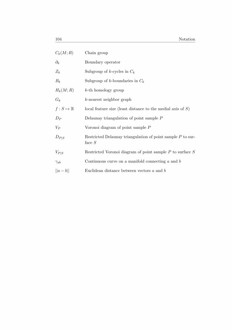
104 Notation
Ck(M ;R) Chain group
∂k Boundary operator
Zk Subgroup of k-cycles in Ck
Bk Subgroup of k-boundaries in Ck
Hk(M ;R) k-th homology group
Gk k-nearest neighbor graph
f : S 7→ R local feature size (least distance to the medial axis of S)
DP Delaunay triangulation of point sample P
VP Voronoi diagram of point sample P
DP |S Restricted Delaunay triangulation of point sample P to sur-
face S
VP |S Restricted Voronoi diagram of point sample P to surface S
γab Continuous curve on a manifold connecting a and b
||a− b|| Euclidean distance between vectors a and b

Zusammenfassung
Wir betrachten das Problem, eine minimale Kreisbasis eines ungerichteten,
Kanten-gewichteten Graphen G mit m Kanten und n Knoten zu berechnen.
Hierbei assoziieren wir mit jedem Kreis einen 0, 1 Inzidenzvektor. Der
Vektorraum uber F2, der durch diese Vektoren erzeugt wird, heißt Kreis-
raum von G. Eine Menge von Kreisen wird als Kreisbasis von G bezeichnet,
wenn sie eine Basis des Kreisraumes von G ist. Eine Kreisbasis heißt min-
imal, wenn die Summe der Gewichte ihrer Kreise minimal ist. Minimale
Kreisbasen werden in vielen Kontexten verwendet, z.B. in der Analyse von
elektrischen Netzwerken und in der Chemie.
Wir prasentieren einen Algorithmus mit Laufzeit O(m2n+mn2 log n) um
eine solche minimale Kreisbasis zu berechnen. Die beste bekannte Laufzeit
war O(mωn), wobei ω der Exponent der Matrix-Multiplikation ist. Zurzeit
bekannt ist, daß ω < 2.376 gilt. Wenn die Kantengewichte ganzzahlig sind,
geben wir einen O(m2n) Algorithmus an. Fur ungewichtete Graphen, die
hinreichend dicht sind, lauft unser Algorithmus in O(mω) Zeit.
Weiterhin entwickeln wir Approximationsalgorithmen fur das Minimale
Kreisbasen Problem. Fur jedes ε > 0 entwickeln wir einen schnellen (1 + ε)-
Approximations Algorithmus. Außerdem, prasentieren wir fur jede ganze
Zahl k ≥ 1 zwei Approximationsalgorithmen, die beide einen Approxima-
tionsfaktor von 2k−1 haben. Der eine hat erwartete Laufzeit O(kmn1+2/k+
mn(1+1/k)(ω−1)) und der andere Laufzeit O(n3+2/k). Fur Graphen, die hin-
reichend dicht sind, sind die Laufzeiten o(mω). Fur spezielle Graphen, wie
planare oder geometrische, prasentieren wir noch schnellere Approximation-
salgorithmen. Unsere Methoden sind auch auf gerichtete Graphen anwend-
bar.
Wir untersuchen das Minimale Kreisbasis Problem ebenfalls aus einer
praktischen Perspektive. Wir beschreiben, wie man den O(m3 +mn2 log n)
Algorithmus von de Pina effizient implementiert. Wir entwickeln verschiedene

106 Zusammenfassung
Heuristiken, die die Laufzeit betrachtlich verbessern. Indem wir die zwei fun-
damental verschiedenen Methoden, eine minimale Kreisbasis zu berechnen,
kombinieren, erhalten wir einen O(m2n2) Algorithmus. Weiterhin vergle-
ichen wir verschiedene Algorithmen anhand von Experimenten.
Schließlich untersuchen wir die minimale Kreisbasis eines”nearest neigh-
bor“ Graphen, der auf eine Stichprobenmenge einer Oberflache im R3 definiert
wird. Wir zeigen, dass unter bestimmten Bedingungen die minimale Kreis-
basis topologische Informationen uber die Oberflache kodiert und Basen der
trivialen und nicht-trivialen Kreise der Oberflache liefert. Wir bestatigen
unsere Ergebnisse anhand von Experimente.

Index
(2k − 1)-approximation
algorithm, 38–50
algebraic framework, 17–24
α-approximation
algorithm, 34–38
α-stretch, see stretch
basis
of trivial cycles, 72
certificate
of optimality, 30
chord, 10
cycle, 8
candidate, 60–62
fundamental, 10
separating, 13
cyclomatic number, 10
deformation, 13, 73
Delaunay, 48, 75–92
Dijkstra’s algorithm, 9, 22, 40, 54
disjoint union
of cycles, 10
edge space, 9
ε-sample, 72–92
locally uniform, 72
(ε, δ)-sample, 72–92
Euler, 91
Gaussian elimination, 17, 60
general position assumption, 75
generators
of non-trivial cycles, 72, 92
genus
of manifold, 13, 72–92
geometric graph, 48
greedy algorithm, 11, 61
heuristic, 53, 88
homeomorphic, 13, 76
homology
basis, 13, 72
shortest, 73
class, 13, 73, 83
cycle, 13
group, 13, 73, 74
simplicial, 13
singular, 13
theory, 12
hybrid algorithm, 61–66
incidence vector, 15, 17, 21, 31, 49
integer weights, 30
k-nearest neighbor graph, 71
LEDA, 51

108 Index
Lipschitz continuous, 75
local feature size, 72–83
loop, 72–92
non-trivial, 72, 73
trivial, 72, 73
lower bound, 38, 83, 93
manifold, 13
compact, 71
smooth, 72
matrix multiplication
fast, 17–32, 66–69
medial axis
of manifold, 72
medial ball, 76
model
non-smooth, 89
NP-complete, 2, 17
orthogonal subspace, 10
planar graph, 47–48, 77, 90
point sample, 71–92
dense, 72
locally uniform, 72, 76
random graph, 52
signed graph, 20, 42, 54, 56
spanner, 39–49
spanning tree, 10, 11, 17, 31, 44
minimum, 39, 68
spring embedder, 90
straight-line drawing, 90
stretch, 35–37, 46, 47
surface, 71
non-smooth, 72
piecewise linear, 72
reconstruction, 89
smooth, 71
torus, 83, 85–92
verification algorithm, 31
vertex space, 9
Voronoi, 75–79
witness, 18, 23, 54