Minimum comparable areas for the period 1872–2010: an ... · dois anos de censo na faixa entre o primeiro e o último censo demográfico 1872-2010

Estud. Econ., São Paulo, vol.47, n.1, p.215-229, jan.-mar. 2017

DOI: http://dx.doi.org/10.1590/0101-416147182phe

Minimum comparable areas for the period 1872–2010: an aggregation of Brazilian municipalities ♦

Philipp EhrlProfessor - Universidade Católica de Brasília Endereço: SGAN 916, Sala A-124, Brasília/DF - CEP: 70790-160 E-mail: [email protected] - https://sites.google.com/site/philippehrl

Submissão: 30/10/2015. Aceite11/10/2016.

AbstractSince the imperial era, the number of municipalities in Brazil has risen continually and substantially. These changes in the delineation of spatial units pose a difficulty for any research that intends to use regional data from different years. The present paper de-velops a routine for the generation of time-consistent ‘Minimum Comparable Areas’ (AMC) for any arbitrary sub-period between two census years in the range between the first and last demographic census 1872–2010. It relies on recently compiled material by the Brazilian Institute for Geography and Statistics (IBGE). The corresponding Stata code is provided in the Appendix of the paper. Thus, the developed AMCs are immediately accessible and enable long-term panel studies with regional data.

KeywordsMinimum Comparable Areas. AMCs. Census of 1872. Brazilian territory.

ResumoDesde a era imperial, o número de municípios no Brasil tem aumentado contínua e substancialmente. Essas mudanças na delimitação das unidades espaciais representam uma dificuldade para qualquer pesquisa que pretenda utilizar dados regionais de dife-rentes anos. O presente artigo desenvolve uma rotina para a geração de “Áreas Mínimas Comparáveis” (AMC) consistentes em tempo para qualquer subperíodo arbitrário entre dois anos de censo na faixa entre o primeiro e o último censo demográfico 1872-2010. Baseia-se em material compilado recentemente pelo Instituto Brasileiro de Geografia e Estatística (IBGE). O código correspondente em Stata é fornecido no Apêndice do artigo. Assim, os AMCs desenvolvidos são imediatamente acessíveis e permitem estudos de painel de longo prazo com dados regionais.

Palavras-ChaveÁreas Mínimas Comparáveis. AMCs. Censo de 1872. Território brasileiro.

Classificação JELR12. N36. B41.

♦ I am grateful to José Angelo Divino, an anonymous referee and seminar participants at the IPEA in Brasília and the UCB for their valuable comments and discussions. Financial support from CAPES is thankfully acknowledged. The Stata code will also be available at https://sites.google.com/site/philippehrl/research


216 Philipp Ehrl

1. Introduction

Panel studies using Brazilian region-specific data encounter a com-mon obstacle. Between the first demographic census in 1872 and the last in 2010, the number of municipalities increased immensely and continually from 642 to 5565. The municipality represents the most disaggregated administrative unit in Brazil. Therefore, everyo-ne who seeks to include economic, demographic or social indicators, which are municipality-specific, in a longitudinal data analysis is constrained to find time-consistent spatial units. The generation of these spatial units becomes more complicated, the longer the analy-zed period and the further it lies in the past. First, problems arise mainly from the data availability of the early census and from the frequent name changes. Second, each municipality existing in 1872 is not simply divided into a subset of new municipalities, but new municipalities are sometimes dismembered from several existing municipalities, or are permanently or temporarily annexed to other municipalities, or border disputes prevail over a long time. These bifurcations in the pedigrees impede that current spatial units are directly reducible to a parent municipality.

The purpose of the present paper is the generation of time-con-sistent regions that allow the construction of panels with munici-pal (or more aggregated regional) data. Such so-called Minimum Comparable Areas (AMC) possess an unambiguous border, which remains unchanged over the period of interest. Due to the ever finer administrative disaggregation of the Brazilian territory, the resulting AMCs differ depending on the period to be investigated. In the present case, the maximum period from the first to the last de-mographic census in Brazil is selected: 1872–2010. The developed method, however, is readily applicable to any other period between two census years. The Stata routine provided in the Appendix in-corporates this flexibility and allows researchers a quick and easy replication of AMCs according to their own demands. To facilitate the application of the generated AMCs and extend its usability to those researchers working with GIS software, shape-files for the most common AMCs are also provided. Since the current version of municipalities’ boarders for which the IBGE provides a shape-file refers to the year 2010, AMC shape-files for all combinations between 2010 and any prior census year are provided online at the journal’s website.

Minimum comparable areas for the period 1872–2010 217


The Brazilian Institute of Geography and Statistics (IBGE, 2011) has recently provided a comprehensive genealogy of municipalities that contains information on all municipalities in all census years. This publication serves as the primary data source in the present procedure and thereby distinguishes itself from previous approaches. The routine developed in the present paper corrects for several in-completenesses and mistakes in the IBGE data and then aggregates municipalities to AMCs in chronological order whenever the bifurca-tions of their pedigrees touch. This is the case, if a new municipality is dismembered from two or more existing municipalities or if two or more municipalities become united. Hence, these origin muni-cipalities are joined to one common AMC and naturally, all other regions that emanate from these municipalities in a later period also become part of the same AMC. In this way, the AMC’s area grows and the number of distinct AMCs in the panel decreases, but ulti-mately, AMCs serve to avoid any problems related to the allocation, comparison etc. of variables that characterize regions.

This paper constitutes a refinement of Reis et al. (2011), who were the first to generate AMCs (for the period 1872–2000) in Brazil. This classification was made available by the Institute of Applied Economic Research (IPEA) and to some researchers it is thus better known as the IPEA AMCs. The idea how AMCs are defined is the same, however, the period, the database and consequently the results are different from the present approach. Reis et al. (2011) use a variety of references, mostly the IBGE, including cartographic ma-terial, especially for the early periods. Apparently, the more recent information in IBGE (2011) is more accurate because it relies on text documents about the genealogy of municipalities and on official data from administrative divisions and the census.1 The number of iden-tified AMCs in Reis et al. (2011) for the period 1872–2000 amou-nts to 432. A higher number of AMCs can be distinguished with the present approach based on the new IBGE data. For 1872–2000, the present methodology yields 485 different AMCs and accounting for the latest developments until 2010, still generates 482 different AMCs. Other shortcomings with the IPEA AMCs, that are resolved here, is that municipalities’ names are provided for each census year so that a matching to any historical census database can be easily conducted. Furthermore, the present approach is flexible and allows

1 The exact extent to which the underlying database in IBGE (2011) differs from Reis et al. (2011) is unfortunately not transparent.


218 Philipp Ehrl

researchers the generation of AMCs for any subperiod between 1872 and 2010.

Silva and Bacha (2011) develop another interesting method for the generation of AMCs. Keeping the territorial division of the start year, the authors propose the creation of Voronoi polygons around existing urban centers to include new dismembered municipalities into these polygons. The advantage is that municipal data can be weighted in the aggregation to the AMC-level so that geographical distances between existing urban centers and new municipalities are taken into account. The application in their paper, however, is restricted to the period 1980–2000 and to regions in the North of Brazil. A limiting factor for an extension of this method to this vast country is the complexity to consider and re-attribute the distribu-tion of all urban settlements in 1872 and 2010. The latter requires the availability of satellite images.

The momentarily developed definition of AMCs is already applied in Ehrl (2016). There, AMCs are the essential basis for the construc-tion of historical instrumental variables to identify agglomeration economies. It turns out that the spatial distribution of liberal and manufacturing professions in the late 19th and early 20th century have a relevant influence on the occupational distribution today. Numerous other papers have previously worked with differently de-fined AMCs. Other studies on the long-term economic development of Brazil that rely on the AMC classification by Reis et al. (2011) are Caselli and Michaels (2013) and Reis (2014). Even studies with a horizon of only ten years and more have to rely on AMCs due to the frequent and large number of changes in the number of Brazilian municipalities, cf. Figure 1 below. Hopefully, these AMCs will also prove to be useful in future cliometric studies and long-term in-vestigations in Brazil. The remainder of the paper is structured as follows. The next section describes the underlying data set and the historical peculiarities which make the generation of AMCs inevi-table. The third section outlines the procedure of the AMC gene-ration. Its complete code for Stata is provided in the Appendix of the paper.



2. Data and background

The starting point for the construction of AMCs is IBGE (2011). It documents the geographical development of the Brazilian territory, its administrative units and resident population therein. The period covered extends over all demographic census, from the first in 1872 to the currently last in 2010. For the reconstruction of the municipal grid, the IBGE apparently relies on the genealogy of municipalities in the period before 1911, IBGE (1959), tables of administrative divisions from 1911 and 1933 as well as information from the pages on the history of municipalities offered by the Federal Ministry of Cities at cidades.ibge.gov.br/. From 1940, the census and statistics on population and geography are already administrated by the IBGE itself.

The initial problem and thus the reason for the developed cons-truction of Minimum Comparable Areas is the enormous increase in the number of municipalities between 1872 and 2010, displayed in Figure 1. As in IBGE (2011), the figure contains the count of municipalities in all available census years. From 1872 to 1900, the population increases significantly in nearly all Federal States and due to this increase in the total population from 9.9 million to 17.4 million the number of municipalities also nearly doubled. The boun-daries of municipalities existing in 1872 are shown in Figure 4 in the Appendix. After 1900, the number of municipalities still increased steadily in each of the more or less 10 years between two demo-graphic census, but the growth rates are lower.2 Between 1950 and 1970, the number of municipalities increases again abruptly. Looking for political self-determination, the number of the smallest autono-mous units more than doubled from 1890 to 3959. Although two decades recorded very low increases, the growth in the number of municipalities to date is unabated. In 2010, their number is already equal to 5565. Not only municipalities but also new Federal States are formed during this period; either by separation, or by political dispute and annexation. Moreover, municipalities frequently chan-ge their names, even in periods when they do not experience any

2 A decree-law (no. 311) from 1938, which is still in force, regulates that a municipality has to have a certain minimum population, a minimum number of constructions, well-defined boundaries and an administrative office within an urban area that has the status of a city. According to IBGE (2011: 16), these rules were exacerbated in an additional law in 1967, which explains the slow increase in the number of municipalities in the years after both changes.


220 Philipp Ehrl

geographic modifications. Municipalities with more than one name in the period 1872–2010 are not the exception but rather the rule.

Figure 1 - Evolution of the number of municipalities over time

Source: IBGE (2011), author’s diagram.

Some more peculiarities in the history of Brazil visible in the data are the following:

• Acre is integrated into Brazilian territory (1903) and becomes a Federal State in 1962.

• The region Amapá was under dispute between Brazil and France and is incorporated into the Brazilian state of Pará (1901).3 It becomes the Federal territory of Amapá in 1943.

• Contentious areas, e.g. the municipality Luís Correia, between the Federal States of Piauí and Ceará (about 1880).

• Ongoing disputes between Portugal and Spain, or respectively later on between Brazil and Argentina, as well as between the Provinces São Paulo and Paraná over the frontiers of several

3 Nevertheless, the region of Amapá is included in the Brazilian Census since its first realiza-tion in 1872, as opposed to the region of Acre.



municipalities (e.g. Joaçaba or Chapecó) located in the South of Brazil.

• Dispute between the Federal States of Espírito Santo and Minas Gerais over the territory of several municipalities (1940s to 1960s).

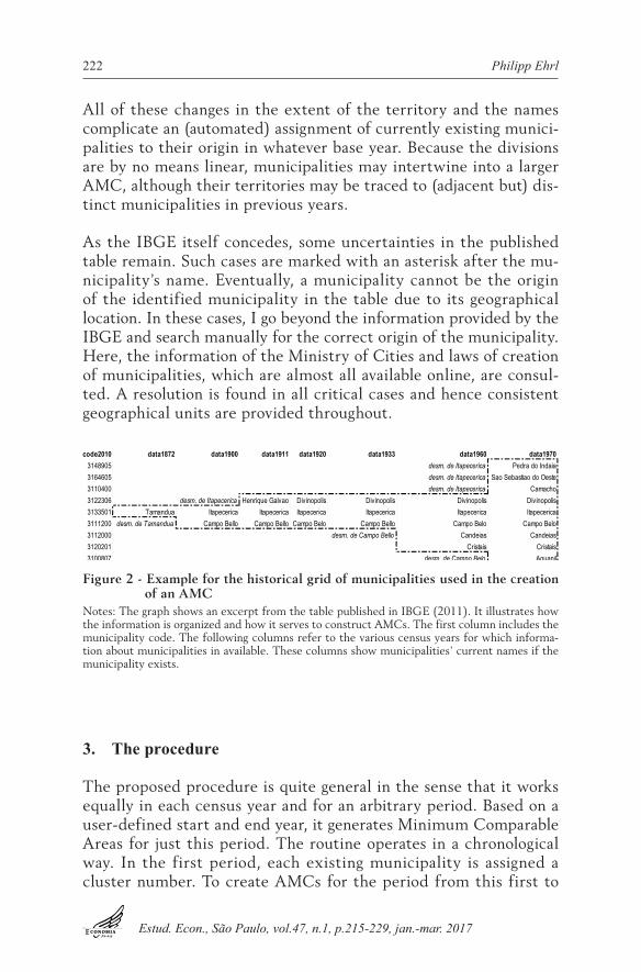
The information published in IBGE (2011) about the genealogy of municipalities and their name changes are also available in the form of a spreadsheet. This table exhibits the names of municipalities and their unique identification code in each line.4 Whereas municipa-lity codes are unique, their names are not.5 At least within Federal States names are required by law to be unique. The columns refer to each year in which a demographic census was conducted. The official code of municipalities corresponds to the currently valid classification, which was defined by the very IBGE. Yet some mu-nicipalities listed in the table cease to exist before 2010. The code of those includes a “999” after the first two digits that refer to the Federal State. Obviously, even those currently non-existing admi-nistrative areas are essential to complete the genealogy of munici-palities. In case a certain municipality exists in one of the Census years, the thereby defined cell of the table contains the current name of the municipality. In case the municipality does not exist, the cell is empty. However, in case a municipality is dismembered from or annexed to other municipalities, those names are provided in the cell to its left, i.e. in the previous census year. For example, the municipality Campo Bello won its autonomy in 1876. As shown in Figure 2, the column of the following census in 1900 contains the name “Campo Bello”, whereas the cell referring to the former census in 1872 contains the information where from Campo Bello was dis-membered. In fact, this displayed evolution of an AMC is quite ‘har-mless’. In the entire table, new municipalities are dismembered from up to five other municipalities. Moreover, some additional notes may also be included in the cells, alongside the municipality’s name (as described in detail in the next section). Since the period between two Census is at least 7 years, it also happens that combinations of annexations and dismemberment can be contained in one cell.

4 For an unknown reason, in some rare cases a municipality has two entries. Fortunately, the information is non-conflicting so that the two lines can be merged.

5 Only about 90% of names are unique in Brazil. The most frequent municipality name is “Bom Jesus” which exists in five different Federal States.


222 Philipp Ehrl

All of these changes in the extent of the territory and the names complicate an (automated) assignment of currently existing munici-palities to their origin in whatever base year. Because the divisions are by no means linear, municipalities may intertwine into a larger AMC, although their territories may be traced to (adjacent but) dis-tinct municipalities in previous years.

As the IBGE itself concedes, some uncertainties in the published table remain. Such cases are marked with an asterisk after the mu-nicipality’s name. Eventually, a municipality cannot be the origin of the identified municipality in the table due to its geographical location. In these cases, I go beyond the information provided by the IBGE and search manually for the correct origin of the municipality. Here, the information of the Ministry of Cities and laws of creation of municipalities, which are almost all available online, are consul-ted. A resolution is found in all critical cases and hence consistent geographical units are provided throughout.

code2010 data1872 data1900 data1911 data1920 data1933 data1960 data19703148905 desm. de Itapecerica Pedra do Indaia3164605 desm. de Itapecerica Sao Sebastiao do Oeste3110400 desm. de Itapecerica Camacho3122306 desm. de Itapecerica Henrique Galvao Divinopolis Divinopolis Divinopolis Divinopolis3133501 Tamandua Itapecerica Itapecerica Itapecerica Itapecerica Itapecerica Itapecerica3111200 desm. de Tamandua Campo Bello Campo Bello Campo Belo Campo Bello Campo Belo Campo Belo3112000 desm. de Campo Bello Candeias Candeias3120201 Cristais Cristais3100807 desm. de Campo Belo Aguanil

Figure 2 - Example for the historical grid of municipalities used in the creation of an AMC

Notes: The graph shows an excerpt from the table published in IBGE (2011). It illustrates how the information is organized and how it serves to construct AMCs. The first column includes the municipality code. The following columns refer to the various census years for which informa-tion about municipalities in available. These columns show municipalities’ current names if the municipality exists.

3. The procedure

The proposed procedure is quite general in the sense that it works equally in each census year and for an arbitrary period. Based on a user-defined start and end year, it generates Minimum Comparable Areas for just this period. The routine operates in a chronological way. In the first period, each existing municipality is assigned a cluster number. To create AMCs for the period from this first to



the subsequent census year, the newly created municipalities du-ring this period are also given a (provisional) cluster number. The assignment of those segregated areas to the previously existing clus-ters is implemented via search and matching of equal municipality names, as suggested in Table 2. If the matching is successful, the cluster numbers of the involved regions as well as of all other muni-cipalities which have same cluster number as the former regions are unified. Due to the many dismemberments and annexations and the problems caused by name changes, multiple sequential repetitions are required in each period until all origins/destinies are assigned and the cluster numbers are equalized.

In the following, the two parts of the AMC generation procedure are laid out. Its complete and commented code is contained in the Appendix of this paper. The code is written for Stata because the software is widespread and its code is relatively easy to understand, albeit it may not be the most efficient way to implement this kind of procedure.

3.1. Preparation of the data set

To preserve clarity, the individual steps of the procedure are numbered and described in note form. These numbers can be re-encountered in the code.

1. Transform the Portuguese accents into simple alphabetic let-ters because Stata cannot display them correctly. Correct spelling of municipality names is essential to perform string matching.

2. Standardize municipality names further, e.g. eliminate super-fluous empty spaces.

3. Reduce information that is given in the cell alongside the name. It is only important to know in each census year whe-ther the municipality is dismembered, annexed, existing or non-existing.

4. Correct typos.


224 Philipp Ehrl

5. Correct inconsistencies that were encountered after or during the preliminary execution of the procedure. Either not all ne-cessary matches could be performed or the result exhibited territorial discontinuities.

6. Account for territorial disputes or inclusion of entirely new areas. On the one hand, some municipalities have their ori-gin outside the Brazilian territory, as in the case of Acre. Consequentially no ‘origin’ can be assigned to them by the procedure. Whether this is problematic depends on the pur-pose of the AMCs but the user needs to be aware of this detail. On the other hand, some municipalities have their ori-gin in another Federal State. Because of the multiple muni-cipality names, the matching procedure is bound to operates only within Federal States, and thus it becomes necessary to align the cluster numbers of those municipalities with chan-ges across States semi-manually right before the end of the code. Until then, these municipalities are treated as if they had no origin.

7. Eliminate the supplement “dismembered from (desmembra-do de)” and “annexed at (anexado a)” in the cells of altered municipalities.

8. Create five new variables (dest1 to dest5) that contain one of the names of the origins/destinies of those altered areas. For existing municipalities, these variables repeat their own name in order to perform the matching.

9. Create a new variable with the number of different origins/destinies, a dummy for ‘original’ municipalities that exist in the start year and a variable that indicates the municipality’s ‘combined’ Federal State.6

6 Recall that some Federal States are only created after 1872. To have a time-consistent clas-sification of Federal States, too, some States need to be combined, e.g. Goiás, Tocantins and Distrito Federal.



3.2. Matching municipalities and equalizing cluster numbers

Having prepared a suitable data set with clean names and auxiliary variables, we are ready to perform the matching between existing and altered municipalities that finally define their inclusion into common AMCs. The description continues the numeration of the steps in the prior sub-section.

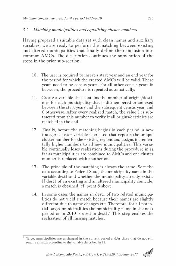
10. The user is required to insert a start year and an end year for the period for which the created AMCs will be valid. These years need to be census years. For all other census years in between, the procedure is repeated automatically.

11. Create a variable that contains the number of origins/desti-nies for each municipality that is dismembered or annexed between the start years and the subsequent census year, and 0 otherwise. After every realized match, the value 1 is sub-tracted from this number to verify if all origins/destinies are matched in the end.

12. Finally, before the matching begins in each period, a new (integer) cluster variable is created that repeats the unique cluster number for the existing regions and assigns incremen-tally higher numbers to all new municipalities. This varia-ble continually loses realizations during the procedure in as far as municipalities are combined to AMCs and one cluster number is replaced with another one.

13. The principle of the matching is always the same. Sort the data according to Federal State, the municipality name in the variable dest1 and whether the municipality already exists. If dest1 of an existing and an altered municipality coincide, a match is obtained, cf. point 8 above.

14. In some cases the names in dest1 of two related municipa-lities do not yield a match because their names are slightly different due to name changes etc. Therefore, for all poten-tial target municipalities the municipality name in the next period or in 2010 is used in dest1.7 This step enables the realization of all missing matches.

7 Target municipalities are unchanged in the current period and/or those that do not still require a match according to the variable described in 11.


226 Philipp Ehrl

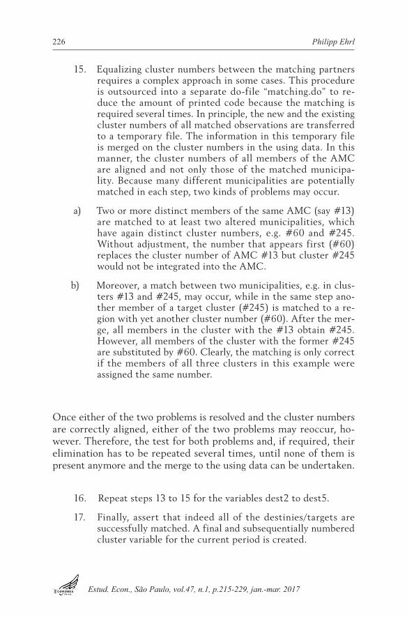
15. Equalizing cluster numbers between the matching partners requires a complex approach in some cases. This procedure is outsourced into a separate do-file “matching.do” to re-duce the amount of printed code because the matching is required several times. In principle, the new and the existing cluster numbers of all matched observations are transferred to a temporary file. The information in this temporary file is merged on the cluster numbers in the using data. In this manner, the cluster numbers of all members of the AMC are aligned and not only those of the matched municipa-lity. Because many different municipalities are potentially matched in each step, two kinds of problems may occur.

a) Two or more distinct members of the same AMC (say #13) are matched to at least two altered municipalities, which have again distinct cluster numbers, e.g. #60 and #245. Without adjustment, the number that appears first (#60) replaces the cluster number of AMC #13 but cluster #245 would not be integrated into the AMC.

b) Moreover, a match between two municipalities, e.g. in clus-ters #13 and #245, may occur, while in the same step ano-ther member of a target cluster (#245) is matched to a re-gion with yet another cluster number (#60). After the mer-ge, all members in the cluster with the #13 obtain #245. However, all members of the cluster with the former #245 are substituted by #60. Clearly, the matching is only correct if the members of all three clusters in this example were assigned the same number.

Once either of the two problems is resolved and the cluster numbers are correctly aligned, either of the two problems may reoccur, ho-wever. Therefore, the test for both problems and, if required, their elimination has to be repeated several times, until none of them is present anymore and the merge to the using data can be undertaken.

16. Repeat steps 13 to 15 for the variables dest2 to dest5.

17. Finally, assert that indeed all of the destinies/targets are successfully matched. A final and subsequentially numbered cluster variable for the current period is created.



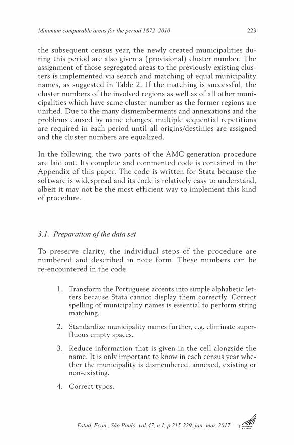
18. Include the next census years and repeat steps 11 to 17, until the procedure for the chosen end years is completed. Figure 3 presents the final result of the delineation of AMCs for the complete period 1872–2010. The bold black lines indicate the frontiers of the AMCs, whereas the thinner lines mark the territory of the current 5565 municipalities. Altogether, 482 AMC can be distinguished. Three of them are located in the current State of Acre. Obviously, the shorter the chosen time span, the more different AMCs can be identified. For example, the period 1872–1950 the procedure yields 538 different AMCs. It is visible that AMCs in the North and center of Brazil are quite large, however, the area of their member municipalities are also far above the average. Note that it is at least possible to distinguish between few AMCs there, whereas the procedure in Reis et al. (2011) yields a single AMC compassing the Federal States Amazonas, Mato Grosso, Mato Grosso do Sul and Rondônia. The obvious re-semblance between the shape of the AMCs and the muni-cipalities in 1872, displayed in Figure 4 in the Appendix, is striking and reassuring that the assignment is correct. A general observation is that with increasing distance to the sea, the surface of the AMCs and municipalities therein also increases, which certainly reflects the colonization scheme of Brazil.

The municipality codes are generated by the IBGE so that the first two digits represent the Federal State, the following four digits serve to identify the municipality in alphabetic order and the last is a con-trol number based on the prior digits (IBGE 2011). In analogy to this pattern, the AMCs are assigned a 5-digit code, where the first two also refer to the (combined) Federal State(s). Because most AMCs are composed of several municipalities, the one with the lowest code in each AMC is selected and these municipalities are sorted in as-cending order in each Federal State. This ranking is equal to the last three digits of the AMCs’ unique and invariable code. A data set with this final AMC classification, the current code of munici-palities, as well as the identifier for the municipalities in the census from 1872 are available upon request from the author.


228 Philipp Ehrl

Figure 3 - Delineation of AMCs and municipalities 1872–2010

Notes: The figure shows the territory of Brazil to date. The fine lines indicate the boarders of the municipalities in the year 2010, whereas the bold lines mark the frontiers of the aggregated Minimum Comparable Areas (AMCs) for the period 1872–2010. Source of the GIS delineation: IBGE.

Bibliography

CASELLI, F. and MICHAELS, G. Do oil windfalls improve living standards? Evidence from Brazil. American Economic Journal: Applied Economics, 5(1), 208-238, 2013.

EHRL, P. Agglomeration economies over 40 years in Brazil. Mimeo, 2016.IBGE. Enciclopédia dos municípios brasileiros, vol. XXVI. IBGE: Rio de Janeiro, 1959.— Evolução da divisão territorial do Brasil 1872–2010. IBGE: Rio de Janeiro, 2011.REIS, E. Spatial income inequality in Brazil, 1872–2000. Economia, 15 (2), 119–140, 2014.—, PIMENTEL, M., ALVARENGA, A. I. and dos SANTOS M. C. H. Áreas mínimas comparáveis para os

períodos intercensitários de 1872 a 2000. In 1o Simpósio Brasileiro de Cartografia histórica, 2011.SILVA, R. R. d. and BACHA, C. J. C. Polígonos de Voronoi como alternativa aos problemas das Áreas

Mínimas Comparáveis: uma análise das mudanças populacionais na região Norte do Brasil. Revista Brasileira de Estudos de População, 28 (1), 133–151, 2011.



Appendices

A. Additional figures

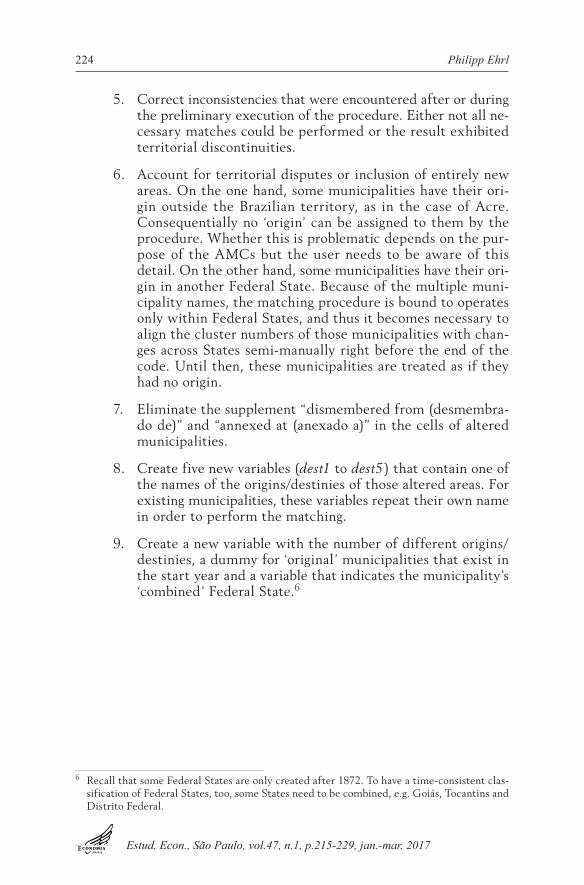
Figure A.1 - Map of the municipal division in 1872

Source: IBGE (2011).

Documents

Minimum comparable areas for the period 1872–2010: an ... · dois anos de censo na faixa entre o primeiro e o último censo demográfico 1872-2010