Minimizing Manufacturing and Quality Costs in ... · Minimizing Manufacturing and Quality Costs in ... account all measures of quality ... Minimizing Manufacturing and Quality Costs

Minimizing Manufacturing and Quality Costs in Multiresponse OptimizationJose L. D. Ribeiro ([email protected]), Flavio S. Fogliatto ([email protected]), arla S. ten Caten, ([email protected])Industrial Engineering & Transportation Dept, Universidade Federal do Rio Grande do Sul, Praca Argentina, 9 / Sala LOPP, Porto Alegre, RS,Brazil. Phone: 55 51 316-4005. FAX: 55 51 316-4007.

Minimizing Manufacturing and Quality Costs inMultiresponse Optimization

Jose Luis Duarte Ribeiro, Dr.([email protected])

Flavio S. Fogliatto, Ph.D.Carla S. ten Caten, M.Sc.

Department of Industrial & Transportation EngineeringUniversidade Federal do Rio Grande do Sul

Praça Argentina, 9 / Sala LOPP - Porto Alegre – RS - Brazil

Abstract

Most industrial processes and products are evaluated by more than one quality

characteristic. To select the best design and operating control factors it is necessary to take into

account all measures of quality simultaneously, in what is known as multiresponse optimization.

Determination of the best operational settings for products or processes is usually

accomplished through single-objective function optimization routines. Here we propose a

new objective function for multiresponse optimization, based on Taguchi’s loss function.

Our function innovates in taking into account manufacturing and quality-related costs in the

optimization, in addition to the usual criteria of minimum response variance and distance-to-

target, and maximum robustness. We also propose a simplified procedure for modeling the

variance of responses from non-replicated factorial designs. The paper contains a case study

from the rubber industry.


2

Introduction

In many experiments it is important to evaluate the same experimental unit with respect

to more than one response. Such experiments are known as multiresponse experiments and are

used in the development and improvement of industrial processes and products. Responses are

measured from experimental units obtained by testing different combination of levels for the

control factors. Ultimately, we want to determine the best control factors settings such that

responses present some desired properties; for example, small distance-to-target and variance.

Determining such settings is ordinarily done using single objective-function optimization

routines. Thus, a central problem in the analysis of multiresponse experiments is finding a

suitable objective function that combines several responses as well as relevant information

related to them.

A number of authors have suggested utility functions that may be used as objective

functions in the optimization of multiresponse experiments. Approaches in the literature may be

arranged in three groups: (i) response surface methodology approaches, including the works of

Lind et al. [1], Myers & Carter [2], Biles [3], Myers et al. [4], Myers & Montgomery [5], Del

Castillo [6], and Kim & Lin [7]; (ii) approaches based on the desirability function, including the

works of Harrington [8], Derringer & Suich [9], Chang & Shivpuri [10], Del Castillo et al. [11],

and Fogliatto et al. [12]; and (iii) approaches based on Taguchi’s Robust Design theory,

including the works of Khuri & Conlon [13], León et al. [14], Logothetis & Haigh [15], Tribus

& Szonyl [16], Yum & Ko [17], Raiman & Case [18], Elsayed & Chen [19], Pignatiello [20],

Ribeiro & Elsayed [21], León [22], and Vinning [23].

Typical criteria in multiresponse optimization include: (i) distance-to-target of response

outcomes, (ii) response variance, (iii) sensitivity of the response to small variations in the


3

settings of the control factors, and (iv) inaccuracy of prediction. All criteria are to be minimized

in the optimization. Criterion (ii) is recommended in cases where the variance of responses can

be described as a function of the experimental control factors. Criterion (iii) is useful when

experiments are carried out in pilot plants or labs to be eventually scaled up. Criterion (iv)

captures the variability in the responses adjusted for how well they can be predicted, given the

experiment performed to estimate the parameters in the prediction model.

All optimization criteria above relate to responses and their desired properties. However,

in several experimental setups a response close to target or with small variance may imply in

unacceptable manufacturing costs. Such costs relate to raw-material, labor, energy, etc. Typical

examples are mixture experiments, where high usage of a given ingredient may result in

undesirable costs. Some utility functions, like those based on Taguchi, search for control factor

settings that minimize costs due to poor quality. Our objective is to search for an optimum that

results in both low quality and low manufacturing costs.

In this paper we extend the quadratic loss function presented in Ribeiro & Elsayed [21] to

include minimum manufacturing costs as an optimality criterion in multiresponse optimization.

We also suggest a new assessment of the quality loss (or proportionality) coefficient in the loss

function. The extended quadratic loss function is explored on a case from the rubber industry.

We also suggest a simplified approach for modeling the variance of responses in non-

replicated factorial experiments. Variance modeling typically requires experiments with several

replications, which is often economically infeasible in practice. Approaches in the literature use

either information from replicates [24], [25], residuals from response models [26], [27], or mixed

response models with noise generated through simulation [28], [29]. Our approach for modeling

the variance of a response uses the residuals from the regression model for the response mean


4

and does not require replications of experimental treatments. The approach suggested here may

be viewed as a simplified version of the one in Box & Meyer [30], although developed

independently.

Finally, we present a five-step procedure for multiresponse optimization and apply it to

the case study data. The proposed steps are: (i) problem identification; (ii) experiment planning

and execution; (iii) individual modeling of response mean and variance; (iv) choice of utility

function and optimization criteria; (v) optimization proper. Steps (i) – (iii) cover early stages of

experimentation and relate mostly to data gathering. Steps (iv) and (v) are directly related to

multiresponse optimization.

In the case study we present here a rubber mixture is to be optimized. Control factors to

be adjusted are process parameters and some ingredients in the mixture. Samples from

experimental treatments are evaluated with respect to ten response variables. Treatments are not

replicated. Optimization goals include: (i) minimization of costs due to poor quality, and (ii)

minimization of manufacturing costs. Criteria considered in (i) include response distance-to-

target, variance, and sensitivity to fluctuations in the settings of the control factors. Criteria

considered in (ii) include raw-material and energy costs.

The rest of this paper is organized as follows. In the next section we present the

quadratic loss function extended to handle manufacturing costs; we also give the details of the

proposed calculation of the proportionality coefficient in the loss function. The third section

presents the approach for variance modeling in non-replicated experiments. The fourth section

gives the procedure steps for multiresponse optimization, which are illustrated by the case study.

A Conclusion closes the paper in the last section.


5

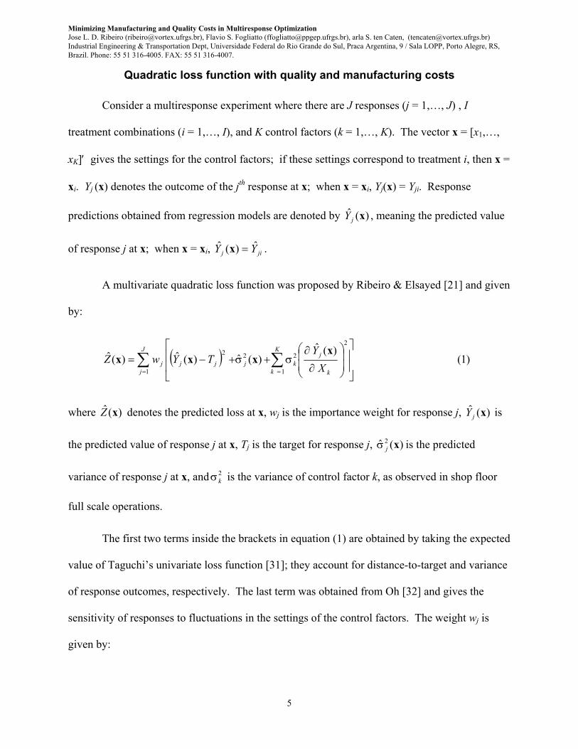
Quadratic loss function with quality and manufacturing costs

Consider a multiresponse experiment where there are J responses (j = 1,…, J) , I

treatment combinations (i = 1,…, I), and K control factors (k = 1,…, K). The vector x = [x1,…,

xK]′ gives the settings for the control factors; if these settings correspond to treatment i, then x =

xi. Yj (x) denotes the outcome of the jth response at x; when x = xi, Yj(x) = Yji. Response

predictions obtained from regression models are denoted by )(ˆ xjY , meaning the predicted value

of response j at x; when x = xi, jij YY ˆ)(ˆ =x .

A multivariate quadratic loss function was proposed by Ribeiro & Elsayed [21] and given

by:

( )

∂

∂σ+σ+−= ∑∑

==

K

k k

jkjjj

J

jj X

YTYwZ

1

2

222

1 )(ˆ

)(ˆ)(ˆ)(ˆ xxxx (1)

where )(ˆ xZ denotes the predicted loss at x, wj is the importance weight for response j, )(ˆ xjY is

the predicted value of response j at x, Tj is the target for response j, )(ˆ 2 xjσ is the predicted

variance of response j at x, and 2kσ is the variance of control factor k, as observed in shop floor

full scale operations.

The first two terms inside the brackets in equation (1) are obtained by taking the expected

value of Taguchi’s univariate loss function [31]; they account for distance-to-target and variance

of response outcomes, respectively. The last term was obtained from Oh [32] and gives the

sensitivity of responses to fluctuations in the settings of the control factors. The weight wj is

given by:


6

2j

jj E

RIw

∆=

where RIj denotes the relative importance of response j and ∆Ej represents one half of the

interval formed by the specification limits for response j. A procedure for determining RIj is

given in the case study section.

Equation (1) provides dimensionless loss values proportional to the low quality in the

product or process under study. In our method, loss values must be converted to dollar values.

For that purpose, a proportionality constant p must be determined. As originally proposed by

Taguchi, p gives the dollar value corresponding to one unit of loss, and is determined using

expert opinion [Taguchi et al. (31)]. We now suggest a simplified procedure for assessing p.

The key to our procedure is establishing the market value of products under extreme

conditions for the set of quality characteristics (QCs). The idea is intuitive: product quality

varies according to how QCs comply to given specifications. A product with a QC beyond spec

limits may be rated “class B” and given a lower market price. Analogously, a product with all

QCs close to target may be rated “class A” and given a premium market price. By determining

two such classes of a product and their respective market values, we are able to find a realistic

measure of the proportionality constant p.

Consider, for example, a class A product rated according to readings ( AAA yyy 321 ˆ,ˆ,ˆ ) of

three QCs (j = 1,2,3); from appropriate substitutions in equation (1), we obtain a loss value of

AZ . A class B product is characterized by readings ( BBB yyy 321 ˆ,ˆ,ˆ ) of the same QCs, with a

predicted loss value of BZ . Market prices are $A and $B for class A and class B products,

respectively. The proportionality constant p is then given by:


7

)ˆˆ()$($$

BA ZZBA

Zp

−−

==∆∆ . (2)

Upon determining p, the predicted loss )(ˆ xZ at a certain control factor setting x may be

converted to dollar values as follows:

)(ˆ)(ˆ xx ZpCQ ×= (3)

where CQ represents the monetary cost of poor quality.

We now want to incorporate manufacturing costs in our search for the best control factors

settings. Start by computing relevant manufacturing costs (e.g., raw material and energy costs)

at each treatment combination. Next, build a regression model relating control factors and

manufacturing costs. Coefficients may be found deterministically. The general form of the

model is:

uXx +β=)(MC , (4)

where CM(x) denotes manufacturing costs at x, X is the (I × R) information matrix of regressors

with R indicating the number of regressors, including the intercept, in the model, β is a (R × 1)

vector of regression coefficients, and u is a (I × 1) vector of residuals (when β is found

deterministically, u = 0). Predictions from equation (4) are denoted by )(ˆ xMC .

An extended multivariate loss function to include manufacturing and poor quality costs is

obtained by adding equations (3) and (4); i.e.,

)(ˆ)(ˆ)(ˆ xxx MQ CCC += (5)

where )(ˆ xC denotes the overall costs incurred by running a process or manufacturing a product


8

under conditions given by x. The objective function in equation (5) is always to be minimized.

A simplified approach to variance modeling

An overview of our approach to variance modeling is as follows. Consider a factorial

experiment with factors at l levels and no replicates. That is a very common situation, since

replication of treatments is usually costly and frequently not performed in practice. Suppose we

determine a regression model relating outcomes of a response j to levels of the control factors;

only significant terms are included in the model. Using predictions from the model, we

determine residuals at each treatment (i.e., difference between predicted and actual outcomes of

j). The residuals give a measure of the variance in the experiment that could not be explained by

the regression model. We want to check if residuals within a given level of a control factor

differ significantly from those at other levels; when that is the case, response variance, as given

by the residuals, may be considered to be a function of that factor.

There are six steps for determining regression models for the variance of a response j:

1. Determine a regression model relating outcomes of response j to experimental control

factors.

2. For a given control factor k plot the residuals at extreme levels and inspect for noticeable

differences; when that is the case, proceed to step 3; otherwise, no model for the variance of

j is likely to be attainable.

3. Compute the sample variances for the residuals at each extreme level of k; say 2)1(, −ks and

2)1(, +ks . We want to test the null hypothesis Ho: variances are the same at extreme levels of k.

For that purpose, an F-test is performed, as follows [33]:


9

2)(,

2)(,

bk

sk

ss

F = ,

for a pair of extreme levels s and b of k (s ≠ b), using the greater of the two variance ratios.

Whenever F ≥ Fα/2, variances are not the same at the two levels (use α ≤ 0.05) and should be

modeled as a function of control factor k. Repeat steps 2 and 3 for all K control factors.

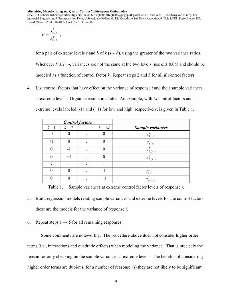
4. List control factors that have effect on the variance of response j and their sample variances

at extreme levels. Organize results in a table. An example, with M control factors and

extreme levels labeled (-1) and (+1) for low and high, respectively, is given in Table 1.

Control factorsk =1 k = 2 … k = M Sample variances-1 0 … 0 2

)1(,1 −s+1 0 … 0 2

)1(,1 +s0 -1 … 0 2

)1(,2 −s0 +1 … 0 2

)1(,2 +s

0 0 … -1 2)1(, −Ms

0 0 … +1 2)1(, +Ms

Table 1. Sample variances at extreme control factor levels of response j.

5. Build regression models relating sample variances and extreme levels for the control factors;

these are the models for the variance of response j.

6. Repeat steps 1 → 5 for all remaining responses.

Some comments are noteworthy. The procedure above does not consider higher order

terms (i.e., interactions and quadratic effects) when modeling the variance. That is precisely the

reason for only checking on the sample variances at extreme levels. The benefits of considering

higher order terms are dubious, for a number of reasons: (i) they are not likely to be significant


10

in practice; (ii) estimates of higher order terms require a large number of data points, which are

not usually available from factorial designs; and (iii) considering higher order terms would

require a more complex model fitting procedure, which is not our objective.

As previously mentioned, the approach above is similar to the one in Box & Meyer [30]

although developed independently. There are two main differences: (i) Box & Meyer provide

means to incorporate interactions in the variance models; and (ii) determination of significant

terms to be included in models is performed visually, through probability plots. Also, their

approach is restricted to 2k factorial designs.

Steps for multiresponse optimization – a case study

There are five steps to optimizing multiresponse experiments; they are: (i) problem

identification; (ii) experiment planning and execution; (iii) modeling of response mean and

variance; (iv) choice of utility function and optimization criteria; (v) optimization proper.

Those steps are briefly introduced in the sections that follow, and illustrated using case study

data.

The case study involves a rubber product used as raw-material in the manufacturing of

automobile tires. The product is manufactured at a chemical plant located in Brazil. The current

formulation is based on specifications defined by clients. The experiment includes twenty-seven

treatments consisting of product made with different formulations and under different processing

conditions. Some of the ingredients are sulfur, synthetic rubber, and carbon black. Processing

conditions relate to the total mixing time. The treatments are evaluated with respect to ten

response variables; some responses are density, rheology measures (such as t10, t90 and MH),

and hardness. Treatments are also evaluated regarding manufacturing costs. The goal is to find


11

settings for the control factors that yield a low cost product with QCs closest to target, with

minimum variance and sensitivity. In what follows, control factors and response variables are

not identified to preserve confidentiality.

A. Problem Identification

Problem identification comprises information gathering on relevant response variables

and control factors. In practice, listing of responses and control factors is not a complex task.

However, choosing responses that reflect QCs relevant to customers and control factors that are

most likely to affect responses is not trivial; that requires a group of individuals knowledgeable

about the product or process under study.

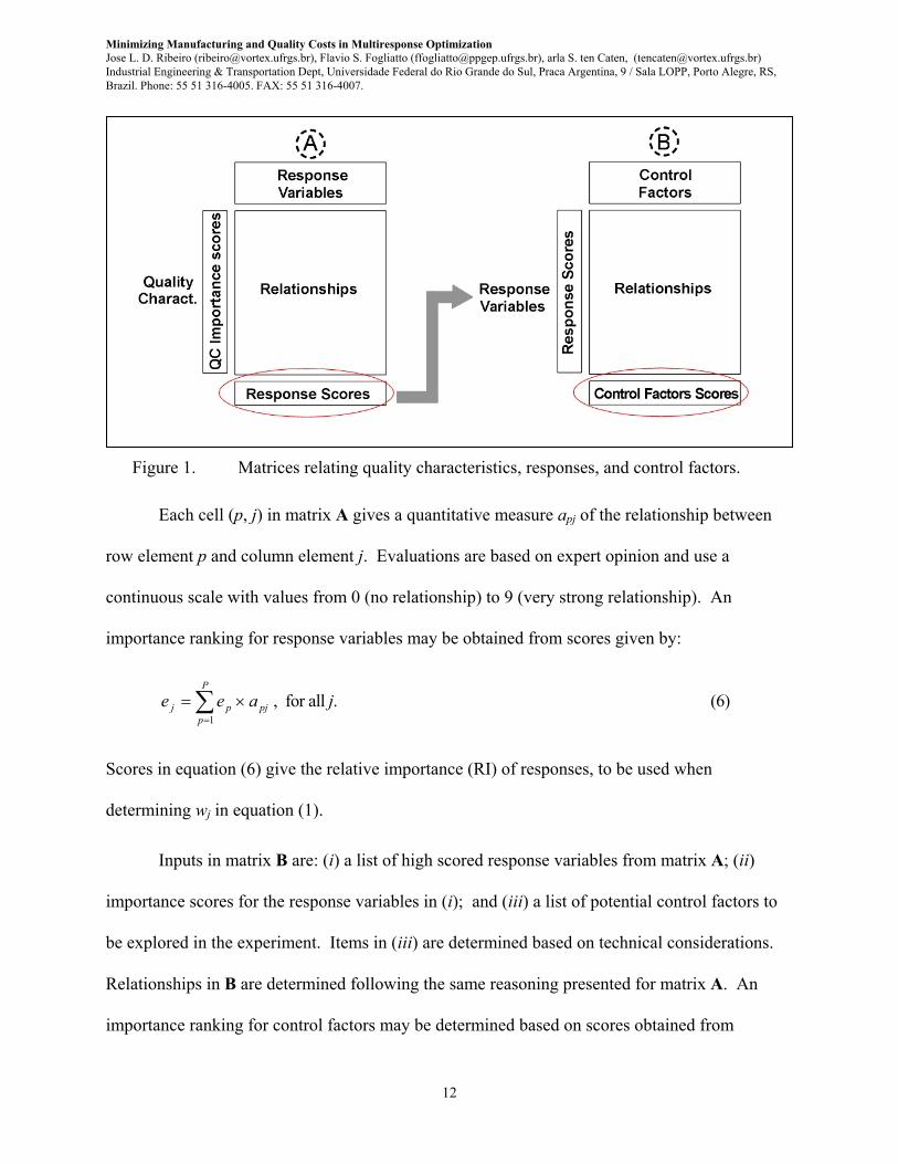
We propose a scheme for prioritizing responses and control factors based on Quality

Function Deployment principles [34, 35]; that is summarized in Figure 1. There are two

matrices in Figure 1. Matrix A relates QCs and response variables; matrix B relates response

variables and control factors.

There are three main inputs in matrix A: (i) a list of P QCs (p = 1,…,P); (ii) importance

scores ep for items in (i); and (iii) a list of J potential response variables (j = 1,…,J) to be

measured in the experiment. The list in (i) should reflect customer’s expectations about the

product or process, and may be developed from joint efforts of a multifunctional team.

Importance scores in (ii) are based mostly on expert opinion; decision analysis methods such as

Saaty’s Analytic Hierarchy Process [36] may be helpful in establishing these scores. Items in

(iii) correspond to measurable variables likely to describe QCs in (i); they are determined from

technical considerations. Elements in (i) and (ii) are written in the rows of A; elements in (iii)

are written in the columns of A.


12

Figure 1. Matrices relating quality characteristics, responses, and control factors.

Each cell (p, j) in matrix A gives a quantitative measure apj of the relationship between

row element p and column element j. Evaluations are based on expert opinion and use a

continuous scale with values from 0 (no relationship) to 9 (very strong relationship). An

importance ranking for response variables may be obtained from scores given by:

∑=

×=P

ppjpj aee

1, for all j. (6)

Scores in equation (6) give the relative importance (RI) of responses, to be used when

determining wj in equation (1).

Inputs in matrix B are: (i) a list of high scored response variables from matrix A; (ii)

importance scores for the response variables in (i); and (iii) a list of potential control factors to

be explored in the experiment. Items in (iii) are determined based on technical considerations.

Relationships in B are determined following the same reasoning presented for matrix A. An

importance ranking for control factors may be determined based on scores obtained from


13

equation (6) and the information in matrix B.

The choice of responses and control factors to be considered in the experiment is based

on their importance scores, as given in matrices A and B above. For each selected response list:

(a) relative importance; (b) type (larger-is-best, smaller-is-best or nominal-is-best); (c) current

observed value (if any); (d) target value; and (e) specification limits. For each selected control

factor list: (a) current setting (if any); (b) allowable setting interval; and (c) flexibility (indicates

difficulty in changing settings of a control factor).

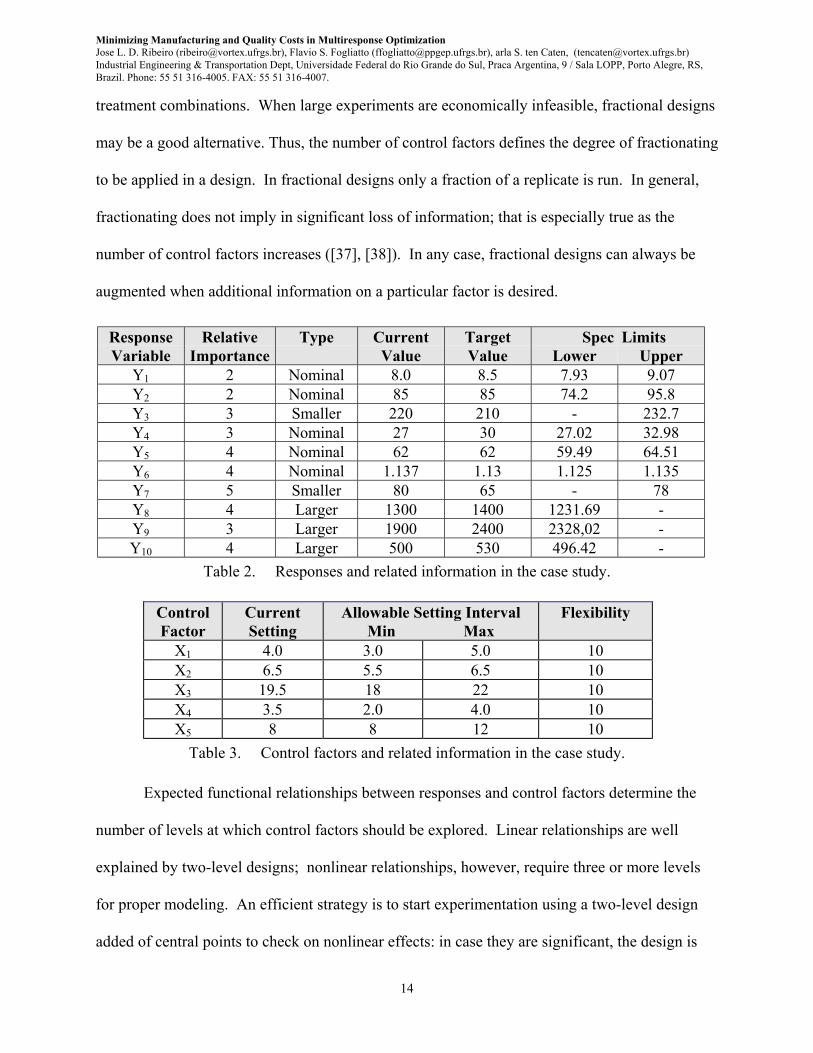
Table 2 gives the responses selected in the case study and related information. Relative

importance values in that table where obtained from a matrix similar to matrix A in Figure 1 and

normalized to a [0,5]-scale with values rounded up to the next integer. For smaller-is-best

(larger-is-best) responses, targets correspond to threshold values from which any smaller (larger)

values are equally desirable and correspond to a zero loss situation.

Table 3 gives the control factors selected in the case study and related information.

Flexibility is measured in a [0, 10]-scale, where 10 denotes a control factor easily adjustable.

B. Experiment Planning and Execution

This section explores technical aspects to be considered when choosing an experimental

design. Since the actual choice of design depends on each particular experimental setup, we

restrict ourselves to providing general guidelines. Three main criteria direct the choice of

experimental design; they are: (i) number of control factors; (ii) functional relationship between

responses and control factors; and (iii) control factor flexibility.

A large number of control factors leads to experiments where many treatment

combinations must be tested. For example, testing 5 factors at two levels each results in 32


14

treatment combinations. When large experiments are economically infeasible, fractional designs

may be a good alternative. Thus, the number of control factors defines the degree of fractionating

to be applied in a design. In fractional designs only a fraction of a replicate is run. In general,

fractionating does not imply in significant loss of information; that is especially true as the

number of control factors increases ([37], [38]). In any case, fractional designs can always be

augmented when additional information on a particular factor is desired.

ResponseVariable

RelativeImportance

Type CurrentValue

TargetValue

SpecLower

LimitsUpper

Y1 2 Nominal 8.0 8.5 7.93 9.07Y2 2 Nominal 85 85 74.2 95.8Y3 3 Smaller 220 210 - 232.7Y4 3 Nominal 27 30 27.02 32.98Y5 4 Nominal 62 62 59.49 64.51Y6 4 Nominal 1.137 1.13 1.125 1.135Y7 5 Smaller 80 65 - 78Y8 4 Larger 1300 1400 1231.69 -Y9 3 Larger 1900 2400 2328,02 -Y10 4 Larger 500 530 496.42 -

Table 2. Responses and related information in the case study.

ControlFactor

CurrentSetting

Allowable Setting IntervalMin Max

Flexibility

X1 4.0 3.0 5.0 10X2 6.5 5.5 6.5 10X3 19.5 18 22 10X4 3.5 2.0 4.0 10X5 8 8 12 10

Table 3. Control factors and related information in the case study.

Expected functional relationships between responses and control factors determine the

number of levels at which control factors should be explored. Linear relationships are well

explained by two-level designs; nonlinear relationships, however, require three or more levels

for proper modeling. An efficient strategy is to start experimentation using a two-level design

added of central points to check on nonlinear effects: in case they are significant, the design is


15

expanded to contemplate three levels of each control factor; for details, see Myers &

Montgomery [5].

Control factor flexibility determines the degree of restriction on randomization. Flexible

control factors are easily adjustable, with levels that may be completely randomized when

running the experiment. Inflexible control factors are difficult to adjust and will be better held in

blocked or split-plot designs. Consider the importance scores for the control factors determined

from the approach in Figure 1. A low-scored inflexible control factor may be efficiently

explored if confounded with blocks in a blocked design. A high-scored inflexible control factor

will be better treated in a split-plot design; for details, see Hicks [38].

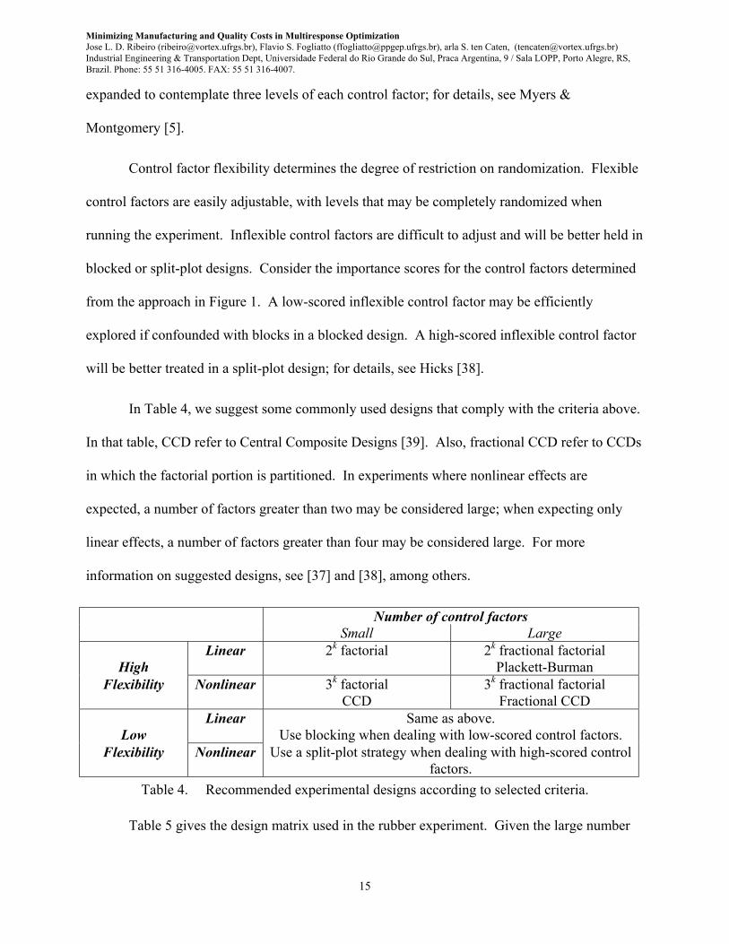
In Table 4, we suggest some commonly used designs that comply with the criteria above.

In that table, CCD refer to Central Composite Designs [39]. Also, fractional CCD refer to CCDs

in which the factorial portion is partitioned. In experiments where nonlinear effects are

expected, a number of factors greater than two may be considered large; when expecting only

linear effects, a number of factors greater than four may be considered large. For more

information on suggested designs, see [37] and [38], among others.

Number of control factorsSmall Large

HighLinear 2k factorial 2k fractional factorial

Plackett-BurmanFlexibility Nonlinear 3k factorial

CCD3k fractional factorial

Fractional CCD

LowLinear Same as above.

Use blocking when dealing with low-scored control factors.Flexibility Nonlinear Use a split-plot strategy when dealing with high-scored control

factors.Table 4. Recommended experimental designs according to selected criteria.

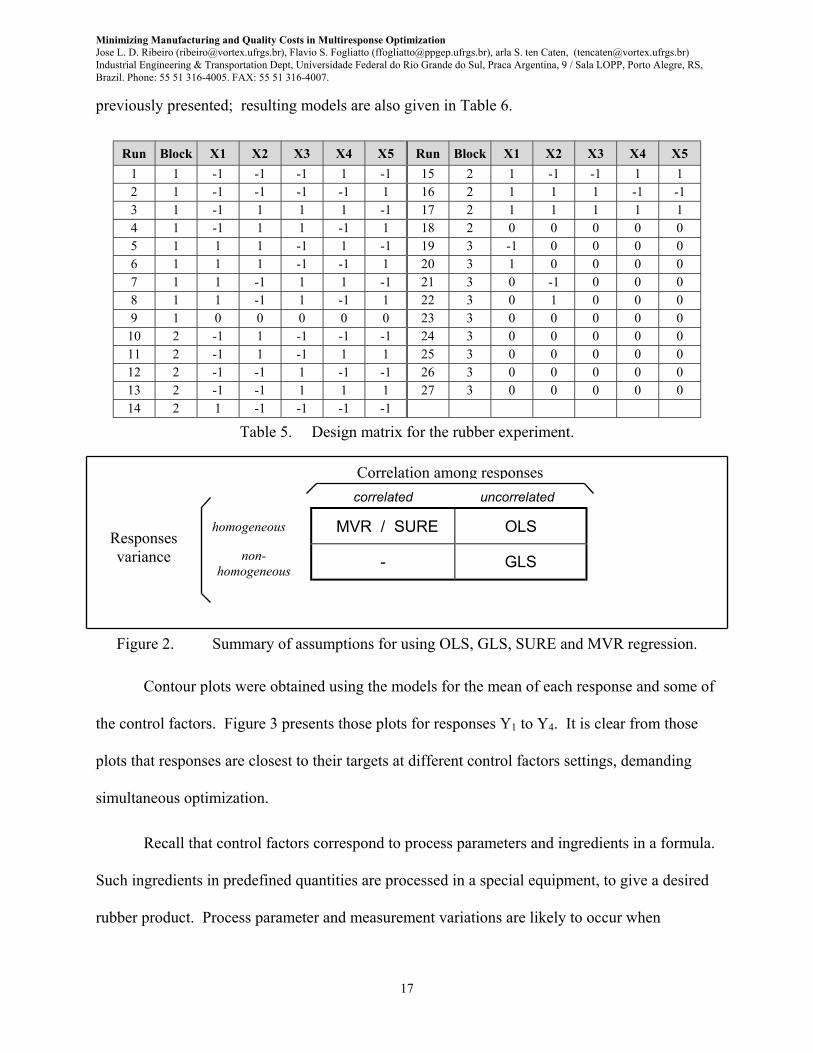
Table 5 gives the design matrix used in the rubber experiment. Given the large number


16

of factors, high control factor flexibility and possibility of nonlinear effects, a fractional CCD

was chosen. The experiment was run in three blocks. The first two blocks (eighteen

experimental runs) correspond to a 25-1 fractional factorial with two center points added to check

on nonlinear effects, which resulted significant. According to technicians knowledgeable about

the product, only control factors X1 and X2 could present nonlinear effects. Runs 24 to 27

correspond to the star portion of a CCD with two factors (α = 1); they were run in a third block

with five additional center points (runs 19 to 23). Notice that factors X3, X4, and X5 were held at

center values in the second block. Runs were randomized within each block.

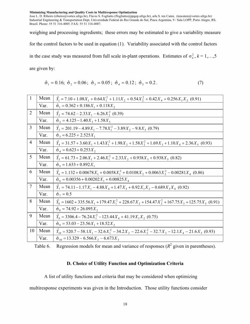
C. Modeling of response mean and variance

We want to develop regression models for the mean and variance of responses, using an

appropriate modeling technique. There are four regression techniques available in the literature,

each related to a different set of assumptions; they are: OLS (ordinary least squares regression),

GLS (generalized least squares), MVR (multivariate regression), SURE (seemingly unrelated

equations regression). OLS and GLS model responses individually; MVR and SURE model

responses simultaneously. Choice of technique is driven by the degree of correlation among

responses and homogeneity of responses variance. A summary of the assumptions for using

each technique is given in Figure 2; these techniques are presented and compared in the context

of multiresponse optimization in Fogliatto & Albin [40].

Although not correlated among themselves, all but one of the responses in Table 2

presented non-homogeneous variances. Thus, GLS regression was used for modeling the means

of responses, with weights given by the reciprocal of the predicted variances at each treatment.

Resulting models are given in Table 6. Variance modeling followed the simplified approach


17

previously presented; resulting models are also given in Table 6.

Run Block X1 X2 X3 X4 X5 Run Block X1 X2 X3 X4 X51 1 -1 -1 -1 1 -1 15 2 1 -1 -1 1 12 1 -1 -1 -1 -1 1 16 2 1 1 1 -1 -13 1 -1 1 1 1 -1 17 2 1 1 1 1 14 1 -1 1 1 -1 1 18 2 0 0 0 0 05 1 1 1 -1 1 -1 19 3 -1 0 0 0 06 1 1 1 -1 -1 1 20 3 1 0 0 0 07 1 1 -1 1 1 -1 21 3 0 -1 0 0 08 1 1 -1 1 -1 1 22 3 0 1 0 0 09 1 0 0 0 0 0 23 3 0 0 0 0 0

10 2 -1 1 -1 -1 -1 24 3 0 0 0 0 011 2 -1 1 -1 1 1 25 3 0 0 0 0 012 2 -1 -1 1 -1 -1 26 3 0 0 0 0 013 2 -1 -1 1 1 1 27 3 0 0 0 0 014 2 1 -1 -1 -1 -1

Table 5. Design matrix for the rubber experiment.

MVR / SURE OLS

- GLS

Figure 2. Summary of assumptions for using OLS, GLS, SURE and MVR regression.

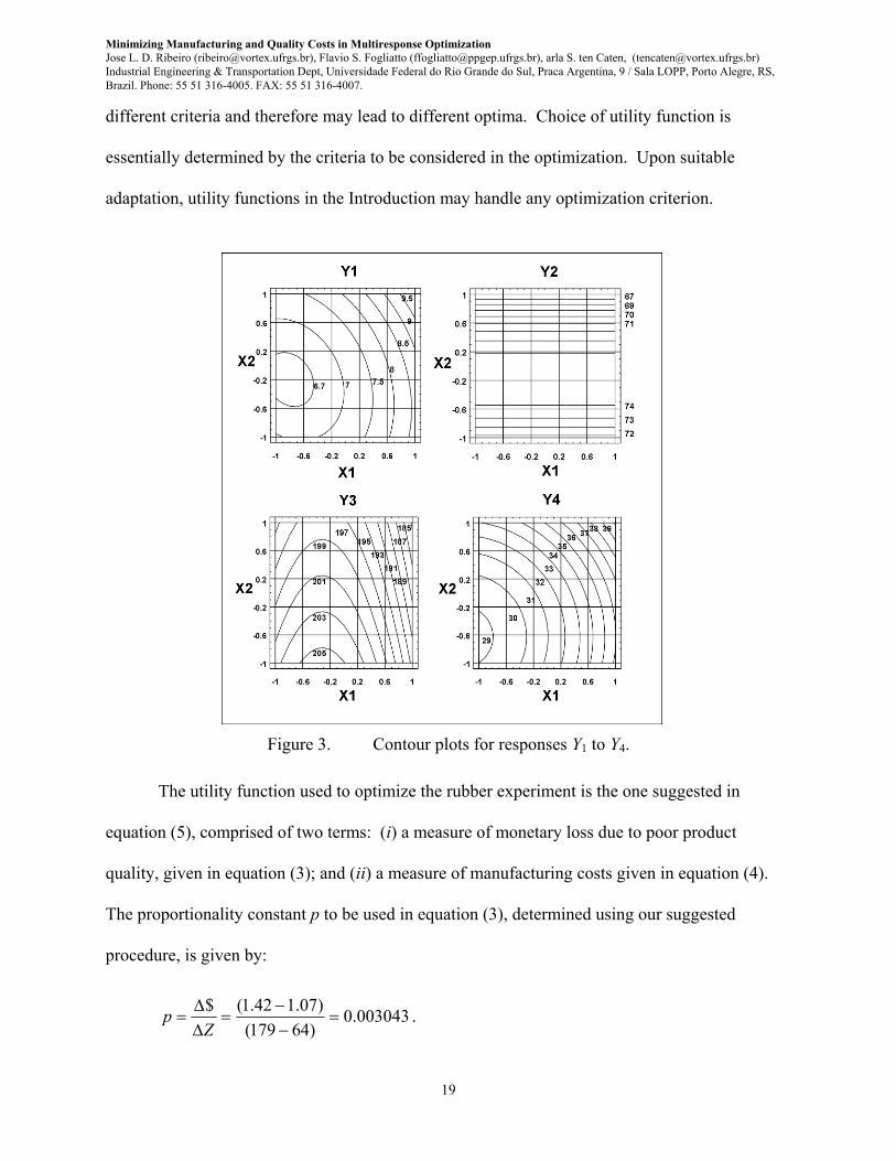
Contour plots were obtained using the models for the mean of each response and some of

the control factors. Figure 3 presents those plots for responses Y1 to Y4. It is clear from those

plots that responses are closest to their targets at different control factors settings, demanding

simultaneous optimization.

Recall that control factors correspond to process parameters and ingredients in a formula.

Such ingredients in predefined quantities are processed in a special equipment, to give a desired

rubber product. Process parameter and measurement variations are likely to occur when

homogeneous

non-homogeneous

Responsesvariance

correlated uncorrelated

Correlation among responses


18

weighing and processing ingredients; these errors may be estimated to give a variability measure

for the control factors to be used in equation (1). Variability associated with the control factors

in the case study was measured from full scale in-plant operations. Estimates of 2kσ , k = 1,…,5

are given by:

;16.0ˆ 1 =σ 06.0ˆ 2 =σ ; 05.0ˆ 3 =σ ; 12.0ˆ 4 =σ ; 2.0ˆ 5 =σ . (7)

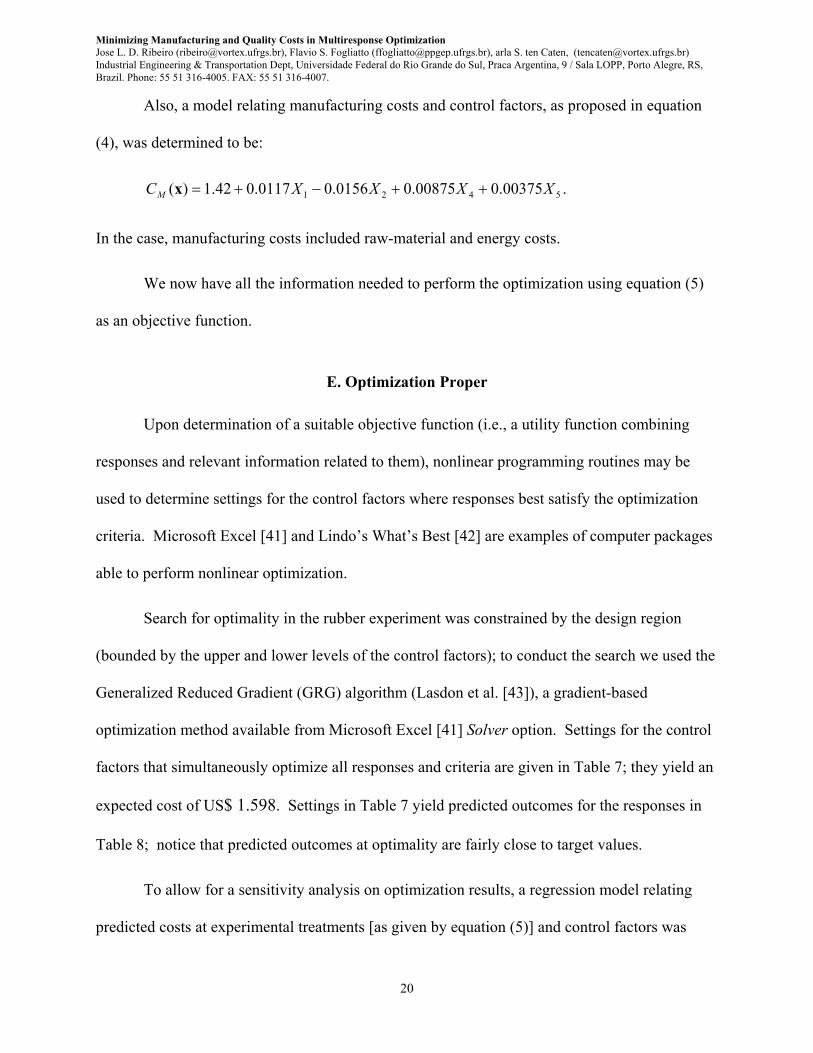
1 Mean 214222

2111 256.042.054.011.164.008.110.7ˆ XXXXXXXY ++++++= (0.91)

Var. 211 118.0186.0362.0ˆ XX ++=σ

2 Mean 2212 26.633.262.74ˆ XXY −−= (0.39)

Var. 532 58.140.1125.4ˆ XX +−=σ

3 Mean 522113 8.989.378.789.419.201ˆ XXXXY −−−−= (0.79)

Var. 13 525.2225.6ˆ X+=σ

4 Mean 543222

2114 36.210.169.158.198.143.160.357.31ˆ XXXXXXXY +++++++= (0.93)

Var. 24 253.0623.0ˆ X+=σ

5 Mean 5322115 938.0938.033.246.206.273.61ˆ XXXXXY +++++= (0.82)

Var. 15 892.0633.1ˆ X+=σ

6 Mean 4222

2116 00281.00063.00108.00058.000678.0132.1ˆ XXXXXY −++++= (0.86)

Var. 416 00825.000202.000356.0ˆ XX ++=σ

7 Mean 43215417 689.092.047.188.417.111.74ˆ XXXXXXXY −++−−= (0.92)Var. 5.0ˆ 7 =σ

8 Mean 53222

2118 75.12575.16747.15467.22847.17956.3351602ˆ XXXXXXY ++++++= (0.91)

Var. 28 095.2692.74ˆ X+=σ

9 Mean 214219 19.4144.12324.764.3306ˆ XXXXY +−−= (0.75)

Var. 219 52.1856.2303.53ˆ XX +−=σ

10 Mean 543222

21110 6.211.127.326.222.346.321.587.520ˆ XXXXXXXY −−−−−−−= (0.93)

Var. 3210 673.6566.6329.13ˆ XX −−=σ

Table 6. Regression models for mean and variance of responses (R2 given in parentheses).

D. Choice of Utility Function and Optimization Criteria

A list of utility functions and criteria that may be considered when optimizing

multiresponse experiments was given in the Introduction. Those utility functions consider


19

different criteria and therefore may lead to different optima. Choice of utility function is

essentially determined by the criteria to be considered in the optimization. Upon suitable

adaptation, utility functions in the Introduction may handle any optimization criterion.

Figure 3. Contour plots for responses Y1 to Y4.

The utility function used to optimize the rubber experiment is the one suggested in

equation (5), comprised of two terms: (i) a measure of monetary loss due to poor product

quality, given in equation (3); and (ii) a measure of manufacturing costs given in equation (4).

The proportionality constant p to be used in equation (3), determined using our suggested

procedure, is given by:

003043.0)64179()07.142.1($=

−−

==Z

p∆∆ .


20

Also, a model relating manufacturing costs and control factors, as proposed in equation

(4), was determined to be:

5421 00375.000875.00156.00117.042.1)( XXXXCM ++−+=x .

In the case, manufacturing costs included raw-material and energy costs.

We now have all the information needed to perform the optimization using equation (5)

as an objective function.

E. Optimization Proper

Upon determination of a suitable objective function (i.e., a utility function combining

responses and relevant information related to them), nonlinear programming routines may be

used to determine settings for the control factors where responses best satisfy the optimization

criteria. Microsoft Excel [41] and Lindo’s What’s Best [42] are examples of computer packages

able to perform nonlinear optimization.

Search for optimality in the rubber experiment was constrained by the design region

(bounded by the upper and lower levels of the control factors); to conduct the search we used the

Generalized Reduced Gradient (GRG) algorithm (Lasdon et al. [43]), a gradient-based

optimization method available from Microsoft Excel [41] Solver option. Settings for the control

factors that simultaneously optimize all responses and criteria are given in Table 7; they yield an

expected cost of US$ 1.598. Settings in Table 7 yield predicted outcomes for the responses in

Table 8; notice that predicted outcomes at optimality are fairly close to target values.

To allow for a sensitivity analysis on optimization results, a regression model relating

predicted costs at experimental treatments [as given by equation (5)] and control factors was


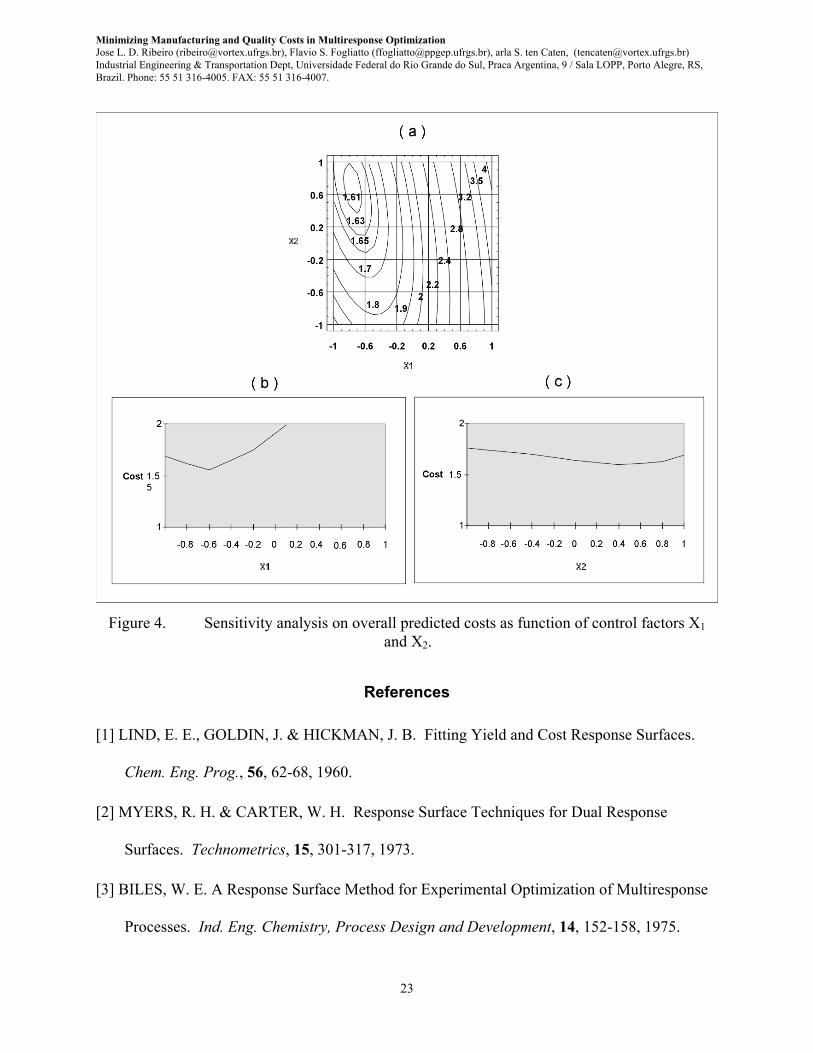
21

determined. Figure 4(a) gives a contour plot obtained using that model and control factors X1

and X2; similar plots were obtained varying levels of different pairs of control factors. Figure

4(b) shows the effects on cost of varying the levels of control factor X1 (all remaining control

factors are set at their optimal levels); Figure 4(c) gives similar results for control factor X2.

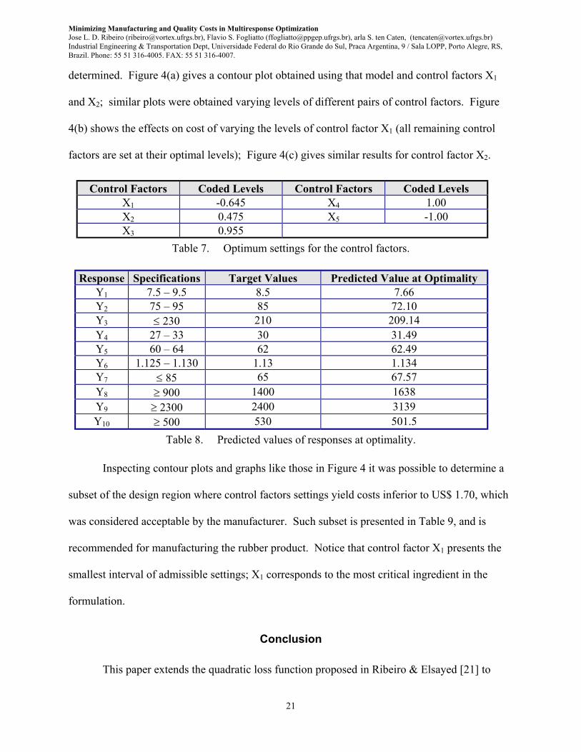
Control Factors Coded Levels Control Factors Coded LevelsX1 -0.645 X4 1.00X2 0.475 X5 -1.00X3 0.955

Table 7. Optimum settings for the control factors.

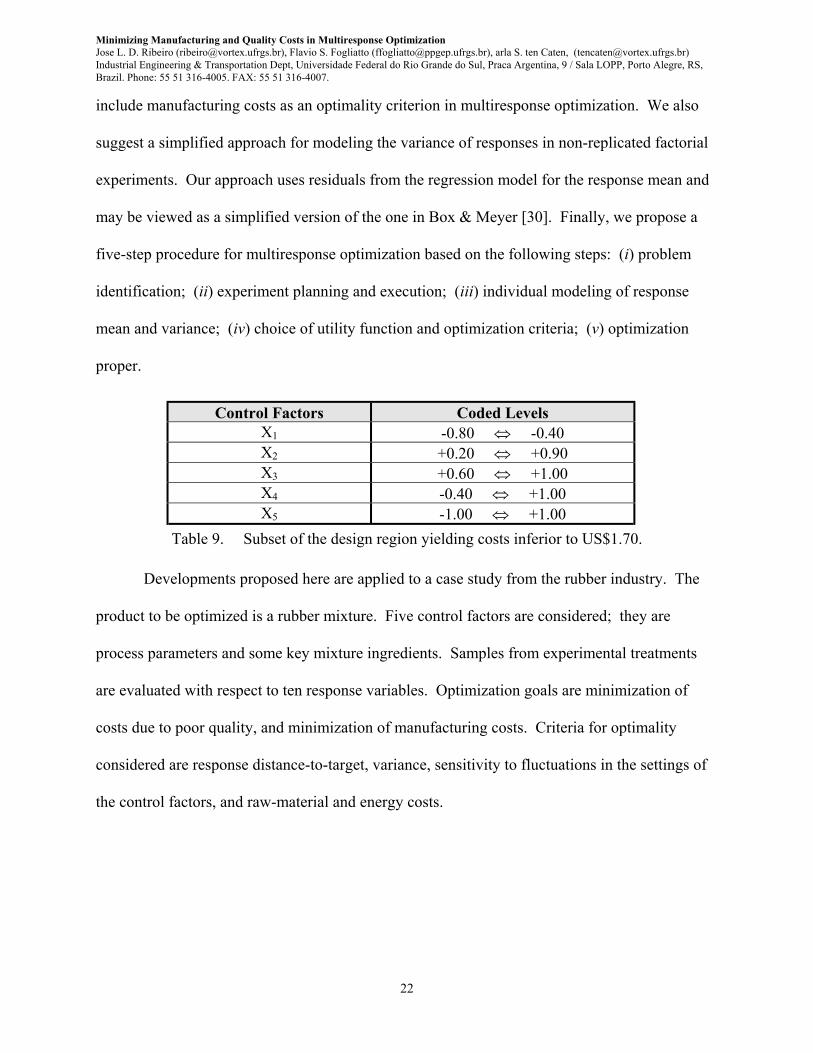
Response Specifications Target Values Predicted Value at OptimalityY1 7.5 – 9.5 8.5 7.66Y2 75 – 95 85 72.10Y3 ≤ 230 210 209.14Y4 27 – 33 30 31.49Y5 60 – 64 62 62.49Y6 1.125 – 1.130 1.13 1.134Y7 ≤ 85 65 67.57Y8 ≥ 900 1400 1638Y9 ≥ 2300 2400 3139Y10 ≥ 500 530 501.5

Table 8. Predicted values of responses at optimality.

Inspecting contour plots and graphs like those in Figure 4 it was possible to determine a

subset of the design region where control factors settings yield costs inferior to US$ 1.70, which

was considered acceptable by the manufacturer. Such subset is presented in Table 9, and is

recommended for manufacturing the rubber product. Notice that control factor X1 presents the

smallest interval of admissible settings; X1 corresponds to the most critical ingredient in the

formulation.

Conclusion

This paper extends the quadratic loss function proposed in Ribeiro & Elsayed [21] to


22

include manufacturing costs as an optimality criterion in multiresponse optimization. We also

suggest a simplified approach for modeling the variance of responses in non-replicated factorial

experiments. Our approach uses residuals from the regression model for the response mean and

may be viewed as a simplified version of the one in Box & Meyer [30]. Finally, we propose a

five-step procedure for multiresponse optimization based on the following steps: (i) problem

identification; (ii) experiment planning and execution; (iii) individual modeling of response

mean and variance; (iv) choice of utility function and optimization criteria; (v) optimization

proper.

Control Factors Coded LevelsX1 -0.80 ⇔ -0.40X2 +0.20 ⇔ +0.90X3 +0.60 ⇔ +1.00X4 -0.40 ⇔ +1.00X5 -1.00 ⇔ +1.00

Table 9. Subset of the design region yielding costs inferior to US$1.70.

Developments proposed here are applied to a case study from the rubber industry. The

product to be optimized is a rubber mixture. Five control factors are considered; they are

process parameters and some key mixture ingredients. Samples from experimental treatments

are evaluated with respect to ten response variables. Optimization goals are minimization of

costs due to poor quality, and minimization of manufacturing costs. Criteria for optimality

considered are response distance-to-target, variance, sensitivity to fluctuations in the settings of

the control factors, and raw-material and energy costs.


23

Figure 4. Sensitivity analysis on overall predicted costs as function of control factors X1and X2.

References

[1] LIND, E. E., GOLDIN, J. & HICKMAN, J. B. Fitting Yield and Cost Response Surfaces.

Chem. Eng. Prog., 56, 62-68, 1960.

[2] MYERS, R. H. & CARTER, W. H. Response Surface Techniques for Dual Response

Surfaces. Technometrics, 15, 301-317, 1973.

[3] BILES, W. E. A Response Surface Method for Experimental Optimization of Multiresponse

Processes. Ind. Eng. Chemistry, Process Design and Development, 14, 152-158, 1975.


24

[4] MYERS, R. H., KHURI, A. I. & VINING, G. Response Surface Alternatives to the Taguchi

Robust Parameter Design Approach. The American Statistician, 46 (2), 131-139, 1992.

[5] MYERS, R. H. & MONTGOMERY, D. C. Response Surface Methodology. John Wiley,

New York, 1995.

[6] Del CASTILHO, E. Multiresponse Process Optimization via Constrained Confidence

Regions. J. Quality Technology, 28(1), 61-70, 1996.

[7] KIM, K. & LIN, D. K. J. Dual response Surface optimization: A Fuzzy Modeling Approach.

Journal of Quality Technology, 30 (1), 1-10, 1998.

[8] HARRINGTON, Jr., E. C. The Desirability Function. Ind. Quality Control, 21(10), 494-

498, 1965.

[9] DERRINGER, G. & SUICH, R. Simultaneous Optimization of Several Response Variables.

Journal of Quality Technology, 12(4), 214-219, 1980.

[10] CHANG, S. & SHIVPURI, R. A Multiple-Objective Decision-Making Approach for

Assessing Simultaneous Improvement in Die Life and Casting Quality in a Die Casting

Process. Quality Engineering, 7, 371-83, 1994.

[11] Del CASTILHO, E., MONTGOMERY, D. C. & McCARVILLE, D. R. Modified

Desirability Functions for Multiple Response Optimization. J. Quality Technology, 28(3),

337-345, 1996.

[12] FOGLIATTO, F. S., ALBIN, S. L. & TEPPER, B.J. A Hierarchical Approach to Optimizing

Descriptive Analysis Multiresponse Experiments. Journal of Sensory Studies. Forthcoming,

1999.


25

[13] KHURI, A. I. & CONLON, M. Simultaneous Optimization of Multiple Responses

Represented by Polynomial Regression Functions. Technometrics, 23 (4), 363-375, 1981.

[14] LEÓN, R. V., SHOEMAKER, A. C. & KACKER, R. N. Performance Measures

Independent of Adjustment - An Explanation and Extension of Taguchi’s Signal-to-Noise

Ratios. Technometrics, 29(3), 253-265, 1987.

[15] LOGOTHETIS, N. & HAIGH, A. Characterizing and Optimizing Multiresponse Processes

by the Taguchi Method. Quality and Reliability Eng. Int., 4, 159-169, 1988.

[16] TRIBUS, M. & SZONYL, G. An Alternative View of the Taguchi Approach. Quality

Progress, 22, 46-52, 1989.

[17] YUM, B. & KO, S. On Parameter Design Optimization Procedures. Qual. Rel. Eng. Int., 7,

39-46, 1991.

[18] RAIMAN, L. B. & CASE, K. E. The Development and Implementation of Multivariate

Cost of Poor Quality Loss Function. IMSE Working Paper 92-152, Penn State Univ, 1992.

[19] ELSAYED, E. A. & CHEN, A. Optimal Levels of Process Parameters for Products With

Multiple Characteristics. Int. J. of Production Research, 31(5), 1117-1132, 1993.

[20] PIGNATIELLO Jr., J. J. Strategies for Robust Multiresponse Quality Engineering. IIE

Transactions, 25, 5-15, 1993.

[21] RIBEIRO, J. L. & ELSAYED, E. A. A Case Study on Process Optimization Using the

Gradient Loss Function, Int. J. Prod. Res., 33 (12), 3233-3248, 1995.

[22] LEÓN, N. A. A Pragmatic Approach to Multiresponse Problems Using Loss Functions.

Quality Engineering, 9, 213-220, 1996.


26

[23] VINING, G.G. (1998). A Compromise Approach to Multiresponse Optimization. Journal

of Quality Technology, 30 (4), 309-313.

[24] BARTLETT, M.S. & KENDALL, D.J. (1946). The statistical analysis of variance-

heterogeneity and the logarithmic transformation. Journal of the Royal Statistical Society,

Ser. B, 8, 128-138.

[25] MYERS, R.H. & MONTGOMERY, D.C. (1995). Response Surface Methodology:

process and product optimization using designed experiments. John Wiley: New York.

[26] HARVEY, A.C. (1976). Estimating regression models with multiplicative

heteroscedascity. Econometrica, 44 (3), 461-465.

[27] CARROLL, R.J. & RUPPERT, D. (1988). Transformation and weighting in regression.

Chapman & Hall: New York.

[28] SHOEMAKER, A.C., TSUI, K.L. & WU, C.F.J. (1991). Economical experimentation

methods for robust design. Technometrics, 33 (4), 415-427.

[29] LUCAS, J.M. (1994). How to achieve a robust process using response surface

methodology. Journal of Quality Technology, 26 (4), 248-260.

[30] BOX, G.E.P. & MEYER, R.D. (1986). Dispersion effects from fractional designs.

Technometrics, 28 (1), 19-27.

[31] TAGUCHI, G., ELSAYED, E.A. & HSIANG, T.C. (1989). Quality Engineering in

Production Systems. McGraw-Hill: New York.

[32] OH, H.L. (1988). Variation Tolerant Design. Proc. Conf. Uncertainty in Eng. Des.,

Maryland.


27

[33] FREUND, J.E. & SIMON, G.A. (1997). Modern Elementary Statistics. 9th Ed., Prentice

Hall: Englewood Cliffs (NJ).

[34] AKAO, Y. (1990). Quality Function Deployment: Integrating Customer Requirements

into Product Design. Productivity Press: Cambridge.

[35] COHEN, L. (1995). Quality Function Deployment: how to make QFD work for you.

Addison-Wesley: Reading (MA).

[36] SAATY, T. L. (1980). The Analytic Hierarchy Process: Planning, priority setting, resource

allocation. McGraw-Hill: New York.

[37] MONTGOMERY, D. C. (1991). Design and Analysis of Experiments. 3rd Ed., John Wiley:

New York.

[38] HICKS, C. R. (1993). Fundamental Concepts in the Design of Experiments. 4th Ed.,

Saunders College Publishing: New York.

[39] BOX, G. E. P. & DRAPER, N. R. (1987). Empirical Model-Building and Response

Surfaces. John Wiley: New York.

[40] FOGLIATTO, F. S. & ALBIN, S. L. (1999). Variance of Predicted Response as an

Optimization Criterion in Multiresponse Experiments. Quality Engineering (forthcoming).

[41] MICROSOFT EXCEL, Ver. 5.0 (1994). User’s Guide. Microsoft Co., Redmond, WA.

[42] WHAT’S BEST. (1998). User’s Manual. Lindo Systems Inc., Chicago.

[43] LASDON, L.S., WAREN, A.D., JAIN, A.& RATNER, M. (1978). Design and Testing of a

Generalized Reduced Gradient Code for Nonlinear Programming. ACM Trans.

Math.Software,4,34-50.


28

Key-Words: Multiresponse optimization, manufacturing costs, experimental design, rubber

industry.

Jose Luis D. Ribeiro is Professor and Head of Department in the Industrial and

Transportation Engineering Department at the Federal University of Rio Grande do Sul,

Brazil. His research field is quality engineering. His work has been applied in areas

including electronics manufacturing, rubber transformation and food processing. Dr. Ribeiro

received his doctorate from the Federal University of Rio Grande do Sul in 1989. Dr. Ribeiro

is serving as President of ABEPRO, the Brazilian Society of Industrial Engineers. He is a

member of ASQ.

Flavio S. Fogliatto is Research Fellow in the Department of Industrial and Transportation

Engineering at the Federal University of Rio Grande do Sul, Brazil. He received his Ph.D. in

Industrial & Systems Engineering from Rutgers University in 1997. His research field is

quality engineering and stochastic modeling. His professional experience is in research and

development of food products and processes. He is a member of ASQ.

Carla S. ten Caten is currently a Ph.D. student in the Department of Ceramics at the Federal

University of Rio Grande do Sul, Brazil. She received her M.S. degree in industrial

engineering from the Federal University of Rio Grande do Sul. Her research interests are in

the area of statistical quality engineering.

Documents

Minimizing Manufacturing and Quality Costs in ... · Minimizing Manufacturing and Quality Costs in ... account all measures of quality ... Minimizing Manufacturing and Quality Costs