1

Minimal Frames and Transparent Frames for Risk, Time, and Uncertainty1

(author names blinded for peer review)

Behavior differs between transparent and nontransparent presentations of decisions, but ‘transparent

presentation’ has not been precisely defined. We formally define ‘transparent frames’ for risk and time,

establish their uniqueness, provide algorithms for constructing them, and compare them to ‘standard’

presentation formats. A logic emerges for predicting systematic shifts in choice under risk and over time,

and how violations of rational choice theory will depend on frames. An experiment verifies most of those

predictions in choice under risk. We extend results to choice under uncertainty and also predict frame

dependence of ambiguity aversion, a result supported by recent experimental evidence.

1. Introduction

Among challenges to the descriptive validity of the expected utility (or EU) hypothesis, none is more

widely studied than Allais’ (1953) common consequence effect, an example of which is shown below.

G1: $500,000 with probability 1 G2: $2,500,000 with probability 0.10

$500,000 with probability 0.89

0 with probability 0.01 G3: $500,000 with probability 0.11 G4: $2,500,000 with probability 0.10

0 with probability 0.89 0 with probability 0.90

When choosing between gambles G1 and G2 and between G3 and G4, many people,

2 including

prominent decision theorists like Leonard Savage, exhibit the choice pattern (G1, G4) in violation of EU.

Savage (1954, p. 102) suggests that people choose G1 over G2 because “they do not find the chance

of winning a very large fortune in place of receiving a large fortune outright adequate compensation for

even a small risk of being left at the status quo” and select G4 over G3 because “the chance of winning is

nearly the same in both gambles, so the larger prize appears preferable.” Savage then reframes the choice

problems as a state-based matrix where states across choice alternatives are correlated (shown below).

Ticket Numbers

1 2 – 11 12 – 100 G1: $500,000 $500,000 $500,000

G2: 0 $2,500,000 $500,000 G3: $500,000 $500,000 0

G4: 0 $2,500,000 0

In these reframed options, the prize depends on a ticket drawn from a bag containing 100 numbered

tickets. Given this reframing, Savage chose in accordance with the independence axiom and in a

1 We thank anonymous referees and an associate editor for many comments that improved this article.

2 Common consequence effects are not always observed in some experiments that pay subjects according to their

choices (using outcomes feasible for actual payment; see e.g. Conlisk 1989, Fan 2002, and Burke et al. 1996).

2

consistently risk averse manner, expressing a preference for G1 over G2 and for G3 over G4. Savage felt

that his revision of the latter choice, brought about by this new frame, had “corrected an error” (p. 103).

Three decades later, Tversky and Kahneman (1986) presented further evidence that framing mediates

decision errors. All 88 of their experimental subjects chose B over A in the choice below, in which

probabilities are expressed as percentages of marbles of different colors in boxes governing each option:

Option A 90% white

$0

6% red

win $45

1% green

win $30

1% blue

lose $15

2% yellow

lose $15

Option B 90% white

$0

6% red

win $45

1% green

win $45

1% blue

lose $10

2% yellow

lose $15

Option B stochastically dominates A since it offers a 1% chance of a larger gain ($45 versus $30) and a

1% chance of a smaller loss (-$10 versus -$15). However, they observed that a majority (58%) of subjects

chose C over D with the alternatives presented differently, as below:

Option C 90% white

$0

6% red

win $45

1% green

win $30

3% yellow

lose $15

Option D 90% white

$0

7% red

win $45

1% green

lose $10

2% yellow

lose $15

One obtains Option C from A by combining the 1% blue and 2% yellow chances of losing $15, and D

from B by combining the 6% red and 1% green chances of winning $45.3 This produces a ‘minimal’

presentation in that the matrix has fewer columns; yet this presentation masks the dominance relation and

juxtaposes the 1% chance of $30 against the 1% chance of -$10, which now drives the choice.

Tversky and Kahneman (1986) propose that the dominance relationship is intuitively ‘more

transparent’ in the choice between options A and B. Hogarth and Reder (1986) note, however, that

“Tversky and Kahneman do not specify the conditions under which people perceive problems as

transparent or opaque” (p. S192); and neither did Savage (1954). This issue has apparently not been

addressed in the subsequent literature: there is no general theory of ‘transparency’ of choice presentations.

We offer precise definitions of presentations or frames for choice under risk and over time, propose a

property list for transparent frames, and show that these properties imply unique presentations of choice

problems. We also define a minimal frame and identify it with many standard presentations of choice

problems. We then apply a model of salience-based choice to derive behavioral predictions in minimal

and transparent frames, and test for these predicted choice differences in a new experiment involving

choice under risk. Finally, we extend the model to choice under ambiguity, where we derive the novel

prediction that ambiguity aversion is frame-dependent. In Section 8 we discuss how this work relates to

3 Birnbaum and Navarrete (1998) and Luce (1998) refer to this combining of the probabilities of identical outcomes

as “coalescing.” Earlier, Starmer and Sugden (1993) had called the opposite operation “event-splitting.”

3

recent literature on perception’s role in choice under risk and over time (Birnbaum 2004; Birnbaum et al.

2008; Bordalo et al., 2012; Loomes 2010; Scholten and Read, 2010, and many others).

2. Presentations or Frames

Figure 1. Presentations or Frames for Decisions under Risk and over Time

Choice Frame for Lotteries

(x1,y1) (p1,q1) (x2,y2) (p2,q2)

(xi,yi) (pi,qi)

(xn,yn) (pn,qn)

𝐩 x1 p1 x2 p2 … xi pi … xn pn 𝐪 y1 q1 y2 q2 … yi qi … yn qn Choice Frame for Income Streams (x1,y1) (r1,t1) (x2,y2) (r2,t2) (xi,yi) (ri,ti) (xn,yn) (rn,tn)

𝐫 x1 r1 x2 r2 … xi ri … xn rn 𝐭 y1 t1 y2 t2 … yi ti … yn tn

2.1 Lotteries, Income Streams and their Frames

Frames present pairs of options as shown in Figure 1. Let 𝑋 be a finite set of potential outcomes. A

lottery is a mapping 𝑝: 𝑋 → [0,1] such that ∑ 𝑝(𝑥) = 1𝑥∈𝑋 , and ∆(𝑋) is the set of all such lotteries.

Consider a pair of one-dimensional finite arrays 𝐩 and 𝐪, representing lotteries 𝑝 and 𝑞 and offering a

finite and equal number of outcomes denoted 𝐱𝐢 and 𝐲𝐢, 𝑖 = 1,2, … , 𝑛, where each 𝐱𝐢 occurs with

probability 𝐩𝐢 and each 𝐲𝐢 occurs with probability 𝐪𝐢: The top panel of Figure 1 illustrates the pair of

arrays. We call ⟦𝐩, 𝐪⟧ a frame or presentation of lottery pair {𝑝, 𝑞}, and say that ⟦𝐩, 𝐪⟧ presents {𝑝, 𝑞}, if

and only if 𝑝(𝑥) = ∑ 𝐩𝐢{𝑖 |𝐱𝐢=𝑥} and 𝑞(𝑦) = ∑ 𝐪𝐢{𝑖 | 𝐲𝐢=𝑦} : In words, all array probabilities of the same

outcome must sum to the outcome’s probability in the lottery presented by that array. Let 𝑠𝑢𝑝𝑝(𝑝) be the

set of outcomes such that 𝑝(𝑥) > 0, called the support of 𝑝( ), and let |𝑠𝑢𝑝𝑝(𝑝)| denote the number of

outcomes in a support. Note that 𝑛 may exceed |𝑠𝑢𝑝𝑝(𝑝)| or |𝑠𝑢𝑝𝑝(𝑞)|: This is a key difference between

frames ⟦𝐩, 𝐪⟧ and the pairs {𝑝, 𝑞} they present.

For decisions over discrete time periods i ∈ {0, 1, 2, …, T}, intertemporal income streams 𝑟:=

(𝑥0, 𝑥1, … , 𝑥𝑇) and 𝑡: = (𝑦0, 𝑦1, … , 𝑦𝑇) assign finite sequences of outcomes to each period; denote the set

of income streams by 𝐶. We also study choices from pairs {𝑟, 𝑡} of income streams presented by frame

⟦𝐫, 𝐭⟧ as illustrated in the lower panel of Figure 1: Finite arrays 𝐫 and 𝐭 present income streams 𝑟 and 𝑡,

offering finite and equal numbers of outcomes 𝐱𝐢 occurring in time periods 𝐫𝐢 and outcomes 𝐲𝐢 occurring

in time periods 𝐭𝐢. Bold font always denotes attributes in frames, while italic font always denotes lotteries,

income streams, and the attributes in their supports.

2.2 Defining Minimal Frames and Transparent Frames

We provide here an intuitive treatment of minimal and transparent frames (our appendix gives formal

definitions and uniqueness demonstrations). Transparent frames resemble Savage’s (1954) state matrix

4

lottery presentations, but remove Savage’s explicitly correlated payoffs. More precisely, as a theoretical

matter, a transparent frame contains no correlational information—whether the actual probability-

generating mechanism for the pair of lotteries implies correlated payoffs or not (as it does in Savage’s

state matrix presentation).4

Minimal frames are compact presentations of choices and, for choice under risk, formalize the

‘prospect’ presentation of lotteries pioneered by Kahneman and Tversky (1979). Minimal frames for

choice under risk contain no redundancy: Minimal frames for choice under risk contain minimal

redundancy: the same outcome only appears more than once in special circumstances.5 if one of the

alternatives is degenerate or where lotteries have different support sizes. Similarly, in minimal frames for

choice over time, any time period appears just once in presentations of income streams, and the frame

contains the fewest columns necessary to present all of the non-zero payoffs in the income streams.

Building on the intuitive examples of Savage (1954) and Tversky and Kahneman (1986), we propose

that a transparent frame for lotteries satisfies five formal properties:

1. Common Consequence Separation: Identify the common consequences (the payoff-probability pairs

that contain the same outcomes and corresponding probabilities) of the lotteries being compared and

separate them from distinct consequences (the other payoff-probability pairs in the frame).

2. Monotonicity: Order the outcomes of distinct consequences in decreasing order such that the ith

best

outcome in one lottery is in the same column as the ith best outcome in the other lottery.

3. Alignment: Set the probabilities within each column equal to each other.

4. Completeness: Ensure that the probabilities for each row in the frame sum to 1.

5. Relevance: Ensure the probabilities in each column vector are positive.

Our appendix provides an algorithm for constructing a unique transparent frame satisfying these five

properties for any lottery pair (including those with different numbers of outcomes in their support).

Together, these properties have intuitive appeal and simplify comparison of alternatives by

articulating relevant information and bringing it into attentional focus. Common Consequence Separation

4 We think any compelling account of transparent presentation requires a normative basis. Under EU theory, payoff

correlation (or lack of it) between alternatives in a pair is normatively irrelevant with completely specified

outcomes: Therefore our definition of transparent presentation proceeds on that basis, not providing correlational

information between alternatives. This does not mean that correlational information would not be provided to the

decision maker in some form (say to a subject in an experiment, where a complete description of how probabilities

are implemented to generate payoffs automatically includes it, as is the case in our experiment here); it just means

the presentation itself does not provide such correlational information. Although we think most decision researchers

regard EU (or SEU) as normative, prominent dissents remain (e.g. Allais 1953 and Ellsberg 1961). We acknowledge

this and grant that a proponent of an alternative normative or rational model might want a different formal definition

of transparent presentation (e.g. one that makes correlational information explicit). 5 The special circumstances are: (i) When one lottery is degenerate (see Section 4 below); and more generally (ii)

When lotteries have different support sizes, the lottery with smaller support size must have one outcome repeated in

order to complete the frame (see Appendix Section A.3 below).

5

isolates shared payoff-probability pairs, thus focusing attention on how the lotteries differ. Monotonicity

ensures that the best payoffs in one lottery are compared to the best payoffs in another lottery. Because

Alignment matches the probability dimensions of all payoff-probability pairs across a pair of alternatives,

one need only compare payoffs and weight them. Completeness ensures that all outcomes in the support

of a lottery are accounted for in the decision; and Relevance ensures that no irrelevant outcomes (those

with probability zero) are considered. We think that, taken together, these properties will help a person

focus on the tradeoffs needed to make a quality decision.

For decisions over time, we propose similar properties that a transparent frame should satisfy:

1. Common Consequence Separation: Identify the common consequences (the payoff-time pairs that

contain the same outcomes and the same corresponding delays) of the income streams being

compared and separate them from distinct consequences.

2. Monotonicity: Order the timing of distinct consequences in strictly increasing order such that the ith

soonest period in one income stream is in the same column as the ith soonest period in the other.

3. Alignment: Set the time periods within each column equal to each other.

4. Completeness: Ensure that all time periods indexed by the income streams are included.

5. Relevance: Ensure that only time periods indexed by the income streams are included.

These five properties also have intuitive appeal and justification. Common consequence separation

puts attention on where the two alternatives differ. Monotonicity reflects the intuition that time has a

natural forward direction and it may help one to consider time periods sequentially. The alignment

property ensures that the time periods within each column of a frame are the same, standardizing

outcomes within each column to have the same ‘time value of money’. Alignment also enables a decision

maker who is comparing two payoff-time pairs in a given pair of columns to focus on the differences in

payoffs, rather than trading off both risk and time within those columns. Completeness ensures that all

relevant time periods and payoffs are considered. The relevance property ensures that only relevant time

periods and payoffs are considered. In particular, it encourages the decision maker to be forward looking

as it does not display sunk costs (e.g., from previous income outcomes) that occurred prior to the dates

indexed by the income streams. We show in the appendix that for any pair of income streams there is a

unique frame satisfying these five properties.

3. Salience Weighted Utility over Presentations

Leland and Schneider’s (2017) Salience Weighted Utility over Presentations (SWUP) is a simple

decision model that operates on frames as we define them here.6 We note, however, that the theory of

framing as developed here is independent of SWUP. In particular, other decision models may be applied

6 Leland and Schneider (2017) focus entirely on developing SWUP, the salience-based decision model for frames,

but do not develop the predictions of this model for different frames (nor test these) as we do here.

6

to minimal and transparent frames and behavior can be experimentally tested in minimal and transparent

frames without necessarily invoking SWUP. In both of these respects, the concepts of minimal and

transparent frames are more general than SWUP. In our analysis, SWUP is one plausible frame-dependent

decision model that we use to illustrate the predicted differences between minimal and transparent frames.

3.1 Salience Weighted Utility over Presentations for Choice under Risk

In a standard EU model of choice under risk, 𝑝 is chosen over 𝑞 if and only if (1) holds:

(1) ∑ 𝑝(𝑥)𝑢(𝑥) > ∑ 𝑞(𝑦)𝑢(𝑦)𝑦∈𝑋𝑥∈𝑋 ,

where 𝑢(𝑥) is a utility function denoting payoffs to the decision maker from outcomes 𝑥. 7 Leland and

Schneider (2017) consider choices over frames as in the top panel of Figure 1, where (1) can be written

equivalently as (2) (recall that bold font denotes outcomes and probabilities in a frame):

(2) ∑ 𝐩𝐢𝑢(𝐱𝐢) > ∑ 𝐪𝐢𝑢(𝐲𝐢)𝑛𝑖=1

𝑛𝑖=1 ,

Inequality (1) pertains to choices over lotteries 𝑝 and 𝑞 (regardless of how they are framed), whereas (2)

pertains to choices over a particular frame ⟦𝐩, 𝐪⟧ presenting lotteries 𝑝 and 𝑞. Note that (1) and (2)

provide an alternative-based evaluation - one lottery is strictly preferred to another, if and only if it yields

a greater expected payoff to the decision maker.

Building on Leland and Sileo (1998), the alternative-based evaluation in (2) may be rewritten

equivalently as an attribute-based evaluation such that 𝐩 is chose over 𝐪 if and only if (3) holds:

(3) ∑ [(𝐩𝐢 − 𝐪𝐢)(𝑢(𝐱𝐢) + 𝑢(𝐲𝐢))/2 + (𝑢(𝐱𝐢) − 𝑢(𝐲𝐢))(𝐩𝐢 + 𝐪𝐢)/2] > 0.𝑛𝑖=1

Note that (2) and (3) operate over frames rather than over lotteries directly. Leland and Schneider (2017)

then allow for the possibility that the agent systematically overweights salient differences in probabilities

and payoffs by introducing salience weights 𝜙(𝐩𝐢, 𝐪𝐢) on probability differences and 𝜇(𝐱𝐢, 𝐲𝐢) on payoff

differences. This yields Leland and Schneider’s Salience-Weighted Utility over Presentations (SWUP)

model of choice under risk, in which 𝐩 is chosen over 𝐪 if and only if

(4) ∑ [𝜙(𝐩𝐢, 𝐪𝐢)(𝐩𝐢 − 𝐪𝐢)(𝑢(𝐱𝐢) + 𝑢(𝐲𝐢))/2 + 𝜇(𝐱𝐢, 𝐲𝐢)(𝑢(𝐱𝐢) − 𝑢(𝐲𝐢))(𝐩𝐢 + 𝐪𝐢)/2] > 0𝑛𝑖=1 .

3.2 Salience Weighted Utility for Choice over Time

One may also derive a SWUP model for framed choice over time (as in the lower panel of Figure 1).

In the discounted utility (or DU) model, a person chooses income stream 𝑎 over 𝑏 if and only if (5) holds:

(5) ∑ 𝛿𝑖𝑢(𝑥𝑖) > ∑ 𝛿𝑖𝑢(𝑦𝑖)𝑇𝑖=0

𝑇𝑖=0 ,

where δ is a constant discount factor. Via steps resembling (2), (3), and (4), Leland and Schneider (2017)

derive (6) from (5), generalizing DU theory to allow for overweighting of salient differences in payoffs

7 All of our theoretical results hold when 𝑢(𝑥) = 𝑥. However we leave open the possibility that 𝑢(𝑥) is weakly

concave for gains (as in standard risk-averse EU), or additionally weakly convex for losses and exhibiting loss

aversion (as in Wakker and Tversky’s 1993 nonstandard Sign-Dependent Expected Utility or SDEU).

7

and time delays. Placing salience weights 𝜃(𝐫𝐢, 𝐭𝐢) on time differences and 𝜇(𝐱𝐢, 𝐲𝐢) on payoff differences

gives this salience-weighted evaluation in which 𝐫 is always chosen over 𝐭 if and only if

(6) ∑ [𝜃(𝐫𝐢, 𝐭𝐢)(𝛿𝐫𝐢 − 𝛿𝐭𝐢)(𝑢(𝐱𝐢

𝑚𝑖 ) + 𝑢(𝐲𝐢))/2 + 𝜇(𝐱𝐢, 𝐲𝐢)(𝑢(𝐱𝐢) − 𝑢(𝐲𝐢))(𝛿

𝐫𝐢 + 𝛿𝐭𝐢)/2] > 0,

whenever the frame ⟦𝐫, 𝐭⟧ presents income streams 𝑟 and 𝑡.

3.3 Salience Weighted Utility for Choice under Ambiguity

Leland and Schneider (2017) introduced SWUP for choices under risk and over time. Here we extend

SWUP to the domain of uncertainty, where probabilities of some events are unknown. Suppose there is a

finite set of possible states of nature 𝑠 ∈ {1,2,… , 𝑆}, where a lottery is assigned to be played in each state.

Denote uncertain prospects by 𝑓 and 𝑔, where 𝑓 assigns lottery 𝑓(𝑠) to each state 𝑠 and 𝑔 assigns lottery

𝑔(𝑠) to each state 𝑠. In the classic alternative-based evaluation, there is assumed to be a unique subjective

probability distribution, 𝜋𝑠, over states (Anscombe and Aumann, 1963) such that 𝑓 is preferred over 𝑔 if

and only if (7) holds (where 𝑓𝑠(𝑥) is the probability of outcome 𝑥 in state 𝑠):

(7) ∑ ∑ 𝜋𝑠[𝑓𝑠(𝑥)𝑢(𝑥)]𝑥∈𝑋𝑠∈𝑆 > ∑ ∑ 𝜋𝑠[𝑔𝑠(𝑦)𝑢(𝑦)].𝑦∈𝑋𝑠∈𝑆

Let there be a frame for each state, where 𝑖𝑠 indexes the ith

attribute in the state 𝑠 frame. Given two multi-

dimensional arrays 𝐟 = {𝐟𝟏, … , 𝐟𝐒} and 𝐠 = {𝐠𝟏, … , 𝐠𝐒}, we define a formula analogous to (5). 𝐟 is always

chosen over 𝐠 if and only if (8) holds:

(8) ∑ ∑ 𝜋𝑠[𝐟𝐢𝐬𝑢(𝐱𝐢𝐬)]𝑛(𝑠)𝑖

𝑆𝑠 > ∑ ∑ 𝜋𝑠[𝐠𝐢𝐬𝑢(𝐲𝐢𝐬)]

𝑛(𝑠)𝑖

𝑆𝑠 .

Next, we introduce the corresponding model of salience-weighted evaluation in which 𝐟 is always chosen

over 𝐠 if and only if (9) holds:

(9) ∑ ∑ 𝜋𝑠[𝜙(𝐟𝐢𝐬, 𝐠𝐢𝐬)(𝐟𝐢𝐬 − 𝐠𝐢𝐬)(𝑢(𝐱𝐢𝐬) + 𝑢(𝐲𝐢𝐬))/2𝑛𝑖=1

𝑆𝑠

+ 𝜇(𝐱𝐢𝐬, 𝐲𝐢𝐬)(𝑢(𝐱𝐢𝐬) − 𝑢(𝐲𝐢𝐬))(𝐟𝐢𝐬 + 𝐠𝐢𝐬)/2] > 0.

We refer to agents who choose according to salience-based evaluation models (the representations 4, 6,

and 9) as focal thinkers since such agents focus on salient differences in attributes. Such an agent chooses

the alternative which ‘looks better’ with respect to that agent’s perceptual system.

3.4 Properties of Salience Perceptions

The salience functions 𝜇, 𝜙 and 𝜃 alone determine how the behavior of a focal thinker differs from a

rational agent (who chooses according to formulas 1, 5 and 7). We assume that salience functions exhibit

the two properties of the perceptual system in Definition 1, introduced by Bordalo et al. (2012).

Definition 1 (Salience Function): A salience function σ(𝐚𝐢, 𝐛𝐢) is any continuous, non-negative and

symmetric (σ(𝐚𝐢, 𝐛𝐢) = σ(𝐛𝐢, 𝐚𝐢)) function of 𝐚𝐢 and 𝐛𝐢 ∈ ℝ that satisfies the following two properties:

1. Ordering: If [𝐚𝐢′, 𝐛𝐢′] ⊂ [𝐚𝐢, 𝐛𝐢] then σ(𝐚𝐢

′, 𝐛𝐢′) < σ(𝐚𝐢, 𝐛𝐢).

2. Diminishing Absolute Sensitivity (DAS): σ(. ) exhibits diminishing sensitivity if for any 𝐚𝐢, 𝐛𝐢, 𝜖 > 0,

σ(𝐚𝐢 + 𝜖, 𝐛𝐢 + 𝜖) < σ(𝐚𝐢, 𝐛𝐢).

8

In addition to properties 1 and 2 from Bordalo et al. (2012), we will allow for the possibility that a

salience function satisfies a third property, increasing proportional sensitivity or IPS:

3. Increasing Proportional Sensitivity (IPS): σ(. ) exhibits increasing proportional sensitivity if for any

𝐚𝐢 > 0, 𝐛𝐢 ≥ 0 and any 𝛼 > 1, σ(𝛼𝐚𝐢, 𝛼𝐛𝐢) > σ(𝐚𝐢, 𝐛𝐢).

There is a close relationship between DAS and IPS: DAS implies that for a fixed absolute difference,

the perceptual system is more sensitive to larger ratios, while IPS implies that for a fixed ratio, the

perceptual system is more sensitive to larger absolute differences. We will show that for focal thinkers,

IPS for 𝜙 implies the general version of the Allais common ratio effect, and DAS for 𝜙 implies ambiguity

aversion in Ellsberg’s paradox in minimal frame presentations. Our approach thus provides a unified

treatment of Allais-style and Ellsberg-style behavior and shows that they can be derived from basic

properties of the probability salience function 𝜙 without requiring any parametric assumptions about the

underlying salience functions or utility functions.

3.5 Computable Parameter-Free Salience Functions for Calculation and Estimation

Computable parameter-free salience functions are useful for both applied theory calculations and

statistical estimation of salience-based models such as SWUP. One alternative is the parameter-free DAS

salience function (Bordalo et al., 2013):

(10) 𝜎(𝐚𝐢, 𝐛𝐢) = |𝐚𝐢−𝐛𝐢|

|𝐚𝐢|+|𝐛𝐢| whenever 𝐚𝐢 > 0 or 𝐛𝐢 > 0; and 𝜎(0,0) = 0.

Although simple and parameter-free, (10) does not satisfy IPS. For our estimations in Section 5.3 below,

we prefer a salience function that satisfies IPS. Given behaviors such as the fourfold pattern of risk

attitudes that follow from IPS (Leland and Schneider, 2017), along with the general form of the Allais

common ratio effect, it seems desirable for a salience function to satisfy that property.

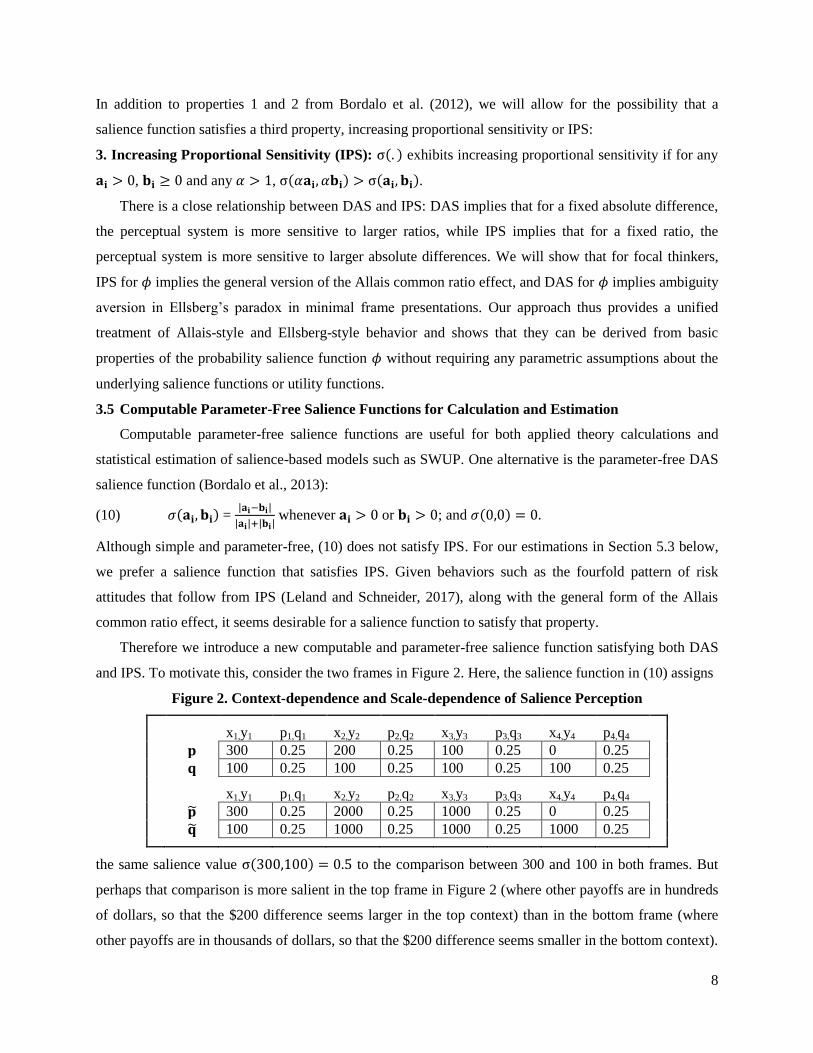
Therefore we introduce a new computable and parameter-free salience function satisfying both DAS

and IPS. To motivate this, consider the two frames in Figure 2. Here, the salience function in (10) assigns

Figure 2. Context-dependence and Scale-dependence of Salience Perception

x1,y1 p1,q1 x2,y2 p2,q2 x3,y3 p3,q3 x4,y4 p4,q4

𝐩 300 0.25 200 0.25 100 0.25 0 0.25

𝐪 100 0.25 100 0.25 100 0.25 100 0.25 x1,y1 p1,q1 x2,y2 p2,q2 x3,y3 p3,q3 x4,y4 p4,q4

�̃� 300 0.25 2000 0.25 1000 0.25 0 0.25

�̃� 100 0.25 1000 0.25 1000 0.25 1000 0.25

the same salience value σ(300,100) = 0.5 to the comparison between 300 and 100 in both frames. But

perhaps that comparison is more salient in the top frame in Figure 2 (where other payoffs are in hundreds

of dollars, so that the $200 difference seems larger in the top context) than in the bottom frame (where

other payoffs are in thousands of dollars, so that the $200 difference seems smaller in the bottom context).

9

The context-dependence and scale-dependence of salience perception illustrated in Figure 2 can be

accommodated by including a function that depends on all outcomes (or all probabilities) in a frame. One

plausible candidate is the Euclidean norm which can be viewed as taking the second moment of value

deviations from 0 for all outcomes (or all probabilities) in a frame. Let (𝐚, 𝐛) denote a vector of length

2𝑛, formed by horizontally concatenating a pair of like dimension vectors in a frame (i.e., all outcomes in

a frame, or all probabilities in a frame); and let ‖𝐚, 𝐛‖ denote the Euclidean norm of the vector (𝐚, 𝐛). A

context-dependent parameter-free DAS-IPS salience function can be defined as in (11):

(11) 𝜎(𝐚𝐢, 𝐛𝐢|𝐚, 𝐛) = |𝐚𝐢−𝐛𝐢|

|𝐚𝐢|+|𝐛𝐢|+‖𝐚,𝐛‖.

This satisfies DAS and IPS for any frame, and under (11) the salience of (300, 100) is greater in the top

frame of Figure 2 than in the bottom frame. We will use this DAS-IPS salience function for SWUP

estimations in Section 5.3 below.

4. Minimal and Transparent Frames for Choice under Risk

We now consider what SWUP implies when alternatives are presented in a minimal versus a

transparent frame, beginning with choices under risk. For frames with degenerate lotteries (those yielding

a single outcome with probability 1), it seems almost unavoidable that one compares each outcome in the

non-degenerate lottery 𝐪 to the unique outcome in the degenerate lottery 𝐩. So when one lottery in a pair

is degenerate, we adopt the convention that monotone minimal frames appear as shown in Figure 3.

Figure 3. Choice Frame with a Degenerate Lottery 𝐩

(𝐱𝟏, 𝐲𝟏) (𝐩𝟏, 𝐪𝟏) (𝐱𝟐, 𝐲𝟐) (𝐩𝟐, 𝐪𝟐) … (𝐱𝐢, 𝐲𝐢) (𝐩𝐢, 𝐪𝐢) … (𝐱𝐧, 𝐲𝐧) (𝐩𝐧, 𝐪𝐧)

𝐩 𝐱 𝐪𝟏 𝐱 𝐪𝟐 … 𝐱 𝐪𝐢 … 𝐱 𝐪𝐧

𝐪 𝐲𝟏 𝐪𝟏 𝐲𝟐 𝐪𝟐 … 𝐲𝐢 𝐪𝐢 … 𝐲𝐧 𝐪𝐧

4.1 The Stochastic Dominance Axiom in Minimal and Transparent Frames

If lottery 𝑝 offers at least as good an outcome as 𝑞 does at every probability increment—and a strictly

better outcome at some probability increment—then 𝑝 stochastically dominates 𝑞. Rational choice

requires consistency with stochastic dominance. Consider the example from Section 1, shown in Figure 4.

Figure 4. Stochastic Dominance in Minimal and Transparent Frames

Stochastic Dominance in the Minimal Frame x1,y1 p1,q1 x2,y2 p2,q2 x3,y3 p3,q3 x4,y4 p4,q4

p′ 0 0.90 45 0.07 -10 0.01 -15 0.02

q′ 0 0.90 45 0.06 30 0.01 -15 0.03 Stochastic Dominance in the Transparent Frame x1,y1 p1,q1 x2,y2 p2,q2 x3,y3 p3,q3 x4,y4 p4,q4 x5,y5 p5,q5

p 45 0.01 -10 0.01 45 0.06 0 0.90 -15 0.02

q 30 0.01 -15 0.01 45 0.06 0 0.90 -15 0.02

10

All subjects chose the stochastically dominant lottery 𝑝 in the transparent frame, but many chose the

dominated lottery 𝑞′ in the minimal frame. For transparent frames, a focal thinker satisfies stochastic

dominance since any differences in (4) favor the stochastically dominant lottery.

4.2 The Independence Axiom in Minimal and Transparent Frames

The Allais common consequence paradox (Allais, 1953) involves choices like those in the left panel

of Figure 5. A decision maker chooses between lottery 𝑞, offering $2400 with certainty and a lottery 𝑝,

offering a 33% chance of $2500, a 66% chance of $2400, and a 1% chance of $0. The decision maker

then chooses between lottery �̃� offering a 34% chance of $2400 and lottery �̃� offering a 33% chance of

$2500. Kahneman and Tversky (1979) report that most subjects choose 𝑞 over 𝑝 and choose �̃� over �̃�.

This preference pattern is inconsistent with EU which predicts preferences of either 𝑝 and �̃� or 𝑞 and �̃�.

In the minimal frame ⟦p, q⟧, the comparison of 2400 and 0 is more salient than that of 2500 and 2400,

favoring 𝑞. However, in the minimal frame ⟦p̃, q̃⟧, the comparison between 2400 and 0 is not cued.

Instead, the decision maker compares the upside of winning 2500 instead of 2400 with the downside of

forfeiting a 1% chance in the probability of winning. To the extent this $100 difference is more salient

Figure 5. The Allais Paradox in Minimal and Transparent Frames

Allais Paradox in Minimal Frames Allais Paradox in Transparent Frames x1,y1 p1,q1 x2,y2 p2,q2 x3,y3 p3,q3 x1,y1 p1,q1 x2,y2 p2,q2 x3,y3 p3,q3

p 2500 0.33 2400 0.66 0 0.01 p 2500 0.33 0 0.01 2400 0.66

q 2400 0.33 2400 0.66 2400 0.01 q 2400 0.33 2400 0.01 2400 0.66 x1,y1 p1,q1 x2,y2 p2,q2 x1,y1 p1,q1 x2,y2 p2,q2 x3,y3 p3,q3

�̃� 2500 0.33 0 0.67 p̃ 2500 0.33 0 0.01 0 0.66

q̃ 2400 0.34 0 0.66 �̃� 2400 0.33 2400 0.01 0 0.66

than the 0.01 difference in probabilities, the decision maker chooses �̃� over �̃�. Now consider the

transparent frames in Figure 5. Here, the components common to each decision (i.e., ($2400, 0.66) in the

choice between 𝑝 and 𝑞 and ($0, 0.66) in the choice between �̃� and �̃�) are isolated and the decision in

both cases depends on comparisons between 2500 and 2400 and between 2400 and 0.

Figure 6 displays a version of Allais’ (1953) common ratio effect—another well-known EU violation.

The minimal frames display a choice between lotteries 𝑝 and 𝑞, offering an 80% chance of $4000 versus

$3000 with certainty, and a choice between �̃� and �̃�, offering a 20% chance of $4000 versus a 25%

chance of $3000. In this version, Kahneman and Tversky (1979) report that a majority of subjects chose 𝑞

over 𝑝 and chose �̃� over �̃� when the choices were presented in minimal frames. This response pattern

violates EU which predicts choices of either 𝑝 and �̃� or 𝑞 and �̃�. In the transparent frames in Figure 6, the

salient comparisons in both choices are between 3000 and 0 and between 4000 and 3000. Since the same

comparisons are focal in both choices, one might predict more consistent behavior in transparent frames.

11

Figure 6. The Common Ratio Effect Presented in Minimal and Transparent Frames

In Minimal Frames In Transparent Frames x1,y1 p1,q1 x2,y2 p2,q2 x1,y1 p1,q1 x2,y2 p2,q2

p 4000 0.80 0 0.20 p 4000 0.80 0 0.20

q 3000 0.80 3000 0.20 q 3000 0.80 3000 0.20 x1,y1 p1,q1 x2,y2 p2,q2 x1,y1 p1,q1 x2,y2 p2,q2 x3,y3 p3,q3

�̃� 4000 0.20 0 0.80 p̃ 4000 0.20 0 0.05 0 0.75

q̃ 3000 0.25 0 0.75 �̃� 3000 0.20 3000 0.05 0 0.75

5. An Experiment on Framing and Decisions under Risk

Our experiment compares the predictions of three models – the leading normative model of decision

making (EU), cumulative prospect theory (CPT) due to Tversky and Kahneman (1992), and the model of

salience weighted utility over presentations (SWUP). Outcomes in our experiment involve only gains, so

the predictions of CPT coincide with those of Quiggin’s (1982) rank-dependent utility (or RDU). We use

SWUP instead of the salience-based model in Bordalo et al. (2012) since our focus is on framing effects.

The model in Bordalo et al. (2012) does not predict framing effects between minimal and transparent

frames, but instead predicts choices are sensitive to correlations between lotteries.

Table 1 shows predictions made by EU, CPT/RDU, and SWUP. Under EU, choices satisfy stochastic

dominance, independence and the property called frame invariance (different presentations of the same

two lotteries will produce the same observed choices). While CPT/RDU permit common ratio and Allais’

Paradox (common consequence) violations of EU, they rule out dominance violations and also imply

frame invariance. SWUP predicts that none of the regularities are observed in transparent frames, but that

all of them can be observed in minimal frames (so SWUP does not predict frame invariance either). For

instance, even with linear utility, SWUP explains the classical versions of the common consequence

effect and common ratio effect in Kahneman and Tversky (1979) and the violation of stochastic

dominance in Tversky and Kahneman (1986) in minimal frames, but SWUP satisfies independence and

stochastic dominance in transparent frames. Our experiment is designed to test these predictions.

Table 1. Predictions of Different Models for Minimal and Transparent Frames

Common Ratio Effect Allais Paradox Dominance Violation

Model Minimal Transparent Minimal Transparent Minimal Transparent

EU * * * * * *

CPT/RDU * *

SWUP * * *

Notes: indicates behavior is predicted; * indicates behavior is not predicted.

12

5.1 Experimental Procedure and Design

We seated 137 subjects8 at visually isolated computer terminals in lab cubicles. Each subject chose

one lottery from a lottery pair (no indifference permitted) for 100 distinct pairs presented sequentially one

at a time on a computer screen. After completing their 100 choices, each subject rolled a pair of ten-sided

dice, randomly selecting one of their 100 chosen lotteries to count for payment: The subject then played

out that lottery by selecting a numbered raffle ticket from an opaque bag, receiving a cash outcome to

keep along with a promised flat $7.00 for timely arrival and participation. Figure 7 shows minimal and

transparent frame versions of one pair, as shown on subjects’ computer screens (just one appearing on any

screen). If a subject chose the ‘red’ lottery, she would draw a ticket from an opaque bag containing 100

red raffle tickets.9 If the number on the ticket was between 1 and 25, she received $30. If the number was

between 26 and 100, she received $0. Computerized instructions (screen prints appear in the

supplementary materials SM) explained this generally, using specific examples and follow-up tests

(which subjects had to correctly answer before proceeding).

Figure 7. A Choice Pair in a Minimal Frame (top) and a Transparent Frame (bottom)

Of the 100 lottery pairs, 40 are test pairs (shown in our SM) for hypothesis tests within and between

transparent and minimal framed pairs, while 60 are extra pairs mostly designed to aid efficient estimation

of structural model parameters. We present lottery pairs in blocked order (randomizing order within each

block of ten pairs) to space related test pairs (also utilizing the extra pairs for this spacing purpose). Of the

40 test pairs, 18 test for common ratio effects in two groups CR.A and CR.B of 9 pairs each; 16 test for

Allais’ Paradox (common consequence effects) in four groups AP.A, AP.B, AP.C, and AP.D of 4 pairs

each; and 6 test for dominance violations in three groups DV.A, DV.B and DV.C of 2 pairs each.

8 The planned sample was 144 subjects (6 sessions of 24 each), but seven scheduled subjects failed to appear.

Subjects were undergraduates students at a U.S. university in April and May of 2016. 9 A separate bag of blue tickets resolved “blue” lotteries: Use of two separate bags induces statistically independent

lotteries. We do this for a specific purpose. Under both Regret Theory (Loomes and Sugden 1987a, p. 274) and the

salience theory of Bordalo et al. (2012, p. 1259), dominance violations should not happen when lotteries are

independent. So with two independent bags, any violations of dominance we observe in minimal frames—predicted

by SWUP—are inconsistent with both Regret Theory and the salience model of Bordalo et al.

13

5.2 Results: Data Patterns and Conventional Hypothesis Tests

Experimental results in the two common ratio groups of pairs appear in the two panels of Figure 8.

The inset in each panel is a prospect presentation of the “root pair” {S,R} generating each group of

common ratio pairs. Because the safe lottery S is degenerate in each root pair, minimal and transparent

presentations of the root pairs are identical: Hence in each panel, only one choice proportion is graphed

above the common ratio of 1 (the root pair). However, minimal and transparent presentations differ for

any pairs {S',R'} with common ratio less than 1 (the other pairs in each group), so two choice proportions

are graphed above those common ratios. The solid (double) line connects minimal (transparent) frame

observed risky lottery choice proportions within each group. We also show a Bayesian 90% confidence

interval (based on the Jeffreys Prior as recommended by Brown, Cai and DasGupta 2001) for each

proportion, and these illustrate two findings: Frame invariance dramatically fails in these common ratio

groups; and relative to minimal framing, transparent framing strongly promotes choice of safe lotteries.

Under Conlisk’s (1989) constant error model and EU, proportions of non-EU choice patterns S ∪ R′

and R ∪ S′ (involving the root pair and any other pair in a group) should be equivalent: Asterisks above

each confidence interval in Figure 8 indicate rejection of this hypothesis (* at 5%, and ** at 1%) by a

likelihood ratio test based on Conlisk’s constant error model. Such rejections are universal in minimal

frames and, moreover, observed minimal frame choice proportions display a characteristic crossing of the

0.5 Rubicon as the common ratio gets low enough. Neither result obtains in transparent frames: Risky

choice proportions rise significantly at the lowest common ratios only, and never exceed 0.5—in keeping

with simple strength-of-preference explanations (and so not clear evidence of an independence violation).

The four panels of Figure 9 show our results in the four Allais Paradox (common consequence)

groups of pairs appear in the four panels of Figure 9. Each group has a pair 1 {S1, R1} and a pair 2

Figure 8: Common Ratio Effect in Minimal (Solid Line) and Transparent Frames (Double Line)

0.07

0.21

0.32

0.45

0.69

0.05 0.070.12

0.32

00.250.50.7511.25

pro

po

rtio

n r

isk

y

common ratio

group A

0.05

**

**

**

**

**

S

R

1 $30

.8

.2

$40

$0

0.13

0.23

0.32

0.45

0.61

0.050.09

0.15

0.31

00.20.40.60.811.2

pro

po

rtio

n r

isk

y

common ratio

group B

**

**

**

**

*

*

S

R

1 $25

.75

.25

$40

$0

14

Figure 9: Allais Paradox in Minimal (Solid Line) and Transparent Frames (Double Line)

Figure 10. EU Consistency and Risk Tolerance in Minimal (black) and Transparent Frames (white)

0.43

0.61

0.41

0.22

0.5 1 1.5 2 2.5

pro

po

rtio

n r

isk

y

group A

classic

**

reverse

**

pair

0.44

0.610.46

0.26

0.5 1 1.5 2 2.5

pro

po

rtio

n r

isk

y

group C

classic

**

reverse

**

pair

0.50

0.77

0.410.34

0.5 1 1.5 2 2.5

pro

po

rtio

n r

isk

y

group B classic

**

pair

0.51

0.75

0.50

0.34

0.5 1 1.5 2 2.5

pro

po

rtio

n r

isk

y

group D classic

**

reverse

**

pair

0.2

0.6

1

pro

po

rtio

n

EUconsistent

0

0.4

0.8

pro

po

rtio

n

risktolerant

15

{S2, R2} formed from pair 1 by changing a common consequence to zero. We presented these pairs in

both minimal and transparent frames, so two choice proportions are graphed above each pair. As in Figure

8, the solid (double) line connects minimal (transparent) frame observed risky lottery choice proportions

within each group, and we show the same type of Bayesian 90% confidence interval for each proportion.

In pair 1 of each common consequence group, SWUP predicts no difference between these choices and

the data bear this out.10

However, pair 2 choice proportions always differ strongly across the two types of

frames: as in the common ratio groups, transparent framing strongly promotes the choice of safe lotteries

relative to minimal framing.

In these groups, under Conlisk’s (1989) constant error model and EU, proportions of non-EU choice

patterns S1 ∪ R2 and R1 ∪ S2 should be equivalent. Asterisks above each confidence interval in Figure 9

indicate rejection of this hypothesis (* at 5%, and ** at 1%) by a likelihood ratio test. Figure 9 shows that

this hypothesis is almost always rejected in both minimal and transparent frames; but there is a strong

difference in the direction of the rejection across these frame types. As predicted by both CPT/RDU and

SWUP, we observe the pattern S1 ∪ R2 significantly more than the pattern R1 ∪ S2 in minimal frames:

This is the ‘classic’ Allais result (and so labeled in Figure 9). However, significant ‘reverse’ Allais results

appear in three of the four groups in transparent frames (S1 ∪ R2 occurs significantly less often than

R1 ∪ S2) and no theory we know of predicts this. SWUP predicts that no significant Allais pattern (classic

or reverse) should appear in transparent frames—as observed in group B, but not in groups A, C, and D.

Choice patterns S1 ∪ S2 and R1 ∪ R2 (in each Allais Paradox group) and choice patterns S ∪ S′ and

R ∪ R′ (in each common ratio group) are consistent with EU. The left panel of Figure 10 shows rates of

EU consistency in transparent frames (the white bars) and minimal frames (the black bars). In all twelve

pairs of pairs, EU consistency in transparent frames exceeds that in minimal frames, with nine of these

twelve comparisons significant (at 10% or better) by likelihood ratio tests. The right panel of Figure 10

compares risk tolerance in minimal and transparent frames.11

Frame invariance (implied by EU and

CPT/RDU) predicts that risk tolerance (R′ or R2 choice proportions) should not significantly differ

between frames, while SWUP predicts greater risk tolerance in minimal frames. In all twelve comparisons

(and significantly at 1% or better), risky choice proportions are greater in minimal than transparent

frames: On average across these twelve pairs, risky choice proportions are 30.9 percentage points higher

in minimal (than transparent) frames.

10

In Figure 5, one can see that the top two framings ⟦𝐩, 𝐪⟧ of {𝑝, 𝑞} are identical except that the transparent frame

isolates the common consequence column block at the right, while the monotone minimal frame places that column

block at the center. Under SWUP such column block switching should have no effect on choice. 11

Here we omit the common ratio “root pairs” {S,R} since the minimal and transparent frame for these pairs are

identical, and also omit Allais Paradox pairs {S1, R1} since SWUP predicts no difference between the minimal and

transparent framings of pair 1 in each common consequence group (see Figure 5 and fn. 9).

16

We expect that, as predicted by SWUP, dominance violations will be common in minimal frames

(which is not predicted by EU or CPT/RDU) but very rare in transparent frames and our data bears this

out. In transparent framings of the dominance violation pairs DV.A, DV.B and DV.C, dominance

violations are just 3%, 2% and 3% of all choices, while in minimal framings dominance violations are

67%, 81% and 57% of all choices. This is a strong failure of frame invariance.

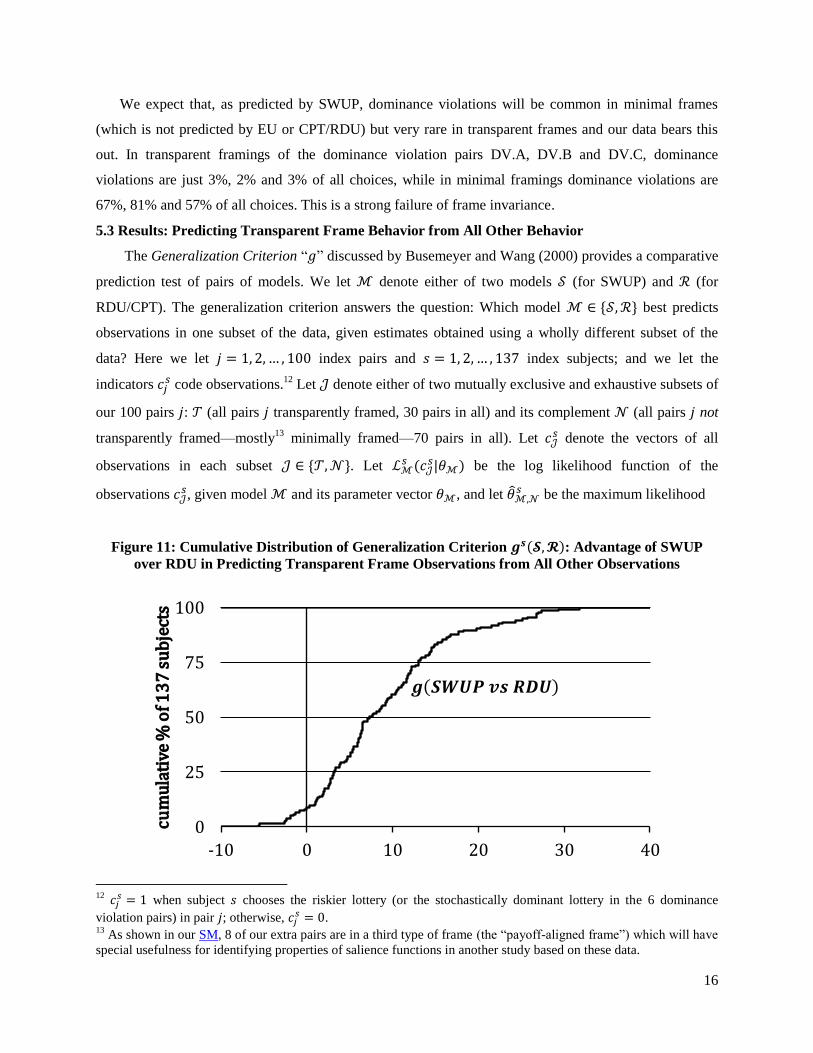
5.3 Results: Predicting Transparent Frame Behavior from All Other Behavior

The Generalization Criterion “𝑔” discussed by Busemeyer and Wang (2000) provides a comparative

prediction test of pairs of models. We let ℳ denote either of two models 𝒮 (for SWUP) and ℛ (for

RDU/CPT). The generalization criterion answers the question: Which model ℳ ∈ {𝒮,ℛ} best predicts

observations in one subset of the data, given estimates obtained using a wholly different subset of the

data? Here we let 𝑗 = 1, 2, … , 100 index pairs and 𝑠 = 1, 2, … , 137 index subjects; and we let the

indicators 𝑐𝑗𝑠 code observations.

12 Let 𝒥 denote either of two mutually exclusive and exhaustive subsets of

our 100 pairs 𝑗: 𝒯 (all pairs 𝑗 transparently framed, 30 pairs in all) and its complement 𝒩 (all pairs 𝑗 not

transparently framed—mostly13

minimally framed—70 pairs in all). Let 𝑐𝒥𝑠 denote the vectors of all

observations in each subset 𝒥 ∈ {𝒯,𝒩}. Let ℒℳ𝑠 (𝑐𝒥

𝑠|𝜃ℳ) be the log likelihood function of the

observations 𝑐𝒥𝑠, given model ℳ and its parameter vector 𝜃ℳ, and let 𝜃ℳ,𝒩

𝑠 be the maximum likelihood

Figure 11: Cumulative Distribution of Generalization Criterion 𝒈𝒔(𝓢,𝓡): Advantage of SWUP

over RDU in Predicting Transparent Frame Observations from All Other Observations

12

𝑐𝑗𝑠 = 1 when subject 𝑠 chooses the riskier lottery (or the stochastically dominant lottery in the 6 dominance

violation pairs) in pair 𝑗; otherwise, 𝑐𝑗𝑠 = 0.

13 As shown in our SM, 8 of our extra pairs are in a third type of frame (the “payoff-aligned frame”) which will have

special usefulness for identifying properties of salience functions in another study based on these data.

0

25

50

75

100

-10 0 10 20 30 40

cum

ula

tive

% o

f 13

7 s

ub

ject

s

𝒈 𝒔

17

estimates of 𝜃ℳ for subject 𝑠, based only on the observation vector 𝑐𝒩𝑠 : Frequently one calls 𝜃ℳ,𝒩

𝑠 the

“in-sample estimates” (a.k.a. “training data” or “calibration” estimates) for each model ℳ and each

subject 𝑠. Our supplementary material SM details the specification and estimation of the two models.

These in-sample estimates—wholly estimated without any transparent frame behavior—then become

predictors of the log likelihood of the “out-of-sample” observations 𝑐𝒯𝑠 in transparently framed pairs: This

measure of prediction information is ℒℳ𝑠 (𝑐𝒯

𝑠 |𝜃ℳ,𝒩𝑠 ). One then compares these information measures for

the pair of models: In our application, the generalization criterion for subject 𝑠 is 𝑔𝑠(𝒮, ℛ) =

2[ℒ𝒮𝑠(𝑐𝒯

𝑠 |𝜃𝒮,𝒩𝑠 ) − ℒℛ

𝑠 (𝑐𝒯𝑠 |�̂�ℛ,𝒩

𝑠 )]. When 𝑔𝑠(𝒮, ℛ) is positive, SWUP’s out-of-sample predictions are

better than those of RDU. Figure 11 shows the cumulative distribution of 𝑔𝑠(𝒮, ℛ) across our 137

subjects and demonstrates that SWUP is the overwhelmingly superior model by the generalization

criterion: 𝑔𝑠(𝒮, ℛ) is positive for 125 of the 137 subjects.

6. Minimal and Transparent Frames for Choice over Time: Present Bias and Hidden Zero Effects

Consider the minimal frames in Figure 12. The stationarity axiom of DU theory implies that people

should choose either 𝐫 and 𝐫′ or 𝐭 and 𝐭′. However, in choices such as these, experiments show that people

frequently choose 𝐫 and 𝐭′, a finding termed present bias (Laibson, 1997). Present bias occurs in the

minimal frames in Figure 12 since the comparison between receiving money today versus in one year is

more salient than the comparison of $75 versus $100, but this monetary comparison is more salient than

receiving payment in 10 or 11 years. However, in transparent frames, the focal comparisons in both

choices are between $75 and $0 and between $100 and $0. Switching from minimal to transparent frames

provides a formal explanation of the hidden zero effect (Magen et al., 2008; Radu et al., 2011; Read et al.,

2017) in which behavior becomes more patient when the opportunity costs of income (such as receiving

$0 instead of $100 in 1 year) are made salient. Transparent frames retain the second choice of 𝐭′ over 𝐫′

from minimal frames, but shift the first choice toward preferring 𝐭 over 𝐫 via the hidden zero effect. The

prediction of more patient behavior in transparent frames is also consistent with the finding by Fisher and

Rangel (2014) that shifting attention from focusing on time to focusing on money reduces impatience

Figure 12. Present Bias in Minimal and Transparent Frames

In Minimal Frames In Transparent Frames x1,y1 Years x1,y1 Years x2,y2 Years

𝐫 75 0 𝐫 75 0 0 1

𝐭 100 1 𝐭 0 0 100 1 x1,y1 Years x1,y1 Years x2,y2 Years

𝐫′ 75 10 𝐫′ 75 10 0 11

𝐭′ 100 11 𝐭′ 0 10 100 11

18

since transparent frames increase the salience of the money dimension relative to minimal frames.

Transparent frames may thus serve to induce more patient behavior and more time consistent behavior.

7. Minimal and Transparent Frames for Choice under Ambiguity: Ellsberg’s Paradox

The SWUP model in (9) predicts ambiguity aversion in minimal frames, but also predicts that

transparent frames will reduce it. To illustrate this we refer to four “option pairs” Schneider, Leland, and

Wilcox (2018) presented to 79 subjects. To understand these option pairs, first suppose that the top pair

{A, B} in Figure 13 was selected for payout at the conclusion of a subject’s session,14

and the subject

chose B from it. The subject then blindly draws one ticket from an opaque bag containing an unknown

mixture of red and blue tickets: If she draws a red ticket, she plays a lottery with a 75% chance of winning

$25 and a 25% chance of winning nothing; but if she draws a blue ticket, she instead plays a lottery with a

25% chance of winning $25 and a 75% chance of winning nothing. If she had chosen option A instead,

she would play a lottery with a 50% chance of winning $25 and a 50% chance of winning nothing

regardless of the ticket color she draws. The pair {A′, B′} is similar except that in option B′ the “good”

state is reversed. For these minimal frames, the experiment replicates Ellsberg’s Paradox, finding that

people do not assign well-defined subjective probabilities to states, but rather prefer alternatives with

known probabilities over unknown probabilities—a preference pattern called ambiguity aversion.

Figure 13. The Ellsberg Paradox in Minimal Frames

Red Ticket

Blue Ticket

A $25 0.50 $0 0.50 $25 0.50 $0 0.50

B $25 0.75 $0 0.25 $25 0.25 $0 0.75

Red Ticket

Blue Ticket

A′ $25 0.50 $0 0.50 $25 0.50 $0 0.50

B′ $25 0.25 $0 0.75 $25 0.75 $0 0.25

With a uniform prior over states

15 and normalizing 𝑢(25) = 1 and 𝑢(0) = 0, SWUP implies that A

is chosen over B in the minimal frame shown in the top panel of Figure 13 if inequality (12) holds:

(12) 0.5𝜙(0.5,0.75)(−0.25) + 0.5𝜙(0.5, 0.25)(0.25) > 0.

By symmetry and DAS, 𝜙(0.5,0.25) > 𝜙(0.5,0.75), so (12) holds for all salience and utility functions.

Intuitively, the salient comparisons between A and B are between a 0.50 probability of winning and a

0.75 probability (in the ‘red’ state) and between probabilities of 0.50 and 0.25 (in the ‘blue’ state).

Diminishing absolute sensitivity implies a focal thinker will be more sensitive to the latter comparison.

Similarly, A′ is chosen over B′ in the bottom panel of Figure 13, yielding ambiguity aversion.

14

A subject chose from 60 pairs and, at the session’s end, one of the 60 pairs was randomly chosen for payout. 15

In estimating a mean-dispersion model of ambiguity preference to explain their data, Schneider, Leland, and

Wilcox (2018) estimate the subjective prior assigned to red and blue ticket states to be near uniform for the great

majority of their 79 subjects.

19

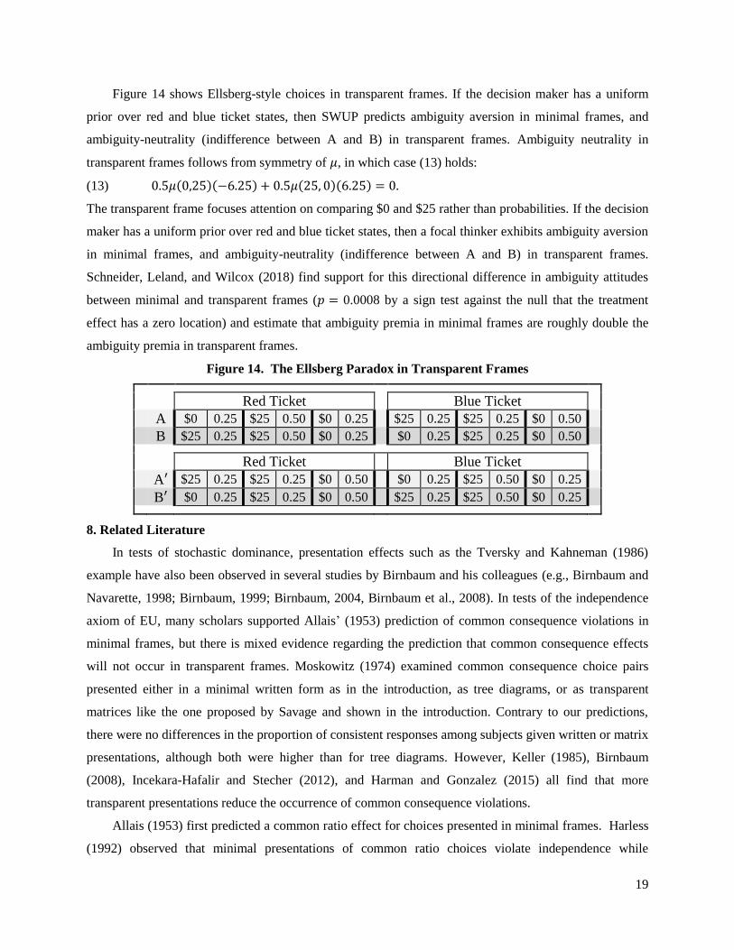
Figure 14 shows Ellsberg-style choices in transparent frames. If the decision maker has a uniform

prior over red and blue ticket states, then SWUP predicts ambiguity aversion in minimal frames, and

ambiguity-neutrality (indifference between A and B) in transparent frames. Ambiguity neutrality in

transparent frames follows from symmetry of 𝜇, in which case (13) holds:

(13) 0.5𝜇(0,25)(−6.25) + 0.5𝜇(25, 0)(6.25) = 0.

The transparent frame focuses attention on comparing $0 and $25 rather than probabilities. If the decision

maker has a uniform prior over red and blue ticket states, then a focal thinker exhibits ambiguity aversion

in minimal frames, and ambiguity-neutrality (indifference between A and B) in transparent frames.

Schneider, Leland, and Wilcox (2018) find support for this directional difference in ambiguity attitudes

between minimal and transparent frames (𝑝 = 0.0008 by a sign test against the null that the treatment

effect has a zero location) and estimate that ambiguity premia in minimal frames are roughly double the

ambiguity premia in transparent frames.

Figure 14. The Ellsberg Paradox in Transparent Frames

Red Ticket

Blue Ticket

A $0 0.25 $25 0.50 $0 0.25 $25 0.25 $25 0.25 $0 0.50

B $25 0.25 $25 0.50 $0 0.25 $0 0.25 $25 0.25 $0 0.50

Red Ticket

Blue Ticket

A′ $25 0.25 $25 0.25 $0 0.50 $0 0.25 $25 0.50 $0 0.25

B′ $0 0.25 $25 0.25 $0 0.50 $25 0.25 $25 0.50 $0 0.25

8. Related Literature

In tests of stochastic dominance, presentation effects such as the Tversky and Kahneman (1986)

example have also been observed in several studies by Birnbaum and his colleagues (e.g., Birnbaum and

Navarette, 1998; Birnbaum, 1999; Birnbaum, 2004, Birnbaum et al., 2008). In tests of the independence

axiom of EU, many scholars supported Allais’ (1953) prediction of common consequence violations in

minimal frames, but there is mixed evidence regarding the prediction that common consequence effects

will not occur in transparent frames. Moskowitz (1974) examined common consequence choice pairs

presented either in a minimal written form as in the introduction, as tree diagrams, or as transparent

matrices like the one proposed by Savage and shown in the introduction. Contrary to our predictions,

there were no differences in the proportion of consistent responses among subjects given written or matrix

presentations, although both were higher than for tree diagrams. However, Keller (1985), Birnbaum

(2008), Incekara-Hafalir and Stecher (2012), and Harman and Gonzalez (2015) all find that more

transparent presentations reduce the occurrence of common consequence violations.

Allais (1953) first predicted a common ratio effect for choices presented in minimal frames. Harless

(1992) observed that minimal presentations of common ratio choices violate independence while

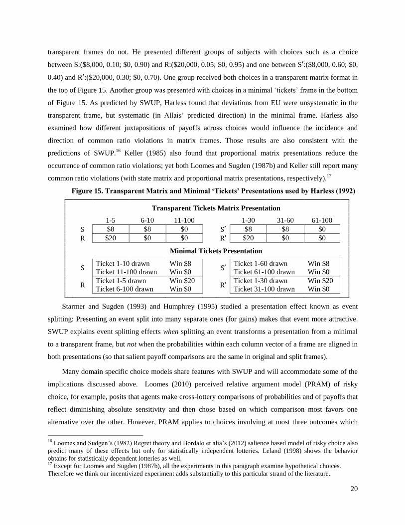
20

transparent frames do not. He presented different groups of subjects with choices such as a choice

between S:($8,000, 0.10; $0, 0.90) and R:($20,000, 0.05; $0, 0.95) and one between S′:($8,000, 0.60; $0,

0.40) and R′:($20,000, 0.30; $0, 0.70). One group received both choices in a transparent matrix format in

the top of Figure 15. Another group was presented with choices in a minimal ‘tickets’ frame in the bottom

of Figure 15. As predicted by SWUP, Harless found that deviations from EU were unsystematic in the

transparent frame, but systematic (in Allais’ predicted direction) in the minimal frame. Harless also

examined how different juxtapositions of payoffs across choices would influence the incidence and

direction of common ratio violations in matrix frames. Those results are also consistent with the

predictions of SWUP.16

Keller (1985) also found that proportional matrix presentations reduce the

occurrence of common ratio violations; yet both Loomes and Sugden (1987b) and Keller still report many

common ratio violations (with state matrix and proportional matrix presentations, respectively).17

Figure 15. Transparent Matrix and Minimal ‘Tickets’ Presentations used by Harless (1992)

Transparent Tickets Matrix Presentation 1-5 6-10 11-100 1-30 31-60 61-100

S $8 $8 $0 S′ $8 $8 $0

R $20 $0 $0 R′ $20 $0 $0 Minimal Tickets Presentation

S Ticket 1-10 drawn Win $8

S′ Ticket 1-60 drawn Win $8

Ticket 11-100 drawn Win $0 Ticket 61-100 drawn Win $0

R

Ticket 1-5 drawn Win $20 R′

Ticket 1-30 drawn Win $20

Ticket 6-100 drawn Win $0 Ticket 31-100 drawn Win $0

Starmer and Sugden (1993) and Humphrey (1995) studied a presentation effect known as event

splitting: Presenting an event split into many separate ones (for gains) makes that event more attractive.

SWUP explains event splitting effects when splitting an event transforms a presentation from a minimal

to a transparent frame, but not when the probabilities within each column vector of a frame are aligned in

both presentations (so that salient payoff comparisons are the same in original and split frames).

Many domain specific choice models share features with SWUP and will accommodate some of the

implications discussed above. Loomes (2010) perceived relative argument model (PRAM) of risky

choice, for example, posits that agents make cross-lottery comparisons of probabilities and of payoffs that

reflect diminishing absolute sensitivity and then chose based on which comparison most favors one

alternative over the other. However, PRAM applies to choices involving at most three outcomes which

16

Loomes and Sudgen’s (1982) Regret theory and Bordalo et alia’s (2012) salience based model of risky choice also

predict many of these effects but only for statistically independent lotteries. Leland (1998) shows the behavior

obtains for statistically dependent lotteries as well. 17

Except for Loomes and Sugden (1987b), all the experiments in this paragraph examine hypothetical choices.

Therefore we think our incentivized experiment adds substantially to this particular strand of the literature.

21

limits its applicability. Scholten and Read's (2010) tradeoff model of intertemporal choices, like SWUP,

posits that decisions result not from alternative-based discounting but from trading off time differences

against payoff differences across alternatives. However, it has not been extended to risky or ambiguous

choice and leaves no room for discounting: SWUP incorporates both discounting and context-

dependence. Birnbaum and Chavez's (1997) transfer-of-attention-exchange (TAX) is an early example of

a model in which aspects of lotteries result in some attributes receiving more attention and

disproportionate weight. TAX predicts the framing effects implied by SWUP for choices under risk but

has not been extended to intertemporal choices nor those under uncertainty.

Loomes and Sudgen's (1982, 1987a) Regret theory and Bordalo et. alia’s (2012) salience theory also

posit comparative decision processes that overweight large payoff differences (either for their potential to

induce regret or as a consequence of their perceived salience). While these models make predictions in

the context of risky choice that are similar to SWUP, their predictions depend critically on whether the

alternatives are assumed to be statistically dependent or independent, as it is the correlation between

lotteries that determines which comparisons are made. Under SWUP, comparisons made are simply

determined by how options are presented and what payoffs and probabilities (or time periods) are aligned

in the presentation, and not at all on how probability-generating mechanisms are related across the two

lotteries in that presentation. Because of this, the dominance violations we observed in our experiment

(which induces statistically independent lotteries) are predicted by SWUP but ruled out by Regret theory

and the salience theory of Bordalo et. alia.18

9. Summary

We now gather our results on framing effects for risk, time, and ambiguity in three propositions.

Earlier in sections 4, 6 and 7 we illustrated the claims in Proposition 1 (see our SM for the calculations).

Proposition 1 (Minimal Frames and Behavioral Biases):

A focal thinker with linear utility 𝑢(𝑥) = 𝑥 and either the DAS (10) or DAS-IPS (11) salience function:

(i) violates stochastic dominance in the minimal frame in Figure 4;

(ii) exhibits the Allais paradox in the minimal frames in Figure 5;

(iii) exhibits the common ratio effect in the minimal frames in Figure 6;

(iv) exhibits present bias in the minimal frames in Figure 12

(for annual discount factor 𝛿 ∈ [0.41, 0.95]); and

(v) exhibits Ellsberg's paradox in the minimal frames in Figure 13.

For minimal frames, we prove more general results regarding two of the most robust and most well-

known violations of EU theory: the Allais common ratio effect and the Ellsberg paradox. Although these

paradoxes are two of the oldest violations of rational choice theory, there has been relatively little work

18

See Loomes and Sugden (1987a, p. 274) and Bordalo et alia (2012, p. 1259).

22

investigating the precise relationship between them. Proposition 2 is proved in our Appendix, for general

versions of the Allais common ratio effect and Ellsberg’s paradox also defined in the Appendix.

Proposition 2 (Allais, Ellsberg, and Salience Perception): For monotone minimal frames:

(i) A focal thinker exhibits the general Allais common ratio effect if and only if 𝜙 satisfies increasing

proportional sensitivity.

(ii) Under a uniform prior, a focal thinker exhibits ambiguity aversion in Ellsberg’s paradox if 𝜙

satisfies diminishing absolute sensitivity.

Proposition 2 is general and establishes that two basic properties of the perceptual system (greater

sensitivity to larger absolute differences for a fixed ratio (IPS), and greater sensitivity to larger ratios for a

fixed absolute difference (DAS)) directly imply the most robust violations of EU theory without any

parametric assumptions regarding the form of the agent’s salience functions or utility functions.

Without defining them precisely, Savage (1954) and Tversky and Kahneman (1986) argued that

transparent presentations would reduce violations of rational choice theory. We formalized ‘transparent

presentation’ of choice alternatives for risk, ambiguity, and time using a set of properties which imply

unique transparent frames. With this done we can now state a theorem concerning transparent frames—

converting a long-standing suggestion into a set of falsifiable statements. Consider four types of

systematic violations of rational choice theory: violations of stochastic dominance, Allais paradox

violations of EU theory, present biased violations of DU theory, and Ellsberg paradox violations of

subjective expected utility (or SEU) theory. We show they should all vanish under our definition of

transparent framing: This Transparent Frame Theorem is proved in our Appendix.

Proposition 3 (Transparent Frame Theorem): For transparent frames, a focal thinker will not exhibit

the following violations of rational choice theory, even if the focal thinker exhibits them in minimal

frames:

(i) Violations of Stochastic Dominance;

(ii) Allais Paradox violations of EU theory;

(iii) Common Ratio violations of EU theory;

(iv) Present Bias violations of DU theory; and

(v) Ellsberg Paradox violations of SEU theory.

The transparent frame theorem is general in that it does not depend on the form of the decision maker’s

salience functions or on the form of the decision maker’s utility function or discount factor or subjective

beliefs, or on the particular parameter values used for the paradoxes, and it applies to choices across the

domains of risk, time, and uncertainty.

For risk, transparent frames are similar to the state matrices employed by Savage (1954) (but

implying neither correlation nor independence between payoffs) and to the ‘canonical split form’ of

23

Birnbaum and Schmidt’s (2015) tree presentation of lotteries, but are distinct in that the canonical split

form does not separate common consequences from distinct consequences. For decisions under risk,

minimal frames are related to Birnbaum’s (1999) tree presentation of lotteries in ‘coalesced form:’ In

particular, a choice set in which all lotteries are in coalesced form generates a minimal frame. We are not

aware of any previous attempt to formalize different presentation formats for income streams over time.

Our definitions of frames and our formal distinctions between minimal and transparent frames

provide a unified foundation for analyzing choice presentations across three major domains of individual

choice. Combine that foundation with a decision model that operates on frames (such as SWUP), and a

formal logic of framing effects emerges. The same mathematical structure—and the same psychological

intuition—explains a variety of the most robust and well-known behavioral biases across the domains of

risk, uncertainty, and time, violating four of the most well-known axioms in rational choice theory

(stochastic dominance, independence, stationarity, and the sure-thing principle). Focal thinkers will

violate these axioms in minimal frames but satisfy them in transparent frames. Evidence from previous

literature and from our own experiment suggests that biases are reduced, but not eliminated, when the

presentation of choice alternatives is made transparent.

Appendix

Here, 𝐯 ≻̂ 𝐰 (𝐯 ~̂ 𝐰) means that for focal thinkers, option 𝑣 ‘looks strictly better than’ (‘looks indifferent

to’) option 𝑤 when a frame ⟦𝐯,𝐰⟧ (of type specified in each proposition) presents the choice pair {𝑣, 𝑤}.

A.1 Proof of Proposition 2 (Allais and Ellsberg in Minimal Frames)

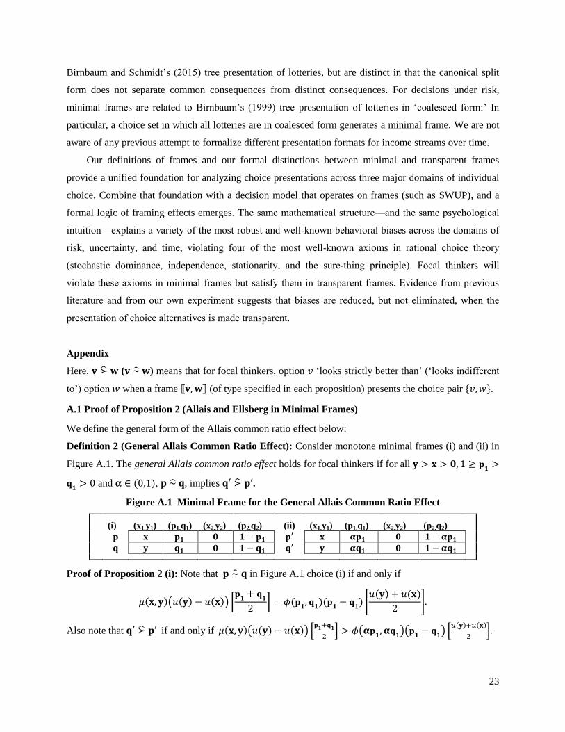
We define the general form of the Allais common ratio effect below:

Definition 2 (General Allais Common Ratio Effect): Consider monotone minimal frames (i) and (ii) in

Figure A.1. The general Allais common ratio effect holds for focal thinkers if for all 𝐲 > 𝐱 > 𝟎, 1 ≥ 𝐩𝟏>

𝐪𝟏> 0 and 𝛂 ∈ (0,1), 𝐩 ~̂ 𝐪, implies 𝐪′ ≻̂ 𝐩′.

Figure A.1 Minimal Frame for the General Allais Common Ratio Effect

(i) (x1,y1) (p1,q1) (x2,y2) (p2,q2) (ii) (x1,y1) (p1,q1) (x2,y2) (p2,q2)

𝐩 𝐱 𝐩𝟏 𝟎 𝟏 − 𝐩𝟏 𝐩′ 𝐱 𝛂𝐩𝟏 𝟎 𝟏 − 𝛂𝐩𝟏

𝐪 𝐲 𝐪𝟏 𝟎 𝟏 − 𝐪𝟏 𝐪′ 𝐲 𝛂𝐪𝟏 𝟎 𝟏 − 𝛂𝐪𝟏

Proof of Proposition 2 (i): Note that 𝐩 ~̂ 𝐪 in Figure A.1 choice (i) if and only if

𝜇(𝐱, 𝐲)(𝑢(𝐲) − 𝑢(𝐱)) [𝐩𝟏+ 𝐪

𝟏

2] = 𝜙(𝐩

𝟏, 𝐪

𝟏)(𝐩

𝟏− 𝐪

𝟏) [𝑢(𝐲) + 𝑢(𝐱)

2].

Also note that 𝐪′ ≻̂ 𝐩′ if and only if 𝜇(𝐱, 𝐲)(𝑢(𝐲) − 𝑢(𝐱)) [𝐩𝟏+𝐪𝟏2

] > 𝜙(𝛂𝐩𝟏, 𝛂𝐪

𝟏)(𝐩

𝟏− 𝐪

𝟏) [

𝑢(𝐲)+𝑢(𝐱)

2].

24

By IPS, scaling 𝛂𝐩𝟏 and 𝛂𝐪

𝟏 each by

1

𝛂 leads to 𝜙(𝛂𝐩

𝟏, 𝛂𝐪

𝟏) < 𝜙(𝐩

𝟏, 𝐪

𝟏) for all 𝛂 ∈ (0,1). Letting

𝐤 ≡ 1/𝛂, the common ratio effect holds if and only if (𝛂𝐩𝟏, 𝛂𝐪

𝟏) < 𝜙(𝐤𝛂𝐩

𝟏, 𝐤𝛂𝐪

𝟏) for all 𝐤 > 1. ∎

Next, consider Ellsberg’s (1961) two-color paradox. There are two urns. Urn 1 contains 50 red and 50

black balls. Urn 2 contains an unknown mixture of 100 red and black balls. A person is given two

choices:

SEU requires choices of either A and D or B and C. However, Ellsberg found that most people choose A

and C (options with objective probabilities) over B and D (options with ambiguous probabilities) thereby

exhibiting ambiguity aversion. The minimal frame for these choices (for each state 𝑠 ∈ {0, 1,… , 100}, the

actual number of red balls in Urn 2) is displayed in Figure A.2, where q(s) is the probability of drawing a

red ball from Urn 2 in state 𝑠.

Figure A.2. Minimal Frame for the Two-Color Ellsberg Paradox

A(s) $100 0.5 $0 0.5

B(s) $100 q(s) $0 1 − q(s) C(s) $100 0.5 $0 0.5

D(s) $100 1 − q(s) $0 q(s)

Definition 3 (Ambiguity Aversion in Ellsberg’s Paradox): For the frames in Figure A.2, a focal thinker

exhibits ambiguity aversion in Ellsberg’s paradox if 𝐀 ≻̂ 𝐁 and 𝐂 ≻̂D.

Proof of Proposition 2 (ii): This proof is for Ellsberg’s two-color paradox. An analogous argument

resolves Ellsberg’s three-color paradox. Let 𝑠 denote the number of red balls in Urn 2. Since the number

of black balls is 100 − 𝑠, the state of the urn is fully characterized by 𝑠. For each state, the presentation

for Choice 1 is given by Figure A.2, where 𝐪(𝐬) is the probability of drawing a red ball from Urn 2 in

state 𝑠. Normalize payoffs such that 𝑢(𝟏𝟎𝟎) = 1, and 𝑢(𝟎) = 0. For a focal thinker, A is chosen over B

if and only if inequality (14) holds. Under a uniform prior, (14) becomes (15):

∑ 𝜋𝑠𝑚𝑠=1 [ϕ(𝟎. 𝟓, 𝐪(𝐬))(𝟎. 𝟓 − 𝐪(𝐬))] > 0.

1

101[∑ ϕ(𝟎. 𝟓, 𝐪(𝐬))(𝟎. 𝟓 − 𝐪(𝐬))𝑠=50

𝑠=0 + ∑ ϕ(𝟎. 𝟓, 𝐪(𝐬))(𝟎. 𝟓 − 𝐪(𝐬))]𝑠=100𝑠=51 > 0which implies

(16) ∑ ϕ(𝟎. 𝟓, 𝐪(𝐬))(𝟎. 𝟓 − 𝐪(𝐬))𝑠=50𝑠=0 + ∑ ϕ(𝟎. 𝟓, 𝟏 − 𝐪(𝐬))(𝐪(𝐬) − 𝟎. 𝟓)𝑠=50

𝑠=0 > 0.

To see that (14) holds, note that for each 𝐪(𝐬) ∈ [0,0.5) diminishing absolute sensitivity and symmetry of

ϕ imply ϕ(𝟎. 𝟓, 𝟏 − 𝐪(𝒔)) < ϕ(𝟎. 𝟓, 𝐪(𝐬)). In particular, by symmetry, ϕ(𝟎. 𝟓, 𝟏 − 𝐪(𝐬)) =

ϕ(𝟎. 𝟓 + 𝟎. 𝟓 − 𝐪(𝐬), 𝐪(𝐬) + 𝟎. 𝟓 − 𝐪(𝐬)) = ϕ(𝟎. 𝟓 + 𝛜, 𝐪(𝐬) + 𝛜). Thus, by diminishing absolute

Choice 1: Choose between A and B

A. Win $100 if red is drawn from Urn 1

B. Win $100 if red is drawn from Urn 2

Choice 2: Choose between C and D

C. Win $100 if black is drawn from Urn 1

D. Win $100 if black is drawn from Urn 2

25

sensitivity, (16) holds, yielding a choice for the risky over the ambiguous urn. The argument follows

analogously for the choice between C and D, resulting in ambiguity aversion. ∎

A.2 Proof of Proposition 3 (Transparent Frame Theorem)

Proof of Proposition 3 (i): Lottery 𝑝 is defined to stochastically dominate 𝑞 if 𝑃(𝑥) ≤ 𝑄(𝑥) for all 𝑥 ∈

X, with at least one strict inequality, where 𝑃(𝑥) and 𝑄(𝑥) are the cumulative distribution functions

corresponding to 𝑝 and 𝑞, respectively. Whenever 𝑝 stochastically dominates 𝑞, 𝐱𝐢 ≥ 𝐲𝐢 and 𝐩𝐢 − 𝐪𝐢 = 0

for all 𝑖 in a transparent frame. Thus, the salience weights in (4) favor 𝐩 over 𝐪 in each binary comparison

where the differences are not zero. ∎

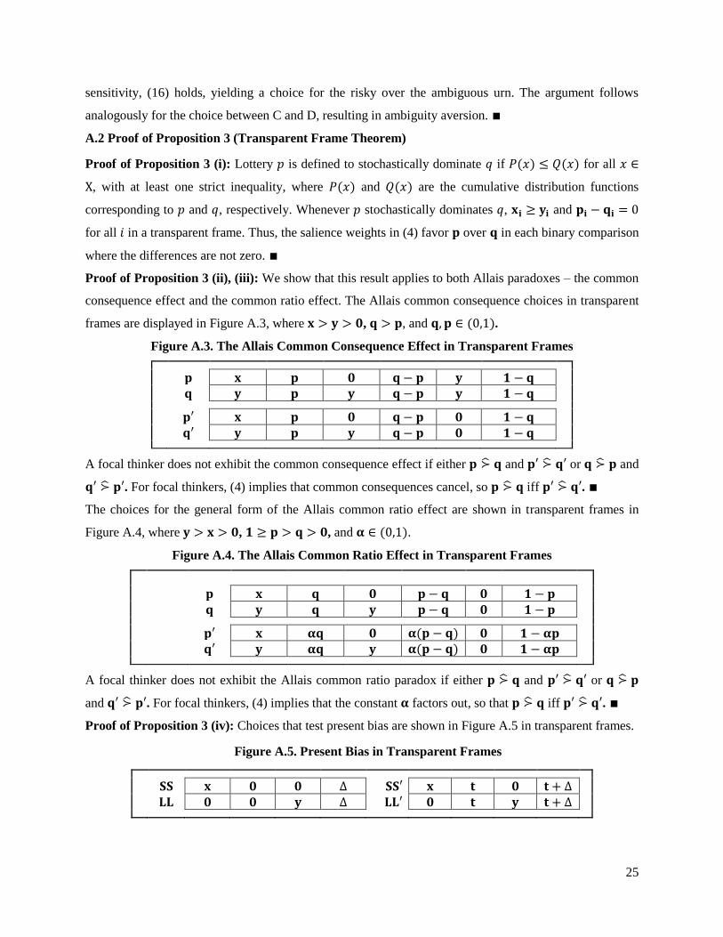
Proof of Proposition 3 (ii), (iii): We show that this result applies to both Allais paradoxes – the common

consequence effect and the common ratio effect. The Allais common consequence choices in transparent

frames are displayed in Figure A.3, where 𝐱 > 𝐲 > 𝟎, 𝐪 > 𝐩, and 𝐪, 𝐩 ∈ (0,1).

Figure A.3. The Allais Common Consequence Effect in Transparent Frames

𝐩 𝐱 𝐩 𝟎 𝐪 − 𝐩 𝐲 𝟏 − 𝐪

𝐪 𝐲 𝐩 𝐲 𝐪 − 𝐩 𝐲 𝟏 − 𝐪

𝐩′ 𝐱 𝐩 𝟎 𝐪 − 𝐩 𝟎 𝟏 − 𝐪

𝐪′ 𝐲 𝐩 𝐲 𝐪 − 𝐩 𝟎 𝟏 − 𝐪

A focal thinker does not exhibit the common consequence effect if either 𝐩 ≻̂ 𝐪 and 𝐩′ ≻̂ 𝐪′ or 𝐪 ≻̂ 𝐩 and

𝐪′ ≻̂ 𝐩′. For focal thinkers, (4) implies that common consequences cancel, so 𝐩 ≻̂ 𝐪 iff 𝐩′ ≻̂ 𝐪′. ∎

The choices for the general form of the Allais common ratio effect are shown in transparent frames in

Figure A.4, where 𝐲 > 𝐱 > 𝟎, 𝟏 ≥ 𝐩 > 𝐪 > 𝟎, and 𝛂 ∈ (0,1).

Figure A.4. The Allais Common Ratio Effect in Transparent Frames

𝐩 𝐱 𝐪 𝟎 𝐩 − 𝐪 𝟎 𝟏 − 𝐩

𝐪 𝐲 𝐪 𝐲 𝐩 − 𝐪 𝟎 𝟏 − 𝐩

𝐩′ 𝐱 𝛂𝐪 𝟎 𝛂(𝐩 − 𝐪) 𝟎 𝟏 − 𝛂𝐩

𝐪′ 𝐲 𝛂𝐪 𝐲 𝛂(𝐩 − 𝐪) 𝟎 𝟏 − 𝛂𝐩

A focal thinker does not exhibit the Allais common ratio paradox if either 𝐩 ≻̂ 𝐪 and 𝐩′ ≻̂ 𝐪′ or 𝐪 ≻̂ 𝐩

and 𝐪′ ≻̂ 𝐩′. For focal thinkers, (4) implies that the constant 𝛂 factors out, so that 𝐩 ≻̂ 𝐪 iff 𝐩′ ≻̂ 𝐪′. ∎

Proof of Proposition 3 (iv): Choices that test present bias are shown in Figure A.5 in transparent frames.

Figure A.5. Present Bias in Transparent Frames

𝐒𝐒 𝐱 𝟎 𝟎 ∆ 𝐒𝐒′ 𝐱 𝐭 𝟎 𝐭 + ∆

𝐋𝐋 𝟎 𝟎 𝐲 ∆ 𝐋𝐋′ 𝟎 𝐭 𝐲 𝐭 + ∆

26

Present bias is absent if either 𝐒𝐒 ≻̂𝐭 𝐋𝐋 and 𝐒𝐒′ ≻̂𝐭 𝐋𝐋′ or 𝐋𝐋 ≻̂𝐭 𝐒𝐒 and 𝐋𝐋′ ≻̂𝐭 𝐒𝐒′. For a focal thinker,

(6) gives both SS ≻̂𝑡 LL iff 𝜇(𝐱, 𝟎)𝑢(𝐱) > 𝜇(𝟎, 𝐲)𝑢(𝐲)𝛿∆ and SS′ ≻̂𝑡 LL′ iff 𝜇(𝐱, 𝟎)𝑢(𝐱)𝛿𝐭 >

𝜇(𝟎, 𝐲)𝑢(𝐲)𝛿𝐭+∆. Since 𝛿𝒕 can be factored out of the latter, SS ≻̂𝑡 LL iff SS′ ≻̂𝑡 LL′. ∎

Proof of Proposition 3 (v): The transparent frames for Choices 1 and 2 in Ellsberg’s two-color paradox

are shown in Figure A.6, where state 𝑠 ∈ {0,1,… ,100} indexes the number of red balls in Urn 2, and

𝑝(𝑠) = |50 − 𝑠|/100. Note that when 𝑝(𝑠) = 0.25, Figure A.6 resembles the frame in Figure 14.

Ellsberg’s paradox absent if either 𝐀 ≻̂ 𝐁 and 𝐃 ≻̂ 𝐂 or 𝐁 ≻̂ 𝐀 and 𝐂 ≻̂ 𝐃 or if there is indifferent in both

choices. Without loss of generality, set 𝑢(100) = 1 and 𝑢(0) = 0. Denote the set of states favoring A by

𝑆 and the set of states favoring B by 𝑆. The SWUP evaluation for the choice between A and B is:

(17) ∑ 𝜋𝑠𝑠∈𝑆 𝜇(100,0)(𝑝(𝑠)) + ∑ 𝜋𝑠𝑠∈𝑆 𝜇(0,100)(−𝑝(𝑠))

Figure A.6. The Ellsberg Paradox in Transparent Frames

States favoring A: 𝑠 ∈ {0,1, … ,50}

States favoring B: 𝑠 ∈ {51,52, … ,100}

A $100 𝑝(𝑠) $100 0.5 − 𝑝(𝑠) $0 0.5 $0 𝑝(𝑠) $100 0.5 $0 0.5 − 𝑝(𝑠)

B $0 𝑝(𝑠) $100 0.5 − 𝑝(𝑠) $0 0.5 $100 𝑝(𝑠) $100 0.5 $0 0.5 − 𝑝(𝑠)

States favoring C: 𝑠 ∈ {51,52, … ,100}

States favoring D: 𝑠 ∈ {0,1, … ,50}

C $100 𝑝(𝑠) $100 0.5 − 𝑝(𝑠) $0 0.5 $0 𝑝(𝑠) $100 0.5 $0 0.5 − 𝑝(𝑠)

D $0 𝑝(𝑠) $100 0.5 − 𝑝(𝑠) $0 0.5 $100 𝑝(𝑠) $100 0.5 $0 0.5 − 𝑝(𝑠)

where 𝜋𝑠 is the subjective probability that the true state is 𝑠. All other differences within each column in

the frame cancel. Under a uniform prior, the decision maker is indifferent between A and B (by symmetry

of 𝜇) in which case the evaluation in (17) equals zero. Moreover, even if the distribution is not uniform,

(17) implies ambiguity neutrality since if (17) is positive, the decision maker would prefer A and D since

the same set of states favor A and D. If (17) is negative, the decision maker prefers B and C. This

argument extends analogously to Ellsberg’s (1961) three-color paradox. ∎

A.3 Minimal Frames

Definition 4 (Minimal Frame: Risk): For two non-degenerate lotteries 𝑝, 𝑞 ∈ ∆(𝑋), frame ⟦𝐩, 𝐪⟧ (such

as in the top panel of Figure 1) is minimal if ∀ 𝐢 ≠ 𝐣, 𝐱𝐢 ≠ 𝐱𝐣 and 𝐲𝐢 ≠ 𝐲𝐣.

Definition 5 (Monotone Frame: Risk): For two non-degenerate lotteries 𝑝, 𝑞 ∈ ∆(𝑋), frame ⟦𝐩, 𝐪⟧ (such

as in the top panel of Figure 1) is monotone if 𝐱𝟏 ≥ 𝐱𝟐 ≥ ⋯ ≥ 𝐱𝐧 and 𝐲𝟏 ≥ 𝐲𝟐 ≥ ⋯ ≥ 𝐲𝐧.

The following result is immediate.

Proposition 4 (Uniqueness of Monotone Minimal Frames: Risk): For any lotteries 𝑝, 𝑞 ∈ ∆(𝑋) with

|𝑠𝑢𝑝𝑝(𝑝)| = |𝑠𝑢𝑝𝑝(𝑞)|, a monotone minimal frame ⟦𝐩, 𝐪⟧ is unique up to the operation of row-

switching.

Proof: A frame that is minimal and monotonic is strictly monotonic. Hence, for two lotteries with the

same support size, the ith best outcome of 𝑝 is in the same column vector as the i

th best outcome of 𝑞.∎

27

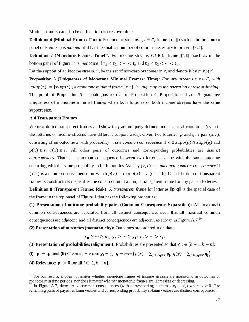
Minimal frames can also be defined for choices over time.

Definition 6 (Minimal Frame: Time): For income streams 𝑟, 𝑡 ∈ 𝐶, frame ⟦𝐫, 𝐭⟧ (such as in the bottom

panel of Figure 1) is minimal if it has the smallest number of columns necessary to present {𝑟, 𝑡}.

Definition 7 (Monotone Frame: Time)19

: For income streams 𝑟, 𝑡 ∈ 𝐶, frame ⟦𝐫, 𝐭⟧ (such as in the

bottom panel of Figure 1) is monotone if 𝐫𝟏 < 𝐫𝟐 < ⋯ < 𝐫𝐧 and 𝐭𝟏 < 𝐭𝟐 < ⋯ < 𝐭𝐧.

Let the support of an income stream, 𝑟, be the set of non-zero outcomes in 𝑟, and denote it by 𝑠𝑢𝑝𝑝(𝑟).

Proposition 5 (Uniqueness of Monotone Minimal Frames: Time): For any streams 𝑟, 𝑡 ∈ 𝐶, with

|𝑠𝑢𝑝𝑝(𝑟)| = |𝑠𝑢𝑝𝑝(𝑡)|, a monotone minimal frame ⟦𝐫, 𝐭⟧ is unique up to the operation of row-switching.

The proof of Proposition 5 is analogous to that of Proposition 4. Propositions 4 and 5 guarantee

uniqueness of monotone minimal frames when both lotteries or both income streams have the same

support size.

A.4 Transparent Frames

We next define transparent frames and show they are uniquely defined under general conditions (even if

the lotteries or income streams have different support sizes). Given two lotteries, 𝑝 and 𝑞, a pair (𝑥, 𝑟),

consisting of an outcome 𝑥 with probability 𝑟, is a common consequence if 𝑥 ∈ 𝑠𝑢𝑝𝑝(𝑝) ∩ 𝑠𝑢𝑝𝑝(𝑞) and

𝑝(𝑥) ≥ 𝑟, 𝑞(𝑥) ≥ 𝑟. All other pairs of outcomes and corresponding probabilities are distinct

consequences. That is, a common consequence between two lotteries is one with the same outcome

occurring with the same probability in both lotteries. We say (𝑥, 𝑟) is a maximal common consequence if

(𝑥, 𝑟) is a common consequence for which 𝑝(𝑥) = 𝑟 or 𝑞(𝑥) = 𝑟 (or both). Our definition of transparent

frames is constructive: it specifies the construction of a unique transparent frame for any pair of lotteries.

Definition 8 (Transparent Frame: Risk): A transparent frame for lotteries ⟦𝐩, 𝐪⟧ is the special case of

the frame in the top panel of Figure 1 that has the following properties:

(1) Presentation of outcome-probability pairs (Common Consequence Separation): All (maximal)

common consequences are separated from all distinct consequences such that all maximal common

consequences are adjacent, and all distinct consequences are adjacent, as shown in Figure A.7.20

(2) Presentation of outcomes (monotonicity): Outcomes are ordered such that

𝐱𝐧 ≥ ⋯ ≥ 𝐱𝟏; 𝐲𝐧 ≥ ⋯ ≥ 𝐲𝟏; 𝐳𝐤 > ⋯ > 𝐳𝟏.

(3) Presentation of probabilities (alignment): Probabilities are presented so that ∀ 𝑖 ∈ [𝑘 + 1, 𝑘 + 𝑛]:

(i) 𝐩𝐢 = 𝐪𝐢; and (ii) Given 𝐱𝐢 = 𝑥 and 𝐲𝐢 = 𝑦, 𝐩𝐢 = 𝑚𝑖𝑛 (𝑝(𝑥) − ∑ 𝐩𝐣,𝑗<𝑖:𝐱𝐣=𝑥 𝑞(𝑦) − ∑ 𝐪𝐣𝑗<𝑖:𝐲𝐣=𝑦 ).

(4) Relevance: 𝐩𝐢 > 𝟎 for all 𝑖 ∈ [1, 𝑘 + 𝑛].

19

For our results, it does not matter whether monotone frames of income streams are monotonic in outcomes or

monotonic in time periods, nor does it matter whether monotonic frames are increasing or decreasing. 20

In Figure A.7, there are 𝑘 common consequences (with corresponding outcomes 𝑧1,…,𝑧𝑘) where 𝑘 ≥ 0. The

remaining pairs of payoff column vectors and corresponding probability column vectors are distinct consequences.

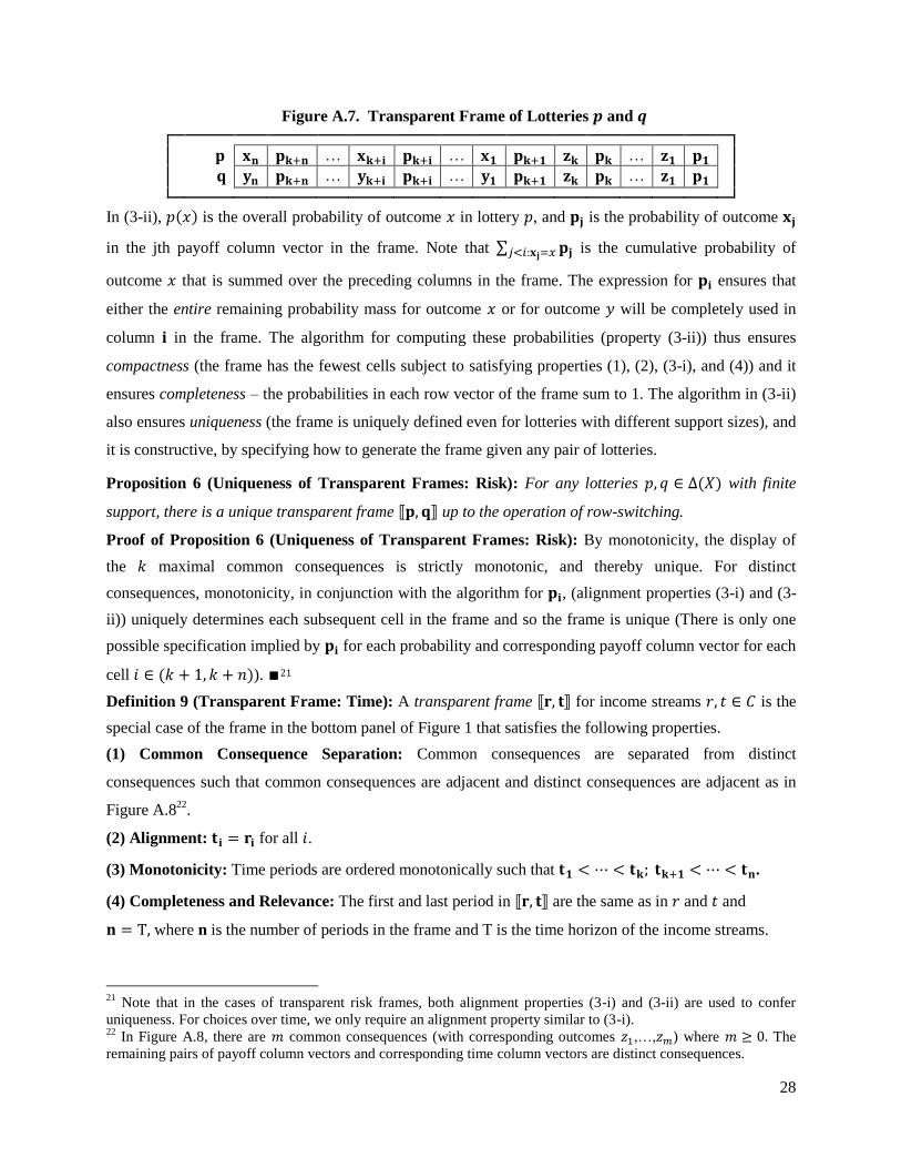
28

Figure A.7. Transparent Frame of Lotteries 𝒑 and 𝒒

𝐩 𝐱𝐧 𝐩𝐤+𝐧 … 𝐱𝐤+𝐢 𝐩𝐤+𝐢 … 𝐱𝟏 𝐩𝐤+𝟏 𝐳𝐤 𝐩𝐤 … 𝐳𝟏 𝐩𝟏

𝐪 𝐲𝐧 𝐩𝐤+𝐧 … 𝐲𝐤+𝐢 𝐩𝐤+𝐢 … 𝐲𝟏 𝐩𝐤+𝟏 𝐳𝐤 𝐩𝐤 … 𝐳𝟏 𝐩𝟏

In (3-ii), 𝑝(𝑥) is the overall probability of outcome 𝑥 in lottery 𝑝, and 𝐩𝐣 is the probability of outcome 𝐱𝐣

in the jth payoff column vector in the frame. Note that ∑ 𝐩𝐣𝑗<𝑖:𝐱𝐣=𝑥 is the cumulative probability of

outcome 𝑥 that is summed over the preceding columns in the frame. The expression for 𝐩𝐢 ensures that

either the entire remaining probability mass for outcome 𝑥 or for outcome 𝑦 will be completely used in

column 𝐢 in the frame. The algorithm for computing these probabilities (property (3-ii)) thus ensures

compactness (the frame has the fewest cells subject to satisfying properties (1), (2), (3-i), and (4)) and it

ensures completeness – the probabilities in each row vector of the frame sum to 1. The algorithm in (3-ii)

also ensures uniqueness (the frame is uniquely defined even for lotteries with different support sizes), and

it is constructive, by specifying how to generate the frame given any pair of lotteries.

Proposition 6 (Uniqueness of Transparent Frames: Risk): For any lotteries 𝑝, 𝑞 ∈ ∆(𝑋) with finite

support, there is a unique transparent frame ⟦𝐩, 𝐪⟧ up to the operation of row-switching.

Proof of Proposition 6 (Uniqueness of Transparent Frames: Risk): By monotonicity, the display of

the 𝑘 maximal common consequences is strictly monotonic, and thereby unique. For distinct

consequences, monotonicity, in conjunction with the algorithm for 𝐩𝐢, (alignment properties (3-i) and (3-

ii)) uniquely determines each subsequent cell in the frame and so the frame is unique (There is only one

possible specification implied by 𝐩𝐢 for each probability and corresponding payoff column vector for each

cell 𝑖 ∈ (𝑘 + 1, 𝑘 + 𝑛)). ∎21

Definition 9 (Transparent Frame: Time): A transparent frame ⟦𝐫, 𝐭⟧ for income streams 𝑟, 𝑡 ∈ 𝐶 is the

special case of the frame in the bottom panel of Figure 1 that satisfies the following properties.

(1) Common Consequence Separation: Common consequences are separated from distinct

consequences such that common consequences are adjacent and distinct consequences are adjacent as in

Figure A.822

.

(2) Alignment: 𝐭𝐢 = 𝐫𝐢 for all 𝑖.

(3) Monotonicity: Time periods are ordered monotonically such that 𝐭𝟏 < ⋯ < 𝐭𝐤; 𝐭𝐤+𝟏 < ⋯ < 𝐭𝐧.

(4) Completeness and Relevance: The first and last period in ⟦𝐫, 𝐭⟧ are the same as in 𝑟 and 𝑡 and

𝐧 = T, where n is the number of periods in the frame and T is the time horizon of the income streams.

21

Note that in the cases of transparent risk frames, both alignment properties (3-i) and (3-ii) are used to confer

uniqueness. For choices over time, we only require an alignment property similar to (3-i). 22

In Figure A.8, there are 𝑚 common consequences (with corresponding outcomes 𝑧1,…,𝑧𝑚) where 𝑚 ≥ 0. The

remaining pairs of payoff column vectors and corresponding time column vectors are distinct consequences.

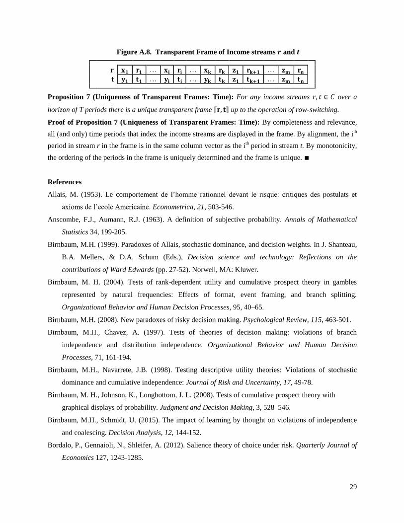
29

Figure A.8. Transparent Frame of Income streams 𝒓 and 𝒕

𝐫 𝐱𝟏 𝐫𝟏 … 𝐱𝐢 𝐫𝐢 … 𝐱𝐤 𝐫𝐤 𝐳𝟏 𝐫𝐤+𝟏 … 𝐳𝐦 𝐫𝐧

𝐭 𝐲𝟏 𝐭𝟏 … 𝐲𝐢 𝐭𝐢 … 𝐲𝐤 𝐭𝐤 𝐳𝟏 𝐭𝐤+𝟏 … 𝐳𝐦 𝐭𝐧

Proposition 7 (Uniqueness of Transparent Frames: Time): For any income streams 𝑟, 𝑡 ∈ 𝐶 over a

horizon of T periods there is a unique transparent frame ⟦𝐫, 𝐭⟧ up to the operation of row-switching.

Proof of Proposition 7 (Uniqueness of Transparent Frames: Time): By completeness and relevance,

all (and only) time periods that index the income streams are displayed in the frame. By alignment, the ith

period in stream r in the frame is in the same column vector as the ith period in stream t. By monotonicity,

the ordering of the periods in the frame is uniquely determined and the frame is unique. ∎

References

Allais, M. (1953). Le comportement de l’homme rationnel devant le risque: critiques des postulats et

axioms de l’ecole Americaine. Econometrica, 21, 503-546.

Anscombe, F.J., Aumann, R.J. (1963). A definition of subjective probability. Annals of Mathematical

Statistics 34, 199-205.

Birnbaum, M.H. (1999). Paradoxes of Allais, stochastic dominance, and decision weights. In J. Shanteau,

B.A. Mellers, & D.A. Schum (Eds.), Decision science and technology: Reflections on the

contributions of Ward Edwards (pp. 27-52). Norwell, MA: Kluwer.

Birnbaum, M. H. (2004). Tests of rank-dependent utility and cumulative prospect theory in gambles

represented by natural frequencies: Effects of format, event framing, and branch splitting.

Organizational Behavior and Human Decision Processes, 95, 40–65.

Birnbaum, M.H. (2008). New paradoxes of risky decision making. Psychological Review, 115, 463-501.

Birnbaum, M.H., Chavez, A. (1997). Tests of theories of decision making: violations of branch

independence and distribution independence. Organizational Behavior and Human Decision

Processes, 71, 161-194.

Birnbaum, M.H., Navarrete, J.B. (1998). Testing descriptive utility theories: Violations of stochastic

dominance and cumulative independence: Journal of Risk and Uncertainty, 17, 49-78.

Birnbaum, M. H., Johnson, K., Longbottom, J. L. (2008). Tests of cumulative prospect theory with

graphical displays of probability. Judgment and Decision Making, 3, 528–546.

Birnbaum, M.H., Schmidt, U. (2015). The impact of learning by thought on violations of independence

and coalescing. Decision Analysis, 12, 144-152.

Bordalo, P., Gennaioli, N., Shleifer, A. (2012). Salience theory of choice under risk. Quarterly Journal of

Economics 127, 1243-1285.

30

Bordalo, P., Gennaioli, N., Shleifer, A. (2013). Salience and consumer choice. Journal of Political

Economy, 121, 803-843.

Brown, L. D., Cai, T. T., DasGupta, A. (2001). Interval estimation for a binomial proportion. Statistical

Science, 16, 101-133.

Burke, M.S., Carter, J. R., Gominiak, R. D., Ohl, D. F. (1996). An experimental note on the Allais

paradox and monetary incentives. Empirical Economics, 21:617-632.

Busemeyer, J., Wang, Y-M. (2000). Model comparisons and model selections based on generalization

criterion methodology. Journal of Mathematical Psychology, 44, 171-189.

Conlisk, J. (1989). Three variants on the Allais example. American Economic Review, 79, 392-407.

Ellsberg, D. (1961). Risk, ambiguity and the Savage axioms. Quarterly Journal of Economics, 75, 643-

669.

Fan, C-P. (2002). Allais paradox in the small. Journal of Economic Behavior and Organization 49:411-

421.

Fisher, G., Rangel, A. (2014). Intertemporal discount rates are mediated by relative attention. Manuscript.

Harless, D. W. (1992). Actions versus prospects: The effect of problem representation on

regret. American Economic Review, 82, 634-649.

Harman, J.L., Gonzalez, C. (2015). Allais from experience: Choice consistency, rare events, and common

consequences in repeated decisions. Journal of Behavioral Decision Making, 28, 369-381.

Hogarth, R.M., Reder, M.W. (1986). Prefatory note. Journal of Business, 59, S181-S183.

Humphrey, S.J. (1995). Event-splitting effects or regret-aversion: more evidence under risk and

uncertainty. Journal of Risk and Uncertainty, 11, 263-274.

Incekara-Hafalir, E., Stecher, J.D. (2012). An experimental test of theories of behavior in Allais-type

tasks. Manuscript, Carnegie Mellon University.

Kahneman, D., Tversky, A. (1979). Prospect theory: An analysis of decision under risk Econometrica, 47,

263-291.

Keller, R.L. (1985). The effects of problem representation on the sure-thing and substitution principles.

Management Science, 31, 738-751.

Laibson, D. (1997). Golden eggs and hyperbolic discounting. Quarterly Journal of Economics 112, 443-

478.

Leland, J. (1998). Similarity judgments in choice under uncertainty: A reinterpretation of three

predictions of regret theory. Management Science, 44, 659-672.

Leland, J., Sileo, P. (1998). The “nothing to gain/nothing to lose” effect – Gambling and insurance

purchase. Manuscript.

31

Leland, J., Schneider, M. (2017). Risk preference, time preference, and salience perception. ESI Working

Paper 16-17, Chapman University, https://digitalcommons.chapman.edu/esi_working_papers/228/.

Loomes, G., Sugden, R. (1982). Regret theory: An alternative theory of rational choice under uncertainty.

Economic Journal, 92, 805-824.

Loomes, G., Sugden, R. (1987a). Testing for regret and disappointment effects in choice under

uncertainty. Economic Journal, Supplement, 97, 118-129.

Loomes, G., Sugden, R. (1987b). Some implications of a more general form of regret theory. Journal of

Economic Theory, 41, 270-287.

Loomes, G. (2010). Modeling choice and valuation in decision experiments. Psychological Review, 117,

902–924.

Luce, R. D. (1998). Coalescing, event commutativity, and theories of utility. Journal of Risk and

Uncertainty, 16, 87–11.

Magen, E., Dweck, C., Gross, J. (2008). The hidden-zero effect. Psychological Science, 19, 648–649.

Moskowitz, H. (1974). Effects of problem representation and feedback on rational behavior in Allais and

Morlat-type problems. Decision Sciences, 5, 225-242.

Prelec, D., Loewenstein, G. (1991). Decision making over time and under uncertainty: A common

approach. Management Science, 37, 770-786.

Prelec, D. (1998). The probability weighting function. Econometrica, 66, 497-527.

Quiggin, J. (1982). A theory of anticipated utility. J. of Econ. Behavior & Organization, 3, 323-343.

Radu, P.T., Yi, R., Bickel, W.K. Gross, J.J., McClure, S.M. (2011). A mechanism for reducing delay

discounting by altering temporal attention. Journal of the Experimental Analysis of Behavior, 96, 36-

385.

Read, D., Olivola, C.Y., Hardisty, D.J. (2017). The value of nothing: Asymmetric attention to opportunity

costs drives intertemporal decision making. Forthcoming, Management Science.

Savage, L. J. (1954). The Foundations of Statistics. New York, Wiley.

Schneider, M., Leland, J., Wilcox, N. (2018). Ambiguity framed. Journal of Risk and Uncertainty

(forthcoming).

Scholten, M., Read, D. (2010). The psychology of intertemporal tradeoffs. Psychological Review, 117,

925–944.

Starmer, C., Sugden, R. (1993). Testing for juxtaposition and event-splitting effects. Journal of Risk and

Uncertainty, 6, 235-254.

Tversky, A., Kahneman, D. (1986). Rational choice and the framing of decisions. Journal of Business,

59, S251-S278.

32

Tversky, A., Kahneman, D. (1992). Advances in prospect theory: Cumulative representation of

uncertainty. Journal of Risk and Uncertainty, 5, 297-323.

Wakker, P., Tversky, A. (1993). An axiomatization of cumulative prospect theory. Journal of Risk and

Uncertainty, 7, 147-176.