Embed Size (px)
Citation preview
Minimal Discrete Curves and Surfaces
A thesis presented
by
Danil Kirsanov
to
The Division of Engineering and Applied Sciences
in partial fulfillment of the requirements
for the degree of
Doctor of Philosophy
in the subject of
Applied Mathematics
Harvard University
Cambridge, Massachusetts
September 2004

c© 2004 Danil KirsanovAll rights reserved.

This version of the thesis differs from the original in the following ways:- Line spacing has been reduced to single-spacing

Thesis advisor: Steven J. Gortler Author: Danil Kirsanov
Minimal Discrete Curves and Surfaces
Abstract
In this thesis, we apply the ideas from combinatorial optimization to find globallyoptimal solutions arising in discrete and continuous minimization problems. Thoughwe limit ourselves with the 1- and 2-dimensional surfaces, our methods can be easilygeneralized to higher dimensions.
We start with a continuous N -dimensional variational problem and show thatunder very general conditions it can be approximated with a finite discrete spatialcomplex. It is possible to construct and refine the complex such that the globallyminimal discrete solution on the complex converges to the continuous solution of theinitial problem.
We develop polynomial algorithm to find the minimal discrete solution on thecomplex and show that embeddability is a crucial property for such a solution toexist.
Later on, we demonstrate that the spatial complex arising in the minimum weighttriangulation problem is not embeddable. Linear programming becomes the maintool to investigate this problem and to develop a practical algorithm for constructingthe minimum weight triangulation of a random point set.
Finally, we consider two curve minimization problems arising in computer graph-ics. Both of them are described by the curves on the piece-wise linear triangulatedsurface. We revisit the geodesic problem, simplify and enhance the well-known exactalgorithm and construct the fast approximate algorithm. We also show that the sil-houette simplification can be done efficiently using the minimization techniques thatwe develop in the previous chapters.
In many cases, the algorithms described in this thesis can be considered as ageneralization of the classical Dijkstra’s shortest path algorithm.
iv
Contents
Abstract . . . . . . . . . . . . . . . . . . . . . . . . . . . . . . . . . . . . . ivContents . . . . . . . . . . . . . . . . . . . . . . . . . . . . . . . . . . . . . vList of Figures . . . . . . . . . . . . . . . . . . . . . . . . . . . . . . . . . . viiiList of Tables . . . . . . . . . . . . . . . . . . . . . . . . . . . . . . . . . . xiiCitations to Published Work . . . . . . . . . . . . . . . . . . . . . . . . . . xiiiAcknowledgments . . . . . . . . . . . . . . . . . . . . . . . . . . . . . . . . xiv
1 Introduction 11.1 Overview . . . . . . . . . . . . . . . . . . . . . . . . . . . . . . . . . . 3
2 Variational Problems 52.1 Contribution . . . . . . . . . . . . . . . . . . . . . . . . . . . . . . . . 62.2 Previous work . . . . . . . . . . . . . . . . . . . . . . . . . . . . . . . 72.3 Main ideas . . . . . . . . . . . . . . . . . . . . . . . . . . . . . . . . . 102.4 Problem definition . . . . . . . . . . . . . . . . . . . . . . . . . . . . 132.5 Grids . . . . . . . . . . . . . . . . . . . . . . . . . . . . . . . . . . . . 14
2.5.1 Sufficient conditions. . . . . . . . . . . . . . . . . . . . . . . . 142.5.2 Univariate variational problem . . . . . . . . . . . . . . . . . . 15
Regular grids. . . . . . . . . . . . . . . . . . . . . . . . . . . . 16Random grids. . . . . . . . . . . . . . . . . . . . . . . . . . . 17Regular versus random . . . . . . . . . . . . . . . . . . . . . . 17
2.5.3 Grids for higher dimensions . . . . . . . . . . . . . . . . . . . 182.5.4 From grids to discrete problem. . . . . . . . . . . . . . . . . . 18
2.6 Algorithms . . . . . . . . . . . . . . . . . . . . . . . . . . . . . . . . . 182.6.1 Univariate problem . . . . . . . . . . . . . . . . . . . . . . . . 19
Additional constraints . . . . . . . . . . . . . . . . . . . . . . 21Duality for minimum functions . . . . . . . . . . . . . . . . . 22Relaxed boundary conditions . . . . . . . . . . . . . . . . . . 24
2.6.2 Minimal cost valid surface . . . . . . . . . . . . . . . . . . . . 242.7 Implementation and results . . . . . . . . . . . . . . . . . . . . . . . 25
2.7.1 Simple examples . . . . . . . . . . . . . . . . . . . . . . . . . 272.7.2 Examples with many local minima . . . . . . . . . . . . . . . 28
2.8 Discussion . . . . . . . . . . . . . . . . . . . . . . . . . . . . . . . . . 31
v
Contents vi
2.9 Proof of the density theorem (2.5.7) . . . . . . . . . . . . . . . . . . . 322.10 Proof of the density theorem (2.5.8) . . . . . . . . . . . . . . . . . . . 342.11 Proof of the duality theorem (2.6.4) . . . . . . . . . . . . . . . . . . . 352.12 Dual graph is bi-chromatic . . . . . . . . . . . . . . . . . . . . . . . . 35
3 Minimum Weight Triangulations 373.1 Edge-based and triangle-based definitions of the problem . . . . . . . 383.2 Previous work on MWT. . . . . . . . . . . . . . . . . . . . . . . . . . 39
3.2.1 Previous edge-based linear programming approach. . . . . . . 403.3 Minimum weight triangulation problem as a spatial complex . . . . . 413.4 Triangle-based linear program . . . . . . . . . . . . . . . . . . . . . . 43
3.4.1 Analysis of the triangle-based integer LP . . . . . . . . . . . . 443.4.2 Solving integer LP using continuous LP . . . . . . . . . . . . . 453.4.3 Double-coverings and non-integer solutions of LP . . . . . . . 453.4.4 Random experiments . . . . . . . . . . . . . . . . . . . . . . . 47
Using previous methods to minimize the number of variables . 473.5 Discussion . . . . . . . . . . . . . . . . . . . . . . . . . . . . . . . . . 473.6 Special cases . . . . . . . . . . . . . . . . . . . . . . . . . . . . . . . . 49
3.6.1 Proof of the theorem 3.4.4 . . . . . . . . . . . . . . . . . . . . 50
4 Geodesics 524.0.2 Related Work . . . . . . . . . . . . . . . . . . . . . . . . . . . 54
4.1 Exact Algorithm . . . . . . . . . . . . . . . . . . . . . . . . . . . . . 544.1.1 Back-tracing the shortest path . . . . . . . . . . . . . . . . . . 554.1.2 Intervals of optimality . . . . . . . . . . . . . . . . . . . . . . 564.1.3 Interval propagation . . . . . . . . . . . . . . . . . . . . . . . 574.1.4 Interval intersection . . . . . . . . . . . . . . . . . . . . . . . . 594.1.5 Interval-based algorithm . . . . . . . . . . . . . . . . . . . . . 594.1.6 Properties of the interval-based algorithm . . . . . . . . . . . 60
4.2 Merge simplifications . . . . . . . . . . . . . . . . . . . . . . . . . . . 614.2.1 Dependence DAG . . . . . . . . . . . . . . . . . . . . . . . . . 62
4.3 Flat-exact algorithm . . . . . . . . . . . . . . . . . . . . . . . . . . . 634.3.1 Simplified interval structure and propagation rules . . . . . . . 634.3.2 Dependance DAG for the simplified algorithm . . . . . . . . . 64
4.4 Results . . . . . . . . . . . . . . . . . . . . . . . . . . . . . . . . . . . 65
5 Silhouettes 705.1 Previous Work . . . . . . . . . . . . . . . . . . . . . . . . . . . . . . 715.2 Approach . . . . . . . . . . . . . . . . . . . . . . . . . . . . . . . . . 72
5.2.1 Loop decomposition . . . . . . . . . . . . . . . . . . . . . . . 725.2.2 Loop picking . . . . . . . . . . . . . . . . . . . . . . . . . . . 735.2.3 Method B: Loop mapping . . . . . . . . . . . . . . . . . . . . 74
Contents vii
5.3 Results . . . . . . . . . . . . . . . . . . . . . . . . . . . . . . . . . . . 765.4 Discussion . . . . . . . . . . . . . . . . . . . . . . . . . . . . . . . . . 77
6 Conclusion 80
Bibliography 82
List of Figures
2.1 Solution of the minimal surface of rotation problem on the regular (a)and random (b) grids. Exact solution is shown as a dashed line. . . . 12
2.2 (a) The graph C2 can be used to obtain a combinatorial problem thatis arbitrarily close to the continuous one. (b) The planar graph Cpl
2 isconstructed by intersection of the set of lines. . . . . . . . . . . . . . 16
2.3 Duality for the minimum valid curve problem. (a) A primal graph withboundary conditions. (b) Source and sink faces and edges are addedto the primal graph. (c) Dual graph is shown in red. (d) The minimalcut of the dual graph. The edges across the cut are shown in black.(e) A cut of the dual graph correspond to a partition of the primalgraph. (f) The boundary of the (R, K) partition is a minimum validcurve on the primal graph. Every edge of the curve corresponds to anedge across the dual cut. . . . . . . . . . . . . . . . . . . . . . . . . . 20
2.4 Construction of the dual directed graph. (a) We want the minimalvalid curve to be a function f(x). (b) Constraints. If an edge e (top)belongs to the solution, the adjacent upper face belongs to a sink partof the cut and the adjacent lower face belongs to a source part of thecut. We enforce this condition by introducing two directed edges inthe dual graph (bottom). The edge with the infinite weight is dashed.(c) The resulting directed dual graph (edges with infinite weights arenot shown). Compare it with fig. 2.3c. . . . . . . . . . . . . . . . . . 22
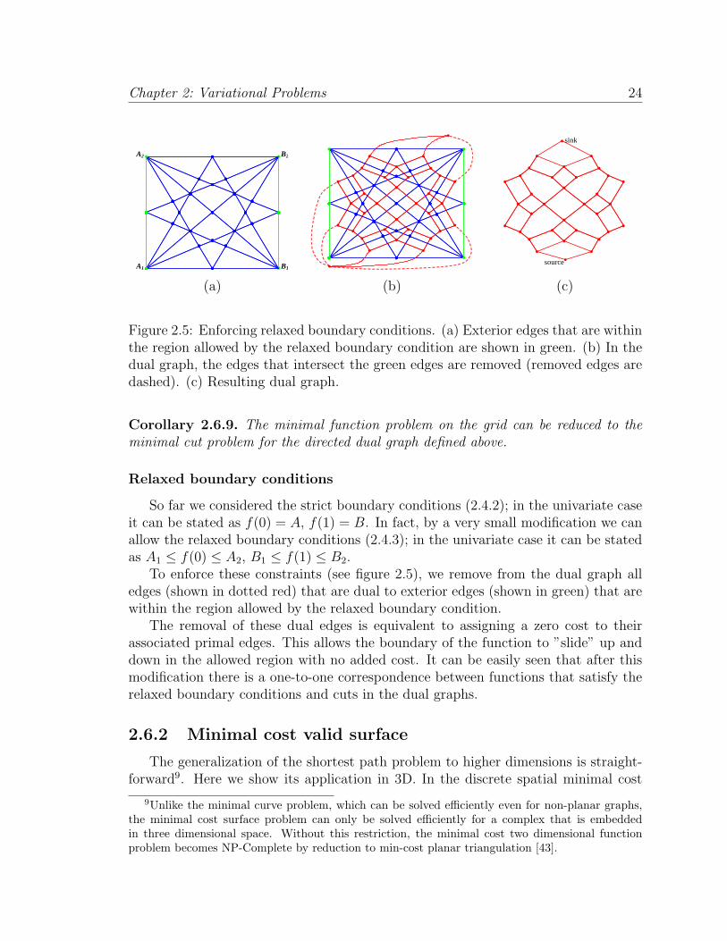
2.5 Enforcing relaxed boundary conditions. (a) Exterior edges that arewithin the region allowed by the relaxed boundary condition are shownin green. (b) In the dual graph, the edges that intersect the green edgesare removed (removed edges are dashed). (c) Resulting dual graph. . 24
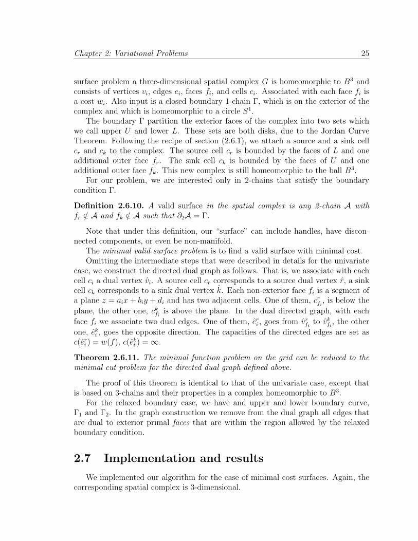
2.6 Results of the plane selection algorithm. Boundary conditions areshown in red. (a) Minimal area surface for the saddle boundary con-ditions, 150 random planes. (b) Membrane in the gravity field, 200random planes. . . . . . . . . . . . . . . . . . . . . . . . . . . . . . . 27
viii
List of Figures ix
2.7 (a) A two-dimensional slice of the density function. Intensity of thecolor is proportional to the density. (b) Numerical optimization meth-ods converge to the local minimum. (c) The minimal discrete surfaceusing a grid of random planes. (d) Our method followed by numericalrelaxation. . . . . . . . . . . . . . . . . . . . . . . . . . . . . . . . . . 30
3.1 n = 5. Solution of the edge-based linear program, the edges withnon-zero variables xi are shown. (a) Integer LP gives minimum weighttriangulation; xi = 1 for all solid edges. (b) Continuous LP gives non-integer solution which is smaller than (a); xi = 1 for the solid edges,xi = 1/3 for the dashed edges. . . . . . . . . . . . . . . . . . . . . . . 41
3.2 A subset of the spatial complex that corresponds to a single triangula-tion. (a) Triangulation of the set of points on the plane. (b) Randomthird coordinate is introduced for each vertex. . . . . . . . . . . . . . 42
3.3 Single- and double- coverings. (a) Triangulation (single-covering) of 6-point set consists of five triangles. (b) Double-covering of the same setconsists of ten triangles. For simplicity, only two triangles are shown,the rest can be obtained by the rotation of this pair around the centerpoint by 4πk/5, where k = 1, 2, 3, 4. (c) The same double-covering. Allten triangles are shown (transparent). Note, that this double-coveringcannot be split onto two triangulations. . . . . . . . . . . . . . . . . . 46
3.4 13-point counterexample for Euclidean MWT. (a) Minimum weighttriangulation weights 18.798. (b) Solution of the continuous LP corre-sponds to a double covering with a weight 18.764. Triangles are showntransparent. . . . . . . . . . . . . . . . . . . . . . . . . . . . . . . . . 46
3.5 Comparison of the linear programming and LMT approach for a ran-dom wheel example. (a) Typical random setup for n = 20. (b) Experi-mental probability of success by LMT (green line) and our LP method(blue line) depends on the number of points in the example. . . . . . 48
3.6 For the convex set S, any non-integer solution x consists of severaltriangulations. Here is how we can extract one of them. (a) Fix anytriangle with a positive xi (dark grey) and one of its vertices. Con-straint (3.4.4) guarantees that going around this vertex in a clockwiseor counter-clockwise direction we can always find a triangle with a pos-itive variable xj. These triangles are shown in light gray. (b) Fixingthe triangles found on the previous step, we can repeat procedure untilthe whole triangulation is complete. . . . . . . . . . . . . . . . . . . . 50
4.1 If the shortest path from the point x2 of the edge e2 crosses the edge e1,the distance function in this point can be computed by theorem (4.1.1). 55
List of Figures x
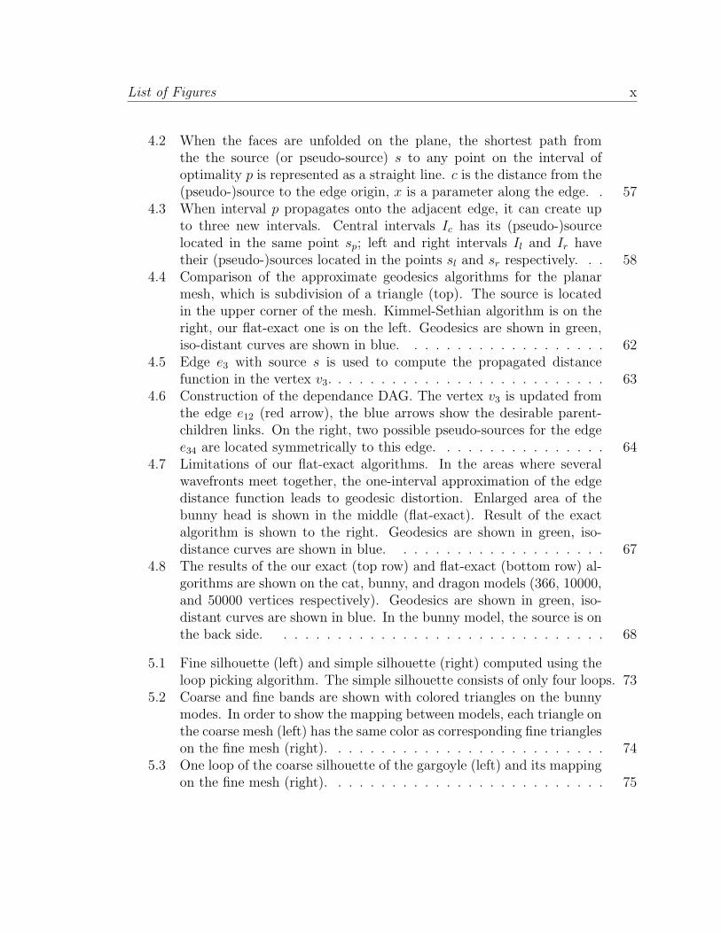
4.2 When the faces are unfolded on the plane, the shortest path fromthe the source (or pseudo-source) s to any point on the interval ofoptimality p is represented as a straight line. c is the distance from the(pseudo-)source to the edge origin, x is a parameter along the edge. . 57
4.3 When interval p propagates onto the adjacent edge, it can create upto three new intervals. Central intervals Ic has its (pseudo-)sourcelocated in the same point sp; left and right intervals Il and Ir havetheir (pseudo-)sources located in the points sl and sr respectively. . . 58
4.4 Comparison of the approximate geodesics algorithms for the planarmesh, which is subdivision of a triangle (top). The source is locatedin the upper corner of the mesh. Kimmel-Sethian algorithm is on theright, our flat-exact one is on the left. Geodesics are shown in green,iso-distant curves are shown in blue. . . . . . . . . . . . . . . . . . . 62
4.5 Edge e3 with source s is used to compute the propagated distancefunction in the vertex v3. . . . . . . . . . . . . . . . . . . . . . . . . . 63
4.6 Construction of the dependance DAG. The vertex v3 is updated fromthe edge e12 (red arrow), the blue arrows show the desirable parent-children links. On the right, two possible pseudo-sources for the edgee34 are located symmetrically to this edge. . . . . . . . . . . . . . . . 64
4.7 Limitations of our flat-exact algorithms. In the areas where severalwavefronts meet together, the one-interval approximation of the edgedistance function leads to geodesic distortion. Enlarged area of thebunny head is shown in the middle (flat-exact). Result of the exactalgorithm is shown to the right. Geodesics are shown in green, iso-distance curves are shown in blue. . . . . . . . . . . . . . . . . . . . 67
4.8 The results of the our exact (top row) and flat-exact (bottom row) al-gorithms are shown on the cat, bunny, and dragon models (366, 10000,and 50000 vertices respectively). Geodesics are shown in green, iso-distant curves are shown in blue. In the bunny model, the source is onthe back side. . . . . . . . . . . . . . . . . . . . . . . . . . . . . . . 68
5.1 Fine silhouette (left) and simple silhouette (right) computed using theloop picking algorithm. The simple silhouette consists of only four loops. 73
5.2 Coarse and fine bands are shown with colored triangles on the bunnymodes. In order to show the mapping between models, each triangle onthe coarse mesh (left) has the same color as corresponding fine triangleson the fine mesh (right). . . . . . . . . . . . . . . . . . . . . . . . . . 74
5.3 One loop of the coarse silhouette of the gargoyle (left) and its mappingon the fine mesh (right). . . . . . . . . . . . . . . . . . . . . . . . . . 75
List of Figures xi
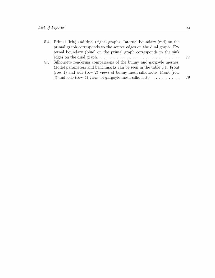
5.4 Primal (left) and dual (right) graphs. Internal boundary (red) on theprimal graph corresponds to the source edges on the dual graph. Ex-ternal boundary (blue) on the primal graph corresponds to the sinkedges on the dual graph. . . . . . . . . . . . . . . . . . . . . . . . . . 77
5.5 Silhouette rendering comparisons of the bunny and gargoyle meshes.Model parameters and benchmarks can be seen in the table 5.1. Front(row 1) and side (row 2) views of bunny mesh silhouette. Front (row3) and side (row 4) views of gargoyle mesh silhouette. . . . . . . . . 79
List of Tables
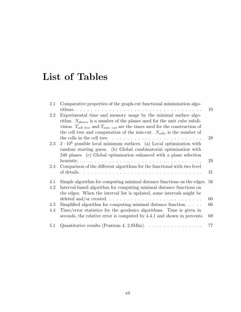
2.1 Comparative properties of the graph-cut functional minimization algo-rithms. . . . . . . . . . . . . . . . . . . . . . . . . . . . . . . . . . . . 10
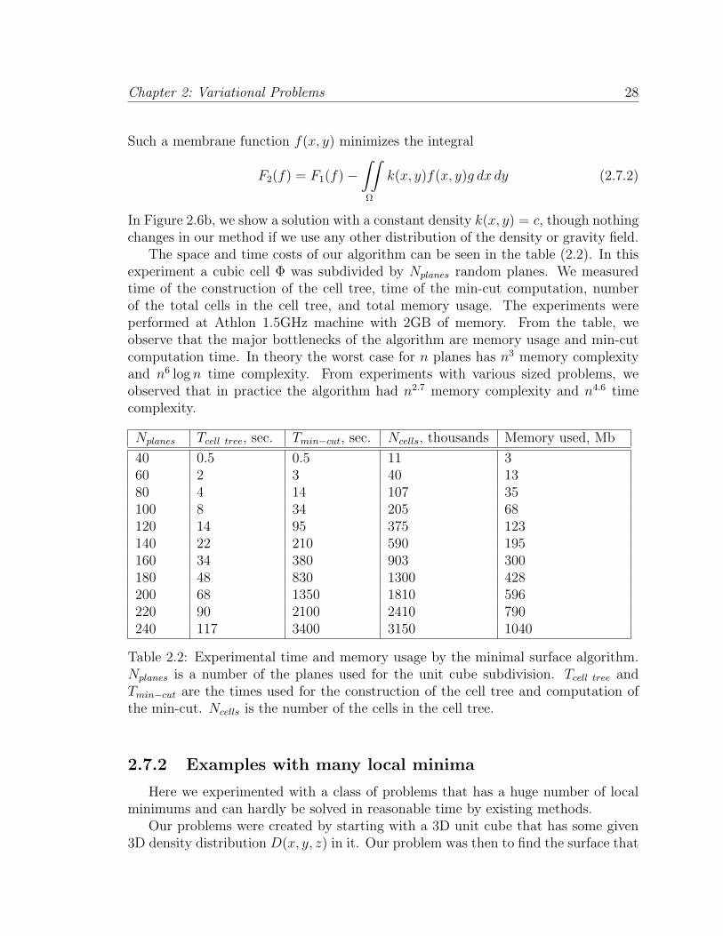
2.2 Experimental time and memory usage by the minimal surface algo-rithm. Nplanes is a number of the planes used for the unit cube subdi-vision. Tcell tree and Tmin−cut are the times used for the construction ofthe cell tree and computation of the min-cut. Ncells is the number ofthe cells in the cell tree. . . . . . . . . . . . . . . . . . . . . . . . . . 28
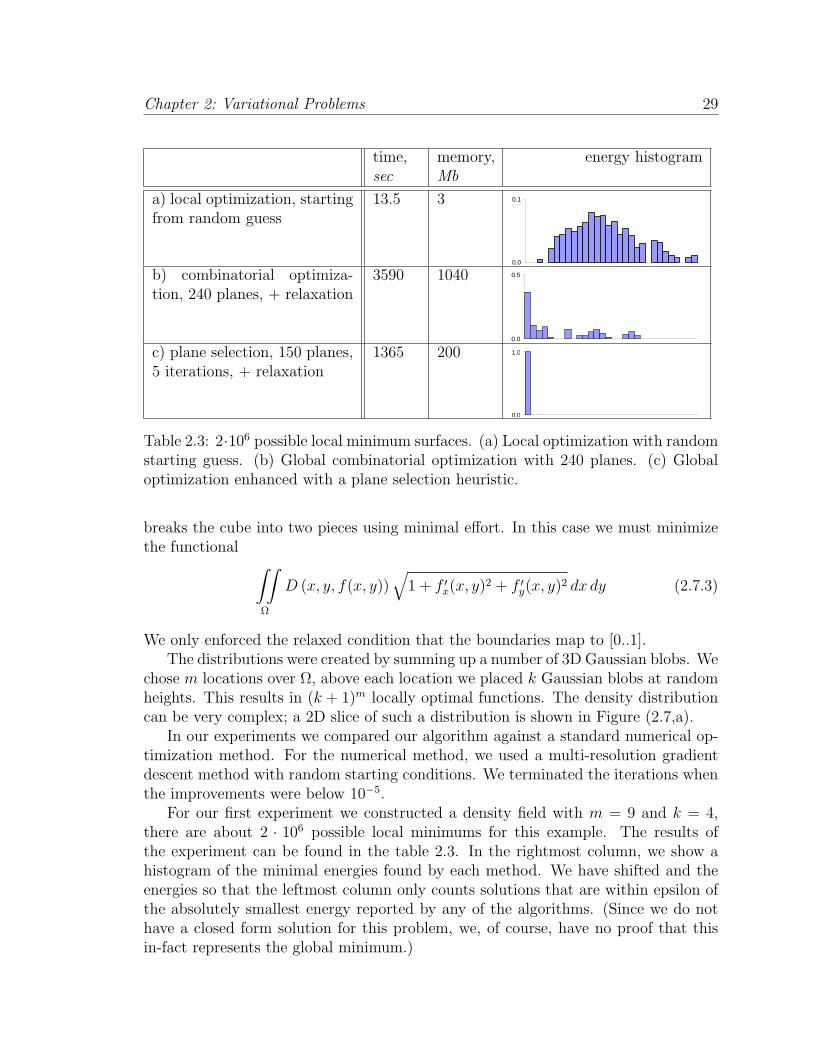
2.3 2 · 106 possible local minimum surfaces. (a) Local optimization withrandom starting guess. (b) Global combinatorial optimization with240 planes. (c) Global optimization enhanced with a plane selectionheuristic. . . . . . . . . . . . . . . . . . . . . . . . . . . . . . . . . . . 29
2.4 Comparison of the different algorithms for the functional with two levelof details. . . . . . . . . . . . . . . . . . . . . . . . . . . . . . . . . . 31
4.1 Simple algorithm for computing minimal distance functions on the edges. 564.2 Interval-based algorithm for computing minimal distance functions on
the edges. When the interval list is updated, some intervals might bedeleted and/or created. . . . . . . . . . . . . . . . . . . . . . . . . . . 60
4.3 Simplified algorithm for computing minimal distance function. . . . . 664.4 Time/error statistics for the geodesics algorithms. Time is given in
seconds, the relative error is computed by 4.4.1 and shown in percents. 69
5.1 Quantitative results (Pentium 4, 2.0Mhz). . . . . . . . . . . . . . . . 77
xii
Citations to Published Work
The application of the discrete algorithms to the variational problems (chapter 2)first appeared as a technical report and is currently submitted to the ACM Journalof Optimization.
”A Discrete Global Minimization Algorithm for Continuous VariationalProblems.”D. Kirsanov, S. J. Gortler.Harvard University Computer Science Technical Report: TR-14-04, July2004.
The geodesic shortest path algorithms (section 4) are described in
”Fast exact and approximate geodesic paths on meshes.”D. Kirsanov, S. Gortler, H. Hoppe.Harvard University Computer Science Technical Report: TR-10-04, May2004.
The silhouette simplification (chapter 5) previously appeared in
”Simple Silhouettes over Complex Surfaces.”D. Kirsanov, P. V. Sander, S. J. Gortler.In Proceedings of First Symposium on Geometry Processing 2003.
xiii
Acknowledgments
First of all, I would like to thank my advisor Steven Gortler and my fellow studentsXianfeng Gu, Pedro Sander, Geetika Tewari, Doug Nachand and Hamilton Chongfrom Harvard Computer Graphics lab. Without their daily support I would neverfinish this thesis.
Leonard McMillan provided very interesting references to the pinwheel tiling andLagrange optimization that otherwise would miss our scope. Hugues Hoppe shared alot of valuable ideas for the geodesic chapter of this paper.
I would like to thank Chris Buehler for help with development of the discreteduality construction and Tom Duchamp for pointing us to the literature on integralcurrents. Ray Jones helped us with the directed duality construction and proposedto test our MWT linear program program on L1 and L∞ metrics.
I am very grateful to Alex Healy, Erik Demaine, Anton Likhodedov, Ilya and BorisBerdnikov for many helpful discussions.
Danil KirsanovCambridge, MA, September 30, 2004
xiv

To my wife Yana.
Introduction 1
1
Chapter 1: Introduction 2
The general idea of this thesis is to investigate some problems where the con-struction of discrete and continuous minimal curves and surfaces is necessary. Thisstatement is very broad, and we limit ourselves with several problems of theoreticaland/or practical importance. In particular, we are interested in finding curves andsurfaces that are globally minimal.
The problems that we examine here come from two different areas. The first areais calculus in variations. We consider a classical formulation of the problem and showthat under very general conditions it is possible to find a globally optimal solution.Interesting enough, the discrete formulation of this problem is closely related to theminimal weight triangulation problem.
In the second part of the thesis we consider more practical problems related tocomputer graphics. Finding the shortest path (geodesic) on the discrete surface is awell-known problem. Though theoretical algorithms are known for a long time, thereare a lot of open question on implementation and approximate solutions. Finally, weinvestigate the problem of silhouette simplification and show that this problem canbe successfully addressed by globally minimal approach.
Contribution In this thesis we present the following contributions:
• A novel algorithm for constructing embeddable spatial complexes that approx-imate continuous minimum of the variational functional.
• A duality algorithm that allows finding the global minimum on the embeddablespatial complex in polynomial time.
• A reduction of the minimum weight triangulation problem to the minimumsurface problem on the non-embeddable spatial complex.
• An integer linear program for the general triangle-based minimum weight tri-angulation problem.
• A continuous linear problem that allows finding the minimal weight triangula-tions for the random point sets.
• A robust modification of the exact algorithm for finding the minimum lengthcurves (geodesics) on a piece-wise linear surfaces (meshes).
• A fast approximate geodesic algorithm.
• A novel method for mesh silhouette simplification that treats the optimal sil-houette as a minimum weight closed curve on a mesh.
• Implementation and testing of all the methods discussed.
Chapter 1: Introduction 3
1.1 Overview
The thesis consists of four major parts.
Variational Problems. We solve for the best function f(x) : Ω ⊂ Rn 7→ Rthat minimizes some functional
∫· · ·
∫
Ω
G(f(x),∇f(x), x) dx. (1.1.1)
with boundary conditions f(∂Ω) = Γ.Under very general conditions this problem can be discretized and related to a
problem of finding minimal cost surface in an (n+1)-dimensional spatial complex. Theglobal minimum of the discrete problem can be found with combinatorial optimizationtechniques (in particular, min-cut).
We pay a special attention to bi-variate variational problems where the solutionis a 2D minimal surface in 3D. We also implement the algorithm and compare it toexisting numerical techniques.
Minimum Weight Triangulations. Minimal weight triangulation (MWT)problem can also be considered as a globally minimal surface in the discrete facecomplex. The main difference of this spatial complex from the complex arising in theprevious problem is that it is not embeddable. It turns out that this property make adramatic difference.
The complexity of MWT is unknown. We construct the linear programming algo-rithm and show that integer solution of this problem corresponds to MWT. Thoughthere exist examples where the solution of the linear program is not integer, ourapproach can be of a practical use for the random point sets.
Geodesics. This chapter describes practical approaches to finding geodesiccurves on the triangulated meshes. We modify the classical MMP algorithm to makeit robust for the meshes of the large size. Because the exact algorithm is non-linear intime and space, we also develop approximation algorithm that works in close to lin-ear time and space. Both algorithm are implemented and compared with the existingmethods.
Silhouettes. Processing silhouettes (edges between front- and back- facing poly-gons) on meshes is quite a challenging practical problem. It is known that for thecomplex meshes the silhouettes can be very noisy and complicated.
We develop the method of constructing the approximate silhouette that have thesame main ”features” as the exact one. It is done by mapping the silhouette fromthe coarse version of the model to the fine one. The problem can be stated as a

Chapter 1: Introduction 4
minimal separating curve on the surface of the fine mesh. It can be approached withthe combinatorial minimization techniques developed in the previous chapters.
Variational Problems 2
5
Chapter 2: Variational Problems 6
In this chapter we apply the ideas from combinatorial optimization to find globallyoptimal solutions of the continuous variational problems. More specifically, supposethat one is given a variational problem to solve for the best function f(x) : Ω ⊂ Rn 7→R that minimizes some functional
∫· · ·
∫
Ω
G(f(x),∇f(x), x) dx. (2.0.1)
with boundary conditions f(∂Ω) = Γ.Most of the existing numerical methods for this classical problem are based on
two approaches: direct methods or Euler-Lagrange differential equation [8, 19]. If weuse direct approach, we describe the function f as a linear combination of some setof fixed basis functions bi(t) with a finite set of coefficients ci
f(x) =∑
i
cibi(x) (2.0.2)
Given this finite dimensional problems, one then solves for the best vector of coeffi-cients ci. This is a standard numerical problem that can be approached with a varietyof numerical algorithms [46].
When a finite element set of basis functions is chosen, we are implicitly discretizingthe domain x ∈ Ω. The discretization becomes explicit in the important case ofthe direct methods that is called a finite-difference approximation. In this case weconsider the basis functions to be small boxes and directly discretize function f andits gradient. In 1-dimensional case it can be written as
f(xi) ≈ ci,∂f
∂x(xi) ≈ ci+1 − ci
h(2.0.3)
It can be shown that under curtain condition the solution of the variational prob-lem (2.0.1) is also a solution of the differential Euler-Lagrange equation
∂G
∂f−
N∑i=1
∂
∂xi
∂G
∂f ′xi
= 0. (2.0.4)
In general, it is a non-linear (possibly degenerate) equation. Though there exist a lotof methods to solve the differential equation (2.0.4) [46], most of them are based onthe discretizations similar to (2.0.2, 2.0.3).
2.1 Contribution
The existing numerical algorithms share the property that (except for simplequadratic problems), one needs to seed the algorithm with some guess c0
i which the
Chapter 2: Variational Problems 7
algorithm iteratively improves upon. As a result, these methods efficiently convergeto some local minimum. For some problems this is acceptable, but for many difficultproblems, one needs to find the absolute best global minimum. The brute force ap-proach to finding the global minimum is to create a large number of starting guesses,and run local optimization from each of these initial states. This is an expensiveprocess, and the problems become even more intractable if one is solving for a higherdimensional problem.
In this chapter we study how combinatorial algorithms (instead of numerical ones)may be applied to these problems to find global minima (instead of local ones). Wherenumerical algorithms discretize the domain Ω and then use floating point numbersto represent functions Ω ⊂ Rn 7→ R, we discretize the space Ω × R. With thisdiscretization, the optimization becomes completely combinatorial in nature. Forexample, suppose Ω = R, then a discretization of Ω × R might be describable as aplanar graph (described with a set of vertices and edges) over R2. In this case, a twopoint boundary value problem reduces to the problem of finding the optimal path ina graph, and it is well known that one can solve for the global discrete minimal pathusing Dijkstra’s algorithm [12]. (see Figure 2.1).
In particular, in this chapter we present the following contributions
• In order to solve the given continuous variational problem, we must be assuredthat, with enough discretization, the solution to the combinatorial problem willbe close to the continuous one. Here we show conditions sufficient to ensurethis, and we demonstrate that these conditions can be met with a sequence ofdeterministic and random grids we construct.
• We prove that, in arbitrary dimension, the resulting combinatorial optimizationproblem can be reduced to an instance of min-cut, over an appropriate dualgraph. In 3D, for example, this gives us a simple algorithm for finding globallyminimum discrete surfaces.
• Finally, we describe some important details about the implementation of ouralgorithm and we show some experimental results demonstrating our method’ssuperiority to traditional numerical approaches.
2.2 Previous work
The literature on finding solutions to variational problems is extensive. For adetailed review, see [13, 19]. Most of the described numerical methods use someform of local descent and can only guarantee convergence to some local minimum.In contrast to all of these methods, our approach has global guarantees even in thepresence of local minima.
Chapter 2: Variational Problems 8
In the literature, there are a few algorithms that are able to find global minimafor certain classes of problems. Here we review and compare them along the followingset of axes.
• Functional: Some of the methods can only solve for minimal area surfaces,where others can minimize energy measured by any first-order functional.
• Boundary condition: Some of the methods search for surfaces that have someproscribed boundary, while others look for closed surfaces that surround certainpoints.
• Topology: Some methods solve for surfaces in R3, while others solve for scalarfunctions over the plane (height fields). Surface-based methods typically findsurfaces of arbitrary topology. It should be noted that to correctly define thecontinuous minimal surface problem one needs to employ the mathematicalmachinery of “integral currents” [41].
• Discrete solution: All of these methods solve the continuous problem by dis-cretizing space and solving a combinatorial optimization problem. They showthat in the limit, the discrete problem produces a solution to the continuousproblem. For some of the methods, the discrete algorithm outputs a specificpiecewise linear surface, other methods only output a volumetric “slab” in whichthe solution must lie.
• Algorithm Some of the methods reduce to MIN-CUT which has the complexityof O(N2 log N), while some reduce to circulation problems with higher com-plexity.
• Experimentation: Some of the methods are described in publications whichinclude experimental results and implementation details.
Hu et al. describe a method that uses MIN-CUT to compute minimal area func-tions [27, 28]. In particular they find the minimal area a two-dimensional functionf : Ω ∈ R2 7→ [a, b] that satisfies boundary conditions f(∂Ω) = Γ. The boundarycurve must be “extremal”, which means that it is on the exterior of volume Ω× [a, b]in which the surface must lie. In their solution, they discretize space into N volumet-ric nodes. They then proceed to find the ”slab” of nodes of some thickness d ¿ 1that satisfies the boundary conditions, separates 3D volume Ω× [a, b] into two piecesand has minimal volume. The discretized version of the latter problem can be solvedusing a MIN-CUT algorithm over an appropriate graph with N nodes and O(N2d3)edges.
Boykov and Kolmogorov have introduced a similar but more sophisticated ap-proach for solving for minimal surfaces using MIN-CUT [6] Similar to Hu, this algo-rithm has two major degrees of freedom: spatial discretization and connectivity. By
Chapter 2: Variational Problems 9
cleverly selecting the weights for the edges in their graph they can solve for a widerclass of functionals than simply “area”. In particular, they allow one to choose an ar-bitrary Riemannian metric over space, and then can solve for the minimal area surface,where area is defined using this new metric. Unfortunately, if one is given a problemin the form of equation (2.0.1) where the function G depends non-quadratically onthe surface normal direction, then their algorithm is not applicable.
In their paper, they solve for closed surfaces; to avoid surface collapse, they alsoimpose an energy term which measures which points are inside and outside the closedsurface. It seems likely that their approach could be generalized to handle extremalboundary curves like Hu et al.
In both the above algorithms, MIN-CUT is used to divide the volumetric nodes ofR3 into slabs. They show that in the limit, the actual minimal solution lies somewherein a shrinking volumetric “slab” determined by the cut. These algorithms do notcompute a specific discrete surface that minimizes the functional over some discretespace.
In contrast to the above methods, our method is applicable to any first orderfunctional. Our discrete algorithm outputs a specific minimal discrete surface, andcan thus be seen as a generalization of the “shortest path problem over a planargraph” to a “smallest surface problem in a spatial CW complex”.
The closest work to ours is the algorithm described in the Ph.D. thesis of JohnSullivan [52]. More generally than the above methods, Sullivan solves for the surfacethat minimizes any arbitrary first order functional. His discrete algorithm outputs aspecific discrete surface. In addition he allows his boundary to be any set of loops,including non-extremal loops and knots. Because of his general treatment of bound-ary conditions his algorithm reduces not to MIN-CUT but to a more complicatednetwork circulation problem. He then solves this problem using an algorithm withtime complexity O(N2A log N), where N is the number of nodes in his discrete graph,and A is the complexity of the solution surface. It is unclear if his approach was everimplemented or compared with numerical methods. In addition, due to the amountof difficult machinery employed, this work has remained somewhat inaccessible andunfortunately unappreciated outside of the minimal surface community.
In contrast to the work of Sullivan, by only allowing extremal boundary conditions,we are able to apply a very simple reduction to obtain an instance of MIN-CUT withtime complexity O(N2 log N). We also describe specific constraints so that we cansolve for minimal functions, which is the focus of this thesis, though removal of theseconstraints would let us solve for minimal surfaces of arbitrary topology as well. Inour work, we use random grids for finding approximate solutions which allows us tosatisfy complicated boundary conditions and to employ practical local grid refinementtechniques. Finally, we describe the details of an implementation and demonstratehow it compares in practice to standard numerical approaches.
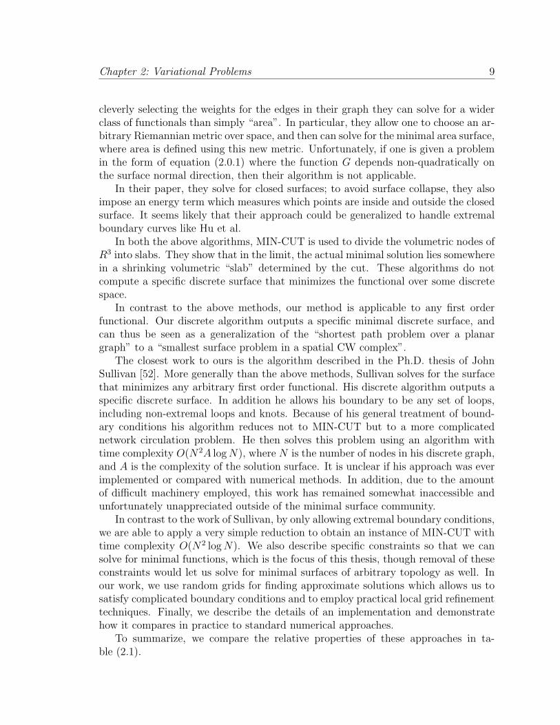
To summarize, we compare the relative properties of these approaches in ta-ble (2.1).
Chapter 2: Variational Problems 10
Algorithm HKR [28] BK [6] Sullivan [52] Our Method
Continuousfunctional
Euclidean Riemannian general general
Boundary external closed surface general externalBoundarycondition
exact orfree
exact or free exact exact or free
Topology functiononly
surface only surface only function and sur-face
Discrete solu-tion
volume volume piece-wise lin-ear surface
piece-wise linearsurface
Method min-cut min-cut min-circulation min-cutExperimentaljustification
no yes no yes
Grids regular regular regular regular and ran-dom
Table 2.1: Comparative properties of the graph-cut functional minimizationalgorithms.
Our research was specifically inspired by recent success of the combinatorial meth-ods in the discrete energy minimization problems emerged from computer vision[9], [7]. Though the problems that arise in this area are completely discrete fromthe very beginning, their method of construction of the directed dual graph can beadopted for our purpose.
Duality between the shortest path and min-cut problem for both directed andundirected planar graphs is well known and described in the literature for differentapplications (see [26] pg.156, [29]). As we will see, this duality can be generalized tohigher dimension, and applied to solve variational problems.
2.3 Main ideas
Before we start the formal proofs, we want to illustrate our main ideas on the 1-dimensional case. An advance reader, who immediately wants to see the mathematicaldefinition of the problem, can skip this example and start reading the chapter 2.4.
As an example, we are going to solve the classical minimization problem and findthe minimal surface of rotation [8]. In this problem we are looking for the functionthat minimizes the functional
1∫
0
|f (x)|√
1 + f ′2x dx (2.3.1)
Chapter 2: Variational Problems 11
given the boundary conditions
f(0) = A, f(1) = B. (2.3.2)
The analytical solution of this problem is
f(x) = Acosh (x cosh(d) + d)
cosh(d),
where d is chosen to satisfy the boundary condition (2.3.2).Our first idea is to discretize both the domain x and the range f arriving at
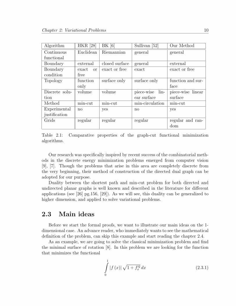
a completely combinatorial problem. We will be looking for a solution among thepiece-wise linear functions described by subsets of a particular grid (Figure 2.1).
In fact, we have to generate a family of the convergent grids. In order for thecombinatorial algorithm to be able to give us information about the continuous solu-tion, we must be able to create a grids which, if dense enough, contain discrete pathsthat are within epsilon of the continuous solution and its derivative. The recipes howto create the convergent grids and the proofs of their correctness can be found in thefollowing chapters.
The integral over the piecewise linear function can be split on the integral over its”edges”
1∫
0
G(f, f ′, x) dx =n−1∑i=0
ai+1∫
ai
G(f, f ′, x) dx =∑
edges
wi. (2.3.3)
For every given edge which is a piece of some line y(x) = kx + b we can compute itsweight as
wi =
ai+1∫
ai
G(kx + b, k, x) dx. (2.3.4)
In particular, in the case of the surface of rotation (2.3.1) we have
wi =√
1 + k2
ai+1∫
ai
|kx + b| dx. (2.3.5)
If the entire edge is in the positive or negative semi-plane, this equation can besimplified to
wi =∣∣0.5kx2 + bx
∣∣√1 + k2
∣∣∣ai+1
ai
. (2.3.6)
In the cases when variational integral is more complicated and the edge weights (2.3.4)cannot be computed analytically, it can be done numerically.
Now we have a completely discrete problem. We have to find a path with minimumweight from point A to point B on the graph. The weight of the path is a sum of the

Chapter 2: Variational Problems 12
0 0.1 0.2 0.3 0.4 0.5 0.6 0.7 0.8 0.9 10.5
0.55
0.6
0.65
0.7
0.75
0.8
0.85
0.9
0.95
1
0 0.1 0.2 0.3 0.4 0.5 0.6 0.7 0.8 0.9 10.5
0.55
0.6
0.65
0.7
0.75
0.8
0.85
0.9
0.95
1
(a) (b)
Figure 2.1: Solution of the minimal surface of rotation problem on the regular (a)and random (b) grids. Exact solution is shown as a dashed line.
weights of its edges. All edges are oriented from left to right, because we want theresulting path to be a function, and their weights are known from (2.3.4). Indeed,that is an exact definition of the famous directed shortest path problem [12]. There aremany efficient algorithms for this problem, best of which have low-order polynomialtime complexity [12]. Applying this method we can find the best approximation ofthe surface of rotation on the given grid (Figure 2.1).
If instead of the boundary conditions (2.3.2) we apply the boundary conditions
A0 ≤ f(0) ≤ A1, B0 ≤ f(1) ≤ B1, (2.3.7)
the only difference in the algorithm will be in changing the single source shortest pathalgorithm to the multiple source one. In this case all nodes that are between A0 andA1 are considered to be sources, and all nodes between B0 and B1 to be destinations.
This type of dicretization easily generalized to arbitrary dimensions, where ourgrid will be constructed by the intersection of the hyper-planes. For example, for var-ional problems over the plane, f : R2 7→ R we will have to construct a minimal surfacein 3D. Though minimal path algorithms cannot be generalized for this purpose, as wewill describe below, minimal surfaces can be found using duality and combinatorialmaxflow/min-cut algorithms. In order for these algorithms to work, we will have toapply some additional restrictions on the grid and functional.
Now we are ready for the formal definition of the variational problem that we areable to solve using our method.
Chapter 2: Variational Problems 13
2.4 Problem definition
Our problem is to find the function f(x) : Ω ⊂ Rn 7→ R that minimizes somefunctional
F (f) =
∫· · ·
∫
Ω
G(f(x),∇f(x), x) dx. (2.4.1)
It is common to apply the strict boundary conditions
f(∂Ω) = Γ(∂Ω), (2.4.2)
but our method will also work with the less restrictive conditions
Γ0(∂Ω) ≤ f(∂Ω) ≤ Γ1(∂Ω). (2.4.3)
We require that the domain Ω is a simply-connected polytope, with boundary ∂Ωhomeomorphic to an n − 1-dimensional sphere Sn−1. For example, for n = 2, Ω is apolygon with no holes and ∂Ω a closed piece-wise linear curve that is homeomorphicto a circle.1
In addition, we require our boundary condition(s) Γ to be described as a piece-wiselinear function with a finite number of pieces.
We require that the solution of the variational problem fs(x) belongs to a functionspace P of continuous bounded piece-wise twice differentiable functions with boundedfirst and second derivatives 2. By ”piece-wise” we mean that if g ∈ P then there existsa subdivision of the domain Ω into a finite set of non-intersecting polytopes Ω =
⋃$g
i ,such that on the internal points of every polytope $g
i the function g is a continuoustwice differentiable function with bounded first and second derivatives. Without theloss of generality, we can scale the problem to make sure that
0 ≤ g(x) ≤ 1,
∣∣∣∣∂g
∂xi
(x)
∣∣∣∣ ≤ Cg1 ,
∣∣∣∣∂2g
∂xi∂xj
(x)
∣∣∣∣ ≤ Cg2 . (2.4.4)
We also require the kernel of the functional (2.4.1) to be nonnegative 3. In otherwords, for all x, y such that x ∈ Ω, 0 ≤ y ≤ 1, and n-dimensional vectors p ∈ Rn wehave
1If we want to be picky, we have to mention that the case n = 1 is a minor exception, because Ωis an interval and ∂Ω is two points.
2Though we will strongly rely on it in the proofs of the correctness of our method, we believethat this assumptions can be weakened in many cases.
3We can weaken the condition (2.4.5), requiring the kernel to be limited from below. Indeed, weknow that if the function fs(x) is a solution of the variational problem with the kernel G(f,∇f, x)then it is also a solution of a problem with the kernel G(f,∇f, x)+C for any constant C. Therefore,if there exists a constant C such that for all x, y, and p in (2.4.5) we have G(y, p, x) ≥ −C, thenthe problem with the kernel G(f,∇f, x) + C will satisfy (2.4.5) and have the same solution fs(x).
Chapter 2: Variational Problems 14
G(y, p, x) ≥ 0. (2.4.5)
This ensures that the weights of all edges of graphs that we construct will be non-negative 4.
2.5 Grids
Our basic approach is to approximate the continuous variational problem with adiscretized combinatorial one which we can globally solve in polynomial time. Forthis scheme to work, it is essential that the discrete solution gives us meaningfulinformation about the continuous minimum. Here we present sufficient conditions forsuch an approach to succeed. Then we describe a grid structure that satisfies theseconditions.
2.5.1 Sufficient conditions.
Let us assume that our variational problem is to be solved over a space of possiblefunctions P with a norm ‖·‖ in it. Our discretized version of the problem will onlyallow for the representation of some other set L ⊂ P . The following lemma states thesufficient conditions to guarantee that our discretized solution will be “close enough”to the actual solution.
Definition 2.5.1. The functional F is continuous in the function space P, iffor any f ∈ P, and any ε > 0 there exists δ > 0 such that if ‖f − g‖ < δ then|F (f)− F (g)| < ε.
Definition 2.5.2. The set L is dense in the set P if for any f ∈ P, and any ε > 0there exists gε ∈ L such that ‖f − gε‖ < ε.
Lemma 2.5.3. Let P be a function space, and ‖·‖ a norm over P. Let F (f) be afunctional that is continuous in P with respect to ‖·‖. Suppose that L ⊂ P is densein P with respect to the norm. Then for any f ∈ P, any ε > 0, any δ > 0 there existsg ∈ L such that
∥∥g − f∥∥ < δ and
∣∣F (g)− F (f)∣∣ < ε.
Proof. Due to the density we can pick a sequence unn=0,1,...,∞ ⊂ L such thatlimn→∞
∥∥un − f∥∥ = 0. In particular, there exists an integer N1 such that for all
n > N1 we have∥∥un − f
∥∥ < δ.Because the functional is continuous, there also exists an integer N2 such that∣∣F (un)− F (f)
∣∣ < ε for all n > N2. Therefore, for any n > max(N1, N2) functiong = un satisfies the requirements of the lemma.
4This is not a necessary condition for the shortest path algorithms in 1D, but will be required inhigher dimensions.
Chapter 2: Variational Problems 15
Corollary 2.5.4. Let us denote Fmin = inff∈P
F (f). If L is dense in P and P is dense
in L, then F (g) ≥ Fmin for any g ∈ L, and for any ε > 0 there exists g ∈ L such that|F (g)− Fmin| < ε.
So, if the functional is continuous and we chose a set of the functions L thatsatisfies the conditions of the corollary, we can solve the problem over this set L andour the energy of our result will be as close to the minimal energy of the originalproblem as we want. In most cases we can also guarantee that the solution of thediscrete problem is close to the solution of the continuous problem under the norm‖·‖.Definition 2.5.5. Let fmin be the global minimum, F (fmin) = Fmin. It is calledan isolated global minimum if for any ε > 0 there exists δ > 0 such that if‖f − fmin‖ > ε, then F (f)− Fmin > δ.
Corollary 2.5.6. If there exists an isolated global minimum fmin, then for any ε, δ >0, there exists g ∈ L such that ‖g − fmin‖ < δ and |F (g)− Fmin| < ε.
In other words, under very general assumptions we can find “good enough” so-lution in our numerical subset L, which can be much simpler then P . In the nextsections we are going to construct such a subset.
2.5.2 Univariate variational problem
Before we go to the higher dimensions, we illustrate our approach for the univariateproblems domain.
Here we describe grids for the univariate minimization problems that satisfy con-ditions (2.4.1 - 2.4.5). Though many constructions are possible, we have chosen thisone because it is easily generalizable to arbitrary dimension.
We assume w.l.o.g. that Ω = [0, 1] and therefore the solution of the univariate vari-ational problem lies in the unit square of the plane Φ = (x, f) | x ∈ [0, 1], f ∈ [0, 1].Define the space P of the allowable solutions as a set of continuous finite piece-wisetwice differentiable functions f : [0, 1] 7→ [0, 1] with bounded first and second deriva-tives. We define the integral norm to be
‖f‖ =
1∫
0
|f(x)|+ |f ′(x)| dx. (2.5.1)
This norm includes a term for both the value and the derivative of the f . As aresult, our functional F , which depends on both value and derivative, is continuouswith respect to this norm. Essentially, this means that two “close” functions musthave similar energy measurements. This continuity is needed in the preconditions ofLemma 2.5.3.

Chapter 2: Variational Problems 16
(a) (b)
Figure 2.2: (a) The graph C2 can be used to obtain a combinatorial problem that isarbitrarily close to the continuous one. (b) The planar graph Cpl
2 is constructed byintersection of the set of lines.
Our strategy is to piecewise linearly embed a planar graph in this square, and thenrepresent possible functions g(x) as piecewise linear paths in this embedded graph.Every path in the graph with monotonically increasing x, from 0 to, 1 corresponds toa piecewise linear function g : [0, 1] 7→ [0, 1]. The set of all possible piecewise linearfunctions generated by the grid R we denote as M(R). For a graph with a finitenumber of vertices the set M(R) is also finite. Obviously, M(R) ⊂ P .
Regular grids.
For univariate minimization problems, we will use a grid such as one shown inFigure (2.2a). This grid, Cn, has n + 1 columns and n2 + 1 rows of vertices. Thedistance between the columns is therefore equal to h = n−1 and the distance betweenthe rows is d = h2 = n−2. Edges are included between each pair of vertices in adjacentcolumns. This graph has about n3 vertices and n5 edges. The number of the possiblefunctions generated by this grid |M(Cn)| = n(2n+2). Fortunately, we will be ableto find the global minimum of these possible functions with efficient combinatorialminimization techniques. This grid has been chosen so that it can represent functionswith a wide variety of values and derivatives. In particular we can state the following:
Theorem 2.5.7. The set
L =∞⋃
n=1
M(Cn)
is dense in P with respect to our norm.
The proof of the theorem is given in the appendix 2.9.Combined with the corollary (2.5.6), this theorems states that if the continuous
problem has an isolated minimal solution, then it is possible to solve the variationalproblems on the grids Cn, and the discrete solution will converges to the actualsolution of the continuous problem when n → ∞. Note, that our definition of the
Chapter 2: Variational Problems 17
grid does not depend on the variational problem. In fact, any continuous variationalproblem that has a solution in the set P can be solved on this grid.
The grid Cn is not planar. As described below, for higher dimensional problems,we will need to have an embeddable grid. The grid Cn can be easily modified to obtainthe embeddable grid Cpl
n as shown in Figure(b). These planar graphs are also densein P because they include all piece-wise linear functions from L, M(Cpl
n ) ⊃M(Cn).
Random grids.
The described regular grid structure can be created as the intersection of sets oflines. As n increases, the lines become more ”dense”, meaning that in the vicinity ofevery point of the plane there pass more and more lines with different positions andorientations. Random grids have the same property, and thus can be used for solvingour continuous variational problems.
The random grid Rn in the unit square of the plane Φ is created by intersectionof n random lines. One vertex is created at each line intersection, and the resultinggraph is planar. Each line is constructed by taking the point p ∈ Φ and orientation≤ c ∈ [−π, π] from some probability distributions 5. The grid Rn+1 can be constructedby adding one random line to Rn. Such families of the grids has a nice property thatM(Rn+1) ⊃M(Rn). The set of all functions generated by the family we will denoteas
Lr =∞⋃
n=1
M(Rn).
Similar to the regular case, we can state the density theorem
Theorem 2.5.8. The set Lr is dense in P.
The proof of the theorem is given in the appendix 2.10.Therefore, we can solve the variational problems in the domain of the random
grids.
Regular versus random
We have shown that univariate variational problems can be numerically solvedin the domains of the regular and random grids. What domain should be chosendepends on the type of the problem. Here we emphasize the major tradeoffs betweenthese approaches.
It can be clearly seen that regular grids Cn are based on the simple blocks that canbe pre-computed for all reasonable n and stored in data files. The graph for the givenproblem can be constructed by joining the blocks together. Such a structure givesus another advantage when the kernel of the functional F (f, f ′, x) does not depend
5In this thesis we will consider uniform distributions unless the different distribution is mentioned.
Chapter 2: Variational Problems 18
on x and the computation of the edge weight is expensive. In this case we have tocompute the weights for the small fraction of the edges and then simply copy thesevalues for the whole structure.
Random grids are more flexible. We can experiment with the density distributionsof the lines, making them more ”dense” in the vicinity of the possible solution. Inorder to produce an ”average” answer and ”deviation” we can run the algorithmseveral times on different random grids. These advantages are often dominant becausefor big meshes the time for the grid construction and weight computing is usually smallcomparing to the other parts of the algorithm. In our implementation we pursuedthe use of random grids.
The solution for the function generating a minimum surface of rotation using bothtypes of grids can be seen on the Figure (2.1).
2.5.3 Grids for higher dimensions
The described grid structure can be created as the intersection of the set of lines.The generalization in higher dimensions is straightforward; the grid is created as theintersection of the set of hyperplanes in the n + 1-dimensional space, Ω× [0, 1]. Withthis grid structure, some function space of piecewise linear functions over Ω can berepresented using appropriate subsets of facets. The proof of the correctness of theseconstructions for the higher dimensions is omitted for the sake of space.
Though regular grids have a clear structure and might be easier to build andinvestigate, random grids are more flexible. Similar to the 1-dimensional case, we canexperiment with the density distributions for the hyperplanes, making them more”dense” in the vicinity of the possible solution. It is also much easier to constructrandom grids that fit the given boundary conditions.
2.5.4 From grids to discrete problem.
The weight of the face can be computed by evaluating the integral (2.4.1) numer-ically or analytically. For instance, for bivariate variational problem every face of thegrid Cn is a convex polygon located on some plane z(x, y) = Ax + By + C with theconstant gradient ∇z = (A,B)T . The cost of the face can be computed as
wi =
∫∫
face
G(Ax + By + C, (A,B)T , x, y
)dx dy. (2.5.2)
2.6 Algorithms
We now have approximated our continuous variational problem by a series ofdiscrete optimization problems. In the univariate case, the discrete problem is a

Chapter 2: Variational Problems 19
shortest path problem, and in the bivariate case is a minimal discrete surface problem.We now wish to find the global optima for these problems. For the shortest pathproblem, we could simply use a standard shortest path algorithm, such as Dijkstra’salgorithm on the grid. Unfortunately, it is not clear how to use these algorithms tosolve for minimal surfaces.
In this section we show how both the discrete path and surface problems maybe globally solved in polynomial time. The basic approach will be to generate anappropriate dual graph from the grid structure. This dual graph will be constructed sothat “cuts” of the graph correspond to paths (surfaces) in the original grid structure.We can then apply well known algorithms to solve for the min-cut of the dual graph.For simplicity, we first demonstrate how these ideas work for the univariate problem.The topological machinery we use is possibly a tad bit heavy for the univariate case,but will be sufficient to generalize to bivariate case. In fact, this machinery can beapplied to variational problems of any dimension.
2.6.1 Univariate problem
For the discrete univariate problem, we are given a planar graph (V, E) that isembedded in <2, with positive weights on each of its edges. We will label the axesof <2 as x and y. Because the graph is embedded, we have not only vertices andedges, but also 2D faces. This collection of vertices edges and faces defines a complex(formally it is a CW complex [22]) that is homeomorphic to the 2D ball (disk) B2.
We wish to compute the minimum weight path that connects two specified verticesthat are on the exterior of this complex. In addition we will want to ensure that theour path corresponds to a function in the original variational setting; that is, thereshould be one y value over each x value. We will deal with this restriction later onin section (2.6.1).
The two boundary vertices A and B partition the exterior edges into two setswhich we call upper U and lower L. We introduce two additional faces, fr and fk, inthe graph. The source face fr is surrounded by edges in L and one additional outeredge er. The sink face fk is constructed by edges in U and one additional outer faceek. With these two added faces and edges, the new complex is still homeomorphic toB2 (see Figure 2.3).
The following are simple definitions from simplicial homology modulo 2 [18].
Definition 2.6.1. A 1-chain in the graph is a union of some edges of the graphC = ∪ei. The boundary of a 1-chain C, which is denoted as ∂1C, is a union ofvertices that are included in C an odd number of times.
Similarly, we define a 2-chain as a union of some faces of the graph A = ∪fi.The boundary ∂2A of a 2-chain A is a union of edges that are included in A an oddnumber of times 6.
6For this 2d complex, any edge can belong to no more then two faces. This is not going to be
Chapter 2: Variational Problems 20
A
B
A
B
sink
source
fr
fk ek
er e
(a) (b) (c)
K
R
A
B
(d) (e) (f)
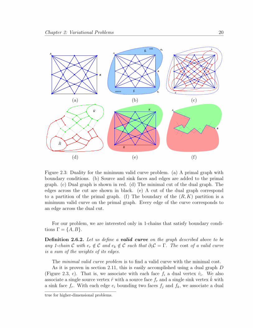
Figure 2.3: Duality for the minimum valid curve problem. (a) A primal graph withboundary conditions. (b) Source and sink faces and edges are added to the primalgraph. (c) Dual graph is shown in red. (d) The minimal cut of the dual graph. Theedges across the cut are shown in black. (e) A cut of the dual graph correspondto a partition of the primal graph. (f) The boundary of the (R, K) partition is aminimum valid curve on the primal graph. Every edge of the curve corresponds toan edge across the dual cut.
For our problem, we are interested only in 1-chains that satisfy boundary condi-tions Γ = A,B.Definition 2.6.2. Let us define a valid curve on the graph described above to beany 1-chain C with er /∈ C and ek /∈ C such that ∂1C = Γ. The cost of a valid curveis a sum of the weights of its edges.
The minimal valid curve problem is to find a valid curve with the minimal cost.As it is proven in section 2.11, this is easily accomplished using a dual graph D
(Figure 2.3, c). That is, we associate with each face fi a dual vertex vi. We alsoassociate a single source vertex r with a source face fr and a single sink vertex k witha sink face fr. With each edge ei bounding two faces fj and fk, we associate a dual
true for higher-dimensional problems.
Chapter 2: Variational Problems 21
edge ei that connects vj and vk. We set the capacity of each dual edge the cost of theassociated primal edge c(ei) = c(ei).
Definition 2.6.3. A cut is a partition of the vertices v into two sets R and K withr ∈ R and k ∈ K. The cost of a cut c(R, K) is the sum of the capacities of the edgesbetween R and K.
Because there is a one-to-one correspondence between the vertices of the dualgraph and the faces of the primal graph, we can also denote the cut as a partition ofthe faces of the primal graph into two 2-chains R and K with fr ∈ R, fk ∈ K.
Theorem 2.6.4. There is a one-to-one correspondence between the valid curves onthe primal graph and cuts on the dual graph. The minimal valid curve problem overthe primal undirected graph is equivalent to a minimal cut problem for the dual graph.
The proof of the theorem is given in the appendix 2.11.The minimal cut is a well-known problem that can be solved in polynomial time.
Additional constraints
In the previous section we considered a general problem of finding a minimal validcurve in G. Here we describe how to solve its restricted version where we want to finda minimal curve with some special properties. Our final purpose is to ensure that thechosen curve is a function.
Theorem (2.6.4) states that every valid curve C corresponds to a cut that is denotedas (RC, KC) in the primal graph and (RC, KC) in the dual graph. If the curve passesthrough an edge e, one of its adjacent faces belongs to the source 2-chain RC and theother one belongs to the sink 2-chain KC. We specify an additional constraint to besatisfied when the curve passes through this edge.
Constraint 2.6.5. Let e to be an edge of the primal graph. We take one of itsadjacent faces and denote it as fR
e , the other one is denoted as fKe . We also denote
corresponding vertices in the dual graph as vRe and vK
e . If e ∈ C, we require thatfR
e ∈ RC and fKe ∈ KC (similarly, vR
e ∈ RC, vKe ∈ KC).
This condition can be specified independently for every edge (and it is quite possi-ble that some face f belongs to a source 2-chain for one edge and belongs to the sink2-chain for another edge). Note, that the constraints do not depend on the particularcurve C and simply narrow the set of possible valid curves on the primal graph.
In order to satisfy constraints (2.6.5), instead of undirected dual graph, we createthe directed dual graph G. If the constraint (2.6.5) is specified for the primal edge e,then the corresponding edge e of the undirected dual graph is split into two directededges eR (from vR
e to vKe ) and eK (from vK
e to vRe ). The capacities of the dual edges
are defined as c(eR) = c(e) and c(eK) = ∞. If the constraint is not specified for e,then the capacities are set as c(eR) = c(eK) = c(e).
Chapter 2: Variational Problems 22
A
B
x
f f
e
sink
source
(a) (b) (c)
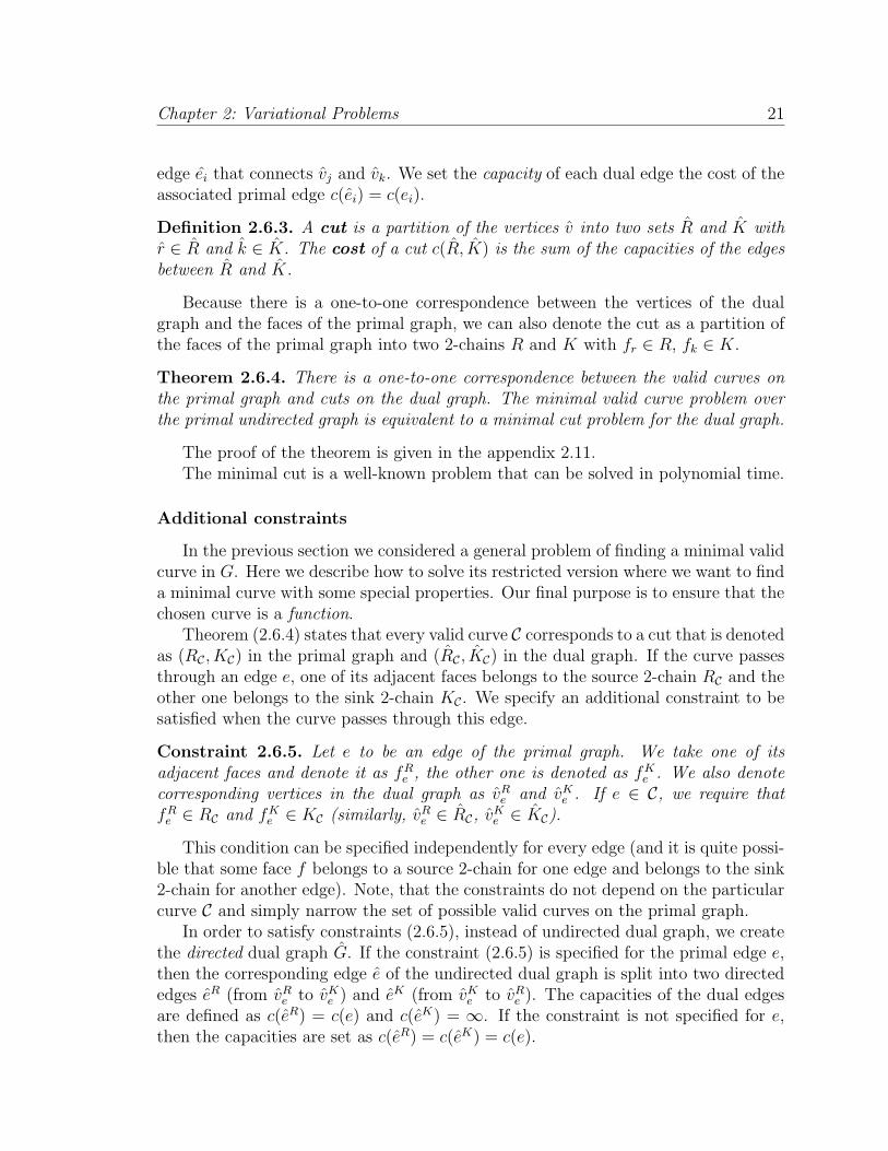
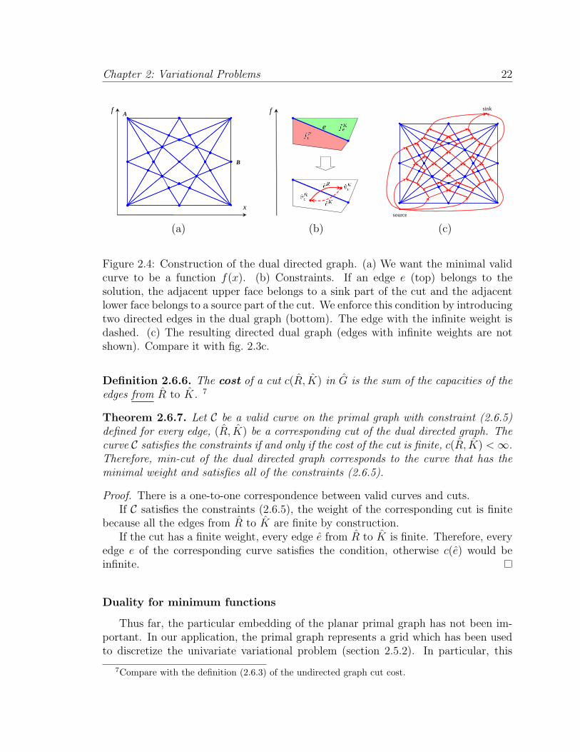
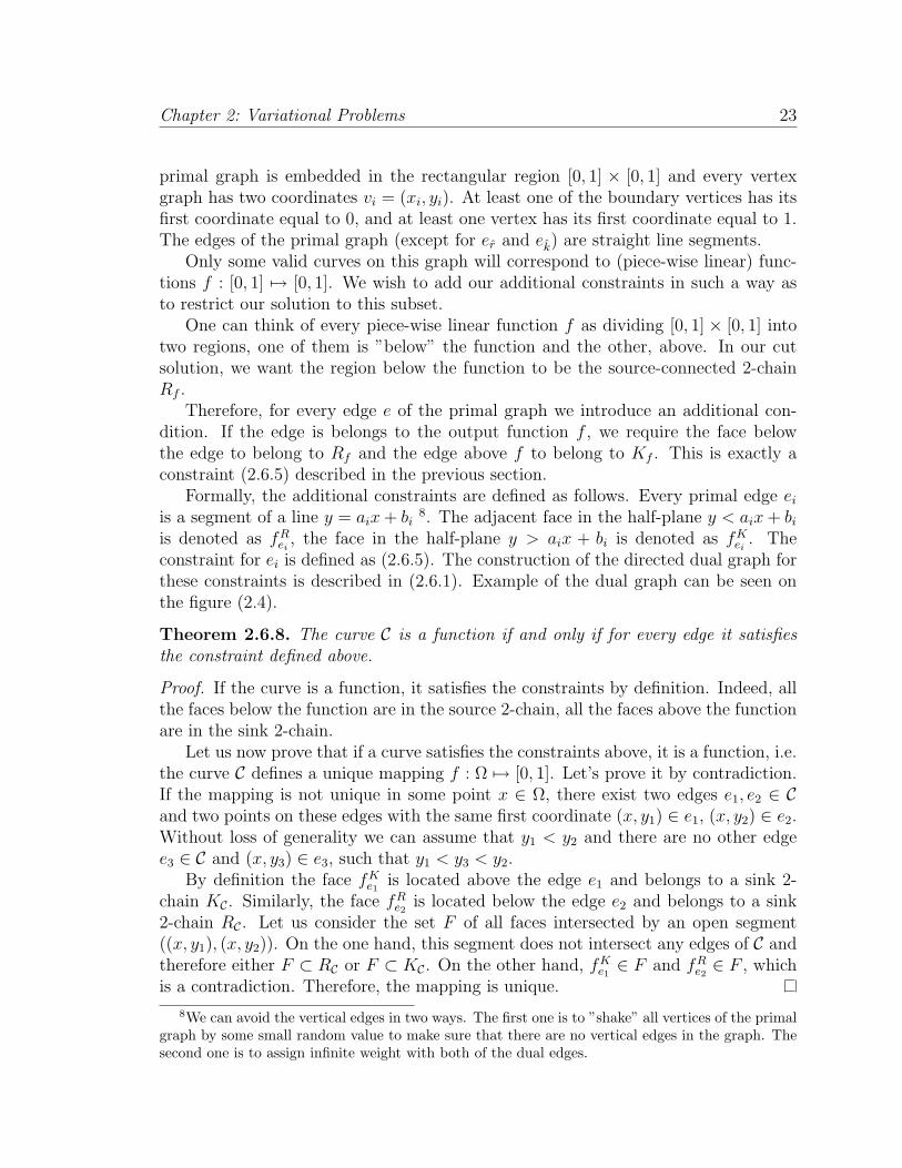
Figure 2.4: Construction of the dual directed graph. (a) We want the minimal validcurve to be a function f(x). (b) Constraints. If an edge e (top) belongs to thesolution, the adjacent upper face belongs to a sink part of the cut and the adjacentlower face belongs to a source part of the cut. We enforce this condition by introducingtwo directed edges in the dual graph (bottom). The edge with the infinite weight isdashed. (c) The resulting directed dual graph (edges with infinite weights are notshown). Compare it with fig. 2.3c.
Definition 2.6.6. The cost of a cut c(R, K) in G is the sum of the capacities of theedges from R to K. 7
Theorem 2.6.7. Let C be a valid curve on the primal graph with constraint (2.6.5)defined for every edge, (R, K) be a corresponding cut of the dual directed graph. Thecurve C satisfies the constraints if and only if the cost of the cut is finite, c(R, K) < ∞.Therefore, min-cut of the dual directed graph corresponds to the curve that has theminimal weight and satisfies all of the constraints (2.6.5).
Proof. There is a one-to-one correspondence between valid curves and cuts.If C satisfies the constraints (2.6.5), the weight of the corresponding cut is finite
because all the edges from R to K are finite by construction.If the cut has a finite weight, every edge e from R to K is finite. Therefore, every
edge e of the corresponding curve satisfies the condition, otherwise c(e) would beinfinite.
Duality for minimum functions
Thus far, the particular embedding of the planar primal graph has not been im-portant. In our application, the primal graph represents a grid which has been usedto discretize the univariate variational problem (section 2.5.2). In particular, this
7Compare with the definition (2.6.3) of the undirected graph cut cost.
Chapter 2: Variational Problems 23
primal graph is embedded in the rectangular region [0, 1] × [0, 1] and every vertexgraph has two coordinates vi = (xi, yi). At least one of the boundary vertices has itsfirst coordinate equal to 0, and at least one vertex has its first coordinate equal to 1.The edges of the primal graph (except for er and ek) are straight line segments.
Only some valid curves on this graph will correspond to (piece-wise linear) func-tions f : [0, 1] 7→ [0, 1]. We wish to add our additional constraints in such a way asto restrict our solution to this subset.
One can think of every piece-wise linear function f as dividing [0, 1] × [0, 1] intotwo regions, one of them is ”below” the function and the other, above. In our cutsolution, we want the region below the function to be the source-connected 2-chainRf .
Therefore, for every edge e of the primal graph we introduce an additional con-dition. If the edge is belongs to the output function f , we require the face belowthe edge to belong to Rf and the edge above f to belong to Kf . This is exactly aconstraint (2.6.5) described in the previous section.
Formally, the additional constraints are defined as follows. Every primal edge ei
is a segment of a line y = aix + bi8. The adjacent face in the half-plane y < aix + bi
is denoted as fRei
, the face in the half-plane y > aix + bi is denoted as fKei
. Theconstraint for ei is defined as (2.6.5). The construction of the directed dual graph forthese constraints is described in (2.6.1). Example of the dual graph can be seen onthe figure (2.4).
Theorem 2.6.8. The curve C is a function if and only if for every edge it satisfiesthe constraint defined above.
Proof. If the curve is a function, it satisfies the constraints by definition. Indeed, allthe faces below the function are in the source 2-chain, all the faces above the functionare in the sink 2-chain.
Let us now prove that if a curve satisfies the constraints above, it is a function, i.e.the curve C defines a unique mapping f : Ω 7→ [0, 1]. Let’s prove it by contradiction.If the mapping is not unique in some point x ∈ Ω, there exist two edges e1, e2 ∈ Cand two points on these edges with the same first coordinate (x, y1) ∈ e1, (x, y2) ∈ e2.Without loss of generality we can assume that y1 < y2 and there are no other edgee3 ∈ C and (x, y3) ∈ e3, such that y1 < y3 < y2.
By definition the face fKe1
is located above the edge e1 and belongs to a sink 2-chain KC. Similarly, the face fR
e2is located below the edge e2 and belongs to a sink
2-chain RC. Let us consider the set F of all faces intersected by an open segment((x, y1), (x, y2)). On the one hand, this segment does not intersect any edges of C andtherefore either F ⊂ RC or F ⊂ KC. On the other hand, fK
e1∈ F and fR
e2∈ F , which
is a contradiction. Therefore, the mapping is unique.
8We can avoid the vertical edges in two ways. The first one is to ”shake” all vertices of the primalgraph by some small random value to make sure that there are no vertical edges in the graph. Thesecond one is to assign infinite weight with both of the dual edges.
Chapter 2: Variational Problems 24
A1
A2
B1
B2
sink
source
(a) (b) (c)
Figure 2.5: Enforcing relaxed boundary conditions. (a) Exterior edges that are withinthe region allowed by the relaxed boundary condition are shown in green. (b) In thedual graph, the edges that intersect the green edges are removed (removed edges aredashed). (c) Resulting dual graph.
Corollary 2.6.9. The minimal function problem on the grid can be reduced to theminimal cut problem for the directed dual graph defined above.
Relaxed boundary conditions
So far we considered the strict boundary conditions (2.4.2); in the univariate caseit can be stated as f(0) = A, f(1) = B. In fact, by a very small modification we canallow the relaxed boundary conditions (2.4.3); in the univariate case it can be statedas A1 ≤ f(0) ≤ A2, B1 ≤ f(1) ≤ B2.
To enforce these constraints (see figure 2.5), we remove from the dual graph alledges (shown in dotted red) that are dual to exterior edges (shown in green) that arewithin the region allowed by the relaxed boundary condition.
The removal of these dual edges is equivalent to assigning a zero cost to theirassociated primal edges. This allows the boundary of the function to ”slide” up anddown in the allowed region with no added cost. It can be easily seen that after thismodification there is a one-to-one correspondence between functions that satisfy therelaxed boundary conditions and cuts in the dual graphs.
2.6.2 Minimal cost valid surface
The generalization of the shortest path problem to higher dimensions is straight-forward9. Here we show its application in 3D. In the discrete spatial minimal cost
9Unlike the minimal curve problem, which can be solved efficiently even for non-planar graphs,the minimal cost surface problem can only be solved efficiently for a complex that is embeddedin three dimensional space. Without this restriction, the minimal cost two dimensional functionproblem becomes NP-Complete by reduction to min-cost planar triangulation [43].
Chapter 2: Variational Problems 25
surface problem a three-dimensional spatial complex G is homeomorphic to B3 andconsists of vertices vi, edges ei, faces fi, and cells ci. Associated with each face fi isa cost wi. Also input is a closed boundary 1-chain Γ, which is on the exterior of thecomplex and which is homeomorphic to a circle S1.
The boundary Γ partition the exterior faces of the complex into two sets whichwe call upper U and lower L. These sets are both disks, due to the Jordan CurveTheorem. Following the recipe of section (2.6.1), we attach a source and a sink cellcr and ck to the complex. The source cell cr is bounded by the faces of L and oneadditional outer face fr. The sink cell ck is bounded by the faces of U and oneadditional outer face fk. This new complex is still homeomorphic to the ball B3.
For our problem, we are interested only in 2-chains that satisfy the boundarycondition Γ.
Definition 2.6.10. A valid surface in the spatial complex is any 2-chain A withfr /∈ A and fk /∈ A such that ∂2A = Γ.
Note that under this definition, our “surface” can include handles, have discon-nected components, or even be non-manifold.
The minimal valid surface problem is to find a valid surface with minimal cost.Omitting the intermediate steps that were described in details for the univariate
case, we construct the directed dual graph as follows. That is, we associate with eachcell ci a dual vertex vi. A source cell cr corresponds to a source dual vertex r, a sinkcell ck corresponds to a sink dual vertex k. Each non-exterior face fi is a segment ofa plane z = aix + biy + di and has two adjacent cells. One of them, cr
fi, is below the
plane, the other one, ckfi
is above the plane. In the dual directed graph, with each
face fi we associate two dual edges. One of them, eri , goes from vr
fito vk
fi, the other
one, eki , goes the opposite direction. The capacities of the directed edges are set as
c(eri ) = w(f), c(ek
i ) = ∞.
Theorem 2.6.11. The minimal function problem on the grid can be reduced to theminimal cut problem for the directed dual graph defined above.
The proof of this theorem is identical to that of the univariate case, except thatis based on 3-chains and their properties in a complex homeomorphic to B3.
For the relaxed boundary case, we have and upper and lower boundary curve,Γ1 and Γ2. In the graph construction we remove from the dual graph all edges thatare dual to exterior primal faces that are within the region allowed by the relaxedboundary condition.
2.7 Implementation and results
We implemented our algorithm for the case of minimal cost surfaces. Again, thecorresponding spatial complex is 3-dimensional.
Chapter 2: Variational Problems 26
The spatial complex is represented using a BSP-tree data structure. In this tree,the root node is associated with the volume of the entire bounding 3D cube. Ran-dom planes entered into the tree one by one. As each plane is entered, each nodewhose associated volume is intersected by the plane is split into two ”child” nodesrepresenting the associated halves of the parent node’s volume. At the end of thisconstruction, each leaf of the tree represents a cell in the spatial complex. The niceproperty of this representation is that the leaves that are intersected by a hyperplanecan be located hierarchically, because the hyperplane intersects the child cell in thebinary tree only if it intersects the parent cell. Some interesting properties of thedual graph are investigated in the section 2.12.
Integrals over each of the faces (2.5.2) are computed analytically or evaluatednumerically by Monte-Carlo methods. We also used the elegant implementation ofthe min-cut algorithm written by Kolmogorov [5].
For problems with a fixed boundary condition Γ we force a small number of theplanes (usually, less than 10% of the total number of the planes) to go through thepiece-wise linear segments of the boundary constraints. In other words, each segmentof the boundary becomes a pencil of planes; the orientations of the planes are chosenrandomly.
As we have proven above, as the number of the planes goes to infinity, the discretesurface will approach the continuous minimal surface. Unfortunately, our computingconstraints currently limit us to the use of only few hundreds of planes. In orderto deal practically with these limitations we have explored the use of a number ofheuristic-extensions.
Relaxation. One obvious extension which we call relaxation is to use the outputof the our combinatorial optimization as the starting guess for a numerical iterativemethod. Because the numerical method only has to discretize the 2D domain, it canbe discretized to a much higher resolution. The goal of this step is to refine the answerto a high-resolution, highly accurate local minima that is nearby to the combinatorialglobal optimum. For our numerical method, we employed a multi-resolution gradientdescent method. The multi-resolution hierarchy was made up of three grids withsizes 20x20, 40x40, and 80x80. A finite differencing approach was used to derive thediscrete optimization problem.
Plane selection. Because we use random grids, a natural way to use themethod is to run the discrete algorithm several times and to pick up the solutionwith the smallest energy. We can use this idea to develop the following extension,which we call plane selection. With this extension we run our discrete algorithmseveral times for a single problem. After each iteration, we keep the planes thathave been included in the current minimum, drop the planes that are not includedin the minimum, and replace these with new random planes. At each iteration, the
Chapter 2: Variational Problems 27
(a) (b)
Figure 2.6: Results of the plane selection algorithm. Boundary conditions are shownin red. (a) Minimal area surface for the saddle boundary conditions, 150 randomplanes. (b) Membrane in the gravity field, 200 random planes.
energy must necessarily not increase. Of course, plane selection can be coupled withrelaxation.
Adaptive Refinement The last extension, to adaptively refine the grid byonly subdividing cells that lie near to the current solution. More specifically, we runthe algorithm a number of times and compute an average solution as well as deviationfrom this average. From these data we construct an upper and lower boundary(”envelope”) of the desired answer. In the succeeding iterations we add more randomplanes, but all the cells above (resp. below) the envelope are merged with the source(resp. sink).
2.7.1 Simple examples
We first show how our algorithm behaves on some simple classical variationalproblems. Next we show how our algorithm works on a problem that has numerouslocal minima.
Our first example is the famous problem of finding the function of the minimalarea that ”spans” a given boundary curve. Such a function f(x, y) minimizes theintegral
F1(f) =
∫∫
Ω
√1 + f ′x(x, y)2 + f ′y(x, y)2 dx dy. (2.7.1)
Figure 2.6a shows the result when using a saddle boundary configuration.A standard elasticity problem is the deformation of a membrane in a gravity field.
Chapter 2: Variational Problems 28
Such a membrane function f(x, y) minimizes the integral
F2(f) = F1(f)−∫∫
Ω
k(x, y)f(x, y)g dx dy (2.7.2)
In Figure 2.6b, we show a solution with a constant density k(x, y) = c, though nothingchanges in our method if we use any other distribution of the density or gravity field.
The space and time costs of our algorithm can be seen in the table (2.2). In thisexperiment a cubic cell Φ was subdivided by Nplanes random planes. We measuredtime of the construction of the cell tree, time of the min-cut computation, numberof the total cells in the cell tree, and total memory usage. The experiments wereperformed at Athlon 1.5GHz machine with 2GB of memory. From the table, weobserve that the major bottlenecks of the algorithm are memory usage and min-cutcomputation time. In theory the worst case for n planes has n3 memory complexityand n6 log n time complexity. From experiments with various sized problems, weobserved that in practice the algorithm had n2.7 memory complexity and n4.6 timecomplexity.
Nplanes Tcell tree, sec. Tmin−cut, sec. Ncells, thousands Memory used, Mb
40 0.5 0.5 11 360 2 3 40 1380 4 14 107 35100 8 34 205 68120 14 95 375 123140 22 210 590 195160 34 380 903 300180 48 830 1300 428200 68 1350 1810 596220 90 2100 2410 790240 117 3400 3150 1040
Table 2.2: Experimental time and memory usage by the minimal surface algorithm.Nplanes is a number of the planes used for the unit cube subdivision. Tcell tree andTmin−cut are the times used for the construction of the cell tree and computation ofthe min-cut. Ncells is the number of the cells in the cell tree.
2.7.2 Examples with many local minima
Here we experimented with a class of problems that has a huge number of localminimums and can hardly be solved in reasonable time by existing methods.
Our problems were created by starting with a 3D unit cube that has some given3D density distribution D(x, y, z) in it. Our problem was then to find the surface that
Chapter 2: Variational Problems 29
time,sec
memory,Mb
energy histogram
a) local optimization, startingfrom random guess
13.5 3
0.0
0.1
b) combinatorial optimiza-tion, 240 planes, + relaxation
3590 1040
0.0
0.5
c) plane selection, 150 planes,5 iterations, + relaxation
1365 200
0.0
1.0
Table 2.3: 2·106 possible local minimum surfaces. (a) Local optimization with randomstarting guess. (b) Global combinatorial optimization with 240 planes. (c) Globaloptimization enhanced with a plane selection heuristic.
breaks the cube into two pieces using minimal effort. In this case we must minimizethe functional
∫∫
Ω
D (x, y, f(x, y))√
1 + f ′x(x, y)2 + f ′y(x, y)2 dx dy (2.7.3)
We only enforced the relaxed condition that the boundaries map to [0..1].The distributions were created by summing up a number of 3D Gaussian blobs. We
chose m locations over Ω, above each location we placed k Gaussian blobs at randomheights. This results in (k + 1)m locally optimal functions. The density distributioncan be very complex; a 2D slice of such a distribution is shown in Figure (2.7,a).
In our experiments we compared our algorithm against a standard numerical op-timization method. For the numerical method, we used a multi-resolution gradientdescent method with random starting conditions. We terminated the iterations whenthe improvements were below 10−5.
For our first experiment we constructed a density field with m = 9 and k = 4,there are about 2 · 106 possible local minimums for this example. The results ofthe experiment can be found in the table 2.3. In the rightmost column, we show ahistogram of the minimal energies found by each method. We have shifted and theenergies so that the leftmost column only counts solutions that are within epsilon ofthe absolutely smallest energy reported by any of the algorithms. (Since we do nothave a closed form solution for this problem, we, of course, have no proof that thisin-fact represents the global minimum.)
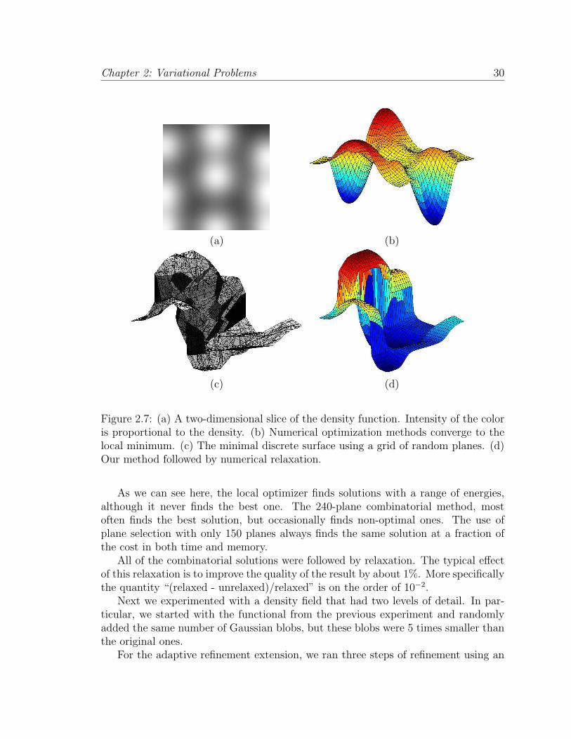
Chapter 2: Variational Problems 30
(a) (b)
(c) (d)
Figure 2.7: (a) A two-dimensional slice of the density function. Intensity of the coloris proportional to the density. (b) Numerical optimization methods converge to thelocal minimum. (c) The minimal discrete surface using a grid of random planes. (d)Our method followed by numerical relaxation.
As we can see here, the local optimizer finds solutions with a range of energies,although it never finds the best one. The 240-plane combinatorial method, mostoften finds the best solution, but occasionally finds non-optimal ones. The use ofplane selection with only 150 planes always finds the same solution at a fraction ofthe cost in both time and memory.
All of the combinatorial solutions were followed by relaxation. The typical effectof this relaxation is to improve the quality of the result by about 1%. More specificallythe quantity “(relaxed - unrelaxed)/relaxed” is on the order of 10−2.
Next we experimented with a density field that had two levels of detail. In par-ticular, we started with the functional from the previous experiment and randomlyadded the same number of Gaussian blobs, but these blobs were 5 times smaller thanthe original ones.
For the adaptive refinement extension, we ran three steps of refinement using an
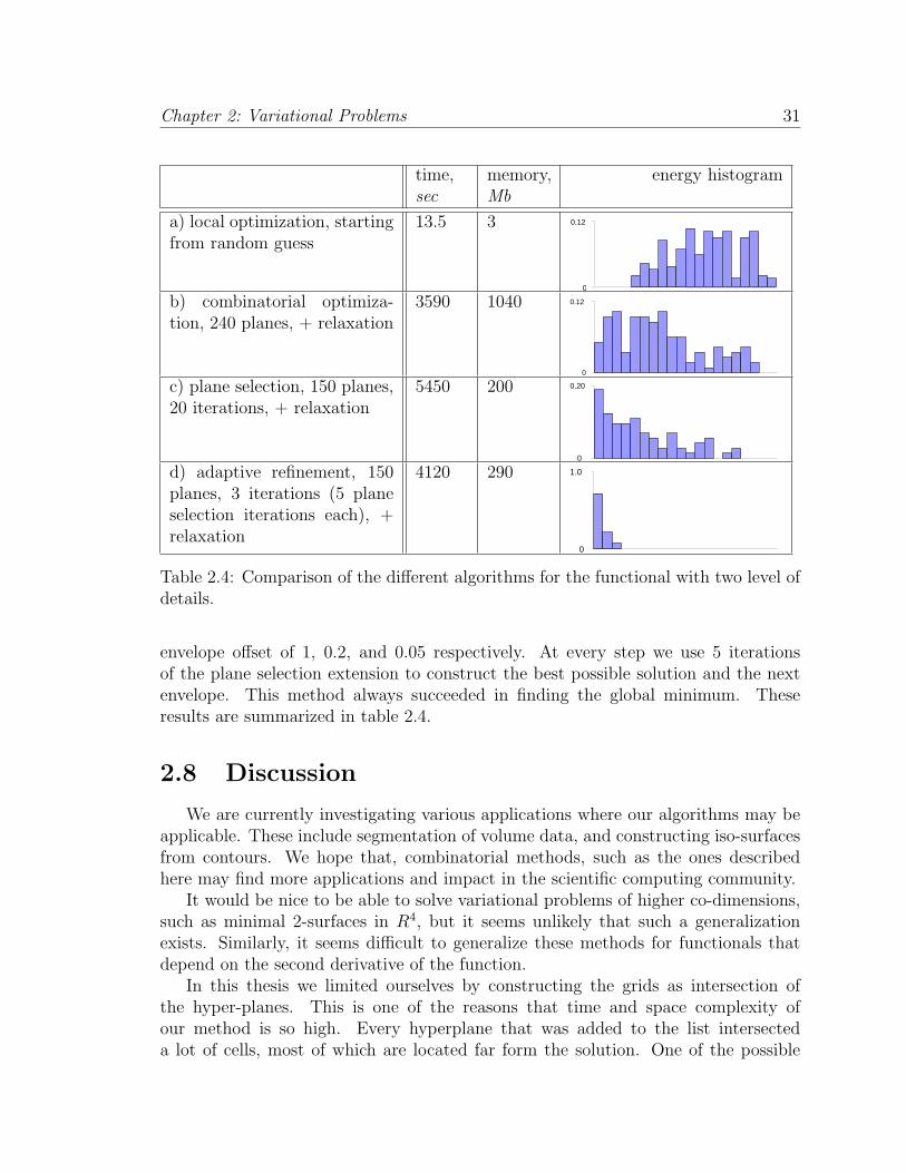
Chapter 2: Variational Problems 31
time,sec
memory,Mb
energy histogram
a) local optimization, startingfrom random guess
13.5 3
0
0.12
b) combinatorial optimiza-tion, 240 planes, + relaxation
3590 1040
0
0.12
c) plane selection, 150 planes,20 iterations, + relaxation
5450 200
0
0.20
d) adaptive refinement, 150planes, 3 iterations (5 planeselection iterations each), +relaxation
4120 290
0
1.0
Table 2.4: Comparison of the different algorithms for the functional with two level ofdetails.
envelope offset of 1, 0.2, and 0.05 respectively. At every step we use 5 iterationsof the plane selection extension to construct the best possible solution and the nextenvelope. This method always succeeded in finding the global minimum. Theseresults are summarized in table 2.4.
2.8 Discussion
We are currently investigating various applications where our algorithms may beapplicable. These include segmentation of volume data, and constructing iso-surfacesfrom contours. We hope that, combinatorial methods, such as the ones describedhere may find more applications and impact in the scientific computing community.
It would be nice to be able to solve variational problems of higher co-dimensions,such as minimal 2-surfaces in R4, but it seems unlikely that such a generalizationexists. Similarly, it seems difficult to generalize these methods for functionals thatdepend on the second derivative of the function.
In this thesis we limited ourselves by constructing the grids as intersection ofthe hyper-planes. This is one of the reasons that time and space complexity ofour method is so high. Every hyperplane that was added to the list intersecteda lot of cells, most of which are located far form the solution. One of the possible
Chapter 2: Variational Problems 32
directions for future research is to construct grids that can be refined locally in order toincrease precision of the approximation without overcomplicating the grid structure.For example, in the planar case we investigated subdivision rules for triangular grids.Unfortunately, the simple subdivision rules (such as 1-to-4 split) do not ensure thenecessary density properties of the resulting grids and more complicated rules (suchas pinwheel grids [47]) are hard to implement and generalize to higher dimensions.
Using spatial octrees (for 3D hyper-planes) is not as elegant and easy to implementas binary trees, but it is likely to increase the performance of the algorithm and betterbalance of the tree.
The dual graphs that arise from our algorithm are very sparse and have a specialstructure. For example, it can be easily shown (section 2.12) that the dual graphof any hyperplane grid is bi-chromatic. Exploiting these properties in MIN-CUTalgorithm seems like a very interesting direction of future research.
2.9 Proof of the density theorem (2.5.7)
Before we begin to prove the theorem, we formulate technical lemma that we willuse in the proof.
Lemma 2.9.1. Let f(x) : [a, b] 7→ R be a twice differentiable function, f(a) = A,f(b) = B. Then there exists such a point x ∈ [a, b] that
df
dx(x) =
B − A
b− a
Corollary 2.9.2. If f(a) = A + ε1, f(b) = B + ε2, then there exists such a pointx ∈ [a, b] that ∣∣∣∣
df
dx(x)− B − A
b− a
∣∣∣∣ ≤|ε1|+ |ε2|
b− a
Theorem 2.9.3. Let us consider a continuous twice differentiable function f(x) :[0, 1] 7→ [0, 1] with bounded first and second derivative, |f ′(x)| ≤ C1, |f ′′(x)| ≤ C2.For any ε > 0 there exists g ∈ L such that ‖f − g‖ < ε.
Proof. Every piecewise linear function generated by the grid Cn can be coded by thesecond coordinate of its vertices
(dk0, dk1, . . . , dkn) | ki ∈0, 1, . . . , n2
,
where d = 1/n2. In this notation the closest piece-wise linear approximation g(x) ofthe function f(x) will look like
(d
[f(0)
d
], d
[f(h)
d
], d
[f(2h)
d
], . . . , d
[f(nh)
d
])
Chapter 2: Variational Problems 33
where [·] denotes the integer part of a number and h = 1/n. By choosing g(x) thisway we make sure that |f(hi)− g(hi)| ≤ d/2 for any i = 0, 1, . . . , n.
Let us now assess the difference between f and g from above, using the fact thatf has limited first and second derivatives.
‖f − g‖ =
1∫
0
|f(x)− g(x)|+ |f ′(x)− g′(x)| dx (2.9.1)
≤ maxx∈[0,1]
(|f(x)− g(x)|) + maxx∈[0,1]
(|f ′(x)− g′(x)|)
The difference |f(x)− g(x)| in the points hi, i = 0, 1, . . . , n is less then d/2 andtherefore
|f(x)− g(x)| ≤ d/2 + C1h (2.9.2)
for all x ∈ [0, 1].Let us take a look on the interval [hi, h(i + 1)] for some 0 ≤ i ≤ n − 1. The
derivative of the piecewise linear function g(x) is constant on this interval and equalto (g(h(i + 1))− g(hi)) /h. We also know that at the ends of the interval the distancebetween f(x) and g(x) is less then d/2. Applying the corollary (2.9.2), we can saythat there exists a point x ∈ [hi, h(i + 1)] such that
|f ′(x)− g′(x)| ≤ d
h.
Using the fact that the second derivative is limited, we can conclude that
|f ′(x)− g′(x)| ≤ d
h+ C2h. (2.9.3)
is true for all x ∈ [hi, h(i + 1)] and therefore for all x ∈ [0, 1].Combining (2.9.1), (2.9.2) and (2.9.3), and taking into account that h = 1/n,
d = 1/n2, we have
‖f − g‖ ≤ d/2 + C1h + d/h + C2h
=1
2n2+
1
n(C1 + C2 + 1) −→
n→∞0.
Thus, for any ε > 0 we can choose such an integer n and such a function g ∈M(Cn) ⊂ L that ‖f − g‖ < ε.
We can easily generalize this theorem for piece-wise differentiable functions.
Corollary 2.9.4. Let us consider a continuous piece-wise twice differentiable func-tion f(x) : [0, 1] 7→ [0, 1] that has a finite number of pieces. The first and secondderivative are defined at every internal point of these pieces and bounded, |f ′(x)| ≤ C1,|f ′′(x)| ≤ C2. For any ε > 0 there still exists g ∈ L such that ‖f − g‖ < ε.
Chapter 2: Variational Problems 34
Proof. We create the piece-wise linear function g the same way we did it in the previ-ous theorem. The only difference from the previous proof is that now the function fhas a finite number of points where the first and second derivatives are discontinuous.Let us consider one of these points x that is covered by k-th segment of the functiong. Because the first derivative is bounded, we have
(k+1)h∫
kh
|f(x)− g(x)|+ |f ′(x)− g′(x)| dx ≤ (2 + C1)h.
Therefore, the total difference introduced by these points of discontinuity goes to zerowhen h goes to zero.
The proof of the theorem (2.5.7) now becomes trivial. We proved that for everyfunction f ∈ P and any ε > 0 there still exists g ∈ L such that ‖f − g‖ < ε.Therefore, L is dense in P .
2.10 Proof of the density theorem (2.5.8)
Our investigation of the random grids will be based on the obvious fact that canbe stated as follows.
Lemma 2.10.1. Let f(x) be a piece-wise linear function with n linear segments, Rm
be a random grid with m ≥ n, and ε > 0. Then there is a non-zero probabilityp(f, m) > 0 that there exists such a function g(x) ∈M(Rm) that ‖f − g‖ < ε.
All the lines are generated independently, therefore we can consider the grid R2m
to be the intersection of two independent grids of the size m. Using the basics of theprobability theory, we can conclude that for the conditions given in the lemma
p(f, 2m) ≥ 2p(f, m)− p(f, m)2.
We know that the sequence pn+1 = pn + pn(1 − pn) with the starting point 0 <p1 < 1 converges to 1. That is why
p(f,m) −→m→∞
1. (2.10.1)
In other words, we can state the following corollary.
Corollary 2.10.2. Let f(x) be a piece-wise linear function, and Rm, m = 1, 2, . . . be a family of the random grids, and ε > 0. Then the probability that there existssuch a function g(x) ∈ Lr that ‖f − g‖ < ε is equal to 1.
Corollary 2.10.3. Let Rm, m = 1, 2, . . . be a family of the random grids. ThenLr is dense in L and therefore Lr is dense in P.
Chapter 2: Variational Problems 35
2.11 Proof of the duality theorem (2.6.4)
In section 2.6.1 we already defined 1- and 2-chains and their boundaries.
Definition 2.11.1. The chain is called closed if its boundary is the empty set.
The following lemmata reduce the minimum valid curve problem to one of planarpartitioning.
Lemma 2.11.2. On our complex, there is a one-to-one correspondence between validcurves and closed 1-chains which include the edge er and do not include ek.
Proof. The correspondence between a 1-chain C satisfying the properties of the lemmaand a valid curve S is C = S ∪ er.
Lemma 2.11.3. On any complex homeomorphic to B2, there is a one-to-one corre-spondence between 2-chains and closed 1-chains. The relationship between the corre-sponding 2-chain A and 1-chain C can be expressed as ∂2A = C.Proof. The first homology group H1 is defined as the quotient group: H1 = ker(∂1)
Im(∂2).
In any complex homeomorphic to B2, H1 is the trivial group (see [18]), thereforeker(∂1) = Im(∂2).
Combining these two lemmas together, we establish the following correspondence.
Theorem 2.11.4. On our complex, there is a one-to-one correspondence betweenvalid curves and 2-chains that include the face fr and do not include the face fk.
Because there is a one-to-one correspondence between the faces of the primalgraph and the vertices of the dual graph, there is also a one-to one correspondencebetween 2-chains that includes the face fr and does not include the face fk and cutsin the dual graph.
This proves theorem (2.6.4).
2.12 Dual graph is bi-chromatic
The dual graph of the complex obtained by the plane intersection has specialproperties. Some of them might be interesting to the future researchers. Note, thatthe complex and dual graph considered here do not include source and sink vertices.
Definition 2.12.1. Let the d-dimensional space be divided by n non-equivalent hyper-planes Aix + Bi = 0, i = 1, 2, . . . , n, Ai is a d-dimensional vector. The subdivisioncode of a point x is an n-dimensional vector b(x)i = sign(Aix + Bi).
Lemma 2.12.2. Two points are located in the same cell if and only if they have thesame subdivision code.
Chapter 2: Variational Problems 36
We do not prove this lemma because of its triviality.
Lemma 2.12.3. Two points are located in the neighboring cells if and only if theirsubdivision codes are the same except for one element which is 1 for one of the pointsand −1 for another.
Proof. Two neighboring cells have one hyperplane that separate them. That is oneexactly one element in their subdivision codes is different.
Lemma 2.12.4. The dual graph of any grid obtained by the hyperplanes intersectionis two-colorable (except for the source and sink vertices).
Proof. For every cell k we can introduce a parameter Pk which is equal to the numberof all positive elements in the cell subdivision code. Let us color with the white colorall the cells where Pk is even and with the black color all the cells where Pk is odd.
By the lemma 2.12.4 all cells have the neighbors of the opposite color only.The dual graph has a vertex for every cell and an edge between every two neigh-
bors. Therefore, the dual graph is also two-colorable.
Minimum WeightTriangulations
3
37
Chapter 3: Minimum Weight Triangulations 38
Finding the minimum weight triangulation of the set of points on the plane isa classical problem of computational geometry. Though it might seem to be veryfar from the problems considered in the previous chapter, these problems exhibit atremendous similarity in the context of spatial complexes. In this chapter we showthat the spatial complexes arising in the minimum weight triangulation are not em-beddable and that embeddability is crucial in finding the solution of the problem inpolynomial time.
Minimal discrete surface on the embeddable complex can be found in polynomialtime using the duality graph introduced in chapter (2.6). While the duality trick doesnot work for non-embeddable complexes, we explore linear programming techniquesto construct an approximate solution for the minimal weight triangulation (MWT)problem.
In particular, we reduce the minimum weight triangulation problem of n pointsto the linear program with O (n3) variables and (in)equalities. This approach has anumber of interesting properties of both theoretical and practical value.
• Integer solution of our linear program is equal to MWT.
• In general case, the straightforward implementation of our approach successfullycomputes MWT of up to two hundreds random points.
• Our approach can be merged with existing methods to provide fast implemen-tations of MWT algorithm.
Though in some special cases we can prove that the solution of our LP is alwaysinteger, in general there exist a counterexamples where the solution of the linearproblem is not integer. Still, we believe that the linear programming approach canbe of a practical use for the MWT problem.
3.1 Edge-based and triangle-based definitions of
the problem
Let S be a set of n points in Euclidean plane. A triangulation of this set isa maximum set of non-crossing edges between the points of S. The weight of thetriangulation is equal to the sum of the lengths of its edges. To avoid degeneracies,in this thesis we suppose that no three points are located on a line, and no twotriangulations of S have the same weights. Clearly, these conditions can always besatisfied by infinitely small perturbation of the positions of the points. The problemof finding the triangulation with the minimum total Euclidean length of it edges ishistorically called the minimum weight triangulation (MWT) problem. This problemis the major problem addressed in this chapter. For the clarity sake, in this text we
Chapter 3: Minimum Weight Triangulations 39
will sometimes call this problem Euclidean MWT. The complexity of the EuclideanMWT problem is currently unknown.
We can also consider the generalization of Euclidean MWT problem when theweights of the edges are arbitrary positive numbers. Let us call this problem thegeneral edge-based MWT problem. This problem is known to be NP-hard.
In this thesis, we redefine triangulation in terms of triangles, which seems morenatural for our approach.
Definition 3.1.1. A set Te of empty triangles consists of all triangles with theendpoints in S that do not have any other points of S in their interiors.
Obviously, any triangulation T consists of the triangles from the set Te. Note,that because the set of points S is non-degenerate, no points can appear exactly onthe edge of any triangle. For our purpose, we introduce the set Q of all points of theplane inside the convex hull of S, and the set E of all points of the plane covered bythe edges with the endpoints in S.
Definition 3.1.2. A set of the triangles T = ti ⊂ Te is a triangulation of thepoint set S if ∪ti = Q, and triangles overlap only by their edges, i.e. ti ∩ tj \ E = ∅.
To make sure that the weight of the triangulation corresponds to the weight fromprevious definitions, we have to remember that every edge in the triangulation belongsto two triangles, except for the edges on the convex hull of S.
Definition 3.1.3. The weight w of the triangle with the edges e1, e2, e3 is computedas
w = α1 |e1|+ α2 |e2|+ α3 |e3| (3.1.1)
where αi = 1 for the edges on the convex hull and αi = 0.5 for all other edges.
After having defined the weight of a triangulation as a sum of the weights of itstriangles, it is possible to talk about MWT. Clearly, for the non-degenerate sets newdefinition of the MWT problem corresponds to the old one.
When the weights of the triangles are arbitrary positive numbers, the problemof finding the triangulation of minimum weights becomes the general triangle-basedMWT problem. Obviously, it is more general than Euclidean and edge-based MWTand therefore it is also NP-hard.
3.2 Previous work on MWT.
In 1977 Lloyd [16] proved that the following problem is equivalent to the 3-satisfiability and therefore NP-complete. If not all edges are allowed, find any trian-gulation that consists of the allowed edges or show that no such triangulation exists.This problem has an immediate application for our case. By assigning zero weight
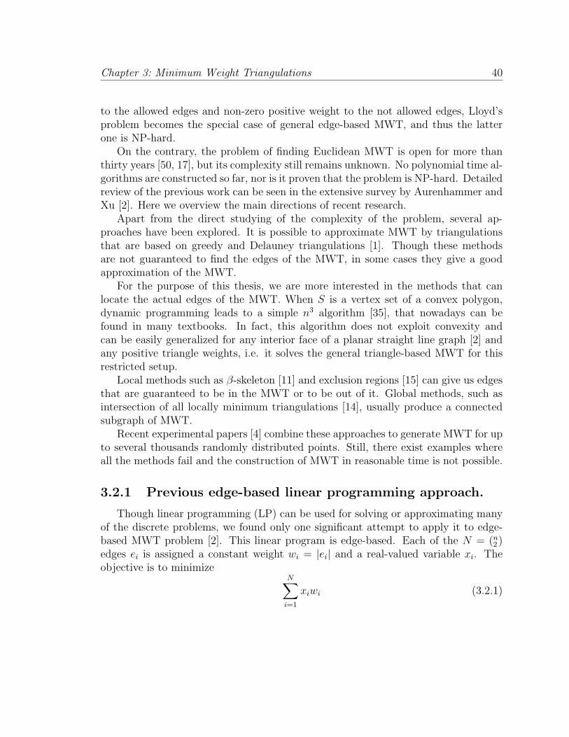
Chapter 3: Minimum Weight Triangulations 40
to the allowed edges and non-zero positive weight to the not allowed edges, Lloyd’sproblem becomes the special case of general edge-based MWT, and thus the latterone is NP-hard.
On the contrary, the problem of finding Euclidean MWT is open for more thanthirty years [50, 17], but its complexity still remains unknown. No polynomial time al-gorithms are constructed so far, nor is it proven that the problem is NP-hard. Detailedreview of the previous work can be seen in the extensive survey by Aurenhammer andXu [2]. Here we overview the main directions of recent research.
Apart from the direct studying of the complexity of the problem, several ap-proaches have been explored. It is possible to approximate MWT by triangulationsthat are based on greedy and Delauney triangulations [1]. Though these methodsare not guaranteed to find the edges of the MWT, in some cases they give a goodapproximation of the MWT.
For the purpose of this thesis, we are more interested in the methods that canlocate the actual edges of the MWT. When S is a vertex set of a convex polygon,dynamic programming leads to a simple n3 algorithm [35], that nowadays can befound in many textbooks. In fact, this algorithm does not exploit convexity andcan be easily generalized for any interior face of a planar straight line graph [2] andany positive triangle weights, i.e. it solves the general triangle-based MWT for thisrestricted setup.
Local methods such as β-skeleton [11] and exclusion regions [15] can give us edgesthat are guaranteed to be in the MWT or to be out of it. Global methods, such asintersection of all locally minimum triangulations [14], usually produce a connectedsubgraph of MWT.
Recent experimental papers [4] combine these approaches to generate MWT for upto several thousands randomly distributed points. Still, there exist examples whereall the methods fail and the construction of MWT in reasonable time is not possible.
3.2.1 Previous edge-based linear programming approach.
Though linear programming (LP) can be used for solving or approximating manyof the discrete problems, we found only one significant attempt to apply it to edge-based MWT problem [2]. This linear program is edge-based. Each of the N = (n
2 )edges ei is assigned a constant weight wi = |ei| and a real-valued variable xi. Theobjective is to minimize
N∑i=1
xiwi (3.2.1)
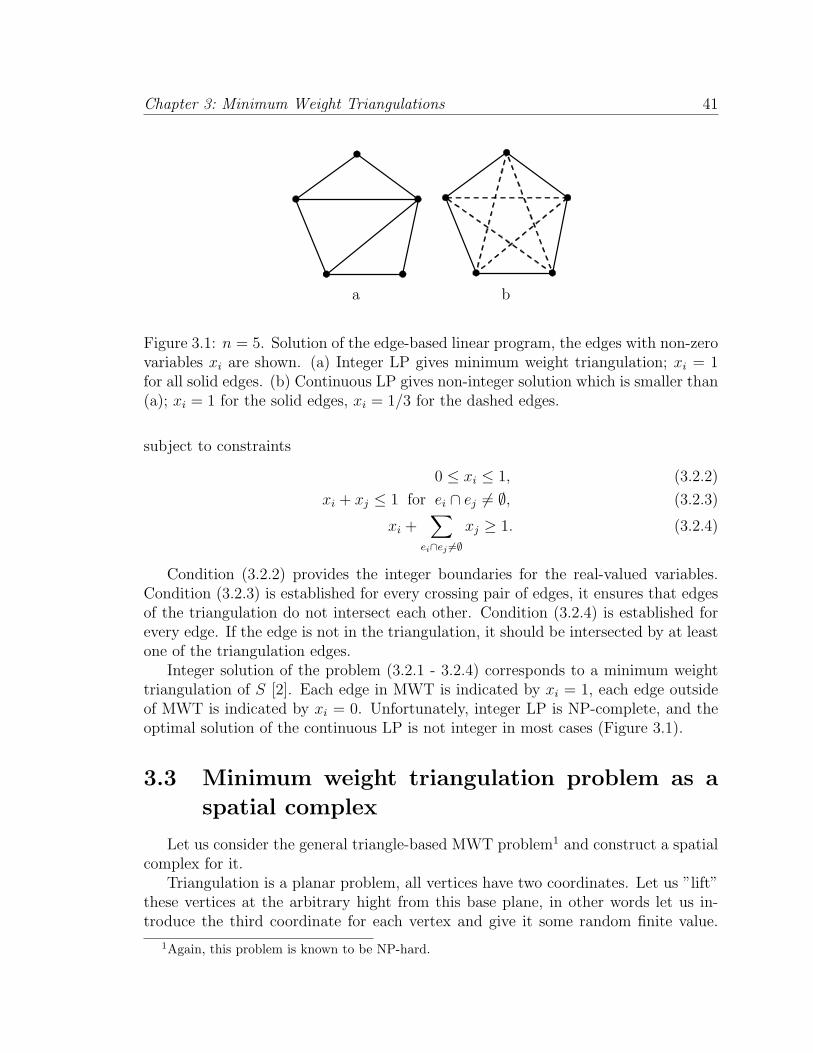
Chapter 3: Minimum Weight Triangulations 41
a b
Figure 3.1: n = 5. Solution of the edge-based linear program, the edges with non-zerovariables xi are shown. (a) Integer LP gives minimum weight triangulation; xi = 1for all solid edges. (b) Continuous LP gives non-integer solution which is smaller than(a); xi = 1 for the solid edges, xi = 1/3 for the dashed edges.
subject to constraints
0 ≤ xi ≤ 1, (3.2.2)
xi + xj ≤ 1 for ei ∩ ej 6= ∅, (3.2.3)
xi +∑
ei∩ej 6=∅xj ≥ 1. (3.2.4)
Condition (3.2.2) provides the integer boundaries for the real-valued variables.Condition (3.2.3) is established for every crossing pair of edges, it ensures that edgesof the triangulation do not intersect each other. Condition (3.2.4) is established forevery edge. If the edge is not in the triangulation, it should be intersected by at leastone of the triangulation edges.
Integer solution of the problem (3.2.1 - 3.2.4) corresponds to a minimum weighttriangulation of S [2]. Each edge in MWT is indicated by xi = 1, each edge outsideof MWT is indicated by xi = 0. Unfortunately, integer LP is NP-complete, and theoptimal solution of the continuous LP is not integer in most cases (Figure 3.1).
3.3 Minimum weight triangulation problem as a
spatial complex
Let us consider the general triangle-based MWT problem1 and construct a spatialcomplex for it.
Triangulation is a planar problem, all vertices have two coordinates. Let us ”lift”these vertices at the arbitrary hight from this base plane, in other words let us in-troduce the third coordinate for each vertex and give it some random finite value.
1Again, this problem is known to be NP-hard.
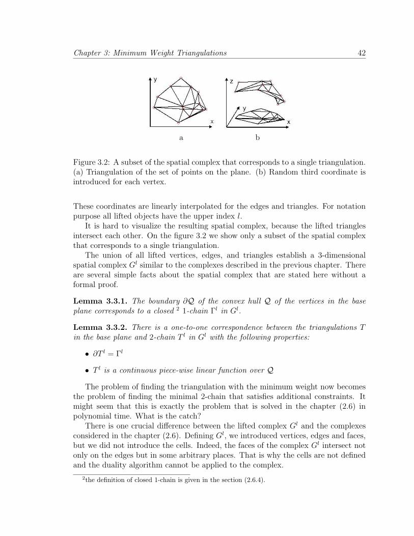
Chapter 3: Minimum Weight Triangulations 42
a b
Figure 3.2: A subset of the spatial complex that corresponds to a single triangulation.(a) Triangulation of the set of points on the plane. (b) Random third coordinate isintroduced for each vertex.
These coordinates are linearly interpolated for the edges and triangles. For notationpurpose all lifted objects have the upper index l.
It is hard to visualize the resulting spatial complex, because the lifted trianglesintersect each other. On the figure 3.2 we show only a subset of the spatial complexthat corresponds to a single triangulation.
The union of all lifted vertices, edges, and triangles establish a 3-dimensionalspatial complex Gl similar to the complexes described in the previous chapter. Thereare several simple facts about the spatial complex that are stated here without aformal proof.
Lemma 3.3.1. The boundary ∂Q of the convex hull Q of the vertices in the baseplane corresponds to a closed 2 1-chain Γl in Gl.
Lemma 3.3.2. There is a one-to-one correspondence between the triangulations Tin the base plane and 2-chain T l in Gl with the following properties:
• ∂T l = Γl
• T l is a continuous piece-wise linear function over QThe problem of finding the triangulation with the minimum weight now becomes
the problem of finding the minimal 2-chain that satisfies additional constraints. Itmight seem that this is exactly the problem that is solved in the chapter (2.6) inpolynomial time. What is the catch?
There is one crucial difference between the lifted complex Gl and the complexesconsidered in the chapter (2.6). Defining Gl, we introduced vertices, edges and faces,but we did not introduce the cells. Indeed, the faces of the complex Gl intersect notonly on the edges but in some arbitrary places. That is why the cells are not definedand the duality algorithm cannot be applied to the complex.
2the definition of closed 1-chain is given in the section (2.6.4).
Chapter 3: Minimum Weight Triangulations 43
Note, that if we could construct the embedding of Gl in 3D such that faces intersecton the edges only, then all the conditions of the chapter (2.6) would be fulfilled andwe could find the minimum triangulation in polynomial time. This might be possible,for example, when not all triangles are allowed in triangulation.
3.4 Triangle-based linear program
Linear programming provides another interesting approach to the MWT problem.The rest of the chapter is devoted to the thorough investigation of this method. Note,that similar linear program can be set up for the spatial complex in the previouschapter, but duality method is more computationally efficient.
Triangle-based linear program is defined as follows. Every triangle ti ∈ Te isassigned a real-valued variable xi. The objective is to minimize the weight of thetriangulation
F (x) =∑Te
xiwi (3.4.1)
Each variable has to be nonnegative.3
xi ≥ 0 (3.4.2)
Every edge of the convex hull ek is in MWT. Therefore, one of the trianglesadjacent to this edge is also represented in MWT. This condition can be expressedby the following equality. ∑
ti3ek
xi = 1 (3.4.3)
Finally, there is an equality for every edge ek that is not on the convex hull. Theline, that this edge belongs to, divides the plane onto two half-planes. The set of thetriangles that are adjacent to ek can be split accordingly onto two sets, T 1
k and T 2k .
If ek belongs to MWT, then exactly one triangle from T 1k and one from T 2
k belong toMWT. If ek is not in MWT, then non of the adjacent triangles is in the MWT. Thisidea is expressed in the following equality.
∑
T 1k
xi =∑
T 2k
xi (3.4.4)
It is interesting to note, that (3.4.1 - 3.4.4) is a direct generalization of the well-known LP approach to the shortest path problem.4
3Unlike (3.2.2), we do not define the upper boundary, because it will be satisfied automatically.4In some sense, we are trying to construct the ”shortest surface” with the boundary condi-
tions (3.4.3) and connectivity condition (3.4.4). The crucial difference between these two problemsis that shortest path LP has integer solutions for any positive weights wi. In our case, the problemof finding the minimum triangulation with arbitrary weights is NP-complete and the success of themethod is provided by the weight definition (3.1.1).
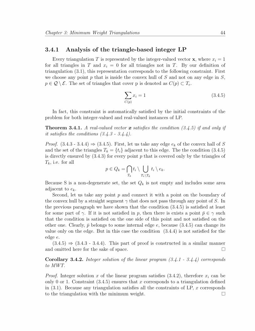
Chapter 3: Minimum Weight Triangulations 44
3.4.1 Analysis of the triangle-based integer LP
Every triangulation T is represented by the integer-valued vector x, where xi = 1for all triangles in T and xi = 0 for all triangles not in T . By our definition oftriangulation (3.1), this representation corresponds to the following constraint. Firstwe choose any point p that is inside the convex hull of S and not on any edge in S,p ∈ Q \ E . The set of triangles that cover p is denoted as C(p) ⊂ Te.
∑
C(p)
xi = 1 (3.4.5)
In fact, this constraint is automatically satisfied by the initial constraints of theproblem for both integer-valued and real-valued instances of LP.
Theorem 3.4.1. A real-valued vector x satisfies the condition (3.4.5) if and only ifit satisfies the conditions (3.4.3 - 3.4.4).
Proof. (3.4.3 - 3.4.4) ⇒ (3.4.5). First, let us take any edge ek of the convex hall of Sand the set of the triangles Tk = ti adjacent to this edge. The the condition (3.4.5)is directly ensured by (3.4.3) for every point p that is covered only by the triangles ofTk, i.e. for all
p ∈ Qk =⋂Tk
ti \⋃
Te\Tk
ti \ ek.
Because S is a non-degenerate set, the set Qk is not empty and includes some areaadjacent to ek.
Second, let us take any point p and connect it with a point on the boundary ofthe convex hull by a straight segment γ that does not pass through any point of S. Inthe previous paragraph we have shown that the condition (3.4.5) is satisfied at leastfor some part of γ. If it is not satisfied in p, then there is exists a point p ∈ γ suchthat the condition is satisfied on the one side of this point and not satisfied on theother one. Clearly, p belongs to some internal edge e, because (3.4.5) can change itsvalue only on the edge. But in this case the condition (3.4.4) is not satisfied for theedge e.
(3.4.5) ⇒ (3.4.3 - 3.4.4). This part of proof is constructed in a similar mannerand omitted here for the sake of space.
Corollary 3.4.2. Integer solution of the linear program (3.4.1 - 3.4.4) correspondsto MWT.
Proof. Integer solution x of the linear program satisfies (3.4.2), therefore xi can beonly 0 or 1. Constraint (3.4.5) ensures that x corresponds to a triangulation definedin (3.1). Because any triangulation satisfies all the constraints of LP, x correspondsto the triangulation with the minimum weight.
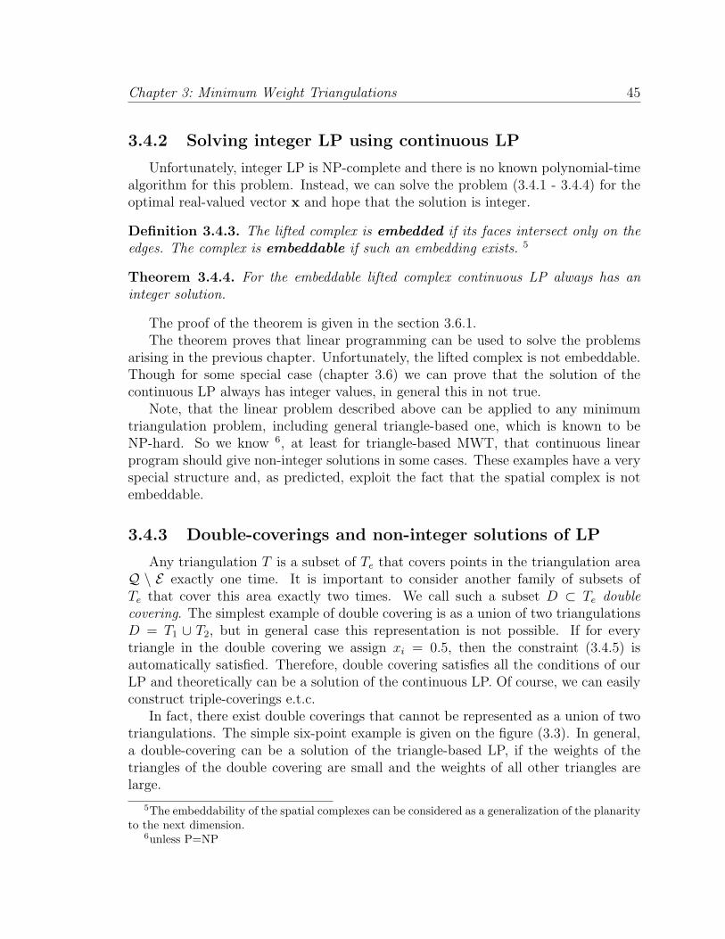
Chapter 3: Minimum Weight Triangulations 45
3.4.2 Solving integer LP using continuous LP
Unfortunately, integer LP is NP-complete and there is no known polynomial-timealgorithm for this problem. Instead, we can solve the problem (3.4.1 - 3.4.4) for theoptimal real-valued vector x and hope that the solution is integer.
Definition 3.4.3. The lifted complex is embedded if its faces intersect only on theedges. The complex is embeddable if such an embedding exists. 5
Theorem 3.4.4. For the embeddable lifted complex continuous LP always has aninteger solution.
The proof of the theorem is given in the section 3.6.1.The theorem proves that linear programming can be used to solve the problems
arising in the previous chapter. Unfortunately, the lifted complex is not embeddable.Though for some special case (chapter 3.6) we can prove that the solution of thecontinuous LP always has integer values, in general this in not true.
Note, that the linear problem described above can be applied to any minimumtriangulation problem, including general triangle-based one, which is known to beNP-hard. So we know 6, at least for triangle-based MWT, that continuous linearprogram should give non-integer solutions in some cases. These examples have a veryspecial structure and, as predicted, exploit the fact that the spatial complex is notembeddable.
3.4.3 Double-coverings and non-integer solutions of LP
Any triangulation T is a subset of Te that covers points in the triangulation areaQ \ E exactly one time. It is important to consider another family of subsets ofTe that cover this area exactly two times. We call such a subset D ⊂ Te doublecovering. The simplest example of double covering is as a union of two triangulationsD = T1 ∪ T2, but in general case this representation is not possible. If for everytriangle in the double covering we assign xi = 0.5, then the constraint (3.4.5) isautomatically satisfied. Therefore, double covering satisfies all the conditions of ourLP and theoretically can be a solution of the continuous LP. Of course, we can easilyconstruct triple-coverings e.t.c.
In fact, there exist double coverings that cannot be represented as a union of twotriangulations. The simple six-point example is given on the figure (3.3). In general,a double-covering can be a solution of the triangle-based LP, if the weights of thetriangles of the double covering are small and the weights of all other triangles arelarge.
5The embeddability of the spatial complexes can be considered as a generalization of the planarityto the next dimension.
6unless P=NP
Chapter 3: Minimum Weight Triangulations 46
a b c
Figure 3.3: Single- and double- coverings. (a) Triangulation (single-covering) of 6-point set consists of five triangles. (b) Double-covering of the same set consists of tentriangles. For simplicity, only two triangles are shown, the rest can be obtained bythe rotation of this pair around the center point by 4πk/5, where k = 1, 2, 3, 4. (c)The same double-covering. All ten triangles are shown (transparent). Note, that thisdouble-covering cannot be split onto two triangulations.
a b
Figure 3.4: 13-point counterexample for Euclidean MWT. (a) Minimum weight tri-angulation weights 18.798. (b) Solution of the continuous LP corresponds to a doublecovering with a weight 18.764. Triangles are shown transparent.
Intuitively, this situation is unlikely to happen when the weights of triangles aredefined as Euclidean length (3.1.1). For example, on the figure (3.3c) we had to userelatively long and ”heavy” edges to construct a double covering. For a long timewe could not construct the counter example for the Euclidean MWT, nor could weprove that the solution of the LP is always integer. Numerous experiments showedthat LP gives integer solution when points are randomly distributed on the plane (theexperiments are described in the following chapters).
The triskaidekaphobic counterexample that we found is surprisingly similar tothe counterexample for LMT method [14]. One vertex is located in the middle, andexactly 13 vertices are uniformly distributed on the unit circle around it (figure 3.4).The weight of the minimal triangulation is 18.798, the weight of the minimal doublecovering is 18.764.
Chapter 3: Minimum Weight Triangulations 47
3.4.4 Random experiments
We believe that the proposed linear program might be of a practical use whenthe vertices are uniformly distributed on the plane. The experiments are essentialto check the robustness of the algorithm. The number of the empty triangles isO(n3). Indeed, in the worst case when S is a vertex set of a convex polygon, everytriangle is possible. The same is the number of inequalities (3.4.2). The numberof equalities (3.4.3 - 3.4.4) is equal to the number of the edges (n
2 ) and thereforequadratic. Given that the best known LP algorithm is cubic, the time complexity ofthe straightforward implementation of the algorithm is O(n9).
We used CPLEX to solve the resulting linear program, points were distributeduniformly in the unit square. For such a setup, our straightforward implementation ofthe algorithm allows to compute MWT of up to two hundreds randomly distributedpoints. For 200 points, the linear program consists of about 70, 000 variables andinequalities and 20, 000 equalities; it takes CPLEX about twenty minutes to converge.
We tested random point sets from 10, 20, 60 and 200 points. The total number ofsets tested is about 100, 000. In all tested cases the solution of the LP problem wasinteger and therefore the exact MWT was constructed.
Using previous methods to minimize the number of variables
The algorithm proposed above is not practical, since for the randomly distributedsets of points it is possible to construct a large subgraph of the MWT for up to hundredthousands points in reasonable time [4]. When the resulting subgraph is connected,each of the remaining faces can be triangulated in O(n3) time. Some modification ofour algorithm should be used when the resulting subgraph is not connected.
Indeed, we can efficiently use the information about edges that are guaranteedto be in MWT and that are guaranteed to be out of MWT. If the curtain edge isguaranteed to be out of MWT, then all the triangles adjacent to this edge are no longervalid and can be ignored in linear program constructing. If the edge is guaranteed tobe in the MWT, then all triangles that intersect this edge can be also eliminated.
In our experiments, we used the diamond test [15] to locate the edges that arenot in MWT. This simple but powerful test significantly reduced the number of thevalid triangles and allowed us to compute MWT of up to two thousands points.
3.5 Discussion
Our method and LMT [14]. Interesting enough, the results of our methodare very similar to the results shown by LMT, though methods are very different bytheir nature. There are two major similarities:
• Both methods seem to work fine for the sets of randomly distributed points on
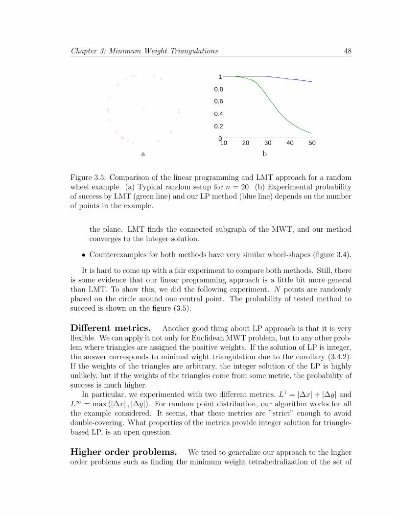
Chapter 3: Minimum Weight Triangulations 48
10 20 30 40 50 0
0.2
0.4
0.6
0.8
1
a b
Figure 3.5: Comparison of the linear programming and LMT approach for a randomwheel example. (a) Typical random setup for n = 20. (b) Experimental probabilityof success by LMT (green line) and our LP method (blue line) depends on the numberof points in the example.
the plane. LMT finds the connected subgraph of the MWT, and our methodconverges to the integer solution.
• Counterexamples for both methods have very similar wheel-shapes (figure 3.4).
It is hard to come up with a fair experiment to compare both methods. Still, thereis some evidence that our linear programming approach is a little bit more generalthan LMT. To show this, we did the following experiment. N points are randomlyplaced on the circle around one central point. The probability of tested method tosucceed is shown on the figure (3.5).
Different metrics. Another good thing about LP approach is that it is veryflexible. We can apply it not only for Euclidean MWT problem, but to any other prob-lem where triangles are assigned the positive weights. If the solution of LP is integer,the answer corresponds to minimal wight triangulation due to the corollary (3.4.2).If the weights of the triangles are arbitrary, the integer solution of the LP is highlyunlikely, but if the weights of the triangles come from some metric, the probability ofsuccess is much higher.
In particular, we experimented with two different metrics, L1 = |∆x| + |∆y| andL∞ = max (|∆x| , |∆y|). For random point distribution, our algorithm works for allthe example considered. It seems, that these metrics are ”strict” enough to avoiddouble-covering. What properties of the metrics provide integer solution for triangle-based LP, is an open question.
Higher order problems. We tried to generalize our approach to the higherorder problems such as finding the minimum weight tetrahedralization of the set of
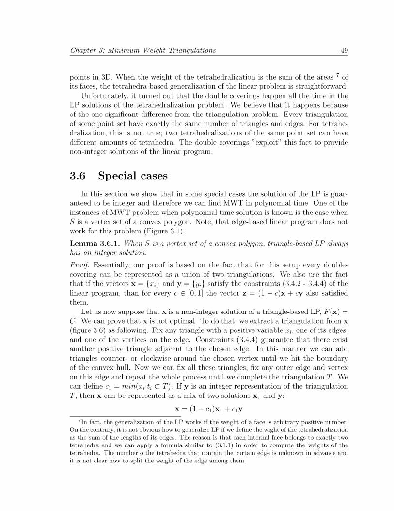
Chapter 3: Minimum Weight Triangulations 49
points in 3D. When the weight of the tetrahedralization is the sum of the areas 7 ofits faces, the tetrahedra-based generalization of the linear problem is straightforward.
Unfortunately, it turned out that the double coverings happen all the time in theLP solutions of the tetrahedralization problem. We believe that it happens becauseof the one significant difference from the triangulation problem. Every triangulationof some point set have exactly the same number of triangles and edges. For tetrahe-dralization, this is not true; two tetrahedralizations of the same point set can havedifferent amounts of tetrahedra. The double coverings ”exploit” this fact to providenon-integer solutions of the linear program.
3.6 Special cases
In this section we show that in some special cases the solution of the LP is guar-anteed to be integer and therefore we can find MWT in polynomial time. One of theinstances of MWT problem when polynomial time solution is known is the case whenS is a vertex set of a convex polygon. Note, that edge-based linear program does notwork for this problem (Figure 3.1).
Lemma 3.6.1. When S is a vertex set of a convex polygon, triangle-based LP alwayshas an integer solution.
Proof. Essentially, our proof is based on the fact that for this setup every double-covering can be represented as a union of two triangulations. We also use the factthat if the vectors x = xi and y = yi satisfy the constraints (3.4.2 - 3.4.4) of thelinear program, than for every c ∈ [0, 1] the vector z = (1 − c)x + cy also satisfiedthem.
Let us now suppose that x is a non-integer solution of a triangle-based LP, F (x) =C. We can prove that x is not optimal. To do that, we extract a triangulation from x(figure 3.6) as following. Fix any triangle with a positive variable xi, one of its edges,and one of the vertices on the edge. Constraints (3.4.4) guarantee that there existanother positive triangle adjacent to the chosen edge. In this manner we can addtriangles counter- or clockwise around the chosen vertex until we hit the boundaryof the convex hull. Now we can fix all these triangles, fix any outer edge and vertexon this edge and repeat the whole process until we complete the triangulation T . Wecan define c1 = min(xi|ti ⊂ T ). If y is an integer representation of the triangulationT , then x can be represented as a mix of two solutions x1 and y:
x = (1− c1)x1 + c1y
7In fact, the generalization of the LP works if the weight of a face is arbitrary positive number.On the contrary, it is not obvious how to generalize LP if we define the wight of the tetrahedralizationas the sum of the lengths of its edges. The reason is that each internal face belongs to exactly twotetrahedra and we can apply a formula similar to (3.1.1) in order to compute the weights of thetetrahedra. The number o the tetrahedra that contain the curtain edge is unknown in advance andit is not clear how to split the weight of the edge among them.
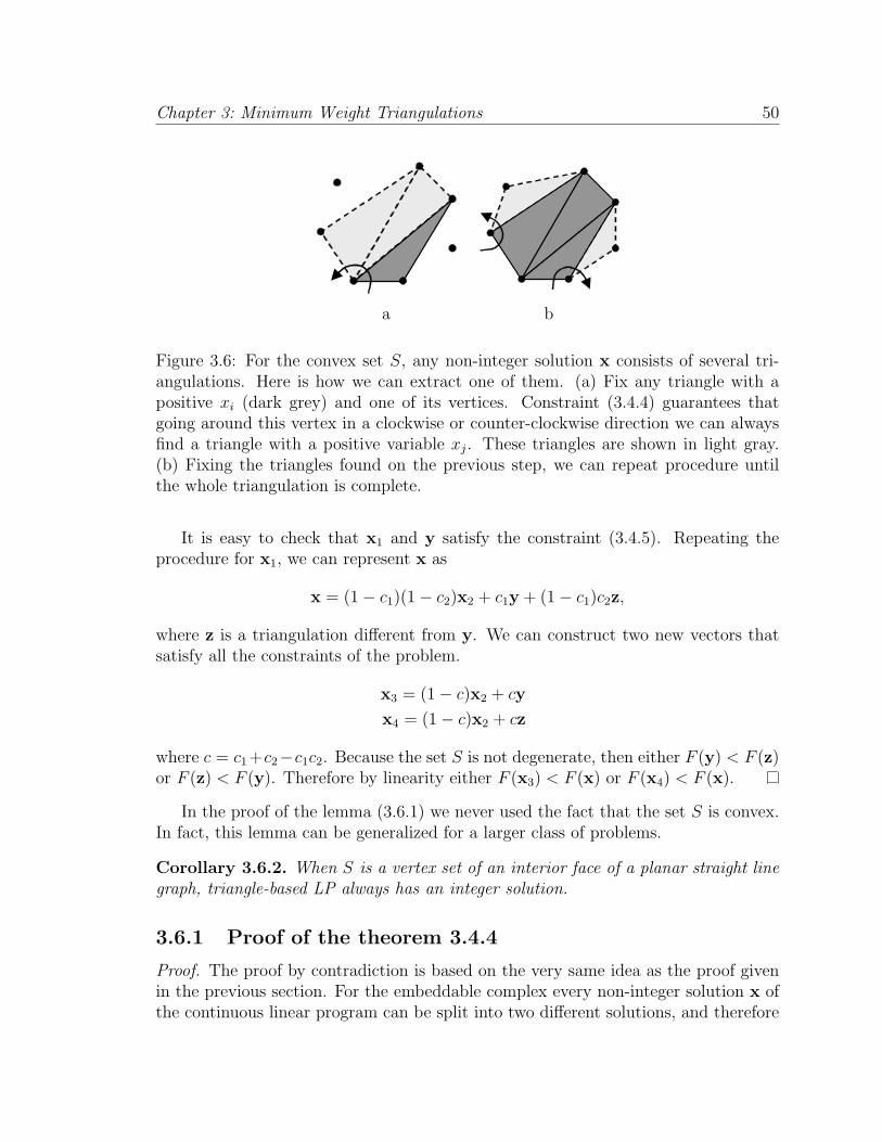
Chapter 3: Minimum Weight Triangulations 50
a b
Figure 3.6: For the convex set S, any non-integer solution x consists of several tri-angulations. Here is how we can extract one of them. (a) Fix any triangle with apositive xi (dark grey) and one of its vertices. Constraint (3.4.4) guarantees thatgoing around this vertex in a clockwise or counter-clockwise direction we can alwaysfind a triangle with a positive variable xj. These triangles are shown in light gray.(b) Fixing the triangles found on the previous step, we can repeat procedure untilthe whole triangulation is complete.
It is easy to check that x1 and y satisfy the constraint (3.4.5). Repeating theprocedure for x1, we can represent x as
x = (1− c1)(1− c2)x2 + c1y + (1− c1)c2z,
where z is a triangulation different from y. We can construct two new vectors thatsatisfy all the constraints of the problem.
x3 = (1− c)x2 + cy
x4 = (1− c)x2 + cz
where c = c1+c2−c1c2. Because the set S is not degenerate, then either F (y) < F (z)or F (z) < F (y). Therefore by linearity either F (x3) < F (x) or F (x4) < F (x).
In the proof of the lemma (3.6.1) we never used the fact that the set S is convex.In fact, this lemma can be generalized for a larger class of problems.
Corollary 3.6.2. When S is a vertex set of an interior face of a planar straight linegraph, triangle-based LP always has an integer solution.
3.6.1 Proof of the theorem 3.4.4
Proof. The proof by contradiction is based on the very same idea as the proof givenin the previous section. For the embeddable complex every non-integer solution x ofthe continuous linear program can be split into two different solutions, and therefore
Chapter 3: Minimum Weight Triangulations 51
it cannot be optimal. Because of the lack of space, here we provide only the generalidea of the proof.
Because the complex Gl is lifted, every triangle tli of the complex can be alsoconsidered as a linear mapping Li of the triangle ti from the base plane Q, i.e.Li : ti ⊂ Q 7→ <.
Definition 3.6.3. The lifted triangle tli is lower than the triangle tlj, if there existsat least one point in the base plane q ∈ ti ∩ tj such that Li(q) < Lj(q).
For the embeddable complexes the notion of ”lower” is well defined, because thetriangles intersect on the edges only. For the non-embeddable complexes this defini-tion does not make a lot of sense and the rest of the proof does not work.
Let us consider the set Ll that consists of the lifted triangles tli with the followingproperties:
• the LP variable xi of this triangle is non-zero, xi > 0
• there is no triangle tlj lower than tli such that xj > 0
We will show now that the 2-chain Ll corresponds to a valid triangulation by thelemma 3.3.2. Indeed, Ll corresponds to a continuous piece-wise linear function overthe domain Q.
• Ll does not cover any area of the domain twice by construction.
• Ll is continuous by the LP constraint (3.4.4).
• Ll fits the boundary condition by the constraint (3.4.3).
Therefore, the triangulation represented by Ll can be an integer solution y of thelinear program. The initial solution x can be split into y and some other solution x1
similar to the previous section,
x = (1− c1)x1 + c1y,
where c1 = min(xi|ti ⊂ Ll).The proof that in this case the initial solution cannot be optimal is given in the
previous section.
Geodesics 4
52
Chapter 4: Geodesics 53
In the previous chapters we considered the problems that could be reduced to the2-dimensional minimal discrete surfaces on the 3-dimensional spatial complexes. Inthe rest of the thesis we will be interested in 1-dimensional minimal curves on thepiece-wise linear triangulated surfaces (meshes).
In this chapter we present practical methods for computing both exact and ap-proximate geodesic (shortest) paths on triangular meshes. These paths typically cutacross faces in the mesh and so are not directly found by graph algorithms (such asDijkstra’s shortest path algorithm). The exact version of the algorithm is based on theinterval propagation idea introduced by Mitchell, Mount, and Papadimitriou 1, andhas the same O(n2 log n) worst case time complexity. The fastest approximate versionworks in roughly O(n log n) time and still guarantees computing exact geodesics onany subdivision of a plane. The desired tradeoff between the time complexity andthe error of the approximation can be achieved by setting the interval simplificationthreshold. The algorithms were evaluated on meshes with up to 100,000 vertices.
Many mesh-processing algorithms require a subroutine that efficiently computesgeodesic paths between vertices on a triangular mesh. When parameterizing a com-plicated mesh, one often breaks it up into a set of charts; (See, for example, [37] fora manual chartification system, and [49] for an automatic one). In these cases, theparameterization can be done more efficiently (with less distortion and better packingefficiency) when the charts are bounded by geodesic paths. Geodesic paths also areneeded when segmenting a mesh into subparts, such as done in [33]. In mesh editingsystems, such as [36], one desires straight boundaries to define the bounding extentsof editing operations.
Many mesh processing algorithms require geodesic distances between vertices in atriangular mesh. For example, radial-basis interpolation over a mesh requires point topoint distances. This type of interpolation is used in numerical applications, such asskinning [51], and in mesh watermarking [45]. Shape analysis algorithms such as [24]use Morse analysis of a geodesic distance field. Mesh parameterization methods [54]based on isomap type algorithms [53] are also driven by point to point geodesicdistances.
In this chapter, we first give a simplified interpretation of, and describe a simpleway to implement, the “MMP exact geodesic algorithm” [40]. The MMP algorithmhas worst case running time of O(n2 log n) but runs much faster on most meshes.The original description of the MMP algorithm is quite complicated, and has neverbeen implemented as far as we can tell. Our simplified interpretation makes animplementation very straightforward. In particular it involves no special handling ofsaddle vertices 2, and guarantees no gaps in the distance field due to numerical errors.
The MMP algorithm splits up each edge on the mesh into a set of smaller intervalsover which exact distance computation can be dealt with atomically. In the second
1Further in the text their algorithm is referred as MMP.2A saddle vertex is a vertex for which the sum of the angles of the adjacent mesh faces is more
than 2π.
Chapter 4: Geodesics 54
part of this chapter, we explain how approximate geodesics can be computed byrunning a version of MMP that skips these edge-splits. This approximate approach is(essentially) of comparable complexity to Dijskstra. Our approximate algorithm alsohas the property that it computes the exact geodesics if given a flat (planar) mesh.
4.0.2 Related Work
An exact geodesic algorithm with worst case time complexity of O(n2) was de-scribed by Chen and Han [10]. This algorithm was partially implemented by Kanevaand O’Rourke [31]. We show in our results section that our exact implementationruns many times faster than that method.
An exact geodesic algorithm with worst case time complexity of O(n log2 n) wasdescribed by Kapoor [32]. This is a very complicated algorithm which calls as “sub-routines” many other complicated computational geometry algorithms. It is not clearif this algorithm will ever be implemented.
Approximate geodesics (with guaranteed error bounds) can be obtained by addingextra edges into the mesh and running Dijsktra on the one-skeleton of this augmentedmesh [30], [38]. These algorithm requires the addition of numerous extra edges toobtain accurate geodesics. The algorithms described in [30] relies on the selectiverefinement, and therefore significantly depends on the first approximation path found.If this approximation is far from the actual solution, the subdivision method mightconverge to the local minimal path (instead of the global geodesic one), or it mighttake a very large number of iterations until the refinement area moves to the vicinityof the actual geodesic and the process converge.
Approximate geodesics are computed by Kimmel and Sethian [34] using an algo-rithm that runs in O(n log n) time. The approximate geodesics found by this methodcan be quite inaccurate, even for planar meshes. We show in our results section thatour approximate geodesic computation is much more accurate than that method.
Polthier and Schmies [44] describe a different definition of a geodesic path onmeshes using a notion of “straightest” instead of “shortest”. This notion may beinappropriate for some applications of geodesics.
4.1 Exact Algorithm
Our implementation of the exact algorithm is based on a very simple idea. Let usfix the source vertex on the mesh. The minimal distance from the source is a scalarfunction that is defined for every point on the surface of the mesh. In particular,for every edge ei, that is parameterized by the parameter x, the minimal distancefunction Dei
(x) is well defined.Let us consider two edges e1 and e2 that belong to the same face. If the shortest
path from some point x2 ∈ e2 goes through the point x1 ∈ e1, then the distance func-
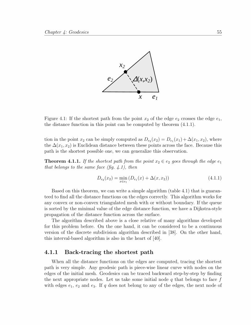
Chapter 4: Geodesics 55
x
∆(x,x2)
e1
e2
x2
Figure 4.1: If the shortest path from the point x2 of the edge e2 crosses the edge e1,the distance function in this point can be computed by theorem (4.1.1).
tion in the point x2 can be simply computed as De2(x2) = De1(x1)+∆(x1, x2), wherethe ∆(x1, x2) is Euclidean distance between these points across the face. Because thispath is the shortest possible one, we can generalize this observation.
Theorem 4.1.1. If the shortest path from the point x2 ∈ e2 goes through the edge e1
that belongs to the same face (fig. 4.1), then
De2(x2) = minx∈e1
(De1(x) + ∆(x, x2)) (4.1.1)
Based on this theorem, we can write a simple algorithm (table 4.1) that is guaran-teed to find all the distance functions on the edges correctly. This algorithm works forany convex or non-convex triangulated mesh with or without boundary. If the queueis sorted by the minimal value of the edge distance function, we have a Dijkstra-stylepropagation of the distance function across the surface.
The algorithm described above is a close relative of many algorithms developedfor this problem before. On the one hand, it can be considered to be a continuousversion of the discrete subdivision algorithm described in [38]. On the other hand,this interval-based algorithm is also in the heart of [40].
4.1.1 Back-tracing the shortest path
When all the distance functions on the edges are computed, tracing the shortestpath is very simple. Any geodesic path is piece-wise linear curve with nodes on theedges of the initial mesh. Geodesics can be traced backward step-by-step by findingthe next appropriate nodes. Let us take some initial node q that belongs to face fwith edges e1, e2 and e3. If q does not belong to any of the edges, the next node of
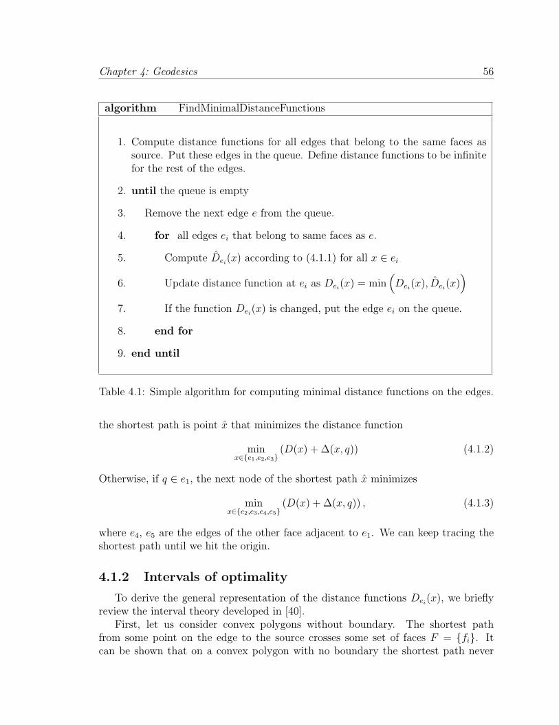
Chapter 4: Geodesics 56
algorithm FindMinimalDistanceFunctions
1. Compute distance functions for all edges that belong to the same faces assource. Put these edges in the queue. Define distance functions to be infinitefor the rest of the edges.
2. until the queue is empty
3. Remove the next edge e from the queue.
4. for all edges ei that belong to same faces as e.
5. Compute Dei(x) according to (4.1.1) for all x ∈ ei
6. Update distance function at ei as Dei(x) = min
(Dei
(x), Dei(x)
)
7. If the function Dei(x) is changed, put the edge ei on the queue.
8. end for
9. end until
Table 4.1: Simple algorithm for computing minimal distance functions on the edges.
the shortest path is point x that minimizes the distance function
minx∈e1,e2,e3
(D(x) + ∆(x, q)) (4.1.2)
Otherwise, if q ∈ e1, the next node of the shortest path x minimizes
minx∈e2,e3,e4,e5
(D(x) + ∆(x, q)) , (4.1.3)
where e4, e5 are the edges of the other face adjacent to e1. We can keep tracing theshortest path until we hit the origin.
4.1.2 Intervals of optimality
To derive the general representation of the distance functions Dei(x), we briefly
review the interval theory developed in [40].First, let us consider convex polygons without boundary. The shortest path
from some point on the edge to the source crosses some set of faces F = fi. Itcan be shown that on a convex polygon with no boundary the shortest path never
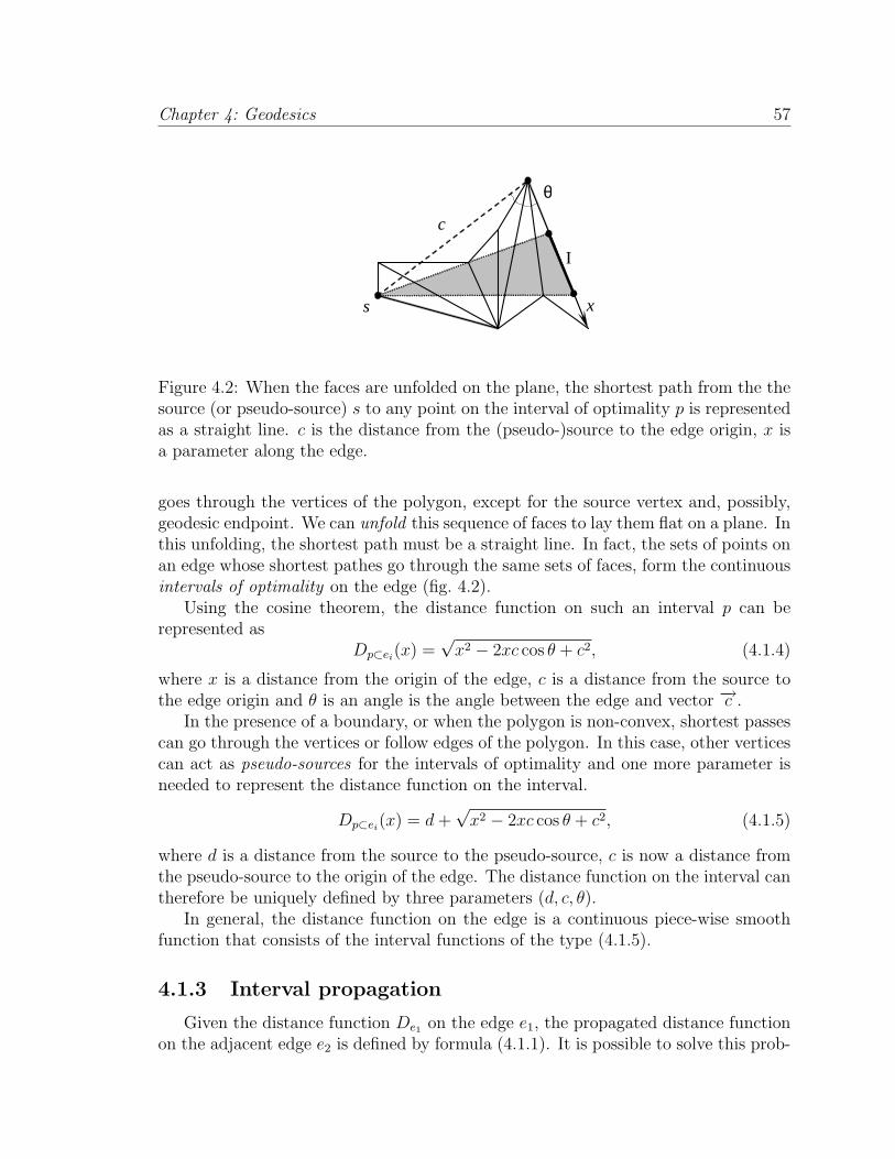
Chapter 4: Geodesics 57
x
c
θ
s
I
Figure 4.2: When the faces are unfolded on the plane, the shortest path from the thesource (or pseudo-source) s to any point on the interval of optimality p is representedas a straight line. c is the distance from the (pseudo-)source to the edge origin, x isa parameter along the edge.
goes through the vertices of the polygon, except for the source vertex and, possibly,geodesic endpoint. We can unfold this sequence of faces to lay them flat on a plane. Inthis unfolding, the shortest path must be a straight line. In fact, the sets of points onan edge whose shortest pathes go through the same sets of faces, form the continuousintervals of optimality on the edge (fig. 4.2).
Using the cosine theorem, the distance function on such an interval p can berepresented as
Dp⊂ei(x) =
√x2 − 2xc cos θ + c2, (4.1.4)
where x is a distance from the origin of the edge, c is a distance from the source tothe edge origin and θ is an angle is the angle between the edge and vector −→c .
In the presence of a boundary, or when the polygon is non-convex, shortest passescan go through the vertices or follow edges of the polygon. In this case, other verticescan act as pseudo-sources for the intervals of optimality and one more parameter isneeded to represent the distance function on the interval.
Dp⊂ei(x) = d +
√x2 − 2xc cos θ + c2, (4.1.5)
where d is a distance from the source to the pseudo-source, c is now a distance fromthe pseudo-source to the origin of the edge. The distance function on the interval cantherefore be uniquely defined by three parameters (d, c, θ).
In general, the distance function on the edge is a continuous piece-wise smoothfunction that consists of the interval functions of the type (4.1.5).
4.1.3 Interval propagation
Given the distance function De1 on the edge e1, the propagated distance functionon the adjacent edge e2 is defined by formula (4.1.1). It is possible to solve this prob-
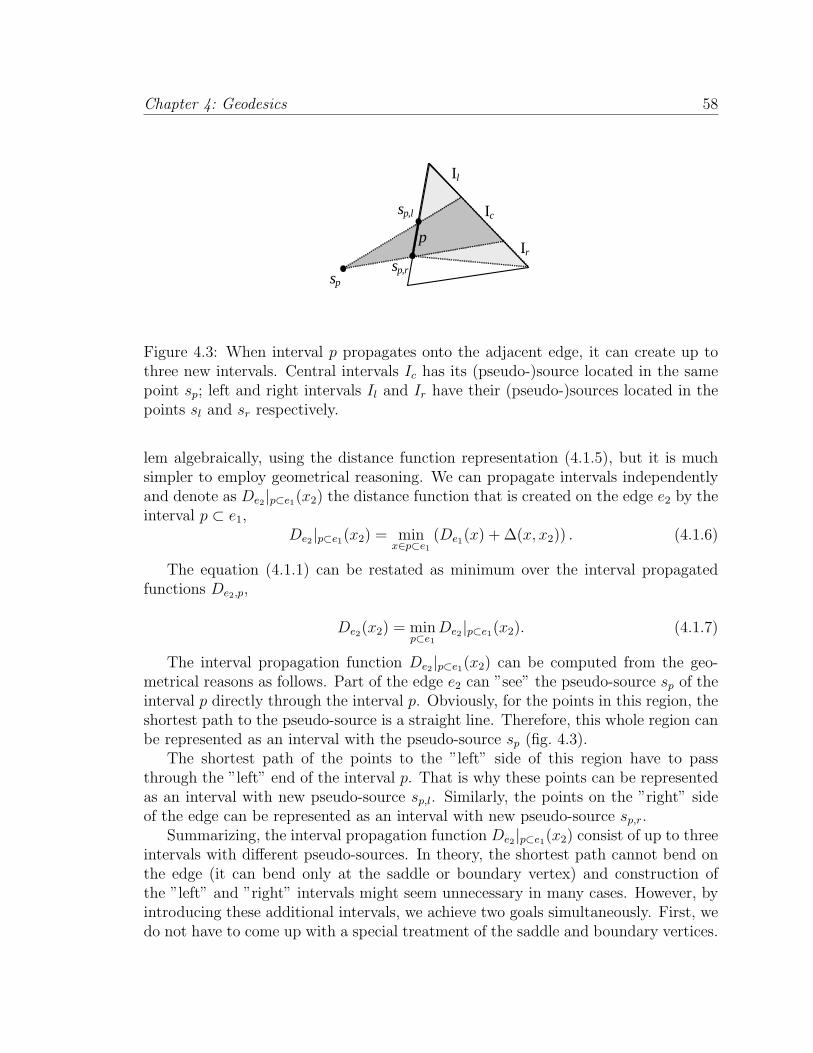
Chapter 4: Geodesics 58
p
sp
Ic sp,l
sp,r
l
Ir
Il
Figure 4.3: When interval p propagates onto the adjacent edge, it can create up tothree new intervals. Central intervals Ic has its (pseudo-)source located in the samepoint sp; left and right intervals Il and Ir have their (pseudo-)sources located in thepoints sl and sr respectively.
lem algebraically, using the distance function representation (4.1.5), but it is muchsimpler to employ geometrical reasoning. We can propagate intervals independentlyand denote as De2|p⊂e1(x2) the distance function that is created on the edge e2 by theinterval p ⊂ e1,
De2|p⊂e1(x2) = minx∈p⊂e1
(De1(x) + ∆(x, x2)) . (4.1.6)
The equation (4.1.1) can be restated as minimum over the interval propagatedfunctions De2,p,
De2(x2) = minp⊂e1
De2|p⊂e1(x2). (4.1.7)
The interval propagation function De2|p⊂e1(x2) can be computed from the geo-metrical reasons as follows. Part of the edge e2 can ”see” the pseudo-source sp of theinterval p directly through the interval p. Obviously, for the points in this region, theshortest path to the pseudo-source is a straight line. Therefore, this whole region canbe represented as an interval with the pseudo-source sp (fig. 4.3).
The shortest path of the points to the ”left” side of this region have to passthrough the ”left” end of the interval p. That is why these points can be representedas an interval with new pseudo-source sp,l. Similarly, the points on the ”right” sideof the edge can be represented as an interval with new pseudo-source sp,r.
Summarizing, the interval propagation function De2|p⊂e1(x2) consist of up to threeintervals with different pseudo-sources. In theory, the shortest path cannot bend onthe edge (it can bend only at the saddle or boundary vertex) and construction ofthe ”left” and ”right” intervals might seem unnecessary in many cases. However, byintroducing these additional intervals, we achieve two goals simultaneously. First, wedo not have to come up with a special treatment of the saddle and boundary vertices.
Chapter 4: Geodesics 59
Second, and more important, this trick provides numerical stability of the algorithmand covers small gaps in the ”wavefront”.
4.1.4 Interval intersection
In order to compute the minimum of two interval functions in formula (4.1.7) andalgorithm (4.1), we need to find the points where two interval functions are equal toeach other. Unlike the interval propagation, this operation is easier to do algebraically.Let us say that two different functions D1(x) and D2(x) are defined on the edge e.We want to find such points x that D1(x) = D2(x). When the pseudo-sources are thesame distance from the initial source, d1 = d2, there is one intersection at most.
x =c22 − c2
1
2 (c1 cos θ1 − c2 cos θ2)(4.1.8)
In general, when d1 6= d2, we have to solve a quadratic equation
Ax2 + Bx + C = 0, (4.1.9)
where
A = P 2 −D2, B = PQ− 2c1 cos θ1D2,
C = Q2/4− c21D
2, P = c1 cos θ1 − c2 cos θ2,
Q = D2 + c21 − c2
2, D = d1 − d2.
4.1.5 Interval-based algorithm
Putting it together, we can now derive final interval-based algorithm. In thisalgorithm, each edge distance function Dei
(x) is represented as a list of intervals Lei.
Therefore, when we propagate an interval onto another edge, we create a new listof intervals that consists of up to three intervals (section 4.1.3). When we find theminimum of two distance function, we intersect two lists of intervals and take thesmallest ones (section 4.1.4).
Obviously, all the edges that belong to the same faces as the source, can be seenfrom the source directly and therefore have only one interval each.
The interval propagation algorithm can be seen in the table (4.2). We maintainthe interval priority queue sorted by the minimum value of the distance functionon the interval. This queue is described in [40] in order to maintain a Dijkstra-styleproperties of the interval propagation. Computing the minimum value of the distancefunction on the interval is straightforward and omitted here for the sake of space.
In our implementation of the algorithm, each interval also has a bit that showsthe direction of the interval propagation. Instead of propagating the interval intotwo directions, we propagate it only into one direction. In practice it makes the codefaster, because the interval propagation procedure is computationally expensive.
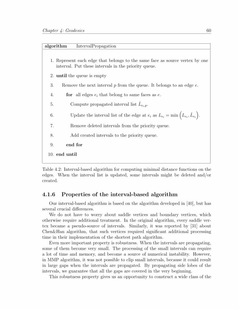
Chapter 4: Geodesics 60
algorithm IntervalPropagation
1. Represent each edge that belongs to the same face as source vertex by oneinterval. Put these intervals in the priority queue.
2. until the queue is empty
3. Remove the next interval p from the queue. It belongs to an edge e.
4. for all edges ei that belong to same faces as e.
5. Compute propagated interval list Lei,p.
6. Update the interval list of the edge at ei as Lei= min
(Lei
, Lei
).
7. Remove deleted intervals from the priority queue.
8. Add created intervals to the priority queue.
9. end for
10. end until
Table 4.2: Interval-based algorithm for computing minimal distance functions on theedges. When the interval list is updated, some intervals might be deleted and/orcreated.
4.1.6 Properties of the interval-based algorithm
Our interval-based algorithm is based on the algorithm developed in [40], but hasseveral crucial differences.
We do not have to worry about saddle vertices and boundary vertices, whichotherwise require additional treatment. In the original algorithm, every saddle ver-tex became a pseudo-source of intervals. Similarly, it was reported by [31] aboutChen&Han algorithm, that such vertices required significant additional processingtime in their implementation of the shortest path algorithm.
Even more important property is robustness. When the intervals are propagating,some of them become very small. The processing of the small intervals can requirea lot of time and memory, and become a source of numerical instability. However,in MMP algorithm, it was not possible to clip small intervals, because it could resultin large gaps when the intervals are propagated. By propagating side lobes of theintervals, we guarantee that all the gaps are covered in the very beginning.
This robustness property gives us an opportunity to construct a wide class of the

Chapter 4: Geodesics 61
approximate algorithms. We can simplify the intervals when they are small or whentwo neighboring intervals are similar. By construction of our algorithm it will neverlead to gaps when the intervals are propagated.
Also, in contrast to [40], we do not have to consider edge-face pairs and can treateach edge independently of where the signal comes from. This simplifies algorithmimplementation.
4.2 Merge simplifications
Unfortunately, the exact algorithm is in the worst case quadratic in memory andn2 log n in time [40]. When the mesh has hundreds of thousands of vertices, thisnon-linear growth can become a bottleneck. The reason of such a growth is that farfrom the source intervals become smaller and smaller. In many cases, a set of smallintervals can be approximated by a single interval with high precision.
In both MMP and Chen&Han algorithms, even the slightest modification of anyinterval could lead to a potential distance function gap somewhere on the mesh. Onthe contrary, our algorithm remains stable after interval approximation, which isdemonstrated in the following lemma.
Lemma 4.2.1. Let us take the results of the exact algorithm, pick one of the edges,ek, and one interval pm on this edge. Let us say that the distance function on thisinterval, Dpm⊂ek
(x) is defined by the constants d, c, θ. Let us also define a new distancefunction Dpm⊂ek
(x) by changing these parameters arbitrarily and re-propagate theinterval through the mesh. Then the resulting distance field in any point of the meshwill not change more than ε, where
ε = maxx|Dpm⊂ek
(x)−Dpm⊂ek(x)|.
To make a bridge to our flat-exact algorithm developed in the next chapter, here wedescribe a possible simplification algorithm that is based on interval merging. Becauseof the perfect results shown by the flat-exact algorithm, we did not implemented themerging algorithm described here.
The easiest merging strategy is to check the neighbors of the interval before itspropagation, and if their distance function are approximated by its distance functionwell enough, merge them together.
There are still two issues remain. First, after a chain of simplifications the algo-rithm can come to the loop, i.e. some interval become modified by its own ”children”intervals. Second, simplifications can create local minimums in the distance field ofthe mesh and the tracing-back algorithm that computes geodesics can stuck in sucha minimum.
It is possible that both issues can be handled by applying some restrictions on thesimplification rules. We did not find the set of restrictions that is elegant and fast tocompute; that is why we resolve both issues by the following method.
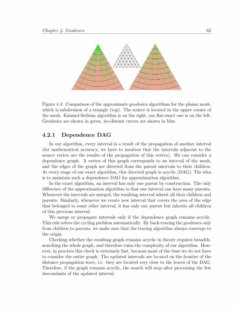
Chapter 4: Geodesics 62
Figure 4.4: Comparison of the approximate geodesics algorithms for the planar mesh,which is subdivision of a triangle (top). The source is located in the upper corner ofthe mesh. Kimmel-Sethian algorithm is on the right, our flat-exact one is on the left.Geodesics are shown in green, iso-distant curves are shown in blue.
4.2.1 Dependence DAG
In our algorithm, every interval is a result of the propagation of another interval(for mathematical accuracy, we have to mention that the intervals adjacent to thesource vertex are the results of the propagation of this vertex). We can consider adependence graph. A vertex of this graph corresponds to an interval of the mesh,and the edges of the graph are directed from the parent intervals to their children.At every stage of our exact algorithm, this directed graph is acyclic (DAG). The ideais to maintain such a dependence DAG for approximation algorithm.
In the exact algorithm, an interval has only one parent by construction. The onlydifference of the approximation algorithm is that one interval can have many parents.Whenever the intervals are merged, the resulting interval inherit all their children andparents. Similarly, whenever we create new interval that covers the area of the edgethat belonged to some other interval, it has only one parent but inherits all childrenof this previous interval.
We merge or propagate intervals only if the dependence graph remains acyclic.This rule solves the cycling problem automatically. By back-tracing the geodesics onlyfrom children to parents, we make sure that the tracing algorithm always converge tothe origin.
Checking whether the resulting graph remains acyclic in theory requires breadth-searching the whole graph, and therefore ruins the complexity of our algorithm. How-ever, in practice this check is extremely fast, because most of the time we do not haveto consider the entire graph. The updated intervals are located on the frontier of thedistance propagation wave, i.e. they are located very close to the leaves of the DAG.Therefore, if the graph remains acyclic, the search will stop after processing the fewdescendants of the updated interval.
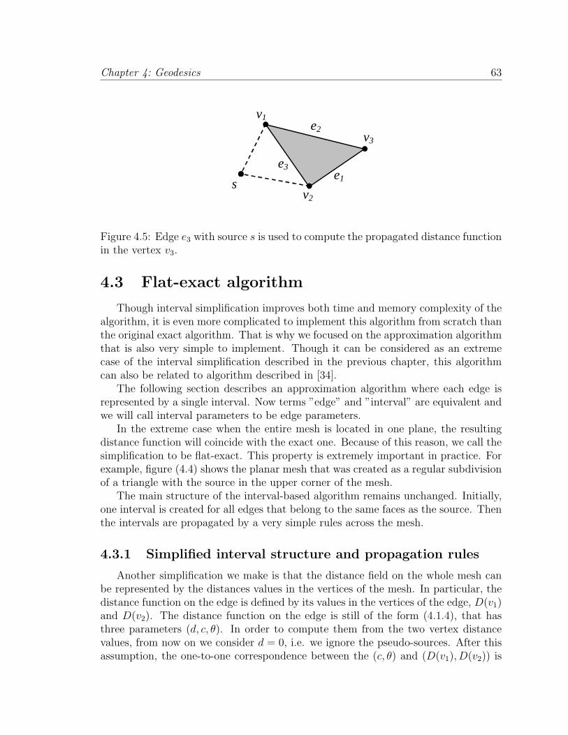
Chapter 4: Geodesics 63
s v2
v1
v3 e2
e1 e3
Figure 4.5: Edge e3 with source s is used to compute the propagated distance functionin the vertex v3.
4.3 Flat-exact algorithm
Though interval simplification improves both time and memory complexity of thealgorithm, it is even more complicated to implement this algorithm from scratch thanthe original exact algorithm. That is why we focused on the approximation algorithmthat is also very simple to implement. Though it can be considered as an extremecase of the interval simplification described in the previous chapter, this algorithmcan also be related to algorithm described in [34].
The following section describes an approximation algorithm where each edge isrepresented by a single interval. Now terms ”edge” and ”interval” are equivalent andwe will call interval parameters to be edge parameters.
In the extreme case when the entire mesh is located in one plane, the resultingdistance function will coincide with the exact one. Because of this reason, we call thesimplification to be flat-exact. This property is extremely important in practice. Forexample, figure (4.4) shows the planar mesh that was created as a regular subdivisionof a triangle with the source in the upper corner of the mesh.
The main structure of the interval-based algorithm remains unchanged. Initially,one interval is created for all edges that belong to the same faces as the source. Thenthe intervals are propagated by a very simple rules across the mesh.
4.3.1 Simplified interval structure and propagation rules
Another simplification we make is that the distance field on the whole mesh canbe represented by the distances values in the vertices of the mesh. In particular, thedistance function on the edge is defined by its values in the vertices of the edge, D(v1)and D(v2). The distance function on the edge is still of the form (4.1.4), that hasthree parameters (d, c, θ). In order to compute them from the two vertex distancevalues, from now on we consider d = 0, i.e. we ignore the pseudo-sources. After thisassumption, the one-to-one correspondence between the (c, θ) and (D(v1), D(v2)) is
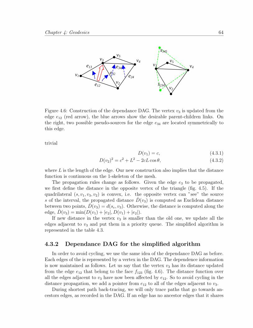
Chapter 4: Geodesics 64
v1
v3
e34
v2
v4 v5
e12
e24
e13
e32
v3
v2
v4 v5
s345
s234
Figure 4.6: Construction of the dependance DAG. The vertex v3 is updated from theedge e12 (red arrow), the blue arrows show the desirable parent-children links. Onthe right, two possible pseudo-sources for the edge e34 are located symmetrically tothis edge.
trivial
D(v1) = c, (4.3.1)
D(v2)2 = c2 + L2 − 2cL cos θ, (4.3.2)
where L is the length of the edge. Our new construction also implies that the distancefunction is continuous on the 1-skeleton of the mesh.
The propagation rules change as follows. Given the edge e3 to be propagated,we first define the distance in the opposite vertex of the triangle (fig. 4.5). If thequadrilateral (s, v1, v3, v2) is convex, i.e. the opposite vertex can ”see” the sources of the interval, the propagated distance D(v3) is computed as Euclidean distancebetween two points, D(v3) = d(se, v3). Otherwise, the distance is computed along theedge, D(v3) = min(D(v1) + |e2|, D(v1) + |e2|).
If new distance in the vertex v3 is smaller than the old one, we update all theedges adjacent to v3 and put them in a priority queue. The simplified algorithm isrepresented in the table 4.3.
4.3.2 Dependance DAG for the simplified algorithm
In order to avoid cycling, we use the same idea of the dependance DAG as before.Each edges of the is represented by a vertex in the DAG. The dependence informationis now maintained as follows. Let us say that the vertex v3 has its distance updatedfrom the edge e12 that belong to the face f123 (fig. 4.6). The distance function overall the edges adjacent to v3 have now been affected by e12. So to avoid cycling in thedistance propagation, we add a pointer from e12 to all of the edges adjacent to v3.
During shortest path back-tracing, we will only trace paths that go towards an-cestors edges, as recorded in the DAG. If an edge has no ancestor edges that it shares
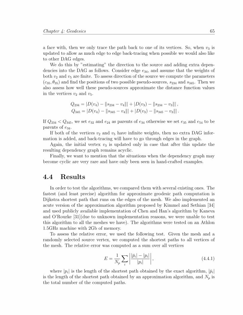
Chapter 4: Geodesics 65
a face with, then we only trace the path back to one of its vertices. So, when v3 isupdated to allow as much edge to edge back-tracing when possible we would also liketo other DAG edges.
We do this by ”estimating” the direction to the source and adding extra depen-dencies into the DAG as follows. Consider edge e34, and assume that the weights ofboth v2 and v5 are finite. To assess direction of the source we compute the parameters(c35, θ35) and find the positions of two possible pseudo-sources, s234 and s345. Then wealso assess how well these pseudo-sources approximate the distance function valuesin the vertices v2 and v5.
Q234 = |D(v4)− ‖s234 − v4‖|+ |D(v3)− ‖s234 − v3‖| ,Q345 = |D(v4)− ‖s345 − v4‖|+ |D(v3)− ‖s345 − v3‖| .
If Q234 < Q345, we set e32 and e24 as parents of e34 otherwise we set e35 and e54 to beparents of e34.
If both of the vertices v2 and v5 have infinite weights, then no extra DAG infor-mation is added, and back-tracing will have to go through edges in the graph.
Again, the initial vertex v3 is updated only in case that after this update theresulting dependency graph remains acyclic.
Finally, we want to mention that the situations when the dependency graph maybecome cyclic are very rare and have only been seen in hand-crafted examples.
4.4 Results
In order to test the algorithms, we compared them with several existing ones. Thefastest (and least precise) algorithm for approximate geodesic path computation isDijkstra shortest path that runs on the edges of the mesh. We also implemented anacute version of the approximation algorithm proposed by Kimmel and Sethian [34]and used publicly available implementation of Chen and Han’s algorithm by Kanevaand O’Rourke [31](due to unknown implementation reasons, we were unable to testthis algorithm to all the meshes we have). The algorithms were tested on an Athlon1.5GHz machine with 2Gb of memory.
To assess the relative error, we used the following test. Given the mesh and arandomly selected source vertex, we computed the shortest paths to all vertices ofthe mesh. The relative error was computed as a sum over all vertices
E =1
Np
∑i
∣∣∣∣|pi| − |pi||pi|
∣∣∣∣ , (4.4.1)
where |pi| is the length of the shortest path obtained by the exact algorithm, |pi|is the length of the shortest path obtained by an approximation algorithm, and Np isthe total number of the computed paths.
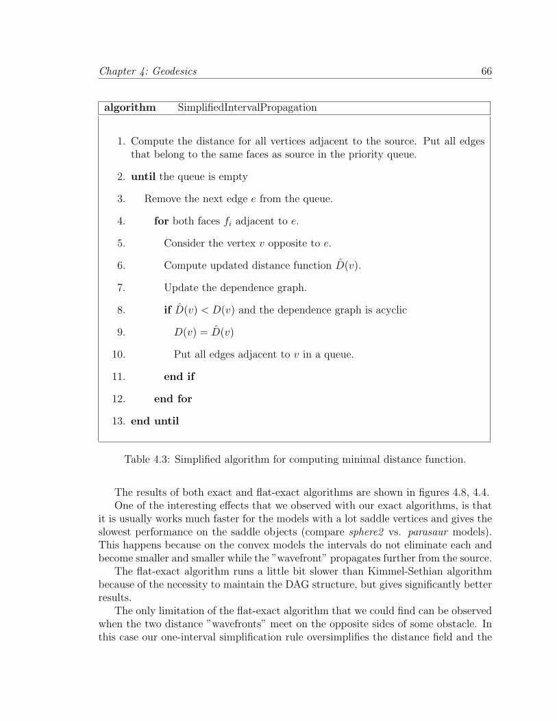
Chapter 4: Geodesics 66
algorithm SimplifiedIntervalPropagation
1. Compute the distance for all vertices adjacent to the source. Put all edgesthat belong to the same faces as source in the priority queue.
2. until the queue is empty
3. Remove the next edge e from the queue.
4. for both faces fi adjacent to e.
5. Consider the vertex v opposite to e.
6. Compute updated distance function D(v).
7. Update the dependence graph.
8. if D(v) < D(v) and the dependence graph is acyclic
9. D(v) = D(v)
10. Put all edges adjacent to v in a queue.
11. end if
12. end for
13. end until
Table 4.3: Simplified algorithm for computing minimal distance function.
The results of both exact and flat-exact algorithms are shown in figures 4.8, 4.4.One of the interesting effects that we observed with our exact algorithms, is that
it is usually works much faster for the models with a lot saddle vertices and gives theslowest performance on the saddle objects (compare sphere2 vs. parasaur models).This happens because on the convex models the intervals do not eliminate each andbecome smaller and smaller while the ”wavefront” propagates further from the source.
The flat-exact algorithm runs a little bit slower than Kimmel-Sethian algorithmbecause of the necessity to maintain the DAG structure, but gives significantly betterresults.
The only limitation of the flat-exact algorithm that we could find can be observedwhen the two distance ”wavefronts” meet on the opposite sides of some obstacle. Inthis case our one-interval simplification rule oversimplifies the distance field and the
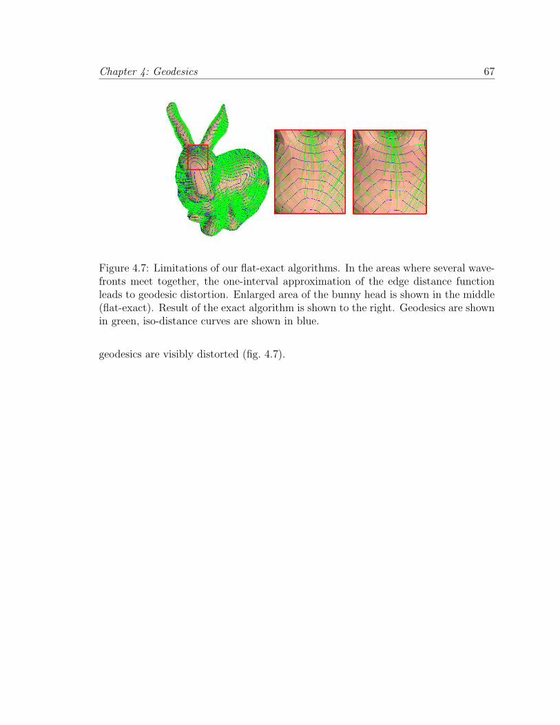
Chapter 4: Geodesics 67
Figure 4.7: Limitations of our flat-exact algorithms. In the areas where several wave-fronts meet together, the one-interval approximation of the edge distance functionleads to geodesic distortion. Enlarged area of the bunny head is shown in the middle(flat-exact). Result of the exact algorithm is shown to the right. Geodesics are shownin green, iso-distance curves are shown in blue.
geodesics are visibly distorted (fig. 4.7).
Chapter 4: Geodesics 68
Figure 4.8: The results of the our exact (top row) and flat-exact (bottom row) al-gorithms are shown on the cat, bunny, and dragon models (366, 10000, and 50000vertices respectively). Geodesics are shown in green, iso-distant curves are shown inblue. In the bunny model, the source is on the back side.
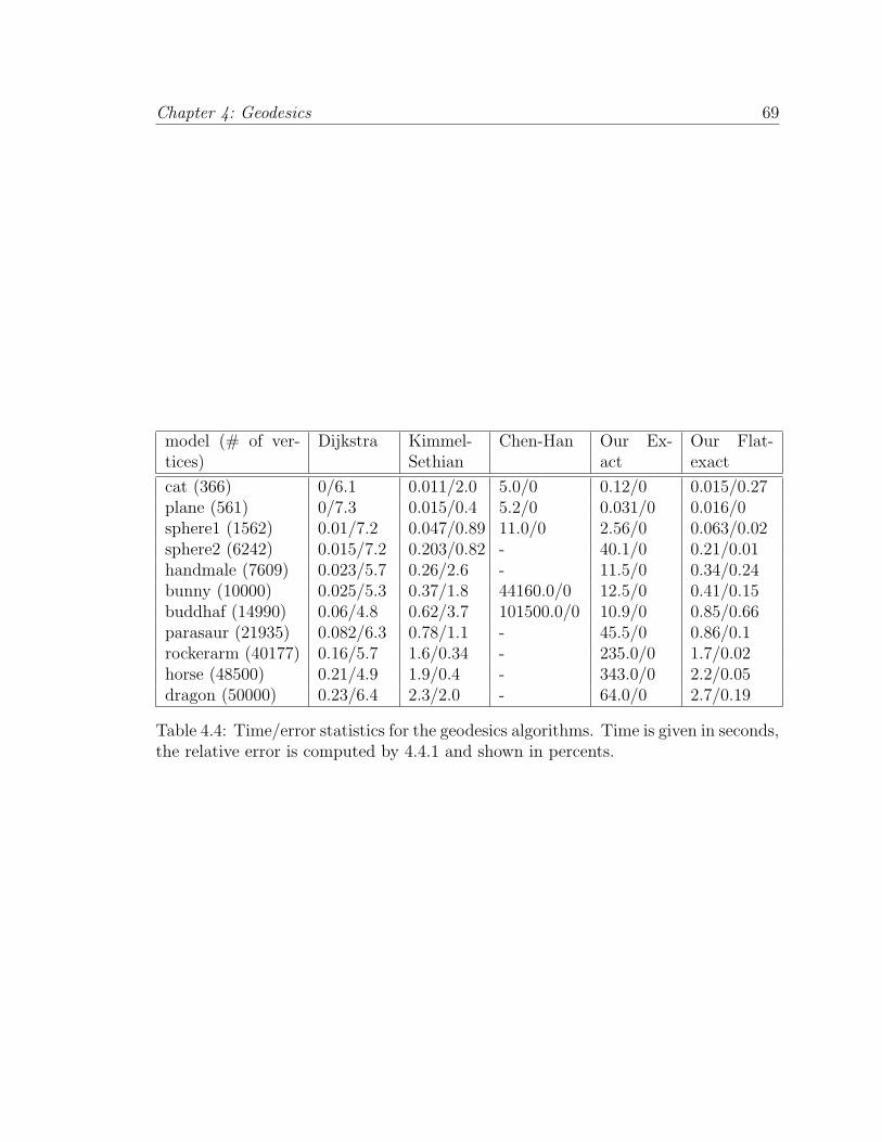
Chapter 4: Geodesics 69
model (# of ver-tices)
Dijkstra Kimmel-Sethian
Chen-Han Our Ex-act
Our Flat-exact
cat (366) 0/6.1 0.011/2.0 5.0/0 0.12/0 0.015/0.27plane (561) 0/7.3 0.015/0.4 5.2/0 0.031/0 0.016/0sphere1 (1562) 0.01/7.2 0.047/0.89 11.0/0 2.56/0 0.063/0.02sphere2 (6242) 0.015/7.2 0.203/0.82 - 40.1/0 0.21/0.01handmale (7609) 0.023/5.7 0.26/2.6 - 11.5/0 0.34/0.24bunny (10000) 0.025/5.3 0.37/1.8 44160.0/0 12.5/0 0.41/0.15buddhaf (14990) 0.06/4.8 0.62/3.7 101500.0/0 10.9/0 0.85/0.66parasaur (21935) 0.082/6.3 0.78/1.1 - 45.5/0 0.86/0.1rockerarm (40177) 0.16/5.7 1.6/0.34 - 235.0/0 1.7/0.02horse (48500) 0.21/4.9 1.9/0.4 - 343.0/0 2.2/0.05dragon (50000) 0.23/6.4 2.3/2.0 - 64.0/0 2.7/0.19
Table 4.4: Time/error statistics for the geodesics algorithms. Time is given in seconds,the relative error is computed by 4.4.1 and shown in percents.

Silhouettes 5
70
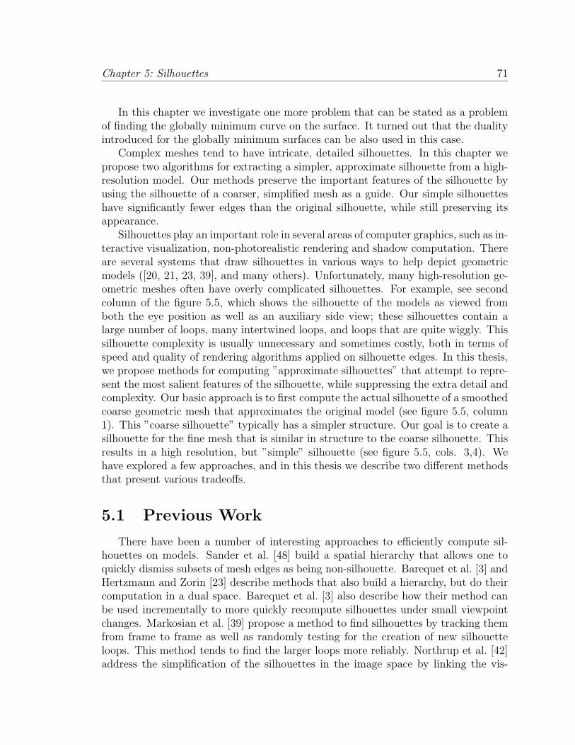
Chapter 5: Silhouettes 71
In this chapter we investigate one more problem that can be stated as a problemof finding the globally minimum curve on the surface. It turned out that the dualityintroduced for the globally minimum surfaces can be also used in this case.
Complex meshes tend to have intricate, detailed silhouettes. In this chapter wepropose two algorithms for extracting a simpler, approximate silhouette from a high-resolution model. Our methods preserve the important features of the silhouette byusing the silhouette of a coarser, simplified mesh as a guide. Our simple silhouetteshave significantly fewer edges than the original silhouette, while still preserving itsappearance.
Silhouettes play an important role in several areas of computer graphics, such as in-teractive visualization, non-photorealistic rendering and shadow computation. Thereare several systems that draw silhouettes in various ways to help depict geometricmodels ([20, 21, 23, 39], and many others). Unfortunately, many high-resolution ge-ometric meshes often have overly complicated silhouettes. For example, see secondcolumn of the figure 5.5, which shows the silhouette of the models as viewed fromboth the eye position as well as an auxiliary side view; these silhouettes contain alarge number of loops, many intertwined loops, and loops that are quite wiggly. Thissilhouette complexity is usually unnecessary and sometimes costly, both in terms ofspeed and quality of rendering algorithms applied on silhouette edges. In this thesis,we propose methods for computing ”approximate silhouettes” that attempt to repre-sent the most salient features of the silhouette, while suppressing the extra detail andcomplexity. Our basic approach is to first compute the actual silhouette of a smoothedcoarse geometric mesh that approximates the original model (see figure 5.5, column1). This ”coarse silhouette” typically has a simpler structure. Our goal is to create asilhouette for the fine mesh that is similar in structure to the coarse silhouette. Thisresults in a high resolution, but ”simple” silhouette (see figure 5.5, cols. 3,4). Wehave explored a few approaches, and in this thesis we describe two different methodsthat present various tradeoffs.
5.1 Previous Work
There have been a number of interesting approaches to efficiently compute sil-houettes on models. Sander et al. [48] build a spatial hierarchy that allows one toquickly dismiss subsets of mesh edges as being non-silhouette. Barequet et al. [3] andHertzmann and Zorin [23] describe methods that also build a hierarchy, but do theircomputation in a dual space. Barequet et al. [3] also describe how their method canbe used incrementally to more quickly recompute silhouettes under small viewpointchanges. Markosian et al. [39] propose a method to find silhouettes by tracking themfrom frame to frame as well as randomly testing for the creation of new silhouetteloops. This method tends to find the larger loops more reliably. Northrup et al. [42]address the simplification of the silhouettes in the image space by linking the vis-

Chapter 5: Silhouettes 72
ible segments into the chains, thus resulting in a simpler, approximate silhouette.Hertzmann and Zorin [23] describe an elegant way of finding simple approximatesilhouettes on meshes. Silhouettes found by this method are quite smooth and arealways comprised as a set of non-intersecting loops. In their method, the silhouetteedges all span across mesh triangles and are not original mesh edges. In our methodsthe silhouette is actually composed of actual mesh edges. Furthermore, redundantshort loops are usually removed from our computed simple silhouettes.
5.2 Approach
The input to our system is a high-resolution fine mesh. From this mesh, we create aprogressive mesh [25]. We then extract a simpler, coarser mesh, and apply smoothingon it in order to prevent artificially generated silhouettes. During runtime, for a givenviewpoint, the objective is to create a silhouette for the fine mesh that is similar instructure to that of the coarse mesh. In this section we will describe two approaches toachieve this objective. In particular we will describe one method in which the set of theedges in the coarse silhouette are constrained to be some subset of the actual silhouetteedges. In this method, loops from the actual silhouette are iteratively included intothe simple silhouette as long as they sufficiently match the coarse silhouette. Thesecond method constrains the simple silhouette to be structurally similar to the coarsesilhouette. For each coarse-silhouette loop, a corresponding loop is found on theoriginal mesh. With this second approach, it may be necessary to sometimes includenon-silhouette edges in the simple silhouette. Next we will describe how we decomposethe silhouette into loops - a sub-step that is required for both methods, - and thenwe present the two silhouette extraction methods.
5.2.1 Loop decomposition
On a smooth surface, the silhouette is comprised of a set of disjoint closed loops.On a triangle mesh, these loops can intersect (for example, a silhouette vertex canbe incident to four silhouette edges) creating a slightly more complicated structure.Our first step will be to take a complicated silhouette and describe it as the union of(possibly intersecting) loops. Given a viewpoint, a silhouette edge is an edge that isadjacent to one front-facing triangle and one back-facing triangle. Silhouette edgesare directed edges, where the left adjacent face is front-facing. A silhouette vertexis a vertex adjacent to a silhouette edge. In particular, on a triangle mesh, thefaces around a silhouette vertex can be partitioned into an alternating set of front-facing and back-facing triangles, thus the number of silhouette edges adjacent to asilhouette vertex must be even. Since each silhouette vertex has an even ”silhouetteedge valence,” we can decompose the silhouette into a set of loops. We desire adecomposition that results in loops without self-intersections. We achieve this by
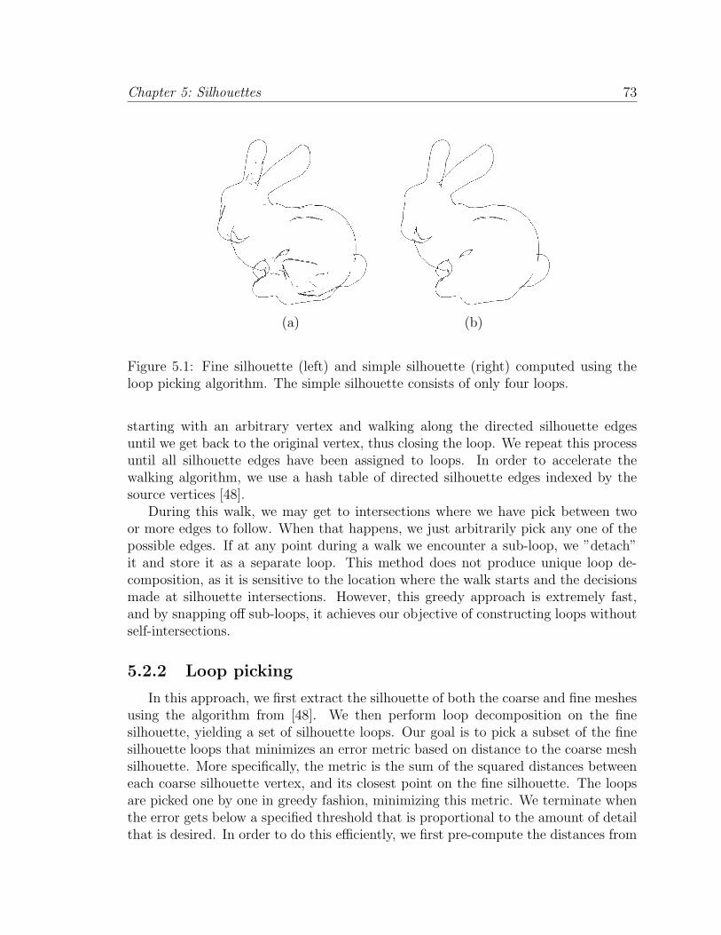
Chapter 5: Silhouettes 73
(a) (b)
Figure 5.1: Fine silhouette (left) and simple silhouette (right) computed using theloop picking algorithm. The simple silhouette consists of only four loops.
starting with an arbitrary vertex and walking along the directed silhouette edgesuntil we get back to the original vertex, thus closing the loop. We repeat this processuntil all silhouette edges have been assigned to loops. In order to accelerate thewalking algorithm, we use a hash table of directed silhouette edges indexed by thesource vertices [48].
During this walk, we may get to intersections where we have pick between twoor more edges to follow. When that happens, we just arbitrarily pick any one of thepossible edges. If at any point during a walk we encounter a sub-loop, we ”detach”it and store it as a separate loop. This method does not produce unique loop de-composition, as it is sensitive to the location where the walk starts and the decisionsmade at silhouette intersections. However, this greedy approach is extremely fast,and by snapping off sub-loops, it achieves our objective of constructing loops withoutself-intersections.
5.2.2 Loop picking
In this approach, we first extract the silhouette of both the coarse and fine meshesusing the algorithm from [48]. We then perform loop decomposition on the finesilhouette, yielding a set of silhouette loops. Our goal is to pick a subset of the finesilhouette loops that minimizes an error metric based on distance to the coarse meshsilhouette. More specifically, the metric is the sum of the squared distances betweeneach coarse silhouette vertex, and its closest point on the fine silhouette. The loopsare picked one by one in greedy fashion, minimizing this metric. We terminate whenthe error gets below a specified threshold that is proportional to the amount of detailthat is desired. In order to do this efficiently, we first pre-compute the distances from
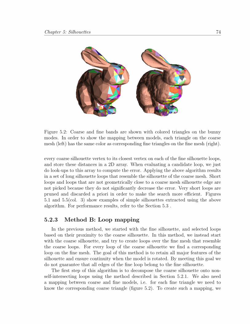
Chapter 5: Silhouettes 74
Figure 5.2: Coarse and fine bands are shown with colored triangles on the bunnymodes. In order to show the mapping between models, each triangle on the coarsemesh (left) has the same color as corresponding fine triangles on the fine mesh (right).
every coarse silhouette vertex to its closest vertex on each of the fine silhouette loops,and store these distances in a 2D array. When evaluating a candidate loop, we justdo look-ups to this array to compute the error. Applying the above algorithm resultsin a set of long silhouette loops that resemble the silhouette of the coarse mesh. Shortloops and loops that are not geometrically close to a coarse mesh silhouette edge arenot picked because they do not significantly decrease the error. Very short loops arepruned and discarded a priori in order to make the search more efficient. Figures5.1 and 5.5(col. 3) show examples of simple silhouettes extracted using the abovealgorithm. For performance results, refer to the Section 5.3 .
5.2.3 Method B: Loop mapping
In the previous method, we started with the fine silhouette, and selected loopsbased on their proximity to the coarse silhouette. In this method, we instead startwith the coarse silhouette, and try to create loops over the fine mesh that resemblethe coarse loops. For every loop of the coarse silhouette we find a correspondingloop on the fine mesh. The goal of this method is to retain all major features of thesilhouette and ensure continuity when the model is rotated. By meeting this goal wedo not guarantee that all edges of the fine loop belong to the fine silhouette.
The first step of this algorithm is to decompose the coarse silhouette onto non-self-intersecting loops using the method described in Section 5.2.1. We also needa mapping between coarse and fine models, i.e. for each fine triangle we need toknow the corresponding coarse triangle (figure 5.2). To create such a mapping, we
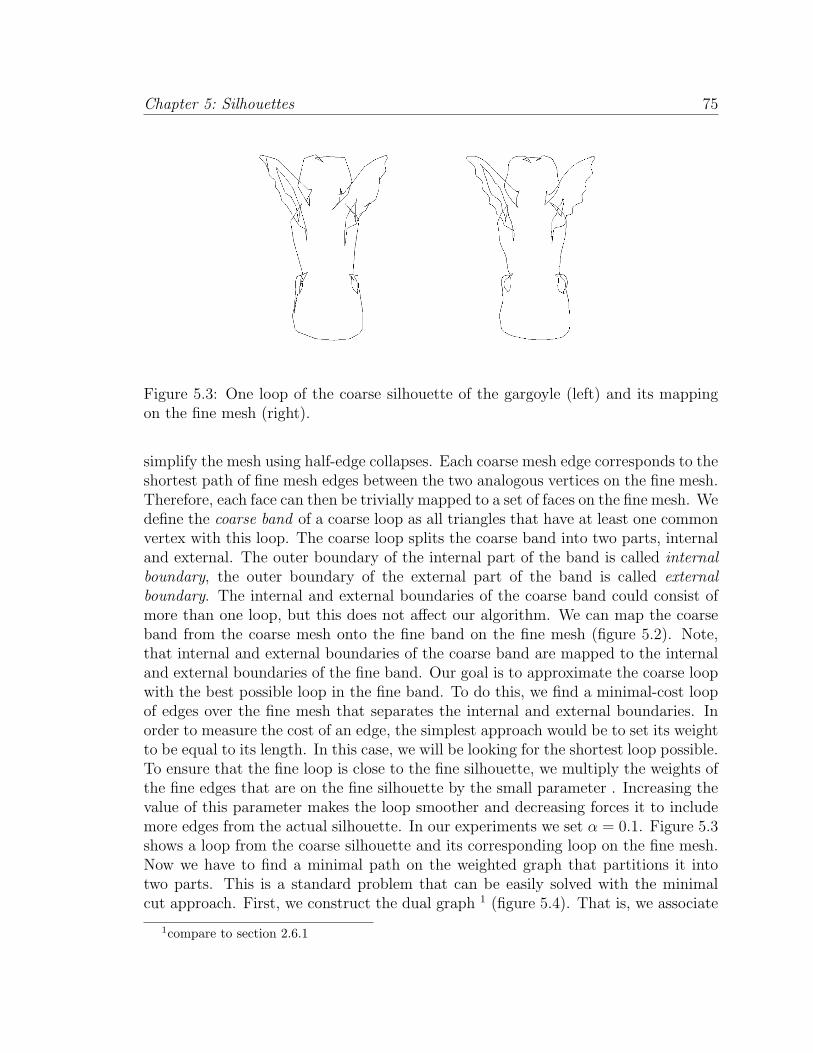
Chapter 5: Silhouettes 75
Figure 5.3: One loop of the coarse silhouette of the gargoyle (left) and its mappingon the fine mesh (right).
simplify the mesh using half-edge collapses. Each coarse mesh edge corresponds to theshortest path of fine mesh edges between the two analogous vertices on the fine mesh.Therefore, each face can then be trivially mapped to a set of faces on the fine mesh. Wedefine the coarse band of a coarse loop as all triangles that have at least one commonvertex with this loop. The coarse loop splits the coarse band into two parts, internaland external. The outer boundary of the internal part of the band is called internalboundary, the outer boundary of the external part of the band is called externalboundary. The internal and external boundaries of the coarse band could consist ofmore than one loop, but this does not affect our algorithm. We can map the coarseband from the coarse mesh onto the fine band on the fine mesh (figure 5.2). Note,that internal and external boundaries of the coarse band are mapped to the internaland external boundaries of the fine band. Our goal is to approximate the coarse loopwith the best possible loop in the fine band. To do this, we find a minimal-cost loopof edges over the fine mesh that separates the internal and external boundaries. Inorder to measure the cost of an edge, the simplest approach would be to set its weightto be equal to its length. In this case, we will be looking for the shortest loop possible.To ensure that the fine loop is close to the fine silhouette, we multiply the weights ofthe fine edges that are on the fine silhouette by the small parameter . Increasing thevalue of this parameter makes the loop smoother and decreasing forces it to includemore edges from the actual silhouette. In our experiments we set α = 0.1. Figure 5.3shows a loop from the coarse silhouette and its corresponding loop on the fine mesh.Now we have to find a minimal path on the weighted graph that partitions it intotwo parts. This is a standard problem that can be easily solved with the minimalcut approach. First, we construct the dual graph 1 (figure 5.4). That is, we associate
1compare to section 2.6.1
Chapter 5: Silhouettes 76
with each face of the band fi a dual vertex Fi. We also create a single source vertexR and a sink vertex K. With each non-boundary edge ei bounding two faces fj andfk, we associate a dual edge Ei that connects Fj and Fk. For each edge ei belongingto the external boundary we associate a dual edge Ei which connects the sink K withthe single face that ei bounds. For each edge ei belonging to the internal boundarywe associate a dual edge Ei which connects the source R with the single face that ei
bounds. We set the capacity of each dual edge the weight of the associated primaledge c(Ei) = wi. We define a cut of the dual graph as a partition of the vertices Fi
into two sets F and Q with R ∈ F and K ∈ Q. The cost of a cut is the sum of thecapacities of the edges between these sets. Similar to section 2.6.1, it can be shownthat the edges across the minimal cut in the dual graph correspond to dual to theedges of the minimal separating path in the primal graph. The only difference is thatin this setup we do not have a boundary and the curve is closed.
In summary, the entire algorithm can be described as follows:
• Preprocess:
– Simplify original mesh and establish mapping between the simplified coarseand the original fine mesh.
• Runtime:
– Decompose coarse silhouette into loops.
– For every coarse loop:
∗ Calculate the coarse band.
∗ Find the internal and external boundaries of the band.
∗ Find the corresponding fine band and its boundaries.
∗ Compute the weights of the edges and create a dual graph.
∗ Compute the min-cut of the dual graph.
∗ Find the corresponding fine loop.
5.3 Results
We implemented both algorithms, and applied them to several models. Table 5.1shows the mesh resolutions and timings of our algorithm on the bunny and gargoylemodels. Figure 5.5 shows silhouette renderings for both methods. We also showside views of the silhouette, in order to demonstrate how intricate the original finemesh silhouette is. For silhouette extraction, we used an optimized version of thealgorithm from Sander et al. [48]. It extracts the silhouette of a 20,000-face bunnymesh in half a millisecond. The loop decomposition step from Section5.2.1 also takesapproximately half a millisecond for that model. The total silhouette extraction time
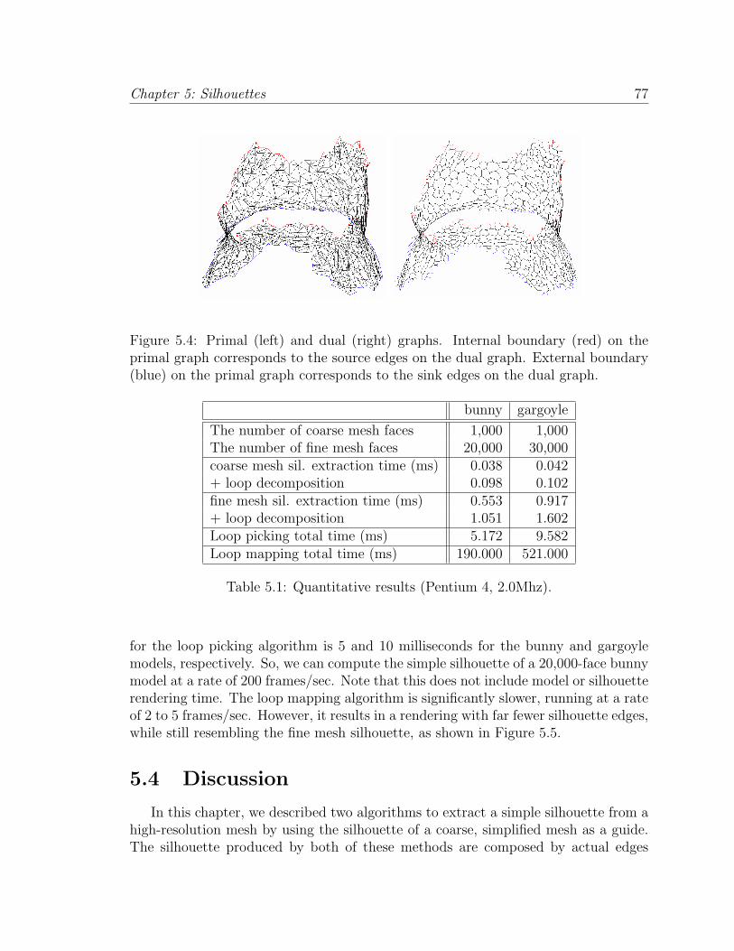
Chapter 5: Silhouettes 77
Figure 5.4: Primal (left) and dual (right) graphs. Internal boundary (red) on theprimal graph corresponds to the source edges on the dual graph. External boundary(blue) on the primal graph corresponds to the sink edges on the dual graph.
bunny gargoyle
The number of coarse mesh faces 1,000 1,000The number of fine mesh faces 20,000 30,000coarse mesh sil. extraction time (ms) 0.038 0.042+ loop decomposition 0.098 0.102fine mesh sil. extraction time (ms) 0.553 0.917+ loop decomposition 1.051 1.602Loop picking total time (ms) 5.172 9.582Loop mapping total time (ms) 190.000 521.000
Table 5.1: Quantitative results (Pentium 4, 2.0Mhz).
for the loop picking algorithm is 5 and 10 milliseconds for the bunny and gargoylemodels, respectively. So, we can compute the simple silhouette of a 20,000-face bunnymodel at a rate of 200 frames/sec. Note that this does not include model or silhouetterendering time. The loop mapping algorithm is significantly slower, running at a rateof 2 to 5 frames/sec. However, it results in a rendering with far fewer silhouette edges,while still resembling the fine mesh silhouette, as shown in Figure 5.5.
5.4 Discussion
In this chapter, we described two algorithms to extract a simple silhouette from ahigh-resolution mesh by using the silhouette of a coarse, simplified mesh as a guide.The silhouette produced by both of these methods are composed by actual edges
Chapter 5: Silhouettes 78
of the original model. The loop picking algorithm is very efficient and extracts asubset of the actual silhouette edges. The loop mapping algorithm is slow, but itis able to capture all the important features of the silhouette with far fewer loops,thus further eliminating the redundancy present on the silhouette of high resolutionmeshes. Another advantage of this method is that only small amount of the edges ofthe fine mesh has to be processed. The major limitation of both proposed approachesis that we cannot guarantee the temporal coherence of the silhouette approximationfor the moving models.
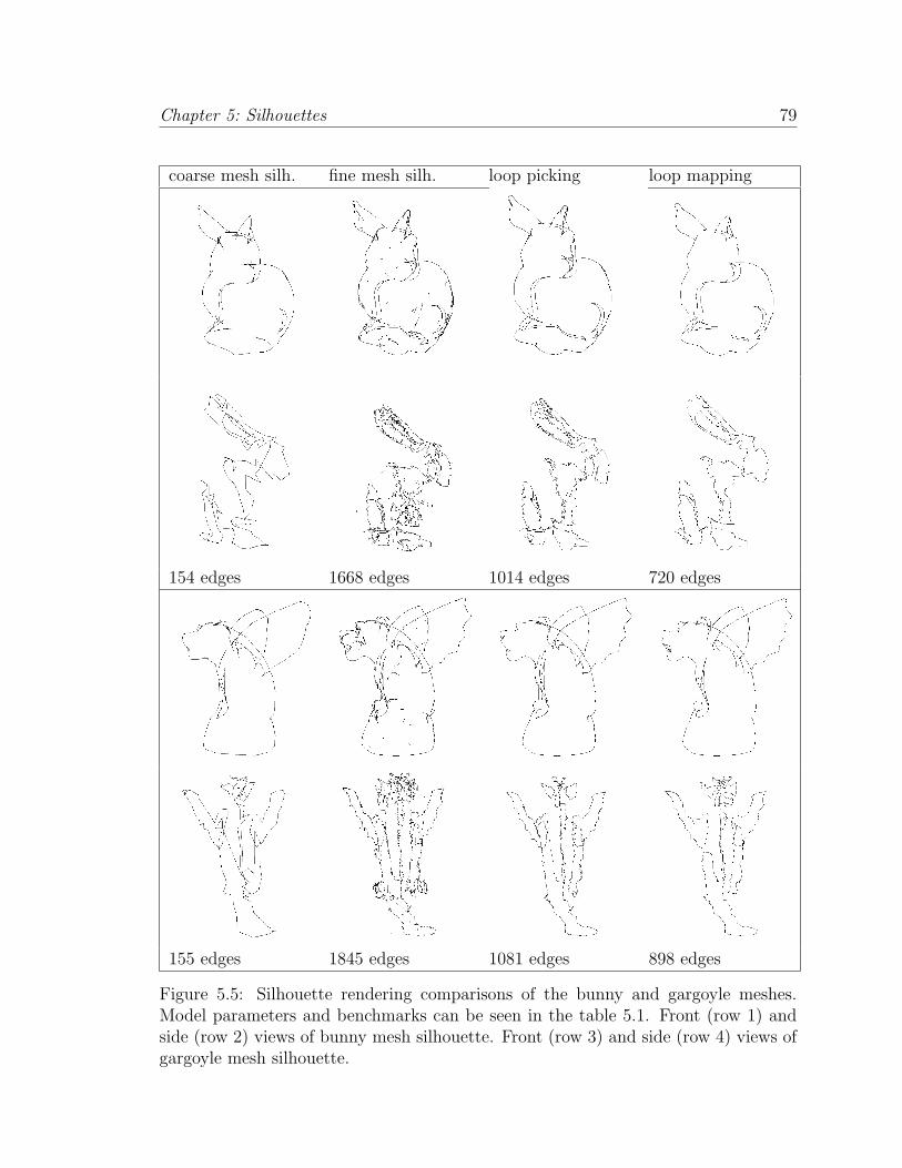
Chapter 5: Silhouettes 79
coarse mesh silh. fine mesh silh. loop picking loop mapping
154 edges 1668 edges 1014 edges 720 edges
155 edges 1845 edges 1081 edges 898 edges
Figure 5.5: Silhouette rendering comparisons of the bunny and gargoyle meshes.Model parameters and benchmarks can be seen in the table 5.1. Front (row 1) andside (row 2) views of bunny mesh silhouette. Front (row 3) and side (row 4) views ofgargoyle mesh silhouette.
Conclusion 6
80
Chapter 6: Conclusion 81
In this thesis we discussed several methods that can be considered to be thegeneralizations of the Dijkstra shortest path method. In chapters 2 and 3 we go tohigher dimensions and explore the problem of ”shortest” discrete surface. The dualityalgorithm described their can be also successfully applied in the 1-dimensional case(chapter 5). In chapter 4 we allow the shortest path to cut across the mesh face andinvestigate the ”continuous” version of Dijkstra.
The main property of all the algorithms described is their ability to find theglobally minimal curves and surfaces in polynomial time. The natural price for thisproperty is the higher-than-linear time and memory complexity 1, which prevents usfrom running the algorithms on the data structures of a very high resolution.
The standard application of these algorithms could be generating the initial guessfor the fast local methods that can be used on a structures of very high resolution butconverge to the local minimums only. The balance between global and local methodsstill remains unclear. There are a lot of open questions in this relatively unexploredtopic.
Another issue considered in this thesis is the close relationship between continuousand discrete methods. It is shown in chapter 2 that the continuous variational problemcan be reduced to a purely discrete combinatorial optimization problem. On the otherhand, in chapter 3 we addressed a discrete minimum weight triangulation problem bya continuous linear programming approach. The geodesic problem on the mesh canbe successfully approached by the discrete algorithm (chapter 3) or by the numericalsolution of the differential equation [34].
Unfortunately, it seems that very often the discrete and continuous communitiesdo not interact very closely. Applied physics and engineering major students often theadvanced algorithms classes; computer science major students ignore the numericalmodelling classes. We hope that our thesis will increase the attention to the problemsthat are located on the boundary of these two worlds.
1n log n Dijkstra shortest path is a nice exception.
Bibliography
[1] Aichholzer, O., and Aurenhammer, F. Constant level greedy triangu-lations approximate the mwt well. Journal of Combinatorial Optimization 2(1999), 361–369.
[2] Aurenhammer, F., and Xu, Y.-F. Optimal triangulations. SFB ReportF003-099, Tu Graz, Austria (1999).
[3] Barequet, G., Duncan, C., Goodrich, T., Kumar, S., and Pop, M.Efficient perspective-accurate silhouette computation. In Symposium on Com-putational Geometry (1999), pp. 60 – 68.
[4] Beirouti, R., and Snoeyink, J. Implementations of the LMT heuristics forminimum weight triangulations. In Proc. 14th ACM Symp. on Comp. Geom.(1998), pp. 96–105.
[5] Boykov, Y., and Kolmogorov, V. An experimental comparison of min-cut/max-flow algorithms for energy minimization in computer vision. In EMM-CVPR (2001).
[6] Boykov, Y., and Kolmogorov, V. Computing geodesics and minimal sur-faces via graph cuts. In Proc. ICCV (2003).
[7] Boykov, Y., Veksler, O., and Zabih, R. Fast approximate energy mini-mization via graph cuts. In Proc. ICCV (1999).
[8] Brechtken-Mandersheid, U. Introduction to the Calculus of Variations.Chapman and Hall, 1991.
[9] Buehler, C., Gortler, S. J., Cohen, M. F., and McMillan, L. Minimalsurfaces for stereo. ECCV (2002), 885–899.
[10] Chen, J., and Han, Y. Shortest paths on a polyhedron; part i: computingshortest paths. Int. J. Comput. Geom. & Appl. 6, 2 (1996), 127–144.
[11] Cheng, S.-W., and Xu, Y.-F. Approaching the largest β-skeleton withina minimum weight triangulation. In Proc. 12th ACM Symp. on Comp. Geom.(1996), pp. 196–203.
82
Bibliography 83
[12] Cormen, T., Leiserson, C., and Rivest, R. Introduction to Algorithms.MIT Press, 2001.
[13] Dacorogna, B. Direct Methods in the Calculus of Variations. Springer-Verlag,1989.
[14] Dickerson, M., and Montague, M. A (usually?) connected subgraph ofthe minimum weight triangulation. In Proc. 12th ACM Symp. on Comp. Geom.(1996), pp. 204–213.
[15] Drysdale, R., McElfresh, S., and Snoeyink, J. On exclusion regions foroptimal triangulations. Discrete Applied Mathematics 109 (2001), 49–65.
[16] E.L.Lloyd. On triangulation of a set of points in the plane. In Proc. 18th IEEESymp. on Foundations of Computer Science (1977), pp. 228–240.
[17] Garey, M., and Johnson, D. Computers and Intractability. A Guide to theTheory of NP-Completeness. W.H. Freeman and Company, 1979.
[18] Giblin, P. J. Graphs, Surfaces and Homology. Chapman and Hill, 1981.
[19] Glowinski, R. Numerical Methods for Nonlinear Variational Problems.Springer-Verlag, 1984.
[20] Gooch, A., Gooch, B., Shirley, P., and Cohen, E. A non-photorealisticlighting model for automatic technical illustration. In SIGGRAPH (1998),pp. 447 – 452.
[21] Gooch, B., Sloan, P., Gooch, A., Shirley, P., and Riesenfeld, R.Interactive technical illustration. In ACM Symposium on Interactive 3D graphics(1999), pp. 31 – 38.
[22] Hatcher, A. Algebraic Topology. Cambridge University Press, 2001.
[23] Hertzmann, A., and Zorin, D. Illustrating smooth surfaces. In SIGGRAPH(2000), pp. 517 – 526.
[24] Hilaga, M., Shinagawa, Y., Kohmura, T., and Kunii, T. L. Topologymatching for fully automatic similarity estimation of 3d shapes. In Proceedings ofACM SIGGRAPH 2001 (2001), Computer Graphics Proceedings, Annual Con-ference Series, pp. 203–212.
[25] Hoppe, H. Progressive meshes. In SIGGRAPH (1996), pp. 99 – 108.
[26] Hu, T. C. Integer Programming and Network Flows. Addison-Wesley, 1969.
Bibliography 84
[27] Hu, T. C., Kahng, A. B., and Robins, G. Optimal minimum-surface com-putations using network flow. To appear in Mathematical Programming .
[28] Hu, T. C., Kahng, A. B., and Robins, G. Solution of the discrete plateauproblem. In Proc. of the National Academy of Sciences (1992), vol. 89, pp. 9235–9236.
[29] Johnson, D. B. Parallel algorithms for minimum cuts and maximum flow inplanar networks. J. of the ACM 34, 4 (1987), 950–967.
[30] Kanai, T., and Suzuki, H. Approximate shortest path on a polyhedral surfaceand its applications. Computer-Aided Design 33, 11 (2001), 801–811.
[31] Kaneva, B., and O’Rourke, J. An implementation of chen & han’s shortestpaths algorithm. In Proc. of the 12th Canadian Conf. on Comput. Geom. (2000),pp. 139–146.
[32] Kapoor, S. Efficient computation of geodesic shortest paths. In Proc. 32ndAnnu. ACM Sympos. Theory Comput. (1999), pp. 770–779.
[33] Katz, S., and Tal, A. Hierarchical mesh decomposition using fuzzy clusteringand cuts. ACM Transactions on Graphics 22, 3 (2003), 954–961.
[34] Kimmel, R., and Sethian, J. A. Computing geodesic paths on manifolds.Proc. National. Academy of Sciences 95, 15 (1998), 8431–8435.
[35] Klincsek, G. Minimal triangulations of polygonal domains. Annals of discretemathematics 9 (1980), 127–128.
[36] Kobbelt, L., Campagna, S., Vorsatz, J., and Seidel, H.-P. Interactivemulti-resolution modeling on arbitrary meshes. In Proceedings of SIGGRAPH 98(1998), Computer Graphics Proceedings, Annual Conference Series, pp. 105–114.
[37] Krishnamurthy, V., and Levoy, M. Fitting smooth surfaces to dense poly-gon meshes. In Proceedings of SIGGRAPH 96 (1996), Computer Graphics Pro-ceedings, Annual Conference Series, pp. 313–324.
[38] Lanthier, M., Maheshwari, A., and Sack, J.-R. Approximating weightedshortest paths on polyhedral surfaces. In Proc. 13th Annu. ACM Sympos. Com-put. Geom. (1997), pp. 274–283.
[39] Markosian, L., Kowalski, M., Trychin, S., Bourdev, L., Goldstein,D., and Hugues, J. Real time non photorealistic rendering. In SIGGRAPH(1997), pp. 415 – 420.
Bibliography 85
[40] Mitchell, J., Mount, D. M., and Papadimitriou, C. H. The discretegeodesic problem. SIAM J. Comput. 16 (1987), 647–668.
[41] Morgan, F. Geometric Measure Theory: a Beginner’s Guide. Academic Press,1988.
[42] Northrup, J., and Markosian, L. Artistic silhouettes: A hybrid approach.In NPAR (2000), pp. 31 – 38.
[43] O’Rourke, J. Computational Geometry in C. Cambridge University Press,1994.
[44] Polthier, K., and Schmies, M. Straightest geodesics on polyhedral surfaces.Mathematical Visualization, Ed: H.C. Hege, K. Polthier, Springer Verlag (1998),391.
[45] Praun, E., Hoppe, H., and Finkelstein, A. Robust mesh watermarking. InProceedings of SIGGRAPH 99 (1999), Computer Graphics Proceedings, AnnualConference Series, pp. 49–56.
[46] Press, W. H., Flannery, B. P., Teukolsky, S. A., and Vetterling,W. T. Numerical Recipes in C: The Art of Scientific Computing. CambridgeUniversity Press, 1992.
[47] Radin, C., and Sadun, L. The isoperimetric problem for pinwheel tilings.Comm. Math. Phys 177 (1996), 255–263.
[48] Sander, P., Gu, X., Gortler, S., Hoppe, H., and Snyder, J. Silhouetteclipping. In SIGGRAPH (2000), pp. 327 – 334.
[49] Sander, P., Wood, Z., Gortler, S., Snyder, J., and Hoppe, H. Multi-chart geometry images. ACM Symposium on Geometry Processing 2003 .
[50] Shamos, M., and Hoey, D. Closest point problems. In Proc. 16th IEEESymp. on Computer Science (1975), pp. 151–162.
[51] Sloan, P.-P. J., III, C. F. R., and Cohen, M. F. Shape by example. In2001 ACM Symposium on Interactive 3D Graphics (2001), pp. 135–144.
[52] Sullivan, J. A Crystalline Approximation Theorem for Hypersurfaces. PhDthesis, Princeton University, 1990.
[53] Tenenbaum, J. B., de Silva, V., and Langford, J. C. A global geometricframework for nonlinear dimensionality reduction. Science 290, 5500 (2000),2319–2323.
Bibliography 86
[54] Zigelman, G., Kimmel, R., and Kiryati, N. Texture mapping using surfaceflattening via multidimensional scaling. IEEE Transactions on Visualization andComputer Graphics 8, 2 (2002), 198–207.


![INFINITE PERIODIC DISCRETE MINIMAL SURFACES WITHOUT … · 2018-10-31 · arXiv:math/0410314v1 [math.DG] 13 Oct 2004 INFINITE PERIODIC DISCRETE MINIMAL SURFACES WITHOUT SELF-INTERSECTIONS](https://img.pdfslide.us/doc/110x75/5f80058690be39132f0dd70a/infinite-periodic-discrete-minimal-surfaces-without-2018-10-31-arxivmath0410314v1.jpg)


![F-MINIMAL SETS...The Sturmian minimal sets [9] and the minimal set of Jones [8, 14.16 to 14.24] are F-minimal sets. A discrete substitution minimal set is an F-minimal set if the cardinality](https://img.pdfslide.us/doc/110x75/5ea2feffcf15c26b0d78bd9a/f-minimal-the-sturmian-minimal-sets-9-and-the-minimal-set-of-jones-8-1416.jpg)


![F-MINIMAL SETS€¦ · The Sturmian minimal sets [9] and the minimal set of Jones [8, 14.16 to 14.24] are F-minimal sets. A discrete substitution minimal set is an F-minimal set if](https://img.pdfslide.us/doc/110x75/6084f15854f7005dbc1e3da1/f-minimal-sets-the-sturmian-minimal-sets-9-and-the-minimal-set-of-jones-8-1416.jpg)