Mini-bucket+ MPLP/SAC

Mini-bucket+MPLP/SAC

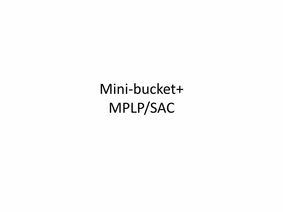
Solving Min-sum problems

• Exact by Bucket elimination

• Bounding scheme: MBE, MPLP, Soft arc-consistency.

• MBE: capitalize on large cluster processed exactly. Similar to i-consistency for large i (parameter z), directional, non-iterative.

• SAC, MPLP: equivalent to arc-consistency. Can be extended to cluster graphs, but may not be efficient. Based on cost shifting subject t equivalence-preserving transformations (EPT)

• Goal: MBE+MPLP/SAC can improve bounds of both in an efficient way.

scopesS

ffF

DDD

XXX

FDXRCOPfinite

m

m

n

n

},...,{SS

functionscost - },...,{

domains - },...,{

variables- },...,{

:where,, a triple is A

1

1

1

1

)(min*

)(

ionCost Funct Global

1

xFF

XfXF

x

m

i i

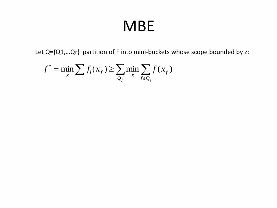
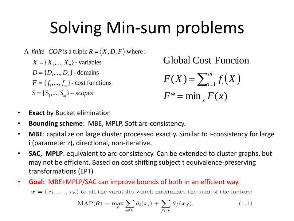
MBE

)(min)(min*

jj Qf

f

Qx

fix

xfxff

Let Q={Q1,…Qr} partition of F into mini-buckets whose scope bounded by z:

4

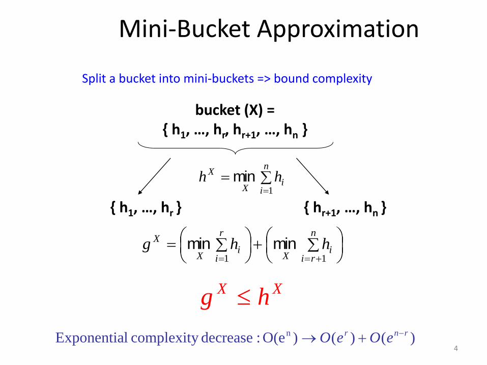
Mini-Bucket Approximation

n

ii

X

X hh1

min

n

rii

X

r

ii

X

X hhg11

minmin

Split a bucket into mini-buckets => bound complexity

)()()O(e :decrease complexity lExponentia n rnr eOeO

bucket (X) ={ h1, …, hr, hr+1, …, hn }

{ h1, …, hr } { hr+1, …, hn }

XX hg

5

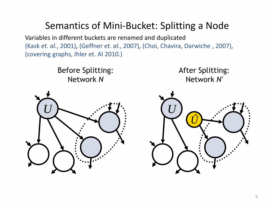
Semantics of Mini-Bucket: Splitting a Node

U UÛ

Before Splitting:

Network N

After Splitting:

Network N'

Variables in different buckets are renamed and duplicated (Kask et. al., 2001), (Geffner et. al., 2007), (Choi, Chavira, Darwiche , 2007), (covering graphs, Ihler et. Al 2010.)

Optimal Soft Arc-consistency

)(])[()(''

' xfixcxfFfi

i

Ff

)())}()({(min)(min)(min)()}(|{

xFpxpxfxpxF f

Ff

i

fscopeX

fxifx

i

fscopeif

fxi

ix

i

fp

Ff

fx

Fpxff

max)(min

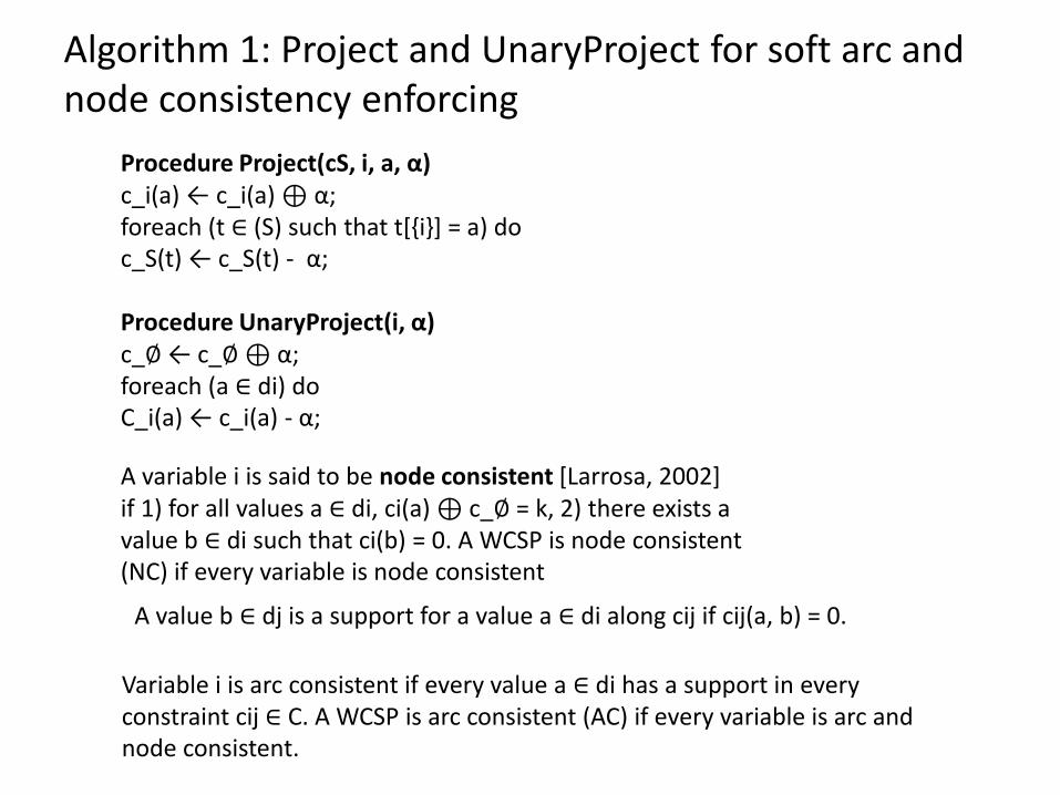
Algorithm 1: Project and UnaryProject for soft arc andnode consistency enforcing

Procedure Project(cS, i, a, α)c_i(a) ← c_i(a) ⊕ α;foreach (t ∈ (S) such that t[{i}] = a) doc_S(t) ← c_S(t) - α;

Procedure UnaryProject(i, α)c_∅ ← c_∅⊕ α;foreach (a ∈ di) doC_i(a) ← c_i(a) - α;

A variable i is said to be node consistent [Larrosa, 2002]if 1) for all values a ∈ di, ci(a) ⊕ c_∅ = k, 2) there exists avalue b ∈ di such that ci(b) = 0. A WCSP is node consistent(NC) if every variable is node consistent

A value b ∈ dj is a support for a value a ∈ di along cij if cij(a, b) = 0.

Variable i is arc consistent if every value a ∈ di has a support in every constraint cij ∈ C. A WCSP is arc consistent (AC) if every variable is arc and node consistent.

1

1

2

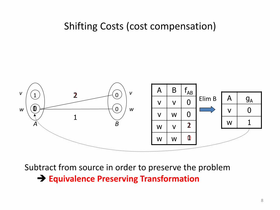
Subtract from source in order to preserve the problem Equivalence Preserving Transformation

Shifting Costs (cost compensation)

w

v v

w

0

0

1

A B1

0

A B fAB

v v 0

v w 0

w v

w w

A gA

v 0

w 11

0

2

1

Elim B

8

• Shifting costs from fAB to AShift(fAB,(A,w),1)

• Can be reversed (e.g. Shift(fAB,(A,w), -1))

0

1

Equivalence Preserving Transformation

w

v v

w

0

0

1

A B1

Arc EPT: shift cost in the scope of 1 cost function

Problem structure preserved

9

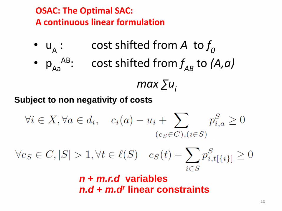
OSAC: The Optimal SAC:A continuous linear formulation

• uA : cost shifted from A to f0

• pAaAB: cost shifted from fAB to (A,a)‏

max ∑ui

n + m.r.d variablesn.d + m.dr linear constraints

Subject to non negativity of costs

10

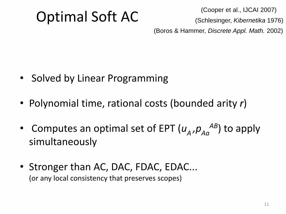
Optimal Soft AC

• Solved by Linear Programming

• Polynomial time, rational costs (bounded arity r)

• Computes an optimal set of EPT (uA ,pAaAB) to apply

simultaneously

• Stronger than AC, DAC, FDAC, EDAC...(or any local consistency that preserves scopes)‏

(Cooper et al., IJCAI 2007)

(Boros & Hammer, Discrete Appl. Math. 2002)

(Schlesinger, Kibernetika 1976)

11

The OSAC algorithmP’= OSAC(P)

)(

][

')()(

ij

i

j

fscopeX

f

xtii ptftf

)}({minmax i

q

i

iDx

pq xcFi

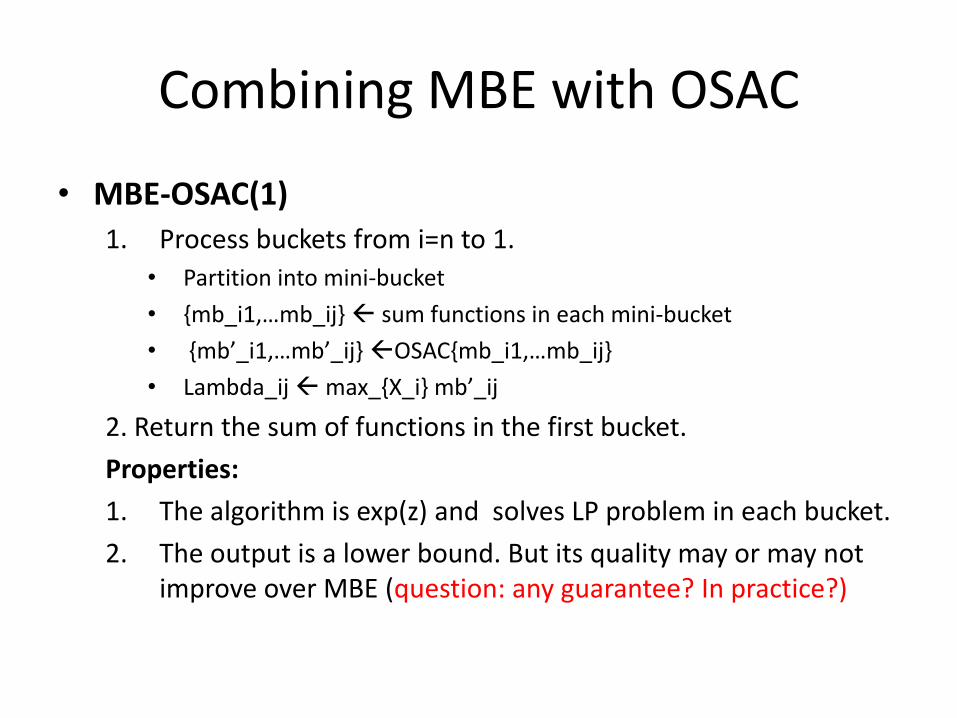
Combining MBE with OSAC

• MBE-OSAC(1)

1. Process buckets from i=n to 1.

• Partition into mini-bucket

• {mb_i1,…mb_ij} sum functions in each mini-bucket

• {mb’_i1,…mb’_ij} OSAC{mb_i1,…mb_ij}

• Lambda_ijmax_{X_i} mb’_ij

2. Return the sum of functions in the first bucket.

Properties:

1. The algorithm is exp(z) and solves LP problem in each bucket.

2. The output is a lower bound. But its quality may or may not improve over MBE (question: any guarantee? In practice?)

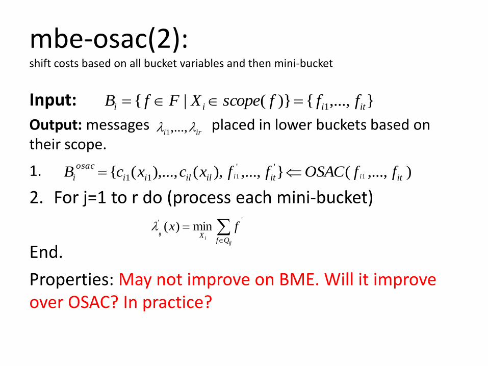
mbe-osac(2): shift costs based on all bucket variables and then mini-bucket

Input:

Output: messages placed in lower buckets based on their scope.

1.

2. For j=1 to r do (process each mini-bucket)

End.

Properties: May not improve on BME. Will it improve over OSAC? In practice?

},...,{)}(|{ 1 itiii fffscopeXFfB

iri ,...,1

),...,(},...,),(),...,({ 11

''

11 ititililii

osac

i ffOSACffxcxcB ii

'' min)(

ij

iij

QfX

fx

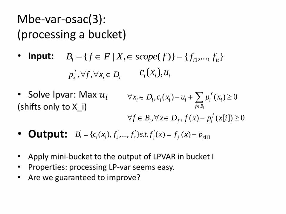
Mbe-var-osac(3): (processing a bucket)

},...,{)}(|{ 1 itiii fffscopeXFfB

ii

f

x Dxfpi

,, iii uxc ),(

0])[()(,,

0)()(,

ixpxfDxBf

xpuxcDx

f

ifi

Bf

i

f

iiiiii

i

][

'''

1

' )()(..},...,),({ ixjjrii pxfxftsffxcBi

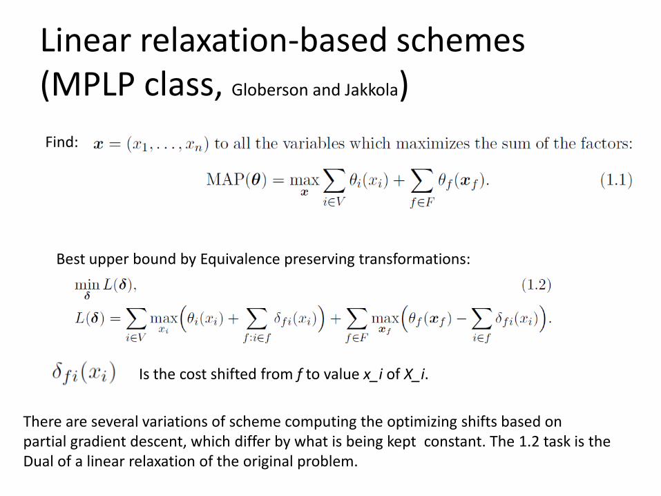
Linear relaxation-based schemes(MPLP class, Globerson and Jakkola)

Find:

Best upper bound by Equivalence preserving transformations:

There are several variations of scheme computing the optimizing shifts based on partial gradient descent, which differ by what is being kept constant. The 1.2 task is theDual of a linear relaxation of the original problem.

Is the cost shifted from f to value x_i of X_i.

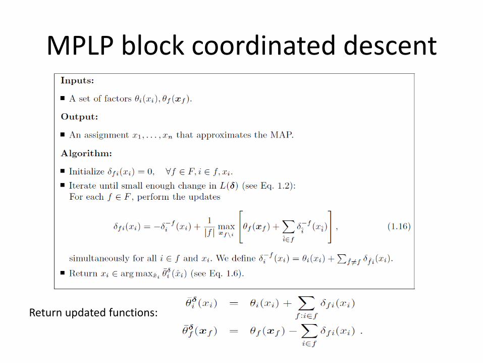
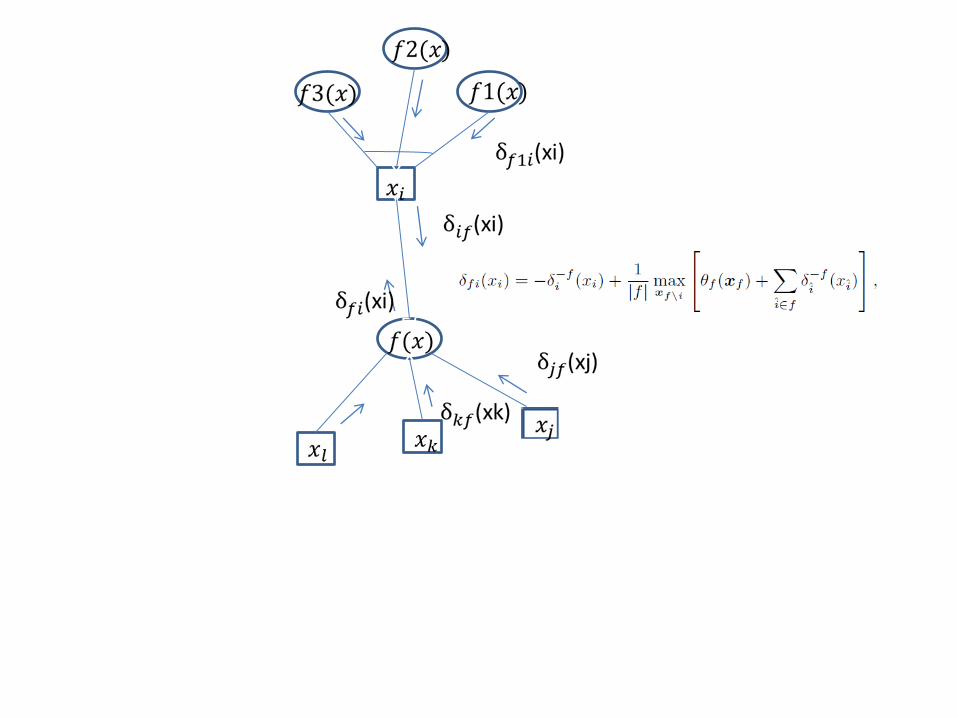
MPLP block coordinated descent

Return updated functions:

F(x

xxxx

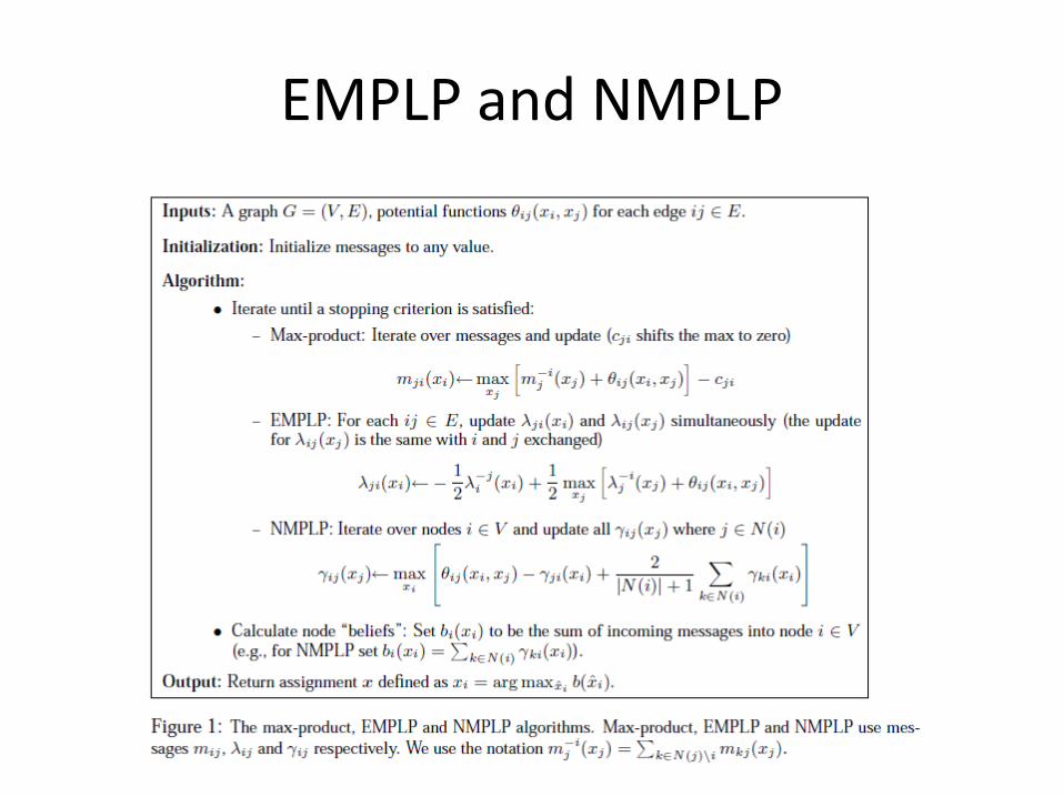
EMPLP and NMPLP

Convergence Properties

Proposition 3 If the fixed point of MPLP has bi(xi) such that for all i the function bi(xi) has ai , then x is the solution to the MAP problem and the LP relaxation is exact.

Proposition 4 When xi are binary, the MPLP fixed point can be used to obtain the primal optimum.

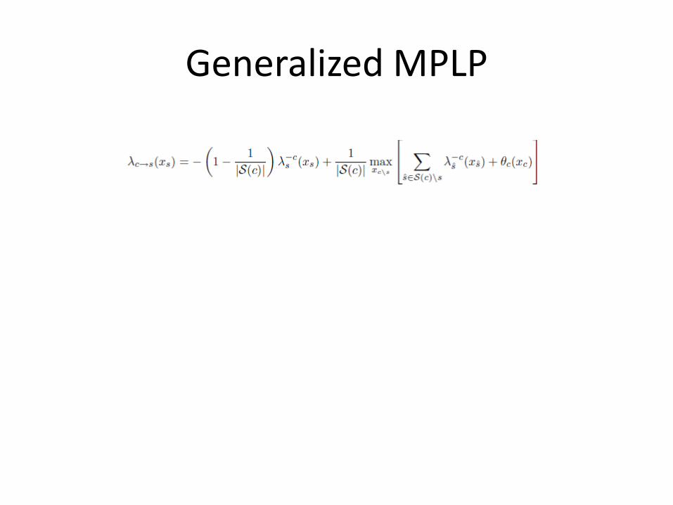
Generalized MPLP

MBE+MPLP

• MPE-MPLP can be combined in a similar ways as with OSAC. Which method can provide guarantee for improvement….

• Use generalized MPLP as a basis…

• Develop directly similar to Alex and Qiang for belief.

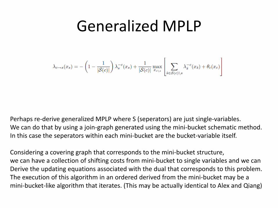
Generalized MPLP

Perhaps re-derive generalized MPLP where S (seperators) are just single-variables.We can do that by using a join-graph generated using the mini-bucket schematic method.In this case the seperators within each mini-bucket are the bucket-variable itself.

Considering a covering graph that corresponds to the mini-bucket structure, we can have a collection of shifting costs from mini-bucket to single variables and we canDerive the updating equations associated with the dual that corresponds to this problem.The execution of this algorithm in an ordered derived from the mini-bucket may be a mini-bucket-like algorithm that iterates. (This may be actually identical to Alex and Qiang)

THE ENDWho wants to grab this?

Local Consistency in ConstraintNetworks

• Massive local inference

– Time efficient (local inference, as mini buckets)– Infer only small constraints, added to the network– No variable is eliminated – Produces an equivalent more explicit problem– May detect inconsistency (prune tree search)

Arc consistency inference in the scope of 1 constraint

25

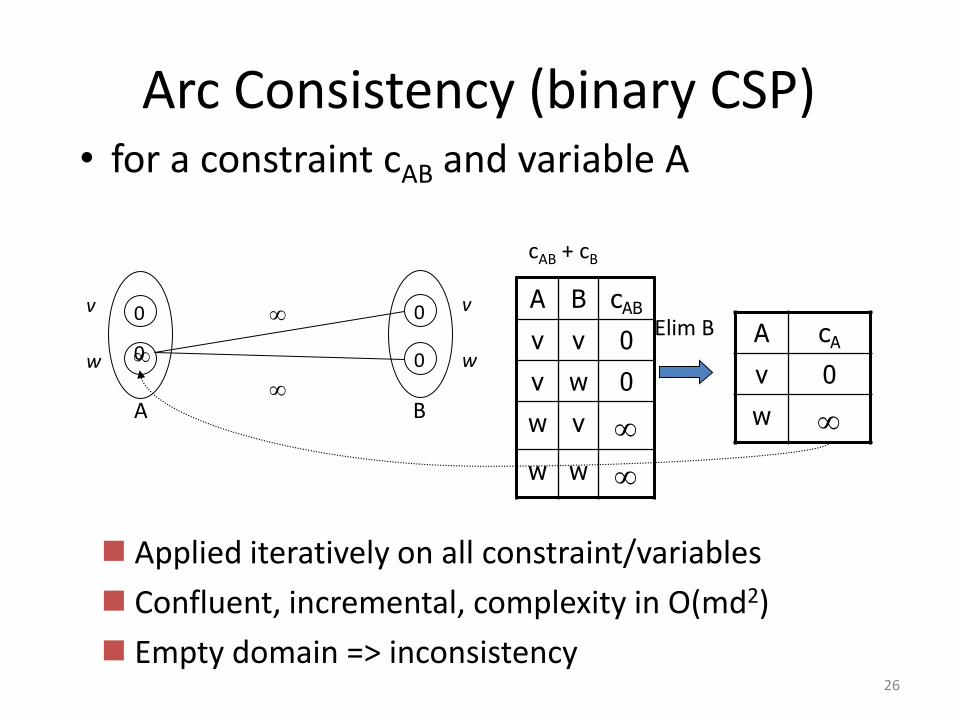
Arc Consistency (binary CSP)• for a constraint cAB and variable A

w

v v

w

0

0

0

0

A B

A B cAB

v v 0

v w 0

w v

w w

A cA

v 0

w

cAB + cB

Elim B

Applied iteratively on all constraint/variables

Confluent, incremental, complexity in O(md2)

Empty domain => inconsistency26

1

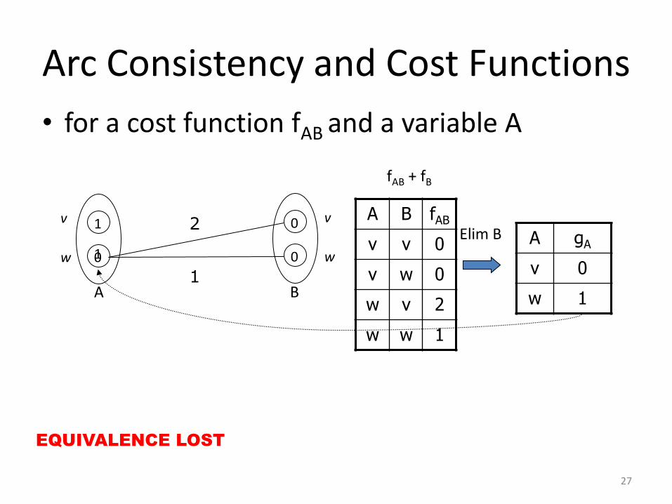
Arc Consistency and Cost Functions

• for a cost function fAB and a variable A

w

v v

w

0

0

1

0

A B

2

1

A B fAB

v v 0

v w 0

w v 2

w w 1

A gA

v 0

w 1

fAB + fB

Elim B

EQUIVALENCE LOST

27

1

1

2

Subtract from source in order to preserve the problem Equivalence Preserving Transformation

Shifting Costs (cost compensation)

w

v v

w

0

0

1

A B1

0

A B fAB

v v 0

v w 0

w v

w w

A gA

v 0

w 11

0

2

1

Elim B

28

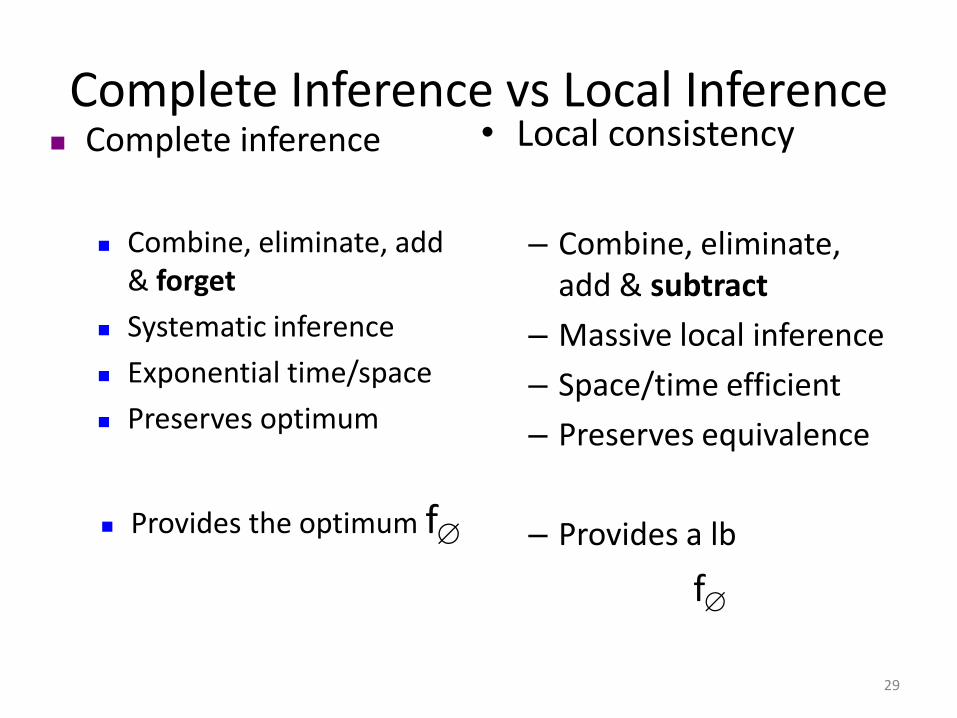
Complete Inference vs Local Inference• Local consistency

– Combine, eliminate, add & subtract

– Massive local inference

– Space/time efficient

– Preserves equivalence

– Provides a lb

f

Complete inference

Combine, eliminate, add & forget

Systematic inference

Exponential time/space

Preserves optimum

Provides the optimum f

29

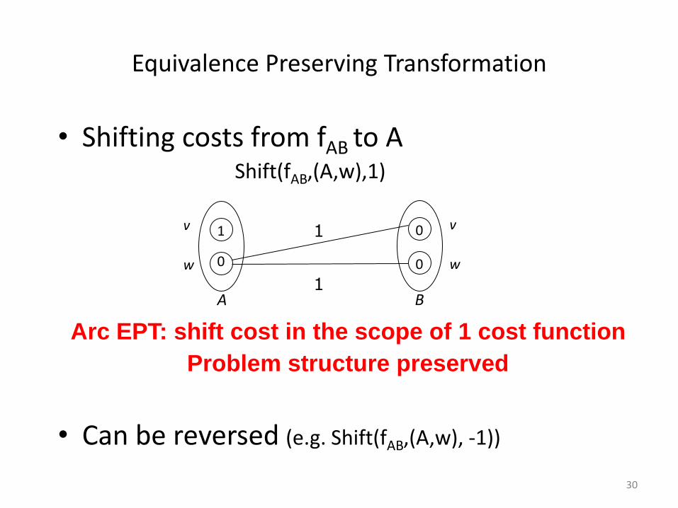
• Shifting costs from fAB to AShift(fAB,(A,w),1)

• Can be reversed (e.g. Shift(fAB,(A,w), -1))

0

1

Equivalence Preserving Transformation

w

v v

w

0

0

1

A B1

Arc EPT: shift cost in the scope of 1 cost function

Problem structure preserved

30

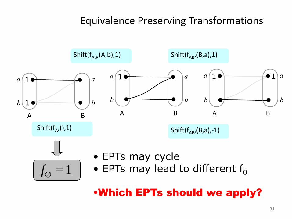
Equivalence Preserving Transformations

1f =

• EPTs may cycle• EPTs may lead to different f0

•Which EPTs should we apply?

Shift(fAB,(A,b),1)

Shift(fA,(),1) Shift(fAB,(B,a),-1)

Shift(fAB,(B,a),1)

A B A B A B

31

Local Consistency

– Equivalence Preserving Transformation

– Chaotic iteration of EPTs

– Optimal set of EPTs

– Improving sequence of EPTs

32

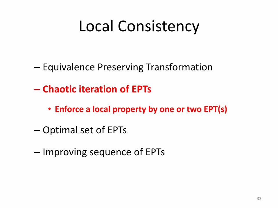
Local Consistency



• Enforce a local property by one or two EPT(s)



33

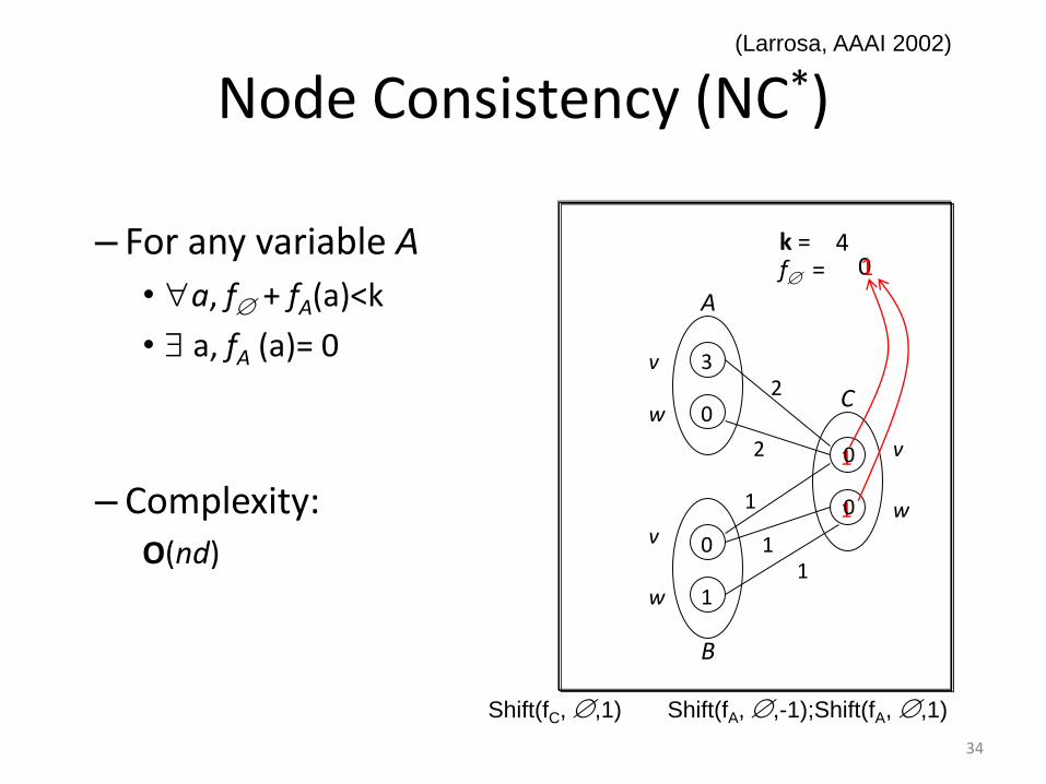
Node Consistency (NC*)

– For any variable A

• a, f + fA(a)<k

• a, fA (a)= 0

– Complexity:O(nd)

w

v

v

v

w

w

f =k =

32

2

11

1

1

1

0

0

1

A

B

C

0

0

014

Shift(fC, ,1) Shift(fA, ,-1);Shift(fA, ,1)

(Larrosa, AAAI 2002)

34

0

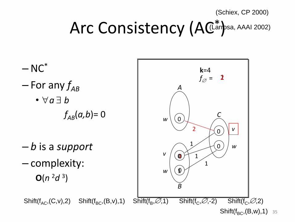
Arc Consistency (AC*)

– NC*

– For any fAB

• a b

fAB(a,b)= 0

– b is a support

– complexity:O(n 2d 3)

wv

v

w

w

f =k=4

2

11

1

0

0

0

0

1

A

B

C

1

12

0

Shift(fAC,(C,v),2) Shift(fBC,(B,v),1)

Shift(fBC,(B,w),1)

Shift(fB,,1) Shift(fC,,-2) Shift(fC,,2)

(Larrosa, AAAI 2002)

(Schiex, CP 2000)

35

1

1

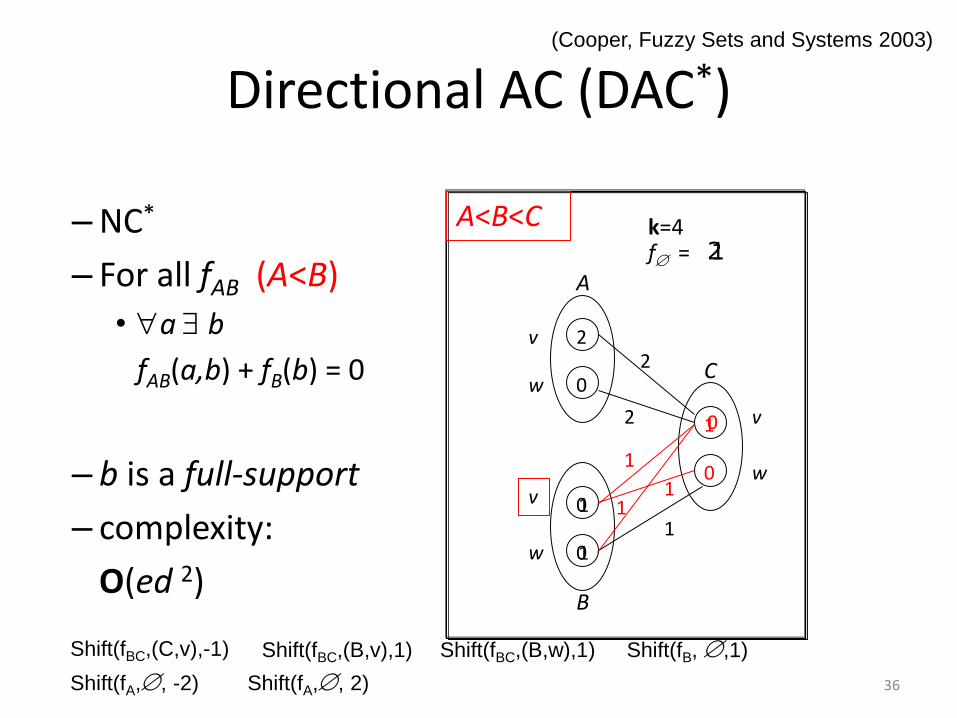
Directional AC (DAC*)

– NC*

– For all fAB (A<B)

• a b

fAB(a,b) + fB(b) = 0

– b is a full-support

– complexity:

O(ed 2)

w

v

v

v

w

w

f =k=4

22

2

1

1

1

0

0

0

0

A

B

C

A<B<C

0

1

1

12

(Cooper, Fuzzy Sets and Systems 2003)

Shift(fBC,(C,v),-1) Shift(fBC,(B,v),1) Shift(fBC,(B,w),1) Shift(fB, ,1)

Shift(fA,, -2) Shift(fA,, 2) 36

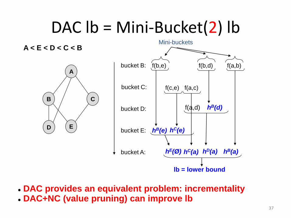
DAC lb = Mini-Bucket(2) lb

bucket A:

bucket E:

bucket D:

bucket C:

bucket B: f(b,e)

f(a,d)

hE(Ø)

hB(e)

hB(d)

hD(a)

f(a,b)f(b,d)

f(c,e) f(a,c)

hC(e)

lb = lower bound

Mini-buckets

A

B C

D E

A < E < D < C < B

hB(a)

DAC provides an equivalent problem: incrementality DAC+NC (value pruning) can improve lb

hC(a)

37

Other « Chaotic » Local Consistencies

• FDAC* = DAC+AC+NC

– Stronger lower bound

– O(end3)

– Better compromise

• EDAC* = FDAC+ EAC (existential AC)

– Even stronger

– O(ed 2 max{nd, k})

– Currently among the best practical choice

(Larrosa & Schiex, IJCAI 2003)

(Cooper, Fuzzy Sets and Systems 2003)

(Larrosa & Schiex, AI 2004)

(Cooper & Schiex, AI 2004)

(Heras et al., IJCAI 2005)

(Sanchez et al, Constraints 2008)

38

Local Consistency



– Optimal set of simultaneously applied EPTs

• Solve a linear problem in rational costs


39

Finding an EPT Sequence Maximizing the LB

Bad news

Finding a sequence of integer arc EPTs that maximizes the lower bound defines an NP-hard problem

(Cooper & Schiex, AI 2004)

40

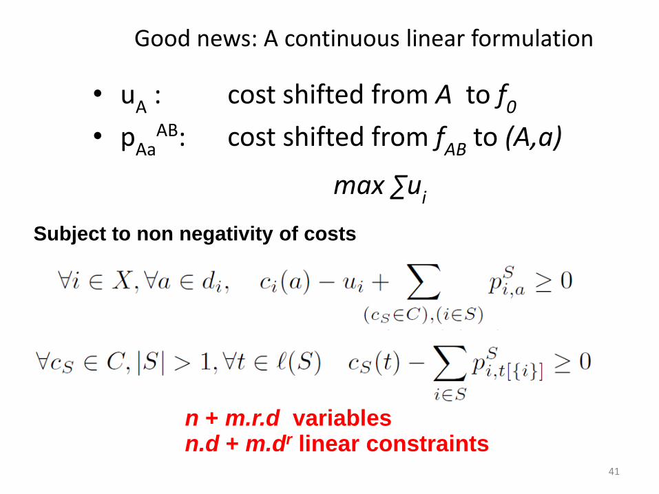
Good news: A continuous linear formulation

• uA : cost shifted from A to f0

• pAaAB: cost shifted from fAB to (A,a)‏

max ∑ui

n + m.r.d variablesn.d + m.dr linear constraints

Subject to non negativity of costs

41

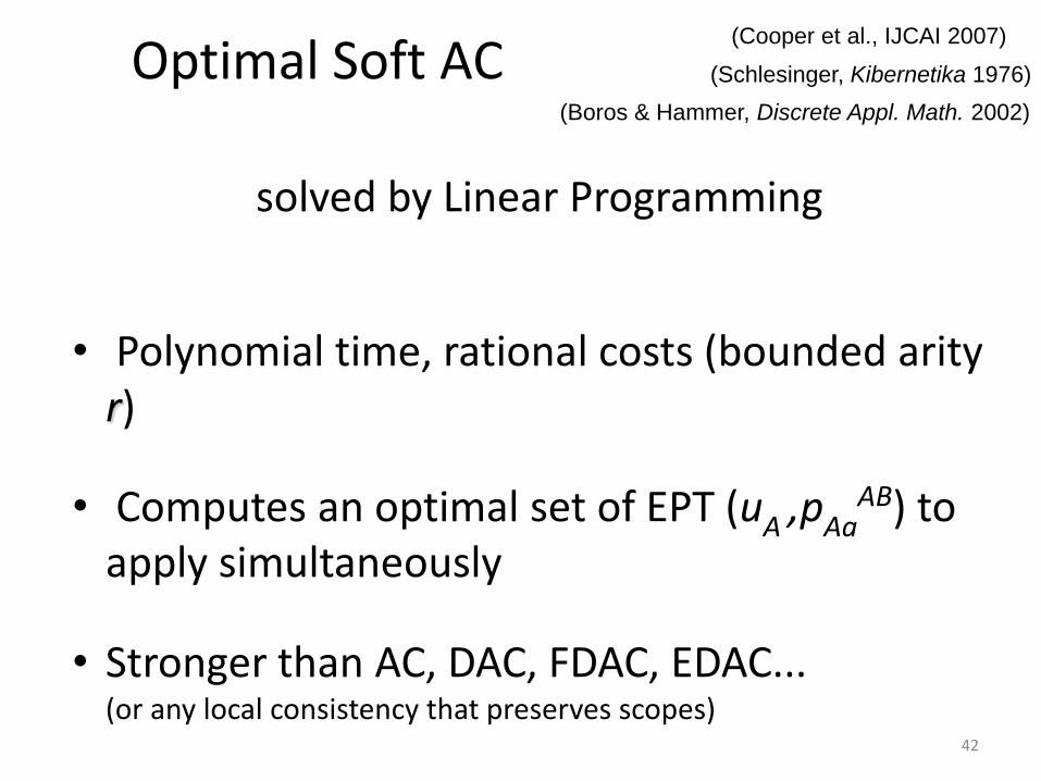
Optimal Soft AC

solved by Linear Programming

• Polynomial time, rational costs (bounded arity r)

• Computes an optimal set of EPT (uA ,pAaAB) to

apply simultaneously

• Stronger than AC, DAC, FDAC, EDAC...(or any local consistency that preserves scopes)‏

(Cooper et al., IJCAI 2007)

(Boros & Hammer, Discrete Appl. Math. 2002)

(Schlesinger, Kibernetika 1976)

42

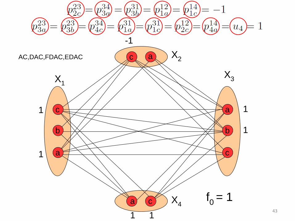
Example-1

1

1

1

1

1

1

f0 = 1

a

bb

c

a c

c

ca

a

X1

X2

X3

X4

AC,DAC,FDAC,EDAC

43

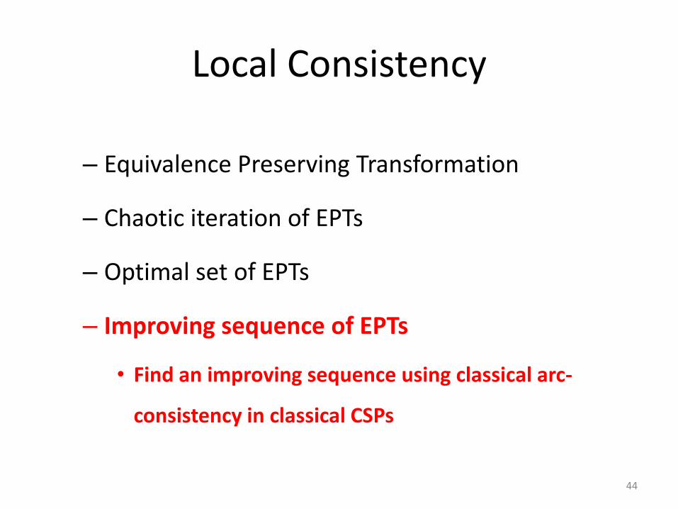
Local Consistency





• Find an improving sequence using classical arc-

consistency in classical CSPs

44

Documents

Mini-bucket+ MPLP/SAC