Minerva: Automated Hardware Optimization Tool

User Manual

Authors: Farnoud Farahmand, Ahmed Ferozpuri,

William Diehl and Kris Gaj

Last update: 12/08/2017

Image courtesy of Carolyn Angus

Content

1. Introduction 2. Previous Work 3. Background 4. Preliminary Investigation 5. Minerva Design Flow 6. Usage 7. Quick Start 8. Input Arguments 9. Report Generation and Minerva Status XML File 10. Result Replication Package Generation 11. References

1

1. Introduction A common way of determining the maximum clock frequency of a digital system is static timing analysis provided by CAD toolsets, such as Xilinx Vivado, Xilinx ISE, and Intel Quartus Prime. Finding the actual maximum clock frequency is difficult, especially in Xilinx Vivado, due to the multitude of tool options, and a complex dependence between the requested clock frequency and the actual clock frequency achieved by the tool. For example, a binary search to find maximum frequency is tedious, time-consuming, and often does not obtain the correct result. Accordingly, we introduce an automated hardware optimization tool called Minerva. Minerva determines the close-to-optimal settings of tools, using static timing analysis and a heuristic algorithm developed by the authors, and targets either optimal throughput or throughput-to-area (TPA) ratio.

Throughput, area, and throughput to area ratio are some of the most important metrics used for hardware evaluation. In hardware, the maximum throughput depends on the maximum clock frequency supported by each algorithm. The maximum clock frequency that can be achieved by a given RTL (Register-Transfer Level) code can be estimated or measured at different stages of the implementation process. The main stages are synthesis, placing and routing (P&R), and actual experimental testing on the board.

The post-synthesis and post place & route results are determined by the FPGA tools using static timing analysis. There are two difficulties associated with static timing analysis of digital systems designed and modeled using hardware description languages, and implemented using FPGAs: 1) The latest version of CAD tools provided by Xilinx (Vivado), does not have the capability to report the maximum frequency achievable for the corresponding code. Essentially, the user requests a target frequency, and the tool reports either a "pass" or "fail" for its attempt to achieve this goal. 2) While there are 25 optimization strategies (i.e., sets of preselected option values) predefined in the tool, applying them sequentially, especially using the Graphical User Interface, is extremely tedious and time consuming.

To overcome the aforementioned difficulties and facilitate hardware benchmarking of algorithms by static timing analysis methods, we introduce Minerva. Minerva is an automated and comprehensive hardware optimization tool. Minerva employs a unique heuristic algorithm, which is customized for frequency search using CAD toolsets, in addition to supporting other standard search techniques. It can incorporate an arbitrary number of predefined or user-defined strategies to achieve the highest possible frequency or frequency/area for each design. Moreover, it takes advantage of multithreading and multi-core execution to significantly reduce run time.

2

2. Previous Work A tool called SUPERCOP, which expedites comparison of software implementations of cryptographic algorithms, is presented in [1]. This open source tool supports the choice of the best compilation options from thousands of different combinations. It also facilitates execution time measurements on multiple computer systems.

In [2], an open-source environment for fair, comprehensive, automated, and collaborative hardware benchmarking of algorithms belonging to the same class is presented. The main part of this environment is the ATHENa tool for optimization of tool options, requested clock frequency, and the starting point of placement. ATHENa provides capabilities similar to our Minerva capabilities for designers targeting FPGA devices from two major vendors, Xilinx and Altera. However, it works only with the previous-generation Xilinx CAD tool (ISE), which will not support Xilinx FPGAs beyond the Series 7 families (Virtex-7, Kintex-7, Artix-7).

3. Background In this section we provide the definitions of some terms used in the rest of this document.

1. Slack time: The slack associated with each connection is the difference between the required time and the arrival time. A positive slack s at some node implies that the arrival time at that node may be increased by s, without affecting the overall delay of the circuit. Conversely, negative slack implies that a path is too slow, and it must be sped up (or the reference signal delayed) if the whole circuit is to work at the desired clock frequency.

2. WNS (Worst Negative Slack): This value corresponds to the worst slack of all the timing paths for max delay analysis. WNS can be positive or negative. If it is positive, then it means that the circuit can work with the requested clock frequency. If it is negative, then it means that the requested clock frequency is too high.

3. TNS (Total Negative Slack): The sum of all WNS violations, when considering only the worst violation for each timing path endpoint. Its value is:

a. Zero when all timing constraints are met for max delay analysis. b. Negative when there are some violations.

3

4. Preliminary Investigation In order to observe the behavior of the Vivado Design Suite in static timing analysis, synthesis and implementation were performed for the VHDL code of 5 CAESAR Round 2 candidates [3]. At first, the same requested clock frequency constraint was used for each algorithm. The target clock frequency was set to 333 MHz, and the theoretically achievable frequency (further referred to as the reference frequency) was calculated based on WNS (Worst Negative Slack), utilizing the following formula:

inimum Clock Period Target Clock Period WNS (1)M = −

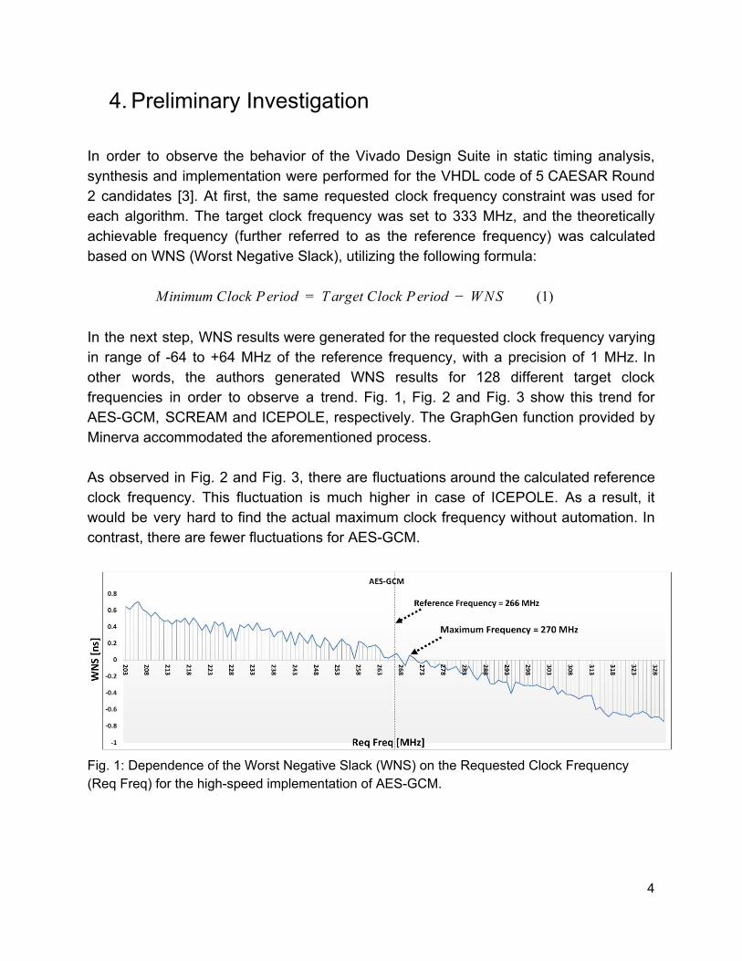
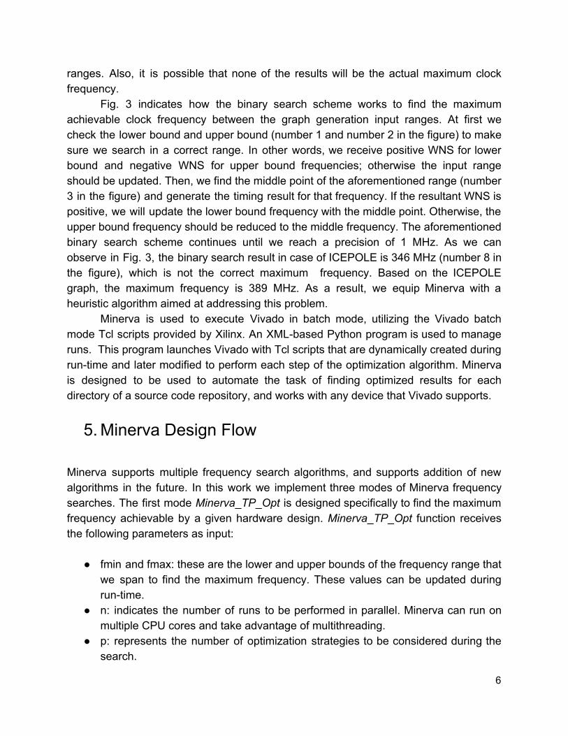
In the next step, WNS results were generated for the requested clock frequency varying in range of -64 to +64 MHz of the reference frequency, with a precision of 1 MHz. In other words, the authors generated WNS results for 128 different target clock frequencies in order to observe a trend. Fig. 1, Fig. 2 and Fig. 3 show this trend for AES-GCM, SCREAM and ICEPOLE, respectively. The GraphGen function provided by Minerva accommodated the aforementioned process. As observed in Fig. 2 and Fig. 3, there are fluctuations around the calculated reference clock frequency. This fluctuation is much higher in case of ICEPOLE. As a result, it would be very hard to find the actual maximum clock frequency without automation. In contrast, there are fewer fluctuations for AES-GCM.

Fig. 1: Dependence of the Worst Negative Slack (WNS) on the Requested Clock Frequency (Req Freq) for the high-speed implementation of AES-GCM.

4

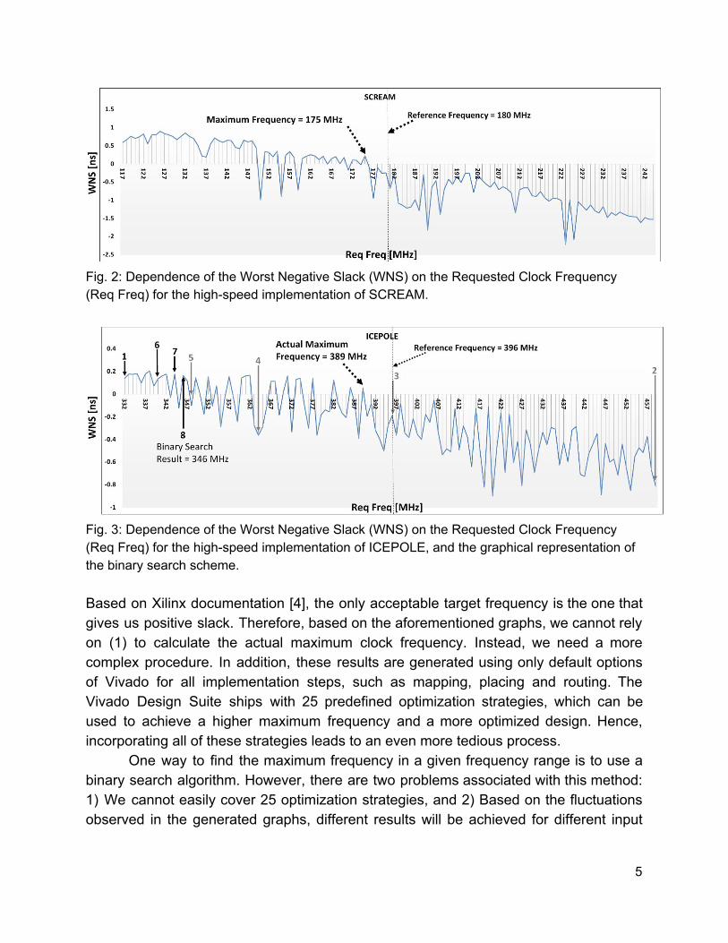
Fig. 2: Dependence of the Worst Negative Slack (WNS) on the Requested Clock Frequency (Req Freq) for the high-speed implementation of SCREAM.

Fig. 3: Dependence of the Worst Negative Slack (WNS) on the Requested Clock Frequency (Req Freq) for the high-speed implementation of ICEPOLE, and the graphical representation of the binary search scheme. Based on Xilinx documentation [4], the only acceptable target frequency is the one that gives us positive slack. Therefore, based on the aforementioned graphs, we cannot rely on (1) to calculate the actual maximum clock frequency. Instead, we need a more complex procedure. In addition, these results are generated using only default options of Vivado for all implementation steps, such as mapping, placing and routing. The Vivado Design Suite ships with 25 predefined optimization strategies, which can be used to achieve a higher maximum frequency and a more optimized design. Hence, incorporating all of these strategies leads to an even more tedious process.

One way to find the maximum frequency in a given frequency range is to use a binary search algorithm. However, there are two problems associated with this method: 1) We cannot easily cover 25 optimization strategies, and 2) Based on the fluctuations observed in the generated graphs, different results will be achieved for different input

5

ranges. Also, it is possible that none of the results will be the actual maximum clock frequency.

Fig. 3 indicates how the binary search scheme works to find the maximum achievable clock frequency between the graph generation input ranges. At first we check the lower bound and upper bound (number 1 and number 2 in the figure) to make sure we search in a correct range. In other words, we receive positive WNS for lower bound and negative WNS for upper bound frequencies; otherwise the input range should be updated. Then, we find the middle point of the aforementioned range (number 3 in the figure) and generate the timing result for that frequency. If the resultant WNS is positive, we will update the lower bound frequency with the middle point. Otherwise, the upper bound frequency should be reduced to the middle frequency. The aforementioned binary search scheme continues until we reach a precision of 1 MHz. As we can observe in Fig. 3, the binary search result in case of ICEPOLE is 346 MHz (number 8 in the figure), which is not the correct maximum frequency. Based on the ICEPOLE graph, the maximum frequency is 389 MHz. As a result, we equip Minerva with a heuristic algorithm aimed at addressing this problem.

Minerva is used to execute Vivado in batch mode, utilizing the Vivado batch mode Tcl scripts provided by Xilinx. An XML-based Python program is used to manage runs. This program launches Vivado with Tcl scripts that are dynamically created during run-time and later modified to perform each step of the optimization algorithm. Minerva is designed to be used to automate the task of finding optimized results for each directory of a source code repository, and works with any device that Vivado supports.

5. Minerva Design Flow Minerva supports multiple frequency search algorithms, and supports addition of new algorithms in the future. In this work we implement three modes of Minerva frequency searches. The first mode Minerva_TP_Opt is designed specifically to find the maximum frequency achievable by a given hardware design. Minerva_TP_Opt function receives the following parameters as input:

● fmin and fmax: these are the lower and upper bounds of the frequency range that we span to find the maximum frequency. These values can be updated during run-time.

● n: indicates the number of runs to be performed in parallel. Minerva can run on multiple CPU cores and take advantage of multithreading.

● p: represents the number of optimization strategies to be considered during the search.

6

● r (precision range size): is the maximum number of frequency targets (higher than the last achieved maximum clock frequency) to be explored. If we achieve positive slack for a frequency in this range, we will continue the search; otherwise we will terminate the process.

This function generates an output report that contains the following information:

1. WNS result for all test cases with the corresponding optimization strategy ID and target clock frequency.

2. WNS and Area results for all target frequencies with positive slack. 3. Maximum frequency with WNS ≥ 0, f_pass_max 4. Minimum Area in the number of LUTs achievable for f_pass_max (denoted by

min_LUTs(f_pass_max)), the corresponding ratio f_pass_max/min_LUTs(f_pass_max), and the corresponding optimization strategy ID.

5. Minimum Area in the number of Slices achievable for f_pass_max (denoted by min\_Slices(f_pass_max)), the corresponding ratio f_pass_max/min_Slices(f_pass_max), and the corresponding optimization strategy ID.

Please note that the Strategy IDs may be different for the outputs 4 and 5. Fig. 4 (a)-(f) completely describes how Minerva_TP_Opt algorithm works. This figure is drawn assuming the following values of the Minerva parameters: fmin=50, fmax=200, n=8, r=8, and p=8. Each column illustrates one requested clock frequency value, and square blocks in that column correspond to optimization strategies. Each square block represents one test case with the optimization strategy ID mentioned inside it. Colors of these blocks are white or gray, indicating positive or negative WNS, respectively. The runs that execute in parallel at each step are represented using dotted boxes.

7

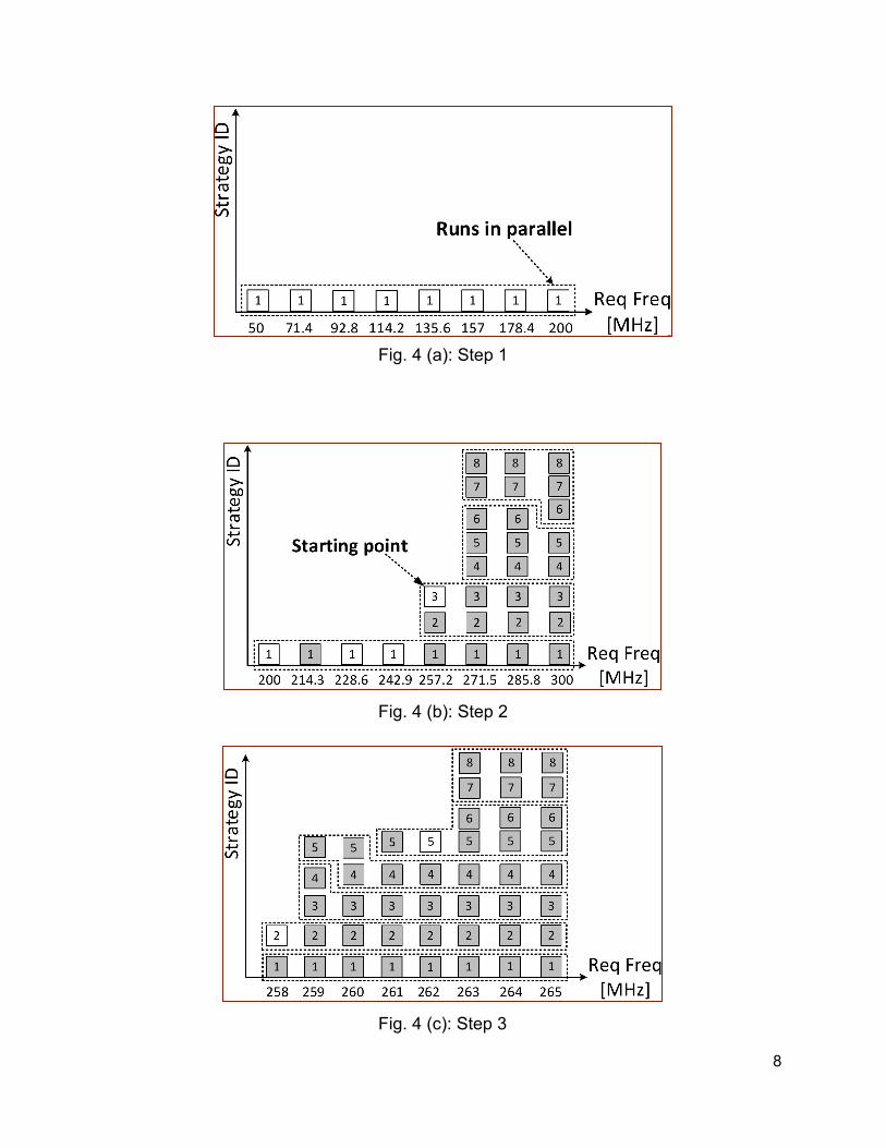
Fig. 4 (a): Step 1

Fig. 4 (b): Step 2

Fig. 4 (c): Step 3

8

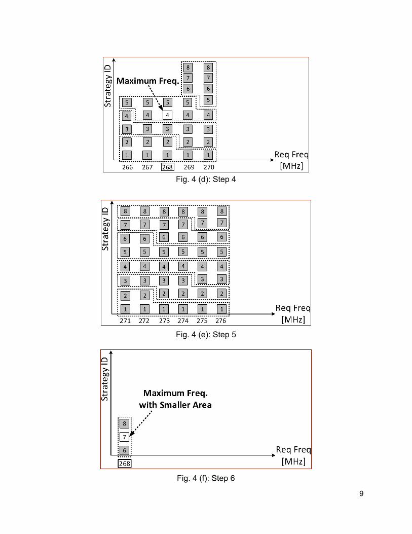
Fig. 4 (d): Step 4

Fig. 4 (e): Step 5

Fig. 4 (f): Step 6

9

Fig. 4 (a) shows the first step in Minerva_TP_Opt algorithm. In the first step, the given frequency range (50 to 200) is divided by (r-1) to have 8 frequencies including 50 and 200, with the same distance between each other, as shown in Fig. 4 (a) Freq axis. Then, WNS results are generated for all of these 8 target frequencies and the default optimization strategy. It is feasible to run all of these target frequencies at the same time, as n is equal to 8 in this example. After WNS results are generated, if the upper bound frequency (fmax) gives us positive slack, we update fmin and fmax values using (2) and (3), and repeat the previous process (step forward).

min(new) fmax(old) (2)f = max(new) fmax(old) 100 (3)f = +

If all of the first 8 target clock frequencies give us negative slack, we step backward by a frequency range of 100 MHz. Accordingly, fmin and fmax are updated using (4) and (5), and the first step is repeated.

min(new) fmin(old) 00 (4)f = − 1 max(new) fmin(old) (5)f =

The aforementioned process leads to finding the maximum frequency, less than

fmax, that gives us positive slack using only the default optimization strategy. As we can observe in Fig. 4 (a), in the first step, positive slack is achieved for fmax (200 MHz). Hence, we step forward and update fmin and fmax to 200 and 300 MHz respectively, see Fig. 4 (b). As shown in this figure, 242.9 MHz is the highest frequency that leads to positive slack with the default optimization strategy.

At this point, the optimization runs are started for the remaining frequencies in this range higher than 242.9 MHz. In this example 257.2 MHz, with optimization strategy number 3 has positive slack, so the maximum frequency is updated to 257.2 MHz. In case of higher frequencies, all 8 optimization strategies fail. Therefore, 257.2 MHz becomes our starting point to begin the next step of frequency search considering 8 optimization strategies and a precision of 1 MHz.

The next step is illustrated in Fig. 4(c). In this step we go forward by 1 MHz. As soon as we find a frequency with positive slack, the lower frequencies and the remaining optimization strategies corresponding to these frequencies are eliminated. The aforementioned procedure is continued until 8 (precision range size) consecutive frequencies fail to provide positive slack for all possible optimization strategies (8 in this example), as shown in Fig. 4(d) and Fig. 4(e). Therefore, in this example, the maximum frequency with WNS=0, f_pass_max, is 268 MHz, using the optimization strategy number 4.

Let us assume that the number of LUTs for Strategy 4 is 1000, and the number

10

of Slices 300. Based on Fig. 4(d), only the first 5 optimization strategies were tested for f_pass_max=268 MHz. Therefore, in the next step, shown in Fig. 4(f), we perform runs for the remaining three strategies at the same maximum clock frequency of 268 MHz. As we can see in this figure, only one of these runs passes with WNS=0, for the strategy ID=7. Now let us assume that the corresponding areas for Strategy 7 are 970 LUTs and 310 Slices. Then, the algorithm returns two sets: {f_pass_max=268 MHz, Minimum number of LUTs achievable for f_pass_max, min_LUTs(268 MHz)=970, the corresponding ratio f_pass_max/min_LUTs(f_pass_max)=268/970, and the corresponding optimization strategy ID=7} as well as {f_pass_max=268 MHz, Minimum number of Slices achievable for f_pass_max, min_Slices(268 MHz)=300, the corresponding ratio f_pass_max/min_Slices(f_pass_max)=268/300, and the corresponding optimization strategy ID=4}.

The second mode of Minerva frequency search (Minerva_TPA_Opt) targets further optimization of the frequency to #LUTs ratio (Throughput to area ratio). This mode can be used after Minerva_TP_Opt search generates the maximum frequency. Minerva_TPA_Opt receives the following parameters as input: 1) f_pass_max (maximum frequency achieved by Minerva_TP_Opt mode), 2) n (number of runs in parallel) and 3) p (number of optimization strategies). The output report contains the same information as the first mode (Minerva_TP_Opt). In this mode, we generate the results for all the frequencies between 96% of f_pass_max and f_pass_max, with a precision of 1 MHz. We also try all possible optimization strategies. At the end, the requested frequency and optimization strategy combination that leads to the best TPA is reported.

The third mode of Minerva frequency search (Minerva_Fast_Opt) is designed to achieve proper results in terms of both throughput and throughput to area ratio in a short amount of time compared to the first and second modes. Based on the results generated for 30 benchmarked authenticated ciphers, we arrived at the optimization strategy that gave us the best throughput to area ratio in most cases, and utilized it as a single optimization strategy. This optimization strategy focused on reducing area by ExploreArea command.

Therefore, Minerva_Fast_Opt works similar to Minerva_TP_Opt ; the only difference is the number of optimization strategies, i.e., two optimization strategies in case of Minerva_Fast_Opt, namely, the default one and the one based on the ExploreArea command.

11

6. Usage Minerva source code can be downloaded from the GMU ATHENa website page available at the following address: https://cryptography.gmu.edu/athena/index.php?id=Minerva Here are the requirements for running Minerva:

1. Linux or Windows operating systems 2. Python version 2 (Minerva fully tested with Python 2.7) 3. Vivado Design Suite (Minerva fully tested with Vivado 2015 and newer)

Note: Make sure to source vivado environmental variable before running minerva (settings64.sh in case of Linux and settings64.bat in case of Windows)

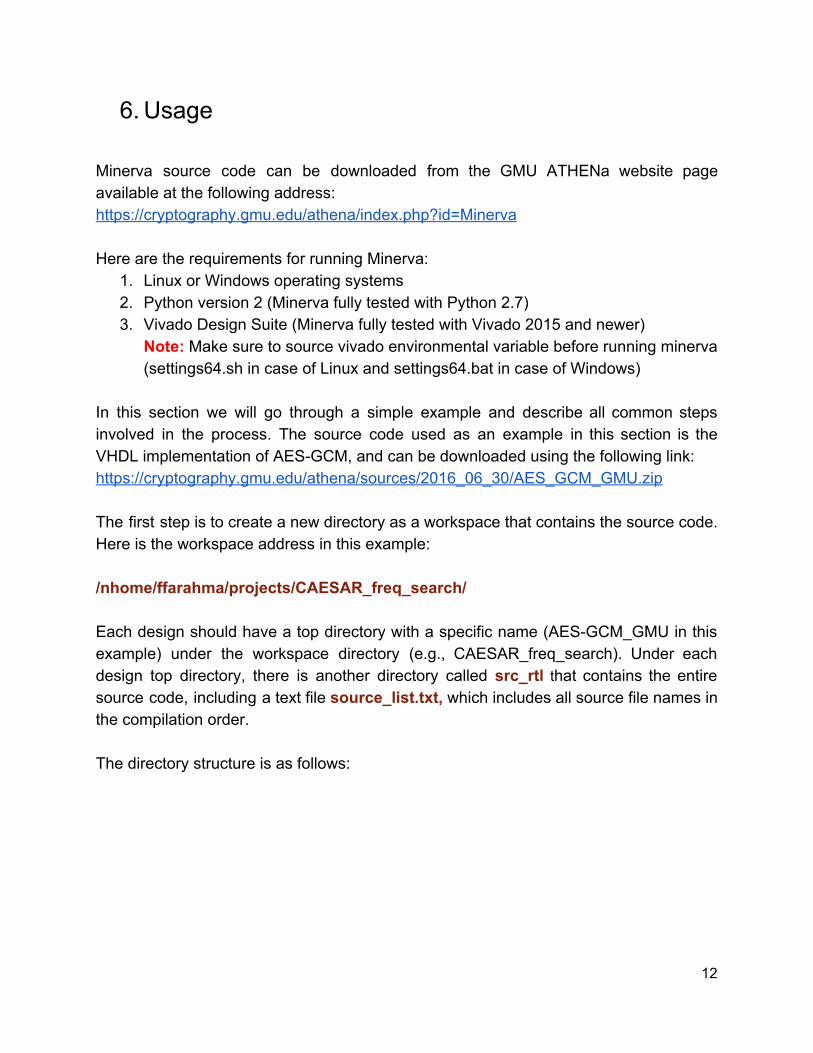
In this section we will go through a simple example and describe all common steps involved in the process. The source code used as an example in this section is the VHDL implementation of AES-GCM, and can be downloaded using the following link: https://cryptography.gmu.edu/athena/sources/2016_06_30/AES_GCM_GMU.zip The first step is to create a new directory as a workspace that contains the source code. Here is the workspace address in this example: /nhome/ffarahma/projects/CAESAR_freq_search/ Each design should have a top directory with a specific name (AES-GCM_GMU in this example) under the workspace directory (e.g., CAESAR_freq_search). Under each design top directory, there is another directory called src_rtl that contains the entire source code, including a text file source_list.txt, which includes all source file names in the compilation order. The directory structure is as follows:

12

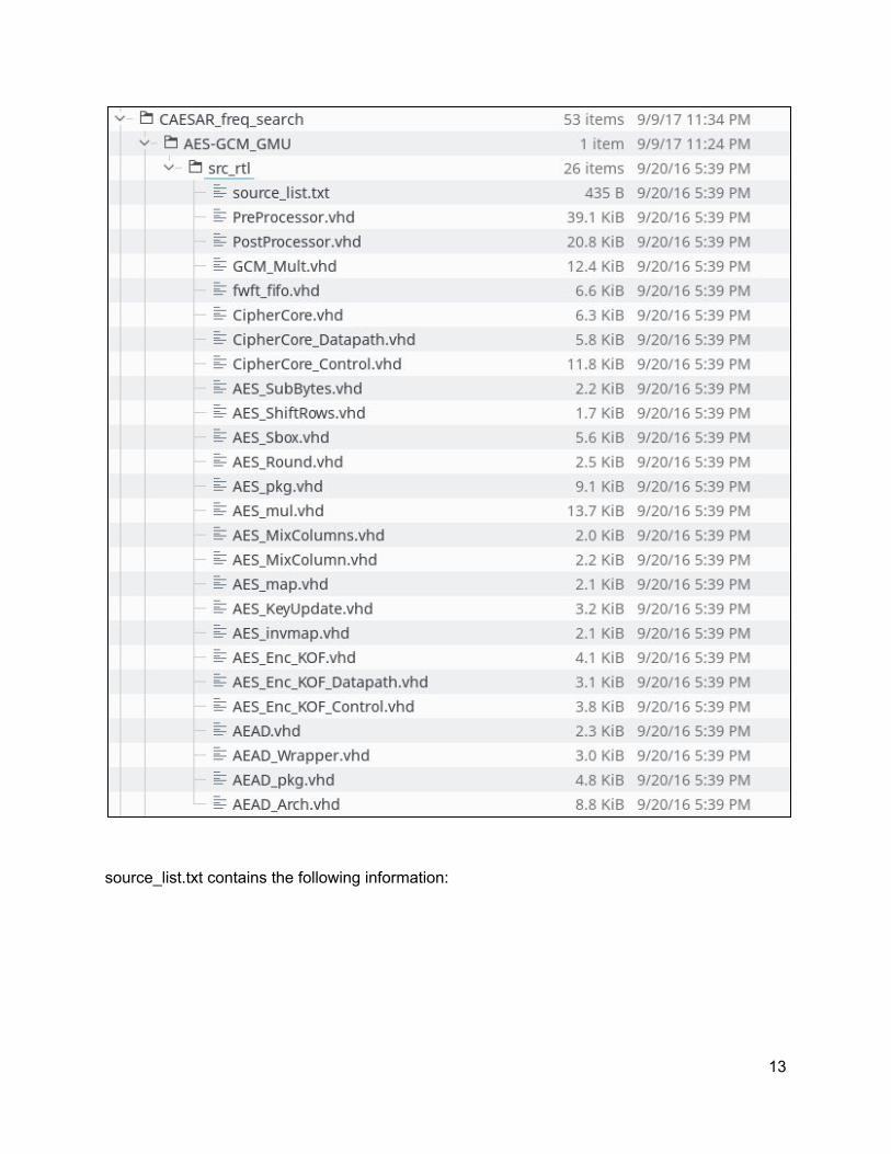
source_list.txt contains the following information:

13

The workspace directory (CAESAR_freq_search) may contain one or more designs that have the same directory structure, where each design has a src_rtl folder containing the corresponding source_list.txt.

At first, the user should run the following command to generate the runs.xml config file based on the available designs and source code under the workspace directory.

14

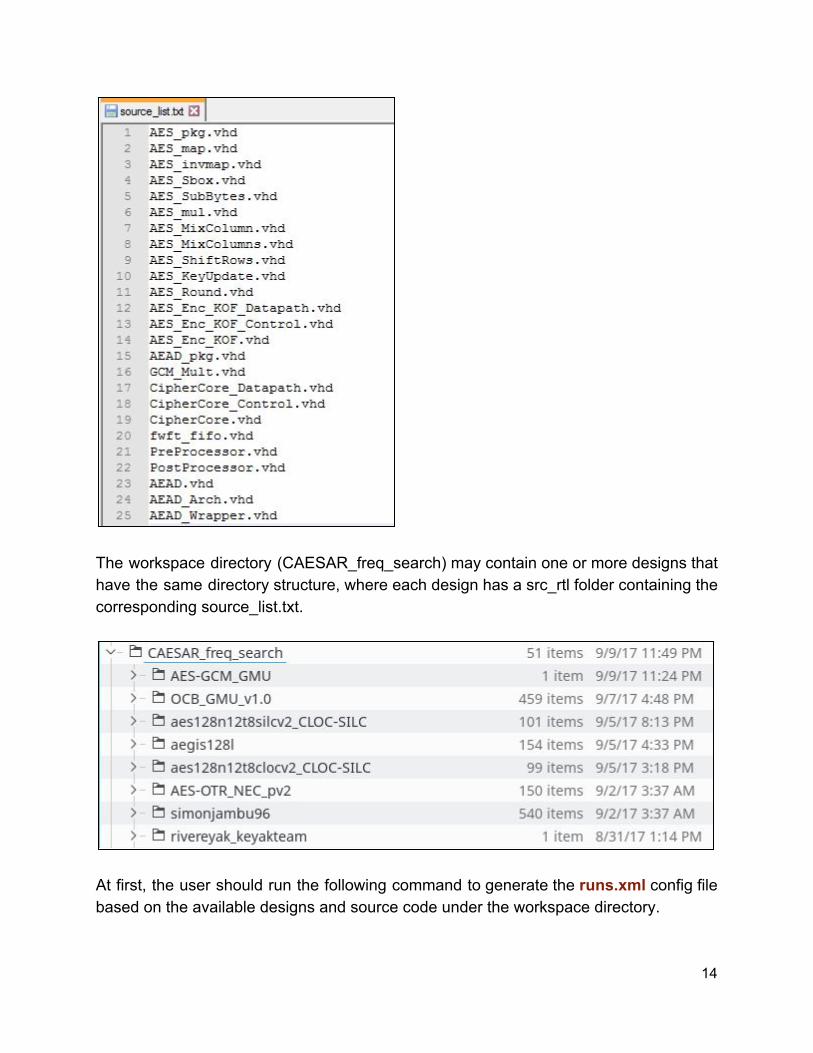
$ python run.py --gen_runs /nhome/ffarahma/projects/CAESAR_freq_search/ The output runs.xml looks like in the following example:

All config files are placed at the following location: /Minerva/config/ Available parts and their corresponding id can be found in the parts.xml, which is located under the config directory. Note: Both runs.xml and parts.xml can be configured manually as well.

15

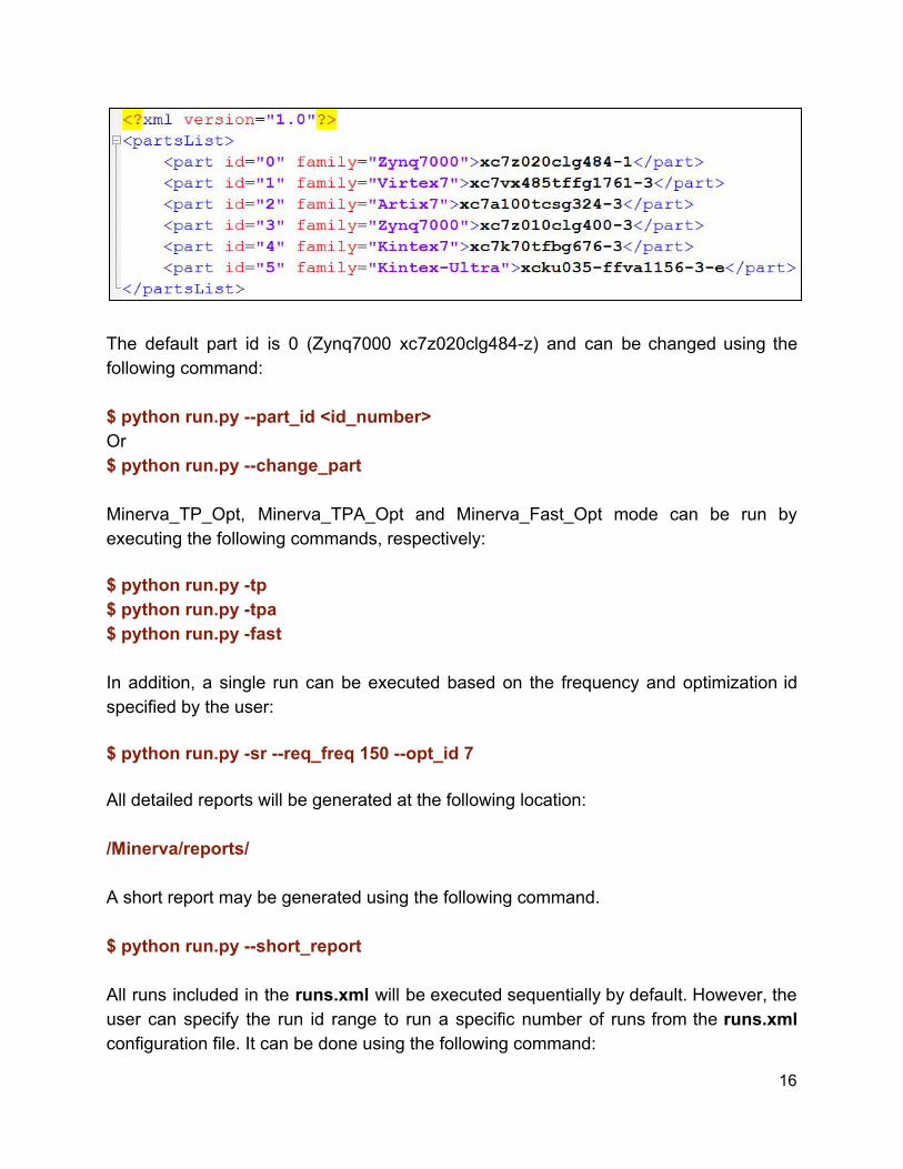
The default part id is 0 (Zynq7000 xc7z020clg484-z) and can be changed using the following command: $ python run.py --part_id <id_number> Or $ python run.py --change_part Minerva_TP_Opt, Minerva_TPA_Opt and Minerva_Fast_Opt mode can be run by executing the following commands, respectively: $ python run.py -tp $ python run.py -tpa $ python run.py -fast In addition, a single run can be executed based on the frequency and optimization id specified by the user: $ python run.py -sr --req_freq 150 --opt_id 7 All detailed reports will be generated at the following location: /Minerva/reports/ A short report may be generated using the following command. $ python run.py --short_report All runs included in the runs.xml will be executed sequentially by default. However, the user can specify the run id range to run a specific number of runs from the runs.xml configuration file. It can be done using the following command:

16

$ python run.py --run_id_range 3 7 In this example, run ids 3, 4, 5, 6 and 7 will be put in the queue and will be run sequentially. The first argument value should be less than or equal to the second argument value. If you plan to generate a result only for one run id, use the same value for both inputs (lower bound and upper bound). For example, if you want to execute only run id 5, you should use a --run_id_range 5 5 command. Parallel execution configuration: The default number of runs in parallel is 6. The user should modify this value based on the available resources on the host machine to achieve the best performance. The estimated suggestion for different platforms is as follows:

● Laptop: 4 to 8 ● Desktop PC: 8 to 16 ● Server: 16 and above

Note: All aforementioned values depend on the amount of memory and available CPU cores.

This configuration can be done using -n argument. The following example indicates the command that runs Minerva_TP_Opt mode for run id 3 to 7 with 8 runs in parallel: $ python run.py -tp --run_id_range 3 7 -n 8

7. Quick Start

In this section we provide a set of commands that you can execute to generate results for AES-GCM. AES-GCM and Minerva source link were provided in the usage section. Linux users: $ source <Vivado location>/Vivado/<Vivado_version>/settings64.sh Windows users: $ <Vivado location>/Vivado/<Vivado_version>/settings64.bat Linux and Windows users: $ cd <Minerva directory address on your pc>

17

$ python run.py --gen_runs <Workspace directory address that contains AES-GCM sources> $ python run.py -tp Note: The default number of parallel runs is 6. You can modify this value based on your available resources on the host machine using the following argument: -n <number_of_parallel_runs> Wait until Minerva be done with the Minerva_TP_Opt mode. In the meantime you can check the status of the current run by checking the Minerva status XML file available in the following location: <AES-GCM sources directory>/minerva_status/AES-GCM_MS.xml Also, you can access the full report available in the following address: <AES-GCM sources directory>/minerva_status/full_reports/AES-GCM_ID0.txt When the Minerva run is done, you can see a short report using the following command: $ python run.py --short_report (follow the instruction printed on the terminal window to see the report) The result replication package can be generated using the following command: $ python run.py -respkg (follow the instruction printed on the terminal window to generate the result replication package) The generated package can be found in the following address: <AES-GCM directory>/result_repl_AES-GCM_<date and time the package generated>.zip

18

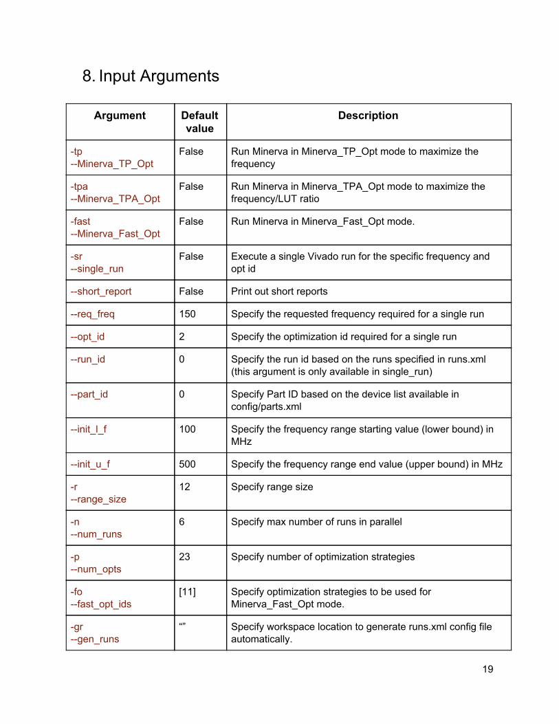
8. Input Arguments

Argument Default value

Description

-tp --Minerva_TP_Opt

False Run Minerva in Minerva_TP_Opt mode to maximize the frequency

-tpa --Minerva_TPA_Opt

False Run Minerva in Minerva_TPA_Opt mode to maximize the frequency/LUT ratio

-fast --Minerva_Fast_Opt

False Run Minerva in Minerva_Fast_Opt mode.

-sr --single_run

False Execute a single Vivado run for the specific frequency and opt id

--short_report False Print out short reports

--req_freq 150 Specify the requested frequency required for a single run

--opt_id 2 Specify the optimization id required for a single run

--run_id 0 Specify the run id based on the runs specified in runs.xml (this argument is only available in single_run)

--part_id 0 Specify Part ID based on the device list available in config/parts.xml

--init_l_f 100 Specify the frequency range starting value (lower bound) in MHz

--init_u_f 500 Specify the frequency range end value (upper bound) in MHz

-r --range_size

12 Specify range size

-n --num_runs

6 Specify max number of runs in parallel

-p --num_opts

23 Specify number of optimization strategies

-fo --fast_opt_ids

[11] Specify optimization strategies to be used for Minerva_Fast_Opt mode.

-gr --gen_runs

“” Specify workspace location to generate runs.xml config file automatically.

19

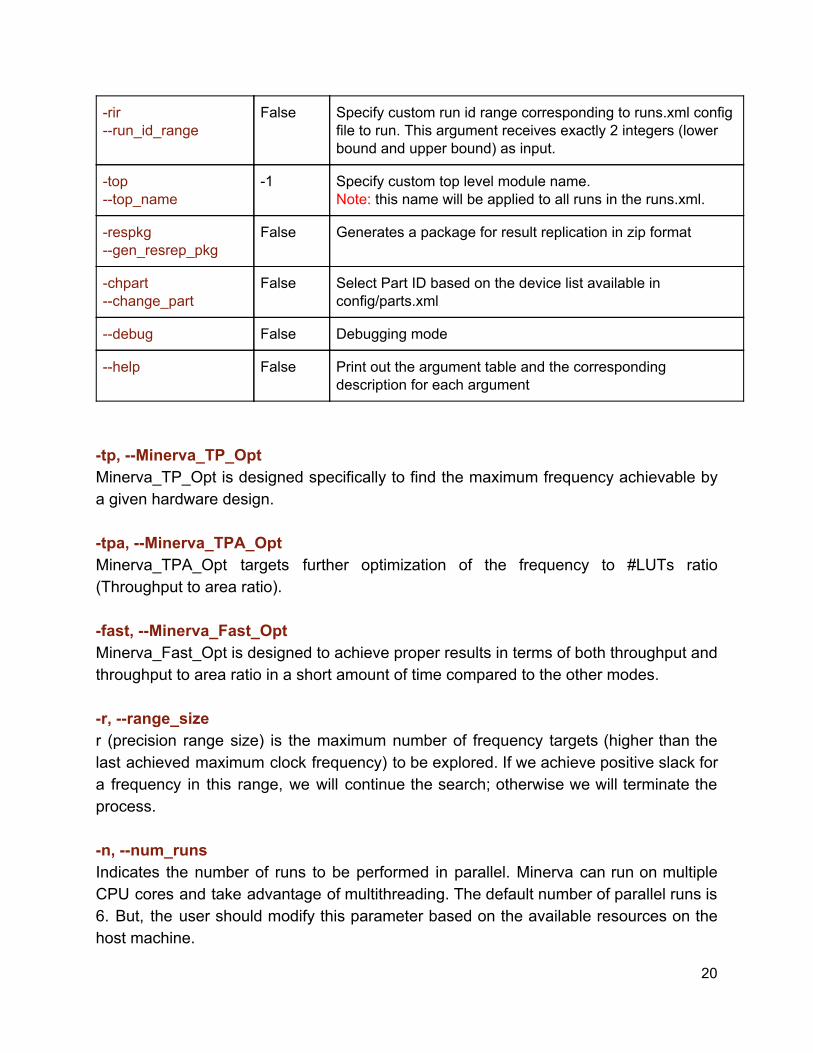
-rir --run_id_range

False Specify custom run id range corresponding to runs.xml config file to run. This argument receives exactly 2 integers (lower bound and upper bound) as input.

-top --top_name

-1 Specify custom top level module name. Note: this name will be applied to all runs in the runs.xml.

-respkg --gen_resrep_pkg

False Generates a package for result replication in zip format

-chpart --change_part

False Select Part ID based on the device list available in config/parts.xml

--debug False Debugging mode

--help False Print out the argument table and the corresponding description for each argument

-tp, --Minerva_TP_Opt Minerva_TP_Opt is designed specifically to find the maximum frequency achievable by a given hardware design. -tpa, --Minerva_TPA_Opt Minerva_TPA_Opt targets further optimization of the frequency to #LUTs ratio (Throughput to area ratio). -fast, --Minerva_Fast_Opt Minerva_Fast_Opt is designed to achieve proper results in terms of both throughput and throughput to area ratio in a short amount of time compared to the other modes. -r, --range_size r (precision range size) is the maximum number of frequency targets (higher than the last achieved maximum clock frequency) to be explored. If we achieve positive slack for a frequency in this range, we will continue the search; otherwise we will terminate the process. -n, --num_runs Indicates the number of runs to be performed in parallel. Minerva can run on multiple CPU cores and take advantage of multithreading. The default number of parallel runs is 6. But, the user should modify this parameter based on the available resources on the host machine.

20

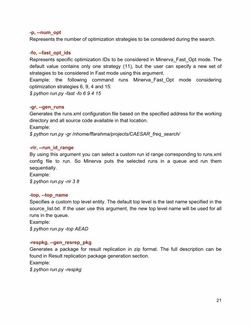
-p, --num_opt Represents the number of optimization strategies to be considered during the search. -fo, --fast_opt_ids Represents specific optimization IDs to be considered in Minerva_Fast_Opt mode. The default value contains only one strategy (11), but the user can specify a new set of strategies to be considered in Fast mode using this argument. Example: the following command runs Minerva_Fast_Opt mode considering optimization strategies 6, 9, 4 and 15: $ python run.py -fast -fo 6 9 4 15 -gr, --gen_runs Generates the runs.xml configuration file based on the specified address for the working directory and all source code available in that location. Example: $ python run.py -gr /nhome/ffarahma/projects/CAESAR_freq_search/ -rir, --run_id_range By using this argument you can select a custom run id range corresponding to runs.xml config file to run. So Minerva puts the selected runs in a queue and run them sequentially. Example: $ python run.py -rir 3 8 -top, --top_name Specifies a custom top level entity. The default top level is the last name specified in the source_list.txt. If the user use this argument, the new top level name will be used for all runs in the queue. Example: $ python run.py -top AEAD -respkg, --gen_resrep_pkg Generates a package for result replication in zip format. The full description can be found in Result replication package generation section. Example: $ python run.py -respkg

21

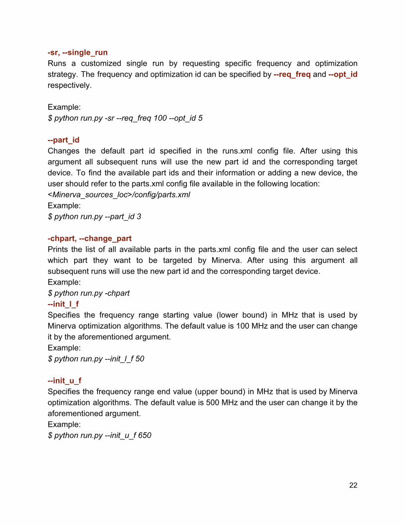
-sr, --single_run Runs a customized single run by requesting specific frequency and optimization strategy. The frequency and optimization id can be specified by --req_freq and --opt_id respectively. Example: $ python run.py -sr --req_freq 100 --opt_id 5 --part_id Changes the default part id specified in the runs.xml config file. After using this argument all subsequent runs will use the new part id and the corresponding target device. To find the available part ids and their information or adding a new device, the user should refer to the parts.xml config file available in the following location: <Minerva_sources_loc>/config/parts.xml Example: $ python run.py --part_id 3 -chpart, --change_part Prints the list of all available parts in the parts.xml config file and the user can select which part they want to be targeted by Minerva. After using this argument all subsequent runs will use the new part id and the corresponding target device. Example: $ python run.py -chpart --init_l_f Specifies the frequency range starting value (lower bound) in MHz that is used by Minerva optimization algorithms. The default value is 100 MHz and the user can change it by the aforementioned argument. Example: $ python run.py --init_l_f 50 --init_u_f Specifies the frequency range end value (upper bound) in MHz that is used by Minerva optimization algorithms. The default value is 500 MHz and the user can change it by the aforementioned argument. Example: $ python run.py --init_u_f 650

22

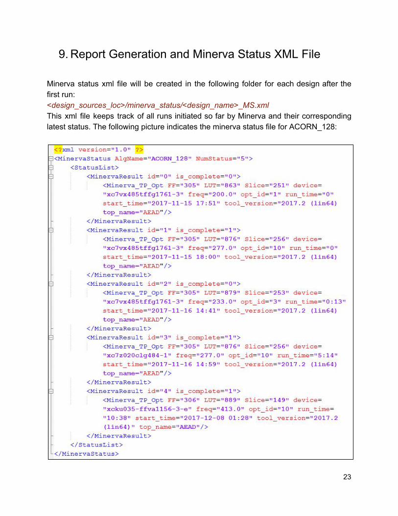
9. Report Generation and Minerva Status XML File Minerva status xml file will be created in the following folder for each design after the first run: <design_sources_loc>/minerva_status/<design_name>_MS.xml This xml file keeps track of all runs initiated so far by Minerva and their corresponding latest status. The following picture indicates the minerva status file for ACORN_128:

23

By looking at this file, the user can see latest status of all runs for each design in real time. In addition, a full report corresponding to each Minerva Result id is available in the following file: <design_sources_loc>/minerva_status/full_reports/<design_name>_ID<result_id>.txt The full reports are also updated in real time.

10. Result Replication Package Generation In this section we provide the instruction required to generate a package that let the user to replicate the results generated by Minerva. This package contains all sources and scripts that are needed to produce the same results with a single run and without using Minerva tool. The following argument let us generate the result replication package: -respkg, --gen_resrep_pkg By executing the following command: $ python run.py -respkg The tool prints out the available designs based on the runs.xml config file and you can enter your desired run id. Then, the tool prints out the available results for that specific design. It also indicates whether each result is based on a completed Minerva run or an incomplete run. Thus, the user can choose his desired result. Next, the user will be asked to choose one of the following options for source code inclusion in the package:

1. Include all source code in the package 2. Include source code url in the package 3. Do not include source code in the package

Finally, tool will generate a Zip file that contains all data that you need to replicate the same result without using Minerva tool. In addition, a readme text file (included in the package) contains the instruction needed to run the scripts included in the package. All result replication packages can be found in the following location: <design sources directory>/result_repl_<design name>_<date and time the package generated>.zip Note: before running the top level script, the user should copy all required source code to the src_rtl directory if they have chosen source code inclusion mode 3 during package generation.

24

11. References [1] D. J. Bernstein and T. Lange. eBACS: ECRYPT Benchmarking of Cryptographic Systems. Accessed August 1, 2017. [Online]. Available:http://bench.cr.yp.to [2] K. Gaj, J.-P. Kaps, V. Amirineni, M. Rogawski, E. Homsirikamol, andB. Y. Brewster, “ATHENa - automated tool for hardware evaluation: Toward fair and comprehensive benchmarking of cryptographic hardware using FPGAs,” in20th International Conference on Field Programmable Logic and Applications, FPL 2010, Milano, Italy, Aug. 31st - Sep. 2nd,2010, pp. 414–421. [3] GMU Source Code of Round 3 & Round 2 CAESAR Candidates, AES-GCM, AES, AES-HLS, and Keccak Permutation F. Accessed August 8, 2017. [Online]. Available:https://cryptography.gmu.edu/athena/index.php?id=CAESAR_source_codes [4] Xilinx. Vivado Design Suite User Guide. [Online]. Available: https://www.xilinx.com/support/documentation/sw_manuals/xilinx2015_1/ug973-vivado-release-notes-install-license.pdf

25