Minding Small Change among Small Firms in Kenya∗

Lori Beaman,† Jeremy Magruder‡ and Jonathan Robinson§

January 2014

Abstract

Many micro-enterprises in Kenya have low productivity. We focus on one particularbusiness decision which may indicate low productivity: keeping enough change on hand tobreak larger bills. This is a surprisingly large problem. Our estimates suggest that the aver-age firm loses approximately 5-8% of total profits because they do not have enough change.We conducted two experiments to shed light on why this happens: surveying firms weeklyabout lost sales, thereby increasing the salience of change, and explicitly informing firmsabout lost sales. We find that both interventions significantly altered change managementand reduced lost sales. This largely rules out many potential explanations such as the risk oftheft or the costs of holding change being too high. One explanation consistent with firms’response to the survey and information on their lost sales is that firms were not perfectlyattentive to change management prior to the interventions.

Keywords: attention and decision making, small firms, Kenya

∗We thank Conner Brannen, Elliott Collins and Sarah Reibstein for excellent research assistance, and Innova-tions for Poverty Action - Kenya for administrative support. We thank Rich Akresh, Gadi Barlevy, Jesse Cunha,Pascaline Dupas, Fred Finan, Seema Jayachandran, Dean Karlan, Cynthia Kinnan, three anonymous refereesand seminar audiences at CEGA, the BREAD junior affiliate pre-conference, the University of Houston-Rice Em-pirical Micro Workshop, NYU, the University of Koln, Oregon State University and IZA for helpful comments.We gratefully acknowledge financial support from the University of California, Santa Cruz. All errors are ourown.†Northwestern University. Email: l-beaman@northwestern.edu‡University of California, Berkeley. Email: jmagruder@berkeley.edu§University of California, Santa Cruz. Email: jmrtwo@ucsc.edu

1

1 Introduction

As Sargent and Velde (2002) describe in “The Big Problem of Small Change,” having a steady

supply of small change and the correct composition of currency denominations is essential for

a well-operating economy. Despite the gains in monetary policy described in their book from

having small change in rich countries, customers often are unable to complete transactions in

developing countries because neither the vendor nor the customer has the correct small change.

The “great Buenos Aires coin shortage” made international news in 2009 (Surowiecki, 2009),

where a black market arose in which coins sold for a 5-10% premium (Keohane, 2008).

We collected data on this phenomenon among 508 small firms in Western Kenya. These

firms are very small: the average firm generates profits of approximately US $20 per week,

and 60% of firms have no employees other than the owner. At baseline, the majority of firms

reported having lost a sale because they lacked change to break a larger bill in the past 7

days; in addition, the average firm owner spent over 2 hours looking for change while customers

waited in that same 7 days. This is wasted time for the customer and also means firms lose

out on sales while they are away looking for change. Using data on weekly profits and hours of

work, we approximate that firms lose 5-8% of profits total from these two components.1 These

lost transactions are all the more striking in that many take place while the firms have cash on

hand, but in denominations which are too large.

Why is this occurring? There are number of potential explanations in which this behav-

ior is optimal for the firm (taking as given the amount of small denominations readily available

in the marketplace).2 First, there are costs to holding and acquiring small change: for example,

holding change - or cash more generally - may mean less inventory. Getting change can be a

time consuming and difficult process: anecdotal evidence suggests that it is not always possible

to get small change even at local banks. Even when change is available at a bank, acquiring

it is a time consuming process. Furthermore, less than half of the business owners have bank

accounts. Second, in some environments, the risk of theft may be affected by cash and change-

1As explained in Table 1, we value the time spent fetching change at the average profit per hour as reportedin our monitoring surveys (dividing weekly profits by 65 hours per week, the average hours reported in ourbackground survey). This is likely a conservative estimate since we anticipate that changeouts occur mostoften during busy periods, when profits may be higher. An alternative back-of-the-envelope calculation, usinginformation on firms’ reported lost sales while away fetching and average lost profits during changeouts, gives asimilar estimate of around 10% of profits.

2We do not address the question of overall efficiency costs of changeouts at a market level. An increase inthe availability of change may well generate additional transactions, generating market level changes, but ourexperiment was not designed to answer this question.

2

holding. Third, holding low change stocks may be an opportunity to hold-up the customer,

selling more or charging higher prices (upselling). Fourth, if there is a fixed amount of demand

in the market and change management requires effort, firms may be colluding together to be

in a low effort equilibrium at the expense of consumers.

By contrast, another set of explanations stem from the idea that firms may have imper-

fect information or imperfect ability to process all available information when making business

decisions. For example, the recent literature on limited attention (Sims, 2003; DellaVigna,

2009) suggests that firms may not be perfectly attending to all business decisions or have lim-

ited capacity to process all available information. We use two simple interventions to shed light

on these two broad sets of explanations.

Our interventions are designed to test if changeholding behavior and profits change in

response to interventions which increase the salience of lost sales, but do not directly affect

the private profitability of changeholding. In the first intervention, we visited firms once per

week to administer a monitoring survey. In this survey, we asked firms about their profits,

sales, and, most importantly, the number of times that they ran out of change (which we term

“changeouts”), and the profits they lost from changeouts. We also ask how long they were

away from the shop in the past week to get change from other businesses, so that we can

estimate sales lost during that time away. Finally, we asked about the amount of cash that

the entrepreneur brought to work (in total and in coins). As the survey did nothing other

than ask these questions of firms, we interpret survey effects as directing the entrepreneur’s

attention towards the change problem. The survey may have induced firms to then process

latent information it already had about the frequency of changeouts and then learn from this

new information. To evaluate the effects of surveying, we randomized the date at which we

started visiting firms. We estimate the effect of being visited by comparing lost sales at a given

period of time between those firms that started the survey earlier to those that started later.

Zwane et al. (2011) and Stango and Zinman (2013) both show that respondents in some cases

change their behavior simply in response to being asked survey questions.

Second, after following firms for two to three weeks, we calculated the amount of money

each firm was losing due to insufficient change, and conducted an information intervention in

which we went over the calculation with a randomly selected subsample of firms in the study.

During this intervention, we informed firms of their own figures, as well as market averages.

We can thus measure whether information has an additional effect, by comparing firms which

3

received information to those that did not, but which both received the same number of reminder

visits.

We find that both interventions had large effects on a variety of outcomes, most impor-

tantly lost sales and change management. The number of changeouts declined by more than

30% due to the information intervention, and the repeated survey also reduced the number of

lost sales due to insufficient change. This translates into less lost revenue and profits directly,

and also indirectly from losing fewer sales while away from the shop fetching change during

the day. These changes in the incidence of changeouts and associated sales and profits are ac-

companied by adjustments in change management behavior. Treatment firms report that they

visit nearby shops for change less often, and that they give out change to nearby businesses less

often. Treatment firms also appear to bring in more cash in the morning. We validate the data

using objective measures of cash on hand.

Our estimates also indicate that these interventions increased reported profits for treat-

ment firms. We asked firms about their profits directly in our weekly survey, as suggested in

de Mel et al. (2009b).3 Profits increased by 8-15% (significant at the 5% level in some specifica-

tions but not all) in response to the information intervention. The confidence interval overlaps

with our estimates from the back-of-the-envelope calculation on lost profits we described above,

though in part because the estimates are imprecise. The confidence interval on profits in the

previous two hours range from 3% to 26%. The profit impacts of the effect of reminders from

the survey itself are very noisy and never statistically significantly positive. Though profits

are estimated with considerable noise (as is typically the case measuring profits in developing

countries (de Mel et al., 2009b)), the results suggests that maintaining enough change repre-

sents a profitable investment, at least in the short run. However, profits may also be subject

to measurement error that causes us to overestimate the effect of the treatments.4 We also

conducted semi-structured interviews at the end of the project, in which respondents reported

that the interventions increased the salience of changeouts and increased total profits.

3We asked respondents about profits in two ways. First, we asked about profits in the previous two hoursusing the question “How much profit have you had in the past 2 hours?” and also profits in the last week withthe question “What was the total income the business earned during the last 7 days after paying all expensesincluding the wages of employees, but not including any income you paid yourself. That is, what were the profitsof your business during the last 7 days?” Therefore weekly profits - and most likely profits in the previous twohours - do not include the costs of the owner’s time. Since getting more change likely increases owner’s laborinputs our estimates of the increase in profits is likely upwardly biased. It is however difficult to value an hourof the owner’s time as well as know how much time he spent over the week getting change.

4Plausible mechanisms which would be consistent with this type of measurement error include if firms in-accurately estimate the costs of holding change or do not properly take into account that they can sometimesincrease the price of items when they have insufficient change when reporting profits to us.

4

Our empirical analysis has a few important weaknesses to highlight. First, we only

measure short-run responses to the survey visits and information campaign (firms are visited

on average for 12 weeks). Second, we rely mainly on self-reported measures of outcomes, with

the exception of a one-time audit we conducted with some firms. This is typical for studies

on business practices of small firms in developing countries, including de Mel et al. (2008), but

one may be concerned about reporting given the high frequency of surveying we did.5 Third,

since more local firms are holding change in response to our intervention, control firms may

also have been affected either through information spreading or through equilibrium effects.

We examine spillovers to control firms’ profits using firms’ GPS coordinates and do not find

evidence of negative spillovers, though there may very well be negative spillovers this test is

unable to detect.6

Nevertheless, the evidence suggests that being surveyed about changeholding, and being

provided information about market-wide changeouts reduces changeouts and increases reported

profits, at least in the short run. This is not consistent with much of the set of privately

profitable explanations for changeouts put forth earlier. If firms were purposively choosing

to hold low change stocks to maximize profits, then surveying them about changeouts and

summarizing their survey responses would not induce a behavioral change. If the return to

inventory stocks is greater than holding change - even if it means occasionally losing a low mark-

up sale - this should be true no matter how many times we survey them. Our interventions

did not change the underlying costs and benefits of changeholding, except potentially through

equilibrium dynamics which we discuss below.

We instead consider two other classes of explanations for this behavior change. First,

we consider the possibility that monitoring induced profitable behavioral change. The empirical

results are consistent with a number of models of inattention. This is most clear with the weekly

surveys, which provided no information at all. Inattention has been modeled in a number of

ways in the literature. Sims (2003) and the related literature on rational inattention puts forth

the idea that agents have limited information-processing capacity. They choose to allocate the

finite resource of attention optimally to information which has the most benefit. The directed

cognition model (Gabaix and Laibson, 2005; Gabaix et al., 2006) argues cognition is costly

5McKenzie (2011) discusses that an advantage of frequent interviews to capture firm profits increases powersignificantly, which is particularly important given how noisy profit estimates are. The potential for misreportingor Hawthorne effects is a disadvantage of the approach, as noted in the paper.

6As discussed in the conclusion, many lost sales from changeouts may be recovered by nearby firms.

5

and assumes agents are partially myopic. Agents then focus on some piece of information

which they believe to be more useful while ignoring others. DellaVigna (2009) in a survey

paper puts forth a simple model of inattention where consumers perceive some attributes of

a product as being opaque, and where salience affects the amount of attention directed at

that opaque attribute. In our setting, the analogue would be that some components of firm

profits are opaque and that increasing salience through reminders would induce firms to learn

about the costs of changeouts.7 Karlan et al. (2011) develop an alternative model where future

expenditure opportunities are not fully attended to, generating predictions similar to many

time inconsistency models. If this model was governing our firms’ behavior, they would need

to receive ongoing reminders to maintain change stocks. Even with such a narrow intervention

and precisely defined business decision as we study here, our results remain consistent with all

of these models of inattention and in particular we cannot say whether the firms’ inattention

is rational or not, nor can we differentiate a number of mechanisms by which inattention may

manifest, such as slow learning about the costs of changeouts in the absence of the intervention,

or the need for reminders to maintain focus on change stocks.8 Our results are not, however,

fully consistent with the model of inattention in Hanna et al. (2012). In their model firms would

not even be able to tell us their lost sales as they would not notice them.

Second, we also consider the possibility that external monitoring led to firms adopting

behavior which is ultimately unprofitable in spite of our short run profit results, either because

profits are mis-measured or because they would become negative in the long-run. Long-run

profit results could be very different in some dynamic equilibrium settings: for example, firms

could have been colluding to maintain low change stocks, and monitoring induced a change in

this behavior. It may also be the case that there are costs to going into change autarky that

firms did not anticipate in the short-run. High turnover among our firms meant that tracking

long-run outcome data was impossible (though it also suggests that these dynamic equilibria

considerations may be muted). While we ultimately do not view adopting counterproductive

behavior as likely, we discuss such possibilities (which may also have implications for other

business training interventions) in section 5.

7The results are therefore consistent with firms learning over time, but that the underlying constraint pre-venting them from learning without our interventions was inattention.

8For example, we cannot say whether firms will revert back to previous behavior without constant remindersor if drawing attention to the problem over one period is sufficient to change behavior in the long-run, since wewere unable to track firms after we stopped surveying them. Also, Banerjee and Mullainathan (2008) suggeststhat owners of small firms must allocate their attention to both business and home decisions, and we are notable to observe the full set of decisions they make.

6

The paper is organized as follows. The experimental design, sampling, and the data are

described in section 2, and the econometric strategy is discussed in section 3. The results are

presented in section 4, including evidence from semi-structured interviews. A discussion of how

to interpret our results and alternative explanations is in section 5. We conclude in section 6.

2 Experimental Design and Data

2.1 Sample

This project intends to assess the impact of increasing the salience of change management

among a representative set of small businesses operating in our study areas in Western Kenya.

To obtain a representative sample, we conducted several full censuses of markets to draw our

sampling frame. More specifically, the project took place in two phases across 10 market centers

near the towns of Bungoma and Chwele. The first, larger phase took place in 7 market centers

between October 2009 and June 2010, while the second phase took place in 3 market centers

between February and April 2011.

In total, we identified 1,195 firms in the two censuses (884 in 2009-10 and 311 in 2011).

As discussed below, a key aspect of our experimental design is randomizing the date at which

we enrolled firms into the study. To do this, each firm identified in the census was given a

randomly determined number, stratified by market center and a set of business types.9 If a

firm could not be enrolled (because they refused or could not be found), we replaced it with

the firm with the next-highest random number.

Overall, we invited 793 firms (538 in 2009-10 and 255 in 2011) to participate in the

project. We successfully enrolled 508 (64%) of these (309 in 2009-10 and 199 in 2011).10 The

firms in the study are fairly heterogeneous in the goods that they sell, as seen in Table 2: our

final sample consists of 24% fruit and vegetable vendors, 37% other types of retail (e.g., shops,

hardware shops, small vendors) and 34% services (e.g., small restaurants, repair, tailoring,

barbers).11

9Since there is a lot of heterogeneity in business type - there were 43 business codes in the census - westratified by the 3 most common (retail shop, fruit and vegetable vendor, and cereal trader) and a combinedresidual “other” category.

10While we have detail only on why firms didn’t participate for part of our sample, a major reason is thatthere is tremendous turnover among these types of businesses. For example, in March 2010, we re-censused thefirms we identified in October 2009 and were able to trace only 50% of the original businesses. This is consistentwith Keats (2012), who finds turnover on the order of 40% over 6 month intervals in a nearby part of Kenya.

11The remaining 5% are classified as “other.”

7

The typical business is small: over 60% of firms have only one worker, the owner. Even

among retail shops, which are generally larger businesses than the fruit and vegetable sellers,

the owner is the only worker in 52% of cases.12 Moreover, only 16% of businesses have any

salaried workers, as shown in Table 2. 56% of firms are operated by women.

The vast majority of transactions are conducted entirely in cash. A small number of

businesses have occasionally conducted transactions using mobile money with a cell phone, as

described in the next section, but other forms of payment are unheard of (for example, credit

or debit card payment). Since payment options other than cash are so limited, it is perhaps not

surprising that change management is a much more serious concern than it would be in many

developed countries.

2.2 Background on Costs of Not Holding Enough Change

As described in the introduction, lost sales because of insufficient change is a prevalent problem

for these firms. Table 1 shows that over 50% of firms reported having lost at least one sale in the

previous 7 days during our first interview with them. Even firms that had not lost any sales in

the past week spent over an hour and a half searching for change for customers during that time

period. Panel B looks at estimates of total lost profits, including lost sales from changeouts and

time spent fetching for change. This back-of-the-envelope calculation suggests that the average

firm loses around 5-8% of profits due to inadequate change, and this figure does not include

other costs such as credit given out to customers because of insufficient change.

How difficult is it to obtain small change? Keeping small change on hand is challenging

but not impossible in this setting. Few firms reported getting change from the bank (15% on

average, though in some markets no firm reported getting change from a bank). In the semi-

structured interviews, firms reported going mainly to other businesses, the M-Pesa (mobile

money) shop or the gas station for change.13 It is not easy to prevent a changeout with a small

change in pricing as a typical changeout in our data is a customer wishing to purchase goods

for 20 Ksh with a 200 Ksh note.

12Note that it is rare for more than one worker to be working at a given time, even in those firms with morethan one employee. Many of these employees tend to the business while the owner is away. An implication ofthe firms having only one worker is that there is not another person available to complete sales while the ownersearches for change.

13While M-Pesa is a promising way to solve the change management problem, only 14% of the sample reportedever using M-Pesa with their customers during this time period - thus, the percentage of firms using it regularlyis likely smaller. Indeed, these businesses were just as likely to experience a changeout at baseline as firms thatdid not use M-Pesa. Given that there are fees associated with M-Pesa use, it is likely not profitable to use it forsmall transactions.

8

2.3 Experimental Design

To understand whether firms have changeouts in part because they are not aware of the profits

they are losing, we conducted two main interventions. First, once firms were enrolled in the

study, we visited them on a weekly basis to administer a short “changeout” questionnaire.

This questionnaire asked firms a number of questions about change management, including the

number of lost sales due to insufficient change in the previous 7 days, the value of these sales,

how much time they spent searching for change, how often they gave or received change from

nearby firms, and how much cash they brought in the morning. The survey also contained

measures of total sales and profits.

The experimental design is based on the idea that the survey itself may serve as a catalyst

for firms to start altering behavior, as lost sales and profits due to poor change management

become more salient. To measure this, we randomized the start date at which we began to

administer the survey to firms. Thus, a comparison of firms which started earlier (and had more

reminders through the surveys) to those firms which started later (and had fewer reminders)

provides an estimate of the causal effect of the survey on behavior.

To provide variation in the number of times a firm had been visited, we randomly

started surveying firms in cohorts. There were 12 cohorts in total (9 in 2009-10 and 3 in

2011). Typically, new cohorts entered the study about every three weeks, though there is some

heterogeneity in the gaps between cohorts. There is also heterogeneity in the number of visits

firms received across cohorts: the mean number of visits to a firm was 12, with a minimum of

8 and a maximum of 18.

The second intervention more explicitly emphasized the costs of insufficient change.

After collecting data for about 6 weeks, we calculated the lost sales for each firm and then

visited firms to give them information on their lost sales (the average number of lost sales and

associated lost revenue and profit, the frequency and duration of leaving their shop unattended

while searching for change, and the amount of goods given out on credit due to insufficient

change). If firms were unaware of how individual changeouts aggregate into total lost profits,

this intervention may also induce changes in change management behavior. Since we could

not provide firms with information without first surveying them, the effect of the information

intervention is in addition to the effect of the weekly survey. We also provided information on

the average amount of lost profits for firms in their market area. Keep in mind, however, that

9

our sample within each market area has a diverse set of businesses. It is therefore likely that

the individual’s own information is much more informative than the market averages (which

were not disaggregated by business type). Accordingly we view the intervention as primarily

providing firms with information they already had but may not have processed.

The empirical strategy to estimate the effect of these two interventions on business

practices can be summarized by the hypothetical example below, which is an abridged version

of the study design:

Week1 2 3 4 5 6

Cohort 1 (Information) v1 v2 v3 v4 v5 Information v6Cohort 1 (No Information) v1 v2 v3 v4 v5 Intervention (Cohort 1) v6Cohort 2 (Information) v1 v2 v3Cohort 2 (No Information) v1 v2 v3

In this example, visits to cohort 1 begin in week 1, cohort 2 begins in week 4, and the

information intervention for cohort 1 is between weeks 5 and 6 (the information intervention

for cohort 2 would be later). In the analysis, we consider the earlier cohort a “veteran” cohort

and the later cohort the “novice” cohort.

Since businesses were randomly allocated to cohorts, we can estimate the impact of the

reminders by comparing visits 4-6 in cohort 1 to visits 1-3 in cohort 2. The impact of the

information intervention is straightforward: we would compare visit 6 for firms which received

the information intervention compared to firms that did not among cohort 1 firms (cohort 2

firms would receive the information intervention at a later week not depicted in the figure).

Empirically, we implement this in two ways: by comparing simple averages across cohorts or

between those who receive information and those who do not; and by running fixed effects

regressions which utilize the experimental variation to estimate effects while controlling for

secular time trends. These strategies are discussed in more detail in section 3.

10

2.4 Data, Sampling, Balance Check and Attrition

There are four main surveys used in the study: the “changeout” survey (which was discussed

above), a background survey, a debriefing survey after the information intervention, and an

endline. The background survey included demographic and background information, as well as

risk and time preferences, access to credit, asset holdings, cognitive ability, and entrepreneurial

disposition.14 The debriefing survey, administered to a subset of respondents, was designed to

make sure that people understood the calculations. At the end of the survey, we asked firms

a few questions about whether they were surprised by the results, whether they intended to

change their behavior and, if so, how. The final component of the data is a semi-structured

endline survey in which we asked respondents questions about their perceptions of the change

problem and how they manage change.

Table 2 demonstrates that characteristics are similar for firms across the 12 cohorts of

the intervention, and among firms given the information intervention versus those who were

not. The specification in Table 2 is a regression of the variable described in each row on

cohort dummy variables, a dummy variable indicating whether the firm was sampled for the

information intervention, and the variables used in stratification: market indicators and dummy

variables for the three largest business types. Column 1 shows the coefficient on the dummy

variable indicating whether the firm received the information intervention. As the table shows,

most of the firm characteristics are balanced. Firms that received the information intervention

are less likely to have a bank account and less likely to keep financial records, both differences

which are marginally significant. Column 3 displays the p value from a joint significance test

of all the cohort indicator variables. There are two characteristics which differ at the 5% level

14The survey was administered during the study and not prior to the changeout survey. Therefore we usetime invariant characteristics or characteristics which are very unlikely to be affected by the two interventionsto confirm balance was achieved through the randomization in Table 2.

11

(risk aversion and whether the home has mud walls), and a third which differs at the 10% level

(whether the firm employs salaried workers). These differences are likely due to random chance.

Given that this study involved finding firms at regular intervals to administer a survey,

a natural concern would be that the results could be affected by attrition. In practice, we find

that 97% of firms had at least 1 visit after the information intervention, and that attrition is

not differential between the information and control groups. In addition, though not reported

in the table, 98% of firms had at least one visit while they were in a more veteran cohort. The

simple mean comparisons, which are described in more detail in the next section, are therefore

unlikely to be driven by attrition.

The remaining concern would be that the firms that stay longer are naturally those

with fewer changeouts. Note that there is not a tremendous amount of partial attrition: we

only missed about 7% out of a total of 5,180 visits which should have occurred.15 Appendix

table A2 indicates that, once firm fixed effects are controlled for, neither of our treatments

are associated with missing a particular visit, with point estimates near 0 and statistically

insignificant. Veteran cohorts are actually more likely to be surveyed than novice cohorts.16

Nevertheless, we instrument for the number of visits with the number of visits which should

have occurred by that time period (which we call the ”ideal” number of visits) in all of our

fixed effects specifications.17 We will also present the results using a variety of specifications,

some which we think are less vulnerable to attrition bias than others, and will show graphically

a dose response with number of visits and frequency of changeouts.

15A comparable study with panel data with small firms is de Mel et al. (2008), where they interviewed 64% ofall firms in all 11 rounds and 93-95% of firms with whom they completed at least 3 waves.

16The reason for this was that it was easier to find firms after establishing a regular schedule with them – onceenrolled, firms essentially completed the survey in all weeks. Thus, if weeks in which firms are not interviewedare weeks in which firms are especially likely to have changeouts, we expected our veteran-novice comparisonsto be biased downwards. However, given that attrition is so low, we do not expect this effect to be substantial.

17A related concern would be non-compliance with the information treatment. We check this in Column (2) ofAppendix Table A3. Ninety-five percent of those sampled for the information intervention actually received it.

12

3 Econometric Strategy

We estimate the effects of our intervention using three different specifications. The first two show

specifications which pool multiple rounds together to focus on simple mean comparisons which

address the impact of the changeout survey and the information intervention in a transparent

way. Our preferred specification uses the full nature of the randomization and the panel data

(with firm fixed effects) to identify the effect of each visit and the information intervention.

3.1 Timing of Cohorts

The changeout survey was administered to each cohort starting at a different time. Therefore,

at any given time, we have a group of veteran cohorts who we have been following for some

time and a group of novice cohorts who are new to the study. As a simple mean comparison,

we divide each firm’s observations into two groups: when it was in the “novice” cohort (when

its cohort was the most recent to join the study), and when it was in a veteran cohort (and

there were other firms who were newer to the project). We then average all observations for

a given firm when it was novice and when it was the veteran cohort, and test whether these

mean outcomes are different using the following specification:

yit = β0 + β1veteranit + δXi + εit (1)

where yit is the mean value for an outcome, such as the number of lost sales due to insufficient

change, for firm i with tenure t ∈ {novice, veteran} and Xi are controls for stratifying variables

(the interactions of market identifiers and business type controls). β1 tells us the effect of

the survey and therefore the impact of making the change problem more salient to firms. In

constructing these means, we exclude all firm-week observations after a firm has received the

13

information intervention, so that we can be sure that the mean differences are not reflecting

the fact that veteran firms are also more likely to have received the information intervention.

Standard errors are clustered at the firm level.

There are several important issues to note. First, not all firms were interviewed in all

weeks, nor interviewed for the maximum number of visits in a given cohort as described above.

In fact, some firms were never interviewed during the ”novice” or ”veteran” period for their wave

(in the period in which information had not yet been shared with treatment firms).18 Second,

some waves (those at the end of the two sampling periods) can by definition never appear as

veteran cohorts (there are 100 such firms). We are therefore left with 866 observations in these

regressions. Since section 2.4 reveals no evidence of differential attrition by treatment status,

a strength of this specification is that some types of selective attrition is unlikely to be driving

the results since outcomes are averaged over multiple weeks.

3.2 Information Intervention: Means

The information intervention, which provided firms with information on the average amount

of money they lost over the previous weeks due to insufficient change, was administered once

among randomly selected firms. All selected firms in a given cohort received the information

at approximately the same time. As a first look at the impact of the information intervention,

we examine only the period after a particular cohort has received the intervention, and ask

whether firms that were randomly selected to receive that intervention lose less sales than firms

that were not. Similar to McKenzie (2011), we control for the mean pre-intervention outcome

to reduce noise in the specification. Specifically, we regress

18For example, for our measure of changeouts, 22 firms never appear as a novice and 28 never appear as aveteran firm in the periods in which information had yet to be delivered.

14

yPOSTi = γ0 + γ1Ii + γ2yPRE

i + δXi + εit (2)

where Ii = 1 if the firm was sampled for information, and yPOSTi and yPRE

i are firm i’s

mean value for the dependent variable, measured over the period following and preceding the

information intervention, respectively. Xi are defined as above. As before, we lose some firms

who did not complete surveys after the date of the information intervention (a total of 11 firms).

3.3 Fixed Effects

The previous two specifications, while transparent, do not allow us to fully take advantage of the

power inherent to the full design. Specifically, at any point in time, our randomization creates

two random intensities of treatment: the number of visits that firms should have received, and

whether or not that firm has received information. In principle, then, we can regress outcomes

on how many visits a firm has received and whether it has received the information intervention,

and both of these variables are exogenous, up to sufficiently flexible time trends. We can also

include business fixed effects to limit the high degree of inter-business variability in the data.

However, there is a small amount of non-random variation in actual visits - some of the firms

we follow are quite mobile and could not be found every week (details discussed in section

2.4). Thus, we instrument the actual number of visits with the assigned number of visits, and

estimate the instrumental variables equivalent of the following specification:

yiw = γ1Niw + γ2Iiw + µi + λm + εivw (3)

where Niw is the number of visits that firm i had received by week w, and Iiw is

whether we had given the firm information by week w. µi are firm fixed effects and λm are

15

month indicator variables19. Standard errors are again clustered by firm. The first stage,

predicting actual visits with assigned visits, is highly significant with a minimum t-statistic over

90. Identification of the number of visits is coming from exogenous variation across cohorts in

the number of assigned visits, while identification of the information effect (separately from

time trends) stems from exogenous variation across cohorts as well as changes within cohorts.20

4 Results

In sections 4.1-4.3, we discuss the impact of the two interventions on outcomes relating to

changeouts, behavioral adjustments in change management, and profits/sales. The correspond-

ing tables, Tables 3, 4, 7 and 8, show the three econometric specifications described above

side-by-side for each outcome.

4.1 Changeouts

Columns (1) through (3) of Table 3 present results from our three empirical specifications where

the dependent variable is an indicator for having experienced a changeout in the past week.

Column (1) reveals that firms that have experienced our survey for some time are, on average, 6

percentage points less likely to experience a changeout in the last week than firms that we have

just enrolled in the project. Since the likelihood of experiencing a changeout among novice

firms (the control) is 52%, this is a 12% change. Column (2) reveals that firms that were

19We include month indicators since week dummy variables would be collinear with firm fixed effects and thevisit count variable

20An important point is that this specification supposes a linear form in the effect of visits on outcome variablesfor simplicity. Given that changes in outcomes within a cohort before and after the information interventionalso contribute to the estimation of that coefficient, it is difficult to interpret the coefficient on the informationintervention as a “pure” effect of information versus the effect of information plus any non-linearity on the effectof repeated reminders. An alternative specification, omitted for brevity, which includes a non-parametric effectof repeat visits in order to isolate the information intervention effect by itself is available from the authors. Theresults are quite similar. Also see Figure 1 and Appendix Figure A1. Of course, even those estimates are hard tointerpret as a “pure” information intervention effect because the intervention occurs within the context of firmsthat were already enrolled in the study, which is why we focus on the joint effects here.

16

randomly selected for our information intervention are similarly 8 percentage points less likely

to experience a changeout than those that were not selected, after the intervention has taken

place. This represents a 20% change compared to the control group of firms that never received

the information.

Finally, Column (3) demonstrates similar trends when business fixed effects are taken

into account, utilizing the time series on each firm. The mean novice firm has been visited about

3 times, while the mean veteran firm has been visited about 7 times; our fixed effects estimates

are thus broadly similar to the mean comparisons (though slightly larger in this case). We also

show these results graphically in Figure 1 and Appendix Figure A1 for a host of outcomes.

These figures show coefficients and associated standard errors for regressions of changeouts on

dummies for the visit number. The dose-response relationship between the number of visits

and the frequency of changeouts is striking, as it also is for many of the other key outcomes.

Columns (4) through (6) of Table 3 look at the number of lost sales experienced in the

past week. Once again, we see that veteran firms in our study and firms that have received

the information intervention both experience fewer lost sales than those that are newly enrolled

or that have not received the information intervention. In particular, column (4) shows that

veteran firms experience almost one fewer (0.9) changeout during this time, a 33% reduction,

and firms that received the information intervention experience a 36% reduction in the number

of changeouts. Moreover, this effect is similar whether we examine only mean differences or

use the full fixed effects specification. Finally, treatment firms also lose fewer sales while away

from the shop fetching change as a result of both interventions. These results are in columns

(7)-(9), and the finding is robust across all three specifications.

Treatment firms also lose less income due to these lost sales, the direct effect of change-

outs. Additionally, they also lose fewer sales while away from their shop to get change during

17

the day, an important indirect effect. Appendix Table A1 shows in columns (1)-(3) that the

information intervention reduced the value of lost sales (revenue) and lost profits from change-

outs in columns (4)-(6). The impact of the information intervention is to reduce lost revenue

by 42% and lost profits by around 33%. Both the veteran firm specification and the visit count

coefficient in the full specification show that being surveyed reduced reported lost revenue and

profits.

4.2 Behavioral Adjustment

Firms can adjust their behavior in a number of ways in order to limit the frequency of change-

outs. They can bring more cash into work in the morning; they can monitor their change flows

over the day; they can prioritize change for higher profit sales; or they can choose to participate

or withdraw from change-sharing relationships among nearby entrepreneurs.

Columns (1) through (3) of Table 4 look at the log quantity of Kenya Shillings in cash

brought into work in the morning, while columns (4) through (6) examine the log quantity of

change (coins) brought in the morning. In all cases in which we take a log transform, we account

for zeros in the underlying measurement by adding one to the measurement before taking the

log. Both dependent variables demonstrate weak evidence that our intervention precipitated

an increase in cash brought into work. In particular, on average, veteran firms bring in about

13% more cash and 25% more change than newer firms, though only the former coefficient

is statistically significant. There is no evidence, however, that the information intervention

affected the amount of change brought in, as the standard errors are large. Columns (7)-(9)

of Appendix Table A1 shows that the number of changeouts which occur while firms have

cash on hand - just not the right bill denominations - also declined, consistent with improved

change management. All in all, we can conclude that there is some weak evidence that firms

18

are bringing more cash into work.

A concern with the results described above is that the outcomes are all based on self

reports, which may be affected by reporting bias. In order to address the provide an objective

measure of behavioral adjustment, we “audited” all firms (199) in the data collection round

conducted in 2011. After asking them how much cash and change they had on hand as done in

the changeout survey, we paid firms a small amount to show us all the money they had on hand,

by denomination. Change is defined as coins, which are denominations up to 20 Ksh. Table

5 shows reassuring evidence that firms tend to report cash on hand truthfully: the objective

measures of cash on hand and change on hand are both significantly correlated with reported

cash/change on hand.

We also use this as an objective measure of cash management to look at the impact of

the two interventions on the amount of change on hand as measured during the audit. As we

have only a small number of audits per firm, we focus on the specification

yit = β1veteranit + β2infoit + δt + εit

where standard errors are clustered at the firm level. This specification compares cohorts which

started earlier in a given interval to firms which started the survey later. Table 6 shows that

the changeout survey led to both more cash on hand and more change on hand.21 This provides

additional evidence that firms are providing fairly accurate information on cash on hand.

A second dimension of possible behavioral adjustment is in how often firms share change

with other market members. Table 7 examines this possibility, where columns (1) through (3)

21The information intervention is not correlated with this objective measure of change or cash on hand in thissample (standard errors are large in both cases). Part of the reason for this may be due to differences between the2011 and 2009-10 sub-samples. Across the board in our data the association between the information interventionand changeholding is much stronger in the 2009-10 sub-sample. Since these are different markets and differenttime periods, we cannot interpret these differences in a meaningful way.

19

examine how frequently the business received change from other businesses and columns (4)

through (6) examine how many times the business gave change to other businesses over the past

week. Veteran firms in our intervention receive change on average 2.4 fewer times per week and

share change with other businesses on average 1.1 fewer time per week. Similarly, upon receiving

the information intervention firms begin receiving and giving out change an additional 1.7 fewer

times per week. The fixed effect specifications in columns (3) and (6) provide qualitatively

similar results. Therefore, we observe firms adjusting their sharing behavior in response to our

intervention. Logically, as these firms are sharing change primarily with other nearby firms,

we may anticipate the presence of spillovers in these variables in particular. In the appendix,

we document that the number of times the business received change from nearby firms is one

of few variables with precisely estimated spillover effects. Table A4 shows that having more

treated firms nearby increased the number of times control firms were receiving change from

nearby firms. This suggests that our estimates on sharing change can be interpreted as both

a reduction in sharing behavior by treatment firms and an increase in sharing behavior by

non-treated firms. For example, if treatment firms are refusing to share change because of the

salience of treatment, the overall pool of potential firms who serve as change sources would

decrease, which could contribute to the higher frequency change sharing of untreated firms.

4.3 Profits

The above evidence suggests that firms became more productive, as they were losing fewer sales

- and associated profits - from changeouts and while away fetching change. We look here at

whether total reported profits have risen. We measured profits through direct elicitation, fol-

lowing de Mel et al. (2009b, 2008) that calculating profits ourselves using revenue and expenses

is less reliable than asking firms directly for profits. In theory, this measure should capture a

20

wide variety of costs including various costs of holding change, and any change in the ability to

increase the price of an item when the customer has insufficient change. It does not, however,

capture the owners’ own time but should capture wages paid to other workers. We will discuss

below potential shortcomings to our measure. We capture profits in two ways: firms were asked

about total profits in the past two hours and over the previous 7 days. We also asked firms

about the quantities sold in the past two hours. As in the rest of the literature, our data on

firm profits is very noisy. We anticipate the reports from the previous two hours to have less

measurement error than the entire last week, though at the cost of actual profits being more

variable at the finer interval. Our firms are quite heterogeneous in profit scale and variability.

In an effort to prevent large outliers in profits from driving our estimates, we use log profits22.

We also estimate firm-specific means and variance across our visits and trim profit and sales

observations where logs of the dependent variable are more than two standard deviations above

or below the mean. This procedure omits between 2.6-3.1% of observations across the three

variables.23

Columns (1) through (3) of Table 8 examine log sales over the past two hours, while

columns (4) through (6) examine log profits in the past 2 hours and columns (7) through (9)

examine weekly profits. In all cases, the data are too noisy for the simple mean comparisons

to deliver significant and robust differences across treatment and control firms, with additional

22We take the log of (profits + 1) to avoid losing observations in which profits are zero. Appendix table A7shows additional specifications.

23It is well established in this literature that profits of micro-enterprises are measured with a significant amountof noise, as discussed in de Mel et al. (2009b); Bruhn et al. (2012). Untrimmed results are qualitatively similar,though sometimes less precisely estimated (for example, the point estimates on 2 hour sales and profits are similarin magnitude and the information intervention is significant at the 10% level). Our procedure is analogous tothe approach in De Mel et al (2009), who trim observations where changes in the profit measure are in the top1% in levels or logs. That approach has the advantage over our approach that long-run steep trends in profitsdo not become trimmed, which could happen with our trimming. However, our approach has the advantagethat negative and positive outliers are treated symmetrically - in the simple differenced approach, if there isa severe negative outlier, it remains in the sample (the difference is not in the top 1% in levels or logs) but,presuming mean reversion in the following observation, that following (less aberrant) observation is trimmed.While we anticipate meaningful effects from solving the changeout problem, we do not anticipate these effects tobe of comparable magnitude to long-run trends in profit growth. As a result, we prefer the symmetric trimmingapproach.

21

visits even being associated with a small but negative effect on weekly profits which is marginally

significant (at the 10% level). However, once firm-specific heterogeneity is controlled for through

fixed effects, we identify a positive and significant (at the 5% level) increase in profits (both

weekly and over 2 hours) and sales associated with the information intervention. Firms that

received our intervention report a 15% increase in sales and profits over the past two hours, and

an 8% increase in profits over the past week.24 This is a large estimated effect, and the standard

errors are also large. The confidence interval on profits in the previous two hours, for example,

includes estimates from 3 to 27%. Our back-of-the-envelope calculation of the total volume

of profits which are lost due to the changeout problem was around 5-10% including the direct

losses from changeouts and indirect losses from time away from the store while fetching change.

There is substantial overlap in the confidence intervals of the two estimates, in part because

both are quite noisy. In the fixed effect specification, the relationship between additional visits

and profits is insignificant across the board with uniformly small point estimates. As a result,

we conclude that responding to the information intervention led to a positive effect on profits

and suggests that responding to the survey did not lead to large negative impacts on profits. It

also suggests that firms were not holding low change stocks in order to increase profits through

upselling, at least in our context.25

It is important to emphasize that these profit results derive from self-reported, short-

run profit measures. We have already discussed how classical measurement error may hinder

inference in this context, and indeed this problem is pervasive in the entrepreneurship literature.

24Since these variables are measured over the last two hours and there are time-of-day trends in profits andsales, there is the potential for time of day to be an important omitted variable. However, similar fixed effectsregressions find no significant relationship between visit count and information intervention in the time of daywe visited firms, and these results are if anything stronger including hour of day fixed effects.

25This is not surprising since a typical changeout is a customer attempting to purchase a 20 Ksh item with a200 Ksh bill. It is unlikely that having no change (or claiming not to) could raise the price that dramatically.Moreover, Appendix Table A6 also indicates that according to the endline survey, only 28% of firms reportupselling and, even for them, this occurs only 7% of the time.

22

Very few business training papers have found significant effects on profits (see McKenzie and

Woodruff (2012) for a review of this literature). Nonetheless, there are several aspects of profit

mismeasurement which may be particularly germane to our context. First, these are short

term profit estimates rather than long run. In section 5, we discuss the potential of equilibrium

behavior change in the long run to change the fundamental profitability of change management.

It is also possible that some behaviors which improve change management negatively impact

profits in the long-run, for example if there are benefits to visiting fellow shop keepers, such

as learning about new products or changing market conditions, which only bear fruit over

long time intervals. If firms do not account for the present value of these interactions - and

indeed, question wording may have led even the most sophisticated firms from accounting for

these benefits - then profits are mismeasured in the short run. Second, it is possible that with

limited attention, our measure of profits is inaccurate as firms overlook some other aspect of

the business. If, for example, firms were not internalizing the carrying costs of holding more

cash, then we may overstate the impact of the interventions on profits26.

We cannot speak directly to either of these mismeasurement possibilities, except through

the more qualitative evidence presented in detail in Section 4.4. The specificity of our inter-

vention does, however, allow us some leverage in interpreting these data. Unlike studies which

focus on more general business training, this intervention targeted a very specific behavior and

finds strong evidence that people carried more change as a result. Respondents, therefore, drew

an inference from our interventions that it would be profitable to hold more change, which is

consistent with the reported data on profits27 and inconsistent with the idea that exposure to

26While it is hard to measure all other aspects of the business, our semi-structured endline surveys suggest thatthis did not happen. While we discuss those results in more detail in Section 4.4, we note here that 62% of firmsreported that profits increased and only 1% reported that paying attention to change crowded out attention onsomething else.

27The fact that firms report higher profits also help to rule out the possibility that respondents were managingtheir business optimally ex ante and changed behavior due only to Hawthorne effects at some cost to theirbusiness. It may be the case that these higher profits can only be accessed in the presence of surveying, consistent

23

changeout risk is profitable. These mismeasurement issues fundamentally also suggest the pres-

ence of limited attention. Suppose firms are mistaken about the profitability of changeholding

in response to our intervention because they do not account for other costs of holding more

change. This means we cannot say that holding more change increases profits for firms, but

the results would still suggest an inattention problem: if firms were fully attentive, they would

not mistakenly think profits had gone up.

4.4 Supporting Evidence from Semi-Structured Interviews

To supplement our main results, we performed two “debriefing” surveys during the experiment.

The first was administered to a subset of individuals after they had received the information

intervention. The second was administered to a subset at the very conclusion of their partici-

pation, and included both those who received information and those who did not.

Panel A of Table 9 presents results from the debriefing interview after the information

intervention. Generally, the results are supportive of our main findings. Interestingly, nobody

reports that they do not keep change because the returns are higher to some other investment

(such as inventory). People were much more likely to say it was because it was hard to get

change or that it takes a long time to get it. Also consistent with our results, people seemed

to be “surprised” by the results of the study - 83% reported that the amount they lost due

to changeouts was more than they had anticipated, and 84% said that holding more change

had higher returns than the next-best alternative investment. Finally, 85% reported that they

planned to adjust their behavior after the intervention, with most saying that they would be

sure to get change either after they finished work in the evening or before they started work

the next day. Only a minority reported that they would have to take money out of other

with rational inattention models such as Sims (2003). In that case, firms could react to the newly processedinformation by re-optimizing and increasing profits even if they were correctly optimizing given the informationand beliefs about the returns to changeholding they had prior to our interventions.

24

investments.

Panel B of Table 9 paints a similar picture in regards to the monitoring visits themselves.

Eighty-six percent of individuals report that the visits changed the way they think about change,

and 75% report that they modified their behavior. As with the information intervention, the

most common adjustments were to get more change in the evening or the morning, and to

bring more change to work from home. Forty-two percent of individuals also say they are

now less likely to give out change. Perhaps more importantly, the responses are supportive of

our finding of an increase in profits: 62% report making more money ultimately from these

behavioral changes, and only 3% of these individuals report that there was any adjustment

period to higher profits. At the same time, relatively few people (23%) report that deciding

how much change to bring is difficult, potentially suggesting that it does not require major

changes in business practices to adjust change behavior.

An important question we do not answer in this paper is whether the increased attention

on change leads to declines in attention in other aspects on the entrepreneur’s life, as is suggested

in Banerjee and Mullainathan (2008). What we can say is that the evidence that the information

intervention increased profits suggests that declines in attention in other aspects of the business

did not come at significant business cost.28

Finally, the endline survey gives some insight into other questions raised by this research.

First, Appendix Table A5 shows that most individuals save their profits for their day at home

(at least for a few days), and that many people report difficulty saving. Only 64% of people

separate their business and personal cash, and 87% report spending more on good days. These

figures (which are very similar to those reported in Kremer et al. (2011)) show how difficult it

is for people to save money when profits are entirely in cash and must be saved at home. It

28Attention declines at home are harder to assess. When we asked our entrepreneurs directly whether theydiverted attention from other considerations, and only 1% responded that they did (see Table 11). Of course,this question may be difficult to answer, and as a result should be interpreted with caution.

25

seems conceivable that people may find it hard to adequately set aside money for change for

the next day.29

5 Discussion

Firms may choose to not hold large quantities of change for a variety of reasons, many of

which would be consistent with standard firm models of optimizing behavior, some of which

are profitable in the short run (for example, because the costs of holding change outweigh the

benefits); others profitable in the long run (for example, through dynamic equilibrium effects or

risk-sharing equilibria), and others which are unprofitable at any horizon. In this discussion,

we want to consider seriously the possibility of mismeasurement in our profit estimates, so that

the estimates in section 4.3 do not rule out explanations which are unprofitable. Indeed, an

inherent limitation in this study is its reliance on self-reported outcomes. This is a common

problem among papers evaluating the impact of various treatments such as business training

(Berge et al., 2011; Field et al., 2010; Karlan and Valdivia, 2011; Klinger and Schuendeln, 2011),

microfinance (Banerjee et al., 2010; Crepon et al., 2011; Karlan and Zinman, 2010), and the

returns to capital (de Mel et al., 2008, 2009a; McKenzie and Woodruff, 2008). As discussed

in section 4.2, we were able to use an objective measure of behavioral change using an audit of

firms to capture their change and cash on hand. This suggests that changeholding did change,

at least in response to multiple visits, and we consider only explanations which are consistent

with increased changeholding.

We devote this section to discussing potential reasons that behaviors may have changed

in response to our intervention, and what that suggests about the underlying motivations for

changeouts.

29Panel B of Appendix Table A6 shows that inventory management problems are not limited to change - shopscommonly stock out of products as well.

26

5.1 Unprofitable Behavior Change

There are two classes of unprofitable behavioral change which merit comment: behavioral

change which is profitable in the short run but unprofitable in the long run (which, given the

short-run nature of our survey, would be consistent with all results presented thus far), and

behavioral change which is unprofitable even in the short run.

5.1.1 Behavioral change which is unprofitable in the short run

While we were able to objectively validate self-reports of changeholding, profits are not easy

to objectively verify. As we discussed in section 4.3, there are a number of factors which

firms may not consider, such as the cost of additional labor or unanticipated future costs of

opting out of change sharing arrangements, which may have lead to over-estimates of profits

among treated firms. This suggests that the potential remains that firms adopt potential

changeholding despite it being privately unprofitable in the short run. Many of the potential

explanations for the changeout problem are consistent with changeouts being profitable in the

short run. These include the possibility that scarce resources are better utilized on other

investments, for example inventory; that the costs of acquiring change outweigh the gains from

reducing changeouts; and that the potential for theft leaves firms averse to holding change. In

the event that firms were not holding change due to a careful consideration of the costs and

benefits associated with changeholding, our interventions should not have affected this decision

under conventional economic modeling. Our interventions did not change the costs of change

acquisition, nor did they change the potential benefit to avoiding a changeout except through

equilibrium effects, which should not increase the potential benefits of changeholding.30 For

30If more nearby firms hold change, then there are fewer local sales which result in a changeout, shrinkingthe number of potential sales available to a firm with adequate change stocks. We discuss the role of potentialdynamic equilibrium effects below.

27

these explanations to be the sole cause of changeouts, then, our results are only consistent

with a model of firm behavior where being surveyed induces firms to adopt behaviors that they

know to be unprofitable. While this sort of firm behavior is difficult to reconcile with most

conventional economic modeling, we cannot rule it out.

5.1.2 Behavioral change which is unprofitable in the long run

A second interpretation of our results is that solving the changeout problem is only profitable

in the short run and costly in the long run, and that our interventions induced myopia among

sample respondents. We should thus think about changeouts in dynamic equilibrium. One

explanation which would be consistent with this is if profit-loss to changeouts are shared within

the marketplace, so that all lost sales caused by changeouts are absorbed by nearby firms.

Our profit results, then, would indicate that increased changeholding allows treatment firms to

capture more sales from their neighbors in the short run.

In the appendix we discuss our spillover analysis, which does not show direct evidence

of negative spillovers on nearby firms’ profits. We suspect that we lack sufficient statistical

power to detect such spillovers. Semi-structured interviews with respondents suggest that most

customers who experience a changeout simply purchase the item from another vendor (see Panel

A of Appendix Table A5). Firms may therefore respond by holding more change to capture more

of total aggregate sales available. However, if their neighbors began holding additional change

as well, then revenues would presumably decrease as treatment firms lose their competitive

advantage.

In this light, one can consider the decision to hold change to be analogous to the classic

prisoner’s dilemma problem: if firms in a marketplace all hold change, then on average they

receive the same revenues as if none of them do but pay the additional cost of maintaining change

28

stocks. Firms therefore would prefer to collude with each other to avoid holding change. Given

that changeouts impose costs on customers too, collusion in low changeholding may be a means

of collectively taking some consumer surplus. However, firms each have an incentive to deviate

from this equilibrium to maximize their share of industry-wide profits. Seen in this light, there

are several potential interpretations of our result: first, it is possible that we suggested a new

deviation to firms which had not previously occurred to them which is profitable in the short-

run. We hold this explanation to be consistent with the role of limited attention: they were

not being sufficiently attentive to devise a strategy for gaining the largest share of available

industry-wide profits possible. An implication is that inducing behavior change among some

firms may push the market towards the unpleasant equilibrium where everyone must hold change

in the long-run. Second, it is possible that firms purposely maintain the preferred equilibrium

through a system of guaranteed punishments for firms that hold ample change, for example

through the threat of moving to the no-changeout equilibrium for some time. In that case,

firms may have been well aware of the potential short-run gains to changeholding but preferred

not to risk long run punishments to achieve them. If so, given that our interventions were

effective at reducing changeouts, we would infer that being surveyed and provided information

induced study firms to value short run profits at the cost of a long run risk of punishment from

other nearby firms in a way they had not previously.

Our experiment did not track firms over the long-run to observe the eventual equilib-

rium. Unfortunately small firms in Kenya exhibit high turnover (Keats, 2012), and our sample

is no exception. As a result, collection of long-run profit data were not possible, and we cannot

make a definitive statement as to how changeholding equilibria responded to our intervention.

However, it is not clear why being surveyed or provided information would induce sample firms

to expose themselves to punishments from other firms if that deviation were not profitable in

29

present value, given that study interventions did not change the underlying incentive struc-

ture.31 Moreover, the same turnover that prevented collecting long-run data also suggests that

cooperation is likely to break down among firms in our setting: if firms are unlikely to stay in a

particular marketplace over time, the range of potential punishments must lessen. Still, while

we have little reason to expect that our interventions changed firms’ intertemporal preferences,

we cannot rule out this possibility.

5.2 Profitable Behavioral Change

The final set of explanations we consider is under the assumption that our measured behavioral

change and profits are accurate. We interpret these results as most consistent with our interven-

tions drawing entrepreneurial focus towards the changeout problem, which may be profitable.

The results are then evidence of a set of explanations consistent of learning, aggregation cost

and inattention models.

One interpretation of the results is that firms are learning over time about the returns

to holding change in response to the survey and the information treatment. The survey in

particular provided no new information to respondents but instead just elicited the information

that firms already had. If the increase in salience about change lead firms to learn about

its importance, we believe this type of learning story falls within the broad class of models of

inattention as firms had previously failed to learn because they were inattentive towards change.

While the information intervention may be providing new information on market averages, the

survey itself is hard to square with a learning story that doesn’t have attention at its core as

the underlying constraint.

The hypothesis that we find most consistent with the observed patterns of behavior

31One explanation which would be consistent with this is if orienting attention towards changeouts made firmsforget about the equilibrium punishment structure, which would again be consistent with a model of limitedattention at work.

30

change is that the interventions made the change management decision more salient and induced

the owners to at least partially process the information that was already available to them or

incorporate that information into their decision process. This hypothesis is consistent with

both the results on behavior change and profits, and a broad literature on limited attention.

An inability to process all available information is at the core of many models of inattention,

including models of rational inattention (Sims, 2003) and the bounded rationality model of

Gabaix and Laibson (2005) incorporates a cognition cost when agents choose to devote time

to reducing uncertainty about a given decision problem. It is difficult if not impossible for us

to determine whether our study firms were optimally allocating attention, particularly given

Banerjee and Mullainathan (2008) argues that the owners of the firms are also choosing whether

to use their finite attention on business decisions versus important matters at home. Our results

are also with consistent with other empirical evidence on the role of salience (Chetty et al., 2009;

Finkelstein, 2009), which support models of shrouded attributes DellaVigna (2009). These

models are in principle difficult to distinguish empirically (which DellaVigna (2009) notes in

his survey piece), and our analysis is no exception.

6 Conclusion

In this paper, we focus on a simple business decision that must be made on a regular basis

by small firms in Western Kenya - how much change to keep on hand to break larger bills.

We document that firms consistently lose a number of sales, both directly and indirectly, by

having insufficient change stocks. Using two simple interventions, we provide evidence which

is consistent with the idea that some business decisions may not be fully attended to. The

interventions make the change management decision more salient and induce the owners to at

least partially (cognitively) process the information that was already available to them, but do

31

not change the financial costs or benefits of changeholding behavior, except potentially through

equilibrium responses. The results show that both interventions increased changeholding and

resulted in fewer lost sales due to insufficient change and a reduction in lost profits. We interpret

this behavioral change as most consistent with a model where limited attention impacts business

profitability in negative ways. Though having change is a relatively straightforward aspect of

running a business, it may be one that is overlooked if owners are constrained in the amount

of attention they can dedicate to the management of their business.

There are some key limitations to the study, including our inability to track firms over

time to see if the changeholding behavior persists beyond a few months. We primarily rely on

self-reports on change management practices and sales / profits, and our measure of profits is

very noisy, though we confirm changes in changeholding behavior through an objective audit

measure.

Despite these limitations, our focus on change management provides some insights into

underlying constraints facing small firms in a developing country context. The particular busi-

ness decision that we study is surely not the most important factor affecting micro-enterprises’

profitability. It is, however, a nontrivial contribution to profits and a good candidate for a deci-

sion affected by limited attention, since other constraints seem less relevant and improvements

are not difficult to ascertain and implement (in contrast to, for example, inventory manage-

ment). While we can not definitively determine that limited attention, much less the precise

model of limited attention, is causing firms to lose out on profits, our results suggest that di-

recting attention towards particular business practices (which is a component of all business

training interventions) may increase firm productivity.

32

References

Banerjee, A., E. Duflo, R. Glennerster, and C. Kinnan (2010). The miracle of microfinance:Evidence from a randomized evaluation. Mimeo, MIT .

Banerjee, A. and S. Mullainathan (2008). Limited attention and income distribution. AmericanEconomic Review 98, 489–493.

Berge, L., K. Bjorvatn, and B. Tungodden (2011). Human and financial capital for microen-terprise development: Evidence from a field and lab experiment. Mimeo, Norwegian Schoolof Economics.

Bruhn, M., D. Karlan, and A. Schoar (2012). The impact of consulting services on small andmedium enterprises: Evidence from a randomized trial in mexico. Mimeo, Yale University .

Chetty, R., K. Kroft, and A. Looney (2009). Salience and taxation: Theory and evidence.American Economic Review 99, 1145–1177.

Conley, T. G. (1999). Gmm estimation with cross sectional dependence. Journal of economet-rics 92 (1), 1–45.

Crepon, B., F. Devoto, E. Duflo, and W. Pariente (2011). Impact of microcredit in rural areasof morocco: Evidence from a randomized evaluation. Mimeo, MIT.

de Mel, S., D. McKenzie, and C. Woodruff (2008). Returns to capital in microenterprises:Evidence from a field experiment. Quarterly Journal of Economics 123, 1329–1372.

de Mel, S., D. McKenzie, and C. Woodruff (2009a). Are women more credit constrained?Experimental evidence on gender and microenterprise returns. American Economic Journal:Applied Economics 1, 1–32.

de Mel, S., D. McKenzie, and C. Woodruff (2009b). Measuring microenterprise profits: Mustwe ask how the sausage is made? Journal of Development Economics 88, 19–31.

DellaVigna, S. (2009). Psychology and economics: Evidence from the field. Journal of EconomicLiterature 47, 315–372.

Field, E., S. Jayachandran, and R. Pande (2010). Do traditional institutions constrain femaleentrepreneurship? A field experiment on business training in india. American EconomicReview 100, 125–129.

Finkelstein, A. (2009). Ez-tax: Tax salience and tax rates. Quarterly Journal of Economics 124,969–1010.

Gabaix, X. and D. Laibson (2005). Bounded rationality and directed cognition. Mimeo, NYU .

Gabaix, X., D. Laibson, G. Moloche, and S. Weinberg (2006). Costly information acquisition:Experimental analysis of a boundedly rational model. The American Economic Review 96,1043–1068.

Hanna, R., S. Mullainathan, and J. Schwartzstein (2012). Learning through noticing: theoryand experimental evidence in farming. BREAD Working Paper 359.

33

Karlan, D., M. McConnell, S. Mullainathan, and J. Zinman (2011). Getting to the top of mind:How reminders increase saving. Mimeo, Yale University .

Karlan, D. and M. Valdivia (2011). Teaching entrepreneurship: Impact of business training onmicrofinance clients and institutions. Review of Economics and Statistics Forthcoming.

Karlan, D. and J. Zinman (2010). Expanding microenterprise credit access: Using randomizedsupply decisions to estimate the impacts in manila. Mimeo, Yale University .

Keats, A. (2012). Occupational choice in rural Kenya: Using subjective expectations data tomeasure credit and insurance constraints. Working paper, UCLA.

Keohane, J. (2008, December 3). Yes, we have no monedas! Slate.

Klinger, B. and M. Schuendeln (2011). Can entrepreneurial activity be taught? Quasi-experimental evidence from central america. World Development 39, 1592–1610.

Kremer, M., J. Lee, J. Robinson, and O. Rostapshova (2011). The return to capital for smallretailers in kenya: Evidence from inventories. Mimeo, Harvard University .

McKenzie, D. (2011). Beyond baseline and follow-up: The case for more T in experiments.World Bank Policy Research Working Paper .

McKenzie, D. and C. Woodruff (2008). Experimental evidence on returns to capital and accessto finance in mexico. World Bank Economic Review 22, 457–482.

McKenzie, D. and C. Woodruff (2012). What are we learning from business training andentrepreneurship evaluations around the developing world? BREAD Working Paper 358.

Sargent, T. J. and F. R. Velde (2002). The Big Problem of Small Change. Princeton, NewJersey 08540: Princeton University Press.

Sims, C. (2003). Implications of rational inattention. Journal of Monetary Economics 50,665–690.

Stango, V. and J. Zinman (2013). Limited and varying consumer attention: Evidence fromshocks to the salience of bank overdraft fees. Mimeo, Dartmouth College.

Surowiecki, J. (2009, June 8). Change we cant believe in. The New Yorker .

Zwane, A., J. Zinman, E. Dusen, W. Pariente, C. Null, E. Miguel, M. Kremer, D. Karlan,R. Hornbeck, X. Gine, E. Duflo, F. Devoto, B. Crepon, and A. Banerjee (2011). Beingsurveyed can change later behavior and related parameter estimates. PNAS 108, 1821–1826.

7 Appendix

7.1 Spillovers and Equilibrium Effects

We anticipate that our treatments may have had two types of spillovers, leading to equilibriumeffects and potentially affecting the interpretation of our estimates. First, firms that are beingtreated may discuss our changeout survey with other nearby firms. To the extent that discus-sions which take place between entrepreneurs serve to remind untreated firms of the changeout

34

problem, we may expect to see attention constraints slacken market-wide when our enumeratorsconduct interventions. Second, changes in treatment firm behavior may directly affect firmsthat are not being treated. Specifically, if firms are capturing a larger fraction of potential salesdue to improved change management, then that may result in other nearby firms experiencingfewer sales. These two types of spillovers should have opposite effects on our estimates: learn-ing spillovers would result in conservative estimates; in contrast, spillovers due to behavioralchanges of treated firms would indicate that our treatments affected market equilibria, so thatour estimated differences are averages of the improved outcomes for treatment firms and theworsened outcomes for control firms.

In the 2011 wave of the survey, we collected GPS coordinates of study firms, allowingus to determine the effects of being near treatment firms on various outcomes. We focus on dif-ferences in reported changeouts and behavior during firms’ first visit as a function of neighbors’treatment status since these visits serve as the cleanest control group.32 The experimentaldesign ensures that on each firm’s first visit there is a random fraction of the other nearbyfirms who have already been enrolled into our study. For different outcome measures yi1, wetherefore regress:

yi1 = β1NumCloseF irmsi1 + β2ShareTreatedi1 + λt + εi1

where λt are month indicator variables as before, NumCloseF irmsi1 indicates thenumber of firms within 100 meters of firm i, and ShareTreatedi1 indicates what fraction ofthose firms are already enrolled in our study.33 Appendix table A4 presents the results of thisestimation. We use Conley (1999) standard errors to allow for spatial correlations, with a cutoffthreshold of 200 meters. Standard OLS errors yield qualitatively similar conclusions.

There are some important spillovers from our treatment on other nearby firms. First,Columns (1) and (2) reveal that firms experience fewer changeouts when other nearby firms aretreated, and the effect on the number of changeouts is significant at the 5% level. This wouldlend support to the learning channel for potential spillovers, and suggest that our estimatesunderestimate the effects of treatment on changeouts34. There are no reported differencesbetween firms in more or less dense treatment areas on the amount of cash or change thatentrepreneurs are bringing into the shop, suggesting that this learning does not affect behavioron that dimension. However, Columns (5) and (6) reveal how these firms are nonetheless ableto reduce changeouts: they are sharing change more frequently (by both giving and receivingchange more times per day, though only the latter is statistically significant).

This suggests that our estimates on sharing change can be interpreted as both a reduc-tion in sharing behavior by treatment firms and an increase in sharing behavior by non-treatedfirms. The results are consistent with the following interpretation: the learning effects appearto be insufficient to change practices outside of the work place (since firms do not adjust theamount of cash brought in), but result in a higher frequency of transactions at the work place.We note that if treatment firms are refusing to share change because of the salience of treatment,

32This restriction prevents us from being able to reliably separate spillovers from the information interventionto those from the changeout survey intervention. Only one cohort of firms in 2011 was enrolled after any hadreceived the information intervention, rendering the share of nearby firms that had received the informationintervention almost completely collinear with the share of nearby firms that were treated, the number of nearbyfirms, and month dummies (the R2 from a regression of share of information firms on those variables at the timeof the first visit is 0.91).

33Results do not change when the radius around firms is increased to 200 meters.34Firms might also experience fewer changeouts because they make fewer transactions, since nearby treatment

firms are losing fewer customers. However, we see no reduction in profits or sales in the last two hours.

35

the overall pool of potential firms to get change from would decrease, which could contributeto the higher frequency change sharing of untreated firms. Finally, Columns (7) and (8) revealthat there are no spillover effects on profits that we can estimate.

7.2 Functional Form Choices on Profits

In the main text of the paper, we measure profits in logs rather than levels. Some of theliterature on entrepreneurship in development countries prefers a level effect for structuralreasons, e.g. de Mel et al. (2008, 2009a) argue they expect a level change in response to anexogenous increase in capital. In our case, we anticipate that better change-holding practiceswould increase the fraction of small-value sales completed at many shops, making the levelsversus logs choice much less clear. We prefer the logged specification for statistical reasons:sample firms are quite heterogeneous in size, and in some ways we anticipate particularlyimportant effects on the small firms. In such a heterogeneous sample, OLS will put relativelymore weight on larger-scale businesses in a levels specification (as those businesses have largerdaily and weekly variance in profits), but treat firms of different sizes equally in a loggedspecification. Nonetheless, for comparability to previous results, columns 1-3 of table A7repeat the profit estimates using levels on the full sample. Estimates show that firms increasesales in 2 hours by 90 shillings, 2 hour profits by 20 shillings, and weekly profits by about 100shillings in response to the information intervention, though these estimates do not quite reachconventional significance thresholds. Columns 4-6 demonstrate that some of the reason for thediscrepancy between these results and the logged results is indeed due to these larger firms:once we omit the top 2% of firms in terms of average weekly income, 2 hour estimates becomemarginally significant and weekly estimates again hover at the threshhold of significance.

36

Mean N(1) (2)

Panel A. Estimates from Weekly Survey

1 if Lost Sale in Previous 7 Days 0.54 507

(0.50)

Number of Lost Sales in Previous 7 Days 3.35 507

(6.71)Value of Lost Sales in Previous 7 Days 268.71 504

(728.70)Lost Profit in Previous 7 Days 68.58 496

(184.90)

Lost Sales when Cash on Hand (But Inadequate Change) in Previous 7 Days 1.88 252

(2.43)Lost sale while Fetching Change in Previous 7 Days 0.45 471

(0.50)Total Number of Lost Sales while Fetching Change in Previous 7 Days 2.17 467

(7.09)Total Time Fetching Change when Could Not Break Bill in Previous 7 Days (Minutes) 135.16 494

(186.60)Profits of Business in Previous 2 Hours (Ksh) 138.82 410

(165.10)Panel B. Estimated Lost Profit1

Direct Lost Profits in previous 7 days 49.72 394

(109.60)Total Time Fetching Change when Could Not Break Bill in Previous 7 Days (Minutes) 136.73 394

(185.20)Total Profits in previous 7 days 1577.33 394

(1367.00)Average Estimated Lost Profits2 119.37 394

(205.80)

Estimated Lost Profits as Percentage of Total Profits

Mean 0.08 394

Standard Deviation (0.09)

Median 0.05

Table 1: Costs of Holding Inadequate Change

Notes: The figures reported are from the first visit with firms. Means are reported in Column 1, with standard deviations in parentheses. There were 508 total firms in the sample but data is missing for some firms on some variables in some weeks (both because the surveys changed slightly over time and because of survey errors).1Figures in Panel B are only reported for firms with non-missing data on weekly profits and estimated lost profits.2This is estimated by lost profits plus time spent fetching change (in hours) multipled by estimated hourly profits (weekly profits / 65 hours per week). Average labor hours per week reported in the background survey was 65.

MeanCoefficient on Information

p -value of joint test of cohort variables N

(1) (2) (3) (4)

Occupation: Fruit and Vegetable Vendor1 0.24 -0.02 0.46 506

(0.04)

Occupation: Other Retail 0.37 0.03 0.69 506

(0.04)

Occupation: Services 0.34 -0.02 0.13 506

(0.04)

Age 34.87 1.11 0.49 498

(10.47) (0.95)

Female 0.56 0.01 0.24 494

(0.04)

Married 0.78 0.05 0.63 496

(0.04)

Number of Children 3.29 0.13 0.66 487

(2.50) (0.23)

Literate in Kiswahili 0.94 -0.03 0.51 487

(0.02)

Years of Education 8.85 -0.40 0.28 497

(3.64) (0.32)

Years Business has been in Operation 5.68 0.56 0.96 455

(5.01) (0.47)

Has Bank Account 0.42 -0.08* 0.74 498

(0.04)

Participates in ROSCA 0.70 -0.01 0.53 497

(0.04)

Keeps Financial Records 0.30 -0.07* 0.13 492

(0.04)

Employs Salaried Workers 0.16 -0.01 0.06* 488

(0.03)

Owns Land 0.69 -0.01 0.29 498

(0.04)

Value of Animals Owned by HH (Ksh) 21539 -479.31 0.42 498

(33718) (3037.16)

Value of Household Assets (Ksh) 27533 -1709.28 0.09 498

(25562) (2167.61)

House has Mud Walls 0.62 0.04 0.02** 498

(0.04)

Ravens Score (percentage correct) 0.40 0.00 0.85 498

(0.24) (0.01)

Risk: Amount Invested of 100 Ksh2 61.39 0.30 0.01*** 497

(17.61) (1.57)Notes: each row (other than the occupation codes) is the regression results of the characteristics in the title column on: indicator variables for treatment cohort, a dummy for whether the firm received the information intervention, market fixed effects and business type controls (used in stratification). For the occupation variables, the business type fixed effects are omitted. Column 1 shows the coefficient on the indicator for the information intervention, and column 3 shows the p value for the joint test of significance of all the cohort dummies.1The remaining occupation category not shown in the table is "other."2Any amount invested in the asset paid off 4 times the amount invested 50% of the time and was lost completely the other 50% of the time.

Table 2: Randomization Check

(1) (2) (3) (4) (5) (6) (7) (8) (9)

Veteran Cohort -0.06*** -0.87*** -0.99***

(0.02) (0.19) (0.23)

Visit Count -0.02*** -0.14*** -0.08*

(0.01) (0.05) (0.05)

Sampled for Information -0.08*** -0.54*** -0.19***

(0.03) (0.15) (0.07)

Given Information -0.10*** -0.65*** -0.27*

(0.03) (0.20) (0.14)

Pre-Information Average 0.48*** 0.28*** 0.26***

of Dependent Variable (0.04) (0.03) (0.02)

Observations 866 497 4828 866 497 4823 857 495 4537

# Firms 508 497 508 508 497 508 508 495 507

Control mean 0.52 0.42 0.54 2.60 1.52 3.37 1.51 0.52 2.19

Control std. dev. 0.39 0.36 0.50 4.08 2.18 6.73 4.22 1.14 7.12

Specification Mean Mean FE-IV Mean Mean FE-IV Mean Mean FE-IV

Sample No Info Post-Info Full No Info Post-Info Full No Info Post-Info Full

Lost Sales while Fetching Change

Table 3: Changeouts and Related Lost Sales

Notes: Columns 1, 4 and 7 are regressions of averages of the dependent variable on an indicator for being in a "veteran"cohort (i.e. a cohort that had started in an earlier wave and that had received more visits). The control group are firms that had started being interviewed later, i.e. the novice cohort. Averages are constructed over intervals in which both were being interviewed. Market identifiers and business type controls, variables used in stratification, are also included. The number of observations reflect the fact that the firm-week observations since a firm received the information intervention are excluded. Standard errors are clustered at the firm level. Columns 2, 5 and 8 present differences between firms that were sampled for the information intervention and firms that were not, after the information had been given (controlling for averages before the information had been given). Market identifiers and business type controls, variables used in stratification, are also included. Columns 3, 6 and 9 are regressions with firm fixed effects. To deal with partial attrition during the survey period, the number of visits is instrumented with the number of visits a firm should have received by that time. The first stage regression is strong, with a t statistic of over 90. Standard errors are clustered at the firm level. The mean and standard deviation are for a control group (novice cohorts in Cols. 1, 4 and 7, firms that were not sampled for information in Cols. 2, 5 and 8, and the firms' first visit in Cols. 3, 6 and 9). Standard errors in parentheses.***, **, and * indicate significance at 1%, 5%, and 10%, respectively.

Number of ChangeoutsHad Changeout

(1) (2) (3) (4) (5) (6)

Veteran Cohort 0.13* 0.25

(0.08) (0.16)

Visit Count 0.01 0.05

(0.02) (0.07)

Sampled for Information 0.06 -0.12

(0.10) (0.18)

Given Information 0.11 -0.09

(0.08) (0.20)

Pre-Information Average 0.71*** 0.29***

of Dependent Variable (0.04) (0.06)

Observations 865 497 4805 326 199 1203

# Firms 508 497 507 199 199 199

Control mean 5.25 5.41 5.19 3.14 3.55 3.13

Control std. dev. 1.50 1.53 1.87 1.54 1.45 2.08

Specification Mean Mean FE-IV Mean Mean FE-IV

Sample No Info Post-Info Full No Info Post-Info Full

(1) (2) (3) (4)

Reported cash on hand 1.02*** 1.01***

(0.02) (0.03)

Reported change on hand 0.97*** 1.01***

(0.04) (0.05)

Firm Fixed Effects No Yes No Yes

Observations 522 522 519 519

# Firms 199 199 199 199

Mean of dependent variable 1254 1254 130 130

Std. dev. Of dept variable 2352 2352 217 217

Ln Change On Hand

Ln Cash On Hand

(1) (2)

Veteran Cohort 0.39** 0.66***

(0.18) (0.22)

Given Information -0.15 0.02

(0.16) (0.20)

Observations 522 522

# Firms 199 199

Control mean 3.70 5.41

Control std. dev. 1.97 2.45

Table 5. Audit Data Quality

Cash on hand in audit Change on hand in audit

Notes: Data from audits conducted in March-April 2011. See Table 4 for notes on definitions of independent variables. Standard errors in parentheses.***, **, and * indicate significance at 1%, 5%, and 10%, respectively.

Table 6. Audit

Notes: see Table 3 for notes on specifications. Exchange rate was rougly 80 Ksh to $1 USD during sample period. There are fewer observations in Columns 1-3 than in other tables because we only asked about the amount of change brought in to work in the latter part of the sample. Standard errors in parentheses and clustered at the firm level in columns 1, 3, 4 and 6.***, **, and * indicate significance at 1%, 5%, and 10%, respectively.

Ln Ksh Brought In Ln Ksh Change Brought in

Table 4. Cash Management

Notes: Data from audits conducted in March-April 2011. Standard errors in parentheses and clustered at the firm level.***, **, and * indicate significance at 1%, 5%, and 10%, respectively.

(1) (2) (3) (4) (5) (6)

Veteran Cohort -2.42*** -1.08***

(0.48) (0.34)

Visit Count -0.44*** -0.17**

(0.11) (0.08)

Sampled for Information -1.68*** -1.66***

(0.50) (0.52)

Given Information -1.51*** -0.76**

(0.44) (0.33)

Pre-Information Average 0.49*** 0.53***

of Dependent Variable (0.04) (0.04)

Observations 808 495 4483 815 495 4449

# Firms 505 495 507 507 495 507

Control mean 13.09 9.51 14.31 9.72 9.51 10.42

Control std. dev. 8.94 7.55 10.59 6.31 7.55 7.47

Specification Mean Mean FE-IV Mean Mean FE-IV

Sample No Info Post-Info Full No Info Post-Info FullNotes: see Table 3 for notes on specifications. Standard errors in parentheses and clustered at the firm level in columns 1, 3, 4 and 6.***, **, and * indicate significance at 1%, 5%, and 10%, respectively.

Table 7. Change Sharing

Times Received Change from Other Business

Times Giving Change to Other Businesses

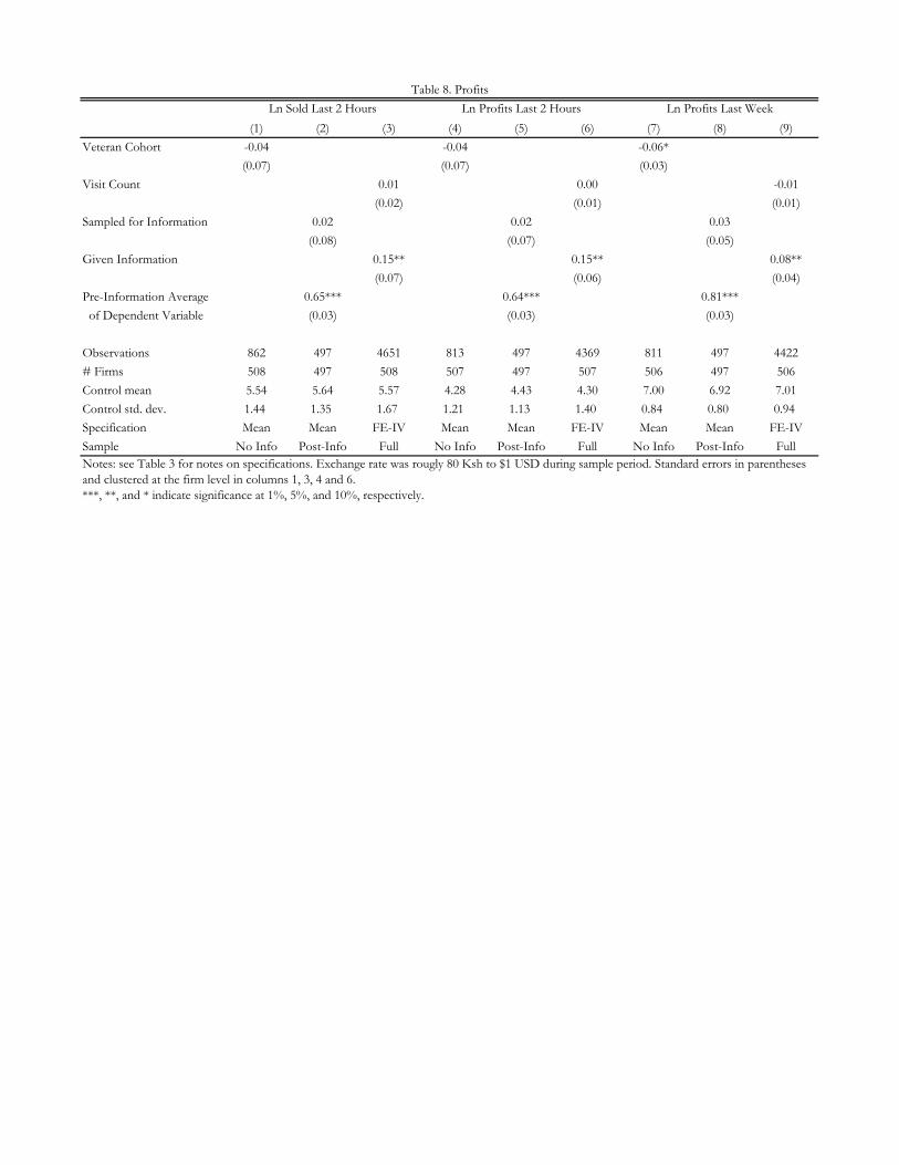
(1) (2) (3) (4) (5) (6) (7) (8) (9)

Veteran Cohort -0.04 -0.04 -0.06*

(0.07) (0.07) (0.03)

Visit Count 0.01 0.00 -0.01

(0.02) (0.01) (0.01)

Sampled for Information 0.02 0.02 0.03

(0.08) (0.07) (0.05)

Given Information 0.15** 0.15** 0.08**

(0.07) (0.06) (0.04)

Pre-Information Average 0.65*** 0.64*** 0.81***

of Dependent Variable (0.03) (0.03) (0.03)

Observations 862 497 4651 813 497 4369 811 497 4422

# Firms 508 497 508 507 497 507 506 497 506

Control mean 5.54 5.64 5.57 4.28 4.43 4.30 7.00 6.92 7.01

Control std. dev. 1.44 1.35 1.67 1.21 1.13 1.40 0.84 0.80 0.94

Specification Mean Mean FE-IV Mean Mean FE-IV Mean Mean FE-IV

Sample No Info Post-Info Full No Info Post-Info Full No Info Post-Info Full

Ln Sold Last 2 Hours Ln Profits Last 2 Hours Ln Profits Last Week

Table 8. Profits

Notes: see Table 3 for notes on specifications. Exchange rate was rougly 80 Ksh to $1 USD during sample period. Standard errors in parentheses and clustered at the firm level in columns 1, 3, 4 and 6.***, **, and * indicate significance at 1%, 5%, and 10%, respectively.

(1) (2)Mean N

Panel A. Information DebriefingAfter going through this calculation: Would you say that change is a bigger problem than you thought? 0.83 48 Would you say that holding more change has higher returns 0.84 45 than the next-best alternative?

Do you plan to change your behavior? 0.85 48If yes, how: Get change in the evening before going home 0.23 43 Get change in the morning before work 0.09 43 Get change in advance of running out during the day 0.28 43 Hold more cash in change (and invest less in something else) 0.12 43 Get change more regularly during day 0.28 43

Panel B. Endline SurveyHave the visits changed your thinking? 0.86 189Have the visits changed your behavior? 0.75 189

If yes, how? Get change in the morning 0.25 142 Get change in the evening 0.12 142 Bring more change to work 0.47 142 Stock less inventory 0.00 142 Manage change better 0.06 142 Give out less change 0.42 142 Give out less credit because don't have enough change 0.11 142

Are you less likely to give out change now? 0.36 188

Do you think you made more money after changing 0.62 186 behavior?If so, how? More sales 0.50 116 More big sales 0.22 116 Lose less customers leaving shop unattended 0.60 116 Greater customer loyalty 0.07 116 Give out less credit 0.28 116

Do you think you made more money immediately? 0.70 116Did you lose some money in adjusting behavior? 0.03 116Is deciding how much change to bring difficult? 0.23 186Have you started paying attention less to something else? 0.01 188

Notes: Data in Panel A collected at endline at conclusion of project. Data in Panel B from debriefing after information intervention. Note that the debriefing was conducted only with firms in the later part of the sample.

Table 9. Evidence from Information Debriefing and Semi-Structured Endline

Figure 1. Trends in Changeouts by Visit Number

.2.3

.4.5

.6

1 2 3 4 5 6 7 8 9 10 11 12Visit number

Average 95% CI

Had a changeout

11.

52

2.5

1 2 3 4 5 6 7 8 9 10 11 12Visit number

Average 95% CI

Ln lost profit from changeouts

2.5

Number of lost salesfrom changeouts

618

Times had to fetch change

Notes: The figures show plots of regressions of the variable described in the figure title on dummy variables for visit count from 1 to 12. The figures were restricted to 12 visits since that was the mean number of visits to a firm - there are fewer observations with visits >12 - and for space considerations.

.51

1.5

2

1 2 3 4 5 6 7 8 9 10 11 12Visit number

Average 95% CI

810

1214

1

1 2 3 4 5 6 7 8 9 10 11 12Visit number

Average 95% CI

(1) (2) (3) (4) (5) (6) (7) (8) (9)

Veteran Cohort -0.32*** -0.25*** -0.21*

(0.12) (0.09) (0.12)

Visit Count -0.10*** -0.08*** -0.01

(0.03) (0.03) (0.04)

Sampled for Information -0.42*** -0.32*** -0.34**

(0.14) (0.11) (0.17)

Given Information -0.54*** -0.42*** -0.43**

(0.14) (0.11) (0.21)

Pre-Information Average 0.52*** 0.50*** 0.37***

of Dependent Variable (0.04) (0.04) (0.05)

Observations 866 497 4814 863 497 4792 648 293 1981

# Firms 508 497 508 508 497 508 436 293 388

Control mean 2.69 2.09 2.89 2.02 1.56 2.14 1.61 1.56 1.89

Control std. dev. 2.19 1.97 2.83 1.73 1.51 2.22 2.00 1.76 2.44

Specification Mean Mean FE-IV Mean Mean FE-IV Mean Mean FE-IV

Sample No Info Post-Info Full No Info Post-Info Full No Info Post-Info Full

Ln Value Lost Sales Ln Value Lost Profits

Appendix Table A1. Value of Lost Sales

Lost Sales Cash on Hand

Notes: see Table 3 for notes on specifications. The exchange rate was rougly 80 Ksh to $1 USD during sample period. Standard errors in parentheses and clustered at the firm level in columns 1, 3, 4, 6, 7 and 9.***, **, and * indicate significance at 1%, 5%, and 10%, respectively.

(1)

Appendix Table A2. Attrition

(1)

Successfully surveyed

Panel A. Fixed Effects

Successfully surveyed

Panel A. Fixed EffectsPlanned Visit Number 0.01

(0 02)(0.02)Given Information 0.01

(0.01)Observations 5180Observations 5180 # Firms 508 Mean of dependent variable 0.93

(1) (2)(1) (2)

Successfully surveyed at least once

Panel B. Simple MeansSampled for Information 0 01Sampled for Information 0.01

(0.01)Veteran cohort 0.02*

(0.01)( )Constant 0.97*** 0.96***

(0 01) (0 01)(0.01) (0.01)Sample Post-information FullObservations 508 916Notes: The dependent variable in Panel A is whether the firm was successfully surveyed thatNotes: The dependent variable in Panel A is whether the firm was successfully surveyed that week. Regressions include week*month fixed effects. In Panel B, Column 1 is restricted to weeks after the information intervention was given and Column 2 includes all weeks Thereweeks after the information intervention was given and Column 2 includes all weeks. There are 916 observations in Column 2 because all 508 firms could have appeared as novice cohorts but only 408 could appear as veteran cohorts (since 100 firms were enrolled at the endcohorts but only 408 could appear as veteran cohorts (since 100 firms were enrolled at the end of the study windows). Standard errors in parentheses and are clustered at the firm level in P l A d C l 2 f P l BPanel A and Column 2 of Panel B. ***, **, and * indicate significance at 1%, 5%, and 10%, respectively.

(2)

Sampled for Information 0.95***(0.01)

Constant 0.00(0.01)

Observations 508R-squared 0.92

Appendix Table A3. First stage for Information Intervention

Received Information

Notes: the dependent variable is whether the firm actually received the information intervention.Standard errors in parentheses. *** indicates significance at 1%.

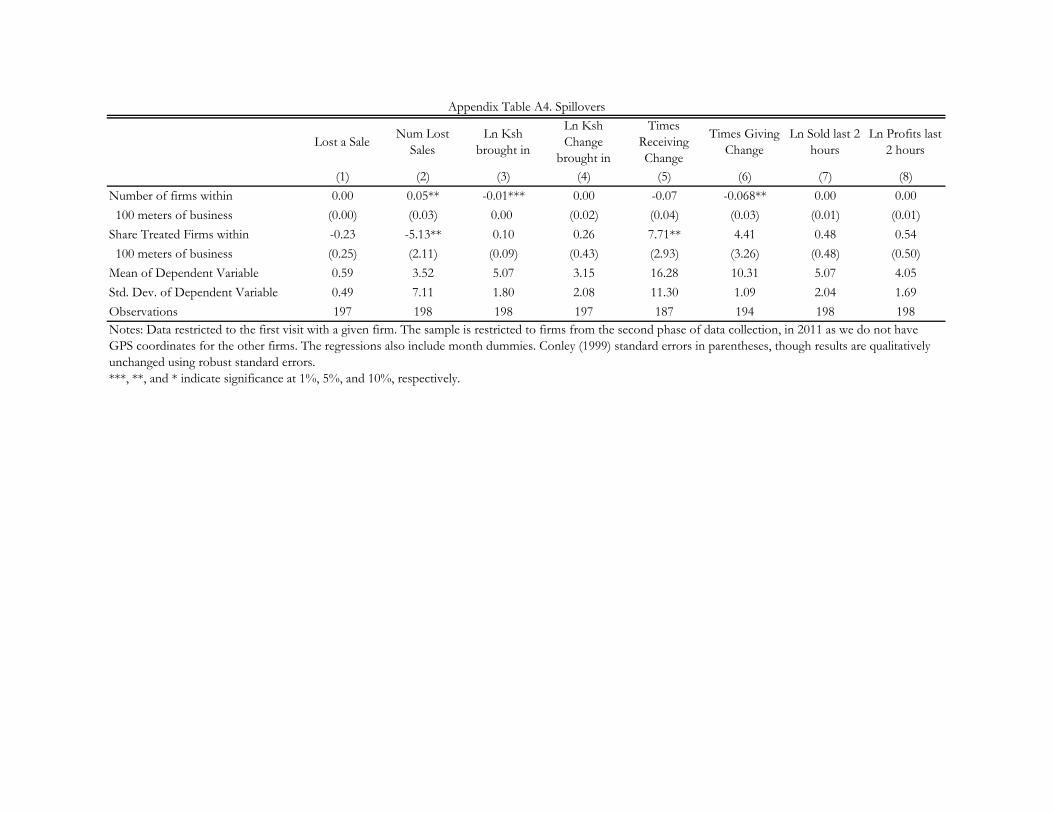
Lost a SaleNum Lost

SalesLn Ksh

brought in

Ln Ksh Change

brought in

Times Receiving Change

Times Giving Change

Ln Sold last 2 hours

Ln Profits last 2 hours

(1) (2) (3) (4) (5) (6) (7) (8)

Number of firms within 0.00 0.05** -0.01*** 0.00 -0.07 -0.068** 0.00 0.00

100 meters of business (0.00) (0.03) 0.00 (0.02) (0.04) (0.03) (0.01) (0.01)

Share Treated Firms within -0.23 -5.13** 0.10 0.26 7.71** 4.41 0.48 0.54

100 meters of business (0.25) (2.11) (0.09) (0.43) (2.93) (3.26) (0.48) (0.50)

Mean of Dependent Variable 0.59 3.52 5.07 3.15 16.28 10.31 5.07 4.05

Std. Dev. of Dependent Variable 0.49 7.11 1.80 2.08 11.30 1.09 2.04 1.69

Observations 197 198 198 197 187 194 198 198

Appendix Table A4. Spillovers

Notes: Data restricted to the first visit with a given firm. The sample is restricted to firms from the second phase of data collection, in 2011 as we do not have GPS coordinates for the other firms. The regressions also include month dummies. Conley (1999) standard errors in parentheses, though results are qualitatively unchanged using robust standard errors.***, **, and * indicate significance at 1%, 5%, and 10%, respectively.

(1)Mean

How do you save money from the business? Bank 0.31 ROSCA 0.56 Home 0.57 M-Pesa 0.22 Other 0.03

What do you do with the cash at the end of the day? Bring home 0.76 Put in bank 0.05 Put in ROSCA 0.31 Put in mobile money account 0.13 Buy items 0.58 Restock 0.31 Other 0.05

When do you deposit money into the savings product? End of day 0.41 Next day 0.05 Later in week 0.46 Later in month 0.08 Do you find it hard to save money? 0.58Do you have full control over your money? 0.90Do you mentally separate business and personal money? 0.64Do you physically separate business and personal money? 0.05Do you consume more when your business has a good day? 0.87Do you have another source of income? 0.29Do you have a mobile money account? 0.77

Appendix Table A5. Cash Management

Notes: Data from semi-structured endline interview. Ther are 238 observations for most variables though the exact sample size differs from question to question.

(1) (2)Mean N

Panel A. Costs of ChangeoutsDo customers ever buy more when you run out of change? 0.28 60

What percentage of the time do customers buy more ? 0.07 17

When you run out of change, do you think the customer ever goes 0.02 60 home without buying the item?

Panel B. Other Inventory Decisions

Value of inventory (trimming top and bottom 1%)1

Wholesale 11655 455(23617)

Retail 17220 456(36437)

Did you have a stockout last week? 0.32 237

If yes, total value of lost sales from stockouts 1241 76(4623)

Notes: data from semi-structured endline interview.1There are many more observations for this variable since the other questions were only asked for a subset of the endline surveys.

Appendix Table A6. Other Information from Endline

Dep VarSold Last 2

HoursProfit Last 2

HoursProfit Last

WeekSold Last 2

HoursProfit Last 2

HoursProfit Last

Week(1) (2) (3) (4) (5) (6)

Visit Count 12.73 -0.28 -14.51 -6.09 -0.82 -18.58

(21.75) (2.38) (12.65) (15.39) (2.37) (12.40)

Given Information 89.53 21.64 97.01 158.10* 26.03* 90.92

(92.26) (14.60) (59.84) (82.37) (14.37) (57.33)

Observations 4801 4488 4522 4690 4407 4444

# Firms 508 507 507 497 497 497

Control mean 681.49 139.15 1566.64 627.44 136.83 1532.72

Control std. dev. 1308.14 165.43 1361.77 1122.72 164.23 1317.81

Specification FE-IV FE-IV FE-IV FE-IV FE-IV FE-IV

Appendix Table A7. Additional Profit Estimates

Full Data Omitting top 2% of Firms

Notes: see Table 3 for notes on specifications. Exchange rate was rougly 80 Ksh to $1 USD during sample period. Standard errors in parentheses and are clustered at the firm level.***, **, and * indicate significance at 1%, 5%, and 10%, respectively. Top 2% of firms is relative to mean weekly profits. The top 2% of firms make over 5500 KSH/week.