MIMO PID tuning via iterated LMI restrictionboyd/papers/pdf/mimo_pid_… · · 2016-08-23INTERNATIONAL JOURNAL OF ROBUST AND NONLINEAR CONTROL Int. J. Robust Nonlinear Control 2016;

INTERNATIONAL JOURNAL OF ROBUST AND NONLINEAR CONTROLInt. J. Robust Nonlinear Control 2016; 26:1718–1731Published online 25 June 2015 in Wiley Online Library (wileyonlinelibrary.com). DOI: 10.1002/rnc.3376

MIMO PID tuning via iterated LMI restriction

Stephen Boyd1, Martin Hast2,*,† and Karl Johan Åström2

1Electrical Engineering, Stanford University, Stanford, CA, 94305, USA2Department of Automatic Control, Lund University, SE-22100, Lund, Sweden

SUMMARY

We formulate multi-input multi-output proportional integral derivative controller design as an optimizationproblem that involves nonconvex quadratic matrix inequalities. We propose a simple method that replacesthe nonconvex matrix inequalities with a linear matrix inequality restriction, and iterates to convergence.This method can be interpreted as a matrix extension of the convex–concave procedure, or as a particularmajorization–minimization method. Convergence to a local minimum can be guaranteed. While we do notknow that the resulting controller is globally optimal, the method works well in practice, and provides asimple automated method for tuning multi-input multi-output proportional integral derivative controllers.The method is readily extended in many ways, for example, to the design of more complex, structuredcontrollers. Copyright © 2015 John Wiley & Sons, Ltd.

Received 5 March 2015; Revised 21 May 2015; Accepted 28 May 2015

KEY WORDS: MIMO PID; controller design; linear matrix inequalities; convex optimization

1. INTRODUCTION

Single-input single-output (SISO) proportional integral derivative (PID) control is the automaticcontrol scheme most widely used in practice, with a long history going back at least 250 years; see[1, Section 1.4]. It has only three parameters to tune, and achieves reasonable or good performanceon a wide variety of plants. The effect of the tuning parameters (or gains) on the closed-loop perfor-mance is well-understood, and there are well-known simple rules for tuning these parameters; see,for example, [1, Chap. 6] or [2]. Systems for automatically tuning SISO PID controllers have beendeveloped, and are available in commercial controllers [1, 3–5]. The authors of this paper recentlydeveloped yet another SISO PID tuning method in [6], which is a precursor for the method describedin this paper.

Single-input single-output PID controllers have been used for multiple-input multiple-output(MIMO) plants for many years. This is generally carried out by pairing inputs (actuators) and out-puts (sensors), and connecting them with SISO PID controllers. These SISO PID controllers canbe tuned one at a time (in ‘successive loop closure’) using standard SISO PID tuning rules. ForMIMO plants that are already reasonably well-decoupled, multi-loop SISO PID design can workwell. Unlike SISO PID design, however, MIMO PID design is more complex; the SISO loops haveto be chosen carefully, and then tuned the correct way in the correct order.

An alternative to multi-loop SISO PID control is to design one MIMO PID controller, whichuses matrix coefficients, all at once. Such a controller potentially uses all sensors to driveall actuators, but it is possible to specify a simpler structure by imposing a sparsity con-straint on the controller gain matrices. Like SISO PID controllers for SISO plants, MIMO PID

*Correspondence to: Martin Hast, Department of Automatic Control, Lund University, Box 118, SE-22100, Lund,Sweden.

†E-mail: [email protected]

Copyright © 2015 John Wiley & Sons, Ltd.

MIMO PID TUNING VIA ITERATED LMI RESTRICTION 1719

controllers can achieve very good performance on a wide variety of MIMO plants, even whenthe plant dynamics are quite coupled. The challenge is in tuning MIMO PID controllers, whichrequire the specification of three matrices, each with a number of entries equal to the num-ber of plant inputs times the number of plant outputs. For example, a MIMO PID controllerfor a plant with four inputs and four outputs requires the specification of up to 48 param-eters. This would be very difficult, if not impossible, to tune by hand one parameter at atime. Hand tuning a MIMO PID controller with 10 inputs and 10 outputs would be impossiblein practice.

In this paper, we describe a method for designing MIMO PID controllers. The method is basedon solving a small number of convex optimization problems, specifically semidefinite programs(SDPs), which can be carried out efficiently. Our method is a local optimization method, and wecannot guarantee that it finds the globally optimal controller parameter values. On many examples,however, the method seems to work very well.

We first describe a basic form for the method. We impose constraints on the sensitivity andcomplementary sensitivity transfer functions, which guarantees closed-loop stability and a MIMOstability margin, and also a limit on actuator effort. The objective is to minimize the low-frequencysensitivity of the closed-loop system, which is an MIMO analog of maximizing the integral gainin the SISO case. In a later section, we describe a number of generalizations of the method. Theseoptimization problems could be solved using other methods, for example, [7] and its references fora number of H1 synthesis approaches.

There is an enormous literature on automated SISO PID tuning, and a very large literature onMIMO PID tuning (e.g., [8] and its references or [9, 10]) including some methods that are veryclose to the one we describe, and others that are close in spirit. We give a more detailed techni-cal analysis of other methods in Section 6.4, after describing the details of our method. But wemention here some earlier work that is very closely related to ours. In [11], the authors also forma linear matrix inequality (LMI)-based restriction of a problem with nonconvex quadratic matrixinequalities, and iterates to convergence. Another previous work that is close in spirit to ours isin [12], which formulates the design problem as involving bilinear matrix inequalities (BMIs),which are in turn solved (approximately) by iteratively solving a set of SDPs. (The connectionbetween our method and BMI formulations will be discussed in Section 6.4.) The closest priorwork appears in [13], which takes a very similar approach to ours. The authors consider MIMOPID design, using frequency-domain specifications, and their algorithm involves LMI restrictionsof nonconvex matrix inequalities, as our method does. We will discuss some of the differences inSection 6.4.

2. MODEL AND ASSUMPTIONS

2.1. Plant

The linear time-invariant plant has m inputs (actuators) and p outputs (sensors), and is givenby its transfer function P.s/ 2 Cp�m or more specifically by its frequency response P.i!/,for ! 2 RC. We do not assume that P is rational; it can, for example, include transportdelay. We assume that the entries of the plant input u.t/ 2 Rm are measured in appropriateunits (or scaled), so their sizes are (roughly) the same order. We make the same assumptionabout the plant output y.t/ 2 Rp . These assumptions justify the use of the (unweighted)`2-norm to measure the actuator effort and deviation of the plant outputs from the refer-ence signal, and more generally, it justifies the use of (unweighted) matrix norms to measureclosed-loop gains.

We make several assumptions about the plant. We assume that p 6 m, that is, there are at least asmany actuators as plant outputs, and that P.0/ is full rank. This makes it possible to achieve perfectreference tracking in steady state (s D 0). We will also assume that the plant is stable and strictlyproper, that is, P.s/ ! 0 as s ! 1. Most of our assumptions can be relaxed or extended to moregeneral settings, but our goal is to keep the ideas simple for now. We will discuss various ways theseassumptions can be relaxed in Section 7.

Copyright © 2015 John Wiley & Sons, Ltd. Int. J. Robust Nonlinear Control 2016; 26:1718–1731DOI: 10.1002/rnc

1720 S. BOYD, M. HAST AND K. J. ÅSTRÖM

Figure 1. Classical feedback interconnection.

2.2. Proportional integral derivative controller

The controller is a PID controller, given by

C.s/ D KP C1

sKI C

s

1C �sKD;

where KP; KI; KD 2 Rm�p are the proportional gain matrix, integral gain matrix, and derivativegain matrix, respectively. The 3mp entries in these matrices are the design parameters we are tochoose. The constant � > 0 is the derivative action time constant, and is assumed to be fixed andresponsibly chosen, for example, a modest fraction of the desired closed-loop response time.

The plant and controller are connected in the classical loop shown in Figure 1, described bythe equations

e D r � y; u D Ce; y D P.uC d/;

where r is the reference input, e is the error, and d is an input-referred plant disturbance. The signalsu and y are the plant input and output, respectively.

2.3. Closed-loop transfer functions

We will be interested in several closed-loop transfer functions that we describe here.

Sensitivity. The transfer function from reference input r to error e is the sensitivity S D .I CPC/�1. The size of S gives a measure of the tracking error; for low frequencies, S should besmall. When S.0/ D 0 (a constraint we will impose), we have perfect static tracking. The maximumsize of S , which occurs near the crossover frequency, is closely related to closed-loop damping andsystem stability.Q-parameter. The transfer function from r to u is denoted Q, defined as Q D C.I C PC/�1.Its size is a measure of the actuator effort. (We use Q to match the notation often used in Youla’sparametrization of closed-loop transfer functions; see [14].)Complementary sensitivity function. The complementary sensitivity function is T D PC.I CPC/�1. It is the closed-loop transfer function from r to y. It is near the identity for low frequencies,and will be small for high frequencies; its maximum size is also related to closed-loop damping.

These three closed-loop transfer functions are sufficient to guarantee a sensible controller design(because P is assumed stable). They are related in various ways, for example, we have

S C T D I; T D PQ; Q D CS:

Other closed-loop transfer functions. Several other closed-loop transfer functions can also be con-sidered. For example, the closed-loop transfer function from the plant disturbance d to the trackingerror e isR D �.ICPC/�1P . It will be clear how our approach extends to other transfer functions.

2.4. Notation

For a complex matrix Z 2 Cp�q , Z� is its (Hermitian) conjugate transpose, kZk denotes thespectral norm, that is, the maximum singular value. For full rank Z, we let �min.Z/ denote itsminimum singular value. A square matrix is Hermitian if Z D Z�. Between Hermitian matrices,the symbol� 0 is used to denote matrix inequality, soZ � 0means thatZ is Hermitian and positivesemidefinite. We use the notation Z�� D .Z�/�1.



For a p � q transfer function H , kHk1 is its H1-norm, kHk1 D sup<s>0 kH.s/k, which canbe expressed as

kHk1 D sup!>0kH.i!/k;

when H is stable (i.e., H 2 Hp�q1 ).

3. DESIGN PROBLEM

3.1. Objective and constraints

Sensitivity and complementary sensitivity peaking. We require kSk1 6 Smax, where Smax > 1.Reasonable values of Smax are in the range 1.1 to 1.6; lower values give a more damped closed-loopsystem. This constraint ensures closed-loop stability. We also require kT k1 6 Tmax, with Tmax > 1.Reasonable values of Tmax are similar to those for Smax.Static and low-frequency sensitivity. Assuming that P.0/KI is nonsingular, we have S.0/ D 0,which means that we have zero error for constant reference signals. The next term in the expansionof the sensitivity near s D 0 is S.s/ � s.P.0/KI/

�1 for jsj small. Our objective will be to attainthe best possible low-frequency sensitivity, which means that we will minimize k.P.0/KI/

�1k. Thisobjective indirectly imposes the condition that we achieve perfect tracking because when it is finite,we have P.0/KI nonsingular.Actuator authority limit. We require that kQk1 6 Qmax. This sets a maximum value for the size ofthe closed-loop actuator signal in response to the reference signal. Because the plant is stable, thisconstraint ensures that the closed-loop system is stable; see [14].

We can determine a reasonable value forQmax as follows. Any controller that has a finite objectivevalue (i.e., achieves perfect reference tracking at s D 0) satisfies T .0/ D I D P.0/Q.0/; this hasthe simple interpretation that at s D 0, the controller inverts the plant. It follows that kQ.0/k >1=�min.P.0//, from which we conclude that kQk1 > 1=�min.P.0//. Thus, we must have Qmax >1=�min.P.0//. The right-hand side can be interpreted as the minimum actuator effort (measuredby kQk1) required to achieve static tracking. A reasonable value for Qmax is therefore a modestmultiple of 1=�min.P.0//, say, 3 to 10.Design problem. Putting it all together, we obtain the problem

minimize k.P.0/KI/�1k;

subject to kSk1 6 Smax;

kT k1 6 Tmax;

kQk1 6 Qmax:

(1)

The variables to be chosen are the coefficient matrices KP; KI; KD; the problem data are the planttransfer function P , the controller derivative time constant � , and the design parameters Smax, Tmax,andQmax. This problem is not convex because the cost function and constraints are not affine expres-sions of the coefficient matrices. Note that the objective contains the implied constraint that P.0/KI

is invertible, which implies that perfect static tracking is achieved for constant reference inputs.

3.2. Sampling semi-infinite constraints

The constraints on the closed-loop transfer functions can be expressed as, for example,

kS.i!/k 6 Smax; 8! > 0:

This is a so-called semi-infinite constraint, because it consists of an infinite number of constraints,one for each ! > 0. Semi-infinite constraints such as these (with one parameter, !) are readilyhandled by choosing a reasonable finite (but large) set of frequency samples 0 < !1 < � � � < !K ,and replacing the semi-infinite constraints with the finite set of constraints at each of the givenfrequencies. For example, we replace the constraint kSk1 6 Smax with kS.i!k/k 6 Smax,k D 1; : : : ; N . Our optimization method has a computational complexity that grows linearly with



N , so we can choose a large enough value of N (say, several hundred or more) that this sam-pling has no practical effect. By ‘reasonable’, we mean that the frequency sampling is fine enoughto catch any rapid changes in the closed-loop transfer function with frequency, and also cover anappropriate range; in particular, we assume that at !1 and !N , the transfer functions are near theirasymptotic values,

S.0/ D 0; T .0/ D I; Q.0/ D KI.P.0/KI/�1

and

S.1/ D I; T .1/ D 0; Q.1/ D KP C .1=�/KD;

respectively.We will use subscripts to denote a transfer function evaluated at the frequency s D i!k . For

example, Pk D P.i!k/, which is a (given) complex matrix. Note that the quantity Ck D C.i!k/

is a complex matrix, and is an affine function of the design variables KP; KP; KD. (We will use thisobservation to arrive at the LMI restriction in Section 5.)

The sampled problem is then

minimize k.P.0/KI/�1k;

subject to kSkk 6 Smax;

kTkk 6 Tmax;

kQkk 6 Qmax;

k D 1; : : : ; N:

(2)

This problem has 3N constraints, each of which has the form of a matrix norm inequality. Thearguments of the matrix norm inequalities, however, are complex functions of the design variablesKP; KI; KD, given by the various formulas for the closed-loop transfer functions.

4. QUADRATIC MATRIX INEQUALITY FORM

In this section, we show how the (frequency sampled) design problem (2) can be casted in a simpleform in which every constraint has the same quadratic matrix inequality (QMI) form

Z�Z � Y �Y; (3)

where both Z and Y are affine functions of the variables.We start with the objective. First, we note that we can just as well maximize �min.P.0/KI/ D

1=k.P.0/KI/�1k. We introduce a new scalar variable t , which we maximize subject to

�min.P.0/KI/ > t . (This is the standard epigraph transformation; see [15, Section 4.2.4].) We thenobserve that

�min.P.0/KI/ > t , .P.0/KI/�.P.0/KI/ � t

2I;

which has the form (3) with Z D P.0/KI and Y D tI , both of which are affine functions of thevariables.

Now, consider the sensitivity peaking limit kSkk 6 Smax. As mentioned earlier, we have

kSkk 6 Smax , .I C PkCk/��.I C PkCk/

�1 � S2maxI

, .I C PkCk/�.I C PkCk/ � .1=S

2max/I;

where in the second line, we have multiplied the left and right sides by .I C PkCk/� and by .I CPkCk/, respectively. This has the QMI form (3) with Z D I C PkCk and Y D .1=Smax/I .

For the complementary sensitivity constraint kTkk 6 Tmax, we have

kTkk 6 Tmax , .I C P �k C�k /�1C �k P

�k PkC.I C PkCk/

�1 � T 2maxI

, .I C PkCk/�.I C PkCk/ � .1=T

2max/.PkCk/

�.PkCk/:



This has the QMI form (3) with Z D I C PkCk and Y D .1=Tmax/PkCk .In a similar way, we have

kQkk 6 Qmax , .I C PkCk/�.I C PkCk/ � .1=Q

2max/C

�k Ck;

which has the QMI form with Z D I C PkCk and Y D .1=Qmax/Ck .We arrive at a problem with the form

maximize tsubject to Z�

kZk � Y

�kYk; k D 1; : : : ;M; (4)

with variables t , KP; KI; KD. (Here, we have M D 3N C 1.) This is the PID controller designproblem in QMI form.

5. LINEAR MATRIX INEQUALITY RESTRICTION

We first show how to form an (convex) LMI restriction for the QMI Z�Z � Y �Y . (See [16] forbackground on matrix inequalities.) The QMI is already convex in Y , so we can focus on Z. Westart with the simple matrix inequality

0 � .Z � QZ/�.Z � QZ/ D Z�Z �Z� QZ � QZ�Z C QZ� QZ;

valid for any matrices Z and QZ. Re-arranging, we obtain

Z�Z � Z� QZ C QZ�Z � QZ� QZ:

The left-hand side is a quadratic function of Z; the right-hand side is an affine function of Z. Itfollows that the matrix inequality

Z� QZ C QZ�Z � QZ� QZ � Y �Y;

which is convex in .Z; Y /, implies Z�Z � Y �Y ; that is, it is a convex restriction of the QMI. Wecan write this convex QMI as an LMI

�Z� QZ C QZ�Z � QZ� QZ Y �

Y I

�� 0: (5)

(Here, Z and Y are the variables; QZ is an arbitrary matrix.) For any matrix QZ, the LMI (5) impliesthe QMI Z�Z � Y �Y . We call it the LMI restriction of the QMI, obtained at point QZ.

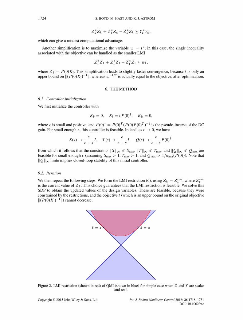
The LMI restriction of the QMI is illustrated in Figure 2, for the simple case of real scalar Z andY . In this case, the QMI is ´2 > y2, which gives the two lightly shaded cones in the figure, withblue boundary. The LMI restriction at Q́ is given by 2 Q́´ � Q́2 > y2, shown as the shaded regionbounded by the parabola, with red boundary. The two boundaries touch at the point where ´ D Q́ .

Now, consider the QMI form PID controller design problem (4). Given any matrices QZ1; : : : ; QZM ,we can form the LMI restricted problem

maximize t

subject to

�Z�kQZk C QZ

�kZk � QZ

�kQZk Y

�k

Yk I

�� 0; k D 1; : : : ;M: (6)

This problem has linear objective and LMI constraints, and so is an SDP [17]. It is readily solved(globally). Note that any solution of the LMI restriction is feasible for the QMI problem. The LMIrestriction, however, need not be feasible; this depends on the choice of QZk .

Simplifications. In the inequalities associated with Sk , the matrix Yk does not depend on thecontroller parameters (i.e., is constant). In this case, we can work directly with the smaller(equivalent) LMIs



Z�kQZk C QZ

�kZk �

QZ�kQZk � Y

�k Yk;

which can give a modest computational advantage.

Another simplification is to maximize the variable w D t2; in this case, the single inequalityassociated with the objective can be handled as the smaller LMI

Z�1QZ1 C QZ

�1Z1 �

QZ�1QZ1 � wI;

where Z1 D P.0/KI. This simplification leads to slightly faster convergence, because t is only anupper bound on k.P.0/KI/

�1k, whereas w�1=2 is actually equal to the objective, after optimization.

6. THE METHOD

6.1. Controller initialization

We first initialize the controller with

KP D 0; KI D �P.0/�; KD D 0;

where � is small and positive, and P.0/� D P.0/T .P.0/P.0/T /�1 is the pseudo-inverse of the DCgain. For small enough �, this controller is feasible. Indeed, as � ! 0, we have

S.s/!s

� C sI; T .s/!

�

� C sI; Q.s/!

�

� C sP.0/�;

from which it follows that the constraints kSk1 6 Smax, kT k1 6 Tmax, and kQk1 6 Qmax arefeasible for small enough � (assuming Smax > 1, Tmax > 1, and Qmax > 1=�min.P.0//). Note thatkQk1 finite implies closed-loop stability of this initial controller.

6.2. Iteration

We then repeat the following steps. We form the LMI restriction (6), using QZk D Zcurrk

, where Zcurrk

is the current value of Zk . This choice guarantees that the LMI restriction is feasible. We solve thisSDP to obtain the updated values of the design variables. These are feasible, because they wereconstrained by the restrictions, and the objective t (which is an upper bound on the original objectivek.P.0/KI/

�1k) cannot decrease.

Figure 2. LMI restriction (shown in red) of QMI (shown in blue) for simple case when Z and Y are scalarand real.



6.3. Convergence

The iterates are all feasible (and we have closed-loop stability since kQk1 is finite), and the objectiveis nonincreasing. Because it is non-negative, the objective converges. We can stop when not muchprogress is being made, which is typically after 10 or fewer iterations. At convergence, the optimalvalue of t , which is in general an upper bound on the original objective k.P.0/KI/

�1k, is actuallyequal to this value. (When we optimize with the variable w, it is directly equal to the objective.)

6.4. Connections, interpretations, and prior work

Our method is similar to, but not the same as, the convex–concave method for the SISO casedescribed in [6]. In that paper, we linearize a scalar inequality of the form jZj > jY j, which is notthe same as linearizing (as we do here) the quadratic inequality jZj2 > jY j2. The idea of lineariz-ing concave terms in an otherwise convex optimization problem, which gives a convex restriction,is an old one that has been (re-)invented many times, for many applications; see, for example, thereferences in [18] or [19]. The idea of linearizing a matrix inequality is given in [18].

The convex–concave procedure is in turn a special case of a very general method for finding alocal minimum of a nonconvex optimization problem. In each iteration, we replace the objectivefunction and each constraint function by a convex majorization that is tight at the given point, andsolve the resulting convex problem. This idea traces back at least to 1970 [20], and has been widelyused since then; see [18].

There is also a very close connection of our method to BMIs and methods for them, such asalternating minimization over the two groups of variables. The connection is easiest to see and stateswhen Z and Y have the same dimensions (in general, the inequality Z�Z � Y �Y implies that theyhave the same number of columns). Define

U D .1=2/.Z C Y /; V D .1=2/.Z � Y /;

so Z D U C V and Y D U � V . Then we have

Z�Z � Y �Y , .U C V /�.U C V / � .U � V /�.U � V /

, U �U C V �U C U �V C V �V � U �U � V �U � U �V C V �V

, V �U C U �V � 0;

which we recognize as a BMI in U and V . Thus, our QMI can be expressed as an equivalent BMI.MIMO PID design via BMIs is discussed in [12].

The closest prior work is [13], which contains many of the ideas we use in the present paper. Theauthors develop quadratic matrix inequalities similar to the ones we use here, and derive a methodfor MIMO PID design that uses LMI restrictions, as we do. While the two methods are clearlyclosely related, we are unable to derive our exact algorithm from theirs. We can identify severaldifferences in the approach. First, we consider separate closed-loop transfer functions (e.g., S , T ,andQ), where they lump them together into one block closed-loop transfer function. One advantageof considering these classical closed-loop transfer functions separately is that we can give simpleand universal choices for the upper bound (such as 1.4, for example, for S ). Second, we considerstable plants, which allow us to give a simple low-gain PID initialization. Finally, we consider ageneric QMI, and develop a simple universal LMI restriction, which allows us to derive a simplealgorithm for design of MIMO PID controllers that minimize low-frequency sensitivity subject toclassical constraints on S , T , and Q.

7. EXTENSIONS AND VARIATIONS

In this section, we list various extensions and variations on the MIMO PID controller design prob-lem, starting with simple ones and moving to more complex ones. While the basic iteration willwork in all of these variations, the design must start from a feasible initial controller, which may bea challenge to find, depending on the variation. (We make more specific comments about this in thesucceeding text.)



Exchanging objectives and constraints. As always, we can exchange constraints and objective; forexample, we could impose a constraint on k.P.0/KI/

�1k, and instead minimize another objective,such as kQk1. In this example, we would be minimizing actuator effort for a given fixed limit onthe low-frequency sensitivity.Frequency-dependent bounds. The bounds Smax; Tmax;Qmax could be functions of frequency. Thiscould be used to shape the various closed-loop transfer functions in more sophisticated ways thandescribed here. This extension is also used in, for example, [13].Other closed-loop transfer functions. The same approach works for other closed-loop transfer func-tions. For example, consider R D �.I CPC/�1P , which is the closed-loop transfer function fromdisturbance to error. A limit on R, say, kRk1 6 Rmax, can be expressed as a QMI as follows:

kRkk 6 Rmax , .I C PkCk/.I C PkCk/� � .1=R2max/PkP

�k ;

which has the QMI form with Z D .I C PkCk/� and Y D .1=Rmax/P

�k

. (Note the Hermitianconjugates in this case.) (The method proposed in [13] can also accommodate constraints on theseother transfer functions.)Low-frequency disturbance optimization. We can optimize low-frequency values ofR instead of S .At low frequencies, we have

R.s/ D �S.s/P.s/ � �s.P.0/KI/�1P.0/;

and we arrive at a very similar problem, which is also easily expressed in our QMI form.High-frequency roll-off. Our method relies only on the fact that C.s/ is a linear function of thedesign variables KP; KI; KD. This allows us to use many other variations on the PID controller. Asan example of simple variation that is very useful in practice, we can use the controller

C.s/ D

�1

1C s� C .s�/2=2

��KP C

1

sKI C sKD

�;

where � > 0 is a (fixed) time constant. Here, we have an ideal PID controller, with a second-orderhigh-frequency roll-off.Unstable plants. The method can be extended to handle unstable plants, but in this case, the initialcontroller must stabilize and also satisfy the constraints; see, for example, [6]. (To satisfy the con-straints, they can initially be relaxed.) When initialized this way, all iterates (and the final controllerdesign) will be stabilizing. More sophisticated methods (say, with the addition of slack variables)could handle the case when an initial stabilizing controller is not known; for example, the methodpresented in [13] handles unstable plants.More outputs than actuators. We can handle the case when p > m (more outputs than actuators),so perfect static tracking cannot be achieved. In this case, we cannot have zero sensitivity at s D 0,but we can optimize over the value of S.0/, for example, minimize or limit its norm.Convex constraints on controller parameters. Any convex constraints on the controller parameterscan be imposed. For example, we can limit the values of any of the coefficients. A very interestingoption here is to limit the sparsity pattern of C by requiring some entries to be zero. This givesstructured MIMO PID controller design [21].

The simple initialization method described in Section 6.1 will generally not work when thecontroller parameters are constrained, for example, when a specific sparsity pattern is imposed.Convex cost terms. We can add any convex function of the controller parameters to the objective.For example, we can add regularization to the objective, that is, a function that encourages thecontroller parameters to be small. The classical example is the sum of squares term

�Xij

�.KP/

2ij C .KI/

2ij C .KD/

2ij

�;



where � > 0 is a parameter used to trade off low-frequency rejection and the size of the con-troller parameters (measured by the sum of squares). This can be useful to reduce injection ofmeasurement noise into the control loop.

A very interesting regularization is one that encourages sparsity in the controller parameters,such as

�Xij

max¹.KP/ij ; .KI/ij ; .KD/ij º:

This regularization will encourage sparsity in C.s/; for similar work; see, for example, [22] (forsparse controller design) and [23] (for sparsity of blocks of regressors in statistics).Closed-loop convex constraints. We can also add any constraint or objective term that is convex inthe closed-loop transfer functions; see the book in [14]. For example, we could include time-domainconstraints such as a maximum step response settling time. The very same method (with some addedterms to handle the added constraints) will work.Robustness to plant variations. We can wrap robustness to plant variations into the method. A par-ticularly simple (but very effective) method that gives robustness is to require that the constraintshold not only for one plant but also for several or many plausible values of the plant transfer function.This leads to a bigger problem to solve, but the same method works.More general controllers. Finally, it should be clear that, just as in the method presented in [13],our method works for any linearly parametrized controller, and not just the simple PID structurethat we have focused here. For more general structures, the design initialization can become achallenge, however.

8. EXAMPLES

In this section, we describe numerical results for a classic MIMO plant, the two-input two-outputWood–Berry binary distillation column described in [24]. The computations were carried out usingthe Matlab-based convex modeling framework CVX [25, 26] using the SDPT3 software [27, 28] forsolving the SDP.

The plant transfer function is

P.s/ D

266412:8e�s

16:7s C 1

�18:9e�3s

21:0s C 1

6:6e�7s

10:9s C 1

�19:4e�3s

14:2C 1

3775 :

Each entry is a first-order system with a time delay. The dynamics are quite coupled, so finding agood MIMO PID controller is not simple. Several design methods and actual designs for this planthave been proposed in the literature, including [29–31]. Our method produced quite similar results,with the same or better metrics judged by our objectives (naturally).

We used design parameters

Smax D 1:4; Tmax D 1:4; Qmax D 3=�min.P.0// D 0:738:

The derivative action time constant is chosen to be � D 0:3. The semi-infinite constraints are sam-pled using N D 300 logarithmically spaced frequency samples in the interval

�10�3; 103

. The

initial design uses the method described in Section 6.1 with � D 0:01.The algorithm converges in seven iterations (which takes a 153 s to run in our simple

implementation on a standard desktop computer with an Intel Core I7 processor) to the values

KP D

�0:1750 �0:0470�0:0751 �0:0709

�; KI D

�0:0913 �0:03450:0402 �0:0328

�; KD D

�0:1601 �0:00510:0201 �0:1768

�;

which achieve objective value k.P.0/KI/�1k D 2:25. The resulting closed-loop transfer function

singular values are plotted versus frequency in Figure 3, along with the imposed limits.



Figure 3. Closed-loop transfer function singular values versus frequency, with constraints shown in red.

Figure 4. Closed-loop transfer function singular values versus frequency, with constraints shown in red, fordiagonal PID design.

To demonstrate one simple extension, we also carry out MIMO PID design with the additionalconstraint that the controller is diagonal, that is, consists of two SISO PID loops. We initialize thealgorithm with low-gain PI control from y1 to u1 and from y2 to u2, using the (diagonal) controller

KP D 10�3

�1 0

0 �1

�; KI D 10

�3

�1 0

0 �1

�; KD D 0:



Figure 5. Closed-loop step response from r to y for the MIMO PID controller (blue) and the diagonal PIDcontroller (red).

Figure 6. Closed-loop step response from r to u for the MIMO PID controller (blue) and the diagonal PIDcontroller (red).

(The minus sign in the 2,2 entry is due to the negative 2,2 value of the 2,2 entry of P.0/.) Thealgorithm converges in eight iterations (taking a few minutes in our simple implementation) tothe controller

KP D

�0:1535 0

0 �0:0692

�; KI D

�0:0210 0

0 �0:0136

�; KD D

�0:1714 0

0 �0:1725

�;



which achieves objective value k.P.0/KI/�1k D 13:36, considerably worse than the objective value

obtained with a general MIMO PID controller. The resulting closed-loop transfer function singularvalues are plotted in Figure 4. We can see that low-frequency sensitivity is considerably worsethan that achieved by the full MIMO controller, for example, by noting the value of kS.!/k2 for! D 10�2.

The step responses of T , the transfer function from r to y, are plotted in Figure 5, for both thefull MIMO PID controller and the diagonal PID controller. Here, too, we can observe the worselow-frequency rejection for the diagonal PID design, for example, in the larger off-diagonal entriesof the step response.

The step responses of Q, the transfer function from r to u, are plotted in Figure 6, for both thefull MIMO PID controller and the diagonal PID controller.

9. CONCLUSIONS

In this paper, we have described a simple method for effectively designing MIMO PID controllersfor stable plants given by transfer function (at an appropriate set of frequencies). The method relieson solving a short sequence of SDPs (typically 10 or fewer), and although it cannot guaranteefinding the globally optimal design, it appears to find very good designs in practical problems. Themethod is related to several other methods for MIMO PID design, and relies on ideas that have beenused in several other contexts in optimization, such as the convex–concave procedure, and iterativeconvex restriction.

REFERENCES

1. Åström KJ, Hägglund T. Advanced PID Control. Instrumentation, Systems, and Automation Society: ResearchTriangle Park, NC, 2006.

2. Luyben WL. Simple method for tuning SISO controllers in multivariable systems. Industrial & EngineeringChemistry Process Design and Development 1986; 25(3):654–660.

3. Garpinger O, Hägglund T. A software tool for robust PID design. Proceedings 17th IFAC World Congress, Seoul,Korea, 2008; 6416–6421.

4. Garpinger O, Hägglund T, Åström KJ. Criteria and trade-offs in PID design. Ifac Conference on Advances in pidControl, Brescia, Italy, March 2012; 47–52.

5. Vilanova R, Visioli A. PID Control in the Third Millennium: Lessons Learned and New Approaches. Springer Verlag:New York, 2012.

6. Hast M, Åström K, Bernhardsson B, Boyd S. PID design by convex–concave optimization. Proceedings EuropeanControl Conference, Zürich, Switzerland, July 2013; 4460–4465.

7. Apkarian P, Noll D. NonsmoothH1 synthesis. IEEE Transactions on Automatic Control 2006; 51(1):71–86.8. Åström KJ, Panagopoulos H, Hägglund T. Design of PI controllers based on non-convex optimization. Automatica

1998; 34(5):585–601.9. Panagopoulos H, Åström KJ, Hägglund T. Design of PID controllers based on constrained optimisation.

IEE Proceedings on Control Theory and Applications 2002; 149(1):32–40.10. Saeki M, Kashiwagi K, Wada N. Design of multivariableH1 PID controller using frequency response. Proceedings

of the 2007 IEEE International Conference on Control Applications, Singapore, October 2007; 1565–1570.11. Lin C, Wang QG, Lee TH. An improvement on multivariable PID controller design via iterative LMI approach.

Automatica 2004; 40(3):519–525.12. Bianchi FD, Mantz RD, Christiansen CF. Multivariable PID control with set-point weighting via BMI optimisation.

Automatica 2008; 44(2):472–478.13. Saeki M, Ogawa M, Wada N. Low-order H1 controller design on the frequency domain by partial optimization.

International Journal of Robust and Nonlinear Control 2010; 20:323–333.14. Boyd S, Barratt C. Linear Controller Design—Limits of Performance. Prentice-Hall: Englewood Cliffs, NJ, 1991.15. Boyd S, Vandenberghe L. Convex Optimization. Cambridge University Press: Cambridge, NY, 2004.16. Boyd S, Ghaoui LE, Feron E, Balakrishnan V. Linear Matrix Inequalities in System and Control Theory, Studies in

Applied Mathematics, vol. 15. SIAM: Philadelphia, PA, 1994.17. Vandenberghe L, Boyd S. Semidefinite programming. SIAM Review March 1996; 38(1):49–95.18. Lipp T, Boyd S. Extensions and variations on the convex–concave procedure, 2014.19. Yuille A, Rangarajan A. The concave–convex procedure. Neural Computation 2003; 15(4):915–936.20. Ortega R, Rheinboldt W. Iterative Solutions of Nonlinear Equations in Several Variables. Academic Press:

New York, NY, 1970.21. Saeki M. Fixed structure PID controller design for standardH1 control problem. Automatica 2006; 42(1):93–100.



22. Lin F, Fardad M, Jovanovic M. Sparse feedback synthesis via the alternating direction method of multipliers.Proceedings of the American Control Conference, Montreal, Canada, 2012; 4765–4770.

23. Zou H, Hastie T. Regularization and variable selection via the elastic net. Journal of the Royal Statistical Society:Series B (Statistical Methodology) 2005; 67(2):301–320.

24. Wood R, Berry M. Terminal composition control of a binary distillation column. Chemical Engineering Science1973; 28(9):1707–1717.

25. Research CVX. CVX: Matlab software for disciplined convex programming, version 2.0, 2012. (Available from:http://cvxr.com/cvx) [Accessed on 1 June 2015].

26. Grant M, Boyd S. Graph implementations for nonsmooth convex programs. In Recent Advances in Learning andControl, Blondel V, Boyd S, Kimura H (eds)., Lecture Notes in Control and Information Sciences. Springer-VerlagLimited: London, 2008; 95–110.

27. Toh K-C, Todd MJ, Tütüncü RH. SDPT3—A Matlab software package for semidefinite programming, version 1.3.Optimization Methods and Software 1999; 11(1-4):545–581.

28. Tütüncü RH, Toh K-C, Todd MJ. Solving semidefinite-quadratic-linear programs using SDPT3. MathematicalProgramming 2003; 95(2):189–217.

29. Dong J, Brosilow C. Design of robust multivariable PID controllers via IMC. Proceedings of the American ControlConference 1997; 5:3380–3384.

30. Wang Q, Zou B, Lee T, Bi Q. Auto-tuning of multivariable PID controllers from decentralized relay feedback.Automatica 1997; 33(3):319–330.

31. Tan W, Chen T, Marquez H. Robust controller design and PID tuning for multivariable processes. Asian Journal ofControl 2002; 4(4):439–451.


http://cvxr.com/cvx

Documents

MIMO PID tuning via iterated LMI restrictionboyd/papers/pdf/mimo_pid_… · · 2016-08-23INTERNATIONAL JOURNAL OF ROBUST AND NONLINEAR CONTROL Int. J. Robust Nonlinear Control 2016;