Embed Size (px)
Citation preview
IMPERIAL COLLEGE LONDON
MIMO HSDPA Using System Value Approach
Hamdi Joudeh
Supervisor: DR. M.K. GURCAN
This report is submitted in partial fulfilment of the requirements for the Degree of
Master of Science (MSc) and the Diploma of Imperial College (DIC)
Department of Electrical and Electronic Engineering
Imperial College London
September 2011
Abstract
Multi-code transmission systems such as HSDPA suffer from severe throughput losses in
frequency selective channels. Energy-constrained rate optimization schemes e.g. the two-
group resource allocation algorithm, improve the performance of HSDPA in such conditions.
However, the computational complexity of such algorithms makes them unattractive solu-
tions. System value approach has been developed recently to reduce the computational
complexity required to perform energy-constrained rate optimization for multi-code trans-
mission systems. This report presents the work done on combining the two-group algorithm
improved by system value approach with MIMO HSDPA. A MIMO HSDPA model that can be
used with different MIMO pre-processing schemes and offers flexibility for resource alloca-
tion was developed. Simulations showed that system value approach significantly reduces
computational complexity. However, bit rates are slightly over-estimated due to approxi-
mation errors. This error was reduced by using optimum and suboptimal channel selec-
tion schemes which were developed to improve the throughput as well. Furthermore, the
developed channel selection schemes provided flexible selection between MIMO diversity
and spatial multiplexing and hence improved performance in MIMO channels with spa-
tial correlations. The improved MIMO HSDPA system gave up to 65% increase in average
throughput over the current standard for a typical urban channel model. Finally, the com-
putational complexity was further reduced using a combination of interference cancelation
and recursive matrix inversion calculations.
i
Contents
Abstract i
Contents ii
List of Figures v
List of Tables vi
Acknowledgement viii
Acronyms ix
Notation xi
1 Introduction 1
1.1 MIMO HSDPA . . . . . . . . . . . . . . . . . . . . . . . . . . . . . . . . . . . . 2
1.1.1 Performance In Frequency Selective Channels . . . . . . . . . . . . . . 2
1.2 Problem Overview . . . . . . . . . . . . . . . . . . . . . . . . . . . . . . . . . 3
1.2.1 Computational Complexity . . . . . . . . . . . . . . . . . . . . . . . . 3
1.2.2 System Value Approach . . . . . . . . . . . . . . . . . . . . . . . . . . 4
1.2.3 This Project . . . . . . . . . . . . . . . . . . . . . . . . . . . . . . . . . 4
1.3 Report Organization . . . . . . . . . . . . . . . . . . . . . . . . . . . . . . . . 4
2 MIMO HSDPA Model 6
2.1 System Model . . . . . . . . . . . . . . . . . . . . . . . . . . . . . . . . . . . . 6
2.1.1 MIMO Signature Sequences . . . . . . . . . . . . . . . . . . . . . . . . 7
2.1.2 MIMO Channel . . . . . . . . . . . . . . . . . . . . . . . . . . . . . . . 7
ii
CONTENTS iii
2.1.3 Received MIMO Signature Sequences . . . . . . . . . . . . . . . . . . . 8
2.1.4 Data Transmission . . . . . . . . . . . . . . . . . . . . . . . . . . . . . 10
2.1.5 MIMO Despreading Filter . . . . . . . . . . . . . . . . . . . . . . . . . 11
2.2 MIMO Radio Channel . . . . . . . . . . . . . . . . . . . . . . . . . . . . . . . 13
2.2.1 Statistical Channel Model . . . . . . . . . . . . . . . . . . . . . . . . . 14
2.2.2 Power Delay Profile . . . . . . . . . . . . . . . . . . . . . . . . . . . . . 14
2.2.3 Spatial Correlation . . . . . . . . . . . . . . . . . . . . . . . . . . . . . 15
2.2.4 Generation of a Fading Correlated MIMO Channel . . . . . . . . . . . 16
2.3 Link Level Simulation . . . . . . . . . . . . . . . . . . . . . . . . . . . . . . . 19
2.3.1 Radio Channel Model . . . . . . . . . . . . . . . . . . . . . . . . . . . 20
2.3.2 System Parameters . . . . . . . . . . . . . . . . . . . . . . . . . . . . . 21
2.3.3 Generating Multiple MIMO Channels . . . . . . . . . . . . . . . . . . . 22
3 Resource Allocation 23
3.1 MIMO HSDPA Standard . . . . . . . . . . . . . . . . . . . . . . . . . . . . . . 23
3.1.1 D-TxAA Model . . . . . . . . . . . . . . . . . . . . . . . . . . . . . . . 24
3.1.2 Precoding Weights Selection . . . . . . . . . . . . . . . . . . . . . . . . 25
3.1.3 Single-Stream Mode . . . . . . . . . . . . . . . . . . . . . . . . . . . . 26
3.1.4 Resource Allocation . . . . . . . . . . . . . . . . . . . . . . . . . . . . 27
3.1.5 Wasted SNIR . . . . . . . . . . . . . . . . . . . . . . . . . . . . . . . . 29
3.2 Constrained Optimization . . . . . . . . . . . . . . . . . . . . . . . . . . . . . 30
3.2.1 Equal-Rate Margin Adaptive Loading . . . . . . . . . . . . . . . . . . . 30
3.2.2 Residual Energy . . . . . . . . . . . . . . . . . . . . . . . . . . . . . . 31
3.2.3 Two-Group Rate Adaptive Loading . . . . . . . . . . . . . . . . . . . . 32
3.2.4 Two-Group Loading with Single-Stream Mode . . . . . . . . . . . . . . 33
3.2.5 Computational Complexity . . . . . . . . . . . . . . . . . . . . . . . . 33
3.3 Simulation and Analysis . . . . . . . . . . . . . . . . . . . . . . . . . . . . . . 34
3.3.1 Total Throughput . . . . . . . . . . . . . . . . . . . . . . . . . . . . . . 34
3.3.2 Number of Applied Channels . . . . . . . . . . . . . . . . . . . . . . . 35
3.3.3 Matrix Inversions . . . . . . . . . . . . . . . . . . . . . . . . . . . . . . 37
CONTENTS iv
4 System Values 39
4.1 Signature Sequence Design and Channel Selection . . . . . . . . . . . . . . . 39
4.1.1 Optimum MIMO Signature Sequences . . . . . . . . . . . . . . . . . . 39
4.1.2 Channel Selection using Water-Filling . . . . . . . . . . . . . . . . . . 41
4.2 System Values . . . . . . . . . . . . . . . . . . . . . . . . . . . . . . . . . . . . 42
4.2.1 Gurcan system values and upper bounds . . . . . . . . . . . . . . . . . 43
4.3 Resource Allocation With System Values . . . . . . . . . . . . . . . . . . . . . 44
4.3.1 Improved Two-Group Rate Adaptive Loading . . . . . . . . . . . . . . 46
4.3.2 Optimum Channel Selection For Two-Group Loading . . . . . . . . . . 47
4.3.3 Suboptimal Channel Selection For Two-Group Loading . . . . . . . . . 48
4.3.4 Computational Complexity . . . . . . . . . . . . . . . . . . . . . . . . 49
4.4 Successive Interference Cancelation . . . . . . . . . . . . . . . . . . . . . . . . 50
4.4.1 SIC implementation . . . . . . . . . . . . . . . . . . . . . . . . . . . . 50
4.4.2 Iterative Energy and Covariance Matrix Inversion Calculations . . . . . 51
4.5 Simulation and Analysis . . . . . . . . . . . . . . . . . . . . . . . . . . . . . . 54
4.5.1 Total System Value . . . . . . . . . . . . . . . . . . . . . . . . . . . . . 54
4.5.2 Total Throughput . . . . . . . . . . . . . . . . . . . . . . . . . . . . . . 55
4.5.3 Matrix inversions . . . . . . . . . . . . . . . . . . . . . . . . . . . . . . 57
4.5.4 Spatial Correlation . . . . . . . . . . . . . . . . . . . . . . . . . . . . . 58
4.5.5 Approximation Error and Energy Margin . . . . . . . . . . . . . . . . . 60
4.5.6 SIC . . . . . . . . . . . . . . . . . . . . . . . . . . . . . . . . . . . . . . 61
5 Conclusion 65
A I-METRA Channel Parameters 67
B Simulation Package 68
B.1 Initialization . . . . . . . . . . . . . . . . . . . . . . . . . . . . . . . . . . . . 68
B.2 Resource Allocation Schemes . . . . . . . . . . . . . . . . . . . . . . . . . . . 69
B.3 Presentation . . . . . . . . . . . . . . . . . . . . . . . . . . . . . . . . . . . . . 70
References 71

List of Figures
2.1 Ped-A and Ped-B power delay profiles. . . . . . . . . . . . . . . . . . . . . . . 20
2.2 Ped-A and Ped-B modified power delay profiles. . . . . . . . . . . . . . . . . . 20
3.1 TGmode and D-TxAA - Throughput - Ped-A. . . . . . . . . . . . . . . . . . . . . 35
3.2 TGmode and D-TxAA - Throughput - Ped-B. . . . . . . . . . . . . . . . . . . . . 36
3.3 TGmode and D-TxAA - Number of Channels Applied . . . . . . . . . . . . . . . 36
3.4 Total Two-Group throughput for different energy error values. . . . . . . . . . 38
3.5 Number of matrix inversions for different energy error values. . . . . . . . . . 38
4.1 Total system value for different energy allocation schemes. . . . . . . . . . . . 54
4.2 Upper bounds, D-TxAA and TGSV schemes - Throughput - Ped-A. . . . . . . . 55
4.3 Upper bounds, D-TxAA and TGSV schemes - Throughput - Ped-B. . . . . . . . . 56
4.4 Number of matrix inversions for different schemes for energy error 0% and
1%. . . . . . . . . . . . . . . . . . . . . . . . . . . . . . . . . . . . . . . . . . 57
4.5 Throughput and number of applied channels - Ped-A(corr). . . . . . . . . . . . 59
4.6 Throughput and number of applied channels - Ped-B(corr). . . . . . . . . . . . 59
4.7 Approximation error - Throughput and energy margin - Water-filling selection 61
4.8 Approximation error - Throughput and energy margin - Suboptimal selection 62
4.9 Approximation error - Throughput and energy margin - Optimum selection . . 63
4.10 Energy margin for system value two-group with SIC energy calculations . . . 63
B.1 General steps for resource allocation schemes programs. . . . . . . . . . . . . 69
v
List of Tables
2.1 Simulation Parameters . . . . . . . . . . . . . . . . . . . . . . . . . . . . . . . 21
3.1 Average number of matrix inversions for different energy error values. . . . . 37
4.1 Maximum required matrix inversions for different resource allocation schemes. 50
4.2 Matrix inversion required for system value with SIC. . . . . . . . . . . . . . . 54
4.3 Average capacity increase for different two-group schemes compared to D-
TxAA. . . . . . . . . . . . . . . . . . . . . . . . . . . . . . . . . . . . . . . . . 56
4.4 Average number of matrix inversion for different schemes. . . . . . . . . . . . 58
4.5 Average number of matrix inversion - SIC energy calculation. . . . . . . . . . 61
A.1 I-METRA channel parameters for Ped-A(corr) and Ped-B(corr). . . . . . . . . . . 67
B.1 Resource allocation schemes MATLAB programs. . . . . . . . . . . . . . . . . 69
vi

To Yousef...
vii

Acknowledgement
My effort alone could not have produced this thesis. A number of individuals provided
invaluable support and guidance, which helped shape both the contents and process of
completing the work.
My first thanks go to my supervisor Dr. Mustafa K. Gurcan who kindly invested his time
to teach me how to think creatively and become a true researcher. His brilliant insights
have, undoubtedly, opened for me new horizons.
I would also like to thank all teaching staff in the department of Electrical and Electronic
Engineering who gave me support and from whom I learned during the MSc course at
Imperial College.
Many thanks to Hani Qaddumi Scholarship Foundation without whose help, it would
have been impossible for me to study in the UK.
Last but certainly not least, I wish to acknowledge the critical role my family has played
in helping me become the person I am.
viii
Acronyms
2G Second Generation
3G Third Generation
3GPP Third Generation Partnership Project
AMC Adaptive Modulation And Coding
AoA Angle Of Arrival
AS Angle Spread
CSI Channel State Information
DSL Digital Subscriber Line
D-TxAA Dual-Stream Transmit Antenna Array
FDD Frequency Division Duplex
GSM Global System for Mobile Communication
HSDPA High Speed Downlink Packet Access
HSPA High Speed Packet Access
HSUPA High Speed Uplink Packet Access
ICI Inter-Code Interference
i.i.d Independent and Identically Distributed
I-METRA Intelligent Multi-Element Transmit and Receive Antennas
ISI Inter-Symbol Interferences
ix

ACRONYMS x
LOS line of sight
MCS Modulation and Coding Scheme
MIMO Multiple-Input Multiple-Output
MMSE Minimum Mean Square Error
MSE Mean Square Error
NLOS No Line Of Sight
OVSF Orthogonal Variable Spread Factor
PAS Power Angular Spectrum
PCI Precoding Control Indicator
PDP Power Delay Profile
SIC Successive Interference Cancelation
SISO Single-Input Single-Output
SNIR Signal to Noise and Interference Ration
SNR Signal to Noise Ration
SVD Singular Value Decomposition
TTI Transmission Time Interval
TxAA Transmit Diversity Antenna Array
UE User Equipment
UMTS Universal Mobile Telephone System
WCDMA Wideband Code Division Multiple Access

Notation
A Matrix
~a, ~A Column vector
a, A Scalar
A (col : l) lth column of matrix A
|~a| Norm of vector ~a
|a| Absolute value of a
E [ . ] Expectation operator
(.)T Transpose
(.)H Complex conjugate transpose (Hermitian)
diag (~a) Diagonal matrix of vector ~a
diag (A) Vector of diagonal elements of matrix A
rank (A) Rank of matrix A
trace (A) Trace of matrix A (summation of diagonal elements)
⊗ Kronecker product
� Hadamard product
〈X,Y 〉 Cross correlation between X and Y
IN (N ×N) Identity matrix
~0N (N × 1) Vector of zeros
xi
Chapter 1
Introduction
The Global System for Mobile Communication (GSM) is probably the most successful second
generation (2G) mobile communication system. Introduced in the early 90s of the last
century to offer voice communication services and short text messaging, GSM was further
enhanced to include data transmission. However, GSM was never intended to be used as a
data network as it was based on circuit switched technology [14]. The increasing demand
for multimedia communication and data access fuelled the development of third generation
(3G) mobile communication systems. Universal Mobile Telephone System introduce by the
Third Generation Partnership Project (3GPP) in Release 99 was born with the new century
and it is considered the 3G legal inheritor of GSM. UMTS uses wideband code division
multiple access (WCDMA) as the air interface technology and provides internetworking
with deployed GSM networks [22].
The theoretical maximum throughput for UMTS Release 99 is 2 Mbps. However, the
peak data rate is limited to 384 kbps in practice. This enabled low-end data applications
but it was obvious that it would not withstand the increase in demand for mobile data
services. High Speed Downlink Packet Access (HSDPA) was one of the solutions introduced
to meet this demand. HSDPA was introduced as part of UMTS Release 5 to enable high speed
data access. HSDPA is based on multi-code transmission where several signature sequences
(spreading codes) are applied as parallel channels to provide users with a mobile service
similar to the one provided by fixed Digital Subscriber Lines (DSL). HSDPA uses techniques
including Adaptive Modulation and Coding (AMC), fast link adaption and fast physical layer
1
CHAPTER 1. INTRODUCTION 2
retransmission to realise a peak data rate of 14 Mbps. In UMTS Release 6, techniques used
with HSDPA were extended to be used in the uplink direction. This is known as High Speed
Uplink Packet Access (HSUPA) and together with HSDPA they form what is known as High
Speed Packet Access (HSPA) [22].
1.1 MIMO HSDPA
WCDMA UMTS and HSPA achieved remarkable global success and continuous increase in
mobile broadband drove further improvements [9]. To increase spectral efficiency and
throughput, Multiple-Input Multiple-Output (MIMO) techniques were applied to HSDPA
in Release 7 as part of evolved HSPA (HSPA+) achieving a peak downlink rate of 28 Mbps.
Later releases included more improvements that will be discussed in chapter 3.
Generally speaking, MIMO systems usually operates in one of two modes; spatial mul-
tiplexing mode or transmit diversity mode [10]. For spatial multiplexing, multiple data
streams are transmitted simultaneously over orthogonal beams using precoding and mul-
tiple transmit antennas. For transmit diversity, one data stream is transmitted where pre-
coding over the multiple transmit antennas is used to enhance the received signal quality
and hence increase data rate. MIMO HSDPA is no exception as precoding is used on top of
spreading either to reuse the set of signature sequences over multiple data streams (spatial
multiplexing) or to improve the detection of the same number of signature sequences used
for Single-Input Single-Output (SISO) HSDPA (transmit diversity).
1.1.1 Performance In Frequency Selective Channels
Peak rates estimated for HSDPA generally assume perfect channel conditions. However, dif-
ferent environments would give different channel conditions which are not always perfect.
Frequency selective channels are known to have a bad effect on multi-code transmission
systems. The transmitted signal arrives with different delays and a signature sequence is
generally non-orthogonal to delayed versions of itself or other sequences. For significant
delay spreads, orthogonality of sequences is destroyed [25] causing inter-code interference
(ICI). In addition to ICI, MIMO HSDPA also suffers from inter-stream interference [34] as
delay spread damages precoding orthogonality as well. Furthermore, measurement based
CHAPTER 1. INTRODUCTION 3
evaluations for MIMO HSDPA show that measured rates are far from achievable throughputs
for urban scenarios where delay spread can be significant [29].
1.2 Problem Overview
The Resource allocation scheme used in MIMO HSDPA standards allocate equal energies
to all signature sequences in operation [6]. Bit rates are allocated equally to all signature
sequences that belong to the same precoded data stream. In frequency selective channels,
the system suffers from ICI and inter-stream interference as discussed earlier. Different
signature sequences will experience different signal to noise and interference ration (SNIR)
at the receiver. Hence, the bit rate of sequences in a given data stream will be limited to the
bit rate operational by the sequence with the least quality. Using equalization is common
for such conditions [25,28]. However, when the delay spread is significant, a receiver with
moderate complexity only reduces the channel effect and orthogonality is not restored.
This problem can be approached by combining equalization at the receiver with energy
control at the transmitter to achieve minimum possible ICI [33]. A constrained optimization
process based on equal-rate margin adaptive loading can be used to calculate energies and
bit rate to operate. This process includes a search for the maximum possible bit rate using
iterative energy calculations. The bit rate is chosen from a finite set provided by AMC which
possible results in quantization loss. Quantization loss can be reduced (and hence the bit
rate increased) using smaller bit granularities. However, it may be wise to avoid using very
small bit granularities as it would lengthen the iterative search operation. Quantization
loss can also be reduced using two-group rate adaptive loading where a higher bit rate is
assigned to a number of signature sequences known as the second group [20].
1.2.1 Computational Complexity
Originally developed for SISO HSDPA, two-group rate adaptive loading can be applied to
MIMO HSDPA with some modification. However, the main holdback is that constrained
optimization based algorithms are computationally heavy. This is due to the a large number
of matrix inversions required for iterative bit rate search and energy calculations. This
computational complexity may not be suitable for mobile applications with limited battery

CHAPTER 1. INTRODUCTION 4
life and signal processing capabilities
1.2.2 System Value Approach
System value approach [17] was developed to reduce the computational complexity re-
quired to perform rate optimization for multi-code transmission systems. System value ap-
proach significantly reduces the number of matrix inversions required to perform equal-rate
margin adaptive loading and two-group rate adaptive loading. Furthermore, system value
approach can be combined with interference cancelation and recursive matrix calculations
to reduce complexity to a level that can be practical for implementation.
1.2.3 This Project
The main focus of this project is the downlink single user throughput where all available
signature sequences are allocated to one User Equipment (UE). The throughput is improved
by combining system value approach and MIMO HSDPA. The accuracy of the new approach
is tested, limits are explored and performance is improved using channel selection. Further-
more, the system value improved MIMO HSDPA system is compared to the current HSDPA
system standardized by 3GPP. All results and plots provided in this project are based on
MATLAB simulations.
1.3 Report Organization
This report consists of five chapters. After this chapter, chapter 2 describes the MIMO HS-
DPA model used throughout this work. This includes MIMO channel model and the MIMO
receiver model. Furthermore, the method used to generate MIMO channels for simulation
and other simulation parameters are described.
The HSDPA model described in chapter 2 is used to model the MIMO HSDPA standard at
the beginning of chapter 3. The rest of chapter 3 deals with resource allocation beginning
with the scheme used in the current standard which is followed by a modified two-group
resource allocation algorithm for MIMO HSDPA. Simulation results associated with perfor-
mance evaluation and analysis are provided at the end of the chapter.

CHAPTER 1. INTRODUCTION 5
Chapter 4 starts by providing optimum signature sequence design and water-filing based
channel selection which are essential for the system value approach. Afterwards, system
value approach is presented followed by an improved two-group loading schemes using
system values. Furthermore, improved signature sequence selection schemes are presented.
Interference cancellation and energy calculations are provided before presenting simulation
results and analysis at the end of the chapter.
Finally, Chapter 5 concludes this report. The five chapters are followed by a couple of
Appendices including MIMO channel correlation parameters used and explanation for the
MATLAB simulation package developed as part of this project. The full MATLAB code is
provided in the associated CD.
Chapter 2
MIMO HSDPA Model
This chapter introduces the MIMO HSDPA model used throughout the report. This model
includes the MIMO receiver design and signal to noise and interference ratio (SNIR) cal-
culations. The MIMO channel model used throughout this report is also described in this
chapter including the method used to generate different MIMO channels. Finally, the link
level simulator parameters used in this work are discussed at the end of this chapter.
2.1 System Model
This section presents some of the MIMO system parameters and provides formulation for
the MIMO signature sequences used throughout this report.
We assume a MIMO multi-code CDMA system applying Nt transmit antennas, Nr receive
antennas and a spreading factor per transmit antenna equal to N . Ideally, a maximum of
min (Nt, Nr) independent data streams can be multiplexed given typical MIMO channel
conditions [31]. The total number of available channels 1 Ktotal can reach min (Nt, Nr)N .
However, the number of channels for the user data transmission K is usually less than
the total number of available channels K < Ktotal as one (or more) signature sequence is
preserved for common channels.
A common formulation is done by loading each of the data streams with N (or less)
channels where the set of N signature sequences is typically reused over all data streams.
1The term ”channel” is used in this report to refer to a code channel spread by a signature sequence. However,the term ”MIMO channel” refers to the radio channel response.
6
CHAPTER 2. MIMO HSDPA MODEL 7
This is usually followed by a MIMO pre-processing stage where each data stream is weighted
by Nt weights and transmitted over the Nt antennas [11].
2.1.1 MIMO Signature Sequences
The model given in this report integrates all MIMO pre-processing into the signature se-
quences and assumes that each channel is spread using Nt different signature sequences,
one for each transmit antenna. The set of Nt signature sequences used to spread a given
channel form what is defined as a MIMO signature sequence which is NNt chips long. For
the K channels used in data transmission, the NtN ×K MIMO signature sequence matrix
given as
S = [~s1, · · ·~sK−1, ~sK ]
=[ST1 , · · · ,STNt
]T(2.1)
where the vectors have the properties of unity norm |~sk|2 = 1 and the N ×K matrix Snt is
the ntht transmit antenna signature sequence matrix.
This formulation serves the purpose of looking at the MIMO multi-code system as a SISO
system extended to include more channels and helps applying existing theory. However,
even though the MIMO signature sequences have extended lengths, the same spreading
factor per antenna is used and there is no need to increase bandwidth or decrease symbol
rate.
2.1.2 MIMO Channel
A MIMO channel is generally viewed as a set of NrNt MIMO paths connecting each transmit
antenna to all receive antennas. When the radio channel is frequency selective, each of the
MIMO paths is formulated as a multipath fading channel on its own. However, these MIMO
paths can be correlated as we will see later.
Assuming that the number of resolvable paths at each antenna is L, the multipath chan-
nel impulse response vector for the MIMO path between the ntht transmit antenna and the
CHAPTER 2. MIMO HSDPA MODEL 8
nthr receive antenna is given as
~h(nr,nt) =[h
(nr,nt)0 , h
(nr,nt)1 , · · · , h(nr,nt)
L−1
]T(2.2)
where the lth tap represents the channel response at delay lTc and with Tc being the chip
period. The (N + L− 1) ×N channel convolution matrix [20] of the MIMO path from the
ntht transmit antenna to the nthr receive antenna is formed as
H(nr,nt) =
h(nr,nt)0 0 · · · 0
... h(nr,nt)0
...
h(nr,nt)L−1
.... . . 0
0 h(nr,nt)L−1 h
(nr,nt)0
......
. . ....
0 0 · · · h(nr,nt)L−1
(2.3)
and the Nr (N + L− 1)×NtN MIMO channel convolution matrix can be formed as
H =
H(1,1) · · · H(1,Nt)
.... . .
...
H(Nr,1) · · · H(Nr,Nt)
(2.4)
When simulations are carried out, a fading radio channel would generally follow a stan-
dard power delay profile (PDP). This will be discussed in more depth alongside with corre-
lations between MIMO paths in section 2.2.
2.1.3 Received MIMO Signature Sequences
The MIMO channel convolution matrix convolves the MIMO signature sequence matrix S
and yields the Nr (N + L− 1)×K MIMO receiver signature sequence matrix given as
Q = HS
= [~q1, · · · ~qK−1, ~qK ]
=[QT
1 , · · · ,QTNr
]T(2.5)
CHAPTER 2. MIMO HSDPA MODEL 9
where the (N+L−1)×K matrix Qnr is the nthr receive antenna receiver signature sequence
matrix. The same concept applied to S is applied here where the Nr (N + L− 1) chips long
received MIMO signature sequence for a given channel is formed by stacking Nr received
signature sequences, one from each receive antenna.
In the presence of more than one resolvable path (L > 1), signature sequences per re-
ceive antenna would be longer than signature sequences per transmit antennas. This causes
inter-symbol interference (ISI) that should be considered and dealt with at the receiver. The
Nr (N + L− 1) × 3K extended receiver signature sequence matrix - incorporating ISI - is
formulated as
Qe =[Q,Q(−1),Q(+1)
](2.6)
where Q(−1) = H(−1)S =[~q
(−1)1 , · · · , ~q(−1)
K
]is the MIMO receiver signature sequence matrix
for the previous symbol and Q(+1) = H(+1)S =[~q
(+1)1 , · · · , ~q(+1)
K
]is the MIMO receiver
signature sequence matrix for the next symbol. H(−1) is the channel convolution matrix for
the previous symbol period which given as
H(−1) =
(JT)N H(1,1) · · ·
(JT)N H(1,Nt)
.... . .
...(JT)N H(Nr,1) · · ·
(JT)N H(Nr,Nt)
(2.7)
and H(+1) is the channel convolution matrix for the next symbol period which is given as
H(+1) =
JNH(1,1) · · · JNH(1,Nt)
.... . .
...
JNH(Nr,1) · · · JNH(Nr,Nt)
(2.8)
where the (N + L− 1)× (N + L− 1) shift matrix J is given as [30]
J =
~0TN+L−2 0
IN+L−2~0N+L−2
(2.9)
When the matrix J(JT)
operates on a column vector, it downshift (upshift) the column
by N chips filling the top (bottom) of the column with N zeros.
CHAPTER 2. MIMO HSDPA MODEL 10
2.1.4 Data Transmission
In HSDPA, bits are encapsulated in packets with lengths determined by the transmission
time interval (TTI). The number of symbols per channel transmitted over one TTI is constant
and given as
N (x) =TTINTc
(2.10)
Typically, the transmitter adapts the transmission rate by changing the modulation and
coding combination. This is done every TTI as information regarding channel estimation is
fed back from the receiver [14]. For simplicity, it is assumed that the radio channel is a block
fading channel [36] where the channel response is constant over a TTI. Hence, all symbols
in a block of N (x) symbols per channel would - hypothetically - experience the same channel
conditions. A block of normalized transmitted M-QAM symbols for K channels formulates a
N (x) ×K transmit symbol matrix given as
X = [~x1, · · · , ~xK ] (2.11)
where symbols for each channel have unity average energy. The average symbol energy
assigned to each channel is controlled by the K ×K amplitude matrix given as
A = diag(√
E1,√E2, · · · ,
√EK
)(2.12)
where Ek is the average symbol energy assigned to channel k. Energies satisfy∑K
k=1Ek ≤
ET where ET is the total available energy per symbol period at the transmitter. After as-
signing energies to the K channels, symbols are spread using S and then transmitted using
the Nt transmit antennas.
At the receiver, the received chips are formulated using the same concept used in 2.1.3
where chips received from theNr receive antennas and belonging to the same symbol period
are stacked to form a received symbol chip vector. The N (x) received symbols chip vectors
CHAPTER 2. MIMO HSDPA MODEL 11
form the Nr (N + L− 1)×N (x) received symbols matrix which can be written as
R = QeAeX + N
= [~r1, · · · , ~rN(x) ]
=[RT1 , · · · ,RTNr
]T(2.13)
where Rnr is the (N + L− 1) × N (x) received symbols matrix at the nthr receiver antenna
and N is the Nr (N + L− 1) ×N (x) noise matrix assuming a white Gaussian radio channel
with sampled noise variance at the receiver N0 = 2σ2. ISI is incorporated in R by using the
3K × 3K extended amplitude matrix given as
Ae = diag(√
E1, · · · ,√EK ,
√E1, · · · ,
√EK ,
√E1, · · · ,
√EK
)= I3 ⊗ A (2.14)
and the 3K ×N (x) extended transmit symbol matrix is given as
X =[X,X(−1),X(+1)
]T(2.15)
where X(−1)(
X(+1))
contains symbols transmitted in the previous (next) symbol period and
can be obtained by shifting columns of X down (up) by one and filling the top (bottom) of
the X with K zeros.
The formulation of R makes it easy to apply the MIMO despreading filter provided in
the next subsection. However, if it is required to stack the received chips in the same way
in a practical system, intersection between adjacent symbol periods when L > 1 should be
considered.
2.1.5 MIMO Despreading Filter
Orthogonal signature sequences are generally used to spread channels in HSDPA. For fre-
quency selective channels (L > 1), the received signal suffers from ISI as shown in the R
model. ISI destroys orthogonality of signature sequences [25] producing inter-code inter-
ference (ICI) between the received signature sequences and degrading the performance of
CHAPTER 2. MIMO HSDPA MODEL 12
the conventional matched filter RAKE receiver [26]. Alternatively, Minimum Mean Square
Error (MMSE) equalization partially restore orthogonality providing improved performance
over conventional RAKE [15], [27].
For SISO and SIMO multi-code systems, MMSE filter coefficients calculation at the re-
ceiver takes ICI in consideration. However, For a MIMO multi-code system, spatial inter-
ference between signals transmitted on different transmit antennas should be considered in
addition to ICI [28]. An MMSE filter is generally followed by a despreading stage where
data streams belonging to different channels are separated.
The filter used throughout this report operates on signals received from the Nr antennas
[11] and performs equalization and despreading simultaneously. The formulation of Q and
R makes it possible to use the same approach used in [19] for SISO to design a MIMO
MMSE despreading filter. The filter coefficients for channel k can be found by minimizing
the mean square error (MSE) given as
ξ2k = E
[(xk − ~wHk ~r
)2], k = 1, · · · ,K (2.16)
where xk is a symbol transmitted over channel k with unity average energy and ~r is the
Nr (N + L− 1)× 1 MIMO received chip vector formulated by stacking the chip vectors cor-
responding to the same symbol period of xk and obtained from theNr receive antennas. The
Nr (N + L− 1)×1 vector of MIMO despreading filter coefficients obtained from minimizing
ξ2k is given as
~wk =√EkC−1~qk , k = 1, · · · ,K (2.17)
where C is the Nr (N + L− 1)×Nr (N + L− 1) covariance matrix at the receiver given as
C = E[~r~rH
]= QeA
2eQ
He + 2σ2INr(N+L−1) (2.18)
A normalized vector that compensates for the path and filtering losses is given as
~wn,k =C−1~qk
~qHk C−1~qk(2.19)
CHAPTER 2. MIMO HSDPA MODEL 13
where ~wHn,k~qk = 1 is satisfied. The received symbols vector for the kth channel can be
obtained as
~χTk = ~wHn,kR (2.20)
The MSE for the kth channel after using ~wn,k can be written as ξ2k = 1−Ek~qHk C−1~qk from
which the SNIR at the output of the filter for the kth channel γk can be obtained as
γk =1− ξ2
k
ξ2k
=Ek~q
Hk C−1~qk
1− Ek~qHk C−1~qk(2.21)
SNIR calculation inherits the covariance matrix inversion process required to obtain the
filter coefficients. This can create a computational problem when energy optimization is
performed as with will see in the next chapter.
2.2 MIMO Radio Channel
A radio channel can experience two types of fading; large scale fading and small scale fading
(referred to as multipath fading). Large scale fading affects the mean power of the received
signal. It is mainly caused by path loss and shadowing and occurs over relatively large
distances. On the other hand, small scale fading affects the instantaneous amplitude and
phase of the received signal. It is mainly caused by constructive and destructive additions
of multipath signals and varies over very short distances [35].
For simplification, it is assumed that there is no inter-cell interference. It is also assumed
that the channel is normalized and hence average received power is not attenuated. As a
result, large scale fading is not considered in the model. However, the potential capacity
of a MIMO system strongly depends on the multipath richness that creates decorrelations
between MIMO paths [32]. Hence small scale fading plays a main role in modelling a MIMO
channel.
CHAPTER 2. MIMO HSDPA MODEL 14
2.2.1 Statistical Channel Model
A multipath fading channel can be statistically characterized by its Power Delay Profile
(PDP) and Doppler Power Spectrum. The PDP mainly defines delay spread where the
Doppler power spectrum defines the coherent time [16]. It is assumed that the radio chan-
nel is a block fading channel and the channel is re-estimated for each block of data, therefore
the Doppler power spectrum is not considered in the channel model. On the other hand,
the power delay profile specifies the time dispersion and frequency selectivity of the channel
which plays a vital role in this work.
For a MIMO channel, the mean angle of arrival (AoA) and the Power Angular Spectrum
(PAS)- which defines the angule spread (AS) - characterize the correlations between MIMO
paths. These correlations have significant impact of the number sub-channels a MIMO chan-
nel can offer and hence its capacity. The statistical MIMO channel model given in [32] maps
any given PDP and integrates spatial correlations as well. In the following subsections, the
model will be adjusted to match the formulation given in this report.
2.2.2 Power Delay Profile
For a radio channel with L resolvable paths, the discrete PDP sampled at periods of Tc is
given as
P (n) =
L−1∑l=0
Plδ (n− l) (2.22)
where Pl is the power at the lth tap (delay lTc). It is assumed that the different NrNt MIMO
paths have the same PDP and hence the average power of channel taps for a given delay is
constants and given as
Pl = E[∣∣∣h(nr,nt)
l
∣∣∣2] (2.23)
for all l ∈ [1, · · · , L− 1], nt ∈ [1, · · · , Nt] and nr ∈ [1, · · · , Nr].
CHAPTER 2. MIMO HSDPA MODEL 15
2.2.3 Spatial Correlation
The spatial correlation between a pair of antennas mainly depends on the mean angle of
arrival (AoA) and the PAS. If the PAS has a small AS, most sub-rays forming resolvable paths
arrive at each antenna from the same angle creating high spatial correlation.
When the distance between the transmitter and receiver is sufficiently larger than their
antennas spacing (which is generally the case), the MIMO paths correlations can be obtained
from the spatial correlations between the receiving antennas and the spatial correlations
between the transmitting antennas. The spatial correlation between two receive antennas
is given as
ρr (nr1, nr2) =⟨h
(nr1,nt)l , h
(nr2,nt)l
⟩(2.24)
for all nr1 and nr2 ∈ [1, · · · , Nr] and nt ∈ [1, · · · , Nt] and
〈X,Y 〉 =E [XY ]− E [X] E [Y ]√(
E [X2]− E [X]2)(
E [Y 2]− E [Y ]2) (2.25)
In the same manner, correlation between transmit antennas can be written as
ρt (nt1, nt2) =⟨h
(nr,nt1)l , h
(nr,nt2)l
⟩(2.26)
for nt1 and nt2 ∈ [1, · · · , Nt] and nr ∈ [1, · · · , Nr]. It is assumed that the correlation between
two receive (transmit) antennas is independent of the transmit (receive) antenna [32].
The correlation between a given pair of antennas is independent of l and channel taps
are uncorrelated from one delay to another regardless of the transmitting and receiving
antennas
⟨h
(nr,nt)l1
, h(nr,nt)l2
⟩= 0 ,for l1 6= l2 (2.27)
The Nr × Nr receiver correlation matrix can be formed from the spatial correlation
CHAPTER 2. MIMO HSDPA MODEL 16
coefficients as follows
Rr =
ρr (1, 1) · · · ρr (1, Nr)
.... . .
...
ρr (Nr, 1) · · · ρr (Nr, Nr)
(2.28)
In the same manner, the Nt ×Nt transmitter correlation matrix can be formed as follows
Rt =
ρt (1, 1) · · · ρt (1, Nt)
.... . .
...
ρt (Nt, 1) · · · ρt (Nt, Nt)
(2.29)
The correlation between the MIMO path connecting ntht1 transmit antenna to the nthr1
receive antenna and the MIMO path connecting the ntht2 transmitting antenna to the nthr2 re-
ceiving antenna can be calculated from the spatial correlation coefficients at the transmitter
and receiver as
ρ (nr1nt1, nr2nt2) =⟨h
(nr1,nt1)l , h
(nr2,nt2)l
⟩= ρr (nr1, nr2) ρt (nt1, nt2) (2.30)
The NrNt × NrNt MIMO paths correlation matrix can be formulated using the transmitter
correlation matrix and the receiver correlation matrix as follows
RMIMO = Rr ⊗ Rt (2.31)
2.2.4 Generation of a Fading Correlated MIMO Channel
When simulation is carried out, it is required to generate NrNt vectors each with L taps.
Each of the vectors corresponds to a MIMO path and correlations should be reflected in
them. For a given MIMO path with no line-of-sight (NLOS), taps are usually modelled
as random variables with Rayleigh-distributed amplitudes and uniformly-distribute phases.
However, in the presence of a dominating line-of-sight (LOS), the first tap (arriving at delay
zero) has Ricean-distributed amplitude and uniformly-distribute phase where the rest of the
taps follow the same NLOS distribution.
CHAPTER 2. MIMO HSDPA MODEL 17
The tap vectors to be generated for all MIMO paths form the NrNt × L MIMO channel
taps matrix given as
Htap =[~h(1,1), · · · ,~h(1,Nt), · · · ,~h(Nr,1), · · · ,~h(Nr,Nr)
]T(2.32)
Given the PDP of the channel, the MIMO paths correlation matrix RMIMO and the Ricean
factor KRic, Htap is generated as follows.
Generating Correlated Random Variables:
The NrNt × L random matrix V is generated with elements of independent and identically
distributed (i.i.d) circularly symmetric complex Gaussian random variables with zero mean
and unity variance 2 CN (0, 1). Elements of V have Rayleigh-distributed amplitudes and
uniformly-distribute phases. To create correlations between the elements of each column of
V, the NrNt ×NrNt mapping matrix CR is used as
VCorr = CRV (2.33)
assuming that each element in a given column of VCorr is a linear combination of the ele-
ments in the corresponding column in V [24]. Given that elements of V have zero mean and
unity variance and assuming that applying CR does not change the mean and variance, the
MIMO paths correlation matrix can be written as
RMIMO = E[VCorr (col : l) VCorr (col : l)H
]= E
[CRV (col : l) V (col : l)H CHR
](2.34)
where X (col : l) refers to the lth column of a matrix X. As E[V (col : l) V (col : l)H
]= INrNt
We conclude that the mapping matrix should satisfy
RMIMO = CRCHR (2.35)
To calculate CR from RMIMO, square-root decomposition can be used if correlations are real
or lower-Cholsky decomposition if correlations are complex [12].
2CN(0, σ2
)can be generated as Z = X + jY where X and Y are i.i.d N
(0, σ
2
2
).
CHAPTER 2. MIMO HSDPA MODEL 18
Power Shaping and Rician Fading:
Having the correlations between MIMO paths mapped, taps need to be power shaped to
follow a given PDP and Rician fading of zero delay taps should be adjusted in the presence
of a dominating LOS. The L× L power shaping matrix AP is given as
AP = diag
(√P0
KRic + 1,√P1, · · · ,
√PL−1
)(2.36)
and the NrNt × L LOS matrix HLOS is given as
HLOS =
√KRicP0
KRic + 1
1 0 · · · 0
......
. . ....
1 0 · · · 0
(2.37)
the MIMO channel taps matrix can be generated as
Htap = HLOS + VCorrAP (2.38)
When there is NLOS (KRic = 0), the mean matrix will be all zeros. However, when a LOS
is present (KRic 6= 0), the first column of the mean matrix will be non-zero where a fraction
of first taps power will be a assigned to the fixed LOS components.
AoA Adjustment:
When a signal arrives at the receive antennas with AoA 6= 0, different receive antennas will
receive the signal with different phase shifts due to the difference in distance travelled. It
is important to map this in the channel especially in the presence of non-zero correlations
between MIMO paths. However, this is not as important in the case of zero spatial correla-
tions as paths experience random phase variations between different antennas due to large
AS [12].
For a uniform linear array of antennas, the mean phase shift at each antenna relative to
the first antenna form the receive array steering vector given as
~c (φ) = [c1 (φ) , · · · , cNr (φ)]T (2.39)
CHAPTER 2. MIMO HSDPA MODEL 19
where φ is the mean AoA of the signal. Elements of the array steering vector are given as
cnr (φ) = fnr (φ) e−j2π(nr−1)(d/λ)sin(φ) , nr = 1, · · · , Nr (2.40)
where d is the spacing between the antennas, λ is the wavelength and fnr (φ) is the complex
radiation pattern of the nthr receive antenna. It is assumed that all antennas have isotropic
radiation patterns and hence fnr (φ) = 1 for nr = 1, · · · , Nr. This way, all elements of the
steering vector will have unity magnitudes and the c1 (φ) will be the reference with zero
phase for all φ. For a given delay, it is assumed that all MIMO paths arrive with the same
mean AoA defined as φl , l = 0, · · · , L− 1. The array steering vectors for the L paths form
the NrNt × L angle adjustment matrix as follows
Wc = [~c (φ0) , · · · ,~c (φL−1)]⊗~1Nt (2.41)
from which Htap can be modified as
Htap,c = Wc �Htap (2.42)
where MIMO paths for a given delay and corresponding to the same receive antenna are
multiplied by the same steering coefficient.
2.3 Link Level Simulation
Simulations are widely used to evaluate the performance of mobile communication net-
works and systems. This is generally carried out over two levels; link level simulation and
system level simulation [7]. Link level simulation considers a single transmitter (Node B)
and a single receiver (UE). However, system level simulation considers multiple transmitters
and receivers to model the network performance in general.
Throughout this report, it is assumed that all resources in a given cell are dedicated
to a single user. The main comparison parameter between different schemes is the single
user average throughput for a given MIMO channel. Therefore, link level simulation is
mainly considered throughout this work. This section provides description for the link level
CHAPTER 2. MIMO HSDPA MODEL 20
simulator and the simulation parameters.
2.3.1 Radio Channel Model
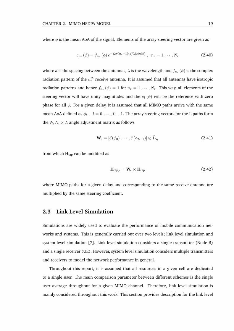
Two channel models are used throughout this report; ITU Pedestrian-A (Ped-A) and ITU
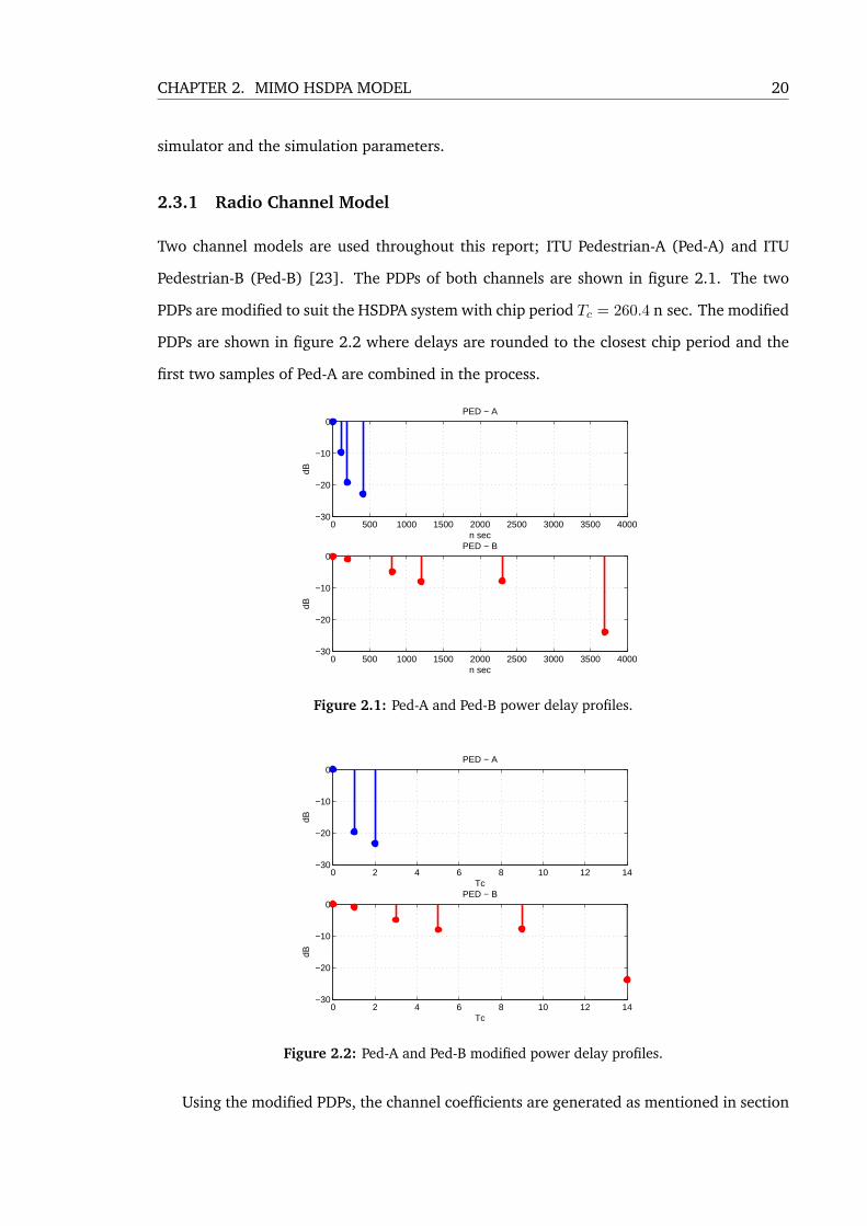
Pedestrian-B (Ped-B) [23]. The PDPs of both channels are shown in figure 2.1. The two
PDPs are modified to suit the HSDPA system with chip period Tc = 260.4 n sec. The modified
PDPs are shown in figure 2.2 where delays are rounded to the closest chip period and the
first two samples of Ped-A are combined in the process.
0 500 1000 1500 2000 2500 3000 3500 4000−30
−20
−10
0
n sec
dB
PED − A
0 500 1000 1500 2000 2500 3000 3500 4000−30
−20
−10
0
n sec
dB
PED − B
Figure 2.1: Ped-A and Ped-B power delay profiles.
0 2 4 6 8 10 12 14−30
−20
−10
0
Tc
dB
PED − A
0 2 4 6 8 10 12 14−30
−20
−10
0
Tc
dB
PED − B
Figure 2.2: Ped-A and Ped-B modified power delay profiles.
Using the modified PDPs, the channel coefficients are generated as mentioned in section
CHAPTER 2. MIMO HSDPA MODEL 21
2.2 where spatial correlations are assumed to be zero if not mentioned otherwise. The
background noise at the receiver is modelled as additive white Gaussian noise with fixed
single sided power spectral density N0 = 0.02.
2.3.2 System Parameters
The MIMO configuration throughout this work is set to 2 × 2 MIMO where Nr = Nt = 2.
This is the most common configuration for MIMO HSDPA and it is well defined in standards.
The spreading factor per transmit antenna is set to N = 16 and the maximum number
of channels available for user data transmission is limited to K = 30. The chip rate is
given as fc = 1Tc
= 3.84Mchip/sec. Scrambling codes are not considered in the model
or implemented in the simulations as a single user is only considered without inter-cell
interference.
It is assumed that information bits transmitted over one symbol period in a single chan-
nel can be selected from a range defined as {0, 0.25, · · · , 5.75, 6}. The bit granularity is 0.25
and the maximum realizable rate is 6 bits per symbol per channel when 64-QAM is applied.
Furthermore, the modulation gap Γ is assumed to be 0 dB. More about bit rates is available
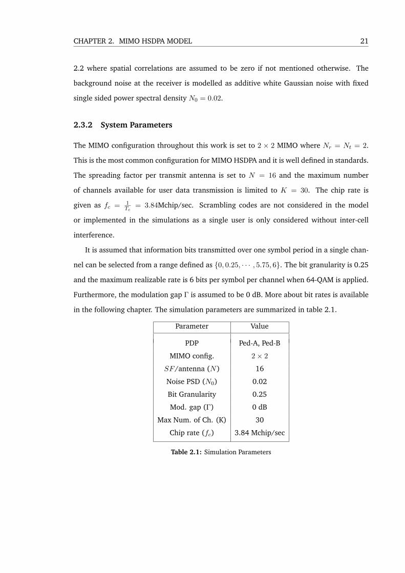
in the following chapter. The simulation parameters are summarized in table 2.1.
Parameter Value
PDP Ped-A, Ped-B
MIMO config. 2× 2
SF/antenna (N) 16
Noise PSD (N0) 0.02
Bit Granularity 0.25
Mod. gap (Γ) 0 dB
Max Num. of Ch. (K) 30
Chip rate (fc) 3.84 Mchip/sec
Table 2.1: Simulation Parameters
CHAPTER 2. MIMO HSDPA MODEL 22
2.3.3 Generating Multiple MIMO Channels
The channel coefficients are generated using Rayleigh (or Ricean) random variables. There-
fore, their instantaneous values can vary even if the PDP and spatial correlation matrix were
constant. It is assumed that the MIMO channel stays constant during the transmission of one
packet. However, to evaluate the overall performance for a given PDP and spatial correla-
tion matrix, the MIMO channel is generated multiple times and parameters to be observed
as total throughput or allocated energies are averaged over the generated channels. The
number of channels generated is set to 20 where averages of observed parameters usually
converge to constant values.
Chapter 3
Resource Allocation
In mobile radio communications systems, resources such as bandwidth and energy are lim-
ited. This fact makes utilizing available resources very important. In this work we assume
that bandwidth is fully utilized and we try to tackle the problem of energy utilization. This
can be done by optimizing the energy allocation scheme which has a significant impact on
the throughput of HSDPA systems especially in frequency selective channels.
This chapter starts by describing the current MIMO HSDPA standard highlighting the
energy allocation scheme used. Other resource allocation schemes are then discussed before
presenting simulation results.
3.1 MIMO HSDPA Standard
MIMO HSDPA was standardized by 3GPP in Release 7 in order to increase HSDPA through-
put. The Dual-Stream Transmit Antenna Array (D-TxAA) scheme was chosen as the MIMO
extension for the frequency division duplex (FDD) mode of HSDPA. D-TxAA has two modes
of operation; dual-stream mode and singe-stream mode [1].
In dual-stream mode, two independent data streams are transmitted; a primary stream
and a secondary stream. The two streams are spatially multiplexed using precoding weights
and transmitted simultaneously using both transmit antennas. Each data stream can carry
up to N − 1 channels and both streams use the same set of signature sequences achieving
code reuse. If the SNIR at the receiver is not sufficient to decode a second data stream, the
secondary data stream will be switched off and the system will operate under single-stream
23
CHAPTER 3. RESOURCE ALLOCATION 24
mode where one data stream is precoded and transmitted over both antennas [22].
In Release 8, the peak throughput was further increased by introducing higher-order
modulation for MIMO HSDPA [4]. Dual-Cell HSDPA (DC-HSDPA) introduced for SISO in
Release 8 was extended to include MIMO in Release 9 [5]. In DC-HSDPA, one HSDPA re-
ceiver will receive two different carriers each from a different cell. This improves the achiev-
able throughput especially for receivers near the edge of a cell. The concept of DC-HSDPA
was further extended to include more cells (carriers) in Four-Carrier HSDPA introduced in
Release 10 [2] and Eight-Carrier HSDPA introduced in Release 11 [3].
This work is mainly concerned about single user throughput when operating using one
carrier. Hence, Multi-Carrier HSDPA are not considered in this work.
3.1.1 D-TxAA Model
In this subsection, a model for D-TxAA will be given. Modelling will be limited to 2 × 2
MIMO configuration which is most common for MIMO HSDPA.
D-TxAA uses a fixed spreading factor per transmit antenna N = 16 and a set of 15
OVSF (orthogonal variable spread factor) signature sequences for data transmission. The
15 orthonormal signature sequences form the 16×15 OVSF signature sequence matrix given
as
SOVSF16 = [~sOVSF16,1, · · ·~sOVSF16,14, ~sOVSF16,15] (3.1)
where each vector represents a signature sequence. Assuming that the system is operating
in dual-stream mode, the maximum number of channels that can be used for data transmis-
sion is K = 30. The channels are divided into two data streams, a primary stream and a
secondary stream. The same matrix SOVSF16 is used to spread channels in both data streams.
After spreading, each of the data streams is weighted using a pair of precoding weights and
then transmitted over both transmit antennas. Precoding weights for both streams form the
2× 2 precoding matrix [11] given as
WD =
w(1)p w
(1)s
w(2)p w
(2)s
= [~wp, ~ws] (3.2)
CHAPTER 3. RESOURCE ALLOCATION 25
where w(nt)p is the ntht transmit antenna precoding weight for the primary data stream and
w(nt)s is the ntht transmit antenna precoding weight for the secondary data stream. By inte-
grating signature sequences and precoding, the 32× 30 MIMO signature sequence matrix S
can be obtained as
S = WD ⊗ SOVSF16 =
w(1)p SOVSF16 w
(1)s SOVSF16
w(2)p SOVSF16 w
(2)s SOVSF16
(3.3)
Given that vectors of SOVSF16 are orthonormal, if ~wp and ~ws are orthonormal, then the
system can be viewed as if it uses 30 orthonormal signature sequences each having the
length of 32.
3.1.2 Precoding Weights Selection
The precoding weights are drawn from a closed-loop transmit diversity code book where
w(1)p and w(1)
s are equal and have a constant real value given as
w(1)p = w(1)
s =1√2
and w(2)p and w(2)
s have variable complex values defined as
w(2)p ∈
{1 + j
2,1− j
2,−1 + j
2,−1− j
2
}
w(2)s = −w(2)
p
The primary precoding vector and secondary precoding vector are orthonormal regardless
of the values drawn. Therefore, the two data streams are transmitted on orthogonal beams
[22] where the same set of signature sequences is reused.
The precoding weights are selected to maximize the SNIR at the receiver and hence
achive the highest throughput for a given channel. This process is carried out by the receiver
and a precoding control indicator (PCI) - carrying information about the preferred weights
- is fed back to the transmitter [1]. The selection can be performed by choosing w(2)p that
CHAPTER 3. RESOURCE ALLOCATION 26
maximizes the following expression [8]
w(2)p : max
(~wHp Gh ~wp
)(3.4)
where Gh is the 2L× 2 Grammian matrix of the channel response vectors given as
Gh =
~h(1,1) ~h(1,2)
~h(2,1) ~h(2,2)
H ~h(1,1) ~h(1,2)
~h(2,1) ~h(2,2)
(3.5)
Once the transmitter receives the PCI which refers to the value of w(2)p , both precoding
vectors can be calculated and used for beamforming.
3.1.3 Single-Stream Mode
The SNIR at the receiver may be insufficient to transmit two data streams. In this case, the
secondary stream is switched off and the system will operate in a single-stream mode which
is backwards compatible with the transmit diversity antenna array (TxAA) mode. The same
precoding applies but the precoding matrix will be reduced to the primary precoding vector
WS =
w(1)p
w(2)p
= ~wp (3.6)
the number of channels available for data transmission reduces to 15 and the MIMO signa-
ture sequence matrix is formulated as
S = WS ⊗ SOVSF16 =
w(1)p SOVSF16
w(2)p SOVSF16
(3.7)
Although the number of channels used with TxAA is same as SISO, TxAA generally
performs better than SISO as it exploits the diversity gain of the radio channel. For receivers
with one antenna, TxAA can also be used in a MISO configuration [5].
CHAPTER 3. RESOURCE ALLOCATION 27
3.1.4 Resource Allocation
HSDPA uses AMC to control the transmission bit rates over channels [22]. The bit rate in
bits per symbol period for a single channel is defined as
b (p) , p = 1, · · · , P (3.8)
which is chosen from a finite set of P discrete bit rates achieved by changing the Modulation
and Coding Scheme (MCS).
For dual-stream mode, all channels belonging to the same data stream operate on the
same bit rate. However, bit rates for the two data streams are not necessarily the same. The
bit rate for primary channels is defined as b (pp) where the bit rate for secondary channels
is defined as b (ps). If the system operates in single-stream mode, only b (pp) needs to be
assigned. The values of b (pp) and b (ps) depend on the SNIR at the output of the despreading
filter for all channels in operation. Assuming that the signals are despread at the receiver
using a MIMO MMSE despreading filter, the total throughput of the system is given next.
Dual-Stream mode
All HSDPA standards (including MIMO HSDPA) allocate equal energies to channel used in
data transmission [6]. Assuming that the system uses the K data transmission channels,
energy used to transmit one symbol over the kth channel is given as
Ek =ETK
, k = 1, · · · ,K (3.9)
and SNIR at the output of the MIMO MMSE despreading filter for the kth channel is calcu-
lated as
γk =ETK ~qHk C−1~qk
1− ETK ~qHk C−1~qk
, k = 1, · · · ,K (3.10)
Assuming that channels 1, · · · , K2 belong to the primary data stream and channels(K2 + 1
), · · · ,K
CHAPTER 3. RESOURCE ALLOCATION 28
belong to the secondary data stream, bpp and bps are chosen to satisfy
γ(bpp)≤ γk , k = 1, · · · , K
2(3.11)
γ (bps) ≤ γk , k =
(K
2+ 1
), · · · ,K (3.12)
where γ (bp) is the minimum SNIR at the output of the receiver a channel should have to be
able to transmit bp bits per symbol period. For M-QAM and modulation gap value Γ, γ(bpp)
and γ (bps) are given as
γ(bpp)
= Γ(
2bpp − 1)
(3.13)
γ (bps) = Γ(
2bps − 1)
(3.14)
The total achievable bit rate in bits per symbol period is given as
RT =K
2
(bpp + bps
)(3.15)
Single-Stream mode
When the secondary stream is switched off, the number of available data transmission chan-
nels reduces to K2 . Energy used to transmit one symbol over the kth channel is given as
Ek =2ETK
, k = 1, · · · , K2
(3.16)
and SNIR at the output of the MIMO MMSE despreading filter for the kth channel is calcu-
lated as
γk =2ETK ~qHk C−1~qk
1− 2ETK ~qHk C−1~qk
, k = 1, · · · , K2
(3.17)
It is important to note that C used in (3.10) is not the same as C used in (3.17). The
former uses all MIMO signature sequences and energies calculated from (3.9). However,
the later uses half the number of MIMO signature sequences and energies calculated from
(3.16). All channels belong to one data stream and bp is chosen satisfy
γ (bp) ≤ γk , k = 1, · · · , K2
(3.18)
CHAPTER 3. RESOURCE ALLOCATION 29
where
γ (bp) = Γ(
2bp − 1)
(3.19)
The total achievable bit rate in bits per symbol period is given as
RT =K
2bp (3.20)
Mode Selection
After choosing the precoding vector, the receiver carries out received SNIR calculations
for both single and double stream modes which require two covariance matrix inversions.
The rates for double-stream mode bpp and bps and the single stream-mode rate bp are then
calculated. The receiver would report that double-stream mode is preferred if
(bpp + bps
)> bp
otherwise the receiver would report that using on stream is preferred.
3.1.5 Wasted SNIR
For a given data stream, the bit rate used for channels is bounded to the bit rate achievable
by the channel with the worst condition. This produces wasted SNIR which comes from
channels with better conditions. The total wasted SNIR for double-stream mode is given as
Wasted SNIR =
K∑k=1
ETK ~qHk C−1~qk
1− ETK ~qHk C−1~qk
− K
2
(Γ(
2bpp − 1)
+ Γ(
2bps − 1))
(3.21)
For single-stream mode, the wasted SNIR is given as
Wasted SNIR =
K2∑
k=1
2ETK ~qHk C−1~qk
1− 2ETK ~qHk C−1~qk
− K
2Γ(
2bp − 1)
(3.22)
In frequency selective radio channels, the wasted SNIR can be significant as different chan-
nels would have different conditions due to ISI and ICI. The next section will demonstrate
CHAPTER 3. RESOURCE ALLOCATION 30
how to utilize the wasted SNIR to transmit higher bit rates.
3.2 Constrained Optimization
The wasted SNIR produced by equal-energy loading can be utilized by energy-constrained
rate optimization (constrained optimization) which uses iterative calculations to find the
bit rate and the transmission energies. This will be applied to both single-stream and
dual-stream modes. However, in dual-stream mode data streams are not separated and
all channels are considered in the same bit assignment process. Optimizing bit rates for
the two streams separately may offer higher throughput, but the complexity is significantly
increased as well.
The optimization methods are first presented assuming that all channels are applied,
then single-stream mode and mode selection are discussed afterwards.
3.2.1 Equal-Rate Margin Adaptive Loading
In a multi-code transmission system where the same bit rate is used over all channels, equal-
rate margin adaptive loading is used to maximize the sum capacity especially when different
signature sequences experience different SNIRs at the receiver. Equal-rate margin adaptive
loading makes sure that each channel produces minimum possible interference by allocating
just enough energy to satisfy a target SNIR [33]. The target SNIR corresponding to a bit
rate bp is given as γ∗ (bp) = Γ(2bp − 1
)where the bit rate index p is selected to maximize
the total achievable bit rate such as
p : max RT = Kb (p) (3.23)
subject to the energy constraint given as
K∑k=1
Ek (bp) ≤ ET <K∑k=1
Ek (bp+1) (3.24)
For an MMSE despreading filter, the maximum p that satisfies (3.23) and (3.24) and the
energies for different channels can be calculated iteratively as follows:

CHAPTER 3. RESOURCE ALLOCATION 31
1. The bit rate index is initialized as p = 1.
2. The energies are initialized as Ek(0) = ETK , k = 1, · · · ,K and the iterations index is
initialized as i = 1.
3. Ae(i) is calculated by plugging Ek(i−1), k = 1, · · · ,K into equation (2.14).
4. C(i) is calculated by plugging Ae(i) into equation (2.18).
5. The inverse of the covariance matrix in calculated and the new set of energies is
calculated as
Ek(i) =Γ(2bp − 1
)(1 + Γ
(2bp − 1
))~qHk C−1
(i) ~qk, k = 1, · · · ,K
6. If Ek(i) ≈ Ek(i−1) for k = 1, · · · ,K or i = Imax1 go to the next step. Otherwise,
i = i+ 1 and steps are repeated starting from step 3.
7. If∑K
k=1Ek(i) > ET , then p = p− 1 and search is complete. Otherwise, p = p+ 1 and
steps are repeated starting from step 2.
After finding the bit rate index p and the transmission energies, the MIMO MMSE despread-
ing filter coefficients are calculated using equation (2.19). It is assumed that there is a
perfect feedback link between the receiver and transmitter used to report the transmission
energies and rate to be used by the transmitter.
3.2.2 Residual Energy
Assuming an infinite set of bit rates where bit granularity goes to zero, bp will be selected
such as∑K
k=1Ek (bp) = ET . However, zero bit granularity is not practically achievable as bp
is selected from a finite set to satisfy (3.24) where equality is not necessarily satisfied. This
produces residual energy given as
ER = ET −K∑k=1
Ek (bp) (3.25)
The residual energy is not used to transmit any useful data and produces a gap between the
achievable capacity curves for continuous and discrete rates.1Imax is the maximum number of iterations required to calculate a set of energies.

CHAPTER 3. RESOURCE ALLOCATION 32
3.2.3 Two-Group Rate Adaptive Loading
In order to utilize the residual energy produced by using discrete bit rates with equal-rate
margin adaptive loading, a two-group rate adaptive loading scheme was implemented in
[20,21]. Two-group loading algorithm assigns an adjacent higher bit rate bp+1 tom channels
known as the second group. Assuming that channels are ordered in a way such that
Ej (bp+1)− Ej (bp) < Ek (bp+1)− Ek (bp) , j > k and j, k = 1, · · · ,K (3.26)
then the number of channels in the second group m is chosen to maximize the total achiev-
able bit rate such as
m : max RT = (K −m) b (p) +mb (p+ 1) (3.27)
subject to the energy constraint given as
K−m∑k=1
Ek (bp) +
K∑k=K−m+1
Ek (bp+1) ≤ ET <K−m+1∑k=1
Ek (bp) +
K∑k=K−m+2
Ek (bp+1) (3.28)
Iterative calculation is used to calculate the maximum m that satisfies (3.27) and (3.28) as
follows:
1. Equal-rate margin adaptive loading is carried out to find p.
2. The number of channels in the second group is initialized as m = 1.
3. The energies are initialized as Ek(0) = ETK , k = 1, · · · ,K and the iterations index is
initialized as i = 1.
4. Ae(i) is calculated by plugging Ek(i−1), k = 1, · · · ,K into equation (2.14) and C(i) is
calculated by plugging Ae(i) into equation (2.18).
5. The inverse of the covariance matrix in calculated and the new set of energies is
CHAPTER 3. RESOURCE ALLOCATION 33
calculated as
Ek(i) =Γ(2bp − 1
)(1 + Γ
(2bp − 1
))~qHk C−1
(i) ~qk, k = 1, · · · ,K −m
Ek(i) =Γ(2bp+1 − 1
)(1 + Γ
(2bp+1 − 1
))~qHk C−1
(i) ~qk, k = (K −m+ 1) , · · · ,K
6. If Ek(i) ≈ Ek(i−1) for k = 1, · · · ,K or i = Imax go to the next step. Otherwise, i = i+1
and steps are repeated starting from step 4.
7. If∑K
k=1Ek(i) > ET , then m = m − 1 and search is complete. Otherwise, m = m + 1
and steps are repeated starting from step 3.
Using two-group rate adaptive loading, the same total rate realised by equal-rate margin
adaptive loading with zero bit granularity is roughly achieved using two discrete bit rates
and without a significant increase in complexity.
3.2.4 Two-Group Loading with Single-Stream Mode
Switching off the second stream may improve performance in some MIMO channel condi-
tions. The same two-group algorithm explained in the previous subsection can be applied
to a single data stream by using the K2 signature sequences given in (3.7).
To select the best mode of operation, the two-group loading algorithm should be per-
formed twice and the mode with the higher total rate will be chosen. However, performing
two-group loading algorithm is computationally heavy for most mobile application which
will be discussed in the following subsection.
3.2.5 Computational Complexity
The main holdback of using constrained optimization is the computational complexity of
the algorithms. This is due to the high number of covariance matrix inversions required
when performing equal-rate margin adaptive and two-group rate adaptive loading.
When equal-rate margin adaptive loading is performed, the search for p requires up to
P energy calculation processes as the allocated bit rate can be the last one in the group
of available rates. Each energy calculation process requires up to Imax iterations. Each
CHAPTER 3. RESOURCE ALLOCATION 34
iteration would require a covariance matrix inversion to calculate the new set of energies
and the total number of matrix inversions can reach PImax. If two-group loading algorithm
is to be performed as well, this would add up to (K − 1) Imax covariance matrix inversions
required to find m. The total number of matrix inversions required to perform two-group
loading algorithm can go up to (P +K − 1) Imax.
Furthermore, selecting the mode of operation weather it is single-stream or double-
stream would require up to(P + K
2 − 1)Imax matrix inversions to perform two-group load-
ing algorithm for half the number of channels. Hence, the maximum total number of matrix
inversions required to perform two-group loading with best mode selection is(2P + 3K
2 − 2)Imax.
3.3 Simulation and Analysis
The values of the simulation parameters are given in section 2.3. Performance comparison
is carried out between D-TxAA MIMO HSDPA standard and the one improved using con-
strained optimization. An evaluation of the computational complexity required to run the
two-group loading algorithm is also provided in this section.
3.3.1 Total Throughput
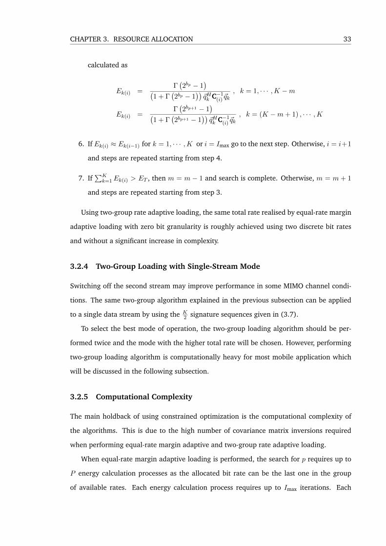
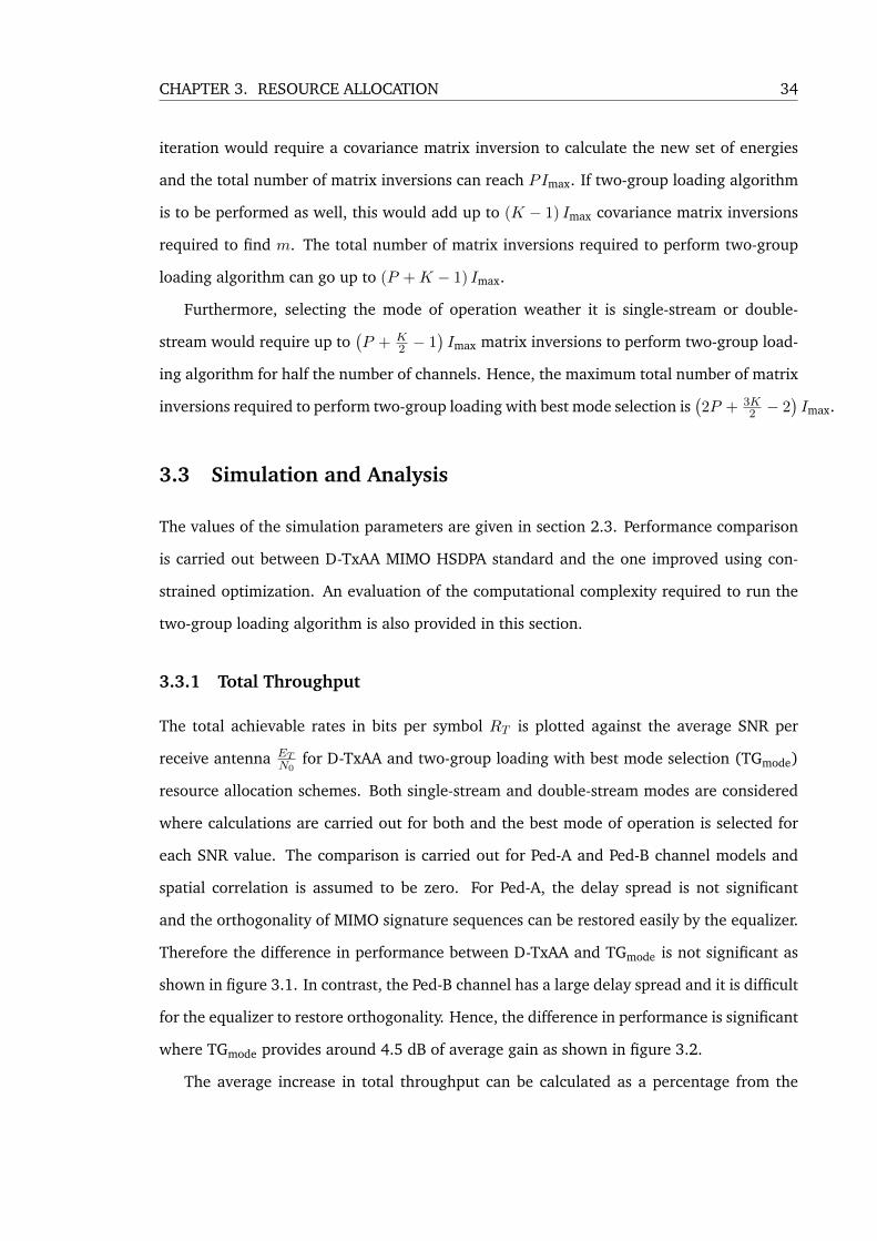
The total achievable rates in bits per symbol RT is plotted against the average SNR per
receive antenna ETN0
for D-TxAA and two-group loading with best mode selection (TGmode)
resource allocation schemes. Both single-stream and double-stream modes are considered
where calculations are carried out for both and the best mode of operation is selected for
each SNR value. The comparison is carried out for Ped-A and Ped-B channel models and
spatial correlation is assumed to be zero. For Ped-A, the delay spread is not significant
and the orthogonality of MIMO signature sequences can be restored easily by the equalizer.
Therefore the difference in performance between D-TxAA and TGmode is not significant as
shown in figure 3.1. In contrast, the Ped-B channel has a large delay spread and it is difficult
for the equalizer to restore orthogonality. Hence, the difference in performance is significant
where TGmode provides around 4.5 dB of average gain as shown in figure 3.2.
The average increase in total throughput can be calculated as a percentage from the
CHAPTER 3. RESOURCE ALLOCATION 35
average rate of D-TxAA as follows:
Rinc =E[RT,TGmode
]− E [RT,D-TxAA]
E [RT,D-TxAA](3.29)
Where average rates are obtained from averaging over the SNR range. TGmode provides
around 7% increase over D-TxAA for Ped-A. This is not significant as expected for Ped-A
channel mode. However, for Ped-B channel mode the increase is around 40%.
0 5 10 15 20 25 30 350
20
40
60
80
100
120
140
160
180
ET/N0 dB
RT
bits
/sym
bol
TG
mode
D−TxAA
Figure 3.1: TGmode and D-TxAA - Throughput - Ped-A.
3.3.2 Number of Applied Channels
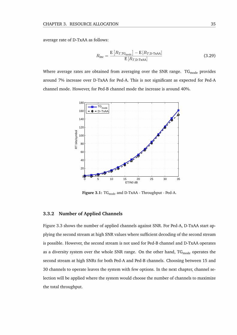
Figure 3.3 shows the number of applied channels against SNR. For Ped-A, D-TxAA start ap-
plying the second stream at high SNR values where sufficient decoding of the second stream
is possible. However, the second stream is not used for Ped-B channel and D-TxAA operates
as a diversity system over the whole SNR range. On the other hand, TGmode operates the
second stream at high SNRs for both Ped-A and Ped-B channels. Choosing between 15 and
30 channels to operate leaves the system with few options. In the next chapter, channel se-
lection will be applied where the system would choose the number of channels to maximize
the total throughput.
CHAPTER 3. RESOURCE ALLOCATION 36
0 5 10 15 20 25 30 350
10
20
30
40
50
60
70
80
90
100
ET/N0 dB
RT
bits
/sym
bol
TG
mode
D−TxAA
Figure 3.2: TGmode and D-TxAA - Throughput - Ped-B.
5 10 15 20 25 30 350
5
10
15
20
25
30
35
ET/N0 dB
Cha
nnel
s U
sed
Ped−A
TG
mode
D−TxAA
5 10 15 20 25 30 350
5
10
15
20
25
30
35
ET/N0 dB
Cha
nnel
s U
sed
Ped−B
TG
mode
D−TxAA
Figure 3.3: TGmode and D-TxAA - Number of Channels Applied
CHAPTER 3. RESOURCE ALLOCATION 37
3.3.3 Matrix Inversions
For P = 24, K = 30 and Imax = 50, the maximum number of matrix inversions required
to run TGmode is 3400. However, this upper bound is not necessarily reached. The actual
number of matrix inversions required can be controlled by allowing an error rate in the
energy calculation process. The energy error is calculated as a percentage of the total
available energy as follows
errorE =
∑Kk=1
(Ek(i) − Ek(i−1)
)ET
(3.30)
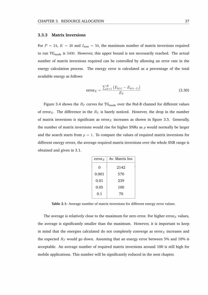
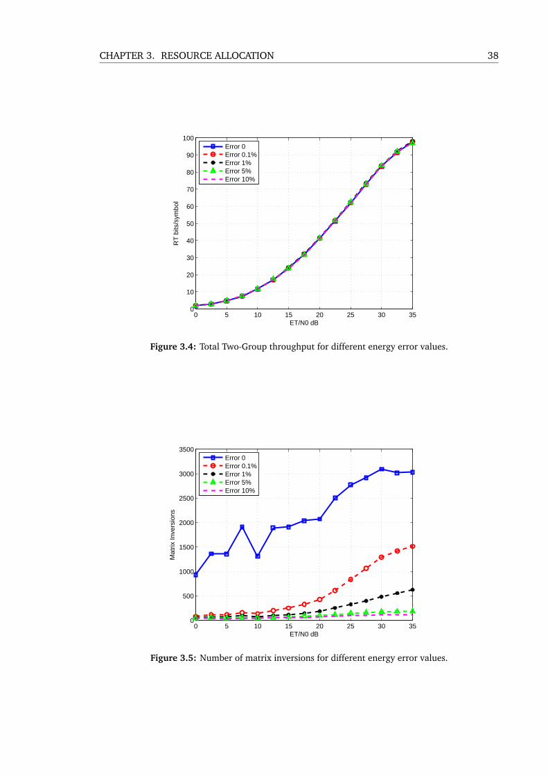
Figure 3.4 shows the RT curves for TGmode over the Ped-B channel for different values
of errorE . The difference in the RT is barely noticed. However, the drop in the number
of matrix inversions is significant as errorE increases as shown in figure 3.5. Generally,
the number of matrix inversions would rise for higher SNRs as p would normally be larger
and the search starts from p = 1. To compare the values of required matrix inversions for
different energy errors, the average required matrix inversions over the whole SNR range is
obtained and given in 3.1.
errorE Av. Matrix Inv.
0 2142
0.001 570
0.01 239
0.05 100
0.1 70
Table 3.1: Average number of matrix inversions for different energy error values.
The average is relatively close to the maximum for zero error. For higher errorE values,
the average is significantly smaller than the maximum. However, it is important to keep
in mind that the energies calculated do not completely converge as errorE increases and
the expected RT would go down. Assuming that an energy error between 5% and 10% is
acceptable. An average number of required matrix inversions around 100 is still high for
mobile applications. This number will be significantly reduced in the next chapter.
CHAPTER 3. RESOURCE ALLOCATION 38
0 5 10 15 20 25 30 350
10
20
30
40
50
60
70
80
90
100
ET/N0 dB
RT
bits
/sym
bol
Error 0Error 0.1%Error 1%Error 5%Error 10%
Figure 3.4: Total Two-Group throughput for different energy error values.
0 5 10 15 20 25 30 350
500
1000
1500
2000
2500
3000
3500
ET/N0 dB
Mat
rix In
vers
ions
Error 0Error 0.1%Error 1%Error 5%Error 10%
Figure 3.5: Number of matrix inversions for different energy error values.
Chapter 4
System Values
In the previous chapter, performance of MIMO HSDPA in frequency selective channels was
improved in terms of total throughput by using two-group resource allocation. However, the
process is computationally heavy as it requires a significant number of covariance matrix in-
versions and may be impractical for applications with limited signal processing capabilities.
In this chapter, system value approach is used to reduce the number of matrix inver-
sions required to implement two-group loading. System value approach is optimized using
channel selection schemes that replace mode selection used in the previous chapter. Fur-
thermore, interference cancelation with recursive matrix inversion calculations are used to
eliminate the remaining matrix inversions after using system value approach. System value
approach works best with optimum MIMO signature sequences. Hence, the chapter starts
by presenting the optimum sequence design.
4.1 Signature Sequence Design and Channel Selection
4.1.1 Optimum MIMO Signature Sequences
In frequency selective radio channels, the multipath nature destroys orthogonality between
the MIMO signature sequences used earlier. This creates cross-correlations between re-
ceived MIMO signature sequences causing ICI. Assuming perfect channel state information
(CSI) where the multipath radio channel is known to the transmitter, the MIMO signature
sequences can be adapted to consider the multipath channel effect and produce orthogonal
39
CHAPTER 4. SYSTEM VALUES 40
received MIMO signature sequences with zero cross-correlations such as
〈~qi, ~qj〉 = ~qHi ~qj = 0 , i, j = 1, · · · ,K and i 6= j (4.1)
MIMO signature sequences that satisfy (4.1) can be obtained by combining singular
value decomposition (SVD) with the MIMO channel convolution matrix H. The MIMO sig-
nature sequences are given as the Eigen vectors of theNtN×NtN channel Grammian matrix
defined as
GH = HHH (4.2)
Eigen vectors of GH can be obtained from the eigen decomposition given as
GH = VHDHVHH (4.3)
where DH = diag (~µH) is the diagonal matrix of the eigen values which are defined in a
vector as ~µH = [µH,1, µH,2, · · · , µH,NtN ]. VH is the eigen vectors matrix defined as VH =
[~vH,1, ~vH,2, · · · , ~vH,NtN ]. Using VH as the MIMO signature sequences matrix, the correlations
between the received MIMO signature sequences are obtained from the Grammian matrix
of the received MIMO signature sequences as
(HVH)H HVH = VHH VHDHVHH VH
= DH (4.4)
with zero cross-correlations and channels power gains given by the diagonal terms (eigen
values). The channel Grammian matrix produces NtN eigen vectors and corresponding
eigen values. However, the number of non-zeros eigen values is determined by the rank of
the channel Grammian matrix which is conditioned by
rank(HHH
)≤ min (Nt, Nr)N (4.5)
and hence the maximum number of channels that can be used is limited to Ktotal ≤
min (Nt, Nr)N and the MIMO signature sequences are chosen as the eigen vectors in VH
CHAPTER 4. SYSTEM VALUES 41
corresponding to non-zero eigen values. If K channels are used in data transmission where
K < Ktotal, the optimum MIMO signature sequence matrix is given as
S = [~vH,1, ~vH,2, · · · , ~vH,K ] , µH,1, · · · , µH,K 6= 0 (4.6)
and the MIMO receiver signature sequence matrix Q is obtained using (2.5). The diagonal
terms of the received MIMO signature sequences Grammian matrix represent channels gains
given as
|hH,k|2 =[QHQ
]k,k
= µH,k , k = 1, · · ·K (4.7)
When optimum MIMO signature sequences are used, received MIMO signature sequences
have zero-cross correlations and channel gains provide a good indicator for the quality of
channels. Channels gains can be used to order the channels instead of incremental ener-
gies when two-group loading is performed. The channel ordering may not be the same as
the one with incremental energies as ISI is still present and shifted parts of the sequences
are not orthogonal. However, the two ordering schemes will give very close results as the
equalizer minimizes the effect of ISI.
4.1.2 Channel Selection using Water-Filling
In the previous chapter, the maximum rate was obtained by using either half the number of
channels or the full number of channels where each half formed a data stream. This may
lead to include bad channels sometimes which may limit the rate or exclude good channels
from switching off the second stream. Channel selection can be used to identify and exclude
bad channels giving the transmitter more control over the signature sequences to achieve
higher throughput.
Water-filling optimization is generally used For parallel channels with different gains to
provide optimum channel selection and energy distribution in order to maximize the sum
capacity [13]. When optimum MIMO signature sequences are used and ISI effect is ignored,
water-filling can be used to identify and exclude weak channels as follows:
1. The matrix S is re-ordered in a way such that the channel gains corresponding to
signature sequences are in a descending order.
CHAPTER 4. SYSTEM VALUES 42
2. The matched filter receiver channel-SNR gk is calculated for the K channels as
gk =|hH,k|2
2σ2, k = 1, . . .K (4.8)
3. The number of channels to be used K∗ is initialized as K∗ = K.
4. The water-filling constant is calculated as
KWF =1
K∗
(ET +
1
Γ
K∗∑k=1
1
gk
)(4.9)
5. Energies for K∗ channels are calculated as
Ek,WF = KWF −1
Γgk, k = 1, . . .K∗ (4.10)
6. If EK∗,WF < 0, The number of channels to be used is set to K∗ = K∗−1 and steps are
repeated starting from step 4. Otherwise the number of codes to be used is set to K∗
by removing the last K −K∗ columns from S and Q can be calculated using equation
(2.5).
Using the resulting energies and the K∗ selected optimum codes, the water-filling ca-
pacity that gives a performance upper bound for a given MIMO channel can be calculated
as
CWF =
K∗∑k=1
log2
(1 +
Ek,WF ~qHk C−1~qk
Γ(1− Ek,WF ~q
Hk C−1~qk
)) (4.11)
where C is calculated using the optimum MIMO signature sequences and the water-filling
allocated energies.
4.2 System Values
System values are new parameters that play a key role in reducing the computational com-
plexity required to perform equal-rate margin adaptive loading and two-group rate adaptive
CHAPTER 4. SYSTEM VALUES 43
loading algorithms [17]. The system value for the kth channel is defined as
λk = Ek~qHk C−1~qk
=[A2QHC−1Q
]k,k
, k = 1, . . .K (4.12)
System values for the K channels form a K × 1 system value vector as
~λ = [λ1, λ2, · · · , λK ]T
= diag(A2QHC−1Q
)(4.13)
The kth channel SNIR at the output of the MIMO MMSE despreading filter can be written in
terms of the system value as
γk =λk
1− λk, k = 1, . . .K (4.14)
4.2.1 Gurcan system values and upper bounds
The system values obtained from distributing energy equally over the K∗ signature se-
quences selected by water-filling are referred to as Gurcan’s system values which can be
written in a vector as
~λG = diag
(ETK∗QH
(ETK∗QeQ
He + 2σ2INr(N+L−1)
)−1
Q
)(4.15)
The summation of Gurcan’s system values is given as
λT,G = trace
(ETK∗QH
(ETK∗QeQ
He + 2σ2INr(N+L−1)
)−1
Q
)(4.16)
For a given channel, the summation of system values corresponding to unequal energy
loading are upper bounded by the summation of system values corresponding to equal
energy loading if the same energy constraint is satisfied [17]. Hence, λT,G gives an upper
bound referred to as Gurcan’s upper bound for total system values. Assuming that channels
can be loaded with non-equal rates and optimum signature sequences are used, the capacity
CHAPTER 4. SYSTEM VALUES 44
corresponding to Gurcan’s system values is referred to as Gurcan capacity and it is given as
CG =K∗∑k=1
log2
1 +
[ETK∗ QH
(ETK∗ QeQ
He + 2σ2INr(N+L−1)
)−1Q]k,k
Γ
(1−
[ETK∗ QH
(ETK∗ QeQ
He + 2σ2INr(N+L−1)
)−1Q]k,k
) (4.17)
The Gurcan capacity is found to approach the water-filling capacity and can be used as
an upper bound to compare the performance of different resource allocation schemes and
different signature sequences.
4.3 Resource Allocation With System Values
When equal-rate margin adaptive loading is performed, energy is allocated in a way such
that all channels meet a target SNIR. This is the same as performing inverse channel loading
where the channel seems to be the same for all signature sequences. Assuming that optimum
signature sequences are used where ICI is minimized and ignoring ISI for a while, a channel
gain given by |hH,k|2 would be the only factor determining the channel quality. Therefore,
energies for inverse channel loading can be calculated as
Ek,Inv =ET
|hH,k|2∑K
i=11
|hH,i|2, k = 1, · · · ,K (4.18)
Inverse channel energies can be used to produce the inverse channel system values given in
the vector ~λInv where all elements have very close values. The sum of the channel inversion
system values is found to be close in value to the total system value corresponding to equal
energy loading [17]. Hence, the following approximation holds
λk,Inv ≈ λmean =1
Ktrace
(ETK
QH
(ETK
QeQHe + 2σ2INr(N+L−1)
)−1
Q
), k = 1, · · · ,K
(4.19)
This approximation can be used to find the target system value and hence the target SNIR
for equal-rate margin adaptive loading with zero bit granularity. However, energy calcula-
tion given in equation (4.18) would not be accurate especially if non optimum signature
sequences are used. Energies can be calculated iteratively to meet a target SNIR that corre-
CHAPTER 4. SYSTEM VALUES 45
sponds to a target system value given as
λ∗ = λmean (4.20)
which is derived from the relation given in equation (4.19). An approximation for the total
capacity for equal-rate margin adaptive loading with zero bit granularity is given as
CMA = Klog2
(1 +
λmeanΓ (1− λmean)
)(4.21)
In practice, zero bit granularity is not achievable as discussed earlier. However, the same
concept can be applied for equal-rate margin adaptive loading with discrete bit rates. For
a set of P discrete bit rates, the target system value is chosen to maximize the rate p as
follows
max p : λ∗ (bp) ≤ λmean , p ∈ {1, · · · , P} (4.22)
where the target system value for a given bit rate is calculated as
λ∗ (bp) =Γ(2bp − 1
)1 + Γ
(2bp − 1
) , p = 1, · · · , P (4.23)
Furthermore, the total system value upper bound given by equal energy loading can be
used to determine the number of channels in the second group m if two-group loading is to
be used. The value of m is selected to satisfy
max m : (K −m)λ∗ (bp) +mλ∗ (bp+1) ≤ Kλmean , m ∈ {1, · · · ,K − 1} (4.24)
where K −m channels would have a target system value of λ∗ (bp) and m channels would
have the target system value of λ∗ (bp+1). Energies for the K channels that satisfy the
SNIRs corresponding to the target system values can be calculated iteratively as described
in the previous chapter. The main benefit from using system values is the elimination of the
iterative search for p and m and hence reducing the number of covariance matrix inversions
required to run two-group loading algorithm. This will be discussed more thoroughly in
subsection 4.3.4.

CHAPTER 4. SYSTEM VALUES 46
4.3.1 Improved Two-Group Rate Adaptive Loading
Optimum MIMO signature sequences and channel selection can be used to improve the
performance of two-group loading. Applying channel selection excludes weak channels
and removes the confusion around using single-stream or double-streams as the number
of channels will be pre-determined. The steps to perform two-group loading simplified by
system value approach and improved by optimum MIMO signature sequences and channel
selection are given as follows:
1. Water-filling is used to determine K∗.
2. The matrix S is re-ordered in a way such that the channel gains corresponding to
signature sequences are in an ascending order and Q and Qe are calculated using
equations (2.5) and (2.6) respectively.
3. Energies are initialized as Ek(i=0) = ETK∗ , k = 1, . . .K∗ and the iteration index is set
to i = 1.
4. The extended amplitude matrix Ae(i=1) is formulated using Ek(i=0) and the covariance
matrix C(i=1) is calculated by plugging Ae(i=1) into equation (2.18).
5. The mean of the Gurcan system values is calculated as
λmean =1
K∗ trace(ETK∗QHC−1
(i=1)Q)
6. Two target system values for the first and second group are selected such as
λ∗ (bp) ≤ λmean < λ∗ (bp+1) , p ∈ 1, · · · , P
where λ∗ (bp) =Γ(2bp−1)
1+Γ(2bp−1)and λ∗ (bp+1) =
Γ(2bp+1−1)1+Γ(2bp+1−1)
and bp and bp+1 are the bit
rates for the first and second group respectively.
7. The number of channels in the second group is determined by calculating the largest
m that satisfies
(K∗ −m)λ∗ (bp) +mλ∗ (bp+1) < λT,G , m ∈ 1, · · · ,K∗ − 1
CHAPTER 4. SYSTEM VALUES 47
8. Energies to be allocated are then calculated iteratively as
Ek(i) (bp) =λ∗ (bp)
~qHk C−1(i) ~qk
, k = 1, . . .K∗ −m
Ek(i) (bp+1) =λ∗ (bp+1)
~qHk C−1(i) ~qk
, k = (K∗ −m+ 1) , . . .K∗
where C(i) which is used to calculate Ek(i) is calculated using Ek(i−1). The iterations
are repeated until Ek(i) ≈ Ek(i−1) for k = 1, . . .K∗, or i reaches Imax.
4.3.2 Optimum Channel Selection For Two-Group Loading
The channel selection scheme used earlier is based on water-filling. This gives optimum se-
lection when water-filling loading is used where different channels are assigned distinct bit
rates. However, for two-group loading which is based on equal-rate margin adaptive load-
ing, the SNIR for channels is brought up to meet a target SNIR. Therefore, some channels
which are assigned smaller amount of energy in water-filling would require more energy for
two-group loading. Excluding those channels may improve the total achievable rate.
Two-group loading was originally introduced to realise the total rate of equal-rate mar-
gin adaptive loading with zero bit granularity using non zero bit granularity. Hence, op-
timization is carried out with respect to equal-rate margin adaptive loading with zero bit
granularity and it applies for two-group loading. The optimization steps are given as follows
1. The matrix S is re-ordered in a way such that the channel gains corresponding to
signature sequences are in a descending order.
2. The optimum number of channels to be used K∗Opt is initialized as K∗
Opt = 1.
3. The signature sequence matrix of theK∗Opt sequences is found as SK∗
Opt=[~s1, · · · , ~sK∗
Opt
]from which QK∗
Optand Qe,K∗
Optcan be calculated using equations (2.5) and (2.6) respec-
tively.
4. The mean of the total system value upper bound over the K∗Opt channels is calculates
as
λmean,K∗Opt
=1
K∗Opt
trace
ETK∗
OptQHK∗
Opt
(ETK∗
OptQe,K∗
OptQHe,K∗
Opt+ 2σ2INr(N+L−1)
)−1
QK∗Opt
CHAPTER 4. SYSTEM VALUES 48
5. The total capacity for equal-rate margin adaptive loading with zero bit granularity
when using K∗Opt channels is calculates as
CK∗Opt
= K∗Optlog2
1 +λmean,K∗
Opt
Γ(
1− λmean,K∗Opt
)
6. If CK∗Opt≥ CK∗
Opt−1, K∗ = K∗Opt + 1 and steps are repeated starting from step 3.
However, if CK∗Opt< CK∗
Opt−1, the optimum number of channels to be used is given as
K∗Opt − 1.
The optimum channel selection gives improved performance over water-filling based se-
lection especially for MIMO channels with non-zero spatial correlations where water-filling
fails to identify some weak channels as shown in simulation results in section 4.5. However,
using optimum channel selection adds extra matrix inversions which are meant to be min-
imized. The number of matrix inversions required to perform optimum channels selection
is discussed in subsection 4.3.4. A suboptimal channel selection scheme which does not
require any matrix inversions in presented in the next subsection.
4.3.3 Suboptimal Channel Selection For Two-Group Loading
If optimum MIMO signature sequences are used, suboptimal channel selection for two-
group loading can be obtained using inverse channel energy loading. The general idea is
the same idea used with optimum channel selection where the number of applied channels is
changed and total capacity is tested. However, to avoid matrix inversions ISI is ignored and
hence a matched filter SNR is used instead of MMSE SNIR. The steps with full explanation
are given as follows
1. The matrix S is re-ordered in a way such that the channel gains corresponding to
signature sequences are in a descending order.
2. The optimum number of channels to be used K∗Sub is initialized as K∗
Sub = 1.
3. The signature sequence matrix of signature sequences SK∗Sub
is found from which QK∗Sub
is calculated
CHAPTER 4. SYSTEM VALUES 49
4. The K∗Sub channels gains are obtained as
[|hH,1|2 , · · · ,
∣∣∣hH,K∗Sub
∣∣∣2] = diag(
QHK∗
SubQK∗
Sub
)
5. Inverse channel energies for the K∗Sub channels are calculated as
Ek,Inv =ET
|hH,k|2∑K∗
Subi=1
1
|hH,i|2, k = 1, · · · ,K∗
Sub
6. The inverse channel capacity for matched filter receiver is calculated as
CK∗Sub
=
K∗Sub∑
k=1
log2
(1 +
Ek,Inv |hH,k|2
2σ2
)
7. If CK∗Sub≥ CK∗
Sub−1, K∗ = K∗Sub + 1 and steps are repeated starting from step 3.
However, if CK∗Sub
< CK∗Sub−1, the optimum number of channels to be used is given as
K∗Sub − 1.
4.3.4 Computational Complexity
The main motivation behind finding the system value approach is to eliminate the itera-
tive search for p and m and reduce the number of covariance matrix inversions. Assuming
that optimum MIMO signature sequences are used, one covariance matrix inversion is re-
quired to calculate the total system value for equal energy loading from which p and m
are obtained. Furthermore, this covariance matrix inversion can be used to perform the
first iteration when energies are calculated iteratively and the rest of the iterations would
require up to Imax− 1 matrix inversions depending on the energy error allowed. Hence, the
maximum number of matrix inversions required to perform two-group loading with system
value approach is Imax compared to (P +K−1)Imax when constrained optimization is used.
Furthermore, if optimum channel selection is implemented, up to K matrix inversions
are required to determine the optimum number of channels. Hence the total number of
matrix inversions required to perform two-group loading with optimum channels selection
using system value approach can reach Imax + K − 1 compared to (KP +∑K−1
k=1 k)Imax if
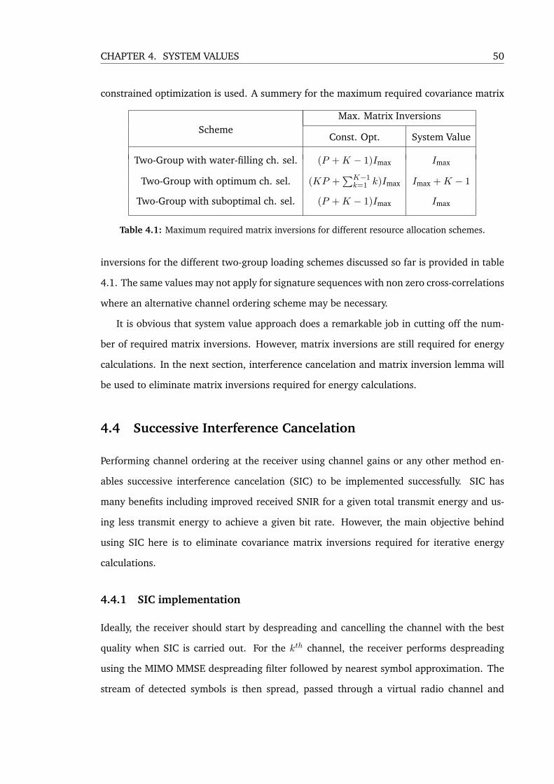
CHAPTER 4. SYSTEM VALUES 50
constrained optimization is used. A summery for the maximum required covariance matrix
Max. Matrix InversionsScheme
Const. Opt. System Value
Two-Group with water-filling ch. sel. (P +K − 1)Imax Imax
Two-Group with optimum ch. sel. (KP +∑K−1
k=1 k)Imax Imax +K − 1
Two-Group with suboptimal ch. sel. (P +K − 1)Imax Imax
Table 4.1: Maximum required matrix inversions for different resource allocation schemes.
inversions for the different two-group loading schemes discussed so far is provided in table
4.1. The same values may not apply for signature sequences with non zero cross-correlations
where an alternative channel ordering scheme may be necessary.
It is obvious that system value approach does a remarkable job in cutting off the num-
ber of required matrix inversions. However, matrix inversions are still required for energy
calculations. In the next section, interference cancelation and matrix inversion lemma will
be used to eliminate matrix inversions required for energy calculations.
4.4 Successive Interference Cancelation
Performing channel ordering at the receiver using channel gains or any other method en-
ables successive interference cancelation (SIC) to be implemented successfully. SIC has
many benefits including improved received SNIR for a given total transmit energy and us-
ing less transmit energy to achieve a given bit rate. However, the main objective behind
using SIC here is to eliminate covariance matrix inversions required for iterative energy
calculations.
4.4.1 SIC implementation
Ideally, the receiver should start by despreading and cancelling the channel with the best
quality when SIC is carried out. For the kth channel, the receiver performs despreading
using the MIMO MMSE despreading filter followed by nearest symbol approximation. The
stream of detected symbols is then spread, passed through a virtual radio channel and

CHAPTER 4. SYSTEM VALUES 51
subtracted from the received signal. Assuming that vectors of S are ordered in a way such
that the channel gains corresponding to signature sequences are in an ascending order
where channels are despread starting from the last channel and SIC is implemented, then
channel k will have to deal with k − 1 interfering channels instead of K − 1.
The number of interfering channels and the receiver covariance matrix used to calculate
the MIMO despreading filter coefficients change depending on the channel number k. The
receiver covariance matrix Ck used to design the receiver for channel k can be calculated
recursively from
Ck= Ck−1 + Ek ~qk ~qHk + Ek~q
(−1)k ~q
(−1)Hk + Ek ~q
(+1)k ~q
(+1)Hk (4.25)
where the covariance matrix when all channels are cancelled is given as
C0=2σ2INr(N+L−1) (4.26)
The MIMO MMSE despreading filter coefficients vector is calculated as
~wSIC,k =C−1k ~qk
~qHk C−1k ~qk
(4.27)
Even though the recursive construction of the covariance matrix and despreading coeffi-
cients starts from k = 1 up to k = K, the despreading and interference cancelling is carried
out starting from k = K and goes down as mentioned earlier.
4.4.2 Iterative Energy and Covariance Matrix Inversion Calculations
When SIC is implemented at the receiver, the transmission energy can be calculated us-
ing the recursive property of the covariance matrix and the matrix inversion lemma. The
knowledge of C−1k−1 is sufficient to calculate the energy value Ek. Then C−1
k can be obtained
recursively from C−1k−1 and Ek. In the same manner, C−1
k is used to calculate Ek+1 and so on.
This does not require any matrix inversion processes as the only matrix inversion required
is C−10 which is calculated as
C−10 =
(2σ2)−1
INr(N+L−1) (4.28)

CHAPTER 4. SYSTEM VALUES 52
The detailed steps and equations required to carry out this process are given as follows
1. The channel index is initialized k = 1 and the first inverse covariance matrix obtained
from equation (4.28).
2. The previous symbol vector and the next symbol vector are defined as
~qk,1 = ~q(−1)k = H(−1)~sk (4.29)
~qk,2 = ~q(+1)k = H(+1)~sk (4.30)
3. The distance vectors are defined as
~d = C−1k−1~qk (4.31)
~d1 = C−1k−1~qk,1 (4.32)
~d2 = C−1k−1~qk,2 (4.33)
4. The weighting functions are defined as
ξ = ~dH ~qk (4.34)
ξ1 = ~dH1 ~qk,1 (4.35)
ξ2 = ~dH2 ~qk,2 (4.36)
ξ3 = ~dH ~qk,1 (4.37)
ξ4 = ~dH ~qk,2 (4.38)
5. Having found the two-group algorithm parameters p andm previously, the target SNIR
is defined as
γ∗k = Γ(
2bp − 1), k ∈ [1, · · · , (K −m)] (4.39)
γ∗k = Γ(
2bp+1 − 1), k ∈ [(K −m+ 1) , · · · ,K] (4.40)
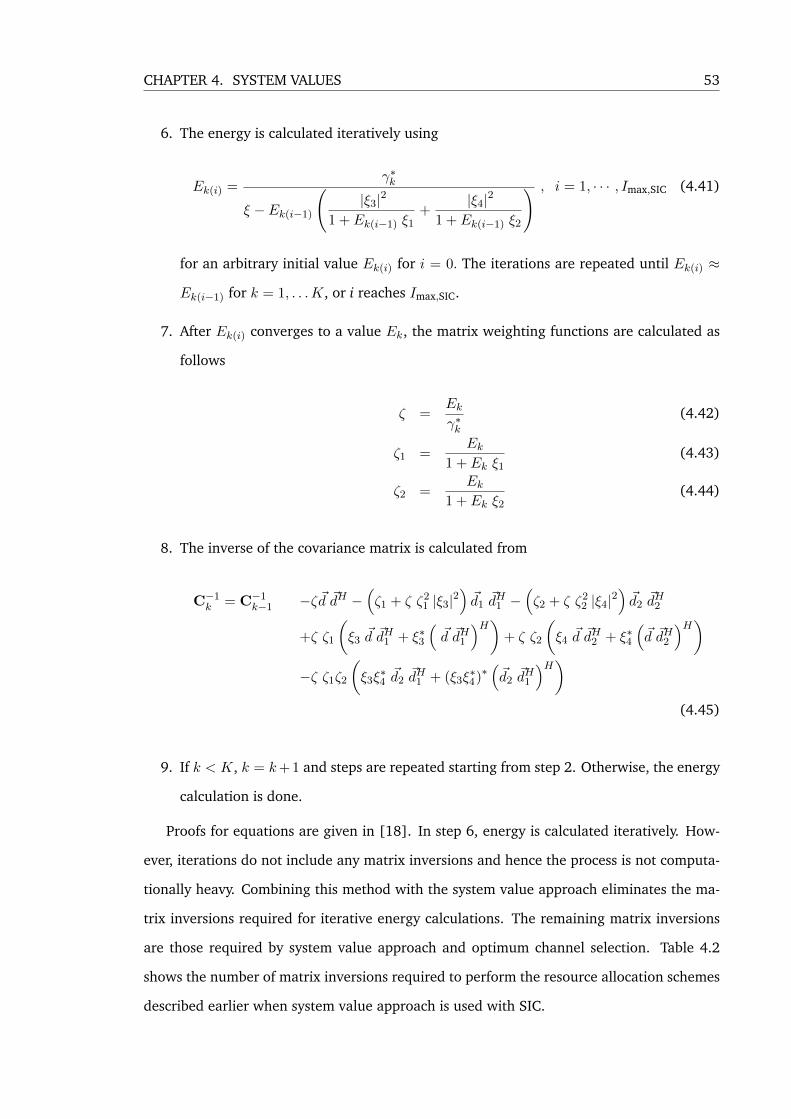
CHAPTER 4. SYSTEM VALUES 53
6. The energy is calculated iteratively using
Ek(i) =γ∗k
ξ − Ek(i−1)
(|ξ3|2
1 + Ek(i−1) ξ1+
|ξ4|2
1 + Ek(i−1) ξ2
) , i = 1, · · · , Imax,SIC (4.41)
for an arbitrary initial value Ek(i) for i = 0. The iterations are repeated until Ek(i) ≈
Ek(i−1) for k = 1, . . .K, or i reaches Imax,SIC.
7. After Ek(i) converges to a value Ek, the matrix weighting functions are calculated as
follows
ζ =Ekγ∗k
(4.42)
ζ1 =Ek
1 + Ek ξ1(4.43)
ζ2 =Ek
1 + Ek ξ2(4.44)
8. The inverse of the covariance matrix is calculated from
C−1k = C−1
k−1 −ζ ~d ~dH −(ζ1 + ζ ζ2
1 |ξ3|2)~d1~dH1 −
(ζ2 + ζ ζ2
2 |ξ4|2)~d2~dH2
+ζ ζ1
(ξ3~d ~dH1 + ξ∗3
(~d ~dH1
)H)+ ζ ζ2
(ξ4~d ~dH2 + ξ∗4
(~d ~dH2
)H)−ζ ζ1ζ2
(ξ3ξ
∗4~d2~dH1 + (ξ3ξ
∗4)∗(~d2~dH1
)H)(4.45)
9. If k < K, k = k+ 1 and steps are repeated starting from step 2. Otherwise, the energy
calculation is done.
Proofs for equations are given in [18]. In step 6, energy is calculated iteratively. How-
ever, iterations do not include any matrix inversions and hence the process is not computa-
tionally heavy. Combining this method with the system value approach eliminates the ma-
trix inversions required for iterative energy calculations. The remaining matrix inversions
are those required by system value approach and optimum channel selection. Table 4.2
shows the number of matrix inversions required to perform the resource allocation schemes
described earlier when system value approach is used with SIC.
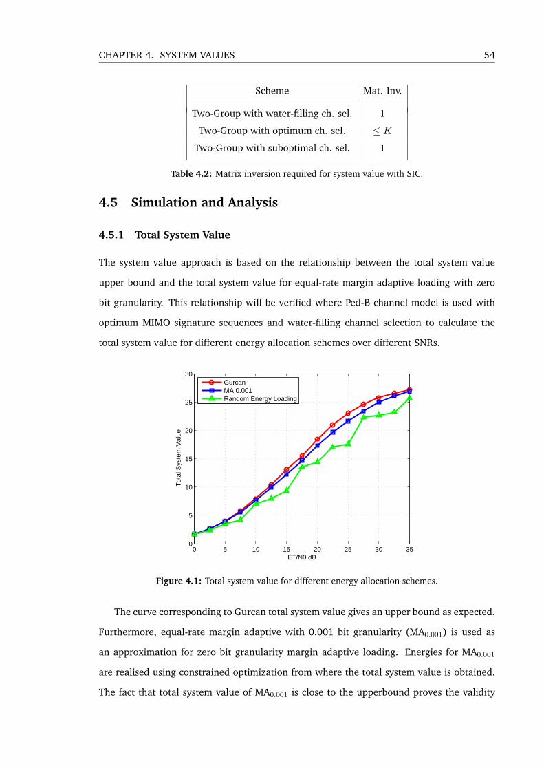
CHAPTER 4. SYSTEM VALUES 54
Scheme Mat. Inv.
Two-Group with water-filling ch. sel. 1
Two-Group with optimum ch. sel. ≤ K
Two-Group with suboptimal ch. sel. 1
Table 4.2: Matrix inversion required for system value with SIC.
4.5 Simulation and Analysis
4.5.1 Total System Value
The system value approach is based on the relationship between the total system value
upper bound and the total system value for equal-rate margin adaptive loading with zero
bit granularity. This relationship will be verified where Ped-B channel model is used with
optimum MIMO signature sequences and water-filling channel selection to calculate the
total system value for different energy allocation schemes over different SNRs.
0 5 10 15 20 25 30 350
5
10
15
20
25
30
ET/N0 dB
Tot
al S
yste
m V
alue
GurcanMA 0.001Random Energy Loading
Figure 4.1: Total system value for different energy allocation schemes.
The curve corresponding to Gurcan total system value gives an upper bound as expected.
Furthermore, equal-rate margin adaptive with 0.001 bit granularity (MA0.001) is used as
an approximation for zero bit granularity margin adaptive loading. Energies for MA0.001
are realised using constrained optimization from where the total system value is obtained.
The fact that total system value of MA0.001 is close to the upperbound proves the validity
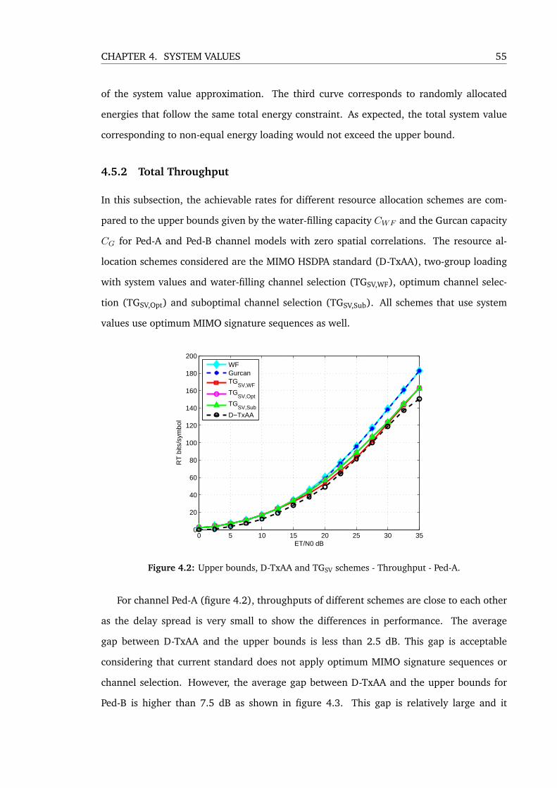
CHAPTER 4. SYSTEM VALUES 55
of the system value approximation. The third curve corresponds to randomly allocated
energies that follow the same total energy constraint. As expected, the total system value
corresponding to non-equal energy loading would not exceed the upper bound.
4.5.2 Total Throughput
In this subsection, the achievable rates for different resource allocation schemes are com-
pared to the upper bounds given by the water-filling capacity CWF and the Gurcan capacity
CG for Ped-A and Ped-B channel models with zero spatial correlations. The resource al-
location schemes considered are the MIMO HSDPA standard (D-TxAA), two-group loading
with system values and water-filling channel selection (TGSV,WF), optimum channel selec-
tion (TGSV,Opt) and suboptimal channel selection (TGSV,Sub). All schemes that use system
values use optimum MIMO signature sequences as well.
0 5 10 15 20 25 30 350
20
40
60
80
100
120
140
160
180
200
ET/N0 dB
RT
bits
/sym
bol
WFGurcanTG
SV,WFTG
SV,OptTG
SV,Sub
D−TxAA
Figure 4.2: Upper bounds, D-TxAA and TGSV schemes - Throughput - Ped-A.
For channel Ped-A (figure 4.2), throughputs of different schemes are close to each other
as the delay spread is very small to show the differences in performance. The average
gap between D-TxAA and the upper bounds is less than 2.5 dB. This gap is acceptable
considering that current standard does not apply optimum MIMO signature sequences or
channel selection. However, the average gap between D-TxAA and the upper bounds for
Ped-B is higher than 7.5 dB as shown in figure 4.3. This gap is relatively large and it
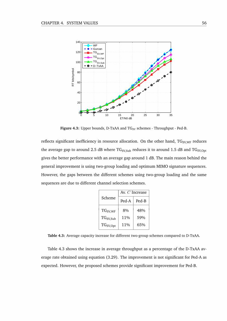
CHAPTER 4. SYSTEM VALUES 56
0 5 10 15 20 25 30 350
20
40
60
80
100
120
140
ET/N0 dB
RT
bits
/sym
bol
WFGurcanTG
SV,WFTG
SV,OptTG
SV,Sub
D−TxAA
Figure 4.3: Upper bounds, D-TxAA and TGSV schemes - Throughput - Ped-B.
reflects significant inefficiency in resource allocation. On the other hand, TGSV,WF reduces
the average gap to around 2.5 dB where TGSV,Sub reduces it to around 1.5 dB and TGSV,Opt
gives the better performance with an average gap around 1 dB. The main reason behind the
general improvement is using two-group loading and optimum MIMO signature sequences.
However, the gaps between the different schemes using two-group loading and the same
sequences are due to different channel selection schemes.
Av. C IncreaseScheme
Ped-A Ped-B
TGSV,WF 8% 48%
TGSV,Sub 11% 59%
TGSV,Opt 11% 65%
Table 4.3: Average capacity increase for different two-group schemes compared to D-TxAA.
Table 4.3 shows the increase in average throughput as a percentage of the D-TxAA av-
erage rate obtained using equation (3.29). The improvement is not significant for Ped-A as
expected. However, the proposed schemes provide significant improvement for Ped-B.
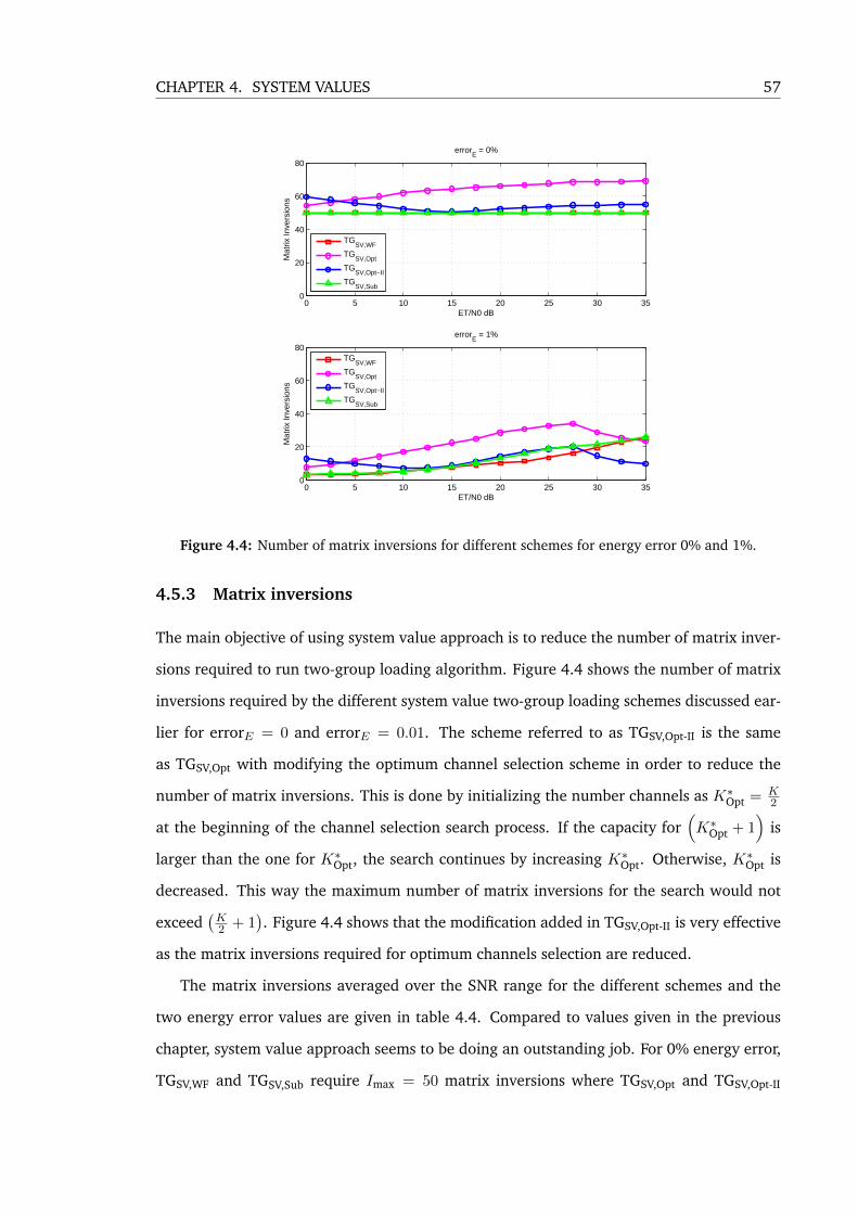
CHAPTER 4. SYSTEM VALUES 57
0 5 10 15 20 25 30 350
20
40
60
80
ET/N0 dB
Mat
rix In
vers
ions
errorE = 0%
TGSV,WF
TGSV,Opt
TGSV,Opt−II
TGSV,Sub
0 5 10 15 20 25 30 350
20
40
60
80
ET/N0 dB
Mat
rix In
vers
ions
errorE = 1%
TG
SV,WF
TGSV,Opt
TGSV,Opt−II
TGSV,Sub
Figure 4.4: Number of matrix inversions for different schemes for energy error 0% and 1%.
4.5.3 Matrix inversions
The main objective of using system value approach is to reduce the number of matrix inver-
sions required to run two-group loading algorithm. Figure 4.4 shows the number of matrix
inversions required by the different system value two-group loading schemes discussed ear-
lier for errorE = 0 and errorE = 0.01. The scheme referred to as TGSV,Opt-II is the same
as TGSV,Opt with modifying the optimum channel selection scheme in order to reduce the
number of matrix inversions. This is done by initializing the number channels as K∗Opt = K
2
at the beginning of the channel selection search process. If the capacity for(K∗
Opt + 1)
is
larger than the one for K∗Opt, the search continues by increasing K∗
Opt. Otherwise, K∗Opt is
decreased. This way the maximum number of matrix inversions for the search would not
exceed(K2 + 1
). Figure 4.4 shows that the modification added in TGSV,Opt-II is very effective
as the matrix inversions required for optimum channels selection are reduced.
The matrix inversions averaged over the SNR range for the different schemes and the
two energy error values are given in table 4.4. Compared to values given in the previous
chapter, system value approach seems to be doing an outstanding job. For 0% energy error,
TGSV,WF and TGSV,Sub require Imax = 50 matrix inversions where TGSV,Opt and TGSV,Opt-II
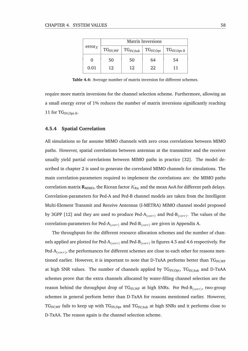
CHAPTER 4. SYSTEM VALUES 58
Matrix InversionserrorE TGSV,WF TGSV,Sub TGSV,Opt TGSV,Opt-II
0 50 50 64 54
0.01 12 12 22 11
Table 4.4: Average number of matrix inversion for different schemes.
require more matrix inversions for the channel selection scheme. Furthermore, allowing an
a small energy error of 1% reduces the number of matrix inversions significantly reaching
11 for TGSV,Opt-II.
4.5.4 Spatial Correlation
All simulations so far assume MIMO channels with zero cross correlations between MIMO
paths. However, spatial correlations between antennas at the transmitter and the receiver
usually yield partial correlations between MIMO paths in practice [32]. The model de-
scribed in chapter 2 is used to generate the correlated MIMO channels for simulations. The
main correlation-parameters required to implement the correlations are: the MIMO paths
correlation matrix RMIMO, the Ricean factorKRic and the mean AoA for different path delays.
Correlation-parameters for Ped-A and Ped-B channel models are taken from the Intelligent
Multi-Element Transmit and Receive Antennas (I-METRA) MIMO channel model proposed
by 3GPP [12] and they are used to produce Ped-A(corr) and Ped-B(corr). The values of the
correlation-parameters for Ped-A(corr) and Ped-B(corr) are given in Appendix A.
The throughputs for the different resource allocation schemes and the number of chan-
nels applied are plotted for Ped-A(corr) and Ped-B(corr) in figures 4.5 and 4.6 respectively. For
Ped-A(corr), the performances for different schemes are close to each other for reasons men-
tioned earlier. However, it is important to note that D-TxAA performs better than TGSV,WF
at high SNR values. The number of channels applied by TGSV,Opt, TGSV,Sub and D-TxAA
schemes prove that the extra channels allocated by water-filling channel selection are the
reason behind the throughput drop of TGSV,WF at high SNRs. For Ped-B(corr), two-group
schemes in general perform better than D-TxAA for reasons mentioned earlier. However,
TGSV,WF fails to keep up with TGSV,Opt and TGSV,Sub at high SNRs and it performs close to
D-TxAA. The reason again is the channel selection scheme.
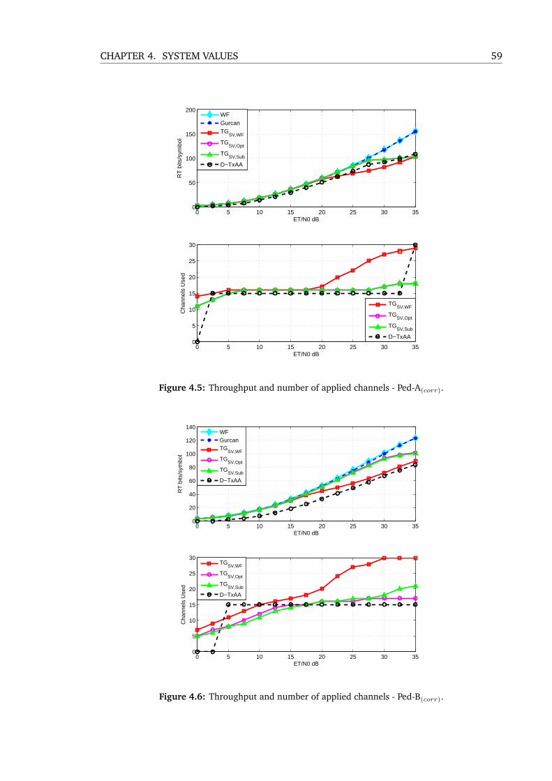
CHAPTER 4. SYSTEM VALUES 59
0 5 10 15 20 25 30 350
50
100
150
200
ET/N0 dB
RT
bits
/sym
bol
WFGurcanTG
SV,WF
TGSV,Opt
TGSV,Sub
D−TxAA
0 5 10 15 20 25 30 350
5
10
15
20
25
30
ET/N0 dB
Cha
nnel
s U
sed
TGSV,WF
TGSV,Opt
TGSV,Sub
D−TxAA
Figure 4.5: Throughput and number of applied channels - Ped-A(corr).
0 5 10 15 20 25 30 350
20
40
60
80
100
120
140
ET/N0 dB
RT
bits
/sym
bol
WFGurcanTG
SV,WF
TGSV,Opt
TGSV,Sub
D−TxAA
0 5 10 15 20 25 30 350
5
10
15
20
25
30
ET/N0 dB
Cha
nnel
s U
sed
TG
SV,WF
TGSV,Opt
TGSV,Sub
D−TxAA
Figure 4.6: Throughput and number of applied channels - Ped-B(corr).
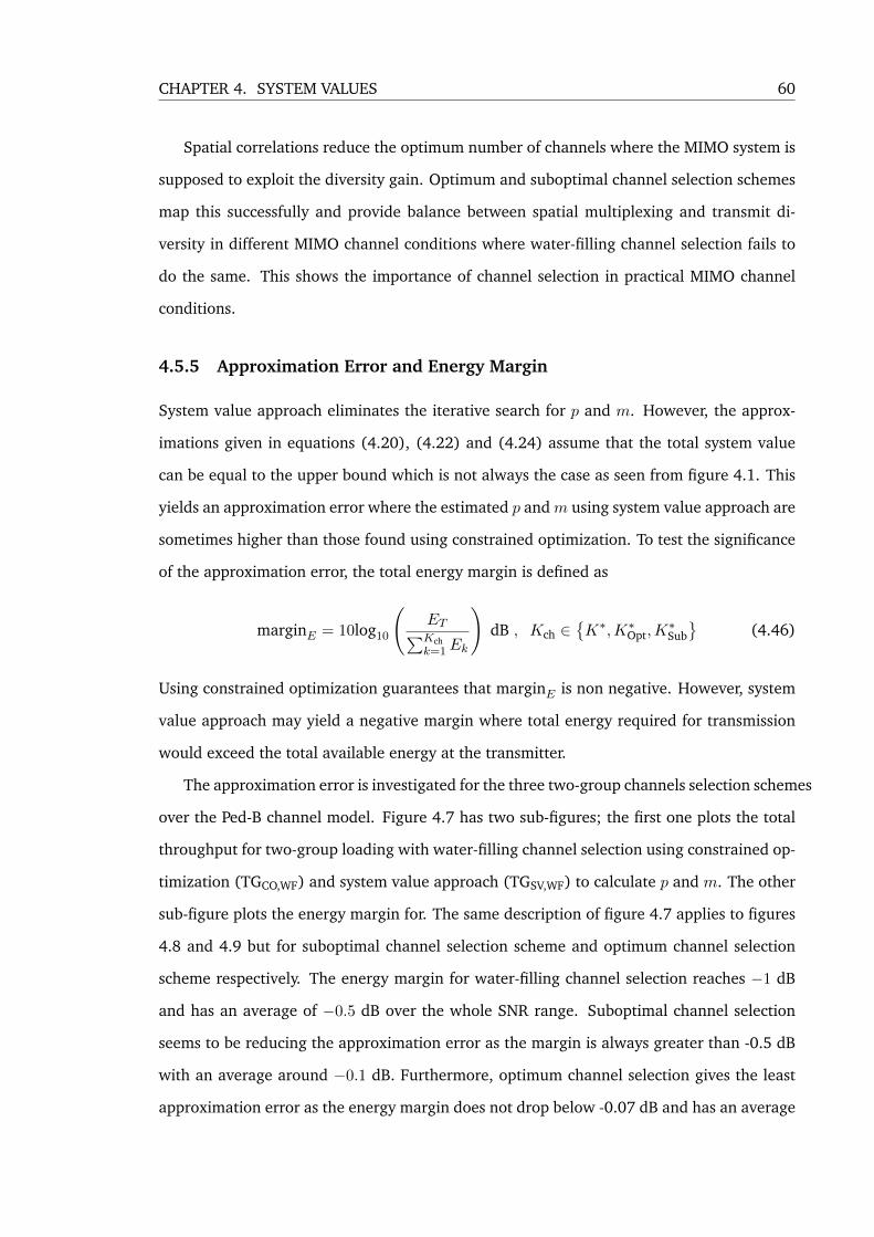
CHAPTER 4. SYSTEM VALUES 60
Spatial correlations reduce the optimum number of channels where the MIMO system is
supposed to exploit the diversity gain. Optimum and suboptimal channel selection schemes
map this successfully and provide balance between spatial multiplexing and transmit di-
versity in different MIMO channel conditions where water-filling channel selection fails to
do the same. This shows the importance of channel selection in practical MIMO channel
conditions.
4.5.5 Approximation Error and Energy Margin
System value approach eliminates the iterative search for p and m. However, the approx-
imations given in equations (4.20), (4.22) and (4.24) assume that the total system value
can be equal to the upper bound which is not always the case as seen from figure 4.1. This
yields an approximation error where the estimated p andm using system value approach are
sometimes higher than those found using constrained optimization. To test the significance
of the approximation error, the total energy margin is defined as
marginE = 10log10
(ET∑Kchk=1Ek
)dB , Kch ∈
{K∗,K∗
Opt,K∗Sub
}(4.46)
Using constrained optimization guarantees that marginE is non negative. However, system
value approach may yield a negative margin where total energy required for transmission
would exceed the total available energy at the transmitter.
The approximation error is investigated for the three two-group channels selection schemes
over the Ped-B channel model. Figure 4.7 has two sub-figures; the first one plots the total
throughput for two-group loading with water-filling channel selection using constrained op-
timization (TGCO,WF) and system value approach (TGSV,WF) to calculate p and m. The other
sub-figure plots the energy margin for. The same description of figure 4.7 applies to figures
4.8 and 4.9 but for suboptimal channel selection scheme and optimum channel selection
scheme respectively. The energy margin for water-filling channel selection reaches −1 dB
and has an average of −0.5 dB over the whole SNR range. Suboptimal channel selection
seems to be reducing the approximation error as the margin is always greater than -0.5 dB
with an average around −0.1 dB. Furthermore, optimum channel selection gives the least
approximation error as the energy margin does not drop below -0.07 dB and has an average
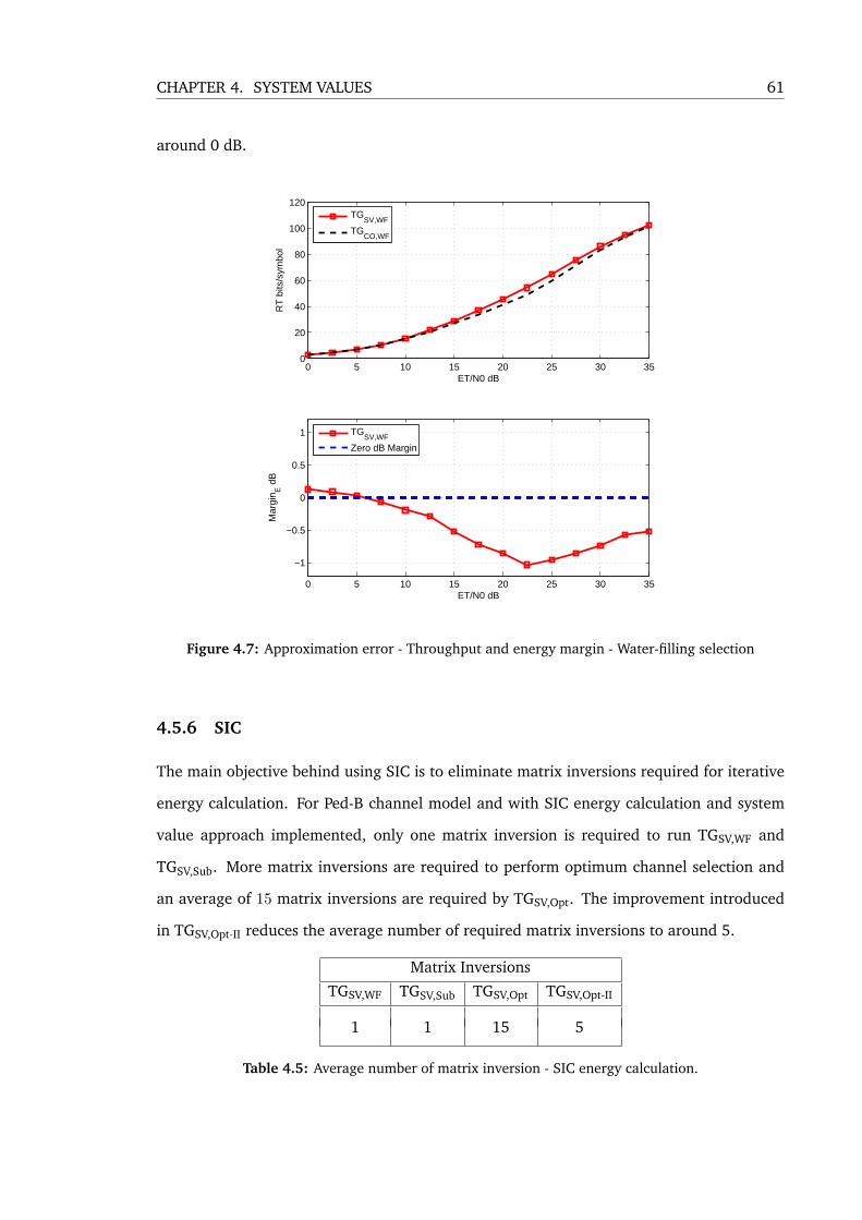
CHAPTER 4. SYSTEM VALUES 61
around 0 dB.
0 5 10 15 20 25 30 350
20
40
60
80
100
120
ET/N0 dB
RT
bits
/sym
bol
TG
SV,WF
TGCO,WF
0 5 10 15 20 25 30 35
−1
−0.5
0
0.5
1
ET/N0 dB
Mar
gin E
dB
TG
SV,WF
Zero dB Margin
Figure 4.7: Approximation error - Throughput and energy margin - Water-filling selection
4.5.6 SIC
The main objective behind using SIC is to eliminate matrix inversions required for iterative
energy calculation. For Ped-B channel model and with SIC energy calculation and system
value approach implemented, only one matrix inversion is required to run TGSV,WF and
TGSV,Sub. More matrix inversions are required to perform optimum channel selection and
an average of 15 matrix inversions are required by TGSV,Opt. The improvement introduced
in TGSV,Opt-II reduces the average number of required matrix inversions to around 5.
Matrix Inversions
TGSV,WF TGSV,Sub TGSV,Opt TGSV,Opt-II
1 1 15 5
Table 4.5: Average number of matrix inversion - SIC energy calculation.
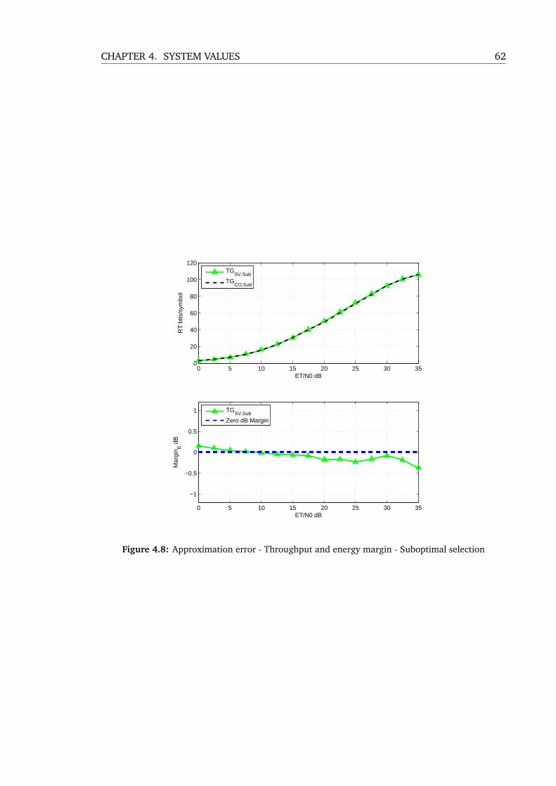
CHAPTER 4. SYSTEM VALUES 62
0 5 10 15 20 25 30 350
20
40
60
80
100
120
ET/N0 dB
RT
bits
/sym
bol
TG
SV,Sub
TGCO,Sub
0 5 10 15 20 25 30 35
−1
−0.5
0
0.5
1
ET/N0 dB
Mar
gin E
dB
TG
SV,Sub
Zero dB Margin
Figure 4.8: Approximation error - Throughput and energy margin - Suboptimal selection
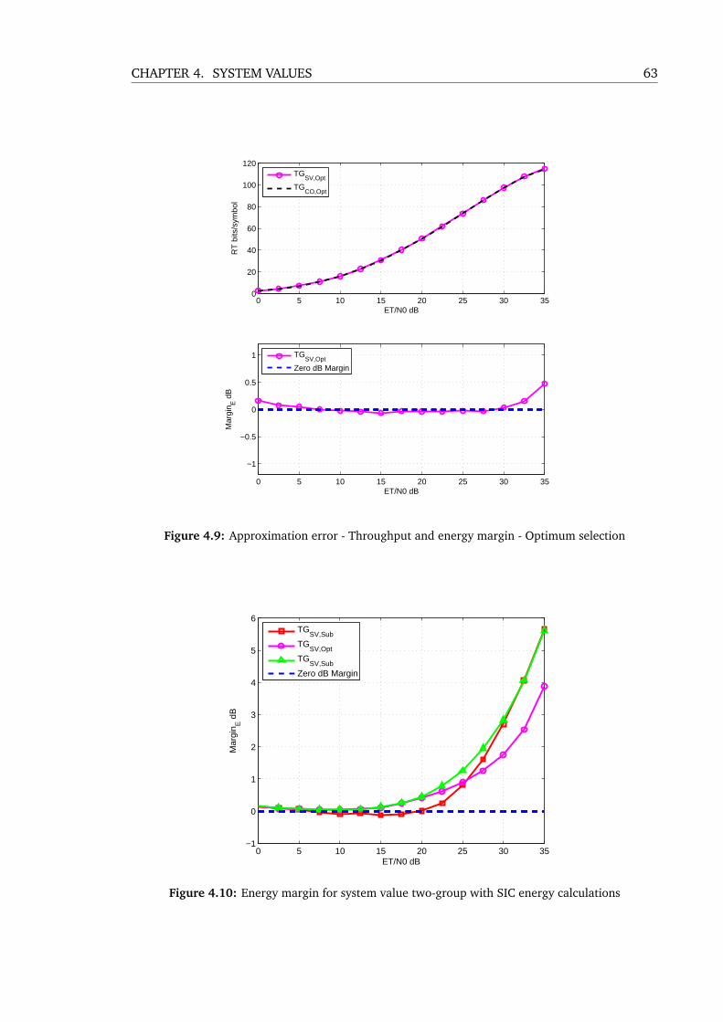
CHAPTER 4. SYSTEM VALUES 63
0 5 10 15 20 25 30 350
20
40
60
80
100
120
ET/N0 dB
RT
bits
/sym
bol
TG
SV,Opt
TGCO,Opt
0 5 10 15 20 25 30 35
−1
−0.5
0
0.5
1
ET/N0 dB
Mar
gin E
dB
TG
SV,Opt
Zero dB Margin
Figure 4.9: Approximation error - Throughput and energy margin - Optimum selection
0 5 10 15 20 25 30 35−1
0
1
2
3
4
5
6
ET/N0 dB
Mar
gin E
dB
TG
SV,Sub
TGSV,Opt
TGSV,Sub
Zero dB Margin
Figure 4.10: Energy margin for system value two-group with SIC energy calculations

CHAPTER 4. SYSTEM VALUES 64
Another interesting thing to look at when SIC is implemented, is the energy margin.
Figure 4.10 plots the energy margins for the different schemes over Ped-B channel mode.
SIC has eliminated the negative margins of TGSV,Sub and TGSV,Opt where a negative margin
still appears for TGSV,WF. However, this negative margin is not significant as in the worst
case it does not drop below -0.1 dB. At high SNR values, the energy margins for different
schemes grow positively exceeding 5 dB for TGSV,WF and TGSV,Sub. This is expected as SIC
reduces interference and hence increases the potential capacity of channels. However, SIC
was mainly considered to simplify calculations and increasing the assigned rates was not
considered.

Chapter 5
Conclusion
Currently deployed MIMO HSDPA systems suffer from severe throughput losses in frequency
selective channels with significant delay spread. Such radio channel conditions are typical
for urban environments. Throughput losses are caused by inefficient resource allocation,
particularly the manner in which energy is distributed among different code channels. The
resource allocation scheme adapted by MIMO HSDPA distributes energy among all available
channels and rates are controlled per data stream where all channels belonging to the same
data stream are assigned the same bit rate. Furthermore, the system can choose to operate
in single-stream mode (transmit diversity) or dual-stream mode (spatial multiplexing).
It was found that using energy-constrained rate optimization, particularly two-group
loading algorithm, provides around 40% increase in average throughput for ITU Ped-B chan-
nel model. However, the computational complexity required to run the algorithm is high for
the majority of mobile applications due to the large number of covariance matrix inversions
required. System value approach and optimum signature sequence design were applied
to MIMO HSDPA in order to reduce computational complexity and improve performance.
The approach was found to work well and the number of matrix inversions was reduced
from the order of hundreds to the order of tens. However, system value approach produced
approximation error which results in a small negative energy margin. The main contribu-
tion of this work is the optimum and suboptimal channel selection schemes developed to
be used with system value approach. Optimum channel selection scheme improves average
throughput, reduces approximation error and reduces throughput loss in the presence of
65

CHAPTER 5. CONCLUSION 66
spatial correlations. Furthermore, channel selection provides automatic transition between
transmit diversity and spatial multiplexing and hence eliminates the confusion associated
with using single-stream mode or double-stream mode. However, optimum channel selec-
tion requires a few extra matrix inversion operations. Suboptimal channel selection provides
improvements very close to those provided by optimum channel selection without requiring
the extra matrix inversions. For ITU Ped-B channel mode, two-group loading improved by
system value approach, optimum signature sequences and channel selection provides up to
65% and 60% increase in average throughput for optimum channel selection and subopti-
mal channel selection respectively.
Finally, interference cancelation with recursive matrix inversions was tested with the sys-
tem value approach. This brought down the number of matrix inversions to one and elimi-
nated the negative energy margin for optimum and suboptimal channel selection schemes.
Interference cancelation produces a significant positive energy margin at high SNRs which
can be used to transmit extra data. However, interference cancelation was used mainly to
eliminate matrix inversions required by iterative energy calculation. Considering interfer-
ence cancelation to increase throughput is one of the points that can be considered in a
future work based on this project. Other suggested points that need to be explored include:
1. Combining the improved recourse allocation schemes with recently proposed 3GPP
improvements such as multiple-carrier MIMO HSDPA.
2. Considering system level modelling and simulation to test the overall system perfor-
mance and combining it with the link level model provided in this project.
3. Considering the multi-user problem where channels are allocated to multiple users in
the same cell.
4. Developing practical solutions for implementation problems such as the perfect CSI
assumed for energy allocation feedback and optimum signature sequences.
5. Implementing the system practically using software defined radio and testing it in a
proper environment to see if it performs as the theory states.
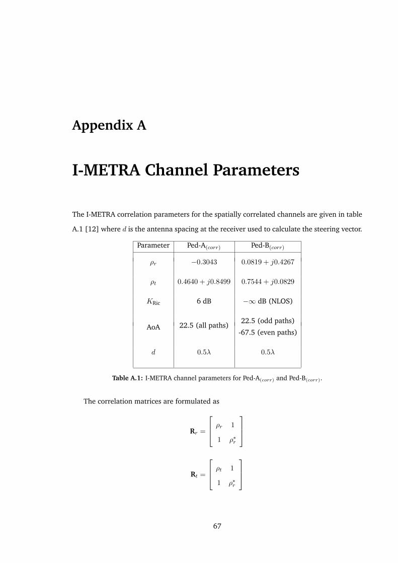
Appendix A
I-METRA Channel Parameters
The I-METRA correlation parameters for the spatially correlated channels are given in table
A.1 [12] where d is the antenna spacing at the receiver used to calculate the steering vector.
Parameter Ped-A(corr) Ped-B(corr)
ρr −0.3043 0.0819 + j0.4267
ρt 0.4640 + j0.8499 0.7544 + j0.0829
KRic 6 dB −∞ dB (NLOS)
22.5 (odd paths)AoA 22.5 (all paths)
-67.5 (even paths)
d 0.5λ 0.5λ
Table A.1: I-METRA channel parameters for Ped-A(corr) and Ped-B(corr).
The correlation matrices are formulated as
Rr =
ρr 1
1 ρ∗r
Rt =
ρt 1
1 ρ∗r
67
Appendix B
Simulation Package
This Appendix provides general explanation for the simulation package created as part of
this project. The programs and functions are all written using MATLAB and the full codes
are available in the associated CD. The programs can be divided into three categories; ini-
tialization, resource allocation schemes and presentation. Programs falling in each category
will be discussed alongside with functions used for each program.
B.1 Initialization
The first initialization program is Initialize Parameters.m. This program initializes the pa-
rameters given in table 2.1 except the channel model. The parameters are saved in a .mat
file which is loaded when running programs that need those parameters. The second ini-
tialization program is PDP.m. This program modifies the PDPs given by ITU to match the
HSDPA system. The function PDP conv.m is used in the process to re-sample the original
PDP at appropriate periods.
The las initialization program is Create MIMO ch.m This program creates MIMO chan-
nels required for the simulations and saves them in .mat files so that simulations for dif-
ferent schemes use exactly the same channels. This program uses the functions h gen.m,
MIMO PedA.m and MIMO PedB.m to create the four MIMO paths vectors for customized
PDP and correlations, I-METRA Ped-A and I-METRA Ped-B respectively.
68
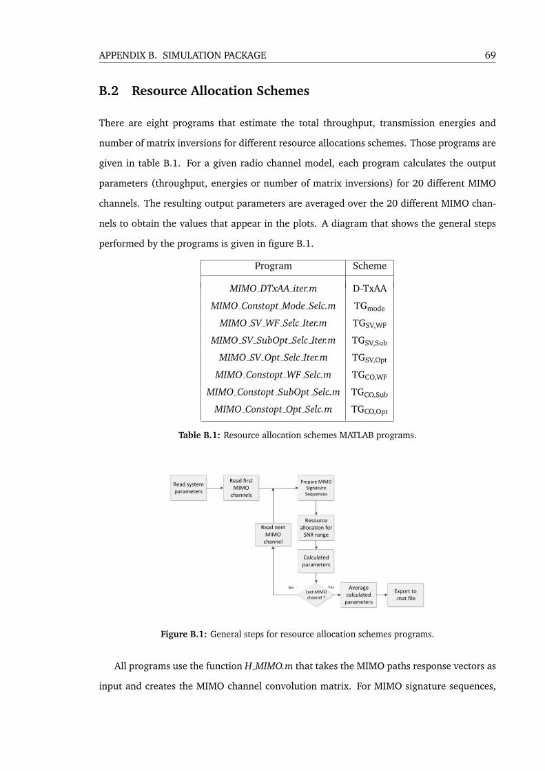
APPENDIX B. SIMULATION PACKAGE 69
B.2 Resource Allocation Schemes
There are eight programs that estimate the total throughput, transmission energies and
number of matrix inversions for different resource allocations schemes. Those programs are
given in table B.1. For a given radio channel model, each program calculates the output
parameters (throughput, energies or number of matrix inversions) for 20 different MIMO
channels. The resulting output parameters are averaged over the 20 different MIMO chan-
nels to obtain the values that appear in the plots. A diagram that shows the general steps
performed by the programs is given in figure B.1.
Program Scheme
MIMO DTxAA iter.m D-TxAA
MIMO Constopt Mode Selc.m TGmode
MIMO SV WF Selc Iter.m TGSV,WF
MIMO SV SubOpt Selc Iter.m TGSV,Sub
MIMO SV Opt Selc Iter.m TGSV,Opt
MIMO Constopt WF Selc.m TGCO,WF
MIMO Constopt SubOpt Selc.m TGCO,Sub
MIMO Constopt Opt Selc.m TGCO,Opt
Table B.1: Resource allocation schemes MATLAB programs.
Read system parameters
Read first MIMO
channels
Prepare MIMO Signature
Sequences
Resource allocation for
SNR range
Calculated parameters
Last MIMO channel ?
Read next MIMO
channel
YesNo Average calculated
parameters
Export to .mat file
Figure B.1: General steps for resource allocation schemes programs.
All programs use the function H MIMO.m that takes the MIMO paths response vectors as
input and creates the MIMO channel convolution matrix. For MIMO signature sequences,
APPENDIX B. SIMULATION PACKAGE 70
the function OVSF Pre.m is used by the first two programs in table B.1 to create OVSF signa-
ture sequences with precoding where precoding changes according to the MIMO channel.
The rest of the programs use the function Opt Sig.m to create optimum MIMO signature
sequences. MIMO DTxAA iter.m uses the functions TxAA.m and DTxAA.m to perform single-
stream loading and double-stream loading respectively where MIMO Constopt Mode Selc.m
uses TG Original.m to do both single-stream and double-stream constrained optimization
two-group loading.
For two-group with system value approach, all programs have the same structure but dif-
fer in the channel selection scheme. MIMO SV WF Selc Iter.m uses the function C WF.m to
perform water-filling channel selection and calculate the water-filling capacity. The function
Gurcan.m is used to find the total system value upper bound and calculate Gurcan’s capacity
where the function TG p m.m uses system value approach to calculate p and m. Further-
more, the functions E TG iter.m and E TG SIC.m calculate energies iteratively and using SIC
respectively. Following the same structure, the only change in MIMO SV SubOpt Selc Iter.m
and MIMO SV Opt Selc Iter.m is in the channel selection scheme. The functions SubOpt Selec.m
and Opt Selec.m are used for suboptimal and optimum channel selection schemes respec-
tively. Finally, the last three programs in B.1 apply optimum sequences and channel selec-
tion with the function TG p m const opt.m to calculate p, m and energies using constrained
optimization.
The values that result from the programs described in this section are stored in different
.mat files. The same program may have more than one .mat destination for different channel
models.
B.3 Presentation
The presentation program plot results.mat uses the .mat files produced from running all
previous programs and produces the figures used in this report. Some calculations related
to different observations are carried out using the same program as well.
References
[1] 3GPP. “Technical Specification Group Radio Access Network; Multiple Input Multiple
Output in UTRA; (Release 7)”. TR 25.876 V7.0.0, 3GPP, Mar. 2007.
[2] 3GPP. “Overview of 3GPP Release 10”. V0.1.1, 3GPP, Jun. 2011.
[3] 3GPP. “Overview of 3GPP Release 11”. V0.0.7, 3GPP, Jun. 2011.
[4] 3GPP. “Overview of 3GPP Release 8”. V0.2.3, 3GPP, Jun. 2011.
[5] 3GPP. “Overview of 3GPP Release 9”. V0.2.2, 3GPP, Jun. 2011.
[6] 3GPP. “Technical Specification Group Radio Access Network; Physical layer procedures
(FDD); (Release 10)”. TS 25.214 V10.3.0, 3GPP, Jun. 2011.
[7] 3GPP. “Technical Specification Group Radio Access Network; Spatial channel model
for Multiple Input Multiple Output (MIMO) simulations; (Release 10)”. TR 25.996
V10.0.0, 3GPP, Mar. 2011.
[8] Eduardo Zacarıas B. “Adaptive transmit beamforming with closed loop feedback in
MIMO systems”. In S-72.333 Postgraduate Course in Radio Communications. Helsinki
University of Technology, Signal Processing Laboratory, 2004.
[9] J. Bergman, D. Gerstenberger, F. Gunnarsson, and S. Strom. “Continued HSPA Evolu-
tion of mobile broadband”. Ericsson Review, (no.1), 2009.
[10] Ezio Biglieri, Robert Calderbank, Anthony Constantinides, Andrea Goldsmith, Aro-
gyaswami Paulraj, and Vincent H. Poor. “MIMO Wireless Communications”. Cambridge
University Press, January 2007.
71
REFERENCES 72
[11] D. Bosanska, C. Mehlfuhrer, and M. Rupp. “Performance Evaluation of Intra-cell Inter-
ference Cancelation in D-TxAA HSDPA”. In Proceedings 2008 International ITG Work-
shop on Smart Antennas (WSA 2008), Darmstadt, Feb. 2008.
[12] Yong Soo Cho, Jaekwon Kim, Won Young Yang, and Chung-Gu Kang. “MIMO-OFDM
Wireless Communications with MATLAB”. John Wiley and Sons, 2010.
[13] Thomas M. Cover and Joy A. Thomas. “Elements of information theory”. Wiley-
Interscience, New York, NY, USA, 1991.
[14] M. Cvitkovic, B. Modlic, and G. Sisul. “High Speed Downlink Packet Access Principles”.
ELMAR, pages 125 – 128, 2007.
[15] S. Geirhofer, C. Mehlfuhrer, and M. Rupp. “Design and real-time measurement of
HSDPA equalizers”. In Signal Processing Advances in Wireless Communications, 2005
IEEE 6th Workshop on, pages 166 – 170, Jun. 2005.
[16] Andrea Goldsmith. “Wireless Communications”. Cambridge University Press, New York,
NY, USA, 2005.
[17] M. Gurcan. “Gurcan’s system value and upper bounds for total system value and sum
capacity for K multicode parallel channel SISO and MIMO systems”, Unpublished.
Imperial College London, 2011.
[18] M. Gurcan. “Iterative energy and inverse covariance matrix calculation for successive
interference calculation for WCDMA HSDPA systems”, Unpublished. Imperial College
London, 2011.
[19] M. Gurcan. “Presentation 8: High Spead Downlink Packet Access System”. In Mobile
Radio Communications Lecture Notes. Imperial College London, Mar. 2011.
[20] Zhenfeng He and M. Gurcan. “The Rate Adaptive Throughput Maximization in PAM-
Modulated Overloaded System”. In Wireless Communications and Networking Confer-
ence, 2009. WCNC 2009. IEEE, pages 1–6, Apr. 2009.
[21] Zhenfeng He, M. Gurcan, and H. Ghani. “Time-efficient resource allocation algorithm
over HSDPA in femtocell networks”. In IEEE 21st International Symposium on Personal,
REFERENCES 73
Indoor and Mobile Radio Communications Workshops (PIMRC Workshops), 2010. IEEE,
pages 197–202, 2010.
[22] Harri Holma and Antti Toskala. “WCDMA for UMTS: HSPA Evolution and LTE”. John
Wiley & Sons, Inc., New York, NY, USA, 2007.
[23] ITU. “Recommendation ITU-R M.1225: Guidelines For Evaluation of Radio Transmis-
sion Technologies for IMT-2000”. Technical report, ITU, 1997.
[24] T. Klingenbrunn and P. Mogensen. “Modelling frequency correlation of fast fading in
frequency hopping GSM link simulations”. In Vehicular Technology Conference, 1999.
VTC 1999 - Fall. IEEE VTS 50th, volume 4, pages 2398 – 2402, 1999.
[25] Krauss, T.P. and Zoltowski, M.D. and Leus, G. “Simple MMSE equalizers for CDMA
downlink to restore chip sequence: comparison to zero-forcing and RAKE”. In Inter-
national Conference On Acoustics, Speech, And Signal Processing, 2000. ICASSP 2000.
IEEE, volume 5, pages 2865 – 2868, 2000.
[26] Lang Tong and Alle-jan Van Der Veen and Patrick Dewilde and Youngchul Sung. “Blind
Decorrelating RAKE Receivers for Long-Code WCDMA”. IEEE Trans. Signal Processing,
51:1642–1655, 2002.
[27] Love, R. and Stewart, K. and Bachu, R. and Ghosh, A. “MMSE equalization for UMTS
HSDPA”. In Vehicular Technology Conference, 2003. VTC 2003-Fall. IEEE 58th , vol-
ume 4, pages 2416 – 2420, 2003.
[28] Mailaender, L. “Linear MIMO equalization for CDMA downlink signals with code
reuse”. IEEE Transactions on Wireless Communications, 4(5):2423 – 2434, 2005.
[29] Christian Mehlfuhrer, Sebastian Caban, and Markus Rupp. “MIMO HSDPA Throughput
Measurement Results in an Urban Scenario”. In VTC Fall, pages 0–, 2009.
[30] Jason W. P. Ng and Athanassios Manikas. “A Space-Diffused Spatial-Temporal ARray
(STAR) Receiver for DS-CDMA System”. International Journal HERMIS-mu-pi (Mathe-
matics and Informatics Science), 4:131–152, 2003.
REFERENCES 74
[31] Arogyaswami J. Paulraj, Dhananjay A. Gore, Rohit U. Nabar, and Helmut Bolcskei.
“An overview of MIMO communications - A key to Gigabit wireless”. Proceedings of
the IEEE, 92(2):198–218, Feb. 2004.
[32] K.I. Pedersen, J.B. Andersen, J.P. Kermoal, and P. Mogensen. “A stochastic multiple-
input-multiple-output radio channel model for evaluation of space-time coding algo-
rithms”. In Vehicular Technology Conference, 2000. IEEE VTS-Fall VTC 2000. 52nd,
volume 2, pages 893 –897 vol.2, 2000.
[33] Bessem Sayadi, Stefan Ataman, and Inbar Fijalkow. “Joint Downlink Power Control
and Multicode Receivers for Downlink Transmissions in High Speed UMTS”. EURASIP
J. Wireless Comm. and Networking, 2006, 2006.
[34] Shakti Prasad Shenoy, Irfan Ghauri, and Dirk T. M. Slock. “Receiver Designs For MIMO
HSDPA”. In ICC, pages 941–945, 2008.
[35] B. Sklar. “Rayleigh fading channels in mobile digital communication systems .I. Char-
acterization”. Communications Magazine, IEEE, 35(7):90–100, 1997.
[36] A. M. Torello. “CPICH Power Optimization for MIMO HSDPA”. MSc. Thesis, Vienna
University of Technology, 2009.