11 Analysis of Industrial Robot Structure and Milling Process Interaction for Path Manipulation

J. Bauer, M. Friedmann, T. Hemker, M. Pischan, C. Reinl , E.Abele, O. von Stryk

Abstract Industrial robots are used in a great variety of applications for hand-ling, welding, assembling and milling operations. Especially for machining opera-tions industrial robots represent a cost-saving and flexible alternative compared to standard machine tools. Reduced pose and path accuracy, especially under process force load due to the high mechanical compliance, restrict the use of industrial ro-bots for further machining applications. In this chapter a method is presented to predict and compensate path deviation of robots resulting from process forces. A process force simulation based on a material removal calculation is proposed. Fur-thermore, a rigid multi-body dynamic system’s model of the robot is extended by joint elasticities and tilting effects that are modeled by spring-damper-models at actuated and additional virtual axes. By coupling the removal simulation with the robot model the interaction of the milling process with the robot structure can be analyzed by evaluation of path deviation and surface structure. With the knowl-edge of interaction along the milling path a general model-based path correction strategy is presented to significantly improve accuracy in milling operations.

11.1. Introduction

Major fields of machining applications for industrial robots are automated pre-ma-chining, deburring and fettling of cast parts or trimming of carbon fiber reinforced laminate. Due to its kinematic structure with 6 axes the robot can cover a large working space and is able to reach difficult work piece positions, so that it can be applied to perform complex machining operations. Therefore, compared to stan-dard machine tools, industrial robots offer an economic and flexible machining al-ternative. However, industrial robots do not provide a high absolute and repeat ac-curacy. Current industrial robot systems reach a repeat accuracy of 0.06 mm. Un-der process load, e.g., in milling operation an additional deflection of the tool cen-ter point (TCP) occurs. Measured deflections of 0.25 mm under process loads of 100 N in earlier tests [1] confirmed the expected compliance. Therefore, when us-ing an industrial robot for milling applications, inaccuracies of the serial robot kinematic, the low structural stiffness and the effective process forces are leading to path deviations. The results are unwanted trajectory deviations, which lead to

errors in dimension and a reduced surface quality of the work piece. These devia-tions mainly consist of a static offset overlaid with a low frequency oscillation of the tool [2].

In order to increase the milling accuracy with present process forces of the milling operation a model-based path manipulation module for robots is devel-oped. This module consists of a robot and a milling force model to predict path er-rors in advance of a real milling operation. Additionally, the simulation module al-lows the investigation and analysis of the interaction of milling force and motion of the robot. Finally, the proposed strategy for modeling and simulation serves as basis for an efficient offline correction of path deviations.

Overall objective

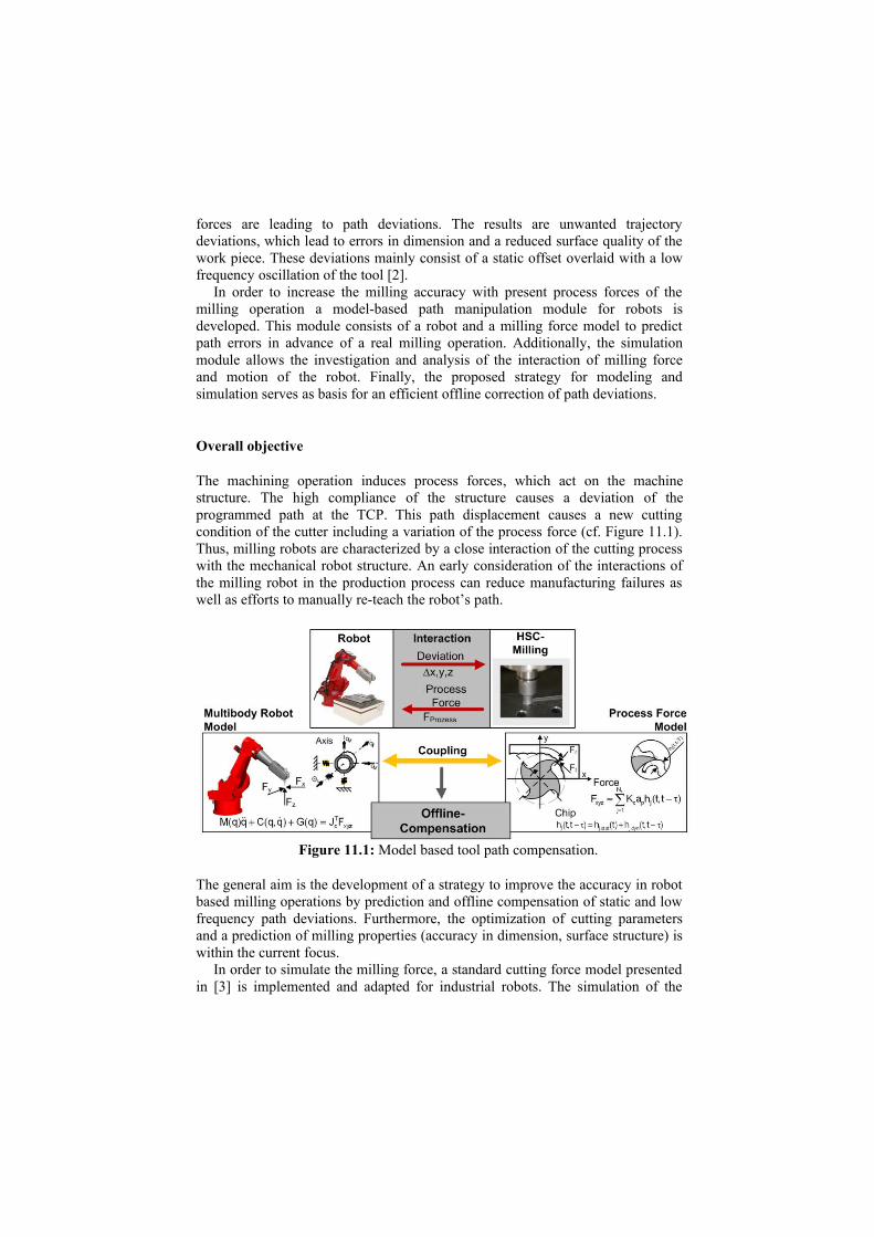
The machining operation induces process forces, which act on the machine struc-ture. The high compliance of the structure causes a deviation of the programmed path at the TCP. This path displacement causes a new cutting condition of the cut-ter including a variation of the process force (cf. Figure 11.1). Thus, milling robots are characterized by a close interaction of the cutting process with the mechanical robot structure. An early consideration of the interactions of the milling robot in the production process can reduce manufacturing failures as well as efforts to manually re-teach the robot’s path.

Figure 11.1: Model based tool path compensation.

The general aim is the development of a strategy to improve the accuracy in robot based milling operations by prediction and offline compensation of static and low frequency path deviations. Furthermore, the optimization of cutting parameters and a prediction of milling properties (accuracy in dimension, surface structure) is within the current focus.

In order to simulate the milling force, a standard cutting force model presented in [3] is implemented and adapted for industrial robots. The simulation of the ro-bot’s motion dynamics is based on the Newton-Euler-formulation. The model is

3

based on a fine granular description of the kinematic structure and dynamical properties. It allows the introduction of arbitrary rotational axes to model elastic deformation. Additional properties are added to consider tilting of the axes and backlash of the gears.

For both sub-models different experimental investigations are conducted to de-termine the model parameters describing the physical behavior of the robot and the machining process. Both models are initially tested independently and then coupled to simulate the machine process interaction. Two methods of model based offline path compensation ˗ based on ideal milling forces and deviation mirroring ˗ are presented. Finally robot milling experiments are carried out to proof the com-pensation concepts.

11.2. Robot and Milling Force Modeling

In order to study the interaction of machine structure, i.e. the industrial robot, and the removal process, a fine granular robot model and a milling force model are de-veloped.

11.2.1. Extended Robot Kinematic and Dynamics Modeling

In this section the modeling and simulation of the kinematic and dynamics of the robot's motion are discussed. Special interest is taken into the modeling of elastici-ties of the robot, which have a high impact on the robot's motion if the robot expe-riences forces. The presented approach is based on a modular methodology for modeling which allows the integration of arbitrary axes of motion without the need to reimplement of the equations of the robot dynamics.

Modeling the kinematical structure

As elastic motions of the robot may not only appear around the axes of the robots drives, but also around additional axes, an extended kinematical model has been derived. In this section the kinematic model is discussed using homogeneous transformations in a 4x4-matrix representation.

For better readability the abbreviations

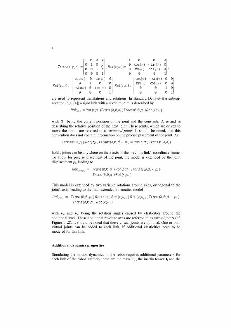
4

are used to represent translations and rotations. In standard Denavit-Hartenberg-notation (e.g. [4]) a rigid link with a revolute joint is described by

with ibeing the current position of the joint and the constants di, ai and i de-scribing the relative position of the next joint. These joints, which are driven to move the robot, are referred to as actuated joints. It should be noted, that this con-vention does not contain information on the precise placement of the joint. As

holds, joints can be anywhere on the z-axis of the previous link's coordinate frame. To allow for precise placement of the joint, the model is extended by the joint dis -placement pi, leading to

This model is extended by two variable rotations around axes, orthogonal to the joint's axis, leading to the final extended kinematics model

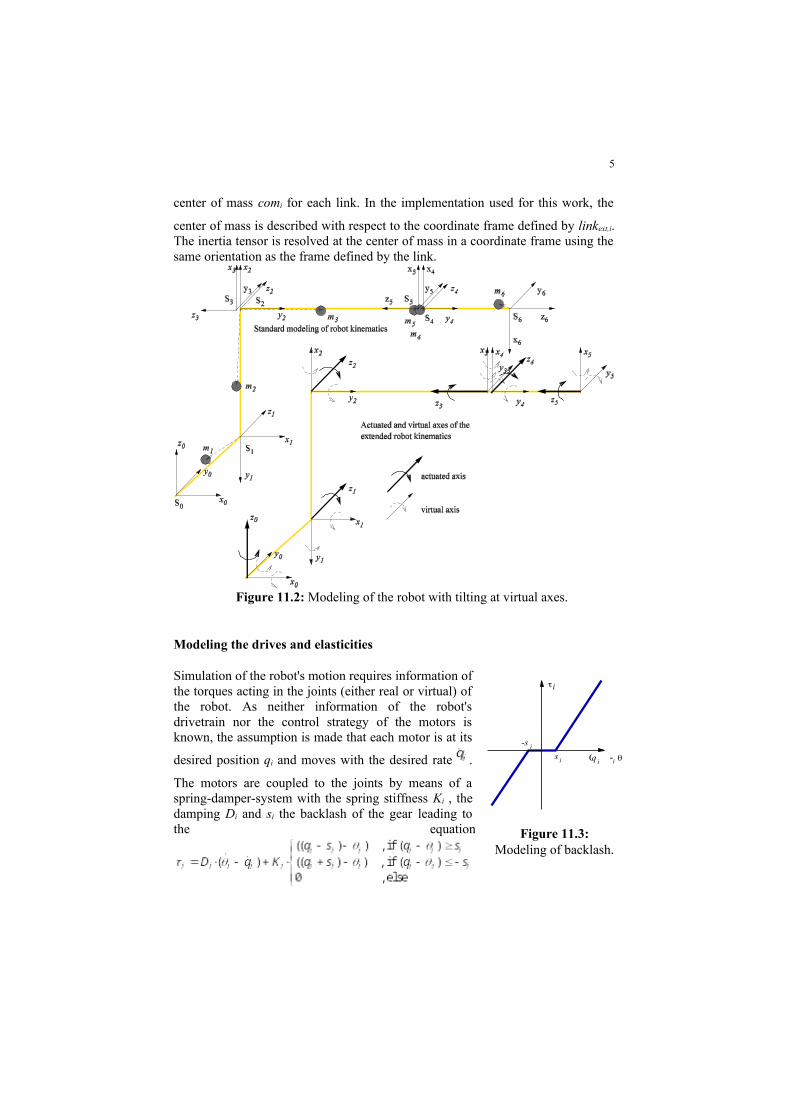
with x,i and y,i being the rotation angles caused by elasticities around the addi-tional axes. These additional revolute axes are referred to as virtual joints (cf. Fig-ure 11.2). It should be noted that these virtual joints are optional. One or both vir -tual joints can be added to each link, if additional elasticities need to be modeled for this link.

Additional dynamics properties

Simulating the motion dynamics of the robot requires additional parameters for each link of the robot. Namely these are the mass mi , the inertia tensor Ii and the

5

center of mass comi for each link. In the implementation used for this work, the

center of mass is described with respect to the coordinate frame defined by linkext,i. The inertia tensor is resolved at the center of mass in a coordinate frame using the same orientation as the frame defined by the link.

Figure 11.2: Modeling of the robot with tilting at virtual axes.

Modeling the drives and elasticities

Simulation of the robot's motion requires information of the torques acting in the joints (either real or virtual) of the robot. As neither information of the robot's drive-train nor the control strategy of the motors is known, the assumption is made that each motor is at its desired

position qi and moves with the desired rate . The mo-

tors are coupled to the joints by means of a spring-damper-system with the spring stiffness Ki , the damp-ing Di and si the backlash of the gear leading to the equation

s i

-s i

ti

q i(-)i

Figure 11.3: Model-ing of backlash.

6

for the torques in the actuated joints (cf. Figure 11.3). Note that this convention also allows for elasticities and damping around the actuated axes which may occur because of the gears used in the drivetrain.

Torques acting on virtual joints are calculated in the same way with the excep-tion that the desired position and rate always are zero and that there is no backlash,

Forward dynamics simulation

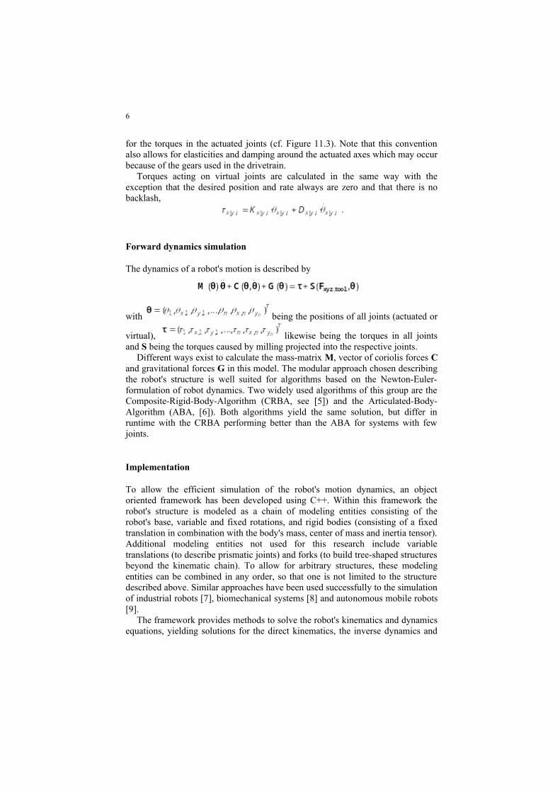
The dynamics of a robot's motion is described by

with being the positions of all joints (actuated or

virtual), likewise being the torques in all joints and S being the torques caused by milling projected into the respective joints.

Different ways exist to calculate the mass-matrix M, vector of coriolis forces C and gravitational forces G in this model. The modular approach chosen describing the robot's structure is well suited for algorithms based on the Newton-Euler-for-mulation of robot dynamics. Two widely used algorithms of this group are the Composite-Rigid-Body-Algorithm (CRBA, see [5]) and the Articulated-Body-Al-gorithm (ABA, [6]). Both algorithms yield the same solution, but differ in runtime with the CRBA performing better than the ABA for systems with few joints.

Implementation

To allow the efficient simulation of the robot's motion dynamics, an object ori-ented framework has been developed using C++. Within this framework the ro-bot's structure is modeled as a chain of modeling entities consisting of the robot's base, variable and fixed rotations, and rigid bodies (consisting of a fixed transla-tion in combination with the body's mass, center of mass and inertia tensor). Addi-tional modeling entities not used for this research include variable translations (to describe prismatic joints) and forks (to build tree-shaped structures beyond the kinematic chain). To allow for arbitrary structures, these modeling entities can be combined in any order, so that one is not limited to the structure described above. Similar approaches have been used successfully to the simulation of industrial ro-bots [7], biomechanical systems [8] and autonomous mobile robots [9].

The framework provides methods to solve the robot's kinematics and dynamics equations, yielding solutions for the direct kinematics, the inverse dynamics and the forward dynamics. Currently the forward dynamics is based on the CRBA and ABA to allow the selection of the better performing algorithm, depending on the complexity of the robot.

7

Due to this modular description of the robot, the structure of the simulated ro-bot can be exchanged easily without the need to derive new equations of motion. Thus it is possible to select (and re-select) the virtual joints required for a specific milling simulation, depending on the concrete robot. For the purpose of parameter estimation and trajectory optimization the framework also allows calculating de-rivatives of the simulated robot's motion with respect to any modeling parameters.

This feature is based on the ADOL-C library [10] for automated derivation of C++-functions. Depending on the current use of the developed framework one can either use the special types provided by ADOL-C (if derivatives are required) or the standard floating point types of the machine (no derivatives available, but faster execution). By this feature, it is possible to use the same implementation of the model either for parameter estimation or for the simulation of the milling process, as well as for applying numerical optimal control methods [11], without changes in the sourcecode.

11.2.2 Process Force Calculation

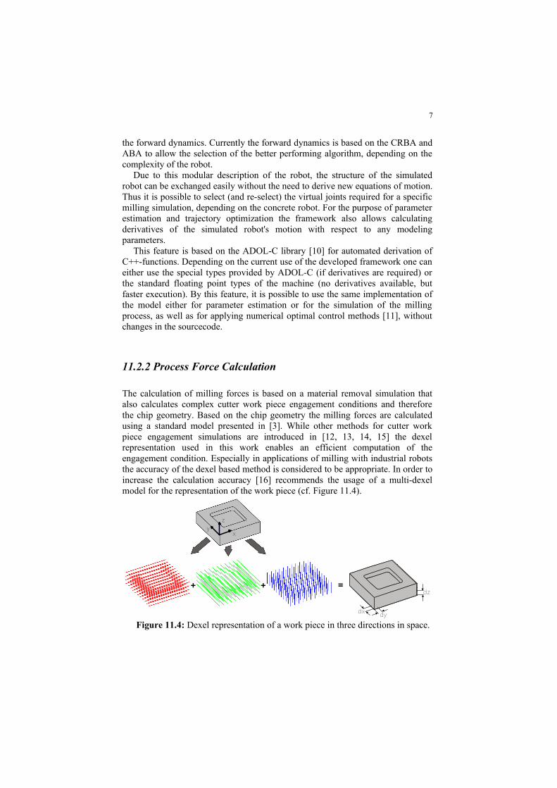
The calculation of milling forces is based on a material removal simulation that also calculates complex cutter work piece engagement conditions and therefore the chip geometry. Based on the chip geometry the milling forces are calculated using a standard model presented in [3]. While other methods for cutter work piece engagement simulations are introduced in [12, 13, 14, 15] the dexel repre-sentation used in this work enables an efficient computation of the engagement condition. Especially in applications of milling with industrial robots the accuracy of the dexel based method is considered to be appropriate. In order to increase the calculation accuracy [16] recommends the usage of a multi-dexel model for the representation of the work piece (cf. Figure 11.4).

+ + =

xy

z

dx dy

dz

Figure 11.4: Dexel representation of a work piece in three directions in space.

Thereby the description of a single dexel is done by line equations,

8

Here, p is a point on the line, d is the line direction, t is the scaling factor and s the starting point in space. The work piece is modeled using a multi-dexel representa-tion compromising dexel directions in x, y and z. The discretization of the work piece is defined by the dexel distances dx, dy and dz. In order to receive a suffi-cient accuracy of the force calculation the relation kd between the dexel discretiza-tion and the tool radius R is considered,

.

During a simulated milling operation the tool moves through the work piece in discrete time steps ti. The incremental size of the time step is dt.

In every time step ti=1,…, nint the material removal is calculated, whereis the tooth passing time calculated by

with the number of revolution n and the number of teeth

11.2.2.1. Calculation of the Chip Geometry

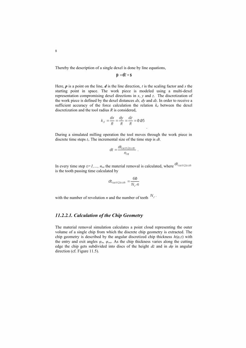
The material removal simulation calculates a point cloud representing the outer volume of a single chip from which the discrete chip geometry is extracted. The chip geometry is described by the angular discretized chip thickness h(φ,z) with the entry and exit angles φin, φout. As the chip thickness varies along the cutting edge the chip gets subdivided into discs of the height dz and in dφ in angular di-rection (cf. Figure 11.5).

h(φ,z)

dz

dφx

y

z

dzap

y

x

radialz

Figure 11.5: Discretized chip geometry.

9

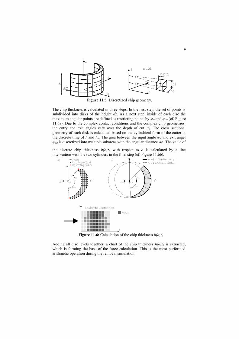
The chip thickness is calculated in three steps. In the first step, the set of points is subdivided into disks of the height dz. As a next step, inside of each disc the maxi-mum angular points are defined as restricting points by φin and φout (cf. Figure 11.6a). Due to the complex contact conditions and the complex chip geometries, the entry and exit angles vary over the depth of cut ap. The cross sectional geome-try of each disk is calculated based on the cylindrical form of the cutter at the dis-crete time of ti and ti-1. The area between the input angle φin and exit angel φout

is

discretized into multiple subareas with the angular distance dφ. The value of the discrete chip thickness h(φ,z) with respect to φ is calculated by a line intersection with the two cylinders in the final step (cf. Figure 11.6b).

x

y

x

y

h

t(i-1)t(i-1) t(i)t(i)

φin

φoutφout

φin

φ

zh(φ,z)

Chart of the Chipthicknessz

a) b)Chip Point CloudRestricting Points

DexelAnalytic Cutter CylinderAnalytic Chip Geometry

Figure 11.6: Calculation of the chip thickness h(φ,z).

Adding all disc levels together, a chart of the chip thickness h(φ,z) is extracted, which is forming the base of the force calculation. This is the most performed arithmetic operation during the removal simulation.

11.2.2.2. Cutting Force Model

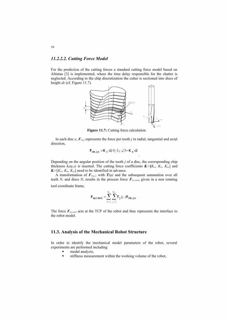
For the prediction of the cutting forces a standard cutting force model based on Altintas [3] is implemented, where the time delay responsible for the chatter is ne-glected. According to the chip discretization the cutter is sectioned into discs of height dz (cf. Figure 11.7).

10

Fa

FrFt

dz

Fx, tool

Fy, tool

Fz, tool

disk e

Figure 11.7: Cutting force calculation

In each disc e, Frta,j represents the force per tooth j in radial, tangential and axial direction,

.

Depending on the angular position of the tooth j of a disc, the corresponding chip thickness hj(φ,z) is inserted. The cutting force coefficients Kc=[Krc, Ktc, Kac] and Ke=[Kre, Kte, Kae] need to be identified in advance.

A transformation of Frta,j,e with T(φ) and the subsequent summation over all teeth Nz and discs Ne results in the process force Fxyz,tool, given in a non rotating

tool coordinate frame,

The force Fxyz,tool acts at the TCP of the robot and thus represents the interface to

the robot model.

11.3. Analysis of the Mechanical Robot Structure

In order to identify the mechanical model parameters of the robot, several experi-ments are performed including

modal analysis, stiffness measurement within the working volume of the robot, stiffness measurement of the structural robot components.

In the following subsections, the investigations are presented and the consequen-tial model adaptations are considered.

11

11.3.1. Modal Analysis

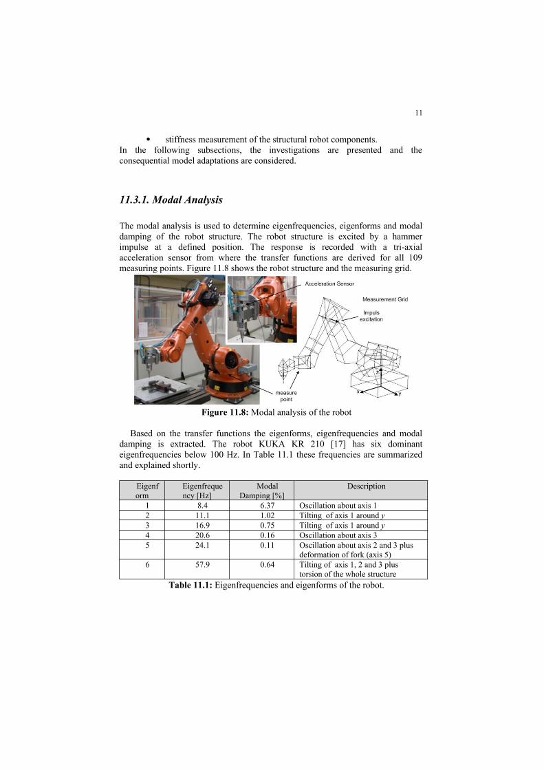
The modal analysis is used to determine eigenfrequencies, eigenforms and modal damping of the robot structure. The robot structure is excited by a hammer im-pulse at a defined position. The response is recorded with a tri-axial acceleration sensor from where the transfer functions are derived for all 109 measuring points. Figure 11.8 shows the robot structure and the measuring grid.

Figure 11.8: Modal analysis of the robot

Based on the transfer functions the eigenforms, eigenfrequencies and modal damping is extracted. The robot KUKA KR 210 [17] has six dominant eigenfre-quencies below 100 Hz. In Table 11.1 these frequencies are summarized and ex-plained shortly.

Eigenform

Eigenfrequency [Hz]

Modal Damping [%]

Description

1 8.4 6.37 Oscillation about axis 12 11.1 1.02 Tilting of axis 1 around y3 16.9 0.75 Tilting of axis 1 around y4 20.6 0.16 Oscillation about axis 35 24.1 0.11 Oscillation about axis 2 and 3 plus

deformation of fork (axis 5)6 57.9 0.64 Tilting of axis 1, 2 and 3 plus

torsion of the whole structureTable 11.1: Eigenfrequencies and eigenforms of the robot.

11.3.2. Static Stiffness within Working Space

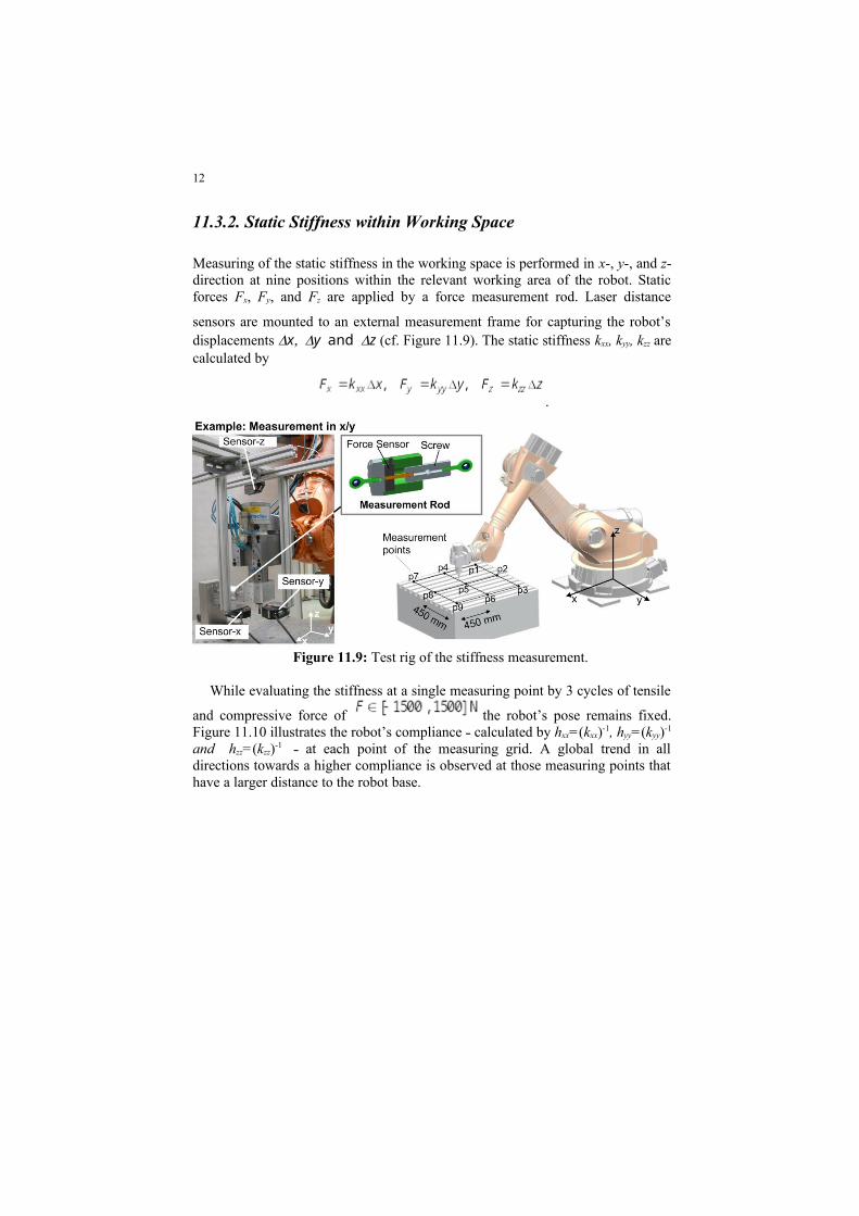
Measuring of the static stiffness in the working space is performed in x-, y-, and z-direction at nine positions within the relevant working area of the robot. Static

12

forces Fx, Fy, and Fz are applied by a force measurement rod. Laser distance sen-

sors are mounted to an external measurement frame for capturing the robot’s dis-placements xyandz (cf. Figure 11.9). The static stiffness kxx, kyy, kzz are cal-culated by

.

Figure 11.9: Test rig of the stiffness measurement.

While evaluating the stiffness at a single measuring point by 3 cycles of tensile

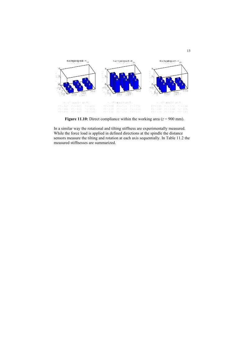
and compressive force of the robot’s pose remains fixed. Figure 11.10 illustrates the robot’s compliance ˗ calculated by hxx=(kxx)-1, hyy=(kyy)-1

and hzz=(kzz)-1 ˗ at each point of the measuring grid. A global trend in all direc-tions towards a higher compliance is observed at those measuring points that have a larger distance to the robot base.

Figure 11.10: Direct compliance within the working area (z = 900 mm).

13

In a similar way the rotational and tilting stiffness are experimentally measured. While the force load is applied in defined directions at the spindle the distance sensors measure the tilting and rotation at each axis sequentially. In Table 11.2 the measured stiffnesses are summarized.

14

Mech. Robot Component Rotational Stiffness [Nm/rad]Axis 1 8,937e-6Axis 2 6,343e-6Axis 3 2,357e-5Axis 4 7,804e-5Axis 5 1,047e-4Axis 6 2,052e-4

Table 11.2: Rotational robot stiffness at axes 1 – 6.

11.3.3. Parameter Identification

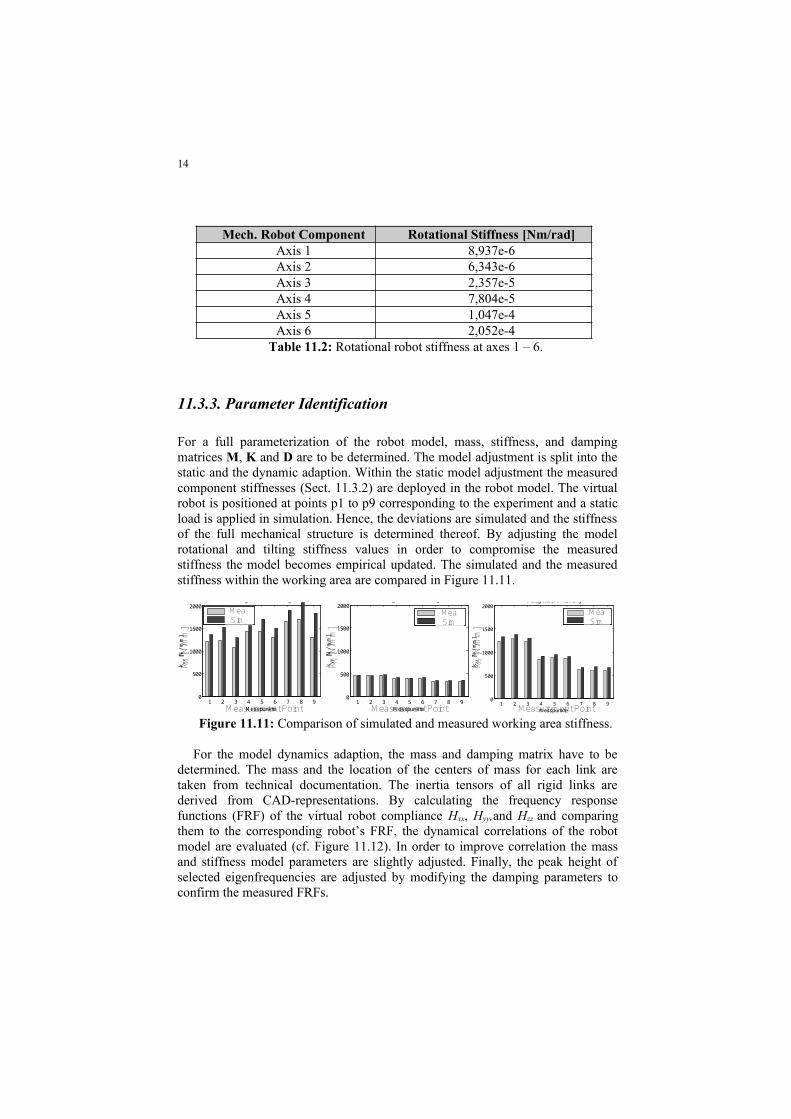
For a full parameterization of the robot model, mass, stiffness, and damping matri-ces M, K and D are to be determined. The model adjustment is split into the static and the dynamic adaption. Within the static model adjustment the measured com-ponent stiffnesses (Sect. 11.3.2) are deployed in the robot model. The virtual robot is positioned at points p1 to p9 corresponding to the experiment and a static load is applied in simulation. Hence, the deviations are simulated and the stiffness of the full mechanical structure is determined thereof. By adjusting the model rotational and tilting stiffness values in order to compromise the measured stiffness the model becomes empirical updated. The simulated and the measured stiffness within the working area are compared in Figure 11.11.

1 2 3 4 5 6 7 8 90

500

1000

1500

2000Steifigkeit in Z-Richtung

Messpunkte

k zz [N

/ m

m]

MessungSimulation

1 2 3 4 5 6 7 8 90

500

1000

1500

2000Steifigkeit in X-Richtung

Messpunkte

k xx [N

/ m

m]

MessungSimulation

1 2 3 4 5 6 7 8 90

500

1000

1500

2000Steifigkeit in Y-Richtung

Messpunkte

k yy [N

/ m

m]

MessungSimulation

k xx [

N/m

m]

k yy [

N/m

m]

k zz [

N/m

m]

Mea

Measurement PointMeasurement Point Measurement Point

MeaSim

MeaSim

MeaSim

Figure 11.11: Comparison of simulated and measured working area stiffness.

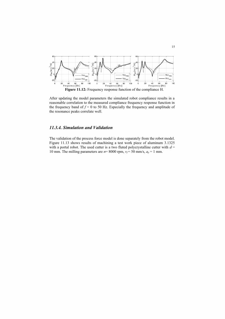
For the model dynamics adaption, the mass and damping matrix have to be de-termined. The mass and the location of the centers of mass for each link are taken from technical documentation. The inertia tensors of all rigid links are derived from CAD-representations. By calculating the frequency response functions (FRF) of the virtual robot compliance Hxx, Hyy,and Hzz and comparing them to the corre-sponding robot’s FRF, the dynamical correlations of the robot model are evaluated (cf. Figure 11.12). In order to improve correlation the mass and stiffness model parameters are slightly adjusted. Finally, the peak height of selected eigenfrequen-cies are adjusted by modifying the damping parameters to confirm the measured FRFs.

15

Figure 11.12: Frequency response function of the compliance H.

After updating the model parameters the simulated robot compliance results in a reasonable correlation to the measured compliance frequency response function in the frequency band of f = 0 to 50 Hz. Especially the frequency and amplitude of the resonance peaks correlate well.

11.3.4. Simulation and Validation

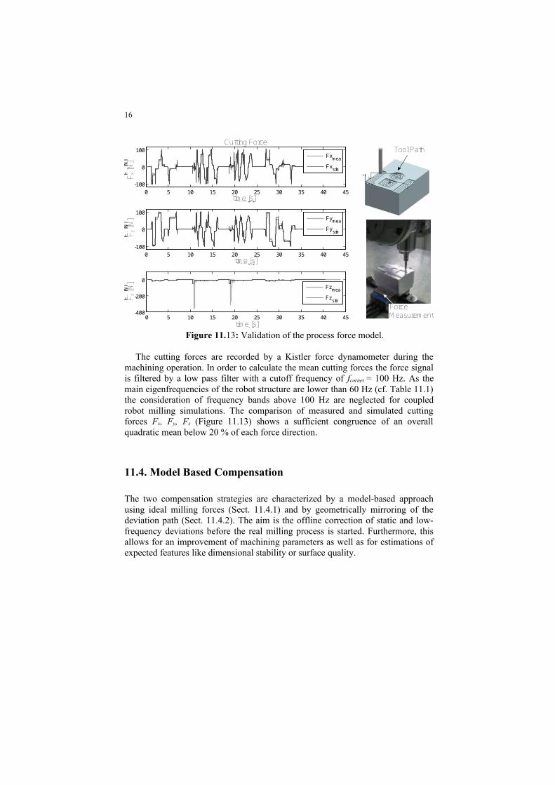
The validation of the process force model is done separately from the robot model. Figure 11.13 shows results of machining a test work piece of aluminum 3.1325 with a portal robot. The used cutter is a two fluted polycrystalline cutter with d = 10 mm. The milling parameters are n= 8000 rpm, vf = 50 mm/s, ap = 1 mm.

16

0 5 10 15 20 25 30 35 40 45-100

0

100

Zeit [s]

F x [N]

Fxmea

Fxsim

0 5 10 15 20 25 30 35 40 45-100

0

100

Zeit [s]

F y [N]

Fymea

Fysim

0 5 10 15 20 25 30 35 40 45-400

-200

0

Zeit [s]

F z [N]

Fzmea

Fzsim

Tool PathCutting Force

ForceMeasurement

time [s]

time [s]

time [s]

F z [N

]F y

[N]

F x [N

]

Figure 11.13: Validation of the process force model.

The cutting forces are recorded by a Kistler force dynamometer during the ma-chining operation. In order to calculate the mean cutting forces the force signal is filtered by a low pass filter with a cutoff frequency of fcorner = 100 Hz. As the main eigenfrequencies of the robot structure are lower than 60 Hz (cf. Table 11.1) the consideration of frequency bands above 100 Hz are neglected for coupled robot milling simulations. The comparison of measured and simulated cutting forces Fx, Fy, Fz (Figure 11.13) shows a sufficient congruence of an overall quadratic mean below 20 % of each force direction.

11.4. Model Based Compensation

The two compensation strategies are characterized by a model-based approach us-ing ideal milling forces (Sect. 11.4.1) and by geometrically mirroring of the devia-tion path (Sect. 11.4.2). The aim is the offline correction of static and low-fre-quency deviations before the real milling process is started. Furthermore, this al-lows for an improvement of machining parameters as well as for estimations of expected features like dimensional stability or surface quality.

17

11.4.1. Compensation by Ideal Milling Forces

The proposed model-based compensation strategy consists of three steps: (1) A simulation run assuming an idealized robot, (2) the computation of reference joint positions, and (3) a transformation into compensating track points.

Assuming a known ideal TCP trajectory, this idealized path is initially simu-lated without considering elasticities in the robot’s dynamics, i.e. real joint posi-

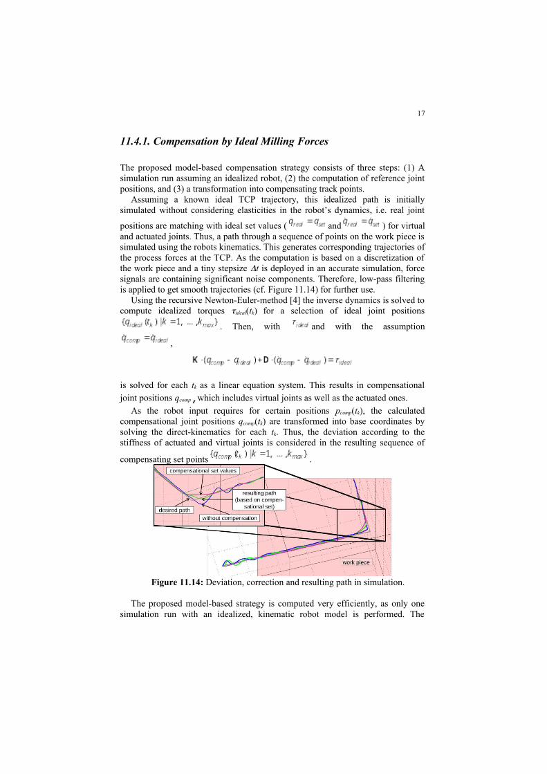
tions are matching with ideal set values ( and ) for virtual and actuated joints. Thus, a path through a sequence of points on the work piece is simulated using the robots kinematics. This generates corresponding trajectories of the process forces at the TCP. As the computation is based on a discretization of the work piece and a tiny stepsize t is deployed in an accurate simulation, force signals are containing significant noise components. Therefore, low-pass filtering is applied to get smooth trajectories (cf. Figure 11.14) for further use.

Using the recursive Newton-Euler-method [4] the inverse dynamics is solved to compute idealized torques tideal(tk) for a selection of ideal joint positions

. Then, with and with the assumption

,

is solved for each tk as a linear equation system. This results in compensational joint positions qcomp,which includes virtual joints as well as the actuated ones.

As the robot input requires for certain positions pcomp(tk), the calculated compen-sational joint positions qcomp(tk) are transformed into base coordinates by solving the direct-kinematics for each tk. Thus, the deviation according to the stiffness of actuated and virtual joints is considered in the resulting sequence of compensating

set points .

Figure 11.14: Deviation, correction and resulting path in simulation.

The proposed model-based strategy is computed very efficiently, as only one simulation run with an idealized, kinematic robot model is performed. The even-

18

tual solution of one linear equation system per interpolation point can be done real-time.

11.4.2. Compensation by Deviation Mirroring

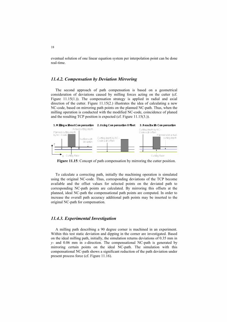
The second approach of path compensation is based on a geometrical consider-ation of deviations caused by milling forces acting on the cutter (cf. Figure 11.15(1.)). The compensation strategy is applied in radial and axial direction of the cutter. Figure 11.15(2.) illustrates the idea of calculating a new NC-code, based on mirroring path points on the planned NC-path. Thus, when the milling operation is conducted with the modified NC-code, coincidence of planed and the resulting TCP position is expected (cf. Figure 11.15(3.)).

Cutting force

Actual cutting depth

Cutting depth by NC- Code with offset

Surface with deviation

Planned cutting depthby NC- Code

1. Milling without Compensation 2. Using Compensation Offset 3. Result with CompensationCutting depth by NC-Code with offset

Planned and actual cutting depth

Cutting forcex

z

Figure 11.15: Concept of path compensation by mirroring the cutter position.

To calculate a correcting path, initially the machining operation is simulated using the original NC-code. Thus, corresponding deviations of the TCP become available and the offset values for selected points on the deviated path to corre-sponding NC-path points are calculated. By mirroring this offsets at the planned, ideal NC-path the compensational path points are computed. In order to increase the overall path accuracy additional path points may be inserted to the original NC-path for compensation.

11.4.3. Experimental Investigation

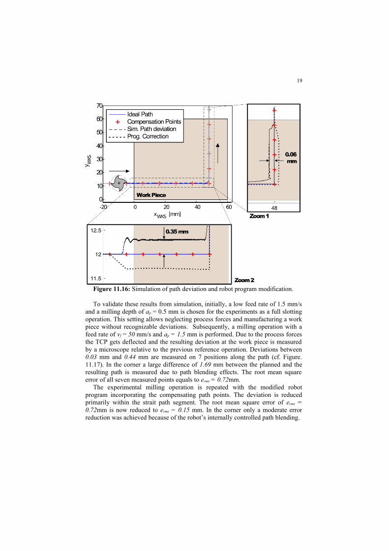
A milling path describing a 90 degree corner is machined in an experiment. Within this test static deviation and dipping in the corner are investigated. Based on the ideal milling path, initially, the simulation returns deviations of 0.35 mm in y- and 0.06 mm in x-direction. The compensational NC-path is generated by mir-roring certain points on the ideal NC-path. The simulation with this compensa-tional NC-path shows a significant reduction of the path deviation under present process force (cf. Figure 11.16).

19

Figure 11.16: Simulation of path deviation and robot program modification.

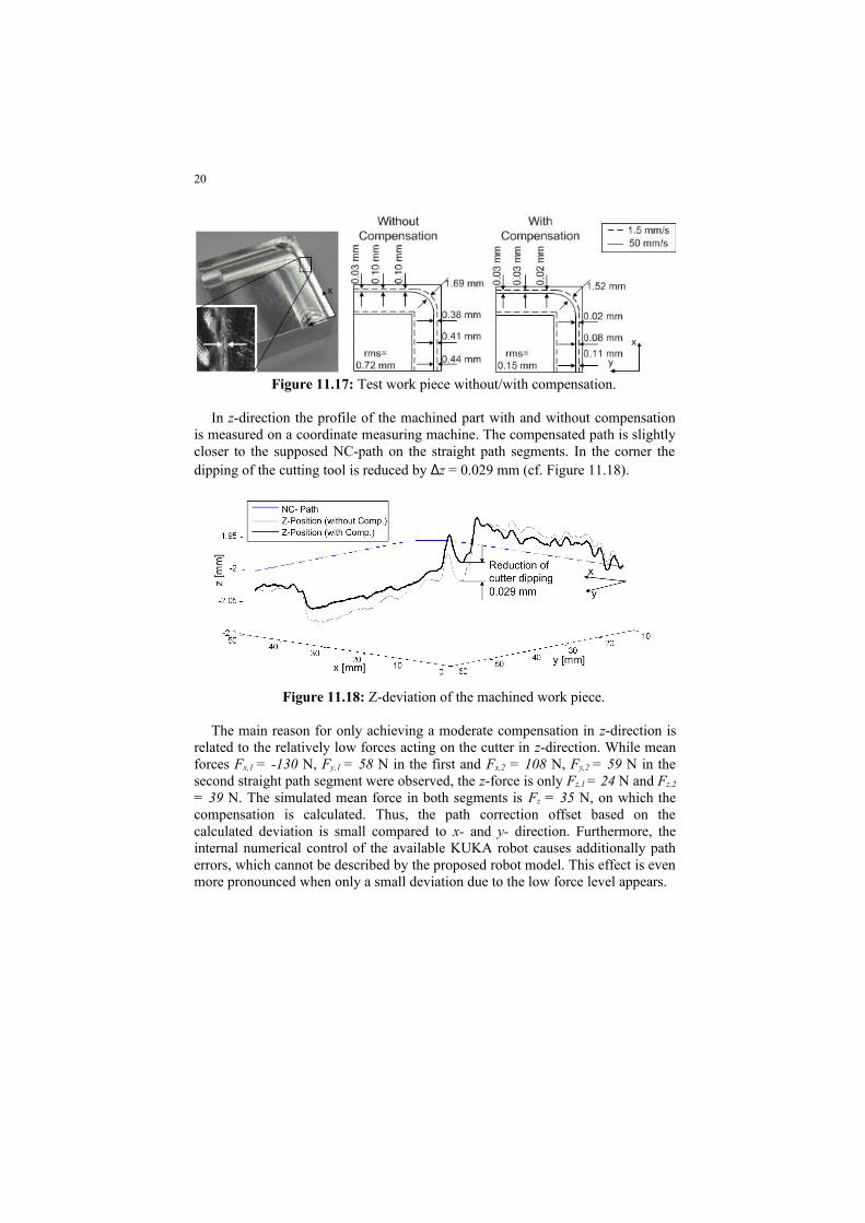
To validate these results from simulation, initially, a low feed rate of 1.5 mm/s and a milling depth of ap = 0.5 mm is chosen for the experiments as a full slotting operation. This setting allows neglecting process forces and manufacturing a work piece without recognizable deviations. Subsequently, a milling operation with a feed rate of vf = 50 mm/s and ap = 1.5 mm is performed. Due to the process forces the TCP gets deflected and the resulting deviation at the work piece is measured by a microscope relative to the previous reference operation. Deviations between 0.03 mm and 0.44 mm are measured on 7 positions along the path (cf. Figure. 11.17). In the corner a large difference of 1.69 mm between the planned and the resulting path is measured due to path blending effects. The root mean square er-ror of all seven measured points equals to erms = 0.72mm.

The experimental milling operation is repeated with the modified robot pro-gram incorporating the compensating path points. The deviation is reduced pri-marily within the strait path segment. The root mean square error of erms = 0.72mm is now reduced to erms = 0.15 mm. In the corner only a moderate error re-duction was achieved because of the robot’s internally controlled path blending.

20

Figure 11.17: Test work piece without/with compensation.

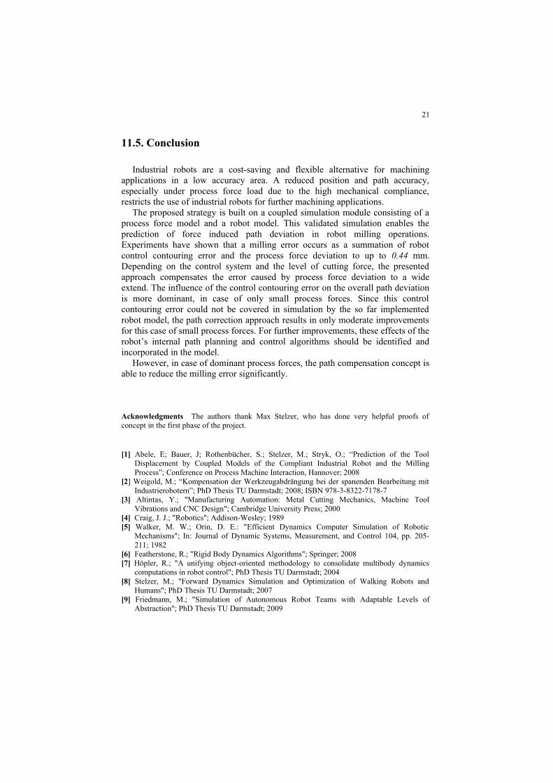
In z-direction the profile of the machined part with and without compensation is measured on a coordinate measuring machine. The compensated path is slightly closer to the supposed NC-path on the straight path segments. In the corner the dipping of the cutting tool is reduced by ∆z = 0.029 mm (cf. Figure 11.18).

Figure 11.18: Z-deviation of the machined work piece.

The main reason for only achieving a moderate compensation in z-direction is related to the relatively low forces acting on the cutter in z-direction. While mean forces Fx,1 = -130 N, Fy,1 = 58 N in the first and Fx,2 = 108 N, Fy,2 = 59 N in the second straight path segment were observed, the z-force is only Fz,1 = 24 N and Fz,2

= 39 N. The simulated mean force in both segments is Fz = 35 N, on which the compensation is calculated. Thus, the path correction offset based on the calcu-lated deviation is small compared to x- and y- direction. Furthermore, the internal numerical control of the available KUKA robot causes additionally path errors, which cannot be described by the proposed robot model. This effect is even more pronounced when only a small deviation due to the low force level appears.

21

11.5. Conclusion

Industrial robots are a cost-saving and flexible alternative for machining appli-cations in a low accuracy area. A reduced position and path accuracy, especially under process force load due to the high mechanical compliance, restricts the use of industrial robots for further machining applications.

The proposed strategy is built on a coupled simulation module consisting of a process force model and a robot model. This validated simulation enables the pre-diction of force induced path deviation in robot milling operations. Experiments have shown that a milling error occurs as a summation of robot control contouring error and the process force deviation to up to 0.44 mm. Depending on the control system and the level of cutting force, the presented approach compensates the er-ror caused by process force deviation to a wide extend. The influence of the con-trol contouring error on the overall path deviation is more dominant, in case of only small process forces. Since this control contouring error could not be covered in simulation by the so far implemented robot model, the path correction approach results in only moderate improvements for this case of small process forces. For further improvements, these effects of the robot’s internal path planning and con-trol algorithms should be identified and incorporated in the model.

However, in case of dominant process forces, the path compensation concept is able to reduce the milling error significantly.

Acknowledgments The authors thank Max Stelzer, who has done very helpful proofs of con-cept in the first phase of the project.

[1] Abele, E; Bauer, J; Rothenbücher, S.; Stelzer, M.; Stryk, O.; “Prediction of the Tool Dis -placement by Coupled Models of the Compliant Industrial Robot and the Milling Process”; Conference on Process Machine Interaction, Hannover; 2008

[2] Weigold, M.; “Kompensation der Werkzeugabdrängung bei der spanenden Bearbeitung mit Industrierobotern”; PhD Thesis TU Darmstadt; 2008; ISBN 978-3-8322-7178-7

[3] Altintas, Y.; "Manufacturing Automation: Metal Cutting Mechanics, Machine Tool Vibra-tions and CNC Design"; Cambridge University Press; 2000

[4] Craig, J. J.; "Robotics"; Addison-Wesley; 1989[5] Walker, M. W.; Orin, D. E.: "Efficient Dynamics Computer Simulation of Robotic Mecha -

nisms"; In: Journal of Dynamic Systems, Measurement, and Control 104, pp. 205-211; 1982 [6] Featherstone, R.; "Rigid Body Dynamics Algorithms"; Springer; 2008[7] Höpler, R.; "A unifying object-oriented methodology to consolidate multibody dynamics

computations in robot control"; PhD Thesis TU Darmstadt; 2004[8] Stelzer, M.; "Forward Dynamics Simulation and Optimization of Walking Robots and Hu-

mans"; PhD Thesis TU Darmstadt; 2007 [9] Friedmann, M.; "Simulation of Autonomous Robot Teams with Adaptable Levels of Abstrac-

tion"; PhD Thesis TU Darmstadt; 2009[10] Walther, A.; Griewank, A: “ADOL-C: A Package for the Automatic Differentiation of Al-

gorithms Written in C/C++” Version 2.1.12, Documentation https://projects.coin-or.org/ADOL-C

22

[11] von Stryk, O.: „User's Guide for DIRCOL (Version 2.1): a direct collocation method for the numerical solution of optimal control problems.”, TU Darmstadt, 2000; available at http://www.sim.informatik.tu-darmstadt.de/sw/dircol

[12] Rehling, S.; „Technologische Erweiterung der Simulation von NC-Fertigungsprozessen"; PhD Thesis Universität Hannover; 2009

[13] Surmann, T.; Geometrisch-physikalische Simulation der Prozessdynamik für das fünfachsige Fräsen von Freiformflächen"; PhD Thesis TU Dortmund; 2005

[14] Stautner, M.; "Simulation und Optimierung der mehrachsigen Fräsbearbeitung"; PhD Thesis TU Dortmund, ; München 2002; ISBN 3-8027-8732-3

[15] Selle, J.; Technologiebasierte Fehlerkorrektur für das NC-Schlichtfräsen"; PhD Thesis Universität Hannover; 2005

[16] Weinert, K.; Müller, H.; Kreis, W.; Surmann, T.; Ayasse, J.; Schüppstuhl, T.; Kneupner, K.; "Diskrete Werkstückmodellierung zur Simulation von Zerspanprozessen"; In: Zeitschrift für wirtschaftlichen Fabrikbetrieb: ZWF, pp. 385-389; München 2002; ISSN 0932-0482

[17] KUKA Roboter GmbH. Data sheet KR 210-2. http://www.kuka-robotics.com, Gersthofen - Germany, Jul 2009.