Embed Size (px)
Citation preview

UNIVERSITY OF CALIFORNIASanta Barbara
Millimeter Wave MIMO: Design and Evaluation
of Practical System Architectures
A Dissertation submitted in partial satisfactionof the requirements for the degree of
Doctor of Philosophy
in
Electrical and Computer Engineering
by
Eric G. Torkildson
Committee in Charge:
Professor Upamanyu Madhow, Chair
Professor Shivkumar Chandrasekaran
Professor Jerry Gibson
Professor Mark Rodwell
December 2010

Abstract
Millimeter Wave MIMO: Design and Evaluation of
Practical System Architectures
Eric G. Torkildson
Unlicensed spectrum at 60 GHz and the E-band frequencies spans multiple
GHz, enabling wireless links to reach multi-Gb/s speeds. In this work, we pro-
pose increasing speeds further by leveraging spatial multiplexing gains at millime-
ter (mm) wave. To this end, we design and evaluate practical MIMO architec-
tures that address the unique challenges and opportunities associated with mm
wave communication. We begin by recognizing that the mm wave channel is pre-
dominantly line-of-sight (LOS), and develop arrays that provide robust spatial
multiplexing gains in this environment. Noting that the cost and power consump-
tion of ADCs become limiting factors as bandwidths scale to multiple GHz, we
then propose a hierarchical approach to MIMO signal processing. Spatial process-
ing, including beamforming and spatial multiplexing, is performed on a slow time
scale and followed by separate temporal processing of each of the multiplexed data
streams. This design is implemented in a four-channel hardware prototype.
We then investigate mm wave spatial multiplexing for short range indoor ap-
plications, first by quantifying fundamental limits in LOS environments, and then
ii
by investigating performance in the presence of multipath and LOS blockage. For
linear arrays with constrained form factor, an asymptotic analysis (as the number
of antenna elements gets large) based on properties of prolate spheroidal wave
functions shows that a sparse array producing a spatially uncorrelated channel
matrix effectively provides the maximum number of spatial degrees of freedom in
a LOS environment, but that substantial beamforming gains can be obtained by
using a denser array. This motivates a system architecture that utilizes arrays
of subarrays to provide both directivity and spatial multiplexing gains. The per-
formance of this system is evaluated in a simulated indoor environment using a
ray-tracing model that incorporates multipath effects and potential LOS block-
age. Our numerical results provide insight into the spatial variations of attainable
capacity within a room, and the combinations of beamsteering and spatial multi-
plexing used in different scenarios.
Professor Upamanyu Madhow
Dissertation Committee Chair
iii
Contents
Abstract ii
List of Figures vi
List of Tables viii
1 Introduction 11.1 LOS Spatial Multiplexing at mm Wave Frequencies . . . . . . . . 51.2 Hierarchical MIMO Signal Processing: Architecture and Prototype 61.3 Feasibility and Performance Study of Indoor mm Wave MIMO Links 81.4 Related Work . . . . . . . . . . . . . . . . . . . . . . . . . . . . . 9
2 LOS Spatial Multiplexing Over Millimeter-Wave Links 112.1 LOS Spatial Multiplexing . . . . . . . . . . . . . . . . . . . . . . 12
2.1.1 LOS MIMO Channel Model . . . . . . . . . . . . . . . . . 132.1.2 The Rayleigh Spacing Criterion . . . . . . . . . . . . . . . 152.1.3 Application to mm-Wave Links . . . . . . . . . . . . . . . 17
2.2 Spatial Correlation at Non-Optimal LinkRanges . . . . . . . . . . . . . . . . . . . . . . . . . . . . . . . . . . . . 21
2.2.1 Noise Enhancement at Non-Optimal Link Ranges . . . . . 242.3 Optimized Nonuniform Arrays . . . . . . . . . . . . . . . . . . . . 27
2.3.1 4-element Nonuniform Array Analysis . . . . . . . . . . . . 272.3.2 Optimization Procedure and Results . . . . . . . . . . . . 31
2.4 Rank Adaptation . . . . . . . . . . . . . . . . . . . . . . . . . . . 342.5 Discussion . . . . . . . . . . . . . . . . . . . . . . . . . . . . . . . 39
iv
3 Hierarchical MIMO Signal Processing: Architecture and Proto-type 403.1 Two-level mm-Wave MIMO Architecture . . . . . . . . . . . . . . 43
3.1.1 Pilot-Symbol-Aided Channel EstimationBackground . . . . . . . . . . . . . . . . . . . . . . . . . . . . . . 433.1.2 System Architecture . . . . . . . . . . . . . . . . . . . . . 453.1.3 Channel Model . . . . . . . . . . . . . . . . . . . . . . . . 48
3.2 Spatial Interference Suppression . . . . . . . . . . . . . . . . . . . 503.2.1 DFT-Based Channel Estimation: . . . . . . . . . . . . . . 533.2.2 Least Squares Channel Estimation: . . . . . . . . . . . . . 553.2.3 Closed-Loop Equalization: . . . . . . . . . . . . . . . . . . 573.2.4 Simulation Results . . . . . . . . . . . . . . . . . . . . . . 62
3.3 Hardware Prototype . . . . . . . . . . . . . . . . . . . . . . . . . 673.3.1 Transmitter and Receiver Electronics . . . . . . . . . . . . 673.3.2 Experimental Results . . . . . . . . . . . . . . . . . . . . . 70
3.4 Discussion . . . . . . . . . . . . . . . . . . . . . . . . . . . . . . . 73
4 Feasibility and Performance Study of Indoor mm-Wave MIMOLinks 764.1 Fundamental Limits of LOS MIMO . . . . . . . . . . . . . . . . . 77
4.1.1 LOS MIMO Channel Model . . . . . . . . . . . . . . . . . 784.1.2 Spatial Degrees of Freedom . . . . . . . . . . . . . . . . . 80
4.2 LOS mm-Wave MIMO Architecture . . . . . . . . . . . . . . . . . 874.2.1 Waterfilling Benchmark . . . . . . . . . . . . . . . . . . . 884.2.2 Transmit Beamsteering/Receive MMSE . . . . . . . . . . . 89
4.3 Indoor Propagation Model . . . . . . . . . . . . . . . . . . . . . . 924.4 Results . . . . . . . . . . . . . . . . . . . . . . . . . . . . . . . . . 95
4.4.1 Performance of Waterfilling Benchmark . . . . . . . . . . . 964.4.2 Performance of Transmit Beamsteering/ReceiveMMSE . . . . . . . . . . . . . . . . . . . . . . . . . . . . . . . . . 1004.4.3 Transmitter Alignment . . . . . . . . . . . . . . . . . . . . 103
4.5 Discussion . . . . . . . . . . . . . . . . . . . . . . . . . . . . . . . 104
5 Conclusions and Future Work 1085.1 Directions for Future Work . . . . . . . . . . . . . . . . . . . . . . 110
Bibliography 112
v

List of Figures
2.1 Aligned uniform linear arrays. . . . . . . . . . . . . . . . . . . . . 142.2 Subarray configurations. . . . . . . . . . . . . . . . . . . . . . . . 192.3 Spatial correlation in H . . . . . . . . . . . . . . . . . . . . . . . 222.4 Array response at various link ranges. . . . . . . . . . . . . . . . . 232.5 Noise enhancement as a function of range. . . . . . . . . . . . . . 252.6 Correlation ρ(1, 4) . . . . . . . . . . . . . . . . . . . . . . . . . . . 282.7 Optimization metric γ for symmetric 4-element array. . . . . . . . 302.8 Maximum noise enhancement as a function of range for an opti-mized 4-element array. . . . . . . . . . . . . . . . . . . . . . . . . . . . 322.9 Maximum noise enhancement as a function of range for an opti-mized 5-element array. . . . . . . . . . . . . . . . . . . . . . . . . . . . 332.10 Maximum noise enhancement as a function of range for an opti-mized 6-element array. . . . . . . . . . . . . . . . . . . . . . . . . . . . 342.11 I as a function of Ns, the number of independent transmitted signals. 372.12 Rank adaptation strategy compared to channel capacity. . . . . . 38
3.1 Two-level system architecture. . . . . . . . . . . . . . . . . . . . . 463.2 Open-loop spatial equalizer structure. . . . . . . . . . . . . . . . . 513.3 Closed-loop frequency domain spatial equalizer structure. . . . . . 583.4 Discrete Fourier transform of received signal. . . . . . . . . . . . . 593.5 SIR using DFT-based spatial equalizer. . . . . . . . . . . . . . . . 643.6 SIR using LSE-based spatial equalizer. . . . . . . . . . . . . . . . 653.7 SIR using closed-loop spatial equalizer. . . . . . . . . . . . . . . . 663.8 Transmitter prototype block diagram. . . . . . . . . . . . . . . . . 683.9 Receiver prototype block diagram. . . . . . . . . . . . . . . . . . . 693.10 Photograph of prototype receiver. . . . . . . . . . . . . . . . . . . 713.11 Measured power spectrums of signals and interference. . . . . . . 733.12 Eye patterns before and after equalization. . . . . . . . . . . . . . 75
vi

4.1 Squared singular values of discrete ULA channel matrix. . . . . . 814.2 Eigenvalues of continuous array channel. . . . . . . . . . . . . . . 854.3 Array of subarrays architecture. . . . . . . . . . . . . . . . . . . . 874.4 Indoor environment model. . . . . . . . . . . . . . . . . . . . . . . 934.5 Channel capacity with waterfilling benchmark scheme as a functionof transmitter coordinates. . . . . . . . . . . . . . . . . . . . . . . . . . 964.6 NLOS channel capacity with waterfilling benchmark scheme. . . . 984.7 Transmit eigenvector field patterns in LOS blockage scenario. . . . 994.8 Channel capacity as a function average transmit power per antenna. 1004.9 LOS channel capacity under TX beamsteering/RX MMSE scheme. 1014.10 NLOS channel capacity under TX beamsteering/RX MMSE scheme. 1034.11 Capacity-maximizing beamsteering directions in NLOS scenario. . 1064.12 CDF of spectral efficiency using various transmitter alignments. . 107
vii

List of Tables
2.1 Sample array configurations . . . . . . . . . . . . . . . . . . . . . 172.2 Link budget for SISO link. . . . . . . . . . . . . . . . . . . . . . . 182.3 Normalized element positions for optimized nonuniform arrays. . . 33
3.1 Link budget . . . . . . . . . . . . . . . . . . . . . . . . . . . . . . 723.2 SIR and BER Measurements . . . . . . . . . . . . . . . . . . . . . 72
viii
Chapter 1
Introduction
With an abundance of unlicensed and uncrowded spectrum, the 60 GHz and E-
band (71-76 GHz, 81-86 GHz) frequencies represent a frontier for modern wireless
communications. The large swaths of available bandwidth allow wireless links
to achieve unprecedented speeds. On the other hand, multi-Gbps data rates,
hardware limitations, and mm wave propagation characteristics present system
designers with a new set of challenges. Our goal in this dissertation is to design and
evaluate practical architectures that address these challenges while capitalizing on
the abundant spectrum. In particular, we investigate the feasibility of designing
multi-antenna mm wave systems that employ spatial multiplexing to improve
spectral efficiency and increase data rates.
Spatial multiplexing involves transmitting independent data streams in paral-
lel over a multiple-input multiple-output (MIMO) channel. If the signals arrive at
the receiver with sufficiently different spatial signatures, the transmitted signals
1

Chapter 1. Introduction
can be separated out. Since it was first proposed by [1] and [2], spatial multiplex-
ing has generated tremendous interest in the literature, and the technology has
been successfully integrated with commercial products, such as 802.11n wireless
local area network (WLAN) radios. While fundamental MIMO concepts are inde-
pendent of the operating frequency, much of the existing MIMO literature makes
assumptions about the wireless channel and hardware capabilities that may not
hold at mm wavelengths. In particular, we identify several key characteristics
that differentiate mm wave from lower frequencies (i.e. 1-5 GHz), including the
following:
• Directionality: Assuming omnidirectional transmission, path loss scales
as λ2, resulting in a 22 dB loss at 60 GHz as compared to 5 GHz. Due to
the limitations of today’s mm wave devices, this loss cannot be offset simply
by increasing transmit power. Instead, it necessitates the use of directional
transmission. For antennas of a fixed aperture, directivity scales as 1/λ2.
Factoring in both the transmit and receive antennas, directional 60 GHz
links end up with net gain of 1/λ2.
• Sparse multipath: Measurement studies have observed relatively high
reflection loss at mm wave frequencies, with multipath reflections tending to
be more specular than diffuse [3] [4]. These observations, coupled with weak
2

Chapter 1. Introduction
diffraction characteristics and directional transmission, result in a channel
with sparse, highly-attenuated multipath components.
• Large bandwidth: The 60 GHz band offers 7 GHz of unlicensed bandwidth
in the United States, while the 70/80 GHz bands offer 10 GHz. While this
allows for higher data rates, it also places an excessive burden on analog-
to-digital converters (ADCs) and modern DSP-centric communication ar-
chitectures. High-precision ADCs capable of sampling over several GHz of
bandwidth are prohibitive in terms of cost, power consumption, or avail-
ability [5]. This requires us to consider system architectures and signal
processing techniques that eliminate reliance on high-rate, high-precision
ADCs.
• Additional hardware limitations: The difficulty of generating large
amounts of transmit power using emerging silicon implementations drives us
towards power-efficient communication (i.e., small constellations) over large
bands (1-5 GHz). In contrast, the trend in MIMO systems at lower car-
rier frequencies is to use bandwidth-efficient communication over relatively
narrow bands (20-40 MHz).
Throughout this work, our design choices are guided by these properties. We
also take the potential applications of mm wave links into account, which include:
3

Chapter 1. Introduction
Long-range outdoor links: We assume long-range outdoor links operate
in the 70/80 GHz bands, which avoid the high level of oxygen absorption that
occurs near 60 GHz. Potential applications for outdoor mm wave links include
wireless backhaul and high-speed mesh networks [6]. As an example of the speeds
attainable by mm wave MIMO, consider a 1 km LOS link operating in the 71-76
GHz band, where a single 5 Gbps data stream can be achieved by a conservative
design of QPSK with an excess bandwidth of 100%. By using four antennas each
at the transmitter and the receiver, with inter-antenna spacing of about 1 meter,
we can achieve four-fold spatial multiplexing. This yields a data rate of 20 Gbps,
which can be further doubled by using dual polarization at each antenna, leading
to an aggregate rate of 40 Gbps.
Short-range indoor links: Indoor applications of mm wave links include
high-definition (HD) multimedia transmission and high-speed data sync. Single-
antenna 60 GHz commercial products are currently entering the market, and
standardization efforts include the recently published IEEE 802.15.3c-2009 [7]
and ECMA-387 [8] standards, as well as emerging industry-backed specifications
such as WiGig [9] and WirelessHD [10]. MIMO links would allow higher quality
video streaming (i.e. faster framerates, higher color depth) and faster data sync.
The main contributions of this dissertation are summarized in the following
sections.
4

Chapter 1. Introduction
1.1 LOS Spatial Multiplexing at mm Wave Fre-
quencies
As mentioned above, the channels we consider have strong line-of-sight (LOS)
components and sparse multipath due to antenna directionality and high reflec-
tion loss. As a result, we begin by focusing exclusively on the LOS channel
component, and investigating its relationship to geometry of the transmit and
receive antenna arrays. Spatial multiplexing over a LOS channel is possible as-
suming appropriate spacing between antenna elements [11]. Given knowledge of
the link range and carrier frequency, a uniform linear or rectangular array can
be designed that provides a spatially uncorrelated MIMO channel [12], [13]. We
review this result before investigating how deviation from the nominal link range
impacts system performance.
In scenarios of practical interest, a link may be deployed over an actual link
range that differs from the nominal. When this occurs, the use of uniformly spaced
arrays can result in a highly correlated, and even rank deficient, channel. In order
to reduce the impact of spatial correlation over link ranges of interest, we consider
the use of optimized non-uniform arrays, and show that suitably optimized non-
uniform spacing of antennas can yield more robust performance than uniform
arrays of the same size.
5

Chapter 1. Introduction
In the event that the channel becomes highly correlated, the receiver may be
unable to recover the transmitted signals. We propose a rank adaptation scheme
that adjusts the number of transmitted signals based on the extent of channel
correlation. The performance of this scheme is evaluated through simulation and,
despite the sub-optimal nature of its implementation, is shown to offer reasonable
performance in comparison to the channel capacity.
1.2 Hierarchical MIMO Signal Processing: Ar-
chitecture and Prototype
Since high-precision ADCs become a limiting factor as bandwidths scale up to mul-
tiple GHz, we require novel architectures and signal processing methods that avoid
this bottleneck. For some tasks, such as the demodulation of small-constellation
signals, low-precision (1-3 bits) ADCs may suffice. Other receiver processing,
including conventional channel estimation methods, high-precision sampling is
a prerequisite. To this end, we propose a hierarchical approach that decouples
the signal processing tasks of spatial equalization and signal demodulation. The
linear spatial equalizer at the receiver adapts its coefficients by monitoring low-
frequency pilot tones embedded in the transmitted signals. Equalization is per-
formed at baseband using analog hardware. The recovered signals at the output
6
Chapter 1. Introduction
of the equalizer can then be sampled at the full rate with low precision and de-
modulated.
Three methods of choosing the spatial equalizer coefficients are considered.
The first two compute an explicit channel estimate, which in turn can be used to
estimate the zero-forcing (ZF) or minimum mean squared error (MMSE) equalizer
coefficients. The third approach adapts the equalizer weights iteratively based on
feedback from the output of the equalizer. The three methods are described in
detail and their performance is evaluated through simulation.
We then describe a 60 GHz mm wave MIMO prototype built at UCSB by
Dr. Colin Sheldon with assistance from Dr. Munkyo Seo and the author. The
prototype provides a proof of concept for LOS spatial multiplexing, and achieves
an aggregate data rate of 2.4 Gbps by multiplexing four channels at 600 Mbps. It
has demonstrated the feasibility of LOS spatial multiplexing both outdoors [14]
over 41 m range, and indoors over 5 m [15]. Spatial equalization was implemented
at baseband using analog components and an adaptive controller capable of mon-
itoring the embedded low-frequency pilot tones. The prototype was designed to
operate at 60 GHz due to the widespread availability of 60 GHz components and
fewer regulations relative to the E-band. Specifically, the FCC requires that links
operating in the 71-76 GHz or 81-86 GHz bands are registered and have anten-
7
Chapter 1. Introduction
nas with a minimum directivity of 43 dBi and a maximum beamwidth of 1.6.
Experimental results are provided and discussed.
1.3 Feasibility and Performance Study of Indoor
mm Wave MIMO Links
While it has been shown that suitably choosing antenna spacing produces orthog-
onal eigenmodes for LOS spatial multiplexing, we show here, for the example of
linear arrays, that this strategy is effectively optimal in terms of maximizing the
number of degrees of freedom for a given array length. Our analysis is based
on the limit of a continuous linear array, where the channel spatial eigenmodes
are prolate spheroidal waveforms, analogous to the classical analysis of time- and
band-limited systems.
We then evaluate the performance of an array of subarrays architecture, where
the subarrays provide beamsteering gains, and are spaced to provide spatial mul-
tiplexing gains with eigenmodes which are orthogonal for a LOS link at a nominal
range. We evaluate its performance in the sparse multipath environment resulting
from highly directive transmissions using geometrical optics (i.e., ray tracing) to
model the channel, with a view to quantifying variations in performance with the
relative location of transmitter and receiver, and with LOS blockage. We compare
8

Chapter 1. Introduction
a waterfilling benchmark against a strategy with independent transmit beamsteer-
ing for each subarray, together with linear MMSE spatial interference suppression
at the receiver. Our numerical results provide insight into how the spatial eigen-
modes and the achievable capacity vary with the propagation environment. We
conclude that the spatial multiplexing gain provided by our architecture is robust
to LOS blockage and to variations in the locations of the transmitter and receiver
within the room, while requiring a reasonably small power per transmit element
realizable by low-cost CMOS processes.
1.4 Related Work
Interest in mm wave communications has been prompted, in part, by recent ad-
vances in mm wave IC design. 60 GHz and E-band ICs have been demonstrated
in CMOS technology [16] [17] [18] [19], and integrated mm-wave phased-array ICs
have been demonstrated in CMOS and SiGe technologies [20] [21]. Progress in
IC design have been accompanied by system-level advances. The authors of [22]
describe a 6-Gbit/s link operating in the 81-86 GHz frequency band achieving a
spectral efficiency of 2.4-bit/s/Hz. This system uses frequency-domain multichan-
nel multiplexing to achieve the given spectral efficiency. This is complementary
9
Chapter 1. Introduction
to the approach described herein, which increases spectral efficiency through the
use of spatial multiplexing.
The number of spatial degrees of freedom of a MIMO channel given array
aperture constraints was previously evaluated in [23] in the context of a scattering
environment. Their derivation uses the plane wave approximation, which holds
when antenna spacing is small relative to the wavelength, in which case a LOS
channel is limited to a single spatial degree of freedom. Our interest here is in
antennas with larger antenna spacing (feasible because the wavelength is so small),
where purely LOS channels can indeed offer multiple degrees of freedom. The
capacity of LOS MIMO channels was previously studied by several authors [11],
[24], [13], [12], with a view to identifying the optimal antenna array geometries that
maximize the LOS channel capacity. In this paper, we show that such geometries
are indeed near-optimal in terms of degrees of freedom maximization, given a
constraint on the node form factor.
10

Chapter 2
LOS Spatial Multiplexing OverMillimeter-Wave Links
Multiple-input, multiple-output processing involves multiplexing multiple inde-
pendent signals in the spatial dimension, thereby increasing throughput without
requiring increased bandwidth or transmit power. In this chapter, we consider
applying MIMO processing to mm-wave links operating in the 60 GHz and 75-85
GHz frequency ranges. In particular, noting that the mm-wave channel is typically
dominated by a line-of-sight component, we investigate spatial multiplexing over
a LOS MIMO channel. While conventional MIMO channel models often assume
independent random gains between antennas, representative of a rich multipath
environment, the LOS MIMO channel is determined by the geometry and align-
ment of the antenna arrays at each node. As such, the arrays should be designed
with the goal of producing a robust full-rank channel.
11
Chapter 2. LOS Spatial Multiplexing Over Millimeter-Wave Links
We begin this chapter by reviewing the LOS MIMO channel model and de-
riving the antenna geometry that maximizes capacity over this channel. We then
consider these results in the context of mm-wave systems. In Section 2.2, we in-
vestigate the effect of spatial correlation on system performance, motivating the
study of nonuniform linear arrays in Section 2.3. We find that, in comparison to
uniform linear arrays, nonuniform arrays can be made less susceptible to spatial
correlation and channel rank deficiency. In Section 2.4, we discuss a rank adapta-
tion strategy designed to maintain high throughput if the channel becomes highly
correlated. We conclude with Section 2.5.
2.1 LOS Spatial Multiplexing
Several characteristics of the 60 GHz and 75/85 GHz bands distinguish mm-wave
communication from wireless communication at lower frequencies. For instance,
mm-wave links may be directional by necessity, due to the fact that, for omnidi-
rectional transmission, path loss scales as λ−2, where λ is the carrier wavelength.
This amounts to a 22 dB loss at 60 GHz as compared to 5 GHz, which can be
offset through the use of directional antennas and/or antenna arrays. Given a
fixed antenna aperture area, directivity scales as λ−2, resulting in a net gain of
λ−2 when the transmit and receive antennas are both taken into account.
12

Chapter 2. LOS Spatial Multiplexing Over Millimeter-Wave Links
Conventional MIMO links rely on a rich scattering environment to ensure
that transmitted signals arrive at the receiver with different enough spatial sig-
natures that they can be separated out through spatial processing. But as a
result of using highly directional antennas, in addition to higher reflection loss
at mm-wavelengths, multipath is attenuated and the LOS channel component is
dominant (assuming it is unobstructed). Multiplexing over LOS channels is pos-
sible if antenna arrays are of sufficient size. In this section, we derive the optimal
antenna spacing that maximizes capacity over the LOS MIMO channel.
2.1.1 LOS MIMO Channel Model
Consider a point-to-point LOS link with an N -element antenna array at each
node. Assuming no temporal intersymbol interference, which is a reasonable ap-
proximation given the narrow beams radiated by highly directive antennas, the
N × 1 received signal vector r is given by
r = Hs+ n, (2.1)
where s is the N × 1 transmitted vector, n is an N × 1 zero mean circularly
symmetric complex white Gaussian noise vector with covariance Rn = 2σ2IN and
IN is the N × N identity matrix. H is an N × N channel matrix with entries
hm,n corresponding to the complex channel gain from the nth transmit element
13

Chapter 2. LOS Spatial Multiplexing Over Millimeter-Wave Links
R
d Δp(2,1)
1
2
3
N
Figure 2.1: Aligned uniform linear arrays.
to the mth receive element. Assuming a strictly LOS channel with no signal path
loss (the loss is accounted for in the link budget), the elements of the channel
matrix are given by hm,n = e−j2πp(m,n)/λ, where p(m,n) is the path length from nth
transmit element to the mth receive element and λ is the carrier wavelength. Only
the relative phase shifts between elements of H are of interest, so for notational
convenience we normalize hm,n by a factor of ej2πR/λ, resulting in
hm,n = e−j2π(p(m,n)−R)/λ = e−j2π∆p(m,n)/λ, (2.2)
where ∆p(m,n) = p(m,n)−R.
14

Chapter 2. LOS Spatial Multiplexing Over Millimeter-Wave Links
Specializing to linear arrays aligned to the broadside of each other, as shown
in Fig. 2.1, let x = [x1, x2, . . . , xN ] specify the positions of the N array elements
relative to the top of the array, i.e. x1 = 0 and xN = L, where L is the total
length of the array. ∆p(m,n) can now be expressed as
∆p(m,n) =√
(xm − xn)2 +R2 − R ≈ (xm − xn)2
2R, (2.3)
with the approximation holding for |xm − xn| ≪ R. The entries of the channel
matrix can be approximated as
hm,n ≈ e−jπ(xm−xn)2/(Rλ). (2.4)
Given λ and R, it is possible to position the array elements such that each
column of H is orthogonal to every other column. This allows all N signals
to be recovered without any suffering performance degradation due to spatial
interference. In the next section, we review an array design which meets this
criteria.
2.1.2 The Rayleigh Spacing Criterion
Consider the simple example of two N -element uniform linear arrays (ULAs)
aligned to the broadside of each other as in Fig. 2.1. Assume the link range is
known, and given by Ro. The spacing between adjacent elements is d, resulting
in a position vector of x = [0, d, 2d, . . . , (N − 1)d]. The path length difference
15
Chapter 2. LOS Spatial Multiplexing Over Millimeter-Wave Links
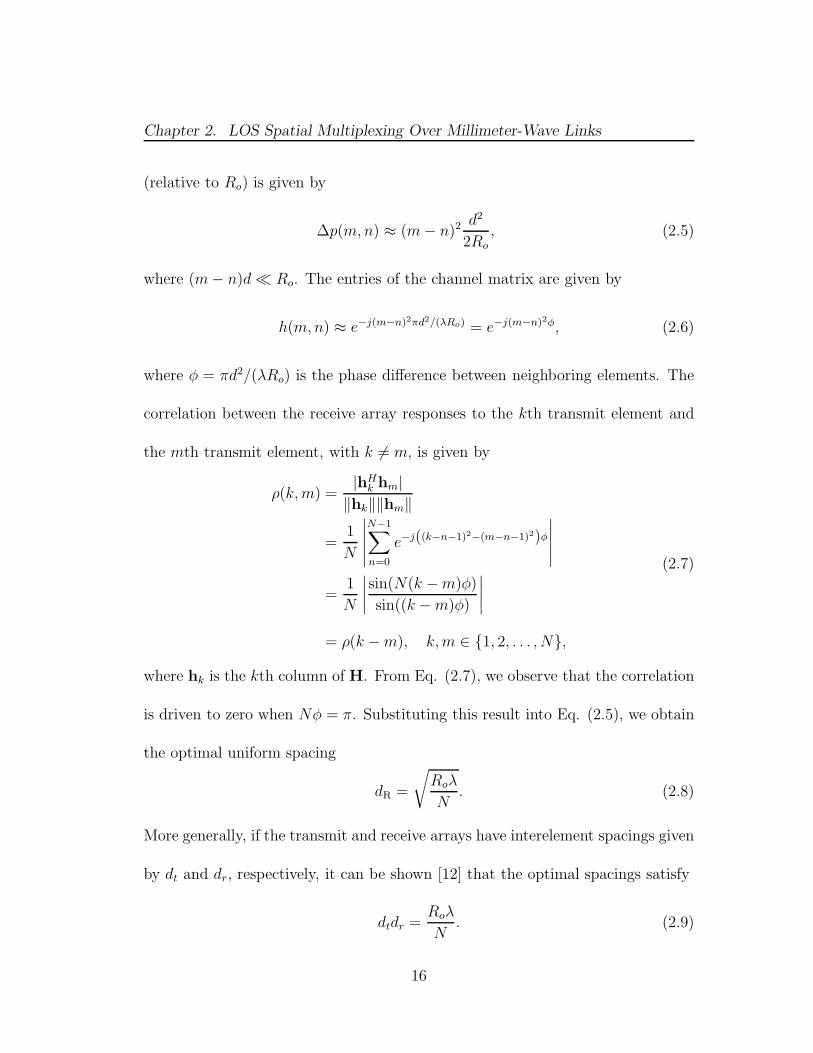
(relative to Ro) is given by
∆p(m,n) ≈ (m− n)2d2
2Ro, (2.5)
where (m− n)d≪ Ro. The entries of the channel matrix are given by
h(m,n) ≈ e−j(m−n)2πd2/(λRo) = e−j(m−n)2φ, (2.6)
where φ = πd2/(λRo) is the phase difference between neighboring elements. The
correlation between the receive array responses to the kth transmit element and
the mth transmit element, with k 6= m, is given by
ρ(k,m) =|hH
k hm|‖hk‖‖hm‖
=1
N
∣
∣
∣
∣
∣
N−1∑
n=0
e−j((k−n−1)2−(m−n−1)2)φ
∣
∣
∣
∣
∣
=1
N
∣
∣
∣
∣
sin(N(k −m)φ)
sin((k −m)φ)
∣
∣
∣
∣
= ρ(k −m), k,m ∈ 1, 2, . . . , N,
(2.7)
where hk is the kth column of H. From Eq. (2.7), we observe that the correlation
is driven to zero when Nφ = π. Substituting this result into Eq. (2.5), we obtain
the optimal uniform spacing
dR =
√
Roλ
N. (2.8)
More generally, if the transmit and receive arrays have interelement spacings given
by dt and dr, respectively, it can be shown [12] that the optimal spacings satisfy
dtdr =Roλ
N. (2.9)
16

Chapter 2. LOS Spatial Multiplexing Over Millimeter-Wave Links
Table 2.1: Sample array configurations. Lengths given in meters.
Ro N = 2 N = 3 N = 41 km 1.41 2.31 3.00100 m 0.44 0.73 0.955 m 0.11 0.18 0.23
Eq. (2.9) also specifies the optimal element spacing of N × N uniform square
arrays aligned broadside [13].
We refer to (2.9) as the Rayleigh spacing criterion. In the field of diffraction
limited optics, the Rayleigh criterion states an imaging array consisting of N
elements spaced distance dr apart has an angular resolution of θR ≈ λ/(drN).
Two distant objects a distance R from the imaging array, and a distance dt ≪ R
from one other, have angular separation θT ≈ dT/R. In order to resolve the
objects, it is required that θT ≥ θR. Equating the two quantities, we arrive at the
same condition given in (2.9).
A more general expression for the optimal uniform spacing is provided by
Bohagen et al. in [25] [12], where authors consider linear and rectangular arrays
facing arbitrary directions.
2.1.3 Application to mm-Wave Links
The length of a Rayleigh spaced array scales in proportion to√λ. While this re-
sults in impractically large arrays at lower frequencies, arrays are more moderately
17
Chapter 2. LOS Spatial Multiplexing Over Millimeter-Wave Links
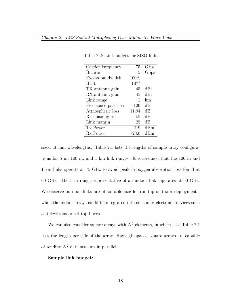
Table 2.2: Link budget for SISO link.
Carrier Frequency 75 GHzBitrate 5 GbpsExcess bandwidth 100%BER 10−9
TX antenna gain 45 dBiRX antenna gain 45 dBiLink range 1 kmFree-space path loss 129 dBAtmospheric loss 11.94 dBRx noise figure 6.5 dBLink margin 25 dBTx Power 21.9 dBmRx Power -23.0 dBm
sized at mm wavelengths. Table 2.1 lists the lengths of sample array configura-
tions for 5 m, 100 m, and 1 km link ranges. It is assumed that the 100 m and
1 km links operate at 75 GHz to avoid peak in oxygen absorption loss found at
60 GHz. The 5 m range, representative of an indoor link, operates at 60 GHz.
We observe outdoor links are of suitable size for rooftop or tower deployments,
while the indoor arrays could be integrated into consumer electronic devices such
as televisions or set-top boxes.
We can also consider square arrays with N2 elements, in which case Table 2.1
lists the length per side of the array. Rayleigh-spaced square arrays are capable
of sending N2 data streams in parallel.
Sample link budget:
18
Chapter 2. LOS Spatial Multiplexing Over Millimeter-Wave Links
MBIC
Antenna elements
Parabolic Dishes
MBIC
Printed Circuit Board
(a) Telescopic Dish Configuration (b) Planar Configuration
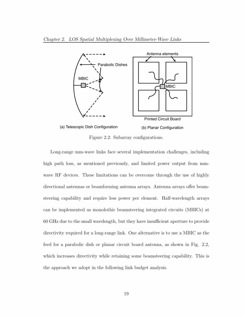
Figure 2.2: Subarray configurations.
Long-range mm-wave links face several implementation challenges, including
high path loss, as mentioned previously, and limited power output from mm-
wave RF devices. These limitations can be overcome through the use of highly
directional antennas or beamforming antenna arrays. Antenna arrays offer beam-
steering capability and require less power per element. Half-wavelength arrays
can be implemented as monolothic beamsteering integrated circuits (MBICs) at
60 GHz due to the small wavelength, but they have insufficient aperture to provide
directivity required for a long-range link. One alternative is to use a MBIC as the
feed for a parabolic dish or planar circuit board antenna, as shown in Fig. 2.2,
which increases directivity while retaining some beamsteering capability. This is
the approach we adopt in the following link budget analysis.
19
Chapter 2. LOS Spatial Multiplexing Over Millimeter-Wave Links
To evaluate the feasibility of long-range mm-wave links, we compute the link
budget for a 5 Gbps 75 GHz single-input single-output (SISO) link with a 1 km
link range. Each antenna consists of a beamsteering 4 × 4 square array (which
we refer to as a subarray, to distinguish it from a larger Rayleigh-spaced array)
mounted on a 30 cm diameter dish antenna with a 2 beamwidth, providing a
directivity of G = 45dB.
The minimum received power is given PRX = Q2kbTFB, where kB is the
Boltzmann constant, T is the temperature, F is the received noise figure, B is the
bandwidth, and Q = 6 for QPSK with an uncoded bit error rate of 10−9. The
bandwidth is 5 GHz assuming QPSK modulation with 100% excess bandwidth.
The received power according to Friis’ transmission equation is
PRX
PTX
=GTGRλ
16πR2e−αR (2.10)
where α is atmospheric attenuation, which dominates over the (λ/R)2 in foul
weather conditions. We allow for heavy rain by setting α = 11.94 dB/km [26],
[27].
The resulting link budget is summarized in Table 2.2. Including a 25 dB link
margin, we find that the link can be maintained using 160 mW transmit power at
each subarray, or 10 mW per subarray element. This SISO link forms the building
block of a larger MIMO link, which can reduce the required transmit power further
through array processing gains. These calculations support the notion that long
20

Chapter 2. LOS Spatial Multiplexing Over Millimeter-Wave Links
range links are feasible using moderate transmit power per element. The “array
of subarrays” approach is applied to indoor links in Chapter 4.
2.2 Spatial Correlation at Non-Optimal Link
Ranges
When the Rayleigh criterion is met, the channel matrix is scaled unitary and the
(noisy) transmitted signal vector s can be recovered through spatial equalization
without suffering degradation of the signal-to-noise (SNR) ratio. However, when
the link operates at a range R 6= Ro, correlation will be present among columns
of H and spatial equalization can cause an increase in noise power. This is likely
to occur in practice, because the precise link range R may be unknown during the
design and manufacture of an array.
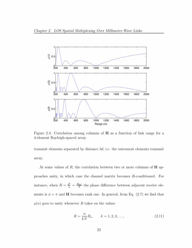
Consider a 4-element ULA array. Fig. 2.3 plots the correlation ρ(k−m) of the
receive array responses to transmit elements k and m as the link range is varied
from R = 0.2Ro to R = Ro. ρ(1) is the correlation between adjacent columns
of H, i.e. correlation among the receive array responses to neighboring trans-
mit elements. Similarly, ρ(2) corresponds to transmit elements separated by 2d.
Hence, it represents correlation between responses to the first and third transmit
elements or the second and fourth transmit elements. Finally, ρ(3) corresponds to
21
Chapter 2. LOS Spatial Multiplexing Over Millimeter-Wave Links
200 400 600 800 1000 1200 1400 1600 1800 20000
0.5
1ρ
(1)
200 400 600 800 1000 1200 1400 1600 1800 20000
0.5
1
ρ(2
)
200 400 600 800 1000 1200 1400 1600 1800 20000
0.5
1
Range (m)
ρ(3
)
Figure 2.3: Correlation among columns of H as a function of link range for a4-element Rayleigh-spaced array.
transmit elements separated by distance 3d, i.e. the outermost elements transmit
array.
At some values of R, the correlation between two or more columns of H ap-
proaches unity, in which case the channel matrix becomes ill-conditioned. For
instance, when R = d2
λ= RRC
Nthe phase difference between adjacent receive ele-
ments is φ = π and H becomes rank one. In general, from Eq. (2.7) we find that
ρ(n) goes to unity whenever R takes on the values
R =n
kNRo, k = 1, 2, 3, . . . , (2.11)
22
Chapter 2. LOS Spatial Multiplexing Over Millimeter-Wave Links
x x x x0
0.2
0.4
0.6
0.8
1
Position
Arr
ay r
esp
on
se
R = Ro
x x x x0
0.2
0.4
0.6
0.8
1
Position
Arr
ay r
esp
on
se
R = 0.75 Ro
x x x x0
0.2
0.4
0.6
0.8
1
Position
Arr
ay r
esp
on
se
R = 0.5 Ro
x x x x0
0.2
0.4
0.6
0.8
1
Position
Arr
ay r
esp
on
se
R = 0.25 Ro
1 2 3 4 1 2 3 4
1 2 3 4 1 2 3 4
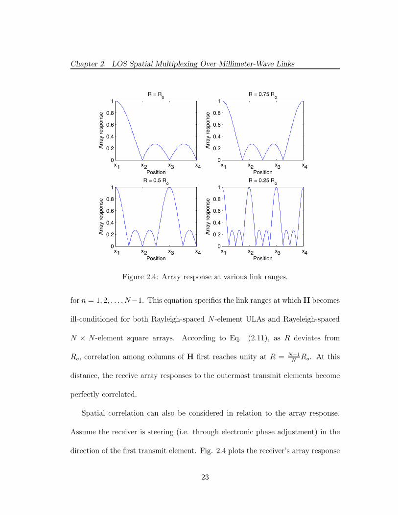
Figure 2.4: Array response at various link ranges.
for n = 1, 2, . . . , N−1. This equation specifies the link ranges at which H becomes
ill-conditioned for both Rayleigh-spaced N -element ULAs and Rayeleigh-spaced
N × N -element square arrays. According to Eq. (2.11), as R deviates from
Ro, correlation among columns of H first reaches unity at R = N−1N
Ro. At this
distance, the receive array responses to the outermost transmit elements become
perfectly correlated.
Spatial correlation can also be considered in relation to the array response.
Assume the receiver is steering (i.e. through electronic phase adjustment) in the
direction of the first transmit element. Fig. 2.4 plots the receiver’s array response
23

Chapter 2. LOS Spatial Multiplexing Over Millimeter-Wave Links
to a point source source moving across the line connecting the transmit elements.
When R = R0 and the Rayleigh criterion is satisfied, the interfering transmitters
fall into nulls in the array pattern. At R = 0.75, however, the fourth transmit
element falls within a grating lobe of the receive array response, which accounts
for the high value of ρ(3) at this link range. Similarly, the third element falls
within a grating lobe at R = Ro/2, and all elements coincide with grating lobes
at R = R0/4.
2.2.1 Noise Enhancement at Non-Optimal Link Ranges
To assess the impact of spatial correlation on system performance, we will consider
the output of a zero-forcing (ZF) spatial equalizer. The ZF equalizer cancels out
spatial interference entirely by filtering the received signal vector by the pseudo-
inverse of the channel matrix, given by
CZF = H† = HH(HHH)−1. (2.12)
H is typically invertible (although possibly ill-conditioned), in which case the
pseudo-inverse and inverse coincide. The output of the zero-forcing equalizer is
y = CZF (Hs+ n) = s + n, (2.13)
where n is an N × 1 complex Gaussian noise vector with covariance 2σ2CHZFCZF.
The ZF equalizer eliminates spatial interference entirely at the cost of an increase
24

Chapter 2. LOS Spatial Multiplexing Over Millimeter-Wave Links
0.4 1 1.60
5
10
15
20
25
30
35
R/R
No
ise
en
ha
nce
me
nt (d
B)
Maximum
Mean
γu
o
Figure 2.5: Noise enhancement as a function of range.
in noise power, referred to as noise enhancement. For a given array configuration
x, the noise enhancement incurred by the ith transmitted signal is given by
ηi(x, R) = ‖hi‖2‖ci‖2 = N‖ci‖2, (2.14)
where ci is the ith column of CZF and the dependence of ci on x and R is implicit.
The mean noise enhancement is given by
η(x, R) =1
N
N∑
i=1
ηi(R) =N∑
i=1
1
λ2i
, (2.15)
where λi are the singular values of H evaluated at R.
25

Chapter 2. LOS Spatial Multiplexing Over Millimeter-Wave Links
Fig. 2.5 plots the mean noise enhancement, η(xu, R), and the maximum noise
enhancement, maxi ηi(xu, R), of the 4-element Rayleigh-spaced array. Note that
noise enhancement increases as soon as R deviates from Ro. A link budget analysis
suggests that, even under unfavorable weather conditions, the link margin can be
set as high as 10 to 20 dB [28]. A portion of the link margin can be allocated
to offsetting the effects of noise enhancement. However, the noise enhancement
far exceeds the entire link margin at ranges of 375 m, 500 m, and 750 m, i.e. at
ranges given by Eq. (2.11) where the correlation among columns of H approaches
unity.
Although other spatial equalization methods (eigenchannel transmission, BLAST,
and MMSE) could be considered, these schemes suffer performance degradation at
the same link ranges as the ZF receiver due to spatial correlation in the channel.
In particular, MMSE and ZF equalization give similar performance at moderate
to high SNRs, with the MMSE receiver tending to the ZF receiver asymptoti-
cally as the SNR gets large. Thus we focus on noise enhancement as a simple
SNR-independent metric of array performance.
In the the following section, we consider the use of optimized nonuniform arrays
that sacrifice optimality at Ro to provide acceptable performance over a larger set
of link ranges. By breaking the uniformity of the array, the noise enhancement
spikes closest to Ro can be avoided.
26

Chapter 2. LOS Spatial Multiplexing Over Millimeter-Wave Links
2.3 Optimized Nonuniform Arrays
Let [R1, R2] denote the interval about Ro for which the maximum noise enhance-
ment remains below a given threshold η. Defining γ = R2 − R1, the goal of our
optimization will be to find a nonuniform linear array that maximizes γ. We
denote the maximum value by γo and define γu as the value of our metric when
using Rayleigh-spaced uniform arrays. For example, consider the four-element
uniform array optimized for some link range Ro. Setting η = 6 dB, we have
R1 = .8Ro and R2 = 1.4Ro, as shown in Fig. 2.5. The link will operate reliably
given R/Ro ∈ [0.8, 1.4], corresponding to γu = 0.6.
2.3.1 4-element Nonuniform Array Analysis
To gain insight into the optimization problem, we begin with 4-element Rayleigh-
spaced arrays at both ends of the link. The array is optimized for link range Ro.
Keeping the outer two elements fixed, we allow the inner two elements to shift
inward or outward in position by an equal amount, maintaining symmetry about
the center of the array. The element positions are given by x = [0, αdR, (3 −
α)dR, 3dR], with α = 1 corresponding to the original Rayleigh-spaced array.
As shown by Fig. 2.5, γu is limited by the rightmost spike in noise enhance-
ment, which occurs at 3Ro/4. This spike is the result of high correlation between
27
Chapter 2. LOS Spatial Multiplexing Over Millimeter-Wave Links
0.4 0.6 0.8 1 1.2 1.4 1.6−1
−0.5
0
0.5
1(a
)
R/Ro
ρ(3)1st term2nd term
0.4 0.6 0.8 1 1.2 1.4 1.6−1
−0.5
0
0.5
1
R/Ro
(b)
ρ(3)1st term2nd term
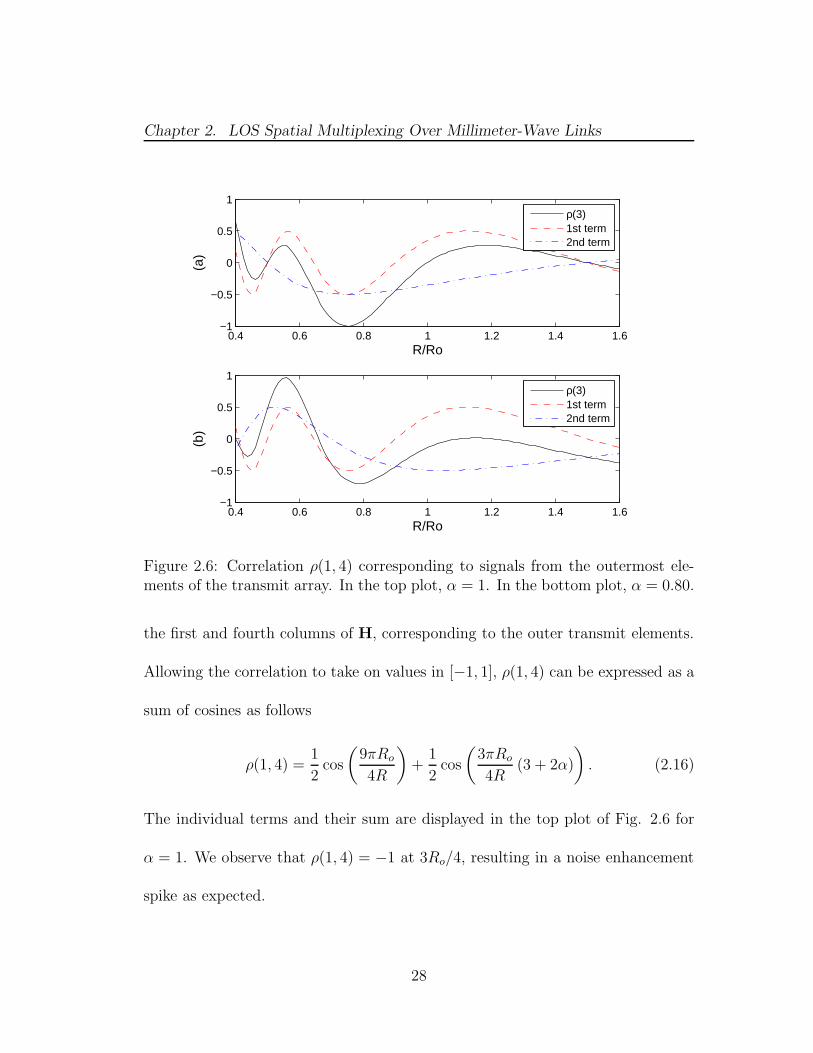
Figure 2.6: Correlation ρ(1, 4) corresponding to signals from the outermost ele-ments of the transmit array. In the top plot, α = 1. In the bottom plot, α = 0.80.
the first and fourth columns of H, corresponding to the outer transmit elements.
Allowing the correlation to take on values in [−1, 1], ρ(1, 4) can be expressed as a
sum of cosines as follows
ρ(1, 4) =1
2cos
(
9πRo
4R
)
+1
2cos
(
3πRo
4R(3 + 2α)
)
. (2.16)
The individual terms and their sum are displayed in the top plot of Fig. 2.6 for
α = 1. We observe that ρ(1, 4) = −1 at 3Ro/4, resulting in a noise enhancement
spike as expected.
28
Chapter 2. LOS Spatial Multiplexing Over Millimeter-Wave Links
The first term, plotted as a dashed line, is independent of the choice of α while
the second term is dependent. We can predict that a good choice of α is one that
avoids coinciding positive or negative peaks among the cosine terms in the range
interval of interest.
Setting η = 6 dB, the the metric γ has been computed numerically for α ∈
[0, 1.5], with the results shown in Fig. 2.7. We find that the nonuniform array
outperforms the Rayleigh-spaced array for any values of α between 0.45 and 1.
The optimal value occurs at α = 0.802. Although not shown, the correlations
ρ(1, 2) and ρ(3, 4) grow large for α < 0.5, resulting in a low value of γ. This
is as expected, because the receiver has difficulty resolving the inner and outer
elements when they are placed close together.
As shown in the Fig. 2.6, the optimal value of α reduces ρ(3) at values of
R surrounding Ro. This provides an intuitive notion of what constitutes a good
nonuniform array, however, it also highlights the complexity of the problem. First,
the distance between adjacent peaks of each cosine term shrinks as R decreases,
thus it becomes increasingly difficult to ensure that peaks do not coincide as R
decreases. In fact, even in the optimized case, negative peaks coincide at R = 500
m, resulting in a sharp spike in noise enhancement at this range. Second, we have
constrained ourselves to a nonuniform array that is symmetric about the center
29

Chapter 2. LOS Spatial Multiplexing Over Millimeter-Wave Links
0 0.2 0.4 0.6 0.8 1 1.2 1.40
0.1
0.2
0.3
0.4
0.5
0.6
0.7
0.8
α
γ (m
)
Figure 2.7: Optimization metric γ for symmetric 4-element array.
of the array. Asymmetric arrays may perform significantly better, although they
are considerably more difficult to characterize analytically.
Based on these factors, we proceed to perform a numerical optimization of
asymmetric nonuniform arrays. Because the number of elements in a mm-wave
MIMO array is limited by practical constraints on the array’s physical size, ex-
haustive search for optimal positions remains a computationally feasible option.
30

Chapter 2. LOS Spatial Multiplexing Over Millimeter-Wave Links
2.3.2 Optimization Procedure and Results
The optimization procedure is first performed on a 4-element array with an ex-
pected link range ofRo = 1 km. Our optimization goal is to maximize γ = R2−R1,
where [R1, R2] is the interval about Ro on which the noise enhancement remains
below η = 6 dB. The array length is fixed at L = 3dR, i.e. the length of a 4-element
Rayleigh spaced optimized for a link range of Ro. The antenna position vector
is given by x = [0, x2, x3, 3dR] with x2 ∈ [0, 1.5dR] and x3 ∈ [1.5dR, 3dR]. The
optimal element positions, determined through exhaustive search, are given by
xo = [0, 0.87dR, 2.36dR, 3dR]. In Fig. 2.8, we plot the mean SNR gain (normalized
to 0 dB at Ro), defined as
SNR(R) =
(
Ro
R
)2
η(xo, R),
where the factor (Ro/R)2 accounts for path loss. We note that while the maximum
link range is slightly decreased, the nonuniform array eliminates large spikes in
the noise enhancement completely and could be used over a much wider set of
link ranges without concern that the SNR would dip below an acceptable level.
The procedure was repeated for a 5-element array with η increased to 6.97 dB
to account for the additional receive array processing gain provided by the extra
array element. Fig. 2.9 plots the resulting normalized SNR. Similarly, a 6-element
array was optimized with η = 7.76 dB, and the normalized SNR is plotted in Fig.
31

Chapter 2. LOS Spatial Multiplexing Over Millimeter-Wave Links
0.4 0.6 0.8 1 1.2 1.4 1.6−35
−30
−25
−20
−15
−10
−5
0
5
10
R/Ro (m)
Normalized SNR (dB)
Optimized non−uniform
Uniform
γo
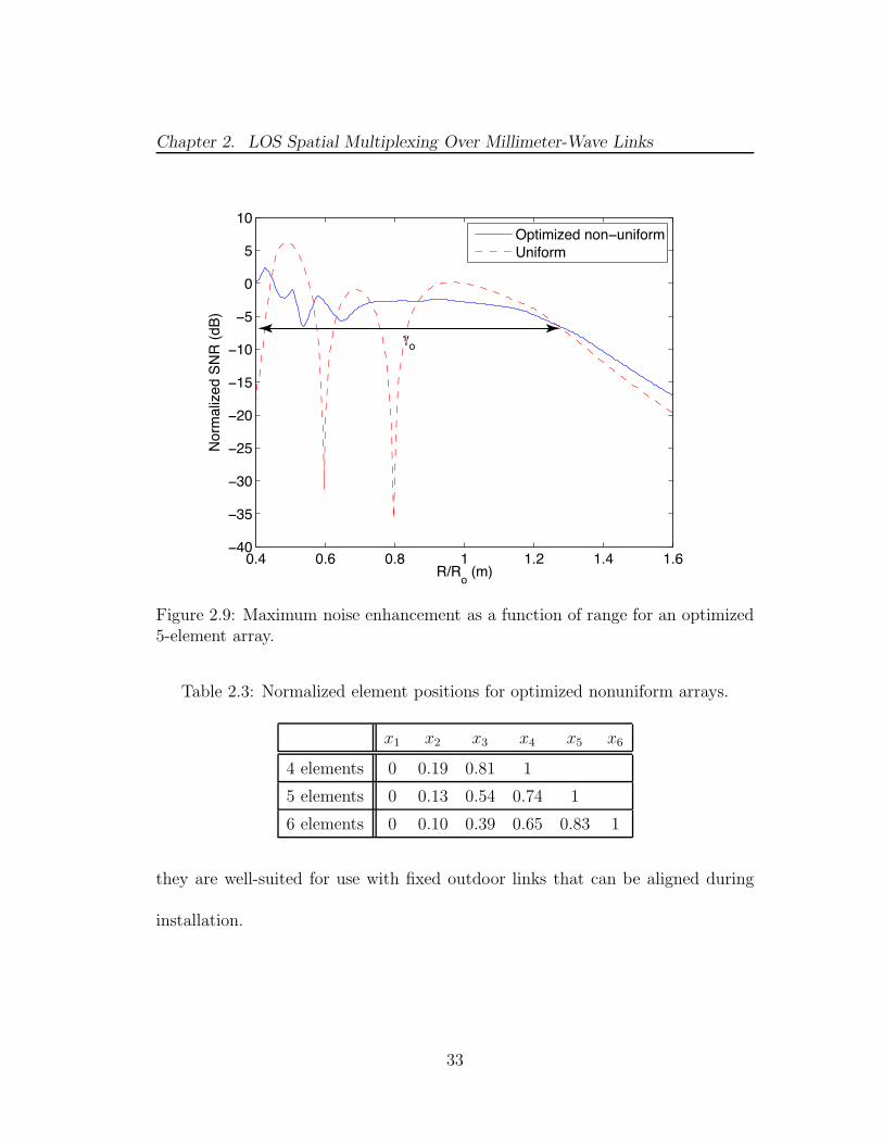
Figure 2.8: Maximum noise enhancement as a function of range for an optimized4-element array.
2.10. In both cases γo provides a significant improvement over γu. The optimized
antenna positions are for 3, 4, and 5-element arrays normalized to unit length are
provided in Table 2.3.
We observe that γu decreases by roughly 20% with each additional array ele-
ment, γo remains nearly constant. This trend suggests that the benefit of nonuni-
form optimization grows with increasing N . We note that during optimization,
we assumed the arrays were aligned, and non-uniform arrays may not necessarily
perform better than uniform arrays when the arrays are misaligned. As such,
32
Chapter 2. LOS Spatial Multiplexing Over Millimeter-Wave Links
0.4 0.6 0.8 1 1.2 1.4 1.6−40
−35
−30
−25
−20
−15
−10
−5
0
5
10
R/Ro (m)
Normalized SNR (dB)
Optimized non−uniform
Uniform
γo
Figure 2.9: Maximum noise enhancement as a function of range for an optimized5-element array.
Table 2.3: Normalized element positions for optimized nonuniform arrays.
x1 x2 x3 x4 x5 x6
4 elements 0 0.19 0.81 1
5 elements 0 0.13 0.54 0.74 1
6 elements 0 0.10 0.39 0.65 0.83 1
they are well-suited for use with fixed outdoor links that can be aligned during
installation.
33

Chapter 2. LOS Spatial Multiplexing Over Millimeter-Wave Links
0.4 0.6 0.8 1 1.2 1.4 1.6−40
−35
−30
−25
−20
−15
−10
−5
0
5
R/Ro (m)
Normalized SNR (dB)
Optimized non−uniform
Uniform
γo
Figure 2.10: Maximum noise enhancement as a function of range for an optimized6-element array.
2.4 Rank Adaptation
In the case that a LOS MIMO channel becomes highly correlated due mismatch
between the antenna spacing and the link range, the receiver may be unable to re-
cover the transmitted signal from the interferer(s). In the worst case, the channel
matrix becomes rank deficient, and the interfering signals will be irrecoverable.
The transmitter can adapt to such a scenario by reducing the number of indepen-
dent signals it attempts to transmit simultaneously. Specifically, if the receiver
responses to two (or more) transmitters are highly correlated, the transmitter
34
Chapter 2. LOS Spatial Multiplexing Over Millimeter-Wave Links
can send a single data stream over these antennas. If there is a strong negative
correlation between transmitters, one of the signals should be inverted.
For instance, consider a four element array that satisfies the Rayleigh criterion
at some range Ro. As we saw in Section 2.2, the receiver is unable to distinguish
the signals transmitted by the first and fourth antennas at R = 0.75Ro. In this
case, there is a strong positive correlation and the transmitter should send an
identical signal from these antennas. At R = Ro/2, signals 1 and 3 cannot be
jointly recovered, nor can signals 2 and 4, and it would be preferable to send two
independent signals.
To evaluate the performance of this scheme, we model the N×1 received signal
vector as
y = HQx+ n, (2.17)
where x ∈ CNs×1 is the transmitted signal vector with entries satisfying E(|xn|2) =
P , Q ∈ RN×Ns is a rank adaptation matrix, and n ∼ CN (0, IN) is complex addi-
tive white Gaussian noise. The entries of Q, selected from −1, 0, 1, specify how
the Ns signals are distributed to N transmit antennas. Each row is constrained
to have a single non-zero entry to ensure that each antenna transmits a single
stream. For instance, if a common signal is sent over the first and fourth antennas
35

Chapter 2. LOS Spatial Multiplexing Over Millimeter-Wave Links
of a four element array, Q is given by
Q =
1 0 0
0 1 0
0 0 1
1 0 0
.
We assume the signals are recovered at the receiver using a ZF equalizer with
weights C = (HQ)†. The nth output of the ZF equalizer is given by
yn = xn + wn, n = 1, 2, . . . , Ns, (2.18)
where w ∼ CN(0, ‖cn‖2) and cn is the n row of C. The maximum rate at which
the system can transmit information reliably is given by
I = maxNs,Q
Ns∑
n=1
log2(1 +P
‖cn‖2), (2.19)
We note that ZF equalization and equal power allocation are suboptimal strate-
gies, but practical design choices for mm-wave systems. We can evaluate how
suboptimal the proposed system is by comparing I to the channel capacity, the
maximum rate of reliable communication over the channel, given by
C =N∑
n=1
log2(1 + Pnσ2n), (2.20)
where 1N
∑
n Pn = P is the power allocation under the waterfilling allocation
scheme and σ2n is the nth eigenvalue of HHH [1].
36

Chapter 2. LOS Spatial Multiplexing Over Millimeter-Wave Links
0.2 0.4 0.6 0.8 1 1.2 1.4 1.6 1.8 2 0
5
10
15
20
25
30
35
R/Ro
Spe
ctra
l effi
cien
cy (
bps/
Hz)
N
s = 4
Ns = 3
Ns = 2
Ns = 1
Figure 2.11: I as a function of Ns, the number of independent transmitted signals.
I was evaluated through simulation for a LOS MIMO link using 4-element
Rayleigh-spaced arrays. Path loss is accounted for by setting the power P at
range R equal to
P (R) =
(
R
Ro
)210
4,
which is normalized such that the equalized signals have a signal-to-noise ratio
(SNR) of 10 dB at R = Ro. Fig. 2.11 plots I as a function of normalized link
range for fixed values of Ns. We observe many link ranges where transmitting
fewer than four independent data streams is optimal. This is true, as expected,
37

Chapter 2. LOS Spatial Multiplexing Over Millimeter-Wave Links
0.2 0.4 0.6 0.8 1 1.2 1.4 1.6 1.8 2 0
5
10
15
20
25
30
35
R/Ro
Spe
ctra
l Effi
cien
cy (
bps/
Hz)
Rank adaptationChannel capacityEqual power eigenmode transmission
Figure 2.12: Rank adaptation strategy compared to channel capacity.
at the ranges where the correlation rises sharply due to grating lobe interference.
It is also holds when the link range is roughly 20% larger than Ro.
Fig. 2.12 compares I to the channel capacity. We also compute (2.20) under
equal power allocation, which we refer to as equal power eigenmode transmission.
Averaged over 0.2 ≤ R/Ro ≤ 2, the spectral efficiency of the rate adaptation
scheme is 1.37 bps/Hz lower than channel capacity, and 1.03 bps/Hz lower than
equal power eigenmode transmission.
38

Chapter 2. LOS Spatial Multiplexing Over Millimeter-Wave Links
2.5 Discussion
In this chapter, we presented a case for the use of nonuniform arrays in LOS
MIMO systems. In practice, the precise distance between nodes may be unknown
during the array design process. Therefore, we examined how system performance
is affected when array size and link range are are not matched according to the
Rayleigh spacing criterion. Under a zero-forcing equalization scheme, significant
degradation of SNR at the output of the equalizer may occur. Seeking to minimize
these effects, alternate array geometries were considered. It was demonstrated that
non-uniform antenna spacing can provide acceptable performance over a larger set
of link ranges than uniform Rayleigh spacing.
We also considered the rank adaptation strategy, in which the number of inde-
pendent data streams transmitted simultaneously is varied according to the degree
of spatial correlation in the channel. Rate adaptation was shown to be an effective
strategy when the channel matrix is rank deficient or ill-conditioned.
39

Chapter 3
Hierarchical MIMO SignalProcessing: Architecture andPrototype
In the previous chapter, we focused on how the LOS MIMO channel is impacted
by antenna array geometry. We now broaden our scope to consider designing
a practical mm-wave link that leverages these results. In particular, we consider
some of the challenges that arise when a MIMO system scales to larger bandwidths
and multi-Gbps symbol rates. High-precision sampling, a critical component of
today’s DSP-centric designs, becomes prohibitive in cost and power consumption
at multiGHz rates. To obviate the need high-speed, high-precision analog-to-
digital converters (ADCs), we propose a two-level architecture that decouples the
signal processing tasks of spatial equalization and demodulation. More specifically,
spatial equalization is applied to the baseband signals in the analog domain, and
equalizer training occurs at a slower time-scale, permitting the use of low-rate,
40

Chapter 3. Hierarchical MIMO Signal Processing: Architecture and Prototype
full-precision ADCs. The equalized channels can then each be sampled at a high
rate using low-precision ADCs, which are sufficient for demodulation of the small
constellation signals currently used for mm-wave communications.
The two-level architecture has been implemented as a four-channel mm-wave
MIMO hardware prototype with an aggregate data rate of 2.5 Gbps. To the
best of our knowledge, the prototype provided the first demonstration of LOS
spatial multiplexing at mm-wave frequencies. It consists of off-shelf mm-wave
and RF components and a printed circuit board (PCB) based spatial equalization
network. The link was tested at 5 m in an indoor office environment and at 41 m
in an outdoor environment.
The mm-wave hardware for the prototype was built by Dr. Colin Sheldon
and the adaptive spatial interference suppression scheme was implemented by Dr.
Munkyo Seo. The author built the FPGA-based transmitter, and was responsible
for Matlab post-processing of complex baseband samples. The prototype was
co-supervised by Profs. Mark Rodwell and Upamanyu Madhow.
A detailed description of the prototype hardware can be found in [15] [29]
[14] and in Dr. Colin Sheldon’s PhD dissertation [30]. The focus here is on
describing the system-level architecture and algorithms, including new block-based
algorithms for spatial interference suppression that were not implemented on the
prototype.
41

Chapter 3. Hierarchical MIMO Signal Processing: Architecture and Prototype
The main contributions of this chapter are as follows:
• We propose a two-level architecture for mm-wave MIMO links that decouples
the tasks of equalization and signal demodulation into two separate time
scales, thereby avoiding a need for costly high-precision, high-speed ADCs.
• Three spatial equalization methods are introduced. We evaluation their per-
formance through simulation and discuss various tradeoffs associated with
their use.
• A four-channel mm-wave MIMO prototype was designed and tested. It
provides proof-of-concept for mm-wave LOS spatial multiplexing and the
two-level signal processing architecture. We provide a description of the
prototype and a summary of experimental results at the end of this chapter.
The chapter is organized as follows. Section 3.1 introduces the two-level mm-
wave MIMO architecture and provides the channel model. Spatial equalization
and channel estimation is considered in the context of the proposed architecture
in Section 3.2. The prototype system is described in Section 3.3 and experimental
results are discussed. The chapter concludes with a summary of results in Section
3.4.
42

Chapter 3. Hierarchical MIMO Signal Processing: Architecture and Prototype
3.1 Two-level mm-Wave MIMO Architecture
We begin by reviewing traditional training-based channel estimation methods and
considering their viability when scaled to multi-Gbps speeds. This motivates the
introduction of the proposed architecture in Section 3.1.2.
3.1.1 Pilot-Symbol-Aided Channel Estimation
Background
A spatial equalizer attempts to eliminate spatial interference by reversing the
effects of a MIMO channel. To accomplish this, an equalizer may require an
explicit estimate of the channel. Under conventional methods of training-based
channel estimation, known pilot symbols are multiplexed with data symbols to
facilitate channel estimation at the receiver. This technique is commonly used
in existing wireless standards, including GSM, WCDMA, CDMA-2000, and the
various 802.11 standards, as well as wireline systems such as cable and DSL [31].
For multiantenna channel estimation, we assume a discrete-time block-fading
MIMO channel modeled by
Y = HX+W, (3.1)
where X ∈ CNT×B represents a a block of symbols transmitted over NT transmit
antennas and B time slots, Y ∈ CNR×B is the signal received over NR receive
43
Chapter 3. Hierarchical MIMO Signal Processing: Architecture and Prototype
antennas, W ∈ CNR×B is additive noise, and H ∈ CNR×NT is the channel. The
transmitted signal, including pilot symbols, is given by
xk,n =√αk,ndk,n +
√
βk,npk,n, k = 1, . . . , NT , n = 1, . . . , B, (3.2)
where xk,n is the signal transmitted from the kth antenna at time slot n, dk,n is
an unknown data symbol with zero mean and unit variance, and pk,n is a training
symbol with |pk,n| = 1. The power allocated to data and training symbols are
given by αk,n and βk,n, respectively. The form of 3.2 permits training signals to
be interspersed, clustered together, or embedded with data signals.
Equation (3.1) is a linear channel model and permits straightforward appli-
cation of the linear least squares (LSE) or linear minimum mean squared error
(MMSE) estimators to acquire a channel estimate [32]. The channel estimate, in
turn, can be used to recover the transmitted signals from interference using, for
example, the ZF filter.
Modern digital communication receivers commonly sample signals with 6-12
bits of precision, which is sufficient for the pilot-symbol-aided channel estimation
techniques just described to approach full-precision performance. MultiGbps links
operating in the 60 GHz band, however, require sampling rates on the order of
several GHz. As bandwidth and data rates scale up, the cost, power consumption,
and availability of high-speed, high-precision ADCs becomes prohibitive [5]. As
44
Chapter 3. Hierarchical MIMO Signal Processing: Architecture and Prototype
a result, the ADC becomes a limiting factor in designing affordable multiGbps
mm-wave MIMO architectures.
This bottleneck could potentially be avoided by using significantly lower pre-
cision ADCs (i.e. 1-3 bits) than are currently employed. Application of the
linear LSE or MMSE estimator to this highly-quantized data would produce a
poor channel estimate. However, information theoretic studies of SISO links have
demonstrated that the capacity loss resulting from the use of low-precision ADCs
is relatively small, assuming a non-dispersive channel with perfect synchroniza-
tion [33]. Methods of performing various receiver tasks using highly quantized
data have been considered in the literature, including amplitude estimation [34],
frequency estimation [35], direction of arrival estimation [36], and SISO channel
impulse response estimation [37]. MIMO channel estimation using coarse quan-
tization was recently addressed in [38], although the proposed estimator requires
operation in the low-SNR regime and provides relatively coarse estimates when
using 1- or 2-bit quantizers. We propose an alternate approach to channel esti-
mation in the following section.
3.1.2 System Architecture
In this section, we consider the alternate approach of a two-level architecture
that performs spatial equalizer adaptation and channel demodulation on separate
45

Chapter 3. Hierarchical MIMO Signal Processing: Architecture and Prototype
(a) Transmitter
Slow time scale
Analog
Spatial
Equalization
Electronics
R
Fast time scale
(b) Receiver
Figure 3.1: Two-level system architecture.
46
Chapter 3. Hierarchical MIMO Signal Processing: Architecture and Prototype
time scales. The architecture derives from the realization that, for the reasons
described above, channel estimation benefits from full-precision sampling, while
low-precision sampling suffices for other tasks, such as the demodulation of small-
constellation signals. Fig. 3.1 is a block diagram of the proposed system. The
transmitter combines each ofNT baseband data streams with a unique narrowband
pilot signal, which we take to be a low-frequency (i.e. 10-100 kHz range) sinusoid.
The signals are upconverted to 60 GHz and transmitted over an array of NT
elements. The signals are received over an NR element array and downconverted
to complex baseband. The baseband signals are spatially equalized in the analog
domain before the recovered signals are sampled with high-rate, low-precision
ADCs and demodulated.
The spatial equalizer coefficients are determined through an explicit or im-
plicit channel estimate which is derived through processing of the embedded pilot
signals. The pilot signals have significantly lower bandwidth than the data, which
may span several GHz. The received signals can therefore be filtered and sam-
pled at a high precision using inexpensive low rate ADCs. Fig. 3.1 depicts an
open-loop architecture, where an explicit estimate of the channel is formed from
observations of the pilot tones. This estimate is in turn used to compute the
equalizer coefficients. A feedback-based architecture is also considered, where the
equalizer controller observes the pilot tones to estimate the symbol-to-interference
47

Chapter 3. Hierarchical MIMO Signal Processing: Architecture and Prototype
ratio (SIR) at the equalizer output. The controller adjusts the equalizer weights
adaptively to maximize the measured SIR. In this case, an explicit channel esti-
mate is not formed. Both designs are considered in more detail in 3.2.
3.1.3 Channel Model
The continuous-time complex baseband signal received at themth receive antenna
is given by
rm(t) = ei(2πf0t+φ0)
NT∑
n=1
hm,n (pn(t) + dn(t)) + wm(t), (3.3)
where hm,n is the complex channel gain between the mth receive antenna and nth
transmit antenna, pn(t) and dn(t) are the nth pilot signal and data signal, respec-
tively, wm(t) is complex white Gaussian noise with power spectral density N0,
and f0 and φ0 are a carrier frequency offset and phase offset, respectively, which
allow for mismatch between the carrier signals at the transmitter and receiver.
We assume |f0| < fM , where fM denotes the maximum possible carrier frequency
offset.
The nth data signal is given by
dn(t) =
√
1
NT
∞∑
l=−∞
sn,lg(t− lTd − τ), n = 1, . . . , NT , (3.4)
where Td is the symbol rate, g(t) is a pulse shape satisfying ||g(t)||2 = Td, τ is an
unknown time delay, and the complex data symbols sn,l satisfy E[sn,ls∗m,k] =
48

Chapter 3. Hierarchical MIMO Signal Processing: Architecture and Prototype
Esδnmδlk. This signal is summed at the transmitter with the nth pilot signal,
given by
pn(t) =
√
α
NT
exp (i (2πfnt+ φn)) , (3.5)
where α is a scaling factor, fn is a given frequency, and φn is an unknown phase
offset. We assume |hm,n|2 = 1, and hence α is the received power of each pilot
tone.
The spatial interference cancellation algorithms described herein operate on
the received signal after it has been low-pass filtered and sampled. We take the
filter to be ideal low-pass with one-sided bandwidth B/2, where B ≪ 1/Td. The
sampling rate, denoted by Fs > 2(fM +maxn fn), is chosen independently of the
data, which is treated as noise by the interference cancellation algorithm. The
filtering and sampling operations produce the discrete-time signal
rm[k] = LPFrm(kTs) (3.6)
= ei(2πf0kTs+φ0)
NT∑
n=1
hm,n
(√
α
NT
pn(kTs) +
√
1
NT
dn(kTs)
)
+ wm[k], (3.7)
where Ts = 1/Fs, dn(t) is a low-pass filtered version of dn(t), and wm[k] is zero
mean, complex Gaussian noise with variance 2σ2N = N0B. In the frequency range
−B/2 < f < B/2, we assume the PSD of the data signal is roughly flat and equal
to Td, which is satisfied, for instance, by the pulse g(t) = sinc(t/Td). The nth
49

Chapter 3. Hierarchical MIMO Signal Processing: Architecture and Prototype
filtered data stream is represented in discrete time as
dn[k] = BTd
∞∑
l=−∞
sn,lsinc (B (kTs − lTd − τ)) . (3.8)
Noting that BTd ≪ 1, we observe that dn[k] is the sum of a large number of
independent random variables, and can be approximated as a zero mean Gaussian
random variable with variance 2σ2d = E[|dn[k]|2] = BTdEs. We assume that the
sampling rate Fs equals an integer multiple of B and the data and noise terms of
the sampled received signal are uncorrelated, and hence independent, in time.
The low-pass filtered, discrete-time received signal can be expressed in vector
notation as
r[k] = ei(2πf0kTs+φ0)H
(√
α
NTp[k] +
√
1
NTd[k]
)
+w[k] (3.9)
where H ∈ CNR×NT is the channel matrix whose (m,n)th entry is hm,n, p[k] ∈
CNT×1 is the sampled pilot tone vector whose nth entry is pn(kTs), d[k] ∼
CN (0, 2σ2dINT
) represents filtered data, and w[k] ∼ CN (0, 2σ2NINR
) is complex
white Gaussian noise.
3.2 Spatial Interference Suppression
The spatial equalizer is implemented as a linear filter in the analog domain using
array of variable-gain amplifiers (VGAs) as shown in Fig. 3.2. NR complex-valued
50
Chapter 3. Hierarchical MIMO Signal Processing: Architecture and Prototype
Recovered
signal 1
Recovered
signal 2
Interference
Suppression
Algorithm
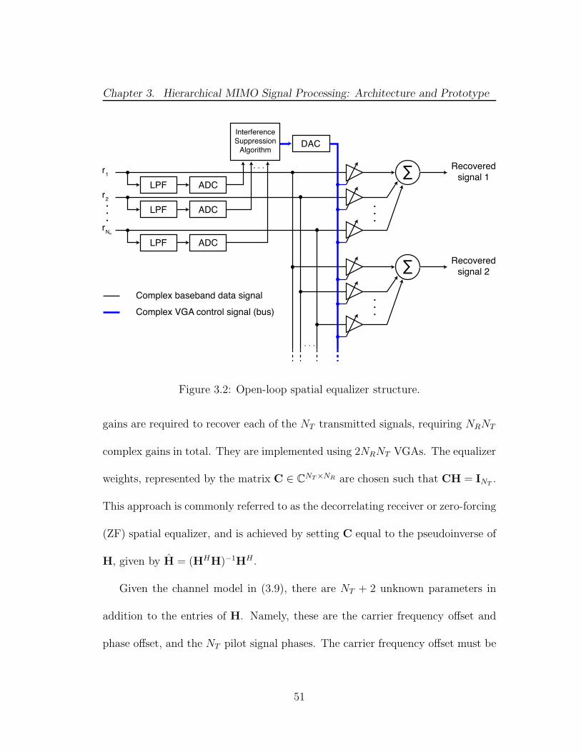
Figure 3.2: Open-loop spatial equalizer structure.
gains are required to recover each of the NT transmitted signals, requiring NRNT
complex gains in total. They are implemented using 2NRNT VGAs. The equalizer
weights, represented by the matrix C ∈ CNT×NR are chosen such that CH = INT.
This approach is commonly referred to as the decorrelating receiver or zero-forcing
(ZF) spatial equalizer, and is achieved by setting C equal to the pseudoinverse of
H, given by H = (HHH)−1HH .
Given the channel model in (3.9), there are NT + 2 unknown parameters in
addition to the entries of H. Namely, these are the carrier frequency offset and
phase offset, and the NT pilot signal phases. The carrier frequency offset must be
51

Chapter 3. Hierarchical MIMO Signal Processing: Architecture and Prototype
estimated, either implicitly or explicitly, to obtain an estimate of H. However, we
now show that the unknown carrier and pilot phases can be ignored during the
estimation process if we allow the recovered signals at the output of the spatial
equalizer to have arbitrary phase. Specifically, we allow CH = φHINT, where
|φ(n)|2 = 1 for n = 1, 2, . . . , NT .
We define the nth entry of p0[k] as pn[k] = exp(i2πfn), i.e. the nth sampled
pilot tone assuming φn = 0. We also define
ΦD = diag([ei(phi1+phi0), ei(phi2+phi0), . . . ei(phiNT+phi0)]).
We then have the equality
ei(2πf0kTs+φ0)Hp[k] = ei(2πf0kTs)H0p0[k],
where H0 = HΦHD . If we assume φn = 0 for n = 0, 1, . . . , NT during estimation,
our channel estimator will produce an estimate H of H0 rather than of H. When
H = H0, the estimate satisfies
H†H = (ΦDHHHΦH
D)−1(HΦD)
HH (3.10)
= Φ−D1(H
HH)−1Φ−HD ΦH
DHHH (3.11)
= Φ−1D , (3.12)
and is thus valid for the purpose of ZF equalization. We can henceforth assume
the carrier and pilot phases to be zero.
52

Chapter 3. Hierarchical MIMO Signal Processing: Architecture and Prototype
We consider three spatial equalization schemes. The first two schemes compute
estimates of the channel matrix in different ways, and use these estimates to
perform ZF equalization. The third is a closed-loop iterative approach that adapts
the equalizer weights based on observations of the equalized signal.
3.2.1 DFT-Based Channel Estimation:
The samples of the kth received signal stream in (3.6) can be rewritten
rm[k] =
√
α
NT
NT∑
n=1
hm,n exp(−i2π(fn − f0)kTs) + z[k], (3.13)
where z[k] is a composite noise combining the data and additive noise terms. The
channel estimation problem is equivalent to finding the frequencies and complex
amplitudes of NT tones from a set of noisy discrete-time samples. This problem of
estimating the amplitude and frequency of a single tone from discrete-time obser-
vations was addressed in [39]. There, the authors showed that the ML estimates
of these parameters were related to the discrete-time Fourier transform (DTFT)
of the sampled signal, given by
A(f) =1
L
L−1∑
n=0
s[k] exp(−i2πflTs),
where L is the number of observations and s[l] = a exp(i2πfelTs) are the noisy
samples of a complex sinusoid. Specifically, the ML estimate of fe is given by
fe = argmaxf,a
|A(f)|,
53

Chapter 3. Hierarchical MIMO Signal Processing: Architecture and Prototype
and the ML estimate of a is
a = A(fe).
Thus the problem requires finding the value of the DTFT where its magnitude
reaches is maximum value. The ML solution can be approximated by performing
these operations over the DFT rather than the DTFT. Alternatively, if an explicit
estimate of the noise variance is found, the channel estimate could be used to
implement MMSE equalization. For the relatively high SNR and well-conditioned
channel matrices in our application, the MMSE and ZF solutions give similar
performance.
The generalization to estimating the amplitudes of NT tones is straightforward
if we assume the pilot tones are separated in frequency by at least 2fM , where
|f0| < fM . The process is as follows:
1. Given L discrete-time observations of the mth received signal, compute
Rm[l], the N -point DFT.
2. For n in 1 to NT , search for the maximum of |Am[l]| over the frequency bins
corresponding to the window fn−fM ≤ f ≤ fn+fM . Denote the bin where
this occurs by n∗m,n. Then hm,n = Am[n
∗m,n].
The individual estimates hm,n form the entries of H. The channel estimate can
be used to perform ZF equalization, with the equalizer weights given by C = H†.
54

Chapter 3. Hierarchical MIMO Signal Processing: Architecture and Prototype
3.2.2 Least Squares Channel Estimation:
We next consider choosing the equalizer weights based on the least-squares esti-
mate (LSE) of H. We begin by reviewing the LS estimate of a MIMO channel
matrix given a linear channel model. The linear MIMO channel is given by
Y = HX+V, (3.14)
where Y ∈ CNR×L represents the received signal vector collected over L time
instants, X ∈ NT ×L is a block of known training data that has been transmitted,
and V ∈ NR × L is the measurement error, in our case taken to be additive
Gaussian noise. We assume L > NT so that we have more measurements than the
NTNR unknown variables in H. The LS estimate of H given this channel model
is given by
H = YX†, (3.15)
where X† = XH(XXH)−1 is the Moore Penrose pseudo-inverse.
We now consider the least squares in the context of the proposed architec-
ture. The equalizer operates on a block of the past L consecutive samples of
the low-pass filtered discrete-time received signal vector r, as given by R[k] =
[r [k − L+ 1] , r [k − L+ 2] , . . . , r [k]]. R[k] can expressed in terms of its con-
stituent signals as
R[k] = (1NR×1f [k]) (
H
(√
α
NTP[k] +
√
1
NTD[k]
))
+W[k] (3.16)
55

Chapter 3. Hierarchical MIMO Signal Processing: Architecture and Prototype
where 1NR×1 is the NR × 1 all-ones vector, and the nth entry of f [k] ∈ C1×L is
ei2πf0(k−L+n)Ts, and W[k] ∈ CNR×L is additive white Gaussian noise with inde-
pendent identically distributed (i.i.d.) entries in CN (0, 2σ2N). Eq. (3.16) can be
alternatively be expressed as
R[k] = HP′[k] + Z[k], (3.17)
where the filtered data and noise terms have been combined into a single noise
term Z[k], and
P′[k] =
√
α
NTP[k] (1NT×1f [k]) . (3.18)
The columns of Z[k] are zero mean with covariance2σ2
d
NTHHH+ 2σ2
NINR.
Our channel model (3.17) differs from the linear model (3.14) in that the
training data vector P′[k] is subject to an unknown carrier frequency offset. Since
the frequency is a non-linear parameter in the channel model, it must be estimated
prior to taking the linear LS estimate of H. We note that the carrier frequency
offset has the effect of shifting the pilot tones in frequency by f0. Since the pilot
tone frequencies fn are known, estimating f0 amounts to estimating the frequencies
of the shifted pilot tones. The (approximate) frequencies of the pilot tones are
easily observed by locating the impulses in the discrete Fourier transform (DFT) of
the received signal. As described in Section 3.2.1, the DFT peak detection method
approximates the ML estimate. An N -point FFT gives a frequency resolution of
56

Chapter 3. Hierarchical MIMO Signal Processing: Architecture and Prototype
Fs/(2N), which may be the limiting factor in our estimate of f0. If sufficient FFT
resolution is unavailable, numerical methods may be used instead to maximize
the DTFT of the received signal [39].
Using f0, our estimate of f0, we can form an estimate P′[k] of the frequency-
shifted pilot tones as specified in (3.18). It follows that the LS estimate of H is
given by
H = R[k]P′[k]†. (3.19)
The channel estimate can then be used to find ZF or MMSE equalizer weights.
As described, the channel estimate is formed from simultaneous processing of
NR × L measurements. An alternative to block-based least squares estimation is
to employ the recursive least squares (RLS) [40].
3.2.3 Closed-Loop Equalization:
The last method we consider uses the closed-loop equalizer structure shown in
Fig. 3.3 to recover a desired signal. In this approach, the interference cancellation
algorithm observes the equalizer output in the frequency domain using the fast
Fourier transform (FFT). The pilot tones embedded in the received signal appear
as impulses in the frequency domain, as shown in Fig. 3.4a. The nth impulse
lies within the frequency window fn − fM ≤ f ≤ fn + fM , where fM accounts
for possible frequency translation due to carrier frequency offset. By comparing
57

Chapter 3. Hierarchical MIMO Signal Processing: Architecture and Prototype
Interference
Suppression
Algorithm
Figure 3.3: Closed-loop frequency domain spatial equalizer structure.
the relative magnitudes of these impulses, the signal-to-interference ratio (SIR)
can be estimated. The interference cancellation algorithm iteratively adjusts the
equalizer weights, reevaluating the SIR after each adjustment. In this manner,
the weights converge to a solution with high SIR as shown in Fig. 3.4a, where
the interference caused by the 2nd, 3rd, and 4th transmitted signals has been
eliminated. Note that the equalizer in Fig. 3.3 recovers one of the NT transmit-
ted signals, and thus a receiver must include NT such structures to recover all
transmitted signals.
As an example, we consider the iterative weight adjustment scheme that was
used in the hardware prototype discussed in Section 3.3. Consider the task of
58

Chapter 3. Hierarchical MIMO Signal Processing: Architecture and Prototype
0 10 20 30 40 50 600
0.2
0.4
0.6
0.8
1
f (kHz)
|R(f
)|
(a) Before equalization
0 10 20 30 40 50 600
1
2
3
4
5
6
7
f (kHz)
|R(f
)|
(b) After equalization
Figure 3.4: Discrete Fourier transform of received signal.
recovering the kth transmitted signal, with the corresponding equalizer weights
specified by the kth row of C, denoted by ck. We begin by describing the process
used to estimate the SIR of the desired pilot signal. When required to estimate
the SIR at some discrete time n, the interference cancellation algorithm forms y
from the following N consecutive samples of the equalized low-pass signal, given
by
y = ckR (3.20)
where R = [r [n] r [n+ 1] . . . r [n +N − 1]], and we assume ck remains constant
over the observation window. The FFT is then performed on y to estimate the SIR
by observing the relative powers of the pilot signals in the frequency domain. This
is achieved by recording the peak value, denoted by Pj , of the squared magnitude
of the FFT in the frequency range fj − fM ≤ f ≤ fj + fM for j = 1, 2, . . . , NT .
59
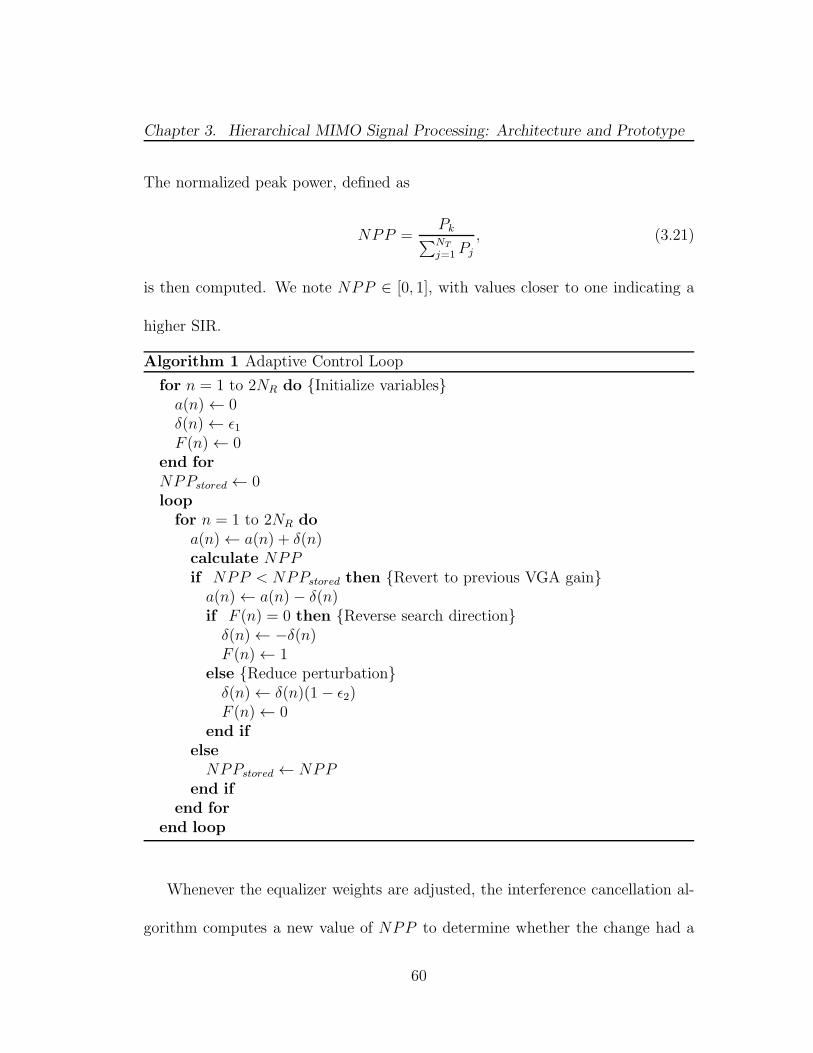
Chapter 3. Hierarchical MIMO Signal Processing: Architecture and Prototype
The normalized peak power, defined as
NPP =Pk
∑NT
j=1 Pj
, (3.21)
is then computed. We note NPP ∈ [0, 1], with values closer to one indicating a
higher SIR.
Algorithm 1 Adaptive Control Loop
for n = 1 to 2NR do Initialize variablesa(n)← 0δ(n)← ǫ1F (n)← 0
end forNPPstored ← 0loopfor n = 1 to 2NR doa(n)← a(n) + δ(n)calculate NPPif NPP < NPPstored then Revert to previous VGA gaina(n)← a(n)− δ(n)if F (n) = 0 then Reverse search directionδ(n)← −δ(n)F (n)← 1
else Reduce perturbationδ(n)← δ(n)(1− ǫ2)F (n)← 0
end ifelseNPPstored ← NPP
end ifend for
end loop
Whenever the equalizer weights are adjusted, the interference cancellation al-
gorithm computes a new value of NPP to determine whether the change had a
60

Chapter 3. Hierarchical MIMO Signal Processing: Architecture and Prototype
positive or negative impact on the SIR. The equalizer weights are implemented
as VGA gains applied to the in-phase and quadrature components of the complex
baseband received signal. Letting a ∈ R2NR×1 represent the VGA gains, we set
the mapping between the complex weight vector and and the real VGA gains as
a(2n − 1) = ℜ (ck(n)) and a(2n) = ℑ (ck(n)) for n = 1, 2, . . . , NR. The iterative
process of adjusting the VGA gains is described in Algorithm 1, where the input
parameters ǫ1 and ǫ2 are chosen as small values less than one. With each iteration,
the algorithm adjusts the VGA gains consecutively in the directions that increase
the NPP. If gain adjustments in both the positive and negative directions reduce
the NPP, a smaller adjustment is applied to that VGA in the following iteration.
Note that, while not explicitly stated in Algorithm 1, the weights may be
normalized periodically to ensure they remain within the bounds imposed by the
VGA hardware.
Note that this approach makes no explicit computation of the optimal equalizer
weights, and relies instead on evaluating the effect of small perturbations to the
VGA weights. As such, the algorithm does not need accurate knowledge of the
mapping between the control signal applied to the VGA and the corresponding
gain applied to the received signal. Also note that the interfering pilot tones will
be reduced in power until they reach the noise level. At this point, the peak
detect algorithm used to calculate NPP will be unable to distinguish the pilot
61

Chapter 3. Hierarchical MIMO Signal Processing: Architecture and Prototype
tones from the noise. This prevents the pilot tones interference from being nulled
further at the price of noise enhancement. Hence, this method may converge to the
linear MMSE solution which minimizes the signal-to-interference-and-noise ratio
(SINR), rather than the ZF solution which minimizes the SIR. Under low SNR
conditions, the linear MMSE equalizer outperforms the ZF equalizer. However, in
the scenario under consideration, where the pilot tones are likely high above the
noise floor, the two solutions will essentially coincide.
The example weight adjustment scheme was described in detail because it was
used in the mm-wave MIMO hardware prototype. It should be possible to ob-
tain improved adaptive algorithms, however, that provably converge to the linear
MMSE equalizer, (e.g., using coarse frequency estimation followed by differential
MMSE), while maintaining the advantage of not requiring precise calibration of
the VGA weights.
3.2.4 Simulation Results
The performance of the proposed spatial equalizer adaptation schemes is evaluated
through simulation. We consider a point-to-point MIMO link with four antennas
at each node. We assume the LOS channel model described in 2.1.1. It is also
assumed that the antenna arrays are Rayleigh spaced, and hence HHH = NT INR.
As such, the entries of Z in (3.17) are i.i.d. zero-mean complex Gaussian random
62

Chapter 3. Hierarchical MIMO Signal Processing: Architecture and Prototype
variables with variance 2σ2Z = 2(σ2
d + σ2N ). We define the pilot-to-noise ratio as
PNR = α/σ2Z .
The pilot tones have frequencies 25 kHz, 30 kHz, 35 kHz, and 40 kHz. The
carrier frequency offset is a uniformly distributed random variable taking values
in the range -1 kHz < f0 < 1 kHz, while the carrier and pilot phases are uniformly
distributed in [0, 2π]. The sample rate is Fs = 125 kHz.
The performance of each equalizer is evaluated in terms of the signal-to-
interference ratio (SIR) at its output. With ck representing the kth row of C,
we define s = ckH. The SIR of the kth recovered signal is then given by
SIRk =s[k]2
∑
n 6=k s[n]2, k = 1, . . . , NT . (3.22)
We first consider the performance of the DFT-based spatial equalizer. The
SIR is plotted in Fig. 3.5 as a function of the DFT length, taken by factors of
two for efficient FFT implementation. We observe that the SIR increases linearly
with the DFT length.
Next, we assess the performance of the LSE-based spatial equalizer. We as-
sume the carrier frequency offset has initially been estimated to within 1 Hz. Fig.
3.6 plots the SIR as a function of the (unweighted) LS observation window. A
larger observation improves the channel estimate essentially through filtering the
measurement noise. However, this improvement is offset by the effect of error in
the carrier frequency offset estimate. This effect increases observation window
63
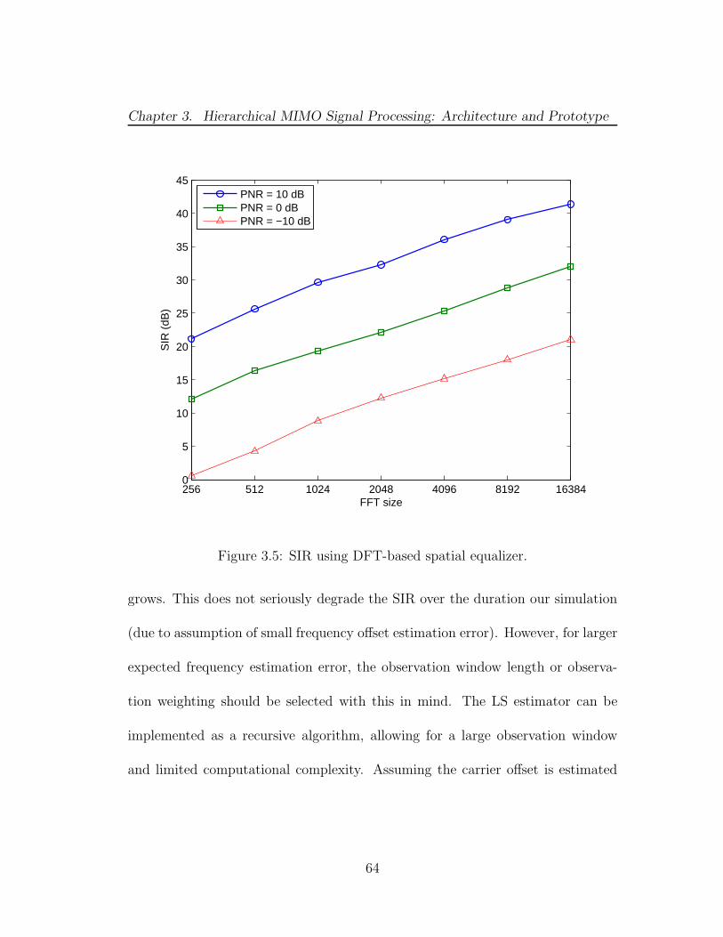
Chapter 3. Hierarchical MIMO Signal Processing: Architecture and Prototype
256 512 1024 2048 4096 8192 163840
5
10
15
20
25
30
35
40
45S
IR (
dB)
FFT size
PNR = 10 dBPNR = 0 dBPNR = −10 dB
Figure 3.5: SIR using DFT-based spatial equalizer.
grows. This does not seriously degrade the SIR over the duration our simulation
(due to assumption of small frequency offset estimation error). However, for larger
expected frequency estimation error, the observation window length or observa-
tion weighting should be selected with this in mind. The LS estimator can be
implemented as a recursive algorithm, allowing for a large observation window
and limited computational complexity. Assuming the carrier offset is estimated
64

Chapter 3. Hierarchical MIMO Signal Processing: Architecture and Prototype
512 5632 10752 15872 20992 2611215
20
25
30
35
40
45
50
55
Batch size (samples)
SIR
(dB
)
PNR = 10 dBPNR = 0 dBPNR = −10 dB
Figure 3.6: SIR using LSE-based spatial equalizer.
accurately, this allows the LS estimator to achieve a higher SIR than the other
methods we consider.
Finally, we consider the closed-loop FFT-based spatial equalizer. A 512-point
FFT is performed after each perturbation of the equalizer weights. The average
SIR is plotted as a function of control loop iterations in Fig. 3.6 for several values
of PNR. We observe that over the course of the first roughly twenty iterations,
the SIR increases by nearly 20 dB. This can be attributed to the equalizer rapidly
65

Chapter 3. Hierarchical MIMO Signal Processing: Architecture and Prototype
0 50 100 150 200 250 300−5
0
5
10
15
20
25
30
Iteration count
SIR
(dB
)
PNR = 10 dBPNR = 5 dBPNR = 0 dB
Figure 3.7: SIR using closed-loop spatial equalizer.
converging to a coarse approximation of the optimal equalizer weights. Further
refinement of the equalizer weights is then possible as the perturbations are grad-
ually reduced in magnitude. Compared to the other equalization schemes, this
method adapts relatively slowly over time. At a minimum, it takes roughly 80 ms
to obtain an SIR of 15 dB, and 800 ms to obtain an SIR of 25 dB at a PNR of 10
dB. In practice, however, this process can take significantly longer depending on
the hardware implementation, as described in the next section.
66
Chapter 3. Hierarchical MIMO Signal Processing: Architecture and Prototype
3.3 Hardware Prototype
The two-level mm-wave MIMO architecture was implemented as a 60 GHz hard-
ware prototype using commercially available mm-wave and RF components and
a printed circuit board spatial equalization network. The prototype was initially
designed as a two-channel 60 GHz MIMO link with a manually tuned spatial
equalization network that operated at IF frequencies. This system successfully
demonstrated point-to-point 60 GHz in both short-range ( 5 m) indoor [41] and
longer range (41 m) outdoor environments [14]. The most recent version of the
prototype, described in this section and [15], features four-channel communication
with a aggregate data rate of 2.4 Gbps and adaptive spatial equalization applied
at baseband. The spatial equalizer is adapted using the iterative FFT-based pro-
cedure described in Section 3.2.
The prototype was demonstrated in an indoor office environment at a link
range of 5 m. Experimental results provided at the end of this section include bit
error rate (BER) and SIR measurements.
3.3.1 Transmitter and Receiver Electronics
The transmitter is shown in Fig. 3.8. Four data bitstreams are generated by
an FPGA at a rate of 600 Mbps. The FPGA implements four linear feedback
67

Chapter 3. Hierarchical MIMO Signal Processing: Architecture and Prototype
DTX1
TX2
TX3
TX4
Up-conv.
Up-conv.
Up-conv.
Up-conv.
S/G3GHz S/G 14.25GHz
25kHz
30kHz
35kHz
40kHz
4-channelPRBS
FPGA
Channel 1
Channel 2
Channel 3
Channel 4
Figure 3.8: Transmitter prototype block diagram.
shift registers (LFSRs) which produce maximum-length pseudorandom binary se-
quences (PRBSs) of lengths 220− 1, 222− 1, 223− 1, and 225− 1 bits. The digital
bit sequences are converted to antipodal analog signals and each is combined with
pilot tone of 30 kHz, 35 kHz, 40 kHz, or 45 kHz. The combined signals are up-
converted to 3 GHz IF and then to 60 GHz RF before being transmitted over a
ULA of four 24 dBi standard gain horn antennas. The inter-antenna spacing is
chosen as 7.9 cm, which satisfies the Rayleigh criterion given the 5 m link range.
68

Chapter 3. Hierarchical MIMO Signal Processing: Architecture and Prototype
RX4
RX3
RX2
RX1
Down-conv.
Down-conv.
Down-conv.
Down-conv.
D
S/G19.23GHz
I/QDemod.I/QDemod.
I/QDemod.
S/G 2.31GHz
I/QDemod.
I/QDemod.
I1
Q1
BasebandChannelSeparationElectronics
I2
Q2
I3
Q3
I4
Q4
Control Loop
Recovered Signals
64 ControlSignals
Channel 1 I & Q
Channel 2 I & Q
Channel 3 I & Q
Channel 4 I & Q
Figure 3.9: Receiver prototype block diagram.
The receiver, shown in Fig. 3.9, receives the signals over a four-element
Rayleigh-spaced array consisting of 24 dBi horn antennas. The received signals
are downconverted to a 2.31 GHz IF frequency, and I/Q demodulators convert
the IF signal to baseband. The I and Q signals are split and distributed to eight
spatial equalization boards, which individually recover the I or Q components
of a single channel. The boards include an array of VGAs, implemented as full
four-quadrant analog multipliers. This allows an arbitrary complex gain to be
applied to each received signal. The scaled signals are summed using an 8:1 resis-
tor power combiner matched to 50 Ω. The recovered signals were digitized using
69
Chapter 3. Hierarchical MIMO Signal Processing: Architecture and Prototype
two-channel oscilloscope and stored on a computer for offline Differential PSK
(DPSK) demodulation and bit error rate analysis.
The VGAs are adaptively tuned using the closed-loop FFT-based equalization
method previously described. The received signals are low-pass filtered and sam-
pled at a rate of 125 kHz, which can achieved using low-cost multi-channel ADCs.
An FFT of the digitized signals is performed and analyzed using a laptop com-
puter, which outputs control signals that run through a 64-channel D/A converter
board to the VGAs. An update of all 64 VGA voltages takes on the order of one
second and is sufficient to track slowly-varying changes in the channel. The up-
date time could be reduced by using a faster D/A interface, which is the limiting
factor to the loop speed.
3.3.2 Experimental Results
To evaluate the prototype’s performance, the transmitter and receiver were tested
in an office environment at a 5 m link range as shown in Fig. 3.10. Table 3.1
provides a link budget of the experimental setup.
Spatial equalizer performance was evaluated in a two stage process. First,
the adaptive equalizer control loop was allowed to run until the SIR stabilized.
Next, the interfering signals were switched off, and the received power spectrum
of the desired signal was measured at the output of the spatial equalizer. Then,
70

Chapter 3. Hierarchical MIMO Signal Processing: Architecture and Prototype
Figure 3.10: Photograph of prototype receiver.
the desired channel was switched off, the interfering signals were re-activated,
and their power was measured. In this manner, the powers of the desired signal
and interference was measured for each of the four channels. The received power
spectrums are shown in Fig. 3.11, and the SIR for each channel is provided in
Table 3.2. Channels 1, 2, and 4 had similar interference suppression performance.
The relatively poor performance of channel 3 is due to the third signal being
received with less power. Additional measurements are required to determine the
underlying cause.
71
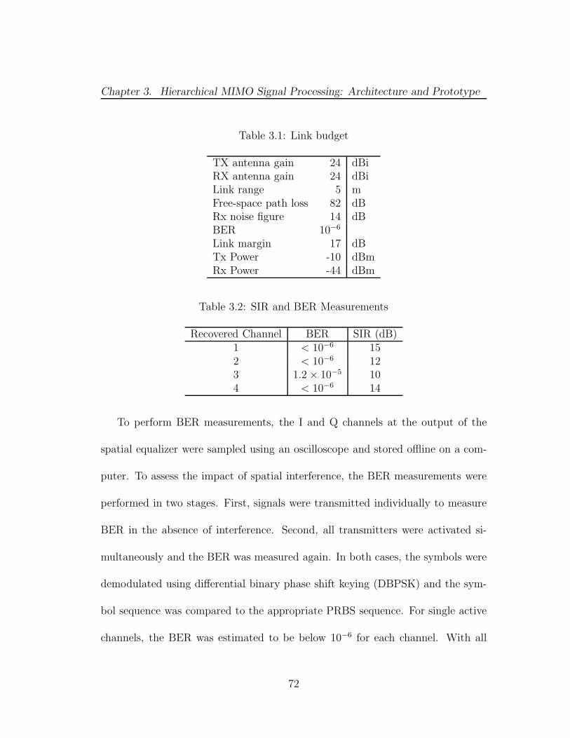
Chapter 3. Hierarchical MIMO Signal Processing: Architecture and Prototype
Table 3.1: Link budget
TX antenna gain 24 dBiRX antenna gain 24 dBiLink range 5 mFree-space path loss 82 dBRx noise figure 14 dBBER 10−6
Link margin 17 dBTx Power -10 dBmRx Power -44 dBm
Table 3.2: SIR and BER Measurements
Recovered Channel BER SIR (dB)1 < 10−6 152 < 10−6 123 1.2× 10⁻⁵ 104 < 10−6 14
To perform BER measurements, the I and Q channels at the output of the
spatial equalizer were sampled using an oscilloscope and stored offline on a com-
puter. To assess the impact of spatial interference, the BER measurements were
performed in two stages. First, signals were transmitted individually to measure
BER in the absence of interference. Second, all transmitters were activated si-
multaneously and the BER was measured again. In both cases, the symbols were
demodulated using differential binary phase shift keying (DBPSK) and the sym-
bol sequence was compared to the appropriate PRBS sequence. For single active
channels, the BER was estimated to be below 10−6 for each channel. With all
72
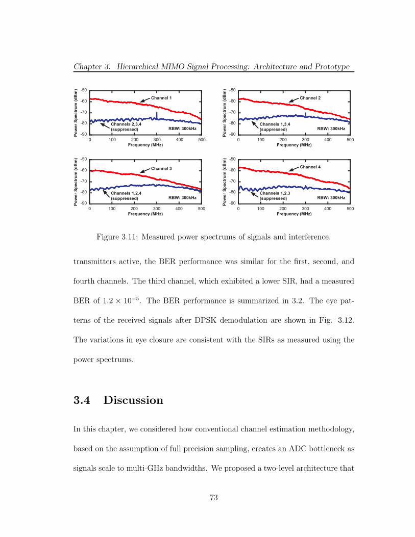
Chapter 3. Hierarchical MIMO Signal Processing: Architecture and Prototype
-90
-80
-70
-60
-50
0 100 200 300 400 500
Po
wer
Sp
ectr
um
(d
Bm
)
Frequency (MHz)
Channel 1
Channels 2,3,4
(suppressed) RBW: 300kHz
-90
-80
-70
-60
-50
0 100 200 300 400 500
Po
wer
Sp
ec
tru
m (
dB
m)
Frequency (MHz)
Channel 2
Channels 1,3,4
(suppressed) RBW: 300kHz
-90
-80
-70
-60
-50
0 100 200 300 400 500
Po
wer
Sp
ec
tru
m (
dB
m)
Frequency (MHz)
Channel 3
Channels 1,2,4
(suppressed) RBW: 300kHz
-90
-80
-70
-60
-50
0 100 200 300 400 500
Po
we
r S
pec
tru
m (
dB
m)
Frequency (MHz)
Channel 4
Channels 1,2,3
(suppressed) RBW: 300kHz
Figure 3.11: Measured power spectrums of signals and interference.
transmitters active, the BER performance was similar for the first, second, and
fourth channels. The third channel, which exhibited a lower SIR, had a measured
BER of 1.2 × 10⁻⁵. The BER performance is summarized in 3.2. The eye pat-
terns of the received signals after DPSK demodulation are shown in Fig. 3.12.
The variations in eye closure are consistent with the SIRs as measured using the
power spectrums.
3.4 Discussion
In this chapter, we considered how conventional channel estimation methodology,
based on the assumption of full precision sampling, creates an ADC bottleneck as
signals scale to multi-GHz bandwidths. We proposed a two-level architecture that
73

Chapter 3. Hierarchical MIMO Signal Processing: Architecture and Prototype
decouples the processing tasks of spatial equalization and data demodulation. By
performing these tasks at separate time scales, the need for costly high-precision,
high-speed ADCs is avoided. We considered several methods of computing the
spatial equalizer weights, based either on channel estimation or closed-loop adap-
tation, and we evaluated their performance through simulation. Low signal-to-
interference ratios can be achieved using any of the proposed methods, and each
offers various tradeoffs in terms of their implementation complexity. There re-
main open questions regarding the adaptive scheme, as it is not yet clear what
perturbation weights are optimal, or whether they could be adapted in a more
efficient manner.
A four-channel hardware prototype operating at 60 GHz offers proof-of-concept
for LOS mm-wave MIMO multiplexing and the two-level architecture. Experimen-
tal results suggest that two-level architecture is a viable approach for practical
mm-wave MIMO systems.
74
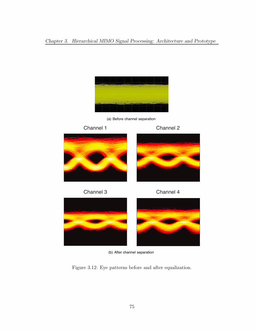
Chapter 3. Hierarchical MIMO Signal Processing: Architecture and Prototype
(a) Before channel separation
Channel 4
Channel 2
Channel 3
Channel 1
(b) After channel separation
Figure 3.12: Eye patterns before and after equalization.
75
Chapter 4
Feasibility and PerformanceStudy of Indoor mm-WaveMIMO Links
In this chapter, we evaluate the feasibility of mm-wave MIMO links designed
for short-range indoor applications. This scenario requires that we consider the
effects of array form factor constraints, potential LOS blockage, and multipath
reflections. We begin by establishing fundamental limits on the number of spatial
degrees of freedom available over a LOS channel given array length constraints.
We find that the Rayleigh spaced arrays described in Chapter 2 are essentially
optimal in terms of maximizing the spatial degrees of freedom. Increasing the
antenna count further primarily provides beamforming gain. This motivates a
proposed array-of-subarrays architecture, whose performance we evaluate in a
simulated indoor environment. A practical transmit beamsteering/receive MMSE
scheme is compared against a waterfilling benchmark in both LOS and NLOS
76
Chapter 4. Feasibility and Performance Study of Indoor mm-Wave MIMO Links
settings, and variations in channel capacity due to node placement are examined.
We find that significant spatial multiplexing gains are available throughout the
indoor environment. While LOS blockage can substantially reduce throughput at
low power levels, this effect is lessened when the spectral efficiency is limited by
the use of small signal constellations, which are commonly used in practice due
to the limited power levels generated by mm wave electronics.
The chapter is organized as follows. In Section 4.1, we review the array geome-
try criterion that guarantees an orthogonal channel matrix for LOS MIMO. We
then show that this is near-optimal by deriving a limit on the number of spatial
degrees of freedom with array length (i.e. form factor) constraints. An system
architecture that provides array gain and spatial multiplexing gain is introduced
in Section 4.2. An indoor environment modeled using ray-tracing techniques is
described in Section 4.3. In Section 4.4, the performance of the proposed architec-
ture is evaluated in terms of channel capacity under LOS and non-LOS (NLOS)
conditions. Conclusions are discussed in Section 4.5.
4.1 Fundamental Limits of LOS MIMO
In this section, we derive limits on the number of spatial degrees of freedom of a
LOS MIMO channel given array length constraints. We find that the form factors
77

Chapter 4. Feasibility and Performance Study of Indoor mm-Wave MIMO Links
of typical consumer electronics devices are sufficient to allow multiple degrees of
freedom.
4.1.1 LOS MIMO Channel Model
We briefly restate the channel model introduced in Chapter 2. Consider a link
consisting of two N -element arrays. Assuming a flat-fading MIMO channel, the
received signal vector y ∈ CN×1 is given by
y = Hx+w, (4.1)
where x ∈ CN×1 is the transmitted signal vector, H ∈ CN×N is the channel matrix,
w ∈ CN×1 is additive complex white Gaussian noise with with covariance N0INt,
and IN is the N × N identity matrix. In a purely LOS channel, the complex
channel gain hm,n, representing the (m,n)th element of H, can be modeled as
hm,n =λ
4πpm,nexp
(
−j 2πλpm,n
)
, (4.2)
where λ is the carrier wavelength and pm,n is the path length from the nth transmit
antenna to the mth receive antenna.
Assuming the arrays are uniformly-spaced and aligned broadside, the path
length is given by pm,n =√
R2 − (mdT − ndR)2, where R is the link range, and
dR and dT denote the distance between neighboring receive antennas and transmit
antennas, respectively. When R is much larger than the length of either array, we
78

Chapter 4. Feasibility and Performance Study of Indoor mm-Wave MIMO Links
can approximate the path length by pm,n ≈ R+ (mdt − ndr)2/(2R). The channel
gain is then
hm,n ≈λ
4πRexp
(
−j 2πλ
(
R +(mdT − ndR)
2
2R
))
. (4.3)
In contrast to a NLOS MIMO channel, which is highly dependent on the surround-
ing multipath scattering environment, we note that the LOS MIMO channel is
specified by the carrier frequency and the relative positions of the array elements.
We first consider the setting where the number of antenna elements (rather than
the array lengths) is fixed. We demonstrated in Chapter 2 that the optimal uni-
form spacing is given by
dTdR =Rλ
N. (4.4)
When this condition holds, H is a scaled unitary matrix with equal singular values,
which we denote by σn for n = 1, . . . , N . Each non-zero singular value corresponds
to an eigenmode (or eigenchannel) over which data can be transmitted. We refer
to a pair of arrays satisfying (4.4) as Rayleigh spaced or optimally spaced ULAs.
Now, if the lengths of the transmit and receive arrays are constrained and N
is arbitrary, we can determine from (4.4) the maximum number of antennas that
can be supported while preserving the orthogonality condition. Noting that the
length of a ULA is given by L = d(N − 1), where d is the inter-element spacing,
79
Chapter 4. Feasibility and Performance Study of Indoor mm-Wave MIMO Links
and solving (4.4) for N , the maximum number of antennas is given by
NU = ⌊1 + LTLR
2λR+
1
2
√
(
2 +LTLR
λR
)2
− 4⌋, (4.5)
where LT is the maximum transmit array length, LR is the maximum receive array
length, and ⌊a⌋ is the largest integer less than or equal to a.
Equation (4.5) specifies the maximum number of spatial degrees of freedom
available to a LOS MIMO link while satisfying both the orthogonality condition
and a set of array length constraints. Such a design may be termed an opti-
mally spaced sparse array, where the sparsity is required for orthogonality. In the
next section, we investigate what can be gained by forgoing orthogonality and
increasing the antenna count of our fixed-length arrays beyond NU .
4.1.2 Spatial Degrees of Freedom
Equation (4.5) specifies the maximum number of spatial degrees of freedom avail-
able to a LOS MIMO link while satisfying both the orthogonality condition and
a set of array length constraints. We may ask what can be gained by forgoing
orthogonality and increasing the antenna count of our fixed-length arrays beyond
NU . We first consider two LOS MIMO links as an example. The first link uses op-
timally spaced arrays, with N = 8, λ = 5 mm, R = 5 m, and LT = LR = 39.1 cm.
The squared singular values the associated channel matrix, plotted in Fig. 4.1, are
80
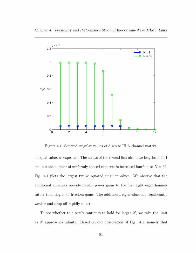
Chapter 4. Feasibility and Performance Study of Indoor mm-Wave MIMO Links
0 2 4 6 8 10 120
0.2
0.4
0.6
0.8
1
1.2x 10
−6σ n2
n
N = 8N = 32
Figure 4.1: Squared singular values of discrete ULA channel matrix.
of equal value, as expected. The arrays of the second link also have lengths of 39.1
cm, but the number of uniformly spaced elements is increased fourfold to N = 32.
Fig. 4.1 plots the largest twelve squared singular values. We observe that the
additional antennas provide mostly power gains to the first eight eigenchannels
rather than degree of freedom gains. The additional eigenvalues are significantly
weaker and drop off rapidly to zero.
To see whether this result continues to hold for larger N , we take the limit
as N approaches infinity. Based on our observation of Fig. 4.1, namely that
81

Chapter 4. Feasibility and Performance Study of Indoor mm-Wave MIMO Links
additional antennas seem to yield primarily array processing gains to the first NU
eigenmodes, we may expect the squared singular values to increase in proportion to
N2. This follows from the fact that, under a transmit power constraint, transmit
beamforming and receive beamforming each provide a factor of N power gain. We
therefore introduce a normalized form of the channel matrix given by
H =4πR
λNH, (4.6)
where the 1/N scaling factor normalizes the squared singular values by 1/N2.
With this choice of normalization,∑N
n=1 σ2n = 1, where σn are the singular values
of H. Substituting H for H in (4.1) and disregarding additive noise, the signal at
the kth receive antenna is given by
yk =1
N
N∑
m=0
exp
(
−j 2πλ
(
R +(mdT − ndR)
2
2R
))
xm. (4.7)
In the limit as N goes to infinity and the interelement spacing becomes infinitesi-
mal, we can express the received signal at point p ∈ [−LR/2, LR/2] on the receive
array as
y(p) =1
LT
e−j 2πλR
∫ LT /2
−LT /2
e−j 2πλ
(q−p)2
2R x(q)dq, (4.8)
where x(q) is the transmitted signal at point q ∈ [−LT /2, LT/2] on the transmit
array.
The integral kernel
G(p, q) =e−j 2π
λR
LT
e−j 2πλ
(q−p)2
2R . (4.9)
82
Chapter 4. Feasibility and Performance Study of Indoor mm-Wave MIMO Links
was previously studied in the context of the diffraction limited optics by Thaning
et al. in [42], and the analysis here follows their approach. Equation (4.9) can be
expanded via the spectral theorem as
G(p, q) =
∞∑
n=1
gna∗n(q)bn(p), (4.10)
where gn and an(q) are the eigenvalues and eigenfunctions of the integral equation
|gn|2an(q) =∫ LT /2
−LT /2
K(q′, q)an(q′)dq′, (4.11)
and where
K(q′, q) =
∫ LR/2
−LR/2
G∗(p, q)G(p, q′)dp. (4.12)
The functions bn(p) are defined by
gnbn(p) =
∫ LT /2
−LT /2
G(p, q)an(q)dq.
The functions an(q), which are ordered such that |g1| ≥ |g2| ≥ . . . ≥ |gn|, form
an orthonormal set over the interval [−LT /2, LT/2], and hence the received signal
can be expressed as
y(p) =
∞∑
n=1
gnAnbn(p), (4.13)
where
An =
∫ LT /2
−LT /2
a∗n(pT )x(pT )dpT .
83
Chapter 4. Feasibility and Performance Study of Indoor mm-Wave MIMO Links
We note that, although y(p) is represented in (4.13) by an infinite summation,
y(p) can be represented to a given level of accuracy using only a finite number of
terms.
Expressing the eigenfunctions in the form
an(q) = exp(
jπ
λRq2)
αn(q), (4.14)
we can substitute (4.14) and (4.12) into (4.11) to obtain the following equation
L2T
λR|gn|2αn(q) =
∫ LT /2
−LT /2
sin 2πW (q − q′)
π(q − q′)αn(q
′)dq′, (4.15)
where W = LR/(2λR). The integral equation (4.15) defines a set of prolate
spheroidal wavefunctions (PSWFs), a family of functions investigated extensively
by Slepian et al. in the context of bandlimited and approximately time-limited
signals. The eigenvalues |gn|2 are related to vn, the eigenvalues of the PSWFs, by
|gn|2 = vnλR/L2T . A well-known property of the PSWFs is that their eigenvalues
remain approximately equal to one until n nears a critical value, given here by
S = 2WLT =LTLR
λR, (4.16)
after which they drop off rapidly to zero. Correspondingly, An drops off to zero
for n > S, and the received signal y(p) is specified to a high degree of accuracy by
the first S + 1 values of An. We conclude that the number of degrees of freedom
of the continuous array link is limited to approximately
NC =LTLR
λR+ 1. (4.17)
84

Chapter 4. Feasibility and Performance Study of Indoor mm-Wave MIMO Links
NC ≈ NU , although as a result of factoring out the beamforming gain, NC is
generally a more conservative estimate of the degrees of freedom.
0 2 4 6 8 10 120
0.02
0.04
0.06
0.08
0.1
0.12
0.14
0.16
0.18
σ2 n
n
ULA, N = 8Continuous array
Figure 4.2: Eigenvalues of continuous array channel.
Fig. 4.2 plots the first twelve eigenvalues of the continuous array channel, |gn|2
for n = 1, . . . , 12, when R = 5 m, and LT = LR = 39.1 cm. Their transition to zero
is centered around S = 6.125, in agreement with (4.16). Relating these results
to discrete ULAs, we observe that for large values of N , the squared singular
value σ2n increases by an amount proportional to |gn|2 when an additional element
is added to the array. Thus |gn|2 describe how the power gain provided by an
85

Chapter 4. Feasibility and Performance Study of Indoor mm-Wave MIMO Links
additional antenna is distributed among the eigenchannels of a ULA link when
N ≫ NU . Comparing Fig. 4.2 and Fig. 4.1, we find that squared singular values
of the N = 32 ULA link are approximately proportional to the continuous array
eigenvalues.
The preceding asymptotic analysis yields fairly specific guidelines for trans-
ceiver design. First, increasing antenna count beyond the optimally spaced sparse
design is an impractical means of increasing the number of degrees of freedom:
while the power gain may be sufficient that more than NU eigenchannels are uti-
lized under a given power allocation scheme, these modes will remain significantly
weaker than the dominant modes. Indeed, for the form factors and ranges of inter-
est for indoor mm-wave MIMO, the number of dominant modes is already quite
large. However, while optimally spaced sparse arrays are, in fact, near-optimal in
the number of spatial degrees of freedom they provide, our analysis also indicates
that the SNR per degree of freedom can be significantly improved by increas-
ing the number of elements. This observation motivates the array of subarrays
architecture presented in the following section.
86
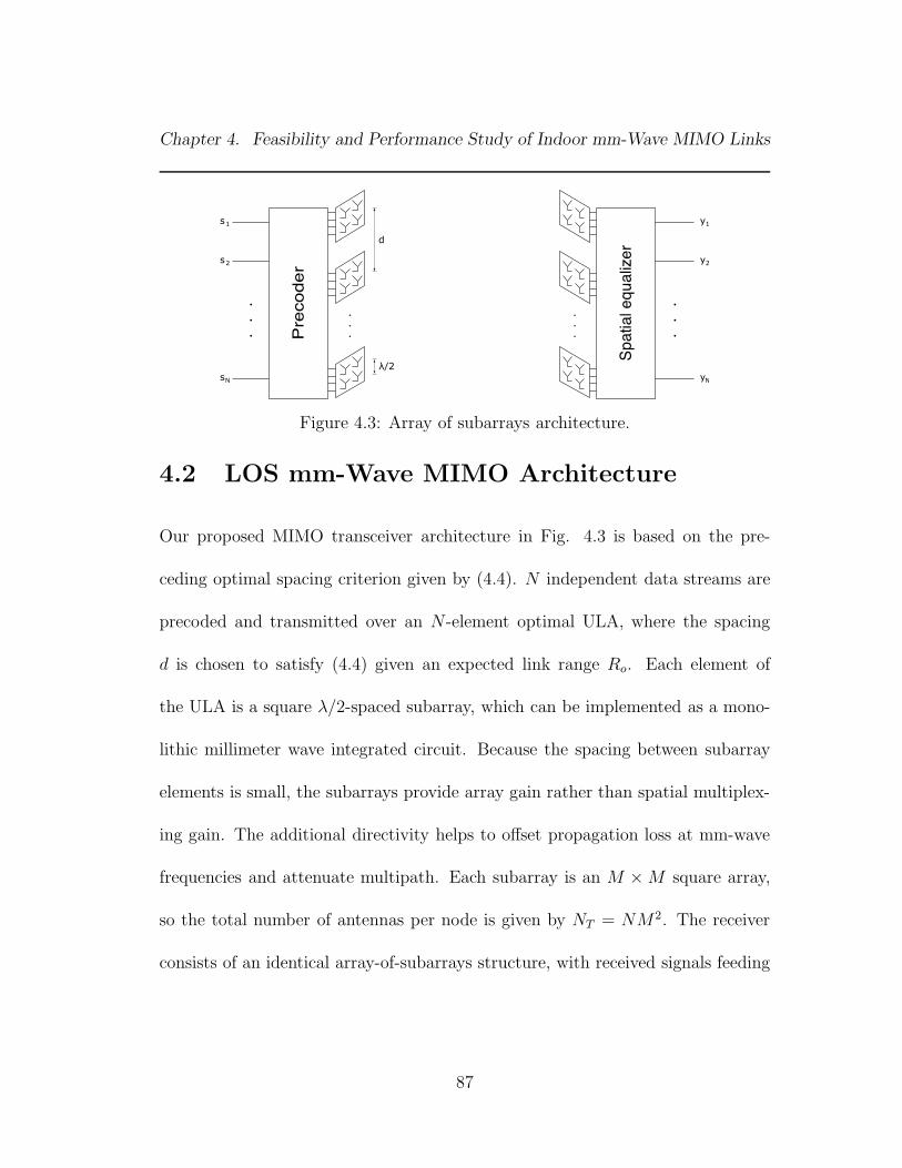
Chapter 4. Feasibility and Performance Study of Indoor mm-Wave MIMO Links
Precoder
Sp
atia
l e
qu
aliz
er
Figure 4.3: Array of subarrays architecture.
4.2 LOS mm-Wave MIMO Architecture
Our proposed MIMO transceiver architecture in Fig. 4.3 is based on the pre-
ceding optimal spacing criterion given by (4.4). N independent data streams are
precoded and transmitted over an N -element optimal ULA, where the spacing
d is chosen to satisfy (4.4) given an expected link range Ro. Each element of
the ULA is a square λ/2-spaced subarray, which can be implemented as a mono-
lithic millimeter wave integrated circuit. Because the spacing between subarray
elements is small, the subarrays provide array gain rather than spatial multiplex-
ing gain. The additional directivity helps to offset propagation loss at mm-wave
frequencies and attenuate multipath. Each subarray is an M ×M square array,
so the total number of antennas per node is given by NT = NM2. The receiver
consists of an identical array-of-subarrays structure, with received signals feeding
87
Chapter 4. Feasibility and Performance Study of Indoor mm-Wave MIMO Links
into a equalizer designed to null spatial interference. We now describe two spatial
equalization and modulation schemes based on the above architecture.
4.2.1 Waterfilling Benchmark
Our performance benchmark is standard waterfilling based eigenmode transmis-
sion. This employs a transmit precoder and a receive spatial equalizer based on
the singular value decomposition (SVD) of the channel matrix H, such that the
channel is decomposed into N non-interfering parallel subchannels, or eigenmodes.
The SVD of the channel matrix H is given by
H = UΣVH,
where U,V ∈ CNT×NT are unitary and Σ ∈ RNT×NT is a diagonal matrix whose
nonzero entries are the ordered singular values ofH, given by σ1 ≥ σ2 ≥ . . . ≥ σNT.
Let VN andUN denote the matrices composed of the first N columns ofV andU,
respectively. The data vector s is premultiplied by VN at the transmit precoder
stage and the received data r is filtered by UHN , resulting in
y = UHNr = UH
N (HVNs+w) = ΣNs+ w,
where ΣN is the N×N submatrix consisting of the first N columns and N rows of
Σ. Note that the distribution of the noise component remains unchanged because
the columns of UN are orthonormal. Effectively, the channel is decomposed into
88
Chapter 4. Feasibility and Performance Study of Indoor mm-Wave MIMO Links
N parallel subchannels of the form
yi = σisi + wi i = 1, 2, . . . , N.
The channel capacity, given by
C =
N∑
i
(
logµσ2
i
N0
)+
, (4.18)
is achieved when the input symbols si are Gaussian distributed and the power
allocated to the ith channel, denoted by Pi = E[|si|2], obeys the waterfilling
power allocation policy. Pi is given by
Pi =
(
µ− N0
σ2i
)+
, (4.19)
where a+ indicates max0, a, the value of µ is chosen such that∑
i Pi = PT , and
PT is a total power constraint. If (µ−N0/λ2i ) < 0, no power or data is allocated
to the ith eigenchannel.
4.2.2 Transmit Beamsteering/Receive MMSE
While the previous scheme provides an upper bound on link performance, it is im-
portant to identify more conservative performance estimates that represent typical
hardware and signal processing constraints. To this end, we consider a scheme in
which the transmitter sends a single data stream from each subarray, with each
subarray limited to beamsteering in a given direction. We assume the transmitter
89

Chapter 4. Feasibility and Performance Study of Indoor mm-Wave MIMO Links
knows the directions of the LOS and first-order reflection paths to the receiver
(these can be learned by scanning at start-up), and beamsteering is constrained
along these paths. The transmitter beamsteers in the direction(s) that maximize
the sum-rate spectral efficiency. The constellation per data stream is fixed (we
use 16QAM in our numerical results). The spatially multiplexed data streams can
now interfere with each other, and we employ linear MMSE spatial interference
suppression to separate them out at the receiver.
Note that, as demonstrated in recent hardware prototypes [15], spatial pro-
cessing (e.g., linear interference suppression) for a quasi-static channel can be
performed in our architecture on a slow time scale using (digitally controlled) ana-
log processing, thus avoiding the need for high-speed analog-to-digital converters
(ADCs) with large dynamic range. Digitization can be performed with ADCs
with lower dynamic range after separation of the multiplexed data streams.
The beamsteering weight applied to the antenna in the kth column and lth
row of the jth subarray is given by
ajkl = exp (−iπ ((k − 1) cos θj sinφj + (l − 1) cosφj)) k, l ∈ 1, 2, . . . ,M,
(4.20)
where θj and φj are the azimuthal and polar steering angles, respectively. Let
ajkl be the (k, l)th entry of the M × M matrix A(θj, φj) and let a(θj , φj) =
vec (A(θj , φj)) be the vector formed from concatenating the columns of A(θj , φj).
90

Chapter 4. Feasibility and Performance Study of Indoor mm-Wave MIMO Links
The precoding matrix G is given by
G =1
M
a(θ1, φ1) 0 · · · 0
0 a(θ2, φ2) · · ·...
......
. . . 0
0 · · · 0 a(θN , φN)
(4.21)
where 0 is an M2 × 1 vector of zeros.
At the receiver, full channel state information is assumed. The input to the
spatial equalizer is given by
r = HGs+w = Hs+w (4.22)
where s is the N×1 data vector, G is the NM2×N steering matrix, and H = HG
is an NM2×N equivalent channel matrix combining the propagation environment
and the steering matrix. We now assume equal power allocation across data
streams, such that E[|si|2] = PT/N . The equalizer output is given by
y = CHr = CH(
Hs +w)
(4.23)
where equalizer coefficients are specified by C. The coefficients of the MMSE
equalizer are given by
CMMSE =
(
PT
NHHH + PNINM2
)−1PT
NH, (4.24)
where PN = N0B is the noise power and B is the bandwidth.
91

Chapter 4. Feasibility and Performance Study of Indoor mm-Wave MIMO Links
The signal to interference and noise ratio (SINR) at the kth output of the
equalizer is given by
γk =PT
N|cHk Hk|2
PT
N
∑
j 6=k |cHj Hk|2 + PNcHk ck, (4.25)
where ck is the kth column of CMMSE. The spectral efficiency is computed with
the interference treated as Gaussian noise, and with the symbol constellation
restricted to 16-QAM.
4.3 Indoor Propagation Model
The optimal antenna spacing criterion given by (4.4) assumes the transmit and
receive arrays are aligned parallel, the channel is purely LOS, and the link range
is known a priori. For practical indoor applications, none of these assumptions
hold, and we wish to evaluate the performance of the proposed architecture when
operating under more realistic scenarios. To this end, we present a indoor en-
vironment propagation model that allows us to assess the impact of multipath
propagation, link range variations, and LOS blockage.
The propagation environment, shown in Fig. 4.4, is a room of dimensions 5 m
× 5 m × 3 m. The receive array lies horizontally along the plane of the front wall,
centered at coordinates (2.5 m, 0, 1.5 m). The transmitter’s position is variable,
and given by coordinates (x, y, 1.5 m), where 0 ≤ x ≤ 5 m and 0 ≤ y ≤ 5 m.
92
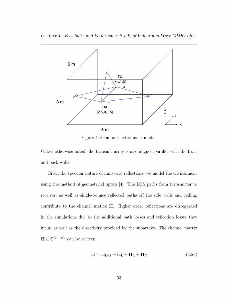
Chapter 4. Feasibility and Performance Study of Indoor mm-Wave MIMO Links
Figure 4.4: Indoor environment model.
Unless otherwise noted, the transmit array is also aligned parallel with the front
and back walls.
Given the specular nature of mm-wave reflections, we model the environment
using the method of geometrical optics [4]. The LOS paths from transmitter to
receiver, as well as single-bounce reflected paths off the side walls and ceiling,
contribute to the channel matrix H. Higher order reflections are disregarded
in the simulations due to the additional path losses and reflection losses they
incur, as well as the directivity provided by the subarrays. The channel matrix
H ∈ CNT×NT can be written
H = HLOS +HL +HR +HC (4.26)
93
Chapter 4. Feasibility and Performance Study of Indoor mm-Wave MIMO Links
where HLOS is the LOS component, HL and HR are the components resulting
from the left and right wall reflections, respectively, and HC is the contribution
of the ceiling reflections. The (m,n)th entry of HLOS is given by
hLOS(m,n) =λ
4πpLOS(m,n)e−i 2π
λpLOS(m,n). (4.27)
The (m,n)th entry of HL is given by
hL(m,n) = Γ⊥(θL)λ
4πpL(m,n)e−i 2π
λpL(m,n) (4.28)
where pL(m,n) is the length of the path from the nth transmit antenna to the
point of reflection on the left wall to the mth receive antenna, and θL is the
reflected ray’s angle of incidence. Γ⊥(θL) is the perpendicular Fresnel reflection
coefficient [43]. The entries of HR are similarly defined, with pR(m,n) and θR
replacing pL(m,n) and θL. The (m,n)th entry of HC is given by
hC(m,n) = Γ‖(θC)λ
4πpC(m,n)e−i 2π
λpC(m,n) (4.29)
where Γ‖(θC) is the parallel reflection coefficient. We assume the floor is carpeted,
and we hence ignore floor reflections due to the high reflection loss of carpeted
surfaces [44].
There are two scenarios where modification of (4.26) is required. The first is
in the case of LOS blockage, referred to herein as the non-LOS (NLOS) scenario,
which we model by removing the HLOS term from (4.26). The second scenario
94

Chapter 4. Feasibility and Performance Study of Indoor mm-Wave MIMO Links
may occur when we alter the alignment of transmit array. Namely, if we rotate
the array around the vertical axis that passes through its midpoint, a point of
reflection on the left or wall may fall behind the array. Since we assume the
energy radiated behind the array is highly attenuated by the transmitting device
itself, this reflection component is omitted.
4.4 Results
In this section, we evaluate the spectral efficiency achieved by the mm-wave MIMO
architectures proposed in Section 4.2 using the indoor propagation model.
The system and environment parameters are as follows. The room dimensions
are 5 m × 5 m × 3 m. The spacing between subarrays, given by d =√
2.5λN
,
is chosen such that the LOS component of the channel is spatially uncorrelated
when the transmit node is located at the center the room. The arrays are formed
from 4×4 λ/2-spaced subarrays. The overall array length is thus L = (N −1)d+
1.5λ. The link operates at a carrier frequency of 60 GHz, with a corresponding
wavelength of λ = 5 mm. The noise power at the receiver is given by PN = kTBF ,
where k is the Boltzmann constant, B = 2.16 GHz is the bandwidth, T = 300
K is the operating temperature, and F = 10 dB is the noise figure. The relative
95
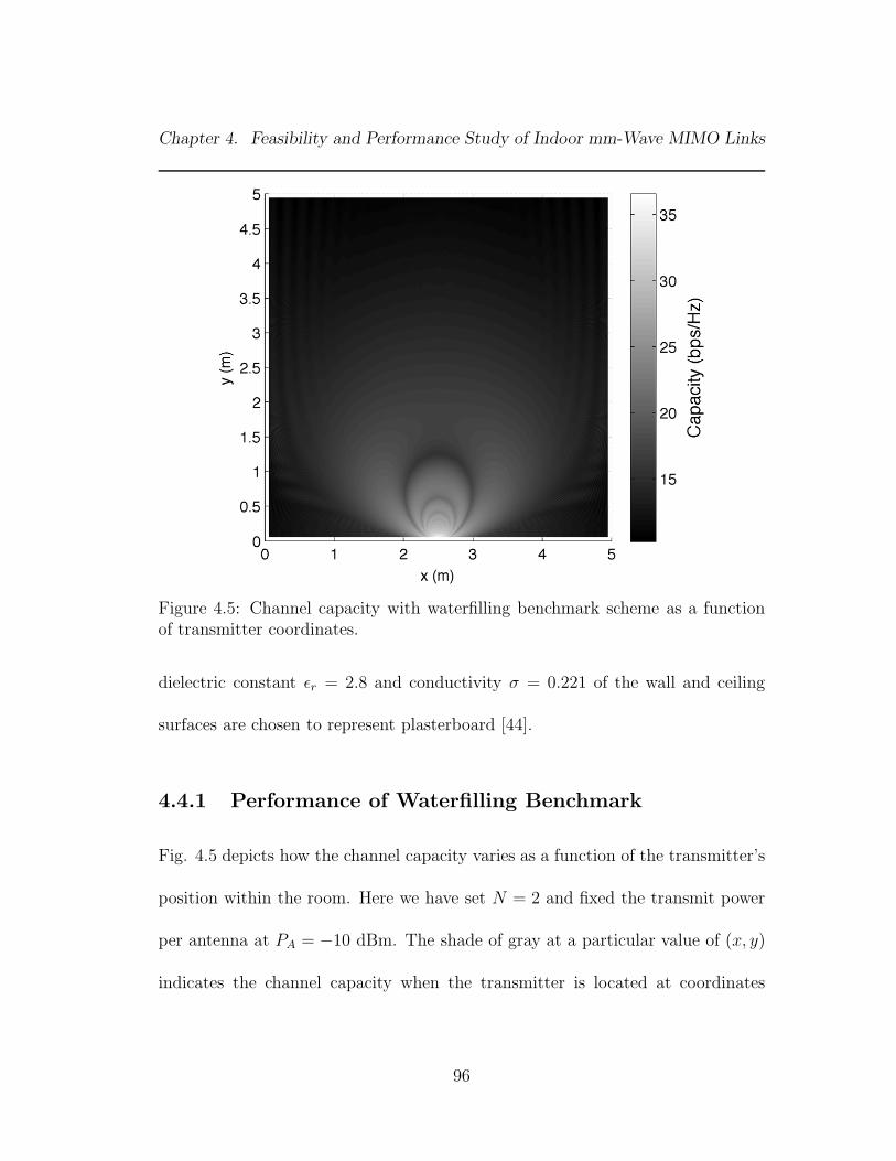
Chapter 4. Feasibility and Performance Study of Indoor mm-Wave MIMO Links
Figure 4.5: Channel capacity with waterfilling benchmark scheme as a functionof transmitter coordinates.
dielectric constant ǫr = 2.8 and conductivity σ = 0.221 of the wall and ceiling
surfaces are chosen to represent plasterboard [44].
4.4.1 Performance of Waterfilling Benchmark
Fig. 4.5 depicts how the channel capacity varies as a function of the transmitter’s
position within the room. Here we have set N = 2 and fixed the transmit power
per antenna at PA = −10 dBm. The shade of gray at a particular value of (x, y)
indicates the channel capacity when the transmitter is located at coordinates
96

Chapter 4. Feasibility and Performance Study of Indoor mm-Wave MIMO Links
(x, y). The plot can be interpreted as a top-down view of the room with the
receiver located at (2.5, 0). The capacity is primarily affected by two factors:
path loss and spatial correlation. Path loss causes the received signal power,
and hence the capacity, to decrease as the transmitter moves farther from the
receiver. Spatial correlation fluctuates in a more complex manner based on the
link geometry. Given the proposed architecture, the channel is represented by a
32×32 matrix. We expect two of the thirty-two eigenmodes to be dominant when
the spatial correlation between subarrays is low. This happens, for instance, when
the transmitter is placed at the center of the room and the optimal ULA criterion
is satisfied. The spatial correlation may increase at other transmitter positions, in
which case the second eigenchannel becomes much weaker than the first. As the
transmitter moves from the center of the room towards the receiver, for instance,
a series of rings alternating between low and high correlation is observed. These
particular fluctuations arise from the correlation in the LOS component of the
channel matrix and are independent of the multipath environment.
Fig. 4.6 plots the capacity as a function of the transmitter’s position assuming
LOS blockage. As expected, the absence of the dominant LOS signal compo-
nent results in lower SNR and capacity throughout the room. In contrast to the
LOS scenario, however, the NLOS channel does not exhibit large fluctuations in
capacity due to path loss. Instead, we observe small-scale fluctuations in capac-
97
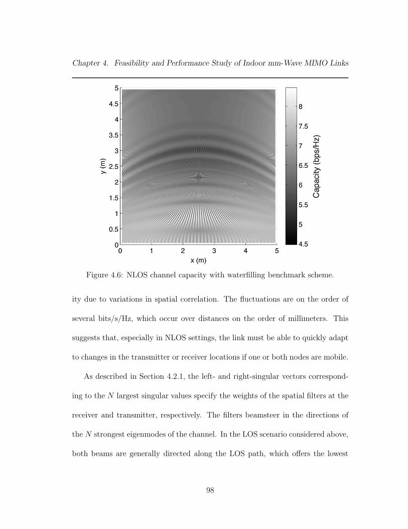
Chapter 4. Feasibility and Performance Study of Indoor mm-Wave MIMO Links
Figure 4.6: NLOS channel capacity with waterfilling benchmark scheme.
ity due to variations in spatial correlation. The fluctuations are on the order of
several bits/s/Hz, which occur over distances on the order of millimeters. This
suggests that, especially in NLOS settings, the link must be able to quickly adapt
to changes in the transmitter or receiver locations if one or both nodes are mobile.
As described in Section 4.2.1, the left- and right-singular vectors correspond-
ing to the N largest singular values specify the weights of the spatial filters at the
receiver and transmitter, respectively. The filters beamsteer in the directions of
the N strongest eigenmodes of the channel. In the LOS scenario considered above,
both beams are generally directed along the LOS path, which offers the lowest
98

Chapter 4. Feasibility and Performance Study of Indoor mm-Wave MIMO Links
Figure 4.7: Transmit eigenvector field patterns in LOS blockage scenario.
path loss and reflection loss. When the LOS path is blocked, the link must utilize
wall and/or ceiling reflections to close the link. In Fig. 4.7, the radiation patterns
produced by the first and second right-singular (transmit) vectors are shown when
the transmitter is located in the center of the room. The first eigenvector beam-
steers in the directions of the wall reflections, while the second eigenvector utilizes
the ceiling reflection. Grating lobes are caused by the subarrays being separated
by several wavelengths.
99
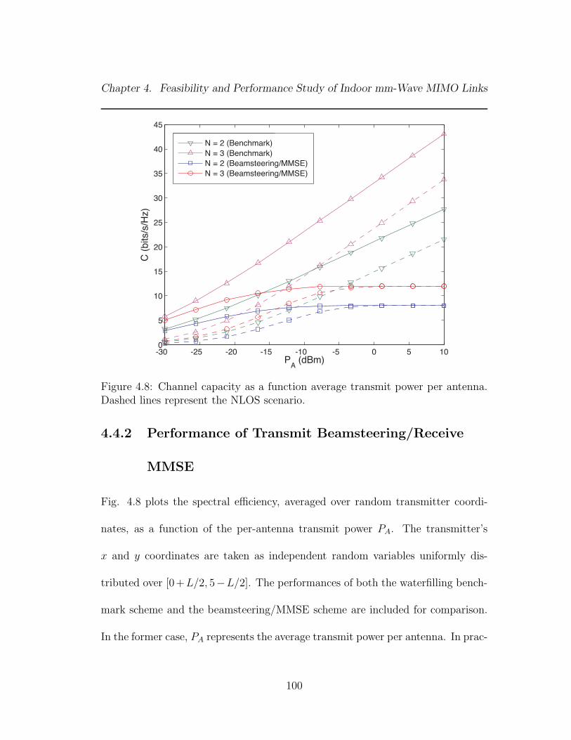
Chapter 4. Feasibility and Performance Study of Indoor mm-Wave MIMO Links
-30 -25 -20 -15 -10 -5 0 5 100
5
10
15
20
25
30
35
40
45
PA (dBm)
C (
bits/s
/Hz)
N = 2 (Beamsteering/MMSE)
N = 3 (Beamsteering/MMSE)
N = 3 (Benchmark)
N = 2 (Benchmark)
Figure 4.8: Channel capacity as a function average transmit power per antenna.Dashed lines represent the NLOS scenario.
4.4.2 Performance of Transmit Beamsteering/Receive
MMSE
Fig. 4.8 plots the spectral efficiency, averaged over random transmitter coordi-
nates, as a function of the per-antenna transmit power PA. The transmitter’s
x and y coordinates are taken as independent random variables uniformly dis-
tributed over [0+L/2, 5−L/2]. The performances of both the waterfilling bench-
mark scheme and the beamsteering/MMSE scheme are included for comparison.
In the former case, PA represents the average transmit power per antenna. In prac-
100

Chapter 4. Feasibility and Performance Study of Indoor mm-Wave MIMO Links
Figure 4.9: LOS channel capacity under TX beamsteering/RX MMSE scheme.
tice, each antenna element would be peak power limited, which is a constraint
imposed on the more practical beamsteering/MMSE scheme. We observe that
when the constellation is restricted to 16-QAM, the spectral efficiency reaches
a 4N bps/HZ limit as PA increases. This reduces the impact of LOS blockage
on spectral efficiency under the beamsteering/MMSE scheme when the transmit
power is sufficiently high.
The spectral efficiency is plotted as a function of transmitter position in Fig.
4.9 with N = 2 and P = −10 dBm. The sum-rate capacity approaches the
constellation-constrained limit of 8 bps/Hz when the transmitter is placed near
101
Chapter 4. Feasibility and Performance Study of Indoor mm-Wave MIMO Links
the center of the room. Uncoded data can be transmitted at a symbol error rate
of Pe ≤ 10−5 through 85.5% of the room, and at a symbol error rate of Pe ≤ 10−10
through 73.5% of the room. When the channel is ill-conditioned, such as when the
transmitter is placed in one of the front corners, an adaptive link can maintain
a low error rate by increasing the transmit power, reducing the constellation size
(e.g. QPSK or BPSK), or coding the data symbols. Through 86% of the room,
the transmitter beamsteers both signals in the direction of the LOS path. If the
LOS channel component is ill-conditioned, which occurs when the transmitter is
placed in one of the front corners of the room, the spectral efficiency is increased
by beamsteering one or both subarrays along a reflected path.
When the LOS path is blocked, the spectral efficiency throughout the room
varies from 3.2 to 6.5 bps/Hz as shown in Fig. 4.10. Reliable uncoded trans-
mission at the full 8 bps/Hz rate requires an additional 15 - 20 dBm of power.
Alternatively, the transmitter can adapt the coding or modulation scheme to im-
prove link reliability. Fig. 4.11 plots beamsteering directions that maximize the
sum-rate capacity in the NLOS scenario. When the transmitter is located in the
back half of the room, for example, the optimal strategy is to steer each subarray
towards a different wall reflection. In the front half of the room, it is typically
optimal to steer one beam towards the ceiling reflection, and the other towards the
102
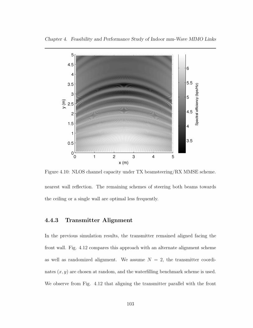
Chapter 4. Feasibility and Performance Study of Indoor mm-Wave MIMO Links
Figure 4.10: NLOS channel capacity under TX beamsteering/RX MMSE scheme.
nearest wall reflection. The remaining schemes of steering both beams towards
the ceiling or a single wall are optimal less frequently.
4.4.3 Transmitter Alignment
In the previous simulation results, the transmitter remained aligned facing the
front wall. Fig. 4.12 compares this approach with an alternate alignment scheme
as well as randomized alignment. We assume N = 2, the transmitter coordi-
nates (x, y) are chosen at random, and the waterfilling benchmark scheme is used.
We observe from Fig. 4.12 that aligning the transmitter parallel with the front
103

Chapter 4. Feasibility and Performance Study of Indoor mm-Wave MIMO Links
wall offers the best performance in the NLOS scenario. This occurs because at
any given location, the transmitter can beamsteer off either the left or side wall.
The second alignment scheme we consider is pointing the transmitter at the re-
ceiver. This offers the best performance when the LOS path is unobstructed.
When the LOS path is blocked, however, the nearest side wall may lie behind
the array, and as a result, the transmitter must rely on the far wall to provide
a reflected path. Finally, we consider the case where the transmit direction is a
uniform random variable chosen in the range [−90, 90] with the two extreme
values corresponding to the transmitter pointing toward the left and right walls,
respectively. Comparing all schemes, we find that the spectral efficiency remains
fairly robust to transmitter misalignment.
4.5 Discussion
We have established that spatial multiplexing gains can be layered on top of
beamforming gains for indoor 60 GHz links, for nodes whose form factors conform
to typical consumer electronics and computing devices. Relating the LOS MIMO
channel to prolate spheroidal waveforms, whose eigenvalues drop off sharply around
a value related to the array lengths, shows that an array of subarrays architecture
is near-optimal: the subarray spacing can be adjusted to provide the maximum
104

Chapter 4. Feasibility and Performance Study of Indoor mm-Wave MIMO Links
number of degrees of freedom for a given form factor, while using multiple antenna
elements within a subarray provides beamforming gain and reduces the transmit
power per element.
Our simulations indicate that the architecture provides spatial multiplexing
gains throughout an indoor environment, and that these gains are robust to node
placement and LOS blockage as long as we can electronically steer the beam for
each subarray. For a fixed constellation (which caps the maximum link speed),
variations in spectral efficiency due to node placement are reduced. The impact
of alignment between the transmitter and receiver arrays, and the geometry of
the spatial eigenmodes as a function of node placement and LOS blockage, are
discussed. Our promising results motivate future work on extensive performance
evaluation for packetized communication with specific coded modulation schemes
and signal processing algorithms, and on hardware implementation of the proposed
architecture with careful partitioning of analog and digital signal processing.
105
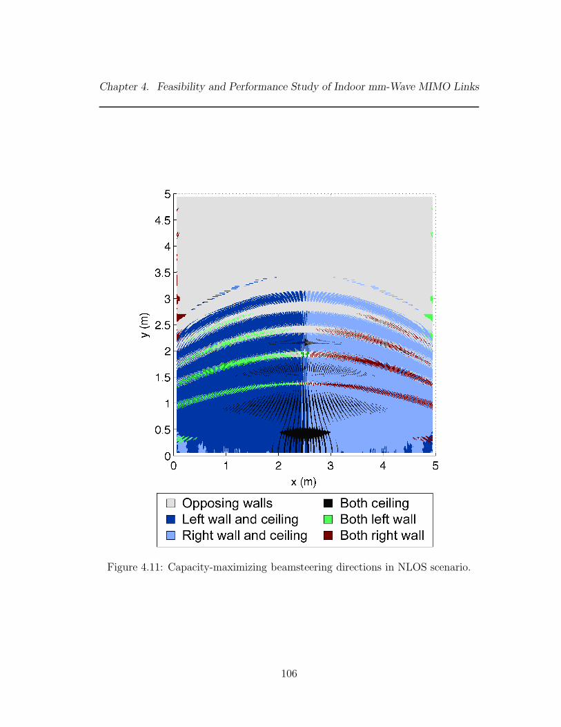
Chapter 4. Feasibility and Performance Study of Indoor mm-Wave MIMO Links
Figure 4.11: Capacity-maximizing beamsteering directions in NLOS scenario.
106

Chapter 4. Feasibility and Performance Study of Indoor mm-Wave MIMO Links
0 5 10 15 20 25 300
0.1
0.2
0.3
0.4
0.5
0.6
0.7
0.8
0.9
1
CT (bps/Hz)
Pr(
C <
CT)
TX parallel with front wall
TX pointing at RX
Random TX alignment
Figure 4.12: Cumulative distribution function of the spectral efficiency using var-ious transmitter alignments. Dashed lines represent the NLOS scenario.
107

Chapter 5
Conclusions and Future Work
We considered the whether practical communication systems could achieve spatial
multiplexing gains while operating at mm-wave frequencies. We began by identi-
fying the key properties of the mm-wave band that result in new challenges and
opportunities for MIMO systems. This motivated our examination of three main
subjects, summarized as follows.
Based on the observation that the mm-wave channel is predominantly line-of-
sight, we investigated the relation between antenna array geometry and spatial
multiplexing. We found that, while Rayleigh-spaced uniform linear arrays maxi-
mize the channel capacity when the link range is known, they can perform poorly
when the range deviates from nominal. When multiple transmitters fall within the
grating lobes of the receiver’s array response, the channel becomes rank deficient
and the corresponding signals cannot be separated. In response, we proposed using
non-uniform linear arrays, which were found to increase robustness under range
108

Chapter 5. Conclusions and Future Work
uncertainty. In addition, we proposed a practical rank adaptation scheme that
reduces the number of transmitted streams when the channel is highly correlated.
Next we considered how, as bandwidths scale to multiple GHz, the cost of
high-precision ADCs becomes prohibitive. In order to avoid this bottleneck, we
propose decoupling the signal processing tasks of spatial equalization and signal
demodulation. The spatial equalizer weights are determined from observations
of low-frequency pilot tones embedded in the transmitted signals. Since the pi-
lot tones fall within a narrow frequency band, they can be observed with a slow
sampling rate. Equalization is carried out in the analog domain, using a net-
work of variable gain amplifiers. The equalized signals can then be sampled at
the full rate using 1-3 bit ADCs, which provide adequate precision for data de-
modulation. Several estimation/adaptation schemes for spatial equalization are
evaluated and discussed. We reviewed experimental results from a four-channel
hardware prototype demonstrating the viability the proposed architecture.
Finally, we evaluated the feasibility of mm-wave MIMO for indoor links, which
are characterized by limited array form factors, multipath reflections, and poten-
tial LOS blockage. We identified fundamental limits on the spatial degrees of
freedom available over a LOS channel when using arrays of fixed sized. We found
that Rayleigh-spaced arrays are essentially optimal in terms of spatial degrees of
freedom, and additional antennas provide only beamforming gain. This result
109

Chapter 5. Conclusions and Future Work
motivated our array of subarrays architecture, which utilizes subarrays of half-
wavelength spaced elements for steering capability and array gain. We evaluated
the performance of this architecture using ray-tracing modeling of an indoor envi-
ronment. A sub-optimal transmission and reception scheme, chosen to represent
today’s mm-wave hardware and signal processing constraints, was evaluated rel-
ative to an optimal system. We found that indoor mm-wave MIMO links can
attain spatial multiplexing gains even when the LOS is blocked.
5.1 Directions for Future Work
We proposed decoupling spatial equalization and demodulation as a means to
avoid high-precision sampling at multiGbps rates. An alternative solution involves
developing new signal processing algorithms that operate on highly quantized (1-
3 bit) measurements. This has already shown to be a viable approach for many
signal processing tasks [33], [34], [35], [36], [37]. Results in [38] suggest that this
approach could be used for MIMO channel estimation, however the mean squared
estimation error is fairly high for 1-bit quantization. However, research is active
in this area, and it remains to be seen whether further improvements are possible.
As discussed in [30], the hardware prototype could be improved using custom
ICs rather than off-the-shelf components, allowing higher bandwidths and a re-
110
Chapter 5. Conclusions and Future Work
duction in hardware cost. Dual polarization or larger 2-dimensional arrays could
also be used to increase data rates. The heuristic adaptation algorithm imple-
mented in the hardware prototype, while sufficient for proof-of-concept, lacks a
firm foundation within the frameworks of estimation or adaptive filtering. Perfor-
mance may improve using adaptive algorithms, such as differential MMSE, that
provably converge to the linear MMSE solution.
In the context of indoor mm-wave MIMO links, many implementation issues
remain open. For instance, spatial equalization in the proposed decoupled archi-
tecture occurs at a relatively slow time scale, making it most suitable for slowly-
varying channels. Indoor environments may be subject to rapid variations due to
the movement of people within the environment, possibly leading to LOS block-
age. It remains unclear whether spatial multiplexing gains can be maintained in
the face of rapid and severe channel fluctuations.
111

Bibliography
[1] I. E. Telatar, “Capacity of multi-antenna Gaussian channels,” AT&T BellLab Internal Tech. Memo., Oct. 1995.
[2] G. J. Foschini and M. Gans, “On the limits of wireless communications in afading environment when using multiple antennas,” Wireless Personal Com-munications, vol. 6, no. 3, p. 311, Mar. 1998.
[3] H. Xu, V. Kukshya, and T. Rappaport, “Spatial and temporal characteristicsof 60-GHz indoor channels,” IEEE J. Sel. Areas Commun., vol. 20, no. 3, pp.620–630, Apr. 2002.
[4] P. F. M. Smulders, “Deterministic modelling of indoor radio propagation at40-60 Ghz,” Wireless Personal Communications, vol. 4, no. 2, pp. 127–135,Jun. 1994.
[5] R. Walden, “Performance trends for analog to digital converters,” Commu-nications Magazine, IEEE, vol. 37, no. 2, pp. 96 –101, Feb. 1999.
[6] S. Singh, R. Mudumbai, and U. Madhow, “Distributed coordination with deafneighbors: Efficient medium access for 60 ghz mesh networks,” in INFOCOM,2010 Proceedings IEEE, Mar. 2010, pp. 1 –9.
[7] IEEE Std 802.15.3c-2009 (Amendment to IEEE Std 802.15.3-2003), Oct.2009.
[8] High Rate 60 GHz PHY, MAC and HDMI PAL, 1st ed., ECMA-387, Dec.2008.
[9] Wireless Gigabit Alliance. [Online]. Available: http://wirelessgigabitalliance.org/
[10] WirelessHD. [Online]. Available: http://www.wirelesshd.org/
112
Bibliography
[11] D. Gesbert, H. Bolcskei, D. Gore, and A. Paulraj, “Outdoor MIMO wire-less channels: models and performance prediction,” IEEE Trans. Commun.,vol. 50, no. 12, pp. 1926–1934, Dec. 2002.
[12] F. Bohagen, P. Orten, and G. Oien, “Design of optimal high-rank line-of-sightMIMO channels,” Wireless Communications, IEEE Transactions on, vol. 6,no. 4, pp. 1420–1425, April 2007.
[13] P. Larsson, “Lattice array receiver and sender for spatially orthonormalMIMO communication,” Vehicular Tech. Conf., IEEE 61st, vol. 1, pp. 192–196 Vol. 1, May 2005.
[14] C. Sheldon, E. Torkildson, M. Seo, C. P. Yue, M. Rodwell, and U. Mad-how, “Spatial multiplexing over a line-of-sight millimeter-wave MIMO link:A two-channel hardware demonstration at 1.2Gbps over 41m range,” in 38thEuropean Microwave Conference, Oct. 2008.
[15] C. Sheldon, M. Seo, E. Torkildson, M. Rodwell, and U. Madhow, “A 2.4Gb/s millmeter-wave link using adaptive spatial multiplexing,” IEEE Int.AP-S Symp., Jul. 2010.
[16] C. H. Doan, S. Emami, A. M. Niknejad, and R. W. Brodersen, “Millimeter-wave cmos design,” IEEE Journal of Solid-State Circuits, vol. 40, pp. 144–155, 2005.
[17] B. Heydari, M. Bohsali, E. Adabi, and A. Niknejad, “Millimeter-wave devicesand circuit blocks up to 104 ghz in 90 nm cmos,” Solid-State Circuits, IEEEJournal of, vol. 42, no. 12, pp. 2893 –2903, Dec. 2007.
[18] M. Khanpour, K. Tang, P. Garcia, and S. Voinigescu, “A wideband w-bandreceiver front-end in 65-nm cmos,” Solid-State Circuits, IEEE Journal of,vol. 43, no. 8, pp. 1717 –1730, Aug. 2008.
[19] B. Razavi, “A 60-ghz cmos receiver front-end,” Solid-State Circuits, IEEEJournal of, vol. 41, no. 1, pp. 17 – 22, Jan. 2006.
[20] X. Guan, H. Hashemi, and A. Hajimiri, “A fully integrated 24-ghz eight-element phased-array receiver in silicon,” Solid-State Circuits, IEEE Journalof, vol. 39, no. 12, pp. 2311 – 2320, Dec. 2004.
[21] A. Natarajan, A. Komijani, X. Guan, A. Babakhani, and A. Hajimiri, “A77-ghz phased-array transceiver with on-chip antennas in silicon: Transmit-ter and local lo-path phase shifting,” Solid-State Circuits, IEEE Journal of,vol. 41, no. 12, pp. 2807 –2819, Dec. 2006.
113
Bibliography
[22] V. Dyadyuk, J. Bunton, J. Pathikulangara, R. Kendall, O. Sevimli, L. Stokes,and D. Abbott, “A multigigabit millimeter-wave communication systemwith improved spectral efficiency,” Microwave Theory and Techniques, IEEETransactions on, vol. 55, no. 12, pp. 2813–2821, Dec. 2007.
[23] A. Poon, R. Brodersen, and D. Tse, “Degrees of freedom in multiple-antennachannels: a signal space approach,” Information Theory, IEEE Transactionson, vol. 51, no. 2, pp. 523–536, Feb. 2005.
[24] I. Sarris and A. Nix, “Design and performance assessment of maximum capac-ity MIMO architectures in line-of-sight,” Communications, IEE Proc., vol.153, no. 4, pp. 482–488, Aug. 2006.
[25] F. Bohagen, P. Orten, and G. Oien, “Optimal design of uniform rectangularantenna arrays for strong line-of-sight MIMO channels,” EURASIP J. Wirel.Commun. Netw., vol. 2007, no. 2, pp. 12–12, 2007.
[26] R. Olsen, D. Rogers, and D. Hodge, “The aRb relation in the calculation ofrain attenuation,” IEEE Trans. Antennas Propag., vol. 26, no. 2, pp. 318–329,Mar. 1978.
[27] Y. Karasawa and Y. Maekawa, “Ka-band Earth-space propagation researchin Japan,” Proc. IEEE, vol. 85, no. 6, pp. 821–842, Jun. 1997.
[28] E. Torkildson, B. Ananthasubramaniam, U. Madhow, and M. Rodwell,“Millimeter-wave MIMO: Wireless links at optical speeds,” in Proc. of 44thAllerton Conference on Communication, Control and Computing, Sep. 2006.
[29] C. Sheldon, M. Seo, E. Torkildson, M. Rodwell, and U. Madhow, “Four-channel spatial multiplexing over a millimeter-wave line-of-sight link,” IEEE- MTTS International Microwave Symposium, Jun. 2009.
[30] C. Sheldon, “Adaptive spatial multiplexing for millimeter-wave communica-tion links,” Ph.D. dissertation, Univeristy of California, Santa Barbara, 2009.
[31] L. Tong, B. Sadler, and M. Dong, “Pilot-assisted wireless transmissions: gen-eral model, design criteria, and signal processing,” Signal Processing Maga-zine, IEEE, vol. 21, no. 6, pp. 12 – 25, Nov. 2004.
[32] M. Dong and L. Tong, “Optimal design and placement of pilot symbolsfor channel estimation,” Signal Processing, IEEE Transactions on, vol. 50,no. 12, pp. 3055 – 3069, Dec. 2002.
114

Bibliography
[33] J. Singh, O. Dabeer, and U. Madhow, “Communication limits with low preci-sion analog-to-digital conversion at the receiver,” in Communications, 2007.ICC ’07. IEEE International Conference on, Jun. 2007, pp. 6269 –6274.
[34] D. Rousseau, G. V. Anand, and F. Chapeau-Blondeau, “Nonlinear estimationfrom quantized signals: Quantizer optimization and stochastic resonance,” inProc. 3rd Int. Symp. Physics in Signal and Image Processing, Jan. 2003, pp.89–92.
[35] T. Andersson, M. Skoglund, and P. Handel, “Frequency estimation by 1-bitquantization and table look-up processing,” in Proc. Europ. Signal ProcessingConf., Sep. 2000, pp. 1807–1810.
[36] O. Bar-Shalom and A. Weiss, “Doa estimation using one-bit quantizedmeasurements,” Aerospace and Electronic Systems, IEEE Transactions on,vol. 38, no. 3, pp. 868 – 884, Jul. 2002.
[37] O. Dabeer and U. Madhow, “Channel estimation with low-precision analog-to-digital conversion,” in Communications (ICC), 2010 IEEE InternationalConference on, May 2010, pp. 1 –6.
[38] A. Mezghani, F. Antreich, and J. Nossek, “Multiple parameter estimationwith quantized channel output,” in Smart Antennas (WSA), 2010 Interna-tional ITG Workshop on, Feb. 2010, pp. 143 –150.
[39] D. Rife and R. Boorstyn, “Single tone parameter estimation from discrete-time observations,” Information Theory, IEEE Transactions on, vol. 20,no. 5, pp. 591 – 598, Sep. 1974.
[40] J. M. Mendel, Lessons in Estimation Theory for Signal Processing, Commu-nications, and Control. Prentice Hall, 1995.
[41] C. Sheldon, E. Torkildson, M. Seo, C. P. Yue, M. Rodwell, and U. Madhow,“A 60ghz line-of-sight 2×2 MIMO link operating at 1.2Gbps,” in IEEE An-tennas and Propagation Society International Symposium Digest, Jul. 2008.
[42] A. Thaning, P. Martinsson, M. Karelin, and A. T. Friberg, “Limits of diffrac-tive optics by communication modes,” Journal of Optics A: Pure and AppliedOptics, vol. 5, no. 3, p. 153, 2003.
[43] T. S. Rappaport, Wireless Communications: Principles and Practice. NewJersey: Prentice Hall, 2002.
115

Bibliography
[44] K. Sato, H. Kozima, H. Masuzawa, T. Manabe, T. Ihara, Y. Kasashima, andK. Yamaki, “Measurements of reflection characteristics and refractive indicesof interior construction materials in millimeter-wave bands,” in VehicularTech. Conf., IEEE 45th, vol. 1, Jul. 1995, pp. 449–453.
116