AD-R 37 372MISCELLANEOUS PAPER EL-79-6

MILITARY HYDROLOGY

-Report 20RESERVOIR OUTFLOW (RESOUT) MODEL

by

U Ralph A. Wurbs, Stuart T. Purvis

Texas A&M Research Foundationi College Station, Texas 77843

DTICA S ELECTE

JUN 2 8 19911

,7 vDil

April 1991

Report 20 of a Series

Approved For Public Release; Distribution Unlimited

Iin-UAyCroEgnr(Prepared for DEPARTMENT OF THE ARMY mm_=US Army Corps of Engineers REM

Washington, DC 20314-1000 0

Ur'ler Contract No. DACA39-87-M-0674DA Prceict No. 4A762719AT40 0)Tas' ,. BO, Work Unit 052

Monitored by Environmental LaboratoryUS Army Engineer Waterways Experiment Station

3909 Halls Ferry Road, Vicksburg, Mississippi 39180-6199a 24 165

Destroy this report when no longer needed. Do not returnit to the originator.

The findings in this report are not to be construed as an officialDepartment of the Army position unless so designated

by other authorized documents.

The contents of this report are not to be used foradvertising, publication, or promotional purposes.Citation of trade names does not constitute anofficial endorsement or approval of the use of

such commercial products.

Unclassified

SECURITY CLASS:FICATION OF THIS PAGE

i Form ApprovedREPORT DOCUMENTATION PAGE OMBNo. 0704-0188

la. REPORT SECURITY CLASSIFICATION lb RESTRICTIVE MARKINGS

2a. SECURITY CLASSIFICATION AUTHORITY 3 DISTRIBUTION/AVAILABILITY OF REPORT

2b. DECLASSIFICATIONIDOWNGRADING SCHEDULE Approved for public release; distributionunlimited.

4. PERFORMING ORGANIZATION REPORT NUMBER(S) 5 MONITORING ORGANIZATION REPORT NUMBER(S)

_ _Miscellaneous Paper EL-79-66a. NAME OF PERFORMING ORGANIZATION |6b OFFICE SYMBOL 7a. NAME OF MONITORING ORGANIZATION

(if appitcable) USAEWESTexas A&M Research Foundation Environmental Laboratory

6c. ADDRESS (Cty, State, and ZIP Code) 7b. ADDRESS (City, State, and ZIP Code)

College Station, TX 77843 3909 Halls Ferry Road, Vicksburg, MS 39180-6199

Ba. NAME OF FUNDING/SPONSORING 8b OFFICE SYMBOL 9 PROCUREMENT INSTRUMENT IDENTIFICATION NUMBERORGANIZATION DEPARTMENT OF THE (if applicable)

ARMY, US Army Corps of Enginee s Contract No. DACA39-.7-M-0674Bc. ADDRESS (City, State, and ZIP Code) 10 SOURCE OF FUNDING NUMBERS

PROGRAM PROJECT ' TASK " WORK UNITELEMENT NO NO4A 7 6 27 19 NO jACCESSION NO

Washington, DC 20314-1000 , AT40 BO IB11. TITLE (Include Security Classification)

Military Hvdrolopv: Report 20, Reservoir Outflow (RESOUT) Model12. PERSONAL AUTHOR(S)

Wurbs, Ralph A., and Purvis. Stuart "I13a. TYPE OF REPORT 13b. TIME COVERED 14 DATE OF REPORT (Year, Month, Day) 15. PAGE COUNT

Report 20 of a seriesi FROM TO, Aoril 1991 , 1AR16. SUPPLEMENTARY NOTATION

Available from National Technical Information Service, 5285 Port Royal Road, Springfield,VA 99161

17 COSATI CODES 18 SUBJECT TERMS (Continue on reverse if necessary and identify by block number)FIELD GROUP SUB-GROUIP Computer modeling Military hydrology Spillways

Dams Outlet worksHvdraul in q

19. ABSTRACT (Continue on reverse if necessary and identify by block number)

This report documents the development of the Reservoir Outflow (RESOUT) Model. Thevarious types of structures that are used for discharging water at a dam are identified,and the basic hydraulic equations are presented. These computational procedures are thenpresented in a computer code written for an MS-DOS microcomputer. Input instructions andexample applications are also included,

20 DISTRIBUTION/AVAILABILITY OF ABSTRACT 21 ABSTRACT SECURITY CLASSIFICATION

Xi UNCLASSIFIED/UNLIMITED [0 SAME AS RPT - DTIC USERS I 11nln ai fipd22a. NAME OF RESPONSIBLE INDIVIDUAL 22b TELEPHONE (include Area Code) 22c OFFICE SYMBOL

DD Form 1473, JUN 86 Previous editions are obsolete. SECURITY CLASSIFICATION OF THIS PAGE

Unclassified

SECURITY CLASSIFICATION OF THIS PAGE

SECURITY CLASSIFICATION OF THIS PAGE

PREFACE

The work documented in this report was conducted for the Environmental

Laboratory (EL) of the US Army Engineer Waterways Experimenc Station (WES)

under a contract between the Texas A & M Research Foundation and WES entitled

"Development of a Reservoir Outflow Hydrograph Microcomputer Model," Contract

No. DACA39-87-M-0674. The work was sponsored by the Headquarters, US Army

Corps of Engineers (HQUSACE), under Department of the Army Project

No. 4A762719AT40, Task Area BO, Work Unit 052. LTC T. Scott was the HQUSACE

Technical Monitor.

The study was conducted and the report prepared by Dr. Ralph A. Wurbs,

Department of Civil Engineering, Texas A&M University (TAMU), College Station,

TX, and Mr. Stuart T. Purvis, also of TAMU. The report was edited by

Ms. Janean Shirley of the WES Information Technology Laboratory.

The contract was monitored at WES by Messrs. Mark R. Jourdan and John G.

Collins, Environmental Constraints Group (ECG), Environmental Systems Division

(ESD), EL, under the general supervision of Mr. Malcolm Keown, Chief, ECG:

Dr. Victor E. Lagarde, Chief, ESD; and Dr. John Harrison, Chief, EL. Techni-

cal review was provided by Messrs. Jourdan and Collins, and by Mr. Bobby J.

Brown, Hydraulics Laboratory, WES.

COL Larry B. Fulton, EN, was Commander and Director of WES.

Dr. Robert W. Whalin was Technical Director.

This report should be cited as follows:

Wurbs, Ralph A., and Purvis, Stuart T. 1991. "Military Hydrology;Report 20, Reservoir Outflow (RESOUT) Model," MiscellaneousPaper EL-79-6; prepared by Texas A&M Research Foundation, College Sta-tion, TX, for US Army Engineer Waterways Experiment Station, Vicksburg,MS.

Aoesion iorKTIS GJRA&ZDTIC TABUnarounced I3Justifloation

Distrlbutlon/

Availability CodesAwail and/or

Dist SpecialL,\

CONTENTS

PREFACE................................................................1.I

CONVERSION FACTORS, NON SI TO SI (METRIC) UNITS OF MEASUREMENT ............ 3

PART I: INTRODUCTION................................................. 4

Background........................................................ 4Purpose and Scope................................................. 5Military Significance of Damis and Reservoirs ....................... 5

PART II: DAMS AND APPURTENANT STRUCTURES............................... 7

Dam Types and Configurations ...................................... 7Spillways......................................................... 9Outlet Works ..................................................... 14Other Structures ................................................. 17

PART III: REVIEW OF BASIC HYDRAULIC EQUATIONS .......................... 19

Continuity Equation......... ..................................... 19Energy Equation .................................................. 20Head Loss Equations .............................................. 20Weir Equations ................................................... 22Orifice Equations ................................................ 26

PART IV: RESERVOIR OUTFLOW COMPUTATIONAL PROCEDURES ................... 29

Introductory Overview of Rating Curves ............................ 29Rating Curves for Uncontrolled Ogee Spillways ..................... 31Rating Curves for Uncontrolled Broad-Crested Spillways ............. 46Rating Curves for Spillway Cates.................................. 47Drop Inlet Spillways.............................................. 52Rating Curves for Outlet Works.................................... 54Breach Simulation ................................................ 68Storage Routing .................................................. 74

PART V: RESERVOIR OUTFLOW (RESOUT) COMPUTER PROGRAM DESCRIPTION ....... 78

Summary of Program Capabilities................................... 78Program Structure ................................................ 79

PART VI: SUMMARY AND RECOMMENDATIONS.................................. 84

REFERENCES............................................................ 85

APPENDIX A: INPUT DATA INSTRUCTIONS.................................... Al

APPENDIX B: EXAMPLE PROBLEMS........................................... Bl

APPENDIX C-..LS OF VARIABLES.......................................... C1

APPEN4DIX D: LISTING OF COMPUTER PROGRAM................................ Dl

2

CONVERSION FACTORS, NON-SI TO SI (METRIC)UNITS OF MEASUREMENTS

Non-SI units of measurement used in this report can be converted to

SI (metric) units as follows:

Multiply By To Obtain

cubic feet 0.02831685 cubic metres

feet 0.3048 metres

inches 2.54 centimetres

3

MILITARY HYDROLOGY

RESERVOIR OUTFLOW (RESOUT) MODEL

PART I: INTRODUCTION

Background

1. Under the Meteorological/Environmental Plan for Action, Phase I,

approved for implementation on 26 January 1983, the US Army Corps of Engineers

(USACE) has been tasked to implement a research, development, testing, and

evaluation program that will: (a) provide the Army with environmental effects

information needed to operate in a realistic battlefield environment, and (b)

provide the Army with the capability for near-real-tme environmental effects

assessment on military materiel and operations in combat. In response to this

tasking, the Directorate for Research and Development, USACE, initiated the

AirLand Battlefield Environment (ALBE) Thrust program. Iis program will

develop the technologies to provide the field Army with the operational capa-

bility to perform and exploit battlefield effects assessments for tactical

advantage.

2. Military hydrology, one facet of the ALBE Thrust, is a specialized

field of study that deals with the effects of surface and sub-surface water on

planning and conducting military operations. In 1977, Headquarters, US Army

Corps of Engineers (HQUSACE), approved a military hydrology research program.

Management responsibility was subsequently assigned to the Environmental Lab-

oratory, US Army Engineer Waterways Experiment Station (WES), Vicksburg, MS.

3. The objective of military hydrology research is to develop an

improved hydrologic capability for the Armed Forces with emphasis on applica-

tions in the tactical environment. To meet this overall objective, research

is being conducted in four areas: (a) weather-hydrology interactions;

(b) state of the ground; (c) streamflow; and (d) water supply.

4. This report contributes to the streamflow modeling area. Streamflow

modeling is oriented toward the development of procedures for rapidly fore-

casting streamflow parameters including discharge, velocity, depth, width, and

flooded area from natural and man-induced hydrologic events. Specific work

efforts include: (a) the development of simple and objective streamflow

4

forecasting procedures suitable for Army Terrain Team use; (b) the adaptation

of procedures to automatic data processing equipment available to Terrain

Teams; (c) the development of procedures for accessing and processing infor-

mation included in digital terrain data bases; and (d) the development of

streamflow analysis and display concepts.

Purvose and ScoRe

5. A major objective of the USACE military hydrology research is to

provide the Armed Forces with improved capabilities for forecasting the down-

stream flood flow impacts resulting from controlled or uncontrolled (dam-

breach) releases from dams, levees, and dikes. The microcomputer program and

accompanying material presented in this report focus specifically on improving

military capabilities for predicting reservoir discharge rates.

6. A package of procedures is presented for computing outlet structure

rating curves and outflow hydrographs for various structure configurations.

The computations consist of: (a) developing a relationship between water sur-

face elevation and discharge thLcugh the outlet structures and/or breach; and,

(b) routing a hydrograph through the reservoir. The computational procedures

are coded for an IBM PC-compatible microcomputer. Applications could involve

predicting reservoir outflows for given conditions; determining outlet struc-

ture gate openings or breach size required to achieve specified outflows; or

analyzing reservoir drawdowns.

Military Significance of Dams and Reservoirs

7. Most major rivers throughout the world are regulated by systems of

dams and reservoirs. Streamflow conditions are highly dependent upon man's

operation of reservoirs as well as nature's provision of precipitation. Dams

are necessary to control flooding and utilize the surface water resource for

beneficial purposes such as agricultural, municipal, and industrial water sup-

ply, hydroelectric power generation, and navigation. Although dams have been

constructed for thousands of years, tremendous growth in the number and size

of dams has occurred during the past half-century.

8. Dams are potential targets for attacks, including terrorism during

peacetime as well as military actions during war. Modern weapons provide the

capability to inflict any degree of damage to a dam, ranging from removal of a

5

spillway gate to complete destruction of the dam. Loss of the services pro-

vided by a dam could, in many cases, seriously diminish industrial productiv-

ity and overall support of the war effort. Downstream flooding caused by

demolition of high dams t'n many rivers throughout the world would cause cata-

strophic damage and loss of life.

9. A potential deterrent to an attack on a strategically located dam

is to partially empty the reservoir whenever a significant threat of attack is

considered to exist. Drawdown plans could be developed which consider draw-

down times for various inflow conditions and release constraints and the

impacts on reservoir services.

10. Reservoir gates can be operated or a dam breached to induce flood-

ing during military operations. Under appropriate circumstances, reservoir

releases can serve as an offensive weapon to damage and disrupt activities in

the downstream flood plain. The obstacle effect of induced flooding can also

significantly strengthen defensive operations. Reservoirs can be effective in

the rapid creation of barriers under expedient conditions. River-crossing

operations in the combat zone may be delayed or prevented. The presence of a

dam in a headwaters area under the control of the opposing force may necessi-

tate the assembly and construction of river-crossing equipment capable of

withstanding a major flood wave or series of flood waves, thereby acting as a

deterrent to the operation. The obstacle effects of induced flooding include:

(a) increasing velocities and stages to impede river-crossing operations;

(b) destruction of bridges and other facilities; and (c) inundation of flood

plain lands to adversely impact trafficability.

11. The reservoir itself may provide an obstacle to combat operations

upstream of the dam. Situations could occur in which trade-offs exist between

using a limited supply of water to maintain high water levels above the dam

versus downstream-induced flooding.

12. Combat operations can also be significantly impacted by streamflow

conditions resulting from precipitation events. Reservoir operation is an

important consideration in forecasting streamflow conditions to be expected

from precipitation events. Discharges at a location on a river depend upon

releases from upstream reservoirs and runoff from the uncontrolled watershed

area below the reservoirs. Backwater effects from downstream reservoirs can

also be significant.

6

PART II: DAMS AND APPURTENANT STRUCTURES

13. A reservoir project includes various water control structures.

Spillways allow flood waters to be discharged while preventing damage to the

dam. Outlet works regulate the release or withdrawal of water for beneficial

purposes. Water may be released to the river below the dam or withdrawn from

the reservoir to be conveyed by pipeline or canal to the location where it is

used. Hydroelectric power plants require appurtenant water control facili-

ties. Navigation locks may be included in a dam to facilitate river trans-

port. The configuration of the dam and appurtenant structures is unique for

each project. However, general characteristics of typical types of structures

are described in the following paragraphs. In-depth treatments of dam and

appurtenant structure design are provided by the US Bureau of Reclamation

(USBR) (1976, 1977a, 1977b); Thomas (1976); Golze (1977); and Davis and

Sorensen (1984).

Dam Types and Configurations

14. Although timber, steel, and stone masonry have been used in con-

structing dams, most dams are earth-fill, rock-fill, or concrete. Dams such

as earth-fill and rock-fill, constructed of natural excavated materials placed

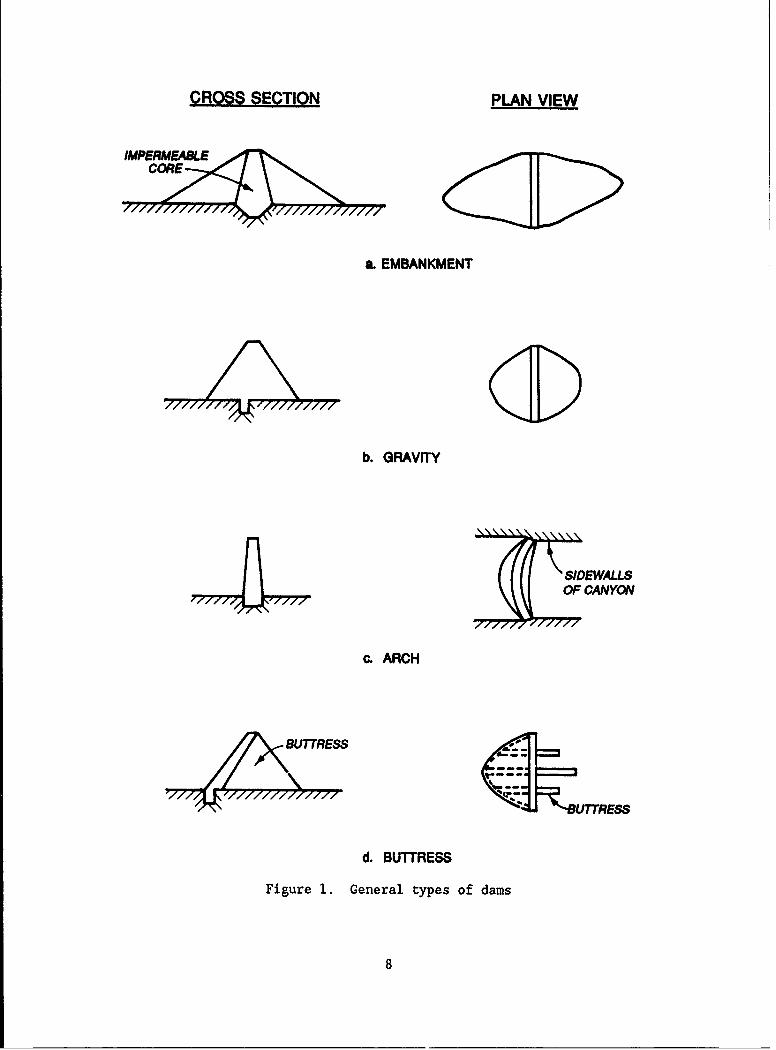
without addition of binding material, are termed embankments. As illustrated

in Figure 1, concrete dams may be categorized as gravity, arch, or buttress.

The stability of a gravity dam is derived primarily from its weight. Arch and

buttress designs reduce the amount of concrete required to withstand the

forces acting on a dam. Arch dams transmit most of the horizontal thrust of

the water stored behind them to the abutments and have thinner cross sections

than gravity dams. A buttress dam consists of a watertight upstream face sup-

ported on the downstream side by a series of intermittent supports termed

buttresses.

15. The 34,798 large dams included in the World Register of Dams

(International Commission on Large Dams 1984) are distributed between types as

follows: earth-fill and rock-fill, 83 percent of the dams; gravity, 11 per-

cent; arch, 4 percent; buttress, I percent; and multiple arch, 1 percent. The

353 dams with heights greater than 100 m are distributed as follows: earth-

fill and rock-fill, 41 percent; gravity, 22 percent; arch, 34 percent; but-

tress, 3 percent; and multiple arch, 0.3 percent of the dams. Almost all of

7

ROS SECTION PLAN VIEW

& EMBANKMENT

b. GRAVITY

ISIEWAULS

c. ARCH

BL17UTRESS

/#7 UTR ES S

d. BUTTRESS

Figure 1. General types of dams

8

the embankment dams are earth-fill, but some are rock-fill, and some are a

combination of earth-fill and rock-fill.

16. Dams are also classified as overflow or non-overflow. Overflow

dams are designed for water to flow over their crests. Non-overflow dams are

designed to not be overtopped. Overflow dams are limited essentially to con-

crete. Earth-fill and rock-fill dams are damaged by the erosive action of

overflowing water and, consequently, supplemental concrete structures are

required to serve as spillways. Most dams are non-overflow.

17. More than one type of dam may be included in a single structure.

For example, a concrete section may contain a spillway, with the remainder of

the dam being an earthfill embankment. Curved dams may combine both gravity

and arch effects to achieve stability.

Spillways

18. A spillway is a safety valve for a dam. Spillways provide the

capability to release flood waters or other inflows in excess of normal stor-

age and outlet capacities. The excess water is drawn from the top of the

impounded pool and conveyed through a spillway structure and appurtenant chan-

nel to the river below the dam. A spillway may be used to allow normal river

flows to pass over, through, or around the dam whenever the reservoir is full.

Spillways also protect the dam from extreme flood events. Spillway capacity

is a critical factor in dam safety, particularly for embankment dams which are

likely to be destroyed if overtopped.

19, A spillway may be controlled or uncontrolled. A controlled spill-

way has gates which can be used to adjust the flow rate. Many reservoirs have

a s.ingle spillway. Some reservoirs have two or more spillways; a service

spillway to convey frequently occurring overflows, and one or more emergency

spillways used only during extreme flood events. For some reservoir configu-

rations, water flows through the spillway a large portion of the time, while

in other cases, the spillway is designed to be used only for an extreme flood

event expected to occur possibly once in several hundred years.

Types of spillways

20. A variety of configurations have been adopted in spillway design.

Spillways may be categorized by the path the water takes en route over,

through, or around the dam. Typical varieties include overflow, chute, side-

channel, and shaft spillways.

9

21. Overflow spillway, An overflow spillway is a section of dam

designed to permit water to flow over the crest. In some cases, the entire

length of the dam is an overflow spillway. Overflow spillways are widely used

on concrete gravity, arch, and buttress dams. Some earthfill dams have a con-

crete gravity section designed to serve as an overflow spillway.

22. Chute spillway, A spillway in which water flows from the reservoir

to the downstream river through an open channel, located either along a dam

abutment or through a saddle some distance from the dam, is called a chute,

open channel, or trough type spillway. The chute spillway has been used with

earth-fill dams more often than any other type of spillway. The chute may be

paved with concrete or asphalt. In some cases in which the spillway is

expected to be rarely needed, an unpaved chute through a saddle may be used,

realizing that some erosion damage will result whenever the infrequent flood

does occur.

23. Side-channel spillway. In a side-channel spillway, water flows

over the crest into an open channel running parallel to the crest. The crest

is usually a concrete gravity section, but it may consist of pavement laid on

an earth embankment or the natural ground surface. This type of spillway is

used in narrow canyons where sufficient crest length is not available for

overflow or chute spillways.

24. Drop inlet spillway The drop inlet spillway is also known as a

morning-glory or shaft spillway. The water drops through a vertical or

inclined shaft to a horizontal conduit or tunnel under, around, or through the

dam. Drop inlet spillways are often used where there is inadequate space for

other types of spillways. The inlet may consist of either a square-edged or

rounded entrance.

Crest shape

25. A spillway control section may be a simple flat, broad-crested weir

or, alternatively, may be curved to increase the hydraulic efficiency. The

ogee-shaped spillway crest has a curved profile designed to approximate the

shape of the lower nappe of a ventilated sheet falling from a sharp-crested

weir. At the design head, water flows smoothly over che crest with little

resistance from the concrete surface, thus maximizing the discharge. The pro-

file below the upper curve of the ogee spillway is continued tangent along a

slope, often with a reverse curve at 'he bottom of the slope directing the

flow onto the apron of a stilling basin. The entrance to drop inlet spillways

typically consists of a circular ogee weir.

10

Spillway components

26. Spillways typically include an entrance structure or overflow

crest, discharge channel or conduit, terminal structure, and approach and out-

let channels.

27. In some situations, such as an overflow spillway over a concrete

dam, approach and outlet channels may not be required. The water flows

directly from the reservoir over the spillway to the river below. However, in

many cases, channels are provided to direct the flow to the spillway entrance

structure and to convey the flow from the terminal structure back to the

river.

28. Water is conveyed from the entrance structure over, around, under,

or through the dam to the terminal structure in channels, conduits, or tun-

nels. As previously discussed, spillways can be classified based on the con-

veyance method. However, a few spillways have no conveyance structure. For

example, the discharge may fall freely through the air from an arch dam crest,

or flow may be released directly along an abutment to cascade down the hill-

side.

29. The difference in elevaticn between the reservoir water surface and

downstream river results in extremely high flow velocities at the spillway

exit. Consequently, energy dissipation is usually required to prevent damag-

ing erosion. A principal function of a terminal structure is to dissipate

kinetic energy prior to release of the water to the outlet channel or river.

Concrete stilling basins are typically provided to facilitate loss of energy

in the turbulence of a hydraulic jump. Baffle blocks and end sills increase

the efficiency of the energy loss in the basin. Other types of terminal

devices include deflector buckets where flow is projected as a free-

discharging upturned jet to fall into the stream channel some distance below

the end of the spillway. Erosion in the stream bed may be minimized by fan-

ning the jet into a thin sheet by the use of a flaring deflector.

Spillway crest gates

30. An ungated or free-overflow spillway crest automatically regulates

the discharge as a function of the elevation of the reservoir water surface,

without requiring release decisions by an operator. Additional control of the

storage capacity above the spillway crest can be provided by crest gates. The

full-discharge capacity of the spillway may be utilized during extreme flood

events with water being stored behind closed gates during non-flooding or less

severe flooding situations. Many types of spillway crest gates have been

11

devised. Several common types are illustrated in Figure 2 and described in

the following paragraphs.

31. Lift gates, Rectangular lift gates span horizontally between guide

grooves in supporting piers. The support guides may be either vertical or

inclined slightly downstream. The gates are raised or lowered by an overhead

hoist. Water flows over the spillway crest, under the opened gate. The gates

are typically made of steel, but at some dams are timber or concrete.

32. The edges of a lift gate may bear directly on the supporting

guides. However, the sliding friction that must be overcome to operate the

gate limits the gate size for which this type of installation is practical.

Rollers or wheels are often used to reduce the frictional resistance and

thereby permit use of a larger gate and/or smaller hoist. Large lift gates

are often built in two horizontal sections so that the upper portion may be

lifted and removed from the guides before the lower portion is moved. This

design reduces the load on the hoisting mechanism and minimizes the headroom

required.

33. Tainter gates, The tainter, or radial, gate is probably the most

widely used type of crest gate for large installations. Tainter gates are

usually constructed of steel or a combination of steel and wood. The cylin-

drical face of the gate is supported by radial arms attached to trunnions set

in the downstream portion of the piers on the spillway crest. The gate pivots

around the trunnions as it is opened or closed. Water flows between the bot-

tom of the gate and the spillway crest when the gate is raised. Flexible

fabric or rubber stripping is used to form a water seal between the gate and

the piers and spillway crest.

34. The gate face is made concentric to the pivot pins so that the

entire force of the water passes through the pins. Thus, the moment required

to be overcome in raising and lowering the gate is minimized. Counterweights

are often used to partially counterbalance the weight of the gate and thus

reduce the required capacity cf the hoist. The small hoisting effort needed

to operate tainter gates makes hand operation practical on small installa-

tions. However, gates are typically operated by cables fixed to motor-driven

winches set on platforms above the gate.

35. Tainter gates vary in size from 1 m to over 10 m in height and from

2 to 20 m in width. A spillway may contain as many as 20 or more gates, set

side by side. Each gate may have its independent hoisting mechanism, or a

common unit may be moved from gate to gate.

12

HOIGT OIST

GATEGUIDE

ROLLERS

SPILWA CREST

a. Tainter gate b. Lift gate

WWATER

c. Rolling gate d. Drum gate

Figure 2. Types of spillway crest gates

13

36. Due to the relatively small hoisting forces involved, tainter gates

are more adaptable than other types of gates to operation by automatic control

apparatus. Multiple gates can be arranged to open automatically at succes-

sively increasing reservoir levels. Some gates may be opened automatically

with the remaining gates on the spillway requiring manual operation.

37. Rolling gates, A rolling, or roller, gate consists of a steel

cylinder spanning between the piers. Each pier has an inclined rack which

engages gear teeth encircling the ends of the cylinder. The gate is rolled up

the rack with a cable and hoist, allowing water to flow beneath the gate.

Rolling gates are well adapted to long spans of moderate height.

38. Drum gates, A drum gate consists of a hollow drum which, in the

lowered or open position, fits in a recess in the top of the spillway. When

water flows over the spillway crest and into the recess, the gate is lifted,

completely or at least partially, by the buoyant force.

39. Stop logs, Stop logs are sometimes used as an economical substi-

tute for more elaborate gates where relatively close spacing of piers is not

objectionable and gate openings are required only infrequently. Stop logs are

horizontal beams or girders set one upon the other to form a bulkhead sup-

ported in grooves in piers at each end of the span. Discharge is controlled

by installing and removing stop logs. The logs may be raised by hand or with

a hoist.

Outlet Works

40. Whereas spillways are provided to handle floods and other inflows

surpassing the reservoir storage capacity, an outlet works is used for normal

project operations. Outlet works control the storage capacity below the

spillway crest elevation. Releases are made to meet municipal, industrial,

and agricultural water supply needs, to maintain flows in the river downstream

for navigation, pollution abatement, and preservation of aquatic life, and for

other beneficial purposes. An outlet works also serves to empty the reservoir

to allow inspection, maintenance, and repairs to the dam and other structures.

Outlet works may also be used for flood control, to evacuate storage below the

spillway crest in anticipation of flood inflows, or to supplement spillway

releases during and after a flood event.

41. At some dams, an outlet works has been combined with a service

spillway and used in conjunction with a secondary emergency spillway. In this

14

situation, the usual outlet works design is modified to include an overflow

weir which automatically bypasses surplus inflows whenever the reservoir rises

above the normal storage level. Extreme flood events exceeding the capacity

of the combined service spillway and outlet works are handled by a separate

emergency spillway.

42. In many cases, outlet works empty into the river channel below the

dam. The water may serve instream purposes and/or be withdrawn from the river

at some distance below the dam. In other cases, the outlet works discharges

directly into a canal or pipe conveyance system for transport to the location

of water use.

Outlet works components

43. An outlet works typically consists of a sluiceway, intake struc-

ture, gates or valves, terminal structure, and entrance and exit channels.

44. Sluiceways, A sluiceway is a passageway through, under, or around

a dam. Sluiceways for concrete dams generally pass through the dam. Often

the outlet conduit is placed through a spillway overflow section, using a com-

mon stilling basin to dissipate energy for both spillway and outlet works

flows. For embankment dams, the sluiceway is typically placed outside the

limits of the embankment fill material. If a conduit is placed through an

embankment, collars are normally used to reduce seepage along the outside of

the conduit. Sluiceways are typically concrete, though steel or other mate-

rials may be used. Tunnels through rock abutments are sometimes constructed

without lining. Cross sections may be circular or rectangular. In large con-

crete dams, multiple smaller conduits are often used instead of a single large

conduit.

45. Intake structures. Although the entrance to a sluiseway may be an

integral part of the dam or another structure, most outlet works have an

intake structure. The primary function of the intake structure is to permit

withdrawal of water from the reservoir over a range of pool levels and to

protect the conduit from damage or clogging as a result of waves, currents,

debris, or ice. Intake structures vary from a simple concrete block support-

ing the end of a pipe to elaborate concrete intake towers.

46. An intake structure may either be submerged or extended as a tower

to some height above the maximum reservoir water surface, depending on its

function. A submerged intake consists of a rock-filled crib or concrete block

which supports the end of the conduit. Submerged intakes are widely used on

small projects because of their low cost.

15

47. A tower is required if operating gates are located at the intake or

if a platform is needed for installing stop logs or maintaining and cleaning

trashracks and fish screens. Intake towers are usually provided with ports at

various levels which may aid flow regulation and permit some selection of the

quality of water to be withdrawn. A wet intake tower consists of a concrete

shell filled with water to the level of the reservoir dnd has a vertical shaft

inside connected to the withdrawal conduit. Gates are normally provided on

the inside shaft to regulate flow. With a dry intake tower, the entry ports

arc connected directly to the sluiceway, without water entering the tower.

48. Intake structures are often provided with trashracks to prevent

entrance of debris. Trashrack structures can be found in various designs and

configurations. The racks usually consist of steel bars spaced several centi-

meters apart. Debris accumulations may be removed by hand or by automatic

power-driven rack rakes. Sometimes screens are also provided to prevent fish

from being carried through the outlet works.

Gates and valves

49. Intake structures usually contain control devices. In some cases,

normal flow regulation is achieved by gates or valves at the intake. In other

cases, flow is regulated by gates or valves located in the sluiceway some

distance downstream of the entrance. However, additional gates are still pro-

vided in the intake structure to de-water the conduit for inspections or

repairs. A valve in the interior of the sluiceway may be used to regulate

flow, with intake gates being used routinely to keep the sluiceway empty dur-

ing periods of no releases.

50. Entrance gates, Gates at the sluiceway entrance are often used to

regulate flow for projects with heads less than roughly 30 m. For higher

heads, due to cavitation and vibration problems associated with partly opened

gates under high heads, entrance gates are usually used only to de-water the

sluiceway for maintenance and repair of the conduit or downstream gates.

Small gates on low-head installations are often simple sliding gates operatedby hand or motor-powered drives. Slide gates often have bronze bearing sur-

faces to minimize friction. Rollers are required for high-head installations

or for very large gates under low heads.

51. Tractor gates are often used for outlet works under high heads. A

tractor gate is rectangular in shape and lifts vertically in grooves. Wedge-

shaped roller trains are attached to the back of the gate on either side. As

the gate is lowered into the closed position, its downward motion is halted

16

when its bottom edge comes in contact with the bottom of the gate frame. The

roller trains, moving in slots beside the gate, continue their downward move-

ment, and because of their wedge shape, permit the gate to move a small dis-

tance downstream. The pressure of the water forces the gate tightly into the

gate frame to form a watertight seal. Air ducts are sometimes provided in the

sluiceway to reduce cavitation during gate operation. Hoisting equipment is

located above the gate.

52. Ports in wet intake towers are typically controlled by gates

mounted either inside or outside the shaft. The gates consist of a steel

plate and framework which can be raised or lowered to cover C:he port opening.

53. Bulkheads and stop logs are often provided for de-watering the

sluiceway and possibly the intake tower for maintenance and repairs. Bulkhead

slots may be provided in the intake structure with the bulkheads being hoisted

into place when needed.

54. Interior gate valves, At many dams, releases are regulated by

valves located in the sluiceway at some distance downstream of the entrance.

For sluiceways in gravity dams, the valve operating mechanism is often in a

gallery inside the dam. In other cases, the operating mechanism extends to

the surface of the dam. For heads under 25 m, flow is often regulated by gate

settings. For greater heads, gates are ordinarily used in only the fully open

or fully closed position. High-head regulating valves, such as needle and

Howell-Bunger valves, allow varying valve settings. Multiple sluices allow

discharge rates to be varied by the number of sluices open.

Other Structures

55. Other water control structures associated with dams include water

supply intake and diversion structures, hydroelectric power plants, and navi-

gation locks.

Water supply diversions

56. Water for agricultural, municipal, industrial, and other uses may

be withdrawn directly from the reservoir or from the river at some distance

below the dam. Intake towers with pumps may be located near the dam or in the

upper reaches of a reservoir. Water is pumped from the reservoir to be con-

veyed by pipeline to the location where it is used. In other cases, water

released through outlet works is pumped from the river at downstrea,

locations.

17

57. The term "barrage" is sometimes used to refer to relatively low-

head diversion dams often associated with irrigation. The function of a bar-

rage is to raise the river level sufficiently to divert flow into a water

supply canal.

Hydroelectric Rower pRlan

58. Each hydroelectric power project has its own unique layout and

design. The powerhouse may be located at one end of the dam, directly down-

stream from the dam, or between buttresses in a buttress dam. In some cases,

water is conveyed through a penstock to a powerhouse located some distance

below the dam. With favorable topography, a high head can be achieved in this

manner, even with a low dam. A re-regulating dam is often provided below the

hydroelectric plant.

59. A hydroelectric power project typically includes, in some form, a

diversion and intake structure, a penstock or conduit to convey the water from

the reservoir to the turbines, the turbines and governors, housing for the

equipment, transformers, and transmission lines to distribution centers. A

forebay or surge tank regulates the head. Trashracks and gates are typically

provided in the intake structure. A draft tube delivers the water from the

turbines to the tailrace, through which it is returned to the river.

Navigation locks

60. Dams on rivers used for navigation often include locks. A naviga-

tion lock is a rectargular box-like structure with gates at either end that

allows vessels to move upstream or downstream through a dam. Lockage occurs

as follows (assuming a vessel is traveling upstream): (a) the lock chamber is

emptied, (b) the downstream gate is opened and the vessel enters the lock,

(c) the chamber is filled, with the water lifting the vessel to the level of

the reservoir, (d) the upstream gate is opened and the vessel departs. A lock

at the Ust-Kamengorsk Dam on the Irtish River in the USSR has a lift of 42 m.

The highest lock in the United States is the John Day lock on the Columbia

River at 34.5 m (Linsley and Franzini 1979).

18

PART III: REVIEW OF BASIC HYDRAULIC EQUATIONS

61. Reservoir outlet structures consist of weirs, orifices, conduits,

and open channels. Discharges through the structures are determined using

fundamental equations of hydraulics, including energy, continuity, head loss,

weir, and orifice equations. The equations are covered in standard textbooks

and handbooks, such as Brater and King (1976), Davis and Sorensen (1984),

Morris and Wiggert (1972), and French (1985), and are reproduced below for

ready reference. The application of the basic equations to the specific prob-

lem of computing discharges through various types of reservoir control struc-

tures is addressed in Part IV.

Continuity Equation

62. The continuity equation expresses the concept of conservation of

mass. Fluid is neither lost nor gained. For steady, incompressible flow, the

continuity equation may be expressed as follows:

Q = VIA, = V2A2 (1)

where

Q - discharge

V - average velocity

A - cross-sectional area

The subscripts refer to the location of the cross section.

63. Flow is classified as steady when the flow characteristics, such as

discharge, velocity, and depth, are constant over time. Flow characteristics

change over time in unsteady flow. Determining a reservoir outflow hydrograph

using storage routing is an unsteady flow problem. The storage form of the

continuity equation for unsteady flow is as follows:

I - 0 = dS/dt (2)

where

I = inflow rate

19

0 - outflow rate

dS/dt - change in storage with respect to time

For computational purposes, the equation is written in finite difference form

as follows:

(I1 + 12)/2 - (o1 + 02)/2 (S2 - S1 )/t (3)

where the subscripts I and 2 refer to the beginning and end of a computational

time interval t.

Energy Eauation

64. The principle of conservation of energy may be expressed as

follows:

Z1 + P2/? + V12g - Z 2 + P2/ V/2g +h (4)

where

Z - vertical distance above an arbitrary horizontal datum

p - pressure

7 - unit weight of the fluid

g - gravitational acceleration constant

hL - head loss

This equation states that the energy at one point in a fluid (subscript 1) is

equal to the energy at any downstream location (subscript 2), plus the energy

losses occurring between the two locations. The energy is expressed in terms

of head, which is energy per unit weight of fluid, with units of ft-lb/lb or

N-m/N (ft or m). Total head is the summation of elevation head (Z), pressure

head (p/7), and velocity head (V2/2g).

Head Loss Equations

65. The Manning and Darcy-Weisbach equations are widely used to esti-

mate the head loss (hL) term in the energy equation. The Manning equation is

a general-purpose formula relating discharge or velocity to channel

20

characteristics for uniform flow. It is also used to estimate head loss for

gradually varied flow. Although associated primarily with open channel flow,

the Manning equation can also be applied to pipe flow. The Darcy-Weisbach

equation is limited strictly to pipe flow.

Manning equation

66. The Manning equation is as follows:

Q= (1.486/n) A R2/3 S112 (English units)(5)

Q = (1/n) A R2/3S1/2 (metric units)

where

n - empirically determined roughness coefficient

R - hydraulic radius, ft or m

S - slope of the e- 4rgy line

The hydraulic radius R - A/WP, where WP - the wetted perimeter. The Manning

equation was developed for uniform flow, for which the slope of the energy

line (S) is equal to the slope of the water surface (hydraulic grade line in

pipe flow) and channel bottom. Standard hydraulic references, such as Chow

(1959), provide empirical data to aid in estimating the roughness

coefficient (n).

67. Since hL - SL, where L is the length of channel or pipe, the

Manning equation can be expressed in terms of head loss as follows:

hL = n2V2L/2.22R4 /3 (English units)(6)

or hL = n2V2L/R4/3 (metric units)

In gradually varied flow, V and R are estimated as the average of the values

at either end of the reach.

Darcy-Weisbach equation

68. The head loss due to friction in a straight section of pipe may be

estimated by the Darcy-Weisbach equation:

21

hL = OL/D) (V2/2g) (7)

where

D - pipe diameter

f - empirical friction factor

The friction factor (f) can be determined as a function of pipe diameter, pipe

roughness, and velocity, using the Moody diagram and accompanying tables found

in standard hydraulics references such as Davis and Sorensen (1984) and

Linsley and Franzini (1979).

Weir Eauations

Definition of terms

69. A weir is a notch of regular form through which water flows. The

term is also applied to the structure containing such a notch (Brater and King

1976). The crest of a weir is the edge or surface over which the water flows.

A weir with a sharp upstream corner, or edge, such that the water breaks con-

tact with the crest is called a sharp-crested weir. A broad-crested weir has

a horizontal, or nearly horizontal, crest sufficiently long in the direction

of flow so that the nappe will be supported and hydrostatic pressure will be

fully developed for at least a short distance. A weir crest may also be

rounded. Sharp-crested weirs are typically used as flow-measuring devices.

Broad-crested and round-crested weirs are commonly incorporated in hydraulic

structures to control the flow of water. Flow measurement is a secondary

function in this case. Ogee spillways, discussed later, are designed to

approximate flow conditions over a sharp-crested weir. Weirs can also be

categorized by the shape of the notch, such as rectangular, triangular, or

trapezoidal. If the weir length is less than the width of the approach chan-

nel, it is said to have end contractions. A suppressed weir is one with no

end contractions. Types of weirs are illustrated in Figure 3.

70. The sheet of water flowing over a weir is termed a nappe. Free

discharge means the nappe discharges into the air. If the tailwater is above

the weir crest, the weir is said to be submerged, or drowned.

Basic form of weir equations

71. Flow over a weir is a complex phenomenon requiring an empirical,

rather than a rigorous analytical, solution. Flow patterns vary from one weir

22

H

a. SHARP-CRESTED WEIR

b. ROUND-CRESTED WEIR

c. BROAD-CRESTED WEIR

Figure 3. Types of weirs

23

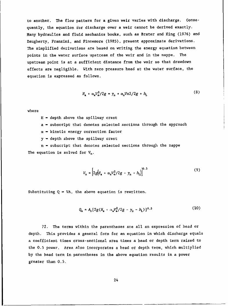
to another. The flow pattern for a given weir varies with discharge. Conse-

quently, the equation for discharge over a weir cannot be derived exactly.

Many hydraulics and fluid mechanics books, such as Brater and King (1976) and

Daugherty, Franzini, and Finnemore (1985), present approximate derivations.

The simplified derivations are based on writing the energy equation between

points in the water surface upstream of the weir and in the nappe. The

upstream point is at a sufficient distance from the weir so that drawdown

effects are negligible. With zero pressure head at the water surface, the

equation is expressed as follows.

Ha + caV/2g = yn+ cnVn2/2g + hL (8)

whereH - depth above the spillway crest

a - subscript that denotes selected sections through the approach

- kinetic energy correction factor

y - depth above the spillway crest

n - subscript that denotes selected sections through the nappe

The equation is solved for Vn.

vn=[~gi~a~ aV;/2g - yn- hL)] 9

Substituting Q - VA, the above equation is rewritten.

Qn = A.[2g(H, 8 aV2/2g - y - hL)1 0 5 (10)

72. The terms within the parentheses are all an expression of head or

depth. This provides a general form for an equation in which discharge equals

a coefficient times cross-sectional area times a head or depth term raised to

the 0.5 power. Area also incorporates a head or depth term, which multiplied

by the head term in parentheses in the above equation results in a power

greater than 0.5.

24

73. For a rectangular weir, area is depth times weir length. The weir

discharge equation is typically expressed in the general form

Q = CLH.5)

where C is an empirical coefficient reflecting all variables not included in

the L and H terms.

74. For a weir with a triangular-shaped notch, the cross-sectional flow

area is H2tano/2, where 0 is the notch angle. Thus, the weir discharge

equation for a triangular weir is typically expressed in the general form:

Q = CH2.5 (12)

75. Weir equations are necessarily empirical. Most investigators have

used the 1.5 and 2.5 exponents indicated above, with values of C being deter-

mined empirically from laboratory or prototype measurements. However, in some

cases, the weir equation has been expressed as

Q = CHn (13)

with both C and the exponent n being fitted to empirical data.

76. The head term (H) is often defined as total specific energy above

the weir crest elevation, including both flow depth and velocity head. Alter-

natively, the head may be defined as depth only, with approach velocity being

reflected, along with many other variables, in the weir coefficient (C).

Weir coefficients

77. The weir discharge coefficient (C) is a function of a number of

factors, including the weir shape and configuration, upstream flow conditions,

and downstream submergence effects. Conditions increasing frictional resis-

tance, turbulence, and the resulting energy losses decrease the weir coeffi-

cient and corresponding discharge. A round-crested weir will be more

hydraulically efficient with a larger coefficient than a broad-crested weir,

all other conditions being constant. The sharp-crested weir has the largest

possible coefficient.

25

78. The theoretical maximum value of C for a rectangular broad-crested

weir is 3.087, for length (L) and head (H) expressed in feet and discharge (Q)

in cubic feet per second, resulting in the following weir equation.

Q = 3.087 LH1 5 (14)

The value of 3.087 for C assumes the upstream corner of the weir is rounded to

entirely prevent contraction and that flow over the weir goes through critical

depth. This is the maximum value of the coefficient that can be obtained for

broad-crested weirs under any conditions. Sharp-crested and round-crested

weirs have higher coefficients. If L and H are expressed in metres and Q in

cubic metres per second, the maximum value for C is 1.705 rather than 3.087.

79. For other than the ideal condition described above, weir discharge

coefficients must be determined empirically. Coefficient values are typically

estimated based on published data, which have been developed from laboratory

and prototype tests. Brater and King (1976) and Bos (1976 and 1985) reference

the various laboratory studies which have been conducted and present weir

coefficient formulas and data for various types of weirs and flow conditions.

Weir coefficients for spillways are discussed later in this report.

Orifice Equations

Definition of terms

80. An orifice is an opening with closed perimeter and of regular form

through which water flows. If the opening flows only partially full, the ori-

fice becomes a weir. An orifice with a sharp upstream edge, as illustrated in

Figure 4, is called a sharp-edged orifice. An orifice with prolonged sides is

called a tube. The depth of water producing discharge is the head. The

stream of water which issues from an orifice is termed the jet. Discharge is

free or submerged, depending on whether the jet is discharging into air or

under water. The jet issuing from a sharp-edged orifice contracts until it

reaches the vena contracta. At the vena contracta, the paths of all elements

of the jet are parallel and the pressure in the jet can be assumed to be equal

to that in the surrounding fluid.

26

SHARP-EDGED ORIFICE b. TUBE ORIFICE

Figure 4. Types of orifices

Basic form of orifice equations

81. The energy equation written from any point upstream of the orifice

(subscript 1) to the vena contracta (subscript 2), taking the datum plane

through the center of the orifice, is

v1/2g + p11- = V2/2g = P2 hL (15)

which can be rearranged to

V2 = [2g(p1 -y - p217 + V2/2g - hL)]0 5 (16)

Since point 2 is located in the vena contracta, the pressure is that of the

surrounding fluid. For discharge into the atmosphere, p is zero. Assuming

negligible approach velocity, V, is zero. Replacing Pil/ with head (H) and

neglecting energy losses, the velocity in the vena contracta is

V2 = (2gH)0.5 (17)

The discharge is the product of the velocity and the area at the vena con-

tracta. The coefficient of discharge (C) reflects energy losses and the ratio

27

of the area of the vena contracta to the area of the orifice. Thus, the dis-

charge equation for an orifice can be expressed as

Q a CA(2gH)0.5 (18)

82. When the head is relatively small compared with the size of the

orifice, the discharge for a rectangular orifice is given as follows

Q = 2/3C(2g) 0. 5 L(H1 5 - '0.5) (19)

where

L - orifice width

H, - head above the top of the orifice

H2 - head above the bottom of the orifice

The expression 2/3C(2g)0 5 is often designated as an overall coefficient.

Orifice coefficients

83. The orifice discharge coefficient (C) depends upon head, design,

and shape of the orifice, approach channel flow conditions, and downstream

discharge conditions. Coefficient values are typically estimated based on

published data, which have been developed from laboratory and prototype

experiments. For a sharp-edged circular orifice, C - Q/(A(2gH)0'5) has a

value of about 0.60 for a wide range of heads. C is dimensionless and thus

the same for metric and English units. Brater and King (1976) and Bos (1976)

reference the various laboratory studies which have been conducted and present

orifice coefficient formulas and data for various types of orifices and flow

conditions. Discharge coefficients for outlet works and spillway gate open-

ings are addressed in Part IV.

28

PART IV: RESERVOIR OUTFLOW COMPUTATIONAL PROCEDURES

84. The Reservoir Outflow (RESOUT) Model is a generalized computer pro-

gram for determining discharges from reservoirs. The program consists of a

flexible package of procedures, with various options which can be used as

needed in a wide range of applications. Applications could involve predicting

reservoir outflows for given conditions; determining outlet structure gate

openings or breach size required to achieve specified outflows; or analyzing

reservoir drawdowns. Part V of this report is a description of the computer

program. The computational procedures included in the model are outlined in

the present chapter.

85. Three basic types of computations are involved: (a) developing

rating curves, (b) storage routing, and (c) breach simulation. Rating curves

can be developed for various types of outlet structures. For certain applica-

tions, outlet structure rating curves may be the only output desired. For

example, the rating curves may be used to determine gate openings required to

achieve specified discharges. In other applications, the computed rating

curve may be provided as input to the reservoir routing computations. For

given reservoir inflows, storage characteristics, and a given outlet structure

rating curve, storages and outflows are computed as a function of time. The

breach simulation is a special option which allows an opening in the dam,

which grows larger over time, to be incorporated in the reservoir routing.

Evaporation losses and target outflows can also be included in the routing.

Introductory Overview of Rating Curves

86. A rating curve is the relationship between reservoir water surface

elevation and discharge through an outlet structure. Discharge is a function

of head, or water depth, above the spillway crest or outlet opening. A family

(,f rating curves is required to express the water surface elevation versus

discharge relationship as a function of gate opening. Rating, or discharge,

curves provide fundamental information for real-time reservoir operation as

well as for mathematical modeling studies. Since stage is much easier to mea-

sure than discharge, the discharge from a reservoir is determined by applying

the measured water surface elevation to the rating curve. For a given

measured reservoir level, rating curves are used to select a gate opening or

number of sluices to open to achieve a desired release rate.

29

87. Rating curves are teveloped as an integral part of the design of a

reservoir project and are available for operational purposes after completion

of construction. Rating curves for existing structures can also be developed

from actual measurements of stage and discharge. However, military situations

could result in the need to compute rating curves for existing projects under

expedient conditions with limited data.

88. Rating curve computation procedures are based on weir and orifice

equations. Uncontrolled spillways are weirs, modeled using weir equations. A

dam breach is a weir with time-varying dimensions. Gate openings at gated

spillways are orifices. Discharge through an outlet works conduit is also

computed using a form of the orifice equation. Methods are incorporated into

the weir and orifice computations to reflect approach velocity, submergence,

and other conditions. Empirical data are required to estimate values for the

coefficients for various types and configurations of structures.

89. Procedures followed by USAGE in the hydraulic design of spillways

and outlet works, including development of rating curves, are outlined in

Engineer Manuals (USAGE 1963, 1965), which rely heavily upon hydraulic design

criteria prepared for OCE by WES (US Army, Office, Chief of Engineers 1988).

USBR provides another authoritative reference on hydraulic design of spillways

and outlet works (1977), which includes empirical coefficients and other data

needed for developing rating curves for various types of structures. This

general topic area is also included in textbooks and handbooks including Chow

(1959) and Davis and Sorensen (1984). USACE and USBR use many of the same

methods and data. USAGE and USBR studies also form the basis for much of the

material presented in the hydraulics textbooks and handbooks. Studies accom-

plished in conjunction with the Boulder Canyon Project (USBR 1948) are an

example of early work which significantly contributed to design procedures and

empirical data still in use today. The American Society of Civil Engineers

(ASCE) developed a comprehensive bibliography (ASCE 1963). Maynord (1985)

describes recent investigations at WhS on spillway crest shapes and associated

discharge coefficients. The procedures outlined below and incorporated in the

RESOUT Model are based primarily on USAGE references, with some additional

methods and data from USBR and other sources.

30

Rating Curves for Uncontrolled Ogee Spillways

90. The characteristics of flow over a sharp-crested weir were recog-

nized early in the history of hydraulics as the basis for design of round-

crested spillways (Chow 1959). The ogee crest profile is designed to conform

to the shape of the underside of the nappe of flow over a sharp-crested weir.

The ogee shape is commonly used for spillways because it maximizes hydraulic

efficiency. The spillway width required for a specified design head and dis-

charge is minimized. Ogee crests are used with overflow, chute, or side-

channel spillways, with development of rating curves being essentially the

same for the different spillway types.

91. The Corps of Engineers and Bureau of Reclamation have conducted

extensive studies on the hydraulics of ogee spillways and have developed stan-

dard design methods, including techniques and data for developing rating

curves (USACE 1965 and USBR 1977). The data reproduced here are s'rictly

applicable to ogee spillways designed in accordance with standard USACE and

USBR criteria. However, these and similar available data are also useful,

though somewhat more approximate, for making estimates of discharges at dams

throughout the world, even if the exact criteria and methods followed in their

design vary from the standard designs for which the data are valid.

Weir eauation

92. The discharge-versus-head relationship for flow over an uncon-

trolled ogee spillway is computed using the weir equation

= 1.5 (20)

Approach velocity is reflected in the energy head (H.). The weir coefficient

(C) is a function of energy head and submergence conditions as well as spill-

way shape. For a standard ogee design, the crest shape is set by the head

(Hd) for which the spillway is designed. The effects of abutments and piers

on discharge may be taken into account by reducing the net crest length to an

effective length (L). Discharge (Q) is computed for a given water depth or

head (H). Since H. also includes velocity head which is a function of Q, an

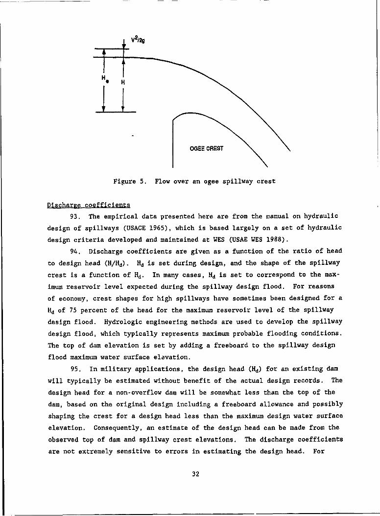
iterative solution is required. Flow over an ogee weir is illustrated by

Figure 5.

31

V2/29

He H

Figure 5. Flow over an ogee spillway crest

Discharge coefficients

93. The empirical data presented here are from the manual on hydraulic

design of spillways (USACE 1965), which is based largely on a set of hydraulic

design criteria developed and maintained at WES (USAE WES 1988).

94. Discharge coefficients are given as a function of the ratio of head

to design head (H/Hd). Hd is set during design, and the shape of the spillway

crest is a function of Hd. In many cases, Hd is set to correspond to the max-

imum reservoir level expected during the spillway design flood. For reasons

of economy, crest shapes for high spillways have sometimes been designed for a

Hd of 75 percent of the head for the maximum reservoir level of the spillway

design flood. Hydrologic engineering methods are used to develop the spillway

design flood, which typically represents maximum probable flooding conditions.

The top of dam elevation is set by adding a freeboard to the spillway design

flood maximum water surface elevation.

95. In military applications, the design head (Hd) for an existing dam

will typically be estimated without benefit of the actual design records. The

design head for a non-overflow dam will be somewhat less than the top of the

dam, based on the original design including a freeboard allowance and possibly

shaping the crest for a design head less than the maximum design water surface

elevation. Consequently, an estimate of the design head can be made from the

observed top of dam and spillway crest elevations. The discharge coefficients

are not extremely sensitive to errors in estimating the design head. For

32

example, increasing the design head by 25 percent decreases the discharge

coefficients and corresponding discharges by a range of 0-3.5 percent depend-

ing on the head (H).

96. A distinction is made between high-overflow spillways, which have

a negligible velocity of approach, and low-overflow spillways, wVhich have a

significant velocity of approach that affects both the shape of the crest and

the discharge coefficients. Discharge over a high-overflow spillway is also

not affected by downstream submergence conditions.

97. With negligible velocity of approach, the energy head (H,) term in

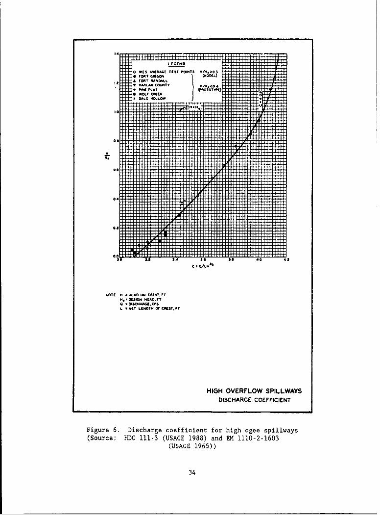
the weir equation becomes simply the head (H). Figure 6 presents values of

the discharge coefficient (C) as a function of H/Hd for the standard USACE

high-overflow ogee design. The figure is based on a laboratory study con-

ducted by WES and prototype data available from USACE District offices. C

varies from a lower limit of 3.1 for H/Hd of 0.0, to 4.03 for H/Hd of 1.0.

The lower limit of C of 3.1 is comparable to the theoretical value of 3.087

for a broad-crested weir. The upper range of discharge coefficient values is

comparable to the coefficient for a sharp-crested weir. H/Hd of 1.33 corre-

sponds to the maximum H for the spillway design flood for a design with Hd set

as 75 percent of the maximum head during the spillway design flood.

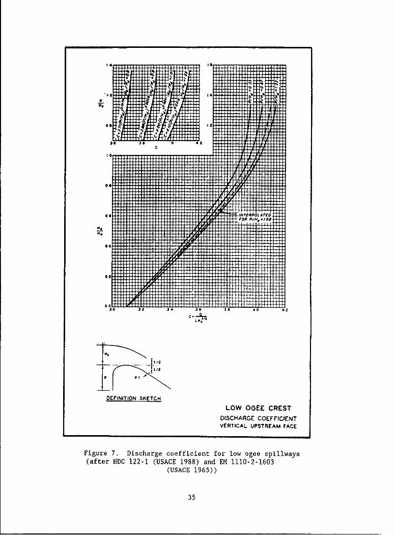
98. Discharge coefficients for low overflow spillways are presented in

Figure 7, which is also based on WES laboratory studies. A set of C versus

H./Hd curves is provided for alternative ratios of crest height (P) to design

head (Hd). A spillway with a P/Hd ratio of 1.33 or greater is considered a

high overflow spillway, and the discharge coefficient no longer varies with

P/Hd. The curve in Figure 7 for P/Hd of 1.33 is identical to the curve in

Figure 6.

99. The curves in Figure 7 are coded into the RESOUT model in table

format. To apply this option, the user must specify values for Hd and P. The

program uses linear interpolation to obtain values from the table. Alterna-

tively, the user may input his own table of C versus H/Hd to the computer

program.

Approach velocity head

100. The energy head (He) includes the water depth (H) over the crest

and the approach velocity head (V2/2g) as follows

33

0OCN: iA FON RT .SO MTIs A FORTG NA LL

L KMELENGH COUNMT FTH<0

HIGH OVEALO SPILLWAYSEDICAG COELFCIEN

Figurea6 Discarge cofIin o ihoe p wy

344

0/4

VERTIAL UPSTEAM FACE

35 32 34 ~3 8 40 4

H. _H + V2/2g (21)

The approach velocity (V) is computed as

V = Q/A (22)

where

A - (Po + H) W

assuming the approach channel can be approximated as rectangular in shape with

an approach depth (P, - H) and width (W). The approach depth includes head

over the spillway crest (H) and depth below the crest (P,).

101. An iterative solution of the weir equation is required. For a

given head (H), zero velocity is assumed to start the computations. Q is com-

puted with the weir equation. This Q, as computed assuming zero velocity

head, is then used to estimate a velocity head. Q is then recomputed. The

velocity head can continue to be iteratively corrected until changes no longer

occur.

102. RESOUT performs the computations with Po and W provided as input

data. Spillways at some reservoirs have a well-defined approach channel. In

other cases, the entire reservoir width may be considered as the approach to

the spillway. However, engineering judgment is typically required to deline-

ate an effective area through which significant flow to the spillway will

occur. The section should extend through the point at which the head (H) is

defined.

Correction for upstream face slope

103. The curves in Figure 7 are for an ogee spillway with a vertical

upstream face. Figure 8 shows the effects on discharge of a sloping upstream

face (USBR 1977b). The ratio of the discharge coefficient for an ogee crest

with a sloping upstream face to the coefficient for a vertical face is plotted

versus P/H, where P is the crest height and H0 is the design energy head.

For small ratios of approach depth to head on the crest, sloping the upstream

face of the spillway results in an increase in the coefficient of discharge.

For large P/H0 ratios, the effect is a decrease in the discharge coefficient.

Although Figure 7 is expressed in terms of design energy head (HO), the curves

can be used for energy heads (He) other than the design energy head. The

36

1.0.

...,L0h Ang~le with! ... :Lh 0 Slope the Verti€ol

No263:3 _ \ 2:3- - " 3394 1'z , Pi 3:3- 45000'

O..-

0

0 0 10

VALUES OF

Figure 8. Ogee spillway discharge coefficient correction for slopingupstream face (after USBR (1977) Figure 251)

RESOUT computer program allows the user to enter correction factors by which

the discharge coefficients are multiplied.

Submerged flow

104. A weir is said to be submerged when th.. tailwater is higher than

the crest. Although spillways are typically not submerged, this flow condi-

tion can occur at low dams. Submergence causes flow to become unstable, and

the accuracy of discharge predictions is decreased.

105. Extensive studies on submerged ogee weirs were performed by the

USBR (1948). The chart reproduced in Figure 9 was originally developed from

these studies and later verified and modified by WES. The chart is based on

201 experimental data points. Figure 9 shows the reduction in discharge coef-

i.cient caused by submerged flow conditions. Other approaches for determining

the effects of submergence on weir coefficients are outlined by Brater and

King (1976).

106. In Figure 9, the percent decrease in discharge coefficient is

expressed as a function of the terms hd/H. and (hd + d)/H., which includes

tailwater depth (d), the vertical distance from the tailwater elevation to the

reservoir water surface elevation (hd), and energy head (H,). With these

variables known, the percent decrease in discharge coefficient is determined

from the chart. The free or unsubmerged discharge coefficient is then reduced

by this percentage.

37

-N AT SECT A U 4Aacro -

+ U

-4 o 4o 5 o 0 ~ .

2j;1

I_' 2

0-20 _0 s 0 . 3 2

h 8 ,-d

:4W( In 14

Figur 9. ee spliwa dicag cofice tcorcinfrsb0egdfo. atrIIG114(SG698)adE 10210

(UAE16)Blt 3

107. In the studies that led to development of the chart, flow was

categorized based on the flow condition prevalent on the downstream apron;

i.e., (a) supercritical flow, (b) subcritical flow involving hydraulic jump,

(c) flow accompanied by a drowned jump with diving jet, and (d) flow approach-

ing complete submergence. The general pattern of the curves shows that, for

low ratios of (hd + d)/H., the flow is supercritical and the reduction in dis-

charge coefficient is affected primarily by this ratio and is practically

independent of hd/He. The cross section BB in the upper right corner of the

chart shows the variation of (hd + d)/H. for hd/H. of 0.78. On the other hand,

for large values of (hd + d)/H., the reduction in discharge coefficient is

affected primarily by the ratio hd/H,. Under this condition, for values of

hd/H. less than 0.10, the flow approaches complete submergence. For values of

hd/H. greater than 0.10, the flow is accompanied by a drowned jump with diving

jet. The cross section AA shows the variations of hd/H. at (hd + d)/He near

5.0. Subcritical flow occurs in the region indicated on the chart. Other

regions for transitional flow conditions are also shown.

108. Figure 9 is coded into the RESOUT computer program in the form of

a table, which was previously developed and incorporated into the HEC-I Flood

Hydrograph Package (US Army Engineer Hydrologic Engineering Center 1985). The

table included in HEC-I and RESOUT is shown here as Table 1. RESOUT reads the

table using linear interpolation.

109. A tailwater depth (d) is required for the submerged flow computa-

tions. RESOUT computes the tailwater depth using the Manning equation and

user-supplied cross-sectional geometry. A representative downstream cross

section is defined by an inputted channel top width-versus-elevation table and

a value for the Manning roughness coefficient (Tables 2 and 3). Alterna-

tively, a tailwater depth-versus-discharge table can be provided as input to

RESOUT. If the tailwater is significantly affected by downstream backwater

effects, the tailwater depth-versus-discharge relationship can be developed

using a backwater model such as the HEC-2 computer program (US Army Engineer

Hydrologic Engineering Center 1982).

Abutment and pier contractions

110. Piers are constructed to form the sides of the gates in gated

spillways. Piers may also support a roadway over the spillway or serve other

purposes. The hydraulic effect of piers is to contract the flow and, thus, to

alter the effective crest length of the spillway. Flow contractions also

occur at the abutments on either end of the spillway crest.

39

0 in0 .-4 .4N N m Ua . 0 0 0 0 i 0

0; N4 .4 m4 0% rs 4 N 4 .-4 0 0 0

000~ OU 00 m fnIt0 0

000t N000 mN IN 00

W0 0% r-. .4 r- 'a 4 N . 0 0 0 04 M 400000000 00 0 0 0 0

m , 'a 00r N 00 0 00 U, NO

44m~.4m0u~m 4 m 000

0 00outm UN ooN 0

00 0% N 0 1 m 1-4A 'a 0 N . 04 0 04ow t00%HO0UNM0000 0

N000M04000 0 00U 0 0

0- W 0 - 0 N 4 -40 , -4 .04 0MH4

o~ oI o0in 4 5 .'0 0000c i

V 0 Cn ,-4 ,-4

+ ~0 00 0 -0 0 0 00 0

000 0 M 0 -M4 U0 0 0, 440

Omn -4.f-4

~~~0 0 0 ,4m I 0%D 0 0 0 0~ 0-

-440 , , 4m-. 0 % 00 f- r

0 0% t m00U m 4 0 n 0 0 0 m

04N4

0 UUm4 4 'a m mm m-

4 mN r4 H-4 r0%1.-4

0 N00m U0 00 00 00 t

0% 4 0% U, w 0n m 0 m 00 00 m m 00m

q in m N 4 4 4 -4 4 -4 -4 -4 -4 H4

400

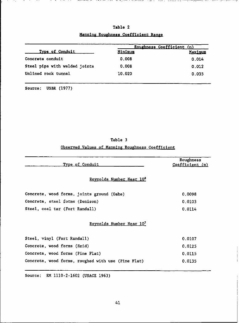
Table 2

Manning Roughness Coefficient Range

Roughness Coefficient (n)Tyie of Conduit Minimum Maxi

Concrete conduit 0.008 0.014

Steel pipe with welded joints 0.008 0.012

Unlined rock tunnel 10.020 0.035

Source: USBR (1977)

Table 3

Observed Values of Manning Roughness Coefficient

RoughnessType of Conduit Coefficient (n)

Reynolds Number Near 108

Concrete, wood forms, joints ground (Oahe) 0.0098

Concrete, steel forms (Denison) 0.0103

Steel, coal tar (Fort Randall) 0.0114

Reynolds Number Near 107

Steel, vinyl (Fort Randall) 0.0107

Concrete, wood forms (Enid) 0.0125

Concrete, wood forms (Pine Flat) 0.0115

Concrete, wood forms, roughed with use (Pine Flat) 0.0135

Source: EM 1110-2-1602 (USACE 1963)

41

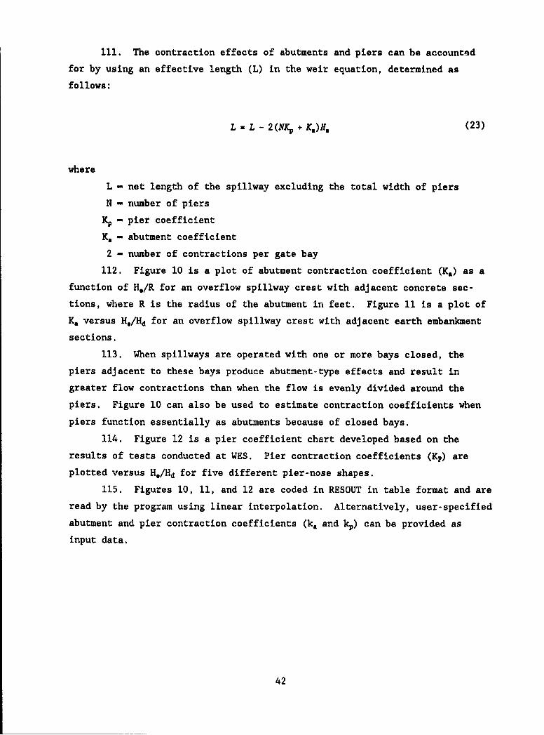
111. The contraction effects of abutments and piers can be accounted

for by using an effective length (L) in the weir equation, determined as

follows:

Lu L - 2(NKC + K.)R. (23)

where

L - net length of the spillway excluding the total width of piers

N - number of piers

K% - pier coefficient

Ka - abutment coefficient

2 - number of contractions per gate bay

112. Figure 10 is a plot of abutment contraction coefficient (Ka) as a

function of H./R for an overflow spillway crest with adjacent concrete sec-

tions, where R is the radius of the abutment in feet. Figure 11 is a plot of

Ka versus H./Hd for an overflow spillway crest with adjacent earth embankment

sections.

113. When spillways are operated with one or more bays closed, the

piers adjacent to these bays produce abutment-type effects and result in

greater flow contractions than when the flow is evenly divided around the

piers. Figure 10 can also be used to estimate contraction coefficients when

piers function essentially as abutments because of closed bays.

114. Figure 12 is a pier coefficient chart developed based on the

results of tests conducted at WES. Pier contraction coefficients (Kp) are

plotted versus H./Hd for five different pier-nose shapes.

115. Figures 10, 11, and 12 are coded in RESOUT in table format and are

read by the program using linear interpolation. Alternatively, user-specified

abutment and pier contraction coefficients (k. and k.) can be provided as

input data.

42

120

BAS1C EQUATION0

Q •C(L- 2(NKp+K,)H.IH.'0"

100 WHERE-"

SUGGESTEDO -Q OISCHARGE,CFS.ESIGN CURVE C * DISCHARGE COEFFICIENT.

_ -NET LENGTH OF CREST. FT.N -NUMBER OF PIERS.Kp -PIER CONTRACTION COEFFICIENT.K&- ABUTMENT CONTRACTION COEFFICIENT.

8o - He - TOTAL HEAD ON CREST, FT.

i-•A O0

0 SYMBOL PROJECT It W/L W/H0 o 0 OW o0 4 .55 096

• a 0 FOLSOM 6 2.10 3770 PHILPOTT 5 2.67 I 42

0 O • PINE FLAT* 4 2.12 1 77• 0 0 a CENTER HILL* 5 363 948

4.0 -?GWATED SPILLWAY WITH PIERS

U 0

0aS0 0 000 NOTE R -RADIUS OF ABUTMENT, FT

0 0 W.WIDTH OF APPROACH REPRODUCED IN2C MODELFT.

0 0 L -GROSS WIDTH OF SPILLWAY, FT.O 0 H -DEPTH OF APPROACH IN MODEL , FT

0-02 00 0.2K,

(

OVERFLOW SPILLWAY CREST WITHADJACENT CONCRETE SECTIONS

ABUTMENT CONTRACTION COEFFICIENTHYDRAULIC DESIGN CHART 111-3/I

. .... ... .. WE$ 0-60

Figure 10. Abutment contraction coefficient for concrete sections(after HDC 111-3/1 (USACE 1988) and EM 1110-2-1603 (USACE 1965)

Plate 8)

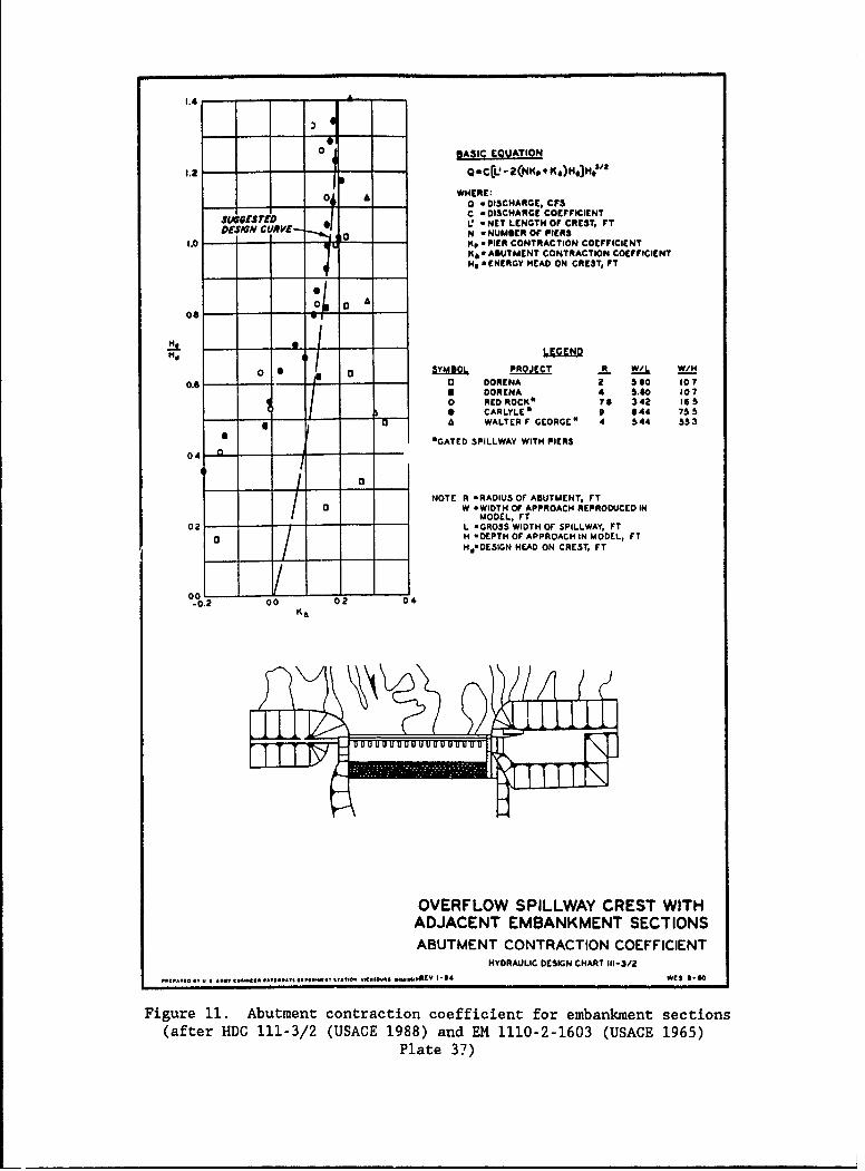
1.4 - - - - --

o AsC EQUATION

. - Q-CLZ(NKpK)H#) 03/2

O £ WHERE:Q - DISCHARGE, CFS

$UGGES$TED C :DISCHARGE COEFFICIENTVNRE NET LENGTH OF CREST, rT

I --- I O 1 N *NUMBER OF PIERS.0 Kp - PIER CONTRACTION corFICINT

K& - ABUTMENT CONTRACTION COEFFICIENTH9 a ENERGY HEAD ON CREST, FT

08 w !

0 YBL PROJECT A W/L W/N0.- a DORENA 2 s0 107

- ORENA 4 S0 1070 RED ROCK* 78 342 165

CARLYLE * 9 844 755- - h WALTER F GEORGE* 4 544 553

B -GATED SPILLWAY WITH PIERS

04 -

NOTE R -RADIUS OF ABUTMENT, FTW -WIDTH OF APPROACH REPRODUCED IN

MODEL, FT02 -L GROSS WIDTH OF SPILLWAY, FT

0 H -DEPTH OF APPROACH IN MODEL, FT

H •DESIGN HEAD ON CREST, FT

-0.2 -0 02 04K&

OVERFLOW SPILLWAY CREST WITHADJACENT EMBANKMENT SECTIONSABUTMENT CONTRACTION COEFFICIENT

HYDRAULIC DESIGN CHART 111-3/2

**Et***.. ....V i,.t*A6,**DlfN i . ,,, . 6 Aw.ACV 1.04 e 0

Figure 11. Abutment contraction coefficient for embankment sections(after HDC 111-3/2 (USACE 1988) and EM 1110-2-1603 (USACE 1965)

Plate 37)

(W

I&I1

03

bi 0. ..

4 p 4 f

Pm~~~ ,-P4eto

z in

4~r g C

& .4 )

04

*1*4

0*0

4/I4-awaM~~~~4 Nrga0 L4~o02M4 g~

451

Rating Curves for Uncontrolled Broad-Crested Spillways

116. Various types of spillways have crests which are simple broad-

crested weirs. Discharge through a broad-crested spillway or other structures

involving weirs is computed using the weir equation

Q = CLHI.5 (11)

for a rectangualr weir, where L is the weir length and H is head, or

Q = CZH2.5 (24)

for a triangular weir, where Z is the side slope of the notch, or

Q = C1.1 5 + C2Z12. 5 (25)

for a trapezoidal-shaped weir, where the first term represents the rectangular

and the second term the triangular components of the trapezoid.

117. Discharge coefficient (C) values of 3.1 for rectangular and 2.45

for triangular weirs or triangular components of trapezoidal weirs are typi-

cally considered to be conservatively high but reasonable values, assuming

units of feet and cubic feet per second are used in the weir equation. The

discharge coefficient values would be 1.71 and 1.35, respectively, for rectan-

gular and triangular weirs if units of metres and cubic metres per second are

used.

118. The RESOUT model applies correction factors to the weir equation

for approach velocity (k,) and submergence (k,) effects as follows.

Q kvkCLH1.5 (26)

119. The approach velocity correction factor (kv) is given by the fol-

lowing equation, which was developed by Fread (1984) from data presented by

Brater (1959).

46

Ic-, u 1.0 + 0.023 Q2/[W2 (P0 + H) 2H] (27)

assuming the approach channel can be approximated as rectangular in shape with

an approach depth (Po+H) and width (W). The approach depth includes head over

the spillway crest (H) and depth below the crest (P.).

120. The submergence correction factor (k.) is given as follows (Fread

1984 and Vennard 1954).

k. = 1.0 If t/H . 0.67 (28)

k, 1.0 - 27.8 [(ht/H) - 0.67]3 (29)

where ht is the height of the tailwater over the weir crest and H is the

height of the reservoir water surface over the weir crest. RESOUT computes

tailwater depth using the Manning equation and user-supplied cross-sectional

geometry for a representative downstream cross section. Alternatively, a

tailwater depth versus discharge table can be provided as input to RESOUT.

Rating Curves for Spillway Gates

121. RESOUT includes two approaches for developing rating curves for

partly open spillway gates. Both approaches are based on forms of the orifice

equation.

122. The basic equation for a high head orifice with a free-falling

nappe Is

Q = CA(2gH) 0 .5 (30)

where Q denotes discharge, C is the discharge coefficient, A denotes orifice

area, and H is the head measured from the center of the orifice. This equa-

tion is incorporated in RESOUT and can be used for various types of gates.

The empirical discharge coefficient data discussed later were developed spe-

cifically for tainter gates on ogee spillways.

47

123. Another orifice equation applicable to flow through a rectangular

orifice with a low ratio of head to orifice height is

QG = Cd(2g) 0° 5L(H 1 5 - HT"5 ) (31)

where H and HT are the head to the bottom and top, respectively, of the ori-

fice. The vertical lift gate analysis approach discussed below is based on

this form of orifice equation.

Vertical lift gates

124. The basic equation for flow through a rectangular orifice with a

low ratio of head-to-orifice height given above can be combined with the equa-

tion for flow over a weir

Q = C(2g)0 5 LH3/2 (32)

to obtain

QG/Q = p{i - [(H - Go)/H] 1 5 ) (33)

where p is the ratio Cd/D and Go is the gate opening Ht-H.

125. Figure 13 is a plot of experimental data of the ratio %/Q against

the bracketed term in the equation above for vertical lift gates on ogee

spillways (USACE 1965). The slope of the line represents the coefficient A.

A study at WES based on available model results indicates that p - 1.14 for

low heads (H/Hd < 0.5) and 1.04 for high heads (H/Hd - 1.0). The curves can

be interpolated for H/Hd values between 0.5 and 1.0.

126. The RESOUT computer program includes the above equation. The free

overflow Q is computed using the weir equation. The coefficient is determined

based on a computed H and user-inputted Hd. The term in brackets is computed

based on a user-inputted G,. The discharge through the gate opening is then

computed as

48

O8 x

0. - - LOW Ef - -

04

01

INCRASING GATE oIONING---

01 1 1-D 01 02 0j3 04 05, 0t4 0.7 0.4l 011

NOTE 0 2 FREE FL OW DISCHARGE AT HEAD H.OscOISCHAAG[ AT HIEAD H AND GATE

0ODININ 00LEEN

Svm&Ol PROJECT HEAD,_r T

x GORGE HIGH 45.01 GORqGE miGH 25 00 BLUESTONE 30 09 OlL J[ STONE I S,0a FALCON 53,1)0 FALCON 2330 MAHON, NGN 30. 0

w a MAHON NG ISO

CREST GATESDEF N S CVER, ICAL LIFTFNEON DSKCHG ADISCHARGE COEFFICIENTS

Figure 13. Vertical lift gate discharge coefficient

(after HDC 312 (USACE 1988) and EM 1110-2-1603(USACE 1965) Plate 49)

49

QG = {1 - [(H - G.)/H] .5)Q (34)

127. As the gate is raised, the ratio of head on the gate to the total

head becomes smaller, and the abscissa in Figure 13 becomes larger. The nappe

breaks free from the gate lip at an abscissa value of about 0.9. The corre-

sponding ratio of head on the gate to bead on the crest is about 0.21. The

value for the transition from orifice flow to free overflow when the gate is

raised is probably different from the reverse transition when the gate is

lowered. When the gate lip extends only a small distance into the flow, there

is a violent top roller and the transition phenomenon is difficult to observe.

Tainter gates

128. Discharge coefficients applicable to tainter gates on high over-

flow ogee spillways are presented in Figure 14 for the orifice equation in the

form

Q = CGoB(2gH) 0 -5 (35)

where

Go - net gate opening in feet

B - is the gate width in feet

H - head-to-center-of-the-gate opening in feet

Two discharge coefficient curves are presented, one for gate seats located at

the crest axis and a second for gate seats located at 0.1 < X/Hd < 0.3,

where X is the horizontal distance between the crest axis and gate seat. The

value of C ranges from 0.67 to 0.73 for various gate openings.

129. The flow boundaries formed by the gate and crest surfaces are com-

parable to those of a funnel or an orifice formed by converging plane sur-

faces. The discharge coefficient (C) is a function of the angle (1) formed by

the intersection of the tangent to the gate lip and the tangent to the crest

curve at the nearest point of the curve to thp vate lip.

130. RESOUT requires user-specified discharge coefficient values to be

inputted for each gate opening considered using this option. Discharge

coefficients for tainter gates on ogee-shaped spillway crests can be estimated

based on judgment using the data presented in Figure 14 as a general guide.

50

to .Io

aas

04kc

__ - -

q- - -K - df M

10 •~r VA,,M ." P4r

' T DEFINITION STETGHT-

DDISCHARGE CCFFCCT N)

osca S T[ l[a lG.r1

D toGAti wIO?'14.PT T,.€ io curs o ,. SPILLWAY TINTER GATESDISCHARGE COEFFICIENTS

Figure 14. Tainter gate discharge coefficient(after HDC 311-1 (USACE 1988) and EM 1110-2-1603

(USACE 1965) Plate 46)

51

Other types of gates can be analyzed with RESOUT as well, with the hydraulic

efficiency of the gate configuration being reflected in the inputted discharge

coefficient value.

Drop Inlet Spillways

131. The drop inlet spillway, also known as the morning-glory or shaft

spillway, is illustrated in Figure 15. The outflow is conveyed by a vertical

or sloping shaft to a horizontal tunnel or conduit through the dam. Both the

ogee crest and the flat or broad-crested shapes have been used for the

entrance weir. The ogee crest has the advantage of hydraulic efficiency.

132. Drop inlet spillways may operate under both free and submerged

discharge conditions. For small heads, discharge through the spillway is

controlled by flow conditions at the crest. The vertical transition below the

crest will flow partly full and the flow will cling to the sides of the shaft.

As the flow over the crest increases, the annular nappe will become thicker

and eventually the nappe flow will converge into a solid vertical jet, as

illustrated by Figure 15. The point where the annular nappe joins the solid

jet is called the crotch. After the solid jet forms, a boil will occupy the

region above the crotch. Both the crotch and the top of the boil become pro-

gressively higher with larger discharges. For high heads, the crotch and boil

may flood out, showing only a slight depression and eddy at the surface.

133. Free discharge weir flow prevails until the nappe converges to

form a solid jet. The weir flow will be affected by submergence after the

crotch and boil form. Ultimately the crest will drown out. At less than

design heads, the transition from free to submerged flow and vice versa may be

accompanied by violent surging in the vertical shaft.

134. The discharge through a drop inlet spillway can be computed using

the modified weir equation

Q = C(2 R)H1 5 (36)

52

MAXIMUM DESIGN WATERSURFACE ELEVATION

SPILLWAY CREST .- ' // N

/ DAM "N/,,

/CONDUIT

a. Spillway profile

WATER SURFACE

MORNING GLORY CRESTH

SHARP-CRESTED WEIR

b. Section through spillway entrance

Figure 15. Drop inlet spillway schematic

53

135. The above equation is included in RESOUT. C and R must be pro-

vided by the user as input data.

136. The discharge coefficient C is difficult to precisely estimate.

Discharge coefficients based on flow measurements over sharp-crested weirs are

presented in Figure 16. This data, published by the USBR (1977) and repro-

duced by USACE (1965), can be used as general guidance for estimating dis-

charge coefficients for drop inlet spillways with circular ogee-shaped

entrances.

137. Figure 16 is a plot of C versus Hd/R for an ogee spillway crest.

C depends upon the ratio of the approach depth (P.) to the radius (R). These

spillway dimension terms are defined schematically in Figure 15. The coeffi-

cients in Figure 16 are for the design head. The coefficients (C) are valid

for both free and submerged flow conditions. Free flow prevails for Hd/R

ratios up to approximately 0.45. As the H/R ratio increases above 0.45, par-

tial submergence occurs. When the H/R ratio approaches 1.0, the weir is com-

pletely submerged. With submerged flow, a further increase in head on the

crest results in a comparatively small increase in discharge.

138. Figure 16 is for the design head. For purposes of developing a

rating curve, Figure 16 can be used in combination with Figure 17 (USBR 1977).

The discharge coefficient corresponding to a Hd/R ratio of 0.3 is determined

from Figure 16. Ratios of the coefficient of discharge for a specified head

to the Figure 16 value for Hd/R of 0.3 are given in Figure 17 as a function of

H/R.

Rating Curves for Outlet Works

139. An outlet works consists of one or more conduits or sluices

through the dam, and associated intake and exit structures. Gates and valves

are incorporated into an outlet works to control the flow rate. Methods for

analyzing flow through a conduit vary depending on whether the conduit is

flowing full or partly full. If the water surface stays below the top of the

conduit, the conduit becomes an open channel, and the flow is governed by

principles of open channel flow. The hydraulics of a conduit flowing full are

governed by pressure conduit flow. The computational procedures incorporated

in RESOUT are for conduits flowing full.

54

It

0 15

00

1 0 14 to 22 9$ 310 34I 34 42DISCHARGE COEFFICIENT - C

NOTE CURVES ARE TAKEN FROM USSR I.QSMAL IA AND ARE BASED ON WAGNER'SDATA FOR FULLY AERATED FLOW OVER A

EQUATION SHARP- CRESED WEIRDASHED CURVES ARE GASO ON L TRAPOLATM°VALUISOr Hd/R(PLATE 54)

WHERRE P- •APPROACH DEPTH TO SHARP CREST. FT,

0 *OISCHARGtCFSC *DISCHARGE COEFFICIENTR *RADIUS Of SHARP CREST, FTH, $DSIGN HEAD ON SPILLWAYCREST. FT

MORNING GLORY SPILLWAYSDISCHARGE COEFFICIENT

DESIGN HEAD

Figure 16. Drop inlet spillway discharge coefficient for designhead (after USBR (1977b) and EM 1110-2-1603 (USACE 1965) Plate 55)

55

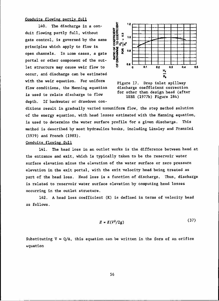
Conduits flowing Rartly full

140. The discharge in a con- 12 -1 - ----

duit flowing partly full, without --1.0gate control, is governed by the same N -

principles which apply to flow in or

open channels. In some cases, a gate R

portal or other component of the out- L - --

U. 0.6 - - - - - - - -

let structure may cause weir flow to 0 0 0.1 02 0.3 0.4 0.6

occur, and discharge can be estimated

with the weir equation. For uniform Figure 17. Drop inlet spillway

flow conditions, the Manning equation discharge coefficient correctionflow for other than design head (afteris used to relate d~scharge to flow17b Fgre24

USBR (1977b) Figure 284)

depth. If backwater or drawdown con-

ditions result in gradually varied nonuniform flow, the step method solution

of the energy equation, with head losses estimated with the Manning equation,

is used to determine the water surface profile for a given discharge. This

method is described by most hydraulics books, including Linsley and Franzini

(1979) and French (1985).

Conduits flowing full

141. The head loss in an outlet works is the difference between head at

the entrance and exit, which is typically taken to be the reservoir water

surface elevation minus the elevation of the water surface or zero pressure

elevation in the exit portal, with the exit velocity head being treated as

part of the head loss. Head loss is a function of discharge. Thus, discharge

is related to reservoir water surface elevation by computing head losses

occurring in the outlet structure.

142. A head loss coefficient (K) is defined in terms of velocity head

as follows.

H = K(V 2/2g) (37)

Substituting V - Q/A, this equation can be written in the form of an orifice

equation

56

Q = A(2gH/K) 0.5 (38)

where A is the conduit cross-sectional area. The factor (l/K)0.5 is analogous

to the orifice discharge coefficient. K is a total-loss coefficient which

typically will be the sum of several component-loss coefficients

K = k, + k2 + k3 + ... (39)

where ki represents loss coefficients for outlet structure components such as

trashracks, intake structures, gates, transitions, and the conduit itself.

143. The above equation is incorporated into RESOUT. The discharge

coefficient (K) for friction losses in the conduit is computed by the program

using either the Darcy-Weisbach or Manning equations. The total K for all

other outlet structure components is provided as input data by the user.

144. The head (H) is the reservoir water surface elevation minus the

water surface or zero pressure elevation in the exit portal. Figure 18 shows

the results of laboratory tests made at the State University of Iowa relating

the zero pressure elevation at the exit portal of a circular conduit to the

Froude number for the flow in the conduit (USACE 1963).

145. The suggested design curve in Figure 18 is coded into RESOUT as a

table which is read by linear interpolation. RESOUT computes the Froude num-

ber for a given discharge and conduit diameter. The elevation of the zero

pressure point above the invert of the exit portal is determined from the

relationship shown in Figure 18. The head (H) is computed as the difference

in reservoir water surface elevation and exit portal zero pressure elevation.

Alternatively, a discharge versus water surface (or zero pressure) elevation

relationship can be provided as user-specified input data.

Partly open gate control

146. When conduits are operated under head with gates partly open,

pressure flow occurs upstream from the gate and if tailwater level permits,

open channel flow occurs downstream from the gate. The discharge control is

located at the gate. The equation

57

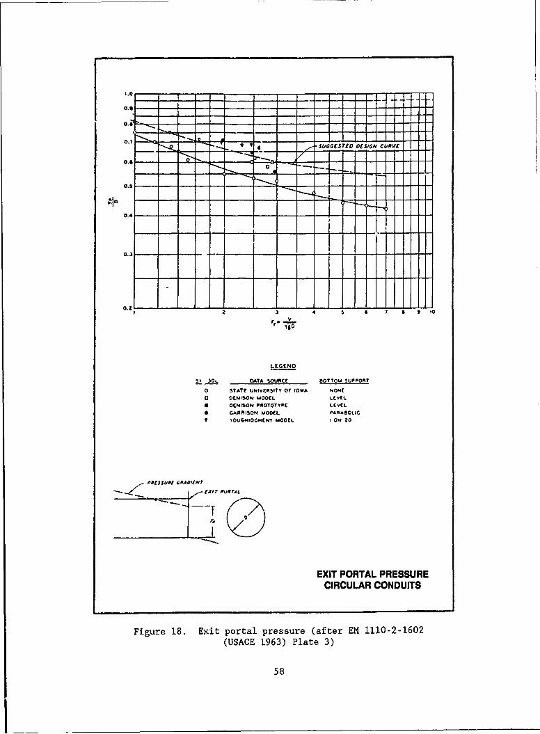
0. - - - I I

0.7 0 "A- -"-L ' a sucST1 DiSI ! i AI

o.-* -" - ..- . --1-' - . -.,- - - :

0.2-

I 1 4 5 6 7 a : '0

fr.

LEGEND

21 J"s DATA SOUCE BOTTOM SUPPORT

* STATE UN~vERSITY OF IOWA NONE

* DENISON MODEL LEVELD ENISON PROTOTYPE LEVEL

* GARRISON MODEL PARABOLIC9 vOUG#4IOGI4ENT MODEL I ON 20

, lT PI4 I''

EXIT PORTAL PRESSURECIRCULAR CONDUITS

Figure 18. Exit portal pressure (after EM 1110-2-1602(USAGE 1963) Plate 3)

58

II

Q - A (2gH/K)°5 (40)

is applicable to partly opened gates. A is the area of the gate opening. The

loss coefficient K includes the gate loss and contraction coefficients in

addition to coefficients for the other losses, such as entrance and friction,

which occur upstream of the gate. All loss coefficients should be expressed

as coefficients of the velocity head at the gate opening.

147. In cases such as this, in which velocity head varies between loca-

tions in the conduit, equivalent K values can be determined based on the con-

tinuity equation.

Since

Q = V1A1 - V2A2 (41)

then

V2 = (A1/A2)V, (42)

and

= (A1/A2)2V[ (43)

Therefore, the loss coefficient (K) at location 1 can be expressed as a coef-

ficient of the velocity head at location 2 by multiplying K by (A1/A2)2.

Conduit friction losses

148. Head losses in a straight length of conduit can be estimated with

a number of alternative empirical formulas, such as the Darcy-Weisbach,

Manning, Hazen-Williams, and Scobey equations. The Darcy-Weisbach and Manning

equations are incorporated as options in the RESOUT computer program.

149. Manning equation. The Manning equation can be expressed as

hf = (On2L/R 4/1 ) (V2/2g) (44)

for which the head loss coefficient (kf) becomes

59

kf On 2L/R 4/3 (45)

The 0 includes the 2g term and the conversion factor from English to metric

units. The value of 0 is 19.62 when metric units are used and 29.1 for

English units. Ranges of values for the Manning roughness coefficient (n) for

various types of outlet conduits are presented by the USBR (1977) and repro-

duced here as Table 2. Measured n values at several USACE dams are cited in

Table 3 (USAGE 1965).

150. Darcy-Weisbach eguation, The head loss resulting from pipe fric-

tion may also be determined using the Darcy-Weisbach equation

hf= f(L/D) (V2/2g) (46)

151. The friction factor (f) is a function of the relative roughness

(e/D) of the pipe and the Reynolds number (R.) of the flow.

&,= DV/v (47)

where v is the kinematic viscosity, which is 0.000001003 m2/sec for water at a

temperature of 200 C. If R. is less than 2,100, the flow is laminar. The

flow is turbulent for R. over 3,000. Between these values, a transitional

type of flow exists. The relative roughness (e/D) of a pipe depends on the

absolute effective roughness (e) of the interior surface and the diameter (D).

A hydraulically smooth pipe is a flow condition in which the wall roughness is

completely covered by a laminar boundary layer. For a given Reynolds number,

the smooth pipe curve in the Moody diagram is the lower limit for the value of

the friction factor (f). The Moody diagram reproduced in Figures 19 and 20

illustrates the various flow regions. Measured data from a number of USAGE

projects are plotted on Figures 19 and 20, respectively, for concrete and

steel conduits (USAGE 1965).

152. The Moody diagram is coded in the RESOUT computer program in the

form of the equations for smooth pipe, fully rough, and transitional flow con-

ditions. The von Karman and Prandtl equation for smooth pipe flow is

60

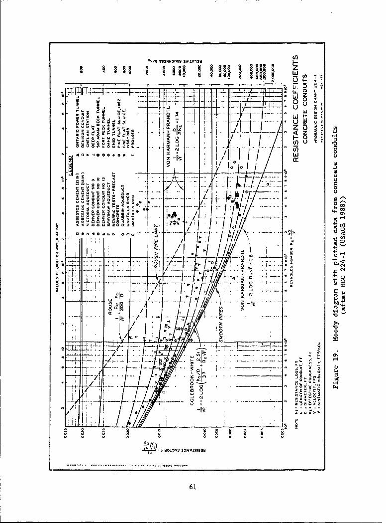
8 8 8 88 gi 8 88 § §L§ J2N~~ 't 0S U

I I I Is 'G- 5

r~L a. ~N

20 (fl ZZ L L

0 0 m -

< A_

N3 0 1. -i Mo-. (D +.

z f~l 0 0

A. / I 1 4

z "Z z Z 444

0~ ~ ~ ."1 u u/I-.//A4

4, > >. >. x, u4D w ,' zrz z Z II C

'n wnI wi w' Ii0 32441#

-eo x.0. t c onCc N

t-d-.

0 ID

z 0' 4~~ cq~

0~ .0

I 0~0

D' 00 00 >4 4 Id

C. r 6 0b cm . . . - - N

2 I

O~~ 0

3~NV±SIS3

61 0 b

%14/0 993NHOfl0 3AI±V13ts

0 wQ 0 0 22 00I C4 Z

00 Z x

-LL 0- ww5 .c

< U w. oa.

0, w~ N, , C4~- . <L I'

z 0 cr.

N j Jtij4- 0 o.c

1 1

Z. < 4 ~ .oo

4 l i v 0 0

/ -3. 0' 4 o .J

0 -_T _

Cl I,

I' I t i i llo') i * L AIv 4)

*~ 4.,j ~

/ 00

2 ...... F -

0 0 0 00

0~~ 0 0>0 0 0

+A0 (o) jiJY 0:I0YsI V

62 a > ,

1/() 0 5 .2 Log &(f)0 5 - 0.8 (48)

The friction factor (f) for smooth pipe flow is a function of only the

Reynolds number (R.).

153. The von Karman-Prandtl rough pipe equation is

11(f)0-5 - -2 Log (D/2e) + 1.74 (49)

Rough pipe is a function of relative roughness (e/D), but is independent of

the Reynolds number.

154. The lower limit of the rough flow zone is defined as follows:

11(f)" - (RPe)/(200D) (50)

155. The area o' the Moody diagram between the smooth pipe curve and

the rough flow limit is a transition region. The Colebrook and White equation

for transition flow

11(f) 0 '5 = -2 Log (e/3.7D) + [2.51/PR(f) 0 5 ] (51)

includes both Reynolds number and relative roughness.

156. RESOUT computes the frictional head loss in a conduit using the

Darcy-Weisbach equation with conduit length (L), diameter (D), and absolute

roughness (e) and the kinematic viscosity (u) of the water specified by the

user as input data. Effective roughness (e) values for various types of con-

duits are shown in Table 4.

Noncircular conduits

157. The Darcy-Weisbach equation is expressed in terms of conduit diam-

eter. The Manning equation is also coded in RESOUT based on a user-supplied

conduit diameter. Thus, the frictional head loss computations assume the con-

duit has a circular cross section. However, the head loss in a noncircular

conduit can be assumed to be the same as the head loss in a circular conduit

63

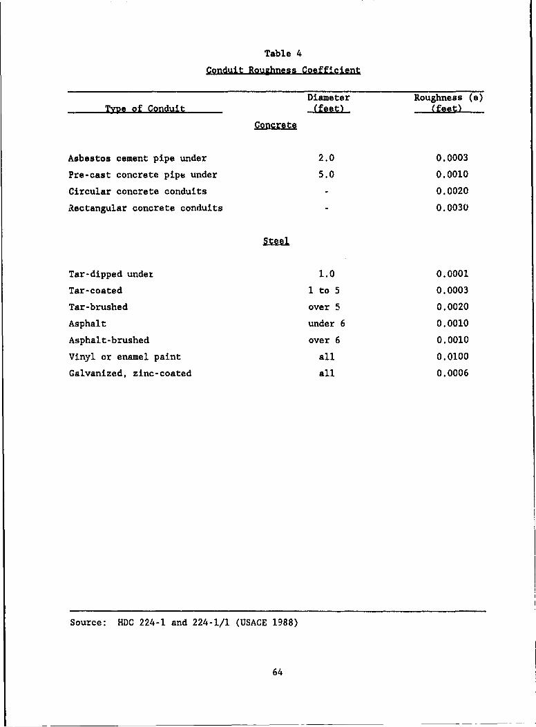
Table 4

Conduit Roughness Coefficient

Diameter Roughness (e)

Type of Conduit (feet) (feet)Concrete

Asbestos cement pipe under 2.0 0.0003

Pre-cast concrete pipe under 5.0 0.0010

Circular concrete conduits 0.0020

Rectangular concrete conduits 0.0030

Steel

Tar-dipped under 1.0 0.0001

Tar-coated 1 to 5 0.0003

Tar-brushed over 5 0.0020

Asphalt under 6 0.0010

Asphalt-brushed over 6 0.0010

Vinyl or enamel paint all 0.0100

Galvanized, zinc-coated all 0.0006

Source: HDC 224-1 and 224-1/1 (USACE 1988)

64

having an equivalent hydraulic radius (Cox 1973). The equivalent diameter (D)

is computed as

D = 4R u 4(A/WP) (52)

where R is the hydraulic radius of the noncircular conduit which equals the

cross-sectional area (A) divided by the wetted perimeter (WP). Hydraulic

radius formulas for various common conduit shapes are presented in Figure 21.

Other head losses

158. The total head loss coefficient (K) is the summation of the loss

coefficients (ki) for each structure component which produces a head loss. In

addition to losses due to conduit friction, head losses are caused by trash-

racks, entrance curves, bulkhead and gate slots, transitions, piers, exit con-

tractions, deflectors, and the exit. Partially open gates and valves control

the discharge rate by causing a head loss.

159. In applying RESOUT, the user inputs a single K value which is the

summation of all component loss coeff~cients, with the exception of the coef-

ficient for conduit losses which can be computed by the model using the

Darcy-Weisbach or Manning equations. Thus, the loss coefficient values ki,

other than for conduit friction, are estimated and totalled independently of

RESOUT, and the total K is provided as input to the computer program.

160. Engineering judgment is required to estimate loss coefficient val-

ues for the particular reservoir for which a rating curve is being developed.

Empirical loss coefficient data for various outlet structure components are

presented by WES (USACE 1963, 1965), and USBR (1977). Selected data are

reproduced here. The loss coefficients discussed below are applicable to the

velocity head in conduits under pressure flow conditions with the entrance

submerged. Loss coefficients for open channel flow are typically

significantly higher than for pressure conduit flow.

161. Trashrack loss, Head loss coefficients for trashracks depend upon

the bar thickness, bar shape, and spacing. Loss coefficients are provided in

Figure 22 as a function of the ratio (Ar) of the area of bars to area of sec-

tion for alternative trashrack designs. This data should provide conserva-

tively high values for unclogged trashracks. However, the values may be

increased in applications invo'ving significant accumulation of debris on the

trashrack. Trash structures which consist of widely spaced structural members

65

WETTED HYDRAULICAREA PERIMETER RADIUS

SECTION (A) (WP) (R)

]BH 2(B + H) 2(B+H

7_2 770 _.4 4

2 BH 1 TR2

1 R2 B+2H+nR 77R

2 ~B + 2H + 77 R

HI or BH + wR2 2(H+nR) BH+ R2

2(H + v R)

77 R2

H(+ B) 7R2 B+ (2 (B24 7R H (B A B) +-2-

H +B+ - 2 B+2(H2 +(AB) 2)' +nR

3.3172 R2 6.5338 R 0.5077 R

HYDRAULIC ELEMENTS

CONDUIT SECTIONSPRESSURE FLOW

HYDRAULIC DESIGN CHART 224-2

WES 5-?5

Figure 21. Hydraulic elements for conduit sections (after HDC 224-2

(USACE 1988))

66

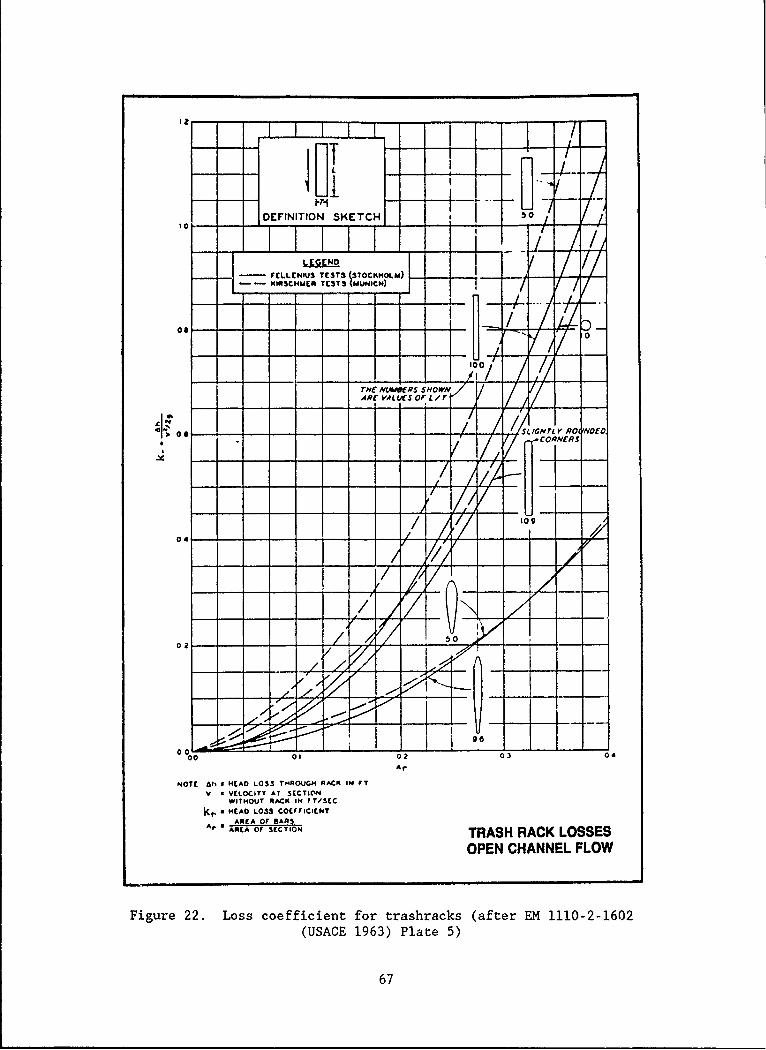
~oI- - It

* *CAOLOS C EENDAELL* ARE OF3T (BARS RACK

A IEAOHMECI TRASH LOSSESH

OPEN CHANNELFLOW

Figure 2. Los coeffcient or trashrcs(fetl 10210

> ~USC 1963)r Ro Plat 5

67AER

without rack bars will cause very little head loss, and a loss coefficient in

the range of 0-0.02 might be used.

162. Intake structure loss, The intake structure loss coefficient val-

uea shown in Table 5 were compiled by the USBR (1977) from various sources.

The results of USACE (1963) analyses of prototype and model data for several

projects are presented in Figure 23. The USACE coefficients represent the

entire intake structure including the entrance, gate slots, and transition.

For just gate slots, a loss coefficient of 0.01 is suggested for each pair of

gate slots. A loss coefficient of 0.05 is suggested for a pier with rounded

ends.

163. Bend loss. The bend loss, in addition to conduit friction loss,

is a function of bend radius, pipe diameter, and deflection angle of the bend.

Curves showing bend loss coefficients are reproduced as Figure 24. The curves

are applicable to circular conduits and to rectangular conduits for which the

width-height ratio does not vary greatly from unity, in which case D is taken

equal to the conduit height for vertical bends and the conduit width for hori-

zontal bends.

164. Exit constriction loss, In computing discharge through a conduit

which contains an exit constriction, all losses should be expressed in terms

of the velocity head corresponding to the smallest cross-sectional area of the

constriction and that area used in the basic discharge-head equation. Conduit

losses expressed in terms of velocity head corresponding to the cross-

sectional area of the conduit at the point where the loss occurs may be con-

verted to terms of the velocity head corresponding to the smallest

constriction area. The former loss coefficients are multiplied by a factor

A2/A2, where A, and A2 are the areas of the conduit at the point of loss

occurrence and at the constriction, respectively.

165. Exit velocity head. A loss coefficient of 1.0 is used to repre-

sent the velocity head at the exit.

Breach Simulation

166. In addition to using outlet structures, reservoir releases during

military operations can be achieved by breaching the dam. A portion of a dam

may be destroyed by explosives or other means. Dam breaches can also be

caused by the reservoir level overtopping the dam. In certain situations,

outlet structure gates may be closed and/or openings otherwise blocked to

68

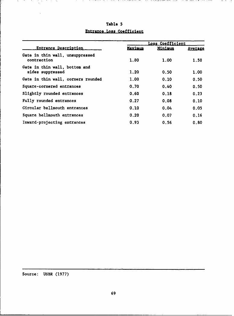
Table 5

Entrance Loss Coefficient

Loss CoefficientEntrance Descrintion Maximum Minimum vere

Gate in thin wall, unsuppressedcontraction 1.80 1.00 1.50

Gate in thin wall, bottom andsides suppressed 1.20 0.50 1.00

Gate in thin wall, corners rounded 1.00 0.10 0.50

Square-cornered entrances 0.70 0.40 0.50

Slightly rounded entrances 0.60 0.18 0.23

Fully rounded entrances 0.27 0.08 0.10

Circular bellmouth entrances 0.10 0.04 0.05

Square bellmouth entrances 0.20 0.07 0.16

Inward-projecting entrances 0.93 0.56 0.80

Source: USBR (1977)

69

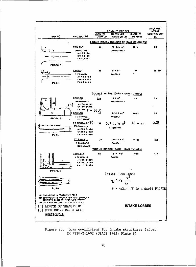
AVERAGECONDUIT PROPER INTAKE

LENGTH REYNOLDS VELOCITY COEFFICIENTSHAPE PROJECT (I) "IAM (2) NUMBER (2) HEAD (I)

SINGLE INTAKE (CONCRETE DAM CONDUITS)

A PINE FLAT 5 2 9-36 x tO' 65-01 016

(PROTOTYPE) (PROTOTYPE)A*90. 6,30

0 -SO. ?C.0. C. I?

PROFILE

w 2 3 67 x10, 0 007()(I 20 MOOGL) (MOCEL)

. . . . . A- 7 S. 2

C-00 0. E.5 7PLAN r4 3.G-I 4

DOUBLE INTAKE (EARTH DAM TUNNEL)

A MMO 0 02x10 6 Olt(PROTOTYP() (PROTOTYPE)

(4 A:250. B390

T C o 490.O 200_ t C' o- T " 5.3.00 EN$ 4? 112-96XIO' 61-42 012

0.25 MODEL) (MOOL)PROFILE (SEE ASOVE)

T RANDALL(S) 3, 0.7-1.5x106 16 - 72 0.25

(PROOTYP) II .0OT1PE)D A-240. 8 00 e OTTpr

C-23 0. 0-220

PLAN E C I1 0. T-490

rT RANDALL 39 0 9-10 x 10, 46-06 006

(1 25 MODEL) (MODEL)(SEE ASOVr)

TRIPLE INTAKE (EARTH DAM TUNNEL)

TINSAof 11,4 1 x10, ?_50 033

( 36 MOE LI (MODEL)A- 300.8.220C. 160.D.90

/c, T_ .. 'D C- 75. T660

PROFILE

INTAKE HCAD L SS:

D L 2g

PLAN V " VELtCcJIY IP CONLUTT PROPER

(I) DIMENSIONS IN PROTOTYPE FEET

(2) E0UIVALENT DIAMETER FOn NON-CIRCULARSECTIONS EASED ON .YORAULIC RADIUS

(3) D0S NOT INCLUOE GATE SLOT LOSSES

(4) LENGTH OF TRANSITION INTAKE LOSSES(5) ROOF CURVE MAJOR AXIS

HORIZONTAL

Figure 23. Loss coefficient for intake structures (afterEM 1110-2-1602 (USAGE 1963) Plate 6)

70

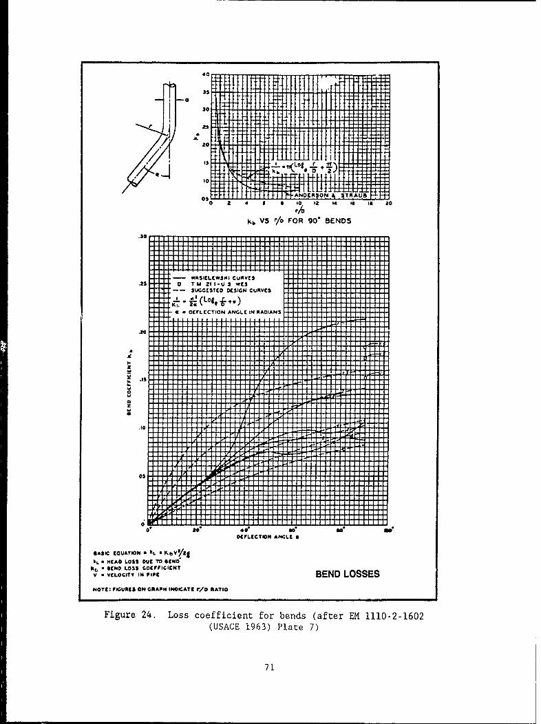
* 4t40

03

22

MMLECImlw ANL *

hLV r/ FORO LOSS OBENDSN

*~ -EN SUOSSTE DESIGNIN LOSSES

NOE ICRE O GAP I DTEFETO r/ ATIO INRDIN

Figure 24, Loss coefiit fo bed (aI e EM10-10(USAGE 1963 Plte7

71

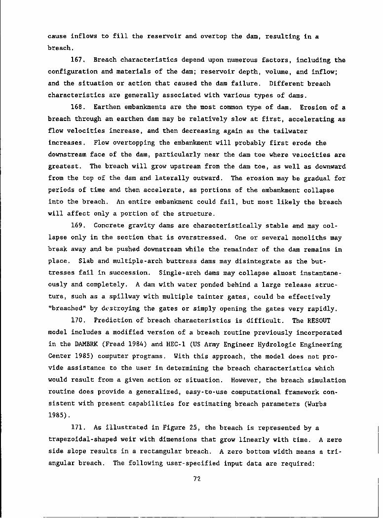
cause inflows to fill the reservoir and overtop the dam, resulting in a

breach.

167. Breach characteristics depend upon numerous factors, including the

configuration and materials of the dam; reservoir depth, volume, and inflow;

and the situation or action that caused the dam failure. Different breach

characteristics are generally associated with various types of dams.

168. Earthen embankments are the most common type of dam. Erosion of a

breach through an earthen dam may be relatively slow at first, accelerating as

flow velocities increase, and then decreasing again as the tailwater

increases. Flow overtopping the embankment will probably first erode the

downstream face of the dam, particularly near the dam toe where velocities are

greatest. The breach will grow upstream from the dam toe, as well as downward

from the top of the dam and laterally outward. The erosion may be gradual for

periods of time and then accelerate, as portions of the embankment collapse

into the breach. An entire embankment could fail, but most likely the breach

will affect only a portion of the structure.

169. Concrete gravity dams are characteristically stable and may col-

lapse only in the section that is overstressed. One or several monoliths may

break away and be pushed downstream while the remainder of the dam remains in

place. Slab and multiple-arch buttress dams may disintegrate as the but-

tresses fail in succession. Single-arch dams may collapse almost instantane-

ously and completely. A dam with water ponded behind a large release struc-

ture, such as a spillway with multiple tainter gates, could be effectively

"breached" by destroying the gates or simply opening the gates very rapidly.

170. Prediction of breach characteristics is difficult. The RESOUT

model includes a modified version of a breach routine previously incorporated

in the DAMBRK (Fread 1984) and HEC-I (US Army Engineer Hydrologic Engineering

Center 1985) computer programs. With this approach, the model does not pro-

vide assistance to the user in determining the breach characteristics which

would result from a given action or situation. However, the breach simulation

routine does provide a generalized, easy-to-use computational framework con-

sistent with present capabilities for estimating breach parameters (Wurbs

1985).

171. As illustrated in Figure 25, the breach is represented by a

trapezoidal-shaped weir with dimensions that grow linearly with time. A zero

side slope results in a rectangular breach. A zero bottom width means a tri-

angular breach. The following user-specified input data are required:

72

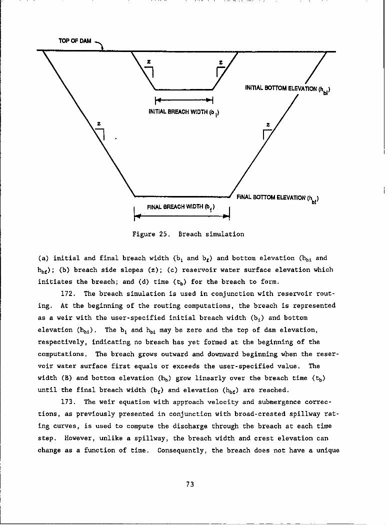
TOP OF DAM Z /INITIAL BOTTOM ELEVATION (h bl

INITIAL BREACH WIDTH (b I)

FINAL BOTTOM ELEVATION (hbf)

L FINAL BREACH WIDTH (bf),-

Figure 25. Breach simulation

(a) initial and final breach width (bi and bf) and bottom elevation (hbi and

hbf); (b) breach side slopes (z); (c) reservoir water surface elevation which

initiates the breach; and (d) time (tb) for the breach to form.

172. The breach simulation is used in conjunction with reservoir rout-

ing. At the beginning of the routing computations, the breach is represented

as a weir with the user-specified initial breach width (bk) and bottom

elevation (hbi). The bi and hbi may be zero and the top of dam elevation,

respectively, indicating no breach has yet formed at the beginning of the

computations. The breach grows outward and downward beginning when the reser-

voir water surface first equals or exceeds the user-specified value. The

width (B) and bottom elevation (hb) grow linearly over the breach time (tb)

until the final breach width (bf) and elevation (hbf) are reached.

173. The weir equation with approach velocity and submergence correc-

tions, as previously presented in conjunction with broad-crested spillway rat-

ing curves, is used to compute the discharge through the breach at each time

step. However, unlike a spillway, the breach width and crest elevation can

change as a function of time. Consequently, the breach does not have a unique

73

rating curve. The weir discharge computations are performed simultaneously

with the routing computations.

174. The weir equation is written as follows.

Q = k,(CrBH' 5 + Ct H2 .5 ) (53)

where

k, - 1.0 + 0.023Q2/[W 2 (h-hf) 2 (h-hb)]

k. - 1.0 if (ht-hb)/(h-hb) - 0.67

k. - 1.0 - 27.8 [(ht-hb)/(h-hb)] - 0.67) 3otherwise

B - bf if t-t - tb

B - bi + (bf-b±)(t-to)/(tb-to) otherwise

hb - hbf if t-t 0 - t b

hb - hbi - (hbi-hbf)(t-to)/(tb-to) otherwise

H - h - hb

The approach velocity and submergence correction factors are denoted by k, and

k., respectively. Cr and Ct denote discharge coefficients for the rectangular

and triangular portions of the trapezoidal weir. Cr and Ct are userspecified,

with default values of 3.1 and 2.45 coded in RESOUT. B is the width of the

rectangular portion of the weir at time t, and z is the breach side slope. At

any time (t), the reservoir water surface, breach bottom, and tailwater eleva-

tions are h, hb, and ht, respectively. The initial and final elevations of

the breach bottom are denoted hb± and hbf. The initial and final breach widths

are b i and bf, respectively. The breach begins to grow at time to .

Storage Routing

175. Reservoir routing consists of computing outflow as a function of

time, using the continuity equation

(I + 12)12 - (.1 + 02)/2 = (S 2 - S) I t (54)

74

where I, 0, and S denote inflow, outflow, and storage, respectively. The sub-

scripts 1 and 2 refer to the beginning and end of a computational intErval t.

At each time step, 02 and S2 are unknown. Values for 01 and S, are known from

the computations for the previous time step. Values for I, and 12 are

obtained from a known inflow hydrograph. A single-value relationship is

assumed to exist between storage and outflow. Reservoir water surface

elevation versus outflow and storage relationships are combined to obtain a

storage-versus-outflow relationship.

176. RESOUT contains two reservoir storage routing options. Both are

based on the continuity equation. One is an iterative and the other a non-

iterative solution of the continuity equation. The modified Puls method is a

noniterative solution algorithm which requires a rating curve as input. When

using this option in RESOUT, rating curves are computed for the various outlet

structures and combined prior to the routing computations. The computed com-

bined rating curve then becomes input for the routing routine. However, if a

dam breach is included in the anIysis, an iterative solution of the contin-

uity equation is required because the water surface elevation versus discharge

relationship varies with time. Consequently, a second routing option is used

for computing an outflow bdrograph involving a dam breach. Rating curves for

other outlet structures can also be included. Inclusion of reservoir evapora-

tion also requires an iterative solution. Thus, the iterative solution of the

continuity equation option must be used if a dam breach or reservoir evapora-

tion is included in the routing. Otherwise, modified Puls routing can be

used.

Modified Puls routing

177. The modified Puls or storage indication method of storage routing

is based on rearranging the continuity equation as follows:

2S2/ t + 02 = 1 1 + 12 + 2s1 / t + 01 (55)

where at each computational time step, the right-hand side of the equation is

known. The left-hand side is termed the storage indication. The storage

indication is computed for each time step using the above equation. Outflow

is determined from a relationship between (2S/ t + 0) and outflow. The method

is described by Viessman, Knapp, Lewis, and Harbaugh (1977) and Linsley and

Franzini (1979).

75

178. An elevation-versus-storage relationship and elevation-versus-

outflow relationship are combined to develop an elevation-versus-outflow rela-

tionship. The storage indication relationship (2S/ t + 0 versus 0) is

developed from the storage-versus-outflow relationship. The modified Puls

method can be used whenever a rating curve is available. In applying RESOUT,

the rating curve may be computed or provided as input data by the user.

Iterative solutionof continuity equation

179. In the case of a dam breach simulation, the discharge-versus-

elevation relationship varies with time as the breach grows. At each step of

the routing computations, the outflow and storage must be determined itera-

tively. For an assumed end-of-period storage and corresponding water surface

elevation, the outflow is computed using the weir equation. The computed

outflow is then used to revise the storage estimate.

180. Reservoir evaporation can also be included in this routing option.

Beginning and end-of-period storages are averaged to obtain an average storage

during the computational interval t. The storage is then combined with a

user-supplied reservoir elevation versus surface area relationship to deter-

mine an average srface area during the period. Evaporation is computed by

multiplying the water surface area by an evaporation rate, which is specified

by the user as input data.

Reservoir drawdown analysis

181. Military applications of the RESOUT model could involve the draw-

down or emptying of a reservoir. For example, reservoir releases may be used

to induce flooding or create barriers during combat operations. The reservoir

itself may provide an obstacle to combat operations above the dam. Another

example is the situation in which a strategically located dam is potentially

subject to enemy attack directed at destroying the dam to induce downstream

flooding. Drawdon plans could be developed for partially or completely

emptying the reservoir whenever a significant threat of attack is considered

to exist.

182. The reservoir routing capabilities of RESOUT can be used to per-

form drawdown analyses for various applications. Reservoir storage levels and

discharges are computed as a function of time for a given operating plan. An

operating plan is specified by the user as an outlet capacity rating curve and

target outflow hydrograph. Release targets, as specified by the user-supplied

target outflow hydrograph, are made at each time step of the routing unless

76

constrained by the outlet capacity or availability of water. Input data for

the routing computations include an inflow hydrograph, outlet capacity rating

curve, target outflow hydrograph, initial reservoir storage level, evaporation

rate, and reservoir storage-versus-elevation relationship.

77

PART V: RESERVOIR OUTFLOW (RESOUT) COMPUTER PROGRAM DESCRIPTION

183. The reservoir outflow (RESOUT) microcomputer model is a general-

ized software package for developing outlet structure rating curves and per-

forming storage routing computations. The procedures incorporated in the

program are outlined in Part IV of this report. Input data instructions,

example problems, definition of variables, and a program listing are provided

in Appendixes A, B, C, and D, respectively. A general description of the

program is provided below.

Summary of Program Capabilities

184, RESOUT is a flexible package with a number of options which can be

used as needed depending on the application. Rating curves (reservoir water

surface elevation-versus-discharge relationships) can be developed for a com-

prehensive range of outlet structure types and configurations. Storage rout-

ing computations can be performed to determine an outflow hydrograph

(discharge-versus-time relationship). A rating curve for the outlet struc-

tures is part of the input data required for the reservoir routing computa-

tions. Discharge through a dam breach, with breach dimensions which increase

linearly over time, can be included in the routing. Reservoir evaporation can

also be included. A drawdown analysis can be performed for a given operating

plan, which is specified by an outlet capacity rating curve and target outflow

hydrograph.

185. RESOUT develops rating curves using basic weir and orifice

equations. The rating curve computations are organized by outlet structure

category as follows: (a) uncontrolled ogee spillway; (b) uncontrolled broad-

crested spillway; (c) two alternative approaches for modeling gated spillways;

(d) drop inlet spillways; and, (e) outlet works. Since the computations are

based on fundamental equations representing the hydraulics of weirs and

orifices, the procedures are adaptable to the full spectrum of outlet struc-

ture types and designs. Rating curves for several outlet structures and/or

gate openings can be computed in a single run of the model for a single

reservoir.

186. Discharge coefficients and other empirical data presented in

Part IV are coded into the model, for the convenience of the user.

78

Alternatively, values for the required coefficients can be provided by the

user as input data.

187. RESOUT contains two reservoir routing routines. The modified Puls

method is a noniterative solution of the continuity equation. The second

option is an iterative solution of the continuity equation. RESOUT uses the

modified Puls approach unless a dam breach, reservoir evaporation, and/or

target outflow hydrograph are included in the simulation, in which case an

iterative solution is required.

Program Structure

188. RESOUT is a batch-oriented program written in ANSI standard

FORTRAN 77 to execute in a 640K, IBM-compatible microcomputer. It is composed

of a main driver program and a series of subroutines that may be called by the

main program or from other subroutines. The subroutines are listed in

Table 6. The array sizes are set to a maximum of 100 due to memory restric-

tions. The variable names are, in most cases, set to the maximum of six char-

acters to be most descriptive of the value they represent.

Input data

189. The inputs to the program are on multi-valued records. These

records are generated using any standard line editor. Their general format is

two capitalized alphanumeric characters followed by up to 10 fields of data.

The data cannot extend past column 80 in the input record, and there must be

at least one blank space between individual values. The majority of these

records are input using the RDIN subroutine.

190. If the record sequence is in error, execution is terminated, and

an error message i3 printed through subroutire ERR. This output will also

list the ID of the record in error. No error checking of the actual input

values is done.

Header intornation

191. "he main body of the program first inputs the names of the files

to be used. The names of these files are limited to eight characters to be in

agreement with standard MS-DOS practice. Any characters in excess of this

will be truncated. The program will then verify that the requ-. ted files

exist and create the output file. if required.

79

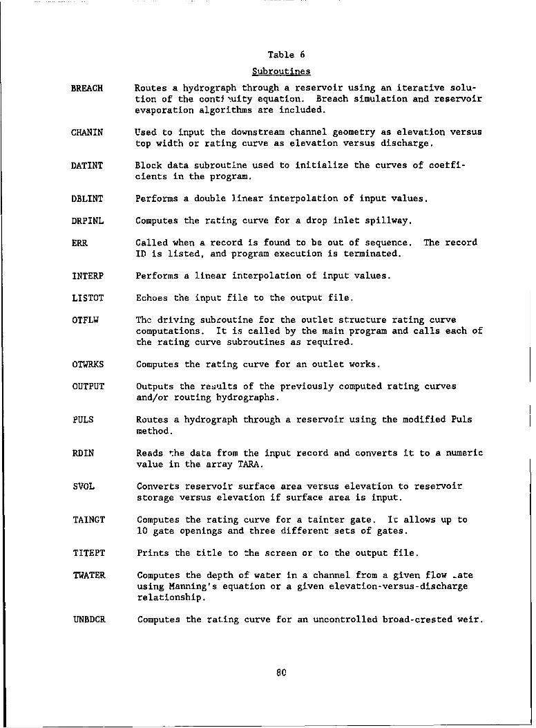
Table 6

Subroutines

BREACH Routes a hydrograph through a reservoir using an iterative solu-tion of the contl'.uity equation. Breach simulation and reservoirevaporation algorithms are included.

CHANIN Used to input the downstream channel geometry as elevation versustop width or rating curve as elevation versus discharge.

DATINT Block data subroutine used to initialize the curves of coetfi-cients in the program.

DBLINT Performs a double linear interpolation of input values.

DRPINL Computes the rating curve for a drop inlet spillway.

ERR Called when a record is found to be out of sequence. The recordID is listed, and program execution is terminated.

INTERP Performs a linear interpolation of input values.

LISTOT Echoes the input file to the output file.

OTFLW Thc driving subroutine for the outlet structure rating curvecomputations. It is called by the main program and calls each ofthe rating curve subroutines as required.

OTWRKS Computes the rating curve for an outlet works.

OUTPUT Outputs the results of the previously computed rating curvesand/or routing bydrographs.

PULS Routes a hydrograph through a reservoir using the modified Puls

method.

RDIN Reads the data from the input record and converts it to a numericvalue in the array TARA.

SVOL Converts reservoir surface area versus elevation to reservoir

storage versus elevation if surface area is input.

TAINGT Computes the rating curve for a tainter gate. It allows up to

10 gate openings and three different sets of gates.

TITEPT Prints the title to the screen or to the output file.

TWATER Computes the depth of water in a channel from a given flow .ateusing Manning's equation or a given elevation-versus-dischargerelationship.

UNBDCR Computes the rating curve for an uncontrolled broad-crested weir.

80

UNCNOG Computes the rating curve for an uncontrolled ogee spillway.

VLIFTG Computes the rating curve for a vertical lift gate. It allows upto 10 gate openings and three different sets of gates.

81

192. The program will then read in three ID records. The labels on

these records are limited to 78 characters. These records are for user

identification of the output only.

193. An 10 record is next read to determine if the input data are to be

echoed to the output file. If they are, subroutine LISTOT is called, and the

input file is listed out.

194. A KK record is the next input. The information provided on this

field is limited to 40 characters and is echoed out as the reservoir name in

the output.

Rating curve generation

195. The downstream channel geometry or rating curve is next input

through the use of the subroutine CHANIN. From the elevation-versus-top width

or elevation-versus-discharge information provided as input data, the depth of

flow in the downstream channel is calculated by subroutine TWATER for use in

the submergence computations in subroutines UNBDCR and UNCNOG. With the

elevation-versus-top width input option, the Manning equation is used in

subroutine TWATER for the computation of flow depth.

196. The next section of the program calculates the rating curves by

calling the subroutine OTFLW. At least one structure must be specified. If

no outflow is desired, d rating curve with a zero outflow for all elevations

may be used. The subroutines for the different types of outlet structures

specified by the user are called as needed. The final result from this sec-

tion is one combined rating curve that is used in the routing section of the

program.

197. The user may, at this point, terminate the program by the inser-

tion of a ZZ record. The output generated will be the series of rating curves

requested by the user, and no routing will be done.

Routing

198. If routing is required, reservoir storage data are next inputted

to the program. Reservoir water surface elevation versus either storage or

water surface area are entered. If the latter is chosen, subroutine SVOL

computes reservoir storage volume from the given surface areas. The elevation

included in the inputted storage or area data must encompass the elevations

given as minimum and maximum for the computation of rating curves.

199. The starting reservoir water surface elevation and the inflow

hydrograph are provided as input data. A maximum of 99 discharges may be

entered from the inflow hydrograph records.

82

200. Routing is performed with either subroutine PULS or subroutine

BREACH, depending on whether the continuity equation can be solved by the

noniterative modified Puls approach. An iterative solution algorithm is

required if a breach simulation or evaporation is included in the routing.

The target release hydrograph option is also combined with the iterative solu-

tion method.

201. The standard modified Puls routing method is incorporated into

subroutine PULS. The storage indication curve (2S/At+O versus outflow) is

developed. Using the inflow hydrograph and this relationship, an outflow is

generated for each time step. Using the rating curve generated previously,

the water surface elevation is also calculated.

202. An iterative solution of the continuity equation, which is incor-

porated in the BREACH subroutine, is used for performing a drawdown analysis

with a specified target release hydrograph. For each time interval, the tar-

get release is made unless constrained by water available from storage and

inflow or the outlet capacity rating curve. Reservoir evaporation can also be

included in the analysis.

203. The BREACH subroutine also contains the breach simulation algo-

rithm. The modified Puls method of routing is used until the reservoir water

surface elevation reaches the user-specified elevation at which a breach will

occur. Once this elevation has been reached, the outflow from the outlet

structures is combined with flow through the breach to determine total out-

flow from the dam. The breach is characterized by the initial breach eleva-

tion and width, final elevation and width, side slope, and time from the start

of the breach until the final width and elevation are reached. For each time

step, the flow is divided between the rectangular and triangular sections of

the breach. Any flow over the top of the dam is also considered as flow

through a rectangular weir section. The bi-section method of convergence is

used in the iterative solution algorithm.

204. The end result of each of the routings is an outflow hydrograph

consisting of up to 99 discharges at the time intervals specified by the user.

After the rating curves have been developed and the routing, if requested, is

performed, the generated values are printed out. The output will include all

rating curves and the outflow hydrograph.

83

PART VI: SUMMARY AND RECOMMENDATIONS

205. Barrier creation resulting from the regulation of reservoir struc-

tures can inflict severe damage on military operations. Ferrying and bridging

operations can be completely halted by flood waves emanating from upstream

reservoirs. Pulsating flood waves can be propagated throughout downstream

river reaches by opening and closing the gated spillways. In a defensive sce-

nario, a potential deterrent to an attack on a strategically located Oam could

be to partially empty the reservoir whenever a significant threat of ttack is

considered to exist.

206. The ability to predict the extent of downstream flooding resulting

from reservoir regulation should be considered an important part of contin-

gency planning. This report provides the procedures necessary to make these

predictions.

207. Different types of dams, spillways, and outlet structures require

different computational procedures. This report identifies the various types

of structures that may make up a reservoir, and presents the basic hydraulic

equations for each. These computational procedures are then coded for an IBM

PC-compatible microcomputer. Input instructions and example applications are

also included. These applications include: (a) predicting reservoir outflow

for given conditions, (b) determining outlet structure gate openings or breach

size required to achieve specified outflows, and (c) analysis of reservoir

drawdowns.

208. The following recommendations are made, so that the procedures

developed may be useful to the military in the field:

a. Procedures should be tested on specific reservoirs, and a com-parison made between predicted and actual discharge. Thesereservoirs would ideally be located outside of the US, sincethe equations in the procedures have been used in the designof most US structures.

b. Sensitivity of the results to many of the required parametersshould be determined in order to identify the most criticalparameters.

c. Procedures developed in this report should be linked to arouting capability, so thdt effects of reservoir regulationcan be predicted at any point downstream. Likely candidatesinclude: MILHY, TACDAM, and DAMBRK. By including these pro-cedures in MILHY, an inflow hydrograph to the reservoir couldalso be integrated. TACDAM and DAMBRK currently model onlydam breaches, so the inclusion of the developed procedureswould make these packages useful over a broader spectrum.

84

REFERENCES

American Society of Civil Engineers. 1963. "Bibliography on the HydraulicDesign of Spillways," Journal of the Hydraulics Division, ASCE Task Force onthe Hydraulic Design of Spillways, Vol 89, No. HY4, pp 117-139.

Bos, M. B. 1985. Long-Throated Flumes and Broad-Crested Weirs, MartinusNijhoff and Dr. W. Junk, Publishers, Dordrecht, The Netherlands.

Bos, M. G., ed. 1976. Discharge Measurement Structures, International Insti-tute for Land Reclamation and Improvement, Wageningen, The Netherlands.

Brater, E. F. 1959. "Hydraulics," Civil Engineering Handbook, L. C.Urquhart, ed., McGraw-Hill, New York, pp 4.44-4.60.

Brater, E. F., and King, H. W. 1976. Handbook of Hydraulics, 6th ed.,

McGraw-Hill, New York.

Chow, Ven Te. 1959. Open Channel Hydraulics, McGraw-Hill, New York.

Cox, R. G. 1973. "Resistance Losses in Noncircular Flood Control Conduitsand Sluices," Miscellaneous Paper H-73-1, US Army Engineer Waterways Experi-ment Station, Vicksburg, MS.

Daugherty, R. L., Franzini, J. B., and Finnemore, E. J. 1985. Fluid Mechan-ics with Engineering Applications, 8th ed., McGraw-Hill, New York.

Davis, C. V., and Sorensen, K. E., eds. 1984. Handbook of Applied Hydraul-ics, 3rd. ed., McGraw-Hill, New York.

Fread, D. L. 1984. "DAMBRK: The NWS Dam-Break Flood Forecasting Model,"

National Weather Service, Silver Spring, MD.

French, R. H. 1985. Open-Channel Hydraulics, McGraw-Hill, New York.

Golze, A. R., ed. 1977. Handbook of Dam Engineering,. Van Nostrand ReinholdCo., New York.

International Commission on Large Dams. 1984. "World Register of Dams,"

Paris, France.

Linsley, Ray K., and Franzini, Joseph B. 1979. Water Resources Engineering,3rd ed., McGraw-Hill, New York.

Maynord, S. T. 1985, "General Spillway Investigation; Hydraulic Model Inves-tigation," Technical Report HL-85-1, US Army Engineer Waterways ExperimentStation, Vicksburg, MS.

Morris, H. M., and Wiggert, J. M. 1972. Applied Hydraulics in Engineering,

2nd ed., Ronald Press, New York.

Thomas, H. H. 1976. The Engineering of Large Dams. John Wiley and Sons,London, Great Britain.

US Army Corps of Engineers. 1963. "Hydraulic Design of Reservoir Outlet

Structures," Engineer Manual 1110-2-1602, Washington DC.

_ 1965. "Hydraulic Design of Spillways," Engineer Manual 1110-2-1603, Washington, DC.

US Army Engineer Hydrologic Engineering Center. 1982. "HEC-2, Water SurfaceProfiles; User's Manual," Davis, CA.

85

US Army Engineer Hydrologic Engineering Center. 1985. "HEC-l, Flood Hydro-graph Package; User's Manual," Davis, CA.

US Army, Office, Chief of Engineers, Hydraulic Design Criteria. prepared bythe US Army Engineer Waterways Experiment Station, Vicksburg, MS, loose-leafby serials, through the 18th issue, Dec 1988.

US Bureau of Reclamation. 1948. "Studies of Crests for Overfall Dams;Part VI: Hydraulic Investigations," Boulder Canyon Project Final Reports,Bulletin 3, Denver, CO.

1976. Design of Gravity Dams, Denver, CO.

1977a. Design of Arch Dams, Denver, CO.

1977b. Design of Small Dams, Denver, CO.

Vennard, J. K. 1954. Elementary Fluid Mechanics, John Wiley and Sons, NewYork.

Viessman, W., Knapp, J. W., Lewis, G. L., and Harbaugh, T. E. 1977. Intro-duction to Hydrology, 2nd ed., Harper and Row.

Wurbs, R. A. 1985. "Military Hyirology; Report 9, State-of-the-Art Reviewand Annotated Bibliography of Dam-Breach Flood Forecasting," MiscellaneousPaper EL-79-6, US Army Engineer Waterways Experiment Station, Vicksburg, MS.

86

* APPENDIX A: INPUT DATA INSTRUCTIONS

RECORD FIELD FIELD CONTENTS

ID Model Run ID Record (three records required)

Col 1+2 ID

1 Any label up to 78 characters long.

10 Output Control Record (one required)

Col 1+2 10

1 0 or blank Do not echo input file to output file1 Echo input file to output file

2 0 English units1 Metric units

KK Reservoir Identifier (one required)

Col 1+2 KK

1 Any label up to 40 characters

Al

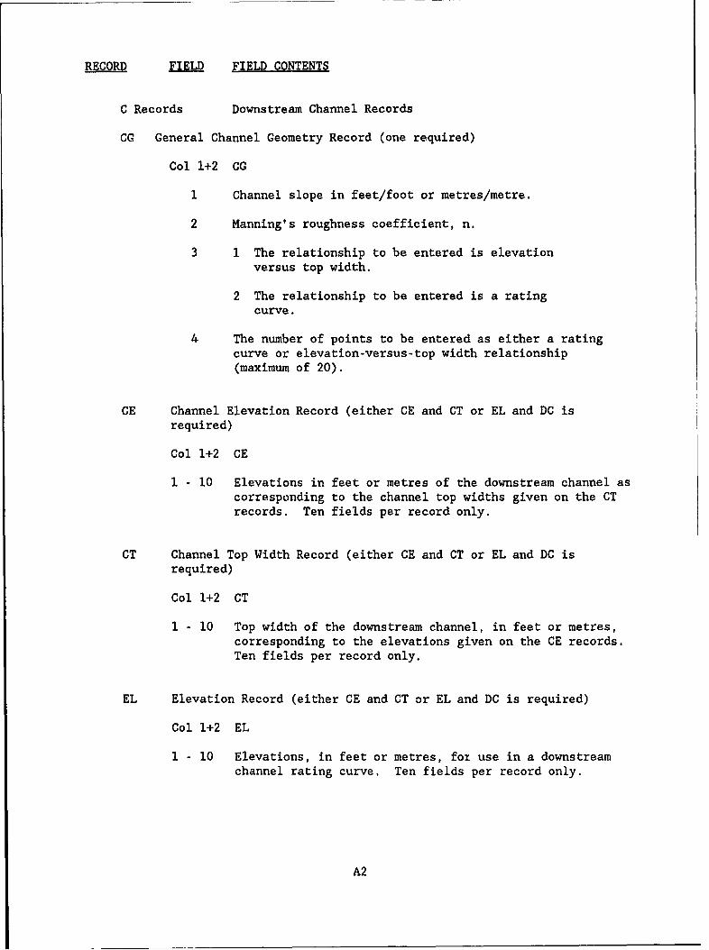
RECORD FIELD FIELD CONTENTS

C Records Downstream Channel Records

CG General Channel Geometry Record (one required)

Col 1+2 CG

1 Channel slope in feet/foot or metres/metre.

2 Manning's roughness coefficient, n.

3 1 The relationship to be entered is elevationversus top width.

2 The relationship to be entered is a ratingcurve.

4 The number of points to be entered as either a ratingcurve or elevation-versus-top width relationship(maximum of 20).

CE Channel Elevation Record (either CE and CT or EL and DC is

required)

Col 1+2 CE

1 - 10 Elevations in feet or metres of the downstream channel ascorresponding to the channel top widths given on the CTrecords. Ten fields per record only.

CT Channel Top Width Record (either CE and CT or EL and DC is

required)

Col 1+2 CT

1 - 10 Top width of the downstream channel, in feet or metres,corresponding to the elevations given on the CE records.Ten fields per record only.

EL Elevation Record (either CE and CT or EL and DC is required)

Col 1+2 EL

1 - 10 Elevations, in feet or metres, foz use in a downstreamchannel rating curve, Ten fields per record only.

A2

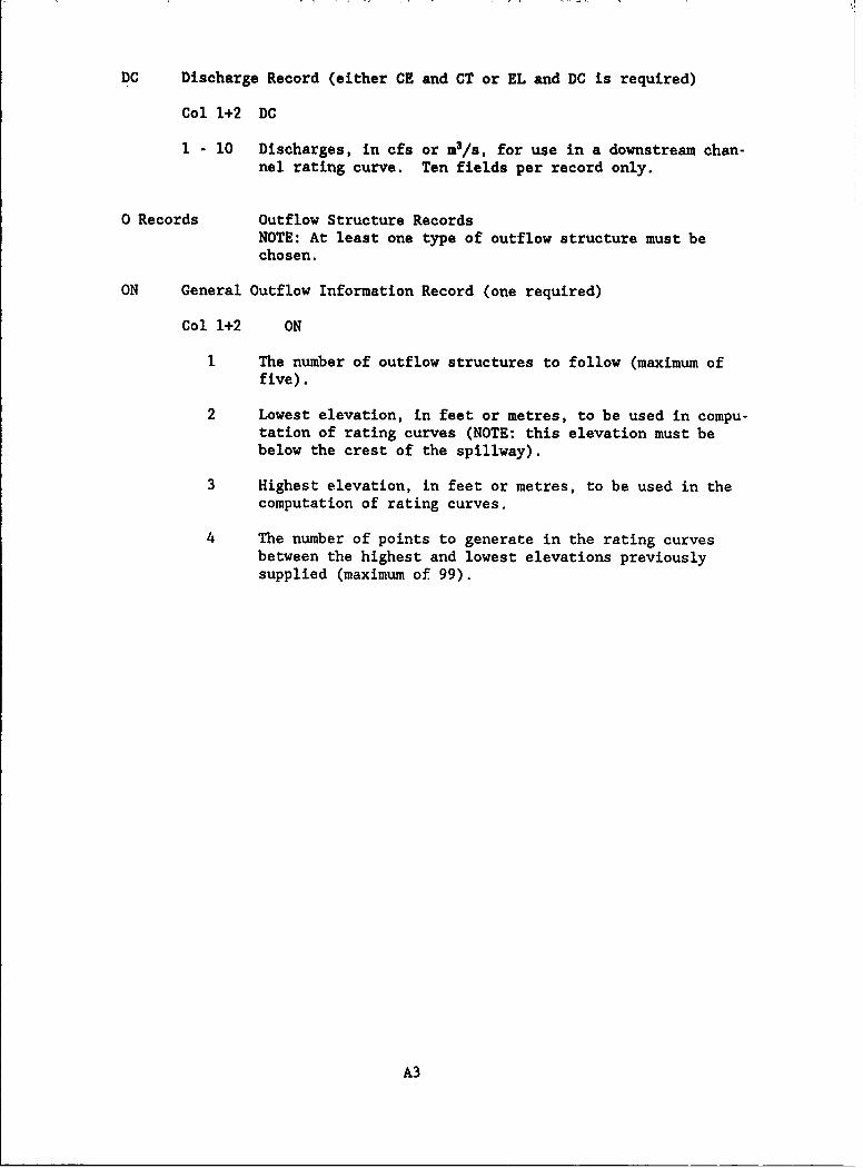
DC Discharge Record (either CE and CT or EL and DC is required)

Col 1+2 DC

1 - 10 Discharges, in cfs or m3/s, for use in a downstream chan-nel rating curve. Ten fields per record only.

O Records Outflow Structure RecordsNOTE: At least one type of outflow structure must bechosen.

ON General Outflow Information Record (one required)

Col 1+2 ON

I The number of outflow structures to follow (maximum offive).

2 Lowest elevation, in feet or metres, to be used in compu-tation of rating curves (NOTE: this elevation must bebelow the crest of the spillway).

3 Highest elevation, in feet or metres, to be used in thecomputation of rating curves.

4 The number of points to generate in the rating curvesbetween the highest and lowest elevations previouslysupplied (maximum of 99).

A3

RFIEL FIELD CONTENTS

UO Uncontrolled Ogee SpillwayTwo Records Required

Record 1Col 1+2 UO

1 Kp + Use the given pier contraction coefficient.

0 Use no pier contraction coefficient.

- Use the internal tables to generate a pier con-traction coefficient.

2 Ka + Use the given abutment contraction coefficient.

0 Use no abutment contraction coefficient.

- Use the internal tables to generate an abutmentcontraction coefficient.

3 C + Use the given weir flow coefficient.

0 Use the internal tables to generate a weir flowcoefficient.

4 Approach width, in feet or metres, of channel leading toogee spillway.

5 Approach depth, in feet or metres, of channel leading toogee spillway.

6 Height of crest, in feet or metres, above approach apron orapproach channel.

7 Design head, in feet or metres.

8 Number of piers in the spillway.

9 Net length, in feet or metres, of the spillway excluding thetotal width of included piers.

10 Pier type of the included piers (1-4).

A4

RQU EUL FIELD CONTENTS

Record 2

Col 1+2 UO

1 Elevation, in feet or metres, of the crest of thespillway.

2 1 The material immediately adjacent to the spillway isconcrete.

2 The material immediately adjacent to the spillway isearth.

3 The adjacent section radius, in feet or metres, if the

material is concrete.

4 Cs + Use the given submergence coefficient.

0 Make no correction for submergence.

- Use the internal tables to generate a submer-gence coefficient.

5 Number of slope face correction factor pairs for non-vertical slopes that will appear on the following records(maximum of 99)

Record 3Col 1+2 UO

1-10 Head, in feet or metres, over the spillway correspondingto the following slope face correction factors. Use asmany records as required with 10 values per record.

Record 4Col 1+2 UO

1-10 Slope face correction factors corresponding to the pre-vious heads over the spillway.

A5

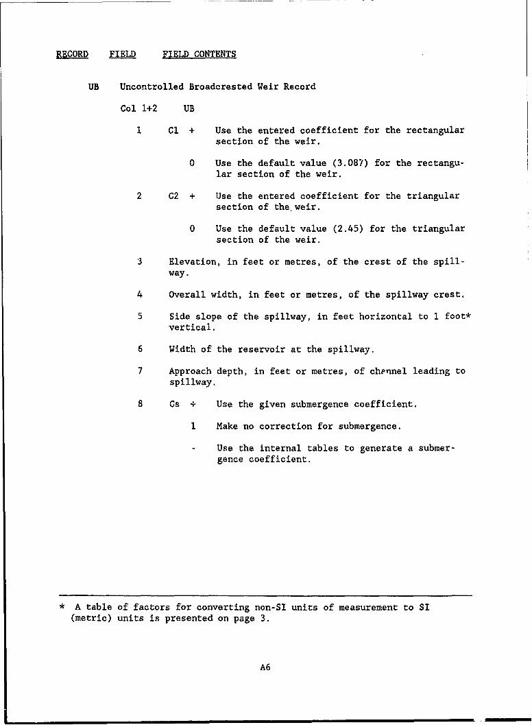
RECORD FIELD FIELD CONTENTS

UB Uncontrolled Broadcrested Weir Record

Col 1+2 UB

I Cl + Use the entered coefficient for the rectangularsection of the weir.

0 Use the default value (3.087) for the rectangu-lar section of the weir.

2 C2 + Use the entered coefficient for the triangularsection of the weir.

0 Use the default value (2.45) for the triangularsection of the weir.

3 Elevation, in feet or metres, of the crest of the spill-

way.

4 Overall width, in feet or metres, of the spillway crest.

5 Side slope of the spillway, in feet horizontal to 1 foot*vertical.

6 Width of the reservoir at the spillway.

7 Approach depth, in feet or metres, of chennel leading tospillway.

8 Cs + Use the given submergence coefficient.

I Make no correction for submergence.

- Use the internal tables to generate a submer-

gence coefficient.

* A table of factors for converting non-SI units of measurement to SI(metric) units is presented on page 3.

A6

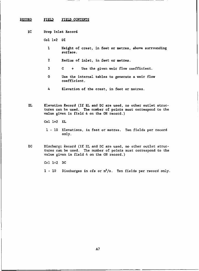
RECORD EIELD FIELD CONTENTS

DI Drop Inlet Record

Col 1+2 DI

1 Height of crest, in feet or metres, above surroundingsurface.

2 Radius of inlet, in feet or metres.

3 C + Use the given weir flow coefficient.

0 Use the internal tables to generate a weir flowcoefficient.

4 Elevation of the crest, in feet or metres.

EL Elevation Record (If EL and DC are used, no other outlet struc-tures can be used. The number of points must correspond to thevalue given in field 4 on the ON record.)

Col 1+2 EL

1 - 10 Elevations, in feet or metres. Ten fields per recordonly.

DC Dischargc Record (If EL and DC are used, no other outlet struc-tures can be used. The number of points must correspond to thevalue given in field 4 on the ON record.)

Col 1+2 DC

1 - 10 Discharges in cfs or m3/s. Ten fields per record only.

A7

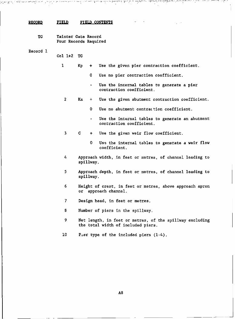
RECORD FIELD FIELD CONTENTS

TG Tainter Gate RecordFour Records Required

Record 1

Col 1+2 TG

1 Kp + Use the given pier contraction coefficient.

0 Use no pier contraction coefficient.

- Use the internal tables to generate a piercontraction coefficient.

2 Ka + Use the given abutment contraction coefficient.

0 Use no abutment contraction coefficient.

- Use the internal tables to generate an abutmentcontraction coefficient.

3 C + Use the given weir flow coefficient.

0 Use the internal tables to generate a weir flowcoefficient.

4 Approach width, in feet or metres, of channel leading tospillway.

5 Approach depth, in feet or metres, of channel leading tospillway.

6 Height of crest, in feet or metres, above approach apron

or approach channel.

7 Design head, in feet or metres.

8 Number of piers in the spillway.

9 Net length, in feet or metres, of the spillway excluding

the total width of included piers.

10 Pier type of the included piers (1-4).

A8

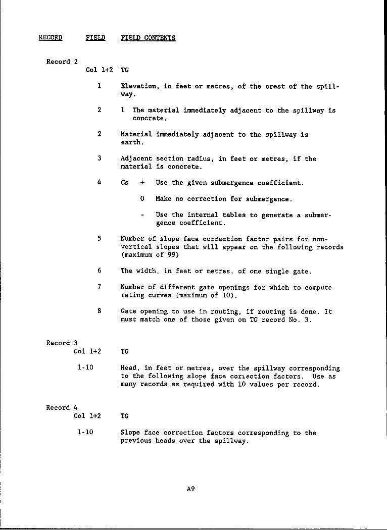
RECORD FIELD FIELD CONTENTS

Record 2Col 1+2 TG

1 Elevation, in feet or metres, of the crest of the spill-way.

2 1 The material immediately adjacent to the spillway isconcrete.

2 Material immediately adjacent to the spillway isearth.

3 Adjacent section radius, in feet or metres, if the

material is concrete.

4 Cs + Use the given submergence coefficient.

0 Make no correction for submergence.

- Use the internal tables to generate a submer-gence coefficient.

5 Number of slope face correction factor pairs for non-vertical slopes that will appear on the following records(maximum of 99)

6 The width, in feet or metres, of one single gate.

7 Number of different gate openings for which to compute

rating curves (maximum of 10).

8 Gate opening to use in routing, if routing is done. Itmust match one of those given on TG record No. 3.

Record 3Col 1+2 TG

1-10 Head, in feet or metres, over the spillway correspondingto the following slope face correction factors. Use asmany records as required with 10 values per record.

Record 4Col 1+2 TG

1-10 Slope face correction factors corresponding to theprevious heads over the spillway.

A9

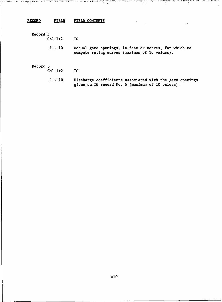
REGORD FELD FIELD CONTENTS

Record 5Col 1+2 TG

1 - 10 Actual gate openings, in feet or metres, for which tocompute rating curves (maximum of 10 values).

Record 6Col 1+2 TG

1 - 10 Discharge coefficients associated with the gate openingsgiven on TG record No. 5 (maximum of 10 values).

AlO

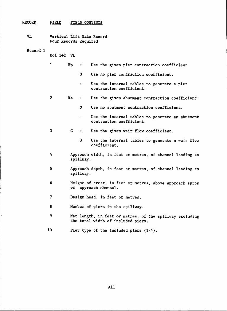
RECORD FIELD FIELD CONTENTS

VL Vertical Lift Gate RecordFour Records Required

Record 1

Col 1+2 VL

1 Kp + Use the given pier contraction coefficient.

0 Use no pier contraction coefficient.

- Use the internal tables to generate a piercontraction coefficient.

2 Ka + Use the given abutment contraction coefficient.

0 Use no abutment contraction coefficient.

- Use the internal tables to generate an abutmentcontraction coefficient.

3 C + Use the given weir flow coefficient.

0 Use the internal tables to generate a weir flowcoefficient.

4 Approach width, in feet or metres, of channel leading tospillway.

5 Approach depth, in feet or metres, of channel leading tospillway.

6 Height of crest, in feet or metres, above approach apron

or approach channel.

7 Design head, in feet or metres.

8 Number of piers in the spillway.

9 Net length, in feet or metres, of the spillway excludingthe total width of included piers.

10 Pier type of the included piers (1-4).

All

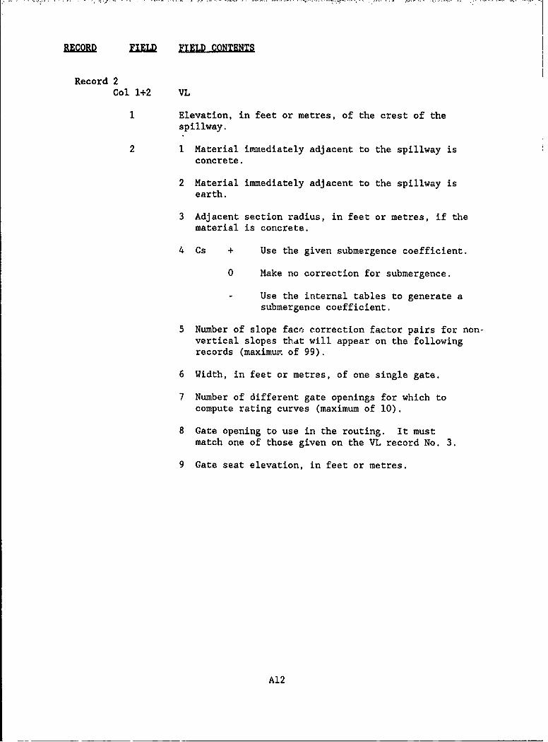
RECORD FIELD CONTENTS

Record 2Col 1+2 VL

Elevation, in feet or metres, of the crest of thespillway.

2 1 Material immediately adjacent to the spillway isconcrete.

2 Material immediately adjacent to the spillway isearth.

3 Adjacent section radius, in feet or metres, if thematerial is concrete.

4 Cs + Use the given submergence coefficient.

0 Make no correction for submergence.

- Use the internal tables to generate asubmergence coefficient.

5 Number of slope face. correction factor pairs for non-vertical slopes that will appear on the followingrecords (maximur of 99).

6 Width, in feet or metres, of one single gate.

7 Number of different gate openings for which to

compute rating curves (maximum of 10).

8 Gate opening to use in the routing. It must

match one of those given on the VL record No. 3.

9 Gate seat elevation, in feet or metres.

A12

RECORD FIELD FIELD CONTENTS

Record 3Col 1+2 VL

1-10 Head, in feet or metres, over the spillway correspondingto the following slope face correction factors. Use asmany records as required with 10 values per record.

Record 4Col 1+2 VL

1-10 Slope face correction factors corresponding tc the previ-ous heads over the spillway.

Record 5Col 1+2 VL

1 - 10 The actual gate openings, in feet or metres, for which tocompute rating curves (maximum of 10 values).

Al3

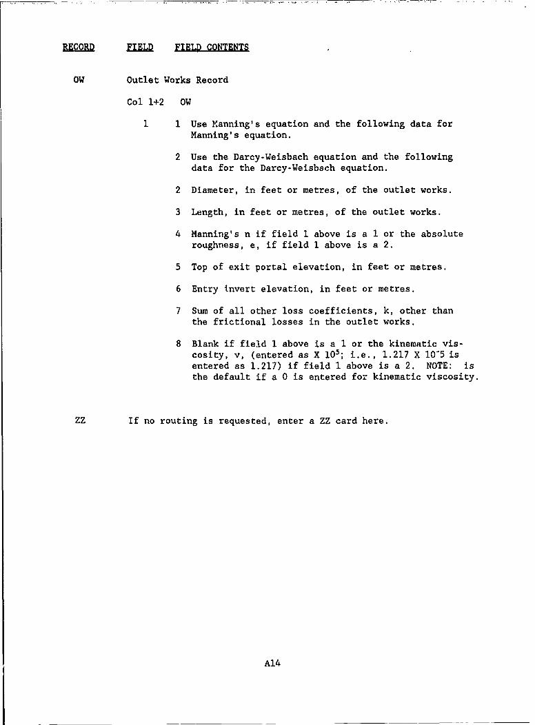
RECRD FIELD FIELD CONTENTS

OW Outlet Works Record

Col 1+2 OW

1 1 Use Manning's equation and the following data forManning's equation.

2 Use the Darcy-Weisbach equation and the followingdata for the Darcy-Weisbach equation.

2 Diameter, in feet or metres, of the outlet works.

3 Length, in feet or metres, of the outlet works.

4 Manning's n if field 1 above is a 1 or the absoluteroughness, e, if field 1 above is a 2.

5 Top of exit portal elevation, in feet or metres.

6 Entry invert elevation, in feet or metres.

7 Sum of all other loss coefficients, k, other thanthe frictional losses in the outlet works.

8 Blank if field I above is a 1 or the kinematic vis-cosity, v, (entered as X 105; i.e., 1.217 X 10-5 isentered as 1.217) if field 1 above is a 2. NOTE: isthe default if a 0 is entered for kinematic viscosity.

ZZ If no routing is requested, enter a ZZ card here.

A14

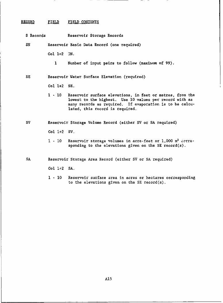
MFIELD FIELD CONTENTS

S Records Reservoir Storage Records

SN Reservoir Basic Data Record (one required)

Col 1+2 3N.

1 Number of input pairs to follow (maximum of 99).

SE Reservoir Water Surface Elevation (required)

Col 1+2 SE.

1 - 10 Reservoir surface elevations, in feet or metres, from thelowest to the highest. Use 10 values per record with asmany records as required. If evaporation is to be calcu-lated, this record is required.

SV Reservoir Storage Volume Record (either SV or SA required)

Col 1+2 SV.

1 - 10 Reservoir storage volumes in acre-feet or 1,000 m3 corre-sponding to the elevations given on the SE record(s).

SA Reservoir Storage Area Record (either SV or SA required)

Col 1+2 SA.

1 - 10 Reservoir surface area in acres or hectares corresponding

to the elevations given on the SE record(s).

A15

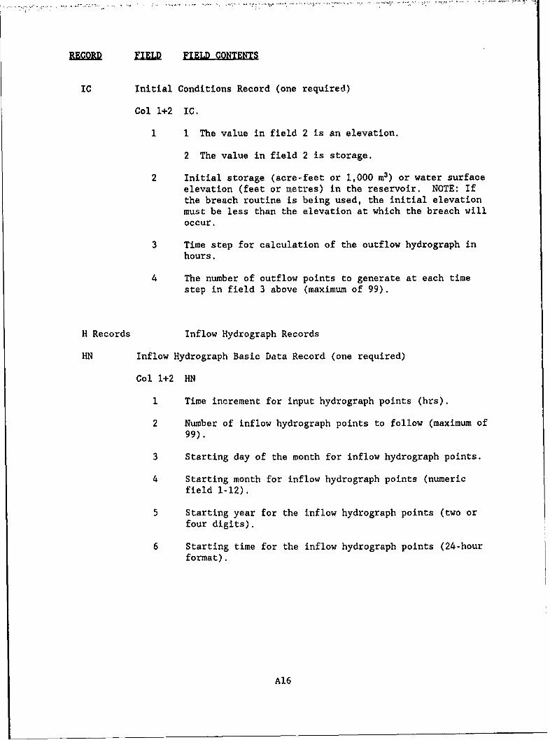
RECORD FLD FELD CONTENTS

IC Initial Conditions Record (one required)

Col 1+2 IC.

1 1 The value in field 2 is an elevation.

2 The value in field 2 is storage.

2 Initial storage (acre-feet or 1,000 m3) or water surfaceelevation (feet or metres) in the reservoir. NOTE: Ifthe breach routine is being used, the initial elevationmust be less than the elevation at which the breach willoccur.

3 Time step for calculation of the outflow hydrograph inhours.

4 The number of outflow points to generate at each timestep in field 3 above (maximum of 99).

H Records Inflow Hydrograph Records

HN Inflow Hydrograph Basic Data Record (one required)

Col 1+2 HN

1 Time increment for input hydrograph points (hrs).

2 Number of inflow hydrograph points to follow (maximum of99).

3 Starting day of the month for inflow hydrograph points.

4 Starting month for inflow hydrograph points (numericfield 1-12).

5 Starting year for the inflow hydrograph points (two orfour digits).

6 Starting time for the inflow hydrograph points (24-hourformat).

A16

RECORD FIELD FIELD CONTENTS

HI Inflow Hydrograph Record (required)

Col 1+2 HI

1 - 10 Values of inflow hydrograph at the end of each timeincrement in field I of HN record in cfs or m3/s. Use asmany records as required.

Routing RecordsNOTE: If no routing is chosen, only the rating curves will becomputed and output.

DB Dam Breach Record

Record 1Col 1+2 DB

1 Elevation, in feet or metres, of the top of the dam.

2 Elevation, in feet or metres, of the top of the breach.

3 The initial width, in feet or metres, of the breach.

4 Elevation, in feet or metres, of the bottom of thebreach.

5 The final width, in feet or metres, of the breach.

6 The side slope of the breach, in units horizontal to

one unit vertical.

7 The time required to reach maximum breach size, in hours.

8 Weir flow coefficient for a rectangular weir. If 0 isentered, 3.1 will default.

9 Weir flow coefficient for a triangular weir. If 0 isentered, 2.45 will default.

10 Width of the reservoir at the dam, in feet or metres.

Al7

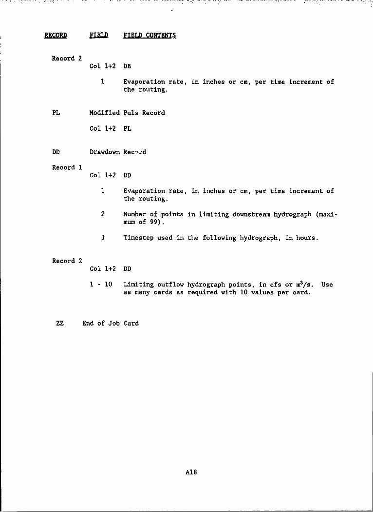
RECORD ELM FIELD CONTEI

Record 2Col 1+2 DB

1 Evaporation rate, in inches or cm, per time increment ofthe routing.

PL Modified Puls Record

Col 1+2 PL

DD Drawdown Rec-:d

Record 1Col 1+2 DD

1 Evaporation rate, in inches or cm, per time increment ofthe routing.

2 Number of points in limiting downstream hydrograph (maxi-mum of 99).

3 Timestep used in the following hydrograph, in hours.

Record 2Col 1+2 DD

1 - 10 Limiting outflow hydrograph points, in cfs or m3/s. Useas many cards as required with 10 values per card.

ZZ End of Job Card

A18

APPENDIX B: EXAMPLE PROBLEMS

1. A series of eight example problems are presented here to illustrate

the capabilities of RESOUT. The first six examples consist of computing rat-

ing curves for various types of outlet structures. Example 7 is a drawdown

analysis, which combines rating curve and routing computations. Example 8 is

a breach simulation. The model output, including an input data listing, is

reproduced for each example. The reader should refer to Appendix A for a

description of each of the input data records used in the examples.

Example 1: Rating Curves for an Ogee Spillway,with Tainter Gate, and Outlet Works

2. The first example involves developing rating curves for alternative

gate openings for a single tainter gate on an ogee spillway. A rating curve

for the outlet works is also computed and combined with the spillway rating

-. ve for a specified gate opening.

3. The RESOUT output for this example is presented on the following

pages. As indicated by the input data echo included in the output, header

information is provided by the required three model run identifier (ID)

records and one reservoir identifier (KK) record. The output control (10)

record specifies that the input data file be echoed to the output file and

that English units be used. Thus, the discharges in the computed outlet

structure rating tables are given in units of cubic feet per second.

4. A rating table (water surface elevation in feet versus discharge in

cubic feet per second) for the channel downstream of the dam is provided by

the channel geometry (CG), elevation (EL), and discharge (DC) records. This

tailwater rating curve is used by the model to test and correct the spillway

discharge for submergence conditions.

5. The outflow information (ON) record specifies two outlet structures

(outlet works and gated ogee spillway), with discharges to be commuted for

40 evenly spaced reservoir water surface elevations between 465 and 505 feet.

6. The first tainter gate (TG) record and first five fields of the

second TG record provide the input data used by the model to compute

discharges over the uncontrolled weir for reservoir water surface elevations

below the elevation at which gate control occurs. The first TG record speci-

fies use of the abutment contraction and discharge coefficient data coded into

the model. Since a single gate bay is being modeled, piers are not included

Bl

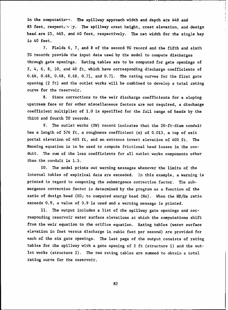
in the computatior'!. The spillway approach width and depth are 440 and

85 feet, respecth-e.y. The spillway crest height, crest elevation, and design

head are 25, 465, and 40 feet, respectively. The net width for the single bay

is 40 feet.

7. Fields 6, 7, and 8 of the second TO record and the fifth and sixth

TG records provide the input data used by the model to compute discharges

through gate openings. Rating tables are to be computed for gate openings of

2, 4, 6, 8, 10, and 40 ft, which have corresponding discharge coefficients of

0.68, 0.68, 0.68, 0.68, 0.71, and 0.71. The rating curves for the first gate

opening (2 ft) and the outlet works will be combined to develop a total rating

curve for the reservoir.

8. Since corrections to the weir discharge coefficients for a sloping

upstream face or for other miscellaneous factors are not required, a discharge

coefficient multiplier of 1.0 is specified for the full range of heads by the

third and fourth TG records.

9. The outlet works (OW) record incicates that the 20-ft-diam conduit

has a length of 576 ft, a roughness coefficient (n) of 0.013, a top of exit

portal elevation of 405 ft, and an entrance invert elevation of 400 ft. The

Manning equation is to be used to compute frictional head losses in the con-

duit. The sum of the loss coefficients for all outlet works components other

than the conduit is 1.5.

10. The model prints out warning messages whenever the limits of the

internal tables of empirical data are exceeded. In this example, a warning is

printed in regard to computing the submergence correction factor. The sub-

mergence correction factor is determined by the program as a function of the

ratio of design head (HD) to computed energy head (He). When the HD/He ratio

exceeds 0.9, a value of 0.9 is used and a warning message is printed.

11. The output includes a list of the spillway gate openings and cor-

responding reservoir water surface elevations at which the computations shift

from the weir equation to the orifice equation. Rating tables (water surface

elevation in feet versus discharge in cubic feet per second) are provided for

each of the six gate openings. The last page of the output consists of rating

tables for the spillway with a gate opening of 2 ft (structure i) and the out-

let works (structure 2). The two rating tables are summed to obtain a total

rating curve for the reservoir.

B2

XXXXX XXXXX XXXXX XXXXX X X XXXXX

X X X X X X X X X

X X X X X X X X X

XXXXX XXXX XXXXX X X X X X

X X X X X X X X X

X X X X X X X X X

X X XXXXX XXXXX XXXXX XXXXX X

Reservoir Outflow Model

Developed

by

Stuart T. Purvis

Ralph A. Wurbs

Civil Engineering Department

Texas A&M University

for

Environmental Systems Division

US Army Engineer Waterways Experiment Station

Figure BI. RESOUT output for sample problem I

(Sheet 1 of 6)

B3

Example 1Rating curves for an Ogee Spillway, with Tainter Gate,and Outlet Works

ID Example 1ID Rating curves for an Ogee Spillway, with Tainter Gate,ID and Outlet Works10 1 0KK Test ReservoirCG 0 0 2 10EL 370 380 390 400 405 410 415 420 425 430DC 0 5000 12500 35000 55000 90000 143000 230000 367000 535000ON 2 465 505 40TG 0 -1 0 440 85 25 40 0 40 0TG 465 1 4 -1 2 40 6 2TG 0 45TG 1 1TG 2 4 6 8 10 40TG .68 .68 .68 .68 .71 .71OW 1 20 576 .013 405 400 1.5zzThe Units are English

KK Test Reservoir

Tainter Gates on the Spillway Crest*WARNING HD/He > .90 - .90 USED FOR COMPUTATION OF Cs# 29*WARNING HD/He > .90 - .90 USED FOR COMPUTATION OF Cs# 30*WARNING HD/He > .90 - .90 USED FOR COMPUTATION OF Cs# 31*WARNING HD/He > .90 - .90 USED FOR COMPUTATION OF Cs# 32*WARNING HD/He > .90 - .90 USED FOR COMPUTATION OF Cs# 33*WARNING HD/He > .90 - .90 USED FOR COMPUTATION OF Cs# 34*WARNING HD/He > .90 - .90 USED FOR COMPUTATION OF Cs# 35*WARNING HD/He > .90 - .90 USED FOR COMPUTATION OF Cs# 36*WARNING HD/He > .90 - .90 USED FOR COMPUTATION OF Cs# 37*WARNING HD/He > .90 - .90 USED FOR COMPUTATION OF Cs# 38*WARNING HD/He > .90 - .90 USED FOR COMPUTATION OF Cs# 39*WARNING HD/He > .90 - .90 USED FOR COMPUTATION OF Cs# 40*WARNING HD/He > .90 - .90 USED FOR COMPUTATION OF Cs# 41

Outlet Works

Figure Bl. (Sheet 2 of 6)

B4

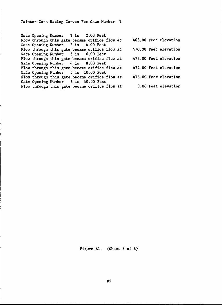
Tainter Gate Rating Curves For Gaze Number 1

Gate Opening Number 1 is 2.00 FeetFlow through this gate became orifice flow at 468.00 Feet elevationGate Opening Number 2 is 4.00 FeetFlow through this gate became orifice flow at 470.00 Feet elevationGate Opening Number 3 is 6.00 FeetFlow through this gate became orifice flow at 472.00 Feet elevationGate Opening Number 4 is 8.00 FeetFlow through this gate became orifice flow at 474.00 Feet elevationGate Opening Number 5 is 10.00 FeetFlow through this gate became orifice flow at 476.00 Feet elevationGate Opening Number 6 is 40.00 FeetFlow through this gate became orifice flow at 0.00 Feet elevation

Figure BI. (Sheet 3 of 6)

B5

Gate Opening NumberElevation 1 2 3 4 5465.00 0.00 0.00 0.00 0.00 0.00466.00 124.72 124.72 124.72 124.72 124.72467.00 352.01 352.01 352.01 352.01 352.01468.00 617.39 645.30 645.30 645.30 645.30469.00 756.14 991.35 991.35 991.35 991.35470.00 873.12 1512.28 1382.45 1382.45 1382.45471.00 976.17 1746.23 1813.34 1813.34 1813.34472.00 1069.34 1952.35 2619.35 2280.09 2280.09473.00 1155.02 2138.69 2928.52 2779.67 2779.67474.00 1234.77 2310.05 3208.03 3904.69 3309.57475.00 1309.67 2469.54 3465.07 4277.38 3867.73476.00 1380.52 2619.35 3704.32 4620.09 5582.60477.00 1447.90 2761.03 3929.02 4939.09 6029.90478.00 1512.28 2895.80 4141.55 5238.69 6446.24479.00 1574.03 3024.56 4343.70 5522.07 6837.27480.00 1633.45 3148.06 4536.84 5791.60 7207.11481.00 1690.78 3266.90 4722.10 6049.12 7558.88482.00 1746.23 3381.56 4900.35 6296.13 7895.00483.00 1799.97 3492.46 5072.34 6533.80 8217.37484.00 1852.16 3599.95 5238.69 6763.13 8527.57485.00 1902.91 3704.32 5399.92 6984.93 8826.87486.00 1952.35 3805.82 5556.47 7199.90 9116.36487.00 2000.56 3904.69 5708.74 7408.63 9396.92488.00 2047.64 4001.12 5857.04 7611.65 9669.36489.00 2093.66 4095.28 6001.68 7809.39 9934.32490.00 2138.69 4187.32 6142.91 8002.24 10192.40491.00 2182.79 4277.38 6280.97 8190.55 10444.10492.00 2226.02 4365.58 6416.06 8374.63 10689.88493.00 2268.42 4452.03 6548.37 8554.75 10930.13494.00 2310.05 4536.84 6678.05 8731.16 11165.21495.00 2350.94 4620.09 6805.26 8904.07 11395.44496.00 2391.13 4701.87 6930.14 9073.69 11621.12497.00 2430.65 4782.25 7052.81 9240.19 11842.49498.00 2469.54 4861.30 7173.38 9403.75 12059.81499.00 2507.83 4939.09 7291.95 9564.50 12273.27500.00 2545.55 5015.67 7408.63 9722.61 12483.08501.00 2582.71 5091.10 7523.50 9878.18 12689.43502.00 2619.35 5165.42 7636.64 10031.34 12892.47503.00 2655.48 5238.69 7748.13 10182.19 13092.37504.00 2691.12 5310.96 7858.04 10330.85 13289.26505.00 2726.30 5382.25 7966.43 10477.39 13483.27

Figure BI. (Sheet 4 of 6)

B6

Tainter Gate Rating Curves For Gate Number 1

Elevation 6 7 8 9 10465.00 0.00466.00 124.72467.00 352.01468.00 645.30469.00 991.35470.00 1382.45471.00 1813.34472.00 2280.09473.00 2779.67474.00 3309.57475.00 3867.73476.00 4452.37477.00 5061.96478.00 5695.13479.00 6350.69480.00 7027.55481.00 7724.72482.00 8441.32483.00 9176.50484.00 9929.52485.00 10699.67486.00 11486.28487.00 12288.75488.00 13106.48489.00 13938.94490.00 14785.61491.00 15646.00492.00 16519.65493.00 17406.12494.00 18304.98495.00 19215.83496.00 20138.29497.00 21071.98498.00 22016.55499.00 22971.67500.00 23937.00501.00 24912.21502.00 25897.02503.00 26891.12504.00 27894.22505.00 28906.04

Figure BI. (Sheet 5 of 6)

B7

Outflow Rating Curves

Outflow Structure Number 1 is a Tainter Gate on Spillway Crest at an openingof 2.00 FeetOutflow Structure Number 2 is an Outlet Works

O'tflow StructureElevation 1 2 3 4 5 Total

465.00 0.00 15414.19 0.00 0.00 0.00 15414.19466.00 124.72 15528.95 0.00 0.00 0.00 15653.67467.00 352.01 15643.71 0.00 0.00 0.00 15995.72468.00 617.39 15758.47 0.00 0.00 0.00 16375.86469.00 756.14 15871.53 0.00 0.00 0.00 16627.67470.00 873.12 15983.28 0.00 0.00 0.00 16856.40471.00 976.17 16093.67 0.00 0.00 0.00 17069.84472.00 1069.34 16203.06 0.00 0.00 0.00 17272.40473.00 1155.02 16311.87 0.00 0.00 0.00 17466.89474.00 1234.77 16420.03 0.00 0.00 0.00 17654.80475.00 1309.67 16527.21 0.00 0.00 0.00 17836.88476.00 1380.52 16633.88 0.00 0.00 0.00 18014.39477.00 1447.90 16739.87 0.00 0.00 0.00 18187.77478.00 1512.28 16845.00 0.00 0.00 0.00 18357.28479.00 1574.03 16949.70 0.00 0.00 0.00 18523.73480.00 1633.45 17053.56 0.00 0.00 0.00 18687.01481.00 1690.78 17156.82 0.00 0.00 0.00 18847.61482.00 1746.23 17259.64 0.00 0.00 0.00 19005.88483.00 1799.97 17361.51 0.00 0.00 0.00 19161.49484.00 1852.16 17463.07 0.00 0.00 0.00 19315.22485.00 1902.91 17563.82 0.00 0.00 0.00 19466.74486.00 1952.35 17664.08 0.00 0.00 0.00 19616.43487.00 2000.56 17763.83 0.00 0.00 0.00 19764.39488.00 2047.64 17862.84 0.00 0.00 0.00 19910.48489.00 2093.66 17961.58 0.00 0.00 0.00 20055.24490.00 2138.69 18059.40 0.00 0.00 0.00 20198.09491.00 2182.79 18157.06 0.00 0.00 0.00 20339.85492.00 2226.02 18253.82 0.00 0.00 0.00 20479.84493.00 2268.42 18350.38 0.00 0.00 0.00 20618.80494.00 2310.05 18446.16 0.00 0.00 0.00 20756.21495.00 2350.94 18541.66 0.00 0.00 0.00 20892.60496.00 2391..13 18636.48 0.00 0.00 0.00 21027.61497.00 2430.65 18730.98 0.00 0.00 0.00 21161.63498.00 2469.54 18824.R5 0.00 0.00 0.00 21294.39499.00 2507.83 18918.38 0.00 0.00 0.00 21426.21500.00 2545.55 19011.30 0.00 0.00 0.00 21556.85501.00 2582.71 19103.93 0.00 0.00 0.00 21686.64502.00 2619.35 i9195.91 0.00 0.00 0.00 21815.26503.00 2655.48 19287.68 0.00 0.00 0.00 21943.15504.00 2691.12 19378.74 0.00 0.00 0.00 22069.86505.00 2726.30 19469.68 0.00 0.00 0.00 22195.99

Figure BI. (Sheet 6 of 6)

B8

Example 2: Rating Curves for an Ogee Spillwaywith Multiple Tainter Gates and Outlet Works

12. The second example uses the same reservoir as the first example.

the only difference is that the spillway rating curve includes flow through 14

tainter gates. All gates have the same opening. Rating curves are developed

for six alternative gate openings. Thirteen type 2 piers are added to the

input data.

Example 2Rating Curves for an Ogee Spillway with Multiple Tainter Gatesand Outlet Works

ID Example 2ID Rating Curves for an Ogee Spillway with Mulciple Tainter GatesID10 1 0KK Test ReservoirCG 0 0 2 10EL 370 380 390 400 405 410 415 420 425 430DC 0 5000 12500 35000 55000 90000 143000 230000 367000 535000ON 2 465 505 40TG 0 -1 0 664 85 25 40 13 560 2TG 465 1 4 -1 2 40 6 2TG 0 45TG 1 1TG 2 4 6 8 10 40TG .68 .68 .68 .68 .71 .71OW 1 20 576 .013 405 400 1.5zz

Figure B2. RESOUT output for example problem 2 (Sheet 1 of 5)

B9

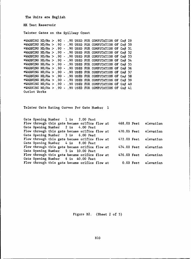
The Units are English

KK Test Reservoir

Tainter Gates on the Spillway Crest

*WARNING HD/He > .90 - .90 USED FOR COMPUTATION OF Cs# 29*WARNING HD/He > .90 - .90 USED FOR COMPUTATION OF Cs# 30*WARNING HD/He > .90 - .90 USED FOR COMPUTATION OF Cs# 31*WARNING HD/He > .90 - .90 USED FOR COMPUTATION OF Cs# 32*WARNING HD/He > .90 - .90 USED FOR COMPUTATION OF Cs# 33*WARNING HD/He > .90 - .90 USED FOR COMPUTATION OF Cs# 34*WARNING HD/He > .90 - .90 USED FOR COMPUTATION OF Cs# 35*WARNING HD/He > .90 - .90 USED FOR COMPUTATION OF Cs# 36*WARNING HD/ie > .90 - .90 USED FOR COMPUTATION OF Cs# 37*WARNING HD/He > .90 - .90 USED FOR COMPUTATION OF Cs# 38*WARNING HD/He > .90 - .90 USED FOR COMPUTATION OF Cs# 39*WARNING HD/He > .90 - .90 USED FOR COMPUTATION OF Cs# 40*WARNING HD/He > .90 - .90 USED FOR COMPUTATION OF Cs# 41

Outlet Works

Tainter Gate Rating Curves For Gate Number 1

Gate Opening Number 1 is 2.00 FeatFlow through this gate became orifice flow at 468.00 Feet elevationGate Opening Number 2 is 4.00 FeetFlow through this gate became orifice flow at 470.00 Feet elevationGate Opening Number 3 is 6.00 FeetFlow through this gate became orifice flow at 472.00 Feet elevationGate Opening Number 4 is 8.00 FeetFlow through this gate became orifice flow at 474.00 Feet elevationGate Opening Number 5 is 10.00 FeetFlow through this gate became orifice flow at 476.00 Feet elevationGate Opening Number 6 is 40.00 FeetFlow through this gate became orifice flow at 0.00 Feet elevation

Figure B2. (Sheet 2 of 5)

B1O

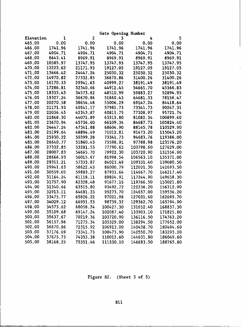
Gate Opening NumberElevation 1 2 3 4 5465.00 0.00 0.00 0.00 0.00 0.00466.00 1741.96 1741.96 1741.96 1741.96 1741.96467.00 4904.71 4904.71 4904.71 4904.71 4904.71468.00 8643.41 8969.91 8969.91 8969.91 8969.91469.00 10585.97 13747.95 13747.95 13747.95 13747.95470.00 12223.62 21171.93 19127.05 19127.05 19127.05471.00 13666.42 24447.24 25030.32 25030.32 25030.32472.00 14970.82 27332.85 36670.86 31400.26 31400.26473.00 16170.33 29941.63 40999.27 38191.49 38191.49474.00 17286.81 32340.66 44912.45 54665.70 45366.83475.00 18335.43 34573.62 48510.99 59883.27 52894.95476.00 19327.24 36670.86 51860.43 64681.33 78156.47477.00 20270.58 38654.48 55006.29 69147.24 84418.64478.00 21171.93 40541.17 57981.73 73341.73 90247.31479.00 22036.45 42343.87 60811.75 77308.97 95721.74480.00 22868.30 44072.89 63515.80 81082.34 100899.60481.00 23670.94 45736.60 66109.34 84687.73 105824.40482.00 24447.24 47341.88 68604.90 88145.78 110529.90483.00 25199.64 48894.49 71012.81 91473.20 115043.20484.00 25930.22 50399.28 73341.73 94683.76 119386.00485.00 26640.77 51860.43 75598.91 97788.98 123576.20486.00 27332.85 53281.53 77790.65 100798.60 127629.00487.00 28007.83 54665.70 79922.30 103720.90 131556.90488.00 28666.93 56015.67 81998.54 106563.10 135371.00489.00 29311.21 57333.87 84023.49 109331.40 139080.50490.00 29941.63 58622.43 86000.79 112031.30 142693.50491.00 30559.05 59883.27 87933.64 114667.70 146217.40492.00 31164.24 61118.11 89824.91 117244.90 149658.30493.00 31757.90 62328.48 91677.16 119766.50 153021.80494.00 32340.66 63515.80 93492.72 122236.20 156312.90495.00 32913.11 64681.33 95273.70 124657.00 159536.20496.00 33475.77 65826.22 97021.98 127031.60 162695.70497.00 34029.12 66951.53 98739.32 129362.70 165794.90498.00 34573.62 68058.24 100427.30 131652.40 168837.30499.00 35109.68 69147.24 102087.40 133903.10 171825.80500.00 35637.67 70219.36 103720.90 136116.50 174763.20501.00 36157.96 71275.34 105329.00 138294.50 177652.00502.00 36670.86 72315.92 106913.00 140438.70 180494.60503.00 37176.69 73341.73 108473.90 142550.70 183293.20504.00 37675.73 74353.38 110012.60 144631.80 186049.60505.00 38168.25 75351.46 111530.10 146683.50 188765.80

Figure B2. (Sheet 3 of 5)

BlI

Tainter Gate Rating Curves For Gate Number

Elevation 6 7 8 9 10

465.00 0.00466.00 1741.96467.00 4904.71468.00 8969.91469.00 13747.95470.00 19127.05471.00 25030.32472.00 31400.26473.00 38191.49474.00 45366.83475.00 52894.95476.00 60748.87477.00 68904.98478.00 77342.26479.00 86041.84480.00 94986.62481.00 104160.90482.00 113550.20483.00 123141.00484.00 132921.00485.00 142878.10486.00 153001.60487.00 163280.70488.00 173705.60489.00 184266.80490.00 194955.30491.00 205762.30492.00 216679.70493.00 227699.30494.00 238813.50495.00 250014.90496.00 261296.30497.00 272650.70498.00 284071.40499.00 295552.00500.00 307085.90501.00 318667.30502.00 330289.80503.00 341947.80504.00 353635.60505.00 365347.60

Figure B2. (Sheet 4 of 5)

B12

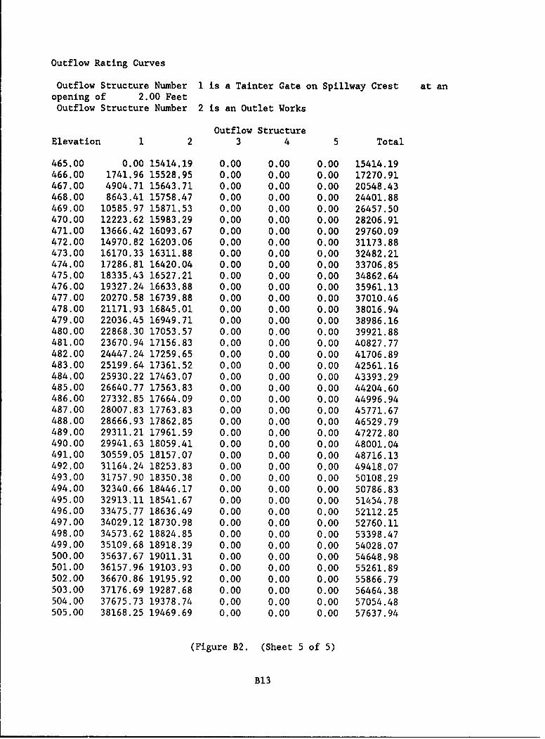
Outflow Rating Curves

Outflow Structure Number i is a Tainter Gate on Spillway Crest at anopening of 2.00 FeetOutflow Structure Number 2 is an Outlet Works

Outflow StructureElevation 1 2 3 4 5 Total

465.00 0.00 15414.19 0.00 0.00 0.00 15414.19466.00 1741.96 15528.95 0.00 0.00 0.00 17270.91467.00 4904.71 15643.71 0.00 0.00 0.00 20548.43468.00 8643.41 15758.47 0.00 0.00 0.00 24401.88469.00 10585.97 15871.53 0.00 0.00 0.00 26457.50470.00 12223.62 15983.29 0.00 0.00 0.00 28206.91471.00 13666.42 16093.67 0.00 0.00 0.00 29760.09472.00 14970.82 16203.06 0.00 0.00 0.00 31173.88473.00 16170.33 16311.88 0.00 0.00 0.00 32482.21474.00 17286.81 16420.04 0.00 0.00 0.00 33706.85475.00 18335.43 16527.21 0.00 0.00 0.00 34862.64476.00 19327.24 16633.88 0.00 0.00 0.00 35961.13477.00 20270.58 16739.88 0.00 0.00 0.00 37010.46478.00 21171.93 16845.01 0.00 0.00 0.00 38016.94479.00 22036.45 16949.71 0.00 0.00 0.00 38986.16480.00 22868.30 17053.57 0.00 0.00 0.00 39921.88481.00 23670.94 17156.83 0.00 0.00 0.00 40827.77482.00 24447.24 17259.65 0.00 0.00 0.00 41706.89483.00 25199.64 17361.52 0.00 0.00 0.00 42561.16484.00 25930.22 17463.07 0.00 0.00 0.00 43393.29485.00 26640.77 17563.83 0.00 0.00 0.00 44204.60486.00 27332.85 17664.09 0.00 0.00 0.00 44996.94487.00 28007.83 17763.83 0.00 0.00 0.00 45771.67488.00 28666.93 17862.85 0.00 0.00 0.00 46529.79489.00 29311.21 17961.59 0.00 0.00 0.00 47272.80490.00 29941.63 18059.41 0.00 0.00 0.00 48001.04491.00 30559.05 18157.07 0.00 0.00 0.00 48716.13492.00 31164.24 18253.83 0.00 0.00 0.00 49418.07493.00 31757.90 18350.38 0.00 0.00 0.00 50108.29494.00 32340.66 18446.17 0.00 0.00 0.00 50786.83495.00 32913.11 18541.67 0.00 0.00 0.00 51454.78496.00 33475.77 18636.49 0.00 0.00 0.00 52112.25497.00 34029.12 18730.98 0.00 0.00 0.00 52760.11498.00 34573.62 18824.85 0.00 0.00 0.00 53398.47499.00 35109.68 18918.39 0.00 0.00 0.00 54028.07500.00 35637.67 19011.31 0.00 0.00 0.00 54648.98501.00 36157.96 19103.93 0.00 0.00 0.00 55261.89502.00 36670.86 19195.92 0.00 0.00 0.00 55866.79503.00 37176.69 19287.68 0.00 0.00 0.00 56464.38504.00 37675.73 19378.74 0.00 0.00 0.00 57054.48505.00 38168.25 19469.69 0.00 0.00 0.00 57637.94

(Figure B2. (Sheet 5 of 5)

B13

Examole 3s Rating Curves for an Ogee Spillwaywith a Vertical Lift Gate

13. The third example consists of computing rating tables for four

alternative gate openings for a single vertical lift gate on an ogee spillway.

Example 3Rating Curves for an Ogee Spillway with a VerticalLift Gate

ID Example 3ID Rating Curves for an Ogee Spillway with a VerticalID Lift Gate10 1 0KK Test ReservoirCG 0 0 2 10EL 390 4C0 410 420 425 430 435 440 445 450DC 0 500 i?50 3500 4500 4800 6000 8000 10000 100000ON 1 465 505 40VL 0 -1 0 440 85 25 40 0 40 0VL 465 1 4 -1 2 40 4 2 463VL 0 45VL 1 1VL 1 2 3 5zz

Figure B3. RESOUT output for example problem 3 (Sheet 1 of 4)

B14

The Units are English

KK Test Reservoir

Vertical Lift Gates

*WARNING HD/He > .90 - .90 USED FOR COMPUTATION OF Cs# 23*WARNING HD/He > .90 - .90 USED FOR COMPUTATION OF Cs# 24*WARNING HD/He > .90 - .90 USED FOR COMPUTATION OF Cs# 25*WARNING HD/He > .90 - .90 USED FOR COMPUTATION OF Cs# 26*WARNING HD/He > .90 - .90 USED FOR COMPUTATION OF Cs# 27*WARNING HD/He > .90 - .90 USED FOR COMPUTATION OF Cs# 28*WARNING HD/He > .90 - .90 USED FOR COMPUTATION OF Cs# 29*WARNING HD/He > .90 - .90 USED FOR COMPUTATION OF Cs# 30*WARNING HD/He > .90 - .90 USED FOR COMPUTATION OF Cs# 31*WARNING HD/He > .90 - .90 USED FOR COMPUTATION OF Cs# 32*WARNING HD/He > .90 - .90 USED FOR COMPUTATION OF Cs# 33*WARNING HD/He > .90 - .90 USED FOR COMPUTATION OF Cs# 34*WARNING HD/He > .90 - .90 USED FOR COMPUTATION OF Cs# 35*WARNING HD/He > .90 - .90 USED FOR COMPUTATION OF Cs# 36*WARNING HD/He > .90 - .90 USED FOR COMPUTATION OF Cs# 37*WARNING HD/He > .90 - .90 USED FOR COMPUTATION OF Cs# 38*WARNING HD/He > .90 - .90 USED FOR COMPUTATION OF Cs# 39*WARNING HD/He > .90 - .90 USED FOR COMPUTATION OF Cs# 40*WARNING HD/He > .90 - .90 USED FOR COMPUTATION OF Cs# 41

Vertical Lift Gate Rating Curves For Gate Number 1

Gate Opening Number 1 is 1.00 FeetFlow through this gate became orifice flow at 465.00 Feet elevationGate Opening Number 2 is 2.00 FeetFlow through this gate became orifice flow at 466.00 Feet elevationGate Opening Number 3 is 3.00 FeetFlow through this gate became orifice flow at 467.00 Feet elevationGate Opening Number 4 is 5.00 FeetFlow through this gate became orifice flow at 469.00 Feet elevation

Figure B3. (Sheet 2 of 4)

B15

Gate Opening NumberElevation 1 2 3 4 5465.00 0.00 0.00 0.00 0.00466.00 124.72 124.72 124.72 124.72467.00 348.96 352.01 352.01 352.01468.00 394.96 645.30 645.30 645.30469.00 435.77 829.88 991.35 991.35470.00 472.76 907.58 1300.83 1382.45471.00 506.75 978.48 1412.36 1813.34472.00 538.32 1043.97 1514.67 2280.09473.00 567.89 1105.04 1609.58 2511.25474.00 595.73 1162.38 1698.36 2670.45475.00 622.10 1216.53 1781.94 2819.08476.00 647.17 1267.91 1861.04 2958.83477.00 671.09 1316.84 1936.21 3090.96478.00 693.97 1363.58 2007.91 3216.44479.00 715.92 1408.37 2076.50 3336.05480.00 737.03 1451.37 2142.28 3450.41481.00 757.35 1492.75 2205.50 3560.06482.00 776.96 1532.63 2266.39 3665.41483.00 795.91 1571.15 2325.13 3766.85481-.00 814.25 1608.38 2381.88 3864.68485.00 832.00 1644.43 2436.79 3959.18486.00 849.23 1679.37 2489.97 4050.59487.00 865.95 1713.26 2541.54 4139.13488.00 882.19 1746.18 2591.59 4224.96489.00 897.98 1778.18 2640.22 4308.27490.00 913.35 1809.30 2687.50 4389.19491.00 928.32 1839.59 2733.51 4467.87492.00 942.90 1869.10 2778.31 4544.42493.00 957.11 1897.86 2821.95 4618.94494.00 970.98 1925.90 2864.50 4691.55495.00 984.51 1953.26 2906.00 4762.33496.00 997.72 1979.97 2946.50 4831.36497.00 1010.62 2006.05 2986.04 4898.72498.00 1023.23 2031.53 3024.66 4964.48499.00 1035.56 2056.43 3062.40 5028.71500.00 1047.62 2080.78 3099.29 5091.47501.OQ 1059.41 2104.59 3135.36 5152.81502.00 1070.94 2127.88 3170.64 5212.79503.00 1082.12 2150.45 3204.81 5270.89504.00 1092.95 2172.32 3237.94 5327.20505.00 103.55 2193.73 3270.37 5382.31

Figure B3. (Sheet 3 of 4)

B16

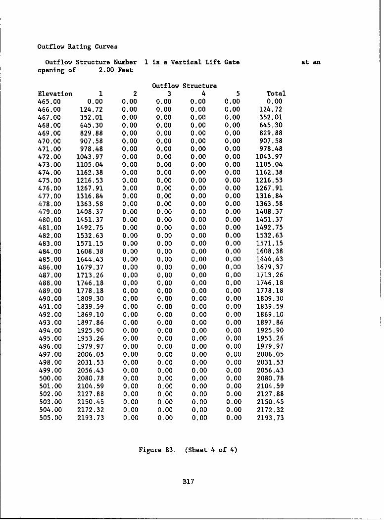
Outflow Rating Curves

Outflow Structure Number 1 is a Vertical Lift Gate at anopening of 2.00 Feet

Outflow StructureElevation 1 2 3 4 5 Total465.00 0.00 0.00 0.00 0.00 0.00 0.00466.00 124.72 0.00 0.00 0.00 0.00 124.72467.00 352.01 0.00 0.00 0.00 0.00 352.01468.00 645.30 0.00 0.00 0.00 0.00 645.30469.00 829.88 0.00 0.00 0.00 0.00 829.88470.00 907.58 0.00 0.00 0.00 0.00 907.58471.00 978.48 0.00 0.00 0.00 0.00 978.48472.00 1043.97 0.00 0.00 0.00 0.00 1043.97473.00 1105.04 0.00 0.00 0.00 0.00 1105.04474.00 1162.38 0.00 0.00 0.00 0.00 1162.38475.00 1216.53 0.00 0.00 0.00 0.00 1216.53476.00 1267.91 0.00 0.00 0.00 0.00 1267.91477.00 1316.84 0.00 0.00 0.00 0.00 1316.84478.00 1363.58 0.00 0.00 0.00 0.00 1363.58479.00 1408.37 0.00 0.00 0.00 0.00 1408.37480.00 1451.37 0.00 0.00 0.00 0.00 1451.37481.00 1492.75 0.00 0.00 0.00 0.00 1492.75482.00 1532.63 0.00 0.00 0.00 0.00 1532.63483.00 1571.15 0.00 0.00 0.00 0.00 1571.15484.00 1608.38 0.00 0.00 0.00 0.00 1608.38485.00 1644.43 0.00 0.00 0.00 0.00 1644.43486.00 1679.37 0.00 0.00 0.00 0.00 1679.37487.00 1713.26 0.00 0.00 0.00 0.00 1713.26488.00 1746.18 0.00 0.00 0.00 0.00 1746.18489.00 1778.18 0.00 0.00 0.00 0.00 1778.18490.00 1809.30 0.00 0.00 0.00 0.00 1809.30491.00 1839.59 0.00 0.00 0.00 0.00 1839.59492.00 1869.10 0.00 0.00 0.00 0.00 1869.10493.00 1897.86 0.00 0.00 0.00 0.00 1897.86494.00 1925.90 0.00 0.00 0.00 0.00 1925.90495.00 1953.26 0.00 0.00 0.00 0.00 1953.26496.00 1979.97 0.00 0.00 0.00 0.00 1979.97497.00 2006.05 0.00 0.00 0.00 0.00 2006.05498.00 2031.53 0.00 0.00 0.00 0.00 2031.53499.00 2056.43 0.00 0.00 0.00 0.00 2056.43500.00 2080.78 0.00 0.00 0.00 0.00 2080.78501.00 2104.59 0.00 0.00 0.00 0.00 2104.59502.00 2127.88 0.00 0.00 0.00 0.00 2127.88503.00 2150.45 0.00 0.00 0.00 0.00 2150.45504.00 2172.32 0.00 0.00 0.00 0.00 2172.32505.00 2193.73 0.00 0.00 0.00 0.00 2193.73

Figure B3. (Sheet 4 of 4)

B17

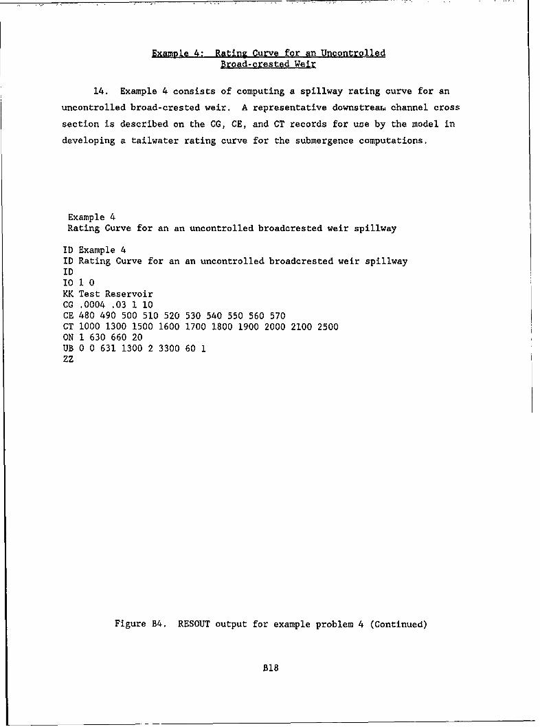
Example 4: Rating Curve for an UncontrolledBroad-crested Weir

14. Example 4 consists of computing a spillway rating curve for an

uncontrolled broad-crested weir. A representative downstrea, channel cross

section is described on the CG, CE, and CT records for use by the model in

developing a tailwater rating curve for the submergence computations.

Example 4Rating Curve for an an uncontrolled broadcrested weir spillway

ID Example 4ID Rating Curve for an an uncontrolled broadcrested weir spillwayIDi0 1 0KK Test ReservoirCG .0004 .03 1 10CE 480 490 500 510 520 530 540 550 560 570CT 1000 1300 1500 1600 1700 1800 1900 2000 2100 2500ON 1 630 660 20UB 0 0 631 1300 2 3300 60 1zz

Figure B4. RESOUT output for example problem 4 (Continued)

BIB

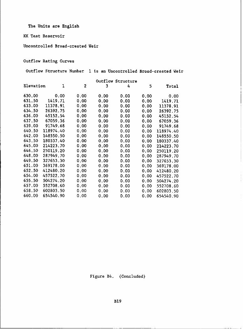
The Units are English

KK Test Reservoir

Uncontrolled Broad-crested Weir

Outflow Rating Curves

Outflow Structure Number I is an Uncontrolled Broad-crested Weir

Outflow StructureElevation 1 2 3 4 5 Total

630.00 0.00 0.00 0.00 0.00 0.00 0.00631.50 1419.71 0.00 0.00 0.00 0.00 1419.71633.00 11378.91 0.00 0.00 0.00 0.00 11378.91634.50 26392.75 0.00 0.00 0.00 0.00 26392.75636.00 45152.54 0.00 0.00 0.00 0.00 45152.54637.50 67059.36 0.00 0.00 0.00 0.00 67059.36639.00 91749.68 0.00 0.00 0.00 0.00 91749.68640.50 118974.40 0.00 0.00 0.00 0.00 118974.40642.00 148550.50 0.00 0.00 0.00 0.00 148550.50643.50 180337.40 0.00 0.00 0.00 0.00 180337.40645.00 214223.70 0.00 0.00 0.00 0.00 214223.70646.50 250119.20 0.00 0.00 0.00 0.00 250119.20648.00 287949.70 0.00 0.00 0.00 0.00 287949.70649.50 327653.30 0.00 0.00 0.00 0.00 327653.30651.00 369178.00 0.00 0.00 0.00 0.00 369178.00652.50 412480.20 0.00 0.00 0.00 0.00 412480.20654.00 457522.70 0.00 0.00 0.00 0.00 457522.70655.50 504274.20 0.00 0.00 0.00 0.00 504274.20657.00 552708.60 0.00 0.00 0.00 0.00 552708.60658.50 602803.50 0.00 0.00 0.00 0.00 602803.50660.00 654540.90 0.00 0.00 0.00 0.00 654540.90

Figure B4. (Concluded)

B19

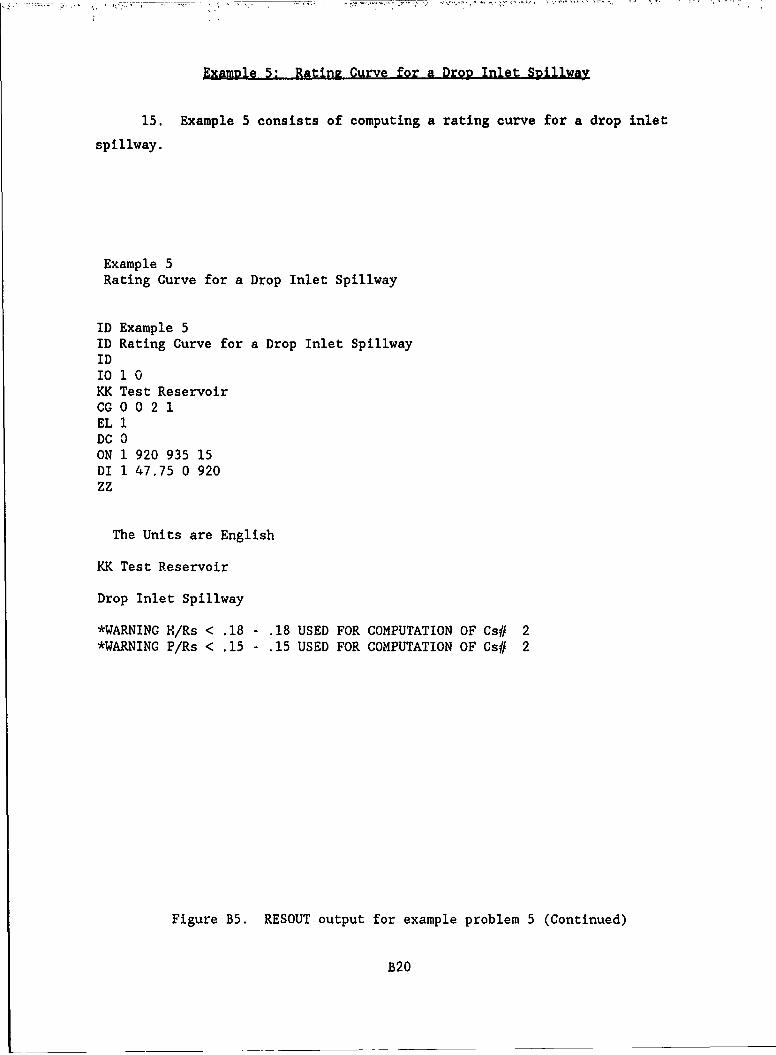
Example 5: Rating Curve for a DroR Inlet Spillway

15. Example 5 consists of computing a rating curve for a drop inlet

spillway.

Example 5Rating Curve for a Drop Inlet Spillway

ID Example 5ID Rating Curve for a Drop Inlet SpillwayID10 1 0KK Test ReservoirCC 0 0 2 1EL 1DC 0ON 1 920 935 15DI 1 47.75 0 920zz

The Units are English

KK Test Reservoir

Drop Inlet Spillway

*WARNING H/Rs < .18 - .18 USED FOR COMPUTATION OF Cs# 2*WARNING P/Rs < .15 - .15 USED FOR COMPUTATION OF Cs# 2

Figure B5. RESOUT output for example problem 5 (Continued)

B20

Outflow Rating Curves

Outflow Structure Number 1 is a Drop Inlet Spillway

Outflow StructureElevation 1 2 3 4 5 Total920.00 0.00 0.00 0.00 0.00 0.00 0.00921.00 1206.09 0.00 0.00 0.00 0.00 1206.09922.00 3411.33 0.00 0.00 0.00 0.00 3411.33923.00 6267.02 0.00 0.00 0.00 0.00 6267.02924.00 9648.70 0.00 0.00 0.00 0.00 9648.70925.00 13484.47 0.00 0.00 0.00 0.00 13484.47926.00 17725.80 0.00 0.00 0.00 0.00 17725.80927.00 22337.06 0.00 0.00 0.00 0.00 22337.06928.00 27290.65 0.00 0.00 0.00 0.00 27290.65929.00 32564.37 0.00 0.00 0.00 0.00 32564.37

930.00 38139.85 0.00 0.00 0.00 0.00 38139.85931.00 44001.55 0.00 0.00 0.00 0.00 44001.55932.00 50136.13 0.00 0.00 0.00 0.00 50136.13933.00 56531.95 0.00 0.00 0.00 0.00 56531.95934.00 63178.75 0.00 0.00 0.00 0.00 63178.75935.00 70067.38 0.00 0.00 0.00 0.00 70067.38

Figure B5. (Concluded)

B21

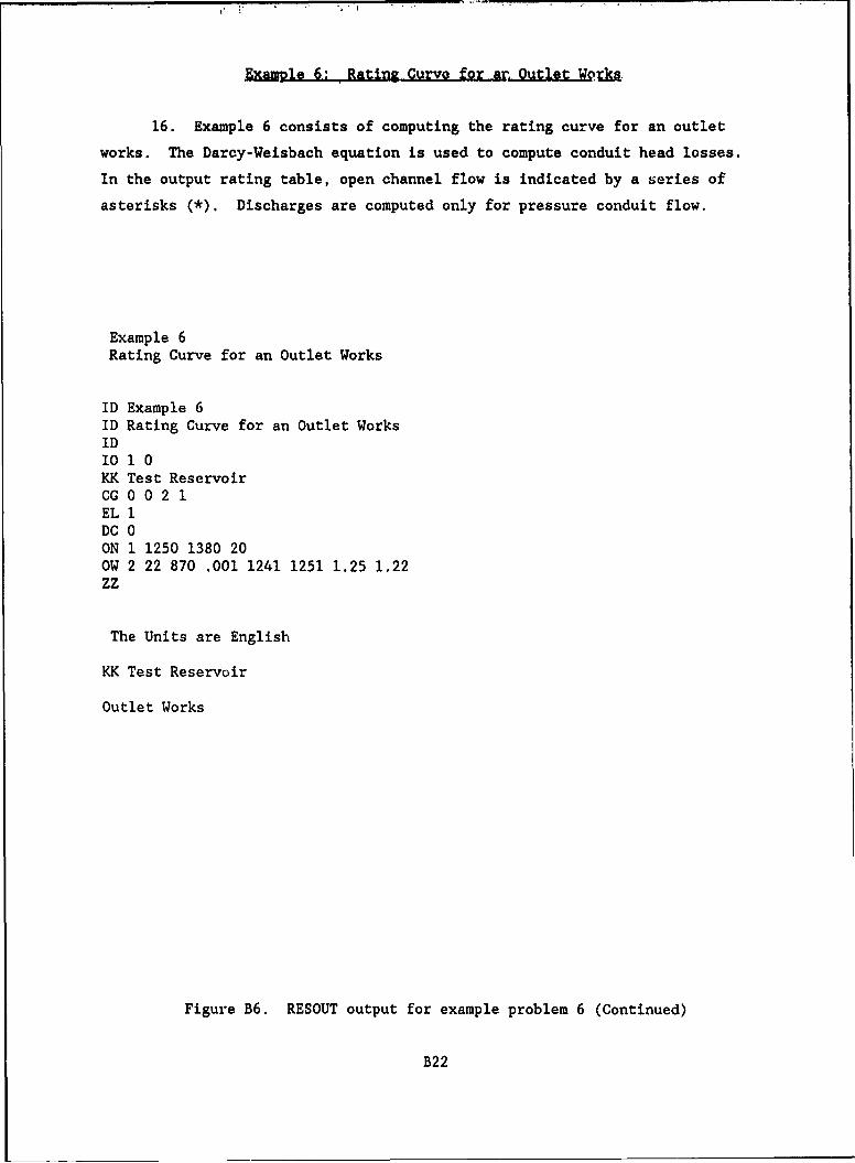
Examle 6: Rating CurvQa for a. Outlet Hpa.

16. Example 6 consists of computing the rating curve for an outlet

works. The Darcy-Weisbach equation is used to compute conduit head losses.

In the output rating table, open channel flow is indicated by a series of

asterisks (*). Discharges are computed only for pressure conduit flow.

Example 6Rating Curve for an Outlet Works

ID Example 6ID Rating Curve for an Outlet WorksID10 1 0KK Test ReservoirCG 0 0 2 1EL 1DC 0ON 1 1250 1380 20OW 2 22 870 .001 1241 1251 1.25 1.22zz

The Units are English

KK Test Reservoir

Outlet Works

Figure B6. RESOUT output for example problem 6 (Continued)

B22

Outflow Rating Curves

Outflow Structure Number .1 is an Outlet Works

Outflow StructureElevation 1 2 3 4 5 Total1250.00 0.00 0.00 0.00 0.00 0.00 0.001256.50 ********** 0.00 0.00 0.00 0.00 **********

1263.00 ********** 0.00 0.00 0.00 0.00 **********

1269.50 ********** 0.00 0.00 0.00 0.00 **********

1276.00 15547.86 0.00 0.00 0.00 0.00 15547.861282.50 16702.04 0.00 0.00 0.00 0.00 16702.041289.00 17856.21 0.00 0.00 0.00 0.00 17856.211295.50 18889.37 0.00 0.00 0.00 0.00 18889.371302.00 19861.64 0.00 0.00 0.00 0.00 19861.641308.50 20783.14 0.00 0.00 0.00 0.00 20783.141315.00 21660.10 0.00 0.00 0.00 0.00 21660.101321.50 22500.90 0.00 0.00 0.00 0.00 22500.901328.00 23309.89 0.00 0.00 0.00 0.00 23309.891334.50 24094.26 0.00 0.00 0.00 0.00 24094.261341.00 24852.32 0.00 0.00 0.00 0.00 24852.321347.50 25586.22 0.00 0.00 0.00 0.00 25586.221354.00 26298.10 0.00 0.00 0.00 0.00 26298.101360.50 26990.69 0.00 0.00 0.00 0.00 26990.691367.00 27668.11 0.00 0.00 0.00 0.00 27668.111373.50 28328.26 0.00 0.00 0.00 0.00 28328.261380.00 28970.18 0.00 0.00 0.00 0.00 28970.18

Figure B6. (Concluded)

B23

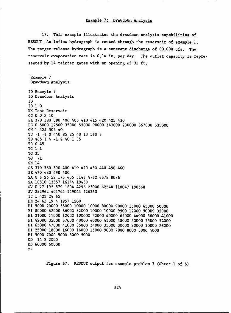
Example 7: Drawdown Analysis

17. This example illustrates the drawdown analysis capabilities of

RESOUT. An inflow hydrograph is routed through the reservoir of example 1.

The target release hydrograph is a constant discharge of 60,000 cfs. The

reservoir evaporation rate is 0.14 in. per day. The outlet capacity is repre-

sented by 14 tainter gates with an opening of 35 ft.

Example 7Drawdown Analysis

ID Example 7ID Drawdown AnalysisIDI0 1 0KK Test ReservoirCG 0 0 2 10EL 370 380 390 400 405 410 415 420 425 430DC 0 5000 12500 35000 55000 90000 143000 230000 367000 535000ON 1 425 505 40TG -1 -1 0 440 85 25 40 13 560 3TO 465 1 4 -1 2 40 1 35TO 0 45TG 1 1TO 3iTG .71SN 14SE 370 380 390 400 410 420 430 440 450 460SE 470 480 490 500SA 0 6 26 52 173 455 3143 4762 6378 8076SA 10510 13357 16144 19438SV 0 27 192 579 1604 4296 23000 62548 118047 190568SV 282962 401742 549044 726360IC 1 428 24 65HN 24 65 19 4 1957 1200HI 5000 20000 35000 10000 10000 80000 90000 15000 65000 50000HI 80000 62000 66000 82000 10000 10000 9500 12000 50000 32000HI 21000 11000 12000 100000 32000 40000 65000 44000 38C00 41000HI 42000 35000 37000 40000 40000 45000 48000 50000 75000 54000HI 65000 47000 41000 35000 34000 35000 30000 30000 30000 28000HI 25000 18000 16000 16000 15000 9000 7000 8000 5000 4000HI 5000 7000 5000 5000 5000DD .14 2 2000DD 60000 60000zz

Figure B7. RESOUT output for example problem 7 (Sheet 1 of 6)

B24

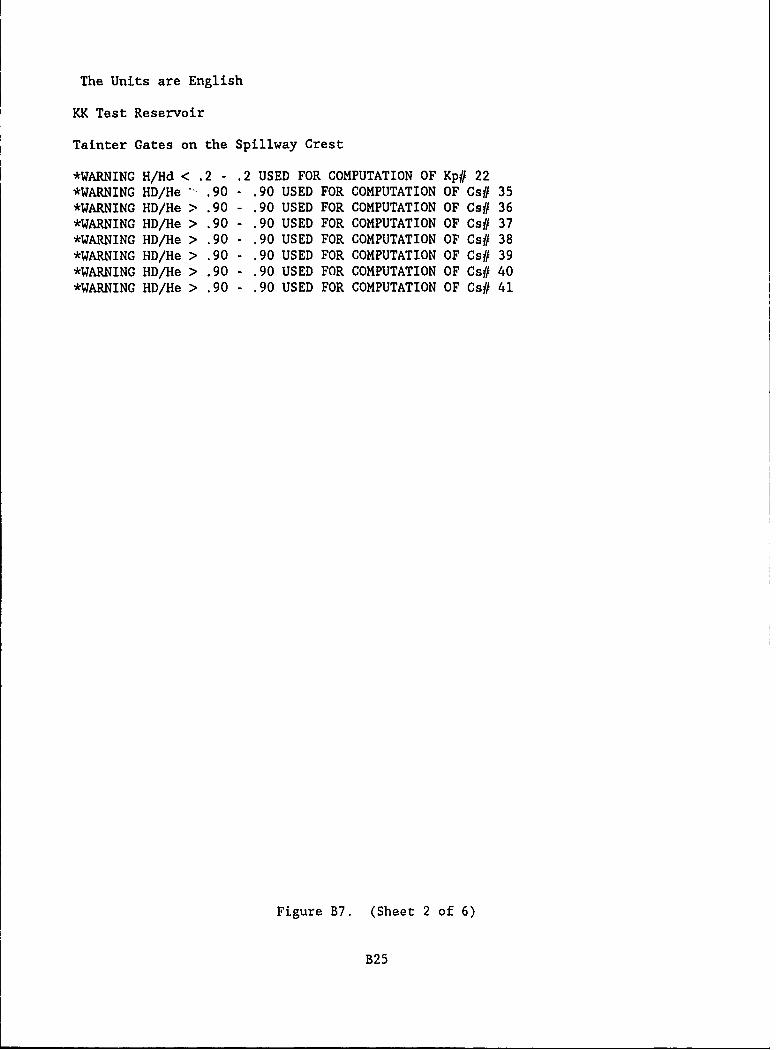
The Units are English

KK Test Reservoir

Tainter Gates on the Spillway Crest

*WARNING H/Hd < .2 - .2 USED FOR COMPUTATION OF Kp# 22*WARNING HD/He - .90 - .90 USED FOR COMPUTATION OF Cs# 35*WARMING HD/He > .90 - .90 USED FOR COMPUTATION OF Cs# 36*WARNING HD/He > .90 - .90 USED FOR COMPUTATION OF Cs# 37*WARNING HD/He > .90 - .90 USED FOR COMPUTATION OF Cs# 38*WARNING HD/He > .90 - .90 USED FOR COMPUTATION OF Cs# 39*WARNING HD/He > .90 - .90 USED FOR COMPUTATION OF Cs# 40*WARNING HD/He > .90 - .90 USED FOR COMPUTATION OF Cs# 41

Figure B7. (Sheet 2 of 6)

B25

Tainter Gate Rating Curves For Gate Number 1

Gate Opening Number 1 is 35.00 FeetFlow through this gate became orifice flow at 501.00 Feet elevation

Gate Opening NumberElevation 1 2 3 4 5

425.00 0.00427.00 0.00429.00 0.00431.00 0.00433.00 0.00435.00 0.00437.00 0.00439.00 0.00441.00 0.00443.00 0.00445.00 0.00447.00 0.00449.00 0.00451.00 0.00453.00 0.00455.00 0.00457.00 0.00459.00 0.00461.00 0.00463.00 0.00465.00 0.00467.00 4950.73469.00 13899.67471.00 25352.64473.00 38759.65475.00 53794.70477.00 70231.89479.00 87900.35481.00 106663.10483.00 126405.90485.00 147030.30487.00 168449.10489.00 190584.30491.00 213364.40493.00 236723.30495.00 260599.40497.00 284934.90499.00 309674.80501.00 480333.80503.00 505631.70505.00 529722.70

Figure B7. (Sheet 3 of 6)

B26

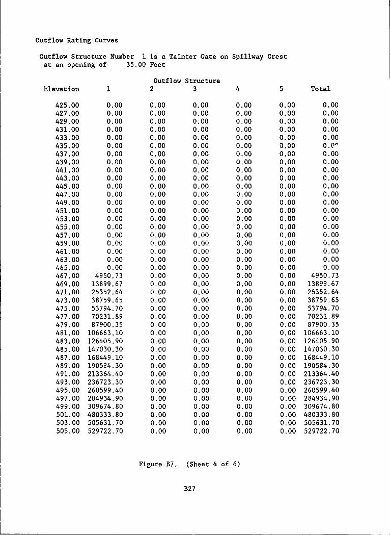
Outflow Rating Curves

Outflow Structure Number I is a Tainter Gate on Spillway Crestat an opening of 35.00 Feet

Outflow StructureElevation 1 2 3 4 5 Total

425.00 0.00 0.00 0.00 0.00 0.00 0.00427.00 0.00 0.00 0.00 0.00 0.00 0.00429.00 0.00 0.00 0.00 0.00 0.00 0.00431.00 0.00 0.00 0.00 0.00 0.00 0.00433.00 0.00 0.00 0.00 0.00 0.00 0.00435.00 0.00 0.00 0.00 0.00 0.00 0.0437.00 0.00 0.00 0.00 0.00 0.00 0.00439.00 0.00 0.00 0.00 0.00 0.00 0.00441.00 0.00 0.00 0.00 0.00 0.00 0.00443.00 0.00 0.00 0.00 0.00 0.00 0.00445.00 0.00 0.00 0.00 0.00 0.00 0.00447.00 0.00 0.00 0.00 0.00 0.00 0.00449.00 0.00 0.00 0.00 0.00 0.00 0.00451.00 0.00 0.00 0.00 0.00 0.00 0.00453.00 0.00 0.00 0.00 0.00 0.00 0.00455.00 0.00 0.00 0.00 0.00 0.00 0.00457.00 0.00 0.00 0.00 0.00 0.00 0.00459.00 0.00 0.00 0.00 0.00 0.00 0.00461.00 0.00 0.00 0.00 0.00 0.00 0.00463.00 0.00 0.00 0.00 0.00 0.00 0.00465.00 0.00 0.00 0.00 0.00 0.00 0.00467.00 4950.73 0.00 0.00 0.00 0.00 4950.73469.00 13899.67 0.00 0.00 0.00 0.00 13899.67471.00 25352.64 0.00 0.00 0.00 0.00 25352.64473.00 38759.65 0.00 0.00 0.00 0.00 38759.65475.00 53794.70 0.00 0.00 0.00 0.00 53794.70477.00 70231.89 0.00 0.00 0.00 0.00 70231.89479.00 87900.35 0.00 0.00 0.00 0.00 87900.35481.00 106663.10 0.00 0.00 0.00 0.00 106663.10483.00 126405.90 0.00 0.00 0.00 0.00 126405.90485.00 147030.30 0.00 0.00 0.00 0.00 147030.30487.00 168449.10 0.00 0.00 0.00 0.00 168449.10489.00 190524.30 0.00 0.00 0.00 0.00 190584.30491.00 213364.40 0.00 0.00 0.00 0.00 213364.40493.00 236723.30 0.00 0.00 0.00 0.00 236723.30495.00 260599.40 0.00 0.00 0.00 0.00 260599.40497.00 284934.90 0.00 0.00 0.00 0.00 284934.90499.00 309674.80 0.00 0.00 0.00 0.00 309674.80501.00 480333.80 0.00 0.00 0.00 0.00 480333.80503.00 505631.70 0.00 0.00 0.00 0.00 505631.70505.00 529722.70 0.00 0.00 0.00 0.00 529722.70

Figure B7. (Sheet 4 of 6)

B27

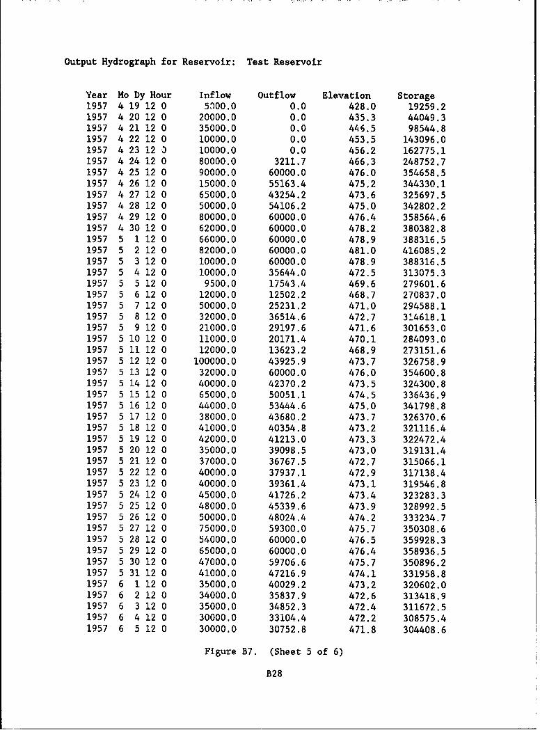
Output Hydrograph for Reservoir: Test Reservoir

Year Mo Dy Hour Inflow Outflow Elevation Storage1957 4 19 12 0 510000 0.0 428.0 19259.21957 4 20 12 0 20000.0 0.0 435.3 44049.31957 4 21 12 0 35000.0 0.0 446.5 98544.81957 4 22 12 0 10000.0 0.0 453.5 143096.01957 4 23 12 0 10000.0 0.0 456.2 162775.11957 4 24 12 0 80000.0 3211.7 466.3 248752.71957 4 25 12 0 90000.0 60000.0 476.0 354658.51957 4 26 12 0 15000.0 55163.4 475.2 344330.11957 4 27 12 0 65000.0 43254.2 473.6 325697.51957 4 28 12 0 50000.0 54106.2 475.0 342802.21957 4 29 12 0 80000.0 60000.0 476.4 358564.61957 4 30 12 0 62000.0 60000.0 478.2 380382.81957 5 1 12 0 66000.0 60000.0 478.9 388316.51957 5 2 12 0 82000.0 60000.0 481.0 416085.21957 5 3 12 0 10000.0 60000.0 478.9 388316.51957 5 4 12 0 10000.0 35644.0 472.5 313075.31957 5 5 12 0 9500.0 17543.4 469.6 279601.61957 5 6 12 0 12000.0 12502.2 468.7 270837.01957 5 7 12 0 50000.0 25231.2 471.0 294588.11957 5 8 12 0 32000.0 36514.6 472.7 314618.11957 5 9 12 0 21000.0 29197.6 471.6 301653.01957 5 10 12 0 11000.0 20171.4 470.1 284093.01957 5 11 12 0 12000.0 13623.2 468.9 273151.61957 5 12 12 0 100000.0 43925.9 473.7 326758.91957 5 13 12 0 32000.0 60000.0 476.0 354600.81957 5 14 12 0 40000.0 42370.2 473.5 324300.81957 5 15 12 0 65000.0 50051.1 474.5 336436.91957 5 16 12 0 44000.0 53444.6 475.0 341798.81957 5 17 12 0 38000.0 43680.2 473.7 326370.61957 5 18 12 0 41000.0 40354.8 473.2 321116.41957 5 19 12 0 42000.0 41213.0 473.3 322472.41957 5 20 12 0 35000.0 39098.5 473.0 319131.41957 5 21 12 0 37000.0 36767.5 472.7 315066.11957 5 22 12 0 40000.0 37937.1 472.9 317138.41957 5 23 12 0 40000.0 39361.4 473.1 319546.81957 5 24 12 0 45000.0 41726.2 473.4 323283.31957 5 25 12 0 48000.0 45339.6 473.9 328992.51957 5 26 12 0 50000.0 48024.4 474.2 333234.71957 5 27 12 0 75000.0 59300.0 475.7 350308.61957 5 28 12 0 54000.0 60000.0 476.5 359928.31957 5 29 12 0 65000.0 60000.0 476.4 358936.51957 5 30 12 0 47000.0 59706.6 475.7 350896.21957 5 31 12 0 41000.0 47216.9 474.1 331958.81957 6 1 12 0 35000.0 40029.2 473.2 320602.01957 6 2 12 0 34000.0 35837.9 472.6 313418.91957 6 3 12 0 35000.0 34852.3 472.4 311672.51957 6 4 12 0 30000.0 33104.4 472.2 308575.41957 6 5 12 0 30000.0 30752.8 471.8 304408.6

Figure B7. (Sheet 5 of 6)

B28

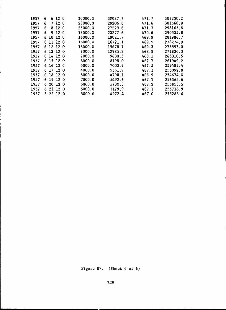
1957 6 6 12 0 30000.0 30087.7 471.7 303230.21957 6 7 12 0 28000.0 29206.6 471.6 301668.91957 6 8 12 0 25000.0 27229.6 471.3 298165.81957 6 9 12 0 18000.0 23277.6 470.6 290535.81957 6 10 12 0 16000.0 19021.7 469.9 281986.71957 6 11 12 0 16000.0 16721.1 469.5 278274.91957 6 12 12 0 15000.0 15678.7 469.3 276593.01957 6 13 12 0 9000.0 12985.2 468.8 271834.31957 6 14 12 0 7000.0 9680.5 468.1 265010.51957 6 15 12 0 8000.0 8198.0 467.7 261949.21957 6 16 12 C 5000.0 7003.9 467.5 259483.41957 6 17 12 0 4000.0 5361.9 467.1 256092.81957 6 18 12 0 5000.0 4798.1 466.9 254674.01957 6 19 12 0 7000.0 5492.6 467.1 256362.61957 6 20 12 0 5000.0 5730.3 467.2 256853.51957 6 21 12 0 5000.0 5179.9 467.1 255716.91957 6 22 12 0 5000.0 4972.4 467.0 255288.6

Figure B7. (Sheet 6 of 6)

B29

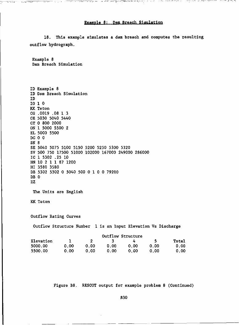
Example 8: Dam Breach Simulation

18. This example simulates a dam breach and computes the resulting

outflow hydrograph.

Example 8Dam Breach Simulation

ID Example 8ID Dam Breach SimulationID10 1 0KK TetonCG .0019 .08 1 3CE 5030 5040 5440CT 0 800 2000ON 1 5000 5500 2EL 5000 5500DC 0 0SN 8SE 5040 5075 5100 5150 5200 5250 5300 5320SV 500 750 17500 51000 102000 167000 249000 286000IC 1 5302 .25 10HN 10 2 1 1 87 1200HI 3580 3580DB 5302 5302 0 5040 500 0 1 0 0 79200DB 0zz

The Units are English

KK Teton

Outflow Rating Curves

Outflow Structure Number 1 is an Input Elevation Vs Discharge

Outflow StructureElevation 1 2 3 4 5 Total5000.00 0.00 0.00 0.00 0.00 0.00 0.005500.00 0.00 0.00 0.00 0.00 0.00 0.00

Figure B8. RESOUT output for example problem 8 (Continued)

B30

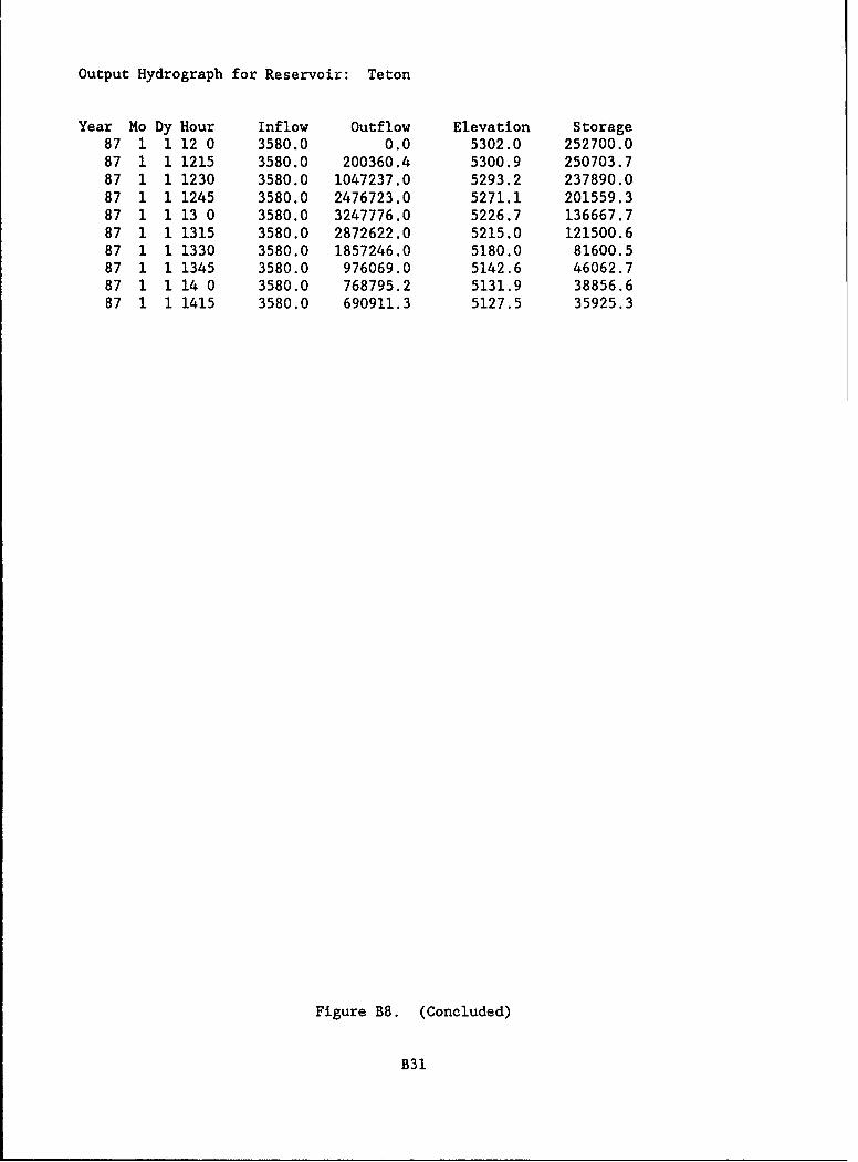
Output Hydrograph for Reservoir: Teton

Year Mo Dy Hour Inflow Outflow Elevation Storage87 1 1 12 0 3580.0 0.0 5302.0 252700.087 1 1 1215 3580.0 200360.4 5300.9 250703.787 1 1 1230 3580.0 1047237.0 5293.2 237890.087 1 1 1245 3580.0 2476723.0 5271.1 201559.387 1 1 13 0 3580.0 3247776.0 5226.7 136667.787 1 1 1315 3580.0 2872622.0 5215.0 121500.687 1 1 1330 3580.0 1857246.0 5180.0 81600.587 1 1 1345 3580.0 976069.0 5142.6 46062.787 1 1 14 0 3580.0 768795.2 5131.9 38856.687 1 1 1415 3580.0 690911.3 5127.5 35925.3

Figure B8. (Concluded)

B31

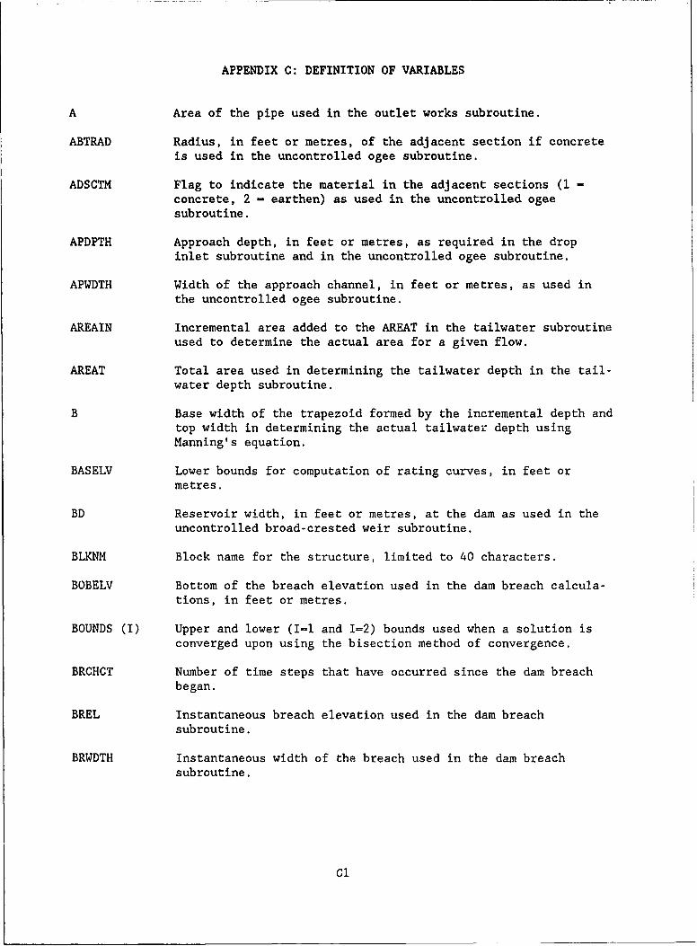
APPENDIX C: DEFINITION OF VARIABLES

A Area of the pipe used in the outlet works subroutine.

ABTRAD Radius, in feet or metres, of the adjacent section if concreteis used in the uncontrolled ogee subroutine.

ADSCTM Flag to indicate the material in the adjacent sections (1 -concrete, 2 - earthen) as used in the uncontrolled ogeesubroutine.

APDPTH Approach depth, in feet or metres, as required in the dropinlet subroutine and in the uncontrolled ogee subroutine.

APWDTH Width of the approach channel, in feet or metres, as used inthe uncontrolled ogee subroutine.

AREAIN Incremental area added to the AREAT in the tailwater subroutineused to determine the actual area for a given flow.

AREAT Total area used in determining the tailwater depth in the tail-water depth subroutine.

B Base width of the trapezoid formed by the incremental depth andtop width in determining the actual tailwater depth usingManning's equation.

BASELV Lower bounds for computation of rating curves, in feet ormetres.

BD Reservoir width, in feet or metres, at the dam as used in theuncontrolled broad-crested weir subroutine.

BLKNM Block name for the structure, limited to 40 characters.

BOBELV Bottom of the breach elevation used in the dam breach calcula-tions, in feet or metres.

BOUNDS (I) Upper and lower (I-1 and 1=2) bounds used when a solution isconverged upon using the bisection method of convergence.

BRCHCT Number of time steps that have occurred since the dam breachbegan.

BREL Instantaneous breach elevation used in the dam breachsubroutine.

BRWDTH Instantaneous width of the breach used in the dam breachsubroutine.

Cl

CBI Weir coefficient used for the horizontal section of the breachand overflow section of the dam.

CB2 Weir coefficient used for the triangular section of the breachsection of the dam.

CE (I) Channel elevations of downstream channel corresponding to chan-nel top widths, in feet or metres. Limited to 20 points.

CHANEL (I) Downstream channel elevation array to be used in conjunctionwith a user-specified elevation-versus-discharge curve in feetor metres. Limited to 100 points.

CHANQ (I) Downstream channel discharge array to be used in conjunctionwith a user-specified elevation-versus-discharge curve in cubicfeet per second or cubic metres per second. Limited to100 points.

CIHY Current time inflow hydrograph value (corresponds to CTM).

CKA (I,J) Array containing the relationship between He/R and abutmentcontraction coefficient for uncontrolled ogee spillways withadjacent concrete sections.

CO Circular crest coefficient as used in the drop inletsubroutine.

COARA (I,J) Array that contains the relationship between the circular crestcoefficient to approach depth/radius for different approachdepths. It is used in the drop inlet subroutine.

COESUB Submergence coefficient as input to the uncontrolled ogeesubroutine.

CONV Conversion factors used throughout the program. They aredependent on whether the units are English or metric.

CORDCK Two-character ID used to check card sequencing.

CRDID Temporary location used to store the first two letters of aninput record.

CRSTEL Crest elevation of either the tainter gate or the vertical liftgate.

CRSTHT Height of the spillway crest above the approach apron as usedin the uncontrolled ogee subroutine.

CRSTWD Width of the crest, in feet or metres, in the uncontrolledbroad-crested weir subroutine.

C2

CSLOPE Downstream channel slope in feet/foot or metres/metre.

CT (I) Channel top widths of downstream channel corresponding tochannel elevations in feet or metres. Limited to 20 points.

CTM Current time since the simulation began. Used in the dambreach subroutine.

CV Coefficient for correction for velocity of approach as used inthe dam breach routine and the uncontrolled broadcrested weirsubroutine.

D Pipe diameter, in feet or metres, used in the outlet workssubroutine.

DC Discharge coefficient as used in the uncontrolled ogeesubroutine.

DC133 (I,J) Array containing the relationship between He/Hd and dischargecoefficient for a P/Hd of 1.33. It is used in the uncontrolledogee spillway routine.

DC33 (I,J) Array containing the relationship between He/Hd and dischargecoefficient for a P/Hd of .33. It is used in the uncontrolledogee spillway routine.

DC67 (I,J) Array containing the relationship between He/Hd and dischargecoefficient for a P/Hd of .67. It is used in the uncontrolledogee spillway routine.

DESHD Design head, in feet or metres, as used in the uncontrolledogee subroutine.

DIFF Difference between the upper and lower bounds used when check-ing convergence.

DIFF2 Difference between the upper and lower bounds used when check-ing convergence.

DTMO Term 2S/t - 0 (2 x storage/time - outflow). Used in modifiedPuls subroutine.

DTPO Term 2S/t + 0 (2 x storage/time + outflow). Used in modifiedPuls subroutine.

DW Reservoir width, in feet or metres, at the dam used in the dambreach subroutine.

DWORMN Flag to tell whether to use Manning's equation or the Darcy-Weisbach equation to determine the frictional loss coefficientin the outlet works subroutine.

C3

DY Difference between the Yl data and the Y2 data in the doublelinear interpolation subroutine.

Absolute roughness of the pipe to be used in the Darcy-Weisbach equations in the outlet works subroutine.

ED Absolute roughness divided by the pipe diameter (relativeroughness).

EKA (I,J)A Array containing the relationship between He/R and the abutmentcontraction coefficient for uncontrolled ogee spillways withadjacent earthen sections.

ELDTOP Elevation, in feet or metres, of the downstream top of the exitportal as used in the outlet works subroutine.

ELEV Actual distance from the bottom of the channel to the watersurface.

ELEV Array of elevations in the outlet works subroutine generated bychoosing values of flow. The array is later interpolated fromto determine the flows at the elevations in RE.

ELINVT Elevation, in feet or metres, of the upstream invert as used in

the outlet works subroutine.

ELOG Conversion from log base 10 to natural log.

ELVMAX Upper bounds for computation of rating curves, in feet ormetres.

ELVSTP Elevation step, in feet or metres, determined by (ELVMAX -BASELV)/NRTPTS.

ENGMET English/metric flag, 0 if English units are to be used and 1 ifmetric units.

ESPLWD Calculated effective spillway width, in feet or metres, as usedin the uncontrolled ogee subroutine.

EVAPRT The evaporation rate, as entered, in inches or centimetres.

EVIS The absolute roughness divided by the kinematic viscosity asused by the outlet works routine.

F Darcy-Welsbach frictional loss coefficient (f) in the pipe ascomputed by the Jeppson routine in the outlet works subroutine.

FL Frictional length of the pipe as used in the outlet works

subroutine.

C4

FROUNO Froude number as calculated for use in determining the outletportal pressure in the outlet works subroutine.

FS Square root of f as calculated by the Jeppson routine of the

Darcy-Weisbach section of the outlet works subroutine.

FW Final width of the dam breach, in feet or metres.

G Acceleration due to gravity, set by type of units.

GATBOT Elevation of the bottom of the gate opening as computed by thevertical lift gate subroutine.

GATWDT Gate width of either the vertical lift gates or the taintergates. NOTE: GATWDT is the width of one gate only.

GTSTEL Gate seat elevation used in the vertical lift gate subroutine.

HI Head above the bottom of the gate in the vertical lift gatesubroutine.

H2 Head above the gate seat elevation in the vertical lift gatesubroutine.

HDHD Actual head on the crest divided by the design head as used inthe uncontrolled ogee subroutine.

HDRS Head on the crest divided by the radius of the drop inlet inthe drop inlet subroutine.

HE Energy head as calculated in the uncontrolled ogee subroutine.

HEAD Resistance loss, in feet, for use in the Manning equation inthe outlet works subroutine.

HEDHD Energy head divided by the design head as used in the uncon-trolled ogee subroutine.

HGUESS Initial guess of water surface elevation as used in the Darcy-Weisbach equations in the outlet works subroutine.

HL Head loss as computed by the Jeppson routine in the Darcy-Weisbach section of the outlet works subroutine.

IflNT2 Multiple use counter.

IDANMO Indicator of how many days there are in a particular month asused in the output subroutine.

IDATE (1,J) Array that keeps track of the time, day, month, and year of the

outflow hydrograph as used in the output hydrograph.

IFNAM Input file name (limited to 8 characters).

INIT A general-use counter variable.

C5

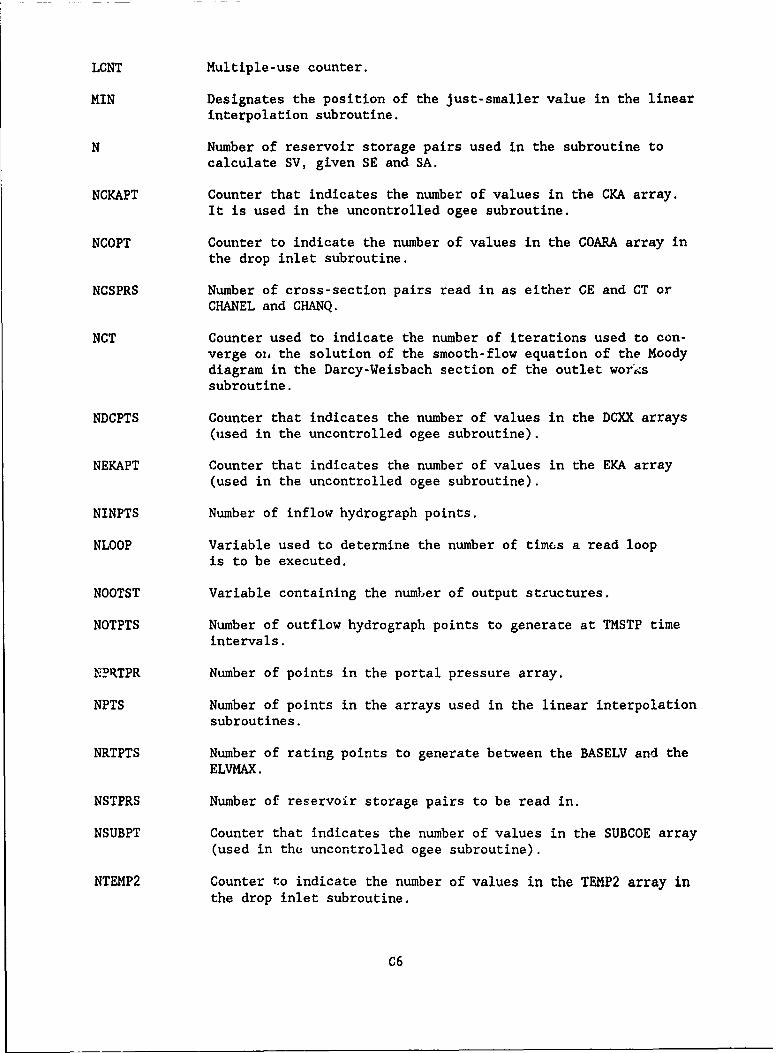
LCNT Multiple-use counter.

MIN Designates the position of the just-smaller value in the linearinterpolation subroutine.

N Number of reservoir storage pairs used in the subroutine tocalculate SV, given SE and SA.

NCKAPT Counter that indicates the number of values in the CKA array.It is used in the uncontrolled ogee subroutine.

NCOPT Counter to indicate the number of values in the COARA array inthe drop inlet subroutine.

NCSPRS Number of cross-section pairs read in as either CE and CT orCHANEL and CHANQ.

NCT Counter used to indicate the number of iterations used to con-verge oz, the solution of the smooth-flow equation of the Moodydiagram in the Darcy-Weisbach section of the outlet workssubroutine.

NDCPTS Counter that indicates the number of values in the DCXX arrays(used in the uncontrolled ogee subroutine).

NEKAPT Counter that indicates the number of values in the EKA array

(used in the uncontrolled ogee subroutine).

NINPTS Number of inflow hydrograph points.

NLOOP Variable used to determine the number of times a read loopis to be executed.

NOOTST Variable containing the number of output structures.

NOTPTS Number of outflow hydrograph points to generate at TMSTP timeintervals.

NPRTPR Number of points in the portal pressure array.

NPTS Number of points in the arrays used in the linear interpolationsubroutines.

NRTPTS Number of rating points to generate between the BASELV and theELVMAX.

NSTPRS Number of reservoir storage pairs to be read in.

NSUBPT Counter that indicates the number of values in the SUBCOE array

(used in thu uncontrolled ogee subroutine).

NTEMP2 Counter to indicate the number of values in the TEMP2 array in

the drop inlet subroutine.

C6

NTGATE Variable that counts the number of tainter gates that have beenused (a maximum of three).

NTGTOP (I) Number of tainter gate openings. For each of up to threetainter gates, the number of gate openings to compute ratingcurves for is stored here.

NVAL Counter used to keep up with the number of values calculatedthat will be used for convergence by the bisection method inthe uncontrolled broad-crested weir subroutine.

NVLFGT Variable that counts the number of vertical lift gates thathave been specified (maximum of three).

NVLFOP (I) Number of vertical lift gate openings. For each of up to threevertical lift gates, the number of gate openings to computerating curves for is stored here.

OD (I,J) Outflow rating curve array. Up to five (J) different struc-tures with the sum of them placed in the sixth (J) position andused as the rating curve for routing. Limited to 100 pointsper structure (I).

ODI Composite outflow rating curve (column 6 in OD) used in dam

breach calculation.

OFNAM Output file name (limited to 8 characters).

OTBRCH Reservoir outflow due to the breach.

OTHY (I) Outflow hydrogrnph points from any routing method, in cubicfeet per second or cubic metres per second. Limited to100 points.

OTSTR Outflow of the reservoir due to the outlet structures. Used inthe dam breach subroutine.

OTSTTY (I) Output structure type array. Contains the name of each of thefive (1) chosen output structures.

OTWEIR Outflow due to weir flow in the overtopping of the dam in thedam breach subroutine.

OUT Reservoir outflow due to both the dam breach and the outletstructures. Used in the dam breach subroutine.

OUTLST String variable used to echo the input data file to the outputfield if requested.

PAR Equation eV (f/8)/(kinematic viscosity) which is used as acheck to determine if the pipe is wholly rough. It is used inthe Darcy-Weisbach section of the outlet works subroutine.

PDID Crest height divided by the design head as used in the uncon-trolled ogee subroutine.

C7

PDRS Approach depth divided by the radius of the drop inlet in the

drop inlet subroutine.

PIERNO Number of piers as used in the uncontrolled ogee subroutine.

PIERTY Type of piers as defined by EM 1110-2-1603, 111-11, as used inthe uncontrolled ogee subroutine.

PIHY Previous time inflow hydrograph value (corresponas to PTM).

PORTPR Exit portal pressure array containing numerically digitizeddata from the curves in EM 1110-2-1602, App. III,Figure 111-5.

PRTFLG Print flag. Set to 1 if input data are to be echoed to outputfile.

PSUB Submergence coefficient as used in the uncontrolled ogeesubroutine.

PTM Previous time. Used in the dam breach subroutine.

Q Flow, in cubic feet per second or cubic metres per second, usedin the tailwater computation subroutine. Also used as an arraycontaining the upper and lower bounds to be tested for conver-gence to a solution in the uncontrolled broad-crested weirsubroutine and the uncontrolled ogee subroutine.

RADIUS Radius, in feet or metres, of the drop inlet in the drop inletsubroutine.

RE (I) Reservoir elevation array. Array containing the elevationscomputed from the given minimum and maximum elevations andnumber of included divisions, in feet or metres. Limited to100 points.

REY Reynolds number, as calculated and used in the Darcy-Weisbachsection of the outlet works subroutine.

RIHY (I) Inflow hydrograph array. Limited to 100 points.

RIHYT (I) Inflow hydrograph time array. Value at the end of eachtimestep is computed from the time step entered. Limited to100 points.

RISM Sum of the current and previous inflow hydrograph points. Usedin the modified Puls subroutine and the dam breach subroutineuntil the breach elevation is reached.

RIW Initial width of the dam breach, in feet or metres.

RK Sum of any other minor loss coefficients to be used in the

outlet works subroutine.

C8

RKA Abutment contraction coefficient as used in the uncontrolledogee subroutine.

RKNWN Known values of an equation. The actual contents vary byusage.

RKP Pier contraction coefficient as used in the uncontrolled ogeesubroutine.

RKPARA (I,J) Array containing the relationship between H/Hd and pier con-traction coefficient for uncontrolled ogee spillways.

RKS Submergence correction for tailwater effects on weir outflow.

RKSCHK Flag used to calculate which equation to use in the calculationof the submergence correction coefficient used in the dambreach subroutine.

RKSFLG Index calculated to determine if the submergence correctionshould be made. It is used in the uncontrolled ogee spillwayroutine.

RKTOT Value for Kf as computed using the Manning equation in the out-let works subroutine.

RLFTSD Left side of the dam breach equations used to determineconvergence.

RLPYR Indicator to determine if the year given is a leap year or not,as used in the output subroutine.

RMANN Manning's N of downstream channel.

RMAXFL Maximum downstream channel capacity or release to be main-tained, in cubic feet per second or cubic metres per second,Used in the modified Puls subroutine.

RMNFCT Conversion factor used in Manning's equation that is set basedon whether the units are English or metric.

RTFLG Routing flag. Set to 1 if a routing was done. Used to deter-mine if outflow hydrograph is to be printed.

RTSDE The right side of the dam breach equations used to determineconvergence.

RYR Year, as used in the output subroutine.

SA (I) Reservoir surface areas corresponding to reservoir storageelevations, In acres or hectares. Limited to 100 points.

SE (I) Reservoir storage elevations corresponding to reservoir storagevolumes, in feet or metres. Limited to 100 points.

C9

SLOPE First best guess of the slope of the energy line to get aninitial solution for the Manning equation in the outlet workssubroutine.

SLP Side slope of the channel segment used for determining theactual tailwater depth.

SLPFCC Slope face correction factor for non-vertical approach slopesas used in the uncontrolled ogee subroutine.

SPLNW Net length of the spillway, in feet or metres, excluding thetotal pier width as used in the uncontrolled ogee subroutine.

STDY Starting day of the month.

STMN Starting month of the year.

STORI Storage at the beginning of the current time period. Used inthe modified Puls subroutine and the dam breach subroutineuntil the breach elevation is reached.

STOR2 Storage at the end of the current time period. Used in themodified Puls subroutine and the dam breach subroutine untilthe breach elevation is reached.

STORGE Value of storage as printed out in the output subroutine.

STTM Starting time of day (24-hour format).

STYR Starting year (two digits).

SUBCLM (I,J) Array containing the relationships defining the submergencecoefficient boundary values for uncontrolled ogee spillways.

SUBCOE (I,J) Array containing the relationships defining the submergencecoefficients for uncontrolled ogee spillways.

SV (I) Reservoir storage volume corresponding to reservoir storageelevations in acre-feet or 1,000 cubic metres. Limited to100 points.

TARA (I) Temporary array used to input 10 values from disk input files.

TELEV Temporary elevation of the water surface used in the dam breachand outlet works subroutines.

TEMP (I,J) Temporary use array used for multiple purposes throughoutthe program.

TEMP2 (I,J) Array containing the bounds for the curves defined byCOARA in the drop inlet subroutine.

¢io

TGATOD(I,J,K) Tainter gate outflow rating curve array. Allows up to three(I) tainter gates each with up to 99 points calculated (J) foreach of 10 (K) gate openings. The values correspond to thosein the reservoir elevation array.

TGTEL (I,J) Tainter gate elevation at which orifice flow occurs for thattainter gate (I) and that gate opening (J).

TGTLBL A character label used to check for the use of tainter gates inthe output subroutine.

TGTOPS(I,J,K) Tainter gate opening array. For each of a maximum of three(I) different tainter gates, there can be up to 10 (J) openingseach having associated with them an opening size in feet ormetres (K-1) and a coefficient C (K-2).

TGTUSE (I) Tainter gate opening to use in routing, in feet or metres.Limited to one per structure and three different tainter gates.

TITLE (I) The three (I) lines, each 78 characters long, set aside for theproblem title.

TMINC Time increment used for inflow hydrograph points, in hours.

TMMAX Time to reach maximum dam breach size, in hours.

TMSTP Time step, ip hours, associated with the generation of the

outflow hydrograph.

TOBELV Top of the breach elevation used in the dam breach calcula-tions, in feet or metres.

TODELV Top of dam elevation, in feet or metres, associated with modi-fied Puls routing.

TOTEVP Total evaporation, in acre-feet or hectare-metres, as cal-culated for the average surface area.

TQ Initial, temporary value of the outflow as generated using thevalue of SLOPE and Manning's equation in the outlet workssubroutine.

TSTRNG Temporary string variable used to read all but the record ID.Used in the data input subroutine.

TWCFLG Flag used to signal if channel input is a set of CE versus CTor elevation versus discharge.

TWD Tailwater depth, as calculated by the tailwater subroutineusing Manning's equation or the input elevation-versus-discharge relationship.

UNIT A character label used to print out the appropriate units, infeet or metres.

CI0

UNKWNS Unknown values of an equation used to compare to the knowns,RKNWN, for use in determining the actual values using thebisection method of convergence.

V Velocity, as used in Manning's equation, in the outlet workssubroutine.

VAL Interpolated value returned from the double linear interpola-tion subroutine.

VIS Kinematic viscosity X 105 of the fluid in question, as used inthe outlet works subroutine.

VLFCOR Correction to flow for the presence of the vertical lift gateover weir flow.

VLFEL (1,J) Vertical lift gate elevation at which orifice flow occurs forthat vertical lift gate (I) and that gate opening (J).

VLFLBL Cha-acter label used to check for the use of vertical liftgates in the output subroutine.

VLFOPS(I,J,K) Vertical lift gate opening array. For each of a maximum ofthree (I) different vertical lift gates, there can be up to 10(J) openings, each having associated with them an opening sizein feet or metres (K-1) and a coefficient C (K-2).

VLFTOD(I,J,K) Vertical lift gate outflow rating curve array. Allows up tothree (I) vertical lift gates each with up to 99 points calcu-lated (J) for each of 10 (K) gate openings. The values cor-respond to those in the reservoir elevation array.

VLFUSE (I) Vertical lift gate opening to use in routing, in feet ormetres. Limited to one per structure and three different ver-tical lift gates.

WEIRL The length of the dam that is actuall; overtopped. Used in thedam breach subroutine.

WETPER Wetted perimeter, in feet or metres, as used in the outletworks subroutine.

WSEL (I) Water surface elevations computed when routing an inflow hydro-Sraph by any method, in feet or metres. Limited to 100 points.

X The X range used in the linear interpolation subroutine. Alsoused as the X value to locate in the double linear interpola-tion subroutine.

Xl The first X range used in the double linear interpolation sub-

routine.

X2 The second X range used in the double linear interpolationsubroutine.

C12

XLUP The X value to look up using the linear interpolationsubroutine.

Y The Y range used in the linear interpolation subroutine. Alsoused as the Y value to locate in the double linear interpola-tion subroutine.

Yl The first Y range used in the double linear interpolationsubroutine.

Y2 The second Y range used in the double linear interpolationsubroutine.

YDD The value of Yd/D in the outlet works subroutine.

YINC The Y value to locate in the double linear interpolationsubroutine.

YNEW The interpolated value returned from the linear interpolationsubroutine.

Z Side slope of the dam breach, in feet (metres) horizontal to1 foot (0.3048 metre) vertical.

C13

APPENDIX D: LISTING OF PROGRAM

CC Reservoir Routing Program with Outlet StructuresC Created by: Stuart T. PurvisC At: Texas A&14 University

DIMENSION RIHY(lOO) ,TAkA(lO) ,SV(lOO) ,SE(l00) ,SA(lOO),lOD(l00,6) ,WSEL(lOO) ,OTHY(lOO) ,CE(20) ,CT(20) ,RIHYT(100),2RE(l00),TGATOD(3,100,l0),TGTEL(3,l0),TGTOPS(

3 ,lO,2),

3TGTUSE(3) ,NTGTOP(3) ,VLFTOD(3,l00,l0) ,VLFEL(3,l0) ,VLFOPS(3,l0,2),

4VLFUSE(3) ,NVLFOP(3) ,CHANEL(100) ,CHANQ(100) ,TEMP(100,2)

CHARACTER*78 TITLE(3) ,IFNAM*8 ,OFNAM*8 ,CRDID*2CPkRACTER*40 BLKNM, OTSTTY( 5)

CC Sets the initial conditions in reservoir data to be tested for later.

CDO 100 1-1,5

SV (I) --1.0SE(I)--l.0SA(I)--l.0CHANEL(I)-0.TARA(I)-0.OTARA(I+5)-0. 0

100 CONTINUEDO 103 1-1,3

103 TGTOPS(I,l,l)-0.DO 106 1-1,100

DO 107 J-1,6OD(I ,3) -0.

107 CONTINUERIHY(I)-0.

106 CONTINUEPRTFLG-0.RTFLG-0.ENGMET-0.NOUT-6CALL TITEPT (TITLE,NOUT)WRITE (6,900)READ (5,920) IFNAMOPEN (UNIT-l, FILE-IFNAM, STATUS-' OLD' ,ACCESS-' SEQUENTIAL' ,FORM-

1' FORMATTED' ,BLANK-'NULL')WRITE (6,910)READ (5,920) OFNAMOPEN (UNIT-2 ,FILE-OFNAM, STATUS-'UNKNOWN' ,ACCESS-' SEQUENTIAL',

lFORM-' FORMATTED' ,BIANK-'NULL')OPEN (UNI C-3 ,STATUS-' SCRATCH' ,ACCESS-' SEQUENTIAL' ,FORM-

1'FORMATTED' ,BLANK-'NULL')NOUT-2CALL TITEPT (TITLE,NOUT)DO 110 1-1,3

Dl

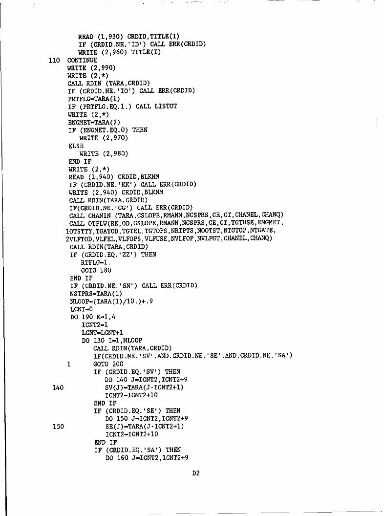
READ (1,930) CRDID,TITLE(I)IF (CRDID.NE.'IDI) CALL ERR(CRDID)WRITE (2,960) TITLE(I)

110 CONTINUEWRITE (2,990)WRITE (2,*)CALL RDIN (TARA,CRDID)IF (CRDID.NE.'I0') CALL ERR(CRDID)PRTFLG-TARA( 1)IF (PRTFLG.EQ.1.) CALL LISTOTWRITE (2,*)ENGMET-TARA (2)IF (ENGMET.EQ.O) THEN

WRITE (2,970)ELSE

WRITE (2,980)END IFWRITE (2,*)READ (1,940) CRDID,BLKNMIF (CRDID.NE.'KK') CALL ERR(CRDID)WRITE (2,940) CRDID,BLKNMCALL RDIN(TARA, CRDID)IF(CRDID.NE.'CG') CALL ERR(CRDID)CALL CHANIN (TARA,CSLOPE,RMANN,NCSPRS,CE,CT,CHANEL,CHANQ)CALL OTFLW(RE,OD,CSLOPE,RMANN,NCSPRS,CE,CT,TGTUSE,ENGMET,1OTSTTY, TGATOD ,TOTEL, TGTOPS ,NRTPTS ,NOOTST ,NTGTOP ,NTCATE,

2VLFTOD ,VLFEL, VLFOPS ,VLFUSE ,NVLFOP ,NVLFGT, CHANEL, CHANQ)

CALL RDIN(TARA, CRDID)IF (CRDID.EQ.'ZZ') THEN

RTFLG-1.COTO 180

END IFIF (CRDID.NE.'SN') CALL ERR(CRDID)NSTPRS-TARA(1)NLOOP-(TARA(1)/1O. )+. 9LCNT-0DO 190 K-1,4

ICNT2-1LCNT-LCNT+lDO 130 I-1,NLOOP

CALL RDIN(TARA, ORDID)IF(CRDID.NE. 'SV' .AND.CRDID.NE. 'SE' .AND.CRDID.NE. 'SA')

1 COTO 200IF (CRDID.EQ.-SV') THEN

DO 140 J-ICNT2,ICNT2+9140 SV(J)-TARA(J-ICNT2+1)

ICNT2-ICNT2+1OEND IFIF (CRDID.EQ.-SE') THEN

DO 150 J-ICNT2,ICNT2+9150 SE(J)-TARA(J-ICNT2+1)

ICNT2-ICNT2+1OEND IFIF (CRDID.EQ.-SA') THEN

DO 160 J-ICNT2,ICNT2+9

D2

160 SA(J)-TARA(J-ICNT2+1)ICNT2-ICNT2+10

END IF130 CONTINUE190 CONTINUE200 CONTINUE

IF (SE(1).LT.O.OR.LCNT.EQ.1) CALL ERR(CRDID)IF (SV(1).LT.O.AND.SA(1).LT.0) CALL ERR(CRDID)IF (SV(2).LT.O) CALL SVOL(SV,SE,SA,ENGMET)IF (CRDID.NE.'IC') CALL ERR(CRDID)WSEL(1)-TARA(2)TMSTP-TARA( 3)/24.NOTPTS-TARA(4)IF (TARA(1).EQ.2) CALL INTERP(NSTPRS,SV,SE,TARA(2) ,WSEL(1))CALL RDIN(TARA, CRDID)IF (CRDID.NE.-HN') CALL ERR(CRDID)TMINC-.TARA(1)/24.NINPTS-TARA(2)STDY-TARA(3)STMN-TARA (4)STYR-TARA( 5)STTM-TARA(6)NLOOP.-(TARA(2)/1O. )+.9TEMP(1, 1)-O.DO 115 I-1,NINPTS-1

TEMP(I+1 ,1).-I*TMINC115 CONTINUE

ICNT2-1DO 120 I-1,NLOOP

CALL RDIN(TEMP(ICNT2,2) ,CRDID)IF (CRDID.NE.'HI') CALL ERR(CRDID)ICNT2-ICNT2+1O

120 CONTINUERIHYT(1)'-O.RIHY(1)-TEMP(1 ,2)DO 116 I-2,NOTPTS

RIHYT(I)-(I-1)*TMSTPIF ((I-1)*TM-OTP.LE.TEMP(NINPTS,1)) THEN

CALL INTERP(NINPTS,TEMP(1,1),TEMP(1,2),RIHYT(I),RIHY(X))ELSE

RIHY(I)-TEMP(NINPTS, 1)END IF

116 CONTINUECALL RDIN (TARA,CRDID)IF (CRDID.EQ. 'DB'.OR.CRDID.EQ. 'DD') THEN

CALL BREACH (TARA,WSEL,SV,SE,NINPTS,OTHY,NSTPRS,OD(1,6),1 RIHY,CSLOPE,RMANN,NCSPRS,CE,CT,CB1,CB2, ENGMET,RIHYT,2 NTT,TMSTP,TMINC ,NRTPTS ,RE, CHANEL, CHANQ, SA, CRDID)ELSE

CALL PULS(NINPTS,NSTPRS,SV,SE,OD(1,6) ,TMINC,RIHY,OTHY,2 WSEL, ENO4ET ,NOTPTS ,TMSTP ,RIHYT,NRTPTS ,RE ,CRDID,TARA)END IF

D3

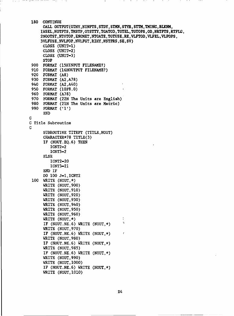
180 CONTINUECALL OUTPUT(OTHY,NINPTS,STDY,STMN,STYR,STTM,TMI14C,BIKNM,

1WSEL,NOTPTS ,TMSTP ,OTSTTY,TGATOD ,TGTEL, TGTOPS ,OD ,NRTPTS ,RTFLG,2NOOTST ,NTCGT0P, ENGMET,NTGATE ,TGTUSEP RE ,VLFTOD,VLFEL,VLFOPS,3VLFUSE ,NVLFOP ,NVLFGT,RIHY, NSTFRS ,SE, SV)CLOSE (UNIT-i)CLOSE (UNIT-2)CLOSE (UNIT-3)STOP

900 FORMAT (l5HINPUT FILENAME?)910 FORMAT (16HOUTPUT FILENAME?)920 FORMAT (A8)930 FORMAT (A2,A78)940 FORMAT (A2,A40)950 FORMAT (10F8.0)960 FORMAT (A78)970 FORMAT (22H The Units are English)980 FORMAT (21H The Units are Metric)990 FORMAT ('1')

ENDCC Title SubroutineC

SUBROUTINE TITEPT (TITLE,NOUT)CHARACTER*78 TITLE(3)IF (NOUT.EQ.6) THEN

ICNT2-2ICNT3-2

ELSEICNT2-20ICNT3-21

END IFDO 100 J-l,ICNT2

100 WRITE (NOUT,*)WRITE (NOUT,900)WRITE (NOUT,910)WRITE (NOUT,920)WRITE (NOUT,930)WRITE (NOUT,940)WRITE (NOUT,950)WRITE (NOUT,960)WRITE (NOUT,*)IF (NOUT.NE.6) WRITE (NOUT,*)WRITE (NOUT,970)IF (NOUT.NE.6) WRITE (NOUT,*)WRITE (NOUT,980)IF (NOUT.NE.6) WRITE (NOUT,*)WRITE (NOUT,985)IF (NOUT.NE.6) WRITE (NOUT,*)WRITE (NOUT,990)WRITE (NOUT,1000)IF (NOUT.NE.6) WRITE (NOUT,*)WRITE (NOUT,l0lO)

D4

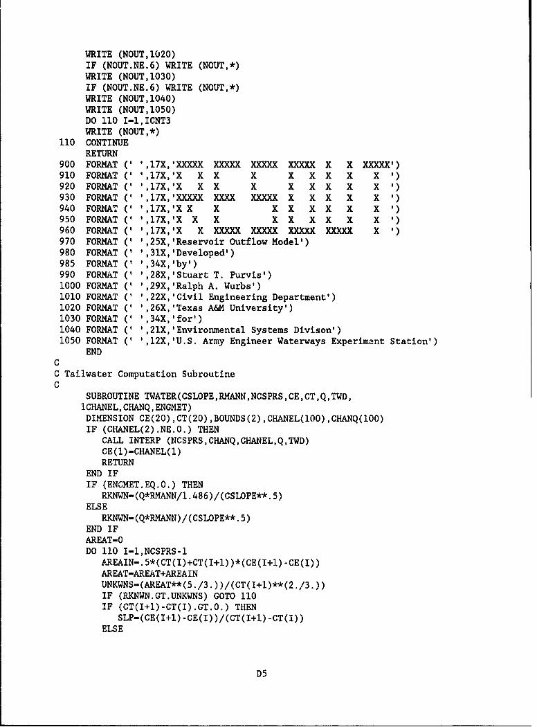
WRITE (NOUT,1020)IF (NOUT.NE.6) WRITE (NOUT,*)WRITE (NOUT,1030)IF (NOUT.NE.6) WRITE (NOUT,*)WRITE (NOUT, 1040)WRITE (NOUT,1050)DO 110 I-1,ICNT3WRITE (NOUT,*)

110 CONTINUERETURN

900 FORMAT (',t 17X,'XXXXX XXXXX XXXXX XXXXX X X XXXXX')910 FORMAT (' ,17X,'X X X X X X X X x '920 FORMAT C' ,17X,'X X X X X X X X X '930 FORMAT ('',17X,'XXXXX XXXX XXXXX X X X X X '940 FORMAT( ',17X,'X X X X X X X X X '950 FORMAT (' ,17X,'X X X X X X X X X '960 FORMAT (' ,17X,'X X XXXXX XXXXX XXXXX XXXXX X '970 FORMAT ('',25X,'Reservoir Outflow Model')980 FORMAT ('',31X,'Developed')985 FORMAT (' ',34X,'by')990 FORMAT ('',28X,'Stuart T. Purvis')1000 FORMAT ('',29X,'Ralph A. Wurbs')1010 FORMAT (' ,22X,'Civi1 Engineering Department')1020 FORMAT ('',26X,'Texas A&M University')1030 FORMAT ('',34X,'for')1040 FORMAT (' ',21X,'Environmental Systems Divison')1050 FORMAT (' ',12X,'U.S. Army Engineer Waterways Experimant Station')

ENDCC Tailwater Computation SubroutineC

SUBROUTINE TWATER(CSLOPE,RMANN,NCSPRS ,CE,CT,Q,TWD,iCHANEL, CHANQ, ENGMET)

DIMENSION GE(20),CT(20),BOUNDS(2),CHANEL(100),CHANQ(100)IF (CHANEL(2).NE.0.) THEN

CALL INTERP (NCSPRS ,CHANQ ,CHANEL, Q,TWD)CE(1)-CHANEL(l)RETURN

END IFIF (ENGMET.EQ.0.) THEN

RKNWN-(Q*RMANN/ . 486)/(CSLOFE**.5)ELSE

RKNWN(Q*RMANN)/(CSLOPE**.5)END IFAREAT-ODO 110 I-l,NCSPRS-l

A.REAIN-. 5*(CT(I)+CT(I+1) )*(CE(I+l) -CE(I))AREAT-AREAT+AREAINUNKWNS-(AREAT**(5./3. ))/(CT(I+1)**(2./3.))IF (RKNIJN.GT.UNKWNS) GOTO 110IF (CT(I+l)-CT(I).GT.O.) THEN

SLP-(CE(I+l) -CE(I) )/(CT(I+l) -CT(I))ELSE

D5

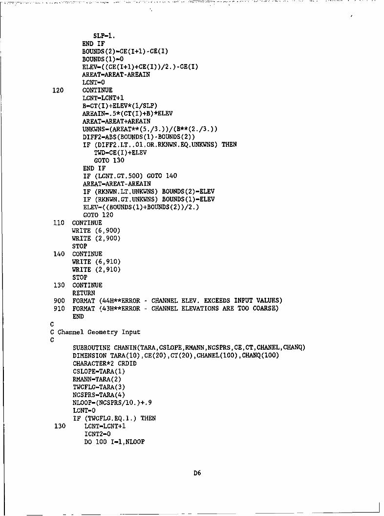
SLP-1.END IFBOUNDS(2)'-CE(I+1) -CE(I)BOUNDS (1)-OELEV-( (CE(I+1)+CE(I) )/2. )-CE(I)AREAT-AREAT -AREAINLCNT-O

120 CONTINUELCNT-LCNT+1B-CT( I)+ELEV*(1/SLP)AREAIN-. 5*(CT(I)+B)*ELEVAREAT-AREAT+AREAINUNKWNS-(AREAT**(5 ./3. ))/(B**(2 ./3.))DIFF2-ABS(BOUNDS(1) -BOUNDS(2))IF (DIFF2.LT. .01.OR.RKNWN.EQ.UNKWNS) THEN

TWD-CE(I)+ELEVCOTO 130

END IFIF (LCNT.GT.500) COTO 140AREAT-AREAT -AREAINIF (RKNWN.LT.UNKWNS) BOUNDS(2)-ELEVIF (RKNWN.GT.UNKWNS) BOUNDS(1)-ELEVELEV-((BOUNDS(1)+BOUNDS(2))/2.)COTO 120

110 CONTINUEWRITE (6,900)WRITE (2,900)STOP

140 CONTINUEWRITE (6,910)WRITE (2,910)STOP

130 CONTINUERETURN

900 FORMAT (44H**ERROR - CHANNEL ELEV. EXCEEDS INPUT VALUES)910 FORMAT (43H**ERROR - CHANNEL ELEVATIONS ARE TOO COARSE)

ENDCC Channel Geometry InputC

SUBROUTINE CHANIN(TARA, CSLOPE,RMANN,NCSPRS ,CE,CT, CHANEL, CHANQ)DIMENSION TARA(1O) ,CE(20) ,CT(20) ,CHANEL(100) ,CHANQ(100)CHARACTER*2 CRDIDCSLOPE-TARA (1)RMANN-TARA( 2)TWCFLG-TARA( 3)NCSPRS-TARA(4)NLOOP-(NCSPRS/1O. )+. 9LCNT-0IF (TWCFLG.EQ.1.) THEN

130 LCNT-LCNT+1ICNT2-ODO 100 I-1,NLOOP

D6

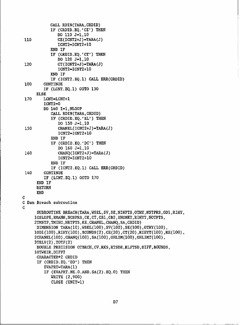
CALL RDIN(TARA,CRDID)IF (CRDID.EQ.'CE-) THEN

DO 110 J-1,10110 CE(ICNT2+J)-TARA(J)

ICNT2-ICNT2+10END IFIF (CRDID.EQ.'CT-) THEN

DO 120 J-1,10120 CT(ICNT2+J)-TARA(J)

ICNT2-ICNT2+10END IFIF (ICNT2.EQ.1) CALL ERR(CRDID)

100 CONTINUEIF (LCNT.EQ.1) COTO 130

ELSE170 LCNT-LCNT+1

ICNT2-0DO 140 I-1,NLOOP

CALL RDIN(TARA,CRDID)IF (CRDID.EQ.'EL-) THEN

DO 150 J-1,10150 CHANEL(ICNT2+J)-TARA(J)

ICNT2-ICNT2+10END IFIF (CRDID.EQ.'DC') THEN

DO 160 J-1,10160 CHANQ(ICNT2+J)-TARA(J)

ICNT2-ICNT2+10END IFIF (ICNT2.EQ.1) CALL ERR(CRDID)

140 CONTINUEIF (LCNT.EQ.1) COTO 170

END IFRETURNEND

CC Dam Breach subroutineC

SUBROUTINE BREACH(TARA,WSEL, SV, SE,NINPTS ,OTHY,NSTPRS ,ODi ,RIHY,1CSLOPE ,RMANN ,NCSPRS ,CE, CT, CB1 ,CB2 ,ENGMET ,RIHYT ,NOTPTS,2TMSTP,TMINC ,NRTPTS ,RE ,CHANEL, CHANQ, SA, CRDID)DIMENSION TARA(1O),WSEL(100),SV(100),SE(100),OTHY(100),

1OD1(100) ,RIHY(100) ,BOUNDS(2) ,CE(20) ,CT(20) ,RIHYT(100) ,RE(100),2CHANEL(100) ,CHANQ(100) ,SA(100) ,OHLIM(100) ,OHLIMT(100),3TELV(2) ,TOTF(2)DOUBLE PRECISION OTBRCH, CV ,RKS ,RTSDE ,RLFTSD, DIFF, BOUNDS,

1OTWEIR, DIFF2CHARACTER*2 CRDIDIF (CRDID.EQ.'DD') THEN

EVAPRT-TARA(1)IF (EVAPRT.NE.0.AND.SA(2).EQ.0) THEN

WRITE (2,900)CLOSE (UNIT-i)

D7

CLOSE (UNIT-2)CLOSE (UNIT-3)STOP

END IFNOHPTS-TARA(2)OHTMST-TARA(3)/24.NLOOP-(TARA(2)/1O. )+.9DO 130 I-1,NOHPTS

OHLIMT(I)-(I-1)*OHTMST130 CONTINUE

ICNT2-1DO 140 I-1,NLOOP

CALL RDIN(TARA,CRDID)IF (CRDID.NE.'DD') CALL ERR(CRDID)DO 150 J-ICNT2,ICNT2+9

150 OHLIM(J)-TARA(J -ICNT2+1)ICNT2-ICNT2+1O

140 CONTINUETOBELV-0.

ELSETODELV-TARA (1)TOBELV-TARA(2)RIW-TARA( 3)BOBELV-TARA(4)FW-TARA( 5)Z-TARA (6)TMI4AX-TARA( 7)IF (TARA(8).LE.O) THEN

CB1-3.1ELSE

CB1-TARA( 8)END IFIF (TARA(9).LE.0) THEN

CB2-2.45ELSE

CB2-TARA(9)END IFDW-TARA( 10)CALL RDIN (TARA,CRDID)IF (CRDID.NE.'DB') CALL ERR (CRDID)EVAPRT-TARA (1)IF (EVAPRT.NE.0.AND.SA(2).EQ.O) THEN

WRITE (2,900)CLOSE (UNIT-i)CLOSE (UNIT-2)CLOSE (UNIT-3)STOP

END IFEND I FBRCHCT-OBREL-TOBELVOTBRCH-O.OTWEIR-O.

D8

IF (ENGMET.EQ.1) THENCONV-1000.CONV2-1O.

ELSECONV-43560.CONV2-12.

END IFCALL INTERP(NRTPTS,RE,0D1,WSEL(l) ,OTHY(l))IF (CRDID.EQ.'DD') THEN

IF (OTHY~i) .GT.OHLIM(1)) OTHY(1)-OHLIM(1)END IFDO 110 I-2,NOTPTS

ICNT1-1CTM-(I-1)*TMSTPIF (CTM.LT.O.) CTM-0.PTM-(I-2)*TMSTPIF (PTM.LT.O.) PTM-0.CALL INTERP(NOTPTS ,RIHYT,RIHY,CTM,CIHY)CALL INTERP (NOTPTS ,RIHYT,RIHY,PTM,PIHY)RISI4-CIHY+PIHYCALL INTERP(NSTPRS,SE,SV,WSEL(I-1) ISTORl)RLFTSD-( (TMSTP*86400. )*(RISM-OTHY(I.1) ))/CONV+2 .*STOR1BOUNDS (2)-SE(NSTPRS)BOUNDS C )-SE(l)TELEV-(BOUNDS(1)+BOUNDS(2))/2.

120 CONTINUEIF (CRDID.NE.'DD') THEN

IF (TELEV.GE.TOBELV.AND.I.EQ.2) BRCHCT-1.IF (TELEV.LE.TOBELV.AND.I.EQ.1) BRCHCT-0.IF (TELEV.GE.BREL) THEN

BREL-TOBELV-BRCHCT*( (TODELV-BOBELV)/(TMMAX/24. ))*TMSTPEND IFIF (BREL.LT.BOBELV) BREL-BOBELVBRWDTH.=RIW+BRCHCT*( (FW-RIW)/(TMMAX/24. ))*TMSTPIF (BRWDTH.GT.FW) BRWDTH-FW

END IFIF (EVAPRT.NE.O.) THEN

CALL INTERP (NSTPRS,SE,SA,WSEL(I-1) ,AREA1)CALL INTERP (NSTPRS ,SE, SA ,TELEV ,AREA2)AVAREA-(AREA1+AREA2)/2.TOTEVP-AVAREA*EVAPRT/CONV2

ELSETOTEVP-O.

END IFCALL INTERP(NSTPRS ,SE,SV,TELEV, STOR2)STOR2-STOR2 -TOTEVPCALL INTERP (NSTPRS ,SV, SE, STOR2 ,TELEV)CALL INTERP(NRTPTS ,RE,OD1 ,TELEV,OTSTR)IF (TELEV.GE.BREL.AND.CRDID.EQ.'DB') THEN

IF (OTBRCH.LT.O.) OTBRCH-O.OUT-OTSTR+OTBRCHCALL TWATER (CSLOPE,RMANN,NCSPRS,CE,CT,OUT,TWD,

ICHANEL, CHANQ, ENOMET)

D9

IF (TELEV-BREL.GT.O.) THENRKSCHK-(TWD -EREL) /(TELEV-BREL)

ELSERKSCHK-O.

END IFIF(RKSCHK.LT.O.67) THEN

RKS-1.ELSE

RKS-1.O-27.8*(((TWD-BREL)/(TELEV-BREL))-O.67)**3.END IFCV-1. 0+0 .02 3*(OUT**2.)/( (DW**2.)*((TELEV-BOBELV)**2.)(TELEV-BREL))OTBRCH-CB1*CV*RKS*BRWDTH* (TELEV-BREL)**1. 5+CB2*CV*RKS*Z*(TELEV-BREL)**2.5WEIRL-DW-BRWDTH- 2 *(TODELV-BREL)*ZIF (TELEV-TODELV. LE.0. OR. BOBELV. EQ. TODELV) THEN

OTWEIR-OELSE

OTWEIR-CBI*WEIRL*(TELEV-TODELV)**1.5END IF

ELSEOTBRCH-O.OTWEIR-O.

END IFRTSDE-.*STOR2+( (TMSTP*86400. )*(OTSTR+OTBRCH+OTWEIR) )/CONVDIFF-ABS (RTSDE-RLFTSD)IF (ICNT1.EQ.1) THEN

TELV (1) -TELEVTOTF (1)-OTBRCH

END IFIF (DIFF.LT.1.5 OR.(TELV(1)-TELEV.EQ.0.AND.ICNT1.GT.2)) THEN

IF (TELV(1)-TELEV.EQ.O.AND.ICNT1.GT.2) THENWSEL(I) -(TELV(1) +a-ELV(2) )/2.IF (CRDID.EQ.'DD') THEN

CALL INTERP(NRTPTS,RE,0D1,WSEL(I) ,OTHY(T))ELSE

OTBRCH-(TOTF(1)+a-OTF(2) )/2.OTHY(JI)-OTSTR+OTBRCH+OTWEIR

END IFELSE

WSEL( I)-TELEVOTHY (I) -OTSTR+OTBRCH+OTWEIR

END IFIF (GRDID.EQ.'DD') THEN

IF (CTM.GT.OHLIMT(NOHPTS)) THENRMAXFL-OHLIM(NOHPTS)

ELSECALL INTERP (NOHPTS ,OHLIMT ,OHLIM,0TH, RMAXFL)

END IFIF (OTHY(I).GT.RMAXFL) THEN

OTHY( I)-RMAXFLSTOR2-((( .5*(TMSTP*86400. )*(RISM-OTHY(I-1).OTHY(I))))/CONVISTORl)

D10

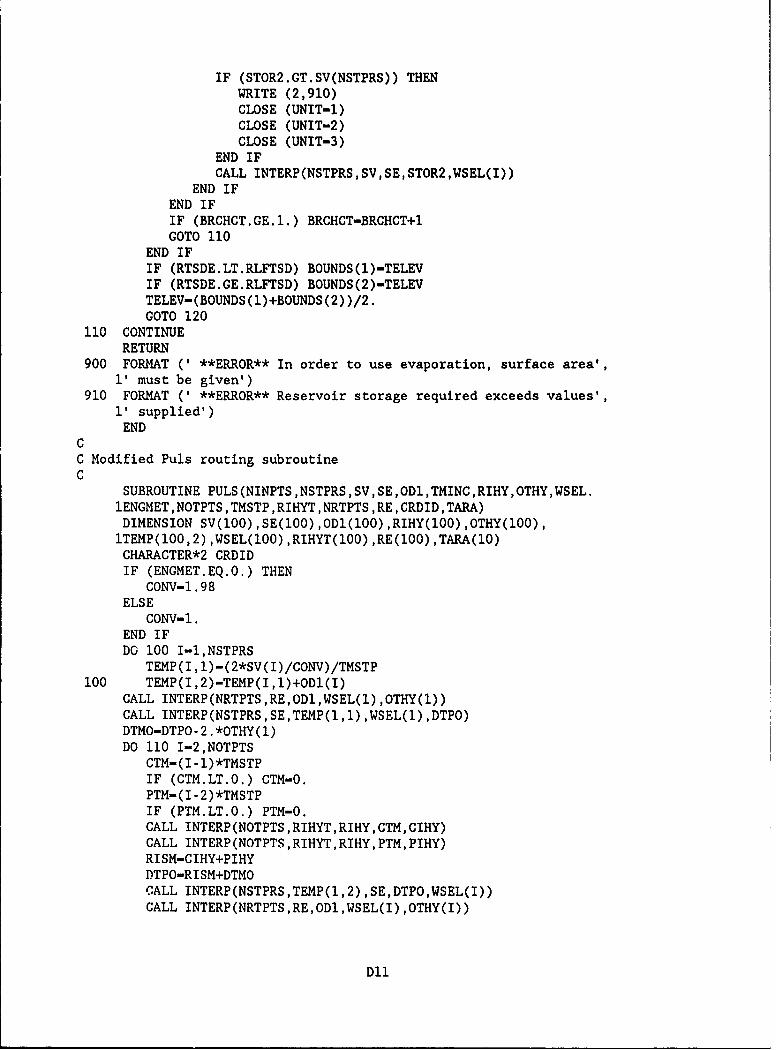
IF (STOR2.GT.SV(NSTPRS)) THENWRITE (2,910)CLOSE (UNIT-i)CLOSE (UNIT-2)CLOSE (UNIT-3)

END IFCALL INTERP(NSTPRS, SV, SE, STOR2 ,WSEL(I))

END IFEND IFIF (BRCHCT .GE. 1.) BRCHCT-BRCHCT+1GOTO 110

END IFIF (RTSDE.LT.RLFTSD) BOUNDS (1)-TELEVIF (RTSDE.GE.RLFTSD) BOUNDS(2)-TELEVTELEV-(BOUNDS(l)+BOUNDS(2) )/2.COTO 120

110 CONTINUERETURN

900 FORMAT (' **ERROR** In order to use evaporation, surface area',1' must be given')

910 FORMAT (I **ERROR** Reservoir storage required exceeds values',1' supplied')END

CC Modified Puls routing subroutineC

SUBROUTINE PULS (NINPTS ,NSTPRS ,SV, SE ,OD1 ,TMINC ,RIHY,OTHY,WSEL.lENOMET ,NOTPTS ,TMSTP ,RIHYT ,NRTPTS ,R,CRDID ,TARA)DIMENSION SV(100),SE(100),OD1(100),RIHY(100),OTHY(100),

1TEMP(100,2) ,WSEL(100) ,RIHYT(100) ,RE(100) ,TARA(1O)CHARACTER*2 CRDIDIF (ENGMET.EQ.O.) THEN

CONV-1 .98ELSE

CONV-1.END IFDO 100 I-1,NSTPRS

TEMP(I ,1)-(2*SV(I)/CONV)/TMSTP100 TEMP(I,2)-TEMP(I,1)+ODI(I)

CALL INTERP(NRTPTS,RE,0D1,WSEL(l) ,OTHY(1))CALL INTERP(NSTPRS,SE,TEMP(1,1) ,WSEL(1) ,DTPO)DTMO-DTPO -2.*OTHY( 1)DO 110 I-2,NOTPTS

CTM-(I-1)*TMSTPIF (CTM.LT.O.) CTM=O.PTM-(I -2)*TMSTPIF (PTM.LT.O.) PTM-O.CALL INTERP (NOTPTS ,RIHYT ,RIHY, CTM, CIHY)CALL INTERP (NOTPTS ,RIHYT ,RIHY, PTM, PIHY)RI SM-C IHY+PIHYDTPO=RI SM+DTMOCALL INTERP(NSTPRS,TEMP(1,2) ,SE,DTPO,WSEL(I))CALL INTERP(NRTPTS,RE,0D1,WSEL(I) ,OTHY(I))

Dll

DTMO-DTPO-2.*OTHY(I)110 CONTINUE

RETURNEND

CC Input subroutineC

SUBROUTINE RDIN(TARA,CRDID)DIMENSION TARA(1O)CHARACTER*2 CRDID,TSTRNG*78DO 110 1-1,10

110 TARA(I)-O.00READ (1,900) CRDID,TSTRNGIF (CRDID.EQ.'ZZ') THEN

GOTO 100END IFREWIND (UNIT-3)WRITE (3,910) TSTRNGREWIND (UNIT-3)READ (3,*,END-100) (TARA(L),L-1,10)

100 CONTINUERETURN

900 FORMAT (A2,A78)910 FORMAT (A78)

ENDCC List Input FileC

SUBROUTINE LISTOTCHARACTER*80 OUTLSTREWIND (UNIT-i)DO 100 1-1,500

READ (1,900,END-11O) OUTLSTWRITE (2,900) OUTLST

100 CONTINUEWRITE (2,910)STOP

110 CONTINUEREWIND (UNIT-i)DO 120 1-1,4

READ (1,900) OUTLST120 CONTINUE

WRITE (2,920)RETURN

900 FORMAT (A80)910 FORMAT (37H*ERROR - Input File Exceeds 500 Lines)920 FORMAT ('I')

ENDCC Error subroutineC

SUBROUTINE ERR(CRDID)CHARACTER*2 CRDID

D12

WRITE (2,900) CRDIDWRITE (6,900) CRDIDCLOSE (UNIT-i)CLOSE (UNIT-2)CLOSE (UNIT-3)STOPRETURN

900 FORMAT (47HERROR - CARD SEQUENCE OR NUMERIC ERROR AT CARD ,A2)END

CC Linear Interpolation subroutineC

SUBROUTINE INTERP(NPTS,X,Y,XLUPYNEW)DIMENSION X(100),Y(100)CIARACTER*2 CRDIDDO 100 J-2,NPTS

IF (XLUP.EQ.X(J)) THENYNEW-Y(J)RETURN

END IFIF (XLUP.GT.X(J))GOTO 100MIN-J-IGOTO 110

100 CONTINUEWRITE (2,900)CLOSE (UNIT-i)CLOSE (UNIT-2)CLOSE (UNIT-3)STOP

110 YNEW-Y(MIN)+((XLUP-X(MIN))*((Y(MIN+1)-Y(MIN))/(X(MIN+I)-1X(MIN')))RETURN

900 FORMAT (31HInterpolated Value Out of Range)END

CC Double linear interpolation routineC

SUBROUTINE DBLINT(NPTS,X1,YI,X2,Y2,DY,X,Y,VAL)DIMENSION XI(100),YI(100),X2(100),Y2(100),TEMP(2)CHARACTER*2 CRDIDDO 100 I-2,NPTS

IF (X.GT.XI(I)) COTO 100MIN-I-lGOTO 110

100 CONTINUEWRITE (2,900)CLOSE (UNIT-i)CL$SE (JNIT-2)CLOSE (UNIT-3)STOP

110 TEMP(1)-Yl(MIN)+((X-XI(MIN))*((YI(MIN+1)-Y1(MIN))/(Xl(MIN+I)-1Xl(MIN))))DO 120 I-2,NPTS

D13

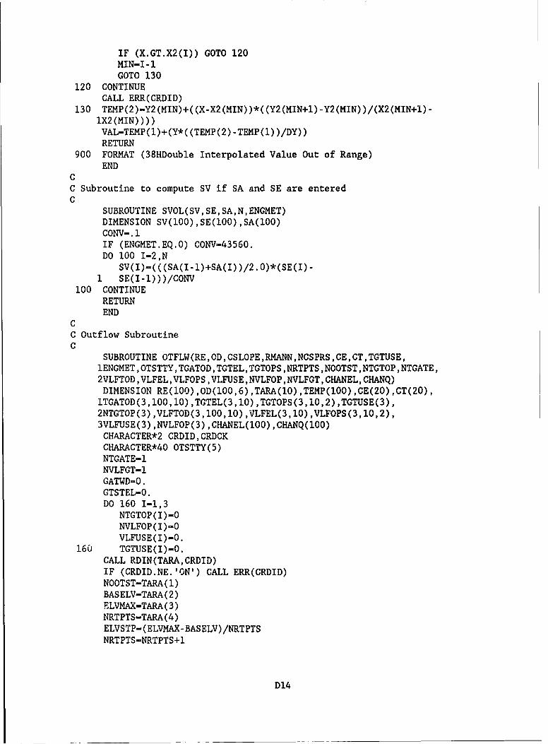
IF (X.GT.X2(I)) GOTO 120MIN-I-1GOTO 130

120 CONTINUECALL ERR(CRDID)

130 TEMP(2)-Y2(MIN)+((X-X2(MIN))*((Y2(MIN+1)-Y2(MIN))/(X2(MIN+i)-1X2(MIN))))VAL-TEMP(1)+(Y*( (TEMP(2) -TEMP(l) )/DY))RETURN

900 FORMAT (38HDouble Interpolated Value Out of Range)END

CC Subroutine to compute SV if SA and SE are enteredC

SUBROUTINE SVOL(SV,SE, SA,N, ENOMET)DIMENSION SV(100) ,SE(lOO) ,SA(100)CONV-. 1IF (ENGMET.EQ.0) CONV-43560.DO 100 I-2,N

SV(I)-((C(SA(I-l)+SA(I) )/2.O)*(SE(I) -1 SE(I-1)))/CONV

100 CONTINUERETURNEND

CC Outflow SubroutineC

SUBROUTINE OTFLW(RE ,CD , SLOPE ,RMANN,NCSPRS ,CE, CT,TGTUSE,1ENGMET ,OTSTTY ,TGATOD,TGTEL, TGTOPS,NRTPTS ,NOOTST ,NTGTOP ,NTGATE,2VLFTOD ,VLFEL,VLFOPS ,VLFUSE ,NVLFOP ,NVLFGT, CHANEL, CHANQ)DIMENSION RE(lOO),OD(100,6),TARA(lO),TEMP(lOO),CE(20),CT(20),

1TGATOD(3,1OO,lO) ,TGTEL(3,1O) ,TGTOPS(3,1O,2) ,TGTUSE(3),2NTGTOP(3) ,VLFTOD(3,100,1O) ,VLFEL(3,lO) ,VLFOPS(3,1O,2),3VLFUSE(3) ,NVLFOP(3) ,CHANEL(100),CHANQ(100)CHARACTER*2 ORDID, CRDCKCHARACTER*40 OTSTTY(5)NTGATE-lNVLFGT-1GATWD-O.GTSTEL-O.DO 160 1-1,3

NTGTOP(I)=ONVLFOP(I)-OVLFUSE(I)-O.

160 TGTUSE(I)-O.CALL RDIN(TARA,CRDID)IF (CRDID.NE.'ON') CALL ERR(CRDID)NOOTST-TARA (1)BASELV-TARA(2)FELVMAX-TARA (3)NRTPTS-TARA (4)ELVSTP-( ELVMAX- BASELV) /NRTPTSNRTPTS-NRTPTS+l

D14

DO 120 I-1,NRTPTSQD(I,6)-O.O

120 RE(I)-BASELV+(I-1)*ELVSTPDO 100 I-1,NOQTST

CALL RDIN(TARA,CRDID)IF (CRDID.EQ.1UO') THEN

CRDCK-'UO'CALL UNONOG (RE,TEMP ,NCSPRS ,CE, CT, ENGMET,TARA, CRDID,

1 CSLOPE,RMANN,NRTPTS ,CRDCK,NTGTOP,TGTUSE,GATWD,NTGATE,2 ORSTEL, GTSTEL, CHANEL, CHANQ ,PIERNO)

OTSTTY(I)-'Uncontrolled Ogee Spillway'END IFIF (CRDID.EQ.'UB') THEN

CALL UNBDCR (RE,TEMP,NCSPRS,CE,CT,ENGMET,TARA,CRDID,1OSLOPE ,RMANN ,NRTPTS ,CHANEL, CHANQ)

OTSTTY(I )-'Uncontrolled Broadcrested Weir'END IFIF (CRDID.EQ.'DI') THEN

CALL DRPINL (RE ,TEMP, ENGMET,TARA, CRDID,NRTPTS)OTSTTY(I)-'Drop Inlet Spillway'

END IFIF (CRDID.EQ.'TG') THEN

CRDCK-'TG'WRITE (2,*)WRITE (2,930)WRITE (2,*)CALL UNCNOG (RE,TEMP,NCSPRS,CE,CT,ENGMET,TARA,CRDID,

IOSLOPE ,RMANN ,NRTPTS ,CRDCK, NTGTOP ,TGTUSE, GATWD ,NTGATE,2 CSE,GTSTEL, CHANEL, CHANQ, PIERNQ)

CALL TAINGT (RE ,TEMP, NTGTOP ,NRTPTS ,GATWD, ENGMET,1TOATOD ,TOTEL, CRSTEL, TGTOPS ,NTGATE, PIER.NO)

OTSTTY(I)-'Tainter Gate on Spillway Crest'NTCATE-NTGATE+1

END IFIF (CRDID.EQ.'VL') THEN

CRDCK=' VL'WRITE (2,*)WRITE (2,940)WRITE (2,*)CALL UNCNOG (RE,TEMP,NCSPRS,CE,CT,ENGMET,TARA,CRDID,

1CSLOPE, RMANN ,NRTPTS ,CRDCK ,NVLFOP ,VLFUSE, GATWD ,NVLFGT,2 CRSTEL, CTSTEL, CHANEL, CHANQI PIERNO)

CALL VLIFTG (RE ,TEMP ,NVLFOP ,NRTPTS ,GATWD, ENGMET,IVLFTOD ,VLFEL, ORSTEL, VLFOPS ,NVLFGT ,GTSTEL)

OTSTTY(I)-'Vertical Lift Gate'NVLFGT-NVLFGT+1

END IFIF (CRDID.EQ.'OW') THEN

CALL OTWRKS (TEMP ITARA ,RE, NRTPTS ,ENGMET)OTSTTY(I)-' Outlet Works'

END IFIF (CRDID.EQ.'EL' .OR.CRDID.EQ.'DC') THEN

OTSTTY(I)-' Input Elevation Vs Discharge'

D15

NLOOP-(NRTPTS/1O. )+. 9LCNT-O

230 LCNT-LCNT+lICNT2-1DO 220 K-1,NLOOP

IF (LCNT.NE.1) CALL RDIN(TARA,CRDID)IF (CRDID.EQ.'EL') THEN

DO 200 J-ICNT2,ICNT2+9200 RE(J)-TARA(J-ICNT2+1)

ICNT2-ICNT2+1OEND IFIF (CRDID.EQ.'DC') THEN

DO 210 J-ICNT2,ICNT2+9OD(J ,6)-TARA(J-ICNT2+1)

210 OD(J,I)-TARA(J-ICNT2+1)ICNT2-ICNT2+1O

END IFIF (ICNT2.EQ.1) CALL ERR(CRDID)

220 CONTINUEIF (LCNT.EQ.1) GOTO 230IF (NOOTST.GT.1) THEN

WRITE (6,910)CLOSE (UNIT-3)CLOSE (UNIT-2)CLOSE (UNIT=1)STOP

END IFNTGATE=ONVLFGT-ONRTPTS-~NRTPTS -1RETURN

END IFIF (CRDID.NE. 'TC' .AND.CRDID.NE. 'VL') THEN

DO 110 J=1,NRTPTSOD(J ,6)-OD(J, 6)+TEMP(J)

110 OD(J,I)-TEMP(J)COTO 100

END IFIF (N-TGATE.GT.4) THEN

WRITE (2,920)CLOSE (UNIT=1)CLOSE (UNIT=2)CLOSE (UNIT-3)STOP

END IFIF (NTGATE.EQ.1) THEN

INDX1-1ELSE

INDX1=NTGATE- 1END IFIF (CRDID.EQ.'TC'.AND.TGTUSE(INDX1).NE.O.) THEN

DO 130 K-1,NTGTOP(INDX1)IF (TGTOPS(INDX1,K,1) .EQ.TGTUSE(INDX1)) GOTO 140

D16

130 CONTINUEWRITE (2,900)STOP

140 CONTINUEDO 150 J-1,NRTPTS

OD(J,6)-OD(J,6)+TGATOD(INDXl,J,K)150 OD(J,I)-TGATOD(INDXI,J,K)

END IFIF (NVLFGT.GT.4) THEN

WRITE (2,920)CLOSE (UNIT-i)CLOSE (UNIT-2)CLOSE (UNIT-3)STOP

END IFIF (NVLFGT.EQ.1) THEN

INDX1-1ELSE

INDX1-NVLFGT-1END IFIF (CRDID.EQ.'VL'.AND.VLFUSE(INDX1).NE.0.) THEN

DO 170 K-1,NVLFOP(INDX1)IF (VLFOPS(INDXI,K,I).EQ.VLFUSE(INDX1)) GOTO 180

170 CONTINUEWRITE (2,900)STOP

180 CONTINUEDO 190 J-1,NRTPTS

OD(J,6)-OD(J,6)+VLFTOD(INDX1,J,K)190 OD(J,I)-VLFTOD(INDXI,J,K)

END IF100 CONTINUE

NVLFGT-NVLFGT-1NTGATE-NTGATE-1RETURN

900 FORMAT (43H**ERROR - Gate Opening Chosen Is NOT Listed)910 FORMAT (43H**ERROR - ED Cards Must Be Used Alone ONLY!)920 FORMAT (30H**ERROR - Only 3 Gate Openings)930 FORMAT (35HTainter Gates on the Spillway Crest)940 FORMAT (19HVertical Lift Gates)

ENDCC Outlet Works SubroutineC

SUBROUTINE OTWRKS (TEMP,TARA,RE,NRTPTS,ENGMET)DTMENSION TEMP(100),TARA(10),RE(100),PORTPR(100,2),Q(100),IELEV(100)DATA (PORTPR(I,l),I-I,16) /l.,1.2,1.4,1.6,1.8,2.,2.5,3.,3.5,4.,14.5,5.,5.5,6.,6.5,7./DATA (PORTPR(I,2),I-1,16) /.75,.685,.65,.62,.59,.57,.535,.505,1.485,.47,.465,.445,.44,.43,.435,.42/NPRTPR-16DWORMN-TARA(1)

D17

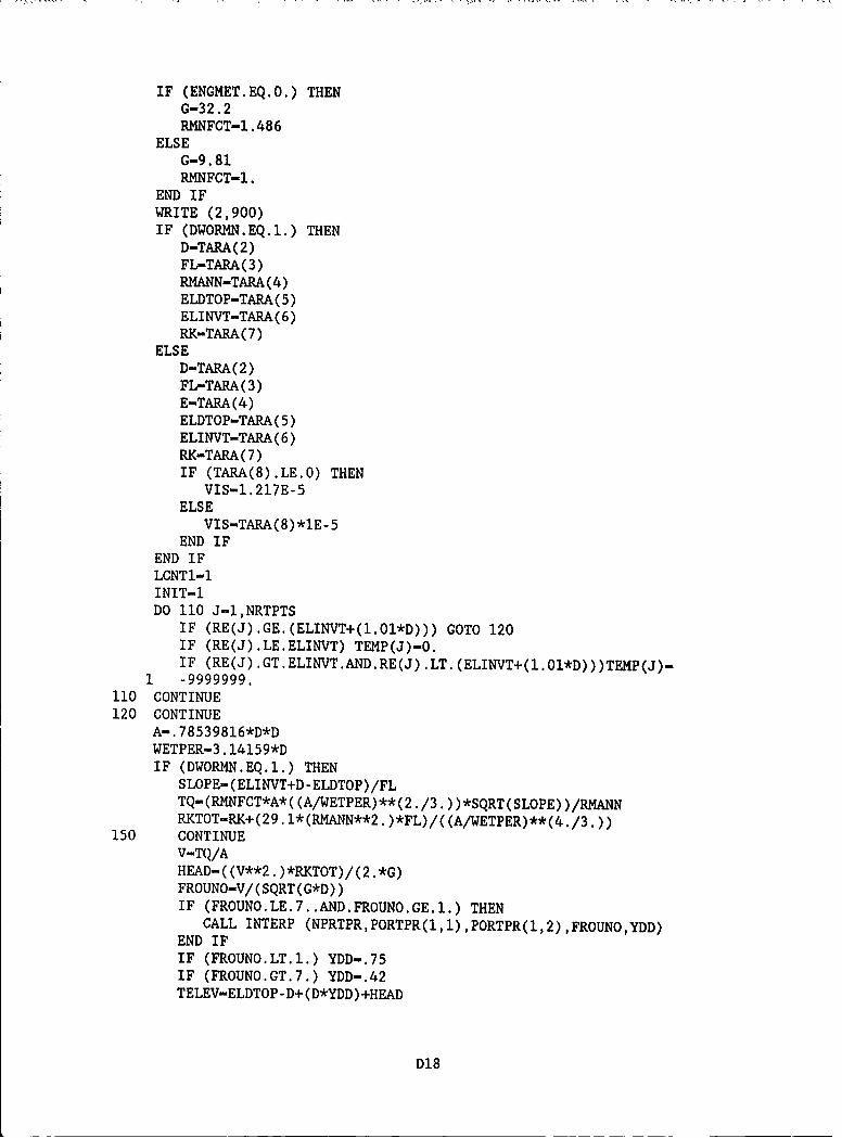
IF (ENGMET.EQ.O.) THENG-32.2RMNFCT-1 .486

ELSEG-9 .81RMNFCT-1.

END IFWRITE (2,900)IF (DWORMN.EQ.1.) THEN

D-TARA(2)FL-TARA (3)RMANN-TARA (4)ELDTOP-TARA (5)ELINVT-TARA (6)RK-TARA (7)

ELSED-TARA(2)FL-TARA(3)E-TARA (4)ELDTOP-TARA (5)ELINVT-TARA (6)RK-TARA (7)IF (TARA(8).LE.0) THEN

VIS-1 .217E-5ELSE

VIS-TARA(8)*1E-5END IF

END IFLCNT1-1IN IT-iDO 110 J-1,NRTPTS

IF (RE(J).GE.(ELINVT+(1.O1*D))) GOTO 120IF (RE(J).LE.ELINVT) TEMP(J)-O.IF (RE(J).GT.ELINVT.AND.RE(J).LT.(ELINVT+(1.1*D)))TEP(J).

1 -9999999.110 CONTINUE120 CONTINUE

A-. 78539816*D*DWETPER-3 .14159*DIF (DWORMN.EQ.1.) THEN

SLOPE- (ELINVT+D -ELDTOP)/FLTQ-(RMNFCT*A*( (A/WETPER)**(2 ./3. ))*SQRT(SLOPE) )/RMANNRKTOT-RK+(29 .1*(RMANN**2. )*FL)/( (A/WETPER)**(4 */3.))

150 CONTINUEV-TQ/AHEAD-((V**2. )*RJ(TOT)/(2 .*G)FROUNO-V/ (SQRT (G*D))IF (FROUNO.LE.7. .AND.FROUNO.GE.1.) THEN

CALL INTERP (NPRTPR, PORTPR( , 1), PORTPR( 1,2), FROUNO ,YDD)END IFIF (FROUNO.LT.1.) YDD-.75IF (FROUNO.GT.7.) YDD-.42TELEV-ELDTOP -D+ (D*YDD) +HEAD

D18

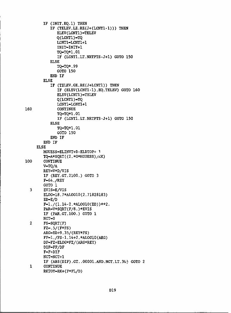
IF (INIT.EQ.1) THENIF (TELEV.LE.RE(J+(LCNT1-1))) THEN

ELEV (LCNT1) -TELEVQ(LCNT1)-TQLCNTI-LCNT1+1INIT-INIT+lTQ-TQ*1.01IF (LCNT1.LT.NRTPTS-J+1) COTO 150

ELSETQ-TQ*. 99COTO 150

END IFELSE

IF (TELEV.GE.RE(J4-LCNT1)) THENIF (ELEV(LCNT1-1).EQ.TELEV) COTO 160ELEV (LCNT1 )-TELEVQ(LCNT1)-TQLCNTI-LCNT1+1

160 CONTINUETQ-TQ*1 .01IF (LCNT1.LT.NRTPTS-J+1) COTO 150

ELSETQ-TQ*1.01GOTO 150

END IFEND IF

ELSEHGUESS-ELINVT+D- ELDTOP+ 1TQ-A*SQRT( (2 .*G*HGUESS),'xa)

100 CONTINUEV-TQ/AREY-V*D/VISIF (REY.GT.2100.) COTO 3F-64 ./REYCOTO 1

3 EVIS-E/VISELOG-18.7*ALOG1O(2 .71828183)ED-E/DF-1./(1. 14.2.*ALOG1O(ED))**2.PAR-V*SQRT(F/8. )*EVISIF (PAR.GT.100.) COTO 1NCT-O

2 FS-SQRT(F)FZ-. 5/(F*FS)ARG-ED+9 .35/(REY*FS)FF- . /FS-i. 14+2 .*ALOG1O (ARG)DF=FZ+ELOG*FZ/ (ARG*REY)DIF-FF/DFF-F+DI FNCT-NCT+lIF (ABS(DIF).GT. .00001.AND.NCT.LT.3G) GOTO 2

1 CONTINUERXTOT-RK+ (F*FL/D)

D19

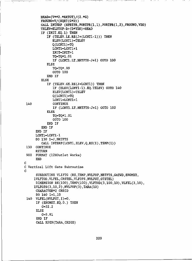
HEAD-(V**2 .*BI(TOT)/(2 .*G)FROUNO-V/ (SQRT (G*D))CALL INTERP (NPRTPR,PORTPR(1,1) ,PORTPR(1,2),FROUNO,YDD)TELEV-ELDTOP -D+ (D*YDD) +HEADIF (INIT.EQ.1) THEN

IF (TELEV.LE.RE(J+(LCNT1-1))) THENELEV (LONT ) -TELEVQ(LCNT1)-TQLCNT1-LCNT1+1INIT-INIT+1TQ-TQ*1.O1IF (LCNT1.LT.NRTPTS-J+1) GOTO 100

ELSETQ-TQ*. 99GOTO 100

END IFELSE

IF (TELEV.GE.RE(J+LCNT1)) THENIF (ELEV(LCNT1-1).EQ.TELEV) GOTO 140ELEV (LONTi) -TELEVQ(LCNTI)-TQLCNT1-LCNT1+1

140 CONTINUEIF (LCNT1.LT.NRTPTS-J+1) GOTO 100

ELSETQ-TQ*1 .01GOTO 100

END IFEND IF

END IFLCNT1-LCNT1 -1DO 130 I-J,NRTPTS

CALL INTERP(LCNT1,ELEV,Q,RE(I),TEMP(I))130 CONTINUE

RETURN900 FORMAT (l2HOutlet Works)

ENDCC Vertical Lift Gate SubroutineC

SUBROUTINE VLIFTG (RE, TEMP ,NVLFOP,NRTPTS ,GATWD,ENGMET,1VLFTOD ,VLFEL, ORSTEL ,VLFOPS ,NVLFGT ,GTSTEL)DIMENSION RE(100),TEMP(100),VLFTOD(3,100,1O),VLFEL(3,1O),1VLFOPS(3,1O,2) ,NVLFOP(3) ,TARA(1O)CHARACTER*2 ORDIDDO 140 1-1,10

140 VLFEL(NVLFGT, I)-O.IF (ENGMET.EQ.O.) THEN

G-32.2ELSE

G-9.81END IFCALL RDIN(TARA, ORDID)

D20

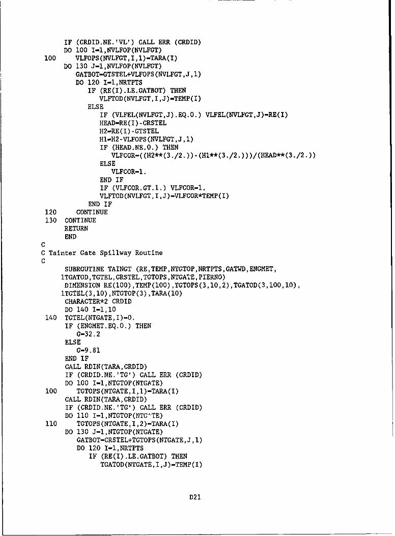
IF (CRDID.NE.'VL') CALL ERR (CRDID)DO 100 I-1,NVLFOP(NVLFGT)

100 VLFOPS(NVLFGT,I,1)-TARA(I)DO 130 J-1,NVLFOP(NVLFGT)

CATBOT-GTSTEL+VLFOPS (NVLFGT ,J, 1)DO 120 I-1,NRTPTS

IF (RE(I).LE.GATBOT) THENVLFTOD(NVLFGT, I,J)-TEI4P(I)

ELSEIF (VLFEL(NVLFGT,J) .EQ.O.) VLFEL(NVLPGT,J)-RE(I)HEAD-RE(I) -CRSTELH2-RE(I) -GTSTELHl-H2-VLFOPS(NVLFGT,J ,1)IF (HEAD.NE.O.) THEN

ELSEVLFCOR-l.

END IFIF (VLFCOR.GT.1.) VLFCOR-1.VLFTOD(NVLFGT, I,J)-VLFCOR*TEMP(I)

END IF120 CONTINUE130 CONTINUE

RETURNEND

CC Tainter Gate Spillway RoutineC

SUBROUTINE TAINGT (RE, TEMP ,NTGTOP ,NRTPTS ,GATWD ,ENGMET,iTGATOD ,TGTEL, CRSTEL, TOTOPS ,NTGATZE, PIERNO)DIMENSION RE(100),TEMP(100),TGTOPS(3,10,2),TGATOD(3,100,10),1TGTEL(3,10) ,NTGTOP(3) ,TARA(10)CHARACTER*2 ORDIDDO 140 1-1,10

140 TGTEL(NTGATE, I)-0.IF (ENGMET.EQ.O.) THEN

G-32.2ELSE

G-9.81END IFCALL RDIN(TARA, ORDID)IF (CRDID.NE.'TC') CALL ERR (CRDID)DO 100 I-1,NTGTOP(NTGATE)

100 TGTOPS(NTGATE, I, 1)-TARA(I)CALL RDIN(TARA, CRDID)IF (CRDID.NE.'TG') CALL ERR (CRDID)DO 110 I-1,NTGTOP(NTGATE)

110 TGTOPS(NTCATE, I, 2)-TARA(I)DO 130 J-1,NTGTOP(NTGATE)

GATBOT-CRSTEL+TGTOPS (NTCATE, J, 1)DO 120 I-1,NRTPTS

IF (RE(I).LE.GATBOT) THENTGATOD(NTGATE,I ,J)-TEMP(I)

D21

ELSEIF (TGTEL(NTGATE,J).EQ.0.) TGTEL(NTGATE,J)-RE(I)HEAD-RE(I)-CRSTELTGATOD(NTGATE,I,J)-(TGTOPS(NTGATE,J,2)*

1 TGTOPS(NTGATE,J,1)*GATWD*SQRT(2.*G*2 (HEAD-(.5*TGTOPS(NTGATE,J,1)))))*(PIERNO+1.)

END IF120 CONTINUE130 CONTINUE

RETURNEND

CC Drop Inlet SpillwayC

SUBROUTINE DRPINL (RE,TEMP,ENGMET,TARA,CRDID,NRTPTS)DIMENSION RE(100),TEMP(100),TARA(1O),COARA(100,4),TEMP2(100,2)CHARACTER*2 CRDIDDATA (COARA(I,1),I-1,20) /.18,.2,.3,.4,.5,.6,.7,.8,.9,1.,1.1,11.2,1.3,1.4,1.5,1.6,1.7,1.8,1.9,2./DATA (COARA(I,2),I-1,20) /3.92,3.89,3.75,3.57,3.37,3.1,2.79,2.48,12.23,2.04,1.86,1.71,1.59,1.47,1.38,1.29,1.2,1.15,1.08,1.02/DATA (COARA(I,3),I-1,20) /3.99,3.98,3.86,3.7,3.5,3.24,2.91,2.6,12.34,2.12,1.94,1.79,1.65,1.54,1.44,1.34,1.26,1.19,1.12,1.09/DATA (COARA(I,4),I-1,20) /4.02,4.,3.87,3.72,3.54,3.32,3.02,2.68,12.4,2.2,2.01,1.86,1.7,1.59,1.48,1.39,1.3,1.23,1.17,1.11/NCOPT-20APDPTH-TARA(1)RADIUS-TARA(2)CO-TARA(3)CRSTEL-TARA(4)WRITE (2,*)WRITE (2,900)WRITE (2,*)DO 100 I-1,NRTPTS

HEAD-RE(I)-CRSTELIF (HEAD.LE.0) THEN

TEMP(1)-O.GOTO 100

END IFPDRS-APDPTH/RADIUSHDRS-HEAD/RADIUSIF (CO.LE.0.) THEN

IF (HDRS.LT..18) THENWRITE (2,910) IIF (PDRS.GT..15.AND.PDRS.LT.2.) THEN

DO 110 J-1,3110 TEMP2(J,2)-COARA(1,J+I)

TEMP2(I,I)-2.0TEMP2(2,1)-.3TEMP2(3,1)-.15NTEMP2-3CALL INTERP (NTEMP2,TEMP2(1,I),TEMP2(1,2),PDRS,CO)

END IF

D22

IF (PDRS.LE. .15) THEN00-4.02WRITE (2,920) I

END IFIF (PDRS.GE.2.) THEN

C0-3.92WRITE (2,930) I

END IFEND IFIF (HDRS.GT.2.0) THEN

WRITE (2,940) IIF (PDRS.CT. .15.AND.PDRS.LT.2.) THEN

DO 120 J-1,3120 TEMP2(J,2)-COARA(20,J+l)

TEMP2(1 , )-2.0TEMP2(2 ,1)-.3TEMP2(3 ,1)-.15NTEMP2-3CALL INTERP (NTEMP2,TEMP2(,),TEMP2(1,2),PDRS,CO)

END IFIF (PDRS.LE. .15) THEN

00-1.11WRITE (2,920) I

END IFIF (PDRS.GE.2.) THEN

C0-1.02WRITE (2,930) I

END IFEND IFIF (PDRS.LE.2. .AND.PDRS.GE. .3) THEN

DY-2.0- .3YINC-PDRS- .3CALL DBLINT(NCOPT,COARA(1,1),COARA(1,2),COARA(1,1),

1 COARA(1,3),DY,HDRS,YINC,CO)END IFIF (PDRS.LE. .3.AND.PDRS.GE. .15) THEN

DY-. 3- .15YINC-PDRS- .15CALL DBLINT(NCOPT,COARA(1,1),COARA(1,3),COARA(1,1),

1 COARA(1,4),DY,HDRS,YINC,CO)END IF

END IFTEMP(I)=CO*2.*RADIUS*3.14159*(HEAD**(3./2.))

100 CONTINUERETURN

900 FORMAT (l9HDrop Inlet Spillway)910 FORMAT (53H*WARNING H/Rs < .18 - .18 USED FOR COMPUTATION OF Cs#,

113)920 FORMAT (53H*WARNING P/Rs < .15 - .15 USED FOR COMPUTATION OF CsjI,

113)930 FORMAT (53H*WARNING P/Rs > 2.0 - 2.0 USED FOR COMPUTATION OF Cs#,

113)

D23

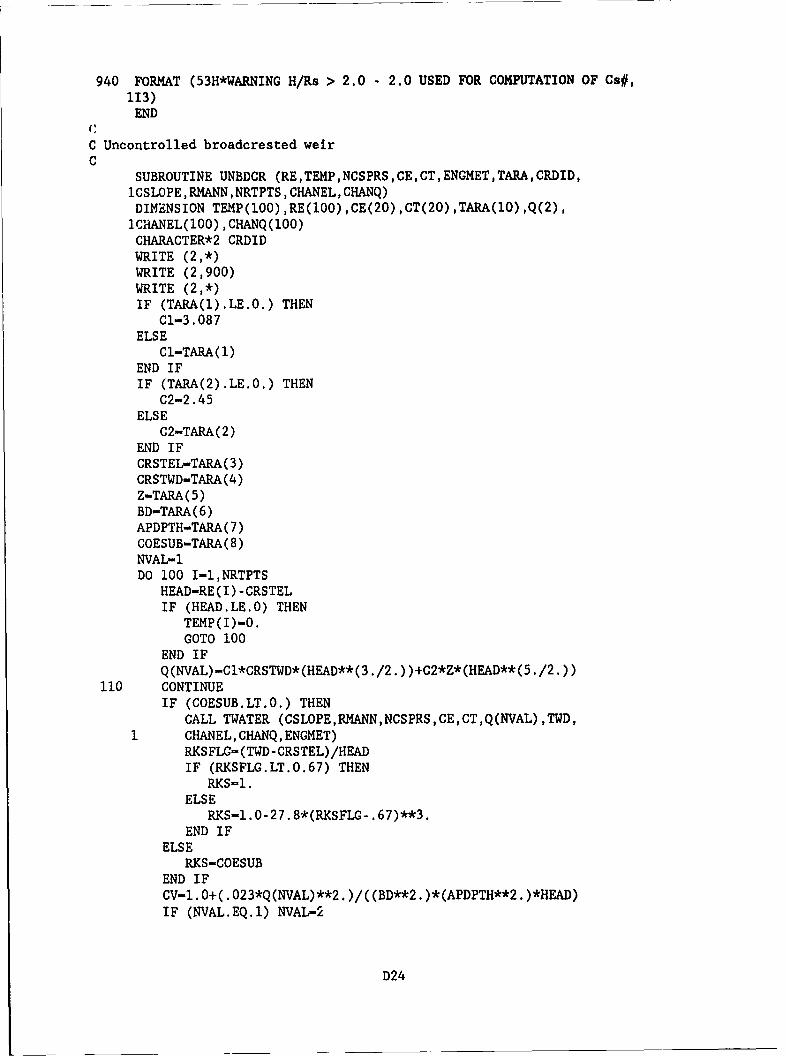
940 FORMAT (53H*WARNING H/Rs > 2.0 - 2.0 USED FOR COMPUTATION OF Cs#,113)END

r

C Uncontrolled broadcrested weirC

SUBROUTINE UNBDCR (RE ,TEMP ,NCSPRS ,CE, CT, ENGMET, TAA, CRDID,lOSLOPE ,RMANN, NRTFTS ,CHANEL, CHANQ)DIME~NSION TEMP(lOO),RE(l0O),CE(20),CT(20),TARA(lO),Q(2),

1CI-HAN EL(lOO) ,CHANQ(lOO)CHARACTER*2 ORDIDWRITE (2,*)WRITE (2,900)WRITE (2,*)IF (TARA(l).LE.O.) THEN

Cl-3.087ELSE

Ci-TARA (1)END IFIF (TARA(2).LE.O.) THEN

C2-2.45ELSE

C2-TARA(2)END IFCRSTEL-TARA( 3)CRSTWD-TARA(4)Z-TARA (5)BD-TARA (6)APDPTH-TARA(7)COESUB-TARA (8)NVAL-lDO 100 I-l,NRTPTS

HEAD-RE(I) -ORSTELIF (HEAD.LE.O) THEN

TEMP(I)-O.GOTO 100

END IFQ(NVAL)-Cl*CRSTWD*(HEAD**(3./2. ))+C2*Z*(HEAD**(5./2.))

110 CONTINUEIF (COESUB.LT.O.) THEN

CALL TWATER (CSLOPE,RM'ANN,NCSPRS,CE,CT,Q(NVAL) ,TWD,1 CHANEL, CHANQ, ENGMET)

RKS FLO- (TWD -CRS TEL) /HEADIF (RKSFLG.LT.O.67) THEN

RKS-1.ELSE

RKS-1.O-27.8*(RKSFLG- .67)**3.END IF

ELSERKS-COESUB

END IFCV-1.O ( .023*Q(NVAL)**2. )/((BD**2. )*(APDPTH**2. )*HEAD)IF (NVAL.EQ.1) NVAL-2

D24

Q(NVAL)=Cl*CRSTWD*CV*RKS*.(HEAD**(3 ./2. ))+C2*Z*CV*RKS*(HEAD**1 (5./2.))DIFF-ABS (Q(1) -Q(2))IF (DIFF.GT. .05) THEN

Q(1)-Q(2)GOTO 110

END IFTEMP (I) -Q (2)

100 CONTINUERETURN

900 FORMAT (30HUncontrolled Broadcrested Weir)END

CC Uncontrolled ogee spillway subroutineC

SUBROUTINE UNCHOG (RE ,TEMP ,NCSPRS ,CE, CT, ENGMET,TARA, CRDID,1CSLOPE ,RMANN,NRTPTS,CRDCK,NTGTOP ,TGTUSE,GATWD,NTGATE,CRSTEL,2GTSTE,CHANEL,CHANQ, PIERNO)DIMENSION RE(lOO),TARA(lO),TEMP(lOO),Q(3),DC33(100,2),1DC67(lOO,2) ,DC133(lOO,2) ,CE(20) ,CT(20) ,CKA(100,2) ,TGTUSE(3),2EKA(lOO,2) ,RKPARA(100,5) ,SUBCOE(lOO,l9) ,SUBCLM(lOO,2) ,NTGTOP(3),3CHANEL(lOO) ,CHANQ(100) ,SLFCHD(lOO) ,SLPFCC(lOO)CHARACTER*2 CRDID ,CRDCKCOMMON /COMBLK/ DC33,DC67,DC133,CKA,EKA,RKPARA,SUBCOE,SUBCLM4DO 130 1-1,15

DC33(l,l)-(I-1)*.lDC67(I,l)=(I-l)*.lDC133(I, l)=(I-1)*. 1EKA (I ,1)- (I-i) **1CKA(I,1)-I+l.RKPARA(I, l)-.2*(I-1)

130 CONTINUEoC33(15, 1)-i .34D-C67(15 ,1)-i. 33DC133(15 ,1)-1.4DC33(16 ,1)-10.DC67(16,1)-10.DC133(16,1)-10.CKA(1,l)-2.15RKPARA(13 ,1)-1.325NDCPTS-16NCKAPT-10NEKAPT-15NSUBPT-14DO 110 1-1,41

110 TEMP(I)-O.RKP-TARA(1)RKA-TARA (2)DC-TARA(3)APWDTH-TARA(4)APDPTH-TARA(5)CRSTHT-TARA( 6)DESHD-TARA( 7)

D2 5

PIERliO-TARA( 8)SPLNW-TARA(9)PIERTY-TARA( 10)CALL RDIN (TARA,CRDID)IF (CRDID.NE.CRDCK) CALL ERR(CRDID)ORSTEL-TARA (1)ADSCTM-TARA( 2)ABTRAD-TARA (3)IF (TARA(4).EQ.O.) THEN

COESUB-1.ELSE

COESUB-TARA (4)END IFNSLFCC-TARA (5)IF (CRDCK.EQ. 'TO' .OR.CRDCK.EQ. 'VL') THEN

GATWD-TARA(6)NTGTOP(NTCATE)-TARA( 7)TGTUSE(NTGATE)-TARA(8)GTSTEL-TARA( 9)

END IFNLOOP-(NSLFCC/1O. )+.9I CNT2-ODO 140 I-1,NLOOP

CALL RDIN (TARA,CRDID)IF (CRDID. NE. ORDOK) CALL ERR(CRDID)DO 150 J-1,10

150 SLFCHD(J+ICNT2)-TARA(J)ICNT2-ICNT2+10

140 CONTINUEICNT2-ODO 160 I-1,NLOOP

CALL RDIN (TARA,CRDID)IF (CRDID.NE.CRDCK) CALL ERR(CRDID)DO 170 J-1,10

170 SLPFCC(J+ICNT2)-TARA(J)ICNT2-ICNT2+1O

160 CONTINUEIF (ENGMET.EQ.O.) THEN

G-32.2ELSE

G-9.81END IFNQ-1PDHD-CRSTHT/DESHDIF (CRDCK.EQ.'UO') THEN

WRITE (2,*)WRITE (2,900)WRITE (2,*)

END IFIF (PDHD.LT. .33) WRITE (2,910)IF (PDHD.GT.1.33) WRITE (2,920)DO 100 I-1,NRTPTS

v-0.

D26

IF (RE(I).LE.CRSTEL) GOTO 100HEAD-RE(I) -CRSTELAREA- (APDPTH4-HEAD) *APWDTHHHDFLG-O.IF (RKP.LT.O.) THEN

HDHD-HEAD/DESHDIF (HDHD.LT. .2) THEN

HHDFLG-1.IF (PIERTY.EQ.1) RKP-.047IF (PIERTY.EQ.2) RKP-.095IF (PIERTY.EQ.3) RKP-.081IF (PIERTY.EQ.4) RKP-.101

END IFIF (HDHD.GT.1.325) THEN

HHDFLG-2.IF (PIERTY.EQ.1) RKP-.000IF (PIERTfY.EQ.2) RKP-- .009IF (PIERTY.EQ.3) RKP-- .014IF (PIER',-Y.EQ.4) RKP-- .031

END IFIF (HDRD.GE. .2.AND.HDHD.LE.1.325) THEN

IF (PIERTY.EQ.1.) CALL INTERP (NKPPT,RKPARA(l,1),I RKPARA(1,2),HDHD,RKP)

IF (PIERTY.EQ.2.) CALL INTERP (NKPPT,RKPARA(l,1),1 RKPARA(1,3),HDHD,RKP)

IF (±-IIRTY.EQ.3.) CALL INTERP (NKPPT,RKPARA(l,1),1 RKPARA(1,4),HDHD,RKP)

IF (PTERTY.EQ.4.) CALL INTERP (NKPPT,RKPARA(1,1),1 RKPARA(1,5),HDHD,RKP)

END IFEND IF

120 CONTINUEHE-HEAD+( (V**2. )/(2 .*G))HbDHD-HE/DESHDIF (DC.LE.0) THEN

IF (PDHD.LE. .33) CALL INTERP (NDCPTS,DC33(1,1),DC33(1,2),1 HEDHD,DC)

IF (PDHD.GE.1.33)CALL INTERP (NDCPTS,DC133(1,1),DC133(1,2),1 HEDHD,DC)

IF (PDHD.EQ. .67) CALL INTERP (NDCPTS,DC67(1,1),DC67(1,2),1 HEDHD,DC)

IF (PDHD.GT. .33.AND.PDHD.LT. .67) THENDY-.67- *33YINC-PDHD- .33CALL DBLINT(NDCPTS,DC33(1,1),DC33(1,2),DC67(1,1),

1 DC67(1,2),DY,HEDHD,YINC,DC)END IFIF (PDHD.GT. .67.AND.PDHD.LT.1.33) THEN

DY-1.33-.67YINC-PDHD- .67CALL DB)aNT(NDCPTS,D 67(..1),DC67(1,2),DC133(1,1),

1 DC133(1,2),DY,HEDHD,YINC DC)END IF

D27

END IFHERFLG-O.IF (RKA.LT.O) THEN

IF (ADSCTM.EQ.1.) THENHEDR-HE/ABTRADIF (HEDR.LT.2.15) THEN

RKA-.043HERFLG-1.

END IFIF (HEDR.GT.11.) THEN

RKA-.1OHERFLG-2.

END IFIF (HEDR.GE.2.15.AND.HEDR.LE.11.) THEN

CALL INTERP (NCKAPT,CKA(100,1) ,CKA(100,2) ,HEDR,RKA)END IF

ELSEIF (HEDHD.LT.O.) RKA-O.IF (HEDHD.GT.1.4) RKA-.2IF (HEDHD.GE.O.AND.HEDHD.LE.1.4) THEN

CALL INTERP (NEKAPT,EKA(100,1) ,EKA(100,1) ,HEDHD,RKA)END IF

END IFEND IFESPLWD-SPLNW- 2. * (PIERQ*RKP+.) *HECALL INTERP (NSLFCC, SLFCHD, SLPFCC ,HEAD,SLFCCF)Q(NQ)-DC*SLFCCF*ESPLWD*HE**(3 ./2.)HEDFLC-O.HDHFLG-O.IF (GOESUB.LT.O) THEN

CALL TWATF.R (CSLOPE,RMANN,NCSPRS,CE,CT,Q(NQ) ,TWD,CHANEL,CHANQ,ENGMET)IF (CHANEL(2).NE.O.) CE(l)'-CHANEL(l)TWD-TWD-CE(l)Y1-(HE+CRSTEL-C'E(1) )/HEHDDHE-(HE+CRSTEL-CE(l) -TWD)/H.IF (HDDHE.LE.O.) THEN

HDHFLG-1.PSUB-iQO.

END IFIF (HDDHE.GT. .9.AND.Y1.LT.1.07) PSUB-15.IF (HDDHE.UT. .9.AND.Y1.GT.4.5) PSUB-O.IF (HDDHE.GT. .9.AND.Y1.GE.1.07.AND.Y1.LE.4.5) THEN

NTEMPT-18HDHFLG-2.CALL INTERP(NTEMPT,SUBCL4(1,1) ,SUBCLI4(1,2) ,Y1,PSUB)

END IFIF (HDDHE.GT.O.AND.HDDHE.LE. .9) THEN

TF (Y1.LT.1.07) THENHEDFLG-1.CAL.L INTER? (NSUBPT,SUBCOE(1,1) ,SUBCOE(1,2) ,HDDHE,PSUB)

END IF

D28

IF (Y1.GT.4.50) THENHEDFLG-2.CALL INTERP(NSUBPT, SUBCQE(1, 1) ,SUBCOE(1,19) ,HDDHE,PSUB)

END IFIF (Y1.GE.1.07.AND.Y1.LE.1.1) THEN

DY-1. 1-1. 07YINC-Y1-1 .07CALL DBLINT(NSUBPT,SUBCOE(1,1) ,SUBCOE(1,2),SUBCOE(1,1),SUBCOE(1,3),DY,HDDHE,YINC,PSUB)

END IFIF (Y1.GE.1.1.AND.Y1.LE.1.15) THEN

DY-i. 15-1. 1YINC-YI-1.1CALL DBLINT(NSUBPT, SUBCOE(1, 1) ,SUBCOE(1, 3),SUBCOE(1,1),SUBCOE(1,4),DY,HDDHE,YINC,PSUB)

END IFIF (Y1.CE.1.15.AND.Y1.LE.1.2) THEN

DY-1.2-1.15YINC-Y1-1 .15CALL DBLINT(NSUBPT,SUBCOE(1,1) ,SUBCOE(1,4),SUBCOE(1,1),SUBCOE(1,5),DY,HDDHE,YINC,PSUB)

END IFIF (Y1.GE.1.2.AND.Y1.LE.1.3) THEN

DY-i. 3-1.2YINC-Y1-1.2CALL DBLINT(NSUBPT,SUBCOE(1,1) ,SUBCOE(1,5),SUBCOE(1,1),SUBCOE(1,6),DY,HDDHE,YINC,PSUB)

END IFIF (Y1.GE.1.3.AND.Y1.LE.1.4) THEN

DI-1.4-1.3YINC-Y1-1.3CALL DBLINT(NSUBPT,SUBCOE(1,1) ,SUBC0E(".,6),SUBCOE(1,1),SUBCOE(1,7),DY,HDDHE,YINC,PSUB)

END IFIF (Y1.GE.1.4.AND.Y1.LE.1.5) THEN

DY-i. 5-1.4YINC-Y1-1 .4CALL DBLINT(NSUBPT,SUBCOE(1,1) ,SUBCOE(1,7),SUBCOE(1,1),SUBCOE(1,8),DY,HDDHE,YINC,PSUB)

END IFIF (Y1.GE.1.5.AND.Y1.LE.1.6) THEN

DY-i .6-1.5YINC-Y1-1.5CALL DBLINT(NSUBPT,SUBCOE(1,1) ,SUBCOE(1,8),SUBCOE(1,1),SURCOE(1,9),DY,HDDHE,YIIC,PSUB)

END IFIF (Y1.GE.1.6.AND.Y1.LE.1.7) THEN

DY-i .7-1.6YINC-Y1-1 .6CALL DBLINT(NSUBPT, SUBCOE(1, 1) ,SUBCOE(1 ,9),SUBCOE(1,1),SUBCOE(1,10),DY,HDDHE,YINC,PSUB)

END IF

D29

IF (Yl.GE.1.7.AND.Y1.LE.1.8) THENDY-i. 8-1. 7YINC-Y1-1.7CALL DBLINT(NSUBPT, SUBCOE(1, 1) ,SUBCOE(1 ,1O),SUBCOE(1,1),SUBCOE(1,11),DY,HDDHE,YINC,PSUB)

END IFIF (Y1.GE.1.8.AND.Yl.LE.1.9) THEN

DY-1.9-1.8YINC-Yl-1.8CALL DBLINT(NSUBPT,SUBCOE(1,l) ,SUBCOE(1,11),SUBCOE(l,l),SUBCOE(1,12),DY,HDDHE,YINC,PSUB)

END IFIF (Y1.GE.1.9.AND.Yl.LE.2.O) THEN

DY-2 .0-1.9YINC-Y1-1 .9CALL DBLINT(NSUBPT, SUBCOE(1, 1), SUBCOE(1 ,12),SUBCOE(1,l),SUBCOE(1,13),DY,HDDHE,YINC,PSUB)

END IFIF (Y1.GE.2.0.AND.Y1.LE.2.25) THEN

DY-2. 25-2.YINC-Y1-2.CALL DBLINT(NSUBPT:SUBCOE(1,1) ,SUBCOE(1,13),SUBCOE(1,1),SUBCOE(1,14),DY,HDDHE,YINC,PSUB)

END IFIF (Y1.GE.2.25.AND.Yl.LE.2.5) THEN

DY-2.5-2.25YINC-Y1-2 .25CALL DBLINT(NSUBPT,SUBCOE(1,1) ,SUBCQE(1, 14),SUBCOE(1,l),SUBCOE(1,15),i)Y,HDDHE,YINC,PSUB)

END IFIF (Y1.GE.2.5.AND.Y1.LE.3.0) THEN

DY-3.0-2.5YINC-Y1-2 .5CALL DBLINT(NSUBPT,SUBCOE(1,l) ,SUBCOE(1,15),SUBCOE(1,1),SUBCOE(1,16),DY,HDDHE,YINC,PSUB)

END IFIF (YI.GE.3.0.AND.Y1.LE.3.5) THEN

DY-3.5-3.OYINC-Y1-3 .0CALL DBLINT(NSUBPT,SUBCOE(1, 1),SUBCOE(1,16),SUBCOE(l,I),SUBCQE(1,17),DY,HDDHE,YINC,PSUB)

END IFIF (Y1.GE.3.5.AND.Y1.LE.4.0) THEN

DY-4. 0-3. 5YINC-Y1-3 .5CALL DBLINT(NSUBPT,SUBCOE(1,1) ,SUBCOE(1,17),SUBCOE(l,1),SUBCOE(1,18),DY,HDDHE,YINC,PSUB)

END IFIF (Y1.GE.4.0.AND.Y1.LE.4.5) THEN

DY-4. 5-4.0YINC-Y1-4 .0CALL DBLINT(NSUBPT, SUBCOE(1, 1) ,SUBCOE(1,18),SUBCOE(l,1),SUBCOE(1,19),DY,HDDHE,YINC,PSUB)

D30

END IFEND IFQ(NQ)-Q(NQ)-.01*PSUB*Q(NQ)

ELSEQ(NQ)-Q(NQ)*COESUB

END IFV-Q (NQ)/AREAIF (NQ.EQ.1) THEN

NQ-2GOTO 120

ELSEDIFF-ABS(Q(1)-Q(2))IF (DIFF.GT..O) THEN

Q(1)-Q(2)GOTO 120

ELSETEMP(I)-Q(2)IF (HHDFLC.EQ.1.) WRITE (2,950) IIF (HHDFLG.EQ.2.) WRITE (2,960) IIF (HDHFLG.EQ.1.) WRITE (2,990) IIF (HDHFLG.EQ.2.) WRITE (2,1000) IIF (HEDFLG.EQ.1.) WRITE (2,970) IIF (HEDFLG.EQ.2.) WRITE (2,980) IIF (HERFLG.EQ.1.) WRITE (2,930) IIF (HERFLG.EQ.2.) WRITE (2,940) INQ-1

END IFEND IF

100 CONTINUERETURN

900 FORMAT (26HUncontrolled Ogee Spillway)910 FORMAT (51H*WARNING P/Hd < .33 .33 USED FOR COMPUTATION OF C)920 FORMAT (53H*WARNING P/Hd > 1.33 - 1.33 USED FOR COMPUTATION OF C)930 FORMAT (54H*WARNING He/R < 2.15 - 2.15 USED FOR COMPUTATION OF Ka)940 FORMAT (54H*WARNING He/R > 11.0 - 11.0 USED FOR COMPUTATION OF Ka)950 FORMAT (51H*WARNING H/Hd < .2 - .2 USED FOR COMPUTATION OF Kp#,I3)960 FORMAT (53H*WARNING H/Hd > 1.3 - 1.3 USED FOR COMPUTATION OF Kp#,

113)970 FORMAT (54H*WARNING He+D/He<1.07-1.07 USED FOR COMPUTATION OF Cs#,

113)980 FORMAT (54H*WARIIING He+D/He>4.50-4.50 USED FOR COMPUTATION OF Cs#,

113)990 FORMAT (54H*WARNING HD/He < 0.0 - 0.0 USED FOR COMPUTATION OF Cs#,

113)1000 FORMAT (54H*WARNING HD/He > .90 - .90 USED FOR COMPUTATION OF Cs#,

l13)END

CC Output SubroutineC

SUBROUTINE OUTPUT(OTHY,NINPTS,STDY,STMN,STYR,STTM,TMINC,BLKNM,1WSEL,NOTPTS,TMSTP,OTSTTY,TGATOD,TGTEL,TGTOPS,OD,NRTPTS,RTFLG,

D31

2NOOTST ,NTGTOP,ENGMET,NTGATE,TGTUSE,RE,VLFTOD,VLFEL, VLFOPS,3VLFUSE,NVLFOP,NVLFGT,RIHY,NSTPRS ,SE, SV)DIMENSION OTHY(100) ,IDATE(100,5) ,WSEL(100) ,TGATOD(3,100,1O),1TGTEL(3,10) ,TGTOPS(3,1O,2) ,OD(100,6) ,TGTUSE(3) ,NTGTOP(3) ,RE(100),2VLFTOD(3,100,1O) ,VLFEL(3,10) ,VLFOPS(3,1O,2) ,VLFUSE(3) ,NVLFOP(3),3RIHY(100) ,SE(100) ,SV(100)CHARACTER*40 BLKNM,OTSTTY(5) ,VLFLBL,TGTLBLCHARACTER*6 UNITVLFLBL-'Vertical Lift Gate'TGTLBL-'Tainter Gate on Spillway Crest'IF (ENGMET.EQ.O.) THEN

UNIT-' Feet'ELSE

UIT-'Meters'END IFDO 230 J-1,NTGATE

IF (TGTOPS(J,1,1).NE.O.) THENWRITE (2,950)WRITE (2,*)WRITE (2,*)WRITE (2,960) JWRITE (2,*)WRITE (2,*)DO 100 I-1,NTGTOP(J)

WRITE (2,970) I,TGTOPS(J,I,1),UNITWRITE (2,980) TGTEL(J,I),UNIT

100 CONTINUEWRITE (2,*)WRITE (2,*)WRITE (2,990)LFSTPT-1LLSTPT-LFSTPT+4IF (NTGTOP(J).LE.5) THEN

LLSTPT-NTGTOP (.J)END IF

220 CONTINUEWRITE (2,1000) LFSTPT ,LFSTPT+1 ,LFSTPT+2 ,LFSTPT+3 ,LFSTPT+4DO 210 I-1,NRTPTS

WRITE (2,1010) RE(I), (TGATOD(J,I,K) ,K-LFSTPT,LLSTPT)210 CONTINUE

IF (NTGTOP(J).GT.5.AND.LFSTPT.LT.6) THENLFSTPT-6LLSTPT-NTGTOP (J)WRITE (2,950)WRITE (2,960) JWRITE (2,*)GOTO 220

END IFEND IF

230 CONTINUEDO 240 J-1,NVLFGT

IF (VLFOPS(J,1,1).NE.0.) THENWRITE (2,950)

D32

WRITE (2,*)WRITE (2,*)WRITE (2,1020) JWRITE (2,*)WRITE (2,*)DO 250 I-1,NVLFOP(J)

WRITE (2,970) I,VLFOPS(J,I,I),UNITWRITE (2,980) VLFEL(J,I),UNIT

250 CONTINUEWRITE (2,*)WRITE (2,*)WRITE (2,990)LFSTPT-1LLSTPT-LFSTPT+4IF (NVLFOP(J).LE.5) THEN

LLSTPT-NVLFOP (J)END IF

260 CONTINUEWRITE (2,1000) LFSTPT,LFSTPT+1,LFSTPT+2,LFSTPT+3,LFSTPT+4DO 270 I-1,NRTPTS

WRITE (2,1010) RE(I),(VLFTOD(J,I,K),K-LFSTPT,LLSTPT)270 CONTINUE

IF (NVLFOP(J).GT.5.AND.LFSTPT.LT.6) THENLFSTPT-6LLSTPT-NVLFOP(J)WRITE (2,950)WRITE (2,1020) JWRITE (2,*)GOTO 260

END IFEND IF

240 CONTINUEWRITE (2,950)WRITE (2,*)WRITE (2,1030)WRITE (2,*)LCNT3-1LCNT4-1DO 280 J-1,NOOTST

WRITE(2,1040) J,OTSTTY(J)IF (OTSTTY(J).EQ.TGTLBL) THEN

WRITE (2,1050) TGTUSE(LCNT3),UNITLCNT3-LCNT3+1

END IFIF (OTSTTY(J).EQ.VLFLBL) THEN

WRITE (2,1050) VLFUSE(LCNT4),UNITLCNT4-LCNT4+1

END IF280 CONTINUE

WRITE (2,*)WRITE (2,1060)WRITE (2,1070) (1,1-1,5)WRITE (2,*)

D33

DO 290 J-1,NRTPTSWRITE (2,1080) RE(J) ,(OD(J,K) ,K-1,6)

290 CONTINUEIF (RTFLG.EQ.0) THEN

WRITE (2,950)WRITE (2,*)WRITE (2,*)WRITE (2,910) BLKNMWRITE (2,*)WRITE (2,*)WRITE (2,930)TMSTP-TMSTP*1440.IDATE(1, 1)-STYRIDATE(1, 2)-STMNIDATE(1, 3)-STDYIDATE(1, 5)-AMOD(STTH/100, 2. )*100 . 5IDATE(1 ,4)-STTH/100.DO 120 J-2,NOTPTS

IDATE(J , 5,-.IDATE(J-1 ,5)+TMSTPDO 115 11-1,4

115 IDATE(J,I1)-IDATE(J-1,I1)DO 130 K-1,100

IF(IDATE(J,5).LT.60) COTO 140IDATE(J ,4)-IDATE(J ,4)+1

130 IDATE(J,5)-IDATE(J,5)-60140 CONTINUE

DO 150 K-1,100IF(IDATE(J,4).LT.24) COTO 160IDATE(J ,3)-IDATE(J ,3)+1

150 IDATE(J,4)-IDATE(J,4)-24160 CONTINUE

IDANMO-30IF (IDATE(J,2).EQ.1.OR.IDATE(J,2).EQ.3.0ft.IDATE(J,2).

1 EQ.5.OR.IDATE(J,2).EQ.7.OR.IDATE(J,2).EQ.8.OR.IDATE(J,2).2 EQ.10.OR.IDATE(J,2).EQ.12) IDANM4O-31

IF (IDATE(J,2).NE.2) COTO 170IDANMO-28RYR-IDATE(J, 1)RLPYR-AMOD(ABS(RYR-1988)/4. ,2.)IF (RLPYR.hQ.O) IDANMO-29

170 CONTINUEIF(IDATE(J,3).LE.IDANMO) COTO 180IDATEJ,2)-IDATE(J ,2)+1TDI.TE(J ,3)-IDATE(J ,3) -IDANI4OIF (IDATE(J,2).LE.12) GOTO 190IDATE(J , )-IDATE(J ,1)+1IDATE(J ,2)-IDATE(J ,2) -12

190 CONTINUECOTO 160

180 CONTINUE120 CONTINUE

Do 200 J-1,NOTPTSCALL INTERP (NSTPRS ,SE, SV,WSEL(J) ,STQRGE)

D34

WRITE (2,940) (IDATE(J,L),L-1,5),RIHY(J),OTHY(J),WSEL(J),1 STORGE

200 CONTINUEEND IFRETURN

910 FORMAT (33HOutput Hydrograph for Reservoir: ,A40)920 FORMAT (F4.0)930 FORMAT (20H Year Mo Dy Hour,5X,'Inflow',5X,'Outflow',5X,

l'Elevation',5X,'Storage')940 FORMAT (4X,14,3(lX,12),I2,4(3X,FIO.l))950 FORMAT ('1')960 FORMAT (42HTainter Gate Rating Curves For Gate Number,13)970 FORMAT (20HGate Opening Number ,13,' is ',F6.2,' ',A6)980 FORMAT (45HFlow through this gate became orfice flow at

lFIO.2,' ',A6,' elevation')990 FORMAT (' ',30X,'Gate Opening Number')

1000 FORMAT (' ',' Elevation',SX,13,4(9X,13))1010 FORMAT (' ',F1O.2,5(2X,F1O.2))1020 FORMAT (48HVertical Lift Gate Rating Curves For Gate Number,13)1030 FORMAT (21HOutflow Rating Curves)1040 FORMAT (' ','Outflow Structure Number',13,' is a ',A40)1050 FORMAT (' ',' at an opening of',FlO.2,' ',A6)1060 FORMAT (' ',29X,'Outflow Structure')1070 FORMAT (' ',' Elevation',5X,13,4(8X,13),6X,' Total')1080 FORMAT (' ',FIO.2,6(1X,Fl0.2))

ENDCC Internal Curve InitializationC

BLOCK DATA DATINTDIMENSION DC33(100,2),DC67(100,2),DC133(100,2),CKA(I00,2),1EKA(100,2),RKPARA(100,5),SUBCOE(100,19),SUBCLM(IO0,2)COMMON /COMBLK/ DC33,DC67,DC133,CKA,EKA,RKPARA,SUBCOE,SUBCLMDATA (DC33(I,2),I-I,16) /3.1,3.195,3.29,3.385,3.475,3.565,3.65,13.73,3.8,3.86,3.9,3.93,3.945,3.955,3.96,3.96/DATA (DC67(I,2),I-1,16) /3.1,3.2,3.305,3.405,3.505,3.595,3.69,13.775,3.85,3.91,3.96,3.99,4.015,4.035,4.04,4.04/DATA (DC133(I,2),I-l,16) /3.1,3.215,3.325,3.43,3.53,3.63,3.725,13.82,3.9,3.97,4.025,4.065,4.105,4.125,4.14,4.14/DATA (CKA(I,2),I-I,10) /.043,.057,.07,.079,.086,.091,.093,.095,1.098,.1/DATA (EKA(1,2),I-l,15) /0.,.029,.052,.071,.09,.11,.123,.135,1.148,.161,.'73,.182,.189,.192,.2/DATA (RKPARAk(I,2),I-I,13) /.047,.038,.031,.0285,.029,.029,.025,1.022,.016,.01,.004,0.,0./DATA (RKPARA(I,3),I-1,13) /.095,.075,.0585,.044,.0325,.029,.025.

1.021,.012,.0025,-.003,-.008,-.009/DATA (RKPARA(I,4),I-1,13) /.081,.063,.048,.033,.025,.018,.009,1.002,0.,-.007,-.012,-.014,-.014/DATA (RKPARA(I,5),I-I,13) /.101,.001,-.0075,-.011,-.015,-.019,

1-.018,-.0175,-.018,-.02,-.025,-.03,-.031/DATA (SUBCOE(I,l),I-1,14) /0.,.05,.1,.15,.2,.25,.3,.4,.5,.6,1.7,.8,.85,.9/

D35

DATA (SUBCOE(I,2),I-1,14) /100.,55.,36.5,27.5,21.,18.,16.,15.,115,15.,15.,15.,15.,15./DATA (SUBCOE(I,3),I-1,14) /100.,54.,35.,25.,18.,15.5,13.5,13.,

113.,13.,13.,13.,13.,13./DATA (SUBCOE(I,4),I-l,14) /100.,52.,33.,22.,17.,13.5,12.,10.,

110. ,10. ,10. ,10. ,10. ,10./DATA (SUBCOE(I,5),I-1,14) /100.,49.,31.,19.5,15.,12.,10.5,8.,

18.,8.,8.,8.,8.,8./DATA (SUBCOE(I,6),I-1,14) /100.,45.,27.,17.5,13.,10.,8.,5.5,

15.5,5.5,5.5,5.5,5.5,5.5/DATA (SUBCOE(I,7),I-1,14) /100.,42.,23.5,15.5,11.3,8.4,6.1,3.6,

13.3,3.3,3.3,3.3,3.3,3.3/DATA (SUBCOE(I,8),I-1.14) /100.,40.,21.,14.,9.8,7.2,4.3,2.5,2.,

12.,2.,2.,2.,2./DATA (SUBCOE(I,9),I-1,14) /100.,39.,19.,13.5,9.,6.,3.7,1.8,1.2,

DATA (SUBCOE(I,10),I-1,14) /100.,38.,18.5,13.,8.5,5.4,3.3,1.7,1.96,.9,.8,.7,.7,.7/DATA (SUBCOE(I,11),I-1,14) /100.,38.,18.,12.5,8.2,5.,3.1,1.5,1.87,.75,.5,.49,.49,.49/DATA (SUBCOE(I,12),I-1,14) /100.,37.5,18.785,12.45,8.,4.9,3.,11.45,.857,.525,.475,.45,.445,.445/DATA (SUBCOE(I,13),I-1,14) /100.,39.,18.88,12.21,8.,4.914,3.02,11.438,.842,.515,.45,.415,.41,.4/DATA (SUBCOE(I,14),I-1,14) /100.,40.5,19.52,12.63,8.19,5.375,13.333,1.625,.853,.562,.39,.323,.31,.3/DATA (SUBCOE(I,15),I-1,14) /100.,43.,21.15,13.44,8.56,5.888,3.82,11.888,.933,.6,.385,.25,.22,.2/DATA (SUBCOE(I,16),I-1,14) /100.,53.,26.25,15.,9.41,7.,5.123,12.717,1.62,.86,.47,.11,.03,0./DATA (SUBCOE(I,17),I-1,14) /100.,58.,29.,17.,11.2,7.85,6.08,3.73,12.24,1.27,.69,.2,0.,0./DATA (SUBCOE(I,18),I-1,14) /100.,60.,31.,18.3,12.,8.5,6.66,4.19,12.7,1.65,.93,.34,0.,0./DATA (SUBCOE(I,19),I-1,14) /100.,60.,32.,21.,13.,9.,7.,4.5,2.9,

11.8,1.,..3,0.,0./

DATA (SUBCLM(I,1),I-1,18) /1.07,1.10,1.15,1.2,1.3,1.4,1.5,1.6,1.7,11.8,1.9,2.,2.25,2.5,3.,3.5,4.,4.5/DATA (SUBCLM(I,2),I-1,18) /15.,13.,10.,8.,5.5,3.3,2.,1.1,.7,.49,

1.445,.4,.3,.2,0.,0.,0.,0./END

D36

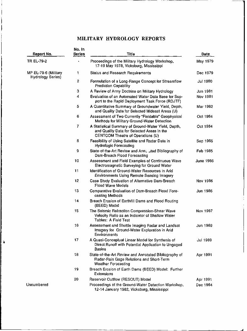
MILITARY HYDROLOGY REPORTS

No. InReport No. Series Title Date

TR EL-79-2 - Proceedings of the Military Hydrology Workshop, May 197917-19 May 1978, Vicksburg, Mississippi

MP EL-79-6 (Military 1 Status and Research Requirements Dec 1979Hydrology Series)

2 Formulation of a Long-Range Concept for Streamflow Jul 1980Prediction Capability

3 A Review of Army Doctrine on Military Hydrology Jun 19814 Evaluation of an Automated Water Data Base for Sup- Nov 1981

port to the Rapid Deployment Task Force (RDJTF)5 A Quantitative Summary of Groundwater Yield, Depth, Mar 1982

and Quality Data for Selected Mideast Areas (U)6 Assessment of Two Currently "Fieldable" Geophysical Oct 1984

Methods for Military Ground-Water Detection7 A Statistical Summary of Ground-Water Yield, Depth, Oct 1984

and Quality Data for Selected Areas in theCENTCOM Theatre of Operations (U)

8 Feasibility of Using Satellite and Radar Data in Sep 1985Hydrologic Forecasting

9 State-of-the-Art Review and Ann:. .ated Bibliography of Feb 1985Dam-Breach Flood Forecasting

10 Assessment and Field Examples of Continuous Wave June 1986Electromagnetic Surveying for Ground Water

11 Identification of Ground-Water Resources in AridEnvironments Using Remote Sensing Imagery

12 Case Study Evaluation of Alternative Dam-Breach Nov 1986Flood Wave Models

13 Comparative Evaluation of Dam-Breach Flood Fore- Jun 1986casting Methods

14 Breach Erosion of Earthfill Dams and Flood Routing(BEED) Model

15 The Seismic Refraction Compression-Shear Wave Nov 1987Velocity Ratio as an Indicator of Shallow WaterTables: A Field Test

16 Assessment and Shuttle Imaging Radar and Landsat Jun 1989Imagery for Ground-Water Exploration in AridEnvironments

17 A Quasi-Conceptual Linear Model for Synthesis of Jul 1989Direct Runoff with Potential Application to UngagedBasins

18 State-of-the-Art Review and Annotated Bibliography of Apr 1991Radar-Rain Gage Relations and Short-TermWeather Foracasting

19 Breach Erosion of Earth Dams (REEDN Mon-de!I: Further

Extensions20 Reservoir Outflow (RESOUT) Model Apr 1991

Unnumbered Proceedings of the Ground-Water Detection Workshop, Dec 198412-14 January 1982, Vicksburg, Mississippi