Embed Size (px)
Citation preview
Air Force Institute of TechnologyAFIT Scholar
Theses and Dissertations Student Graduate Works
3-23-2018
Military Application of Aerial PhotogrammetryMapping Assisted by Small Unmanned Air VehiclesKijun Lee
Follow this and additional works at: https://scholar.afit.edu/etd
Part of the Navigation, Guidance, Control and Dynamics Commons
This Thesis is brought to you for free and open access by the Student Graduate Works at AFIT Scholar. It has been accepted for inclusion in Theses andDissertations by an authorized administrator of AFIT Scholar. For more information, please contact [email protected].
Recommended CitationLee, Kijun, "Military Application of Aerial Photogrammetry Mapping Assisted by Small Unmanned Air Vehicles" (2018). Theses andDissertations. 1897.https://scholar.afit.edu/etd/1897

MILITARY APPLICATION OF AERIAL PHOTOGRAMMETRY MAPPING ASSISTED BY SMALL UNMANNED AIR VEHICLES
THESIS
Major Kijun. Lee
AFIT-ENV-MS-18-M-219
DEPARTMENT OF THE AIR FORCE AIR UNIVERSITY
AIR FORCE INSTITUTE OF TECHNOLOGY
Wright-Patterson Air Force Base, Ohio
DISTRIBUTION STATEMENT A. APPROVED FOR PUBLIC RELEASE; DISTRIBUTION UNLIMITED.

The views expressed in this thesis are those of the author and do not reflect the official policy or position of the United States Air Force, Department of Defense, or the United States Government. This material is declared a work of the U.S. Government and is not subject to copyright protection in the United States.
AFIT-ENV-MS-18-M-219 MILITARY APPLICATION OF AERIAL PHOTOGRAMMETRY MAPPING ASSISTED BY
SMALL UNMANNED AIR VEHICLES
THESIS
Presented to the Faculty
Department of Systems Engineering and Management
Graduate School of Engineering and Management
Air Force Institute of Technology
Air University
Air Education and Training Command
In Partial Fulfillment of the Requirements for the Degree of
Master of Science in Systems Engineering
Kijun Lee, MS
Major, ROKAF
March 2018
DISTRIBUTION STATEMENT A. APPROVED FOR PUBLIC RELEASE; DISTRIBUTION UNLIMITED.
AFIT-ENV-MS-18-M-219 MILITARY APPLICATION OF AERIAL PHOTOGRAMMETRY MAPPING ASSISTED BY
SMALL UNMANNED AIR VEHICLES
Major Kijun Lee, MS
ROKAF
Committee Membership:
David R. Jacques, Ph.D. Chair
John M. Colombi, Ph.D. Member
Lt. Col. A. M. Cox, Ph.D. Member
iv
AFIT-ENV-MS-18-M-219
Abstract
This research investigated the practical military applications of the photogrammetric
methods using remote sensing assisted by small unmanned aerial vehicles (SUAVs). The
research explored the feasibility of UAV aerial mapping in terms of the specific military
purposes, focusing on the geolocational and measurement accuracy of the digital models, and
image processing time. The research method involved experimental flight tests using low-cost
Commercial off-the-shelf (COTS) components, sensors and image processing tools to study
key features of the method required in military like location accuracy, time estimation, and
measurement capability. Based on the results of the data analysis, two military applications are
defined to justify the feasibility and utility of the methods. The first application is to assess the
damage of an attacked military airfield using photogrammetric digital models. Using a hex-
rotor test platform with Sony A6000 camera, georeferenced maps with 1 meter accuracy was
produced and with sufficient resolution (about 1 cm/pixel) to identify foreign objects on the
runway. The other case examines the utility and quality of the targeting system using geo-
spatial data from reconstructed 3-Dimensional (3-D) photogrammetry models. By analyzing 3-
D model, operable targeting under 1meter accuracy with only 5 percent error on distance, area,
and volume were observed.

v
Acknowledgments
The time for this research gives me great pleasure to express my sincere appreciation
and gratitude for the meritorious supports and dedication of the Team AFIT and my family
staying with me during this program. I would like to show my deep appreciation to my
academic advisor, Dr. David Jacques, who taught me, guided to the right track, and support
my research. Also, I can’t imagine that successfully completed my test flight without the
exceptionally great support and assistance from the AFIT’s ANT LAB staffs.
My sincere thanks to my sponsor and prior Dean of AFIT’s Civil Engineering
department. I successfully completed my new challenge with his warm welcome and support.
Furthermore, in recognition of my gratitude to the sacrifice of his father, who was a hero of the
Korean War and rescued 950 orphans in the operation “Kiddy Car Airlift", I offer my sincere
appreciation and respect to him on behalf of Republic of Korea Airforce.
Major Kijun Lee
vi
Table of Contents
Page
Abstract ......................................................................................................................................... 4
Acknowledgments ......................................................................................................................... 5
Table of Contents .......................................................................................................................... 6
List of Figures ............................................................................................................................. 10
List of Tables ............................................................................................................................... 13
I. Introduction ............................................................................................................................ 1
Background ............................................................................................................................ 1
Motivation .............................................................................................................................. 2
Problem statement.................................................................................................................. 2
Research objectives................................................................................................................ 3
Investigative question ............................................................................................................ 3
Scope ...................................................................................................................................... 4
Assumptions........................................................................................................................... 5
Limitations ............................................................................................................................. 5
Thesis organization ................................................................................................................ 6
II. Literature Review .................................................................................................................. 7
Definition of UAV Photogrammetry ..................................................................................... 7
Flight planning for image acquisition .................................................................................... 8
Structure-from-Motion (SfM) photogrammetry Algorithm ................................................ 11
Model reconstruction ........................................................................................................... 13
vii
Photogrammetry accuracy ................................................................................................... 15
Case study of UAV photogrammetry .................................................................................. 20
Summary .............................................................................................................................. 23
III. Methodology ...................................................................................................................... 24
System architecture .............................................................................................................. 25
Definition of Hypothesis ...................................................................................................... 25
IV. Experiment Design............................................................................................................. 31
Test objective ....................................................................................................................... 31
Vehicle description .............................................................................................................. 31
Sensor description ................................................................................................................ 33
Test facilities description ..................................................................................................... 34
Test scenario description ..................................................................................................... 35
V. Analysis and Results .......................................................................................................... 40
General Report ..................................................................................................................... 40
Geolocation accuracy analysis ............................................................................................. 43
Regression analysis for the processing time ........................................................................ 49
Measurement performance analysis..................................................................................... 54
Hypothesis review................................................................................................................ 56
VI. Military application: Runway damage assessment system ................................................ 58
Introduction .......................................................................................................................... 58
Definitions ........................................................................................................................... 59
CONOPS .............................................................................................................................. 60
System configuration ........................................................................................................... 63
viii
Use case study ...................................................................................................................... 64
Activity diagram .................................................................................................................. 65
System analysis .................................................................................................................... 66
VII. Military application: Remote SUAV ISR system assisted by photogrammetry ............ 72
Introduction .......................................................................................................................... 72
Definition ............................................................................................................................. 73
CONOPS .............................................................................................................................. 74
System configuration ........................................................................................................... 76
Use case study ...................................................................................................................... 78
Activity diagram .................................................................................................................. 79
System analysis .................................................................................................................... 80
VIII. Conclusion and recommendation ................................................................................... 84
Conclusion ........................................................................................................................... 84
Recommendations ................................................................................................................ 86
Bibliography ................................................................................................................................ 88
Appendix ..................................................................................................................................... 93
Appendix A: System configurations ................................................................................ 93
Appendix B: Sony A6000 Camera Remote triggering procedure ................................... 95
Appendix C: Canon S110 Camera Remote triggering procedure .................................... 96
Appendix D: KAP UAV Exposure Control Script parameter setup [27] ........................ 99
Appendix E: Pix4D’s 3-D error estimation from tie points [31] ................................... 103
Appendix F: AFI Doc 5028-Multirotor photogrammetry mapping ............................... 105
Appendix G: Pix4D Quality Reports (Himsel test site) ................................................. 138

ix
Appendix H: Pix4D Quality Reports (Runaway damage assessment project) .............. 145
Appendix I: Pix4D Quality Reports (Remote SUAV ISR system project) ................... 151
Appendix J: Test flight log ............................................................................................. 157
x
List of Figures
Page Figure 1: Typical acquisition and processing pipeline for UAV images [1]. ............................................... 9
Figure 2: Left: GCPs on the edges: large vertical errors around a tall corn field and far from GCPs; Right:
GCPs on the edges and one more in the middle of the field: vertical errors dramatically are reduced [5]. 11
Figure 3: Typical SfM pipeline (top row) turns 2D images into 3D geometry [12] ................................... 13
Figure 4: UAV photogrammetry point cloud (Left) and LiDAR point cloud (Right) [18]......................... 16
Figure 5: Building height (= 8.02cm) in UAV photogrammetry point cloud (left) and LiDAR point cloud
(=8.01cm) (right) [18]. ................................................................................................................................ 16
Figure 6: Dependence of accuracy from the ground resolution (Ground sampling distance) of the original
images for various datasets with using GCPs(left) and without using those(right) [20]. ........................... 17
Figure 7: Top view of surveyed stockpile (Site A) with line of cross section [21]. ................................... 18
Figure 8: Top view with color coded deviation between LiDAR and DSM for Site B [21]. ..................... 19
Figure 9: Overview of UAV based close-range rapid aerial monitoring system [23]. ............................... 21
Figure 10: RADAS workflow [25]. ............................................................................................................ 22
Figure 11: Methodology overview. ............................................................................................................. 24
Figure 12: Test System architecture............................................................................................................ 25
Figure 13: Hypothesis of the model's geolocation accuracy. ...................................................................... 26
Figure 14: Position deviations between computed location from 2-D match points (Green cross) and input
GCP coordinates (Yellow cross) on the same feature point in two images. ............................................... 27
Figure 15: Hypothesis of the model processing time. ................................................................................. 29
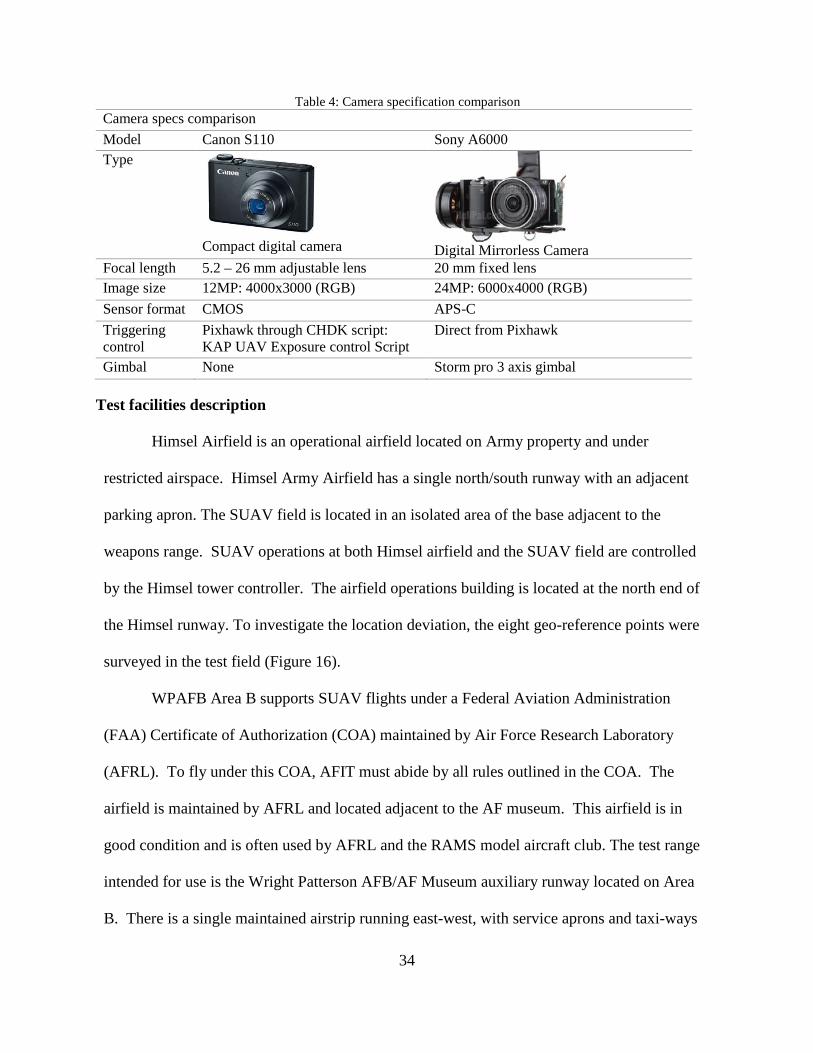
Figure 16: Himsel Airfield test area(left) and WPAFB test area (right). .................................................... 35
Figure 17: Trimble geo 7x (left) and manual Ground Control Point (30 x 25 cm). .................................... 35
Figure 18: Sample GSD calculation at 27 meters for Canon S110 camera [5]. .......................................... 36
Figure 19: Distance covered on the ground by two overlapped images in the flight direction(left) and the
sensor width placed perpendicular to the flight direction(right) [4]. .......................................................... 37
Figure 20: Flight profiles picture for the oblique circle survey (left) and mission plan (right). ................. 39
Figure 21: Orthomosaic map(left), DEM(center), and 3-D map with computed camera locations(right) of
the Himsel test field. ................................................................................................................................... 40
Figure 22: Computed camera location on the point cloud (Top), orthomosaic map of the WPAFB airfield
(Middle) and DEM (Bottom). ..................................................................................................................... 41
Figure 23: Object identification of orthomosaic by 25 meters altitude flight(left) and 50 meters flight
xi
(right). ......................................................................................................................................................... 41
Figure 24: Sparse point cloud after initial processing (top left), designating the processing region (top
middle), densified point cloud (top right), left side view of 3-D model (bottom right), rear view of 3-D
model (center), and right side view of 3-D model (bottom left). ................................................................ 42
Figure 25: Re-optimization workflow using GCPs. .................................................................................... 43
Figure 26: GCP distribution on the point cloud before re-optimization (Top left), location bias before re-
optimization (Top right), location bias after re-optimization (Bottom right), GCP distribution on the point
cloud after re-optimization (Bottom left). ................................................................................................... 44
Figure 27: RMS error comparison with and without GCPs. ....................................................................... 45
Figure 28: Geolocation accuracy variance comparison depending on GSD values.................................... 46
Figure 29: Geolocation accuracy variance comparison depending on image overlap rates. ...................... 47
Figure 30: Geolocation accuracy variance comparison upon UAV's airspeed of an image collection flight.
.................................................................................................................................................................... 49
Figure 31: WPAFB’s airfield Orthomosaic and DEM constructed with different number of images; 5
images (Top left), 10 images (Top right), 15 images (Bottom right), and 20 images (Bottom left). .......... 50
Figure 32: Model A (IV-> DV) regression chart; Relationship between input images and processing time.
.................................................................................................................................................................... 51
Figure 33: Model B (IV-> MED) regression chart; Relationship between input images and key points. .. 52
Figure 34: Model C (MED-> DV) regression chart; Relationship between input key points and processing
time. ............................................................................................................................................................ 53
Figure 35: Linear measurements of trailer using Pix4D mapper desktop. .................................................. 55
Figure 36: Area measurement (left) and volumetric (right) using Pix4D mapper desktop. ........................ 56
Figure 37: OV-1 for rapid runway damage assessment system using SUAV system. ............................... 61
Figure 38: Physical system decomposition of the runway damage assessment system. ............................. 63
Figure 39: Functional system decomposition of the runway damage assessment system. ......................... 64
Figure 40: Activity diagram for runway damage assessment system. ........................................................ 66
Figure 41: Gantt chart for the timeline of runway damage assessment. ..................................................... 66
Figure 42: Survey planning result of Ardupilot mission planner. ............................................................... 69
Figure 43: Ray cloud (Top), Orthomosaic (middle), and DSM (low) of test runway using single flight
path, 60% image overlapping rate, and 80 meters altitude. ........................................................................ 69
Figure 44: Identified small UXO (top left), medium UXO (top right), circular crater (bottom left), and
rectangular crater (bottom right) on the orthomosaic. ................................................................................ 70
Figure 45: Pix4D cloud service sample project of Sinclair National UAS Training and Certificate Center.
xii
.................................................................................................................................................................... 71
Figure 46: Operation View (OV-1) of the remote SUAV ISR system. ...................................................... 75
Figure 47: Physical decomposition of the remote UAV ISR system. ......................................................... 77
Figure 48: Functional decomposition of the remote UAV ISR system. ..................................................... 78
Figure 49: Activity diagram of the SUAV remote ISR system. ................................................................. 80
Figure 50: 3-D model's location accuracy measure using pre-measured GCPs. ......................................... 81
Figure 51: Target Location Error Categories. [31] ..................................................................................... 82
Figure 52: Multi aspect targeting by 3-D model. ........................................................................................ 83
Figure 53: Base map of the Google earth and the map with imported orthomosaic into Google earth
(right). ......................................................................................................................................................... 84
Figure 54: Pix4D's cloud-based 3-D modeling service (left) and Dronedeploy's cloud-based service
(right). ......................................................................................................................................................... 84
xiii
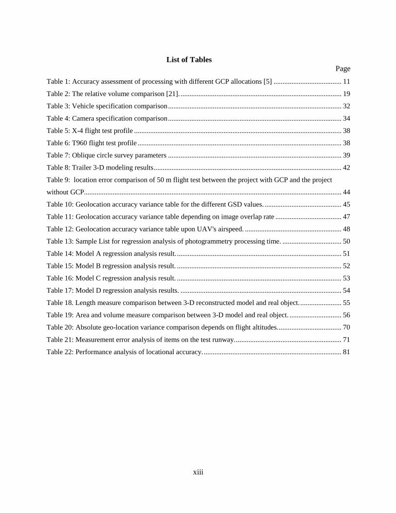
List of Tables Page
Table 1: Accuracy assessment of processing with different GCP allocations [5] ...................................... 11
Table 2: The relative volume comparison [21]. .......................................................................................... 19
Table 3: Vehicle specification comparison ................................................................................................. 32
Table 4: Camera specification comparison ................................................................................................. 34
Table 5: X-4 flight test profile .................................................................................................................... 38
Table 6: T960 flight test profile .................................................................................................................. 38
Table 7: Oblique circle survey parameters ................................................................................................. 39
Table 8: Trailer 3-D modeling results ......................................................................................................... 42
Table 9: location error comparison of 50 m flight test between the project with GCP and the project
without GCP................................................................................................................................................ 44
Table 10: Geolocation accuracy variance table for the different GSD values. ........................................... 45
Table 11: Geolocation accuracy variance table depending on image overlap rate ..................................... 47
Table 12: Geolocation accuracy variance table upon UAV's airspeed. ...................................................... 48
Table 13: Sample List for regression analysis of photogrammetry processing time. ................................. 50
Table 14: Model A regression analysis result. ............................................................................................ 51
Table 15: Model B regression analysis result. ............................................................................................ 52
Table 16: Model C regression analysis result. ............................................................................................ 53
Table 17: Model D regression analysis results. .......................................................................................... 54
Table 18. Length measure comparison between 3-D reconstructed model and real object. ....................... 55
Table 19: Area and volume measure comparison between 3-D model and real object. ............................. 56
Table 20: Absolute geo-location variance comparison depends on flight altitudes. ................................... 70
Table 21: Measurement error analysis of items on the test runway. ........................................................... 71
Table 22: Performance analysis of locational accuracy. ............................................................................. 81
1
MILITARY APPLICATION OF AERIAL PHOTOGRAMMETRY MAPPING ASSISTED BY SMALL UNMANNED AIR VEHICLES
I. Introduction
Background
Historically, the development of Unmanned Aerial Vehicles (UAVs) was primarily
initiated by the military [1]. UAVs have been used in unmanned inspection, surveillance,
reconnaissance, and geographical survey for the military integrating remote sensing
technology [2]. In the last decade, the low-cost Small Unmanned Vehicles (SUAV) have
made significant advances in the commercial field, in addition to the military field. In
particular, the advanced photogrammetry technology has reduced the cost of aerial mapping
and improved the quality of results. The imagery taken by UAVs have been manipulated to
produce various digital models through photogrammetric processing in numerous commercial
fields like survey, inspection and archeology. For this reason, photogrammetry has been
replacing existing aerial survey using manned vehicles with Light Detection and Ranging
(LIDAR) on UAVs.
Advanced UAV technologies are a crucial alternative for providing a low-cost and
high-efficiency imagery. In addition, the development of image processing technology has
made remarkable progress in terms of cost effectiveness as well. Aerial mapping using a
low-cost SUAV has become an alternative to acquire various image resources, reducing
manpower and the development cost for military applications. The obtained images are
processed to create digital models such as textured 3 dimensional (3-D) models,
orthomosaic, Digital Elevation Models(DEMs), Digital Terrain Model (DTM), and Digital
Surface Model (DSM) using 3D modeling tools [3]. Furthermore, these processed image
2
models are fused with web-based networks and will be able to be reproduced as geospatial
data to support critical decision making.
Motivation
In the past decade, technology used in photogrammetry has continued to advance in
parallel with UAV remote sensing with a variety of sectors [3]. In particular, geo-referenced
products from the photogrammetry including DEM, orthomosaic, and 3-D maps have been
used and reproduced as geospatial data in the Geographic Information System (GIS) network.
The method looks to be compatible with and useful to intelligence support systems for
military operations using low-cost UAVs. In most countries, historically, the DoD has relied
on high-cost Command, Control, Communications, Computers, Intelligence, Surveillance and
Reconnaissance (C4ISR) assets to support their operations and decision making. Looking for
efficiencies, the DoD increasingly has been turning to civil and commercial technologies.
UAV aerial photogrammetry in civilian fields presents possible solutions for effective
intelligence, surveillance, and reconnaissance systems using low-cost commercial SUAV
platforms. After computer processing through commercial modeling tools, military users will
be able to visualize the obtained image data in geographical models with geolocation
information in a 3-axis coordinate system. Through the graphical intelligence support, the
system will be able to enhance the situational awareness in the operation field and support
leadership’s decision making.
Problem statement
Even though SUAV photogrammetry has been used widely in commercial
applications, there are many open questions regarding the utility and effectiveness of this
3
technology within the military. Hence, related research is needed to investigate the critical
features of aerial mapping and photogrammetry regarding what factors impact the quality and
timeliness of the product for the military missions. SUAV aerial mapping assisted by modern
photogrammetry is finding wide applications in civil and commercial field, but applying this
in the military field will require system verification as the system must meet stricter user
requirements needed in specific military area such as data accuracy, and reliability, and agile
delivery time. Thus, this study defined the investigative questions to justify how the method
would meet the critical requirements for military purposes.
Research objectives
The first objective of this research is to show the relationship among potential factors
contributing to the location accuracy, processing time, and measurement reliability. They will
be used to suggest a system configuration, processing time estimation and considerations for a
robust operational system. Secondly, this study analyzes two military applications to show
how this emerging technology could be used effectively within the military. In the case of
Rapid Airfield Damage Assessment System (RADAS), the military civil engineering case is
presented and methods for application of this technology is discussed. In addition, a remote
ISR system using urban area mapping with SUAVs is presented. These applications are
evaluated using flight tests to obtain operable image data, and the data is processed to evaluate
the system performance.
Investigative question
• What factors impact the absolute geolocational accuracy derived from the location in
the map?
4
Absolute accuracy is defined as “the extent to which the calculated position of a
point on a map corresponds to its actual position in a fixed coordinate system in the real
world [4].” Based on the literature review, the research established three predictors to
investigate the impact on each accuracy.
• Existence of Ground Control Points (GCPs)
• The Ground Sample Distance(GSD) of the obtained imagery.
• The vehicle’s airspeed while capturing images in a mission plan.
• The image overlapping rate over each image.
• What factors impact the map processing time to deliver the digital maps and 3-D
models?
The predictors the researcher came up with are shown below,
• The number of images which input into the processor.
• The number of matching points that the processor can extract from each image.
• How accurate is the capability of measurements using reconstructed models generated
by collected images from the SUAV?
The capabilities of interest are shown below,
• The performance of the linear measurement.
• The performance of the area measurement.
• 3-dimensional volumetric performance
Scope
The research scope includes three stages: (1) presenting the actionable system
architecture to show the general understanding of the system; (2) framing hypotheses on the
critical questions and definition of the independent and dependent variables on the expected
5
results; (3) collecting data from the ground, flight test and previous research results; (4)
processing the data to construct 3-D models and analyzing the results to justify the hypothesis;
(5) applying the method in each military application, e.g., the runway damage assessment and
remote SUAV ISR system.
Assumptions
Photogrammetric terms are sometimes defined differently by various researchers and
publication venues. Primarily, this study followed the American Society for Photogrammetry
and Remote Sensing (ASPRS) terminologies referenced by Chapter 1 of [3]. For differences
in terminology between the processing software and ASPRS, terminology in the software were
used to avoid the confusion.
Photogrammetry model processing requires georeferenced data where the images are
taken in the coordinates system. Most COTS UAV platforms are supporting automatic built-in
geotagging functions in the system, but the custom UAV system used in this research required
extra work to download the geotag data by connecting to the autopilot’s data-flash logs.
Nevertheless, the research omitted the geotagging process time from the workflow as this
issue might be resolved using different hardware platforms.
Limitations
This research used pre-existing hardware, Ground Control Station (GCS), and data
processing software options. This choice reduced the schedule risk involved with hardware
and software integration. Additionally, it reduced the schedule duration of safety reviews, and
avoided unnecessary customization.
Secondly, although the Pix4D mapper [4] image processing software provides either
6
stationary desktop service or cloud-based remote processing service, the desktop processing
method was primarily used in data analysis since most imagery data was collected from
military facility, which placed restrictions on the use of a commercial. For the reason, this
research utilized the sample projects supported by the National UAS Training and Certificate
Center in Sinclair community college in order to show the cloud-based processing application.
Lastly, the navigation GPS (Global Positioning System) / GNSS (Global Navigation
Satellite System) used in test flights was a consumer grade GPS utilizing a single frequency
(L1) and Real-Time Kinematic (RTK) processing. This was a low-cost component, but less
accurate than high-end GPS for professional survey. This project did not require centimeter
level’s data accuracy, so the standard GPS error was deemed acceptable for the project
requirement.
Thesis organization
In Chapter Ⅱ, a thorough review of the literature, the key concepts used in the research
and previous research results will be addressed. In Chapter Ⅲ, the methodology to extend the
research will be presented. In Chapter Ⅳ, the designed experiments will be introduced to
verify the photogrammetric features such as geolocational accuracy, measurement and
processing time estimation. Chapter Ⅴ presents the data analysis walkthroughs and results
from reconstructed 3-D models with respect to the investigative questions. Chapter Ⅵ and Ⅶ
present the case studies for the military applications using the method in each military
challenge with a system perspective. Finally, in Chapter Ⅷ, the conclusions will be drawn
from the entirety of the research accomplished, and recommendations for future work to be
done will be described.
7
II. Literature Review
Key concepts
Definition of UAV Photogrammetry
The term Unmanned Aerial System(UAS) has been adopted by the US Department of
Defense to cover the full range of unmanned air vehicles, while the term drone has been
common in the civilian sector [5]. According to the UAV international definition, UAV is
defined as “a generic aircraft design to operate with no human pilot onboard [1], [6].”
Photogrammetry has been defined by the American Society for Photogrammetry and Remote
Sensing “as the art, science, and technology of obtaining reliable information about physical
objects and environment through processes of recording, measuring, and interpreting
photographic images and patterns of recorded radiant electromagnetic energy and other
phenomena [3].” Accordingly, Henri Eisenbeiß (2009) introduced the term UAS
Photogrammetry : “Photogrammetry describes photogrammetric measurement platforms,
which operate as either remotely controlled, semi-autonomously, or autonomously, all without
a pilot sitting in the platform, and the photogrammetric processing of UAS images [7]”.
Aerial photogrammetry was developed using manned vehicles with high-cost sensors
like LiDAR (Light Detection and Ranging) and, or high-end aerial cameras. However, with
the development of advanced autopilots compatible with a survey mission planner,
GPS/GNSS aided navigation, high-performance image processing tools and a user-friendly
interface are making the UAV a preferred platform for aerial photogrammetry. The former
flies relatively high latitude fight ensuring more time for image acquisition and covering vast
8
coverage areas. Moreover, the high-end aerial photographic cameras having high resolution
and low lens distortion provide a significantly larger effective dimension of the captured
image. Generally, commercial SUAV carries low-cost consumer grade digital cameras [8] that
induce relatively more distortion than a high-end one. Nevertheless, a SUAV is capable of low
altitude flight which can compensate for camera resolution issues, and the cost effectiveness
can significantly increase the market competitiveness for survey applications. Moreover, in
unmanned aerial photography, the latest image processing technology is used to compensate
for the limitations by quickly matching a number of multiple images with small effective areas
[2].
Flight planning for image acquisition
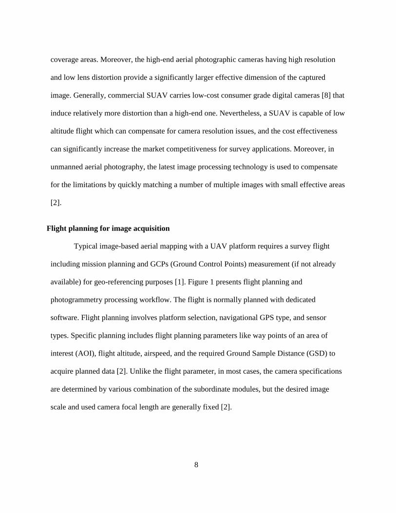
Typical image-based aerial mapping with a UAV platform requires a survey flight
including mission planning and GCPs (Ground Control Points) measurement (if not already
available) for geo-referencing purposes [1]. Figure 1 presents flight planning and
photogrammetry processing workflow. The flight is normally planned with dedicated
software. Flight planning involves platform selection, navigational GPS type, and sensor
types. Specific planning includes flight planning parameters like way points of an area of
interest (AOI), flight altitude, airspeed, and the required Ground Sample Distance (GSD) to
acquire planned data [2]. Unlike the flight parameter, in most cases, the camera specifications
are determined by various combination of the subordinate modules, but the desired image
scale and used camera focal length are generally fixed [2].
9
Figure 1: Typical acquisition and processing pipeline for UAV images [1].
Unlike the past classical survey missions, these days, various automated mission
planning tools are widely used in commercial application. Using the automatic survey mission
planning tools, the operator can plan the flight and determine critical mission data like
expected GSD, flight time, and required number of images based on given data input such as
flight parameters and a camera specification.
In selecting a camera, most types of camera including Digital Single-Lens Reflex
(DSLR), compact digital camera, multi spectrum, sports cameras, and even cellphone cameras
are compatible with the method. For more accurate data, a camera with bigger sensor size and
image size [9] is preferred and global shutter type cameras yield more accurate and
undistorted imagery data than rolling shutter cameras [10].
The GPS navigation module embedded in the UAV affects the accuracy of the UAV’s
navigation and collected data [1]. The UAV flight is usually aided by the onboard GPS/INS
navigation devices for autonomous flights: takeoff, navigation, landing and to guide the image
acquisition [2]. In most cases, low-cost SUAVs use single frequency GPS with meter level
positioning accuracy, but advanced navigation GPS instruments, based on double frequency
10
positioning or the use of RTK, can improve the quality of positioning to the centimeter level
[1]. Even though less costly RTK modules like Neo-M8P from Ublox Inc [11] have been
developed, they are still more costly than the low-cost solutions commonly used.
The camera shooting rate significantly effects the model quality as the reconstruction
algorithms are based on the number of common features from overlapped images [12].
Accordingly, the proper overlapping rate should be planned before flight [2]. To verify that
there is enough overlap between the images, the recommended minimum rate should be 75%
frontal and 60% side overlap in general cases, 85% frontal and 70% side overlap for forests
and dense vegetation and fields, 85% frontal overlap for single track corridor mapping, and
60% side overlap if the corridor is acquired using two flight paths [4].
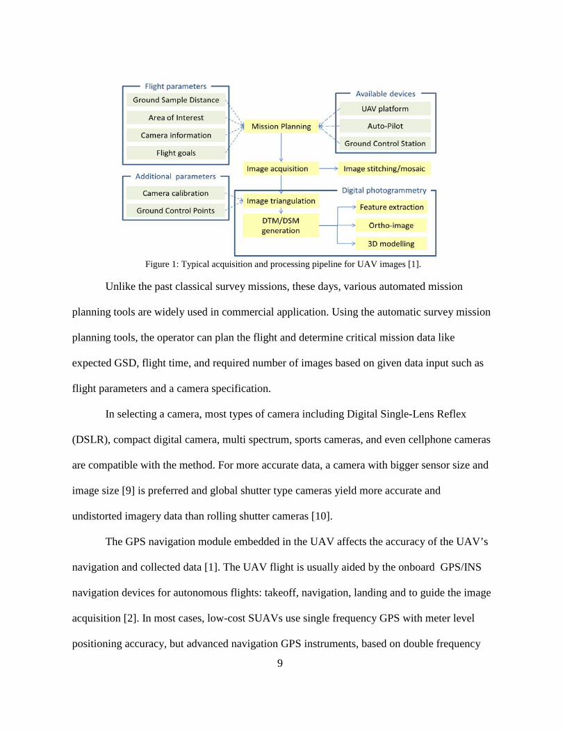
The existence of GCPs is critical to the reconstructed model’s geolocational accuracy
as GCPs provide the geodetic references for orientating common feature points in the world
coordinate system. Even if the image data is taken using SUAV with commercial grade low-
cost GPS, the model accuracy can be improved to the level of a high-end UAV with RTK GPS
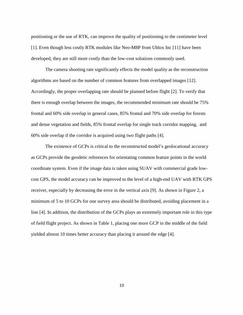
receiver, especially by decreasing the error in the vertical axis [9]. As shown in Figure 2, a
minimum of 5 to 10 GCPs for one survey area should be distributed, avoiding placement in a
line [4]. In addition, the distribution of the GCPs plays an extremely important role in this type
of field flight project. As shown in Table 1, placing one more GCP in the middle of the field
yielded almost 10 times better accuracy than placing it around the edge [4].
11
Figure 2: Left: GCPs on the edges: large vertical errors around a tall corn field and far from GCPs; Right: GCPs on the edges and one more in the middle of the field: vertical errors dramatically are reduced [5].
Table 1: Accuracy assessment of processing with different GCP allocations [5]
Structure-from-Motion (SfM) photogrammetry Algorithm
At present, photogrammetry has been advanced dramatically with the development of
computer vision science for three-dimensional (3-D) modeling. Currently, photogrammetry
refers to construction of the 3-D models using the 2-dimensional (2-D) images to provide the
measurement data [13]. Structure from Motion(SFM) is a reconstruction algorithm used in
modern photogrammetry software to orient the physical features and camera poses used within
a defined coordinate system [13]. A subsequent procedure then extracts a high resolution and
12
color-coded point cloud to represent the object [14]. SfM assists photogrammetry by
automatically detecting and matching features across multiple images, then triangulating
positions [13]. SfM photogrammetry, accordingly, offers the possibility of fast, automated and
low-cost acquisition of 3-D data using almost every kind of consumer grade camera including
cell-phone cameras [13] [14]. For this reason, most photographic applications including Pix4D
mapper [4] and Agisoft’s Photoscan [15] incorporate the SfM algorithm in their initial
processing pipelines. Historically, this was developed 40 years ago, but the work procedure
was highly intensive and required professional workstations to get the practical processing
performance [13]. Advanced computer technology has made the SfM process with consumer
level computers more practical in the last decade.
E. B. Peterson et.al [13] illustrated the general SfM workflow in their white paper as
three processes: 1) organize and load images, 2) model “Sparse cloud”, and 3) model “Dense
cloud”. The first step is to process raw image data and enable the software to match the
features. A sparse point cloud, then, is generated by matching ‘features’, recognizable patterns
among the pixels [13]. The software triangulates the points to represent those matches as X, Y,
Z coordinates with pixel colors assigned to the points, and then repeats the process to get the
sparse point cloud [13]. Finally, based on the scene geometry of the object’s point cloud, the
point densification is conducted to enhance the visualization of the model.
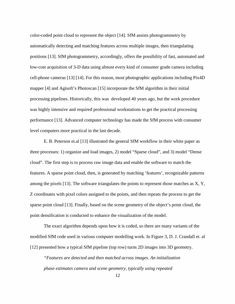
The exact algorithm depends upon how it is coded, so there are many variants of the
modified SfM code used in various computer modelling work. In Figure 3, D. J. Crandall et. al
[12] presented how a typical SfM pipeline (top row) turns 2D images into 3D geometry.
“Features are detected and then matched across images. An initialization
phase estimates camera and scene geometry, typically using repeated
13
(incremental) rounds of bundle adjustment, followed by a final round of
bundle adjustment to solve for camera and scene geometry. In contrast, we
propose initializing with a multi-stage optimization (bottom row) that
combines discrete belief propagation and continuous optimization [12].”
Figure 3: Typical SfM pipeline (top row) turns 2D images into 3D geometry [12]
Model reconstruction
After the data acquisition, the imagery can be used for model reconstruction such as
3D maps, stitched mosaic maps (orthomosaic), and Digital Elevation Maps (DEM) including
Digital Surface Maps (DSM) and Digital Terrain Maps (DTM) by the photogrammetric
process [3]. In this case, camera calibration and image triangulation are initially performed to
generate a DEM. These products can be used for the production of ortho-images, 3D modeling
applications, or for the extraction of further metric information [1]. Primarily, this research
used Pix4D’s Pix4D mapper as a photogrammetry tool.
Pix4D mapper
One tool for photogrammetric processing is Pix4D mapper that is currently powering
commercial drone mapping software like 3DR’s Site Scan and ESRI’s Drone2Map [4], [16].
The basic processing principle is based on computer vision algorithms, SfM, to match the key
feature points quickly like Agisoft’s Photoscan, but modifications are added for fast processing,
14
enhanced visualization, and user convenience [8].
Pix4D mapper’s overall processing procedure is composed of three steps; Initial
processing, point cloud and mesh, and DSM, orthomosaic and Index [4].
a. “Initial Processing automatically performs a camera calibration to extract key-
points, have a same point in multiple images, to triangulate the intrinsic and
extrinsic camera parameters using the software's advanced Automatic Aerial
Triangulation (AAT) and Bundle Block Adjustment (BBA). A simple 3D point
cloud is computed and a low-resolution DSM and orthomosaic are generated and
displayed in the quality report.
b. Next step is the Point Cloud and Mesh that generates a dense 3D point cloud and a
3D textured mesh in detail. Each point represents the extracted key point on 3 axis
frame which have a geolocation data.
c. The last step is DSM, Orthomosaic and Index which generate the DSM,
orthomosaic, index map [4].”
The most prominent feature of Pix4D mapper is the ability to provide initial processing
products quickly after initial processing using sparse point cloud data. This enables the user to
identify the raw data quality and provide affordable “proto” models for fast delivery [4].
Unlike the previous tools, this provides a user friendly Graphical User Interface (GUI), and
has a straight forward work flow that is easy to carry out with the minimum prior experience
[17]. The Pix4D software supports three platforms: cloud-based processing service, desktop,
or mobile. [4] These services provide wide applicability to users who have a variety of work
environments. Cloud-based service provides fully automated processing once users upload
their data on the website with simple options. The user can download or share the fully
15
reconstructed models with other users. These features of cloud services seem to have potential
feasibility with GIS network service. The desktop-based service provides more detailed
processing options to meet the professional user needs and secure work environment for users
who don’t want to open or share their data with others. The processing work fully depends on
the user hardware performance, and many require high performance processors to ensure
reasonable delivery time. Lastly, mobile applications are working as compact survey options,
which are compatible with popular UAV models for various commercial purposes, receiving
and transmitting image data captured from UAVs.
Photogrammetry accuracy
For the photogrammetry accuracy, a variety of research has been conducted in the past
decade. Ideally, the position accuracy of the reconstructed model is described as horizontally
(X-Y coordinates) 1 ~ 2 times GSD and vertically (Z coordinate) 1 ~ 3 times GSD. This
assumes the model is constructed using well surveyed GCPs or image coordinates from RTK
GPS; if not, the accuracy could vary depending on a variety of reasons [4].
Modern photogrammetry has been often compared to LiDAR which has been widely
used in the conventional aerial survey sector. However, LiDAR solutions are substantially
more expensive and require a higher level of technical expertise to operate [18]. A recurring
question is on the relative accuracy performance of the UAV photogrammetry to the LiDAR
scanning option [18]. To get the answer regarding the accuracy performance of
photogrammetry compared to LiDAR, O’Neil-Dunne performed LiDAR and photogrammetric
mapping and compared the generated point cloud data shown in Figure 4 [18]. In spite of no
GCPs in the project, the results show that the photogrammetry method produced a higher
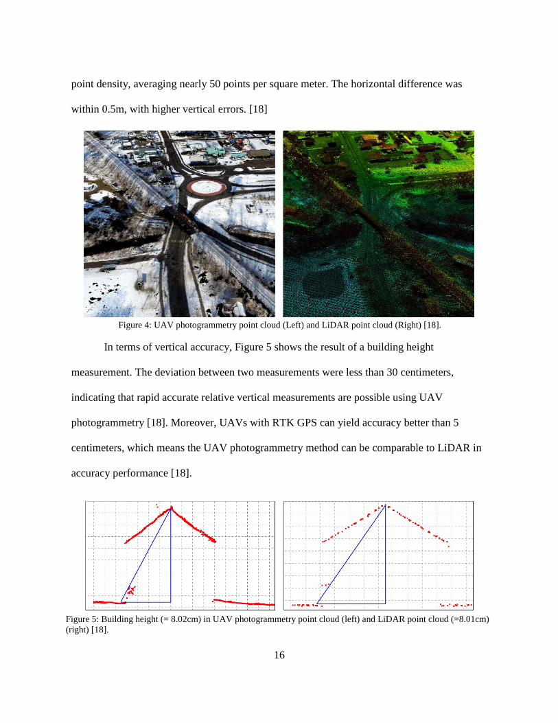
16
point density, averaging nearly 50 points per square meter. The horizontal difference was
within 0.5m, with higher vertical errors. [18]
Figure 4: UAV photogrammetry point cloud (Left) and LiDAR point cloud (Right) [18].
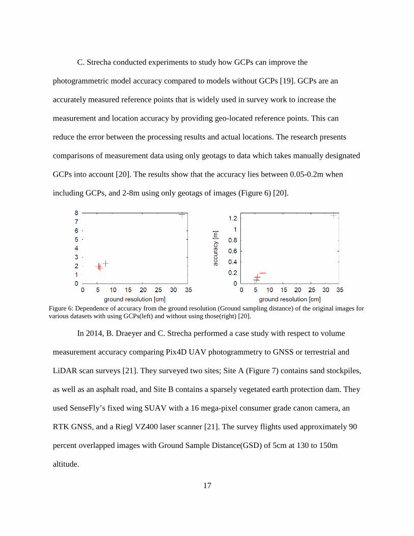
In terms of vertical accuracy, Figure 5 shows the result of a building height
measurement. The deviation between two measurements were less than 30 centimeters,
indicating that rapid accurate relative vertical measurements are possible using UAV
photogrammetry [18]. Moreover, UAVs with RTK GPS can yield accuracy better than 5
centimeters, which means the UAV photogrammetry method can be comparable to LiDAR in
accuracy performance [18].
Figure 5: Building height (= 8.02cm) in UAV photogrammetry point cloud (left) and LiDAR point cloud (=8.01cm) (right) [18].
17
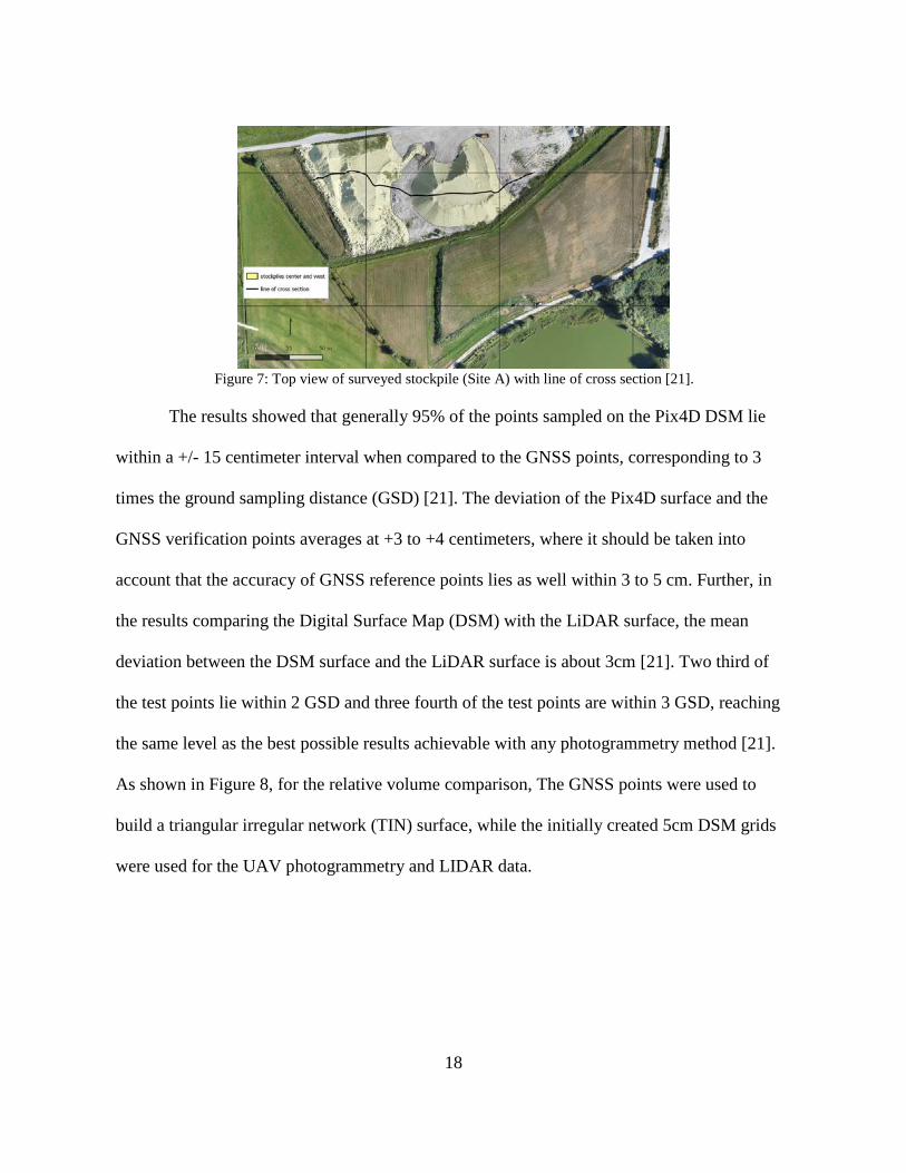
C. Strecha conducted experiments to study how GCPs can improve the
photogrammetric model accuracy compared to models without GCPs [19]. GCPs are an
accurately measured reference points that is widely used in survey work to increase the
measurement and location accuracy by providing geo-located reference points. This can
reduce the error between the processing results and actual locations. The research presents
comparisons of measurement data using only geotags to data which takes manually designated
GCPs into account [20]. The results show that the accuracy lies between 0.05-0.2m when
including GCPs, and 2-8m using only geotags of images (Figure 6) [20].
Figure 6: Dependence of accuracy from the ground resolution (Ground sampling distance) of the original images for various datasets with using GCPs(left) and without using those(right) [20].
In 2014, B. Draeyer and C. Strecha performed a case study with respect to volume
measurement accuracy comparing Pix4D UAV photogrammetry to GNSS or terrestrial and
LiDAR scan surveys [21]. They surveyed two sites; Site A (Figure 7) contains sand stockpiles,
as well as an asphalt road, and Site B contains a sparsely vegetated earth protection dam. They
used SenseFly’s fixed wing SUAV with a 16 mega-pixel consumer grade canon camera, an
RTK GNSS, and a Riegl VZ400 laser scanner [21]. The survey flights used approximately 90
percent overlapped images with Ground Sample Distance(GSD) of 5cm at 130 to 150m
altitude.
18
Figure 7: Top view of surveyed stockpile (Site A) with line of cross section [21].
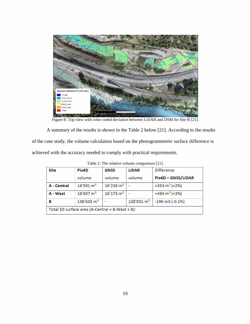
The results showed that generally 95% of the points sampled on the Pix4D DSM lie
within a +/- 15 centimeter interval when compared to the GNSS points, corresponding to 3
times the ground sampling distance (GSD) [21]. The deviation of the Pix4D surface and the
GNSS verification points averages at +3 to +4 centimeters, where it should be taken into
account that the accuracy of GNSS reference points lies as well within 3 to 5 cm. Further, in
the results comparing the Digital Surface Map (DSM) with the LiDAR surface, the mean
deviation between the DSM surface and the LiDAR surface is about 3cm [21]. Two third of
the test points lie within 2 GSD and three fourth of the test points are within 3 GSD, reaching
the same level as the best possible results achievable with any photogrammetry method [21].
As shown in Figure 8, for the relative volume comparison, The GNSS points were used to
build a triangular irregular network (TIN) surface, while the initially created 5cm DSM grids
were used for the UAV photogrammetry and LIDAR data.
19
Figure 8: Top view with color coded deviation between LiDAR and DSM for Site B [21].
A summary of the results is shown in the Table 2 below [21]. According to the results
of the case study, the volume calculation based on the photogrammetric surface difference is
achieved with the accuracy needed to comply with practical requirements.
Table 2: The relative volume comparison [21].
20
Case study of UAV photogrammetry
Intelligence, surveillance, and reconnaissance (ISR)
UAVs were originally developed for military applications, with situational awareness
in the battlefield avoiding the risk of human pilots [1]. In the military context, ISR was the
initial motivation for UAV development [22]. Nowadays, large unmanned aircraft have been
developed as broad-area surveillance for border control and restricted area surveillance. The
larger tactical platform is usually preferred for ISR as they implement real-time image or
video downloads easier than mini or micro UAVs [22]. Similar to the military cases, UAVs
have been used as communication relays from the battlefield, decoys to enemy radars, search-
and-rescue, or disaster management [22]. An example of military UAVs for ISR is Boeing’s
ScanEagle, a 20 kg Maximum Take-Off Weight (MTOW) fixed-wing vehicle with a wingspan
of 3 m, used by the U.S. Navy. As standard payload, it carries either an inertially stabilized
electro-optical or an infrared camera to collect the imagery, which enable the tactical
commanders to achieve enhanced Situational Awareness(SA) [22].
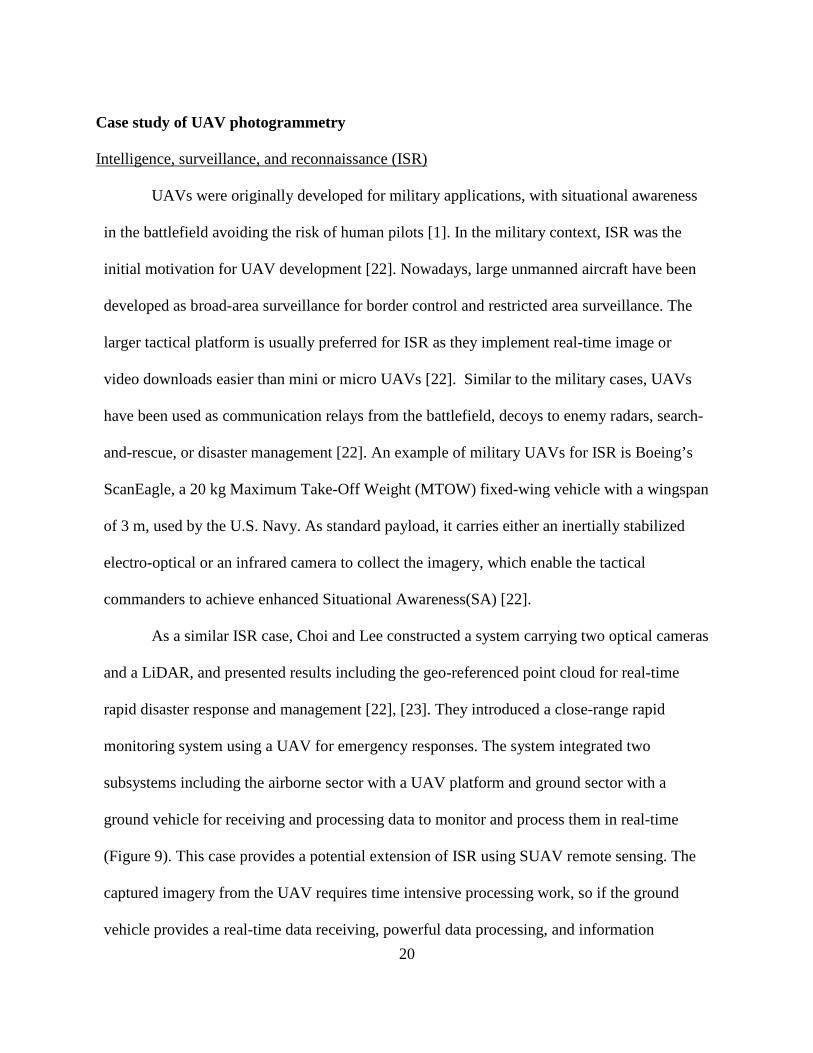
As a similar ISR case, Choi and Lee constructed a system carrying two optical cameras
and a LiDAR, and presented results including the geo-referenced point cloud for real-time
rapid disaster response and management [22], [23]. They introduced a close-range rapid
monitoring system using a UAV for emergency responses. The system integrated two
subsystems including the airborne sector with a UAV platform and ground sector with a
ground vehicle for receiving and processing data to monitor and process them in real-time
(Figure 9). This case provides a potential extension of ISR using SUAV remote sensing. The
captured imagery from the UAV requires time intensive processing work, so if the ground
vehicle provides a real-time data receiving, powerful data processing, and information
21
transmission capabilities, the information delivery time would be significantly improved.
Figure 9: Overview of UAV based close-range rapid aerial monitoring system [23].
Survey and Inspection
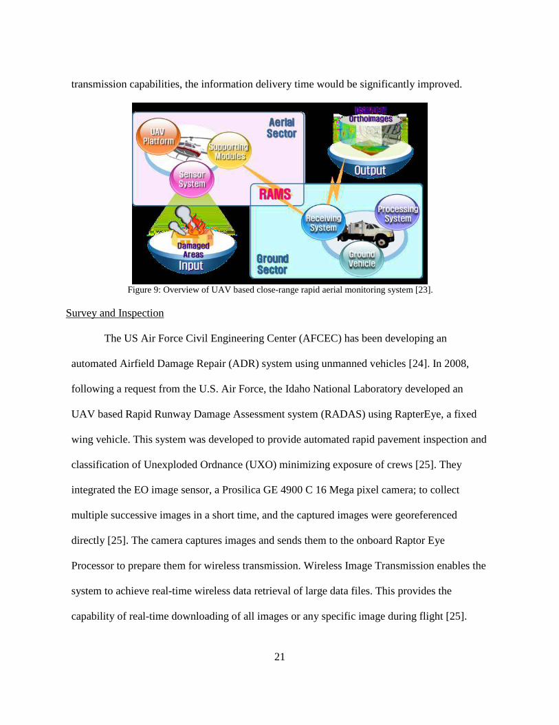
The US Air Force Civil Engineering Center (AFCEC) has been developing an
automated Airfield Damage Repair (ADR) system using unmanned vehicles [24]. In 2008,
following a request from the U.S. Air Force, the Idaho National Laboratory developed an
UAV based Rapid Runway Damage Assessment system (RADAS) using RapterEye, a fixed
wing vehicle. This system was developed to provide automated rapid pavement inspection and
classification of Unexploded Ordnance (UXO) minimizing exposure of crews [25]. They
integrated the EO image sensor, a Prosilica GE 4900 C 16 Mega pixel camera; to collect
multiple successive images in a short time, and the captured images were georeferenced
directly [25]. The camera captures images and sends them to the onboard Raptor Eye
Processor to prepare them for wireless transmission. Wireless Image Transmission enables the
system to achieve real-time wireless data retrieval of large data files. This provides the
capability of real-time downloading of all images or any specific image during flight [25].
22
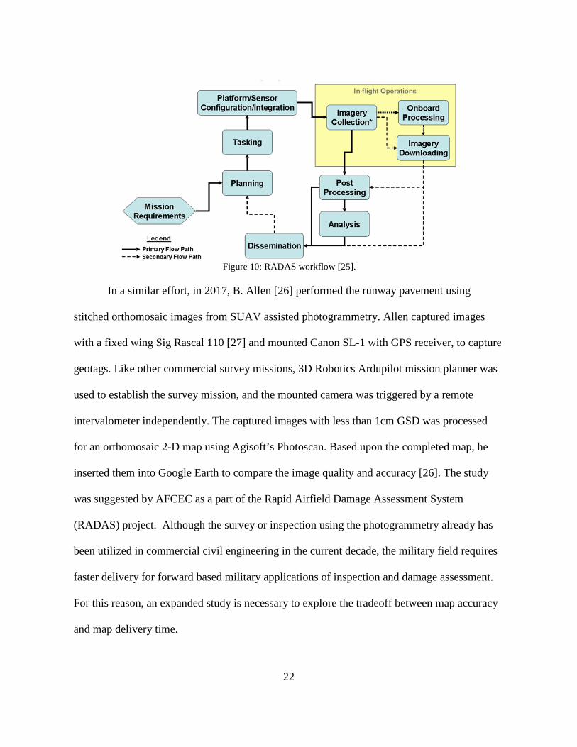
Figure 10: RADAS workflow [25].
In a similar effort, in 2017, B. Allen [26] performed the runway pavement using
stitched orthomosaic images from SUAV assisted photogrammetry. Allen captured images
with a fixed wing Sig Rascal 110 [27] and mounted Canon SL-1 with GPS receiver, to capture
geotags. Like other commercial survey missions, 3D Robotics Ardupilot mission planner was
used to establish the survey mission, and the mounted camera was triggered by a remote
intervalometer independently. The captured images with less than 1cm GSD was processed
for an orthomosaic 2-D map using Agisoft’s Photoscan. Based upon the completed map, he
inserted them into Google Earth to compare the image quality and accuracy [26]. The study
was suggested by AFCEC as a part of the Rapid Airfield Damage Assessment System
(RADAS) project. Although the survey or inspection using the photogrammetry already has
been utilized in commercial civil engineering in the current decade, the military field requires
faster delivery for forward based military applications of inspection and damage assessment.
For this reason, an expanded study is necessary to explore the tradeoff between map accuracy
and map delivery time.
23
Summary
Citing previous research, key terminology used in this research like SUAV,
photogrammetry, and related terms were described and defined. The general workflow for
SUAV photogrammetry that has been conducted in similar research areas so far was
introduced. This provided references to design test flights including platform selection and
mission planning for ideal results. For technical background, SfM was introduced to
understand the principle and algorithms for modern photogrammetry. This assists
photogrammetry by automatically detecting and matching features across multiple images,
then triangulating their positions to locate them in coordinate system. Based on this research,
past experiments were addressed to identify locating performance and measurement accuracy
by comparing photogrammetry results with LiDAR scanning. Lastly, related application
studies were addressed to set the general research orientation and goals for actionable
application cases in the military field using the method.
24
III. Methodology
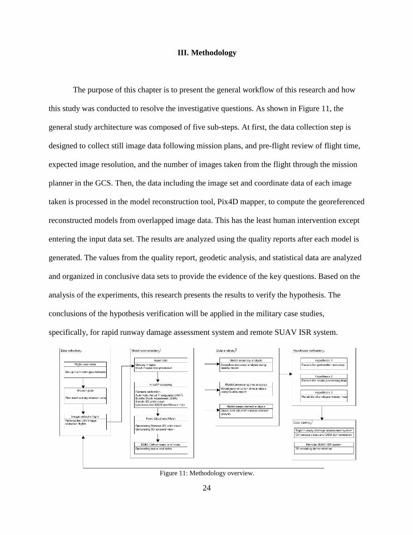
The purpose of this chapter is to present the general workflow of this research and how
this study was conducted to resolve the investigative questions. As shown in Figure 11, the
general study architecture was composed of five sub-steps. At first, the data collection step is
designed to collect still image data following mission plans, and pre-flight review of flight time,
expected image resolution, and the number of images taken from the flight through the mission
planner in the GCS. Then, the data including the image set and coordinate data of each image
taken is processed in the model reconstruction tool, Pix4D mapper, to compute the georeferenced
reconstructed models from overlapped image data. This has the least human intervention except
entering the input data set. The results are analyzed using the quality reports after each model is
generated. The values from the quality report, geodetic analysis, and statistical data are analyzed
and organized in conclusive data sets to provide the evidence of the key questions. Based on the
analysis of the experiments, this research presents the results to verify the hypothesis. The
conclusions of the hypothesis verification will be applied in the military case studies,
specifically, for rapid runway damage assessment system and remote SUAV ISR system.
Figure 11: Methodology overview.
25
System architecture
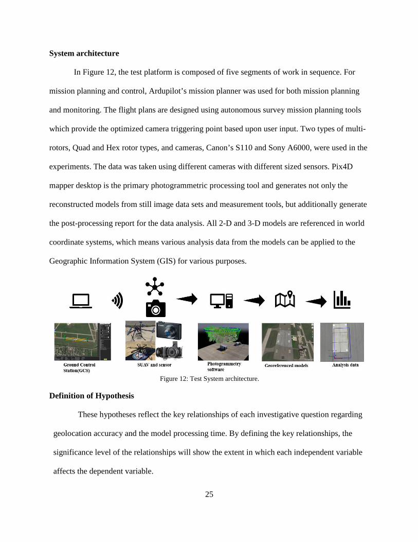
In Figure 12, the test platform is composed of five segments of work in sequence. For
mission planning and control, Ardupilot’s mission planner was used for both mission planning
and monitoring. The flight plans are designed using autonomous survey mission planning tools
which provide the optimized camera triggering point based upon user input. Two types of multi-
rotors, Quad and Hex rotor types, and cameras, Canon’s S110 and Sony A6000, were used in the
experiments. The data was taken using different cameras with different sized sensors. Pix4D
mapper desktop is the primary photogrammetric processing tool and generates not only the
reconstructed models from still image data sets and measurement tools, but additionally generate
the post-processing report for the data analysis. All 2-D and 3-D models are referenced in world
coordinate systems, which means various analysis data from the models can be applied to the
Geographic Information System (GIS) for various purposes.
Figure 12: Test System architecture.
Definition of Hypothesis
These hypotheses reflect the key relationships of each investigative question regarding
geolocation accuracy and the model processing time. By defining the key relationships, the
significance level of the relationships will show the extent in which each independent variable
affects the dependent variable.
26
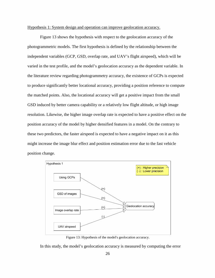
Hypothesis 1: System design and operation can improve geolocation accuracy.
Figure 13 shows the hypothesis with respect to the geolocation accuracy of the
photogrammetric models. The first hypothesis is defined by the relationship between the
independent variables (GCP, GSD, overlap rate, and UAV’s flight airspeed), which will be
varied in the test profile, and the model’s geolocation accuracy as the dependent variable. In
the literature review regarding photogrammetry accuracy, the existence of GCPs is expected
to produce significantly better locational accuracy, providing a position reference to compute
the matched points. Also, the locational accuracy will get a positive impact from the small
GSD induced by better camera capability or a relatively low flight altitude, or high image
resolution. Likewise, the higher image overlap rate is expected to have a positive effect on the
position accuracy of the model by higher densified features in a model. On the contrary to
these two predictors, the faster airspeed is expected to have a negative impact on it as this
might increase the image blur effect and position estimation error due to the fast vehicle
position change.
Figure 13: Hypothesis of the model's geolocation accuracy.
In this study, the model’s geolocation accuracy is measured by computing the error
27
between the initial location using geotagged coordinates of camera location data and the
computed positions estimated by the photogrammetric process. It is clear that the absolute
location error primarily depends on the vehicle’s GPS performance, but the extent to how the
computed points in the map match the initial coordinates is additionally affected by many
other factors like the flight parameters setting or choosing different processing options. For
instance, if the initial coordinates are assumed perfectly precise, the only error would be
generated by the deviation between the initial location and computed locations of those same
point. Conclusively, the model is assessed as more accurate when two locations are as close as
possible. Accordingly, the location error represents the model’s location accuracy when using
the same GPS to get image coordinates. To study the quantitative location error, the Root
Mean Square Error (RMSE) data in the absolute accuracy variance table from the Pix4d’s post
process reports is used to show the position accuracy performance, which is calculated
between the computed location (location of features on a map / reconstructed model /
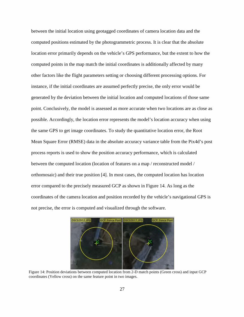
orthomosaic) and their true position [4]. In most cases, the computed location has location
error compared to the precisely measured GCP as shown in Figure 14. As long as the
coordinates of the camera location and position recorded by the vehicle’s navigational GPS is
not precise, the error is computed and visualized through the software.
Figure 14: Position deviations between computed location from 2-D match points (Green cross) and input GCP coordinates (Yellow cross) on the same feature point in two images.
28
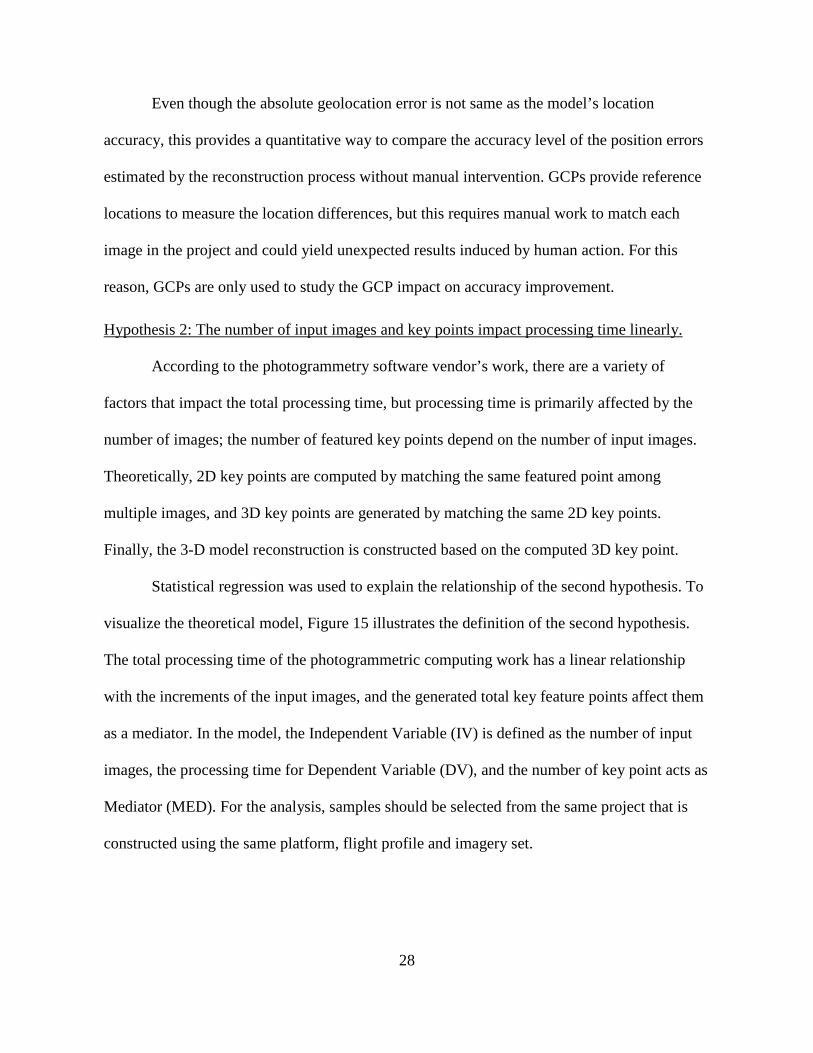
Even though the absolute geolocation error is not same as the model’s location
accuracy, this provides a quantitative way to compare the accuracy level of the position errors
estimated by the reconstruction process without manual intervention. GCPs provide reference
locations to measure the location differences, but this requires manual work to match each
image in the project and could yield unexpected results induced by human action. For this
reason, GCPs are only used to study the GCP impact on accuracy improvement.
Hypothesis 2: The number of input images and key points impact processing time linearly.
According to the photogrammetry software vendor’s work, there are a variety of
factors that impact the total processing time, but processing time is primarily affected by the
number of images; the number of featured key points depend on the number of input images.
Theoretically, 2D key points are computed by matching the same featured point among
multiple images, and 3D key points are generated by matching the same 2D key points.
Finally, the 3-D model reconstruction is constructed based on the computed 3D key point.
Statistical regression was used to explain the relationship of the second hypothesis. To
visualize the theoretical model, Figure 15 illustrates the definition of the second hypothesis.
The total processing time of the photogrammetric computing work has a linear relationship
with the increments of the input images, and the generated total key feature points affect them
as a mediator. In the model, the Independent Variable (IV) is defined as the number of input
images, the processing time for Dependent Variable (DV), and the number of key point acts as
Mediator (MED). For the analysis, samples should be selected from the same project that is
constructed using the same platform, flight profile and imagery set.
29
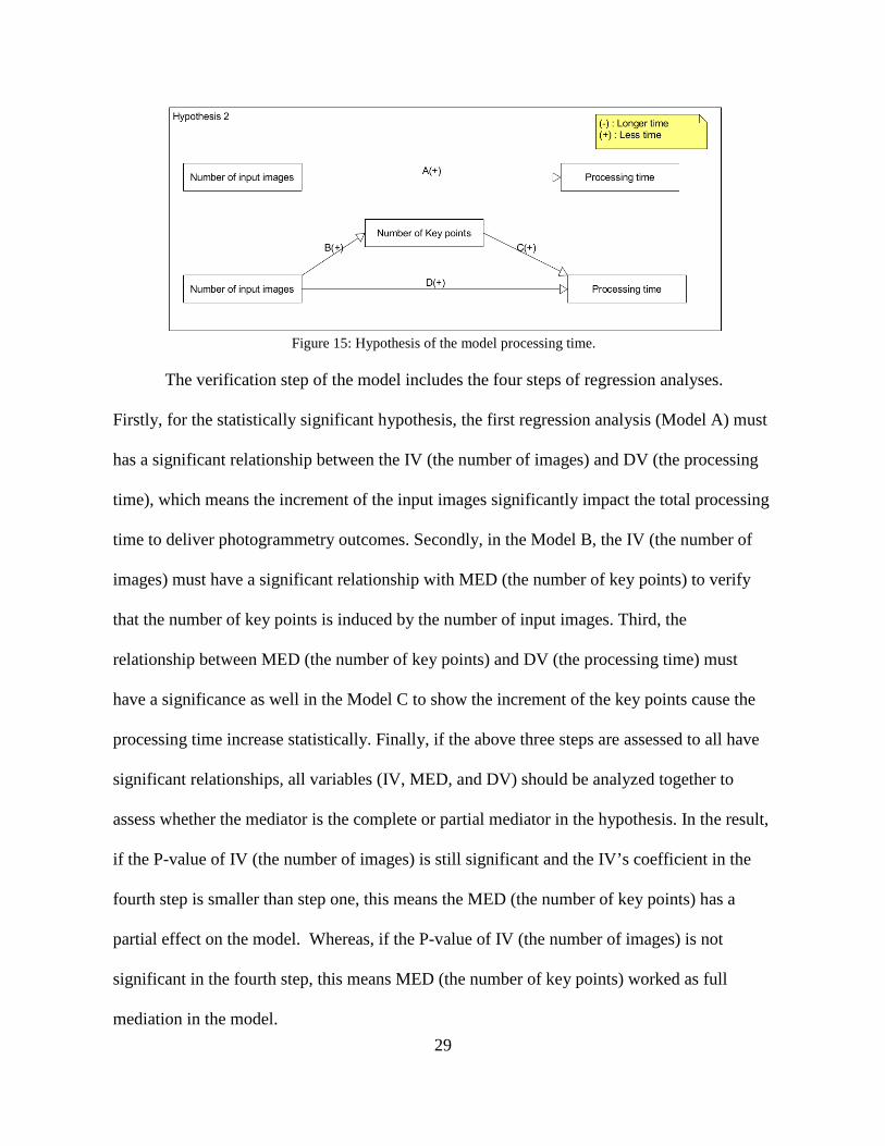
Figure 15: Hypothesis of the model processing time.
The verification step of the model includes the four steps of regression analyses.
Firstly, for the statistically significant hypothesis, the first regression analysis (Model A) must
has a significant relationship between the IV (the number of images) and DV (the processing
time), which means the increment of the input images significantly impact the total processing
time to deliver photogrammetry outcomes. Secondly, in the Model B, the IV (the number of
images) must have a significant relationship with MED (the number of key points) to verify
that the number of key points is induced by the number of input images. Third, the
relationship between MED (the number of key points) and DV (the processing time) must
have a significance as well in the Model C to show the increment of the key points cause the
processing time increase statistically. Finally, if the above three steps are assessed to all have
significant relationships, all variables (IV, MED, and DV) should be analyzed together to
assess whether the mediator is the complete or partial mediator in the hypothesis. In the result,
if the P-value of IV (the number of images) is still significant and the IV’s coefficient in the
fourth step is smaller than step one, this means the MED (the number of key points) has a
partial effect on the model. Whereas, if the P-value of IV (the number of images) is not
significant in the fourth step, this means MED (the number of key points) worked as full
mediation in the model.
30
Hypothesis 3: Estimates of length, area, and volume are accurate within 5% using
photogrammetric techniques.
The last investigative question is how reliable measurements are from
photogrammetric reconstructed models generated by collecting images from the SUAV.
This criteria for evaluating hypothesis 3 are as follows;
• The photogrammetric linear measure is within five percent of the real value.
• The photogrammetric area measure is within five percent of the real value.
• The photogrammetric volumetric is within five percent of the real value.
Photogrammetric measurements rely on the camera orientation error results due to lens
distortion and the rolling shutter effect [10][28]. Since all manufactured cameras have some
distortion error [28], it is impossible to construct the photogrammetric model perfectly without
using any ground referenced points. However, establishing GCPs in all military cases may be
infeasible, so it is important to understand how the lack of GCPs affects model’s measurement
accuracy. Five percent margin is a system capability requirement that is assessed to be a
reasonable measurement performance for rapid inspections or surveys in military.
31
IV. Experiment Design
This chapter illustrates the test objectives, test platforms, available test facilities, and
the scenario including the flight profile to study the research subject. The tests were performed
on three occasions at the UAV test field at Wright Patterson Air Force Base (WPAFB) and
Himsel airfield at Camp Atterbury army base. The UAV platforms, X-4 (Quad rotor) and
T960 (Hex rotor) were built to perform the image collection for the research. Generally, the
workflow followed the system architecture mentioned in Chapter Ⅲ and the additional details
of the three objectives are listed below. The flight profiles were designed to test the hypothesis
and the sequences were performed with fully automated flights following the GCS mission
plan with the exception of take-off and landing. Ultimately, the flights provided the imagery
data with a geo-referenced location which are required for software data processing.
Test objective
Test Objective 1 is to collect the overlapped image data for topographic maps with the
X-4 vehicle and Canon S110 camera. This test was not only collecting data, but also used to
verify the method through analysis of a small size data set for the conceptual system
development sequence.
Objective 2 is to capture still imagery using the Sony Alpha A6000 camera on the
T960 multi-rotor vehicle. This test was executed with a custom UAV to collect the image data
at higher altitudes and across a wider area than the X-4. The flight profiles include the runway
survey scenario as well as the verification.
Vehicle description
These tests will utilize 3D Robotics X-4 multi-rotors and Tarot T960 equipped with
32
autopilots, GPS receivers, and other sensors required to perform autonomous navigation. The
two vehicles fall under the small Unmanned Aerial System (UAS) Group 1 category. These
vehicles are monitored and controlled from a central Ground Control Station (GCS) and were
equipped with a camera to collect data. The characteristic comparison is shown in Table 3 and
Appendix A.
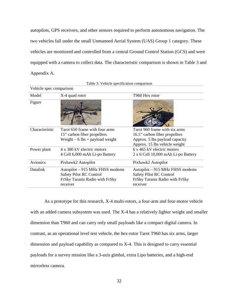
Table 3: Vehicle specification comparison Vehicle spec comparison Model X-4 quad rotor T960 Hex rotor Figure
Characteristic Tarot 650 frame with four arms
15” carbon fiber propellers Weight – 6 lbs + payload weight
Tarot 960 frame with six arms 16.5” carbon fiber propellers Approx. 5 lbs payload capacity Approx. 15 lbs vehicle weight
Power plant 4 x 380 kV electric motors 4 Cell 6,000 mAh Li-po Battery
6 x 465 kV electric motors 2 x 6 Cell 10,000 mAh Li-po Battery
Avionics Pixhawk2 Autopilot Pixhawk2 Autopilot Datalink Autopilot – 915 MHz FHSS modems
Safety Pilot RC Control FrSky Taranis Radio with FrSky receiver
Autopilot – 915 MHz FHSS modems Safety Pilot RC Control FrSky Taranis Radio with FrSky receiver
As a prototype for this research, X-4 multi-rotors, a four-arm and four-motor vehicle
with an added camera subsystem was used. The X-4 has a relatively lighter weight and smaller
dimension than T960 and can carry only small payloads like a compact digital camera. In
contrast, as an operational level test vehicle, the hex-rotor Tarot T960 has six arms, larger
dimension and payload capability as compared to X-4. This is designed to carry essential
payloads for a survey mission like a 3-axis gimbal, extra Lipo batteries, and a high-end
mirrorless camera.
33
Sensor description
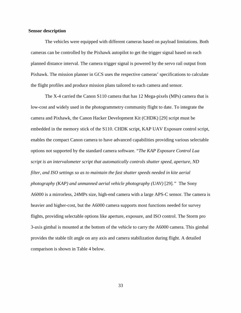
The vehicles were equipped with different cameras based on payload limitations. Both
cameras can be controlled by the Pixhawk autopilot to get the trigger signal based on each
planned distance interval. The camera trigger signal is powered by the servo rail output from
Pixhawk. The mission planner in GCS uses the respective cameras’ specifications to calculate
the flight profiles and produce mission plans tailored to each camera and sensor.
The X-4 carried the Canon S110 camera that has 12 Mega-pixels (MPs) camera that is
low-cost and widely used in the photogrammetry community flight to date. To integrate the
camera and Pixhawk, the Canon Hacker Development Kit (CHDK) [29] script must be
embedded in the memory stick of the S110. CHDK script, KAP UAV Exposure control script,
enables the compact Canon camera to have advanced capabilities providing various selectable
options not supported by the standard camera software. “The KAP Exposure Control Lua
script is an intervalometer script that automatically controls shutter speed, aperture, ND
filter, and ISO settings so as to maintain the fast shutter speeds needed in kite aerial
photography (KAP) and unmanned aerial vehicle photography (UAV) [29].” The Sony
A6000 is a mirrorless, 24MPs size, high-end camera with a large APS-C sensor. The camera is
heavier and higher-cost, but the A6000 camera supports most functions needed for survey
flights, providing selectable options like aperture, exposure, and ISO control. The Storm pro
3-axis gimbal is mounted at the bottom of the vehicle to carry the A6000 camera. This gimbal
provides the stable tilt angle on any axis and camera stabilization during flight. A detailed
comparison is shown in Table 4 below.
34
Table 4: Camera specification comparison Camera specs comparison Model Canon S110 Sony A6000 Type
Compact digital camera
Digital Mirrorless Camera Focal length 5.2 – 26 mm adjustable lens 20 mm fixed lens Image size 12MP: 4000x3000 (RGB) 24MP: 6000x4000 (RGB) Sensor format CMOS APS-C Triggering control
Pixhawk through CHDK script: KAP UAV Exposure control Script
Direct from Pixhawk
Gimbal None Storm pro 3 axis gimbal
Test facilities description
Himsel Airfield is an operational airfield located on Army property and under
restricted airspace. Himsel Army Airfield has a single north/south runway with an adjacent
parking apron. The SUAV field is located in an isolated area of the base adjacent to the
weapons range. SUAV operations at both Himsel airfield and the SUAV field are controlled
by the Himsel tower controller. The airfield operations building is located at the north end of
the Himsel runway. To investigate the location deviation, the eight geo-reference points were
surveyed in the test field (Figure 16).
WPAFB Area B supports SUAV flights under a Federal Aviation Administration
(FAA) Certificate of Authorization (COA) maintained by Air Force Research Laboratory
(AFRL). To fly under this COA, AFIT must abide by all rules outlined in the COA. The
airfield is maintained by AFRL and located adjacent to the AF museum. This airfield is in
good condition and is often used by AFRL and the RAMS model aircraft club. The test range
intended for use is the Wright Patterson AFB/AF Museum auxiliary runway located on Area
B. There is a single maintained airstrip running east-west, with service aprons and taxi-ways
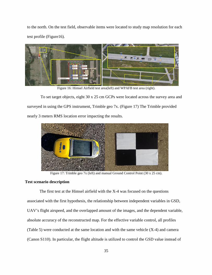
35
to the north. On the test field, observable items were located to study map resolution for each
test profile (Figure16).
Figure 16: Himsel Airfield test area(left) and WPAFB test area (right).
To set target objects, eight 30 x 25 cm GCPs were located across the survey area and
surveyed in using the GPS instrument, Trimble geo 7x. (Figure 17) The Trimble provided
nearly 3 meters RMS location error impacting the results.
Figure 17: Trimble geo 7x (left) and manual Ground Control Point (30 x 25 cm).
Test scenario description
The first test at the Himsel airfield with the X-4 was focused on the questions
associated with the first hypothesis, the relationship between independent variables in GSD,
UAV’s flight airspeed, and the overlapped amount of the images, and the dependent variable,
absolute accuracy of the reconstructed map. For the effective variable control, all profiles
(Table 5) were conducted at the same location and with the same vehicle (X-4) and camera
(Canon S110). In particular, the flight altitude is utilized to control the GSD value instead of
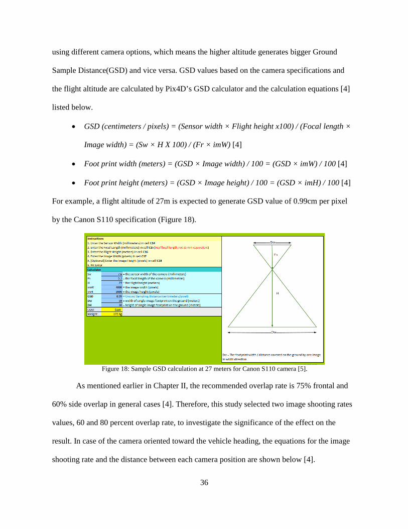
36
using different camera options, which means the higher altitude generates bigger Ground
Sample Distance(GSD) and vice versa. GSD values based on the camera specifications and
the flight altitude are calculated by Pix4D’s GSD calculator and the calculation equations [4]
listed below.
• GSD (centimeters / pixels) = (Sensor width × Flight height x100) / (Focal length ×
Image width) = (Sw × H X 100) / (Fr × imW) [4]
• Foot print width (meters) = (GSD × Image width) / 100 = (GSD × imW) / 100 [4]
• Foot print height (meters) = (GSD × Image height) / 100 = (GSD × imH) / 100 [4]
For example, a flight altitude of 27m is expected to generate GSD value of 0.99cm per pixel
by the Canon S110 specification (Figure 18).
Figure 18: Sample GSD calculation at 27 meters for Canon S110 camera [5].
As mentioned earlier in Chapter Ⅱ, the recommended overlap rate is 75% frontal and
60% side overlap in general cases [4]. Therefore, this study selected two image shooting rates
values, 60 and 80 percent overlap rate, to investigate the significance of the effect on the
result. In case of the camera oriented toward the vehicle heading, the equations for the image
shooting rate and the distance between each camera position are shown below [4].
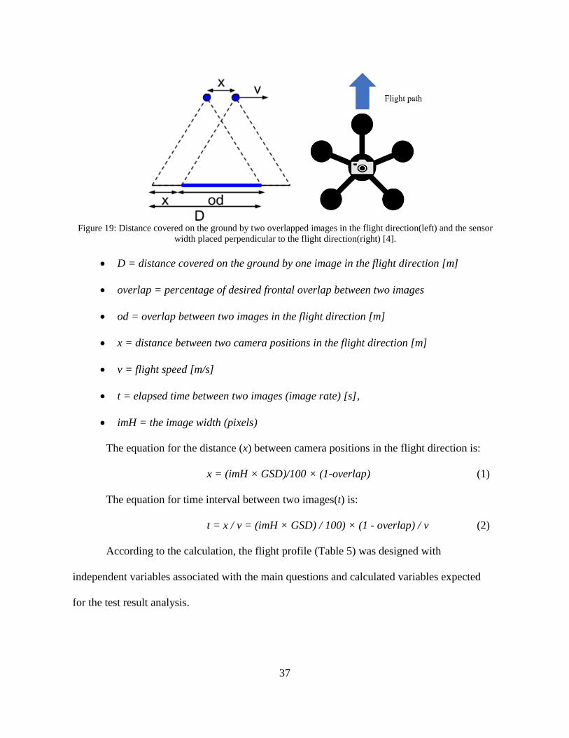
37
Figure 19: Distance covered on the ground by two overlapped images in the flight direction(left) and the sensor
width placed perpendicular to the flight direction(right) [4].
• D = distance covered on the ground by one image in the flight direction [m]
• overlap = percentage of desired frontal overlap between two images
• od = overlap between two images in the flight direction [m]
• x = distance between two camera positions in the flight direction [m]
• v = flight speed [m/s]
• t = elapsed time between two images (image rate) [s],
• imH = the image width (pixels)
The equation for the distance (x) between camera positions in the flight direction is:
x = (imH × GSD)/100 × (1-overlap) (1)
The equation for time interval between two images(t) is:
t = x / v = (imH × GSD) / 100) × (1 - overlap) / v (2)
According to the calculation, the flight profile (Table 5) was designed with
independent variables associated with the main questions and calculated variables expected
for the test result analysis.
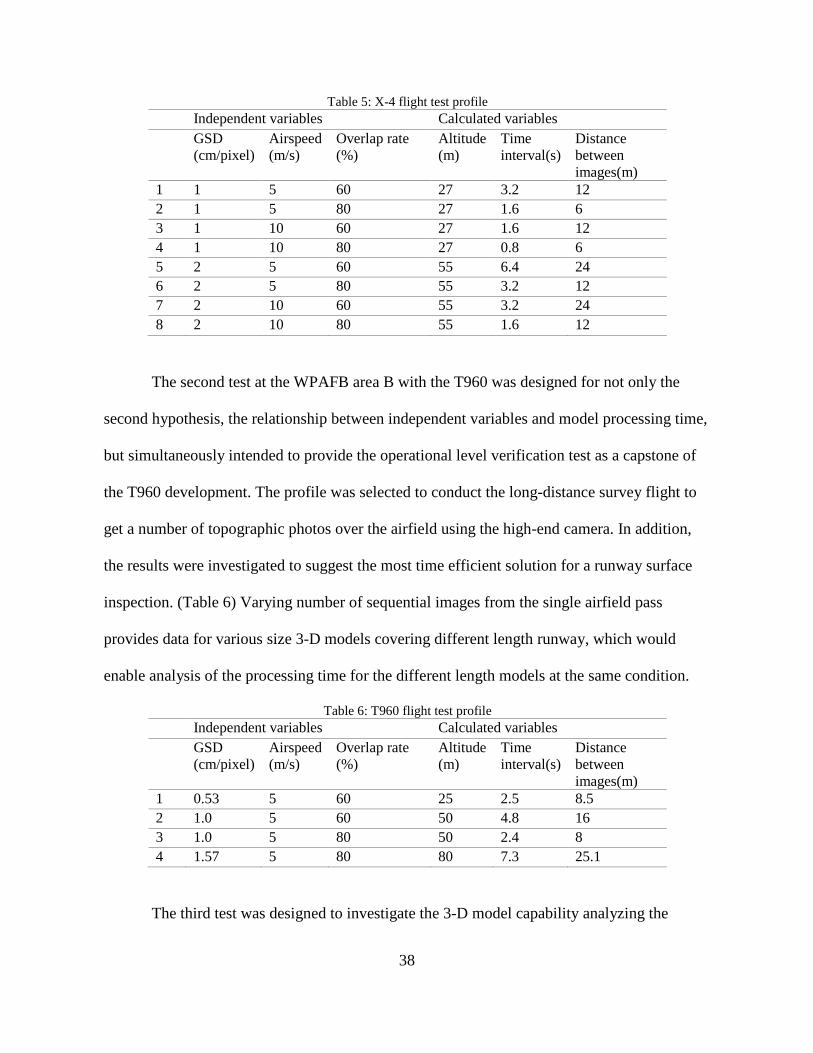
38
Table 5: X-4 flight test profile Independent variables Calculated variables
GSD (cm/pixel)
Airspeed (m/s)
Overlap rate (%)
Altitude (m)
Time interval(s)
Distance between images(m)
1 1 5 60 27 3.2 12 2 1 5 80 27 1.6 6 3 1 10 60 27 1.6 12 4 1 10 80 27 0.8 6 5 2 5 60 55 6.4 24 6 2 5 80 55 3.2 12 7 2 10 60 55 3.2 24 8 2 10 80 55 1.6 12
The second test at the WPAFB area B with the T960 was designed for not only the
second hypothesis, the relationship between independent variables and model processing time,
but simultaneously intended to provide the operational level verification test as a capstone of
the T960 development. The profile was selected to conduct the long-distance survey flight to
get a number of topographic photos over the airfield using the high-end camera. In addition,
the results were investigated to suggest the most time efficient solution for a runway surface
inspection. (Table 6) Varying number of sequential images from the single airfield pass
provides data for various size 3-D models covering different length runway, which would
enable analysis of the processing time for the different length models at the same condition.
Table 6: T960 flight test profile Independent variables Calculated variables
GSD (cm/pixel)
Airspeed (m/s)
Overlap rate (%)
Altitude (m)
Time interval(s)
Distance between images(m)
1 0.53 5 60 25 2.5 8.5 2 1.0 5 60 50 4.8 16 3 1.0 5 80 50 2.4 8 4 1.57 5 80 80 7.3 25.1
The third test was designed to investigate the 3-D model capability analyzing the
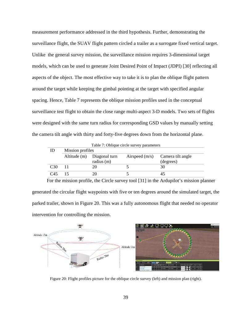
39
measurement performance addressed in the third hypothesis. Further, demonstrating the
surveillance flight, the SUAV flight pattern circled a trailer as a surrogate fixed vertical target.
Unlike the general survey mission, the surveillance mission requires 3-dimensional target
models, which can be used to generate Joint Desired Point of Impact (JDPI) [30] reflecting all
aspects of the object. The most effective way to take it is to plan the oblique flight pattern
around the target while keeping the gimbal pointing at the target with specified angular
spacing. Hence, Table 7 represents the oblique mission profiles used in the conceptual
surveillance test flight to obtain the close range multi-aspect 3-D models. Two sets of flights
were designed with the same turn radius for corresponding GSD values by manually setting
the camera tilt angle with thirty and forty-five degrees down from the horizontal plane.
Table 7: Oblique circle survey parameters ID Mission profiles
Altitude (m) Diagonal turn radius (m)
Airspeed (m/s) Camera tilt angle (degrees)
C30 11 20 5 30 C45 15 20 5 45
For the mission profile, the Circle survey tool [31] in the Ardupilot’s mission planner
generated the circular flight waypoints with five or ten degrees around the simulated target, the
parked trailer, shown in Figure 20. This was a fully autonomous flight that needed no operator
intervention for controlling the mission.
Figure 20: Flight profiles picture for the oblique circle survey (left) and mission plan (right).
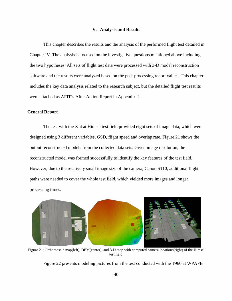
40
V. Analysis and Results
This chapter describes the results and the analysis of the performed flight test detailed in
Chapter Ⅳ. The analysis is focused on the investigative questions mentioned above including
the two hypotheses. All sets of flight test data were processed with 3-D model reconstruction
software and the results were analyzed based on the post-processing report values. This chapter
includes the key data analysis related to the research subject, but the detailed flight test results
were attached as AFIT’s After Action Report in Appendix J.
General Report
The test with the X-4 at Himsel test field provided eight sets of image data, which were
designed using 3 different variables, GSD, flight speed and overlap rate. Figure 21 shows the
output reconstructed models from the collected data sets. Given image resolution, the
reconstructed model was formed successfully to identify the key features of the test field.
However, due to the relatively small image size of the camera, Canon S110, additional flight
paths were needed to cover the whole test field, which yielded more images and longer
processing times.
Figure 21: Orthomosaic map(left), DEM(center), and 3-D map with computed camera locations(right) of the Himsel
test field.
Figure 22 presents modeling pictures from the test conducted with the T960 at WPAFB
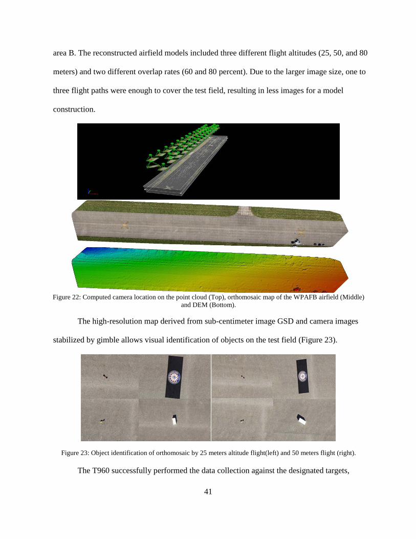
41
area B. The reconstructed airfield models included three different flight altitudes (25, 50, and 80
meters) and two different overlap rates (60 and 80 percent). Due to the larger image size, one to
three flight paths were enough to cover the test field, resulting in less images for a model
construction.
Figure 22: Computed camera location on the point cloud (Top), orthomosaic map of the WPAFB airfield (Middle)
and DEM (Bottom).
The high-resolution map derived from sub-centimeter image GSD and camera images
stabilized by gimble allows visual identification of objects on the test field (Figure 23).
Figure 23: Object identification of orthomosaic by 25 meters altitude flight(left) and 50 meters flight (right).
The T960 successfully performed the data collection against the designated targets,
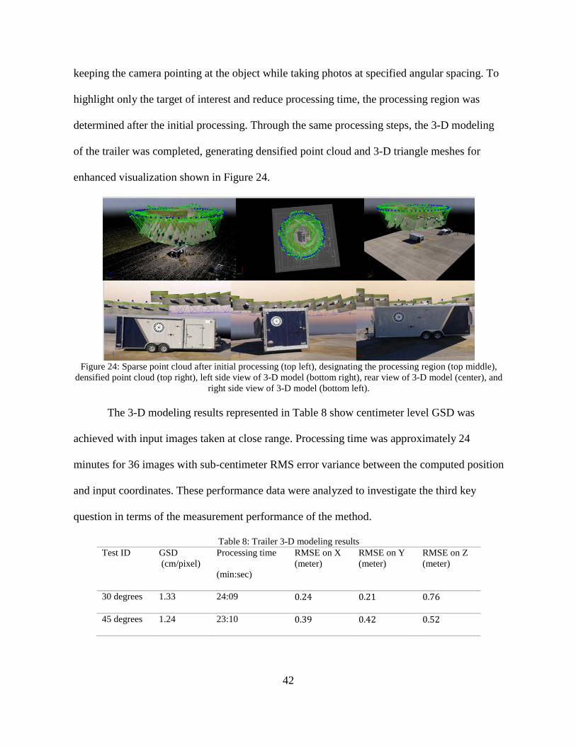
42
keeping the camera pointing at the object while taking photos at specified angular spacing. To
highlight only the target of interest and reduce processing time, the processing region was
determined after the initial processing. Through the same processing steps, the 3-D modeling
of the trailer was completed, generating densified point cloud and 3-D triangle meshes for
enhanced visualization shown in Figure 24.
Figure 24: Sparse point cloud after initial processing (top left), designating the processing region (top middle),
densified point cloud (top right), left side view of 3-D model (bottom right), rear view of 3-D model (center), and right side view of 3-D model (bottom left).
The 3-D modeling results represented in Table 8 show centimeter level GSD was
achieved with input images taken at close range. Processing time was approximately 24
minutes for 36 images with sub-centimeter RMS error variance between the computed position
and input coordinates. These performance data were analyzed to investigate the third key
question in terms of the measurement performance of the method.
Table 8: Trailer 3-D modeling results Test ID GSD
(cm/pixel) Processing time
(min:sec)
RMSE on X (meter)
RMSE on Y (meter)
RMSE on Z (meter)
30 degrees 1.33 24:09 0.24 0.21 0.76
45 degrees 1.24 23:10 0.39 0.42 0.52
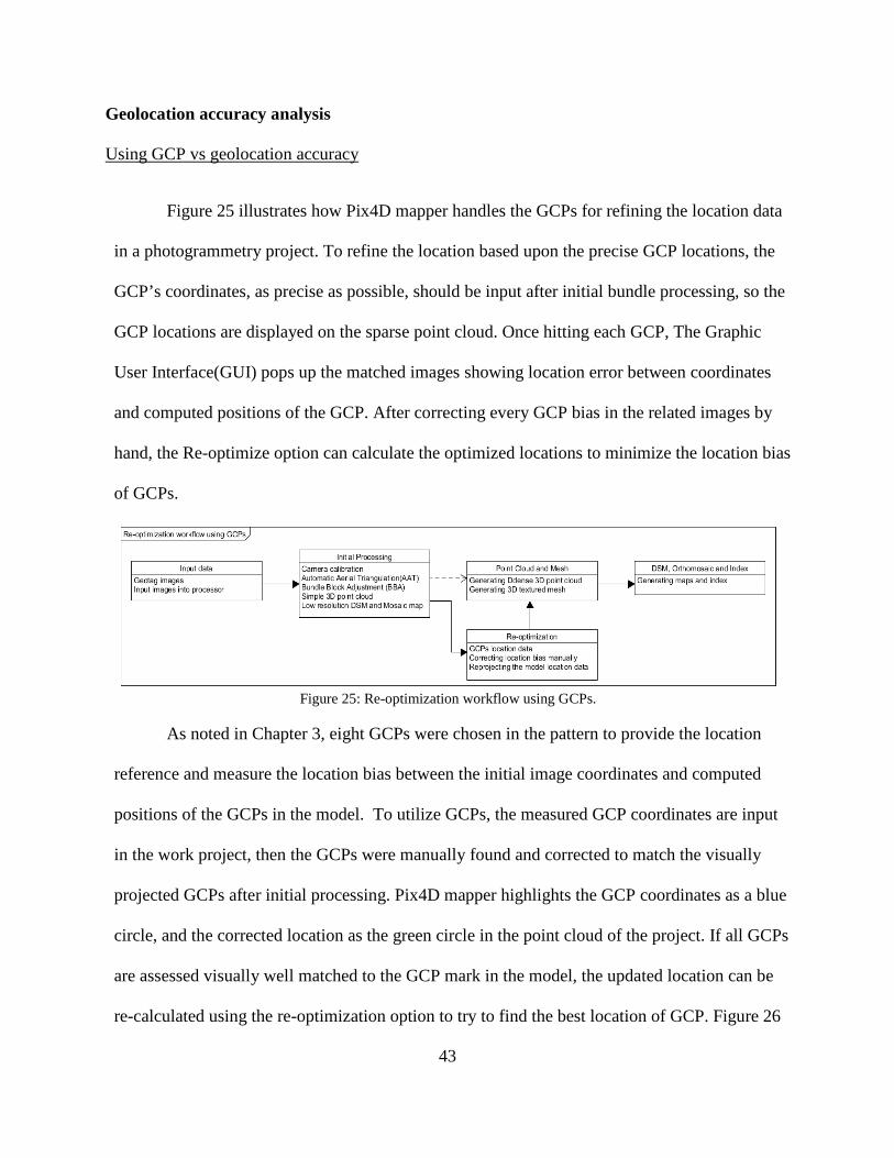
43
Geolocation accuracy analysis
Using GCP vs geolocation accuracy
Figure 25 illustrates how Pix4D mapper handles the GCPs for refining the location data
in a photogrammetry project. To refine the location based upon the precise GCP locations, the
GCP’s coordinates, as precise as possible, should be input after initial bundle processing, so the
GCP locations are displayed on the sparse point cloud. Once hitting each GCP, The Graphic
User Interface(GUI) pops up the matched images showing location error between coordinates
and computed positions of the GCP. After correcting every GCP bias in the related images by
hand, the Re-optimize option can calculate the optimized locations to minimize the location bias
of GCPs.
Figure 25: Re-optimization workflow using GCPs.
As noted in Chapter 3, eight GCPs were chosen in the pattern to provide the location
reference and measure the location bias between the initial image coordinates and computed
positions of the GCPs in the model. To utilize GCPs, the measured GCP coordinates are input
in the work project, then the GCPs were manually found and corrected to match the visually
projected GCPs after initial processing. Pix4D mapper highlights the GCP coordinates as a blue
circle, and the corrected location as the green circle in the point cloud of the project. If all GCPs
are assessed visually well matched to the GCP mark in the model, the updated location can be
re-calculated using the re-optimization option to try to find the best location of GCP. Figure 26
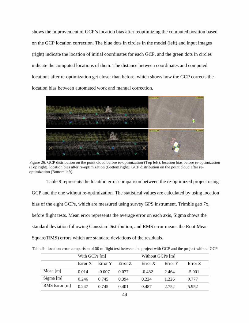
44
shows the improvement of GCP’s location bias after reoptimizing the computed position based
on the GCP location correction. The blue dots in circles in the model (left) and input images
(right) indicate the location of initial coordinates for each GCP, and the green dots in circles
indicate the computed locations of them. The distance between coordinates and computed
locations after re-optimization get closer than before, which shows how the GCP corrects the
location bias between automated work and manual correction.
Figure 26: GCP distribution on the point cloud before re-optimization (Top left), location bias before re-optimization (Top right), location bias after re-optimization (Bottom right), GCP distribution on the point cloud after re-optimization (Bottom left).
Table 9 represents the location error comparison between the re-optimized project using
GCP and the one without re-optimization. The statistical values are calculated by using location
bias of the eight GCPs, which are measured using survey GPS instrument, Trimble geo 7x,
before flight tests. Mean error represents the average error on each axis, Sigma shows the
standard deviation following Gaussian Distribution, and RMS error means the Root Mean
Square(RMS) errors which are standard deviations of the residuals.
Table 9: location error comparison of 50 m flight test between the project with GCP and the project without GCP
With GCPs [m] Without GCPs [m] Error X Error Y Error Z Error X Error Y Error Z Mean [m] 0.014 -0.007 0.077 -0.432 2.464 -5.901 Sigma [m] 0.246 0.745 0.394 0.224 1.226 0.777 RMS Error [m] 0.247 0.745 0.401 0.487 2.752 5.952
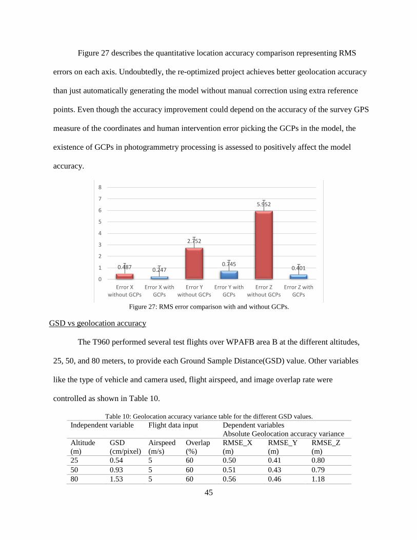
45
Figure 27 describes the quantitative location accuracy comparison representing RMS
errors on each axis. Undoubtedly, the re-optimized project achieves better geolocation accuracy
than just automatically generating the model without manual correction using extra reference
points. Even though the accuracy improvement could depend on the accuracy of the survey GPS
measure of the coordinates and human intervention error picking the GCPs in the model, the
existence of GCPs in photogrammetry processing is assessed to positively affect the model
accuracy.
Figure 27: RMS error comparison with and without GCPs.
GSD vs geolocation accuracy
The T960 performed several test flights over WPAFB area B at the different altitudes,
25, 50, and 80 meters, to provide each Ground Sample Distance(GSD) value. Other variables
like the type of vehicle and camera used, flight airspeed, and image overlap rate were
controlled as shown in Table 10.
Table 10: Geolocation accuracy variance table for the different GSD values. Independent variable Flight data input Dependent variables
Absolute Geolocation accuracy variance Altitude (m)
GSD (cm/pixel)
Airspeed (m/s)
Overlap (%)
RMSE_X (m)
RMSE_Y (m)
RMSE_Z (m)
25 0.54 5 60 0.50 0.41 0.80 50 0.93 5 60 0.51 0.43 0.79 80 1.53 5 60 0.56 0.46 1.18
0.487 0.247
2.752
0.745
5.952
0.401
0
1
2
3
4
5
6
7
8
Error Xwithout GCPs
Error X withGCPs
Error Ywithout GCPs
Error Y withGCPs
Error Zwithout GCPs
Error Z withGCPs
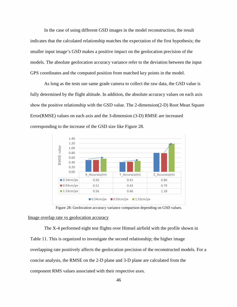
46
In the case of using different GSD images in the model reconstruction, the result
indicates that the calculated relationship matches the expectation of the first hypothesis; the
smaller input image’s GSD makes a positive impact on the geolocation precision of the
models. The absolute geolocation accuracy variance refer to the deviation between the input
GPS coordinates and the computed position from matched key points in the model.
As long as the tests use same grade camera to collect the raw data, the GSD value is
fully determined by the flight altitude. In addition, the absolute accuracy values on each axis
show the positive relationship with the GSD value. The 2-dimension(2-D) Root Mean Square
Error(RMSE) values on each axis and the 3-dimension (3-D) RMSE are increased
corresponding to the increase of the GSD size like Figure 28.
Figure 28: Geolocation accuracy variance comparison depending on GSD values.
Image overlap rate vs geolocation accuracy
The X-4 performed eight test flights over Himsel airfield with the profile shown in
Table 11. This is organized to investigate the second relationship; the higher image
overlapping rate positively affects the geolocation precision of the reconstructed models. For a
concise analysis, the RMSE on the 2-D plane and 3-D plane are calculated from the
component RMS values associated with their respective axes.
X_Accuracy(m) Y_Accuracy(m) Z_Accuracy(m)0.54cm/px 0.50 0.41 0.800.93cm/px 0.51 0.43 0.791.53cm/px 0.56 0.46 1.18
0.000.200.400.600.801.001.201.40
RM
SE v
alue
0.54cm/px 0.93cm/px 1.53cm/px

47
Table 11: Geolocation accuracy variance table depending on image overlap rate Independent variable Overlap (%)
Dependent variables Geolocational accuracy(meter) RMSE_X RMSE_Y RMSE_Z RMSE(X,Y) RMSE(X,Y,Z)
60%/27m/5ms 0.89 4.17 1.14 3.02 2.55 80%/27m/5ms 0.82 2.32 0.90 1.74 1.51 60%/27m/10ms 1.02 3.57 1.22 2.62 2.26 80%/27m/10ms 1.30 3.86 0.62 2.88 2.38 60%/55m/5ms 1.09 2.89 0.45 2.18 1.80 80%/55m/5ms 0.97 3.35 0.48 2.47 2.03 60%/55m/10ms 1.75 4.35 0.54 3.32 2.73 80%/55m/10ms 1.87 4.51 0.35 3.45 2.83 The results are graphed in Figure 29 to compare pair results with only different image
overlap rates, 60 and 80 percent, at a glance. Unlike with the initial hypothesis, the result
shows that the overlap rate is not correlated with the initial expectation. Only the test set at 27
meters altitude and 5 m/s airspeed meet the expectation that the error will be lower as the
image overlap is higher, but the other three sets of tests show the opposite results. They show
almost similar performance in that the higher overlap flights have lager RMS error of location
than lower overlap flight data. Accordingly, the relationship between the overlap rate and
location accuracy is not assessed to have a positive relationship once using only these results.
Figure 29: Geolocation accuracy variance comparison depending on image overlap rates.
60%/27m/5ms
80%/27m/5ms
60%/27m/10ms
80%/27m/10ms
60%/55m/5ms
80%/55m/5ms
60%/55m/10ms
80%/55m/10ms
RMSE(X,Y) 3.02 1.74 2.62 2.88 2.18 2.47 3.32 3.45RMSE(X,Y,Z) 2.55 1.51 2.26 2.38 1.80 2.03 2.73 2.83
0.00
0.50
1.00
1.50
2.00
2.50
3.00
3.50
4.00
RMSE
val
ue
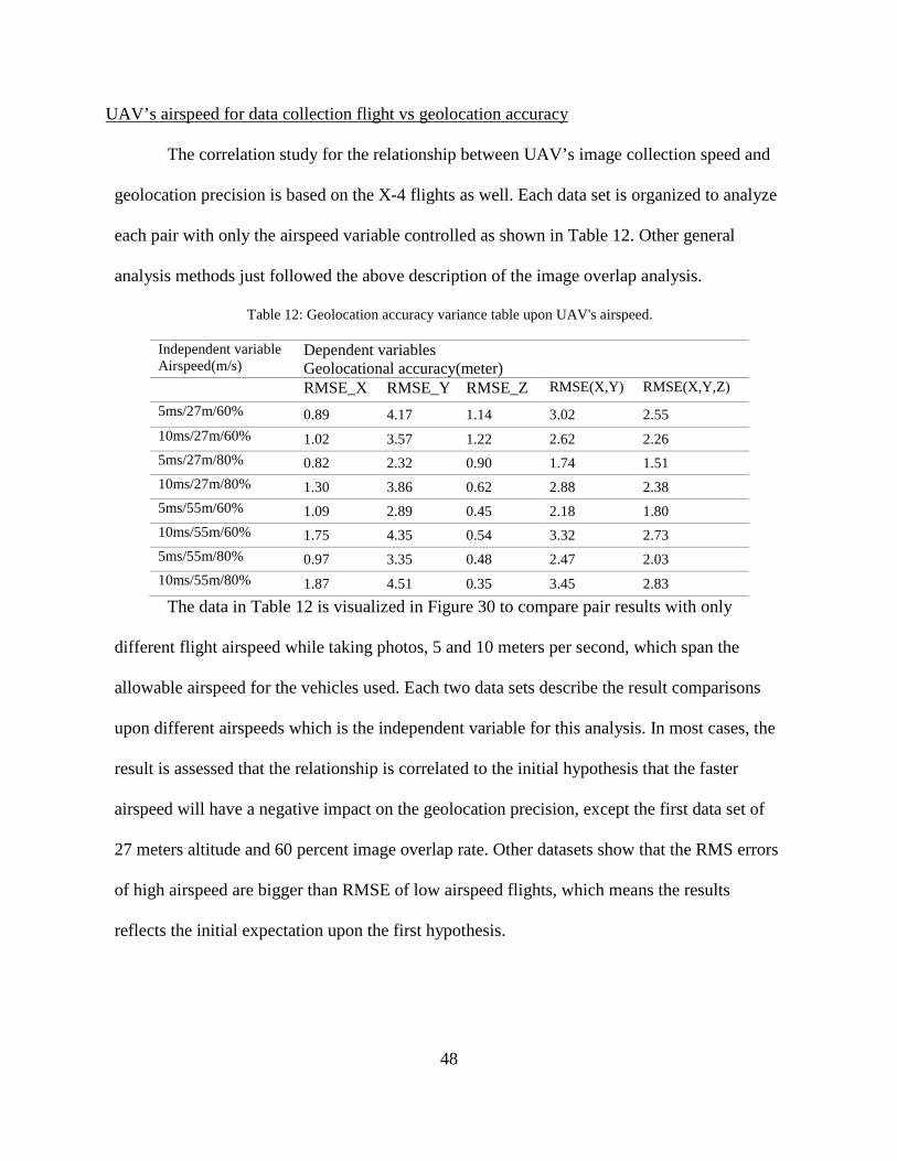
48
UAV’s airspeed for data collection flight vs geolocation accuracy
The correlation study for the relationship between UAV’s image collection speed and
geolocation precision is based on the X-4 flights as well. Each data set is organized to analyze
each pair with only the airspeed variable controlled as shown in Table 12. Other general
analysis methods just followed the above description of the image overlap analysis.
Table 12: Geolocation accuracy variance table upon UAV's airspeed.
Independent variable Airspeed(m/s)
Dependent variables Geolocational accuracy(meter) RMSE_X RMSE_Y RMSE_Z RMSE(X,Y) RMSE(X,Y,Z)
5ms/27m/60% 0.89 4.17 1.14 3.02 2.55 10ms/27m/60% 1.02 3.57 1.22 2.62 2.26 5ms/27m/80% 0.82 2.32 0.90 1.74 1.51 10ms/27m/80% 1.30 3.86 0.62 2.88 2.38 5ms/55m/60% 1.09 2.89 0.45 2.18 1.80 10ms/55m/60% 1.75 4.35 0.54 3.32 2.73 5ms/55m/80% 0.97 3.35 0.48 2.47 2.03 10ms/55m/80% 1.87 4.51 0.35 3.45 2.83
The data in Table 12 is visualized in Figure 30 to compare pair results with only
different flight airspeed while taking photos, 5 and 10 meters per second, which span the
allowable airspeed for the vehicles used. Each two data sets describe the result comparisons
upon different airspeeds which is the independent variable for this analysis. In most cases, the
result is assessed that the relationship is correlated to the initial hypothesis that the faster
airspeed will have a negative impact on the geolocation precision, except the first data set of
27 meters altitude and 60 percent image overlap rate. Other datasets show that the RMS errors
of high airspeed are bigger than RMSE of low airspeed flights, which means the results
reflects the initial expectation upon the first hypothesis.
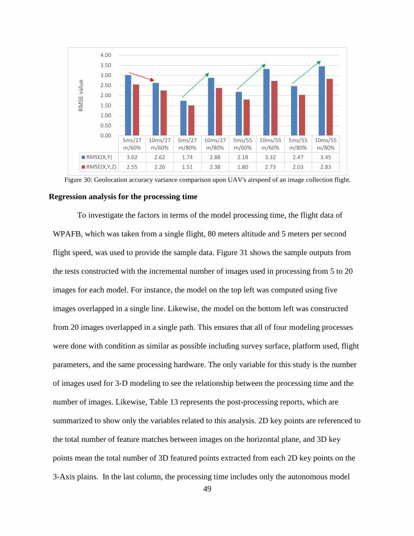
49
Figure 30: Geolocation accuracy variance comparison upon UAV's airspeed of an image collection flight.
Regression analysis for the processing time
To investigate the factors in terms of the model processing time, the flight data of
WPAFB, which was taken from a single flight, 80 meters altitude and 5 meters per second
flight speed, was used to provide the sample data. Figure 31 shows the sample outputs from
the tests constructed with the incremental number of images used in processing from 5 to 20
images for each model. For instance, the model on the top left was computed using five
images overlapped in a single line. Likewise, the model on the bottom left was constructed
from 20 images overlapped in a single path. This ensures that all of four modeling processes
were done with condition as similar as possible including survey surface, platform used, flight
parameters, and the same processing hardware. The only variable for this study is the number
of images used for 3-D modeling to see the relationship between the processing time and the
number of images. Likewise, Table 13 represents the post-processing reports, which are
summarized to show only the variables related to this analysis. 2D key points are referenced to
the total number of feature matches between images on the horizontal plane, and 3D key
points mean the total number of 3D featured points extracted from each 2D key points on the
3-Axis plains. In the last column, the processing time includes only the autonomous model
5ms/27m/60%
10ms/27m/60%
5ms/27m/80%
10ms/27m/80%
5ms/55m/60%
10ms/55m/60%
5ms/55m/80%
10ms/55m/80%
RMSE(X,Y) 3.02 2.62 1.74 2.88 2.18 3.32 2.47 3.45RMSE(X,Y,Z) 2.55 2.26 1.51 2.38 1.80 2.73 2.03 2.83
0.00
0.50
1.00
1.50
2.00
2.50
3.00
3.50
4.00
RMSE
val
ue
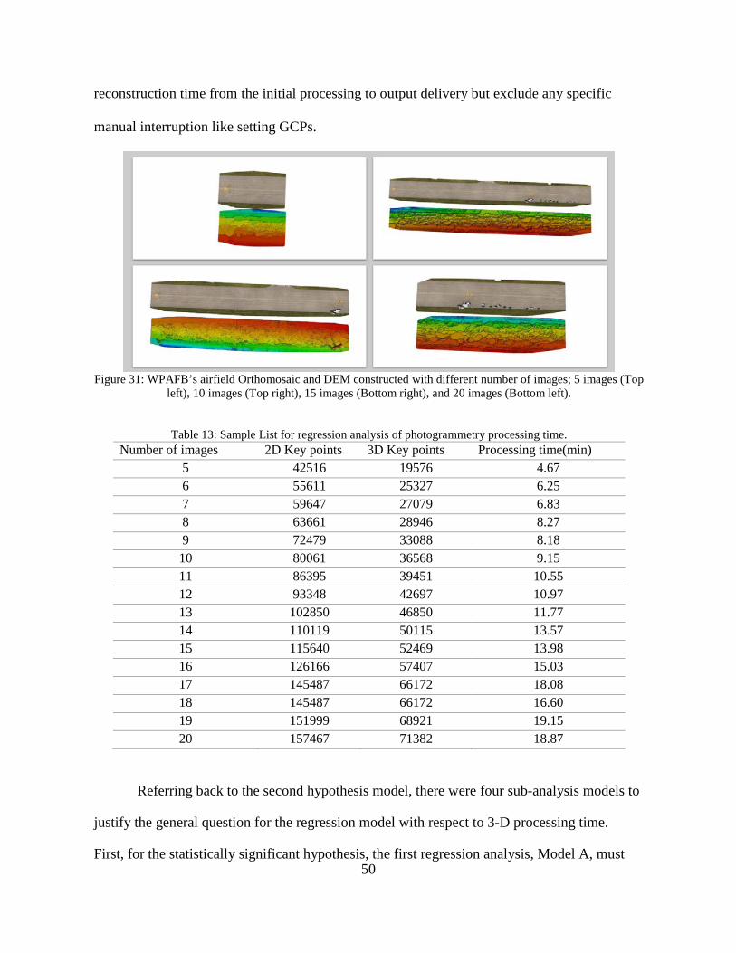
50
reconstruction time from the initial processing to output delivery but exclude any specific
manual interruption like setting GCPs.
Figure 31: WPAFB’s airfield Orthomosaic and DEM constructed with different number of images; 5 images (Top
left), 10 images (Top right), 15 images (Bottom right), and 20 images (Bottom left).
Table 13: Sample List for regression analysis of photogrammetry processing time. Number of images 2D Key points 3D Key points Processing time(min)
5 42516 19576 4.67 6 55611 25327 6.25 7 59647 27079 6.83 8 63661 28946 8.27 9 72479 33088 8.18
10 80061 36568 9.15 11 86395 39451 10.55 12 93348 42697 10.97 13 102850 46850 11.77 14 110119 50115 13.57 15 115640 52469 13.98 16 126166 57407 15.03 17 145487 66172 18.08 18 145487 66172 16.60 19 151999 68921 19.15 20 157467 71382 18.87
Referring back to the second hypothesis model, there were four sub-analysis models to
justify the general question for the regression model with respect to 3-D processing time.
First, for the statistically significant hypothesis, the first regression analysis, Model A, must
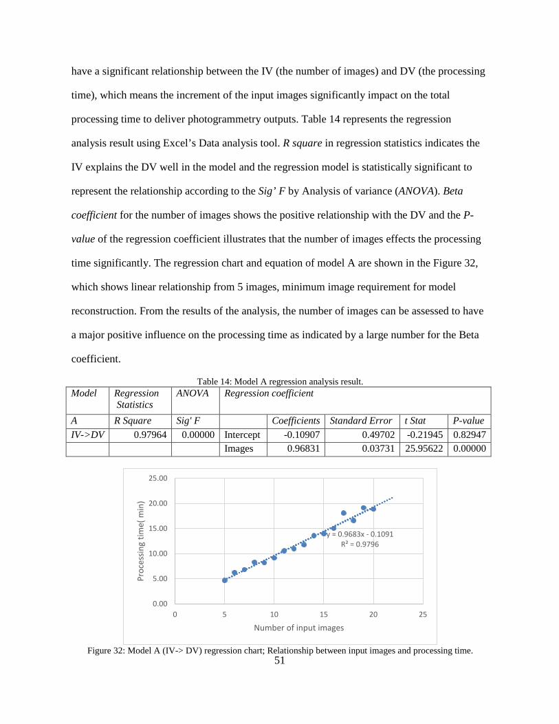
51
have a significant relationship between the IV (the number of images) and DV (the processing
time), which means the increment of the input images significantly impact on the total
processing time to deliver photogrammetry outputs. Table 14 represents the regression
analysis result using Excel’s Data analysis tool. R square in regression statistics indicates the
IV explains the DV well in the model and the regression model is statistically significant to
represent the relationship according to the Sig’ F by Analysis of variance (ANOVA). Beta
coefficient for the number of images shows the positive relationship with the DV and the P-
value of the regression coefficient illustrates that the number of images effects the processing
time significantly. The regression chart and equation of model A are shown in the Figure 32,
which shows linear relationship from 5 images, minimum image requirement for model
reconstruction. From the results of the analysis, the number of images can be assessed to have
a major positive influence on the processing time as indicated by a large number for the Beta
coefficient.
Table 14: Model A regression analysis result. Model Regression
Statistics ANOVA Regression coefficient
A R Square Sig' F Coefficients Standard Error t Stat P-value IV->DV 0.97964 0.00000 Intercept -0.10907 0.49702 -0.21945 0.82947 Images 0.96831 0.03731 25.95622 0.00000
Figure 32: Model A (IV-> DV) regression chart; Relationship between input images and processing time.
y = 0.9683x - 0.1091R² = 0.9796
0.00
5.00
10.00
15.00
20.00
25.00
0 5 10 15 20 25
Proc
essin
g tim
e( m
in)
Number of input images
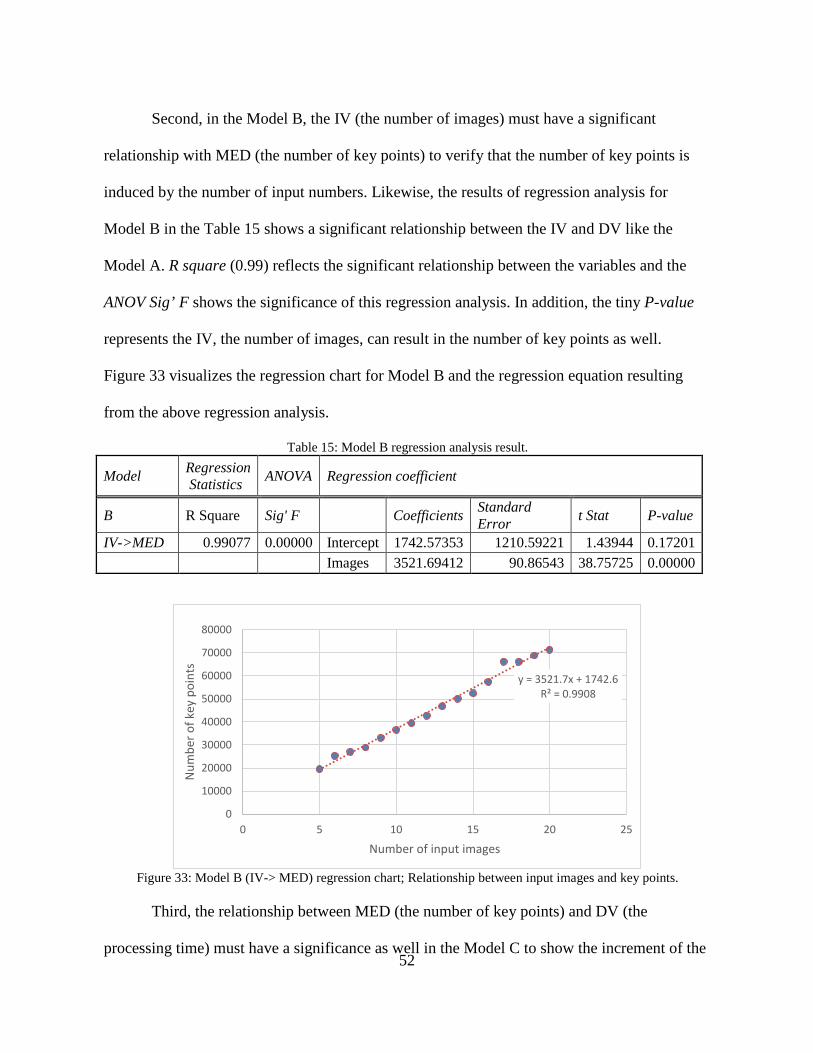
52
Second, in the Model B, the IV (the number of images) must have a significant
relationship with MED (the number of key points) to verify that the number of key points is
induced by the number of input numbers. Likewise, the results of regression analysis for
Model B in the Table 15 shows a significant relationship between the IV and DV like the
Model A. R square (0.99) reflects the significant relationship between the variables and the
ANOV Sig’ F shows the significance of this regression analysis. In addition, the tiny P-value
represents the IV, the number of images, can result in the number of key points as well.
Figure 33 visualizes the regression chart for Model B and the regression equation resulting
from the above regression analysis.
Table 15: Model B regression analysis result.
Model Regression Statistics ANOVA Regression coefficient
B R Square Sig' F Coefficients Standard Error t Stat P-value
IV->MED 0.99077 0.00000 Intercept 1742.57353 1210.59221 1.43944 0.17201 Images 3521.69412 90.86543 38.75725 0.00000
Figure 33: Model B (IV-> MED) regression chart; Relationship between input images and key points.
Third, the relationship between MED (the number of key points) and DV (the
processing time) must have a significance as well in the Model C to show the increment of the
y = 3521.7x + 1742.6R² = 0.9908
0
10000
20000
30000
40000
50000
60000
70000
80000
0 5 10 15 20 25
Num
ber o
f key
poi
nts
Number of input images
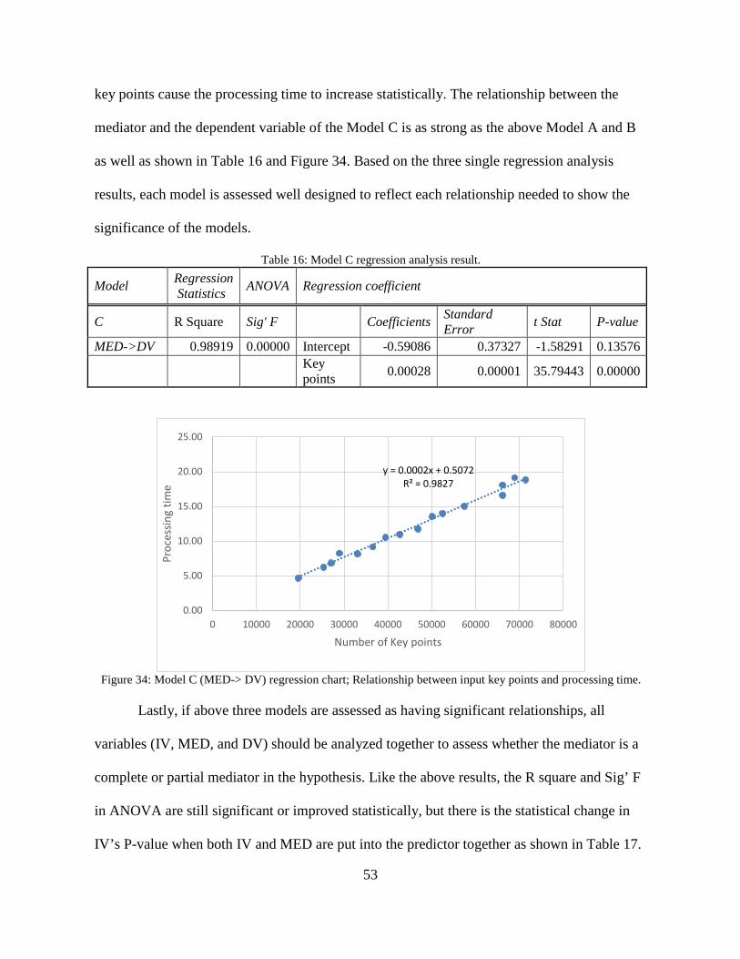
53
key points cause the processing time to increase statistically. The relationship between the
mediator and the dependent variable of the Model C is as strong as the above Model A and B
as well as shown in Table 16 and Figure 34. Based on the three single regression analysis
results, each model is assessed well designed to reflect each relationship needed to show the
significance of the models.
Table 16: Model C regression analysis result.
Model Regression Statistics ANOVA Regression coefficient
C R Square Sig' F Coefficients Standard Error t Stat P-value
MED->DV 0.98919 0.00000 Intercept -0.59086 0.37327 -1.58291 0.13576
Key points 0.00028 0.00001 35.79443 0.00000
Figure 34: Model C (MED-> DV) regression chart; Relationship between input key points and processing time.
Lastly, if above three models are assessed as having significant relationships, all
variables (IV, MED, and DV) should be analyzed together to assess whether the mediator is a
complete or partial mediator in the hypothesis. Like the above results, the R square and Sig’ F
in ANOVA are still significant or improved statistically, but there is the statistical change in
IV’s P-value when both IV and MED are put into the predictor together as shown in Table 17.
y = 0.0002x + 0.5072R² = 0.9827
0.00
5.00
10.00
15.00
20.00
25.00
0 10000 20000 30000 40000 50000 60000 70000 80000
Proc
essin
g tim
e
Number of Key points
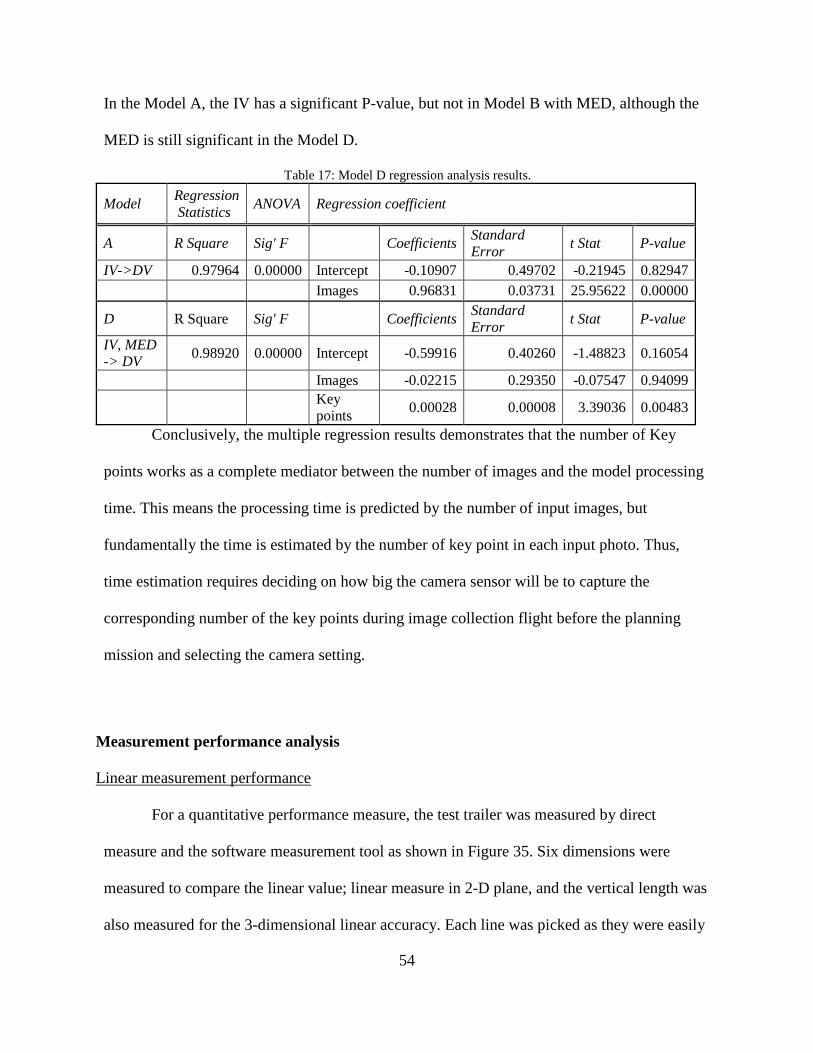
54
In the Model A, the IV has a significant P-value, but not in Model B with MED, although the
MED is still significant in the Model D.
Table 17: Model D regression analysis results.
Model Regression Statistics ANOVA Regression coefficient
A R Square Sig' F Coefficients Standard Error t Stat P-value
IV->DV 0.97964 0.00000 Intercept -0.10907 0.49702 -0.21945 0.82947 Images 0.96831 0.03731 25.95622 0.00000
D R Square Sig' F Coefficients Standard Error t Stat P-value
IV, MED -> DV 0.98920 0.00000 Intercept -0.59916 0.40260 -1.48823 0.16054
Images -0.02215 0.29350 -0.07547 0.94099
Key points 0.00028 0.00008 3.39036 0.00483
Conclusively, the multiple regression results demonstrates that the number of Key
points works as a complete mediator between the number of images and the model processing
time. This means the processing time is predicted by the number of input images, but
fundamentally the time is estimated by the number of key point in each input photo. Thus,
time estimation requires deciding on how big the camera sensor will be to capture the
corresponding number of the key points during image collection flight before the planning
mission and selecting the camera setting.
Measurement performance analysis
Linear measurement performance
For a quantitative performance measure, the test trailer was measured by direct
measure and the software measurement tool as shown in Figure 35. Six dimensions were
measured to compare the linear value; linear measure in 2-D plane, and the vertical length was
also measured for the 3-dimensional linear accuracy. Each line was picked as they were easily
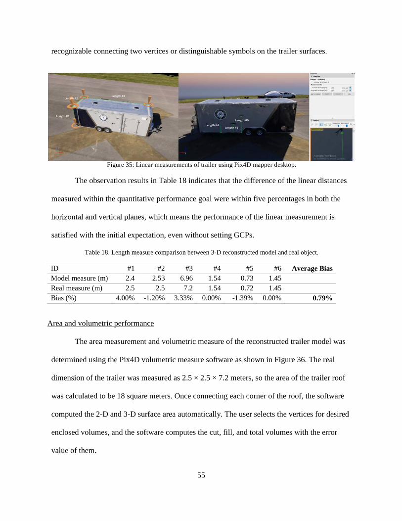
55
recognizable connecting two vertices or distinguishable symbols on the trailer surfaces.
Figure 35: Linear measurements of trailer using Pix4D mapper desktop.
The observation results in Table 18 indicates that the difference of the linear distances
measured within the quantitative performance goal were within five percentages in both the
horizontal and vertical planes, which means the performance of the linear measurement is
satisfied with the initial expectation, even without setting GCPs.
Table 18. Length measure comparison between 3-D reconstructed model and real object.
ID #1 #2 #3 #4 #5 #6 Average Bias Model measure (m) 2.4 2.53 6.96 1.54 0.73 1.45 Real measure (m) 2.5 2.5 7.2 1.54 0.72 1.45 Bias (%) 4.00% -1.20% 3.33% 0.00% -1.39% 0.00% 0.79%
Area and volumetric performance
The area measurement and volumetric measure of the reconstructed trailer model was
determined using the Pix4D volumetric measure software as shown in Figure 36. The real
dimension of the trailer was measured as 2.5 × 2.5 × 7.2 meters, so the area of the trailer roof
was calculated to be 18 square meters. Once connecting each corner of the roof, the software
computed the 2-D and 3-D surface area automatically. The user selects the vertices for desired
enclosed volumes, and the software computes the cut, fill, and total volumes with the error
value of them.
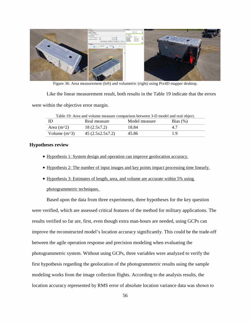
56
Figure 36: Area measurement (left) and volumetric (right) using Pix4D mapper desktop.
Like the linear measurement result, both results in the Table 19 indicate that the errors
were within the objective error margin.
Table 19: Area and volume measure comparison between 3-D model and real object. ID Real measure Model measure Bias (%) Area (m^2) 18 (2.5x7.2) 18.84 4.7 Volume (m^3) 45 (2.5x2.5x7.2) 45.86 1.9
Hypotheses review
• Hypothesis 1: System design and operation can improve geolocation accuracy.
• Hypothesis 2: The number of input images and key points impact processing time linearly.
• Hypothesis 3: Estimates of length, area, and volume are accurate within 5% using
photogrammetric techniques.
Based upon the data from three experiments, three hypotheses for the key question
were verified, which are assessed critical features of the method for military applications. The
results verified so far are, first, even though extra man-hours are needed, using GCPs can
improve the reconstructed model’s location accuracy significantly. This could be the trade-off
between the agile operation response and precision modeling when evaluating the
photogrammetric system. Without using GCPs, three variables were analyzed to verify the
first hypothesis regarding the geolocation of the photogrammetric results using the sample
modeling works from the image collection flights. According to the analysis results, the
location accuracy represented by RMS error of absolute location variance data was shown to
57
increase as the input image was collected using higher speed flight. Theoretically, fast
movement while taking photo has a blur effect on the photo, so in this case, a camera with a
corresponding fast shutter speed is required to get the sharp image. If there is no option to
select the camera specification, lower airspeed might be a reasonable compromise. Likewise,
the small GSD from low flight altitude or better sensor specification has a positive effect on
the position accuracy of the photogrammetry result. GSD represents the pixel size in a image,
and the small GSD means the image has high density of points. Accordingly, the high density
of the smaller pixels contributes to the better location accuracy. The overlap effect was not
consistent to prove the significance of the relationship with location accuracy. The higher
overlapping rate among images was expected to produce more accurate models, but the results
were not consistent with the initial expectation. For the study, only sixty and eighty percent of
frontal overlap rate were used, but more samples using various frontal and side overlap should
have been used for this. In the analysis of the second hypothesis, the processing time can be
estimated by the number of images with a mediation effect of the number of key points
depending on the sensor size. From the result, the regression equation we can utilize to
estimate the processing time is:
Processing time (timeI) = 0.9683× input image - 0.1091 (3)
The equation provides the reference for how a large camera sensor should be selected for a
specific mission, how wide area will be covered within the limited mission hours, and how
long it will take to deliver the final outputs. Lastly, the linear distance, area measurement, and
volumetric using the photogrammetric model was shown to be within five percents of
measured values, even without using GCPs. The results are assessed to be sufficient to
consider SUAV photogrammetry methods for military applications that need reasonable
reponse time, but not centimeter-level accuracy.
58
VI. Military application: Runway damage assessment system
This chapter describes the applied demonstration of the runway damage assessment
system using the method described and verified in Chapters Ⅳ and Ⅴ. This chapter is
organized along a systematic approach including problem analysis, CONOPS, system
decomposition, use case study, and the system analysis. The example of the 3-D model and
maps are modified from the flight test samples.
Introduction
Problem statement
Inspection and assessment of a damaged runway are, currently, a manpower intensive
activity that impacts the ability to meet rapid repair timelines. With a requirement to provide
inspection, assessment, and repair of a runway within 8 hours of incurred damaged, the Air
Force needs to reduce the time required to perform these activities. Based on currently
projected repair capabilities, there is a requirement to provide inspection and assessment
within 1 to 1.5 hours, with sufficiently accurate assessment data to support immediate
deployment of manpower and the required amount of material prior to initiation of repair
actions, With the rapid emergence of SUAV technologies, there are new opportunities to
automate and accelerate the timelines associated with runway inspection and repair. While the
user (AF Civil Engineering crews) are open to SUAV solutions, they don’t have dedicated
pilots to perform inspection actions. For this reason, any SUAV solution must be operable by
non-pilots. The descriptive military challenge of the problem is described below :
• Forward-based Civil Engineering crews would like to provide inspection and
assessment of a damaged runway and adjacent taxiways and parking aprons within 1-
59
1.5 hours after an attack has occurred;
• The resulting information from the inspection and assessment process must be sufficient
to immediately stage crews and material to begin runway repair actions;
• Forward-based operators would like a simplified interface and low workload for the
above tasks so the system can be operated by non-pilot crew members.
Definitions
Operator
The operator is well trained to operate the UAV and has enough technical and
operational skill for the appropriate mission.
Engineering Assistant (EA)
The Engineering Assistant is capable of utilizing the photogrammetry software to
construct 3-D models and calculate the optimal repair pattern, minimizing the amount of labor
and material needed to repair an operating runway strip.
Civil engineering Cloud-based Network System (CCNS)
The CCNS is an authorized intra network system that has its own IP address and
network. Only authorized personnel or devices can access the network for connecting and data
utilization. Once any GCSs are accessed, the operator can collaborate and annotate projects
online, then share maps, models, and analytics with a simple URL.
Small Unmanned Air Vehicle (SUAV)
The SUAV is a package consisting of the small unmanned vehicle including the
autopilot, transmitter and receiver, sensor package, and maintenance kit. It is operable by one
individual and has a functional capability for individual take-off, landing, and airfield survey.
The general inspection flight autonomously follows a pre-planned mission, but if necessary,
60
the operator can take control manually from the auto-flight system. The sensor has sufficient
resolution to remotely identify and geo-locate unexploded ordnance (UXO), craters, and
cracks, and estimate required fill volume. Sensor data will be saved in onboard memory and
transmitted to the ground station in real-time.
Ground Control Station (GCS)
The GCS is hardware and software including a survey mission planning application,
flight monitoring, maintenance kit, and photogrammetry modeling software. It is operable by
one individual and has a functional capability for autonomous survey mission plan, post flight
feedback, analysis, and enough processing capability to power the modeling software. This
enables one GCS to work with one module from flight planning to damage assessment. In
addition, the GCS shall be capable to connect to the CCNS to share new data and utilize the
past data from the cloud database.
CONOPS
Purpose
The purpose of the system is to deliver timely and relevant inspection and assessment
of runways and the associated taxiways and parking aprons to Civil Engineering crews
prepared for runway repair actions.
Scope
This case study is intended to be an Enabling Concept and is written at the tactical
level. Specifically, the SUAV CONOPS will describe the anticipated utilization by
AF Civil Engineering crews, and supporting context required to provide rapid runway
inspection and assessment at a forward deployed airfield.
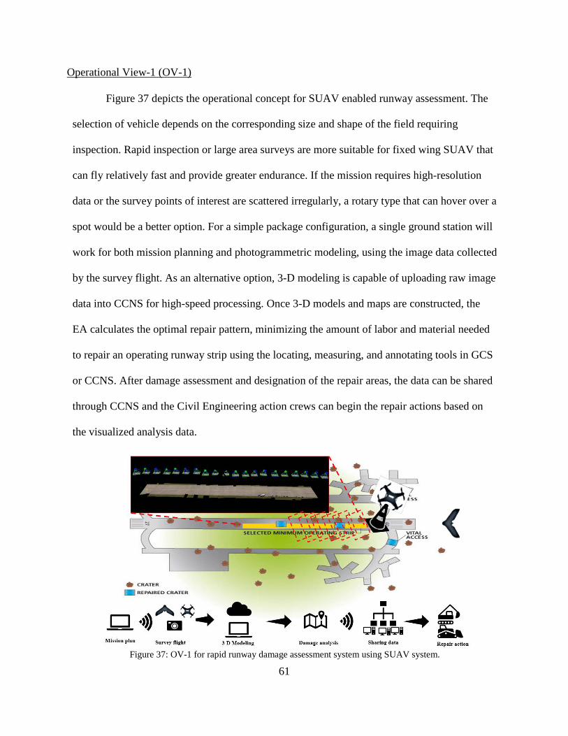
61
Operational View-1 (OV-1)
Figure 37 depicts the operational concept for SUAV enabled runway assessment. The
selection of vehicle depends on the corresponding size and shape of the field requiring
inspection. Rapid inspection or large area surveys are more suitable for fixed wing SUAV that
can fly relatively fast and provide greater endurance. If the mission requires high-resolution
data or the survey points of interest are scattered irregularly, a rotary type that can hover over a
spot would be a better option. For a simple package configuration, a single ground station will
work for both mission planning and photogrammetric modeling, using the image data collected
by the survey flight. As an alternative option, 3-D modeling is capable of uploading raw image
data into CCNS for high-speed processing. Once 3-D models and maps are constructed, the
EA calculates the optimal repair pattern, minimizing the amount of labor and material needed
to repair an operating runway strip using the locating, measuring, and annotating tools in GCS
or CCNS. After damage assessment and designation of the repair areas, the data can be shared
through CCNS and the Civil Engineering action crews can begin the repair actions based on
the visualized analysis data.
Figure 37: OV-1 for rapid runway damage assessment system using SUAV system.
62
User requirements
The proposed concept will provide forward deployed Civil Engineering units the
capability to conduct rapid runway inspection and assessment using a SUAV. Specifically, the
use of the SUAV will allow operators to perform the functions listed here.
• Rapidly setup and deploy a SUAV from areas adjacent to an airstrip, without the benefit
of ground power and communication systems.
• Cover an area associated with one or more runways and the adjacent taxiways and
parking aprons.
• Utilize sensor payloads and assessment methods/algorithms capable of providing
actionable information regarding runway damage.
- Location of unexploded ordnance
- Location of damage (craters and spalls)
- Depth and size of holes (volumetric information is useful)
- Size of debris above the paved surface
• Monitor system status and sensor data in real time using a ground station and
communication with the air vehicle(s).
• Conduct SUAV operations while maintaining situational awareness of the location
around the operator.
• Be able to safely recover the vehicle in the event of lost comm, loss of GPS, or
premature battery depletion.
• Complete all actions above within 1-1.5 hours.
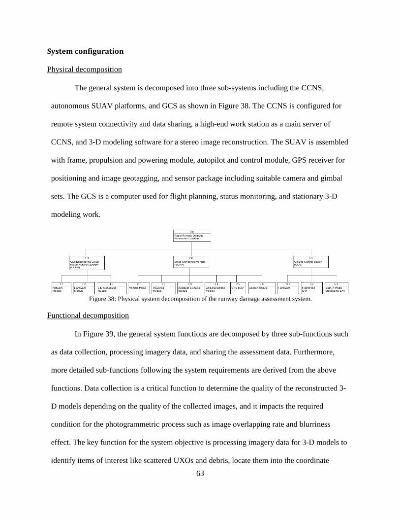
63
System configuration
Physical decomposition
The general system is decomposed into three sub-systems including the CCNS,
autonomous SUAV platforms, and GCS as shown in Figure 38. The CCNS is configured for
remote system connectivity and data sharing, a high-end work station as a main server of
CCNS, and 3-D modeling software for a stereo image reconstruction. The SUAV is assembled
with frame, propulsion and powering module, autopilot and control module, GPS receiver for
positioning and image geotagging, and sensor package including suitable camera and gimbal
sets. The GCS is a computer used for flight planning, status monitoring, and stationary 3-D
modeling work.
Figure 38: Physical system decomposition of the runway damage assessment system.
Functional decomposition
In Figure 39, the general system functions are decomposed by three sub-functions such
as data collection, processing imagery data, and sharing the assessment data. Furthermore,
more detailed sub-functions following the system requirements are derived from the above
functions. Data collection is a critical function to determine the quality of the reconstructed 3-
D models depending on the quality of the collected images, and it impacts the required
condition for the photogrammetric process such as image overlapping rate and blurriness
effect. The key function for the system objective is processing imagery data for 3-D models to
identify items of interest like scattered UXOs and debris, locate them into the coordinate
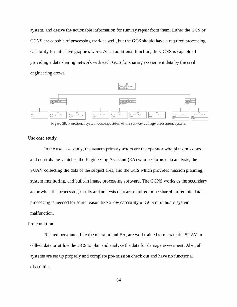
64
system, and derive the actionable information for runway repair from them. Either the GCS or
CCNS are capable of processing work as well, but the GCS should have a required processing
capability for intensive graphics work. As an additional function, the CCNS is capable of
providing a data sharing network with each GCS for sharing assessment data by the civil
engineering crews.
Figure 39: Functional system decomposition of the runway damage assessment system.
Use case study
In the use case study, the system primary actors are the operator who plans missions
and controls the vehicles, the Engineering Assistant (EA) who performs data analysis, the
SUAV collecting the data of the subject area, and the GCS which provides mission planning,
system monitoring, and built-in image processing software. The CCNS works as the secondary
actor when the processing results and analysis data are required to be shared, or remote data
processing is needed for some reason like a low capability of GCS or onboard system
malfunction.
Pre-condition
Related personnel, like the operator and EA, are well trained to operate the SUAV to
collect data or utilize the GCS to plan and analyze the data for damage assessment. Also, all
systems are set up properly and complete pre-mission check out and have no functional
disabilities.
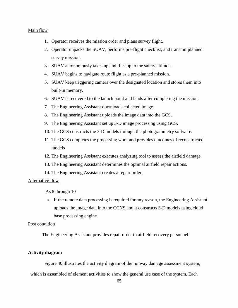
65
Main flow
1. Operator receives the mission order and plans survey flight.
2. Operator unpacks the SUAV, performs pre-flight checklist, and transmit planned
survey mission.
3. SUAV autonomously takes up and flies up to the safety altitude.
4. SUAV begins to navigate route flight as a pre-planned mission.
5. SUAV keep triggering camera over the designated location and stores them into
built-in memory.
6. SUAV is recovered to the launch point and lands after completing the mission.
7. The Engineering Assistant downloads collected image.
8. The Engineering Assistant uploads the image data into the GCS.
9. The Engineering Assistant set up 3-D image processing using GCS.
10. The GCS constructs the 3-D models through the photogrammetry software.
11. The GCS completes the processing work and provides outcomes of reconstructed
models
12. The Engineering Assistant executes analyzing tool to assess the airfield damage.
13. The Engineering Assistant determines the optimal airfield repair actions.
14. The Engineering Assistant creates a repair order.
Alternative flow
As 8 through 10
a. If the remote data processing is required for any reason, the Engineering Assistant
uploads the image data into the CCNS and it constructs 3-D models using cloud
base processing engine.
Post condition
The Engineering Assistant provides repair order to airfield recovery personnel.
Activity diagram
Figure 40 illustrates the activity diagram of the runway damage assessment system,
which is assembled of element activities to show the general use case of the system. Each
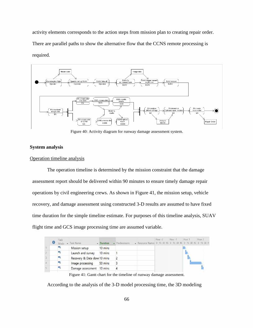
66
activity elements corresponds to the action steps from mission plan to creating repair order.
There are parallel paths to show the alternative flow that the CCNS remote processing is
required.
Figure 40: Activity diagram for runway damage assessment system.
System analysis
Operation timeline analysis
The operation timeline is determined by the mission constraint that the damage
assessment report should be delivered within 90 minutes to ensure timely damage repair
operations by civil engineering crews. As shown in Figure 41, the mission setup, vehicle
recovery, and damage assessment using constructed 3-D results are assumed to have fixed
time duration for the simple timeline estimate. For purposes of this timeline analysis, SUAV
flight time and GCS image processing time are assumed variable.
Figure 41: Gantt chart for the timeline of runway damage assessment.
According to the analysis of the 3-D model processing time, the 3D modeling
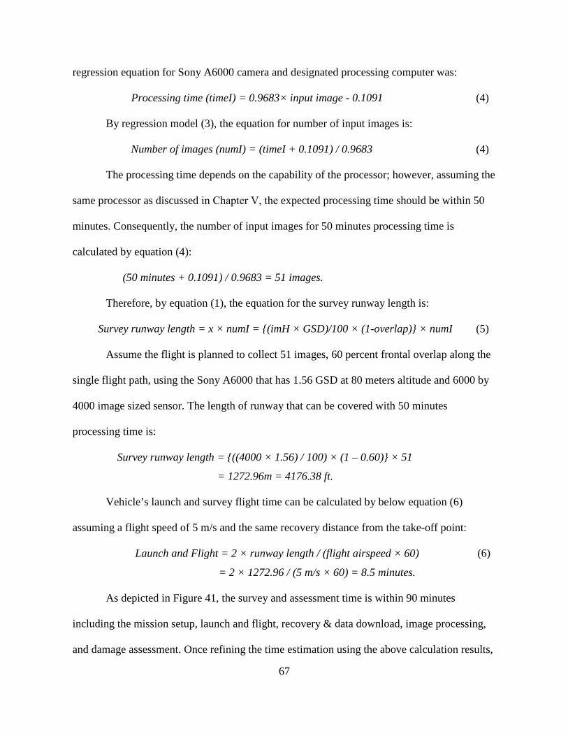
67
regression equation for Sony A6000 camera and designated processing computer was:
Processing time (timeI) = 0.9683× input image - 0.1091 (4)
By regression model (3), the equation for number of input images is:
Number of images (numI) = (timeI + 0.1091) / 0.9683 (4)
The processing time depends on the capability of the processor; however, assuming the
same processor as discussed in Chapter Ⅴ, the expected processing time should be within 50
minutes. Consequently, the number of input images for 50 minutes processing time is
calculated by equation (4):
(50 minutes + 0.1091) / 0.9683 = 51 images.
Therefore, by equation (1), the equation for the survey runway length is:
Survey runway length = x × numI = {(imH × GSD)/100 × (1-overlap)} × numI (5)
Assume the flight is planned to collect 51 images, 60 percent frontal overlap along the
single flight path, using the Sony A6000 that has 1.56 GSD at 80 meters altitude and 6000 by
4000 image sized sensor. The length of runway that can be covered with 50 minutes
processing time is:
Survey runway length = {((4000 × 1.56) / 100) × (1 – 0.60)} × 51
= 1272.96m = 4176.38 ft.
Vehicle’s launch and survey flight time can be calculated by below equation (6)
assuming a flight speed of 5 m/s and the same recovery distance from the take-off point:
Launch and Flight = 2 × runway length / (flight airspeed × 60)
= 2 × 1272.96 / (5 m/s × 60) = 8.5 minutes.
(6)
As depicted in Figure 41, the survey and assessment time is within 90 minutes
including the mission setup, launch and flight, recovery & data download, image processing,
and damage assessment. Once refining the time estimation using the above calculation results,
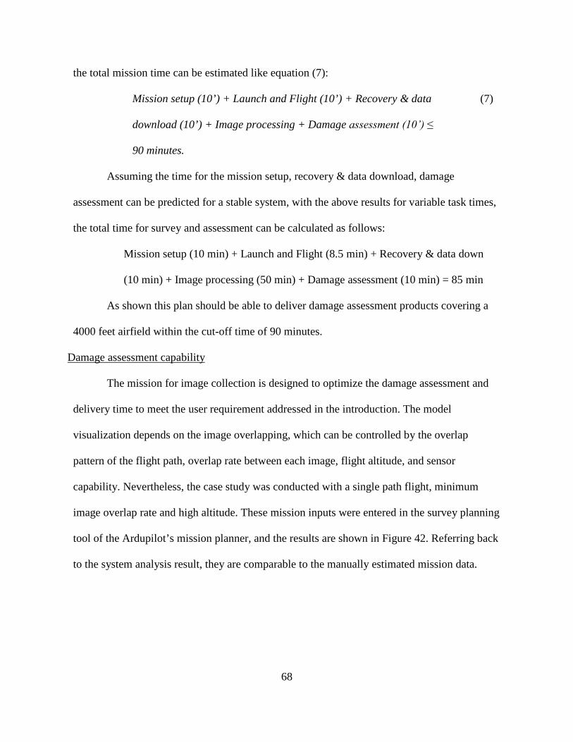
68
the total mission time can be estimated like equation (7):
Mission setup (10’) + Launch and Flight (10’) + Recovery & data
download (10’) + Image processing + Damage assessment (10’) ≤
90 minutes.
(7)
Assuming the time for the mission setup, recovery & data download, damage
assessment can be predicted for a stable system, with the above results for variable task times,
the total time for survey and assessment can be calculated as follows:
Mission setup (10 min) + Launch and Flight (8.5 min) + Recovery & data down
(10 min) + Image processing (50 min) + Damage assessment (10 min) = 85 min
As shown this plan should be able to deliver damage assessment products covering a
4000 feet airfield within the cut-off time of 90 minutes.
Damage assessment capability
The mission for image collection is designed to optimize the damage assessment and
delivery time to meet the user requirement addressed in the introduction. The model
visualization depends on the image overlapping, which can be controlled by the overlap
pattern of the flight path, overlap rate between each image, flight altitude, and sensor
capability. Nevertheless, the case study was conducted with a single path flight, minimum
image overlap rate and high altitude. These mission inputs were entered in the survey planning
tool of the Ardupilot’s mission planner, and the results are shown in Figure 42. Referring back
to the system analysis result, they are comparable to the manually estimated mission data.
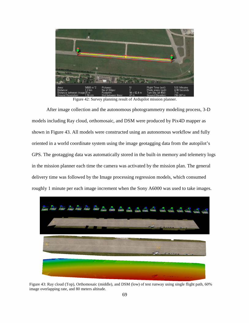
69
Figure 42: Survey planning result of Ardupilot mission planner.
After image collection and the autonomous photogrammetry modeling process, 3-D
models including Ray cloud, orthomosaic, and DSM were produced by Pix4D mapper as
shown in Figure 43. All models were constructed using an autonomous workflow and fully
oriented in a world coordinate system using the image geotagging data from the autopilot’s
GPS. The geotagging data was automatically stored in the built-in memory and telemetry logs
in the mission planner each time the camera was activated by the mission plan. The general
delivery time was followed by the Image processing regression models, which consumed
roughly 1 minute per each image increment when the Sony A6000 was used to take images.
Figure 43: Ray cloud (Top), Orthomosaic (middle), and DSM (low) of test runway using single flight path, 60% image overlapping rate, and 80 meters altitude.
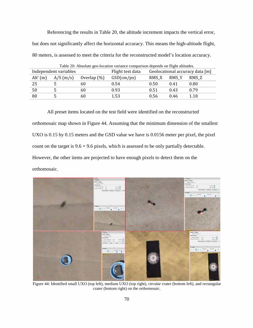
70
Referencing the results in Table 20, the altitude increment impacts the vertical error,
but does not significantly affect the horizontal accuracy. This means the high-altitude flight,
80 meters, is assessed to meet the criteria for the reconstructed model’s location accuracy.
Table 20: Absolute geo-location variance comparison depends on flight altitudes. Independent variables Flight test data Geolocational accuracy data [m] Alt’ (m) A/S (m/s) Overlap (%) GSD(cm/px) RMS_X RMS_Y RMS_Z 25 5 60 0.54 0.50 0.41 0.80 50 5 60 0.93 0.51 0.43 0.79 80 5 60 1.53 0.56 0.46 1.18
All preset items located on the test field were identified on the reconstructed
orthomosaic map shown in Figure 44. Assuming that the minimum dimension of the smallest
UXO is 0.15 by 0.15 meters and the GSD value we have is 0.0156 meter per pixel, the pixel
count on the target is 9.6 × 9.6 pixels, which is assessed to be only partially detectable.
However, the other items are projected to have enough pixels to detect them on the
orthomosaic.
Figure 44: Identified small UXO (top left), medium UXO (top right), circular crater (bottom left), and rectangular
crater (bottom right) on the orthomosaic.
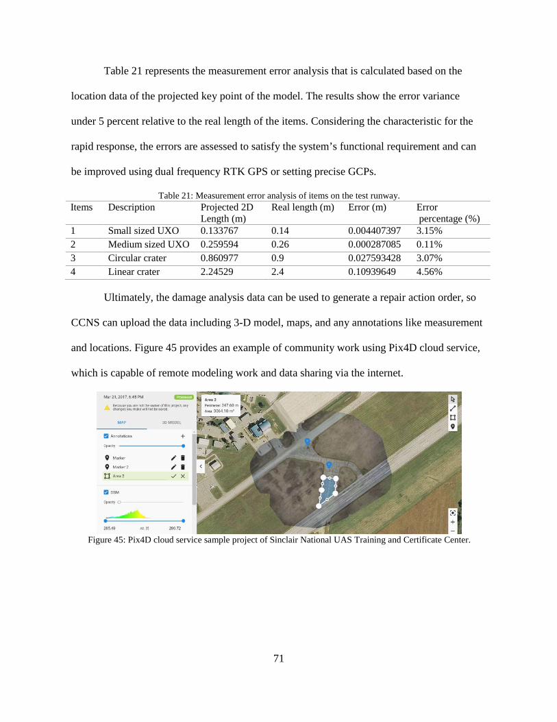
71
Table 21 represents the measurement error analysis that is calculated based on the
location data of the projected key point of the model. The results show the error variance
under 5 percent relative to the real length of the items. Considering the characteristic for the
rapid response, the errors are assessed to satisfy the system’s functional requirement and can
be improved using dual frequency RTK GPS or setting precise GCPs.
Table 21: Measurement error analysis of items on the test runway. Items Description Projected 2D
Length (m) Real length (m) Error (m) Error
percentage (%) 1 Small sized UXO 0.133767 0.14 0.004407397 3.15% 2 Medium sized UXO 0.259594 0.26 0.000287085 0.11% 3 Circular crater 0.860977 0.9 0.027593428 3.07% 4 Linear crater 2.24529 2.4 0.10939649 4.56%
Ultimately, the damage analysis data can be used to generate a repair action order, so
CCNS can upload the data including 3-D model, maps, and any annotations like measurement
and locations. Figure 45 provides an example of community work using Pix4D cloud service,
which is capable of remote modeling work and data sharing via the internet.
Figure 45: Pix4D cloud service sample project of Sinclair National UAS Training and Certificate Center.
72
VII. Military application: Remote SUAV ISR system assisted by photogrammetry
This chapter describes an SUAV ISR system using the method verified through the
Chapter Ⅳ and Ⅴ. The general flow of this chapter is similar to Chapter Ⅵ, but primarily
focused on the 3-D model feature and the application of remote processing. The example of
the 3-D model comes from the oblique 3-D modeling in Chapter Ⅳ and the samples of the
cloud-based service projects conducted by the National UAV training Center of Sinclair
Community College.
Introduction
Problem statement
The ISR assets in most armed forces and their respective countries are assessed to be
essential military assets to support the Joint Targeting cycle [30] and Effects-Based operation
(EBO). However, they have been driving cost overruns and long-term development. GPS
coordinates and images from satellite and JSTARS are used to support friendly operations like
air interdiction and air to ground bombing, but it is not always timely or cost efficient. In urban
area operation, increased possibility of unconventional warfare has yielded a complex
environment to execute the precision attack without collateral damage to civilians and friendly.
For this reason, there have been many cases where warfare has dragged on over time despite
early dominant battle field superiority. Hence, more flexible targeting platforms are required
that are easy to develop and deploy in that kind of operation without high-cost and long
development times. As a reasonable solution for targeting, current commercial UAV
photogrammetry has been widely used to get Geographic information, and this same
technology could provide operable ISR information for military operations. This will provide
73
target models for forward deployed Joint Terminal Attack Controllers (JTAC), either manned
or unmanned striker units, not only ground forces, Close Air Support (CAS), and where ISR
support is needed.
Definition
Operator
The operator is well trained to operate the UAV and has enough technical and
operational skill for a surveillance mission planning as a main mission planner and controller
for SUAV.
SUAV
The SUAV is the package of the small unmanned vehicle addressed in Chapter Ⅵ,
including the autopilot, transmitter and receiver, sensor package, and maintenance kit. It be
operable by one individual, has a functional capability for take-off, landing, and surveillance
flight, and has compact size for survivability over the enemy area. The general surveillance
flight shall autonomously follow a pre-planned mission, but if necessary, the operator can take
control manually from the auto-flight system. The sensor has sufficient resolution to provide
identification of target of interest. The sensor will be mounted on a gimbal, which makes the
sensor stable and can be pointed toward the target. Sensor data is saved in onboard memory
and transmitted to the ground station in real-time.
Joint ISR Cloud-based Network System (JICNS)
As a notional secured network system for military operations, JICNS is the cloud-based
network system to deal with ISR imagery intelligence from various sources, provides remote
processing of target 3-D models, and provides targeting assessment. This is stationed on the
ground or airborne C2 asset and can communicate with the operating GCS.

74
GCS
The GCS is computer and communication equipment with mission planning and flight
monitoring software. It is operable by one individual, and connects to the JICNS to upload raw
image data and download ISR data from cloud data-based network and Ground C2 assets.
Striker assets
Striker assets include air, ground, and maritime armed forces designated in the specific
battle area to carry out the surface attack to the joint target established by the area Joint forces
commander.
Target
In joint operations terminology, the target is a set of Joint Desired Point of Impact
(JDPI), which has been identified, but not yet cleared for physical attack. This is simply
defined as a general enemy object intended to execute a physical attack by friendly strikers.
CONOPS
Purpose
The purpose of the system is to deliver timely and reliable targeting using well-
constructed 3- dimensional target models. The models will be constructed from imagery
collected by. This CONOPS describes surveillance mission against stationed target using
multirotor, which collects target imagery for 3-D model of targets.
Scope
This is intended to provide military guidance or perspective for conceptual SUAV
targeting platforms to help armed forces operations. The application scope is limited to
close-range, stationary targeting, and imagery intelligence. [30] It includes Find, Fix,
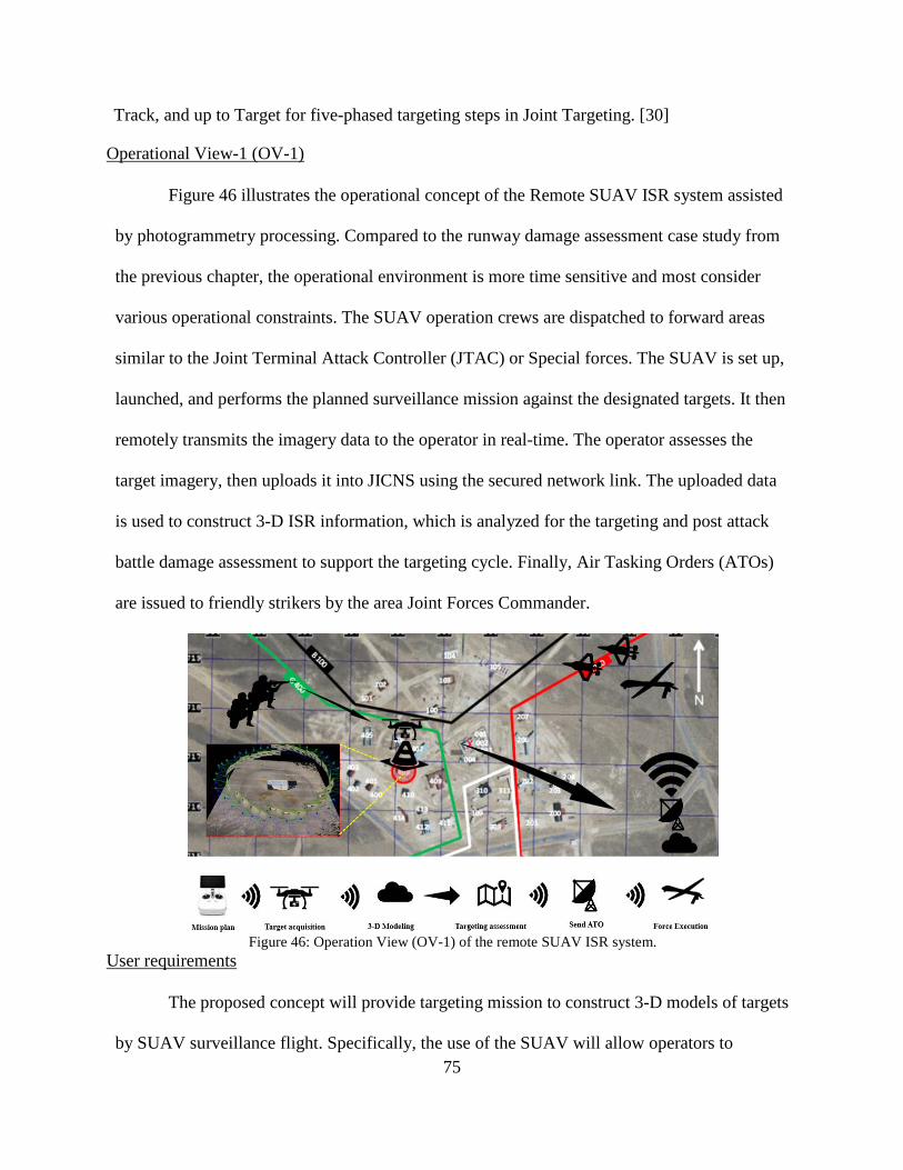
75
Track, and up to Target for five-phased targeting steps in Joint Targeting. [30]
Operational View-1 (OV-1)
Figure 46 illustrates the operational concept of the Remote SUAV ISR system assisted
by photogrammetry processing. Compared to the runway damage assessment case study from
the previous chapter, the operational environment is more time sensitive and most consider
various operational constraints. The SUAV operation crews are dispatched to forward areas
similar to the Joint Terminal Attack Controller (JTAC) or Special forces. The SUAV is set up,
launched, and performs the planned surveillance mission against the designated targets. It then
remotely transmits the imagery data to the operator in real-time. The operator assesses the
target imagery, then uploads it into JICNS using the secured network link. The uploaded data
is used to construct 3-D ISR information, which is analyzed for the targeting and post attack
battle damage assessment to support the targeting cycle. Finally, Air Tasking Orders (ATOs)
are issued to friendly strikers by the area Joint Forces Commander.
Figure 46: Operation View (OV-1) of the remote SUAV ISR system.
User requirements
The proposed concept will provide targeting mission to construct 3-D models of targets
by SUAV surveillance flight. Specifically, the use of the SUAV will allow operators to
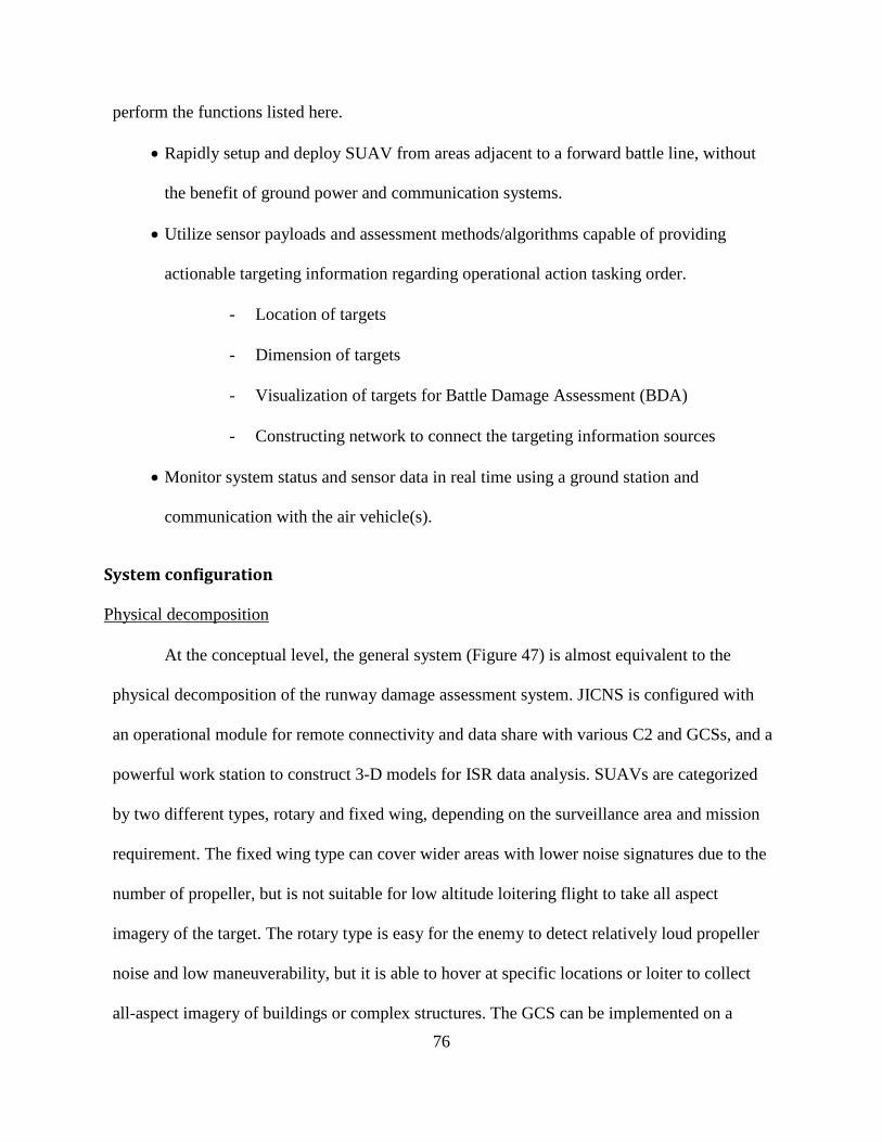
76
perform the functions listed here.
• Rapidly setup and deploy SUAV from areas adjacent to a forward battle line, without
the benefit of ground power and communication systems.
• Utilize sensor payloads and assessment methods/algorithms capable of providing
actionable targeting information regarding operational action tasking order.
- Location of targets
- Dimension of targets
- Visualization of targets for Battle Damage Assessment (BDA)
- Constructing network to connect the targeting information sources
• Monitor system status and sensor data in real time using a ground station and
communication with the air vehicle(s).
System configuration
Physical decomposition
At the conceptual level, the general system (Figure 47) is almost equivalent to the
physical decomposition of the runway damage assessment system. JICNS is configured with
an operational module for remote connectivity and data share with various C2 and GCSs, and a
powerful work station to construct 3-D models for ISR data analysis. SUAVs are categorized
by two different types, rotary and fixed wing, depending on the surveillance area and mission
requirement. The fixed wing type can cover wider areas with lower noise signatures due to the
number of propeller, but is not suitable for low altitude loitering flight to take all aspect
imagery of the target. The rotary type is easy for the enemy to detect relatively loud propeller
noise and low maneuverability, but it is able to hover at specific locations or loiter to collect
all-aspect imagery of buildings or complex structures. The GCS can be implemented on a
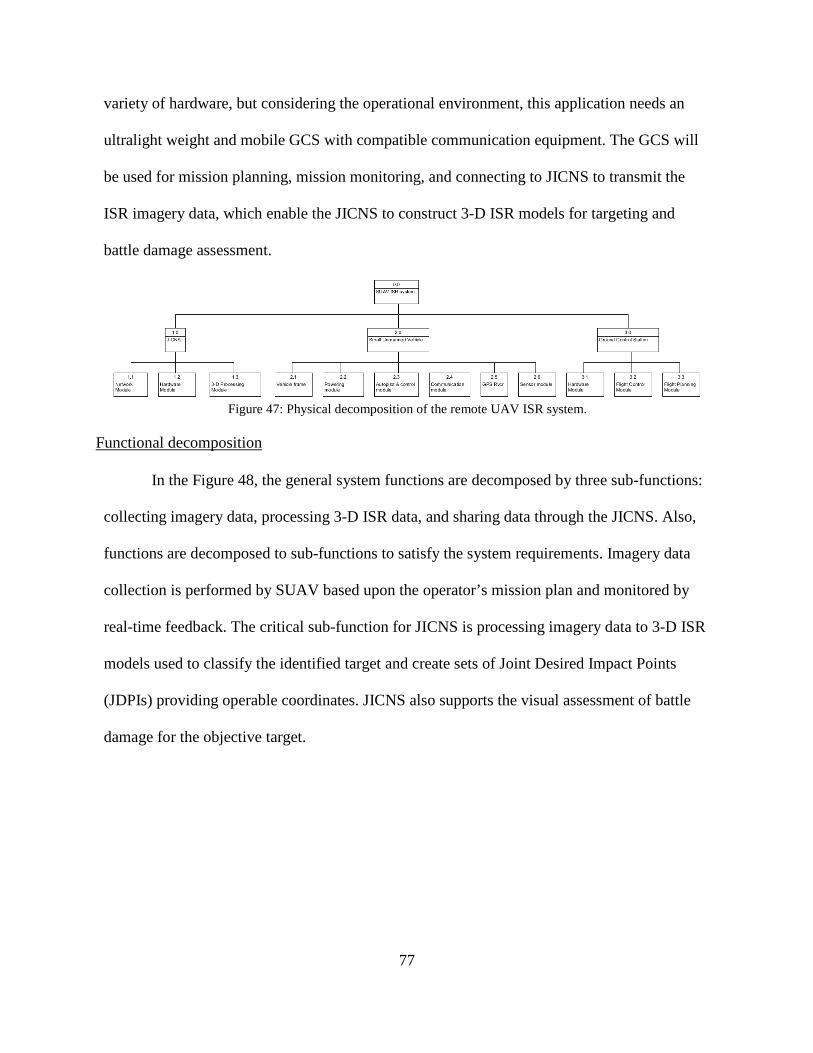
77
variety of hardware, but considering the operational environment, this application needs an
ultralight weight and mobile GCS with compatible communication equipment. The GCS will
be used for mission planning, mission monitoring, and connecting to JICNS to transmit the
ISR imagery data, which enable the JICNS to construct 3-D ISR models for targeting and
battle damage assessment.
Figure 47: Physical decomposition of the remote UAV ISR system.
Functional decomposition
In the Figure 48, the general system functions are decomposed by three sub-functions:
collecting imagery data, processing 3-D ISR data, and sharing data through the JICNS. Also,
functions are decomposed to sub-functions to satisfy the system requirements. Imagery data
collection is performed by SUAV based upon the operator’s mission plan and monitored by
real-time feedback. The critical sub-function for JICNS is processing imagery data to 3-D ISR
models used to classify the identified target and create sets of Joint Desired Impact Points
(JDPIs) providing operable coordinates. JICNS also supports the visual assessment of battle
damage for the objective target.
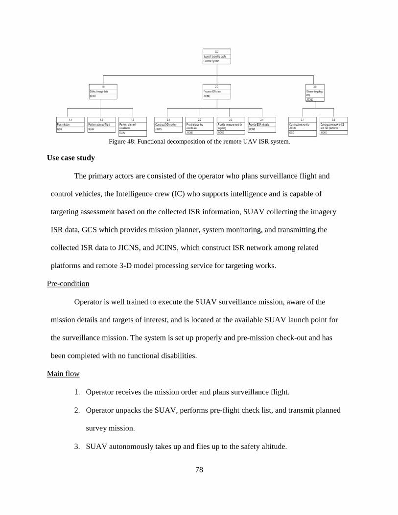
78
Figure 48: Functional decomposition of the remote UAV ISR system.
Use case study
The primary actors are consisted of the operator who plans surveillance flight and
control vehicles, the Intelligence crew (IC) who supports intelligence and is capable of
targeting assessment based on the collected ISR information, SUAV collecting the imagery
ISR data, GCS which provides mission planner, system monitoring, and transmitting the
collected ISR data to JICNS, and JCINS, which construct ISR network among related
platforms and remote 3-D model processing service for targeting works.
Pre-condition
Operator is well trained to execute the SUAV surveillance mission, aware of the
mission details and targets of interest, and is located at the available SUAV launch point for
the surveillance mission. The system is set up properly and pre-mission check-out and has
been completed with no functional disabilities.
Main flow
1. Operator receives the mission order and plans surveillance flight.
2. Operator unpacks the SUAV, performs pre-flight check list, and transmit planned
survey mission.
3. SUAV autonomously takes up and flies up to the safety altitude.
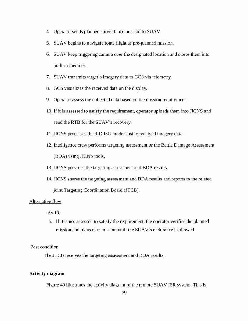
79
4. Operator sends planned surveillance mission to SUAV
5. SUAV begins to navigate route flight as pre-planned mission.
6. SUAV keep triggering camera over the designated location and stores them into
built-in memory.
7. SUAV transmits target’s imagery data to GCS via telemetry.
8. GCS visualizes the received data on the display.
9. Operator assess the collected data based on the mission requirement.
10. If it is assessed to satisfy the requirement, operator uploads them into JICNS and
send the RTB for the SUAV’s recovery.
11. JICNS processes the 3-D ISR models using received imagery data.
12. Intelligence crew performs targeting assessment or the Battle Damage Assessment
(BDA) using JICNS tools.
13. JICNS provides the targeting assessment and BDA results.
14. JICNS shares the targeting assessment and BDA results and reports to the related
joint Targeting Coordination Board (JTCB).
Alternative flow
As 10.
a. If it is not assessed to satisfy the requirement, the operator verifies the planned
mission and plans new mission until the SUAV’s endurance is allowed.
Post condition
The JTCB receives the targeting assessment and BDA results.
Activity diagram
Figure 49 illustrates the activity diagram of the remote SUAV ISR system. This is
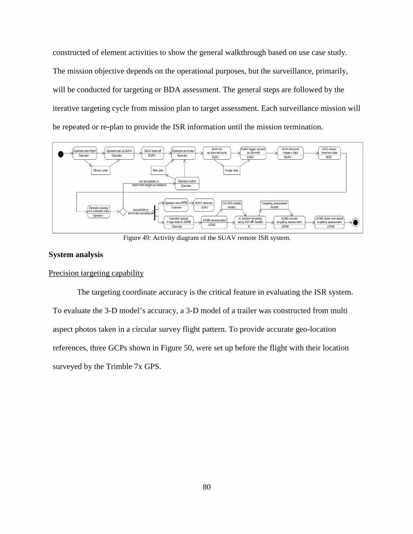
80
constructed of element activities to show the general walkthrough based on use case study.
The mission objective depends on the operational purposes, but the surveillance, primarily,
will be conducted for targeting or BDA assessment. The general steps are followed by the
iterative targeting cycle from mission plan to target assessment. Each surveillance mission will
be repeated or re-plan to provide the ISR information until the mission termination.
Figure 49: Activity diagram of the SUAV remote ISR system.
System analysis
Precision targeting capability
The targeting coordinate accuracy is the critical feature in evaluating the ISR system.
To evaluate the 3-D model’s accuracy, a 3-D model of a trailer was constructed from multi
aspect photos taken in a circular survey flight pattern. To provide accurate geo-location
references, three GCPs shown in Figure 50, were set up before the flight with their location
surveyed by the Trimble 7x GPS.
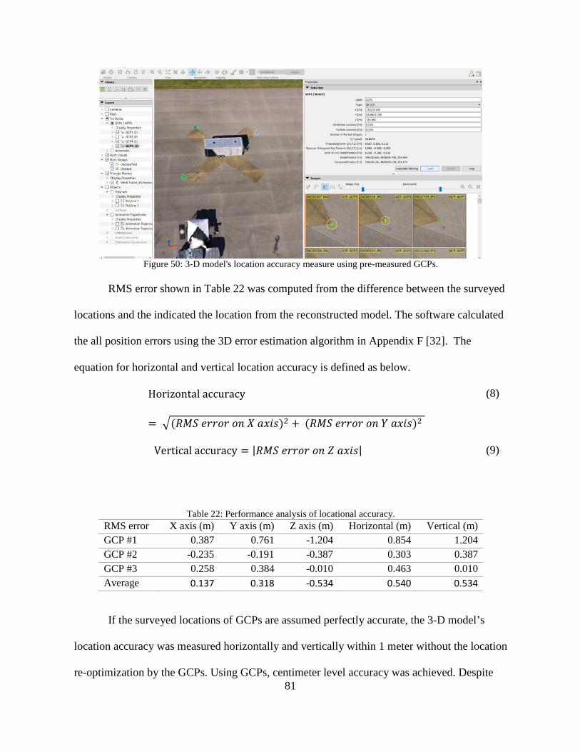
81
Figure 50: 3-D model's location accuracy measure using pre-measured GCPs.
RMS error shown in Table 22 was computed from the difference between the surveyed
locations and the indicated the location from the reconstructed model. The software calculated
the all position errors using the 3D error estimation algorithm in Appendix F [32]. The
equation for horizontal and vertical location accuracy is defined as below.
Horizontal accuracy
= �(𝑅𝑅𝑅𝑅𝑅𝑅 𝑒𝑒𝑒𝑒𝑒𝑒𝑒𝑒𝑒𝑒 𝑒𝑒𝑜𝑜 𝑋𝑋 𝑎𝑎𝑎𝑎𝑎𝑎𝑎𝑎)2 + (𝑅𝑅𝑅𝑅𝑅𝑅 𝑒𝑒𝑒𝑒𝑒𝑒𝑒𝑒𝑒𝑒 𝑒𝑒𝑜𝑜 𝑌𝑌 𝑎𝑎𝑎𝑎𝑎𝑎𝑎𝑎)2
(8)
Vertical accuracy = |𝑅𝑅𝑅𝑅𝑅𝑅 𝑒𝑒𝑒𝑒𝑒𝑒𝑒𝑒𝑒𝑒 𝑒𝑒𝑜𝑜 𝑍𝑍 𝑎𝑎𝑎𝑎𝑎𝑎𝑎𝑎| (9)
Table 22: Performance analysis of locational accuracy.
RMS error X axis (m) Y axis (m) Z axis (m) Horizontal (m) Vertical (m) GCP #1 0.387 0.761 -1.204 0.854 1.204 GCP #2 -0.235 -0.191 -0.387 0.303 0.387 GCP #3 0.258 0.384 -0.010 0.463 0.010 Average 0.137 0.318 -0.534 0.540 0.534
If the surveyed locations of GCPs are assumed perfectly accurate, the 3-D model’s
location accuracy was measured horizontally and vertically within 1 meter without the location
re-optimization by the GCPs. Using GCPs, centimeter level accuracy was achieved. Despite
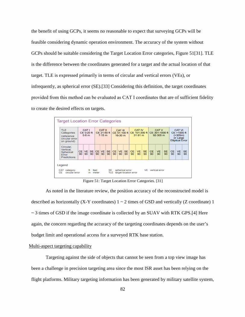
82
the benefit of using GCPs, it seems no reasonable to expect that surveying GCPs will be
feasible considering dynamic operation environment. The accuracy of the system without
GCPs should be suitable considering the Target Location Error categories, Figure 51[31]. TLE
is the difference between the coordinates generated for a target and the actual location of that
target. TLE is expressed primarily in terms of circular and vertical errors (VEs), or
infrequently, as spherical error (SE).[33] Considering this definition, the target coordinates
provided from this method can be evaluated as CAT Ⅰ coordinates that are of sufficient fidelity
to create the desired effects on targets.
Figure 51: Target Location Error Categories. [31]
As noted in the literature review, the position accuracy of the reconstructed model is
described as horizontally (X-Y coordinates) 1 ~ 2 times of GSD and vertically (Z coordinate) 1
~ 3 times of GSD if the image coordinate is collected by an SUAV with RTK GPS.[4] Here
again, the concern regarding the accuracy of the targeting coordinates depends on the user’s
budget limit and operational access for a surveyed RTK base station.
Multi-aspect targeting capability
Targeting against the side of objects that cannot be seen from a top view image has
been a challenge in precision targeting area since the most ISR asset has been relying on the
flight platforms. Military targeting information has been generated by military satellite system,
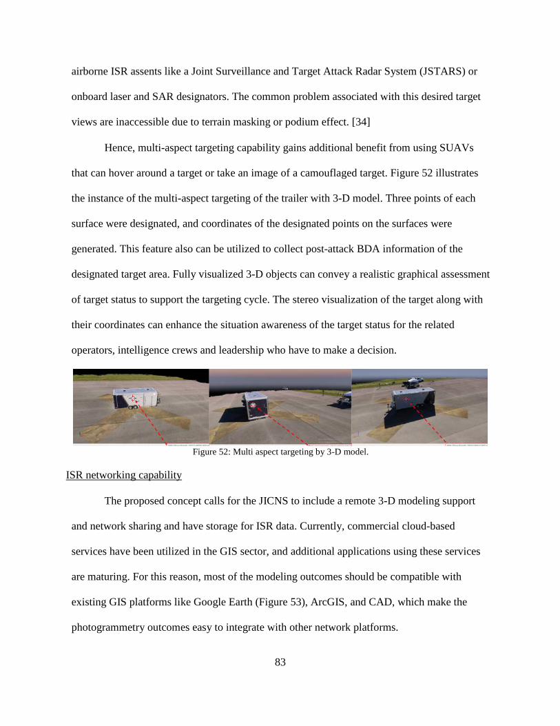
83
airborne ISR assents like a Joint Surveillance and Target Attack Radar System (JSTARS) or
onboard laser and SAR designators. The common problem associated with this desired target
views are inaccessible due to terrain masking or podium effect. [34]
Hence, multi-aspect targeting capability gains additional benefit from using SUAVs
that can hover around a target or take an image of a camouflaged target. Figure 52 illustrates
the instance of the multi-aspect targeting of the trailer with 3-D model. Three points of each
surface were designated, and coordinates of the designated points on the surfaces were
generated. This feature also can be utilized to collect post-attack BDA information of the
designated target area. Fully visualized 3-D objects can convey a realistic graphical assessment
of target status to support the targeting cycle. The stereo visualization of the target along with
their coordinates can enhance the situation awareness of the target status for the related
operators, intelligence crews and leadership who have to make a decision.
Figure 52: Multi aspect targeting by 3-D model.
ISR networking capability
The proposed concept calls for the JICNS to include a remote 3-D modeling support
and network sharing and have storage for ISR data. Currently, commercial cloud-based
services have been utilized in the GIS sector, and additional applications using these services
are maturing. For this reason, most of the modeling outcomes should be compatible with
existing GIS platforms like Google Earth (Figure 53), ArcGIS, and CAD, which make the
photogrammetry outcomes easy to integrate with other network platforms.
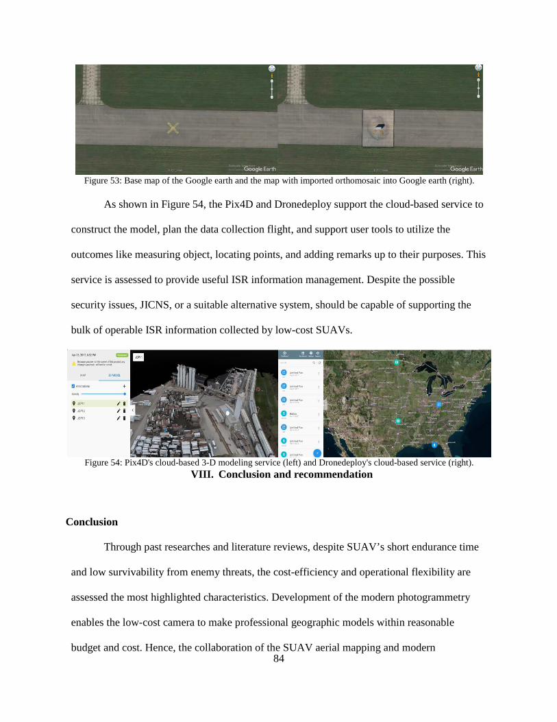
84
Figure 53: Base map of the Google earth and the map with imported orthomosaic into Google earth (right).
As shown in Figure 54, the Pix4D and Dronedeploy support the cloud-based service to
construct the model, plan the data collection flight, and support user tools to utilize the
outcomes like measuring object, locating points, and adding remarks up to their purposes. This
service is assessed to provide useful ISR information management. Despite the possible
security issues, JICNS, or a suitable alternative system, should be capable of supporting the
bulk of operable ISR information collected by low-cost SUAVs.
Figure 54: Pix4D's cloud-based 3-D modeling service (left) and Dronedeploy's cloud-based service (right).
VIII. Conclusion and recommendation
Conclusion
Through past researches and literature reviews, despite SUAV’s short endurance time
and low survivability from enemy threats, the cost-efficiency and operational flexibility are
assessed the most highlighted characteristics. Development of the modern photogrammetry
enables the low-cost camera to make professional geographic models within reasonable
budget and cost. Hence, the collaboration of the SUAV aerial mapping and modern
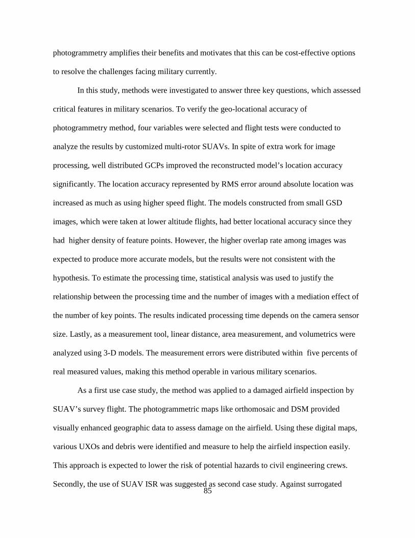
85
photogrammetry amplifies their benefits and motivates that this can be cost-effective options
to resolve the challenges facing military currently.
In this study, methods were investigated to answer three key questions, which assessed
critical features in military scenarios. To verify the geo-locational accuracy of
photogrammetry method, four variables were selected and flight tests were conducted to
analyze the results by customized multi-rotor SUAVs. In spite of extra work for image
processing, well distributed GCPs improved the reconstructed model’s location accuracy
significantly. The location accuracy represented by RMS error around absolute location was
increased as much as using higher speed flight. The models constructed from small GSD
images, which were taken at lower altitude flights, had better locational accuracy since they
had higher density of feature points. However, the higher overlap rate among images was
expected to produce more accurate models, but the results were not consistent with the
hypothesis. To estimate the processing time, statistical analysis was used to justify the
relationship between the processing time and the number of images with a mediation effect of
the number of key points. The results indicated processing time depends on the camera sensor
size. Lastly, as a measurement tool, linear distance, area measurement, and volumetrics were
analyzed using 3-D models. The measurement errors were distributed within five percents of
real measured values, making this method operable in various military scenarios.
As a first use case study, the method was applied to a damaged airfield inspection by
SUAV’s survey flight. The photogrammetric maps like orthomosaic and DSM provided
visually enhanced geographic data to assess damage on the airfield. Using these digital maps,
various UXOs and debris were identified and measure to help the airfield inspection easily.
This approach is expected to lower the risk of potential hazards to civil engineering crews.
Secondly, the use of SUAV ISR was suggested as second case study. Against surrogated
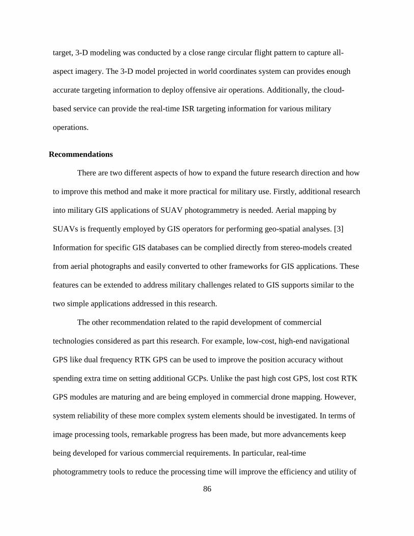
86
target, 3-D modeling was conducted by a close range circular flight pattern to capture all-
aspect imagery. The 3-D model projected in world coordinates system can provides enough
accurate targeting information to deploy offensive air operations. Additionally, the cloud-
based service can provide the real-time ISR targeting information for various military
operations.
Recommendations
There are two different aspects of how to expand the future research direction and how
to improve this method and make it more practical for military use. Firstly, additional research
into military GIS applications of SUAV photogrammetry is needed. Aerial mapping by
SUAVs is frequently employed by GIS operators for performing geo-spatial analyses. [3]
Information for specific GIS databases can be complied directly from stereo-models created
from aerial photographs and easily converted to other frameworks for GIS applications. These
features can be extended to address military challenges related to GIS supports similar to the
two simple applications addressed in this research.
The other recommendation related to the rapid development of commercial
technologies considered as part this research. For example, low-cost, high-end navigational
GPS like dual frequency RTK GPS can be used to improve the position accuracy without
spending extra time on setting additional GCPs. Unlike the past high cost GPS, lost cost RTK
GPS modules are maturing and are being employed in commercial drone mapping. However,
system reliability of these more complex system elements should be investigated. In terms of
image processing tools, remarkable progress has been made, but more advancements keep
being developed for various commercial requirements. In particular, real-time
photogrammetry tools to reduce the processing time will improve the efficiency and utility of

87
the method. Removing the time gap between data collection and modeling can extend the
method application in the military areas that are more time sensitive and require agile
response. A few commercial drone mapping company like DroneDeploy [9] launched real-
time drone mapping solution for agriculture applications, but deeper studies should be done to
optimize the tradeoff between stereo model quality and image processing time through the
GCS using telemetry data from SUAV.
88
Bibliography
[1] F. Nex and F. Remondino, “UAV for 3D mapping applications: a review,” Appl.
Geomatics, vol. 6, no. 1, pp. 1–15, 2013.
[2] F. Remondino, L. Barazzetti, F. Nex, M. Scaioni, and D. Sarazzi, “Uav
Photogrammetry for Mapping and 3D Modeling – Current Status and Future
Perspectives,” ISPRS - Int. Arch. Photogramm. Remote Sens. Spat. Inf. Sci., vol.
XXXVIII-1/, no. September, pp. 25–31, 2012.
[3] P. R. Wolf, B. A. Dewitt, and B. E. Wilkinson, Elements of photogrammetry with
application in GIS. .
[4] “Pix4D - Drone Photogrammetry Software for Desktop + Cloud + Mobile.”
[Online]. Available: https://pix4d.com/. [Accessed: 04-Oct-2017].
[5] T. Schenk, “Concepts and algorithms in digital photogrammetry,” ISPRS J.
Photogramm. Remote Sens., vol. 49, no. 6, pp. 2–8, 1994.
[6] “UVS International – Remotely Piloted Systems : Promoting International
Cooperation & Coordination.” [Online]. Available: https://uvs-
international.org/. [Accessed: 04-Oct-2017].
[7] H. Eisenbeiß, E. T. H. Zurich, H. Eisenbeiß, and E. T. H. Zürich, UAV
photogrammetry, no. 18515. 2009.
[8] N. Micheletti, J. H. Chandler, and S. N. Lane, “Structure from Motion (SfM)
Photogrammetry,” Br. Soc. Geomorphol. Geomorphol. Tech., vol. 2, no. 2, pp. 1–
12, 2015.
[9] D. Deploy, “DroneDeploy’s 2017 Drone Buyer’s Guide The Ultimate Guide to
Choosing a Mapping Drone for Your Business 03 Aerial Insights,” 2017.
[10] J. Vautherin et al., “PHOTOGRAMMETRIC ACCURACY AND MODELING OF
ROLLING SHUTTER CAMERAS.”
[11] B. I. Smith, “How to Improve the Map Quality from your Drone,” pp. 1–8, 2017.
[12] D. J. Crandall, A. Owens, N. Snavely, and D. P. Huttenlocher, “SfM with MRFs:
Discrete-continuous optimization for large-scale structure from motion,” IEEE
89
Trans. Pattern Anal. Mach. Intell., vol. 35, no. 12, pp. 2841–2853, 2013.
[13] E. B. Peterson, M. Klein, and R. L. Stewart, Whitepaper on Structure from Motion
(SfM) Photogrammetry: Constructing Three Dimensional Models from
Photography, no. October. 2015.
[14] R. Szeliski, “Structure from motion,” pp. 303–334, 2011.
[15] “Agisoft PhotoScan.” [Online]. Available: http://www.agisoft.com/. [Accessed: 13-
Oct-2017].
[16] “Drone2Map for ArcGIS - Turn Your Drone Into an Enterprise GIS Productivity
Tool | Esri.” [Online]. Available: http://www.esri.com/products/drone2map.
[Accessed: 13-Oct-2017].
[17] R. Niederheiser, M. MokroA, J. Lange, H. Petschko, G. Prasicek, and S. O.
Elberink, “Deriving 3D point clouds from terrestrial photographs - Comparison of
different sensors and software,” Int. Arch. Photogramm. Remote Sens. Spat. Inf.
Sci. - ISPRS Arch., vol. 41, no. July, pp. 685–692, 2016.
[18] C. U. A. S. Advancement, T. H. E. P. Man, S. Photon, and S. Review, “TAKING
UAS Photogrammetric Point,” no. August, 2015.
[19] O. Küng et al., “the Accuracy of Automatic Photogrammetric Techniques on Ultra-
Light Uav Imagery,” ISPRS - Int. Arch. Photogramm. Remote Sens. Spat. Inf. Sci.,
vol. XXXVIII-1/, pp. 125–130, 2012.
[20] O. Küng et al., “the Accuracy of Automatic Photogrammetric Techniques on Ultra-
Light Uav Imagery,” ISPRS - Int. Arch. Photogramm. Remote Sens. Spat. Inf. Sci.,
vol. XXXVIII-1/, pp. 125–130, 2012.
[21] B. Draeyer and C. S. February, “White paper : How accurate are UAV surveying
methods ? answer . A comparison between Pix4D UAV photogrammetry software
and,” no. February, pp. 1–8, 2014.
[22] I. Colomina and P. Molina, “Unmanned aerial systems for photogrammetry and
remote sensing: A review,” ISPRS Journal of Photogrammetry and Remote
Sensing. 2014.
[23] K. Choi and I. Lee, “A Uav Based Close-Range Rapid Aerial Monitoring System
90
for Emergency Responses,” ISPRS - Int. Arch. Photogramm. Remote Sens. Spat.
Inf. Sci., vol. XXXVIII-1/, no. September, pp. 247–252, 2012.
[24] S. Publishers and D. S. News, “Satnews Daily June 15,” no. 1868392077, pp. 3–4,
2017.
[25] B. Feedstock, “Idaho National Laboratory,” 2014.
[26] A. Stitched, I. From, and A. N. Unmanned, “ACTIONABLE STITCHED IMAGES
FROM AN UNMANNED AERIAL.”
[27] “Rascal - Model Airplane Kit - SIG Mfg. Co., Inc.” [Online]. Available:
http://www.sigmfg.com/IndexText/SIGRC80.html. [Accessed: 23-Jan-2018].
[28] L. M. Accuracy and D. J. I. D. Platforms, “Linear Measurement Accuracy of DJI
Drone Platforms and Photogrammetry.”
[29] “KAP & UAV Exposure Control Intervalometer Script - page 1 - Completed
and Working Scripts - CHDK Forum.” [Online]. Available:
https://chdk.setepontos.com/index.php?topic=10822. [Accessed: 30-Oct-2017].
[30] “full-text.”
[31] “Community: — ArduPilot documentation.” [Online]. Available:
http://ardupilot.org/ardupilot/index.html. [Accessed: 07-Dec-2017].
[32] C. Strecha, “Pix4D - Error Estimation,” vol. 1, no. 3, pp. 1–3, 2014.
[33] “Close Air Support,” 2014.
[34] J. Pub, “Joint Laser Designation Procedures (Jlaser),” no. June, 1991.
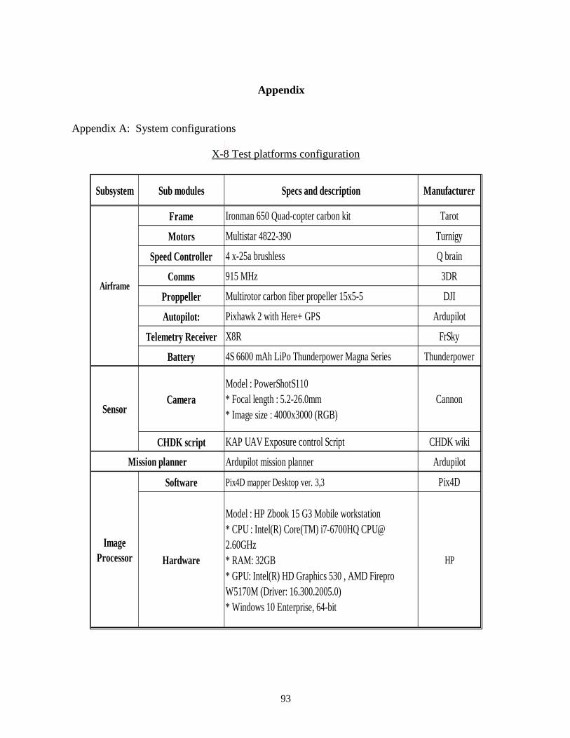
93
Appendix
Appendix A: System configurations
X-8 Test platforms configuration
Subsystem Sub modules Specs and description Manufacturer
Frame Ironman 650 Quad-copter carbon kit Tarot
Motors Multistar 4822-390 Turnigy
Speed Controller 4 x-25a brushless Q brain
Comms 915 MHz 3DR
Proppeller Multirotor carbon fiber propeller 15x5-5 DJI
Autopilot: Pixhawk 2 with Here+ GPS Ardupilot
Telemetry Receiver X8R FrSky
Battery 4S 6600 mAh LiPo Thunderpower Magna Series Thunderpower
CameraModel : PowerShotS110* Focal length : 5.2-26.0mm* Image size : 4000x3000 (RGB)
Cannon
CHDK script KAP UAV Exposure control Script CHDK wiki
Ardupilot mission planner Ardupilot
Software Pix4D mapper Desktop ver. 3,3 Pix4D
Hardware
Model : HP Zbook 15 G3 Mobile workstation* CPU : Intel(R) Core(TM) i7-6700HQ [email protected]* RAM: 32GB* GPU: Intel(R) HD Graphics 530 , AMD FireproW5170M (Driver: 16.300.2005.0)* Windows 10 Enterprise, 64-bit
HPImage
Processor
Airframe
Sensor
Mission planner
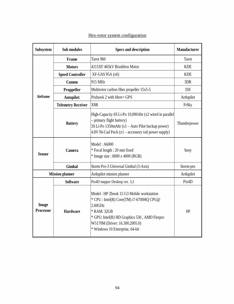
94
Hex-rotor system configuration
Subsystem Sub modules Specs and description Manufacturer
Frame Tarot 960 Tarot
Motors 4215XF 465kV Brushless Motor KDE
Speed Controller XF-UAS 95A (x6) KDE
Comms 915 MHz 3DR
Proppeller Multirotor carbon fiber propeller 15x5-5 DJI
Autopilot: Pixhawk 2 with Here+ GPS Ardupilot
Telemetry Receiver X8R FrSky
Battery
High-Capacity 6S Li-Po 10,000Ahr (x2 wired in parallel– primary flight battery)3S Li-Po 1350mAhr (x1 – Auto Pilot backup power)4.8V Ni-Cad Pack (x1 – accessory rail power supply)
Thunderpower
CameraModel : A6000* Focal length : 20 mm fixed* Image size : 6000 x 4000 (RGB)
Sony
Gimbal Storm Pro-3 Universal Gimbal (3-Axis) Storm-pro
Ardupilot mission planner Ardupilot
Software Pix4D mapper Desktop ver. 3,3 Pix4D
Hardware
Model : HP Zbook 15 G3 Mobile workstation* CPU : Intel(R) Core(TM) i7-6700HQ [email protected]* RAM: 32GB* GPU: Intel(R) HD Graphics 530 , AMD FireproW5170M (Driver: 16.300.2005.0)* Windows 10 Enterprise, 64-bit
HP
Airframe
Sensor
Mission planner
ImageProcessor
95
Appendix B: Sony A6000 Camera Remote triggering procedure
1. Auto pilot setting
a. Parameter setting
i. CAM_DURATION 1
ii. CAM_SERVO_OFF 1600
iii. CAM_SERVO_ON 2200
iv. CAM_TRIGG_TYPE 0
v. RC10_FUNCTION 10(Only 1 RC you use)
vi. RC10_TRIM 900
vii. RC10_MAX 2200
viii. CH 7 : Camera Trigger
b. Camera Gimbal setting (Open Initial setup | Optional Hardware | Camera Gimbal)
i. Shutter : RC 10(Servo rail you choose for camera)
ii. Servo Limits Min : 900
iii. Servo Limits Max : 2200
iv. Shutter Pushed : 2200
v. Shutter Not Pushed : 1600
vi. Duration : 10
2. Camera setting
a. Battery fully charged
b. Camera Mode selection
i. S (Shutter speed primary) and set below 1/1000 shutter speed
c. Camera menu setting
i. ISO: below 100 or Auto
ii. AWB: Daylight
iii. Image Size: L(24M) (set size you want)
iv. Quality : Fine
v. Pwr Save Start Time : 30 min
vi. Face Detection : Off
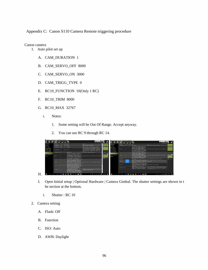
96
Appendix C: Canon S110 Camera Remote triggering procedure
Canon camera
1. Auto pilot set up
A. CAM_DURATION 1
B. CAM_SERVO_OFF 8000
C. CAM_SERVO_ON 3000
D. CAM_TRIGG_TYPE 0
E. RC10_FUNCTION 10(Only 1 RC)
F. RC10_TRIM 8000
G. RC10_MAX 32767
i. Notes:
1. Some setting will be Out Of Range. Accept anyway.
2. You can use RC 9 through RC 14.
H.
I. Open Initial setup | Optional Hardware | Camera Gimbal. The shutter settings are shown in the section at the bottom.
i. Shutter : RC 10
2. Camera setting
A. Flash: Off
B. Function
C. ISO: Auto
D. AWB: Daylight

97
E. Image Size: L
F. Image Quality: Fine/Superfine
G. Menu
H. AF Frame: Center
I. Digital Zoom: Off
J. AF-Point Zoom: Off
K. Servo AF: Off
L. AF assist beam: Off
M. Flash Settings
N. Red Eye correction: Off
O. Red-Eye Lamp: Off
P. Date Stamp: Date & Time
Q. Power Saving...
R. Auto Power Down: Off
S. Display Off: 1 min
T. IS Settings...
U. IS Mode: Shoot Only
V. Powered IS: Off
W. GPS: On
3. CHDK set up
A. Function
B. Autostart: On
C. Save Params: ON
D. Remote Parameters: Enable Remote
E. Menu
F. Extra Photo Operations...

98
G. Disable Overrides: Disable
H. Override Shutter Speed: 1/1600
I. Value Factor: 1
J. Override Subj. Dist V: 65535
K. Value Factor: 1
L. Custom Auto ISO...
M. Enable custom auto ISO
N. Minimal: 1/1000
O. Clear override values @start: Disable
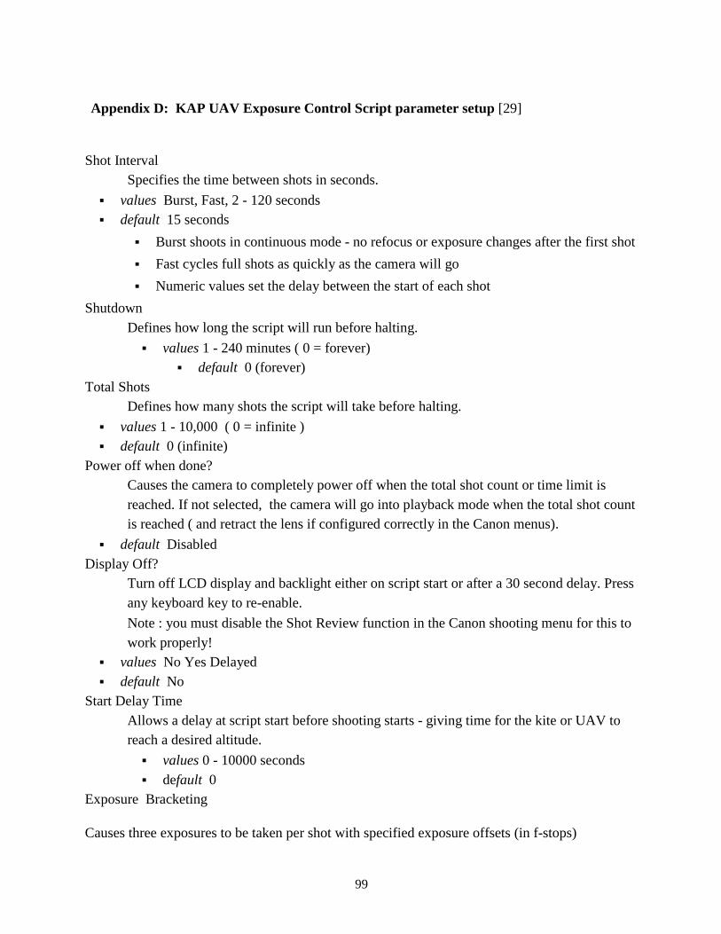
99
Appendix D: KAP UAV Exposure Control Script parameter setup [29]
Shot Interval
Specifies the time between shots in seconds. values Burst, Fast, 2 - 120 seconds default 15 seconds
Burst shoots in continuous mode - no refocus or exposure changes after the first shot Fast cycles full shots as quickly as the camera will go Numeric values set the delay between the start of each shot
Shutdown Defines how long the script will run before halting. values 1 - 240 minutes ( 0 = forever)
default 0 (forever) Total Shots
Defines how many shots the script will take before halting. values 1 - 10,000 ( 0 = infinite ) default 0 (infinite)
Power off when done? Causes the camera to completely power off when the total shot count or time limit is reached. If not selected, the camera will go into playback mode when the total shot count is reached ( and retract the lens if configured correctly in the Canon menus).
default Disabled Display Off?
Turn off LCD display and backlight either on script start or after a 30 second delay. Press any keyboard key to re-enable. Note : you must disable the Shot Review function in the Canon shooting menu for this to work properly!
values No Yes Delayed default No
Start Delay Time Allows a delay at script start before shooting starts - giving time for the kite or UAV to reach a desired altitude. values 0 - 10000 seconds default 0
Exposure Bracketing
Causes three exposures to be taken per shot with specified exposure offsets (in f-stops)
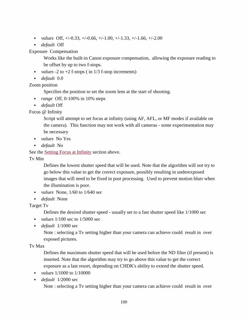
100
values Off, +/-0.33, +/-0.66, +/-1.00, +/-1.33, +/-1.66, +/-2.00 default Off
Exposure Compensation Works like the built-in Canon exposure compensation, allowing the exposure reading to be offset by up to two f-stops.
values -2 to +2 f-stops ( in 1/3 f-stop increments) default 0.0
Zoom position Specifies the position to set the zoom lens at the start of shooting.
range Off, 0-100% in 10% steps default Off
Focus @ Infinity Script will attempt to set focus at infinity (using AF, AFL, or MF modes if available on the camera). This function may not work with all cameras - some experimentation may be necessary
values No Yes default No
See the Setting Focus at Infinity section above. Tv Min
Defines the lowest shutter speed that will be used. Note that the algorithm will not try to go below this value to get the correct exposure, possibly resulting in underexposed images that will need to be fixed in post processing. Used to prevent motion blurr when the illumination is poor.
values None, 1/60 to 1/640 sec default None
Target Tv Defines the desired shutter speed - usually set to a fast shutter speed like 1/1000 sec
values 1/100 sec to 1/5000 sec default 1/1000 sec
Note : selecting a Tv setting higher than your camera can achieve could result in over exposed pictures.
Tv Max Defines the maximum shutter speed that will be used before the ND filter (if present) is inserted. Note that the algorithm may try to go above this value to get the correct exposure as a last resort, depending on CHDK's ability to extend the shutter speed.
values 1/1000 to 1/10000 default 1/2000 sec
Note : selecting a Tv setting higher than your camera can achieve could result in over
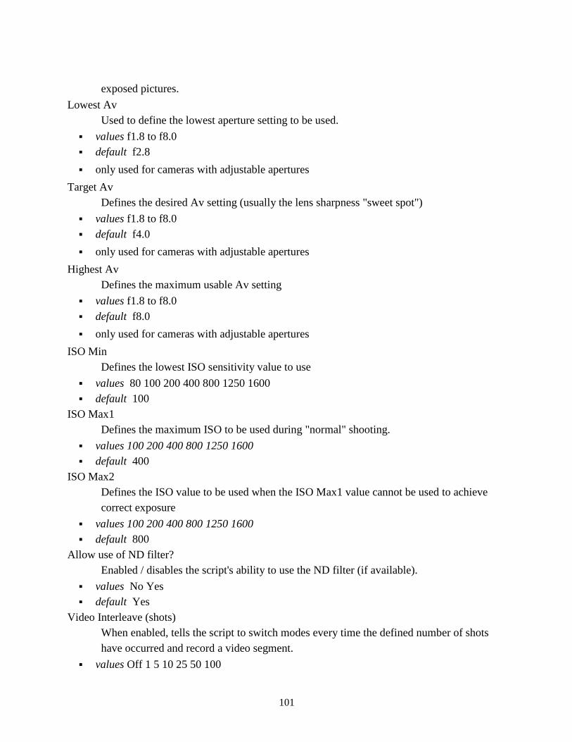
101
exposed pictures. Lowest Av
Used to define the lowest aperture setting to be used. values f1.8 to f8.0 default f2.8 only used for cameras with adjustable apertures
Target Av Defines the desired Av setting (usually the lens sharpness "sweet spot")
values f1.8 to f8.0 default f4.0 only used for cameras with adjustable apertures
Highest Av Defines the maximum usable Av setting
values f1.8 to f8.0 default f8.0 only used for cameras with adjustable apertures
ISO Min Defines the lowest ISO sensitivity value to use
values 80 100 200 400 800 1250 1600 default 100
ISO Max1 Defines the maximum ISO to be used during "normal" shooting.
values 100 200 400 800 1250 1600 default 400
ISO Max2 Defines the ISO value to be used when the ISO Max1 value cannot be used to achieve correct exposure
values 100 200 400 800 1250 1600 default 800
Allow use of ND filter? Enabled / disables the script's ability to use the ND filter (if available).
values No Yes default Yes
Video Interleave (shots) When enabled, tells the script to switch modes every time the defined number of shots have occurred and record a video segment.
values Off 1 5 10 25 50 100
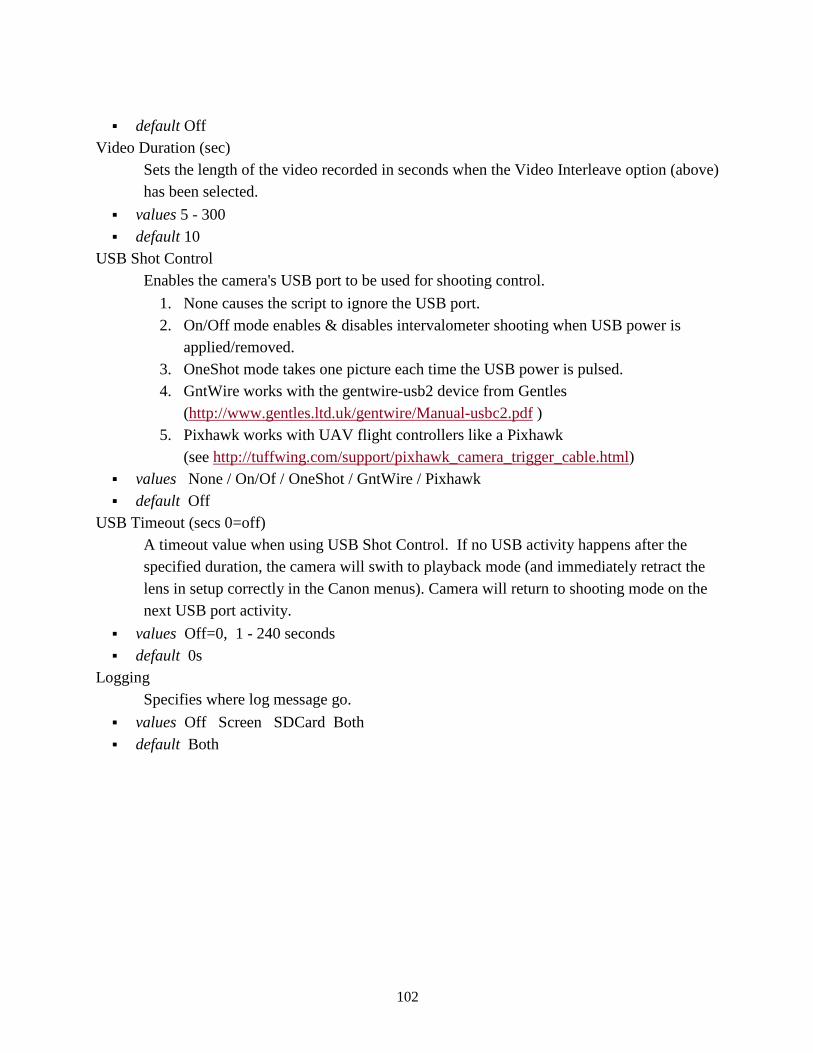
102
default Off Video Duration (sec)
Sets the length of the video recorded in seconds when the Video Interleave option (above) has been selected.
values 5 - 300 default 10
USB Shot Control Enables the camera's USB port to be used for shooting control.
1. None causes the script to ignore the USB port. 2. On/Off mode enables & disables intervalometer shooting when USB power is
applied/removed. 3. OneShot mode takes one picture each time the USB power is pulsed. 4. GntWire works with the gentwire-usb2 device from Gentles
(http://www.gentles.ltd.uk/gentwire/Manual-usbc2.pdf ) 5. Pixhawk works with UAV flight controllers like a Pixhawk
(see http://tuffwing.com/support/pixhawk_camera_trigger_cable.html) values None / On/Of / OneShot / GntWire / Pixhawk default Off
USB Timeout (secs 0=off) A timeout value when using USB Shot Control. If no USB activity happens after the specified duration, the camera will swith to playback mode (and immediately retract the lens in setup correctly in the Canon menus). Camera will return to shooting mode on the next USB port activity.
values Off=0, 1 - 240 seconds default 0s
Logging Specifies where log message go.
values Off Screen SDCard Both default Both
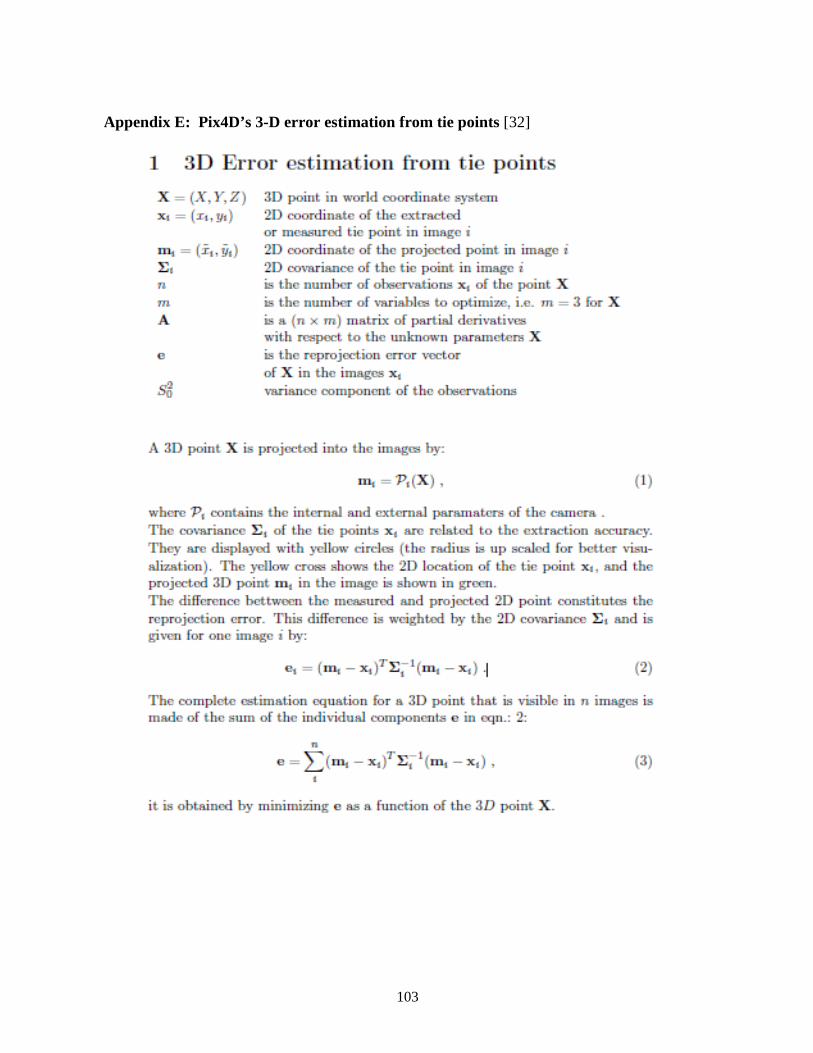
103
Appendix E: Pix4D’s 3-D error estimation from tie points [32]
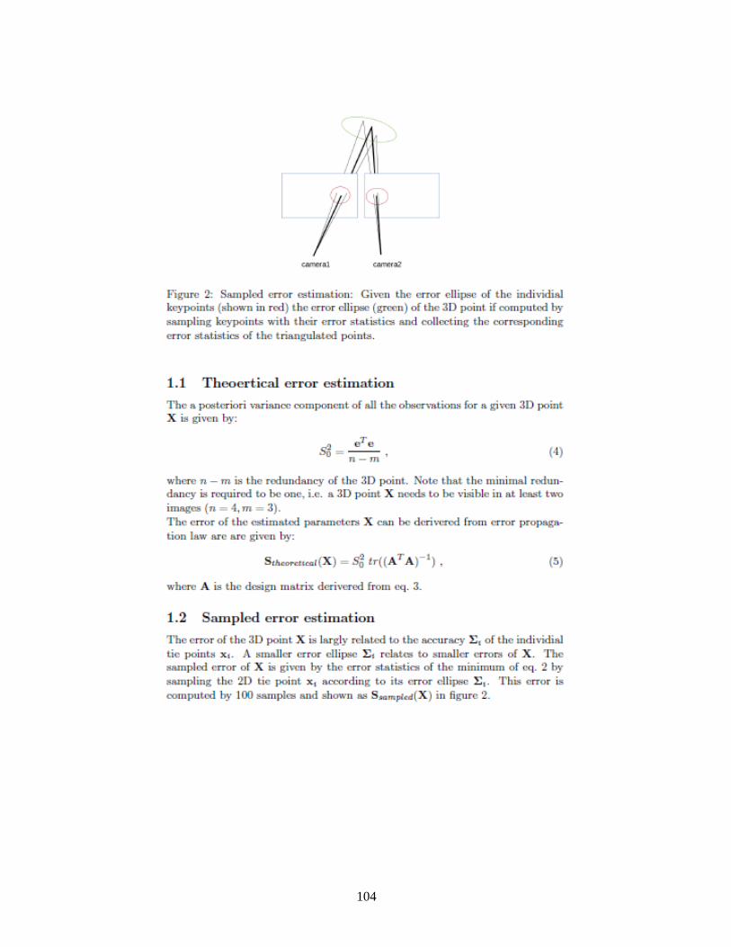
104
105
Appendix F: AFI Doc 5028-Multirotor photogrammetry mapping PROJECT DESCRIPTION
1. SUMMARY OF CHANGES
a. There was not much change of physical specification, but the control board in the gimbal was changed and modulated the gain to ensure more stable gimbal performance.
b. The AFIT team has flown a Tarot T960 for almost similar flight two month ago.
2. BACKGROUND
a. Description:
This is the test flight for individual research to study UAV assisted photogrammetry method for military application. This test has performed in conceptual level with X-8 and T960 and it was successful. Therefore, general workflow will follow the previous flight sequence. Additional details of the four core test objectives are listed below.
Test Objective 1 is to complete the runway survey mission with T960 varying different parameter to collect data.
Test Objective 2 is to perform the circular survey mission flying around model of the object(Trailer) to reconstruct 3D model of the object.
b. Purpose: These tests are the final capstone for the research. Based on the latest development test, the
test profile will be performed in a operational level. The sequence should be performed fully automated flow based on the planned mission and provide the imagery data with georeferenced location data, which is required in software data processing.
c. List of AFIT and non-AFIT assets at risk:
i. One (1) Tarot T960 multi-rotor UAS with pixhawk autopilot ii. One (1) Sony Alpha A6000 camera, lenses, controllers
iii. AFIT Personnel (a mix of military and civilian staff and students)
106
iv. A vehicle and trailer owned and operated by CESI (civilian contractor) v. Any personnel within a ½ mile radius of airfield
vi. Any vehicles (including aircraft) parked within operational radius
d. Location of test:
WPAFB, behind USAF Museum and/or Himsel Airfield, Camp Atterbury Joint Maneuver Training Center, IN
e. Planned dates of the test:
10 October - 19 October 2017 for subsystems, integration, and operational tests
f. Number of projected flights during the test period:
Approximately 8 flights for 1st objective and 2 flights for 2nd objective.
3. MISHAP RESPONSIBILITIES a. Should an incident occur in which the UAS is damaged or destroyed, the AFIT Flight
Test Safety Officer (FTSO) will be notified via the After Action Report.
b. WPAFB If an incident occurs in which property or personnel on WPAFB is damaged/injured, the installation emergency 911 service will be notified immediately. In addition, the AFIT Safety Office will be notified within 5 working days per AFIT’s Mishap Notification Procedures. Serious mishaps must be reported immediately.
AFIT Safety Office (Tim Thomas, 255-3636 x3627, Cell Phone 937-479-9715)
If an injury or illness results in lost duty time or hospitalization, then the AFIT Safety Office
will be notified immediately. The Principal Investigator will be responsible for submitting any of the required mishap reports as defined in AFIT’s Mishap Notification Procedures. For further information, refer to the Mishap Notification Procedures posted in the Safety folder under the ‘Mishap Reporting’ tab on the AFIT Intranet site.
c. Camp Atterbury. If an incident occurs in which property owned by the Army, Camp Atterbury, or civilians is damaged and/or any personnel are injured, the Camp Atterbury
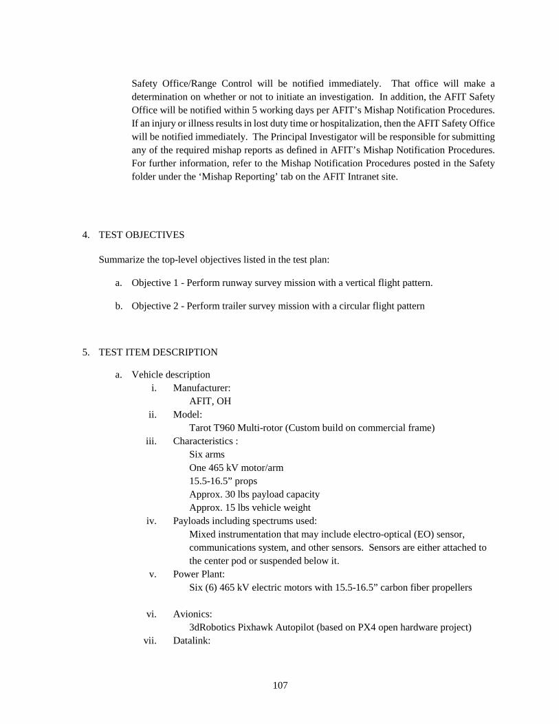
107
Safety Office/Range Control will be notified immediately. That office will make a determination on whether or not to initiate an investigation. In addition, the AFIT Safety Office will be notified within 5 working days per AFIT’s Mishap Notification Procedures. If an injury or illness results in lost duty time or hospitalization, then the AFIT Safety Office will be notified immediately. The Principal Investigator will be responsible for submitting any of the required mishap reports as defined in AFIT’s Mishap Notification Procedures. For further information, refer to the Mishap Notification Procedures posted in the Safety folder under the ‘Mishap Reporting’ tab on the AFIT Intranet site.
4. TEST OBJECTIVES Summarize the top-level objectives listed in the test plan:
a. Objective 1 - Perform runway survey mission with a vertical flight pattern.
b. Objective 2 - Perform trailer survey mission with a circular flight pattern
5. TEST ITEM DESCRIPTION
a. Vehicle description i. Manufacturer:
AFIT, OH ii. Model:
Tarot T960 Multi-rotor (Custom build on commercial frame) iii. Characteristics :
Six arms One 465 kV motor/arm 15.5-16.5” props Approx. 30 lbs payload capacity Approx. 15 lbs vehicle weight
iv. Payloads including spectrums used: Mixed instrumentation that may include electro-optical (EO) sensor, communications system, and other sensors. Sensors are either attached to the center pod or suspended below it.
v. Power Plant: Six (6) 465 kV electric motors with 15.5-16.5” carbon fiber propellers
vi. Avionics: 3dRobotics Pixhawk Autopilot (based on PX4 open hardware project)
vii. Datalink:
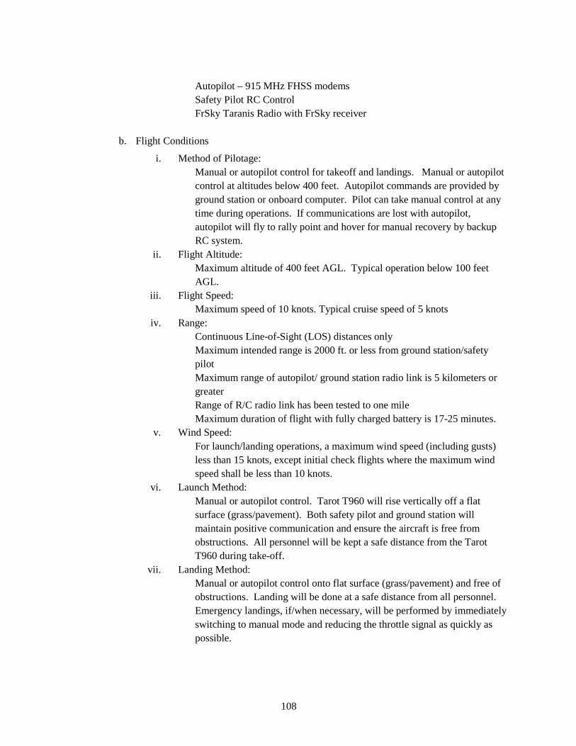
108
Autopilot – 915 MHz FHSS modems Safety Pilot RC Control FrSky Taranis Radio with FrSky receiver
b. Flight Conditions
i. Method of Pilotage: Manual or autopilot control for takeoff and landings. Manual or autopilot control at altitudes below 400 feet. Autopilot commands are provided by ground station or onboard computer. Pilot can take manual control at any time during operations. If communications are lost with autopilot, autopilot will fly to rally point and hover for manual recovery by backup RC system.
ii. Flight Altitude: Maximum altitude of 400 feet AGL. Typical operation below 100 feet AGL.
iii. Flight Speed: Maximum speed of 10 knots. Typical cruise speed of 5 knots
iv. Range: Continuous Line-of-Sight (LOS) distances only Maximum intended range is 2000 ft. or less from ground station/safety pilot Maximum range of autopilot/ ground station radio link is 5 kilometers or greater Range of R/C radio link has been tested to one mile Maximum duration of flight with fully charged battery is 17-25 minutes.
v. Wind Speed: For launch/landing operations, a maximum wind speed (including gusts) less than 15 knots, except initial check flights where the maximum wind speed shall be less than 10 knots.
vi. Launch Method: Manual or autopilot control. Tarot T960 will rise vertically off a flat surface (grass/pavement). Both safety pilot and ground station will maintain positive communication and ensure the aircraft is free from obstructions. All personnel will be kept a safe distance from the Tarot T960 during take-off.
vii. Landing Method: Manual or autopilot control onto flat surface (grass/pavement) and free of obstructions. Landing will be done at a safe distance from all personnel. Emergency landings, if/when necessary, will be performed by immediately switching to manual mode and reducing the throttle signal as quickly as possible.
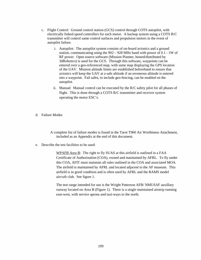
109
c. Flight Control: Ground control station (GCS) control through COTS autopilot, with electrically linked speed controllers for each motor. A backup system using a COTS R/C transmitter will control same control surfaces and propulsion motors in the event of autopilot failure.
i. Autopilot: The autopilot system consists of on-board avionics and a ground station, communicating using the 902 – 928 MHz band with power of 0.1 - 1W of RF power. Open source software (Mission Planner, hosted/distributed by 3dRobotics) is used for the GCS. Through this software, waypoints can be entered over a geo-referenced map, with same map displaying the GPS location of the UAV. Mission altitude limits are established beforehand to ensure that avionics will keep the UAV at a safe altitude if an erroneous altitude is entered into a waypoint. Fail safes, to include geo-fencing, can be enabled on the autopilot.
ii. Manual: Manual control can be executed by the R/C safety pilot for all phases of flight. This is done through a COTS R/C transmitter and receiver system operating the motor ESC’s.
d. Failure Modes
A complete list of failure modes is found in the Tarot T960 Air Worthiness Attachment, included as an Appendix at the end of this document.
e. Describe the test facilities to be used:
WPAFB Area B: The right to fly SUAS at this airfield is outlined in a FAA Certificate of Authorization (COA), owned and maintained by AFRL. To fly under this COA, AFIT must maintain all rules outlined in the COA and associated MOA. The airfield is maintained by AFRL and located adjacent to the AF museum. This airfield is in good condition and is often used by AFRL and the RAMS model aircraft club. See figure 1.
The test range intended for use is the Wright Patterson AFB/ NMUSAF auxillary runway located on Area B (Figure 1). There is a single maintained airstrip running east-west, with service aprons and taxi-ways to the north.
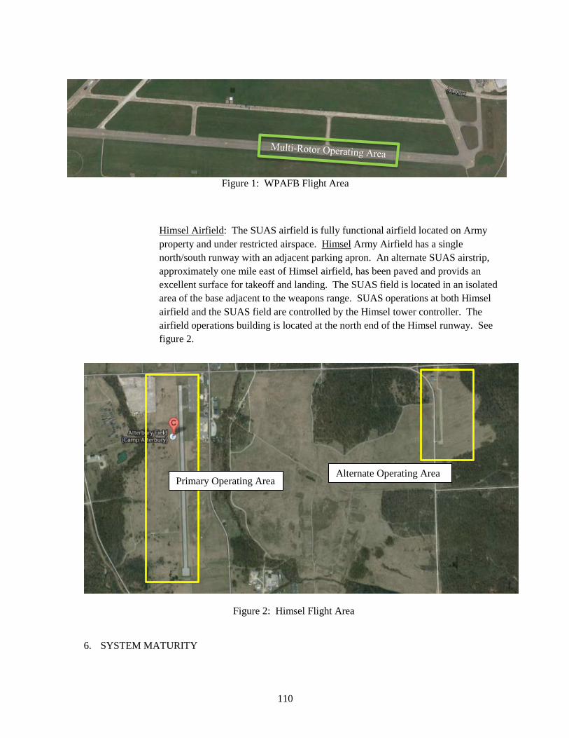
110
Figure 1: WPAFB Flight Area
Himsel Airfield: The SUAS airfield is fully functional airfield located on Army property and under restricted airspace. Himsel Army Airfield has a single north/south runway with an adjacent parking apron. An alternate SUAS airstrip, approximately one mile east of Himsel airfield, has been paved and provids an excellent surface for takeoff and landing. The SUAS field is located in an isolated area of the base adjacent to the weapons range. SUAS operations at both Himsel airfield and the SUAS field are controlled by the Himsel tower controller. The airfield operations building is located at the north end of the Himsel runway. See figure 2.
Figure 2: Himsel Flight Area
6. SYSTEM MATURITY
Primary Operating Area Alternate Operating Area
111
a. Describe testing that supports readiness:
The Tarot T960 (hexcopter) is lately completed the performance verification. Therefore, the same autopilot and ground station software will be used for the test that has previously been used for past multirotors. The safety pilot is skilled in operating multi-rotor vehicles, and there are two ground station operators capable of providing console operation for multi-rotor tests. Motor/prop testing was conducted using the motor test stand.
b. Previous lessons learned:
Familiar procedures for operating multi-rotors with the Pixhawk autopilot will be followed. Operators and observers will remain clear of the “Return to Launch” point to ensure that an unexpected RTL mode change will not hazard personnel. Direct overflight of personnel will not be performed, and all tests will be conducted at a safe distance from ground station and observer personnel (> 30 feet). To ensure bolts and screws do not come loose during flight, high strength Locktite threadlock will be used along with witness marks on all critical connections. Additionally, all motor mounts will use a minimum of four bolts to reduce the likelihood of a motor coming loose in flight.
c. Authorized flight:
This flight is authorized by the AFIT Military Flight Release (MFR) which has been reviewed and approved by the Unmanned Aerial Systems Airworthiness office at AFLCMC.
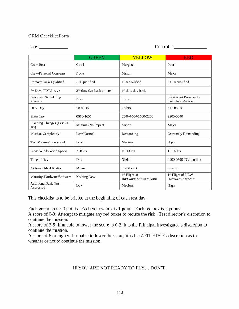
112
ORM Checklist Form Date: ____________ Control #:______________
This checklist is to be briefed at the beginning of each test day. Each green box is 0 points. Each yellow box is 1 point. Each red box is 2 points. A score of 0-3: Attempt to mitigate any red boxes to reduce the risk. Test director’s discretion to continue the mission. A score of 3-5: If unable to lower the score to 0-3, it is the Principal Investigator’s discretion to continue the mission. A score of 6 or higher: If unable to lower the score, it is the AFIT FTSO’s discretion as to whether or not to continue the mission.
IF YOU ARE NOT READY TO FLY… DON’T!
GREEN YELLOW RED Crew Rest Good Marginal Poor
Crew/Personal Concerns None Minor Major
Primary Crew Qualified All Qualified 1 Unqualified 2+ Unqualified
7+ Days TDY/Leave 2nd duty day back or later 1st duty day back
Perceived Scheduling Pressure None Some Significant Pressure to
Complete Mission
Duty Day <8 hours >8 hrs >12 hours
Showtime 0600-1600 0300-0600/1600-2200 2200-0300
Planning Changes (Last 24 hrs) Minimal/No impact Minor Major
Mission Complexity Low/Normal Demanding Extremely Demanding
Test Mission/Safety Risk Low Medium High
Cross Winds/Wind Speed <10 kts 10-13 kts 13-15 kts
Time of Day Day Night 0200-0500 TO/Landing
Airframe Modification Minor Significant Severe
Maturity-Hardware/Software Nothing New 1st Flight of Hardware/Software Mod
1st Flight of NEW Hardware/Software
Additional Risk Not Addressed Low Medium High
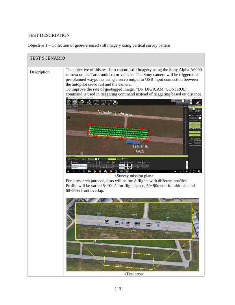
113
TEST DESCRIPTION Objective 1 – Collection of georeferenced still imagery using vertical survey pattern
TEST SCENARIO
Description The objective of this test is to capture still imagery using the Sony Alpha A6000 camera on the Tarot multi-rotor vehicle. The Sony camera will be triggered at pre-planned waypoints using a servo output to USB input connection between the autopilot servo rail and the camera. To improve the rate of geotagged image, “Do_DIGICAM_CONTROL” command is used in triggering command instead of triggering based on distance.
<Survey mission plan>
For a research purpose, tests will be run 8 flights with different profiles. Profile will be varied 5~10m/s for flight speed, 50~90meter for altitude, and 60~80% front overlap.
<Test area>
Trailer & GCS
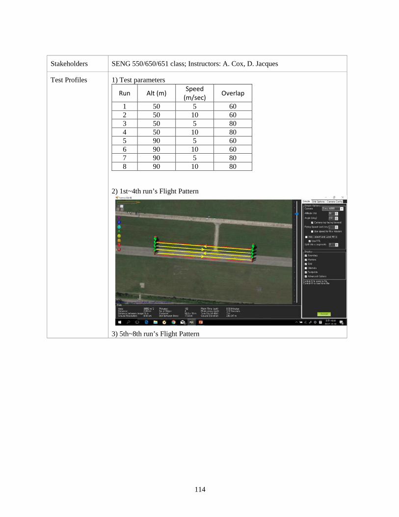
114
Stakeholders SENG 550/650/651 class; Instructors: A. Cox, D. Jacques
Test Profiles 1) Test parameters
Run Alt (m) Speed (m/sec) Overlap
1 50 5 60 2 50 10 60 3 50 5 80 4 50 10 80 5 90 5 60 6 90 10 60 7 90 5 80 8 90 10 80
2) 1st~4th run’s Flight Pattern
3) 5th~8th run’s Flight Pattern
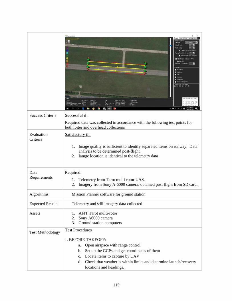
115
Success Criteria Successful if:
Required data was collected in accordance with the following test points for both loiter and overhead collections
Evaluation Criteria
Satisfactory if:
1. Image quality is sufficient to identify separated items on runway. Data analysis to be determined post-flight.
2. Iamge location is identical to the telemetry data
Data Requirements
Required:
1. Telemetry from Tarot multi-rotor UAS. 2. Imagery from Sony A-6000 camera, obtained post flight from SD card.
Algorithms Mission Planner software for ground station
Expected Results Telemetry and still imagery data collected
Assets 1. AFIT Tarot multi-rotor 2. Sony A6000 camera 3. Ground station computers
Test Methodology Test Procedures 1. BEFORE TAKEOFF:
a. Open airspace with range control. b. Set up the GCPs and get coordinates of them c. Locate items to capture by UAV d. Check that weather is within limits and determine launch/recovery
locations and headings.

116
e. Setup GCS and operating area IAW AFIT Document 5028. f. Preprogram the desired flight path of the vehicle to ensure the entire
test is conducted in front of the test team with no direct overhead flights.
g. Complete all required preflight checklists for UAS. h. Activate a remote triggering and camera set up.
2. LAUNCH:
a. Ensure that all present personnel are aware of launch. b. Move multi-rotor to desired return to launch position c. Arm multi-rotor d. Safety pilot performs manual takeoff of leader multi-rotor e. Safety pilot announces that aircraft is airborne. f. Climb to pre-briefed transition altitude. g. Transition to pre-briefed test-point operating area.
3. EXECUTE TEST POINTS: a. Switch vehicle over to auto mode b. Observe GCS showing the camera triggering marks over the survey
points c. Observe vehicle executing planned test points, and monitor battery
voltage and current consumed d. If sufficient battery power remains, an additional test point may be
conducted if it does not require a change to the camera angle e. If remaining battery power is insufficient to accomplish additional
test points, proceed to recovery
4. RECOVERY: a. Transition aircraft to safety pilot control. b. Ensure landing area is clear of personnel and equipment. c. Navigate aircraft to pre-briefed recovery location. d. Begin descent and entry into landing pattern. e. Safety pilot announces landing to all present personnel. f. Execute recovery.
5. AFTER RECOVERY:
a. Disarm multi-rotors b. Ensure telemetry on GCS is saved. c. Remain clear of propeller. d. Disconnect battery prior to moving aircraft by hand. e. Power off camera (as required) and download captured images in
GCS. f. Power off RC transmitter (as required). g. Close airspace with range control if done for the day.

117
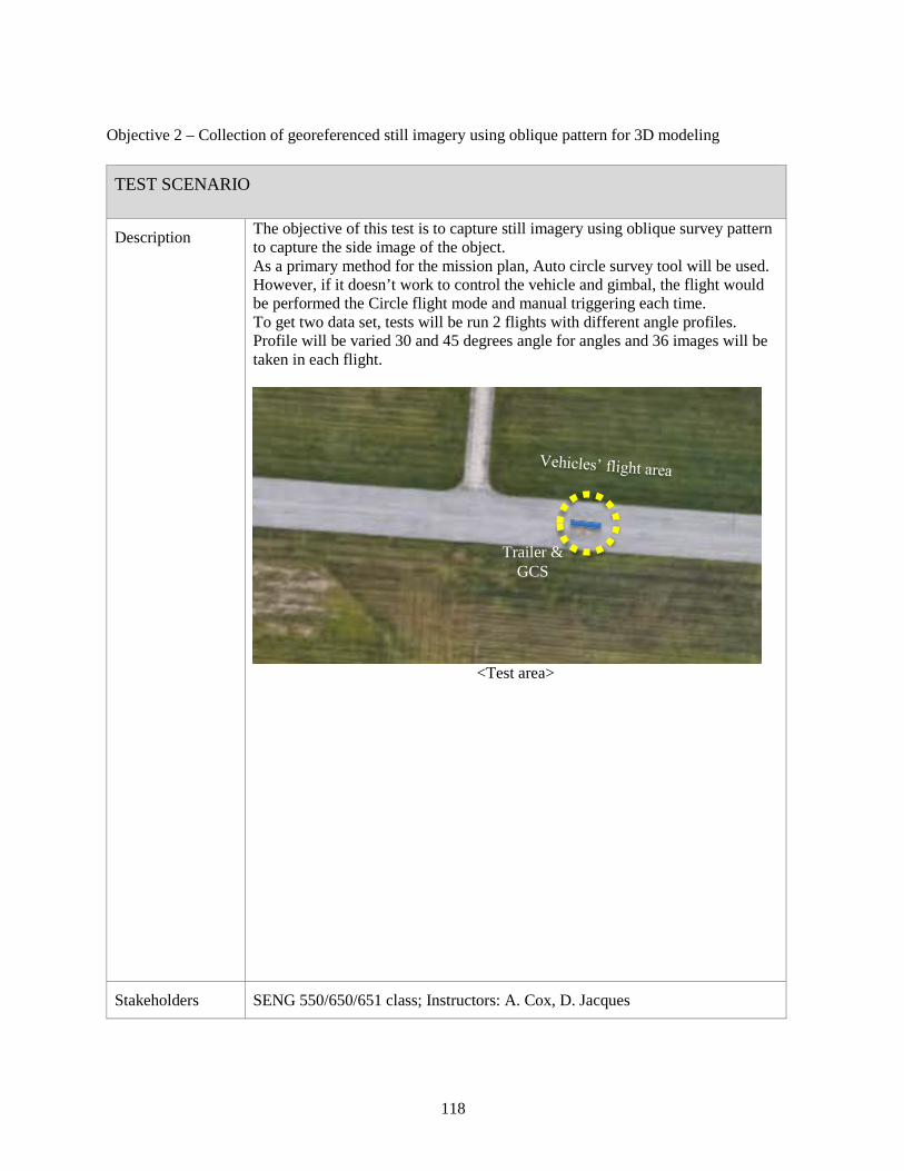
118
Objective 2 – Collection of georeferenced still imagery using oblique pattern for 3D modeling
TEST SCENARIO
Description The objective of this test is to capture still imagery using oblique survey pattern to capture the side image of the object. As a primary method for the mission plan, Auto circle survey tool will be used. However, if it doesn’t work to control the vehicle and gimbal, the flight would be performed the Circle flight mode and manual triggering each time. To get two data set, tests will be run 2 flights with different angle profiles. Profile will be varied 30 and 45 degrees angle for angles and 36 images will be taken in each flight.
<Test area>
Stakeholders SENG 550/650/651 class; Instructors: A. Cox, D. Jacques
Trailer & GCS
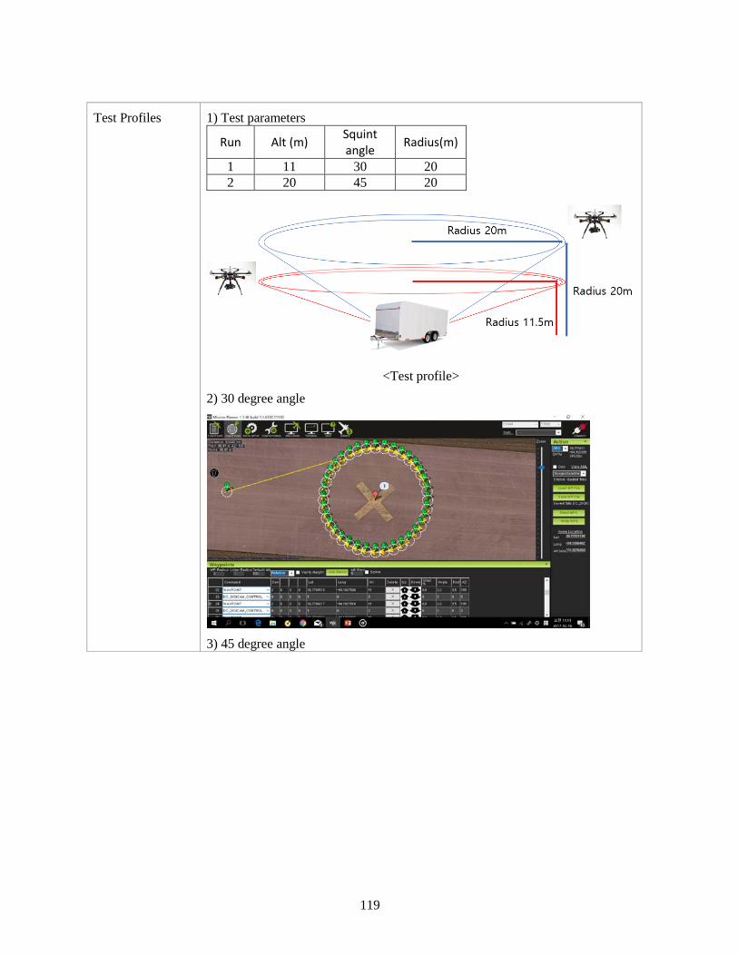
119
Test Profiles 1) Test parameters
Run Alt (m) Squint angle Radius(m)
1 11 30 20 2 20 45 20
<Test profile>
2) 30 degree angle
3) 45 degree angle
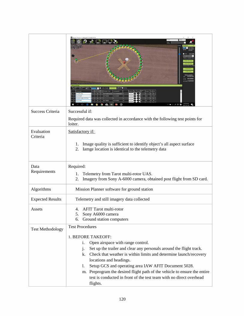
120
Success Criteria Successful if:
Required data was collected in accordance with the following test points for loiter.
Evaluation Criteria
Satisfactory if:
1. Image quality is sufficient to identify object’s all aspect surface 2. Iamge location is identical to the telemetry data
Data Requirements
Required:
1. Telemetry from Tarot multi-rotor UAS. 2. Imagery from Sony A-6000 camera, obtained post flight from SD card.
Algorithms Mission Planner software for ground station
Expected Results Telemetry and still imagery data collected
Assets 4. AFIT Tarot multi-rotor 5. Sony A6000 camera 6. Ground station computers
Test Methodology Test Procedures 1. BEFORE TAKEOFF:
i. Open airspace with range control. j. Set up the trailer and clear any personals around the flight track. k. Check that weather is within limits and determine launch/recovery
locations and headings. l. Setup GCS and operating area IAW AFIT Document 5028. m. Preprogram the desired flight path of the vehicle to ensure the entire
test is conducted in front of the test team with no direct overhead flights.

121
n. Complete all required preflight checklists for UAS. o. Activate a remote triggering and camera set up.
2. LAUNCH:
h. Ensure that all present personnel are aware of launch. i. Move multi-rotor to desired return to launch position j. Arm multi-rotor k. Safety pilot performs manual takeoff of leader multi-rotor l. Safety pilot announces that aircraft is airborne. m. Climb to pre-briefed transition altitude. n. Transition to pre-briefed test-point operating area.
3. EXECUTE TEST POINTS:
f. Switch vehicle over to auto mode g. Observe GCS showing the camera triggering marks over the survey
points h. Observe vehicle executing planned test points, and monitor battery
voltage and current consumed i. If sufficient battery power remains, an additional test point may be
conducted if it does not require a change to the camera angle j. If remaining battery power is insufficient to accomplish additional
test points, proceed to recovery
4. RECOVERY: g. Transition aircraft to safety pilot control. h. Ensure landing area is clear of personnel and equipment. i. Navigate aircraft to pre-briefed recovery location. j. Begin descent and entry into landing pattern. k. Safety pilot announces landing to all present personnel. l. Execute recovery.
5. AFTER RECOVERY:
h. Disarm multi-rotors i. Ensure telemetry on GCS is saved. j. Remain clear of propeller. k. Disconnect battery prior to moving aircraft by hand. l. Power off camera (as required) and download captured images in
GCS. m. Power off RC transmitter (as required). n. Close airspace with range control if done for the day.
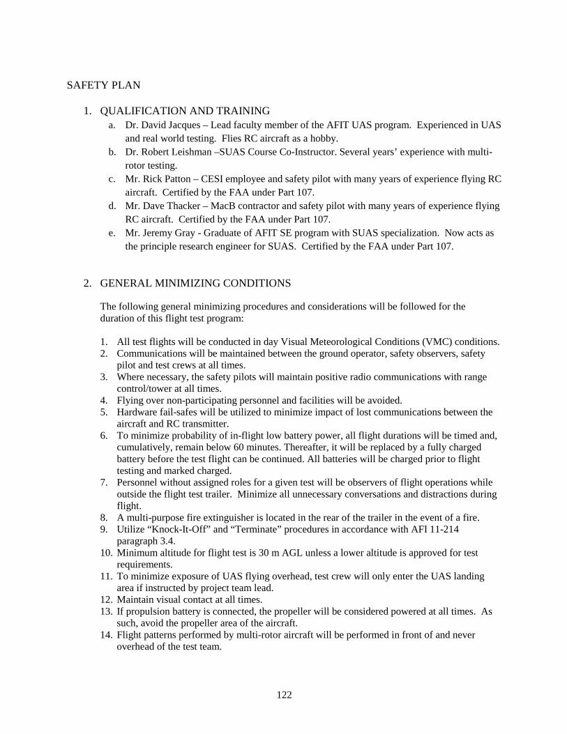
122
SAFETY PLAN
1. QUALIFICATION AND TRAINING a. Dr. David Jacques – Lead faculty member of the AFIT UAS program. Experienced in UAS
and real world testing. Flies RC aircraft as a hobby. b. Dr. Robert Leishman –SUAS Course Co-Instructor. Several years’ experience with multi-
rotor testing. c. Mr. Rick Patton – CESI employee and safety pilot with many years of experience flying RC
aircraft. Certified by the FAA under Part 107. d. Mr. Dave Thacker – MacB contractor and safety pilot with many years of experience flying
RC aircraft. Certified by the FAA under Part 107. e. Mr. Jeremy Gray - Graduate of AFIT SE program with SUAS specialization. Now acts as
the principle research engineer for SUAS. Certified by the FAA under Part 107.
2. GENERAL MINIMIZING CONDITIONS
The following general minimizing procedures and considerations will be followed for the duration of this flight test program:
1. All test flights will be conducted in day Visual Meteorological Conditions (VMC) conditions. 2. Communications will be maintained between the ground operator, safety observers, safety
pilot and test crews at all times. 3. Where necessary, the safety pilots will maintain positive radio communications with range
control/tower at all times. 4. Flying over non-participating personnel and facilities will be avoided. 5. Hardware fail-safes will be utilized to minimize impact of lost communications between the
aircraft and RC transmitter. 6. To minimize probability of in-flight low battery power, all flight durations will be timed and,
cumulatively, remain below 60 minutes. Thereafter, it will be replaced by a fully charged battery before the test flight can be continued. All batteries will be charged prior to flight testing and marked charged.
7. Personnel without assigned roles for a given test will be observers of flight operations while outside the flight test trailer. Minimize all unnecessary conversations and distractions during flight.
8. A multi-purpose fire extinguisher is located in the rear of the trailer in the event of a fire. 9. Utilize “Knock-It-Off” and “Terminate” procedures in accordance with AFI 11-214
paragraph 3.4. 10. Minimum altitude for flight test is 30 m AGL unless a lower altitude is approved for test
requirements. 11. To minimize exposure of UAS flying overhead, test crew will only enter the UAS landing
area if instructed by project team lead. 12. Maintain visual contact at all times. 13. If propulsion battery is connected, the propeller will be considered powered at all times. As
such, avoid the propeller area of the aircraft. 14. Flight patterns performed by multi-rotor aircraft will be performed in front of and never
overhead of the test team.

123
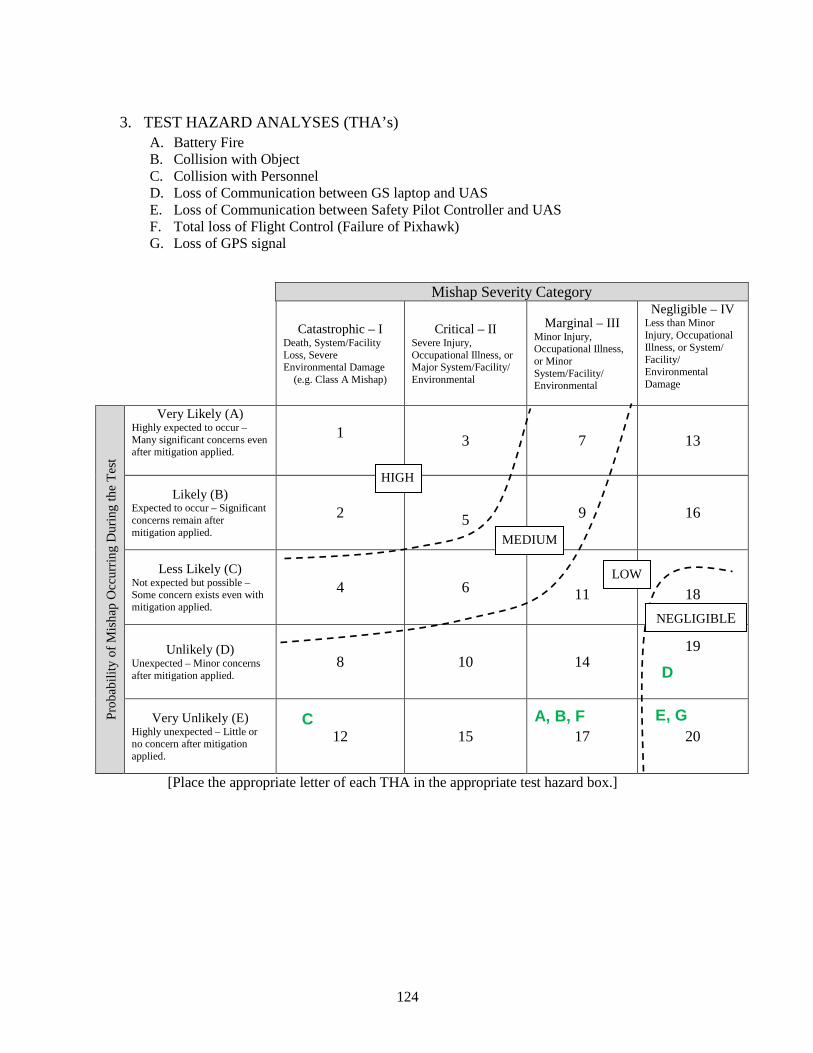
124
3. TEST HAZARD ANALYSES (THA’s) A. Battery Fire B. Collision with Object C. Collision with Personnel D. Loss of Communication between GS laptop and UAS E. Loss of Communication between Safety Pilot Controller and UAS F. Total loss of Flight Control (Failure of Pixhawk) G. Loss of GPS signal
[Place the appropriate letter of each THA in the appropriate test hazard box.]
Mishap Severity Category
Catastrophic – I Death, System/Facility Loss, Severe Environmental Damage
(e.g. Class A Mishap)
Critical – II Severe Injury, Occupational Illness, or Major System/Facility/ Environmental
Marginal – III Minor Injury, Occupational Illness, or Minor System/Facility/ Environmental
Negligible – IV Less than Minor Injury, Occupational Illness, or System/ Facility/ Environmental Damage
Prob
abili
ty o
f Mis
hap
Occ
urrin
g D
urin
g th
e Te
st
Very Likely (A) Highly expected to occur – Many significant concerns even after mitigation applied.
1 3 7 13
Likely (B) Expected to occur – Significant concerns remain after mitigation applied.
2
5 9 16
Less Likely (C) Not expected but possible –Some concern exists even with mitigation applied.
4 6
11
18
Unlikely (D) Unexpected – Minor concerns after mitigation applied.
8 10 14 19
Very Unlikely (E) Highly unexpected – Little or no concern after mitigation applied.
12 15 17 20
HIGH
MEDIUM
LOW
NEGLIGIBLE
A, B, F E, G
D
C

125
TEST HAZARD ANALYSIS (THA) Page 1/7 TEST SERIES MISHAP CAT/PROBABILITY
Pave Scout Tarot T960 Developmental/Operational Testing III/Very Unlikely PREPARED BY SIGNATURE Dr. David Jacques AFIT FLIGHT TEST SAFETY OFFICER SIGNATURE
Andrew Lingenfelter, Capt

126
HAZARD: Battery Fire CAUSE: 1. Uncontrolled discharge of power from the battery leading to overheating and fire (thermal runaway) 2. Overcharging of battery leading to thermal runaway due to charger malfunction or human input error 3. Battery circuitry or subsystem component failure or wiring malfunction 4. Battery puncture EFFECT: 1. Loss of UAS 2. Injury to personnel 3. High temperature, toxic fire
MINIMIZING PROCEDURES: 1. (1,2,3) All batteries will be placed in fireproof metal containers to prevent damage during transportation. 2. (1,2,3) All batteries will be charged using authorized battery chargers and by personnel trained in the
proper recharging techniques. Battery will be placed in fireproof pouch during charging. 3. (2) All batteries will be charged in approved locations while monitored and placed in fire proof pouches. 4. (1,2,3) Only the proper battery types for the specified aircraft will be used. 5. (1,2,3) Only authorized Electronic Speed Controllers (ESCs) for the specified battery size will be utilized. 6. (1,2,3) Load balancer will be used when charging flight batteries. 7. (2) Downed aircraft will be approached with caution due to the increased possibility of a battery fire. 8. (1,2,3) Damaged batteries will be safely stored away from other flammable items and within a fireproof
metal container.
CORRECTIVE ACTIONS: If the battery begins to smoke while charging:
1. Move battery in fireproof pouch outdoors. 2. Keep battery in fireproof pouch and place it on a hardened surface away from flammable objects.
If the battery catches fire during ground operations:
1. Announce battery fire and avoid toxic fumes created by the battery fire. 2. The person nearest to the fire extinguisher will use the fire extinguisher to put out the fire. 3. The person in communication with the field controller will notify the field controller of the emergency via
the radio.
If the battery catches fire while in flight:
1. Announce battery fire. 2. The pilot in command will immediately land the aircraft (make attempt to land on hard surface). 3. All personal will remain away from the aircraft until the safety pilot deems it safe to approach and put out
the fire with the fire extinguisher. 4. The person in communication with the field controller will notify the field controller of the emergency via
the radio.
MARKS: None

127
TEST HAZARD ANALYSIS (THA) Page 2/7 TEST SERIES MISHAP CAT/PROBABILITY
Pave Scout Tarot T960 Developmental/Operational Testing III/Very Unlikely PREPARED BY SIGNATURE Dr. David Jacques
AFIT FLIGHT TEST SAFETY OFFICER SIGNATURE
Andrew Lingenfelter, Capt

128
HAZARD: Collision with Object CAUSE: 1. Bird strike 2. Collision with other aircraft 3. Collision with ground based obstructions EFFECT:
1. Loss of UAS 2. Property damage
MINIMIZING PROCEDURES:
1. (1,2,3) Safety observers will be used to augment safety pilot. 2. (2) Communicate with the tower before testing to verify clear airspace. 3. (3) Identification of ground based obstructions (hazards) in area of operation before testing. 4. (3) Flight path will be adjusted in order to avoid ground based obstructions.
CORRECTIVE ACTIONS:
1. Announce collision with object. 2. Discontinue testing and verify there are no injuries. 3. Assess extent of damage. 4. Notify tower if hit or near miss with non-AFIT aircraft occurs. 5. Document exact damage with photos/video. 6. Follow mishap reporting procedures per section 3 of Project Description (page 2). 7. Examine and, if possible, repair the UAS. 8. If operational, perform a trim flight to verify functionality.
REMARKS: None
TEST HAZARD ANALYSIS (THA) Page 3/7 TEST SERIES MISHAP CAT/PROBABILITY
Pave Scout Tarot T960 Developmental/Operational Testing I/Very Unlikely PREPARED BY SIGNATURE
Dr. David Jacques AFIT FLIGHT TEST SAFETY OFFICER SIGNATURE

129
Andrew Lingenfelter, Capt
HAZARD: Collision with Personnel CAUSE: 1. Personnel interference during takeoff/landing 2. Loss of control of vehicle EFFECT:
1. Personnel injury 2. Loss of UAS
MINIMIZING PROCEDURES:
1. (1) Launch/landing area will be cleared of all nonessential personnel during these phases of flight and launch and recovery of the aircraft will be announced loudly to all personnel.
2. (1, 2) All personnel will maintain situational awareness of vehicle/flight status and personnel in and around the test area.
3. (2) Test crew will only enter the UAS landing strip upon instruction by project team lead.
CORRECTIVE ACTIONS:
1. Discontinue testing and assess extent of injuries. 2. Coordinated through installation emergency 911 service if injury is severe and requires emergency
services; perform any necessary first aid until help arrives. 3. Follow mishap reporting procedures per section 3 of Project Description (page 3). 4. Verify suitability of crew composition to carry on. 5. If suitable, examine and, if possible, repair the UAS. 6. If operational, perform a trim flight to ensure functionality.
REMARKS: None

130
TEST HAZARD ANALYSIS (THA) Page 4/7 TEST SERIES MISHAP CAT/PROBABILITY
Pave Scout Tarot T960 Developmental/Operational Testing IV/Unlikely PREPARED BY SIGNATURE
Dr. David Jacques AFIT FLIGHT TEST SAFETY OFFICER SIGNATURE
Andrew Lingenfelter, Capt

131
HAZARD: Loss of Communication between GS laptop and UAS CAUSE: 1. Signal interference 2. Onboard APM transmitter /receiver failure 3. GS transmitter /receiver failure 4. UAS flying out of range 5. Automatic waypoint algorithm overrides GS inputs EFFECT:
1. Vehicle spirals to ground 2. Unplanned off-field landing 3. Loss of control of aircraft
MINIMIZING PROCEDURES:
1. (1,2,3,5) Verify serviceability of communication equipment prior to test. Verify integrity of the antennae. Verify communication equipment batteries are adequately charged.
2. (4) Limit operation within maximum range of previously conducted test with same autopilot configuration. 3. (1,2,3,4) Lost link fail-safes (return to launch and loiter) will be pre-programmed. 4. (1,2,3,4) Separate communication system for safety pilot. 5. (2,3) Pre-flight checklist will be conducted.
CORRECTIVE ACTIONS:
1. Ground operator will immediately announce lost communications so the test team can help visually track the UAS.
2. Attempt to re-establish communications with the UAS. 3. If link cannot be re-established, switch to manual mode. 4. Safety pilot will land the UAS manually. 5. Examine and repair communication system. 6. Disable all scripts running on Ground Station when manual mode is selected by safety pilot.
REMARKS: None

132

133
TEST HAZARD ANALYSIS (THA) Page 5/7 TEST SERIES MISHAP CAT/PROBABILITY
Pave Scout Tarot T960 Developmental/Operational Testing IV/Very Unlikely PREPARED BY SIGNATURE
Dr. David Jacques AFIT FLIGHT TEST SAFETY OFFICER SIGNATURE
Andrew Lingenfelter, Capt

134
HAZARD: Loss of Communication between Safety Pilot Controller and UAS 1. Signal interference 2. Onboard RC transmitter /receiver failure 3. Safety Pilot controller transmitter /receiver failure 4. UAS flying out of range 5. Automatic waypoint algorithm overrides safety pilot inputs EFFECT:
1. Vehicle spirals to ground 2. Unplanned off-field landing 3. Loss of control of aircraft
MINIMIZING PROCEDURES:
1. (1,2,3,5) Verify serviceability of communication equipment prior to test. Verify integrity of the antennae. Verify communication equipment batteries are adequately charged.
2. (4) Limit operation within maximum range of previously conducted test using same RC configuration. 3. (1) Coordinate flight operations and frequencies with test range authorities. 4. (1,2,3,4) Lost link fail-safes (return to launch and loiter) will be pre-programmed. 5. (1,2,3) Separate communication system for auto pilot. 6. (2,3) Pre-flight checklist will be conducted.
CORRECTIVE ACTIONS:
1. Safety pilot will immediately announce lost communications so the test team can help visually track the UAS.
2. Attempt to re-establish communications with the UAS. 3. If link cannot be re-established, ground operator will set way points to return the UAS back to the launch
area. 4. Ground operator will initiate automatic landing from the GS. 5. Examine and repair communication system. 6. Disable all scripts running on Ground Station when manual mode is selected by safety pilot.
REMARKS: None
TEST HAZARD ANALYSIS (THA) Page 6/7
TEST SERIES Pave Scout Tarot T960 Developmental/Operational Testing
MISHAP CAT/PROBABILITY III/Very Unlikely
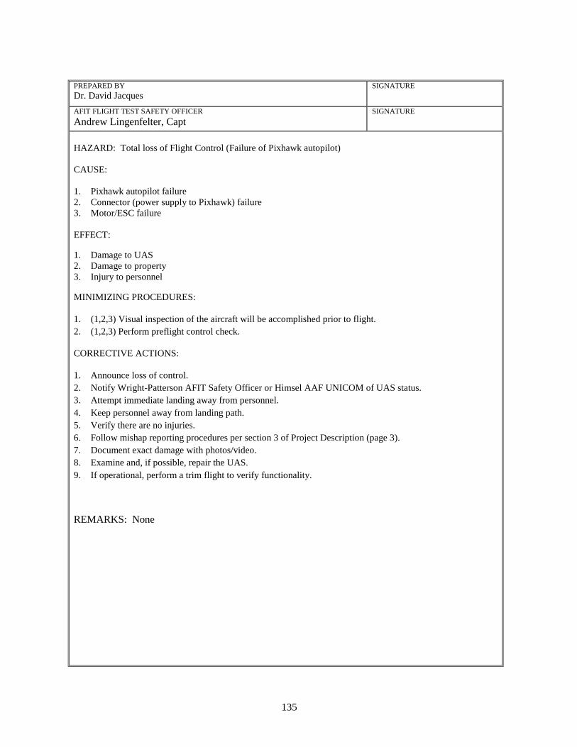
135
PREPARED BY Dr. David Jacques
SIGNATURE
AFIT FLIGHT TEST SAFETY OFFICER Andrew Lingenfelter, Capt
SIGNATURE
HAZARD: Total loss of Flight Control (Failure of Pixhawk autopilot) CAUSE: 1. Pixhawk autopilot failure 2. Connector (power supply to Pixhawk) failure 3. Motor/ESC failure EFFECT:
1. Damage to UAS 2. Damage to property 3. Injury to personnel
MINIMIZING PROCEDURES:
1. (1,2,3) Visual inspection of the aircraft will be accomplished prior to flight. 2. (1,2,3) Perform preflight control check.
CORRECTIVE ACTIONS:
1. Announce loss of control. 2. Notify Wright-Patterson AFIT Safety Officer or Himsel AAF UNICOM of UAS status. 3. Attempt immediate landing away from personnel. 4. Keep personnel away from landing path. 5. Verify there are no injuries. 6. Follow mishap reporting procedures per section 3 of Project Description (page 3). 7. Document exact damage with photos/video. 8. Examine and, if possible, repair the UAS. 9. If operational, perform a trim flight to verify functionality.
REMARKS: None
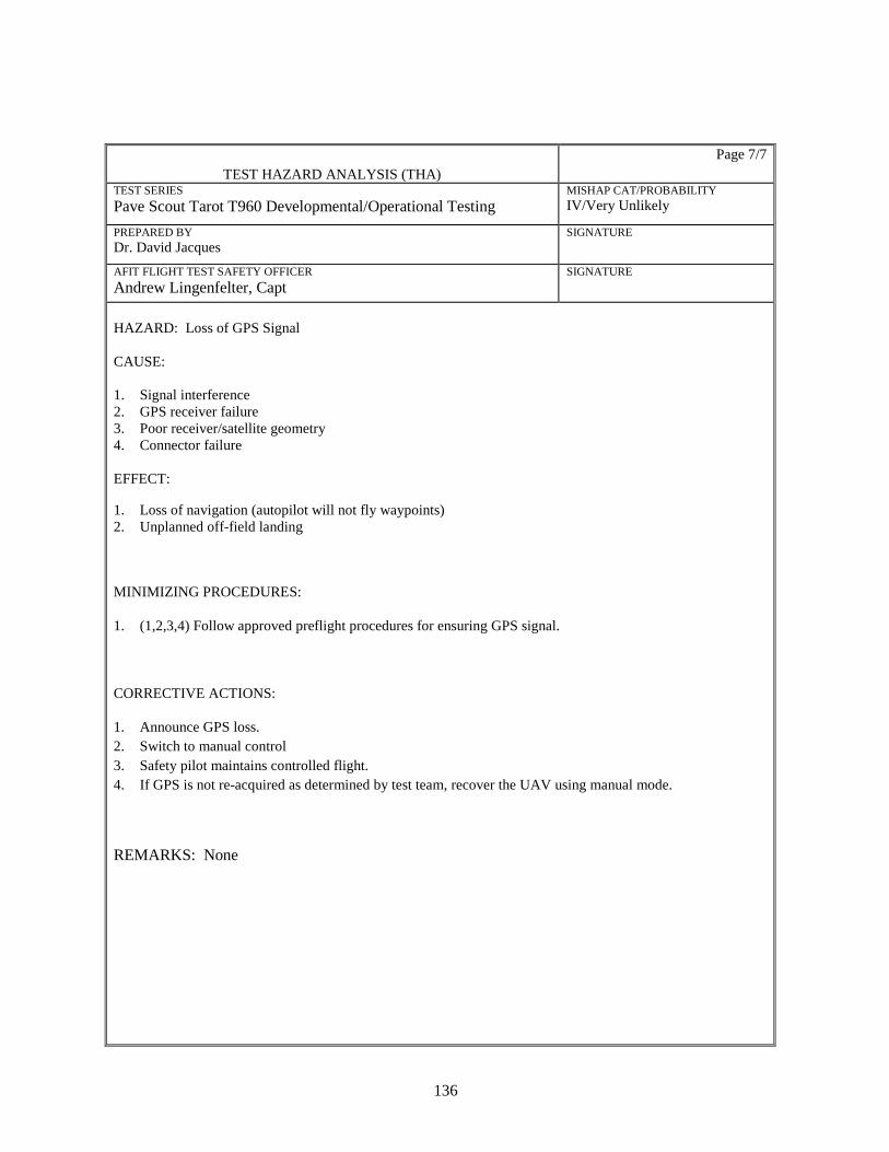
136
TEST HAZARD ANALYSIS (THA) Page 7/7
TEST SERIES Pave Scout Tarot T960 Developmental/Operational Testing
MISHAP CAT/PROBABILITY IV/Very Unlikely
PREPARED BY Dr. David Jacques
SIGNATURE
AFIT FLIGHT TEST SAFETY OFFICER Andrew Lingenfelter, Capt
SIGNATURE
HAZARD: Loss of GPS Signal CAUSE: 1. Signal interference 2. GPS receiver failure 3. Poor receiver/satellite geometry 4. Connector failure EFFECT:
1. Loss of navigation (autopilot will not fly waypoints) 2. Unplanned off-field landing
MINIMIZING PROCEDURES:
1. (1,2,3,4) Follow approved preflight procedures for ensuring GPS signal.
CORRECTIVE ACTIONS:
1. Announce GPS loss. 2. Switch to manual control 3. Safety pilot maintains controlled flight. 4. If GPS is not re-acquired as determined by test team, recover the UAV using manual mode.
REMARKS: None
137
AFTER ACTION REPORT Per ENOI 91-6, the After Action Report should be submitted to the FTSO no later than 7 calendar days from the completion of the test.
1. Use this section to briefly describe how the test was carried out. Were there any unusual
events?
• The test went as planned. But the test required charging the battery each runs as the flight time required more battery consumption due to the flight plan and wind effect.
• Comm status was degraded when the vehicle flew away above 50meter, so the test
parameter was modified from 50, and 90meter to 25, and 50 meter to maintain the Comm’ connection.
2. What test execution/safety lessons were learned during the test event?
• The test data showed the Hex-rotor platform looks satisfied performance to collecting imagery data in terms of the geo-locational accuracy, imagery visual quality, and data reliability.
• The gimbal control command, “Set_ROI”, was successfully control that the autopilot enable to point to the point of interest. Therefore, the command is expected to control either the gimbal or autopilot once the gimbal hook up to the Pixhawk.
• T-log data was not successfully saved in mission planner, so the geotag data was not able to extract from t-log. But, the Data-flash log in the Pixhawk had a full log data including camera shooting data and can be downloaded by USB cable to ground station.
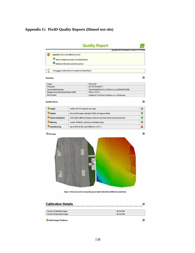
138
Appendix G: Pix4D Quality Reports (Himsel test site)
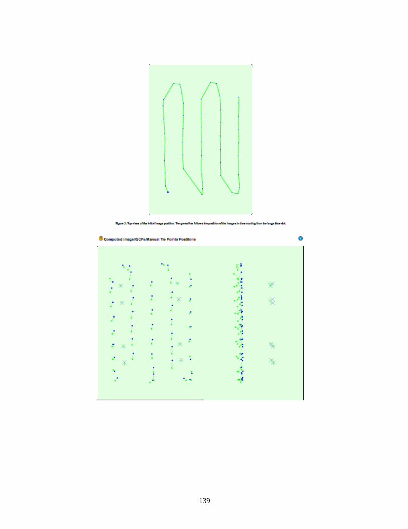
139
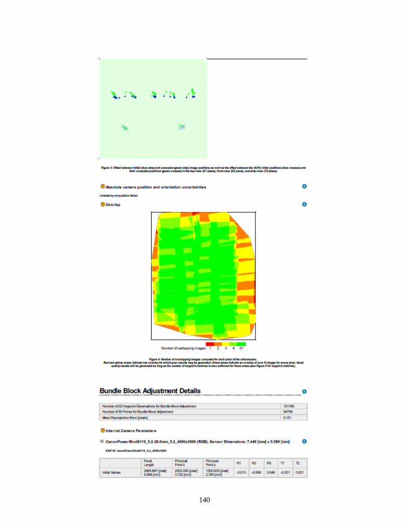
140
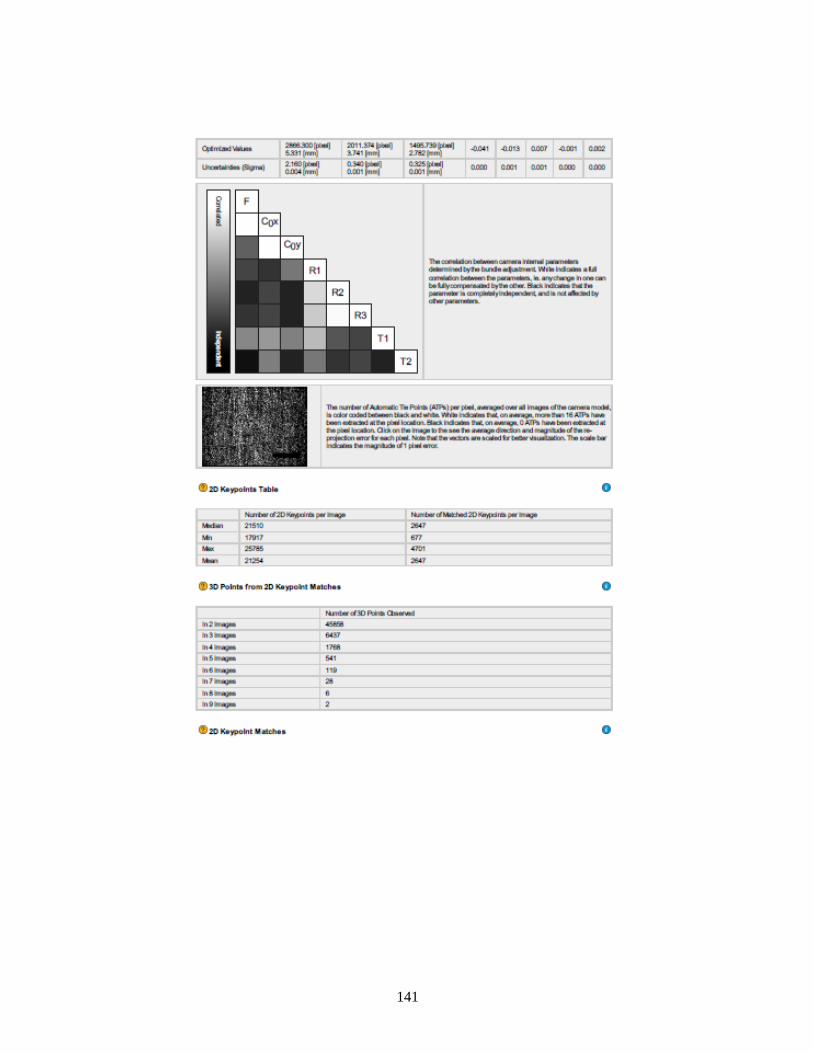
141
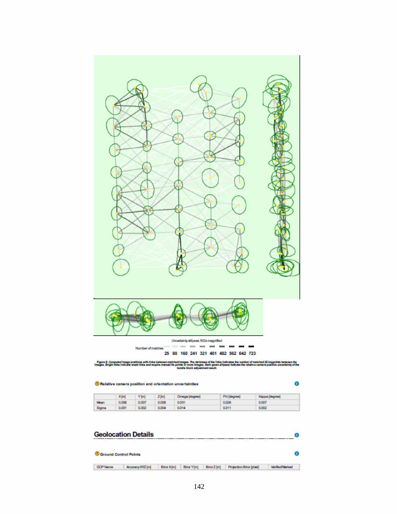
142
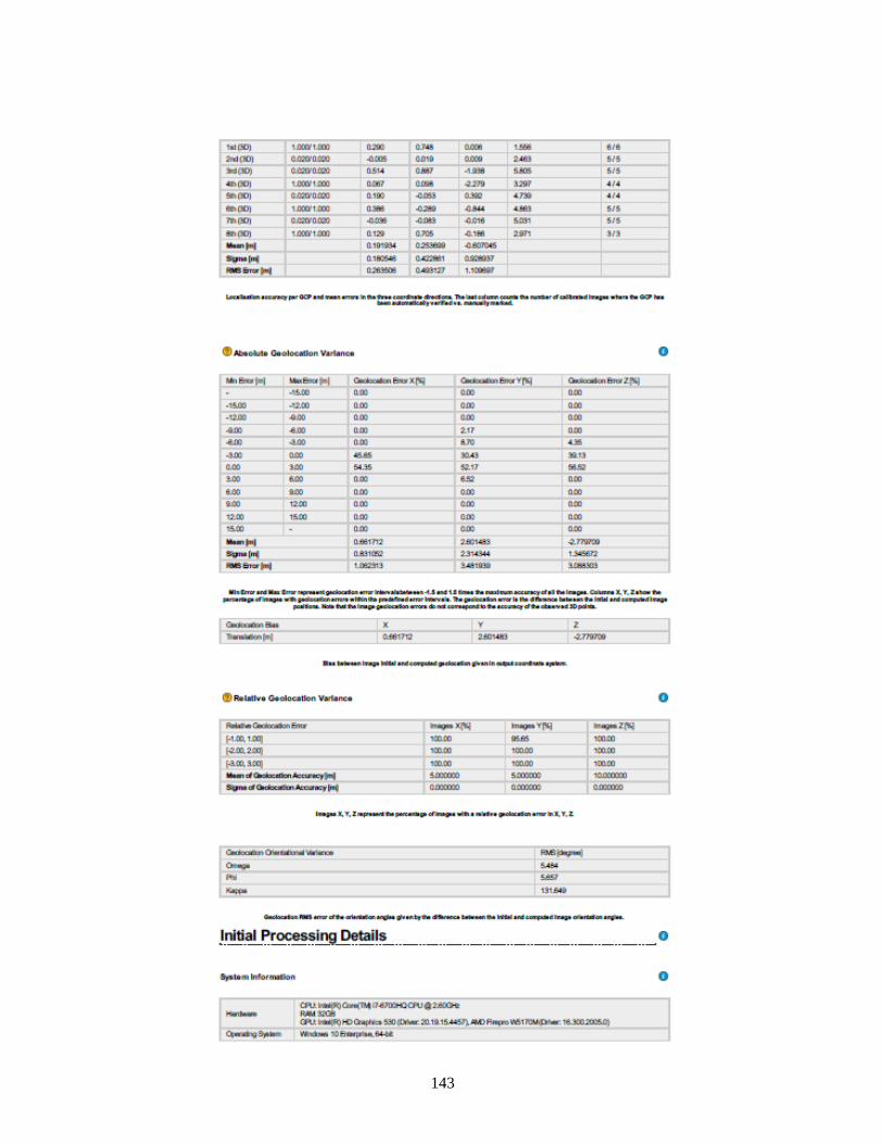
143
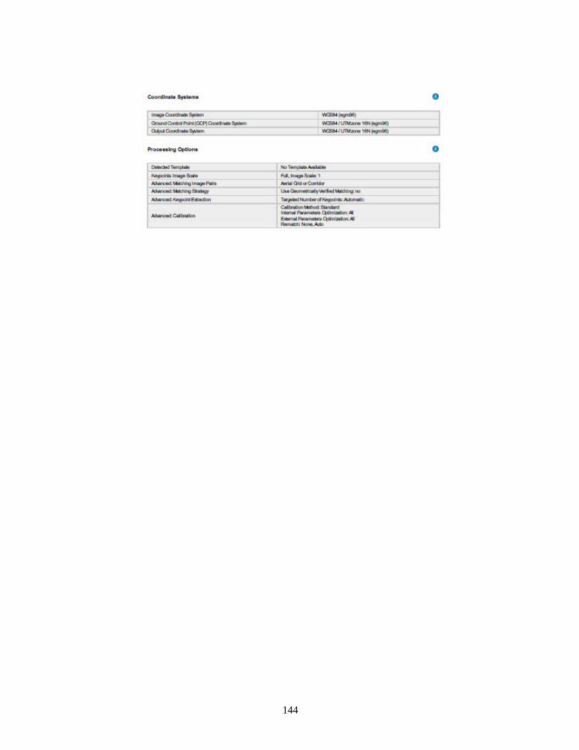
144

145
Appendix H: Pix4D Quality Reports (Runaway damage assessment project)
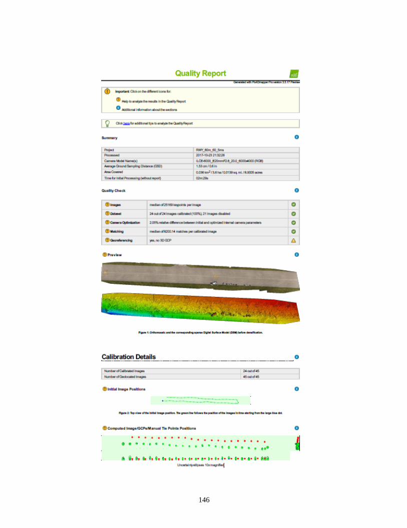
146
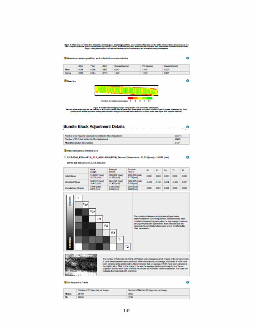
147
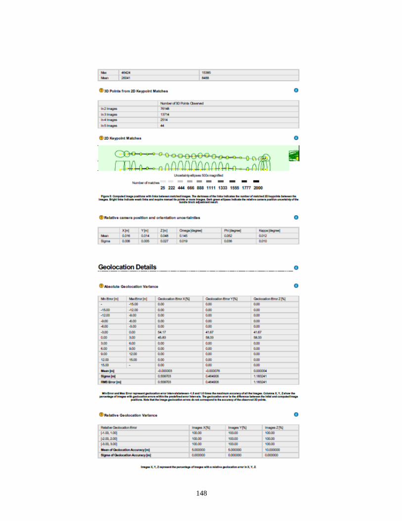
148
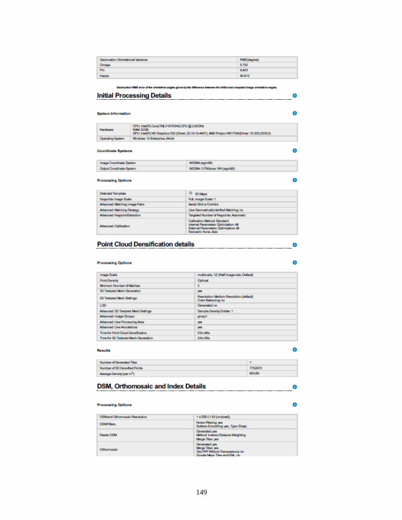
149

150
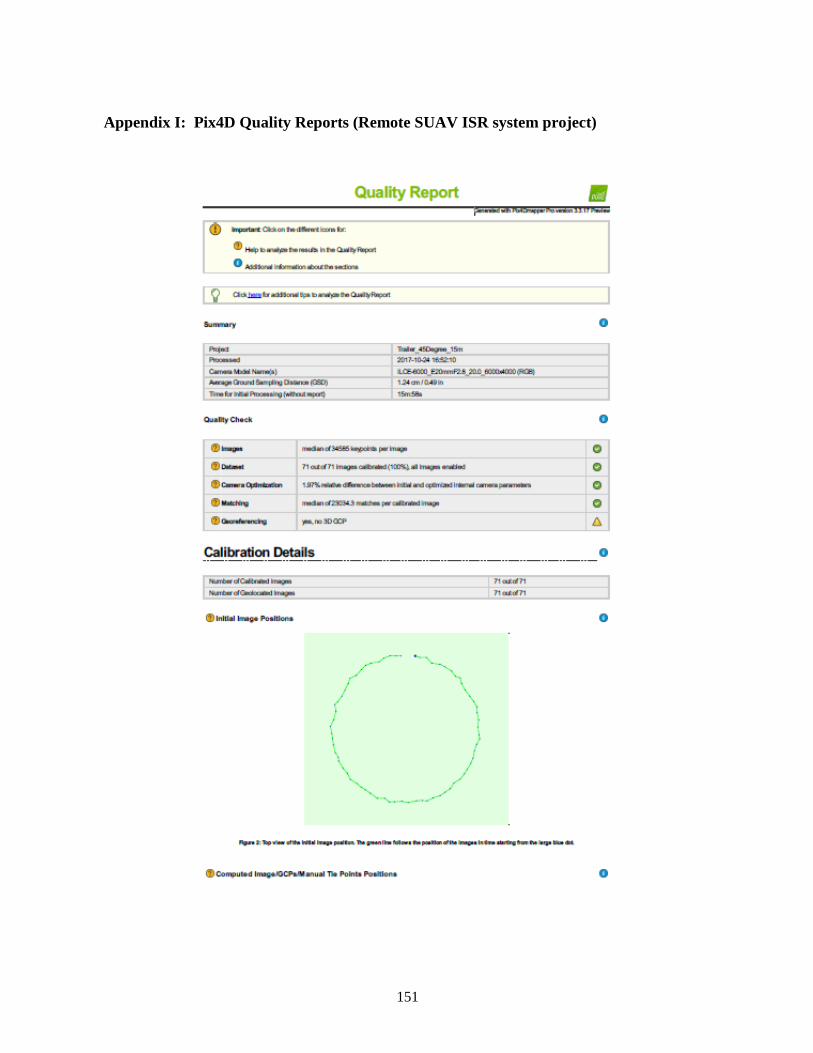
151
Appendix I: Pix4D Quality Reports (Remote SUAV ISR system project)
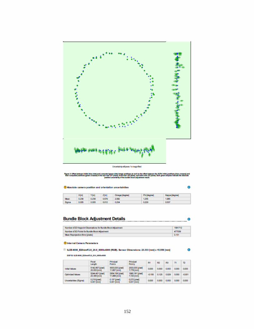
152
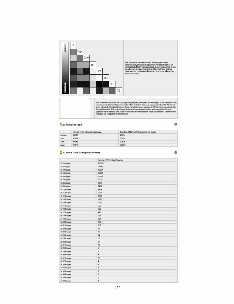
153
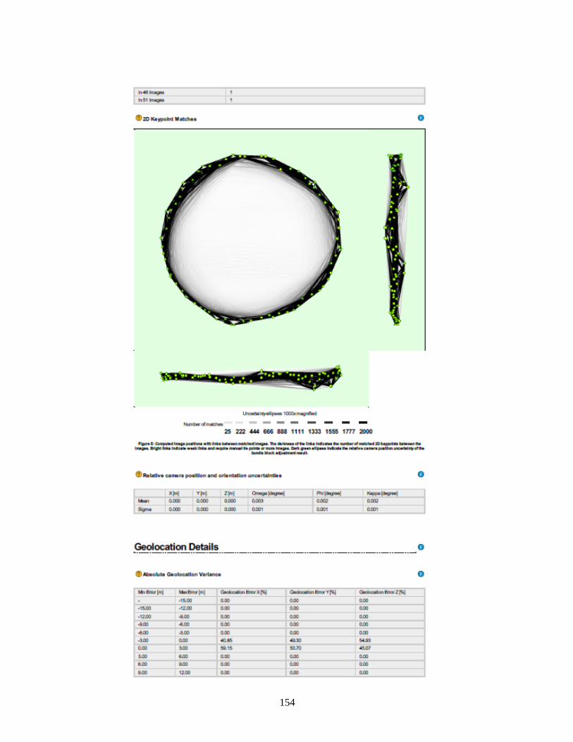
154
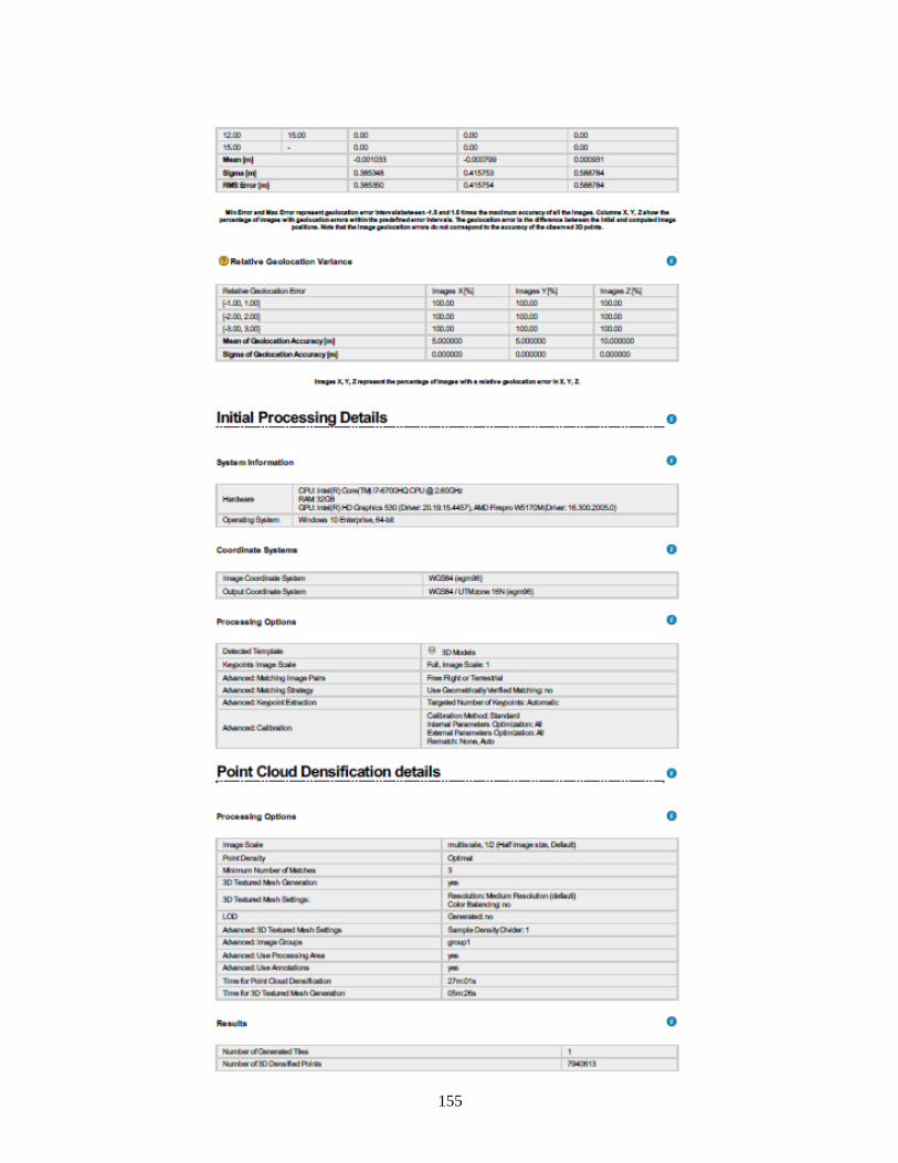
155
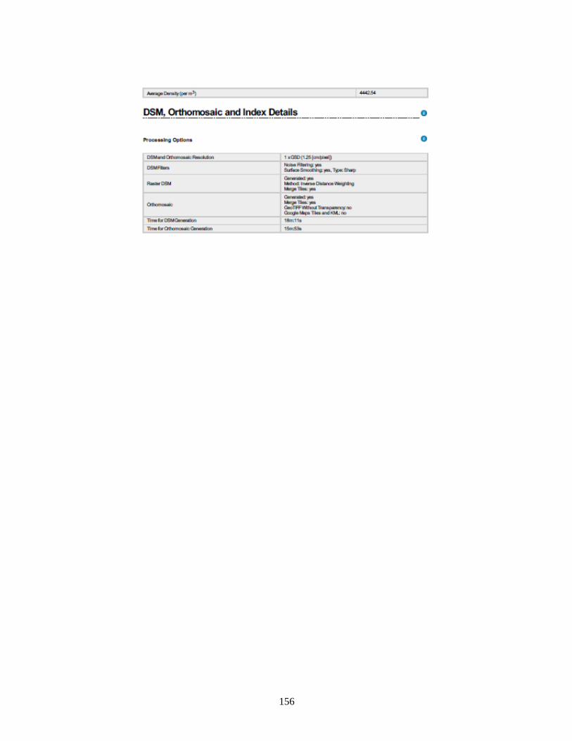
156
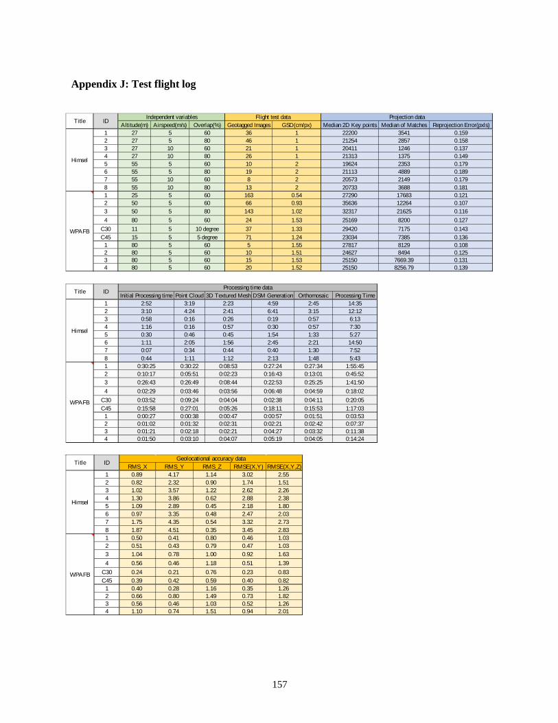
157
Appendix J: Test flight log
Altitude(m) Airspeed(m/s) Overlap(%) Geotagged Images GSD(cm/px) Median 2D Key points Median of Matches Reprojection Error(pxls)1 27 5 60 36 1 22200 3541 0.1592 27 5 80 46 1 21254 2857 0.1583 27 10 60 21 1 20411 1246 0.1374 27 10 80 26 1 21313 1375 0.1495 55 5 60 10 2 19624 2353 0.1796 55 5 80 19 2 21113 4889 0.1897 55 10 60 8 2 20573 2149 0.1798 55 10 80 13 2 20733 3688 0.1811 25 5 60 163 0.54 27290 17683 0.1212 50 5 60 66 0.93 35636 12264 0.1073 50 5 80 143 1.02 32317 21625 0.1164 80 5 60 24 1.53 25169 8200 0.127
C30 11 5 10 degree 37 1.33 29420 7175 0.143C45 15 5 5 degree 71 1.24 23034 7385 0.136
1 80 5 60 5 1.55 27817 8129 0.1082 80 5 60 10 1.51 24627 8494 0.1253 80 5 60 15 1.53 25150 7669.39 0.1314 80 5 60 20 1.52 25150 8256.79 0.139
WPAFB
ID Independent variables Flight test dataTitle
Himsel
Projection data
Initial Processing time Point Cloud 3D Textured Mesh DSM Generation Orthomosaic Processing Time1 2:52 3:19 2:23 4:59 2:45 14:352 3:10 4:24 2:41 6:41 3:15 12:123 0:58 0:16 0:26 0:19 0:57 6:134 1:16 0:16 0:57 0:30 0:57 7:305 0:30 0:46 0:45 1:54 1:33 5:276 1:11 2:05 1:56 2:45 2:21 14:507 0:07 0:34 0:44 0:40 1:30 7:528 0:44 1:11 1:12 2:13 1:48 5:431 0:30:25 0:30:22 0:08:53 0:27:24 0:27:34 1:55:452 0:10:17 0:05:51 0:02:23 0:16:43 0:13:01 0:45:523 0:26:43 0:26:49 0:08:44 0:22:53 0:25:25 1:41:504 0:02:29 0:03:46 0:03:56 0:06:48 0:04:59 0:18:02
C30 0:03:52 0:09:24 0:04:04 0:02:38 0:04:11 0:20:05C45 0:15:58 0:27:01 0:05:26 0:18:11 0:15:53 1:17:03
1 0:00:27 0:00:38 0:00:47 0:00:57 0:01:51 0:03:532 0:01:02 0:01:32 0:02:31 0:02:21 0:02:42 0:07:373 0:01:21 0:02:18 0:02:21 0:04:27 0:03:32 0:11:384 0:01:50 0:03:10 0:04:07 0:05:19 0:04:05 0:14:24
Processing time data
WPAFB
IDTitle
Himsel
RMS_X RMS_Y RMS_Z RMSE(X,Y) RMSE(X,Y,Z)1 0.89 4.17 1.14 3.02 2.552 0.82 2.32 0.90 1.74 1.513 1.02 3.57 1.22 2.62 2.264 1.30 3.86 0.62 2.88 2.385 1.09 2.89 0.45 2.18 1.806 0.97 3.35 0.48 2.47 2.037 1.75 4.35 0.54 3.32 2.738 1.87 4.51 0.35 3.45 2.831 0.50 0.41 0.80 0.46 1.032 0.51 0.43 0.79 0.47 1.033 1.04 0.78 1.00 0.92 1.634 0.56 0.46 1.18 0.51 1.39
C30 0.24 0.21 0.76 0.23 0.83C45 0.39 0.42 0.59 0.40 0.82
1 0.40 0.28 1.16 0.35 1.262 0.66 0.80 1.49 0.73 1.823 0.56 0.46 1.03 0.52 1.264 1.10 0.74 1.51 0.94 2.01
Geolocational accuracy data
WPAFB
IDTitle
Himsel
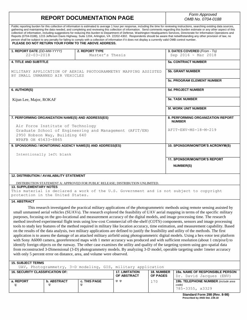
REPORT DOCUMENTATION PAGE Form Approved OMB No. 0704-0188
Public reporting burden for this collection of information is estimated to average 1 hour per response, including the time for reviewing instructions, searching existing data sources, gathering and maintaining the data needed, and completing and reviewing this collection of information. Send comments regarding this burden estimate or any other aspect of this collection of information, including suggestions for reducing this burden to Department of Defense, Washington Headquarters Services, Directorate for Information Operations and Reports (0704-0188), 1215 Jefferson Davis Highway, Suite 1204, Arlington, VA 22202-4302. Respondents should be aware that notwithstanding any other provision of law, no person shall be subject to any penalty for failing to comply with a collection of information if it does not display a currently valid OMB control number. PLEASE DO NOT RETURN YOUR FORM TO THE ABOVE ADDRESS.
1. REPORT DATE (DD-MM-YYYY) 22-03-2018
2. REPORT TYPE Master’s Thesis
3. DATES COVERED (From - To)
Sep 2016 ~ Mar 2018
4. TITLE AND SUBTITLE
5a. CONTRACT NUMBER
MILITARY APPLICATION OF AERIAL PHOTOGRAMMETRY MAPPING ASSISTED
BY SMALL UNMANNED AIR VEHICLES
5b. GRANT NUMBER
5c. PROGRAM ELEMENT NUMBER
6. AUTHOR(S)
5d. PROJECT NUMBER
Kijun Lee, Major, ROKAF
5e. TASK NUMBER
5f. WORK UNIT NUMBER
7. PERFORMING ORGANIZATION NAME(S) AND ADDRESS(ES) AND ADDRESS(ES)
8. PERFORMING ORGANIZATION REPORT NUMBER
Air Force Institute of Technology
Graduate School of Engineering and Management (AFIT/EN)
2950 Hobson Way, Building 640
WPAFB OH 45433-8865
AFIT-ENV-MS-18-M-219
9. SPONSORING / MONITORING AGENCY NAME(S) AND ADDRESS(ES) 10. SPONSOR/MONITOR’S ACRONYM(S)
Intentionally left blank
11. SPONSOR/MONITOR’S REPORT
NUMBER(S)
12. DISTRIBUTION / AVAILABILITY STATEMENT
DISTRIBUTION STATEMENT A: APPROVED FOR PUBLIC RELEASE; DISTRIBUTION UNLIMITED.
13. SUPPLEMENTARY NOTES This material is declared a work of the U.S. Government and is not subject to copyright
protection in the United States.
14. ABSTRACT
This research investigated the practical military applications of the photogrammetric methods using remote sensing assisted by
small unmanned aerial vehicles (SUAVs). The research explored the feasibility of UAV aerial mapping in terms of the specific military
purposes, focusing on the geo-locational and measurement accuracy of the digital models, and image processing time. The research
method involved experimental flight tests using low-cost Commercial off-the-shelf (COTS) components, sensors and image processing
tools to study key features of the method required in military like location accuracy, time estimation, and measurement capability. Based
on the results of the data analysis, two military applications are defined to justify the feasibility and utility of the methods. The first
application is to assess the damage of an attacked military airfield using photogrammetric digital models. Using a hex-rotor test platform
with Sony A6000 camera, georeferenced maps with 1 meter accuracy was produced and with sufficient resolution (about 1 cm/pixel) to
identify foreign objects on the runway. The other case examines the utility and quality of the targeting system using geo-spatial data
from reconstructed 3-Dimensional (3-D) photogrammetry models. By analyzing 3-D model, operable targeting under 1meter accuracy
with only 5 percent error on distance, area, and volume were observed.
15. SUBJECT TERMS UAV, Photogrammetry, 3-D modeling, GIS, military application
16. SECURITY CLASSIFICATION OF:
17. LIMITATION OF ABSTRACT
18. NUMBER OF PAGES
19a. NAME OF RESPONSIBLE PERSON Dr. David Jacques (ENV)
a. REPORT U
b. ABSTRACT U
c. THIS PAGE U
U U 170
19b. TELEPHONE NUMBER (include area
code) 785-3355, x3329
Standard Form 298 (Rev. 8-98) Prescribed by ANSI Std. Z39.18