MILES: Multiple-Instance Learning via Embedded Instance Selection

MILES: Multiple-Instance Learningvia Embedded Instance Selection

Yixin Chen, Member, IEEE, Jinbo Bi, Member, IEEE, and James Z. Wang, Senior Member, IEEE

Abstract—Multiple-instance problems arise from the situations where training class labels are attached to sets of samples (named

bags), instead of individual samples within each bag (called instances). Most previous multiple-instance learning (MIL) algorithms are

developed based on the assumption that a bag is positive if and only if at least one of its instances is positive. Although the assumption

works well in a drug activity prediction problem, it is rather restrictive for other applications, especially those in the computer vision area.

We propose a learning method, MILES (Multiple-Instance Learning via Embedded instance Selection), which converts the multiple-

instance learning problem to a standard supervised learning problem that does not impose the assumption relating instance labels to bag

labels. MILES maps each bag into a feature space defined by the instances in the training bags via an instance similarity measure. This

feature mapping often provides a large number of redundant or irrelevant features. Hence, 1-norm SVM is applied to select important

features as well as construct classifiers simultaneously. We have performed extensive experiments. In comparison with other methods,

MILES demonstrates competitive classification accuracy, high computation efficiency, and robustness to labeling uncertainty.

Index Terms—Multiple-instance learning, feature subset selection, 1-norm support vector machine, image categorization, object

recognition, drug activity prediction.

Ç

1 INTRODUCTION

MULTIPLE-INSTANCE learning (MIL) was introduced byDietterich et al. [19] in the context of drug activity

prediction. It provides a framework to handle the scenarioswhere training class labels are naturally associated with setsof samples, instead of individual samples. In recent years, avariety of learning problems (e.g., drug activity prediction[19], [35], stock market prediction [36], data mining applica-tions [46], image retrieval [56], [60], natural scene classifica-tion [37], text categorization [2], and image categorization[16]) have been tackled as multiple-instance problems.

1.1 Multiple-Instance Problems

A multiple-instance problem involves ambiguous trainingexamples: A single example is represented by several featurevectors (instances), some of which may be responsible for theobserved classification of the example; yet, the training labelis only attached to the example instead of the instances. Themultiple-instance problem was formally introduced in thecontext of drug activity prediction [19], while a similar type oflearning scenario was first proposed in [13].

The goal of drug activity prediction is to foretell thepotency of candidate drug molecules by analyzing a collec-tion of previously synthesized molecules whose potencies arealready known. The potency of a drug molecule is determined

by the degree to which it binds to a site of medical interest onthe target protein. The three-dimensional structure of a drugmolecule decides principally the binding strength: A drugmolecule binds to the target protein if the shape of themolecule conforms closely to the structure of the binding site.Unfortunately, a molecule can adopt a wide range of shapesby rotating some of its internal bonds. Therefore, without theknowledge of the three-dimensional structure of the targetprotein, which is in general not available, knowing that apreviously-synthesized molecule binds to the target proteindoes not directly provide the binding information on theshapes of the molecule. For the multiple-instance problem in[19], training examples are molecules (named bags [35]). Abag contains several shapes, called instances, of the molecule.A label of binding or not binding is attached to each training baginstead of its instances. The goal is to learn the concept ofbinding, hence, to predict whether a new bag, i.e., a new drugmolecule, binds to the target protein. Note that a bag is amultiset in that the order of the instances is ignored; yet, themultiplicity is explicitly significant, i.e., a bag may containidentical instances.

Far beyond the drug activity prediction problem, themultiple-instance problem emerges naturally in a variety ofchallenging learning problems in computer vision, includingnatural scene classification [37], content-based image retrie-val [34], [56], [60], [15], image categorization [6], [32], [16],and object detection and recognition [40], [1], [21], [20], [45],[40], [42], [5]. Generally speaking, the goal of all theseproblems is to learn visual concepts from labeled images.The multiple-instance situation arises in these learningproblems because of the choice of image representation. Asingle image in [37], [56], [60] is represented by a collection offixed-size blocks. In [16], an image is characterized byregions obtained from image segmentation. In [1], [21], [20],[45], [17], [42], [5], an image is described by a set of patchesinvariant to certain geometric transformations. These imagepatches are typically generated by salient region detectors

IEEE TRANSACTIONS ON PATTERN ANALYSIS AND MACHINE INTELLIGENCE, VOL. 28, NO. 12, DECEMBER 2006 1931

. Y. Chen is with the Department of Computer and Information Science,University of Mississippi, 201 Weir Hall, University, MS 38677.E-mail: [email protected].

. J. Bi is with Computer Aided Diagnosis and Therapy Solutions, SiemensMedical Solutions, Inc., MS51, 51 Valley Stream Parkway, Malvern, PA19355. E-mail: [email protected].

. J.Z. Wang is with the College of Information Sciences and Technology andthe Department of Computer Science and Engineering, The PennsylvaniaState University, University Park, PA 16802. E-mail: [email protected].

Manuscript received 6 Oct. 2005; revised 1 Mar. 2006; accepted 13 Apr. 2006;published online 12 Oct. 2006.Recommended for acceptance by Z. Ghahramani.For information on obtaining reprints of this article, please send e-mail to:[email protected], and reference IEEECS Log Number TPAMI-0544-1005.

0162-8828/06/$20.00 � 2006 IEEE Published by the IEEE Computer Society

[27], interest point detectors [38], and edge-based detectors[52]. In all of the previously mentioned learning problems,training labels are attached to images instead of the blocks,regions, or patches contained in the images. These learningproblems match squarely with the bag-of-instances model:An image is a bag that contains instances corresponding toblocks, regions, or patches; instance labels are only indirectlyaccessible through the labels attached to bags.

1.2 Previous Work Related to Multiple-InstanceLearning

One of the earliest algorithms for learning from multiple-instance examples was developed by Dietterich et al. [19] fordrug activity prediction. The key assumption of their MILformulation is that: A bag is positive if at least one of itsinstances is a positive example; otherwise, the bag is negative.Their algorithm, named the axis-parallel rectangle (APR)method [19], attempts to find an APR by expanding orshrinking a hyperrectangle in the instance feature space tomaximize the number of instances from different positivebags enclosed by the rectangle while minimizing the numberof instances from negative bags within the rectangle. A bag isclassified as positive if at least one of its instances falls withinthe APR;otherwise, the bagisclassifiedasnegative.Anumberof theoretical results have been obtained following the APRframework [4], [10], [33]. De Raedt showed the connectionbetween MIL and inductive logic programming [18].

The basic idea of APR was extended in different ways thatled to several MIL algorithms. Maron and Lozano-Perez [35]proposed a general framework, named diverse density (DD),which has been tested on applications including stock marketprediction [36], natural scene classification [37], and content-based image retrieval [56], [60]. Diverse density measures aco-occurrence of similar instances from different positivebags. The desired concept is learned by maximizing theDD function. Zhang and Goldman [61] combined the idea ofexpectation-maximization (EM) with DD and developed analgorithm, EM-DD, to search for the most likely concept.Andrews et al. [2] formulated MIL as a mixed integerquadratic program. Integer variables are selector variablesthat select a positive instance from each positive bag. Theiralgorithm, which is called MI-SVM, has an outer loop and aninner loop. The outer loop sets the values of the selectorvariables. The inner loop then trains a standard supportvector machine, SVM, in which the selected positive instancesreplace the positive bags. Later, Andrews and Hofmann [3]developed an algorithm based on a generalization of linearprogramming boosting. Ramon and De Raedt presented aneural networks framework for MIL [43]. A similar methodhas been derived in [59]. Wang and Zucker [53] presented twovariants of the k-nearest neighbor algorithm (Bayesian-kNNand Citation-kNN) using Hausdorff distance. Zhou andZhang [63] proposed ensembles of multi-instance learners,which achieved competitive test results on the benchmarkdata sets of drug activity prediction.

All the above MIL formulations explicitly or implicitlyencode the assumption that a bag is positive if and only if atleast one of its instances is positive. The assumption is valid indrug activity prediction. Typically, there is a single shape thatallows binding; hence, it is natural to relate the instance labelsto the bag label through a disjunction (or a soft disjunction)function. However, for applications such as object recogni-tion, a negative bag (e.g., a background image without the

object of interest) may also contain instances that look similarto parts of the object. In other words, if a positive instance labelindicates that the instance appears to be part of the object, anegative bag may contain positive instances as well. Severalalgorithms have been proposed to tackle this type of situation.Scott et al. [47] developed a method in which a bag is positiveif and only if it contains a collection of instances, each near oneof a set of target points. In [60], Zhang et al. observed that theaverage prediction of a collection of classifiers, constructedfrom the EM-DD algorithm with different starting points, isusually more accurate than the prediction given by anyindividual classifier in a content-based image retrievalexperiment. Chen and Wang [16] proposed a MIL framework,DD-SVM, which, instead of taking the average prediction ofclassifiers built from the EM-DD, trains an SVM in a featurespace constructed from a mapping defined by the localmaximizers and minimizers of the DD function. Through thefeature mapping, DD-SVM essentially converts MIL to astandard supervised learning problem.

There is an abundance of prior work that uses standardsupervised learning techniques to solve multiple-instanceproblems. Zucker and Chevaleyre [65] applied decision treesand decision rules to a generalized multiple-instance pro-blem. Gartner et al. [22] designed a kernel for multiple-instance data. Hence, SVMs can be learned directly from thetraining bags. Xu and Frank [58] proposed logistic regressionand boosting approaches for MIL with the assumption that allinstances contribute equally and independently to a bag’slabel. Weidmann et al. [55] introduced a two-level learningframework in which a bag is transformed into a meta-instancethat can be learned by a propositional method. In a recentwork [44], Ray and Craven compared several MIL methodswith their supervised counterparts. They observed thatalthough some MIL methods consistently outperformed theirsupervised counterparts, in several domains, a supervisedalgorithm gave the best performance among all the MILalgorithms they tested.

In the area of computer vision, several standard super-vised learning techniques have been adapted for objectdetection and recognition where the underlying learningproblems are essentially the multiple-instance problem [1],[21], [17], [42], [5]. Fergus et al. [21] presented a generativeapproach to learning and recognizing an object class fromimages. Each image (bag) is represented as a collection ofimage patches (instances) produced by a scale invariantdetector [26]. An object is modeled as a group of patches,which are assumed to be generated by a probabilistic model.The model is estimated by maximizing the likelihoodfunction using the EM technique. Agarwal and Roth [1]described a discriminative approach for object detection. Avocabulary of object parts is constructed from a set of sampleimages. The multiple-instance representation of each image isthen transformed to a binary feature vector based on thevocabulary. Each binary feature indicates whether or not apart or relation occurs in the image. The classifier is learnedusing the Sparse Network of Winnows (SNoW) framework.Csurka et al. [17] proposed an object categorization methodusing the bag-of-keypoints model, which is identical to thebag-of-instances model. An image is represented by acollection of affine invariant patches. Vector quantization isapplied to the descriptors of all image patches to generate apredetermined number of clusters. Each image is thentransformed to an integer-valued feature vector indicating

1932 IEEE TRANSACTIONS ON PATTERN ANALYSIS AND MACHINE INTELLIGENCE, VOL. 28, NO. 12, DECEMBER 2006

the number of patches assigned to each cluster. Classifiers areimplemented as Naive Bayes and SVM. Opelt et al. [42]described a boosting approach to object detection where, ateach iteration, the weak hypothesis finder selects one localimage patch and one type of local descriptor. Bar-Hillel et al.[5] proposed a boosting technique that learns a generativeobject model in a discriminative manner.

1.3 An Overview of Our Approach

The approach we take to tackle the multiple-instance problemfurther extends ideas from the diverse density framework[35], [16] and the wrapper model in feature selection [29]. Ourapproach identifies instances that are relevant to the observedclassification by embedding bags into an instance-basedfeature space and selecting the most important features. Wedefine a similarity measure between a bag and an instance.The coordinates of a given bag in the feature space representthe bag’s similarities to various instances in the training set.The embedding produces a possibly high-dimensional spacewhen the number of instances in the training set is large. Inaddition, many features may be redundant or irrelevantbecause some of the instances might not be responsible for theobserved classification of the bags, or might be similar to eachother. It is essential and indispensable to select a subset ofmapped features that is most relevant to the classificationproblem of interest. Although any feature selectionapproaches could be applied for this purpose, we choose ajoint approach that constructs classifiers and selects impor-tant features simultaneously. Specifically, we use the 1-normSVM method because of its excellent performance in manyapplications [8], [64]. Since each feature is defined by aninstance, feature selection is essentially instance selection.Therefore, we name our approach MILES, Multiple-InstanceLearning via Embedded instance Selection.

The proposed approach has the following characteristics:

. Broad adaptability: It provides a learning frameworkthat converts a multiple-instance problem to asupervised learning problem. It demonstrates highlycompetitive classification accuracy in our empiricalstudies using benchmark data sets from differentapplication areas. Moreover, in comparison with theDD-SVM algorithm [16], the proposed approach isless sensitive to the class label uncertainties.

. Low complexity: It is efficient in computationalcomplexity, therefore, can potentially be tailored totasks that have stringent time or resource limits.According to our empirical studies, the learningprocess of the proposed approach is on average oneorder of magnitude faster than that of the algorithmsdescribed in [21] and [16].

. Prediction capability: In some multiple-instanceproblems, classification of instances is at least asimportant as the classification of bags. The proposedapproach supports instance naming, i.e., predictinginstance labels. This is in contrast to the methodsdescribed in [53], [16], [17], [42].

1.4 Outline of the Paper

The remainder of the paper is organized as follows:Section 2 describes an instance-based embedding of bagsthat transforms every bag to a uniform representation.Section 3 is dedicated to the description of a joint featureselection and classification method using a 1-norm SVM. A

concrete 1-norm SVM formulation is presented. Section 4

provides an algorithmic view of the approach. In Section 5,

we explain the extensive experimental studies conducted

and demonstrate the results. We conclude and discuss

possible future work in Section 6.

2 INSTANCE-BASED EMBEDDING OF BAGS

We introduce the instance-based embedding in this section.

Before discussing the mathematical definition of the

mapping, we first give a brief review of the diverse density

framework based on [36], [35] which forms the conceptual

basis of the instance-based feature mapping. We denote

positive bags as Bþi and the jth instance in that bag as xþij.

The bag Bþi consists of nþi instances xþij, j ¼ 1; � � � ; nþi .

Similarly, B�i , x�ij, and n�i represent a negative bag, the jth

instance in the bag, and the number of instances in the bag,

respectively. When the label on the bag does not matter, it

will be referred to as Bi with instances as xij. All instances

belong to the feature space XX. The number of positive

(negative) bags is denoted as ‘þ ð‘�Þ. For the sake of

convenience, when we line up all instances in all bags

together, we reindex these instances as xk, k ¼ 1; � � � ; n,

where n ¼P‘þ

i¼1 nþi þ

P‘�

i¼1 n�i .

2.1 Review of Diverse Density

The diverse density framework was derived in [36], [35]

based on the assumption that there exists a single target

concept, which can be used to label individual instances

correctly. If we denote a given concept class as C, the diverse

density of a concept t 2 C is defined as the probability1 that the

concept t is the target concept given the training bags [36]:

DDðtÞ ¼ PrðtjBþ1 ; � � � ;Bþ‘þ ;B�1 ; � � � ;B�‘�Þ: ð1Þ

The target concept that is most likely to agree with the data

is then determined by maximizing this probability. Apply-

ing Bayes’ rule to (1) and further assuming that all bags are

conditionally independent given the true target concept, we

can write (1) as

DDðtÞ ¼ PrðtÞQ‘þ

i¼1 PrðBþi jtÞQ‘�

i¼1 PrðB�i jtÞPrðBþ1 ; � � � ;Bþ‘þ ;B�1 ; � � � ;B�‘�Þ

¼Q‘þ

i¼1 PrðBþi ÞQ‘�

i¼1 PrðB�i ÞPrðBþ1 ; � � � ;Bþ‘þ ;B�1 ; � � � ;B�‘�ÞPrðtÞ‘þþ‘��1

" #

Y‘þi¼1

PrðtjBþi ÞY‘�i¼1

PrðtjB�i Þ" #

:

ð2Þ

If we assume a uniform prior on t, for given training

bags, maximizing DDðtÞ is equivalent to maximizing the

second factor in (2), i.e.,Q‘þ

i¼1 PrðtjBþi ÞQ‘�

i¼1 PrðtjB�i Þ. Maron

[36] proposes several ways to estimate PrðtjBiÞ for various

concept classes. For example, if C is a single point concept

class, where every concept corresponds to a single point in

XX, the most-likely-cause estimator [36] is then defined as:

CHEN ET AL.: MILES: MULTIPLE-INSTANCE LEARNING VIA EMBEDDED INSTANCE SELECTION 1933

1. Here, C is assumed to be a countable set. Otherwise, the diversedensity should be interpreted as probability density instead of probability.To simplify the notations, we use PrðÞ to represent either probability orprobability density.

PrðtjBþi Þ / maxj

exp �k xþij � t k2

�2

!ð3Þ

PrðtjB�i Þ / 1�maxj

exp �k x�ij � t k2

�2

!; ð4Þ

where � is a predefined scaling factor.An optimization algorithm, such as a gradient descent

approach [35] or EM-DD [61], is used to search for a targetconcept that achieves maximal DD. Neither the gradientdescent algorithm nor EM-DD can guarantee the globaloptimality and, hence, they may get stuck at local solutions.Typically, multiple runs with different starting search pointsare necessary. Therefore, the process of maximization is oftenvery time-consuming.

2.2 Instance-Based Feature Mapping

The DD framework can be interpreted from a feature selectionpoint of view as follows: For a given concept class C, eachconcept t 2 C is viewed as an attribute or a feature (which isdenoted as ht) for the bags; and the value of the feature forbag Bi is defined as

htðBiÞ ¼ PrðtjBiÞ: ð5Þ

If C is a countable set, i.e., C ¼ ft1; t2; � � � ; tj; � � � � � �g, then

½ht1ðBiÞ; ht2ðBiÞ; � � � ; htjðBiÞ; � � ��T ¼

Prðt1jBiÞ;Prðt2jBiÞ; � � � ;PrðtjjBiÞ; � � �� T

determines the values of all the attributes (or features) forbag Bi. We denote as IFC the space defined by ht1 ; ht2 ; � � � ;htj ; � � � � � � . As a result, each bag can be viewed as a point in IFC,and ½PrðtjjBþ1 Þ; � � � ;PrðtjjBþ‘þÞ; PrðtjjB�1 Þ; � � � ;PrðtjjB�‘�Þ�

T

realizes the feature htj for all the bags.Under the uniform prior assumption on concepts, it is

not difficult to see that finding a concept to maximize theDD function in (2) is equivalent to selecting one feature, htj ,to maximize the following measure:

fðhtjÞ ¼Y‘þi¼1

htjðBþi ÞY‘�i¼1

htjðB�i Þ ¼Y‘þi¼1

PrðtjjBþi ÞY‘�i¼1

PrðtjjB�i Þ:

From the perspective of feature selection, the DD frameworkappears to be rather restrictive because it always seeks for oneand only one feature. Can we improve the performance bysearching for multiple features? This is the basic motivation ofour approach. In particular, our approach further extends theidea from the DD framework in constructing the features,which is described below. It then applies 1-norm SVM tobuild classifiers and select features simultaneously. Thedetails of the joint feature selection and classificationapproach will be discussed in Section 3.

The new feature mapping is derived based on (5). First,we need to specify a concept class. We choose to use thesingle point concept class. In addition, we assume that theremay exist more than one target concept (the exact numberneeds to be determined by the feature selection process)and a target concept can be well approximated by aninstance in the training bags. In other words, each instancein the training bags is a candidate for target concepts.Therefore, each instance corresponds to a concept, i.e.,

C ¼ fxk : k ¼ 1; � � � ; ng; ð6Þ

where xk are those reindexed instances as defined at thebeginning of Section 2. Furthermore, we assume that atarget concept can be related to either positive bags ornegative bags, whereas, in the DD framework, the targetconcept is defined for positive bags only. Under thissymmetric assumption and our choice of concept class in(6), the most-likely-cause estimator in (3) and (4) can bewritten, independent of the bag label, as

PrðxkjBiÞ / sðxk;BiÞ ¼ maxj

exp �k xij � xk k2

�2

� �:

sðxk;BiÞ can also be interpreted as a measure of similaritybetween the concept xk and the bag Bi: The similaritybetween a concept and a bag is determined by the conceptand the closest instance in the bag. A bag Bi is thenembedded in IFC with coordinates mðBiÞ defined as

mðBiÞ ¼ ½sðx1;BiÞ; sðx2;BiÞ; � � � ; sðxn;BiÞ�T : ð7Þ

For a given training set of ‘þ positive bags and ‘�

negative bags, applying the mapping (7) yields thefollowing matrix representation of all training bags in IFC:

½mþ1 ; � � � ;mþ‘þ ;m�1 ; � � � ;m�‘� �¼ ½mðBþ1 Þ; � � � ;mðBþ‘þÞ;mðBþ1 Þ; � � � ;mðB�‘�Þ�

¼

sðx1;Bþ1 Þ � � � ðx1;B�‘�Þsðx2;Bþ1 Þ � � � ðx2;B�‘�Þ

..

. . .. ..

.

sðxn;Bþ1 Þ � � � sðxn;B�‘�Þ

2666664

3777775;

where each column represents a bag, and the kth feature inIFC realizes the kth row of the matrix, i.e.,

sðxk; �Þ ¼ ½sðxk;Bþ1 Þ; � � � ; sðxk;Bþ‘þÞ; sðxk;B�1 Þ; � � � ; sðxk;B�‘�Þ�:

Intuitively, if xk achieves high similarity to some positivebags and low similarity to some negative bags, the featureinduced by xk, sðxk; �Þ, provides some “useful” informationin separating the positive and negative bags. Next, wepresent a simple example to illustrate the efficiency of themapping (7).

2.3 An Example

We formulate a multiple-instance problem where each

instance is generated by one of the following two-dimen-

sional probability distributions: N1�Nð½5; 5�T ; IÞ, N2 � Nð½5;� 5�T ; IÞ, N3 � Nð½�5; 5�T ; IÞ, N4 � Nð½�5;�5�T ; IÞ, and

N5 � Nð½0; 0�T ; IÞ, where Nð½5; 5�T ; IÞ denotes the normal

distribution with mean ½5; 5�T and identity covariance matrix.

Each bag comprises at most eight instances. A bag is labeled

positive if it contains instances from at least two different

distributions among N1, N2, and N3. Otherwise, the bag is

negative.Using this model, we generated 20 positive bags and

20 negative bags with a total of 219 instances. Fig. 1a depictsall the instances on a two-dimensional plane. Note thatinstances from negative bags mingle with those from positivebags because a negative bag may include instances fromany one, but only one, of the distributions N1, N2, and N3.


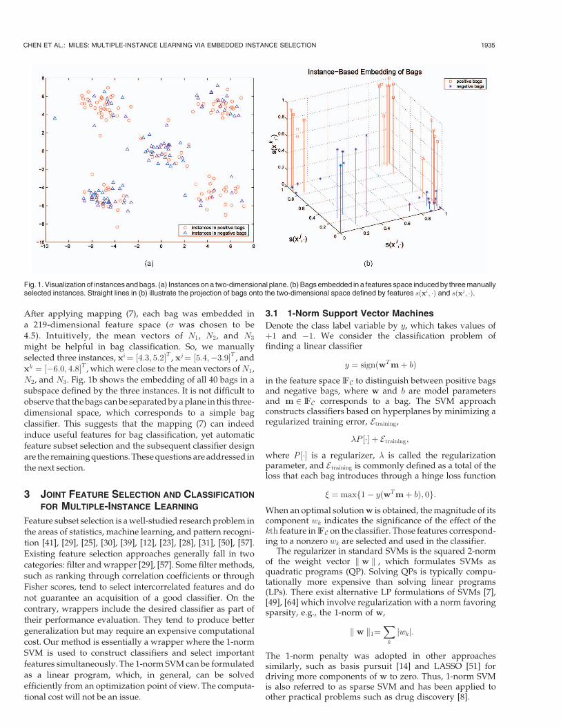
After applying mapping (7), each bag was embedded in

a 219-dimensional feature space (� was chosen to be

4.5). Intuitively, the mean vectors of N1, N2, and N3

might be helpful in bag classification. So, we manually

selected three instances, xi¼ ½4:3; 5:2�T , xj¼ ½5:4;�3:9�T , and

xk ¼ ½�6:0; 4:8�T , which were close to the mean vectors ofN1,

N2, and N3. Fig. 1b shows the embedding of all 40 bags in a

subspace defined by the three instances. It is not difficult to

observe that the bags can be separated by a plane in this three-

dimensional space, which corresponds to a simple bag

classifier. This suggests that the mapping (7) can indeed

induce useful features for bag classification, yet automatic

feature subset selection and the subsequent classifier design

are the remaining questions. These questions are addressed in

the next section.

3 JOINT FEATURE SELECTION AND CLASSIFICATION

FOR MULTIPLE-INSTANCE LEARNING

Feature subset selection is a well-studied research problem in

the areas of statistics, machine learning, and pattern recogni-

tion [41], [29], [25], [30], [39], [12], [23], [28], [31], [50], [57].

Existing feature selection approaches generally fall in two

categories: filter and wrapper [29], [57]. Some filter methods,

such as ranking through correlation coefficients or through

Fisher scores, tend to select intercorrelated features and do

not guarantee an acquisition of a good classifier. On the

contrary, wrappers include the desired classifier as part of

their performance evaluation. They tend to produce better

generalization but may require an expensive computational

cost. Our method is essentially a wrapper where the 1-norm

SVM is used to construct classifiers and select important

features simultaneously. The 1-norm SVM can be formulated

as a linear program, which, in general, can be solved

efficiently from an optimization point of view. The computa-

tional cost will not be an issue.

3.1 1-Norm Support Vector Machines

Denote the class label variable by y, which takes values ofþ1 and �1. We consider the classification problem offinding a linear classifier

y ¼ signðwTmþ bÞ

in the feature space IFC to distinguish between positive bagsand negative bags, where w and b are model parametersand m 2 IFC corresponds to a bag. The SVM approachconstructs classifiers based on hyperplanes by minimizing aregularized training error, Etraining,

�P ½�� þ Etraining;

where P ½�� is a regularizer, � is called the regularizationparameter, and Etraining is commonly defined as a total of theloss that each bag introduces through a hinge loss function

� ¼ maxf1� yðwTmþ bÞ; 0g:

When an optimal solution w is obtained, the magnitude of itscomponent wk indicates the significance of the effect of thekth feature in IFC on the classifier. Those features correspond-ing to a nonzero wk are selected and used in the classifier.

The regularizer in standard SVMs is the squared 2-normof the weight vector k w k , which formulates SVMs asquadratic programs (QP). Solving QPs is typically compu-tationally more expensive than solving linear programs(LPs). There exist alternative LP formulations of SVMs [7],[49], [64] which involve regularization with a norm favoringsparsity, e.g., the 1-norm of w,

k w k1¼Xk

jwkj:

The 1-norm penalty was adopted in other approachessimilarly, such as basis pursuit [14] and LASSO [51] fordriving more components of w to zero. Thus, 1-norm SVMis also referred to as sparse SVM and has been applied toother practical problems such as drug discovery [8].


Fig. 1. Visualization of instances and bags. (a) Instances on a two-dimensional plane. (b) Bags embedded in a features space induced by three manuallyselected instances. Straight lines in (b) illustrate the projection of bags onto the two-dimensional space defined by features sðxi; �Þ and sðxj; �Þ.

Another characteristic of the MIL problem is that trainingsets in many MIL problems are very imbalanced betweenclasses, e.g., the number of negative bags can be much largerthan the number of positive bags. To tackle this imbalancedissue and make classifiers biased toward the minor class, asimple strategy we used is to penalize differently on errorsproduced, respectively, by positive bags and by negativebags. Hence, the 1-norm SVM is formulated as follows:

minw;b;�;� �Xnk¼1

jwkj þ C1

X‘þi¼1

�i þ C2

X‘�j¼1

�j

s:t: ðwTmþi þ bÞ þ �i � 1; i ¼ 1; � � � ; ‘þ;� ðwTm�j þ bÞ þ �j � 1; j ¼ 1; � � � ; ‘�;�i; �j � 0; i ¼ 1; � � � ; ‘þ; j ¼ 1; � � � ; ‘�;

ð8Þ

where ��, �� are hinge losses. Choosing unequal values forparameters C1 and C2 will penalize differently on falsenegatives and false positives. Usually, C1 and C2 are chosenso that the training error is determined by a convexcombination of the training errors occurred on positive bagsand on negative bags. In other words, let C1 ¼ � andC2 ¼ 1� �, where 0 < � < 1.

To form an LP for the 1-norm SVM, we rewritewk ¼ uk � vk, where uk; vk � 0. If either uk or vk has to equalto 0, we have jwkj ¼ uk þ vk. The LP is then formulated invariables u, v, b, ��, and �� as

minu;v;b;�;��;��;��;� �Xnk¼1

ðuk þ vkÞ þ �X‘þi¼1

�i þ ð1� �ÞX‘�j¼1

�j

s:t: ½ðu� vÞTmþi þ b� þ �i � 1; i ¼ 1; � � � ; ‘þ;� ½ðu� vÞTm�j þ b� þ �j � 1; j ¼ 1; � � � ; ‘�;uk; vk � 0; k ¼ 1; � � � ; n;�i; �j � 0; i ¼ 1; � � � ; ‘þ; j ¼ 1; � � � ; ‘�:

ð9Þ

Solving LP (9) yields solutions equivalent to those obtainedby the 1-norm SVM (8) because any optimal solution to (9) hasat least one of the two variables uk and vk equal to 0 for allk ¼ 1; � � � ; n. Otherwise, assume uk � vk > 0 without loss ofgenerality, and we can find a better solution by setting uk ¼uk � vk and vk ¼ 0, which contradicts the optimality of ðu;vÞ.

Let w� ¼ u� � v� and b� be the optimal solution of (9). Themagnitude of w�k determines the influence of the kth featureon the classifier. The set of selected features is given asfsðxk; �Þ : k 2 Ig, where

I ¼ fk : jw�kj > 0g

is the index set for nonzero entries in w�. The classificationof bag Bi is computed as

y ¼ signXk2I

w�ksðxk;BiÞ þ b� !

: ð10Þ

3.2 Instance Classification

In some multiple-instance problems, classification of in-stances is at least as important as the classification of bags. Forone example, an object detection algorithm needs not only toidentify whether or not an image contains a certain object, butalso to locate the object (or part of the object) from the image if

it contains the object. Under the multiple-instance formula-tion, this requires the classification of the bags (containing anobject versus not containing any such object) as well as theinstances in a bag that correspond to the object. The classifier(10) predicts a label for a bag. Next, we introduce a way toclassify instances based on a bag classifier.

The basic idea is to classify instances according to theircontributions to the classification of the bag. Instances in a bagcan be grouped into three classes: positive class, negative class,and void class. An instance in bag Bi is assigned to the positiveclass (negative class) if its contribution to

Pk2I w

�ksðxk;BiÞ

is greater than or equal to (or less than) a threshold. Aninstance is assigned to the void class if it makes nocontribution to the classification of the bag.

Given a bag Bi with instances xij, j ¼ 1; � � � ; ni, we definean index set U as

U ¼ j� : j� ¼ arg maxj


�2

� �; k 2 I

� �:

It is not difficult to verify that the evaluation of (10) only needsthe knowledge of the instances xij� , j

� 2 U. In this sense, Udefines a minimal set of instances responsible for theclassification of Bi. Hence, removing an instance xij� , j

� =2Ufrom the bag will not affect the value of

Pk2I w

�ksðxk;BiÞ in

(10), and f1; � � � ; nigminus the set U specifies the instances inthe void class. Since there can be more than one instance inthe bagBi that maximizes expð� kxij�xkk2

�2 Þ for a given xk; k 2 I ,we denote the number of maximizers for xk by mk. Also, aninstance xij� , j

� 2 U can be a maximizer for different xks,k 2 I . Hence, for each j� 2 U, we define

I j� ¼ k : k 2 I ; j� ¼ arg maxj


�2

� �� :

All the features sðxk;BiÞ; k 2 I j� can be computed from xij� ,i.e., sðxk;BiÞ ¼ sðxk; fxij�gÞ for k 2 I j� .

It is straightforward to show that I ¼Sj�2U I j� and, in

general, I j�1TI j�2 6¼ ; for arbitrary j�1 6¼ j�2 2 U. In fact, the

number of appearances of k in I j�1; � � � ; I j�jUj is mk. We then

rewrite the bag classifier (10) in terms of the instancesindexed by U:

y ¼ signXj�2U

gðxij� Þ þ b� !

;

where

gðxij� Þ ¼Xk2I j�

w�ksðxk;xij� Þmk

ð11Þ

determines the contribution of xij� to the classification of thebag Bi. The instances can be classified according to (11): Ifgðxij� Þ > � , xij� belongs to the positive class; otherwise, xij�belongs to the negative class. The choice of � is applicationspecific and is an interesting research problem for its ownsake. In our experiments, the parameter � is chosen to bebag dependent as � b�

jUj .Next, we present one simple example to illustrate the

major steps in the above instance classification process.

Example. We assume that five features are selected by 1-normSVM and denote these features as sðx1; �Þ; � � � ; sðx5; �Þ.Therefore, I ¼ f1; 2; 3; 4; 5g. A bag Bi, containing four


instances (xi1, xi2, xi3, and xi4), is classified as positive. Thekey information needed in computing sðxk;BiÞ is thenearest neighbors of xk in the instances of Bi. Suppose that

xi2;xi3 are the nearest neighbors of x1;

xi1 is the nearest neighbor of x2;



xi3 is the nearest neighbor of x5:

ð12Þ

Instances xi1, xi2, and xi3 are the nearest neighbors of at leastone of xks, so U ¼ f1; 2; 3g. Since xi4 is not the nearestneighbor for any of xks, xi4 is assigned to the void class.Because x1 has two nearest neighbors, it yields m1 ¼ 2.Similarly, we have m2 ¼ m3 ¼ m4 ¼ m5 ¼ 1. From (12), wefind that xi1 is the nearest neighbor of x2 and x4. So, xi1determines the values of features sðx2; �Þ and sðx4; �Þ.Therefore, I1 ¼ f2; 4g. Similarly, we derive I 2 ¼ f1g andI 3 ¼ f1; 3; 5g. In other words, the instance xi1 contributes tothe classification of Bi via features sðx2; �Þ and sðx4Þ, theinstance xi2 contributes to the classification via sðx1; �Þ, andthe instance xi3 contributes to the classification via sðx1; �Þ,sðx3; �Þ, and sðx5; �Þ. The labels of instances xi1, xi2, and xi3can be predicted using (11).

4 AN ALGORITHMIC VIEW

We summarize the above discussion in pseudo code. Theinput is a set of labeled bags D, parameters �2, �, and �. Thecollection of instances from all the bags is denoted asC ¼ fxk : k ¼ 1; � � � ; ng. The following pseudo code learns abag classifier defined by w� and b�Þ.Algorithm 4.1: Learning Bag Classifier1 FOR (every bag Bi ¼ fxij : j ¼ 1; � � � ; nig in D)2 FOR (every instance xk in C)3 d ¼ minj k xij � xk k4 the kth element of mðBiÞ is sðxk;BiÞ ¼ e�

d2

�2

5 END

6 END

7 solve the LP in (9)

8 OUTPUT (w� and b�)

The pseudocode for instance classification is given below.The input is a bag Bi ¼ fxij : j ¼ 1; � � � ; nig, which isclassified as positive by a bag classifier ðw�; b�Þ. The outputis a list of positive instances along with their contributionsto the classification of the bag.

Algorithm 4.2: Instance Classification of Bag Bi

1 let I ¼ fk : jw�kj > 0g2 let U ¼ fj� : j� ¼ arg minj k xij � xk k; k 2 Ig3 initialize mk ¼ 0 for every k in I4 FOR (every j� in U)5 I j� ¼ fk : k 2 I ; j� ¼ arg minj k xij � xk kg6 mk mk þ 1 for every k in I j�7 END

8 FOR (every xij� with j� in U)

9 compute gðxij� Þ using (11)

10 END

11 OUTPUT (all xij� satisfying gðxij� Þ > � b�

jUj)

These outputs xij� correspond to positive instances.

5 EXPERIMENTAL RESULTS

We present systematic evaluations of the proposed MILframework, MILES, based on three publicly availablebenchmark data sets. In Section 5.1, we compare MILESwith other MIL methods using the benchmark data sets inMIL, MUSK data sets [19]. In Section 5.2, we test theperformance of MILES on a region-based image categoriza-tion problem using the same data set as in [16], andcompare MILES with other techniques. In Section 5.3, Weapply MILES to an object class recognition problem [21].MILES is compared to several techniques specificallydesigned for the recognition task. Computational issuesare discussed in Section 5.4. A Matlab implementation ofMILES is available at http://www.cs.olemiss.edu/~ychen/MILES.html.

5.1 Drug Activity Prediction

5.1.1 Experimental Setup

The MUSK data sets, MUSK1 and MUSK2, are benchmarkdata sets for MIL. Both data sets are publicly available fromthe UCI Machine Learning Repository [9]. The data setsconsist of descriptions of molecules. Specifically, a bagrepresents a molecule. Instances in a bag represent low-energy shapes of the molecule. To capture the shape ofmolecules, a molecule is placed in a standard position andorientation and then a set of 162 rays emitting from the originis constructed to sample the molecular surface approxi-mately uniformly [19]. There are also four features thatdescribe the position of an oxygen atom on the molecularsurface. Therefore, each instance in the bags is represented by166 features. MUSK1 has 92 molecules (bags), of which 47 arelabeled positive, with an average of 5.17 shapes (instances)per molecule. MUSK2 has 102 molecules, of which 39 arepositive, with an average of 64.69 shapes per molecule.

Three parameters �2 (in the most-likely-cause estimator),�, and � (in the LP) need to be specified for MILES. We fixed� ¼ 0:5 to penalize equally on errors in the positive class andthe negative class. The parameters � and �2 were selectedaccording to a twofold cross-validation on the training set.We chose � from 0.1 to 0.6 with step size 0.01, and �2 from105 to 9� 105 with step size 5� 104. We found that � ¼ 0:45and �2 ¼ 5� 105 gave the minimum twofold cross-valida-tion error on MUSK1, and � ¼ 0:37 and �2 ¼ 8� 105 gave thebest twofold cross-validation performance on MUSK2.These values were fixed for the subsequent experiments.The linear program of 1-norm SVM was solved using CPLEXversion 9.0 [24].

5.1.2 Classification Results

Table 1 shows the prediction accuracy. We observedvariations on the average accuracy of tenfold cross-validation for different random runs. The predictionaccuracy in 15 runs varied from 84.1-90.2 percent forMUSK1, and from 84.5-91.5 percent for MUSK2. Therefore,we reported the mean and 95 percent confidence intervalof the results of 15 runs of tenfold cross-validation forMILES. We also included the results using the leave-one-out test for comparison with certain algorithms.

Table 1 summarizes the performance of 12 MIL algo-rithms in the literature: APR [19], DD [35], DD-SVM [16],


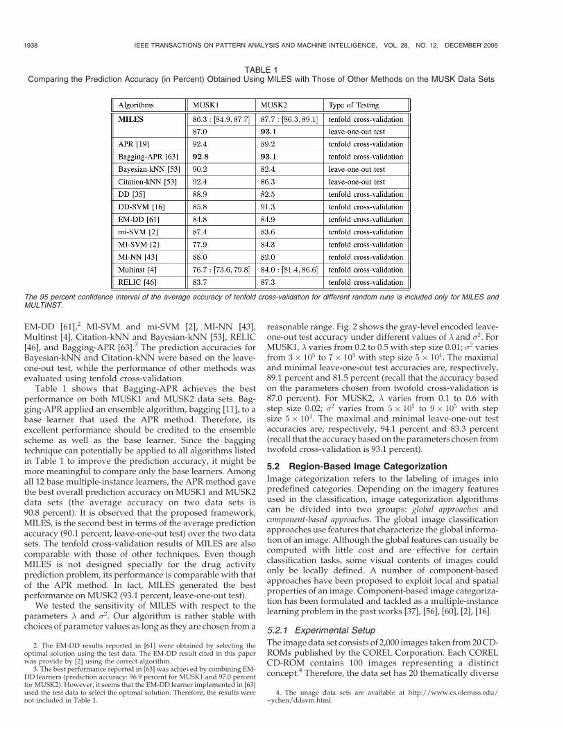
EM-DD [61],2 MI-SVM and mi-SVM [2], MI-NN [43],Multinst [4], Citation-kNN and Bayesian-kNN [53], RELIC[46], and Bagging-APR [63].3 The prediction accuracies forBayesian-kNN and Citation-kNN were based on the leave-one-out test, while the performance of other methods wasevaluated using tenfold cross-validation.

Table 1 shows that Bagging-APR achieves the bestperformance on both MUSK1 and MUSK2 data sets. Bag-ging-APR applied an ensemble algorithm, bagging [11], to abase learner that used the APR method. Therefore, itsexcellent performance should be credited to the ensemblescheme as well as the base learner. Since the baggingtechnique can potentially be applied to all algorithms listedin Table 1 to improve the prediction accuracy, it might bemore meaningful to compare only the base learners. Amongall 12 base multiple-instance learners, the APR method gavethe best overall prediction accuracy on MUSK1 and MUSK2data sets (the average accuracy on two data sets is90.8 percent). It is observed that the proposed framework,MILES, is the second best in terms of the average predictionaccuracy (90.1 percent, leave-one-out test) over the two datasets. The tenfold cross-validation results of MILES are alsocomparable with those of other techniques. Even thoughMILES is not designed specially for the drug activityprediction problem, its performance is comparable with thatof the APR method. In fact, MILES generated the bestperformance on MUSK2 (93.1 percent, leave-one-out test).

We tested the sensitivity of MILES with respect to theparameters � and �2. Our algorithm is rather stable withchoices of parameter values as long as they are chosen from a

reasonable range. Fig. 2 shows the gray-level encoded leave-one-out test accuracy under different values of � and �2. ForMUSK1, � varies from 0.2 to 0.5 with step size 0.01; �2 variesfrom 3� 105 to 7� 105 with step size 5� 104. The maximaland minimal leave-one-out test accuracies are, respectively,89.1 percent and 81.5 percent (recall that the accuracy basedon the parameters chosen from twofold cross-validation is87.0 percent). For MUSK2, � varies from 0.1 to 0.6 withstep size 0.02; �2 varies from 5� 105 to 9� 105 with stepsize 5� 104. The maximal and minimal leave-one-out testaccuracies are, respectively, 94.1 percent and 83.3 percent(recall that the accuracy based on the parameters chosen fromtwofold cross-validation is 93.1 percent).

5.2 Region-Based Image Categorization

Image categorization refers to the labeling of images intopredefined categories. Depending on the imagery featuresused in the classification, image categorization algorithmscan be divided into two groups: global approaches andcomponent-based approaches. The global image classificationapproaches use features that characterize the global informa-tion of an image. Although the global features can usually becomputed with little cost and are effective for certainclassification tasks, some visual contents of images couldonly be locally defined. A number of component-basedapproaches have been proposed to exploit local and spatialproperties of an image. Component-based image categoriza-tion has been formulated and tackled as a multiple-instancelearning problem in the past works [37], [56], [60], [2], [16].


The image data set consists of 2,000 images taken from 20 CD-ROMs published by the COREL Corporation. Each CORELCD-ROM contains 100 images representing a distinctconcept.4 Therefore, the data set has 20 thematically diverse


2. The EM-DD results reported in [61] were obtained by selecting theoptimal solution using the test data. The EM-DD result cited in this paperwas provide by [2] using the correct algorithm.

3. The best performance reported in [63] was achieved by combining EM-DD learners (prediction accuracy: 96.9 percent for MUSK1 and 97.0 percentfor MUSK2). However, it seems that the EM-DD learner implemented in [63]used the test data to select the optimal solution. Therefore, the results werenot included in Table 1.

4. The image data sets are available at http://www.cs.olemiss.edu/~ychen/ddsvm.html.

TABLE 1Comparing the Prediction Accuracy (in Percent) Obtained Using MILES with Those of Other Methods on the MUSK Data Sets

The 95 percent confidence interval of the average accuracy of tenfold cross-validation for different random runs is included only for MILES andMULTINST.

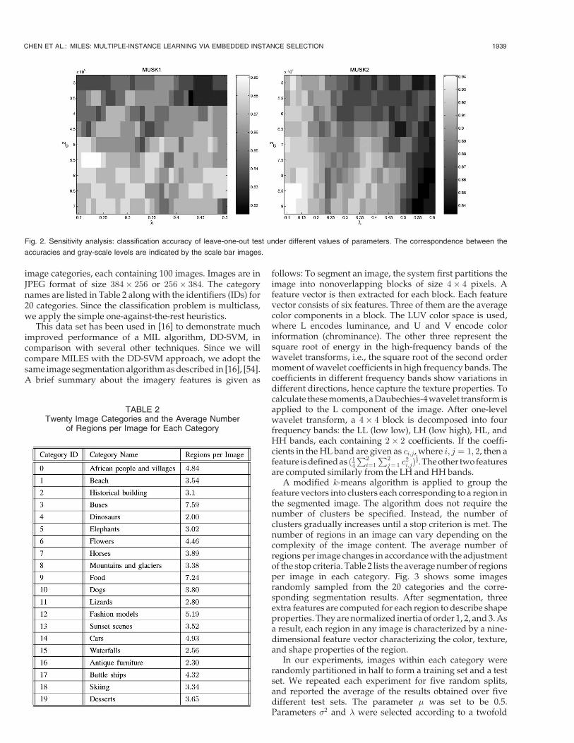
image categories, each containing 100 images. Images are inJPEG format of size 384� 256 or 256� 384. The categorynames are listed in Table 2 along with the identifiers (IDs) for20 categories. Since the classification problem is multiclass,we apply the simple one-against-the-rest heuristics.

This data set has been used in [16] to demonstrate muchimproved performance of a MIL algorithm, DD-SVM, incomparison with several other techniques. Since we willcompare MILES with the DD-SVM approach, we adopt thesame image segmentation algorithm as described in [16], [54].A brief summary about the imagery features is given as

follows: To segment an image, the system first partitions theimage into nonoverlapping blocks of size 4� 4 pixels. Afeature vector is then extracted for each block. Each featurevector consists of six features. Three of them are the averagecolor components in a block. The LUV color space is used,where L encodes luminance, and U and V encode colorinformation (chrominance). The other three represent thesquare root of energy in the high-frequency bands of thewavelet transforms, i.e., the square root of the second ordermoment of wavelet coefficients in high frequency bands. Thecoefficients in different frequency bands show variations indifferent directions, hence capture the texture properties. Tocalculate these moments, a Daubechies-4 wavelet transform isapplied to the L component of the image. After one-levelwavelet transform, a 4� 4 block is decomposed into fourfrequency bands: the LL (low low), LH (low high), HL, andHH bands, each containing 2� 2 coefficients. If the coeffi-cients in the HL band are given as ci;j, where i; j ¼ 1; 2, then afeature is defined as ð14

P2i¼1

P2j¼ 1 c

2i;jÞ

12. The other two features

are computed similarly from the LH and HH bands.A modified k-means algorithm is applied to group the

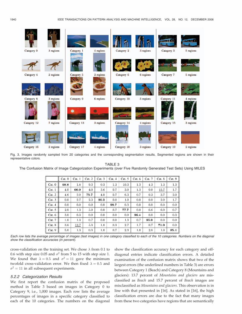
feature vectors into clusters each corresponding to a region inthe segmented image. The algorithm does not require thenumber of clusters be specified. Instead, the number ofclusters gradually increases until a stop criterion is met. Thenumber of regions in an image can vary depending on thecomplexity of the image content. The average number ofregions per image changes in accordance with the adjustmentof the stop criteria. Table 2 lists the average number of regionsper image in each category. Fig. 3 shows some imagesrandomly sampled from the 20 categories and the corre-sponding segmentation results. After segmentation, threeextra features are computed for each region to describe shapeproperties. They are normalized inertia of order 1, 2, and 3. Asa result, each region in any image is characterized by a nine-dimensional feature vector characterizing the color, texture,and shape properties of the region.

In our experiments, images within each category wererandomly partitioned in half to form a training set and a testset. We repeated each experiment for five random splits,and reported the average of the results obtained over fivedifferent test sets. The parameter � was set to be 0.5.Parameters �2 and � were selected according to a twofold


Fig. 2. Sensitivity analysis: classification accuracy of leave-one-out test under different values of parameters. The correspondence between the

accuracies and gray-scale levels are indicated by the scale bar images.

TABLE 2Twenty Image Categories and the Average Number

of Regions per Image for Each Category

cross-validation on the training set. We chose � from 0.1 to

0.6 with step size 0.05 and �2 from 5 to 15 with step size 1.

We found that � ¼ 0:5 and �2 ¼ 11 gave the minimum

twofold cross-validation error. We then fixed � ¼ 0:5 and

�2 ¼ 11 in all subsequent experiments.

5.2.2 Categorization Results

We first report the confusion matrix of the proposed

method in Table 3 based on images in Category 0 to

Category 9, i.e., 1,000 images. Each row lists the average

percentages of images in a specific category classified to

each of the 10 categories. The numbers on the diagonal

show the classification accuracy for each category and off-

diagonal entries indicate classification errors. A detailed

examination of the confusion matrix shows that two of the

largest errors (the underlined numbers in Table 3) are errors

between Category 1 (Beach) and Category 8 (Mountains and

glaciers): 13.7 percent of Mountains and glaciers are mis-

classified as Beach and 15.7 percent of Beach images are

misclassified as Mountains and glaciers. This observation is in

line with that presented in [16]. As stated in [16], the high

classification errors are due to the fact that many images

from these two categories have regions that are semantically


Fig. 3. Images randomly sampled from 20 categories and the corresponding segmentation results. Segmented regions are shown in theirrepresentative colors.

TABLE 3The Confusion Matrix of Image Categorization Experiments (over Five Randomly Generated Test Sets) Using MILES

Each row lists the average percentage of images (test images) in one category classified to each of the 10 categories. Numbers on the diagonalshow the classification accuracies (in percent).

related and visually similar, such as regions correspondingto mountain, river, lake, and ocean.

We compared the overall prediction accuracy of MILESwith that of DD-SVM [16], MI-SVM [2], and a methodproposed in [17] (we call it k-means-SVM to simplify thediscussions). k-means-SVM constructed a region vocabu-lary by clustering regions using the k-means algorithm.Each image was then transformed to an integer-valuedfeature vector indicating the number of regions assigned toeach cluster. SVMs were constructed using these integer-valued features. The size of the vocabulary and theparameters of k-means-SVM were chosen according to atwofold cross-validation using all 2,000 images. The averageclassification accuracies over five random test sets and thecorresponding 95 percent confidence intervals are providedin Table 4. On both data sets, the performance of MILES issignificantly better than that of MI-SVM and k-means-SVM.MILES outperforms DD-SVM, though the difference is notstatistically significant as the 95 percent confidence intervalsfor the two methods overlap.

5.2.3 Sensitivity to Labeling Noise

The results in Section 5.2.2 demonstrate that the perfor-mance of MILES is highly comparable with that of DD-SVM. Next, we compare MILES with DD-SVM in terms ofthe sensitivity to the noise in labels. Sensitivity to labelingnoise is an important performance measure for classifiersbecause in many practical applications, it is usuallyimpossible to get a “clean” data set and the labelingprocesses are often subjective. In terms of binary classifica-tion, we define the labeling noise as the probability that animage is mislabeled. In this experiment, training sets withdifferent levels of labeling noise were generated as follows.We first randomly picked d% of positive images and d% ofnegative images from a training set. Then, we modified thelabels of the selected images by negating their labels, i.e.,positive (negative) images were labeled as negative (posi-tive) images. Finally, we put these images with new labelsback to the training set. The new training set has d% ofimages with negated labels (or “noisy” labels).

We compared the classification accuracy of MILES withthat of DD-SVM for d ¼ 0 to 30 (with step size 2) based on200 images from Category 2 (Historical buildings) andCategory 7 (Horses). The reason of selecting these twocategories is that both DD-SVM and MILES produce almostperfect classification accuracies at d ¼ 0, which makes thema good data set for comparing sensitivities at different levels

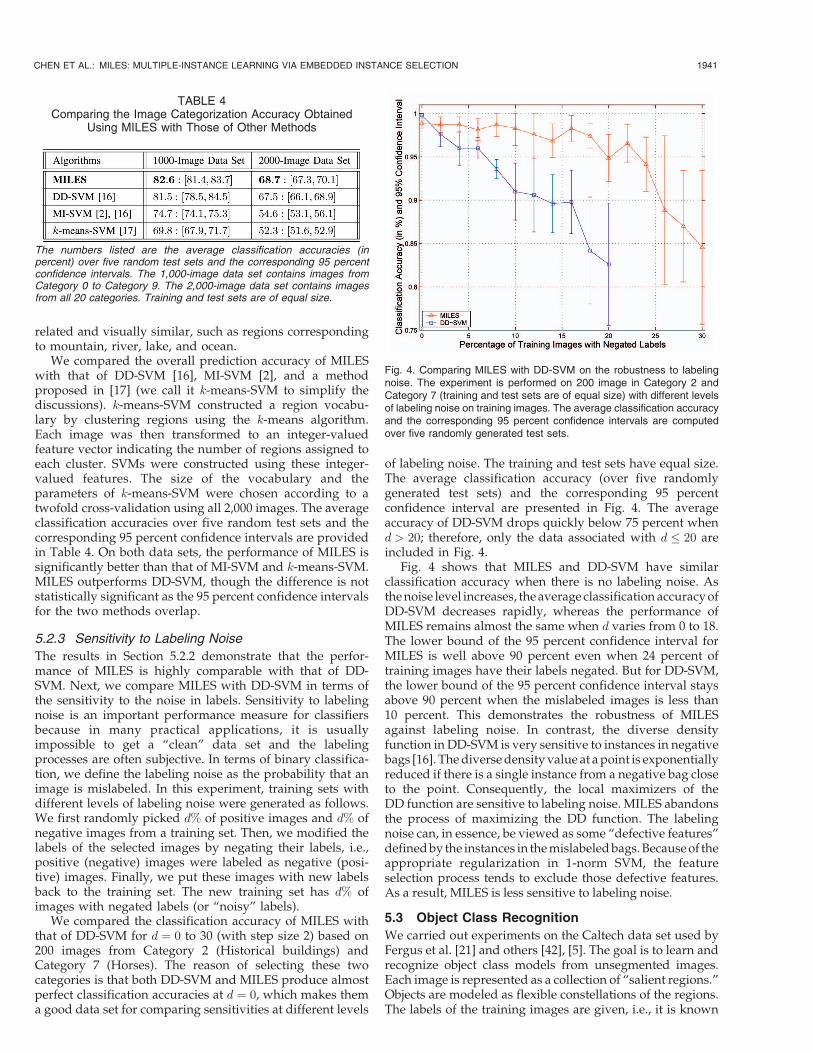
of labeling noise. The training and test sets have equal size.The average classification accuracy (over five randomlygenerated test sets) and the corresponding 95 percentconfidence interval are presented in Fig. 4. The averageaccuracy of DD-SVM drops quickly below 75 percent whend > 20; therefore, only the data associated with d 20 areincluded in Fig. 4.

Fig. 4 shows that MILES and DD-SVM have similarclassification accuracy when there is no labeling noise. Asthe noise level increases, the average classification accuracy ofDD-SVM decreases rapidly, whereas the performance ofMILES remains almost the same when d varies from 0 to 18.The lower bound of the 95 percent confidence interval forMILES is well above 90 percent even when 24 percent oftraining images have their labels negated. But for DD-SVM,the lower bound of the 95 percent confidence interval staysabove 90 percent when the mislabeled images is less than10 percent. This demonstrates the robustness of MILESagainst labeling noise. In contrast, the diverse densityfunction in DD-SVM is very sensitive to instances in negativebags [16]. The diverse density value at a point is exponentiallyreduced if there is a single instance from a negative bag closeto the point. Consequently, the local maximizers of theDD function are sensitive to labeling noise. MILES abandonsthe process of maximizing the DD function. The labelingnoise can, in essence, be viewed as some “defective features”defined by the instances in the mislabeled bags. Because of theappropriate regularization in 1-norm SVM, the featureselection process tends to exclude those defective features.As a result, MILES is less sensitive to labeling noise.

5.3 Object Class Recognition

We carried out experiments on the Caltech data set used byFergus et al. [21] and others [42], [5]. The goal is to learn andrecognize object class models from unsegmented images.Each image is represented as a collection of “salient regions.”Objects are modeled as flexible constellations of the regions.The labels of the training images are given, i.e., it is known


TABLE 4Comparing the Image Categorization Accuracy Obtained

Using MILES with Those of Other Methods

The numbers listed are the average classification accuracies (inpercent) over five random test sets and the corresponding 95 percentconfidence intervals. The 1,000-image data set contains images fromCategory 0 to Category 9. The 2,000-image data set contains imagesfrom all 20 categories. Training and test sets are of equal size.

Fig. 4. Comparing MILES with DD-SVM on the robustness to labelingnoise. The experiment is performed on 200 image in Category 2 andCategory 7 (training and test sets are of equal size) with different levelsof labeling noise on training images. The average classification accuracyand the corresponding 95 percent confidence intervals are computedover five randomly generated test sets.

whether or not a training image contains a certain object froma particular class. However, the labels of the salient regions ineach training image are unknown, so it is not clear whichsalient regions correspond to the object, and which are not.This learning situation can be viewed as a multiple-instanceproblem. We compared MILES with the Fergus method [21]as well as the approaches described in [5], [42].


The image data set was downloaded from the Website ofRobotics Research Group at the University of Oxford.5 Itcontains the following four object classes and backgroundimages: Airplanes (800 images), Cars (800 images), Faces(435 images), Motorbikes (800 images), and Background(900 general background and 1,370 road background).

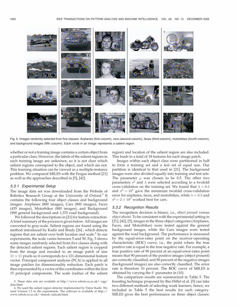
We followed the descriptions in [21] for feature extraction.A brief summary of the process is given below. All images areconverted to gray-scale. Salient regions are found using themethod introduced by Kadir and Brady [26] , which detectsregions that are salient over both location and scale.6 In ourexperiments, the scale varies between 5 and 50. Fig. 5 showssome images randomly selected from five classes along withthe detected salient regions. Each salient region is croppedfrom the image and rescaled to an image patch of size11� 11 pixels so it corresponds to a 121-dimensional featurevector. Principal component analysis (PCA) is applied to allimage patches for dimensionality reduction. Each patch isthen represented by a vector of the coordinates within the first15 principal components. The scale (radius of the salient

region) and location of the salient region are also included.This leads to a total of 18 features for each image patch.

Images within each object class were partitioned in halfto form a training set and a test set of equal size. Ourpartition is identical to that used in [21]. The backgroundimages were also divided equally into training and test sets.The parameter � was chosen to be 0.5. The other twoparameters �2 and � were selected according to a twofoldcross-validation on the training set. We found that � ¼ 0:5and �2 ¼ 105 gave the minimum twofold cross-validationerror for airplanes, faces, and motorbikes, while � ¼ 0:5 and�2¼ 2� 105 worked best for cars.

5.3.2 Recognition Results

The recognition decision is binary, i.e., object present versusobject absent. To be consistent with the experimental setting in[21], [42], [5], images in the three object categories (Airplanes,Faces, and Motorbikes) were tested against the generalbackground images, while the Cars images were testedagainst the road background. The performance is measuredby the equal-error-rates point on the receiver-operatingcharacteristic (ROC) curve, i.e., the point where the truepositive rate is equal to the true negative rate. For example, atrue positive rate of 90 percent at an equal-error-rates pointmeans that 90 percent of the positive images (object present)are correctly classified, and 90 percent of the negative images(background images) are also correctly classified. The errorrate is therefore 10 percent. The ROC curve of MILES isobtained by varying the b� parameter in (10).

The comparison results are summarized in Table 5. Theboosting technique proposed by Bar-Hillel et al. [5] can taketwo different methods of selecting weak learners, hence, weincluded in Table 5 the best results for each category.MILES gives the best performance on three object classes:


5. These data sets are available at http://www.robots.ox.ac.uk/~vgg/data.html.

6. We used the salient region detector implemented by Timor Kadir. Weused Version 1.5 in the experiments. The software is available at http://www.robots.ox.ac.uk/~timork/salscale.html.

Fig. 5. Images randomly selected from five classes: Airplanes (first column), cars (second column), faces (third column), motorbikes (fourth column),

and background images (fifth column). Each circle in an image represents a salient region.

The error rates of MILES over airplanes, faces, andmotorbikes are around 20.4, 13.9, and 48 percent, respec-tively, of those of the second best (the Fergus method onAirplanes and Faces, the Bar-Hillel method on Motorbikes).The method proposed by Bar-Hillel et al. [5] gave the bestresults on Cars category. The overall recognition perfor-mance of MILES appears to be very competitive.

5.3.3 Selected Features and Instance Classification

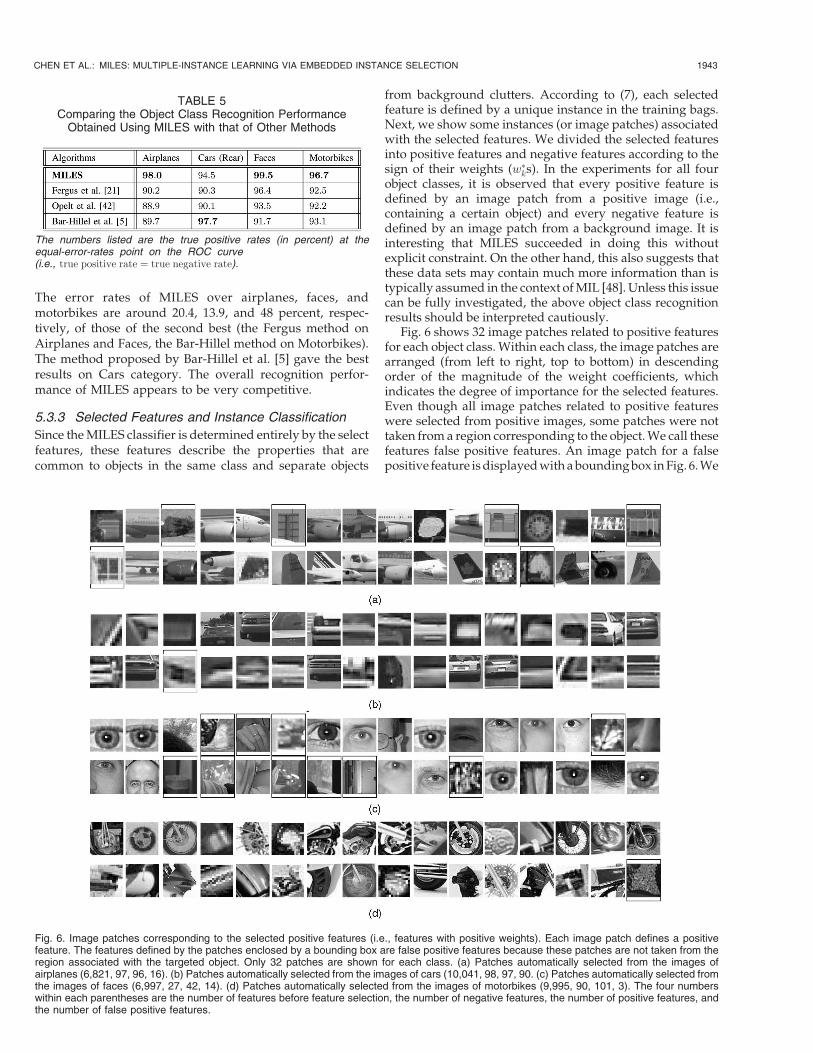
Since the MILES classifier is determined entirely by the selectfeatures, these features describe the properties that arecommon to objects in the same class and separate objects

from background clutters. According to (7), each selectedfeature is defined by a unique instance in the training bags.Next, we show some instances (or image patches) associatedwith the selected features. We divided the selected featuresinto positive features and negative features according to thesign of their weights (w�ks). In the experiments for all fourobject classes, it is observed that every positive feature isdefined by an image patch from a positive image (i.e.,containing a certain object) and every negative feature isdefined by an image patch from a background image. It isinteresting that MILES succeeded in doing this withoutexplicit constraint. On the other hand, this also suggests thatthese data sets may contain much more information than istypically assumed in the context of MIL [48]. Unless this issuecan be fully investigated, the above object class recognitionresults should be interpreted cautiously.

Fig. 6 shows 32 image patches related to positive featuresfor each object class. Within each class, the image patches arearranged (from left to right, top to bottom) in descendingorder of the magnitude of the weight coefficients, whichindicates the degree of importance for the selected features.Even though all image patches related to positive featureswere selected from positive images, some patches were nottaken from a region corresponding to the object. We call thesefeatures false positive features. An image patch for a falsepositive feature is displayed with a bounding box in Fig. 6. We


TABLE 5Comparing the Object Class Recognition Performance

Obtained Using MILES with that of Other Methods

The numbers listed are the true positive rates (in percent) at theequal-error-rates point on the ROC curve(i.e., true positive rate ¼ true negative rate).

Fig. 6. Image patches corresponding to the selected positive features (i.e., features with positive weights). Each image patch defines a positivefeature. The features defined by the patches enclosed by a bounding box are false positive features because these patches are not taken from theregion associated with the targeted object. Only 32 patches are shown for each class. (a) Patches automatically selected from the images ofairplanes (6,821, 97, 96, 16). (b) Patches automatically selected from the images of cars (10,041, 98, 97, 90. (c) Patches automatically selected fromthe images of faces (6,997, 27, 42, 14). (d) Patches automatically selected from the images of motorbikes (9,995, 90, 101, 3). The four numberswithin each parentheses are the number of features before feature selection, the number of negative features, the number of positive features, andthe number of false positive features.

also included in the figure the number of features beforefeature selection (i.e., the number of instances in all trainingbags), the number of negative features, the number of positivefeatures, and the number of false positive features. Asindicated by these numbers, the solution of MILES is verysparse. On average, more than 98 percent of the weights arezero. The results also seem to suggest that the featureselection process of MILES can, to some extent, capture thecharacteristics of an object class.

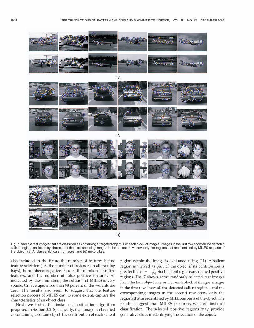
Next, we tested the instance classification algorithmproposed in Section 3.2. Specifically, if an image is classifiedas containing a certain object, the contribution of each salient

region within the image is evaluated using (11). A salient

region is viewed as part of the object if its contribution is

greater than � ¼ � b�

jUj . Such salient regions are named positive

regions. Fig. 7 shows some randomly selected test images

from the four object classes. For each block of images, images

in the first row show all the detected salient regions, and the

corresponding images in the second row show only the

regions that are identified by MILES as parts of the object. The

results suggest that MILES performs well on instance

classification. The selected positive regions may provide

generative clues in identifying the location of the object.


Fig. 7. Sample test images that are classified as containing a targeted object. For each block of images, images in the first row show all the detectedsalient regions enclosed by circles, and the corresponding images in the second row show only the regions that are identified by MILES as parts ofthe object. (a) Airplanes, (b) cars, (c) faces, and (d) motorbikes.

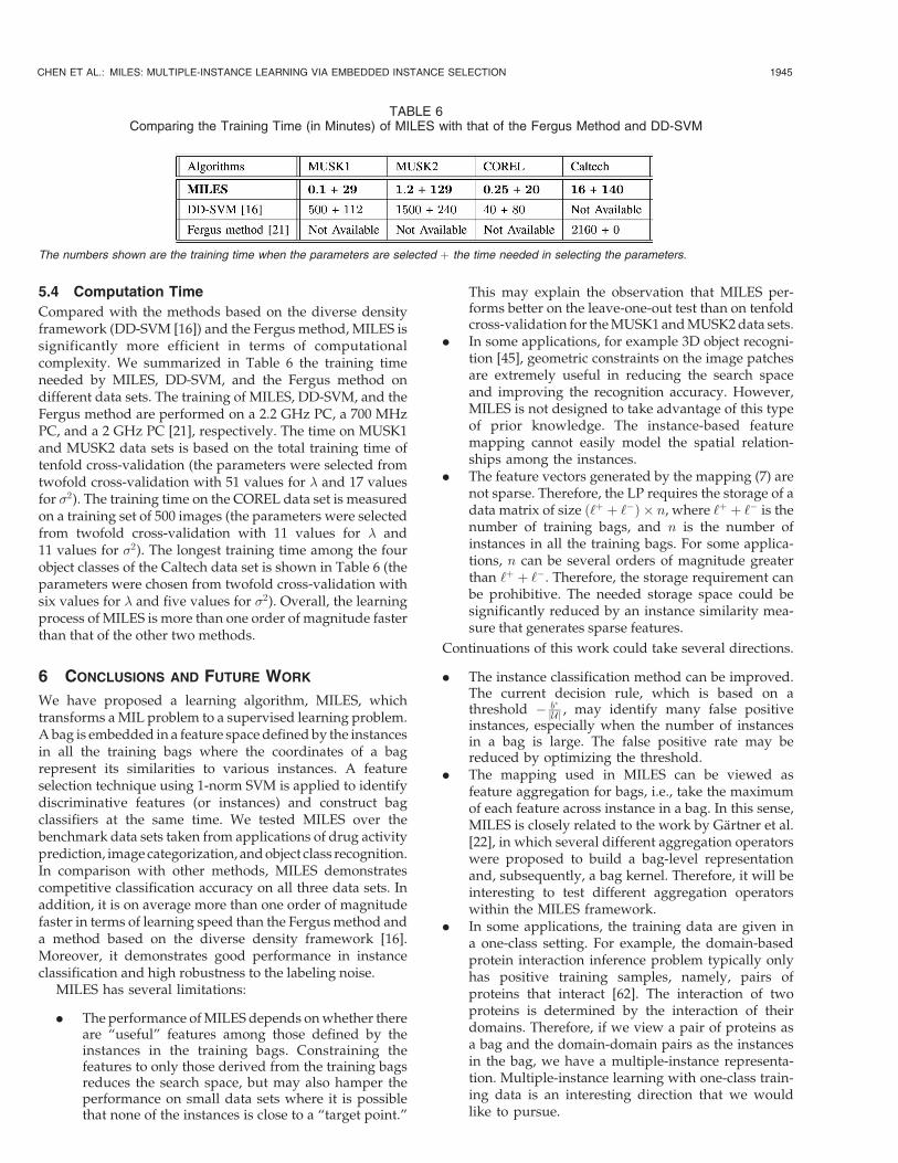
5.4 Computation Time

Compared with the methods based on the diverse densityframework (DD-SVM [16]) and the Fergus method, MILES issignificantly more efficient in terms of computationalcomplexity. We summarized in Table 6 the training timeneeded by MILES, DD-SVM, and the Fergus method ondifferent data sets. The training of MILES, DD-SVM, and theFergus method are performed on a 2.2 GHz PC, a 700 MHzPC, and a 2 GHz PC [21], respectively. The time on MUSK1and MUSK2 data sets is based on the total training time oftenfold cross-validation (the parameters were selected fromtwofold cross-validation with 51 values for � and 17 valuesfor �2). The training time on the COREL data set is measuredon a training set of 500 images (the parameters were selectedfrom twofold cross-validation with 11 values for � and11 values for �2). The longest training time among the fourobject classes of the Caltech data set is shown in Table 6 (theparameters were chosen from twofold cross-validation withsix values for � and five values for �2). Overall, the learningprocess of MILES is more than one order of magnitude fasterthan that of the other two methods.

6 CONCLUSIONS AND FUTURE WORK

We have proposed a learning algorithm, MILES, whichtransforms a MIL problem to a supervised learning problem.A bag is embedded in a feature space defined by the instancesin all the training bags where the coordinates of a bagrepresent its similarities to various instances. A featureselection technique using 1-norm SVM is applied to identifydiscriminative features (or instances) and construct bagclassifiers at the same time. We tested MILES over thebenchmark data sets taken from applications of drug activityprediction, image categorization, and object class recognition.In comparison with other methods, MILES demonstratescompetitive classification accuracy on all three data sets. Inaddition, it is on average more than one order of magnitudefaster in terms of learning speed than the Fergus method anda method based on the diverse density framework [16].Moreover, it demonstrates good performance in instanceclassification and high robustness to the labeling noise.

MILES has several limitations:

. The performance of MILES depends on whether thereare “useful” features among those defined by theinstances in the training bags. Constraining thefeatures to only those derived from the training bagsreduces the search space, but may also hamper theperformance on small data sets where it is possiblethat none of the instances is close to a “target point.”

This may explain the observation that MILES per-forms better on the leave-one-out test than on tenfoldcross-validation for the MUSK1 and MUSK2 data sets.

. In some applications, for example 3D object recogni-tion [45], geometric constraints on the image patchesare extremely useful in reducing the search spaceand improving the recognition accuracy. However,MILES is not designed to take advantage of this typeof prior knowledge. The instance-based featuremapping cannot easily model the spatial relation-ships among the instances.

. The feature vectors generated by the mapping (7) arenot sparse. Therefore, the LP requires the storage of adata matrix of size ð‘þ þ ‘�Þ � n, where ‘þ þ ‘� is thenumber of training bags, and n is the number ofinstances in all the training bags. For some applica-tions, n can be several orders of magnitude greaterthan ‘þ þ ‘�. Therefore, the storage requirement canbe prohibitive. The needed storage space could besignificantly reduced by an instance similarity mea-sure that generates sparse features.

Continuations of this work could take several directions.

. The instance classification method can be improved.The current decision rule, which is based on athreshold � b�

jUj , may identify many false positiveinstances, especially when the number of instancesin a bag is large. The false positive rate may bereduced by optimizing the threshold.

. The mapping used in MILES can be viewed asfeature aggregation for bags, i.e., take the maximumof each feature across instance in a bag. In this sense,MILES is closely related to the work by Gartner et al.[22], in which several different aggregation operatorswere proposed to build a bag-level representationand, subsequently, a bag kernel. Therefore, it will beinteresting to test different aggregation operatorswithin the MILES framework.

. In some applications, the training data are given ina one-class setting. For example, the domain-basedprotein interaction inference problem typically onlyhas positive training samples, namely, pairs ofproteins that interact [62]. The interaction of twoproteins is determined by the interaction of theirdomains. Therefore, if we view a pair of proteins asa bag and the domain-domain pairs as the instancesin the bag, we have a multiple-instance representa-tion. Multiple-instance learning with one-class train-ing data is an interesting direction that we wouldlike to pursue.


TABLE 6Comparing the Training Time (in Minutes) of MILES with that of the Fergus Method and DD-SVM

The numbers shown are the training time when the parameters are selected þ the time needed in selecting the parameters.

MILES can be integrated into a target tracking system forobject detection. Evaluation of different feature selectiontechniques and investigation of the connection between thecurrent approach and generative probabilistic methods arealso interesting.

ACKNOWLEDGMENTS

Y. Chen is supported by a Louisiana Board of Regents RCSprogram under Grant No. LBOR0077NR00C, the US NationalScience Foundation EPSCoR program under Grant No. NSF/LEQSF(2005)-PFUND-39, the Research Institute for Children,and the University of New Orleans. This research work wasconducted when Y. Chen was with the Department ofComputer Science at University of New Orleans, NewOrleans, Lousiana and when J. Bi was with the Departmentof Mathematical Sciences at Rensselaer Polytechnic Institute,110 8th Street, Troy, New York. J.Z. Wang is supported by theUS National Science Foundation under Grant Nos. IIS-0219272, IIS-0347148, and ANI-0202007, The PennsylvaniaState University, and the PNC Foundation. The authorswould like to thank the anonymous reviewers and theassociate editor for their comments which have led toimprovements of this paper. They would also like to thankTimor Kadir for providing the salient region detector and RobFergus for sharing the details on the object class recognitionexperiments.

Y. Chen developed the MILES algorithm and performedthe experimental studies. J. Bi collaborated on the algorithmdesign for feature selection and classification and on thedrug activity prediction experiments. Y. Chen and J. Biprepared the initial manuscript. J.Z. Wang collaborated onthe region-based image categorization application of theproposed methods and provided assistance in the revisionof the manuscript.

REFERENCES

[1] S. Agarwal and D. Roth, “Learning a Sparse Representation forObject Detection,” Proc. Seventh European Conf. Computer Vision,vol. 4, pp. 113-130, 2002.

[2] S. Andrews, I. Tsochantaridis, and T. Hofmann, “Support VectorMachines for Multiple-Instance Learning,” Advances in NeuralInformation Processing Systems 15, pp. 561-568, 2003.

[3] S. Andrews and T. Hofmann, “Multiple-Instance Learning viaDisjunctive Programming Boosting,” Advances in Neural Informa-tion Processing Systems 16, pp. 65-72, 2004.

[4] P. Auer, “On Learning from Mult-Instance Examples: EmpiricalEvaluation of a Theoretical Approach,” Proc. 14th Int’l Conf.Machine Learning, pp. 21-29, 1997.

[5] A. Bar-Hillel, T. Hertz, and D. Weinshall, “Object Class Recogni-tion by Boosting a Part-Based Model,” Proc. IEEE Int’l Conf.Computer Vision and Pattern Recognition, vol. 1, pp. 702-709, 2005.

[6] K. Barnard, P. Duygulu, D. Forsyth, N. De Freitas, D.M. Blei, andM.I. Jordan, “Matching Words and Pictures,” J. Machine LearningResearch, vol. 3, pp. 1107-1135, 2003.

[7] K.P. Bennett, “Combining Support Vector and MathematicalProgramming Methods for Classification,” Advances in KernelMethods-Support Vector Machines, B. Scholkopf, C. Burges, andA. Smola, eds., pp. 307-326, 1999.

[8] J. Bi, K.P. Bennett, M. Embrechts, C. Breneman, and M. Song,“Dimensionality Reduction via Sparse Support Vector Machines,”J. Machine Learning Research, vol. 3, pp. 1229-1243, 2003.

[9] C.L. Blake and C.J. Merz, UCI Repository of Machine LearningDatabases, http://www.ics.uci.edu/~mlearn/, 1998.

[10] A. Blum and A. Kalai, “A Note on Learning from Multiple-InstanceExamples,” Machine Learning, vol. 30, no. 1, pp. 23-29, 1998.

[11] L. Breiman, “Bagging Predictors,” Machine Learning, vol. 24,pp. 123-140, 1996.

[12] M. Bressan and J. Vitria, “On the Selection and Classification ofIndependent Features,” IEEE Trans. Pattern Analysis and MachineIntelligence, vol. 25, no. 10, pp. 1312-1317, Oct. 2003.

[13] B.G. Buchanan and T.M. Mitchell, “Model-Directed Learning ofProduction Rules,” Pattern-Directed Inference Systems, pp. 297-312,Academic Press, 1978.

[14] S.S. Chen, D.L. Donoho, and M.A. Saunders, “Atomic Decom-position by Basis Pursuit,” SIAM J. Scientific Computing, vol. 20,no. 1, pp. 33-61, 1998.

[15] Y. Chen and J.Z. Wang, “A Region-Based Fuzzy Feature MatchingApproach to Content-Based Image Retrieval,” IEEE Trans. PatternAnalysis and Machine Intelligence, vol. 24, no. 9, pp. 1252-1267, Sept.2002.

[16] Y. Chen and J.Z. Wang, “Image Categorization by Learning andReasoning with Regions,” J. Machine Learning Research, vol. 5,pp. 913-939, 2004.

[17] G. Csurka, C. Bray, C. Dance, and L. Fan, “Visual Categorizationwith Bags of Keypoints,” Proc. ECCV ’04 Workshop StatisticalLearning in Computer Vision, pp. 59-74, 2004.

[18] L. De Raedt, “Attribute-Value Learning versus Inductive LogicProgramming: The Missing Links,” Lecture Notes in ArtificialIntelligence, vol. 1446, pp. 1-8, 1998.

[19] T.G. Dietterich, R.H. Lathrop, and T. Lozano-Perez, “Solving theMultiple Instance Problem with Axis-Parallel Rectangles,” Artifi-cial Intelligence, vol. 89, nos. 1-2, pp. 31-71, 1997.

[20] G. Dorko and C. Schmid, “Selection of Scale-Invariant Parts forObject Class Recognition,” Proc. IEEE Int’l Conf. Computer Vision,vol. 1, pp. 634-639, 2003.

[21] R. Fergus, P. Perona, and A. Zisserman, “Object Class Recognitionby Unsupervised Scale-Invariant Learning,” Proc. IEEE Int’l Conf.Computer Vision and Pattern Recognition, vol. 2, pp. 264-271, 2003.

[22] T. Gartner, A. Flach, A. Kowalczyk, and A.J. Smola, “Multi-Instance Kernels,” Proc. 19th Int’l Conf. Machine Learning, pp. 179-186, 2002.

[23] F.J. Iannarilli, Jr. and P.A. Rubin, “Feature Selection for MulticlassDiscrimination via Mixed-Integer Linear Programming,” IEEETrans. Pattern Analysis and Machine Intelligence, vol. 25, no. 6,pp. 779-783, June 2003.

[24] ILOG, ILOG CPLEX 6.5 Reference Manual, ILOG CPLEX Division,Incline Village, NV, 1999.

[25] A. Jain and D. Zongker, “Feature Selection: Evaluation, Applica-tion, and Small Sample Performance,” IEEE Trans. Pattern Analysisand Machine Intelligence, vol. 19, no. 2, pp. 153-158, Feb. 1997.

[26] T. Kadir and M. Brady, “Scale, Saliency and Image Description,”Int’l J. Computer Vision, vol. 45, no. 2, pp. 83-105, 2001.

[27] T. Kadir, A. Zisserman, and M. Brady, “An Affine InvariantSalient Region Detector,” Proc. Eighth European Conf. ComputerVision, pp. 404-416, 2004.

[28] B. Krishnapuram, A.J. Hartemink, L. Carin, and M.A.T. Figueir-edo, “A Bayesian Approach to Joint Feature Selection andClassifier Design,” IEEE Trans. Pattern Analysis and MachineIntelligence, vol. 26, no. 9, pp. 1105-1111, Sept. 2004.

[29] R. Kohavi and G.H. John, “Wrappers for Feature SubsetSelection,” Artificial Intelligence, vol. 97, nos. 1-2, pp. 273-324, 1997.

[30] N. Kwak and C.-H. Choi, “Input Feature Selection by MutualInformation Based on Parzen Window,” IEEE Trans. PatternAnalysis and Machine Intelligence, vol. 24, no. 12, pp. 1667-1671,Dec. 2002.

[31] M.H.C. Law, M.A.T. Figueiredo, and A.K. Jain, “SimultaneousFeature Selection and Clustering Using Mixture Models,” IEEETrans. Pattern Analysis and Machine Intelligence, vol. 26, no. 9,pp. 1154-1166, Sept. 2004.

[32] J. Li and J.Z. Wang, “Automatic Linguistic Indexing of Pictures bya Statistical Modeling Approach,” IEEE Trans. Pattern Analysis andMachine Intelligence, vol. 25, no. 9, pp. 1075-1088, Sept. 2003.

[33] P.M. Long and L. Tan, “PAC Learning Axis-Aligned Rectangleswith Respect to Product Distribution from Multiple-InstanceExamples,” Machine Learning, vol. 30, no. 1, pp. 7-21, 1998.

[34] B.S. Manjunath and W.Y. Ma, “Texture Features for Browsing andRetrieval of Image Data,” IEEE Trans. Pattern Analysis and MachineIntelligence, vol. 18, no. 8, pp. 837-842, Aug. 1996.

[35] O. Maron and T. Lozano-Perez, “A Framework for Multiple-Instance Learning,” Advances in Neural Information ProcessingSystems 10, pp. 570-576, 1998.

[36] O. Maron, “Learning from Ambiguity,” Dept. of Electrical andComputer Science, Massachusetts Inst. of Technology, Cambridge,1998.


[37] O. Maron and A.L. Ratan, “Multiple-Instance Learning forNatural Scene Classification,” Proc. 15th Int’l Conf. MachineLearning, pp. 341-349, 1998.

[38] K. Mikolajczyk and C. Schmid, “Scale & Affine Invariant InterestPoint Detectors,” Int’l J. Computer Vision, vol. 60, no. 1, pp. 63-86,2004.

[39] P. Mitra, C.A. Murthy, and S.K. Pal, “Unsupervised FeatureSelection Using Feature Similarity,” IEEE Trans. Pattern Analysisand Machine Intelligence, vol. 24, no. 3, pp. 301-312, Mar. 2002.

[40] A. Mohan, C. Papageorgiou, and T. Poggio, “Example-Based ObjectDetection in Images by Components,” IEEE Trans. Pattern Analysisand Machine Intelligence, vol. 23, no. 4, pp. 349-361, Apr. 2001.

[41] J. Novovicova, P. Pudil, and J. Kittler, “Divergence Based FeatureSelection for Multimodal Class Densities,” IEEE Trans. PatternAnalysis and Machine Intelligence, vol. 18, no. 2, pp. 218-223, Feb. 1996.

[42] A. Opelt, M. Fussenegger, A. Pinz, and P. Auer, “WeakHypotheses and Boosting for Generic Object Detection andRecognition,” Proc. Eighth European Conf. Computer Vision, vol. 2,pp. 71-84, 2004.

[43] J. Ramon and L. De Raedt, “Multi Instance Neural Networks,”Proc. ICML-2000 Workshop Attribute-Value and Relational Learning,2000.

[44] S. Ray and M. Craven, “Supervised versus Multiple InstanceLearning: An Empirical Comparison,” Proc. 22nd Int’l Conf.Machine Learning, pp. 697-704, 2005.

[45] F. Rothganger, S. Lazebnik, C. Schmid, and J. Ponce, “3D ObjectModeling and Recognition Using Affine-Invariant Patches andMulti-View Spatial Constraints,” Proc. IEEE Int’l Conf. ComputerVision and Pattern Recognition, vol. 2, pp. 272-277, 2003.

[46] G. Ruffo, “Learning Single and Multiple Decision Trees forSecurity Applications,” PhD Dissertation, Dept. of ComputerScience, Univ. of Turin, Italy, 2000.

[47] S.D. Scott, J. Zhang, and J. Brown, “On Generalized Multiple-Instance Learning,” Int’l J. Computational Intelligence and Applica-tions, vol. 5, no. 1, pp. 21-35, 2005.

[48] J. Sivic, B.C. Russell, A.A. Efros, A. Zisserman, and W.T. Freeman,“Discovering Object Categories in Image Collections,” Proc. Int’lConf. Computer Vision, vol. I, pp. 370-377, 2005.

[49] A.J. Smola, B. Scholkopf, and G. Gatsch, “Linear Programs forAutomatic Accuracy Control in Regression,” Proc. Int’l Conf.Artificial Neural Networks, pp. 575-580, 1999.

[50] P. Somol, P. Pudil, and J. Kittler, “Fast Branch & Bound Algorithmsfor Optimal Feature Selection,” IEEE Trans. Pattern Analysis andMachine Intelligence, vol. 26, no. 7, pp. 900-912, July 2004.

[51] R. Tibshirani, “Regression Shrinkage and Selection via theLASSO,” J. Royal Statistical Soc., Series B, vol. 58, pp. 267-288, 1996.

[52] T. Tuytelaars and L. Van Gool, “Matching Widely SeparatedViews Based on Affine Invariant Regions,” Int’l J. Computer Vision,vol. 59, no. 1, pp. 61-85, 2004.

[53] J. Wang and J.-D. Zucker, “Solving the Multiple-Instance Problem:A Lazy Learning Approach,” Proc. 17th Int’l Conf. MachineLearning, pp. 1119-1125, 2000.

[54] J.Z. Wang, J. Li, and G. Wiederhold, “SIMPLIcity: Semantics-Sensitive Integrated Matching for Picture Libraries,” IEEE Trans.Pattern Analysis and Machine Intelligence, vol. 23, no. 9, pp. 947-963,Sept. 2001.

[55] N. Weidmann, E. Frank, and B. Pfahringer, “A Two-LevelLearning Method for Generalized Multi-Instance Problems,” Proc.European Conf. Machine Learning, pp. 468-479, 2003.

[56] C. Yang and T. Lozano-Perez, “Image Database Retrieval withMultiple-Instance Learning Techniques,” Proc. IEEE Int’l Conf.Data Eng., pp. 233-243, 2000.

[57] L. Yu and H. Liu, “Efficient Feature Selection via Analysis ofRelevance and Redundancy,” J. Machine Learning Research, vol. 5,pp. 1205-1224, 2004.

[58] X. Xu and E. Frank, “Logistic Regression and Boosting for LabeledBags of Instances,” Proc. Pacific-Asia Conf. Knowledge Discovery andData Mining, pp. 272-281, 2004.

[59] M.-L. Zhang and Z.-H. Zhou, “Improve Multi-Instance NeuralNetworks through Feature Selection,” Neural Processing Letters,vol. 19, no. 1, pp. 1-10, 2004.

[60] Q. Zhang, S.A. Goldman, W. Yu, and J. Fritts, “Content-BasedImage Retrieval Using Multiple-Instance Learning,” Proc. 19th Int’lConf. Machine Learning, pp. 682-689, 2002.

[61] Q. Zhang and S.A. Goldman, “EM-DD: An Improved Multiple-Instance Learning Technique,” Advances in Neural InformationProcessing Systems 14, pp. 1073-1080, 2002.

[62] Y. Zhang, H. Zha, C. Chu, and X. Ji, “Towards Inferring ProteinInteractions: Challenges and Solutions,” EURASIP J. Applied SignalProcessing, special issue on advanced signal/image processingtechniques for bioinformatics, 2006.

[63] Z.-H. Zhou and M.-L. Zhang, “Ensembles of Multi-InstanceLearners,” Lecture Notes in Artificial Intelligence, vol. 2837,pp. 492-502, 2003.

[64] J. Zhu, S. Rosset, T. Hastie, and R. Tibshirani, “1-Norm SupportVector Machines,” Advances in Neural Information ProcessingSystems 16, pp. 49-56, 2004.

[65] J.-D. Zucker and Y. Chevaleyre, “Solving Multiple-Instance andMultiple-Part Learning Problems with Decision Trees and RuleSets, Application to the Mutagenesis Problem,” Lecture Notes inArtificial Intelligence, vol. 2056, pp. 204-214, 2001.

Yixin Chen (S’99-M’03) received the BSdegree from the Department of Automation,Beijing Polytechnic University, China, in 1995,the MS degree in control theory and applicationfrom Tsinghua University, China, in 1998, andthe MS and PhD degrees in electrical engineer-ing from the University of Wyoming, Laramie, in1999 and 2001, respectively. In 2003, hereceived the PhD degree in computer sciencefrom The Pennsylvania State University, Uni-

versity Park. From August 2003 to July 2006, he was an assistantprofessor in the Department of Computer Science, University of NewOrleans. Since August 2006, he has been an assistant professor atthe Department of Computer and Information Science, The Universityof Mississippi, University. His research interests include machinelearning, data mining, computer vision, bioinformatics, and roboticsand control. Dr. Chen is a member of the ACM, the IEEE, the IEEEComputer Society, the IEEE Neural Networks Society, and the IEEERobotics and Automation Society.

Jinbo Bi received the PhD degree in mathe-matics from Rensselaer Polytechnic Institute in2003. She also received the BS and MSdegrees, respectively, in applied mathematicsand in automatic control, from the BeijingInstitute of Technology. Since 2003, she hasbeen a staff scientist at Siemens MedicalSolutions at Malvern, Pennsylvania, where sheworks on machine learning theory and algo-rithms with application to computer aided cancer

and abnormality detection and diagnosis. Her research interests includemathematical programming, statistical learning, machine learning, datamining, and dimensionality reduction. She is a member of the IEEE.

James Z. Wang received the BS degree(summa cum laude) in mathematics and com-puter science from the University of Minnesota,Twin Cities, in 1994, the MSc degree inmathematics and the MSc degree in computerscience from Stanford University, Stanford,California, in 1997, and the PhD degree inmedical information sciences from the StanfordUniversity Biomedical Informatics Program andComputer Science Database Group in 2000.

Since 2000, he has been the holder of the endowed PNC TechnologiesCareer Development Professorship and a faculty member at the Collegeof Information Sciences and Technology, the Department of ComputerScience and Engineering, and the Integrative Biosciences Program atthe Pennsylvania State University, University Park. He is a recipient of aUS National Science Foundation Career award in support of hisresearch program. He is a senior member of the IEEE and the IEEEComputer Society.

. For more information on this or any other computing topic,please visit our Digital Library at www.computer.org/publications/dlib.


Documents

MILES: Multiple-Instance Learning via Embedded Instance Selection