Embed Size (px)
Citation preview

Mildly explosive autoregression under weak and strong dependence
by
Tassos Magdalinos
Granger Centre Discussion Paper No. 08/05

Mildly explosive autoregression under weak andstrong dependence
Tassos MagdalinosGranger Centre for Time Series Econometrics
University of Nottingham
May 15, 2008
Abstract
A limit theory is developed for mildly explosive autoregression under both weaklyand strongly dependent innovation errors. We �nd that the asymptotic behaviour ofthe sample moments is a¤ected by the memory of the innovation process both in thein the form of the limiting distribution and, in the case of long range dependence, inthe rate of convergence. However, this e¤ect is not present in least squares regressiontheory as it is cancelled out by the interaction between the sample moments. As aresult, the Cauchy regression theory of Phillips and Magdalinos (2007a) is invariantto the dependence structure of the innovation sequence even in the long memory case.
Keywords: Central limit theory, Explosive autoregression, Long memory, Cauchydistribution.
1. Introduction
Autoregressive processes of the form
yt = �yt�1 + �t �t =d NID�0; �2
�with an explosive root j�j > 1 were �rst discussed in early contributions by White(1958) and Anderson (1959). Assuming a zero initial condition for yt, a Cauchy limittheory was derived for the OLS/ML estimator �̂n = (
Pnt=1 yt�1yt)
�Pnt=1 y
2t�1��1:
�n
�2 � 1 (�̂n � �)) C as n!1, (1)
where C denotes a standard Cauchy variate. It is important to note that the Gaus-sianity assumption imposed on the innovation sequence (�t)t2N cannot be relaxedwithout changing the asymptotic distribution in (1). Anderson (1959) provides ex-amples demonstrating that central limit theory does not apply and that the asymp-totic distribution of the least squares estimator is characterised by the distributionalassumptions imposed on the innovations. Thus, no general asymptotic inference ispossible for purely explosive autoregressions.The situation becomes more favourable to least squares regression when the ex-
plosive root approaches unity as the sample size n tends to in�nity. Phillips andMagdalinos (2007a, hereafter PMa) and Giraitis and Phillips (2006) considered au-toregressive processes with root �n = 1 + c=n�, � 2 (0; 1). When c > 0, such rootsare explosive in �nite samples and approach unity with rate slower than O (n�1).The asymptotic behaviour of such �mildly explosive�or �moderately explosive�au-toregressions is more regular than that of their purely explosive counterparts. Underthe assumption of i.i.d. innovations with �nite second moment, PMa establish cen-tral limit theorems for sample moments generated by mildly explosive processes andobtain the following least squares regression theory:
1
2cn��nn (�̂n � �n)) C as n!1. (2)
This Cauchy limit theory is invariant to both the distribution of the innovations andto the initialization of the mildly explosive process.The results of PMa were generalised by Phillips and Magdalinos (2007b, hereafter
PMb) to include a class of weakly dependent innovations. Aue and Horvath (2007)relaxed the moment conditions on the innovations by considering an i.i.d. innovationsequence that belongs to the domain of attraction of a stable law. The limitingdistribution in this case takes the form of a ratio of two independent and identicallydistributed stable random variables, which reduces to a Cauchy distribution when theinnovations have �nite variance. Multivariate extensions are included in Magdalinosand Phillips (2008).
1
In this paper, we consider mildly explosive autoregressions generated by a corre-lated innovation sequence that may exhibit long range dependence. We show thatcentral limit theory continues to apply and that the asymptotic behaviour of theleast squares estimator is given by (2). Although the asymptotic behaviour of thesample variance and the sample covariance is a¤ected by long range dependence bothin the rate of convergence and in the form of the limiting distribution, their ratio isnot a¤ected by the memory of the innovation sequence. Hence, the mildly explosiveregression theory of PMa is invariant to the dependence structure of the innovationsequence even in the long memory case. Our results generalise those in PMa and PMb
and are complementary to the results in Aue and Horvath (2007).
2. Main results
Consider the mildly explosive process
Xt = �nXt�1 + ut; t 2 f1; :::; ng (3)
�n = 1 +c
n�; � 2 (0; 1) ; c > 0 (4)
with innovations (ut)t2N and initialization X0 that satisfy the following conditions.
Assumption LP. For each t 2 N, ut has Wold representation
ut =1Xj=0
cj"t�j;
where, given the natural �ltration Ft := � ("t; "t�1; :::), ("t;Ft)t2Z is a martingale dif-ference sequence, ("2t )t2Z is a uniformly integrable sequence with EFt�1 ("
2t ) = �2 for
all t 2 Z, and (cj)j�0 is a sequence of constants satisfying one of the following con-ditions:
(i)P1
j=0 jcjj <1:
(ii) For each j 2 Ncj = L (j) j��; for some � 2 (1=2; 1)
where L : (0;1) ! (0;1) is a slowly varying function at in�nity such that' (t) := L (t) t�� is eventually non-increasing (i.e. ' is non-increasing on[t0;1) for some t0 > 0) and
supt2[0;B]
t�L (t) <1 for any �; B > 0: (5)
(iii) cj = �j�1, j 2 N, for some � 6= 0.
2
Assumption IC. X0 can be any �xed constant or a random process X0 (n) ; in-dependent of � (u1; :::; un) ; satisfying X0 (n) = op
�n�=2
�under Assumption LP(i),
X0 (n) = op�n(3=2��)�L (n�)
�under LP(ii) and X0 (n) = op
�n�=2 log n
�under LP(iii).
Under Assumption LP, (ut)t2N is a covariance stationary linear process, since(cj)j�0 is square summable and ("t)t2Z is an uncorrelated sequence with constantvariance. Uniform integrability of ("2t )t2Z controls the the tails of the distribution ofeach element of ("t)t2Z and is equivalent to �
2 < 1 when ("t)t2Z is an identicallydistributed sequence. Thus, the primitive innovations "t considered in this paperbelong to a more general class than the i.i.d. (0; �2) family considered in PMb.Assumption LP(i) ensures absolute summability of the autocovariance function
of ut thereby giving rise to a weakly dependent innovation sequence. Note thatLP(i) further extends the class of weakly dependent innovation sequences of PMb byrequiring a weaker summability condition on (cj)j�0 than the condition
P1j=0 j jcjj <
1 imposed in PMb.Assumption LP(ii) implies that
P1j=0 jE (uju1)j = 1 and induces strong de-
pendence (or long memory) in the innovation sequence. The parametrisation cj =L (j) j�� is standard for stationary linear processes that exhibit long memory, see e.g.Giraitis, Koul and Surgailis (1996) and Wu and Min (2005). The memory parameter� can be expressed in standard AFRIMA notation as � = 1 � d, d 2 (0; 1=2), soAssumption LP(ii) includes stationary AFRIMA processes.Recall that a function L is slowly varying at 1 if and only if
limt!1
L (ut)
L (t)= 1 for any u > 0 (6)
(see Bingham Goldie and Teugels (1987) hereafter referred to as BGT). The assump-tion that ' (t) = L (t) t�� is eventually non-increasing ensures the validity of anEuler-type approximation (cf. Lemma A4) used in the calculation of the asymptoticvariance of various sample moments. The class of functions de�ned by the aboveassumption includes di¤erentiable slowly varying functions as a subclass (see BGT,Theorem 1.5.5). Assumption (5) is a standard requirement for the validity of Abeliantheorems for integrals involving regularly varying functions in a neighbourhood of theorigin (see BGT, Proposition 4.1.2(a) and Lemma A3 below). BGT, Seneta (1976)and Korevaar (2004) o¤er a detailed discussion of slow and regular variation. Seealso Phillips (2007) for an application of di¤erentiable slowly varying functions toregression theory.As in the analysis of Anderson (1959) and PMa, least squares regression theory is
driven by the stochastic sequences
Yn (�) :=1
n(32��)�
�n(�)Xt=1
��tn un+1�t (7)
3
and
Zn (�) :=1
n(32��)�
�n(�)Xt=1
��tn ut (8)
with �n = 1 + c=n� as de�ned in (3) and
�n (�) =
�n�
2
�for some � 2
��;min
�3�
2; 1
��: (9)
For notational convenience, we write Yn (1) and Zn (1) for the sequences in (7) and (8)under both Assumption LP(i) and Assumption LP(iii). This convention is justi�edsince formally substituting � = 1 in (7) and (8) produces the n�=2 normalisation thatapplies under weak dependence.By covariance stationarity of the innovation sequence ut, Yn (�) and Zn (�) have
identical variance given by
1
n(3�2�)�
24�n(�)Xt=1
��2tn u (0) + 2
�n(�)Xt=1
��2tn
�n(�)�tXh=1
��hn u (h)
35 for all n 2 N (10)
where u (h) := E (utut�h) denotes the autocovariance function of ut. The asymptoticbehaviour as n ! 1 of the common variance of Yn (�) and Zn (�) depends on thememory properties of the innovation sequence ut; as the following result shows.
Lemma 1. Let Zn (�) be the sequence de�ned in (8), !2 = �2�P1
j=0 cj
�2and
� (x) =R10ux�1e�udu. Then, as n!1:
(i) Under Assumption LP(i), E�Zn (1)
2�! !2=2c:
(ii) Under Assumption LP(ii), L (n�)�2E�Zn (�)
2�! V�, where
V� := �2c2��3� (1� �)2sin (��)
sin f� (2�� 1)g : (11)
(iii) Under Assumption LP(iii), (log n�)�2E�Zn (1)
2�! �2�2=2c.
The proof of Lemma 1 can be found in Section 3. The argument is facilitated byemploying an Abelian theorem and an Euler-type approximation established, respec-tively, by Lemma A3 and Lemma A4 in the Appendix.Determining the joint asymptotic behaviour of Yn (�) and Zn (�) is the key to
establishing a limit theory for explosive and mildly explosive autoregressions. Wepresent the results for the short memory and long memory case separately in thefollowing two lemmas, the proof of which can be found in Section 3.
4

Lemma 2. Under Assumption LP(i),
[Yn (1) ; Zn (1)]) [Y1; Z1] as n!1;
where Y1 and Z1 are independent N (0; !2=2c) variates.
Lemma 2 generalises the corresponding results of PMa and PMb by considering alarger class of weakly dependent innovation sequences (ut)t2N.Characterising the joint asymptotic behaviour of Yn (�) and Zn (�) for strongly
dependent innovations is more challenging and the main result is provided below.
Lemma 3. Under Assumption LP(ii) we obtain, for each � 2 (1=2; 1),
1
L (n�)[Yn (�) ; Zn (�)]) [Y�; Z�] as n!1;
where Y� and Z� are independent N (0; V�) random variables and V� is given by (11).
Remark 1. Lemma 3 shows that the introduction of long memory in the innovationsequence a¤ects the components that drive mildly explosive autoregression not onlyin the form of the limiting distribution but also in the rate of convergence. Thiscontrasts the weakly dependent case (see Lemma 2 and PMb) where the result di¤ersfrom the i.i.d. error case of PMa only in the asymptotic variance.
Remark 2. The asymptotic variance in (11) diverges to1 at the boundary values� = 1=2; 1. This is expected at the boundary value � = 1=2 since ut has in�nitevariance for any � � 1=2. On the other hand, � = 1 provides a boundary betweenshort range and long range dependence in the innovation sequence ut. Lemma 3 thenimplies that the distribution of Yn (�) and Zn (�) does not admit a smooth transitionfrom short to long memory. The underlying reason is that the normalisation n(3=2��)�
cannot distinguish between a short memory linear process and a linear process withharmonic coe¢ cients cj as in Assumption LP(iii): Lemma 3 would assign the shortmemory normalisation n�=2 to [Yn (1) ; Zn (1)] generated by the latter process, whichis not su¢ cient since the harmonic series diverges with rate
Pnj=1 j
�1 � log n.As pointed out in Remark 2, a complete discussion of the asymptotic behaviour
of [Yn (�) ; Zn (�)] would have to include the case of transition between short and longrange dependence in the innovations ut. This is the aim of the next result.
Lemma 4. Under Assumption LP(iii)
1
log n�[Yn (1) ; Zn (1)]) [Y 0
1 ; Z01] as n!1;
where Y 01 and Z
01 are independent N
�0; �2�2=2c
�random variables.
5

Remark 3. The slowly varying function L has been replaced by a constant in As-sumption LP(iii) since taking cj = L (j) j�1 would produce a limiting distribution inLemma 4 that is not invariant to the choice of L. The problem is that the asymptoticvariance of �1n Zn (1) can be expressed in terms of the integral In := �1n
R n�=c1
L(z)zdz,
where n := (log n�)�1 L (n�). Assume for simplicity that L is di¤erentiable with
L0 (t)
L (t)=" (t)
tfor all t � 1 (12)
for some function " which determines L and satis�es " (t) ! 0 as t ! 1. Equa-tion (12) can be deduced directly from the Karamata representation of L. Usingintegration by parts and (12) we obtainZ n�=c
1
L (z)
zdz = log (n�=c)L (n�=c)�
Z n�=c
1
L (z)
z" (z) log zdz: (13)
The value of the integral in (13) depends on the choice of " and hence on the choiceof L. If " (z) = (log z)�2 in (12), the second integral in (13) is O (L (n�) log (log n)),giving In ! 1: If " (z) = �= log z for some � 6= 0, (13) yields In ! (1 + �)�1. Theabove observation implies that the asymptotic variance of �1n Yn (1) and
�1n Zn (1)
depends on the choice of L.
Once the joint asymptotic behaviour of Yn (�) and Zn (�) has been derived, it iseasy to obtain the limiting distribution of the sample moments of Xt by employing astandard approximation argument (see Anderson (1959) and PMa) for explosive andmildly explosive processes: roughly, the sample variance and the sample covariancebehave like Zn (�)
2 and Yn (�)Zn (�) respectively.
Lemma 5. Let L denote an arbitrary slowly varying function at in�nity. Then
��2nn
n�n(3�2�)�L (n�)2
nXt=1
X2t�1 =
1
2c
�1
L (n�)Zn (�)
�2+ op (1)
��nnn(3�2�)�L (n�)2
nXt=1
Xt�1ut =Yn (�)
L (n�)
Zn (�)
L (n�)+ op (1)
as n!1 where:
(i) Under Assumption LP(i), � = 1 and L (x) = 1 for all x > 0.
(ii) Under Assumption LP(ii), � 2 (1=2; 1) and L satis�es LP(ii).
(iii) Under Assumption LP(iii), � = 1 and L (x) = log x for all x > 0.
6

Combining Lemma 5 with Lemmas 2, 3 and 4, we deduce that, under the appro-priate normalisation, joint convergence in distribution of
�Pnt=1Xt�1ut;
Pnt=1X
2t�1�
applies under both weak and strong dependence. The asymptotic behaviour of thecentered least squares estimator
�̂n � �n =
Pnt=1Xt�1utPnt=1X
2t�1
is then an immediate consequence of the continuous mapping theorem and the factthat the limiting random vectors (Y1; Z1), (Y�; Z�) and (Y 0
1 ; Z01) of Lemmas 2, 3 and
4 consist of independent components.
Theorem 1. For the mildly explosive process generated by (3) under AssumptionsLP and IC, the following limit theory applies as n!1 :
1
2cn��nn (�̂n � �n)) C as n!1;
where C denotes a standard Cauchy variate.
Remark 4. Theorem 1 shows that the Cauchy regression theory of PMa is invariantto the dependence structure of the innovation sequence even in the long memory case.The limit theory is independent of the memory parameter � and the normalisationconsists only of the parameters c and � that determine the degree of mild explosion,i.e. the neighbourhood of unity that contains the mildly explosive root �n. At �rstglance, this result may seem surprising given that the limit theory for both the samplevariance
Pnt=1X
2t�1 and the sample covariance
Pnt=1Xt�1ut is a¤ected by the presence
of long memory in the innovation sequence both in the rate of convergence and in theform of the limiting distribution. The interaction between these two sample moments,however, cancels out this e¤ect: Lemma 5 implies that the asymptotic behaviour ofthe normalised and centred least squares estimator is driven by the ratio Yn (�) =Zn (�)in which the numerator and the denominator have identical rate of convergence andlimiting distribution (by Lemmas 2, 3 and 4). Therefore, any increase in the rate ofconvergence of Yn (�) is o¤set by an equal increase in the rate of Zn (�), leaving leastsquares regression theory invariant to the degree of persistence of the innovations.This suggests that the least squares estimator retains the rate of convergence ofTheorem 1 under more general innovation processes including non-stationary longmemory, although such a generalisation would require a di¤erent method of proof.
3. Proofs
This section contains the proof of Lemmas 1-5. We begin by establishing some nota-tion. Using the linear process representation of ut, the process Zn (�) de�ned in (8)
7

can be decomposed into the sum of two uncorrelated components:
Zn (�) = Z(1)n (�) + Z(2)n (�) ; (14)
where
Z(1)n (�) =1
n(32��)�
�n(�)Xt=1
��tn
tXj=0
cj"t�j; (15)
Z(2)n (�) =1
n(32��)�
1Xj=1
0@�n(�)Xt=1
��tn ct+j
1A "�j (16)
and �n (�) is the sequence de�ned in (9).The process Yn (�) de�ned in (7) can be written as:
�n(�)Xt=1
��tn un+1�t =
�n(�)Xt=1
��tn
1Xj=0
cj"n+1�t�j =
�n(�)Xt=1
��tn
1Xk=t
ck�t"n+1�k:
Changing the order of summation in the last expression, we obtain the followingdecomposition of Yn (�) into the sum of two uncorrelated components:
Yn (�) = Y (1)n (�) + Y (2)
n (�) ; (17)
where
Y (1)n (�) =
1
n(32��)�
�n(�)Xk=1
kXt=1
��tn ck�t
!"n+1�k (18)
Y (2)n (�) =
1
n(32��)�
Xk>�n(�)
0@�n(�)Xt=1
��tn ck�t
1A "n+1�k: (19)
Finally, we use k�k to denote the Euclidian norm of a vector and k�kr to denotethe Lr norm of a random variable: kXkr = (E jXjr)1=r. Given a �-algebra F , EFand PF denote conditional expectation and conditional probability respectively.
3.1. Proof of Lemma 1
Under Assumption LP(i), the result follows immediately from (14) and Propositions3.2.1 and 3.2.2(ii) below.
8

Proof under Assumption LP(ii). Under Assumption LP(ii), the autocovariancefunction of ut is given by
u (h) = �2
"L (h)h�� +
1Xj=1
cjcj+h
#h 2 N:
Using the Cauchy-Schwarz inequality and the fact the function ' (x) = x��L (x) iseventually non-increasing we obtain, for large enough n,Xj>�n(�)
cjcj+h �X
j>�n(�)
c2j =X
j>�n(�)
' (j)2 �Z 1
�n(�)
' (x)2 dx = O�L�n��2n�(2��1)�
�by (9) and Karamata�s theorem (BGT, Proposition 1.5.8). Thus,
u (h) = �2
24L (h)h�� + �n(�)Xj=1
cjcj+h
35+O�L�n��2n�(2��1)�
�(20)
as n!1, uniformly in h. For brevity, let
�n := n(1��)�L (n�) : (21)
Using the fact that
�n(�)Xt=1
��2tn
�n(�)Xh=�n(�)�t+1
��hn j u (h)j = o�n2����n(�)n
�and
1
n�
�n(�)Xt=1
��2tn ! 1
2c;
(10) implies that the variance of Zn (�) has the following asymptotic behaviour asn!1: Zn (�)L (n�)
22
=1
c
1
�2n
�n(�)Xh=1
��hn u (h) +O
�1
L (n�)2 n2(1��)�
�
=1
c
�2
�2n
�n(�)Xh=1
��hn
24L (h)h�� + �n(�)Xj=1
cjcj+h
35+O
L�n��2
L (n�)21
n(2��1)(���)
!
=1
c
�2
�2n
�n(�)Xh=1
��hn
�n(�)Xj=1
cjcj+h +O
�1
n(1��)�
�
=1
c
�2
�2n
�n(�)Xh=1
e�cn�h
�n(�)Xj=1
cjcj+h + o (1) (22)
9
where the second line follows from (20), the third line follows from Lemma A3 inthe Appendix and the �nal line follows since Lemma A1 in the Appendix and theCauchy-Schwarz inequality imply that
sup1�h��n(�)
����hn � e�cn�h�� 1�2n
�n(�)Xh=1
�n(�)Xj=1
cjcj+h � 1
�2n
0@�n(�)Xj=1
cj
1A2
O
�1
n�=2
�
= O
24 1
n�=2�2n
Z �n(�)
1
' (x) dx
!235= O
0@"L �n��L (n�)
#2n2(1��)(���)
n�=2
1A = o (1)
for all � 2 (�; 3�=2) by Karamata�s theorem. Applying the Euler approximation ofLemma A4 in the Appendix to (22) and letting := c (bt0c+ 1), we obtain Zn (�)L (n�)
22
=1
c
�2
�2n
Z �n(�)
bt0c+1e�
cn�x
Z �n(�)
bt0c+1L (y)L (y + x) y�� (y + x)�� dydx+ o (1)
=�2c2��3
L (n�)2
Z c�n(�)n�
n�
e�uZ c�n(�)
n�
n�
L
�n�z
c
�L
�n� (z + u)
c
�[z (u+ z)]�� dzdu
= �2c2��3Z c�n(�)
n�
n�
e�u [In1 (u) + In2 (u)] du (23)
where
In1 (u) =1
L (n�)2
Z 1
n�
L
�n�
cz
�L
�n�
c(z + u)
�z�� (u+ z)�� dz
In2 (u) =1
L (n�)2
Z c�n(�)n�
1
L
�n�
cz
�L
�n�
c(z + u)
�z�� (u+ z)�� dz:
For some � 2 (0;min f1� �; (2�� 1) =2g) de�ne the regularly varying functions
R (x) = x�L (x) and r (x) = x��L (x) :
By the uniform convergence theorem for regularly varying functions with negativeindex (BGT, Theorem 1.5.2)
supz2[ ;1)
����r (n�z)r (n�)� z��
����! 0 as n!1 (24)
10

for any �xed > 0. In this notation, In2 (u) can be written as
In2 (u) =c�2�
r (n�)2
Z c�n(�)n�
1
r
�n�
cz
�r
�n�
c(z + u)
�z�(���) (u+ z)�(���) dz
=c�2�
r (n�)
Z c�n(�)n�
1
(r�n�
cz�
r (n�)��zc
���)r
�n�
c(z + u)
�[z (u+ z)]�(���) dz
+c��
r (n�)
Z c�n(�)n�
1
r
�n�
c(z + u)
�z�� (u+ z)�(���) dz: (25)
SinceR11z�2(���)dz <1 for � 2 (0; (2�� 1) =2) the �rst term of (25) is bounded by
supz2[1=c;1)
����r (n�z)r (n�)� z��
���� supx2[1=c;1)
����r (n�x)r (n�)
���� c�2� Z 1
1
z�2(���)dz = o (1)
uniformly in u 2 (0;1) ; by (24). Thus, as n!1,
supu>0
�����In2 (u)� c��
r (n�)
Z c�n(�)n�
1
r
�n�
c(z + u)
�z�� (u+ z)�(���) dz
����� = o (1) :
Adding and subtracting [(z + u) =c]�� in the above integral and using (24) in a similarway for the estimation of the remainder term, we obtain
supu>0
�����In2 (u)�Z c�n(�)
n�
1
z�� (u+ z)�� dz
�����! 0 as n!1:
Thus, (9) and the dominated convergence theorem yield, as n!1,Z c�n(�)n�
cn�
e�uIn2 (u) du !Z 1
0
e�uZ 1
1
z�� (u+ z)�� dzdu
=
Z 1
1
ezz��Z 1
z
e�xx��dxdz: (26)
For the �rst term of (23), using the substitution x = z + u we obtainZ c�n(�)n�
n�
e�uIn1 (u) du =
Z 1
n�
L�n�zc
�L (n�)
ezz��Z z+
c�n(�)n�
z+ n�
L�n�xc
�L (n�)
e�xx��dxdz
= c�Z 1
n�
R�n�
cz�
R (n�)ezz����
Z z+c�n(�)n�
z+ n�
L�n�
cx�
L (n�)e�xx��dxdz
=
Z 1
n�
ezz��
Z z+c�n(�)n�
z+ n�
L�n�
cx�
L (n�)e�xx��dx
!dz + o (1)(27)
11
as n!1 because, sinceR 10z����dz <1 for all � 2 (0; 1� �),
Z 1
n�
�����R�n�
cz�
R (n�)��zc
������� ezz����Z z+
c�n(�)n�
z+ n�
L�n�xc
�L (n�)
e�xx��dxdz
� supz2(0;1=c]
����R (n�z)R (n�)� z�
���� Z c�n(�)
n�+1
n�
L�n�xc
�L (n�)
e�xx��dx
!�Z 1
0
z����dz
�= sup
z2(0;1=c]
����R (n�z)R (n�)� z�
����O (1) = o (1)
by the uniform convergence theorem for regularly varying functions with positiveindex (BGT, Theorem 1.5.2) and Lemma A3 in the Appendix. Now the integrand in(27) is bounded by Jn (�) ezz��; where Jn (�) is de�ned (50). By (51), Jn (�) ezz�� isintegrable on [0; 1] and hence the dominated convergence theorem, (6) and (9) yieldZ c�n(�)
n�
n�
e�uIn1 (u) du =
Z 1
0
1[ n� ;1](z) ezz��
Z z+c�n(�)n�
z+ n�
e�xx��L�n�
cx�
L (n�)dx
!dz
!Z 1
0
ezz��Z 1
z
e�xx��dxdz as n!1: (28)
Combining (23), (26) and (28) we obtain Zn (�)L (n�)
22
! �2c2��3Z 1
0
ezz��� (1� �; z) dz as n!1;
where � (x; z) =R1zux�1e�udu denotes the �complementary� incomplete gamma
function. The integral on the right can be evaluated as follows:Z 1
0
ezz��� (1� �; z) dz =1Xj=0
1
j!
Z 1
0
zj��� (1� �; z) dz
=
1Xj=0
1
j!
� (j + 2� 2�)j + 1� �
=�2
sin (��) sin f� (2�� 1)g� (�)2
= � (1� �)2sin (��)
sin f� (2�� 1)g ;
where the integral on the second line is calculated by 6.5.37 of Abramowitz and Stegun(1972) and the last line is obtained by using the duplication formula for the gammafunction.
12

Proof under Assumption LP(iii). Under Assumption LP(iii), an identical argu-ment to that leading to (22) yields Zn (1)log n�
22
=1
c
�2�2
(log n�)2
�n(�)Xh=1
e�cn�h
�n(�)Xj=1
j�1 (j + h)�1 + o (1) as n!1:
Approximating the above sums by integrals using Lemma A4 yields Zn (1)log n�
22
=1
c
�2�2
(log n�)2
Z �n(�)
1
e�cn�x
Z �n(�)
1
y�1 (y + x)�1 dydx+ o (1)
=1
c
�2�2
(log n�)2
Z c�n(�)n�
cn�
z�1Z c�n(�)
n�
cn�
e�u (z + u)�1 dudz
=1
c
�2�2
(log n�)2
Z c�n(�)n�
cn�
z�1ezE1
�z +
c
n�
�dz +O
�e�
c2n���
�where
E1 (z) :=
Z 1
z
x�1e�xdx (29)
denotes the exponential integral. Using the Cauchy-Schwarz inequality, E1 (z) �e�zz�1=2 so
R11ezz�1E1 (z) dz �
R11z�3=2dz <1. Thus, Zn (1)log n�
22
=1
c
�2�2
(log n�)2
Z 1
cn�
z�1ezE1
�z +
c
n�
�dz +O
�1
(log n)2
�:
The asymptotic expansion of E1 (see 5.1.11 in Abramowitz and Stegun, 1972) impliesthat supz2(0;1] jE1 (z) + log zj <1. Hence, approximating E1 (z) by � log z and usingthe power series for the exponential function yields Zn (1)log n�
22
= �1c
�2�2
(log n�)2
Z 1
cn�
z�1ez log zdz +O
�1
log n
�= �1
c
�2�2
(log n�)2
Z 1
cn�
z�1 log zdz +O
�1
n� log n
�! �2�2
2c:
3.2. Proof of Lemma 2
We maintain Assumption LP(i) throughout this subsection.
Proposition 3.2.1. As n!1, Z(2)n (1)!L2 0 and Y(2)n (1)!L2 0.
13

Proof. Since ��tn � 1 for all t andP�n(�)
t=1 ��tn = O (n�) we obtain Z(2)n (1)� 1
n�=2
Xk>bn�=2c
0@�n(�)Xt=1
��tn ct+k
1A "�k
2
2
=�2
n�
bn�=2cXk=1
0@�n(�)Xt=1
��tn ct+k
1A2
��2�n�=2
�n�
1Xt=1
jctj!2! 0;
1
n�=2
Xk>bn�=2c
0@�n(�)Xt=1
��tn ct+k
1A "�k
2
2
=�2
n�
Xk>bn�=2c
0@�n(�)Xt=1
��tn ct+k
1A2
� �2
n�
�n(�)Xt=1
��tnX
k>bn�=2cjct+kj
�n(�)Xs=1
��sn jcs+kj
� 1Xs=1
jcsj!�2
n�
�n(�)Xt=1
��tnX
k>bn�=2cjct+kj
� O (1)X
k>bn�=2cjckj ! 0
by Assumption LP(i). This establishes the result for Z(2)n (1). For Y (2)n (1),
Y (2)n (1)
22=
�2
n�
Xk>�n(�)
0@�n(�)Xt=1
��tn ck�t
1A0@�n(�)Xs=1
��sn ck�s
1A� �2
n�
1Xs=1
jcsj! Xk>�n(�)
�n(�)Xt=1
��tn jck�tj
= O (1)1
n�
8<:b�n(�)=2cXt=1
��tnX
k>�n(�)
jck�tj+�n(�)X
t=b�n(�)=2c+1
��tnX
k>�n(�)
jck�tj
9=;= O
0@ Xk>b�n(�)=2c
jckj
1A+O����n(�)=2n
�= o (1)
as n!1 by Assumption LP(i) and (9).
14

Proposition 3.2.2.
(i) The following approximation is valid under both Assumption LP(ii) with � 2(1=2; 1) and under Assumptions LP(i) and LP(iii) with � = 1: As n!1, Z(1)n (�)�
0@ 1
n(1��)�
�n(�)Xj=0
cj��jn
1A0@ 1
n�=2
�n(�)Xk=0
��kn "k
1A 2
! 0: (30)
(ii) Under Assumption LP(i),
Z(1)n (1) 22; Y (1)
n (1) 22! !2
2cas n!1:
Proof. For part (i), we can write
Z(1)n (�) =1
n(32��)�
�n(�)Xt=0
��tn
tXj=0
cj"t�j
=1
n(32��)�
�n(�)Xj=0
cj
�n(�)Xt=j
��tn "t�j
=1
n(32��)�
�n(�)Xj=0
cj��jn
�n(�)Xt=j
��(t�j)n "t�j
=1
n(32��)�
�n(�)Xj=0
cj��jn
�n(�)�jXk=0
��kn "k;
so, using the inequality�Pr�1
j=0 xj
�2� r
Prj=0 x
2j , the remainder term of (30) can be
estimated by
1
n(3�2�)�
�n(�)Xj=0
cj��jn
�n(�)Xk=�n(�)�j+1
��kn "k
2
2
� n� + 1
n(3�2�)�
�n(�)Xj=0
c2j��2jn
�n(�)X
k=�n(�)�j+1
��kn "k
2
2
��n� + 1
��2
n(3�2�)�
1Xj=0
c2j��2jn
�n(�)Xk=�n(�)�j+1
��2kn
= O�e�cn
���n��(1��)�
� 1Xj=0
c2j ! 0:
Note that this approximation only requires square summability of the sequence (cj)j�0.
15

For part (ii), n��=2P�n(�)
k=0 ��kn "k
22! �2=2c; so, using (30), the asymptotic vari-
ance of Z(1)n (1) will have the required form provided that
�n(�)Xj=0
cj��jn !
1Xj=0
cj as n!1: (31)
Unlike (30), (31) is valid only for absolutely summable sequences (cj)j�0. Since
�n(�)Xj=0
cj��jn =
1Xj=0
cj��jn 1 fj � �n (�)g and
1Xj=0
��cj��jn 1 fj � �n (�)g�� � 1X
j=0
jcjj
absolute summability of (cj)j�0 implies that (31) follows by dominated convergence.
The asymptotic variance of Y (1)n (1) can be shown to be identical to that of Z(1)n (1)
by using the fact that Yn (1) and Zn (1) have the same variance for all n (given by(10)). The triangle inequality for L2 spaces yields��E �X2
�� E
�Y 2��� � kX � Y k2 (kXk2 + kY k2) (32)
for all X; Y 2 L2. Proposition 3.2.1, (14) and the fact that Z(1)n (1) has �nite as-
ymptotic variance imply that Zn (1)� Z
(1)n (1)
2! 0 and supn2N
Z(1)n (1) 2< 1.
Hence, supn2N kZn (1)k2 <1 and (32) yields���kZn (1)k22 � Z(1)n (1) 22
���! 0 as n!1:
By (17) and Proposition 3.2.1 Yn (1)� Y
(1)n (1)
2! 0. Since supn2N kZn (1)k2 <
1, (10) ensures that both supn2N kYn (1)k2 and supn2N Y (1)
n (1) 2are �nite, and
consequently (32) implies that���kYn (1)k22 � Y (1)n (1)
22
���! 0 as n!1:
Since kYn (1)k22 = kZn (1)k22 for all n, the triangle inequality for real numbers yields��� Y (1)
n (1) 22� Z(1)n (1)
22
��� � ���kYn (1)k22 � Y (1)n (1)
22
���+���kZn (1)k22 � Z(1)n (1) 22
���! 0
showing that Y (1)n (1) and Z(1)n (1) have the same asymptotic variance.
16

Proof of Lemma 2. By Propositions 3.2.1, 3.2.2 and (31) we obtain that�Yn (1)Zn (1)
�=
�n(�)Xk=1
�nk + op (1)
where
�nk :=1
n�=2
24 �Pkt=1 �
�tn ck�t
�"n+1�k�P1
j=0 cj
���kn "k
35 (33)
is a martingale di¤erence array with respect to Fk = � ("k; "k�1; :::) since, by (9),2�n (�) � n� < n+1 implying that n+1�k > k for all k 2 f1; :::; �n (�)g. Therefore,Fk�1 � Fn�k so EFk�1 ("n+1�k) = 0, EFk�1
�"2n+1�k
�= �2 and EFk�1 ("k"n+1�k) = 0,
all the above equalities holding almost surely by the chain rule for iterated conditionalexpectations (Kallenberg, 2002, Theorem 6.1(vii)).We now apply a standard martingale CLT on
P�n(�)k=1 �nk (Corollary 3.1 of Hall and
Heyde (1980) or Proposition A1 of Magdalinos and Phillips, (2008)). By Proposition3.2.2, the conditional variance of
P�n(�)k=1 �nk is given by
�n(�)Xk=1
EFk�1�nk�0nk = diag
� Y (1)n (1)
22; Z(1)n (1)
22
�! !2
2cI2
as n!1, where I2 denotes the 2� 2 identity matrix. Therefore, provided that theLindeberg condition
�n(�)Xk=1
EFk�1�k�nkk
2 1 fk�nkk > �g�!p 0 � > 0 (34)
holds, Lemma 1 follows from the aforementioned martingale CLT. To establish (34),
let � := �=�P1
j=0 jcjj�and note that
1 fk�nkk > �g � 1
8<:
kXt=1
jck�tj!2
"2n+1�k +
1Xj=0
jcjj!2
"2k > n��2
9=;� 1
�"2n+1�k + "2k > n��2
� 1
�"2n+1�k > n��2=2
+ 1
�"2k > n��2=2
:
Thus, expanding the left side of (34) and noting that, as n!1,
1
n�
�n(�)Xk=1
8<:��2kn +
kXt=1
��tn ck�t
!29=; = O (1) +1
�2 Y (1)
n (1) 22= O (1)
17

we obtain that the following condition is su¢ cient for (34):
sup1�k��n(�)
maxr;s2Sk
EFk�1 �"2r1�"2s > n��2=2�
1! 0; (35)
where Sk := fk; n+ 1� kg. When r = s, the left side of (35) is bounded by
sup1�j�n
E�"2j1�"2j > n��2=2
�! 0
as n!1 by uniform integrability of�"2j�j2Z. When r < s, the fact that Fk�1 � Fn�k
for all k 2 f1; :::; �n (�)g and the conditional Markov inequality yield
EFk�1�"2r1�"2s > n��2=2
�= EFk�1
�"2k1
�"2n+1�k > n��2=2
�= EFk�1
�"2kEFn�k
�1�"2n+1�k > n��2=2
�= EFk�1
�"2kPFn�k
�"2n+1�k > n��2=2
�� 2
n��2EFk�1
�"2kEFn�k"
2n+1�k
�=2�4
n��2
establishing (35). Since EFk�1�"2n+1�k1 f"2k > n��2=2g
�= �2PFk�1 f"2k > n��2=2g, an
identical argument shows (35) for r > s.
3.3. Proof of Lemma 3 and Lemma 4
We begin by deriving the asymptotic variance of Zn (�). We show that, unlike theweakly dependent case, both components in (14) will contribute to the limiting dis-tribution. We consider each component separately.
Proposition 3.3.1. Under Assumption LP(ii), we obtain, for each � 2 (1=2; 1) 1
L (n�)Z(1)n (�)� c��1� (1� �)
0@ 1
n�=2
�n(�)Xk=0
��kn "k
1A 2
! 0 as n!1 (36)
where �n (�) is the sequence de�ned in (9), and 1
L (n�)Z(1)n (�)
22
! �
2
2
c2��3� (1� �)2 as n!1: (37)
Proof. Lemma A3 in the Appendix shows that
1
L (n�)
1
n(1��)�
�n(�)Xj=0
cj��jn ! c��1� (1� �) as n!1:
Combining the above with (30) and the fact that n��=2P�n(�)
k=0 ��kn "k
22! �2=2c
proves both (36) and (37).
18
Proposition 3.3.2. Under Assumption LP(ii):
(i) For each � 2 (1=2; 1) 1
L (n�)Z(2)n (�)� 1
L (n�)
1
n(32��)�
�n(�)Xj=1
0@�n(�)Xt=1
��tn ct+j
1A "�j
2
! 0; (38)
as n!1, where �n (�) is the sequence de�ned in (9).
(ii) For each � 2 (1=2; 1) 1
L (n�)Z(2)n (�)
22
! �2c2��3� (1� �)2�
sin ��
sin � (2�� 1) �1
2
�: (39)
Proof. The remainder of (38) can be estimated as follows: 1
L (n�)n(32��)�
Xj>�n(�)
nXt=1
��tn ct+j"�j
2
2
=�2
L (n�)2 n2(32��)�
Xj>�n(�)
nXt=1
��tn ct+j
!2
=�2
L (n�)2 n2(32��)�
nXt;s=1
��t�sn
Xj>�n(�)
ct+jcs+j
� �2
L (n�)2 n2(32��)�
nXt;s=1
��t�sn
0@ Xj>�n(�)
c2j
1A= O
�1
L (n�)2n2�
n2(32��)�
� Xj>�n(�)
j�2�L (j)2
= O
�1
n(2��1)(���)
�"L�n��
L (n�)
#2! 0
becauseP
j>�n(�)j�2�L (j)2 = O
�n�(1�2�)L
�n��2�
by Karamata�s theorem. Since
Z(1)n (�) and Z(2)n (�) are uncorrelated, part (ii) follows immediately from (14), Lemma1 and (37).
We now turn our attention to the asymptotic variance of Yn (�).
Proposition 3.3.3. Under Assumption LP(ii):
(i) L (n�)�1 Y (2)n (�)!L2 0:
(ii) For each � 2 (1=2; 1) ; L (n�)�1 Y(1)n (�) and L (n�)�1 Zn (�) have the same
asymptotic variance as n!1, given by (11).
19

Proof. For part (i), since ��in = O�e�
cn�i�as n ! 1 for all i 2 f1; :::; ng and
supi�1 i��L (i) <1 for any � > 0; there exists C 2 (0;1) such that Y (2)
n (�)
L (n�)
2
2
=1
L (n�)2��2n
n(3�2�)�
1Xj=0
n+jXi=j+1
��(n+j�i)n ci"�j
2
2
� Ce�2cn1��
L (n�)2 n(3�2�)�
1Xj=1
e�2cn�j
n+jXi=j+1
ecn�ii�(���)
!2+O
L (n�)�2
n2(1��)�
!;
where � can be chosen as follows:
� 2�0;(1� �) (2�� 1)
2
�: (40)
We nowmake use of the fact that, for any decreasing function f on [0;1),PN
j=k f (j) �R Nk�1 f (x) dx for all k;N 2 N. Since, for large enough n, e c
n�ii�(���) is decreasing in
i we obtainPn+j
i=j+1 ecn�ii�(���) �
R n+jj
ecn�xx�(���)dx. Also, since the function
g (y) = e�2cn�y
�Z n+y
y
ecn�xx�(���)dx
�2=
�Z n
0
ecn�z (z + y)�(���) dz
�2is decreasing,
P1j=1 g (j) �
R10g (y) dy. Denoting by C a �xed �nite constant that
may take di¤erent values and using the bound e�xR x0euu�(���)du � Cx�(���) for all
x bounded away from the origin, we obtain, for large enough n; Y (2)n (�)
L (n�)
2
2
� C
L (n�)2e�2cn
1��
n(3�2�)�
Z 1
0
e�2cn�y
�Z n+y
y
ecn�xx�(���)dx
�2dy + o (1)
=Cn2��
L (n�)2
Z 1
0
"e�(cn
1��+z)Z cn1��+z
z
euu�(���)du
#2dz
� Cn2��
L (n�)2
Z 1
0
�cn1�� + z
��2(���)dz
= O
�1
L (n�)21
n(1��)(2��1)�2�
�= o (1)
as n!1 by the choice of � in (40).For part (ii), the fact that the asymptotic variance of Zn (�) is given by (11)
may be obtained directly from (14), (37) and (39), since Z(1)n (�) and Z(2)n (�) areuncorrelated. The result for Y (1)
n (�) can be shown by using a similar argument tothat used in the proof of Proposition 3.2.2(ii). The triangle inequality gives������ Y (1)
n (�)
L (n�)
2
2
� Zn (�)L (n�)
22
������ ������� Y (1)
n (�)
L (n�)
2
2
� Yn (�)L (n�)
22
������+����� Yn (�)L (n�)
22
� Zn (�)L (n�)
22
����� :20

The second term on the right is identically 0 since Yn (�) and Zn (�) have the samevariance for all n, see (10). The �rst term on the right tends to 0 as n ! 1 since Y (1)n (�)L(n�)
� Yn(�)L(n�)
2! 0 by (17) and part (i).
Proposition 3.3.4. Under Assumption LP(ii), we obtain, for each � 2 (1=2; 1)
L (n�)�1�Z(1)n (�) ; Z(2)n (�) ; Y (1)
n (�)�)�Z(1) (�) ; Z(2) (�) ; Y (�)
�as n!1 (41)
where Z(1) (�) ; Z(2) (�) and Y (�) are independent zero-mean Gaussian random vari-ables with variances given by (37), (39) and (11) respectively.
Proof. By (36) and (38) we obtain that
1
L (n�)
264 Z(1)n (�)
Z(2)n (�)
Y(1)n (�)
375 = �n(�)Xk=1
�nk + op (1) (42)
where
�nk :=
2664c��1� (1� �)n��=2��kn "k
L (n�)�1 n�(32��)�
�P�n(�)t=1 ��tn ct+k
�"�k
L (n�)�1 n�(32��)�
�Pkt=1 �
�tn ck�t
�"n+1�k
3775is a martingale di¤erence array with respect to F�k = � ("�k; "�k�1; :::) since, by (9),n + 1 � k > k > �k for all k 2 f1; :::; �n (�)g, so F�k�1 � Fk�1 � Fn�k. Given theset �k = fk;�k; n+ 1� kg, the above inclusions imply that EF�k�1 ("r"s) = 0 a:s:for all r 6= s, r; s 2 �k.We now apply the martingale CLT used in the proof of Lemma 1 (Hall and Heyde,
1980) onP�n(�)
k=1 �nk:
�n(�)Xk=1
EF�k�1�nk�0nk =
1
L (n�)2diag
h Z(1)n (�) 22; Z(2)n (�)
22; Y (1)
n (�) 22
i! �2c2��3� (1� �)2 diag
�1
2;
sin ��
sin � (2�� 1) �1
2;
sin ��
sin � (2�� 1)
�by (37), (39) and Proposition 3.3.3(ii). Since the limit of the conditional variance ofP�n(�)
k=1 �nk is a diagonal matrix, the limit random vector in (41) consists of uncorre-lated components. It remains to verify the Lindeberg condition
�n(�)Xk=1
EF�k�1�k�nkk
2 1 fk�nkk > �g�!p 0 � > 0: (43)
21

By the Cauchy-Schwarz inequality both�P�n(�)
t=1 ��tn ct+k
�2and
�Pkt=1 �
�tn ck�t
�2are
bounded byP1
j=0 c2jO (n
�) uniformly in k. Therefore, by square summability of(cj)j�0 for each � 2 (1=2; 1) ; there exist �nite constants C1; C2; C3 > 0 such that
1 fk�nkk > �g � 1�"2k > n�C1�
2=3+ 1
�"2�k > n2(1��)�C2�
2=3
+1�"2n+1�k > n2(1��)�C3�
2=3
� 1�"2k > n2(1��)��
+ 1
�"2�k > n2(1��)��
+ 1
�"2n+1�k > n2(1��)��
where � := min fC1; C2; C3g �2=3. Using the above inequality we obtain
�n(�)Xk=1
EF�k�1 �k�nkk2 1 fk�nkk > �g�
1� S sup
1�k��n(�)maxr;s2�k
EF�k�1 �"2r1�"2s > n2(1��)���
1
where S = supn2N
�n��
P�n(�)k=1 ��2kn + ��2
Y (1)n (�)
22+ ��2
Z(2)n (�) 22
�<1. Hence,
sup1�k��n(�)
maxr;s2�k
EF�k�1 �"2r1�"2s > n2(1��)���
1! 0 (44)
is su¢ cient for (43). When r = s,
sup1�k��n(�)
maxr2�k
EF�k�1 �"2r1�"2r > n2(1��)���
1� sup
1�j�nE�"2j1�"2j > n2(1��)��
�! 0
by uniform integrability of�"2j�j2Z. Next, we know by (9) that min (r; s) > �k for all
r; s 2 �k. Therefore, when r > s, the conditional Markov inequality yields
EF�k�1�"2r1�"2s > n2(1��)��
�= EF�k�1
�1�"2s > n2(1��)��
EFr�1
�"2r��
= �2PF�k�1�"2s > n2(1��)��
� �2
n2(1��)��EF�k�1"
2s =
�4
n2(1��)��;
showing (44) for r > s. An identical argument shows (44) for r < s:
EF�k�1�"2r1�"2s > n2(1��)��
�= EF�k�1
�"2rPFs�1
�"2s > n2(1��)��
�� �4
n2(1��)��:
This completes the proof of (43) and the proposition.
Proof of Lemma 3. Lemma 3 follows by Proposition 3.3.4, Proposition 3.3.3(i)and the continuous mapping theorem.
22
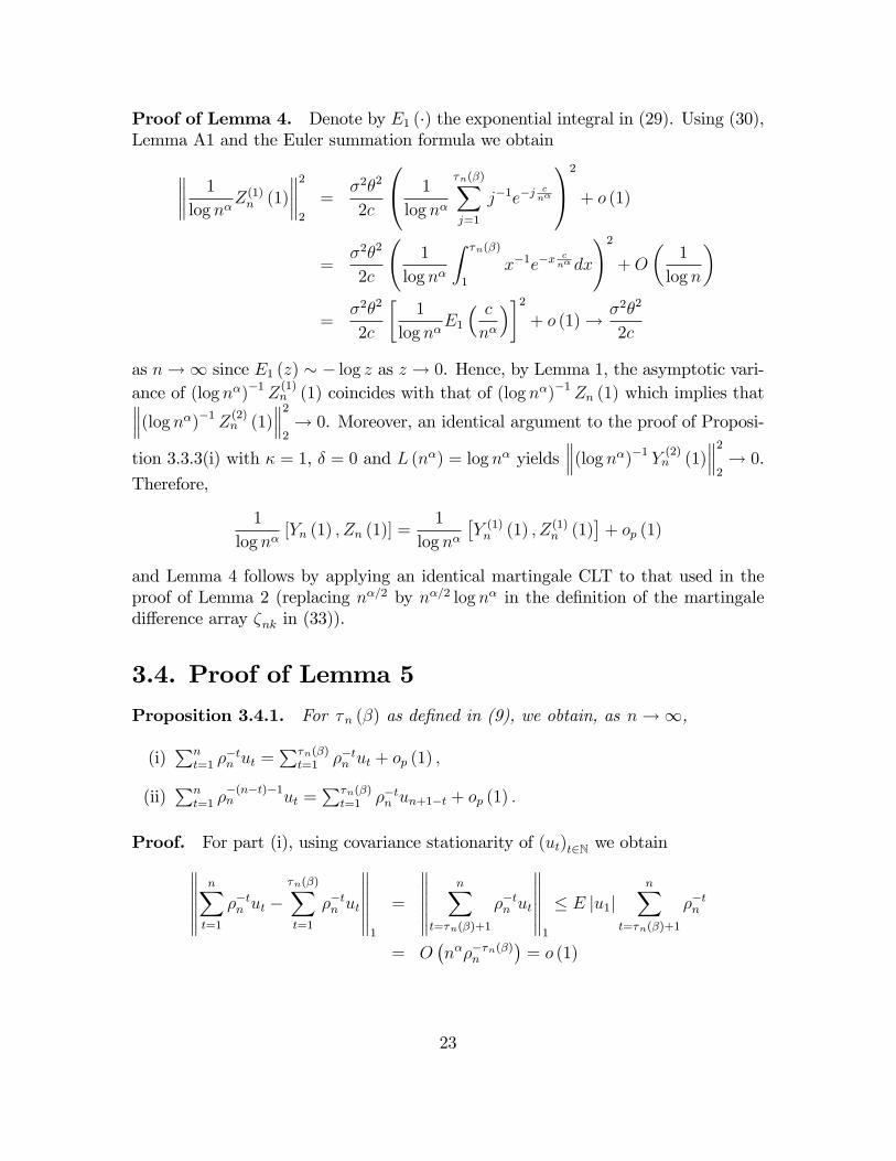
Proof of Lemma 4. Denote by E1 (�) the exponential integral in (29). Using (30),Lemma A1 and the Euler summation formula we obtain 1
log n�Z(1)n (1)
22
=�2�2
2c
0@ 1
log n�
�n(�)Xj=1
j�1e�jcn�
1A2
+ o (1)
=�2�2
2c
1
log n�
Z �n(�)
1
x�1e�xcn� dx
!2+O
�1
log n
�=
�2�2
2c
�1
log n�E1
� c
n�
��2+ o (1)! �2�2
2c
as n!1 since E1 (z) � � log z as z ! 0. Hence, by Lemma 1, the asymptotic vari-ance of (log n�)�1 Z(1)n (1) coincides with that of (log n�)�1 Zn (1) which implies that (log n�)�1 Z(2)n (1)
22! 0. Moreover, an identical argument to the proof of Proposi-
tion 3.3.3(i) with � = 1, � = 0 and L (n�) = log n� yields (log n�)�1 Y (2)
n (1) 22! 0.
Therefore,
1
log n�[Yn (1) ; Zn (1)] =
1
log n��Y (1)n (1) ; Z(1)n (1)
�+ op (1)
and Lemma 4 follows by applying an identical martingale CLT to that used in theproof of Lemma 2 (replacing n�=2 by n�=2 log n� in the de�nition of the martingaledi¤erence array �nk in (33)).
3.4. Proof of Lemma 5
Proposition 3.4.1. For �n (�) as de�ned in (9), we obtain, as n!1,
(i)Pn
t=1 ��tn ut =
P�n(�)t=1 ��tn ut + op (1) ;
(ii)Pn
t=1 ��(n�t)�1n ut =
P�n(�)t=1 ��tn un+1�t + op (1) :
Proof. For part (i), using covariance stationarity of (ut)t2N we obtain nXt=1
��tn ut ��n(�)Xt=1
��tn ut
1
=
nX
t=�n(�)+1
��tn ut
1
� E ju1jnX
t=�n(�)+1
��tn
= O�n����n(�)n
�= o (1)
23

as n!1. For part (ii), sincePn
t=1 ��(n�t)�1n ut =
Pnt=1 �
�tn un+1�t
nXt=1
��(n�t)�1n ut ��n(�)Xt=1
��tn un+1�t
1
=
nX
t=�n(�)+1
��tn un+1�t
1
= O�n����n(�)n
�using the same bound as in part (i).
Proof of Lemma 5. The derivations of this subsection are not a¤ected by thememory of the innovation sequence in any way other than the additional normalisationrequired in the long memory case. Therefore, it is enough to present the argumentfor part (ii) of the lemma. An identical argument is valid for part (i) and part (iii)by making the appropriate adjustment for the normalisation.We start by analysing the sample covariance. For �n as in (21), the initialization
of the mildly explosive process satis�es X0 = op�n�=2�n
�by Assumption IC. Using
the identity Xt�1 = X0�t�1n +
Pt�1j=1 �
t�j�1n uj and Proposition 3.4.1(ii) we obtain
��nnn��2n
nXt=1
Xt�1ut =1
n��2n
(X0
nXt=1
��(n�t)�1n ut + ��nn
nXt=1
t�1Xj=1
�t�j�1n ujut
)
=X0
n�=2�n
Yn (�)
L (n�)+
��nnn��2n
nXt=1
t�1Xj=1
�t�j�1n ujut + op (1)
=��nnn��2n
nXt=1
t�1Xj=1
�t�j�1n ujut + op (1) ; (45)
since Yn (�) =L (n�) = Op (1) by Lemma 3. Now the Cauchy-Schwarz inequality gives ��nnn��2nnXt=1
nXj=t
�t�j�1n ujut
1
� ��nnn��2n
nXt=1
nXj=t
�t�j�1n E jujutj
� E (u21) ��nn
n��2n
nXt=1
�t�1n
nXj=t
��jn
= O
���nn n1+�
n(3�2�)�L (n�)2
�= o (1) :
Thus, (45) and Proposition 3.4.1 yield
��nnn��2n
nXt=1
Xt�1ut =
1
n�=2�n
nXt=1
��(n�t)�1n ut
! 1
n�=2�n
nXj=1
��jn uj
!+ op (1)
=Yn (�)
L (n�)
Zn (�)
L (n�)+ op (1) ; (46)
24

as required. For the sample variance, by taking the square of (3) and summing overt 2 f1; :::; ng we obtain
nXt=1
X2t�1 =
1
�2n � 1
(X2n �X2
0 � 2�nnXt=1
Xt�1ut �nXt=1
u2t
)=
1
�2n � 1�X2n +O
��nn�
2n
��by (46). Thus, since ��nn Xn =
Pnt=1 �
�tn ut and �
2n � 1 = 2c=n� +O (n�2�) ; we obtain
��2nn
n2��2n
nXt=1
X2t�1 =
1
2c
"1
n�=2�n
nXt=1
��tn ut
#2+ op (1)
=1
2c
�1
L (n�)Zn (�)
�2+ op (1)
by Proposition 3.4.1(i). This completes the proof of Lemma 5.
4. Appendix
This section contains some asymptotic results for sums and integrals that are used inthe proof of Lemmas 1, 3 and 4. We begin by showing that the asymptotic equivalence��tn � e�
cn�t as n!1 is valid uniformly in t 2 f1; :::; �n (�)g.
Lemma A1. Let �n (�) be the sequence de�ned in (9). Then
sup1�t��n(�)
����tn � e�cn�t�� = O
�1
n�=2
�as n!1: (47)
Proof. Using the expansion log (1 + x) = x+O (x2) as x! 0, we obtain, as n!1
��tn = expn�t log
�1 +
c
n�
�o= exp
��t�c
n�+O
�1
n2�
���= e�
cn�t
�1�
�exp
�O
�t
n2�
��� 1��
:
Using the mean value theorem and monotonicity of the exponential function we obtainthe following elementary inequality: jex � 1j � xex for all x � 0. Application of this
25
inequality yields
sup1�t��n(�)
����tn � e�cn�t�� � sup
1�t��n(�)
����exp�O� t
n2�
��� 1����
� sup1�t��n(�)
O
�t
n2�
�exp
�O
�t
n2�
��= O
�n3�=2
n2�
�exp
�O
�n3�=2
n2�
��= O
�1
n�=2
�as required.
In the remainder of this section we establish two types of asymptotic results thathave been used in Section 3: An Abelian theorem for integrals involving regularlyvarying functions and approximation of sums by integrals by means of the Eulersummation formula. In the spirit of Apostol (1957) p.202 we derive the following formof the Euler-Maclaurin formula: Let m;M 2 N. If f has �nite variation Vf (m;M)on [m;M ] then applying the integration by parts formula for Stieltjes integrals onRMmf (x) d (x� bxc) yields
MXj=m
f (j)�Z M
m
f (x) dx = f (m) +
Z M
m
(x� bxc) df (x) :
Since x� bxc < 1, the above formula implies the following approximation:�����MXj=m
f (j)�Z M
m
f (x) dx
����� � jf (m)j+ Vf (m;M) m;M 2 N: (48)
Lemma A2 is a standard Abelian theorem, see Korevaar (2004, Proposition 5.4).
Lemma A2. Given a slowly varying function L, let � (x) = x�L (x). If k is realfunction satisfying
R10x� jk (x)j dx <1 for some � 6= 0 and
1
x
Z B
0
k
�t
x
�� (t) dt = o (� (x)) as x!1 (49)
for any B > 0, thenZ 1
0
k (t)� (xt) dt = [1 + o (1)]� (x)
Z 1
0
k (t) t�dt as x!1:
26

Lemma A3. Under Assumption LP(ii), let t0 be a positive constant such that' (t) = L (t) t�� is non-increasing on [t0;1),
In (�; ) =1
L (n�)
Z c�n(�)n�
n�
e�yy��L
�n�y
c
�dy > 0
and �n = L (n�)n(1��)�: Then, the following hold as n!1 :
(i) ��1nP�n(�)
t=1 L (t) t������tn � e�
cn�t��! 0.
(ii)�����1n P�n(�)
t=1 L (t) t��e�cn�t � c��1In (�; bt0c+ 1)
��� = O���1n�:
(iii) In (�; )! � (1� �) for all > 0:
Proof. For part (i), Lemma A1 yields that there exists C 2 (0;1) such that
1
�n
�n(�)Xt=1
L (t) t������tn � e�
cn�t�� � C
�nn�=2
�n(�)Xt=1
t��L (t)
= O
L�n��n(1��)�
L (n�)n�=2n(1��)�
!= o (1)
by Karamata�s theorem, since (9) implies that �=2� (1� �) (� � �) > 0.For part (ii), let fn (t) := L (t) t��e�
cn�t. Since ' (t) non-increasing on [t0;1) so
is fn (t) and
��1n
�n(�)Xt=1
fn (t) = ��1n
�n(�)Xt=bt0c+1
fn (t) +O���1n�:
We now approximate the sum on the right by the corresponding integral using (48).Since fn (�) is non-increasing on [t0;1);
supn2N
Vfn [t0;1) = supn2N
fn (t0) � supt�t0
L (t) t�� <1
so (48) implies that�������n(�)Xj=1
fn (t)�Z �n(�)
bt0c+1fn (t) dt
������ = O���1n�
as n!1:
The result follows sinceR �n(�)bt0c+1 fn (t) dt = c��1In (�; bt0c+ 1) :
27

For part (iii), we apply Lemma A2 on
Jn (�) =1
L (n�)
Z 1
0
e�yy��L
�n�y
c
�dy (50)
=c��+1
' (n�)
Z 1
0
e�cy' (n�y) dy:
SinceR10e�cyy��dy < 1, the integrability condition of Lemma A2 is satis�ed. To
verify (49) write, for any B > 0 and any � 2 (0; 1� �),
1
n�
Z B
0
e�cn�y' (y) dy � 1
n�
Z B
0
' (y) dy � supt2(0;B]
t�L (t)1
n�
Z B
0
y����dy
= supt2[0;B]
t�L (t)B1����
n�= O
�1
n�
�= o (' (n�))
by (5). Thus, using Lemma A2 we obtain
Jn (�)! c��+1Z 1
0
e�cyy��dy = � (1� �) as n!1: (51)
It remains to show that In (�; ) and Jn (�) are asymptotically equivalent:
jIn (�; )� Jn (�)j =1
L (n�)
(Z n�
0
+
Z 1
c�n(�)n�
)e�yy��L
�n�y
c
�dy:
Choosing � 2 (0; 1� �) and using (5), we obtain that the �rst integral is bounded by
supy2[0;1]
y�L (y)c�
n��L (n�)
Z n�
0
y����dy = O
�1
L (n�)n�(1��)
�:
For the second integral, using the property supx�u x��L (x) � u��L (u) as u ! 1
(see Seneta, 1976, p.65) and (9), we obtain the following bound:
n��
c�L (n�)sup
y��n(�)y��L (y)
Z 1
c�n(�)n�
e�ydy = o�e�
c2n���
�:
Thus, jIn (�; )� Jn (�)j ! 0 as n!1 and part (ii) follows by (51).
Lemma A4. Let f (t; y) := L (t+ y) (t+ y)�� L (y) y��, where � 2 (1=2; 1) andL (t) is a slowly varying function such that ' (t) = t��L (t) is eventually non-increasingon [t0;1) : Then, as n!1,
1
�2n
24�n(�)Xt=1
e�cn�t
�n(�)Xj=1
f (t; j)�Z �n(�)
bt0c+1e�
cn�t
Z �n(�)
bt0c+1f (t; y) dydt
35! 0
where �n is the sequence de�ned in (21). Under Assumption LP(iii), the above for-mula applies with f (t; y) = (t+ y)�1 y�1, �n = log n and t0 = 0.
28

Proof. Choosing � 2 (0; 1� �) and � = min (�; �) we obtain
1
�2n
�n(�)Xt=1
e�ctn�
24�n(�)Xj=1
f (t; j)��n(�)X
j=bt0c+1
f (t; j)
35 =1
�2n
�n(�)Xt=1
e�ctn�
bt0cXj=1
f (t; j)
��supt�1
t��L (t)
�2t0
�2n
�n(�)Xt=1
e�ctn� t�(���)
� O (1)1
�2n
Z 1
1
e�ctn� t�(���)dt
= O�n�(1����)�
�� (1� �+ �)! 0:
The above calculation shows that
1
�2n
24�n(�)Xt=1
e�cn�t
�n(�)Xj=1
f (t; j)��n(�)X
t=bt0c+1
e�cn�t
�n(�)Xj=bt0c+1
f (t; j)
35! 0 as n!1
so we only need to apply the Euler approximation (48) to the second sum, wheref (t; j) is non-increasing in both its arguments. We �rst show that
1
�2n
�n(�)Xt=bt0c+1
e�cn�t
�������n(�)X
j=bt0c+1
f (t; j)�Z �n(�)
bt0c+1f (t; y) dy
������! 0 as n!1: (52)
Fixing t and regarding f (t; y) as a function of y, f is non-increasing on [t0;1) soVf [t0;1) = f (t; t0). Using (48), the left side of (52) is bounded by
2
�2n
�n(�)Xt=1
e�cn�tf (t; t0) =
2L (t0) t��0
�2n
�n(�)Xt=1
e�cn�tL (t+ t0) (t+ t0)
��
= O
0@ 1
�2n
�n(�)Xt=1
e�cn�tL (t) t��
1A = O
�1
�n
�by Lemma A3. This shows (52). The lemma will follow from combining (52) and
1
�2n
�������n(�)X
t=bt0c+1
e�cn�t
Z �n(�)
bt0c+1f (t; y) dy �
Z �n(�)
bt0c+1e�
cn�x
Z �n(�)
bt0c+1f (x; y) dydx
������! 0: (53)
Since the function gn (t) = e�cn�tR �n(�)bt0c+1 f (t; y) dy is non-increasing on [t0;1), Vgn [t0;1) =
gn (t0). By (48), the left side of (53) is bounded by
2
�2ngn (t0) �
2
�2n
Z �n(�)
bt0c+1f (t0; y) dy �
2
�2n
Z �n(�)
bt0c+1L (y)2 y�2�dy = O
�1
�2n
�:
29
This shows the lemma under Assumption LP(ii).Under Assumption LP(iii), the same argument applies and the estimation error
is again O���1n�with �n = log n. Note that the absence of the slowly varying
component implies that f (t; j) and gn (t) are non-increasing for all t; j � 1 so wemay take t0 = 0.
References
Abramowitz, M. and I.A. Stegun (1972). Handbook of Mathematical Functions.National Bureau of Standards, Washington.
Aue, A. and L. Horváth (2007). �A limit theorem for mildly explosive autoregressionwith stable errors�. Econometric Theory 23, 201-220.
Anderson, T.W. (1959). �On asymptotic distributions of estimates of parameters ofstochastic di¤erence equations�. Annals of Mathematical Statistics, 30, 676-687.
Apostol, T.M. (1957). Mathematical Analysis. Addison-Wesley.
Bingham, N.H., Goldie, C.M. and J.L. Teugels (1987). Regular Variation. Cam-bridge University Press.
Giraitis, L., Koul, H.L. and D. Surgailis (1996). �Asymptotic normality of regressionestimators with long memory errors�. Statistics and Probability Letters, 29, 317-335.
Giraitis, L. and P. C. B. Phillips (2006). �Uniform Limit Theory for StationaryAutoregression�. Journal of Time Series Analysis, 27, 51-60.
Hall, P. and C.C. Heyde (1980). Martingale Limit Theory and its Application.Academic Press.
Kallenberg, O. (2002). Foundations of Modern Probability. Springer.
Korevaar, J. (2004). Tauberian Theory. Springer-Verlag.
Magdalinos, T. and P. C. B. Phillips (2008). �Limit Theory for CointegratedSystems with Moderately Integrated and Moderately Explosive Regressors�.Econometric Theory, forthcoming.
Phillips, P. C. B. (2007). �Regression with Slowly Varying Regressors and NonlinearTrends�. Econometric Theory, 23, 557-614.
Phillips, P. C. B. and T. Magdalinos (2007a). �Limit theory for Moderate deviationsfrom a unit root.�Journal of Econometrics, 136, 115-130.
30
Phillips, P. C. B. and T. Magdalinos (2007b). �Limit theory for Moderate deviationsfrom a unit root under weak dependence.�in G. D. A. Phillips and E. Tzavalis(Eds.) The Re�nement of Econometric Estimation and Test Procedures: FiniteSample and Asymptotic Analysis. Cambridge University Press.
Seneta, E. (1976). Regularly Varying Functions. Lecture Notes in Mathematics,508. Springer-Verlag.
White, J. S. (1958). �The limiting distribution of the serial correlation coe¢ cientin the explosive case�. Annals of Mathematical Statistics 29, 1188�1197.
Wu, W.B. and W. Min (2005). �On linear processes with dependent innovations�.Stochastic Processes and their Applications 115, 939-958.
31