Embed Size (px)
Citation preview

MIKE 11
A Modelling System for Rivers and Channels
Reference Manual
MIKE BY DHI 2011

2

Please Note
CopyrightThis document refers to proprietary computer software which is protectedby copyright. All rights are reserved. Copying or other reproduction ofthis manual or the related programs is prohibited without prior writtenconsent of DHI. For details please refer to your 'DHI Software LicenceAgreement'.
Limited LiabilityThe liability of DHI is limited as specified in Section III of your 'DHISoftware Licence Agreement':'IN NO EVENT SHALL DHI OR ITS REPRESENTA-TIVES (AGENTSAND SUPPLIERS) BE LIABLE FOR ANY DAMAGES WHATSO-EVER INCLUDING, WITHOUT LIMITATION, SPECIAL, INDIRECT,INCIDENTAL OR CONSEQUENTIAL DAMAGES OR DAMAGESFOR LOSS OF BUSINESS PROFITS OR SAVINGS, BUSINESSINTERRUPTION, LOSS OF BUSINESS INFORMATION OR OTHERPECUNIARY LOSS ARISING OUT OF THE USE OF OR THE INA-BILITY TO USE THIS DHI SOFTWARE PRODUCT, EVEN IF DHIHAS BEEN ADVISED OF THE POSSIBILITY OF SUCH DAMAGES.THIS LIMITATION SHALL APPLY TO CLAIMS OF PERSONALINJURY TO THE EXTENT PERMITTED BY LAW. SOME COUN-TRIES OR STATES DO NOT ALLOW THE EXCLUSION OR LIMITA-TION OF LIABILITY FOR CONSEQUENTIAL, SPECIAL, INDIRECT,INCIDENTAL DAMAGES AND, ACCORDINGLY, SOME PORTIONSOF THESE LIMITATIONS MAY NOT APPLY TO YOU. BY YOUROPENING OF THIS SEALED PACKAGE OR INSTALLING ORUSING THE SOFTWARE, YOU HAVE ACCEPTED THAT THEABOVE LIMITATIONS OR THE MAXIMUM LEGALLY APPLICA-BLE SUBSET OF THESE LIMITATIONS APPLY TO YOUR PUR-CHASE OF THIS SOFTWARE.'
Printing HistoryJune 2004June 2005December 2006November 2007January 2009December 2011
3

4 MIKE 11

C O N T E N T S
5

Hydrodynamic Reference . . . . . . . . . . . . . . . . . . . . . . . . . . . . . . . . 17
1 HD REFERENCE MANUAL . . . . . . . . . . . . . . . . . . . . . . . . . . . . . . 191.1 Manual Format . . . . . . . . . . . . . . . . . . . . . . . . . . . . . . . . . 191.2 A General Description . . . . . . . . . . . . . . . . . . . . . . . . . . . . . 201.3 Bed Resistance . . . . . . . . . . . . . . . . . . . . . . . . . . . . . . . . . 21
1.3.1 Chezy and Manning . . . . . . . . . . . . . . . . . . . . . . . . . . 211.3.2 Relative Resistance . . . . . . . . . . . . . . . . . . . . . . . . . . 221.3.3 Resistance Factor . . . . . . . . . . . . . . . . . . . . . . . . . . . 231.3.4 Resistance Radius . . . . . . . . . . . . . . . . . . . . . . . . . . 231.3.5 Hydraulic Radius . . . . . . . . . . . . . . . . . . . . . . . . . . . 241.3.6 Resistance Radius vs Hydraulic Radius . . . . . . . . . . . . . . 251.3.7 Calculation of resistance using channel bank markers . . . . . . 281.3.8 Additional resistance due to vegetation . . . . . . . . . . . . . . 29
1.4 Boundary Conditions . . . . . . . . . . . . . . . . . . . . . . . . . . . . . . 341.4.1 Resolution . . . . . . . . . . . . . . . . . . . . . . . . . . . . . . . 341.4.2 Which Boundary Condition? . . . . . . . . . . . . . . . . . . . . . 34
1.5 Bridges . . . . . . . . . . . . . . . . . . . . . . . . . . . . . . . . . . . . . . 351.5.1 Arch Bridges (Biery and Delleur) . . . . . . . . . . . . . . . . . . 371.5.2 Arch Bridges (Hydraulics Research (HR) method) . . . . . . . . 391.5.3 Bridge Piers (D’Aubuisson) . . . . . . . . . . . . . . . . . . . . . 401.5.4 Bridge Piers (Nagler) . . . . . . . . . . . . . . . . . . . . . . . . . 421.5.5 Bridge Piers (Yarnell) . . . . . . . . . . . . . . . . . . . . . . . . . 431.5.6 Energy Equation . . . . . . . . . . . . . . . . . . . . . . . . . . . . 441.5.7 Federal Highway Administration (FHWA) WSPRO method . . . 471.5.8 US Bureau of Public Roads (USBPR) method . . . . . . . . . . 601.5.9 Multiple Waterway Opening . . . . . . . . . . . . . . . . . . . . . 611.5.10 Pressure Flow, Federal Highway Administration method . . . . 621.5.11 Road overflow, Federal Highway Administration method . . . . 651.5.12 Fully submerged bridges . . . . . . . . . . . . . . . . . . . . . . . 661.5.13 Trouble shooting for bridge structures . . . . . . . . . . . . . . . 69
1.6 Broad crested Weir . . . . . . . . . . . . . . . . . . . . . . . . . . . . . . . 701.7 Coefficients, HD default parameters . . . . . . . . . . . . . . . . . . . . . 701.8 Computational Grid . . . . . . . . . . . . . . . . . . . . . . . . . . . . . . . 72
1.8.1 General Description . . . . . . . . . . . . . . . . . . . . . . . . . . 721.8.2 Selecting the Area to be Modelled . . . . . . . . . . . . . . . . . 721.8.3 Selecting Model Branches . . . . . . . . . . . . . . . . . . . . . . 731.8.4 Selecting the Grid Spacing . . . . . . . . . . . . . . . . . . . . . . 73
1.9 Control Structures . . . . . . . . . . . . . . . . . . . . . . . . . . . . . . . . 741.9.1 Hydraulic Aspects - Radial Gates . . . . . . . . . . . . . . . . . . 741.9.2 Hydraulic Aspects -Sluice Gates . . . . . . . . . . . . . . . . . . 761.9.3 Hydraulic Aspects - Overflow Structures . . . . . . . . . . . . . . 781.9.4 Hydraulic Aspects - Underflow Structures . . . . . . . . . . . . . 78
6 MIKE 11
1.9.5 Free Flow . . . . . . . . . . . . . . . . . . . . . . . . . . . . . . . . 801.9.6 Drowned Flow . . . . . . . . . . . . . . . . . . . . . . . . . . . . . 81
1.10 Cross-Sections . . . . . . . . . . . . . . . . . . . . . . . . . . . . . . . . . . 811.11 Closed Cross sections, Modelling the Pressurised flow . . . . . . . . . . 841.12 Culverts, Q-h Relations Calculation . . . . . . . . . . . . . . . . . . . . . . 88
1.12.1 Specification . . . . . . . . . . . . . . . . . . . . . . . . . . . . . . 881.12.2 Flow Descriptions . . . . . . . . . . . . . . . . . . . . . . . . . . . 891.12.3 Construction of Q-h Relationships . . . . . . . . . . . . . . . . . . 911.12.4 Closed / Open Section switch . . . . . . . . . . . . . . . . . . . . 921.12.5 Changing Flow Direction . . . . . . . . . . . . . . . . . . . . . . . 931.12.6 Flooded Areas of Adjacent h-points . . . . . . . . . . . . . . . . . 931.12.7 Velocities . . . . . . . . . . . . . . . . . . . . . . . . . . . . . . . . 93
1.13 Dambreak Structure . . . . . . . . . . . . . . . . . . . . . . . . . . . . . . . 931.13.1 Energy equation based dam breach modelling . . . . . . . . . . 941.13.2 Erosion Based Breach Development using the energy equation 961.13.3 NWS DAMBRK dam-breach method . . . . . . . . . . . . . . . 101
1.14 Energy Loss . . . . . . . . . . . . . . . . . . . . . . . . . . . . . . . . . . 1051.15 Flooded Areas, (Storage) . . . . . . . . . . . . . . . . . . . . . . . . . . . 1071.16 Flood control facilities . . . . . . . . . . . . . . . . . . . . . . . . . . . . . 110
1.16.1 Non control . . . . . . . . . . . . . . . . . . . . . . . . . . . . . . 1101.16.2 Constant discharging method Type A . . . . . . . . . . . . . . . 1101.16.3 Constant discharging method Type B . . . . . . . . . . . . . . . 1111.16.4 Constant ratio discharging method Type A . . . . . . . . . . . . 1121.16.5 Constant ratio discharging method Type B . . . . . . . . . . . . 1131.16.6 Bucket-cut (without afterward discharging) . . . . . . . . . . . . 1141.16.7 Non gate discharging by H/Q curve and H/V curve . . . . . . . 1141.16.8 Non gate discharging by orifice size input . . . . . . . . . . . . 115
1.17 Flood plain Encroachment calculations . . . . . . . . . . . . . . . . . . . 1181.17.1 General . . . . . . . . . . . . . . . . . . . . . . . . . . . . . . . . 1181.17.2 Encroachment Methods . . . . . . . . . . . . . . . . . . . . . . . 1201.17.3 Additional specifications for encroachment calculations . . . . 1211.17.4 Cross sections after encroachment . . . . . . . . . . . . . . . . 1221.17.5 Encroachments at structures . . . . . . . . . . . . . . . . . . . . 1231.17.6 Encroachments at nodes . . . . . . . . . . . . . . . . . . . . . . 123
1.18 Flood Plains . . . . . . . . . . . . . . . . . . . . . . . . . . . . . . . . . . 1241.19 Flow Descriptions . . . . . . . . . . . . . . . . . . . . . . . . . . . . . . . 127
1.19.1 Dynamic Wave and High Order Dynamic Wave . . . . . . . . . 1271.19.2 Diffusive Wave . . . . . . . . . . . . . . . . . . . . . . . . . . . . 1281.19.3 Kinematic Wave . . . . . . . . . . . . . . . . . . . . . . . . . . . 1281.19.4 Which Flow Description? . . . . . . . . . . . . . . . . . . . . . . 128
1.20 Initial Conditions . . . . . . . . . . . . . . . . . . . . . . . . . . . . . . . . 1281.20.1 User-Specified . . . . . . . . . . . . . . . . . . . . . . . . . . . . 128
7

1.20.2 Auto Start, Quasi-Steady Solution . . . . . . . . . . . . . . . . . 1291.20.3 Hot Start . . . . . . . . . . . . . . . . . . . . . . . . . . . . . . . . 1291.20.4 Combined Auto Start and user-specified initial conditions . . . . 129
1.21 Kinematic Routing Method . . . . . . . . . . . . . . . . . . . . . . . . . . . 1291.22 Lateral Inflows . . . . . . . . . . . . . . . . . . . . . . . . . . . . . . . . . . 1341.23 Low Flow Conditions . . . . . . . . . . . . . . . . . . . . . . . . . . . . . . 1351.24 Pumps . . . . . . . . . . . . . . . . . . . . . . . . . . . . . . . . . . . . . . 136
1.24.1 Capacity . . . . . . . . . . . . . . . . . . . . . . . . . . . . . . . . 1361.24.2 Start/Stop control . . . . . . . . . . . . . . . . . . . . . . . . . . . 1371.24.3 Internal outlet . . . . . . . . . . . . . . . . . . . . . . . . . . . . . 1371.24.4 External outlet . . . . . . . . . . . . . . . . . . . . . . . . . . . . . 138
1.25 Quasi-Steady Solution . . . . . . . . . . . . . . . . . . . . . . . . . . . . . 1381.26 Quasi-two dimensional steady flow with vegetation . . . . . . . . . . . . 143
1.26.1 Zone classification . . . . . . . . . . . . . . . . . . . . . . . . . . 1461.26.2 Solution algorithm . . . . . . . . . . . . . . . . . . . . . . . . . . . 1551.26.3 Bridges . . . . . . . . . . . . . . . . . . . . . . . . . . . . . . . . . 1611.26.4 Junctions . . . . . . . . . . . . . . . . . . . . . . . . . . . . . . . . 1641.26.5 Variation in water level due to curves . . . . . . . . . . . . . . . . 1651.26.6 Variation in water level due to sand bars . . . . . . . . . . . . . . 166
1.27 Regulating Structures . . . . . . . . . . . . . . . . . . . . . . . . . . . . . 1671.27.1 Function of time . . . . . . . . . . . . . . . . . . . . . . . . . . . . 1671.27.2 Function of h and/or Q . . . . . . . . . . . . . . . . . . . . . . . . 168
1.28 Routing . . . . . . . . . . . . . . . . . . . . . . . . . . . . . . . . . . . . . . 1691.29 Saint Venant Equations . . . . . . . . . . . . . . . . . . . . . . . . . . . . 1701.30 Solution Scheme . . . . . . . . . . . . . . . . . . . . . . . . . . . . . . . . 1711.31 Special Weir . . . . . . . . . . . . . . . . . . . . . . . . . . . . . . . . . . . 1721.32 Stability Conditions . . . . . . . . . . . . . . . . . . . . . . . . . . . . . . . 1731.33 Steady State Energy Equation . . . . . . . . . . . . . . . . . . . . . . . . 1751.34 Structures . . . . . . . . . . . . . . . . . . . . . . . . . . . . . . . . . . . . 180
1.34.1 Zero Flow . . . . . . . . . . . . . . . . . . . . . . . . . . . . . . . . 1811.34.2 Drowned Flow . . . . . . . . . . . . . . . . . . . . . . . . . . . . . 1811.34.3 Free Overflow . . . . . . . . . . . . . . . . . . . . . . . . . . . . . 1821.34.4 Contraction and Expansion Losses . . . . . . . . . . . . . . . . . 1831.34.5 Grid spacing at structures . . . . . . . . . . . . . . . . . . . . . . 1831.34.6 Parallel/Composite Structures . . . . . . . . . . . . . . . . . . . . 183
1.35 Supercritical Flow . . . . . . . . . . . . . . . . . . . . . . . . . . . . . . . . 1841.35.1 Suppression of convective acceleration term . . . . . . . . . . . 1851.35.2 Effect of convective acceleration suppression on Energy Heads . .
1871.36 Supercritical Flow in Structures . . . . . . . . . . . . . . . . . . . . . . . . 187
1.36.1 Flow Directions . . . . . . . . . . . . . . . . . . . . . . . . . . . . 188
8 MIKE 11

1.36.2 Testing for Flow Conditions . . . . . . . . . . . . . . . . . . . . 1881.36.3 Subcritical Flow through Structure . . . . . . . . . . . . . . . . . 1891.36.4 Critical Flow through Structure . . . . . . . . . . . . . . . . . . . 1891.36.5 Supercritical Flow through Structure . . . . . . . . . . . . . . . 1901.36.6 Contraction and Expansion Losses, Sub- and Supercritical Flow . .
1901.37 Tabulated structures . . . . . . . . . . . . . . . . . . . . . . . . . . . . . 1911.38 Time Stepping . . . . . . . . . . . . . . . . . . . . . . . . . . . . . . . . . 1911.39 User Defined Structure . . . . . . . . . . . . . . . . . . . . . . . . . . . . 193
1.39.1 Tips . . . . . . . . . . . . . . . . . . . . . . . . . . . . . . . . . . 1941.40 Weir Formula . . . . . . . . . . . . . . . . . . . . . . . . . . . . . . . . . . 194
1.40.1 Weir Formula 1 . . . . . . . . . . . . . . . . . . . . . . . . . . . . 1951.40.2 Weir Formula 2 (Honma) . . . . . . . . . . . . . . . . . . . . . . 1951.40.3 Weir Formula 3 (Extended Honma) . . . . . . . . . . . . . . . . 195
1.41 Wind . . . . . . . . . . . . . . . . . . . . . . . . . . . . . . . . . . . . . . . 1961.42 References . . . . . . . . . . . . . . . . . . . . . . . . . . . . . . . . . . . 197
Advection-Dispersion / Cohesive Sediment Transport Reference. . . . . . . . . . . . . . . . . . . . . 199
2 AD/CST REFERENCE MANUAL . . . . . . . . . . . . . . . . . . . . . . . . . . 2012.1 Who Should Use This Manual . . . . . . . . . . . . . . . . . . . . . . . . 2012.2 Manual Format . . . . . . . . . . . . . . . . . . . . . . . . . . . . . . . . . 2012.3 A General Description . . . . . . . . . . . . . . . . . . . . . . . . . . . . 2012.4 Advanced Cohesive Sediment Transport . . . . . . . . . . . . . . . . . 202
2.4.1 Cross-Sectional Shear Stress Distribution . . . . . . . . . . . . 2032.4.2 Settling . . . . . . . . . . . . . . . . . . . . . . . . . . . . . . . . 2042.4.3 Deposition . . . . . . . . . . . . . . . . . . . . . . . . . . . . . . 2052.4.4 Sliding . . . . . . . . . . . . . . . . . . . . . . . . . . . . . . . . . 2052.4.5 Erosion . . . . . . . . . . . . . . . . . . . . . . . . . . . . . . . . 2062.4.6 Consolidation . . . . . . . . . . . . . . . . . . . . . . . . . . . . . 206
2.5 Advection-Dispersion Equation . . . . . . . . . . . . . . . . . . . . . . . 2072.6 Boundary Conditions . . . . . . . . . . . . . . . . . . . . . . . . . . . . . 207
2.6.1 Open Boundary Outflow . . . . . . . . . . . . . . . . . . . . . . 2082.6.2 Open Boundary Inflow . . . . . . . . . . . . . . . . . . . . . . . 2082.6.3 Concentration boundary . . . . . . . . . . . . . . . . . . . . . . 2082.6.4 Transport boundary . . . . . . . . . . . . . . . . . . . . . . . . . 2082.6.5 Closed Boundary . . . . . . . . . . . . . . . . . . . . . . . . . . 208
2.7 Deposition, CST . . . . . . . . . . . . . . . . . . . . . . . . . . . . . . . . 2092.8 Dispersion Coefficient . . . . . . . . . . . . . . . . . . . . . . . . . . . . . 2112.9 Erosion, CST . . . . . . . . . . . . . . . . . . . . . . . . . . . . . . . . . . 211
9

2.10 Mass transport and mass balance . . . . . . . . . . . . . . . . . . . . . . 2122.10.1 Mass . . . . . . . . . . . . . . . . . . . . . . . . . . . . . . . . . . 2132.10.2 1st order Decay . . . . . . . . . . . . . . . . . . . . . . . . . . . . 2142.10.3 Transport . . . . . . . . . . . . . . . . . . . . . . . . . . . . . . . . 2142.10.4 Advective transport . . . . . . . . . . . . . . . . . . . . . . . . . . 2142.10.5 Dispersive transport . . . . . . . . . . . . . . . . . . . . . . . . . . 2152.10.6 Mass balance . . . . . . . . . . . . . . . . . . . . . . . . . . . . . 215
2.11 Solution Scheme, AD . . . . . . . . . . . . . . . . . . . . . . . . . . . . . . 2162.11.1 Continuity equation: . . . . . . . . . . . . . . . . . . . . . . . . . . 2162.11.2 Advective-dispersive transport equation: . . . . . . . . . . . . . . 217
2.12 Stability . . . . . . . . . . . . . . . . . . . . . . . . . . . . . . . . . . . . . . 2182.13 Nomenclature . . . . . . . . . . . . . . . . . . . . . . . . . . . . . . . . . . 2182.14 References . . . . . . . . . . . . . . . . . . . . . . . . . . . . . . . . . . . . 220
Non-cohesive Sediment Transport Reference . . . . . . . . . . . . . . . . . . 221
3 NST REFERENCE MANUAL . . . . . . . . . . . . . . . . . . . . . . . . . . . . . 2233.1 Manual Format . . . . . . . . . . . . . . . . . . . . . . . . . . . . . . . . . 2233.2 A General Description . . . . . . . . . . . . . . . . . . . . . . . . . . . . . 2243.3 Sediment transport models . . . . . . . . . . . . . . . . . . . . . . . . . . 2253.4 Bed forms . . . . . . . . . . . . . . . . . . . . . . . . . . . . . . . . . . . . 225
3.4.1 Ripples . . . . . . . . . . . . . . . . . . . . . . . . . . . . . . . . . 2263.4.2 Dunes . . . . . . . . . . . . . . . . . . . . . . . . . . . . . . . . . . 2263.4.3 Plane bed . . . . . . . . . . . . . . . . . . . . . . . . . . . . . . . 2273.4.4 Anti-dunes . . . . . . . . . . . . . . . . . . . . . . . . . . . . . . . 227
3.5 Morphological model . . . . . . . . . . . . . . . . . . . . . . . . . . . . . . 2283.5.1 Updating of bottom level . . . . . . . . . . . . . . . . . . . . . . . 2323.5.2 Boundary Conditions . . . . . . . . . . . . . . . . . . . . . . . . . 2363.5.3 Low flow correction . . . . . . . . . . . . . . . . . . . . . . . . . . 2383.5.4 Hints . . . . . . . . . . . . . . . . . . . . . . . . . . . . . . . . . . 238
3.6 Graded Sediments . . . . . . . . . . . . . . . . . . . . . . . . . . . . . . . 2393.6.1 Boundary conditions . . . . . . . . . . . . . . . . . . . . . . . . . 2433.6.2 Graded sediments boundary conditions . . . . . . . . . . . . . . 244
3.7 Dune dimensions . . . . . . . . . . . . . . . . . . . . . . . . . . . . . . . . 2443.7.1 Equilibrium dune height . . . . . . . . . . . . . . . . . . . . . . . 2443.7.2 Equilibrium dune length . . . . . . . . . . . . . . . . . . . . . . . 2473.7.3 Non-equilibrium dune height . . . . . . . . . . . . . . . . . . . . . 2513.7.4 Non-equilibrium dune length . . . . . . . . . . . . . . . . . . . . . 251
3.8 Flow Resistance . . . . . . . . . . . . . . . . . . . . . . . . . . . . . . . . . 2523.8.1 Flow resistance - dune dimension . . . . . . . . . . . . . . . . . 2533.8.2 Flow Resistance - θ−θ´ Relationship . . . . . . . . . . . . . . . . 2543.8.3 Flow Resistance - White et al. . . . . . . . . . . . . . . . . . . . . 257
10 MIKE 11

3.9 Incipient motion criteria . . . . . . . . . . . . . . . . . . . . . . . . . . . . 2593.9.1 Shield’s critical parameter . . . . . . . . . . . . . . . . . . . . . 2593.9.2 Iwagaki’s critical tractive force . . . . . . . . . . . . . . . . . . . 2603.9.3 Modified Egiazaroff equation . . . . . . . . . . . . . . . . . . . . 260
3.10 Ackers and White model . . . . . . . . . . . . . . . . . . . . . . . . . . . 2613.11 Ashida & Michiue model . . . . . . . . . . . . . . . . . . . . . . . . . . . 264
3.11.1 Bed load . . . . . . . . . . . . . . . . . . . . . . . . . . . . . . . 2643.11.2 Suspended load . . . . . . . . . . . . . . . . . . . . . . . . . . . 264
3.12 Ashida, Takahashi and Mizuyama model (ATM) . . . . . . . . . . . . . 2673.13 Engelund & Fredsøe model . . . . . . . . . . . . . . . . . . . . . . . . . 270
3.13.1 Bed Load . . . . . . . . . . . . . . . . . . . . . . . . . . . . . . . 2703.13.2 Suspended load . . . . . . . . . . . . . . . . . . . . . . . . . . . 271
3.14 Engelund & Hansen model . . . . . . . . . . . . . . . . . . . . . . . . . . 2733.15 Lane & Kalinske model . . . . . . . . . . . . . . . . . . . . . . . . . . . . 2743.16 Meyer-Peter & Müller model . . . . . . . . . . . . . . . . . . . . . . . . . 2753.17 Sato, Kikkawa & Ashida model . . . . . . . . . . . . . . . . . . . . . . . 2773.18 Smart and Jaeggi model . . . . . . . . . . . . . . . . . . . . . . . . . . . 278
3.18.1 Revised transport formula . . . . . . . . . . . . . . . . . . . . . 2783.18.2 MIKE 11 version . . . . . . . . . . . . . . . . . . . . . . . . . . . 279
3.19 van Rijn model . . . . . . . . . . . . . . . . . . . . . . . . . . . . . . . . . 2803.19.1 Bed load . . . . . . . . . . . . . . . . . . . . . . . . . . . . . . . 2803.19.2 Suspended load . . . . . . . . . . . . . . . . . . . . . . . . . . . 282
3.20 Nomenclature . . . . . . . . . . . . . . . . . . . . . . . . . . . . . . . . . 286
Rainfall-Runoff Reference . . . . . . . . . . . . . . . . . . . . . . . . . . . . . . . 293
4 RR REFERENCE MANUAL . . . . . . . . . . . . . . . . . . . . . . . . . . . . . 2954.1 NAM - Introduction . . . . . . . . . . . . . . . . . . . . . . . . . . . . . . 2964.2 Data Requirements . . . . . . . . . . . . . . . . . . . . . . . . . . . . . . 296
4.2.1 Meteorological data . . . . . . . . . . . . . . . . . . . . . . . . . 2974.2.2 Hydrological data . . . . . . . . . . . . . . . . . . . . . . . . . . 298
4.3 Model Structure . . . . . . . . . . . . . . . . . . . . . . . . . . . . . . . . 2994.4 Basic modelling components . . . . . . . . . . . . . . . . . . . . . . . . . 301
4.4.1 Surface storage . . . . . . . . . . . . . . . . . . . . . . . . . . . 3014.4.2 Lower zone or root zone storage . . . . . . . . . . . . . . . . . 3014.4.3 Evapotranspiration . . . . . . . . . . . . . . . . . . . . . . . . . . 3014.4.4 Overland flow . . . . . . . . . . . . . . . . . . . . . . . . . . . . . 3014.4.5 Interflow . . . . . . . . . . . . . . . . . . . . . . . . . . . . . . . . 3024.4.6 Interflow and overland flow routing . . . . . . . . . . . . . . . . 3024.4.7 Groundwater recharge . . . . . . . . . . . . . . . . . . . . . . . 3034.4.8 Soil moisture content . . . . . . . . . . . . . . . . . . . . . . . . 303
11

4.4.9 Baseflow . . . . . . . . . . . . . . . . . . . . . . . . . . . . . . . . 3034.5 Extended groundwater components . . . . . . . . . . . . . . . . . . . . . 303
4.5.1 Drainage to or from neighbouring catchments . . . . . . . . . . . 3034.5.2 Lower groundwater storage . . . . . . . . . . . . . . . . . . . . . 3044.5.3 Shallow groundwater reservoir description . . . . . . . . . . . . 3044.5.4 Capillary flux . . . . . . . . . . . . . . . . . . . . . . . . . . . . . . 304
4.6 Snow module . . . . . . . . . . . . . . . . . . . . . . . . . . . . . . . . . . 3054.6.1 Accumulation and melting of snow . . . . . . . . . . . . . . . . . 3054.6.2 Altitude-distributed snowmelt model . . . . . . . . . . . . . . . . 3064.6.3 Extended components . . . . . . . . . . . . . . . . . . . . . . . . 310
4.7 Irrigation module . . . . . . . . . . . . . . . . . . . . . . . . . . . . . . . . 3104.7.1 Introduction . . . . . . . . . . . . . . . . . . . . . . . . . . . . . . 3104.7.2 Structure of the irrigation module . . . . . . . . . . . . . . . . . . 311
4.8 Model parameters . . . . . . . . . . . . . . . . . . . . . . . . . . . . . . . . 3144.8.1 Surface and root zone parameters . . . . . . . . . . . . . . . . . 3154.8.2 Groundwater parameters . . . . . . . . . . . . . . . . . . . . . . . 3184.8.3 Snow module parameters . . . . . . . . . . . . . . . . . . . . . . 3204.8.4 Irrigation module parameters . . . . . . . . . . . . . . . . . . . . 320
4.9 Initial conditions . . . . . . . . . . . . . . . . . . . . . . . . . . . . . . . . . 3224.10 Model calibration . . . . . . . . . . . . . . . . . . . . . . . . . . . . . . . . 322
4.10.1 Calibration objectives and evaluation measures . . . . . . . . . 3234.10.2 Manual calibration . . . . . . . . . . . . . . . . . . . . . . . . . . . 3244.10.3 Automatic calibration routine . . . . . . . . . . . . . . . . . . . . . 325
4.11 NAM - REFERENCES . . . . . . . . . . . . . . . . . . . . . . . . . . . . . 3304.12 UHM . . . . . . . . . . . . . . . . . . . . . . . . . . . . . . . . . . . . . . . 331
4.12.1 Introduction . . . . . . . . . . . . . . . . . . . . . . . . . . . . . . 3314.12.2 The Loss Model . . . . . . . . . . . . . . . . . . . . . . . . . . . . 3364.12.3 The Unit Hydrograph Routing Model . . . . . . . . . . . . . . . . 3434.12.4 Kinematic wave hydrograph methods . . . . . . . . . . . . . . . 3474.12.5 Calculation timestep . . . . . . . . . . . . . . . . . . . . . . . . . 3514.12.6 UHM - References . . . . . . . . . . . . . . . . . . . . . . . . . . 351
4.13 SMAP . . . . . . . . . . . . . . . . . . . . . . . . . . . . . . . . . . . . . . . 3514.13.1 Introduction . . . . . . . . . . . . . . . . . . . . . . . . . . . . . . 3514.13.2 SMAP model equations . . . . . . . . . . . . . . . . . . . . . . . 352
4.14 Urban . . . . . . . . . . . . . . . . . . . . . . . . . . . . . . . . . . . . . . . 3554.14.1 Introduction . . . . . . . . . . . . . . . . . . . . . . . . . . . . . . 3554.14.2 Urban, model A, Time/area Method . . . . . . . . . . . . . . . . 3564.14.3 Urban, model B, Non-linear Reservoir (kinematic wave) Method . .
3594.15 DRiFt . . . . . . . . . . . . . . . . . . . . . . . . . . . . . . . . . . . . . . . 366
4.15.1 Introduction . . . . . . . . . . . . . . . . . . . . . . . . . . . . . . 3664.15.2 Model structure . . . . . . . . . . . . . . . . . . . . . . . . . . . . 367
12 MIKE 11

4.15.3 Data requirements . . . . . . . . . . . . . . . . . . . . . . . . . . 3684.15.4 Model calibration . . . . . . . . . . . . . . . . . . . . . . . . . . . 3784.15.5 DRiFt references . . . . . . . . . . . . . . . . . . . . . . . . . . . 386
Flood Forecasting Reference . . . . . . . . . . . . . . . . . . . . . . . . . . . . . 389 . . . . . . . . . . . . . . . . . . . . . . . . . . . . . . . . . . . . . . . . . . . . . . . . . 390
5 FF REFERENCE MANUAL . . . . . . . . . . . . . . . . . . . . . . . . . . . . . 3915.1 Introduction . . . . . . . . . . . . . . . . . . . . . . . . . . . . . . . . . . . 3915.2 Updating Procedure . . . . . . . . . . . . . . . . . . . . . . . . . . . . . . 392
5.2.1 Calibration Example . . . . . . . . . . . . . . . . . . . . . . . . . 3995.3 References . . . . . . . . . . . . . . . . . . . . . . . . . . . . . . . . . . . 404
Data assimilation Reference . . . . . . . . . . . . . . . . . . . . . . . . . . . . . 407
6 DATA ASSIMILATION IN MIKE 11 . . . . . . . . . . . . . . . . . . . . . . . . . 4096.1 Data assimilation framework . . . . . . . . . . . . . . . . . . . . . . . . . 4106.2 Ensemble Kalman filter . . . . . . . . . . . . . . . . . . . . . . . . . . . . 412
6.2.1 Model errors described by auto-regressive processes . . . . . 4146.3 Constant weighting function . . . . . . . . . . . . . . . . . . . . . . . . . 415
6.3.1 Error forecast modelling . . . . . . . . . . . . . . . . . . . . . . 4166.4 References . . . . . . . . . . . . . . . . . . . . . . . . . . . . . . . . . . . 418
Appendix A Scientific Background . . . . . . . . . . . . . . . . . . . . . . . . . 421
A.1 SCIENTIFIC BACKGROUND . . . . . . . . . . . . . . . . . . . . . . . . . . . . 423A.1.1 Manual format . . . . . . . . . . . . . . . . . . . . . . . . . . . . . . . . . 423
A.2 AREA PRESERVING SLOT . . . . . . . . . . . . . . . . . . . . . . . . . . . . . 425
A.3 CULVERTS, Q-h RELATIONS CALCULATED . . . . . . . . . . . . . . . . . . 427A.3.1 Loss coefficients . . . . . . . . . . . . . . . . . . . . . . . . . . . . . . . . 427A.3.2 Momentum equation coefficients . . . . . . . . . . . . . . . . . . . . . . 428A.3.3 Critical inflow or outflow . . . . . . . . . . . . . . . . . . . . . . . . . . . 429A.3.4 Critical inflow . . . . . . . . . . . . . . . . . . . . . . . . . . . . . . . . . . 429A.3.5 Critical outflow . . . . . . . . . . . . . . . . . . . . . . . . . . . . . . . . . 430A.3.6 Orifice flow at inflow . . . . . . . . . . . . . . . . . . . . . . . . . . . . . . 430A.3.7 Full culvert flow with free outflow . . . . . . . . . . . . . . . . . . . . . . 431A.3.8 Downstream controlled flow (submerged flow) . . . . . . . . . . . . . . 431A.3.9 Partially full inflow and outflow . . . . . . . . . . . . . . . . . . . . . . . . 432A.3.10Submerged inflow and partially full outflow . . . . . . . . . . . . . . . . 433
13

A.3.11Partially full inflow and submerged outflow . . . . . . . . . . . . . . . . . 434A.3.12Fully submerged . . . . . . . . . . . . . . . . . . . . . . . . . . . . . . . . 434A.3.13Transition between upstream and downstream control . . . . . . . . . . 434
A.4 DELTA COEFFICIENT . . . . . . . . . . . . . . . . . . . . . . . . . . . . . . . . . 437
A.5 THE DOUBLE SWEEP ALGORITHM . . . . . . . . . . . . . . . . . . . . . . . . 439A.5.1 Branch matrix . . . . . . . . . . . . . . . . . . . . . . . . . . . . . . . . . . 439A.5.2 Node matrix . . . . . . . . . . . . . . . . . . . . . . . . . . . . . . . . . . . 441A.5.3 Bandwidth minimisation . . . . . . . . . . . . . . . . . . . . . . . . . . . . 443A.5.4 Boundaries . . . . . . . . . . . . . . . . . . . . . . . . . . . . . . . . . . . . 445
A.6 2-D MAPPING, INTERPOLATION ROUTINE . . . . . . . . . . . . . . . . . . . 449A.6.1 Mapping . . . . . . . . . . . . . . . . . . . . . . . . . . . . . . . . . . . . . 449A.6.2 Generation of a Digital Elevation Model (DEM) . . . . . . . . . . . . . . . 453
A.7 MODIFIED DIFFUSIVE WAVE APPROXIMATION . . . . . . . . . . . . . . . . 455
A.8 SAINT VENANT EQUATIONS . . . . . . . . . . . . . . . . . . . . . . . . . . . . 457
A.9 SOLUTION SCHEME . . . . . . . . . . . . . . . . . . . . . . . . . . . . . . . . . 461A.9.1 Continuity equation . . . . . . . . . . . . . . . . . . . . . . . . . . . . . . . 462A.9.2 Momentum equation . . . . . . . . . . . . . . . . . . . . . . . . . . . . . . 464
A.10 STRUCTURES . . . . . . . . . . . . . . . . . . . . . . . . . . . . . . . . . . . . . 467A.10.1Mathematical treatment . . . . . . . . . . . . . . . . . . . . . . . . . . . . 467A.10.2Expansion and Contraction Coefficients . . . . . . . . . . . . . . . . . . . 470A.10.3Determination of structure geometry . . . . . . . . . . . . . . . . . . . . . 471A.10.4Determination of flow regime . . . . . . . . . . . . . . . . . . . . . . . . . 471A.10.5Determination of flow regime (with Supercritical Flow) . . . . . . . . . . . 473A.10.6Zero flow . . . . . . . . . . . . . . . . . . . . . . . . . . . . . . . . . . . . . 474A.10.7Drowned flow . . . . . . . . . . . . . . . . . . . . . . . . . . . . . . . . . . 474A.10.8Free overflow . . . . . . . . . . . . . . . . . . . . . . . . . . . . . . . . . . 478
A.11 HEAT BALANCE MODULE . . . . . . . . . . . . . . . . . . . . . . . . . . . . . . 483A.11.1General Description . . . . . . . . . . . . . . . . . . . . . . . . . . . . . . 483A.11.2Convection . . . . . . . . . . . . . . . . . . . . . . . . . . . . . . . . . . . . 484A.11.3Vaporisation . . . . . . . . . . . . . . . . . . . . . . . . . . . . . . . . . . . 485A.11.4Shortwave Radiation . . . . . . . . . . . . . . . . . . . . . . . . . . . . . . 487A.11.5Longwave Radiation . . . . . . . . . . . . . . . . . . . . . . . . . . . . . . 491A.11.6References . . . . . . . . . . . . . . . . . . . . . . . . . . . . . . . . . . . 492
14 MIKE 11

A.12 USER DEFINED STRUCTURE . . . . . . . . . . . . . . . . . . . . . . . . . . . 495A.12.1 General . . . . . . . . . . . . . . . . . . . . . . . . . . . . . . . . . . . . 495A.12.2 Example: Structure with Form Loss Coefficient . . . . . . . . . . . . . 500A.12.3 Example: User Defined Output . . . . . . . . . . . . . . . . . . . . . . . 505
A.13 NOMENCLATURE . . . . . . . . . . . . . . . . . . . . . . . . . . . . . . . . . . 511
Appendix B The Mike11.ini file . . . . . . . . . . . . . . . . . . . . . . . . . . . . 517
B.1 MIKE11.INI FILE SETTINGS . . . . . . . . . . . . . . . . . . . . . . . . . . . . 519B.1.1 Introduction . . . . . . . . . . . . . . . . . . . . . . . . . . . . . . . . . . . 519B.1.2 MIKE 11 GIS LINKAGE . . . . . . . . . . . . . . . . . . . . . . . . . . . . 519B.1.3 MIKE 11 HD SETTINGS . . . . . . . . . . . . . . . . . . . . . . . . . . . 519B.1.4 MIKE 11 AD/WQ SETTINGS . . . . . . . . . . . . . . . . . . . . . . . . 529
Index . . . . . . . . . . . . . . . . . . . . . . . . . . . . . . . . . . . . . . . . . . . . . 531
15

16 MIKE 11

H Y D R O D Y N A M I CReference
17

18 MIKE 11
Manual Format
1 HD REFERENCE MANUALThis manual should be used when undertaking hydrodynamic (HD) model applications. It provides a description of aspects which are encountered during the development, calibration and application of an HD model. Detailed technical descriptions of the solution scheme, treatment of struc-tures and other aspects are given in Appendix A (p. 421). The manual should be used in conjunction with the MIKE 11 User Guide.
Some of the features available in the HD module have been developed in cooperation with CTI Engineering, CO., Ltd., Japan. Amongst these are; Tabulated structures, Honma's weir formula, bridges (D’Aubuisson and submerged bridge), Routing along channels, Outflow from Dams/retard-ing basins and the Steady flow with vegetation.
1.1 Manual Format
All descriptions in this Chapter are under headings presented in alphabeti-cal order. A list of headings for this Chapter is given below
A General Description (p. 20)
Bed Resistance (p. 21)
Boundary Conditions (p. 34)
Bridges (p. 35)
Broad crested Weir (p. 70)
Coefficients, HD default parameters (p. 70)
Computational Grid (p. 72)
Control Structures (p. 74)
Cross-Sections (p. 81)
Closed Cross sections, Modelling the Pressurised flow (p. 84)
Culverts, Q-h Relations Calculation (p. 88)
Dambreak Structure (p. 93)
Energy Loss (p. 105)
Flood control facilities (p. 110)
Flood plain Encroachment calculations (p. 118)
Flood Plains (p. 124)
Hydrodynamic Reference 19

HD Reference manual
Flow Descriptions (p. 127)
Initial Conditions (p. 128)
Kinematic Routing Method (p. 129)
Lateral Inflows (p. 134)
Pumps (p. 136)
Quasi-Steady Solution (p. 138)
Quasi-two dimensional steady flow with vegetation (p. 143)
Regulating Structures (p. 167)
Saint Venant Equations (p. 170)
Solution Scheme (p. 171)
Special Weir (p. 172)
Stability Conditions (p. 173)
Steady State Energy Equation (p. 175)
Supercritical Flow (p. 184)
Supercritical Flow in Structures (p. 187)
Tabulated structures (p. 191)
Time Stepping (p. 191)
User Defined Structure (p. 193)
Weir Formula (p. 194)
Wind (p. 196)
References (p. 197)
1.2 A General Description
The MIKE 11 hydrodynamic module (HD) uses an implicit, finite differ-ence scheme for the computation of unsteady flows in rivers and estuaries.
The module can describe sub-critical as well as super critical flow condi-tions through a numerical scheme which adapts according to the local flow conditions (in time and space).
Advanced computational modules are included for description of flow over hydraulic structures, including possibilities to describe structure operation.
20 MIKE 11

Bed Resistance
The formulations can be applied to looped networks and quasi two-dimen-sional flow simulation on flood plains.
The computational scheme is applicable for vertically homogeneous flow conditions extending from steep river flows to tidal influenced estuaries. The system has been used in numerous engineering studies around the world.
1.3 Bed Resistance
MIKE 11 allows for two different types of bed resistance descriptions:
1 Chezy
2 Manning
3 Darcy-Weisbach
The description is set in the Hydrodynamic parameters Editor under the Bed Resistance tab.
1.3.1 Chezy and ManningFor the Chezy description, the bed resistance term in the momentum equa-tion is described as:
(1.1)
Where,
Q is discharge
A is flow area
R is the resistance or hydraulic radius
For the Manning description, the term is:
(1.2)
The Manning number, M, is equivalent to the Strickler coefficient. Its inverse is the more conventional Manning's n. The value of n is typically
gQ QC2AR---------------
gQ QM2AR4 3⁄----------------------
Hydrodynamic Reference 21

HD Reference manual
in the range 0.01 (smooth channel) to 0.10 (thickly vegetated channel). The corresponding values for M are from 100 to 10.
The Chezy coefficient is related to Manning's n by (/7/):
(1.3)
Values for the resistance numbers, C, M or n, should be determined through model calibration where possible, or based on other calibrated models with similar topographic characteristics. A rough guide to values of Manning's n can be found in most publications dealing with open chan-nel hydraulics (e.g. /6/).
The difference between the Chezy and Manning descriptions is the power of R. The Manning description gives a formulation where the value of M can, in general, be considered as independent of the depth of water, while for the Chezy formulation the value of C varies with depth (as implied by Equation (1.3)). If the user feels it is appropriate the Chezy or Manning coefficient can be defined manually as a function of the depth using the resistance factor (in the Cross Section Editor), see Resistance Factor below.
R is calculated using either a Resistance Radius (R*) or a Hydraulic Radius (Rh) formulation as specified by the user in the cross section editor. The default formulation for R may be set individually for each cross section. The formulations for R* and Rh are discussed further on.
The resistance numbers from a calibrated model which were based on a R* formulation should not be directly transferred to a model using the Rh for-mulation, or vice versa. It is, therefore, not recommended that a combina-tion of R* and Rh be used for different cross-sections in a model setup, as this could lead to different calibrated resistance numbers between similar reaches and other problems.
If necessary the values of R in the processed cross-section data can be entered manually.
1.3.2 Relative ResistanceThe variation of resistance across a section can be defined by varying the relative resistance, rr, in the cross section editors raw data menu. The effect of the relative resistance values on the hydraulic parameters in the processed data is dependent on whether a R* or a Rh formulation was spec-
C R16---
n------ MR
16---
= =
22 MIKE 11

Bed Resistance
ified. For details, see Resistance Radius (p. 23) and Hydraulic Radius (p. 24) sections below.
1.3.3 Resistance FactorThe variation of resistance with elevation is defined by varying the resist-ance factor, rf, in the processed data editor. At the start of the computation, rf is multiplied by the resistance number, thus defining the resistance number as a function of water surface elevation. In most cases rf is set to 1.0 (the default) at all elevations.
The effect of rf on the bed resistance term, τr, (see above) in the momen-tum equation is dependent on whether the resistance number is defined as Chezy, Manning M (Strickler) or Manning's n. In the case of Chezy and Strickler, an increase in rf will cause a decrease in resistance, while for Manning's n an increase in rf will increase the resistance.
The effect on τr is not directly related to the square of rf as may be implied by the above equations because A and R will also vary as the bed resist-ance changes.
1.3.4 Resistance RadiusThe resistance radius is calculated as (/8/):
(1.4)
where, y is the local water depth, A is the cross sectional area and B is the water width at the same elevation.
This formulation ensures that the Manning number is almost independent of the water depth in the case of composite cross sections.
The effect of the relative resistance, rr, is included in the above formula-tion by adjusting the physical area to give the effective flow area, Ae as:
(1.5)
where, Ns = Number of sub-sections which equals the number of x-z val-ues in the raw data less one.
R*1A--- y
32---
bd0
B
∫=
AeAi
rri
-----
i 1=
Ns
∑=
Hydrodynamic Reference 23

HD Reference manual
Equation (1.4) now reads as:
(1.6)
1.3.5 Hydraulic RadiusThe hydraulic radius formulation is based on a parallel channel analysis where the total conveyance, K, of the section at a given elevation is equal to the sum of the conveyances of the parallel channels. The parallel chan-nels of a cross-section are defined as those parts of the cross-section where the relative resistance, rr, remains constant.
Where, N is the number of parallel channels we have,
(1.7)
which may be expressed using Manning's n as:
(1.8)
Setting A equal to either the effective flow area of the cross-section as given by Equation (1.5) or the total flow area we have the general formula:
(1.9)
where, Pi is the wetted perimeter of the parallel channel. Pi does not include the interface between adjoining parallel channels, i.e. a zero shear interface has been adopted.
R*1Ae----- y
32---
rr----- bd
0
B
∫=
K Ki
i 1=
N
∑=
ARh
23---
n----------
AiRhi
23---
nrri
------------i 1=
N
∑=
Rh
Ai5 3⁄
rriPi
2 3⁄----------------
i 1=
N
∑
A-------------------------------
32---
=
24 MIKE 11
Bed Resistance
Where the relative resistance is constant across the whole cross-section the well-known form:
(1.10)
is used. Both hydraulic radius using effective flow area and hydraulic radius using total flow area are offered as options in the cross section edi-tor.
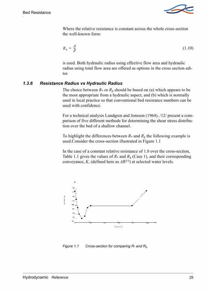
1.3.6 Resistance Radius vs Hydraulic RadiusThe choice between R* or Rh should be based on (a) which appears to be the most appropriate from a hydraulic aspect, and (b) which is normally used in local practice so that conventional bed resistance numbers can be used with confidence.
For a technical analysis Lundgren and Jonsson (1964), /12/ present a com-parison of five different methods for determining the shear stress distribu-tion over the bed of a shallow channel.
To highlight the differences between R* and Rh the following example is used.Consider the cross-section illustrated in Figure 1.1
In the case of a constant relative resistance of 1.0 over the cross-section, Table 1.1 gives the values of R* and Rh (Case 1), and their corresponding conveyance, K, (defined here as AR2/3) at selected water levels.
Figure 1.1 Cross-section for comparing R* and Rh
RhAP---=
Hydrodynamic Reference 25

HD Reference manual
Table 1.1 Conveyance calculations for R* and Rh
Figure 1.2 Plot of conveyance vs elevation
Comparison of the conveyance values, which are plotted in Figure 1.2, provide a guide to how the hydraulic capacity of the section varies with the water level. The figure shows that:
Elev(m)
Area(m2)
R*(m) K
Rh(m)Case 1 K
Rh(m)Case 2 K
100.0 0.0 0.00 0 0.00 0 0.00 0
103.0 101.7 2.19 171 1.89 155 1.89 155
106.0 306.3 4.41 824 3.27 675 3.27 675
106.1344.6 3.85 846 0.89 319 2.98 714
107.0 697.1 2.95 1434 1.74 1009 2.62 1325
108.0 1104.8 3.46 2527 2.64 2110 3.18 2389
110.0 1970.5 5.03 5780 4.36 5259 4.66 5498
113.0 3395.0 7.58 13100 6.75 12126 6.93 12340
26 MIKE 11

Bed Resistance
1 R* allows a smooth transition in the conveyance of the channel as the over bank region becomes flooded, while Rh causes a sharp, incorrect decrease in the conveyance;
2 the conveyance in the deep section is considerably greater for R = R*. This is because R* can over-estimate the conveyance for very deep and narrow cross-sections as its formulation does not fully take into account the friction from the cross-section sides as does the Rh formu-lation.
The conveyance curve for the Rh case can be improved by separating the cross-section illustrated in Figure 1.1 into two parallel channels (main channel and over bank channel) separated by an apparent third channel of zero width at a distance of 110 m along the x axis. This can be done by specifying a change in relative resistance where the two parallel channels meet - which in reality is the norm as the over bank channel typically would have a higher resistance than the main channel. Rh - Case 2 in Table 1.1 is in the case of a rr of 1.1 specified for the channel of zero width, and rr of 1.0 elsewhere. (This has the effect of splitting the section into three parallel channels with the conveyance of the middle channel being zero.) As can be seen in Figure 1.2 a much improved conveyance -elevation relationship results.
In general, R* is suited to sections with significant variations in shape such as over bank flow paths, while Rh, with no variation of rr (i.e. one parallel channel) is more appropriate for very deep and narrow uniform sections. For Rh where over bank flow paths occur adjustment of rr should be made to invoke the parallel channel analysis facility as described above. For wide sections with little variation in depth, R* and Rh will not differ greatly.
In the cross section editors processed Data menu a conveyance column is shown where the conveyance is defined as follows:
For Manning's number
(1.11)
where, rf is the resistance factor.
This is a useful facility to be able to check that the conveyance is increas-ing with increasing height. The conveyance can also be plotted to check a smooth representation.
K rfAR2 3⁄=
Hydrodynamic Reference 27

HD Reference manual
1.3.7 Calculation of resistance using channel bank markersEach cross section in MIKE 11 may be divided into a main channel plus one or two flood plains. The latter may be achieved by the use of the markers indicating the channel banks. The markers are defined by:
– Marker 4: The left low flow bank.
– Marker 5: The right low flow bank.
The markers are used for splitting the cross section into three parallel channels. Thus the reach of the left flood plain is given by markers 1 and 4, the reach of the main channel is defined by markers 4 and 5 and finally the right flood plain is defined through markers 5 and 3. The calculation of the hydraulic parameters is carried out for each of the three channels. From these the compound parameters for the cross section are found through:
Hydraulic radius/resistance radiusUsing a parallel channel analysis the total conveyance may be expressed through
, (1.12)
i.e. the compound conveyance is found as the sum of the conveyance of three channels.
The conveyance of each channel is given by
(1.13)
where i = left fp, channel, right fp.
The compound hydraulic radius /resistance radius is then calculated through
, (1.14)
where the total area Atotal is determined by
.
Kcompound Kleft fp Kchannel Kright fp+ +=
Ki AiRh i,
23---
=
RhKcompound
Atotal---------------------
3 2⁄
=
Atotal Aleft fp Achannel Aright fp+ +=
28 MIKE 11

Bed Resistance
1.3.8 Additional resistance due to vegetationThe dimensionless Darcy-Weisbach coefficient may be expressed through
(1.15)
Where g is the acceleration due to gravity and C is the Chezy coefficient (m½/s).
Alternatively the dimensionless Darcy-Weisbach coefficient λ may be expressed as
(1.16)
This through rearrangement reads
(1.17)
where ks is the resistance number and R the hydraulic radius for the cross section in question.
The objective of the calculation method is to model the shear caused by the velocity distribution between the main channel and the flood plains. This shear is described through an equivalent Darcy-Weisbach coefficient. A coefficient is determined for each side of the cross section. That is one coefficient for the interaction between the left flood plain and the main channel and one for the interaction between the right flood plain and the main channel. The location of the flood plain/main channel interface is indicated by the markers (4 and 5) in Figure 1.3.
λ 8gC2------=
1λ
------- 2– log10ks
14,84R-----------------
⋅=
λ 1
2 log10ks
14,84R-----------------
⋅
2---------------------------------------------------=
Hydrodynamic Reference 29

HD Reference manual
Figure 1.3 Interface between flood plain and main channel
Within each flood plain the vegetation may be taken into account. This is done through a number of user defined parameters:
Ax - The distance between vegetation elements in the flow directionAy - The distance between vegetation elements in the transversal directionDp - The diameter of a vegetation element
Further the individual vegetation elements give rise to a wake. This wake is described through
ANL - The length at which the wake is fully developedANB - Half the width of the fully developed wake
The first of these must satisfy the equation
(1.18)
where depends on the Reynolds number based on the vegetation ele-ment
(1.19)
0,03 0,9ANL
cW∞Dp-----------------
1gANLIE
VT2 2⁄
------------------+ =
cW∞
cW∞ 3,07Re 0,168–= for Re 800<
cW∞ 1= for 800 Re 8000< <
cW∞ 1,2= for Re 8000>
30 MIKE 11

Bed Resistance
The Reynolds number here is defined by
(1.20)
The variation of eq. (1.19) is shown below in Figure 1.4.
Figure 1.4 Non-dimensional constant as a function of Reynolds number
The velocity VT may be expressed using the Chezy formula
(1.21)
which may be written in terms of the Darcy Weisbach as
(1.22)
ReVpDp
ν-------------=
IEVT
2
C2R----------=
IEλVT
2
8gR----------=
Hydrodynamic Reference 31
HD Reference manual
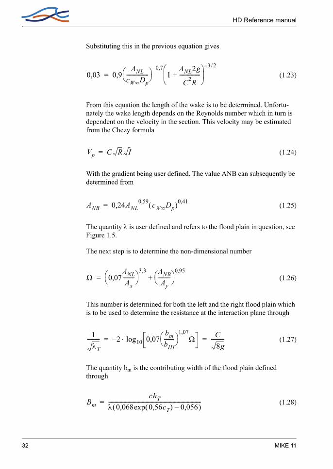
Substituting this in the previous equation gives
(1.23)
From this equation the length of the wake is to be determined. Unfortu-nately the wake length depends on the Reynolds number which in turn is dependent on the velocity in the section. This velocity may be estimated from the Chezy formula
(1.24)
With the gradient being user defined. The value ANB can subsequently be determined from
(1.25)
The quantity λ is user defined and refers to the flood plain in question, see Figure 1.5.
The next step is to determine the non-dimensional number
(1.26)
This number is determined for both the left and the right flood plain which is to be used to determine the resistance at the interaction plane through
(1.27)
The quantity bm is the contributing width of the flood plain defined through
(1.28)
0,03 0,9ANL
cW∞Dp-----------------
0,7–
1ANL2g
C2R----------------+
3 2/–
=
Vp C R I=
ANB 0,24ANL0,59 cW∞Dp( )0,41=
Ω 0,07ANLAx
---------
3,3 ANBAy
---------
0,95+=
1λT
---------- 2– log10 0,07bmbIII--------
1,07
Ω⋅ C8g
----------= =
BmchT
λ 0,068exp 0,56cT( ) 0,056–( )------------------------------------------------------------------------=
32 MIKE 11
Bed Resistance
with
(1.29)
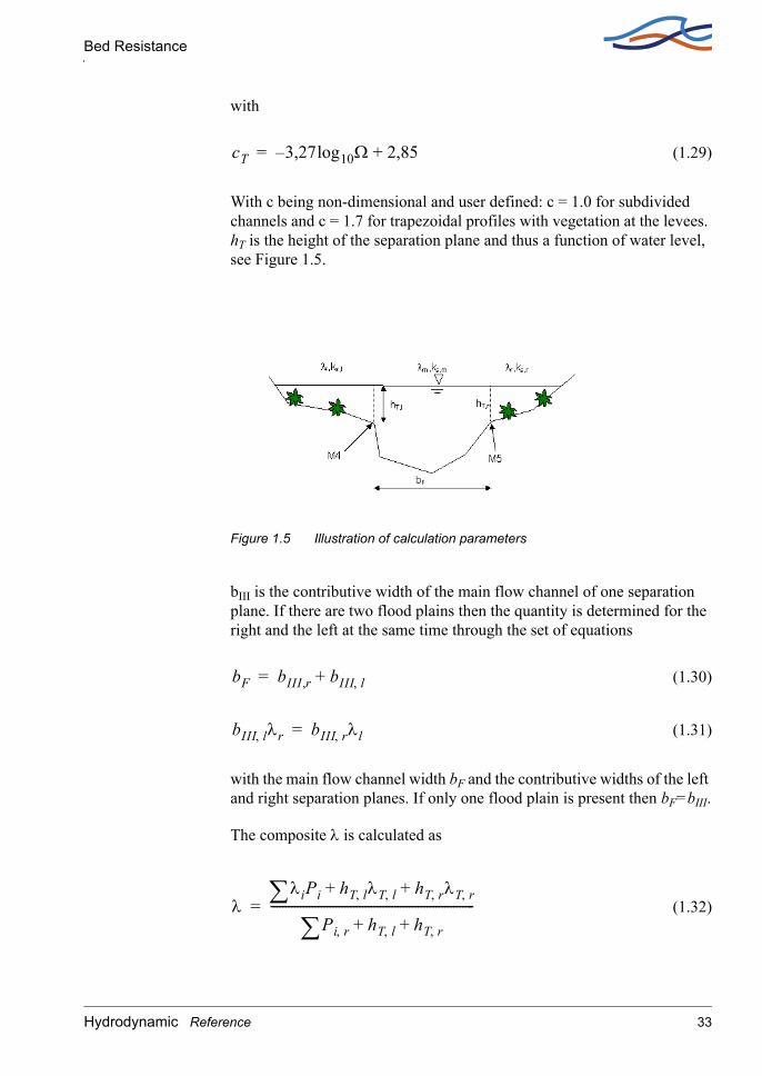
With c being non-dimensional and user defined: c = 1.0 for subdivided channels and c = 1.7 for trapezoidal profiles with vegetation at the levees. hT is the height of the separation plane and thus a function of water level, see Figure 1.5.
Figure 1.5 Illustration of calculation parameters
bIII is the contributive width of the main flow channel of one separation plane. If there are two flood plains then the quantity is determined for the right and the left at the same time through the set of equations
(1.30)
(1.31)
with the main flow channel width bF and the contributive widths of the left and right separation planes. If only one flood plain is present then bF=bIII.
The composite λ is calculated as
(1.32)
cT 3,27– log10Ω 2,85+=
bF bIII r, bIII l,+=
bIII l, λr bIII r, λl=
λλiPi hT l, λT l, hT r, λT r,+ +∑
Pi r, hT l, hT r,+ +∑---------------------------------------------------------------------=
Hydrodynamic Reference 33
HD Reference manual
In terms of the composite Chezy number this may be written
(1.33)
1.4 Boundary Conditions
External boundary conditions are required at all model boundaries, i.e. all upstream and downstream ends of model branches which are not con-nected at a junction. The relationships applied at these limits can consist of:
1 constant values of h or Q
2 time varying values of h or Q
3 a relationship between h and Q (e.g. a rating curve) (Should only be used at downstream boundaries)
The relationships are required to close the system of equations to be solved by the double sweep method, see section A.5 in Appendix A (p. 421).
1.4.1 ResolutionIf the resolution of the time varying boundaries is greater than the time step used in the simulation intermediate values in the boundary condition are determined by linear interpolation. Thus, if scanned data are available to describe the boundary such as is often the case with tide levels to describe a tidal cycle, some pre-processing of the data may be necessary to define a smoother transition between known points, e.g. a spline interpola-tion.
1.4.2 Which Boundary Condition?The choice of boundary condition depends on the physical situation being simulated and the availability of data.
Typical upstream boundaries could be
constant discharge from a reservoir
a discharge hydrograph of a specific event
Typical downstream boundaries include:
1C2------
Pi
Ci2
------hT l,
CT l,2
----------hT r,
CT r,2
----------+ +∑
Pi r, hT l, hT r,+ +∑-----------------------------------------------=
34 MIKE 11

Bridges
constant water level, e.g. in a large receiving water body
time series of water level, e.g. tidal cycle
a reliable rating curve, e.g. from a gauging station
1.5 Bridges
MIKE 11 offers a number of approaches when modelling flow through bridges. The approach to choose should be based on the assumptions for the different methods and the requirements for the modelling.
The bridge modelling approaches can be divided into pure free flow meth-ods and methods which may be combined with submergence/overflow methods. The pure free flow methods can be further sub-divided into methods for piers and methods for arches.
The methods specially designed for piers are
Bridge Piers (Nagler) (p. 42): An orifice type of flow description with the effect of the piers taken into account through an adjustment factor.
Bridge Piers (Yarnell) (p. 43): An equation derived from experiments for normal flow conditions in the sub critical flow range. Again the effect of piers is handled through the use of adjustment factors.
The free flow arch methods available are
Arch Bridges (Biery and Delleur) (p. 37): An orifice type of equation is used to describe the discharge through the bridge. The equation is derived under the assumption of a rectangular channel and is based on a single span arch opening. Multiple arch openings are handled by a simple multiplication factor.
Arch Bridges (Hydraulics Research (HR) method) (p. 39): The HR method is based on laboratory experiments of both single and multi spanned arch bridges in rectangular channels. The method uses tables describing the relation between the blockage ratio, the downstream Froude number and the upstream water level.
The methods than can be combined with both submergence and overflow methods are the following
Hydrodynamic Reference 35
HD Reference manual
Energy Equation (p. 44): A standard step method where a backwater surface profile is determination is used to calculate the discharge through the bridge. The method takes the contraction and expansion loss for bridges of arbitrary shape into account. The method assumes sub-critical flow and may default to critical flow for steep water sur-face gradients.
Federal Highway Administration (FHWA) WSPRO method (p. 47): The FHWA WSPRO method is based on the solution of the energy equation. Contraction loss is taken into account through the calculation of an effective flow length. Expansion losses are determined through the use of numerous experimentally based tables. The method takes the effect of eccentricity, skewness, wingwalls, embankment slope etc. into account through the use of these tables.
US Bureau of Public Roads (USBPR) method (p. 60): The USBPR method estimates free-surface flow assuming normal depth conditions. the method is based on experiments and takes the effect of eccentricity, skewness and piers into account.
The submergence methods available are
Pressure Flow, Federal Highway Administration method (p. 62): Two orifice equation descriptions are used. One for situations when the ori-fice is submerged downstream and modified equation for situations when only the upstream part of the orifice is submerged.
MIKE 11 culvert: A standard MIKE 11 culvert description may be cho-sen for submergence flow. The culvert to be used is specified by the user. The culvert is only active if submergence occurs.
Energy equation: The flow under the bridge is determined through a standard backwater step method. The flow is assumed to be in the sub-critical range and thus the method may default to critical flow. Both contraction and expansion loss is taken into account.
Overflow methods available are:
Energy Equation: The flow over the bridge is determined through a standard backwater step method. The flow is assumed to be in the sub-critical range and thus the method may default to critical flow. Both contraction and expansion loss is taken into account.
Road overflow, Federal Highway Administration method (p. 65): The overflow is modelled using a weir equation taking tail water submer-gence into account through the use of a submergence coefficient. The method may be used for both gravel and paved surfaces.
36 MIKE 11

Bridges
MIKE 11 weir: A standard MIKE 11 weir description may be chosen for overflow. The weir to be used is specified by the user. The weir is only active if overflow occurs.
Finally there are two additional bridge types which are not pre-processed prior to the simulation. These bridge types form part of a separate module.
Bridge Piers (D’Aubuisson) (p. 40): The discharge is determined based on a momentum equation assuming no bed slope and that the friction loss is negligible. The method can handle pure rectangular channel descriptions but also gives the option of using cross sections of arbi-trary shape.
Fully submerged bridges (p. 66): The fully submerged takes the drag of the fully submerged bridge into account. Friction is neglected and the bed is assumed horizontal through the bridge.
1.5.1 Arch Bridges (Biery and Delleur)The Biery and Delleur method is specially designed for semi circular arch bridges. It does not consider skewness, eccentricity, entrance rounding or piers (/10/). The method is based on experiments carried out for a rectan-gular channel.
The discharge, Q, through a semicircular arch in a rectangular channel is calculated from:
(1.34)
where
Coefficient of discharge.
Acceleration due to gravity.
Average water depth upstream of the bridge (= Areaus/Widthus).
Opening width of the arch.
Radius of curvature.
Q 0 7083CD 2g( )1 2⁄ Yus3 2⁄ b 1 0 1294
Yus-Lim
r----------------
2
,– 0 0177Yus-Lim
r----------------
4
,–,=
CD
g
Yus
b
r
Hydrodynamic Reference 37

HD Reference manual
Given that the discharge will decrease for high values of a limit corre-sponding to the maximum discharge is set for :
(1.35)
The upstream depth is taken as the average depth in the upstream cross section. Upstream direction is based on the water level gradient. The coefficient of discharge varies with the bridge opening ratio M and the downstream Froude number . The default table in MIKE 11 is for a semicircular arch models (/3/).
The downstream Froude number is given by:
(1.36)
Where
Discharge.
Total flow area of downstream cross section.
Velocity coefficient in downstream cross section (see eq. (1.54)).
Acceleration due to gravity.
Average depth in downstream cross section (= Areads/Widthds).
The bridge opening ratio M is defined as the ratio between and :
(1.37)
Where
Opening width of the arch (user defined).
Surface width at upstream cross section.
YusYus-Lim
Yus-Lim
Yus forYus
r------- 1,49555<
1,49555r forYus
r------- 1,49555≥
=
Yus
CDFds
Fds
FdsQ
Ads------- αds
gYds----------=
Q
Ads
αds
g
Yds
b B
M bB---=
b
B
38 MIKE 11

Bridges
Figure 1.6 Hydraulic variables for Biery and Delleur and HR Arch Bridge.
The Biery and Delleur method assumes that the water surface is free i.e. submergence is not taken into account. If the bridge that is being modelled is submerged or over topped an alternative modelling method should be chosen.
1.5.2 Arch Bridges (Hydraulics Research (HR) method)The Hydraulics Research method estimates the discharge through an arch bridge by the use of a table describing the relation between the upstream afflux, the blockage ratio and the Froude number. The upstream afflux is defined as the increase in water level from normal depth caused by the bridge. The afflux should theoretically be determined one bridge span upstream of the bridge. Thus as a rule of thumb the upstream cross section should be found one bridge span upstream the bridge opening. The default table in MIKE 11 is valid for semicircular arch models (/3/).
The afflux at the upstream cross section of the bridge.
Average depth of flow downstream the bridge (Areads/Widthds).
The upstream blockage ratio defined as .
The user defined width of the arch.
Upstream water surface width.
Froude number downstream of the bridge.
Hus*
Yds
Jus Jusbarch
bus-----------=
barch
bus
Fds
Hydrodynamic Reference 39

HD Reference manual
The upstream afflux is defined as:
(1.38)
Where:
Water level at upstream cross section.
Water level at downstream cross section.
Discharge.
Conveyance in downstream cross section.
Distance from upstream to downstream cross section.
MIKE 11 determines the discharge based on the upstream and down-stream water level. From the afflux and the upstream blockage ratio a Froude number can be determined through the use of the table expressing the relation between afflux and Froude number. For fixed water levels the Froude number depends solely on the discharge. Since the afflux depends on the discharge an iterative process is needed. If the iterative process does not converge the code defaults to critical discharge at the upstream cross section.
The hydraulic research method assumes that the water surface is free i.e. submergence is not taken into account. If the bridge that is being modelled is submerged or over topped an alternative modelling method should be chosen.
1.5.3 Bridge Piers (D’Aubuisson)Bridge piers may be implemented in MIKE 11 using D’Aubuisson’s for-mula (/10/). The governing equations for bridge piers are derived under the assumption that the bed slope is zero and the effect of the bed friction is negligible. Thus in order to minimise the errors introduced by these assumptions the user should place the cross sections upstream and down-stream close to the bridge. Please note that this bridge type can only be implemented with a special module.
The code provides two alternatives for the implementation of this formula:
Hus* hus hds– Q
Kds--------
2Lus-ds–=
hus
hds
Q
Kds
Lus-ds
40 MIKE 11
Bridges
1 A rectangular channel analysis is used if a positive value is entered for the upstream width of the channel (see section Bridges in the User Guide). D’Aubuisson’s formula for a rectangular channel reads
(1.39a)
where
Q discharge at the bridge piers.
H1 water level downstream of piers.
H2 water level upstream of piers.
C user defined constant determined by pier geometry.
b2 user defined channel width upstream of piers.
h1 local water depth downstream of piers.
wpiers total width of piers.
2 If a non-positive value is entered for the upstream width of the channel (see section Bridges in the User Guide) a momentum equation is solved which takes the effect of an arbitrary shape of the cross section into account:
(1.39b)
where
A1 cross sectional area downstream of bridge piers.
A2 cross sectional area upstream of bridge piers.
Note that if the Froude number is above the criteria of 0.6, the effect of the bridge piers is neglected. The criteria may be altered by setting the varia-ble BRIDGE_FROUDE_CRITERIA in the mike11.ini file.
H2 H1– Q2
2g------ 1
C2 b2 wpiers–( )2h12
-------------------------------------------- 1b2
2 h1 ∆h+( )2-------------------------------–=
H2 H1– Q2
2g------ 1
C2 A1 h1wpiers–( )2--------------------------------------------- 1
A22
-----–=
Hydrodynamic Reference 41

HD Reference manual
1.5.4 Bridge Piers (Nagler)The Nagler equation is experimentally based. The equation is applicable to bridge piers with different pier shapes. The pier shape is taken into account through a so-called coefficient of discharge which is found through a table based on the pier type. The equation is derived from free flow experiments and is not accurate for high velocities (/7/).
Figure 1.7 Type of pier shapes.
The Nagler equation reads:
(1.40)
where:
KN Coefficient of discharge.
Adjustment factor (default 0.3).
Adjustment factor varies with the bridge opening ratio.
g Acceleration due to gravity.
Yds Depth downstream of the bridge.
Vus Velocity upstream the bridge.
Vds Velocity downstream the bridge.
hus Water level in the upstream cross section.
hds Water level in the downstream cross section.
Q KNb 2g Yds θVds
2
2g-------–
hus hds– βVus
2
2g-------+
1 2⁄
=
θ
β
42 MIKE 11

Bridges
b The total bridge opening width excluding the piers.
The coefficient of discharge KN varies with the bridge opening ratio M and the pier shape. The adjustment factor varies with the bridge opening ratio M and the adjustment factor can normally be taken as 0.3. The default tables in MIKE 11 are after Yarnell and Nagler (/10/).
The bridge opening ratio M is defined as the ratio between the flow width in the bridge and the flow width upstream of the bridge b/B.
b Opening width of the arch.
B Opening width at upstream cross section.
Eq. (1.40) can be rewritten as a polynomial of third degree in the dis-charge squared. In case of multiple roots the smallest positive root is cho-sen as the solution.
The structure area is defined as the arch width times the minimum water depth upstream or downstream.
1.5.5 Bridge Piers (Yarnell)Like the Nagler equation, the Yarnell equation considers different pier shapes (see Figure 1.7). The pier shape is accounted for through the so-called pier coefficient. The Yarnell equation is a pure experimentally based equation. The equation assumes free flow. Thus if submergence and possible overtopping is to be modelled an alternative method should be used.
The Yarnell equation reads:
(1.41)
(1.42)
(1.43)
where
K Yarnell’s Piers shape Coefficient.
βθ
hus hds– KYdsFds2 K 5Fds
2 0,6–+( ) α 15α4+( )=
Fds2 Q2
Ads2 2gYds
----------------------=
α 1 bBus-------–=
Hydrodynamic Reference 43

HD Reference manual
g Acceleration due to gravity.
Yds Depth downstream the bridge.
Fds Froude number downstream the bridge.
Channel contraction ratio.
Ads Total flow area of downstream cross section.
b The bridge opening width excluding the piers.
Bus The width of the upstream cross section.
hus Water level in the upstream cross section.
hds Water level in the downstream cross section.
The default tables for pier shape coefficient K are after Yarnell (/10/).
Eq. (1.41) may be re-written as a polynomial of second order in the Froude number squared. If multiple positive roots are present the greatest discharge is chosen.
The structure area is defined as the arch width times the minimum water depth upstream or downstream.
1.5.6 Energy EquationThe energy equation may be used to determine the discharge and the back water profile through the bridge. The energy equation takes friction loss and contraction/expansion losses into account. The method requires four cross sections (see Figure 1.8). River cross sections one and four are defined in the cross-section editor. Bridge cross sections two and three are defined through the bridge geometry in the network editor. Ideally the dis-tance between the bridge and the up- and downstream cross-sections should be of the order b, where b is the bridge opening width. The latter is to ensure that the streamlines are parallel at section one and section four.
The equation solved from section i to i-1 reads
(1.44)
where:
hi Water level at cross-section i.
α
hi 1– h+ v i 1–( ) hi hvi hf i i 1–,( ) he i i 1–,( )+ + +=
44 MIKE 11

Bridges
hvi Velocity head at cross-section i.
hf(i,i-1) Friction losses between cross-section i and i-1.
he(i,i-1)Expansion losses between cross-section i and i-1.
The velocity head is defined as
(1.45)
with the velocity distribution coefficient defined as
(1.46)
(1.47)
(1.48)
(1.49)
Where
Q Discharge at the section.
Velocity distribution coefficient.
k Subsection conveyance.
a Subsection area.
K Total cross section conveyance.
A Total cross section area.
hvαQ2
2gA2------------=
α
ki3 ai
2⁄( )i 1=
N
∑
K3 A3⁄----------------------------=
kiairi
2 3⁄
ni--------------=
K ki
i 1=
N
∑=
A ai
i 1=
N
∑=
α
Hydrodynamic Reference 45
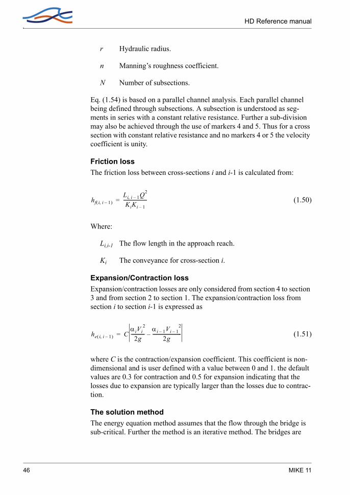
HD Reference manual
r Hydraulic radius.
n Manning’s roughness coefficient.
N Number of subsections.
Eq. (1.54) is based on a parallel channel analysis. Each parallel channel being defined through subsections. A subsection is understood as seg-ments in series with a constant relative resistance. Further a sub-division may also be achieved through the use of markers 4 and 5. Thus for a cross section with constant relative resistance and no markers 4 or 5 the velocity coefficient is unity.
Friction lossThe friction loss between cross-sections i and i-1 is calculated from:
(1.50)
Where:
Li,i-1 The flow length in the approach reach.
Ki The conveyance for cross-section i.
Expansion/Contraction lossExpansion/contraction losses are only considered from section 4 to section 3 and from section 2 to section 1. The expansion/contraction loss from section i to section i-1 is expressed as
(1.51)
where C is the contraction/expansion coefficient. This coefficient is non-dimensional and is user defined with a value between 0 and 1. the default values are 0.3 for contraction and 0.5 for expansion indicating that the losses due to expansion are typically larger than the losses due to contrac-tion.
The solution methodThe energy equation method assumes that the flow through the bridge is sub-critical. Further the method is an iterative method. The bridges are
hf i i 1–,( )Li i 1–, Q2
KiKi 1–---------------------=
he i i 1–,( ) CαiVi
2
2g------------
αi 1– Vi 1–2
2g-------------------------–=
46 MIKE 11

Bridges
pre-calculated based on a set of values for the water levels upstream and downstream. Thus for each set of water level values a discharge is to be determined. The algorithm for determining the discharge has the follow-ing steps:
1 Initial guess for the discharge.
2 Backwater calculation from section 4 to section 3.
3 Backwater calculation from section 3 to section 2 based on the result from step 2.
4 Backwater calculation from section 2 to section 1 based on the result from step 3.
5 The water level determined through step 4 is compared with the actual water level at section 1.
6 Based on the comparison in step 5 the discharge is either modified and the algorithm returns to step 2 or the algorithm terminates if the devia-tion is within acceptable limits.
Throughout the calculation the results are compared with critical flow. If the solution found is below critical water level or if one of the steps 2 - 4 do not converge the code defaults to critical flow at that location. Further if the maximum number of iterations (default 50) is reached without obtaining a valid solution the code defaults to critical flow at section one.
1.5.7 Federal Highway Administration (FHWA) WSPRO methodThe computations of the Federal Highway Administration’s WSPRO computer program have been adapted for the calculation of free-surface flow. Some modifications have been necessary in order to fit the MIKE 11 terminology.
The method is based on a standard step method using the energy equation to find the discharge and the backwater water surface profile through the bridge. The method requires four cross sections (see Figure 1.8). River cross sections one and four are defined in the cross-section editor. Bridge cross sections two and three are defined through the bridge geometry in the network editor. Ideally the distance between the bridge and the up- and downstream cross-sections should be of the order b, where b is the bridge opening width.
Hydrodynamic Reference 47

HD Reference manual
Figure 1.8 Location of cross-sections.
The total energy equation between section one and four can be written:
(1.52)
where:
h1 Water level at cross-section 1.
hv1 Velocity head at cross-section 1.
h4 Water level at cross-section 4.
hv4 Velocity head at cross-section 4.
hf Friction losses between cross-section 1 and 4.
he Expansion losses between cross-section 3 and 4.
The velocity head is defined as
(1.53)
h1 h+ v1 h4 hv4 hf he+ + +=
hvαQ2
2gA2------------=
48 MIKE 11

Bridges
with the velocity distribution coefficient defined as
(1.54)
(1.55)
(1.56)
(1.57)
Where
Q Discharge at the section.
Velocity distribution coefficient.
k Subsection conveyance.
a Subsection area.
K Total cross section conveyance.
A Total cross section area.
r Hydraulic radius.
n Manning’s roughness coefficient.
N Number of subsections.
Eq. (1.54) is based on a parallel channel analysis. Each parallel channel being defined through subsections. A subsection is understood as seg-ments in series with a constant relative resistance. Further a sub-division may also be achieved through the use of markers 4 and 5. Thus for a cross
α
ki3 ai
2⁄( )i 1=
N
∑
K3 A3⁄----------------------------=
kiairi
2 3⁄
ni--------------=
K ki
i 1=
N
∑=
A ai
i 1=
N
∑=
α
Hydrodynamic Reference 49

HD Reference manual
section with constant relative resistance and no markers 4 or 5 the velocity coefficient is unity.
Friction lossWithout spur dykes the friction loss between cross-sections 1 and 2 is cal-culated from:
(1.58)
With spur dykes the friction loss between cross-sections 1 and 2 is aug-mented with the friction along the dykes:
(1.59)
Where:
Lav The effective flow length in the approach reach (see below).
Ld2 The spur dyke length.
K1 The conveyance for cross-section 1.
K2 The conveyance for cross-section 2.
The friction loss from section 2 to 3 is given by
(1.60)
Where:
Lwaterway is the distance from section 2 to section 3.
K3 The conveyance for cross-section 3.
Finally the friction loss from section 3 to section 4 is given by
(1.61)
hf 12( )LavQ2
K1K2--------------=
hf 12( )LavQ2
K1K2--------------
Ld2Q2
K2K2---------------+=
hf 23( )LwaterwayQ2
K2K3-----------------------------=
hf 34( )L34Q2
K3K4--------------=
50 MIKE 11

Bridges
Where:
L34 The flow length from section 3 to 4.
K4 The conveyance for cross-section 4.
Effective flow lengthThe effective flow length is determined based on the conveyance distribu-tion. The effective length is determined as the average length of 20 equal conveyance tubes. The conveyance is here taken as
(1.62)
Eq. (1.62) is found by taking the limit of N parallel stream-tubes as N tends to infinity
(1.63)
Using eq. (1.62) for determining the conveyance has the advantage that the locations of the equal conveyance tubes are well defined. Using eq. (1.62) one can express the location of the first tube as
(1.64)
which is to be solved for x1. For the second tube the equation to be solved is
(1.65)
and so on for the remaining tubes.
The effective flow length is determined under the assumption that the water level in section 1 and 2 are equal. The error made here is minimal since the main contribution to the calculation of the effective flow length
K M H z–( )5 3⁄ xd0
B
∫=
MiAiRi2 3⁄
i 1=
N
∑N ∞→lim Mi H zi–( )∆xi H zi–( )2 3⁄
i 1=
N
∑N ∞→lim=
K20------ M H z–( )5 3⁄ xd
0
x1
∫=
K20------ M H z–( )5 3⁄ xd
x1
x2
∫=
Hydrodynamic Reference 51
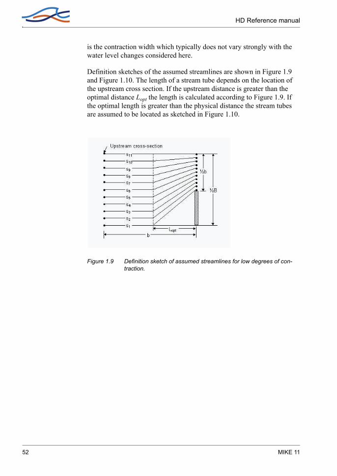
HD Reference manual
is the contraction width which typically does not vary strongly with the water level changes considered here.
Definition sketches of the assumed streamlines are shown in Figure 1.9 and Figure 1.10. The length of a stream tube depends on the location of the upstream cross section. If the upstream distance is greater than the optimal distance Lopt the length is calculated according to Figure 1.9. If the optimal length is greater than the physical distance the stream tubes are assumed to be located as sketched in Figure 1.10.
Figure 1.9 Definition sketch of assumed streamlines for low degrees of con-traction.
52 MIKE 11

Bridges
Figure 1.10 Definition sketch of assumed streamlines for high degrees of con-traction.
The optimum length is defined as:
(1.66)
where
(1.67)
(1.68a)
(1.68b)
(1.68c)
Where:
The total bridge opening width excluding the piers.
The total width of the upstream cross section.
Loptb
π 1 m′–( )-----------------------Φ=
m′ 1 b B⁄–=
Φ 12--- 8
ε2----- 8+ 3
ε---– ε–
8 8ε2+– 3ε– 1ε---–
ln ε 1ε---–
ln–=
ε 1 δ δ2 2δ++ +=
δ 2
1 b2B-------–
πtan2
-----------------------------------------=
b
B
Hydrodynamic Reference 53

HD Reference manual
Effective flow length:
(1.69)
In case the optimal length is greater than the physical distance a parabola is used to describe the stream tubes. Using a coordinate system as indi-cated in Figure 1.17 and the equation used for the right hand side of the channel is given by:
(1.70)
similarly the left hand side uses a parabola described by
(1.71)
Expansion lossThe contraction loss from section 1 to 2 is taken into account through the use of an effective flow length as opposed to the physical distance from section 1 to section 2. No contraction or expansion loss is assumed from section 2 to 3. It is further assumed implicitly that from section 3 to sec-tion 4 only expansion takes place. If no expansion takes place the loss con-sists solely of the fiction loss from section 3 to 4.
Lav120------ Si
i 2=
20
∑S1 S21+( )
2------------------------+=
x 12b------ y2 b2–( )=
x B 12b------– y2 b2–( )=
54 MIKE 11

Bridges
The expansion loss from section 3 to 4 is computed from:
(1.72)
(1.73)
(1.74)
(1.75)
(1.76)
Where:
C Coefficient of discharge
k Subsection conveyance
a Subsection area
K Total cross section conveyance
A Total cross section area
Eqs. (1.75) and (1.76) are based on a parallel channel analysis. Each paral-lel channel being defined through subsections. A subsection is understood as segments in series with a constant relative resistance. Further a sub-division may also be achieved through the use of markers 4 and 5. Thus for a cross section with constant relative resistance and no markers 4 or 5 the velocity coefficient is unity.
Coefficient of dischargeThe coefficient of discharge is a function of the bridge geometry and flow characteristics. Four main types of openings are defined Figure 1.11 to Figure 1.14. For each opening type the coefficient of discharge, C is obtained by a base coefficient C’ and a number of adjustment factors, k.
heQ2
2gA42
------------- 2β4 α4– 2β3A4
A3-----
– α3A4
A3-----
2
+=
β31C----=
α31
C2------=
β4
k2 a⁄( )∑K2 A⁄
-----------------------=
α4
k3 a2⁄( )∑K2 A2⁄
-------------------------=
k Mar2 3⁄=
K k∑=
A a∑=
Hydrodynamic Reference 55

HD Reference manual
The default base coefficients and adjustment factors in MIKE 11 are obtained as described by FHWA /9/.
The coefficient of discharge, C is given by:
(1.77)
Where:
Channel contraction ratio.
Bridge waterway flow length (length from section2 to 3).
Bridge opening width.
Froude number in downstream bridge section.
Table 1.2
Adjustment factor Type Tabular function of:
Base coefficient All , and slope
Froude number I
Corner rounding I and
Wingwall I , and
Average depth II , and slope
Unwetted abutment III , and slope
Wingwall IV , and slope
Eccentricity All
Piles All and
Piers All , and
Elliptical spur dike angularity All and
Straight spur dike offset, All and
Spur dike length, All and
C C′ kF ky kx kθ ke kj ka kb kd⋅ ⋅ ⋅ ⋅ ⋅ ⋅ ⋅ ⋅ ⋅=
C′ m L b⁄
kF F3
kr m r b⁄
kw m w b⁄ WW
ky m Ya Yb+( ) 2b( )⁄
kx x b⁄ L b⁄
kθ m WW
ke Ka Kc⁄
kj m j
kj m L b⁄ j
ka m Ld b⁄
kb m Ld b⁄ d
kd m Ld b⁄
m
L
b
F3
56 MIKE 11

Bridges
Radius of corner rounding.
Wingwall width.
Wingwall angle.
Average water level in bridge section.
Unwetted abutment length.
Ratio of conveyance of the approach section on each side of the projected opening.
Portion of waterway blocked by piers/piles.
Spur dike length.
Spur dike offset.
The channel contraction ratio, is given by:
(1.78)
Where:
The conveyance of that part of section 1 where conveys dis-charge can flow through the bridge opening without contraction.
The total conveyance for cross-section 1.
r
w
WW
Ya Yb+( ) 2b( )⁄
x
Ka Kc⁄ 1≤
j Ap A3⁄=
Ld
bd
m
m 1Kq
K1------–=
Kq
K1
Hydrodynamic Reference 57

HD Reference manual
Figure 1.11 Definition sketch of type I opening, vertical embankments and verti-cal abutments, with or without wingwalls (after Matthai).
Figure 1.12 Definition sketch of type II opening, sloping embankments without wingwalls (after Matthai).
Figure 1.13 Definition sketch of type III opening, sloping embankments and sloping abutments (spillthrough) (after Matthai).
58 MIKE 11

Bridges
Figure 1.14 Definition sketch of type IV opening, sloping embankments and ver-tical abutments with wingwalls (after Matthai).
If the abutments are of different types a value of the coefficient of dis-charge is obtained through a weighted average:
(1.79)
Where:
Coefficient of discharge for left abutment.
Coefficient of discharge for right abutment.
Conveyance for left side.
Conveyance for right side.
The solution methodThe method assumes that the flow through the bridge is sub-critical. Fur-ther the method is an iterative method. The bridges are pre-calculated based on a set of values for the water levels upstream and downstream. Thus for each set of water level values a discharge is to be determined. The algorithm for determining the discharge has the following steps:
1 Initial guess for the discharge.
2 Backwater calculation from section 4 to section 3.
3 Backwater calculation from section 3 to section 2 based on the result from step 2.
4 Backwater calculation from section 2 to section 1 based on the result from step 3.
CCLKL CRKR+
KL KR+---------------------------------=
CL
CR
KL
KR
Hydrodynamic Reference 59

HD Reference manual
5 The water level determined through step 4 is compared with the actual water level at section 1.
6 Based on the comparison in step 5 the discharge is either modified and the algorithm returns to step 2 or the algorithm terminates if the devia-tion is within acceptable limits.
Throughout the calculation the results are compared with critical flow. If the solution found is below critical water level or if one of the steps 2 - 4 do not converge the code defaults to critical flow at that location. Further if the maximum number of iterations (default 50) is reached without obtaining a valid solution the code defaults to critical flow at section one.
1.5.8 US Bureau of Public Roads (USBPR) methodThe USBPR method estimates free-surface flow assuming normal depth conditions. The maximum afflux at section 1 (see Figure 1.8) is here defined by:
(1.80)
Where:
The backwater coefficient.
Average velocity in bridge section at normal depth.
Cross section area at normal depth.
Cross section area at section 1.
Cross section area at section 4.
Acceleration due to gravity.
Velocity distribution coefficient - Equation (1.54).
Velocity distribution coefficient for normal depth.
The velocity distribution coefficient, is a function of and the open-ing ratio. The opening ratio defined by
(1.81)
H1*
H1* k*α2VN2
2
2g--------------- α1
AN2
A4---------
2 AN2
A1---------
2
–VN2
2
2g---------+=
k*
VN2
AN2
A1
A4
g
α1
α2
α2 α1
M 1 b B⁄–=
60 MIKE 11

Bridges
where b is the bridge opening width and B is the width of the upstream river cross-section. In MIKE 11 the coefficient is computed from a user defined table or the pre-computed default table.
The total backwater coefficient is given by:
(1.82)
Where:
Base coefficient. Tabular function of the opening ratio.
Eccentricity coefficient. Tabular function of the opening ratio and the eccentricity.
Skewness coefficient.Tabular function of the opening ratio and skewness angle .
Bridge pier coefficient. Tabular function of opening ratio, the portion of waterway blocked by piers and pier type.
The eccentricity e is given by
(1.83)
where Qleft, Qright are the ratio of discharge of the approach section on each side of the projected opening. The portion of the waterway blocked by piers is user defined an should be understood as the ratio of the pier cross sectional area to the cross sectional area of the waterway without the piers.
The coefficients are computed in MIKE 11 from user defined tables or from the pre-computed default tables.
1.5.9 Multiple Waterway OpeningWhen working with multiple openings each opening is evaluated seper-ately. Up- and downstream cross sections are reduced to the part found in between the stagnation points. The stagnation points are the points in the cross section where the flow splits up between the different water way openings. The default stagnation points are evaluated strictly from a geo-
k* kb* ke
*∆ kφ*∆ kp
*∆+ + +=
kb*
ke*∆
kφ*∆
φ
kp*∆
emin Qleft Qright,( )max Qleft Qright,( )-----------------------------------------=
Hydrodynamic Reference 61

HD Reference manual
metric point of view. The default stagnation points are set so each sub cross section satisfies:
(1.84)
Where:
Width of sub cross section.
Bridge opening width from marker 1 to 3
Total width of all bridge openings.
Total width of cross section from marker 1 to 3.
The user can set the stagnation points if desired.
1.5.10 Pressure Flow, Federal Highway Administration methodDuring significant contact of the water surface with the girders of the bridge structure, free-surface flow cannot exist and pressure flow is etab-lised.
Fully Submerged Orifice flowDischarge through the fully submerged bridge opening is computed by:
(1.85)
Where:
A2 Flow area in the bridge opening.
g Acceleration due to gravity.
h1 Water level in the upstream cross section.
hv1 Velocity head at cross-section 1.
h3 Water level in the downstream bridge section.
hf12 The friction loss from the upstream cross section to the upstream bridge section.
CD Discharge coefficient (default 0.8).
Bsubb
bTotal-------------Btotal=
Bsub
b
bTotal
BTotal
Qorifice CDA2 2g h1 hf12– hv1 h3–+( )=
62 MIKE 11
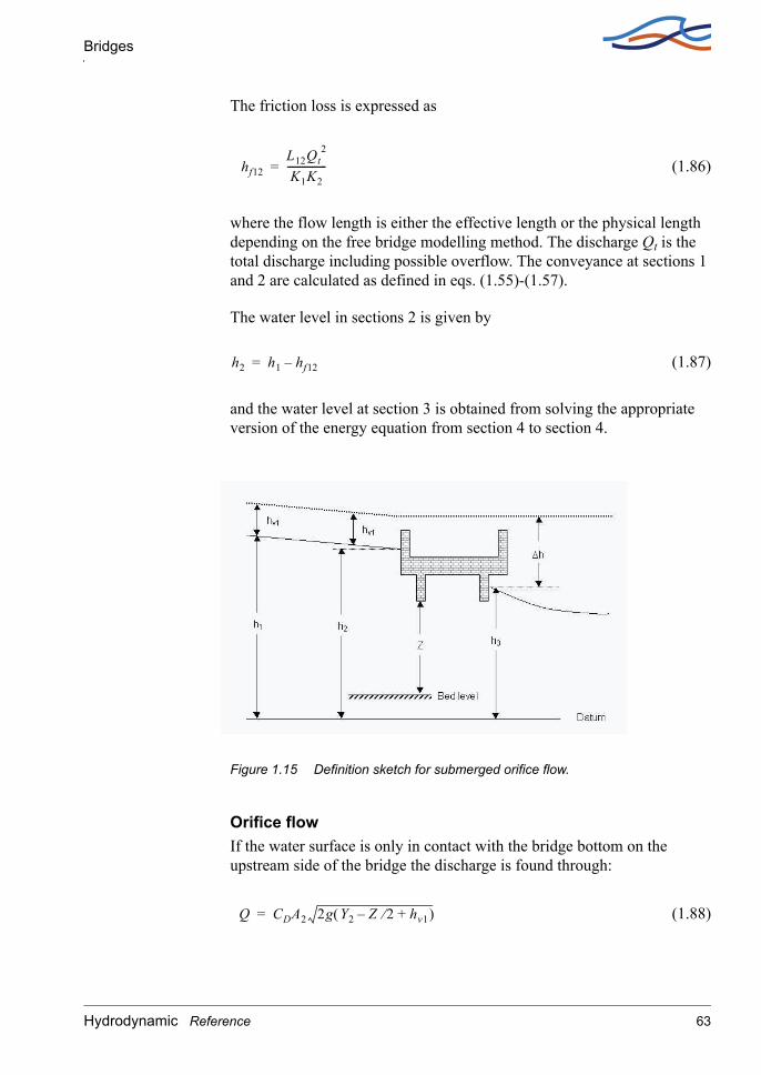
Bridges
The friction loss is expressed as
(1.86)
where the flow length is either the effective length or the physical length depending on the free bridge modelling method. The discharge Qt is the total discharge including possible overflow. The conveyance at sections 1 and 2 are calculated as defined in eqs. (1.55)-(1.57).
The water level in sections 2 is given by
(1.87)
and the water level at section 3 is obtained from solving the appropriate version of the energy equation from section 4 to section 4.
Figure 1.15 Definition sketch for submerged orifice flow.
Orifice flowIf the water surface is only in contact with the bridge bottom on the upstream side of the bridge the discharge is found through:
(1.88)
hf12L12Qt
2
K1K2----------------=
h2 h1 hf12–=
Q CDA2 2g Y2 Z 2⁄– hv1+( )=
Hydrodynamic Reference 63

HD Reference manual
Where:
Discharge coefficient. Tabular function of .
The quantities are defined in Figure 1.16 note that the bed level is defined as
(1.89)
where is the bridge bottom level and .The quantity A2 being the area at the opening and B2 is the width at the bridge bottom level.
Equation (1.88) may be rewritten as
(1.90)
which is a form equivalent to equation (1.85). Note that the discharge coefficient in the two equations are different. To ensure a smooth transi-tion from free orifice flow to submerged orifice flow a linear transition is made on the discharge coefficient from free to submergence. That is for water levels below the level the free submergence coeffi-cient is used whereas as the water level increases downstream and the ori-fice slowly becomes drowned the coefficient changes continuously into the fully submerged value. Further to avoid an abrupt change in the solu-tion when the downstream water level reaches the bottom of the bridge the orifice equation is modified as
(1.91)
where the modified downstream water level is given by
(1.92)
CD Y2 Z⁄
Bed Level bbottom Z–=
bbottom Z A2 B2⁄=
Q CDA2 2g h1 hf12– hv1 bbottomZ2---–
–+ =
bbottom Z 2⁄–
Q CDA2 2g h1 hf12– hv1 h3–+( )=
h3
h3 min h3 bbottom Z 2⁄–,( )=
64 MIKE 11

Bridges
Figure 1.16 Definition sketch for orifice flow.
1.5.11 Road overflow, Federal Highway Administration methodWhen the water surface elevation exceeds the top bridge level the top part of the bridge is assumed to function as a weir. The discharge for the over-flow part is computed using a weir formula:
(1.93)
Where:
Total head for weir flow with respect to bridge top level (see Figure 1.17).
Adjustment factor due to possible submergence from down-stream water level. Tabular function of tail water level and total head .
Coefficient of free discharge. Tabular function of water depth on the structure , the crest length in the flow direction and the total head .
Width of overflow part.
The submergence adjustment factor depends on the ratio of minimum elevation along the top of the embankment to the total head for weir flow .
Q ktCfBWH3 2⁄=
H
ktht
H
Cfhs LR
H
BW
ktht
H
Hydrodynamic Reference 65
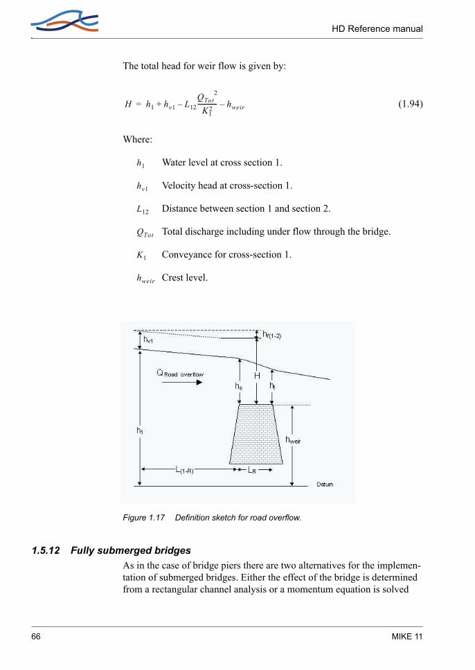
HD Reference manual
The total head for weir flow is given by:
(1.94)
Where:
Water level at cross section 1.
Velocity head at cross-section 1.
Distance between section 1 and section 2.
Total discharge including under flow through the bridge.
Conveyance for cross-section 1.
Crest level.
Figure 1.17 Definition sketch for road overflow.
1.5.12 Fully submerged bridgesAs in the case of bridge piers there are two alternatives for the implemen-tation of submerged bridges. Either the effect of the bridge is determined from a rectangular channel analysis or a momentum equation is solved
H h1 hv1 L12QTot
2
K12
-------------– hweir–+=
h1
hv1
L12
QTot
K1
hweir
66 MIKE 11
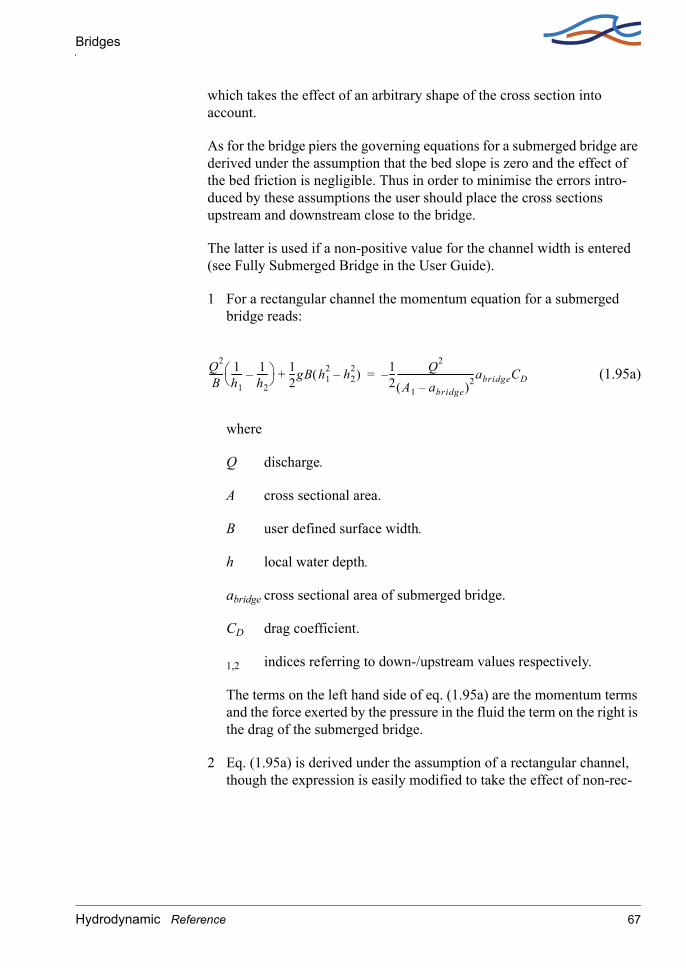
Bridges
which takes the effect of an arbitrary shape of the cross section into account.
As for the bridge piers the governing equations for a submerged bridge are derived under the assumption that the bed slope is zero and the effect of the bed friction is negligible. Thus in order to minimise the errors intro-duced by these assumptions the user should place the cross sections upstream and downstream close to the bridge.
The latter is used if a non-positive value for the channel width is entered (see Fully Submerged Bridge in the User Guide).
1 For a rectangular channel the momentum equation for a submerged bridge reads:
(1.95a)
where
Q discharge.
A cross sectional area.
B user defined surface width.
h local water depth.
abridge cross sectional area of submerged bridge.
CD drag coefficient.
1,2 indices referring to down-/upstream values respectively.
The terms on the left hand side of eq. (1.95a) are the momentum terms and the force exerted by the pressure in the fluid the term on the right is the drag of the submerged bridge.
2 Eq. (1.95a) is derived under the assumption of a rectangular channel, though the expression is easily modified to take the effect of non-rec-
Q2
B------ 1
h1----- 1
h2-----–
12---gB h1
2 h22–( )+ 1
2---– Q2
A1 abridge–( )2----------------------------------abridgeCD=
Hydrodynamic Reference 67

HD Reference manual
tangular channels into account. After this modification the momentum equation reads:
(1.95b)
For both eq.(1.95a) and (1.95b) a modification is applied for situations where the cross sectional area of the bridge is of the same order as the downstream cross sectional area. In such cases the drag will become very large causing among other things numerical problems. This is overcome by applying a suppression of the drag force for small values of A1. The suppression is given by
(1.96)
This suppression is applied to the drag force so that it is given by
(1.97)
The reason for including the suppression factor also in the denominator is to avoid the singularity at A1=abridge. Please note that this suppression is included only so that the simulation can continue at low flow conditions where it is very unlikely that the bridge is submerged i.e. the full equation is unphysical.
For both types of bridges the governing equation can be rearranged so that the discharge is a function of the water level up- and downstream respec-tively i.e.
(1.98)
The coefficients (α,β,γ,δ) in the numerical scheme are found by Taylor expanding eq. (1.98).
Q2 1A1----- 1
A2-----–
12---g h2
2dy h12dy
0
B1
∫–0
B2
∫ 1
2--- Q2
A1 abridge–( )2----------------------------------CDabridge–=
suppdrag
0 for 0A1
abridge------------- 1,1≤<
10A1
abridge------------- 11– for 1,1
A1
abridge-------------< 1,2≤
1 for 1,2A1
abridge-------------<
=
suppdrag12--- Q2
A1 suppdragabridge–( )2------------------------------------------------------CDabridge–
Q f H1 H2,( )=
68 MIKE 11

Bridges
A bridge may generate steep gradients on the water level which may cause numerical instabilities. Therefore it is recommended to increase the parameter delta from its default setting of 0.5. This will have a dissipating effect on the solution thus smoothing out possible numerical wiggles caused by the bridge. If this shifting of the time centering is not applied a reduction of the time step may be necessary. An increase in the number of iterations at each time-step may also be required if a forward centering in time is not applied.
Further even though eq. (1.98) gives a well defined expression for the dis-charge as a function of the up- and downstream water levels the expres-sion does not secure an unambiguous expression for say the upstream water level as a function of the downstream water level and the discharge. In other words for a given value of the discharge and the downstream water level multiple solutions for the upstream water level may exist (this is an inherent feature of the non-linear equations governing the flow through the bridge). Thus in a dynamic solution one may encounter situa-tions where one of the alternative solutions occur. A possible way of over-coming this is to decrease the time step.
Note that if the Froude number is above the criteria of 0.6, the effect of the submerged bridge is neglected. The criteria may be altered by setting the variable BRIDGE_FROUDE_CRITERIA in the mike11.ini file.
1.5.13 Trouble shooting for bridge structuresDuring the simulation the discharge through a bridge is determined from a pre-calculated table (except when using Fully submerged bridge and Bridge piers (D’Aubuisson’s formula)). Each value in the table is found by an iteration process. Using a pre-calculated table decreases the calculation time.
InstabilityFor bridge structures a number of factors can result in instabilities.
Time step: In most cases it is helpful to decrease the MIKE 11 time step.
Delta: Delta is a default value in the HD editor. Increasing delta reduces instabilities. The delta value controls the time centering in the scheme.
Bridge preprocessing: To speed up simulations the bridges are preproc-essed initially at simulation start. The generated H-Q-H tables are saved into files named using the bridge ID. In the present version the files are exported in the dfs2 format which can be readily viewed using standard tools within MIKE Zero. It is recommended to evaluate these files for con-sistency. Note that non-smooth H-Q-H surfaces may be caused by abrupt
Hydrodynamic Reference 69

HD Reference manual
changes in bed friction or geometry. Further consult MIKE11.ini for fur-ther capabilities with regards to bridge preprocessing.
Results‘Curtains’: ‘Curtains’ in the result curve may be a result of the pre-calcu-lated table. Increasing the resolution in the pre-calculated table will gener-ally decrease the ‘curtain’ size. BRIDGE_TABLE_GRID_UPSTREAM and BRIDGE_TABLE_GRID_DOWNSTREAM in Mike11.ini may be used to specify a different resolution for the water levels used for the pre-calculated tables. The default value is 0.1 meters. The value is given in meters.
1.6 Broad crested Weir
The standard formulations for flow over a broad crested weir are estab-lished automatically by the program on the basis of the weir geometry and the user specified head loss and calibration coefficients. These formula-tions assume a hydrostatic pressure distribution on the weir crests. Differ-ent algorithms are used for drowned flow and free overflow, with an automatic switching between the two, as described in the section A.10 Structures (p. 467).
1.7 Coefficients, HD default parameters
ALPHA CoefficientThis is the velocity distribution coefficient used in the momentum equa-tion, see section 1.29 Saint Venant Equations (p. 170). The default value is 1.0.
DELH CoefficientDELH controls the depth and top elevation of the slot in low flow condi-tions. The slot is inserted at height DELH above the river bottom and extends to a depth 5 x DELH below this level. See section 1.21 Kinematic Routing Method (p. 129). The default value is 0.1 m.
DELHS CoefficientDELHS is used to prevent instabilities arising when the water surface gra-dient across a structure changes sign, see section A.10.7 Drowned flow (p. 474). It specifies the water level difference across a weir below which the flow description is linearised to obtain a stable solution. The default value is 0.01 m.
70 MIKE 11

Coefficients, HD default parameters
DELTA CoefficientA forward centring of the ∂h/∂x-term in the numerical scheme has a dissi-pating influence which can be demonstrated using the Taylor-series, see section A.4 DELTA coefficient (p. 437). The forward centring is automat-ically introduced into MIKE 11 where the flow has become supercritical.
The dissipative influence of the forward centring can be controlled by the user for sub-critical flows through the coefficient DELTA (0.5 <= δ <= 1). A value of 0.5 (the default) has no dissipative effect, while a value of 1.0 has maximum influence.
Changing the value of DELTA from its default value should only be car-ried out when "short term" fluctuations are unimportant, as in the case of a wave with a period of several days or longer.
EPS CoefficientEPS is used in the diffusive wave approximation, see sectionA.9 Solution Scheme (p. 461) in Appendix A (p. 421). If the water surface slope becomes greater than EPS then the computational scheme becomes com-pletely upstream centred. The default value is 0.0001.
FroudeExpMIKE 11 offers two alternatives to the suppression of the convective terms in the Momentum equation for supercritical flow. If a negative value is entered for FroudeExp or FroudeMax (see below) then the default sup-pression is applied. FroudeExp is the exponential coefficient in the alter-native suppression term.
FroudeMaxFroudeMax is the value at which the suppression sets in. As above if this is set to a negative value the default suppression is applied.
Inter1MaxThis coefficient gives the maximum number of iterations permitted per time step to obtain a solution at a structure, see section A.10 Structures (p. 467). The default value is 10.
MaxIterSteadyMaxIterSteady gives the maximum number of iterations permitted at each time step to obtain a steady-state water profile solution for the initial con-ditions during an auto-start, see 1.20 Initial Conditions (p. 128) and 1.25 Quasi-Steady Solution (p. 138). The default value is 100.
Hydrodynamic Reference 71

HD Reference manual
NODE CompatibilityThis is a switch to select whether computations at nodes should be carried out with water level compatibility or with energy level compatibility. At present this switch should be set to the default setting of water level since the energy level compatibility has not yet been implemented.
NoITERNoITER specifies the number of iterations used in each time step to obtain a solution. The default value is 1. See section A.9 Solution Scheme (p. 461).
THETATHETA is a parameter used in the resistance term when discretising the momentum equation and is introduced because of the possible rapid varia-tion and reversal of discharge, see section A.9.2 Momentum equation (p. 464). The default value is 1.
Zeta MinThe head loss over structures is calculated according to section A.10 Structures (p. 467). The user has the option of specifying a minimum head loss, Zeta Min which is the lowest acceptable value of the sum of the head loss factors.
1.8 Computational Grid
1.8.1 General DescriptionSelection of the computational grid is without doubt the most important task in the modelling process. A carefully selected computational grid will avoid many problems during the calibration and application phase. It is, however, not possible to give detailed guidelines for how to design the computational grid for all cases. The design should be based on a thorough insight into the hydraulics of the area to be modelled and understanding of how the model works. Experience is therefore a key factor in the selection of the computational grid. Some general guidelines for the less experi-enced user are given below.
1.8.2 Selecting the Area to be ModelledWhen selecting the extent of the area to be modelled the following should be taken into consideration:
topographical/bathymetric data should be available for the entire area, see section 1.10 Cross-Sections (p. 81)
72 MIKE 11

Computational Grid
at the model boundaries time series of water level or discharge or a rat-ing curve should be available, see section 1.4 Boundary Conditions (p. 34)
the boundary should be located at a sufficient distance from the area of interest to ensure that changes in the area of interest being investigated do not affect the boundary. This is of particular importance when the effects of major modifications to the river flow are being investigated, e.g. embankment and channelisation schemes.
1.8.3 Selecting Model BranchesModel branches in MIKE 11 represent flow paths, therefore in many cases it is quite clear where branches should be included in the model. The user must note that selection of model branches should be based on a compro-mise between computational time and level of detail. MIKE 11 is designed in such a way that it is relatively easy to include new model branches to existing setups, thus, in general, it is advisable to limit the number of branches in the initial setup and only include more branches, if required.
The following should be considered:
tributaries can be included in a model setup either as model branches or as lateral inflows. The lateral inflow will cause almost no increase of computational time and will be sufficiently accurate for most minor tributaries. A tributary included as a model branch will give the correct routing (delay and attenuation) of the hydrograph, but will increase data requirements and computational time
model branches are used in the schematisation of quasi 2-D flow between flood cells, see section 1.18 Flood Plains (p. 124).
1.8.4 Selecting the Grid SpacingGiven a hydraulic event to be modelled, the user has to determine the dis-tance between grid points in the model. The inexperienced user should base this selection of grid spacing on trial and error. Ideally, the model should be run first with a very small grid spacing followed by runs with larger grid spacing. The coarsest grid spacing adopted should give only insignificant differences in the results compared with the fine grid simula-tion.
The stability conditions of the model depend mainly on the ratio between the time step and the grid spacing, see section 1.32 Stability Conditions (p. 173), i.e. when the space step is reduced it is also necessary to decrease the time step. The implication is that the computational time increases by a factor of 4 every time the space step is reduced by a factor of 2, thus the number of grid points should be kept as low as possible.
Hydrodynamic Reference 73

HD Reference manual
From a simplified analysis of the numerical scheme it is possible to find some theoretical guidelines for the selection of the grid spacing (see e.g. /1/,). For instance, a certain number of grid points (about 30 to 50) per wave length is required to obtain a reasonable accuracy for the overall solution. In general the wave length(s) of a flow event can be expressed by
(1.99)
where,
L wave length
T duration of event (wave period)
y water depth
In smaller rivers which experience flash floods a representative "wave period" may be a few hours, thus a relatively small grid spacing will be required in order to resolve the flow events. In tidal flow with a period of more than 12 hours the wave length will mostly be very large implying that a very large (20-30 km) grid spacing may be applied. In practice, however, variability of the cross-sectional shape of the river, junctions with tributaries, etc. will require smaller grid spacing.
A relevant length scale for backwater effects is L = y/Ib, where Ib is bottom slope. In models where it is important to resolve backwater effects accu-rately the grid spacing should be selected in such a way that the grid spac-ing is at least 4-6 times smaller than this length scale.
1.9 Control Structures
Control Structures differ from other structure types in two important respects:
1 the structure may be described as either an underflow structure, an overflow structure or a radial gate or a sluice gate. Thus the structure may be described as either a movable weir or a sluice gate respectively;
2 as for dambreak structures, it is not possible to define beforehand the critical flow characteristic (Q-h) relationship of the structure.
1.9.1 Hydraulic Aspects - Radial GatesIn Mike11 radial gates are automatically divided into an underflow part and an overflow part.
L T gy=
74 MIKE 11
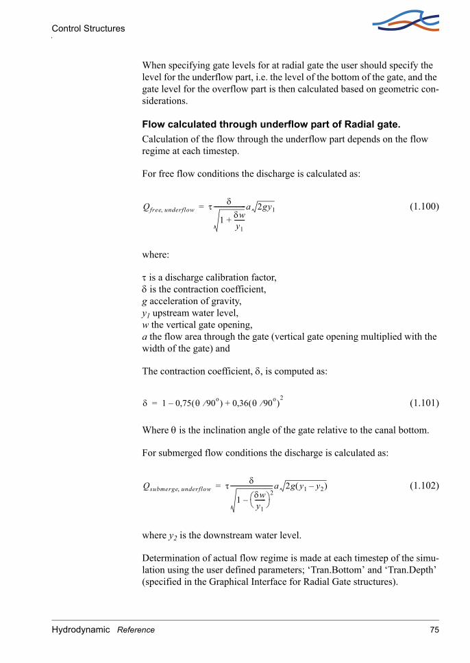
Control Structures
When specifying gate levels for at radial gate the user should specify the level for the underflow part, i.e. the level of the bottom of the gate, and the gate level for the overflow part is then calculated based on geometric con-siderations.
Flow calculated through underflow part of Radial gate.Calculation of the flow through the underflow part depends on the flow regime at each timestep.
For free flow conditions the discharge is calculated as:
(1.100)
where:
τ is a discharge calibration factor, δ is the contraction coefficient, g acceleration of gravity, y1 upstream water level, w the vertical gate opening, a the flow area through the gate (vertical gate opening multiplied with the width of the gate) and
The contraction coefficient, δ, is computed as:
(1.101)
Where θ is the inclination angle of the gate relative to the canal bottom.
For submerged flow conditions the discharge is calculated as:
(1.102)
where y2 is the downstream water level.
Determination of actual flow regime is made at each timestep of the simu-lation using the user defined parameters; ‘Tran.Bottom’ and ‘Tran.Depth’ (specified in the Graphical Interface for Radial Gate structures).
Qfree underflow, τ δ
1 δwy1-------+
---------------------a 2gy1=
δ 1 0,75 θ 90o⁄( )– 0,36 θ 90o⁄( )2
+=
Qsubmerge underflow, τ δ
1 δwy1-------
–2
----------------------------a 2g y1 y2–( )=
Hydrodynamic Reference 75
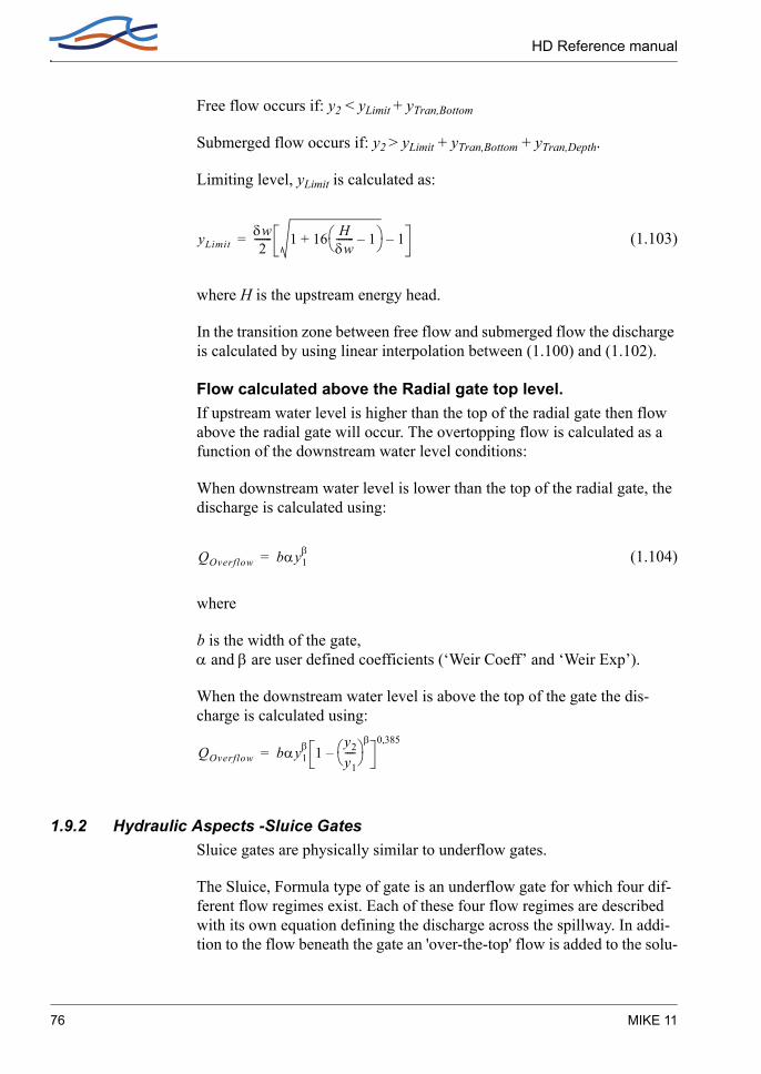
HD Reference manual
Free flow occurs if: y2 < yLimit + yTran,Bottom
Submerged flow occurs if: y2 > yLimit + yTran,Bottom + yTran,Depth.
Limiting level, yLimit is calculated as:
(1.103)
where H is the upstream energy head.
In the transition zone between free flow and submerged flow the discharge is calculated by using linear interpolation between (1.100) and (1.102).
Flow calculated above the Radial gate top level.If upstream water level is higher than the top of the radial gate then flow above the radial gate will occur. The overtopping flow is calculated as a function of the downstream water level conditions:
When downstream water level is lower than the top of the radial gate, the discharge is calculated using:
(1.104)
where
b is the width of the gate, α and β are user defined coefficients (‘Weir Coeff’ and ‘Weir Exp’).
When the downstream water level is above the top of the gate the dis-charge is calculated using:
1.9.2 Hydraulic Aspects -Sluice GatesSluice gates are physically similar to underflow gates.
The Sluice, Formula type of gate is an underflow gate for which four dif-ferent flow regimes exist. Each of these four flow regimes are described with its own equation defining the discharge across the spillway. In addi-tion to the flow beneath the gate an 'over-the-top' flow is added to the solu-
yLimitδw2
------- 1 16 Hδw------- 1–
+ 1–=
QOverflow bαy1β=
QOverflow bαy1β 1
y2
y1----
β
–0,385
=
76 MIKE 11

Control Structures
tion.This happens when the upstream water level exceeds the top of the gate. Which flow regime that applies in a given situation is determined by the values of up- and downstream water level and the gate position. The different flow regimes and when they apply are listed in below table.
H is the upstream water level measured above the sill level, h downstream water level measured above the sill level, g the acceleration of gravity, Go the gate opening, Hg the height of the gate, L the spill way width, yc the critical depth and Q the discharge. H, Hg, h and Go are shown in below definition sketch.
Table 1.3
Flow Condition
Equation Restriction Remarks
Controlled Submerged
(CS)
Also known as sub-merged orifice
Controlled Free (CF)
Also known as free orifice
Un-control-led Sub-merged
(US)
Also known as sub-
merged weir
Un-control-led Free
(UF)
Also known as free weir
Over-the-top
Computed as a free weir
flow
yc aG0H h–
G0-------------
b=
Q L gyc3= h
G0------ 1,0·≥
yc aG0HG0------
b=
Q L gyc3= h
G0------ 1,0< & H
G0------ 1
K----≥
K 23---=
yc aH 1 hH----–
b
=
Q L gyc3= h
G0------ 1,0 H
G0------ 1
K---- & h
H---- K≥,<,<
K 23---=
yc aH=
Q L gyc3=
hG0------ 1,0 H
G0------ 1
K---- & h
H---- K<,<,<
K 23---=
Q L gyc3=
yc a H HG– G0–( )=
H HG G0+( )>
Hydrodynamic Reference 77

HD Reference manual
Figure 1.18 Definition sketch
In order to avoid instabilities due to too sharp limits between the different flow regimes it is possible to define an interval across which the solution varies from one flow type to another. This is done using the 'High Limit' and 'Low Limit' option supplied in the user interface.
1.9.3 Hydraulic Aspects - Overflow StructuresThe calculation of the discharge over a movable weir is identical to that of dambreak structures, i.e. a broad crested weir. The only difference is that the structure width is assumed to remain constant for control and struc-tures.
See section A.10 Structures (p. 467).
1.9.4 Hydraulic Aspects - Underflow StructuresThe type of underflow structures considered in the control structure opera-tion are rectangular in shape, with a vertical sliding or rotating section. The gate will only have a controlling influence on the flow if the gate level is lower than the upstream water level. If this is not the case, the discharge will be calculated assuming an overflow structure where crest level is taken as sill level, as described above.
If the upstream water level is higher than the gate level, the presence of the gate will force the passing water into a jet, the height of which is less than
78 MIKE 11

Control Structures
the gate height due to a severe convergence of streamlines just upstream of the gate. At the point of maximum contraction, called the vena con-tracta, the streamlines are once again parallel to the bed, and a hydrostatic pressure distribution may be assumed to occur here, see Figure 1.19
Figure 1.19 Flow under a vertical sluice gate
This contraction of the flow may cause the formation of supercritical flow in the region of the issuing jet. Should this occur in a channel with a high tail water level, a hydraulic jump may occur downstream of the gate. In either case, the discharge through the gate will be a function of the gate geometry and upstream water level only. This is termed free discharge.
As the tail water rises, the hydraulic jump moves upstream, towards the gate. When the jump reaches the gate, it will completely drown the super-critical jet, and the water level at this point will suddenly rise to the tail water depth. This change in the flow at this instant is discontinuous, due to the discontinuous nature of the hydraulic jump itself. At the point of change over, the discharge will suddenly decrease, and may only increase if the water level upstream of the gate also increases.
The minimum downstream water level at which the hydraulic jump is drowned may be calculated from the hydraulic jump equation:
(1.105)
where, ys and y2 are the water depths (measured above the sill) at the vena contracta and immediately downstream respectively and F is the Froude number corresponding to ys.
y212---ys 1 8F2+ 1–( )=
Hydrodynamic Reference 79

HD Reference manual
1.9.5 Free FlowFor a freely issuing jet (ie.not drowned), the gate discharge is a function of the gate geometry and upstream water level only. The magnitude of the discharge for a given opening will depend on the amount of contraction the jet experiences. The contraction coefficient, Cc, is a measure of this, and is defined as:
(1.106)
The contraction coefficient is dependent on the gate type: for a vertical sluice gate, Cc is in the region 0.61 - 0.63, whereas for a radial gate, the contraction coefficient is dependent on the gate level. The contraction coefficient is in MIKE 11 an input variable and is by default equal to 0.63.
Head losses across the structure are calculated from the standard MIKE 11 descriptions via the user defined values ζin and ζout, see section A.10 Structures (p. 467).
The inflow head loss is assumed to occur in the region of accelerating flow between the point upstream of the gate and the vena contracta. It would be expected to have a value between 0.0 and 0.50. The outflow head loss occurs in the region of flow expansion, between the vena con-tracta and the next downstream h point. Theoretical values of between 0.8 and 1.0 have been calculated for vertical sluice gates, but in practice they can be considerably higher (/14/).
If the flow is determined as free, the energy equation may be applied between the point upstream of the structure and the vena contracta, to yield the free discharge through the gate. Assuming, as in most cases, a zero inflow head loss, it can be shown that this equation is equivalent to the generally accepted form of the vertical sluice equation viz: (/11/)
(1.107)
where, b is the gate width and Cd is the effective discharge coefficient, cal-culated from:
(1.108)
Ccys
gate opening(w)---------------------------------------=
Q Cdbw 2gy1=
CdCc
1 Ccwy1----+
-------------------------=
80 MIKE 11

Cross-Sections
1.9.6 Drowned FlowIf drowned discharge is detected, the energy equation is applied between points upstream and downstream of the structure. Note that in calculating the energy losses, the existence of a ‘submerged´ vena contracta is assumed, overlaid by a body of still water. The energy equation in this form corresponds to the submerged orifice equation of the form:
(1.109)
where, Cd is the effective discharge coefficient and h1 and h2 are upstream and downstream water elevations respectively.
As mentioned previously, the change between free and submerged flow is discontinuous in nature, the free discharge being greater than the corre-sponding drowned discharge for the same water levels and gate opening. Such discontinuities will present numerical problems during a computa-tion which may lead to instabilities and eventual termination of the com-putation. Hence in MIKE 11, a coefficient, ψ, has been introduced in order to make a smooth transition. By use of this coefficient it is possible to expand the transition zone from free flow to drowned flow. The transition zone is defined as:
(1.110)
When downstream water level, y2, is within this interval the discharge through the structure will be calculated using an interpolation between the free flow equation and the drowned flow equation. The value of ψ can be set in the Mike11.ini file placed in the windows directory. The default value is zero corresponding to a discontinuity when changing from free flow to drowned flow. The user should only change this value if instabili-ties are encountered during the simulation. A rule is that the value of ψ should be as low as possible. A first guess at the value of ψ could be 0.01.
1.10 Cross-Sections
The topographical description of the area to be modelled is achieved through the specification of cross-sections of the channel (and flood plain) which lie approximately perpendicular to the direction of flow.
Cross-sections are specified by a number of x-z co-ordinates where x is the transverse distance from a fixed point (often left bank top) and z is the cor-
Q Cdwb 2g h1 h2–( )=
12---ys 1 8F2– 1–( ) 1 ψ–( ) y2
12---y2 1 8F2– 1–( ) 1 ψ+( )<≤
Hydrodynamic Reference 81

HD Reference manual
responding bed elevation. A resistance value (Relative resistance or actual resistance number) can be specified for each pair of co-ordinates (see sec-tion 1.3 Bed Resistance (p. 21)). The transverse extent of each cross-sec-tion depends on whether the flood plain is to be simulated and by what method (see section 1.18 Flood Plains (p. 124)).
The number of cross-sections required is determined from both physical and mathematical requirements. The latter are discussed under section 1.8 Computational Grid (p. 72) and section 1.32 Stability Conditions (p. 173). Physically there should be a sufficient number of cross-sections to define adequately the variation in channel shape along each model branch.
The x-z co-ordinates are entered as raw data in the Cross Section editor. The raw data are then automatically processed into a form used in the hydrodynamic calculations, i.e. the hydraulic parameters; cross-sectional area, hydraulic radius and width are calculated for a number of elevations between a minimum and a maximum which are either determined auto-matically or defined by the user. The processed data may be edited from the processed data editor where two additional hydraulic parameters appear, additional flooded areas and the resistance factor. These are described respectively under the keywords Bed Resistance (p. 21) and Flooded Areas, (Storage) (p. 107).
If, during a simulation, the water level rises above the maximum elevation in the processed data table, the hydraulic area is calculated by assuming the river banks extend vertically upward, (Figure 1.20). Thus, the width remains constant for increasing water levels above the maximum specified elevation. This facility is intended to prevent a simulation from crashing if any initial instabilities occur and not to accommodate a lack of knowledge concerning the cross-section geometry. An error message will occur if the water level becomes more than N times higher than the maximum eleva-tion and the simulation is terminated. Where N by default is 4 but may be changed in the ‘MIKE11.ini’ file see Appendix B.
It is strongly recommended that, in defining the cross-section geometry, the maximum elevation is specified in such a way that the cross-section will accommodate the maximum expected water levels.
There are two circumstances where care is required:
1 where the processed width value has been adjusted to accommodate flooded areas (see also section 1.15 Flooded Areas, (Storage) (p. 107)). This will affect the way in which cross-sectional area is calculated for water levels above the maximum elevation mentioned above and
82 MIKE 11

Cross-Sections
described below. Calculation of area above maximum specified. The cross-sectional area, Anew at hnew is given by:
Anew = Amax + (hnew-hmax) Wmax
where,
hmax is the maximum specified elevation
Wmax is the width at hmax
Amax is the cross-sectional area at hmax
2 Thus, for example, if Wmax has been set to zero in the specification of flooded areas then, for all water levels greater than hmax, the cross-sec-tional areas will remain constant and equal to Amax;.
Figure 1.20 Calculation of area above maximum specified height
Where a relative resistance different from 1.0 has been specified in the raw data e.g. in the flood plain, an incorrect area-elevation relationship will result for water levels in excess of the maximum elevation speci-fied. This is illustrated in Figure 1.21a and Figure 1.21b, depicting the same cross-section but where, in Figure 1.21a, the maximum elevation specified, hmax, is below the highest water level occurring. In this instance the calculated effective area does not account for the relative resistance. In Figure 1.21b, the highest occurring water level is below hmax and the effective area is correctly calculated
Hydrodynamic Reference 83

HD Reference manual
Figure 1.21 Calculation of cross-sectional area for relative resistance values larger than 1.0. a) Highest water level above maximum specified elevation b) Highest water level below maximum specified elevation
1.11 Closed Cross sections, Modelling the Pressurised flow
Pressurised flow computations are facilitated through implementation of a narrow 'slot', as a vertical extension of a closed pipe cross section. Free surface and pressurised flows are thus described within the same basic algorithm, which ensures a smooth and stable transition between the two flow types.
The full flow capacity of a closed conduit (pipe) can be defined as a dis-charge at which the flow depth is equal to the conduit height. Any further increase of discharge fundamentally changes the conditions of flow, i.e. basic assumptions for the derivation of the Saint Venant equations are not valid. Namely, the flow changes from the free surface flow to the pressu-rised flow.
However, it is possible to generalise the equations for free surface flow, so that the pressurised flow in closed conduits is covered. This is done by introducing a fictitious slot in the top of the conduit, see figure 1.22.
The idea of introducing a fictitious slot was first presented by Preissmann and Cunge, 1961, and has since been used by Cunge and Wagner, 1964 (see ref. /15/).
84 MIKE 11

Closed Cross sections, Modelling the Pressurised flow
Figure 1.22 Pipe section with fictitious top slot, usually referred to as a ‘Preissmann’ slot.
The derivation of pressurised flow conditions for free surface flow equa-tions can be obtained from the continuity equation which can be written as:
(1.111)
assuming the density of water, ρ, constant over the cross section.
By partial differentiation is found:
(1.112)
For a circular pipe, it can be shown that the density of the water can be approximated as:
(1.113)
where:
∂ ρQ( )dx
----------------dxdt– ∂ ρA( )dt
---------------dxdt=
∂Q∂x------- Q
ρ---- ∂ρ
∂x------ ∂A
∂t------ A
ρ--- ∂ρ
∂t------⋅+ +⋅+ 0=
ρ ρ0 1 g y D–( )
a02
---------------------+ ≈
Hydrodynamic Reference 85
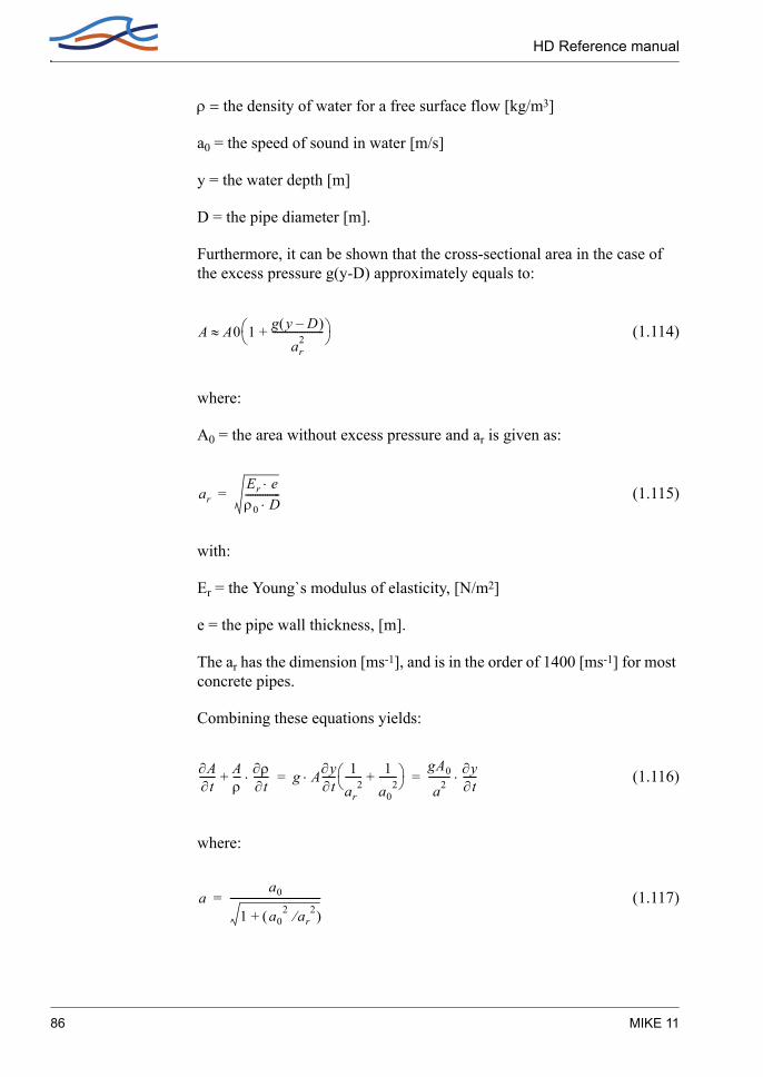
HD Reference manual
ρ = the density of water for a free surface flow [kg/m3]
a0 = the speed of sound in water [m/s]
y = the water depth [m]
D = the pipe diameter [m].
Furthermore, it can be shown that the cross-sectional area in the case of the excess pressure g(y-D) approximately equals to:
(1.114)
where:
A0 = the area without excess pressure and ar is given as:
(1.115)
with:
Er = the Young`s modulus of elasticity, [N/m2]
e = the pipe wall thickness, [m].
The ar has the dimension [ms-1], and is in the order of 1400 [ms-1] for most concrete pipes.
Combining these equations yields:
(1.116)
where:
(1.117)
A A0 1 g y D–( )
ar2
---------------------+ ≈
arEr e⋅ρ0 D⋅--------------=
∂A∂t------ A
ρ--- ∂ρ
∂t------⋅+ g A∂y
∂t----- 1
ar2
------- 1a0
2-------+
⋅gA0
a2--------- ∂y
∂t-----⋅= =
aa0
1 a02 ar
2⁄( )+-------------------------------------=
86 MIKE 11

Closed Cross sections, Modelling the Pressurised flow
‘a’ represents the speed of sound in water considering the compressibility of water and the deformation of the pipe wall.
Equation (3.10) can now be written as:
(1.118)
The analogy with the continuity equation can thus be maintained in case that the fictitious slot width bslot is specified as:
(1.119)
‘a’ is in the order of 1000 [m/s] for most pipes.
In order to obtain a smooth transition between the free surface flow com-putations and pressurised flow computations, it is required to apply a "soft" transition between the actual pipe geometry and the fictitious slot. Such a "smooth" transition has been designed based on a series of tests with various slot configurations. The slot configuration thus obtained ensures stable computations without affecting the accuracy significantly. The applied slot width is larger than the theoretical value. The default rela-tion between relative depth and the slot width as implemented in MIKE 11 is given in table 1.4
Similar principles apply for generating Preissmann slots for the closed rectangular and closed irregular section types. The width of Preissmann slot for irregular closed sections are defined as 10% of maximum width in closed section.
Table 1.4 Relation between relative Depth and top slot width
y/D bslot/D (D=1 m)0.98 0.361.00 0.191.10 0.01661.20 0.01511.50 0.0105
> 1.50 0.0100
∂Q∂x------- Q
ρ---- ∂ρ
∂x------
gA0
a2--------- ∂y
∂t-----⋅+⋅+ 0=
bslot gA0
a2-----⋅=
Hydrodynamic Reference 87

HD Reference manual
1.12 Culverts, Q-h Relations Calculation
The Culverts Q-h Relations calculation are included in order for a pre-cal-culation of free-flow relationship for culverts. Following key issues are to be noted on the calculation of Q-h relations:
the Q-h relationships are calculated by MIKE 11 using the culvert defi-nitions and cross sections up- and downstream. If, for some reason it is required to adjust the calculated values it is possible to change the val-ues in the table and save the network file.
the culvert can be assigned a length, friction coefficient, slope and bend loss coefficient in addition to the conventional parameters
the culvert cross-section can be defined by a standard shape (e.g. circle or rectangle) as well as a irregular shape. Surveyed culvert geometry data entered in the cross-section file can also be chosen as the structure geometry definition.
The facility has been designed for modelling culverts of any shape, length or slope. All flow conditions are represented including full submergence, partial submergence, critical inflow and outflow, orifice flow and full cul-vert flow with a free outflow.
1.12.1 SpecificationThe culvert cross-section shape is specified as either a standard shape (rectangle, circle), an irregular shape defined as a (depth or level)/width relation by the user. Other details required are:
culvert length (m)
upstream and downstream invert levels (m)
number of parallel culverts
friction coefficient (Manning's n)
valve regulation switch which may be set as
– flow only in negative direction (decreasing chainage)
– flow in both directions (none)
– flow only in positive direction (increasing chainage)
closed/open section switch
coefficients in both positive and negative flow directions for:
– inflow losses (typically 0.5)
– outflow losses (typically 1.0)
88 MIKE 11

Culverts, Q-h Relations Calculation
– bend losses (straight culvert would be 0.0)
– free overflow correction coefficient (typically 1.0)
1.12.2 Flow DescriptionsThe flow through a culvert can be broadly classified into three areas for computational purposes. The flow conditions mentioned below are illus-trated in Figure 1.23
Zero FlowThe zero flow condition occurs when one of the following conditions exist:
the culvert is dry
the valve regulation switch is set to negative and the flow would be in a positive direction if the valve was open;
the valve regulation switch is set to positive and the flow would be in the negative direction if the valve was open.
Upstream Controlled FlowThe upstream controlled flow conditions occur when the downstream water level has no influence on the discharge through the culvert. The dis-charge, Q, is therefore solely a function of the river water level at the cul-vert inflow, h1, and can be tabulated (Q-h relation) prior to the simulation, minimising the computational effort required during the simulation. The flow conditions modelled are:
critical inflow
partially full inflow and critical outflow
submerged inflow and critical outflow
orifice flow at inflow with free outflow
full culvert flow with free outflow
Expressions for the loss coefficients, momentum equation coefficients, upstream controlled flow (critical inflow or outflow, orifice flow at inflow and full culvert flow with free outflow) and downstream controlled (sub-merged) flow are described in detail in Appendix A (p. 421). The transi-tion between upstream and downstream control is also described in section A.3.
Hydrodynamic Reference 89

HD Reference manual
.Figure 1.23 Culvert flow conditions
Downstream Controlled FlowDownstream controlled flow or submerged flow occurs when the down-stream water level imposes a constraint on the flow through the culvert. The calculations take place during a simulation because the discharge is a
90 MIKE 11

Culverts, Q-h Relations Calculation
function of both upstream and downstream water levels and therefore is not practical to tabulate. The flow conditions modelled are:
partially full inflow and outflow
submerged inflow and partially full outflow
partially full inflow and submerged outflow
fully submerged
1.12.3 Construction of Q-h RelationshipsThe Q-h relationships (one for each flow direction) are presented for veri-fication under the Q-H relations tab. For convenience, the relationships are given as the water depth, y1, versus Q, not h1 versus Q. The value of h1 is equal to the culvert invert level plus y1. The construction of the Q-h relationship is described below.
First, the hydraulic parameters, area, hydraulic radius and critical flow, are tabulated for depths ranging from zero to full culvert depth. A cosine func-tion is used for setting the tabulated depth values in order to give more detail at the bottom and top of the culvert cross-section where the varia-tion of area and hydraulic radius is very non-linear. The values of area and hydraulic radius are shown under the Hydraulic Parameters tab for verifi-cation purposes only.
If an irregular section shape is specified, and if the depth or level/width table has more than eight pairs of values, the depths in the depth (or level)/width table are used for calculating the hydraulic parameters, other-wise the cosine function is used. This provides the opportunity for the user to specify the depths at which the hydraulic parameters are to be calcu-lated.
Secondly, h1 is calculated for critical depths ranging from zero to that at 95% of the full culvert area. Whether the flow is critical at the inflow or outflow is determined according to the description above.
An iteration procedure is used to calculate h1 because the contraction loss coefficient ζ1, see Appendix A (p. 421), and the inflow river cross-section area A1 are functions of h1. It is therefore necessary to specify the Topo ID in addition to the river name and chainage of the culvert so that A1 can be calculated from the cross-section data base.
At the start of a simulation a check is made that the distance between the upstream and downstream cross-sections minus the culvert length is less than DX-MAX. If this is not the case an error message is given. At present there are no checks comparing the cross-section locations and/or Topo ID
Hydrodynamic Reference 91

HD Reference manual
between that used for calculating the Q-h relations and that used in the simulation. Ideally the upstream and downstream cross-sections should be located immediately upstream and downstream of the culvert.
When critical flow can no longer occur (submerged inflow and/or out-flow), the flow condition will be either orifice flow or full culvert flow. The Q-h relationship continues to be constructed by calculating the dis-charge for increasing values of h1. The maximum value of h1 in the tabula-tion is defined as the greater of (a) the top elevation in the adjacent cross-section, and (b) five times the culvert depth above the invert.
If the inflow river water level exceeds the maximum h1 value during a model simulation, a linear extrapolation is made based on the last two pairs of values in the Q-h relation.
Iteration procedures are also necessary for Qo (orifice flow) and Qp (primed flow). The discharge adopted is taken as the minimum of Qo and Qp. However, once Qp is lower full culvert flow occurs (i.e. Qp < Qo), and the culvert is assumed to remain flowing full, i.e. the culvert is "primed".
For each iteration procedure mentioned above, convergence usually occurs in two to three iterations except in the case when the culvert inflow cross section area, and A1 are of similar magnitude, i.e. as ζ1 approaches zero. A maximum number of one hundred iterations is allowed, and if exceeded a warning message is given. The Q-h relation-ships will be successfully calculated, but the user should check the adja-cent cross-section description and the culvert specifications.
If is greater than A1 or the Q values are decreasing with increasing h the calculation of the Q-h relationships is suspended and warning mes-sages are given. The point in the Q-h relationships where the problem occurred can be observed by going to the bottom of the Q-y tables.
Simulations will not be possible unless the Q-h relationships have been successfully calculated.
If the Topo ID or the upstream and downstream cross-sections are changed, the Q-h relationships have to be recalculated.
1.12.4 Closed / Open Section switchA culvert structure can be modelled as an open section if required by set-ting the Closed / Open switch. An example where this may be used is a "long" weir where the friction along the length of the weir is of impor-tance and/or the flow areas at the entrance and exit are significantly differ-ent.
As1
As1
92 MIKE 11

Dambreak Structure
If set to open the culvert will never run full or partially full, therefore only those flow conditions which represent a free water surface are modelled. When the water level is higher than the soffit the hydraulic parameters are calculated based on a section extended vertically upwards with a width equal to that at the soffit. For example, in the case of a rectangular section the height value is essentially redundant as the cross-section will be mod-elled as an open section of constant width.
In the case of a circular section, this switch is invalid and will be set to closed.
1.12.5 Changing Flow DirectionSee the discussion in section 1.33 Steady State Energy Equation (p. 175) for the treatment of when the flow direction changes between positive and negative directions.
1.12.6 Flooded Areas of Adjacent h-pointsThe flooded or storage areas of the two adjacent h-points are reduced by half of the culvert length multiplied by the cross-section width. In effect the culvert is considered to have a zero contribution to the storage of the system. In the rare case where the storage within the culvert is significant compared to that in the river, the flooded areas at the adjacent h-points should be adjusted using the additional flooded area parameter, see section 1.10 Cross-Sections (p. 81).
1.12.7 VelocitiesThe velocity through a culvert is calculated as Q/Ac in the case of critical inflow or outflow where Ac is the critical flow area, as Q/Afull in the case of orifice flow or full culvert flow and Afull is the full cross-section area of the culvert, and as when the flow is downstream controlled. In the latter case, is equal to the mean of and , the culvert inflow and outflow cross-section areas, respectively.
1.13 Dambreak Structure
A dambreak structure is a composite structure composed of a structure representing the flow over the crest (Crest flow structure) and another structure representing the breach of the dam. The breach can be modelled in two different ways i.e. as a failure of the crest (breach-structure) or as piping failure of the dam (pipe failure structure) followed by breach fail-ure. The crest flow at a dam is calculated as separate structures in a com-posite structure.
Q SsA⁄
Q SsA⁄ Q Ss1
⁄ Q Ss2⁄
Hydrodynamic Reference 93

HD Reference manual
A dambreak structure is a dam in which a breach can develop. The flow through a dam breach may be described in MIKE 11 through the use of the energy equation or alternatively a the calculation method as implemented in National Weather Services (NWS) DAMBRK program. In the follow-ing the two methods are presented separately.
1.13.1 Energy equation based dam breach modellingThe flow at the dambreak structure is quite similar to a broad crested weir, but there are two differences:
1 the shape of the dam changes with time, i.e. the breach increases and the dam crest is shortened. As a consequence the critical flow charac-teristics (Q-h) relationship of the crest and of the breach cannot be cal-culated beforehand
2 the Q-h relationship for the dam crest and the breach are different therefore the flow over the crest and the flow through the breach are calculated separately, see Figure 1.24.
Figure 1.24 Combined flow over breach and crest
Initial breach development
The breach may be initiated in a number of ways depending on the method of calculation used. For the NWS method the breach may be initiated either as a trapezoidal breach or as a piping failure. Using the standard dam breach methods the breach is initiated either as a trapezoidal breach or if the erosion based method is used as a circular piping failure.
Trapezoidal Breach GeometryDuring the development of the breach the trapezoid increases in size and changes shape.
The initial breach shape is described by three parameters as shown in Figure 1.25:
94 MIKE 11

Dambreak Structure
level of the breach bottom (HB)
width of the breach bottom (WB)
side slope of the breach (SS) (horizontal: vertical). The left side slope and the right side slope are equal
The development of the breach can either be specified as a known func-tion of time, or it can be simulated from the sediment transport capacity of the breach flow.
Figure 1.25 The parameters of the breach geometry
Known Geometry Breach DevelopmentThe parameters of the breach are given as a time series in the boundary editor. The time is relative to the start of the breach. Between the specified times the parameters are linearly interpolated as shown in Figure 1.26 for the trapezoidal case. The breach bottom level must not be above the crest level.
Figure 1.26 The breach is specified for example at times 0h and 1h. The dashed line would be the linear interpolation for time 0.5h
Hydrodynamic Reference 95

HD Reference manual
1.13.2 Erosion Based Breach Development using the energy equationIf this mode is chosen the initial and the final breach shape must be speci-fied. The increase of the breach during a time step is calculated from the actual prevailing conditions in the breach itself. The Engelund-Hansen sediment transport formula is used (see equations (3.127) and (3.128)) to calculate the sediment transport in the breach.
As a first step, the flow resistance in terms of the total dimensionless shear stress is calculated, based on the Engelund formulation (see section 3.8.2 Flow Resistance - q-q´ Relationship (p. 254)). This is then compared to the critical shear stress (the Shield´s Criterion, defined by the user). If the computed shear stress is greater than the critical one, then the sediment transport is calculated, otherwise it is set to zero.
The sediment transport rate, qt, calculated from the Engelund-Hansen for-mula is in terms of m2/s per metre-width of pure sediment only, and this must then be related to a change in bed (i.e. breach) level. It is assumed that the breach remains horizontal. From the given upstream and down-stream slopes, the length of the breach in the flow direction, Lb, may be calculated. By application of the sediment continuity equation in the breach, the change in breach level dHb in a time interval dt is given as:
(1.120)
where,
Hb is the breach level
qt is the sediment transport rate (m2/s)
ε is the porosity of the sediment
Lb is the breach length in the direction of flow
t is time
Modelling the variation of the width of the breach perpendicular to the flow direction is more difficult to relate to the classical theories of sedi-ment transport. This is because the development of a wall boundary layer along the often very steep side walls of the breach, the theories for bed load and suspended load do not apply. As an approximation, the sediment transport at the sloping walls is assumed to be proportional to that in the
dHb
dt----------
qt
Lb 1 ε–( )---------------------- =
96 MIKE 11

Dambreak Structure
central part of the breach. The coefficient of proportionality, x, (side ero-sion index) thus relates the increase in breach width, Wb, to depth as:
(1.121)
Generally, the side erosion index is in the order of 0.5-1.0.
Erosion Based Piping FailureAn erosion based failure of a dam may be initially started by piping fail-ure. In this case a flow forms through the dam wall. Erosion of the soil along the "pipe" causes the pipe to enlarge and the flow to increase. Even-tually the dam will collapse into the void created by the piping failure ero-sion.
This failure scenario is modelled as an option in the erosion based breach development, i.e. there are two options for the initial failure process:
1 initial failure by overtopping
2 initial failure by piping (after collapsing the erosion process returns to that of overtopping as described above).
The assumptions adopted for the piping failure are:
the shape of the pipe is circular
the pipe is horizontal
the pipe must always be running full
The location of the pipe centre in the dam cross-section must be within the final breach shape and, if specified, the limiting section shape. When the circumference of the pipe extends outside these shapes, the hydraulic parameters are based on a reduced cross-section as illustrated in Figure 1.27.
dWb
dHb---------- 2x=
Hydrodynamic Reference 97

HD Reference manual
Figure 1.27 Adjustment of a pipe cross-section
The point of collapse is defined by a ratio, which is specified by the user, of the pipe diameter to the distance between the dam crest and the pipe obvert as illustrated in Figure 1.28. Once this ratio is exceeded part of the dam is collapsed to form a breach.
Figure 1.28 Piping failure collapse ratio
The shape of the breach is illustrated in Figure 1.29. The bottom width is first set equal to the pipe diameter and the breach level to the pipe invert. Not all of the collapsed material will typically be carried out without depositing on the bed of the breach. This is accounted for by a volume loss coefficient, flost, which is the fraction of material assumed to be washed out immediately after collapse. The remaining material is evenly distrib-uted on the breach bed as shown in Figure 1.29.
These calculations are made using cross-section areas, not volumes, there-fore, the length of the breach and consequently the upstream and down-stream slopes of the dam faces are not taken into account.
98 MIKE 11

Dambreak Structure
Figure 1.29 Breach shape after collapse
Other parameters required are the initial diameter of the pipe at the start of failure and the pipe roughness, ks, which is used to calculate the Darcy friction factor, f, according to
(1.122)
where, R is the hydraulic radius.
The discharge, Qp, through the pipe is given by
(1.123)
where, A is the flow area, L is the length of the pipe and ∆H is given by
(1.124)
where, h1 is the upstream water level, h2 is the downstream water level and zobv is the obvert of the pipe.
In Equation (1.120) an entrance head loss of half the velocity head in the pipe and, when there is a submerged outlet, an exit loss of one velocity head have been incorporated. Adopting a full velocity head loss in the lat-ter case gives the transition between submerged flow and free outflow to be when the downstream water level, h2, equals the pipe obvert, zobv. (See section 1.12 Culverts, Q-h Relations Calculation (p. 88), for a more detailed discussion.)
1f
----- 2log1012Rks
---------- =
Qp A 2g∆H
1,5 fL4R-------+
--------------------------=
∆H h1 max h2 zobv,( )–=
Hydrodynamic Reference 99

HD Reference manual
The enlargement of the pipe is based on the sediment transport relation-ship described above for breach erosion. The depth of water, yp, used in calculating qt is given by
(1.125)
where, D is the pipe diameter.
By relating the volume of material eroded to the "effective" transport area (adopted here as the pipe length times half the circumference) the change in the pipe radius, ∆Rp, is defined as
(1.126)
where, Ccal is a "calibration" coefficient entered as one of the erosion parameters. No sound recommendation can be given for the value of Ccal. It has been provided so the user can adjust the rate of change of Rp if so desired, or some data becomes available for calibrating the rate of forma-tion of the pipe.
Limiting Cross-SectionThere may be a boundary of an irregular shape beyond which the breach will not develop. This limit may be the surface of hard rock or it may be the natural bottom of the valley. To allow for a boundary of this type a cross section can be specified. In this case only the part of the trapezoid inside the cross-section is used for calculation of the flow. This is illus-trated in Figure 1.30.
yp∆H2
-------- D+=
∆Rp Ccalqt
2Lp 1 ε–( )-------------------------∆t=
100 MIKE 11
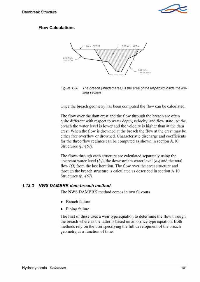
Dambreak Structure
Flow Calculations
Figure 1.30 The breach (shaded area) is the area of the trapezoid inside the lim-iting section
Once the breach geometry has been computed the flow can be calculated.
The flow over the dam crest and the flow through the breach are often quite different with respect to water depth, velocity, and flow state. At the breach the water level is lower and the velocity is higher than at the dam crest. When the flow is drowned at the breach the flow at the crest may be either free overflow or drowned. Characteristic discharge and coefficients for the three flow regimes can be computed as shown in section A.10 Structures (p. 467).
The flows through each structure are calculated separately using the upstream water level (h1), the downstream water level (h2) and the total flow (Q) from the last iteration. The flow over the crest structure and through the breach structure is calculated as described in section A.10 Structures (p. 467).
1.13.3 NWS DAMBRK dam-breach methodThe NWS DAMBRK method comes in two flavours
Breach failure
Piping failure
The first of these uses a weir type equation to determine the flow through the breach where as the latter is based on an orifice type equation. Both methods rely on the user specifying the full development of the breach geometry as a function of time.
Hydrodynamic Reference 101

HD Reference manual
Breach failureThe flow through the trapezoidal breach is given by
(1.127)
where
b The width of the breach bottom
g Acceleration due to gravity
h Upstream water level (reservoir water level)
hb Level of breach bottom
S Side slope of breach
cweir Weir coefficient for horizontal part (=0.546430)
cslope Weir coefficient for slope part (=0.431856)
cv Correction coefficient for approach sections. This coefficient com-pensates for the loss in energy due to the inflow contraction.
ks Correction coefficient due to submergence.
The weir coefficients have been made non-dimensional e.g.
The correction coefficient for the approach section is determined through
(1.128)
where
cB Non-dimensional coefficient (= 0.740256) termed the Brater coeffi-cient
WR Reservoir width given by the un-destroyed crest length.
Q cvks cweirb g h hb–( ) h hb–( ) cslopeS g h hb–( ) h hb–( )2+[ ]=
cweir g 0,546430 9,81 m s2⁄( ) 1,7115 m1 2⁄ s⁄( ) 3,1 ft1 2⁄ s⁄( )= = =
cv 1cBQ2
gWR2 h hb term,–( )2 h hb–( )
-----------------------------------------------------------------+=
102 MIKE 11
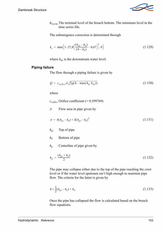
Dambreak Structure
hb,term The terminal level of the breach bottom. The minimum level in the time series file.
The submergence correction is determined through
(1.129)
where hds is the downstream water level.
Piping failureThe flow through a piping failure is given by
(1.130)
where
corifice Orifice coefficient (= 0.599769)
A Flow area in pipe given by
(1.131)
hpt Top of pipe
hb Bottom of pipe
hp Centerline of pipe given by
(1.132)
The pipe may collapse either due to the top of the pipe reaching the crest level or if the water level upstream isn’t high enough to maintain pipe flow. The criteria for the latter is given by
(1.133)
Once the pipe has collapsed the flow is calculated based on the breach flow equations.
ks max 1 27,8hds hb–( )h hb–( )
----------------------- 0,67–
30,–
=
Q corificeA 2g h max hp hds,( )–( )=
A b hpt hb–( ) S hpt hb–( )2+=
hphpt hb+( )
2-----------------------=
h 32--- hpt hb–( ) hb+<
Hydrodynamic Reference 103

HD Reference manual
Crest flowThe flow over the crest of the dam is given by
(1.134)
where
hc the crest level
bc the remaining crest length (perpendicular to the flow)
and the submergence correction given by
(1.135)
Failure momentThe user may choose three different definitions of the failure moment namely
Time in the form of a historic date and time.
Hours from start of simulation. The user specifies a time span in hours before the dam breaches.
A reservoir water level. The reservoir water level is defined as the greatest of the water level on either side of the dam.
Temporal development of breach geometryOnce the failure has initiated the temporal development of the breach will be read from a time series. This time series must contain values for
The breach bottom
The breach side slope
The breach bottom width
Further if piping failure is used the time series must also contain
The upper level of the pipe
Please refer to Figure 1.31.
Q kscweirbc g h hc–( ) h hc–( )=
ks max 1 27,8hds hc–( )h hc–( )
----------------------- 0,67–
30,–
=
104 MIKE 11

Energy Loss
Figure 1.31 Definition sketch for NWS DAMBRK routines.
1.14 Energy Loss
GeneralThe hydrodynamic module includes a facility for modelling the loss of energy at specified river locations. At run-time such points, denoted Energy Loss points, are defined as discharge grid points. At each time level of the computation the discharge at an Energy Loss point is com-puted by use of the energy equation:
(1.136)
in which ∆H is the energy loss encountered in passing the Energy Loss points, g is the acceleration of gravity, Q is the discharge and A is the cross-sectional wetted area at that point. The quantity, ζ, denotes the total energy loss coefficient as specified in the network editor. If applied, the energy loss coefficients described below are added up to yield a total energy loss coefficient.
User-Defined Energy LossIn order to enable the user to model a known energy loss at a river location Eq. (1.136) is applied in conjunction with a user defined loss coefficient, ζ = ζuser.
∆H ζ Q2gA2------------
2=
Hydrodynamic Reference 105

HD Reference manual
Energy Loss Caused by Sudden Flow ContractionThe energy loss caused by contraction of the flow is modelled using Eq. (1.136) in conjunction with a contraction loss coefficient, ζ = ζcont. The contraction coefficient is given by
(1.137)
where ζin is the inflow coefficient specified by the user, V1 is the upstream velocity at the previous water level point and V is the mean (within cross-section) velocity.
Energy Loss Caused by Expansion of the FlowExpansion loss is modelled using the following equation:
(1.138)
in which ζουτ is the outflow coefficient specified in the network editor and V2 is the downstream velocity at the next water level point. The coeffi-cient, ζexpan, replaces ζ in Eq. (1.136).
Energy Loss Caused by an Abrupt Change in River AlignmentIn the case of an abrupt change in river alignment, the energy loss is mod-elled as
(1.139)
in which θ denotes the angular change (deg) in river alignment. The coef-ficient, ζabrupt, replaces ζ in Eq. (1.136).
Energy Loss Caused by a Gradual Change in River AlignmentUsing the analogy of pipe flow, the energy loss is modelled as
(1.140)
where α = 0.2 for rough pipes and α = 0.1 for smooth pipes. The align-ment of the gradual bend is assumed to be circular, the radius of the bend being greater than 4 times the pipe diameter for Eq. (1.140) to prove valid.
ζcont ζin 1V1
V-----–
=
ζ anexp ζout 1V2
V-----–
2
=
ζabrupt 1,1 θ90------
2
=
ζgradual α θsin=
106 MIKE 11

Flooded Areas, (Storage)
The coefficient, ζgradual, replaces ζ in Eq. (1.136). The coefficients, α and θ, are specified in the network editor.
1.15 Flooded Areas, (Storage)
The flooded area, or storage area, is defined at each h point as the summa-tion of the width times the distance between the Q points either side of the cross-section plus the additional flooded area. The width is automatically calculated when the cross-section raw data are processed (see section 1.10 Cross-Sections (p. 81)) or can be specified manually in the cross section editors processed data menu. Additional flooded area data are specified manually by the user in the same editor.
The flooded area may have to be either increased or decreased manually by the user under certain conditions. An increase is necessary where there is an off-stream storage area (e.g. a harbour) connected to the river. A decrease is necessary where there is a duplication of flooded areas, (dis-cussed below).
To increase the flooded area specify additional flooded areas and/or increase the width values in the processed cross section data editor. To decrease the flooded areas reduce the width values in the cross section edi-tors processed data menu.
Note that the width values are not only used for the computation of the flooded area but also in the calculation of the wind friction (see section 1.41 Wind (p. 196)) and in the calculation of cross-sectional area for water levels in excess of the maximum elevation specified (see section 1.10 Cross-Sections (p. 81)). It should be noted that these additional flooded areas are not included in the total surface area in the computation of wind friction (see section 1.41 Wind (p. 196)).
A zero width value can be specified, noting that a zero flooded area at an h-point is not acceptable (or realistic) except where the h-point is con-nected to other h-points at a node (the flooded area at a node is the sum of the flooded areas of the connecting h-points and should also be non-zero).
The modelling of more complex flood plain hydraulics is described sec-tion 1.18 Flood Plains (p. 124).
When simulating the exchange of water between the channel and the flood plain care should be exercised when specifying the storage (width and additional flooded area columns) in order to avoid duplication in the cal-
Hydrodynamic Reference 107

HD Reference manual
culation of storage volumes at nodes and h-grid points. This is illustrated by the following simple example (Figure 1.32).
Figure 1.32 is a schematic diagram of flow in a flood plain: flow in the main channel is represented by branch RIVER; flow between the channel and the flood plain is represented by the two branches SPILL1 and SPILL2 in which the W points represent broad crested weirs; flow along the flood plain is represented by the branch PLAIN. The network has 4 nodes as shown in Figure 1.32. Cross-sections are defined at all h-points as shown in Figure 1.33.
.Figure 1.32 Network for flow in channel and adjacent flood plain
Figure 1.33 Location of cross-sections required for the network shown in Figure 1.32
108 MIKE 11

Flooded Areas, (Storage)
Without modification to the cross-section descriptions, the storage areas for each h-point would be as shown in Figure 1.34 considering each branch separately.
Figure 1.34 Storage areas corresponding to each h-point for each branch
Figure 1.35 below, shows the branches connected again, with those flooded areas which would be duplicated:
Figure 1.35 Duplication of flooded areas if no adjustment is made
In order to overcome this duplication, the values in the width columns of the processed cross-section data should be set to zero for the cross-sec-tions defining the spill units S1-1 and S2-1 and reduced by the appropriate amount for S1-2 and S2-2. The additional flooded area of all four cross-sections at all levels should be zero.
Hydrodynamic Reference 109
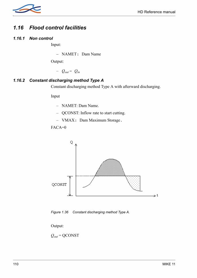
HD Reference manual
1.16 Flood control facilities
1.16.1 Non controlInput:
– NAMET: Dam Name
Output:
– Qout = Qin
1.16.2 Constant discharging method Type AConstant discharging method Type A with afterward discharging.
Input
– NAMET: Dam Name.
– QCONST: Inflow rate to start cutting.
– VMAX: Dam Maximum Storage.FACA=0
Figure 1.36 Constant discharging method Type A.
Output:
Qout = QCONST
110 MIKE 11

Flood control facilities
Dam burst Case
Figure 1.37 Constant discharging method Type A. Dam burst.
1.16.3 Constant discharging method Type BConstant discharging method Type B without afterward discharging.
Input:
– NAMET: Dam Name.
– QCONST: Inflow rate to start cutting.
– VMAX: Dam Maximum Storage.FACA = 0
Hydrodynamic Reference 111

HD Reference manual
Figure 1.38 Constant discharging method Type B.
Output:
– Qout = QCONST.
Dam burst caseQout is the same as for the constant discharging method Type A.
1.16.4 Constant ratio discharging method Type AConstant ratio discharging method Type A with afterward discharging.
Input:
– NAMET: Dam Name.
– QCONST: Inflow rate to start cutting.
– FACA: Cutting Rate.
– VMAX: Dam Maximum Storage.
112 MIKE 11

Flood control facilities
Figure 1.39 Constant ratio discharging method Type A.
Output:
(1.141)
Inner Implementation1 When Inflow < QCONST, Discharge = Inflow.
2 When Inflow > QCONST till inflow peak, discharge Qout is set by Eq. (1.141).
3 After peak, Qout keeps constant at Q2p till S2 ≥ S1, where Q2p is the Qout computed at peak.
4 After S2 ≥ S1, set Discharge = Inflow.
1.16.5 Constant ratio discharging method Type BConstant ratio discharging method Type B without afterward discharging.
Input:
– NAMET: Dam Name.
– QCONST: Inflow rate to start cutting.
– FACA: Cutting rate.
– VMAX: Dam Maximum Storage.
Qout FACA Qin QCONST–( ) QCONST+=
Hydrodynamic Reference 113

HD Reference manual
Output:
(1.142)
1.16.6 Bucket-cut (without afterward discharging)Input:
– NAMET: Dam Name.
– QCONST: Inflow rate to start cutting.– QCONST2: Constant discharging rate.– QCONST3: Inflow rate to increase discharging.– FACA: Decrease of discharging rate per unit time.
– FACB: Increase of discharging rate per unit time.
– VMAX: Dam Maximum Storage.
Output:
1 Qout = QCONST-∆Τ FACA
2 Qout = QCONST
3 Qout = QCONST2+∆Τ FACB
Note ∆T is the time increment per step.
1.16.7 Non gate discharging by H/Q curve and H/V curveInput:
Qout FACA Qin QCONST–( ) QCONST+=
114 MIKE 11

Flood control facilities
– NAMET: Dam Name.
– FASA: Initial Water Level.
– IT1: Number of H/Q relationship.
– IT2: Number of H/V relationship.
– HQ(2,IT1): H/Q relationship.
HQ(1,IT1):Water level of H/Q relationship.
HQ(2,IT1):Discharge of H/Q relationship.
– HV(2,IT2): H/V relationship.
HV(1,IT2): Water level of H/V relationship.
HV(1,IT2): Volume of H/V relationship.
Figure 1.40 Non gate discharging by H/Q-curve and H/V-.curve.
Output:
Qout is calculated through the H/Q or the H/V relationship.
1.16.8 Non gate discharging by orifice size inputInput:
– NAMET: Dam Name.
– IT1: Number of H/V Relationship.
– NANA: Number of spillways.
Hydrodynamic Reference 115
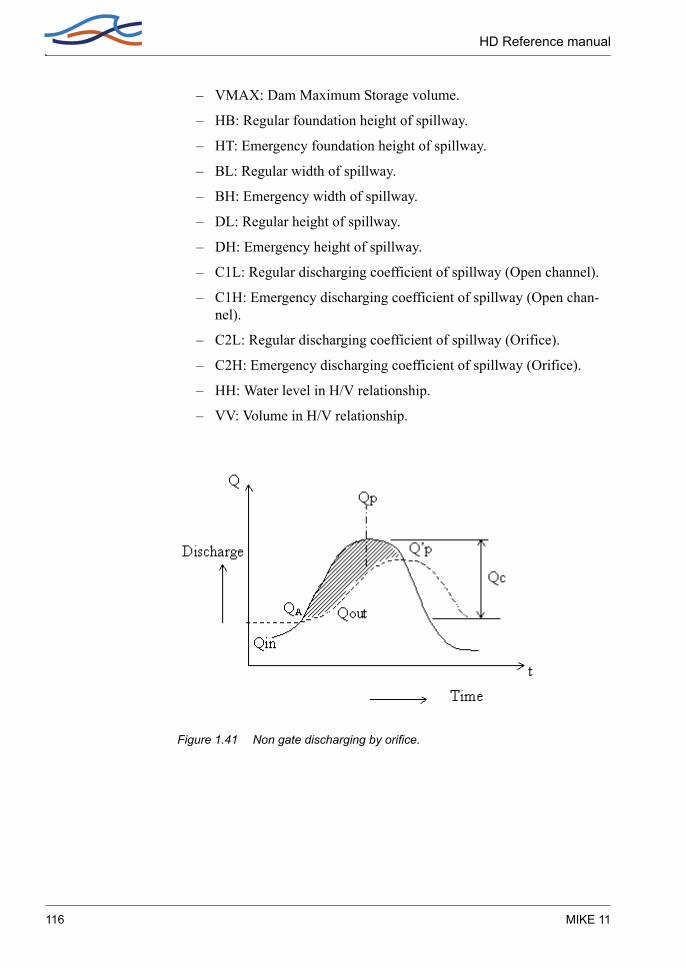
HD Reference manual
– VMAX: Dam Maximum Storage volume.
– HB: Regular foundation height of spillway.
– HT: Emergency foundation height of spillway.
– BL: Regular width of spillway.
– BH: Emergency width of spillway.
– DL: Regular height of spillway.
– DH: Emergency height of spillway.
– C1L: Regular discharging coefficient of spillway (Open channel).
– C1H: Emergency discharging coefficient of spillway (Open chan-nel).
– C2L: Regular discharging coefficient of spillway (Orifice).
– C2H: Emergency discharging coefficient of spillway (Orifice).
– HH: Water level in H/V relationship.
– VV: Volume in H/V relationship.
Figure 1.41 Non gate discharging by orifice.
116 MIKE 11
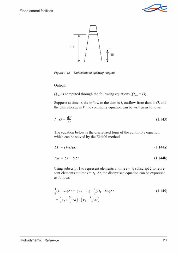
Flood control facilities
Figure 1.42 Definitions of spillway heights.
Output:
Qout is computed through the following equations (Qout = O).
Suppose at time t, the inflow to the dam is I, outflow from dam is O, and the dam storage is V, the continuity equation can be written as follows.
(1.143)
The equation below is the discretised form of the continuity equation, which can be solved by the Ekdahl method.
(1.144a)
(1.144b)
Using subscript 1 to represent elements at time t = t1 subscript 2 to repre-sent elements at time t = t1+∆t, the discretised equation can be expressed as follows
(1.145)
I O– dVdt-------=
∆V I O–( )∆t=
I∆t ∆V O∆t+=
12--- I1 I2+( )∆t V2 V1–( ) 1
2--- O1 O2+( )∆t+
V2O2
2------∆t+
V1O1
2------∆t+
–
=
=
Hydrodynamic Reference 117

HD Reference manual
Setting,
(1.146a)
(1.146b)
we have the following equation
(1.147)
Generally, with the equation
(1.148)
φn+1 can be thus computed sequentially.
1.17 Flood plain Encroachment calculations
The flood plain encroachment module may be used for assessing the impact of a flood plain encroachment on the water level and the energy level. Such assessments are of considerable interest for land developers, engineers etc.
The module works by manipulating the user specified cross sections by inserting encroachment stations thus contracting the cross sectional area with a rise in water level as a result.
Note: The encroachment module only works with a Quasi Steady State module installed. Only the default steady state solver may be used with the encroachment module. If a different steady state solver is chosen a warn-ing is issued and the steady state solver is set to the default solver. Further the module may only be used in conjunction with a hydrodynamic simula-tion. Thus the advection dispersion, rainfall runoff modules etc. are disa-bled during an encroachment simulation.
1.17.1 GeneralAn encroachment analysis consists of minimum two steady state simula-tions. The first simulation is used to find the water level and discharge
φ V∆t----- 1
2---O+=
ψ V∆t----- 1
2---O–=
φ212--- I1 I2–( ) ψ1+=
φn 1+12--- In In 1+–( ) ψn+=
118 MIKE 11
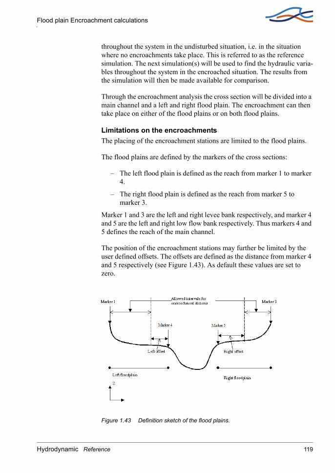
Flood plain Encroachment calculations
throughout the system in the undisturbed situation, i.e. in the situation where no encroachments take place. This is referred to as the reference simulation. The next simulation(s) will be used to find the hydraulic varia-bles throughout the system in the encroached situation. The results from the simulation will then be made available for comparison.
Through the encroachment analysis the cross section will be divided into a main channel and a left and right flood plain. The encroachment can then take place on either of the flood plains or on both flood plains.
Limitations on the encroachmentsThe placing of the encroachment stations are limited to the flood plains.
The flood plains are defined by the markers of the cross sections:
– The left flood plain is defined as the reach from marker 1 to marker 4.
– The right flood plain is defined as the reach from marker 5 to marker 3.
Marker 1 and 3 are the left and right levee bank respectively, and marker 4 and 5 are the left and right low flow bank respectively. Thus markers 4 and 5 defines the reach of the main channel.
The position of the encroachment stations may further be limited by the user defined offsets. The offsets are defined as the distance from marker 4 and 5 respectively (see Figure 1.43). As default these values are set to zero.
Figure 1.43 Definition sketch of the flood plains.
Hydrodynamic Reference 119

HD Reference manual
If the encroachment stations are situated outside the allowed intervals a warning is issued and the encroachment station is set equal to the limiting value (one of the end-points of the interval).
1.17.2 Encroachment MethodsFive different encroachment methods are available:
1 Direct specification of fixed encroachment stations.
2 Specification of a fixed encroachment width.
3 Specified conveyance reduction.
4 Target water level.
5 Encroachment through iteration.
The encroachment module of MIKE 11 facilitates local settings for the individual cross sections. Thus different methods may be used along the same river reach if desired.
Method 1: Direct specification of fixed encroachment stationsThrough this method the user specifies the location of the encroachment stations. The location is specified through the variables Left Position and Right position. Each of the fore mentioned are distances from marker 4 and marker 5 respectively. Thus both Left Position and Right Position should be non-negative. If the latter is not the case the simulation uses the absolute values.
Method 2: Specification of a fixed encroachment widthMethod 2 is very similar to method 1. The encroachment stations are determined from a user defined width being the distance between the left and right encroachment stations. The encroachment stations are placed a distance of half the user specified width from the centre line of the chan-nel. The centre line is here defined as the midpoint of marker 4 and marker 5. If a negative value is entered the simulation will use the absolute value.
Method 3: Conveyance reductionBased on the reference simulation an encroachment simulation is per-formed based on conveyance reduction. Using the water level from the reference simulation the total conveyance at the specific station is deter-mined. The cross section is then encroached until the user specified reduc-tion of conveyance at the reference water level has been reached. If this is not possible the optimal encroachment position is returned. The latter may occur if the user specifies a reduction which is greater than the convey-ance available on the flood plains.
120 MIKE 11

Flood plain Encroachment calculations
Method 4: Target water levelIn method 4 the user defines a target water level. This is done through a water level change which is to be added to the reference water level. The encroachment calculation is then carried out so that the conveyance at this higher level is equal to the total conveyance of the reference simulation.
In other words if the user specifies a rise in the water level ∆H then the module will try to contract the cross section so that the conveyance of the encroached cross section at water level Href + ∆H is equal to the reference situation.
Method 5: Encroachment through iterationIn this method a target value of either water level or energy level is aimed at. The method works by evaluating simulation results and through these modify the cross section until the target value is met. As opposed to method 3 and method 4 this method evaluates the results from simulations instead of just considering conveyance reductions at user specified water levels.
If a non-zero change in water level is specified the method will try to sat-isfy this request. Further if additionally a non-zero energy level change is also entered the method will check if this level is violated. If the latter is the case the method will modify the cross section until the energy level request is satisfied.
If the user only specifies a change in energy level which is non-zero then the module will aim at satisfying this energy level request.
The maximum number of iterations allowed is user defined but is set to 20 per default. If this limit is reached a warning is issued and the best result from the iteration is used as output.
1.17.3 Additional specifications for encroachment calculations
Side specificationThe user may specify whether the encroachments are to take place on
– both flood plains
– the right flood plain
– the left flood plain
If the fixed width method is used (method 2) then the simulation will carry out the encroachment calculations for both flood plains. In the latter case the side specification is ignored.
Hydrodynamic Reference 121
HD Reference manual
Conveyance reduction specificationsMIKE 11 allows three different types of conveyance reduction:
– Equal conveyance reduction: The simulation tries to satisfy the request by reducing the conveyance equally on the flood plains. In accordance with the user specified total reduction (in percentage).
– Relative conveyance reduction: The simulation tries to satisfy the request (total reduction) by reducing the conveyance relative to the conveyance on the flood plains in the reference simulation. This is only of importance if method 3 or 4 is used.
– Specified conveyance reduction: The user specifies the left and right reduction. The total reduction equals the sum of the left and right reduction. Note that this setting has only effect for method 3.
Target valuesFor methods 4 and 5 the user must specify one or more target values.
Target values are of two types:
– Water level change.
– Energy level change.
The target water level is then given by the reference water level plus the user specified water level change. Similarly the target energy level is given by the reference level plus the energy level change.
If method 4 is chosen a non-zero value must be entered for the water level change. The target water level is then used to obtain the placing of the encroachment stations. The energy level is ignored using method 4.
If method 5 is chosen then either a non-zero water level change or a non-zero energy level or both should be entered. If both an energy level and a water level is specifies the simulations aims at satisfying the water level target without violating the energy target level. If only a water level or an energy level is specified the simulation will only try to satisfy this request.
1.17.4 Cross sections after encroachmentThe encroachment module manipulates the cross sections by inserting ‘vertical’ sections at the position of the encroachment stations (see Figure 1.44).
The relative resistance of the left vertical section is set equal to the value at the point just prior to the placement of the vertical section. Similarly the
122 MIKE 11

Flood plain Encroachment calculations
relative resistance of the right vertical section is set equal to the value at the point just post the placement of the vertical section (see Figure 1.45).
Figure 1.44 The geometry of the cross section after encroachments.
Figure 1.45 The definition of the relative resistance on the vertical sections of the flood plain encroachment stations: (a) left flood plain (b) right flood plain.
1.17.5 Encroachments at structuresThe encroachment module does not allow encroachments of cross sections just upstream or downstream of structures.
1.17.6 Encroachments at nodesMIKE 11 uses water level compatibility at nodes, thus all cross sections located at the same node will have equal water level. For this reason MIKE 11 does not permit encroachments at cross sections located at nodes.
Hydrodynamic Reference 123

HD Reference manual
1.18 Flood Plains
Description of flow over flood plains can be achieved with several differ-ent types of model schematisations depending on the topography of the flood plain and the nature of the flow.
In spilling areas natural levees are formed along the river by sedimenta-tion due to the abrupt reduction in flow velocity of the entering water. In predominantly drainage areas, these levees are not present. The principal difference between the two situations is shown in Figure 1.46
Figure 1.46 Principal difference between drainage and spilling areas
This schematisation of the flood plain may not be adequate if sediment transport is to be calculated especially where the hydraulic resistance in the flood plain is significantly different from that in the channel. This is because the sediment transport is very sensitive to the value of velocity and the cross-sectionally averaged velocity will not be representative of the actual velocity in the flood plain. For this situation, the river and flood plain may be schematised separately using two or more parallel model branches connected by broad crested weirs as for the spilling area defined below.
In a typical drainage area, it is generally reasonable to assume that the water level is the same in the river and on the flood plain. The flood plain storage, thus, can be included directly in the modelled river cross section through the width parameter, and only one model h-point is required to determine the water level over the whole area.
In a typical spilling area, the water levels in river and flood plain might differ due to the separation by a levee. One h-point at each side of the levee is thus required to describe the conditions. Between the two h-points a Q-point is placed representing the discharge over the levee. A weir equa-tion is applied to describe the magnitude of the discharge. This discretisa-
124 MIKE 11
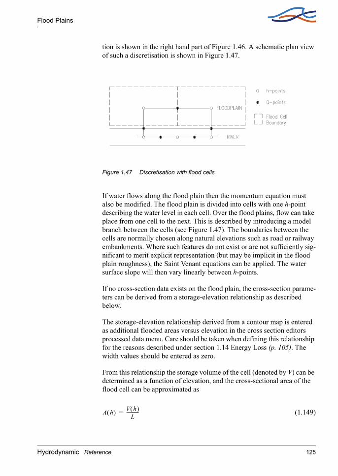
Flood Plains
tion is shown in the right hand part of Figure 1.46. A schematic plan view of such a discretisation is shown in Figure 1.47.
Figure 1.47 Discretisation with flood cells
If water flows along the flood plain then the momentum equation must also be modified. The flood plain is divided into cells with one h-point describing the water level in each cell. Over the flood plains, flow can take place from one cell to the next. This is described by introducing a model branch between the cells (see Figure 1.47). The boundaries between the cells are normally chosen along natural elevations such as road or railway embankments. Where such features do not exist or are not sufficiently sig-nificant to merit explicit representation (but may be implicit in the flood plain roughness), the Saint Venant equations can be applied. The water surface slope will then vary linearly between h-points.
If no cross-section data exists on the flood plain, the cross-section parame-ters can be derived from a storage-elevation relationship as described below.
The storage-elevation relationship derived from a contour map is entered as additional flooded areas versus elevation in the cross section editors processed data menu. Care should be taken when defining this relationship for the reasons described under section 1.14 Energy Loss (p. 105). The width values should be entered as zero.
From this relationship the storage volume of the cell (denoted by V) can be determined as a function of elevation, and the cross-sectional area of the flood cell can be approximated as
(1.149)A h( ) V h( )L
-----------=
Hydrodynamic Reference 125

HD Reference manual
where, L is shown in Figure 1.48.
Figure 1.48 Long section of cell discretisation
This will represent a measure for the average cross-section along the flood plain. The average resistance radius can similarly be approximated with:
(1.150)
When spilling starts, huge flows of water may suddenly be generated, pos-sibly causing numerical instabilities. This problem can be overcome by giving the levee along the river a V-formed shape in the mathematical description, see Figure 1.49.
This ensures that spilling starts gradually instead of instantaneously over the whole section. This corresponds, in fact, to the situation in nature, where the irregularities in levee height cause the spilling to start sooner at some places than at others.
Figure 1.49 V-formed levee long section
R h( ) V h( )S h( )-----------=
126 MIKE 11
Flow Descriptions
The computed water level in the cell is not representative for all locations within the cell, but is an average as shown in Figure 1.48. To interpret the model results, the computed water level should be transformed into an average depth of inundation within the cell as given by:
(1.151)
1.19 Flow Descriptions
The model provides a choice between 3 different flow descriptions:
1 dynamic wave approach which uses the full momentum equation, including acceleration forces, thus allowing the simulation of fast tran-sients, tidal flows, etc. backwater profiles may also be calculated;
2 diffusive wave approach which only models the bed friction, gravity force, and the hydrostatic gradient terms in the momentum equation. This allows the user to take downstream boundary conditions into account, and thus simulate backwater effects;
3 kinematic wave approach. The flow is calculated on the assumption of a balance between the friction and gravity forces.
Depending on the type of problem, the user can choose the most appropri-ate description. All three approaches simulate branched as well as looped networks.
1.19.1 Dynamic Wave and High Order Dynamic WaveThe dynamic and high order dynamic flow description should be used where the change in inertia of the water body over time and space is of importance. This is the case for all tidal flow, and in river systems where the water surface slope, bed slope and bed resistance forces are small.
The high order flow description includes a high order and upstream cen-tred description of the friction terms in the momentum equation. This for-mulation allows the simulations to be done with a larger time step, than would be the case for the non-high order description. The non-high order dynamic formulation is only included to allow re-production of simulation results done in previous version of MIKE 11.
See section 1.29 Saint Venant Equations (p. 170) for details of the govern-ing equations.
average inudation depth V h( )S h( )-----------=
Hydrodynamic Reference 127

HD Reference manual
1.19.2 Diffusive WaveThe diffusive wave description ignores the inertia terms and is therefore suitable for backwater analyses, cases where the bed resistance forces dominate, and for slowly propagating flood waves where the change in inertia is negligible. It is not normally suitable for tidal flows.
The modified ‘diffusive wave approximation’ is derived from the general Saint Venant Equations by neglecting all momentum terms as follows:
This formulation still ensures a backwater description through the ∂h/∂x term. For stability reasons the ∂h/∂x term is dampened in the solution, which means that only relatively steady backwater phenomena (compared to the time step) are resolved.
1.19.3 Kinematic WaveThe assumption of a balance between the friction and gravity means that the kinematic wave approach cannot simulate backwater effects. Thus this description is appropriate for relatively steep rivers without backwater effects.
1.19.4 Which Flow Description?The dynamic wave description is recommended to be used in all cases except where it can be shown that either the diffusive or kinematic descriptions are adequate.
The diffusive and kinematic wave approximations are simplifications of the full dynamic descriptions. They are implemented to offer improved computational efficiency, but should only be used when the omitted terms have insignificant influence. When there is any doubt it is better to use the full dynamic description or trials should be undertaken to establish the dif-ference between alternative methods, and advice sought from experienced persons. It is very important to have a solid understanding of the influence of the different terms.
None of the three wave descriptions includes detailed hydraulic descrip-tions of hydraulic jumps. However, the chosen formulations ensure a cor-rect description upstream and downstream of the jump.
1.20 Initial Conditions
1.20.1 User-SpecifiedThe initial conditions can be specified by the user in the Simulation Editor under the Simulation tab.
128 MIKE 11

Kinematic Routing Method
1.20.2 Auto Start, Quasi-Steady SolutionIn the automatic calculation, a steady state backwater calculation using the steady state version of the Saint Venant Equations is performed to deter-mine the water levels and discharges in the model using the boundary con-dition values at the start of the simulation. An iterative procedure is used to obtain a correct discharge distribution between diverging branches. The maximum number of iterations is specified by the MaxIterSteady (p. 71) in the Hydrodynamic parameters Editor under the Default values tab. See section 1.25 Quasi-Steady Solution (p. 138).
1.20.3 Hot StartUser-specified initial conditions for a simulation can be obtained from an existing result file (.res11) as long as it is complete and exactly compatible with the new computation.
1.20.4 Combined Auto Start and user-specified initial conditionsIn some cases the auto start procedure is not capable of calculating the ini-tial conditions. This is the case for instance if the model includes flood plains described by a separate branch and the initial water level in the main river gives no flow from the main river into the flood plain. The ini-tial h and Q in the flood plain is thus not defined. By specifying the initial h and Q for the flood branch in the Hydrodynamic parameters Editor under the Initial tab, it is still possible to use the auto start procedure for calculating initial h and Q in the main river. The combined auto start and user specified initial conditions is selected by setting the switch in the ini-tial condition box in the simulation editors simulation tab.
1.21 Kinematic Routing Method
GeneralTwo different routing methods have been incorporated into MIKE 11 HD. At a given time level, the routing methods are used to determine the spa-tial variation of the discharge at Kinematic Routing branches. The imple-mented methods are:
Muskingum method
Muskingum-Cunge method
Similarly, two methods have been incorporated into the model, which are used to compute the water level at Kinematic Routing branches:
User-defined discharge-elevation method
Resistance method
Hydrodynamic Reference 129

HD Reference manual
Definition of a Kinematic Routing ElementFigure 1.50 shows an example of a Kinematic Routing branch, at which two Kinematic Routing points are defined. Each point is located at a dis-charge point and the temporal transformation of the discharge takes place at this grid point. The quantification of the discharge at a Kinematic Rout-ing point is obtained by considering the inflows to the Kinematic Routing element in question, cf. Figure 1.50. The inflows constitute the discharge at the upstream elevation point (including lateral inflow at that point) and the sum of the lateral inflows at all interior elevation points of the consid-ered Kinematic Routing element.
The extent of each Kinematic Routing element is governed by the number of Kinematic Routing points specified at each Kinematic Routing branch. The upstream boundary of an element is determined as the larger of the following:
Chainage of upstream node (elevation point)
Chainage of elevation point located just downstream of closest upstream Kinematic Routing point (elevation point)
The definition of a Kinematic Routing element ensures that the entire branch is described correctly regardless of the number of routing elements specified by the user. Note that a Kinematic Routing element is located from one elevation point to the other, while the Kinematic Routing point is located at a discharge point.
Figure 1.50 Definition sketch of MIKE 11 Routing branch, Kinematic Routing elements and transformation points.
130 MIKE 11
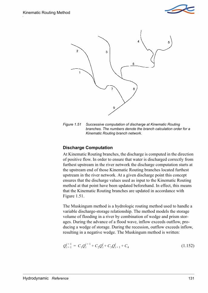
Kinematic Routing Method
Figure 1.51 Successive computation of discharge at Kinematic Routing branches. The numbers denote the branch calculation order for a Kinematic Routing branch network.
Discharge ComputationAt Kinematic Routing branches, the discharge is computed in the direction of positive flow. In order to ensure that water is discharged correctly from furthest upstream in the river network the discharge computation starts at the upstream end of those Kinematic Routing branches located furthest upstream in the river network. At a given discharge point this concept ensures that the discharge values used as input to the Kinematic Routing method at that point have been updated beforehand. In effect, this means that the Kinematic Routing branches are updated in accordance with Figure 1.51.
The Muskingum method is a hydrologic routing method used to handle a variable discharge-storage relationship. The method models the storage volume of flooding in a river by combination of wedge and prism stor-ages. During the advance of a flood wave, inflow exceeds outflow, pro-ducing a wedge of storage. During the recession, outflow exceeds inflow, resulting in a negative wedge. The Muskingum method is written:
(1.152)Qi 1+j 1+ C1Qi
j 1+ C2Qij C3Qi 1+
j C4+ + +=
Hydrodynamic Reference 131

HD Reference manual
where indices i and j, respectively, refer to the considered grid point and time level. The variables, C1 - C4, are given by
(1.153)
(1.154)
(1.155)
(1.156)
In the Muskingum method the computational input parameters, K and x, are fixed in time and space. Since in MIKE 11 HD the time step is fixed, too, Eqs. (1.153) - (1.156) need to be evaluated only once.
At a Kinematic Routing points the discharge variable is updated from one time level to the next on the basis of the previous and new discharges at the location of the upstream boundary of the considered Kinematic Rout-ing element as well as the previous discharge at the Kinematic Routing point in question, cf. Figure 1.50. Moreover, the total lateral inflow to the Kinematic Routing element (denoted Qlat) is evaluated as the mean of the previous and new total lateral inflows for the considered Kinematic Rout-ing element.
In contrast to the Muskingum method, the Muskingum-Cunge method does not take any input parameters, since these are computed at each Kin-ematic Routing point and at each time level.
The Muskingum-Cunge method is based on the diffusion wave model, which neglects local and convective acceleration terms but includes the pressure term. Thus, the Muskingum-Cunge model approximates the dif-fusion of a natural flood wave.
C1∆t 2Kx–
2K 1 x–( ) ∆t+------------------------------------=
C2∆t 2Kx+
2K 1 x–( ) ∆t+------------------------------------=
C32K 1 x–( ) ∆t–2K 1 x–( ) ∆t+------------------------------------=
C4Qlat∆t
2K 1 x–( ) ∆t+------------------------------------=
132 MIKE 11

Kinematic Routing Method
The Muskingum-Cunge computation uses the same equations as the Muskingum method, but the parameters K and x are functions of time and space. They are given by
(1.157)
(1.158)
(1.159)
In Eqs. (1.157) - (1.159), ∆x is the length of the considered Kinematic Routing element and S0 is the bed slope. The variables B, A and Q, respectively, are the width, the cross sectional area and the discharge, all of which represent the Kinematic Routing element in question. The varia-bles x and t are space and time variables, respectively.
The variables, B, A and Q are evaluated at the elevation point just upstream of the considered Kinematic Routing point. Since at this water level point the computation of the water level depends on the new dis-charge computed at the Kinematic Routing point, the discharge at each Kinematic Routing point is obtained by iteration. Typically, about 10 iter-ations are required to obtain an accuracy better than 10-4.
Computation of Water LevelHaving computed the discharge at the Kinematic Routing branch under consideration, all the interior elevation points of that branch are computed. Since Kinematic Routing points are defined as Q-points, computation of the water level may require interpolation between upstream and down-stream information. Consequently, both an upstream search and a down-stream search for a Kinematic Routing point is done. In the case of both an upstream and a downstream Kinematic Routing point, the water level is computed at both Kinematic Routing points and a linear interpolation is made to obtain the water level at the water level point in question.
Should the search efforts fail to find an upstream and a downstream Kine-matic Routing point, the Manning equation is used to compute the water level.
K ∆xck------=
x 12--- 1 Q
BckS0∆x---------------------–
=
ckdQdA------- Q∂
x∂------- x∂
A∂------ Q∂
t∂------- t∂
A∂------+= =
Hydrodynamic Reference 133

HD Reference manual
Regardless of the method used to compute the water level, a check is made to ensure that the computed water level is not located below the top of the slot.
At nodes of Kinematic Routing branches, the water level is computed using the same procedures as currently used in MIKE 11 HD. This con-cept ensures that the water level is continuous from one branch to the other.
If, at a Kinematic Routing point, the user has chosen a QH-relation the discharge computed by use of a Kinematic Routing method is used to interpolate in the QH-table at the elevation point in focus.
If, at a Kinematic Routing point, the user has chosen the Manning resist-ance method the discharge is computed by employment of the Manning equation. It is written
(1.160)
in which M is the Manning resistance number, R is the hydraulic radius, S0 is the bed slope, and A is the cross sectional, wetted area. Since M, R, and A are functions of the water level, the cross sectional area is found by iteration. Once the area has converged to a satisfactory accuracy (10-3), the water level is looked up in the cross section table of MIKE 11 HD.
1.22 Lateral Inflows
A lateral inflow, for example a side tributary which is specified in the Boundary Editor or NAM input which is specified in the River Network Editor under Tabular view: Runoff/groundwater links is described by a Q-t relationship. It represents an addition to the flow in the channel at the point of entry specified in the boundary editor or the network editor respectively, and is thus added into the continuity equation. A lateral momentum contribution is not included. A lateral inflow, therefore, differs from the Q-t relationship which is used in the definition of a regulating structure. For the latter, the Q-t relationship represents the total flow at a control point and replaces the momentum equation at this point, whereas the lateral inflow is an addition to the flow and is not a control point.
Q MR23---S0
12---A=
134 MIKE 11

Low Flow Conditions
1.23 Low Flow Conditions
During low flow, the cross-sections along certain model stretches may "dry out" (meaning that the water level falls below the river bottom). Apart from other problems, this gives numerical difficulties which, if no special measures are taken, prohibits a continuation of the computation.
The problem is handled in MIKE 11 by the aid of two numerical features:
1 A narrow slot below the cross-sections is introduced so that the calcu-lations can continue when the water surface falls below the bottom of the bed. If the water level reaches the bottom of the slot, a small amount of water is automatically added to prevent a complete drying out. The applied slot shape starts at a height DELH above the river bot-tom and extends to 5 x DELH below, Figure 1.52. DELH is specified in the Hydrodynamic parameters Editor under the Default values tab. The description above DELH over the river bottom is not affected by the slot. Below this point, the calculation of both A, R and b is affected as well as the weighting coefficients in the numerical solution. The computed conditions below this point should thus not be given much weight, but should be seen as a "stand-by" condition until flow starts again.
The geometry of the slot may be of two types: 1) the width varies as the square root of the depth in the slot or 2) the geometry is so that the cross sectional area is continuous across the local water level DELH. For the latter case the geometry does not introduce an error in the over-all water amount as long as the water level doesn’t reach the bottom of the slot. For details on the geometry of the slot please refer to section A.2 Area preserving slot (p. 425).
Note: The geometry of the second type of slot is different from earlier versions of MIKE 11 (1999b and prior), and may cause instabilities for some setups which are converted into MIKE 11 2000. To overcome this difficulty the old slot description may be chosen by setting the fol-lowing switch in the MIKE11.ini file (default in v. 2000b and later is OFF):
HD-Variables no 13:
AREA_PRESERVING_SLOT=OFF
2 For low flow conditions the use of the Saint Venant equation to describe the momentum balance becomes unphysical. MIKE 11 han-dles this by gradually substituting the momentum equation for low flow condition with a zero flow condition. This weighting is a function
Hydrodynamic Reference 135

HD Reference manual
of the local water depth and is implemented in such a way that the zero flow condition has full weighting if the water level is less or equal to the local bottom level.
Note: The suppression of the momentum equation for low flow situa-tions is a new feature for MIKE11 (v.2000 and later), and may cause instabilities for some set-ups which are converted from an earlier ver-sion of MIKE 11 (v.1999b and earlier). To overcome this difficulty the suppression may be overruled by setting the following switch in the MIKE11.ini file (default in v. 2000b and later is ON):
HD-Variables no 12:
QZERO_METHOD=OFF.
If one of the two above mentioned switches are set to ON the user might be forced to decrease the time step in a set-up. The gain being the increase in accuracy in the mass balance.
Figure 1.52 Cross-sections with artificial slot
1.24 Pumps
Pump structures in MIKE 11 are divided in two distinct groups, pumps with internal outlet and pumps with external outlet. Pumps with internal outlet increases the local water level within a branch whereas pumps with external outlet pumps water out of the branch
Pumps with internal outlet are like most other structures placed in a Q-point, whereas pumps with external outlet are placed in h-points.
1.24.1 CapacityPumps may be specified either as pumps with fixed capacity or by a pump characteristic. When pumping with fixed capacity the pump pumps with
136 MIKE 11

Pumps
the given rate whenever it is fully on. The only deviations from the speci-fied capacity appears during start-up, close down and when the pump is of.
Alternatively pumps may be specified by a pump characteristic relating the pump discharge to the lift height. The lift height is calculated as the difference between the larger of the downstream water level and the outlet level and the upstream water level.
(1.161)
Examples of pump characteristics are included as Figure 1.46.
Figure 1.53 Pump characteristic examples.
1.24.2 Start/Stop controlThe pumps are controlled by simple start-up and close down periods. The periods specifies the time used by the pump for changing its discharge from full to zero and vice versa.
1.24.3 Internal outletThe equation governing the flow through a pump with internal outlet is obtained by Taylor expansion of the discharge at time step n+1.
∆h max houtlet hdownstream( , ) hupstream–=
Hydrodynamic Reference 137
HD Reference manual
1.24.4 External outletFor the external outlet the pumps are modelled as pumping out of the branch to an outlet with the level specified in the input. Mathematically the pumps are modelled by including a source term in the continuity equa-tion. The source describes the pump discharge at time step n+δ (0<=δ<=1). The discharge at time n+δ is approximated suing linear inter-polation between the pump discharge at time n+1 and at time n. The dis-charge at time n+1 is approximated using Taylor expansion including both timevarying change due to pump start-up/close down and change due to change in water level.
1.25 Quasi-Steady Solution
A solution of the quasi-steady version of the Saint Venant equations is determined iteratively for the automatic calculation of the initial condi-tions. The boundary condition values used are those at the start of the sim-ulation.
The quasi-steady solution is also used for simulation of long term phe-nomena such as morphological changes or the effects of pollutants on water quality. As the calculations are based on steady flow conditions there is no upper stability limit to the computational time step. This ena-bles long term simulations to be carried out at a fraction of the computa-tional time that would be required when using the fully dynamic solution.
Generally, the quasi-steady solution requires discharge boundary condi-tions at all inflow boundaries and water level or Q-h relationships at out-flow boundaries, but the model will often work also for other combinations. However, if only Q-boundaries are specified the steady solution is undefined mathematically, and the model will not work.
In a system without bifurcations the steady solution is easily obtained with a simple backwater solution procedure starting from outflow boundaries and marching against the flow direction from one h-point to the next using an iterative method. At bifurcations the discharge should be divided in the bifurcating branches in such a way that the calculated water levels in the bifurcating branches are identical. This discharge distribution is also obtained via an iteration procedure. Thus, the steady state solution is obtained from a nested iteration procedure, viz. an overall iteration proce-dure to obtain the correct discharge distribution in the system and an itera-tion procedure to calculate the water level difference between neighbouring h-points.
138 MIKE 11

Quasi-Steady Solution
A linear relationship is established between the water levels in the upstream (hupstream) and downstream (hdownstream) nodal point in a branch and the discharge in the branch, i.e.:
(1.162)
This equation has the same structure as used in the fully dynamic model at every time step, see section A.5 The double sweep algorithm (p. 439). The boundary conditions are introduced into the solution in the same way as in the fully dynamic solution (in fact the program code is re-used).
The linear relationship is based on three backwater calculations for each branch, assuming that the downstream water level and discharge are known (in the first iteration step a quite primitive first guess is used). The first backwater calculation is carried out with the current iteration values of the discharge and downstream water level. The second one is carried out with a slightly larger discharge (usually a 20% increase), and the third one with the downstream water level increased by 20% of the downstream water depth. From these three backwater calculations the following rela-tionship is calculated:
(1.163)
Comparing Equations (1.162) and (1.163) it is seen that:
(1.164)
After establishing a linear relationship for each branch, and using a water level compatibility and a continuity equation at each node (e.g. the water levels in all connecting branches have to be identical and the sum of inflow and outflow to the node is zero) a linear system of equations for the water levels in all nodes is obtained (similar to that obtained in the double sweep algorithm). These water levels are subsequently used to calculate
Qbranch e0hupstream e1hdownstream f+ +=
hupstream αhdownstream βQbranch γ+ +=
e01β---=
e1αβ---–=
f γβ---–=
Hydrodynamic Reference 139

HD Reference manual
the discharges in the branches using Equation (1.162). The next iteration starts with the following values
(1.165)
(1.166)
This relaxation of the solution is not required in a single branch system without bifurcations (hence Relax=1). In more complex systems, Relax < 1.0 should be used. The relaxation coefficient (Relax) is an input parame-ter to the model.
There are some pitfalls using the quasi-steady model. For example, from Equation (1.164) it can be seen that when β is very small or zero the solu-tion may become unstable. According to Equation (1.163) this occurs when the upstream water level is independent of the discharge (i.e. nearly horizontal branches). This situation occurs in very short branches with cross-sections which have very large conveyance compared to the dis-charge or in branches with little resistance. In most cases this situation is avoided by increasing the discharge in the backwater simulation with increased Q until β is greater than a threshold value, Beta_Limit. Beta_Limit is an input parameter to the model (default value 10-8). How-ever, occasionally the velocity may increase at greater pace than the water level at the upstream end of a branch causing stability problems. Reasona-ble initial conditions can be obtained by suppressing the convective accel-eration term in the momentum equation.
Another problem may occur in nearly horizontal branches. As mentioned above, the backwater calculation is based on an iterative calculation of water levels from one h-point to the next. If the stop criterion for this iter-ation is of the same order of magnitude as the total water level difference between upstream and downstream ends of the branch, the coefficients in Equation (1.163) (and hence Equation (1.162)) are inaccurately deter-mined which will generate oscillations in the solution and poor conver-gence of the solution algorithm. This problem is overcome by using a stop criterion in the backwater algorithm which is related to the total water level difference in the branch, i.e.:
(1.167)
N = number of h-points in branch
hnew Relax hcalculated 1 Relax–( )hprevious iteration+=
Qnew Relax Qcalculated 1 Relax–( )Qprevious iteration+=
hconv1N---- hupstream hdownstream–( )hconv_factor=
140 MIKE 11

Quasi-Steady Solution
To avoid underflow problems it has been necessary to limit hconv by a min-imum value Min_Hconv_In_Branch. hconv_Factor and Min_Hconv_In_Branch are input parameters with default values of 10-2 and 10-5 respectively. In cases where hconv is limited by min_hconv_in_branch oscillations in the discharge may occur, although the water levels will be stable provided hconv is small. Overall convergence is therefore tested on both h in nodal points and Q in branches, where only one of the two has to be satisfied, i.e. the iteration stops when for all branches:
(Qnew-Qold) < qstop
where,
(1.168)
and
(1.169)
or
(1.170)
qconv_factor and hstop are input parameters with default values 10-3 and 10-4, respectively.
In model setup with structures having a zero flow condition the up- and downstream water levels are uncorrelated, hence no linear relationship (Equations (1.162) and (1.163)) between discharge and up- and down-stream water levels can be established. The model overcomes this problem by introducing a "slot" in the structure as outlined in Figure 1.54.
qstop Qinflowqconv_factor∑=
Qinflow∑ Qmax=
hnew hold–( ) hstop<
Hydrodynamic Reference 141
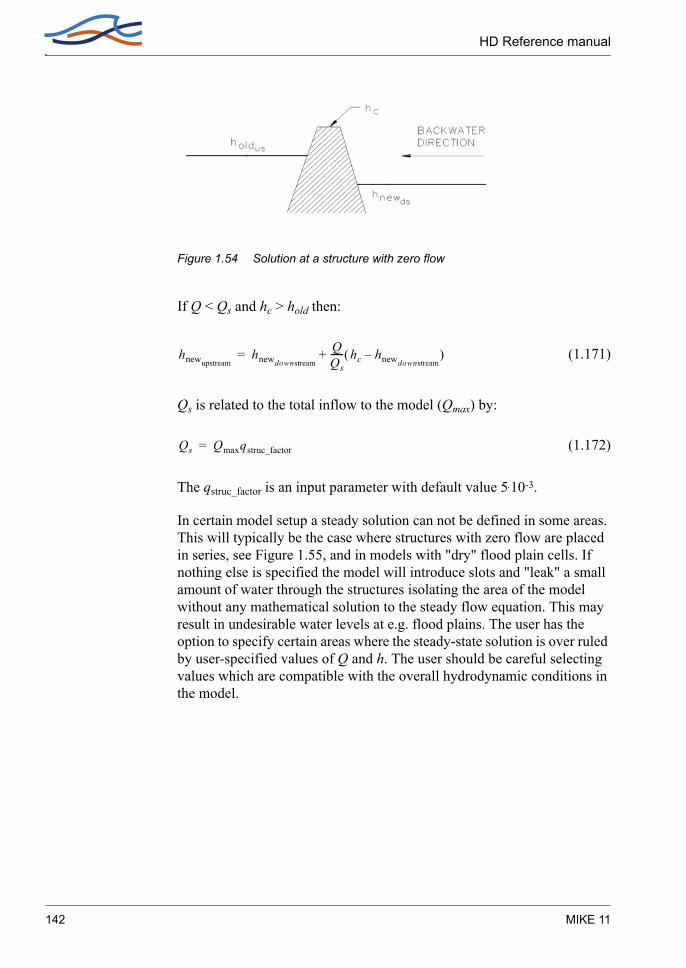
HD Reference manual
Figure 1.54 Solution at a structure with zero flow
If Q < Qs and hc > hold then:
(1.171)
Qs is related to the total inflow to the model (Qmax) by:
(1.172)
The qstruc_factor is an input parameter with default value 5.10-3.
In certain model setup a steady solution can not be defined in some areas. This will typically be the case where structures with zero flow are placed in series, see Figure 1.55, and in models with "dry" flood plain cells. If nothing else is specified the model will introduce slots and "leak" a small amount of water through the structures isolating the area of the model without any mathematical solution to the steady flow equation. This may result in undesirable water levels at e.g. flood plains. The user has the option to specify certain areas where the steady-state solution is over ruled by user-specified values of Q and h. The user should be careful selecting values which are compatible with the overall hydrodynamic conditions in the model.
hnewupstreamhnewdownstream
QQs------ hc hnewdownstream
–( )+=
Qs Qmaxqstruc_factor=
142 MIKE 11

Quasi-two dimensional steady flow with vegetation
Figure 1.55 Areas with undefined steady solution
The simulation time depends on the complexity of the setup. In systems without bifurcation the iteration converges quickly. The input parameters Relax, beta_limit, hconv, min_hconv_in_branch, qconv_factor and qstruc_factor have, naturally, a large effect on the speed of convergence.
In order to optimize the convergence parameters both with respect to accu-racy and computational time it is recommended that the parameters be adjusted so that a satisfactory solution is obtained for a low flow condi-tion. If the parameters are adjusted adequately for the low flow conditions then the parameters will also produce accurate results for higher flow con-ditions.
The optimization is carried out by running the hydrodynamic model for constant low flow conditions until steady conditions are obtained. These results can then be compared with those obtained using the quasi-steady model. It has to be emphasized that the parameters are 'model specific', i.e. each model setup and associated flow conditions require an individual optimization of the parameters.
1.26 Quasi-two dimensional steady flow with vegetation
The module takes the effects of vegetation into account for steady flow. Each cross section is divided into subsections. Each subsection being one of four different types:
Normal zones (p. 146).
Vegetation zones (p. 150).
Vegetation zones adjacent to river levee (adjacent vegetation zones) (p. 154).
Dead water zones (p. 155).
Hydrodynamic Reference 143

HD Reference manual
The analysis is based on a parallel channel assumption, where the exchange of momentum between adjacent channels is taken into consider-ation. The extent of each of the parallel channels/subsections is based on the classification of the individual points in the cross section profile. The extent of a given subsection of a certain type is found as the extent of con-secutive points being of this specific type. The type of the individual seg-ments is determined on the basis of the end point of the segment.
The exchange of momentum between the different subsections is mod-elled as a shear stress using an expression of the following form
(1.173)
where ρ is the density of the water f is a mixing coefficient and ∆V is the velocity difference across the given boundary. For a water-water boundary between subsections i and i+1 the difference in the average velocity is given by ∆V = Vi-Vi+1. For a water-vegetation boundary the velocity dif-ference is given by ∆V = Vi, since it is assumed that there is no flow among the vegetation. The mixing coefficients or diffusion coefficients have (empirically found) default values but can be altered by the user in the Hydrodynamic parameters Editor if desired (see section 5.20 Mixing Coefficients (p. 309) in the User Guide). Dead water subsections are treated as sections where the velocity is equal to zero.
For each cross section it is assumed that the parallel channels all have the same energy slope I for a given water level. Based on this assumption a momentum equation is applied to each subsection in the cross section:
(1.174a)
for .
τ ρf∆V ∆V=
ρgni
2Vi2
Ri1 3⁄
-----------Pbed i, τw l i, , Pw l i, , τw r i, , Pw r i, ,
τv l i, , Pv l i, , τv r i, , Pv l i, ,
+ +
+ + ρgAiI=
i 1 … N, ,=
144 MIKE 11

Quasi-two dimensional steady flow with vegetation
If a resistance radius formulation is used the momentum equation (1.174a) reads
(1.174b)
for .
where:
ρ density of water.
g acceleration due to gravity.
Ri hydraulic/resistance radius of subsection. i.
ni Manning’s roughness of subsection i.
Vi average velocity of subsection i.
Pbed,i wetted perimeter of river bed/top of submerged vegetation of sub-section i.
τw,l/r,i shear on left/right water-water boundary respectively of subsection i.
Pw,l/r,i ‘wetted perimeter’ of left/right water-water boundary respectively of subsection i (see Figure 1.56).
τv,l/r,i shear on left/right water-vegetation boundary respectively of sub-section i
Pv,l/r,i ‘wetted perimeter’ of left/right water-vegetation boundary respec-tively of subsection i (see Figure 1.56).
Ai water area of subsection i.
I energy slope at considered cross section.
N number of subsections at considered cross section.
ρgni
2Vi2
Ri4 3⁄
-----------Ai τw l i, , Pw l i, , τw r i, , Pw r i, ,
τv l i, , Pv l i, , τv r i, , Pv l i, ,
+ +
+ + ρgAiI=
i 1 … N, ,=
Hydrodynamic Reference 145

HD Reference manual
Figure 1.56 Definition of ‘wetted perimeters’ of a subsection. In the above the right ‘wetted perimeter’ of the vegetation-water boundary is zero.
Further the subsection average velocities Vi must satisfy a mass balance equation i.e.
, (1.175)
where Q is the discharge at the given cross section.
Thus the problem consists of solving N+1 algebraic non-linear equations for the same number of unknowns (subsection velocities and the energy slope I). To this end Newton Raphson’s method is used.
1.26.1 Zone classification
Normal zonesZones, which are not dead water zones (zones with velocity equal to zero) and do not have any vegetation, are termed normal zones. The code pro-vides three alternatives for the calculation of the hydraulic radius for a normal subsection:
ViAi
i 1=
N
∑ Q=
146 MIKE 11

Quasi-two dimensional steady flow with vegetation
1 Resistance radius (p. 147).
2 Depth integrated hydraulic radius (p. 147).
3 Hydraulic radius (p. 147).
The radius is set in the "Mike11.ini" file which is located in the "WIN-DOWS" directory. The QSSVEG_RADIUS variable is set to either 1,2 or 3 respectively.
Resistance radiusThe resistance radius and Manning’s n of a given normal subsection is cal-culated on the basis of
, (1.176)
where A is the water area of the subsection, h the local water depth and y0, yN are the end points respectively of the subsection.
Depth integrated hydraulic radiusFor a profile without any vertical walls the hydraulic radius and Man-ning’s n of a given normal subsection may be calculated on the basis of
, (1.177)
where A is the water area of the subsection, h the local water depth and y0, yN are the end points respectively of the subsection.
Hydraulic radiusFor a subsection with vertical walls and non-varying Manning’s n the clas-sical expression used for calculating the subsections hydraulic radius is given by
(1.178)
Rh1A--- h3 2⁄ dy
y0
yN
∫
2= nc
h3 2⁄ dyy0
yN
∫h3 2⁄
n----------dy
y0
yN
∫------------------------=
Rh1A--- h5 3⁄ dy
y0
yN
∫
3 2⁄= nc
h5 3⁄ dyy0
yN
∫h5 3⁄
n----------dy
y0
yN
∫------------------------=
RhAP---=
Hydrodynamic Reference 147

HD Reference manual
For varying Manning’s n the formula used for calculating the hydraulic radius is
(1.179)
where
(1.180)
and Ai,Pc,i are the area and wetted perimeter of the given segment i respec-tively (see Figure 1.57). If the segment does not have vertical walls then Pc,i=Pi.
Figure 1.57 The determination of hydraulic radius for a segment with vertical side walls. The compound wetted perimeter of the segment is also illustrated.
Rh
AiRi2 3⁄
i 1=
N
∑
Ai
i 1=
N
∑
-------------------------
3 2⁄
=
RiAi
Pc i,---------=
148 MIKE 11
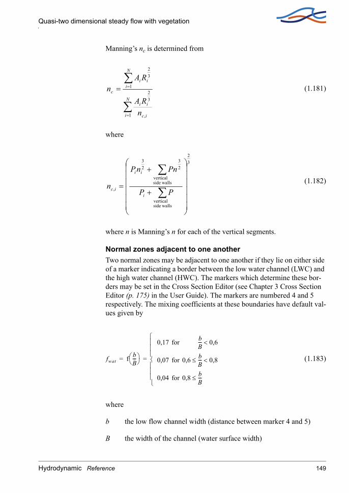
Quasi-two dimensional steady flow with vegetation
Manning’s nc is determined from
(1.181)
where
(1.182)
where n is Manning’s n for each of the vertical segments.
Normal zones adjacent to one anotherTwo normal zones may be adjacent to one another if they lie on either side of a marker indicating a border between the low water channel (LWC) and the high water channel (HWC). The markers which determine these bor-ders may be set in the Cross Section Editor (see Chapter 3 Cross Section Editor (p. 175) in the User Guide). The markers are numbered 4 and 5 respectively. The mixing coefficients at these boundaries have default val-ues given by
(1.183)
where
b the low flow channel width (distance between marker 4 and 5)
B the width of the channel (water surface width)
∑
∑
=
==N
i ic
ii
N
iii
c
nRA
RAn
1 ,
32
1
32
32
wallssidevertical
wallssidevertical
23
23
,
+
+
=∑
∑
PP
PnnP
ni
ii
ic
fwat f bB---
0,17 for bB--- 0,6<
0,07 for 0,6 bB--- 0,8<≤
0,04 for 0,8 bB---≤
= =
Hydrodynamic Reference 149

HD Reference manual
The mixing coefficient may be changed under the Mixing Coefficients tab (see 5.20 Mixing Coefficients (p. 309) in the User Guide).
Vegetation zonesVegetation zones are implemented so that the top of the vegetation is hori-zontal. This horizontal level is defined as the average elevation of the veg-etation zone plus the average vegetation height in the zone i.e.
(1.184)
where z is the vertical coordinate given with respect to the given datum and hv is the local vegetation height (see Figure 1.58).
Figure 1.58 The implementation of vegetation subsections in a cross section profile. The profile on the right is the one used for the calculations.
Figure 1.58 illustrates the implementation of a vegetation zone. If the pro-file has a steep gradient this implementation may give rise to a riverbed having a vertical segment. These vertical segments need special consider-ation when calculating hydraulic radius and compound roughness of the subsection.
horizontal level 1y2 y1–--------------- zdy 1
y2 y1–--------------- hvdy
y1
y2
∫+y1
y2
∫=
150 MIKE 11

Quasi-two dimensional steady flow with vegetation
Figure 1.59 A vegetation zone with a steep gradient in the bed topography. (a) Raw data. (b) The profile used for the computations.
The hydraulic radius of a vegetation subsection is calculated using the fol-lowing formula (see Figure 1.59):
(1.185)
where
for i≠1,N, (1.186a)
(1.186b)
(1.186c)
Rh
AiRi2 3⁄
i 1=
N
∑
A-------------------------
3 2⁄
=
RiAi
∆yi--------
h∆yi
∆yi----------- h= = =
A h ∆yi
i 1=
N
∑ hL= =
∆yi yi yi 1––=
Hydrodynamic Reference 151

HD Reference manual
For the two segments with a partially vertical wetted perimeter the follow-ing expressions are used
(1.187a)
(1.187b)
Manning’s n is calculated on the basis of the following formula:
(1.188)
where ni is Manning’s n of segment i with n1,nN given by
(1.189a)
(1.189b)
and
nl,nr are Manning’s n of the vertical sections to the left and right of the panel respectively
nl,veg is Manning’s n of the vegetation section to the far left of the panel
nl,veg is Manning’s n of the vegetation section to the far right of the panel
ll Pyyh
PyAR
+∆∆
=+∆
=1
1
1
11
rN
N
rN
NN Py
yh
PyA
R+∆
∆=
+∆=
∑
∑
=
==N
i i
ii
N
iii
c
nRA
RAn
1
32
1
32
n1Plnl
3 2⁄ ∆y1n1 veg,3 2⁄+
Pl ∆y1+---------------------------------------------
2 3⁄
=
nNPrnr
3 2⁄ ∆yNnN veg,3 2⁄+
Pr ∆yN+-----------------------------------------------
2 3⁄
=
152 MIKE 11

Quasi-two dimensional steady flow with vegetation
As can be seen if Pr=Pl=0 then the expressions simply become
and (1.190)
(1.191)
If further Manning’s n is constant through the subsection then n=nc
The mixing coefficients at the subsection boundaries have default values, but may be changed by the user under the Mixing Coefficients tab.
Figure 1.60 Illustration of mixing coefficients at a vegetation zone.
The effect of vegetation is most significant for values of the average vege-tation height being of the same order of magnitude as the local water depth. To model this the vegetation height (hv) is taken as being equal to the local water depth (h) for hv>0.9h (see Figure 1.60). In other words the water above the vegetation is only considered if it takes up more than 10% of the total panel area (water and vegetation). The mixing coefficient at a
Rc h=
ncL
∆yi
ni--------
i 1=
N
∑
-----------------=
Hydrodynamic Reference 153

HD Reference manual
vegetation boundary is a function of the width to height ratio of the vege-tation given by
(1.192)
where
hv Average vegetation height of panel.
Wv Total width of vegetation panel.
fveg,b Mixing coefficient used at vegetation zone adjacent to levee (see eq. (1.193)).
fveg,i Mixing coefficient at of independent vegetation zone equal to 0.1 by default but may be changed by the user in the Hydrodynamic parameters Editor under the Mixing Coefficients tab.
Vegetation zones adjacent to river levee (adjacent vegetation zones)Vegetation subsections next to either of the rivers levees are treated more or less as independent vegetation zones. The difference in formulation lies in the values for the mixing coefficients. For an adjacent vegetation the following values are used as default:
(1.193)
and
(1.194)
where the function f is the one used for the mixing coefficients at high/low water channel boundaries (e.g. (1.183)), Wb is the width of the bank vege-tation zone and B is the width of the water surface, dead water zones not included (see Figure 1.61).
fveg
0 forWveg
hv----------- 1<
fveg b,Wv
hv-------
0,34
for 1Wveg
hv----------- 34,5<≤
fveg i, for 34,5Wveg
hv-----------≤
=
fveg bank, 0,03=
fwat f 1 2Wb
B-------–
=
154 MIKE 11
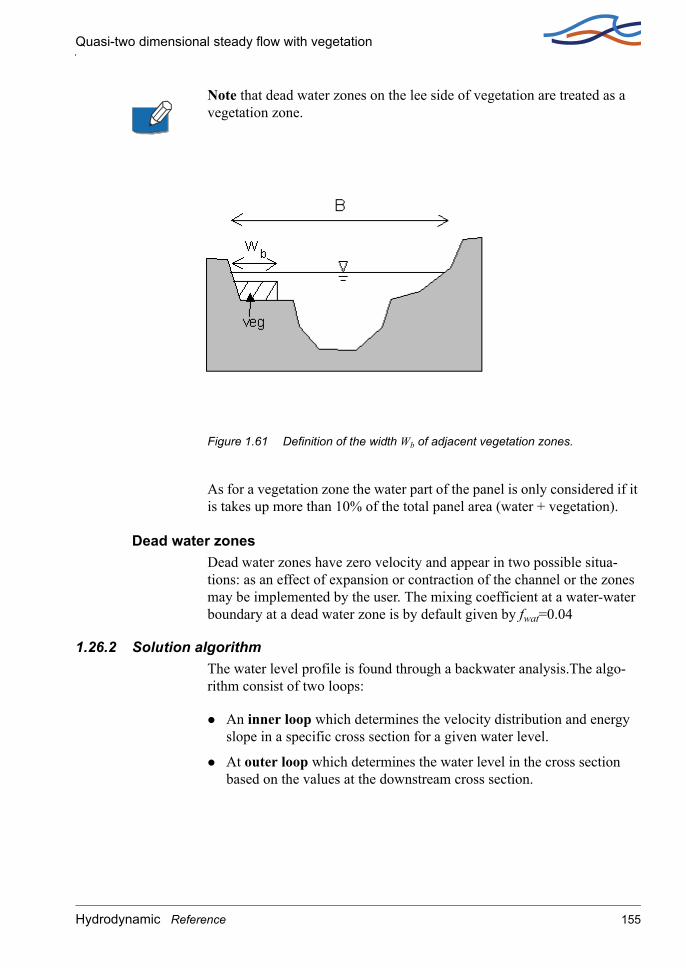
Quasi-two dimensional steady flow with vegetation
Note that dead water zones on the lee side of vegetation are treated as a vegetation zone.
Figure 1.61 Definition of the width Wb of adjacent vegetation zones.
As for a vegetation zone the water part of the panel is only considered if it is takes up more than 10% of the total panel area (water + vegetation).
Dead water zonesDead water zones have zero velocity and appear in two possible situa-tions: as an effect of expansion or contraction of the channel or the zones may be implemented by the user. The mixing coefficient at a water-water boundary at a dead water zone is by default given by fwat=0.04
1.26.2 Solution algorithmThe water level profile is found through a backwater analysis.The algo-rithm consist of two loops:
An inner loop which determines the velocity distribution and energy slope in a specific cross section for a given water level.
At outer loop which determines the water level in the cross section based on the values at the downstream cross section.
Hydrodynamic Reference 155

HD Reference manual
Inner loop: Determination of subsection velocities and energy gradient for fixed water level.The inner loop solves the momentum equation and the mass balance equa-tion for a given water level.
The system of equations to be solved can be written on the following form
(1.195a)
(1.195b)
If a hydraulic resistance formulation is used then equation (1.195a) is for-mulated as
(1.195c)
where .
Let
and (1.196a)
(1.196b)
be N-dimensional vectors. Newton-Raphson’s method can then be expressed as
, (1.197a)
(1.197b)
fi V1 … VN I, , ,( ) ρgni
2Vi2
Ri1 3⁄
-----------Pbed i, τw l i, , Pw l i, , τw r i, , Pw r i, ,
τv l i, , Pv l i, , τv l i, , Pv l i, , ρgAiI–
+ +
+ + 0
=
=
g V1 … VN, ,( ) ViAi Q–i 1=
N
∑ 0= =
fi V1 … VN I, , ,( ) ρgni
2Vi2
Ri4 3⁄
-----------Ai τw l i, , Pw l i, , τw r i, , Pw r i, ,
τv l i, , Pv l i, , τv l i, , Pv l i, , ρgAiI–
+ +
+ + 0
=
=
i 1 … N., ,=
f V1 … VN I, , ,( ) f1 … fN, ,( )=
V V1 … VN, ,( )=
Vm 1+ Vm ∆Vm 1++=
Im 1+ Im ∆Im 1++=
156 MIKE 11

Quasi-two dimensional steady flow with vegetation
where m is the iteration number and , are found as the solution of
(1.198)
The above system is not tridiagonal, and the double sweep algorithm thus cannot be applied directly. On the other hand the matrix is tridiagonal since each subsection only interacts with adjacent subsections. This tridiagonal structure is utilized in the following way. Consider the first N equations of the above system:
(1.199)
This system may be solved with respect to giving an expression linear in :
(1.200)
By taking the scalar product with and inserting the last equation of the linear system one finds
, (1.201)
which can be solved with respect to giving:
(1.202)
The expression for is now easily computed. Notice that and are obtained by solving a tridiagonal system with two right hand sides.
∆Vm 1+ ∆Im 1+
∂f Vm Im,( )∂V
-------------------------- ∂f Vm Im,( )∂I
--------------------------
∂g Vm( )∂V
------------------- 0
∆Vm 1+
∆Im 1+
f Vm Im,( )–
g Vm( )–=
∂f Vm Im,( ) ∂V⁄
∂f Vm Im,( )∂V
--------------------------∆Vm 1+ f Vm Im,( )– ∂f Vm Im,( )∂I
--------------------------∆Im 1+–=
∆Vm 1+
∆Im 1+
∆Vm 1+ ∂f Vm Im,( )∂V
--------------------------
1–– f Vm Im,( )
∂f Vm Im,( )∂V
--------------------------
1– ∂f Vm Im,( )∂I
--------------------------∆Im 1+– x1 x2∆Im 1++
=
=
∂g Vm( )∂V
-------------------
∂g Vm( )∂V
-------------------∆Vm 1+ g Vm( )– ∂g Vm( )∂V
-------------------x1∂g Vm( )
∂V-------------------x2∆Im 1++= =
∆Im 1+
∆Im 1+g Vm( )– ∂g Vm( )
∂V-------------------x1–
∂g Vm( )∂V
-------------------x2
---------------------------------------------------=
∆Vm 1+ x1 x2
Hydrodynamic Reference 157

HD Reference manual
Outer loop: The determination of the water levelThe inner loop is used for determining the velocity distribution in a cross section for a given value of the water level. The outer loop is the determi-nation of the water level in each cross section. For the latter a momentum equation is solved for neighbouring cross sections:
(1.203)
Where
α velocity distribution coefficient.
A water area of cross section.
H water level.
βι suppression factor for the panel i (see Suppression of the convective terms (p. 159)).
∆X distance between cross sections.
Further terms with subscript 1 are values at the downstream cross section and terms with subscript 2 are evaluated at the upstream cross section. The goal is the determination of H2 being the upstream value of the water level. Terms with subscript 2 in the above equation implicitly depend on the water level H2 one therefore needs to run the inner loop to determine the subsection velocities and energy gradient for each new value of H2. Since all other values can be determined on the basis of H2, the above equation constitutes essentially an equation in one unknown (H2). The solution to this equation is found by iteration. To ensure convergence a bisection method is used.
α 1A--- Vi
2Aiβi
2g----------------
i 1=
N
∑
2
α 1A--- Vi
2Aiβi
2g----------------
i 1=
N
∑
1
– H1 H2–
12--- 1
A---
ni2Vi
2
Ri1 3⁄
-----------Pbed i,
i 1=
N
∑
1
1A---
ni2Vi
2
Ri1 3⁄
-----------Pbed i,
i 1=
N
∑
2
+ ∆X
12--- 1
ρgA---------- τw l i, , Pw l i, , τw r i, , Pw r i, , τv l i, , Pv l i, , τv r i, , Pv r i, ,++ +( )
i 1=
N
∑1
∆X
12--- 1
ρgA---------- τw l i, , Pw l i, , τw r i, , Pw r i, , τv l i, , Pv l i, , τv r i, , Pv r i, ,++ +( )
i 1=
N
∑2
∆X
+
+
+
=
158 MIKE 11

Quasi-two dimensional steady flow with vegetation
As an alternative to the above equation for obtaining the water level the law of energy conservation is available for cases with no vegetation/dead water zones:
(1.204)
To use the energy equation for the determination of the water level the "QSSVEG_ENERGY" variable should be set to "ON" in the "Mike11.ini" file located in the "WINDOWS" directory.
Note that when utilizing the energy equation the cross section is consid-ered as one panel thus the inner loop for determining the velocity distribu-tion is not needed.
Suppression of the convective termsThere are three alternatives for the suppression of the convective terms in either of the equations (1.203) and (1.204):
1 The Froude number is calculated for each of the panels upstream and downstream and the maximum of these Froude numbers is used for determining the suppression factor according to section 1.35.1 Sup-pression of convective acceleration term (p. 185).
2 A suppression factor is calculated and used for each panel upstream and downstream. Thus the suppression factor is specific to each panel in the cross sections. The suppression factors are found according to 1.35.1 Suppression of convective acceleration term (p. 185).
3 No suppression is applied to the convective terms. Caution is recom-mended when using this possibility since it may cause severe numerical instability.
The suppression strategy is set using the variable "QSSVEG_SUPPRESSION_STRATEGY" in the "Mike11.ini" file located in the "WINDOWS" directory.
Upstream centering of bed friction termTo increase the numerical stability of the algorithm an upstream centering of the friction terms may be applied.
H2αβ2
2g---------
Q2
A2------
2
+ H1αβ1
2g---------
Q1
A1------
2
+– 12---
n12Q1
2
A12R1
4 3⁄-----------------
n22Q2
2
A22R2
4 3⁄-----------------+
∆X=
Hydrodynamic Reference 159
HD Reference manual
The centering is given by:
(1.205)
Subscripts up and down refer to upstream and downstream values respec-tively.
The terms fric are given by
(1.206a)
if a resistance radius or depth integrated hydraulic radius formulation is chosen and by
(1.206b)
if a hydraulic radius formulation is chosen.
The weighting term b1 is calculated from
(1.207)
where Frmax is the maximum Froude number of the upstream and down-stream cross sections. The Froude number is expressed as
(1.208)
The centering can be switched on by setting the variable "QSSVEG_CENTERING_FRICTION" to "ON" in the "Mike11.ini" file located in the "WINDOWS" directory.
frictionb1
fricdown-----------------
1 b– 1
fricup--------------+
1–
, for fricup fricdown<
b1fricdown 1 b1–( )fricup+ , for fricup fricdown≥
=
fric 12A-------
ni2Vi
2
Ri4 3⁄
-----------Ai
i 1=
N
∑=
fric 12A-------
ni2Vi
2
Ri1 3⁄
-----------Pi
i 1=
N
∑=
b10,1 0,4 1 Frmax
2–( )+ , for Frmax 1<
0,1 , for Frmax 1≥
=
Fr QA gR---------------=
160 MIKE 11

Quasi-two dimensional steady flow with vegetation
1.26.3 BridgesWhen utilising the steady flow with vegetation module it is possible to include the effect of bridges on the water level. The water level increment is calculated under the assumption that the bed slope is zero and the effect of the bed friction is negligible. Thus in order to minimise the errors intro-duced by these assumptions the user should place the cross sections upstream and downstream of the bridge close to the bridge.
Bridges may be of two types:
Bridge Piers (p. 161).
Submerged bridges (p. 162).
Note that the increment due to bridges is only considered if the Froude number of the flow is less than 0.6. If this is not the case a warning is issued.
Bridge PiersThe increment in water level due to bridge piers is found on the basis of D’Aubuisson’s formula (/10/). The code provides two alternatives for the implementation of this formula:
1 A rectangular channel analysis is used if a positive value is entered for the upstream width of the channel (see section Bridges in the User Guide) thus the increment is obtained through
(1.209a)
where
∆h increment in water level due to the presence of bridge piers.
Q1 discharge downstream of piers.
Q2 discharge upstream of piers.
C user defined constant determined by pier geometry.
b2 channel width upstream of piers.
h1 local water depth downstream of piers.
wpiers total width of piers.
∆h 12g------
Q12
C2 b2 wpiers–( )2h12
--------------------------------------------Q2
2
b22 h1 ∆h+( )2
-------------------------------–=
Hydrodynamic Reference 161

HD Reference manual
By rearranging eq. (1.209a) a third degree polynomial in ∆h is obtained. The code determines all real roots of this polynomial and the smallest positive root is used in case of more than one root.
2 If a non-positive value is entered for the upstream width of the channel (see section Bridges in the User Guide) a momentum equation is solved which takes the effect of an arbitrary shape of the cross section into account:
(1.209b)
where
H1 water level downstream of bridge piers.
H2 water level upstream of bridge piers.
Q1 discharge downstream of bridge piers.
Q2 discharge upstream of bridge piers.
h1 water depth downstream of bridge piers.
A1 cross sectional area downstream of bridge piers.
A2 cross sectional area upstream of bridge piers.
C user defined constant determined by pier geometry.
wpiers total width of piers.
Eq. (1.209b) is solved with respect to H2 using a bisection method. Note that iteration is needed since A2 depends on the water level upstream of the piers.
Note that if the Froude number is above the criteria of 0.6, the effect of the bridge piers is neglected. The criteria may be altered by setting the varia-ble BRIDGE_FROUDE_CRITERIA in the mike11.ini file.
Submerged bridgesAs for the case of bridge piers there are two alternatives for the implemen-tation of submerged bridges. Either the effect of the bridge is determined from a rectangular channel analysis or a momentum equation is solved
H2 H1– 12g------
Q12
C2 A1 h1wpiers–( )2---------------------------------------------
Q22
A22
------–=
162 MIKE 11

Quasi-two dimensional steady flow with vegetation
which takes the effect of an arbitrary shape of the cross section into account.
The latter is used if a non-positive value for the channel width is entered (see Fully Submerged Bridge in the User Guide).
1 For a rectangular channel the momentum equation for a submerged bridge reads
(1.210a)
where
Q discharge.
A cross sectional area.
B surface width.
h local water depth.
abridge cross sectional area of submerged bridge.
CD drag coefficient.
1,2 indices referring to down-/upstream values respectively.
The terms on the left hand side of eq. (1.210a) are the momentum terms and the force exerted by the pressure in the fluid the term on the right is the drag of the submerged bridge.
2 Eq. (1.210a) is derived under the assumption of a rectangular channel, though the expression is easily modified to take the effect of non-rec-tangular channels into account. After this modification the momentum equation reads:
(1.210b)
Eq. (1.210b) is solved using bisection. Notice that A2,B2 and h2 depend on the upstream water level H2.
1B---
Q12
h1------
Q22
h2------–
1
2---gB h1
2 h22–( )+ 1
2---–
Q22
A1 abridge–( )2----------------------------------abridgeCD=
Q12
A1------
Q22
A2------– 1
2---g h2
2dy h12dy
0
B1
∫–0
B2
∫ 1
2---
Q22
A1 abridge–( )2----------------------------------CDabridge–=
Hydrodynamic Reference 163
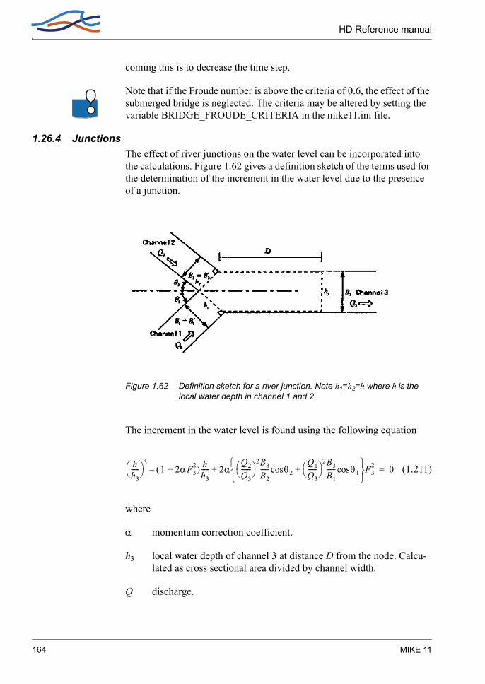
HD Reference manual
coming this is to decrease the time step.
Note that if the Froude number is above the criteria of 0.6, the effect of the submerged bridge is neglected. The criteria may be altered by setting the variable BRIDGE_FROUDE_CRITERIA in the mike11.ini file.
1.26.4 JunctionsThe effect of river junctions on the water level can be incorporated into the calculations. Figure 1.62 gives a definition sketch of the terms used for the determination of the increment in the water level due to the presence of a junction.
Figure 1.62 Definition sketch for a river junction. Note h1=h2=h where h is the local water depth in channel 1 and 2.
The increment in the water level is found using the following equation
(1.211)
where
α momentum correction coefficient.
h3 local water depth of channel 3 at distance D from the node. Calcu-lated as cross sectional area divided by channel width.
Q discharge.
hh3-----
31 2αF3
2+( ) hh3-----– 2α
Q2
Q3------
2B3
B2----- θ2
Q1
Q3------
2B3
B1----- θ1cos+cos
F32+ 0=
164 MIKE 11
Quasi-two dimensional steady flow with vegetation
θ direction angle of river with respect to channel 3.
B width of channel.
F3 Froude number of channel 3 defined by
(1.212)
Further indices refer to the river number in Figure 1.62.
Concerning the derivation of eq. (1.211) please refer to /13/ for details. The equation is derived using a rectangular channel analysis under the assumption of no bed slope. Thus the user should for safety ensure that the bottom level of the three channels meeting in the junction are the same.
The average water depth at distance D along channel 3 is found using lin-ear interpolation if D is not at a cross section. The channel widths are user defined and are entered under the tab named Junctions in the River Net-work Editor (see Junctions in the User Guide). Eq. (1.212) constitutes a third degree polynomial in the ratio h/h3. The code determines all real roots of this equation and in the case of more than one real root chooses the smallest one which is greater than unity.
Since eq. (1.211) is derived under the assumption of a horizontal bed level the average water level in channel 1 and 2 may be expressed as
(1.213)
where ∆h is the increment due to the junction given by
(1.214)
and H3 is the water level in channel 3 at the distance D from the node. The water level given by eq. (1.213) is applied at the first cross section after the junction in channel 1 and 2 respectively.
1.26.5 Variation in water level due to curvesThe effect of river curvature on the water level may be included in the computations. This is done through the W. L. Incr.- Curve dialog tab (sec-tion 5.21 W. L. Incr.- Curve (p. 310) in the User Guide).
F32 Q3
2
gB32h3
3---------------=
H H3 ∆h+=
∆h h3= hh3----- 1–
Hydrodynamic Reference 165

HD Reference manual
The increment is calculated from
(1.215)
where
∆H increment in water level.
B channel width.
rc curvature radius of river.
g acceleration of gravity.
V mean velocity of cross section.
In each branch the curvature radius in the individual digitization point is calculated as the radius of the circle through the digitization point itself, the previous and the next digitization point. The radius in the first and the last digitization point in each branch is respectively set equal to the radius in the second and the last but one digitization point in the branch. Once the curvature radius in the digitization points is calculated, the curvature radius is each grid point is calculated by linear interpolation of the curva-ture radius in the digitization points. This interpolation is based on chain-age.
NOTE! The increment due to curvature is added after the backwater anal-ysis has been done. In other words the increment is added to the steady flow computations. The increments is only added if
(1.216)
is satisfied.
Further if also the variation due to sand bars is considered only the great-est of the two increments is added to the calculated water level.
1.26.6 Variation in water level due to sand barsThe effect of sand bars on the water level may be included in the computa-tions. This is done through the W. L. Incr.- Sand Bars dialog tab (section 5.22 W. L. Incr.- Sand Bars (p. 312) in the User Guide).
∆H 12---BV2
grc----------=
rc
B---- 10<
166 MIKE 11

Regulating Structures
The increment is calculated from
(1.217)
where
∆H increment in water level.
hm mean water depth of low water channel.
B low water channel width.
A curvature radius of river.
Ib slope of the channel bed.
The function f expresses the water level increments dependence on the width/depth-ratio and the bed slope. The function is based on empirical results which are tabulated in MIKE11, any intermediate value is obtained through linear interpolation.
NOTE! The increment due to sand bars is added after the backwater anal-ysis has been done. In other words the increment is added to the steady flow computations. Further if also the variation due to curvature (see sec-tion 1.26.5) is considered only the greatest of the two increments is added to the calculated water level.
1.27 Regulating Structures
Regulating Structures are structures for which the operation is user-defined. They fall into two main categories:
1.27.1 Function of timeA structure may be specified in the River Network Editor → Tabular view: Structures → Regulating with a pre-determined operation as defined by a Q-t relationship specified in the boundary editor. Examples include pumps and some types of reservoir outflows. The Q-t relationship replaces the momentum equation at a Q-point and physically separates the model into upstream and downstream branches. The discharge is interpolated linearly at each time step from the specified Q-t table. The location of the Q-t rela-tionship is specified in the boundary editor.
∆Hhm-------- f B
hm------ 1
Ib----,
=
Hydrodynamic Reference 167

HD Reference manual
1.27.2 Function of h and/or QA structure may also be specified with an operation which is a user-speci-fied function of the water level or discharge at other locations in the model. This function is specified in the River Network Editor → Tabular view: Structures → Regulating → Regulation factor box and is given by:
(1.218)
where,
Qa is the discharge at location a
A is a coefficient given by:
(1.219)
where,
Zb is either water level h, or discharge Q, at location b.
This feature allows the flow at the control point to be related dynamically to any two variables in the system giving flexibility in the description of operating policies. For example, the outflow from a reservoir could be related to the reservoir inflow (location a) and the reservoir stage or a stage downstream (location b). Such an example is illustrated in Figure 1.63 for which the user-defined relationship is indicated in Table 1.5.
Figure 1.63 Reservoir outflow as a user-defined regulating structure
From Table 1.5 and Equations (1.218) and (1.219) it can be seen that when the reservoir is full the outflow at location b (Q) is set equal to the inflow
Q AQa=
A f Zb( )=
168 MIKE 11

Routing
at a (Qa) and that when the reservoir is empty the outflow is set to zero as shown by the expressions in Equation (1.220).
(1.220)
Table 1.5 User-defined relationship for example in Figure 1.63
Q is evaluated explicitly on the basis of the values of Qa and Zb form the previous iteration. If grid point a or b is situated close to the structure and there is little physical damping (like that of a full reservoir), the formula-tion may give rise to numerical instabilities. However, in most practical situations this structure type is used in connection with the operation of a reservoir operating during flood periods where the physical damping from the reservoir will be sufficient to ensure numerical stability.
In some specialized circumstances, a more complex Regulating Structure may be required to adequately describe a particular operation. In this case the MIKE 11 add-on module Control Str. should be used.
1.28 Routing
Non-linear storage function
Governing equationsMomentum equation:
(1.221a)
Reservoir level h(z) A
Full..
Empty
1..0
Q Qa for hb hfull=0 for hb hempty=
=
S KQoP T1Qo–=
Hydrodynamic Reference 169

HD Reference manual
Continuity equation:
(1.221b)
where:
S apparent basin storage.
Qi inflow at water way.
Qo runoff at water way.
T1 time of delay.
K, P constants.
And, T1 is the time of delay:
(1.222)
SolutionThe continuity equation is discretized
, (1.223)
and the momentum equation is substituted giving
(1.224)
1.29 Saint Venant Equations
MIKE 11 HD applied with the dynamic wave description solves the verti-cally integrated equations of conservation of continuity and momentum (the ‘Saint Venant´ equations), based on the following assumptions:
the water is incompressible and homogeneous, i.e. negligible variation in density
dSdt------ Qi Qo–=
Q t( ) Q t T1+( )=
St t∆+ St–t∆
----------------------- QiQo t t∆+, Qo t,+
2----------------------------------–=
KQo t t∆+,P T1Qo t t∆+,– KQo t,
P T1Qo t,–( )–t∆
--------------------------------------------------------------------------------------------------- QiQo t t∆+, Qo t,+
2----------------------------------–=
170 MIKE 11

Solution Scheme
the bottom-slope is small, thus the cosine of the angle it makes with the horizontal may be taken as 1
the wave lengths are large compared to the water depth. This ensures that the flow everywhere can be regarded as having a direction parallel to the bottom, i.e. vertical accelerations can be neglected and a hydro-static pressure variation along the vertical can be assumed
the flow is subcritical (Supercritical flow is modelled in MIKE 11, using more restrictive conditions, however (see section 1.35)).
The derivation of the equations of continuity and momentum, as used by MIKE 11, is given in section A.8 Saint Venant Equations (p. 457). The resulting equations are:
(1.225a)
(1.225b)
where,
Q discharge
A flow area
q lateral inflow
h stage above datum
C Chezy resistance coefficient
R hydraulic or resistance radius
α momentum distribution coefficient
1.30 Solution Scheme
The solution of the equations of continuity and momentum is based on an implicit finite difference scheme developed by Abbott and Ionescu (1967). Details of the scheme are given in section A.9 Solution Scheme (p. 461).
∂Q∂x------- ∂A
∂t------+ q=
∂Q∂t-------
∂ αQA----
2
∂x------------------- gA∂h
∂x------ gQ Q
C2AR---------------+ + + 0=
Hydrodynamic Reference 171
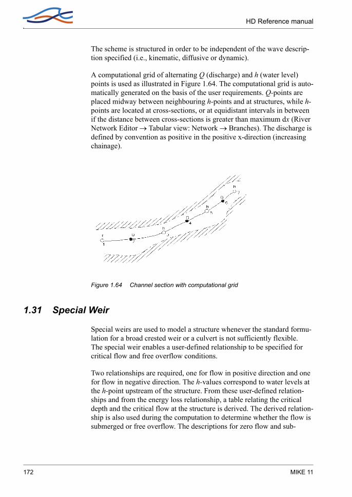
HD Reference manual
The scheme is structured in order to be independent of the wave descrip-tion specified (i.e., kinematic, diffusive or dynamic).
A computational grid of alternating Q (discharge) and h (water level) points is used as illustrated in Figure 1.64. The computational grid is auto-matically generated on the basis of the user requirements. Q-points are placed midway between neighbouring h-points and at structures, while h-points are located at cross-sections, or at equidistant intervals in between if the distance between cross-sections is greater than maximum dx (River Network Editor → Tabular view: Network → Branches). The discharge is defined by convention as positive in the positive x-direction (increasing chainage).
Figure 1.64 Channel section with computational grid
1.31 Special Weir
Special weirs are used to model a structure whenever the standard formu-lation for a broad crested weir or a culvert is not sufficiently flexible. The special weir enables a user-defined relationship to be specified for critical flow and free overflow conditions.
Two relationships are required, one for flow in positive direction and one for flow in negative direction. The h-values correspond to water levels at the h-point upstream of the structure. From these user-defined relation-ships and from the energy loss relationship, a table relating the critical depth and the critical flow at the structure is derived. The derived relation-ship is also used during the computation to determine whether the flow is submerged or free overflow. The descriptions for zero flow and sub-
172 MIKE 11

Stability Conditions
merged flow are given under section 1.33 Steady State Energy Equation (p. 175).
1.32 Stability Conditions
It is not possible to give a single general rule for the selection of ∆t and ∆x covering all possible situations. The user should note that MIKE 11 assumes a linear variation of all the variables between each time step and grid point. Hence one criterion for ∆t and ∆x is that they should be small enough to re-solve non-linear variations in the time and space, respec-tively. For example, simulation of tidal variations require time steps in the order of 10-30 minutes in order to fully describe the tidal cycle in time. Similarly, rapidly changing river geometry requires space steps small enough to describe the topography accurately.
In order to obtain a stable and accurate solution to the finite difference scheme the following conditions have to be fulfilled:
the topographic resolution must be sufficiently fine that non-linearities in water levels and discharges are adequately resolved. The maximum allowable value for ∆x (dx-max) should be selected on this basis
the time step, ∆t, should be fine enough to provide an accurate repre-sentation of a wave. For example, the maximum time step for a tidal simulation is generally around 30 minutes
if structures are being used a smaller time step may be required
the Courant condition (given below) can be used as a guide for select-ing the time step providing the above conditions are also satisfied. Typ-ically a value of Cr is of the order of 10 to 15, but much higher values have been used (up to 100)
(1.226)
where, V is velocity;
the velocity condition as given below can sometimes impose a limita-tion on the time step, ∆t, in the case of rapidly varying cross-sections
(1.227)
Cr∆t V gy+( )
∆x-------------------------------=
V∆t∆x
--------- 1 to 2≤
Hydrodynamic Reference 173

HD Reference manual
The Courant criterionThe term is the celerity of a small disturbance (wave) in shallow water. This assumption is hardly ever satisfied in rivers and channels, where the wave celerity may be significantly smaller.
The Courant criterion is often applied in connection with rivers and chan-nels. The Courant number expresses the number of grid points a wave, generated from a minor disturbance, will move during one time step.
The finite difference scheme used in MIKE 11 (6-point Abbott scheme), allows Courant numbers up to 10-20 if the flow is clearly sub-critical (Froude number less than 1). Computations with a Courant number of 250 have produced results with an error of less than 2% in some very special cases.
The velocity criterionThe velocity criterion requires that ∆t and ∆x are selected in the order that a water body will not be transported more than one grid point per time step. When applying the kinematic wave equation, and at weirs, it is acceptable that the velocity times ∆t/∆x is considerably larger than 1.
An estimation of the qualities of a differential scheme is often based on the following two types of errors:
error in amplitude
error in phase
Figure 1.65 shows the phase error for several Courant numbers as a func-tion of the number of h-points per wave length. It shows, for example, that with 24 h-points per wave length and Cr=2, the computed wave celerity is about 3% too small.
gy
174 MIKE 11

Steady State Energy Equation
Figure 1.65 The phase error as a function of the number of h-points per wave length for a 6-point Abbott scheme.
1.33 Steady State Energy Equation
The steady state is calculated using the energy equation when selecting the switch "Use energy equation" in the page "Quasi Steady" HD parameter editor.
The layout of the energy equation set-up is shown in Figure 1.66.
Figure 1.66 The control volume used for determining the water level profile by
the use of the energy equation.
Hydrodynamic Reference 175

HD Reference manual
The integrated steady state energy equation reads
(1.228)
where
H1, H2 Water levels in cross sections
Q Discharge
α1, α2 Velocity distribution coefficients
g Acceleration due to gravity
A1, A2 Flow areas
he Energy head loss
αM11 User defined velocity distribution coefficient (default = 1)
βsup Suppression factor
The velocity distribution coefficients α1 and α2 are calculated from
(1.229)
where
KLF , KCH and KRFConveyance for left floodplain, channel and right floodplain respectively.
H1 αm11βsupα1Q2
2gA12
--------------- H2 αM11+ βsupα2Q2
2gA22
--------------- he+=+
α
At2 KLF
3
ALF2
------------KCH
3
ACH2
-------------KRF
3
ARF2
------------+ +
K3TOT
----------------------------------------------------------------=
176 MIKE 11
Steady State Energy Equation
ALF , ACH and ARFFlow area for left floodplain, channel and right floodplain respectively.
The conveyance for each subsection is determined as
(1.230)
Where n is the Manning’s number for the cross section. The transversal variation is taken into account through the relative resistance, thus n fac-tors out.
The suppression factor depends on the Froude number and is given by
(1.231)
where the Froude number Fr used is given by
(1.232)
The suppression can be omitted if desired.
The energy head loss consists of a friction loss and a contraction or expan-sion loss
(1.233)
where
the mean reach length
Ifric friction slope
C user defined contraction/expansion coefficient (default 0.1/0.3)
KiAiRi
2 3⁄
n------------------=
βsup1 Fr2– for Fr 1≤
0 for Fr 1>
=
Fr max Q2
A12gR1
------------------ Q2
A22gR2
------------------,
=
he LIfric CαM11a1Q2
2gA12
---------------a2Q2
2gA22
---------------–+=
L
Hydrodynamic Reference 177

HD Reference manual
The friction slope is determined through
(1.234)
with the weighting term defined by
(1.235)
and the average flow area determined by
(1.236)
and the mean Manning’s number
(1.237)
The factor φ increases stability for high Froude numbers through a upstream centering of the friction term as the Froude number increases. If desired the suppression term βsup can be fixed at one thus no suppression is applied and the friction term is thus centered at the midpoint between sections 1 and 2.
The above is the default way of handling the friction slope. MIKE 11 has 4 alternative evaluations of the friction slope. These may be changed by the user. The chosen evaluation method is a global setting thus it is used for all reaches in a given set-up.
The four friction slope alternatives are:
Ifric
Q Q
M2A
----------- 1φA2R2
4 3⁄ 1 φ–( )A1R14 3⁄+
------------------------------------------------------------------
for A1R14 3⁄ A2R2
4 3⁄<
Q Q
M2A
----------- φ 1A2R2
4 3⁄------------------- 1 φ–( ) 1
A1R14 3⁄
-------------------+ for A1R1
4 3⁄ A2R24 3⁄≥
=
φ 910------ 4
10------βsup–
=
A
A 110------ 4
10------βsup+
A1910------ 4
10------– βsup
A2+=
M 12--- M1 M2+( )=
178 MIKE 11
Steady State Energy Equation
Average conveyance:
(1.238)
Average friction:
(1.239)
Geometric mean:
(1.240)
Harmonic mean:
(1.241)
Finally the cross section reach length is determined from
(1.242)
where the index is either 1 or 2.
The mean reach length is found through
(1.243)
IfricQ1 Q2+( )2
K1 K2+( )2---------------------------=
Ifric12---
Q12
K12
---------Q2
2
K22
---------+
=
IfricQ1
2
K12
---------Q2
2
K22
---------=
Ifric 2
Q12
K12
---------Q2
2
K22
---------
Q12
K12
---------Q2
2
K22
---------+
-------------------------=
LiLLFKLF i, LCHKCH i, LRFKRF i,+ +
KTOT i,-----------------------------------------------------------------------------------=
L 12--- L1 L2+( )=
Hydrodynamic Reference 179

HD Reference manual
If no reach lengths are specified for the overflow banks the reach length is set equal to the main channel reach length (standard MIKE 11 method).
1.34 Structures
MIKE 11 includes descriptions for a wide range of structures which act as control points. The formulation of these features permits great flexibility since they range both in their degree of user-intervention and in their level of complexity.
Structures which operation is calculated automatically within the program under sub-critical flow conditions while user-defined Q-h relationships are applied for critical flow conditions are described under the keywords:
Broad crested Weir (p. 70)
Special Weir (p. 172)
Weir Formula (p. 194)
Culverts, Q-h Relations Calculation (p. 88)
The structures which operation is user-defined under all flow conditions are described under section 1.27 Regulating Structures (p. 167). These include both structures with a pre-determined operation such as a pump, (Q = f(t)) and structures for which the operation is a function of water level or discharge at other locations in the model (Q = f(h,Q)).
More complex regulating structures are modelled using the add-on mod-ule described under 1.9 Control Structures (p. 74).
Control structures and dambreak structures, are structures which operation is calculated automatically within the program during all flow conditions.
For the structure types; broad crested weir, special weir culvert, overflow control structure, dam break (crest flow) dam break /breach flow), the hydraulic description is similar and is described below.
The structures are modelled in MIKE 11 as control points at Q-points in the computational grid. Depending on the structure category, a relation-ship between the discharge and the upstream and downstream water levels is determined based on the flow condition, entrance and exit losses, and a critical flow correction factor.
Given the upstream and downstream water level and the river discharge the flow regime can be determined.
180 MIKE 11

Structures
Zero flow in the structure occurs if it is closed by a valve, or if both the upstream and the downstream water levels are below the structure invert (crest level).
To differentiate between free overflow (critical flow) and drowned flow (submerged flow) it is as an initial guess assumed that the flow is critical and the associated discharge is computed. The flow is critical if the energy head at the weir crest is larger than downstream water level. If the flow is not critical a submerged iteration is applied to determine the discharge.
Comparing the critical discharge with the submerged determines the flow regime finally as the smaller discharge is taken.
The different flow conditions defined for a structure are:
Zero Flow
Drowned Flow
Free Overflow
1.34.1 Zero FlowThe flow is set to zero when the water level at both sides of the structure lies below its invert or when the upstream and downstream water levels are equal.
1.34.2 Drowned FlowThe flow on either side of the structure is in the same state as over the structure itself, i.e. both subcritical or both supercritical.
The discharge Q over a broad crested weir, for example, with constant width b in the case of drowned flow is generally given in the following form:
(1.244)
where, µ is the weir discharge coefficient, h1 and h2 the upstream and downstream water levels respective, and Zc the weir crest elevation. This equation is easily converted to a general description for the head loss across a structure.
For further details refer to Appendix A.
Q µb h1 Zc–( ) h1 h2–( )1 2⁄=
Hydrodynamic Reference 181

HD Reference manual
1.34.3 Free OverflowIn the case of free overflow, the water levels at both sides are such that the system seeks to deliver the maximum discharge for a given energy head at the upstream side of the structure. This leads to critical flow at (or very near to) the most narrow section (control section).
In the case of free overflow the discharge is independent of the down-stream water level, i.e. upstream controlled. In principle the discharge can be computed from the condition that the flow is critical at the control sec-tion for the given upstream energy head.
For example, for broad crested weirs with a rectangular cross-section the critical flow discharge is calculated by:
(1.245)
where, Hs is the available energy head above the weir crest and αc is the free overflow factor (in the Head Loss Factors box).
Using Equation (1.245), a relationship between the upstream head and critical flow is tabulated for use by the structures algorithm (see A.10 Structures (p. 467) in Appendix A). The accuracy depends on the refine-ment in the tabulation.
Several factors influence the actual free overflow discharge through a structure:
the section where critical flow occurs is often located downstream of the most narrow section, especially for well designed spillways
the velocity is not distributed uniformly over the cross-section, thus the critical discharge is reduced
the water level is not constant over the cross-section, especially in the case of an irregular section
The critical discharge is therefore corrected with a coefficient, αc, (in the Head Loss Factors box) giving the real discharge as:
(1.246)
Free overflow is modelled on the basis of a relationship between the dis-charge and the upstream water level. The relationship is generated auto-matically by MIKE 11 for the structure types: broad crested weirs and culverts Q/h relations calculated. In the case of user-defined structures
Qc αc1,705bHs3 2⁄=
Q αcQc=
182 MIKE 11

Structures
(i.e. special weirs and culverts) the specified Q/h relation is applied. For the remaining structure types (control structure and dam break (crest flow, breach flow)), the critical discharge is computed during the simulation.
1.34.4 Contraction and Expansion LossesExpressions for the head losses at structures are given in Appendix A. The head losses upstream and downstream of the structures are functions of the coefficients ζin and ζout (specified in the Head Loss Factors box) and the ratios of the structure area and the cross-section areas in the immedi-ately adjacent river, see below.
IMPORTANT! During pre-processing of Q/h-relation in broad crested weirs, the ratio of structure area and river cross-section area is used to compute the Q/h-relation. The expressions require that the cross-sectional area of the river section is always greater than that at the structure. An error message will appear in case the weir area is larger than the up- or downstream cross-sectional area, as it is not possible to establish the Q/h-relation for free overflow. To correct this, check cross-sections and weir geometry. The values of ζin and ζout are typically 0.5 and 1.0, respec-tively.
1.34.5 Grid spacing at structuresIt is necessary to describe a river cross-section immediately upstream and downstream of any structure since the loss formulations are based on the relationships between the available cross-sectional area at the structure and that of the immediately adjacent river. A check in the code requires that these river cross-sections be within maximum dx (River Network Edi-tor → Branches) of the structure. An error message is given if this is not the case.
These relationships are described under section A.10 Structures (p. 467) in Appendix A.
1.34.6 Parallel/Composite StructuresIt is possible to model several structures at the same control point (Q-point) thus modelling a structure composed of several individual struc-tures.
A parallel structure could describe e.g. the structures in connection with a hydro power station, i.e. to model the combination of turbines, ship locks, and spillway structures. Another application could be to model fish friendly structures in irrigation channels, etc.
A parallel/composite structure is defined simply by specifying the location (same river name and chainage) for each individual structure.
Hydrodynamic Reference 183

HD Reference manual
The discharge for the composite structure is computed by treating each structure separately and adding the coefficients for each structure and applying the final coefficients in the final solution for the Q-point, i.e.:
(1.247a)
(1.247b)
(1.247c)
(1.247d)
where,
c,s represents the coefficient for the composite structure
s,i represents coefficient for the i structure
n represent number of structures in the composite/parallel structure.
1.35 Supercritical Flow
The solution scheme in MIKE11 will not truly simulate supercritical flow. The solution scheme is designed for subcritical flow, and compensations are made to enable supercritical flow to occur. As discussed below (Sup-pression of convective acceleration term (p. 185)), the β factor reduces the convective momentum term at a rate according to the Froude number. This means that model results will be less accurate with increasing Froude number.
For supercritical flow a reduced momentum equation (Saint Venant Equa-tion) is applied which neglects the convective momentum term:
(1.248)
αc s, αs i,
i 1=
n
∑=
βc s, 1=
γc s, γs i,
i 1=
n
∑=
δc s, δs i,
i 1=
n
∑=
∂Q∂t------- gA∂h
∂x------ gQ Q
C2AR---------------+ + 0=
184 MIKE 11

Supercritical Flow
As long as the flow situation is not changing rapidly compared to the velocity, the description will still remain accurate. The advantage is that a stable solution can still be obtained within the same algorithmic structure as that used for sub-critical flow. For the transition from sub-critical to supercritical flow, a gradual reduction of the momentum terms is made resulting in a smooth description. Similarly, the differential equation is gradually centred upstream as the influence of the upstream conditions increases.
1.35.1 Suppression of convective acceleration termThe characteristics of the St. Venant equations are given by
(1.249)
where
Q the discharge
A cross-sectional area
w surface width of cross-section
g acceleration due to gravity
F Froude number
For F > 1 the characteristics are both positive, implying that the St. Venant Equations take two upstream boundary conditions, and for F = 1 the solu-tion becomes singular. The numerical algorithm adopted in MIKE 11 is based on a staggered computational grid and cannot accommodate two boundary conditions at the same boundary or a singular solution. To avoid these situations a modified momentum equation is implemented in MIKE 11, viz.
(1.250)
where
H water surface elevation
α momentum distribution coefficient
C1 2,QA---- gA w⁄± Q
A---- 1 1
F---±
= =
∂Q∂t------- β
∂ αQA----
2
∂x------------------- gA∂h
∂x------ friction+ + + 0=
Hydrodynamic Reference 185

HD Reference manual
β factor for suppression of convective momentum term
The default formulation in MIKE 11 is
(1.251)
This ensures excellent stability properties of the numerical solution and is sufficiently accurate for most flood routing studies where generally the Froude number is relatively small and the resolution used is coarse ( ).
For water surface profiling with high Froude number and small space steps (space step = O (water depth)) an alternative formulation has been implemented, viz.
(1.252)
For the default value of a and b (a=1 and b=2) the two characteristics never have the same sign; they are either of different sign ( ) or one is zero ( ). The variation of β is shown in Figure 1.67. The alternative formulation is somewhat less stable than the default (Equation (1.251)) and therefore requires the application of a smaller time step for high Froude numbers. The solution is, however, considerably more accurate for high Froude numbers. Various tests have shown that the new formulation performs well for transition from sub- to supercritical flow, whereas hydraulic jumps are less accurate.
Note that a and b can be adjusted and do not necessarily have to be set at a=1 and b=2. However the solution scheme is unstable if the suppression factor β lies outside the curve shown in Figure 1.67. Thus a=0.5 and b=2 can be applied, but a=2 and b=2 cannot.
The alternative formulation can be selected by setting the values Froude-Max (a) and FroudeExp (b) to positive values in the Hydrodynamic parameters Editor under the Default values tab.
β 1 F2– for F 1≤0 for F 1>
=
the space step water depth»
β1 for F a≤
1 F 1 a–+( )b⁄ for F a>
=
F 1<F 1≥
186 MIKE 11

Supercritical Flow in Structures
Figure 1.67 Factor for suppression of convective momentum term versus Froude number.
1.35.2 Effect of convective acceleration suppression on Energy HeadsAs discussed, when the solution scheme approaches critical conditions the convective momentum term is gradually reduced. The suppression factor β varies from 1 (full convective term) to 0 (no convective term) according to the Froude number.
The β factor also modifies the energy calculation, thus energy head at any location in a model is affected. This means that when velocities are high (when the convective term is significant), energy head is significantly affected by the value of beta. This can be seen in a profile plot of energy levels along a river reach, which shows that energy is not conserved and varies according to velocity.
1.36 Supercritical Flow in Structures
Structures are used in MIKE11 to represent real structures (weirs, etc.) and locations where critical flow or changes in flow conditions occur. Being a time dependent model, the MIKE11 structures can be subject to a wide range of flow conditions, often more than is usually covered by textbooks. As an illustration, a supercritical flow condition at a structure is likely to occur in MIKE11 when the structure is actually representing something more like a natural cross-section rather than a "typical" structure. This means that the MIKE11 structures need to be capable of simulating flow conditions unlike those that a "typical" structure would encounter.
The solution scheme in MIKE11 will not truly simulate supercritical flow. The solution scheme is designed for subcritical flow, and compensations
Hydrodynamic Reference 187

HD Reference manual
are made to enable supercritical flow to occur (see Suppression of convec-tive acceleration term (p. 185)). Head losses through a structure are pro-portional to the square of the velocity. This means that when supercritical flow occurs (which usually involves high velocities) head losses become more sensitive to changes in velocity. Further, small changes to the head loss coefficients can have a more pronounced effect upon head losses through a structure when velocities are high.
Accurately simulating flow through structures in MIKE11 during fully supercritical flow is difficult, and results should be considered with cau-tion. Having said this, MIKE11 will provide a reasonable representation if supercritical flow occurs during a simulation.
1.36.1 Flow DirectionsIf supercritical flow is occurring either upstream or downstream of a struc-ture it is impossible for the flow direction to change. A change in flow direction can only occur during subcritical flow. Thus, if subcritical flow is occurring, flow direction is calculated by comparison of water level upstream and downstream of the structure. If any other flow condition occurs, flow direction is equal to the previous flow direction.
A zero (or no) flow condition exists when there is subcritical flow and the water levels upstream and downstream of the structure are lower than the invert of the structure. If flow is supercritical then zero flow is impossible.
1.36.2 Testing for Flow ConditionsEnergy levels in MIKE11 are influenced by the convective suppression factor β (see Suppression of convective acceleration term (p. 185)). Also, there are distinctly different formulations for different flow conditions within a structure. This means that the state of flow (sub or super) must be known both upstream and downstream of the structure to decide the appropriate flow regime (either definitively or with other factors). The state of flow upstream and downstream of a structure is found using the Froude Number (FR):
(1.253)
If FR < 1 then subcritical flow, if FR = 1 then critical flow and if FR > 1 then supercritical flow. Using the Froude Number upstream (FR1) and downstream (FR2) of the structure, the following tests are made to decide the flow condition inside the structure:
gyAQ
gyvFR ==
188 MIKE 11
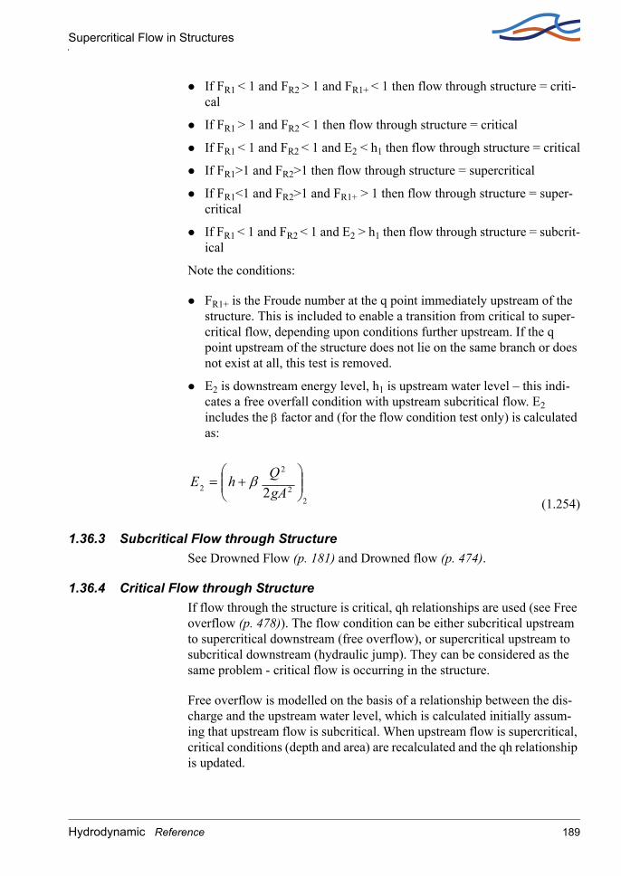
Supercritical Flow in Structures
If FR1 < 1 and FR2 > 1 and FR1+ < 1 then flow through structure = criti-cal
If FR1 > 1 and FR2 < 1 then flow through structure = critical
If FR1 < 1 and FR2 < 1 and E2 < h1 then flow through structure = critical
If FR1>1 and FR2>1 then flow through structure = supercritical
If FR1<1 and FR2>1 and FR1+ > 1 then flow through structure = super-critical
If FR1 < 1 and FR2 < 1 and E2 > h1 then flow through structure = subcrit-ical
Note the conditions:
FR1+ is the Froude number at the q point immediately upstream of the structure. This is included to enable a transition from critical to super-critical flow, depending upon conditions further upstream. If the q point upstream of the structure does not lie on the same branch or does not exist at all, this test is removed.
E2 is downstream energy level, h1 is upstream water level – this indi-cates a free overfall condition with upstream subcritical flow. E2 includes the β factor and (for the flow condition test only) is calculated as:
(1.254)
1.36.3 Subcritical Flow through StructureSee Drowned Flow (p. 181) and Drowned flow (p. 474).
1.36.4 Critical Flow through StructureIf flow through the structure is critical, qh relationships are used (see Free overflow (p. 478)). The flow condition can be either subcritical upstream to supercritical downstream (free overflow), or supercritical upstream to subcritical downstream (hydraulic jump). They can be considered as the same problem - critical flow is occurring in the structure.
Free overflow is modelled on the basis of a relationship between the dis-charge and the upstream water level, which is calculated initially assum-ing that upstream flow is subcritical. When upstream flow is supercritical, critical conditions (depth and area) are recalculated and the qh relationship is updated.
22
2
2 2
+=
gAQhE β
Hydrodynamic Reference 189

HD Reference manual
1.36.5 Supercritical Flow through StructureWhen drowned flow occurs during subcritical flow conditions, the energy equation is used to calculate head loss. When supercritical flow occurs the energy equation becomes very sensitive to small changes in head drop and structure area, to such an extent that it cannot be applied to the MIKE11 structure routines. Instead, the momentum equation is used when a struc-ture is in supercritical flow conditions. This is applied in the same way as for a normal q point in MIKE11, except that structure geometry is used and that friction losses are substituted by the structure losses.
1.36.6 Contraction and Expansion Losses, Sub- and Supercritical FlowConsider the following:
Expansion and contraction losses across a structure are less during supercritical flow compared to subcritical flow.
Losses are a function of velocity head and velocities are much higher during supercritical flow, so model predictions can become extremely sensitive to the value of loss coefficient.
During subcritical flow through a structure, there is an upstream con-traction loss and a downstream expansion loss.
During supercritical flow through a structure, there is an upstream expansion loss and a downstream contraction loss.
MIKE11 modifies the loss coefficients to account for changes in velocity and area through a structure. As discussed in Appendix A.10.1, this accommodates the changes in expansion and contraction that occur during subcritical and supercritical flows.
Care must be taken when selecting loss coefficients, particularly in situa-tions where both subcritical and supercritical flow conditions occur. When flow conditions change from subcritical to supercritical (or the Froude number FR becomes greater than 1), the loss coefficients ζin and ζout (spec-ified in the Head Loss Factors box) are modified:
If FR > 1 in upstream h-point then ζin = ζin / 2
If FR > 1 in downstream h-point then ζout = ζout / 2
Note that this adjustment is not made for bridge structures.
1.37 Tabulated structures
A tabulated structure can be defined as:
190 MIKE 11
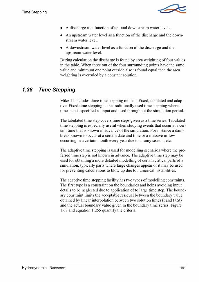
Time Stepping
A discharge as a function of up- and downstream water levels.
An upstream water level as a function of the discharge and the down-stream water level.
A downstream water level as a function of the discharge and the upstream water level.
During calculation the discharge is found by area weighting of four values in the table. When three out of the four surrounding points have the same value and minimum one point outside also is found equal then the area weighting is overruled by a constant solution.
1.38 Time Stepping
Mike 11 includes three time stepping models: Fixed, tabulated and adap-tive. Fixed time stepping is the traditionally used time stepping where a time step is specified as input and used throughout the simulation period.
The tabulated time step covers time steps given as a time series. Tabulated time stepping is especially useful when studying events that occur at a cer-tain time that is known in advance of the simulation. For instance a dam-break known to occur at a certain date and time or a massive inflow occurring in a certain month every year due to a rainy season, etc.
The adaptive time stepping is used for modelling scenarios where the pre-ferred time step is not known in advance. The adaptive time step may be used for obtaining a more detailed modelling of certain critical parts of a simulation, typically parts where large changes appear or it may be used for preventing calculations to blow up due to numerical instabilities.
The adaptive time stepping facility has two types of modelling constraints. The first type is a constraint on the boundaries and helps avoiding input details to be neglected due to application of to large time step. The bound-ary constraint limits the acceptable residual between the boundary value obtained by linear interpolation between two solution times (t and t+∆t) and the actual boundary value given in the boundary time series. Figure 1.68 and equation 1.255 quantify the criteria.
Hydrodynamic Reference 191
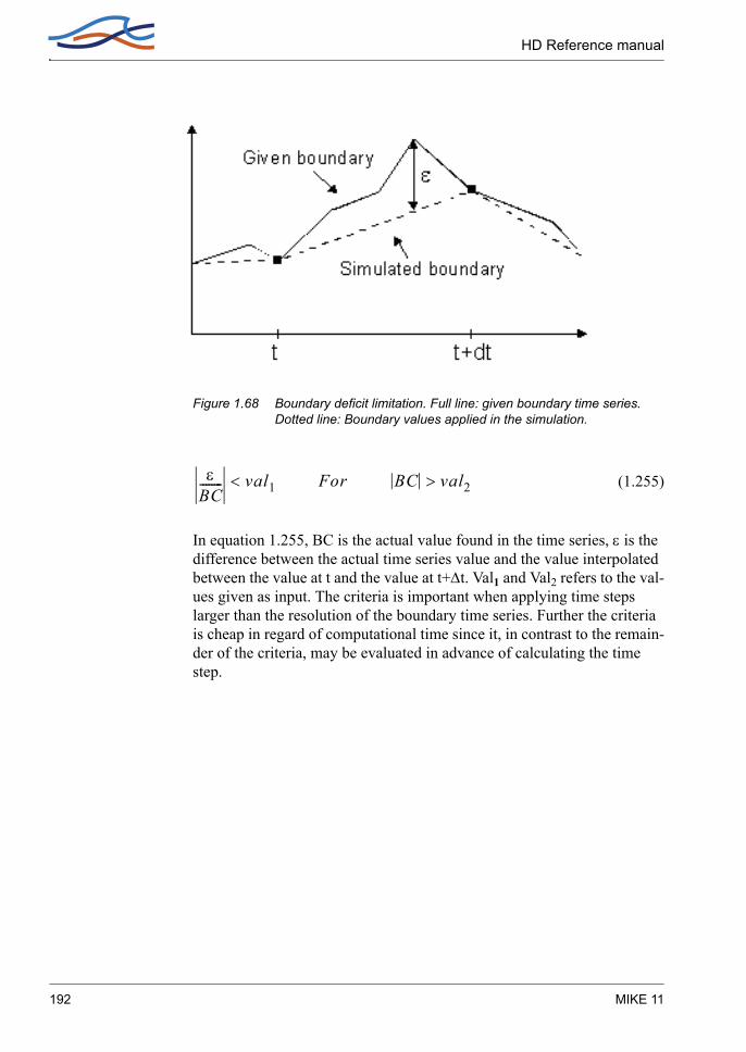
HD Reference manual
Figure 1.68 Boundary deficit limitation. Full line: given boundary time series. Dotted line: Boundary values applied in the simulation.
(1.255)
In equation 1.255, BC is the actual value found in the time series, ε is the difference between the actual time series value and the value interpolated between the value at t and the value at t+∆t. Val1 and Val2 refers to the val-ues given as input. The criteria is important when applying time steps larger than the resolution of the boundary time series. Further the criteria is cheap in regard of computational time since it, in contrast to the remain-der of the criteria, may be evaluated in advance of calculating the time step.
εBC-------- val1< For BC val2>
192 MIKE 11

User Defined Structure
The second type of criteria are limitations to the actual solution calculated. Hence this time step adaption is based on trial and acceptance and is there-fore more expensive in regard of computational time. The criteria are:
(1.256)
(1.257)
(1.258)
(1.259)
(1.260)
(1.261)
In equations 1.256 through 1.261, val1 to val10 are user specified values.
All constraints are optional. In case the constraints are not met the time step is reduced with a factor specified as change ratio in the input. The time step is allowed to vary between a user specified minimum and maxi-mum value.
1.39 User Defined Structure
The user defined structure is available to create customised structures in MIKE11. However, the potential application goes beyond this, allowing for the customisation of almost any specialist application or modification to MIKE11.
When activated, the user defined structure will access a DLL (Dynamic Link Library) written by the user. The Network Editor interface contains a number of variables that can be used in the DLL. In addition, the DLL can access any variable in MIKE11 through several records.
∆Q val3<
-------- val4< for Q val5<
∆h val6<
∆hh
------- val7< for h val8>
CrHDv gD+ ∆t
∆x----------------------------- val9<=
CrADv ∆t∆x
----------- val10<=
Hydrodynamic Reference 193

HD Reference manual
1.39.1 TipsMIKE11 is written in PASCAL using Borland DELPHI. Any code written must be compatible with the compiled unit files (DCU) pro-vided. The easiest way to ensure this is to have Delphi and write your programs in PASCAL.
There are several options specified in the Project Options in Delphi. These options have been set to be compatible with the latest build of MIKE11.
The user defined structure routine is called within the MIKE11 struc-ture procedure. The aim of the structure procedure is to take the most recent flow calculations and produce the coefficients of the momentum equation. These coefficients are then used in the solver.
Therefore, the user defined structure routine (if actually simulating a structure) should use the available flow information to create suitable coefficients for the momentum equation. Any programming performed must consider this. The values of co1, co2, co3 and co4 are set to zero at the commencement of the structure procedure.
The user defined structure routine is called prior to the final sweep in the solution scheme. This means that any output or model parameters for the current timestep have not yet been calculated. Results from the previous timestep are valid.
For more information, see Appendix A.12.
1.40 Weir Formula
With the Weir Formula the discharge through a structure can be modelled by using standard weir formulas.
Figure 1.69 Definition sketch for Weir Flow
194 MIKE 11

Weir Formula
1.40.1 Weir Formula 1Weir formula 1 is based on a standard weir expression, reduced according to the Villemonte formula:
(1.262)
Where Q is discharge through the structure, W is width, C is weir coeffi-cient, k is the weir exponential coefficient, Hus is upstream water level, Hds is downstream water level and Hw is weir crest level. (See Figure 1.69).
1.40.2 Weir Formula 2 (Honma)Weir formula 2 is the Honma formula:
(1.263)
Where Q is the discharge through structure, W is the width, C1 is the first weir coefficient, is the second weir coefficient, g is the acceleration due to gravity Hus is the upstream water level, Hds is the downstream water level and Hw is weir level. (See Figure 1.69).
1.40.3 Weir Formula 3 (Extended Honma)Weir formula 3 is the extended Honma formula
The flow is calculated is three flow regimes called perfect, imperfect and submerged overflow. The choice of regime is defined by the ratio between down stream and upstream water depth above the crest.
(1.264)
W is weir width
H is weir height above cross section invert
Q W= C Hus Hw–( )k 1Hds Hw–Hus Hw–---------------------
k
–0,385
⋅ ⋅ ⋅
Q C1W Hus Hw–( ) Hus Hw–( )
C2W Hds Hw–( ) Hus Hds–( )
forfor
Hds Hw–( ) Hus⁄ 2 3⁄<
Hds Hw–( ) Hus⁄ 2 3⁄≥
=
C2 3 2⁄( ) 3C1=
Q
C0Whu3 2⁄ for hd hu⁄ hd hu⁄( )i≤
C0 α hd hu⁄( )q⋅ β+( )Whu3 2⁄ for othercases
C0 γ hd hu⁄( )r⋅ δ+( )Whd hu hd–( )1 2⁄ for hd hu⁄ hd hu⁄( )s≥
C0 a hu H⁄( )p⋅ b+= for all
=
Hydrodynamic Reference 195

HD Reference manual
hd is the upstream water level above the crest
hu is the down stream water level above the crest
(hd/hu)i is a user specified depth ratio limit between perfect and imperfect flow regime.
(hd/hu)s is a user specified depth ratio limit between imperfect and sub-merged flow regime.
a, b, p, alfa, beta, r, gamma, delta and p are user specified parameters.
MIKE 11 simulation engine or user interface does not check if there is a continuous transition from one flow regime to the next. This has to be ensured by the user through proper selection of the parameters.
1.41 Wind
Wind friction on the water surface can be accounted for in MIKE 11 by inclusion of the wind shear stress in the momentum equation. If wind shear is to be included and a wind field has been specified as a boundary condition in the Boundary Editor then the switch in the Hydrodynamic parameters Editor under the Wind tab has to be set.
The wind shear stress is expressed as:
(1.265)
where,
Cw Wind friction coefficient (approx. 0.0025)
tfac Factor depending on the surrounding topography (1.0 for open water and reduced at locations which are sheltered from the wind)
V10 Velocity 10 m above the water surface
ρa Density of air (approx. 1.2 kg/m3)
The wind force projection in the length direction of the channel is included in the local momentum equation in each Q-point. The wind direction and velocity specified as a time series is implemented in the
τw tfacCwρaV102=
196 MIKE 11
References
boundary editor. The branch orientations are calculated from the network grid which is always oriented north/south. The topographical factor (tfac) can be defined globally or locally for each location (in the Hydrodynamic parameters Editor under the Wind tab). The surface area to which the wind stress applies excludes any additional flooded areas and is equal to the width multiplied by the distance between h-points either side of the Q-point.
1.42 References
/1/ Abbott, M.B., 1979: Computational Hydraulics. Elements of the Theory of Free Surface Flows. Pitman.
/2/ Abbott, M.B. and Ionescu, F., 1967: On the numerical computation of nearly-horizontal flows. J.Hyd.Res., 5, pp. 97-117.
/3/ Bier, P.E. and Delleur, J.W. (1962) Hydraulics of single span bridge constructions. Proceedings of the American Society of Civil Engi-neers, Journal of the Hydraulics Division, 88(HY2), March, 75-108.
/4/ Bradley, J.N., 1978: Hydraulics of Bridge Waterways, Hydraulic Design Series No. 1, Federal Highway Administration, U.S. Department of Transportation, Second Edition, revised March 1978, Washington D.C.
/5/ Carter, R.W.: Computation of Peak Discharge at Culverts, U.S. Geological Survey Circular 376, 1957.
/6/ Chow, V.T., 1959: Open-Channel Hydraulics. McGraw Hill.
/7/ Cunge J.A., Holly F.M., Jr. and Verwey A. (1980): Practical Aspects of Computational River Hydraulics. Pitman.
/8/ Engelund, F., 1966: Hydraulic resistance of alluvial streams. ASCE, Vol. 92, No. Hy. 2.
/9/ Federal Highway Administration, 1986: Bridge Waterways Analy-sis Model: Research Report, Report No. FHWA/RD-86/108, July 1986, Washington D.C.
/10/ Hamil, L., 1999: Bridge Hydraulics. E & FN Spon.
/11/ Henderson, F.M. (1966): Open Channel Flow. MacMillan.
/12/ Lundgren, H. and Jonsson, I.G., 1962: Shear and velocity distribu-
Hydrodynamic Reference 197

HD Reference manual
tion in shallow channels. ASCE, Vol. 90, No. HY1, pp. 1-21.
/13/ Murota, A. and Tada, H. (1989): Modelling of one-dimensional analysis on the open-channel with a tributary.
/14/ Toch, A.J. (1953): Discharge Characteristics of Tainter Gates, Transactions ASCE Paper No. 2739, pp. 290-300.
/15/ Cunge J.A. and Wegner M. (1964): Integration numerique des equa-tions d'ecoulement de Barre de Saint-Venant par un schema implic-ite de differences finies: Application au cas d'une galerie tantot en charge, tantot a surface libre. La Houille Blance, No 1.
198 MIKE 11

A D V E C T I O N - D I S P E R S I O N /C O H E S I V E S E D I M E N T T R A N S P O R T
Reference
199

200 MIKE 11

Who Should Use This Manual
2 AD/CST REFERENCE MANUAL
2.1 Who Should Use This Manual
This manual should be used when undertaking advection-dispersion (AD) or cohesive sediment transport (CST) modelling applications. It provides a description of aspects which are encountered during the development, cal-ibration and application of AD/CST models including detailed technical descriptions of the numerical methods used. The manual should be used in conjunction with the MIKE 11 User Guide.
2.2 Manual Format
All descriptions in this Chapter are under headings presented in alphabeti-cal order. A list of the headings for this Chapter is given below.
A General Description (p. 201)
Advanced Cohesive Sediment Transport (p. 202)
Advection-Dispersion Equation (p. 207)
Boundary Conditions (p. 207)
Deposition, CST (p. 209)
Dispersion Coefficient (p. 211)
Erosion, CST (p. 211)
Solution Scheme, AD (p. 216)
Stability (p. 218)
Nomenclature (p. 218)
References (p. 220)
2.3 A General Description
The advection-dispersion (AD) module is based on the one-dimensional equation of conservation of mass of dissolved or suspended material, i.e. the advection-dispersion equation. The module requires output from the hydrodynamic module, in time and space, in terms of discharge and water level, cross-sectional area and hydraulic radius.
Advection-Dispersion / Cohesive Sediment Transport Reference 201

AD/CST REFERENCE MANUAL
The advection-dispersion equation is solved numerically using an implicit finite difference scheme which, in principle, is unconditionally stable and has negligible numerical dispersion. A correction term has been intro-duced in order to reduce the third order truncation error. This correction term makes it possible to simulate advection-dispersion of concentration profiles with very steep fronts.
The cohesive sediment transport (CST) module also forms part of the AD module. In contrast to the non-cohesive sediment transport (NST) module, the sediment transport cannot be described by local parameters only because the settling velocity of the mostly very fine sediment is very low. The cohesive module uses the AD module to describe the transport of the suspended sediment. Erosion/deposition is modelled as a source/sink term in the advection-dispersion equation. The erosion rate depends on the local hydraulic conditions whereas the deposition rate depends on the con-centration of the suspended sediment and on the hydraulic conditions.
The CST module is not provided with a roughness predictor. It does, how-ever, calculate the erosion/deposition rate directly without applying a con-tinuity equation for the sediment as performed in the morphological NST module. In a similar way to the explicit NST module, the accumulated sediment erosion/deposition during the simulation period is determined.
2.4 Advanced Cohesive Sediment Transport
This add-on module provides an alternative, more complex, analysis for cohesive sediment transport than that in the standard formulation described under Deposition, CST (p. 209) and Erosion, CST (p. 211) (sec-tions 2.7 and 2.9 respectively). This module is especially useful in situa-tions where a mass balance of cohesive sediment is required in order to simulate the accumulation of sediment. Then, knowing the exact location of sediment pools, it is possible to estimate e.g. the siltation in navigation channels, waterways, harbours etc. The module could also be used when resuspension of sediment affects water quality. This is because the resus-pension of cohesive sediment often gives rise to oxygen depletion because of the high organic content and associated oxygen demand (COD) in the cohesive sediment. Likewise resuspension of cohesive sediment can give rise to heavy metal pollution since heavy metals adhere to the sediment.
The advanced cohesive sediment transport module is part of the advec-tion-dispersion (AD) module. As for the standard formulation, the cohe-sive sediment transport is described in the AD-model through the transport of suspended solids. Erosion and deposition of cohesive sedi-ment is represented in the AD-model as a source/sink term. Whereas the
202 MIKE 11

Advanced Cohesive Sediment Transport
erosion rate depends only on local hydraulic conditions (bed shear stress), the deposition rate depends also on the suspended sediment concentration.
In the advanced cohesive model the transport of sediment is described in a pseudo two-dimensional manner through the description of the velocity and shear stress distribution across each section.
In each h-point of the solution domain the cohesive bed layer is modelled as three separate sediment sub-layers. The top layer is named sub-layer 1 and the bottom layer sub-layer 3. The thickness of the three sub-layers is calculated for each increment of elevation describing the cross-section as given in the processed data (see section 1.10 Cross-Sections (p. 81)).
Erosion and deposition rates are then integrated over the cross-section and added to the coefficients in the AD-equation.
The results of the cohesive sediment transport model during a simulation are:
accumulated erosion/deposition.
mass balance of the sub-layers.
mass balance of the total bed layer.
The results are given at h-points only.
The following descriptions are applied in the advanced cohesive model: cross-sectional velocity and shear stress distribution, settling, deposition, sliding, erosion and consolidation.
2.4.1 Cross-Sectional Shear Stress DistributionAssuming the local velocity is proportional with the local water depth, i.e.:
(2.1)
where, y is the local water depth, u the local velocity and c the Chezy con-stant and using the Manning formula
(2.2)
u y1 2⁄∝
u= C Iy( )1 2⁄
QA---- U MR2 3⁄ I1 2⁄= =
Advection-Dispersion / Cohesive Sediment Transport Reference 203

AD/CST REFERENCE MANUAL
where Q is the discharge, A the cross-section area, U the mean velocity, M the Manning number and R the hydraulic or resistance radius (see section 1.3 Bed Resistance (p. 21)) the local velocity can be expressed as:
(2.3)
Using Equation (2.3), the local bed shear stress can be given by:
(2.4)
where τb is the local shear stress, C the Chezy resistance number, ρ the density of water and g the acceleration of gravity.Thus, it can be seen from Equation (2.4) that the local bed shear stress increases with the water depth.
2.4.2 SettlingAn important parameter in the description of the sedimentation of cohe-sive materials is the settling velocity of flocs.
Through extensive field and laboratory studies it is evident that the set-tling velocity is dependent on the suspended sediment concentration. In the present model two settling regimes are described.
The first regime describes the effect of flocculation on settling velocity. Below a user specified suspended sediment concentration the settling velocity is given by:
(2.5)
where WS is the settling velocity of flocs, VC the volume concentration, m a coefficient and k is a constant.
Below the user specified value of suspended sediment concentration, the settling velocity usually increases with concentration due to the enlarge-ment of sediment flocs.
u QA---- y
R*-----
1 2⁄=
τbuC----
2ρg=
Ws kVCm=
204 MIKE 11
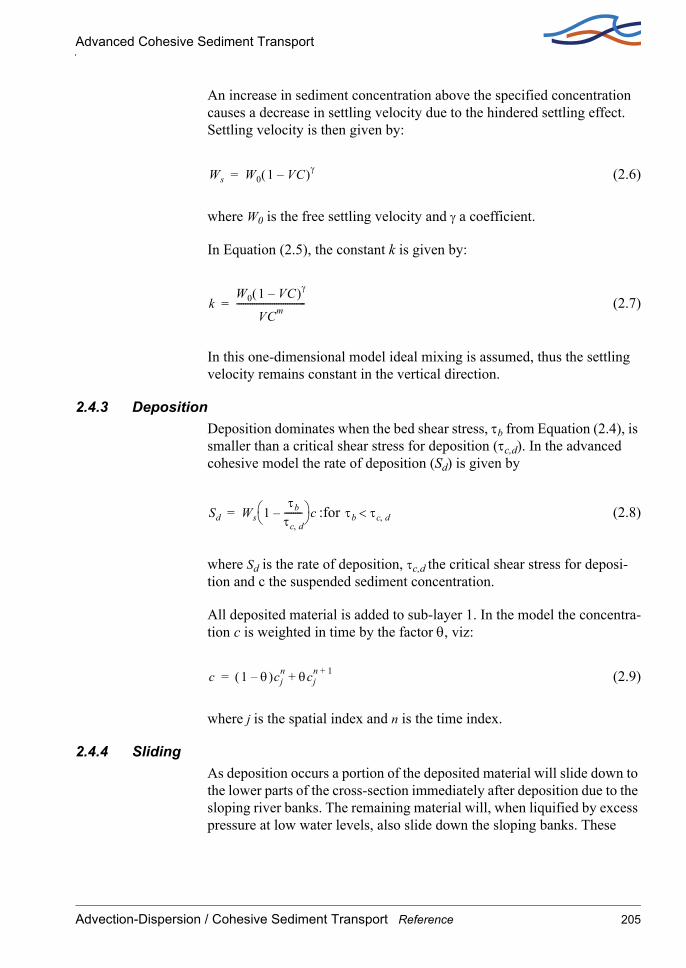
Advanced Cohesive Sediment Transport
An increase in sediment concentration above the specified concentration causes a decrease in settling velocity due to the hindered settling effect. Settling velocity is then given by:
(2.6)
where W0 is the free settling velocity and γ a coefficient.
In Equation (2.5), the constant k is given by:
(2.7)
In this one-dimensional model ideal mixing is assumed, thus the settling velocity remains constant in the vertical direction.
2.4.3 DepositionDeposition dominates when the bed shear stress, τb from Equation (2.4), is smaller than a critical shear stress for deposition (τc,d). In the advanced cohesive model the rate of deposition (Sd) is given by
:for (2.8)
where Sd is the rate of deposition, τc,d the critical shear stress for deposi-tion and c the suspended sediment concentration.
All deposited material is added to sub-layer 1. In the model the concentra-tion c is weighted in time by the factor θ, viz:
(2.9)
where j is the spatial index and n is the time index.
2.4.4 SlidingAs deposition occurs a portion of the deposited material will slide down to the lower parts of the cross-section immediately after deposition due to the sloping river banks. The remaining material will, when liquified by excess pressure at low water levels, also slide down the sloping banks. These
Ws W0 1 VC–( )γ=
kW0 1 VC–( )γ
VCm-------------------------------=
Sd Ws 1τb
τc d,--------–
c= τb τc d,<
c 1 θ–( )cjn θcj
n 1++=
Advection-Dispersion / Cohesive Sediment Transport Reference 205

AD/CST REFERENCE MANUAL
individual processes are modelled as one continuous process with a fric-tion type formula, viz:
(2.10)
where F is the lateral sediment flux, cF the friction coefficient, I the lateral surface slope of the bed layer and D the total thickness of bed layer.
2.4.5 ErosionThe river bed will erode when the applied bed shear stress, τb from Equa-tion (2.4), exceeds a critical shear stress for erosion, (τc,e) which depends on bed material characteristics.
In the present advanced cohesive model two types of erosion are applied, viz:
Instantaneous ErosionInstantaneous erosion occurs when the above mentioned bed shear stress exceeds the critical shear stress for erosion of the sediment. This implies that all sediment is resuspended instantaneously.
Gradual ErosionThe erosion rate is assumed to be a non-linear function of the excess stress, viz:
for (2.11)
where SE is the rate of erosion, E0 the erosion coefficient, τc,e the critical shear stress for erosion and n is the erosion exponent.
For sub-layer 1 it is possible to choose which erosion formulation should be used (Instantaneous or Gradual), while gradual erosion is automatically applied for sub-layers 2 and 3. Thus, it is possible to describe each sub-layer separately through the parameters E0, τc,e and n.
2.4.6 ConsolidationThe transition from sub-layer 1 to sub-layer 2 and from sub-layer 2 to sub-layer 3 is a process that includes both hindered settling and consolidation. The speed of the process is described by transition rates which are speci-fied in the model by the user.
F cF ID3 2⁄=
SE E0τb
τc e,-------- 1–
n
= τb τc e,>
206 MIKE 11
Advection-Dispersion Equation
2.5 Advection-Dispersion Equation
The one-dimensional (vertically and laterally integrated) equation for the conservation of mass of a substance in solution, i.e. the one-dimensional advection-dispersion equation reads:
(2.12)
where C is the concentration, D the dispersion coefficient, A the cross-sec-tional area, K the linear decay coefficient, C2 the source/sink concentra-tion, q the lateral inflow, x the space coordinate and t the time coordinate.
The equation reflects two transport mechanisms:
1 advective (or convective) transport with the mean flow;
2 dispersive transport due to concentrations gradients.
The main assumptions underlying the advection-dispersion equation are:
the considered substance is completely mixed over the cross-sections, implying that a source/sink term is considered to mix instantaneously over the cross-section
the substance is conservative or subject to a first order reaction (linear decay)
Fick's diffusion law applies, i.e. the dispersive transport is proportional to the concentration gradient
2.6 Boundary Conditions
At external boundaries, a series of conditions can be applied:
open boundary outflow
open boundary inflow - User defined values of the concentration (time varying or constant)
closed boundary
∂AC∂t
----------- ∂QC∂x
------------ ∂∂x----- AD∂C
∂x-------
–+ AKC– C2q+=
Advection-Dispersion / Cohesive Sediment Transport Reference 207

AD/CST REFERENCE MANUAL
2.6.1 Open Boundary OutflowThe open boundary outflow condition is
(2.13)
2.6.2 Open Boundary InflowTime varying or constant values of the concentration at an inflow bound-ary are treated similarly to corresponding values of discharges or water levels as discussed in Chapter 1 of this manual.
When an outflow boundary becomes an inflow boundary, the boundary condition changes the user defined value according to:
(2.14)
where Cbf is the boundary concentrations (specified in the input), Cout the concentration at the boundary immediately before the flow direction changed, Kmix a time scale specified in the input and tmix the time since the flow direction changed.
The boundary concentration calculated according to the above is applied differently at open concentration boundaries and at open transport bounda-ries.
2.6.3 Concentration boundaryThe concentration at the boundary is set equal to the calculated.
2.6.4 Transport boundaryThe discharge at the boundary is multiplied with the calculated boundary concentration and added to the AD equation in the first grid point.
Concentration and transport only differ if there is a significant storage of water taken place in the first grid point, i.e. if the discharge at the bound-ary is different from the discharge at the boundary is different from the discharge in the second grid point.
2.6.5 Closed BoundaryThis boundary condition is characterized by Q=0 and
(2.15)
∂2C∂x2--------- 0=
C Cbf Cout Cbf–( )etmixKmix–
+=
∂C∂x------- 0=
208 MIKE 11
Deposition, CST
i.e., no transport through the boundary.
2.7 Deposition, CST
Deposition of suspended material occurs when the mean flow velocity is sufficiently low for particles and sediment flocs to fall to the bed and remain there without becoming resuspended immediately. Particles and flocs remain on the bed if the bed shear stress is less than the critical shear stress for deposition.
The rate of deposition can be expressed by:
for (2.16)
where S is the source term in the advection dispersion equation, C is the concentration of the suspended sediment, w is the mean settling velocity of suspended particles, h* is the average depth through which the particles settle, τc,d is the critical shear stress for deposition and τ is the bed shear stress.
A detailed description on the mean settling velocity is found in the NST-reference manual, section of Suspended Load for the Engelund-Fredsoe sediment transport model.
The bed shear stress can be given by, for instance, the Manning formula:
(2.17)
where ρ is the fluid density, g the acceleration of gravity, M the Manning number, h the flow depth and V the flow velocity.
By substituting the expression for the bed shear stress, equation (2.17) into equation (2.16) the deposition rate can be expressed by equation (2.18):
for (2.18)
where Vc,d is the critical deposition velocity.
S wCh*
-------- 1 ττcd-------–
= τ τc d,≤( )
τ ρg V2
M2h1 3⁄-----------------=
S wCh*
-------- 1 VVcd--------
2–
= V Vcd≤
Advection-Dispersion / Cohesive Sediment Transport Reference 209

AD/CST REFERENCE MANUAL
According to Engelund and Fredsøe (1982), /18/, deposition occurs when-ever:
(2.19)
Hence, by substituting Equation (2.16) and (2.19) into Equation (2.18), Vc,d is expressed as:
(2.20)
The vertical variation of concentration of suspended sediment is defined as:
(2.21)
in which z is the Rouse Number:
(2.22)
and s is a normalized vertical co-ordinate.
Hence, the average depth, h*, through which the particles settle during deposition can be obtained from equation (2.23):
(2.23)
The resulting relation between h*/h and z is shown in Figure 2.1
τρ--- 1,25w≤
Vc d, 1,25wMh1 6⁄
g---------------=
1s--- 1–
z
sd0
1
∫
z w0,4------- τ
ρ---=
h*
h-----
s 1s--- 1–
zds
0
1
∫1s--- 1–
zds
0
1
∫---------------------------------=
210 MIKE 11
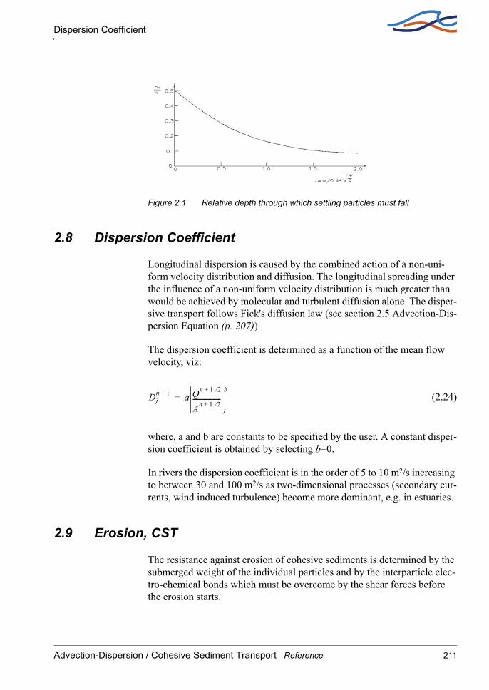
Dispersion Coefficient
Figure 2.1 Relative depth through which settling particles must fall
2.8 Dispersion Coefficient
Longitudinal dispersion is caused by the combined action of a non-uni-form velocity distribution and diffusion. The longitudinal spreading under the influence of a non-uniform velocity distribution is much greater than would be achieved by molecular and turbulent diffusion alone. The disper-sive transport follows Fick's diffusion law (see section 2.5 Advection-Dis-persion Equation (p. 207)).
The dispersion coefficient is determined as a function of the mean flow velocity, viz:
(2.24)
where, a and b are constants to be specified by the user. A constant disper-sion coefficient is obtained by selecting b=0.
In rivers the dispersion coefficient is in the order of 5 to 10 m2/s increasing to between 30 and 100 m2/s as two-dimensional processes (secondary cur-rents, wind induced turbulence) become more dominant, e.g. in estuaries.
2.9 Erosion, CST
The resistance against erosion of cohesive sediments is determined by the submerged weight of the individual particles and by the interparticle elec-tro-chemical bonds which must be overcome by the shear forces before the erosion starts.
Djn 1+ a Qn 1 2⁄+
An 1 2⁄+------------------
j
b=
Advection-Dispersion / Cohesive Sediment Transport Reference 211
AD/CST REFERENCE MANUAL
The rate of erosion has been described by the expression (/16/):
for (2.25)
where S is source term in the advection dispersion equation, τ the bed shear stress, τc,e the critical shear stress for erosion, M* the erodibility of the bed and h the flow depth.
The bed shear stress can be given by, using the Manning formula:
(2.26)
where ρ is the fluid density, g the acceleration of gravity, M the Manning number, h the flow depth, and V the flow velocity.
By substituting Equation (2.25) into Equation (2.26) above, the erosion rate is expressed by:
for (2.27)
where Vc,e is the critical erosion velocity.
2.10 Mass transport and mass balance
The advection/dispersion model computes the concentration of matter in each computational grid point. However, often the transport of matter at a specific location is of more interest. Based on simulated concentrations the total transport (convective and dispersive) is computed at each grid point and the results are stored in a mike11 ‘.res11’ file.
Relating the transport to the change of mass within a control volume at each point a complete mass balance can be established at each time step. The mass balance will automatically reveal any mass error problems.
The AD-mass error is always zero when the conditions below are satis-fied:
The mass error in the hydrodynamic simulation is zero.
SM*
h------- 1 τ
τce------–
= τ τce≥
τ ρg V2
M2h1 3⁄
-----------------=
SM*
h------- 1 V
Vce-------
2–
= V Vce≥
212 MIKE 11
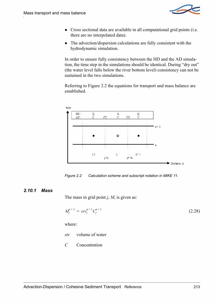
Mass transport and mass balance
Cross sectional data are available in all computational grid points (i.e. there are no interpolated data).
The advection/dispersion calculations are fully consistent with the hydrodynamic simulation.
In order to ensure fully consistency between the HD and the AD simula-tion, the time step in the simulations should be identical. During “dry out” (the water level falls below the river bottom level) consistency can not be sustained in the two simulations.
Referring to Figure 2.2 the equations for transport and mass balance are established.
Figure 2.2 Calculation scheme and subscript notation in MIKE 11.
2.10.1 MassThe mass in grid point j, M, is given as:
(2.28)
where:
stv volume of water
C Concentration
Mjn 1+ stvj
n 1+ Cjn 1+=
Advection-Dispersion / Cohesive Sediment Transport Reference 213

AD/CST REFERENCE MANUAL
2.10.2 1st order DecayThe 1st order decay, D, is calculated as:
(2.29)
where:
K Decay constant (h-1)
F time centring coefficient
The time centering coefficient is given as:
(2.30)
2.10.3 TransportThe total transport is given as the sum of advective and dispersive trans-port into or out of a control volume.
The transport, T, of a component is not calculated in a grid point, but as a transport from one grid point/calculation box to a neighbouring grid point/calculation box, i.e. Tj-½ and Tj+½, see Figure 2.2. However, for pres-entation of the calculated transport in a longitudinal profile, MIKE11 presents Tj+½, at grid point j.
2.10.4 Advective transportThe advective transport, AT, is calculated from the mean value of the dis-charge in two neighbouring control volumes and the concentrations in both boxes. Additionally, the advective transport is corrected with an explicit third order correction term.
(2.31)
Correction term:
(2.32)
Djn 1+ Kj ΦCj
n 1+ 1 Φ–( )Cjn+( )stvj
n 1+=
Φ0,5 0,083Kj∆t+ , for Kj∆t 0,1≤
1Kj∆t-----------– 1
1 eKj∆ t–
–----------------------+ , for Kj∆t 0,1>
=
ATj 1 2⁄+n 1 2⁄+ 1
2--- qj
n 1 2⁄+ qj 1+n 1 2⁄++( ) 1
4--- Cj
n 1+ Cj 1+n 1+ Cj
n Cj 1+n+ + +( ) Corr+
=
Corr Cj 1–n 1 2⁄+ C– j
n 1 2⁄+ Cj 1+n 1 2⁄++( )Corfac=
214 MIKE 11

Mass transport and mass balance
where:
q discharge
and
(2.33)
where σ is the Courant number:
(2.34)
2.10.5 Dispersive transportThe dispersive transport, DT, between two neighbouring control volumes is calculated as follows:
(2.35)
where:
A Area
Diff Dispersion coefficient
2.10.6 Mass balanceThe mass balance, MB, is given as the difference between mass on time n plus all mass transported into the box and mass on time n+1 plus all mass transported out of the control volume:
(2.36)
The total mass balance is given as the sum of all mass balances in the river setup.
corfac
16--- 1 1
2---σ2+
, for σ 1≤
14σ------ , for σ 1>
=
σ u∆t∆x---------=
DTj 1 2⁄+n 1 2⁄+ 1
4--- Aj
n 1+ Aj 1+n 1++( ) Diffj Diffj 1++( )
12--- Cj
n Cj 1+n 1++( )( ) Cj
n Cjn 1++( )–
=
MBjn 1+ Mj
n Mjn 1+
DTj 1 2⁄+n 1 2⁄+ ATj 1 2⁄–
n 1 2⁄+ DTj 1 2⁄–n 1 2⁄+– ATj 1 2⁄+
n 1 2⁄+– LATjn 1 2⁄+ Dj
n 1 2⁄+–+ +( )∆t+–=
Advection-Dispersion / Cohesive Sediment Transport Reference 215

AD/CST REFERENCE MANUAL
2.11 Solution Scheme, AD
The advection-dispersion equation is solved with a fully time and space centred implicit finite difference scheme in order to minimize any artifi-cial (numerical) dispersion. Moreover, it has been ensured that the discre-tization is mass conservative. The finite difference scheme is derived by considering the mass flux into a control volume situated around the grid point j. The boundaries of this control volume are the river bed, the water surface and the two cross-sections situated at j-½ and j+½, respectively, see Figure 2.3.
Figure 2.3 Definition sketch for the control volume.
The two equations considered are the continuity equation and the advec-tive-dispersive transport equation.
2.11.1 Continuity equation:
(2.37)
where C is the concentration, V the storage volume, T the transport through box walls, q the lateral inflow, ∆t the time step, Cq the concentra-tion of lateral inflow source, K the linear decay coefficient, j the grid point and n the time level.
Vjn 1 2⁄+ Cj
n 1+
∆t------------------------------
Vjn 1 2⁄+ Cj
n
∆t------------------------– Tj 1 2⁄+
n 1 2⁄+ Tj 1 2⁄+n 1 2⁄+–+
qn 1 2⁄+ Cqn 1 2⁄+ Vj
n 1 2⁄+ KCjn–=
216 MIKE 11

Solution Scheme, AD
2.11.2 Advective-dispersive transport equation:
(2.38)
where,
is the discharge at the right wall of the box
is the cross sectional area of the right wall
D is the dispersion coefficient
is an upstream interpolated concentration given by:
(2.39)
in which σ is the Courant number (u∆t/∆x). The last term of Equation (2.39) is an explicit third order corrective term.
Substitution and rearrangement of the above equations give a general implicit finite difference equation which relates the concentration in three neighbouring grid points to each other at any time level as:
(2.40)
Unlike the general formulation for water levels and discharges (see Appendix A (p. 421)), the concentrations are defined in each grid point, i.e. non-staggered.
The system of linear equations are solved by the "double sweep" algo-rithm as presented in section 1.30 Solution Scheme (p. 171) and in section A.9 Solution Scheme (p. 461).
Tj ½+n ½+ Qj ½+
n ½+ Cj ½+* Aj ½+
n ½+ DCj 1+
n ½+ Cjn ½+–
∆x-------------------------------–=
Qj ½+n ½+
Aj ½+n ½+
Cj ½+*
Cj ½+* 1
4--- Cj 1+
n 1+ Cjn 1+ Cj 1+
n Cjn+ + +( )
min 16--- 1 σ2
2-----+
14σ------,
Cj 1+n 2Cj
n– Cj 1–n+( )–
=
αjCj 1–n 1+ βjCj
n 1+ γjCj 1+n 1++ + δj=
Advection-Dispersion / Cohesive Sediment Transport Reference 217

AD/CST REFERENCE MANUAL
2.12 Stability
The applied computation scheme in the advection-dispersion model is sta-ble even for large Peclet numbers, ie for:
(2.41)
where,
v is the velocity
∆x is the distance between the computational points
D is the dispersion coefficient.
The space and time step should be selected in such a way that the convec-tive Courant number Cr is less than 1.
(2.42)
Notice that ∆x is the distance between two computational points in the AD computation. MIKE 11 places computational points in the AD scheme in both h- and Q-points, ie ∆x in an AD computation is 0.5 ∆x in the corre-sponding HD computation. Hence if, the time step used in the HD compu-tation criteria has been limited by the velocity criteria, this should be reduced by a factor of two in the succeeding AD computation.
If convective Courant numbers greater than unity appear in the computa-tion, a warning will be displayed. If this warning is ignored more than 5 times, the computation will continue without further warnings. The com-putational results should, in this case, be treated with care, and preferably the computation should be repeated with altered time steps.
2.13 Nomenclature
A cross-sectional area.
C concentration.
Cbf concentration at a model boundary.
Pe v∆xD------ 2>=
Cr v ∆t∆x------ 2<=
218 MIKE 11

Nomenclature
Cout concentration at a model boundary prior to change in the flow direc-tion.
Cq concentration of lateral inflow source.
D dispersion coefficient.
h flow depth.
h* average depth through which particles settle.
I energy slope.
j grid point.
K linear decay coefficient.
Kmix time scale specified in input.
M Manning number.
M* erodibility of the bed.
n time level.
q lateral inflow.
s relative density of sediment.
S source term in advection-dispersion equation.
T transport through control volume walls.
T temperature.
t actual time.
tmix time since flow direction changed.
tup,downtime of sunrise and sunset.
u flow velocity.
V storage volume.
Vc,d critical deposition velocity.
Advection-Dispersion / Cohesive Sediment Transport Reference 219

AD/CST REFERENCE MANUAL
W0 free settling velocity.
WS setting velocity of flocs.
w mean settling velocity of suspended particles.
ρ fluid density.
τ bed shear stress.
τc,d critical shear stress for deposition.
τc,e critical shear stress for erosion.
σ Courant number.
2.14 References
/16/ Ariathurai, R., MacArthur, R.C. & Krone, R.B. (1971): Mathemati-cal Model of Estuarial Sediment Transport. Department of Civil Engineering, University of California at Davis.
/17/ DHI/VKI: River Usk Barrage, Sediment Transport Modelling. June 1990, Volume 2.
/18/ Engelund, F. and Fredsøe, J., 1982. "Hydraulic theory of alluvial rivers", Advances in Hydro Science, Vol. 13, pp. 187-215.
220 MIKE 11

N O N - C O H E S I V E S E D I M E N TT R A N S P O R T
Reference
221

222 MIKE 11

Manual Format
3 NST REFERENCE MANUALThis manual should be used when undertaking sediment transport and/or morphological model applications. It provides a description of aspects which are encountered during the development, calibration and applica-tion of these models. Derivation of resistance and sediment transport rela-tionships are described under the relevant headings. The manual should be used in conjunction with the MIKE 11 User Guide.
Some of the sediment transport formulas and other features of the Non Cohesive Sediment Transport module have been developed in cooperation with CTI Engineering, CO., Ltd., Japan.
3.1 Manual Format
All descriptions in this Chapter are under headings presented in alphabeti-cal order. A list of the headings for this Chapter is given below.
A General Description (p. 224)
Sediment transport models (p. 225)
Bed forms (p. 225)
Morphological model (p. 228)
Graded Sediments (p. 239)
Dune dimensions (p. 244)
Flow Resistance (p. 252)
Incipient motion criteria (p. 259)
Ackers and White model (p. 261)
Ashida & Michiue model (p. 264)
Ashida, Takahashi and Mizuyama model (ATM) (p. 267)
Engelund & Fredsøe model (p. 270)
Engelund & Hansen model (p. 273)
Meyer-Peter & Müller model (p. 275)
Sato, Kikkawa & Ashida model (p. 277)
Smart and Jaeggi model (p. 278)
van Rijn model (p. 280)
Non-cohesive Sediment Transport Reference 223

NST REFERENCE MANUAL
Nomenclature (p. 286)
References (p. 290)
3.2 A General Description
The non-cohesive sediment transport module (NST) can be run in two modes; explicit and morphological. In the explicit mode output is required from the hydrodynamic module (HD) in terms of discharge water levels, (cross-sectional area and hydraulic radius) both in time and space. There is no feedback from the sediment transport calculations to the HD module. Results are in the form of volume transport rates and accumulated vol-umes of deposition or erosion. The explicit mode is useful where signifi-cant morphological changes are unlikely to occur. An estimate of the sediment budget can then be obtained economically with this mode (in terms of computer time).
In the morphological mode sediment transport is calculated in tandem with the HD module. The feedback from the sediment transport calcula-tions to the HD is achieved through solution of the sediment continuity equation and through the updating of the bed resistance and the following sediment transport. Results are in the form of sediment transport rates, bed level changes, resistance number and dune dimensions (depending on the transport relationship adopted). This model requires considerably more computation time than the explicit model but is more representative of the dynamic alluvial processes.
The NST module is equipped with five different models for the calcula-tion of sediment transport rate and alluvial roughness. These are the Enge-lund and Hansen model, the Ackers and White model, and the Smart and Jaeggi model for the calculation of the total load, and the Engelund and Fredsøe and van Rijn models for the calculation of bed load and sus-pended load separately. Branches in the model where no sediment trans-port takes place can be specified as passive branches. All these models can be run using a single representative grain size or using a number of grain sizes representing grain size fractions in graded material as an add-on module. Provision is also made for specifying the geometric standard deviation of the grain size distribution to enable the mean diameter of the suspended bed material to be computed. All the options mentioned above are available in both modes; explicit and morphological.
224 MIKE 11

Sediment transport models
3.3 Sediment transport models
Multiple sediment transport models are available in MIKE 11. These are listed hereunder and described individually in sections below:
Ackers and White model (p. 261),
Ashida & Michiue model (p. 264),
Ashida, Takahashi and Mizuyama model (ATM) (p. 267)
Engelund & Fredsøe model (p. 270),
Engelund & Hansen model (p. 273),
Lane & Kalinske model (p. 274),
Meyer-Peter & Müller model (p. 275),
Sato, Kikkawa & Ashida model (p. 277).
Smart and Jaeggi model (p. 278),
van Rijn model (p. 280),
The selection of transport model for a particular application depends on the nature of the water course under study and on local experience in sedi-ment transport modelling. In the absence of any such knowledge, trial simulations should be carried out with each model to see which gives bet-ter agreement with measurements.
Once the most appropriate transport model has been selected, further adjustments can be made to the predicted transport rates during the cali-bration procedure by the use of the two factors Factor 1 and Factor 2. These are specified in ST parameter editor →Calibration Factors and are used to apply a linear correction factor to the predicted suspended and bed load transport rates, respectively (or to the total load, Factor 1 only).
3.4 Bed forms
The bed of a stream where sediment transport occurs will not generally be flat but will be covered by bed forms belonging to one of the following categories, illustrated in Figure 3.1.
Ripples
Dunes
Non-cohesive Sediment Transport Reference 225
NST REFERENCE MANUAL
Plane bed
Anti-dunes (standing waves - chute and pool)
3.4.1 RipplesRipples are triangular waves with a small wave length (compared to the water depth). Ripples are usually formed in fine sediments at rather low transport rates, while coarse sediments normally form dunes. Ripples are therefore associated with hydraulically smooth beds.
3.4.2 DunesDunes are the most important bed form encountered in river hydraulics and most work on the hydraulic resistance of alluvial rivers has been con-cerned with dune covered beds.
Dunes are large, triangular waves and are long compared to the depth of flow. Dunes are generally irregular and three dimensional.
Both ripples and dunes have a gently curved upstream side and a steep downstream side with a slope close to the angle of repose. At the crest of the bed forms the flow separates and a bottom roller is formed. The forma-tion of ripples and dunes on an originally plane bed has been explained through stability analyses (/26/). Small sinusoidal perturbations of the bed are found to increase with time and the wave length with the highest amplification corresponds to the wave length of the emerging bed waves.
226 MIKE 11

Bed forms
Figure 3.1 Development of bed forms for increasing flow velocity
3.4.3 Plane bedThe stability analyses have shown that, in the case of a high suspended load, a plane bed will remain stable. This is due to the lag between the local hydraulic conditions and the suspended load.
3.4.4 Anti-dunesAnti-dunes appear when the perturbation of the water surface is in phase with the bed perturbations. This occurs when the Froude number, F, exceeds the limit for critical flow:
(3.1)
where,
k is the wave number of the bed forms
D is the water depth.
F kD( )tanhkD
----------------------->
Non-cohesive Sediment Transport Reference 227

NST REFERENCE MANUAL
Anti-dunes are nearly sinusoidal bed waves which generally move upstream. The water surface is also sinusoidal, in phase with the bed waves and with a larger amplitude.
The anti-dunes may vary in a cyclic manner, growing until breaking of the surface wave occurs, after which they are washed out and new, small ones form again.
3.5 Morphological model
The morphological model updates the bed level due to erosion or deposi-tion using the continuity equation for sediment transport. The model updates the level of the entire cross-section or only a part of it (normally representing the river channel) and leaving the bottom level of the remain-ing part of the cross-section (normally representing the flood plains) unchanged. The model distinguishes between the river channel and flood plain using a divide level specified in the cross-section editor, i.e. levels in the cross-section below this divide level are assumed to belong to the river channel. It is possible to specify a specific flood plain resistance (in the HD editor under the flood plain resistance tab) to be used on the flood plain above the level of divide. Note that this facility is only implemented when running the hydrodynamic module and the sediment transport mod-ules coupled i.e. in the morphological mode.
Various possibilities for morphological changing of the cross-section shape is available. If a divide level has been specified only the river chan-nel is updated, which implies that sediment transport only takes place in the river channel.
The sediment transport is calculated on the basis of flow velocity (u), depth (D) and transporting width (Wt) and is obtained in the following way:
(3.2)
(3.3)
(3.4)
where,
uQc
Ac------=
D Rc=
WtAc
Rc-----=
228 MIKE 11
Morphological model
Q is discharge
A is cross-sectional area
R is resistance radius
and subscript c refers to the river channel values. If the cross-sections are not divided into river channel and flood plain components the correspond-ing values for the entire cross-section are used.
Assuming that the friction slope is constant across the free water surface width the discharge in the river channel can be expressed as:
(3.5)
where,
M is Manning roughness coefficient
C is Chezy roughness coefficient
Rt composite resistance radius
Mt composite Manning roughness coefficient
Ct composite Chezy roughness coefficient
Qc Qt
McRc2 3⁄ Ac
MtRt2 3⁄ At
------------------------ Manning No.
CcRc1 2⁄ Ac
CtRt1 2⁄ At
----------------------- Chezy No.
=
Non-cohesive Sediment Transport Reference 229

NST REFERENCE MANUAL
The three latter are given by
(3.6a)
(3.6b)
(3.6c)
Where subscript t refers to the entire cross-section, c to the river channel part and f to the flood plain part.
The sediment continuity equation is solved at h-points using a Preissmann Scheme.
(3.7)
where,
W width of the river channel or entire cross- section, defined as the width of the cross-section at the calculated water surface
∆zn+1 change of bottom level.
= .
sediment transport rate per unit width.
ε porosity of sediment.
ψ space centring coefficient ( ) (PSI: ST parameter editor → Transport Model).
θ time centring coefficient ( ) (FI: ST parameter editor → Transport Model).
RtRcAc RfAf+
At-------------------------------------
2
=
MtMc RcAc Mf RfAf+
RtAt
---------------------------------------------------=
CtCc RcAc Cf RfAf+
RtAt
-------------------------------------------------=
1 ε–( ) 1 ψ–( )W∆zj
n 1+
∆t-------------------- ψ
W∆zj 1+n 1+
∆t--------------------+ θ
Qtj 1+n 1+ Qtj
n 1+–∆x
------------------------------------
1 θ–( )Qtj 1+
n Qtjn–
∆x-----------------------------
+
+ 0=
Qtjn Wtqtj
n
qtjn
0,5 ψ 1≤ ≤
0,5 θ 1≤ ≤
230 MIKE 11

Morphological model
The transport at t = (n+1)∆t is approximated by:
(3.8)
or introducing the term α
(3.9)
where,
u is flow velocity
D is flow depth
and are, by default, calculated assuming locally steady flow (back water curve).
Further, it is possible to select:
and (3.10)
(ST parameter editor →Transport Model →dH/dz switch), which is an acceptable approximation in strongly unsteady (tidal) flow.
and are obtained by numerical differentiation, e.g.:
(3.11)
or
(3.12)
where,
(3.13)
Qtjn 1+ Qtj
n ∂Qt∂u
---------∂u∂z------ ∂Qt
∂D---------∂D
∂z-------+
j∆zj
n 1++=
Qtjn 1+ Qtj
n α∆zjn 1++=
∂u ∂z⁄ ∂D ∂z⁄
∂D∂z------- 1–= ∂u
∂z------D
u---- +1=
∂Qt ∂zu⁄ ∂Qt ∂D⁄
∂Qt∂u
--------- Qt u ∆u D,+( ) Qt u D,( )–∆u
---------------------------------------------------------------≈
∂Qt∂u
--------- Qt u fac D( ) Qt u D,( )–ufac u–
-------------------------------------------------------≈
fac u ∆u+u
----------------=
Non-cohesive Sediment Transport Reference 231

NST REFERENCE MANUAL
and may be set in ST parameter editor →Transport Model → Fac.
3.5.1 Updating of bottom levelVarious assumptions regarding the change in bathymetry of a cross-sec-tion during erosion and deposition can be made. In some cases sediment will accumulate in the deepest parts of the cross-section before deposition occurs closer to the bank (e.g. in a reservoir behind a dam). For tidal estu-aries another deposition pattern with pronounced deposition along the banks can occur. Such considerations are necessary when the results from the MIKE 11 morphological model are interpreted, as the model is only one-dimensional. However, the MIKE 11 provides different options, see below, for how to update the bottom level. The appropriate model should be chosen based on engineering judgement.
Instead of solving equation (3.7) with respect to ∆zn+1, the change in cross-sectional area ∆A is calculated, ∆An+1 = W∆zn+1. The cross-section is subsequently updated (i.e. the processed cross-sectional data tables used in the computation are changed) in one of the following ways, see below and Figure 3.2.
In the following model descriptions subscript i refers to the levels in the processed data table. Subscript k in model 1 refers to the level in the proc-essed data table where the area is larger than the change in cross-section area ∆A.
Model 1 - Deposition in horizontal layers.
Erosion as model 5:
Levels:
(3.14)
Widths: unchanged
zin 1+ zk
n 1+ ∆A Akn–
wk 1+ wk–------------------------ for zi
n zkn
Akn ∆A Ak 1+
n
zin 1+
<<
≤+
zin for zi
n zkn>
=
=
232 MIKE 11

Morphological model
Areas:
(3.15)
Hydraulic radii:
(3.16)
Model 2 - Deposition and erosion uniformly distributed below the water surface. No deposition and erosion above:
Levels:
(3.17)
Widths: unchanged
Areas:
(3.18)
Ain 1+ = 0 for zi
n zkn≤
Ain 1+ = Ai
n ∆A– for zin zk
n>
Rin 1+ = 0 for zi
n zkn≤
Rin 1+ =
zin 1+ zj
n 1+–( )3 2⁄
∆Wj
j 1=
i
∑
Ain 1+
------------------------------------------------------------
2
for zin zk
n>
zin 1+ zi
n ∆Awsurface------------------ for zi
n h≤+=
Wsurface= width of cross section at water surface level h
zin 1+ zi
n for zin h>=
Ain 1+ = Ai
n for zin h≤
Ain 1+ = Ai
n ∆A– for zin h>
Non-cohesive Sediment Transport Reference 233

NST REFERENCE MANUAL
Hydraulic radii:
(3.19)
Model 3 - Deposition and erosion proportional with depth below water surface. No deposition and erosion above:
Levels:
(3.20)
Widths: unchanged
Areas:
(3.21)
Hydraulic radii:
(3.22)
Rin 1+ = Ri
n for zin h≤
Rin 1+ =
zin 1+ zj
n 1+–( )3 2⁄
∆Wj
j 1=
i
∑
Ain 1+
------------------------------------------------------------
2
for zin h>
α = ∆AAsurface
n------------------
zin 1+ zi
n α h zih–( ) for zi
n h≤+=Asurface= area of cross-section at water surface level h
zin 1+ zi
n for zin h>=
Ain 1+ = 1 α–( )Ai
n for zin h≤
Ain 1+ = Ai
n ∆A– for zin h>
Rin 1+ = 1 α–( )Ri
n for zin h≤
Rin 1+ =
zin 1+ zj
n 1+–( )3 2⁄
∆Wj
j 1=
i
∑
Ain 1+
------------------------------------------------------------
2
for zin h>
234 MIKE 11

Morphological model
Model 4 - Deposition and erosion uniformly distributed over the whole cross-sec-tion (i.e. below the bank level):
Levels:
(3.23)
Widths: unchanged
Areas:
(3.24)
Hydraulic radii:
(3.25)
Model 5 - Deposition and erosion proportional with depth below bank level (top level):
Levels:
(3.26)
Widths: unchanged
Areas:
(3.27)
zin 1+ zi
n ∆Awtop----------+=
wtop= width of cross-section at the top level zmax
Ain 1+ Ai
n=
Rin 1+ Ri
n=
α = ∆AAtop
n---------
zin 1+ zi
n α h zih–( )+=
Atop= area of cross-section at top level zmax
Ain 1+ 1 α–( )Ai
n=
Non-cohesive Sediment Transport Reference 235

NST REFERENCE MANUAL
Hydraulic radii:
(3.28)
Figure 3.2 Update of bed level in MIKE 11 morphological model
3.5.2 Boundary ConditionsThe unknown variable in the finite difference scheme is Z. This becomes evident by substituting Equation (3.15) into Equation (3.14). Boundary conditions should therefore be given in terms of bed level variation, although a sediment transport boundary condition can also be given. In this case Equation (3.20) is normally used to determine ∆Z with replaced by the boundary sediment transport. However, when there is a serious imbalance at the boundary point, i.e. when alpha is small and
this formulation may give rise to numerical stability problems. In this case the difference between the transport specified at the boundary and the calculated transport at the in-flow point (first or last grid point
Rin 1+ 1 α–( )Ri
n=
Qtn 1+
Qtbnd Qtn»
236 MIKE 11
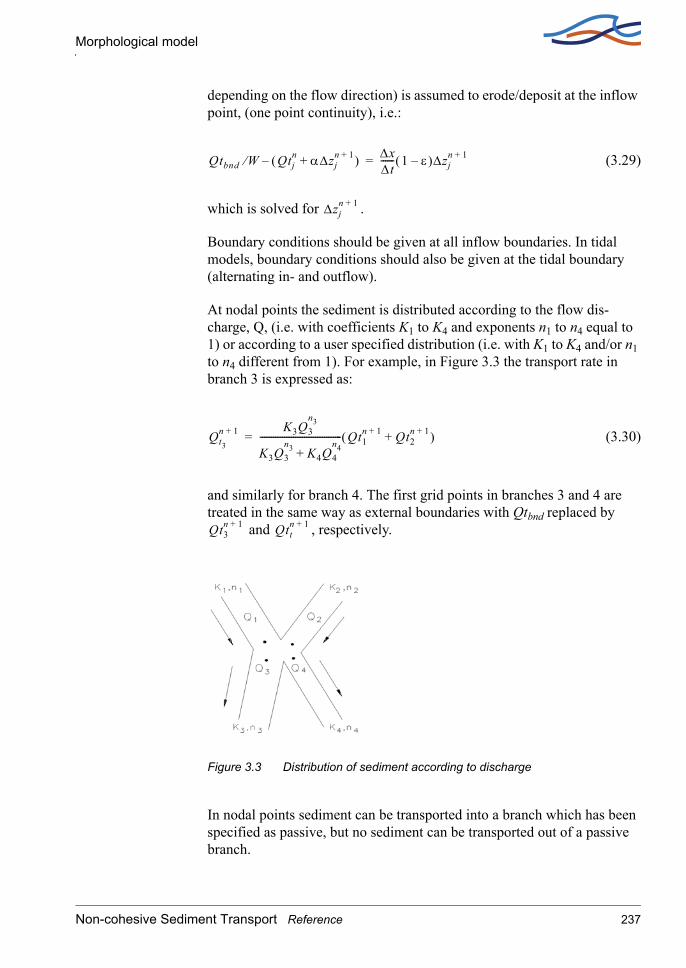
Morphological model
depending on the flow direction) is assumed to erode/deposit at the inflow point, (one point continuity), i.e.:
(3.29)
which is solved for .
Boundary conditions should be given at all inflow boundaries. In tidal models, boundary conditions should also be given at the tidal boundary (alternating in- and outflow).
At nodal points the sediment is distributed according to the flow dis-charge, Q, (i.e. with coefficients K1 to K4 and exponents n1 to n4 equal to 1) or according to a user specified distribution (i.e. with K1 to K4 and/or n1 to n4 different from 1). For example, in Figure 3.3 the transport rate in branch 3 is expressed as:
(3.30)
and similarly for branch 4. The first grid points in branches 3 and 4 are treated in the same way as external boundaries with Qtbnd replaced by
and , respectively.
Figure 3.3 Distribution of sediment according to discharge
In nodal points sediment can be transported into a branch which has been specified as passive, but no sediment can be transported out of a passive branch.
Qtbnd W⁄ Qtjn α∆zj
n 1++( )– ∆x∆t------ 1 ε–( )∆zj
n 1+=
∆zjn 1+
Qt3n 1+ K3Q3
n3
K3Q3n3 K4Q4
n4+------------------------------------- Qt1
n 1+ Qt2n 1++( )=
Qt3n 1+ Qtt
n 1+
Non-cohesive Sediment Transport Reference 237
NST REFERENCE MANUAL
3.5.3 Low flow correctionWhen the water level becomes less than a certain threshold value (delh, given in HD parameter editor → Default Values) the hydrodynamic model introduces an artificial slot, see Chapter 1 HD Reference manual (p. 19). In this case the calculated velocity may have a rather arbitrary value, which may give rise to unrealistically large sediment transport rates. This problem has been solved by multiplying the calculated transport rate with a reduction factor f given by:
(3.31)
3.5.4 HintsThe Preissmann scheme is well suited to the solution of hyperbolic prob-lems with only one characteristic. However, it has a drawback. At small Courant numbers it may generate short wave oscillations (wave length 2∆x). The oscillations can be damped by space forward centring the scheme (i.e. by using a large value of y). This, however, will give rise to numerical dispersion at high Courant numbers. At a later stage an option for automatic selection of the optimum value of y will be incorporated, i.e. the value which just prevents the short wave oscillations.
The factor fac used in the numerical differentiation of the sediment trans-port formula should not be made too small because this will give rise to ‘overshoot´ phenomena in the numerical solution. A value of about 1.5 will be on the safe side in most cases unless very strong gradients occur.
The sediment transport Courant number can be approximated by
(3.32)
This implies that the morphological model can run with a much larger time step than the dynamic flow model and that a quasi-steady flow simu-lation will be sufficiently accurate, (see also de Vries, 1981, /40/). Often the time step will be limited only by the ability to resolve the boundary conditions.
f
0 D delh≤D delh–( )
D-------------------------- delh D 2delh≤<
1 2delh D<
=
Cr 5 ∆t∆x------
qt
D---- 1
1 ε–-----------=
238 MIKE 11

Graded Sediments
3.6 Graded Sediments
An add-on module is available for model applications in non-uniform sed-iments in which the sediment transport can be calculated by fraction and the variation in time and space of the particle size distribution determined. As a general guideline the graded sediment module should be used where the bed shear stress is close to the critical value for erosion. Where the bed shear is much greater than the critical value then using a single representa-tive grain size is acceptable.
The simulation of graded sediment transport is an option available in the morphological mode (see section 3.5 Morphological model (p. 228)) and for each of the 5 sediment transport formulae (see section 3.5.1 Updating of bottom level (p. 232)).
For the simulation of graded sediments and sediment sorting the bed mate-rial is considered to comprise two layers; an active layer overlying a pas-sive layer. This is illustrated in Figure 3.4. The active layer is the layer within which the bed load transport takes place and its depth (Za) is defined as one half of the dune height.
The dune height is predicted according to the selected transport model type, viz.:
Engelund-Hansen
Ackers and White
Engelund-Fredsøe
Smart and Jaeggi
Meyer, Peter and Muller
Sato, Kikkawa and Ashida
Ashida and Michiue
Ashida, Takahashi and Mizuyama (ATM)
where (3.33)
van Rijn
(3.34)
HR---- 2 I
2 I+----------- I 1
3--- 1
θcθ′-----–
=
HR----0,11
dmedR
----------
0,31 exp
u′fuf------
2
1––
26u′fuf------
2
–
Non-cohesive Sediment Transport Reference 239

NST REFERENCE MANUAL
where,
H is the dune height and θ´ and u´f are calculated as described under the appropriate transport-model section.
For decreasing dune height (i.e. decreasing bed shear stress) the minimum dune height is specified by the user.
If erosion of the bed material occurs, the composition of the material in the passive layer (Z-Za) stays the same. However, if deposition occurs active bed material is (instantaneously) mixed with the material in the passive layer and the composition is modified accordingly.
The additional input data required to simulate the transport of graded sedi-ment are the initial percentage size distributions of both the active (Pa) and passive (Pbed) layer (they may have the same distribution initially). The data are specified as a number of fractions, N (referred to by subscript i for class-number), which remain fixed, and the corresponding percentage and mean grain size for the fraction. This percentage varies as sediment is transported selectively and mixed between the layers.
Figure 3.4 Active and passive sediment layers for the simulation of graded sed-iments
The transport and mixing of graded sediments is simulated in the follow-ing manner. The sediment transport is calculated for each specified class size separately. The calculation is modified in two ways from the calcula-tion of a uniform material. Firstly, the criterion for the threshold of move-ment(θc or A in the Ackers and White Model) is modified to allow for the
Zan 1+ 0,5 H=
240 MIKE 11

Graded Sediments
hiding of finer particles and the greater exposure of larger particles as well as the mutual interference between particles of different size. θc is modi-fied by applying Egiazaroff's (1965),/23/, correction factor as follows:
(3.35)
where,
is the dimensionless critical bed shear stress for class i
is the dimensionless critical bed shear stress for a uniform sediment
dmed is the mean grain size of the total sediment population
For the Ackers and White Model, the modified value of A is expressed as follows:
(3.36)
where,
Ai is the critical flow mobility number for class i
A is the critical flow mobility number for a uniform sediment
The second modification is to multiply each class sediment transport, qti, by its percentage contribution, pi. After the transport rate in each class has been calculated, the total transport, qt, is determined by summation over all classes, N:
(3.37)
The sediment continuity equation is then solved in the same way as for a uniform sediment using the total transport to obtain the change in bed level, ∆z. Once ∆z is known the sediment continuity equation is solved for each class size using the class transport rate, qti, and the total bed level
θciθc
ln 19( )
ln19 didmed----------
---------------------
2
=
θci
θc
Ai Adi
dmed----------
0,2–
=
qt qtipi
i 1=
N
∑=
Non-cohesive Sediment Transport Reference 241

NST REFERENCE MANUAL
change,∆z, to obtain the new percentage contribution of the active layer, pi. The following relationships are applied:
The sediment continuity equation for each fraction may be expressed as:
(3.38)
where,
ε is sediment porosity
W is channel width
is the average proportion of class i in both passive and active layer (i.e. over depth Z)
Expanding the first term of Equation (3.38) gives:
(3.39)
in which the time derivatives are expressed by:
(3.40)
and similarly for time level n (subscript i has been removed for conven-ience).
The composition of the material in the passive layer at time level n+1 depends on whether the interface between the active and passive layer moves up or down and is expressed by:
(Erosion):
(3.41)
implying that the passive layer is assumed to be totally mixed.
1 ε–( )∂WpiZ
∂t----------------
∂qti∂x
---------+ 0=
piZ
1 ε–( )∂WpiZ
∂t---------------- 1 ε–( )
∂WpiZ∂t
----------------
jΨ
∂WpiZ∂t
----------------
j 1–1 Ψ–( )+=
pZn 1+
pan 1+ Za
n 1+ pbedn 1+ Zn 1+ Za
n 1+–( )+=
Zn 1+ Zan 1+–( ) Zn Za
n–( )≤
pbedn 1+ pbed
n=
242 MIKE 11
Graded Sediments
(Deposition):
(3.42)
The symbols used in the above expressions are as shown in Figure 3.4.
Similarly, a weighted time average is used to expand the space derivative in the transport term in Equation (3.38).
where, is approximated by:
(3.43)
(3.44)
and
(3.45)
and is calculated for each fraction.
The above expressions, ((3.39) to (3.45)), are solved for the unknowns pa and pbed at time level n+1.
3.6.1 Boundary conditionsThe unknown variable in the finite difference scheme is pi. Boundary con-ditions should therefore be given in terms of fraction values for each frac-tion and bed levels. Boundary conditions can also be specified as fraction sediment transport rates (either defined by a time series file or by defining the sediment supply boundary type). In the case of a fraction sediment transport boundary, Equation (3.44) is normally used to determine with replaced by the boundary sediment transport Qibnd/W. If there is a serious imbalance at the boundary point, i.e. when alpha is small and
Zn 1+ Zan 1+–( ) Zn Za
n–( )>
pbedn 1+ Zn 1+ Za
n 1+–( ) pbedn 1+ Zn Za
n–
12--- pa
n 1+ pan+( ) Zn 1+ Za
n 1+–( ) Zn Zan–( )–[ ]+
=
qtin 1+
∂qti
∂x---------
qti j, qti j 1–,–∆x
-------------------------------1 θ–( ) qti j,
n qti j 1–,n–( )
∆x---------------------------------------------------
θ qti j,n qti j 1–,
n–( )∆x
----------------------------------------+= =
qtin 1+ pai
n 1+ qtn 1+ pai
n qtn 1+– qtin ∆Zn 1+ αi+ +=
αi∂qti∂u
---------∂u∂z------
∂qti∂D---------∂D
∂z-------+=
pai
n 1+
qtin 1+
Non-cohesive Sediment Transport Reference 243

NST REFERENCE MANUAL
, numerical instabilities may occur. In this case a one point con-tinuity equation is solved, i.e.:
(3.46)
The boundary condition is given by the summation of all the fraction sedi-ment boundaries:
(3.47)
3.6.2 Graded sediments boundary conditionsIn the case where Qtbnd=0, i.e. there is no transport of any fraction across the boundary, all the fraction proportions are automatically set to zero except for the most coarse fraction which is set to 1.
The distribution of sediment at nodal points is determined as described below in section 3.5 Morphological model (p. 228).
3.7 Dune dimensions
3.7.1 Equilibrium dune heightWith the model presented by Fredsøe (1979) /30/, /31/ the equilibrium dune height can easily be found as a function of θtop (the dimensionless shear stress taken at the top of the dune).
Figure 3.5 Definition sketch
Qibnd Qtin»
QibndW
------------- qin 1+– ∆x
∆t------ 1 ε–( )∆ PiZ( )=
Qtbnd Qibnd
i 1=
N
∑=
244 MIKE 11

Dune dimensions
The friction factor is assumed to be constant near the dune top. This means that the local dimensionless shear stress, θ, is proportional to the velocity squared:
(3.48)
where,
D is water depth
z is local dune height
H is total dune height
q is flow discharge per unit width
In the case of small transport rates, i.e. bed load only, the local sediment transport can be expressed as a function of θ:
(3.49)
The spatial variation of Φb near the top of the dune is expressed by:
(3.50)
where,
z is the local height of the dune.
The migration velocity of the dune, c, is calculated under the assumption that all of the bed load transport is deposited on the lee side of the dune:
(3.51)
where,
ε = the porosity of the bed material
θ θtopq2
D z–( )2------------------- D H–( )2
q2--------------------- θtop
1 H D⁄–( )2
1 z H⁄–( )2----------------------------= =
Φb Φb θ( )=
∂Φb∂x
----------top
∂Φb∂θ
----------θ θtop=
∂θ∂x------ ∂Φb
∂θ----------
θ θtop=θtop
21 H D⁄–---------------------∂ z D⁄( )
∂x------------------
top= =
cqb
1 ε–( )H---------------------=
qb Φb s 1–( )gd3=
Non-cohesive Sediment Transport Reference 245

NST REFERENCE MANUAL
The change in the bed level near the dune top (on the upstream side) can be expressed as:
(3.52)
using the continuity equation for sediment:
(3.53)
Equations (3.50) and (3.52) can be related to each other as follows:
(3.54)
or as:
(3.55)
Equation (3.55) expresses the equilibrium height of the dunes in the case of pure bed load. At the dune top in which case Equation (3.55) does not apply. However, the equation must still hold a short dis-tance upstream of the top where the local dune height is almost equal to H.
The influence from the suspended loadIf the sediment transport consists of both bed load and suspended load the equations are modified as follows:
The total sediment transport (Φt = Φb + Φs) is still assumed to be a function of the local bed shear stress: Φt = Φt (θ')
Φb is replaced by Φt in Eq. (3.50)
θb is retained in Equations (3.50) and (3.52) as it is assumed that only the bed load is deposited at the lee side of the dune
∂z∂t----- c∂z
∂x-----–
qb
1 ε–( )H---------------------∂z
∂x-----–= =
∂z∂t----- 1
1 ε–-----------
∂qb∂x--------–=
∂Φb
∂θ----------
θ θtop=
2θtop
1 H D⁄–---------------------∂ z D⁄( )
∂x------------------
top
Φb
H D⁄------------∂ z D⁄( )
∂x------------------
top=
H D⁄1 ½H D⁄–--------------------------
Φb
2θ∂Φb
∂θ----------
-----------------
top
=
∂z ∂x⁄ 0=
246 MIKE 11
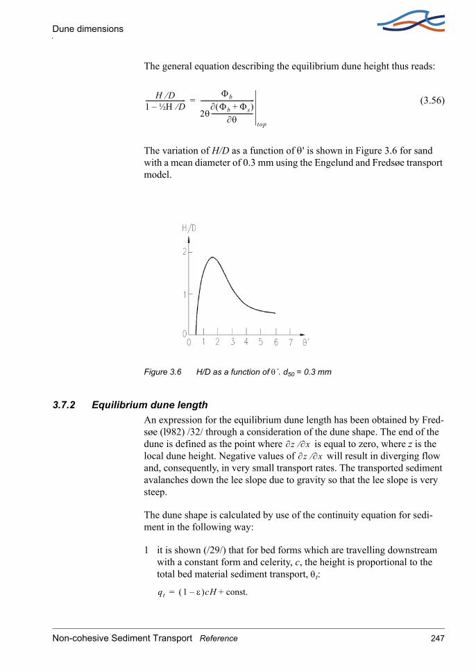
Dune dimensions
The general equation describing the equilibrium dune height thus reads:
(3.56)
The variation of H/D as a function of θ' is shown in Figure 3.6 for sand with a mean diameter of 0.3 mm using the Engelund and Fredsøe transport model.
Figure 3.6 H/D as a function of θ´. d50 = 0.3 mm
3.7.2 Equilibrium dune lengthAn expression for the equilibrium dune length has been obtained by Fred-søe (l982) /32/ through a consideration of the dune shape. The end of the dune is defined as the point where is equal to zero, where z is the local dune height. Negative values of will result in diverging flow and, consequently, in very small transport rates. The transported sediment avalanches down the lee slope due to gravity so that the lee slope is very steep.
The dune shape is calculated by use of the continuity equation for sedi-ment in the following way:
1 it is shown (/29/) that for bed forms which are travelling downstream with a constant form and celerity, c, the height is proportional to the total bed material sediment transport, θt:
H D⁄1 ½H D⁄–--------------------------
Φb
2θ∂ Φb Φs+( )
∂θ---------------------------
-----------------------------------
top
=
∂z ∂x⁄∂z ∂x⁄
qt 1 ε–( )cH const.+=
Non-cohesive Sediment Transport Reference 247

NST REFERENCE MANUAL
where,
H is the dune height
ε is porosity
If only bed load, θb, is considered, the transport is zero in the troughs and the constant is, therefore also zero. Thus:
(3.57)
2 Fredsøe (l982) /32/ calculated the bed load along the dune through a description of the local dimensionless bed shear stress, θt, taken to be proportional to the local mean velocity squared, and a function, f, of the distance from the downstream dune front:
(3.58)
where,
L is the dune length
D is the flow depth.
The function, f, is assumed to be general, regardless of the shape and size of the dune. The bed load transport along the dune is calculated by use of a bed load formula. The effect of gravity on the bed load, θb, is taken into account by adding to θ the correction:
giving (3.59)
where, Φb is the dimensionless bed load transport.
qt 1 ε–( )cH=
θ θt1 H D⁄–( )2
1 z D⁄–( )2---------------------------- f x H⁄( )
f L H⁄( )------------------=
0,1∂z∂x-----– q s 1–( )gd3Φb θ 0,1∂z
∂x-----–
=
248 MIKE 11

Dune dimensions
By combining Equations (3.57) and (3.58) a differential equation describing is found. The dune shape and length is found from the boundary conditions:
for (3.60)
The function, f, has a maximum at x = 17 H so this is the length of the dune if the effect of gravity and suspended load is neglected. For small θt values, however, the effect of gravity is important and causes the dune length to be larger than 17 H.
As indicated above, the calculations are rather laborious and, therefore, the following approximation is suggested for the ratio between the dune height and length for bed load transport only:
(3.61)
where,
θ is the dimensionless bed shear stress
θc is the critical value
Influence of Suspended LoadThe sediment transport has its maximum at the dune crest, see Equation (3.57). The bed load is a function of the local bed shear stress so that the dune crest is the position with maximum bed shear stress in the case of bed load only.
The suspended load is not a function of the local bed shear stress. A spa-tial lag, δ, exists between the hydraulic parameters and the suspended load because it takes some time for the suspended particles to settle or to be picked up from the bed. The lag is given by:
(3.62)
∂z ∂⁄ x
∂z∂x----- = 0
z = H
x L=
HL---- 0,06 146 0,15 θc θ–+( )4,26– for θ 0,15 θc+<
0,06 for 0,15 θc θ≤+
=
δεub
w2--------=
Non-cohesive Sediment Transport Reference 249
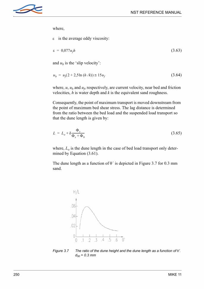
NST REFERENCE MANUAL
where,
ε is the average eddy viscosity:
(3.63)
and ub is the ‘slip velocity’:
(3.64)
where, u, ub and uf, respectively, are current velocity, near bed and friction velocities, h is water depth and k is the equivalent sand roughness.
Consequently, the point of maximum transport is moved downstream from the point of maximum bed shear stress. The lag distance is determined from the ratio between the bed load and the suspended load transport so that the dune length is given by:
(3.65)
where, Lo is the dune length in the case of bed load transport only deter-mined by Equation (3.61).
The dune length as a function of θ´ is depicted in Figure 3.7 for 0.3 mm sand.
Figure 3.7 The ratio of the dune height and the dune length as a function of θ'. d50 = 0.3 mm
ε 0,077ufh=
ub uf 2 2,5ln h k⁄( )+( ) 15uf≅=
L Lo δΦs
Φs Φb+-------------------+=
250 MIKE 11

Dune dimensions
3.7.3 Non-equilibrium dune heightThe rate of change of the dune height has been analysed by Fredsøe (1979), /30/, /31/. It can be described by the equations used to calculate the equilibrium dune height.
The rate of change of the bed level z near the dune top is expressed as:
(3.66)
where the celerity of the dune front is
(3.67)
where, qbt is the transport rate at the dune top, ε is the sediment porosity and is found from the equation of continuity:
(3.68)
Equations (3.66), (3.67) and (3.68) yield:
(3.69)
In order to obtain a value of the change of the dune height which is repre-sentative for most of the dunes, the ‘integrated´ value for : H/L is used in Equation (3.69) leading to:
(3.70)
3.7.4 Non-equilibrium dune lengthAt present no satisfactory theory for the change of dune length exists. The dune length is of less importance for the hydraulic resistance than the dune height, so an approximate description will suffice.
A possible definition of the dune length is the total length of a river reach divided by the number of dunes in that reach. By that definition, the dune
∂c∂t----- c∂z
∂x-----– dz
dt-----+=
cqbt
1 ε–( )H---------------------=
∂z ∂t⁄
∂z∂t----- 1–
1 ε–-----------
∂ qb qs–( )∂x
------------------------top
1–1 ε–-----------
∂ qb qs–( )∂θ
------------------------top
2θtop1 H D⁄–--------------------- ∂z
∂x-----= =
dHdt------- 1
1 ε–-----------∂z
∂x-----
φb
H----- ∂ φb φs–( )
∂θ------------------------
top
2θtop
D H–-------------- s 1–( )gd3–=
∂z ∂x⁄
dHdt------- s 1–( )gd3
1 ε–-----------------------------1
L--- φb
2θtop
D H⁄ 1–---------------------
∂ φb φs–( )∂θ
------------------------top
–=
Non-cohesive Sediment Transport Reference 251

NST REFERENCE MANUAL
length can (under uniform conditions) only be changed, if dunes disappear or new ones are created. Consequently, it seems reasonable to include the average life time of a dune in the expression for dL/dt. A plausible assumption is that the average lifetime T1 of the dunes can also be used as the time scale for the change in dune length:
(3.71)
where, Le is the equilibrium dune length. A stability analysis shows that, if the position of the dune front of a single dune in a row of regular dunes in equilibrium is perturbed, the celerity of the dune c will be reduced regard-less of whether the dune front has been advanced or retarded. This implies that the dunes are unstable. If the dune front is retarded, the dune will be overtaken by the following dune.
The time required for this process has been estimated from the calculated celerity of the dune when the length has been reduced to Le/2. This celerity is about 85-90% of the celerity of the equilibrium dunes. It has, therefore, been estimated that the dune will move a distance of the order of magni-tude l0 Ls before it is overtaken. T1 is thus approximately l0 Le/c, yielding:
(3.72)
where, ε is the sediment porosity.
3.8 Flow Resistance
The calculation of the flow resistance is far more complex in the case of an alluvial river than in the case of a channel with a fixed bed. This is because a large part of the hydraulic resistance in the alluvial case may be caused by a form drag on the bed forms whose configuration is deter-mined by the sediment transport and the flow. The most important bed forms in natural streams are dunes and the flow resistance in the case of a plane bed or a dune covered bed is treated in 3.8.1 Flow resistance - dune dimension (p. 253) and Flow Resistance - q-q´ Relationship (p. 254). For flow resistance according to White et al., see section 3.8.3 Flow Resist-ance - White et al. (p. 257).
dLdt------
L Le–T1
--------------=
dLdt------
L Le–T1
-------------- c L
Le----- 1–
qb1
10 1 ε–( )H---------------------------= =
252 MIKE 11

Flow Resistance
3.8.1 Flow resistance - dune dimensionIf the dimensions (height and length) of the dunes are known, the hydrau-lic resistance (bed shear stress) can be calculated from the water depth and the specific discharge. Furthermore, the portion of the dimensionless bed shear stress, θ´, which is acting as skin friction on the gently curved upstream side of the dunes can be determined.
The total bed shear stress, τ, is split up into the skin friction, τ´, and a por-tion which is caused by the form drag on the dunes τ´´:
(3.73)
τ´´ is mainly caused by the expansion loss behind each dune and can therefore be described as Carnot losses (/29/):
(3.74)
where,
H is the total dune height
D is the flow depth
L is dune length
α is the velocity distribution coefficient which is close to one
u is current velocity
θ the discharge per unit width
Thus, the dimensionless shear stress, θ, can be written as:
(3.75)
θ´ is by definition:
(3.76)
τ τ′ τ″+=
τ″ρ----- αq2D
2L-------------- 1
D---- 1
D H+---------------–
2 αu2H2
2DL----------------≈≈
τs 1–( )ρgd
-------------------------- θ θ′ αu2H2
2 s 1–( )gdDL----------------------------------+= =
θ′ump′f
2
s 1–( )gd----------------------=
Non-cohesive Sediment Transport Reference 253

NST REFERENCE MANUAL
and uf´ can be found from the boundary layer equation:
(3.77)
where,
D´ is the boundary layer thickness (/29/)
k is the equivalent sand size
(3.78)
The four equations can be solved in a few iterations, starting with (3.77), then (3.11.4), (3.75), and (3.78). See also section 3.8.2 Flow Resistance - q-q´ Relationship (p. 254).
3.8.2 Flow Resistance - θ−θ´ RelationshipWhen the bed is covered by bed forms, the total bed shear stress, τ, can be divided into two parts, τ´ and τ´´.
τ´ is the shear stress acting on the gently curved upstream surface of the dunes, and τ´´ is caused by the form drag on the dunes.
Engelund (1966) found, by applying a principle of similarity, that a rela-tionship exists between the dimensionless total bed shear stress, θ, and the dimensionless skin friction, θ´, Figure 3.8. The relationship for a dune covered bed can be approximated by:
(3.79)
where,
and
ρ is the density of water, s is the specific gravity of the bed material, d is the mean grain size of the bed material and g is the acceleration of gravity.
uu′f------ 2,5 ln 30D′
k------------( ) 1–=
D′ Dθ′θ----=
θ′ 0,4θ2 0,06+=
θ τ ρ⁄s 1–( )gd
----------------------= θ′ τ′ ρ⁄s 1–( )gd
----------------------=
254 MIKE 11

Flow Resistance
In the case of a plane bed, the form drag becomes zero and the relationship reads:
(3.80)
The relationship given in Equation (3.79) has been determined from flume observations. However, due to discontinuities in natural rating curves where two water levels may exist for a single discharge, there are two pos-sible solutions to Equation (3.79) rendering it unsuitable for computer modelling. To overcome this problem, Challet and Cunge (1980),/21/ pro-posed a modified θ-θ´ relationship as shown below. This is the formula-tion used in MIKE 11.
for
for
for
for
for
The flow over the ‘smooth’ upstream side of the dune can be described by the boundary layer equation:
(3.81)
u is the mean flow velocity, , D´ is the boundary layer thick-ness, D´ = Dθ´/θ, D is the mean flow depth, and k is the equivalent sand roughness of the dune surface, k~2.5 d.
θ′ θ=
θ 0,06≤ θ′=θ
0,06 θ< 0,30≤ θ′=0,136θ0,292
0,30 θ< 0,90≤ θ′=0,06 0,4θ2+
0,90 θ< 1,10≤ θ′=0,667θ5,24
1,10 θ< θ′=θ
uu′f------ 2,5 ln 30D′
k------------( ) 1–=
u′f τ′ ρ⁄=
Non-cohesive Sediment Transport Reference 255

NST REFERENCE MANUAL
Figure 3.8 Plot of θ versus θ' (experimental data)
Under weak non-uniform flow conditions, the steady state flow conditions can thus be found as a function of the specific discharge and the depth through the following four equations:
(3.82)
(3.83)
, (if θ‘ <= 0.062 then θ = θ‘) (3.84)
(3.85)
Equations (3.82) to (3.85) can be solved by iteration.
u′fu
2,5 ln 30D′2,5d------------
1–-----------------------------------------------=
θ′u′f
2
s 1–( )gd----------------------=
θ θ′ 0,062–( )0,4
-----------------------------=
D′ Dθ′θ----=
256 MIKE 11
Flow Resistance
The Manning or Chezy coefficient can, if required, be calculated from the mean flow velocity, the depth and the total dimensionless bed shear stress, viz:
(3.86)
See also section 3.8.1 Flow resistance - dune dimension (p. 253).
3.8.3 Flow Resistance - White et al.The flow resistance model developed by White et al. (1979) /41/ is an extension to the Ackers and White model (p. 261). The model is semi-empirical; the governing parameters are found by dimensional analysis and, from the analysis of a large amount of data, a functional relationship has been determined.
White et al. suggests that the alluvial roughness is a function of three dimensionless variables defined below, (see also Ackers and White (1973), /19/ and section 3.10 Ackers and White model (p. 261)).
1 A dimensionless grain size, defined as the cube root of the ratio of immersed weight to viscous forces
(3.87)
where,
n is the viscosity of water (~10-6 m2/s)
d is the grain size
2 A general sediment mobility number given by
(3.88)
where,
n is a function of Dgr ranging from 0 (coarse sediment) to 1 (fine sedi-ment)
ρgC2------ θ s 1–( )gdρ
u2------------------------------=
Dgr d g s 1–( )
v2-------------------
1 3⁄=
Fgruf
n
gd s 1–( )--------------------------- u
32 10Dd
---------- log
-----------------------------------
1 n–
=
Non-cohesive Sediment Transport Reference 257

NST REFERENCE MANUAL
n is defined in section 3.10 Ackers and White model (p. 261).
3 A fine grain sediment mobility number given by substituting n=1 in Equation (3.88), i.e.:
(3.89)
– note that (see also section 3.8.2 Flow Resistance - q-q´ Relationship (p. 254)).
Based on a large number of experimental data White et al. found a func-tional relationship of the form:
(3.90)
where, A is the critical mobility number for initiation of motion and is given as a function of Dgr (see section 3.10 Ackers and White model (p. 261)). The range of applicability for Equation (3.90) is F < 0.8 and 1 <Dgr<60.
Curve fitting suggested two different expressions for the right hand side of Equation (3.90), viz:
(3.91)
when Dgr, Fgr and Ffg are based on d35, and
(3.92)
when the parameters are based on d65.
Testing the model on a set of independent data (both experimental and prototype data) White et al. found that Equation (3.91) gave slightly better results than Equation (3.92).
Ffguf
gd s 1–( )---------------------------=
Ffg θ=
Fgr A–Ffg A–----------------- f Dgr( )=
f Dgr( ) 1 0,76 1 1exp Dgrlog( )1,7[ ]------------------------------------------––=
f Dgr( ) 1 0,70 1 1exp 1,4 Dgrlog( )2,65[ ]----------------------------------------------------––=
258 MIKE 11

Incipient motion criteria
An iterative procedure is used to determine the alluvial roughness coeffi-cient. The general sediment mobility number can be expressed in terms of the fine grain mobility as follows:
(3.93)
where, t depends on u, D etc., but is known:
(3.94)
Inserting Equation (3.93) into Equation (3.90) yields:
(3.95)
This formula can be used iteratively to calculate Ffg because both t/f(Dgr) and n are greater than 0 but smaller than 1. Subsequently, Ffg can be sub-stituted into Equation (3.88) to obtain uf. It is now possible, using Equa-tions (3.89) and (3.92) in section 3.10, Ackers and White model, to solve the sediment transport rate.
3.9 Incipient motion criteria
3.9.1 Shield’s critical parameterMany sediment transport theories imply that a certain threshold of the bed shear is exceeded in order to initiate motion. One of the important contri-butions in this respect is the classical work by Shields. The theory will not be described here. Only will be mentioned that Shield established a rela-tion between the particle Reynolds number and a dimensionless parameter for motion, θ. which describes the ratio between driving and stabilising forces.If θ exceeds a certain value θc (Shields critical parameter) then sed-iment motion will initiate.
θc is defined by
(3.96)
Fgr Ffgn t=
t u32 gd s 1–( )
--------------------------------- 10 Dd
---------- log
1 n–=
Ffgt
f Dgr( )---------------Ffg
n 1 1f Dgr( )---------------–
A+=
θcuf c,
2
s 1–( )gd----------------------=
Non-cohesive Sediment Transport Reference 259

NST REFERENCE MANUAL
When the right-hand side exceeds a value of approximately 0.056, then motion will initiate.
3.9.2 Iwagaki’s critical tractive forceWhenever any of the sediment transport formulas Meyer-Peter & Müller, Ashida, Takahashi & Mizuyama, Ashida & Michiue or Sato, Kikkawa & Ashida is chosen and uniform sediments is simulated, then the critical shear stress (or critical tractive force) is estimated by the model of Iwa-gaki. If any other sediment transport formula is used then the critical shear stress is calculated according to the principles of Shields. However, if the following line is set into the file MIKE11.INI in the section [ST_SIMULATION]
CRITICAL_TRACTIVE_FORCE = on
then the critical shear stress is calculated according to Iwagaki’s model for these formulas as well. By default the above parameter is set to ‘off’.
Iwagaki’s Model:The model relates the critical shear velocity uf´,c to the grain diameter d.,
(3.97)
where,
d the average grain diameter
uf´,c the critical friction velocity corresponding to d
3.9.3 Modified Egiazaroff equationIf any of the sediment transport formulas Ashida & Michiue or Sato, Kikkawa & Ashida is chosen and graded sediments simulated, then the critical shear stress (or critical tractive force) is estimated by the modified Egiazaroff model.
Modified Egiazaroff Model:The model modifies the critical shear stress for average grain size by a factor representing the influence of the actual grain size.
u′f c,2
226d for d 0,0065<
8,41d11 32⁄ for 0,0065 d 0,0565<≤55,0d for 0,0565 d 0,118<≤
134,6d31 22⁄ for 0,118 d 0,303<≤80,9d for 0,303 d≤
=
260 MIKE 11

Ackers and White model
(3.98)
where,
di the representative grain diameter for fraction i (cm)
θci the dimensionless critical tractive force corresponding to grain size di.
θc the dimensionless critical tractive force corresponding to the aver-age grain size.
θc is calculated from the relation
(3.99)
where the critical friction velocity uf´,c is determined from Iwagaki’s equa-tion.
3.10 Ackers and White model
Ackers and White (1973) /19/ presented a semi-empirical sediment trans-port model. The model is partly based on dimensional analysis but physi-cal arguments have been used to derive the form of the function that was tested. See also under section 3.8.3 Flow Resistance - White et al. (p. 257).
The Ackers-White transport model reads:
(3.100)
where,
did----- 0,4 θci θc
19,010log19,0 di d )⁄(10log
----------------------------------------
2=;≥
did----- 0 4 θci θc
0,85di d⁄-----------⋅=;,≤
θcu′f c,
2
s 1–( )gd----------------------=
Ggr CFgrA
------- 1–
m=
Non-cohesive Sediment Transport Reference 261

NST REFERENCE MANUAL
Ggr is the general transport parameter, and C, m and A are model param-eters determined from the dimensionless grain diameter, Dgr, defined as:
(3.101)
where,
d is grain size
u is kinematic viscosity
s is the relative density of the sediment.
Fgr in Equation (3.100) is a general sediment mobility number defined as:
(3.102)
where,
uf is the friction velocity
D is water depth
n is a model constant determined from Dgr and ranges from 0 (coarse material) to 1 (fine material).
Inserting these values of n into Equation (3.102) gives the sediment mobil-ity numbers for coarse (Fcg) and fine (Ffg) material, respectively:
(3.103)
(3.104)
Dgr d g s 1–( )
v2-------------------
1 3⁄=
Fgruf
n
gd s 1–( )--------------------------- u
32 10Dd
---------- log
-----------------------------------
1 n–
=
Fcgu
32 gd s 1–( ) 10Dd
---------- log
----------------------------------------------------------=
Ffguf
gd s 1–( )---------------------------=
262 MIKE 11

Ackers and White model
Ggr is the general transport parameter defined as:
(3.105)
where,
X is the sediment transport as a mass flux per unit mass flow rate.
In determining the model parameters, Ackers & White distinguished between three cases, viz. fine grains, coarse grains and a transitional grain size. The classification is based on Dgr.
Dgr < 1 (fine grains):n = 1
A = 0.37
C = 2.95 . 10-4
m = 11
1 < Dgr < 60 (transitional grain size): n = 1.0 - 0.56 log Dgr
log C = 2.86 log Dgr - (log Dgr)2 - 3.53
Dgr > 60 (coarse grains):n = 0
A = 0.17
C = 0.025
m = 1.50
NOTE! When Dgr > 60 the formulation assumes that all material moves as bed load. This might be wrong under extreme conditions.
GgrXDsd--------
uf
u----
n
=
A 0,23Dgr
------------ 0,14+=
m 9,66Dgr---------- 1,34+=
Non-cohesive Sediment Transport Reference 263
NST REFERENCE MANUAL
3.11 Ashida & Michiue model
The Ashida & Michiue model consists of two parts: one which describes bed load, and one describing suspended load transport.
3.11.1 Bed load The bed load model of Ashida & Michiue relates the transport to the fric-tion velocity, critical shear velocity and a effective friction velocity. The bed load equation reads
(3.106)
where is the friction velocity, is the critical friction velocity obtained from Shield’s relation, and is the effective friction velocity determined from the relation
(3.107)
where V is the cross sectional averaged flow velocity, R is hydraulic radius, d is grain diameter and is the dimensionless shear stress related to the grains.
Automatic updating of the bed resistance according to the formulation by Engelund (see page 3.8.2) is optional.
In case of uniform sediments the critical shear stress is computed by the principles of Iwagaki, see section 3.9.2. If graded sediments are modelled then the critical shear stress derived from Iwagaki’s model is further mod-ified by the Egiazaroff equation, see section 3.9.3.
3.11.2 Suspended load The suspended load is computed from the following equation
(3.108)
where,
qs the suspended sediment load per unit width of the channel (m3/s/m)
qb 17u′f eff,
3
s 1–( )g------------------- 1
u′f c,2
u′f2
------------–
1u′f c,
u′f----------–
⋅ ⋅ ⋅=
u′f u′f c,u′f eff,
Vu′f eff,------------- 6,0 5,75 R
d 1 2θ′+( )-------------------------
log⋅+=
θ′
qsi q Cai 1 1κ--- u′
f
V-----⋅+
Λ11κ--- u′
f
V-----Λ2⋅+⋅=
264 MIKE 11
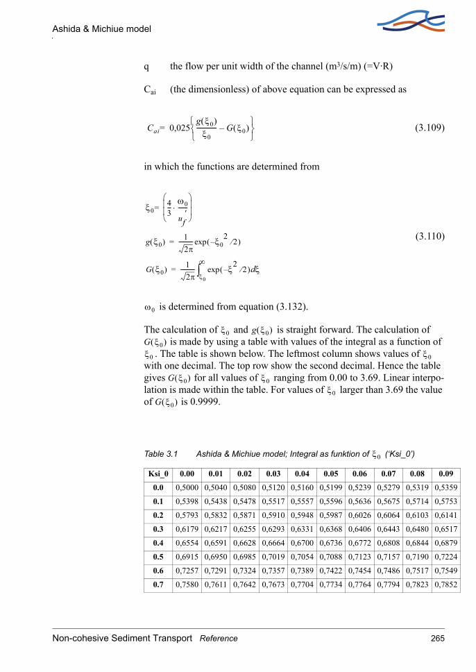
Ashida & Michiue model
9
3
1
7
9
4
9
2
q the flow per unit width of the channel (m3/s/m) (=V·R)
Cai (the dimensionless) of above equation can be expressed as
(3.109)
in which the functions are determined from
(3.110)
is determined from equation (3.132).
The calculation of and is straight forward. The calculation of is made by using a table with values of the integral as a function of
. The table is shown below. The leftmost column shows values of with one decimal. The top row show the second decimal. Hence the table gives for all values of ranging from 0.00 to 3.69. Linear interpo-lation is made within the table. For values of larger than 3.69 the value of is 0.9999.
Table 3.1 Ashida & Michiue model; Integral as funktion of (‘Ksi_0’)
Ksi_0 0.00 0.01 0.02 0.03 0.04 0.05 0.06 0.07 0.08 0.09
0.0 0,5000 0,5040 0,5080 0,5120 0,5160 0,5199 0,5239 0,5279 0,5319 0,535
0.1 0,5398 0,5438 0,5478 0,5517 0,5557 0,5596 0,5636 0,5675 0,5714 0,575
0.2 0,5793 0,5832 0,5871 0,5910 0,5948 0,5987 0,6026 0,6064 0,6103 0,614
0.3 0,6179 0,6217 0,6255 0,6293 0,6331 0,6368 0,6406 0,6443 0,6480 0,651
0.4 0,6554 0,6591 0,6628 0,6664 0,6700 0,6736 0,6772 0,6808 0,6844 0,687
0.5 0,6915 0,6950 0,6985 0,7019 0,7054 0,7088 0,7123 0,7157 0,7190 0,722
0.6 0,7257 0,7291 0,7324 0,7357 0,7389 0,7422 0,7454 0,7486 0,7517 0,754
0.7 0,7580 0,7611 0,7642 0,7673 0,7704 0,7734 0,7764 0,7794 0,7823 0,785
Cai 0,025g ξ0( )
ξ0------------- G ξ0( )–
=
ξ043---
ω0
uf′
-------⋅
=
g ξ0( ) 12π
---------- ξ02
2⁄–( )exp=
G ξ0( ) 12π
---------- ξ22⁄–( )exp ξd
ξ0
∞∫=
ω0
ξ0 g ξ0( )G ξ0( )ξ0 ξ0
G ξ0( ) ξ0ξ0
G ξ0( )
ξ0
Non-cohesive Sediment Transport Reference 265

NST REFERENCE MANUAL
3
9
1
0
5
7
9
1
5
3
6
7
7
7
0
6
6
2
4
4
1
6
0
3
5
7
8
8
9
Λ1 and Λ2 can be expressed by the following equations
(3.111)
0.8 0,7881 0,7910 0,7939 0,7967 0,7995 0,8023 0,8051 0,8078 0,8106 0,813
0.9 0,8159 0,8186 0,8212 0,8238 0,8264 0,8289 0,8315 0,8340 0,8365 0,838
1.0 0,8413 0,8438 0,8461 0,8485 0,8508 0,8531 0,8554 0,8577 0,8599 0,862
1.1 0,8643 0,8665 0,8686 0,8708 0,8729 0,8749 0,8770 0,8790 0,8810 0,883
1.2 0,8849 0,8869 0,8888 0,8907 0,8925 0,8944 0,8962 0,8980 0,8997 0,901
1.3 0,9032 0,9049 0,9066 0,9082 0,9099 0,9115 0,9131 0,9147 0,9162 0,917
1.4 0,9192 0,9207 0,9222 0,9236 0,9251 0,9265 0,9279 0,9292 0,9306 0,931
1.5 0,9332 0,9345 0,9357 0,9370 0,9382 0,9394 0,9406 0,9418 0,9429 0,944
1.6 0,9452 0,9463 0,9474 0,9484 0,9495 0,9505 0,9515 0,9525 0,9535 0,954
1.7 0,9554 0,9564 0,9573 0,9582 0,9591 0,9599 0,9608 0,9616 0,9625 0,963
1.8 0,9641 0,9649 0,9656 0,9664 0,9671 0,9678 0,9686 0,9693 0,9699 0,970
1.9 0,9713 0,9719 0,9726 0,9732 0,9738 0,9744 0,9750 0,9756 0,9761 0,976
2.0 0,9772 0,9778 0,9783 0,9788 0,9793 0,9798 0,9803 0,9808 0,9812 0,981
2.1 0,9821 0,9826 0,9830 0,9834 0,9838 0,9842 0,9846 0,9850 0,9854 0,985
2.2 0,9861 0,9864 0,9868 0,9871 0,9875 0,9878 0,9881 0,9884 0,9887 0,989
2.3 0,9893 0,9896 0,9898 0,9901 0,9904 0,9906 0,9909 0,9911 0,9913 0,991
2.4 09918 0,9920 0,9922 0,9925 0,9927 0,9929 0,9931 0,9932 0,9934 0,993
2.5 0,9938 0,9940 0,9941 0,9943 0,9945 0,9946 0,9948 0,9949 0,9951 0,995
2.6 0,9953 0,9955 0,9956 0,9957 0,9959 0,9960 0,9961 0,9962 0,9963 0,996
2.7 0,9965 0,9966 0,9967 0,9968 0,9969 0,9970 0,9971 0,9972 0,9973 0,997
2.8 0,9974 0,9975 0,9976 0,9977 0,9977 0,9978 0,9979 0,9979 0,9980 0,998
2.9 0,9981 0,9982 0,9982 0,9983 0,9984 0,9984 0,9985 0,9985 0,9986 0,998
3.0 0,9987 0,9987 0,9987 0,9988 0,9988 0,9989 0,9989 0,9989 0,9990 0,999
3.1 0,9990 0,9991 0,9991 0,9991 0,9992 0,9992 0,9992 0,9992 0,9993 0,999
3.2 0,9993 0,9993 0,9994 0,9994 0,9994 0,9994 0,9994 0,9995 0,9995 0,999
3.3 0,9995 0,9995 0,9995 0,9996 0,9996 0,9996 0,9996 0,9996 0,9996 0,999
3.4 0,9997 0,9997 0,9997 0,9997 0,9997 0,9997 0,9997 0,9997 0,9997 0,999
3.5 0,9998 0,9998 0,9998 0,9998 0,9998 0,9998 0,9998 0,9998 0,9998 0,999
3.6 0,9998 0,9998 0,9999 0,9999 0,9999 0,9999 0,9999 0,9999 0,9999 0,999
Table 3.1 Ashida & Michiue model; Integral as funktion of (‘Ksi_0’)ξ0
Λ1a
h a–------------
z 1η--- 1–
zηd
a h⁄
1
∫=
Λ2a
h a–------------
zη 1
η--- 1–ln
zηd
a h⁄
1
∫=
266 MIKE 11
Ashida, Takahashi and Mizuyama model (ATM)
where h is the water depth, a is the reference level at which the sediment concentration is taken (a= 0.05h), and z is an exponent determining the shape of the concentration profile,
(3.112)
in which is the fall velocity, κ is the von-Karman constant (=0.4) and uf´ the friction velocity.
3.12 Ashida, Takahashi and Mizuyama model (ATM)
The Ashida, Takahashi and Mizuyama model is a bed load model. This model relates the bed load transport to effects of channel slope, the bottom shear stress and the critical shear stress for erosion. The model can be applied for uniform sediments as well as for the graded sediment transport model (GST) of MIKE 11. Automatic updating of bed resistance accord-ing to the formulation by Engelund-Hansen (section 3.8.2) is optional.
The bed load transport equation (for uniform sediment) reads:
(3.113)
where:
s is the relative density of sand, g is acceleration of gravity and d the sedi-ment diameter (uniform sized or graded; di)
I is the bed slope of channel (I = = tan(θ) => θ = tan-1(I) )
τ∗ is the dimensionless shear stress
τ*c is the dimensionless critical tractive force (shear stress)
α is a function of tan(θ)=I as defined in Table 3.2 below.
The dimensionless shear stress, τ∗, is originally defined in the ATM-model as;
(3.114)
z ω0 1,2κuf′( )⁄=
ω0
qb s 1–( )gd3 12 24 I–θcos
------------------------ τ*1,5 I–( ) 1 α2 τ*c
τ*------–
1 ατ*c
τ*------–
⋅ ⋅ ⋅=
τ*U*
2
s 1–( ) g d⋅ ⋅-------------------------------=
Non-cohesive Sediment Transport Reference 267

NST REFERENCE MANUAL
where:
U* is the friction velocity defined as;
(3.115)
with Ie being the energy line gradient and R is the hydraulic radius
However, experiments with the above formulation revealed that the use of the energy line gradient in the expression of a governing variable in a fully dynamic model including morphological updates introduces a high risk of instabilities due to the potential locally very dynamic and varying varia-tion of the energy line gradient. An alternative formulation for the calcula-tion of the dimensionless shear stress based on bed resistance has therefore been implemented and replaces the original AMT-formulation.
The alternative formulation for the dimensionless shear stress, τ∗, reads:
(3.116)
where:
u is the average stream velocity
bed resistance is defined either by Chezy number, C or Mannings’s n
NOTE: if τ∗ <= τ∗c then qb = 0 !
Table 3.2 Relationship between tan(θ) and α
tan(θ) = I α α2
0.000 0.922 0.0850.015 0.906 0.8210.022 0.899 0.8070.025 0.898 0.8060.049 0.867 0.7510.100 0.791 0.626
U* g Ie R⋅ ⋅=
τ*u2
C2 s 1–( ) d⋅ ⋅---------------------------------- τ*
n2 u2⋅
R1 3⁄ s 1–( ) d⋅ ⋅---------------------------------------=⇔=
268 MIKE 11
Ashida, Takahashi and Mizuyama model (ATM)
If the ATM-model is applied for graded sediments, eq. (3.113) are adjusted to take into account the different sediment fractions. That is; d is replaced by di, τ∗ is replaced by τ∗ι and τ∗c is replaced by τ∗ci (suffix ‘i’ being the different sediment fractions).
Options for determination of dimensionless critical tractive force, τ*c
The dimensionless critical tractive force, τ*c is determined from τ*cm, the dimensionless critical tractive force (shear stress) corresponding to the average grain size dm.
In case of graded sediments, τ*ci is determined from the Modified Egia-zaroff Model (section 3.9.3) as a function of τ*cm.
For uniform sediments, τ*c is equal to, τ*cm.
Two options for τ*cm is available:
Option 1: User-defined τ*cm (constant for any average grain size dm)
For this option, τ*cm is a constant value defined by the user in the MIKE 11 ST parameter file as the variable; ‘Theta Critical’ in the ‘Transport Model’ page of the sediment transport editor.
Option 2: , τ*cm calculated by Iwagaki’s model
For this option, τ*cm is calculated from Iwagaki’s model (see section 3.9.2) as a function of the average grain size diameter.
Options for the effect of channel slopeEq. (3.113) includes the effect of channel slope I on the bed load. but ATM-model with I=0 is also applied for steep rivers in many practical applications and therefore, different options are available for the channel slope:
Option 1 : I=0:
In this case eq.(3.113) with I=0 and α =0.922 is used:
(3.117)
Option 2: I=Energy Grade
qb s 1–( )gd3 12θcos
------------ τ* i1,5 1 0,85
τ*ci
τ*i-------–
1 0,922τ*ci
τ*i-------–
⋅ ⋅ ⋅=
Non-cohesive Sediment Transport Reference 269

NST REFERENCE MANUAL
In this case, eq. (3.113) is used with I as the local energy grade at each cross section.
Option 3: I = Channel bed slope
In this case, eq. (3.113) is used with I as the local bed slope at each cross section.
3.13 Engelund & Fredsøe model
The sediment transport model presented by Engelund & Fredsøe (1976) /27/ gives a more detailed description of sediment transport and its rela-tion to the flow resistance.
The total sediment transport is split up into bed load and suspended load and the sediment transport is calculated from the skin friction, i.e. the shear stress which is acting on the surface of the dunes, see section 3.8.2 Flow Resistance - q-q´ Relationship (p. 254). It is, at present, doubtful whether the models which split the sediment load into bed load and sus-pended load are more reliable in determining the total transport than the transport formulae which consider the sediment transport as a whole.
It is, however, necessary to distinguish between suspended load and bed load, and to be able to estimate the variation of the sediment transport along the dunes if the river model is to be used to calculate the dimensions of the dunes. Separate computation of suspended load and bed load is also advantageous when calibrating models against measured suspended sedi-ment transport rates. It seems reasonable to expect that future develop-ment will be concerned with this kind of model.
3.13.1 Bed LoadThe velocity of the particles moving as bed load has been found to be:
(3.118)
where,
ubs is the velocity of bed load particles
uf' is the friction velocity
θ is a dimensionless bed shear stress
ubs 10uf′ 1 0,7θc
θ-----–
=
270 MIKE 11

Engelund & Fredsøe model
θc is the critical dimensionless bed shear stress (or Shields' parameter)
The number of moving surface particles per unit area which move is p/d where, d is the mean grain size of the bed material and p is the probability for the particles to move:
(3.119)
θ' is the dimensionless skin friction, see section 3.8.2 Flow Resistance - q-q´ Relationship (p. 254), and β is the dynamic friction coefficient, and is close to 1. p has been determined so that for moderate θ values all of the bed shear stress, τ, exceeding the critical value, τc, is transferred to the bed through drag forces on the moving bed load particles. For high θ values the limiting value for p is 1. By combining Equations (3.1) and (3.118) Engelund & Fredsøe found the following bed load function:
and (3.120)
3.13.2 Suspended loadThe suspended load qs is found as the integral of the current velocity u and the concentration of suspended sediment c:
(3.121)
In this equation a is the thickness of the bed layer which can be approxi-mated by 2 d where, d is the grain diameter and D is the flow depth. The current velocity u at a distance y above bed level, is described by the loga-rithmic velocity profile:
(3.122)
where,
p 1
π6---β
θ′ θc–----------------
4
+
1 4⁄–
=
Φb 5 1
π6---β
θ′ θc–----------------
4
+ θ′ 0,7 θc–( )= Φbqb
s 1–( )gd3-----------------------------=
qs cudya
D
∫=
u 2,5uf′ ln 30y
k---------( )=
Non-cohesive Sediment Transport Reference 271

NST REFERENCE MANUAL
uf´ is the friction velocity and the equivalent sand roughness, k, is equal to 2.5 d.
The concentration is calculated in accordance with the concentration pro-file derived by Rouse (1937):
(3.123)
where,
c is concentration of suspended sediment (at y above bed)
ca is the concentration at the bed
D is depth of water
y is distance from bed level
z is the Rouse number: z = w/(0.4uf´). w is the settling velocity of the sus-pended material given by one of the following expressions depending on the grain size:
(3.124)
Only grains with a settling velocity smaller than 0.8 uf can be carried in suspension and only these grains are considered in the calculation of the effective fall velocity. The grain-size distribution is assumed to have a log-arithmic - normal distribution. The grain sizes not carried in suspension are subtracted from this distribution and the mean grain size of the remain-ing sediment is used in Equation (3.124).
The concentration ca at y = 2 d is, according to Engelund & Fredsøe, determined through dynamic considerations: for increasing values of θ (the non-dimensional bed shear stress), the bed shear stress exceeding θc cannot be transferred by the drag on the bed load particles alone. A part of the bed shear stress is transferred as a dispersive stress, i.e. through colli-
c caD y–
y------------- a
D a–-------------
z
=
w
118------ s 1–( )gd2
v------------------------- for d 0,1 mm<
10νd
--------- 1 0,01 s 1–( )gd3
ν2------------------------------------+
0,5
1–
for 0,1 mm d 1,0 mm≤ ≤
1,1 s 1–( )gd[ ]0,5 for 1,0 mm d<
=
272 MIKE 11

Engelund & Hansen model
sions between suspended particles close to the bed. The dispersive stress is described by the expressions developed by Bagnold (1954), /20/.
The total, non-dimensional bed shear stress corrected for the effect of dunes, θ´, thus is made up of three terms; the critical shear stress, the drag on bed load particles and the dispersive stress from the suspended load:
(3.125)
where, p is the probability of particles to move.
The linear concentration λ is related to ca by:
(3.126)
With known reference concentration, ca, and settling velocity, w, the inte-gral Equation (3.121) can be evaluated with, for instance, the use of the diagrams presented by Einstein (1950), /24/. The integral cannot be expressed in closed form and, during numerical simulations, it must be integrated numerically or, as in MIKE 11, an approximation must be applied.
3.14 Engelund & Hansen model
Engelund and Hansen (1967) /29/ presented a sediment transport formula derived from considerations of the work done by the flow on the sediment being transported. Although the formula was derived for a dune covered bed, it was found also to be applicable to the upper regime (plane bed and anti-dunes).
The Engelund & Hansen transport equation reads:
(3.127)
θ′ θcπ6---βp 0,027sθ′λ2+ +=
ca0,65
1 1λ---+
3
--------------------=
Φ 0,1θ5 2⁄
f----------=
Non-cohesive Sediment Transport Reference 273

NST REFERENCE MANUAL
where, θ is the dimensionless total bed shear stress (see also section 3.8.2 Flow Resistance - q-q´ Relationship (p. 254)) and Φ is the dimensionless sediment transport rate:
(3.128)
qt is the total bed material transport per unit width and f is the friction fac-tor, defined as:
(3.129)
where, uf and u are the friction and current velocities, respectively.
The friction factor may be determined through the calculations outlined in Flow Resistance sections 3.8.1 through 3.8.3.
3.15 Lane & Kalinske model
The Lane & Kalinske model implemented in MIKE 11 computes the sus-pended load based on the work by Lane & Kalinske /33/. Uniform as well as graded sediments can be modelled. The suspended sediment transport formula reads
(3.130)
where q is the flow rate per unit width of the river. is determined by
(3.131)
where uf´ is the friction velocity in, and is the fall velocity which is determined by Rubey’s equation
(3.132)
Φqt
s 1–( )gd3-----------------------------=
f 2uf
2
u2-----=
qs q CoPs
s 106⋅---------------⋅ ⋅=
Co
C0 5,55 12---
uf′
ω0------
ω0
uf′
------
– 2
exp⋅1,61
⋅=
ω0
ω0 s 1–( )gd 23--- 36v2
sgd3-----------+
⋅ 36v2
sgd3-----------
–=
274 MIKE 11

Meyer-Peter & Müller model
in which ν is the kinematic viscosity of water.
Ps from equation (3.130) is determined by integration of the following equation
(3.133)
where with V being the average cross sectional velocity and
κ is the von-Karman constant (=0.4). In equation (3.133) is deter-mined by
= (1-0.05)/NUMBER_OF_ITERATIONS
where the denominator is an integer value defined in the MIKE11.INI file under the sediment transport section where the following must be written:
[ST_SIMULATION]
NUMBER_OF_ITERATIONS = 100
By default 100 iterations are used, but any integer value can be set by the user.
In case graded sediments are modelled, the suspended load is calculated for each fraction using the fraction grain diameter in the equations used. The total suspended load is the sum of the suspended loads from all frac-tions.
3.16 Meyer-Peter & Müller model
The Meyer-Peter & Müller model describes the bed load transport by relating the transport rate to the dimensionless shear stress acting on the grains. The dimensionless transport formula reads
(3.134)
where
is the dimensionless bed load transport
P* 1 1κϕ------- 1( 1nη )+ +
15ω0
uf′
------------η–
exp ηd0,051
∫=
ϕ Vuf
′----=
dη
dη
Φb 8 θ′ 0,047–( )1,5=
Φb
Non-cohesive Sediment Transport Reference 275
NST REFERENCE MANUAL
is the dimensionless shear stress related to grains (skin friction)
The value of must exceed a critical parameter before bed load trans-portation takes place. The absolute bed load transport per unit width of the river is obtained by
where
s is the relative density of sand (=2.65)
g is the acceleration due to gravity
d is the diameter of the grain
In MIKE 11 the transport computation is based on the dimensionless effective shear stress instead of the dimensionless skin friction. In this case the transport equation becomes
(3.135)
where the dimensionless effective shear stress is defined by
(3.136)
with
(3.137)
where
is the bed friction velocity
n is the resistance number
nb is defined by where is the diameter of which 90% are finer.
θ′
θ′ θc
qb Φb s 1–( )gd3=
Φb 8 θeff 0,047–( )1,5=
θeff
θeffueff
2
s 1–( )gd----------------------=
ueff u′fnb
n-----
0,75
⋅=
u′f
nb 0,0192 d90( )16---
⋅= d90
276 MIKE 11
Sato, Kikkawa & Ashida model
The Meyer-Peter & Müller formula can only be applied for uniform sedi-ments. The critical shear stress is computed by the principles of Iwagaki, see section 3.9.2, instead of the traditional Shield’s criteria.
3.17 Sato, Kikkawa & Ashida model
The Sato, Kikkawa and Ashida model is a pure bed load model. The model relates the bed load transport to the bed friction velocity, the bed resistance, the bottom shear stress and the critical shear stress for erosion. The model can be applied for uniform sediments as well as for the graded sediment transport model (GST) of MIKE 11. Automatic updating of the bed resistance according to the formulation by Engelund (see page 3.8.2) is optional.
The bed load transport equation reads:
(3.138)
where is the bed friction velocity, s is the relative density of sand and g the acceleration due to gravity.
The function is obtained from
(3.139)
where n is the Manning’s roughness coefficient.
The last term in equation (3.138) represents a transition from no erosion to full bed load as a function of the relation between bed shear stress (= ) and the critical shear stress (= ). The latter is obtained from the principles of Iwagaki (section 3.9.2) in the case of uni-form sediments. If graded sediments are modelled, then the result from Iwagaki’s model is further modified by the Egiazaroff equation (section 3.9.3). If graded sediments are modelled then the bed load of each sedi-ment fraction is computed from equation (3.138), and the total bed load will be the sum of the fractional bed load transports.
qbu′f
3
s 1–( )g------------------- ϕ n( ) F
τ0
τc----
⋅ ⋅=
u′f
ϕ n( )
ϕ n( )0,623 n 0,025≥,
0,623 40n( ) 3,5– n 0,025<,⋅
=
τ0uf
2 ρ⋅ τc θc s 1–( )ρgd⋅
Non-cohesive Sediment Transport Reference 277

NST REFERENCE MANUAL
3.18 Smart and Jaeggi model
Smart and Jaeggi (1983), /39/ presented a sediment transport formula which calculates the transport of coarse sediments in steep channels/riv-ers. The transport formulae is based on the original Meyer-Peter Müller equation, which was derived from laboratory experiments with non-uni-form sediments of various densities and flume-slopes ranging from 0.04% to 2%.
The original Meyer-Peter Müller equation reads:
(3.140)
where,
φ dimensionless sediment transport
θ dimensionless shear stress
corr.factor for bed form roughness
3.18.1 Revised transport formulaThrough comparison of new laboratory experiments and the original Equation (3.140) it was found that the computed transport is seriously underestimated with slopes steeper than 3%. Smart and Jaeggi therefore proposed a new transport formulation based on Equation (3.140).
At higher slopes, grains in the bed have a slope induced height advantage of those grains immediately downstream of them and the critical shear stress is less than it would be for a flat bed. Shields parameter is therefore adjusted as a function of the slope to horizontal, Eq.(3.141):
(3.141)
where,
θ0cr Shields parameter
α Slope to horizontal of water surface or bottom level
β Angle of repose of submerged bed material (33o)
φ 8Ks
Kr-----
1,5
θ 0,047–1,5
=
Ks
Kr-----
θc θ0cr α 1 αtanβtan
------------– cos=
278 MIKE 11

Smart and Jaeggi model
Including non-uniformity of the sediment as well as the slope induced effect of the transport the revised equation - still based on laboratory experiments - reads:
(3.142)
where,
d90 90%-fractile of the sediment
d30 30%-fractile of the sediment
I Slope (water surface or bottom level)
C Chezy resistance factor
Equation (3.142) is only recommended in the following ranges:
diameter > 0.4 mm
(d90/d30) < 8.5
0.04% < I < 20%
Concerning the available option of updating the bed resistance during a sediment transport simulation it is very important to notice, that there is NO formulation of updating the bed resistance built-in for the Smart and Jaeggi transport model.
However, to maintain the possibility of updating the bed resistance the formulation of the Engelund-Hansen model has been adopted. It is very important to note, that this formulation does not cover the wide range of grain diameter etc. as the Smart-Jaeggi formula does.
For that reason it would be advisable not to select the update bed resist-ance option for a Smart-Jaeggi sediment transport simulation. If used any-way the results should be analysed very carefully to check whether they are reliable or not.
3.18.2 MIKE 11 versionAs an attempt to expand the possibilities for calibration of the sediment transport formula, Equation (3.142) has been implemented in MIKE 11 in such a way, that it is possible for the user to edit the coefficients and expo-nents in the transport equation.
φ 4d90
d30-------
0,2
I0,6cθ0,5 θ θcr–( )=
Non-cohesive Sediment Transport Reference 279
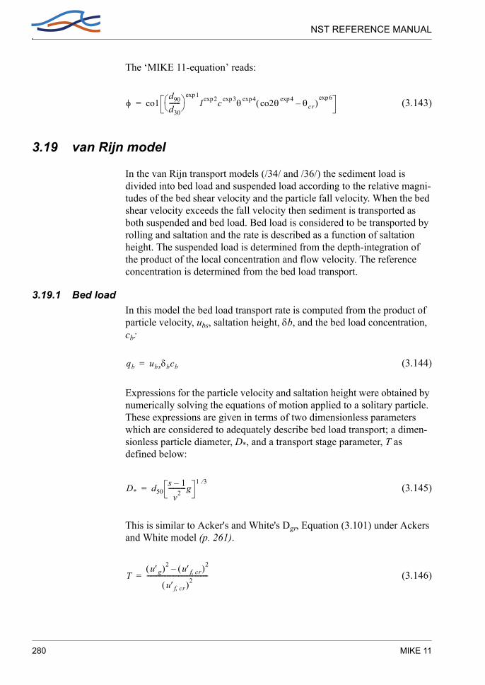
NST REFERENCE MANUAL
The ‘MIKE 11-equation’ reads:
(3.143)
3.19 van Rijn model
In the van Rijn transport models (/34/ and /36/) the sediment load is divided into bed load and suspended load according to the relative magni-tudes of the bed shear velocity and the particle fall velocity. When the bed shear velocity exceeds the fall velocity then sediment is transported as both suspended and bed load. Bed load is considered to be transported by rolling and saltation and the rate is described as a function of saltation height. The suspended load is determined from the depth-integration of the product of the local concentration and flow velocity. The reference concentration is determined from the bed load transport.
3.19.1 Bed loadIn this model the bed load transport rate is computed from the product of particle velocity, ubs, saltation height, δb, and the bed load concentration, cb:
(3.144)
Expressions for the particle velocity and saltation height were obtained by numerically solving the equations of motion applied to a solitary particle. These expressions are given in terms of two dimensionless parameters which are considered to adequately describe bed load transport; a dimen-sionless particle diameter, D*, and a transport stage parameter, T as defined below:
(3.145)
This is similar to Acker's and White's Dgr, Equation (3.101) under Ackers and White model (p. 261).
(3.146)
φ co1d90
d30-------
1expI 2exp c 3exp θ 4exp co2θ 4exp θcr–( )
6exp=
qb ubsδbcb=
D* d50s 1–
v2-----------g
1 3⁄=
Tu′g( )2 u′f cr,( )2–
u′f cr,( )2---------------------------------------=
280 MIKE 11

van Rijn model
u'g is the bed shear velocity, related to grains, and u'f,cr is Shields critical bed shear velocity. u'g is defined so that the influence of bed forms is elim-inated since form drag does not contribute to bed load transport. ug is given by:
(3.147)
where,
u is the mean flow velocity
C' is Chezy's coefficient related to skin friction
C' is expressed as:
(3.148)
where,
R is the hydraulic radius (or resistance radius) related to the bed
3d90 is considered to be the effective roughness height of the plane bed
The following expressions were determined for particle velocity and salta-tion height by applying the equations of motion to a solitary particle:
(3.149)
This expression was determined by expressing the computed particle velocity as a function of flow conditions and sediment size (D*). A parti-cle mobility, ubs, was then defined as:
(3.150)
u′gg
C′-------u=
C′ 18 R3d90----------
log=
ubs
u′f------- 9 2,6 D*( ) 8
θc
θ-----
0,5–log+=
ubs
s 1–( )gd[ ]0,5--------------------------------- 1,5T0,6=
Non-cohesive Sediment Transport Reference 281

NST REFERENCE MANUAL
An expression for the saltation height, δb, is given by:
(3.151)
An expression for the bed load concentration, cb, is obtained from a rear-rangement of Equation (3.144):
(3.152)
Extensive analysis of flume measurements of bed load transport yielded the following expression for the bed load concentration:
(3.153)
where,
co is the maximum bed concentration (= 0.65).
Combining Equations (3.150), (3.151) and (3.153) gives the following expression for bed load transport:
(3.154)
or from Equation (3.120):
(3.155)
This relationship is valid for particles in the range 0.2 to 2.0 mm.
3.19.2 Suspended load This method is based on the computation of a reference concentration determined from the bed load transport. Thus the reference concentration
δbd
------ 0,3D*0,7T0,5=
cbqb
ubs-------δb=
cb
co---- 0,18 T
D*------=
qb
s 1–( )gd503
------------------------------- 0,053T2,1
D*0,3
----------------------=
Φb0,053T2,1
D*0,3
----------------------=
282 MIKE 11

van Rijn model
ca is described as a function of the dimensionless particle diameter D* and transport stage parameter T, (see Bed Load):
(3.156)
(3.157)
where,
u´g is the bed shear velocity related to the grains
u´f,cr is the critical bed shear velocity
The reference concentration is defined for a reference level 'a' below which all sediment is considered to be transported as bed load. The refer-ence level is approximated by:
(3.158)
where,
H is the (known) bed form height
(3.159)
where,
k is the equivalent sand roughness when the bed form dimensions are unknown or a minimum value of
(3.160)
where,
D is water depth
The reference concentration is defined from:
(3.161)
D* d50s 1–( )g
ν2-------------------
1 3⁄=
Tug
′( )2
uf cr,′( )
2–
uf cr,′( )
2------------------------------------=
a 0,5H=
a k=
a 0,01D=
qb cbubsδb cauaa= =
Non-cohesive Sediment Transport Reference 283

NST REFERENCE MANUAL
where,
cb is the bed concentration,
ubs is the velocity of bed load particles
δb is the saltation height. Expressions for these parameters are given in Engelund & Fredsøe model, section 3.13.
ua is the effective particle velocity at reference level a. It is expressed as:
From an examination of flume and field data a value for a of 2.3 was determined. Combining this value with the expressions for δb and cb (as functions of D* and T) the following expression is obtained:
(3.162)
The representative particle size of suspended load is generally finer than that of bed load. Van Rijn relates this particle size, ds to the d50 and geo-metric standard deviation, σs, of the bed material:
for (3.163)
in which σs is given by:
(3.164)
This ds value is then used to calculate fall velocity according to Equation (3.124). The threshold for the initiation of suspension can be determined from the actual flow conditions. Using the overall bed shear stress uf the criterion implemented in the van Rijn model becomes:
, for (3.165)
ua αubs=
ca 0,015d50
a------- T1,5
D*0,3
---------=
ds
d50------- 1 0,011 σs 1–( ) T 25–( )+= T 25<
σs 0,5d84
d50-------
d50
d16-------+
=
ufw---- u
ds----= 1 ds 10≤<
284 MIKE 11

van Rijn model
and
, for (3.166)
In describing the suspended load transport, van Rijn defines a suspension parameter Z which expresses the influence of the upward turbulent fluid forces and the downward gravitational forces. Z is defined as:
(3.167)
where,
uf´ is the over all bed shear velocity
κ is von Karman's constant
β is a coefficient related to the diffusion of sediment particles
An expression for β was derived as:
for (3.168)
Many factors affect the suspension parameter Z, e.g. volume occupied by particles, reduction of fall velocity and damping of turbulence. These effects are grouped into a single correction factor y, which is used to define a modified suspension number Z as shown:
(3.169)
ψ was found to be a function of the main hydraulic parameters:
(3.170)
where,
co is the maximum bed concentration (found to be 0.65)
uf
w---- 0,4= 10 ds<
Z wβκuf
′-----------=
β 1 2 wuf
′----
2+= 0,1 w
uf′
---- 1< <
Z′ Z ψ+=
ψ 2,5 wuf
′----
0,8 ca
co----
0,4=
Non-cohesive Sediment Transport Reference 285

NST REFERENCE MANUAL
The suspended load transport is expressed by Equation (3.121). By com-bining the expression describing the velocity and concentration profiles (Equations (3.122) and (3.123)) with the expressions for Z and y (Equa-tions (3.169) and (3.170)) van Rijn derived the following expression:
(3.171)
in which F is given by:
(3.172)
3.20 Nomenclature
a reference level in calculation of suspended load
a thickness of bed layer
A critical flow mobility number in Ackers and White model
Ai critical flow mobility number in Ackers and White model for class i
c concentration of suspended sediment
c celerity of dune
ca reference sediment concentration
cb concentration of suspended sediment at the bed
co maximum bed concentration
C model parameter in Ackers and White model
d grain size
di representative grain size in class i
D total flow depth
qs FuDca=
F
aD----
Z ′ aD----
1,2–
1 aD----–
Z ′1,2 Z′–[ ]
----------------------------------------------=
286 MIKE 11

Nomenclature
dmed representative grain size of total population
Dgr dimensionless grain diameter, Ackers and White model
D´ boundary layer thickness
D* dimensionless grain diameter, van Rijn Model
ds particle size of suspended sediment
dXX particle size than which XX% is finer
f function
F Froude number
Fcg mobility parameter for coarse material
Ffg mobility parameter for fine material
Fgr general mobility parameter
g acceleration due to gravity
Ggr general transport parameter
h water elevation
H total dune height
k wave number of bed forms
k equivalent sand roughness
L dune length
Le equilibrium dune length
lo dune length, bed load only
m model parameter in Ackers and White model
n model parameter in Ackers and White model
N number of classes in a graded sediment
p probability for particles to move
Non-cohesive Sediment Transport Reference 287

NST REFERENCE MANUAL
pi percentage contribution in class i
pact,bed percentage contributions of class i in active and parent layers, respectively
q flow discharge per unit width
qb bed load transport rate
qbt transport rate at top of dune
qs suspended load transport rate
qt total load transport rate
qti total load transport rate in class i
s specific gravity of sediment
sediment transport rate per unit of width at grid point j and time interval n
sediment transport rate per unit of width at grid point j and time interval n in class i
sediment transport rate at grid point j and time interval n
t parameter dependent on u, h, d (see Equation (3.94) in section 3.8.3 Flow Resistance - White et al. (p. 257).)
T transport stage parameter, van Rijn model
T1 average lifetime of a dune
u mean flow velocity
ua velocity of bed load particles at reference level a
ub near bed velocity
ubs velocity of bed load particles
uf, uf´ bed shear velocity or friction velocity
Ufcr critical bed shear velocity
qtjn
qtj i,n
Qtj i,n W= qtj
n( )
288 MIKE 11

Nomenclature
ug´ bed shear velocity related to the grains
w fall velocity
W width (defined as A/R in code)
X sediment transport, mass flux per unit mass flow rate
y distance above bed level
z local height of dune
z Rouse number
Z bottom level above datum
Z suspension parameter
Z’ modified suspension number
∆z change in bottom level
Za depth of active layer
α velocity distribution coefficient
κ von Karman's constant
β dynamic friction coefficient
β coefficient related to diffusion of sediment particles
δ spatial lag
ε porosity of sediment
ε eddy viscosity
λ linear concentration related to ca
C space centring coefficient
δb saltation height
ρ fluid density
θ dimensionless bed shear stress
Non-cohesive Sediment Transport Reference 289

NST REFERENCE MANUAL
θ time centring coefficient
θc critical dimensionless bed shear stress
θci critical dimensionless bed shear stress for class i
θ’ dimensionless skin friction
θt dimensionless bed shear stress at dune top
τ bed shear stress
τc’ critical bed shear stress
τ’ skin friction
τ form drag
Φ dimensionless sediment transport rate
Φb dimensionless bed load sediment transport rate
Φs dimensionless suspended sediment load transport rate
Φt dimensionless total sediment transport rate
υ kinematic viscosity
ψ correction factor
References/19/ Ackers, P. and White, W.R. (1973). "Sediment transport: new
approach and analysis", Proc. ASCE, JHD, 99, HY11, pp. 2041-2060.
/20/ Bagnold, R.A., 1954. "Experiments on gravity-free dispersion of large solid spheres in a Newtonion fluid under shear". Proc. R. Soc. London (A) 353.
/21/ Challet, J.P. and Cunge, J.A., Simulation of unsteady flow in allu-vial streams, Int. Symp. on river sedimentation March 24-29 1980, Chin. Soc. of Hydr. Eng., Beijing, China 1980.
/22/ Deigaard, R. 1980. "Longitudinal and transverse sorting of grain sizes in alluvial rivers". Series Paper 26, Institute of Hydrodyn. &
290 MIKE 11

Nomenclature
Hydr. Engrg., Technical University of Denmark.
/23/ Egiazaroff, P.I., Calculation of non-uniform sediment concentra-tion, Proc. ASCE HY 4, July 1965.
/24/ Einstein, H.A., 1950. "The bed load function for sediment transpor-tation in open channel flows". U.S. Dept. of Agriculture, Tech. Bul-letin No. 1026.
/25/ Engelund, F., 1966. "Hydraulic resistance of alluvial streams". ASCE, Vol. 92, No. Hy 2.
/26/ Engelund, F., 1970. "Instability of erodible beds". 7. Fluid Mech., Vol. 42, pp. 225-44.
/27/ Engelund, F. and Fredsøe, J., 1976. "A sediment transport model for straight alluvial channels". Nordic Hydrology, Vol. 7, No. 5.
/28/ Engelund, F. and Fredsøe, J., 1982. "Hydraulic theory of alluvial rivers", Advances in Hydro Science, Vol. 13, pp. 187-215.
/29/ Engelund, F. and Hansen, E., 1967. "A monograph on sediment transport in alluvial streams", Teknisk Forlag, Copenhagen.
/30/ Fredsøe, J., 1979. "Unsteady flow in straight alluvial streams: Mod-ifications of individual dunes". J. Fluid Mech., vol. 91, pp. 497-512.
/31/ Fredsøe, J., 1979. "Dimensions of stationary dunes. Part 1. Low sediment transport rate". Prog. Rep. 49, Institute of Hydrodyn. & Hydr. Engrg., Technical University of Denmark.
/32/ Fredsøe, J., 1982. "Shape and Dimensions of stationary dunes in rivers". ASCE, Vol. 108, No. Hy 8.
/33/ Lane, E.W and Kalinske, A.A, 1941. “Engineering calculations of suspended sediment”, Trans.Am.Geophys.Union, vol.22, pp. 603-607.
/34/ Rijn, L.C. van, 1984a, "Part I: Bed load transport", J.Hyd.Eng., 110, 10 Oct.
/35/ Ribberink, J.S, 1987, "Mathematical modelling of one-dimensional morphological changes in rivers with non-uniform sediment". Delft University of Technology, Report No. 87-2.
/36/ Rijn, L.C. van, 1984b, "Part II: Suspended load transport", J. Hyd.
Non-cohesive Sediment Transport Reference 291

NST REFERENCE MANUAL
Eng, 110, 11 Nov.
/37/ Rouse, H., 1937. "Modern conceptions of the mechanics of fluid turbulence". Trans. ASCE, Vol. 102, pp. 463-543.
/38/ Smart G.M., 1984. "Sediment transport formulae for steep chan-nels". Journal of Hydraulic Engineering, vol.110, No.3, March 1984.
/39/ Smart, G.M. and Jaeggi, M.N.R. (1983): "Sediment Transport on Steep Slopes". Mitteilung nr. 64 of the Laboratory for Hydraulics, Hydrology and Glaciology at the Federal Technical University, Zurich.
/40/ Vries, M. de (1981), Morphological Computations, Lecture Notes, (f10a, Delft University of Techn., Dept. of Civ.Eng., Fluid Mech. Group.
/41/ White, W.R., Paris, E. and Bettess, R., 1979. "A new generation method for predicting the frictional characteristics of alluvial streams", Report No. IT 187, Hydr. Res. Station, Wallingford.
292 MIKE 11

R A I N F A L L - R U N O F FReference
293

294 MIKE 11

4 RR REFERENCE MANUALThis manual should be used when undertaking Rainfall-Runoff (RR) mod-elling applications. It provides a description of aspects which are encoun-tered during the development, calibration and application of Rainfall Runoff models including detailed technical descriptions of the hydrologi-cal processes. Four different types of Rainfall-Runoff models are availa-ble:
1 NAM: A lumped, conceptual rainfall-runoff model, simulating the overland-, inter- flow, and base-flow components as a function of the moisture contents in four storages (see Section 4.1-4.11).
2 UHM: The Unit Hydrograph Module includes different loss models (constant, proportional) and the SCS method for estimating storm run-off (see Section 4.12).
3 SMAP: A monthly soil moisture accounting model (see section 4.13).
4 Urban: Two different model runoff computation concepts are available in the Rainfall Runoff Module for fast urban runoff.: A) Time/area Method and B) Non-linear Reservoir (kinematic wave) Method
5 FEH: Flood Estimation Handbook. A method for flood estimation in the UK.
6 DRiFt (Discharge River Forecast): A semi-distributed event model based on a geomorphologic approach.
7 Combined: The runoff from a number of catchments, constituting parts of a larger catchment, can be combined into a single runoff series. Each of the sub- catchments must be specified separately by name, model type, parameters etc. The combined catchment can be defined only after the sub-catchments have been created. The combined catch-ment is defined in the group for combined catchments, which is acti-vated when selecting combined catchment. The runoff from the combined catchment is found by simple addition of the simulated flow from the sub-catchments.
Some of the features in the Rainfall Runoff package have been developed in cooperation with CTI Engineering, CO., Ltd., Japan. Amongst these are additional methods for Calculation of Runoff from catchments and Calcu-lation of Mean Precipitation of basins (method of Thiessen polygons and Isohyetal Mapping).
The manual should be used in conjunction with the MIKE 11 User Man-ual.
Rainfall-Runoff Reference 295
RR reference Manual
4.1 NAM - Introduction
The NAM hydrological model simulates the rainfall-runoff processes occurring at the catchment scale. NAM forms part of the rainfall-runoff (RR) module of the MIKE 11 river modelling system. The rainfall-runoff module can either be applied independently or used to represent one or more contributing catchments that generate lateral inflows to a river net-work. In this manner it is possible to treat a single catchment or a large river basin containing numerous catchments and a complex network of rivers and channels within the same modelling framework.
NAM is the abbreviation of the Danish "Nedbør-Afstrømnings-Model", meaning precipitation-runoff-model. This model was originally developed by the Department of Hydrodynamics and Water Resources at the Techni-cal University of Denmark (/52/),.
A mathematical hydrological model like NAM is a set of linked mathe-matical statements describing, in a simplified quantitative form, the behaviour of the land phase of the hydrological cycle. NAM represents various components of the rainfall-runoff process by continuously accounting for the water content in four different and mutually interrelated storages. Each storage represents different physical elements of the catch-ment. NAM can be used either for continuous hydrological modelling over a range of flows or for simulating single events.
The NAM model can be characterised as a deterministic, lumped, concep-tual model with moderate input data requirements. A description of the classification of hydrological models is given in Abbott and Refsgaard (1996), /42/. Refsgaard and Knudsen (1997), /54/ compare a number of different types of hydrological model, including the NAM model, in terms of both data requirements and model performance.
The NAM model is a well-proven engineering tool that has been applied to a number of catchments around the world, representing many different hydrological regimes and climatic conditions.
4.2 Data Requirements
The basic input requirements for the NAM model consist of:
Model parameters
Initial conditions
Meteorological data
296 MIKE 11

Data Requirements
Streamflow data for model calibration and validation
The basic meteorological data requirements are:
Rainfall
Potential evapotranspiration
In the case of snow modelling the additional meteorological data require-ments are:
Temperature
Radiation (optional)
The NAM model also allows modelling of man-made interventions in the hydrological cycle in terms of irrigation and groundwater pumping. In this case time series of irrigation and groundwater abstraction rates are required.
In this section the meteorological and hydrological data are described. The model parameters and initial conditions are described in the subsequent sections.
4.2.1 Meteorological data
Rainfall (mm)The time resolution of the rainfall input depends on the objective of the study and on the time scale of the catchment response. In many cases daily rainfall values are sufficient, but in rapidly responding catchments where accurate representation of the peak flows is required, rainfall input on a finer resolution may be required. Rainfall data with any (variable) time increments can be specified in the rainfall input. The NAM model will then make the necessary interpolations according to the simulation time step. The rainfall data are treated as accumulated totals so the rainfall associated with any particular time is the rainfall volume since the last entered value.
Potential evapotranspiration (mm)When daily time steps are used, monthly values of potential evapotranspi-ration are usually sufficient. In this case only minor improvements can be obtained by specifying daily values instead of monthly values. For small time steps, however, the diurnal variation of the evapotranspiration may be important. The evapotranspiration data are treated as accumulated totals where the evapotranspiration associated with any particular time is the evapotranspiration since the last entered value.
Rainfall-Runoff Reference 297

RR reference Manual
Temperature (Co)Temperature data are required if snow accumulation and melt are included in the simulations. During the snow season, the time increments in the temperature data should reflect the length of the time step in the simula-tion, e.g. daily mean temperatures. The temperature data at a given time represents the average temperature since the last entered data.
Radiation (W/m2)Actual incoming short wave radiation data can optionally be used as input in the extended snow module. The radiation data at a given time represents the average radiation since the last entered data.
Mean area weightingThe NAM model simulates the rainfall-runoff process in a lumped fashion so provision is given for combining meteorological data from different stations within a single catchment or subcatchment into a single time series of weighted averages. The resulting time series will represent the mean area values of rainfall and potential evapotranspiration for a catch-ment.
The weights are user-defined and can be determined based e.g. on the Thiessen method. In the case of missing values the weighting procedure will redistribute the weights appropriately. Therefore, it is not necessary to specify weight combinations for all possible combinations of missing sta-tions. Alternatively, the user can explicitly specify the weights when data are missing from one or more stations. A weight of “-1” is given to non-reporting stations, indicating missing data.
When rainfall data are available from stations with different reporting fre-quency, e.g. both daily and hourly stations, then the distribution in time of the average catchment rainfall may be determined using a weighted aver-age of the high-frequency stations. It is possible to use all stations to deter-mine the daily mean rainfall over the catchment and subsequently use the hourly stations to distribute this daily rainfall in time. Different weight combinations for different cases of missing values may be applied also to the calculation of the distribution in time.
4.2.2 Hydrological data
Discharge (m3/s)Observed discharge data at the catchment outlet are required for compari-son with the simulated runoff for model calibration and validation. The discharge data at any particular time is the average discharge since the last entered data.
298 MIKE 11
Model Structure
Irrigation (mm)If the irrigation module is included in the NAM simulation, an additional rainfall time series is required to provide information on the amount of irrigation water.
Groundwater abstraction (mm)When the effect of groundwater abstraction is expected to have a signifi-cant effect on the overall groundwater levels or catchment baseflow, pumping rates can be specified to account for these withdrawals. The groundwater abstraction data are treated as accumulated totals where the abstraction associated with any particular time is the abstraction since the last entered value.
4.3 Model Structure
A conceptual model like NAM is based on physical structures and equa-tions used together with semi-empirical ones. Being a lumped model, NAM treats each catchment as a single unit. The parameters and variables represent, therefore, average values for the entire catchment. As a result some of the model parameters can be evaluated from physical catchment data, but the final parameter estimation must be performed by calibration against time series of hydrological observations.
Rainfall-Runoff Reference 299

RR reference Manual
Figure 4.1 Structure of the NAM model.
The model structure is shown in Figure 4.1. It is an imitation of the land phase of the hydrological cycle. NAM simulates the rainfall-runoff proc-ess by continuously accounting for the water content in four different and mutually interrelated storages that represent different physical elements of the catchment. These storages are:
Snow storage
Surface storage
Lower or root zone storage
Groundwater storage
In addition NAM allows treatment of man-made interventions in the hydrological cycle such as irrigation and groundwater pumping.
Based on the meteorological input data NAM produces catchment runoff as well as information about other elements of the land phase of the hydro-logical cycle, such as the temporal variation of the evapotranspiration, soil moisture content, groundwater recharge, and groundwater levels. The
300 MIKE 11
Basic modelling components
resulting catchment runoff is split conceptually into overland flow, inter-flow and baseflow components.
4.4 Basic modelling components
4.4.1 Surface storageMoisture intercepted on the vegetation as well as water trapped in depres-sions and in the uppermost, cultivated part of the ground is represented as surface storage. Umax denotes the upper limit of the amount of water in the surface storage.
The amount of water, U, in the surface storage is continuously diminished by evaporative consumption as well as by horizontal leakage (interflow). When there is maximum surface storage, some of the excess water, PN, will enter the streams as overland flow, whereas the remainder is diverted as infiltration into the lower zone and groundwater storage.
4.4.2 Lower zone or root zone storageThe soil moisture in the root zone, a soil layer below the surface from which the vegetation can draw water for transpiration, is represented as lower zone storage. Lmax denotes the upper limit of the amount of water in this storage.
Moisture in the lower zone storage is subject to consumptive loss from transpiration. The moisture content controls the amount of water that enters the groundwater storage as recharge and the interflow and overland flow components.
4.4.3 EvapotranspirationEvapotranspiration demands are first met at the potential rate from the sur-face storage. If the moisture content U in the surface storage is less than these requirements (U < Ep), the remaining fraction is assumed to be with-drawn by root activity from the lower zone storage at an actual rate Ea. Ea is proportional to the potential evapotranspiration and varies linearly with the relative soil moisture content, L/Lmax, of the lower zone storage
(4.1)
4.4.4 Overland flowWhen the surface storage spills, i.e. when U > Umax, the excess water PN gives rise to overland flow as well as to infiltration. QOF denotes the part
Ea Ep U–( ) LLmax-----------=
Rainfall-Runoff Reference 301

RR reference Manual
of PN that contributes to overland flow. It is assumed to be proportional to PN and to vary linearly with the relative soil moisture content, L/Lmax, of the lower zone storage
(4.2)
where
CQOFis the overland flow runoff coefficient (0 ≤ CQOF ≤ 1)
TOF is the threshold value for overland flow (0 ≤ TOF ≤ 1).
The proportion of the excess water PN that does not run off as overland flow infiltrates into the lower zone storage. A portion, ∆L, of the water available for infiltration, (PN -QOF), is assumed to increase the moisture content L in the lower zone storage. The remaining amount of infiltrating moisture, G, is assumed to percolate deeper and recharge the groundwater storage.
4.4.5 InterflowThe interflow contribution, QIF, is assumed to be proportional to U and to vary linearly with the relative moisture content of the lower zone storage.
(4.3)
where CKIF is the time constant for interflow, and TIF is the root zone threshold value for interflow (0 ≤ TIF ≤ 1).
4.4.6 Interflow and overland flow routingThe interflow is routed through two linear reservoirs in series with the same time constant CK12. The overland flow routing is also based on the linear reservoir concept but with a variable time constant
(4.4)
QOF CQOFL Lmax TOF–⁄
1 TOF–------------------------------------PN for L Lmax TOF>⁄
0 for L Lmax TOF≤⁄
=
QIF CKIF( ) 1– L Lmax TIF–⁄1 TIF–
----------------------------------U for L Lmax TIF>⁄
0 for L Lmax TIF≤⁄
=
CKCK12 for OF OFmin<
CK12OF
OFmin---------------
β–for OF OFmin≥
=
302 MIKE 11

Extended groundwater components
where OF is the overland flow (mm/hour), OFmin is the upper limit for lin-ear routing (= 0.4 mm/hour), and β = 0.4.
The constant β = 0.4 corresponds to using the Manning formula for mod-elling the overland flow. Equation (4.4) ensures in practice that the routing of real surface flow is kinematic, while subsurface flow being interpreted by NAM as overland flow (in catchments with no real surface flow com-ponent) is routed as a linear reservoir.
4.4.7 Groundwater rechargeThe amount of infiltrating water G recharging the groundwater storage depends on the soil moisture content in the root zone
(4.5)
where
TG is the root zone threshold value for groundwater recharge (0 ≤ TG ≤ 1).
4.4.8 Soil moisture contentThe lower zone storage represents the water content within the root zone. After apportioning the net rainfall between overland flow and infiltration to groundwater, the remainder of the net rainfall increases the moisture content L within the lower zone storage by the amount ∆L
(4.6)
4.4.9 BaseflowThe baseflow BF from the groundwater storage is calculated as the out-flow from a linear reservoir with time constant CKBF.
4.5 Extended groundwater components
4.5.1 Drainage to or from neighbouring catchmentsLocal geological conditions may cause part of the infiltrating water to drain to neighbouring catchments. In NAM this loss of water can be described by specifying the ratio of the groundwater catchment area to the topographical catchment area, Carea, with a value less than one. In this case the proportion (1-Carea) of the recharge G is drained to neighbouring
G PN Q– OF( )L Lmax TG–⁄
1 TG–-------------------------------- for L Lmax TG>⁄
0 for L Lmax TG≤⁄
=
∆L PN QOF– G–=
Rainfall-Runoff Reference 303

RR reference Manual
catchments. Similarly, water may be drained from neighbouring catch-ments, implying an increased groundwater recharge in the catchment (Carea > 1).
4.5.2 Lower groundwater storageFor a better description of the baseflow, an additional (lower) groundwater storage can be defined. In this case the upper groundwater storage pro-vides the fast responding component of the baseflow, whereas the lower storage usually has a slower response. The recharge to the lower storage is given as a proportion CQLOW of the total recharge G. The routing from the lower storage is described by a linear reservoir with time constant CKLOW.
4.5.3 Shallow groundwater reservoir descriptionThe groundwater level is calculated from a continuity consideration accounting for recharge G, capillary flux CAFLUX, net groundwater abstraction GWPUMP, and baseflow BF. The inclusion of capillary flux and groundwater pumping are optional. The groundwater storage can be treated in two different ways, either as a simple linear reservoir as described in Section 4.4.9 Baseflow (p. 303) or as a shallow groundwater reservoir.
The shallow groundwater reservoir description is appropriate for lowland catchments with little topographical variation and the potential for water logging. The baseflow is given by
(4.7)
where SY is the specific yield of the reservoir, GWL is the groundwater table depth, and GWLBF0 is the maximum groundwater table depth, which causes baseflow.
The parameter GWLBF0 can be interpreted as the distance between the average ground level of the catchment to the water level of the river. Due to the variation in the river water level throughout the year GWLBF0 can be given a significant annual variation.
4.5.4 Capillary fluxThe capillary flux CAFLUX of water from the groundwater to the lower zone storage is assumed to depend on the depth of the groundwater table
BF GWLBF0 GWL–( )SY CKBF( ) 1– for GWL GWLBF0≤
0 for GWL GWLBF0>
=
304 MIKE 11

Snow module
below the ground surface, GWL, as well as on the relative moisture con-tent, L/Lmax, of the lower zone storage
(4.8)
where GWLFL1 is the groundwater table depth at which the capillary flux is 1 mm/day when the lower zone storage is completely dry. Equation (4.8) provides a good fit to the theoretical relationship between the capil-lary flux, the depth to the water table and the soil moisture content pro
4.6 Snow module
Snow accumulation and melt are important hydrological processes in river basins where the snow pack acts as a storage in which precipitation is retained during the cold season and subsequently released as melt water during the warmer parts of the year.
The snow melt component of the runoff is incorporated as an integrated module within NAM. This component is optional and temperature data is only required if the snow routine is selected. Normally the precipitation enters directly into the surface storage. However, during cold periods pre-cipitation is retained in the snow storage from which it is melted in warmer periods. Two different models can be applied; a simple lumped calculation or a more general approach that divides the catchment into a number of altitude zones with separate snow melt parameters, temperature and precipitation input for each zone.
4.6.1 Accumulation and melting of snowSeveral investigations (e.g. /57/) have shown that the shift between precip-itation in the form of rain and snow usually takes place when the air tem-perature is within a narrow interval close to 0o C. In the snow module it is assumed that the precipitation falls as rain when the air temperature is above a certain base temperature level, T0, which can be specified by the user.
The snowmelt QS is calculated using a degree-day approach
(4.9)
CAFLUX 1 L Lmax⁄– GWLGWLFL1---------------------
α–(mm/day)
α 1,5 0,45GWLFL1+
=
=
QS Csnow T T0–( ) for T T0>
0 for T T0≤
=
Rainfall-Runoff Reference 305
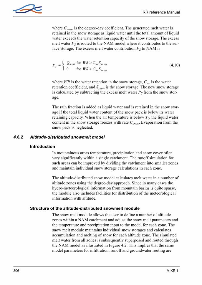
RR reference Manual
where Csnow is the degree-day coefficient. The generated melt water is retained in the snow storage as liquid water until the total amount of liquid water exceeds the water retention capacity of the snow storage. The excess melt water PS is routed to the NAM model where it contributes to the sur-face storage. The excess melt water contribution PS to NAM is
(4.10)
where WR is the water retention in the snow storage, Cwr is the water retention coefficient, and Ssnow is the snow storage. The new snow storage is calculated by subtracting the excess melt water PS from the snow stor-age.
The rain fraction is added as liquid water and is retained in the snow stor-age if the total liquid water content of the snow pack is below its water retaining capacity. When the air temperature is below T0, the liquid water content in the snow storage freezes with rate Csnow. Evaporation from the snow pack is neglected.
4.6.2 Altitude-distributed snowmelt model
IntroductionIn mountainous areas temperature, precipitation and snow cover often vary significantly within a single catchment. The runoff simulation for such areas can be improved by dividing the catchment into smaller zones and maintain individual snow storage calculations in each zone.
The altitude-distributed snow model calculates melt water in a number of altitude zones using the degree-day approach. Since in many cases the hydro-meteorological information from mountain basins is quite sparse, the module also includes facilities for distribution of the meteorological information with altitude.
Structure of the altitude-distributed snowmelt moduleThe snow melt module allows the user to define a number of altitude zones within a NAM catchment and adjust the snow melt parameters and the temperature and precipitation input to the model for each zone. The snow melt module maintains individual snow storages and calculates accumulation and melting of snow for each altitude zone. The simulated melt water from all zones is subsequently superposed and routed through the NAM model as illustrated in Figure 4.2. This implies that the same model parameters for infiltration, runoff and groundwater routing are
PSQmelt for WR CwrSsnow≥
0 for WR CwrSsnow<
=
306 MIKE 11
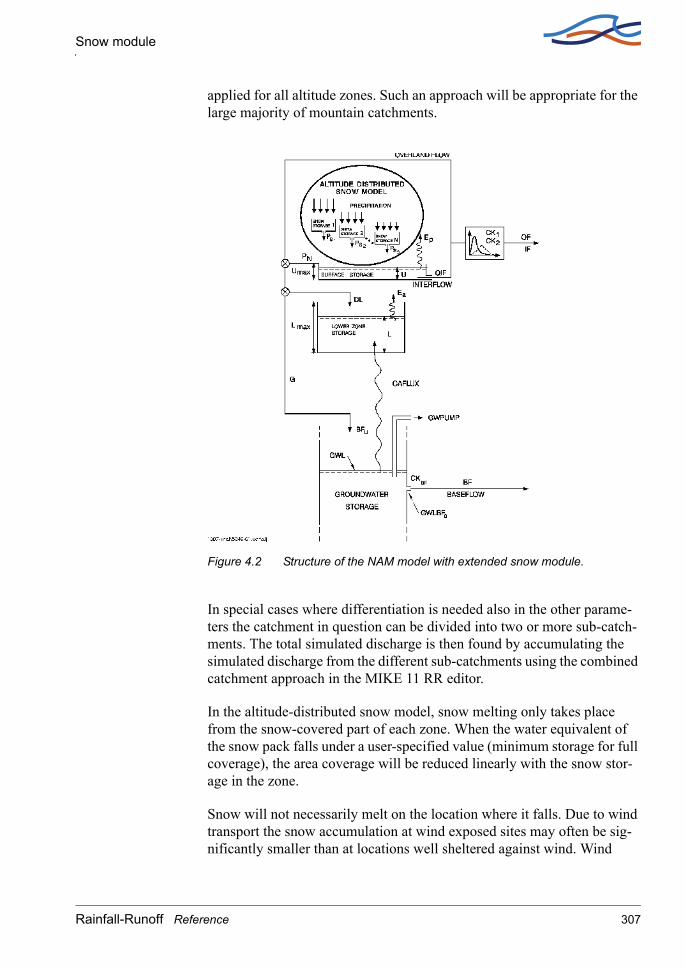
Snow module
applied for all altitude zones. Such an approach will be appropriate for the large majority of mountain catchments.
Figure 4.2 Structure of the NAM model with extended snow module.
In special cases where differentiation is needed also in the other parame-ters the catchment in question can be divided into two or more sub-catch-ments. The total simulated discharge is then found by accumulating the simulated discharge from the different sub-catchments using the combined catchment approach in the MIKE 11 RR editor.
In the altitude-distributed snow model, snow melting only takes place from the snow-covered part of each zone. When the water equivalent of the snow pack falls under a user-specified value (minimum storage for full coverage), the area coverage will be reduced linearly with the snow stor-age in the zone.
Snow will not necessarily melt on the location where it falls. Due to wind transport the snow accumulation at wind exposed sites may often be sig-nificantly smaller than at locations well sheltered against wind. Wind
Rainfall-Runoff Reference 307

RR reference Manual
exposed conditions are often present at higher altitudes where vegetation is sparse and wind velocities generally high. Furthermore, for the higher parts of mountain ranges, steep slopes having a limited snow storage capacity will often dominate. Snow storage in excess of this capacity will at such locations generate avalanches which transport the snow to lower altitudes. Hence, some of the snow falling on wind exposed and/or steep highlands may not melt on the location but be deposited and melting at lower altitudes. To account for such re-distribution of snow and avoid unrealistic accumulation of snow in the cold upper zones a user specified upper limit of the snow storage in the individual zones has been intro-duced in the model. Snow storage exceeding this value will be transferred to the neighbouring lower zone.
Adjustment of temperature and precipitation to altitude zonesThe altitude-distributed snow model operates with three meteorological reference time series; precipitation, temperature and potential evapotran-spiration. In order to account for the large variations in precipitation and temperature with altitude the reference series can be adjusted for each alti-tude zone in two different ways:
lapse rate corrections
individual correction factors applied for each zone
Lapse rate correctionsThe lapse rate correction approach is a very simple but powerful way of adjustment in which the temperature and the precipitation are assumed to vary linearly with the altitude. The only input data required are the aver-age altitude of the various zones, a reference altitude of the time series, and the lapse rates. The temperature lapse rates, however, are known to be quite variable, ranging from high values under dry conditions to lower val-ues under wet conditions. Hence, in the model it is possible to specify two different temperature lapse rates to be used during dry and wet weather conditions, respectively. The model applies the “wet” lapse rate during days with precipitation and the “dry” lapse rate during the rest of the time.
The temperature in each zone is adjusted by the following formula:
(4.11)
where
Tzone temperature in the considered zone
TzoneTref Hzone Href–( )βdry+ for P = 0Tref Hzone Href–( )βwet+ for P > 0
=
308 MIKE 11
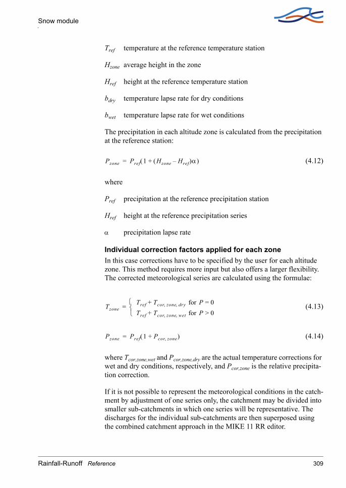
Snow module
Tref temperature at the reference temperature station
Hzone average height in the zone
Href height at the reference temperature station
bdry temperature lapse rate for dry conditions
bwet temperature lapse rate for wet conditions
The precipitation in each altitude zone is calculated from the precipitation at the reference station:
(4.12)
where
Pref precipitation at the reference precipitation station
Href height at the reference precipitation series
α precipitation lapse rate
Individual correction factors applied for each zoneIn this case corrections have to be specified by the user for each altitude zone. This method requires more input but also offers a larger flexibility. The corrected meteorological series are calculated using the formulae:
(4.13)
(4.14)
where Tcor,zone,wet and Pcor,zone,dry are the actual temperature corrections for wet and dry conditions, respectively, and Pcor,zone is the relative precipita-tion correction.
If it is not possible to represent the meteorological conditions in the catch-ment by adjustment of one series only, the catchment may be divided into smaller sub-catchments in which one series will be representative. The discharges for the individual sub-catchments are then superposed using the combined catchment approach in the MIKE 11 RR editor.
Pzone Pref 1 Hzone Href–( )α+( )=
TzoneTref Tcor zone dry,,+ for P = 0Tref Tcor zone wet,,+ for P > 0
=
Pzone Pref 1 Pcor zone,+( )=
Rainfall-Runoff Reference 309

RR reference Manual
4.6.3 Extended components
Seasonal variation of degree-day coefficientThe simple degree-day approach for calculating snow melt cf. (4.9) can be extended by using a seasonal variation of the degree-day coefficient Csnow. This variation reflects in a conceptual way the seasonal variation of the incoming short wave radiation and the variation in the albedo of the snow surface during the snow season. The albedo is very high (about 0.8) for new, cold snow falling in the beginning of the accumulation season and then decreases with the age of the snow (to a minimum value of about 0.3 in the end of the season).
RadiationThe melting effects caused by the absorbed short wave radiation can be explicitly modelled. In this case an additional snow melting is calculated as
(4.15)
where Crad is the radiation coefficient, and R is the incoming short wave radiation. The total amount of snow melt is calculated as the sum of the snow melt rates given by (4.9), (4.15), and (4.16) (optional), respectively.
Condensation of humid air and heat contribution from rainfallThe melting effects from condensation of humid air on the snow surface and the advective heat transferred to the snow pack by precipitation can be explicitly modelled. The effects are calculated as an additional snowmelt
(4.16)
where Crain is a degree-day coefficient, and P is the rainfall. The total amount of snow melt is calculated as the sum of the snow melt rates given by (4.9), (4.15) (optional), and (4.16), respectively.
4.7 Irrigation module
4.7.1 IntroductionMinor irrigation schemes within a catchment will normally have negligi-ble influence on the catchment hydrology, unless transfer of water over catchment boundaries is involved. Large schemes, however, may signifi-cantly affect the runoff and the groundwater recharge through local
∆QS CradR=
∆QS CrainP T T0–( )=
310 MIKE 11

Irrigation module
increases in evapotranspiration and infiltration as well as through opera-tional and field losses.
The irrigation module of NAM may be applied to describe the effect of irrigation on the following aspects:
The overall water balance of the catchment. This will be affected mainly by the increased evapotranspiration and by possible external water sources for irrigation.
Local infiltration and groundwater recharge in irrigated areas.
The distribution of catchment runoff amongst different runoff compo-nents (overland flow, interflow, baseflow). This may be influenced by the increased infiltration in irrigated areas as well as by local abstrac-tion of irrigation water from groundwater or streams.
For each irrigation area within the catchment a NAM subcatchment is defined with individual model parameters. The non-irrigated areas are modelled by defining a general NAM subcatchment. The total simulated discharge is then found by accumulating the simulated discharge from the different sub-catchments using the combined catchment approach in the MIKE 11 RR editor.
4.7.2 Structure of the irrigation moduleThe structure of the irrigation module is illustrated in Figure 4.3.
Rainfall-Runoff Reference 311
RR reference Manual
Figure 4.3 Structure of the NAM irrigation module.
Water supplied to the surface storage in irrigated areas will be a sum of precipitation P and irrigation water Pir. The potential evapotranspiration may vary with crop type and the stage of growth. The irrigation module accounts for this by allowing the user to specify monthly varying crop coefficients Ccrop for each irrigation area. The potential evapotranspiration for a specific crop is given by
(4.17)
where Ep is the reference time series of potential evapotranspiration.
Infiltration I is taken directly from the surface storage to the lower zone and groundwater storages and is calculated as a function of the moisture content in the lower zone L
(4.18)
Ep crop, CcropEp=
I k0infLmax L⁄ for k0infLmax L U<⁄
U for k0infLmax L U≥⁄
=
312 MIKE 11

Irrigation module
where k0inf is an infiltration factor describing the infiltration rate at field capacity (i.e. L = Lmax).
A portion G of the infiltration is assumed to percolate deeper and recharge the groundwater storage. This portion is, as in the general NAM model, calculated as a function of the conditions in the lower zone storage
(4.19)
where TG is the root zone threshold value for groundwater recharge.
The remaining part ∆L is assumed to increase the moisture content in the lower zone
(4.20)
If the maximum surface storage Umax is exceeded, the general NAM model diverts the excess water into overland flow (QOF) and infiltration. In the irrigation module infiltration has been accounted for as described above, and hence the excess water is added directly to overland flow.
Irrigation water can be abstracted from three different sources. The amount of water taken from each source type is determined by specifying fixed percentages of Pir for each source type:
local groundwater (PClgw)
local river (PClr)
external river (PCexr)
The term "local" means within the actual NAM catchment. If irrigation water is abstracted from local groundwater, it will be subtracted from the groundwater storage and the groundwater level will then be reduced with the amount
(4.21)
where SY is the specific yield, and ∆t is the time step used in the calcula-tions.
G IL Lmax TG–⁄
1 TG–-------------------------------- for L Lmax TG>⁄
0 for L Lmax TG≤⁄
=
∆L I G–=
∆GWL∆tPClgwPir
SY----------------------------=
Rainfall-Runoff Reference 313

RR reference Manual
If the water is abstracted from a local river, it will be subtracted from the calculated runoff
(4.22)
If the water is imported from a river outside the NAM catchment (exter-nal), no subtractions are made.
A part of the water diverted for irrigation will be lost on its way to the fields. The losses may include evaporation and seepage from channels, illegal off-takes, and operational losses (i.e. water that is diverted to the irrigation area but is not being utilised). In the irrigation module, the user may specify percentages of the irrigation water Pir that is lost, i.e.
evaporation losses (PCevap)
seepage losses (PCgw)
operational losses contributing to overland flow (PCof)
The losses may vary in time on a monthly basis.
Due to the different losses the irrigation water is reduced with the amount
(4.23)
The operational losses yields an increase in the overland flow
(4.24)
The seepage losses contributes to an increase in the groundwater level
(4.25)
4.8 Model parameters
This section provides a short description of the model parameters, their physical interpretation and importance along with suggestions for parame-ter adjustments in the calibration.
∆Qsim ∆tPClrPir=
∆Pir Pir PCevap PCgw PCof+ +( )=
∆OF ∆tPCofPir=
∆GWL∆tPCgwPir
SY--------------------------=
314 MIKE 11

Model parameters
4.8.1 Surface and root zone parameters
Maximum water content in surface storage Umax
Umax [mm] defines the maximum water content in the surface storage. This storage is interpreted as including the water content in the intercep-tion storage (on vegetation), in surface depression storages, and in the uppermost few cm's of the ground. Typical values of Umax are in the range 10-20 mm.
One important characteristic of the model is that the surface storage must be at its maximum capacity, i.e. U ≥ Umax before any excess water, PN, occurs. In dry periods, the amount of net rainfall that must occur before any overland flow occurs can be used to estimate Umax.
Maximum water content in root zone storage Lmax
Lmax [mm] defines the maximum water content in the lower or root zone storage. Lmax can be interpreted as the maximum soil moisture content in the root zone available for the vegetative transpiration. Ideally, Lmax can then be estimated by multiplying the difference between field capacity and wilting point of the actual soil with the effective root depth. The difference between field capacity and wilting point is referred to as the available water holding capacity (AWHC). For estimation of AWHC, moisture con-tents for different soil types at pF-value 2.5, corresponding approximately to field capacity, and pF-value 4.2, corresponding to wilting point are shown in Table 4.1
It should be noted that Lmax represents the average value for an entire catchment, i.e. an average value for the various soil types and root depths of the individual vegetation types. Hence, Lmax cannot in practice be esti-mated from field data, but an expected interval can be defined.
Since the actual evapotranspiration is highly dependent on the water con-tent of the surface and root zone storages, Umax and Lmax are the primary parameters to be changed in order to adjust the water balance in the simu-lations. In the preliminary stages of the model calibration, it is recom-mended to fix the relation between Umax and Lmax, leaving only one storage parameter to be estimated. As a rule, Umax = 0.1Lmax can be used unless special catchment characteristics or hydrograph behaviour indicate otherwise.
Table 4.1 Moisture content in cm3/cm3 at (effective) saturation (θs) and at pF-values of 2.5(θ2.5) and 4.2(θ4.2), for eleven textural classes and from three sources: (1) Rawls et al. (1982),/53/; (2) Cosby et al.
Rainfall-Runoff Reference 315
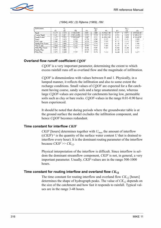
RR reference Manual
(1984),/45/; (3) Rijtema (1969), /56/.
Overland flow runoff coefficient CQOFCQOF is a very important parameter, determining the extent to which excess rainfall runs off as overland flow and the magnitude of infiltration.
CQOF is dimensionless with values between 0 and 1. Physically, in a lumped manner, it reflects the infiltration and also to some extent the recharge conditions. Small values of CQOF are expected for a flat catch-ment having coarse, sandy soils and a large unsaturated zone, whereas large CQOF-values are expected for catchments having low, permeable soils such as clay or bare rocks. CQOF-values in the range 0.01-0.90 have been experienced.
It should be noted that during periods where the groundwater table is at the ground surface the model excludes the infiltration component, and hence CQOF becomes redundant.
Time constant for interflow CKIFCKIF [hours] determines together with Umax the amount of interflow ((CKIF)-1 is the quantity of the surface water content U that is drained to interflow every hour). It is the dominant routing parameter of the interflow because CKIF >> CK12.
Physical interpretation of the interflow is difficult. Since interflow is sel-dom the dominant streamflow component, CKIF is not, in general, a very important parameter. Usually, CKIF-values are in the range 500-1000 hours.
Time constant for routing interflow and overland flow CK12
The time constant for routing interflow and overland flow CK12 [hours] determines the shape of hydrograph peaks. The value of CK12 depends on the size of the catchment and how fast it responds to rainfall. Typical val-ues are in the range 3-48 hours.
316 MIKE 11

Model parameters
The time constant can be inferred from calibration on peak events. If the simulated peak discharges are too low or arriving too late, decreasing CK12 may correct this, and vice versa.
Root zone threshold value for overland flow TOFTOF is a threshold value for overland flow in the sense that no overland flow is generated if the relative moisture content of the lower zone stor-age, L/Lmax, is less than TOF. The behaviour of the threshold value is illus-trated in Figure 4.4. Similarly, the root zone threshold value for interflow TIF and recharge TG act as threshold values for generation of interflow and recharge, respectively.
Figure 4.4 Generation of overland flow.
Physically, the three threshold values should reflect the degree of spatial variability in the catchment characteristics, so that a small homogeneous catchment is expected to have larger threshold values than a large hetero-geneous catchment.
For catchments with alternating dry and wet periods, the threshold values determine the onset of the flow components in the periods where the root zone is being filled up. This can be used in model calibration. It should be noted that the threshold values have no importance in wet periods. The significance of the threshold value varies from catchment to catchment and is usually larger in semi-arid regions.
In areas with alternating dry and wet seasons, TOF can be estimated on the basis of situations where even very heavy rainfall does not give rise to the quick response of the overland flow component. The parameter has an impact only during the first, few weeks of the wet season. Values of TOF in the range 0-0.7 have been experienced.
Root zone threshold value for interflow TIFThe root zone threshold value for interflow has the same function for interflow as TOF has for the overland flow. It is usually not a very impor-tant parameter, and it can in most cases be given a value equal to zero.
Rainfall-Runoff Reference 317

RR reference Manual
4.8.2 Groundwater parameters
Baseflow time constant CKBF
The time constant for baseflow, CKBF [hours], determines the shape of the simulated hydrograph in dry periods. According to the linear reservoir description the discharge in such periods is given by an exponential decay. CKBF can be estimated from hydrograph recession analysis. CKBF-values in the range 500-5000 hours have been experienced.
If the recession analysis indicates that the shape of the hydrograph changes to a slower recession after a certain time, an additional (lower) groundwater storage can be added to improve the description of the base-flow.
Root zone threshold value for groundwater recharge TGThe root zone threshold value for recharge has the same effect on recharge as TOF has on the overland flow. It is an important parameter for simulat-ing the rise of the groundwater table in the beginning of a wet season.
Recharge to lower groundwater storage CQLOW
In some cases the shape of the hydrograph recession changes to a slower recession after a certain period. To simulate this, a lower groundwater storage may be included. The parameter CQLOW determines the proportion of the recharge that percolates to the lower groundwater storage. CQLOW together with CKlow can be estimated from hydrograph recession analysis.
Time constant for routing lower baseflow CKlow
The baseflow from the lower groundwater storage is modelled using a lin-ear reservoir with time constant CKlow [hours]. The time constant can be estimated from hydrograph recession analysis. Usually, CKlow is larger than CKBF.
Ratio of groundwater catchment to topographical catchment area Carea
Drainage to or from neighbouring catchments can be modelled by specify-ing a value of Carea different from 1. Carea specifies the amount of recharge G that is being drained. If Carea < 1, part of the recharge, (1-Carea)G, is drained to another catchment, whereas for Carea > 1, the amount (Carea-1)G is added to the catchment recharge.
Maximum groundwater depth causing baseflow GWLBF0
The maximum depth to the groundwater table for which baseflow occurs, GWLBF0 [m], represents the outflow level of the groundwater reservoir given as the distance between the average ground level of the catchment and the minimum level of the river to which it drains. In low, flat areas the
318 MIKE 11
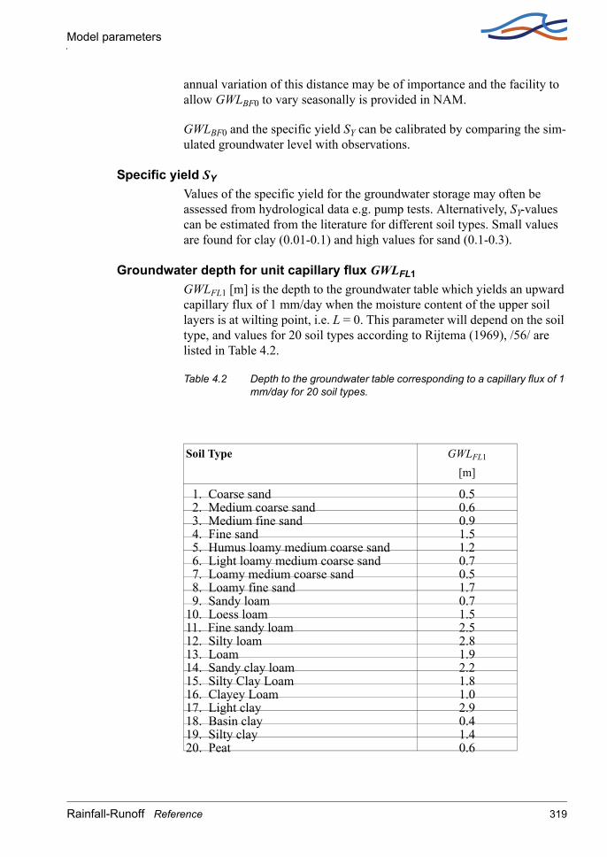
Model parameters
annual variation of this distance may be of importance and the facility to allow GWLBF0 to vary seasonally is provided in NAM.
GWLBF0 and the specific yield SY can be calibrated by comparing the sim-ulated groundwater level with observations.
Specific yield SY
Values of the specific yield for the groundwater storage may often be assessed from hydrological data e.g. pump tests. Alternatively, SY-values can be estimated from the literature for different soil types. Small values are found for clay (0.01-0.1) and high values for sand (0.1-0.3).
Groundwater depth for unit capillary flux GWLFL1
GWLFL1 [m] is the depth to the groundwater table which yields an upward capillary flux of 1 mm/day when the moisture content of the upper soil layers is at wilting point, i.e. L = 0. This parameter will depend on the soil type, and values for 20 soil types according to Rijtema (1969), /56/ are listed in Table 4.2.
Table 4.2 Depth to the groundwater table corresponding to a capillary flux of 1 mm/day for 20 soil types.
Soil Type GWLFL1
[m]
1. Coarse sand 0.5 2. Medium coarse sand 0.6 3. Medium fine sand 0.9 4. Fine sand 1.5 5. Humus loamy medium coarse sand 1.2 6. Light loamy medium coarse sand 0.7 7. Loamy medium coarse sand 0.5 8. Loamy fine sand 1.7 9. Sandy loam 0.710. Loess loam 1.511. Fine sandy loam 2.512. Silty loam 2.813. Loam 1.914. Sandy clay loam 2.215. Silty Clay Loam 1.816. Clayey Loam 1.017. Light clay 2.918. Basin clay 0.419. Silty clay 1.420. Peat 0.6
Rainfall-Runoff Reference 319

RR reference Manual
4.8.3 Snow module parameters
Degree-day coefficient Csnow
The snow melts at a rate defined by the degree-day coefficient Csnow [mm /°C/day]. A seasonal variation of Csnow can be defined in order to account for the seasonal variations of the incoming short wave radiation and the albedo of the snow surface. Typical values of Csnow are in the range 2-4 mm/°C/day.
Base temperature (snow/rain) T0
The precipitation is assumed to fall as snow if the temperature is below the base temperature T0 [°C]. For temperatures above T0 the snow in the snow storage is melting. The base temperature is usually close to zero degrees Celsius.
Radiation coefficient Crad
The radiation coefficient Crad [m2/W/mm/day] determines the rate of snow melting caused by the absorbed short wave radiation.
Rainfall degree-day coefficient Crain
The rainfall degree-day coefficient Crain [mm/mm/°C/day] determines the rate of snow melting caused by condensation of humid air on the snow surface and the advective heat transferred to the snow pack by precipita-tion.
4.8.4 Irrigation module parameters
Infiltration factor K0inf
K0inf [mm/day] is the infiltration factor which, together with the moisture content in the upper and root zone storages, determines the amount of water infiltrating from the surface to the root zone and groundwater stor-age.
320 MIKE 11

Model parameters
Figure 4.5 Infiltration rate as a function of the moisture content in the root zone.
In Figure 4.5 the infiltration rate is shown as a function of the moisture content in the root zone. K0inf is strongly dependent on the soil type and is large for sandy soils and small for clayey soils.
When irrigation water is supplied, the root zone will often be close to sat-uration. Under such conditions the infiltration rate K0inf may converge to the saturated hydraulic conductivity of the soil (Ks). As a guideline Ks-val-ues for different soil types, as estimated by various authors, are presented in Table 4.3.
When the root zone is only partly saturated, the flow dynamics become very complicated and are not properly described in a lumped model like NAM. Furthermore, the soil preparation may have a significant influence on the soil hydraulic conductivity.
Crop coefficients and irrigation lossesThe crop coefficients account for the fact that potential evapotranspiration is dependent of the crop type and the stage of growth. This is achieved by multiplying the input time series of potential evapotranspiration with the crop coefficient. For dry uncropped soils, the crop coefficient will tend to zero while well cropped fields reaching full growth potential could have crop coefficients greater than 1. Further information about how to estimate the crop coefficients is given in /46/. Monthly values of crop coefficients can be specified.
The monthly magnitude and distribution of losses to evaporation, seepage, and overland flow should correspond to the design values of the irrigation scheme unless observations have shown a different distribution.
Table 4.3 Values of saturated hydraulic conductivity Ks for eleven textural classes from six sources (1) Li et al. (1976), /48/; (2) Brakensiek (1979), /43/; (3) Brakensiek et al. (1981), /44/; (4) McCuen et al.
Rainfall-Runoff Reference 321

RR reference Manual
(1981), /50/; (5) Cosby et al. (1984), /45/; (6) Rijtema (1969), /56/. The ratio between the largest and the smallest estimate has been calculated for columns 1-5 and 1-6, respectively.
4.9 Initial conditions
The initial conditions required by the NAM model consist of the initial water contents in the surface and root zone storages, together with initial values of overland flow, interflow, and baseflow.
If a lower groundwater reservoir is specified, the initial baseflow from both the upper and the lower reservoir should be specified. If the snow module is included, the initial value of the snow storage should be speci-fied.
If a simulation commences at the end of a dry period, it is often sufficient to set all initial values to zero, except the water content in the root zone and the baseflow. The water content in the root zone should be about 10-30% of the capacity and the baseflow should be given a value close to the observed discharge.
Improved estimates of the initial conditions may be obtained from a previ-ous simulation, covering several years, by noting the appropriate moisture contents of the root zone and baseflow at the same time of the year as the new simulation will start.
In general it is recommended to disregard the first 3-6 months of the NAM simulation in order to eliminate the influence of erroneous initial condi-tions.
4.10 Model calibration
In the NAM model the parameters and variables represent average values for the entire catchment. While in some cases a range of likely parameter values can be estimated, it is not possible, in general, to determine the val-
322 MIKE 11

Model calibration
ues of the NAM parameters on the basis of the physiographic, climatic and soil physical characteristics of the catchment, since most of the parameters are of an empirical and conceptual nature. Thus, the final parameter esti-mation must be performed by calibration against time series of hydrologi-cal observations.
4.10.1 Calibration objectives and evaluation measuresThe following objectives are usually considered in the model calibration
1 A good agreement between the average simulated and observed catch-ment runoff (i.e. a good water balance)
2 A good overall agreement of the shape of the hydrograph
3 A good agreement of the peak flows with respect to timing, rate and volume
4 A good agreement for low flows
In this respect it is important to note that, in general, trade-offs exist between the different objectives. For instance, one may find a set of parameters that provide a very good simulation of peak flows but a poor simulation of low flows, and vice versa.
In the calibration process, the different calibration objectives 1-4 should be taken into account. If the objectives are of equal importance, one should seek to balance all the objectives, whereas in the case of priority to a certain objective this objective should be favoured.
For a general evaluation of the calibrated model, the simulated runoff is compared with discharge measurements. For individual calibration of the groundwater parameters, the simulated average groundwater level can be compared with groundwater level measurements in the catchments.
Both graphical and numerical performance measures should be applied in the calibration process. The graphical evaluation includes comparison of the simulated and observed hydrograph, and comparison of the simulated and observed accumulated runoff. The numerical performance measures include the overall water balance error (i.e. the difference between the average simulated and observed runoff), and a measure of the overall shape of the hydrograph based on the coefficient of determination or Nash-Sutcliffe coefficient (/51/)
Rainfall-Runoff Reference 323

RR reference Manual
(4.26)
where Qsim,i is the simulated discharge at time i, Qobs,i is the corresponding observed discharge, and is the average observed discharge. A perfect match corresponds to R2 = 1.
An exact agreement between simulations and observations must, however, not be expected. The goodness-of-fit of the calibrated model is affected by different error sources, including
1 Errors in meteorological input data
2 Errors in recorded observations
3 Errors and simplifications inherent in the model structure
4 Errors due to the use of non-optimal parameter values
In model calibration only error source (4) should be minimised. In this respect it is important to distinguish between the different error sources since calibration of model parameters may compensate for errors in data and model structure. For catchments with a low quantity or quality of data, less accurate calibration results may have to be accepted.
Satisfactory calibrations over a full range of flows usually require continu-ous observations of runoff for a period of 3-5 years. Runoff series of a shorter duration, however, will also be useful for calibration, although they do not ensure an efficient calibration of the model. For a proper eval-uation of the reliability and hydrological soundness of the calibrated model it is recommended to validate the model on data not used for model calibration (split-sample test). Some general aspects related to calibration and validation of hydrological models are described in Refsgaard and Storm (1996), /55/.
4.10.2 Manual calibrationThe process of model calibration is normally done either manually or by using computer-based automatic procedures. In this section a manual cali-bration strategy for the NAM model is outlined. Application of an auto-matic optimisation routine for calibration of the basic NAM model is described in the subsequent section.
R2 1
Qobs i, Qsim i,–[ ]2
i 1=
N
∑
Qobs i, Qobs–[ ]2
i 1=
N
∑
--------------------------------------------------–=
Qobs
324 MIKE 11
Model calibration
In manual calibration, a trial-and-error parameter adjustment is made until satisfactory results are obtained. It is recommended, especially for the less experienced users, to change only one parameter between each trial, so that the effect of the change can be easily discerned. The manual calibra-tion strategy outlined below is based on the different rainfall-runoff proc-ess descriptions for calibration of the relevant model parameters, i.e. the parameters that mostly affect the considered process description (see also Section 4.8 Model parameters (p. 314)).
A calibration usually commences by adjusting the water balance in the system. The total evapotranspiration over a certain period should corre-spond to the accumulated net precipitation minus runoff. The evapotran-spiration will increase when increasing the maximum water contents in the surface storage Umax and the root zone storage Lmax, and vice versa.
The peak runoff events are caused by large quantities of overland flow. The peak volume can be adjusted by changing the overland flow runoff coefficient (CQOF), whereas the shape of the peak depends on the time constant used in the runoff routing (CK12).
The amount of base flow is affected by the other runoff components; a decrease in overland flow or interflow will result in a higher baseflow, and vice versa. The shape of the baseflow recession is a function of the base-flow time constant (CKBF). If the baseflow recession changes to a slower recession after a certain time, a lower groundwater reservoir should be added, including calibration of CQlow and CKlow.
Initially, the root zone threshold values TOF, TIF and TG can be set to zero. After a first round of calibration of the parameters Umax, Lmax, CQOF, CK12 and CKBF, the threshold parameters can be adjusted for fur-ther refinement of the simulation results.
For individual calibration of the groundwater parameters GWLBF0 and SY, the simulated groundwater level is compared to observed groundwater levels. Inclusion of the shallow groundwater reservoir description is important in lowland areas, as found e.g. in swamps or river delta areas, where the groundwater table may reach the ground surface during the wet season.
The snow module parameters are calibrated against periods with snow-melt runoff.
4.10.3 Automatic calibration routineFor calibration of the basic NAM model, including the 9 model parame-ters listed in Table 4.4, an automatic optimization routine is available. The
Rainfall-Runoff Reference 325

RR reference Manual
automatic calibration routine is based on a multi-objective optimization strategy in which the four different calibration objectives given above can be optimised simultaneously.
Multi-objective calibration measuresIn automatic calibration, the calibration objectives have to be formulated as numerical goodness-of fit measures that are optimised automatically. For the four calibration objectives defined above the following numerical performance measures are used:
1 Agreement between the average simulated and observed catchment runoff: overall volume error.
2 Overall agreement of the shape of the hydrograph: overall root mean square error (RMSE).
3 Agreement of peak flows: average RMSE of peak flow events.
4 Agreement of low flows: average RMSE of low flow events.
Overall volume error
(4.27)
where
Qobs,i is the observed discharge at time i
Qsim,i is the simulated discharge at time i
θ is the set of model parameters to be calibrated
N is the number of time steps in the calibration period
Overall RMSE
(4.28)
The coefficient of determination in Eq. (4.26) is a transformed and nor-malised measure of the overall RMSE (normalised with respect to the var-iance of the observed hydrograph). Thus, minimisation of (4.28) corresponds to maximising R2.
F1 θ( ) 1N---- Qobs i, Qsim i, θ( )–[ ]
i 1=
N
∑=
F2 θ( ) 1N---- Qobs i, Qsim i, θ( )–[ ]2
i 1=
N
∑1 2⁄
=
326 MIKE 11

Model calibration
Average RMSE of peak flow events
(4.29)
where Mp is the number of peak flow events in the calibration period, and nj is the number of time steps in event no. j. Peak flow events are defined as periods where the observed discharge is above a given (user-specified) threshold level.
Average RMSE of low flow events
(4.30)
where Ml is the number of low flow events in the calibration period. Low flow events are defined as periods where the observed discharge is below a given (user-specified) threshold level.
Optimization algorithmThe multi-objective optimization problem can be formulated as follows
, (4.31)
The optimization problem is said to be constrained in the sense that θ is restricted to the feasible parameter space Θ. The parameter space is defined as a hypercube by specifying lower and upper limits on each parameter. These limits should be chosen according to physical and math-ematical constraints in the model and from modelling experiences.
The solution of (4.31) will not, in general, be a single unique set of param-eters but will consist of the so-called Pareto set of solutions (non-domi-nated solutions), according to various trade-offs between the different objectives. The concept of Pareto optimality implies that the entire param-eter space Θ can be divided into “good” (Pareto optimal) and “bad” solu-tions, and none of the “good” solutions can be said to be “better” than any of the other “good” solutions. A member of the Pareto set will be better than any other member with respect to some of the objectives, but because of the trade-off between the different objectives it will not be better with respect to other objectives.
F3 θ( ) 1Mp------- 1
nj---- Qobs i, Qsim i, θ( )–[ ]2
i 1=
nj
∑j 1=
Mp
∑
1 2⁄
=
F3 θ( ) 1Ml------ 1
nj---- Qobs i, Qsim i, θ( )–[ ]2
i 1=
nj
∑j 1=
Ml
∑
1 2⁄
=
min F1 θ( ) F2 θ( ) F3 θ( ) F4 θ( ),,, θ Θ∈
Rainfall-Runoff Reference 327

RR reference Manual
In practical applications, the entire Pareto set may be too expensive to cal-culate, and one is only interested in part of the Pareto optimal solutions. To estimate only a single point of the Pareto front a single-objective opti-mization problem is defined that aggregates the different objective func-tions F1(θ) – F4(θ). The applied aggregate measure is the Euclidian distance
(4.32)
where Ai are transformation constants. A balanced aggregated measure is defined by assigning transformation constants in (4.32) such that the dif-ferent objectives have equal weight in the optimization. The transforma-tion constants are automatically calculated based on the initially generated population of parameter sets in the optimization loop (/49/).
The optimal parameter set is found by minimising (4.32) with respect to θ. Optimization is performed automatically using the shuffled complex evo-lution (SCE) algorithm (/47/). The SCE method is a global search method in the sense that it is especially designed for locating the global optimum of the objective function and not being trapped in local optima. A detailed description of the algorithm is given in /47/. Implementation and testing of the algorithm for automatic calibration of the NAM model is described in /49/.
User specificationsSpecifications for the NAM auto-calibration module include:
Calibration parameters
Range of calibration parameters
Objective functions
Stopping criterion
Calibration parametersThe automatic calibration routine includes the 9 model parameters shown in Table 4.4. The user specifies the subset of these parameters that should be calibrated automatically.
Range of calibration parametersFor the subset of NAM parameters to be calibrated automatically the user specifies the hypercube search space, i.e. lower and upper bounds on each parameter. The range of the different parameters should reflect the prior
Fagg θ( ) F1 θ( ) A1+( )[ 2 F2 θ( ) A2+( )2
F3 θ( ) A3+( )2 F4 θ( ) A4+( )2 ]1 2⁄
+
+ +
=
328 MIKE 11

Model calibration
knowledge of experienced values for the type of catchment being consid-ered. Default limits based on physical and mathematical model constraints and experienced values for a range of different catchments are provided in Table 4.4.
Table 4.4 Calibration parameters and default hypercube search space
Objective functionsThe user can specify any combination of the 4 objective functions: (1) overall water balance error, (2) overall RMSE, (3) peak flow RMSE, and (4) low flow RMSE. For the peak and low flow RMSE the user should specify the threshold levels for defining peak and low flow events, respec-tively.
The choice of objective functions should reflect the objective of the model simulation. For general hydrological studies, the overall water balance error and overall RMSE is normally applied. If focus of the study is on high or low flows, the peak or low flow RMSE should be included. It is not advised to use only the water balance error for optimisation, since this may provide an unrealistic model calibration.
Stopping criterionThe stopping criterion for the optimisation algorithm is the maximum number of model evaluations. The appropriate number of model evalua-tions depends primarily on the number of calibration parameters and the
Parameter Unit Lower bound Upper bound
Umax [mm] 5 35
Lmax [mm] 50 400
CQOF [-] 0 1
CKIF [hours] 200 2000
CK12 [hours] 3 72
TOF [-] 0 0.9
TIF [-] 0 0.9
TG [-] 0 0.9
CKBF [hours] 500 5000
Rainfall-Runoff Reference 329

RR reference Manual
complexity of the model (interaction between model parameters). A large number of model evaluations are, in general, needed for a complex model with many parameters. This requirement should be balanced against the computing time. For a model calibration that includes all 9 parameters, a maximum number of model evaluations in the range 1000-2000 normally ensures an efficient calibration.
Besides the user-defined stopping criterion, the optimisation algorithm includes a parameter convergence criterion. In this case the optimisation algorithm stops if the entire population of parameter sets in an optimisa-tion loop have converged into the same parameter values.
4.11 NAM - REFERENCES
/42/ Abbott, M.B. and J.C. Refsgaard (eds) (1996), Distributed Hydro-logical Modelling, Kluwer Academic Press, The Netherlands, 321 p.
/43/ Brakensiek, D.L. (1979), Comments on 'Empirical Equations for some soil Hydraulic Properties' by Roger B. Clapp and George M. Hornberger, Water Resources Research, 15 (4), 989-990.
/44/ Brakensiek, D.L., Engleman, R.L. and Rawls, W.J. (1981), Varia-tion within texture classes of soil water parameters, Trans. ASAE, 24, 335-339.
/45/ Cosby, B.J., Hornberger, G.M., Clapp, R.B. and Ginn, T.R. (1984), A statistical exploration of the relationships of soil moisture charac-teristics to the physical properties of soils, Water Resources Research, 20 (6), 682-690.
/46/ Doorenbos, J. and W.O. Pruitt (1977), Guidelines for Predicting Crop Water Requirements. FAO Irrigation and Drainage paper No. 24. Food and Agricultural Organization of the United Nations.
/47/ Duan, Q., Sorooshian, S., Gupta, V. (1992), Effective and efficient global optimization for conceptual rainfall-runoff models, Water Resources Research, 28(4), 1015-1031.
/48/ Li, R.-M., Stevens, M.A. and Simons, D.B. (1976), Solutions to Green-Ampt infiltration equations, J. Irrig. and Drain. Div., Amer. Soc. Civil. Eng., 102 (IR2), 239-248.
/49/ Madsen, H. (1999), Automatic calibration of a conceptual rainfall-
330 MIKE 11

UHM
runoff model using multiple objectives, Journal of Hydrology, Sub-mitted.
/50/ McCuen, R.H., Rawls, W.J. and Brakensiek, D.L. (1981), Statistical analysis of the Brooks-Corey and Green-Ampt parameters across soil textures, Water Resources Research, 17, 1005-1013.
/51/ Nash, I.E. and Sutcliffe, I.V. (1970), River flow forecasting through conceptual models, Part I, Journal of Hydrology, 10, 282-290.
/52/ Nielsen, S.A. and E. Hansen (1973), Numerical simulation of the rainfall runoff process on a daily basis, Nordic Hydrology, 4, 171-190.
/53/ Rawls, W.J., Brakensiek, D.L. and Saxton, K.E. (1982), Estimation of soil water properties, Transactions of the ASAE, 25, 1316-1320.
/54/ Refsgaard, J.C. and J. Knudsen (1997), Operational validation and intercomparison of different types of hydrological models. Water Resources Research, 32(7), 2189-2202.
/55/ Refsgaard, J.C. and Storm, B. (1996), Construction, calibration and validation of hydrological models, In: Distributed Hydrological modelling (eds. M.B. Abbott and J.C. Refsgaard), Kluwer Aca-demic Press, The Netherlands, 41-54.
/56/ Rijtema, P.E. (1969), Soil moisture forecasting, Nota 513, Instituut voor Cultuurtechniek en Waterhuishouding, Wageningen, The Netherlands.
/57/ U.S. Army Corps of Engineers (1956), Snow hydrology: Summary report on snow investigations.
4.12 UHM
4.12.1 IntroductionThe present UHM module simulates the runoff from single storm events by the use of the well known unit hydrograph techniques and constitutes an alternative to the NAM model for flood simulation in areas where no streamflow records are available or where unit hydrograph techniques have already been well established. The module calculates simultaneously the runoff from several catchments and includes facilities for presentation
Rainfall-Runoff Reference 331
RR reference Manual
and extraction of the results. The output from the module can further be used as lateral inflow to the advanced hydrodynamic module in MIKE 11.
In the unit hydrograph module the excess rain is calculated assuming that the losses to infiltration can be described as a fixed initial and constant loss, a proportional loss (the rational method) or by the SCS curve number method.
The excess rainfall is routed to the river by unit hydrograph methods. The module includes the SCS-dimensionless hydrographs as well as facilities for establishing and management of databases with user defined unit hydrographs and time series of recorded rainfall and streamflow.
Storage function method
Basic equationThe continuity equation and momentum equation are given by:
(4.33a)
(4.33b)
where:
Si apparent basin storage.
Qi direct runoff from a basin with consideration of the time of delay (except for base flow).
Ti time of delay.
K,P constants.
f coefficient of inflow.
rave mean rainfall of river basin.
A catchment area.
AdSidt------- f raveA Qi–=
Si KQiP=
332 MIKE 11

UHM
Numerical solutionEquation (4.33a) is approximated as follows:
(4.34a)
(4.34b)
which by rearranging gives
(4.34c)
where:
rt+∆t rainfall intensity at the time t+∆t.
qi,t runoff at the time t (Q/A).
si,t apparent storage at the time t.
∆t time step.
Work out equation (4.34c) numerically using:
(4.35a)
and (4.35b)
(4.35c)
Thus equation (4.34c) now reads
(4.36)
which is solved with respect to x.
Si t t∆+, Si t,– rt t∆+qi t, q– i t t∆+,
2---------------------------–
=
Kqi t t∆+,P Kqi t,
P– rt t∆+qi t, q– i t t∆+,
2---------------------------–
=
2 Kt∆
-----qi t t∆+,
Pq+
i t t∆+,2 rt t∆+
qi t,
2-------– K
t∆-----q
i t,
P+
– 0=
C rt t∆+qi t,
2-------– K
t∆-----q
i t,
P+=
x qi t t∆+,=
2 Kt∆
-----xP x+ 2C– 0=
Rainfall-Runoff Reference 333

RR reference Manual
Quasi-linear function method
Basic equationGenerating rational formula, rectangle unit hydrograph as follows is avail-able.
(4.37)
Or, moving average process as follows, by the time of flood concentration (tc).
(4.38)
Using a kinematic wave method tc is given by:
(4.39)
L is the physical length of the slope, α, m are constants.
The relation between the water depth on the slope (h) and the unit dis-charge (q) is given by
(4.40)
The term m is 3 for laminar flow and 5/3 for Manning type flow.
Take S as the physical average grade of the slope, N as the equivalent roughness of Manning type.
(4.41a)
(4.41b)
U τ( )0 for τ 0 τ tc<,<
1tc--- for 0 τ tc< <
=
q τ( ) 1tc--- re τ( )dτ
t tc–
t
∫=
tcLre
1 m–
α---------------
1 m⁄
=
q αhm=
α SN
-------∝
tc L1 m⁄ N1 m⁄ S 1 2m⁄– re1 m 1–⁄∝
334 MIKE 11

UHM
Kadoya and others get the following experimental equation:
(4.42)
If the flood term tc is fixed, the runoff hydrograph can be computed by equation (4.37). However the outflow would be zero if it passes tc.There-fore, a logarithmic unit hydrograph given by
(4.43)
where k = tc/2 (by Yoshino) is used.
Numerical solutionThe term k in the storage equation is given using time of flood concentra-tion tc by kadoya. Thus the equations to solve are given by
(4.44a)
(4.44b)
where k = tc/2 and tc is given by equation (4.42).
Nakayasu method
Basic equationThe unit hydrograph equation is given by
(4.45)
where:
q(t) Runoff height at time t.
re(t) Effective rainfall intensity in time interval
tc CA0,22re0,35–=
U τ( )0 for τ 0<
1k---e τk– for 0 τ<
=
dSdt------ re q–=
S kq=
q t( ) re t j t∆–( )h j t∆( )j 0=
n
∑=
Rainfall-Runoff Reference 335

RR reference Manual
h(t) Unit hydrograph
∆t Time interval
SolutionThe maximum discharge is given by
(4.46)
The increasing curve in the unit hydrograph is given by
(4.47)
The decreasing curve in the unit hydrograph leads
(4.48)
where:
Qmax Maximum discharge in unit hydrograph.
Qd Unit hydrograph.
A Catchment area.
R0 Rainfall intensity.
T1 Constant.
T0.3 Constant.
4.12.2 The Loss ModelDuring a storm a part of the total rainfall infiltrates the soil. Large parts of the infiltration evaporates or reaches the river a long time after the end of
QmaxAR0
0,3T1 T0,3+----------------------------=
QdQmax----------- t
T1-----
2,4=
Qd
Qmax-----------
0,3t T1–( ) T0,3⁄
for 1Qd
Qmax----------- 0,3>≥
0,3t T1– 0,5T0,3+( ) 1,5T0,3⁄
for 0,3Qd
Qmax----------- 0,32>≥
0,3t T1– 0,5T0,3+( ) 2,0T0,3⁄
for 0,32 QdQmax-----------≥
=
336 MIKE 11

UHM
storm as baseflow. Hence in event models as the present one, it is reasona-ble to describe the major part of the infiltration as loss. The amount of rain actually reaching the river, i.e. the total amount of rainfall less the loss is termed the excess rainfall.
The unit hydrograph module includes three optional methods for calcu-lation of the excess rainfall. They are all lumped models considering each catchment as one unit and hence the parameters represent average values for the catchment.
All the methods include an areal adjustment factor accounting, to some extent, for non uniform distribution the precipitation over the catchment.
Proportional Loss (The rational method)In this method the losses are assumed to be proportional to the rainfall rate and thus the excess rainfall is given by:
(4.49)
where:
Pexcess : Excess rainfall (mm/hr).
a : User defined run-off coefficient between 0 and 1.
Af : Areal adjustment factor.
P : Rainfall (mm/hr).
Fixed Initial Loss and Constant LossFollowing this method no excess rainfall will be generated before a user specified initial loss demand has been met. Subsequently excess rainfall will be generated whenever rainfall rate exceeds a specified constant loss rate i.e.
P* A* a = P fexcess
Rainfall-Runoff Reference 337
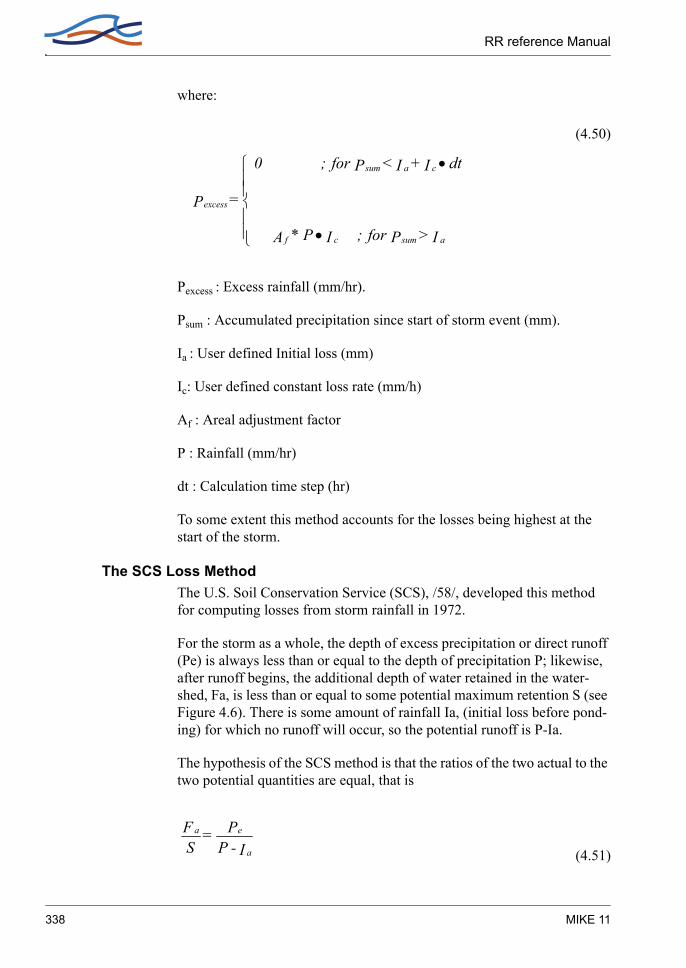
RR reference Manual
where:
(4.50)
Pexcess : Excess rainfall (mm/hr).
Psum : Accumulated precipitation since start of storm event (mm).
Ia : User defined Initial loss (mm)
Ic: User defined constant loss rate (mm/h)
Af : Areal adjustment factor
P : Rainfall (mm/hr)
dt : Calculation time step (hr)
To some extent this method accounts for the losses being highest at the start of the storm.
The SCS Loss MethodThe U.S. Soil Conservation Service (SCS), /58/, developed this method for computing losses from storm rainfall in 1972.
For the storm as a whole, the depth of excess precipitation or direct runoff (Pe) is always less than or equal to the depth of precipitation P; likewise, after runoff begins, the additional depth of water retained in the water-shed, Fa, is less than or equal to some potential maximum retention S (see Figure 4.6). There is some amount of rainfall Ia, (initial loss before pond-ing) for which no runoff will occur, so the potential runoff is P-Ia.
The hypothesis of the SCS method is that the ratios of the two actual to the two potential quantities are equal, that is
(4.51)
•
•
I > P for ; I P* A
dt I + I < P for ; 0
= P
asumcf
casum
excess
I- PP =
SF
a
ea
338 MIKE 11

UHM
From the continuity principle
(4.52)
Combining equations (4.51) and (4.52) gives
(4.53)
which is the basic equation for computing the depth of excess rainfall or direct runoff from a storm by the SCS method.
By study of results from many small experimental watersheds, an empiri-cal relation was developed.
(4.54)
Combining equations (4.53) and (4.54) the basic equation used in this model is derived.
(4.55)
F + I + P = P aae
( ) S+ I - P
I - P = Pa
a2
e
0.2S = I a
( )0.8S + P
0.2S - P = P2
e
Rainfall-Runoff Reference 339

RR reference Manual
Figure 4.6 Variables in the SCS method of rainfall abstractions: Ia = initial abstraction, Pe = accumulated excess rain, Fa = continuing abstrac-tion, P = total rainfall.
The potential maximum retention S is calculated from a dimensionless curve number (CN) using the empirical formula derived by SCS on the basis of rainfall runoff analyses of a large number of catchments.
(4.56)
The curve number depends on the soil type, the land use and the anteced-ent moisture condition (AMC) at the start of the storm.
CN varies between 0, resulting in no runoff, and 100 which generates an excess rain equal to the rainfall. For natural catchments normally 50 < CN < 100.
The model operates with three different antecedent moisture conditions namely:
AMC(I) : Dry conditions close to wilting point.
AMC(II) : Average wet conditions close to field capacity.
AMC(III): Wet conditions close to saturation.
( )( ) (mm) 25.4 10 - 1000/CN = S •
340 MIKE 11

UHM
For each calculation time step the excess rainfall is calculated as the dif-ference between the accumulated excess rainfall Pe at the start and the end of the time step.
Table 4.5 Correlation between SCS Curve numbers and the antecedent mois-ture condition as given in /58/.
The SCS method was developed on the basis of daily rainfall and conse-quently the program considers the beginning of a new 24 hour period as the start of a new storm event i.e.
– Each 24 hour AMC is updated by one class for each 16 mm rain fallen during the simulation period.
Rainfall-Runoff Reference 341

RR reference Manual
– CN and S are recalculated in correspondence with the updated AMC. Conversion of CN due to AMC is done using Table 4.5.
– The accumulated rainfall amount Pe is reset to zero.
NakayasuThe governing equations are given by
for (4.57a)
for (4.58a)
where:
Re Effective rainfall.
SR Cumulative rainfall.
Rsa Saturation rainfall.
α,β Constants.
Figure 4.7 The effective cumulative rainfall as a function of the cumulative rain-fall.
SRe αSRβ= SR Rsa≤
Re SR Rsa – αRsaβ+= SR Rsa>
342 MIKE 11

UHM
f1-RsaThe governing equation is given by
(4.59)
where:
Re Effective rainfall.
SR Cumulative rainfall.
Rsa Saturation rainfall.
Figure 4.8 The effective cumulative rainfall as a function of the cumulative rain-fall.
4.12.3 The Unit Hydrograph Routing Model
Basic AssumptionsThe unit hydrograph method is a simple linear model that can be used to derive the resulting hydrograph from any amount of excess rainfall.
The unit hydrograph is the unit pulse response function of a linear hydro-logical system, i.e. the direct runoff hydrograph resulting from one unit of excess rain with the duration, tr.
Ref1R for 0 SR R1sa≤<
f2R for R1sa SR R2sa≤<
f3R for R2sa SR<
=
Rainfall-Runoff Reference 343

RR reference Manual
The following basic assumptions are inherent in this model:
– The excess rainfall has a constant intensity within the effective duration.
– The excess rainfall is uniformly distributed over the whole catch-ment area.
– The base time of the direct runoff hydrograph resulting from an excess rain with a given duration is constant.
– The ordinates of all direct runoff hydrographs of a common base time are directly proportional to the total amount of excess rain rep-resented by each hydrograph.
– The principle of superposition applies to hydrographs resulting from continuous and/or isolated periods of uniform-intensity excess rain as illustrated on (see Figure 4.9).
– For a given catchment, the hydrograph resulting from a given excess rainfall reflects the unchanging conditions of the catchment.
Figure 4.9 Principle of superposition applied to hydrographs.
Under natural conditions the above assumptions cannot be perfectly met. However in many cases the hydrological conditions come close enough to the above assumptions to generate satisfactory results. A more detailed discussion of the above assumptions can be found in /59/.
344 MIKE 11

UHM
Principle of calculationIn accordance with the principle of superposition, the model for each cal-culation time step determines the responding hydrograph to the excess rainfall, as generated by the loss model during this time step, and add the response to the flow contributions generated in previous time steps.
Types of unit hydrographsA unit hydrograph can be characterized by the duration of the unit rainfall (tr) resulting in the hydrograph and the lag time (tl) defined as the time dif-ference between the centre of the unit rainfall event and the runoff peak.
From these two characteristics the time to peak (Tp), i.e. the time from the start of the storm event until the occurrence of peak runoff can be calcu-lated as:
(4.60)
In reality the unit hydrograph of a given catchment is unique. However, large efforts have been put in development of synthetic unit hydrographs which are more or less generally applicable. Two such hydrographs namely the SCS triangular unit hydrograph and the SCS dimensionless hydrograph (see Figure 4.10) are pre-specified in the model.
Figure 4.10 Soil Conservation Service Synthetic Hydrographs. (a) Dimension-less hydrograph. (b) Triangular hydrograph.
t + /2t = T lrp
Rainfall-Runoff Reference 345

RR reference Manual
The user can either use one of these or choose to apply a user defined hydrograph from the unit hydrograph data base.
The model supports three types of user defined hydrographs:
1 Dimensionless hydrographs specified as the flow divided by the peak flow (q/qp) as a function of the time divided by the time to peak (T/Tp).
2 Catchment specific hydrographs which are entered in dimensions and with correspondent unit rain duration, tr.
3 Instantaneous unit hydrographs derived by the time-area method.
Instantaneous unit hydrographs are automatically converted to hydrographs, i.e. 'dt'-hour-hydrographs with a unit rain duration equal to the calculation time step (dt) after the formula:
qdt(t) = (q(t) + q(t-dt)) / 2 (4.61)
where:
qdt(t) : Ordinate at time = t of the 'dt'-hour-hydrograph.
q(t) : Ordinate at time = t of the instantaneous hydrograph.
t : Actual calculation time.
dt : Calculation time step.
The present version of the program does not include a facility for decon-volution of hydrographs and hence non instantaneous unit hydrographs are assumed to originate from a unit rain of duration equal to the time step.
The user must specify the lag time to be used in a given the calcula-tion.The program will then scale the applied hydrograph accordingly ensuring that the area under the curve is unity.
Lag timeThe lag time can either be specified directly or may be calculated from catchment characteristics using the standard SCS formula:
(4.62)
where:
( ) ( ) ( )Y* 1900/9-1000/CN* 10* 3.28* L = t 0.50.73 0.8l
346 MIKE 11

UHM
t1: Lag time in hours.
L: Hydraulic length of the catchment in km.
CN : SCS curve number.
Y : Average catchment slope in per cent.
A unit-hydrograph derived from a time-area curve is considered catch-ment specific. consequently specification of arbitrary lag times are not allowed if the time-area method is applied. The program will simply use the lagtime implicitly given by the time-area curve.
The time-area method in the UHM-model performs a pure translation of the excess rainfall hydrograph via the drainage network, described using the channel travel time. This results in an outflow hydrograph that ignores watershed storage effects.
4.12.4 Kinematic wave hydrograph methodsRunoff models are classified into two groups; a distributed one and a lumped one. The kinematic wave model is typically of the distributed one.
In the kinematic wave model, catchment area is considered to be com-posed of channels and slopes. The hydraulic equations are applied to slope and river channel, and solved by using kinematic wave theory. As the result, characteristics of the runoff process such as the time of concentra-tion and flow resistance are theoretically described.
Basic equationsEquations of motion and continuity of an open channel flow are
(4.63)
and
(4.64)
where, g: gravitational acceleration, v: velocity, t: time, h: depth, x: dis-tance, z: bed elevation, Ie: energy gradient, A: cross-sectional area, I: inflow rate, F: outflow rate and Q: discharge of the channel.
1g--- v∂
t∂----- v
g--- v∂
x∂----- h∂
x∂----- Ie
vgA------- I F–( )=+ + +
A∂t∂
------ Q∂x∂
------- I F–=+
Rainfall-Runoff Reference 347

RR reference Manual
Generally, the first terms of the left-hand side and the right-hand side of Eq. (4.63) are negligibly small. In the case that the channel is relatively steep, the second and the third terms of the left-hand side of Eq. (4.63) are much smaller than the fourth one. Therefore, this equation is simplified as
(4.65)
Modelling Hill slope:
Kinematic wave equations on a slopeOn a slope as illustrated in Figure 4.11, A=Bh, Q=Bq, I=Brcosθ and F=Bfcosθ, where, B: width of the slope, q: discharge per unit width, r: rainfall intensity, f: infiltration rate, and θ: slope angle.
Figure 4.11 Illustration of slope for kinematic wave equation
Eq. (4.64) is rewritten as
(4.66)
If we apply Manning’s equation to Eq. (4.65) we obtain
(4.67)
where, n: roughness coefficient.
Substituting (4.67) into eq. (4.66) yields
(4.68)
where, re = (r-f)cosθ : effective rainfall intensity.
z∂x∂
----- Ie 0=+
h∂t∂
----- q∂x∂
----- r f–( ) θcos=+
h ksqp , ks
nθsin
--------------- p
and p= 0,6= =
kspqp 1– q∂t∂
----- q∂x∂
----- re=+
348 MIKE 11

UHM
Characteristic curve expression of Eq. (4.68) is
(4.69)
From the above equation, we obtain
(4.70)
(4.71)
and
(4.72)
Rectangular slope modelIf a basin is considered to be rectangular, slope length is a constant
Equation (4.72) is integrated as below:
(4.73)
Relation between ∆x and ∆t is given by Eqs. (4.70) and (4.71) as
(4.74)
By substituting ∆x=l and ∆t=T into Equation (4.73), discharge at the end of a slope is obtained as
(4.75)
dtkspqp 1–------------------- dx
l------ dq
re------==
dxdt------ l
ksp-------q1 p–=
dqdx------ re=
dqdt------ l
ksp-------q1 p– re=
q x ∆x t ∆t+,+( ) qp x t,( ) 1ks---- re td
tt ∆t+( )
∫+ 1 p⁄
=
∆x q x ∆x t ∆t+,+( ) q x t,( )–re
-------------------------------------------------------------- ; re 0>=
∆x ∆tkspqp 1– x t,( )-------------------------------- ; re 0= =
q l t ),( ) 1ks---- re τ( ) τd
t T–
t
∫ 1 p⁄
=
Rainfall-Runoff Reference 349

RR reference Manual
where, l: slope length and T: time of concentration.
Distributed slope length modelGenerally, shape of a basin is not rectangular, but slope length likely to distributes log-normally. In this model, logarithmic normal distribution of slope length is assumed.
Integration of Eq. (4.70) yields
(4.76)
Runoff intensity from a basin, q*, is defined as
(4.77)
where, A: catchment area and L: channel length
In the case that the effective rainfall intensity is constant and continues over a long period of time, i.e. re(t)=r0; , integration of Eq. (4.71) yields and
As q*(t)=r0 in this case we obtain
(4.78)
and
(4.79)
where f(l): density function of slope length.
Substituting Eq. (4.79) into Eq. (4.77) we obtain
(4.80)
l 1ksP-------- q1 p– τd
t T–
t
∫=
q* t( )A q l t,( ) xd0
L
∫=
0 t ∞<≤q l t,( ) lr0= q* t( )A lr0 xd
0
L
∫=
A lr xd0
L
∫=
dA ldx Af l( )dl= =
q* t( ) q l t,( )A
-------------- xd0
L
∫ q l t,( )f l( )l
-------- ld0
∞
∫= =
350 MIKE 11

SMAP
If we use log-normal distribution function for the density function of slope length, then X=log(l), f(l)dl=F(X)dX and
(4.81)
where, Xm =log10 lm, lm: mean slope, S: log10σ and σ: standard deviation of slope length.
Substitution of Eq. (4.81) into Eq. (4.80) yields
(4.82)
4.12.5 Calculation timestepAs no deconvolution of the unit hydrographs stored in the database is per-formed by the model the user must make sure that the specified calcula-tion timestep correspond to the unit rain duration for the unit hydrograph, if a user defined hydrograph is selected.
If the SCS hydrographs are used /59/ suggest the timestep to be selected as 22% of the lag time and that it should not exceed 27% of the lag time.
4.12.6 UHM - References/58/ SCS, National Engineering Handbook, Section 4, Hydrology, Soil
Conservation Service, U.S. Department of Agriculture, 1972.
/59/ Chow, V.T., David R. Maidment, Larry W. Mays. Applied Hydrol-ogy. McGraw-Hill Book Company, 1988.
4.13 SMAP
4.13.1 IntroductionSMAP is a hydrological rainfall-runoff simulation model of the lumped conceptual type. The model continuously accounts for the moisture stor-age in the root zone and in the groundwater of catchment as well as the
F X( ) 12πS
--------------X Xm–( )2
2S2-----------------------
exp=
q* t( ) q l t,( )f l( )l
-------- ld0
∞
∫
cXm– cS( )2
----------2
+ q l t,( )
2πS--------------
X Xm cS2–( )– 2
2S2--------------------------------------------–exp xd
∞–
∞
∫exp
=
=
Rainfall-Runoff Reference 351

RR reference Manual
inter actions between these two storages and their influence on the catch-ment evaporation and runoff.
Just like other continuously moisture accounting rainfall runoff models SMAP needs continuous series of rainfall and potential evapotranspiration from the whole simulation period as input and in addition observed monthly discharges from a period of four to eight years for calibration.
Unlike the NAM model SMAP has been designed to operate on the basis of monthly data. This may save data collection and preprocessing work and may therefore be an advantage in studies where a daily resolution of the output is not required. the model requires calibration against monthly discharges for four to ten year period.
4.13.2 SMAP model equationsSMAP describes the various water exchange processes taking place in a catchment by largely simplified mathematical equations. These equations includes the following five parameters which, when they have been prop-erly calibrated, together reflects the hydrological characteristics of the catchment in question.
The model parameters are:
– Max storage in the root zone (The saturation capacity of the soil storage) (SAT)
– The control exponent of the Evapotranspiration (E1)
– The control exponent of surface runoff (E2)
– The recharge coefficient of the groundwater level (CREC)
– The recession time constant of the groundwater reservoir (CK)
The following parameters are necessary to define the initial conditions for the model:
– The initial rate of content of water in the soil (RSOL initial)
– The base flow outflow from the catchment by the start of the simu-lation period (Qbin)
Qbin will in the model be used to calculate the initial storage in the groundwater reservoir from the formula:
RSUB1 = (QBIN . T.) / S. (1 - CK) (4.83)
where
352 MIKE 11

SMAP
S : Surface of the catchment in km2.
T : Number of seconds in the month.
Figure 4.12 shows the schematics of the SMAP model and indicates how the reservoirs are linked up.
The two linear reservoirs represent the soil moisture and the groundwater reservoir respectively.
The degree of moisture saturation in the root zone is described by the equation:
TU = RSOL/SAT (4.84)
where
RSOL : Level in mm of the soil storage
SAT : Saturation level in mm of the basin.
In each time step a fraction of the rain water is routed instantaneously to the river as surface runoff, While the remaining part of the rainfall feeds the root zone storage. The surface runoff is calculated as:
OF = P * TUE2 (4.85)
where
OF : Surface runoff in mm
P : Precipitation in mm
The parameter E2 is a coefficient control of the surface runoff.
In the soil storage, part of the stored water is extracted as evaporation. SMAP calculates this actual evapotranspiration from the potential eva-potranspiration and the saturation degree of the root zone
Ea = Ep * TUE1 (4.86)
where
Ea : Actual evaporation in mm
Rainfall-Runoff Reference 353

RR reference Manual
EP : Potential evapotranspiration in mm
E1 : Parameter controlling the surface evaporation
The recharge of the groundwater reservoir (groundwater level) is deduced from the root zone storage. The recharge is a function of the saturation degree of the rootzone and the crec parameter:
REC = RSOL * TU4 * CREC (4.87)
where
REC : Recharge in mm
CREC : Recharge coefficient of the groundwater level
The groundwater reservoir is a normal linear reservoir with a time con-stant CK.
The water balance for the root zone and groundwater storages carried out for each calculation time step follows the equations:
RSUB(i+1) = RSUBi + REC – BF (4.88)
RSOL(i+1) = RSOLi + P - Ea - OF - REC (4.89)
where i and i+1 signifies values at two consecutive time steps. And where RSOL and RSUB are the contents of the root zone and groundwater stor-ages.
The total discharge from the catchment is the sum of the surface runoff and the base flow (BF) sum of the surface discharge ES and the basic dis-charge EB result in the output at the control point of the basin, which is:
Q = (ES + EB) (mm) (4.90)
The water contents of the two reservoirs are updated every time step on the basis of the calculated surface runoff, groundwater recharge, actual evaporation and base flow. Since no iterations are carried out in the model the results depend on the calculation selected time step. DHI has found that running the model with daily time steps even with monthly input improves significantly the model performance.
354 MIKE 11

Urban
The entry data are: precipitation (mm/month), evaporation (mm/month), the monthly mean discharge (m3/s or Hm3) which will allow the model calibration.
Figure 4.12 Schematics of the SMAP mode
4.14 Urban
4.14.1 IntroductionTwo different urban runoff computation concepts are available in the Rainfall Runoff Module as two different runoff models:
Model A) Time/area Method
Model B) Non-linear Reservoir (kinematic wave) Method
The two used concepts are the same methods as used in the MOUSE, see MOUSE Surface Runoff models, Reference Manual.
Rainfall-Runoff Reference 355

RR reference Manual
4.14.2 Urban, model A, Time/area Method
IntroductionThe concept of Urban Runoff Model A is founded on the so-called "Time-Area" method. The runoff amount is controlled by the initial loss, size of the contributing area and by a continuous hydrological loss.
The shape of the runoff hydrograph is controlled by the concentration time and by the time-area (T-A) curve. These two parameters represent a con-ceptual description of the catchment reaction speed and the catchment shape.
Hydrological ParametersInitial Loss - defines the precipitation depth, required to start the surface runoff. This is a one-off loss, comprising the wetting and filling of catch-ment depressions. During dry period, the initial storage capacity is increased with the evaporation rate until the initial storage capacity is back to the initial loss capacity. The evaporation rate is specified as a timeseries or alternatively set equal to 0.05 mm/h.
Hydrological Reduction - runoff reduction factor, accounts for water losses caused by e.g. evapo-transpiration, imperfect imperviousness, etc. on the contributing area.
Time/Area Curve - accounts for the shape of the catchment lay-out, determines the choice of the available T/A curve to be used in the compu-tations.
Three pre-defined types of the T/A curves are available:
1 - rectangular catchment
2 - divergent catchment
3 - convergent catchment
Concentration Time - defines the time, required for the flow of water from the most distant part of the catchment to the point of outflow.
Runoff computationThe continuous runoff process is discretised in time by the computational time step dt. The assumption of the constant runoff velocity implies the spatial discretisation of the catchment surface to a number of cells in a
356 MIKE 11

Urban
form of concentric circles with a centre point at the point of outflow. The number of cells equals to:
(4.91)
where:
tc: concentration time
: simulation time step
MIKE 11 calculates the area of each cell on the basis of the specified time-area curve. The total area of all cells is equal to the specified impervious area.
A time-area curve characterises the shape of the catchment, relating the flow time i.e. concentric distance from the outflow point and the corre-sponding catchment sub-area. There are three pre-defined time/area curves available in MIKE 11. Irregularly shaped catchments can be more precisely described by the user-specified T/A curves.
ntc∆t-----=
∆t
Rainfall-Runoff Reference 357

RR reference Manual
Figure 4.13 The three pre-defined time/area curves available in MIKE 11
The runoff starts after the rain depth has exceeded the specified initial loss for the catchment. The runoff stops when the accumulated rain depth on the whole catchment surface regresses below the specified initial loss for the catchment.
At every time step after the start of the runoff, the accumulated volume from a certain cell is moved to the downstream direction. Thus, the actual volume in the cell is calculated as a continuity balance between the inflow from the upstream cell, the current rainfall (multiplied with the cell area) and the outflow to the downstream cell. The outflow from the most down-stream cell is actually the resulting surface runoff hydrograph.
To account for the specified hydrological reduction, the runoff from the impervious surface is reduced by the catchment's hydrological reduction factor.
358 MIKE 11

Urban
4.14.3 Urban, model B, Non-linear Reservoir (kinematic wave) Method
IntroductionThe concept of surface runoff computation of Urban Runoff Model B is founded on the kinematic wave computation. This means that the surface runoff is computed as flow in an open channel, taking the gravitational and friction forces only. The runoff amount is controlled by the various hydrological losses and the size of the actually contributing area.
The shape of the runoff hydrograph is controlled by the catchment param-eters length, slope and roughness of the catchment surface. These parame-ters form a base for the kinematic wave computation (Manning equation).
Model Specific DataLength - conceptually, definition of the catchment shape, as the flow channel. The model assumes a prismatic flow channel with rectangular cross section. The channel bottom width is computed from catchment area and length.
Slope - average slope of the catchment surface, used for the runoff compu-tation according to Manning.
Surface type areas - fractions of the catchment surface belonging to dif-ferent surface types:
– impervious steep
– impervious flat
– pervious -small impermeability
– pervious - medium impermeability
– pervioius - large impermeability
The model applies different hydrological parameters for each of the sur-face types.
Hydrological ParametersWetting loss - one-off loss, accounts for wetting of the catchment surface.
Storage loss - one-off loss, defines the precipitation depth required for filling the depressions on the catchment surface prior to occurrence of run-off.
Start infiltration - defines the maximum rate of infiltration (Horton) for the specific surface type.
Rainfall-Runoff Reference 359

RR reference Manual
End infiltration - defines the minimum rate of infiltration (Horton) for the specific surface type.
Horton's Exponent - time factor "characteristic soil parameter". Deter-mines the dynamics of the infiltration capacity rate reduction over time during rainfall. The actual infiltration capacity is made dependent of time since the rainfall start only.
Inverse Horton´s Equation - time factor used in the "inverse Horton's equation", defining the rate of the soil infiltration capacity recovery after a rainfall, i.e. in a drying period.
Manning's number - Describes roughness of the catchment surface, used in hydraulic routing of the runoff (Manning's formula).
Runoff computationsThe model computations are based on the volume continuity and the kine-matic wave equations.
The first step is the calculation of effective precipitation intensity. The effective precipitation intensity is the precipitation which contributes to the surface runoff.
Next, the hydraulic routing, based on the kinematic wave formula (Man-ning) and volume continuity is applied. The sketch with schematics of the model computation is shown in Figure 4.13.
Figure 4.14 The simulated processes in the Surface runoff model B.
360 MIKE 11
Urban
Computing effective precipitationThe simulated hydrologic processes account for various losses calculated - evaporation, wetting, infiltration and surface storage -according to the conventions and equations presented below. The remaining precipitation is called effective precipitation, defined generally as:
(4.92)
where,
I(t) = Actual precipitation at time t,
IE(t) = Evaporation loss at time t. It should be noted that the
Evaporation loss for the catchment is accounted only if it has been speci-fied as input timeseries
IW(t) = Wetting loss at time t,
II(t) = Infiltration loss at time t,
IS(t) = Surface Storage loss at time t.
The individual terms in the loss equation are fundamentally different, as some terms are continuous where others are discontinuous. If the calcu-lated loss is negative, it is set to zero.
The actual precipitation, I(t), is assumed to be uniformly distributed over the individual catchments. Otherwise, it may vary as a random time func-tion.
The evaporation, IE(t), is a continuous loss that is normally of less signifi-cance for single event simulations. However, on a long-term basis, evapo-ration accounts for a significant part of hydrological losses. If included in
0≥eff
SIWEeff
I
(t)I - (t)I - (t)I - (t)I - I(t) = (t)I
Rainfall-Runoff Reference 361

RR reference Manual
the computation, the evaporation is the first part subtracted from the actual precipitation, according to the following:
(4.93)
where:
I(t) = Actual precipitation at time t,
IE(t) = Evaporation loss at time t.
IPE(t) = Potential evaporation at time t,
y(t) = Accumulated depth at time t.
The wetting, IW(t), is a discontinuous loss. When precipitation starts, a part of the precipitation is used for wetting of the surface if the surface is initially dry. The model assumes that the precipitation remaining after sub-traction of the evaporation loss is used for wetting of the catchment sur-face. When the surface is wet, the wetting loss, IW, is set to zero. This is summarised in the following expression:
(4.94)
where:
I(t) = Actual precipitation at time t,
IE(t) = Evaporation loss at time t.
IW(t) = Wetting loss at time t,
yW = Wetting depth,
y(t) = Accumulated depth at time t.
=<
>≥
)0)(())()(()(
)0)(())()(()()(
tyANDtItI fortI
tyORtItI for tI =t I
PE
PEPE
E
≥≤
<−
))(())()((0
)()()()(
WE
WE
W
ytyORtItI for
ytyfor tItI =t I
362 MIKE 11

Urban
The infiltration, II(t), is the water loss to the lower storage caused by the porosity of the catchment surface. It is assumed that the infiltration starts when the wetting of the surface has been completed. The infiltration loss is calculated according to the following relations:
(4.95)
where:
II(t) = Infiltration loss at time t.
IH(t) = Horton's infiltration at time t (see below),
yW = Wetting depth,
y(t) = Accumulated depth at time t.
The infiltration is a complex phenomenon, dependent on the soil porosity, moisture content, groundwater level, surface conditions, storage capacity, etc. The model calculates the infiltration loss capacity using the well-known Hortons's equation:
(4.96)
where:
IH(t) = Infiltration loss calculated according to Horton
IImax = Maximum infiltration capacity (after a long dry period),
IImin = Minimum infiltration capacity (at full saturation),
t = Time since the start of the reduction process,
ka =Time factor (characteristic soil parameter) for wetting conditions.
<<−−−−
≥−−≥
W
HWEWE
HWEWH
I
yty for tItItItIfortItItI
tItItItIANDytyfor tI =t I
)(0)())()()(()()()(
))()()()(())(()()(
e )I - I( + I = (t)I t-kIIIH
a⋅minmaxmin
Rainfall-Runoff Reference 363

RR reference Manual
In the dry period following the rainfall, the infiltration capacity is gradu-ally recovered to the initial value, using an inverse form of the Horton's equation:
(4.97)
where:
IH(t) = Infiltration loss capacity calculated according to Horton,
IImax = Maximum infiltration capacity (after a long dry period),
IIT = Infiltration capacity at the threshold between the wetting and drying period
t = Time since the start of the recovery process,
kh = Time factor (characteristic soil parameter) for drying conditions.
The surface storage. IS(t), is the loss due to filling the depressions and holes in the terrain. The model begins with the surface storage calculation after the wetting process is completed. The surface storage is filled only if the current infiltration rate is smaller than the actual precipitation intensity reduced by evaporation. The actual surface storage loss is calculated according to the following:
(4.98)
where:
I(t) = Precipitation intensity at time t,
IS(t) = Surface storage loss at time t,
II(t) = Infiltration loss at time t,
IW(t) = Wetting loss at time t,
IE(t) = Evaporation loss at time t,
e )Q - I( + I = (t)I tk-ITIITH
h/1max ⋅
>
≤−−−
+
+
)()(0
)()()()()()()(
SW
SWIWE
S
yyty for
yytyfor tItI tItI =t I
364 MIKE 11

Urban
yW = Wetting depth,
yS = Surface storage depth,
y(t) = Accumulated depth at time t.
The Surface Runoff routingThe runoff starts when the effective precipitation intensity is larger than zero. The hydraulic process is described with the kinematic wave equa-tions for the entire surface at once. This description assumes uniform flow conditions on the catchment surface, i.e. equal water depth over the entire surface of certain category.
This type of runoff model is also called a non-linear reservoir model.
The surface runoff at time t is calculated as:
(4.99)
where:
M = Manning's number,
B = Flow channel width, computed as:
B = A / L
I = Surface slope,
yR(t) = Runoff depth at time t.
The depth yR(t) is determined from the continuity equation:
(4.100)
where:
Ieff = Effective precipitation,
A = Contributing catchment surface area,
dt = Timestep,
)(ty I B M= Q(t) 5/3R
1/2 ⋅⋅⋅
A dtdy = Q(t) - A (t)I
Reff ⋅⋅
Rainfall-Runoff Reference 365
RR reference Manual
dyR = Change in runoff depth.
Impact of Catchment Surface Type on Computations of LossesSurface Runoff Model B distinguishes between up to 5 different catch-ment surface types. This is practically handled by the model so that the individual catchment is split into up to five sub-catchments, each with the area according to the specified percentages for specific surface categories.
For each surface type, only relevant processes are simulated.The model treats every area with different surface category as a sub-catchment, and the runoff computations are performed individually. The total runoff from the entire catchment is obtained then as a sum of runoffs from up to five different sub-catchments.
4.15 DRiFt
4.15.1 IntroductionDRiFt (Discharge River Forecast), a semi-distributed event model based on a geomorphologic approach, is presented. This model is focused on the efficient description of the drainage system in its essential parts: hillslopes and channel networks are addressed with two kinematic scales, which determine the base of the geomorphologic response of the basin. The geo-morphologic module is coupled with a distributed representation of soil infiltration properties, while the rainfall event is schematized with its vari-ability in time and space. The runoff volume is routed with a time variant TUH (T-hour Unit Hydrograph) technique, which takes into account the runoff production variability. Parameters calibration and validation has to be carried out using different intense rainfall events in different size basins. This robust and parsimonious model is able to predict consistently the main features of the hydrograph; the observed parameter invariance with basin size and rainfall intensity within a homogeneous region allows the reliable utilization for engineering purposes as well as for flood fore-casting, especially in regions where many small non-gauged basins are present.
The development of DRiFt has been made by CIMA - Centro di ricerca Interuniversitario in Monitoraggio Ambientale - a research institution of the Universities of Genoa and Basilicata (Italy), in cooperation with ACROTEC S.r.l..
366 MIKE 11

DRiFt
4.15.2 Model structureThe model frame is quite simple and it is focused on the main characteris-tics of the hydrograph: peak and time to peak. Its parameters must be eval-uated by fitting computed hydrographs to observed ones, placing this model in the calibrated parameters models category.
The parameters have an intuitive and direct physical meaning; it is there-fore possible to control their values after the calibration. This is important because it simplifies the validation procedure, but, moreover, because it shows the goodness of the processes schematisation. This schematisation takes into account the spatial variation of inputs such as rainfall, morpho-logic, geological and anthropic characteristics of the basin, but it is lumped in parameters, which represent characteristic values all over the catchment. The model outputs can be obtained in a given location wher-ever in the catchment. From a technical point of view this is the main fea-ture of the model, as it conceals most of the advantages of both distributed and lumped models. The geomorphologic filter, described in detail in sec-tion “Morphological parameters ”. The morphological parameters: ASk and k, is used to distinguish hillslopes and channel network starting from a space-filling representation of the drainage system directly obtainable from Digital Elevation Models (DEM). The routing time of each site in the basin is evaluated assigning different typical velocity values in each pixel pertaining to the basin and classified as hillslope or channel. The two velocities, vh and vc, used to describe the flow routing process in each of the two components of the drainage system are assumed constant; they maintain a physical meaning as the average velocities on hillslopes and in channel network, related to a particular range of discharge, and to the par-ticular class of basin considered.
The Instantaneous Unit Hydrograph (IUH) technique (Sherman,1932), used to determine the basin response is applied with some differences with respect to the classical procedure. Here in fact, the runoff generation is computed in each pixel of the basin at any time step considering the soil infiltration capacity heterogeneity and the rainfall field variability. This leads to a time variant unit response of the basin allowing a better repre-sentation of the real basin behaviour excited by a particular rainfall distri-bution.
Schematically, discharge at any location along the drainage network is represented by the expression:
(4.101)Q t( ) M tdh x( )
vh-------------–
dc x( )vc
------------- x,– xd
B∫=
Rainfall-Runoff Reference 367

RR reference Manual
where B is the drainage basin above the specified location, M(t,x) is the runoff rate at time t and location x, dh(x) denotes the distance from x to the closest stream channel and dc(x) denotes the distance from x to the outlet of the basin specified by the region B. The runoff rate M(t,x) is computed from the rainfall rate P(t,x) using the Soil Conservation Service method (SCS,1972) with the Curve Number parameters locally defined, according to lithology, soil type, land cover and use (see UHM model, paragraph 4.12).
Range of applicability of the model.Typical environments for DRiFt applications are steep and relatively small mountainous catchments, where the draining network is clearly definable.
The model is also suitable to describe hortonian dominated hydrological environments, in general where the catchments’ size does not exceed 3000-4000 km2.
Moreover, the use of DRiFt should be avoided for those basins where sub-surface and base flows are relevant. In particular, presence of karsts phe-nomena might strongly affect the runoff behaviour, modifying groundwater contributions not considered by the model.
Caution is also required in using parameters derived in one hydrological regime for prediction in another region. It is evident that the relative importance and even nature of hydrological processes vary between coun-tries, and from one region to another in the same country. Therefore an “ad hoc” calibration is needed when the hydrological environment changes significantly.
4.15.3 Data requirementsThe basic input requirements for the DRiFt model consists of:
Digital Elevation Model (DEM)
Model parameters
Rainfall data
Streamflow data for model calibration and validation
Information of the previous days precipitation are also required in order to estimate the antecedent soil moisture content.
368 MIKE 11

DRiFt
Digital Elevation Model (DEM) The increasing availability of Digital Elevation Models (DEMs), with the associated possibility of extracting the drainage structure from these rep-resentations, is one of the most important advances in both morphologic and hydrologic studies.
DEMs allow to consider the actual morphology of the basin from a topo-logical point of view.
Hillslopes are areas of topographic divergence, valleys are areas of topo-graphic convergence. Channels appear within areas of topographic con-vergence but are not defined by curvature alone. It is customary (Dietrich et al., 1992) to consider topographic concavity of a site as necessary but not sufficient condition for canalization to occur. The stream or channel network is made up of well-defined banks and sources, the valleys or drainage network are defined on the basis of basin morphometry.
From the availability of accurate DEM data, the convergence (divergence) of topography at any point of the landscape can be measured (see, e.g., Rodríguez-Iturbe and Rinaldo, 1997) and several criteria for the determi-nation of the channeled part of a DEM have been proposed. Anyway, while criteria using topographic convergence are particularly effective when applied to high resolution DEMs, they become meaningless for coarser DEMs, still suitable for hydrologic applications.
The channelled draining network identification is carried out here through a filtering procedure based on an area-slope threshold.
This allows the utilization of a wide range of DEM resolution.
DRiFt was tested on different DEM resolution giving acceptable results in any tested conditions.
However, some studies proved the suitability of the DEM resolution from 225m x 225m to 40m x 40m resolution for hydrologic modeling purposes in the environment analyzed (Molnár and Julien, 2000; Giannoni, 2001) and this is also the suggested range for DRiFt applications.
Model parametersThe model makes use of five parameters. The threshold value ASk and k are addressed to describe the geo-morphology of the environment where the model is applied. Both of them have a long literature background (see, e.g., Roth et al., 1996) with regard to morphologic studies.
Rainfall-Runoff Reference 369

RR reference Manual
Two other parameters are used to determine the time scale of the geomor-phologic hydrograph. They are two characteristic velocities, one for the hillslope links and the other for the channel paths.
The last parameter describes the antecedent soil moisture conditions. It is obviously an event sensitive parameter and has to be introduced by the operator any time a simulation is performed. The evaluation of this param-eter refers to the rainfall cumulate in the period preceding the event.
The morphologic parameters: ASk and kThe hypothesis that in a drainage channel the quantity ASk is approxi-mately constant, or at least greater than a threshold value (Montgomery and Dietrich, 1988, 1992)], is used to develop a threshold criterion able to discriminate between different transport mechanisms, i.e. between chan-neled and non-channeled paths.
The k exponent of the threshold expression is substantially responsible for drainage density redistribution within the basin. This parameter assigns different importance to the slope, magnifying the influence of high slope values in steep zones, acting oppositely in flat areas. The value of k is derived from empirical power law relationships that describe the scaling of geometric hydraulic variables (Leopold et al., 1964; Flint, 1974). One of such relationships links slope and discharge, Q, in the form while a common relationship between discharge and contributing area is
. Combining these, (Flint, 1974) gives , or :
(4.102)
The way in which a natural drainage system respond to systematic spatial and temporal variability of rainfall by adjusting widths, depths, gradients, and its drainage network shape is embedded in these relationships, together with a tendency to quasi-equilibrium, expressed by the observa-tion that the product xz tends to be constant (Flint, 1974).
To apply this filtering procedure, the slope may be computed as the ratio of the difference in elevation between two adjacent cells and their relative distance. Dealing with flows, this is usually calculated in the downward direction. Here, in order to minimize DEM sampling errors, a “quasi-
S Qz∝
S Qx∝ S Axz∝
AS1xz-----–
constant=
370 MIKE 11

DRiFt
local” slope (Giannoni et al., 2000a) is computed taking into account all relative up and downstream cells, as the following scheme;
(4.103)
where Si slope in the cell under study i; zkupstream level of the cell draining to the cell under study; zdownstream level of the cell towards the cell under study drains to.
The quantity ASk is then locally computed, and the cells with a local ASk value greater than the chosen threshold are assumed to represent the initia-tion of the effective channeled structure. When a channel is found it is traced to the outlet following the maximum slope direction. In rainfall-runoff modeling, the identification of channel head points assumes a fore-most significance with regard to the agreement between simulated and recorded hydrographs. This allows the identification of a threshold value supported by empirical evidence and recorded discharge data. The thresh-old calibration procedure is described in section “Morphological parame-ters ”.
Kinematic parametersConstant velocities are assumed for each of the two components of the drainage system even if variable transfer velocities might be associated to the different elements that contribute to the transport of water as function of local properties (e.g. land use, roughness, local slope). On the hillslope portion of the flow path, the use of a single velocity value is justified by the available information, which are usually characterized by a low detail, not suitable to describe a flow velocity relationship able to consider the wide variety of natural characteristics and the complex processes that take place on these elements.
A different situation is found in the channel part of the flow path, where it could be possible to link velocity values with the local characteristics of the drainage network. The kinematic parameters, i.e. flow velocities on hillslope and in the drainage network, can be interpreted from two differ-ent points of view: as lumped hydrological parameters or as an approxi-mation of local hydraulic variables. In the present work they are intended as hydrological parameters, even if they maintain their physical implica-tion as average value for velocities in the channel and on the hillslope paths related to a particular class of events and, therefore, to a particular range of discharge.
Si1
n 1+------------
zkupstream zi–
lki---------------------------------
zi zdownstream–li
------------------------------------+k 1=
n
∑=
Rainfall-Runoff Reference 371

RR reference Manual
Runoff excess: the Soil Conservation Service method The Soil Conservation Service (1972) developed a method for computing rainfall abstractions. For the storm as a whole, excess precipitation depth or direct runoff Pe is always less than or equal to the precipitation depth; likewise, after runoff begins, the additional depth of water retained in the watershed, Fa, is less than or equal to some potential maximum retention S (see Figure 4.15). There is some amount of rainfall Ia (initial abstraction before ponding) for which no runoff will occur, so the potential runoff is P-Ia.
Figure 4.15 SCS abstraction scheme
The hypothesis of the SCS method is that the ratios of the two actual to the two potential quantities are equal, that is
(4.104)
From the continuity principle
(4.105)
FaS
------Pe
P Ia–--------------=
P Pe Ia Fa+ +=
372 MIKE 11

DRiFt
Combing (4.104) and (4.105) to solve for Pe gives:
(4.106)
which is the basic equation for computing the depth of excess rainfall or direct runoff from a storm by the SCS method. By study of results from many small experimental watersheds, an empirical relation was developed for the initial abstraction as:
(4.107)
On this basis
(4.108)
Plotting the data for P and Pe for many watersheds, the SCS found curves of the type shown in Figure 4.16. To standardize these curves, a dimen-sionless curve number CN is defined such that 0<=CN<=100. For imper-vious and water surfaces CN=100.
PeP Ia–( )2
P Ia S+–-----------------------=
Ia 0,2 S=
PeP 0,2 S–( )2
P 0,8 S+-----------------------------=
Rainfall-Runoff Reference 373

RR reference Manual
Figure 4.16 Cumulative direct runoff (SCS method)
The CN and S are related by
(4.109)
where S is in millimeter. The curve numbers shown in Figure 4.16 apply for normal antecedent moisture conditions (AMC II).
For dry conditions (AMC I) or wet conditions (AMC III), equivalent curve number can be computed by:
(4.110)
(4.111)
S 25000CN
--------------- 250–=
CN I( ) 4,2 CN II( )10 0,058 CN II( )–---------------------------------------------=
CN III( ) 23 CN II( )10 0,13 CN II( )+-------------------------------------------=
374 MIKE 11

DRiFt
Application of the Curve Number method to the modelAt this point, only the total depth of excess rainfall or direct runoff during a storm has been computed. By extension of the previous method, the time distribution of abstractions Fa within a storm, thus the relative time distri-bution of excess rainfall, can be found. Solving for Fa from equations (4.104) and (4.105),
(4.112)
Differentiating, and noting that Ia and S are constants,
(4.113)
As as required, but the presence of dP/dt (rainfall intensity) in the numerator means that as the rainfall increases, the rate of retention of water within the watershed tends to increase. This property of the SCS method may not have a strong physical basis.To compute Fa and thus Pe = (1-Fa) it is sufficient to discretize (4.113). In the model this pro-cedure is applied to each pixel that is separately treated on the basis of local soil, land use and urbanization characteristics, summarized in the local CN value. In this way the physical description capacity of the model is increased.
It is necessary to add some more explanations. It is assumed that after the rainfall is filtered by the CN method and has become net rainfall Pe, all this volume is routed to the channel. This is not completely true; it is a simplification justified by the large number of pixels and the relatively long period considered. In reality it may happen that the runoff generated in one pixel will infiltrate during its route to the channel network in another pixel. This part of the runoff, coming from upstream, increases the saturation of this pixel. In this way runoff generation increases and, taken as an average process, this pixel releases what was absorbed by the pixels above. This could change the distribution of routing times locally, but not so strongly to make one think that it is worth-while to take into account the possibility of modelling this process too.
Rainfall inputRainfall data input can be inserted in several way into DRiFt. With respect of the availability of data and the morphology, the user may choose among
FaS P Ia–( )P Ia S+–-----------------------= P Ia≥;
dFadt
--------- S2 dP dt⁄
P Ia S+–( )2------------------------------=
P ∞ dFa dt⁄ 0→( ),→
Rainfall-Runoff Reference 375

RR reference Manual
four different options corresponding to different levels of interpretation of precipitation processes. Here the possible alternatives are explained.
Uniform and constantA constant value of rainfall rate (mm/h) is assumed all around the catch-ment. Many features of the precipitation field, such as spatial and tempo-ral variability, are not represented with this approach, denying to exploit all the model potentiality. The use of this option should be therefore lim-ited to small catchments and brief events. Moreover, in this way quick simulation can be performed to check out the order of magnitude of results.
Uniform and time-variyngA rainfall rate time series is assumed for the whole basin.
The time resolution of the rainfall input is strictly connected to basin size. Usually hourly rainfall rate are suitable, but in very small catchment a finer resolution may be required.
In this case spatial variability is still unpreserved. Unfortunately a wide-spread rainfall cannot be representative of the real precipitation field, especially for those environments usually subjected to convective precipi-tation regimes.
DistributedTime varying precipitation maps can be inserted directly into DRiFt . Rainfall rate values vary from pixel to pixel at each time step allowing to reproduce the spatial heterogenety of rainfall.
Example of this kind of areal information are observation from remote sensors such as radar and satellite.
Precipitation maps from raingaugesIn most common cases, bi-dimensional time-varing precipitation maps are not available and must be created from raingauges’ measurements. These punctual precipitation measurements can be processed in order to extrapo-late the rainfall distribution.
The computational routines implemented in DRiFt correspond to two clas-sical interpolation methods: Thiessen polygons method and Inverse squared distance method.
376 MIKE 11
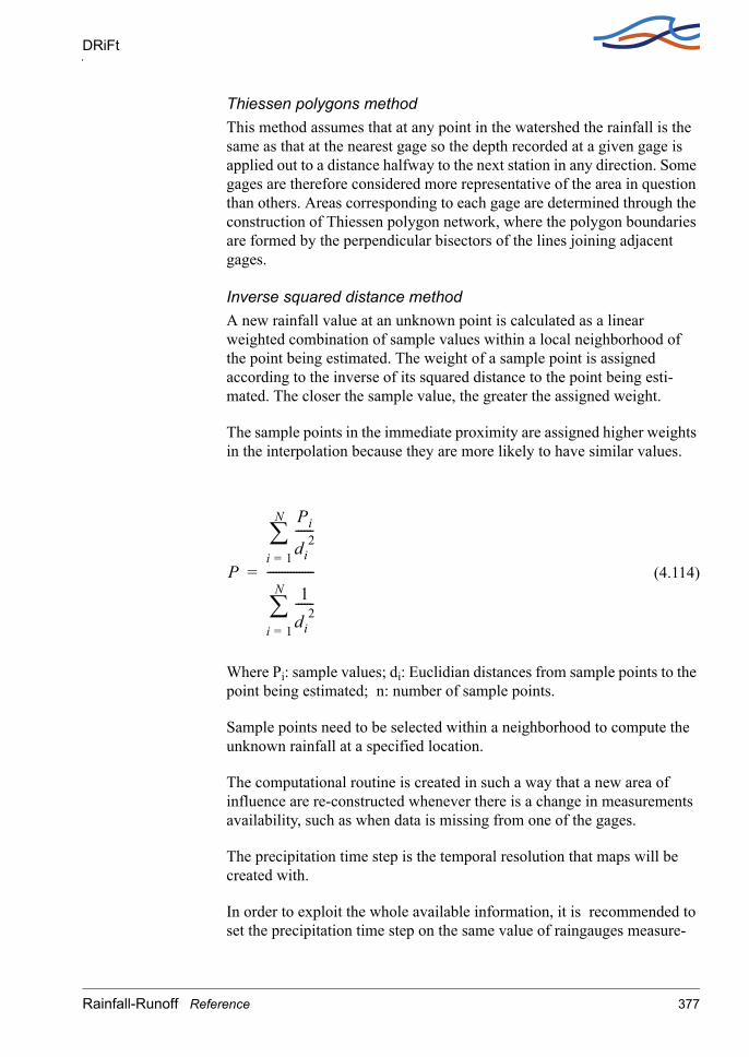
DRiFt
Thiessen polygons method This method assumes that at any point in the watershed the rainfall is the same as that at the nearest gage so the depth recorded at a given gage is applied out to a distance halfway to the next station in any direction. Some gages are therefore considered more representative of the area in question than others. Areas corresponding to each gage are determined through the construction of Thiessen polygon network, where the polygon boundaries are formed by the perpendicular bisectors of the lines joining adjacent gages.
Inverse squared distance methodA new rainfall value at an unknown point is calculated as a linear weighted combination of sample values within a local neighborhood of the point being estimated. The weight of a sample point is assigned according to the inverse of its squared distance to the point being esti-mated. The closer the sample value, the greater the assigned weight.
The sample points in the immediate proximity are assigned higher weights in the interpolation because they are more likely to have similar values.
(4.114)
Where Pi: sample values; di: Euclidian distances from sample points to the point being estimated; n: number of sample points.
Sample points need to be selected within a neighborhood to compute the unknown rainfall at a specified location.
The computational routine is created in such a way that a new area of influence are re-constructed whenever there is a change in measurements availability, such as when data is missing from one of the gages.
The precipitation time step is the temporal resolution that maps will be created with.
In order to exploit the whole available information, it is recommended to set the precipitation time step on the same value of raingauges measure-
P
Pi
di2
------i 1=
N∑
1di
2------
i 1=
N
∑----------------=
Rainfall-Runoff Reference 377

RR reference Manual
ments resolution. Anyway, if temporal variations are not significant, cumulative maps may be introduced with a coarser resolution, speeding up the process computational time. A finer resolution does not improve the data input accuracy and slows down the computational time.
4.15.4 Model calibration
Morphological parameters The morphological exponent k calibration should be performed, modify-ing, only if necessary, typical values suggested in literature (see below “range and typical values” session).
Once k has been set, the value of ASk is quantitatively defined in order to produce a network as natural as possible. The threshold value is therefore tested against four different and nearly independent criteria.
These criteria are here briefly summarized:
1) Graphic controlThe accuracy of the derived network must be checked through a compari-son with the blue lines cartography, even if they are a poor representation of the actual channel network (Montgomery and Foufoula-Georgiou, 1993), and with any other source of knowledge for the basin under analy-sis. This subjective criterion gives a first idea of the order of magnitude of the threshold value. However, its main use is to avoid gross mistakes in the network identification due to DEM errors (e.g., false junctions, miss-ing branches) that might alter the hydrologic response.
378 MIKE 11
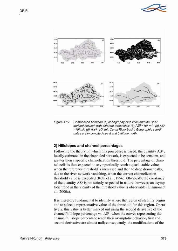
DRiFt
Figure 4.17 Comparison between (a) cartography blue lines and the DEM derived network with different thresholds: (b) ASk=104 m2 ; (c) ASk =105 m2; (d) ASk=106 m2, Centa River basin. Geographic coordi-nates are in Longitude east and Latitude north.
2) Hillslopes and channel percentagesFollowing the theory on which this procedure is based, the quantity ASk , locally estimated in the channeled network, is expected to be constant, and greater then a specific channelization threshold. The percentage of chan-nel cells is thus expected to asymptotically reach a quasi-stable value when the reference threshold is increased and then to drop dramatically, due to the river network vanishing, when the correct channelization threshold value is exceeded (Roth et al., 1996). Obviously, the constancy of the quantity ASk is not strictly respected in nature; however, an asymp-totic trend in the vicinity of the threshold value is observable (Giannoni et al., 2000a).
It is therefore fundamental to identify where the region of stability begins and to select a representative value of the threshold for this region. Opera-tively, this value is better marked out using the second derivative of the channel/hillslope percentage vs. ASk: when the curves representing the channel/hillslope percentage reach their asymptotic behavior, first and second derivative are almost null; consequently, the modifications of the
Rainfall-Runoff Reference 379

RR reference Manual
network for correspondent modification of the thresholds are negligible, and so are the repercussions on the hydrologic response.
An example is exposed in Figure 4.18
Figure 4.18 (a) Hillslope and channel percentages as function of the threshold value for Magra, Centa and Bisagno. The three drainage networks present a similar behavior: a rapid conversion of hillslope cells into channel cells in the zone of low threshold values and an asymptotic trend when higher values are reached. (b) Second derivative of the hillslope percentages vs. ASk .
3) Hillslope's length frequency distributionThe hillslope's length frequency distribution is expected to be heterogene-ous, in accordance with observations (e.g., Wyss, 1988), and well
380 MIKE 11

DRiFt
described by a gamma function (e.g., Gyasi-Agyei et al., 1996). To test the accordance between theoretic distributions and observed frequencies a non-parametric test, as the Kolmogorov-Smirnov test, is proposed.
Example: The results for different orders of magnitude of the threshold value are analyzed for some Ligurian basins. In Figure 4.19 an example of the Kolmogorov-Smirnov test for the Bisagno basin is shown. The hill-slope lengths distribution for ASk =104 m2 and ASk =106 m2 badly fail the test, while the distribution for ASk =105 m2 shapes the theoretic gamma. The discrepancies are mostly due to the digital representation of the hills-lope paths, that allows only discrete travel times values. This is particu-larly true for small values, where the step-like behavior of the empirical function is more evident.
Figure 4.19 Kolmogorov-Smirnov test for cumulative hillslope lengths frequency distribution for three different threshold values: (a) ASk =104 m2 ; (b) ASk =105 m2; (c) ASk =106 m2 , Bisagno basin. The curve in (b) gives the best approximation of the expected gamma function.
4) Hillslope’s length spatial distribution In steep basins, the differences between mountain and valley hillslopes are quite strong. If hillslope lengths were constant over the entire basin, they would not converge on a proper basin response because of a lack in the morphologic variability description. The hillslope elements are not ran-domly joint to the channel: a heterogeneous distribution of hillslope lengths, corresponding to a well-defined spatial distribution over the terri-tory, is expected. Figure 4.20 depicts the hillslope lengths of the Centa basin, which confirms the intuitive idea that short mountain hillslopes are connected to longer channel network paths, while long hillslopes are usu-ally located not far from the outlet.
Rainfall-Runoff Reference 381

RR reference Manual
Figure 4.20 Hillslope lengths spatial distribution, Centa basin. Short mountain hillslopes are connected to longer channel network paths, while long hillslopes are usually located not far from the outlet.
Range and typical valuesIn Flint’s work (Flint, 1974) the exponent k = -(1/xz) takes values in the range from 1.2 to 2.7 with an average of 1.7. The scaling of link slope with contributing area was investigated by Tarboton et al.(1989): a k value equal to 1.67 is estimated from contributing area-slope plots with refer-ence to DEM derived networks. Fiorentino et al. (1993) estimated k=1.75 from an entropy-based morphologic analysis of river basin network. Rodríguez-Iturbe et al. (1992) introduce three principles of optimality for drainage networks; a k value equal to 2 is derived assuming both a linear relation between mean annual discharge and contributing area, i.e. x=1, and a constant flow velocity through the network. These assumptions were relaxed by Molnár and Ramírez (1998): a k=1.6 value is estimated for optimal combinations of channel downstream hydraulic geometry and basin topography for natural drainage systems.
On the basis of the previous considerations, the value 1.7 is assumed as a suitable estimate for the k parameter. Values of k within the 1.6-1.75 range do not produce considerable differences in the values of the others param-eters of the model, as obtained from the complete calibration procedure. The validity of this assumption is qualitatively confirmed by the graphic comparison between the filtered network drainage density distribution and the blue lines, presented in the previous section (Figure 4.17).
382 MIKE 11

DRiFt
On this basis, range and typical values of morphologic parameters are summarized in Table 4.6.
Kinematic parametersThe estimation of kinematic parameters has to be performed using diffe-rent recorded hydrographs in several hydrometric stations, paying particu-lar attention on correctly reproducing the peak discharge value, Qp, and the time when this peak is experienced, tp. Another important issue, that calibration should care for, is consistency of surface runoff volume. The model does not manage the infiltrated part of the rainfall: the shape of the hydrograph is often not preserved, especially in its tail. However, for in the environments that the model intend to analyze, this has a minor role in the characterization of the hydrograph peak.
A sensivity analysis showed that an increase in hillslope velocity lead to a reduction of the hydrograph base and consequently to an increase in the discharge peak value. The same trend is obserbved increasing the channel velocity, while the ratio between the two velocity affects the basic charac-teristics of the hydrograph shape, such as skewness, rising limb, tail.
Range and typical valuesA deep analysis over the Tanaro region (North Italy) was chosen to iden-tify three typical set of kinematic parameters representing its morphologi-cal variability. The region, in fact, includes a mountain zone characterized by very steep catchments, a pede-mountain part and a valley alluvial part. The average velocities decrease from steep mountain sub-catchments to valley basins both on hillslopes and channels. Their values (see Table 4.7) maintain always a physical meaning with regard to the morphology con-sidered (Giannoni et al.,2003) supporting the conviction of a good description capacity of the catchment system offered by the model.
Table 4.6 Range and typical values of morphologic parameters
Range Typical valuesLower bound Upper bound DEM
(40mx40m)DEM
(225mx225)k 1.3 2 1.7 1.7
ASk 102 106 104 105
Rainfall-Runoff Reference 383

RR reference Manual
This corroborates the idea that the model includes the relevant processes that contribute to form the hydrologic response at the basin scale, at least in respect to severe rainfall events in small to medium size catchments in the Mediterranean environment.
Curve NumberCurve numbers have been tabulated by the Soil Conservation Service on the basis of soil type and land use. Four soil groups are defined:
Group A: Deep sand, deep loess, aggregated silt
Group B: Shallow loess, aggregated silts
Group C: Clay loams, shallow sandy loam, soils low in organic content, and soils usually high clay
Group D: Soils that swell significantly when wet, heavy plastic clays, and certain saline soils
The values of CN for various land uses on these soil types are given in Table 4.8. For a watershed made up of several soil types and land uses, a composite CN can be calculated.
Table 4.7 Kinematic parameters range and typical values for Tanaro basin.
Range Typical values (for Tanaro basin)Lower bound
Upper bound
Mountain Pede-moun-tain
Valley
vchannel [m/s] 0.1 10 2.5 2.2 1.5vhillslopes [m/s] 0.001 1 0.16 0.16 0.12
384 MIKE 11

DRiFt
Table 4.8 Runoff coefficient for different condtions (AMCII)
Since the SCS method was developed in the USA, attention must be paid adapting this method to a different application field. In fact, it is an empir-ical method and the large number of experiments that give it reliability were made in a country with its own specific morphology and particular
Rainfall-Runoff Reference 385

RR reference Manual
kind of precipitation. It is therefore not sure that CN values and classifica-tions furnished by the SCS fit every case of study.
Initial conditionThe CN method allows the use of different antecedent soil moisture condi-tions. The program gives the user the possibility of choosing dry, normal or wet conditions at the beginning of each event studied. This is a critical issue, because the moisture content of the soil before a rainfall event has a direct effect on infiltration and thus on runoff .
It is not easy to choose the initial conditions, because many factors concur to make the wetting and drying process very complicated. There is no fixed rule able to identify for one event whether antecedent conditions are wet, normal or dry. Each case is different from one another. In general one should consider how long the interval is between two consequent precipi-tations, vegetal coverage, soil composition, season and all other aspects that affect the evapotranspiration process.
However some indicative tables exist for the range of antecedent moisture conditions for each class; the one the proposed by Chow (1988) is given below (Table 4.9).
4.15.5 DRiFt referencesChow V. T., D. R. Maidment, and L. W. Mays, Applied Hydrology, McGraw Hill, New York, 1988, 572.
Dietrich W. E., C. Wilson, D. R. Montgomery, J. McKean, and R. Bauer, Erosion thresholds and land surface morphology, Geology, 20, 675-679, 1992.
Table 4.9 Suggested classification of antecedent soil moisture classes. (Source: Soil Conservation Service, 1972, table4.2, p.4.12.)
Total 5-day antecedent rainfall (mm)AMC Dormant season Growing seasonType I < 13 < 35Type II 13 - 28 35-53Type III > 28 > 53
386 MIKE 11

DRiFt
Fiorentino, M., P. Claps, and V. P. Singh, An entropy-based morphologi-cal analysis of river basin networks, Water Resour. Res., 29(4), 1215-1224, 1993.
Flint, J. J., Stream gradient as a function of order, magnitude and dis-charge. Water Resour. Res., 10(5), 969-973, 1974.
Giannoni, F., G. Roth, and R. Rudari, A Semi - Distributed Rainfall - Run-off Model Based on a Geomorphologic Approach, Physics and Chemistry of the Earth, 25/7-8, 665-671, 2000a.
Giannoni F., Morphologic analysis of natural drainage networks targeted to the characterization of the hydrologic response, Ph. D Thesis, Univer-sità della Basilicata, 2001.
Giannoni F., G. Roth, and R. Rudari, Can the behaviour of different basins be described by the same model's parameter set? A geomorphologic framework, Physics and Chemistry of the Earth, 28(6-7), 289-295, 2003.
Gyasi-Agyei, Y., F. P. De Troch, and P. A. Troch, A dynamic hillslope response model in a geomorphology based rainfall-runoff model, J. Hydrol., 178, 1-18. 1996.
Leopold, L. B., M. G. Wolman, and J. P. Miller, Fluvial Processes in Geo-morphology, W. H. Freeman, New York, 1964.
Molnár, D. K., and P. Y. Julien, Grid-Size effects on surface runoff mode-ling, J. Hydr. Engrg., ASCE, 5(1), 8-16, 2000.
Molnar, P., and J. A. Ramírez, Energy dissipation theories and optimal channel characteristics of river networks, Water Resour. Res., 34(7), 1809-1818, 1998.
Montgomery, D. R., and W. E. Dietrich, Where do channels begin?, Nature, 336, 232-234, 1988.
Montgomery, D. R., and W. E. Dietrich, Channel initiation and the prob-lem of landscape scale, Science, 225, 826-830, 1992.
Montgomery, D. R., and E. Foufoula-Georgiou, Channel network sources representation using digital elevation model, Water Resour. Res., 29(12), 3925-3934, 1993.
Rodríguez-Iturbe, I., A. Rinaldo, R. Rigon, R. L. Bras, A. Marani, and E. Ijjasz-Vasquez, Energy dissipation, runoff production, and the three-
Rainfall-Runoff Reference 387

RR reference Manual
dimensional structure of river basins, Water Resour. Res., 28(4), 1095-1103, 1992.
Rodríguez-Iturbe, I., and A. Rinaldo, Fractal river basins: chance and self-organization, Cambridge University Press, 1997.
Roth, G., P. La Barbera, and M. Greco, On the description of the basin drainage structure, J. Hydrol., 187, 119-135, 1996.
SCS National Engineering handbook, "Section 4: Hydrology", Soil Con-servation Service, USDA, Washington, D.C., 1972.
Sherman, L. K., Streamflow from rainfall by the unit hydrograph method, Eng. News Rec., 108, 501-505, 1932.
Tarboton, D. G., R. L. Bras, and I. Rodríguez-Iturbe, Scaling and elevation in river networks, Water Resour. Res., 25(9), 2037-2051, 1989.
Wyss, J. D., Hydrologic modelling of New England river basins using radar rainfall data, M. S. thesis, Dep. of Meteor., 164 pp., Mass. Inst. Of Technol., Cambridge, 1988.
388 MIKE 11

F L O O D F O R E C A S T I N GReference
389

390 MIKE 11
Introduction
5 FF REFERENCE MANUALThis manual should be used when undertaking flood forecasting (FF) modelling applications. It provides a description of aspects which are encountered during the development, calibration and application of FF models. The manual should be used in conjunction with the MIKE 11 User Guide.
5.1 Introduction
The demand for means to mitigate the impact of flooding has increased in many parts of the world in recent years, especially where major urban development in the flood plains has taken place.
Flood forecasting systems, producing real-time forecasts of river flows and levels, provide a cost-effective solution to many flood management problems. In addition, the environmental impact of implementing flood forecasting and warning systems is considerably less than many other flood control measures.
Such flood forecasting systems provide
– predictions of the inflow to flood control reservoirs, polders, etc. This will enable reservoir operations that prevent or reduce flooding in the downstream reaches while avoiding unnecessary waste of water resources.
– warnings to local authorities and the affected population of the expected levels and extent of flood inundation
It is very important that the system is able to produce accurate, reliable and timely forecasts as major decisions on reservoir operations, evacua-tion of people, etc. will be based on this information.
Inland flooding may occur due to heavy rainfall in the local catchment area, increasing inflow at upstream boundaries or as a combination of the two. Real-time flood forecasting therefore requires adequate descriptions of the rainfall-runoff process and of the flow in rivers and channels and thus also real-time information on precipitation and river conditions in the area.
The MIKE 11 Flood Forecasting module (MIKE 11 - FF) is designed to perform the calculations required to predict the variation in discharges and water levels in a river system as a result of catchment rainfall and inflow/outflow through boundaries in the river system.
Flood Forecasting 391

FF reference manual
An automatic updating (data assimilation) routine is included in MIKE 11 - FF. In real-time forecasting the simulated discharge/water level generally deviates from the measured discharge/water level. In order to obtain the maximum benefit of the real-time measurements in the forecasts, some kind of updating of the forecasting model is required. Updating consists of conditioning the model predictions to the observed data prior to the Time of Forecast (ToF).
The accuracy of the forecasts will depend on the accuracy of the boundary and rainfall forecasts, the model (calibration and structure) and the effi-ciency of updating routine. The advantages of applying real-time updating to provide accurate flood forecasting are widely recognised (/61/).
MIKE 11 - FF constitute an add on module to MIKE 11, and should be installed along with the hydrodynamic model HD and the rainfall-runoff model NAM.
MIKE 11 FF is designed to minimise the amount of information to be given by the operational forecaster.This is important for real-time applica-tions where reliability and fast performance are crucial.
MIKE 11 - FF has been applied to operational real-time flood forecasting since 1985. Very large applications have been setup for river systems in India and Bangladesh.
MIKE 11 FF can be used in connection with either a manually based or a fully automatic data collection and processing (SCADA) system.
5.2 Updating Procedure
Accurate forecasting requires that the rainfall-runoff model as well as the hydrodynamic model are well calibrated on historical data i.e. that they are able to simulate the water flow very accurately up to the time of fore-cast. Deviations between measured and simulated water levels/discharges will never the less often occur, and it is important that these errors are cor-rected before forecasts are calculated.
Differences in the simulated and observed discharges prior to the time of forecast (ToF) can be attributed to four sources:
1 Errors in the model input data such as precipitation, evaporation, and temperature.
2 Errors in the model parameters due to data limitations, sub-optimal cal-ibrations, etc.
392 MIKE 11

Updating Procedure
3 Errors in the output variables due to the uncertainty in the rating curves and other uncertainties arising from the measurement process.
4 Errors in the model structure due to lumping, inappropriate conceptual-isation of the flood-producing processes, etc.
Forecast updating procedures can be classified according to whether the input variables, state variables, model parameters or output variables are modified. A thorough discussion of the merits and disadvantages of differ-ent updating schemes is provided in Refsgaard, 1997 (/60/). Since the start of DHI's commercial flood forecasting activities in the early 1980's (/62/, /63/, /64/.), the importance of incorporating updating procedures for real-time forecasting was recognised. In the WMO project "Simulated Real-Time Intercomparison of Hydrological Models" DHI submitted two mod-els both based on the NAM model; NAMS11, the predecessor of MIKE 11 FF, and NAMKAL where NAM was formulated in state space form and built into an extended Kalman filter updating. The NAMS11 used output updating based on a error prediction algorithm while NAMKAL provided state variable updating based on the extended Kalman filter.
DHI's NAMS11 showed the best overall results with a ranking of No. 1-2 in the Bird Creek catchment and No. 2-3 in the Orgeval catchment. How-ever it was noted that there was scope for improvement particularly in the case of phase errors. A new procedure that implemented these improve-ments was implemented in the MIKE 11 FF module in 1989, Rungø et al., 1989, (/65/). As a result the standard updating procedure provided by MIKE 11 FF is an improved error correction routine (output updating) capable of distinguishing between phase and amplitude errors.
Two unique features MIKE 11 FF'S updating procedure must be empha-sised.
1 Updating can be carried out directly on either water level or discharge. Many traditional forecast models based on a purely hydrological approach allow updating only on discharge. These discharges are derived from water levels using rating curves which are subject to uncertainties due to measurement errors, loop effects, etc. Direct updating on water levels improves the forecast accuracy significantly.
2 It allows correction of both amplitude errors and phase errors. While traditional updating procedures perform quite well where the devia-tions arise from amplitude or volume errors they generally perform poorly in the case of phase error. Such phase errors may arise from the variable wave speeds for flooding over bank levels or the position and path of storm relative to the catchment outlet.
The two types of errors are illustrated below.
Flood Forecasting 393

FF reference manual
Figure 5.1 Illustration of amplitude and phase error.
The updating procedure distinguishes between the two error types and make corrections accordingly by minimizing the objective function given below:
(5.1)
where
Ae amplitude error (m3/s)
Pe phase error (s)
M measured discharge (m3/s)
Fi Mi Si Ae∆S∆t-------Pe+ +
–2
αQp2 Pe+
1=
n
∑
394 MIKE 11

Updating Procedure
S simulated discharge (m3/s)
F weighting factor
n number of values taken into account
∆S (Si+1 - Si)
∆t time step (s)
α phase factor (s-1)
Qp typical peak discharge (m3/s)
The minimum is found by differentiating the equation with respect to Ae and Pe, and solving these two equations.
A time series of correction discharge is generated on the basis of the iden-tified errors, and introduced as a lateral inflow/outflow to the river at an update point or reach.
These corrections are typically made at several locations in the river sys-tem, where real-time data are available. This will ensure that the simulated flow upstream of forecast points is as correct as possible at Time of Fore-cast (TOF), and this will improve the accuracy of the forecasts.
Deviations found at TOF are likely to persist for some time in the forecast period. Corrections are therefore continued after TOF, but gradually reduced according to a first order decay, as illustrated in Figure 5.2 below.
Flood Forecasting 395

FF reference manual
Figure 5.2 The updating ensures that the simulations are as close to the obser-vations as possible up to the time of forecast. Corrections are con-tinued, but gradually reduced, in the forecast period.
The updating procedure uses a number of parameters that should be found from calibration, using historical peak events.
The purpose of the calibration of the update parameters is to distinguish correctly between deviations in time (phase errors) and deviations in vol-ume (amplitude errors). Only by a correct determination of phase and amplitude errors, will the correction discharge calculated for the forecast-ing period will be correct.
A detailed calibration of parameters should be carried out for each update location.
During calibration the available information stored in the TRF result file should be utilized. The result file contains the following information for all update points:
Phase error after each update iteration
Amplitude error after each update iteration
396 MIKE 11

Updating Procedure
Discharge after each update iteration
Summation of correction discharge after each update iteration
Simulated time series of water level and discharges after each update iteration
Prior to the calibration of the updating parameters, the observed and simu-lated hydrographs at the updating location should be examined. The pur-pose is to determine the phase and amplitude errors which are straightforward to identify from the hydrographs. The results from this evaluation should be compared with the simulated updating results obtained when calibrating the updating parameters.
Max Phase ErrorCorresponds to the largest deviation in time that will be identified as a phase error. If the updating determines a larger phase error it is automati-cally reduced to this value.
Used to limit the interpretation of errors as phase errors. Should only rarely be a limiting factor. If the calculated phase error often reaches this value, the Analysis Period (AP) should be decreased or the value of Alpha increased. In the first calibration the value of Max Phase Error can be set equal to AP.
Analysis period (AP) This is the number of hours back in time from time of forecast that simu-lated and observed flow should be compared. This should as a minimum be larger than the duration of a peak. When hotstarting, analysis will be made for the full analysis period, i.e. including results of the previous sim-ulation.
The order of magnitude will typically be days in very slow responding river systems down to a few hours in very flashy river systems. The AP must be large enough for detection of phase errors.
Time constant in analysis period Recent deviations between simulated and observed flow may be given more weight than those occurring earlier, using first order decay. The time constant determines the reduction of the weighting factor back in time. It should be of the same order of magnitude as the length of the analysis period.
To be used in river systems with very low correlation.
Flood Forecasting 397

FF reference manual
Time constant in forecast period The errors found at Time of Forecast are assumed to be gradually reduced during the forecast period following a first order decay given by this time constant.
A small time constant will rapidly reduce the calculated correction dis-charge during the forecast period. The calibration will show if this is nec-essary. In the first calibration the value can be set equal to AP.
Adjust factor The effect of the updating may be generally reduced by specifying an adjustment factor less than 1.0. This is used e.g. at locations where obser-vations are not considered reliable.
Alpha and Typical Peak Value The Alpha parameter is used in the last term of equation (5.1) to set a rea-sonable limit for the extent to which the updating interprets deviations as phase errors. In case of hydrographs with very small slopes the deviations can often be misinterpreted as phase errors. Initially, Alpha should be set to 0.001 and the Typical Peak Value should be determined from the observed hydrograph. If the calibration results show poor distinction between phase and amplitude errors, Alpha should be changed. If too many of the errors are corrected as phase errors, Alpha should be increased.
Based on the phase and amplitude errors identified by the updating routine a series of correction discharges is calculated. The correction discharges are subsequently added/subtracted from the flows simulated by the hydro-dynamic model.
Updating can be specified on the basis of either discharge or water level measurements. When updating on water levels, the calculation of correc-tion discharge takes into account the conveyance values corresponding to the measured and simulated water levels.
Updating can be specified at any location in the river system where water level and/or discharge information is available in real-time.
An example of the functioning of the updating routine is shown below in Figure 5.3.
398 MIKE 11

Updating Procedure
Figure 5.3 Example of updating.
5.2.1 Calibration ExampleA simple example of an FF calibration using three days of data from a forecasting location is given below. The basis for this example is the measured and simulated hydrographs in Figure 5.4. No forecast period has been simulated i.e. the Time Constant in Forecast Period has not been cal-ibrated. The example should only demonstrate basic principles of how to obtain a correct interpretation of phase and amplitude errors.
Flood Forecasting 399

FF reference manual
Figure 5.4 Example of measured (squares) and simulated (line) discharge at an update location.
From Figure 5.4 it appears that:
The phase error at the peak on the 4/1 is approximately 4.8 hours.
The phase error at the peak on the 6/1 is approximately 2.8 hours.
The amplitude error at the two peaks are approximately 275 m3/s and 75 m3/s respectively.
The amplitude error before the steep rise in the morning of 6/1 is approximately 180 m3/s.
These findings should also be made by the updating routine and can be used as a check of the calibration results.
Determination of Analyse Period (AP) Firstly selection of an appropriate Analyse Period has been investigated. Simulations with AP equal to 3, 6, 12 and 24 hours have been made and it has been assumed that AP = Max Phase Error = Time Constant in AP. Alpha has been set to 0.001 and the Typical Peak Value to 2500 m3/s. The results are shown in Figure 5.5.
400 MIKE 11

Updating Procedure
The simulation with AP = 3 hours is not able to detect the 4.8 hour phase error on the 4/1. Therefore the error here is incorrectly interpreted as amplitude error. The simulation with AP = 24 hours gives an incorrect negative amplitude error in the morning of the 6/1 and an amplitude error that is too large during the peak on the 4/1.
The simulations with AP = 6 and 12 hours both give approximately the same results and match our findings from the hydrograph. A final selec-tion of AP could subsequently be made from calibration on data from other time periods from the this station.
Determination of AlphaFor the calibration of Alpha, simulations with Alpha = 0.0001, 0.001, 0.005 and 0.05 have been made. Other parameters are AP = Time Con-stant in AP = Max Phase Error = 12 hours. Typical Peak Value = 2500 m3/s. The results are shown in Figure 5.6.
It is clearly seen from the results that the large value of Alpha causes the errors to be interpreted as amplitude errors. The best agreement with our findings from the hydrograph is obtained from the results with Alpha = 0.001
Determination of other updating parametersIn a similar manner it is possible to calibrate the remaining updating parameters (see Table 5.1).
Flood Forecasting 401

FF reference manual
Figure 5.5 Results from calibration of the Analyse Period. Analyse Period = Time Constant in Analyse Period = Max Phase Error. Alpha = 0.001 and Typical Peak Value = 2500 m3/s.
402 MIKE 11

Updating Procedure
Figure 5.6 Results from calibration of Alpha. Analyse Period = Time Constant in Analyse Period = Max Phase Error = 12 hours. Typical Peak Value = 2500 m3/s.
Flood Forecasting 403

FF reference manual
Table 5.1
5.3 References
/60/ Refsgaard J.C. Validation and Intercomparison of Different Updat-ing Procedures for Real-Time Forecasting, Nordic Hydrology, 28, pp 65-94, 1997.
/61/ WMO Simulated Real-Time Intercomparison of Hydrological Mod-
Table 5.2
Parameter Main effect Typical value
Max phase error Higher phase errors are automatically reduced to this value
Equal to AP
Analyse Period (AP)
Determine the period where observed and simulated data are analysed
Found by calibra-tion
Time constant in AP
If less than AP, recent devi-ations may be given more weight
Equal to AP
Time constant in forecast period
Corrections at ToF are grad-ually decreased in the fore-cast period by a first order decay with this time con-stant.
Found by calibra-tion
Adjust factor Increasing/decreasing the calculated updating dis-charge
1.0
Alpha An increase in Alpha will cause deviations to be inter-preted more as amplitude errors
Found by calibra-tion
Peak value Highest expected discharge after applying the correc-tion discharge
From observed discharge hydrographs
404 MIKE 11

References
els. Operational Hydrology Report. No. 38. 1992
/62/ Jønch-Clausen, T and J.C. Refsgaard. A mathematical modelling system for flood forecasting, Nordic Hydrology, 15, pp 307-318, 1984.
/63/ Refsgaard J.C. and V.G. Ghanekar. Flood Forecasting, Damodar. World Water, August 1986.
/64/ Refsgaard, J.C., K. Havnø, H.C. Ammentorp and A. Verwey. Appli-cation of hydrological models for flood forecasting and flood con-trol in India and Bangladesh. Advances in Water Resources, 11, 101-105.
/65/ Rungø,. M. J.C. Refsgaard, K. Havnø. The updating procedure in the MIKE 11 modelling system for real-time forecasting.Proceed-ings from the International Symposium on Hydrological Applica-tions of Weather Radar, Salford, UK, August 1989.
Flood Forecasting 405

FF reference manual
406 MIKE 11

D A T A A S S I M I L A T I O NReference
407

408 MIKE 11

6 DATA ASSIMILATION IN MIKE 11Data assimilation is a technique for combining any measurements of the state of the system with the model dynamics in order to improve the knowledge of the system. The data assimilation module in MIKE 11 can be used for assimilation of water level and discharge measurements in the hydrodynamic model and for assimilation of concentration measurements in the advection-dispersion model. Furthermore, the data assimilation module can be used for uncertainty assessment and estimation of model prediction uncertainties.
The data assimilation methods implemented in the MIKE 11 DA module belongs to the class of sequential algorithms. In this case a sequential updating of the model solution is performed during a forward model inte-gration in which the model forecast and the data are melded according to a specific melding scheme. Two different melding schemes based on the Kalman filter are available in MIKE 11:
Ensemble Kalman filter
Constant weighting function method
The ensemble Kalman filter is based on a stochastic model formulation in which model uncertainties are quantified and propgated through the model. This formulation also allows for general uncertainty assessment, i.e. without assimilation of measurements. The constant weighting func-tion method is a deterministic approach that does not explicitly address model uncertainties. Both methods can be formulated in a general filtering framework.
The data assimilation module can be used either in hindcasting mode for process studies and design purposes or as part of an operational forecast-ing system. In either case, the module provides an improved estimate of the state of the system which is consistent with the observed data. In an operational setting the data assimilation module is used for updating the state of the system prior to the time of forecast, and hence providing improved initial conditions for the forecast. After the time of forecast the model can be corrected using forecasts of model errors.
Application examples of the MIKE 11 data assimilation module can be found in Hartnack and Madsen /68/, Madsen et al. /69/ and Madsen and Skotner /70/.
Data assimilation Reference 409
Data assimilation in MIKE 11
6.1 Data assimilation framework
The MIKE 11 model can be described in a deterministic, discrete dynami-cal system setting as
(6.1)
where
xk is the state variables of the system at time step k in terms of h- and Q-points for each branch in the river system and concentration com-ponents in the advection-disperion model (if used).
uk is the forcing terms of the system incorporating all boundary condi-tions, lateral inflow/outflow and possible wind fields.
Φ(⋅) is the model operator representing the numerical scheme of MIKE 11 (one time-step-ahead prediction operator).
It is assumed that water level, discharge and concentration measurements are available at one or more locations in the modelled river system. This is formulated in the measurement equation
(6.2)
where
zk is the vector of measurements.
Ck is a matrix that describes the relation between measurements and state variables, i.e. a mapping of state space to measurement space.
The data assimilation process is a succession of two steps. First, the model is employed to issue a forecast, and then the observed data are meld with the forecast to provide an updated state (analysis step). The analysis step is chosen to be a linear combination of the data and the model, i.e.
(6.3)
where
is the forecast state vector obtained from Eq. (6.1).
xk 1+ Φ xk uk,( )=
zk Ckxk=
xka xk
f Gk zk Ckxkf–( )+=
xkf
410 MIKE 11
Data assimilation framework
is the analysed or updated state vector.
Gk is a weighting matrix (gain matrix).
The vector , denoted the innovation vector, includes the differ-ences between the measurements and their model forecasted equivalents. If the measurements are independent, a sequential update procedure can be used that processes one measurement at a time
(6.4)
where
p is the number of measurements.
is measurement No. j.
is the innovation in measurement point No. j after processing j-1 measurements.
is a weighting vector (gain vector) corresponding to measurement No. j that describes how the innovation is distrib-uted on the state vector.
The shape of the gain reflects the correlation between the measurement and nearby points, taken into account measurement and model uncertain-ties. If the gain in the measurement position is equal to 1, measurements are assumed to be perfect. The smaller gain is chosen the larger uncer-tainty is assumed in the measurement compared to the model uncertain-ties.
The formulation of the gain matrix in Eq. (6.3) or the gain vectors in Eq. (6.4) is the most essential part of the filtering scheme, and the different schemes mainly differ from each other in the way the gains are calculated. The most comprehensive linear melding scheme is the Kalman filter where the gains are determined based on a minimisation of the expected error of the analysed state vector in terms of the errors of both model dynamics and data. In this case the gains are determined sequentially based on a dynamical evolution of the forecast covariance matrix of the state vector.
For high-dimensional systems, as considered here, the propagation of the covariance matrix is the main bottleneck, in most cases imposing an unac-ceptable computational burden for real-time applications. The ensemble
xka
zk Ckxkf–( )
xka j( ) xk
a j 1–( ) gk j, zk j, xka j 1–( )–( ) xk
a 0( ) xkf= j 1 2...,p,=, ,+=
zk j,
zk j, xka j 1–( )–( )
gk j,zk j, xk
a j 1–( )–( )
Data assimilation Reference 411

Data assimilation in MIKE 11
Kalman filter (EnKF) presented by Evensen /67/ approximates the error covariance modelling by an ensemble of state vectors that are propagated according to the model equation (6.1). This approximation reduces signif-icantly the computational burden.
Experiences with the EnKF shows that the computational requirements for obtaining a proper representation of the covariance matrix are of the order of 100 model runs, which may be too expensive in real-time applications. The constant weighting function method developed by Madsen and Skot-ner /70/ is based on predefined gain vectors that are assumed constant in time. In this case the filtering update is only slightly more expensive than a normal model run.
6.2 Ensemble Kalman filter
The Kalman filter is based on a stochastic formulation of the model equa-tion (6.1) and measurement equation (6.2). By including possible errors on the forcing terms the system gets the following stochastic formulation:
(6.5)
where
εk is a vector containing the model error of the forcing terms.
The stochastic representation of the measurements is given by:
(6.6)
where
ηk is a random measurement error vector with zero mean and covari-ance matrix Rk.
The uncertainty of the model forecast is described by the covariance matrix . The Kalman gain to be used in the update equation (6.3) is given by
(6.7)
xk 1+ Φ xk uk εk+,( )=
zk Ckxk ηk+=
Pkf
Gk Pkf Ck
T CkPkf Ck
T Rk+( )1–
=
412 MIKE 11

Ensemble Kalman filter
which depends on the model and measurement covariances. The model covariance expresses how the innovation vector should be distributed on the state vector, and the relation between the model and measurement cov-ariances expresses how much weight should be put on the measurement. The smaller measurement variance as compared to the model variance, the more weight is put on the measurement.
A major shortcoming of the above formulation is the assumption that the covariance matrix is known a priori. For non-linear and high-dimen-sional systems such as MIKE 11 the evaluation of the covariance matrix requires huge computational costs and storage requirements, and hence makes the filtering infeasible for real-time applications.
In the EnKF, the covariance matrix is represented by an ensemble of pos-sible state vectors. Each of these vectors is propagated according to the dynamical system subjected to model errors cf. Eq. (6.5), and the resulting ensemble then provides estimates of the forecast state vector and covari-ance matrix. In the measurement update, the Kalman gain matrix is applied for each of the forecast state vectors. To account for measurement errors, the measurements are represented by an ensemble of possible measurements. The resulting updated sample provides estimates of the updated state vector and covariance matrix.
The EnKF algorithm is summarised below. It is asumed that measurement errors are uncorrelated i.e. the covariance matrix Rk is a diagonal matrix
(6.8)
and hence the sequential updating algorithm in Eq. (6.4) can be applied.
Let there be given a set of M state vectors , where j=1,...,M and k is the time step index.
1 Each member of the ensemble is propagated forward in time according to the stochastic dynamical system given by Eq. (6.5). For each mem-ber of the ensemble the model error is drawn from a Gaussian distribu-tion with zero mean and known covariance.
2 The forecast of the state vector is then estimated as the mean of this ensemble:
(6.9)
Pkf
Rk diag σ12 … σp
2, ,[ ]=
xj k,f
xkf 1
M----- xj k,
f
j 1=
M
∑=
Data assimilation Reference 413
Data assimilation in MIKE 11
3 An estimate of the covariance matrix is found according to:
, (6.10a)
, (6.10b)
4 Each of the ensemble state vectors are updated sequentially using Eq. (6.4). The gain vector for measurement No. i is given by:
(6.11)
In the above sub-/super-script i is a running index indicating elements corresponding to the i´th update using the i´th measurement . The term is the i´th row of the information matrix Ck described earlier.
5 The updated state vector and covariance matrix are estimated as:
, (6.12)
In the implementation of the EnKF the covariance matrix is never cal-culated. All calculations are based on .
When no data are available for updating, only steps 1-3 are carried out. This is the approach taken in MIKE 11 DA when performing uncertainty assessment and making a stochastic or ensemble forecast.
6.2.1 Model errors described by auto-regressive processesThe model errors are defined by auto-regressive processes of first order. Thus, for each uncertain boundary condition l = 1,2,...,L the model errors are described by
, (6.13)
where is randomly drawn from a Gaussian distribution with zero mean and user defined standard deviation σδ,j. Furthermore, all are assumed to be uncorrelated. It should be emphasised that to ensure that the
Pkf 1
M 1–--------------Sk
f Skf( )
T=
Sj k,f xj k,
f xkf–=
gki 1
cki Pk i 1–,
a cki( )
Tσi
2+---------------------------------------------Pk i 1–,
a cki( )
T=
zki
cki
xka 1
M----- xj k,
a
j 1=
M
∑= Pka 1
M 1–--------------Sk
a Ska( )
T=
PkSk
εi k, 1+l φlεi k,
l δi k 1+,l+= i 1 2 … M, , ,=
δi k 1+,l
δi k 1+,l
414 MIKE 11

Constant weighting function
errors do not grow without limit the absolute value of the regression coef-ficients φ must be less than unity.
By using an auto-regressive description the model error has some memory that is propageted as part of the model forecast. In this case the model state is augmented with the model errors that are updated as part of the Kalman filter update scheme. In forecast mode, the model errors at the time of forecast are phased out according to the exponential decay defined by the auto-regressive process.
6.3 Constant weighting function
In the constant weighting function method the gain functions in the update equation (6.4) are assumed to be constant. Three different gain functions are assumed, respectively, a constant (g1), a triangular (g2), and a mixed exponential (g3) distribution
(6.14)
where
g(ξ) is the gain value at the river chainage ξ.
ξUS is the upstream bound for the gain function.
ξDS is the downstream bound for the gain function.
ξMP is the measurement point.
A is the gain amplitude.
g1 ξ( ) A ξUS ξ ξDS≤ ≤,=
g2 ξ( )
Aξ ξUS–
ξMP ξUS–------------------------ ,ξUS ξ ξMP≤ ≤
AξDS ξ–
ξ DS– ξMP–-------------------------- ,ξMP ξ ξDS≤ ≤
=
g3 ξ( ) A 12--- ξ′
1 3⁄----------
2
–
ξ′ ξMP ξ–ξMP ξUS–------------------------= ,ξUS ξ ξMP≤ ≤
ξ′ ξ ξMP–ξDS ξMP–------------------------= ,ξMP ξ ξDS≤<
=exp=
Data assimilation Reference 415

Data assimilation in MIKE 11
Figure 6.1 Definition of gain function for a measurement (update) location.Note that updates cannot take place across river junctions.
The definition of the gain function is illustrated in Figure 6.1. The ampli-tude should reflect the confidence of the observation as compared to the model forecast; that is, if A = 1 the measurement is assumed to be perfect, whereas for smaller A less emphasis is put on the measurement as com-pared to the model forecast. The distribution and the bounds of the gain function should reflect the correlation between the model forecast error at the measurement location and the errors at nearby grid points.
The procedure updates the parts of the state vector that correspond to the measurement variable (e.g. if water levels are measured the water level grid points are updated) using the sequential algorithm in Eq. (6.4). The other parts of the state vector are implicitly updated according to the numerical scheme in the next time step.
6.3.1 Error forecast modellingThe filtering procedure described above can be applied to update the state of the river system up to the time of forecast (or as long as measurements are available). This updated state can then be used as initial conditions for a model forecast. In this case, however, the forecast skills of the model will be limited to a time horizon where the initial conditions are washed out. To keep the model on the "right track" for a longer period the filtering procedure is here combined with error forecasts at the measurement points.
416 MIKE 11

Constant weighting function
Figure 6.2 Illustration of the combined filtering and error forecast procedure.
The principle of this combined approach is illustrated in Figure 6.2. At each update time step in the filtering period (prior to the time of forecast), the model innovation is acquired at all update locations. For each update location this gives rise to a time series of innovations that covers the filter-ing period up to the time of forecast (or the time of the last measurement). At the end of the filtering period, an error forecast model defined at each update location is then used to propagate the innovation in the forecasting period and update the affected state variables accordingly using the filter-ing algorithm in Eq. (6.4).
The error forecast model can be defined as a general linear or non-linear model with a one-step ahead prediction that depends on the previous inno-vations (εk-1, εk-2, ...), the forecasted model state at the present time step ( ), the previous updated model states ( ), and the present and previous model forcings (uk, uk-1, ...)
(6.15)
Equation (6.15) is used recursively by substituting observed innovations with forecasted values.
In the implementation, an equation parser is used that facilitates an easy and flexible definition of error forecast models such as auto-regressive,
xkf xk 1–
a xk 2–a ...,,
εk f εk 1– εk 2– ... xkf, xk 1–
a xk 2–a ... uk uk 1– ...,,,,,,,,( )=
Data assimilation Reference 417

Data assimilation in MIKE 11
moving average models or other linear or non-linear functional forms based on common mathematical operators. Thus, it is possible to define a wide range of error forecast models tailored to the local nature of the model error at each update location.
In order to ensure a fast, accurate and objective derivation of the error forecast models, fully automatic parameter estimation techniques have been incorporated. On the basis of a user-defined time window in the fil-tering period prior to the time of forecast, the parameters of the error fore-cast model are estimated. The error forecast models are updated when a new forecast is to be issued using time series of the most recent innova-tions. This allows the error forecast models to adapt from one forecast to the next to the physical conditions prevailing at the time of forecast with-out any need for calibration or user intervention in general. In the case of a linear error forecast model, the model parameters are estimated using least squares regression techniques, whereas the shuffled complex evolution (SCE) algorithm (Duan et al. /66/) is applied for the parameter optimisa-tion in the case of a non-linear model.
6.4 References
/66/ Duan, Q., Sorooshian, S., Gupta, V., 1992, Effective and efficient global optimization for conceptual rainfall-runoff models, Water Resour. Res., 28(4), 1015-1031.
/67/ Evensen, G., 1994, Sequential data assimilation with a non-linear quasi-geostrophic model using Monte Carlo methods to forecast error statistics, J. Geophys. Res., 99(C5), 10,143-10,162.
/68/ Hartnack, J.N., and Madsen, H.,2001, Data assimilation in river flow modelling, 4th DHI Software Conference, 6-8 June, 2001, Scanticon Conference Centre, Helsingør, Denmark
/69/ Madsen, H., Rosbjerg, D., Damgård, J., Hansen, F.S., 2003, Data assimilation in the MIKE 11 Flood Forecasting system using Kalman filtering, Water Resources Systems - Hydrological Risk, Management and Development (Proceedings of symposium HS02b held during IUGG2003 at Sapporo, July 2003). IAHS Publ. no. 281, 75-81.
/70/ Madsen, H., and Skotner, C., 2004, Adaptive state updating in real-time river flow forecasting - A combined filtering and error fore-
418 MIKE 11

References
casting procedure, J. Hydrology, Submitted.
Data assimilation Reference 419

Data assimilation in MIKE 11
420 MIKE 11

AScientific Background
421

422 MIKE 11

Manual format
A.1 SCIENTIFIC BACKGROUNDThis manual forms an appendix to the MIKE 11 HD Reference Manual.
A.1.1 Manual format
Detailed theoretical descriptions of the following headings are given in this appendix.
Area preserving slot (p. 425)
Culverts, Q-h relations calculated (p. 427)
DELTA coefficient (p. 437)
The double sweep algorithm (p. 439)
2-D Mapping, interpolation routine (p. 449)
Modified diffusive wave approximation (p. 455)
Saint Venant Equations (p. 457)
Solution Scheme (p. 461)
Structures (p. 467)
User Defined Structure (p. 495)
Nomenclature (p. 511)
A Scientific Background 423

Scientific background
424 MIKE 11

Manual format
A.2 AREA PRESERVING SLOTDuring low flow conditions (the local water depth is less than DELH) a slot is introduced into the computations. The slot starts DELH over the bottom and extends 5.DELH below.
There are two different alternatives for the description of the slot.
The classical description is given by
(A.2.1)
where z is the level with respect to the bed level (lowest point).
As an alternative the slot may given a geometry such that the cross sec-tional area varies continuously across the level at which the slot is intro-duced (see Fig A.2.1).
Fig A.2.1 The geometry of the area preserving slot.
B z 5∆h+6∆h
-----------------------B∆=
A Scientific Background 425

Area preserving slot
The slot is chosen so that the width B of the channel is given by the fol-lowing expression
(A.2.2)
where
A∆ is the cross sectional area ∆h above the bottom
B∆ is the channel width at the same level.
∆h is the user defined DELH.
and
(A.2.3)
The choice of slot description is set in the MIKE11.ini file through the variable AREA_PRESERVING_SLOT. The default setting is the classical description e.g. (A.2.1).
B
B∆ ∆h z0–( )∆h z0 5∆h+( )--------------------------------- z 5∆h+( ) for 5∆h z z0≤ ≤–
B∆z0
∆h z0 ∆h–( )-----------------------------– z ∆– h( ) B∆+ for z0 z ∆h≤<
=
z0 ∆h 27---
A∆
B∆------–=
426 MIKE 11

Loss coefficients
A.3 CULVERTS, Q-h RELATIONS CALCULATED
A.3.1 Loss coefficients
The contraction, expansion, friction and bend loss coefficients and the critical flow correction coefficient are described as follows.
A.3.1.1 Entrance loss The contraction loss coefficient, ζ1, is a function of the inflow loss coeffi-cient, ζin, the culvert inflow cross-section area, , and the inflow river cross-section area, A1, see section A.10 Structures (p. 467). Typically, ζin is set to 0.5.
(A.3.1)
A.3.1.2 Expansion loss The expansion loss coefficient, ζ2, is a function of the outflow loss coeffi-cient, ζout, specified in the Network editor → structures → culverts in the Head Loss Factor Box, the culvert outflow cross-section area, , and the outflow river cross-section area, A2, see section A.10 Structures (p. 467). Typically ζout is set to 1.0.
(A.3.2)
A.3.1.3 Friction loss The friction loss coefficient is calculated using the Manning formula, i.e.:
(A.3.3)
where, L is the culvert length, n is Manning's coefficient and R is the mean hydraulic radius along the culvert. The Manning's n value depends on the interior surface of the culvert. Tables of values can be found in open chan-nel or closed conduit hydraulics references such as Chow (1959), /6/ and Henderson (1966), /11/. For a concrete culvert n would typically range from 0.011 to 0.017.
As1
ζ1 ζin 1As1
A1-------–
=
As2
ζ1 ζout 1As2
A2-------–
2
=
ζf2gLn2
R4 3⁄---------------=
A Scientific Background 427

Culverts, Q-h relations calculated
A.3.1.4 Bend and other losses The bend loss coefficient, ζb, is provided for situations where head losses other than from the above occur, for example bends, damaged culverts, trapped debris. The head loss due to ζb is defined in the total head loss given below. For straight culverts in good condition a value of zero would apply.
A.3.1.5 Total head loss through culvertThe total head loss, ∆Hloss, through the culvert is given by
(A.3.4)
where, is the mean cross-section area along the length of the culvert, and Q is the discharge.
A.3.1.6 Critical flow correction factorThe critical and orifice flows are multiplied by the critical flow correction factor, αc, specified in the Network editor → structures → culverts in the Head Loss Factor Box as the Free Overflow Head Loss Factor. Refer to section 1.33 Steady State Energy Equation (p. 175), for more details. Typ-ically a value of 1.0 is used.
A.3.2 Momentum equation coefficients
A.3.2.1 Zero flowThe momentum equation coefficients, see section A.9 Solution Scheme (p. 461), in the case of zero flow are:
(A.3.5)
A.3.2.2 Upstream controlled flowFor upstream controlled flow the coefficients are the same as that described for Structures (p. 467).
∆HlossQ2
2g------
ζ1
As1
2-------
ζf ζb+
Asa
2----------------
ζ2
As2
2-------+ +
=
Asa
α 0 β, 1 γ, 0 δ, 0= = = =
428 MIKE 11

Critical inflow or outflow
A.3.2.3 Downstream controlled flowThe equations for downstream controlled flow through a culvert are an extension of those described in Structures (p. 467). The momentum equa-tion coefficients are calculated as follows:
(A.3.6a)
(A.3.6b)
(A.3.6c)
giving the matrix coefficients at the culvert as:
(A.3.7)
A.3.3 Critical inflow or outflow
In the case of either inflow or outflow being critical the discharge, Qc, for a given critical depth is calculated as:
(A.3.8)
where, Ac is the critical flow area and T is the flow width at the water sur-face.
A.3.4 Critical inflow
Critical flow at the inflow to the culvert occurs when the culvert slope, S0, exceeds the critical flow slope, Sc, as defined by:
and (A.3.9)
Caζ1
As1
2-------
ζf ζb+
Asa
2----------------
ζ2
As2
2------- 1
A12
----- 1A2
2-----+–+ +=
Cb h1 h2–=
Cc sign Ca( ) 2gCa Cb---------------=
α Cc β,– 1 γ, Cc δ, 0= = = =
Qc αcAc gAc
T-----=
S0
zinv1zinv2
–
L--------------------------= Sc
Qcn
AcRc2 3⁄
----------------- 2
=
A Scientific Background 429

Culverts, Q-h relations calculated
where, and are the inflow and outflow invert levels of the cul-vert, and Rc is the hydraulic radius at critical flow.
For the calculation of h1, the inflow water depth is taken as the critical depth. The friction losses and bend losses have no effect on the discharge for this flow condition.
A.3.5 Critical outflow
Critical flow at the outflow to the culvert occurs when S0 is less than Sc.
Before the calculation of h1 can proceed it is necessary to determine the inflow water depth. A standard backwater analysis using a fine increment in water depth is used starting with the critical flow depth at the outflow end and working upstream. The bend losses, if any, are applied at the mid-point along the length of the culvert.
In the situation of the culvert section becoming full (i.e., submerged inflow), the friction slope becomes constant and the backwater analysis adjusts accordingly.
The upstream water level is calculated based on the inflow water depth in the culvert using the iteration procedure described in section 1.12 Cul-verts, Q-h Relations Calculation (p. 88).
A.3.6 Orifice flow at inflow
Orifice flow occurs in short or steep culverts (Figure 1.23(e)). Culverts in which this flow condition occurs are sometimes referred to as "hydrauli-cally short" (/6/). The flow is similar to that which occurs under a sluice gate. The discharge is calculated by:
(A.3.10)
where, C0 is the coefficient of discharge, H1 is the inflow energy head in the river, is the inflow invert level, and Afull is the full cross-section area of the culvert.
The facility to manually specify C0 as a function of y1/D (y1=h1- and D = culvert depth) has been provided in the network editor → structures → culverts → Flow conditions under the Orifice Flow Conditions Tab. It is anticipated that this will be unnecessary in the majority of cases as a
zinv1zinv2
Q0 αcC0Afull 2g H1 zinv1–( )=
zinv1
zinv1
430 MIKE 11
Full culvert flow with free outflow
default is provided (discussed below). However, it does provide the flexi-bility to model a "hydraulically short" culvert, or a sluice gate (zero length) in detail if sufficient information on the discharge coefficient is available. Carter (1957), /5/ provides a detailed analysis and tables of dis-charge coefficients for orifice flow and other flow conditions.
If no values for C0 are specified, a value of 0.65 at a y1/D of 5.0 is adopted. When y1/D is greater than 5.0, C0 remains constant at 0.65, while below 5.0 a linear interpolation is made with the C0 value calculated automati-cally as described in the following.
A value for C0 is automatically calculated at the point of inflow submer-gence if the flow condition is inflow critical. This allows a smooth transi-tion to occur between the two flow conditions. The point of inflow submergence is nominally adopted as 95% of the full culvert flow area. The C0 value calculated is shown in the first row of the C0 versus y/D tables.
A.3.7 Full culvert flow with free outflow
The complement to orifice flow at the inflow is when the culvert is defined as "hydraulically long", i.e., the culvert is flowing full with a free outflow (Figure 1.23 (f)). In this case the discharge, Qp is calculated using:
(A.3.11)
where, H1 is the inflow energy head level in the river and is the out-flow obvert (soffit) level (i.e. invert plus culvert depth).
The outflow energy head level in the above equation has been set to that at the outflow obvert by assuming atmospheric pressure occurs there. This assumption is compatible with the critical outflow flow condition at the point of the outflow becoming submerged as the discharge equations are the same if ζ2 is equal to 1.0. This is important for the transition between upstream and downstream controlled flow conditions as discussed later.
A.3.8 Downstream controlled flow (submerged flow)
In the case of a downstream controlled flow the computation is compli-cated because of the influence of all three cross-sectional areas along the culvert, , and , and the mean hydraulic radius, R. The situation
Qp Afull
2g H1 zobv2–( )
ζ1 ζf ζb 1+ + +-------------------------------------=
zobv2
As1Asa
As2
A Scientific Background 431

Culverts, Q-h relations calculated
is further complicated in the case where the culvert outflow is close to crit-ical flow conditions as the water surface profile through the culvert in these conditions is very non-linear.
A.3.9 Partially full inflow and outflow
An iteration procedure is used to determine , , and R. The itera-tion is made on the water levels in the culvert at the upstream and down-stream ends, Equations (A.3.12a) and (A.3.12b), from which and are calculated. For and R, a linear interpolation of the water level at the culvert mid-point is initially used.
(A.3.12a)
(A.3.12b)
where
(A.3.13)
and are the water levels in the culvert at the inflow and outflow ends, while H1 and H2 are the inflow and outflow energy head levels in the river.
Fig A.3.2 Modelled water surface profile when profile is very non-linear
As1Asa
As2
As1As2
Asa
hs1H1
1 ζ1+( ) H1 H2–( )
CasAs1
2--------------------------------------------–=
hs2H2
1 ζ2–( ) H1 H2–( )
CasAs2
2-------------------------------------------–=
Cas
ζ1
As1
2-------
ζf ζb+( )
Asa
2--------------------
ζ2
As2
2-------+ +=
hs1hs2
432 MIKE 11

Submerged inflow and partially full outflow
When the outflow is close to a critical flow state the water surface profile is highly non-linear, and the friction losses calculated from a linear inter-polation will be too high (Fig A.3.2). To overcome this problem without using a computationally intensive backwater analysis in each iteration, a comparison is made with the friction losses calculated from the backwater analysis for critical outflow, see above. In the case of the losses from the backwater analysis being lower, is calculated as:
(A.3.14)
where, the subscript c refers to the critical flow conditions based on h1. This also ensures a smooth transition between the outflow critical condi-tion and submerged flow providing ζ2 is less than or equal to 1.0.
The iteration procedure typically takes two to three iterations to converge. If the upstream and downstream water levels are changing rapidly more iterations are usually necessary with the number rarely exceeding ten. The maximum number of iterations is controlled by the Inter1Max variable which can be edited in the HD parameter editor →Default values.
A.3.10Submerged inflow and partially full outflow
This flow condition typically occurs when the culvert slope is adverse to the water surface slope as shown in Figure 1.23(h).
The iteration procedure described in “Partially full inflow and outflow (p. 432)” above is used except that the mean cross-section area is adjusted according to:
(A.3.15)
where, Lfull is the length of the culvert which is following full and L is the total length.
A similar adjustment is made to the mean hydraulic radius.
Cas
Cas
2gQc
2------ H1 hc–
Qc2
2gAc2
------------– ζ2
As2
2-------+=
Asa
Lfull
L----------Afull 1
Lfull
L----------–
Afull As2
+
2------------------------+=
A Scientific Background 433

Culverts, Q-h relations calculated
A.3.11 Partially full inflow and submerged outflow
This flow condition occurs in sloping culverts as illustrated in Figure 1.23(i). A similar procedure to that described in “Submerged inflow and partially full outflow” above is used.
A.3.12Fully submerged
Where the culvert is fully submerged (Figure 1.23(j)) the cross-sectional areas and hydraulic radius are equal to those when the culvert is full.
A.3.13Transition between upstream and downstream control
Whether the flow is upstream or downstream controlled is best based on a single criteria. Using a single criteria is preferable for stability reasons and for a smooth transition between flow conditions.
Analysis of the formulations described above, assuming that ζ2 is less than or equal to 1.0, gives the following conclusions:
in the case of either inflow or outflow being critical, then if H2 is below the critical water level, hc, the flow will be critical. If H2 is greater than hc then the flow can be either critical or downstream controlled. The level at which the flow becomes downstream controlled is dependent on the magnitude of ζ2. If ζ2 is equal to 1.0 the change to or from sub-merged flow will be at H2 equal to hc. For ζ2 less than 1.0, which is normally the case, downstream controlled flow will occur at some point above hc.
similarly, the same scenario can be shown to occur for full culvert flow and orifice flow versus fully submerged flow where hc is taken as the outflow obvert (invert plus culvert depth).
This leads to the following criteria for selecting between upstream and downstream flow controls:
if H2 is less than either hc at outflow (critical inflow or outflow) or the downstream obvert (orifice or full culvert flow) then the flow is upstream controlled, otherwise the flow condition which gives the lower discharge is selected
In the case of critical inflow, H2 should be taken as that immediately past the point of critical flow (i.e., at the inflow to the culvert). However, for culverts of non-zero length and/or non-zero bend loss, the energy head
434 MIKE 11

Transition between upstream and downstream control
losses through the culvert are not known and the more conservative approach of using hc at the outflow must be taken. A similar situation applies in the case of orifice flow.
A Scientific Background 435

Culverts, Q-h relations calculated
436 MIKE 11

Transition between upstream and downstream control
A.4 DELTA COEFFICIENTA forward centring of the term in the numerical scheme has a dissi-pative influence which can be demonstrated using the Taylor-series. The forward centring is automatically introduced in MIKE 11 when the flow becomes supercritical in that particular channel section. Additionally, the centring can be specified by the user for sub-critical flows through the centring coefficient DELTA (0.5 <δ< 1).
Introducing the δ value into the terms gives:
(A.4.1)
Using a Taylor series up to the third derivative, these terms become:
(A.4.2)
Similarly for the last term:
(A.4.3)
In this way the formulation of in (A.4.1) becomes (again using a Taylor series):
(A.4.4)
∂h ∂x⁄
∂h∂x------ δ
hj 1+n 1+ hj 1–
n 1+–∆2x
----------------------------- 1 δ–( )hj 1+
n hj 1–n–
∆2x---------------------------+=
hj 1+n 1+ hj 1–
n 1+–∆2x
----------------------------- δ∆2x---------- h 1
1!-----∆2x
2----------∂h
∂x------ 1
2!----- ∆2x
2----------
2∂2h∂x2--------
13!----- ∆2x
2----------
3∂3h∂x3-------- h– 1
1!-----∆2x
2----------∂h
∂x------ 1
2!----- ∆2x
2----------
2∂2h∂x2--------
13!----- ∆2x
2----------
3∂3h∂x3--------
j
n 1+
=δ ∂h∂x------ ∆2x( )
24--------------
2∂3h∂x3--------+
+ +
+
+ +
+
=
1 δ–( )hj 1+
n hj 1–n–
∆2x--------------------------- 1 δ–( ) ∂h
∂x------ ∆2x( )
24--------------
2∂3h∂x3--------+
j
n
=
∂h ∂x⁄
∂h∂x------ δ ∂h
∂x------ 1
1!-----∆t
2----- ∂2h
∂x∂t----------- 1
2!----- ∆t
2-----
2 ∂3h∂x∂t2-------------+ +
j
n ½+
1 δ–( ) ∂h∂x------ 1
1!-----– ∆t
2----- ∂2h
∂x∂t----------- 1
2!----- ∆t
2-----
2 ∂3h∂x∂t2-------------+
j
n ½+
+
∂h∂x------
n ½+2δ 1–( )∆t
2----- ∂2h
∂x∂t-----------
n ½+higher order terms+ +
=
=
A Scientific Background 437

DELTA coefficient
which represents the dissipative effect, when δ>0.5, as the last term becomes positive.
438 MIKE 11

Branch matrix
A.5 THE DOUBLE SWEEP ALGORITHM
A.5.1 Branch matrix
In a grid point the relationship between the variable Zj (either water level hj or discharge Qj) in the point itself and in the neighbouring points is expressed using a linear equation as follows:
(A.5.1)
The lower index in equation (A.5.1) (and the following equations) indi-cates the location along the branch and the upper index (if any) indicates the time step. The coefficients α, β, γ and δ in equation (A.5.1) are in h-points calculated using the finite difference approximation to the continu-ity equation and in the Q-points using the finite difference approximation to the momentum equation (or in case there is a structure in the Q-point using the actual structure algorithm). Section A.9 Solution Scheme (p. 461) gives more details on the finite difference approximation to the Saint Venant equations.
In all grid points along a branch equation (A.5.1) is set up. Assume a branch with n grid points; n is an odd number, as the first and the last grid point in a branch always are h-points. This gives n linear equations with n+2 unknowns. The extra two unknowns come from the equations set up in the first and the last h-point, where respectively Zj-1 and Zj+1 becomes the water level in the node to which the upstream end and the downstream end of the branch is connected. The following shows the n linear equa-tions:
(A.5.2)
Hus in the first equations and Hds in the last equation is the water level in the upstream and downstream node respectively. In MIKE 11 water level
αjZj 1–n 1+ βjZj
n 1+ γjZ1 j+n 1++ + δj=
A Scientific Background 439

The double sweep algorithm
compatibility applies in the nodes, i.e. the water level in the first point in a branch equals the water level in the node to which the upstream end of the branch is connected. In other words h1=Hus. This implies that α1 = -1, β1 = 1, γ1 = 0 and δ1 = 0. Similar in the last grid point hn=Hds and therefore αn = 0, βn = 1, γn = -1 and δn = 0.
If we were dealing with a one-branch system with a water level boundary at each end, then Hus and Hds would be known. There would be only n unknowns left in the n equations, and these would be ready to solve using standard elimination technique. However as MIKE 11 handles several branches, another method has to be applied. To explain this the above n equations are shown in matrix form in equation (A.5.3).
(A.5.3)
Using standard elimination technique the matrix in equation (A.5.3) can be transformed to the matrix in equation (A.5.4).
(A.5.4)
440 MIKE 11

Node matrix
From the matrix (A.5.4) it can be seen that in any grid point the variable Z (water level or discharge) is expressed as a function of the water level in the upstream and downstream node:
(A.5.5)
However, as MIKE 11 operates with branches divided by nodes at external boundary points and at internal branch connections, it is necessary to know the water levels in all nodes before the matrix in (A.5.4) can be solved according to equation (A.5.5).
A.5.2 Node matrix
In nodes a continuity equation covering the surrounding h- and Q-points is set up:
Fig A.5.3 Three-branch node with limit for continuity equation.
Fig A.5.3 gives a close look at the grid points surrounding a node. The finite difference approximation of the continuity equation around the node is given by:
(A.5.6)
Zjn 1+ cj ajHus
n 1+– bjHdsn 1+–=
Hn 1+ Hn–∆t
-------------------------Afl QIn ½+ QO
n ½+
Hn 1+ Hn–∆t
-------------------------Afl⇒
–
12--- QA n 1–,
n QB n 1–,n QC 2,
n–+( )
12--- QA n 1–,
n 1+ QB n 1–,n 1+ QC 2,
n 1+–+( )+
=
=
A Scientific Background 441
The double sweep algorithm
where
QI Sum of inflows
QOSum of outflows
∆t Time step
In equation (A.5.6) QA,n-1, QB,n-1 and QC,2 at time level n+1 can be substi-tuted according to equation (A.5.5), and the following equation is achieved:
(A.5.7)
where
H Water level in the actual node
HA,us Water level in the node in the upstream end of branch A
HB,us Water level in the node in the upstream end of branch B
HC,ds Water level in the node in the upstream end of branch B
An equation similar to (A.5.7) is set up in each node, giving N equations with N unknowns (N is the number of nodes). In these equations the water level in each node becomes a linear function of the water level in the nodes to which the node is directly connected. Assume a configuration of branches as in Fig A.5.4.
Hn 1+ Hn–∆t
-------------------------Afl12--- QA
n QBn Qc
n–+( )
12--- c( A n 1–, aA n 1–, HA us,
n 1+– bA n 1–, Hn 1+–
cB n 1–, aB n 1–, HB us,n 1+– bB n 1–, Hn 1+–
cC 2, aC 2, Hn 1+– bC 2, HC ds,n 1+ )–
+
+
+
=
442 MIKE 11

Bandwidth minimisation
Fig A.5.4 River network with 9 branches and 8 nodes.
In the branch configuration as in Fig A.5.4 eight nodal continuity equa-tions are set up. Fig A.5.5 shows the matrix with x indicating coefficients that are different from zero.
Fig A.5.5 Node matrix for the network in Fig A.5.4 before bandwidth minimisa-tion (RS is the right hand side coefficients).
From the matrix in Fig A.5.5 it can for instance be seen that in node 4 (row 4 in the matrix) the continuity equation (in the form of equation (A.5.7)) becomes a function of the water level in node 1, 4, 5 and 6.
The matrix in Fig A.5.5 can be solved using the standard method of Gaus-sian elimination, and thus the water level in the nodes at time step n+1 is known. Hereafter the water levels and discharges along the branches are calculated using equation (A.5.5).
A.5.3 Bandwidth minimisation
The bandwidth of the matrix in Fig A.5.5 as indicated by the dashed line, is a function of the order in which the nodal points are defined. The band-width of the matrix in Fig A.5.5 is equal to 5. The total amount of compu-tational time will increase with increasing bandwidth. In order to minimise
A Scientific Background 443
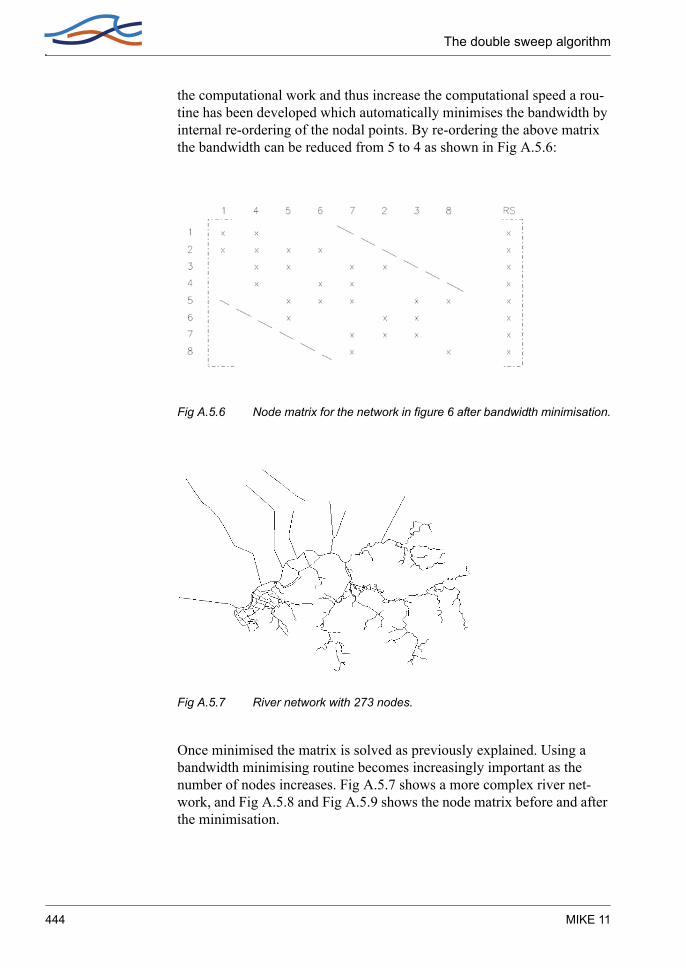
The double sweep algorithm
the computational work and thus increase the computational speed a rou-tine has been developed which automatically minimises the bandwidth by internal re-ordering of the nodal points. By re-ordering the above matrix the bandwidth can be reduced from 5 to 4 as shown in Fig A.5.6:
Fig A.5.6 Node matrix for the network in figure 6 after bandwidth minimisation.
Fig A.5.7 River network with 273 nodes.
Once minimised the matrix is solved as previously explained. Using a bandwidth minimising routine becomes increasingly important as the number of nodes increases. Fig A.5.7 shows a more complex river net-work, and Fig A.5.8 and Fig A.5.9 shows the node matrix before and after the minimisation.
444 MIKE 11

Boundaries
Fig A.5.8 Branch matrix for the network in Fig A.5.7 before bandwidth minimi-sation.
Fig A.5.9 Branch matrix for the network in Fig A.5.7 after bandwidth minimisa-tion.
A.5.4 Boundaries
In MIKE 11 the following three types of boundary conditions can be applied:
A Scientific Background 445

The double sweep algorithm
Water level as a function of time
Discharge as a function of time
A tabulated relation between water level and discharge (Q/h boundary)
Each of the boundary types is taken into account by using a different node equation.
A.5.4.1 Water level as a function of time.In this case the water level in the node at time step n+1 simply becomes the value of the user-specified boundary at time step n+1 ( ) i.e. in the relevant equation (or row) in the node matrix only the diagonal and the right hand side coefficient are different from zero, and equals respectively 1 and .
A.5.4.2 Discharge as function of time.
Fig A.5.10 River branch with discharge boundary.
In this case a local continuity equation covering the area indicated in Fig A.5.10 is set up. Equation (A.5.6) becomes:
(A.5.8)
In equation (A.5.8) Q2 at time step n+1 is substituted with equation (A.5.5) and equation (A.5.9) is achieved.
(A.5.9)
Equation (A.5.9) is similar to equation (A.5.7) and the coefficients in the relevant row in the node matrix can be calculated by re-arranging equation (A.5.9).
Hboundaryn 1+
Hboundaryn 1+
Hn 1+ Hn–∆t
-------------------------Afl12--- Qb
n Q2n–( ) 1
2--- Qb
n 1+ Q2n 1+–( )+=
Hn 1+ Hn–∆t
-------------------------Afl12--- Qb
n Q2n–( ) 1
2--- Qb
n 1+ c2 a2Hn 1+ b2Hdsn 1++ +–( )+=
446 MIKE 11
Boundaries
A.5.4.3 Q/h boundaryIn this case the user specifies a tabulated relation between h and Q. A con-tinuity equation is set up at the boundary in the same way as for a dis-charge boundary. The discharge at the boundary Qb is expressed as a function of the water level in the node using the tabulated relation. This is done as follows:
The index i is found such that , and the ratio a is calcu-lated according to equation (A.5.10).
(A.5.10)
Using linear interpolation between the tabulated values of water levels and discharge equations (A.5.11) and (A.5.12) can be achieved:
(A.5.11)
(A.5.12)
Equations (A.5.11) and (A.5.12) are substituted into equation (A.5.8) and equation (A.5.13) is achieved:
(A.5.13)
Equation (A.5.13) is similar to equation (A.5.7) and the coefficients in the relevant row in the node matrix can be calculated by re-arranging equation (A.5.13).
Htab,i Hn Htab,i+1<≤
aQtab,i+1 Qtab,i–Htab,i+1 Htab,i–----------------------------------=
Qbn 1+ Qtab,i a Hn 1+ Htab,i–( )+=
Qbn Qtab,i a Hn Htab,i–( )+=
Hn 1+ Hn–∆t
-------------------------Afl12--- Qtab,i a Hn Htab,i–( ) Q2
n–+( )
12--- Qtab,i a Hn 1+ Htab,i–( ) Q2
n 1+–+( )+
=
A Scientific Background 447

The double sweep algorithm
448 MIKE 11

Mapping
A.6 2-D MAPPING, INTERPOLATION ROUTINEOutlined below is the interpolation routine used in MIKE 11 to generate the various two-dimensional maps.
A.6.1 Mapping
The mapping of water levels, water depths, velocities and advection dis-persion components from the one-dimensional results to two-dimensional maps are done internally in MIKE 11 through a couple of steps:
Interpolation of cross sections at all digitised points and all interpolated water level grid points.
Linear interpolation of results from the numerical grid to the interpo-lated cross sections.
Spatial interpolation of the bed level from the cross sections to all intermediate cells in the two-dimensional grid within the river bed.
Determination of the velocity profile at all cross sections based on con-veyance distribution.
Spatial interpolation of the required results from the cross sections to all intermediate cells in the two-dimensional grid within the river bed.
A.6.1.1 Interpolation of cross sections at digitised pointsA number of cross sections need to be interpolated for each reach of the river. Below is illustrated a digitised river section. The circles illustrate the digitised points. The cross sections are shown as the full drawn lines.
Figure 6.3 A close up of a digitised network with the cross sections illustrated. The digitised points are shown as circles.
This reach is from MIKE 11’s point of view seen as a straight line with cross sections perpendicular to the river centre line as illustrated in Figure 6.4.
A Scientific Background 449

2-D Mapping, interpolation routine
Figure 6.4 Digitised reach from MIKE 11’s point of view only considering every-thing referenced according to the chainage. The dashed lines are the additionally required cross sections (interpolated).
At every digitised point the river may have a kink. The interpolation of the water depth is greatly simplified if the river and flood way may be divided into 4 sided polygons. This may be achieved by securing that cross sec-tions are available at every digitised point. The resulting network consists of straight line segments with a cross section at each end. The interpola-tion routine used for the cross sections is identical to the one found in the cross section editor. At end points without a cross section the nearest upstream or downstream cross section is reused. The latter is equivalent to the approach used internally in the numerical engine of MIKE 11.
A.6.1.2 Linear interpolation of results from the numerical gridWater levels, discharges and concentrations at the interpolated cross sec-tions are simply found through linear interpolation of the values from the two nearest water level grid points. The interpolation in this step is solely based on the chainage.
A.6.1.3 Spatial interpolation of the bed level from the cross sectionsAt this point the branch consists of a number of segments with a cross sec-tion at each end. Such a segment is termed a mapping box. For each of these mapping boxes a local coordinate/mapping system may be intro-duced as illustrated in Figure 6.5. Note that the mapping is one to one and thus has an inverse. The linear interpolation of values may now be carried out on the rectangular mapping box and then pulled back to the mapping box in the MIKE 11 representation. From here the results may be trans-ferred back to the original geo-referenced mapping box provided that the two cross sections defining the the flood box do not intersect as illustrated in Figure 6.6.
450 MIKE 11

Mapping
Figure 6.5 Local mapping from MIKE 11’s representation of a mapping box to a coordinate system (u,v). The box on the right has a unit length and twice the height. The centre line from the left is mapped onto the line v=0. The extent of the cross sections of the mapping box on the left is defined by the markers 1,2 and 3.
Figure 6.6 Mapping box with intersecting cross sections. In such a case the illustrated part is ignored in the interpolation routine.
The bed level s is well defined at all the cross sections. The bed level at a set of coordinates (u,v) is defined as
(A.6.1)
Using the mapping back to the original system one can hereby obtain the bed level at all intermediate points.
s u v,( ) u 1–( ) s 0 v,( ) u s 1 v,( )⋅+⋅=
A Scientific Background 451

2-D Mapping, interpolation routine
A.6.1.4 Determination of the velocity profile at all cross sectionsThe velocity distribution in a cross section is assumed to be uniform over the depth and vary as the conveyance in the cross section in the transversal direction.
The total conveyance K is in this context defined as
(A.6.2)
Where h is the local water depth, B the water surface width and M is Man-ning’s resistance number. Both the water depth and the resistance are func-tions of the transversal direction x. In the above a Manning’s formulation is used for the resistance, but the approach is similar if a Chezy description is used for the resistance. The 5/3 is then substituted with 3/2 and M is replaced by the Chezy number C.
The velocity for a particular point in a cross section is defined by
(A.6.3)
Hereby a value for the velocity can be found at every point in the cross section and the velocity at intermediate points are found through an inter-polation similar to eq. (A.6.1).
A.6.1.5 Spatial interpolation of the required results from the cross sectionsThe spatial interpolation of results depends on the type of result:
Water levels and concentrations are simply interpolated based on the chainage and are only shown if the water level is above the local bed level.
The water depth is determined as the water level minus the bed level and will only be displayed if the value is positive.
The velocity is interpolated similar to the bed level and is only shown if the local water depth is positive.
K h5 3⁄ M xd0
B
∫=
v x t,( ) Q t( )K
-----------M h2 3⁄⋅=
452 MIKE 11

Generation of a Digital Elevation Model (DEM)
A.6.2 Generation of a Digital Elevation Model (DEM)
The generation of a digital Elevation Model (DEM) in MIKE 11 is done by determining the bed level at all the grid cells lying within a mapping box. If a cell lies in multiple mapping boxes then the average is used for the bed level.
The generation of a DEM may be augmented with one or more back-ground DEMs. If this is the case the user supplied DEM will be applied in the grid cells where no mapping boxes are present.
If multiple DEMs are used the DEMs are ranked and the DEM with the highest rank containing data in the particular cell is used.
Finally the DEM generation allows user supplied topographical informa-tion to be used inside the mapping boxes. In this case the bed level deter-mined through the cross sectional interpolation is overridden by the user supplied topographical values.
A Scientific Background 453

2-D Mapping, interpolation routine
454 MIKE 11
Generation of a Digital Elevation Model (DEM)
A.7 MODIFIED DIFFUSIVE WAVE APPROXIMATIONThe diffusive wave approximation can be written for example for the case of Chezy roughness as:
(A.7.1)
where, S is the slope of the water surface. This equation is linearized through the following approximations:
(A.7.2)
Expressions are now sought for:
(A.7.3)
From the basic equation we have:
and (A.7.4)
and (A.7.5)
Inserting this in the above linearized expression gives:
(A.7.6)
giving:
(A.7.7)
Q ACR1 2⁄ S1 2⁄=
Qn 1+ Qn+½ ∂Q∂h------- hn 1+ hn+½–( )+≈
∂Q∂h------- ∂Q
∂A-------∂A
∂h------ ∂Q
∂R-------∂R
∂h------ ∂Q
∂S-------∂S
∂h------ ∂Q
∂A-------∂A
∂h------ ∂Q
∂R-------∂R
∂h------+≈+ +=
∂Q∂A------- CR1 2⁄ S1 2⁄= ∂A
∂h------ bs=
∂Q∂S------- 1
2---AC R
S---= ∂S
∂h------ 1
∆x------≈
Qn 1+ Qn ½+ C RSbs1
2∆x----------AC R
S---+
hn 1+ hn+½–( )+=
Qn 1+ Qn ½+ bs∆xSA
--------------- 12---+
AC∆x-------- R
S--- hn 1+ hn+½–( )+=
A Scientific Background 455

Modified diffusive wave approximation
456 MIKE 11

Generation of a Digital Elevation Model (DEM)
A.8 SAINT VENANT EQUATIONSMIKE 11 applied with the fully dynamic descriptions solves the vertically integrated equations of conservation of volume and momentum (the ‘Saint Venant’ equations), which are derived on the basis of the following assumptions:
the water is incompressible and homogeneous, i.e. without significant variations in density
the bottom slope is small
the wave lengths are large compared to the water-depth. This ensures that the flow everywhere can be regarded as having a direction parallel to the bottom, i.e. vertical acceleration can be neglected and a hydro-static pressure variation along the vertical can be assumed
the flow is sub-critical
For a rectangular cross-section with a horizontal bottom and a constant width, the conservation of mass and momentum can be expressed as fol-lows (in the first instance neglecting friction and lateral inflows):
Conservation of mass:
(A.8.1)
Conservation of momentum:
(A.8.2)
where, ρ is the density, H the depth, b the width, the average velocity along the vertical and α’ the vertical velocity distribution coefficient.
Introducing the bottom slope, Ib, and allowing for the channel width to vary will give rise to two more terms in the momentum equation. These terms describe the projections in the flow direction of the reactions of the bottom and side-walls to the hydrostatic pressure.
∂ ρHb( )∂t
------------------- ∂ ρHbu( )∂x
----------------------–=
∂ ρHbu( )∂t
----------------------∂ α′ρHbu
2 12---ρgbH2+
∂x----------------------------------------------------------–=
u
A Scientific Background 457
Saint Venant Equations
The momentum equation now becomes:
(A.8.3)
When the water level, h, is introduced into the relationship instead of water depth:
(A.8.4)
and the equations are divided by ρ, the conservation laws of mass and momentum become:
(A.8.5)
(A.8.6)
These equations can be integrated to describe the flow through cross-sec-tions of any shape when divided up into a series of rectangular cross sec-tions as shown in Fig A.8.11:
∂ ρHbu( )∂t
----------------------∂ α′ρHbu
2 12---ρgbH2+
∂x----------------------------------------------------------– ∂b
∂x------ρgH2
2------------- ρgHbIb–+
∂ α′ρHbu2
( )∂x
-------------------------------– b∂ 1
2---ρgH2
∂x--------------------------– ρgHbIb–
=
=
∂h∂x------ Ib
∂H∂x-------+=
∂ Hb( )∂t
--------------- ∂ Hbu( )∂x
-------------------–=
∂ Hbu( )∂t
------------------- ∂ α′Hbu2
( )∂x
---------------------------– Hbg∂h∂x------–=
458 MIKE 11
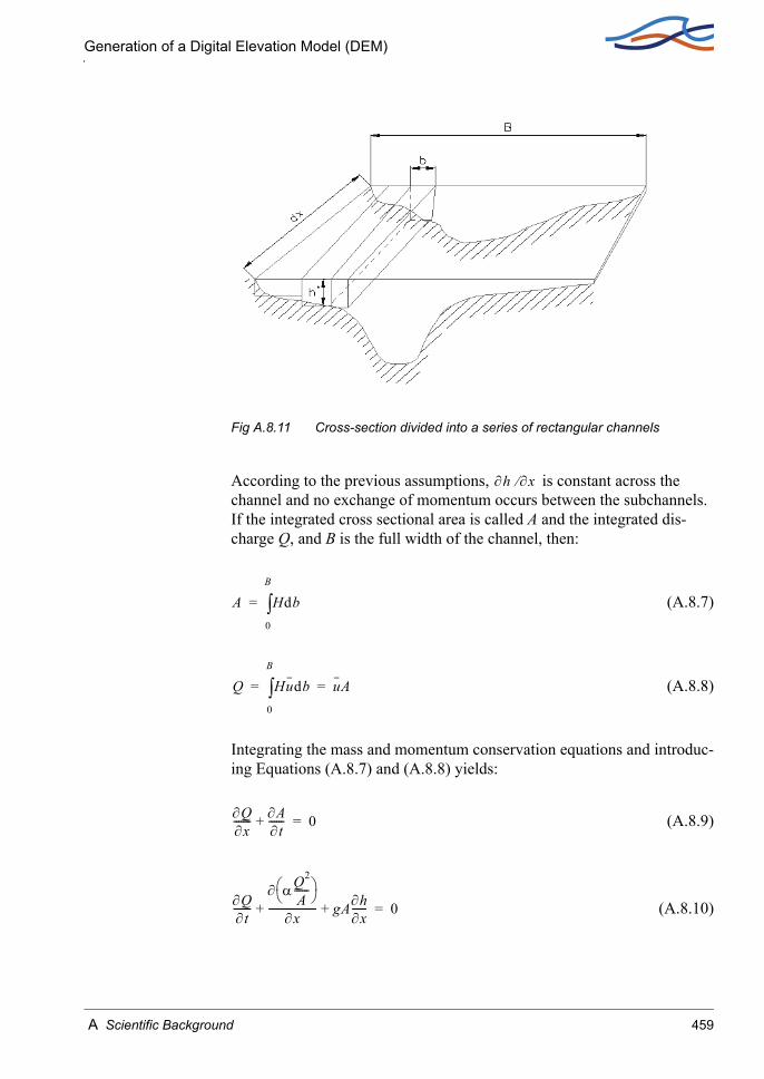
Generation of a Digital Elevation Model (DEM)
Fig A.8.11 Cross-section divided into a series of rectangular channels
According to the previous assumptions, is constant across the channel and no exchange of momentum occurs between the subchannels. If the integrated cross sectional area is called A and the integrated dis-charge Q, and B is the full width of the channel, then:
(A.8.7)
(A.8.8)
Integrating the mass and momentum conservation equations and introduc-ing Equations (A.8.7) and (A.8.8) yields:
(A.8.9)
(A.8.10)
∂h ∂x⁄
A Hdb0
B
∫=
Q Hudb0
B
∫ uA= =
∂Q∂x------- ∂A
∂t------+ 0=
∂Q∂t-------
∂ αQ2
A------
∂x------------------- gA∂h
∂x------+ + 0=
A Scientific Background 459

Saint Venant Equations
Including the hydraulic resistance, e.g. using the Chezy description and the lateral inflow; q into these equations leads to the basic equations used in MIKE 11:
(A.8.11)
(A.8.12)
∂Q∂x------- ∂A
∂t------+ q=
∂Q∂t-------
∂ αQ2
A------
∂x------------------- gA∂h
∂x------ gQ Q
C2AR---------------+ + + 0=
460 MIKE 11

Generation of a Digital Elevation Model (DEM)
A.9 SOLUTION SCHEMEThe solution to the combined system of equations at each time step is per-formed according to the procedure outlined below. The solution method is the same for each model level (kinematic, diffusive, dynamic).
The transformation of Equations (A.8.11) and (A.8.12) in section A.8 Saint Venant Equations (p. 457), to a set of implicit finite difference equa-tions is performed in a computational grid consisting of alternating Q- and h-points, i.e. points where the discharge, Q and water level h, respectively, are computed at each time step, see Fig A.9.12. The computational grid is generated automatically by the model on the basis of the user require-ments. Q-points are always placed midway between neighbouring h-points, while the distance between h-points may differ. The discharge will, as a rule, be defined as positive in the positive x-direction (increasing chainage).
Fig A.9.12 Channel section with computational grid
The adopted numerical scheme is a 6-point Abbott-scheme as shown in Fig A.9.13.
A Scientific Background 461

Solution Scheme
Fig A.9.13 Centred 6-point Abbott scheme
A.9.1 Continuity equation
In the continuity equation the storage width, bs, is introduced as:
(A.9.1)
giving:
(A.9.2)
As only Q has a derivative with respect to x, the equation can easily be centred at an h-point, see Fig A.9.14.
∂A∂t------ bs
∂h∂t------=
∂Q∂x------- bs
∂h∂t------+ q=
462 MIKE 11

Continuity equation
Fig A.9.14 Centring of continuity equation in 6-point Abbott scheme
The derivatives in Equation (A.9.2) are expressed at the time level, n+½, as follows:
(A.9.3)
(A.9.4)
bs in Equation (A.9.2) is approximated by:
(A.9.5)
where:
Ao,j is the surface area between grid point j-1 and j
Ao,j+1 is the surface area between grid point j and j+1
∆2xj is the distance between point j-1 and j+1
∂Q∂x-------
Qj 1+n 1+ Qj 1+
n+( )2
------------------------------------Qj 1–
n 1+ Qj 1–n+( )
2------------------------------------–
∆2xj-------------------------------------------------------------------------------≈
∂h∂t------
hjn 1+ hj
n–( )∆t
----------------------------≈
bsAo,j Ao,j+1+
∆2xj---------------------------=
A Scientific Background 463

Solution Scheme
Substituting for the derivatives in Equation (A.9.2) gives a formulation of the following form:
(A.9.6)
where, α, β and γ are functions of b and δ and, moreover, depend on Q and h at time level n and Q on time level n+½.
A.9.2 Momentum equation
The momentum equation is centred at Q-points as illustrated in Fig A.9.15.
Fig A.9.15 Centring of momentum equation in 6-point Abbott scheme
αjQj 1–n 1+ βjhj
n 1+ γjQj 1+n 1++ + δj=
464 MIKE 11

Momentum equation
The derivatives of Equation (A.8.12) in section A.8 Saint Venant Equa-tions (p. 457), are expressed in the following way:
(A.9.7)
(A.9.8)
(A.9.9)
For the quadratic term in (A.9.8), a special formulation is used to ensure the correct sign for this term when the flow direction is changing during a time step:
(A.9.10)
where, θ can be specified by the user (THETA coefficient under the Default values in the HD parameter editor) and by default is set to 1.0.
With all the derivatives substituted, the momentum equation can be writ-ten in the following form:
(A.9.11)
where,
To obtain a fully centred description of Aj+1, these terms should be valid at time level n+½ which can only be fulfilled by using an iteration. For this reason, the equations are solved by default two times at every time step,
∂Q∂t-------
Qjn 1+ Qj
n–∆t
-------------------------≈
∂ αQ2
A------
∂x-------------------
αQ2
A------
j 1+
n ½+αQ2
A------
j 1–
n ½+–
∆2xj----------------------------------------------------------≈
∂h∂x------
hj 1+n 1+ hj 1+
n+( )2
----------------------------------hj 1–
n 1+ hj 1–n+( )
2---------------------------------–
∆2xj--------------------------------------------------------------------------≈
Q2 θQjn 1+ Qj
n θ 1–( )QjnQj
n–≈
αjhj 1–n 1+ βjQj
n 1+ γjhj 1+n 1++ + δj=
αj f A( )=
βj f Qjn ∆t ∆x C A R ), , ,,,(=
γj f A )(=
δj f A ∆x ∆t α q v θ hj 1–n Qj 1–
n ½+ Qjn hj 1+
n Qj 1+n ½+ ), , , , , , , , ,,,(=
A Scientific Background 465

Solution Scheme
the first iteration starting from the results of the previous time step, and the second iteration using the centred values from this calculation. The number of iterations can be changed using the NoITER coefficient.
466 MIKE 11

Mathematical treatment
A.10 STRUCTURESSome of the structure types described in section 1.33 Steady State Energy Equation (p. 175) share the same mathematical treatment. These are:
broadcrested weir, control structures (overflow and non surcharged underflow structures), dambreak (crest flow and breach flow)
special weir, Q = f(h)
Their Mathematical treatment is described below.
A.10.1Mathematical treatment
The structure description combines a wide range of elements including weirs, narrow cross sections, flood plains, etc. It is obtained by replacing the momentum equation with an h-Q-h relationship, an h-Q relationship, or a Q assignment.
The grid used to describe a structure consists of h-points at either side, and a Q-point at the structure, see Fig A.10.16.
Qs and hs will be used in the following to describe the discharge and the water level at the structure, respectively, i.e. at point j.
Fig A.10.16 Channel with structure and grid
Through numerical experiments, it has been found that the weir discharge relation is best described at time level n+1. If the relation is centred at time level n+½, the product Qn Qn+1, used for the description of the head loss at the weir, may have the same magnitude for a large number of possible
A Scientific Background 467

Structures
combinations of Qn and Qn+1 values. In the centred mass equation, the average value of Qn and Qn+1 is used and oscillations introduced in the numerical process are slightly, or not at all, damped.
Numerically, the description of a compatibility condition forward in time is very convenient. Unlike the numerical description of partial differential equations, no numerical damping of the physical processes is introduced in this way, as the compatibility condition should hold at any point in time. The only error introduced comes from the linearization of the quadratic relation at the new time level.
The solution technique is to replace the coefficients in the general momen-tum equation:
(A.10.1)
with modified coefficients.
The evaluation of these coefficients is outlined in the following discus-sion.
The description generally used for flow through a structure is given by:
(A.10.2)
where, ∆H is the energy head loss over the structure, ζ is a head loss coef-ficient and Vs is the mean cross-sectional velocity at the structure.
In MIKE 11 HD the head loss is divided into inflow (contraction) and out-flow (expansion) components.
In the case of a sudden expansion the energy loss can be described as (A.10.2) and as:
(A.10.3)
Setting (A.10.2) equal to (A.10.3) gives:
(A.10.4)
αjhj 1–n 1+ βjQj
n 1+ γjhj 1+n 1++ + δj=
∆H ζVs
2
2g------=
∆H fV( s V2 )2–
2g-------------------------=
ζ2Vs
2
2g------ f
V( s V2 )2–2g
-------------------------=
468 MIKE 11

Mathematical treatment
which can be reduced to:
(A.10.5)
f, is equal to the user defined outflow head loss coefficient (ζout) and (A.10.5) becomes equal to:
(A.10.6)
Equation (A.10.6) can also be written in the form:
(A.10.7)
Which in case of a single structure (Qs = Q2, see Fig A.10.17) is equal to:
(A.10.8)
For a parallel structure (A.10.7) cannot be reduced to (A.10.8) as ( ) consequently equation (A.10.6) can be applied instead.
A similar approach can be used for adjustment of inflow head loss:
(A.10.9)
where, ζ1 and ζ2 are the adjusted inflow and outflow head loss coefficients calculated using the inflow and outflow loss coefficients (ζin and ζout) specified in the network editor → Structures → Head Loss Factor. A min-imum value for ζ1 and ζ2 can be specified in the HD parameter editor under the Default values tab as ZetaMin. In the case the solution can become unstable (no friction) and specification of a minimum value of ζ1,2, ensures a stable solution.
ζ2 f 1V2
Vs-----–
2
=
ζ2 ζout 1V2
Vs-----–
2
=
ζ2 ζout 1Q2
A2------
As
Qs------–
2
=
ζ2 ζout 1As
A2-----–
2
=
Qs Q2≠
ζ1 ζin 1V1
Vs-----–
=
As A1→
A Scientific Background 469

Structures
Fig A.10.17 Cross-sectional flow areas at a structure
A.10.2Expansion and Contraction Coefficients
As described in the previous section, flow through a structure is described according to:
(A.10.10)
This equation ζ t describes the total head loss coefficient, which is com-posed of entrance (ζ1) and exit (ζ2) coefficients. For subcritical flow the coefficients are related to the input parameters ζin and ζout and the changes in velocity (v) and area (A):
(A.10.11)
For subcritical flow through a structure there is an upstream contraction and a downstream expansion, so equation (A.10.11) works fine. When there is supercritical flow there is an upstream expansion and a down-stream contraction. Thus if supercritical flow occurs then the loss coeffi-
2
2
2gAQh tζ=∆
2
2
121 11
−+
−=+=
AA
vv s
outs
int ζζζζζ
470 MIKE 11

Determination of structure geometry
cients in MIKE11 are no longer valid. To accommodate supercritical flow, calculation of the of entrance (ζ1) and exit (ζ2) coefficients are expanded:
(A.10.12a)
(A.10.12b)
Care must be taken when selecting loss coefficients, particularly in situa-tions where both subcritical and supercritical flow conditions occur. When flow conditions change from subcritical to supercritical (or the Froude number FR becomes greater than 1), the loss coefficients ζin and ζout (spec-ified in the Head Loss Factors box) are modified:
If FR > 1 in upstream h-point then ζin = ζin / 2
If FR > 1 in downstream h-point then ζout = ζout / 2
Note that this adjustment is not made for bridge structures.
A.10.3Determination of structure geometry
For structure types broad crested weir and special weir and the structure geometry is given while the geometry of control structures (crest level) and dambreak structures (crest level and breach width) changes during the computation.
A.10.4Determination of flow regime
Given the upstream and downstream water levels and the discharge, and assuming that these three values are compatible with each other, the type of flow can be determined as follows.
>
−=
<
−=
ss
in
ss
in
vvAA
vvvv
1
2
1
11
1
;1
;1
ζ
ζζ
<
−=
>
−=
22
2
2
22
;1
;1
vvvv
vvAA
ss
out
ss
out
ζ
ζζ
A Scientific Background 471

Structures
For zero flow the upstream and downstream water levels are both below the structure invert (crest level) and the flow regime is subcritical, or the flow direction is opposite valve regulation.
For differentiating between critical and drowned flow it is assumed, in the first instance, that the flow at the weir crest is critical.
The critical discharge is determined for broad crested weirs and special weirs via the tabulated Q/H-relation while it in case of structures with time dependent geometry is computed by critical flow iteration during the sim-ulation. The pre-processed Q/H-relation for broad crested weirs are based on the assumption of a single structure, hence when the broad crested weir is a part of a composite structure the Q/H relation is no longer valid. In this case the critical discharge is computed by iteration during the simula-tion. When special weirs are included in a composite structure it is assumed that the user defined Q/H relations for critical flow takes the changed hydraulic conditions into account. When the upstream flow regime is supercritical, the Q/H relations are also recalculated.
When a long culvert is a part of a composite structure there is no critical discharge iteration i.e. the computed Q/H relation is used to estimate the critical discharge. This approach is assumed valid as the structure area usually is much smaller than the upstream area i.e. hence no need for iteration.
Critical flow occurs (for ζ2 > 1) when the energy head at the crest is larger than the downstream energy head, viz:
(A.10.13)
Critical flow occurs (for ) ( ) when the water level at the crest is larger than the downstream energy head, viz:
(A.10.14)
If the flow is not critical a submerged discharge iteration is performed and the submerged discharge is compared with the critical and the smallest is taken, viz:
critical flow:
As A1«
hs 1 ζ2–( )Qs
2
2gAs2
------------ h2Qs
2
2gA22
------------+≥+
ζ2 1≤ for outflow head loss 1≤
hs h2Qs
2
2gA22
------------+≥
472 MIKE 11

Determination of flow regime (with Supercritical Flow)
Qcritical< Qsubmerged
submerged flow:
Qcritical> Qsubmerged
A.10.5Determination of flow regime (with Supercritical Flow)
Subcritical flow types can be determined given the upstream and down-stream water levels and the discharge, and assuming that these three val-ues are compatible with each other. However, energy levels in MIKE11 are influenced by the convective suppression factor β (see Suppression of convective acceleration term (p. 185)). This means that energy head, par-ticularly at high velocities, can become distorted.
The type of flow therefore considers upstream and downstream water lev-els, discharge and upstream and downstream Froude numbers (FR). If FR < 1 then subcritical flow, if FR = 1 then critical flow and if FR > 1 then super-critical flow. Using the Froude number upstream (FR1) and downstream (FR2) of the structure, the following tests are made to decide the flow con-dition inside the structure:
If FR1 < 1 and FR2 > 1 and FR1+ < 1 then flow through structure = criti-cal
If FR1 > 1 and FR2 < 1 then flow through structure = critical
If FR1 < 1 and FR2 < 1 and E2 < h1 then flow through structure = critical
If FR1>1 and FR2>1 then flow through structure = supercritical
If FR1<1 and FR2>1 and FR1+ > 1 then flow through structure = super-critical
If FR1 < 1 and FR2 < 1 and E2 > h1 then flow through structure = subcrit-ical
Note the conditions:
FR1+ is the Froude number at the q point immediately upstream of the structure. This is included to enable a transition from critical to super-critical flow, depending upon conditions further upstream. If the q point upstream of the structure does not lie on the same branch or does not exist at all, this test is removed.
A Scientific Background 473

Structures
E2 is downstream energy level, h1 is upstream water level – this indi-cates a free overfall condition with upstream subcritical flow. E2 includes the β factor and (for the flow condition test only) is calculated as:
(A.10.15)
For zero flow the upstream and downstream water levels are both below the structure invert (crest level) and the flow regime is subcriti-cal, or the flow direction is opposite valve regulation. If flow is super-critical then zero flow is impossible.
A.10.6Zero flow
For the zero flow case the coefficients are set as follows:
, , , (A.10.16)
A.10.7Drowned flow
For drowned flow the head loss over the structure is represented as:
(A.10.17)
The velocity heads in the upstream and downstream sections need to be described implicitly, as they can be large in magnitude.
Collecting the velocity heads, the equation becomes:
(A.10.18)
22
2
2 2
+=
gAQhE β
αj 0= βj 1= γj 0= δj 0=
hQs
2
2gA2------------+
j 1–
h Q2
2gA2------------+
j 1+
– ζQs Qs
2gAs2
---------------=
hj 1– hj 1+–Qs Qs
2g--------------- ζ
As2
----- 1Aj 1–
2-----------– 1
Aj 1+2
-----------+ =
474 MIKE 11

Drowned flow
Expressing Q at time level n+1 can be done as follows:
(A.10.19)
which by re-arranging gives:
(A.10.20)
Collecting terms in relationship (A.10.20) for flow in both the positive and negative x-directions over this weir, the coefficients become:
(A.10.21a)
(A.10.21b)
(A.10.21c)
(A.10.21d)
where,
(A.10.22a)
(A.10.22b)
For the computation of these coefficients, values for ζ and As are required. Especially, close to the critical flow state, the solution becomes quite sen-
Qsn 1+ 2g hj 1– hj 1+–( )
ζ
As2
----- 1Aj 1–
2-----------– 1
Aj 1+2
-----------+------------------------------------------=
Qsn 1+ hj 1–
n 1+ hj 1+n 1+–( ) 2g
hj 1–n 1+ hj 1+
n 1+–( ) ζ
As2
----- 1Aj 1–
2-----------– 1
Aj 1+2
-----------+
----------------------------------------------------------------------------------=
αj2g
aaba-----------–=
βj 1=
γj2g
aaba-----------=
δj 0=
aaζ
As2
----- 1Aj 1–
2-----------– 1
Aj 1+2
-----------+=
ba hj 1–n 1+ hj 1+
n 1+–=
A Scientific Background 475

Structures
sitive to As values which can be described by the energy head at the struc-ture and the discharge as follows:
(A.10.23)
where,
The solution is found by iterative use of the following equations:
(A.10.24a)
(A.10.24b)
(A.10.24c)
(A.10.24d)
Convergence is normally obtained within a few iterations. A maximum number of iterations is specified in the HD parameter editor under the Default Values tab as the Inter1Max coefficient.
When the water surface gradient across the structure changes sign, so do the denominators in the square roots of Equation (A.10.8). Close to the zero point, the solution is badly defined, and the slightest change in water level difference will cause a large change in discharge. This is a result of the local vertical slope of the response function, see Fig A.10.18, and can produce an instability.
Hs hsQs
2
2gAs2
------------+=
As f hs( )=
As ζ1 ζ2, , f h1 h2 hs, ,( )=
ζ ζ1 ζ2+=
Hs H1ζ1
ζ----- H1 H2–( )–=
hs HsH1 H2–
ζ-------------------–=
476 MIKE 11

Drowned flow
Fig A.10.18 Q = f(∆h) response function and effect of local modification of 1/∆h
The problem can be overcome by a local modification of the 1/∆h function in the discontinuous region, see b) in Fig A.10.18. The corresponding effect on the Q = f(∆h) curve is shown in a) in Fig A.10.18. The range of ∆h over which the modification is applied can be selected according to the current case to be simulated, in order to introduce minimum falsification. This is done in the HD parameter editor → Default Values using the Delhs Coefficient.
A.10.7.1Drowned Flow, SupercriticalWhen drowned flow occurs during subcritical flow conditions, the energy equation is applied to calculate the head loss (A.10.17 (p. 474)). This equation should also be applicable during supercritical flow. However, during supercritical flow this equation becomes very sensitive to small changes in head drop and structure area, to such an extent that it cannot be applied to the MIKE11 structure routines (even if the convective terms are suppressed using the β factor).
So when a structure is in supercritical flow conditions, the momentum equation is solved across the structure rather than the energy equation. This is applied in the same way as for a normal q point in MIKE11, except that structure geometry is used (the estimate for structure depth and area) and that friction losses are substituted by the structure losses.
The general momentum equation is:
(A.10.25a)δγβα =++ +
+++
−11
111
nj
nj
nj hQh
A Scientific Background 477

Structures
The structure is located at a Q point (j), with an upstream h point (j-1) and a downstream h point (j+1). If the β factor is set to 1 the coefficients in the general momentum equation are updated to the following values:
(A.10.25b)
(A.10.25c)
(A.10.25d)
(A.10.25e)
The parameters used in the calculations are ∆ (DELTA coefficient (p. 437)), θ (THETA in Coefficients, HD default parameters (p. 70)), ξt (NEED REF TO GO HERE!), ∆t (time step) and ∆x (grid step).
To estimate the depth in a supercritical structure an iterative solution is used. From an initial estimate of structure area the structure water depth is calculated using the energy equation. Structure area is then updated using the existing Q/H relations. Iterations continue until successive structure area estimates are within a specified tolerance (CONV_F) or exceed a given maximum (MAX_ITER or INTER1MAX, Default values (p. 270)).
A.10.8Free overflow
For free overflow a tabulated relationship is used to define Q as a function of the upstream water level, h1. The table is calculated automatically in the case of a broadcrested weir or defined by the user for special weirs. The number of points in the table is defined by the user.
sgA- CO1 ==α
222 CO2
s
t
gAQ
txζ
β +∆∆==
sgA CO3 == γ
( ) ( ) tQxgAQ
hhs
tnnjj
∆∆+−+−∆==+−
22
1gA CO42
2
s 11
ζθδ
478 MIKE 11

Free overflow
A.10.8.1Critical dischargeThe critical discharge over a broadcrested weir is found by integrating the local critical velocity over the structure width. Thus the critical dis-charge is given by
(A.10.26)
where W is the structure width, hs(x) the local structure depth and x a coor-dinate along the cross sectional profile. The velocity head at the structure is determined as
(A.10.27)
For a rectangular weir the structure depth is independent of x and eqs. (A.10.26)-(A.10.27) become
(A.10.28)
(A.10.29)
The actual discharge has a correction factor, αc, applied which can be determined in practice by comparing the tabulated function generated by the model with the measured, or otherwise expected, relationship.
The locally linear relationship, see Fig A.10.19, with coefficients defined at time level (n+½)∆t then becomes:
(A.10.30)
ghs
Qc ghs x( )hs x( )dx0
W
∫=
Hvelocity
12--- ghs x( )hs
2 x( )dx0
W
∫
ghs x( )hs x( )dx0
W
∫------------------------------------------------=
Qc ghshsW=
Hvelocity12---hs=
Qjn 1+ a1hj sign Q( )–
n 1+ b1+=
A Scientific Background 479

Structures
giving coefficients in the relationship (A.10.1), for flow in both the posi-tive and negative x-direction, as:
(A.10.31a)
(A.10.31b)
(A.10.31c)
(A.10.31d)
where,
(A.10.32a)
(A.10.32b)
(A.10.32c)
Fig A.10.19 Linearized relationship used for the implicit description of a Q-h rela-tion
αj a11 sign Q( )+( )
2---------------------------------–=
βj1
FOF-----------=
γj a11 sign– Q( )( )
2------------------------------–=
δj b1=
FOF free overflow factor=
a1 sign Q( )Qk Qk 1––hk hk 1––-------------------------=
b1 sign Q( )Qk 1– a1hk 1––=
480 MIKE 11

Free overflow
For structures with time dependent geometry the free over flow discharge is computed as follows.
The head loss over the structure is represented by:
(A.10.33)
Collecting the velocity heads and expressing Qs at time level n+1, the equation becomes:
(A.10.34)
which by rearranging gives:
(A.10.35)
Collecting terms in relationship(A.10.35) for flow over this weir, the coef-ficients become:
(A.10.36a)
(A.10.36b)
(A.10.36c)
(A.10.36d)
h Q2
2gA2------------+
j 1–
h2Qs
2
2gAs2
------------+
– ζ1Qs Qs
2gAs2
---------------=
Qs2g hj 1– hs–( )1 ζ1+
As2
-------------- 1Aj 1–
2-----------–
---------------------------------=
Qsn 1+ hj 1–
n 1+ hs–( ) 2g
hj 1– hs–( )1 ζ1+
As2
-------------- 1Aj 1–
2-----------–
----------------------------------------------------------------=
αj2g
aabb-----------FOF–=
βj 1=
γj 0=
δj hs2g
aabb-----------FOF–=
A Scientific Background 481

Structures
where,
(A.10.37a)
(A.10.37b)
aa1 ζ1+
As2
-------------- 1Aj 1–
2-----------–=
bb hj 1– hs–=
482 MIKE 11

General Description
A.11 HEAT BALANCE MODULE
A.11.1 General Description
The heat balance module is used for simulation of heat transfer between the water body and it's surroundings. The heat balance equation can be expressed as:
(A.11.1)
where
q change in the heat capacity of the water body.
qtrib is heat transfer from tributary inflow.
qr iis the heat transfer from diffuse sources.
qp is the heat transfer from precipitation.
qe is loss of energy due evaporation.
qc is the convective heat transfer.
qs is the shortwave radiation.
qsr is the reflected shortwave radiation.
qsu is the shortwave radiation emitted from the water body.
ql is the longwave radiation above the sea surface.
qlr is the reflected longwave radiation.
qlu is the emittance of longwave energy from the water body.
qa is the loss of energy from outflow.
∆q qtrib= qr qp qc qs qsr– qsu–q1 qlr– qlu– qa– qg qsed
+ ++ +
–+ +
∆
A Scientific Background 483

Heat Balance Module
Some of the terms have been excluded from the heat balance module, since they have no, or only minor influence on the total heat budget. Fur-thermore, some of the terms are lumped into a single term, e.g. as for the longwave radiation. The following terms are set to zero in the heat balance module:
qr = 0 , qp = 0 , qg = 0 , qsed = 0 , qlr = 0 and qsu = 0,
After which equation (A.11.1) can be reduced to:
(A.11.2)
A.11.2 Convection
The heat exchange due to convection depends on the type of boundary layer between the sea surface and the atmosphere. Generally, this bound-ary layer is known to be turbulent and the following relationships between heat exchange and wind speed, air and sea temperature can be established /4/:
If Tair > Tw :
(A.11.3)
otherwise:
(A.11.4)
where
qg is the heat exchange between ground and water body.
qσεδ is the heat exchange between sediment and water body.
is the air density (kg/m3)
Cair is the specific heat of air, 1007 J/( )
∆q qtrib= qc qs qsr– q1 qlu– qa–+ +–
qc ρairCairCc W10 U– Tw Tair–( )=
qc ρairCwCc W10 U– Tw Tair–( )=
ρair
kg K°⋅
484 MIKE 11

Vaporisation
The convective heat flux varies between 0-100 W/m².
A.11.3 Vaporisation
By combining Dalton's law /3/ with the formulation proposed by Friehe & Smidth (1976) /4/ the following relationship for the vaporative heat loss can be derived :
(A.11.5)
where
Cw is the specific heat of water, 4186 J/( )
W10 is the wind speed 10 m above the sea surface
U is the surface flow velocity
Tw is the absolute temperature of the sea
Tair is the absolute temperature of the air
Cc is the sensible transfer coefficient, given as
L is the latent heat of vaporization, j/kg
Ce is the moisture coefficient,
W2 is the wind speed 2 m above sea surface
Qw is the water vapour density close to the surface
Qa is the water vapour density in the atmosphere
a and b is user specified coefficients
kg K°⋅
1,41 10 3–⋅
qe LCe a bW2+( ) Qw Qa–( )=
2,5 106⋅
1,32 10 3–⋅
A Scientific Background 485

Heat Balance Module
Measurements of Qw and Qa are not directly available, but Qw and Qa can be related to the vapour pressure as /4/ :
(A.11.6)
and
(A.11.7)
The vapour pressure close to the sea surface ew can be expressed by the water temperature, under the condition that the air close to the sea surface is saturated and have the same temperature as the water:
(A.11.8)
where
The vapour pressure in the air above the sea surface ea depends on the air temperature and the relative humidity R:
(A.11.9)
By combining equation (A.11.5) with equations (A.11.8) and (A.11.9) the final expression for the evaporative heat loss yields:
(A.11.10)
where P is a latent constant being 4370 .
K is a constant being 5418 K
Tk is the temperature at 0 C being 273.15 K
Qw0,2167
Tw----------------ew=
Qa0,2167
Tair----------------ea=
ew 6,11eK 1
Tk----- 1
Tw-------–
=
°
ea R6,11eK 1
Tk----- 1
Tair----------–
=
qe P a bW2+( ) eK 1
Tk----- 1
Tw-------–
Ts----------------------- Re
K 1Tk----- 1
Tair----------–
Tiar-----------------------------–=
J K/m3⋅
486 MIKE 11

Shortwave Radiation
During cooling of a water mass the heat loss due to vaporization has a major effect and typical varies between 0-100 W/m².
A.11.4 Shortwave Radiation
Radiation from the sun consist of electromagnetic waves with wave lengths varying from 1000 to 30000 Å. Most of the radiation will be absorbed in ozone layer, leaving only a fraction of the energy to reach the surface of the Earth. Furthermore the spectrum changes, when sunrays pass through the atmosphere. Most of the infrared and ultraviolet com-pound is absorbed, so the solar radiation on the earth mostly consist of light with wave lengths between 4000-9000 Å. This radiation is termed the shortwave radiation.
The intensity of the shortwave radiation depends on:
1 The distance between the earth and the sun.
2 The declination angle and latitude.
3 Extraterrestrial radiation.
4 Cloudiness and amount of water vapor in the atmosphere.
The calculation of the shortwave radiation is based on the following for-mulations.
A.11.4.1 Distance between the Earth and the SunThe mean distance between the Earth and the Sun r0 is 149597890 km.
Spencer /1/ has developed the following expression to determine the excentricity correction factor E0.
(A.11.11)
where is the day angle given as :
(A.11.12)
E0r0
r----
2
1,000110 0,034221 Γ 0,001280 Γ
0,000719 2Γ 0,000077 2Γsin+cos
+sin+cos+= =
Γ
Γ 2π dn 1–( )
365---------------------=
A Scientific Background 487

Heat Balance Module
where
A.11.4.2 Solar Declination and Day LengthThe daily rotation of the Earth around the polar axes contributes to changes of the solar radiation. The seasonal radiation is governed by the declination angle. Spencer /1/ presented the following expression to deter-mine the declination angle .
(A.11.13)
where is are measured in radians.
The day length Nd varies with . For a given latitude (North positive, South negative) the day length is expressed as:
(A.11.14)
and the sunrise angle is:
(A.11.15)
A.11.4.3 Extraterrestrial RadiationThe intensity of shortwave radiation on a surface parallel with the surface of the Earth changes with the angle of incident. The highest intensity is measured at noon where the sun is in zenith and the lowest during sunrise and sunset. The extraterrestrial intensity of shortwave radion on a surface parallel to the Earth surface q0 can be expressed as /1/:
(A.11.16)
r is the actual distance between the Earth and the Sun expressed in km.
dn is the day number given as 1 the 1st day of January and 365 the the 31st day of December. It is assumed that February always have 28 days.
δ
δ 0,006918 0,399912 Γcos 0,070257 Γsin
0,006758 2Γcos 0,000907 2Γsin
0,002697 3Γcos 0,00148 3Γsin+
–+
–+–(
)
=
δ
δ φ
Nd24π------ φ δtantan–( )=
ωsr
ωsr cos 1– φ δtantan–( )=
q0 qscE0 δ φ 24π------
π24------
δ φ ωicoscoscossin+sinsin =
488 MIKE 11

Shortwave Radiation
where
By integrating equation (A.11.16) over one day, the daily extraterrestrial radiation H0 is derived as:
(A.11.17)
A.11.4.4 Radiation under Cloudy SkiesFor determination of daily radiation under cloudy skies H, Ångstrom /1/ has proposed the following relationship between the daily insulation and the number of bright sunshine hours n:
(A.11.18)
Rietvald found the values of a and b, could be determined based on the mean annual value of bright sunshine hours n and the average length of a day 19 given as:
(A.11.19)
and
(A.11.20)
The coefficients a and b are subject to changes according to topographical shading.
The average hourly shortwave radiation qs can the be found as:
(A.11.21)
is defined in equation (A.11.25) and is called the hour angle
qsc is the solar constant measured to 1376 W/m²
ωi
H024π------qscE0 φ δ ωsrsin ωsr ωsrcos–( )coscos=
HH0------ a b n
Nd------+=
Nd
a 0,1 0,24 nNd------
+=
b 0,38 0,08 Nd
n------
+=
qsHH0------
q0 a3 b3 ωicos+( )=
A Scientific Background 489

Heat Balance Module
where
(A.11.22)
and
(A.11.23)
is the hour angle.
If the time is measured in local time, the hour angle is given as:
(A.11.24)
Et is varying during the year and is called the equation of time given as:
(A.11.25)
where Et is measured in minutes.
The time meridian Ls is the standard longitude for the time zone and LE is the local longitude (west positive, east negative). The longitude correction is 4 minutes for every degree.
The summer time correction is + 1 hour, if the clock is 1 hour ahead.
A.11.4.5 AlbedoSolar radiation that impinges on the sea surface does not all penetrate the water surface. Parts of the radiation are reflected back to its surroundings, and are lost from the system unless it is backscattered from the atmos-phere or the surrounding topography. This reflection of the solar energy is termed the albedo. The amount of energy which is lost due to albedo,
a3 0,409 0,5016 ωsrπ3---–
sin+=
b3 0,6609 0,4767 ωsrπ3---–
sin–=
ωi
ωiπ12------ 12 correction for summertime
Et
60------
460------ Ls LE–( )
–
local time in hours–
–+
=
Et 0,000075 0,001868 Γcos 0,032077 Γsin0,014615 2Γcos 0,04089 2Γsin–
––+() 229,18( )
=
490 MIKE 11

Longwave Radiation
depends on the angle of incidence and angle of refraction. The reflection can be expressed in Fresnel's law /7/, which is valid for a smooth sea:
(A.11.26)
where
The reflected shortwave radiation can now be expressed as:
(A.11.27)
The reflection coefficient varies from 5 - 40 %.
A.11.5 Longwave Radiation
A body or a surface emits electromagnetic energy at all wave lengths of the spectrum. The longwave radiation consists of waves with wave length between 9000-25000 Å. The radiation in this interval is termed the infra-red radiation and is emitted from the atmosphere and the sea surface. The longwave emittance from the sea surface to the atmosphere minus the longwave radiation from the atmosphere to the sea surface is called the net longwave radiation. Brunt has related the net longwave radiation with the following parameters:
1 Cloudiness defined by number of sunshine hours.
2 Air temperature measured in Kelvin degrees.
3 Vapour pressure in the air, at the actual level of relative humidity and air temperature.
The formulation used in MIKE is based on Brunt's general equation for net out-going longwave radiation /2/ given as:
(A.11.28)
i is the angle of incidence
r is the refraction angle
α
α 12--- sin2 i r–( )
sin2 i r+( )-------------------------- tan2 i r–( )
tan2 i r+( )--------------------------+
=
qsr αqs=
α
qnl qlu q1 σT4n a b ed–( ) c d+( )=–=
A Scientific Background 491

Heat Balance Module
where a, b, c and d are coefficients given as:
(A.11.29)
A.11.6 References
ed is the vapour pressure at dew-point temperature measured in mb
n is the number of sunshine hours
Nd is the number of possible sunshine hours
is Stefan Boltzman's given as
/1/ Muhammed Iqbal, An introduction to solar radiation, Ace-demic Press, 1983.ISBN 0-12-373752-4
/2/ M.E.Jensen, R.D. Burman, and R.G. Allen, Evapo-transpi-ration and Irrigation Requirements, ASCE 1990.ISBN 0-87262-763-2
/3/ Peter S. Eagleson, Dynamic Hydrology, McGraw-Hill, 1970.
/4/ Swedish Council for Building Research, Jörgen Sahlberg, A hydrodynamic model for heat contents calculation on lakes at the ice formation date.Document D4:1984, 1984
/5/ Gunnar Lindh and Martin Falkenmark, En inledning til vattenresurslären, Norway 1972.
a 0,56 b 0,77 mb 1 2/– c 0,10 d 0,90=,=,=,=
σ 5,6697 10 8– Wm2 K⋅( )
--------------------⋅
492 MIKE 11

References
/6/ Poul Harremoës and Anders Malmgren-Hansen, Lærebog i vandforurening, Polyteknisk forlag, Denmark 1990. SBN 87-502-0671-0
/7/ Robert G. Wetzel, Limnology, Saunders College Publish-ing, 1983.ISBN 0-03-057913-9
A Scientific Background 493

Heat Balance Module
494 MIKE 11

General
A.12 USER DEFINED STRUCTURE
A.12.1 General
A.12.1.1IntroductionThe user defined structure is available to create customised structures in MIKE11. However, the potential application goes beyond this, allowing for the customisation of almost any specialist application or modification to MIKE11.
When activated, the user defined structure will access a DLL (Dynamic Link Library) written by the user. The Network Editor interface contains a number of variables that can be used in the DLL. In addition, the DLL can access any variable in MIKE11 through several records.
The following gives a description of the user defined structure, including coding issues and a description of parameters. Two examples of possible applications are given. The first example also provides an insight into the computational requirements for developing a structure within the MIKE11 solution scheme.
A.12.1.2 RequirementsObviously, knowledge of computer programming is necessary. MIKE11 is written in PASCAL using Borland DELPHI. Any code written must be compatible with the compiled unit files (DCU) provided. The easiest way to ensure this is to have Delphi and write your programs in PASCAL.
The user defined structure option has an extremely broad area of possible application. It is possible to modify or interrogate most components of MIKE11. However, there is a difference between knowledge of hydraulics and knowledge of computational hydraulics. An understanding of compu-
A Scientific Background 495

User Defined Structure
tational hydraulics is essential if you wish to modify or insert anything into the MIKE11 computational scheme. On the other hand, coding to pro-duce customised output formats shouldn't be as difficult to achieve.
A.12.1.3 General Coding IssuesWhen a user defined structure is specified, MIKE11 will search for a pro-cedure in a dynamic link library (DLL). The name of the DLL and the name of the procedure can be either default names or can be specified in the network editor interface.
The specifications of the DLL must match the specifications that MIKE11 is expecting. This includes specific compiler details and variable access. The DLL must use the MIKE11 unit rivdecl, which contains record decla-rations. There are several DCU files that are linked into the project to do this.
The basic structure of the DLL is shown below:
Library struc1;
uses SysUtils, Classes, rivdecl;
procedure user_written_code ( user_ptr : weir_struc; information on structures grid_ptr : grid_struc; information on grid structure mm_act : mm_ptr; information on simulation iter_nr : integer; iteration when procedure called nt : integer ); timestep when procedure calledcdecl; export;
var// insert local variables here
begin// user defined code goes hereend;
exports user_written_code;beginend.
A.12.1.4 MIKE11 InterfaceA structure must be defined in the network editor to access the user defined code. Note that a structure will always alter the network. If you wish to use the user defined code in a non-intrusive way (say to produce customised output formats), create a dummy branch (with dummy bound-aries) and place it in the network file isolated from the actual model net-work.
The Network Editor interface provides application specific information to the user written code (Fig A.12.20):
496 MIKE 11

General
Fig A.12.20 Network Editor Interface
A.12.1.5 Description of ParametersThe user defined code calls five parameters. The last two are variables, while the first three are records. Details are as follows:
user_ptruser_ptr is a pointer of type weir_struc, declared in the unit rivdecl. It contains information relating to the structures in the model and their spec-ifications. Some useful variables within the record are as follows:
location - where is the structure
location.id_name - name of branch
location.id_mil - chainage of structure
weir_grid - see next description of grid_ptr
struc_type - user defined in this case
Further, the following are the entries inserted in the User Defined Struc-ture dialog box in the network editor. These are also located in the user_ptr record. The descriptions in brackets reference the title and column title of each entry in the dialog:
NoOfUserDefinedArrays (Array 1)
A Scientific Background 497

User Defined Structure
UserDefArray1Col1[] (Array 1, D1) - Array of 2 column arrays
UserDefArray1Col2[] (Array 1, D2)
NoOfUserDefinedIntegers (Integers)
UserDefInteger[] (Integers, I) - Array of integers
NoOfUserDefinedDoubles (Doubles)
UserDefDouble[] (Doubles, D) - Array of Doubles (double precision reals)
NoOfUserDefinedPointers (Pointers)
UserDefPointer[].P1String (Pointers, River) - Array of pointers to a grid, branch or node, where each pointer contains a string (river name), double (chainage) and integer (grid=1, branch=2, node=3)
UserDefPointer[].P2Double (Pointers, Chainage)
UserDefPointer[].P3Integer (Pointers, Type)
UserDefPointer[].UserDefGridP (not shown in dialog) - If type is Grid, pointer to grid variables at location
UserDefPointer[].UserDefBranchP (not shown in dialog) - If type is Branch, pointer to branch variables at location
UserDefinedPointer[].UserDefNodeP (not shown in dialog) - If type is Node, pointer to node variables at location
NoOfUserDefinedMiscData (Misc)
UserDefMiscData[].P1String (Misc, Str) - Array of record containing string, integer and doubles. The first string entry (if not NIL) is the name of the DLL. The second string entry (if not NIL) is the name of the procedure. Otherwise, default values are 'USER_WRITTEN_DLL.DLL' and 'user_written_code'.
UserDefMiscData[].P2Integer (Misc, I1)
UserDefMiscData[].P3Integer (Misc, I2)
UserDefMiscData[].P4Integer (Misc, I3)
UserDefMiscData[].P5Integer (Misc, I4)
UserDefMiscData[].P6Double (Misc, D1)
UserDefMiscData[].P7Double (Misc, D2)
UserDefMiscData[].P8Double (Misc, D3)
UserDefMiscData[].P9Double (Misc, D4)
498 MIKE 11

General
UserDefTextfile - Type textfile, use to assign a globally declared unit number to a file name.
grid_ptrgrid_ptr is a pointer of type grid_struc, declared in the unit rivdecl. It contains information relating to all the grid points in the model. Some use-ful variables within the record (among many others) are as follows:
grid_loc - as for location in user_ptr.
area - cross-sectional area
flarea - storage area at water level h
radius - hydraulic or resistance radius
resnum - resistance number
width - width of cross-section
dx - distance between structure and grid point downstream
d2x - distance between upstream and downstream grid points.
xcoor - x-coordinate of point
ycoor - y-coordinate of point
h - water level at time n+½
q - discharge at time n+½
hq0 - water level (h point) or discharge (q point) at time n
hq1 - water level (h point) or discharge (q point) at time n+1
co1, co2, co3, co4 - coefficients applied to solution scheme
prev_grid - pointer to previous grid (same information listed here except at previous grid)
next_grid - pointer to previous grid (same information listed here except at next grid)
actlev - pointer to cross-section information - also useful to determine if grid point is h point or Q point (for Q point, actlev = NIL)
mm_actmm_act is a pointer of type mm, declared in the unit rivdecl. It con-tains information relating to the MIKE11 simulation, which is essen-tially all the information. Some useful variables within the record (among many others) are as follows:
nnt - number of timesteps
A Scientific Background 499

User Defined Structure
dt - timestep in seconds
time_on_monitor - pointer to time on monitor, containing year, month, day, hour, min, sec, datestring, timestring
time_act - pointer to current simulation time, containing year, month, day, hour, min, sec, datestring, timestring
time_start_simul - pointer to simulation start time, containing year, month, day, hour, min, sec, datestring (not used), timestring (not used)
time_end_simul - pointer to simulation end time, containing year, month, day, hour, min, sec, datestring (not used), timestring (not used)
nr_iter - iteration number (same as variable called explicitly)
progDir - directory location of executable
dataDir - directory location of simulation files
iter_nrThe structure routines are called at each iteration in a given timestep (see the User Reference A.8 for details on this). iter_nr is the number of the particular iteration.
ntThe timestep of the particular structure call.
A.12.2 Example: Structure with Form Loss Coefficient
DescriptionThis is an example of a structure defined by a simple loss coefficient applied to the velocity head. The equation is:
(A.12.1)
where:
∆h is head drop across the structure;
F is an input form loss coefficient;
v is velocity through the structure; and
g is gravity.
gvFh2
2
=∆
500 MIKE 11

Example: Structure with Form Loss Coefficient
MIKE11 uses flows, so the equation can be rewritten in terms of flow Q and area A. Flow direction is dependent upon the sign of ∆h. To include this direction dependency, the equation can be rewritten:
(A.12.2)
Scheme FormulationTo incorporate this structure into MIKE11, the equation must be re-arranged into a finite difference form, with a staggered grid centred on a q point:
(A.12.3)
where;
α, β, γ and δ are coefficients (co1, co2, co3 and co4 in the MIKE11 code);
n is the timestep; and
j is space step.
Consider the structure equation at a time mid-way between timesteps at n+½ and across a staggered grid centred on a Q point:
(A.12.4)
Placing the terms on one side:
(A.12.5)
The values of h and Q are only solved at times n and n+1. Therefore, a time-centring factor (θ) is used to describe the terms (say h):
(A.12.6)
Q ∆h 2gA2
F ∆h--------------=
δγβα =++ ++
++−
11
111
nj
nj
nj hQh
Q jn 1 2⁄+ hj 1– hj 1+–( )n 1 2⁄+ 2gA2
F hj 1– hj 1+–( )n 1 2⁄+-------------------------------------------------------=
( ) ( ) 022 ½1½
11
2½½
1½11
2
=−
++−
− +++
+−
++−+
+−
njn
jj
nj
njn
jj
hhhF
gAQhhhF
gA
( ) nnn hhh θθ −+= ++ 11½
A Scientific Background 501

User Defined Structure
Assuming that within the square root term, the equation now becomes:
(A.12.7)
Rearranging this into the finite difference form:
(A.12.8)
Thus, the coefficients in the equation become:
(A.12.9)
(A.12.10)
(A.12.11)
(A.12.12)
Note that if ∆h = 0, the square root term has no solution. In this case, co1 = 1, co2 = 0, co3 = -1 and co4 = 0.
( ) ( ) hhhhh njj
njj ∆=−=− +−
++− 11
½11
θ 2gA2
F ∆h--------------h j 1–
n 1+– Q jn 1+ 2gA2
F ∆h--------------h j 1+
n 1++ +
1 θ–( ) 2gA2
F ∆h--------------h j 1–
n– Q jn 2gA2
F ∆h--------------h j 1+
n+ +
+
0=
θ 2gA2
F ∆h--------------h j 1–
n 1+– θQ jn 1+ θ 2gA2
F ∆h--------------h j 1+
n 1++ +
1 θ–( ) 2gA2
F ∆h--------------h j 1–
n Q jn– 2gA2
F ∆h--------------h j 1+
n–
=
co1 α θ 2gA2
F ∆h--------------–= =
co2 β θ= =
co3 γ θ 2gA2
F ∆h--------------= =
co4 δ 1 θ–( ) 2gA2
F ∆h--------------h j 1–
n Q jn– 2gA2
F ∆h--------------h j 1+
n–= =
502 MIKE 11

Example: Structure with Form Loss Coefficient
MIKE11 Variables RequiredTo code this, the following parameters are required. grid_ptr is at the Q point, which is a user defined structure:
α = grid_ptr^.co1
β = grid_ptr^.co2
γ = grid_ptr^.co3
δ = grid_ptr^.co4
A = grid_ptr^.area
= grid_ptr^.hq0
= grid_ptr^.prev_grid^.hq0
= grid_ptr^.next_grid^.hq0
MIKE11 ApplicationA simple model has been created for this structure. It consists of a rectan-gular channel (length 1000 m, width 100 m and slope of 1 in 1000) with the structure in the centre (chainage 500 m). Water level boundaries at each end are specified. The upstream water level is fixed at 1 m (which is also the initial water level). The downstream water level is lowered at a linear rate from 1 m to 0.5 m over a period of 1½ hours. It is then main-tained at 0.5 m for an additional 1½ hours. Bed friction is Manning M = 30, and the timestep is 1 minute.
The user defined structure has been defined. The first string in the Miscel-laneous entry contains the name of the DLL that will be accessed by MIKE11. The second string contains the name of the procedure that will be accessed. Note that if no entries are specified, the default DLL is 'USER_WRITTEN_DLL.DLL' and the procedure name is 'user_written_code'. For this example:
user_ptr^.UserDefMiscData[1].P1String = 'form_loss_struc1.DLL'
user_ptr^.UserDefMiscData[2].P1String = 'user_written_code'
For flexibility for this particular problem, the time centring factor and form loss coefficient are specified in the interface. The first double in the Double entry is the time centring factor (θ). The second entry is the form loss coefficient (F). Thus, the variables theta and formC are local variables defined by:
user_ptr^.UserDefinedDouble[1] = theta
user_ptr^.UserDefinedDouble[2] = formC
njQ
njh 1−
njh 1+
A Scientific Background 503

User Defined Structure
User Defined CodeThe code for this example is as follows:
library form_loss_struc1;
uses dialogs, // message dialogs math, // power fúnction SysUtils, Classes, rivdecl; // access to MIKE11
procedure user_written_code ( user_ptr : weir_struc; information on structures grid_ptr : grid_struc; information on grid points mm_act : mm_ptr; information on simulation iter_nr : integer; iteration when procedure called nt : integer ); timestep when procedure calledcdecl; export;
const grav = 9.81;
var theta, formC, h_ups, h_dws, sqterm : double; stemp : string;
begin user_written_code
// if first timestep and first iteration, print a message to screen with// the values of THETA and FORMC if (nt = 1) and (iter_nr = 1) then begin stemp := 'USER DEFINED STRUCTURE WITH FORM LOSS COEFFICIENT' + char(13) + char(13) + 'User Defined DLL: form_loss_struc1' + chr(13) + 'Written by CFN' + char(13) + 'THETA = ' + FloatTostrF(user_ptr^.UserDefDouble[1],fffixed,5,2) + chr(13) + 'FORMLOSS = ' + FloatTostrF(user_ptr^.UserDefDouble[2],fffixed,5,2); messagedlg(stemp,mtinformation,[MBOK],0); end;
// assign local variables theta and formC theta := user_ptr^.UserDefDouble[1]; formC := user_ptr^.UserDefDouble[2];
// assign local variables h_ups and h_dws// defined from prev_grid (upstream) and next_grid (downstream) h_ups := grid_ptr^.prev_grid^.hq0; h_dws := grid_ptr^.next_grid^.hq0;
// set terms of momentum coefficient for case of h_ups = h_dws grid_ptr^.co1 := 1; grid_ptr^.co2 := 0; grid_ptr^.co3 := -1; grid_ptr^.co4 := 0;
// if there is a water level gradient change the terms if h_ups <> h_dws then begin
// calculate the square root term, used in the momentum terms sqterm := sqrt( 2*grav * power(grid_ptr^.area,2) / formC / abs(h_ups - h_dws) );
// terms of momentum coefficient grid_ptr^.co1 := -theta * sqterm;
504 MIKE 11

Example: User Defined Output
grid_ptr^.co2 := theta; grid_ptr^.co3 := theta * sqterm; grid_ptr^.co4 := (1-theta) * (sqterm * h_ups - grid_ptr^.hq0 - sqterm * h_dws);
end;
end; of user_written_code
exports user_written_code;beginend.
TestingRun this simulation using a range of different form loss coefficients and time centring coefficients. THETA can vary between 0 and 1. THETA = 0.5 is a fully centred scheme. When 0 < THETA < 0.5 the solution scheme is unstable. For THETA = 0.5 the solution is stable and non-dissipative. For 0.5 < THETA < 1.0 the solution is stable and dissipative.
This structure is identical to an energy loss structure, applying a user defined energy loss coefficient (specified in the Network Editor). Repeat this test using an energy loss structure rather than a user defined structure. The results should be identical.
A.12.3 Example: User Defined Output
MIKE11 simulations can be performed over very long periods of time. To minimise output file size there is a Storing Frequency option in the simu-lation editor, where results are saved at a specified frequency of the simu-lated timestep. However situations arise where output is required at every timestep at specific locations, while in the same simulation still having global output at a longer timestep.
Consider for example long term tidal variation in an estuary, where analy-sis of tidal range (difference in maximum and minimum water levels dur-ing a tidal cycle) and mean sea level change (moving average of tide levels) is required. Calculation of these parameters requires model output at small time increments (of the order of 15 to 30 minutes for semi-diurnal tidal cycles). Depending on the size of the model, extraction of this infor-mation at all grid points for a long term simulation would produce a large output file. To reduce output file size there is an option in the network edi-tor to select which grid points will store results. However, this may not always be the most convenient solution.
This example will describe the programming required to create a time series output of water levels or flows at specified locations in a model. The output will be at each simulation timestep. Details are as follows:
A Scientific Background 505

User Defined Structure
The DLL name is 'TIME_SERIES_OUTPUT.DLL'.
The procedure name is user_written_code.
The user defined structure will be inserted into a dummy branch of an existing model. The structure will not be used or considered as part of the existing model.
It is intended that this code will be generic. This means it should be applicable to many different applications.
The output file format will be CSV (comma separated ASCII format), which can be easily read using EXCEL. The output file is 'time_series_output.csv' which has a column separator ';'.
The coding must consider that the user defined code is called prior to the final sweep in the solution scheme. This means that water levels and flows for the current timestep have not yet been calculated and that the results from the previous timestep must be presented. The code writes the result from the previous timestep on one line, then writes the current time on the next line. This staggered approach will produce a file where the output time is consistent with the standard MIKE11 result files.
The variable saved to output is hq0. As well as being the results of the pre-vious timestep, hq0 is water levels at h points and flows at Q points. Therefore output using this program can be either water level or flow, depending upon selection of h or Q output point.
ApplicationThe following shows an example where time series output has been speci-fied in an existing model. The model network initially consisted of three branches. An additional dummy branch (called DUMMY) has been cre-ated which is not connected to the other branches. This branch contains the user defined structure. Dummy boundary conditions (say uniform water levels at each end of the branch) are applied. The tabular view of the user defined structure is as follows:
506 MIKE 11

Example: User Defined Output
Fig A.12.21 Network Editor Tabular View of Example 2
The structure is location at chainage 10 in the dummy branch. There are two Pointers to grid points, defined by the River name and Chainage. The Type of both is Grid. These pointers will be the locations at which model results will be presented.
In the Misc field, the first string (Str) entry contains the name of the DLL. The second string entry contains the name of the procedure. The third string entry contains the name of the output file, which is read by the user defined code. The fourth string contains the column separator to be used in the output file. If no entries are specified in the Misc field, the default DLL is 'USER_WRITTEN_DLL.DLL', the procedure name is 'user_written_code, the output file is 'time_series_output.csv', and the col-umn separator is ','.
User Defined CodeThe code for this example is as follows:
library time_series_output;
uses SysUtils, Classes, rivdecl; // access to MIKE11
procedure user_written_code ( user_ptr : weir_struc; information on structures grid_ptr : grid_struc; information on grid points mm_act : mm_ptr; information on simulation iter_nr : integer; iteration when procedure called
A Scientific Background 507

User Defined Structure
nt : integer ); timestep when procedure calledcdecl; export;
var outfile : string; i : integer; delim : string; grid_act : grid_struc; branch_act : branch_struc; hout : array [1..50] of double; // up to 50 output locations
begin user_written_code
// only perform saving of output if at the last iteration of each timestep!! if (iter_nr = mm_act^.nr_iter) then begin
// use default column separater unless specified in UDS input delim := ','; if user_ptr^.NoOfUserDefinedMiscData > 3 then delim := user_ptr^.UserDefMiscData[4].P1String;
// loop through branches and grid points in branches to find locations that// match user defined pointer list branch_act := mm_act^.first_branch; while branch_act <> NIL do // loop branches, starting at first branch begin grid_act := branch_act^.fgrid_ptr; while grid_act <> NIL do // loop all grid points in branch begin for i := 1 to user_ptr^.NoOfUserDefinedPointers do // loop pointer list begin if user_ptr^.UserDefPointer[i].UserDefGridP = grid_act then begin // assign values to hq0 // hp0 is result at previous timestep - // the latest (h) has not been been calculated yet. hout[i] := grid_act^.hq0; end; end; grid_act := grid_act^.next_grid; end; branch_act := branch_act^.next_bran; end;
// first timestep, so find filename, assign file to unit, rewrite and write headers// the name of the output file is 'time_series_output.csv'// unless specified otherwise in MiscData[3] if (nt = 1) then begin outfile := mm_act^.dataDir + 'time_series_output.csv'; if user_ptr^.NoOfUserDefMiscData > 2 then outfile := user_ptr^.UserDefMiscData[3].P1String;
assignfile(user_ptr^.UserDefTextfile,outfile); rewrite(user_ptr^.UserDefTextfile); write(user_ptr^.userdefTextfile,'Timestep' + delim + 'DATE' + delim + 'TIME'); for i := 1 to user_ptr^.NoOfUserDefinedPointers do // loop through pointer list write(user_ptr^.UserDefTextfile, delim + user_ptr^.UserDefPointer[i].P1String + ' ' + FloatTostrF(user_ptr^.UserDefPointer[i].P2Double,fffixed,6,3)); writeln(user_ptr^.UserDefTextfile); end
// if not first timestep, write out results in hout to output file// keep on the same line, but put a new line at the end else begin for i := 1 to user_ptr^.NoOfUserDefinedPointers do write(user_ptr^.UserDefTextfile, delim + FloatTostrF(hout[i],fffixed,10,5)); writeln(user_ptr^.UserDefTextfile);
508 MIKE 11

Example: User Defined Output
end;
// if the last timestep then close the file// if not, as time is offset write the current timestep on a new line if (nt >= mm_act^.nnt) then close(user_ptr^.UserDefTextfile) else write(user_ptr^.UserDefTextfile, InttoStr(nt) + delim + mm_act^.time_act.datestring + delim + mm_act^.time_act.timestring);
end; of last iterationend; of user_written_code
exports user_written_code;beginend.
OutputOutput is in a CSV format, which can be opened using Excel:
A Scientific Background 509

User Defined Structure
510 MIKE 11

Example: User Defined Output
A.13 NOMENCLATUREA flow area
A1 inflow river cross-section area
A2 outflow river cross-section area
Abc critical flow area in breach
Ac critical flow area
Ae effective flow area
Afull full cross-section area of culvert
culvert inflow cross-section area
culvert outflow cross-section area
average of and
B full width of channel
b width of rectangular channel
b gate width
bs structure width
bs storage width
C Chezy coefficient
Cc contraction coefficient
Ccal calibration coefficient
Cd discharge coefficient
Co discharge coefficient
Cr Courant number
Cw wind friction coefficient
As1
As2
AsaAs1
As2
A Scientific Background 511
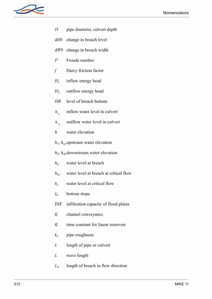
Nomenclature
D pipe diameter, culvert depth
dHb change in breach level
dWb change in breach width
F Froude number
f Darcy friction factor
H1 inflow energy head
H2 outflow energy head
HB level of breach bottom
inflow water level in culvert
outflow water level in culvert
h water elevation
h1, husupstream water elevation
h2, hdsdownstream water elevation
hb water level at breach
hbc water level at breach at critical flow
hc water level at critical flow
Ib bottom slope
INF infiltration capacity of flood plains
K channel conveyance
K time constant for linear reservoir
ks pipe roughness
L length of pipe or culvert
L wave length
Lb length of breach in flow direction
hs1
hs2
512 MIKE 11

Example: User Defined Output
Lfull length of culvert flowing full
M Manning number
n Manning's n
P wetted perimeter
Q discharge
Qb breach flow
Qbc critical flow in breach
Qc critical flow
Qo orifice flow
QP primed flow
QP discharge through a pipe
QR return flow
q lateral inflow per unit width
qloss total water loss rate
qlossINFinfiltration loss rate
qlossRSloss rate from river to retention storage
qt sediment transport rate per unit width
rf resistance factor
rr relative resistance
R resistance or hydraulic radius
Rh hydraulic radius
Rt resistance radius
S water surface slope
Sc critical flow slope
A Scientific Background 513

Nomenclature
SI storage content of linear infiltration storage
Smax maximum retention storage
So culvert slope
SS side slope of breach
T duration of event (wave period)
tfac topographic factor
u average velocity along vertical
V1 velocity at h1
V10 velocity 10 m above water surface
Vb velocity in breach
Vbc critical velocity in breach
WB width of breach bottom
WFL filled retention storage (flood width)
Wmin minimum river width for which losses occur
WR average (flooded) river width
W water width corresponding to water elevation h
w gate opening
x side erosion index
y local water depth
yp depth of water in pipe
ys depth at vena contracta
y1 upstream water depth
y2 downstream water depth
Zc weir crest elevation
514 MIKE 11

Example: User Defined Output
inflow culvert invert level
outflow culvert invert level
obvert level of pipe
outflow obvert level
α momentum distribution coefficient
α' vertical velocity distribution coefficient
αc free overflow factor
ε porosity of sediment
ρ density
ρa density of air
τr bed resistance term
τw wind shear stress
µ submerged flow coefficient or weir discharge coefficient
ζ headloss coefficient
ζin inflow loss coefficient
ζout outflow loss coefficient
ζ1 contraction loss coefficient
ζ2 expansion loss coefficient
ζb bend loss coefficient
ζf friction loss coefficient
∆H inflow head loss
∆Hloss total head loss
∆Rp change in pipe radius
zinv1
zinv2
zobv
zobv2
A Scientific Background 515

Nomenclature
516 MIKE 11

BThe Mike11.ini file
517

518 MIKE 11

Introduction
B.1 MIKE11.INI FILE SETTINGS
B.1.1 Introduction
The MIKE11.ini-file offers a possibility of changing settings within the calculation part of MIKE 11 by adjusting values of below listed environ-ment variables.
B.1.2 MIKE 11 GIS LINKAGE
Linkage of MIKE 11 Results with the ArcView based MIKE 11 GIS Inter-face.
Usage of MIKE 11 GIS Interface may require activation of variables to produce and export simulation information to text-files.
The default settings should only be changed if 3D-analyst is not installed. If required the ON/OFF switch can be used to ensure that ASCII results are ported to the msd directory. The switch should be set to ON if 3D Ana-lyst is not installed.
Variables available:
M11GIS_OUTPUT Values: ON/OFF
M11GIS_FILE_FORMATValues: ASCII/BINARY (Must be ASCII on PC-version)
M11GIS_DATABASEValues: DATABASE NAME (Not Used in PC-Version)
B.1.3 MIKE 11 HD SETTINGS
HD-Variables no 1:Flow-directions used when applying Wind stress in a HD-simulation is calculated automatically during reading of input data. The calculated flow directions is saved in a ASCII file named ‘FLOWDIR.TXT’ by activating the variable:
B The Mike11.ini file 519

MIke11.ini file settings
CREATE_FLOWDIR_FILEValues: ON/OFF
In case the calculated flow-directions needs to be modified the user can manually edit the text-file ‘FLOWDIR.TXT’ and activate the variable:
FLOWDIR_FROM_FILEValues: ON/OFF
By activating this variable, MIKE 11 HD will read and utilise flow-direc-tions from the ASCII text-file.
HD-Variables no 2:Previous versions of MIKE 11 (before version 4.01) only included the Divide section feature (Cross section database) in Sediment Transport morphological simulations.
Version 4.01 or newer can utilise this feature also in pure HD-simulation.
Activate / deactivate by setting the variable:
DIVIDE_FLP_AND_RIVER_IN_HDSIMULValues: ON/OFF
HD-Variables no 3:Maximum depth exceedance. The exceedance of water level above any cross section bank-levels during a simulation can be controlled by adjust-ing the variable:
WL_EXCEEDANCE_FACTORValues: Any positive integer.
Default = 4
HD-Variables no 4:Coefficient for centering iterative calculation of sub-merged discharge. Default value is 1.0, corresponding to full centering towards to most recently calculated value. Only values between 0.5 and 1.0 allowed.
STRUCTURE_ITERATION_CENTERINGValues: 0.5-1.0
520 MIKE 11
MIKE 11 HD SETTINGS
HD-Variables no 5:After reading of input files, non-critical errors may occur in some of the input data. These warnings are informed to the user by a message box, and a user action is required to continue the simulation.
To avoid this user action, it is possible to switch off the appearance of the warnings message box with the below variable.
SHOW_WARNING_MESSAGEBOXValues: ON/OFF
HD-Variables no 6:Variable defining the maximum allowable number of iterations during one time step in situations where one or several control structures are solved using the iterative calculation mode.
MAX_GATE_ITERATIONSValues: Any positive integer.
Default value is 50.
HD-Variables no 7:A new and improved structure solution has been implemented.
In some situations results close to the structure can be different from results obtained using the previous structure solution. To keep using the old solution this variable should equal ON.
OLD_STRUCTURE_SOLUTIONValues: ON/OFF.
Default is OFF meaning that the new solution is used.
HD-Variables no 8:Transition from critical to subcritical flow through submerged underflow structures is discontinuous in nature. To avoid numerical problems the ‘SUBMERGED_UNDERFLOW_COEFFICIENT’ is introduced to make a smooth transition. This coefficient only works when OLD_STRUCTURE_SOLUTION is equal to OFF.
SUBMERGED_UNDERFLOW_COEFFICIENTValues: 0.0-1.0
B The Mike11.ini file 521

MIke11.ini file settings
Default value is 0.0. If the value is increased the transition is made less abrupt.
HD-Variables no 9:Variables defining up- and downstream grid size for precalculated tables.
Default value 0.1 meter.
BRIDGE_TABLE_GRID_UPSTREAM=0.1
BRIDGE_TABLE_GRID_DOWNSTREAM=0.1
Variable defining maximum number of iterations for precalculating tables.
BRIDGE_TABLE_MAX_ITERATIONS=50
HD-Variables no 10:Bridges using the FHWA method for submergence uses per default two orifice equations for submergence. The user may choose to use different to restrict the calculation method for orifice type flow:
0 : No orifice equation is used
1 : Only submerged orifice equation used
2 : Both submerged orifice (downstream) and non-submerged ori-fice equation.
Default value
BRIDGE_ORIFICE_FLOW=2
The reach length for the FHWA method is determined based on an equal conveyance tube analysis. If the reach length should only be based on the physical distance from the adjacent cross section to the bridge the variable 'USE_FHWA_REACH_LENGTH' may be used.
Default value
USE_FHWA_REACH_LENGTH = ON
522 MIKE 11

MIKE 11 HD SETTINGS
HD-Variables no 11:The velocity distribution coefficient for bridge calculations is set to unity per default.The coefficient may be calculated based on con-veyance distribution.To do the latter the variable 'USE_ALPHA' may be used.
Default value
USE_ALPHA = OFF
HD-Variables no 12:When the h-Q-h relations calculated for bridges a filter may be applied.There are three different filters available. Whether or not aa filter is applied is controlled by the variables 'SMOOTH_BRIDGE_SURFACE' and 'SMOOTH_BRIDGE_SURFACE_LOOPS'. The first variable takes values in the range -1-3 where
-1 : The H-Q-H surface is forced to be increasing for increasing water level difference.
0 : No filter
1 : Filter with weights on adjacent terms in the grid given by
2 : Filter with weights as below
3 : Filter given by
1 1 11 1 11 1 1
1 1 11 4 11 1 1
B The Mike11.ini file 523

MIke11.ini file settings
The second variable controls the number of times the filter is applied. The greater the value the smoother the h-Q-h relation.
Default values
SMOOTH_BRIDGE_SURFACE = 0
SMOOTH_BRIDGE_SURFACE_LOOPS = 0
HD-Variables no 13:The generation of H-Q-H relations for bridges may be time con-suming.The H-Q-H relation may be read from a previous run. To achieve this the preprocessed file(s) need to be present in the work-ing directory (the location of the sim11 file). To enable this feature the variable 'BRIDGE_PREPROCESSED' should be set to ON.
Further the format of the preprocessed files should also be speci-fied. The two formats available are 'ASCII' and 'DFS2'. The format is set using the variable 'BRIDGE_FILE_FORMAT'.
Default values
BRIDGE_PREPROCESSED = OFF
BRIDGE_FILE_FORMAT = DFS2
HD-Variables no 14:At low flow conditions a slot is introduced. The amount of water in this slot may be included in the calculation of the mass error by setting this variable to ON. This setting has no effect on the rest of the simulation only on the mass error calculation for water levels in the slot.
SLOT_VOLUME_CORRECTIONValues: ON/OFF.
Default is OFF.
1 2 12 4 21 2 1
524 MIKE 11

MIKE 11 HD SETTINGS
HD-Variables no 15:The critical discharge calculation over a broad crested weir is part of the necessary preprocessing of data. The critical discharge is found as an inte-gration of the local critical velocity over the whole weir cross sectional area. This integration may either be carried out numerically using the trap-ezoidal rule or analytically using linear interpolation between data points. The latter is achieved by setting WEIR_QH_CALC_NUM_INTEGRATE to OFF. Earlier versions of MIKE11 used the former integration i.e. numerical integration. Thus to ensure backward compatibility this switch should be set to ON. Default is ON. Also note that to make this setting work the MIKE11.INI file MUST be located in the WINDOWS or WINNT directory.
WEIR_QH_CALC_NUM_INTEGRATEValues: ON/OFF.
Default is OFF.
HD-Variables no 16:Variable used to fade out the effect of the momentum equation for low flow conditions. Only used for dynamic simulations.
QZERO_METHODValues: ON/OFF.
Default is ON.
HD-Variables no 17:Variable used to implement an area preserving slot for low flow condi-tions.
AREA_PRESERVING_SLOTValues: ON/OFF.
Default is OFF.
HD-Variables no 18:Variable used in connection with the 'Triple Zone Approach' for bed resist-ance specification in the HD Parameter file. Variable BEDRES_TRANSFER_INTERVAL defines the depth below the zone divider where a cosine transfer function is activated to go from one zone's bed resistance value to another zones value.
B The Mike11.ini file 525

MIke11.ini file settings
BEDRES_TRANSFER_INTERVALValues: positive real numbers
Default is 0.1
HD-Variables no 19:Variable used to activate lateral outflow corrections. For low flow condi-tions this initiates a check on the amount of water available before extrac-tion through a lateral outflow. If a possible lateral outflow demand cannot be met a warning is issued at the end of the simulation along with the total unsatisfied demand (volume of water for the whole period).
Q_LAT_CORRECTION Values: ON/OFF.
Default is ON.
HD-Variables no 20:Variable used to revert back to the 1999b version. Due to improvements and error corrections in version 2000 the results obtained using this ver-sion may differ from results obtained in version 1999b. In order to avoid recalibration of a 1999b setup the variable 1999B_REVERSABILITY has been introduced.
1999B_REVERSABILITY Values: ON/OFF.
Default is OFF.
HD-Variables no 28:Variable used to enable the reading of lateral sources from a result file. Only effective for hydrodynamic simulations using lateral inflows from SHE.
LATERAL_INFLOW_FROM_RESULT_FILEValues: ON/OFF.
Default is OFF.
HD-Variables no 30:Temporary switch for defining language in Engine. Final implementation will make simulation editor able to send information about current lan-guage version.
526 MIKE 11

MIKE 11 HD SETTINGS
Present Language-types available:
0: Standard/Default - working as all previous releases of English versions
1: Japanese/MultiByteCharacterSet version - Case sensitivity on strings filenames etc. activated!
LANGUAGE_VERSIONValues: 0/1.
Default is 0.
HD-Variables no 31:Froude value at which the effect of fully submerged bridges and bridge piers are ignored.
BRIDGE_FROUDE_CRITERIAValues: positive real numbers
Default is 0.6
HD-Variables no 32:Switch between radius formulations in QSSVEG:
1 As requested by CTI (based on integrated y^5/3)
2 Resistance radius as default in M11 (based on integrated y^3/2)
3 Hydraulic radius (R=A/P)
QSSVEG_RADIUSValues: 1,2,3.
Default is 1.
HD-Variables no 33:Switch between suppression strategies of convective terms in QSSVEG:
1 The Froude number is calculated for each of the panels upstream and downstream and the maximum of these Froude numbers is used for determining the suppression factor.
2 A suppression factor is calculated and used for each panel upstream and downstream. Thus the suppression factor is specific to each panel in the cross sections.
B The Mike11.ini file 527

MIke11.ini file settings
3 No suppression is applied to the convective terms. Caution is recom-mended when using this possibility since it may cause severe numeri-cal instability.
QSSVEG_SUPPRESSION_STRATEGYValues: 1,2,3
Default: 1
HD-Variables no 34:To increase the numerical stability of the algorithm an upstream centering of the friction terms may be applied.
QSSVEG_CENTERING_FRICTIONValues: ON/OFF
Default: OFF
HD-Variables no 35:Please note that when utilizing the quasi two dimensional steady state with vegetation module, additional data can be obtained by setting the follow-ing switch: CREATE_QSSVEG_VELOCITY_FILE=ON
With this setting 8 .txt-files are generated and saved in the working direc-tory i.e. where the simulation file is stored.
The files are titled:
QSSVEG_velocities: Velocity and area of the individual panels.
QSSVEG_velocities_add1: Energy slope, low water channel width, high water channel width, Radius, wetted perimeter and Manning’s n of the individual panels.
QSSVEG_velocities_add2: Height of water/water interface, water/vege-tation interface of the individual panels.
QSSVEG_velocities_add3: Mixing coefficients of the individual panels.
QSSVEG_velocities_add4: Shear forces of the individual panels normal-ised with density.
QSSVEG_junctions: The appropriate parameters used for obtaining the water level increment due to the junction and the water level increment in the channels meeting at the junction.
528 MIKE 11
MIKE 11 AD/WQ SETTINGS
QSSVEG_sandbars_curves: Water level increments due to sandbars and river curvature.
QSSVEG_bridges: The water level increments due to bridges.
CREATE_QSSVEG_VELOCITY_FILEValues: ON/OFF
Default: OFF
HD-Variables no 36:For use with the quasi two dimensional steady state with vegetation mod-ule when utilizing the water level increment due to curvature feature. The limit on the ratio of the curvature radius to the width for which the incre-ment is to be added.
LIMIT_ON_QSSVEG_CURVATURE_CALCValues: Any positive value.
Default: 10
B.1.4 MIKE 11 AD/WQ SETTINGS
AD-Variables no 1:Automatic creation of Error log-file from AD-Simulations containing e.g. Courant number warnings can be disabled by changing the variable:
ADLOGValues: ON/OFF
AD-Variables no 2:When water is abstracted in the AD-model (from negative lateral sources or evaporation) the concentration of the abstracted water is the same as that in the abstraction point/reach.
The ‘ZERO_CONC_IN_AD_LAT_OUTFLOW’ variable introduces a switch to the AD-model so that abstracted water is removed with a con-centration of zero, typically resulting in an increasing concentration in the water body during the abstraction.
ZERO_CONC_IN_AD_LAT_OUTFLOW Values: ON/OFF.
B The Mike11.ini file 529

MIke11.ini file settings
Default is OFF
530 MIKE 11

I N D E X
531

Index
AAckers and White model . . . . . . 261Advection-dispersion . . . . . . . . . 201Advection-dispersion equation . . . 207
Discritization . . . . . . . . . . . . 217
BBandwidth minimisation . . . . . . . 443Bed forms . . . . . . . . . . . . . . . 225
Anti-dunes . . . . . . . . . . . . . 227Dunes . . . . . . . . . . . . . . . 226Plane bed . . . . . . . . . . . . . 227Ripples . . . . . . . . . . . . . . . 226
Bed load . . . . . . . . . . . . . . . . 270Bed resistance . . . . . . . . . . . . . 21Bottom level
Updating . . . . . . . . . . . . . . 232Boundaries . . . . . . . . . . . . . . 445
Discharge as function of time . . 446Q/h boundary . . . . . . . . . . . 447Water level as a function of time 446
Boundary conditions . . . . . . . 34, 207Non-cohesive sediment transport 243Resolution . . . . . . . . . . . . . . 34
Branch matrix . . . . . . . . . . . . . 439Bridges . . . . . . . . . . . . . . 35, 161
Piers . . . . . . . . . . . . 40, 42, 161Submerged . . . . . . . . . . 66, 162
CClosed boundary
AD . . . . . . . . . . . . . . . . . 208Cohesive sediment transport . .201, 202
Advanced . . . . . . . . . . . . . 202Deposition . . . . . . . . . . . . . 209Erosion . . . . . . . . . . . . . . . 211
Computational grid . . . . . . . . . . . 72Area selection . . . . . . . . . . . . 72Branch selection . . . . . . . . . . 73
Concentration boundary . . . . . . . 208Continuity equation
Advection-dispersion . . . . . . . 216Hydrodynamic . . . . . . . . . . . 462
Control structures . . . . . . . . . . . 74Drowned flow . . . . . . . . . . . . 81
Free flow . . . . . . . . . . . . . . . 80Overflow . . . . . . . . . . . . . . . 78Underflow . . . . . . . . . . . . . . 78
Cross sections . . . . . . . . . . . . . 81Culverts . . . . . . . . . . . . . . . . 427
Critical inflow . . . . . . . . . . . . 429Critical inflow or outflow . . . . . 429Critical outflow . . . . . . . . . . . 430Full flow . . . . . . . . . . . . . . . 431Fully submerged . . . . . . . . . . 434Loss cocefficients . . . . . . . . . 427Momentum equation . . . . . . . 428Orifice flow . . . . . . . . . . . . . 430Partially full . . . . . . . .432, 433, 434Submerged flow . . . . . . . . . . 431Transition up-/downstream controlled flow . . . . . . . . . . . . . . . . . 434
Culverts, Q-h Relations Calculated . . 88Closed/Open section switch . . . . 92Construction of Q-h relationships . 91Flooded areas . . . . . . . . . . . . 93Flow descriptions . . . . . . . . . . 89Flow direction . . . . . . . . . . . . 93Specification . . . . . . . . . . . . . 88Velocities . . . . . . . . . . . . . . . 93
DDambreak Structure . . . . . . . . . . 93
Breach geometry . . . . . . . . . . 94Erosion based breach development 95, . . . . . . . . . . . . . . . . . . . 96Flow calculations . . . . . . . . . 101Known breach development geometry . . . . . . . . . . . . . . . 95Limiting cross-section . . . . . . . 100Piping failure . . . . . . . . . . .96, 97
Darcy-Weisbach . . . . . . . . . .21, 29Diffusive wave approximation . . . . 455Digital Elevation Model (DEM) . . . 453Dispersion coefficient . . . . . . . . 211Double sweep algorithm . . . . . . . 439Dune
Dimension . . . . . . . . . . . . . 253Equilibrium height . . . . . . . . . 244Equilibrium length . . . . . . . . . 247
532 MIKE 11
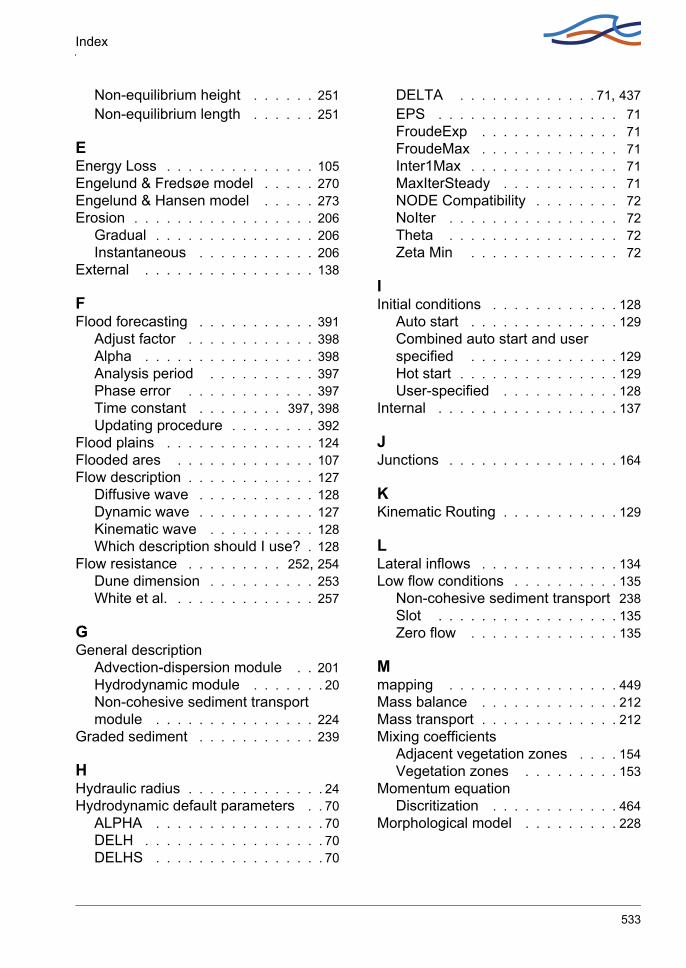
Index
Non-equilibrium height . . . . . . 251Non-equilibrium length . . . . . . 251
EEnergy Loss . . . . . . . . . . . . . . 105Engelund & Fredsøe model . . . . . 270Engelund & Hansen model . . . . . 273Erosion . . . . . . . . . . . . . . . . . 206
Gradual . . . . . . . . . . . . . . . 206Instantaneous . . . . . . . . . . . 206
External . . . . . . . . . . . . . . . . 138
FFlood forecasting . . . . . . . . . . . 391
Adjust factor . . . . . . . . . . . . 398Alpha . . . . . . . . . . . . . . . . 398Analysis period . . . . . . . . . . 397Phase error . . . . . . . . . . . . 397Time constant . . . . . . . . 397, 398Updating procedure . . . . . . . . 392
Flood plains . . . . . . . . . . . . . . 124Flooded ares . . . . . . . . . . . . . 107Flow description . . . . . . . . . . . . 127
Diffusive wave . . . . . . . . . . . 128Dynamic wave . . . . . . . . . . . 127Kinematic wave . . . . . . . . . . 128Which description should I use? . 128
Flow resistance . . . . . . . . . 252, 254Dune dimension . . . . . . . . . . 253White et al. . . . . . . . . . . . . . 257
GGeneral description
Advection-dispersion module . . 201Hydrodynamic module . . . . . . . 20Non-cohesive sediment transport module . . . . . . . . . . . . . . . 224
Graded sediment . . . . . . . . . . . 239
HHydraulic radius . . . . . . . . . . . . . 24Hydrodynamic default parameters . . 70
ALPHA . . . . . . . . . . . . . . . . 70DELH . . . . . . . . . . . . . . . . . 70DELHS . . . . . . . . . . . . . . . . 70
DELTA . . . . . . . . . . . . . 71, 437EPS . . . . . . . . . . . . . . . . . 71FroudeExp . . . . . . . . . . . . . 71FroudeMax . . . . . . . . . . . . . 71Inter1Max . . . . . . . . . . . . . . 71MaxIterSteady . . . . . . . . . . . 71NODE Compatibility . . . . . . . . 72NoIter . . . . . . . . . . . . . . . . 72Theta . . . . . . . . . . . . . . . . 72Zeta Min . . . . . . . . . . . . . . 72
IInitial conditions . . . . . . . . . . . . 128
Auto start . . . . . . . . . . . . . . 129Combined auto start and user specified . . . . . . . . . . . . . . 129Hot start . . . . . . . . . . . . . . . 129User-specified . . . . . . . . . . . 128
Internal . . . . . . . . . . . . . . . . . 137
JJunctions . . . . . . . . . . . . . . . . 164
KKinematic Routing . . . . . . . . . . . 129
LLateral inflows . . . . . . . . . . . . . 134Low flow conditions . . . . . . . . . . 135
Non-cohesive sediment transport 238Slot . . . . . . . . . . . . . . . . . 135Zero flow . . . . . . . . . . . . . . 135
Mmapping . . . . . . . . . . . . . . . . 449Mass balance . . . . . . . . . . . . . 212Mass transport . . . . . . . . . . . . . 212Mixing coefficients
Adjacent vegetation zones . . . . 154Vegetation zones . . . . . . . . . 153
Momentum equationDiscritization . . . . . . . . . . . . 464
Morphological model . . . . . . . . . 228
533

Index
NNAM . . . . . . . . . . . . . . . . . . 296
Accumulation and melting of snow . 305Adjustment of temperature and pre-cipitation to altitude zones . . . . 308Altitude-distributed snowmelt model 306Base temperature (snow/rain) T0 320Baseflow . . . . . . . . . . . . . . 303Baseflow time constant CKBF . 318Basic modelling components . . 301Capilary flux . . . . . . . . . . . . 304Crop coefficients and irrigation losses . . . . . . . . . . . . . . . 321Degree-day coefficient Csnow . 320Evapotranspiration . . . . . . . . 301Extended groundwater components 303Extended snow melt components 310Groundwater depth for unit capillary flux GWLFL1 . . . . . . . . . . . 319Groundwater recharge . . . . . . 303Infiltration factor K0inf . . . . . . 320Initial conditions . . . . . . . . . . 322Interflow . . . . . . . . . . . . . . 302Interflow and overland flow routing . 302Irrigation module . . . . . . . . . 310Lower groundwater storage . . . 304Lower zone or root zone storage 301Maximum groundwater depth causing baseflow GWLBF0 . . . . . . . . 318Maximum water content in root zone storage Lmax . . . . . . . . . . . 315Maximum water content in surface storage Umax . . . . . . . . . . . 315Model parameters . . . . . . . . 314Model Structure . . . . . . . . . . 299Overland flow . . . . . . . . . . . 301Overland flow runoff coefficient CQOF . . . . . . . . . . . . . . . 316Radiation coefficient Crad . . . . 320Rainfall degree-day coefficient Crain320
Ratio of groundwater catchment to topographical catchment area Carea318Recharge to lower groundwater stor-age CQLOW . . . . . . . . . . . . 318Root zone threshold value for ground-water recharge TG . . . . . . . . 318Root zone threshold value for interflow TIF . . . . . . . . . . . . . . . . . 317Root zone threshold value for over-land flow TOF . . . . . . . . . . . 317Shallow groundwater reservoir description . . . . . . . . . . . . . 304Snow module . . . . . . . . . . . 305Soil moisture content . . . . . . . 303Specific yield SY . . . . . . . . . 319Structure of the altitude-distributed snowmelt module . . . . . . . . . 306Structure of the irrigation module 311Surface storage . . . . . . . . . . 301Time constant for interflow CKIF 316Time constant for routing interflow and overland flow CK12 . . . . . . . . 316Time constant for routing lower base-flow CKlow . . . . . . . . . . . . . 318
Node matrix . . . . . . . . . . . . . . 441Non-cohesive sediment transport . . 223Non-cohesive transport module . . . 202
OOpen Boundary Inflow
AD . . . . . . . . . . . . . . . . . . 208
PPumps . . . . . . . . . . . . . . . . . 136
QQuasi-steady solution . . . . . . . . 138
Horizontal branches . . . . . . . . 140Relaxation . . . . . . . . . . . . . 140Undefined solution . . . . . . . . 142Underflow . . . . . . . . . . . . . 141
Quasi-two dimensional steady flow with vegetation . . . . . . . . . . . . . . 143
Energy equation . . . . . . . . . . 159
534 MIKE 11

Index
Governing equations . . . . 143, 144Suppression of convective terms 159Upstream centering of friction term .159Zone classification . . . . . . . . 143
RRelative resistance . . . . . . . . . . . 22Resistance radius . . . . . . . . . . . . 23
SSaint Venant Equations . . . . . . . 170Saint Venant equations . . . . . . . 457
Conservation of mass . . . . . . 457Conservation of momentum . . . 457
Sandbars effect on the water level . 166Scientific background
Hydrodynamic . . . . . . . . . . . 423Sediment
Consolidation . . . . . . . . . . . 206Deposition . . . . . . . . . . . . . 205Settling . . . . . . . . . . . . . . . 204Sliding . . . . . . . . . . . . . . . 205
Sediment transport models . . . . . 225Shear stress distribution . . . . . . . 203Smart and Jaeggi model . . . . . . . 278Solution scheme
Advection-dispersion . . . . . . . 216Dynamic . . . . . . . . . . . . . . 171Hydrodynamic . . . . . . . . . . . 461Quasi-steady . . . . . . . . . . . . 138
Stability conditionsDynamic solver . . . . . . . . . . 173
Structures . . . . . . . . . . . . . . . 467Determination of flow regime 471, 473Drowned flow . . . . . . . . . . . 474Free overflow . . . . . . . . . . . 478Geometry . . . . . . . . . . . . . . 471Mathematical treatment . . . . . 467Regulating . . . . . . . . . . . . . 167Zero flow . . . . . . . . . . . . . . 474
Suspended load . . . . . . . . . 246, 249
TTransport boundary . . . . . . . . . 208
Vvan Rijn model . . . . . . . . . . . . . 280
WWater level variations due to curves 165Weir
Broadcrested . . . . . . . . . . . . 70Formula . . . . . . . . . . . . . . . 194Special . . . . . . . . . . . . . . . 172
Wind . . . . . . . . . . . . . . . . . . 196
535

Index
536 MIKE 11