MIGRATORY SHOREBIRD AND VEGETATION EVALUATION … · migratory shorebird and vegetation evaluation of chickaloon flats, kenai national wildlife refuge, alaska by sadie e. g. ulman

MIGRATORY SHOREBIRD AND VEGETATION EVALUATION

OF CHICKALOON FLATS,

KENAI NATIONAL WILDLIFE REFUGE, ALASKA

by

Sadie E. G. Ulman

A thesis submitted to the Faculty of the University of Delaware in partial

fulfillment of the requirements for the degree of Master of Science in Wildlife Ecology

Fall 2012

Copyright 2012 Sadie E. G. Ulman

All Rights Reserved

MIGRATORY SHOREBIRD AND VEGETATION EVALUATION

OF CHICKALOON FLATS,

KENAI NATIONAL WILDLIFE REFUGE, ALASKA

by

Sadie E. G. Ulman

Approved: __________________________________________________________

Christopher K. Williams, Ph.D.

Professor in charge of thesis on behalf of the Advisory Committee

Approved: __________________________________________________________

Douglas W. Tallamy, Ph.D.

Chair of the Department of Entomology and Wildlife Ecology

Approved: __________________________________________________________

Mark Rieger, Ph.D.

Dean of the College of Agriculture and Natural Sciences

Approved: __________________________________________________________

Charles G. Riordan, Ph.D.

Vice Provost for Graduate and Professional Education

iii

ACKNOWLEDGMENTS

I would like to thank my advisor Dr. Chris Williams for the support, knowledge, and

advice throughout this research process. I am incredibly grateful for the encouragement,

insight, and inspiration of Dr. John Morton (Kenai National Wildlife Refuge). Thank you

to my committee members, Dr. Jeff Buler and Dr. Greg Shriver, whose advice and

support and help I have appreciated throughout my research.

Thank you to the Kenai National Wildlife Refuge, U. S. Fish and Wildlife

Service, University of Delaware, and a University of Delaware Research Foundation

grant for financially supporting this research. The staff at Kenai NWR were an invaluable

resource. A special thanks to the knowledgeable biology personnel. Thanks to Toby

Burke and Todd Eskelin for sharing your vast knowledge of Kenai birds. Thank you to T.

Burke and J. Morton for spending time on Chickaloon and providing insight on the area

and system. I want to thank Scott McWilliams and Adam Smith from the University of

Rhode Island and Richard Doucett from Northern Arizona University for conducting

stable isotope analysis and offering suggestions to improve my research. Steve Van

Wilgenburg from the National Hydrology Research Centre (Saskatoon, SK) offered

invaluable help with probability assignments. Thanks to Keith Hobson of Prairie and

Northern Wildlife Research Centre (Saskatoon, SK) for overall comments and

encouragement regarding geographic assignment using stable hydrogen isotope analysis.

From the University of Delaware; C. Golt, M. Moore, and J. McDonald provided

iv

equipment or lab space for weighing samples and B. Mearns, J. McKenzie, and T.

DeLiberty offered technical advice.

Thanks to all my friends and graduate students who have laughed with me

along the way. I wish to thank my amazing family and friends for encouragement. Thank

you to my parents and in-laws who have shown unbelievable support, and a love of birds

too. Mom and Dad - thank you for pointing out every animal when I was a kid and

instilling love and appreciation for wildlife and the outdoors. To my siblings, Sam and

Dessa, thanks for exploring the wilds with me. Finally, a most heart-felt thank you to my

field technician and husband, Sean, for making months in the Alaskan wilderness and our

lives together an on-going enjoyable adventure. I love you.

v

TABLE OF CONTENTS

LIST OF TABLES ....................................................................................................... vii

LIST OF FIGURES ....................................................................................................... ix

ABSTRACT ................................................................................................................... xi

CHAPTERS

1 STABLE ISOTOPES INFER GEOGRAPHIC ORIGINS OF

SHOREBIRDS USING AN ALASKAN ESTUARY DURING

MIGRATION ...................................................................................................... 1

1.1 Introduction ................................................................................................ 1 1.2 Study Area ................................................................................................. 7

1.3 Methods...................................................................................................... 8 1.4 Results ...................................................................................................... 14 1.5 Discussion ................................................................................................ 19

2 AVIAN USE OF CHICKALOON FLATS ON ALASKA'S SOUTH-

CENTRAL COAST .......................................................................................... 43

2.1 Introduction .............................................................................................. 43 2.2 Study Area ............................................................................................... 45

2.3 Methods.................................................................................................... 46 2.4 Results ...................................................................................................... 48

2.5 Discussion ................................................................................................ 52

3 SATELLITE IMAGE BASED VEGETATION CLASSIFICATION AND

CHANGE OVER 30 YEARS ON CHICKALOON FLATS ........................... 67

3.1 Introduction .............................................................................................. 67 3.2 Study Area ............................................................................................... 69 3.3 Methods.................................................................................................... 71

3.4 Results ...................................................................................................... 77

3.5 Discussion ................................................................................................ 80

LITERATURE CITED ..................................................................................... 97

APPENDIX A: PLOTS OF 13

C AND 15

N FOR SIX MIGRATORY

SHOREBIRD SPECIES ........................................................................ 118

vi

APPENDIX B: ALASKA'S FIVE BIRD CONSERVATION REGIONS ..... 122

APPENDIX C: DAILY OBSERVATIONS OF AVIAN SPECIES OF

CHICKALOON FLATS IN 2009 AND 2010 ....................................... 123

APPENDIX D: AVIAN BREEDING SPECIES OF CHICKALOON

FLATS, 2009-2010 ................................................................................ 125

Figure D.1 .............................................................................................. 128

APPENDIX E: ALL 95 AVIAN SPECIES RECORDED ON

CHICKALOON FLATS DURING SPRING AND FALL OF 2009-

2010........................................................................................................ 129

APPENDIX F: PLANT SPECIES OF VEGETATED CLASSIFICATION

TYPES OF CHICKALOON FLATS USED FOR SUPERVISED

CLASSIFICATION ............................................................................... 142

APPENDIX G: 287 VEGETATION POINTS VISITED DURING 2009-

2010........................................................................................................ 146

APPENDIX H: EXTREME TIDAL EVENTS SUSTAIN FORAGING

HABITAT FOR MIGRATING SHOREBIRDS ON AN ALASKAN

ESTUARY ............................................................................................. 154

Table H.1................................................................................................ 162

Figure H.1 .............................................................................................. 163

Figure H.2 .............................................................................................. 164

Figure H.3 .............................................................................................. 165

APPENDIX I: UNIVERSITY OF DELAWARE INSTITUTIONAL

ANIMAL USE AND CARE COMMITTEE PROTOCOL ................... 166

vii

LIST OF TABLES

Table 1.1 Stable isotope values (‰), with agriculture or non-agriculture

influence, from summer and winter grown primary feathers of six

shorebird species captured during spring and/or fall migrations on

Chickaloon Flats, Kenai National Wildlife Refuge, Alaska ................... 33

Table 2.1 Number of transects and visits from 43 avian surveys conducted on

Chickaloon Flats, Kenai National Wildlife Refuge, 2009–

2010.Transects and visits are shown by season, year, vegetation

classification type, and plot. ................................................................... 57

Table 2.2 Shorebird species population estimates (± SE) across total area of

landcover types during 7 spring migration weeks and 9 fall migration

weeks. Mean values account for species-specific detectability and

were derived for (a) All combined 18 species, (b) greater yellowlegs,

(c) lesser yellowlegs, (d) least sandpiper, (e) pectoral sandpiper, and

(f) dowitcher species. Population estimates derived from density at

100 m fixed radius plot and extrapolated across landcover type area.

Sample size of visits (N=) are indicated at each week and landcover

class. Spring dates start on April 26 (week 1) and finish June 14 (end

week 7). Fall dates start on June 28 (week 1) and finish August 30

(end week 9)... .................................................................................. 58-63

Table 3.1 Area data for each of the five land cover classes used in the

maximum likelihood supervised classification of 2005 imagery. Area

is represented in hectares ........................................................................ 86

Table 3.2 Overall accuracy, reported in percentage, and Kappa coefficient for

each supervised classification method, maximum likelihood and

minimum distance, for 1975 and 2005 classifications using Landsat

imagery of Chickaloon Flats ................................................................... 87

viii

Table 3.3 Class confusion matrix of 5 land cover classes used in maximum

likelihood and minimum distance supervised classifications of 1975

Landsat MSS and 2005 Landsat TM imagery. Classes are: Creeping

and Large alkali-grass (AG–LG), Type 3 Mud (3M), Marsh

community, Floating marsh, and Seaside arrow-grass (MC–FM–SG),

Mud, and Water. Class cover types produced from training data are

in columns and reference test ground points in rows. Producer

accuracy is assessment of how accurately the analyst classified the

image data by land cover types. User accuracy is assessment of how

well the classification performed with ground truth data by land

cover types. All numbers are percentages. ....................................... 88-89

Table 3.4 Area of land cover classes and % of total Chickaloon area in 1970

and 2005 and difference in area between those time periods. Area is

in hectares. *Water was not a separate class in 1970, so 2005 area of

water is added into this class .................................................................. 90

Table 3.5 Point to point comparison of land cover classifications from 1970–

1971 to 2009–2010. The eight land cover types in point to point

comparison and number of ground truthed points are: LG (Large

alkali-grass, N=38), FM (Floating marsh, N=14), MUD (Mud,

N=57), AG (Creeping alkali-grass, N=27), SG (Seaside arrow-grass,

N=30), MC (Marsh community, N=33), 3M (Type 3 Mud, N=40),

and RS (Ramenski sedge, N=39). Bog and Alder are additional land

cover types used only in Reclassification due to small area of types.

Percentage of points classified as the same land cover type in both

time periods represented as % same. Percentage of points reclassified

as different land cover type in 2009–2010 than 1970–1971

represented as % reclassify ............................................................... 91-92

Table H.1 Significant factors (extreme tide event, weekly maximum tide,

weekly maximum temperature, and/or weekly cumulative

precipitation) in determining auto correlated surface areas of 14

ephemeral pools over time (P ≤ 0.10) between 24 April – 28 August

2010 on Chickaloon Flats, Kenai National Wildlife Refuge, Alaska.

Table shows p-values of significant factors .......................................... 163

ix

LIST OF FIGURES

Figure 1.1 Location of Chickaloon Flats, most northern portion of Kenai

National Wildlife Refuge, Alaska ........................................................... 34

Figure 1.2 Probable breeding origins of greater yellowlegs (Tringa

melanoleuca) captured during migration on Chickaloon Flats, Kenai

National Wildlife Refuge, Alaska. Individuals (n=66) were assigned

geographic origins using a likelihood-based assignment based on

deuterium (D) values of feathers. Map represents the sum of origin

assignments across all birds .................................................................... 35

Figure 1.3 Probable breeding origins of lesser yellowlegs (Tringa flavipes)

captured during migration on Chickaloon Flats, Kenai National

Wildlife Refuge, Alaska. Individuals (n=26) were assigned




Figure 1.4 Probable wintering origins of lesser yellowlegs (Tringa flavipes)


Wildlife Refuge, Alaska. Individuals (n=4) were assigned geographic

origins using a likelihood-based assignment based on deuterium (D)

values of feathers. Map represents the sum of origin assignments

across all birds ........................................................................................ 37

Figure 1.5 Probable wintering origins of least sandpiper (Calidris minutilla)


Wildlife Refuge, Alaska. Individuals (n=13) were assigned




Figure 1.6 Probable wintering origins of pectoral sandpiper (Calidris

melanotos) captured during migration on Chickaloon Flats, Kenai

National Wildlife Refuge, Alaska. Individuals (n=11) were assigned




x

Figure 1.7 Probable breeding origins of short-billed dowitcher (Limnodromus

griseus caurinus) captured during migration on Chickaloon Flats,

Kenai National Wildlife Refuge, Alaska. Individuals (n=26) were

assigned geographic origins using a likelihood-based assignment

based on deuterium (D) values of feathers. Map represents the sum

of origin assignments across all birds. .................................................... 40

Figure 1.8 Probable a) primary molt and b) wintering origins of long-billed

dowitcher (Limnodromus scolopaceus) captured during migration on

Chickaloon Flats, Kenai National Wildlife Refuge, Alaska.

Individuals (n=7 and 4) were assigned geographic origins using a

likelihood-based assignment based on deuterium (D) values of

feathers. Maps represent the sum of origin assignments across all

birds .................................................................................................. 41-42

Figure 2.1 Location of Chickaloon Flats, Kenai National Wildlife Refuge,

Alaska. Land-cover type classifications overlaid with four study

plots (2 x 4 km) ...................................................................................... 64

Figure 2.2 All survey points (visits) for avian surveys during spring and fall

2009 and 2010. Each point was a 100 m fixed-radius plot within a

single land cover type ............................................................................. 65

Figure 2.3 Weekly population estimates from ground survey data in a) 2009 and

b) 2010 for 18 shorebird species across Chickaloon Flats, Alaska. ....... 66

Figure 3.1 Location of Chickaloon Flats, Kenai National Wildlife Refuge,

Alaska ..................................................................................................... 93

Figure 3.2 Intertidal estuarine areas of Cook Inlet and Prince William Sound,

Alaska derived from National Wetlands Inventory data from the U.

S. Fish and Wildlife Service. The estuarine area of Chickaloon Flats

makes up 15,214 ha (7%) of the total 218, 376 ha shown on the map ... 94

Figure 3.3 The community types of Chickaloon Flats digitized from cover maps

from Quimby (1972). Four study plots (2 x 4 km) with 287 randomly

assigned vegetation data points across Mud and each of the ten

vegetated community types. Plots are from west (Plot 1) to east (Plot

4) ............................................................................................................. 95

Figure 3.4 The 2005 maximum likelihood supervised classification of

Chickaloon Flats with five land class covers .......................................... 96

xi

Figure D.1 Locations of 56 nests of 11 species opportunistically found within

and between four study plots during 2010 on Chickaloon Flats .......... 128

Figure H.1 Outline of Chickaloon Flats with 2 visualizations of extreme tide

event inundation. Representation (shaded grey) of difference in July

extreme tide inundation between west and east. This shaded extreme

tide area only shows marked locations of ground observed

inundation, and is not a complete portrayal of extreme tide

inundation across the flats. Two time-series photographs of extreme

tide showing sheet flow (location 1: July 22, 2009) versus slough

breaching (location 2: August 12, 2010) depending on position on

flats ....................................................................................................... 163

Figure H.2 Visual interpretation of seasonal and annual variations of frequency,

duration, and height of extreme tide events from 2004–2010 during

spring and fall migration periods. Length of horizontal bars represent

duration, in days, of extreme tides. NOAA tide predictions from Fire

Island, AK station. ................................................................................ 164

Figure H.3 The monthly cumulative precipitation for 2009 and 2010 and the 30-

year monthly average from Anchorage Forecast Office station,

NOAA. April through August of 2009 was slightly below average,

but followed the 30-year average trend. 2010 was an unusual

precipitation year, compared to 30-year average, with most months

being above average, with the exceptions of May and August, which

fell below. ............................................................................................. 165

xii

ABSTRACT

I conducted my research on Chickaloon Flats, Kenai National Wildlife Refuge,

which is a tidal mudflats located along the northern part of the Kenai Peninsula in upper

Cook Inlet, Alaska, 2009–2010. It is a protected coastal estuary stopover area along the

Pacific Flyway, covering 7% of the total estuarine intertidal area of Cook Inlet and Prince

William Sound. Almost one-third (23 of 73) of shorebird species recorded in Alaska use

this stopover during spring and/or fall migrations. My objectives included 1) creating a

current vegetation classification map and quantify vegetation changes from 1975 to 2005,

2) identify the driving factors of ephemeral pool presence, 3) document avian use of

Chickaloon Flats during migration periods, and 4) conduct a multi-isotopic approach to

estimate probable breeding and/or wintering origins of six species of shorebirds using

Chickaloon during spring and fall migration of 2009 and 2010.

I analyzed Hydrogen (D), Carbon (13

C), and Nitrogen (15

N) isotopes from

feathers and performed a likelihood-based assignment to inform North American (NA)

and South American (SA) origins of six shorebird species. Only lesser yellowlegs

feathers (Tringa flavipes) indicated wintering (n=4, coastal SA) and breeding (n=26,

central Alaska) ranges. Estimated wintering ranges for least sandpipers (Calidris

minutilla, n=13) occurred in southern NA to northern SA, long-billed dowitchers

(Limnodromus scolopaceus, n=8) occurred in Mexico, and pectoral sandpipers (Calidris

xiii

melanotos, n=11) occurred in northeastern SA. Estimated breeding ranges for greater

yellowlegs (Tringa melanoleuca, n=67) occurred in southwest Alaska, and short-billed

dowitcher (Limnodromus griseus caurinus, n=26) occurred in south-central Alaska. The

analysis of stable isotopes to infer molt origins of birds is a useful and important tool in

migration and conservation studies. I determined probable origins of long-distance

shorebird migrants, some of high conservation concern, using an Alaskan stopover site,

which identified habitats and previously unknown areas used by Alaskan breeding

shorebirds.

I observed 95 bird species throughout the spring and fall of 2009 and 2010, with

26 of those species breeding on Chickaloon. I observed several pulses of total birds

during spring migration, and a more protracted fall migration with variable smaller pulses

of birds. Estimated maximum daily shorebird numbers are 5,638 during spring migration,

and 20,297 during fall migration.

I created a recent vegetation classification of 7 vegetation types on Chickaloon

Flats using 2005 Landsat TM imagery. I also quantified change of 3 mud/vegetation

cover types from 1975–2005. The vegetated community type remained relatively stable

over the 30-year period, while the mud and mixed mud/vegetation cover types closest to

Cook Inlet showed a relatively-small amount of change over time. The greatest change

was an increase in mud area, indicating that the vegetated areas of Chickaloon may be

slowly converting to a less productive mud community type.

xiv

My research highlights the overall importance and value of Chickaloon Flats

as a stopover and breeding grounds for a diversity of avian species, and long-distance

migrant shorebirds in particular.

1

Chapter 1

STABLE ISOTOPES INFER GEOGRAPHIC ORIGINS OF SHOREBIRDS

USING AN ALASKAN ESTUARY DURING MIGRATION

Introduction

Determining the locations of migratory birds during their annual cycle is increasingly

important to developing conservation strategies (Hobson 1999a, Hebert and Wassenaar

2005, Webster and Marra 2005). For long-distance migrants, like many shorebirds,

strategic stops rich in food are imperative for successful migration and subsequent

nesting success (Castro and Myers 1993, Atkinson et al. 2005, O’Brien et al. 2006,

Alaska Shorebird Group 2008, Yerkes et al. 2008). Therefore, identifying high-quality

stopover sites along migration corridors aids in local habitat conservation and

management (Rocque et al. 2006, Hobson and Wassenaar 2008, Alaska Shorebird Group

2008). There are gaps in our knowledge of avian migratory movement patterns,

particularly at relatively discrete stopover sites and for small-bodied species that have not

been researched using tracking devices or other extrinsic markers (Inger and Bearhop

2008). In order to better recognize and respond to global-scale threats to shorebirds and

to identify critical habitats that need protection, understanding movements within and

among landscapes is crucial (Alaska Shorebird Group 2008).

One relatively new technique to trace wildlife migration and identify important

stopover areas is stable isotope analysis. An advantage of this methodology is it can

2

effectively provide migratory information associated with relatively-small stopover areas

that would have low sample sizes using traditional methods of band returns or telemetry.

Although numerous isotopic studies have been conducted on waterfowl migration, less is

known about shorebirds (see Yerkes et al. 2008 for review of previous research). The use

of stable isotopes is an intrinsic technique that does not require a previous capture to infer

migratory origins (Inger and Bearhop 2008). Animals absorb isotopes from food and

deposit them in body tissues. The most commonly used tissues for stable isotope analysis

of avian migrations are feathers, muscle, and blood (Bearhop et al. 2003). Metabolically

inert tissues, such as feathers, maintain a signature that corresponds to what was eaten

during the relatively short period of synthesis (Rubenstein and Hobson 2004, Hobson and

Wassenaar 2008) and can infer origins of feather molt (Chamberlain et al. 1997, Marra et

al. 1998, Hobson 1999a, Caccamise et al. 2000, Rocque et al. 2006) as well as habitat

information of the corresponding molt location (Atkinson et al. 2005). This allows

individuals to be sampled in one season (i.e., summer) to estimate origin of feather

growth during another season (i.e., winter).

Three stable isotopes are primarily used in isotopic analysis and have different

functions in identifying habitat use: stable-carbon isotope (δ13

C), stable-nitrogen isotope

(δ15

N), and stable-hydrogen isotope or deuterium (i.e., 2H/

1H measured as δD) (Hobson

and Wassenaar 2008). Although there has been concern over using single stable isotopes

to estimate geographic origin (δD, Smith et al. 2009), the accuracy of geospatially

distinct selected habitats can be improved by evaluating a mutli-isotopic spectrum (δ13

C,

δ15

N, and δD together). For example, Atkinson et al. (2005) used stable isotope ratios of

3

carbon and nitrogen in red knot flight feathers to identify at least three discrete wintering

areas in eastern North and South America.

Large-scale gradients in stable-carbon isotopes (δ13

C) can also delineate habitat

use of wildlife because of global differences in plant tissue with different photosynthetic

pathways (C3 vs. C4 or Crassulacean acid metabolism (CAM; Kelly 2000) as well as

between terrestrial freshwater and marine food webs (Fry and Sherr 1989, Hobson and

Sealy 1991, Korner et al. 1991, Hobson 1999a, b). Stable-carbon isotope values of ≤ -

20‰ indicate freshwater and >-20‰ marine (coastal) values (Fry and Sherr 1989,

Hobson and Sealy 1991). Plants using the C4 and CAM pathways grow in arid

environments and have higher δ13

C values than C3 plants that tend to grow in cooler, wet

areas (Atkinson et al. 2005). Additionally, C3 plants in hotter conditions use water more

efficiently and therefore become more enriched in δ13

C than those in cooler conditions

(Marra et al. 1998, Hobson and Wassenaar 2008). The different photosynthetic pathways

of plants can be used to distinguish the North American isoscapes, and animal

movements can be tracked across these isoclines. Alisauskas et al. (1998) identified

migratory populations of lesser snow geese (Chen caerulescens) by examining 13

C

signatures consistent with C4 corn habitat used by residents versus C3 non-corn habitat

used by migrants.

The mapping of spatial variation in plant stable-nitrogen isotopes (δ15

N) has

received less attention than δ13

C (Amundson et al. 2003). The plant nitrogen isoscapes

show that plant δ15

N is related to the nitrogen cycle and negatively correlated with

precipitation (Austin and Vitousek 1998, Handley et al. 1999) and positively correlated

4

with temperature (Amundson et al. 2003). Studies have shown that dietary δ15

N of

kangaroos (Murphy and Bowman 2006) and warblers (Chamberlain et al. 2000) is linked

to climate, likely through the openness of the nitrogen cycle. Stable nitrogen isotopes can

provide information on agricultural influences; however, higher 13

C and 15

N values are

also found in marine systems and enriched at higher trophic levels. Lower 15

N values

(<9‰) in feathers are associated with nonagricultural areas compared to feathers

collected in C3 agricultural areas (Hebert and Wassenaar 2001, 2005). There are

predictable changes in 13

C and 15

N between terrestrial and marine environments.

Marine environments are enriched in carbon and nitrogen, meaning 13

C and 15

N values

increase with salinity (Hobson 1999a). 15

N values in intertidal habitats may depend

upon several things, including: large-scale gradients of the marine environment, degree of

influence of terrestrial and freshwater habitats, and anthropogenic inputs (Atkinson et al.

2005).

Hydrogen isotope ratios (δD) in feathers correlate with the δD of local

precipitation patterns where the feathers were grown (Atkinson et al. 2005). Deuterium

values in North American precipitation show a continent-wide pattern with a latitudinal

gradient of enriched values in the Southeast to more depleted values in the Northwest

(Hobson and Wassenaar 2008). Deuterium base maps provide a spatial reference to help

detect migratory patterns, and therefore can be a potentially powerful tool from a science

and conservation standpoint. Deuterium has been used to identify natal, wintering, and

molting areas of waterfowl (Hobson 1999a, 2005, Rubenstein and Hobson 2004, Hebert

and Wassenaar 2005, Clark et al. 2006, Yerkes et al. 2008) and numerous other bird and

5

invertebrate species (Hobson and Wassenaar 1997, Dunn et al. 2006, Hobson et al. 2006,

Hobson et al. 2007, Perez and Hobson 2007, Hobson and Wassenaar 2008).

The accuracy and precision of using stable hydrogen isotopes to examine

migration questions are dependent upon the accuracy and precision of the precipitation

(Dp) maps. It is important to consider the limitations associated with deuterium base

maps and apply practical expectations of the accuracy of the origin prediction (Farmer et

al. 2008). There are three factors involved with the decoupling of modeled deuterium

map values and observed tissue isotopic signatures at a given location, including: 1)

fractionation in feathers may occur during the assimilation of isotope signatures, 2) local

biogeochemical processes, like evaporation, can modify surface and ground water, which

would incorrectly reflect isotope precipitation values, and 3) the value of Dp from a

single year can vary around the 40-year mean (Farmer et al. 2008). Inter-annual variation

in Dp, however, is an underlying source of uncertainty involved in all systems and with

all isotopic geographic assignments, and can be considered a baseline of isotopic

signature variability in feathers (Farmer et al. 2008). Uncertainty in geographic

assignment in stable isotope studies will always be present, and is something that must be

dealt with (Farmer et al. 2008). Several studies (Hobson et al. 2001, Wunder et al. 2005,

Szymanski et al. 2007) indicate that deuterium signatures do not allow for assigning

origins below a resolution of 5–9 latitude, but adding 13

C and 15

N can increase

assignment precision.

Using stable isotope data of individuals caught on stopover sites can provide

information on both breeding and wintering grounds of migrating birds. Alaska’s huge

6

size and northern latitude make it a critical region for migrating and breeding birds

(Alaska Shorebird Group 2008). Alaska hosts one-third (73) of the world’s species of

shorebirds (Alaska Shorebird Group 2008), and as much as 50% of all shorebirds (7–12

million) in North America (Lanctot 2003). Not only is it important as breeding grounds,

there are five Western Hemisphere Shorebird Reserve Network recognized shorebird

migration stopover and staging sites within Alaska. The Kenai National Wildlife Refuge

(Kenai NWR), located in south-central Alaska, is qualitatively known as an important

migratory stopover and breeding grounds for many shorebird species and poses a

potential bottleneck (Isleib 1979) where birds pass through both spring and fall.

Chickaloon Flats along the northern Kenai NWR is recognized as a valuable waterfowl

habitat, where thousands of waterfowl annually use the marsh for nesting, feeding, and

resting (Alaska Department of Fish and Game et al. 1972). Of the 73 shorebird species

recorded in Alaska, there are 37 common shorebird breeding species (Alaska Shorebird

Group 2008). Almost two-thirds (23 of 37) of those species use Chickaloon during spring

and/or fall migration, with 7 being confirmed breeders (pers. obs). More than one-third of

the 73 shorebird species have an annual roundtrip migration route of ≤ 30,000 km

(Alaska Shorebird Group 2008).

The movement of individuals between summer and winter populations, as well as

stopover sites, is described by migratory connectivity (Webster et al. 2002). Using stable

isotopes, patterns of migratory connectivity have been established for various bird species

(Pain et al. 2004, Norris et al. 2006, Hobson et al. 2010).Webster et al, (2002) proposed a

qualitative measure of migratory connectivity, with ‘strong’ connectivity when most

7

individuals from a breeding population move to the same wintering location and ‘weak’

connectivity when individuals from a breeding population spread throughout several

wintering sites, For most species, the degree of connectivity will lie between ‘strong’ and

‘weak’ designations (Webster et al. 2002).

My objective was to use stable isotope (D, 13

C, and 15

N) analyses of 6

shorebird species to determine broad spatial scale breeding and wintering origin and

habitat use of migrating shorebirds using Chickaloon as a stopover site during both spring

and fall (Quimby 1972) including greater yellowlegs (Tringa melanoleuca), lesser

yellowlegs (Tringa flavipes), least sandpiper (Calidris minutilla), pectoral sandpiper

(Calidris melanotos), short-billed dowitcher (Limnodromus griseus caurinus), and long-

billed dowitcher (Limnodromus scolopaceus).

Study area

Chickaloon Flats is a tidal mudflat located along the northern part of the Kenai

Peninsula (Figure 1.1). Tidal range in this area is 9.2 m, which is the second greatest in

the world behind Bay of Fundy (11.7 m) (Mulherin et al. 2001). The area of vegetation is

6,894 ha (10,974 ha including mud) at high tide, and entails about 1% of the 773,759 ha

Kenai NWR. Chickaloon has a high diversity of plant species due to the overlap of arctic

and temperate species (Vince and Snow 1984), and the patterns of vegetation are largely

due to saltwater and freshwater interactions, land subsistence from 1964 earthquake, and

tides (Neiland 1971, Quimby 1972, Committee on the Alaska Earthquake 1973).

8

The flats support a diverse but low abundance of avian species during migration

and breeding periods (see Chapter 2). Chickaloon Flats, located in upper Cook Inlet, is a

relatively-small protected coastal estuary stopover site along the Pacific Flyway

compared to other Alaskan estuary areas (e.g., Yukon-Kuskokwim River Delta, Copper

River Delta, Kvichak Bay). As an estuary, this area can provide predictable tidal habitats

and a reliable (compared to interior wetlands) source of abundant resources (Colwell

2010). Cook Inlet provides high-latitude migratory birds with the last considerable area

of ice-free littoral habitat before reaching their breeding grounds (Gill and Tibbitts 1999).

Methods

Feather sampling

During the spring and fall migration periods of 2009 and 2010, I collected

shorebirds primarily with drop nets (Doherty 2009); but occasionally with Coda net-gun

or lethal collection. Sampling occurred at various sites across the study area, primarily in

tidally influenced areas with mixed mud and vegetation. Most sampling took place

directly east of Pincher Creek, with a couple of sites near Big Indian Creek and west of

Pincher Creek. Individuals were banded with a United States Fish and Wildlife Service

aluminum band and aged by plumage characteristics. Five structural variables (exposed

culmen, nares, tarsus, wing chord, and tail) were measured to the nearest 0.1 mm and

body mass to the nearest 0.1 g. The first primary feather and ~350 L blood (for dietary

study) were taken from every individual. If bird was older than a hatch-year, a rectrice,

9

and/or tertial were collected depending on molt. All trapping and handling techniques

were approved by the University of Delaware Animal Use and Care Committee (#1191).

Stable Isotope Analysis

Prior to analysis, I cleaned all feathers following a standard two-step method using both

detergent and a 2:1 chloroform: methanol solution (Partitte and Kelly 2009). Choice of

cleaning solvents affects stable-isotope ratios of bird feathers, and order of use may

influence variation in data (Partitte and Kelly 2009). Therefore, I first cleaned all feathers

with 1:30 solution of Fisher Versa-Clean detergent: deionized water, then rinsed three

times with deionized water and put in fume hood to dry for 24 hours. Feathers were then

placed in a sealed jar containing a 2:1 chloroform: methanol solvent and shaken for 45

seconds under the fume hood. Feathers were removed from solvent and dried for at least

24 hours under a fume hood.

I used the same part of each feather for analysis (Smith et al. 2009) and excluded

the rachis (Wassenaar and Hobson 2006). For δ13

C and δ15

N, I weighed 1.1 0.2 mg of

feather material into a tin capsule (Costech; #041061) and weighed 350 g 10g into a

silver capsule (Costech; #041066) for D.

Isotopic ratios are expressed as per mil (‰) deviation from the standard using the

delta (δ) notation:

isotopeRsample

Rstandard

1

1000 (1)

where isotope is the sample isotope ratio (i.e. D,13

C, or 15

N) relative to a standard, and

R is the ratio of heavy to light isotopes (D/1H,

13C/

12C,

15N/

14N) in the sample standard.

10

Isotope ratios are expressed in δ notation as parts per thousand (‰) relative to deuterium,

13

C, and 15

N reported as ‰ deviation from the international reference standards Vienna

Standard Mean Ocean Water Standard Light Antarctic Precipitation (VSMOW-SLAP)

scale, Vienna Pee Dee Belemnite, and AIR, respectively.

Carbon and nitrogen isotopic analyses were performed at both the U.S.

Environmental Protection Agency Atlantic Ecology Division laboratory and Colorado

Plateau Stable Isotope Laboratory. Analysis at the U.S. Environmental Protection Agency

Atlantic Ecology Division laboratory was performed using a Carlo-Erba NA 1500 Series

II Elemental Analyzer interfaced with an Elementar Optima isotope ratio mass

spectrometer. Samples were combusted (1020oC, chromic oxide catalyst) sending CO2

and N2 to the mass spectrometer for the measurement of carbon and nitrogen isotope

ratios, respectively. Two internal laboratory standards (dogfish muscle) were used for

every 10 unknowns in sequence. The internal standard had a running average δ13

C and

δ15

N measurement precision (standard deviation) of ±0.17‰ and ±0.16‰, respectively.

Based on the assessment of the reproducibility of tissue sampled δ13

C and δ15

N

measurements in this study, and propagating the measurement precision of the internal

standard, reported tissue δ13

C and δ15

N measurements had measurement precisions of ±

1.00‰ and ± 0.41‰, respectively. Carbon and nitrogen stable isotope analysis at the

Colorado Plateau Stable Isotope Laboratory was performed using a Carlo Erba NC2100

Elemental analyzer interfaced to a Thermo Electron Delta Plus Advantage stable isotope

ratio mass spectrometer. An internal laboratory standard (NIST 1547 - peach leaves) was

used for every 10 unknowns in sequence. The internal standard has a running average

11

δ13

C and δ15

N measurement precision (standard deviation) of ±0.10‰ and ± 0.20‰,

respectively. δ13

C values were normalized on the VPDB scale using IAEA-CH6 (-

10.45‰) and IAEA-CH7 (-32.15‰). δ15

N values were normalized on the AIR scale

using IAEA-N1 (0.43‰) and IAEA-N2 (20.41‰).

Hydrogen stable isotope analysis was performed only at the Colorado Plateau

Stable Isotope Laboratory using a Thermal Conversion Elemental Analyzer (TC/EA)

interfaced with a Thermo Electron Delta Plus XL stable isotope ratio mass spectrometer.

Stable-hydrogen isotope measurements were performed on H2 from high temperature

(1400C) flash pyrolysis. Measurement precision based on replicate measurements of

within-run standards of three keratin laboratory reference materials (Spectrum Chemical

keratin: D = -117.5‰, Bowhead Whale Baleen (BWB): D = -108‰, and Cow Hoof

Standard (CHS): D = -187‰), resulted in accurate and precise SD values of 2.2‰

(n=18), 1.9‰ (n=6), and 2.3‰ (n=6), respectively. The control keratin reference

standards yield a long-term SD of 3‰.

Statistical analysis

Before assigning feather samples to feather deuterium isoscapes, I used δ13

C and δ15

N

values to classify samples as agricultural or nonagricultural and freshwater or marine

(Yerkes et al. 2008). Using the 15

N values, feathers 9‰ were considered to come from

an agricultural area, whereas all others were from nonagricultural sources (Yerkes et al.

2008). Using 13

C values, samples were classified as freshwater if ≤ -20‰ and marine if

> -20‰ (Fry and Sherr 1989, Hobson and Sealy 1991, Hobson 1999a, Yerkes et al.

2008). If samples indicated evidence of marine inputs, I made no attempt to assign origin

12

based on D of feathers (hereafter Df) because assigning origin based on Df is

unreliable when influenced by marine inputs (Larson and Hobson 2009). Using 3C

values to inform on marine versus terrestrial inputs before assigning samples to feather

deuterium isoscapes is the most useful use of a multi-isotope dataset like this (Larson and

Hobson 2009), although it is not preferred by some (e.g., Rocque et al. 2009).

Additionally, the remaining measured Df values cannot be directly assigned to

deuterium isoscapes without consideration of possible sources of error. To incorporate

estimates of uncertainty in geographic assignment, I used a likelihood-based assignment

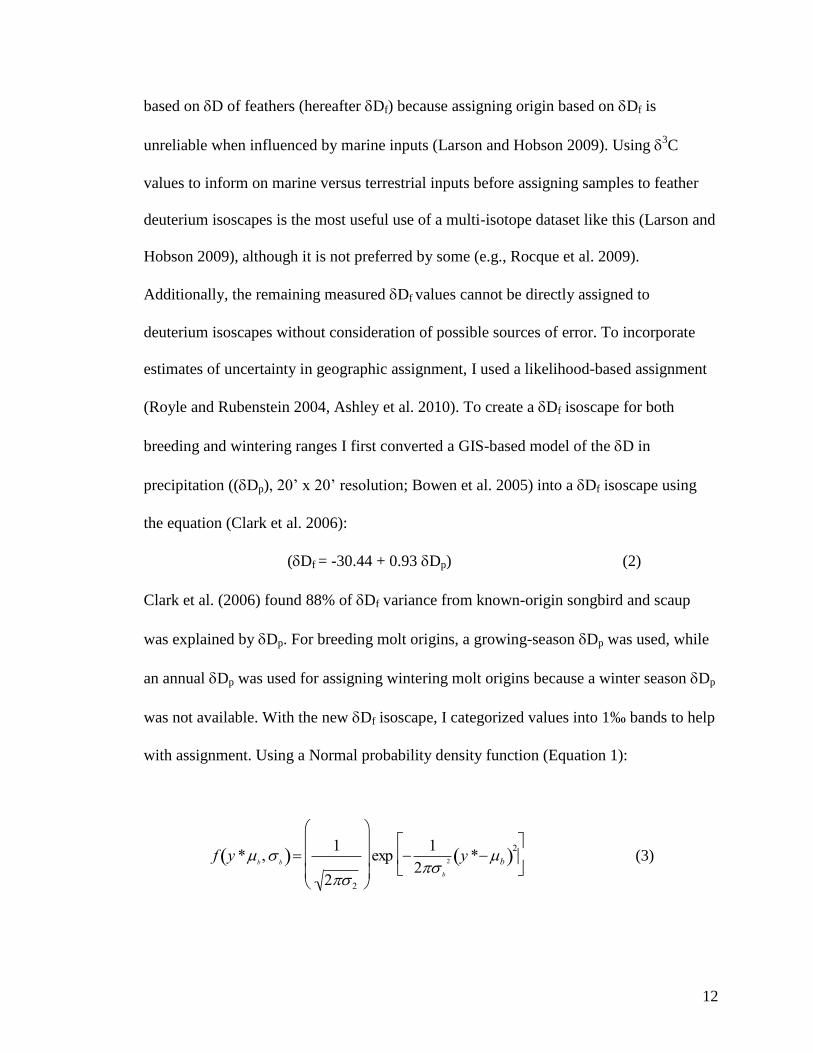
(Royle and Rubenstein 2004, Ashley et al. 2010). To create a Df isoscape for both

breeding and wintering ranges I first converted a GIS-based model of the D in

precipitation ((Dp), 20’ x 20’ resolution; Bowen et al. 2005) into a Df isoscape using

the equation (Clark et al. 2006):

(Df = -30.44 + 0.93 Dp) (2)

Clark et al. (2006) found 88% of Df variance from known-origin songbird and scaup

was explained by Dp. For breeding molt origins, a growing-season Dp was used, while

an annual Dp was used for assigning wintering molt origins because a winter season Dp

was not available. With the new Df isoscape, I categorized values into 1‰ bands to help

with assignment. Using a Normal probability density function (Equation 1):

f y *b,

b 1

2 2

exp 1

2b

2 y *b 2

(3)

13

each individual bird of a given species was evaluated on the likelihood that a given

isotope band (b) within the isoscape represented a potential geographic origin (y*). The

probability that potential origin is represented by a given band is represented by f (y*|b,

b). The expected mean Df for that band is shown by b. The expected deviation (b) of

Df between individuals molting feathers at the same location was estimated to be 12.8‰

using the standard deviation of the residuals from Equation 3 (Ashley et al. 2010). The

probabilities (Equation 3) were then normalized to estimate the probability of geographic

origin:

bf y * |b, b

f y* |b, b b-1

B

(4)

Isoscape classification

Individual birds for each of the six shorebird species were assigned to the Df isoscape

by using a 2:1 odds ratio that the assigned geographic origin (1‰ band) was correct

relative to incorrect. The isotopic bands in the upper 67% of estimated probabilities of

origin (Equation 4) were used to sum results for each individual assignment across all

individuals of the same species. Based on the odds ratio, this resulted in an individual

bird being assigned to multiple isotopic bands representing probable geographic origins

for that bird. Prior to mapping origins, ArcGIS v.10 Spatial Analyst (ESRI 2011) was

used to clip the Df isoscape to breeding and/or wintering ranges (Ridgely et al. 2007) of

14

each of the six species. Species range data was provided by NatureServe in collaboration

with Robert Ridgely, James Zook, The Nature Conservancy - Migratory Bird Program,

Conservation International - CABS, World Wildlife Fund - US, and Environment Canada

- WILDSPACE. To portray probable origins, the odds ratio results were put onto both an

unaltered map and the species range-clipped Df isoscape using Spatial Analyst to

reclassify the overall isoscape based on number of individuals designated to each of the

1‰ isotopic bands.

Bird Conservation Regions (BCRs) from the North American Bird Conservation

Initiative (NABCI; U.S. NABCI Committee 2000a, b) and the ecological regions

(ecoregions; descriptions in Gallant et al. 1995) of Alaska are used as basic conservation

units to further discuss breeding origins of Alaskan shorebird species migrating through

Chickaloon Flats. Description of BCRs and ecoregions related to Alaskan shorebirds are

found in the Alaska Shorebird Conservation Plan (Alaska Shorebird Group 2008). To

help describe the wintering origins of these shorebirds, I used the terrestrial ecoregions of

the world (descriptions in Olson et al. 2001).

Results

Greater yellowlegs

Of the 69 individuals captured during the spring and fall migrations of 2009 and

2010, only 3 were after-hatch year (AHY) birds. Two AHY birds captured during spring

migration were classified as marine in origin (13

C values >-20‰) and were not assigned

to origins using the Df isoscape. These two birds had 15

N values 9‰, and are

15

classified as from an agriculture source. The remaining AHY would provide inference on

wintering areas, however a likelihood-based assignment was not completed with a single

sample. None of the hatch year (HY) birds (n=66) were classified as marine in origin, and

only one was from an agricultural source (Table 1.1, Appendix Aa).

Stable hydrogen analyses of first primary feather of migrating HY greater

yellowlegs examined on Chickaloon Flats during fall migration indicated that migrant

greater yellowlegs bred in southwestern Alaska (Figure 1.2). The highest numbers of

probable origins lie in Western Alaska BCR2 and to a lesser extent in the Northwestern

Interior Forest BCR4 and North Pacific Rainforest BCR5 (Appendix B). This included 11

Alaska ecoregions, with highest numbers in Subarctic Coastal Plains, Ahklun and

Kilbuck Mountains, Bristol Bay-Nushagak Lowlands, Alaska Peninsula Mountains,

Interior Forested Lowlands and Uplands, and Interior Bottomlands.

Lesser yellowlegs

Of the 34 individuals captured, 6 were AHY birds. Two AHY birds (33%) were

classified as marine in origin (13

C values >-20‰) and were not assigned to origins using

the Df isoscape. Of the remaining four, two indicated influences from agriculture

sources (Table 1.1, Appendix Ab). None of the HY birds (n=28) were classified as

marine in origin, and only two showed influences from an agriculture source (Table 1.1,

Appendix Ac).

Stable hydrogen analyses of first primary feathers of migrating HY lesser

yellowlegs indicated they were born in highest numbers in the western portion of the

16

Northwestern Interior Forest BCR4, while smaller numbers show probable origins in the

northeastern portion of Western Alaska BCR2, the southern portion of Arctic Plains and

Mountains BCR3, and the northern portion of North Pacific Rainforest BCR5 (Figure

1.3, Appendix B). The probable natal origins of these birds encompass 11 different

ecoregions of Alaska, with highest numbers in five ecoregions including Interior Forested

Lowlands and Uplands, Highlands, and Bottomlands, Cook Inlet, and Alaska Range.

Analyses of primary feathers of AHY birds (n=4) indicated that migrant lesser yellowlegs

had various wintering origins ranging from southeastern North America through South

America (Figure 1.4), including 44 different ecoregions. North American probable

origins include the Florida peninsula, most of the Caribbean Islands, and coastal Texas

and Louisiana. Locations in South America include: northeastern Venezuela, almost all

of Guyana, Suriname and French Guiana, northeastern Brazil, western Peru into Bolivia

around Lake Titicaca, along the border of Chile and Argentina, and the southern tips of

Chile and Argentina.

Least sandpiper

All of the 13 individuals captured were AHY birds. Two birds (13%) captured

during migration were classified as marine in origin (13

C values >-20‰) and were not

assigned an origin using the Df isoscape. One of the birds showed agriculture values

(15

N values 9‰), and the other did not. Of the 13 birds used to assign origin, only 1

showed 15

N value from an agriculture source (Table 1.1, Appendix Ad).

17

Stable hydrogen analyses of first primary feather of migrating least sandpipers

examined on Chickaloon Flats during spring and fall migration indicated that migrant

least sandpipers wintered throughout most of the range (Figure 1.5), including 129

different ecoregions. These sampled least sandpipers exhibit weak migratory connectivity

due to origins spread throughout the wintering range. The highest numbers of birds show

probable North American origins in southwestern Oregon, western California, and central

Arizona and New Mexico. However moderate probability of origins occur in Central and

South America including Belize, northern Guatemala, eastern Honduras and Nicaragua,

Costa Rica, Panama, central Ecuador, and Colombia (Figure 1.5).

Pectoral sandpiper

Each of the 23 individuals captured were AHY birds. Three pectoral sandpipers

(13%) captured from spring migration were classified as marine in origin (13

C values >-

20‰) and were not assigned to origins using the Df isoscape. Ten individuals were not

used in assigning origin due to deuterium values more enriched than any value existing in

the Df to which they would have been assigned. Eight of the 11 birds showed agriculture

values (Table 1.1, Appendix Ae).

Stable hydrogen analyses of first primary feather of spring migrating pectoral

sandpipers indicated that they wintered in northern coastal South America (Figure 1.6)

across 11 ecoregions. More specifically, birds originated in northeast Venezuela, northern

Guyana and Suriname, most of French Guiana, north central interior Brazil, and an

isolated area in southeast Peru (Figure 1.6).

18

Short-billed dowitcher

Of the 44 individuals captured, 18 were aged as AHY birds. All 18 AHY

individuals (100%) captured during spring migration were classified as marine in origin

(13

C values >-20‰) and were not assigned to origins using the Df isoscape. All of these

birds exhibited 15

N values indicating an agriculture source. None of the HY birds (n=26)

were classified as marine in origin or had values showing an agriculture source (Table

1.1, Appendix Af).

Stable hydrogen analyses of first primary feathers of migrating HY birds

examined on Chickaloon Flats indicated that migrant short-billed dowitchers were born

in Northwestern Interior Forest (BCR4) and North Pacific Rainforest (BCR5) (Figure 1.7,

Appendix M) across the Alaska Peninsula Mountains, Cook Inlet, Alaska Range, and

Pacific Coastal Mountains ecoregions.

Long-billed dowitcher

Each of the 8 individuals captured were AHY birds. One bird (13%) captured

during migration was classified as marine (13

C values >-20‰) and was not assigned an

origin using the Df isoscape. This individual and the remaining 7 all showed 15

N values

indicating a non-agriculture source (Table 1.1, Appendix Ag).

Stable hydrogen analyses of first primary feather of migrating AHY long-billed

dowitchers examined on Chickaloon Flats indicated that migrant long-billed dowitchers

molted primaries at a variety of possible stopovers across western United States and

19

Canada (Figure 1.8a). Analyses of alternate tertial feathers indicate various wintering

origins of the same individuals, from central California along the western portion of Lake

Tahoe, southern Baja California, both coasts of Mexico, southern Texas east through

southeastern North Carolina, and southern Guatemala and El Salvador (Figure 1.8b).

Discussion

Stable isotope results from 6 long-distant migrant shorebird species have helped

to illustrate the importance of Chickaloon Flats as a stopover in south central Alaska. In

addition to geographic origin (D) of migrating shorebirds, stable isotopes (13

C and

15

N) have provided information on migratory connectivity and broad habitat signatures

within those probable origins.

Greater yellowlegs

The greater yellowlegs is one of the least-studied shorebirds in North America,

and any information on migration is useful. Migration is across both interior and coastal

regions, but more numerous along the coast, especially in the fall. Spring migration starts

earlier than other shorebirds, between early February and March and through early June.

Birds arrive at the breeding grounds in boreal-forest from south Alaska east to

Newfoundland (O’Brien et al. 2006) mostly in late April. Fall migration is from late June

to late November, and adult fall migration peaks during the third week of July in south-

central Alaska. Additionally, Elphick and Tibbitts (1998) report (via R. Gill pers. comm.)

that on the Alaska Peninsula, a peak, of mostly juveniles, occurs in mid-October. Winter

20

range is along the coast from southern British Columbia and Connecticut down

throughout Central and South America and the West Indies (O’Brien et al. 2006).

Definitive prebasic molt in adults is complete and starts immediately after breeding with

some feathers on head, mantle, or chest, or scapulars. Primaries molt from P1 outward,

often beginning before leaving breeding grounds, suspended during migration, and

completed on wintering grounds between late November and early February (Morrison

1984, O’Brien et al. 2006).

The isotope results of my study show that during breeding season, greater

yellowlegs are locally abundant in BCR 2 and 4, and these regions are of known

importance to the species (Alaska Shorebird Group 2008). My analysis indicates a strong

migratory connectivity between Chickaloon Flats and the breeding origins of greater

yellowlegs. My data (n=66) provide a robust characterization of connectivity, and

corroborate known large-scale Alaskan breeding areas (Elphick and Tibbitts 1998).

Geographic origins implied by stable-isotope measurements suggest the importance of

the ecoregions of southwestern Alaska for the production of Alaska breeding greater

yellowlegs migrating through Chickaloon Flats. The origin results from this isotope

analysis provide probable breeding locations for this shorebird species of moderate

conservation concern (Alaska Shorebird Group 2008). With exception of a single bird

with agriculture values, the overall habitat signature of breeding greater yellowlegs

indicate similar habitat signatures (Appendix Aa).

21

Lesser yellowlegs

The lesser yellowlegs continental population has declined by an estimated 16.5%

per year during the past 40 years (Sauer et al. 2007). Lesser yellowlegs are a priority

shorebird species in BCR 4 for both breeding season and during migration (Alaska

Shorebird Group 2008). The declining population size and nonbreeding area threats from

hunting, loss and degradation of habitats and oil development are enough to consider

lesser yellowlegs as a species of high concern (Alaska Shorebird Group 2008). The lesser

yellowlegs migrates in high numbers during spring and fall migration in interior North

America and is widespread elsewhere during migration, but in relatively low numbers.

Primary spring migration routes are midcontinental, mostly west of the Mississippi River,

and fall routes are midcontinental and along the Atlantic coast (Tibbitts and Moskoff

1999). Median first spring arrival date in Anchorage is 27 April. Birds start to move

south late June-October, sometimes into November, starting with failed breeders in late

June, successful breeders in mid July, and juveniles late July-early August (Tibbitts and

Moskoff 1999). Molt out of juvenal plumage occurs on wintering grounds, and includes

head-and-body feathers and inner rectrices. Primary flight feather molt takes place

entirely on wintering grounds (O’Brien et al. 2006).

My isotope analyses have helped to identify Chickaloon as a migratory stopover

area and to provide numerous wintering areas of lesser yellowlegs, which was one of

many proposed research priorities of this species (Tibbitts and Moskoff 1999).

Additionally, the Lesser Yellowlegs Conservation Plan (Clay et al. 2012) illustrated the

need for researching migratory connectivity (i.e. stable isotopes) as well as quantifying

22

the importance of the Guiana Coast and coastal wetlands of Chile as wintering habitat.

My data have provided a bit more information in each of those gaps in knowledge. My

limited winter data indicate a weak migratory connectivity for lesser yellowlegs, although

the sample size (n=4) is small. Additional samples would provide a more robust data set

of wintering origins to better determine degree of connectivity. However, my isotope

analyses indicate several regions of importance for wintering lesser yellowlegs. The bay

of Lake Titicaca showed probable origins for the highest number of wintering lesser

yellowlegs. This area is an important aquatic ecosystem habitat for both resident and

migratory avian species (Canales 1996), and indicates wintering importance of lesser

yellowlegs that breed in western interior Alaska and migrate through south-central

Alaska. This species also shows origins along the productive north coast of South

America, where there are four WSHRN sites of hemispheric importance. These suitable

nonbreeding habitats have potential threats from oil pollution and habitat conversion and

degradation (Kushlan et al. 2002). Lesser yellowlegs caught on Chickaloon indicate the

importance of the area as both a spring and fall migration stopover site to birds of

wintering locations covering a wide diversity of ecoregions and latitudes.

Geographic origins suggest the importance of the ecoregions of western interior

Alaska for the production of Alaska breeding lesser yellowlegs migrating through

Chickaloon Flats. My data indicate a rather strong connectivity between breeding

grounds and stopover site; although a larger sample size would provide a more robust

characterization of connectivity. Lesser yellowlegs primarily breed in open boreal forest

and forest/tundra transition habitats (O’Brien et al. 2006) and these wetland-breeding

23

habitats are drying as a result of recent climate change (Klein et al. 2005). The drying of

these wetland habitats within BCR 4 is of most immediate concern regarding shorebirds

(Alaska Shorebird Group 2008). Within the possible breeding origins, lesser yellowlegs

may also show different habitat ranges, with two of the 28 having slightly higher 15

N

values in this terrestrial system.

Least sandpiper

The least sandpiper is widespread and has the broadest and southernmost breeding

distribution of all the Nearctic Calidris sandpipers. Migration occurs between

subarctic/boreal breeding areas and Central and northern South American wintering

areas. Western populations migrate through interior North America to the Gulf Coast and

Central America, or down the Pacific Coast to northwestern South America. Spring

migrants start arriving in western Alaska by 10 May (Peterson et al. 1991), and numbers

peak at Nelson Lagoon, central Alaska, in late June (Gill and Jorgenson 1979). There are

two fall migration peaks with the adults migrating late June, females before males, and

juveniles following early to mid-August (O’Brien et al. 2006). Definitive basic molt is

complete, with primaries molted from P1 outward, and occurs on the wintering grounds.

The timing of molt varies with length of migration. Short distance migrants wintering in

California begin molt in July and complete flight feather molt by October and body molt

by November (Page 1974). In contrast, birds wintering in northern South America begin

their molt in August-September and finish by December-early January (Spaans 1976).

24

Definitive alternate plumage molt is incomplete, occurs January-June, and includes head,

neck, mantle, most scapulars, and some upper wing and tail coverts.

Geographic origins implied by my analyses suggest the importance of

southwestern Oregon, central New Mexico and Arizona, and California for the highest

numbers of wintering least sandpipers. These origins confirm the known, widespread

wintering range of least sandpipers (Nebel and Cooper 2008), and suggest weak

migratory connectivity with probable origins spread across the entire range. A larger

sample size would help to differentiate potential origins and better characterize

connectivity. The Californian Central Valley is one of the most important shorebird

migration and wintering regions in western North America (Shuford et al. 1998), and

along with the California coast, hosts some of the highest numbers of wintering origins of

least sandpipers from the present study. Threats to shorebirds wintering in the Central

Valley include poor water quality, changing agriculture practices, and loss of habitat to

urbanization (Shuford et al. 1998). Shorebird habitat has disappeared at a high rate, and

Speth (1979) suggests that more than 70% of Californian intertidal wetlands were altered

for human needs during the 100 years preceding his study. There are, however, five

WHSRN sites to help protect these Californian habitats of regional, international, and

hemispheric importance. Another high concentration of probable origins falls along

Ecuador and Colombia, another site of high coastal productivity (Hötker et al. 1998,

Butler et al. 2001). In the probable wintering locations, there are a variety of habitat

signatures (Appendix Ad). Within these terrestrial birds, a single least sandpiper shows

higher 15

N values, indicating agriculture influences. The remaining twelve individuals

25

have similar 13

C values, but represent a spectrum of 15

N values, which may reflect

foraging at various trophic levels.

Pectoral sandpiper

Pectoral sandpiper is the longest distance migrant of the North American

shorebirds (O’Brien et al 2006) and is a species of low conservation concern in Alaska

(Alaska Shorebird Group 2008).They breed in North American and Siberian wet tundra

and winter primarily in southern South America. Spring migration takes place between

late February and late June. In Alaska, pectoral sandpipers arrive nearly simultaneously

on arctic breeding grounds in late May-early June (Pitelka 1959). Fall migration is

between late June-early December. Males depart breeding territories by early to mid-July

(Snyder 1957, Pitelka 1959). At this time, they disappear quickly from breeding areas,

most moving south to subarctic wetland. Females leave breeding areas in northern Alaska

early to mid-August (Pitelka 1959). Young will depart from breeding areas 4–6 weeks

after hatching in mid-late August, at which point they have achieved adult body size

(Pitelka 1959). Juveniles will go through a complete prejuvenile molt within several

weeks of hatching and before fall migration (Holmes and Pitelka 1998). Definitive

prebasic molt in adults is complete and begins late summer with feathers on head, back,

mantle, or sides of breast, but arrested until after southward migration (Cramp and

Simmons 1983, Higgins and Davies 1996). Molt occurs mainly on wintering grounds

from late October - February and involves head, neck, mantle, scapulars, and underparts

26

first, followed by remainder of body, tail, and wings (Cramp and Simmons 1983, Higgins

and Davies 1996).

Geographic origins from this study suggest the importance of the Guiana Coast

(~2,000 km section between the Orinoco and Amazon Rivers) (Spaans 1978), to

wintering pectoral sandpipers. The probable origins fall within the broad, known

wintering range (Holmes and Pitelka 1998), and may provide more information about

Alaskan breeding birds by highlighting northern South America. These results indicate

strong migratory connectivity between Chickaloon and wintering origins, but this

measure could be more powerful with an increased sample size. As previously stated, this

coastal area is highly productive and has several established WSHRN sites to help with

habitat conservation efforts of this long-distance migrant. Spaans (1978) reported

pectoral sandpipers as scarce along the Surinam coast, preferring inland to coastal tidal

flats. Looking at broad habitat signatures within the predicted origins, 8 of the 11 birds

indicate agriculture influence, although the means of two groups overlap standard

deviations, indicating more similar influences. I excluded ten individuals from

geographic assignment due to their apparent use of ephemeral wetlands. Feathers from

shorebirds using ephemeral sources may show more inter-annual Dp variation due to

assimilation of signatures reflecting a single precipitation event (Farmer et al. 2008).

Short-billed dowitcher

Short-billed dowitchers (Limnodromus griseus) are a common and noticeable

intermediate coastal migrant, preferring mudflats and saline habitats (Jehl et al. 2001).

27

Although widespread, there is a lack of study of migratory biology on this species,

particularly on the west coast (Jehl et al. 2001). There are three subspecies, L.g. griseus;

hendersoni; caurinus, each with separate breeding grounds and migration routes. Short-

billed dowitchers only breed in boreal and subarctic regions of North America, which

extend nearly coast to coast across these regions of Canada and Alaska (Jehl et al. 2001).

The L. g. caurinus subspecies has an estimated global breeding population size of 75,000

(Morrison et al. 2006) and breeds entirely within Alaska (Alaska Shorebird Group 2008).

This subspecies is one of priority and high conservation concern due to its small

population size, a relatively restricted breeding distribution, potential nonbreeding habitat

threats, and declines in other populations (Alaska Shorebird Group 2008). This is a

priority species for BCR 4 during breeding and migration periods and Cook Inlet (Gill

and Tibbitts 1999), and Chickaloon Flats in particular, have been shown to be important

areas during these periods. L.g. caurinus migrates mainly along the Pacific coast, with

peak migration through west coast in mid-late April. Birds depart in early May, flying

directly to the coast of southern Alaska, where numbers peak in early-mid May (5–10

May in Homer, Alaska; West 1996) before dispersing to breeding grounds. Adults leave

breeding grounds first, and are present in the Pacific Northwest between late June-mid

July, followed by juvenile peak numbers between August-early September (O’Brien et al.

2006).

Geographic origins implied by my stable-isotope measurements suggest the

importance of the Cook Inlet ecoregion for breeding short-billed dowitchers. The

caurinus subspecies is known to be a common breeder in the Prince William Sound

28

region (Isleib and Kessel 1973), which my results support. My data indicate a strong

connectivity between Chickaloon and the probable breeding origins. Due to the

relatively-small Alaskan breeding range and the clumped nature of probable origins

within that range, my data provide a robust characterization of short-billed dowitcher

migratory connectivity between Chickaloon and breeding sites. My results support the

findings of Gill and Tibbitts (1999) that Cook Inlet unvegetated intertidal areas support

breeding and migrating Limnodromus griseus caurinus subspecies.

Long-billed dowitcher

Long-billed dowitchers have rather distinct breeding and wintering grounds, and

are a species of moderate conservation concern in Alaska (Alaska Shorebird Group

2008). Little is known about their migration in general, and almost nothing is known

about where specific breeding populations winter. Spring migration takes place between

early February and late May, with peak numbers through southern Alaska in early to mid-

May (O’Brien et al. 2006). Long-billed dowitchers arrive at breeding grounds, primarily

in coastal tundra, mid-late May. Fall migration takes place between early July-December.

Adults migrate south 1–2 months earlier than juveniles (Takekawa and Warnock 2000),

departing early-mid August moving to coastal areas (O’Brien et al. 2006). On Seward

Peninsula, main migration of failed breeders and adult females occurs early to mid-July,

while the remainder of adults migrate by the end of July and juveniles will migrate in

early September; latest individuals 27 September (Kessel 1989). Juveniles will go

through a complete prejuvenile molt within several weeks of hatching (Takekawa and

29

Warnock 2000). Definitive prebasic molt in adults is complete and begins late July-

August away from the breeding grounds and is completed rapidly and finishes by

September (Paulson 1993, Putnam 2005, O’Brien et al. 2006).

Geographic origins implied by stable-isotope measurements from my study

suggest the importance of western North America and Canada for molt and stopover sites

and southern North America and coastal Mexico for wintering areas of long-billeds that

migrate through Chickaloon Flats. The results from probable primary molt locations

agree with the known primary molt range (Putnam 2005), but may provide more insight

into use of specific stable wetlands. My probable origins agree with established wintering

areas across the entire range (Takekawa and Warnock 2000). Results indicate a weak

connectivity for both molt and winter locations, but these characterizations would be

more robust and informative if sample sizes were increased. Long-billed dowitchers are

molt-migrants, meaning the primary feathers are molted between the breeding and

wintering grounds, which is rare in shorebirds (Putnam 2005). Most flight feathers are

molted at large, stable, inland wetlands alongside thousands of other long-billeds

(Putnam 2005). These refueling and molting sites are important for long-term stopovers,

especially if birds are estimated to complete molt in 66 days (Putnam 2005) and take

another 10 days for refueling (found in short-billeds by Jehl 1963). Stable carbon and

nitrogen values indicate these birds are feeding in similar habitats on these molting and

refueling stopovers.

Long-distance shorebird migrants rely on stopover sites to take advantage of

seasonally abundant food resources. There is not only importance in a network of

30

stopover sites (Skagen and Knopf 1994a, Skagen and Knopf 1994b, Farmer and Parent

1997) along a flyway, but also those ranging in sizes from small (Skagen and Knopf

1993) to large (Connors et al. 1979, Isleib 1979). Chickaloon is on the lower size-end,

with an area of 10,684 ha, but this does not deem it an insignificant migration stopover.

The importance of a stopover location within a migration flyway (Isleib 1979) can also be

critical to migrating birds. Most of the Nearctic shorebirds that breed in western Alaska

utilize a narrow migration corridor that follows the coast, which also presents

topographic and climatic obstacles (Isleib 1979). Chickaloon is located in Upper Cook

Inlet, nestled in Turnagain Arm against the western edge of the Kenai and Chugach

mountains, and may be more difficult for avian species to access during northern

migration because of these mountain barriers. Results from stable isotope analyses of six

shorebird species with widespread breeding and wintering origins have shown that

Chickaloon Flats plays an important role in providing a refueling area during critically

important times during the annual cycle.

The widespread geographic breeding and wintering origins and diverse habitat use

of six long-distant migrant species highlights the importance of Chickaloon Flats, Kenai

NWR, as a distinct shorebird stopover within the Cook Inlet ecoregion and Northwestern

Interior Forest BCR 4 during both spring and fall migration. Species breeding origins

were from four of the five Bird Conservation Regions in Alaska: Western Alaska, Arctic

Plains and Mountains, Northwestern Interior Forest, and North Pacific Rainforest.

Connors et al. (1979) found that shorebirds changed habitat use toward the end of

breeding season, and moved from upland tundra breeding sites to coastal littoral staging

31

areas. Chickaloon may provide this essential post-breeding coastal staging and foraging

habitat before the long southern migration, as illustrated through probable breeding

origins of both the greater and lesser yellowlegs (Figure 1.2 and 1.3). Wintering regions

of shorebirds using Chickaloon Flats are widespread by encompassing 15 southern North

American states, Mexico, Baja California, Caribbean Islands, all Central American

countries, and 11 different South American countries. I found that the wintering origins

of the shorebird species migrating through Chickaloon Flats generally mimic the coastal

zones of high productivity, which hold major concentrations of shorebirds (Hötker et al.

1998, Butler et al. 2001). Most of these highly productive areas with major

concentrations of birds are recognized as Western Hemisphere Shorebird Reserve

Network (WHSRN) sites. WSHRN is a site-specific, hemispheric-scale shorebird

conservation strategy developed in the mid-1980s to help address population declines in

shorebirds. However, due to marine signatures that would enrich deuterium, some

locations may be biased in the assignment of geographic origin. This possible bias may

slightly alter the origin assignment, but will still provide valuable, previously unknown,

information about the broad geographic origins of individuals.

I found one of the main areas of wintering origins to be along the north coast of

South America, which is thought to be the most important wintering area for Nearctic

shorebirds and supporting 85.6% of South American shorebirds (Morrison and Ross

1989). Within this coastal area, the importance of the Guiana Coast from Orinoco to

Amazon Rivers is connected to mudflat habitats that are fed from the dynamic coastal

system associated with the Amazon River (Reynaud 1992). The Guiana coast alone holds

32

42.1% of South American medium-sized shorebirds (Morrison and Ross 1989). The high

concentration of shorebirds in this area is most likely related to the high coastal zone

primary productivity of the region (Butler et al. 2001). The presence of suitable habitat

and high biological productivity in adjacent coastal waters are major factors in the

distribution and abundance of shorebirds on the wintering grounds (Butler et al. 2001).

Although coastal estuaries tend to support large concentrations of shorebirds, the

importance of agricultural land to wintering shorebirds should not be overlooked (Evans-

Ogden et al. 2008). The most common explanation of shorebirds feeding in agriculture

fields is related to insufficient energy intake from intertidal feeding (Goss-Custard 1969,

Heppleston 1971). Juveniles tend to feed more in riskier habitats than adults (Warnock

1990), as well as forage in agriculture areas (Evans-Ogden 2005), which emphasizes the

importance of fields in supporting shorebird populations. Studies on oystercatchers in the

United Kingdom (Stillman et al. 2001) and dunlin on the Fraser Delta (Evans-Ogden

2005) show the importance of intertidal areas with adjacent agriculture fields for

wintering shorebird populations. Within the breeding and wintering isotopic signatures of

the 6 shorebird species, I found a variety of habitat preferences associated with

agricultural habitats. Because feathers are inert, all isotope signatures are associated with

feather molt location and therefore agricultural signatures can be related to assigned

geographic location.

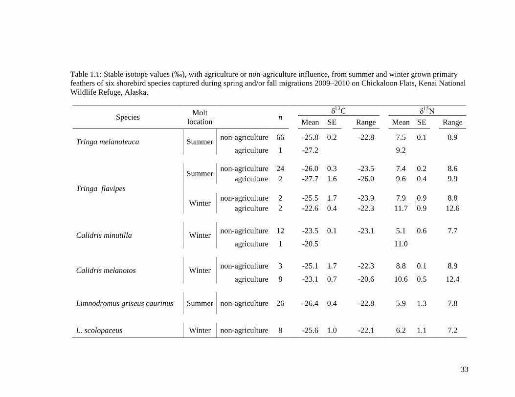
33

Table 1.1: Stable isotope values (‰), with agriculture or non-agriculture influence, from summer and winter grown primary

feathers of six shorebird species captured during spring and/or fall migrations 2009–2010 on Chickaloon Flats, Kenai National

Wildlife Refuge, Alaska.

Species Molt

location

n

C

Mean SE Range Mean SE Range

Tringa melanoleuca Summer non-agriculture 66 -25.8 0.2

-22.8 7.5 0.1

8.9

agriculture 1 -27.2 9.2

Tringa flavipes

Summer non-agriculture 24 -26.0 0.3 -23.5 7.4 0.2 8.6

agriculture 2 -27.7 1.6 -26.0 9.6 0.4 9.9

Winter non-agriculture 2 -25.5 1.7 -23.9 7.9 0.9 8.8

agriculture 2 -22.6 0.4 -22.3 11.7 0.9 12.6

Calidris minutilla Winter non-agriculture 12 -23.5 0.1

-23.1 5.1 0.6

7.7

agriculture 1 -20.5 11.0

Calidris melanotos Winter non-agriculture 3 -25.1 1.7

-22.3 8.8 0.1

8.9

agriculture 8 -23.1 0.7 -20.6 10.6 0.5 12.4

Limnodromus griseus caurinus Summer non-agriculture 26 -26.4 0.4

-22.8 5.9 1.3

7.8

L. scolopaceus Winter non-agriculture 8 -25.6 1.0 -22.1 6.2 1.1 7.2

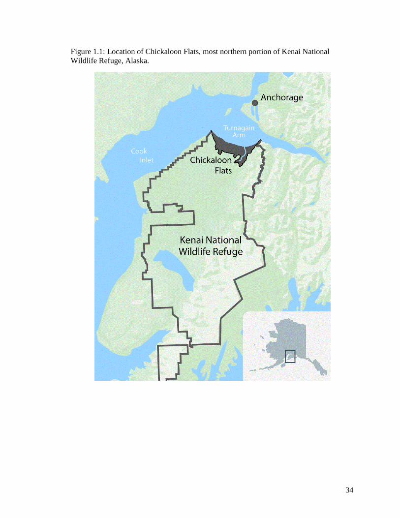
34

Figure 1.1: Location of Chickaloon Flats, most northern portion of Kenai National

Wildlife Refuge, Alaska.

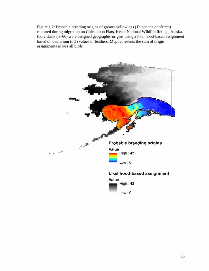
35

Figure 1.2: Probable breeding origins of greater yellowlegs (Tringa melanoleuca)

captured during migration on Chickaloon Flats, Kenai National Wildlife Refuge, Alaska.

Individuals (n=66) were assigned geographic origins using a likelihood-based assignment

based on deuterium (D) values of feathers. Map represents the sum of origin

assignments across all birds.

36

Figure 1.3: Probable breeding origins of lesser yellowlegs (Tringa flavipes) captured

during migration on Chickaloon Flats, Kenai National Wildlife Refuge, Alaska.




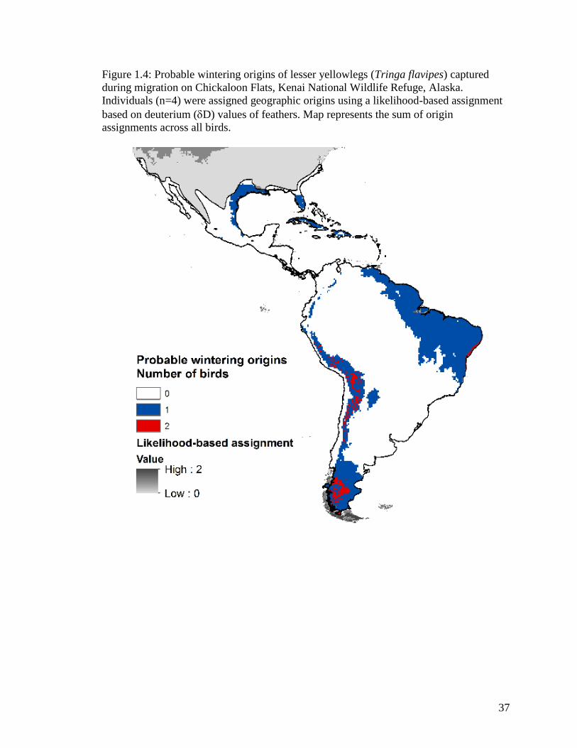
37

Figure 1.4: Probable wintering origins of lesser yellowlegs (Tringa flavipes) captured





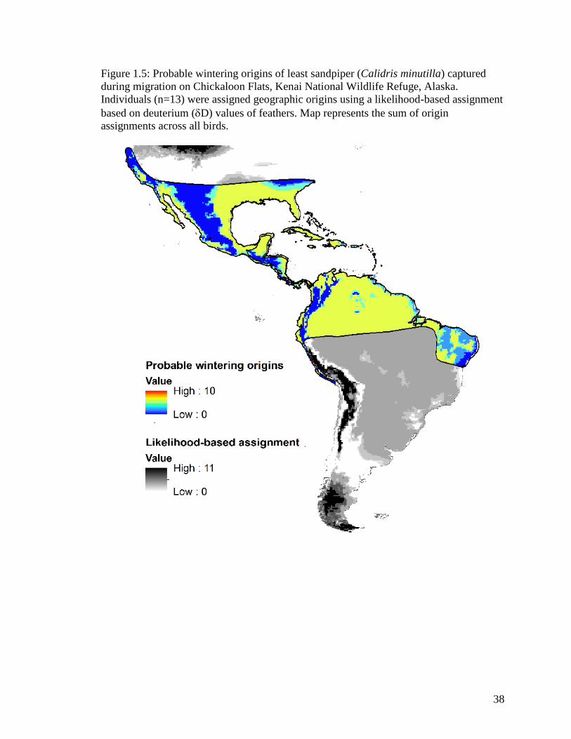
38

Figure 1.5: Probable wintering origins of least sandpiper (Calidris minutilla) captured





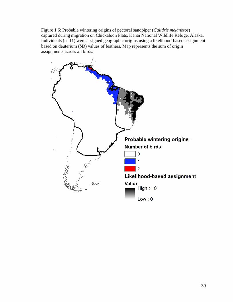
39

Figure 1.6: Probable wintering origins of pectoral sandpiper (Calidris melanotos)

captured during migration on Chickaloon Flats, Kenai National Wildlife Refuge, Alaska.




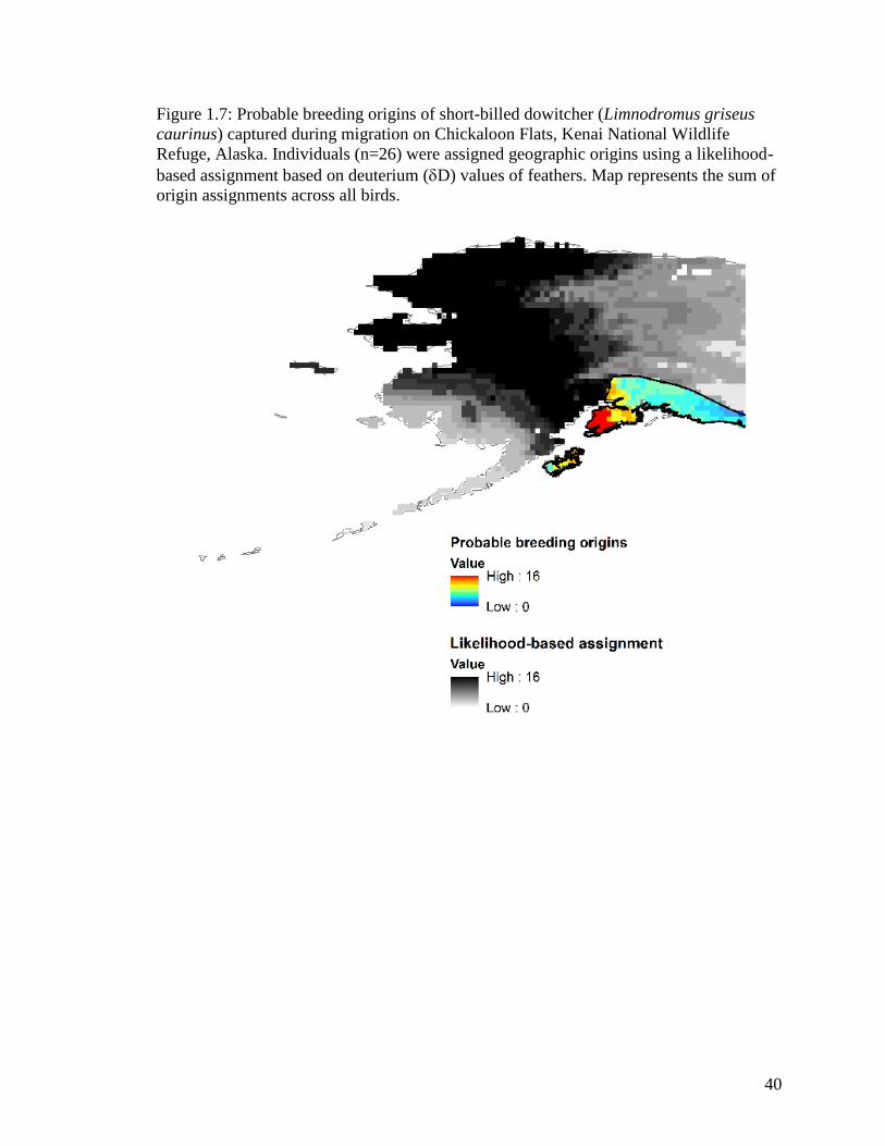
40

Figure 1.7: Probable breeding origins of short-billed dowitcher (Limnodromus griseus

caurinus) captured during migration on Chickaloon Flats, Kenai National Wildlife

Refuge, Alaska. Individuals (n=26) were assigned geographic origins using a likelihood-

based assignment based on deuterium (D) values of feathers. Map represents the sum of

origin assignments across all birds.

41

Figure 1.8: Probable a) primary molt and b) wintering origins of long-billed dowitcher

(Limnodromus scolopaceus) captured during migration on Chickaloon Flats, Kenai

National Wildlife Refuge, Alaska. Individuals (n=7 and 4) were assigned geographic

origins using a likelihood-based assignment based on deuterium (D) values of feathers.

Maps represent the sum of origin assignments across all birds.

a.

.

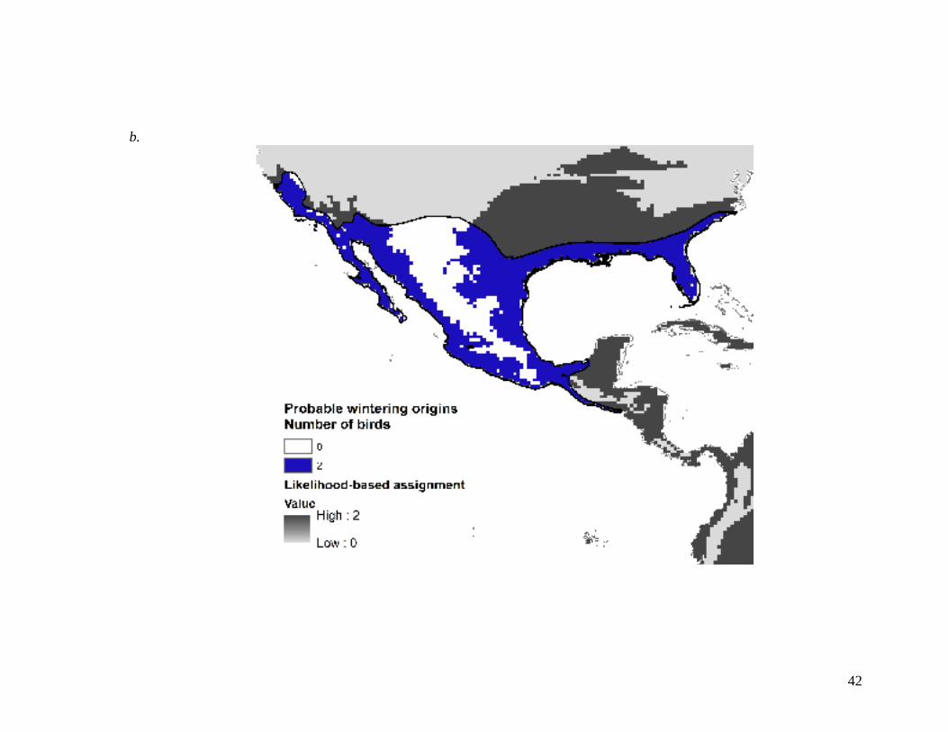
42

b.

43

Chapter 2

AVIAN USE OF CHICKALOON FLATS

ON ALASKA’S SOUTH-CENTRAL COAST

Introduction

Stopover sites along migration routes are important for supporting and sustaining

birds as they move between primary wintering, breeding, and staging grounds (Skagen

and Knopf 1994a,Skagen and Knopf 1994b, Farmer and Parent 1997). Shorebird

migration is of an opportunistic nature (Skagen and Knopf 1993), and conservation of a

network of migration stopovers should contain protected wetlands dispersed widely over

the landscape (Haig et al. 1998, Skagen et. al. 2008). Therefore, the importance of

particular sites in a network of migration stopovers extends beyond counts of individuals

(Bibby 2003). A location may be rarely used, but can be a critical connection to breeding

areas (Skagen and Knopf 1994b) or buffer environmental stochasticity; e.g. during a cold

or dry season or other unusual circumstances such as timing of spring weather near the

breeding grounds (Klaassen 2003).

Of particular concern to spring migrating shorebirds is finding ice-free areas with

open water and critical foraging habitat. Unlike waterfowl, spring shorebird migration

through Alaska occurs in a shorter period of time beginning late April, peaking the first

week of May, and finishing mid-May (Gill and Tibbitts 1999, Alaska Shorebird Working

Group 2000). Therefore, environmental stochasticity and habitat ice-over have the

potential to influence a large portion of spring migrants in Alaska.

44

Chickaloon Flats, an estuary on Alaska’s south-central coast that consists

primarily of unconsolidated mudflats and 10 other vegetated communities occurring

along a salinity gradient, fits into the aforementioned conservation strategy as a protected

coastal stopover site along the Pacific Flyway. As an estuary, this area can provide

predictable tidal habitats and a reliable source (compared to interior wetlands) of

abundant resources (Colwell 2010). During years of late ice-out, Chickaloon may provide

more favorable, ice-free habitats for early spring migrants than other local or regional

locations. Cook Inlet provides northern migrating birds with the last considerable area of

ice-free littoral habitat before the breeding grounds (Gill and Tibbitts 1999). The

availability of early spring ice-free habitat may provide critical foraging habitats for birds

encountering iced-over habitats elsewhere in the area (Gill and Tibbitts 1999).

Historically, Chickaloon Flats was thought to be an important avian migratory

stopover; however, confirmatory ground surveys of shorebirds have not been conducted

since Quimby (1972). Quimby (1972) found avian use of vegetated communities to be

variable, with most shorebird species utilizing unvegetated mud areas intensively, marsh

vegetated communities moderately, and salt-tolerant vegetation/mud areas infrequently to

moderately. However, the vegetation composition of Chickaloon Flats has changed over

a 35-year period following the 1964 Earthquake, which registered 9.2 on the Richter

scale and caused the land to drop as much as 4 m including decreases in emergent marsh

communities and areas of exposed mud and increases in vegetated areas with a mix of

mud and salt-tolerant species. I postulated that shorebird use of Chickaloon Flats may

have changed to reflect the changing landscape over the past 35 years (see Chapter 3).

45

Due to a lack of information, my first objective was to observe current shorebird

use of Chickaloon Flats during spring and fall migration, focusing on six species: (greater

yellowlegs Tringa melanoleuca, lesser yellowlegs Tringa flavipes, least sandpiper

Calidris minutilla, pectoral sandpiper Calidris melanotos, and short-billed and long-

billed dowitcher Limnodromus griseus caurinus and L. scolopaceus). My second

objective was to determine differential shorebird use among the various wetland

landcover types within the Flats.

Study area

Chickaloon Flats, Alaska, is a mudflat complex located on the Kenai National

Wildlife Refuge along Turnagain Arm in Cook Inlet (Figure 2.1). Tidal range within this

area is 9.2 m, which is second greatest in the world behind Bay of Fundy (11.7 m)

(Mulherin et al. 2001). Vegetated communities comprise 6,695 ha at high tide (9,533 ha

including mud at low tide), and entails about 1% of the 773,759 ha Kenai National

Wildlife Refuge. Chickaloon Flats has a high diversity of plant species due to the overlap

of arctic and temperate species (Vince and Snow 1984), and the patterns of vegetation are

largely due to saltwater and freshwater interactions, land subsistence from the 1964

earthquake, and tides (Neiland 1971, Quimby 1972, and Committee on the Alaska

Earthquake 1973). Vegetation composition on Chickaloon Flats, initially described using

10 plant community types (Neiland 1971, Quimby 1972) shows spatial patchiness along a

salinity gradient toward Cook Inlet. In addition to mud, the 6 landcover types prevalent

enough to be surveyed in this study follow Quimby’s (1972) names: Seaside arrow-grass,

46

Large alkali-grass, Creeping alkali-grass, Marsh, Floating marsh, and Type 3 Mud. For

this study, 4 plots (2 km by 4 km) were established to sample all landcover types and

avian abundance. Plots were spread across Chickaloon, and chosen by accessibility via

the three current aircraft landing strips.

Methods

Landcover

Of the 10 landcover classifications described by Quimby (1972), Bog, Alder, Ramenski

sedge, and Marsh fringe communities were not included in avian surveys due to narrow

and sparse distribution. The remaining landcover classifications were grouped into four

types; Creeping-Large alkali-grass, Floating marsh-Marsh community-Seaside arrow-

grass, Mud, and Type 3 Mud. These types were used for analyses of avian survey data.

Avian surveys

To estimate avian diversity and abundance throughout the spring and fall, 2009–2010, I

conducted surveys to quantify avian use of different landcover classes. Forty-five avian

surveys (Gregory et al. 2004) were conducted throughout spring and fall of 2009 and

2010 every 5–10 days. A survey consisted of 5 to 7 independent transects, with 3 to 5

independent survey points (hereafter called visits) in each transect. Surveys were started

between 0730–0830 and 1930–2030 because previous observations concluded that avian

use of Chickaloon was linked more to a diurnal cycle rather than tidal stages. I and one

other observer conducted a survey; each person completed 3 or 4 transects during a single

47

survey period, depending on landcover type and slough layout within a plot. Transect

locations were randomly chosen every survey for each landcover type and were sampled

without replacement to ensure maximum spatial coverage throughout survey periods. A

robust spatial distribution of transects was a goal in order to incorporate variation of

landcover quality present throughout the study area.

A survey point (visit) was a 100 m fixed-radius plot located entirely within a

single landcover type. I assumed observations between points were independent. Each

point along a transect was surveyed once. At each survey point, the observer stopped for

5 minutes and recorded every individual within the 100 m radius, ignoring fly-overs and

ensuring birds were not double-counted. Infrequently, birds were disturbed when walking

between points, and these birds were not recorded. When community types were narrow

(~300 m), transects ran down the middle to allow for a sample plot to fall completely

within a habitat. Depending on the length of habitat type, transects ran 400–800 m, with

the longest transect being the goal.

Density estimates

To estimate densities and detection probabilities of shorebird species, I used negative

binomial N-mixture models (Royle 2004a) to evaluate which survey covariate (habitat,

season, time of day, and weekly time-period) influenced the detection probability in the

pcount function of the ‘unmarked’ package (Fiske and Chandler 2011) for the software R

V2.14.0 (R Development Core Team 2011). This approach allows density estimates using

point count data, while incorporating the underlying detection process (Royle 2004b). In

48

all species, season most influenced detectability, and was used as the detection

probability covariate in each model.

I estimated densities of 6 common shorebird species; lesser yellowlegs, greater

yellowlegs, pectoral sandpiper, least sandpiper, and short- and long-billed dowitcher. I

combined the two dowitcher species in the analysis to eliminate possible inaccuracies in

estimates and to account for any observer bias and field identification errors. I also

analyzed all 18 observed shorebird species pooled across the survey. To determine both

spatial and temporal variation, the density (expressed as number detected per 100 m

fixed-radius plot) of each species was determined for each combination of four landcover

class types, spring and fall seasons, and weekly time-periods.

To generate an estimate of actual daily population size, in one-week increments,

across all of Chickaloon Flats, I did a simple area expansion because derived density

estimates were from a sample unit of known area (Royle 2004b). This produces a useful

estimate of population size. I used the following area estimates for area expansion:

creeping-large alkali-grass community (3,444 ha), floating marsh-marsh community-

seaside arrow-grass (1,806 ha), mud (2,838 ha), and Type 3 mud (1,174 ha). Marsh

community does not include area of permanent ponds. Mud includes a portion of coastal

mudflats (at low tide) projected into Cook Inlet, as well as bare mud areas between

vegetated communities and sloughs.

Results

I conducted 43 surveys, which consisted of 938 survey points across both spring and fall

of 2009 and 2010 (Table 2.1). The average survey time per day was 2 h 47 min and

49

ranged from 1 h 47 min – 3 h 34 min. To improve analysis, survey dates were grouped

into a single ‘weekly time-period’, broken into 7 weeks during spring migration and 9

weeks in the fall. Ideally there would have been a more balanced temporal and spatial

distribution of surveys across study plots, but due to logistical constraints in plot

accessibility, sampling effort varied across the 4 plots. Plots 1 and 2 were surveyed at 5–

10 day intervals (Plot 1 N=17 surveys, Plot 2 N=16). Plot 3 was only visited during fall

2010, so only 2 surveys were conducted. I did not include those points in analysis

because the plot was not fully represented across both years and season. Plot 4 was

visited during spring and fall of both years, with 2–3 surveys per visit (N=10 surveys).

Of 95 bird species observed during the entire study (Appendix E), 42 were

recorded during avian point-transect surveys in 2009 and 2010, including 18 shorebird

species: black-bellied plover (Pluvialis squatarola, N= 37 detections), American-golden

plover (Pluvialis dominica, N= 1), semipalmated plover (Charadrius semipalmatus, N=

36), greater yellowlegs (N= 273), lesser yellowlegs (N= 344), solitary sandpiper (Tringa

solitaria, N= 6), whimbrel (Numenius phaeopus, N= 7), hudsonian godwit (Limosa

haemastica, N= 32), black turnstone (Arenaria melanocephala, N= 9), red knot (Calidris

canutus, N= 1), semipalmated sandpiper (Calidris pusilla, N= 6), western sandpiper

(Calidris mauri, N= 3), least sandpiper (N= 411), pectoral sandpiper (N= 286), short-and

long-billed dowitcher (N= 353), Wilson’s snipe (Gallinago delicata, N= 170), and red-

necked phalarope (Phalaropus lobatus, N= 218).

The detection probability of individual species for spring ranged from 0.37 to

0.92, whereas the fall was much lower with a range of 0.02 to 0.40. The combined

50

shorebird species detectability was 0.37 in spring and 0.15 in the fall. Greater yellowlegs

was 0.56 in spring and 0.11 in fall, and lesser yellowlegs 0.70 and 0.03. Least sandpiper

had 0.70 spring detectability and the highest fall detectability with 0.40. Pectoral

sandpiper had the highest in the spring at 0.92 and lowest in fall with 0.02. The spring

detection for short- and long-billed dowitchers was 0.44 and fall was again the lowest

with 0.02.

There were inter-annual and seasonal variations in estimated abundance of

shorebirds (Figure 2.3). In both years, more shorebirds used Chickaloon Flats during the

fall migration. Spring migration was concentrated, whereas fall was protracted with

several migration pulses. Table 2 shows the weekly population estimates for all shorebird

species (N=18), greater and lesser yellowlegs, least and pectoral sandpiper, and dowitcher

species, recorded during ground surveys during spring and fall migration in 2009 and

2010. Pectoral sandpiper and dowitcher species were the only species more abundant

during surveys in the spring than fall. Results from combined shorebird species show

larger shorebird populations in the fall (Table 2.2a). The highest daily estimate for the

spring occurred during the week of 10 May with an estimated 22,758 (± 3,519) birds

across all of Chickaloon (Table 2.2a). There were several high estimates during the fall

migration, with numerous pulses occurring the weeks of 5 July (85,203 ± 22,373), 26

July (94,646 ± 25, 315), and 9 August (97,465 ± 30,122). The most abundant shorebird

species in the spring was the dowitcher, but the least sandpiper and greater yellowlegs

were the most abundant in the fall.

51

The timing of migration pulses and estimated number of birds that make up these

pulses varied with species (Table 2.2). Greater yellowlegs abundance peaked in the

spring (3,891 ± 1,723) during the week of 10 May, with a prominent fall pulse occurring

the week of 9 Aug (48,435 ± 11,321) (Table 2.2b). Lesser yellowlegs exhibited a gradual

increase to the spring maximum of 20,536 (±12,200) individuals during the first week of

June, with a slight increase in fall use of 24,117 (± 11,741) during the week of 19 July

(Table 2.2c). Least sandpipers arrived earlier in the spring, with 5,125 (± 2,000) birds

passing through during the first week of May and a much smaller pulse (606 ± 437)

heading into first week of June. There were several pulses during fall migration (Table

2.2d), with the largest two occurring the first week of July (48,920± 8,606) and last week

of July (32,615 ± 7,119). Pectoral sandpipers had obvious migration pulses in both

migration periods (Table 2.2e). The two spring high pulses of 18,044 (± 4,902) and

17,484 (± 4,943) individuals were greater than the largest fall pulse (15,167 ± 6,437).

Dowitchers had multiple pulses throughout both spring and fall (Table 2.2f), with the

largest spring pulse (27,627 ± 11,218) in their first appearance on second week of May,

and a similar fall pulse (26,253 ± 6,970) in second week of July.

Shorebirds used landcover types differently (Table 2.2). The Creeping-Large

alkali community type was most-densely used by greater yellowlegs, and second most-

densely used for all other species. Population estimates for Floating marsh-Marsh

community-Seaside arrow-grass landcover type were highest for lesser yellowlegs,

pectoral sandpiper and dowitchers. The Mud community was not used by pectoral

sandpipers and of minor importance for all other species. The Type 3 Mud was the most-

52

densely used landcover type for least sandpipers; in contrast, it was least used by all other

shorebird species.

Discussion

Chickaloon Flats is an estuary that supports a diversity of avian species during

spring and fall migration periods. I observed 39 species and 33 species, respectively,

during spring and fall migration. With a peak daily population estimate of 22,758 (±

3,519) shorebirds in the spring and 94,646 (± 25,345) in the fall, this stopover site

(Warnock 2010) has potential to host high numbers of birds for relatively short periods of

time.

Vegetation types on Chickaloon Flats vary in area, distribution, and surface water

presence. Vegetation composition on Chickaloon Flats changed over a 35-year period

following the 1964 Earthquake based on Landsat imagery and point-to-point

comparisons. Overall, both the emergent marsh communities and areas of exposed mud

have decreased, while vegetated communities with a mix of mud and salt-tolerant species

have increased in area. This changing vegetation composition has likely influenced the

abundance and diversity of avian species using Chickaloon Flats.

Marsh community-Floating marsh-Seaside arrow-grass was the most used

landcover type by shorebird species except the least sandpiper. This landcover type also

decreased 7.0% in area from 1970 to 2005. The importance of this vegetation

classification type is complicated by the dynamics of ephemeral pools within it.

Ephemeral pools are significantly affected by extreme tidal events, which are variable

53

and sparse in occurrence. I observed the vast majority of shorebirds utilizing this area as

roosting grounds rather than for foraging. On numerous accounts, I observed flocks of

40–200 shorebirds leave a marsh roosting area just before high tide and fly towards Cook

Inlet, likely to forage on mudflats as high tide ebbed and exposed moist sediments.

Creeping-Large alkali-grass supported high numbers of shorebirds, and was the

only landcover type that increased (16.8%) in area over the 35-year period. This

landcover type occupied the most area, making up 36.1 % of the area of Chickaloon in

2005.

Mud is a relatively important habitat type for shorebirds in general, but was not

highly used by the 6 focal species. Mud decreased 7.3% in area from 1970 to 2005, and

could also alter the long-term use of some shorebird species. Chickaloon Flats has

relatively hard mud, possibly due to long exposure between high tides. This may deter

species which forage by probing because substrate penetrability varies with compaction,

and may therefore affect foraging rates (Myers et al. 1980). Probing shorebirds prefer

fine, soft sediments compared with the coarse, firm sediment preferred by species which

eat off the surface (Colwell 2010). In addition to the mud itself, Mud type (as defined

here) consists of sloughs of various sizes, ranging from small channels draining

ephemeral pools to larger freshwater (but tidal) creeks such as Big Indian and Pincher

Creeks. A variety of shorebird species were observed feeding along these sloughs and at

all tidal stages. In contrast to hard-pan mudflats that are available for foraging around

high tides, sloughs provide softer substrate throughout the day for foraging shorebirds.

54

Type 3 Mud, described as mud with sparse patches of alkali-grass, supported the

lowest numbers of shorebirds, apart from the least sandpiper. This landcover type

decreased slightly in area (2.5%) over the 35-year period, and probably has had minimal

long-term impacts in numbers of birds using Chickaloon.

Short- and long-billed dowitchers used Chickaloon Flats in greater numbers in the

spring than fall, while greater yellowlegs and least sandpipers were more abundant during

the fall. Shorebird migration is more protracted in the fall, and I was unable to sample

bird density throughout the entire fall migration period. Therefore, fall estimates may be

lower for some species. For example, pectoral sandpipers are late fall migrants and I was

only able to observe the first part of their southern migration, and most likely did not

capture peak abundances. Detectability of each species was much higher in the spring.

Low detection probability during the fall may be attributed to vegetation growth, and

therefore lower visibility.

Long-distance shorebird migrants rely on stopover sites to take advantage of

seasonally abundant food resources. There is not only importance in a network of

stopover sites (Skagen and Knopf 1994a, Skagen and Knopf 1994b, Farmer and Parent

1997) along a flyway, but also those ranging in sizes from small (Skagen and Knopf

1993) to large (Connors et al. 1979, Isleib 1979). Unlike a major stopover like the Copper

River Delta, which supports hundreds of thousands of migrating shorebirds on a daily

basis in the spring (Bishop et al. 2000), Chickaloon supports an estimated maximum

spring daily total of 17,304 (± 3,238) birds.

55

The importance of the location of a stopover within a migration flyway (Isleib

1979) can also be critical to migrating birds. Most of the Nearctic shorebirds that breed in

western Alaska use a narrow migration corridor that follows the coast, which also

presents topographic and climatic obstacles (Isleib 1979). Birds are funneled into coastal

south-central Alaska and are offered two main areas, Copper River Delta and Lower

Cook Inlet, with suitable shallow estuarine, tidal mudflats, and marsh areas to rest and

refuel (Isleib 1979). The Copper River Delta area offers >100,000 ha of shorebird habitat,

while the areas of Lower Cook Inlet, situated 300 km to the west, offer several estuaries

an order of magnitude smaller (Isleib 1979, Gill and Tibbitts 1999). There are differences

in relative community composition between these areas during spring migration. At least

20 shorebird species have been recorded on the Copper River Delta, of which the western

sandpiper and dunlin have the greatest relative numbers (Christensen et al. 2000), while

lesser yellowlegs and Limnodromus species have greatest relative numbers of the 24

shorebird species of Chickaloon Flats.

Isleib (1979) reported fall shorebird migrations in south-coastal Alaska are not as

intense as spring migration. Aerial surveys conducted by Gill and Tibbitts (1999) support

this conclusion, averaging 40,485 shorebirds per day during spring in contrast to only 730

per day during fall in the Lower Cook Inlet. However, I estimated 5 times more shorebird

use of Turnagain Arm during the fall than spring. Chickaloon Flats is located in the

Upper Cook Inlet, nestled in Turnagain Arm against the western edge of the Kenai and

Chugach mountains. Relative to the Copper River Delta and Lower Cook Inlet,

56

Chickaloon Flats may be more difficult for avian species to access during northern

migration because of these mountain barriers (Figure 2.2).

As shown through stable isotope analysis (see Chapter 1), Chickaloon provides a

stopover site for numerous long-distance migrant shorebird species that breed in Alaska

and winter from southern North America down through central South America. Connors

et al. (1979) found that shorebirds changed habitat use toward the end of breeding season,

and moved from upland tundra breeding sites to coastal littoral staging areas. Chickaloon

may provide this essential post-breeding roosting and foraging habitat for shorebirds

before beginning the long southern migration, as illustrated through probable breeding

origins of both greater and lesser yellowlegs utilizing Chickaloon as a post-breeding site.

This study indicates that shorebird use of Chickaloon is much more extensive

during the southern migration. There are fewer spring migration peaks, with fall

migration showing a more protracted, variable migration. With an area of 9,533 ha,

Chickaloon Flats is relatively-small, yet offers 7% of estuarine intertidal shorebird habitat

in the south-central Alaskan region. Chickaloon supports Although Chickaloon Flats is

not recognized as a major stopover for migrating shorebirds, it is an important area

utilized by a diverse amount of avian species throughout the annual cycle.

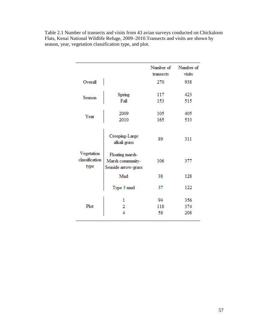
57

Table 2.1 Number of transects and visits from 43 avian surveys conducted on Chickaloon

Flats, Kenai National Wildlife Refuge, 2009–2010.Transects and visits are shown by

season, year, vegetation classification type, and plot.

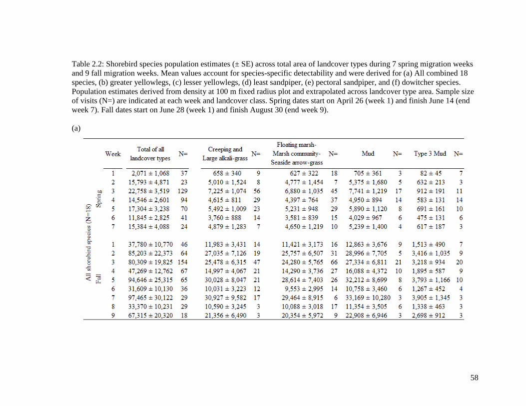
58

Table 2.2: Shorebird species population estimates (± SE) across total area of landcover types during 7 spring migration weeks

and 9 fall migration weeks. Mean values account for species-specific detectability and were derived for (a) All combined 18

species, (b) greater yellowlegs, (c) lesser yellowlegs, (d) least sandpiper, (e) pectoral sandpiper, and (f) dowitcher species.

Population estimates derived from density at 100 m fixed radius plot and extrapolated across landcover type area. Sample size

of visits (N=) are indicated at each week and landcover class. Spring dates start on April 26 (week 1) and finish June 14 (end

week 7). Fall dates start on June 28 (week 1) and finish August 30 (end week 9).

(a)

59

(b)

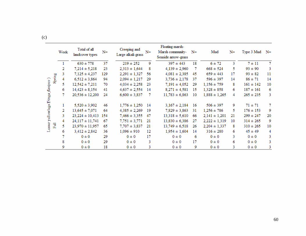
60

(c)

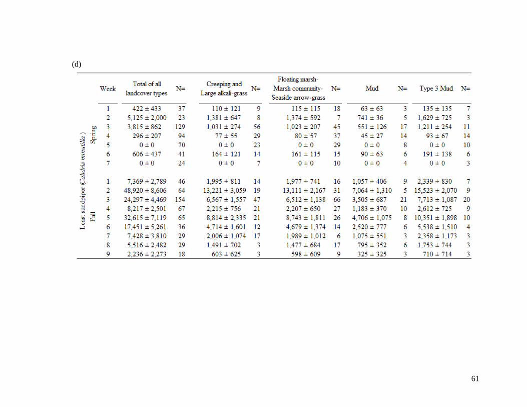
61

(d)

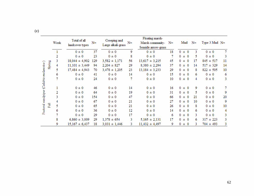
62

(e)

63

(f)

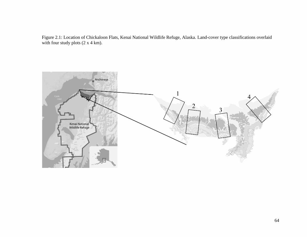
64

Figure 2.1: Location of Chickaloon Flats, Kenai National Wildlife Refuge, Alaska. Land-cover type classifications overlaid

with four study plots (2 x 4 km).

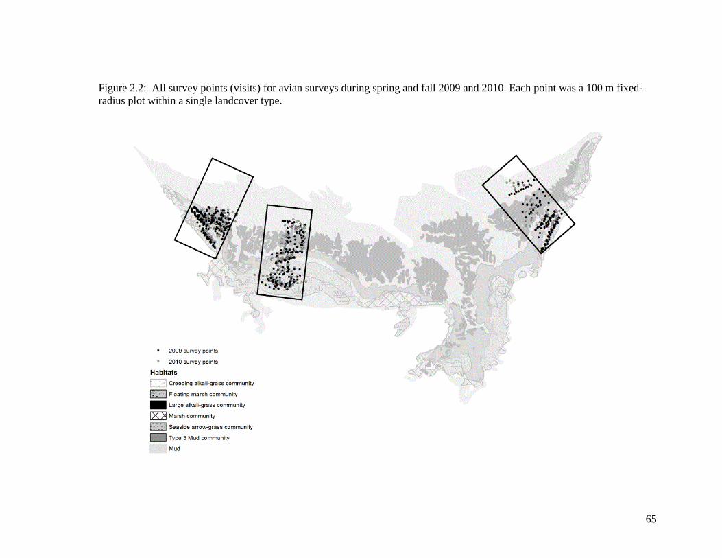
65

Figure 2.2: All survey points (visits) for avian surveys during spring and fall 2009 and 2010. Each point was a 100 m fixed-

radius plot within a single landcover type.

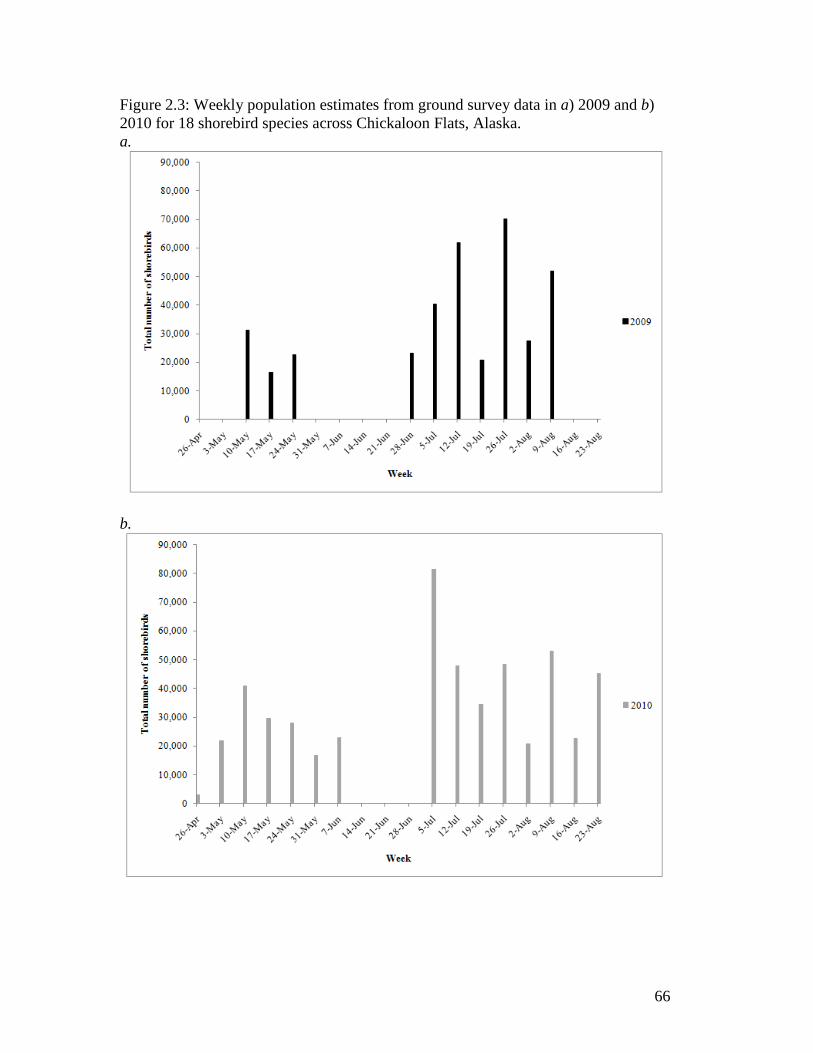
66

Figure 2.3: Weekly population estimates from ground survey data in a) 2009 and b)

2010 for 18 shorebird species across Chickaloon Flats, Alaska.

a.

b.

67

Chapter 3

SATELLITE IMAGE BASED VEGETATION CLASSIFICATION AND CHANGE

OVER 30 YEARS ON CHICKALOON FLATS

Introduction

Alaska experiences postseismic vertical motions from the large megathrust

earthquakes caused by its location on a convergent plate boundary (Larsen et al. 2005).

The 1964 ‘Good Friday’ Earthquake was one of the strongest earthquakes in recent time;

registering between 8.3–8.6 on the Richter scale with its epicenter about 125 km east of

Anchorage in the Chugach Mountains, and significantly changed the landscape, and

consequently the vegetation, of the surrounding areas. Thilenius (1990) showed the

change in landscape greatly altered the tidal regime, and therefore the rate and pattern of

vegetation succession on the Copper River Delta. Atwater et al. (2001) showed that

following the subsidence caused by the 1964 earthquake, vegetated estuary areas in

Turnagain Arm were turned to barren tidal flats (although these have aggraded rapidly

and vegetation on the flats is maturing). Findings from those Turnagain Arm mudflats

showed that sediment quickly filled in available areas following subsidence from the

1964 Earthquake (Atwater et al. 2001), and deposition slowed and sediment became finer

into the 1980’s (Bartsch-Winkler 1988). Unlike most intertidal environments, Turnagain

Arm has a clear lack of infauna (Bartsch-Winkler and Ovenshine 1984), which may be

due to high amounts of suspended sediment from glacial rivers and erosion, as well as

swift moving currents and tidal bore presence (Bartsch-Winkler and Ovenshine 1984). It

68

is unknown whether these changes have impacted the condition of the estuary and

subsequently the use by avifauna.

Anecdotal field observations from 2009 showed vast mud areas spread within the

Large alkali-grass and Creeping alkali-grass vegetated communities. These observations,

paired with the knowledge that changes in elevation and vegetation (Thilenius 1990,

Atwater et al. 1991) are produced by sea-level rise, postseismic vertical motions, and

rapid uplift have prompted a discussion of the current health of the Chickaloon estuary.

These vast mud areas could be a product of landscape change following the 1964

Earthquake, which could have altered the tidal regime (Thilenius 1990) and increased

aggradations (Atwater et al. 1991) with sediment lacking infauna (Bartsch-Winkler and

Ovenshine1984). Alternatively, the vegetation succession could be occurring at a more

rapid rate following the earthquake (much like the Copper River Delta, Thilenius 1990)

and the current areas of mud pans are smaller than more recent post-earthquake mud

areas. Due to the historical thought that Chickaloon Flats was an important avian

migratory stopover, with relative regional importance in terms of estuarine intertidal area

within Cook Inlet and Prince William Sound, there was a need to evaluate the current

vegetation classification and determine if any changes have occurred since the last

ground study in 1970 and 1971 (Quimby 1972). Therefore, the objectives of this study

were to create an updated vegetation classification map of Chickaloon Flats, and quantify

any changes in both non-vegetated and vegetation communities from 1975 to 2005.

69

Study Area

Cook Inlet is an important Alaskan water body with more than half (over

400,000) of the state’s human population residing along its shores and watershed. It is a

multi-use area used for commercial and recreational fishing, cargo transportation, and oil

and gas exploration and production in northern areas since the 1960’s (Mulherin et al.

2001). Chickaloon Flats is located along the northern part of the Kenai Peninsula (Figure

3.1), entailing about 10,000 ha of the 773,759 ha Kenai National Wildlife Refuge.

Turnagain Arm, an extension of Cook Inlet, bounds the flats to the north, the Kenai

Mountains to the east and southeast, and Kenai Lowlands to the south and west. Several

riverine systems flow into this complex including the Chickaloon River, Big and Little

Indian Creeks, and Pincher Creek. Chickaloon is an estuary of regional importance,

representing 7% of all estuarine intertidal areas of the Cook Inlet and Prince William

Sound area (Figure 3.2). Large alkali-grass (Puccinellia grandis), and creeping alkali-

grass (Puccinellia phryganodes) are dominant in areas of higher salinity; lyngbye sedge

(Carex lyngbvaei) and creeping spike-rush (Scirpus paludosus) are dominant in areas of

lower salinity; however, much of the estuary is unconsolidated mudflats.

Similar to Susitna Flats on the northern side of Cook Inlet, Chickaloon has high

plant diversity due to the overlap of arctic and temperate plant species (Vince and Snow

1984). This overlap gives rise to a complex of vegetation zones unique to south-central

Alaska (Vince and Snow 1984). Vegetation patterns of Chickaloon were initially

described in 1971–1972 using 10 plant communities (Neiland 1971, Quimby 1972). The

70

10 vegetated communities occur in salinity gradients toward Cook Inlet and in slightly

different sequences and areas across Chickaloon (Figure 3.3).

Changes in elevation of a landscape can greatly alter vegetation structure and

composition (Thilenius 1990, Atwater et al. 2001). The landscape of Chickaloon Flats

has been altered due to subsidence, uplift, and siltation. Chickaloon is located in one of

the major earthquake zones of the world and was significantly affected by the earthquake

of March 27, 1964 (Committee on the Alaska Earthquake 1973). The region subsided in

1964 with the earthquake, causing considerable changes in land structure, and has been

uplifting since (Jeff Freymueller pers. comm.). Freymueller et al. (2008) found large,

very rapid uplifts on the Kenai Peninsula following this earthquake, which could have

drastically altered the landscape. The 1964 tectonic uplift of tidal areas in the Copper

River Delta resulted in a loss of tidal influence, which caused sudden changes in the

composition and structure of vegetation (Thilenius 1990, Boggs and Shephard 1999). In

addition to the tectonic uplift, the land elevation of Chickaloon Flats is changing from the

rapid uplift in southern Alaska due to glacial unloading and melting ice fields (Larsen et

al. 2005). Comparing data from 1964 to the late 1990’s, the cumulative 30-year uplift

reached 90 cm in the middle of the Kenai Peninsula and more than 1 m at Turnagain Arm

(Freymueller et al. 2008). Chickaloon Flats has experienced uplift from ~30 cm in west to

75–80 cm in east (Jeff Freymueller pers. comm.) since originally subsiding 61 cm to 137

cm west to east (Quimby 1972) following the 1964 Earthquake. Since 1990, uplift rates

have continued by ~9 mm per year raising the flats by an additional 10 cm by the year

71

2000. Considering subsidence and uplift after earthquake, the net change in land

elevation results in a drop of 21 cm in west to about 47-52 cm in the east.

In addition to uplift, the elevation is increasing annually due to sediment

accretion. Vince and Snow (1984) showed a positive correlation with siltation rates and

flooding frequency on Susitna Flats, and recorded a range of annual siltation of 4.0-10.3

mm in 1978 and 9.7-14.3 mm in 1979 for the outer mudflats. If I was to assume

minimum and maximum annual siltation rates from that study and apply those to

Chickaloon, there may have been an additional 13.6 cm to 48.62 cm from sediment

accretion across the outer mudflats since the 1964 Earthquake. The net effects of

subsidence, tectonic and rapid uplift, and siltation accretion could almost equal (Boggs

2000), or increase the overall elevation across the flats.

The changes in elevation following the 1964 Earthquake have been shown to

influence vegetation on mudflats in Turnagain Arm (Atwater et al. 2001) and Copper

River Delta (Thilenius 1990), and I predict similar changes may have occurred on

Chickaloon Flats. I hope to depict some of those vegetation landscape changes through

this study.

Methods

I utilized information from Quimby’s (1972) land cover classification, my current

land cover classification of ground-truthed points, and Landsat imagery from 1975 and

2005. Quimby created a land cover map by delineating communities from ground survey

information and using both black and white aerial photographs taken in June 1970 by the

72

Bureau of Land Management for the base map, and 35mm colored transparencies of July

1970 to identify plant communities. I then digitized the delineated land cover

communities.

The plant communities typically occurred from Turnagain arm to the forest in the

following sequence; Large alkali-grass, Ramenski sedge, Type 3 Mud, Creeping alkali-

grass, Marsh, Seaside arrow-grass, Floating marsh, Bog, Alder, and Marsh Fringe.

Descriptions are derived from Quimby (1972), scientific names from Hultén (1968), and

a list of all plant species within each community is in Appendix F. Large alkali-grass is

the most abundant community, comprising primarily of large alkali-grass, seaside arrow-

grass (Triglochin maritimum), goose-tongue (Plantago maritima juncoides) and large

mud pans throughout. Ramenski sedge is a rare inland community primarily made of

clumped ramenski sedge (Carex Raménskii) surrounding drainage sloughs. Type 3 Mud

is primarily unvegetated except for creeping spike-rush (Scirpus paludosus), and was

formed by siltation of previously vegetated areas. The Creeping alkali-grass community

is primarily made of creeping alkali-grass, seaside arrow-grass, shallow ponds, and mud.

Marsh consists primarily of Lyngbye sedge (Carex Lyngbyaéi) and various other sedge

species that bordered numerous permanent ponds of varying depths. Although seaside

arrow-grass community is principally made of seaside arrow-grass, it has complex

vegetation patterns and dead black spruce (Picea mariana) trees throughout, both

possibly resulting from revegetation following the 1964 Earthquake. Floating marsh is

dominated by sedges, and contains floating mats of diverse vegetation, few permanent

ponds, and dead black spruce. Bog community is nearest the forest edge and consists of

73

sedges, dwarf birch (Betula nana), and dwarf willows (Salix sp.). The Alder community

is an uncommon, mainly inland community, containing alders (Alnus sp.) as well as

species found in Floating marsh. Marsh-fringe was another uncommon community type,

and much like Alder, contained a mix of inland and wetland species.

For logistical reasons and to ensure spatial coverage of this almost 10,000 ha

study area, I assigned 4 sampling plots (2 km x 4 km) across Chickaloon Flats (Figure

3.3) based on location of airplane landing strips. Per plot, I used the GIS Hawth’s Tools’

‘generation of random points’ to randomly select 20 points within mud and 10 points

within each of the 10 land cover types (to total 330 points, 80 points for mud and 250

points across vegetated types). However, not all land cover types were found in each of

the plots, so some types have smaller sample sizes. Ground truthed data from

corresponding time periods were used to determine the true land cover represented by

each pixel grouping in each year. The vegetation type classifications of points for the

1975 imagery were assigned directly from types derived from digitized vegetation

community maps from Quimby (1972). I assumed these vegetated community boundaries

to be accurately drawn from ground survey information. For the 2005 imagery, I used

current land cover data from my field observations in 2009 and 2010 to assign vegetation

classes for training data used for classification (Table 3.1). I collected vegetation data

(Figure 3.3) from Plots 1, 2, and 4 between 28 June 2009–18 July 2009 and from Plot 3,

between 20–23 July 2010. At each of the vegetation points, I visually estimated percent

cover of each plant species at two spatial scales. The small scale was a 1-m square

divided into four quadrants, and the larger was a 20-m radius circle. The use of two

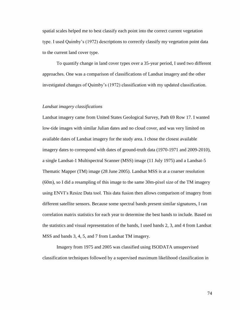
74

spatial scales helped me to best classify each point into the correct current vegetation

type. I used Quimby’s (1972) descriptions to correctly classify my vegetation point data

to the current land cover type.

To quantify change in land cover types over a 35-year period, I used two different

approaches. One was a comparison of classifications of Landsat imagery and the other

investigated changes of Quimby’s (1972) classification with my updated classification.

Landsat imagery classifications

Landsat imagery came from United States Geological Survey, Path 69 Row 17. I wanted

low-tide images with similar Julian dates and no cloud cover, and was very limited on

available dates of Landsat imagery for the study area. I chose the closest available

imagery dates to correspond with dates of ground-truth data (1970-1971 and 2009-2010),

a single Landsat-1 Multispectral Scanner (MSS) image (11 July 1975) and a Landsat-5

Thematic Mapper (TM) image (28 June 2005). Landsat MSS is at a coarser resolution

(60m), so I did a resampling of this image to the same 30m-pixel size of the TM imagery

using ENVI’s Resize Data tool. This data fusion then allows comparison of imagery from

different satellite sensors. Because some spectral bands present similar signatures, I ran

correlation matrix statistics for each year to determine the best bands to include. Based on

the statistics and visual representation of the bands, I used bands 2, 3, and 4 from Landsat

MSS and bands 3, 4, 5, and 7 from Landsat TM imagery.

Imagery from 1975 and 2005 was classified using ISODATA unsupervised

classification techniques followed by a supervised maximum likelihood classification in

75

Environment for Visualizing Images (ENVI) 4.8 software. From the ISODATA

classification, pure classes were identified and initially assigned one of twelve land cover

classifications: Mud, Type 3 Mud, Creeping alkali-grass, Large alkali-grass, Marsh

community, Floating marsh, Seaside arrow-grass, Bog, Alder, Marsh fringe, and

Ramenksi sedge and Water (permanent ponds). Many classes were mixed, and required

further rounds of ISODATA clustering to obtain pure classes of each type. In order to

avoid inaccurate representation of classes with overlapping spectral signatures and

smaller areas, I did not include Bog, Alder, Marsh fringe, and Ramenksi sedge

communities in the final classifications. Due to the similar species composition

(Appendix F) of some land cover classes, and therefore similar spectral signatures, I

lumped together Creeping alkali-grass and Large alkali-grass, as well as Marsh

community, Floating marsh, and Seaside arrow-grass for a more accurate analysis. The

elimination of some classes and the combination of others resulted in five final land cover

classes for analysis of Landsat imagery. I used the five-class data derived from the

ISODATA method as training data for the supervised classification.

To ensure that I chose the most accurate supervised classification, I performed

both a maximum likelihood and minimum distance supervised classification of the

imagery using ENVI 4.8. A maximum likelihood calculates the probability that a given

pixel belongs to a particular class. I applied a probability threshold of 0.1, which resulted

in a more accurate classification than a threshold of zero. The minimum distance uses the

mean vectors of each training data point and calculates the Euclidean distance from each

unknown pixel to the mean vector for each class, and each pixel is assigned to the closest

76

class. Overall accuracies of the classified images are based on an average of each the

class accuracies, and were used to determine preferred classification method.

1970 to 2005 land cover change

Within this comparison, I used two approaches to look at general change in land cover

type. First, I took the areas for each land cover class delineated by Quimby in 1970, and

compared overall change (in hectares) to those land classes in the current 2005

classification. Because the final land cover classes between years are not directly

comparable, the same class combinations were used as in the Landsat imagery

classification for 2005, and a few more classes were lumped for 1970 classification. For

the 1970 classification, I added Ramenski sedge, Bog, Alder, and Marsh fringe to the

Marsh community, Floating marsh, and seaside arrow-grass land cover class. There was

no Water category in 1970 classification, so Water was combined with the marsh-like

class in 2005. The final groupings resulted in four land cover classes for area

comparisons between 1970 and 2005.

The second approach provided more precise information on changes within each

individual land cover class. For this method I took a point to point approach, and

compared the 2005 land cover classification of each visited vegetation point to the 1970

land cover classification of each point; determining the percentage of points that

remained the same during the time period.

77

Results

Landsat imagery classifications

I ran an initial maximum likelihood supervised classification including all 11 classes,

resulting in an overall classification accuracy of 41.79%. Because of this low accuracy, I

ultimately grouped similar land cover types together according to species composition.

Consequently, I ended up using Mud, Type 3 Mud, Water, and 2 classes of mixed

vegetated community types (Table 3.1). Both the current vegetation type map of

Chickaloon Flats and estimated land cover class areas were derived from the 2005

maximum likelihood classification (86.31% overall accuracy; Figure 3.4). The 2005

classification provided updated information on the current land cover classes of

Chickaloon. Of the 9,533 ha used in this classification (Table 3.1), 5,250 ha (55.0%) are

classified as vegetated, 4,012 ha (42.1%) as Mud, and 271 ha (2.9%) as Water.

The 278 vegetated points were used to create a training data set for each class via

ISODATA clustering. The total area covered by all vegetation points was 867.1 ha,

which encompassed 33.0% of the area of Chickaloon, and ranged from 4.4 to 13.0%

coverage of a land cover class (Table 3.1). The points used for the Water class (15.0% of

class) were not ground-truthed, but assigned to areas of known permanent water (Table

3.1). Training data used for supervised classifications covered a range of 11.9 to 99.1% of

area of each of the land cover classes (Table 3.1).

Both overall accuracy and the Kappa coefficient are used in determining the best

classification method. The Kappa coefficient, scaled between 0 and 1, is used to test if the

classification map is significantly better than a randomly generated classification and

78

represents the proportion of agreement acquired after the chance agreement is removed

(Foody 1992). The maximum likelihood method resulted in the most accurate

classification for the current land cover of Chickaloon, with an overall accuracy of

86.31% and a Kappa coefficient of 0.8056 for the 2005 classification (Table 3.2). The

minimum distance was less accurate, with a 71.43% overall and 0.6151 Kappa. The 1975

classifications were extremely inaccurate (11.2% and 11.8%) for both supervised

methods (Table 3.2). Due to the poor accuracy of the 1975 imagery, I did not compute

change statistics using 1975 and 2005 Landsat imagery.

The class confusion matrix of each year and supervised classification method

demonstrate where the errors in classification lie. The matrices for 1975 (Table 3.3)

indicate that most of the inaccuracies are associated with the misidentification of points

to the AG-LG class. This class represented the vast majority of the total area of

Chickaloon in the 1975 Landsat classifications, so most points were classified as such,

even though ground-truth data characterized the points in a different land cover type. Due

to better accuracy of the 2005 classifications, the 2005 matrices provide more useful

information for each land cover class (Table 3.3). The 2005 maximum likelihood

classification shows that the Marsh community-Floating marsh-Seaside arrow-grass,

Mud, and Water land cover types had high accuracies (Table 3.3), while the two

remaining class types, Type 3 Mud and Creeping alkali-grass-Large alkali-grass, had

moderate accuracies. The misidentifications of points amongst these two classes (Table

3.3) are mainly from AG-LG points misclassified as MC-FM-SG land cover type, and

3M points misclassified as AG-LG type.

79

Quimby to Ulman comparison

The comparison of land cover class areas from 1970 (ground-truthed aerial photos) to

2005 (supervised classification) indicated a loss of total area in 3 of the 4 land cover

classes, while the Creeping alkali-grass and Large alkali-grass type increased in area

(Table 3.4). This land cover type increased by 16.8%, while the others decreased from

2.5 to 7.3% (Table 3.4).

I collected species composition and coverage information at 278 vegetation

points, and reclassified many of the points from the 1970–1971 characterization derived

from digitized aerial photos (Table 3.5). For example, across all 4 plots, I visited 40

randomly selected points within the 1970–1971 characterized Type 3 Mud land cover

class. Of these 40 points, I classified only 11 points (27.5%) as Type 3 Mud in 2009–

2010, and reclassified the other 29 (72.5%) to different vegetation land cover types

(Appendix G). For these point to point comparisons I looked at change among 8

individual vegetation land classes, which ranged from 19.4% to 91.8% (Table 3.5).

Large alkali-grass had the least amount of change from 1970–1971 to 2009–2010, with

19.4 %. Most of the change (13.2%) was to unvegetated mud classes, with the remaining

to the closely associated Creeping alkali-grass type. Floating marsh had 21.4% change to

the more landward land class types of either Bog or Alder. Less than half of Mud

changed; 42.1% to the vegetated classes of Large alkali-grass (31.6%) and Creeping

alkali-grass (10.5%), and only 1.8% to unvegetated Type 3 Mud. About half of Creeping

alkali-grass type changed, mainly to Large alkali-grass (29.6%). Seaside arrow-grass

changed to both landward (43.3%) and seaward (16.7%) land cover types. Most of the

80

change for Marsh community was to Floating marsh (39.4%), with the others spread

across vegetated (18.2%) and unvegetated (3%) land cover types. Type 3 Mud had a

significant amount (65%) of points that changed to Large alkali-grass type and 7.5%

across Mud or Ramenski sedge. The class with the most change was Ramenski sedge,

with only 8.2% of points unchanged. The majority (81.6%) of Ramenski sedge changed

to other vegetated land cover types, with 10.2% to unvegetated mud classes.

Discussion

My inability to discriminate unique spectral signatures between all original land

cover classes and the extreme inaccuracies of the 1975 supervised classification did not

allow for a detailed and robust land cover type change analysis. The types described by

Quimby (1972) included many with similar species and mud composition, which resulted

in overlapping spectral signatures. Unlike upland plant communities, the effective

quantification of wetlands through remote sensing is challenging due to the spatial

distribution and diverse species composition (Ozesmi and Bauer 2002). The land cover

types with overlapping signatures had to be grouped together to ensure a more accurate

classification (Jensen 1996), which resulted in a coarser classification.

I chose to lump several classes together based on mud and vegetation cover

characteristics. Joining classes of similar structure helped alleviate the troubles of spectral

signature overlap and improve classification accuracy. The final classification using

Landsat imagery resulted in five combined land cover types, which is not directly

comparable to that of Quimby’s, but is the most accurate current land cover classification

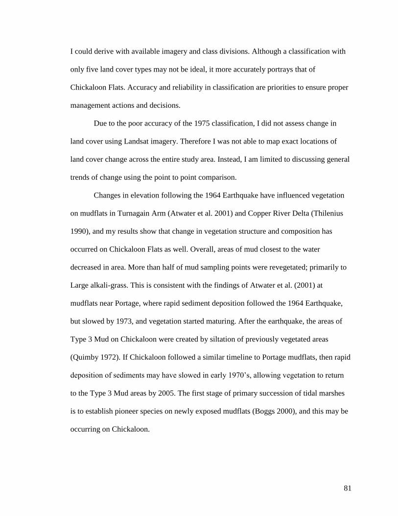
81

I could derive with available imagery and class divisions. Although a classification with

only five land cover types may not be ideal, it more accurately portrays that of

Chickaloon Flats. Accuracy and reliability in classification are priorities to ensure proper

management actions and decisions.

Due to the poor accuracy of the 1975 classification, I did not assess change in

land cover using Landsat imagery. Therefore I was not able to map exact locations of

land cover change across the entire study area. Instead, I am limited to discussing general

trends of change using the point to point comparison.

Changes in elevation following the 1964 Earthquake have influenced vegetation

on mudflats in Turnagain Arm (Atwater et al. 2001) and Copper River Delta (Thilenius

1990), and my results show that change in vegetation structure and composition has

occurred on Chickaloon Flats as well. Overall, areas of mud closest to the water

decreased in area. More than half of mud sampling points were revegetated; primarily to

Large alkali-grass. This is consistent with the findings of Atwater et al. (2001) at

mudflats near Portage, where rapid sediment deposition followed the 1964 Earthquake,

but slowed by 1973, and vegetation started maturing. After the earthquake, the areas of

Type 3 Mud on Chickaloon were created by siltation of previously vegetated areas

(Quimby 1972). If Chickaloon followed a similar timeline to Portage mudflats, then rapid

deposition of sediments may have slowed in early 1970’s, allowing vegetation to return

to the Type 3 Mud areas by 2005. The first stage of primary succession of tidal marshes

is to establish pioneer species on newly exposed mudflats (Boggs 2000), and this may be

occurring on Chickaloon.

82

More inland vegetated classes increased in area over the 35-year period. Of these

two types, Large alkali-grass occupied the largest area (Quimby 1972) and changed the

least, while Creeping alkali-grass changed to both inland and seaward land classes. The

most inland land cover types representing the more stable marsh-like communities

decreased in area as a whole. The overall direction of vegetation change within this land

cover class was toward the less established, early successional (Neiland 1971, Quimby

1972) seaward communities. Quimby (1972) demonstrated that Creeping alkali grass

established in marsh areas that had been silted over following subsidence from the

earthquake, and that the Marsh community was more extensive prior to the earthquake,

and may be continuing to decrease due to drainage of permanent and semi-permanent

ponds. Quimby (1972) indicated that the overall effect of the earthquake on vegetation

was to promote early successional plant communities (Creeping alkali-grass) while

decreasing more stable plant communities (Marsh community), and my results support

this observation.

In addition to the post-earthquake subsidence and uplift, sediment accretion may

also change elevation, and thereby influence vegetation structure on Chickaloon. Rates of

sediment accretion are higher in vegetated areas, because plants slow the water and trap

sediments (Boggs 2000), and siltation will continue to increase land elevation relative to

mean high tide (Thilenius 1990, Boggs 2000). Although the rapid deposition has ceased,

annual siltation of the mudflats continues, and is positively correlated with frequency of

flooding events (Vince and Snow 1984). Quimby (1972) measured silt deposition of

several locations within Type 3 Mud during the peak flooding months of August and

83

September 1970, and found silt deposits ranged from 6.4mm to 25.4 mm. This

considerable amount of siltation could still be within the rapid deposition time frame

following the earthquake, but indicates that silt accretion can play a dynamic role in

vegetation structure of Chickaloon. As land elevation increases from siltation, this alters

the frequency and locations of tidal inundations (Boggs 2000), which in turn can change

vegetation structure and composition (Neiland 1971).

In addition to changes elevation may cause, the patterns of vegetation on

Chickaloon are largely due to tides, and salt water and fresh water interactions (Neiland

1971, Quimby 1972). Neiland (1971) presented five physical factors that affect

vegetation: 1) duration and number of times of inundation; 2) amount and duration of

water retained; 3) location and rate of cutting by drainage ditches; 4) amounts of salt and

fresh water received and retained; and 5) erosion and deposition rates of sediments. I

found a temporal and spatial variation in tidal inundation from extreme tide events

(Appendix H), which may have partially affected the patterns of vegetation currently on

Chickaloon. Tidal inundations of vegetated areas are infrequent, which may be

compounded by an increase in elevation due to sediment accretion. Because duration of

tidal flooding is a dominant factor in salt marsh salinity (Mahall and Park 1976),

vegetation types with more salt-tolerant species may not be receiving enough tidal

inundation, and may be converting to areas containing no plants or less salt-tolerant plant

species. If infrequency of tidal inundations causes a decrease in alkali-tolerant species, I

should see an overall decrease in alkali-dominated land cover types. My results actually

show the opposite, with an overall increase (16.8%) in land cover classes with salt-

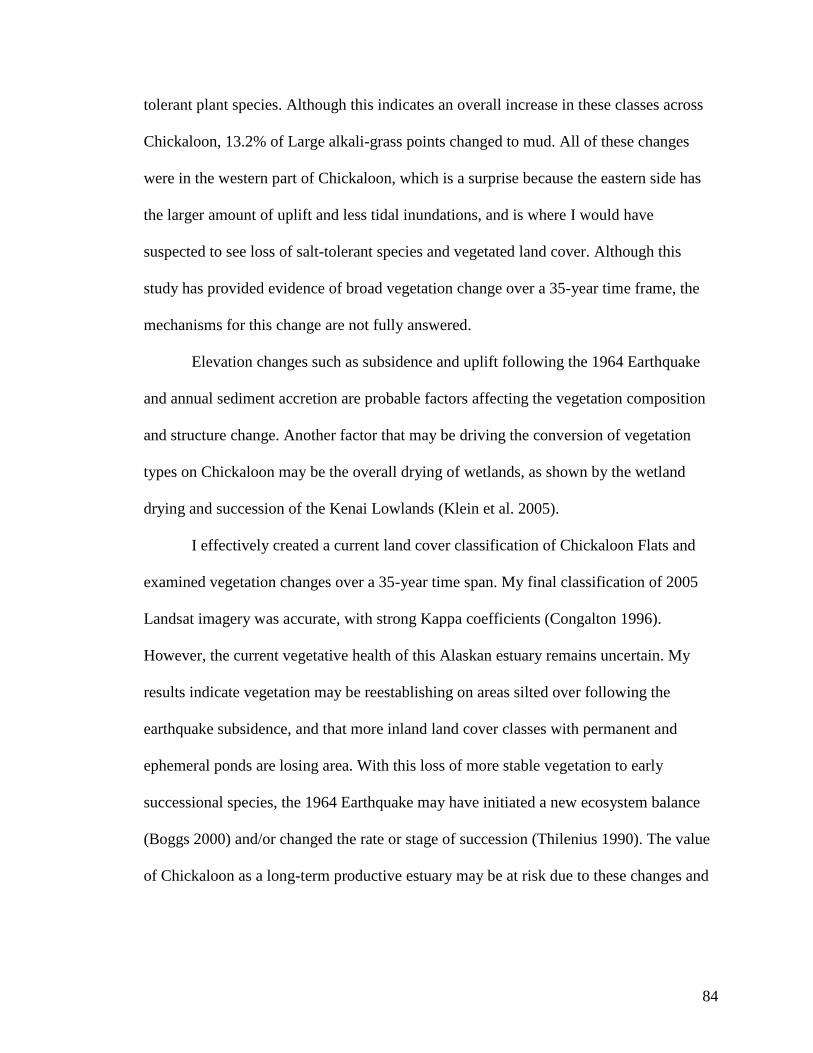
84

tolerant plant species. Although this indicates an overall increase in these classes across

Chickaloon, 13.2% of Large alkali-grass points changed to mud. All of these changes

were in the western part of Chickaloon, which is a surprise because the eastern side has

the larger amount of uplift and less tidal inundations, and is where I would have

suspected to see loss of salt-tolerant species and vegetated land cover. Although this

study has provided evidence of broad vegetation change over a 35-year time frame, the

mechanisms for this change are not fully answered.

Elevation changes such as subsidence and uplift following the 1964 Earthquake

and annual sediment accretion are probable factors affecting the vegetation composition

and structure change. Another factor that may be driving the conversion of vegetation

types on Chickaloon may be the overall drying of wetlands, as shown by the wetland

drying and succession of the Kenai Lowlands (Klein et al. 2005).

I effectively created a current land cover classification of Chickaloon Flats and

examined vegetation changes over a 35-year time span. My final classification of 2005

Landsat imagery was accurate, with strong Kappa coefficients (Congalton 1996).

However, the current vegetative health of this Alaskan estuary remains uncertain. My

results indicate vegetation may be reestablishing on areas silted over following the

earthquake subsidence, and that more inland land cover classes with permanent and

ephemeral ponds are losing area. With this loss of more stable vegetation to early

successional species, the 1964 Earthquake may have initiated a new ecosystem balance

(Boggs 2000) and/or changed the rate or stage of succession (Thilenius 1990). The value

of Chickaloon as a long-term productive estuary may be at risk due to these changes and

85

loss of marsh, or there may be no risk at all if Chickaloon has been reset on the rate and

stage of succession. Chickaloon Flats is currently and has been historically used by a

diversity of avian species for both a migratory stopover and breeding site, and the change

in vegetation over a 35-year timeframe may not alter the overall importance and value of

this area to avian species.

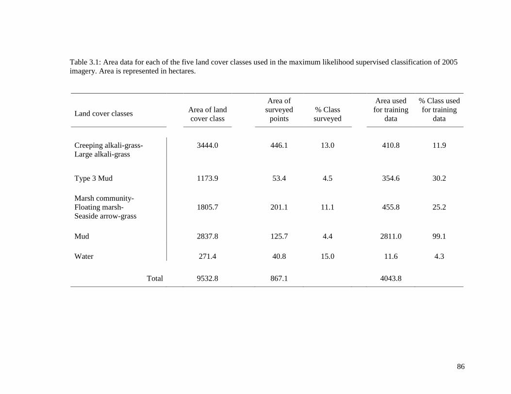
86

Table 3.1: Area data for each of the five land cover classes used in the maximum likelihood supervised classification of 2005

imagery. Area is represented in hectares.

Land cover classes

Area of land

cover class

Area of

surveyed

points

% Class

surveyed

Area used

for training

data

% Class used

for training

data

Creeping alkali-grass-

Large alkali-grass

3444.0

446.1

13.0

410.8

11.9

Type 3 Mud 1173.9 53.4 4.5 354.6 30.2

Marsh community-

Floating marsh-

Seaside arrow-grass

1805.7

201.1

11.1

455.8

25.2

Mud 2837.8 125.7 4.4 2811.0 99.1

Water 271.4 40.8 15.0 11.6 4.3

Total 9532.8 867.1 4043.8

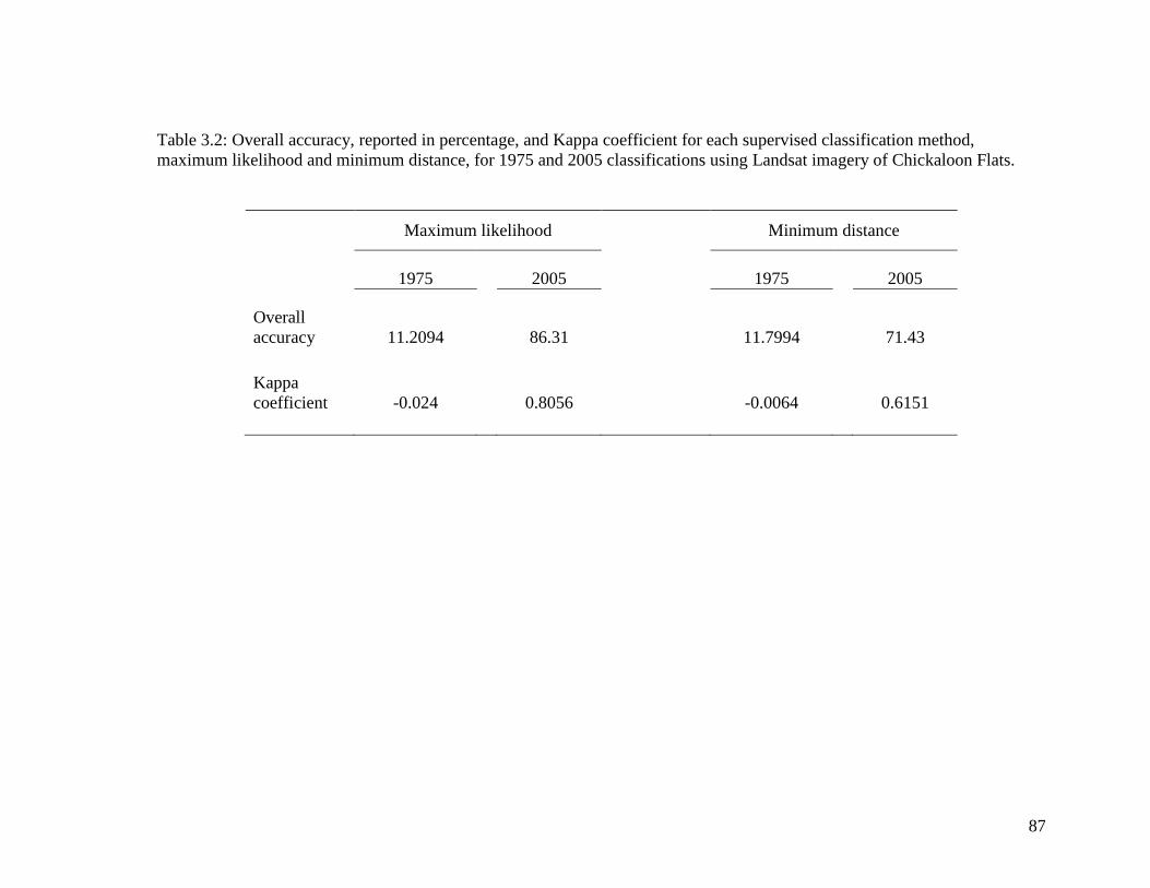
87

Table 3.2: Overall accuracy, reported in percentage, and Kappa coefficient for each supervised classification method,

maximum likelihood and minimum distance, for 1975 and 2005 classifications using Landsat imagery of Chickaloon Flats.

Maximum likelihood Minimum distance

1975 2005 1975 2005

Overall

accuracy 11.2094 86.31 11.7994 71.43

Kappa

coefficient -0.024 0.8056 -0.0064 0.6151

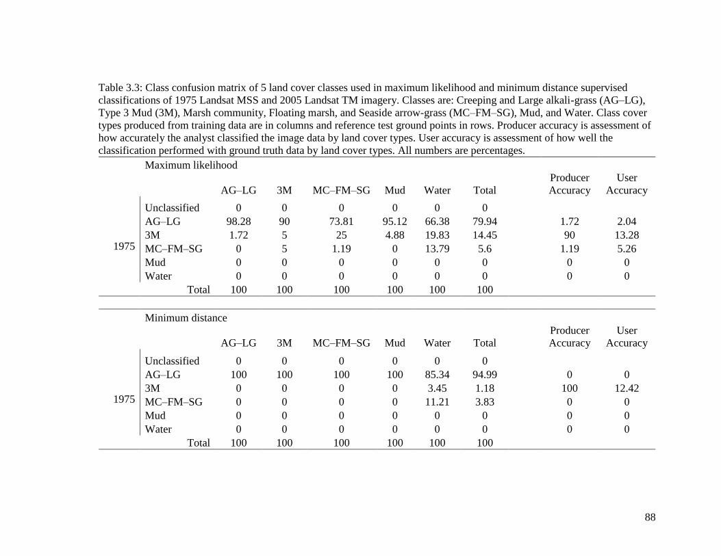
88

Table 3.3: Class confusion matrix of 5 land cover classes used in maximum likelihood and minimum distance supervised

classifications of 1975 Landsat MSS and 2005 Landsat TM imagery. Classes are: Creeping and Large alkali-grass (AG–LG),

Type 3 Mud (3M), Marsh community, Floating marsh, and Seaside arrow-grass (MC–FM–SG), Mud, and Water. Class cover

types produced from training data are in columns and reference test ground points in rows. Producer accuracy is assessment of

how accurately the analyst classified the image data by land cover types. User accuracy is assessment of how well the

classification performed with ground truth data by land cover types. All numbers are percentages.

Maximum likelihood

AG–LG 3M MC–FM–SG Mud Water Total

Producer

Accuracy

User

Accuracy

1975

Unclassified 0 0 0 0 0 0

AG–LG 98.28 90 73.81 95.12 66.38 79.94 1.72 2.04

3M 1.72 5 25 4.88 19.83 14.45 90 13.28

MC–FM–SG 0 5 1.19 0 13.79 5.6 1.19 5.26

Mud 0 0 0 0 0 0 0 0

Water 0 0 0 0 0 0 0 0

Total 100 100 100 100 100 100

Minimum distance


Producer

Accuracy

User

Accuracy

1975


AG–LG 100 100 100 100 85.34 94.99 0 0

3M 0 0 0 0 3.45 1.18 100 12.42

MC–FM–SG 0 0 0 0 11.21 3.83 0 0

Mud 0 0 0 0 0 0 0 0

Water 0 0 0 0 0 0 0 0

Total 100 100 100 100 100 100

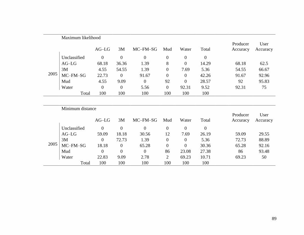
89

Maximum likelihood


Producer

Accuracy

User

Accuracy

2005


AG–LG 68.18 36.36 1.39 8 0 14.29 68.18 62.5

3M 4.55 54.55 1.39 0 7.69 5.36 54.55 66.67

MC–FM–SG 22.73 0 91.67 0 0 42.26 91.67 92.96

Mud 4.55 9.09 0 92 0 28.57 92 95.83

Water 0 0 5.56 0 92.31 9.52 92.31 75

Total 100 100 100 100 100 100

Minimum distance


Producer

Accuracy

User

Accuracy

2005


AG–LG 59.09 18.18 30.56 12 7.69 26.19 59.09 29.55

3M 0 72.73 1.39 0 0 5.36 72.73 88.89

MC–FM–SG 18.18 0 65.28 0 0 30.36 65.28 92.16

Mud 0 0 0 86 23.08 27.38 86 93.48

Water 22.83 9.09 2.78 2 69.23 10.71 69.23 50

Total 100 100 100 100 100 100

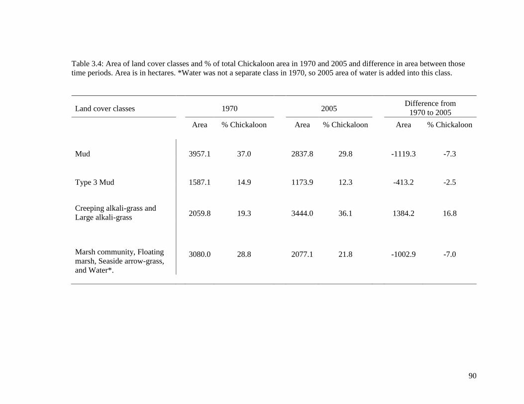
90

Table 3.4: Area of land cover classes and % of total Chickaloon area in 1970 and 2005 and difference in area between those

time periods. Area is in hectares. *Water was not a separate class in 1970, so 2005 area of water is added into this class.

Land cover classes 1970 2005

Difference from

1970 to 2005

Area % Chickaloon Area % Chickaloon Area % Chickaloon

Mud 3957.1 37.0 2837.8 29.8 -1119.3 -7.3

Type 3 Mud 1587.1 14.9 1173.9 12.3 -413.2 -2.5

Creeping alkali-grass and

Large alkali-grass 2059.8 19.3 3444.0 36.1 1384.2 16.8

Marsh community, Floating

marsh, Seaside arrow-grass,

and Water*.

3080.0 28.8 2077.1 21.8 -1002.9 -7.0

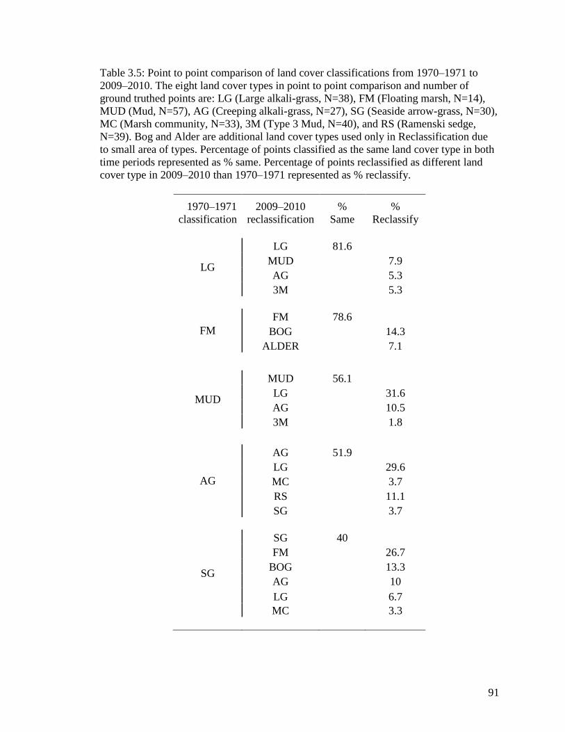
91

Table 3.5: Point to point comparison of land cover classifications from 1970–1971 to

2009–2010. The eight land cover types in point to point comparison and number of

ground truthed points are: LG (Large alkali-grass, N=38), FM (Floating marsh, N=14),

MUD (Mud, N=57), AG (Creeping alkali-grass, N=27), SG (Seaside arrow-grass, N=30),

MC (Marsh community, N=33), 3M (Type 3 Mud, N=40), and RS (Ramenski sedge,

N=39). Bog and Alder are additional land cover types used only in Reclassification due

to small area of types. Percentage of points classified as the same land cover type in both

time periods represented as % same. Percentage of points reclassified as different land

cover type in 2009–2010 than 1970–1971 represented as % reclassify.

1970–1971

classification

2009–2010

reclassification

%

Same

%

Reclassify

LG

LG 81.6

MUD 7.9

AG 5.3

3M 5.3

FM

FM 78.6

BOG 14.3

ALDER 7.1

MUD

MUD 56.1

LG 31.6

AG 10.5

3M 1.8

AG

AG 51.9

LG 29.6

MC 3.7

RS 11.1

SG 3.7

SG

SG 40

FM 26.7

BOG 13.3

AG 10

LG 6.7

MC 3.3

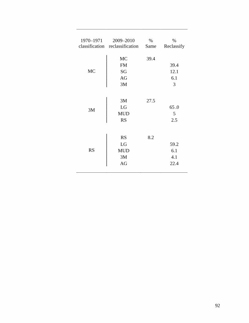
92

1970–1971

classification

2009–2010

reclassification

%

Same

%

Reclassify

MC

MC 39.4

FM 39.4

SG 12.1

AG 6.1

3M 3

3M

3M 27.5

LG 65 .0

MUD 5

RS 2.5

RS

RS 8.2

LG 59.2

MUD 6.1

3M 4.1

AG 22.4

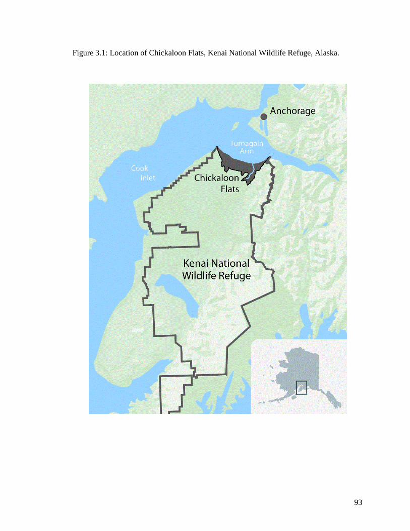
93

Figure 3.1: Location of Chickaloon Flats, Kenai National Wildlife Refuge, Alaska.

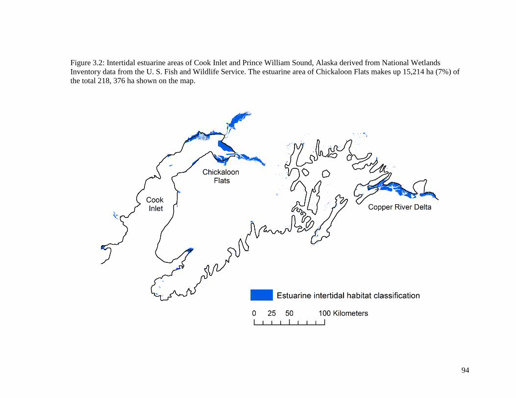
94

Figure 3.2: Intertidal estuarine areas of Cook Inlet and Prince William Sound, Alaska derived from National Wetlands

Inventory data from the U. S. Fish and Wildlife Service. The estuarine area of Chickaloon Flats makes up 15,214 ha (7%) of

the total 218, 376 ha shown on the map.

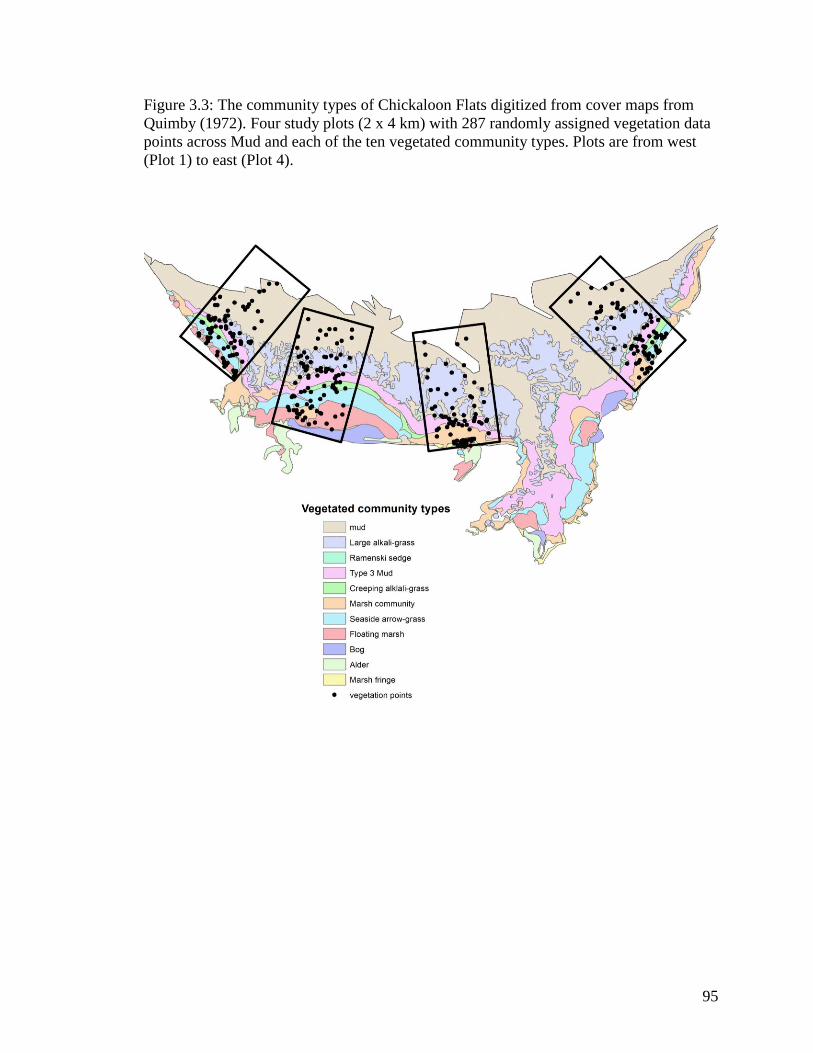
95

Figure 3.3: The community types of Chickaloon Flats digitized from cover maps from

Quimby (1972). Four study plots (2 x 4 km) with 287 randomly assigned vegetation data

points across Mud and each of the ten vegetated community types. Plots are from west

(Plot 1) to east (Plot 4).

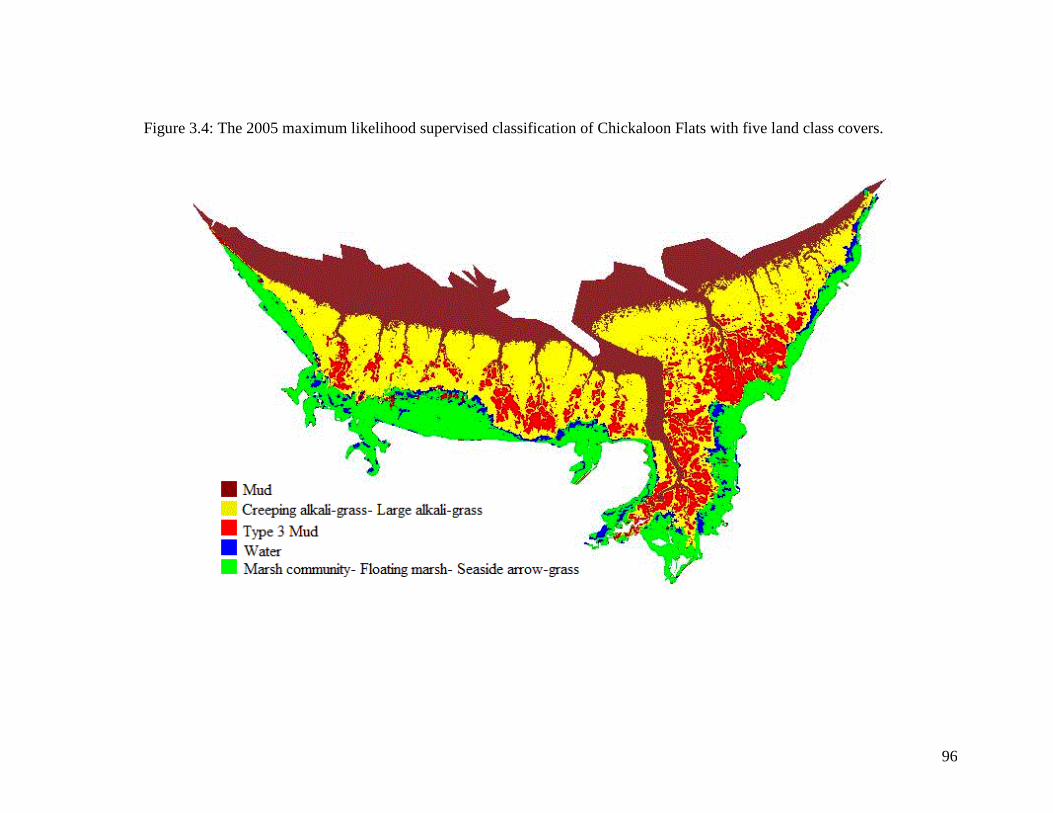
96

Figure 3.4: The 2005 maximum likelihood supervised classification of Chickaloon Flats with five land class covers.

97

LITERATURE CITED

Alaska Department of Fish and Game (ADF&G), Alaska Department of Natural

Resources, U.S. Forest Service, U.S. Department of the Interior Bureau of Sport

Fisheries and Wildlife. 1972. Memorandum of Understanding-Chickaloon Flats

Management Agreement.

Alaska Shorebird Group. 2000. A Conservation Plan for Alaska Shorebirds. Version 1.0.

Alaska Shorebird Group, Anchorage, Alaska, USA.

Alaska Shorebird Group. 2008. Alaska Shorebird Conservation Plan. Version II. Alaska

Shorebird Group, Anchorage, Alaska.

Alisauskas, R. T., E. E. Klaas, K. A. Hobson, and C. D. Ankney. 1998. Stable-carbon

isotopes support use of adventitious color to discern winter origins of lesser snow

geese. Journal of Field Ornithology 69:262–268.

Amundson, R., A. T. Austin, E. A. G. Schuur, K. Yoo, V. Matzek, C. Kendall, A.

Uebersax, D. Brenner, and W. T. Baisden. 2003. Global patterns of the isotopic

composition of soil and plant nitrogen. Global Biogeochemical Cycles 17:1031.

Ashley, P., K. A. Hobson, S. L. Van Wilgenburg, N. North, and S. A. Petrie. 2010.

Linking Canadian harvested juvenile American black ducks to their natal areas

using stable isotope (D, 13

C, and 15

N) methods. Avian Conservation and

Ecology 5:7.

98

Atkinson, P. W., A. J. Baker, R. M. Bevan, N. A. Clark, K. B. Cole, P. M. Gonzalez, J.

Newton, L. J. Niles, and R. A. Robinson. 2005. Unraveling the migration and

moult strategies of a long-distance migrant using stable isotopes: Red Knot

Calidris canutus movements in the Americas. Ibis 147:738–749.

Atwater, B. F., D. K. Yamaguchi, S. Bondevik, W. A. Barnhardt, L. J. Amidon, B. E.

Benson, G. Skjerdal, J. A. Shulene, and F. Nanayama. 2001. Rapid resetting of an

estuarine recorder of the 1964 Alaska earthquake. Geology Society of America

Bulletin 113: 1193-1204.

Austin, A. T. and P. M. Vitousek. 1998. Nutrient dynamics on a precipitation gradient in

Hawaii. Oecologia 113:519–529.

Bartsch-Winkler, S. and A. T. Ovenshine. 1984. Macrotidal subarctic environment of

Turnagain and Knik Arms, Upper Cook Inlet, Alaska: sedimentology of the

intertidal zone. Journal of Sedimentary Petrology 54:122–1238.

Bearhop, S., S. Waldron, S. C. Votier, and R. W. Furness. 2002. Factors that influence

assimilation rates and fractionation of nitrogen and carbon stable isotopes in avian

blood and feathers. Physiological and Biochemical Zoology 75:451–458.

Bearhop, S., R. W. Furness, G. M. Hilton, S. C. Votier, and S. Waldron. 2003. A forensic

approach to understanding diet and habitat use from stable isotope analysis of

(avian) claw material. Functional Ecology 17:270–275.

Bibby, C. J. 2003. Conservation of Migratory Birds. pp. 407–420 in P. Berthold, E.

Gwinner and E. Sonnenschein (eds.). Avian Migration. Springer-Verlag Berlin

Deidelberg, Germany.

99

Bibby, C. J., and N. D. Burgess. 2000. Bird Census Techniques. Academic Press,

Burlington, Massachusetts, USA.

Bishop, M., P. M. Meyers, and P. F. McNeley. 2000. A method to estimate migrant

shorebird numbers on the Copper River Delta. Journal of Field Ornithology

71:627–637.

Boggs, K. 2000. Classification of community types, successional sequences, and

landscapes of the Copper River Delta, Alaska. General Technical Report PNW-

GTR-469. Portland, OR: U. S. Department of Agriculture, Forest Service, Pacific

Northwest Research Station. 244 p.

Boggs, K. and M. Shephard. 1999. Response of marine deltaic surfaces to major

earthquake uplifts in southcentral Alaska. Wetlands 19:13-27.

Bowen, G. J., L. I. Wassenaar, and K. A. Hobson. 2005. Global application of stable

hydrogen and oxygen isotopes to wildlife forensics. Oecologia 143:337–348.

Butler, R. W., N. C. Davidson, and R. I. G. Morrison. 2001. Global-scale shorebird

distribution in relation to productivity of near-shore ocean waters. The

International Journal of Waterbird Biology 24:224–232.

Caccamise, D. F., L. M. Reed, P. M. Castelli, S. Wainright, and T. C. Nichols. 2000.

Distinguishing migratory and resident Canada geese using stable isotope analysis.

Journal of Wildlife Management 64:1084–1091.

Canales, A. G. 1996. Migratory bird activity in the bay of Lake Titicaca, Puno, Peru.

International Wader Studies 8:62.

100

Castro G., and J. P. Myers. 1993. Shorebird predation on eggs of horseshoe crabs during

spring stopover on Delaware Bay. Auk 110:927–930.

Chamberlain C. P., J. D. Blum, R. T. Holmes, X. Feng, T. W. Sherry, and G. R. Graves.

1997. The use of isotope tracers for identifying populations of migratory birds.

Oecologia 109:132–141.

Chamberlain, C. P., S. Bensch, X. Feng, S. Akesson, and T. Andersson. 2000. Stable

isotopes examined across a migratory divide in Scandinavian willow warblers

(Phylloscopus trochilus trochilus and Phylloscopus trochilus acredula) reflect

their African winter quarters. Proceedings of the Royal Society of London Series

B-Biological Sciences. 267:43–48.

Christensen, H. H., L. Mastrantonio, J. C. Gordon, and B. T. Bormann. 2000. Alaska’s

Copper River: humankind in a changing world. General Technical Report PNW-

GTR-480. Portland, OR: U. S. Department of Agriculture, Forest Service, Pacific

Northwest Research Station. 20 p.

Clark R. G., K. A. Hobson, and L. I. Wassenaar. 2006. Geographic variation in isotopic

(δ13

C, δ15

N, δD) composition of feathers and claws from lesser scaup and

northern pintail: implications for studies of migratory connectivity. Canadian

Journal of Zoology 84:1395–1401.

Clay, R. P., A. J. Lesterhuis, and S. Centrón. 2012. Conservation Plan for the Lesser

Yellowlegs (Tringa flavipes). Version 1.0. Manomet Center for Conservation

Sciences, Manomet, Massachusetts.

101

Colwell, M. 2010. Shorebird Ecology, Conservation, and Management. University of

California Press. Berkeley and Los Angeles, California.

Committee on the Alaska Earthquake of the Division of Earth Sciences National

Research Council. 1973. The Great Alaska Earthquake of 1964. National

Academy of Sciences, Washington D.C., USA.

Congalton, R. G. 1996. Accuracy Assessment: A Critical Component of Land Cover

Mapping. Pages 19–131 in Gap Analysis: a landscape approach to biodiversity

planning. J. M. Scott, T. H. Tear, and F. W. Davis, eds. American Society for

Photogrammetry and Remote Sensing, Bethesda, Maryland.

Connors, P. G., J. P. Myers, and F. A. Pitelka. 1979. Seasonal habitat use by arctic

Alaskan shorebirds. Studies in Avian Biology 2:101–111.

Cramp, S., and K. E. L. Simmons. 1983. Handbook of the birds of Europe, the Middle

East and North Africa: the birds of the western palearctic. Volume 3. Oxford

University Press, Oxford, United Kingdom.

Doherty, J. P. 2009. A modern, portable drop net can safely capture a suite of shorebirds.

Waterbirds 32:472– 475.

Dunn E. H., K. A. Hobson, L. I. Wassennar, D. J. T. Hussell, and M. L. Allen. 2006.

Identification of summer origins of songbirds migrating through southern Canada

in autumn. Avian Conservation and Ecology 1:4.

Elphick, C. S., and T. L. Tibbitts. 1998. Greater Yellowlegs (Tringa melanoleuca), The

102

Birds of North America Online (A. Poole, Ed.). Ithaca: Cornell Lab of

Ornithology; Retrieved from the Birds of North America Online:

http://bna.birds.cornell.edu.bnaproxy.birds.cornell.edu/bna/species/355

doi:10.2173/bna.355.

ESRI. 2011. ArcGIS Desktop: Release 10. Redlands, California: Environmental Systems

Research Institute.

Evans-Ogden, L. J., K. A. Hobson, D. B. Lank, and S. Bittman. 2005. Stable isotope

analysis reveals that agricultural habitat provides an important dietary component

for nonbreeding Dunlin. Avian Conservation and Ecology 1:3.

Evans-Ogden, L. J., S. Bittman, and D. B. Lank. 2008. A review of agricultural land use

by shorebirds with special reference to habitat conservation in the Fraser River

Delta, British Columbia. Canadian Journal of Plant Science 88:71–83.

Farmer, A. H., and A. H. Parent. 1997. Effects of the landscape on shorebird movements

at spring migration stopovers. The Condor 99:698–707.

Farmer, A., B. S. Cade, and J. Torres-Dowdall. 2008. Fundamental limits to the accuracy

of deuterium isotopes for identifying the spatial origin of migratory animals.


Fiske, I. and R. Chandler. 2011. unmarked: An R package for fitting hierarchical models

of wildlife occurrence and abundance. Journal of Statistical Software. 43:1–23.

URL http://www.jstatsoft.org/v43/i10/.

Foody, G. 1992. On the compensation for chance agreement in image classification

103

accuracy assessment. Photogrammetric Engineering and Remote Sensing

58:1459–1460.

Freymueller, J. T., H. Woodard, S. Cohen, R. Cross, J. Elliott, C. Larsen, S. Hreinsdottir,

and C. Zweck. 2008. Active deformation processes in Alaska, based on 15 years

of GPS measurements. Pages 1–42 in Active Tectonics and Seismic Potential of

Alaska. J. T. Freymueller, P. J. Haeussler, R. Wesson, and G. Ekstrom, eds.

Fry, B., and E. B. Sherr. 1989. δ13

C measurements as indicators of carbon flow in marine

and freshwater ecosystems. Pages 196–229 in Stable isotopes in ecological

research. P. W. Rundel, J. R. Ehleringer, and K. A. Nagy, eds. Springer-Verlag.

Berlin, Germany.

Gallant, A. L., E. F. Binnian, J. M. Omernik, and M. B. Shasby. 1995. Ecoregions of

Alaska. U. S. Geological Survey Professional Paper 1567, Washington D. C. 73

pp.

Gibson, D. D., R. E. Gill Jr., S. C. Heinl, A. J. Lang, T. G. Tobish Jr., and J. J. Withrow.

2012. Checklist of Alaska birds. 18th

edition. University of Alaska museum,

Fairbanks, AK.

Gill Jr., R. and P. D. Jorgenson. 1979. A preliminary assessment of timing and migration

of shorebirds along the northcentral Alaska Peninsula. Pages 113-123 in

Shorebirds in marine environments. Studies in avian biology, no. 2. F. A. Pitelka,

ed. Cooper Ornithological Society, Lawrence, Kansas.

104

Gill Jr., R. E., and T. L. Tibbitts. 1999. Seasonal shorebird use of intertidal habitats in

Cook Inlet, Alaska. Final report. U.S. Department of the Interior, U.S. Geological

Survey, Biological Resources Division and OCS Study, MMS 99–0012. 55 p.

Goss-Custard, J. D. 1969. The winter feeding ecology of the Redshank Tringa tetanus.

Ibis 111:338–356.

Gregory, R. D., D. W. Gibbons, and P. F. Donald. 2004. Bird census and survey

techniques. Pages 17–57 in Bird Ecology and Conservation. W. J. Sutherland, I.

Newton, and R. E. Green, eds. Oxford University Press Inc., New York, USA.

Haig, S. M., D. W. Mehlman, and L. W. Oring. 1998. Avian movements and wetland

connectivity in landscape conservation. Conservation Biology 12:749–758.

Handley, L. L., A. T. Austin, D. Robinson, C. M. Scrimgeour, J. A. Raven, T. H. E.

Heaton, S. Schmidt, and G. R. Stewart. 1999. The N-15 natural abundance (δN-

15) of ecosystem samples reflects measures of water availability. Australian

Journal of Plant Physiology. 26:185–199.

Hebert, C. E., and L. I. Wassenaar. 2005. Feather stable isotopes in western North

American waterfowl: spatial patterns, underlying factors, and management

implications. Wildlife Society Bulletin 33:92–102.

Heppleston, P. R. 1971. The feeding ecology of Oystercatchers (Haematopus ostralegus

L.) in winter in northern Scotland. Journal of Animal Ecology 40:651–672.

Hicks, S. D., and M. W. Szabados. 2006. Understanding tides. Center for Operational

Oceanographic Products and Services. 83 p.

105

Higgins, P. J., and S. J. J. F. Davies. 1996. Handbook of Australian, New Zealand, and

Antarctic birds. Oxford University Press, Melbourne.

Hobson, K. A. 1999a. Tracing origins and migration of wildlife using stable isotopes: a

review. Oecologia 120:314–326.

Hobson, K. A. 1999b. Stable-carbon and nitrogen isotope ratios of songbird feathers

grown in two terrestrial biomes: implications for evaluating trophic relationships

and breeding origins. Condor 101:799–805.

Hobson, K. A. 2005. Using stable isotopes to trace long-distance dispersal in birds and

other taxa. Diversity and Distribution 11:157–164.

Hobson, K. A., and L. I. Wassenaar. 1997. Linking breeding and wintering grounds of

Neotropical migrant songbirds using stable hydrogen isotope analysis of feathers.


Hobson, K. A., and L. I. Wassenaar. 2008. Tracking animal migration with stable

isotopes. Academic Press, Oxford.

Hobson, K. A., and S. G. Sealy. 1991. Marine protein contributions to the diet of northern

saw-whet owls on the Queen Charlotte Islands: a stable isotope approach. Auk

108:437–440.

Hobson, K. A., K. P. McFarland, L. I. Wassenaar, C. C. Rimmer, and J. E. Goetz. 2001.

Linking breeding and wintering grounds of Bicknell’s thrushes using stable

isotope analyses of feathers. Auk 118:16–23.

Hobson, K. A., S. Van Wilgenburg, L. I. Wassenaar, H. Hands, W. P. Johnson, M.

O'Meilia, and P. Taylor. 2006. Using stable isotope analysis of feathers to

106

delineate origins of harvested sandhill cranes in the central flyway of North

America. Waterbirds 29:137–147.

Hobson, K. A., S. Van Wilgenburg, L. I. Wassenaar, F. Moore, J. Farrington J. 2007.

Estimating origins of three species of Neotropical migrants at a Gulf coast

stopover site: combining stable isotope and GIS tools. Condor 109:256–267.

Hobson, K. A., R. Greenberg, S. L. Van Wilgenburg, and C. Mettke-Hofmann. 2010.

Migratory connectivity in the rusty blackbird: isotopic evidence from feathers of

historical and contemporary specimens. Condor 112:778–788.

Holmes, R. T. and F. A. Pitelka. 1998. Pectoral Sandpiper (Calidris melanotos), The




doi:10.2173/bna.348.

Hötker, H., A. E. Lebedev, P. S. Tomkovich, A. J. Gromadzk, N. C. Davidson, J. Evans,

D. A. Stroud, and R. B. West. 1998. Migration and international conservation of

waders: Research and conservation on north Asian, African, and European

flyways. International Wader Studies 10:1–526.

Hultén, E. 1968. Flora of Alaska and neighboring Territories. Stanford University Press,

Stanford, California.

Inger, R., and S. Bearhop. 2008. Applications of stable isotope analyses to avian ecology.

Ibis 150:447–461.

107

Isleib, M. E. 1979. Migratory shorebird populations on the Copper River Delta and

eastern Prince William Sound, Alaska. Studies in Avian Biology 2:125–129.

Isleib, M. E. and B. Kessel. 1973. Birds of the North Gulf Coast- Prince William Sound

Region, Alaska. University of Alaska, Fairbanks, Alaska.

Jehl, J. R. 1963. An investigation of fall-migrating dowitchers in New Jersey. Wilson

Bulletin 75:250–261.

Jehl, Jr., J. R., J. Klima and R. E. Harris. 2001. Short-billed Dowitcher

(Limnodromus griseus), The Birds of North America Online (A. Poole, Ed.).

Ithaca: Cornell Lab of Ornithology; Retrieved from the Birds of North America

Online: http://bna.birds.cornell.edu.bnaproxy.birds.cornell.edu/bna/species/564

doi:10.2173/bna.564.

Jensen, J. R. 1996. Introductory digital image processing: a remote sensing perspective.

Second edition. Prentice-Hall, Inc. New Jersey.

Kelly, J. F. 2000. Stable isotopes of carbon and nitrogen in the study of avian and

mammalian trophic ecology. Canadian Journal of Zoology 78:1–27.

Kessel, B. 1989. Birds of the Seward Peninsula, Alaska. University of Alaska Press.

Fairbanks, Alaska.

Klaassen, M. 2003. Relationships between migration and breeding strategies

in Arctic breeding birds. Pages 237–249 in Avian Migration. P. Berthold, E.

Gwinner and E. Sonnenschein, eds. Springer-Verlag Berlin Deidelberg, Germany.

Klein, E., E. E. Berg, and R. Dial. 2005. Wetland drying and succession across the Kenai

Peninsula lowlands, south-central Alaska. Canadian Journal of Forest Research

108

35:1931–1941.

Korner, C., G. D. Farquhar, and S. C. Wong. 1991. Carbon isotope discrimination by

plants follows latitudinal and altitudinal trends. Oecologia 88:30–40.

Kushlan, J. A., M. J. Steinkamp, K. C. Parsons, J. Capp, M. Acosta Cruz, M. Coulter, I.

Davidson, L. Dickson, N. Edelson, R. Elliot, R. M. Erwin, S. Hatch, S. Kress, R.

Milko, S. Miller, K. Mills, R. Paul, R. Phillips, J. E. Saliva, B. Sydeman, J. Trapp,

J. Wheeler, and K. Wohl. 2002 Waterbird Conservation for the Americas: The

North American Waterbird Conservation Plan, Version 1. Waterbird Conseration

for the Americas, Washington D. C., United States. 78 pp.

Lanctot, R. 2003. Alaska is extraordinary when it comes to shorebirds. The Arctic

Warbler 9:1–2.

Larsen, C. F., R. J. Motyka, J. T Freymueller, K. A. Echelmeyer, and E. R. Ivins. 2005.

Rapid viscoelastic uplift in southeast Alaska caused by post-Little Ice Age glacial

retreat. Earth and Planetary Science Letters 237:548–560.

Larson, K. and K. A. Hobson. 2009. Assignment to breeding and wintering grounds using

stable isotopes: a comment on lessons learned by Rocque et al. Journal of

Ornithology. 150:709–712.

Lourenço, P. M., J. P. Granadeiro, and J. M. Palmeirim. 2005. Importance of drainage

channels for waders foraging on tidal flats: relevance for the management of

estuarine wetlands. Journal of Applied Ecology 42:477–486.

Mahall, B. E. and R. B. Park. 1976. The ecotone between Spartina fliosa trin. And

109

Salicornia virginica L. in salt marshes of northern San Francisco Bay. Journal of

Ecology 64:793–809.

Marra, P. P., K. A. Hobson, and R. T. Holmes. 1998. Linking winter and summer events

in a migratory bird using stable-carbon isotopes. Science 282:1884–1886.

Morrison, R. I. G. 1984. Migration system of some New World shorebirds. Pages 125–

202 in Behavior of marine animals. Vol. 6. Shorebird: migration and foraging

behavior. J. Burger and B. L. Olla, eds. Plenum Press, New York.

Morrison, R. I. G. and R. K. Ross. 1989. Shorebird distribution and coastal environments

in South America. in Atlas of Nearctic shorebirds on the coast of South America.

Chapter 4:119–122.

Morrison, R. I. G., B. J. McCaffery, R. E. Gill, S. K. Skagen, S. L. Jones, G. W. Page, C.

L. Gratto-Trevor, and B. A. Andres. 2006. Population estimates of North American

shorebirds, 2006. Wader Study Group Bulletin 111:67–85.

Mulherin, N. D., W. B. Tucker III, O. P. Smith, and W. J. Lee. 2001. Marine ice atlas for

Cook Inlet, Alaska. Engineer Research and Development Center Cold Regions

and Engineering Laboratory. Hanover, New Hampshire. Report SF298.

Murphy, B. P., and D. Bowman. 2006. Kangaroo metabolism does not cause the

relationship between bone collagen δ15

N and water availability. Functional

Ecology 20:1062–1069.

Myers, J. P., S. L. Williams, and F. A. Pitelka, 1980. An experimental analysis of prey

availability for Sanderlings (Aves: Scolopacidae) feeding on sandy beach

crustaceans. Canadian Journal of Zoology 58:1564–1574.

110

National Marine Fisheries Service [NMFS]. 2008. Conservation Plan for the Cook Inlet

beluga whale (Delphinapterus leucas). National Marine Fisheries Service, Juneau,

Alaska.

National Oceanic and Atmospheric Administration [NOAA]. 2010. National Weather

Service internet services team. Daily precipitation for Anchorage, Alaska.

http://cdo.ncdc.noaa.gov/dly/DLY. Accessed 10 November 2010.

Nebel, S. and J. M. Cooper. 2008. Least sandpiper (Calidris minutilla), The Birds of

North America Online (A. Poole, Ed.). Ithaca: Cornell Lab of Ornithology;

Retrieved from the Birds of North America Online:

http://bna.birds.cornell.edu.bnaproxy.birds.cornell.edu/species/115

doi:10.2173/bna.115

Neiland, B. J. 1971. Survey of vegetational and environmental patterns of the Chickaloon

Flats, Kenai Peninsula, Alaska: a report to the Kenai National Moose Range.

Bureau of Fish and Wildlife. U. S. Department of the Interior.

Norris, D. R., P. P. Marra, G. J. Bowen, L. M. Ratcliffe, J. A. Royle, and T. K. Kyser.

2006. Migratory connectivity of a widely distributed songbird, the American

redstart (Setophaga ruticilla). Ornithological Monographs 61:14–28.

North American Bird Conservation Initiative (NABCI), U.S. Committee, 2009. The State

of the Birds, United States of America, 2009. U.S. Department of Interior:

Washington, DC. 36 pages.

O’Brien, M., R. Crossley, and K. Karlson. 2006. The Shorebird Guide. Houghton Mifflin

Company. Boston and New York.

http://bna.birds.cornell.edu.bnaproxy.birds.cornell.edu/species/115

111

Olson, D. M., E. Dinerstein, E. D. Wikramanayake, N. D. Burgess, G. V. N. Powell, E.

C. Underwood, J. A. D’amico, I. Itoua, H. E. Strand, J. C. Morrison, C. J. Loucks,

T. F. Allnutt, T. H. Ricketts, Y. Kura, J. F. Lamoreux, W. W. Wettengel, P.

Hedao, and K. R. Kassem.2001. Terrestrial ecoregions of the world: a new map of

life on Earth. BioScience 51:933–938.

Ozesmi, S. L. and M. E. Bauer. 2002. Satellite remote sensing of wetlands. Wetlands

Ecology and Management 10:381–402.

Page, G. 1974. Molt of wintering least sandpipers. Bird Banding 45:93–105.

Pain, D. J., R. E. Green, B. Gießing, A. Kozulin, A. Poluda, U. Ottosson, M. Flade, and

G. M. Hilton. 2004. Using stable isotopes to investigate migratory connectivity of

the globally threatened aquatic warble Acrocephalus paludicola. Oecologia

138:168–174.

Partitte, J. M. and J. F. Kelly. 2009. Effect of cleaning regime on stable-isotope ratios of

feathers in Japanese quail (Coturnix japonica). Auk 126:165–174.

Paulson, D. 1993. Shorebirds of the Pacific Northwest. University of Washington Press

and Seattle Audubon Society. Seattle, Washington.

Perez, G., and K. A. Hobson. 2007. Feather deuterium measurements reveal origins of

migratory western loggerhead shrikes (Lanius ludovicianus excubitorides)

wintering in Mexico. Diversity and Distributions 13:166–171.

Petersen, M. R., D. N. Weir, and M. H. Dick. 1991. Birds of the Kilbuck and Ahklun

Mountain region, Alaska. North American Fauna 76:1–158.

Pitelka, F. A. 1959. Numbers, breeding schedule, and territoriality in Pectoral Sandpipers

112

of northern Alaska. Condor 61:233–264.

Putnam, C. 2005. A tale of two strategies: fall molts of adult dowitchers. Birding 37:380–

390.

Quimby, R. L. 1972. Waterbird habitat and use of Chickaloon Flats. M.S. Thesis,

University of Alaska, Fairbanks, Alaska.

R Development Core Team. 2011. R: A language and environment for statistical

computing. R Foundation for Statistical Computing, Vienna, Austria. ISBN 3-

900051-07-0, URL http://www.R-project.org/.

Reynaud, P. A. 1992. Importance of littoral mudflats for migrant and resident avifauna.

Pages 457–467 in Evolution des littoraux de Guyane et de la zone caraïbe

méridionale pendant le quaternaire. Prost Marie-Therese (ed). Cayenne, French

Guiana.

Ridgely, R. S., T. F. Allnutt, T. Brooks, D. K. McNicol, D. W. Mehlman, B. E. Young,

and J. R. Zook. 2007. Digital Distribution Maps of the Birds of the Western

Hemisphere, version 3.0. NatureServe, Arlington, Virginia, USA.

Rocque, D. A., M. Ben-David, R. P. Barry, and K. Winker. 2006. Assigning birds to

wintering and breeding grounds using stable isotopes: lessons from two feather

generations among three intercontinental migrants. Journal of Ornithology

147:395–404.

Rocque, D. A., M. Ben-David, R. P. Barry, and K. Winker. 2009. Wheatear molt and

assignment tests: ongoing lessons in using stable isotopes to infer origins. Journal

of Ornithology 150:931–934.

113

Royle, J. A.. 2004a. Generalized estimators of avian abundance from count survey data.

Animal Biodiversity and Conservation. 27:375–386.

Royle, J. A. 2004b. N-Mixture models for estimating population size from spatially

replicated counts. Biometrics. 60:108–115.

Royle, J. A. and D. R. Rubenstein. 2004. The role of species abundance in determining

breeding origins of migratory birds with stable isotopes. Ecological Applications

14:1780–1788.

Rubenstein, D. R., and K. A. Hobson. 2004. From birds to butterflies: animal movement

patterns and stable isotopes. Trends in Ecology and Evolution 19:256–263.

Sauer, J. R., J. E. Hines, and J. Fallon. 2007. The North American Breeding Bird

Survey, Results and Analysis, 1966–2007. Version 5.15. 2008. USGS Patuxent

Wildlife Research Center, Laurel, Maryland.

Schalles, J. F., and D. J. Shure. 1989. Hydrology, community structure, and productivity

patterns of a dystrophic Carolina Bay wetland. Ecological Monographs. 59:365–

385.

Scheffers, B. R., J. B. C. Harris, and D. G. Haskell. 2006. Avifauna associated with

ephemeral ponds on the Cumberland Plateau, Tennessee. Journal of Field

Ornithology 77:178–183.

Shuford, W. D., G. W. Page, and J. E. Kjelmyr. 1998. Patterns and dynamics of shorebird

use of California’s Central Valley. The Condor 100:227–244.

Silveira, J. G. 1998. Avian uses of vernal pools and implications for conservation

practice. Pages 92–106 in Ecology, conservation, and management of vernal pool

114

ecosystems– Proceedings from a 1996 Conference. C. W. Witham, E. T. Bauder,

D. Belk, W. R. Ferren Jr., and R. Ornduff, eds. California Native Plant Society,

Sacramento, California, USA.

Skagen, S. K. and F. L. Knopf. 1993. Toward Conservation of Midcontinental Shorebird

Migrations. Conservation Biology 7:533–541.

Skagen, S. K. and F. L. Knopf. 1994a. Residency patterns of migrating sandpipers at a

midcontinental stopover. Condor 96:949–958.

Skagen, S. K. and F. L. Knopf. 1994b. Migrating shorebirds and habitat dynamics at a

prairie wetland complex. Wilson Bulletin 106:91–105.

Skagen, S. K., C. P. Melcher, and D. A. Haukos. 2008.Reducing sedimentation of

depressional wetlands in agricultural landscapes. Wetlands 28:594–604.

Smith, A. D., C. A. Lott, J. P. Smith, K. C. Donohue, S. Wittenberg, K. G. Smith, and L.

Goodrich. 2009. Deuterium measurements of raptor feathers: does a lack of

reproducibility compromise geographic assignment? Auk 126:41–46.

Snyder, L. L. 1957. Arctic birds of Canada. University of Toronto Press, Toronto.

Spaans, A. L. 1976. Molt of flight and tail feathers of the Least sandpiper in Surinam,

South America. Bird Banding 47:359–364.

Spaans, A. L. 1978. Status and numerical fluctuations of some North American waders

along the Surinam Coast. The Wilson Bulletin 90:60–83.

Speth, J. 1979. Conservation and management of coastal wetlands in California. Studies

in Avian Biology 2:151–155.

Stillman, R. A., J. D. Goss-Custard, A. D. West, S. E. A. Le V. dit Durell, S. McGrorty,

115

R. W. G. Caldow, K. J. Norris, I. G. Johnstone, B. J. Ens, J. van der Meer, and P.

Triplet. 2001. Predicting wader mortality and population size under different

regimes of shellfishery management. Journal of Applied Ecology 38:857–868.

Szymanski, M. L., A. D. Afton, and K. A. Hobson. 2007. Use of stable isotope

methodology to determine natal origins of Mallards at a fine scale within the

upper Midwest. Journal of Wildlife Management 71: 1317–1324.

Takekawa, J. Y. and N. Warnock. 2000. Long-billed Dowitcher (Limnodromus

scolopaceus), The Birds of North America Online (A. Poole, Ed.). Ithaca: Cornell

Lab of Ornithology; Retrieved from the Birds of North America Online:


doi:10.2173/bna.493.

Thilenius, J. F. 1990. Plant succession on earthquake uplifted coastal wetlands, Copper

River Delta, Alaska. Northwest Science 64:259-262.

Tibbitts, T. L. and W. Moskoff. 1999. Lesser Yellowlegs (Tringa flavipes), The




doi:10.2173/bna.427

Townshend, D. J. 1981. The importance of field feeding to the survival of wintering male

and female curlews Numenius arquata on Tees Estuary. Pages 261–273 in

Feeding and survival strategies of estuarine organisms. N. V. Jones, and W. J.

Wolff, eds. Plenum Press, New York, USA.

116

U.S. NABCI Committee. 2000a. North American Bird Conservation Initiative Bird

Conservation Regions map. U.S. Fish and Wildlife Service, Arlington, Virginia.

http://www.nabci-us.org/aboutnabci/map.pdf

U.S. NABCI Committee. 2000b. Bird Conservation Region descriptions: A supplement

to the North American Bird Conservation Initiative Bird Conservation Regions

map. U.S. Fish and Wildlife Service, Arlington, Virginia. 38 pp. http://www.nabci-

us.org/aboutnabci/bcrdescrip.pdf

Vince, S. W. and A. A. Snow. 1984. Plant zonation in an Alaskan salt marsh. Journal of

Ecology 72:651–667.

Warnock, N. D. 1990. Apparent age-segregation of Dunlin within Bolinas Lagoon- a

preliminary study. Wader Study Group Bulletin 60: 27–30.

Warnock, N. 2010. Stopping vs. staging: the difference between a hop and a jump.

Journal of Avian Biology 41:621–626.

Wassenaar, L. I., and K. A. Hobson. 2006. Stable-hydrogen isotope heterogeneity in

keratinous materials: mass spectrometry and migratory wildlife tissue sampling

strategies. Rapid Communications in Mass Spectrometry 20:1–6.

Webster, M. S., P. P. Marra, S. M. Haig, S. Bensch, and R. T. Holmes. 2002. Links

between worlds: unraveling migratory connectivity. Trends in Ecology and

Evolution 17:76–83.

Webster, M. S., and P. P. Marra. 2005. The importance of understanding migratory

connectivity and seasonal interactions. Pages 199-209 in Birds of Two Worlds:

117

The Ecology and Evolution of Migration (R. Greenberg and P. P. Marra, eds.).

Johns Hopkins University, Baltimore, Maryland.

West, G. C. 1996. Shorebird guide for Kachemak Bay and Homer, Alaska. Pratt Mus.

and Birdside Studios, Homer, AK.

Wunder, M. B., C. L. Kester, F. L. Knopf, and R. O. Rye. 2005. A test of geographic

assignment using stable isotope tracers in feathers of known origin. Oecologia.

144: 607–617.

Yerkes, T., K. A. Hobson, L. I. Wasserman, R. Macleod, and J. M. Coluccy. 2008. Stable

isotopes (δD, δ13

C, δ15

N) reveal associations among geographic location and

condition of Alaskan northern pintails. Journal of Wildlife Management 72:715–

725.

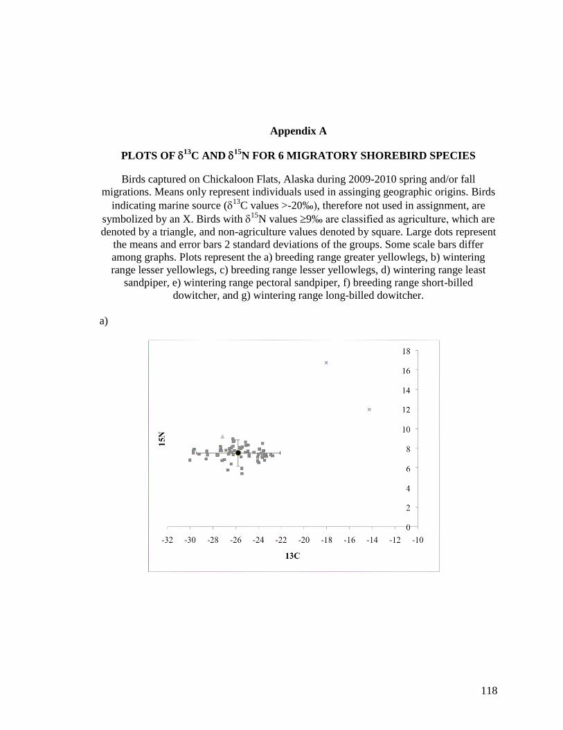
118

Appendix A

PLOTS OF 13

C AND 15

N FOR 6 MIGRATORY SHOREBIRD SPECIES

Birds captured on Chickaloon Flats, Alaska during 2009-2010 spring and/or fall

migrations. Means only represent individuals used in assinging geographic origins. Birds

indicating marine source (13

C values >-20‰), therefore not used in assignment, are

symbolized by an X. Birds with 15

N values 9‰ are classified as agriculture, which are

denoted by a triangle, and non-agriculture values denoted by square. Large dots represent

the means and error bars 2 standard deviations of the groups. Some scale bars differ

among graphs. Plots represent the a) breeding range greater yellowlegs, b) wintering

range lesser yellowlegs, c) breeding range lesser yellowlegs, d) wintering range least

sandpiper, e) wintering range pectoral sandpiper, f) breeding range short-billed

dowitcher, and g) wintering range long-billed dowitcher.

a)

119

b)

c)

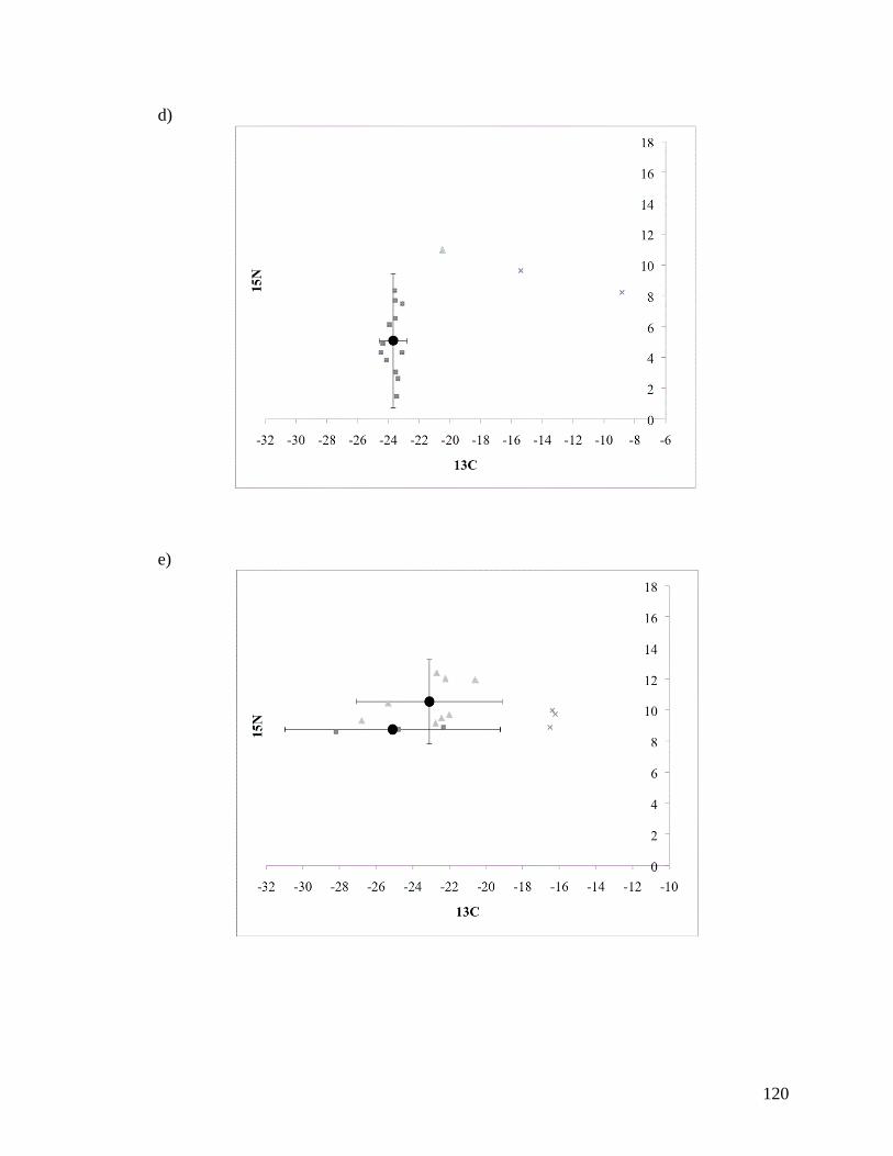
120

d)

e)

121

f)

g)

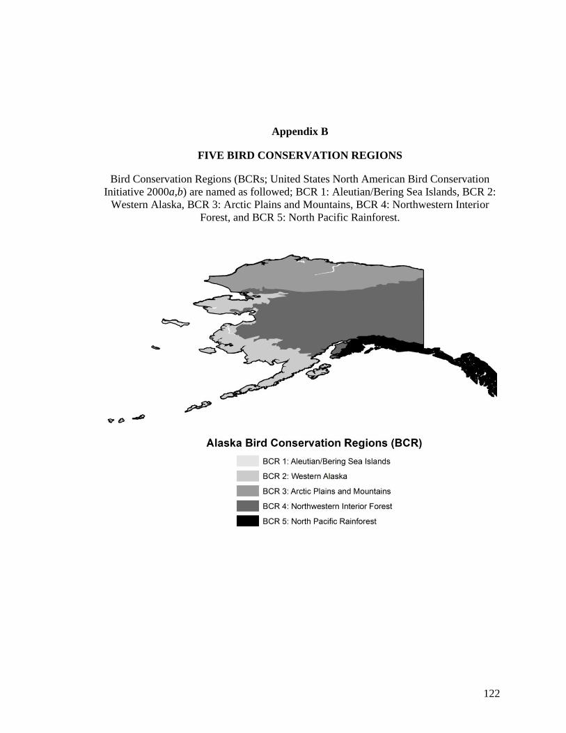
122

Appendix B

FIVE BIRD CONSERVATION REGIONS

Bird Conservation Regions (BCRs; United States North American Bird Conservation

Initiative 2000a,b) are named as followed; BCR 1: Aleutian/Bering Sea Islands, BCR 2:

Western Alaska, BCR 3: Arctic Plains and Mountains, BCR 4: Northwestern Interior

Forest, and BCR 5: North Pacific Rainforest.

123

Appendix C

DAILY OBSERVATIONS OF AVIAN SPECIES OF CHICKALOON FLATS IN

2009 AND 2010

An additional avian survey method was to maintain a daily log of bird species and

estimated abundance of each species. This was not a structured survey, rather a record of

birds encountered each day while conducting related fieldwork. Although there were not

set transects followed daily, there was a certain degree of repetition for area coverage,

with walking routes to, from, and within plots. The daily species log information utilizes

every daily count and does not take into consideration weather variables, which may

reduce detection of some forest species (Bibby and Burgess 2000).

To look at seasonal and yearly avian diversity, I compared mean number of avian

species at the study area level between seasons within years and within season between

years using a Student’s t-test (P ≤ 0.05). I also compared total avian abundance at the

study area level between seasons within years and within season between years using a

Student’s t-test (P ≤ 0.05). Finally, I compared total shorebird abundance at the study

area level between seasons within years and within season between years using a

Student’s t-test (P ≤ 0.05).

Results

To capture an overall idea of species diversity and abundance throughout the

spring and fall migration periods, the daily observation was a valuable resource. The

daily species richness fluctuated from 4–43 during spring seasons (5–26 May 2009 and

124

20 April – 14 June 2010) and 5–28 species during fall (27 June – 6 August 2009, 15–18

August 2009 and 8 July – 25 August 2010). Fall shorebird migration is protracted late

June through mid-September (Gill and Tibbitts 1999), and therefore this study did not

quite capture the entire fall migration period.

Daily observation data from 2009 and 2010 indicate Chickaloon was utilized by

more species during fall migration than spring in 2009 (t65 = -12.00, P < 0.01) and more

in spring than fall for 2010 (t101 = 2.89, P < 0.01). Comparing between years, there was

also a lower diversity during spring 2009 than in 2010 (t75 = -7.14, P < 0.01), but no

difference between fall 2009 and 2010 (t91 = -1.82, P =0.07). In addition to species

diversity, there was also a higher sum of all species abundance during spring than fall of

both years (2009: t65 = 8.96, P < 0.01; 2010: t101 = 2.89, P < 0.01). Although there was no

difference in abundance in fall between 2009 and 2010 (t91 = 1.80, P = 0.08), there were

higher total abundances during spring 2009 than in 2010 (t75 = 7.14, P < 0.01), but that

may have been biased by a difference in number and timing of spring sampling days

between years.

Focusing on 14 shorebird species, There was no difference in abundance of the

sum of 14 shorebird species between spring and fall for 2009 (t65 = 1,773, P = 0.08), but

a significantly higher abundance for 2010 (t101 = 9.343, P < 0.01). Although there was no

difference in shorebird abundance in spring between 2009 and 2010 (t75 = 1.807, P =

0.07), fall 2009 had significantly higher abundance than fall 2010 (t91 = 10.67, P < 0.01).

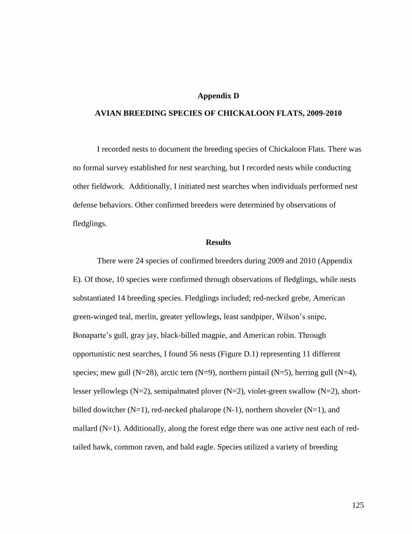
125

Appendix D

AVIAN BREEDING SPECIES OF CHICKALOON FLATS, 2009-2010

I recorded nests to document the breeding species of Chickaloon Flats. There was

no formal survey established for nest searching, but I recorded nests while conducting

other fieldwork. Additionally, I initiated nest searches when individuals performed nest

defense behaviors. Other confirmed breeders were determined by observations of

fledglings.

Results

There were 24 species of confirmed breeders during 2009 and 2010 (Appendix

E). Of those, 10 species were confirmed through observations of fledglings, while nests

substantiated 14 breeding species. Fledglings included; red-necked grebe, American

green-winged teal, merlin, greater yellowlegs, least sandpiper, Wilson’s snipe,

Bonaparte’s gull, gray jay, black-billed magpie, and American robin. Through

opportunistic nest searches, I found 56 nests (Figure D.1) representing 11 different

species; mew gull (N=28), arctic tern (N=9), northern pintail (N=5), herring gull (N=4),

lesser yellowlegs (N=2), semipalmated plover (N=2), violet-green swallow (N=2), short-

billed dowitcher (N=1), red-necked phalarope (N-1), northern shoveler (N=1), and

mallard (N=1). Additionally, along the forest edge there was one active nest each of red-

tailed hawk, common raven, and bald eagle. Species utilized a variety of breeding

126

habitats of Chickaloon. The majority of the waterfowl (N= 7) and gull (32) nests were

located around the large permanent ponds in Plot 2 in Floating marsh, Marsh community,

and Seaside-arrow grass land cover types. The arctic tern nests were in Type 3 Mud

community, typically found in dry clumps of large alkali-grass in the middle of mud

pans. Semipalmated plover nests were also in Type 3 Mud community, in bigger patches

of large alkali-grass. Although similar time was spent on Plot 1 and Plot 2, no nests were

found on Plot 1, potentially attributed to the smaller, narrower area of possible nesting

habitats and lack of permanent ponds. Extreme tide events do not usually occur during

nesting season, so areas usually exposed to tidal waters during spring and fall are

protected from flooding events during nesting season.

Discussion

Of the 24 breeding species, 5 are species of conservation concern. On the Kenai

Peninsula, the red-necked phalarope has declined by 40% over the last ten years (pers.

comm. T. Eskelin). A single nest was found during 2009 in the Marsh community. Short-

billed dowitcher is a species of high conservation concern with long-term declines

(NABCI 2009). Short-billed dowitcher is a confirmed breeder, with a single nest found

on Plot 4 and two chicks observed foraging on Plot 2 in 2010. Lesser yellowlegs and least

sandpiper are both experiencing long-term declines as well (NABCI 2009). Two lesser

yellowlegs nests were found in 2010 and least sandpiper is a suspected breeder. Another

species with declining numbers suspected to breed on Chickaloon is the rusty blackbird,

which has declined by 75% in the past 40 years (NABCI 2009). Rusty blackbirds often

127

nest on margins of beaver ponds (Avery 1995), and one pair was seen throughout

spring/summer seasons during 2009 and 2010 near the beaver pond on Pincher Creek.

In addition, a pair of Wilson’s phalaropes (Phalaropus tricolor) was observed and

documented on June 7, 2010 on the east-central part of Plot 2. Although there were

attempts to relocate birds in the following days, they were not seen again. Wilson’s

phalarope is listed as rare (annual or possibly annual in small numbers; most such species

occur at the perimeter of Alaska) according to the Checklist of Alaska Birds (Gibson et

al. 2012), however this pair was the first documented sighting of the species on the Kenai

National Wildlife Refuge.

Although the numbers of breeding individuals is low for all species, especially

those of concern, Chickaloon provides productive breeding habitat for a variety of

migratory species.

128

Figure D.1: Locations of 56 nests of 11 species opportunistically found within and between four study plots during 2010 on

Chickaloon Flats.

129

Appendix E

ALL 95 AVIAN SPECIES RECORDED ON CHICKALOON FLATS DURING SPRING AND FALL OF 2009-2010

a) Spring survey dates 4–26 May 2009 and 21 April – 12 June 2010 and b) fall dates were 27 June – 6 August 2009, 15–18

August 2009 and 8 July – 25 August 2010. All survey dates are indicated by grey, daily presence of each species is indicated

by black, and non-survey days are indicated by white. Confirmed breeding status indicated by *. No assumptions on observing

all breeding species.

a)

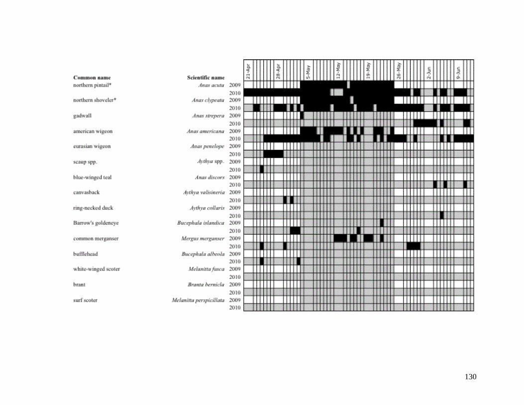
130

131

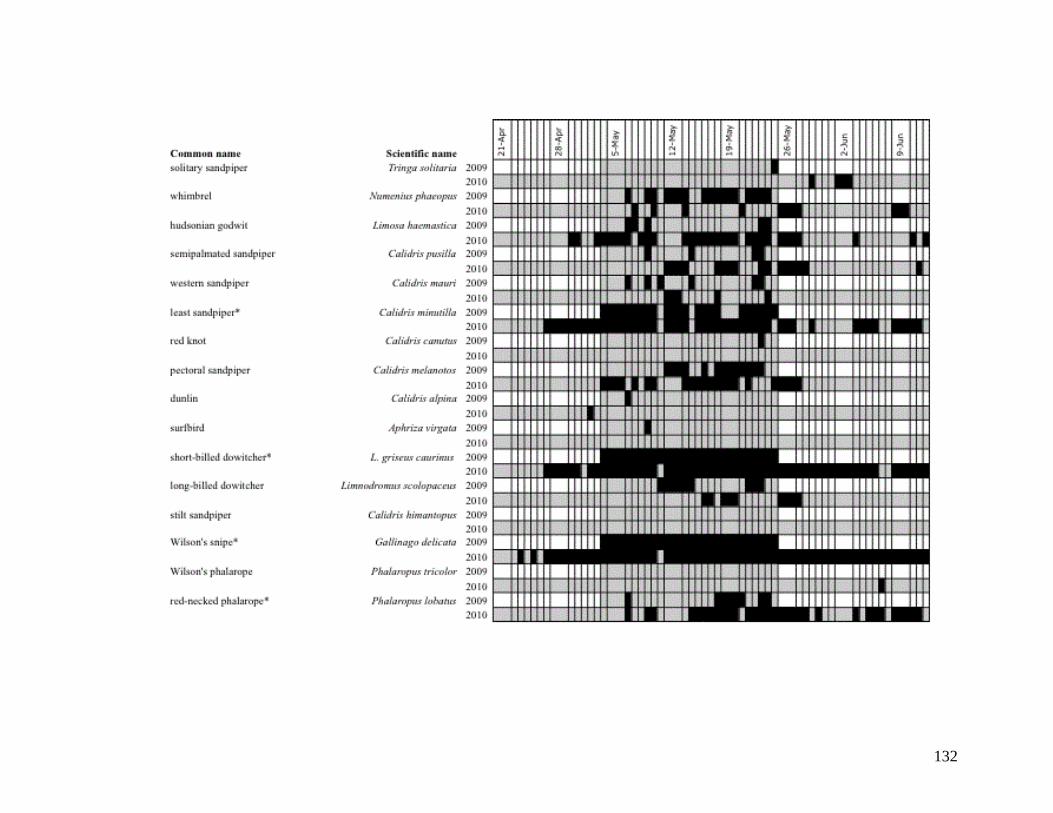
132

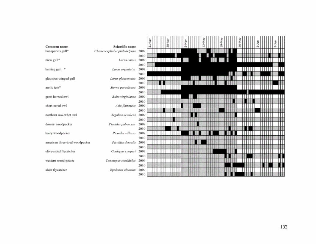
133

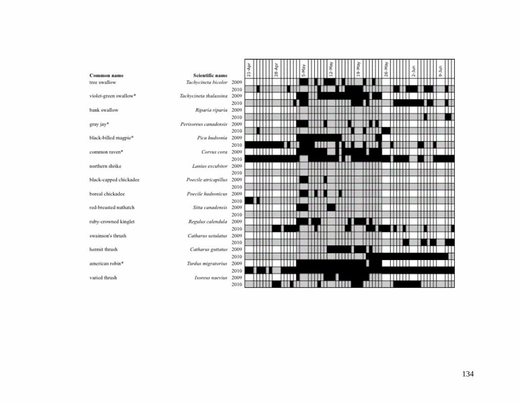
134

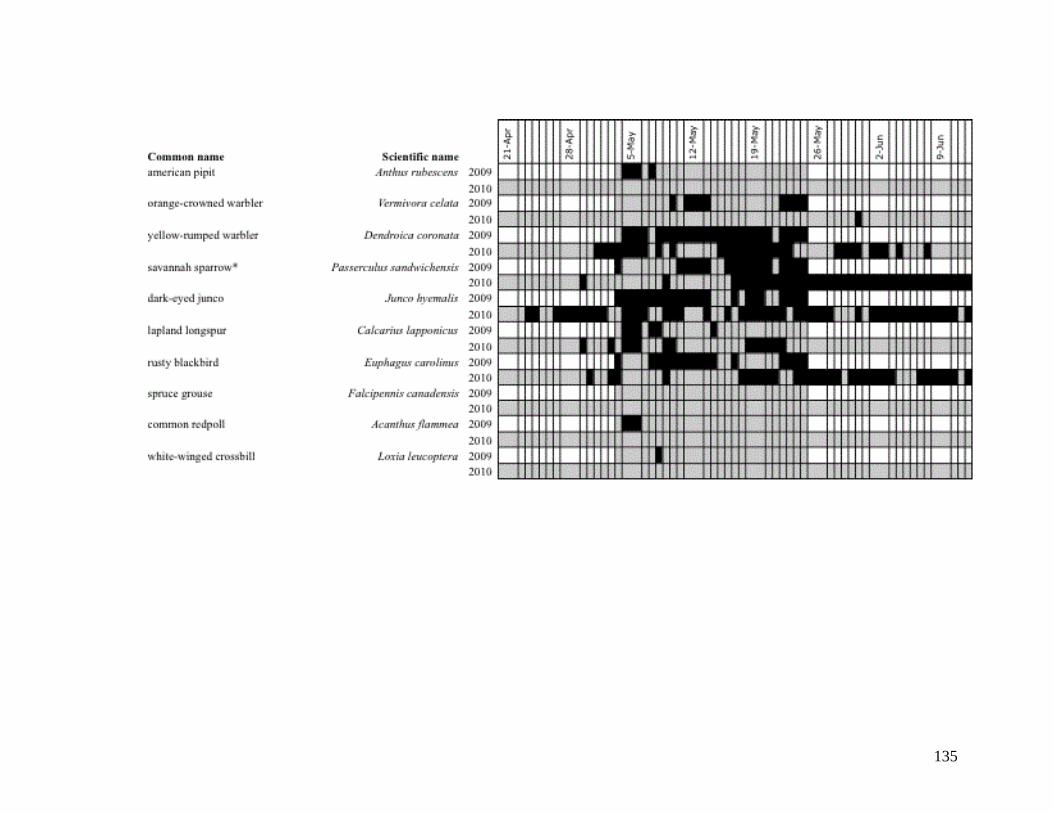
135

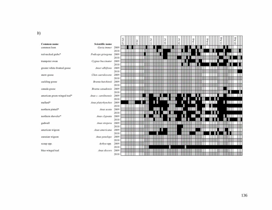
136

b)

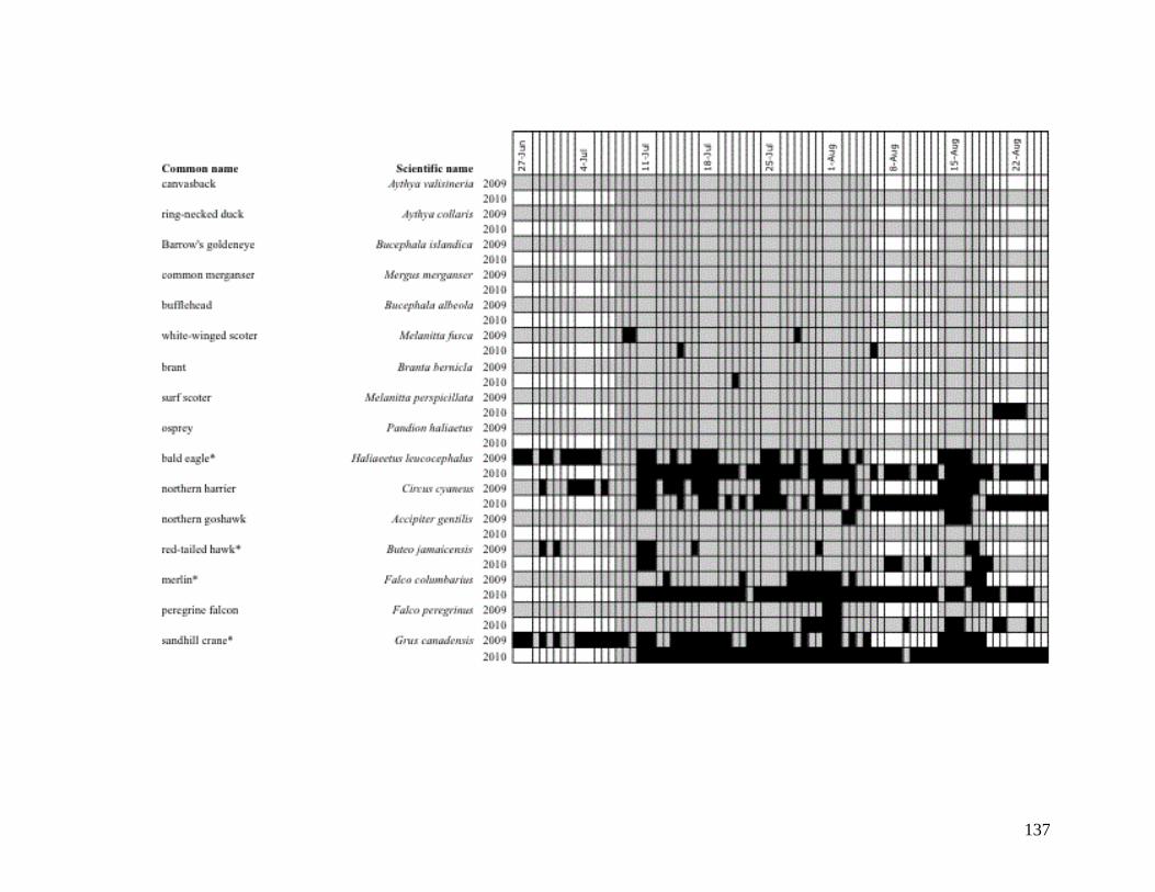
137

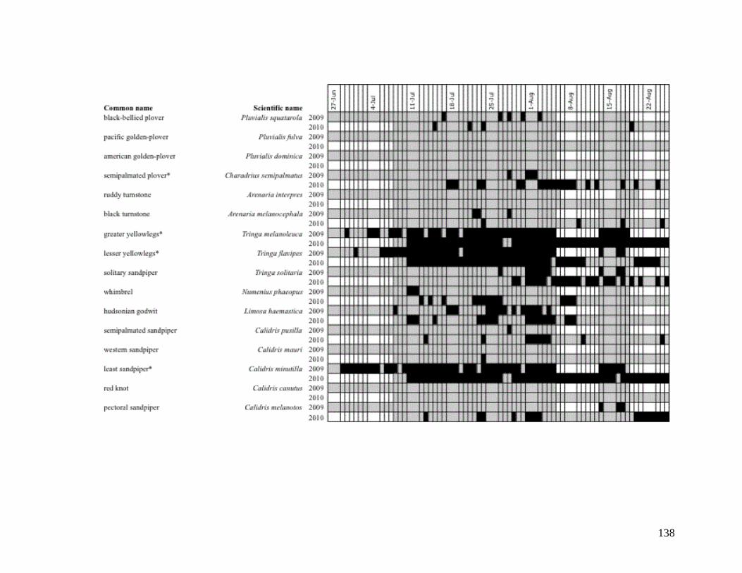
138

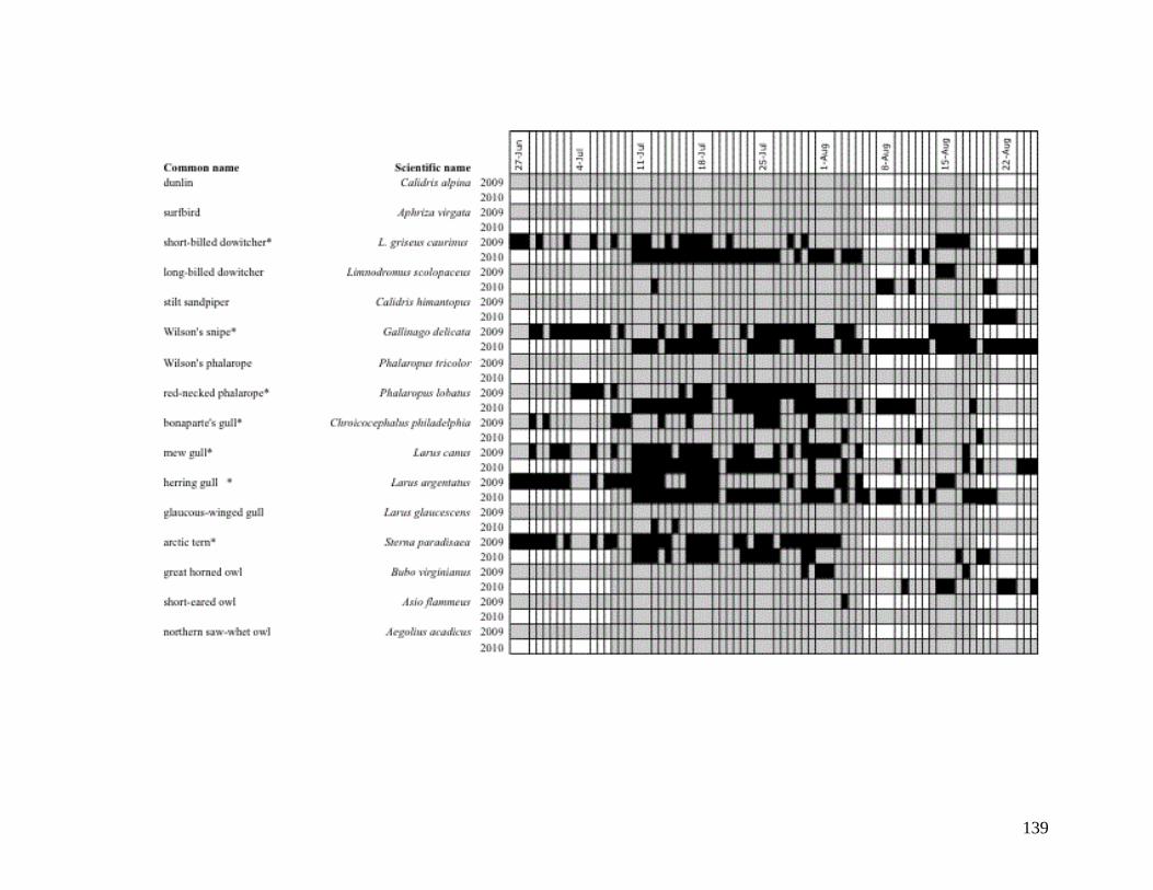
139

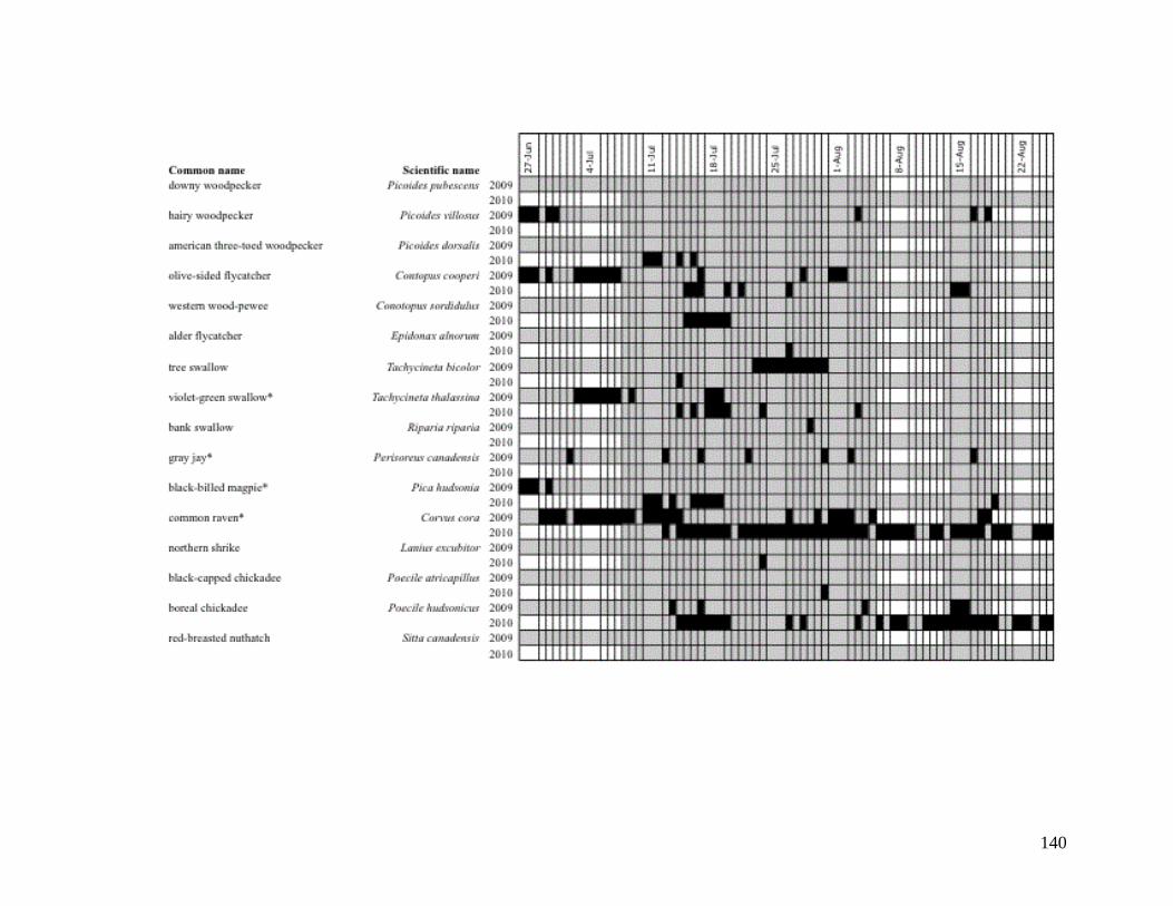
140

141

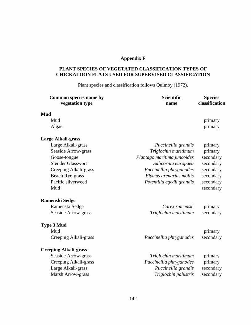
142

Appendix F

PLANT SPECIES OF VEGETATED CLASSIFICATION TYPES OF

CHICKALOON FLATS USED FOR SUPERVISED CLASSIFICATION

Plant species and classification follows Quimby (1972).

Common species name by

vegetation type

Scientific

name

Species

classification

Mud

Mud primary

Algae primary

Large Alkali-grass

Large Alkali-grass Puccinellia grandis primary

Seaside Arrow-grass Triglochin maritimum primary

Goose-tongue Plantago maritima juncoides secondary

Slender Glasswort Salicornia europaea secondary

Creeping Alkali-grass Puccinellia phryganodes secondary

Beach Rye-grass Elymus arenarius mollis secondary

Pacific silverweed Potentilla egedii grandis secondary

Mud secondary

Ramenski Sedge

Ramenski Sedge Carex ramenski primary

Seaside Arrow-grass Triglochin maritimum secondary

Type 3 Mud

Mud primary


Creeping Alkali-grass


Creeping Alkali-grass Puccinellia phryganodes primary

Large Alkali-grass Puccinellia grandis secondary

Marsh Arrow-grass Triglochin palustris secondary

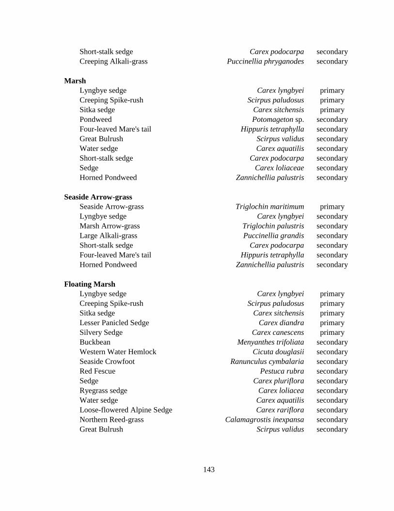
143

Short-stalk sedge Carex podocarpa secondary


Marsh

Lyngbye sedge Carex lyngbyei primary

Creeping Spike-rush Scirpus paludosus primary

Sitka sedge Carex sitchensis primary

Pondweed Potomageton sp. secondary

Four-leaved Mare's tail Hippuris tetraphylla secondary

Great Bulrush Scirpus validus secondary

Water sedge Carex aquatilis secondary


Sedge Carex loliaceae secondary

Horned Pondweed Zannichellia palustris secondary

Seaside Arrow-grass


Lyngbye sedge Carex lyngbyei secondary


Large Alkali-grass Puccinellia grandis secondary


Four-leaved Mare's tail Hippuris tetraphylla secondary

Horned Pondweed Zannichellia palustris secondary

Floating Marsh

Lyngbye sedge Carex lyngbyei primary

Creeping Spike-rush Scirpus paludosus primary

Sitka sedge Carex sitchensis primary

Lesser Panicled Sedge Carex diandra primary

Silvery Sedge Carex canescens primary

Buckbean Menyanthes trifoliata secondary

Western Water Hemlock Cicuta douglasii secondary

Seaside Crowfoot Ranunculus cymbalaria secondary

Red Fescue Pestuca rubra secondary

Sedge Carex pluriflora secondary

Ryegrass sedge Carex loliacea secondary


Loose-flowered Alpine Sedge Carex rariflora secondary

Northern Reed-grass Calamagrostis inexpansa secondary

Great Bulrush Scirpus validus secondary

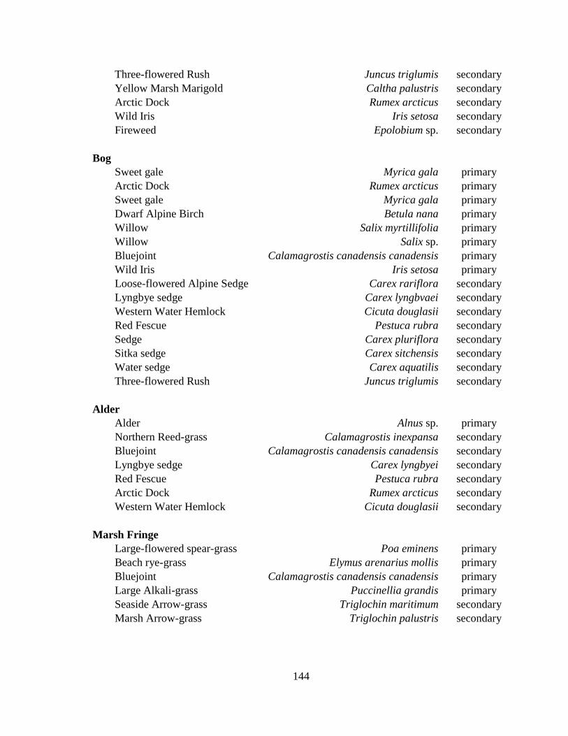
144

Three-flowered Rush Juncus triglumis secondary

Yellow Marsh Marigold Caltha palustris secondary

Arctic Dock Rumex arcticus secondary

Wild Iris Iris setosa secondary

Fireweed Epolobium sp. secondary

Bog

Sweet gale Myrica gala primary

Arctic Dock Rumex arcticus primary

Sweet gale Myrica gala primary

Dwarf Alpine Birch Betula nana primary

Willow Salix myrtillifolia primary

Willow Salix sp. primary

Bluejoint Calamagrostis canadensis canadensis primary

Wild Iris Iris setosa primary

Loose-flowered Alpine Sedge Carex rariflora secondary

Lyngbye sedge Carex lyngbvaei secondary



Sedge Carex pluriflora secondary

Sitka sedge Carex sitchensis secondary


Three-flowered Rush Juncus triglumis secondary

Alder

Alder Alnus sp. primary

Northern Reed-grass Calamagrostis inexpansa secondary

Bluejoint Calamagrostis canadensis canadensis secondary



Arctic Dock Rumex arcticus secondary


Marsh Fringe

Large-flowered spear-grass Poa eminens primary

Beach rye-grass Elymus arenarius mollis primary

Bluejoint Calamagrostis canadensis canadensis primary

Large Alkali-grass Puccinellia grandis primary

Seaside Arrow-grass Triglochin maritimum secondary


145


Goose-tongue Plantago maritima juncoides secondary

Pacific silverweed Potentilla egedii grandis secondary

Arctic daisy Chrysanthemum arcticum secondary


Squirrel-tail barley Hordeum jubatum secondary

Star flower Trientalis europaea secondary

Red top Agrostis sp. secondary

Dogwood Cornus sp. secondary

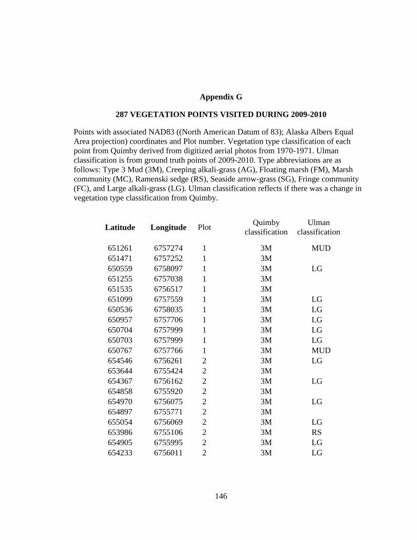
146

Appendix G

287 VEGETATION POINTS VISITED DURING 2009-2010

Points with associated NAD83 ((North American Datum of 83); Alaska Albers Equal

Area projection) coordinates and Plot number. Vegetation type classification of each

point from Quimby derived from digitized aerial photos from 1970-1971. Ulman

classification is from ground truth points of 2009-2010. Type abbreviations are as

follows: Type 3 Mud (3M), Creeping alkali-grass (AG), Floating marsh (FM), Marsh

community (MC), Ramenski sedge (RS), Seaside arrow-grass (SG), Fringe community

(FC), and Large alkali-grass (LG). Ulman classification reflects if there was a change in

vegetation type classification from Quimby.

Latitude Longitude Plot Quimby

classification

Ulman

classification

651261 6757274 1 3M MUD

651471 6757252 1 3M

650559 6758097 1 3M LG

651255 6757038 1 3M

651535 6756517 1 3M

651099 6757559 1 3M LG

650536 6758035 1 3M LG

650957 6757706 1 3M LG

650704 6757999 1 3M LG

650703 6757999 1 3M LG

650767 6757766 1 3M MUD

654546 6756261 2 3M LG

653644 6755424 2 3M

654367 6756162 2 3M LG

654858 6755920 2 3M

654970 6756075 2 3M LG

654897 6755771 2 3M

655054 6756069 2 3M LG

653986 6755106 2 3M RS

654905 6755995 2 3M LG

654233 6756011 2 3M LG

147

660050 6754338 3 3M LG

659032 6754342 3 3M LG

659198 6754398 3 3M LG

658968 6754284 3 3M

659116 6754220 3 3M LG

659597 6754242 3 3M LG

659122 6754331 3 3M LG

660129 6754287 3 3M LG

659136 6754310 3 3M LG

665817 6757430 3 3M LG

666157 6757435 3 3M

654234 6756011 3 3M

665739 6756908 3 3M LG

665703 6757053 3 3M LG

330458 6757050 4 3M

330709 6757438 4 3M LG

340180 6756726 4 3M LG

330702 6756738 4 3M

340197 6757036 4 3M LG

650389 6758008 1 AG

651151 6756741 1 AG RS

650680 6757396 1 AG

651029 6757046 1 AG

651213 6756747 1 AG

650318 6757695 1 AG

650425 6757599 1 AG RS

650444 6757733 1 AG RS

650073 6757951 1 AG

655229 6755547 2 AG LG

654775 6755594 2 AG LG

654836 6755562 2 AG LG

654927 6755423 2 AG LG

653763 6755448 2 AG

655048 6755766 2 AG LG

654482 6755643 2 AG

653894 6755570 2 AG

653993 6755426 2 AG

341130 6757196 4 AG LG

341172 6757106 4 AG

330775 6756293 4 AG MC

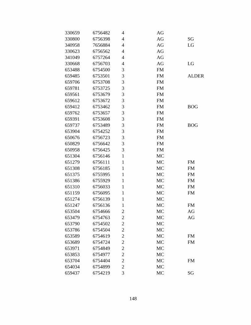
148

330659 6756482 4 AG

330800 6756398 4 AG SG

340958 7656884 4 AG LG

330623 6756562 4 AG

341049 6757264 4 AG

330668 6756703 4 AG LG

653488 6754500 3 FM

659485 6753501 3 FM ALDER

659706 6753708 3 FM

659781 6753725 3 FM

659561 6753679 3 FM

659612 6753672 3 FM

659412 6753462 3 FM BOG

659762 6753657 3 FM

659391 6753608 3 FM

659737 6753489 3 FM BOG

653904 6754252 3 FM

650676 6756723 3 FM

650829 6756642 3 FM

650958 6756425 3 FM

651304 6756146 1 MC

651279 6756111 1 MC FM

651308 6756185 1 MC FM

651375 6755995 1 MC FM

651386 6755929 1 MC FM

651310 6756033 1 MC FM

651159 6756095 1 MC FM

651274 6756139 1 MC

651247 6756136 1 MC FM

653504 6754666 2 MC AG

653479 6754763 2 MC AG

653790 6754502 2 MC

653786 6754504 2 MC

653589 6754619 2 MC FM

653689 6754724 2 MC FM

653971 6754849 2 MC

653853 6754977 2 MC

653704 6754404 2 MC FM

654034 6754899 2 MC

659437 6754219 3 MC SG

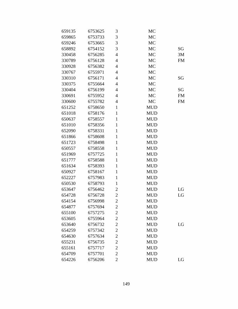
149

659135 6753625 3 MC

659865 6753733 3 MC

659246 6753665 3 MC

658892 6754152 3 MC SG

330458 6756285 4 MC 3M

330789 6756128 4 MC FM

330928 6756382 4 MC

330767 6755971 4 MC

330310 6756171 4 MC SG

330375 6755664 4 MC

330404 6756199 4 MC SG

330691 6755952 4 MC FM

330600 6755782 4 MC FM

651252 6758650 1 MUD

651018 6758176 1 MUD

650637 6758557 1 MUD

651010 6758356 1 MUD

652090 6758331 1 MUD

651866 6758608 1 MUD

651723 6758498 1 MUD

650557 6758558 1 MUD

651969 6757725 1 MUD

651777 6758588 1 MUD

651634 6758393 1 MUD

650927 6758167 1 MUD

652227 6757983 1 MUD

650530 6758793 1 MUD

653647 6756462 2 MUD LG

654728 6756728 2 MUD LG

654154 6756998 2 MUD

654877 6757694 2 MUD

655100 6757275 2 MUD

653605 6755964 2 MUD

653640 6756732 2 MUD LG

654259 6757342 2 MUD

654630 6757634 2 MUD

655231 6756735 2 MUD

655161 6757717 2 MUD

654709 6757701 2 MUD

654226 6756206 2 MUD LG

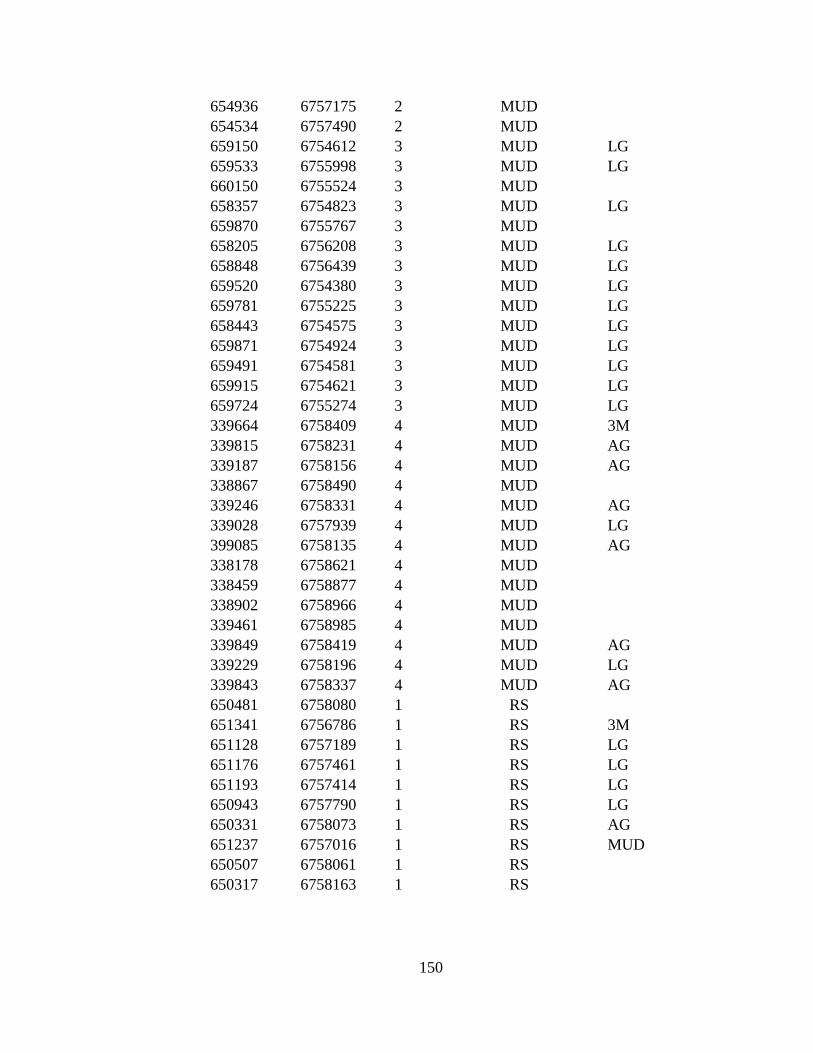
150

654936 6757175 2 MUD

654534 6757490 2 MUD

659150 6754612 3 MUD LG

659533 6755998 3 MUD LG

660150 6755524 3 MUD

658357 6754823 3 MUD LG

659870 6755767 3 MUD

658205 6756208 3 MUD LG

658848 6756439 3 MUD LG

659520 6754380 3 MUD LG

659781 6755225 3 MUD LG

658443 6754575 3 MUD LG

659871 6754924 3 MUD LG

659491 6754581 3 MUD LG

659915 6754621 3 MUD LG

659724 6755274 3 MUD LG

339664 6758409 4 MUD 3M

339815 6758231 4 MUD AG

339187 6758156 4 MUD AG

338867 6758490 4 MUD

339246 6758331 4 MUD AG

339028 6757939 4 MUD LG

399085 6758135 4 MUD AG

338178 6758621 4 MUD

338459 6758877 4 MUD

338902 6758966 4 MUD

339461 6758985 4 MUD

339849 6758419 4 MUD AG

339229 6758196 4 MUD LG

339843 6758337 4 MUD AG

650481 6758080 1 RS

651341 6756786 1 RS 3M

651128 6757189 1 RS LG

651176 6757461 1 RS LG

651193 6757414 1 RS LG

650943 6757790 1 RS LG

650331 6758073 1 RS AG

651237 6757016 1 RS MUD

650507 6758061 1 RS

650317 6758163 1 RS

151

653810 6756203 1 RS LG

654353 6756290 2 RS LG

654529 6756153 2 RS LG

653909 6758934 2 RS LG

653435 6755755 2 RS LG

654635 6756251 2 RS LG

653835 6756245 2 RS LG

654754 6756198 2 RS LG

653855 6756343 2 RS LG

659304 6754265 3 RS LG

658683 6754566 3 RS LG

658961 6754449 3 RS LG

660385 6753934 3 RS 3M

659862 6754367 3 RS

658840 6754525 3 RS LG

660303 6754372 3 RS LG

658745 6754520 3 RS MUD

659883 6754490 3 RS LG

659873 6754406 3 RS LG

330831 6757511 4 RS LG

330622 6756978 4 RS LG

330575 6757017 4 RS LG

340245 6756828 4 RS LG

340268 6756536 4 RS LG

330368 6757077 4 RS LG

339991 6756203 4 RS MUD

341000 6757622 4 RS LG

340213 6756797 4 RS LG

341243 6757664 4 RS LG

659972 6757645 1 SG FM

650056 6757630 1 SG FM

650128 6757923 1 SG MC

651081 6756726 1 SG

650374 6757556 1 SG FM

653220 6754763 2 SG

653388 6754759 2 SG AG

654877 6755512 2 SG LG

654465 6755307 2 SG LG

653167 6754884 2 SG AG

654330 6755165 2 SG AG

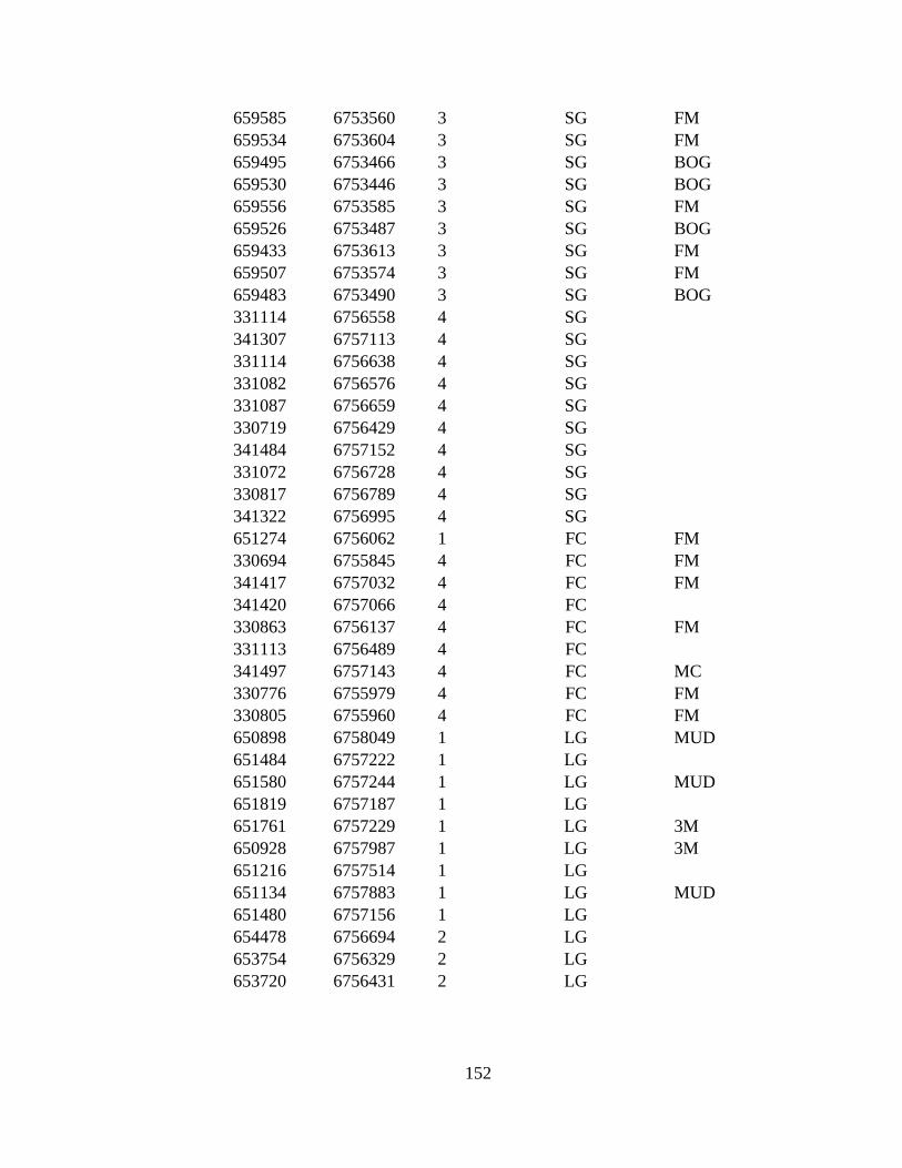
152

659585 6753560 3 SG FM

659534 6753604 3 SG FM

659495 6753466 3 SG BOG

659530 6753446 3 SG BOG

659556 6753585 3 SG FM

659526 6753487 3 SG BOG

659433 6753613 3 SG FM

659507 6753574 3 SG FM

659483 6753490 3 SG BOG

331114 6756558 4 SG

341307 6757113 4 SG

331114 6756638 4 SG

331082 6756576 4 SG

331087 6756659 4 SG

330719 6756429 4 SG

341484 6757152 4 SG

331072 6756728 4 SG

330817 6756789 4 SG

341322 6756995 4 SG

651274 6756062 1 FC FM

330694 6755845 4 FC FM

341417 6757032 4 FC FM

341420 6757066 4 FC

330863 6756137 4 FC FM

331113 6756489 4 FC

341497 6757143 4 FC MC

330776 6755979 4 FC FM

330805 6755960 4 FC FM

650898 6758049 1 LG MUD

651484 6757222 1 LG

651580 6757244 1 LG MUD

651819 6757187 1 LG

651761 6757229 1 LG 3M

650928 6757987 1 LG 3M

651216 6757514 1 LG

651134 6757883 1 LG MUD

651480 6757156 1 LG

654478 6756694 2 LG

653754 6756329 2 LG

653720 6756431 2 LG

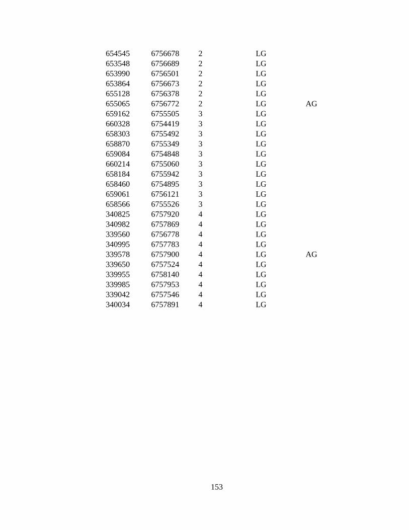
153

654545 6756678 2 LG

653548 6756689 2 LG

653990 6756501 2 LG

653864 6756673 2 LG

655128 6756378 2 LG

655065 6756772 2 LG AG

659162 6755505 3 LG

660328 6754419 3 LG

658303 6755492 3 LG

658870 6755349 3 LG

659084 6754848 3 LG

660214 6755060 3 LG

658184 6755942 3 LG

658460 6754895 3 LG

659061 6756121 3 LG

658566 6755526 3 LG

340825 6757920 4 LG

340982 6757869 4 LG

339560 6756778 4 LG

340995 6757783 4 LG

339578 6757900 4 LG AG

339650 6757524 4 LG

339955 6758140 4 LG

339985 6757953 4 LG

339042 6757546 4 LG

340034 6757891 4 LG

154

Appendix H

EXTREME TIDAL EVENTS SUSTAIN FORAGING HABITAT FOR

MIGRATING SHOREBIRDS ON AN ALASKAN ESTUARY

Introduction

Ephemeral pools in tidal estuaries are temporary sources of water represented by a

variety of shapes and sizes, and are usually lacking in fish, but abundant in invertebrates

(Scheffers et al. 2006). Ephemeral pools can provide key foraging areas for both resident

and migratory waterfowl and shorebirds (Haig et al. 1998, Silveira 1998). Most pools are

initially filled by snow and ice melt, with varying periods of recharging water via tidal

flow and precipitation. Some are consistently recharged with daily flooding tides, which

provide reliable foraging habitat.

Other areas do not experience consistent flooding, and pools dry up as spring

progresses, being sustained only by precipitation (Schalles and Shure 1989). These

ephemeral pools dry up, leaving deeper permanent ponds as the only reliable water

source in some areas. While the edges of permanent ponds provide roosting sites for

birds, they do not provide optimal foraging depths like ephemeral pools (Silveira 1998).

Therefore, the availability of ephemeral pools as foraging habitat for migrating waterfowl

and shorebirds is critical in some areas, and knowing the factors that drive these

ephemeral pools is important for habitat management and species conservation.

155

During a study of shorebird use on a coastal estuary in south-central Alaska, we

gradually realized that the hydrology of ephemeral pools we were studying was atypical

of most tidal systems. The goal of this research was to determine what environmental

factors (maximum weekly high tide, extreme tide event presence in that week, maximum

weekly temperature, and cumulative weekly precipitation) are most important in

determining presence and surface area of ephemeral pools on Chickaloon.

Study Area

Chickaloon Flats is a 10,000 ha tidal estuary located along Turnagain Arm in

upper Cook Inlet, on the Kenai National Wildlife Refuge, Alaska. Several riverine

systems flow into this complex including the Chickaloon River, Big and Little Indian

Creeks, and Pincher Creek. Seaside arrow-grass (Triglochin maritimum), Large alkali-

grass (Puccinellia grandis), and Creeping alkali-grass (Puccinellia phryganodes) are

dominant in areas of higher salinity; Lyngbye sedge (Carex lyngbvaei) and Creeping

spike-rush (Scirpus paludosus) are dominant in areas of lower salinity; however, much of

the estuary is unconsolidated mudflats.

Tides are an important ecological factor in Cook Inlet and on Chickaloon Flats.

The shape and depth of Cook Inlet generates very large tidal amplitude. Cook Inlet tides

are semi-diurnal with a mean tidal range of 9.2 m, which is second greatest in the world

behind Bay of Fundy (11.7 m) (Mulherin et al. 2001).

Despite this high tidal variation, sheet flow of saltwater over Chickaloon Flats is a

relatively rare event. Unlike most estuaries that experience saltwater inundation twice

156

daily, saltwater only overflows the banks of tidal sloughs during extreme tide events. An

extreme tide event is when tide levels exceed 8.84 m (Quimby 1972, pers. obs.) and

water overflows the sloughs and spreads across the flats (pers. obs.). Extreme tide events

occur cyclically on Chickaloon Flats, usually during February, March, August, and

September (Quimby 1972).

This unusual flooding regime is made even more so by the peculiar topography

due to tectonic subsidence in the aftermath of an earthquake in 1964. Extreme tides

inundate Chickaloon at varying levels depending on west-east location (Figure H.1, pers.

obs.). On the western side, extreme tides completely submerge most vegetated

communities almost to the forest edge. Approximately 4 km to the east of that area,

extreme tides do not inundate in a wave, but rather flooding occurs from sloughs being

breached and water overflowing onto vegetated communities. Extreme tides on the far

eastern side (Figure H.1) near Big Indian Creek do not completely submerge vegetated

areas, and only partially submerge the plant community closest to Cook Inlet. This west-

east inundation gradient prevents some habitats from receiving the recharging waters

from predictable extreme tides.

Methods

I monitored surface areas of pools beginning 24 April 2010, when initial water

came from melting ice. I measured the width and length as surface area of each pool to

the nearest 0.25 m, once a week for 18 weeks, with the exception of weeks 8–11 because

I was not in the field. Due to the absence of measurements for weeks 8–11, only dried up

157

pools (areas of zero) for both weeks 7 and 12 were used in analysis. This excluded 7

pools that were recharged with water during the weeks of no measurements. Sample size

for analysis was 14 ephemeral pools. An auto-regressive lag-1 model (p ≤ 0.10) was run

on each of the 14 pools to determine what main effects (maximum weekly high tide,

extreme tide event presence in that week, maximum weekly temperature, and cumulative

weekly precipitation) influenced the auto correlated surface area of ephemeral pools over

time. This model identified the primary factors in determining surface area while

accounting for temporal correlation in pool size.

Results

The occurrence of an extreme tide event was a significant factor in determining

surface area in 12 of 14 pools (Table H.1). Weekly maximum tide was also a significant

factor for 2 of the 14 ephemeral pools. No single factor significantly determined surface

area for two of the pools. Temperature and weekly cumulative precipitation did not

significantly influence pool surface area.

Extreme tides (>8.84 m) were the most important dynamic in determining size of

ephemeral pools. Extreme tides are temporally variable across seasons and years, and

typically occur only 4–5 times from April through August in a given year. Over the 7-

year span of 2004–2010 there were only 17 total extreme tide events during spring

migration and 15 during fall (Figure H.2), with a range of only 1-3 extreme events during

both spring and fall of those years. Not only are these extreme tide events variable in

seasonal occurrence, but also in duration. Over those 7 years, the average duration of an

158

extreme tide event was 3.76 days (range 2-7 days) during spring, and 3.27 days (range 2-

6 days) for fall. The variation in seasonal occurrence and duration may substantially

change the amount and extent to which reliable shorebird foraging habitat is available.

Though temporally variable, tides are periodic and predictable because of the

gravitational effect of the sun and moon (Hicks 2006). From 2004–2010 the first extreme

tide event of spring occurred from 1–16 April 2004–2010, with the second spring tide

occurring during 26 April – 24 May (Figure H.2). Extreme tide events are also variable

in their height, ranging from 8.9–9.7 m across 32 tide events from 2004–2010. This

seasonal variation in extreme tides affects when pools are recharged, and can therefore

significantly influence the distribution of, and available water in ephemeral pools

available during shorebird and waterfowl migrations.

Although I did not find precipitation to be a significant predictor of pool surface

area, it is possible this result was biased by higher precipitation in 2010 (NOAA 2010).

While conducting other research on the study area during 2009, I anecdotally noted and

photographed that the longevity and availability of ephemeral pools was lower.

Comparing the available ephemeral pools between 2009 and 2010, 2009 was much drier

with less available surface water, most likely linked to precipitation (Figure H.3).

Evaluating photos from the second week in July of 2009 and 2010, the 2009 season was

less green and much drier (with no ground water present) including noticeable saltpans in

east. This comparison represents precipitation only, as extreme tides occurred 19 and 71

days, respectively, before photos were taken. Taking into account observations and

photos, precipitation may help to sustain ephemeral pools between extreme tide events.

159

Discussion

The presence of ephemeral pools throughout the Chickaloon landscape has the

potential to provide important shorebird foraging habitat, especially during spring

migration. It is critically important for shorebirds to replenish energy reserves at stopover

sites and staging areas to successfully complete a long-distance migration (Skagen and

Knopf 1993). Shorebirds migrate along flyways with knowledge of their ever-changing

environment and may choose a stopover site based on the occurrence of a flooded

landscape that offers potential foraging habitats (Colwell 2010). This importance of water

presence at a stopover site emphasizes the significance of the timing, duration, and height

of extreme tide events on Chickaloon Flats during spring and fall migration periods.

In addition to the variation of timing, duration, and height of extreme tides, the

west-east inundation gradient is a further influence on the location and amount of habitat

receiving recharging waters. The variation in water inundation across Chickaloon may be

due to a combination of the west-east subsidence and uplift gradients. The 1964

Earthquake registered between 8.3–8.6 on the Richter scale with its epicenter about 129

km east of Chickaloon in the Chugach Mountains. The flats subsided from the

earthquake, with a 61 cm drop in the west to 137 cm in the east (Quimby 1972), and has

experienced uplift since then from ~30 cm in west to 75–80 cm in east (Jeff Freymueller

pers. comm.). These two gradients may help to explain the distribution of available

ephemeral pools in relation to amount of recharging waters received from extreme tide

events, with the majority occurring on the western portion of Chickaloon. Due to the

seasonality of extreme tide occurrences, the timing of these inundations could change the

160

temporal availability of ephemeral pools, which consequently alters the available

shorebird foraging area.

The amount of flooding can also be influenced by wind coming off Turnagain

Arm, with excessive winds causing more inundation. When extreme tide events

coincided with heavy winds, saltwater inundation was more extensive (pers. obs.). Pools

would continuously drain via shallow channels until the next high tide cycle would slow

or stop the flow. Pools were recharged with saltwater during extreme tides, so water was

typically retained in pools longer following an extreme high tide. The coastal

environment of Chickaloon Flats is very unique when considering the amount of

subsidence in the aftermath of the earthquake combined with uplift, and the low

occurrence of flooding by extreme tide events.

Tides also have an effect on the vegetation patterns (Neiland 1971). The daily

change of tidal heights alters the frequency and duration of inundation of vegetated areas,

which affects the plant species present in those communities. The infrequency of extreme

tide occurrence has the potential to provide just enough salt-water inundation to halt any

salt-intolerant plants from being successful and not enough salt-water inundation for

success of alkali species. This combination, along with silt deposition, could be a

principal reason for changes in vegetated communities. An analysis of sequential Landsat

imagery from 1975–2005 suggests that estuary vegetation is gradually being replaced by

bare mud, rather than transitioning to other floral communities (see Chapter 3). Because

ephemeral pool foraging areas are in vegetated areas, the transition of vegetated habitat to

161

mud may decrease the area available for sustaining ephemeral pools, therefore reducing

overall shorebird foraging habitat and the value of Chickaloon as a stopover site.

In addition to foraging in ephemeral pools, shorebirds were also seen foraging in

sloughs, primarily following high tides when prey would be exposed. Sloughs represent

another foraging resource on Chickaloon with patchy distribution (Lourenco et al. 2005)

and temporal restriction. Sloughs may provide widespread, predictable, and reliable

foraging habitats throughout the seasons and inclement weather (Townshend 1981), and

may be an important additional foraging habitat, especially when ephemeral pools are not

abundant (Myers et al. 1980).

Taking into account the influences (timing, duration, and height of extreme tides,

winds, and west-east gradient) involved with recharging the system with saltwater and

precipitation helping to sustain the pools, the presence of ephemeral pools may vary

markedly across seasons and years. The unreliable nature of ephemeral pools is

concerning, and the attraction of this area as a dependable resource for migrating

shorebirds may be diminishing. The presence and amount of ephemeral pools, and

therefore the overall value of Chickaloon Flats as a feeding area for migrating shorebirds,

are at risk due to uplift (Freymueller pers. comm.) and siltation of Turnagain Arm

(NMFS 2008). Even with the variable nature of foraging habitat and the potential lower

use of the area in the future, Chickaloon can be a critical connection to breeding areas for

individuals (Skagen and Knopf 1994a).

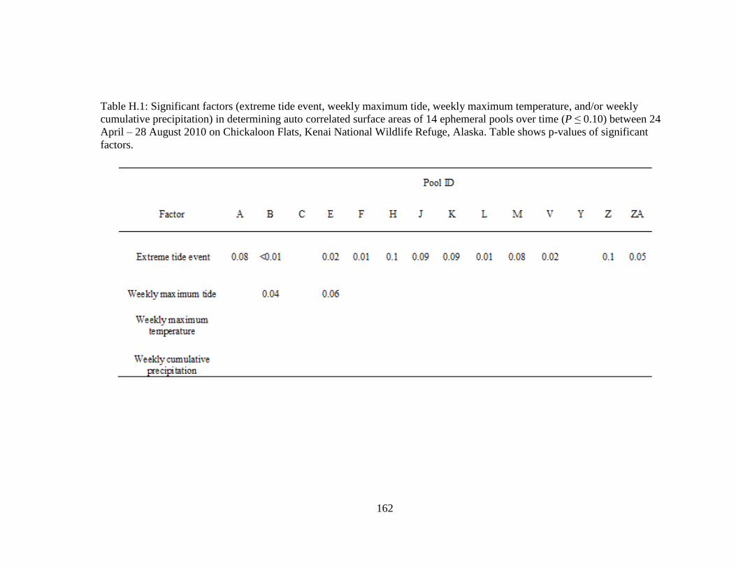
162

Table H.1: Significant factors (extreme tide event, weekly maximum tide, weekly maximum temperature, and/or weekly

cumulative precipitation) in determining auto correlated surface areas of 14 ephemeral pools over time (P ≤ 0.10) between 24

April – 28 August 2010 on Chickaloon Flats, Kenai National Wildlife Refuge, Alaska. Table shows p-values of significant

factors.

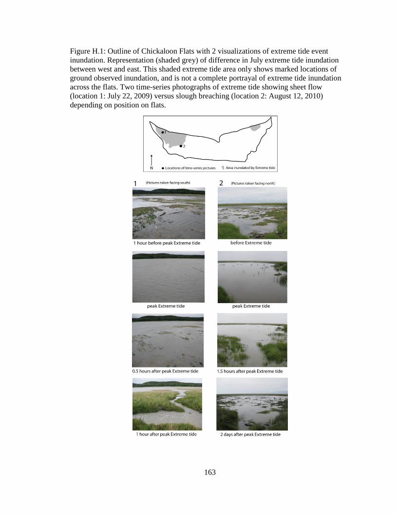
163

Figure H.1: Outline of Chickaloon Flats with 2 visualizations of extreme tide event

inundation. Representation (shaded grey) of difference in July extreme tide inundation

between west and east. This shaded extreme tide area only shows marked locations of

ground observed inundation, and is not a complete portrayal of extreme tide inundation

across the flats. Two time-series photographs of extreme tide showing sheet flow

(location 1: July 22, 2009) versus slough breaching (location 2: August 12, 2010)

depending on position on flats.

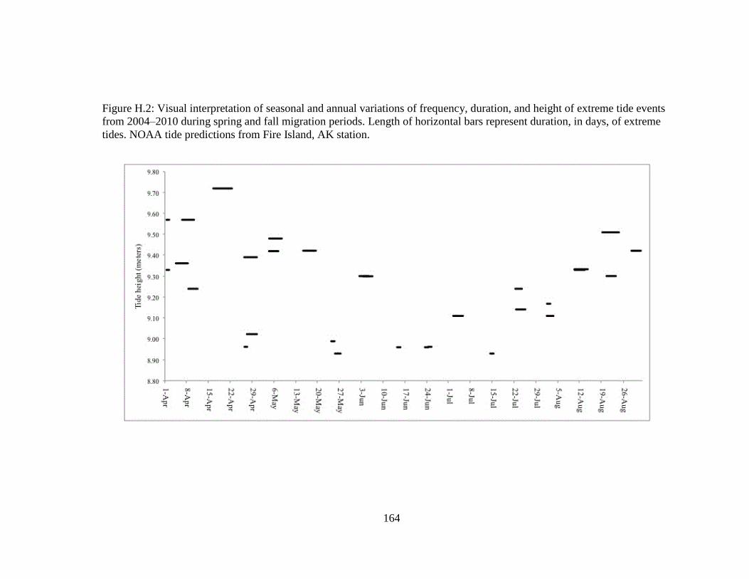
164

Figure H.2: Visual interpretation of seasonal and annual variations of frequency, duration, and height of extreme tide events

from 2004–2010 during spring and fall migration periods. Length of horizontal bars represent duration, in days, of extreme

tides. NOAA tide predictions from Fire Island, AK station.

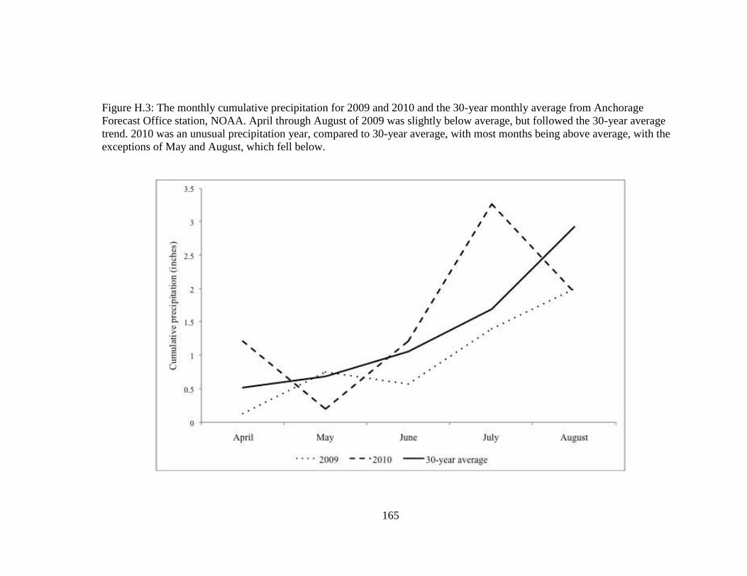
165

Figure H.3: The monthly cumulative precipitation for 2009 and 2010 and the 30-year monthly average from Anchorage

Forecast Office station, NOAA. April through August of 2009 was slightly below average, but followed the 30-year average

trend. 2010 was an unusual precipitation year, compared to 30-year average, with most months being above average, with the

exceptions of May and August, which fell below.

166

Appendix I

Documents

MIGRATORY SHOREBIRD AND VEGETATION EVALUATION … · migratory shorebird and vegetation evaluation of chickaloon flats, kenai national wildlife refuge, alaska by sadie e. g. ulman