MIGRATION AND INFORMAL INSURANCE

By

Costas Meghir, Ahmed Mushfiq Mobarak, Corina Mommaerts, and Melanie Morten

July 2019

Revised December 2020

COWLES FOUNDATION DISCUSSION PAPER NO. 2185R2

COWLES FOUNDATION FOR RESEARCH IN ECONOMICS YALE UNIVERSITY

Box 208281 New Haven, Connecticut 06520-8281

http://cowles.yale.edu/

Migration and Informal Insurance *

Costas Meghir †

Yale University, IFS, IZA, CEPR and NBERAhmed Mushfiq Mobarak ‡

Yale University and NBER

Corina Mommaerts §

University of Wisconsin – Madison and NBERMelanie Morten ¶

Stanford University and NBER

Current version: December 22, 2020

Abstract

We document that an experimental intervention offering transport subsidies for poorrural households to migrate seasonally in Bangladesh improved risk sharing. A theo-retical model of endogenous migration and risk sharing shows that the effect of sub-sidizing migration depends on the underlying economic environment. If migrationis risky, a temporary subsidy can induce an improvement in risk sharing and enableprofitable migration. We estimate the model and find that the migration experimentincreased welfare by 12.9%. Counterfactual analysis suggests that a permanent, ratherthan temporary, decline in migration costs in the same environment would result in areduction in risk sharing.

Keywords: Informal Insurance, Migration, Bangladesh, RCTJEL Classification: D12, D91, D52, O12, R23

*We thank the editor Dirk Krueger and four anonymous referees for helpful comments. We alsothank Pascaline Dupas, Andrew Foster, John Kennan, Ethan Ligon, Fabrizio Perri, Mark Rosenzweig,Rob Townsend, and Alessandra Voena for comments. We are grateful to seminar participants at the 2014IFS/CEAR Household Workshop, the 2015 SED meeting, the 2015 Barcelona Summer Workshop, the 8thInternational Conference on Migration and Development, the 2017 NBER Summer Institute, Princeton Uni-versity, University of Namur, Paris School of Economics, Toulouse School of Economics, the University ofKansas, and the University of California, Berkeley. Costas Meghir thanks the Cowles Foundation and ISPSat Yale for financial support. Some of the computing for this project was performed on the Sherlock cluster.We would like to thank Stanford University and the Stanford Research Computing Center for providingcomputational resources and support that contributed to these research results. Any errors are our own.

†Email: c.meghir@yale.edu‡Email: ahmed.mobarak@yale.edu§Email: cmommaerts@wisc.edu¶Email: memorten@stanford.edu

1 Introduction

Poverty is highly concentrated in rural areas. Four out of every five poor households

in Asia are rural (Asian Development Bank, 2007), and many of these households rely

on risky, weather-dependent agricultural activities. Rural livelihoods are therefore both

volatile across years, and fluctuate across seasons with the crop cycle. To address this

uncertainty, agrarian households smooth consumption and manage risk using two pri-

mary mechanisms: they share risk with other members of their community (Munshi and

Rosenzweig, 2016; Ferrara, 2003), and they migrate to diversify income sources (Banerjee

and Duflo, 2007). However, each of these mechanisms is imperfect. Informal risk shar-

ing provides only partial insurance (Townsend, 1994; Ligon et al., 2002; Kinnan, 2020),

and migration may be costly or itself risky (Bazzi, 2017; Beam et al., 2016). The two ap-

proaches may also interact with one another. The presence of a safety net at home might

either facilitate or deter risky migration. New migration opportunities might either un-

dermine informal insurance schemes by providing exit options or, conversely, produce

spillover benefits for other members of the network through transfers and sharing of the

extra migration income. Therefore to understand the overall welfare effects of encourag-

ing migration, it is necessary to consider the effects of migration on risk sharing.

In this paper, we study the interaction between migration and social safety nets by

examining how new migration opportunities affect the nature and extent of informal risk

sharing within those villages. We have three main objectives. The first is to empirically

estimate the causal effect of migration subsidies on risk sharing. We take advantage of the

randomized controlled trial (RCT) described in Bryan et al. (2014) in which households

1

in rural Bangladesh were randomly offered subsidies to migrate temporarily during the

agricultural lean season. While existing evaluations of the program consider only the

effects on direct beneficiaries (Bryan et al., 2014; Lagakos et al., 2018), we analyze the

spillover effects on the entire risk-sharing network. The second objective is to interpret

and explain our empirical findings using a model of endogenous risk sharing and en-

dogenous migration, allowing for the complex set of interactions between the two. We

build upon the model in Morten (2019) and show that migration subsidies can interact

with the underlying risk environment to generate either positive or negative spillovers;

this is an important insight because it demonstrates that the welfare effects of policy are

heavily context dependent. We thus characterize key features of the environment and of

preferences that can alter how these policies interact. Our third objective is to estimate

this model using the experimental variation, use these estimates to quantify the welfare

effects of migration subsidies that we implemented, and consider counterfactual policies

of permanent migration subsidies and unconditional cash transfers.

The Bangladesh experiment provided very poor agrarian households money for the

round-trip bus fare (worth USD 8.50) conditional on one member migrating temporar-

ily. Bryan et al. (2014) present the effects of the experiment on direct beneficiaries. The

subsidy offer led to a 22 percentage point increase in migration in the first year, house-

hold consumption increased by 30% for those induced to migrate, and migration rates

remained 11 percentage points higher during the next lean season, one year after the

one-time subsidy was removed. Our analysis goes beyond these direct benefits and con-

siders the indirect spillover effects on households in the village that did not send mi-

grants themselves. We document several types of experimental evidence that suggest

2

that risk sharing improved in treatment villages. For both migrants and non-migrants,

actual transfers between households increased, households in treatment villages became

more likely to report that they receive help from family and friends in the village, and

treatment reduced the effect of household income on household consumption by over

seven percentage points (a reduction of 40%). We also show that these results are not

driven by an increase in self-insurance (savings) nor by an increase in measurement error.

These changes in risk sharing imply that analyzing only the direct effects of the migration

subsidies gives an incomplete picture of the overall welfare effects.

Next, in order to understand why subsidies for migration led to an improvement in

risk sharing in this context, we develop a model in which both migration and risk sharing

are endogenous and jointly determined. The model allows us to study the underlying

economic mechanisms that link migration and risk sharing, which is important because

our results are in contrast to Morten (2019), who found that in rural India, an increase in

migration led to a crowding-out, rather than a crowding-in, of informal insurance. We

reconcile these conflicting empirical results by showing that it is possible to get either

crowd-in or crowd-out of risk sharing from the same theoretical model under different

local conditions and preferences and also different assumptions about the permanence

of the policy itself. Our model augments Morten (2019), which considers a model with

limited commitment constraints on risk sharing (Kocherlakota, 1996; Ligon et al., 2002;

Krueger and Perri, 2010) and an endogenous migration decision based on the net return

to migrating (Harris and Todaro, 1970). To that we add the possibility that migrants de-

velop contacts in the city, allowing them to better obtain jobs. This “asset” can lead to

persistence in migration episodes. We model the migration subsidy in a flexible, agnostic

3

way: alongside the USD 8.50 financial subsidy, we allow the experiment to change the

utility value of migrating resulting from the encouragement offered by the experimental

design and from the fact that increased migration allowed people to migrate with their

friends. We estimate the value of this “utility subsidy” by matching the experimental

responses of migration and risk sharing.1

As mentioned above, the model can explain why a migration subsidy can induce ei-

ther an improvement or a decline in risk sharing in different contexts. In many settings,

migration is a risky lottery: a household gives up some income in the village for a chance

at income in the destination (Harris and Todaro, 1970). A migration subsidy increases the

return to migrating, which may have two effects. On the one hand, increasing migration

may increase the total resources available to the village, thus increasing the social return to

the village of pooling income through risk sharing. On the other hand, the migration sub-

sidy increases the private return to migrating, thus affecting the incentive to participating

in risk sharing. For example, if it is very risky to migrate, the private return to migrating

may be much lower than the social return because without insurance migration is simply

too risky to undertake. In contrast, if it is relatively safe to migrate, then the migrant may

not need the safety net provided by the network, and a migration subsidy may lead to

crowding-out of informal risk sharing. We show, by simulating the model for different

values of migration risk and subsidy levels, that we can indeed generate both positive

and negative spillovers of a migration subsidy on risk sharing.

While the RCT allows us to estimate the effect of the subsidies on risk sharing directly,

1A later round of experiments in the same villages found that people are more likely to migrate whenothers in the village are offered subsidies, even if they themselves were not subsidy recipients (Akram etal., 2018).

4

the issues discussed above demonstrate that a theoretical framework is essential to un-

derstand the underlying reasons behind our empirical result of improved risk sharing

and how it may change in other contexts. We thus use the results from the RCT to es-

timate a model that allows us to identify the underlying parameters. By combining our

model with experimental variation, we achieve cleaner identification by not having to

rely only on observational data, as Morten (2019) did. The model itself provides a pow-

erful toolkit for analyzing alternative policies, and the resulting combination adds to a

nascent but growing literature that combines RCTs and structural models (see, for exam-

ple, Attanasio et al. (2012); Todd and Wolpin (2006); Kaboski and Townsend (2011)). We

estimate parameters that characterize income processes, migration costs, migration asset

paths, and preferences to match experimental outcomes over three periods. Our model

can replicate the dynamics and treatment effects of migration and risk sharing.

Using these estimates, we quantify the overall welfare effect of the migration subsidies

and conduct counterfactual experiments to evaluate different policy levers. We estimate

that the experiment led to an increase in welfare equivalent to a 12.9% permanent increase

in consumption the year the experimental subsidies were disbursed, net of the subsidy

itself. While some of this gain is due to increased resources from migration, the welfare

gain is three times higher after accounting for the improvement in risk sharing compared

to the gain without accounting for the improvement in risk sharing. We also show that

alternative policies can have very different effects on risk sharing and welfare: an uncon-

ditional cash transfer leads to a slight improvement in risk sharing but a negligible effect

on welfare, while a permanent conditional subsidy leads to a worsening of risk sharing

but a positive welfare gain.

5

Our analysis has two important implications for understanding policy impacts and

the development process. First, it is crucial to account for spillover effects – which may

be negative or positive – to understand the full welfare effect of any policy that addresses

the income stream of households. This finding resonates with the growing literature

estimating spillover effects from financial inclusion initiatives, which can also have ei-

ther positive or negative interactions with risk-sharing (see, e.g., Angelucci and de Giorgi

(2009) and Dupas et al. (2017)). Second, while in the current paper we focus on the causal

effect of subsidizing migration on risk sharing, the fact that migration and risk sharing

are jointly determined implies that any change to the ability of households to share risk

may also affect migration. The underlying ability – whether through the economic envi-

ronment or other policies – for households to share risk may thus itself influence whether

households adopt new income-generating methods such as migration.

The paper continues by describing the data and experimental results on risk sharing

in Sections 2 and 3. We then move to the model of endogenous risk sharing and migration

in Section 4. We describe our estimation procedure in Section 5 and show, by simulating

the model locally around our estimates, the key comparative statics driving the mecha-

nisms in the model. We then consider model counterfactuals in Section 6 and conclude

by discussing the broader implications of our findings for understanding the interaction

between informal insurance and technology adoption.

6

2 Data

The experiment randomly offered some households subsidies to temporarily emigrate

from villages in a poor region of northern Bangladesh. This region is prone to a period of

preharvest seasonal deprivation during September to December known as Monga, which

was the original motivation for the experimental intervention.2 Bryan et al. (2014) pro-

vides additional details on the experiment and reports on the program evaluation, focus-

ing on the direct beneficiaries. In this section, we describe the experiment and the data

that is critical for understanding our analysis of the risk-sharing effects of this experiment.

The migration subsidy treatment was randomized at the village level. For all villages

in our sample, a census was conducted to ascertain eligibility for the experiment, where

eligibility was consistently defined as households who reported (a) having low levels of

landholding and (b) that a household member had to skip at least one meal during the

prior Monga season. In total, 56% of households satisfied both criteria. From the census,

19 households from each village were randomly selected from the group of eligible house-

holds to participate in the experiment and surveys, and these 19 households comprise our

analysis sample. In treatment villages, all 19 households were offered the subsidy; in con-

trol villages none were offered the subsidy.

The migration subsidy was an offer of 600 Taka (USD 8.50) conditional on one person

from the household migrating, with an additional 200 Taka given if the migrant reported

to our enumerators in the destination. This amount is sufficient to cover the cost of a2Income and consumption levels drop by roughly 50% and 25%, respectively during this period (Khand-

ker, 2012). Up to 60% of our sample respondents report missing meals during this period. This same phe-nomenon, colloquially known as the “hunger season,” is prevalent in many poor agrarian societies aroundthe world.

7

return bus ticket and a few days food in the destination. The subsidy was offered in the

form of a grant in 37 villages or a zero-interest loan in 31 additional villages. We follow

Bryan et al. (2014) and combine these two into a 68-village “incentive” arm, and com-

pare that against a 32-village “control arm” (composed of 16 villages where we provided

general information about migration opportunities and 16 others where we did nothing).

The subsidies were distributed in August–September 2008. We will make use of three

periods of data: (a) a pre-intervention survey conducted in July 2008, (b) effects during the

intervention year, collected in 2008–2009, and (c) longer-run post-intervention data col-

lected in 2011, approximately two-and-a-half years after the experiment. We rely heavily

on 2011 data for our analysis of risk sharing because it is the only round to contain annual

data on income, consumption, and migration. We provide a summary of the timing of the

interventions and data collection in Appendix Table 2.

Table 1 shows summary statistics for the sample of households in 2011 that we use for

estimation, which includes the 1900 households from the original experiment plus 627

new households from 33 randomly selected new villages in the same two districts using

the same eligibility criteria.3 Statistics are shown separately for all households (column 1),

households in control villages (column 2), and households in incentive villages (column

3). Our main measures of interest are income, consumption, and migration rates, but we

also show summary statistics of other measures of consumption smoothing. For income

and consumption, we exclude outliers by trimming the top and bottom percentiles as well

as households whose migration or treatment status is missing.4

3In 2011, additional experiments were also run in the sample. Our primary analysis focuses on analyz-ing the longer-run effects of the original (2008) experiments. We discuss robustness tests addressing the

8

Table 1: Summary statistics (post-intervention)

mean/sd All villages Control villages Treatment villages

Total income 9782 9502 10056(4847) (4728) (4947)

Home income 8947 8770 9119(4866) (4721) (4999)

City income (among migrant households) 2074 1959 2171(1318) (1304) (1323)

Total consumption 19177 18883 19460(5880) (6038) (5713)

Any savings in last 12 months 0.47 0.43 0.51(0.50) (0.49) (0.50)

Amount, among those who saved 368.96 363.45 373.49(568.28) (619.28) (523.07)

Any transfers received from community 0.57 0.57 0.56(0.50) (0.49) (0.50)

Amount, if any transfers received 5641 4808 6470(11912) (7707) (14925)

Any transfers given to community 0.18 0.15 0.20(0.38) (0.36) (0.40)

Amount, if any transfers given 2775 2001 3368(6671) (3858) (8157)

Household size 4.05 4.04 4.06(1.43) (1.38) (1.48)

% Migrant households 0.41 0.39 0.44(0.49) (0.49) (0.50)

Number of households 1928 946 982

Note: Income, consumption, savings, and transfers are in Taka (approximately 75 Taka per USD in 2011).Income and consumption are annual and per capita.

9

2.1 Income

We use three measures of income in our analysis: home income, city income, and total

income. Home income comprises income earned by the household in the rural village and

consists of wage income, non-farm business income, agricultural income (crops and non-

crops, valued at prices they would have obtained if they sold them), and miscellaneous

income such as lottery winnings and interest income. We do not include transfers from

other members of the community in income. City income is defined as earnings (both

monetary and in the form of housing and food) during migration episodes, net of travel

costs (such as train, bus, and rickshaw) to and from the migration destination. Total

income is the sum of home income and city income. Each of these measures span the

previous 12 months and are thus annual measures of income.5

Following Bryan et al. (2014), we convert these measures to per capita amounts by

dividing by the household size, defined as all individuals reported to be living in the

house for at least seven days at the time of the interview (which may or may not include

additional (2011) experiments in Section 3.4For the original balance tables of the baseline sample in 2008, see Bryan et al. (2014). Since the focus of

their paper was not risk sharing, we additionally plot the distributions of baseline income and consumptionin Appendix Figure 4 and show that neither the difference in means nor the difference in distributions arestatistically significant from zero between treatment and control households. Additionally, the baseline”treatment” effect from a risk-sharing regression (as described in Section 3) using baseline income andconsumption results in a small and insignificant coefficient of 0.026 with standard error 0.028. Our mainsample trims the top and bottom 5% of the data; we show in Appendix Table 7 that our results are robustto using more conservative trimming thresholds. Average income is 5% higher and average consumptionis 3% higher with a 1% trim.

5Specifically, to capture daily wage employment respondents were asked about the daily wage in cashin the past 12 months and the number of days worked, as well as in-kind payment with quantity andprice. Salaried workers were asked how many months worked, the monthly cash salary, and other in-kindbenefits converted to Taka. For non-agricultural enterprises, respondents were asked how many months itoperated in the past 12 months, profits, and share kept by the household. For agricultural crop and non-crop production, the total of each crop produced in the past 12 months was asked, and the amount sold andmoney obtained minus cost. Migration income was ascertained over the last 4 months. Other income wasalso asked about the past 12 months.

10

migrants, depending on when they returned home).6 City income is around 20% of home

income, and households in treatment villages have slightly higher home income and city

income than households in control villages.

2.2 Consumption

Our measure of consumption closely follows Bryan et al. (2014) and consists of 215 food

items and 63 non-food items. Some of these items have a weekly recall and others have a

bi-weekly or monthly recall, so we convert these items to annual and per capita amounts

in order to be consistent with our measure of income. Like income, consumption for

households in treatment villages is higher than consumption for households in control

villages.7

2.3 Other summary statistics

Households in our sample typically contain four members, and around 40% of house-

holds sent a migrant over the course of the year. 47% of households saved some amount

during the year, but the amounts were very small (under 400 Taka). In contrast, many

households gave or received transfers from other households in the community: 57%

received transfers, averaging 5,600 Taka, and 18% gave transfers, averaging 2,800 Taka.8

6In the next section we show that our main estimated treatment effect of income on consumption isrobust to alternative household size definitions, including the current number of household members atthe time of the interview and the number of household members who are living in the house for at least 14days at the time of the interview.

7Total consumption is higher than total income, as is often found in rural household survey data col-lected in agrarian areas. The ratio of income to consumption, however, does not vary significantly betweentreatment and control households.

8The summary statistics in Table 1 show that average transfers received by members in the sampleare approximately six times larger than average transfers sent. The reason for this difference is that onlythe poorest households in the village (based on land holdings and on experiencing hunger the previous

11

Appendix Tables 3 and 4 give more information on the migration experience, based

on surveys of incentivized migrants in the destination and survey data from both in-

centivized and nonincentivized migrants at endline. Based on the endline data, 65% of

migrants migrated to a rural area. 54% of migrants worked in the agricultural sector,

24% worked as non-agricultural day laborers, 10% in the transportation sector, and 12%

in other sectors. 56% of migrants reported earning less than they expected. Survey data

from incentivized migrants in the destination shows that 98% of migrants found work,

with 89% reporting that the wage was higher than their home wage. Migrants predom-

inantly traveled in groups, with only 22% migrating alone. 70% of migrants split food

costs and accommodation with their group members, and 73% of migrants exchanged

information about jobs with other members in their group.

3 Effect of the experiment on risk sharing

As Table 1 shows, households often engage in direct transfers between each other, pre-

sumably as a way to protect themselves against bad income realizations. In this section,

we empirically investigate whether offering migration subsidies affects the functioning

of risk-sharing networks. We take the risk-sharing network to be the village. By com-

paring treatment villages to control villages, we conduct direct tests of the effect of the

experiment on several measures of transfers and risk sharing.

year) were eligible for the experiment and thus included in the dataset; we verify in Appendix C that, asexpected, net transfers out increase with income. We note that any imbalance in the total amount of incometo be shared amongst eligible households does not affect the regressions within the observed data, as thevillage fixed effect controls for the total resources in the network. However, one caveat to our structuralestimation is that we estimate the model using only data on eligible households.

12

3.1 Effect on financial transfers

We start by showing that actual transfers, as well as the household’s self-reported willing-

ness to ask for help, were affected by the migration subsidies. Table 2 regresses these mea-

sures on treatment to test whether the experiment changed these beliefs in the financial

arrangements between villagers (“Willingness to help”) and the transfers that occurred

(“Actual transfers”).

Each row in the first column is a separate regression of the effect of treatment on

each outcome between community members (i.e., family, friends, and other villagers).

The second column contains the mean of the variable among households in the control

group. The top panel suggests that the experiment significantly increased the willingness

of households to interact financially. For example, 57% of households in control villages

report that community members would ask them for help, and treatment increases that

by 11 percentage points. Not only are such intentions affected in villages where migration

subsidies were offered, but actual amounts of transfers also increased as a result of treat-

ment. While there is no change detected in the probability of receiving a transfer, treat-

ment increased the value of transfers received (among those who did receive) by 1,821

Taka off a base of 4,808 Taka, or 38%. The results for transfers given are even stronger: a

3.6 percentage point increase in the propensity to give, and a 1,310 Taka (65%) increase in

the amount given, conditional on giving. Since we collect data on a set of people within

the village who recently received external migration subsidies, it is perhaps sensible that

the results on “transfers given” are larger than those on “transfers received.”

Perhaps the act of migration leads to migrants bringing back gifts for friends in the

13

Table 2: Treatment effect on transfers within the community

Treatment effect Control mean

Willingness to helpCommunity member would help you 0.030 0.85

(0.020)... and you would ask for help 0.025 0.83

(0.020)Community member would ask you for help 0.109∗∗∗ 0.57

(0.033)... and you would help them 0.109∗∗∗ 0.53

(0.032)Actual transfers

Receive any transfer from community member -0.024 0.57(0.022)

Amount, if any transfer received (Tk) 1821∗∗∗ 4808(678)

Give any transfer to community member 0.036∗∗ 0.15(0.018)

Amount, if any transfer given (Tk) 1310∗∗ 2001(558)

Note: The sample includes households from the 2011 survey. Each cell is a separate regression of the effectof treatment on whether the source denoted in the row would behave as described. Each regression alsocontrols for upazila (county). Standard errors, clustered by village, are in parentheses, and the mean of thecontrol group is in square brackets. ∗ p < 0.10, ∗∗ p < 0.05, ∗∗∗ p < 0.01.

14

village, which could be why we observe the increase in “transfers given,” but this does

not signal a broader improvement in risk sharing. In Appendix Table 5 we repeat the

analysis of transfers separately for households that sent a migrant in the past year and

those that did not.9 The results show similar effects for both the migrant and non-migrant

samples. Migration not only increased the willingness to share risk among particular

households that were induced by the experiment to send a migrant but strengthened

informal relationships within a village more broadly.

There are three takeaways from these results. First, there is a strong norm that house-

holds would provide and receive financial assistance among each other, as shown in the

summary statistics of Table 1. Second, the point estimates show that the migration experi-

ment significantly increased the willingness of households to participate in these arrange-

ments as well as actual transfers between households. Third, this increase is not limited to

households that were induced to migrate: non-migrant households in treatment villages

also reported an increase in the ability to use these informal arrangements.

3.2 Effect on the exposure of consumption to income

Since it is difficult for survey data to enumerate the full range of relevant gifts, transfers,

and loans, or to determine whether these transfers were made in response to an income

shock or otherwise, we now investigate the effect of the experiment on the extent to which

income relates to consumption. We test two key ideas. First, we explore the exposure of

consumption to income as a measure of informal insurance within the village. Second,

9Although this sample split is endogenous to the decision to migrate, we argue that it provides sug-gestive evidence of risk-sharing benefits spilling over to households in the village that did not receive thedirect migration incentives provided by the experiment.

15

we investigate whether the experiment changed this exposure.

We first consider the exposure of consumption to income in control villages by regress-

ing log of per capita household consumption on three alternative measures of log of per

capita household income using the following regression:

log Civ = γv +β log Yiv +εiv (1)

where log Civ and log Yiv are household i’s log per-capita consumption and income, re-

spectively, in village v. Village fixed effects γv control for aggregate shocks to consump-

tion.10 The main parameter of interest is β, which captures the exposure of consumption

to income, conditional on differences in aggregate resources across villages.

Table 3: Exposure of consumption to income among control villages

Log consumption

(1) (2) (3)

Log total income 0.165∗∗∗

(0.021)Log village income 0.122∗∗∗

(0.018)Log migration income 0.117∗∗∗

(0.032)

Sample Full Full MigrantsObservations 911 946 350R2 0.217 0.194 0.298

Note: The sample includes households in control villages in the 2011 survey. The dependent variable islog of annual total per-capita consumption and the independent variable is log of annual per-capita totalincome. Each model also includes village fixed effects. Standard errors, clustered by village, are in paren-theses. ∗ p < 0.10, ∗∗ p < 0.05, ∗∗∗ p < 0.01

10Below, when we go on to consider the effect of the program on the exposure of consumption to income,we also include household fixed effects to control for permanent income differences and the results weobtain do not change significantly.

16

Table 3 reports the results of Equation (1) using total income (column 1), home in-

come (column 2), and city income among migrant households (column 3) in the sample

of control villages in the “post-intervention” period. In all cases, the income coefficient

is significantly different from zero, consistent with the absence of full insurance, and its

value below one is also consistent with the presence of a substantial degree of partial

insurance in the non-treatment state.

The next sets of regressions leverage the experimental variation in the data to test

whether a one-time exogenous decrease in migration costs via the experiment led to a

change in the coefficient on log income in the consumption regression in a subsequent

year. We augment Equation (1) to allow the transmission parameter β to vary by whether

the village is in the treatment sample:

log Civ = γv +β0 log Yiv +β1 (log Yiv ∗ Tv) +εiv (2)

where Tv is an indicator variable taking a value of 1 if the village is a treatment village.11

The main parameter of interest in this regression is β1, which captures the effect of the

migration treatment on the exposure of consumption to income.

Column (1) in Table 4 reports β0 and β1 using total per-capita income and consump-

tion. We find a negative coefficient on the interaction between log income and the mi-

gration treatment, consistent with an improvement in risk sharing. Specifically, treatment

11The treatment indicator captures villages randomized to receive migration subsidies in 2008. As de-scribed in Footnote 3, additional experiments were implemented in 2011. We control for the additionalround of treatments through the village fixed effects and additional interaction terms between log incomeand 2011 treatment arms. The 2011 treatments were implemented outside the Monga period (around April)and did not have any effects on the coefficient on log income. We also run these specifications using onlyhouseholds that did not receive any additional 2011 experiments (i.e., were ”pure” control villages) in Ap-pendix Table 8. We find similar results.

17

reduced the effect of household income on household consumption by over seven per-

centage points. Compared to an exposure of consumption to income shocks of 16%, the

migration treatment cuts this exposure by around 40%. These estimates are robust to the

definition of household size and household composition (see Appendix Table 9) and are

particularly large given that they are intent-to-treat estimates.12

Table 4: Effect of migration incentives on the exposure of consumption to income

Round 4 Diff in Diff

(1) (2) (3) (4) (5) (6)

Log income (round 4) 0.157∗∗∗ 0.169∗∗∗ 0.130∗∗∗ 0.140∗∗∗ 0.112∗∗ 0.109∗∗

(0.027) (0.028) (0.028) (0.029) (0.054) (0.046)Treatment effect on log income -0.073∗∗∗ -0.066∗∗ -0.072∗∗∗ -0.061∗∗ -0.077 -0.099∗∗

(0.027) (0.027) (0.027) (0.026) (0.061) (0.046)

Village-round FE X X X X X XHousehold FE X XHousehold head controls X XResource controls X XIncludes baseline X XIncludes 2013 X

Observations 1857 1857 1857 1857 2166 4371R squared 0.186 0.221 0.217 0.267 0.791 0.721

Note: Table presents coefficients of the effect of log annual per capita income on log annual per capita con-sumption and the interaction with treatment (β0 and β1 from Equation 2). All models control for villagefixed effects and all other interactions between treatment and log income as well as log income interactedwith 2011 treatments. Column (2) additionally adds household head controls, column (3) adds householdresource controls, and column (4) adds both household head and resource controls. Columns (5) and (6)show the result of difference-in-difference specifications, with the first coefficient shown being the inter-action between log income and round 4, and the second coefficient shown being the interaction betweentreatment, log income, and a post-experiment indicator. Column (5) includes baseline data, and column (6)includes both baseline and 2013 data, and both include household fixed effects. ∗ p < 0.10, ∗∗ p < 0.05, ∗∗∗

p < 0.01

One concern with the interpretation of these estimates is that the cross-sectional co-

efficient on log income may be conflating a risk-sharing effect with a level difference in

permanent income. Thus, Columns (2)-(6) of Table 4 report a variety of robustness checks

12We report ITT rather than LATE (IV) estimates because treating one household may affect a neighbor’sconsumption through changes in demand for transfers – even absent sharing any extra migration income –so the exclusion restriction for the IV would be violated.

18

to control for such differences. 13 Columns (2)-(4) add observable characteristics to the

specification, including household head controls (e.g., education) in column (2), house-

hold resource controls (e.g., characteristics of the house) in column (3), and both house-

hold head and resource controls in column (4). The coefficients on both β0 and β1 are

very similar across specifications, with β1 ranging from -0.061 to -0.072.14 To allow for

permanent income differences, columns (5) and (6) control for household fixed effects in

an approach dating back to Townsend (1994) by leveraging baseline data (column 5) and

additionally 2013 data (column 6).15 Using a difference-in-difference specification,16 these

columns show similar results; we lose significance on the treatment effect when control-

ling for household fixed effects with just two observations per household, but it returns

with three observations. Overall, the differences across columns in bothβ0 andβ1 are not

statistically distinguishable. In addition to these robustness checks, we note that these re-

gressions should be interpreted in conjunction with the previous transfer evidence; both

provide evidence consistent with an improvement in risk sharing in treatment villages. In

sum, using different methods, all of our results taken together point to an improvement

in risk sharing in treatment villages as a result of the intervention.

13Additionally, we note that treatment was randomly allocated, so even if the cross-sectional coefficienton log income is biased (because both income and consumption may depend on permanent unobservedheterogeneity), the treatment effect does not necessarily suffer from bias. Appendix A.1 derives the condi-tions for the treatment effect to be unbiased in the presence of permanent unobserved heterogeneity. Thekey condition is that the treatment effect on log income is additive. Our empirical result that the treatmenteffect is stable with and without fixed effects is consistent with this theoretical result.

14Results are also similar if we focus only on villages that were included in the baseline experimentalsample.

15A caveat with the 2013 data—and the reason we do not use it elsewhere in the paper— is that there aredata quality concerns. Specifically, there was a significant amount of political strikes and strike-inducedviolence in 2013, which made data collection difficult and likely changed migration behavior considerably(see Akram et al. (2018) for more details).

16The treatment effect on log income in columns 5 and 6 is the interaction between log income, the treat-ment indicator, and the post-experiment indicator.

19

Another potential concern with the results in Table 4 is that our ability to measure in-

come for treatment households may be less accurate than for control households, either

because migration income is inherently more difficult for the econometrician to capture,

or because migration income is easier to hide both from other households and from the

econometrician.17 If such measurement error were classical, either of these measurement

issues may create an attenuation bias in treatment effect estimates. To investigate this,

we repeat the analysis from Table 4 among households that did not send a migrant.18

We present results in Appendix Table 8. While this is an endogenously selected sample,

our ability to measure their income should not vary by treatment, and hence, this exer-

cise should help to address the measurement concerns. The results show that treatment

also reduces the coefficient on log income for non-migrant households, suggesting that

measurement concerns are not driving the treatment effects we observe in Table 4. These

estimates are consistent with the experiment changing the risk-sharing equilibrium be-

tween all households in the network, not only the subset who were induced to migrate.

A final concern is that the coefficient β could mechanically decrease if the variance of

income increased as a result of the experiment. While the result mentioned above show-

17Appendix Table 6 report the effects of various sub-treatments that could help discern the presence ofhidden income (Townsend, 1982; Rogerson, 1985; Ligon, 1998; Kinnan, 2020). If migration makes it easierto hide income because some of the income is earned away from other villagers’ watchful eyes, risk shar-ing can break down. To investigate the relevance of hidden income in our setting, we take advantage ofsub-treatment variations in the experiment, where some of those receiving migration subsidy offers wereadditionally required to migrate in groups. Those group members were either assigned by the experi-menters in one sub-treatment or self-formed by the migrants in another. Columns (2) and (3) show that thetreatment effect on the correlation between own-income and own-consumption continues to be negative,even when migrants are required to travel in groups or to particular destinations. There is no statisticallysignificant change in the treatment effect when one of these requirements is imposed. This result suggeststhat hidden income may not be a key constraint limiting risk sharing in this setting. Our model presented inthe next Section, therefore, focuses on limited commitment (as opposed to hidden income) as the primaryfriction undermining risk sharing.

18In addition, we run reverse regressions of log income on log consumption in Appendix Table 10, and theratios of the “forward” and reverse regression coefficients are very similar between treatment and controlsamples.

20

ing that the coefficient also decreased among non-migrants should alleviate this concern,

a more structural measure of risk sharing is the difference in the consumption equivalents

between autarky and participating in the network. We consider this alternative measure

later in the paper and show that it is consistent with our measure of the exposure of con-

sumption to income.

3.3 Effects on savings

A change in the exposure of consumption to income does not necessarily imply a change

in risk sharing across households if the migration subsidy offers also increased the house-

hold’s ability to save. These households could be using savings (as opposed to migration

and sharing risk with other households) as an alternative consumption-smoothing mech-

anism (although this would not explain why we see an improvement in risk sharing even

among non-migrant households). In Table 5, we test the effect of the experiment on the

amount saved over the past 12 months. Columns (1) and (2) show that there is no signifi-

cant effect of treatment on the amount saved, both among the full sample of households

(column 1) and the sample of those that reported saving a non-zero amount (column 2).

Not only are the treatment effects small and indistinguishable from zero, but mean

savings is also very small. For example, mean savings in the control group is 155 Taka,

which is 1.6% of their total annual income of 9,502 Taka.19 This is consistent with the

fact that these households are extremely poor, and the marginal propensity to consume

any extra migration income during this lean (hungry) season is very high. These null

19Additionally, Appendix Table 12 reports statistics of additional measures of savings against villageincome for control villages and shows that mean liquid and cash savings are around 5% of mean householdincome and 10% of the standard deviation of household income.

21

Table 5: Treatment effect on savings per capita

Amount saved in last 12 months (Taka)

(1) (2)Unconditional Conditional on any

Treatment 33.4 5.4(21.0) (37.4)

Mean amount saved, control group 155.3 363.5Observations 2359 1101R2 0.01 0.02

Note: The sample includes households from the 2011 survey. The dependent variable is the amount saved(in Taka) per capita in the previous year, including zeros (column 1) and excluding zeros (column 2). Bothmodels control for upazila (county) and 2011 treatment arms. Standard errors, clustered by village, are inparentheses. ∗ p < 0.10, ∗∗ p < 0.05, ∗∗∗ p < 0.01

savings results, coupled with substantial reductions in the coefficient on log income in

the consumption regressions and significant increases in financial transfers, all point to

the experiment causing a substantial improvement in the willingness and ability to share

risk in treatment villages. To understand why this happened, we next turn to a model of

endogenous migration and risk sharing.

4 Joint model of risk sharing and migration

We consider a joint model of risk sharing and migration based on Morten (2019). House-

holds make migration decisions taking into account the returns to migrating, including

risk-sharing transfers. We assume that risk sharing is constrained by limited commitment

frictions (Kocherlakota, 1996; Ligon et al., 2002; Krueger and Perri, 2010). Other frictions

could affect informal risk sharing, such as moral hazard or hidden income, but several

pieces of indirect evidence suggest that they are likely not key constraints: the treatment

effect is the same across treated households that had to travel in unassigned versus as-

22

signed groups and to unassigned versus assigned destinations (Appendix Table 6), and

the treatment effect is similar across home income and migration income (Appendix Table

11), which we would not expect if migration income is easier to hide.20

We extend the limited commitment framework in Morten (2019) to allow for a migra-

tion asset, which we think of as a job connection in the destination. This asset can be

accumulated (or lost) over time, based on the experiences of the migrant in the destina-

tion. This extension will allow the model to approximate the fact that migrants tend to

return to the same employer – for example, Bryan et al. (2014) find that 60% of incen-

tivized migrants return to work for the same employer – which in turn allows the model

to explain why the one-time experiment led to persistent effects on migration. In this

setting, therefore, migration serves two purposes. First, within a period, it potentially

increases the income available to the household. Second, because it allows individuals to

update their migration asset, it provides a dynamic payoff for the future.

We model risk sharing as between two households, denoted by i = 1, 2, with iden-

tical preferences. We assume that households cannot save, which is consistent with the

empirical finding in Section 3 that savings are very low and did not respond to the exper-

iment, and has the benefit of making the model more tractable.21 The timing of the model

is as follows. There are two sub-periods: a before-migration period, when the village in-

20Additionally, while other work has argued that permanent migrants may indeed have incentives tohide their income from family members (Joseph et al., 2015; Baseler, 2018), 76% of the temporary migrantsin our setting migrate with someone else, 84% of temporary migrants worked with another person from thesame village, and of those that did, they worked with on average 6 other migrants from the same village.Thus it may be harder to hide income in this setting.

21The role of savings, especially hidden savings, may be important, however we note that in a limitedcommitment environment, agents will not use private savings when public storage is optimal (Abrahamand Laczo, 2018). That is, the equilibrium of the limited commitment model excluding private savings (butwith public savings) is the same as the equilibrium of the model including it.

23

come state is realized and migration decisions are made, and an after-migration period,

when migration outcomes are realized and transfers and consumption occur. We describe

what happens in each sub-period below. Figure 1 summarizes the model timing.

Figure 1: Model timeline

Model period Activities State of the world

Start of period t — Start-of-period job contacts (At) ht = st, AtBefore migration — Observe village state (st)

Migration decision ( jt)

After migration — Exogenous creation of job contacts (At) ht = ht, jt, qt, At(ht, jt)Observe migration state (qt)Make risk-sharing transfersConsumeReturn to villageExogenous separation of job contacts (At+1)

Start of period t + 1 — Start-of-period job contacts (At+1) ht+1 = st+1, At+1Observe village state (st+1)

At the start of period t both households are in the village. Each household receives a

village income, ei(st), where st denotes the realization (from a set of finite possibilities) of

the state in the village. Each household i, based on its past migration, either has (ait = 1)

or does not have (ait = 0) an active job connection in the city at the start of the period.

We denote the before-migration job contact assets of both households by the vector At =

a1t , a2

t . The before-migration state is summarized by ht = st, At.

Next, each household decides whether to migrate based on the expected return to

migrating. Each household either sends a migrant (Iit = 1) or does not send a mi-

grant (Iit = 0); we summarize the migration outcome of both households by the vector

jt = I1t , I2

t . Migration income is uncertain and is not observed until after the migration

24

decision is made.22 Migration involves a financial cost, dfint , which may be negative if mi-

gration is subsidized. In addition to financial concerns, migration also involves a utility

cost dutilityt .23 After migrating, migrants who migrated without a job contact match with

a provider with an exogenous probability πget contact; those who migrated with a contact

already in hand keep it. Migrants then learn the state of the world in the destination,

qt, which is drawn from a finite set. We assume that the migration asset is specific to

the individual and cannot be shared.24 The after-migration job contact vector is given by

At(ht, jt). Net migration income depends on the state of the world and the job contact,

less any net financial cost to migrate. Total household income depends therefore on the

realization of the state of the world in the village, the migration decision, the realization

of the state of the world in the destination, the realization of the migration asset, and the

net financial migration cost. Letting ht = ht, jt, qt, At( jt, At), after-migration income

for household i is given by yi(ht, dfint ).25

At the end of the period all migrants return to the village. At that point, a household

22The assumption that migrants do not know their income before they migrate is consistent with surveyresponses where 14% of migrants said they earned more than expected, 33% said they earned less thanexpected, and 62% said they earned same as expected (we note that this doesn’t add up to 100% becausethere are sometimes multiple episodes per household). Additionally, Bryan et al. (2014) show that migrationoutcomes in 2008 predict remigration in 2009 only for the treatment (and not the control) group, consistentwith the treatment group not having information about their ability at migration.

23We assume that all households face the same cost of migrating. An alternative way to write the problemwould be to allow households to have different costs of migrating, as considered in Lagakos et al. (2018).In this case, the migration rule would additionally depend on the costs of migrating.

24The migration literature has emphasized the role of social networks in providing information (Masseyet al., 2003; Munshi, 2003). Based on surveys with migrants in the destination, 72.3% of people reporteither giving or receiving information about jobs from people in their current travel group. However,when looking at actual remigration behavior, Bryan et al. (2014) find that previous migration was the onlyfactor that predicts repeat migration and that the number of friends and/or relatives who migrated is nota significant predictor. One way to reconcile these two facts is to consider that information from migrantsaffects the probability of getting a job contact once in the destination, but this information is not transferablebetween migrants and nonmigrants. This therefore matches the modeling choice to make the migrationasset individual-specific.

25This general formulation allows for the case in which migrant households also receive some incomefrom the village (for example, if other household members still work).

25

is separated from their migration contact with a probability that depends on whether

they migrated in the period or not. With probability π lose contact, mig a migrant household

who had an active job contact loses it; with probability π lose contact, nonmig a nonmigrant

household who had an active job contact loses it. The job contact assets of each household

at the beginning of period t + 1 are given by the vector At+1(ht). The state of the world at

the beginning of period t+ 1 is thus summarized by ht+1 = st+1, At+1. The mechanism

design problem then repeats itself in the following period.

To determine the risk-sharing capabilities between households, it is useful to first de-

scribe the optimization problem if each household is independent (i.e., not part of a risk-

sharing arrangement). Households solve maximization problems at two points in time

that result in the before-migration value, Ωi(h), and the after-migration value, Ωi(h).

The before-migration value is the expected utility at the time the household is deciding

whether or not to migrate:

Ωi(h) = maxIi

∑h

πh|h,Ii

[u(yi(h, dfin))− Ii(h)dutility +β∑

h′πh′|hΩ

i(h′)

](3)

The after-migration value is the expected utility once the migration decision has been

made and the household learns if it has a job contact, and then learns the state of the

world in the destination:

Ωi(h) = u(yi(h, dfin))− Ii(h)dutility +β∑h′πh′|hΩ

i(h′) (4)

Equations 3 and 4 are important objects for determining the value of migration subsidies

26

in an environment without spillovers as well as for determining the credible threat points

in the full endogenous risk-sharing model.

We can now describe the full model, in which both risk sharing and migration are

endogenously determined. The optimization problem involves migration choices of both

households and the net transfer from household one to household two, τ , to maximize to-

tal welfare. This problem is constrained by two sets of incentive compatibility constraints

(one for each household at the before-migration stage, and one for each household at

the after-migration stage), as well as a promise-keeping constraint that household one

receives the utility promised to them. We follow the solution concept proposed in Ligon

et al. (2002) by solving for the conditional Pareto frontier that maximizes the utility of

household two given a promised level of utility to household one. Because households

make choices at two points in time during a period, we define two Pareto frontiers: first,

the frontier that maximizes the before-migration utility of household two, V(h), given a

state-dependent level of before-migration promised utility, U(h), to household one. Sec-

ond, the after-migration frontier maximizes the after-migration utility of household two,

V(h), conditional on the after-migration state h.

We solve the model in two steps. Starting in the second sub-period, we solve for

optimal transfers τ(h, dfin) and continuation utility U(h′) for all future states h′:

V(h, U(h)) = maxτ(h,dfin),U(h′)∀h′

u(

y2(h, dfin) + τ(h, dfin))− I2(h)dutility +β∑

h′πh′|hV(h′, U(h′))

(5)

subject to a promise-keeping constraint that household 1 receives their promised util-

27

ity:

(λh) : u(y1(h, dfin)− τ(h, dfin))− I1(h)dutility +β∑h′πh′|hU(h′) ≥ U(h) (6)

and incentive compatibility constraints for the before-migration problem in the following

period for both households:

(βπh′|hφ1hh′) : U(h′) ≥ Ω1(h′) ∀h′ (7)

(βπh′|hφ2hh′) : V(h′, U(h′)) ≥ Ω2(h′) ∀h′ (8)

Then, given this optimized Pareto frontier, the planner solves for the optimal after-

migration utility promised to household one, U(h) and the optimal migration outcome of

the two households j = I1, I2.

V(h, U(h)) = maxj

maxU(h)∀h

[∑h

πh|h, jV(h, U(h))

](9)

subject to satisfying a promise-keeping constraint that expected utility for household

1 for migration outcome j is equal to their before-migration expected utility:

(λ j) : ∑h

πh| jU(h) ≥ U(h) ∀ j (10)

and incentive compatibility constraints for the after-migration problem in the second

28

sub-period for both households:

(πh|h, jα1h) : U(h) ≥ Ω1(h) ∀h (11)

(πh|h, jα2h) : V(h, U(h)) ≥ Ω2(h) ∀h (12)

The first order conditions (which are given in Appendix A.2.1) imply that the Pareto

weight follows a modified simple updating rule, as in Ligon et al. (2002) and Morten

(2019). The updating rule has two steps; a before-migration update and an after-migration

one. The history up to the end of period t− 1 is given by ht−1 = h0, h1, ..., ht−1. Given

an initial before-migration Pareto weight λit(ht, ht−1), the after-migration Pareto weight is

given by:

λit(ht, ht−1) =

λih, if λi

t(ht, ht−1) ≤ λih

λit(ht, ht−1) if λi

t(ht, ht−1) ∈ [λih, λ

ih]

λih if λi

t(ht, ht−1) ≥ λih

(13)

And the before-migration Pareto weight the following period is given by:

λit+1(ht+1, ht) =

λih′ , if λi

t(ht, ht−1) ≤ λih′

λit(ht, ht−1), if λi

t(ht, ht−1) ∈ [λih′ , λ

ih′ ]

λih′ if λi

t(ht, ht−1) ≥ λih′

(14)

While the model presented above applies to two households, we extend the theoretical

29

model to N households26 in Appendix A.2.2, following Ligon et al. (2002). To implement

the N-household model we construct an aggregated ”rest of village” household, giving

that household income such that yrov = Y − yi, where Y is the total resources of the vil-

lage (accounting for migration and migration income earned). We then solve the limited

commitment model assuming that there is household i and the rest of the village. There

is one additional step needed to implement the N-household approximation. When we

simulate the model we do not literally simulate only two households. We instead sim-

ulate N households who each follow the policy rule we derive for the two-household

case. We thus need to ensure the aggregate budget constraint is satisfied (the budget

constraint is automatically satisfied with only two households). We only use the bound

in the interval that corresponds to the incentive constraint for household i. We combine

this lower bound with an additional first order condition, that the rate of growth of rel-

ative marginal utility for unconstrained households is equal, from the N-person model.

We thus estimate one additional parameter which scales the marginal utility of uncon-

strained households in order to satisfy the economy-wide budget constraint.27 We solve

for the equilibrium policy functions, taking into account the before- and after- migration

incentive constraints for all households and the budget account for the economy (which

includes income earned from the endogenous migration decision), and solving the full

26We rule out coalitional deviations such as those studied by Genicot and Ray (2003) and Bold and Broer(2016).

27We estimate a scaling factor, ζt, such that the Pareto weight becomes λit = max(ζtλ

it−1, λ). We solve ζt

to set total consumption equal to total income, i.e., ∑i cit(h

t, λit(ζt)) = ∑i yi

t(ht). In the initial steady state,

this requires solving for one ζ−1 to satisfy the budget constraint. Once we introduce the experiment into themodel we need to solve for a sequence of ζt such that λi

t = max(ζtλit−1, λ) and the invariant distribution of

income is equal to the invariant distribution of consumption, for each t. We solve for one scaling parameterin the pre-experiment steady stateζ−1, one for the year of the experimentζ0, and one for each year t after theexperiment (ζ1,ζ3, ...,ζT), until the economy has converged back to the equilibrium steady state (measuredby ζT = ζ−1). In practice, the economy converges back to the steady state 6 periods after the experiment.

30

transition path of the economy after the implementation of the temporary subsidy (which

is introduced in the next subsection).28 Solving the model is computationally intensive;

we implement the estimation on a high-performance computer cluster. We discuss the

computational algorithm in Appendix A.3 and provide evidence that the computational

approximation works well.

4.1 Introducing the experiment into the model

We introduce the experiment into the model as an unanticipated shock. The experiment

changes the financial cost of migrating, dfint .29 We also allow the experiment to change the

utility cost of migrating, dutilityt , for example, by either providing an endorsement effect or

by generating a utility benefit of migrating with friends. In estimation, we fix the financial

cost but are agnostic about whether the experiment led to an additional utility benefit and

thus estimate this parameter based on the observed treatment effects.

The experiment changes the value of autarky, given by equation 3 (for before-migration)

and equation 4 (for after-migration). The experiment thus affects the risk-sharing equi-

librium through two channels. First, the experiment has a direct effect on the social plan-

ner’s problem (given by Equation 5 and Equation 9). Second, the experiment indirectly

changes the incentive compatibility constraints through its effect on the autarky value for

28To ensure that first order conditions hold, we smooth our objective function so that all migration statesoccur with positive probability.

29We are primarily exploiting the effects of the 2008 experiment which is the first time the villagers hadengaged with migration subsidies. If households instead believed that the subsidies would continue thenthe risk-sharing effects may differ. Indeed, one of our counterfactuals in Section 6 asks exactly this questionand studies the case where subsidies were permanent, instead of temporary. We find in that case that therisk-sharing effects would be negative instead of positive. An intermediate approach would be the onestudied by Ligon and Schechter (2019), who introduce a probability that the experiment is played eachperiod.

31

households.

5 Estimation

The model described in Section 4 provides a framework to understand the mechanisms

underlying the impacts of the migration subsidy experiment as well as to evaluate other

potential counterfactual policies. To investigate how well the model captures economic

behavior, we structurally estimate the model using moments based on the experimental

variation. There are 13 model parameters, including: (a) the home income process (mean

and standard deviation), (b) the city income process for migrants with a job contact (mean

and standard deviation), (c) the migration contact process (probability of gaining or losing

a contact, conditional on migrating or not), (d) migration costs (utility cost, opportunity

cost, and utility subsidy),30 and (e) risk aversion and the discount factor. We estimate

the model by simulated method of moments (McFadden, 1989; Pakes and Pollard, 1989)

using an identity weight matrix. We next discuss the choice of moments and provide a

heuristic discussion of identification.

5.1 Identification

We use the experimental intervention to help identify the model. The experiment both

provides a genuine source of exogenous variation and allows us to account for the utility

aspects of the experiment that would otherwise not be identifiable.31 To estimate the pa-

30We net out financial costs of migration from income, and so only estimate the utility cost of migrating.31See Attanasio et al. (2012) for a discussion of the advantages of using experimental variation to identify

structural models.

32

rameters of our model, we construct moments from the data and match them to simulated

moments from the model. Here we provide a heuristic discussion of identification based

on how the chosen moments are informative about the parameters. We focus primarily

on data collected after the experiment was conducted, combined with data on migration

during the experiment to capture migration dynamics. It is important to note that each

moment is related to many parameters and we do not imply that there is a one-to-one

relationship between each parameter and a moment. Table 7 lists the full set of moments

matched in estimation.

The first set of parameters are those that determine the home income distribution and

the city income distribution for migrants with a contact. To focus on the role of uncer-

tainty, we set the income distribution in the city for migrants without a contact to be

equivalent to receiving zero income. To identify these distributions, we match means and

standard deviations of the city income distribution for migrants, and means and stan-

dard deviations of home income for migrants and non-migrants separately. Note that

these moments are not moments of the true underlying distribution; they are a selected

and censored distribution due to endogenous migration decisions. Thus our simulated

moments explicitly account for this endogeneity by modeling the selection and censoring.

Specifically, we model censoring by assuming that migrants give upα% of their home in-

come y, whereα is the estimated opportunity cost of migrating. For migrants, this means

that mean observed income will be equal to (1−α)E(y|migrant), and for non-migrants

mean observed income will be equal to E(y|non-migrant), neither of which are neces-

sarily equal to the mean of the underlying home income distribution E(y). Thus, the

observed home income distribution will differ from the true distribution because of the

33

combination of (a) selection into migration, which will typically be households with low

home income draws, and (b) censoring of home income of migrants due to the opportu-

nity cost of migration. We therefore use the observed home income for both migrants and

nonmigrants to jointly estimate the mean and variance of home income. The opportunity

cost of migration is then identified as the residual – given the selection into migration –

that equalizes observed and true home income.32

Another set of parameters relate to the migration asset, which captures job contacts

formed as a result of past migration episodes and leads to state dependence in migra-

tion. The parameters that characterize this asset include three probabilities: obtaining a

contact (πget contact), losing a previously formed contact if one migrates (π lose contact, mig),

and losing a previously formed contact if one does not migrate (π lose contact, nomig). To

identify these parameters, we construct moments that capture migration transitions con-

ditional on earlier migration histories. More specifically, we construct eight moments

from the data to identify these parameters: the mean migration rate in control villages;

the treatment effect of the experiment on migration during the experiment and after the

experiment; the share of people who do not migrate either during or after the experiment

(both the control village mean and the treatment effect); and the share of people who

migrate both during and after the experiment (again, both the control village mean and

32We assume that households are not liquidity constrained. The limited commitment model assumes nosavings and so there is no liquidity on hand other than current income. One could specify that a householdneeds to have enough current income to pay the migration cost, however, this would likely be inefficient:the equilibrium of the risk-sharing model would be that the network “lends” money to people to migrate asthe network benefits the most if low-income households migrate. However, if households were constrained,it may affect the estimation of key parameters: for example, if poorer households were liquidity constrainedand so did not migrate, actual migrants may be those with slightly higher incomes in the village than whatwe simulated, and so we may be underestimating the opportunity cost of migrating. It could also be thatwe overestimate the utility cost of migration by mistakenly attributing low migration rates to a high utilitycost of migration rather than a constraint.

34

the treatment effect). The experimental variation plays an important role here because it

exogenously induces a number of people to migrate who did not have any previous mi-

gration history and thus helps identify the probability of obtaining a contact by observing

the re-migration rate following the first migration episode.

Migration rates also play a key role in identifying the opportunity cost (i.e., the share

of home income given up) of migrating (αy) and the utility cost of migrating (dutility).33

Moreover, the treatment effect on migration rates helps identify the utility subsidy in the

experiment (∆dutility), conditional on changes in migration due to effect of treatment on

the migration asset. The decline in the treatment effect over time suggests that the utility

subsidy decays over time, so we estimate the fraction of the utility subsidy that is still

present in the period after the experiment.

The remaining parameters are risk aversion and the discount factor. We identify them

primarily using moments related to risk sharing, as these preference parameters help de-

termine the level of risk sharing attainable in the economy.34 For example, the discount

factor–or patience–is relevant to risk sharing because part of the return to risk sharing

occurs in the future. We run the same consumption regressions on the simulated data

as we ran in Section 3. We treat the coefficients from this auxiliary regression as sum-

mary measures of risk sharing (risk sharing (control) and risk sharing (treatment effect),

respectively) and target these coefficients in the estimation.

33We directly net out the observed financial costs of migration from our measure of city income. Observedfinancial costs are the answer to the following survey question: “During your travel from your village to themigration destination, what was the total travel cost (include all costs related to travel such as bus/train,ricksaw etc)?”

34Of course, other parameters also determine risk sharing, such as migration rates and income distribu-tions because migration is risky and therefore a high level of risk aversion would imply a lower rate ofmigration for a given income gain.

35

5.2 Estimation results

Table 6 reports our parameter estimates. We compute standard errors by numerical ap-

proximation (see Appendix A.5 for details). The parameters determining the contact rate

of migration are all in line with intuition. The estimates imply that, at the end of the pe-

riod, 44% of migrants who hold an asset lose it and 66% of nomigrants who still had an

active asset lose it, although estimated imprecisely. For migrants who leave without an

asset, 79% would acquire one. We estimate that the opportunity cost of migrating is equal

to 15% of village income.35 This is in addition to the direct cost of migration, which we

observe. The size of the utility subsidy is estimated to be 0.08 utils (equivalent to 2.3%

of total utility of 3.23). Note that although the intervention only occurred in one period,

its impact on both migration and risk sharing is felt over future periods. We implement

this by estimating the decay rate of the utility subsidy of 0.15 to match the dynamics in

the data. Finally, we estimate a CRRA parameter of 1.9, showing moderate levels of risk

aversion and not dissimilar to what is found on consumption studies in other countries

(Blundell et al., 1994; Attanasio and Weber, 1995). In our main estimates, we set the dis-

count factor to 0.7 and undertake robustness to this value in Appendix Table 14.

In Table 7 we show how these parameter estimates match the targeted moments. Fo-

cusing on the treatment effects on migration and risk sharing, the model matches the

decline in risk sharing as a result of the experiment reasonably well, predicting a decline

of 5.5 percentage points in the risk sharing β coefficient for the post-intervention period

35We estimate the opportunity cost to match the observed home income of migrants. The estimatedopportunity cost is lower than the average migration trip length of 75 days (approximately 20% of theyear), but these two do not necessarily need to align, especially if people migrate in periods of the yearwhen income is lower.

36

Table 6: Parameter estimates

PreferencesCRRA parameter 1.88

(0.037)Opportunity cost of migration 0.15

(0.088)Utility cost of migrating 0.075

(0.0051)Utility subsidy 0.075

(0.025)Decay rate of utility subsidy 0.15

(0.83)Income processesMean home income 2.23

(0.23)Std. home income 0.58

(0.0040)Mean city income with contact 0.38

(0.17)Std. city income with contact 0.78

(0.074)DynamicsProb. get contact 0.79

(0.28)Prob. lose contact if migrate 0.44

(0.85)Prob. lose contact if don’t migrate 0.66

(5.62)

Model criterion 1.715

Notes: The table shows parameter estimates andstandard errors. The parameter estimates arise fromestimating the model by simulated method of mo-ments. The analytical standard errors are computedby numerical differentiation. The mean level of util-ity in control villages is 3.23.

37

(compared with a seven percentage point decline in the data). The model also captures

the treatment effect on migration during the RCT (35% in the model compared with 22%

in the data during the experiment, and 15% compared with 9% after the experiment). The

persistence of the migration effect is also captured well: we estimate an increase of 14%

in the share of people migrating both during and after the experiment, close to the 15%

rate in the data, and estimate a decrease of 16% in the share of people migrating neither

during nor after the experiment, compared with 17% in the data. Overall, the model is

capable of fitting the main patterns in the data, including the change in risk sharing and

the dynamics of migration, even with such a parsimonious specification.

Table 7: Model fit

Data Model

Risk sharing (control) 0.16 0.16Risk sharing (treatment effect) -0.073 -0.055Mean migration rate 0.39 0.45Mig. treatment effect (during RCT) 0.22 0.35Mig. treatment effect (after RCT) 0.094 0.15Migrate neither during/after RCT (control) 0.49 0.32Migrate during and after RCT (control) 0.23 0.22Migrate neither during/after RCT (treatment effect) -0.17 -0.16Migrate during and after RCT (treatment effect) 0.15 0.14Mean log home income (migrant) 1.80 1.57Std. log home income (migrant) 0.67 0.29Mean log home income (nonmigrant) 2.13 2.63Std. log home income (nonmigrant) 0.56 0.33Log std. mig. income (migrant) 0.27 0.23Log mean mig. income (nonmigrant prior pd.) 0.60 0.39Log mean mig. income (migrant prior pd.) 0.73 0.51

Model criterion 1.72

Notes: The table shows the targeted moments in the data (column (1)) and in theestimated model (column (2)).

38

5.2.1 Robustness checks of estimates

We run several robustness checks of our estimates. In Appendix Table 13 we re-estimate

the model without a utility effect of the experiment. We find that the models without the

utility effect cannot match the risk-sharing level or treatment effect, a fact that is consistent

with our discussion of what is driving the experimental results in the following section. In

Appendix Table 14 we show the values of the function for different points of the discount

factor grid. The fit of the model is best for a discount factor of 0.7.

5.3 Comparative statics

In this section, we discuss the intuition about the key forces driving migration and risk-

sharing outcomes – including the role of migration subsidies – and verify this intuition

through showing local comparative statics around the estimated values of the model pa-

rameters. We show that migration subsidies can either crowd in risk sharing or crowd out

risk sharing, depending on the underlying parameters and the nature of the subsidies.

The underlying intuition to understand the effect of a migration subsidy on income is

that risky migration is effectively a lottery (Harris and Todaro, 1970): by paying a migra-

tion cost, the migrant gets a new income draw from a support that may include both very

low incomes as well as very high ones. The option to migrate leads to a tradeoff for risk

sharing. On the one hand, migration introduces an additional source of income that – in

expectation – increases the total resources available to the network and thereby increases

the gains from sharing risk. On the other hand, migration may change the private ability

to smooth risk and thus change the incentive to share risk. The specific type of subsidy

39

may also matter: a financial subsidy directly affects marginal utility (and hence the valu-

ation of the income risk) whereas a utility subsidy does not change marginal utility (and

hence does not affect the valuation of income risk).

To illustrate the mechanisms in the model, we simulate the effects of providing fi-

nancial and utility subsidies on migration and risk sharing. We consider an increase in

migration income variance around the estimated parameter values from Section 5.2.

Panel (a) of Figure 2 plots the baseline level of migration and risk sharing against the

income risk of migrating. Panel (ai) shows that the baseline level of migration is higher

(45%) under limited commitment than under autarky (0%). We do not find that the base-

line migration rates vary greatly with income risk, reflecting both the migration cost (for

the autarkic case) as well as the relatively low (14%) opportunity cost (i.e., how much vil-

lage income needs to be given up) of migrating. Panel (aii) shows the baseline risk shar-

ing effect. As migration income becomes riskier, risk sharing improves. Panel (aiii) shows

welfare, measured in consumption-equivalent units, of each regime. Because households

value insurance, welfare in the limited commitment regime is about 4% higher than wel-

fare under autarky; the gap between autarky and limited commitment welfare increases

as risk sharing improves.

Next, we consider the effects of a financial, utility, and combined subsidy to migrate.

Computational Result 1. A financial subsidy leads to a larger difference between the welfare

gain under autarky and the welfare gain under limited commitment when income is riskier

Panel (b) of Figure 2 plots the effect of a financial subsidy to migrate. Panel (bi) shows

that the financial subsidy induces more autarkic migration when migration is riskier. This

40

is because a financial subsidy, by giving a guaranteed income, provides a form of insur-

ance. Insurance is generally more valuable when income risk is higher. The effect on

migration under limited commitment is flat across the income risk: the network already

provides insurance against the risk of migrating and so the financial subsidy is not as

important in encouraging migration. Panel (bii) shows the estimated treatment effect on

risk sharing. For low levels of income risk, a financial subsidy leads to an improvement

in risk sharing (i.e., a reduction in the risk-sharing β). For high levels of income risk, risk

sharing worsens. Panel (biii) shows the relative welfare effect of the policy. In autarky,

the welfare gain of the subsidy is highest when income is riskier, reflecting the insurance

benefit. With limited commitment, the welfare gain of the subsidy is lowest when income

is riskier, reflecting the loss of insurance.36

Computational Result 2. A utility subsidy leads to a smaller difference between the welfare gain

under autarky and the welfare gain under limited commitment when income is riskier

Panel (c) of Figure 2 plots the effect of a utility subsidy to migrate. Panel (ci) shows

that the utility subsidy induces migration under autarky (from a baseline level of autar-

kic migration of zero). The migration effect under limited commitment also increases

as income is riskier, despite the higher baseline rate. Panel (cii) shows that shows that

there is a large overall improvement in risk sharing (i.e., a negative treatment effect on

the risk-sharing β) across the range. The estimated improvement in risk sharing is largest

when income is less risky. Panel (ciii) shows that welfare increase is larger under limited

commitment than under autarky, reflecting the gain due to the large improvement in risk36The overall decrease in welfare is due to two factors: first, the social planner is optimizing a Pareto-

weighted sum of individual weights, but the figure plots the (unweighted) welfare gain to the averageindividual; second, migration is costly and so the increased migration leads to an increase in costs.

41

sharing. The gap between the welfare gain under autarky and the welfare gain under

limited commitment narrows as the gain in risk sharing falls.

Finally, Panel (d) of Figure 2 plots the effect of a combined (financial and utility) sub-

sidy to migrate. The combined subsidy follows the general pattern of the utility subsidy.

This is because the model jointly matches both the income risk and risk-sharing effect

of the experiment. Given the level of income risk in the economy, the estimated utility

cost matches the improvement in risk sharing; the model estimates imply that the utility

subsidy must be large, and thus the utility subsidy is an important driver of the experi-

mental finding. We return to this point when discussing the experimental effects in the

next section.

What explains these results? The main intuition to understand the differing slopes of

migration subsidies on risk sharing is to understand when the private value to the in-

dividual of migrating increases relatively more than the public value to the network as

a whole. For transparency, the comparative statics presented above considered a local

change in the estimated variance. Because income is log-normally distributed, this thus

conflates both an increase in the mean and an increase in the variance in income. We re-

peat the exercise in Appendix Figure 3 where we consider a mean-preserving increase in

the riskiness of migration income. In the case of a mean-preserving spread there is a clear

difference between a financial and a utility subsidy. If income is risky, then providing a

financial subsidy provides self-insurance to an individual, increasing the autarkic value

to the individual. A financial subsidy also increases the value of migrating under per-

fect risk sharing but because income risk is already perfectly pooled the financial subsidy

does not provide an additional insurance benefit. Thus, the private return to migrating

42

Figure 2: Comparative statics around income risk: utility and financial subsidies

(a) Control group (b) Treatment effect: financial subsidy

(c) Treatment effect: utility subsidy (d) Treatment effect: combined subsidy

Note: Migration income risk is measured relative to the baseline estimate of the log-normalstandard deviation (i.e., a value of 1 is the baseline estimate).

43

increases more than the social return, tightening the incentive compatibility constraint

and crowding out risk sharing. A utility subsidy has the opposite effect: because it does

not alter marginal utility it does not provide additional insurance. When income is not

risky, independent households are already willing to migrate, and so the utility subsidy

simply provides additional utility. When income is very risky, an independent household

is not willing to migrate and thus cannot benefit from the utility subsidy. At the same

time, the household values having insurance from the network as it allows them to mi-

grate. A utility subsidy does not put additional pressure on the incentive compatibility

constraints and so risk sharing tends to improve. The simulated mean-preserving com-

parative statics match these predictions. We provide a further theoretical discussion of

the difference between a financial and a utility subsidy in Appendix A.4.2.

5.4 Simulating the experiment inside the model

We now simulate the experiment to study the dynamic effects of the subsidy as well

as to decompose the change in risk sharing into separate components attributable to the

financial subsidy and to the change in utility costs of migration induced by the experiment

(utility subsidy).

Figure 3 plots the time path of migration and risk sharing.37 Panel (a) shows the

combined effect from the two subsidies (financial and utility). The left figure shows the

migration response. Panels (b) and (c) show the effect of the financial and utility com-

ponents of the experiment, respectively. In the post intervention period, we find that

37Appendix Figure 5 shows the same figure for alternative estimates where we do not include the migra-tion asset or where we do not allow the model to affect utility.

44

the financial component has approximately the same magnitude effect on encouraging

migration (15.1 percentage points) as the utility shock (16.2 percentage points), but the fi-

nancial shock leads to a much more modest improvement in risk sharing compared with

the utility shock (0.6 percentage points compared with 5.5 percentage points).

To benchmark the magnitude of the estimated utility shock, note that the subsidy is

equivalent to removing the migration cost entirely for the one period (and then decaying

over time). Is this reasonable? While the utility cost effect of the experiment is unob-

servable, there is indirect evidence that the experiment did affect the cost of migrating.

For example, follow up experiments in the same villages (Akram et al., 2018) found that

the probability of migration for someone who themselves did not receive a subsidy was

9.6% higher if the person was in a village where approximately 70% of the residents were

offered a subsidy to migrate compared with a control village. This result suggests that mi-

gration costs fall when more people migrate, which would be one channel for the utility

cost effect we estimate.

Table 8 converts these results into welfare gains of the experiment in units of perma-

nent consumption equivalents. The baseline experiment (“Temporary combined shock”)

led to an increase in welfare equivalent to a permanent 12.9% increase in consumption,

net of the financial subsidy itself, the year the experimental subsidies were disbursed. In

comparison, the estimated gain of the experiment without accounting for the risk-sharing

response would be a consumption-equivalent gain of 3.4%. In other words, welfare gains

are three times higher when accounting for spillover effects of the experiment through

risk sharing.38

38These results persisted in the subsequent period. In the post-experiment period, because of the persis-

45

Figure 3: Effect of the experiment on migration and risk sharing

(a) Combined effect

(b) Financial component (c) Utility component

46

Table 8: Effect of the experiment on risk sharing and welfare

Endogenous risk sharing Autarky

(1) (2) (3)

Risk sharingCons-equiv

(Net of subsidy)Cons-equiv

(Net of subsidy)

Temporary combined shock -0.0876 0.129 0.0335Permanent combined shock 0.0289 0.135 0.0978Temporary CCT -0.0102 -0.0239 -0.00287Temporary UCT -0.0125 -0.00509 0.00638

Notes: Table shows the welfare effects estimated in the active intervention period. Note thatthe risk-sharing moment targeted during estimation is risk sharing during the subsequent postintervention period. The measure of risk sharing is the percentage point change in the risk-sharingβ; a negative number reflects an improvement in risk sharing. The consumption equiv-alent gain is the percent point increase after subtracting off the direct amount of the transfers.

In sum, our model of endogenous migration and risk sharing can replicate key fea-

tures of the economic environment and experimental setting in rural Bangladesh. Using

the model, we show that both the financial and utility components of the migration sub-

sidies have important effects on migration, risk sharing, and welfare, and that ignoring

the welfare effects stemming from risk-sharing improvements leads to an underestimate

of the overall benefits of the subsidies. We next turn to alternative counterfactual poli-

cies as a way to further understand the economic forces that drive the codetermination of

migration and risk sharing.

tent improvement in risk sharing, the welfare gains of the experiment were equivalent to a 8.9% permanentincrease in consumption, compared to a 1.8% increase under autarky. These numbers are not presented inTable 8.

47

6 Counterfactuals

In this section, we use our model to conduct two alternative policy experiments: first,

the effect of a permanent subsidy rather than temporary subsidy; and second, an uncon-

ditional (rather than conditional) cash transfer. Both counterfactual policies have clear

links to actual development policies. First, development agencies often pilot programs

before deciding to roll them out and make them permanent. Understanding any differ-

ential effects between a short-term and a longer-term subsidy is thus important. Sec-

ond, while many countries have enacted conditional cash transfer policies (for example,

Progresa/Oportunidades in Mexico), a growing set of programs, notably GiveDirectly,

provide unconditional cash transfers because they argue that the administrative costs of

unconditional transfers are lower. We are thus interested in whether an unconditional

transfer would yield different welfare effects than the conditional one.

Figure 4 shows the migration and risk sharing effects of a temporary subsidy (i.e., our

main results) in Panel (a) and the effects of a permanent subsidy in Panel (b). We expect

that the permanent subsidy may differ from the temporary subsidy for two reasons: first,

the fact that the subsidy is permanent implies a permanent improvement in the outside

option which could make risk sharing less important, and second, the fact that migration

is persistent may imply that the average migrant improves their job contacts over time,

reducing the risk of migration. We find that the permanent subsidy leads to the opposite

effect – a crowding-out, rather than a crowding-in – than the temporary subsidy.39 In

our context, making the subsidy permanent would lead to a permanent 2.9 percentage

39Appendix Figure 6 considers the decomposition of the permanent shock into the financial and utilitycomponents.

48

point worsening in risk sharing. We estimate that a permanent subsidy would generate a

13.5% increase in welfare; this number is just 40% (viz., 300% for the temporary subsidy)

higher than the equivalent value under autarky, reflecting the negative effect on welfare

from the loss of insurance. This finding has an important implication for the validity of

extrapolating from RCTs to alternative longer-term policies: in this case the experimental

evidence, which is by nature short-lived, has the opposite implications for risk sharing

than the permanent policy.

Figure 4: Temporary vs permanent subsidy

(a) Temporary subsidy (b) Permanent subsidy

Note: Shock is both financial and utility shock.

We next consider an unconditional cash transfer (UCT) rather than a conditional cash

transfer (CCT,) in Figure 5. The UCT does not change migration and leads to a small

improvement in risk sharing. Because everyone in the village receives the UCT, whereas

only those who migrate receive a CCT, the UCT is a much larger income transfer. As

such, the driving force in the risk-sharing effect is an income effect, compared with the

driving force for the CCT coming through the income risk of migrating. Table 8 shows

that, because the UCT does not cause any externalities through risk sharing, its welfare

49

gain is essentially zero once the value of the subsidy is netted out.

Figure 5: One-time financial subsidy: conditional vs. unconditional

(a) Temporary conditional subsidy (b) Temporary unconditional subsidy

Note: The left panel shows the effect of an 800 Taka financial subsidy conditional on mi-grating. The right panel shows the effect of an unconditional 800 Taka financial subsidy.There is no utility subsidy in either case.

7 Conclusion

Our paper makes several contributions to our understanding of the trade-offs involved

with experimentally introducing new income opportunities into a village. The experi-

ment we use is described in Bryan et al. (2014): households in rural Bangladesh were

randomly offered subsidies to migrate temporarily during the agricultural lean season.

We focus on the interaction between migration and social safety nets and examine how

new migration opportunities affect the nature and extent of informal risk sharing within

villages. It is not obvious the direction these effects will take, as they depend on the

nature of the intervention and the local context. Understanding the effects of facilitat-

ing migration also has broad relevance in many developing countries with high levels of

agricultural risk.

50

Our first contribution, based directly on the experimental results, is to show that

the subsidy (i) increased transfers between households, (ii) increased the willingness of

households to help others, and (iii) reduced the exposure of household consumption on

household income, consistent with improved risk sharing. In order to understand this

result, as well as the broader policy implications, we build a model that reveals the con-

ditions under which risk sharing improves. Our model draws on Morten (2019), which

includes limited commitment constraints on risk sharing (Kocherlakota, 1996; Ligon et al.,

2002) and an endogenous migration decision based on the net return of migrating (Harris

and Todaro, 1970), and adds a dynamic component making migration state-dependent.

We next show that the model can produce both improvements and declines in risk

sharing. The key forces are the riskiness of the migration option and the expected value

of city income. A risky migration option, which on average yields substantial returns,

encourages risk sharing in exchange for the benefit of this potentially large return. On the

other hand a relatively safe migration option, made easier by the intervention, discour-

ages risk sharing because it also substantially improves the outside autarky option. Other

factors also play a role, such as the relative size of financial and utility migration costs;

our analysis points to many of these factors and how they interact.

We then fit our model to the experimental data to provide a framework to interpret the

experimental findings and to evaluate the welfare effects of the program. The model fits

the experimental treatment effects on migration and risk sharing reasonably well, provid-

ing a set of parameters that is consistent with improvements in the amount of insurance

available. We use the model to conduct alternative policy experiments in which the sub-

sidy is decomposed and made permanent, and show that a permanent utility subsidy

51

leads to a permanent improvement in risk sharing while a permanent financial subsidy

leads to a permanent decline in risk sharing. This result serves to illustrate how experi-

mental evidence, which may involve only temporary interventions, may have very dif-

ferent impacts than longer-term policies.

These findings suggest a broader policy implication: the effectiveness of safety net

programs and conditional transfers very much depends on how community networks

operate and on the risk/return profile of the activities encouraged. In our experimental

setting, the subsidy led to a positive spillover on risk sharing, generating larger welfare

gains than in the absence of risk sharing. Nevertheless, we also show that in slightly

different contexts, the opposite may occur. As a result, it is important to take into account

these spillover effects when designing social protection programs.

52

References

Abraham, Arpad and Sarolta Laczo, “Efficient Risk Sharing with Limited Commitmentand Hidden Storage,” Review of Economic Studies, 2018, 85 (3), 1389–1424.

Akram, Agha Ali, Shyamal Chowdhury, and Ahmed Mushfiq Mobarak, “Effects of Emi-gration on Rural Labor Markets,” 2018.

Angelucci, Manuela and Giacomo de Giorgi, “Indirect Effects of an Aid Program: Howdo Cash Transfers Affect Ineligibles’ Consumption?,” American Economic Review, 2009,99 (1), 486–508.

Asian Development Bank, “Rural Poverty Reduction and Inclusive Growth,” TechnicalReport September 2007.

Attanasio, Orazio and Guglielmo Weber, “Is Consumption Growth Consistent with In-tertemporal Optimization? Evidence from the Consumer Expenditure Survey,” Journalof Political Economy, 1995, 103 (6), 1121–1157.

, Costas Meghir, and Ana Santiago, “Education Choices in Mexico: Using a StructuralModel and a Randomized Experiment to Evaluate PROGRESA,” Review of EconomicStudies, 2012, 79 (1), 37–66.

Banerjee, Abhijit and Esther Duflo, “The Economic Lives of the Poor,” Journal of EconomicPerspectives, 2007, 21 (1), 141–167.

Baseler, Travis, “Hidden Income and the Perceived Returns to Migration: ExperimentalEvidence from Kenya,” 2018.

Bazzi, Samuel, “Wealth Heterogeneity and the Income Elasticity of Migration,” AmericanEconomic Journal: Applied Economics, 2017, 9 (2), 219–255.

Beam, Emily, David McKenzie, and Dean Yang, “Unilateral Facilitation Does Not RaiseInternational Labor Migration from the Philippines,” Economic Development and CulturalChange, 2016, 64 (2), 323–358.

Blundell, R., M. Browning, and C. Meghir, “Consumer Demand and the Life-Cycle Allo-cation of Household Expenditures,” The Review of Economic Studies, 1994, 61 (1), 57–80.

Bold, Tessa and Tobias Broer, “Risk-Sharing in Village Economies Revisited,” 2016, (June).

Bryan, Gharad, Shyamal Chowdhury, and Ahmed Mushfiq Mobarak, “Under-investmentin a Profitable Technology : The Case of Seasonal Migration in Bangladesh,” Economet-rica, 2014, 82 (5), 1671–1748.

Chiappori, Pierre-Andre, K Samphantharak, Sam Schulhofer-Wohl, and Robert MTownsend, “Heterogeneity and Risk Sharing in Village Economies,” Quantitative Eco-nomics, 2014, 5 (1), 1–27.

53

Dupas, Pascaline, Anthony Keats, and Jonathan Robinson, “The Effect of Savings Ac-counts on Interpersonal Financial Relationships: Evidence from a Field Experiment inRural Kenya,” Economic Journal, 2017, (2015), 1–38.

Ferrara, Eliana La, “Kin Groups and Reciprocity: A Model of Credit Transactions inGhana,” The American Economic Review, 2003, 93 (5), 1730–1751.

Genicot, Garance and Debraj Ray, “Group Formation in Risk-Sharing Arrangements,”The Review of Economic Studies, 2003, 70 (1), 87–113.

Hansen, Bruce E, “Econometrics,” 2016.

Harris, John and Michael Todaro, “Migration, Unemployment and Develpment: A Two-Sector Analysis,” The American Economic Review, 1970, 60 (1), 126–142.

Joseph, Thomas, Yaw Nyarko, and Shing yi Wang, “Asymmetric Information and Remit-tances: Evidence from Matched Administrative Data,” NBER Working Paper, 2015.

Kaboski, Joseph P and Robert M Townsend, “A Structural Evaluation of a Large-ScaleQuasi-Experimental Microfinance Initiative,” Econometrica, 2011, 79 (5), 1357–1406.

Khandker, Shahidur R., “Seasonality of Income and Poverty in Bangladesh,” Journal ofDevelopment Economics, mar 2012, 97 (2), 244–256.

Kinnan, Cynthia, “Distinguishing Barriers to Insurance in Thai Villages,” Journal of Hu-man Resources (forthcoming), 2020.

Kocherlakota, N, “Implications of Efficient Risk Sharing without Commitment,” Reviewof Economic Studies, 1996, 63 (4), 595–609.

Krueger, Dirk and Fabrizio Perri, “Public versus Private Risk Sharing,” Journal of EconomicTheory, 2010, 146 (3), 920–956.

Lagakos, David, Mushfiq Mobarak, and Michael Waugh, “The Welfare Effects of Encour-aging Rural-Urban Migration,” NBER Working Paper, 2018.

Ligon, Ethan, “Risk sharing and information in village economies,” Review of EconomicStudies, 1998.

and Laura Schechter, “Structural Experimentation to Distinguish between Models ofRisk Sharing with Frictions in Rural Paraguay,” Economic Development and CulturalChange, 2019.

, Jonathan Thomas, and Tim Worrall, “Informal Insurance Arrangements with LimitedCommitment: Theory and Evidence from Village Economies,” The Review of EconomicStudies, 2002, 69 (1), 209–244.

Massey, Douglas, Jorge Durand, and Nolan Malone, Beyond Smoke and Mirrors: MexicanImmigration in an Era of Economic Integration, Russell Sage Foundation, 2003.

54

Mazzocco, M and S Saini, “Testing Efficient Risk Sharing with Heterogeneous Risk Pref-erences,” American Economic Review, 2012, 102 (1), 428–468.

McFadden, Daniel, “A Method of Simulated Moments for Estimation of Discrete Re-sponse Models Without Numerical Integration,” Econometrica, 1989, 57 (5), 995–1026.

Morten, Melanie, “Temporary Migration and Endogenous Risk Sharing in Village India,”Journal of Political Economy, 2019, 127 (1), 1–46.

Munshi, K, “Networks in the Modern Economy: Mexican Migrants in the US Labor Mar-ket,” Quarterly Journal of Economics, 2003, 118 (2), 549–597.

Munshi, Kaivan and Mark Rosenzweig, “Networks and Misallocation: Insurance, Migra-tion, and the Rural-Urban Wage Gap,” American Economic Review, 2016, 106 (1), 46–98.

Pakes, A and D Pollard, “Simulation and the Asymptotics of Optimization Estimators,”Econometrica, 1989, 57 (5), 1027–1057.

Rogerson, William, “Repeated Moral Hazard,” Econometrica, 1985, 53 (1), 69–76.

Todd, Petra and Kenneth Wolpin, “Assessing the Impact of a School Subsidy Program inMexico: Using a Social Experiment to Validate a Dynamic Behavioral Model of ChildSchooling and Fertility,” American Economic Review, 2006, 96 (5), 1384–1417.

Townsend, Robert M, “Optimal Multiperiod Contracts and the Gain from Enduring Re-lationships under Private Information,” The Journal of Political Economy, 1982.

, “Risk and Insurance in Village India,” Econometrica, 1994, 62 (3), 539–591.

55

Appendix

Table of ContentsA Theoretical appendix 57

A.1 Deriving the bias in cross-sectional risk sharing regressions . . . . . . . . . 57

A.2 Model extensions . . . . . . . . . . . . . . . . . . . . . . . . . . . . . . . . . 61

A.3 Computational algorithm . . . . . . . . . . . . . . . . . . . . . . . . . . . . 65

A.4 Properties of migration decision . . . . . . . . . . . . . . . . . . . . . . . . . 69

A.5 Standard errors . . . . . . . . . . . . . . . . . . . . . . . . . . . . . . . . . . 77

B Empirical appendix 78

B.1 Magnitude of transfers in and transfers out . . . . . . . . . . . . . . . . . . 78

B.2 Appendix Tables . . . . . . . . . . . . . . . . . . . . . . . . . . . . . . . . . 80

B.3 Appendix Figures . . . . . . . . . . . . . . . . . . . . . . . . . . . . . . . . . 92

56

A Theoretical appendix

A.1 Deriving the bias in cross-sectional risk sharing regressions

In this appendix we derive the bias of the treatment effect of the risk sharing coefficientin a cross-sectional Townsend-style regression. We follow Chiappori et al. (2014) in de-riving the risk-sharing test from first principles. We assume that household i has CRRApreferences over consumption with a coefficient of relative risk aversion ofσi, which maybe heterogeneous across households. In each period t, the social planner problem maxi-mizes the sum of utilities of all households in the village, weighted by household paretoweights λi, subject to a budget constraint that total income is equal to total consumption:

maxcit ,∀i

∑iλi

c1−σiit

1−σisuch that ∑

icit = ∑

iyit

The first order conditions yield the following relationship for consumption, where λtis the Pareto multiplier on the village budget constraint:

log cit =log λi

σi− λt

σi

This forms the basis of the standard Townsend test for risk sharing:

log cit =log λi

σi− λt

σi+α × log yit

= ui + xit +α × log yit

where we use ui and xit as shorthands, andα = 0 under full risk sharing. We follow mostof the literature in assuming homogeneous risk preferences (i.e.,σi = σ so xit = xt).40 Thestandard approach to estimating this equation is to add village-time fixed effects to con-trol for xt and household fixed effects to control for unobserved household heterogeneityui.

Neglecting household fixed effects can introduce bias in α if ui is correlated with in-dividual income. We show, however, that the effect of a randomized treatment on thisrisk-sharing coefficient is not necessarily biased under certain conditions. Denoting thetreatment T, the new equation (purged of village-time effects and suppressing the t sub-script because we only use a cross-section) is:

log ci = ui +γT +α × log yi +β× T× log yi

and the corresponding estimating equation is:

c = αy +γT +βyT + δu +ε (15)

where c is log consumption, y is log income, u is an individual heterogeneity term thatcan capture an individual’s pareto weight, and T is treatment, which might be correlated

40Interesting exceptions are Chiappori et al. (2014) and Mazzocco and Saini (2012).

57

with y but is otherwise uncorrelated with all other terms. We are interested in whether βis biased when u is unobserved and cannot be controlled.

The standard OLS formula for the coefficients of Equation (15) gives:αγβ

=

1NΣ

yT

yT

[y T yT]−1

1NΣ

yT

yT

(αy +γT +βyT + δu +ε) (16)

The concern is the effect of δu on β in this equation, so we concentrate on that term (ifzero, then the bias of β is zero): 1

NΣ

yT

yT

[y T yT]−1

1NΣ

yT

yT

(δu) (17)

The matrix that needs to be inverted is:

1NΣ

yT

yT

[y T yT]=

var(y) cov(y, T) cov(y, yT)cov(y, T) var(T) cov(T, yT)

cov(y, yT) cov(T, yT) var(yT)

Inverting this matrix, whose determinant is D, and plugging the inverted matrix into themain equation gives:

δ

D

... ... ...... ... ...

cov(y, T) cov(T, yT)− var(T) cov(y, yT) ... var(T) var(y)− cov(y, T)2

cov(y, u)0

cov(yT, u)

(18)

where we have omitted the first two rows because they do not matter for the bias ofβ andthe bottom middle column because it gets multiplied by cov(T, u), which is zero becausethe treatment is randomized.

To solve the bias of β, we must specify y. We next go through several examples:

A.1.1 Bias when treatment and income are uncorrelated

We begin with y = u + η. Remembering that T is independent of all unobserved compo-nents (u, ε and η) in this case, the various covariance terms are:

cov(y, T) = 0cov(T, yT) = var(T)E(u + η)

cov(y, yT) = E(T) var(u + η)

var(y) = var(u + η)

cov(y, u) = var(u)cov(yT, u) = var(u)E(T)

58

Plugging these in and letting δ∗ = δD gives:

Bias =δ∗[−E(T) var(T) var(u + η) var(u) + var(T) var(u + η) var(u)E(T)]=δ∗[0]=0

So Eβ = β (it is unbiased) when y = u + η and u is omitted, implying an unbiasedestimate of the effect of treatment on the degree of risk sharing.

A.1.2 Bias when treatment affects income in an additive fashion

Now let the treatment affect income such that y = u + η+φT. The various covarianceterms become:

cov(y, T) = φ var(T)cov(T, yT) = var(T)[φ+ E(u + η)]

cov(y, yT) = φ var(T)[φ+ E(u + η)] + E(T) var(u + η)

var(y) = var(u + η) +φ2 var(T)cov(y, u) = var(u)

cov(yT, u) = var(u)E(T)

Plugging these in gives:

Bias =δ∗[var(u)(φ var(T)2[φ+ E(u + η)]−φ var(T)2[φ+ E(u + η)]− var(T)E(T) var(u + η)

)+ var(u)E(T) var(T)

(var(u + η) +φ2 var(T)−φ2 var(T)

)]

=δ∗[− var(u) var(T)E(T) var(u + η) + var(u)E(T) var(T) var(u + η)]

=δ∗[0]=0

So Eβ = β (it is unbiased) when y = u + η+φT and u is omitted, implying an unbiasedestimate of the effect of treatment on the degree of risk sharing.

A.1.3 Bias when treatment affects income in a multiplicative fashion

Now suppose y = φTu + η. The various covariance terms become:

cov(y, T) = φE(u) var(T)cov(T, yT) = [φE(u) + E(n)] var(T)

cov(y, yT) = φ2 var(uT) + E(T) var(η) +φE(η)E(u) var(T)

var(y) = φ2 var(uT) + var ηcov(y, u) = φ var(u)E(T)

cov(yT, u) = φE(T) var(u)

59

Plugging these in gives:

Bias =δ∗[φE(T) var(u)(φ2E(u)2 var(T)2 −φ2 var(T) var(uT)− var(T) var(η)E(T)

+φ2 var(T) var(uT) + var(T) var(η)−φ2E(u)2 var(T)2)]

=δ∗φ var(u) var(η) var(T)E(T)(1− E(T))

=δ∗φ var(u) var(η) var(T)2

So the treatment effect on risk sharing is biased in this case. Thus, when treatment af-fects income in a log-additive way, then there is no bias, but if the proportional effect oftreatment varies with the level of income then there is bias resulting from the omission ofcontrols for permanent income (fixed effects). The bias will in general depend on the ex-tent of departure from proportionality. While admittedly a strong condition, in practice,simulations show that small departures from proportionality only cause small biases.

60

A.2 Model extensions

This subsection (i) derives the first order conditions for the two household model, and (ii)extends the model to N households.

A.2.1 First order conditions for two-household model

After-migration problemThe after-migration problem is the following:

V(h, U(h)) = maxτ ,U(h′)∀h′

u(

y2(h, dfin) + τ(h, dfin))− I2(h)dutility +β∑

h′πh′|hV(h′, U(h′))

(19)subject to a promise-keeping constraint for household 1:

(λh) : u(y1(h, dfin)− τ(h, dfin))− Ii(h)dutility +β∑h′πh′|hU(h′) ≥ U(h); (20)

an incentive compatibility constraint for household 1 (multiplying the multiplier by λhβπh′|h):

(λhβπh′|hφ1h′ ,h) : U(h′) ≥ Ω1(h′) ∀h′; (21)

and an incentive compatibility constraint for household 2 (multiplying the multiplier byβπh′|h):

(βπh′|hφ2h′ ,h) : V(h′, U(h′)) ≥ Ω2(h′) ∀h′ (22)

The first order conditions yield:

u1(c2(h))u1(c1(h))

= λh (23)

V2(h′, U(h′)) = λh

(1 +φ1h′ ,h

)

(1 +φ2h′ ,h

)(24)

and the envelope condition yields:

V2(h, U(h)) = λh (25)

Before-migration problemThe before-migration problem is:

V(h, U(h)) = maxj maxU(h)∀h

∑h

πh|h, jV(h, U(h)) (26)

subject to a promise-keeping constraint that needs to hold for each migration outcome j:

(λ j) : ∑h

πh|h, jU(h) ≥ U(h) ∀ j; (27)

61

an incentive compatibility constraint for household 1 (multiplying the multiplier by λ jπh|h, j):

(λ jπh|h, jα1h) : U(h) ≥ Ω1(h) ∀h; (28)

and an incentive compatibility constraint for household 2 (multiplying the multiplier byπh|h, j):

(πh|h, jα2h) : V(h, U(h)) ≥ Ω2(h) ∀h (29)

The first order condition yields:

V2(h, U(h)) = −λ j(1 +α1

h)

(1 +α2h)∀h (30)

and the envelope condition yields:

V2(h, U(h)) = −λ j ∀ j (31)

Updating rulesThis section derives the updating rule for the Pareto weight. Consider an initial before-

migration Pareto weight of λt.Equations 30, 25, and 23 imply that:

λt =u1(c2

t (ht))

u1(c1t (ht))

= −λt(1 +α1

ht)

(1 +α2ht)

(32)

Then, equation 24 implies that:

λt+1 = V2(ht+1, U(ht+1)) = λt

(1 +φ1ht+1 ,ht

)

(1 +φ2ht+1 ,ht

)(33)

And so equations 30, 25, and 23 imply that:

λt+1 =u1(c2

t+1(ht+1))

u1(c1t+1(ht+1))

= −λt+1

(1 +α1ht+1

)

(1 +α2ht+1

)(34)

Notice that this implies that the change in the ratio of marginal utilities is given by

u1(c2(ht+1))/u1(c1(ht+1))

u1(c2(ht))/u1(c1(ht))=λt+1

λt=

(1 +φ1ht+1 ,ht

)(1 +α1ht+1

)

(1 +φ2ht+1 ,ht

)(1 +α2ht+1

)(35)

If neither household is constrained (α1ht+1

= α2ht+1

= φ1ht+1 ,ht

= φ2ht+1 ,ht

=0) then the rateof growth of relative marginal utility is zero. Otherwise, the change in marginal utilityadjusts towards whichever household has the binding participation constraints.

Consumption is derived from the after-migration first order conditions as follows:

62

u1(c1)

u1(c2)= λ (36)

c1 + c2 = Y (37)

and implies that consumption is given by:

c1 =λ−1γ

1 + λ−1γ

Y (38)

c2 =1

1 + λ−1γ

Y (39)

A.2.2 Extension to N household case

The model presented in the paper consists of two households. Here we extend the modelto N households. Now, the Pareto frontier traces out the utility to household N, givenpromised utility to households 1, ..., N − 1.

The after-migration problem is:

V(h, U1(h), U2(h), ..., UN−1(h)) = maxτi ,Ui(h′)∀h′∀i=1,...,N−1

u

(yN(h, dfin) +

N−1

∑i=1

τi(h, dfin)

)− IN(h)dutility +β∑

h′πh′|hV(h′, U1(h′), U2(h′), ..., UN−1(h′)) (40)

subject to promise-keeping constraints for each household i = 1, ..., N − 1:

(λih) : u(yi(h, dfin)−τi(h, dfin))− Ii(h)dutility +β∑

h′πh′|hUi(h′) ≥ Ui(h), ∀i = 1, ..., N− 1;

(41)incentive compatibility constraints for each household i = 1, ..., N − 1 (multiplying themultiplier by λi

hβπh′|h):

(λihβπh′|hφ

ih′ ,h) : Ui(h′) ≥ Ωi(h′) ∀h′, ∀i = 1, ..., N − 1; (42)

and an incentive compatibility constraint for household N (multiplying the multiplier byβπh′|h):

(βπh′|hφNh′ ,h) : V(h′, U(h′)) ≥ ΩN(h′) ∀h′ (43)

The before-migration problem is:

V(h, U1(h), U2(h), ..., UN−1(h)) = maxj maxUi(h)∀h,∀i=1,...,N−1

∑h

πh|h, jV(h, U1(h), U2(h), ...UN−1(h))

(44)

63

subject to a promise-keeping constraint for each household i = 1, ..., N − 1:

(λij) : ∑

h

πh|h, jU(h) ≥ U(h)∀ j, ∀i = 1, ..., N − 1; (45)

incentive compatibility constraints for each household i = 1, ..., N − 1 (multiplying themultiplier by λi

jπh|h, j):

(λijπh|h, jα

ih) : Ui(h) ≥ Ωi(h) ∀h, ∀i = 1, ..., N − 1; (46)

and an incentive compatibility constraint for household N (multiplying the multiplier byπh|h, j):

(πh|h, jαNh ) : V(h, U1(h), U2(h), ..., UN−1(h)) ≥ ΩN(h) ∀h (47)

Similar to the two household model, the rate of growth of marginal utility for any twohouseholds i and g is given by:

u1(cg(ht+1))/u1(ci(ht+1))

u1(cg(ht))/u1(ci(ht))=λt+1

λt=

(1 +φiht+1 ,ht

)(1 +αiht+1

)

(1 +φght+1 ,ht

)(1 +αght+1

)(48)

If neither household is constrained (αiht+1

= αght+1

= φiht+1 ,ht

= φght+1 ,ht

=0) then the rateof growth of relative marginal utility is constant (but unknown) for the two households.This equation therefore gives one more equation that, together with the budget constraintthat total income equals total consumption, allows us to estimate the level of utility. Todo this we estimate scaling factors, ζt, where t indexes the time period relative to theone-off experiment, such that total consumption is equal to total income. That is, we findζt such that λi

t = max(ζtλit−1, λ) and the invariant distribution of income is equal to the

invariant distribution of consumption (i.e., ∑i cit(h

t, λit(ζt)) = ∑i yi

t(ht)). We solve for one

scaling parameter in the pre-experiment steady state ζ−1, one for the year of the experi-ment ζ0, and one for each year t after the experiment (ζ1,ζ3, ...,ζT), until the economy hasconverged back to the equilibrium steady state (measured by ζT = ζ−1).

Consumption is derived from the after-migration first order conditions as follows. Ifpreferences are Gorman-aggregable, then the following system of equations:

u1(ci)

u1(cN)= λi, ∀i = 1, ..., N − 1 (49)

∑ ci = Y (50)

imply that consumption is given by:

ci =

(λi)

−1γ

1+∑i 6=N(λi)−1γ

Y, if i 6= N

1

1+∑i 6=N(λi)−1γ

Y, if i = N(51)

Thus, the aggregate “rest of village” household is given by

crov = ∑i 6=N

=∑i 6=N(λ

i)−1γ

1 + ∑i 6=N(λi)−1γ

Y (52)

64

A.3 Computational algorithm

We solve the problem using a similar algorithm to that in Morten (2019). We solve thealgorithm assuming that there are two households: an individual household and the “restof the village” household. We solve by value function iteration for two grids: the before-migration grid and the after-migration grid. Relative to Morten (2019), we additionallyconsider both a migration asset as well as a temporary experiment shock. This introducestwo additional state variables–the asset and the time relative to the experiment–into thealgorithm.

The before-migration grid has the following state variables: λ, s, A, t where λ is thebefore-migration Pareto weight; s is the state of the world in the village; A is before-migration assets, and t measures time relative to the temporary shock: t = −1, 0, 1, ..., Twhere T is large enough so that the economy has returned to the steady-state equilibrium(in practice, this occurs by T = 7).

The after-migration grid has the following state variables: λ, s, q, j, A, t where λ isthe after-migration Pareto weight, s is the state of the world in the village, q is the stateof world in the destination, j indexes the migration decision, A is after-migration assets,and t measures time relative to the temporary shock.

The algorithm loops through five steps to solve the problem. First, holding the scal-ing factor and the distribution of agents across the state space constant, it solves for theoptimal order for agents to migrate under perfect risk sharing. Second, iterating througheach possible migration outcome (in the given order of migration), it solves for the opti-mal lower and upper bounds of the before-migration and after-migration Pareto weights.Third, it chooses the migration decision that maximizes total welfare. Fourth, it updatesthe distribution of agents across the state space, accounting for the updated migrationrule and interval bounds, and iterates until it finds a fixed point for total income (whichis affected by migration) in the economy. Fifth, it solves for a fixed point of the scalingfactors such that the economy-wide budget constraint is satisfied and then iterates until afixed point of the scaling factors is found.

The algorithm requires the following steps. Let i index the before-migration grid pointλi, si, Ai, ti and i index the after-migration grid point λi, si, qi, ji, Ai, ti.

1. Choose an initial before-migration distribution of agents across the state space Π0 =λ, s, A, t. We set Π0 = Π01, Π02, ..., Π0T, with Π0t =

1number elements(λ,s,A)

.

2. Solve the algorithm under perfect risk sharing to find the before-migration valuefunction under perfect risk sharing and the order of migration (see Appendix A.4.1).

(a) Compute the return to agent i migrating: income gaini = ei(s)−Emi(q, A)

(b) Guess an initial sort order for agents to migrate: D0 = f (income gaini, Ai, λi)

(c) Consider each migration possibility from j = 0 (i.e., no agent migrates) toj = N (i.e., all agents migrate), imposing the sort order D0

i. Compute the total resources in the economy under migration rule j basedon village income and the expected income gain

ii. Assign consumption based on the Pareto weight λi

65

iii. Compute total welfare Wj = ∑i λi(u(ci)− I jdutility cost)

(d) Compute the change in total welfare as one additional person migrates: ∆Wj =Wj+1 −Wj

(e) Order agents in terms of decreasing marginal change in welfare from migrat-ing: D1 = f (∆Wj)

(f) Compare sort order D0 and D1. Iterate Steps 2c to 2e until the sort order hasconverged.

3. Choose an initial scaling vector Z. We set Z0 = ζ0,ζ1, ...,ζT = 1.

4. Solve the limited commitment algorithm

(a) Choose an initial before-migration value function V0. A good choice isV0 = max(Wperfect(λ, s, A, t), Ω(λ, s, A, t)).

(b) For each migration outcome j = 1,..., T+1 given by the sort order Dperfect:

i. Compute the total resources in the economy under migration rule j basedon village income and the expected income gain. Assign income to therest-of-village (ROV) household such that yi

j + yROV,ij = Yj.

ii. Compute the after-migration value functions Vi0, j = f (λ, s, q, j, A, t) and

VROV,i0, j = f (λ, s, q, j, A, t), assigning consumption based on the after-migration

Pareto weight λi, and the future continuation value Vi0, j(λ, s, A, t) and VROV,i

0, j (λ, s, A, t).

iii. Impose after-migration incentive constraintsA. Find λ s.t. Vi

0, j(λ, s, q, j, A, t) = Ωi(s, q, j, A, t)

B. Find λ s.t. VROV,i0, j (λ, s, q, j, A, t) = ΩROV(s, q, j, A, t)

C. Impose the IC constraints by updating the Pareto weight: λ1 = min(max(ζtλ, λ), λ)

D. Update Vi1, j(λ, s, q, j, A, t) = Vi

0, j(λ1, s, q, j, A, t) and VROV,i1, j (λ, s, q, j, A, t) =

VROV,i0, j (λ1, s, q, j, A, t)

iv. Compute the before-migration expected value, applying the migration rulej: Vi

0, j = f (λ, s, q, j, A, t); VROV,i0, j = f (λ, s, q, j, A, t)

v. Impose the before-migration incentive constraintsA. Find λ s.t. Vi

0, j(λ, s, q, j, A, t) = Ωi(s, q, j, A, t)

B. Find λ s.t. VROV,i0, j (λ, s, q, j, A, t) = ΩROV,i(s, q, j, A, t)

C. Find the updated Pareto weight that satisfies both constraints: λ1 =min(max(λ, λ), λ)

D. Update the value functions: Vi1, j(λ, s, A, t) = Vi

0, j(λ1, s, A, t) and VROV1, j (λ, s, A, t) =

VROV,i0, j (λ1, s, A, t)

(c) Iterate Steps 4(b)i to 4(b)vD until the before-migration value function has con-verged i.e., |Vi

1 j −Vi0 j| < ε for some small ε.

66

(d) Compute total welfare for migration decision j by Wj = ∑i(λiVi1 j + VROV

1 j )

(e) Choose j that maximizes total welfare and save total resources Y1 = Yj

5. Compute the new distribution of agents across the state space, imposing the migra-tion policy function and the before-migration and after-migration intervals

6. Repeat Steps 4(b)i to 4e until total resources Y1 has converged. This implies that themigration decision has reached a fixed point.

7. Find the values of the scaling factors that solve the budget constraint: solve Z1 =ζ∗−1,ζ∗0 , ...,ζ∗T such that excess demand is equal to zero for each t.

8. Update Z0 and iterate Steps 4-7 until |Z1 − Z0| < ε for some small ε.

A.3.1 Checking N household approximation

Our ”rest of village” approach is based on the approach in Ligon et al. (2002). As de-scribed by the algorithm, we then solve the limited commitment model assuming thatthere is household i and the rest of the village. This means that we are assuming thatthe multiplier on the incentive compatibility constraint is equal to the sum of the N − 1individual constraints. This is a large assumption, and so it is natural to ask how close thecomputational approximation is. Fortunately, the approximation appears to work well.For a version of the model without aggregate shocks and without endogenous migration,it is possible to solve the model for a continuum of agents, following Krueger and Perri(2010). The tables below (replicated from the appendix in Morten (2019)) compare themodel solution to the continuum case with the ”rest of village” approximation. The num-ber of households in the table refers to how many average households the rest of village isassumed to incorporate (this essentially sets the ”size” of the rest of the village relative toone household). As the table shows, the approximation between solving the model withthe continuum and the discrete method is fairly close on several measures of income andconsumption.

67

Appendix Figure 1: Table from Morten (2019)

Appendix Table 27: Comparison of discrete approximation to continuum

Continuum Discrete(1) (2) (3) (4) (5)

4 HH 10 HH 30 HH 50 HH

Mean income 1.500 1.500 1.500 1.500 1.500Mean consumption 1.500 1.500 1.500 1.500 1.500Min consumption 1.073 1.099 1.099 1.099 1.099Max consumption 1.765 1.807 1.790 1.694 1.631Standard deviation consumption 0.160 0.315 0.301 0.222 0.163Correlation income, consumption 0.808 0.976 0.964 0.876 0.806Risk sharing beta 0.324 0.767 0.726 0.486 0.328

Notes: Table compares the limited commitment solution calculated two different methods.

G Computational appendix

This computational appendix discusses the accuracy of the discrete ap-proximation and provides details on the algorithms used to solve the model.

G.1 Accuracy of the discrete approximation

It is possible to check the accuracy of the approximation method againstan alternative method of assuming that there are a continuum of agentsand solving the limited commitment model and comparing the simulateddistributions of consumption. The following section does this. I do thisfor the case of the standard limited commitment model. It is necessary toshut down aggregate shocks to solve the continuum model because of thestandard problem that the total resources will be an infinitely-dimensionedobject. I use the algorithm for the continuum case outlined in Krueger andPerri (2010). Table 27 compares the two solution methods, solved for boththe continuum and the discrete case. The number of households representshow many households are averaged to construct the “rest of the village”household. The correlation between the solution found in the continuumand discrete case is high.

95

68

A.4 Properties of migration decision

This section examines the migration decision. First, we derive the migration rule un-der perfect risk sharing to show how the policy rule depends on both the Pareto weightand the gain from migrating. Next, we show the how the properties of the transfer (i.e.,whether it is financial or utility) interact with the value of the subsidy and the autarkymigration decision.

A.4.1 Optimal migration under perfect risk sharing

This section derives the migration rule under perfect risk sharing.If household i is in the village, they earn ei. If they migrate, they earn Emi and need

to pay the utility cost d. The social planner chooses migration (I) and consumption c foreach household by maximizing:

maxIi ,cii=1,...,N

∑iλi [u(ci)− Iid]

such that ∑i ci = ∑i ((1− Ii)ei + Imi)Notice that because of the utility cost of migrating, this problem is not equivalent to

simply (i) maximizing total resources and (ii) dividing them based on Pareto weights – itis particularly costly to the social planner to send households with a large Pareto weightto migrate. The optimal migration rule will be a function of the returns to migrating andthe Pareto weight.

Conditional on migration decisions, total resources are given by Y. The FOC implythat each household receives a shareαi(λi) of total resources:

λiu′(ci) = λ ju′(c j), ∀i, ju′(ci)

u′(c j)=λ j

λi(ci

c j

)−γ=λ j

λi

ci = c j

(λ j

λi

)−1γ

= λ1γ

i c j

And, then, imposing the budget constraint:

69

∑i

ci =Y

c j

(1 + ∑

i 6= jλ

1γ

i

)=Y

c j =1

1 + ∑i 6= j λ1γ

i

Y

→ ci =λ

1γ

i

1 + ∑i 6= j λ1γ

i︸ ︷︷ ︸αi

Y

(and, note, λi =[αi

1−αi

]γ).

Which households should migrate? Conditional on N − 1 migration decisions, thetotal resources, assuming that total income from the other N − 1 households is y, is:

Yno mig = yi + Y

Ymig = mi + Y

The return to the network of i migrating is proportional to the gain in income of mi-grating:

∑iλi[u(αiYmig)− u(αiYnomig)

]≈∑

iλiαiu′(αiYno mig)∆Ymig-no mig

The cost to the network of i migrating is:

−λid

So it is optimal for i to migrate, holding everything else constant, if:

∑iλiαiu′(αiYno mig)∆Ymig-no mig > λid

Notice that if λi = 1∀i, this implies that αi =1N , and we get that migration is optimal

if the marginal benefit exceeds the marginal cost:

u′(

Yno mig

N

)∆Ymig-no mig >

dN

70

Notice that to compute this we need to know total resources of all other households.Without any constraints, we should consider 2N permutations of which agent migrates,which is infeasible. Instead, we note that migration will depend on the return, ∆Ymig-no mig,and the cost which is proportional to λi. We want to find the correct order that peoplewould migrate so we can consider the net return of the next agent to migrate holdingall others constant, which only has dimension N, which is feasible. We can do this by(i) guessing a migration order, based on return and Pareto weight, (ii) assuming this isthe correct order, compute total resources sequentially and then the net return to migrat-ing, (iii) check the order we guessed is correct, (iv) if not, update the proposed order ofmigration and compute again until we have the order correct.

71

A.4.2 Value of subsidies: perfect risk sharing compared to autarky

This appendix derives some results regarding the welfare gain of a financial subsidy com-pared to a utility subsidy. We then use these results to develop intuition for when a mi-gration subsidy will lead to a crowding-out of risk sharing and when it will lead to acrowding-in. We consider two extremes: perfect risk sharing, where all income is equallypooled and so consumption is equivalent to mean income, and autarky, where house-holds consume their own income.

The key insight is that a financial subsidy acts as insurance and so it provides a largerwelfare gain if income is risky compared to if income is less risky. A utility subsidydoes not provide insurance. It thus provides a relatively lower benefit when income isrisky compared with when income is less risky. In comparison, if all income is equallypooled, neither the welfare value of the financial subsidy nor the utility subsidy dependon income.

Consider a migration income process, ym ∼ F(µm,σm). Define implicitly three cer-tainty equivalent values of migrating – no subsidy, financial subsidy, and utility subsidy,respectively – by:

u(ce) = Eu(ym)

u(cefin) = Eu(ym + dfin)

u(ceutility) = Eu(ym) + dutility

Define the change in utility as the new utility minus the no-subsidy utility:

∆cefin = cefin − ce

∆ceutility = ceutility − ce

Consider a mean-preserving change in the distribution arising from increasing thestandard deviation of the income distribution. If utility is concave, then the followingstatements are true:

1. ∂ce∂σm

< 0 i.e., a riskier income stream has a lower certainty equivalent value.

2. ∂∆cefin

∂σm> 0 i.e., the increase in the certainty equivalent value of a financial transfer

increases in the riskiness of migration income. This is because a financial transfer ismore valuable when income is lower, which, for a mean-preserving spread, occurswhen the variance of income is larger.

3. ∂∆ceutility

∂σm< 0 i.e., the increase in the certainty equivalent value of a utility subsidy

decreases in the riskiness of migration income. This is because a riskier incomeprocess has a lower ce, and given utility curvature, a smaller consumption increaseis required to generate the same utility gain.

72

Appendix Figure 2 gives a numerical example to illustrate the difference between afinancial and a utility shock. Panel (a) plots the utility of the migration gamble in gray,where the standard deviation is given by the x-axis. As expected, the value of the gambleis decreasing in income risk. The dashed line shows the value of the gamble when there isa financial shock. Panel (b) plots the implied gain in consumption equivalent units. Theconsumption equivalent gain is increasing in income risk. Panel (c) and (d) repeat theexercise for a utility shock. In panel (c), the utility shock leads to a parallel shift in utility.Panel (d) shows that the consumption-equivalent value of the utility shock decreases withincome risk.

Instead, if income was fully pooled, households consume expected income. Define the(equivalent) expected income of migrating under three scenarios – no subsidy, financialsubsidy, and utility subsidy, respectively – by:

Ey = Emym

Efiny = Emym + dfin

u(Eutilityy ) = u(Ey) + dutility

Define the change in expected income as the new (equivalent) expected income minusthe no-subsidy expected income:

∆Efiny = Efin

y − Ey (= dfin)

∆Eutilityy = Eutility

y − Ey

Both ∆Efiny and ∆Eutility

y are independent of income risk.The solid magenta line in Appendix Figure 2 illustrates the change in equivalent ex-

pected income under perfect risk sharing for a financial shock (Panel (b)) and a utilityshock (Panel (d)) for the case of a normally-distributed income variable and log utility.As expected, these quantities do not depend on income risk.

When households are independent, migration decisions are made based on the cer-tainty equivalent value of migration. If households instead were fully pooling incomerisk, migration decisions would be made based on expected income. A financial subsidywill have a larger effect on the certainty equivalent value of migrating relative to the ex-pected income when income is riskier. In this case, we may expect the incentive effect tobe tighter and hence risk sharing to reduce. On the other hand, a utility subsidy will havea smaller effect on the certainty equivalent value of migrating when income is riskier.This may lead to a looser incentive effect and an improvement in risk sharing.

Appendix Figure 3 shows the local derivatives around the point estimates when weconsider a mean-preserving change in the income variance, compared to the example. InFigure 2 in the paper we considered a local change in the estimated variance. Becauseincome is log-normally distributed, this thus conflated both an increase in the mean andan increase in the variance in income. In comparison, when we hold the mean effectconstant we see comparative statics that align exactly with the intuition above.

73

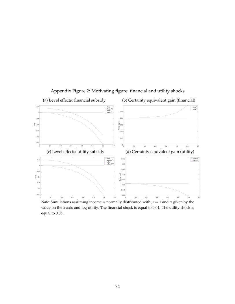
Appendix Figure 2: Motivating figure: financial and utility shocks

(a) Level effects: financial subsidy

0 0.1 0.2 0.3 0.4 0.5 0.6 0.7

-0.25

-0.2

-0.15

-0.1

-0.05

0

0.05

Utilit

y

Eu(y)

Eu(y+dfin)

u(Ey)

u(Ey+dfin)

(b) Certainty equivalent gain (financial)

0 0.1 0.2 0.3 0.4 0.5 0.6 0.70

0.01

0.02

0.03

0.04

0.05

Cons. equiv

.

CEfin

Eyfin

(c) Level effects: utility subsidy

0 0.1 0.2 0.3 0.4 0.5 0.6 0.7

-0.25

-0.2

-0.15

-0.1

-0.05

0

0.05

Utilit

y

Eu(y)

Eu(y)+dutility

u(Ey)

u(Ey)+dutility

(d) Certainty equivalent gain (utility)

0 0.1 0.2 0.3 0.4 0.5 0.6 0.7

0.04

0.045

0.05

0.055

0.06

0.065

0.07

0.075

Cons. equiv

.

CEutility

Eyutility

Note: Simulations assuming income is normally distributed with µ = 1 and σ given by thevalue on the x axis and log utility. The financial shock is equal to 0.04. The utility shock isequal to 0.05.

74

Computational Result 3. The derivative of the change in risk sharing is increasing in the mean-preserving riskiness of migration income with a financial subsidy

Panel (b) of Appendix Figure 3 plots the effect of a financial subsidy to migrate. Panel(bi) shows that the financial subsidy induces migration under autarky, but only for lowlevels of income risk. Migration under limited commitment increases by 15%, indepen-dent of income risk. Panel (bii) shows that risk sharing improves overall (i.e., the esti-mated effect on beta is negative). The improvement in risk sharing is largest when in-come is least risky, although the magnitude is very small in all cases. Panel (biii) showsthat welfare increases slightly under autarky, and there is a very small decrease in esti-mated welfare (because the utility cost of migrating may not be fully compensated) underlimited commitment.

Computational Result 4. The derivative of the change in risk sharing is decreasing in the mean-preserving riskiness of migration income with a utility subsidy

Panel (c) of Appendix Figure 3 plots the effect of a utility subsidy to migrate. Panel(ci) shows that the utility subsidy induces migration under autarky, with the largest effectwhen income is least-risky. The migration effect under limited commitment is relativelyflat, although slightly higher when income is less risky. Panel (cii) shows that shows thatrisk sharing improves overall (i.e., the estimated effect on beta is negative). In comparisonto the financial subsidy, the improvement in risk sharing is largest when income is themost risky. Panel (ciii) shows that welfare increase is larger under limited commitmentthan under autarky; the gap is larger the riskier income is.

75

Appendix Figure 3: Comparative statics around income risk: utility and financial subsi-dies (rescaling mean)

(a) Control group (b) Treatment effect: financial subsidy

(c) Treatment effect: utility subsidy (d) Treatment effect: combined subsidy

Note: Migration income risk is measured relative to the baseline estimates (i.e., a valueof 1 is the baseline estimate). The log-normal distribution is rescaled so that the mean isconstant as the risk increases.

76

A.5 Standard errors

To compute standard errors we numerically approximate the variance-covariance matrix.Following the notation in Hansen (2016), the SMM estimator minimizes the weighteddeviations of the simulated moment conditions, gi(β), ∀i = 1, ..., l. The moment vectorhas dimension (l × 1) and the parameter vector, β, has dimension (k× 1).

The SMM estimator minimizes:

βSMM = argminβ g(β)′Wg(β)

where W is a weight matrix of dimension l × l. The variance-covariance matrix is givenby:

Vβ =(Q′WQ

)−1 (Q′WΩWQ) (

Q′WQ)−1

The matrix Q is a l × k gradient matrix of the derivatives of each simulated moment toeach parameter:

Q = E ∂

∂β′g(β)

We estimate Q by numerical differentiation, taking step sizes of 1% of the estimated value.Because our problem is discrete, we smooth the objective function by a smoothing param-eter λ = 1e−4 so that it is possible to compute the numerical derivatives. We approximateΩ by the sample analog of the simulated moments:

Ω = Eg(β)g(β)′

77

B Empirical appendix

This appendix provides additional details on empirical issues. We start by discussingtransfers and additional results from migrant surveys. We then include supplementarytables and figures discussed in the text.

B.1 Magnitude of transfers in and transfers out

The summary statistics in Table 1 show that average transfers received by members inthe sample is larger than the total transfers given by the sample. The reason for thisdifference is that only the poorest households in the village (based on land holdings andon experiencing hunger the previous year) were eligible for the experiment. Data wasonly collected on eligible households, not on the wealthier ineligible households. Thus, ifthere were transfers between eligible and noneligible households we should expect givingto be smaller than receipts in our sample.

We show in Appendix Table 1 that, as expected, households that are richer transfermore than households that are poorer. The first four rows show mean income in column1 and net giving (transfers given minus transfers received) as a percent of income in col-umn 2, by income quartile in the data. Net transfers in as a fraction of income decreasesmonotonically with income: the poorest income quartile has 64% of income coming fromnet transfers in, while the richest income quartile has 19% of income coming from nettransfers in. We then construct linear predictions of these patterns in columns 3 and 4,and extrapolate to the missing top 3/7ths of the income distribution in rows 5 through 7.Once we do this exercise, we estimate that, at the village level, net giving would be 1723Taka, suggesting that this linear approximation of transfers over the income distributioncan explain the transfer imbalance fairly well.

We note that any imbalance in the total amount of income to be shared amongst eligi-ble households does not affect the Townsend regressions within the observed data, as thevillage fixed effect is controlling for the total resources in the network. However, this ispotentially a concern for the structural estimation, as we impose that total income is equalto total consumption when solving the model. Unfortunately, given the data we have, weare not able to adjust for this in the structural estimation.

78

Appendix Table 1: Extrapolated net giving

Data Linear prediction

Income group Mean income Net giving Mean income Net giving Net giving(% of income) (% of income) (level)

Data: income quartile1 4176 -0.64 3678 -0.57 -21032 7349 -0.35 7560 -0.43 -32163 10372 -0.23 11443 -0.28 -31914 16111 -0.19 15326 -0.13 -2029

Extrapolated/missing income groups5 19209 0.01 2716 23091 0.16 37087 26974 0.31 8282

Overall net giving 1723

Note: Our data (control villages) consists of the bottom 4/7ths of the income distribution of villages, andthus the first four rows and first two columns show mean income and mean net giving (transfers givenminus received) as a percent of income. The third and fourth columns report a linear prediction of the firsttwo columns, and the fifth through seventh rows extrapolate to the rest of the village. The final columnmultiplies the fifth and sixth columns to get net giving, and the final row sums this column.

79

B.2 Appendix Tables

Appendix Table 2: Experimental design and data collection timeline

Round Date Obs Data Model period Experiments

Migration Income Consumption Townsend test? Main Additional

1 July 2008Planting

1900 HH100 villages X 12 months Varies

(1 wk - 12 mo) Robustness Pre X X

2 Nov 2008Monga

1900 HH100 villages X 4 months Varies

(1 wk - 4 mo) X Active X X

3 Nov 2009Monga

1900 HH100 villages X X

Varies(1 wk - 12 mo) X X X X

4 July 2011Planting

2527 HH133 villages X 12 months Varies

(1 wk - 12 mo) X Post X X

5 Dec 2013Monga

2527 HH133 villages X 12 months Varies

(1 wk - 3 mo) Robustness X X X

Note: The row in bold (Round 4) is the data round primarily used in the analysis in the paper.Experiments in Round 2 were: Cash, credit, info, control.Experiments in Round 4 were: Rain insurance, price insurance, credit, conditional credit, job leads, control.Experiments in Round 5 were: Credit, job leads, control.Consumption recall periods varied by category: Food: 1 week, or 2 weeks if didn’t consume in past 1week; fuel/transport expenses: 1 week; utility bills/rent/health expenses/personal items/entertainment:1 month; clothing/furniture/events/education/durable purchases: 12 months in rounds 1, 3, and 4, 4months in round 2, and 3 months in round 5.

80

Appendix Table 3: Migration experiences (destination data)

Mean Std. Div Min Max Obvs.Did you find a job at destination? 0.979 0.143 0.0 1.0 145Do you think the income/wage is more than your area? 0.890 0.314 0.0 1.0 145Did anyone from your travel group help in getting the job? 0.338 0.475 0.0 1.0 145Did anyone else known to you help in getting the job? 0.234 0.425 0.0 1.0 145Did anyone from your travel group or someone else help you in getting the job? 0.545 0.500 0.0 1.0 145Did you migrate alone? 0.228 0.421 0.0 1.0 145Did you expend other costs jointly with your group member? 0.330 0.472 0.0 1.0 112Did you expend costs for food jointly with your group member? 0.703 0.463 0.0 1.0 37Did you expend travel costs jointly with your group member? 0.811 0.397 0.0 1.0 37Did you expend other costs jointly with your group member (specify)? 0.622 0.492 0.0 1.0 37Are you currently sharing accommodations with a member of your travel group? 0.705 0.458 0.0 1.0 112Did you only give job information to someone in your travel group? 0.152 0.360 0.0 1.0 112Did you both give and receive job information from someone in your travel group? 0.464 0.501 0.0 1.0 112Did you neither give nor receive job info from someone in your travel group? 0.277 0.449 0.0 1.0 112How many times did you eat in the last week? 20.510 1.768 7.0 21.0 145How many times did you have a full meal during the last week? 17.959 3.603 5.0 21.0 145How many times did you have a meal with meat during the last week? 7.972 4.278 0.0 21.0 145How many times did you have a meal with rice during the last week? 19.138 3.499 3.0 21.0 145How much did you spend on food in total during the last week? 16.943 26.170 0.0 95.7 145How much did you receive from your employer for food during the last week? 101.437 37.048 0.0 262.9 145How much did you spend on accommodation during the last week? 0.901 2.630 0.0 15.0 145How much did you spend on other expenditure during the last week? 8.453 8.035 0.0 69.3 145How much did you receive as charity during the last week? 0.116 0.921 0.0 10.0 145Did you only receive job information from someone in your travel group? 0.107 0.311 0.0 1.0 112Statistics taken from the 2008 destination survey. Monetary values are in Taka.

81

Appendix Table 4: Migration experiences (endline data)

(1) (2) T-testNot Incentivized Incentivized Difference

Variable Mean/SE Mean/SE (1)-(2)

Did you migrate to a rural area? 0.652(0.031)

0.661(0.027)

-0.008

When you migrated, did you migrate alone? 0.266(0.040)

0.258(0.023)

0.009

Did you migrate with the same person last year? 0.429(0.054)

0.481(0.027)

-0.051

Did you work in the agricultural sector? 0.538(0.034)

0.609(0.030)

-0.071

Did you work in the transportation sector? 0.103(0.034)

0.090(0.014)

0.013

Did you work as a non-ag. day laborer? 0.239(0.038)

0.178(0.023)

0.061

Did you work in a different sector? 0.120(0.024)

0.123(0.018)

-0.003

Did you earn more than expected? 0.147(0.028)

0.219(0.024)

-0.072*

Did you earn less than expected? 0.560(0.035)

0.491(0.028)

0.069

Did you earn the same as expected? 0.293(0.033)

0.290(0.023)

0.003

How much did you earn in cash? 3448.995(294.937)

3370.511(207.954)

78.483

How much did you earn in non-monetary support? 845.163(112.789)

1007.192(87.802)

-162.029

How much money did you send back home? 976.902(225.667)

660.644(83.199)

316.258

What were the savings from migration? 1554.685(116.222)

1883.278(101.400)

-328.593**

N 184 489Clusters 31 68

Notes: Taken from 2008 endline survey The value displayed for t-tests are the differencesin the means across the groups. Standard errors are clustered at variable village. ***, **,and * indicate significance at the 1, 5, and 10 percent critical level.

82

Appendix Table 5: Treatment effect on transfers within the community, by migration status

All households Migrant households Non-migrant households

Treatment Control Treatment Control Treatment Controleffect mean effect mean effect mean

Willingness to helpCommunity member would help you 0.030 0.85 0.045 0.85 0.032 0.85

(0.020) (0.030) (0.022)... and you would ask for help 0.025 0.83 0.034 0.83 0.031 0.83

(0.020) (0.031) (0.023)Community member would ask you for help 0.109∗∗∗ 0.57 0.140∗∗∗ 0.59 0.091∗∗ 0.56

(0.033) (0.043) (0.037)... and you would help them 0.109∗∗∗ 0.53 0.129∗∗∗ 0.55 0.094∗∗∗ 0.51

(0.032) (0.044) (0.035)Actual transfers

Receive any transfer from community member -0.024 0.57 -0.003 0.55 -0.015 0.59(0.022) (0.036) (0.028)

Amount, if any transfer received (Tk) 1821∗∗∗ 4808 648 4169 3175 5185(678) (593) (1108)

Give any transfer to community member 0.036∗∗ 0.15 0.049 0.17 0.028 0.14(0.018) (0.031) (0.020)

Amount, if any transfer given (Tk) 1310 2001 816 1984 1937∗ 2014(558) (677) (1024)

Note: The sample includes households from the 2011 survey. Columns 1 and 2 contain all households, columns 3 and 4 contain migrant households,and columns 5 and 6 contain non-migrant households. Each cell is a separate regression of the effect of treatment on whether the source denoted inthe row would behave as described. Each regression also controls for upazila (county). Standard errors, clustered by village, are in parentheses, andthe mean of the control group is in the second column of each set. ∗ p < 0.10, ∗∗ p < 0.05, ∗∗∗ p < 0.01

83

Appendix Table 6: Effect of migration incentives on exposure of consumption to income,cross-treatments

Log total consumption

(1) (2) (3)

Log income 0.157∗∗∗ 0.156∗∗∗ 0.158∗∗∗

(0.027) (0.027) (0.028)Log income x treatment -0.073∗∗∗

(0.027)Treatment group restrictions

Log income x unassigned group -0.085∗∗

(0.035)Log income x self-formed group -0.018

(0.033)Log income x assigned group -0.106∗∗∗

(0.037)Treatment destination restrictions

Log income x unassigned destination -0.065∗∗

(0.030)Log income x assigned destination -0.082∗∗

(0.032)unconditional credit × logy -0.020 -0.020 -0.021

(0.038) (0.039) (0.039)

Observations 1857 1857 1857R-squared 0.186 0.188 0.187

Note: The sample includes households from the 2011 survey. The dependent variable is log annual per-capita total consumption. The main independent variable is log annual per-capita income, interacted withthe respective treatment variable. All models control for village fixed effects and log income interacted with2011 treatment arms. Standard errors, clustered by village, are in parentheses. ∗ p < 0.10, ∗∗ p < 0.05, ∗∗∗

p < 0.01

84

Appendix Table 7: Effect of migration incentives on exposure of consumption to income, alternative trims

Log total consumption

5% trim 2.5% trim 1% trim

(1) (2) (3) (4) (5) (6) (7) (8) (9)

Log income (round 4) 0.157∗∗∗ 0.112∗∗ 0.109∗∗

(0.027) (0.054) (0.046)Treatment effect on log income -0.073∗∗∗ -0.077 -0.099∗∗

(0.027) (0.061) (0.046)Log income (round 4) 0.137∗∗∗ 0.086∗∗∗ 0.073∗∗

(0.024) (0.025) (0.028)Treatment effect on log income -0.050∗∗ -0.049 -0.049

(0.023) (0.040) (0.034)Log income (round 4) 0.148∗∗∗ 0.106∗∗ 0.118∗∗

(0.027) (0.051) (0.051)Treatment effect on log income -0.081∗∗∗ -0.044 -0.073

(0.025) (0.065) (0.051)

Village-round FE X X X X X X X X XHousehold FE X X X X X XIncludes baseline X X X X X XIncludes 2013 X X X

Observations 1857 2166 4371 2251 3142 5635 2097 2366 4691R squared 0.186 0.791 0.721 0.193 0.775 0.696 0.186 0.782 0.717

Note: Table presents coefficients of the effect of log annual per capita income on log annual per capita consumption and the interaction with treatment(β0 and β1 from Equation 2). The sample in columns (1)-(3) uses income and consumption measures with a 5% trim (our main analysis sample), thesample in columns (4)-(6) use a 2.5% trim, and columns (7)-(9) use a 1% trim. All models control for village fixed effects and all other interactionsbetween treatment and log income as well as log income interacted with 2011 treatments. For each trim set, the first column includes only 2011 data,the second reports the results from a difference-in-difference specification with household fixed effects that includes baseline data and 2011 data,and the third column reports the results from a difference-in-difference specification with household fixed effects that includes baseline data, 2011data, and 2013 data. Standard errors, clustered by village, are in parentheses. ∗ p < 0.10, ∗∗ p < 0.05, ∗∗∗ p < 0.01

85

Appendix Table 8: Effect of migration incentives on exposure of consumption to income, alternative samples

Log total consumption

Main sample Controls in later experiment Non-migrant households

(1) (2) (3) (4) (5) (6) (7) (8) (9)

Log income (round 4) 0.157∗∗∗ 0.112∗∗ 0.109∗∗ 0.193∗∗∗ 0.116 0.105∗ 0.167∗∗∗ 0.128∗∗ 0.193∗∗∗

(0.027) (0.054) (0.046) (0.032) (0.071) (0.053) (0.034) (0.057) (0.056)Treatment effect on log income -0.073∗∗∗ -0.077 -0.099∗∗ -0.137∗∗∗ -0.116 -0.073 -0.081∗∗ -0.098 -0.117∗∗

(0.027) (0.061) (0.046) (0.046) (0.103) (0.095) (0.033) (0.080) (0.052)

Village-round FE X X X X X X X X XHousehold FE X X X X X XIncludes baseline X X X X X XIncludes 2013 X X X

Observations 1857 2166 4371 497 786 1305 1140 1302 2734R squared 0.186 0.791 0.721 0.171 0.771 0.708 0.224 0.800 0.760

Note: Table presents coefficients of the effect of log annual per capita income on log annual per capita consumption and the interaction with treatment(β0 and β1 from Equation 2). The sample in columns (1)-(3) is our main sample of households from the 2011 survey, the sample in columns (4)-(6)includes households from the 2011 survey that were in control villages in the 2011 treatments, and the sample in columns (7)-(9) include non-migranthouseholds from the 2011 survey. All models control for village fixed effects, and columns (1)-(3) and (7)-(9) also control for log income interactedwith 2011 treatment arms. For each sample set, the first column includes only 2011 data, the second reports the results from a difference-in-differencespecification with household fixed effects that includes baseline data and 2011 data, and the third column reports the results from a difference-in-difference specification with household fixed effects that includes baseline data, 2011 data, and 2013 data. Standard errors, clustered by village, arein parentheses. ∗ p < 0.10, ∗∗ p < 0.05, ∗∗∗ p < 0.01

86

Appendix Table 9: Effect of migration incentives on exposure of consumption to income,different household size assumptions

Log total consumption

Size: past 7 days current past 14 days equiv. scale 7 days + mig(main spec.)

(1) (2) (3) (4) (5)

Log income x treat, size: past 7 days -0.073∗∗∗

(0.027)Log income x treat, size: current -0.046∗

(0.026)Log income x treat, size: past 14 days -0.077∗∗∗

(0.026)Log income x treat, size: equiv. scale -0.080∗∗∗

(0.026)Log income x treat, size: 7 days + migrants -0.069∗∗

(0.027)

Observations 1857 1854 1860 1854 1858R-squared 0.186 0.183 0.191 0.221 0.184

Note: The sample includes households from the 2011 survey. The dependent variable is log of annual per-capita total consumption. The main independent variable is log of annual per capita income, interactedwith treatment. The definition of household size used to calculate per capita terms is the total numberof household members present in at least the past 7 days at the time of the interview in column (1), thetotal number of household members currently present at the time of the interview in column (2), the totalnumber of household members present in at least the past 14 days at the time of the interview in column(3), an equivalence scale in column (4), and the total number of household members present in the past 7days plus any migrants who have not yet returned in column (5). We use Townsend’s equivalence scale inwhich the weights are: 1.0 for adult males, 0.9 for adult females, 0.94 for males 13-18, 0.83 for females 13-18,0.67 for children 7-12, 0.52 for children 4-6, 0.32 for children 1-3, and 0.05 for infants. All models control forlog of income interacted with 2011 treatment arms and village fixed effects. Standard errors, clustered byvillage, are in parentheses. ∗ p < 0.10, ∗∗ p < 0.05, ∗∗∗ p < 0.01

87

Appendix Table 10: Effect of migration incentives on exposure of consumption to income,reverse regression

(1) (2)Log consumption (fwd) Log income (rev)

Log income x control 0.204∗∗∗

(0.045)Log income x treatment 0.131∗∗∗

(0.043)Log consumption x control 0.567∗∗∗

(0.118)Log consumption x treatment 0.385∗∗∗

(0.120)

Fwd/Rev ratio, control 0.360Fwd/Rev ratio, treat 0.342Observations 1857 1857R-squared 0.186 0.166

Note: The sample includes households from the 2011 survey. In column (1) the dependent variable is log ofannual per-capita total consumption and the main independent variable is log of annual per-capita income,interacted with the respective treatment variable. In column (2) the dependent and independent variablesare reversed. All models control for village fixed effects and the independent variable interacted with 2011treatment arms. Standard errors, clustered by village, are in parentheses. ∗ p < 0.10, ∗∗ p < 0.05, ∗∗∗

p < 0.01

88

Appendix Table 11: Effect of migration incentives on exposure of consumption to income,by income components

Log total consumption

(1) (2) (3)

Log income x treatment -0.073∗∗∗

(0.027)Log village income x treatment -0.069∗∗∗

(0.024)Log migration income x treatment -0.048

(0.036)

Observations 1857 1857 792R-squared 0.186 0.179 0.263

Note: The sample includes households from the 2011 survey. The dependent variable is log of annual per-capita total consumption and the main independent variable is log of annual per-capita income, interactedwith the respective treatment variable. Income is defined as total income in column (1), village income incolumn (2), and migration income (among migrants) in column (3). All models control for village fixedeffects and the independent variable interacted with 2011 treatment arms. Standard errors, clustered byvillage, are in parentheses. ∗ p < 0.10, ∗∗ p < 0.05, ∗∗∗ p < 0.01

Appendix Table 12: Savings compared to income

Round 1 Round 2 Round 4

Liquid assetsMean liquid assets 91 148 296Mean liquid assets saved recently* 2 3 32

Cash savingsMean cash savings 228 215 163Mean cash saved in past 12 months 155

IncomeMean village income 6185 3999 8770Mean migration income (migrants) 2760 1959Mean total income 4819 9502SD village income 3366 3085 4721SD migration income (migrants) 2178 1304SD total income 3455 4728

Note: Table reports data from control villages only. All numerical values are in per capita terms. *Liquidassets saved recently corresponds to the last 4 months for round 2 and the last 12 months for rounds 1 and4.

89

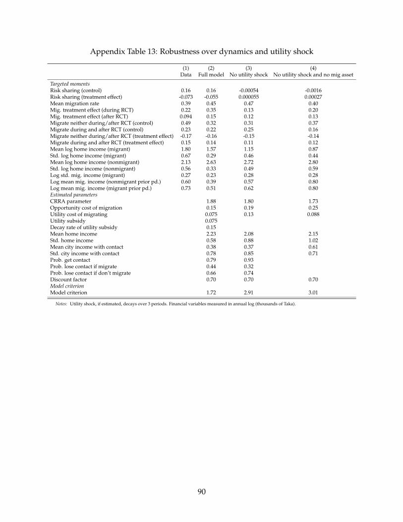
Appendix Table 13: Robustness over dynamics and utility shock

(1) (2) (3) (4)Data Full model No utility shock No utility shock and no mig asset

Targeted momentsRisk sharing (control) 0.16 0.16 -0.00054 -0.0016Risk sharing (treatment effect) -0.073 -0.055 0.000055 0.00027Mean migration rate 0.39 0.45 0.47 0.40Mig. treatment effect (during RCT) 0.22 0.35 0.13 0.20Mig. treatment effect (after RCT) 0.094 0.15 0.12 0.13Migrate neither during/after RCT (control) 0.49 0.32 0.31 0.37Migrate during and after RCT (control) 0.23 0.22 0.25 0.16Migrate neither during/after RCT (treatment effect) -0.17 -0.16 -0.15 -0.14Migrate during and after RCT (treatment effect) 0.15 0.14 0.11 0.12Mean log home income (migrant) 1.80 1.57 1.15 0.87Std. log home income (migrant) 0.67 0.29 0.46 0.44Mean log home income (nonmigrant) 2.13 2.63 2.72 2.80Std. log home income (nonmigrant) 0.56 0.33 0.49 0.59Log std. mig. income (migrant) 0.27 0.23 0.28 0.28Log mean mig. income (nonmigrant prior pd.) 0.60 0.39 0.57 0.80Log mean mig. income (migrant prior pd.) 0.73 0.51 0.62 0.80Estimated parametersCRRA parameter 1.88 1.80 1.73Opportunity cost of migration 0.15 0.19 0.25Utility cost of migrating 0.075 0.13 0.088Utility subsidy 0.075Decay rate of utility subsidy 0.15Mean home income 2.23 2.08 2.15Std. home income 0.58 0.88 1.02Mean city income with contact 0.38 0.37 0.61Std. city income with contact 0.78 0.85 0.71Prob. get contact 0.79 0.93Prob. lose contact if migrate 0.44 0.32Prob. lose contact if don’t migrate 0.66 0.74Discount factor 0.70 0.70 0.70Model criterionModel criterion 1.72 2.91 3.01

Notes: Utility shock, if estimated, decays over 3 periods. Financial variables measured in annual log (thousands of Taka).

90

Appendix Table 14: Robustness over discount factor and subsistence

(1) (2) (3) (4)Data β = 0.7 β = 0.8 β = 0.9

Risk sharing (control) 0.16 0.16 0.082 -0.0054Risk sharing (treatment effect) -0.073 -0.055 -0.045 0.00037Mean migration rate 0.39 0.45 0.45 0.44Mig. treatment effect (during RCT) 0.22 0.35 0.35 0.16Mig. treatment effect (after RCT) 0.094 0.15 0.15 0.12Migrate neither during/after RCT (control) 0.49 0.32 0.33 0.34Migrate during and after RCT (control) 0.23 0.22 0.22 0.22Migrate neither during/after RCT (treatment effect) -0.17 -0.16 -0.15 -0.14Migrate during and after RCT (treatment effect) 0.15 0.14 0.13 0.11Mean log home income (migrant) 1.80 1.57 1.61 1.34Std. log home income (migrant) 0.67 0.29 0.30 0.51Mean log home income (nonmigrant) 2.13 2.63 2.67 3.06Std. log home income (nonmigrant) 0.56 0.33 0.33 0.61Log std. mig. income (migrant) 0.27 0.23 0.25 0.27Log mean mig. income (nonmigrant prior pd.) 0.60 0.39 0.39 0.64Log mean mig. income (migrant prior pd.) 0.73 0.51 0.51 0.68Estimated parametersCRRA parameter 1.88 1.94 1.75Opportunity cost of migration 0.15 0.14 0.16Utility cost of migrating 0.075 0.072 0.11Utility subsidy 0.075 0.076 0.058Decay rate of utility subsidy 0.15 0.13 0.41Mean home income 2.23 2.26 2.38Std. home income 0.58 0.58 1.01Mean city income with contact 0.38 0.37 0.48Std. city income with contact 0.78 0.80 0.78Prob. get contact 0.79 0.78 0.94Prob. lose contact if migrate 0.44 0.44 0.42Prob. lose contact if don’t migrate 0.66 0.66 0.68Discount factor 0.70 0.80 0.90Model criterionModel criterion 1.72 2.09 2.80

Notes: The cost to consume a subsistence level of consumption, estimated to be 600 calories per day, isestimated to be 250 Taka/month (3000 Taka annually). Because the model is measured in income, notconsumption, units, we set the subsistence level to 1000 Taka instead of 3000 Taka to match the proportionof people below subsistence as measured by income with the proportion of people below subsistence asmeasured by consumption.

91

B.3 Appendix Figures

Appendix Figure 4: Distributions of baseline annual village income and consumption, bytreatment

Difference in means: 158.6 (152.5)Kolmogorov-Smirnov test p-value: 0.46

0.0

0005

.000

1.0

0015

Den

sity

0 5000 10000 15000Baseline village income (Taka)

Control Treatment

Difference in means: 54.8 (197.6)Kolmogorov-Smirnov test p-value: 0.96

0.0

0005

.000

1.0

0015

Den

sity

5000 10000 15000 20000 25000Baseline consumption (Taka)

Control Treatment

Notes: Top figure is baseline annual village income and the bottom figure is baseline annual consumption,in Taka. Black lines are treatment households and gray lines are control households. The dotted verticallines are the means of the distributions.

92

Appendix Figure 5: Dynamics of migration subsidy: Robustness

(a) Mig asset X; utility sub. X (b) Mig asset X; utility sub. X

(c) Mig asset X; utility sub. X

93

Appendix Figure 6: Decomposition of permanent shock

(a) Temporary: financial shock only (b) Permanent: financial shock only

(c) Temporary: utility shock only (d) Permanent: utility shock only

(e) Temporary: combined shock (f) Permanent: combined shock

94