Migrants and Firms: Evidence from China *

Clement Imbert Marlon Seror Yifan ZhangYanos Zylberberg

December 14, 2020

Abstract

How does rural-urban migration shape urban production in developing

countries? We use longitudinal data on Chinese manufacturing firms between

2000 and 2006, and exploit exogenous variation in rural-urban migration in-

duced by agricultural income shocks for identification. We find that, when im-

migration increases, manufacturing production becomes more labor-intensive

and productivity declines. We investigate the reorganization of production us-

ing patent applications and product information. We show that rural-urban

migration induces both labor-oriented technological change and the adoption

of labor intensive product varieties.

JEL codes: D24; J23; J61; O15.

*Imbert: University of Warwick, BREAD, CEPR and JPAL, c.imbert@warwick.ac.uk; Seror:Universite du Quebec a Montreal, University of Bristol, DIAL, Institut Convergences Migrations,seror.marlon@uqam.ca; Zhang: Chinese University of Hong Kong, yifan.zhang@cuhk.edu.hk; Zyl-berberg: University of Bristol, CESifo, the Alan Turing Institute, yanos.zylberberg@bristol.ac.uk.We thank Samuel Bazzi, Loren Brandt, Holger Breinlich, Gharad Bryan, Juan Chen, GiacomoDe Giorgi, Maelys De La Rupelle, Sylvie Demurger, Taryn Dinkelman, Christian Dustmann, BenFaber, Giovanni Facchini, Greg Fischer, Richard Freeman, Albrecht Glitz, Doug Gollin, AndreGroeger, Flore Gubert, Naijia Guo, Marc Gurgand, Seema Jayachandran, Marieke Kleemans, Jes-sica Leight, Florian Mayneris, David McKenzie, Alice Mesnard, Dilip Mookherjee, Joan Monras,Melanie Morten, Albert Park, Sandra Poncet, Markus Poschke, Simon Quinn, Mark Rosenzweig,Gabriella Santangelo, Michael Song, Jon Temple, Chris Udry, Gabriel Ulyssea, Thomas Vendryes,Chris Woodruff, Daniel Yi Xu, Dean Yang, and numerous conference and seminar participantsfor useful comments. We are grateful to Christine Valente and Eric Verhoogen for their insightsat the early stage of the project. Seror gratefully acknowledges support from the Arthur SachsScholarship Fund. The usual disclaimer applies.

1

1 Introduction

Firms in developing countries have lower productivity per worker (Hall and Jones,

1999). A number of factors explain this pattern, such as an imperfect access to

capital (Banerjee and Duflo, 2014), inputs (Boehm and Oberfield, 2020), technol-

ogy (Howitt, 2000), international markets (Verhoogen, 2008), or poor management

practices (Bloom et al., 2013; Atkin et al., 2017). Another potential factor may be

the abundance of migrant labor. The process of economic development induces large

movements of rural workers from agriculture to manufacturing (Lewis, 1954), which

could reduce firms’ incentives to adopt productivity-enhancing technologies (Lewis,

2011). Despite its relevance, empirical evidence on the role of rural-urban migration

in shaping urban production in developing countries is scarce.

This paper is the first to estimate the causal effect of rural migrant inflows on

urban production in the process of structural transformation. We use longitudinal

micro data on Chinese manufacturing firms between 2000 and 2006 and a popula-

tion micro-census that allows us to measure rural-urban migration. We instrument

migrant flows to Chinese cities using exogenous shocks to agricultural income in

rural areas, which trigger rural-urban migration. We first identify the effect of mi-

gration on factor cost, factor use, and factor productivity at destination. We then

characterize the restructuring of production at destination through the analysis of

technological innovation and product choice within production units.

Providing empirical evidence on the causal impact of labor inflows on manu-

facturing production requires large and exogenous migrant flows to cities. Our

methodology proceeds in two steps. In the first step, we isolate exogenous varia-

tion in agricultural income by combining innovations in world prices for agricultural

commodities with variation in cropping patterns across prefectures of origin.1 In

the second step, we combine these predictors of rural emigration (the “shift”) with

historical migration patterns between prefectures (the “share”). The resulting shift-

share instrument strongly predicts migrant inflows to cities and exhibits substantial

variation across prefectures of destination.

We use the shift-share design to estimate the impact of rural-urban migration

flows on manufacturing firms. We find that migration exerts a downward pressure

on labor cost. After an influx of migrants, manufacturing production becomes much

more labor-intensive, as capital does not adjust to changes in employment, and value

added per worker sharply decreases.

Although our main results focus on firms that are observed every year between

1Prefectures are the second administrative division in China, below the province. There wereabout 330 prefectures in 2000.

2

2000 and 2006, the composition of the manufacturing sector is in constant evolution

during the period, and many firms enter and exit the sample. When we consider all

firms present in the sample at any point in time, the shift towards labor intensive

production and the decline in productivity following a migration shock are even

more pronounced. This suggests that following a migration shock, labor-intensive,

low productivity firms are less likely to die, and more likely to grow.

Our findings are robust to numerous sensitivity checks, e.g., excluding industries

that process agricultural goods, controlling for industry fixed effects, or accounting

for a demand shift for the final good. The identification assumption underlying our

shift-share design is that “shifts”, i.e., agricultural income shocks driven by cropping

patterns and price innovations, are numerous and as good as random (Borusyak et

al., 2018).2 We provide support for this assumption by transforming our baseline

specification at destination into a specification looking at the effect of shifts on trans-

formed outcomes across origins (Borusyak et al., 2018). We use this specification

to test that pre-trends in outcomes are not correlated with future migration shocks.

We also test that our results are not driven by the lagged effects of past migration

waves (Jaeger et al., 2018). We finally rely on the recent contribution of Adao et al.

(2019b) to discuss the correct inference for our shift-share design.

Changes in input mix may reflect changes in the nature of manufacturing goods,

or changes in technology to produce a similar output (as in Beaudry and Green,

2003). We look for evidence of adjustments along both margins. To better char-

acterize the impact of labor inflows on the production process, we first exploit the

textual descriptions of products as reported by manufacturing establishments. More

specifically, we associate a unique HS6 product code to each product, and we charac-

terize the direction of a change in output mix by looking at factor use within product

classes. We find that rural-urban migration tilts production toward products that

are labor-intensive and with low human capital intensity. Using a match between

manufacturing firms and patent applications (He et al., 2018), we also find evidence

of a marked decrease in patenting, concentrated in categories linked to fundamental

innovation and new production methods, and in patent classes that are capital- and

skill-intensive. Finally, we explore whether changes in technology and input mix

are systematically related to endogenous product choice. We find that firms that

experience an increase in labor supply through migration change their input mix,

irrespective of a possible change in product. By contrast, the decline in patenting

2Another recent contribution discusses identification in shift-share designs when “shares” areas good as random, numerous, and dispersed (Goldsmith-Pinkham et al., forthcoming). In ourshift-share design, shares are previous settlement patterns and may reflect the expectations ofmigrants about the future evolution of urban production.

3

only occurs among firms that also adjust their product in response to migration.

These results suggest that there is directed technological change for a given output

mix (as in Beaudry and Green, 2003), but that product choice is also a margin of

adjustment: innovative firms, which would have pushed the technological frontier

through capital-augmenting innovation, now prefer to shift along the frontier and

adopt more labor-intensive product varieties.

Our empirical setting, which provides a unique opportunity to study the effect

of rural migrants on manufacturing firms, also has important limitations. First,

we do not observe changes in the skill composition of the workforce within firms.3

Second, the identification of causal estimates relies on unexpected variation in rural-

urban migration, which may induce a different adjustment by firms than long-term

trends in labor supply.4 Third, rural migrants may impact other markets than la-

bor markets, e.g., through demand for non-tradable goods at destination.5 Fourth,

our difference-in-difference setting implies that the estimates cannot be extrapolated

at the level of the country, without understanding the magnitude of general equi-

librium effects (Adao et al., 2019a; Beraja et al., 2019). Finally, we only observe

manufacturing firms; our analysis cannot shed light on the implications of migration

on aggregate productivity, or on productivity gaps across sectors.

Our paper contributes to four different strands of literature. First, we use

product-level information and patent data to estimate the effect of labor supply

shocks on factor use, product choice, and technological adoption at the establish-

ment level. This approach relates to the growing literature that estimates the impact

of immigration on factor use at destination (Lewis, 2011; Peri, 2012; Accetturo et

al., 2012; Olney, 2013; Dustmann and Glitz, 2015; Kerr et al., 2015; Mitaritonna

et al., 2017). In contrast with a literature that focuses on international migration

to developed countries, we study rural-urban migration in a developing country, a

context which is less studied but equally important: in 2010, there were as many in-

ternal migrants in China alone than international migrants worldwide (205 million).

A related literature looks specifically at the positive contribution of the immigra-

tion of scientists (e.g., Moser et al., 2014) or inventors (e.g., Akcigit et al., 2016) on

innovation in the United States. In our context, internal migrants are mostly low-

skilled, so that they are substitutes for capital and capital-enhancing technological

3In Appendix E.3, we use a survey of urban workers and find negative wage effects amonglow-skilled natives following a migration shock, but no effect on employment, and no effect fornatives with tertiary education.

4While shocks to rural-urban migration may trigger a different response, these agriculturalshocks have little effect on the characteristics of the average migrant, as we show in Appendix C.3.

5We find, for instance, evidence that migrant flows increase consumer prices at destination (seeAppendix E.3, exploiting a survey of urban workers).

4

innovation.6 Our result that firms adopt more labor intensive technology following a

migrant inflow is closer to Lewis (2011), who studies the inflow of unskilled migrants

to the United States and its impact on the (non-)adoption of automation machinery.

Our focus on the absorption of rural migrants in the urban sector of a fast-growing

economy echoes a second, older literature that looks at cities of the developing world

(Harris and Todaro, 1970; Fields, 1975). This literature emphasizes the role of

labor market imperfections, with rural migrants transiting through unemployment or

informal employment upon arrival. By contrast, our findings suggest that migrants

swiftly find their way into formal manufacturing firms. We document employment

responses to labor supply shocks that are compatible with a relatively flexible labor

market, although labor market frictions are likely pervasive in urban China. Such

labor market imperfections may be related to job search frictions (Abebe et al., 2016;

Alfonsi et al., 2017), informality (Meghir et al., 2015; Ulyssea, 2018) or institutional

constraints, e.g., minimum wages (Mayneris et al., 2018; Hau et al., 2018). Another

source of labor market imperfections is mobility rigidity, leading to large productivity

gaps across space and sectors in developing countries (Gollin et al., 2014; Bryan and

Morten, 2019), and in China (Brandt et al., 2013; Tombe and Zhu, 2019).

Our study also contributes to the literature on structural transformation, which

describes the shift of production factors from the traditional sector to the modern

sector in developing economies (Lewis, 1954; Herrendorf et al., 2015). The finding

that migration boosts urban employment relates to “labor push” models which argue

that, by releasing labor, agricultural productivity gains may trigger industrialization

(Alvarez-Cuadrado and Poschke, 2011; Gollin et al., 2002; Bustos et al., 2016).7 In

order to identify migration inflows that are exogenous to labor demand at destina-

tion, our paper takes the opposite approach to “labor pull” models, in which rural

migrants are attracted by increased labor productivity in manufacturing (Facchini

et al., 2015). Closely related to our paper, Bustos et al. (2018) find that regions of

6The non-adjustment of capital to labor supply may reflect a high substitutability betweencapital and low-skilled labor, or the existence of credit constraints. We calibrate a CES productionfunction at the sectoral level using estimates for the United States (Oberfield and Raval, 2014)and show that, when accounting for the complementarity/substitutability between factors, themarginal product of labor falls sharply, the marginal product of capital rises faintly, and total factorproductivity slightly decreases. This finding would be consistent with some degree of credit marketimperfections. We also look at treatment heterogeneity across firms with different characteristicsat baseline (e.g., factor returns or ownership structure), possibly facing different access to capital(Song et al., 2011; Midrigan and Xu, 2014). We do not find large treatment heterogeneity alongthese baseline firm characteristics.

7Our results depart from the traditional “labor push” interpretation in that migration fromrural areas is triggered by a negative shock to agricultural productivity (as in Groger and Zyl-berberg, 2016; Feng et al., 2017; Minale, 2018). Worse economic conditions at origin lower theopportunity cost of migrating, an effect which dominates an (opposite) effect operating throughtighter liquidity constraints (Angelucci, 2015; Bazzi, 2017).

5

Brazil that benefited from genetically-engineered soy specialized in low-productivity,

low-innovation manufacturing, and argue that the effect is driven by the inflow of

unskilled labor released by agriculture. Our contribution is to identify the effect of

rural migrant labor supply on urban production independently from factors such as

consumer demand (Santangelo, 2016) and capital availability (Marden, 2015; Bustos

et al., 2016), and to document changes in products and technology at the firm level.

Our empirical analysis finally relates to the literature that estimates the effect

of immigration on labor markets (Card and DiNardo, 2000; Card, 2001; Borjas,

2003), and more specifically to studies of internal migration (e.g., Boustan et al.,

2010; El Badaoui et al., 2017; Imbert and Papp, 2019; Kleemans and Magruder,

2018). Since internal migrants are usually closer substitutes to resident workers

than international migrants to natives, the literature on internal migration tends

to find larger negative effects on wages at destination. In China, the evidence is

mixed: De Sousa and Poncet (2011) find a negative effect, Meng and Zhang (2010)

no effect and Combes et al. (2015) a positive effect. Ge and Yang’s (2014) structural

estimates suggest that migration depressed urban unskilled wages by 20% in the

1990s and 2000s, which is consistent with our own estimates.

Our analysis relies on a significant methodological contribution: we process tex-

tual product descriptions using a Natural Language Processing (NLP) algorithm to

characterize product choice within manufacturing firms in China. A text-based ap-

proach to product classification has been used by Hoberg and Phillips (2016) to cap-

ture fine-grained product differentiation and study how firms distinguish themselves

from close competitors in the United States. Our approach differs from theirs in

that our objective is to allocate product descriptions into existing, standard product

categories rather than identifying new, and more precise, product clusters. Observ-

ing product and technology adoption at the firm level is rare in developing countries.

The few exceptions, reviewed in Verhoogen (2020), are contributions looking at spe-

cific sub-sectors (e.g., Atkin et al., 2017), or the papers documenting the expansion

in product scope when firms gain access to new imported inputs (Goldberg et al.,

2010; Bas and Paunov, 2019). Our classification can be useful for research using

data on Chinese manufacturing firms, e.g., to study the effect of trade on product

choice and technology. The method can also be applied to other contexts in which

product or industry information comes as a free-text description.

The remainder of the paper is organized as follows. Section 2 presents data

sources and the empirical strategy. Section 3 describes the effect of immigration on

factor cost and factor use. Section 4 characterizes the reorganization of production

through product choice and technological innovation. Section 5 briefly concludes.

6

2 Data and empirical strategy

This section describes the data on production and migrants, explains how we identify

exogenous variation in migrant inflows, and presents the empirical specification.

2.1 Firms and migrants

Measure of production in cities Our main data source is a census of Chi-

nese manufacturing firms conducted by the National Bureau of Statistics (NBS).8

The NBS implements a yearly census of all state-owned manufacturing enterprises

and all non-state manufacturing firms with sales exceeding RMB 5 million (approx.

$600,000). Although the sample does not include smaller firms, it accounts for 90%

of total manufacturing output. Firms can be matched across years: our main analy-

sis focuses on the balanced panel of 31,886 firms present every year between 2000 and

2006. The NBS collects information on location, industry, ownership type, export-

ing activity, number of employees, and a wide range of accounting variables (sales,

inputs, value added, wage bill, fixed assets, financial assets, etc.). We divide total

compensation (including housing and pension benefits) by employment to compute

the compensation rate and we construct real capital as in Brandt et al. (2014).

There are three potential issues with the NBS data. First, matching firms over

time is difficult because of frequent changes in identifiers. We apply the fuzzy al-

gorithm from Brandt et al. (2014) to detect “identifier-switchers”, using firm name,

address, and phone number etc. Second, although we use the term “firm” in this pa-

per, the NBS data cover “legal units” (faren danwei), which roughly correspond to

the definition of “establishments” in the United States.9 Third, the RMB 5 million

threshold may not be strictly implemented: private firms may enter the database a

few years after having reached the sales cut-off or continue to participate in the cen-

sus even if their annual sales fall below the threshold. We cannot measure delayed

entry into the sample, but there are very few surveyed firms below the threshold, as

Figure 1 shows.

Our baseline outcomes include compensation per worker, employment, capital-

to-labor ratio, and value added per worker. Table 1 provides descriptive statistics

of our key outcomes in 2000 and 2006 for the balanced sample and for the whole

sample of firms. The study period is one of fast manufacturing growth: employment

8The following discussion partly borrows from Brandt et al. (2014), and a detailed descriptionof data construction choices is provided in Appendix A.1.

9Different subsidiaries of the same enterprise may be surveyed, provided they meet a numberof criteria, including having their own names, being able to sign contracts, possessing and usingassets independently, assuming their liabilities, and being financially independent. The share ofsingle-plant firms is above 90% over our period of interest (Brandt et al., 2014).

7

in the balanced sample increases by 26%, capital per worker by 25%, and value

added per worker by 57%. Labor costs per worker also increase by about 8% per

year, much faster than inflation, which is about 2% per year over the period. There

is also rapid growth in the number of manufacturing establishments: sample size is

multiplied by about six between 2000 and 2006, so that firms of the balanced sample

represent 43% of manufacturing establishments in 2000, but only 7% in 2006. Firms

in the balanced sample are larger, and more capital-intensive at baseline, and they

grow faster than the average firm between 2000 and 2006. While they have higher

productivity per worker and pay higher wages than the average firm at baseline,

productivity and wages grow faster in the average firm.

The NBS does not provide a precise, systematic classification of products. In-

stead, it collects textual descriptions of up to three main products without standard-

izing them. We develop a Natural Language Processing algorithm to match product

information with a unique HS 6-digit code, through the systematic comparison of the

textual description provided by manufacturing firms with descriptions of each HS

6-digit code. In a first step, we collect descriptions in Mandarin of the standardized

HS 6-digit product classification. We clean all textual descriptions by applying a

tokenizer (“jieba”) which groups characters into words, and by deleting stop words.

This step transforms a list of characters into a sequence of identified, relevant words.

In a second step, we use the powerful neural net developed by Google (“word2vec”)

in order to represent every contiguous sequence of words in a vector space. The

neural net needs to be trained, and we rely on the word embeddings provided by Li

et al. (2018) and trained on the Wikipedia corpus. This representation allows us to

compute the distance between any sequences of words, by using their projection onto

the vector space. We then compute the average similarity score between all contigu-

ous sequences of words within the product description and word sequences within

HS 6-digit descriptions. The output of this procedure is a classification of products

with (i) the most likely HS 6-digit code—with the highest similarity score—and (ii)

a similarity score to account for possible measurement error.10 Linking products to

HS 6-digit codes allows for a precise characterization of firm production, e.g., by us-

ing production patterns within a product class. We classify the products associated

at baseline with firms whose capital intensity is higher than the median as “high

capital-to-labor ratio” and those associated with firms with a share of workers with

high school education higher than the median as “high education” products.11

Finally, to measure technological innovation, we use the bridge constructed by

10We provide a detailed description of our text-based classification in Appendix A.2.11We also use HS-6 digit codes to identify possible linkages across firms through input-output

accounts or technological closeness, as in Bloom et al. (2013).

8

He et al. (2018) to match the NBS firm data with all patents submitted to the

State Intellectual Property Office (SIPO). The data cover three main categories of

patents: design (external appearance of the final product), innovation (fundamental

innovations in methods) and utility (changes in processing, shape or structure of

products). We also use the patent code and categorize patents by the characteristics

of firms that submitted patents with the same code at baseline. Specifically, we

define as “high capital-to-labor ratio” all patent codes associated in 2000 with firms

that had a capital-to-labor ratio above median (measured in 2000), and as “high

education” all patent codes associated in 2000 with firms that had above median

share of employees with at least high school education (measured in 2004).

Migration flows To measure migration flows, we use the representative 2005 1%

Population Survey (hereafter, “2005 Mini-Census”), collected by the National Bu-

reau of Statistics.12 The sampling frame of the 2005 Mini-Census covers the entire

population at their current place of residence, regardless of whether they hold lo-

cal household registration (hukou), i.e., including migrants. The census collects

information on occupation, industry, income, ethnicity, education level, and housing

characteristics; it also provides us with key information regarding migration history.

First, we observe the household registration type (agricultural or non-agricultural),

place of registration, and place of residence at the prefecture level.13 Second, mi-

grants are asked the main reason for leaving their place of registration, which year

they left, and their place of residence one and five years before the interview.14 We

combine these two pieces of information to create a matrix of rural-urban migration

flows between all Chinese prefectures every year between 2000 and 2005. We only

include migrants who were 15 to 64 years at the time of migration, and exclude

migrants who study or migrated to study (less than 5% of the total).

The relocation of workers across prefectures is driven by preferences, migration

frictions but also, especially during the study period, by labor demand and labor

12These data have also been used, among others, by Combes et al. (2015); Facchini et al. (2015);Meng and Zhang (2010); Tombe and Zhu (2019).

13During our period of interest, barriers to mobility come from restrictions due to the registrationsystem. These restrictions do not impede rural-urban migration but limit the benefits of ruralmigrants’ long-term settlement in urban areas. See Appendix B.1 for more details about howmobility restrictions are applied in practice and the rights of rural migrants in urban China.

14A raw measure of migration flows may not account for two types of migration spells: stepand return migration. Step migration occurs when migrants transit through another city beforereaching their destination, so that the date of departure from the place of registration differs fromthe date of arrival at the current destination. Return migration occurs when migrants leave theirplaces of registration after 2000 but come back before 2005, so that they do not appear as migrantsin the Mini-Census. Appendix B.2 shows that return migration is substantial while step migrationis negligible, and explains how we adjust migration flows to account for return migration.

9

supply shocks.15 Since our objective is to identify the adjustment of production to

migrant inflows in cities, our setting lends itself to the use of a shift-share design (as

in Card, 2001, for instance), in which labor supply shocks across origins (“shifts”)

are combined with historical migration patterns (“shares”) into an instrument for

migrant inflows.16

2.2 A shift-share instrument

In this section, we construct a shift-share instrument, zd, for migrant flows to a

destination d by combining an exogenous shock to agricultural income at origin

o ∈ Θ, so, with settlement patterns of past migration waves, λod:

zd =∑

o∈Θr{d}

λodso.

Agricultural income shocks The agricultural income shock, so, is obtained from

interacting origin-specific cropping patterns and innovations in commodity prices.

We first construct a measure of cropping patterns in each prefecture by combining

a baseline measure of harvested area with potential yield.17 We use a geo-coded map

of harvested areas in China from the 2000 World Census of Agriculture, in order

to construct the total harvested area hco for a given crop c in a given prefecture

o. Information on potential yield per hectare is extracted from the Global Agro-

Ecological Zones Agricultural Suitability and Potential Yields (GAEZ) and collapsed

at the prefecture level, yco.18 We compute potential agricultural output for each crop

in each prefecture as the product of total harvested area and average potential yield,

i.e., qco = hco × yco. By construction, the potential agricultural output, qco, is time-

invariant and is measured at the beginning of the study period. Figure 2 displays

potential output qco for rice and cotton, and illustrates the wide cross-sectional

variation in agricultural portfolio across Chinese prefectures.

To measure innovation in commodity prices, we use Agricultural Producer Prices

(APP, 1991–2016) from the FAO, which reports yearly prices “at the farm gate” in

each producing country per tonne and in USD between 1991 and 2016. We focus

15We provide descriptive statistics on migration patterns across regions, and we discuss theselection of migrants in Appendix B.3.

16Appendix C.1 develops a stylized theoretical model to explain the economic mechanisms be-hind the shift-share instrument.

17Appendix C.2 describes in more detail how we construct the agricultural income shock andprovides summary statistics about the variation in cropping patterns across prefectures and regions.

18These maps are provided by the Food and Agriculture Organization (FAO) and the In-ternational Institute for Applied Systems Analysis (IIASA), and they are available online fromhttp://www.fao.org/nr/gaez/about-data-portal/en/.

10

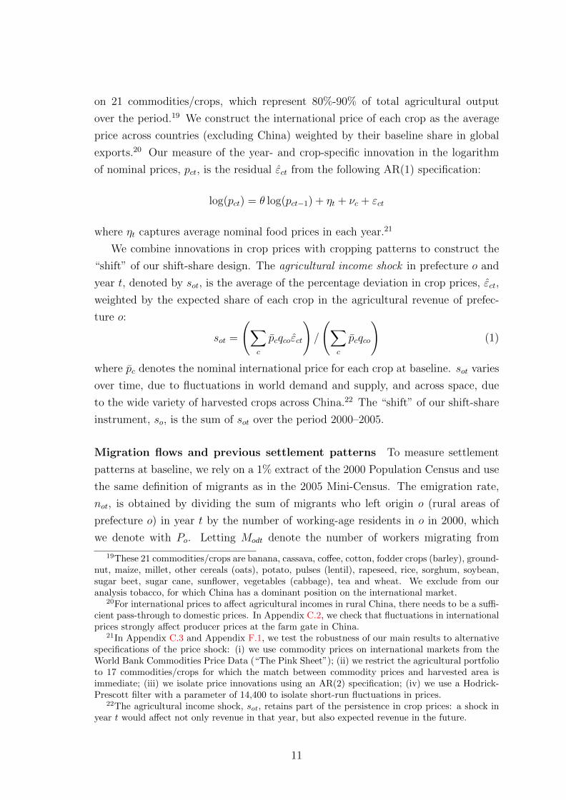
on 21 commodities/crops, which represent 80%-90% of total agricultural output

over the period.19 We construct the international price of each crop as the average

price across countries (excluding China) weighted by their baseline share in global

exports.20 Our measure of the year- and crop-specific innovation in the logarithm

of nominal prices, pct, is the residual εct from the following AR(1) specification:

log(pct) = θ log(pct−1) + ηt + νc + εct

where ηt captures average nominal food prices in each year.21

We combine innovations in crop prices with cropping patterns to construct the

“shift” of our shift-share design. The agricultural income shock in prefecture o and

year t, denoted by sot, is the average of the percentage deviation in crop prices, εct,

weighted by the expected share of each crop in the agricultural revenue of prefec-

ture o:

sot =

(∑c

pcqcoεct

)/

(∑c

pcqco

)(1)

where pc denotes the nominal international price for each crop at baseline. sot varies

over time, due to fluctuations in world demand and supply, and across space, due

to the wide variety of harvested crops across China.22 The “shift” of our shift-share

instrument, so, is the sum of sot over the period 2000–2005.

Migration flows and previous settlement patterns To measure settlement

patterns at baseline, we rely on a 1% extract of the 2000 Population Census and use

the same definition of migrants as in the 2005 Mini-Census. The emigration rate,

not, is obtained by dividing the sum of migrants who left origin o (rural areas of

prefecture o) in year t by the number of working-age residents in o in 2000, which

we denote with Po. Letting Modt denote the number of workers migrating from

19These 21 commodities/crops are banana, cassava, coffee, cotton, fodder crops (barley), ground-nut, maize, millet, other cereals (oats), potato, pulses (lentil), rapeseed, rice, sorghum, soybean,sugar beet, sugar cane, sunflower, vegetables (cabbage), tea and wheat. We exclude from ouranalysis tobacco, for which China has a dominant position on the international market.

20For international prices to affect agricultural incomes in rural China, there needs to be a suffi-cient pass-through to domestic prices. In Appendix C.2, we check that fluctuations in internationalprices strongly affect producer prices at the farm gate in China.

21In Appendix C.3 and Appendix F.1, we test the robustness of our main results to alternativespecifications of the price shock: (i) we use commodity prices on international markets from theWorld Bank Commodities Price Data (“The Pink Sheet”); (ii) we restrict the agricultural portfolioto 17 commodities/crops for which the match between commodity prices and harvested area isimmediate; (iii) we isolate price innovations using an AR(2) specification; (iv) we use a Hodrick-Prescott filter with a parameter of 14,400 to isolate short-run fluctuations in prices.

22The agricultural income shock, sot, retains part of the persistence in crop prices: a shock inyear t would affect not only revenue in that year, but also expected revenue in the future.

11

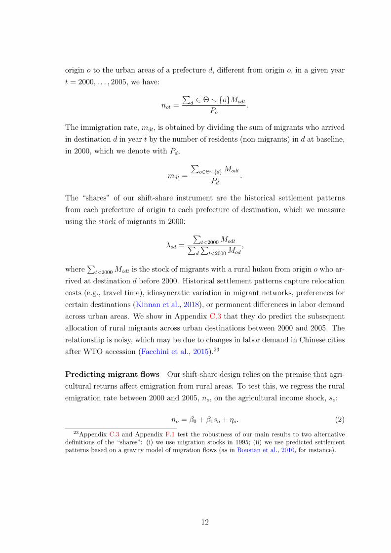
origin o to the urban areas of a prefecture d, different from origin o, in a given year

t = 2000, . . . , 2005, we have:

not =

∑d ∈ Θ r {o}Modt

Po.

The immigration rate, mdt, is obtained by dividing the sum of migrants who arrived

in destination d in year t by the number of residents (non-migrants) in d at baseline,

in 2000, which we denote with Pd,

mdt =

∑o∈Θr{d}Modt

Pd.

The “shares” of our shift-share instrument are the historical settlement patterns

from each prefecture of origin to each prefecture of destination, which we measure

using the stock of migrants in 2000:

λod =

∑t<2000Modt∑

d

∑t<2000Mod

,

where∑

t<2000Modt is the stock of migrants with a rural hukou from origin o who ar-

rived at destination d before 2000. Historical settlement patterns capture relocation

costs (e.g., travel time), idiosyncratic variation in migrant networks, preferences for

certain destinations (Kinnan et al., 2018), or permanent differences in labor demand

across urban areas. We show in Appendix C.3 that they do predict the subsequent

allocation of rural migrants across urban destinations between 2000 and 2005. The

relationship is noisy, which may be due to changes in labor demand in Chinese cities

after WTO accession (Facchini et al., 2015).23

Predicting migrant flows Our shift-share design relies on the premise that agri-

cultural returns affect emigration from rural areas. To test this, we regress the rural

emigration rate between 2000 and 2005, no, on the agricultural income shock, so:

no = β0 + β1so + ηo. (2)

23Appendix C.3 and Appendix F.1 test the robustness of our main results to two alternativedefinitions of the “shares”: (i) we use migration stocks in 1995; (ii) we use predicted settlementpatterns based on a gravity model of migration flows (as in Boustan et al., 2010, for instance).

12

Panel A of Table 2 presents the estimates.24 Emigration between 2000 and 2005 is

negatively correlated with the agricultural income shock. A 10% lower agricultural

income (about one standard deviation in so) is associated with a 1.2 p.p. higher

migration incidence.25 The negative relationship between agricultural income and

migration suggests that migration decisions are driven by the opportunity cost of

migration, rather than by liquidity constraints (Angelucci, 2015; Bazzi, 2017).26

We construct our shift-share instrument by combining the agricultural income

shock across origins with earlier migration patterns:

zd =∑

o∈Θr{d}

λodso. (3)

To check that the instrument is a good predictor of immigration flows, we regress

the actual immigration rate between 2000 and 2005, md, on zd:

md = α0 + α1zd + ηd. (4)

Panel B of Table 2 presents the estimates. The relationship is significant and nega-

tive: it is the first stage of the empirical strategy that we describe next.

2.3 Empirical strategy and identification

Empirical strategy Our baseline specification considers a specification in differ-

ence using the balanced panel of firms present every year between 2000 and 2006.

We regress the change in outcomes between 2000 and 2006, ∆yid, for a firm i in

prefecture d on the sum of yearly migration flows over the period, md:

∆yid = α + βmd + εid, (5)

where standard errors are clustered at the level of the prefecture of destination and

each observation is weighted by firm employment at baseline, eid. Migration flows

may reflect a surge in labor demand after opening to trade or local investment

24In the baseline specifications, we apply a 99% winsorization to emigration and immigrationrates. Appendix C.3 and Appendix F.2 test the sensitivity of our findings to the definition ofmigration: all migrants; males only; low-skilled only; no adjustment for return migration; andincluding outliers.

25This semi-elasticity corresponds to an elasticity of -2.7. We show in Appendix C.1 thatthe elasticity of the emigration rate to the agricultural revenue may be interpreted as the shapeparameter for the distribution of worker preferences for different locations, as is common in modelsof New Economic Geography (Monte et al., 2018; Bryan and Morten, 2019; Monras, 2020).

26In the Chinese context, workers migrate without their families, low-skill jobs in cities are easyto find, and the fixed cost of migration is relatively low. Chinese households also have high savings,so that the impact of short-term fluctuations in agricultural prices on wealth is small.

13

in infrastructure and amenities. In order to isolate a supply-driven component in

the relocation of workers, we use the shift-share variable zd (see Equation 3) as an

instrument for the immigration rate md and estimate Equation (5) with 2SLS. We

have already reported a prefecture-level equivalent of the first stage by regressing

the immigration rate on the instrument in Equation (4).

Identification and inference A recent literature discusses identification and in-

ference in shift-share designs (Adao et al., 2019b; Borusyak et al., 2018; Goldsmith-

Pinkham et al., forthcoming). It suggests that consistency can be achieved if either

the shares (Goldsmith-Pinkham et al., forthcoming) or the shifts (Borusyak et al.,

2018) are exogenous. In our setting, the shares—previous settlement patterns—

reflect the expectations of workers about the evolution of labor demand across des-

tinations; they are likely endogenous to production outcomes in cities. Instead,

the validity of our shift-share design relies on the assumption that shifts—the agri-

cultural income shocks—are exogenous to manufacturing outcomes. Specifically,

following Borusyak et al. (2018), a shift-share estimator would be consistent under

two conditions: (i) shifts are quasi-randomly assigned across origins, and (ii) there

are many uncorrelated shifts. Given our empirical strategy, condition (i) is likely to

hold: innovations in the international price of agricultural commodities are driven

by world supply and demand and are likely exogenous from the point of view of

each Chinese prefecture at baseline.27 Condition (ii) may not be verified: the shifts

are spatially correlated in our setting, since they combine innovations in crop prices

with cropping patterns, which are strongly determined by geography (see Figure 2).

To discuss these issues, we apply the equivalence result of Borusyak et al. (2018),

and transform our firm-level specification (5) into a shift-level (i.e. an origin-level)

specification. In our setting, this equivalence result conveys a simple intuition. Our

shift-share design transforms agricultural income shocks at origin into shocks to

firms at destination via a matrix of migration patterns. The equivalence result of

Borusyak et al. (2018) allows us to invert this transformation and estimate, at the

origin-level, the effect of agricultural income shocks on firm outcomes in the typical

destination, i.e. on a weighted average of firm outcomes using migration patterns

as weights. Concretely, we first aggregate firm-level outcomes yid into destination-

level outcomes yd. We then construct the weights λod = edλod/∑

d edλod, where

λod are historical migration shares and ed is total employment in prefecture d at

baseline. Finally, we compute transformed outcomes yo =∑

d λodyd and transformed

27We exclude from the analysis the only crop for which China is a price setter on the internationalmarkets, tobacco, which also happens to be produced in a specific region of China.

14

immigration mo =∑

d λodmd and estimate the following equation:

∆yo = α + βmo + εo. (6)

where the agricultural income shock, so, is used as an instrument for mo. Following

Borusyak et al. (2018), we use this specification to discuss identification and test for

pre-trends in outcomes between 1998–2000. We also check two conditions about the

distribution of migration patterns: (i) the Herfindahl index of origin contributions,∑o(∑

d λod)2, is small so that the effect is not driven by a few origins; (ii) the

Herfindahl indices of settlement patterns,∑

o λ2od, are not too small on average so

that shocks do not affect all destinations to the same extent. Finally, outcomes

may be correlated across destinations with similar migration shares, which implies

that standard inference may be invalid. We use the method proposed by Adao et

al. (2019b) to provide valid standard errors in our shift-share design; we also use

specification (6) to provide standard errors accounting for spatial correlation across

origins (e.g., using Conley, 1999).

Even if the shifts are randomly assigned across origins, we need the exclusion

restriction to hold: agricultural income shocks in rural hinterlands should only affect

firm outcomes in cities through the relocation of workers. However, changes in the

price of agricultural output may affect local industries that use agricultural products

as intermediate inputs. We check that our results are robust to excluding firms that

process agricultural goods and to controlling for industry-specific trends. Second,

cities and their surroundings are also integrated through final goods markets, so

that agricultural income in rural hinterlands may affect demand for manufactured

products in cities (Santangelo, 2016). We alleviate this concern by (i) excluding

migration within a 300km radius, (ii) controlling for the agricultural income shock

in neighboring prefectures, (iii) controlling for market access, and (iv) considering

only exporting firms, less dependent on local demand. Finally, the shift-share instru-

ment correlates with past migration by construction, which may influence current

outcomes (a concern raised by Jaeger et al., 2018). We address this concern by

(i) controlling for the stock of immigrants at baseline and (ii) checking that lagged

shocks (1993–1998) do not explain later changes in outcomes.

3 Migration, labor cost, and factor demand

This section quantifies the effect of migrant labor supply on labor cost, factor de-

mand, and factor productivity at destination.

15

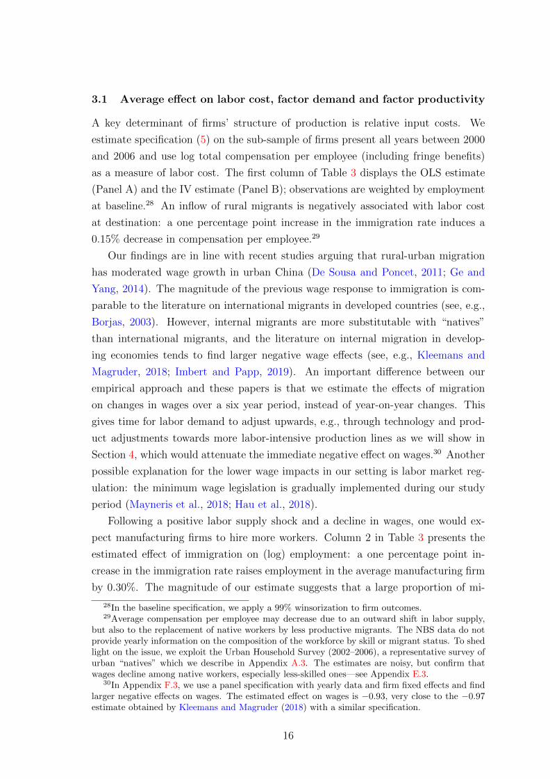
3.1 Average effect on labor cost, factor demand and factor productivity

A key determinant of firms’ structure of production is relative input costs. We

estimate specification (5) on the sub-sample of firms present all years between 2000

and 2006 and use log total compensation per employee (including fringe benefits)

as a measure of labor cost. The first column of Table 3 displays the OLS estimate

(Panel A) and the IV estimate (Panel B); observations are weighted by employment

at baseline.28 An inflow of rural migrants is negatively associated with labor cost

at destination: a one percentage point increase in the immigration rate induces a

0.15% decrease in compensation per employee.29

Our findings are in line with recent studies arguing that rural-urban migration

has moderated wage growth in urban China (De Sousa and Poncet, 2011; Ge and

Yang, 2014). The magnitude of the previous wage response to immigration is com-

parable to the literature on international migrants in developed countries (see, e.g.,

Borjas, 2003). However, internal migrants are more substitutable with “natives”

than international migrants, and the literature on internal migration in develop-

ing economies tends to find larger negative wage effects (see, e.g., Kleemans and

Magruder, 2018; Imbert and Papp, 2019). An important difference between our

empirical approach and these papers is that we estimate the effects of migration

on changes in wages over a six year period, instead of year-on-year changes. This

gives time for labor demand to adjust upwards, e.g., through technology and prod-

uct adjustments towards more labor-intensive production lines as we will show in

Section 4, which would attenuate the immediate negative effect on wages.30 Another

possible explanation for the lower wage impacts in our setting is labor market reg-

ulation: the minimum wage legislation is gradually implemented during our study

period (Mayneris et al., 2018; Hau et al., 2018).

Following a positive labor supply shock and a decline in wages, one would ex-

pect manufacturing firms to hire more workers. Column 2 in Table 3 presents the

estimated effect of immigration on (log) employment: a one percentage point in-

crease in the immigration rate raises employment in the average manufacturing firm

by 0.30%. The magnitude of our estimate suggests that a large proportion of mi-

28In the baseline specification, we apply a 99% winsorization to firm outcomes.29Average compensation per employee may decrease due to an outward shift in labor supply,

but also to the replacement of native workers by less productive migrants. The NBS data do notprovide yearly information on the composition of the workforce by skill or migrant status. To shedlight on the issue, we exploit the Urban Household Survey (2002–2006), a representative survey ofurban “natives” which we describe in Appendix A.3. The estimates are noisy, but confirm thatwages decline among native workers, especially less-skilled ones—see Appendix E.3.

30In Appendix F.3, we use a panel specification with yearly data and firm fixed effects and findlarger negative effects on wages. The estimated effect on wages is −0.93, very close to the −0.97estimate obtained by Kleemans and Magruder (2018) with a similar specification.

16

grant workers is not hired by the firms in our sample: they may be hired by smaller

firms, work in other sectors (e.g., construction), or transit through unemployment

or self-employment (Giulietti et al., 2012; Zhang and Zhao, 2015).

Migrant labor supply shocks strongly affect relative factor use at destination. As

column 3 of Table 3 shows, the capital-to-labor ratio decreases by 0.43% following

a one percentage point increase in the migration rate, which suggests that capital

does not adjust to the increase in employment. There are three possible reasons for

this finding. First, firms that expand may belong to sectors with relatively high sub-

stitutability between capital and labor. A moderate (and negative) adjustment of

capital could then be an optimal response. Second, credit constraints or adjustment

costs may prevent firms from reaching the optimal use of production factors. To

shed light on these two channels, we study treatment heterogeneity in Appendix E.1

and estimate migration effects for (i) firms in sectors with high elasticity of sub-

stitution between factors and (ii) public sector firms, which have an easier access

to credit (Brandt et al., 2013). We do not find evidence of heterogeneous effects

along these dimensions. A third possible reason for the lack of adjustment of capital

may be that firms change the organization of their production lines and adopt new

technologies with different factor intensities. We provide evidence in support for this

interpretation in Section 4.

Finally, the average product of labor falls sharply in response to migrant inflows.

An additional percentage point in the immigration rate decreases value added per

worker by 0.44% (column 4 of Table 3). Since employment increases by 0.30%, the

coefficient implies that the labor supply shock has a negative, albeit small, effect

on value added at the firm level. Firm expansion may come at a cost; for instance,

new hires may need to be trained and production lines may need to be adjusted.

In Appendix D.1, we develop and estimate a quantitative framework a la Oberfield

and Raval (2014) which allows for sector-specific complementarities between capital

and labor, and we compute the marginal revenue of capital and labor, as well as

total factor productivity for each firm. We then estimate the effect of migration on

these productivity measures, and show that the marginal revenue product of labor

falls markedly when immigration increases, the marginal revenue product of capital

rises slightly, and total factor productivity decreases moderately (Appendix D.2).

The response of manufacturing firms to internal immigration in China resonates

with Lewis’s (2011) findings on Mexican immigration to the United States in the

1980s and 1990s: firms choose not to mechanize due to the availability of cheap la-

bor. We provide additional support for this interpretation in Section 4, by shedding

light on the adoption of new products and new technologies. The rest of this sec-

17

tion provides sensitivity analysis of our baseline results, starting with compositional

effects and sample choice, and ending with a discussion of identification.

3.2 Aggregation, firm selection and entry/exit

Immigration may change the allocation of factors across firms: in that case, its effect

on aggregate outcomes may differ from its effect on firm-level outcomes.

We first investigate the effect of immigration on aggregate outcomes constructed

from the baseline sample of firms present every year in the NBS data between 2000

and 2006. We compute the sum of employment, wage bill, value added and capital

across firms, and construct our main outcomes—compensation per worker, employ-

ment, capital-labor ratio and value added per worker—at the sector × prefecture

level. We then estimate specification (5), with a sector × prefecture as the unit

of observation. Panel A of Table 4 presents the results. The effects on labor cost,

employment, capital-to-labor ratio, and value-added per worker are similar to the

within-firm results from Table 3, which suggests that compositional effects within

the balanced sample are small. Appendix E.1 provides corroborating evidence: we

find little evidence of heterogeneous effects along firm characteristics such as capital

intensity or output per worker at baseline. We also present the outcome of an aggre-

gation at the prefecture level in Appendix E.2 and show similar estimates to Table 3.

This suggests that the reallocation across sectors is small, which is consistent with

the literature on developed countries (Dustmann and Glitz, 2015).

Immigration may also affect firm entry and exit, so that results based on firms

present from 2000–2006 would miss part of its aggregate impact. To account for the

potential effect on entry into and exit from the sample, we construct outcomes at

the sector × prefecture level using all firms observed at any point in the NBS data

between 2000 and 2006. The results are shown in Panel B of Table 4. The wage

response to a one percentage point increase in the immigration rate is −0.17%, close

to the estimate using the balanced sample (−0.13%). By contrast, the employment

effect is twice larger within the unbalanced sample, suggesting that an important

share of migrant workers are absorbed by new entrants or future exiters (as in

Dustmann and Glitz, 2015). Accounting for entry into and exit from our sample

amplifies the effect of migration on production: the selection effect seems to favor

firms with low capital intensity and low productivity per worker.

We provide direct evidence on firm selection in Appendix E.2, with the caveat

that we do not observe all firms but only those above the RMB 5 million sales

threshold. We first estimate the effect of migration on profitability and on the

probability that an establishment reports net profits in the balanced sample of firms.

18

We find that migration increases the profitability of incumbent firms. Second, we

study firm entry and exit: we consider as entrants firms that appeared in the sample

and who were created between 2000 and 2006, and as exiters firms that disappear

from the sample between these dates. We find that migration lowers firm exit

and entry. Taken together, these results suggest that cheaper labor allows low-

productivity, low-profitability incumbent firms to survive, or at least to remain large

enough to stay in the sample.

3.3 Sensitivity analysis, identification and inference

We now provide a thorough discussion of the different threats to the validity of

our estimates: we first consider potential failures of the exclusion restriction and

we discuss identification in our shift-share design (Borusyak et al., 2018); we then

discuss inference following the recent contribution of Adao et al. (2019b).

Identification We interpret our estimates as the effect of immigration on man-

ufacturing production. One concern is that the shift-share instrument, which is a

combination of agricultural income shocks and migration patterns, may have inde-

pendent effects on production in cities. In other words, the exclusion restriction may

fail. First, destinations could be affected by the commodity price shock through the

market for intermediary goods. Rural hinterlands may be producing goods which di-

rectly enter the production of final goods in urban centers, e.g., cotton. In Panel A of

Table 5, we reproduce Table 3 but exclude industries that use agricultural products

as intermediate inputs. In Panel B, we add 2-digit industry fixed effects as controls

in specification (5). Second, if rural dwellers consume the final goods produced in

urban areas, agricultural income shocks would affect the demand for manufacturing

goods. To address this concern, we exclude from the analysis all migration flows be-

tween prefectures that are less than 300 km apart (Panel C). We also control for the

shocks in neighboring prefectures weighted by the inverse of distance in Panel D.

Assuming that trade follows a gravity model, this specification allows us to con-

trol for rural-urban spillovers through goods markets, so that the identification only

comes from idiosyncratic variation in migration patterns (not related to distance,

but due for example to historical events, see Kinnan et al., 2018). We perform two

other robustness checks: we control for a measure of market access—the sum of

the rural population in all prefectures weighted by the inverse of the distance to

the prefecture where the firm is located (Panel E),—and we restrict the sample to

exporting firms at baseline, arguably less exposed to variation in local demand for

their final product (Panel F). Finally, the shares of our shift-share design reflect his-

19

torical migration patterns (Jaeger et al., 2018); our estimates may be conflating the

effect of current migration shocks with the lagged effect of past shocks. To address

this, we control for the stock of immigrants at baseline and allow it to have inde-

pendent effects on outcomes (Panel G). In all instances, the estimates are similar

to the main results, which provides reassurance that our estimates do capture the

effect of current migration on production.31

A recent literature discusses identification in a shift-share design (Borusyak et

al., 2018; Goldsmith-Pinkham et al., forthcoming). As explained in Section 2, we

follow Borusyak et al. (2018): we invert the transformation of shifts into a shift-

share variable, and we consider instead transformed outcomes at the level of shifts.

In our setting, this amounts to estimating Equation (6), which regresses a weighted

average of firm outcomes across origins on a weighted average of immigration in-

strumented by the shifts, using migration patterns as weights. The transformed

specification can be interpreted as estimating the effect of push shocks on outcomes

at the “typical” destination, across the different origins. We present the OLS esti-

mates in Panel A of Table 6 and the 2SLS estimates in Panel B. Consistent with

the equivalence result of Borusyak et al. (2018), the origin-level estimates are very

similar to our destination-level results (Table 3). In Panel C, we show a reduced-

form specification where transformed firm outcomes are directly explained by the

agricultural income shock. This reduced form approach offers the opportunity to

correlate firm outcomes with counterfactual shocks. In Panel D, we provide a test

of the parallel trends assumption and regress pre-treatment differences in outcomes

(1998–2000) on the shocks computed over the study period (2000–2005). The es-

timates are quite small: urban centers whose hinterlands would later be exposed

to agricultural shocks follow similar trends than others before 2000–2005. Finally,

we perform a placebo regression with lagged agricultural income shocks (computed

over 1993–1998) as the independent variable. This specification tests whether past

shocks and previous immigration waves predict the future evolution of outcomes at

destination through a sluggish restructuring of production (Jaeger et al., 2018). We

do not find strong supporting evidence for a persistent effect of past shocks on urban

production.

31The effect of immigration on firms itself could be multifaceted. Our preferred interpretationis that new workers affect labor markets and the relative abundance of production factors in cities.However, new workers in cities are also consumers of non-tradable goods, which may benefit firmsproviding these goods (e.g., housing services) or affect firms relying on these goods or services (e.g.,with a highly land-intensive production). We provide some evidence that rural-urban migrationaffects living standards at destination in Appendix E.3.

20

Inference The clustering of standard errors in our main specification does not

account for the heteroskedasticity induced by (i) the correlation in outcomes across

prefectures with similar exposure to shocks and (ii) the correlation in agricultural

income shocks across origins. Appendix F.2 provides a sensitivity analysis for infer-

ence. We first compute robust standard errors, standard errors clustered at the level

of the province of destination, and use a more continuous modeling of spatial auto-

correlation (following Conley, 1999). As argued by Adao et al. (2019b), however, the

heteroskedasticity induced by shift-share designs may not be adequately captured

by spatial clustering. For instance, migrants from the same origin may join similar

industries across different destinations, so that firms in these destinations experience

correlated shocks even if they are not geographically close. We thus use the inference

method proposed by Adao et al. (2019b) and report the AKM and AKM0 standard

errors. Another concern is that the shifts are spatially auto-correlated across pre-

fectures of origin, so that there is less independent variation than a destination-level

analysis would suggest. The transformation suggested by Borusyak et al. (2018)

offers the opportunity to better account for spatial correlation across origins. In Ap-

pendix F.2, we estimate Equation (6) with standard errors clustered at the province

level and standard errors accounting for spatial auto-correlation (Conley, 1999). Our

estimates remain precisely estimated regardless of the inference method.

4 Restructuring of production

This section characterizes the restructuring of production following the arrival of

new workers. Specifically, we investigate whether manufacturing firms change their

output mix, whether they shift patenting away from capital-enhancing and skill-

enhancing technologies, and how much of the observed adjustments in factor use

and patenting can be explained by endogenous product choice.

Product choice We investigate changes in production lines, which we measure via

changes in the (main) end product.32 We classify products based on their product

class, as defined by a unique product description or by the product code assigned by

our algorithm (see Section 2). We proxy the skill intensity of each product class by

the average share of the workforce with a high-school degree and capital intensity by

the average capital-to-labor ratio among firms whose main products belong to this

32While our baseline analysis focuses on the first product declared by firms, we exploit thereporting of up to three products in Appendix E.4. We estimate the effect of immigration onthe number of products and changes in their “similarity”, as measured with linguistic distance orthrough input/output accounts. We find little effect on either outcome.

21

class at baseline. We estimate specification (5) at the establishment level between

2000 and 2006, and we control for fixed effects at the level of the product code at

baseline in order to capture the adoption of new products while keeping fixed the

initial distribution of products across destinations.

We first use the textual description to detect any change in the (main) end

product between 2000 and 2006, and we determine the direction of the change using

the characteristics of the average establishment providing the same description at

baseline. Panel A of Table 7 presents the results. Establishments in prefectures that

experience large immigration flows are more likely to change the textual description

of their main product in 2000–2006 (column 1); a one percentage point increase

in the immigration rate raises the probability to provide two distinct descriptions

by 0.20 percentage points. The effect is mostly driven by a transition towards

products with lower human capital (columns 2 and 3) and lower physical capital

intensity (columns 4 and 5). Distinct textual descriptions could however refer to

the same product class. We exploit the Natural Language Processing algorithm

described in Section 2 to assign a unique HS-6 product category to each description,

and we replicate the previous exercise with these newly-defined product categories

in Panel B of Table 7. A one percentage point increase in the immigration rate

raises the probability to change HS codes in 2000–2006 by 0.12 percentage points—

a marginal change explained by the transition towards products that are typically

produced by low-skilled and labor-abundant firms.

We provide further results on endogenous product choice in Appendix E.4. First,

we leverage the linguistic similarity score between two HS product codes, as provided

by our textual analysis. We compute the human or physical capital intensity of a

given product code as the weighted average of capital intensity across all firms

weighted by the similarity score with their own product code. This method allows

for a more continuous product characterization than the first classification we use,

which attributes a score of 1 when product classes coincide and 0 otherwise. Second,

we compute the human or physical capital intensity of each product code using an

input/output matrix rather than language similarity. Indeed, the adjustment of

production lines may affect some products which are ultimately produced by capital-

intensive firms, but heavily rely on intermediary inputs provided by labor-intensive

firms. The conclusion is the same in both exercises: there is an adjustment of

production lines toward low-skilled, labor-intensive production. We also estimate

possible changes in the technological content of products by exploiting a measure of

cross-industry patent citations in the United States (Bloom et al., 2013). We find

evidence that firms re-orient their production towards products that are less reliant

22

on technological innovation (i.e., with fewer and more concentrated citations across

industries).

Innovation We now use a more direct observation of technological change within

firms, through their patenting behavior. We exploit the match provided by He et

al. (2018) between the NBS sample of manufacturing establishments and patents

submitted to the State Intellectual Property Office (renamed as China National In-

tellectual Property Administration in 2018). The description of each patent provides

a detailed classification of its technological content. We use this classification to qual-

ify the nature of technological innovation, using average characteristics of firms that

submitted a patent within each subcategory at baseline. Specifically, we classify a

patent as high-education if the average share of workforce with a high school degree

among firms that submitted patents at baseline was above the median. Similarly

we classify a patent as high-capital-to-labor ratio if firms that submitted patents

in the same class had above-median capital-to-labor ratio on average. This exer-

cise assumes that: (i) capital-intensive firms primarily patent capital-augmenting

technologies; (ii) technology is homogeneous within a patent class.

We estimate specification (5) at the establishment-level between 2000 and 2006,

and regress the difference in the probability to submit a patent application between

2000 and 2006 on the immigration rate, instrumented by the shift-share instrument.

Panel A of Table 8 shows that the probability to submit a patent decreases by 0.47

percentage point (from an average of 4 percentage points) after a ten percentage

points increase in the immigration rate. The effect is mostly driven by the inven-

tion and utility patent categories (see columns 3 to 4), which suggests a decline in

fundamental innovation and in the creation of new production processes. Rural-

urban migration does not only affect the pace of technological progress, but also

its direction. The drop in patenting is most pronounced for skill-enhancing and

capital-enhancing technologies (see Panel B of Table 8). In response to the migra-

tion shock, manufacturing establishments are less likely to push the technological

frontier, especially so towards technologies using scarcer resources.

Product choice, factor use, and patenting We have documented a restruc-

turing of production through (a) the adjustment of factor use and technology, and

(b) the adoption of low-skilled, labor-intensive products. We now quantify the role

of product choice in the adoption of more labor-intensive organizational forms. We

regress changes in factor use and patenting on a dummy for firms that changed

their main product in 2000–2006, on the immigration rate, and on the interaction

23

between product change and immigration. The immigration rate and its interac-

tion are instrumented by the shift-share instrument and by its interaction with the

product change dummy. As product change is affected by immigration and responds

to a broad range of other unobserved factors (e.g., international demand), the esti-

mates do not have a causal interpretation and the results are only suggestive of the

mediation effect of product choice.

We present the results of this specification in Table 9. The coefficients on the

product change dummy across columns 1 to 4 suggest that, absent immigration, a

change in product is associated with a shift towards capital-intensive technologies.

Following an immigration shock, all firms adjust their input mix by using more labor

and less capital, whether they change products or not (see the estimate on ‘Migra-

tion’, column 1). In stark contrast, the decline in patenting only occurs within firms

that change their output mix, especially for patents related to production processes

(see columns 2–4). These findings shed new light on the adjustment of technology

to the supply of the different production factors. One margin of adjustment occurs

keeping the same output mix (Beaudry and Green, 2003). Another important mar-

gin of adjustment, identified by Goldberg et al. (2010) and Bas and Paunov (2019)

in the response to new imported inputs, derives from endogenous product choice.

5 Conclusion

This paper provides unique evidence on the causal effect of rural-urban migration

on manufacturing production in China. We combine information on migration flows

with longitudinal data on manufacturing establishments between 2000 and 2006, a

period of rapid structural transformation and sustained manufacturing growth. We

instrument immigrant flows using a shift-share design, which combines shocks to

agricultural income due to cropping patterns and fluctuations in international crop

prices with historical migration patterns between rural and urban areas. We find

that migration decreases labor costs and increases employment, and that manufac-

turing production becomes more labor-intensive, as capital does not adjust. We are

also able to document the reorganization of production following the labor supply

shocks through the unique observation of product choice and patent applications.

Our results show that the abundance of rural migrant labor induces labor-oriented

directed technological change and the adoption of labor-intensive product varieties

within manufacturing firms. This mechanism is likely at play in other developing

countries that are currently in the process of structural transformation. Over the

last decade, China has experienced a sharp trend reversal with slower rural-urban

migration and faster automation in manufacturing (Cheng et al., 2019).

24

References

Abebe, Girum, Stefano Caria, Marcel Fafchamps, Paolo Falco, Simon Franklin,and Simon Quinn, “Anonymity or Distance? Job Search and Labour Market Exclu-sion in a Growing African City,” CSAE Working Paper Series 2016.

Accetturo, Antonio, Matteo Bugamelli, and Andrea Roberto Lamorgese, “Wel-come to the machine: firms’ reaction to low-skilled immigration,” Bank of Italy WorkingPaper, 2012, 846.

Adao, Rodrigo, Costas Arkolakis, and Federico Esposito, “Spatial linkages, globalshocks, and local labor markets: Theory and evidence,” Technical Report, NationalBureau of Economic Research 2019.

, Michal Kolesar, and Eduardo Morales, “Shift-share designs: Theory and infer-ence,” The Quarterly Journal of Economics, 2019, 134 (4), 1949–2010.

Akcigit, Ufuk, Salome Baslandze, and Stefanie Stantcheva, “Taxation and theinternational mobility of inventors,” American Economic Review, 2016, 106 (10), 2930–81.

Alfonsi, Livia, Oriana Bandiera, Vittorio Bassi, Robin Burgess, Imran Rasul,Munshi Sulaiman, and Anna Vitali, “Tackling Youth Unemployment: Evidencefrom a Labour Market Experiment in Uganda,” Technical Report 64, STICERD, LSEDecember 2017.

Alvarez-Cuadrado, Francisco and Markus Poschke, “Structural Change Out ofAgriculture: Labor Push versus Labor Pull,” American Economic Journal: Macroeco-nomics, July 2011, 3 (3), 127–58.

Angelucci, Manuela, “Migration and Financial Constraints: Evidence from Mexico,”The Review of Economics and Statistics, March 2015, 97 (1), 224–228.

Atkin, David, Azam Chaudhry, Shamyla Chaudry, Amit K Khandelwal, andEric Verhoogen, “Organizational barriers to technology adoption: Evidence fromsoccer-ball producers in Pakistan,” The Quarterly Journal of Economics, 2017, 132 (3),1101–1164.

Autor, David H, David Dorn, and Gordon H Hanson, “The China syndrome: Locallabor market effects of import competition in the United States,” American EconomicReview, 2013, 103 (6), 2121–68.

Badaoui, Eliane El, Eric Strobl, and Frank Walsh, “Impact of Internal Migrationon Labor Market Outcomes of Native Males in Thailand,” Economic Development andCultural Change, 2017, 66, 147–177.

Banerjee, Abhijit V. and Esther Duflo, “Do Firms Want to Borrow More? TestingCredit Constraints Using a Directed Lending Program,” Review of Economic Studies,2014, 81 (2), 572–607.

Bas, Maria and Caroline Paunov, “What gains and distributional implications resultfrom trade liberalization?,” 2019.

25

Bazzi, Samuel, “Wealth heterogeneity and the income elasticity of migration,” AmericanEconomic Journal: Applied Economics, 2017, 9 (2), 219–55.

Beaudry, Paul and David A Green, “Wages and employment in the United Statesand Germany: What explains the differences?,” American Economic Review, 2003, 93(3), 573–602.

Beraja, Martin, Erik Hurst, and Juan Ospina, “The aggregate implications ofregional business cycles,” Econometrica, 2019, 87 (6), 1789–1833.

Bloom, Nicholas, Mark Schankerman, and John Van Reenen, “Identifying tech-nology spillovers and product market rivalry,” Econometrica, 2013, 81 (4), 1347–1393.

Boehm, Johannes and Ezra Oberfield, “Misallocation in the Market for Inputs: En-forcement and the Organization of Production,” Technical Report, National Bureau ofEconomic Research 2018.

and , “Misallocation in the Market for Inputs: Enforcement and the Organization ofProduction,” CEPR Discussion Papers 14482, C.E.P.R. Discussion Papers March 2020.

Borjas, George J., “The Labor Demand Curve Is Downward Sloping: Reexamining TheImpact Of Immigration On The Labor Market,” The Quarterly Journal of Economics,November 2003, 118 (4), 1335–1374.

Borusyak, Kirill, Peter Hull, and Xavier Jaravel, “Quasi-experimental shift-shareresearch designs,” Technical Report, National Bureau of Economic Research 2018.

Boustan, Leah Platt, Price V. Fishback, and Shawn Kantor, “The Effect of Inter-nal Migration on Local Labor Markets: American Cities during the Great Depression,”Journal of Labor Economics, October 2010, 28 (4), 719–746.

Brandt, Loren, Johannes Van Biesebroeck, and Yifan Zhang, “Challenges ofworking with the Chinese NBS firm-level data,” China Economic Review, 2014, 30 (C),339–352.

, Trevor Tombe, and Xiaodong Zhu, “Factor market distortions across time, spaceand sectors in China,” Review of Economic Dynamics, 2013, 16 (1), 39–58.

Bryan, Gharad and Melanie Morten, “The aggregate productivity effects of internalmigration: Evidence from indonesia,” Journal of Political Economy, 2019, 127 (5),2229–2268.

Buera, Francisco J, Joseph P Kaboski, and Yongseok Shin, “Finance and de-velopment: A tale of two sectors,” The American Economic Review, 2011, 101 (5),1964–2002.

Bustos, Paula, Bruno Caprettini, and Jacopo Ponticelli, “Agricultural productiv-ity and structural transformation: Evidence from Brazil,” American Economic Review,2016, 106 (6), 1320–65.

, Juan Manuel Castro Vincenzi, Joan Monras, and Jacopo Ponticelli, “Struc-tural Transformation, Industrial Specialization, and Endogenous Growth,” CEPR Dis-cussion Papers 13379, C.E.P.R. Discussion Papers December 2018.

26

Card, David, “Immigrant Inflows, Native Outflows, and the Local Labor Market Impactsof Higher Immigration,” Journal of Labor Economics, 2001, 19 (1), 22–64.

and John DiNardo, “Do Immigrant Inflows Lead to Native Outflows?,” AmericanEconomic Review, 2000, 90 (2), 360–367.

Chen, Shuai, Paulina Oliva, and Peng Zhang, “The effect of air pollution on migra-tion: evidence from China,” Technical Report, National Bureau of Economic Research2017.

Cheng, Hong, Ruixue Jia, Dandan Li, and Hongbin Li, “The Rise of Robots inChina,” Journal of Economic Perspectives, May 2019, 33 (2), 71–88.

Combes, Pierre-Philippe, Sylvie Demurger, and Shi Li, “Migration externalitiesin Chinese cities,” European Economic Review, 2015, 76 (C), 152–167.

Conley, Timothy G, “GMM estimation with cross sectional dependence,” Journal ofEconometrics, 1999, 92 (1), 1–45.

Davis, Steven J and John C Haltiwanger, “Job creation and destruction,” MIT PressBooks, 1998, 1.

Demurger, Sylvie, Marc Gurgand, Shi Li, and Ximing Yue, “Migrants as second-class workers in urban China? A decomposition analysis,” Journal of ComparativeEconomics, December 2009, 37 (4), 610–628.

Dustmann, Christian and Albrecht Glitz, “How Do Industries and Firms Respondto Changes in Local Labor Supply?,” Journal of Labor Economics, 2015, 33 (3), 711 –750.

Ebenstein, Avraham and Yaohui Zhao, “Tracking rural-to-urban migration in China:Lessons from the 2005 inter-census population survey,” Population Studies, 2015, 69 (3),337–353.

Facchini, Giovanni, Maggie Y. Liu, Anna Maria Mayda, and Minghai Zhou,“The impact of China’s WTO accession on internal migration,” 2015.

Fan, Cindy C., China on the Move, Routledge, 2008.

Feng, Shuaizhang, Yingyao Hu, and Robert Moffitt, “Long run trends in unemploy-ment and labor force participation in urban China,” Journal of Comparative Economics,2017, 45 (2), 304 – 324.

Fields, Gary S, “Rural-urban migration, urban unemployment and underemployment,and job-search activity in LDCs,” Journal of development economics, 1975, 2 (2), 165–187.

Freeman, Richard, Wenquan Liang, Ran Song, and Christopher Timmins,“Willingness to pay for clean air in China,” Journal of Environmental Economics andManagement, 2019, 94, 188–216.

Ge, Suqin and Dennis Tao Yang, “Changes In China’s Wage Structure,” Journal ofthe European Economic Association, 04 2014, 12 (2), 300–336.

27

Giulietti, Corrado, Guangjie Ning, and Klaus F Zimmermann, “Self-employmentof rural-to-urban migrants in China,” International Journal of Manpower, 2012, 33 (1),96–117.

Goldberg, Pinelopi Koujianou, Amit Kumar Khandelwal, Nina Pavcnik, andPetia Topalova, “Imported intermediate inputs and domestic product growth: Evi-dence from India,” The Quarterly journal of economics, 2010, 125 (4), 1727–1767.

Goldsmith-Pinkham, Paul, Isaac Sorkin, and Henry Swift, “Bartik Instruments:What, When, Why, and How,” American Economic Review, forthcoming.

Gollin, Douglas, David Lagakos, and Michael E. Waugh, “The Agricultural Pro-ductivity Gap,” The Quarterly Journal of Economics, 2014, 129 (2), 939–993.

, Stephen Parente, and Richard Rogerson, “The Role of Agriculture in Develop-ment,” American Economic Review, May 2002, 92 (2), 160–164.

Groger, Andre and Yanos Zylberberg, “Internal Labor Migration as a Shock CopingStrategy: Evidence from a Typhoon,” American Economic Journal: Applied Economics,April 2016, 8 (2), 123–53.

Hall, Robert E. and Charles I. Jones, “Why do Some Countries Produce So MuchMore Output Per Worker than Others?,” The Quarterly Journal of Economics, 1999,114 (1), 83–116.

Harris, John R. and Michael P. Todaro, “Migration, Unemployment and Devel-opment: A Two-Sector Analysis,” The American Economic Review, 1970, 60 (1), pp.126–142.

Hau, Harald, Yi Huang, and Gewei Wang, “Firm response to competitive shocks:Evidence from China’s minimum wage policy,” SFI Research Paper, 2018, (16-47).

He, Zi-Lin, Tony W Tong, Yuchen Zhang, and Wenlong He, “A database linkingChinese patents to China’s census firms,” Scientific data, 2018, 5, 180042.

Herrendorf, Berthold, Christopher Herrington, and Akos Valentinyi, “SectoralTechnology and Structural Transformation,” American Economic Journal: Macroeco-nomics, October 2015, 7 (4), 104–33.

Hoberg, Gerard and Gordon Phillips, “Text-based network industries and endoge-nous product differentiation,” Journal of Political Economy, 2016, 124 (5), 1423–1465.

Howitt, Peter, “Endogenous Growth and Cross-Country Income Differences,” AmericanEconomic Review, September 2000, 90 (4), 829–846.

Hsieh, Chang-Tai and Peter J. Klenow, “Misallocation and Manufacturing TFPin China and India,” The Quarterly Journal of Economics, November 2009, 124 (4),1403–1448.

Imbert, Clement and John Papp, “Short-term Migration, Rural Public Works, andUrban Labor Markets: Evidence from India,” Journal of the European Economic Asso-ciation, 03 2019, 18 (2), 927–963.

28

Jaeger, David A, Joakim Ruist, and Jan Stuhler, “Shift-Share Instruments and theImpact of Immigration,” CEPR Discussion Papers 12701, C.E.P.R. Discussion PapersFebruary 2018.

Kerr, Sari Pekkala, William R. Kerr, and William F. Lincoln, “Skilled Immigra-tion and the Employment Structures of US Firms,” Journal of Labor Economics, 2015,33 (S1), S147 – S186.

Kinnan, Cynthia, Shing-Yi Wang, and Yongxiang Wang, “Access to Migration forRural Households,” American Economic Journal: Applied Economics, October 2018,10 (4), 79–119.

Kleemans, Marieke and Jeremy Magruder, “Labour Market Responses To Immigra-tion: Evidence From Internal Migration Driven By Weather Shocks,” Economic Journal,August 2018, 128 (613), 2032–2065.

Lewis, Arthur, “Economic Development with Unlimited Supplies of Labour,” TheManchester School, 1954, 22 (2), 139–191.

Lewis, Ethan, “Immigration, Skill Mix, and Capital Skill Complementarity,” The Quar-terly Journal of Economics, 2011, 126 (2), 1029–1069.

Li, Shen, Zhe Zhao, Renfen Hu, Wensi Li, Tao Liu, and Xiaoyong Du, “Analog-ical Reasoning on Chinese Morphological and Semantic Relations,” in “Proceedings ofthe 56th Annual Meeting of the Association for Computational Linguistics (Volume 2:Short Papers)” Association for Computational Linguistics 2018, pp. 138–143.

Llull, Joan, “Immigration, Wages, and Education: A Labour Market Equilibrium Struc-tural Model,” The Review of Economic Studies, 2018, 85 (3), 1852–1896.

Marden, Sam, “The agricultural roots of industrial development: “forward linkages” inreform era China,” 2015. Manuscript.

Mayneris, Florian, Sandra Poncet, and Tao Zhang, “Improving or disappearing:Firm-level adjustments to minimum wages in China,” Journal of Development Eco-nomics, 2018, 135, 20–42.

Meghir, Costas, Renata Narita, and Jean-Marc Robin, “Wages and informality indeveloping countries,” American Economic Review, 2015, 105 (4), 1509–46.

Meng, Xin and Dandan Zhang, “Labour Market Impact of Large Scale Internal Mi-gration on Chinese Urban ’Native’ Workers,” IZA Discussion Papers 5288 October 2010.

Midrigan, Virgiliu and Daniel Yi Xu, “Finance and misallocation: Evidence fromplant-level data,” The American Economic Review, 2014, 104 (2), 422–458.

Mikolov, Tomas, Ilya Sutskever, Kai Chen, Greg S Corrado, and Jeff Dean,“Distributed representations of words and phrases and their compositionality,” in “Ad-vances in neural information processing systems” 2013, pp. 3111–3119.

Minale, Luigi, “Agricultural productivity shocks, labour reallocation and rural-urbanmigration in China,” Journal of Economic Geography, 2018, p. lby013.

29

Mitaritonna, Cristina, Gianluca Orefice, and Giovanni Peri, “Immigrants andfirms’ outcomes: Evidence from France,” European Economic Review, 2017, 96, 62–82.

Monras, Joan, “Immigration and Wage Dynamics: Evidence from the Mexican PesoCrisis,” Working Papers hal-01127022, HAL March 2015.

, “Economic Shocks and Internal Migration,” CEPR Discussion Papers 12977, C.E.P.R.Discussion Papers June 2018.

, “Immigration and wage dynamics: Evidence from the mexican peso crisis,” Journalof Political Economy, 2020, 128 (8), 3017–3089.

Monte, Ferdinando, Stephen J Redding, and Esteban Rossi-Hansberg, “Com-muting, migration, and local employment elasticities,” American Economic Review,2018, 108 (12), 3855–90.

Moser, Petra, Alessandra Voena, and Fabian Waldinger, “German Jewish emigresand US invention,” American Economic Review, 2014, 104 (10), 3222–55.

Munshi, Kaivan, “Networks in the modern economy: Mexican migrants in the US labormarket,” The Quarterly Journal of Economics, 2003, 118 (2), 549–599.

Oberfield, Ezra and Devesh Raval, “Micro data and macro technology,” 2014.

Olney, William W, “Immigration and firm expansion,” Journal of Regional Science,2013, 53 (1), 142–157.

Park, Albert, “Rural-urban inequality in China,” in Shahid Yusuf and Karen Nabeshima,eds., China Urbanizes: Consequences, Strategies, and Policies, The World Bank, 2008.

Peri, Giovanni, “The Effect Of Immigration On Productivity: Evidence From U.S.States,” The Review of Economics and Statistics, February 2012, 94 (1), 348–358.

Santangelo, Gabriella, “Firms and Farms: The Impact of Agricultural Productivity onthe Local Indian Economy,” 2016. Manuscript.

Song, Yang, “What should economists know about the current Chinese hukou system?,”China Economic Review, 2014, 29, 200–212.

Song, Zheng, Kjetil Storesletten, and Fabrizio Zilibotti, “Growing Like China,”American Economic Review, 2011, 101 (1), 196–233.

Sousa, Jose De and Sandra Poncet, “How are wages set in Beijing?,” Regional Scienceand Urban Economics, 2011, 41 (1), 9–19.

Stewart, Ricky L, Jessica Brede Stone, and Mary L Streitwieser, “US benchmarkinput-output accounts, 2002,” Survey of Current Business, 2007, 87 (10), 19–48.

Tombe, Trevor and Xiaodong Zhu, “Trade, Migration, and Productivity: A Quanti-tative Analysis of China,” American Economic Review, May 2019, 109 (5), 1843–72.

Ulyssea, Gabriel, “Firms, Informality, and Development: Theory and Evidence fromBrazil,” American Economic Review, August 2018, 108 (8), 2015–47.

30

Verhoogen, Eric, “Firm-Level Upgrading in Developing Countries,” Technical Report,Mimeo 2020.

Verhoogen, Eric A., “Trade, Quality Upgrading, and Wage Inequality in the MexicanManufacturing Sector,” The Quarterly Journal of Economics, 2008, 123 (2), 489–530.

Zhang, Junfu and Zhong Zhao, “Social-family network and self-employment: evidencefrom temporary rural-urban migrants in China,” IZA Journal of Labor & Development,2015, 4 (1), 4.

Zhang, Li and Li Tao, “Barriers to the acquisition of urban hukou in Chinese cities,”Environment and Planning A, 2012, 44 (12), 2883–2900.

31

Figures and tables

Figure 1. Distribution of revenue across firms (NBS, 2000–2006).

Sources: Firm-level data from the National Bureau of Statistics (NBS), 2000–2006. The revenue threshold forappearing in the NBS Census of above-scale firms is RMB 5,000,000, corresponding to ln(5, 000) ≈ 8.52 along thelogarithmic scale (of revenues expressed in thousands of RMB).

Figure 2. Potential output in China for rice and cotton (2000).

(a) Paddy rice. (b) Cotton.

Notes: These maps represent the potential output constructed from interacting harvested areas (2000) and potentialyield (GAEZ model) for two common crops in China, i.e., paddy rice (left panel) and cotton (right panel).

32

Table 1. Summary statistics of key firm-level outcomes.

Balanced sample of firms Unbalanced sample of firms2000 2006–2000 2000 2006–2000

Labor cost 2.282 0.572 2.170 0.615Employment 4.901 0.261 4.406 0.040K/L ratio 3.802 0.254 3.701 0.069Y/L ratio 3.680 0.565 3.570 0.637Immigration rate - 0.329 - 0.316

Observations 31,886 31,886 79,983 454,783

Sources: NBS firm-level data (2000, 2006). This table presents the baseline value in 2000 andgrowth between 2000–2006 for the key outcome variables. The first and second columns reportstatistics based on the balanced sample of firms; the third and fourth columns report statisticsbased on all firms present in the NBS data. Labor cost is the (log) compensation per workerincluding social security and housing benefits. Employment is the (log) number of workers. K/Lratio is the (log) ratio of fixed assets to employment. Y/L ratio is the (log) ratio of value added toemployment. Immigration rate is the ratio of immigrants between 2000 and 2005 to the numberof urban residents at destination in 2000.

Table 2. Origin-based migration predictions.

EmigrationInter-prefecture Outside 300-km radius

Panel A: Emigration rate from origin

Price shock -0.117 -0.045(0.019) (0.019)

Observations 335 335

ImmigrationInter-prefecture Outside 300-km radius

Panel B: Immigration rate at destination

Shift-share instrument -1.620 -1.306(0.425) (0.368)

Observations 316 316

Notes: Robust standard errors are reported between parentheses. In Panel A, the dependentvariable is the number of rural emigrants to urban areas in other prefectures or in prefectureslocated outside of a 300-km radius around the origin, divided by the number of rural residents atorigin. In Panel B, the dependent variable is the number of rural immigrants from other prefecturesor prefectures located outside of a 300-km radius around the destination divided by the number ofurban residents at destination. See Section 2 and Equations (2) and (4) for a more comprehensivedescription of the two specifications.

33

Table 3. Impact of migration inflows on urban firms.

Labor cost Employment K/L ratio Y/L ratio(1) (2) (3) (4)

Panel A: OLS estimates

Migration -0.172 0.270 -0.269 -0.339(0.057) (0.035) (0.044) (0.071)

Observations 31,886 31,886 31,886 31,886

Panel B: IV estimates

Migration -0.147 0.294 -0.431 -0.437(0.062) (0.053) (0.095) (0.108)

Observations 31,886 31,886 31,886 31,886F-stat. (first stage) 23.60 23.60 23.60 23.60

Notes: Standard errors are clustered at the prefecture level and reported between parentheses.The sample is composed of the firms present every year in the NBS firm census between 2000 and2006. Migration is the immigration rate, i.e., the migration flow divided by destination populationat baseline. Labor cost is the (log) compensation per worker including social security and housingbenefits. Employment is the (log) number of workers. K/L ratio is the (log) ratio of fixed assetsto employment. Y/L ratio is the (log) ratio of value added to employment. See Section 2 andEquation (5) for a description of the IV specification.

34

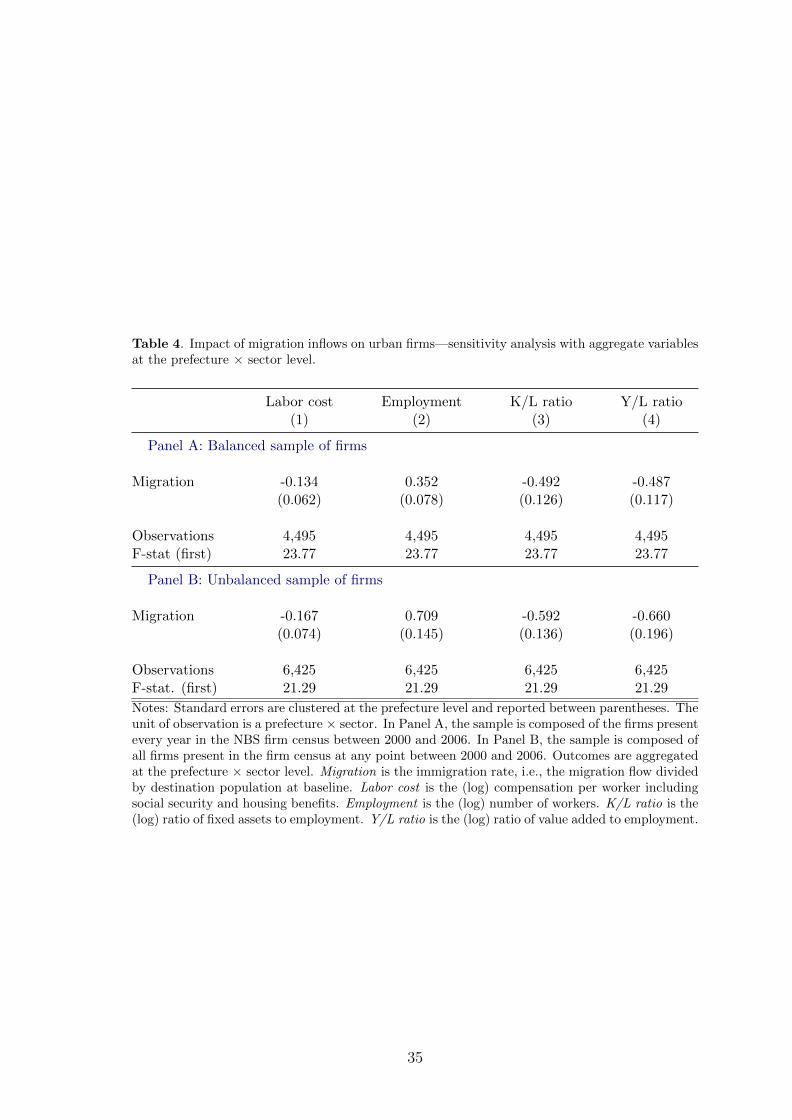
Table 4. Impact of migration inflows on urban firms—sensitivity analysis with aggregate variablesat the prefecture × sector level.

Labor cost Employment K/L ratio Y/L ratio(1) (2) (3) (4)

Panel A: Balanced sample of firms

Migration -0.134 0.352 -0.492 -0.487(0.062) (0.078) (0.126) (0.117)

Observations 4,495 4,495 4,495 4,495F-stat (first) 23.77 23.77 23.77 23.77

Panel B: Unbalanced sample of firms

Migration -0.167 0.709 -0.592 -0.660(0.074) (0.145) (0.136) (0.196)

Observations 6,425 6,425 6,425 6,425F-stat. (first) 21.29 21.29 21.29 21.29

Notes: Standard errors are clustered at the prefecture level and reported between parentheses. Theunit of observation is a prefecture × sector. In Panel A, the sample is composed of the firms presentevery year in the NBS firm census between 2000 and 2006. In Panel B, the sample is composed ofall firms present in the firm census at any point between 2000 and 2006. Outcomes are aggregatedat the prefecture × sector level. Migration is the immigration rate, i.e., the migration flow dividedby destination population at baseline. Labor cost is the (log) compensation per worker includingsocial security and housing benefits. Employment is the (log) number of workers. K/L ratio is the(log) ratio of fixed assets to employment. Y/L ratio is the (log) ratio of value added to employment.

35

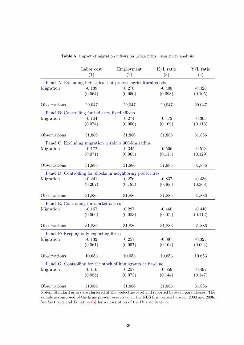
Table 5. Impact of migration inflows on urban firms—sensitivity analysis.

Labor cost Employment K/L ratio Y/L ratio(1) (2) (3) (4)

Panel A: Excluding industries that process agricultural goodsMigration -0.139 0.276 -0.408 -0.428

(0.064) (0.050) (0.093) (0.105)

Observations 29,047 29,047 29,047 29,047

Panel B: Controlling for industry fixed effectsMigration -0.104 0.274 -0.472 -0.365

(0.074) (0.056) (0.109) (0.113)

Observations 31,886 31,886 31,886 31,886

Panel C: Excluding migration within a 300-km radiusMigration -0.172 0.345 -0.506 -0.513

(0.071) (0.065) (0.115) (0.129)

Observations 31,886 31,886 31,886 31,886

Panel D: Controlling for shocks in neighboring prefecturesMigration -0.241 0.276 -0.837 -0.436

(0.267) (0.185) (0.466) (0.368)

Observations 31,886 31,886 31,886 31,886

Panel E: Controlling for market accessMigration -0.167 0.297 -0.460 -0.440

(0.066) (0.053) (0.102) (0.112)

Observations 31,886 31,886 31,886 31,886

Panel F: Keeping only exporting firmsMigration -0.132 0.257 -0.387 -0.325

(0.061) (0.057) (0.104) (0.094)

Observations 10,653 10,653 10,653 10,653

Panel G: Controlling for the stock of immigrants at baselineMigration -0.110 0.257 -0.559 -0.497

(0.088) (0.072) (0.144) (0.147)

Observations 31,886 31,886 31,886 31,886

Notes: Standard errors are clustered at the prefecture level and reported between parentheses. Thesample is composed of the firms present every year in the NBS firm census between 2000 and 2006.See Section 2 and Equation (5) for a description of the IV specification.

36

Table 6. Impact of migration inflows on urban firms—transformation from destinations to originsfollowing Borusyak et al. (2018).

Labor cost Employment K/L ratio Y/L ratio(1) (2) (3) (4)

Panel A: OLS

Transformed migration -0.173 0.295 -0.436 -0.459(0.019) (0.013) (0.018) (0.017)

Observations 335 335 335 335

Panel B: IV

Transformed migration -0.147 0.294 -0.431 -0.437(0.029) (0.019) (0.024) (0.029)

Observations 335 335 335 335F-stat. (first stage) 102.9 102.9 102.9 102.9

Panel C: Reduced form

Price shock 0.232 -0.465 0.683 0.692(0.053) (0.049) (0.084) (0.084)

Observations 335 335 335 335

Panel D: Parallel trends (1998–2000)

Price shock 0.004 -0.102 0.025 0.178(0.032) (0.023) (0.031) (0.050)

Observations 335 335 335 335

Panel E: Lagged Shocks (1993–1998)

Price shock -0.199 -0.150 0.202 0.026(0.079) (0.080) (0.115) (0.116)

Observations 335 335 335 335

Notes: Robust standard errors are reported between parentheses. The sample is composed ofthe 335 prefectures of origin. The dependent variables and Transformed migration are variables atdestination (outcomes and the immigration rate) transformed into variables across origins, througha combination of (i) migration patterns between origins and destinations, and (ii) employment levelswithin destinations at baseline (see Section 2).

37

Table 7. Impact of migration inflows on urban firms—production restructuring.

Change in product Any High ed. Low ed. High K/L Low K/L(1) (2) (3) (4) (5)

Panel A: Using unique descriptions to define product categories

Migration 0.205 -0.001 0.206 0.049 0.157(0.049) (0.028) (0.036) (0.038) (0.026)

Observations 27,062 27,062 27,062 27,062 27,062

Panel B: Using HS codes to define product categories

Migration 0.120 0.001 0.118 -0.011 0.131(0.035) (0.022) (0.030) (0.024) (0.029)

Observations 27,062 27,062 27,062 27,062 27,062

Notes: Standard errors are clustered at the prefecture level and reported between parentheses. Thesample is composed of the firms present every year in the NBS firm census between 2000 and 2006and whose main product was matched to a HS6 code by the NLP algorithm described in Section 2.Migration is the immigration rate, i.e., the migration flow divided by destination population atbaseline. The dependent variables are dummy variables equal to one if there is any change inthe main product (1), and if this change goes toward products manufactured by establishmentswith a more (2) or less (3) educated workforce, and by more (4) or less (5) capital-abundantestablishments. See Section 2 and Equation (5) for a description of the IV specification.

38

Table 8. Impact of migration inflows on urban firms—technological innovations.

New patent Any Design Invention Utility(1) (2) (3) (4)

Panel A: Patent categories

Migration -0.047 -0.006 -0.035 -0.027(0.016) (0.010) (0.012) (0.015)

Observations 31,886 31,886 31,886 31,886

New patent High ed. Low ed. High K/L Low K/L(1) (2) (3) (4)

Panel B: Patent characteristics

Migration -0.045 -0.018 -0.046 -0.014(0.017) (0.012) (0.014) (0.012)

Observations 31,886 31,886 31,886 31,886

Notes: Standard errors are clustered at the prefecture level and reported between parentheses. Thesample is composed of the firms present every year in the NBS firm census between 2000 and 2006.Migration is the immigration rate, i.e., the migration flow divided by destination population atbaseline. The dependent variable is the difference in the probability to submit a patent applicationbetween 2000 and 2006. In Panel A, we distinguish three categories: design, invention and utility.In Panel B, we divide patents into technologies associated with high/low average human capital,and labor-abundant technologies versus capital-abundant ones. See Section 2 and Equation (5) fora description of the IV specification.

39

Table 9. Impact of migration inflows on urban firms—changes in product, and changes in factoruse and technology.

K/L Ratio PatentsAny new Any innovation Any utility

(1) (2) (3) (4)

Change 0.084 0.053 0.026 0.033(0.037) (0.015) (0.012) (0.013)

Migration -0.353 0.018 -0.023 0.018(0.141) (0.031) (0.019) (0.023)

Migration × Change -0.123 -0.103 -0.027 -0.078(0.111) (0.035) (0.023) (0.028)

Observations 27,062 27,062 27,062 27,062

Notes: Standard errors are clustered at the prefecture level and reported between parentheses. Thesample is composed of the firms present every year in the NBS firm census between 2000 and 2006and whose main product was matched to a HS6 code by the NLP algorithm described in Section 2.Migration is the immigration rate, i.e., the migration flow divided by destination population atbaseline. Change is a dummy variable equal to one for firms that changed their main product in2000–2006. See Section 2 and Equation (5) for a description of the IV specification.

40

FOR ONLINE PUBLICATION

A Measures of production and labor cost in cities 42

A.1 A census of large manufacturing firms . . . . . . . . . . . . . . . . . . 42

A.2 A text-based classification of products . . . . . . . . . . . . . . . . . 45

A.3 A survey of urban workers . . . . . . . . . . . . . . . . . . . . . . . . 48

B Migration flows: construction and description 50

B.1 Elements of context . . . . . . . . . . . . . . . . . . . . . . . . . . . . 50

B.2 Data sources and construction of migration flows . . . . . . . . . . . 51

B.3 Migration patterns and the selection of migrants. . . . . . . . . . . . 55

C A shift-share instrument for migration flows 59

C.1 A stylized model . . . . . . . . . . . . . . . . . . . . . . . . . . . . . 59

C.2 Shocks to rural livelihoods . . . . . . . . . . . . . . . . . . . . . . . . 62

C.3 Sensitivity analysis and robustness checks . . . . . . . . . . . . . . . 64

D Migration and factor productivity 70

D.1 Quantitative framework . . . . . . . . . . . . . . . . . . . . . . . . . 70

D.2 Effect of migration on factor productivity . . . . . . . . . . . . . . . . 72

D.3 Heterogeneous firm technology and labor efficiency . . . . . . . . . . 74

E Additional results on heterogeneity and firm entry/exit 78

E.1 Treatment heterogeneity across urban establishments . . . . . . . . . 78

E.2 Aggregation and entry/exit . . . . . . . . . . . . . . . . . . . . . . . 79

E.3 Worker heterogeneity and compositional effects at destination . . . . 82

E.4 Complements on production restructuring . . . . . . . . . . . . . . . 84

F Sensitivity analysis 88

F.1 The shift-share design . . . . . . . . . . . . . . . . . . . . . . . . . . 88

F.2 The empirical specification . . . . . . . . . . . . . . . . . . . . . . . . 88

F.3 Beyond the cross-sectional analysis . . . . . . . . . . . . . . . . . . . 90

41

A Measures of production and labor cost in cities

In this Appendix, we describe the census of large manufacturing establishments, we

detail our product classification, and we describe a survey of urban residents.

A.1 A census of large manufacturing firms

Description Our measures of urban production are derived from the census of

“above-scale” manufacturing establishments conducted by the National Bureau of

Statistics (NBS). The NBS implements a census of all state-owned manufacturing

enterprises and all non-state manufacturing firms with sales exceeding RMB 5 mil-

lion, or about $600,000 over that period.

The data cover the manufacturing sector over the period 1992–2009. The set of

variables changes across years and we restrict ourselves to the period 2000–2006 in

the baseline specification, in order to ensure consistent outcome measures. We focus

on the balanced panel of firms in most of our analysis. In contrast with firm-level

data in developed countries, matching firms over time in the NBS is difficult because

of frequent changes in identifiers. In order to match “identifier-switchers,” we use

the fuzzy algorithm developed by Brandt et al. (2014), which uses slowly-changing

firm characteristics such as name, address, and phone number. While total sample

size ranges between 150,000 and 300,000 per year, we end up with about 32,000

firms when we limit the sample to the balanced panel.33

The data contain a wealth of information on manufacturing plants. Besides the

location, industry, ownership type, exporting activity, and number of employees,

they offer a wide range of accounting variables (e.g., output, input, value added,

wage bill, fixed assets, financial assets, etc.). We use these variables to construct

the firm-level measures of factor choices, costs, and productivity. Finally, each firm

reports its three main products as a textual description that we exploit with a

language processing algorithm in order to generate a consistent HS6-code.

Descriptive statistics and sample selection Table A1 displays descriptive

statistics for the sample of all firm × year observations over the period 2000–2006,

the balanced panel, and the sub-samples of new entrants and exiters. Firms of the

33Although we use the term “firm” in the paper, the NBS data cover “legal units” (farendanwei): different subsidiaries of the same enterprise may be surveyed, provided they meet anumber of criteria, including having their own names, being able to sign contracts, possessing andusing assets independently, assuming their liabilities, and being financially independent. While thisdefinition of units of observation may be unfamiliar to readers accustomed to U.S. or European data,“legal units” almost perfectly overlap with plants in practice, which is also true of establishmentsin the U.S. In 2006, almost 97% of the units in our data corresponded to single-plant firms.

42

balanced panel are larger and more capitalized than the average firm (see Panel

A). They are also more likely to be publicly owned.34 The difference between the

balanced panel and whole sample comes from inflows (new entrants) and outflows

(exiters). The third and fourth columns of Table A1 better characterize these two

categories of firms. Firms on the brink of exit are small, under-capitalized, un-

productive, and less likely to be located in an industrial cluster. New entrants are

equally small and under-capitalized, but comparatively productive. Finally, the pe-

riod of interest is a period of public sector downsizing. While private firms still

accounted for a relatively small share of the economic activity in the 1990s, they

represented over 80% of total value added by the end of the 2000s. We see indeed

that new entrants are disproportionately privately owned.

Issues This “above-scale” census raises a number of challenges. First, the census

covers the universe of state-owned enterprises but only a selected sample of private

establishments, even if together they account for about 90% of the manufacturing

output. The RMB 5 million threshold that defines whether a non-publicly owned

firm belongs to the NBS census may not be perfectly implemented. Surveyors may

not correctly predict the level of sales before implementing the census, and some

firms only entered the database several years after having reached the sales cut-off.35

Figure 1 however shows that this is unlikely to be a major issue, as the threshold is

sharp.

Second, firms may under-report the number of workers. Indeed, firm size serves

as a basis for taxation by the local labor department, and migrants, who represent a

large share of the workforce, may be easier to under-report. Workers hired through a

“labor dispatching” (laodong paiqian) company are not included in the employment

variable. The wage bill may also be slightly under-estimated as some components of

worker compensation are not recorded in all years, e.g., pension contributions and

housing subsidies, which are reported only since 2003 and 2004, respectively, but

accounted for only 3.5% of total worker compensation in 2007.

Third, a few variables are not documented in the same way as in standard firm-

level data. Fixed assets are reported by summing nominal values at the time of

purchase. We use the procedure developed in Brandt et al. (2014) to account for

depreciation: (i) We calculate the nominal rate of growth in the capital stock (using a

34Ownership type is defined based on official registration (qiye dengji zhuce leixing). Table A1uses three categories: (i) state-owned, hybrid or collective, (ii) domestic private, and (iii) foreignprivate firms, including those from Hong Kong, Macau, and Taiwan.

35Conversely, about 5% of private and collectively owned firms, which are subject to the thresh-old, continue to participate in the census even if their annual sales fall short of the threshold.

43

Table A1. Firm characteristics (2000–2006).

All firms Balanced Exiters Entrants2000–2006

Panel A: Outcome variables

Labor cost 2.53 2.49 2.33 2.56(0.67) (0.68) (0.77) (0.65)

Employment 4.64 5.09 4.19 4.47(1.06) (1.06) (1.04) (1.03)

K/L ratio 3.68 3.90 3.50 3.54(1.28) (1.18) (1.34) (1.32)

Value added 8.57 8.95 7.91 8.42(1.16) (1.14) (1.09) (1.16)

Panel B: Characteristics

Public 0.13 0.18 0.24 0.09(0.34) (0.39) (0.43) (0.29)

Export 0.21 0.33 0.14 0.20(0.41) (0.47) (0.34) (0.40)

Large 0.43 0.45 0.33 0.34(0.49) (0.50) (0.47) (0.47)

High-skill 0.45 0.45 0.45 0.44(0.50) (0.50) (0.50) (0.50)

Unionized 0.08 0.10 0.11 0.08(0.27) (0.30) (0.32) (0.28)

Ind. park 0.13 0.11 0.10 0.16(0.34) (0.31) (0.30) (0.37)

Observations 1,350,167 227,031 136,587 519,261

Notes: NBS firm-level data (2000–2006). Standard deviations are reported in parentheses. All variables in Panel Aare in logarithms. All variables in Panel B are dummy-coded and defined for the first year in the sample. Publicis equal to 1 if the firm is state- or collective-owned in 2000. A similar definition applies to Export, Unionized, andInd. park, which are equal to 1 if the firm exported, had a trade union, and operated in an industrial park in thefirst year, respectively. Large is defined as equal to 1 if the firm belonged to the top 50% of the distribution interms of employment. High-skill is equal to 1 if the firm belongs to an industry with an above-median share oftertiary-educated employees.

2-digit industry by province average in 1993–1998) to compute nominal capital stock

in the start-up year. (ii) Real capital in the start-up year is obtained using a chain-

linked investment deflator (based on separate price indices for equipment-machinery

and buildings-structures, and weighted by fixed investment shares provided by the

NBS). (iii) We move forward to the first year in the database, assuming a rate of

depreciation of 9% per year and using annual deflators. (iv) Once a firm enters the

database, we use the nominal figures provided in the data to compute the change

in nominal capital stock in a given year and deflate it. If past investments and

44

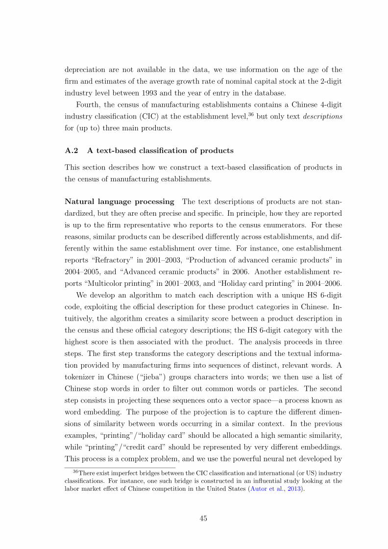
depreciation are not available in the data, we use information on the age of the

firm and estimates of the average growth rate of nominal capital stock at the 2-digit

industry level between 1993 and the year of entry in the database.

Fourth, the census of manufacturing establishments contains a Chinese 4-digit

industry classification (CIC) at the establishment level,36 but only text descriptions

for (up to) three main products.

A.2 A text-based classification of products

This section describes how we construct a text-based classification of products in

the census of manufacturing establishments.

Natural language processing The text descriptions of products are not stan-

dardized, but they are often precise and specific. In principle, how they are reported

is up to the firm representative who reports to the census enumerators. For these

reasons, similar products can be described differently across establishments, and dif-

ferently within the same establishment over time. For instance, one establishment

reports “Refractory” in 2001–2003, “Production of advanced ceramic products” in

2004–2005, and “Advanced ceramic products” in 2006. Another establishment re-

ports “Multicolor printing” in 2001–2003, and “Holiday card printing” in 2004–2006.

We develop an algorithm to match each description with a unique HS 6-digit

code, exploiting the official description for these product categories in Chinese. In-

tuitively, the algorithm creates a similarity score between a product description in

the census and these official category descriptions; the HS 6-digit category with the

highest score is then associated with the product. The analysis proceeds in three

steps. The first step transforms the category descriptions and the textual informa-

tion provided by manufacturing firms into sequences of distinct, relevant words. A

tokenizer in Chinese (“jieba”) groups characters into words; we then use a list of

Chinese stop words in order to filter out common words or particles. The second

step consists in projecting these sequences onto a vector space—a process known as

word embedding. The purpose of the projection is to capture the different dimen-

sions of similarity between words occurring in a similar context. In the previous

examples, “printing”/“holiday card” should be allocated a high semantic similarity,

while “printing”/“credit card” should be represented by very different embeddings.

This process is a complex problem, and we use the powerful neural net developed by

36There exist imperfect bridges between the CIC classification and international (or US) industryclassifications. For instance, one such bridge is constructed in an influential study looking at thelabor market effect of Chinese competition in the United States (Autor et al., 2013).

45

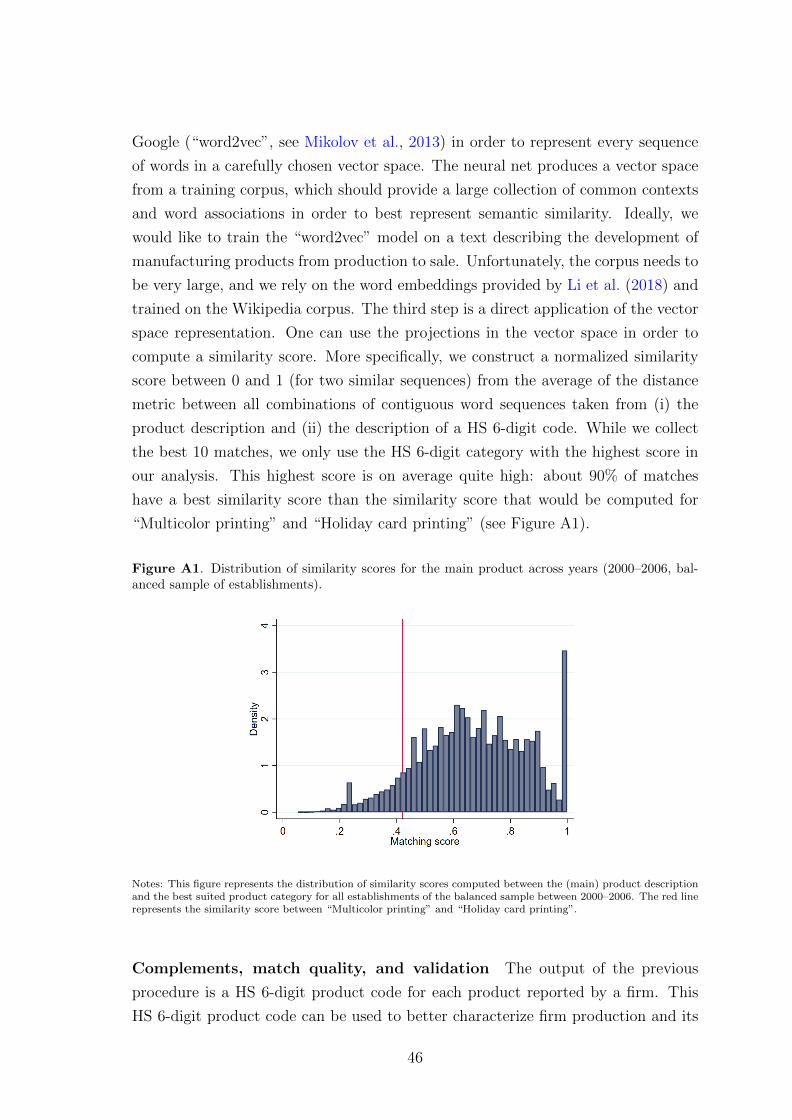
Google (“word2vec”, see Mikolov et al., 2013) in order to represent every sequence

of words in a carefully chosen vector space. The neural net produces a vector space

from a training corpus, which should provide a large collection of common contexts

and word associations in order to best represent semantic similarity. Ideally, we

would like to train the “word2vec” model on a text describing the development of

manufacturing products from production to sale. Unfortunately, the corpus needs to

be very large, and we rely on the word embeddings provided by Li et al. (2018) and

trained on the Wikipedia corpus. The third step is a direct application of the vector

space representation. One can use the projections in the vector space in order to

compute a similarity score. More specifically, we construct a normalized similarity

score between 0 and 1 (for two similar sequences) from the average of the distance

metric between all combinations of contiguous word sequences taken from (i) the

product description and (ii) the description of a HS 6-digit code. While we collect

the best 10 matches, we only use the HS 6-digit category with the highest score in

our analysis. This highest score is on average quite high: about 90% of matches

have a best similarity score than the similarity score that would be computed for

“Multicolor printing” and “Holiday card printing” (see Figure A1).

Figure A1. Distribution of similarity scores for the main product across years (2000–2006, bal-anced sample of establishments).

Notes: This figure represents the distribution of similarity scores computed between the (main) product descriptionand the best suited product category for all establishments of the balanced sample between 2000–2006. The red linerepresents the similarity score between “Multicolor printing” and “Holiday card printing”.

Complements, match quality, and validation The output of the previous

procedure is a HS 6-digit product code for each product reported by a firm. This

HS 6-digit product code can be used to better characterize firm production and its

46

evolution during our period of interest.

We first use the HS 6-digit product code as a label capturing the specificity

of a given production process. The underlying assumption is that the production

process is quite homogeneous within a HS 6-digit product code, such that the relative

factor use of firms producing a certain product is indicative of factor shares in

production. Letting ri,p denote the relative factor share, e.g., capital to labor or the

share of high-skilled workers, in firm i producing product p at baseline, we construct

rp as the average factor share required by the production of p. One could then

characterize the direction of a change from product p to product q by comparing rp

to rq. One issue with the previous characterization is that it only accounts for the

factor share within the firm, and not possibly along the whole production line leading

to the final good. We use input-output accounts in the United States (in 2002,

Stewart et al., 2007) to construct a measure of factor use along the production chain,

sp =∑

i αp,qri,q1p(i)=q/∑

i αp,q1p(i)=q, where αp,q is the contribution of product q in

the production of p.

Second, we use the HS 6-digit product code to measure the production “width”

of a firm: the number of different products produced by the establishment; and

their similarity. We count the number of different product descriptions, but also the

number of different HS product codes for different levels of disaggregation (e.g., 6

digit or 3-digit). We construct three different measures of similarity, γp,q, between

products p and q: a measure based on language proximity; a measure based on

production proximity; and a measure based on technological proximity. We construct

language proximity as the average of similarity scores between the descriptions of

unique pairs of products (only one pair if there are two products reported by the

establishment, three pairs if there are three products). We construct production

proximity in a similar manner using the previous input/output measure, αp,q. We

construct technological proximity using a technology closeness measure, τp,q, derived

from patent (cross-)citations between different industries, {Ti,j}i,j, in the United

States (Bloom et al., 2013).37

Third, we rely on the previous technology closeness measure to construct: the

intensity of technological spillovers for a given product, {τp,q}p,q; the number of links

to other industries,∑

q 6=p 1τp,q>0; and a Herfindahl index based on technology close-

ness,∑

q 6=p τ2p,q/(

∑q 6=p τp,q)

2. These variables capture the intensity and the “width”

of technological spillovers.

37We need to mediate these measures through a bridge B between HS6 product codes andStandard Industrial Classification (SIC) codes: τ = B′TB.

47

A.3 A survey of urban workers

In order to study the impact of immigration on local labor markets and isolate equi-

librium effects on wages from compositional effects, we use the Urban Household

Survey (UHS) collected by the National Bureau of Statistics. The UHS is a survey

of urban China, with a consistent questionnaire since 1986 but considered represen-

tative from 2002 onward, and our description will correspond to this latter period.

The survey is based on a three-stage stratified random sampling. Its design is sim-

ilar to that of the Current Population Survey in the United States (Ge and Yang,

2014; Feng et al., 2017) and includes 18 provinces and 207 prefectures. The data are

cross-sectional, with a sample size that ranges from 70,000 to 90,000 individuals in

2002–2006.38

The UHS is a rich dataset with detailed information on individual employment,

income, and household characteristics. We construct a measure of real wages as

the monthly wages divided by a prefecture- and year-specific consumer price index,

which we compute using the detailed household-level consumption data. We also

construct three employment outcomes: wage employment, unemployment, and self-

employment (which also includes firm owners). Table A2 provides some descriptive

statistics of key variables over the period 2002–2006 and shows that the sample is

similar to the locally registered urban hukou holders in the Mini-Census data (see

Table B3) in terms of demographics and sector of activity, although they tend to

be more educated, have a higher probability of being employed, and earn a higher

monthly income.

38While all households living in urban areas are eligible, sampling still ignores urban dwellersliving in townships and in suburban districts (Park, 2008). Rural-urban migrants, who are morelikely to live in peripheral areas of cities, are therefore underrepresented.

48

Table A2. Descriptive statistics on urban residents from the UHS data (2002–2006).

Mean Standard deviation

Age 43.1 11.0Female 0.50 0.50Married 0.88 0.33Education:

Primary education 0.05 0.21Lower secondary 0.28 0.45Higher secondary 0.26 0.44Tertiary education 0.41 0.49

Not employed 0.23 0.42Self-employed/Firm owner 0.05 0.22Employee 0.72 0.45

Public sector 0.68 0.47Private sector 0.32 0.47

Total monthly income (RMB) 1,294 1,123Hours worked per week 44.5 9.20Industry:

Agriculture 0.01 0.10Mining 0.02 0.14Manufacturing 0.24 0.42Utilities 0.03 0.18Construction 0.03 0.17Wholesale and retail trade 0.12 0.33Other tertiary 0.42 0.50

Observations 338,221Notes: All variables except Age, Income, and Hours worked per week are dummy-coded. The table displays averagesover the period 2002–2006. The sample is restricted to locally registered urban hukou holders aged 15–64.

49

B Migration flows: construction and description

In this Appendix, we provide elements of context about migration in China, we

describe the construction of migration flows from retrospective questions, and we

discuss key descriptive statistics.

B.1 Elements of context

An important feature of China’s society is the division of the population according

to its household registration or hukou status. Chinese citizens are classified along

two dimensions: their hukou type (hukou xingzhi)—agricultural (nongye) or non-

agricultural (fei nongye)—and hukou location (hukou suozaidi). Hukou characteris-

tics, which are recorded in the household registration booklet, may not correspond

to actual occupation and location.

Since the inception of the reforms in the late 1970s, rules regarding migration

within China have been relaxed. Labor mobility remains subject to legal require-

ments, e.g., being lawfully employed at destination, but the large flows of internal

migrants that have characterized China’s recent development show that barriers are

low in practice, at least for individual migration. Migrants however do not enjoy

the same rights as the locally registered population. Whereas an agricultural hukou

grants access to land, non-agricultural-hukou holders enjoy public services in their

cities of registration. Access to welfare benefits and public services (e.g., enrollment

in local schools, access to health care, urban pension plans, and subsidized housing)

is conditional on being officially recorded as a local urban dweller. Migrants thus

face a higher cost of living in cities and are supposed to return to their places of

registration for basic services such as education and health care or they are charged

higher fees (Song, 2014). Labor outcomes are also affected as local governments may

issue regulations restricting access to job opportunities or rely on informal guide-

lines to employers to favor local permanent residents. This is likely to impede family

migration, reduce migrant workers’ bargaining power, and lock them in a position

of “second-class workers” (Demurger et al., 2009).

Despite the rigidity of the hukou system and the persistently low rate of hukou

conversion, reforms have progressively been introduced during the structural trans-

formation of China. Since the 1980s, China has experienced a gradual devolution

of power from the central to local governments in terms of hukou policy: rules and

implementation vary substantially across places and over time. Provincial govern-

ments set guidelines, and specific rules are then determined by prefectures, which

in practice hold the most power over hukou policy (Song, 2014). Two reforms were

50

introduced in recent years. First, the distinction between agricultural and non-

agricultural hukou was abolished within local jurisdictions in about one third of

Chinese provinces. Albeit an important evolution, this reform does not affect rural-

urban migrants who come from other prefectures. Second, hukou conversion rules

have been gradually loosened. The main channels to change one’s hukou from agri-

cultural to non-agricultural used to include recruitment by an SOE, receiving college

education or joining the army. These conditions have been relaxed since 2000, espe-

cially in small cities and towns that attract fewer migrants (Zhang and Tao, 2012).

In larger cities, however, conditions for eligibility are tough, so that hukou conversion

reforms primarily benefit the richest and highly educated (Song, 2014).

The identification strategy described in Section 2 allows us to deal with the

potential endogeneity of migration policy to local factor demand. The shift-share

instrument is indeed likely to be orthogonal to such dynamics.

B.2 Data sources and construction of migration flows

Data description In order to measure migration flows, we use the 2005 1% Pop-

ulation Survey, also called “2005 Mini-Census”.39

The 2005 1% Population Survey constitutes a 1.3% [sic] sample of the popula-

tion selected from 600,000 primary census enumeration districts using a three-stage

cluster sampling (Ebenstein and Zhao, 2015). The sampling weights provided by the

National Bureau of Statistics (NBS) account for the underlying proportional proba-

bility sampling scheme based on the 2004 population registry of the Public Security

Bureau. The 2005 Mini-Census was used to test new ways of recording migration

and uses the same questionnaire and definitions as the 2010 Census.

A few caveats are in order. First, the sampling frame of the 2005 1% Population

Survey contains information on population by registration. High-immigration areas

could thus be under-sampled. Comparing the flows for 2005 in the 2005 Mini-Census

and 2010 Census, we indeed find a small discrepancy that we attribute to coverage

issues. Second, the 2005 Mini-Census offers a set of variables similar to standard

censuses, i.e., prefecture-level information on the place of “current residence” and

on hukou location. However, the 2005 Mini-Census records the timing of departure

39After the beginning of the reforms and loosening of restrictions on mobility, there was a growingdisconnect between census data focusing on hukou location and the rising “floating population” ofnon-locally registered citizens. The 2000 Population Census was the first census to acknowledgethis gap and record migrants’ places of residence—provided they had been living there for morethan 6 months (Ebenstein and Zhao, 2015). In addition to the place of residence (at the prefecturelevel in our data), hukou location (province level) and hukou type, the 2000 Population Censuscontains retrospective information on the place of residence 5 years before the survey (provincelevel) and the reason for departure if residence and registration hukou do not coincide.

51

from a migrant’s place of registration rather than of arrival at destination. This is

not an issue as long as there is no step migration, i.e., if rural dwellers move directly

to their final destinations. Third, the data do not record the place of residence at

high enough resolution to unambiguously infer whether a migrant is residing in a

rural or urban area. Nevertheless, rural-rural migration represents a small share

of emigration from rural areas, mostly explained by marriage—which usually gives

right to local registration (Fan, 2008).40 Fourth, we cannot account for migrants

who changed their hukou location or type. This is quite innocuous given that hukou

conversion is marginal.

Migration flow construction The retrospective data on migration spells in the

Mini-Census allows us to construct yearly migration flows over the period 2000–2005.

These flows are directly observed rather than computed as a difference of stocks as

common in the migration literature.

We construct annual migration flows between all prefectures of origin and desti-

nation by combining information on the current place of residence (the destination),

the place of registration (the origin), and the year in which the migrant left the

origin. One advantage of working with those data is that they are representative of

the whole population, irrespective of their hukou status. However, not all migration

spells are observed. We describe below (i) which migration spells are directly ob-

served and which spells are omitted, and (ii) how we can infer some of the unobserved

spells and adjust the raw migration flows.

Not all migration spells are observed in the data. We only observe single migra-

tion spells, i.e., migration spells in which the interviewed individual is at destination

at the time of interview, and whose origin coincides with the hukou location. For

these individuals, the origin is deduced from their hukou location, and the date of

their unique relocation is available. All other types of migration histories during the

five years preceding the interview are less straightforward to identify. For instance,

if one individual were to leave her hukou location to city A in 2002 and then relocate

to city B in 2005, we would only record the last relocation. In such step migration

cases, we would correctly specify the departure time from origin, but we would in-

correctly attribute arrival dates at destination for the last spell and we would miss

arrival in city A. If, instead, one individual were to leave her hukou location to

city A in 2002 and then return to her hukou location by 2005, we would miss her

entire migration history. In such return migration cases, we would incorrectly omit

40In the 2005 Mini-Census, only 6.45% of agricultural-hukou holders who migrated betweenprefectures reported having left their places of registration to live with their spouses after marriage.See Table B2 for further descriptive statistics on reasons for moving.

52

emigration flows from origins and immigration to destinations.

The incidence of step migration and return migration spells can, however, be

measured. The 2005 Mini-Census records where individuals were living 1 and 5

years before the survey (province level). We can estimate how many migrants re-

port different destinations between 2000 and 2005, which would be a proxy for step

migration, and we can observe total return migration between 2000 and 2005, and

2004 and 2005. We first study the importance of step migration. Among migrants

who were in their provinces of registration in 2000 and in other provinces in 2005,

we compute the fraction that lived in yet another province in 2004. A minority of

migrants have changed provinces of destination between 2004 and 2005 (see Fig-

ure B1). Step migration is not only low but concentrated in the first year after the

first migration spell. In other words, step migration induces errors in arrival and

departure dates that are quite small. Adjusting for step migration would require

strong assumptions about the intermediate destination, which is not observed in the

data; we thus do not correct migration flows for step migration.

Figure B1. Share of step migrants as a function of age and time since departure.

(a) Age. (b) Years since emigration.

Source: 2005 1% Population Survey.Notes: The sample comprises all working-age (15–64) agricultural-hukou holders who were living in a provincedifferent from their province of registration in 2004 and left their prefecture of registration less than 6 years priorto the interview.

We then consider the extent of return migration. Among all migrants from rural

areas who were living in their provinces of registration in 2000 and in other provinces

in 2004, we compute the fraction that had returned to their provinces of registration

by 2005. This share is not negligible: In a given year, between 4 and 6% of rural

migrants who had left their provinces of registration in the last 6 years go back to

their hukou locations. Return migration is an important phenomenon, which leads

us to underestimate true migration flows and the effect of shocks on emigration.

53

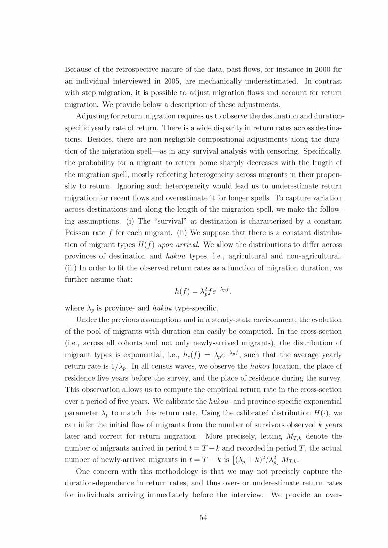
Because of the retrospective nature of the data, past flows, for instance in 2000 for

an individual interviewed in 2005, are mechanically underestimated. In contrast

with step migration, it is possible to adjust migration flows and account for return

migration. We provide below a description of these adjustments.

Adjusting for return migration requires us to observe the destination and duration-

specific yearly rate of return. There is a wide disparity in return rates across destina-

tions. Besides, there are non-negligible compositional adjustments along the dura-

tion of the migration spell—as in any survival analysis with censoring. Specifically,

the probability for a migrant to return home sharply decreases with the length of

the migration spell, mostly reflecting heterogeneity across migrants in their propen-

sity to return. Ignoring such heterogeneity would lead us to underestimate return

migration for recent flows and overestimate it for longer spells. To capture variation

across destinations and along the length of the migration spell, we make the follow-

ing assumptions. (i) The “survival” at destination is characterized by a constant

Poisson rate f for each migrant. (ii) We suppose that there is a constant distribu-

tion of migrant types H(f) upon arrival. We allow the distributions to differ across

provinces of destination and hukou types, i.e., agricultural and non-agricultural.

(iii) In order to fit the observed return rates as a function of migration duration, we

further assume that:

h(f) = λ2pfe

−λpf .

where λp is province- and hukou type-specific.

Under the previous assumptions and in a steady-state environment, the evolution

of the pool of migrants with duration can easily be computed. In the cross-section

(i.e., across all cohorts and not only newly-arrived migrants), the distribution of

migrant types is exponential, i.e., hc(f) = λpe−λpf , such that the average yearly

return rate is 1/λp. In all census waves, we observe the hukou location, the place of

residence five years before the survey, and the place of residence during the survey.

This observation allows us to compute the empirical return rate in the cross-section

over a period of five years. We calibrate the hukou- and province-specific exponential

parameter λp to match this return rate. Using the calibrated distribution H(·), we

can infer the initial flow of migrants from the number of survivors observed k years

later and correct for return migration. More precisely, letting MT,k denote the

number of migrants arrived in period t = T −k and recorded in period T , the actual

number of newly-arrived migrants in t = T − k is[(λp + k)2/λ2

p

]MT,k.

One concern with this methodology is that we may not precisely capture the

duration-dependence in return rates, and thus over- or underestimate return rates

for individuals arriving immediately before the interview. We provide an over-

54

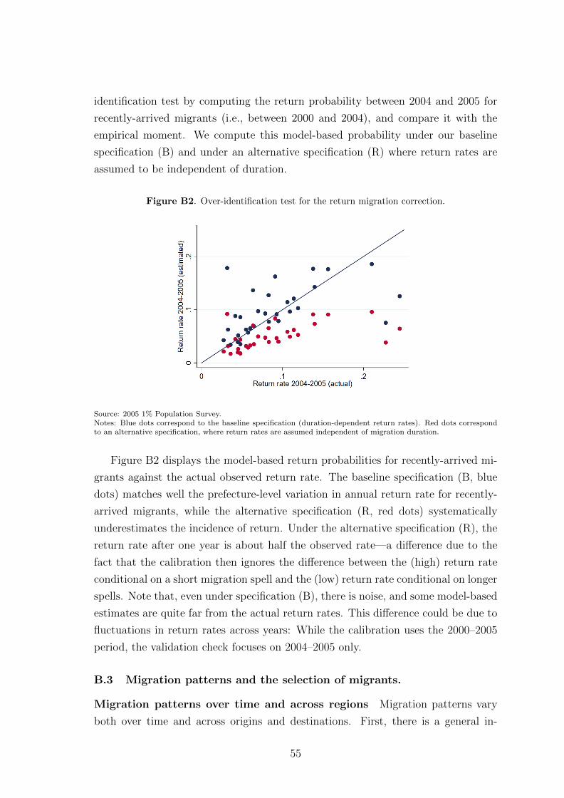
identification test by computing the return probability between 2004 and 2005 for

recently-arrived migrants (i.e., between 2000 and 2004), and compare it with the

empirical moment. We compute this model-based probability under our baseline

specification (B) and under an alternative specification (R) where return rates are

assumed to be independent of duration.

Figure B2. Over-identification test for the return migration correction.

Source: 2005 1% Population Survey.Notes: Blue dots correspond to the baseline specification (duration-dependent return rates). Red dots correspondto an alternative specification, where return rates are assumed independent of migration duration.

Figure B2 displays the model-based return probabilities for recently-arrived mi-

grants against the actual observed return rate. The baseline specification (B, blue

dots) matches well the prefecture-level variation in annual return rate for recently-

arrived migrants, while the alternative specification (R, red dots) systematically

underestimates the incidence of return. Under the alternative specification (R), the

return rate after one year is about half the observed rate—a difference due to the

fact that the calibration then ignores the difference between the (high) return rate

conditional on a short migration spell and the (low) return rate conditional on longer

spells. Note that, even under specification (B), there is noise, and some model-based

estimates are quite far from the actual return rates. This difference could be due to

fluctuations in return rates across years: While the calibration uses the 2000–2005

period, the validation check focuses on 2004–2005 only.

B.3 Migration patterns and the selection of migrants.

Migration patterns over time and across regions Migration patterns vary

both over time and across origins and destinations. First, there is a general in-

55

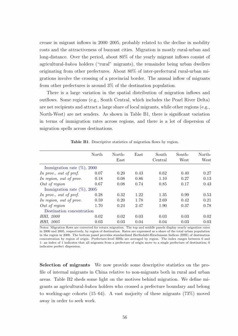
crease in migrant inflows in 2000–2005, probably related to the decline in mobility

costs and the attractiveness of buoyant cities. Migration is mostly rural-urban and

long-distance. Over the period, about 80% of the yearly migrant inflows consist of

agricultural-hukou holders (“rural” migrants), the remainder being urban dwellers

originating from other prefectures. About 80% of inter-prefectural rural-urban mi-

grations involve the crossing of a provincial border. The annual inflow of migrants

from other prefectures is around 3% of the destination population.

There is a large variation in the spatial distribution of migration inflows and

outflows. Some regions (e.g., South Central, which includes the Pearl River Delta)

are net recipients and attract a large share of local migrants, while other regions (e.g.,

North-West) are net senders. As shown in Table B1, there is significant variation

in terms of immigration rates across regions, and there is a lot of dispersion of

migration spells across destinations.

Table B1. Descriptive statistics of migration flows by region.

North North- East South South- North-East Central West West

Immigration rate (%), 2000In prov., out of pref. 0.07 0.20 0.43 0.62 0.40 0.27In region, out of prov. 0.18 0.08 0.86 1.10 0.27 0.13Out of region 0.67 0.08 0.74 0.85 0.17 0.43

Immigration rate (%), 2005In prov., out of pref. 0.28 0.32 1.22 1.35 0.99 0.53In region, out of prov. 0.59 0.20 1.78 2.69 0.42 0.21Out of region 1.70 0.24 2.47 1.90 0.37 0.78

Destination concentrationHHI, 2000 0.02 0.02 0.03 0.03 0.03 0.02HHI, 2005 0.03 0.03 0.04 0.04 0.03 0.03Notes: Migration flows are corrected for return migration. The top and middle panels display yearly migration ratesin 2000 and 2005, respectively, by region of destination. Rates are expressed as a share of the total urban populationin the region in 2000. The bottom panel provides standardized Herfindahl-Hirschmann Indices (HHI) of destinationconcentration by region of origin. Prefecture-level HHIs are averaged by region. The index ranges between 0 and1: an index of 1 indicates that all migrants from a prefecture of origin move to a single prefecture of destination; 0indicates perfect dispersion.

Selection of migrants We now provide some descriptive statistics on the pro-

file of internal migrants in China relative to non-migrants both in rural and urban

areas. Table B2 sheds some light on the motives behind migration. We define mi-

grants as agricultural-hukou holders who crossed a prefecture boundary and belong

to working-age cohorts (15–64). A vast majority of these migrants (73%) moved

away in order to seek work.

56

Table B2. Descriptive statistics from the 2005 Mini-Census.

Reason for moving Count Share of migrants

Work or business 102,388 73.32Follow relatives 16,454 11.78Marriage 9,006 6.45Support from relatives/friends 5,859 4.20Education and training 1,956 1.40Other 3,987 2.85Notes: This table displays descriptive statistics on rural migrants’ reasons for migrating.Rural migrants are definedas inter-prefectural migrants with an agricultural hukou and aged 15–64.

Rural-urban migrants are a selected sample of the origin population. We provide

some elements of comparison between migrants and stayers in Table B3. Migrants

tend to be younger, more educated, and more often single than the non-migrant

rural population. They are also more likely to be self-employed or employees and to

work in the private sector. The rural-urban productivity gap appears to be massive,

as the migrants’ monthly income is more than twice as large as the stayers’, which

may reflect both selection and different returns to skills in urban and rural areas.

Rural-urban migrants are however also different from urban residents. As is usual

with studies of internal migration, we consider in our baseline specification that mi-

grants and locally registered non-agricultural-hukou holders are highly substitutable.

Table B3 provides summary statistics on key characteristics of inter-prefectural mi-

grants and compares them with the locally registered urban population. Migrants

and natives are significantly different on most accounts, the former being on average

younger, less experienced, less educated, more likely to be illiterate, and more often

employed without a labor contract. Rural-urban migrants are also over-represented

in privately owned enterprises and in manufacturing and construction industries:

89% of them are employed in the private sector as against 28% of locally registered

hukou holders; and the share of rural-urban migrants working in manufacturing and

construction is 51% and 9%, as against 20% and 4% for urban residents, respectively.

Finally, migrants earn 17% less than urban residents.

To summarize, (i) migrants are selected at origin, (ii) they choose their des-

tination, and (iii) they differ from urban workers along observable characteristics.

Our empirical strategy, based on exogenous variation in agricultural prices at origin,

is affected by the previous issues as follows. First, compliers are selected and our

estimates are a local average treatment effect; we shed some light on this issue in Sec-

tion C. Second, Chinese rural-urban migrants may not compete with urban residents

for the exact same jobs; they may also be less productive for a given job. We further

57

quantify the bias induced by the hypothesis of homogeneous labor productivity in

Appendix D.3.

Table B3. Migrant selection (2005 Mini-Census).

Rural-urban Local Non-migrantmigrants urban hukou rural hukou

Age 28.25 37.18 33.81Female 0.49 0.49 0.50Married 0.54 0.64 0.56Education:

Primary education 0.23 0.17 0.38Junior high school 0.54 0.30 0.36Senior high school 0.13 0.26 0.06Tertiary education 0.02 0.19 0.00

Unemployed 0.02 0.07 0.01Self-employed/Firm owners 0.13 0.06 0.05Employees 0.58 0.35 0.08...of which:

Public sector 0.11 0.72 0.21Private sector 0.89 0.28 0.79

Out of the labor force 0.25 0.57 0.45Monthly income (RMB) 961.0 1155.2 401.4Hours worked per week 55.18 45.87 45.09Industry:

Agriculture 0.05 0.06 0.78Manufacturing 0.51 0.20 0.08Construction 0.09 0.04 0.03Wholesale and retail trade 0.15 0.14 0.04Other tertiary 0.20 0.51 0.06

Observations 139,813 678,614 1,716,269Notes: All variables except Age, Monthly income, and Hours worked per week are dummy-coded. The sample isrestricted to individuals aged 15–64. Descriptive statistics for Monthly income (RMB), Hours worked per week, andindustrial sectors are restricted to individuals who reported positive working hours in the past week.

58

C A shift-share instrument for migration flows

This Appendix develops a stylized, static model of location choice in order to derive

our main empirical specification and justify the use of a shift-share instrument for

migration inflows to Chinese cities.

C.1 A stylized model

Environment The economy is composed of a unit mass of workers, born at dif-

ferent locations o ∈ Θ. Let po denote the number of workers born at location o.

Workers live for one period only. They are mobile and have heterogeneous pref-

erences over the various locations in which they can provide one unit of labor. For

the sake of exposition, we do not explicitly distinguish rural locations from urban

ones, and any birth location can be a destination and reciprocally. A worker born

at origin o and deciding to work in destination d ∈ Θ receives utility:

uiod =biodwdκod

,

where biod is the idiosyncratic amenity draw related to a destination d for worker i,

wd is the exogenous revenue associated with providing labor at destination d, and

κod ≥ 1 is a migration “iceberg” cost capturing migration costs, commuting costs,

or cultural differences between origin and destination.

As usual in New Economic Geography framework (see Monte et al., 2018; Bryan

and Morten, 2019, for instance), the heterogeneity in preferences for locations across

workers is represented by a Frechet distribution. Workers observe their preferences

before choosing to work at a certain destination, and the worker-specific idiosyncratic

amenity is drawn independently across workers and locations as follows,

biod ∼ God(b) = e−Bodb−ε

,

where Bod is a distribution-location parameter which can be interpreted as the rel-

ative preferences of the workers from origin o for the specific location d, and ε > 0.

A worker chooses to locate in a destination d if her utility is greater there than in

any other locations. With the previous Frechet distribution, the ex-ante probability

that a worker chooses destination d is,

µod =Bod (wd/κod)

ε∑d∈D Bod (wd/κod)

ε .

We assume that Boo >> Bod/κod for any destination d 6= o; we normalize kappaoo =

59

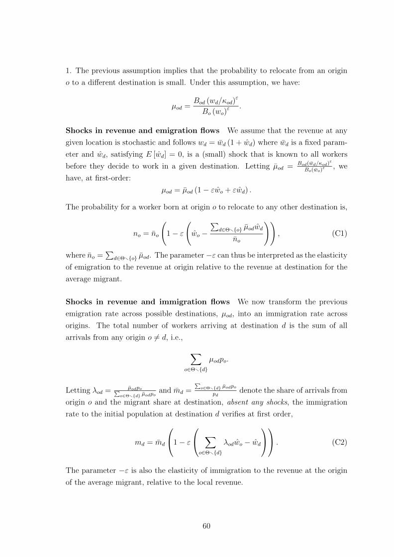
1. The previous assumption implies that the probability to relocate from an origin

o to a different destination is small. Under this assumption, we have:

µod =Bod (wd/κod)

ε

Bo (wo)ε .

Shocks in revenue and emigration flows We assume that the revenue at any

given location is stochastic and follows wd = wd (1 + wd) where wd is a fixed param-

eter and wd, satisfying E [wd] = 0, is a (small) shock that is known to all workers

before they decide to work in a given destination. Letting µod = Bod(wd/κod)ε

Bo(wo)ε , we

have, at first-order:

µod = µod (1− εwo + εwd) .

The probability for a worker born at origin o to relocate to any other destination is,

no = no

(1− ε

(wo −

∑d∈Θr{o} µodwd

no

)), (C1)

where no =∑

d∈Θr{o} µod. The parameter−ε can thus be interpreted as the elasticity

of emigration to the revenue at origin relative to the revenue at destination for the

average migrant.

Shocks in revenue and immigration flows We now transform the previous

emigration rate across possible destinations, µod, into an immigration rate across

origins. The total number of workers arriving at destination d is the sum of all

arrivals from any origin o 6= d, i.e., ∑o∈Θr{d}

µodpo.

Letting λod = µodpo∑o∈Θr{d} µodpo

and md =∑o∈Θr{d} µodpo

pddenote the share of arrivals from

origin o and the migrant share at destination, absent any shocks, the immigration

rate to the initial population at destination d verifies at first order,

md = md

1− ε

∑o∈Θr{d}

λodwo − wd

. (C2)

The parameter −ε is also the elasticity of immigration to the revenue at the origin

of the average migrant, relative to the local revenue.

60

Push, pull factors and a shift-share instrument We now introduce additional

sources of shocks: amenity shocks at different locations, Bod = Bod

(1 + Bod

), and

shocks to the relocation costs, κod = κod (1 + κod). At first order, the immigration

rate to the initial population at destination d verifies,

md = md

(1 + xDd + xOd

), (C3)

where xDd is a pull factor and xOd is a push factor, defined by:{xDd = εwd +

∑o∈Θr{d} λod

(Bod − εκod

)xOd =

∑o∈Θr{d} λod

(−Boo − εwo

)The immigration rate is driven by a set of pull and push shocks. Immigration is

expected to increase following positive shocks to revenue and amenity at destination

and negative shocks to relocation costs for the average immigrant. Immigration

is expected to increase following negative shocks to amenities and revenues at the

origin of the average immigrant.

In practice, most of the variation underlying immigrant flows to cities relates to

labor demand at origin and destination, and to barriers to migration (Bryan and

Morten, 2019; Tombe and Zhu, 2019), even though a few recent contributions have

highlighted the role of amenities, and pollution in particular, in driving labor flows

to Chinese cities (Chen et al., 2017; Freeman et al., 2019). The researcher interested

in evaluating the causal effect of migration flows on the structure of production, i.e.,

yd = f(md), faces an identification issue.

To isolate variation in the relocation of workers that is orthogonal to labor de-

mand and consumption patterns in cities, we consider exogenous variation in revenue

at origin so, and we construct a shift-share instrument, zd, for the immigration rate

md by combining origin shocks with the migration patterns,

zd =∑

o∈Θr{d}

λodso. (C4)

The shift-share design transforms shocks at origins in a similar way as the model

allocates migration flows, but it requires exogenous shocks pushing migrants toward

cities. We discuss the construction of these shocks next.

61

C.2 Shocks to rural livelihoods

The shift-share design relies on exogenous variation in agricultural livelihoods so.

This section describes the construction of a shift from variation in cropping patterns

combined with innovations in the World demand for commodities.

Cropping patterns across Chinese prefectures Each Chinese prefecture has

a distinct agricultural portfolio, resulting from water management, other local tech-

nologies, inherent soil characteristics, and climate. To isolate a component in the

agricultural portfolio that is orthogonal to adjustments in land use, technological

choice or worker-specific productivity, we estimate cropping patterns using a mea-

sure of land use at baseline and a measure of potential yield, as calculated from soil

and climate characteristics. Harvested areas come from the 2000 World Census of

Agriculture, which provides a geo-coded map of harvested areas for each crop at a

30 arc-second resolution (approximately 10 km). We overlay this map with a map

of prefectures and construct the total harvested area hco for a given crop c and a

given prefecture o. Yields come from the Global Agro-Ecological Zones (GAEZ)

Agricultural Suitability and Potential Yields dataset. The GAEZ dataset uses infor-

mation on crop requirements (i.e., stage-specific crop water requirements) and soil

characteristics (i.e., the ability of the soil to retain and supply nutrients) to generate

the potential yield for each crop and soil type, under different levels of input and

both for rain-fed and irrigated agriculture. We use the high-input scenarios and

weight the rain-fed and irrigated yields by the share of rain-fed and irrigated land in

harvested areas in 2000 to construct potential yield qco for each crop c and prefecture

o.

Table C1 shows the variation in harvested areas across prefectures, by crop and

by region. We focus on the four most important crops—rice, wheat, maize, and

soy—and on the high-input scenarios. As expected, some crops are more spatially

concentrated than others, within the different regions. Rice, for instance, is absent

from the colder and drier northern regions. Table C1 however shows that there is

substantial regional variation, and no crop is cultivated in a single region, or a region

specializing in a single crop. A large part of the cross-sectional variation that we

exploit does not come from regional differences, but from more local and granular

disparities across prefectures.41

International price variation and domestic prices The construction of our

shocks to rural livelihoods relies on exogenous variation in World demand for com-

41An illustration of these regional differences is also provided in Figure 2 of the paper.

62

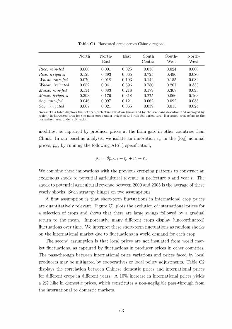
Table C1. Harvested areas across Chinese regions.

North North- East South South- North-East Central West West

Rice, rain-fed 0.000 0.001 0.025 0.038 0.024 0.000Rice, irrigated 0.129 0.393 0.965 0.725 0.496 0.080Wheat, rain-fed 0.070 0.018 0.193 0.142 0.155 0.082Wheat, irrigated 0.652 0.041 0.696 0.780 0.267 0.333Maize, rain-fed 0.134 0.383 0.218 0.179 0.307 0.093Maize, irrigated 0.393 0.176 0.318 0.275 0.066 0.163Soy, rain-fed 0.046 0.097 0.121 0.062 0.092 0.035Soy, irrigated 0.067 0.021 0.065 0.039 0.015 0.024

Notes: This table displays the between-prefecture variation (measured by the standard deviation and averaged byregion) in harvested area for the main crops under irrigated and rain-fed agriculture. Harvested area refers to thenormalized area under cultivation.

modities, as captured by producer prices at the farm gate in other countries than

China. In our baseline analysis, we isolate an innovation εct in the (log) nominal

prices, pct, by running the following AR(1) specification,

pct = θpct−1 + ηt + νc + εct

We combine these innovations with the previous cropping patterns to construct an

exogenous shock to potential agricultural revenue in prefecture o and year t. The

shock to potential agricultural revenue between 2000 and 2005 is the average of these

yearly shocks. Such strategy hinges on two assumptions.

A first assumption is that short-term fluctuations in international crop prices

are quantitatively relevant. Figure C1 plots the evolution of international prices for

a selection of crops and shows that there are large swings followed by a gradual

return to the mean. Importantly, many different crops display (uncoordinated)

fluctuations over time. We interpret these short-term fluctuations as random shocks

on the international market due to fluctuations in world demand for each crop.

The second assumption is that local prices are not insulated from world mar-

ket fluctuations, as captured by fluctuations in producer prices in other countries.

The pass-through between international price variations and prices faced by local

producers may be mitigated by cooperatives or local policy adjustments. Table C2

displays the correlation between Chinese domestic prices and international prices

for different crops in different years. A 10% increase in international prices yields

a 2% hike in domestic prices, which constitutes a non-negligible pass-through from

the international to domestic markets.

63

Figure C1. Price deviations from trends on international commodity markets, 1995–2010.

(a) Innovations from an AR(1). (b) HP-filtered prices.

Source: authors’ calculations using the World Bank Commodities Price Data (“The Pink Sheet”).Notes: These series represent the AR(1) and Hodrick-Prescott residuals of the logarithm of inter-national commodity prices, computed separately for three commodities: banana, rice, and cotton.

Table C2. Correlation between international crop prices and local Chinese prices/production.

Price (producer gate in China)(1) (2)

Price (international) 0.225 0.182(0.026) (0.042)

Observations 245 245Year fixed effects No YesNotes: Standard errors are reported between parentheses and clustered at the crop level. The unit of observationis a crop × year. The crops are banana, cassava, coffee, cotton, barley, groundnut, maize, millet, oats, potato,lentil, rapeseed, rice, sorghum, soybean, sugar beet, sugar cane, sunflower, cabbage, tea and wheat. The sampleis an unbalanced panel between 1991 and 2016. Both regressions include crop fixed effects, time trends, the (log)harvested area, and the (log) yield, and are weighted by the value of exports (in tonnes) over the period 1995–2010.

C.3 Sensitivity analysis and robustness checks

This section describes a sensitivity analysis of the shift-share design; we leave the

sensitivity of the second stage of the analysis to Appendix F.

The shift The baseline specification isolates an innovation in crop prices from run-

ning an AR(1) regression on Agricultural Producer Prices from the FAO, averaged

across all producing countries but China. We provide in Table C3 a sensitivity anal-

ysis where the price shock is constructed: (i) using commodity prices as extracted

from the World Bank Commodities Price Data (“The Pink Sheet”, based on prices

64

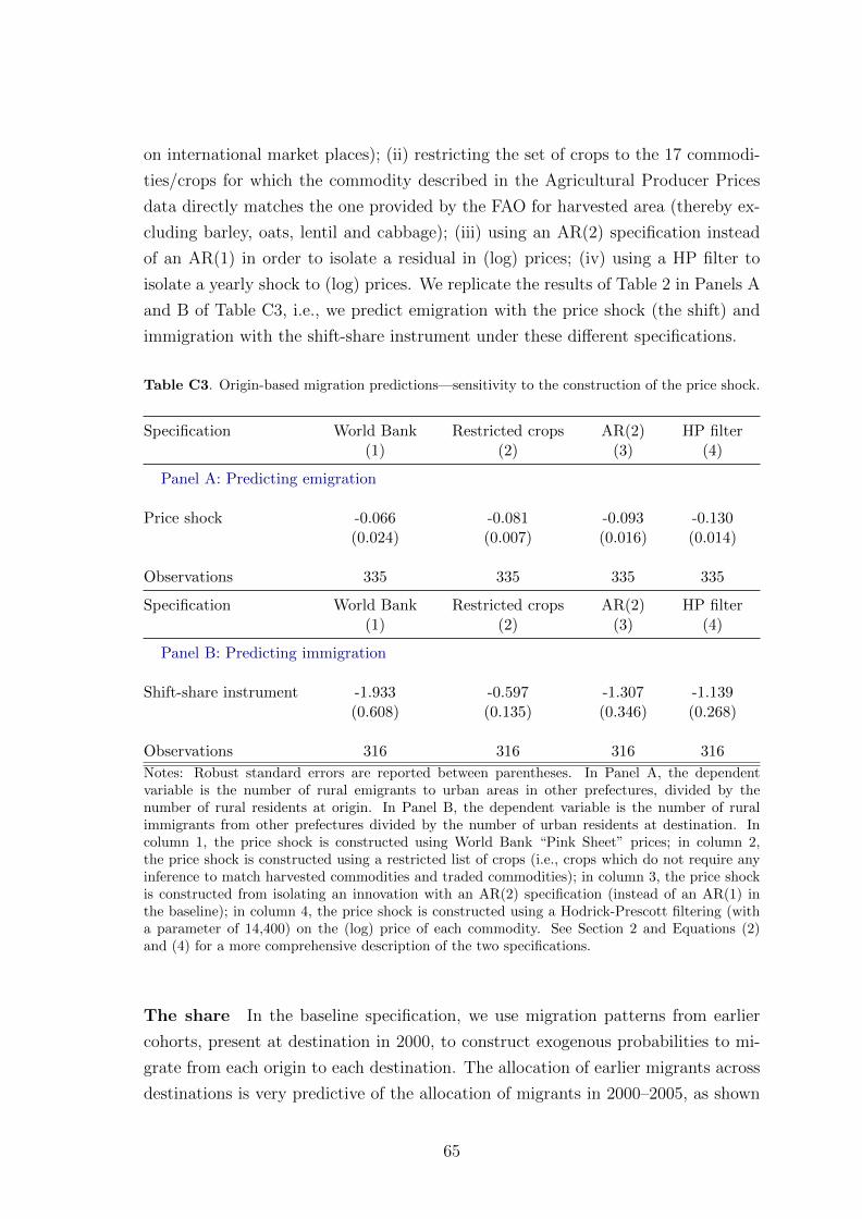
on international market places); (ii) restricting the set of crops to the 17 commodi-

ties/crops for which the commodity described in the Agricultural Producer Prices

data directly matches the one provided by the FAO for harvested area (thereby ex-

cluding barley, oats, lentil and cabbage); (iii) using an AR(2) specification instead

of an AR(1) in order to isolate a residual in (log) prices; (iv) using a HP filter to

isolate a yearly shock to (log) prices. We replicate the results of Table 2 in Panels A

and B of Table C3, i.e., we predict emigration with the price shock (the shift) and

immigration with the shift-share instrument under these different specifications.

Table C3. Origin-based migration predictions—sensitivity to the construction of the price shock.

Specification World Bank Restricted crops AR(2) HP filter(1) (2) (3) (4)

Panel A: Predicting emigration

Price shock -0.066 -0.081 -0.093 -0.130(0.024) (0.007) (0.016) (0.014)

Observations 335 335 335 335

Specification World Bank Restricted crops AR(2) HP filter(1) (2) (3) (4)

Panel B: Predicting immigration

Shift-share instrument -1.933 -0.597 -1.307 -1.139(0.608) (0.135) (0.346) (0.268)

Observations 316 316 316 316

Notes: Robust standard errors are reported between parentheses. In Panel A, the dependentvariable is the number of rural emigrants to urban areas in other prefectures, divided by thenumber of rural residents at origin. In Panel B, the dependent variable is the number of ruralimmigrants from other prefectures divided by the number of urban residents at destination. Incolumn 1, the price shock is constructed using World Bank “Pink Sheet” prices; in column 2,the price shock is constructed using a restricted list of crops (i.e., crops which do not require anyinference to match harvested commodities and traded commodities); in column 3, the price shockis constructed from isolating an innovation with an AR(2) specification (instead of an AR(1) inthe baseline); in column 4, the price shock is constructed using a Hodrick-Prescott filtering (witha parameter of 14,400) on the (log) price of each commodity. See Section 2 and Equations (2)and (4) for a more comprehensive description of the two specifications.

The share In the baseline specification, we use migration patterns from earlier

cohorts, present at destination in 2000, to construct exogenous probabilities to mi-

grate from each origin to each destination. The allocation of earlier migrants across

destinations is very predictive of the allocation of migrants in 2000–2005, as shown

65

in Figure C2. One advantage of using earlier cohorts is that the shares, {λod}, are

independent of amenity or productivity shocks at destination.

Figure C2. Origin-destination migration—the role of previous migration patterns.

Notes: The probabilities for a migrant in d to come from a certain prefecture o, in 2000–2005 (y-axis), and before2000 (x-axis), are constructed with the 2005 1% Population Survey. Observations are origin × destination couples,and they are grouped by bins of previous migration incidence (bins of 0.025).

One concern with the baseline specification is that these shares may still be

correlated with future outcomes through the delayed effects of earlier migration

waves (Jaeger et al., 2018). While our identification strategy does not rely on shares

being exogenous (as in Goldsmith-Pinkham et al., forthcoming) but on shifts being

exogenous (Adao et al., 2019b; Borusyak et al., 2018), we provide a robustness check

for our first stage in column 1 of Table C4 using the origin of migrants arrived before

1995 and still present at destination in 2000 in order to estimate migration patterns

between origins and destinations.

An alternative to this procedure is to estimate a gravity model to predict pre-

vious migration (as in Boustan et al., 2010) and use this prediction to redistribute

emigration flows across the various destinations. We create a measure of travel cost

tod between origin o and destination d using the road and railway networks at base-

line. We then predict the migration patterns from earlier cohorts, λod, using this

distance together with a measure of population at destination. This procedure gives

us a prediction λod that we can combine with the shifts to generate a shift-share

instrument, as in Equation (4). This shift-share instrument also provides a strong

first stage for our analysis (see column 2 of Table C4).42

42Figure C3 offers visual evidence of the distance gradient in preferred migration routes. Thereis a strong and significant inverse relationship between the share of migrants from origin o todestination d (among all migrants from o) and distance between o and d.

66

Table C4. Origin-based migration predictions—sensitivity to the construction of the matrix ofmigration patterns.

Pre-1995 migrant shares Gravity model(1) (2)

Shift-share instrument -0.865 -0.910(0.292) (0.251)

Observations 316 316

Notes: Robust standard errors are reported between parentheses. The dependent variable is thenumber of rural immigrants from other prefectures divided by the number of urban residents atdestination. In column 1, the matrix of migration patterns is constructed using the stock ofmigrants at destination in 2000, having arrived in 1995 or before; in column 2, the matrix ofmigration patterns is constructed from a gravity model. See Section 2 and Equation (4) for a morecomprehensive description of the specification.

Figure C3. Origin-destination migration—the role of distance.

Notes: Migration flows constructed with the 2005 Mini-Census. Observations are origin × destination couples andgrouped by bins of distance (25 km).

Other measures of migration flows In the baseline specification, we use mi-

grant flows of workers between 15 and 64 years old and who crossed a prefecture

boundary to construct the migration rates and the patterns of settlement. We fur-

ther rely on migration flows corrected for return migration. In Table C5, we depart

from this baseline and allow for various definitions of a migration spell. We show

the relationship between the immigration rate and the shift-share instrument when

we define migrant flows: (i) irrespective of the migration motive (column 1), (ii)

based on males only (column 2), (iii) based on individuals with secondary educa-

tion or less (column 3), (iv) restricting migrant spells to those occurring between

67

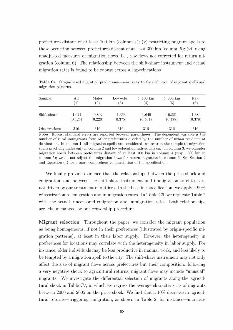
prefectures distant of at least 100 km (column 4); (v) restricting migrant spells to

those occurring between prefectures distant of at least 300 km (column 5); (vi) using

unadjusted measures of migration flows, i.e., raw flows not corrected for return mi-

gration (column 6). The relationship between the shift-share instrument and actual

migration rates is found to be robust across all specifications.

Table C5. Origin-based migration predictions—sensitivity to the definition of migrant spells andmigration patterns.

Sample All Males Low-edu. > 100 km > 300 km Raw(1) (2) (3) (4) (5) (6)

Shift-share -1.621 -0.802 -1.363 -1.649 -0.881 -1.380(0.425) (0.220) (0.375) (0.461) (0.478) (0.378)

Observations 316 316 316 316 316 316

Notes: Robust standard errors are reported between parentheses. The dependent variable is thenumber of rural immigrants from other prefectures divided by the number of urban residents atdestination. In column 1, all migration spells are considered; we restrict the sample to migrationspells involving males only in column 2 and low-education individuals only in column 3; we considermigration spells between prefectures distant of at least 100 km in column 4 (resp. 300 km incolumn 5); we do not adjust the migration flows for return migration in column 6. See Section 2and Equation (4) for a more comprehensive description of the specification.

We finally provide evidence that the relationships between the price shock and

emigration, and between the shift-share instrument and immigration to cities, are

not driven by our treatment of outliers. In the baseline specification, we apply a 99%

winsorization to emigration and immigration rates. In Table C6, we replicate Table 2

with the actual, uncensored emigration and immigration rates: both relationships

are left unchanged by our censorship procedure.

Migrant selection Throughout the paper, we consider the migrant population

as being homogeneous, if not in their preferences (illustrated by origin-specific mi-

gration patterns), at least in their labor supply. However, the heterogeneity in

preferences for locations may correlate with the heterogeneity in labor supply. For

instance, older individuals may be less productive in manual work, and less likely to

be tempted by a migration spell to the city. The shift-share instrument may not only

affect the size of migrant flows across prefectures but their composition: following

a very negative shock to agricultural returns, migrant flows may include “unusual”

migrants. We investigate the differential selection of migrants along the agricul-

tural shock in Table C7, in which we regress the average characteristics of migrants

between 2000 and 2005 on the price shock. We find that a 10% decrease in agricul-

tural returns—triggering emigration, as shown in Table 2, for instance—increases

68

Table C6. Origin-based migration predictions—sensitivity to outliers.

Emigration rate Immigration rate(1) (2)

Price shock -0.118(0.019)

Shift-share instrument -2.304(0.797)

Observations 335 316

Notes: Robust standard errors are reported between parentheses. In column 1, the dependentvariable is the number of rural emigrants to urban areas in other prefectures divided by the numberof rural residents at origin. Compared to Table 2, migrant flows are not winsorized. In column 2,the dependent variable is the number of rural immigrants from other prefectures divided by thenumber of urban residents at destination. See Section 2 and Equations (2) and (4) for a morecomprehensive description of the two specifications.

the probability that: (i) migrants are males by 0.5 p.p. (column 1), (ii) migrants

have university education by 0.6 p.p. (column 2), (iii) migrants are not married by

1.8 p.p. (column 3). All these effects are however quite small. Column 4 shows

that a 10% drop in agricultural returns decreases the age of the average migrant by

0.037 years, an effect indistinguishable from 0. Finally, a 15% drop in agricultural

returns increases the probability that the average migrant returns between 2004 and

2005 by about 1 percentage point. The marginal migrant is slightly less attached to

destinations than the average migrant.

Table C7. Origin-based migration predictions—selection of migrants.

Characteristics Male Low-education Married Age Return rate(1) (2) (3) (4) (5)

Price shock -0.051 0.058 0.178 0.370 -0.068(0.037) (0.046) (0.067) (1.353) (0.027)

Observations 334 334 334 334 334

Notes: Robust standard errors are reported between parentheses. In columns 1–3, the dependentvariable is the share of migrants with the following characteristics: male (column 1), educationalattainment lower than high school (column 2), and married (column 3); in column 4, the dependentvariable is the age of the migrant in 2005; and in column 5, the outcome is the share of returneesbetween 2004 and 2005 among inter-provincial rural migrants who emigrated between 2000 and2004 (the price shock is then defined over the period 2000–2004).

69

D Migration and factor productivity

This Appendix develops a quantitative framework of firm production, in which

there are sector-specific complementarities between capital and labor (Oberfield and

Raval, 2014), in order to estimate the impact of migration on factor productivity.

The section is organized as follows. We first derive equations characterizing the

optimization program of firms, and we describe the steps for estimating the model

parameters: the elasticity of substitution between capital and labor; factor shares;

and the elasticity of substitution between product varieties. Second, we describe

the effect of migration on factor productivity at destination. Third, we discuss the

possible biases related to the imperfect observation of the firm technology and of

labor efficiency.

D.1 Quantitative framework

Environment The economy is composed of D prefectures. In each prefecture d,

the economy is divided into sectors within which there is monopolistic competition

between a large number of firms. The final good is produced from the combination

of sectoral outputs, and each sectoral output is itself a CES aggregate of firm-specific

differentiated goods. Firms face iso-elastic demand with σ denoting the elasticity of

substitution between the different varieties of the sectoral good. In what follows, we

drop prefecture indices for the sake of exposition.

Total sectoral output in a product market (sector × prefecture) is given by the

following CES production function:

y =

[∑i

xiyσ−1σ

i

] σσ−1

, (D1)

where xi captures consumer preferences for product variety i. Each firm i thus faces

the following demand for its product variety i:

yi = (pi/p)−σxσi y (D2)

where pi is the unit price for variety i, and p is the price index at the product market

level. We assume that a firm i produces according to a CES production function:

yi = Ai [αkρi + (1− α)lρi ]

1ρ , (D3)

where ρ, governing the elasticity of substitution between capital and labor, is as-

70

sumed constant over time and within sector, and α characterizes the sector-specific

share of capital in production.

Firm i maximizes the following program,

π = maxpi,yi,li,ki

{piyi − wli − rki} , (D4)

subject to demand for its specific variety (D2) and the production function (D3).

The previous program determines factor demand across sectors,(1− 1/σ)

αkρiαkρi + (1− α)lρi

piyi = rki

(1− 1/σ)(1− α)lρi

αkρi + (1− α)lρipiyi = wli.

Aggregating at the sector level and using a first order approximation brings:(1− 1/σ)

αKρ

αKρ

+ (1− α)LρPY = rK

(1− 1/σ)βL

ρ

αKρ

+ (1− α)LρPY = wL,

which characterize factor demand at the sector level.

Estimation The following fundamentals of the model need to be estimated: the

degree of substitution between capital and labor (ρ), the factor intensity (α), the

elasticity of substitution between product varieties (σ).

The key parameter is the elasticity of substitution between factors: the factor

intensity and the elasticity of substitution between product varieties can be imputed

from factor shares and the ratio of profits to revenues. Indeed, we can infer within-

product competition σ from the mere observation of aggregate profits and aggregate

revenues:

1/σ = Π/PY .

In a similar fashion, we can use the aggregate first-order condition relating labor

costs to revenues in order to identify the capital share α, once ρ is known:

α =(1−X)L

ρ

(1−X)Lρ

+XKρ ,

where X = wL/[(1− 1/σ)PY

].

The issue is to provide an estimate for the elasticity of substitution. One option

71

is to use estimates provided by Oberfield and Raval (2014) for the United States in

1997. Another option is to use their estimation strategy on our dataset. To do so,

we combine the two first-order conditions and derive the firm-specific relative factor

demand:

ln (ki/li) =1

1− ρln

(α

1− α

)+

1

1− ρln (w/r) + εi,

where εi is a noise which captures unobserved firm heterogeneity (e.g., firm-specific

relative factor intensity as described in Section D.3), which we assume, as in Ober-

field and Raval (2014), to be normally distributed within a sector and a prefecture.

Identifying the elasticity of substitution from the previous relationship is chal-

lenging because omitted variation (e.g., a labor productivity shock) may influence

relative factor prices and relative factor use. However, the arrival of migrants shifts

the relative price of labor downward, an effect that is orthogonal to omitted varia-

tion related to labor demand. We can identify the parameter ρ using the variation

in relative factor prices across prefectures induced by the shift-share instrument zdt.

More specifically, the strategy for estimating the elasticity of substitution relies on

the relative factor demand equation,

ln (kidt/lidt) =1

1− ρln

(α

1− α

)+

1

1− ρ(widt) + ηt + νd + εidt, (D5)

where i denotes a manufacturing establishment, d the prefecture and t the year, and

widt, the average compensation rate in establishment i at time t, is instrumented

by the shift-share instrument zdt. The identification of Equation (D5) hinges on

variation across prefectures and over time in relative factor prices and requires the

following assumptions. First, we assume that ρ and α are constant over time and

across all firms. Second, the rental cost of capital is not observed and possible

differences in access to capital across prefectures are assumed orthogonal to the

shift-share instrument. We report the estimated ρ in Table D1.

D.2 Effect of migration on factor productivity

The previous estimates for sectoral production allow us to construct factor produc-

tivity from the observation of output and factor use at the establishment level. In

this section, we use model-based measures of factor productivity to estimate the

impact of immigration on productivity at destination. We estimate Equation (5)

using the marginal revenue product of labor, marginal revenue product of capital

and total factor productivity in revenue terms as dependent variables (all in logs).

In Panel A of Table D2, we use factor productivity as constructed with sectoral

72

Table D1. Elasticities of relative factor use to the relative factor price.

Relative factor use

Labor cost 0.810(0.246)

Observations 191,316F-stat. (first stage) 5.49Notes: Standard errors are clustered at the prefecture level and reported between parentheses. The sample iscomposed of the 31,886 firms present every year in the NBS firm census between 2001 and 2006. All specificationsinclude year fixed effects and sector × year fixed effects. Labor cost is the average compensation rate in theprefecture—ln (wdt) in Equation (D5),—and Relative factor use is ln (ksdt/lsdt).

Table D2. Impact of migration inflows on product of factors.

Labor pr. Capital pr. Total fact. pr.(1) (2) (3)

Panel A: Oberfield and Raval (2014) for US 1997

Migration -0.748 0.138 -0.231(0.172) (0.087) (0.076)

Observations 30,556 30,556 30,556

Labor pr. Capital pr. Total fact. pr.(1) (2) (3)

Panel B: Own estimate

Migration -1.041 0.364 -0.253(0.234) (0.124) (0.077)

Observations 30,556 30,556 30,556

Notes: Standard errors are clustered at the prefecture level and reported between parentheses.Each cell is the outcome of a separate regression. The sample is composed of the firms presentevery year in the NBS firm census between 2000 and 2006. Labor pr. is the (log) marginal revenueproduct of labor; Capital pr. is the (log) marginal revenue product of capital; Total fact. prod. isthe (log) total factor productivity in revenue terms. These quantities are computed using a CESproduction function with the elasticities of substitution of Oberfield and Raval (2014) (UnitedStates, 1997, see Panel A) and our own estimate (Panel B).

estimates of ρ from Oberfield and Raval (2014) for the United States in 1997. The

first column reports how the marginal return to labor responds to migrant inflows.

The elasticity with respect to migration is about −0.75. In parallel, the marginal

revenue product of capital responds positively to the labor supply shift (column 2).

There is some evidence of a negative effect on total factor productivity (column 3). In

Panel B of Table D2, we use our own estimates of ρ to construct factor productivity,

73

and find qualitatively similar results as in Panel A. Capital and labor are more

complementary than what Oberfield and Raval’s (2014) estimates would imply; the

arrival of immigrants without further capitalization affects labor productivity more

strongly than in the previous specification.

This exercise may however suffer from two biases that we describe next: firm

technology may be endogenous and result from a choice (as illustrated by the re-

optimization of production lines shown in Section 4); labor may not be homogeneous.

D.3 Heterogeneous firm technology and labor efficiency

This section discusses the possible biases induced by heterogeneous firm technology,

and by heterogeneity in labor efficiency between migrants and urban residents.

Technology choice We consider the previous framework and assume that indi-

vidual firms are characterized by (residual) technological choices—different product

varieties require different production technologies.43 Within a sector, some estab-

lishments rely on a labor-intensive technology and are labor-abundant, while others

are capital-abundant.

yi = Ai [αikρi + βil

ρi ]

1ρ ,

where ρ, governing the elasticity of substitution between capital and labor, is as-

sumed constant over time and within sector, and (αi, βi) characterizes the firm-

specific technology—unobserved to the econometrician. We rationalize differences

in factor use across production units by technological choices: individual firms pro-

duce different varieties, involving more or less labor-intensive production lines.

Heterogeneous firm technology has two implications on the estimation of our pro-

duction estimates. First, it rationalizes the heterogeneity in factor demand across

manufacturing establishments within the same market. Indeed, for a given technol-

ogy (αi, βi), firm i maximizes the following program,

π (αi, βi) = maxpi,yi,li,ki

{piyi − wli − rki} , (D6)

subject to demand for its specific variety and the production function. This maxi-

mization program leads to the following firm-specific relative factor demand:

ln (ki/li) =1

1− ρln

(α

1− α

)+

1

1− ρln (w/r) +

1

1− ρln

(αi(1− α)

αβi

),

43This feature may capture the wide dispersion in relative factor use within prefecture andindustry—See Appendix A.

74

where the last term can be interpreted as the noise in Equation (D5).

Second, firms may select their product varieties as a response to changes in

factor costs. They would then maximize the indirect profit, π (αi, βi), subject to a

sector-specific technological frontier,

[(αi/α)τ + (βi/(1− α))τ ]1τ ≤ 1, (D7)

where τ is the curvature of the technological frontier. With endogenous technology

choice, optimal factor demand verifies:

ln

(kili

)= − τ

(τ − 1) (1− ρ)− ρln

(α

1− α

)− 1

1− ρ− ρτ−1

ln( rw

).

This equation implies that, if the technological frontier is concave (τ > 1), the

elasticity of factor demand is larger in absolute value than with a fixed technology.

At heart, following an outward shift in labor supply, firms do not only substitute

labor for capital until they adjust marginal product of factors as evaluated at their

current technology; they also eventually adjust their technology toward more labor-

intensive product varieties and this effect adds to the direct impact.

This adjustment may explain why the wedge between the marginal product of

labor and its marginal cost decreases with immigrant inflows, and why capital pro-

ductivity slightly increases. Firms become more labor-abundant in prefectures ex-

periencing large migrant inflows, specifically so by adopting more labor-intensive

production lines. A competing explanation is that we assume away any productiv-

ity difference between migrant and resident workers in the baseline; any discrepancy

between the productivity of urban residents and rural-urban migrants would gener-

ate a bias in the estimated effect of migrant inflows on factor productivity.

Heterogeneous labor and the impact of migration In the baseline model

of production, labor and wage rates are measured in efficient units. In the data,

however, the corresponding variables (employment and labor cost) do not allow us to

distinguish between worker types, and we cannot compute efficient labor units. This

limitation may bias the estimated effect of migrant inflows on factor productivity.

More specifically, the decrease in the observed labor productivity may reflect the

lower productivity of the marginal migrant.

In this extension, we allow workers to differ in productivity and assume that these

differences are observable to the manufacturing firm. Consider two worker types,

residents indexed by r and migrants indexed by m, and let h = lr + γlm denote

efficient labor units, where γ < 1 and l = lr + lm is observed employment. For the

75

sake of exposition, we omit the indices and consider the production technology,

y = A [αkρ + (1− α)hρ]1ρ .

The first-order conditions give us:MPL = (1− 1/σ)

αkρ−1

αkρ + (1− α)hρpy = r

MPK = (1− 1/σ)(1− α)hρ−1

αkρ + (1− α)hρpy = w,

where w = wr = wm/γ is the wage rate.

In the empirical exercise, we use the observed revenues py, the total employment

cost wh, the observed capital k, and the observed units of labor l in order to compute

the labor cost,w = w

(h

l

), returns to factors,

MPL = (1− 1/σ)αkρ−1

αkρ + (1− α)lρpy = MPL

(l

h

)ρ−1αkρ + (1− α)hρ

αkρ + (1− α)lρ

MPK = (1− 1/σ)(1− α)lρ−1

αkρ + (1− α)lρpy = MPK

αkρ + (1− α)hρ

αkρ + (1− α)lρ,

and revenue-based total factor productivity, pA = pA

(αkρ + (1− α)hρ

αkρ + (1− α)lρ

)1/ρ

, which

all differ from their actual values.

In what follows, we quantify the bias induced by differences in the estimation of

the elasticities of these quantities to a marginal increase of the number of migrant

workers lm. For simplicity, we will keep the other factors k and lr constant. These

elasticities are:∂ ln(w)

∂lm=∂ ln(w)

∂lm− (1− γ)lr

(lr + γlm) (lr + lm)

for the labor cost,

∂ ln(MPL)

∂lm=∂ ln(MPL)

∂lm+

∂

∂lmln

[αkρ + βhρ

αkρ + βlρ

]+ (ρ− 1)

(1− γ)lr(lr + γlm) (lr + lm)

∂ ln(MPK)

∂lm=∂ ln(MPK)

∂lm+

∂

∂lmln

[αkρ + βhρ

αkρ + βlρ

]for the returns to factors, and

∂ ln(pA)

∂lm=∂ ln(pA)

∂lm+

1

ρ

∂

∂lmln

[αkρ + βhρ

αkρ + βlρ

]

76

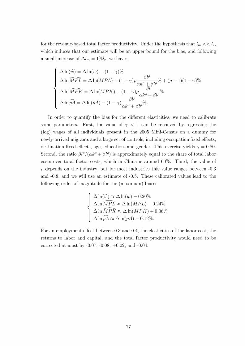
for the revenue-based total factor productivity. Under the hypothesis that lm << lr,

which induces that our estimate will be an upper bound for the bias, and following

a small increase of ∆lm = 1%lr, we have:

∆ ln(w) = ∆ ln(w)− (1− γ)%

∆ ln MPL = ∆ ln(MPL)− (1− γ)ρβlρ

αkρ + βlρ% + (ρ− 1)(1− γ)%

∆ ln MPK = ∆ ln(MPK)− (1− γ)ρβlρ

αkρ + βlρ%

∆ ln pA = ∆ ln(pA)− (1− γ)βlρ

αkρ + βlρ%.

In order to quantify the bias for the different elasticities, we need to calibrate

some parameters. First, the value of γ < 1 can be retrieved by regressing the

(log) wages of all individuals present in the 2005 Mini-Census on a dummy for

newly-arrived migrants and a large set of controls, including occupation fixed effects,

destination fixed effects, age, education, and gender. This exercise yields γ = 0.80.

Second, the ratio βlρ/(αkρ + βlρ) is approximately equal to the share of total labor

costs over total factor costs, which in China is around 60%. Third, the value of

ρ depends on the industry, but for most industries this value ranges between -0.3

and -0.8, and we will use an estimate of -0.5. These calibrated values lead to the

following order of magnitude for the (maximum) biases:∆ ln(w) ≈ ∆ ln(w)− 0.20%

∆ ln MPL ≈ ∆ ln(MPL)− 0.24%

∆ ln MPK ≈ ∆ ln(MPK) + 0.06%

∆ ln pA ≈ ∆ ln(pA)− 0.12%.

For an employment effect between 0.3 and 0.4, the elasticities of the labor cost, the

returns to labor and capital, and the total factor productivity would need to be

corrected at most by -0.07, -0.08, +0.02, and -0.04.

77

E Additional results on heterogeneity and firm entry/exit

This Appendix provides complementary results to the baseline analysis: on treat-

ment heterogeneity along a set of important firm characteristics (e.g., factor use at

baseline, factor product at baseline, firm ownership); on firm entry into, and exit

from, the survey of manufacturing establishments; on the wage of urban residents;

on the restructuring of production lines.

E.1 Treatment heterogeneity across urban establishments

The analysis of Section 3 focuses on the change within the average establishment.

The shift toward a more labor-intensive production structure may also involve a

reallocation of resources across establishments (Dustmann and Glitz, 2015). We

now provide evidence on the heterogeneous absorption of migrants in the urban

economy and its (limited) aggregate implications.

We study the heterogeneous response in factor demand by interacting migrant

inflows with the following firm characteristics at baseline: (a) we label as capital-

abundant all firms with a capital-to-labor ratio at baseline above the median in

their sector and prefecture; (b) we label as labor-productive all firms with a value

added per worker at baseline above the median in their sector and prefecture; (c)

we isolate firms within a sector with high degree of substitution between capital

and labor (ρ); (d) we isolate firms with educational requirement above the sector

median, as calculated from the proportion of workers with high-school attainment

or less in 2004; (e) we separate public establishments from privately-owned firms,

(f) we isolate establishments with some exports at baseline, in 2000.

We report the heterogeneous effects of migration on our baseline outcomes, and

along the previous characteristics, in Table E1. The reduction in labor cost is re-

markably homogeneous across firms; all firms seem to face similar labor market

conditions. In response to the labor supply shift, we find that capital-abundant

firms recruit more than the average firm (column 2). However, firms with higher av-

erage labor productivity are less likely to expand in response to the migration shock.

Migrant workers are predominantly recruited by “capital-rich” firms in a given sec-

tor and location; they are hired by firms where labor productivity is slightly lower.44

44Interpreting these findings requires understanding the nature of heterogeneity within our sur-vey of manufacturing establishments. First, disparities in labor productivity may arise from un-observed technological differences across production units. In a similar vein, factor use at baselinemay reflect firm-specific factor complementarities in production or complementarities in produc-tion with other unobserved factors (e.g., skilled labor) that are heterogeneously allocated acrossestablishments. Second, the initial dispersion in productivity across firms may reflect factor marketimperfections (as in Hsieh and Klenow, 2009). Firms with a high return to labor may be constrained

78

This observation contrasts with empirical regularities of firm growth in developed

economies: employment flows are typically directed toward productive firms (see

Davis and Haltiwanger, 1998, for evidence in the U.S.). A possible explanation is

that we study large labor supply shocks, which may have different allocative proper-

ties from the smaller idiosyncratic labor demand shocks that usually drive employ-

ment growth. Our findings are also different from Dustmann and Glitz (2015), who

find that more labor-abundant firms expand relative to capital-abundant firms.

We explore in Panel C and D whether sectoral differences in production matter,

notably through the complementarity between labor and capital, or through skill

requirements. We do not find that migrant workers sort themselves into sectors

with high elasticity of substitution between capital and labor, or with low education

requirements. The interaction coefficients are quite small in both cases. We finally

interact the immigration rate with a dummy for public firms (Panel E) and exporting

firms (Panel F). We do not find that migrants are less likely to be hired in public

establishments, in which insiders are likely to receive substantial benefits, and in

exporting firms which can arguably expand their production, facing more gradual

decreasing returns to scale.

E.2 Aggregation and entry/exit

Aggregation at the prefecture level In Section 3, we explore the aggregate

effects of factor reallocation across firms by aggregating outcomes at the prefecture

× sector level. Conceptually, this neutralizes the effect of a possible reallocation

of factors within sectors. We now report estimates from specification (5) with out-

comes aggregated at the prefecture level (see Table E2). The results are similar in

magnitude to the previous aggregation at the prefecture × sector level: the effect

of a reallocation of factors across industries on aggregate productivity is negligible,

as most of the reallocation occurs within sectors. This finding is consistent with the

literature in developed countries (Lewis, 2011; Dustmann and Glitz, 2015).

Entry/Exit In Section 3, we present the effect of immigrant flows on aggregate

outcomes including firms of the unbalanced sample, and we find that allowing for

firm entry and exit magnifies the negative effect of migration on relative factor use

in hiring labor, e.g., because of information asymmetry between job seekers and employers (Abebeet al., 2016; Alfonsi et al., 2017), the intervention of intermediaries, and the prevalence of migrantnetworks (Munshi, 2003). Capital productivity dispersion may be indicative of capital market dis-tortions (Buera et al., 2011; Midrigan and Xu, 2014). Third, productivity differences across firmsmay capture entrepreneur characteristics, management practices (Bloom et al., 2013) or differ-ences in the organization of production (Akcigit et al., 2016; Boehm and Oberfield, 2018). Betterentrepreneurs or organizations would be captured by high productivity within a sector.

79

Table E1. Impact of migration inflows on urban firms—heterogeneity across firms.

Labor cost Employment K/L ratio Y/L ratio(1) (2) (3) (4)

Panel A: Capital to labor ratioMigration -0.124 0.269 -0.363 -0.412

(0.071) (0.053) (0.095) (0.100)Migration × High K/L -0.070 0.078 -0.227 -0.087

(0.083) (0.055) (0.090) (0.078)

F-stat. (first stage)† 11.97 11.97 11.97 11.97

Panel B: Output to labor ratioMigration -0.116 0.306 -0.363 -0.303

(0.075) (0.050) (0.106) (0.110)Migration × High Y/L -0.068 -0.048 -0.164 -0.308

(0.088) (0.065) (0.091) (0.086)

F-stat. (first stage)† 11.77 11.77 11.77 11.77

Panel C: Elasticity of substitutionMigration -0.155 0.281 -0.461 -0.446

(0.060) (0.051) (0.097) (0.110)Migration × High ρ 0.020 0.033 0.077 0.024

(0.069) (0.058) (0.069) (0.070)

F-stat. (first stage)† 11.80 11.80 11.80 11.80

Panel D: Educational requirementMigration -0.133 0.268 -0.468 -0.427

(0.058) (0.056) (0.111) (0.115)Migration × High share -0.028 0.058 0.080 -0.021of educated (0.065) (0.044) (0.076) (0.075)

F-stat. (first stage)† 11.51 11.51 11.51 11.51

Panel E: Public ownershipMigration -0.106 0.233 -0.464 -0.362

(0.065) (0.051) (0.104) (0.097)Migration × Public -0.049 0.006 0.228 -0.225

(0.132) (0.117) (0.182) (0.169)

F-stat. (first stage)† 8.88 8.88 8.88 8.88

Panel F: Exporting at baselineMigration -0.072 0.357 -0.505 -0.517

(0.128) (0.084) (0.131) (0.195)Migration × Exporting -0.060 -0.100 0.117 0.192

(0.122) (0.088) (0.120) (0.159)

F-stat. (first stage)† 11.76 11.76 11.76 11.76Observations 31,886 31,886 31,886 31,886

Notes: Standard errors are clustered at the prefecture level and reported between parentheses. †

The IV specification uses two endogenous variables and two instruments; the critical value for weakinstruments is then 7.03 (at 10%).

80

Table E2. Impact of migration inflows on urban firms—sensitivity analysis with aggregate vari-ables at the prefecture level.

Labor cost Employment K/L ratio Y/L ratio(1) (2) (3) (4)

Panel A: Balanced sample of firms

Migration -0.113 0.284 -0.459 -0.475(0.062) (0.071) (0.125) (0.120)

Observations 315 315 315 315F-stat (first) 23.52 23.52 23.52 23.52

Panel B: Unbalanced sample of firms

Migration -0.184 0.627 -0.626 -0.626(0.083) (0.159) (0.120) (0.184)

Observations 316 316 316 316F-stat. (first) 21.13 21.13 21.13 21.13

Notes: Robust standard errors are reported between parentheses. The unit of observation is aprefecture. In Panel A (resp. Panel B), the sample is composed of the firms present every yearin the NBS firm census between 2000 and 2006 (resp. all firms present in the NBS firm censusbetween 2000 and 2006); outcomes are then aggregated at the prefecture level. Migration is theimmigration rate, i.e., the migration flow divided by destination population at baseline. Labor costis the (log) compensation per worker including social security. Employment is the (log) number ofworkers within the firm. K/L ratio is the (log) ratio of fixed assets to employment. Y/L ratio isthe (log) ratio of value added to employment.

and labor productivity. This extension provides additional insights into the selection

of establishments into survival, or entry.

We first estimate the effect of migration on profits. We consider the balanced

sample of firms and construct the ratio of profits to revenues (profitability) and a

dummy equal to one if profits are positive. Columns 1 and 2 of Table E3 present the

estimates of specification 5 for these two outcomes. The arrival of low-skill workers

does affect profitability in the average establishment (see column 1); it also markedly

increases the probability that an establishment reports net profits (see column 2),

thus mostly benefiting low-profitability establishments. A ten percentage points

increase in the immigration rate increases the probability that firms make profit by

1.1 percent. Cheaper labor makes the least profitable firms break even.

We now estimate the more direct effect of migration on firm entry into, and exit

from, the survey of manufacturing establishments. Since we only observe firms above

a given sales threshold (see Appendix Section A and Figure 1), we only measure en-

try and exit into and from our sample, which is a combination of actual entry and

81

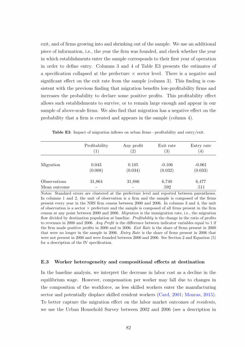
exit, and of firms growing into and shrinking out of the sample. We use an additional

piece of information, i.e., the year the firm was founded, and check whether the year

in which establishments enter the sample corresponds to their first year of operation

in order to define entry. Columns 3 and 4 of Table E3 presents the estimates of

a specification collapsed at the prefecture × sector level. There is a negative and

significant effect on the exit rate from the sample (column 3). This finding is con-

sistent with the previous finding that migration benefits low-profitability firms and

increases the probability to declare some positive profits. This profitability effect

allows such establishments to survive, or to remain large enough and appear in our

sample of above-scale firms. We also find that migration has a negative effect on the

probability that a firm is created and appears in the sample (column 4).

Table E3. Impact of migration inflows on urban firms—profitability and entry/exit.

Profitability Any profit Exit rate Entry rate(1) (2) (3) (4)

Migration 0.043 0.105 -0.106 -0.061(0.008) (0.034) (0.032) (0.033)

Observations 31,864 31,886 6,740 6,477Mean outcome - - .592 .511

Notes: Standard errors are clustered at the prefecture level and reported between parentheses.In columns 1 and 2, the unit of observation is a firm and the sample is composed of the firmspresent every year in the NBS firm census between 2000 and 2006. In columns 3 and 4, the unitof observation is a sector × prefecture and the sample is composed of all firms present in the firmcensus at any point between 2000 and 2006. Migration is the immigration rate, i.e., the migrationflow divided by destination population at baseline. Profitability is the change in the ratio of profitsto revenues in 2000 and 2006. Any Profit is the difference between indicator variables equal to 1 ifthe firm made positive profits in 2000 and in 2006. Exit Rate is the share of firms present in 2000that were no longer in the sample in 2006. Entry Rate is the share of firms present in 2006 thatwere not present in 2000 and were founded between 2000 and 2006. See Section 2 and Equation (5)for a description of the IV specification.

E.3 Worker heterogeneity and compositional effects at destination

In the baseline analysis, we interpret the decrease in labor cost as a decline in the

equilibrium wage. However, compensation per worker may fall due to changes in

the composition of the workforce, as less skilled workers enter the manufacturing

sector and potentially displace skilled resident workers (Card, 2001; Monras, 2015).

To better capture the migration effect on the labor market outcomes of residents,

we use the Urban Household Survey between 2002 and 2006 (see a description in

82

Appendix A) and we estimate:

∆yd = α + βmd + Xdγ + εd, (E1)

where yd is the average labor market outcome of individuals surveyed in prefecture

d between 2002 and 2006, md is the immigration rate between 2001 and 2005—

instrumented by the shift-share instrument zd, and Xd is a vector of average indi-

vidual characteristics, including marital status, gender, and age.

Panel A of Table E4 presents the results computed from all urban residents. In

column 1, the dependent variable is a measure of real hourly wages. The wage of

residents falls by 0.30% when the migration rate increases by one percentage point—

an effect that is imprecisely estimated due to the lower number of prefectures in the

UHS. In columns 2 to 4, we analyze the possible displacement of urban residents.

Rural-urban migration has no significant effect on the allocation of urban residents

between wage employment, unemployment, and self-employment, which implies that

the urban residents mostly adjust to an immigration shock by accepting lower wages.

In Panel B, we derive the same results, but computed from low-skilled residents only,

and find qualitatively similar results.

Table E4. Impact of migration inflows on urban residents.

Wage Employee Unemployed Self-employed(1) (2) (3) (4)

Panel A: All urban residents

Migration -0.298 -0.041 0.020 0.021(0.300) (0.114) (0.088) (0.060)

Observations 187 187 187 187F-stat. (first stage) 15.29 15.29 15.29 15.29

Panel B: Low-skill urban residents

Migration -0.979 -0.079 0.057 0.022(0.412) (0.095) (0.107) (0.047)

Observations 187 187 187 187F-stat. (first stage) 20.21 20.21 20.21 20.21

Notes: Robust standard errors are reported between parentheses. In Panel A, the dependent vari-able is constructed from the difference in outcomes between 2002 and 2006, for all urban residents.In Panel B, we restrict the data construction to urban residents with educational attainment lowerthan a high school degree. Wage is the (log) hourly wage in real terms. Employee is a dummy forreceiving a wage, while Self-employed is a dummy equal to 1 for individuals who are self-employedor employers.

83

There are various reasons for which the wage of residents would be expected to

be less elastic to the arrival of immigrants than the average manufacturing wage:

labor markets may be partly segmented; the wages of incumbent workers may be

more rigid than hiring wages; migrants may be less productive than residents, and

the recruitment of lower-productivity workers could account for part of the decline in

average labor cost. We find however that the decrease in wages of low-skill residents

is larger than the labor cost response estimated using firm-level data (see Table 3).

This difference could arise from the migration effect on firms outside our sample

of manufacturing establishments, which are formal production units and in which

there may exist bargaining frictions inducing (some) nominal downward rigidities.

Table E5. Impact of migration inflows on prices in cities.

CPI CPI (food) CPI (non-food)(1) (2) (3)

Migration 0.327 -0.237 0.564(0.141) (0.102) (0.216)

Observations 187 187 187F-stat. (first stage) 15.29 15.29 15.29

Notes: Standard errors are clustered at the prefecture level and reported between parentheses. TheCPI s are the (log) Consumer Price Indices, as computed from the average prices and quantitiesreported in the UHS survey.

We also use the UHS to shed light on the evolution of living standards in cities.

In Table E5, we report the estimates from specification (E1) with (log) consumer

prices as dependent variables. We find that there is an indirect impact of new

workers in cities, as consumers of non-tradable goods. These new residents may

boost demand for some non-tradable goods, which may benefit firms providing these

goods (e.g., housing) or affect firms relying on these goods or services (e.g., with a

land-intensive production). We find however that food prices decrease, an effect

which is a byproduct of our shift-share design: crop prices affect living costs in

neighboring cities both through the arrival of migrants and through the price of

food.

E.4 Complements on production restructuring

The text analysis associates HS 6-digit product codes for (up to) three main prod-

ucts at the establishment level. In Section 4, we rely on this classification to observe

changes in the main product and characterize the direction of this change in terms

84

of input. This section provides complements to this analysis and looks at: changes

in the human- and physical-capital intensity of products measured through prod-

uct similarity and the input-output matrix, changes in the technological content of

products; changes in the number of products reported by establishments; changes

in product similarity for establishments reporting several products.

We use specification (5), in which the causal impact of migration is identified

from a long difference in outcomes between the beginning and the end of the period.

As in Section 4, we clean the estimates from fixed effects at the level of the HS

6-digit code for the main product in 2000. In Table E6, we adopt two alternative

ways of classifying products as skill- and capital-intensive. We first use the language

proximity score provided by the Natural Language Processing algorithm, and com-

pute for the main product of each firm the average skill- and capital-intensity of all

the other firms weighted by the proximity of the HS-6 code of their final product.

The results in Panel A of Table E6 are very similar to those of Table 7: follow-

ing a migration shock firms adopt products that are more similar to those of firms

with low-skill and low-capital intensity. Next, we use the input-output matrix, and

compute for the main product of each firm the average skill- and capital-intensity

of all the other firms weighted by the input-output matrix coefficients. The results

in Panel B of Table E6 suggest that firms adopt products that use inputs coming

from low-skill low-capital firms, or that are used themselves as inputs by firms with

low-skill low-capital production methods.

In Panel A of Table E7, we identify the causal impact of migration on the tech-

nological content of products. We compute three measures of technology, all based

on the index of technology closeness between different industries developed in Bloom

et al. (2013) and based on U.S. patent citations, which we transform into technol-

ogy closeness between different products, {τp,q}p,q. In the first column, we report

changes in the sum of the technology closeness index across industries,∑

q τp,q, for

an establishment whose main product is p. This variable captures the intensity

of technological spillovers for a given product. In the second column, we report

changes in the number of links to other industries, i.e.,∑

q 6=p 1τp,q>0. In the third

column, we report changes in the Herfindahl index based on technology closeness, i.e.,∑q 6=p τ

2p,q/(

∑q 6=p τp,q)

2. These latter two variables capture the width of technology

spillovers across industries: a product with a small number of links to other indus-

tries or a large Herfindahl index would indicate a “niche technology.” Panel A of

Table E7 shows that migration pushes establishments towards products with fewer

and more concentrated citations across industries. This observation may explain

part of the reduction in patenting observed in Section 4: following an expansion of

85

Table E6. Impact of migration inflows on urban firms—production restructuring—alternativeclassifications.

Change in product High ed. Low ed. High K/L Low K/L(1) (2) (3) (4)

Panel A: Using language proximity to characterize products

Migration 0.025 0.068 0.027 0.067(0.034) (0.026) (0.029) (0.023)

Observations 19,189 19,189 19,189 19,189

Panel B: Using input-output links to characterize products

Migration -0.006 0.147 0.073 0.069(0.023) (0.036) (0.029) (0.022)

Observations 22,151 22,151 22,151 22,151

Notes: Standard errors are clustered at the prefecture level and reported between parentheses.The sample is composed of the firms present every year in the NBS firm census between 2000 and2006. Migration is the immigration rate, i.e., the migration flow divided by destination populationat baseline. The dependent variables are dummy variables equal to one if there is any change inthe main product (1), and if this change goes toward products manufactured by establishmentswith a more (2) or less (3) educated workforce, and by more (4) or less (5) capital-abundantestablishments. See Section 2 and Equation (5) for a description of the IV specification.

labor supply, firms reorient their production lines towards products that are “less

reliant on” technological innovation.

In Panel B of Table E7, we identify the causal impact of migration on the number

of different products produced by the establishment. Two products are considered

to be different if they have different textual descriptions in column 1, different HS 6-

digit product codes in column 2, and different HS 3-digit product codes in column 3.

We find that migration increases the number of products, even though the effects

are quite small and not statistically significant (e.g., a 10% increase in the migration

rate increases the number of different HS 3-digit product codes produced by the

firm by 0.0077). In Panel C, the sample consists of establishments reporting at

least two product codes in 2000 and in 2006, and we look at the causal impact of

migration on indices of similarity between these products. These indices of similarity

are constructed as an average of proximity measures between the different unique

pairs of products. We construct these similarity indices from language proximity

(see Appendix A.2), the input-output matrix (using input-output accounts in the

United States, in 2002, Stewart et al., 2007), and the technology closeness measure

(Bloom et al., 2013). We do not find strong evidence that the similarity changes

86

markedly along any of these three dimensions.

Table E7. Impact of migration inflows on urban firms—technological content, number of products,and similarity between products.

Technological content Citations Cross-citations Herfindahl(1) (2) (3)

Panel A: Technological contentMigration -0.008 -7.722 0.023

(0.004) (2.193) (0.008)

Observations 27,062 27,062 3,681F-stat. (first stage) 23.05 23.05 20.84

Number of products Text HS6 HS3(1) (2) (3)

Panel B: Number of productsMigration 0.146 0.077 0.062

(0.070) (0.063) (0.059)

Observations 27,062 25,273 25,273F-stat. (first stage) 23.05 22.46 22.46

Similarity index Language I/O Technology(1) (2) (3)

Panel C: Similarity between productsMigration 0.009 -0.002 -0.036

(0.019) (0.003) (0.022)

Observations 2,815 2,761 2,776F-stat. (first stage) 23.31 23.05 23.11

Notes: Standard errors are clustered at the prefecture level and reported between parentheses.The sample is composed of the firms present every year in the NBS firm census between 2000and 2006. In Panel A, we rely on the measure of technology closeness between different industriesdeveloped in Bloom et al. (2013) and based on U.S. patent citations. The dependent variablesare: (1) the sum of technology closeness measures across industries; (2) the sum of technologylinks with other industries (technology closeness measure different than zero); (3) a Herfindahlindex of technology closeness measures across industries. In Panel B, the dependent variables arethe number of different products produced by the establishment. Two products are consideredto be different if they have different descriptions (column 1), different HS 6-digit product codes(column 2), different HS 3-digit product codes (column 3). In Panel C, the sample is constitutedof establishments having at least two products in 2000 and in 2006. The dependent variables aresimilarity indices based on language proximity (see Appendix A.2), an input-output matrix (usinginput-output accounts in the United States, in 2002, Stewart et al., 2007), and the technologycloseness measure (Bloom et al., 2013).

87

F Sensitivity analysis

In this Appendix, we investigate the robustness of our results to variations along the

different steps of the empirical method. We first assess the sensitivity of the emigra-

tion effect to alternative specifications of the shift-share design; we then consider the

robustness of our findings to other aspects of the baseline specification (definition of

migrant flows, sample selection and outliers, spatial correlation); we finally discuss

an alternative strategy exploiting the yearly variation in price shocks and migrant

flows over the period 2000–2005.

F.1 The shift-share design

This section assesses the robustness of our baseline second-stage estimates (specifi-

cation 5) to the exact construction of the shift-share instrument.

The shift We proceed as in Appendix C.3—which describes the sensitivity of our

first stage to the shift-share design—and we consider the following alternative spec-

ifications for the shift-share instrument: (i) we use prices from the World Bank

Commodities Price Data; (ii) we restrict the set of crops; (iii) we use an AR(2)

specification instead of an AR(1); (iv) we isolate innovations in commodity prices

with a HP filter. We replicate the results of Table 4 in Table F1 under these dif-

ferent specifications. As apparent from Table F1, our main findings are robust to

alternative specifications for the “shift.”

The share We show in Panels A and B of Table F2 that our main findings are

robust to alternative specifications for the “share.” More specifically, we construct

the shift-share instrument using (a) previous migrant cohorts, arrived at destination

before 1995, and (b) a reallocation of migrants across prefectures along a gravity

model, as in Appendix C.3.

F.2 The empirical specification

Definition of migrant flows We show in Table F3 that our main findings are

robust to alternative sample choices to define migration spells: all migrant spells,

irrespective of their motive (Panel A), males only (Panel B), individuals with sec-

ondary education or less (Panel C), migrant spells between prefectures distant of at

least 100 km (Panel D), migrant spells between prefectures distant of at least 300

km (Panel E), migration flows not corrected for return migration (Panel F).

88

Table F1. Impact of migration inflows on urban firms—sensitivity to the construction of the priceshock.

Labor cost Employment K/L ratio Y/L ratio(1) (2) (3) (4)

Panel A: World Bank “Pink Sheet” pricesMigration -0.107 0.305 -0.462 -0.398

(0.067) (0.065) (0.113) (0.115)

Observations 31,886 31,886 31,886 31,886

Panel B: Restricted list of cropsMigration -0.245 0.259 -0.386 -0.515

(0.076) (0.047) (0.088) (0.116)

Observations 31,886 31,886 31,886 31,886

Panel C: AR(2) specificationMigration -0.144 0.298 -0.430 -0.433

(0.062) (0.054) (0.095) (0.108)

vations 31,886 31,886 31,886 31,886

Panel D: HP-filtered pricesMigration -0.199 0.279 -0.436 -0.484

(0.067) (0.047) (0.091) (0.113)

Observations 31,886 31,886 31,886 31,886

Notes: Standard errors are clustered at the prefecture level and reported between parentheses. Thesample is composed of the firms present every year in the NBS firm census between 2000 and 2006.In Panel A, the price shock is constructed using World Bank “Pink Sheet” prices; in Panel B,the price shock is constructed using a restricted list of crops (i.e., crops which do not require anyinference to match harvested commodities and traded commodities); in Panel C, the price shockis constructed from isolating an innovation with an AR(2) specification (instead of an AR(1) inthe baseline); in Panel D, the price shock is constructed using a Hodrick-Prescott filtering (with aparameter of 14,400) on the (log) price of each commodity. See Section 2 and Equation (5) for adescription of the IV specification.

Censorship and outliers In the baseline specification (5), we apply a 99% win-

sorization to firm outcomes and immigration rates. We show in Panels A, B and C

of Table F4 that our main findings are robust to using the actual, uncensored im-

migration rate, the actual, uncensored firm outcomes, or both.

Spatial correlation The clustering of standard errors in the baseline specifica-

tion (5) imperfectly deals with the heteroskedasticity induced by the multiplicative

structure of shift-share designs and the spatial auto-correlation in shifts (and shares).

In this extension, we provide a sensitivity analysis of our main findings (Table 3)

89

Table F2. Impact of migration inflows on urban firms—sensitivity to the construction of thematrix of migration patterns.

Labor cost Employment K/L ratio Y/L ratio(1) (2) (3) (4)

Panel A: Pre-1995 migrant sharesMigration -0.182 0.271 -0.410 -0.453

(0.073) (0.056) (0.096) (0.119)

Observations 31,886 31,886 31,886 31,886

Panel B: Shares predicted from gravity modelMigration -0.137 0.296 -0.389 -0.446

(0.062) (0.054) (0.083) (0.104)

Observations 31,886 31,886 31,886 31,886

Notes: Standard errors are clustered at the prefecture level and reported between parentheses.The sample is composed of the firms present every year in the NBS firm census between 2000 and2006. In Panel A, the matrix of migration patterns is constructed using the stock of migrants atdestination in 2000, having arrived in 1995 or before; in Panel B, the matrix of migration patternsis constructed from a gravity model. See Section 2 and Equation (5) for a description of the IVspecification.

relying on the inference results developed in Adao et al. (2019b), and the transfor-

mation suggested by Borusyak et al. (2018).

We first consider the baseline specification at the level of destinations in Panel A

of Table F5, and replace our standard errors clustered at the level of prefectures by:

(i) standard errors clustered at the level of the 60 Chinese provinces, (ii) a contin-

uous modeling of the heteroskedasticity across prefectures of destination (following

Conley, 1999). We then consider the estimates suggested by Adao et al. (2019b):

we report the baseline AKM and AKM0 estimates for the standard errors, as well

as a specification allowing for clustering.

In Panel B, we apply standard procedures to deal with heteroskedasticity in

a transformed specification at origin (Borusyak et al., 2018). We report (i) robust

standard errors, (ii) standard errors clustered at the level of the 60 Chinese provinces,

(iii) a continuous modeling of the heteroskedasticity across prefectures of origin

(following Conley, 1999).

F.3 Beyond the cross-sectional analysis

In this robustness exercise, we exploit yearly variation in origin-specific shocks to

migration and yearly immigrant flows to cities in order to identify the restructuring

of production within the panel of establishments in 2001–2006.

90

Table F3. Impact of migration inflows on urban firms—sensitivity to the definition of migrantspells and migration patterns.

Labor cost Employment K/L ratio Y/L ratio(1) (2) (3) (4)

Panel A: all migrantsMigration -0.147 0.294 -0.431 -0.437

(0.062) (0.053) (0.095) (0.108)

Observations 31,886 31,886 31,886 31,886

Panel B: male migrantsMigration -0.273 0.565 -0.846 -0.825

(0.121) (0.104) (0.192) (0.211)

Observations 31,886 31,886 31,886 31,886

Panel C: low-education migrantsMigration -0.170 0.342 -0.504 -0.513

(0.072) (0.067) (0.120) (0.135)

Observations 31,886 31,886 31,886 31,886

Panel D: Migrant spells > 100 kmMigration -0.136 0.281 -0.437 -0.421

(0.061) (0.049) (0.100) (0.107)

Observations 31,886 31,886 31,886 31,886

Panel E: Migrant spells > 300 kmMigration -0.001 0.263 -0.601 -0.395

(0.107) (0.066) (0.185) (0.157)

Observations 31,886 31,886 31,886 31,886

Panel F: No adjustment for return migrationMigration -0.168 0.336 -0.493 -0.500

(0.070) (0.063) (0.112) (0.126)

Observations 31,886 31,886 31,886 31,886

Notes: Standard errors are clustered at the prefecture level and reported between parentheses.The sample is composed of the firms present every year in the NBS firm census between 2000and 2006. In Panel A, all migration spells are considered; we restrict the sample to males onlyin Panel B, and to low-education individuals in Panel C; we consider migration spells betweenprefectures distant of at least 100 km in Panel D (resp. 300 km in Panel E); we do not adjust themigration flows for return migration in Panel F. See Section 2 and Equation (5) for a descriptionof the IV specification.

The unit of observation is a firm i in year t = {2001, . . . , 2006} and prefecture

91

Table F4. Impact of migration inflows on urban firms—sensitivity to outliers.

Labor cost Employment K/L ratio Y/L ratio(1) (2) (3) (4)

Panel A: No winsorizing of firm outcomesMigration -0.146 0.341 -0.422 -0.460

(0.064) (0.059) (0.098) (0.109)

Observations 31,886 31,886 31,886 31,886

Panel B: No winsorizing of migration ratesMigration -0.079 0.158 -0.232 -0.235

(0.042) (0.057) (0.088) (0.096)

Observations 31,886 31,886 31,886 31,886

Panel C: No winsorizing (outcomes or migration rates)Migration -0.078 0.183 -0.227 -0.247

(0.043) (0.062) (0.090) (0.093)

Observations 31,886 31,886 31,886 31,886

Notes: Standard errors are clustered at the prefecture level and reported between parentheses. Thesample is composed of the firms present every year in the NBS firm census between 2000 and 2006.In Panel A, firm outcomes are not winsorized, but migrant flows are. In Panel B, migrant flowsare not winsorized, but firm outcomes are. In Panel C, neither firm outcomes nor migrant flowsare winsorized. See Section 2 and Equation (5) for a description of the IV specification.

Table F5. Impact of migration inflows on urban firms—alternative standard errors.

Labor cost Employment K/L ratio Y/L ratio(1) (2) (3) (4)

Panel A: Destination (firm-level)Coefficient on migration -0.147 0.295 -0.432 -0.438S.E. Prefecture Cluster (baseline) 0.062 0.053 0.095 0.109S.E. Province Cluster 0.068 0.040 0.078 0.071S.E. Conley (300km radius) 0.059 0.044 0.072 0.047S.E. AKM (1) 0.030 0.020 0.025 0.028S.E. AKM (0) 0.031 0.021 0.027 0.029S.E. AKM (Province Cluster) 0.042 0.027 0.039 0.036

Panel B: Origin (prefecture-level)Coefficient on Migration -0.147 0.294 -0.431 -0.437S.E. Robust (baseline) 0.029 0.019 0.024 0.026S.E. Province Cluster 0.056 0.035 0.055 0.040S.E. Conley (300km radius) 0.058 0.030 0.056 0.040

Notes: The sample is composed of the firms present every year in the NBS firm census between2000 and 2006. See Section 2 and Equation (5) for a description of the IV specification.

92

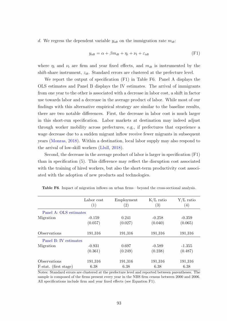
d. We regress the dependent variable yidt on the immigration rate mdt:

yidt = α + βmdt + ηi + νt + εidt (F1)

where ηi and νt are firm and year fixed effects, and mdt is instrumented by the

shift-share instrument, zdt. Standard errors are clustered at the prefecture level.

We report the output of specification (F1) in Table F6. Panel A displays the

OLS estimates and Panel B displays the IV estimates. The arrival of immigrants

from one year to the other is associated with a decrease in labor cost, a shift in factor

use towards labor and a decrease in the average product of labor. While most of our

findings with this alternative empirical strategy are similar to the baseline results,

there are two notable differences. First, the decrease in labor cost is much larger

in this short-run specification. Labor markets at destination may indeed adjust

through worker mobility across prefectures, e.g., if prefectures that experience a

wage decrease due to a sudden migrant inflow receive fewer migrants in subsequent

years (Monras, 2018). Within a destination, local labor supply may also respond to

the arrival of low-skill workers (Llull, 2018).

Second, the decrease in the average product of labor is larger in specification (F1)

than in specification (5). This difference may reflect the disruption cost associated

with the training of hired workers, but also the short-term productivity cost associ-

ated with the adoption of new products and technologies.

Table F6. Impact of migration inflows on urban firms—beyond the cross-sectional analysis.

Labor cost Employment K/L ratio Y/L ratio(1) (2) (3) (4)

Panel A: OLS estimatesMigration -0.159 0.241 -0.258 -0.359

(0.057) (0.027) (0.040) (0.065)

Observations 191,316 191,316 191,316 191,316

Panel B: IV estimatesMigration -0.931 0.697 -0.589 -1.355

(0.361) (0.249) (0.238) (0.487)

Observations 191,316 191,316 191,316 191,316F-stat. (first stage) 6.38 6.38 6.38 6.38

Notes: Standard errors are clustered at the prefecture level and reported between parentheses. Thesample is composed of the firms present every year in the NBS firm census between 2000 and 2006.All specifications include firm and year fixed effects (see Equation F1).

93