Migrants and Economic Performance in the EU15: their

FIW, a collaboration of WIFO (www.wifo.ac.at), wiiw (www.wiiw.ac.at) and WSR (www.wsr.ac.at)

Migrants and Economic Performance in the EU15: their allocations across countries,

industries and job types and their (productivity) growth impacts at the

sectoral and regional levels

Michael Landesmann, Robert Stehrer und Mario Liebensteiner

FIW Research Reports 2009/10 N° 09 April 2010

Studies regarding the migrants’ impact upon performance variables and in particular upon productivity growth – which is the focus of this study - are few although there has been an increased interest in this area. This study addresses this issue in a cross-country and regional perspective with a focus on EU-27 countries at the industry level. In the first part of the study the focus is on employment patterns of migrants regarding their shares in employment, the composition in terms of places of origin, and an important aspect of the analysis is the study of their ‘skills’ (measured by educational attainment levels) and the utilisation of these skills relative to those of domestic workers. The second part of the study conducts a wide range of ‘descriptive econometric’ exercises analysing the relationship between migrants employment across industries and regions and output and productivity growth. We do obtain robust results with respect to the positive impact of the presence of high-skilled migrants especially in high-education-intensive industries and also more generally – but less robustly – on the relationship between productivity growth and the shares of migrants and of high-skilled migrants in overall employment. There is also an analysis of the impact of different policy settings with respect to labour market access of migrants and to anti-discrimination measures. The latter have a significant positive impact on migrants’ contribution to productivity growth. In the analysis of impacts of migrants on value added and labour productivity growth at the regional level we add migration variables to robust determinants of growth and find positive and significant relationships between migrants’ shares (and specifically of high-skilled migrants) and regional productivity growth. The limitations of the study with respect to data issues, causality and selection effects are discussed which give scope for further research.

The FIW Research Reports 2009/10 present the results of four thematic work packages ‘Microeconomic Analysis based on Firm-Level Data’, ‘Model Simulations for Trade Policy Analysis’, ‘Migration Issues’, and ‘Trade, Energy and Environment‘, that were commissioned by the Austrian Federal Ministry of Economics, Family and Youth (BMWFJ) within the framework of the ‘Research Centre International Economics” (FIW) in November 2008.

FIW Research Reports 2009/10

Abstract

Migrants and Economic Performance in the EU15: their allocations across countries, industries and job types

and their (productivity) growth impacts at the sect oral and regional levels

Michael Landesmann, Robert Stehrer und Mario Liebensteiner

FIW – Research Centre International Economics

The study was commissioned by the Austrian Federal Ministry of Economy, Family and Youth (BMWFJ) within

the scope of the Research Centre International Economics (FIW) and funded out of the Austrian Federal

Government's "Internationalisation Drive".

Vienna, February 2010

Wiener Institut für

Internationale

Wirtschaftsvergleiche

The Vienna Institute

for International

Economic Studies

Contents

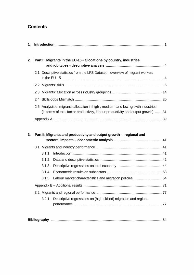
1. Introduction ................................................................................................................... 1

2. Part I: Migrants in the EU-15 - allocations by c ountry, industries

and job types - descriptive analysis ............................................................. 4

2.1 Descriptive statistics from the LFS Dataset – overview of migrant workers

in the EU-15 ............................................................................................................ 4

2.2 Migrants’ skills ........................................................................................................ 6

2.3 Migrants’ allocation across industry groupings .................................................... 14

2.4 Skills-Jobs Mismatch ............................................................................................ 20

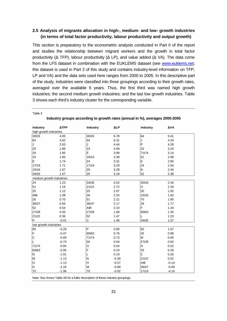
2.5 Analysis of migrants allocation in high-, medium- and low- growth industries

(in terms of total factor productivity, labour productivity and output growth) ....... 31

Appendix A ................................................................................................................... 39

3. Part II: Migrants and productivity and output gr owth – regional and

sectoral impacts - econometric analysis ................................................... 41

3.1 Migrants and industry performance ..................................................................... 41

3.1.1 Introduction ............................................................................................... 41

3.1.2 Data and descriptive statistics .................................................................. 42

3.1.3 Descriptive regressions on total economy ............................................... 44

3.1.4 Econometric results on subsectors .......................................................... 53

3.1.5 Labour market characteristics and migration policies ............................. 64

Appendix B – Additional results ................................................................................... 71

3.2. Migrants and regional performance ..................................................................... 77

3.2.1 Descriptive regressions on (high-skilled) migration and regional

performance ............................................................................................. 77

Bibliography ...................................................................................................................... 84

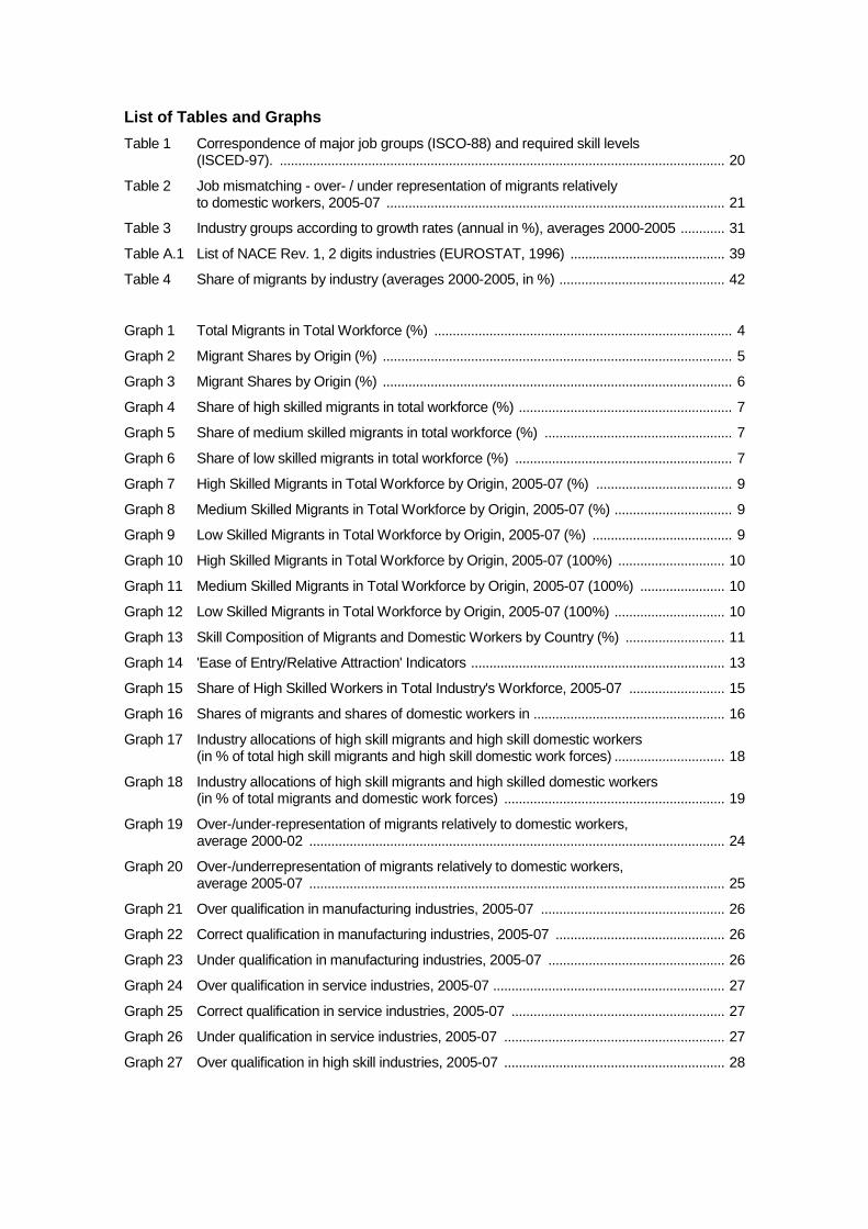
List of Tables and Graphs

Table 1 Correspondence of major job groups (ISCO-88) and required skill levels (ISCED-97). ......................................................................................................................... 20

Table 2 Job mismatching - over- / under representation of migrants relatively to domestic workers, 2005-07 ............................................................................................ 21

Table 3 Industry groups according to growth rates (annual in %), averages 2000-2005 ............ 31

Table A.1 List of NACE Rev. 1, 2 digits industries (EUROSTAT, 1996) .......................................... 39

Table 4 Share of migrants by industry (averages 2000-2005, in %) ............................................. 42

Graph 1 Total Migrants in Total Workforce (%) ................................................................................. 4

Graph 2 Migrant Shares by Origin (%) ............................................................................................... 5

Graph 3 Migrant Shares by Origin (%) ............................................................................................... 6

Graph 4 Share of high skilled migrants in total workforce (%) .......................................................... 7

Graph 5 Share of medium skilled migrants in total workforce (%) ................................................... 7

Graph 6 Share of low skilled migrants in total workforce (%) ........................................................... 7

Graph 7 High Skilled Migrants in Total Workforce by Origin, 2005-07 (%) ..................................... 9

Graph 8 Medium Skilled Migrants in Total Workforce by Origin, 2005-07 (%) ................................ 9

Graph 9 Low Skilled Migrants in Total Workforce by Origin, 2005-07 (%) ...................................... 9

Graph 10 High Skilled Migrants in Total Workforce by Origin, 2005-07 (100%) ............................. 10

Graph 11 Medium Skilled Migrants in Total Workforce by Origin, 2005-07 (100%) ....................... 10

Graph 12 Low Skilled Migrants in Total Workforce by Origin, 2005-07 (100%) .............................. 10

Graph 13 Skill Composition of Migrants and Domestic Workers by Country (%) ........................... 11

Graph 14 'Ease of Entry/Relative Attraction' Indicators ..................................................................... 13

Graph 15 Share of High Skilled Workers in Total Industry's Workforce, 2005-07 .......................... 15

Graph 16 Shares of migrants and shares of domestic workers in .................................................... 16

Graph 17 Industry allocations of high skill migrants and high skill domestic workers (in % of total high skill migrants and high skill domestic work forces) .............................. 18

Graph 18 Industry allocations of high skill migrants and high skilled domestic workers (in % of total migrants and domestic work forces) ............................................................ 19

Graph 19 Over-/under-representation of migrants relatively to domestic workers, average 2000-02 ................................................................................................................. 24

Graph 20 Over-/underrepresentation of migrants relatively to domestic workers, average 2005-07 ................................................................................................................. 25

Graph 21 Over qualification in manufacturing industries, 2005-07 .................................................. 26

Graph 22 Correct qualification in manufacturing industries, 2005-07 .............................................. 26

Graph 23 Under qualification in manufacturing industries, 2005-07 ................................................ 26

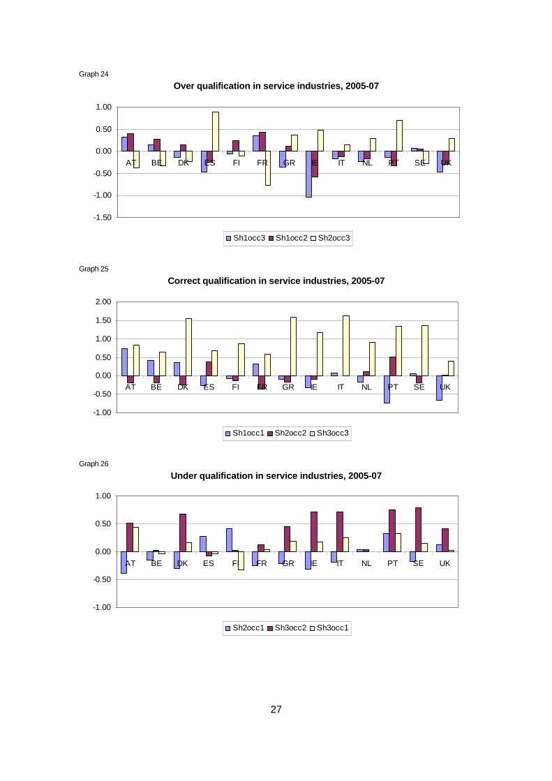
Graph 24 Over qualification in service industries, 2005-07 ............................................................... 27

Graph 25 Correct qualification in service industries, 2005-07 .......................................................... 27

Graph 26 Under qualification in service industries, 2005-07 ............................................................ 27

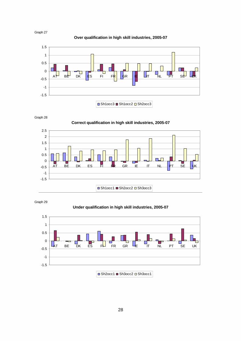
Graph 27 Over qualification in high skill industries, 2005-07 ............................................................ 28

Graph 28 Correct qualification in high skill industries, 2005-07 ........................................................ 28

Graph 29 Under qualification in high skill industries, 2005-07 .......................................................... 28

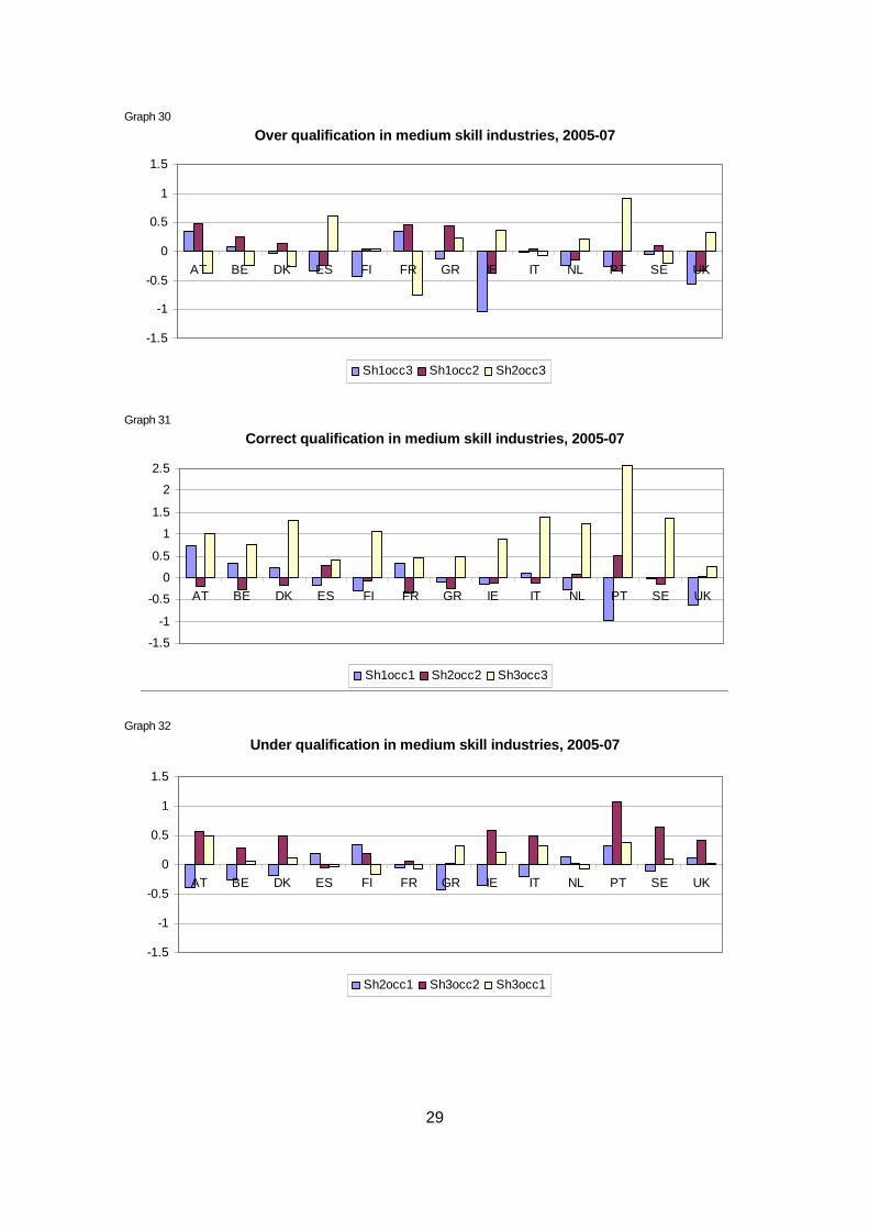
Graph 30 Over qualification in medium skill industries, 2005-07 ...................................................... 29

Graph 31 Correct qualification in medium skill industries, 2005-07 ................................................. 29

Graph 32 Under qualification in medium skill industries, 2005-07 .................................................... 29

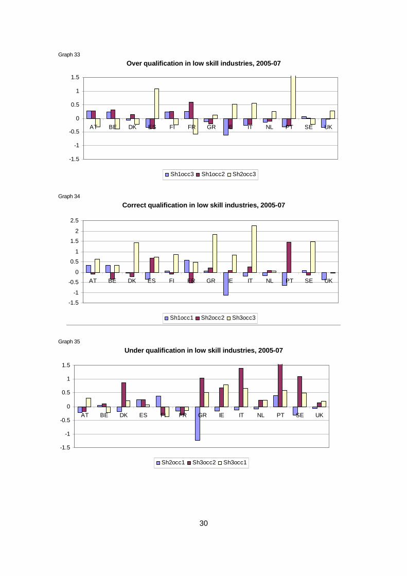
Graph 33 Over qualification in low skill industries, 2005-07 .............................................................. 30

Graph 34 Correct qualification in low skill industries, 2005-07 ......................................................... 30

Graph 35 Under qualification in low skill industries, 2005-07 ........................................................... 30

Graph 36 Migrant shares (averages 2000-2005) .............................................................................. 33



Graph 39 Revised Migrant shares (averages 2000-2005) ................................................................ 36



1

1. Introduction

This study follows up work originally started under a contract from the European

Commission as a background study for the European Competitiveness Report under the

title ‘Migration, Skills, and Productivity’ (for details see Huber et al., 2009).

However, the work contained in the present study is a new text based on completely new

calculations and new econometric work regarding the relationship between migrants and

economic performance.

Work in this (as in the previous) study is mostly based on exploiting the data contained in

the European Labour Force Statistics (LFS) which allows an identification of labour force

and employees by place of birth, age, gender, by educational attainment levels, industries

and regions in which they work, types of occupations etc. The coverage of ‘migrants’,

defined in this study as born outside the country of residence, might not be properly

representative as the LFS has not been originally conceived as using appropriate sampling

techniques along all the above dimensions. Also, the coverage of migrants in the LFS

country samples might be sparse in absolute numbers. As a result one has to be rather

careful which detail is being looked at (e.g. the breakdown of migrants by place of birth, or

by industry or region they are employed in, or by age cohort, etc.) in different parts of the

analysis. Over time and as awareness of the very important challenge which migration

poses to the European policy agenda grows, we are convinced that LFS (and other)

statistics will attempt to pay careful attention to representativeness of migrants in the

respective samples. At the moment we shall have to use this data-set with an appropriate

caveat.

The LFS data have in this report been supplemented with industrial statistics (specifically

the EUKLEMS database see www.euklems.net) in order to capture industry performance

variables and with EU regional statistics in order to conduct the econometric analysis at the

NUTS 2-digit regional level.

Although the results in this study are still preliminary (e.g. issues of causality require much

further work), we believe that this and the previous study (see Huber et al, 2009) is

nonetheless a pioneering attempt to focus on an issue related to migrants’ presence in

European economies which has so far not received the due attention it deservs, at least at

the cross-European level which we have aimed at. The reason for this is that most

economic/econometric studies of migrants’ impact has been aimed at labour market

impacts, i.e. upon wage and employment impacts on domestic labour forces. The studies

regarding the migrants’ impact upon performance variables, in particular upon productivity

growth, are few although there has been an increased interest in this area more recently

(see e.g. Hunt and Gauthier-Loiselle, 2009; Peri, 2009; Paserman, 2008). What has been

2

done so far on this topic has been well reviewed in the Huber et al study (see the literature

review in Ch.1 of that study) and therefore we shall not review the literature over here (see,

however, our bibliography). Almost without exception the studies in the area ‘migration and

productivity’ have so far been done using individual country data-sets and not in the cross-

European setting we adopt in this study. In this sense we think that this study and its

predecessor will pave the way towards much further work which will recognise the complex

impact of migrants upon economic performance in a cross-European context. This is of

importance as Europe develops further in the direction of an integrated labour market and

migration research in Europe has nonetheless the benefit of the existence of a multitude of

national and regional policy settings which affect the utilisation of migrants’ potentials, their

selection, their allocations across jobs, industries and regions and hence their impact upon

economic performance. From this perspective, Europe offers currently, both statistically

and methodologically, a unique opportunity to study the issue of migrants’ roles in affecting

economic performance and which policy-settings affect that impact. Hence, we are

convinced that this study will soon be followed by others exploiting the increased

availability of cross-country data-sets and the motivation to study migrants’ impacts upon

economic performance in heterogeneous social and policy-settings.

The study comprises the following:

Part I (‘Migrants in the EU-15 - allocations by country, industries and job types - descriptive

analysis’) analyses the position of migrants in the EU15 economies. We look at details

regarding their shares in employment, the composition in terms of places of origin, and an

important aspect of the analysis is the study of their ‘skills’ (measured by educational

attainment levels) and the utilisation of these skills relative to those of domestic workers.

We see how the skill composition differs across economies and we analyse the allocation

of migrants’ skills in different sectors of the economy; here we distinguish between sectors

which more generally require relatively more ‘high’, ‘medium’ and ‘lower level skills’. In an

analysis of skills-jobs matching we present indicators of ‘mismatches’ in the sense of

differences between migrant and domestic workers in the utilisation of skills in different

types of ‘jobs’. Finally, in preparation of the econometric analysis undertaken in Part II, we

analyse the allocation of migrants (again differentiated by skill groups) across fast, medium

and slow output and productivity growth industries.

Part II (‘Migrants and productivity growth – regional and sectoral impacts - econometric

analysis’) conducts a wide range of ‘descriptive econometric’ exercises to study the

relationship between migrants employment across industries and regions and output and

productivity growth. We call these exercises ‘descriptive econometric’ because the issues

of causality and selectivity could not be properly addressed with the data-set we had at our

disposal and hence further research will be called forth in this respect. We do find robust

results with respect to the positive impact of the presence of high-skilled migrants

especially in high-education-intensive industries and also more generally – but less

3

robustly – on the relationship between productivity growth and the shares of migrants and

of high-skilled migrants in overall employment. There is also an analysis of the impact of

different policy settings with respect to labour market access of migrants and to anti-

discrimination measures. The latter have a significant positive impact on migrants’

contribution to productivity growth. The analysis of regional impacts of migrants on value

added and labour productivity growth builds on a prior extensive study analysing regional

growth patterns (see Crespo Cuaresmo et al, forthcoming) which had narrowed down the

range of robust explanatory variables through Bayesian econometric techniques. In this

study the migration variables are added as explanatory variables and we find positive and

significant effects of migrants’ shares (and specifically of high-skilled migrants) on regional

productivity growth. The analysis here still suffers from the limitations of being able to apply

a satisfactory approach to determine causality.

4

2. Part I. Migrants in the EU-15 - allocations by c ountry, industries and job types - descriptive analysis

2.1 Descriptive statistics from the LFS Dataset – o verview of migrant workers in the EU-15

This study uses the Labour Force Survey (LFS) data provided by EUROSTAT for the

EU15 member states over the period 2000-2007. Migrants, in this analysis, are defined as

employees born abroad. The dataset provides information about the origin of a country’s

workers and will be explained in detail further below. Due to a lack of data for Germany the

country had to be excluded. Also Luxemburg is excluded from most graphs because of its

extreme outliers. This might be the case because of the very small size of the country,

situated in the middle of Europe and due to its special tax benefits. The examination of the

data set led to the exclusion of the year 2000 for Sweden. In that year all foreign workers

were declared as domestic workers. A similar problem led to the exclusion of Italy’s first

period’s values (we shall report mostly 3-year averages for the periods 2000-02 and 2005-

07). We also had doubts about some data for the second period in Ireland. However,

EUROSTAT assured us that some undeclared answers (with regard to place of birth) can

be regarded as foreign workers – nevertheless, it is not possible to make sure from which

countries these workers originate from.

Graph 1

Migrants in Total Workforce (%)

0

5

10

15

20

AT ES SE IE NL UK FR BE IT GR PT DK FI

Period 2000-02 Period 2005-07

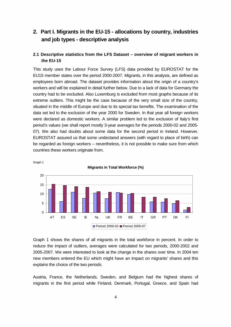
Graph 1 shows the shares of all migrants in the total workforce in percent. In order to

reduce the impact of outliers, averages were calculated for two periods, 2000-2002 and

2005-2007. We were interested to look at the change in the shares over time. In 2004 ten

new members entered the EU which might have an impact on migrants’ shares and this

explains the choice of the two periods.

Austria, France, the Netherlands, Sweden, and Belgium had the highest shares of

migrants in the first period while Finland, Denmark, Portugal, Greece, and Spain had

5

shares below 6%. Spain and Ireland faced the most dramatic changes from period one to

period two by 8.7 and 6.0 percentage points respectively. Great Britain, Sweden, Greece,

and Finland had the second highest positive changes in a range from 3.5 to 2.3

percentage points. France is the only country which had a negative change in the share of

migrants by -0.3 percentage points.

Graph 2

Migrant Shares by Origin (%)

0.02.0

4.06.0

8.010.0

12.014.0

16.0

00-0

2

05-0

7

00-0

2

05-0

7

00-0

2

05-0

7

00-0

2

05-0

7

00-0

2

05-0

7

00-0

2

05-0

7

00-0

2

05-0

7

00-0

2

05-0

7

00-0

2

05-0

7

00-0

2

05-0

7

00-0

2

05-0

7

00-0

2

05-0

7

00-0

2

05-0

7

AT BE DK ES FI FR GR IE IT NL PT SE UK

Western Europe EU12 Europe Rest Rest of World Rich Rest of World Medium + Poor

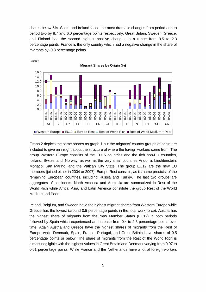
Graph 2 depicts the same shares as graph 1 but the migrants’ country groups of origin are

included to give an insight about the structure of where the foreign workers come from. The

group Western Europe consists of the EU15 countries and the rich non-EU countries,

Iceland, Switzerland, Norway, as well as the very small countries Andorra, Liechtenstein,

Monaco, San Marino, and the Vatican City State. The group EU12 are the new EU

members (joined either in 2004 or 2007). Europe Rest consists, as its name predicts, of the

remaining European countries, including Russia and Turkey. The last two groups are

aggregates of continents. North America and Australia are summarized in Rest of the

World Rich while Africa, Asia, and Latin America constitute the group Rest of the World

Medium and Poor.

Ireland, Belgium, and Sweden have the highest migrant shares from Western Europe while

Greece has the lowest (around 0.5 percentage points in the total work force). Austria has

the highest share of migrants from the New Member States (EU12) in both periods

followed by Spain which experienced an increase from 0.4 to 2.3 percentage points over

time. Again Austria and Greece have the highest shares of migrants from the Rest of

Europe while Denmark, Spain, France, Portugal, and Great Britain have shares of 0.5

percentage points or below. The share of migrants from the Rest of the World Rich is

almost negligible with the highest values in Great Britain and Denmark varying from 0.97 to

0.61 percentage points. While France and the Netherlands have a lot of foreign workers

6

from the Rest of the World Medium and Poor, Spain and Great Britain experienced a big

increase over the two periods. Spain attracted a lot of workers from Africa due to its

geographical position. An explanation for France’s high share of migrants from the rather

Poor Rest of the World is the influx of workers from former colonies. This is also the case

for the Netherlands, Portugal, and Great Britain.

Graph 3

Migrant Shares by Origin (%)

0%

20%

40%

60%

80%

100%

00-0

2

05-0

7

00-0

2

05-0

7

00-0

2

05-0

7

00-0

2

05-0

7

00-0

2

05-0

7

00-0

2

05-0

7

00-0

2

05-0

7

00-0

2

05-0

7

00-0

2

05-0

7

00-0

2

05-0

7

00-0

2

05-0

7

00-0

2

05-0

7

00-0

2

05-0

7


Western Europe EU12 Europe Rest RestWorld Rich RestWorld Medium + Poor

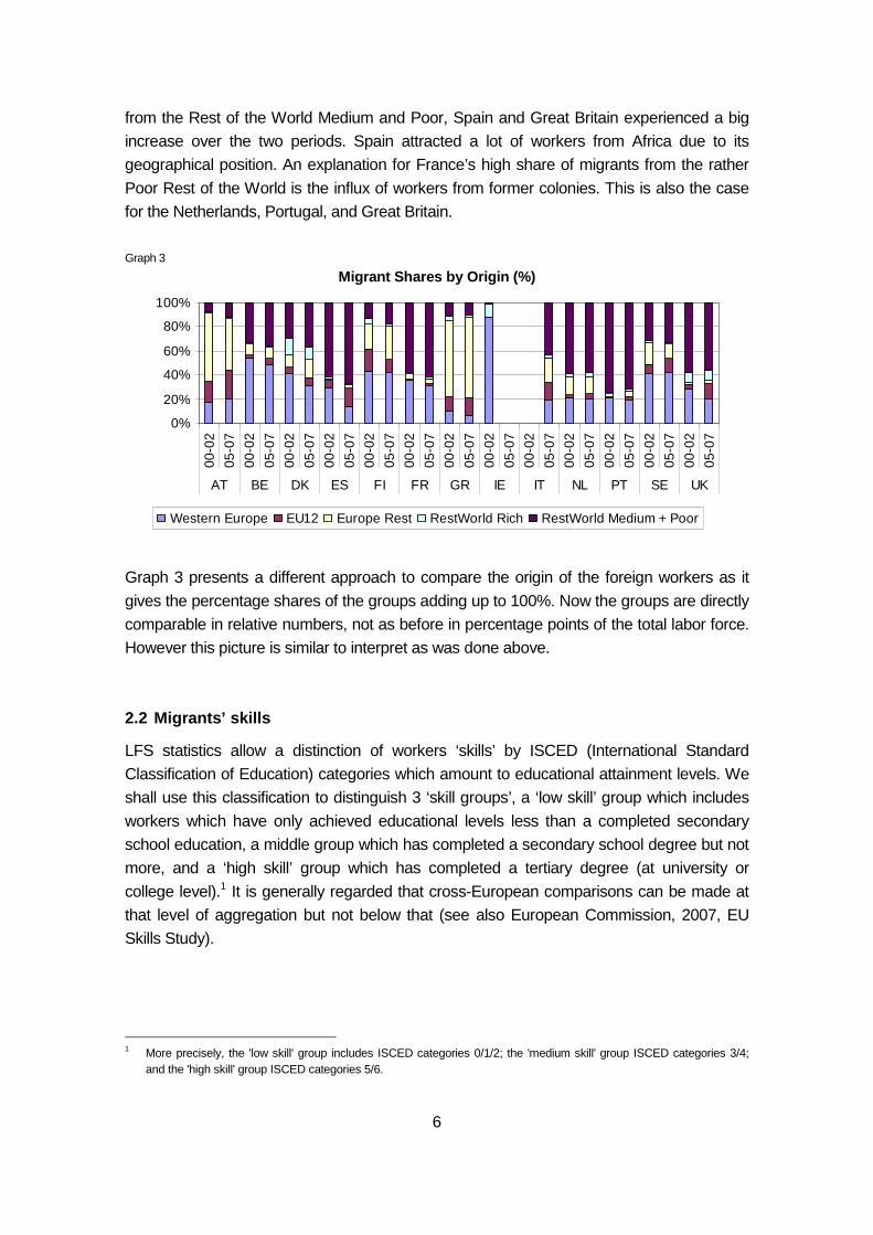
Graph 3 presents a different approach to compare the origin of the foreign workers as it

gives the percentage shares of the groups adding up to 100%. Now the groups are directly

comparable in relative numbers, not as before in percentage points of the total labor force.

However this picture is similar to interpret as was done above.

2.2 Migrants’ skills

LFS statistics allow a distinction of workers ‘skills’ by ISCED (International Standard

Classification of Education) categories which amount to educational attainment levels. We

shall use this classification to distinguish 3 ‘skill groups’, a ‘low skill’ group which includes

workers which have only achieved educational levels less than a completed secondary

school education, a middle group which has completed a secondary school degree but not

more, and a ‘high skill’ group which has completed a tertiary degree (at university or

college level).1 It is generally regarded that cross-European comparisons can be made at

that level of aggregation but not below that (see also European Commission, 2007, EU

Skills Study).

1 More precisely, the 'low skill' group includes ISCED categories 0/1/2; the 'medium skill' group ISCED categories 3/4;

and the 'high skill' group ISCED categories 5/6.

7

Graph 4

Share of high skilled migrants in total workforce ( %)

0

2

4

6

8

10

IE SE UK BE ES NL AT FR DK PT GR IT FI

per 00-02 per 05-07

Graph 5

Share of medium skilled migrants in total workforce (%)

0

2

4

6

8

10

AT SE UK NL IE ES IT BE FR GR DK PT FI

per 00-02 per 05-07

Graph 6

Share of low skilled migrants in total workforce (% )

0

2

4

6

8

10

ES AT FR GR PT IT BE NL SE IE UK DK FI

per 00-02 per 05-07

8

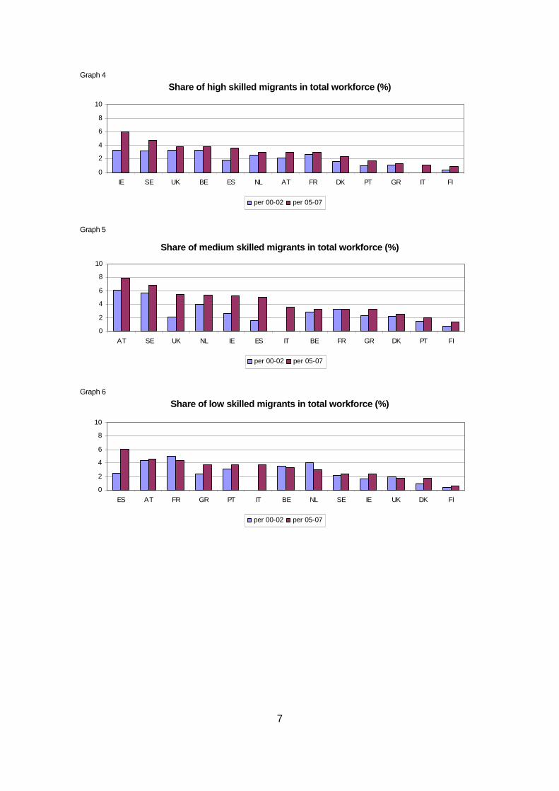
Starting with the shares of high skilled migrants (i..e. those with completed tertiary degrees)

in the total workforce, these are shown in graph 4. Great Britain, Belgium, Ireland, and

Sweden have high initial shares while in Greece, Portugal and Finland these range around

1% or below. All countries faced an increase in high skilled foreign workers. Especially

Ireland and Sweden have experienced dramatic positive changes making them the leading

countries in this group.

The graphs 5 and 6 show the shares of medium skilled and low skilled migrants per

country. Austria has a high share of medium skilled foreign workers compared to its high

and low skilled ratios. Spain experienced very big increases from period 1 to period 2

across all three skill groups.

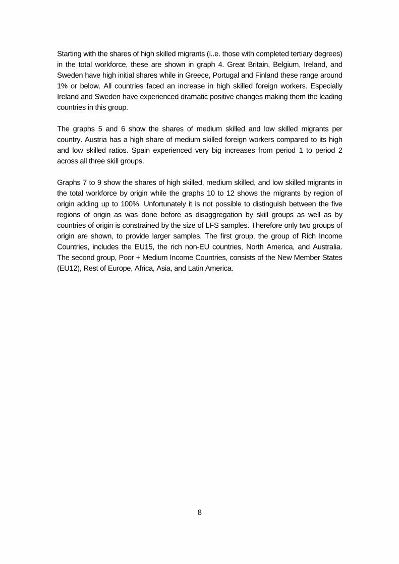
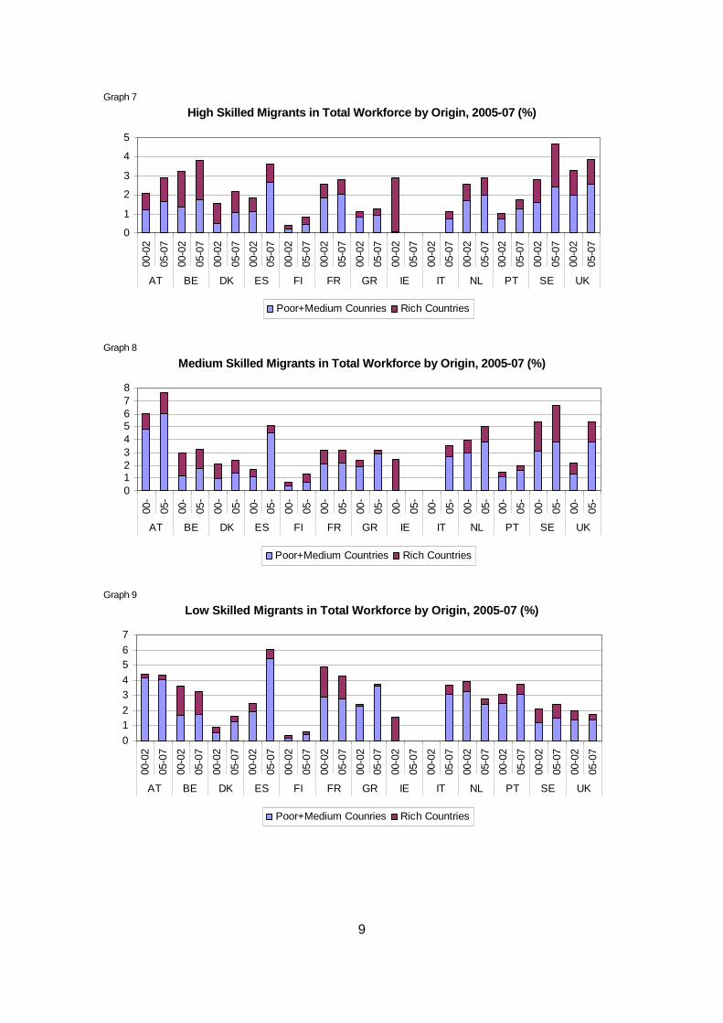
Graphs 7 to 9 show the shares of high skilled, medium skilled, and low skilled migrants in

the total workforce by origin while the graphs 10 to 12 shows the migrants by region of

origin adding up to 100%. Unfortunately it is not possible to distinguish between the five

regions of origin as was done before as disaggregation by skill groups as well as by

countries of origin is constrained by the size of LFS samples. Therefore only two groups of

origin are shown, to provide larger samples. The first group, the group of Rich Income

Countries, includes the EU15, the rich non-EU countries, North America, and Australia.

The second group, Poor + Medium Income Countries, consists of the New Member States

(EU12), Rest of Europe, Africa, Asia, and Latin America.

9

Graph 7

High Skilled Migrants in Total Workforce by Origin, 2005-07 (%)

0

1

2

3

4

500

-02

05-0

7

00-0

2

05-0

7

00-0

2

05-0

7

00-0

2

05-0

7

00-0

2

05-0

7

00-0

2

05-0

7

00-0

2

05-0

7

00-0

2

05-0

7

00-0

2

05-0

7

00-0

2

05-0

7

00-0

2

05-0

7

00-0

2

05-0

7

00-0

2

05-0

7


Poor+Medium Counries Rich Countries

Graph 8

Medium Skilled Migrants in Total Workforce by Origi n, 2005-07 (%)

012345678

00-

05-

00-

05-

00-

05-

00-

05-

00-

05-

00-

05-

00-

05-

00-

05-

00-

05-

00-

05-

00-

05-

00-

05-

00-

05-


Poor+Medium Countries Rich Countries

Graph 9

Low Skilled Migrants in Total Workforce by Origin, 2005-07 (%)

0

12

34

56

7

00-0

2

05-0

7

00-0

2

05-0

7

00-0

2

05-0

7

00-0

2

05-0

7

00-0

2

05-0

7

00-0

2

05-0

7

00-0

2

05-0

7

00-0

2

05-0

7

00-0

2

05-0

7

00-0

2

05-0

7

00-0

2

05-0

7

00-0

2

05-0

7

00-0

2

05-0

7



10

Graph 10

High Skilled Migrants in Total Workforce by Origin, 2005-07 (100%)

0%

20%

40%

60%

80%

100%

00-0

2

05-0

7

00-0

2

05-0

7

00-0

2

05-0

7

00-0

2

05-0

7

00-0

2

05-0

7

00-0

2

05-0

7

00-0

2

05-0

7

00-0

2

05-0

7

00-0

2

05-0

7

00-0

2

05-0

7

00-0

2

05-0

7

00-0

2

05-0

7

00-0

2

05-0

7



Graph 11

Medium Skilled Migrants in Total Workforce by Origi n, 2005-07 (100%)

0%

20%

40%

60%

80%

100%

00-0

2

05-0

7

00-0

2

05-0

7

00-0

2

05-0

7

00-0

2

05-0

7

00-0

2

05-0

7

00-0

2

05-0

7

00-0

2

05-0

7

00-0

2

05-0

7

00-0

2

05-0

7

00-0

2

05-0

7

00-0

2

05-0

7

00-0

2

05-0

7

00-0

2

05-0

7


Poor+Medium Countries Rich Countries

Graph 12

Low Skilled Migrants in Total Workforce by Origin, 2005-07 (100%)

0%

20%

40%

60%

80%

100%

00-0

2

05-0

7

00-0

2

05-0

7

00-0

2

05-0

7

00-0

2

05-0

7

00-0

2

05-0

7

00-0

2

05-0

7

00-0

2

05-0

7

00-0

2

05-0

7

00-0

2

05-0

7

00-0

2

05-0

7

00-0

2

05-0

7

00-0

2

05-0

7

00-0

2

05-0

7



11

In most countries the larger share of even the high skilled migrants in total employees

comes from the Poor and Medium Income Countries. This is not true for Belgium,

Denmark, and Ireland in the first period. The most likely explanation is that these countries

have rich neighbouring countries eager to work there. When looking at the evenly

distributed high skilled migrant workers in Denmark, Finland, and Sweden, this hypothesis

seems to hold also for the Scandinavian countries more generally. Ireland has a share of

2.8 percent of migrants in the total workforce from Rich Source Countries (data here are

restricted to the first period) compared to 0.1 percent from the Poor and Medium Countries

– this means that almost 97% of the high skilled migrants come from Rich Income

Countries. However, a range of economies (Spain, France, Greece, Portugal, Italy,

Netherlands, UK) source a larger share of their migrants with tertiary degrees from Middle

and Poor Income countries.

Graph 13

Skill Composition of Migrants and Domestic Workers by Country (%)

0%

20%

40%

60%

80%

100%

D M D M D M D M D M D M D M D M D M D M D M D M D M D M D M

AT BE DK ES FI FR GR IE IT LU NL PT SE UK EU15

Low Skilled Medium Skilled High Skilled

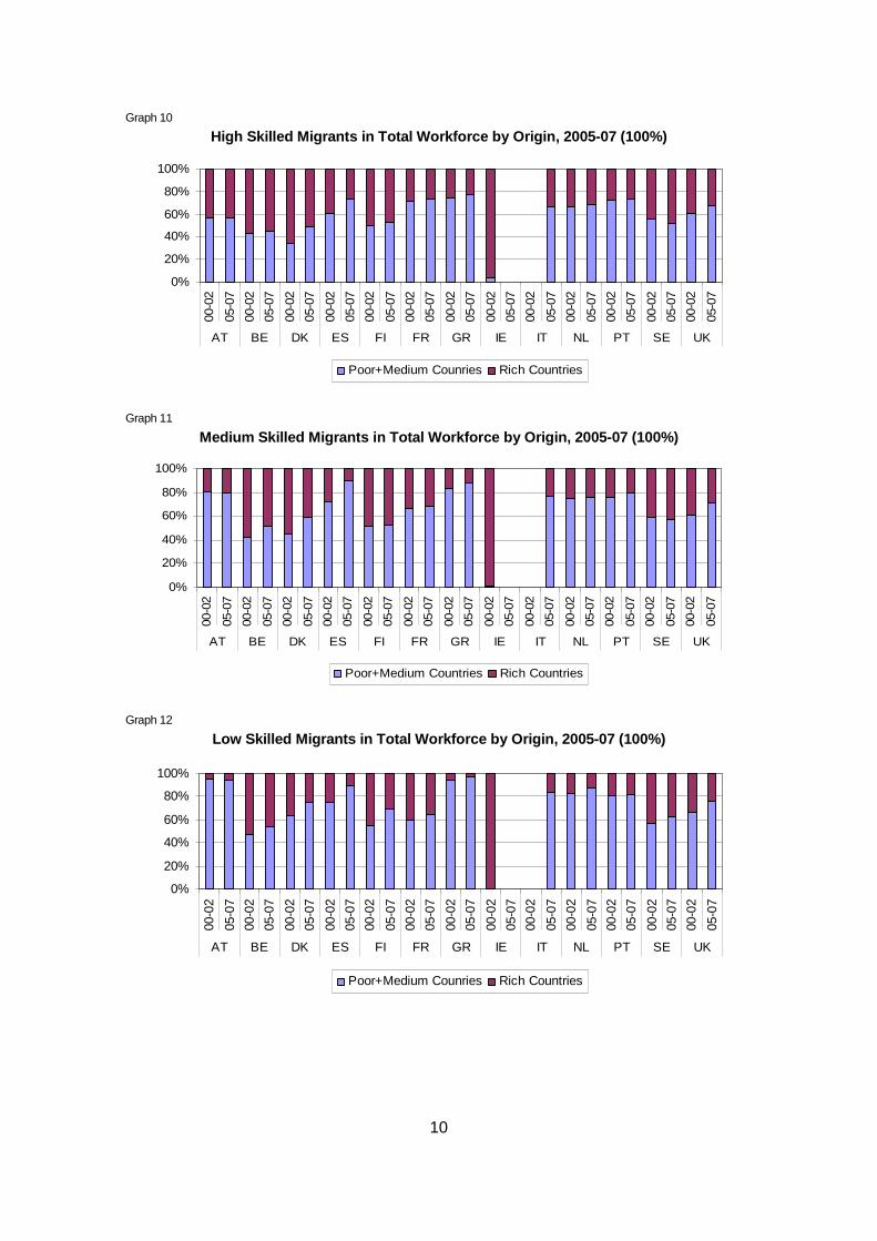
Graph 13 shows the skill composition of domestic and migrant workers by country as well

as the structure of the EU15 on average over the period 2005-2007. Worth noticing is that

Austria, Belgium, Denmark, Finland, France, Greece, Italy, Luxemburg, the Netherlands,

and Sweden have relatively more low skilled migrants than low skilled domestic workers.

Spain, Ireland, Portugal, and the United Kingdom show a reverse picture. There are

relatively more low skilled domestics than migrants. It is also interesting to point out

countries in which the share of high skilled migrants is greater than the share of high skilled

domestic workers. This is true for Denmark, Ireland, Luxemburg, Portugal, Sweden, and

the United Kingdom. Spain, Finland, Greece, Italy, and the Netherlands have relatively

more high skilled domestic workers than foreign workers while Austria, Belgium, and

France are almost equally distributed.

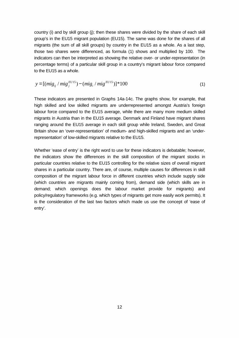
Next we want to check on a comparative basis which skill group is more or less

represented in a country’s labour force relative to what happens at the EU15 level. For this

purpose we calculate an ‘ease of entry’ indicator (y) by country and for each skill group of

migrants. This is done by calculating the shares of migrants in the total workforce (mig) by

12

country (i) and by skill group (j); then these shares were divided by the share of each skill

group’s in the EU15 migrant population (EU15). The same was done for the shares of all

migrants (the sum of all skill groups) by country in the EU15 as a whole. As a last step,

those two shares were differenced, as formula (1) shows and multiplied by 100. The

indicators can then be interpreted as showing the relative over- or under-representation (in

percentage terms) of a particular skill group in a country’s migrant labour force compared

to the EU15 as a whole.

15 15[( / ) ( / )]*100EU EU

ij j iy mig mig mig mig= − (1)

These indicators are presented in Graphs 14a-14c. The graphs show, for example, that

high skilled and low skilled migrants are underrepresented amongst Austria’s foreign

labour force compared to the EU15 average, while there are many more medium skilled

migrants in Austria than in the EU15 average. Denmark and Finland have migrant shares

ranging around the EU15 average in each skill group while Ireland, Sweden, and Great

Britain show an ‘over-representation’ of medium- and high-skilled migrants and an ‘under-

representation’ of low-skilled migrants relative to the EU15.

Whether ‘ease of entry’ is the right word to use for these indicators is debatable; however,

the indicators show the differences in the skill composition of the migrant stocks in

particular countries relative to the EU15 controlling for the relative sizes of overall migrant

shares in a particular country. There are, of course, multiple causes for differences in skill

composition of the migrant labour force in different countries which include supply side

(which countries are migrants mainly coming from), demand side (which skills are in

demand; which openings does the labour market provide for migrants) and

policy/regulatory frameworks (e.g. which types of migrants get more easily work permits). It

is the consideration of the last two factors which made us use the concept of ‘ease of

entry’.

13

Graph 14

'Ease of Entry/Relative Attraction' Indicators

Graph 14a

Low Skilled Migrants, 2005-07 (%)

-80

-60

-40

-20

0

20

40

60


Graph 14b

Medium Skilled Migrants, 2005-07 (%)

-30

-20

-10

0

10

20

30

40

50


Graph 14c

High Skilled Migrants, 2005-07 (%)

-60

-40

-20

0

20

40

60

80

100


14

2.3 Migrants’ allocation across industry groupings

In the following we use an industrial break-down and group industries in terms of three

clusters depending upon skill-intensity. We then check the relative allocation of migrant

workers across these clusters and also analyse their qualifications compared to those of

domestic workers in these clusters.

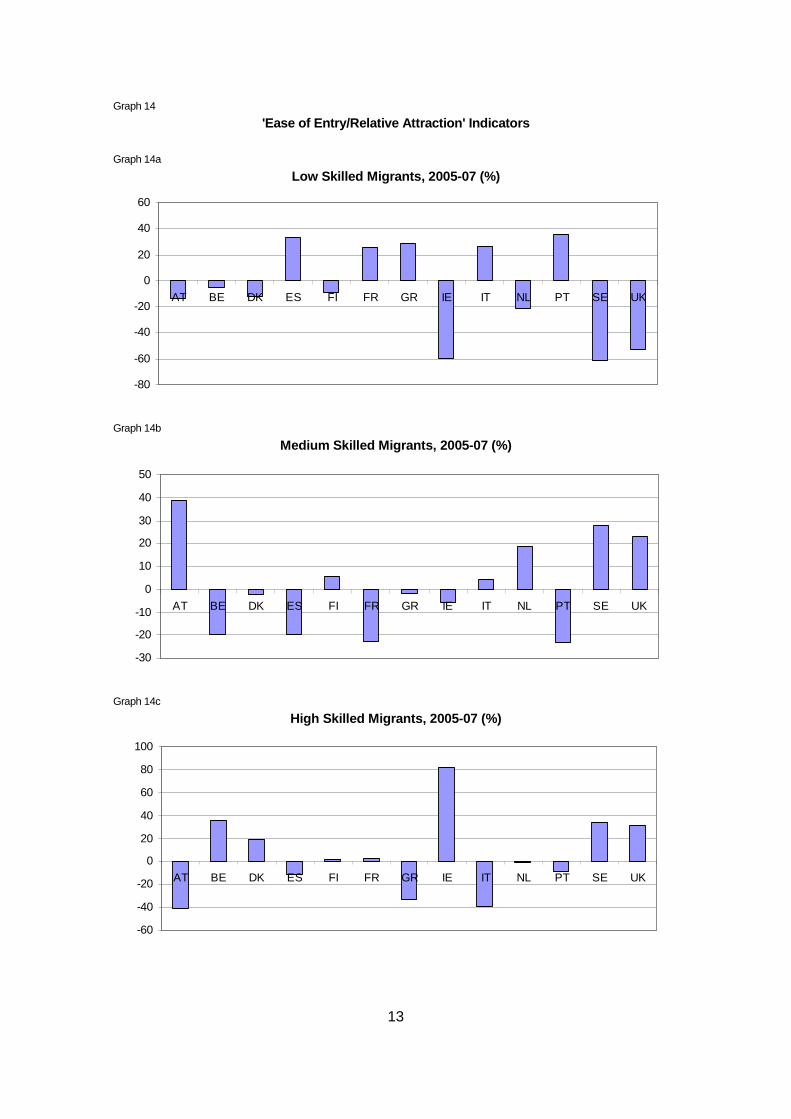
Let us start with the definition of the industry clusters: The graphs 15a to 15c depict the

shares of high educated workers in the total workforce per NACE Rev. 1 (2 digits) industry

as means over the period 2005-07. The industries are grouped into 3 clusters where graph

15a shows the group of industries with the highest shares of high educated workers. Thus,

this industry cluster will be called high skill industries from now on. The graphs 16a and 16c

show the group of industries with intermediate shares of high skilled workers (medium skill

industries) and the group of the lowest shares (low skill industries). Each of these industry

groupings accounts for approximately 33% of the total workforce in the EU15 which

explains why they include different numbers of NACE Rev. 1 industries. Table A.4 in the

appendix provides a complete list of the industries in these clusters including their shares

of workers in total employment.

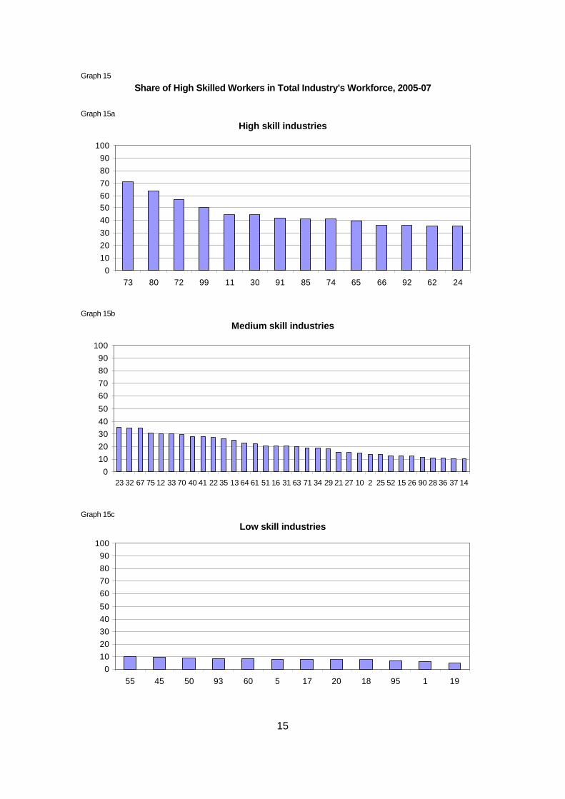
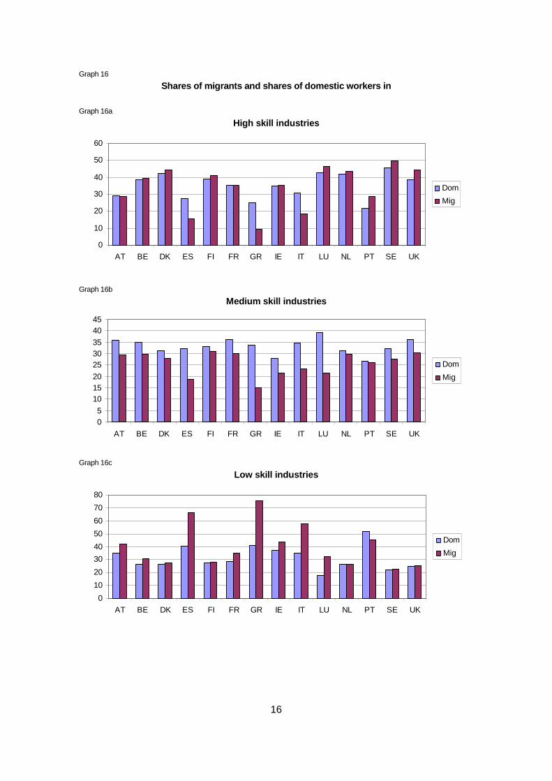
We start with analysing the distribution of migrants across the three industry groupings. In

Graphs 17a to 17c we can see the shares of migrants and of domestic workers employed

in the three different industry groupings (hence these shares must add up to 100% across

industry groups). The distribution of workers across industry groupings reflects the

composition of industries in a country’s economy, i.e. whether high- or medium- or low-skill

industries are more strongly represented in a country’s economy, and the graphs also

show whether the distribution of domestic workers as compared to migrants across these

industry groupings is different or rather similar.

15

Graph 15

Share of High Skilled Workers in Total Industry's W orkforce, 2005-07

Graph 15a

High skill industries

0

10

20

30

40

5060

70

80

90

100

73 80 72 99 11 30 91 85 74 65 66 92 62 24

Graph 15b

Medium skill industries

0

10

20

30

40

50

60

70

80

90

100

23 32 67 75 12 33 70 40 41 22 35 13 64 61 51 16 31 63 71 34 29 21 27 10 2 25 52 15 26 90 28 36 37 14

Graph 15c

Low skill industries

0

10

20

30

40

50

60

70

80

90

100

55 45 50 93 60 5 17 20 18 95 1 19

16

Graph 16

Shares of migrants and shares of domestic workers i n

Graph 16a


0

10

20

30

40

50

60

AT BE DK ES FI FR GR IE IT LU NL PT SE UK

Dom

Mig

Graph 16b


05

101520

253035

4045


Dom

Mig

Graph 16c


0

10

20

30

40

50

60

70

80


Dom

Mig

17

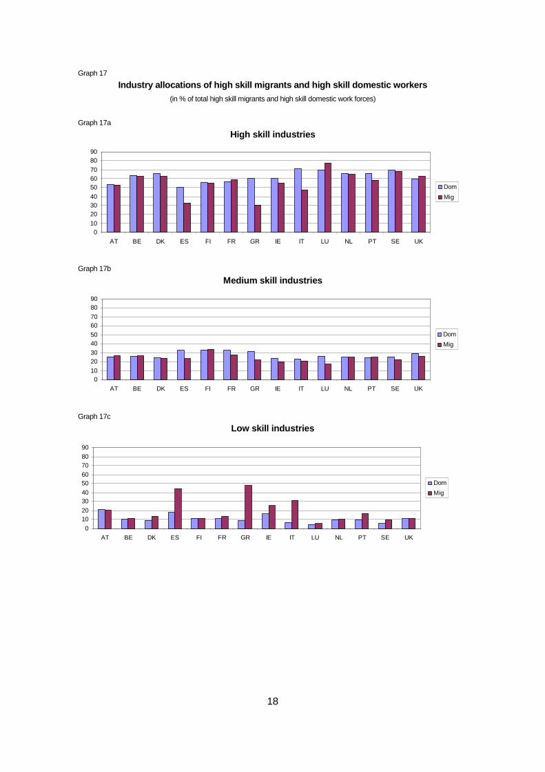
Graphs 17a to 17c focus on the distribution of high skilled migrants (i.e. migrants with

completed tertiary degrees) and of high skilled domestic workers across the three industry

groupings. Hence we can see in which industries high skilled personnel is mainly

employed and, again, whether there are differences in the allocation of high-skilled

migrants as compared to high-skilled domestic workers across the three industry

groupings.

The first thing we see from these graphs is that the industry classification (which has been

constructed from using data on the allocation of high-skilled employees in total across the

EU15 economy as a whole, also works on the whole also for individual countries. I.e. with

few exceptions (e.g. Greece and Portugal) there is a larger share of high skilled migrants

and of domestic workers employed in the high-skill industries than in the medium- or low-

skill industries also at the individual country level.

Secondly, in many countries (Austria, Belgium, Denmark, Finland, France, Sweden, UK)

the relative allocation of highly skilled personnel across the industry groupings is not very

different across migrants and domestic workers. Exceptions are Spain, Greece, Ireland,

Italy, Portugal, i.e. the Southern European economies, where there is a lower share of high

skilled migrants employed in the high-skill industries compared to domestic workers and,

symmetrically, a higher share in low skill industries. The opposite is the case in France,

Luxembourg and the UK where high skilled migrants are relatively more strongly allocated

in high-skill industries.

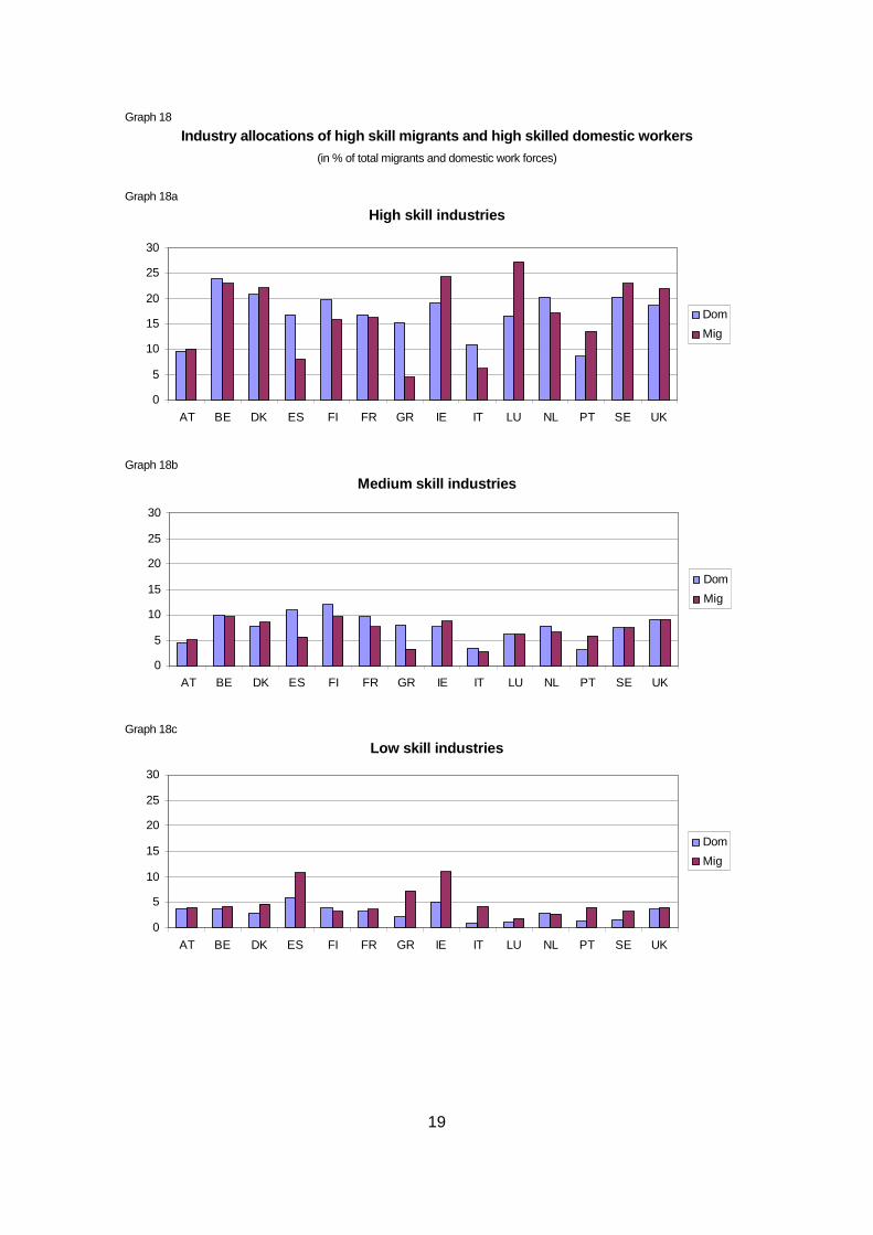
Finally, in graphs 18a to 18c we can see how important high-skilled workers (domestic and

migrant) are in the total labour forces of the three industry groupings. Here we can see, for

example, the very low share of high skilled personnel (migrants and domestic workers) in

Austria, Spain, Greece and Portugal in the high-skill industries which reflects the relatively

low share of high-skilled in the overall labour force in these countries. The shares of high-

skilled in countries like Belgium, Denmark, Finland, France, Ireland, Netherlands, Sweden

and the UK are between 10 to 15 percentage points higher than in the first group of

countries and Denmark, Ireland, Luxembourg, Portugal, Sweden and Great Britain benefit

from a strong boost to the presence of high-skilled personnel in high-skill industries through

the stronger presence of high-skill migrants in these industries than that of domestic

workers.

18

Graph 17

Industry allocations of high skill migrants and hig h skill domestic workers (in % of total high skill migrants and high skill domestic work forces)

Graph 17a


010

203040

506070

8090


Dom

Mig

Graph 17b


010

2030

4050

6070

8090


Dom

Mig

Graph 17c


0

1020

3040

5060

7080

90


Dom

Mig

19

Graph 18

Industry allocations of high skill migrants and hig h skilled domestic workers (in % of total migrants and domestic work forces)

Graph 18a


0

5

10

15

20

25

30


Dom

Mig

Graph 18b


0

5

10

15

20

25

30


Dom

Mig

Graph 18c


0

5

10

15

20

25

30


Dom

Mig

20

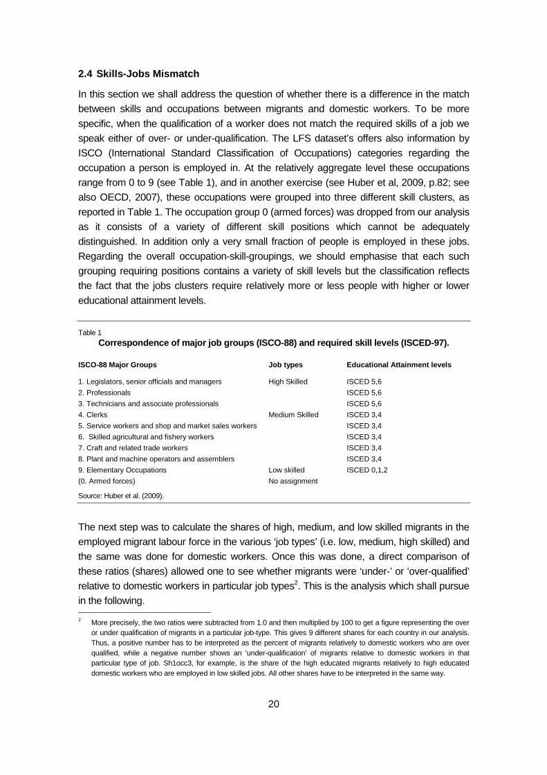
2.4 Skills-Jobs Mismatch

In this section we shall address the question of whether there is a difference in the match

between skills and occupations between migrants and domestic workers. To be more

specific, when the qualification of a worker does not match the required skills of a job we

speak either of over- or under-qualification. The LFS dataset’s offers also information by

ISCO (International Standard Classification of Occupations) categories regarding the

occupation a person is employed in. At the relatively aggregate level these occupations

range from 0 to 9 (see Table 1), and in another exercise (see Huber et al, 2009, p.82; see

also OECD, 2007), these occupations were grouped into three different skill clusters, as

reported in Table 1. The occupation group 0 (armed forces) was dropped from our analysis

as it consists of a variety of different skill positions which cannot be adequately

distinguished. In addition only a very small fraction of people is employed in these jobs.

Regarding the overall occupation-skill-groupings, we should emphasise that each such

grouping requiring positions contains a variety of skill levels but the classification reflects

the fact that the jobs clusters require relatively more or less people with higher or lower

educational attainment levels.

Table 1

Correspondence of major job groups (ISCO-88) and re quired skill levels (ISCED-97).

ISCO-88 Major Groups Job types Educational Attainme nt levels

1. Legislators, senior officials and managers High Skilled ISCED 5,6

2. Professionals ISCED 5,6

3. Technicians and associate professionals ISCED 5,6

4. Clerks Medium Skilled ISCED 3,4

5. Service workers and shop and market sales workers ISCED 3,4

6. Skilled agricultural and fishery workers ISCED 3,4

7. Craft and related trade workers ISCED 3,4

8. Plant and machine operators and assemblers ISCED 3,4

9. Elementary Occupations Low skilled ISCED 0,1,2

(0. Armed forces) No assignment

Source: Huber et al. (2009).

The next step was to calculate the shares of high, medium, and low skilled migrants in the

employed migrant labour force in the various ‘job types’ (i.e. low, medium, high skilled) and

the same was done for domestic workers. Once this was done, a direct comparison of

these ratios (shares) allowed one to see whether migrants were ‘under-’ or ‘over-qualified’

relative to domestic workers in particular job types2. This is the analysis which shall pursue

in the following. 2 More precisely, the two ratios were subtracted from 1.0 and then multiplied by 100 to get a figure representing the over

or under qualification of migrants in a particular job-type. This gives 9 different shares for each country in our analysis. Thus, a positive number has to be interpreted as the percent of migrants relatively to domestic workers who are over qualified, while a negative number shows an ‘under-qualification’ of migrants relative to domestic workers in that particular type of job. Sh1occ3, for example, is the share of the high educated migrants relatively to high educated domestic workers who are employed in low skilled jobs. All other shares have to be interpreted in the same way.

21

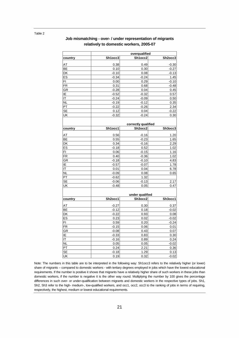
Table 2

Job mismatching - over- / under representation of m igrants relatively to domestic workers, 2005-07

overqualified country Sh1occ3 Sh1occ2 Sh2occ3

AT 0.38 0.49 -0.30 BE 0.10 0.30 -0.27 DK -0.10 0.08 -0.13 ES -0.34 -0.24 1.45 FI 0.00 0.29 -0.10 FR 0.31 0.68 -0.48 GR -0.28 0.04 0.45 IE -0.52 -0.32 0.57 IT -0.24 -0.09 0.50 NL -0.19 -0.12 0.35 PT -0.22 -0.26 2.34 SE 0.12 0.04 -0.22 UK -0.32 -0.24 0.30

correctly qualified country Sh1occ1 Sh2occ2 Sh3occ3

AT 0.56 -0.16 1.20 BE 0.55 -0.23 1.65 DK 0.34 -0.16 2.29 ES -0.18 0.52 1.02 FI 0.06 -0.15 1.16 FR 0.40 -0.36 1.02 GR -0.18 -0.10 4.83 IE -0.57 -0.07 1.78 IT 0.01 0.04 6.78 NL -0.09 0.08 0.65 PT -0.62 1.32 SE -0.06 -0.13 2.17 UK -0.48 0.05 0.47

under qualified country Sh2occ1 Sh3occ2 Sh3occ1

AT -0.27 0.30 0.37 BE -0.12 0.18 -0.02 DK -0.22 0.93 0.08 ES 0.23 0.02 -0.02 FI 0.59 0.20 -0.24 FR -0.15 0.06 0.01 GR -0.08 0.43 0.07 IE -0.33 0.83 0.30 IT -0.16 0.89 0.24 NL 0.05 0.05 -0.02 PT 0.24 2.21 0.36 SE -0.18 1.29 0.13 UK 0.19 0.32 -0.02

Note: The numbers in this table are to be interpreted in the following way: Sh1occ3 refers to the relatively higher (or lower) share of migrants – compared to domestic workers - with tertiary degrees employed in jobs which have the lowest educational requirements. If the number is positive it shows that migrants have a relatively higher share of such workers in these jobs than domestic workers, if the number is negative it is the other way round. Multiplying the number by 100 gives the percentage differences in such over- or under-qualification between migrants and domestic workers in the respective types of jobs. Sh1, Sh2, Sh3 refer to the high- medium-, low-qualified workers, and occ1, occ2, occ3 to the ranking of jobs in terms of requiring, respectively, the highest, medium or lowest educational requirements.

22

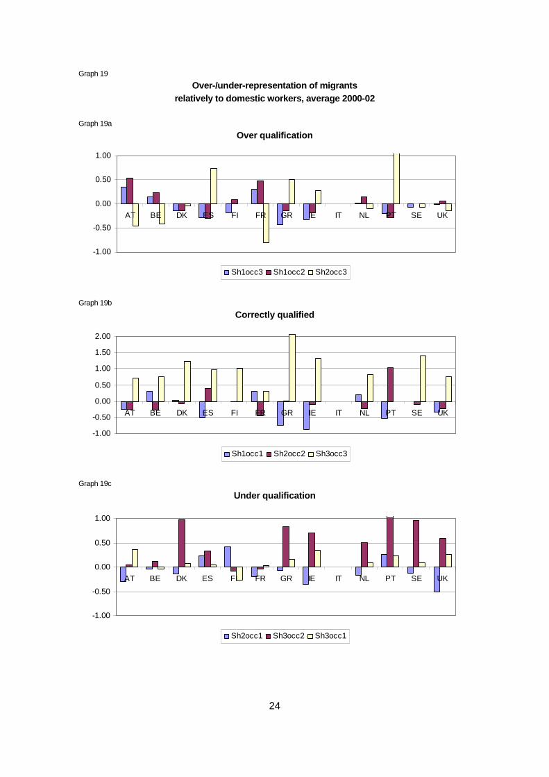
The graphs 19 and 20 should give the reader an insight of how the migrants and domestic

workers are distributed among the different occupation-skill-groups over the periods 2000-

02 and 2005 to 2007. To make the graphical analysis easier, the original shares were

transformed into logs, to range around zero. The zero line, in this case, would refer to an

equal representation of migrants and domestic workers in terms of educational attainment

levels in a specific job. This approach will be used throughout all graphs in this section to

obtain a picture of relative jobs-skills mismatching of migrants relative to domestic workers.

Especially the issue of relative ‘over-qualification’ of migrants is an important issue as it is a

form of “brain waste” in the sense that a migrant worker is employed in a particular job

which does not require his or her higher level of education (always compared to the

domestic labour force).

Of course, skills-jobs mis-match analysis is a difficult issue and cannot simply be studied by

comparing formal educational attainment levels (i.e. primary, secondary and tertiary

degrees) as, in the first instance, the detailed content of the educational curricula can be

quite different and, furthermore, there are other than ‘formal’ qualifications (e.g. language)

which might be very important distinguishing characteristics between different workers

(migrants and domestic workers, or migrants from different places of origin). Nonetheless,

given that we do not have information other than formal educational qualifications we shall

pursue the analysis of ‘over-qualification’, ‘under-qualification’, and ‘correct qualification’ on

that basis.

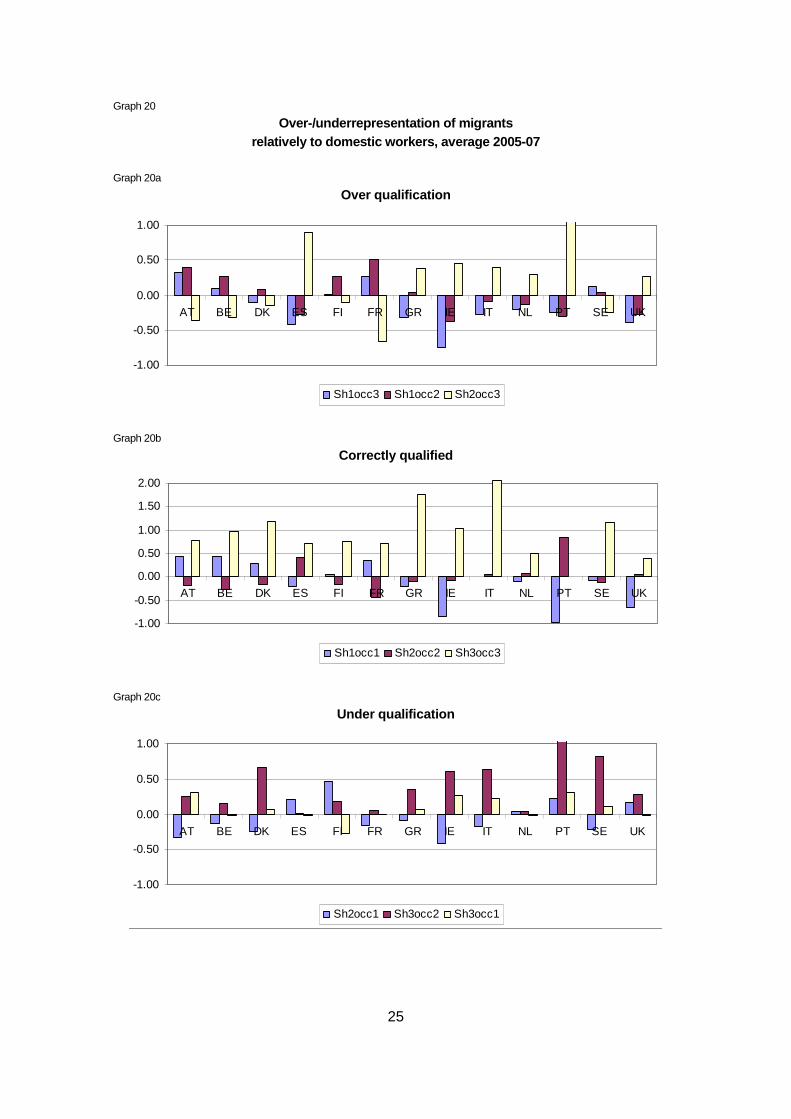
Let us start with an interpretation of the results shown in graphs 19a-19c and 20a-20c in

which the relative skills-jobs allocations of migrants relative to domestic workers is shown

for periods 2000-02 and 2005-07 respectively. We shall select only a few of the most

striking facts:

- First, the pattern is relatively persistent over time, hence we shall focus on the most

recent period depicted in Graphs 20a-20c.

- When we look at the most striking feature of ‘over-qualification’, we see that the

most pervasive feature across countries is that a lot of medium-educated migrants

work in low skill jobs (Sh2occ3); in two countries, Austria and France we also find a

rather strong relative allocation of highly educated migrants to work in medium- and

even in low-skill jobs (Sh1occ2 and Sh1occ3). Both these two types of features can

be interpreted medium- or high-skill migrants find it difficult to get either their

qualifications properly recognised or that they miss other than formal qualifications

or that there are indeed barriers to entry (temporary or longer-term) which bar them

from doing the jobs for which they would otherwise be formally qualified.

- As regards, ‘correct qualification’, i.e. migrants working in exactly those jobs for

which they are qualified, we see that the most pervasive feature is that many more

‘low qualified migrants’ work in ‘low-skill jobs’ than is the case for low skilled

domestic workers (see Sh3occ3); this can be interpreted as a rather strong

23

substitution effect of low-skilled migrants for low-skilled domestic workers in these

types of jobs.

- In terms of ‘under-qualification’ we find that in many countries we find ‘low skill

migrant workers’ being strongly represented in ‘medium skill jobs’ (Sh3occ2). This

could be seen as a type of complementarity in particular jobs where low-skill

activities are carried out by migrants in jobs which are predominantly defined as

‘medium skilled jobs’ (think about the construction jobs or jobs in the services

sectors).

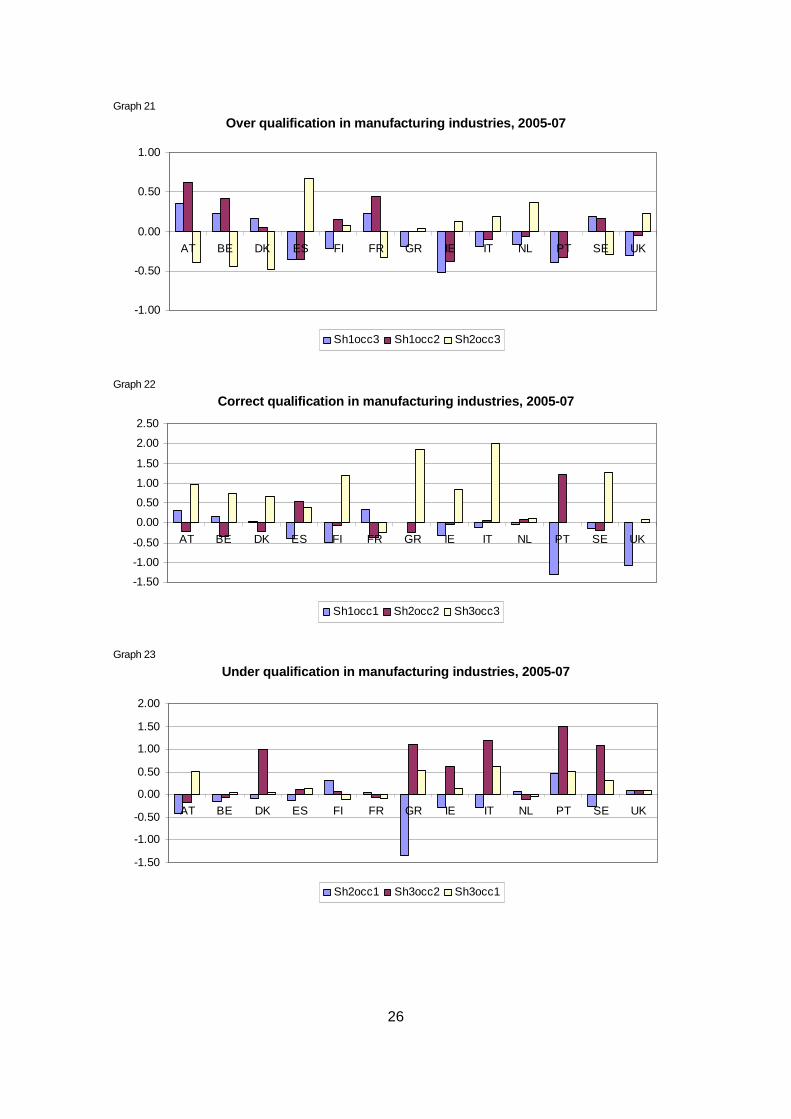
The following sets of graphs (21-26 and 27-35) breaks down the analysis conducted above

for the aggregate economies into sub-groups of industries:

Graphs 21-26 splits up the economy into manufacturing industries (NACE Rev. 1 industries

15 to 37) and business service industries (NACE Rev. 1 industries 50 to 74) and then

conducts the same type of analysis as before but for these two sub-groups of industries.

Graphs 27-31 uses the industry breakdown already adopted in section 2.3 into ‘high-

medium- and low-skill industries’ (see previous graphs 15a-15c) and conducts the analysis

for these sub-groups of industries.

We shall not go over a detailed examination of these results, but let us pick up one feature

as an example for this type of analysis:

- It is interesting that quite a few countries (Austria, Belgium, Denmark, Finland,

France, Netherlands) rely over-proportionately (compared to domestic workers) on

migrant workers with tertiary degrees to work in high-skill jobs in high-skill

industries. This is an important feature which could be explained by an important

‘skills need’ in high-skill industries which is closed - at least to some extent – by

highly trained migrants.

We leave the rest of the analysis of specific country and industry features to the reader.

24

Graph 19

Over-/under-representation of migrants relatively to domestic workers, average 2000-02

Graph 19a

Over qualification

-1.00

-0.50

0.00

0.50

1.00


Sh1occ3 Sh1occ2 Sh2occ3

Graph 19b

Correctly qualified

-1.00

-0.50

0.00

0.50

1.00

1.50

2.00



Graph 19c

Under qualification

-1.00

-0.50

0.00

0.50

1.00



25

Graph 20

Over-/underrepresentation of migrants relatively to domestic workers, average 2005-07

Graph 20a

Over qualification

-1.00

-0.50

0.00

0.50

1.00



Graph 20b

Correctly qualified

-1.00

-0.50

0.00

0.50

1.00

1.50

2.00



Graph 20c

Under qualification

-1.00

-0.50

0.00

0.50

1.00



26

Graph 21

Over qualification in manufacturing industries, 200 5-07

-1.00

-0.50

0.00

0.50

1.00



Graph 22

Correct qualification in manufacturing industries, 2005-07

-1.50

-1.00

-0.50

0.00

0.50

1.00

1.50

2.00

2.50



Graph 23

Under qualification in manufacturing industries, 20 05-07

-1.50

-1.00

-0.50

0.00

0.50

1.00

1.50

2.00



27

Graph 24

Over qualification in service industries, 2005-07

-1.50

-1.00

-0.50

0.00

0.50

1.00



Graph 25

Correct qualification in service industries, 2005-0 7

-1.00

-0.50

0.00

0.50

1.00

1.50

2.00



Graph 26

Under qualification in service industries, 2005-07

-1.00

-0.50

0.00

0.50

1.00



28

Graph 27

Over qualification in high skill industries, 2005-0 7

-1.5

-1

-0.5

0

0.5

1

1.5



Graph 28

Correct qualification in high skill industries, 200 5-07

-1.5

-1

-0.5

0

0.5

1

1.5

2

2.5



Graph 29

Under qualification in high skill industries, 2005- 07

-1.5

-1

-0.5

0

0.5

1

1.5



29

Graph 30

Over qualification in medium skill industries, 2005 -07

-1.5

-1

-0.5

0

0.5

1

1.5



Graph 31

Correct qualification in medium skill industries, 2 005-07

-1.5

-1

-0.5

0

0.5

1

1.5

2

2.5



Graph 32

Under qualification in medium skill industries, 200 5-07

-1.5

-1

-0.5

0

0.5

1

1.5



30

Graph 33

Over qualification in low skill industries, 2005-07

-1.5

-1

-0.5

0

0.5

1

1.5



Graph 34

Correct qualification in low skill industries, 2005 -07

-1.5

-1

-0.5

0

0.5

1

1.5

2

2.5



Graph 35

Under qualification in low skill industries, 2005-0 7

-1.5

-1

-0.5

0

0.5

1

1.5



31

2.5 Analysis of migrants allocation in high-, medi um- and low- growth industries (in terms of total factor productivity, labour prod uctivity and output growth)

This section is preparatory to the econometric analysis conducted in Part II of the report

and studies the relationship between migrant workers and the growth in total factor

productivity (∆ TFP), labour productivity (∆ LP), and value added (∆ VA). The data come

from the LFS dataset in combination with the EUKLEMS dataset (see www.euklems.net;

this dataset is used in Part 2 of this study and contains industry-level information on TFP,

LP and VA) and the data sets used here ranges from 2000 to 2005. In this descriptive part

of the study, industries were classified into three groupings according to their growth rates,

averaged over the available 6 years. Thus, the first third was named high growth

industries; the second medium growth industries; and the last low growth industries. Table

3 shows each third’s industry cluster for the corresponding variable.

Table 3

Industry groups according to growth rates (annual i n %), averages 2000-2005

Industry ∆TFP Industry ∆LP Industry ∆VA high growth industries 30t33 4.05 30t33 6.78 64 5.61 64 3.62 64 6.31 J 4.33 J 2.63 J 4.44 P 4.28 20 1.86 23 4.09 23 3.24 29 1.85 E 3.99 71t74 3.14 23 1.83 15t16 3.39 51 2.98 E 1.74 24 3.31 E 2.80 17t19 1.71 17t19 3.29 24 2.54 15t16 1.67 29 3.28 N 2.40 34t35 1.57 20 3.18 52 2.38 medium growth industries 24 1.23 34t35 3.02 30t33 2.34 51 1.19 21t22 2.72 O 2.26 25 1.12 25 2.67 20 1.92 AtB 1.08 26 2.24 15t16 1.92 26 0.70 51 2.21 70 1.90 36t37 0.55 36t37 2.17 29 1.77 52 0.54 AtB 2.10 F 1.43 27t28 0.50 27t28 1.69 60t63 1.35 21t22 0.36 52 1.47 L 1.23 P -0.01 C 1.46 34t35 1.07 low growth industries 50 -0.29 P 0.95 50 1.07 F -0.47 60t63 0.76 25 0.98 C -0.69 71t74 0.73 M 0.95 L -0.73 50 0.64 27t28 0.60 71t74 -0.84 O 0.54 H 0.52 60t63 -0.95 F 0.24 26 0.28 N -1.01 L 0.19 C 0.26 M -1.13 N -0.30 21t22 0.02 O -1.13 H -0.57 AtB -0.14 H -1.16 M -0.69 36t37 -0.69 70 -1.96 70 -0.92 17t19 -4.16

Note: See Annex Table A6 for a fuller description of these industry groupings.

32

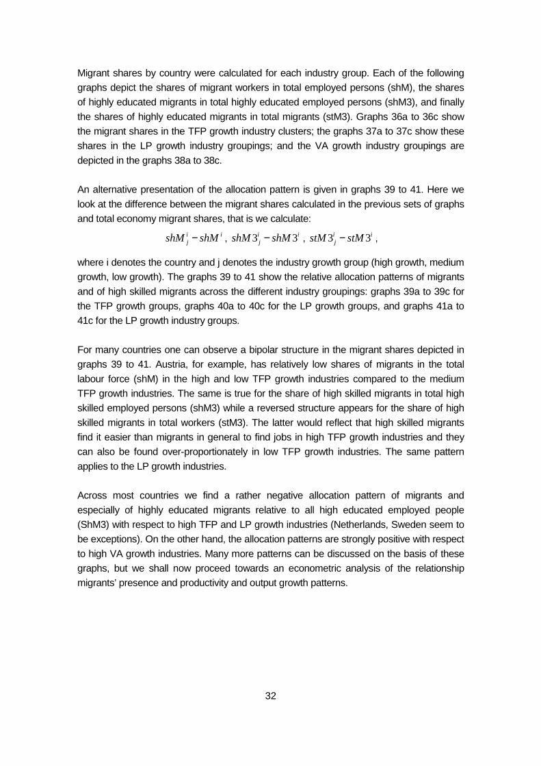
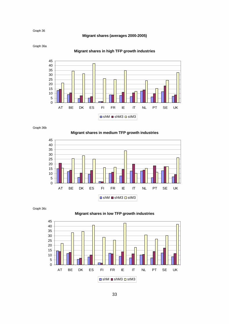
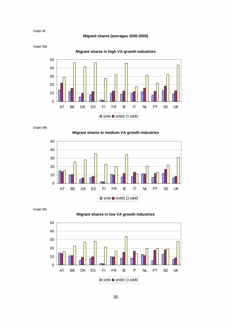
Migrant shares by country were calculated for each industry group. Each of the following

graphs depict the shares of migrant workers in total employed persons (shM), the shares

of highly educated migrants in total highly educated employed persons (shM3), and finally

the shares of highly educated migrants in total migrants (stM3). Graphs 36a to 36c show

the migrant shares in the TFP growth industry clusters; the graphs 37a to 37c show these

shares in the LP growth industry groupings; and the VA growth industry groupings are

depicted in the graphs 38a to 38c.

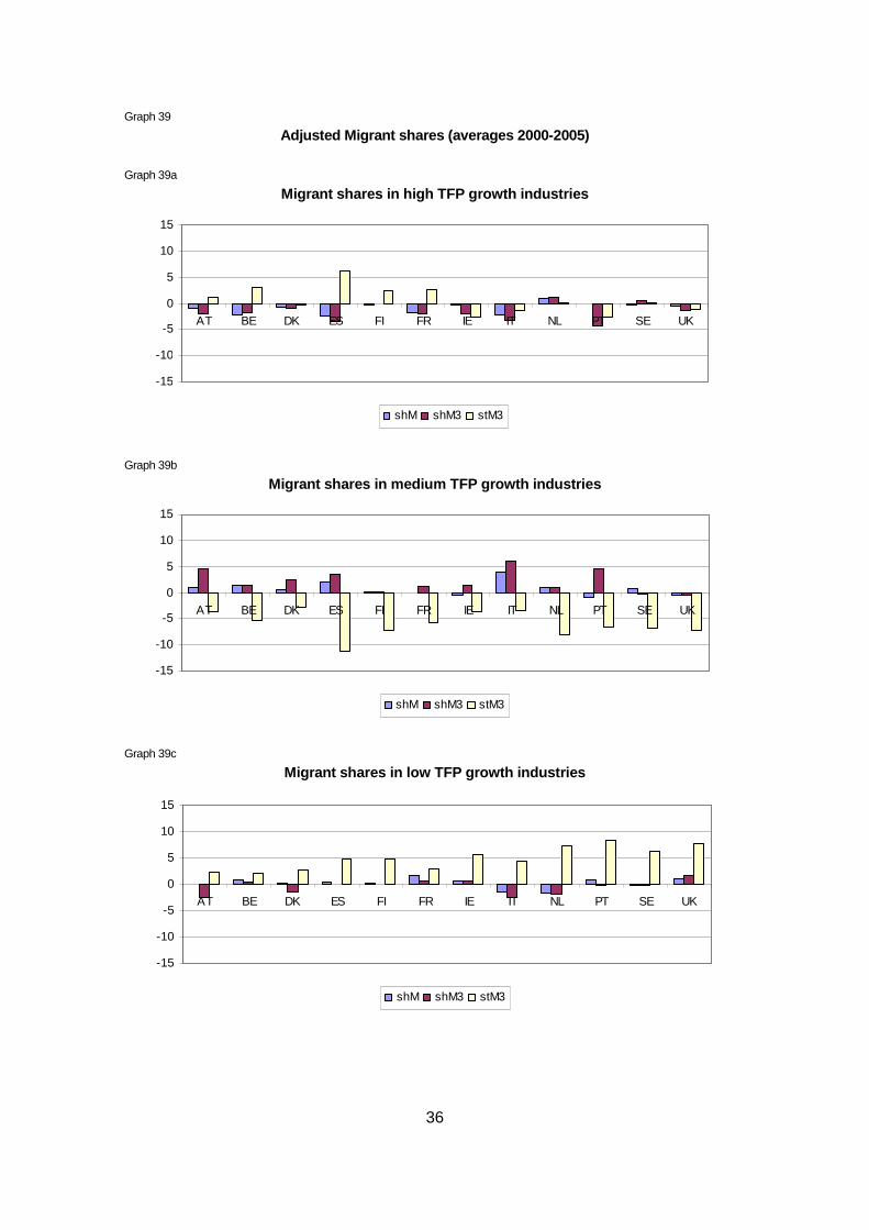
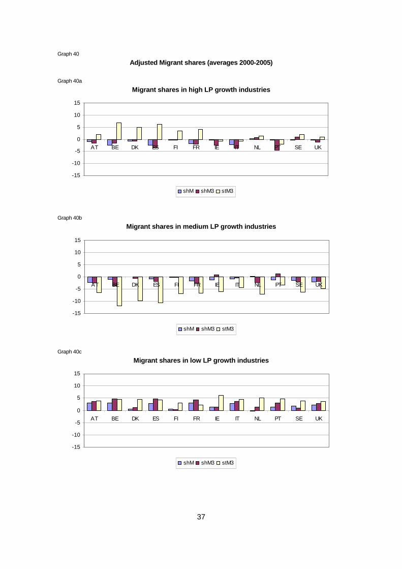
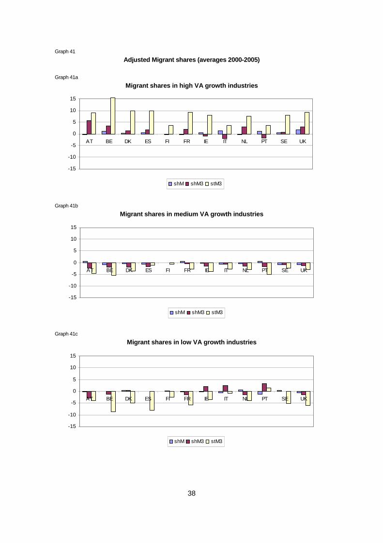
An alternative presentation of the allocation pattern is given in graphs 39 to 41. Here we

look at the difference between the migrant shares calculated in the previous sets of graphs

and total economy migrant shares, that is we calculate:

i ijshM shM− , 3 3i i

jshM shM− , 3 3i ijstM stM− ,

where i denotes the country and j denotes the industry growth group (high growth, medium

growth, low growth). The graphs 39 to 41 show the relative allocation patterns of migrants

and of high skilled migrants across the different industry groupings: graphs 39a to 39c for

the TFP growth groups, graphs 40a to 40c for the LP growth groups, and graphs 41a to

41c for the LP growth industry groups.

For many countries one can observe a bipolar structure in the migrant shares depicted in

graphs 39 to 41. Austria, for example, has relatively low shares of migrants in the total

labour force (shM) in the high and low TFP growth industries compared to the medium

TFP growth industries. The same is true for the share of high skilled migrants in total high

skilled employed persons (shM3) while a reversed structure appears for the share of high

skilled migrants in total workers (stM3). The latter would reflect that high skilled migrants

find it easier than migrants in general to find jobs in high TFP growth industries and they

can also be found over-proportionately in low TFP growth industries. The same pattern

applies to the LP growth industries.

Across most countries we find a rather negative allocation pattern of migrants and

especially of highly educated migrants relative to all high educated employed people

(ShM3) with respect to high TFP and LP growth industries (Netherlands, Sweden seem to

be exceptions). On the other hand, the allocation patterns are strongly positive with respect

to high VA growth industries. Many more patterns can be discussed on the basis of these

graphs, but we shall now proceed towards an econometric analysis of the relationship

migrants’ presence and productivity and output growth patterns.

33

Graph 36

Migrant shares (averages 2000-2005)

Graph 36a

Migrant shares in high TFP growth industries

05

1015202530354045

AT BE DK ES FI FR IE IT NL PT SE UK

shM shM3 stM3

Graph 36b

Migrant shares in medium TFP growth industries

05

1015202530354045


shM shM3 stM3

Graph 36c

Migrant shares in low TFP growth industries

05

1015202530354045


shM shM3 stM3

34

Graph 37


Graph 37a

Migrant shares in high LP growth industries

05

1015202530354045


shM shM3 stM3

Graph 37b

Migrant shares in medium LP growth industries

05

1015202530354045


shM shM3 stM3

Graph 37c

Migrant shares in low LP growth industries

05

1015202530354045


shM shM3 stM3

35

Graph 38


Graph 38a

Migrant shares in high VA growth industries

0

10

20

30

40

50


shM shM3 stM3

Graph 38b

Migrant shares in medium VA growth industries

0

10

20

30

40

50


shM shM3 stM3

Graph 38c

Migrant shares in low VA growth industries

0

10

20

30

40

50


shM shM3 stM3

36

Graph 39

Adjusted Migrant shares (averages 2000-2005)

Graph 39a

Migrant shares in high TFP growth industries

-15

-10

-5

0

5

10

15


shM shM3 stM3

Graph 39b

Migrant shares in medium TFP growth industries

-15

-10

-5

0

5

10

15


shM shM3 stM3

Graph 39c

Migrant shares in low TFP growth industries

-15

-10

-5

0

5

10

15


shM shM3 stM3

37

Graph 40


Graph 40a

Migrant shares in high LP growth industries

-15

-10

-5

0

5

10

15


shM shM3 stM3

Graph 40b

Migrant shares in medium LP growth industries

-15

-10

-5

0

5

10

15


shM shM3 stM3

Graph 40c

Migrant shares in low LP growth industries

-15

-10

-5

0

5

10

15


shM shM3 stM3

38

Graph 41


Graph 41a

Migrant shares in high VA growth industries

-15

-10

-5

0

5

10

15


shM shM3 stM3

Graph 41b

Migrant shares in medium VA growth industries

-15

-10

-5

0

5

10

15


shM shM3 stM3

Graph 41c

Migrant shares in low VA growth industries

-15

-10

-5

0

5

10

15


shM shM3 stM3

39

Appendix A

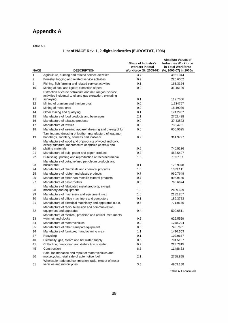
Table A.1

List of NACE Rev. 1, 2 digits industries (EUROSTAT, 1996)

NACE DESCRIPTION

Share of Industry's workers in total

Workforce (%, 2005-07)

Absolute Values of Industries Workforce

in Total Workforce (%, 2005-07) in 1000s

1 Agriculture, hunting and related service activities 3.7 4951.044 2 Forestry, logging and related service activities 0.2 220.6002 5 Fishing, fish farming and related service activities 0.1 163.3164 10 Mining of coal and lignite; extraction of peat 0.0 31.46129

11

Extraction of crude petroleum and natural gas; service activities incidental to oil and gas extraction, excluding surveying 0.1 112.7606

12 Mining of uranium and thorium ores 0.0 1.734797 13 Mining of metal ores 0.0 18.49986 14 Other mining and quarrying 0.1 174.2967 15 Manufacture of food products and beverages 2.1 2762.438 16 Manufacture of tobacco products 0.0 37.43523 17 Manufacture of textiles 0.5 733.4781 18 Manufacture of wearing apparel; dressing and dyeing of fur 0.5 656.9625

19 Tanning and dressing of leather; manufacture of luggage, handbags, saddlery, harness and footwear 0.2 314.9727

20

Manufacture of wood and of products of wood and cork, except furniture; manufacture of articles of straw and plaiting materials 0.5 740.5136

21 Manufacture of pulp, paper and paper products 0.3 463.5497 22 Publishing, printing and reproduction of recorded media 1.0 1397.87

23 Manufacture of coke, refined petroleum products and nuclear fuel 0.1 173.9078

24 Manufacture of chemicals and chemical products 1.0 1383.111 25 Manufacture of rubber and plastic products 0.7 960.7648 26 Manufacture of other non-metallic mineral products 0.7 998.9135 27 Manufacture of basic metals 0.6 766.6674

28 Manufacture of fabricated metal products, except machinery and equipment 1.8 2439.699

29 Manufacture of machinery and equipment n.e.c. 1.6 2132.207 30 Manufacture of office machinery and computers 0.1 189.3763 31 Manufacture of electrical machinery and apparatus n.e.c. 0.6 771.0156

32 Manufacture of radio, television and communication equipment and apparatus 0.4 500.6511

33 Manufacture of medical, precision and optical instruments, watches and clocks 0.5 629.5529

34 Manufacture of motor vehicles 0.9 1278.294 35 Manufacture of other transport equipment 0.6 743.7681 36 Manufacture of furniture; manufacturing n.e.c. 1.1 1416.303 37 Recycling 0.1 102.0657 40 Electricity, gas, steam and hot water supply 0.5 704.5107 41 Collection, purification and distribution of water 0.2 228.7815 45 Construction 8.5 11488.83

50 Sale, maintenance and repair of motor vehicles and motorcycles; retail sale of automotive fuel 2.1 2765.865

51 Wholesale trade and commission trade, except of motor vehicles and motorcycles 3.6 4903.188

Table A.1 continued

40

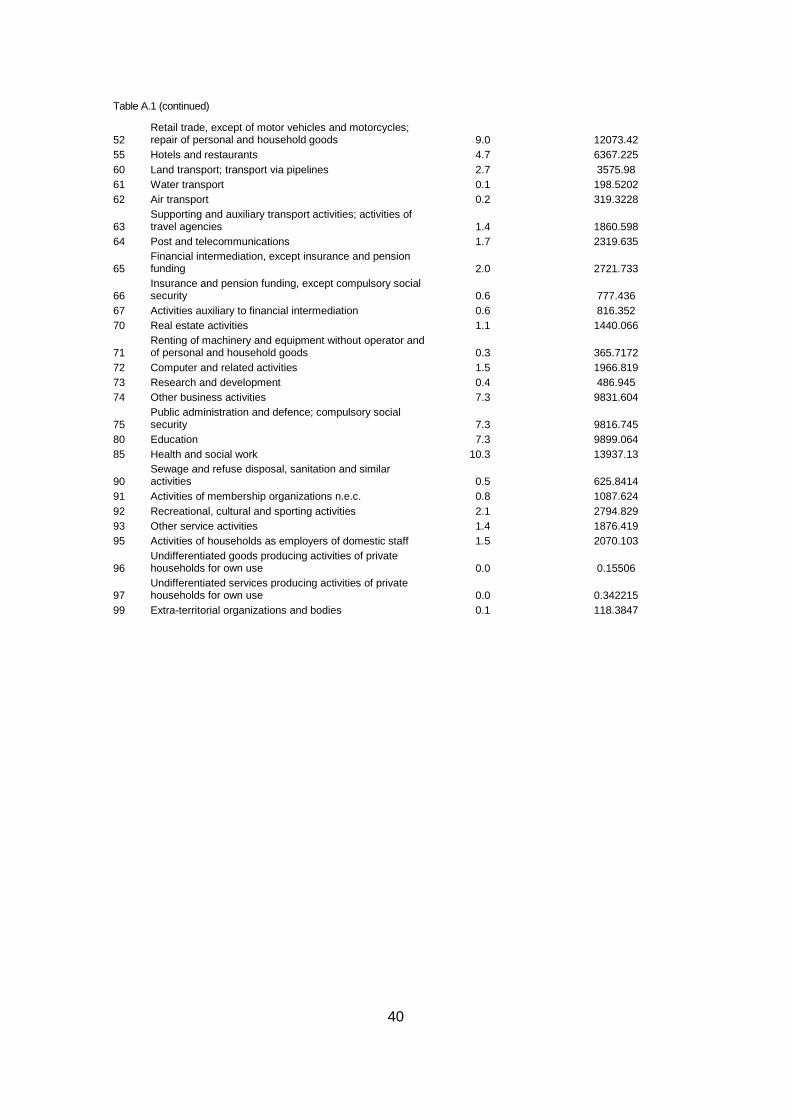
Table A.1 (continued)

52 Retail trade, except of motor vehicles and motorcycles; repair of personal and household goods 9.0 12073.42

55 Hotels and restaurants 4.7 6367.225 60 Land transport; transport via pipelines 2.7 3575.98 61 Water transport 0.1 198.5202 62 Air transport 0.2 319.3228

63 Supporting and auxiliary transport activities; activities of travel agencies 1.4 1860.598

64 Post and telecommunications 1.7 2319.635

65 Financial intermediation, except insurance and pension funding 2.0 2721.733

66 Insurance and pension funding, except compulsory social security 0.6 777.436

67 Activities auxiliary to financial intermediation 0.6 816.352 70 Real estate activities 1.1 1440.066

71 Renting of machinery and equipment without operator and of personal and household goods 0.3 365.7172

72 Computer and related activities 1.5 1966.819 73 Research and development 0.4 486.945 74 Other business activities 7.3 9831.604

75 Public administration and defence; compulsory social security 7.3 9816.745

80 Education 7.3 9899.064 85 Health and social work 10.3 13937.13

90 Sewage and refuse disposal, sanitation and similar activities 0.5 625.8414

91 Activities of membership organizations n.e.c. 0.8 1087.624 92 Recreational, cultural and sporting activities 2.1 2794.829 93 Other service activities 1.4 1876.419 95 Activities of households as employers of domestic staff 1.5 2070.103

96 Undifferentiated goods producing activities of private households for own use 0.0 0.15506

97 Undifferentiated services producing activities of private households for own use 0.0 0.342215

99 Extra-territorial organizations and bodies 0.1 118.3847

41

3. Part II: Migrants and productivity and output gr owth – regional and sectoral impacts - econometric analys is

3.1 Migrants and industry performance

3.1.1 Introduction

In this part of the study we present descriptive econometric evidence on the relation of

migrant variables and industry performance. For the latter we use change in total factor

productivity, labour productivity and value added growth. Total factor productivity measures

are taken from the EU KLEMS database3 which provides total factor productivity measures

at the disaggregated level for almost all countries for which also migrant variables are

available (see Timmer et al., 2008, for details). In the growth accounting exercise the

change in output (i.e. value added as we consider value added TFP) of a particular industry

i is expressed as the weighted growth of inputs and total factor productivity (TFP), i.e.

jtjktk jktit TFPXsY lnlnln ∆+∆=∆ ∑

where i denotes the sector, t is time, Y is value added, s denotes two-period average

shares and k denotes the factors of production (e.g. capital, labour); TFP is total factor

productivity. Measures of labour inputs in the EU KLEMS database are based on detailed

hours worked data by education, age and gender and capital stock is broken down into

several asset types. The shares are constructed using information of factor prices. This

equation is based on various assumptions (competitive factor markets, full input utilization

and constant returns to scale). Under these strict neo-classical assumptions TFP growth

should measure disembodied technical change. However as it is measured as a residual

this terms also includes a number of other effects like changes in returns to scale, mark-

ups, measurement errors, and unmeasured inputs. (For technical details see Timmer et al.,

2008, and Jorgenson et al., 2005). Total factor productivity growth is thus calculated taking

into account different types of labour (by educational levels, age structures and gender

differences). However, the calculations do not differentiate between domestic and foreign

workers which could have an additional effect. The use of migrant labour on total factor

productivity could be positive or negative: it could be positive e.g. when there is a ‘gain

from variety’ i.e. migrants add certain skills which domestic workers do not possess (see

Ottaviano and Peri, 2006a and 2006b), or they could contribute more work effort given the

same level of skills, or they allow the use of a better mix of skills in case there are skill

supply constraints, etc. The impact could, of course, also be negative, in case migrant

workers' actual skills are less than those formally measured, or work attitudes are worse

compared to domestic workers, or a more heterogeneous work force gives more cause to

frictions and thus reduced work performance, etc. All these possible effects have not been

taken into account when one constructed the measure of TFP in the EUKLEMS database

3 www.euklems.net

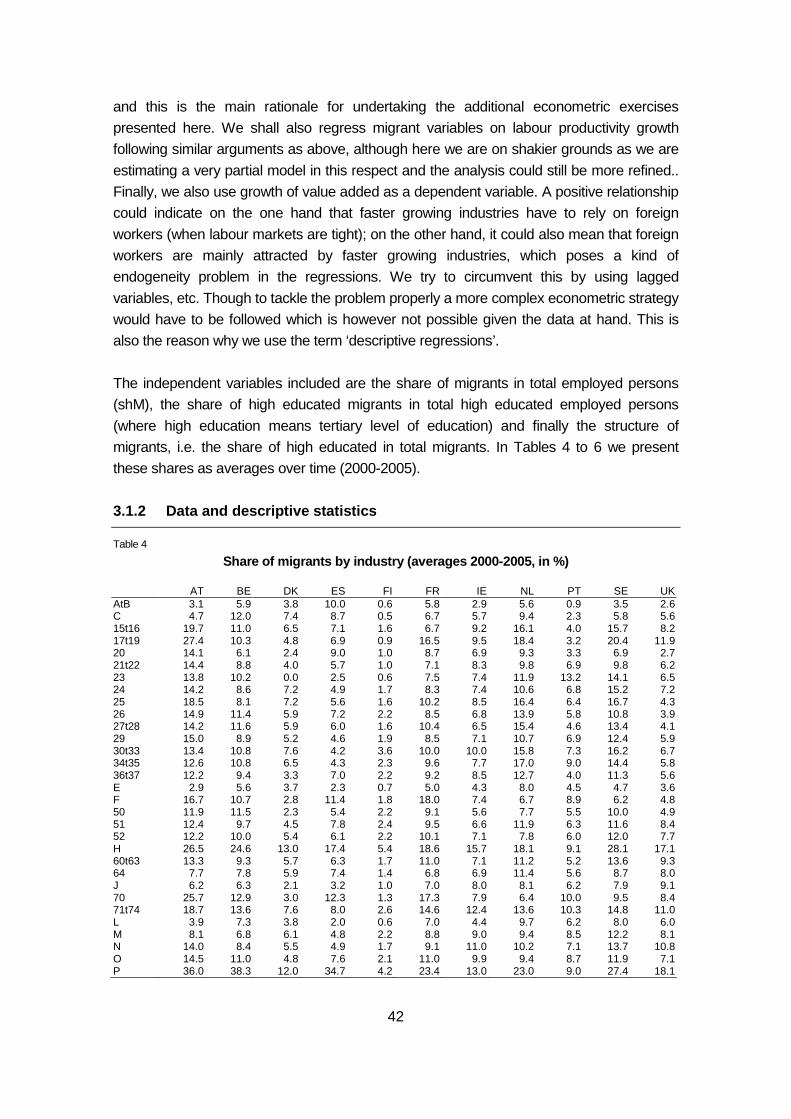
42

and this is the main rationale for undertaking the additional econometric exercises

presented here. We shall also regress migrant variables on labour productivity growth

following similar arguments as above, although here we are on shakier grounds as we are

estimating a very partial model in this respect and the analysis could still be more refined..

Finally, we also use growth of value added as a dependent variable. A positive relationship

could indicate on the one hand that faster growing industries have to rely on foreign

workers (when labour markets are tight); on the other hand, it could also mean that foreign

workers are mainly attracted by faster growing industries, which poses a kind of

endogeneity problem in the regressions. We try to circumvent this by using lagged

variables, etc. Though to tackle the problem properly a more complex econometric strategy

would have to be followed which is however not possible given the data at hand. This is

also the reason why we use the term ‘descriptive regressions’.

The independent variables included are the share of migrants in total employed persons

(shM), the share of high educated migrants in total high educated employed persons

(where high education means tertiary level of education) and finally the structure of

migrants, i.e. the share of high educated in total migrants. In Tables 4 to 6 we present

these shares as averages over time (2000-2005).

3.1.2 Data and descriptive statistics

Table 4

Share of migrants by industry (averages 2000-2005, in %)

AT BE DK ES FI FR IE NL PT SE UK AtB 3.1 5.9 3.8 10.0 0.6 5.8 2.9 5.6 0.9 3.5 2.6 C 4.7 12.0 7.4 8.7 0.5 6.7 5.7 9.4 2.3 5.8 5.6 15t16 19.7 11.0 6.5 7.1 1.6 6.7 9.2 16.1 4.0 15.7 8.2 17t19 27.4 10.3 4.8 6.9 0.9 16.5 9.5 18.4 3.2 20.4 11.9 20 14.1 6.1 2.4 9.0 1.0 8.7 6.9 9.3 3.3 6.9 2.7 21t22 14.4 8.8 4.0 5.7 1.0 7.1 8.3 9.8 6.9 9.8 6.2 23 13.8 10.2 0.0 2.5 0.6 7.5 7.4 11.9 13.2 14.1 6.5 24 14.2 8.6 7.2 4.9 1.7 8.3 7.4 10.6 6.8 15.2 7.2 25 18.5 8.1 7.2 5.6 1.6 10.2 8.5 16.4 6.4 16.7 4.3 26 14.9 11.4 5.9 7.2 2.2 8.5 6.8 13.9 5.8 10.8 3.9 27t28 14.2 11.6 5.9 6.0 1.6 10.4 6.5 15.4 4.6 13.4 4.1 29 15.0 8.9 5.2 4.6 1.9 8.5 7.1 10.7 6.9 12.4 5.9 30t33 13.4 10.8 7.6 4.2 3.6 10.0 10.0 15.8 7.3 16.2 6.7 34t35 12.6 10.8 6.5 4.3 2.3 9.6 7.7 17.0 9.0 14.4 5.8 36t37 12.2 9.4 3.3 7.0 2.2 9.2 8.5 12.7 4.0 11.3 5.6 E 2.9 5.6 3.7 2.3 0.7 5.0 4.3 8.0 4.5 4.7 3.6 F 16.7 10.7 2.8 11.4 1.8 18.0 7.4 6.7 8.9 6.2 4.8 50 11.9 11.5 2.3 5.4 2.2 9.1 5.6 7.7 5.5 10.0 4.9 51 12.4 9.7 4.5 7.8 2.4 9.5 6.6 11.9 6.3 11.6 8.4 52 12.2 10.0 5.4 6.1 2.2 10.1 7.1 7.8 6.0 12.0 7.7 H 26.5 24.6 13.0 17.4 5.4 18.6 15.7 18.1 9.1 28.1 17.1 60t63 13.3 9.3 5.7 6.3 1.7 11.0 7.1 11.2 5.2 13.6 9.3 64 7.7 7.8 5.9 7.4 1.4 6.8 6.9 11.4 5.6 8.7 8.0 J 6.2 6.3 2.1 3.2 1.0 7.0 8.0 8.1 6.2 7.9 9.1 70 25.7 12.9 3.0 12.3 1.3 17.3 7.9 6.4 10.0 9.5 8.4 71t74 18.7 13.6 7.6 8.0 2.6 14.6 12.4 13.6 10.3 14.8 11.0 L 3.9 7.3 3.8 2.0 0.6 7.0 4.4 9.7 6.2 8.0 6.0 M 8.1 6.8 6.1 4.8 2.2 8.8 9.0 9.4 8.5 12.2 8.1 N 14.0 8.4 5.5 4.9 1.7 9.1 11.0 10.2 7.1 13.7 10.8 O 14.5 11.0 4.8 7.6 2.1 11.0 9.9 9.4 8.7 11.9 7.1 P 36.0 38.3 12.0 34.7 4.2 23.4 13.0 23.0 9.0 27.4 18.1

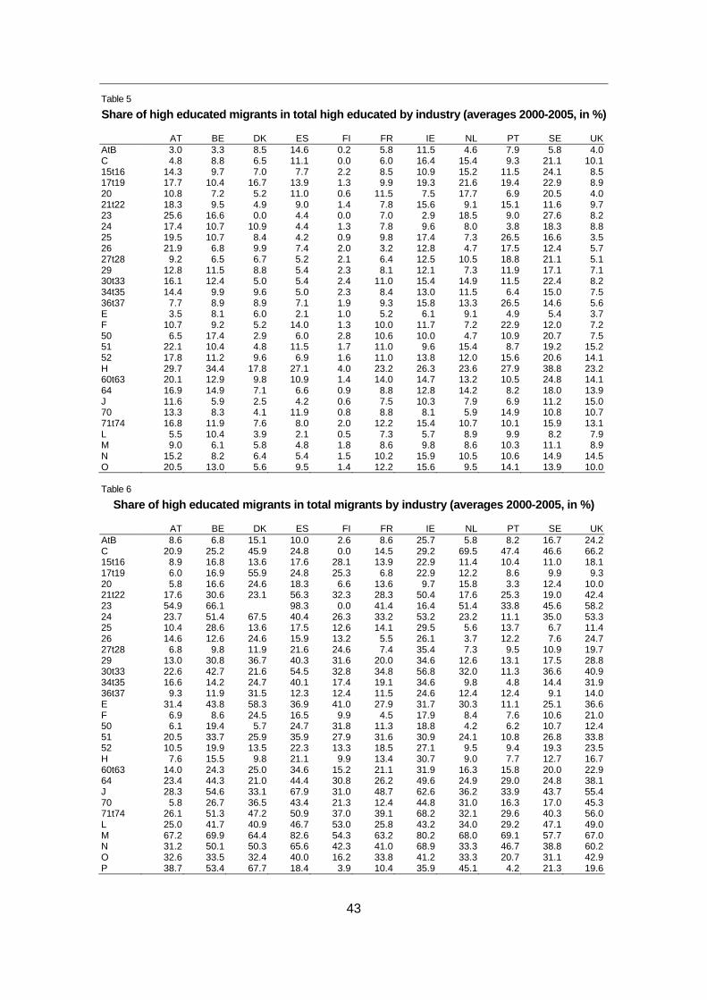
43

Table 5

Share of high educated migrants in total high educa ted by industry (averages 2000-2005, in %)

AT BE DK ES FI FR IE NL PT SE UK AtB 3.0 3.3 8.5 14.6 0.2 5.8 11.5 4.6 7.9 5.8 4.0 C 4.8 8.8 6.5 11.1 0.0 6.0 16.4 15.4 9.3 21.1 10.1 15t16 14.3 9.7 7.0 7.7 2.2 8.5 10.9 15.2 11.5 24.1 8.5 17t19 17.7 10.4 16.7 13.9 1.3 9.9 19.3 21.6 19.4 22.9 8.9 20 10.8 7.2 5.2 11.0 0.6 11.5 7.5 17.7 6.9 20.5 4.0 21t22 18.3 9.5 4.9 9.0 1.4 7.8 15.6 9.1 15.1 11.6 9.7 23 25.6 16.6 0.0 4.4 0.0 7.0 2.9 18.5 9.0 27.6 8.2 24 17.4 10.7 10.9 4.4 1.3 7.8 9.6 8.0 3.8 18.3 8.8 25 19.5 10.7 8.4 4.2 0.9 9.8 17.4 7.3 26.5 16.6 3.5 26 21.9 6.8 9.9 7.4 2.0 3.2 12.8 4.7 17.5 12.4 5.7 27t28 9.2 6.5 6.7 5.2 2.1 6.4 12.5 10.5 18.8 21.1 5.1 29 12.8 11.5 8.8 5.4 2.3 8.1 12.1 7.3 11.9 17.1 7.1 30t33 16.1 12.4 5.0 5.4 2.4 11.0 15.4 14.9 11.5 22.4 8.2 34t35 14.4 9.9 9.6 5.0 2.3 8.4 13.0 11.5 6.4 15.0 7.5 36t37 7.7 8.9 8.9 7.1 1.9 9.3 15.8 13.3 26.5 14.6 5.6 E 3.5 8.1 6.0 2.1 1.0 5.2 6.1 9.1 4.9 5.4 3.7 F 10.7 9.2 5.2 14.0 1.3 10.0 11.7 7.2 22.9 12.0 7.2 50 6.5 17.4 2.9 6.0 2.8 10.6 10.0 4.7 10.9 20.7 7.5 51 22.1 10.4 4.8 11.5 1.7 11.0 9.6 15.4 8.7 19.2 15.2 52 17.8 11.2 9.6 6.9 1.6 11.0 13.8 12.0 15.6 20.6 14.1 H 29.7 34.4 17.8 27.1 4.0 23.2 26.3 23.6 27.9 38.8 23.2 60t63 20.1 12.9 9.8 10.9 1.4 14.0 14.7 13.2 10.5 24.8 14.1 64 16.9 14.9 7.1 6.6 0.9 8.8 12.8 14.2 8.2 18.0 13.9 J 11.6 5.9 2.5 4.2 0.6 7.5 10.3 7.9 6.9 11.2 15.0 70 13.3 8.3 4.1 11.9 0.8 8.8 8.1 5.9 14.9 10.8 10.7 71t74 16.8 11.9 7.6 8.0 2.0 12.2 15.4 10.7 10.1 15.9 13.1 L 5.5 10.4 3.9 2.1 0.5 7.3 5.7 8.9 9.9 8.2 7.9 M 9.0 6.1 5.8 4.8 1.8 8.6 9.8 8.6 10.3 11.1 8.9 N 15.2 8.2 6.4 5.4 1.5 10.2 15.9 10.5 10.6 14.9 14.5 O 20.5 13.0 5.6 9.5 1.4 12.2 15.6 9.5 14.1 13.9 10.0

Table 6

Share of high educated migrants in total migrants b y industry (averages 2000-2005, in %)

AT BE DK ES FI FR IE NL PT SE UK AtB 8.6 6.8 15.1 10.0 2.6 8.6 25.7 5.8 8.2 16.7 24.2 C 20.9 25.2 45.9 24.8 0.0 14.5 29.2 69.5 47.4 46.6 66.2 15t16 8.9 16.8 13.6 17.6 28.1 13.9 22.9 11.4 10.4 11.0 18.1 17t19 6.0 16.9 55.9 24.8 25.3 6.8 22.9 12.2 8.6 9.9 9.3 20 5.8 16.6 24.6 18.3 6.6 13.6 9.7 15.8 3.3 12.4 10.0 21t22 17.6 30.6 23.1 56.3 32.3 28.3 50.4 17.6 25.3 19.0 42.4 23 54.9 66.1 98.3 0.0 41.4 16.4 51.4 33.8 45.6 58.2 24 23.7 51.4 67.5 40.4 26.3 33.2 53.2 23.2 11.1 35.0 53.3 25 10.4 28.6 13.6 17.5 12.6 14.1 29.5 5.6 13.7 6.7 11.4 26 14.6 12.6 24.6 15.9 13.2 5.5 26.1 3.7 12.2 7.6 24.7 27t28 6.8 9.8 11.9 21.6 24.6 7.4 35.4 7.3 9.5 10.9 19.7 29 13.0 30.8 36.7 40.3 31.6 20.0 34.6 12.6 13.1 17.5 28.8 30t33 22.6 42.7 21.6 54.5 32.8 34.8 56.8 32.0 11.3 36.6 40.9 34t35 16.6 14.2 24.7 40.1 17.4 19.1 34.6 9.8 4.8 14.4 31.9 36t37 9.3 11.9 31.5 12.3 12.4 11.5 24.6 12.4 12.4 9.1 14.0 E 31.4 43.8 58.3 36.9 41.0 27.9 31.7 30.3 11.1 25.1 36.6 F 6.9 8.6 24.5 16.5 9.9 4.5 17.9 8.4 7.6 10.6 21.0 50 6.1 19.4 5.7 24.7 31.8 11.3 18.8 4.2 6.2 10.7 12.4 51 20.5 33.7 25.9 35.9 27.9 31.6 30.9 24.1 10.8 26.8 33.8 52 10.5 19.9 13.5 22.3 13.3 18.5 27.1 9.5 9.4 19.3 23.5 H 7.6 15.5 9.8 21.1 9.9 13.4 30.7 9.0 7.7 12.7 16.7 60t63 14.0 24.3 25.0 34.6 15.2 21.1 31.9 16.3 15.8 20.0 22.9 64 23.4 44.3 21.0 44.4 30.8 26.2 49.6 24.9 29.0 24.8 38.1 J 28.3 54.6 33.1 67.9 31.0 48.7 62.6 36.2 33.9 43.7 55.4 70 5.8 26.7 36.5 43.4 21.3 12.4 44.8 31.0 16.3 17.0 45.3 71t74 26.1 51.3 47.2 50.9 37.0 39.1 68.2 32.1 29.6 40.3 56.0 L 25.0 41.7 40.9 46.7 53.0 25.8 43.2 34.0 29.2 47.1 49.0 M 67.2 69.9 64.4 82.6 54.3 63.2 80.2 68.0 69.1 57.7 67.0 N 31.2 50.1 50.3 65.6 42.3 41.0 68.9 33.3 46.7 38.8 60.2 O 32.6 33.5 32.4 40.0 16.2 33.8 41.2 33.3 20.7 31.1 42.9 P 38.7 53.4 67.7 18.4 3.9 10.4 35.9 45.1 4.2 21.3 19.6

44

3.1.3 Descriptive regressions on total economy

We now present some regression results for the three independent and the set of

dependent variables. As the shares of migrants in total persons employed (ShM) and the

shares of high-educated migrants in total high-educated people (ShM3) correlate to some

extent (the coefficient of correlation being about 0.6 for the pooled cross-section sample for

instance) we also show results when including only one of them to circumvent problems

with multicollinearity. We present both cross-section results for both the pooled sample and

the individual countries and panel data results. For the former we calculated the average

growth rates of total factor productivity, labour productivity and value added growth and

regressed them on the initial values with respect to migration. A typical regression would

read for example (in the cross-section case)

ictictictictict DummiesstMshMshMTFP εβββα +++++=∆ 33 121

where Dummies denote a set of country and/or industry dummies and ε denotes the

usual error term. For the panel regression we use a similar equation with the proper error

term specification.

3.1.3.1 Cross-section results

In Table 7 we present the first set of regression results. Each column shows a different

specification with respect to variables included. Columns 1-4 report the results when

including all three migrant variables with different sets of dummies (for countries and

industries); in columns 5-8 the variable shM3 (the share of high-educated migrants in total

high-educated employed persons) is left out due to correlation with the share of high-

educated migrants in total migrants (stM3); conversely in column 9-12 we skipped stM3.

With respect to total factor productivity we find significantly positive effects for

specifications 7 and 8 for both the share of migrants and the share of high-educated

migrants in total migrants and also in specification 9. Using the specification with the best

goodness of fit, the effect is however quite small. Turning to labour productivity as a

dependent variable we find only a significant effect of the share of high-educated migrants

in total high-educated employed persons in specification 1. With respect to growth of value

added we find more often significant effects, in particular for the share of high-educated

migrants in total migrants, though the effect becomes less significant when including

dummy variables. It even disappears when including both industry and country dummies.

Summarising, this set of results does not hint towards a negative effect of the impact of

migrants on industry performance measures, though they are also not showing a robust

positive significant effect of migration. In the Appendix Tables B.1-B.3 we present country

specific results. There is no clear and consistent pattern across countries though the

migration variables tend to be more often negative and for some countries significantly so.

As in this case the variation is only across industries one can however not rule out

endogeneity effects: If migrants are mostly occupied in low growth industries we would

45

expect to find a negative effect, though across countries the effect tends to be positive

though not necessarily significant.

3.1.3.2 Panel results on pooled sample

Next we turn to panel regression results. In Table 8 we show results when regressing the

growth rate (of total factor productivity, labour productivity and value added) on the

contemporaneous variables. Again we report different specifications with respect to

inclusion of country, industry and year dummies and including shM and shM3 separately.

In this specification we find no significant effect of migrant variables on total factor

productivity growth or labour productivity growth. Only when using value added growth as

dependent variable we find a positive significant effect of the share of high-educated

migrants in total migrants (stM3) in a number of specifications. This significance gets lost

however when including industry dummies.

In Table 9 we present similar results however using migrant variables lagged by one year.

In this case we find more often significantly negative effects of migrant variables on total

factor productivity and labour productivity growth. For value added growth we again find a

similar pattern as above; there is a significant positive effect which however vanishes when

taking industry-specific effects into account.

Finally, we regress the dependent variables on changes in the migrant variables. These

results are reported in Table 10. In this case we find strongly significant positive variables,

in particular for the change in the share of migrants in total persons employed with less

significant effects regarding the skill composition of migrants. For both these variables, i.e.

the share of high-educated migrants in total high-educated persons employed and the

share of high-educated migrants in total migrants, no robust significant effects appear. This

is mostly the case for all three performance variables used in this study.

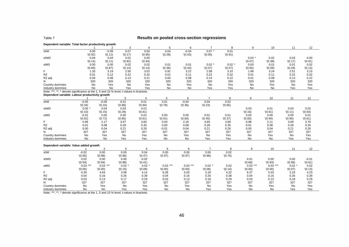
46

Table 7 Results on pooled cross-section regressions

Dependent variable: Total factor productivity growt h 1 2 3 4 5 6 7 8 9 10 11 12 shM 0.00 -0.09 0.07 0.00 0.04 -0.04 0.07 * 0.01 '(0.92) '(0.12) '(0.17) '(0.95) '(0.28) '(0.43) '(0.05) '(0.91) shM3 0.04 0.04 0.01 0.00 0.04 * 0.02 0.03 0.00 '(0.14) '(0.11) '(0.82) '(0.94) '(0.07) '(0.38) '(0.17) '(0.91) stM3 0.00 0.00 0.02 0.02 0.01 0.01 0.02 * 0.02 * 0.00 0.01 0.01 0.02 '(0.69) '(0.87) '(0.14) '(0.14) '(0.36) '(0.43) '(0.07) '(0.07) '(0.65) '(0.59) '(0.29) '(0.13) F 1.33 3.19 2.50 3.02 0.91 3.22 2.58 3.10 1.99 3.24 2.51 3.10 R2 0.01 0.12 0.22 0.32 0.01 0.11 0.22 0.32 0.01 0.11 0.22 0.32 R2 adj. 0.00 0.08 0.13 0.21 0.00 0.08 0.14 0.22 0.01 0.08 0.13 0.22 N 320 320 320 320 320 320 320 320 320 320 320 320 Country dummies No Yes No Yes No Yes No Yes No Yes No Yes Industry dummies No No Yes Yes No No Yes Yes No No Yes Yes Note: ***, **, * denote significance at the 1, 5 and 10 % level; t-values in brackets. Dependent variable: Labour productivity growth 1 2 3 4 5 6 7 8 9 10 11 12 shM -0.05 -0.09 0.01 0.01 0.01 -0.04 0.04 0.02 '(0.34) '(0.10) '(0.86) '(0.94) '(0.79) '(0.36) '(0.23) '(0.65) shM3 0.05 * 0.04 0.03 0.01 0.03 0.01 0.03 0.02 '(0.10) '(0.15) '(0.29) '(0.61) '(0.16) '(0.61) '(0.11) '(0.50) stM3 -0.01 0.00 0.00 0.01 0.00 0.00 0.01 0.01 0.00 0.00 0.00 0.01 '(0.62) '(0.72) '(0.85) '(0.61) '(0.91) '(0.83) '(0.45) '(0.37) '(0.83) '(0.94) '(0.90) '(0.61) F 0.96 2.17 3.57 3.60 0.04 2.16 3.65 3.69 0.98 2.11 3.69 3.70 R2 0.01 0.08 0.29 0.35 0.00 0.08 0.28 0.35 0.01 0.08 0.29 0.35 R2 adj. 0.00 0.04 0.21 0.26 -0.01 0.04 0.21 0.26 0.00 0.04 0.21 0.26 N 327 327 327 327 327 327 327 327 327 327 327 327 Country dummies No Yes No Yes No Yes No Yes No Yes No Yes Industry dummies No No Yes Yes No No Yes Yes No No Yes Yes Dependent variable: Value added growth 1 2 3 4 5 6 7 8 9 10 11 12 shM -0.02 0.00 0.00 0.04 0.00 0.00 0.00 0.02 '(0.65) '(0.99) '(0.96) '(0.47) '(0.97) '(0.97) '(0.96) '(0.76) shM3 0.02 0.00 0.00 -0.02 0.01 0.00 0.00 -0.01 '(0.54) '(0.94) '(0.98) '(0.41) '(0.68) '(0.93) '(0.99) '(0.61) stM3 0.03 *** 0.03 *** 0.02 * 0.02 * 0.03 *** 0.03 *** 0.02 * 0.02 0.03 *** 0.03 *** 0.02 * 0.02 '(0.00) '(0.00) '(0.10) '(0.09) '(0.00) '(0.00) '(0.06) '(0.14) '(0.00) '(0.00) '(0.07) '(0.13) F 4.30 4.63 3.08 4.14 6.28 5.03 3.19 4.22 6.37 5.03 3.19 4.23 R2 0.04 0.16 0.26 0.39 0.04 0.16 0.26 0.38 0.04 0.16 0.26 0.39 R2 adj. 0.03 0.13 0.17 0.29 0.03 0.13 0.18 0.29 0.03 0.13 0.18 0.29 N 327 327 327 327 327 327 327 327 327 327 327 327 Country dummies No Yes No Yes No Yes No Yes No Yes No Yes Industry dummies No No Yes Yes No No Yes Yes No No Yes Yes Note: ***, **, * denote significance at the 1, 5 and 10 % level; t-values in brackets.

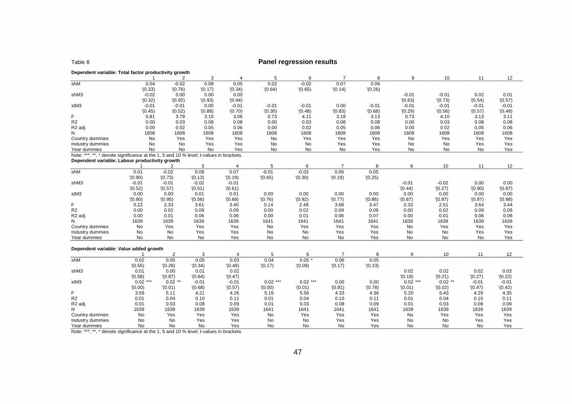
47

Table 8 Panel regression results Dependent variable: Total factor productivity growt h 1 2 3 4 5 6 7 8 9 10 11 12 shM 0.04 -0.02 0.08 0.05 0.02 -0.02 0.07 0.06 '(0.33) '(0.76) '(0.17) '(0.34) '(0.64) '(0.65) '(0.14) '(0.26) shM3 -0.02 0.00 0.00 0.00 -0.01 -0.01 0.02 0.01 '(0.32) '(0.92) '(0.93) '(0.94) '(0.63) '(0.73) '(0.54) '(0.57) stM3 -0.01 -0.01 0.00 -0.01 -0.01 -0.01 0.00 -0.01 -0.01 -0.01 -0.01 -0.01 '(0.45) '(0.52) '(0.88) '(0.70) '(0.30) '(0.48) '(0.83) '(0.68) '(0.29) '(0.56) '(0.57) '(0.48) F 0.81 3.79 3.10 3.06 0.73 4.11 3.18 3.13 0.73 4.10 3.13 3.11 R2 0.00 0.03 0.08 0.08 0.00 0.03 0.08 0.08 0.00 0.03 0.08 0.08 R2 adj. 0.00 0.02 0.05 0.06 0.00 0.02 0.05 0.06 0.00 0.02 0.05 0.06 N 1608 1608 1608 1608 1608 1608 1608 1608 1608 1608 1608 1608 Country dummies No Yes Yes Yes No Yes Yes Yes No Yes Yes Yes Industry dummies No No Yes Yes No No Yes Yes No No Yes Yes Year dummies No No No Yes No No No Yes No No No Yes Note: ***, **, * denote significance at the 1, 5 and 10 % level; t-values in brackets. Dependent variable: Labour productivity growth 1 2 3 4 5 6 7 8 9 10 11 12 shM 0.01 -0.02 0.08 0.07 -0.01 -0.03 0.06 0.05 '(0.90) '(0.73) '(0.13) '(0.19) '(0.65) '(0.30) '(0.19) '(0.25) shM3 -0.01 -0.01 -0.02 -0.01 -0.01 -0.02 0.00 0.00 '(0.52) '(0.57) '(0.51) '(0.61) '(0.44) '(0.27) '(0.90) '(0.87) stM3 0.00 0.00 0.01 0.01 0.00 0.00 0.00 0.00 0.00 0.00 0.00 0.00 '(0.90) '(0.95) '(0.56) '(0.68) '(0.76) '(0.92) '(0.77) '(0.86) '(0.87) '(0.87) '(0.87) '(0.98) F 0.22 2.33 3.61 3.40 0.14 2.48 3.68 3.47 0.33 2.51 3.64 3.44 R2 0.00 0.02 0.09 0.09 0.00 0.02 0.09 0.09 0.00 0.02 0.09 0.09 R2 adj. 0.00 0.01 0.06 0.06 0.00 0.01 0.06 0.07 0.00 0.01 0.06 0.06 N 1639 1639 1639 1639 1641 1641 1641 1641 1639 1639 1639 1639 Country dummies No Yes Yes Yes No Yes Yes Yes No Yes Yes Yes Industry dummies No No Yes Yes No No Yes Yes No No Yes Yes Year dummies No No No Yes No No No Yes No No No Yes Dependent variable: Value added growth 1 2 3 4 5 6 7 8 9 10 11 12 shM 0.02 0.05 0.05 0.03 0.04 0.05 * 0.06 0.05 '(0.55) '(0.26) '(0.34) '(0.49) '(0.17) '(0.09) '(0.17) '(0.23) shM3 0.01 0.00 0.01 0.02 0.02 0.02 0.02 0.03 '(0.58) '(0.87) '(0.64) '(0.47) '(0.18) '(0.21) '(0.27) '(0.22) stM3 0.02 *** 0.02 ** -0.01 -0.01 0.02 *** 0.02 *** 0.00 0.00 0.02 *** 0.02 ** -0.01 -0.01 '(0.00) '(0.01) '(0.68) '(0.57) '(0.00) '(0.01) '(0.81) '(0.78) '(0.01) '(0.02) '(0.47) '(0.42) F 3.59 5.11 4.21 4.26 5.16 5.56 4.33 4.36 5.20 5.43 4.29 4.35 R2 0.01 0.04 0.10 0.11 0.01 0.04 0.10 0.11 0.01 0.04 0.10 0.11 R2 adj. 0.01 0.03 0.08 0.09 0.01 0.03 0.08 0.09 0.01 0.03 0.08 0.09 N 1639 1639 1639 1639 1641 1641 1641 1641 1639 1639 1639 1639 Country dummies No Yes Yes Yes No Yes Yes Yes No Yes Yes Yes Industry dummies No No Yes Yes No No Yes Yes No No Yes Yes Year dummies No No No Yes No No No Yes No No No Yes Note: ***, **, * denote significance at the 1, 5 and 10 % level; t-values in brackets.

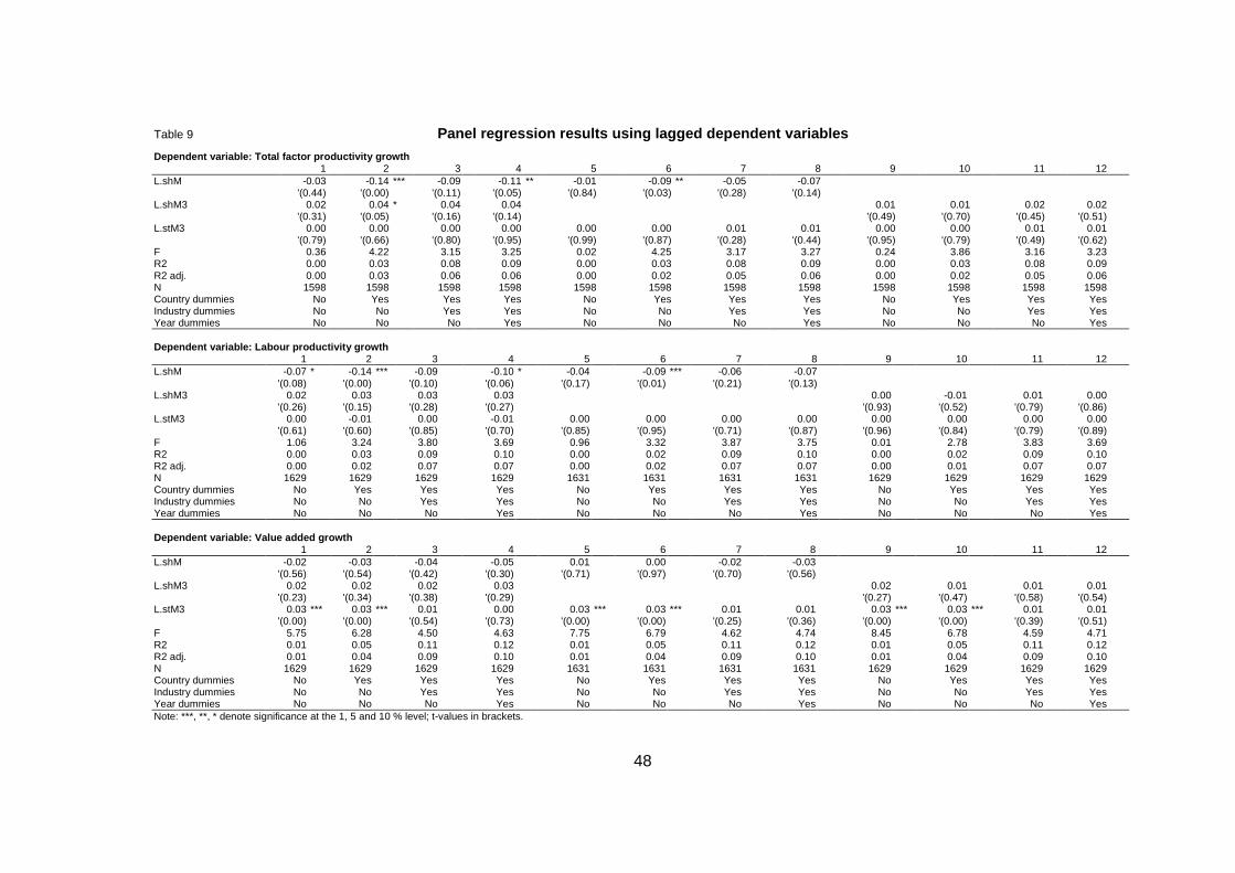
48

Table 9 Panel regression results using lagged dependent var iables Dependent variable: Total factor productivity growt h 1 2 3 4 5 6 7 8 9 10 11 12 L.shM -0.03 -0.14 *** -0.09 -0.11 ** -0.01 -0.09 ** -0.05 -0.07 '(0.44) '(0.00) '(0.11) '(0.05) '(0.84) '(0.03) '(0.28) '(0.14) L.shM3 0.02 0.04 * 0.04 0.04 0.01 0.01 0.02 0.02 '(0.31) '(0.05) '(0.16) '(0.14) '(0.49) '(0.70) '(0.45) '(0.51) L.stM3 0.00 0.00 0.00 0.00 0.00 0.00 0.01 0.01 0.00 0.00 0.01 0.01 '(0.79) '(0.66) '(0.80) '(0.95) '(0.99) '(0.87) '(0.28) '(0.44) '(0.95) '(0.79) '(0.49) '(0.62) F 0.36 4.22 3.15 3.25 0.02 4.25 3.17 3.27 0.24 3.86 3.16 3.23 R2 0.00 0.03 0.08 0.09 0.00 0.03 0.08 0.09 0.00 0.03 0.08 0.09 R2 adj. 0.00 0.03 0.06 0.06 0.00 0.02 0.05 0.06 0.00 0.02 0.05 0.06 N 1598 1598 1598 1598 1598 1598 1598 1598 1598 1598 1598 1598 Country dummies No Yes Yes Yes No Yes Yes Yes No Yes Yes Yes Industry dummies No No Yes Yes No No Yes Yes No No Yes Yes Year dummies No No No Yes No No No Yes No No No Yes Dependent variable: Labour productivity growth 1 2 3 4 5 6 7 8 9 10 11 12 L.shM -0.07 * -0.14 *** -0.09 -0.10 * -0.04 -0.09 *** -0.06 -0.07 '(0.08) '(0.00) '(0.10) '(0.06) '(0.17) '(0.01) '(0.21) '(0.13) L.shM3 0.02 0.03 0.03 0.03 0.00 -0.01 0.01 0.00 '(0.26) '(0.15) '(0.28) '(0.27) '(0.93) '(0.52) '(0.79) '(0.86) L.stM3 0.00 -0.01 0.00 -0.01 0.00 0.00 0.00 0.00 0.00 0.00 0.00 0.00 '(0.61) '(0.60) '(0.85) '(0.70) '(0.85) '(0.95) '(0.71) '(0.87) '(0.96) '(0.84) '(0.79) '(0.89) F 1.06 3.24 3.80 3.69 0.96 3.32 3.87 3.75 0.01 2.78 3.83 3.69 R2 0.00 0.03 0.09 0.10 0.00 0.02 0.09 0.10 0.00 0.02 0.09 0.10 R2 adj. 0.00 0.02 0.07 0.07 0.00 0.02 0.07 0.07 0.00 0.01 0.07 0.07 N 1629 1629 1629 1629 1631 1631 1631 1631 1629 1629 1629 1629 Country dummies No Yes Yes Yes No Yes Yes Yes No Yes Yes Yes Industry dummies No No Yes Yes No No Yes Yes No No Yes Yes Year dummies No No No Yes No No No Yes No No No Yes Dependent variable: Value added growth 1 2 3 4 5 6 7 8 9 10 11 12 L.shM -0.02 -0.03 -0.04 -0.05 0.01 0.00 -0.02 -0.03 '(0.56) '(0.54) '(0.42) '(0.30) '(0.71) '(0.97) '(0.70) '(0.56) L.shM3 0.02 0.02 0.02 0.03 0.02 0.01 0.01 0.01 '(0.23) '(0.34) '(0.38) '(0.29) '(0.27) '(0.47) '(0.58) '(0.54) L.stM3 0.03 *** 0.03 *** 0.01 0.00 0.03 *** 0.03 *** 0.01 0.01 0.03 *** 0.03 *** 0.01 0.01 '(0.00) '(0.00) '(0.54) '(0.73) '(0.00) '(0.00) '(0.25) '(0.36) '(0.00) '(0.00) '(0.39) '(0.51) F 5.75 6.28 4.50 4.63 7.75 6.79 4.62 4.74 8.45 6.78 4.59 4.71 R2 0.01 0.05 0.11 0.12 0.01 0.05 0.11 0.12 0.01 0.05 0.11 0.12 R2 adj. 0.01 0.04 0.09 0.10 0.01 0.04 0.09 0.10 0.01 0.04 0.09 0.10 N 1629 1629 1629 1629 1631 1631 1631 1631 1629 1629 1629 1629 Country dummies No Yes Yes Yes No Yes Yes Yes No Yes Yes Yes Industry dummies No No Yes Yes No No Yes Yes No No Yes Yes Year dummies No No No Yes No No No Yes No No No Yes Note: ***, **, * denote significance at the 1, 5 and 10 % level; t-values in brackets.

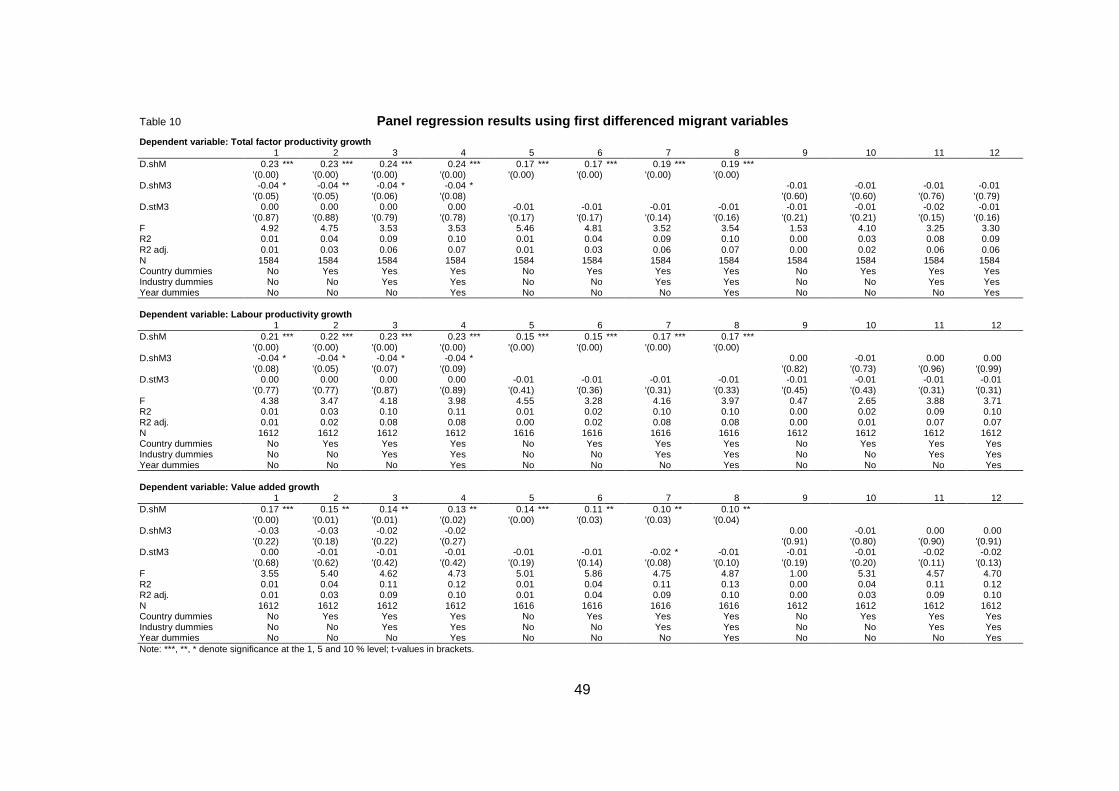
49

Table 10 Panel regression results using first differenced mi grant variables Dependent variable: Total factor productivity growt h 1 2 3 4 5 6 7 8 9 10 11 12 D.shM 0.23 *** 0.23 *** 0.24 *** 0.24 *** 0.17 *** 0.17 *** 0.19 *** 0.19 *** '(0.00) '(0.00) '(0.00) '(0.00) '(0.00) '(0.00) '(0.00) '(0.00) D.shM3 -0.04 * -0.04 ** -0.04 * -0.04 * -0.01 -0.01 -0.01 -0.01 '(0.05) '(0.05) '(0.06) '(0.08) '(0.60) '(0.60) '(0.76) '(0.79) D.stM3 0.00 0.00 0.00 0.00 -0.01 -0.01 -0.01 -0.01 -0.01 -0.01 -0.02 -0.01 '(0.87) '(0.88) '(0.79) '(0.78) '(0.17) '(0.17) '(0.14) '(0.16) '(0.21) '(0.21) '(0.15) '(0.16) F 4.92 4.75 3.53 3.53 5.46 4.81 3.52 3.54 1.53 4.10 3.25 3.30 R2 0.01 0.04 0.09 0.10 0.01 0.04 0.09 0.10 0.00 0.03 0.08 0.09 R2 adj. 0.01 0.03 0.06 0.07 0.01 0.03 0.06 0.07 0.00 0.02 0.06 0.06 N 1584 1584 1584 1584 1584 1584 1584 1584 1584 1584 1584 1584 Country dummies No Yes Yes Yes No Yes Yes Yes No Yes Yes Yes Industry dummies No No Yes Yes No No Yes Yes No No Yes Yes Year dummies No No No Yes No No No Yes No No No Yes Dependent variable: Labour productivity growth 1 2 3 4 5 6 7 8 9 10 11 12 D.shM 0.21 *** 0.22 *** 0.23 *** 0.23 *** 0.15 *** 0.15 *** 0.17 *** 0.17 *** '(0.00) '(0.00) '(0.00) '(0.00) '(0.00) '(0.00) '(0.00) '(0.00) D.shM3 -0.04 * -0.04 * -0.04 * -0.04 * 0.00 -0.01 0.00 0.00 '(0.08) '(0.05) '(0.07) '(0.09) '(0.82) '(0.73) '(0.96) '(0.99) D.stM3 0.00 0.00 0.00 0.00 -0.01 -0.01 -0.01 -0.01 -0.01 -0.01 -0.01 -0.01 '(0.77) '(0.77) '(0.87) '(0.89) '(0.41) '(0.36) '(0.31) '(0.33) '(0.45) '(0.43) '(0.31) '(0.31) F 4.38 3.47 4.18 3.98 4.55 3.28 4.16 3.97 0.47 2.65 3.88 3.71 R2 0.01 0.03 0.10 0.11 0.01 0.02 0.10 0.10 0.00 0.02 0.09 0.10 R2 adj. 0.01 0.02 0.08 0.08 0.00 0.02 0.08 0.08 0.00 0.01 0.07 0.07 N 1612 1612 1612 1612 1616 1616 1616 1616 1612 1612 1612 1612 Country dummies No Yes Yes Yes No Yes Yes Yes No Yes Yes Yes Industry dummies No No Yes Yes No No Yes Yes No No Yes Yes Year dummies No No No Yes No No No Yes No No No Yes Dependent variable: Value added growth 1 2 3 4 5 6 7 8 9 10 11 12 D.shM 0.17 *** 0.15 ** 0.14 ** 0.13 ** 0.14 *** 0.11 ** 0.10 ** 0.10 ** '(0.00) '(0.01) '(0.01) '(0.02) '(0.00) '(0.03) '(0.03) '(0.04) D.shM3 -0.03 -0.03 -0.02 -0.02 0.00 -0.01 0.00 0.00 '(0.22) '(0.18) '(0.22) '(0.27) '(0.91) '(0.80) '(0.90) '(0.91) D.stM3 0.00 -0.01 -0.01 -0.01 -0.01 -0.01 -0.02 * -0.01 -0.01 -0.01 -0.02 -0.02 '(0.68) '(0.62) '(0.42) '(0.42) '(0.19) '(0.14) '(0.08) '(0.10) '(0.19) '(0.20) '(0.11) '(0.13) F 3.55 5.40 4.62 4.73 5.01 5.86 4.75 4.87 1.00 5.31 4.57 4.70 R2 0.01 0.04 0.11 0.12 0.01 0.04 0.11 0.13 0.00 0.04 0.11 0.12 R2 adj. 0.01 0.03 0.09 0.10 0.01 0.04 0.09 0.10 0.00 0.03 0.09 0.10 N 1612 1612 1612 1612 1616 1616 1616 1616 1612 1612 1612 1612 Country dummies No Yes Yes Yes No Yes Yes Yes No Yes Yes Yes Industry dummies No No Yes Yes No No Yes Yes No No Yes Yes Year dummies No No No Yes No No No Yes No No No Yes Note: ***, **, * denote significance at the 1, 5 and 10 % level; t-values in brackets.

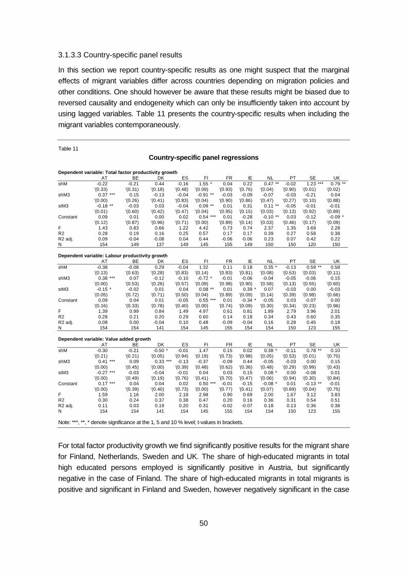
50

3.1.3.3 Country-specific panel results

In this section we report country-specific results as one might suspect that the marginal

effects of migrant variables differ across countries depending on migration policies and

other conditions. One should however be aware that these results might be biased due to

reversed causality and endogeneity which can only be insufficiently taken into account by

using lagged variables. Table 11 presents the country-specific results when including the

migrant variables contemporaneously.

Table 11

Country-specific panel regressions

Dependent variable: Total factor productivity growt h AT BE DK ES FI FR IE NL PT SE UK shM -0.22 -0.21 0.44 -0.16 1.55 * 0.04 0.22 0.47 ** -0.02 1.23 *** 0.79 ** '(0.33) '(0.31) '(0.18) '(0.48) '(0.09) '(0.93) '(0.76) '(0.04) '(0.90) '(0.01) '(0.02) shM3 0.37 *** 0.15 -0.13 -0.04 -0.91 ** -0.03 -0.09 -0.07 -0.03 -0.21 0.04 '(0.00) '(0.26) '(0.41) '(0.83) '(0.04) '(0.90) '(0.86) '(0.47) '(0.27) '(0.10) '(0.88) stM3 -0.18 ** -0.03 0.03 -0.04 0.09 ** 0.01 0.31 0.11 ** -0.05 -0.01 -0.01 '(0.01) '(0.60) '(0.42) '(0.47) '(0.04) '(0.95) '(0.15) '(0.03) '(0.13) '(0.92) '(0.89) Constant 0.09 0.01 0.00 0.02 0.54 *** 0.01 -0.28 -0.10 ** 0.03 -0.12 -0.09 * '(0.12) '(0.87) '(0.96) '(0.71) '(0.00) '(0.89) '(0.14) '(0.03) '(0.46) '(0.17) '(0.09) F 1.43 0.83 0.66 1.22 4.42 0.73 0.74 2.37 1.35 3.69 2.28 R2 0.28 0.19 0.16 0.25 0.57 0.17 0.17 0.39 0.27 0.58 0.38 R2 adj. 0.09 -0.04 -0.08 0.04 0.44 -0.06 -0.06 0.23 0.07 0.42 0.22 N 154 149 137 149 145 155 149 150 150 120 150 Dependent variable: Labour productivity growth AT BE DK ES FI FR IE NL PT SE UK shM -0.38 -0.08 0.29 -0.04 1.32 0.11 0.18 0.35 * -0.13 0.59 ** 0.58 '(0.13) '(0.63) '(0.28) '(0.83) '(0.14) '(0.83) '(0.81) '(0.08) '(0.53) '(0.03) '(0.11) shM3 0.38 *** 0.07 -0.12 -0.10 -0.72 * -0.01 -0.06 -0.04 -0.05 -0.06 0.15 '(0.00) '(0.53) '(0.26) '(0.57) '(0.09) '(0.98) '(0.90) '(0.58) '(0.13) '(0.55) '(0.60) stM3 -0.15 * -0.02 0.01 0.04 0.08 ** 0.01 0.39 * 0.07 -0.03 0.00 -0.03 '(0.05) '(0.72) '(0.71) '(0.50) '(0.04) '(0.89) '(0.09) '(0.14) '(0.39) '(0.98) '(0.66) Constant 0.09 0.04 0.01 -0.05 0.55 *** 0.01 -0.34 * -0.05 0.03 -0.07 0.00 '(0.16) '(0.33) '(0.78) '(0.40) '(0.00) '(0.74) '(0.09) '(0.30) '(0.34) '(0.23) '(0.96) F 1.39 0.99 0.84 1.49 4.97 0.61 0.81 1.89 2.79 3.96 2.01 R2 0.28 0.21 0.20 0.29 0.60 0.14 0.18 0.34 0.43 0.60 0.35 R2 adj. 0.08 0.00 -0.04 0.10 0.48 -0.09 -0.04 0.16 0.28 0.45 0.18 N 154 154 141 154 145 155 154 154 150 123 155 Dependent variable: Value added growth AT BE DK ES FI FR IE NL PT SE UK shM -0.30 -0.21 -0.50 * -0.01 1.47 0.15 0.02 0.38 * -0.11 0.78 ** 0.10 '(0.21) '(0.21) '(0.05) '(0.94) '(0.19) '(0.73) '(0.98) '(0.05) '(0.53) '(0.01) '(0.70) shM3 0.41 *** 0.09 0.33 *** -0.13 -0.37 -0.09 0.44 -0.05 -0.03 0.00 0.15 '(0.00) '(0.45) '(0.00) '(0.39) '(0.48) '(0.62) '(0.36) '(0.48) '(0.29) '(0.99) '(0.43) stM3 -0.27 *** -0.03 -0.04 -0.01 0.04 0.03 0.15 0.08 * 0.00 -0.08 0.01 '(0.00) '(0.49) '(0.19) '(0.76) '(0.41) '(0.70) '(0.47) '(0.06) '(0.94) '(0.30) '(0.84) Constant 0.17 *** 0.04 0.04 0.02 0.50 *** -0.01 -0.15 -0.08 * 0.01 -0.13 ** -0.01 '(0.00) '(0.39) '(0.40) '(0.73) '(0.00) '(0.77) '(0.41) '(0.07) '(0.69) '(0.04) '(0.75) F 1.59 1.16 2.00 2.18 2.98 0.90 0.69 2.00 1.67 3.12 3.83 R2 0.30 0.24 0.37 0.38 0.47 0.20 0.16 0.36 0.31 0.54 0.51 R2 adj. 0.11 0.03 0.19 0.20 0.31 -0.02 -0.07 0.18 0.13 0.36 0.38 N 154 154 141 154 145 155 154 154 150 123 155

Note: ***, **, * denote significance at the 1, 5 and 10 % level; t-values in brackets.

For total factor productivity growth we find significantly positive results for the migrant share

for Finland, Netherlands, Sweden and UK. The share of high-educated migrants in total

high educated persons employed is significantly positive in Austria, but significantly

negative in the case of Finland. The share of high-educated migrants in total migrants is

positive and significant in Finland and Sweden, however negatively significant in the case

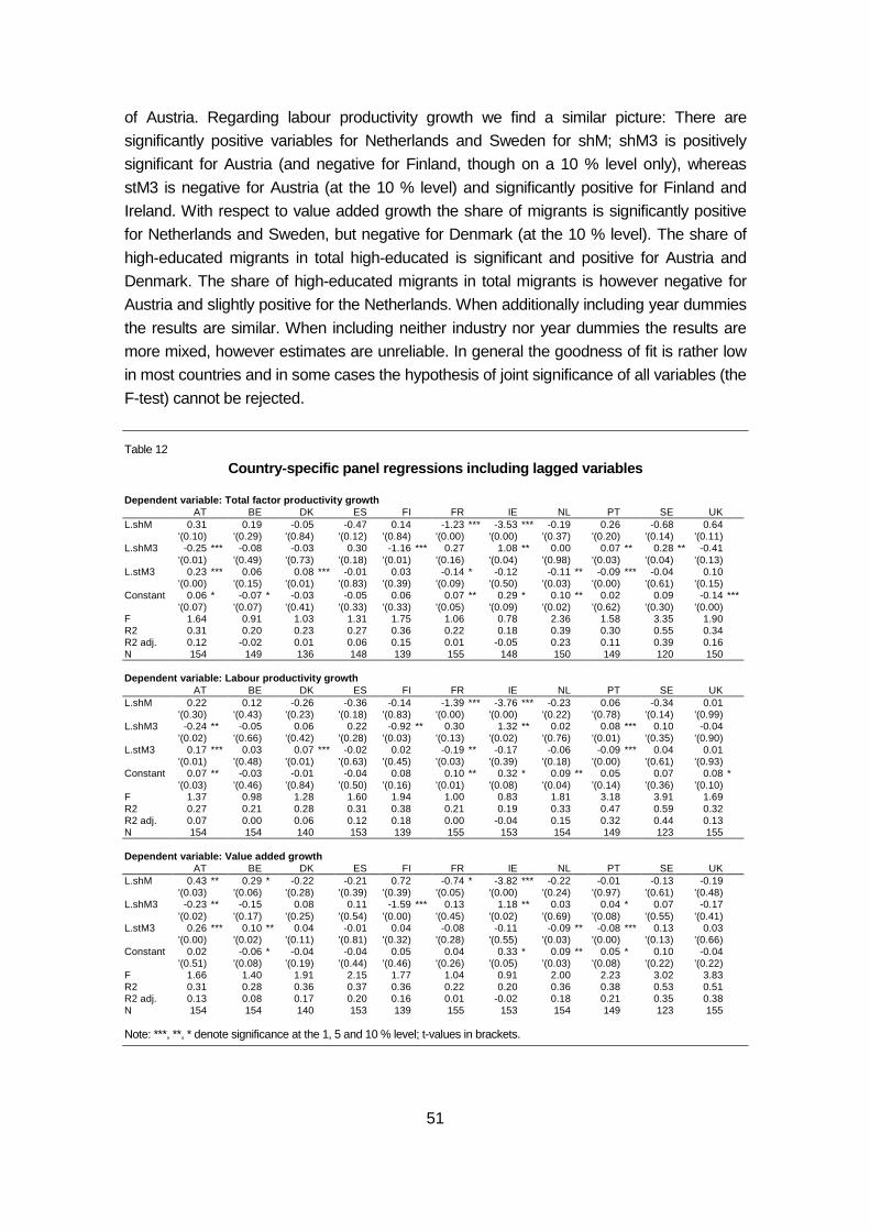
51

of Austria. Regarding labour productivity growth we find a similar picture: There are

significantly positive variables for Netherlands and Sweden for shM; shM3 is positively

significant for Austria (and negative for Finland, though on a 10 % level only), whereas

stM3 is negative for Austria (at the 10 % level) and significantly positive for Finland and

Ireland. With respect to value added growth the share of migrants is significantly positive

for Netherlands and Sweden, but negative for Denmark (at the 10 % level). The share of

high-educated migrants in total high-educated is significant and positive for Austria and

Denmark. The share of high-educated migrants in total migrants is however negative for

Austria and slightly positive for the Netherlands. When additionally including year dummies

the results are similar. When including neither industry nor year dummies the results are

more mixed, however estimates are unreliable. In general the goodness of fit is rather low

in most countries and in some cases the hypothesis of joint significance of all variables (the

F-test) cannot be rejected.

Table 12

Country-specific panel regressions including lagged variables

Dependent variable: Total factor productivity growt h AT BE DK ES FI FR IE NL PT SE UK L.shM 0.31 0.19 -0.05 -0.47 0.14 -1.23 *** -3.53 *** -0.19 0.26 -0.68 0.64 '(0.10) '(0.29) '(0.84) '(0.12) '(0.84) '(0.00) '(0.00) '(0.37) '(0.20) '(0.14) '(0.11) L.shM3 -0.25 *** -0.08 -0.03 0.30 -1.16 *** 0.27 1.08 ** 0.00 0.07 ** 0.28 ** -0.41 '(0.01) '(0.49) '(0.73) '(0.18) '(0.01) '(0.16) '(0.04) '(0.98) '(0.03) '(0.04) '(0.13) L.stM3 0.23 *** 0.06 0.08 *** -0.01 0.03 -0.14 * -0.12 -0.11 ** -0.09 *** -0.04 0.10 '(0.00) '(0.15) '(0.01) '(0.83) '(0.39) '(0.09) '(0.50) '(0.03) '(0.00) '(0.61) '(0.15) Constant 0.06 * -0.07 * -0.03 -0.05 0.06 0.07 ** 0.29 * 0.10 ** 0.02 0.09 -0.14 *** '(0.07) '(0.07) '(0.41) '(0.33) '(0.33) '(0.05) '(0.09) '(0.02) '(0.62) '(0.30) '(0.00) F 1.64 0.91 1.03 1.31 1.75 1.06 0.78 2.36 1.58 3.35 1.90 R2 0.31 0.20 0.23 0.27 0.36 0.22 0.18 0.39 0.30 0.55 0.34 R2 adj. 0.12 -0.02 0.01 0.06 0.15 0.01 -0.05 0.23 0.11 0.39 0.16 N 154 149 136 148 139 155 148 150 149 120 150 Dependent variable: Labour productivity growth AT BE DK ES FI FR IE NL PT SE UK L.shM 0.22 0.12 -0.26 -0.36 -0.14 -1.39 *** -3.76 *** -0.23 0.06 -0.34 0.01 '(0.30) '(0.43) '(0.23) '(0.18) '(0.83) '(0.00) '(0.00) '(0.22) '(0.78) '(0.14) '(0.99) L.shM3 -0.24 ** -0.05 0.06 0.22 -0.92 ** 0.30 1.32 ** 0.02 0.08 *** 0.10 -0.04 '(0.02) '(0.66) '(0.42) '(0.28) '(0.03) '(0.13) '(0.02) '(0.76) '(0.01) '(0.35) '(0.90) L.stM3 0.17 *** 0.03 0.07 *** -0.02 0.02 -0.19 ** -0.17 -0.06 -0.09 *** 0.04 0.01 '(0.01) '(0.48) '(0.01) '(0.63) '(0.45) '(0.03) '(0.39) '(0.18) '(0.00) '(0.61) '(0.93) Constant 0.07 ** -0.03 -0.01 -0.04 0.08 0.10 ** 0.32 * 0.09 ** 0.05 0.07 0.08 * '(0.03) '(0.46) '(0.84) '(0.50) '(0.16) '(0.01) '(0.08) '(0.04) '(0.14) '(0.36) '(0.10) F 1.37 0.98 1.28 1.60 1.94 1.00 0.83 1.81 3.18 3.91 1.69 R2 0.27 0.21 0.28 0.31 0.38 0.21 0.19 0.33 0.47 0.59 0.32 R2 adj. 0.07 0.00 0.06 0.12 0.18 0.00 -0.04 0.15 0.32 0.44 0.13 N 154 154 140 153 139 155 153 154 149 123 155 Dependent variable: Value added growth AT BE DK ES FI FR IE NL PT SE UK L.shM 0.43 ** 0.29 * -0.22 -0.21 0.72 -0.74 * -3.82 *** -0.22 -0.01 -0.13 -0.19 '(0.03) '(0.06) '(0.28) '(0.39) '(0.39) '(0.05) '(0.00) '(0.24) '(0.97) '(0.61) '(0.48) L.shM3 -0.23 ** -0.15 0.08 0.11 -1.59 *** 0.13 1.18 ** 0.03 0.04 * 0.07 -0.17 '(0.02) '(0.17) '(0.25) '(0.54) '(0.00) '(0.45) '(0.02) '(0.69) '(0.08) '(0.55) '(0.41) L.stM3 0.26 *** 0.10 ** 0.04 -0.01 0.04 -0.08 -0.11 -0.09 ** -0.08 *** 0.13 0.03 '(0.00) '(0.02) '(0.11) '(0.81) '(0.32) '(0.28) '(0.55) '(0.03) '(0.00) '(0.13) '(0.66) Constant 0.02 -0.06 * -0.04 -0.04 0.05 0.04 0.33 * 0.09 ** 0.05 * 0.10 -0.04 '(0.51) '(0.08) '(0.19) '(0.44) '(0.46) '(0.26) '(0.05) '(0.03) '(0.08) '(0.22) '(0.22) F 1.66 1.40 1.91 2.15 1.77 1.04 0.91 2.00 2.23 3.02 3.83 R2 0.31 0.28 0.36 0.37 0.36 0.22 0.20 0.36 0.38 0.53 0.51 R2 adj. 0.13 0.08 0.17 0.20 0.16 0.01 -0.02 0.18 0.21 0.35 0.38 N 154 154 140 153 139 155 153 154 149 123 155


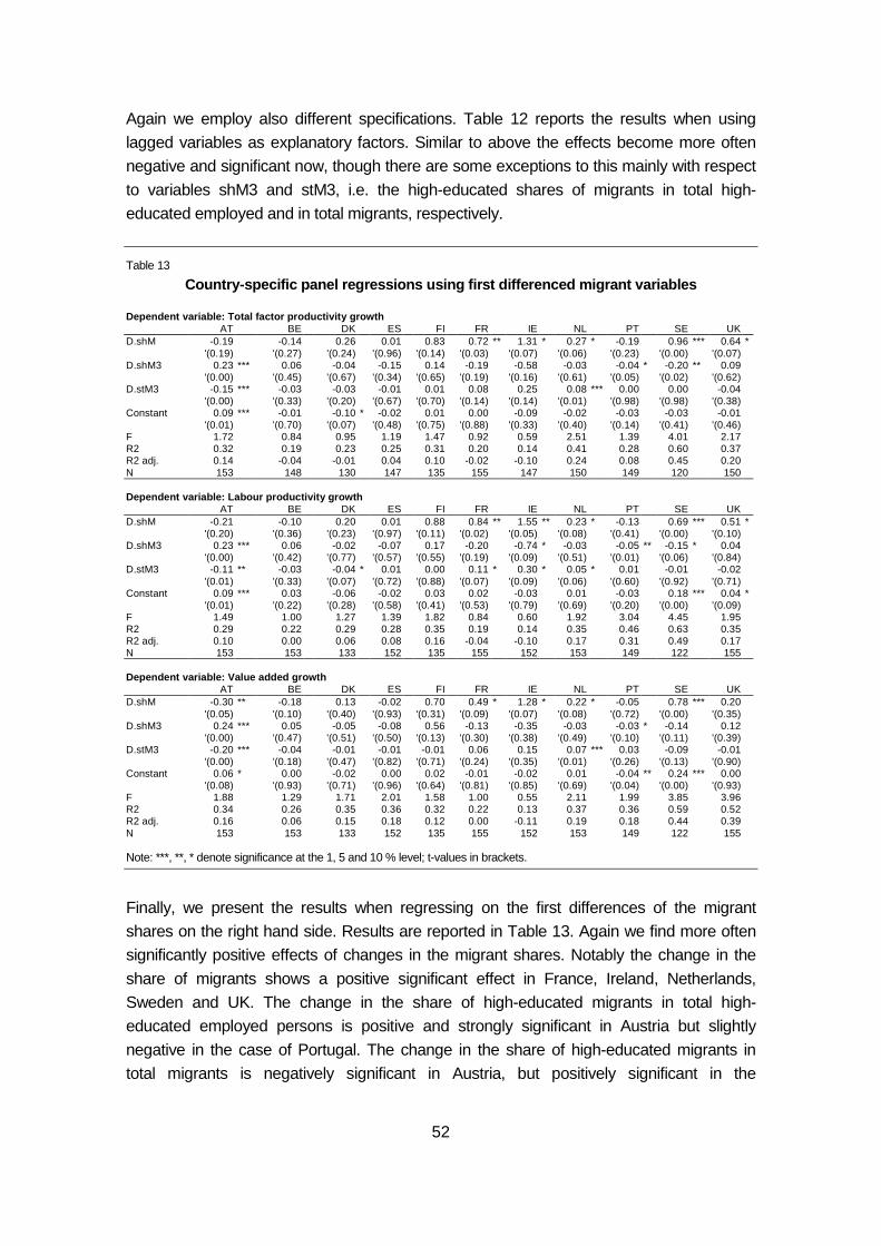
52

Again we employ also different specifications. Table 12 reports the results when using

lagged variables as explanatory factors. Similar to above the effects become more often

negative and significant now, though there are some exceptions to this mainly with respect

to variables shM3 and stM3, i.e. the high-educated shares of migrants in total high-

educated employed and in total migrants, respectively.

Table 13

Country-specific panel regressions using first diff erenced migrant variables

Dependent variable: Total factor productivity growt h AT BE DK ES FI FR IE NL PT SE UK D.shM -0.19 -0.14 0.26 0.01 0.83 0.72 ** 1.31 * 0.27 * -0.19 0.96 *** 0.64 * '(0.19) '(0.27) '(0.24) '(0.96) '(0.14) '(0.03) '(0.07) '(0.06) '(0.23) '(0.00) '(0.07) D.shM3 0.23 *** 0.06 -0.04 -0.15 0.14 -0.19 -0.58 -0.03 -0.04 * -0.20 ** 0.09 '(0.00) '(0.45) '(0.67) '(0.34) '(0.65) '(0.19) '(0.16) '(0.61) '(0.05) '(0.02) '(0.62) D.stM3 -0.15 *** -0.03 -0.03 -0.01 0.01 0.08 0.25 0.08 *** 0.00 0.00 -0.04 '(0.00) '(0.33) '(0.20) '(0.67) '(0.70) '(0.14) '(0.14) '(0.01) '(0.98) '(0.98) '(0.38) Constant 0.09 *** -0.01 -0.10 * -0.02 0.01 0.00 -0.09 -0.02 -0.03 -0.03 -0.01 '(0.01) '(0.70) '(0.07) '(0.48) '(0.75) '(0.88) '(0.33) '(0.40) '(0.14) '(0.41) '(0.46) F 1.72 0.84 0.95 1.19 1.47 0.92 0.59 2.51 1.39 4.01 2.17 R2 0.32 0.19 0.23 0.25 0.31 0.20 0.14 0.41 0.28 0.60 0.37 R2 adj. 0.14 -0.04 -0.01 0.04 0.10 -0.02 -0.10 0.24 0.08 0.45 0.20 N 153 148 130 147 135 155 147 150 149 120 150 Dependent variable: Labour productivity growth AT BE DK ES FI FR IE NL PT SE UK D.shM -0.21 -0.10 0.20 0.01 0.88 0.84 ** 1.55 ** 0.23 * -0.13 0.69 *** 0.51 * '(0.20) '(0.36) '(0.23) '(0.97) '(0.11) '(0.02) '(0.05) '(0.08) '(0.41) '(0.00) '(0.10) D.shM3 0.23 *** 0.06 -0.02 -0.07 0.17 -0.20 -0.74 * -0.03 -0.05 ** -0.15 * 0.04 '(0.00) '(0.42) '(0.77) '(0.57) '(0.55) '(0.19) '(0.09) '(0.51) '(0.01) '(0.06) '(0.84) D.stM3 -0.11 ** -0.03 -0.04 * 0.01 0.00 0.11 * 0.30 * 0.05 * 0.01 -0.01 -0.02 '(0.01) '(0.33) '(0.07) '(0.72) '(0.88) '(0.07) '(0.09) '(0.06) '(0.60) '(0.92) '(0.71) Constant 0.09 *** 0.03 -0.06 -0.02 0.03 0.02 -0.03 0.01 -0.03 0.18 *** 0.04 * '(0.01) '(0.22) '(0.28) '(0.58) '(0.41) '(0.53) '(0.79) '(0.69) '(0.20) '(0.00) '(0.09) F 1.49 1.00 1.27 1.39 1.82 0.84 0.60 1.92 3.04 4.45 1.95 R2 0.29 0.22 0.29 0.28 0.35 0.19 0.14 0.35 0.46 0.63 0.35 R2 adj. 0.10 0.00 0.06 0.08 0.16 -0.04 -0.10 0.17 0.31 0.49 0.17 N 153 153 133 152 135 155 152 153 149 122 155 Dependent variable: Value added growth AT BE DK ES FI FR IE NL PT SE UK D.shM -0.30 ** -0.18 0.13 -0.02 0.70 0.49 * 1.28 * 0.22 * -0.05 0.78 *** 0.20 '(0.05) '(0.10) '(0.40) '(0.93) '(0.31) '(0.09) '(0.07) '(0.08) '(0.72) '(0.00) '(0.35) D.shM3 0.24 *** 0.05 -0.05 -0.08 0.56 -0.13 -0.35 -0.03 -0.03 * -0.14 0.12 '(0.00) '(0.47) '(0.51) '(0.50) '(0.13) '(0.30) '(0.38) '(0.49) '(0.10) '(0.11) '(0.39) D.stM3 -0.20 *** -0.04 -0.01 -0.01 -0.01 0.06 0.15 0.07 *** 0.03 -0.09 -0.01 '(0.00) '(0.18) '(0.47) '(0.82) '(0.71) '(0.24) '(0.35) '(0.01) '(0.26) '(0.13) '(0.90) Constant 0.06 * 0.00 -0.02 0.00 0.02 -0.01 -0.02 0.01 -0.04 ** 0.24 *** 0.00 '(0.08) '(0.93) '(0.71) '(0.96) '(0.64) '(0.81) '(0.85) '(0.69) '(0.04) '(0.00) '(0.93) F 1.88 1.29 1.71 2.01 1.58 1.00 0.55 2.11 1.99 3.85 3.96 R2 0.34 0.26 0.35 0.36 0.32 0.22 0.13 0.37 0.36 0.59 0.52 R2 adj. 0.16 0.06 0.15 0.18 0.12 0.00 -0.11 0.19 0.18 0.44 0.39 N 153 153 133 152 135 155 152 153 149 122 155


Finally, we present the results when regressing on the first differences of the migrant

shares on the right hand side. Results are reported in Table 13. Again we find more often

significantly positive effects of changes in the migrant shares. Notably the change in the

share of migrants shows a positive significant effect in France, Ireland, Netherlands,

Sweden and UK. The change in the share of high-educated migrants in total high-

educated employed persons is positive and strongly significant in Austria but slightly

negative in the case of Portugal. The change in the share of high-educated migrants in

total migrants is negatively significant in Austria, but positively significant in the

53

Netherlands. With respect to labour productivity growth we find similar results; these are

however more often significant (the second variable, shM3, negatively so in most cases,

and the third, stM3, positively significant). This is also the case when testing for the effects

of migration on value added growth.

Finally, we also run the same set of regressions excluding either the share of high-

educated migrants in total high educated employed persons (shM3) or the share of

migrants in total employed for reasons of multicollinearity. In these cases the results are

more mixed across countries. In particular, we find in some cases significantly positive

effects when including the share of migrants along with the share of high-educated

migrants in total migrants only. These results are reported as Appendix Tables B.4 and

B.5, respectively.

3.1.4 Econometric results on subsectors

We proceed with the analysis by splitting the sample into manufacturing (NACE rev. 1

15-37) and market services (NACE rev.1 50-74). Further, we split the sample by skill

intensities based on the taxonomy suggested by Pender (2007) which was adapted to the

EU KLEMS sectoral classification. The exact list of industries and the underlying taxonomy

is provided in Appendix Table B.6. Here we differentiate between high, medium and low-

skill intensive industries. The reason for splitting up the sample to groups of sectors is that

one might expect that migrants might be concentrated in particular jobs (or sectors) which

might have a differentiated impact. Further, the effect of migrant labour might be more

important in some sectors compared to others (e.g. potential of spillover effects, learning

requirements, …). Furthermore, recent results suggest a differentiated impact (see e.g.

Paserman, 2008).

In this part we can no longer estimate the impact of migrant labour on a country-by-country

basis due the limited number of observations available. More importantly, it might even be

more interesting to focus on cross-country differences, i.e. asking whether in a particular

sector (or a group of sectors sharing particular characteristics) the impact of migrant labour

on industry performance matters in a positive way. With respect to specifications we again

present first cross-country results and then panel regression results.

3.1.4.1 Cross-section results

In Table 14 we report the results for manufacturing and in Table 15 the results for service

industries. Again we report twelve different specifications which differ with respect to the

variables included. In case of manufacturing we find again a positive impact of migration on

total factor productivity and also labour productivity growth at least at the 10 % significance

level. However, in most cases the significance vanishes when including both country and

industry dummies. With respect to the variables it seems that the skill structure of migrants

54

seems to be the most important one. We also find a significant positive effect on value

added growth; in this case it is mainly the variable capturing the share of high-educated

migrants in total migrants which matters. For service industries we find no evidence for

total factor productivity growth. Results are inconclusive and in some cases even negative

for labour productivity growth. However, the significance vanishes when including industry

and/or country dummies. Only for value added growth we find a positive impact, again

mainly for the variable on the structure of migrants (stM3).

Tables 16 and 17 report the results for industries classified as low-educational intensive

and high-educational intensive, respectively.4 As one can see, results for low-educational

intensive industries are rather mixed, in most cases not significant and in some cases even

negative. The exception to this is the share of high-educated migrants in total migrants

which often is positively significant for labour productivity growth as dependent variable.

This is quite different when looking at the results for high-educational intensive industries.

For this group of industries we find in many cases positive and strongly significant effects

on all three dependent variables. In particular, the share of high-educated migrants in total

high-educated employed persons is strongly significant also with a rather large impact.

These results are in line with those found in Paserman (2008) for example.

4 Results for medium educational intensive industries are available upon request.

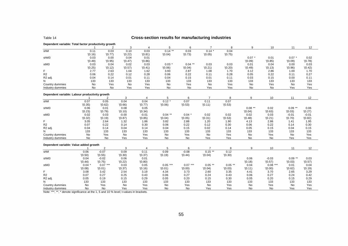
55

Table 14 Cross-section results for manufacturing industries Dependent variable: Total factor productivity growt h 1 2 3 4 5 6 7 8 9 10 11 12 shM 0.11 0.03 0.10 0.03 0.14 ** 0.03 0.14 * 0.04 '(0.16) '(0.77) '(0.22) '(0.81) '(0.04) '(0.73) '(0.05) '(0.75) shM3 0.03 0.00 0.04 0.01 0.07 * 0.01 0.07 * 0.02 '(0.49) '(0.95) '(0.47) '(0.86) '(0.09) '(0.85) '(0.09) '(0.78) stM3 0.03 0.04 0.02 0.03 0.03 * 0.04 ** 0.03 0.03 0.01 0.04 0.00 0.03 '(0.25) '(0.12) '(0.57) '(0.41) '(0.06) '(0.04) '(0.21) '(0.20) '(0.49) '(0.13) '(0.96) '(0.42) F 2.77 2.63 1.04 1.62 3.93 2.87 1.08 1.70 3.12 2.86 1.00 1.70 R2 0.06 0.22 0.12 0.28 0.06 0.22 0.11 0.28 0.05 0.22 0.11 0.27 R2 adj. 0.04 0.14 0.01 0.11 0.04 0.15 0.01 0.11 0.03 0.15 0.00 0.11 N 133 133 133 133 133 133 133 133 133 133 133 133 Country dummies No Yes No Yes No Yes No Yes No Yes No Yes Industry dummies No No Yes Yes No No Yes Yes No No Yes Yes Dependent variable: Labour productivity growth 1 2 3 4 5 6 7 8 9 10 11 12 shM 0.07 0.05 0.04 0.04 0.12 * 0.07 0.11 0.07 '(0.35) '(0.62) '(0.66) '(0.77) '(0.06) '(0.53) '(0.11) '(0.53) shM3 0.06 0.01 0.08 0.05 0.08 ** 0.02 0.09 ** 0.06 '(0.23) '(0.79) '(0.10) '(0.34) '(0.04) '(0.63) '(0.03) '(0.27) stM3 0.02 0.03 -0.00 -0.01 0.04 ** 0.04 * 0.02 0.02 0.02 0.03 -0.01 -0.01 '(0.32) '(0.19) '(0.87) '(0.85) '(0.04) '(0.05) '(0.31) '(0.53) '(0.48) '(0.21) '(0.70) '(0.82) F 3.05 2.64 1.32 1.86 3.82 2.88 1.20 1.90 4.13 2.86 1.41 1.95 R2 0.07 0.22 0.14 0.30 0.06 0.22 0.12 0.30 0.06 0.22 0.14 0.30 R2 adj. 0.04 0.14 0.04 0.14 0.04 0.15 0.02 0.14 0.05 0.15 0.04 0.15 N 133 133 133 133 133 133 133 133 133 133 133 133 Country dummies No Yes No Yes No Yes No Yes No Yes No Yes Industry dummies No No Yes Yes No No Yes Yes No No Yes Yes Dependent variable: Value added growth 1 2 3 4 5 6 7 8 9 10 11 12 shM 0.06 -0.07 0.09 0.11 0.09 -0.08 0.15 ** 0.12 '(0.50) '(0.55) '(0.30) '(0.37) '(0.19) '(0.44) '(0.04) '(0.30) shM3 0.04 -0.02 0.06 0.01 0.06 -0.03 0.09 ** 0.03 '(0.44) '(0.75) '(0.22) '(0.80) '(0.18) '(0.57) '(0.03) '(0.57) stM3 0.04 * 0.07 *** 0.03 0.05 0.05 *** 0.07 *** 0.05 ** 0.05 ** 0.04 0.08 *** 0.01 0.04 '(0.08) '(0.01) '(0.37) '(0.16) '(0.01) '(0.00) '(0.04) '(0.03) '(0.11) '(0.00) '(0.62) '(0.19) F 3.08 3.42 2.54 3.19 4.34 3.73 2.60 3.35 4.41 3.70 2.65 3.29 R2 0.07 0.27 0.25 0.43 0.06 0.27 0.24 0.43 0.06 0.27 0.24 0.42 R2 adj. 0.05 0.19 0.15 0.29 0.05 0.20 0.15 0.30 0.05 0.20 0.15 0.29 N 133 133 133 133 133 133 133 133 133 133 133 133 Country dummies No Yes No Yes No Yes No Yes No Yes No Yes Industry dummies No No Yes Yes No No Yes Yes No No Yes Yes Note: ***, **, * denote significance at the 1, 5 and 10 % level; t-values in brackets.

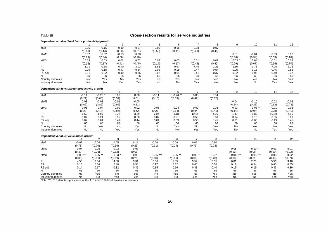
56

Table 15 Cross-section results for service industries Dependent variable: Total factor productivity growt h 1 2 3 4 5 6 7 8 9 10 11 12 shM -0.06 -0.16 0.10 0.07 -0.05 -0.15 0.08 0.07 '(0.50) '(0.14) '(0.23) '(0.51) '(0.50) '(0.11) '(0.21) '(0.48) shM3 0.02 0.02 -0.03 0.00 -0.01 -0.04 0.03 0.02 '(0.79) '(0.84) '(0.68) '(0.98) '(0.80) '(0.54) '(0.59) '(0.81) stM3 0.03 0.03 0.02 0.02 0.03 0.03 0.01 0.02 0.03 * 0.04 * 0.01 0.01 '(0.15) '(0.17) '(0.41) '(0.45) '(0.14) '(0.17) '(0.45) '(0.42) '(0.09) '(0.07) '(0.64) '(0.54) F 1.21 0.88 6.40 3.03 1.81 0.97 7.40 3.28 1.60 0.75 7.06 3.23 R2 0.06 0.18 0.47 0.54 0.05 0.18 0.47 0.54 0.05 0.15 0.46 0.53 R2 adj. 0.01 -0.02 0.40 0.36 0.02 -0.01 0.41 0.37 0.02 -0.05 0.40 0.37 N 66 66 66 66 66 66 66 66 66 66 66 66 Country dummies No Yes No Yes No Yes No Yes No Yes No Yes Industry dummies No No Yes Yes No No Yes Yes No No Yes Yes Dependent variable: Labour productivity growth 1 2 3 4 5 6 7 8 9 10 11 12 shM -0.14 -0.23 * 0.06 0.06 -0.11 -0.24 ** 0.05 0.04 '(0.21) '(0.06) '(0.51) '(0.61) '(0.18) '(0.03) '(0.42) '(0.70) shM3 0.03 -0.01 -0.01 -0.05 -0.04 -0.10 0.02 -0.03 '(0.69) '(0.89) '(0.92) '(0.61) '(0.54) '(0.23) '(0.63) '(0.71) stM3 0.03 0.04 -0.00 0.02 0.03 0.04 -0.00 0.02 0.03 0.06 ** -0.01 0.02 '(0.28) '(0.14) '(0.96) '(0.42) '(0.27) '(0.14) '(0.94) '(0.49) '(0.14) '(0.04) '(0.78) '(0.49) F 1.52 1.07 8.72 3.89 2.24 1.18 10.14 4.16 1.47 0.82 10.00 4.16 R2 0.07 0.21 0.55 0.60 0.07 0.21 0.55 0.60 0.04 0.16 0.55 0.60 R2 adj. 0.02 0.01 0.49 0.44 0.04 0.03 0.50 0.45 0.01 -0.03 0.49 0.45 N 66 66 66 66 66 66 66 66 66 66 66 66 Country dummies No Yes No Yes No Yes No Yes No Yes No Yes Industry dummies No No Yes Yes No No Yes Yes No No Yes Yes Dependent variable: Value added growth 1 2 3 4 5 6 7 8 9 10 11 12 shM -0.02 -0.04 0.05 0.11 -0.06 -0.09 0.02 0.10 '(0.78) '(0.70) '(0.56) '(0.25) '(0.31) '(0.24) '(0.73) '(0.28) shM3 -0.04 -0.08 -0.03 -0.03 -0.05 -0.10 * -0.01 -0.01 '(0.49) '(0.20) '(0.62) '(0.66) '(0.23) '(0.09) '(0.90) '(0.93) stM3 0.05 *** 0.05 ** 0.03 * 0.03 0.05 *** 0.05 ** 0.03 * 0.02 0.06 *** 0.05 *** 0.03 0.02 '(0.00) '(0.01) '(0.09) '(0.25) '(0.00) '(0.01) '(0.09) '(0.28) '(0.00) '(0.01) '(0.10) '(0.39) F 4.50 2.04 4.80 3.31 6.56 2.05 5.52 3.55 6.81 2.23 5.50 3.40 R2 0.18 0.34 0.40 0.56 0.17 0.32 0.40 0.56 0.18 0.34 0.40 0.55 R2 adj. 0.14 0.17 0.32 0.39 0.15 0.16 0.33 0.40 0.15 0.19 0.33 0.39 N 66 66 66 66 66 66 66 66 66 66 66 66 Country dummies No Yes No Yes No Yes No Yes No Yes No Yes Industry dummies No No Yes Yes No No Yes Yes No No Yes Yes Note: ***, **, * denote significance at the 1, 5 and 10 % level; t-values in brackets.

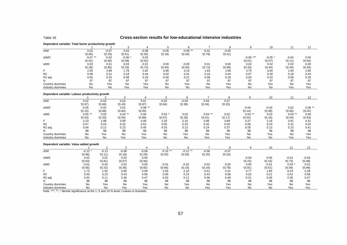
57

Table 16 Cross-section results for low-educational intensive industries Dependent variable: Total factor productivity growt h 1 2 3 4 5 6 7 8 9 10 11 12 shM 0.02 -0.07 0.04 -0.08 -0.05 -0.09 ** -0.01 -0.05 '(0.65) '(0.25) '(0.51) '(0.30) '(0.18) '(0.04) '(0.78) '(0.41) shM3 -0.07 ** -0.02 -0.06 * 0.03 -0.06 *** -0.05 * -0.04 0.00 '(0.02) '(0.65) '(0.09) '(0.52) '(0.01) '(0.07) '(0.11) '(0.94) stM3 0.03 0.01 0.03 -0.01 0.00 -0.00 0.01 0.00 0.02 0.02 0.02 0.00 '(0.28) '(0.85) '(0.33) '(0.73) '(0.94) '(0.93) '(0.72) '(0.99) '(0.33) '(0.44) '(0.44) '(0.93) F 2.55 2.89 1.78 2.82 0.96 3.14 1.63 2.96 3.75 3.00 1.93 2.90 R2 0.08 0.31 0.19 0.44 0.02 0.31 0.16 0.44 0.07 0.30 0.18 0.43 R2 adj. 0.05 0.20 0.08 0.29 -0.00 0.21 0.06 0.29 0.05 0.20 0.09 0.28 N 97 97 97 97 97 97 97 97 97 97 97 97 Country dummies No Yes No Yes No Yes No Yes No Yes No Yes Industry dummies No No Yes Yes No No Yes Yes No No Yes Yes Dependent variable: Labour productivity growth 1 2 3 4 5 6 7 8 9 10 11 12 shM 0.02 -0.03 0.04 0.01 -0.02 -0.04 0.04 0.07 '(0.67) '(0.69) '(0.43) '(0.87) '(0.64) '(0.38) '(0.34) '(0.25) shM3 -0.05 -0.02 0.01 0.08 ** -0.04 -0.03 0.02 0.08 ** '(0.15) '(0.68) '(0.83) '(0.05) '(0.14) '(0.38) '(0.56) '(0.02) stM3 0.05 ** 0.03 0.04 ** 0.00 0.03 * 0.02 0.04 ** 0.02 0.04 ** 0.03 0.03 ** 0.00 '(0.03) '(0.26) '(0.03) '(0.89) '(0.07) '(0.28) '(0.01) '(0.17) '(0.02) '(0.16) '(0.04) '(0.93) F 2.23 1.98 3.59 4.06 2.25 2.16 3.99 3.89 3.27 2.16 3.91 4.31 R2 0.07 0.24 0.32 0.53 0.05 0.23 0.32 0.50 0.06 0.23 0.31 0.53 R2 adj. 0.04 0.12 0.23 0.40 0.03 0.13 0.24 0.37 0.05 0.13 0.23 0.41 N 98 98 98 98 98 98 98 98 98 98 98 98 Country dummies No Yes No Yes No Yes No Yes No Yes No Yes Industry dummies No No Yes Yes No No Yes Yes No No Yes Yes Dependent variable: Value added growth 1 2 3 4 5 6 7 8 9 10 11 12 shM -0.12 * -0.13 -0.08 -0.08 -0.10 ** -0.12 ** -0.06 -0.07 '(0.06) '(0.11) '(0.18) '(0.29) '(0.03) '(0.03) '(0.20) '(0.20) shM3 0.02 0.01 0.02 0.00 -0.04 -0.05 -0.01 -0.03 '(0.63) '(0.81) '(0.57) '(0.94) '(0.22) '(0.15) '(0.73) '(0.48) stM3 -0.01 -0.02 0.02 0.00 -0.01 -0.02 0.02 0.00 0.00 -0.01 0.03 * 0.01 '(0.56) '(0.23) '(0.35) '(0.82) '(0.66) '(0.23) '(0.24) '(0.78) '(0.81) '(0.51) '(0.09) '(0.49) F 1.73 1.92 5.90 5.09 2.50 2.10 6.51 5.41 0.77 1.83 6.24 5.28 R2 0.05 0.23 0.43 0.58 0.05 0.23 0.43 0.58 0.02 0.21 0.42 0.58 R2 adj. 0.02 0.11 0.36 0.47 0.03 0.12 0.36 0.48 -0.01 0.09 0.35 0.47 N 98 98 98 98 98 98 98 98 98 98 98 98 Country dummies No Yes No Yes No Yes No Yes No Yes No Yes Industry dummies No No Yes Yes No No Yes Yes No No Yes Yes Note: ***, **, * denote significance at the 1, 5 and 10 % level; t-values in brackets.

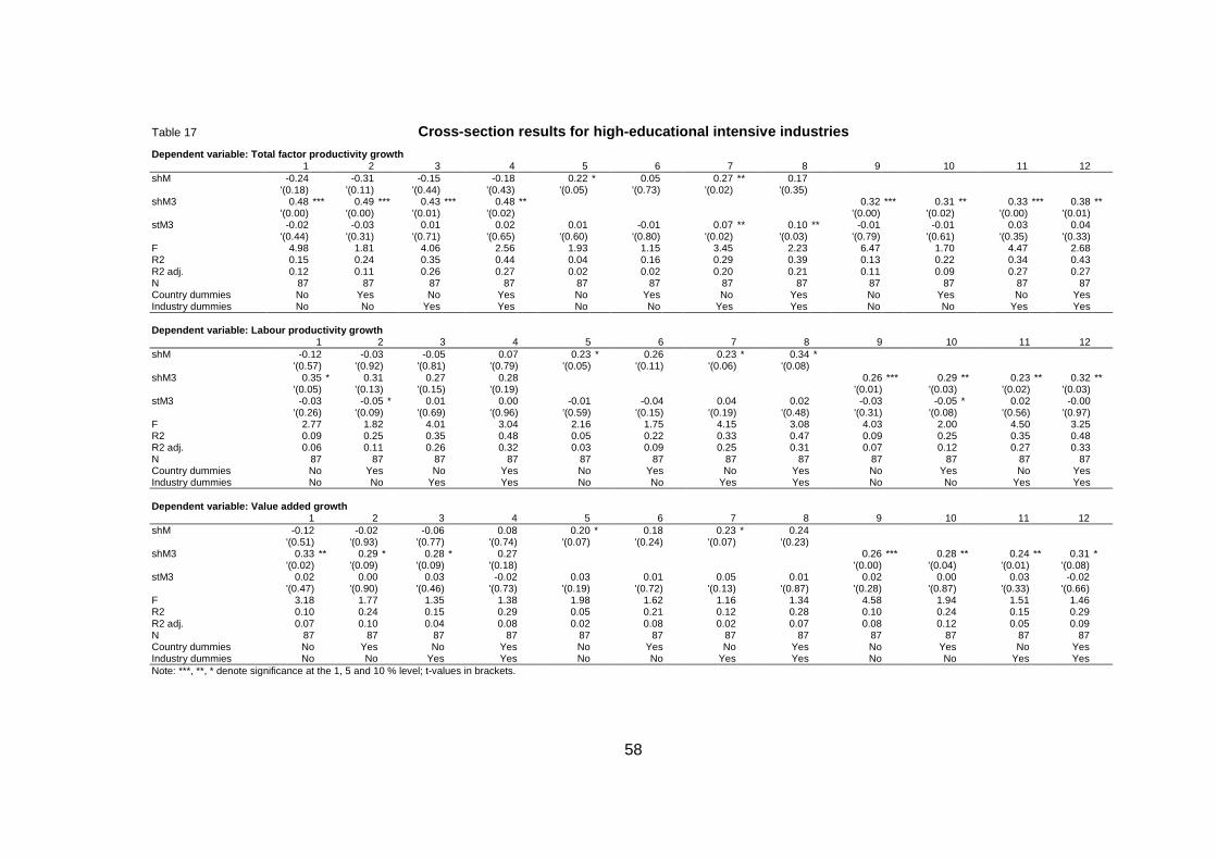
58

Table 17 Cross-section results for high-educational intensiv e industries Dependent variable: Total factor productivity growt h 1 2 3 4 5 6 7 8 9 10 11 12 shM -0.24 -0.31 -0.15 -0.18 0.22 * 0.05 0.27 ** 0.17 '(0.18) '(0.11) '(0.44) '(0.43) '(0.05) '(0.73) '(0.02) '(0.35) shM3 0.48 *** 0.49 *** 0.43 *** 0.48 ** 0.32 *** 0.31 ** 0.33 *** 0.38 ** '(0.00) '(0.00) '(0.01) '(0.02) '(0.00) '(0.02) '(0.00) '(0.01) stM3 -0.02 -0.03 0.01 0.02 0.01 -0.01 0.07 ** 0.10 ** -0.01 -0.01 0.03 0.04 '(0.44) '(0.31) '(0.71) '(0.65) '(0.60) '(0.80) '(0.02) '(0.03) '(0.79) '(0.61) '(0.35) '(0.33) F 4.98 1.81 4.06 2.56 1.93 1.15 3.45 2.23 6.47 1.70 4.47 2.68 R2 0.15 0.24 0.35 0.44 0.04 0.16 0.29 0.39 0.13 0.22 0.34 0.43 R2 adj. 0.12 0.11 0.26 0.27 0.02 0.02 0.20 0.21 0.11 0.09 0.27 0.27 N 87 87 87 87 87 87 87 87 87 87 87 87 Country dummies No Yes No Yes No Yes No Yes No Yes No Yes Industry dummies No No Yes Yes No No Yes Yes No No Yes Yes Dependent variable: Labour productivity growth 1 2 3 4 5 6 7 8 9 10 11 12 shM -0.12 -0.03 -0.05 0.07 0.23 * 0.26 0.23 * 0.34 * '(0.57) '(0.92) '(0.81) '(0.79) '(0.05) '(0.11) '(0.06) '(0.08) shM3 0.35 * 0.31 0.27 0.28 0.26 *** 0.29 ** 0.23 ** 0.32 ** '(0.05) '(0.13) '(0.15) '(0.19) '(0.01) '(0.03) '(0.02) '(0.03) stM3 -0.03 -0.05 * 0.01 0.00 -0.01 -0.04 0.04 0.02 -0.03 -0.05 * 0.02 -0.00 '(0.26) '(0.09) '(0.69) '(0.96) '(0.59) '(0.15) '(0.19) '(0.48) '(0.31) '(0.08) '(0.56) '(0.97) F 2.77 1.82 4.01 3.04 2.16 1.75 4.15 3.08 4.03 2.00 4.50 3.25 R2 0.09 0.25 0.35 0.48 0.05 0.22 0.33 0.47 0.09 0.25 0.35 0.48 R2 adj. 0.06 0.11 0.26 0.32 0.03 0.09 0.25 0.31 0.07 0.12 0.27 0.33 N 87 87 87 87 87 87 87 87 87 87 87 87 Country dummies No Yes No Yes No Yes No Yes No Yes No Yes Industry dummies No No Yes Yes No No Yes Yes No No Yes Yes Dependent variable: Value added growth 1 2 3 4 5 6 7 8 9 10 11 12 shM -0.12 -0.02 -0.06 0.08 0.20 * 0.18 0.23 * 0.24 '(0.51) '(0.93) '(0.77) '(0.74) '(0.07) '(0.24) '(0.07) '(0.23) shM3 0.33 ** 0.29 * 0.28 * 0.27 0.26 *** 0.28 ** 0.24 ** 0.31 * '(0.02) '(0.09) '(0.09) '(0.18) '(0.00) '(0.04) '(0.01) '(0.08) stM3 0.02 0.00 0.03 -0.02 0.03 0.01 0.05 0.01 0.02 0.00 0.03 -0.02 '(0.47) '(0.90) '(0.46) '(0.73) '(0.19) '(0.72) '(0.13) '(0.87) '(0.28) '(0.87) '(0.33) '(0.66) F 3.18 1.77 1.35 1.38 1.98 1.62 1.16 1.34 4.58 1.94 1.51 1.46 R2 0.10 0.24 0.15 0.29 0.05 0.21 0.12 0.28 0.10 0.24 0.15 0.29 R2 adj. 0.07 0.10 0.04 0.08 0.02 0.08 0.02 0.07 0.08 0.12 0.05 0.09 N 87 87 87 87 87 87 87 87 87 87 87 87 Country dummies No Yes No Yes No Yes No Yes No Yes No Yes Industry dummies No No Yes Yes No No Yes Yes No No Yes Yes Note: ***, **, * denote significance at the 1, 5 and 10 % level; t-values in brackets.

59

When using panel fixed effects regressions (Tables 18 and 19 report the results for

contemporaneous variables for manufacturing and services respectively) we again find a

significant and positive role for the share of migrants on total factor productivity and labour

productivity growth in manufacturing industries, but not so for value added growth. For

service industries these effects are even stronger; in particular the structure of migration

(i.e. the share of high-educated migrants in total migrants) is often positively significant with

total factor productivity growth as dependent variable; but also so for value added growth

though to a less extent. These conclusions also hold when using lagged variables as

explanatory factors. In some cases, however, the effects then become even negative.

When using first differences as independent variables we find often significantly positive

effects in manufacturing industries, for services however only the change in the share of

migrants is positively related to labour productivity growth.

In Tables 20 and 21 we show similar results however distinguishing between low-

educational intensive and high-educational intensive industries. With respect to the former

group of industries we often find insignificant and sometimes negative effects. Again this is

quite different for high-educational intensive industries. Here the coefficients are positive

and significant for all three dependent variables and also in most of the specifications. The

results further suggest that the share of high-educated migrants relative to total high-

educated persons employed (shM3) matters most. Similar conclusions hold when using

lagged variables (though significance sometimes disappears when including industry

dummies). Somewhat contrary to the results so far however the first differences variables

are not particularly important.5

5 Further results using lagged dependent variables and first differenced regressors are available upon request.

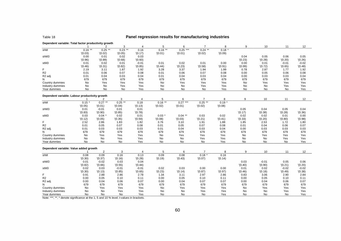
60

Table 18 Panel regression results for manufacturing industri es Dependent variable: Total factor productivity growt h 1 2 3 4 5 6 7 8 9 10 11 12 shM 0.16 ** 0.25 ** 0.23 ** 0.16 0.16 ** 0.25 *** 0.24 ** 0.18 * '(0.03) '(0.02) '(0.05) '(0.17) '(0.01) '(0.01) '(0.02) '(0.09) shM3 0.00 0.01 0.02 0.03 0.04 0.05 0.06 0.05 '(0.96) '(0.89) '(0.68) '(0.60) '(0.23) '(0.28) '(0.20) '(0.26) stM3 0.01 0.02 0.01 -0.01 0.01 0.02 0.01 0.00 0.00 0.01 -0.01 -0.02 '(0.46) '(0.31) '(0.82) '(0.85) '(0.44) '(0.23) '(0.58) '(0.91) '(0.99) '(0.72) '(0.65) '(0.48) F 2.19 3.11 1.87 1.92 3.28 3.37 1.94 1.99 0.78 2.87 1.77 1.92 R2 0.01 0.06 0.07 0.08 0.01 0.06 0.07 0.08 0.00 0.05 0.06 0.08 R2 adj. 0.01 0.04 0.03 0.04 0.01 0.04 0.03 0.04 0.00 0.03 0.03 0.04 N 679 679 679 679 679 679 679 679 679 679 679 679 Country dummies No Yes Yes Yes No Yes Yes Yes No Yes Yes Yes Industry dummies No No Yes Yes No No Yes Yes No No Yes Yes Year dummies No No No Yes No No No Yes No No No Yes Dependent variable: Labour productivity growth 1 2 3 4 5 6 7 8 9 10 11 12 shM 0.15 * 0.27 ** 0.25 ** 0.18 0.16 ** 0.27 *** 0.25 ** 0.19 * '(0.05) '(0.01) '(0.04) '(0.13) '(0.02) '(0.01) '(0.02) '(0.08) shM3 0.01 -0.01 0.01 0.01 0.05 0.04 0.05 0.04 '(0.83) '(0.90) '(0.85) '(0.78) '(0.17) '(0.38) '(0.28) '(0.36) stM3 0.03 0.04 * 0.02 0.01 0.03 * 0.04 ** 0.03 0.02 0.02 0.02 0.01 0.00 '(0.12) '(0.05) '(0.35) '(0.59) '(0.08) '(0.03) '(0.21) '(0.41) '(0.33) '(0.20) '(0.80) '(0.98) F 2.52 2.86 1.83 1.82 3.76 3.10 1.91 1.88 1.85 2.53 1.72 1.80 R2 0.01 0.05 0.07 0.08 0.01 0.05 0.07 0.08 0.01 0.04 0.06 0.07 R2 adj. 0.01 0.03 0.03 0.03 0.01 0.04 0.03 0.04 0.00 0.03 0.03 0.03 N 679 679 679 679 679 679 679 679 679 679 679 679 Country dummies No Yes Yes Yes No Yes Yes Yes No Yes Yes Yes Industry dummies No No Yes Yes No No Yes Yes No No Yes Yes Year dummies No No No Yes No No No Yes No No No Yes Dependent variable: Value added growth 1 2 3 4 5 6 7 8 9 10 11 12 shM 0.08 0.09 0.16 0.13 0.09 0.08 0.18 * 0.16 '(0.30) '(0.37) '(0.16) '(0.28) '(0.19) '(0.43) '(0.07) '(0.14) shM3 0.01 -0.02 0.03 0.04 0.03 -0.01 0.05 0.06 '(0.82) '(0.66) '(0.55) '(0.44) '(0.40) '(0.90) '(0.21) '(0.20) stM3 0.02 0.03 -0.01 -0.01 0.02 0.03 0.00 0.00 0.01 0.02 -0.02 -0.02 '(0.30) '(0.13) '(0.85) '(0.65) '(0.23) '(0.14) '(0.87) '(0.97) '(0.46) '(0.18) '(0.49) '(0.38) F 0.91 2.88 2.86 2.78 1.34 3.11 2.97 2.86 0.83 3.06 2.90 2.84 R2 0.00 0.05 0.10 0.11 0.00 0.05 0.10 0.11 0.00 0.05 0.10 0.11 R2 adj. 0.00 0.04 0.06 0.07 0.00 0.04 0.07 0.07 0.00 0.04 0.06 0.07 N 679 679 679 679 679 679 679 679 679 679 679 679 Country dummies No Yes Yes Yes No Yes Yes Yes No Yes Yes Yes Industry dummies No No Yes Yes No No Yes Yes No No Yes Yes Year dummies No No No Yes No No No Yes No No No Yes Note: ***, **, * denote significance at the 1, 5 and 10 % level; t-values in brackets.

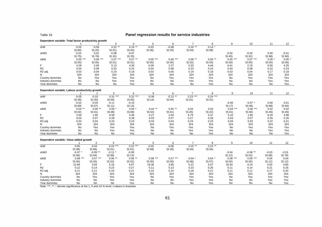
61

Table 19 Panel regression results for service industries Dependent variable: Total factor productivity growt h 1 2 3 4 5 6 7 8 9 10 11 12 shM -0.02 -0.09 0.22 ** 0.19 ** -0.03 -0.08 0.16 ** 0.14 * '(0.80) '(0.25) '(0.01) '(0.04) '(0.46) '(0.20) '(0.04) '(0.08) shM3 -0.01 0.01 -0.08 -0.07 -0.02 -0.02 0.00 -0.01 '(0.75) '(0.78) '(0.20) '(0.25) '(0.45) '(0.52) '(0.98) '(0.90) stM3 0.05 *** 0.06 *** 0.07 *** 0.07 ** 0.05 *** 0.06 *** 0.06 ** 0.05 ** 0.05 *** 0.07 *** 0.05 * 0.05 * '(0.00) '(0.00) '(0.01) '(0.01) '(0.00) '(0.00) '(0.02) '(0.03) '(0.00) '(0.00) '(0.05) '(0.06) F 4.28 2.09 5.13 4.30 6.39 2.27 5.33 4.44 6.41 2.15 5.00 4.25 R2 0.04 0.08 0.23 0.24 0.04 0.08 0.23 0.24 0.04 0.08 0.22 0.23 R2 adj. 0.03 0.04 0.19 0.18 0.03 0.05 0.19 0.18 0.03 0.04 0.17 0.18 N 324 324 324 324 324 324 324 324 324 324 324 324 Country dummies No Yes Yes Yes No Yes Yes Yes No Yes Yes Yes Industry dummies No No Yes Yes No No Yes Yes No No Yes Yes Year dummies No No No Yes No No No Yes No No No Yes Dependent variable: Labour productivity growth 1 2 3 4 5 6 7 8 9 10 11 12 shM -0.05 -0.10 0.31 *** 0.32 *** -0.08 -0.13 ** 0.23 *** 0.24 *** '(0.49) '(0.26) '(0.00) '(0.00) '(0.14) '(0.04) '(0.01) '(0.01) shM3 -0.02 -0.03 -0.11 -0.10 -0.05 -0.07 * 0.00 0.01 '(0.69) '(0.57) '(0.11) '(0.13) '(0.17) '(0.08) '(0.98) '(0.94) stM3 0.04 ** 0.05 ** 0.05 * 0.05 * 0.04 ** 0.05 ** 0.03 0.03 0.04 *** 0.06 *** 0.02 0.02 '(0.02) '(0.01) '(0.08) '(0.08) '(0.02) '(0.01) '(0.25) '(0.22) '(0.01) '(0.00) '(0.46) '(0.45) F 3.56 1.90 6.59 5.36 5.27 2.04 6.79 5.47 5.10 1.95 6.20 4.98 R2 0.03 0.07 0.28 0.28 0.03 0.07 0.27 0.28 0.03 0.07 0.26 0.26 R2 adj. 0.02 0.04 0.24 0.23 0.03 0.04 0.23 0.23 0.03 0.03 0.22 0.21 N 324 324 324 324 324 324 324 324 324 324 324 324 Country dummies No Yes Yes Yes No Yes Yes Yes No Yes Yes Yes Industry dummies No No Yes Yes No No Yes Yes No No Yes Yes Year dummies No No No Yes No No No Yes No No No Yes Dependent variable: Value added growth 1 2 3 4 5 6 7 8 9 10 11 12 shM 0.05 0.04 0.24 *** 0.22 *** -0.02 -0.06 0.15 ** 0.15 ** '(0.38) '(0.56) '(0.01) '(0.01) '(0.58) '(0.28) '(0.04) '(0.04) shM3 -0.07 * -0.09 ** -0.11 * -0.09 -0.04 -0.08 ** -0.03 -0.01 '(0.09) '(0.04) '(0.06) '(0.13) '(0.12) '(0.02) '(0.58) '(0.79) stM3 0.08 *** 0.07 *** 0.06 ** 0.06 ** 0.08 *** 0.07 *** 0.04 * 0.04 * 0.08 *** 0.06 *** 0.04 0.04 '(0.00) '(0.00) '(0.02) '(0.02) '(0.00) '(0.00) '(0.08) '(0.07) '(0.00) '(0.00) '(0.12) '(0.12) F 13.94 3.93 5.18 4.97 19.36 3.85 5.22 5.07 20.54 4.24 4.92 4.80 R2 0.12 0.14 0.23 0.27 0.11 0.13 0.23 0.26 0.11 0.14 0.21 0.25 R2 adj. 0.11 0.11 0.19 0.21 0.10 0.10 0.18 0.21 0.11 0.11 0.17 0.20 N 324 324 324 324 324 324 324 324 324 324 324 324 Country dummies No Yes Yes Yes No Yes Yes Yes No Yes Yes Yes Industry dummies No No Yes Yes No No Yes Yes No No Yes Yes Year dummies No No No Yes No No No Yes No No No Yes Note: ***, **, * denote significance at the 1, 5 and 10 % level; t-values in brackets.

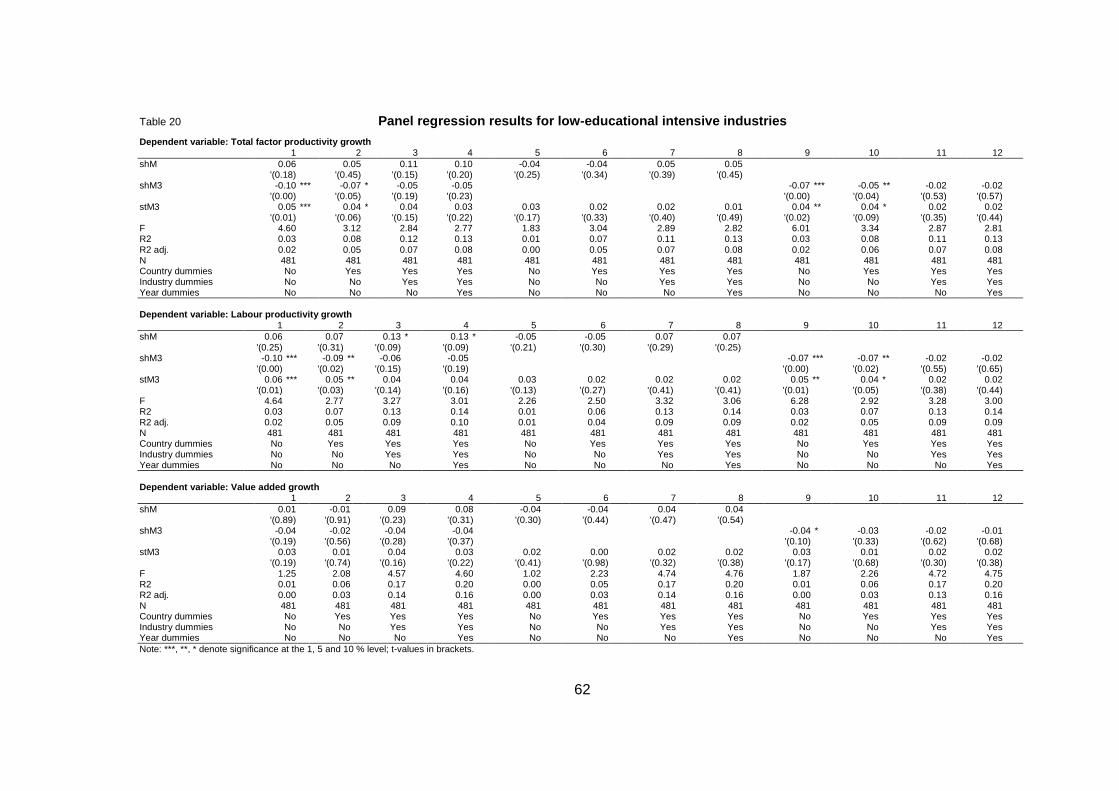
62

Table 20 Panel regression results for low-educational intens ive industries Dependent variable: Total factor productivity growt h 1 2 3 4 5 6 7 8 9 10 11 12 shM 0.06 0.05 0.11 0.10 -0.04 -0.04 0.05 0.05 '(0.18) '(0.45) '(0.15) '(0.20) '(0.25) '(0.34) '(0.39) '(0.45) shM3 -0.10 *** -0.07 * -0.05 -0.05 -0.07 *** -0.05 ** -0.02 -0.02 '(0.00) '(0.05) '(0.19) '(0.23) '(0.00) '(0.04) '(0.53) '(0.57) stM3 0.05 *** 0.04 * 0.04 0.03 0.03 0.02 0.02 0.01 0.04 ** 0.04 * 0.02 0.02 '(0.01) '(0.06) '(0.15) '(0.22) '(0.17) '(0.33) '(0.40) '(0.49) '(0.02) '(0.09) '(0.35) '(0.44) F 4.60 3.12 2.84 2.77 1.83 3.04 2.89 2.82 6.01 3.34 2.87 2.81 R2 0.03 0.08 0.12 0.13 0.01 0.07 0.11 0.13 0.03 0.08 0.11 0.13 R2 adj. 0.02 0.05 0.07 0.08 0.00 0.05 0.07 0.08 0.02 0.06 0.07 0.08 N 481 481 481 481 481 481 481 481 481 481 481 481 Country dummies No Yes Yes Yes No Yes Yes Yes No Yes Yes Yes Industry dummies No No Yes Yes No No Yes Yes No No Yes Yes Year dummies No No No Yes No No No Yes No No No Yes Dependent variable: Labour productivity growth 1 2 3 4 5 6 7 8 9 10 11 12 shM 0.06 0.07 0.13 * 0.13 * -0.05 -0.05 0.07 0.07 '(0.25) '(0.31) '(0.09) '(0.09) '(0.21) '(0.30) '(0.29) '(0.25) shM3 -0.10 *** -0.09 ** -0.06 -0.05 -0.07 *** -0.07 ** -0.02 -0.02 '(0.00) '(0.02) '(0.15) '(0.19) '(0.00) '(0.02) '(0.55) '(0.65) stM3 0.06 *** 0.05 ** 0.04 0.04 0.03 0.02 0.02 0.02 0.05 ** 0.04 * 0.02 0.02 '(0.01) '(0.03) '(0.14) '(0.16) '(0.13) '(0.27) '(0.41) '(0.41) '(0.01) '(0.05) '(0.38) '(0.44) F 4.64 2.77 3.27 3.01 2.26 2.50 3.32 3.06 6.28 2.92 3.28 3.00 R2 0.03 0.07 0.13 0.14 0.01 0.06 0.13 0.14 0.03 0.07 0.13 0.14 R2 adj. 0.02 0.05 0.09 0.10 0.01 0.04 0.09 0.09 0.02 0.05 0.09 0.09 N 481 481 481 481 481 481 481 481 481 481 481 481 Country dummies No Yes Yes Yes No Yes Yes Yes No Yes Yes Yes Industry dummies No No Yes Yes No No Yes Yes No No Yes Yes Year dummies No No No Yes No No No Yes No No No Yes Dependent variable: Value added growth 1 2 3 4 5 6 7 8 9 10 11 12 shM 0.01 -0.01 0.09 0.08 -0.04 -0.04 0.04 0.04 '(0.89) '(0.91) '(0.23) '(0.31) '(0.30) '(0.44) '(0.47) '(0.54) shM3 -0.04 -0.02 -0.04 -0.04 -0.04 * -0.03 -0.02 -0.01 '(0.19) '(0.56) '(0.28) '(0.37) '(0.10) '(0.33) '(0.62) '(0.68) stM3 0.03 0.01 0.04 0.03 0.02 0.00 0.02 0.02 0.03 0.01 0.02 0.02 '(0.19) '(0.74) '(0.16) '(0.22) '(0.41) '(0.98) '(0.32) '(0.38) '(0.17) '(0.68) '(0.30) '(0.38) F 1.25 2.08 4.57 4.60 1.02 2.23 4.74 4.76 1.87 2.26 4.72 4.75 R2 0.01 0.06 0.17 0.20 0.00 0.05 0.17 0.20 0.01 0.06 0.17 0.20 R2 adj. 0.00 0.03 0.14 0.16 0.00 0.03 0.14 0.16 0.00 0.03 0.13 0.16 N 481 481 481 481 481 481 481 481 481 481 481 481 Country dummies No Yes Yes Yes No Yes Yes Yes No Yes Yes Yes Industry dummies No No Yes Yes No No Yes Yes No No Yes Yes Year dummies No No No Yes No No No Yes No No No Yes Note: ***, **, * denote significance at the 1, 5 and 10 % level; t-values in brackets.

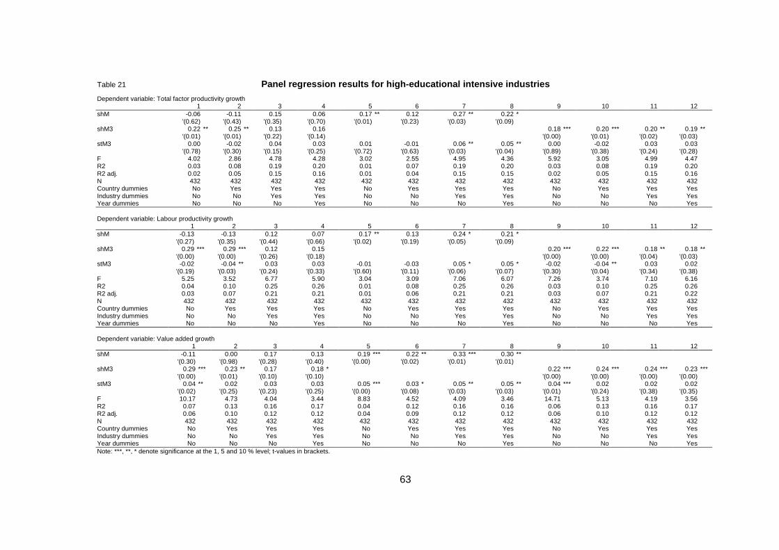
63

Table 21 Panel regression results for high-educational inten sive industries

Dependent variable: Total factor productivity growth 1 2 3 4 5 6 7 8 9 10 11 12 shM -0.06 -0.11 0.15 0.06 0.17 ** 0.12 0.27 ** 0.22 * '(0.62) '(0.43) '(0.35) '(0.70) '(0.01) '(0.23) '(0.03) '(0.09) shM3 0.22 ** 0.25 ** 0.13 0.16 0.18 *** 0.20 *** 0.20 ** 0.19 ** '(0.01) '(0.01) '(0.22) '(0.14) '(0.00) '(0.01) '(0.02) '(0.03) stM3 0.00 -0.02 0.04 0.03 0.01 -0.01 0.06 ** 0.05 ** 0.00 -0.02 0.03 0.03 '(0.78) '(0.30) '(0.15) '(0.25) '(0.72) '(0.63) '(0.03) '(0.04) '(0.89) '(0.38) '(0.24) '(0.28) F 4.02 2.86 4.78 4.28 3.02 2.55 4.95 4.36 5.92 3.05 4.99 4.47 R2 0.03 0.08 0.19 0.20 0.01 0.07 0.19 0.20 0.03 0.08 0.19 0.20 R2 adj. 0.02 0.05 0.15 0.16 0.01 0.04 0.15 0.15 0.02 0.05 0.15 0.16 N 432 432 432 432 432 432 432 432 432 432 432 432 Country dummies No Yes Yes Yes No Yes Yes Yes No Yes Yes Yes Industry dummies No No Yes Yes No No Yes Yes No No Yes Yes Year dummies No No No Yes No No No Yes No No No Yes Dependent variable: Labour productivity growth 1 2 3 4 5 6 7 8 9 10 11 12 shM -0.13 -0.13 0.12 0.07 0.17 ** 0.13 0.24 * 0.21 * '(0.27) '(0.35) '(0.44) '(0.66) '(0.02) '(0.19) '(0.05) '(0.09) shM3 0.29 *** 0.29 *** 0.12 0.15 0.20 *** 0.22 *** 0.18 ** 0.18 ** '(0.00) '(0.00) '(0.26) '(0.18) '(0.00) '(0.00) '(0.04) '(0.03) stM3 -0.02 -0.04 ** 0.03 0.03 -0.01 -0.03 0.05 * 0.05 * -0.02 -0.04 ** 0.03 0.02 '(0.19) '(0.03) '(0.24) '(0.33) '(0.60) '(0.11) '(0.06) '(0.07) '(0.30) '(0.04) '(0.34) '(0.38) F 5.25 3.52 6.77 5.90 3.04 3.09 7.06 6.07 7.26 3.74 7.10 6.16 R2 0.04 0.10 0.25 0.26 0.01 0.08 0.25 0.26 0.03 0.10 0.25 0.26 R2 adj. 0.03 0.07 0.21 0.21 0.01 0.06 0.21 0.21 0.03 0.07 0.21 0.22 N 432 432 432 432 432 432 432 432 432 432 432 432 Country dummies No Yes Yes Yes No Yes Yes Yes No Yes Yes Yes Industry dummies No No Yes Yes No No Yes Yes No No Yes Yes Year dummies No No No Yes No No No Yes No No No Yes Dependent variable: Value added growth 1 2 3 4 5 6 7 8 9 10 11 12 shM -0.11 0.00 0.17 0.13 0.19 *** 0.22 ** 0.33 *** 0.30 ** '(0.30) '(0.98) '(0.28) '(0.40) '(0.00) '(0.02) '(0.01) '(0.01) shM3 0.29 *** 0.23 ** 0.17 0.18 * 0.22 *** 0.24 *** 0.24 *** 0.23 *** '(0.00) '(0.01) '(0.10) '(0.10) '(0.00) '(0.00) '(0.00) '(0.00) stM3 0.04 ** 0.02 0.03 0.03 0.05 *** 0.03 * 0.05 ** 0.05 ** 0.04 *** 0.02 0.02 0.02 '(0.02) '(0.25) '(0.23) '(0.25) '(0.00) '(0.08) '(0.03) '(0.03) '(0.01) '(0.24) '(0.38) '(0.35) F 10.17 4.73 4.04 3.44 8.83 4.52 4.09 3.46 14.71 5.13 4.19 3.56 R2 0.07 0.13 0.16 0.17 0.04 0.12 0.16 0.16 0.06 0.13 0.16 0.17 R2 adj. 0.06 0.10 0.12 0.12 0.04 0.09 0.12 0.12 0.06 0.10 0.12 0.12 N 432 432 432 432 432 432 432 432 432 432 432 432 Country dummies No Yes Yes Yes No Yes Yes Yes No Yes Yes Yes Industry dummies No No Yes Yes No No Yes Yes No No Yes Yes Year dummies No No No Yes No No No Yes No No No Yes Note: ***, **, * denote significance at the 1, 5 and 10 % level; t-values in brackets.

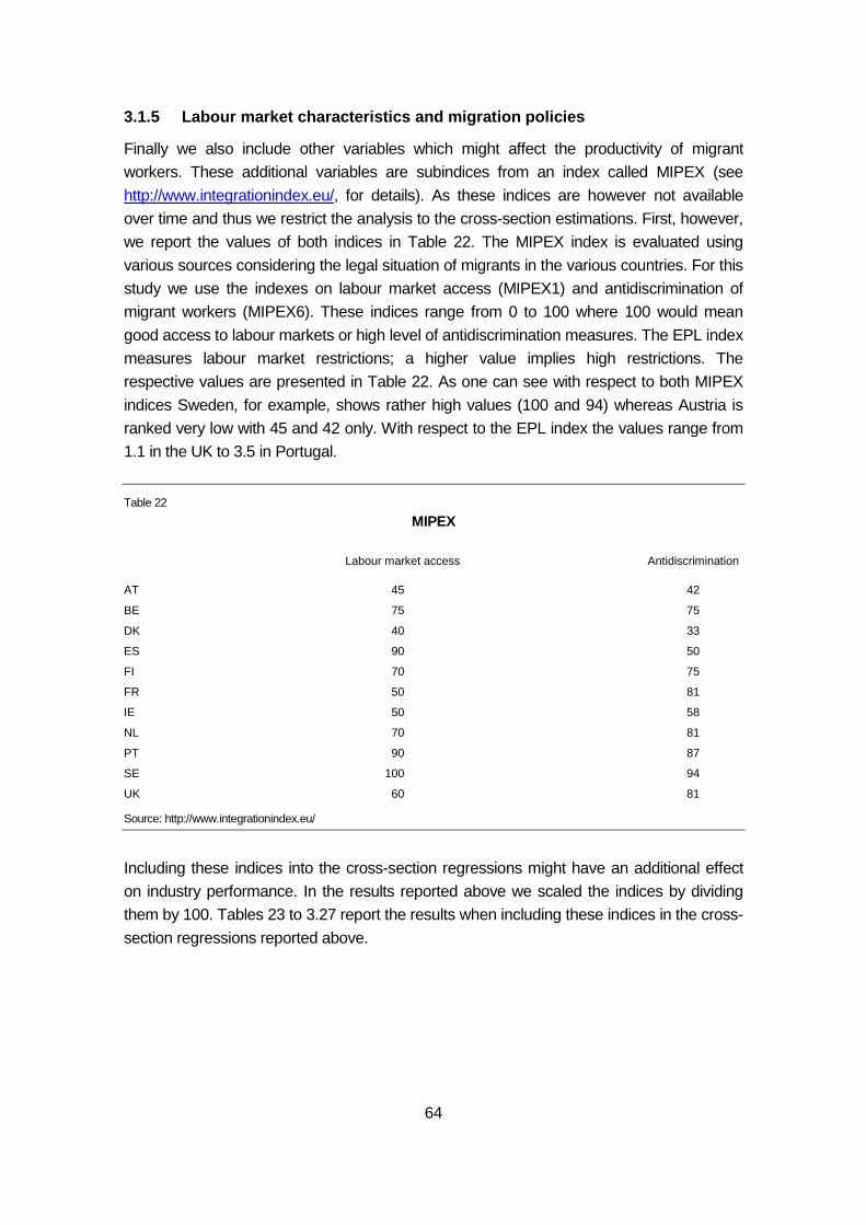
64

3.1.5 Labour market characteristics and migration policies

Finally we also include other variables which might affect the productivity of migrant

workers. These additional variables are subindices from an index called MIPEX (see

http://www.integrationindex.eu/, for details). As these indices are however not available

over time and thus we restrict the analysis to the cross-section estimations. First, however,

we report the values of both indices in Table 22. The MIPEX index is evaluated using

various sources considering the legal situation of migrants in the various countries. For this

study we use the indexes on labour market access (MIPEX1) and antidiscrimination of

migrant workers (MIPEX6). These indices range from 0 to 100 where 100 would mean

good access to labour markets or high level of antidiscrimination measures. The EPL index

measures labour market restrictions; a higher value implies high restrictions. The

respective values are presented in Table 22. As one can see with respect to both MIPEX

indices Sweden, for example, shows rather high values (100 and 94) whereas Austria is

ranked very low with 45 and 42 only. With respect to the EPL index the values range from

1.1 in the UK to 3.5 in Portugal.

Table 22

MIPEX

Labour market access Antidiscrimination

AT 45 42

BE 75 75

DK 40 33

ES 90 50

FI 70 75

FR 50 81

IE 50 58

NL 70 81

PT 90 87

SE 100 94

UK 60 81

Source: http://www.integrationindex.eu/

Including these indices into the cross-section regressions might have an additional effect

on industry performance. In the results reported above we scaled the indices by dividing

them by 100. Tables 23 to 3.27 report the results when including these indices in the cross-

section regressions reported above.

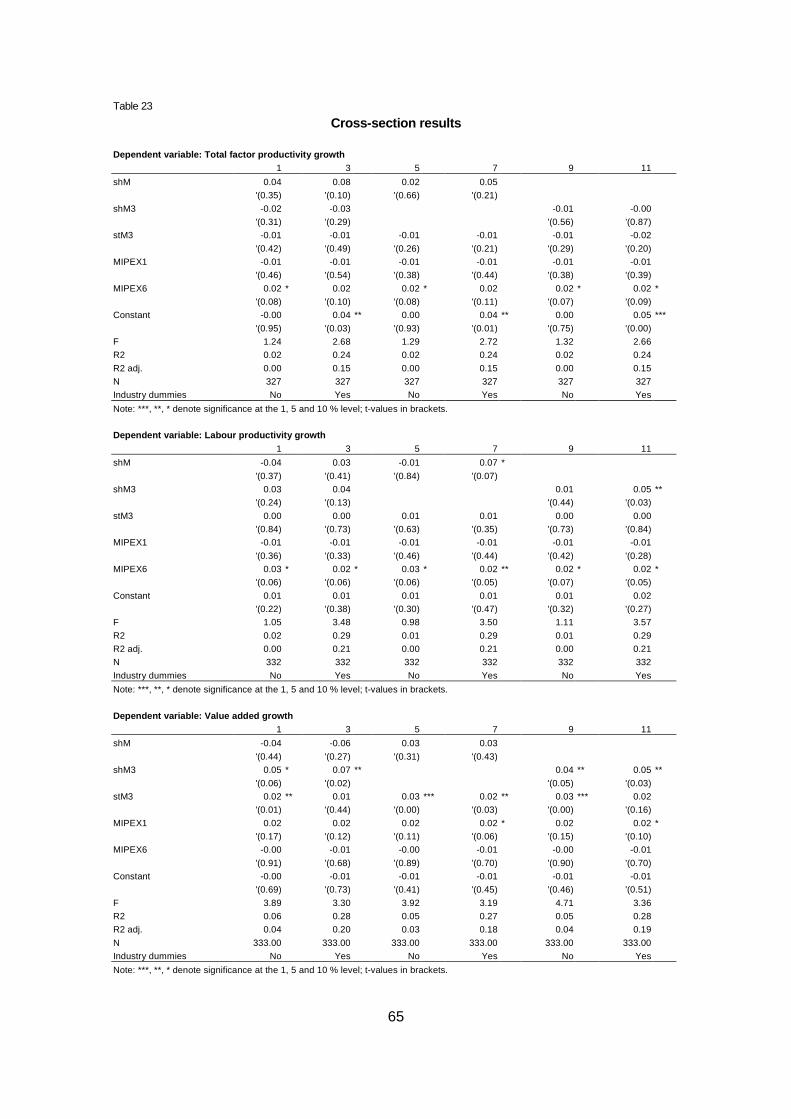
65

Table 23

Cross-section results

Dependent variable: Total factor productivity growt h

1 3 5 7 9 11

shM 0.04 0.08 0.02 0.05

'(0.35) '(0.10) '(0.66) '(0.21)

shM3 -0.02 -0.03 -0.01 -0.00

'(0.31) '(0.29) '(0.56) '(0.87)

stM3 -0.01 -0.01 -0.01 -0.01 -0.01 -0.02

'(0.42) '(0.49) '(0.26) '(0.21) '(0.29) '(0.20)

MIPEX1 -0.01 -0.01 -0.01 -0.01 -0.01 -0.01

'(0.46) '(0.54) '(0.38) '(0.44) '(0.38) '(0.39)

MIPEX6 0.02 * 0.02 0.02 * 0.02 0.02 * 0.02 *

'(0.08) '(0.10) '(0.08) '(0.11) '(0.07) '(0.09)

Constant -0.00 0.04 ** 0.00 0.04 ** 0.00 0.05 ***

'(0.95) '(0.03) '(0.93) '(0.01) '(0.75) '(0.00)

F 1.24 2.68 1.29 2.72 1.32 2.66

R2 0.02 0.24 0.02 0.24 0.02 0.24

R2 adj. 0.00 0.15 0.00 0.15 0.00 0.15

N 327 327 327 327 327 327

Industry dummies No Yes No Yes No Yes


Dependent variable: Labour productivity growth

1 3 5 7 9 11

shM -0.04 0.03 -0.01 0.07 *

'(0.37) '(0.41) '(0.84) '(0.07)

shM3 0.03 0.04 0.01 0.05 **

'(0.24) '(0.13) '(0.44) '(0.03)

stM3 0.00 0.00 0.01 0.01 0.00 0.00

'(0.84) '(0.73) '(0.63) '(0.35) '(0.73) '(0.84)

MIPEX1 -0.01 -0.01 -0.01 -0.01 -0.01 -0.01

'(0.36) '(0.33) '(0.46) '(0.44) '(0.42) '(0.28)

MIPEX6 0.03 * 0.02 * 0.03 * 0.02 ** 0.02 * 0.02 *

'(0.06) '(0.06) '(0.06) '(0.05) '(0.07) '(0.05)

Constant 0.01 0.01 0.01 0.01 0.01 0.02

'(0.22) '(0.38) '(0.30) '(0.47) '(0.32) '(0.27)

F 1.05 3.48 0.98 3.50 1.11 3.57

R2 0.02 0.29 0.01 0.29 0.01 0.29

R2 adj. 0.00 0.21 0.00 0.21 0.00 0.21

N 332 332 332 332 332 332



Dependent variable: Value added growth

1 3 5 7 9 11

shM -0.04 -0.06 0.03 0.03

'(0.44) '(0.27) '(0.31) '(0.43)

shM3 0.05 * 0.07 ** 0.04 ** 0.05 **

'(0.06) '(0.02) '(0.05) '(0.03)

stM3 0.02 ** 0.01 0.03 *** 0.02 ** 0.03 *** 0.02

'(0.01) '(0.44) '(0.00) '(0.03) '(0.00) '(0.16)

MIPEX1 0.02 0.02 0.02 0.02 * 0.02 0.02 *

'(0.17) '(0.12) '(0.11) '(0.06) '(0.15) '(0.10)

MIPEX6 -0.00 -0.01 -0.00 -0.01 -0.00 -0.01

'(0.91) '(0.68) '(0.89) '(0.70) '(0.90) '(0.70)

Constant -0.00 -0.01 -0.01 -0.01 -0.01 -0.01

'(0.69) '(0.73) '(0.41) '(0.45) '(0.46) '(0.51)

F 3.89 3.30 3.92 3.19 4.71 3.36

R2 0.06 0.28 0.05 0.27 0.05 0.28

R2 adj. 0.04 0.20 0.03 0.18 0.04 0.19

N 333.00 333.00 333.00 333.00 333.00 333.00



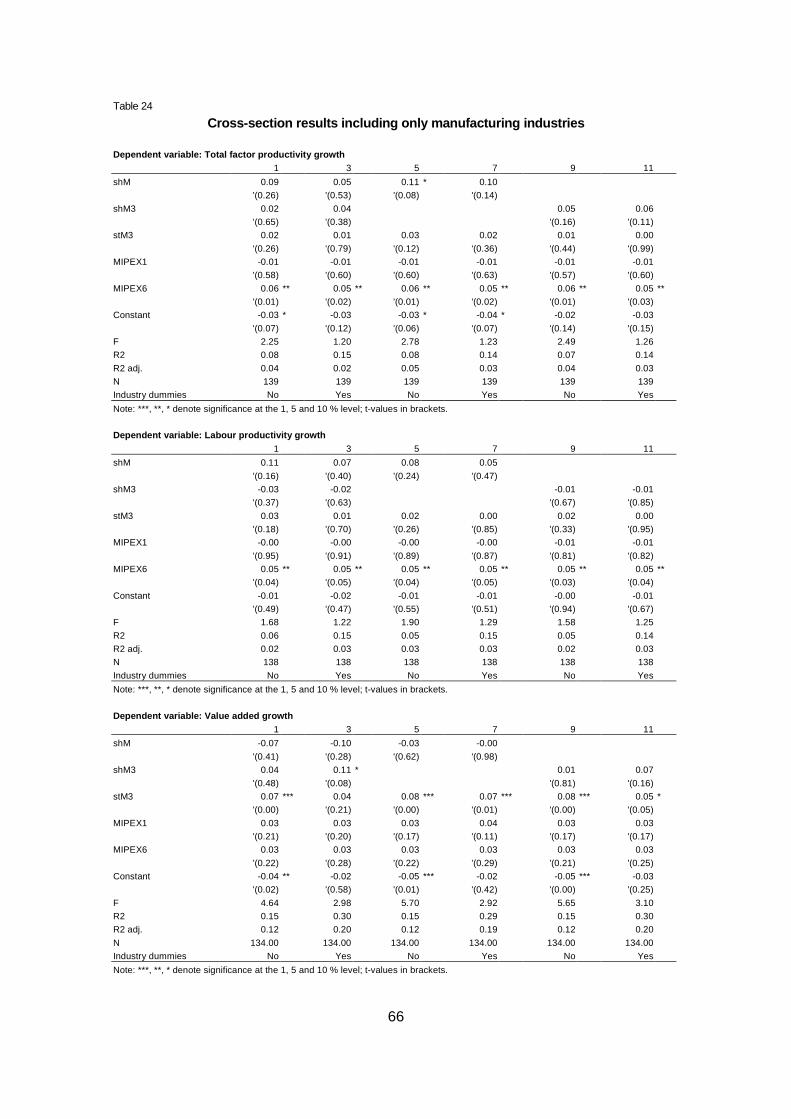
66

Table 24

Cross-section results including only manufacturing industries


1 3 5 7 9 11

shM 0.09 0.05 0.11 * 0.10

'(0.26) '(0.53) '(0.08) '(0.14)

shM3 0.02 0.04 0.05 0.06

'(0.65) '(0.38) '(0.16) '(0.11)

stM3 0.02 0.01 0.03 0.02 0.01 0.00

'(0.26) '(0.79) '(0.12) '(0.36) '(0.44) '(0.99)

MIPEX1 -0.01 -0.01 -0.01 -0.01 -0.01 -0.01

'(0.58) '(0.60) '(0.60) '(0.63) '(0.57) '(0.60)

MIPEX6 0.06 ** 0.05 ** 0.06 ** 0.05 ** 0.06 ** 0.05 **

'(0.01) '(0.02) '(0.01) '(0.02) '(0.01) '(0.03)

Constant -0.03 * -0.03 -0.03 * -0.04 * -0.02 -0.03

'(0.07) '(0.12) '(0.06) '(0.07) '(0.14) '(0.15)

F 2.25 1.20 2.78 1.23 2.49 1.26

R2 0.08 0.15 0.08 0.14 0.07 0.14

R2 adj. 0.04 0.02 0.05 0.03 0.04 0.03

N 139 139 139 139 139 139




1 3 5 7 9 11

shM 0.11 0.07 0.08 0.05

'(0.16) '(0.40) '(0.24) '(0.47)

shM3 -0.03 -0.02 -0.01 -0.01

'(0.37) '(0.63) '(0.67) '(0.85)

stM3 0.03 0.01 0.02 0.00 0.02 0.00

'(0.18) '(0.70) '(0.26) '(0.85) '(0.33) '(0.95)

MIPEX1 -0.00 -0.00 -0.00 -0.00 -0.01 -0.01

'(0.95) '(0.91) '(0.89) '(0.87) '(0.81) '(0.82)

MIPEX6 0.05 ** 0.05 ** 0.05 ** 0.05 ** 0.05 ** 0.05 **

'(0.04) '(0.05) '(0.04) '(0.05) '(0.03) '(0.04)

Constant -0.01 -0.02 -0.01 -0.01 -0.00 -0.01

'(0.49) '(0.47) '(0.55) '(0.51) '(0.94) '(0.67)

F 1.68 1.22 1.90 1.29 1.58 1.25

R2 0.06 0.15 0.05 0.15 0.05 0.14

R2 adj. 0.02 0.03 0.03 0.03 0.02 0.03

N 138 138 138 138 138 138




1 3 5 7 9 11

shM -0.07 -0.10 -0.03 -0.00

'(0.41) '(0.28) '(0.62) '(0.98)

shM3 0.04 0.11 * 0.01 0.07

'(0.48) '(0.08) '(0.81) '(0.16)

stM3 0.07 *** 0.04 0.08 *** 0.07 *** 0.08 *** 0.05 *

'(0.00) '(0.21) '(0.00) '(0.01) '(0.00) '(0.05)

MIPEX1 0.03 0.03 0.03 0.04 0.03 0.03

'(0.21) '(0.20) '(0.17) '(0.11) '(0.17) '(0.17)

MIPEX6 0.03 0.03 0.03 0.03 0.03 0.03

'(0.22) '(0.28) '(0.22) '(0.29) '(0.21) '(0.25)

Constant -0.04 ** -0.02 -0.05 *** -0.02 -0.05 *** -0.03

'(0.02) '(0.58) '(0.01) '(0.42) '(0.00) '(0.25)

F 4.64 2.98 5.70 2.92 5.65 3.10

R2 0.15 0.30 0.15 0.29 0.15 0.30

R2 adj. 0.12 0.20 0.12 0.19 0.12 0.20

N 134.00 134.00 134.00 134.00 134.00 134.00



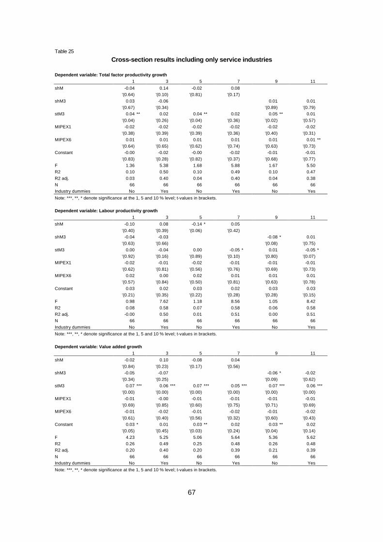
67

Table 25

Cross-section results including only service indust ries


1 3 5 7 9 11

shM -0.04 0.14 -0.02 0.08

'(0.64) '(0.10) '(0.81) '(0.17)

shM3 0.03 -0.06 0.01 0.01

'(0.67) '(0.34) '(0.89) '(0.79)

stM3 0.04 ** 0.02 0.04 ** 0.02 0.05 ** 0.01

'(0.04) '(0.26) '(0.04) '(0.36) '(0.02) '(0.57)

MIPEX1 -0.02 -0.02 -0.02 -0.02 -0.02 -0.02

'(0.38) '(0.39) '(0.39) '(0.36) '(0.40) '(0.31)

MIPEX6 0.01 0.01 0.01 0.01 0.01 0.01 **

'(0.64) '(0.65) '(0.62) '(0.74) '(0.63) '(0.73)

Constant -0.00 -0.02 -0.00 -0.02 -0.01 -0.01

'(0.83) '(0.28) '(0.82) '(0.37) '(0.68) '(0.77)

F 1.36 5.38 1.68 5.88 1.67 5.50

R2 0.10 0.50 0.10 0.49 0.10 0.47

R2 adj. 0.03 0.40 0.04 0.40 0.04 0.38

N 66 66 66 66 66 66




1 3 5 7 9 11

shM -0.10 0.08 -0.14 * 0.05

'(0.40) '(0.39) '(0.06) '(0.42)

shM3 -0.04 -0.03 -0.08 * 0.01

'(0.63) '(0.66) '(0.08) '(0.75)

stM3 0.00 -0.04 0.00 -0.05 * 0.01 -0.05 *

'(0.92) '(0.16) '(0.89) '(0.10) '(0.80) '(0.07)

MIPEX1 -0.02 -0.01 -0.02 -0.01 -0.01 -0.01

'(0.62) '(0.81) '(0.56) '(0.76) '(0.69) '(0.73)

MIPEX6 0.02 0.00 0.02 0.01 0.01 0.01

'(0.57) '(0.84) '(0.50) '(0.81) '(0.63) '(0.78)

Constant 0.03 0.02 0.03 0.02 0.03 0.03

'(0.21) '(0.35) '(0.22) '(0.28) '(0.28) '(0.15)

F 0.98 7.62 1.18 8.56 1.05 8.42

R2 0.08 0.58 0.07 0.58 0.06 0.58

R2 adj. -0.00 0.50 0.01 0.51 0.00 0.51

N 66 66 66 66 66 66




1 3 5 7 9 11

shM -0.02 0.10 -0.08 0.04

'(0.84) '(0.23) '(0.17) '(0.56)

shM3 -0.05 -0.07 -0.06 * -0.02

'(0.34) '(0.25) '(0.09) '(0.62)

stM3 0.07 *** 0.06 *** 0.07 *** 0.05 *** 0.07 *** 0.06 ***

'(0.00) '(0.00) '(0.00) '(0.00) '(0.00) '(0.00)

MIPEX1 -0.01 -0.00 -0.01 -0.01 -0.01 -0.01

'(0.69) '(0.85) '(0.60) '(0.75) '(0.71) '(0.69)

MIPEX6 -0.01 -0.02 -0.01 -0.02 -0.01 -0.02

'(0.61) '(0.40) '(0.56) '(0.32) '(0.60) '(0.43)

Constant 0.03 * 0.01 0.03 ** 0.02 0.03 ** 0.02

'(0.05) '(0.45) '(0.03) '(0.24) '(0.04) '(0.14)

F 4.23 5.25 5.06 5.64 5.36 5.62

R2 0.26 0.49 0.25 0.48 0.26 0.48

R2 adj. 0.20 0.40 0.20 0.39 0.21 0.39

N 66 66 66 66 66 66



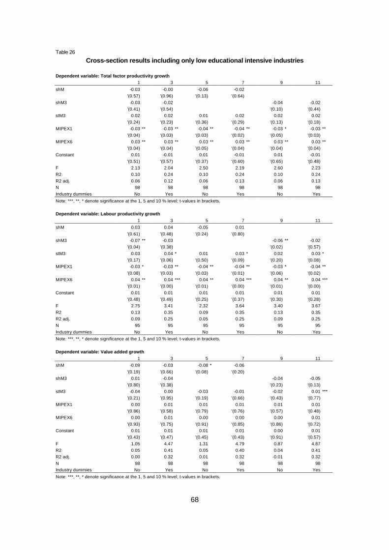
68

Table 26

Cross-section results including only low educationa l intensive industries


1 3 5 7 9 11

shM -0.03 -0.00 -0.06 -0.02

'(0.57) '(0.96) '(0.13) '(0.64)

shM3 -0.03 -0.02 -0.04 -0.02

'(0.41) '(0.54) '(0.10) '(0.44)

stM3 0.02 0.02 0.01 0.02 0.02 0.02

'(0.24) '(0.23) '(0.36) '(0.29) '(0.13) '(0.18)

MIPEX1 -0.03 ** -0.03 ** -0.04 ** -0.04 ** -0.03 * -0.03 **

'(0.04) '(0.03) '(0.03) '(0.02) '(0.05) '(0.03)

MIPEX6 0.03 ** 0.03 ** 0.03 ** 0.03 ** 0.03 ** 0.03 **

'(0.04) '(0.04) '(0.05) '(0.04) '(0.04) '(0.04)

Constant 0.01 -0.01 0.01 -0.01 0.01 -0.01

'(0.51) '(0.57) '(0.37) '(0.60) '(0.65) '(0.48)

F 2.13 2.04 2.50 2.19 2.60 2.23

R2 0.10 0.24 0.10 0.24 0.10 0.24

R2 adj. 0.06 0.12 0.06 0.13 0.06 0.13

N 98 98 98 98 98 98




1 3 5 7 9 11

shM 0.03 0.04 -0.05 0.01

'(0.61) '(0.48) '(0.24) '(0.80)

shM3 -0.07 ** -0.03 -0.06 ** -0.02

'(0.04) '(0.38) '(0.02) '(0.57)

stM3 0.03 0.04 * 0.01 0.03 * 0.02 0.03 *

'(0.17) '(0.06) '(0.50) '(0.09) '(0.20) '(0.08)

MIPEX1 -0.03 * -0.03 ** -0.04 ** -0.04 ** -0.03 * -0.04 **

'(0.08) '(0.03) '(0.03) '(0.01) '(0.06) '(0.02)

MIPEX6 0.04 ** 0.04 *** 0.04 ** 0.04 *** 0.04 ** 0.04 ***

'(0.01) '(0.00) '(0.01) '(0.00) '(0.01) '(0.00)

Constant 0.01 0.01 0.01 0.01 0.01 0.01

'(0.48) '(0.49) '(0.25) '(0.37) '(0.30) '(0.28)

F 2.75 3.41 2.32 3.64 3.40 3.67

R2 0.13 0.35 0.09 0.35 0.13 0.35

R2 adj. 0.09 0.25 0.05 0.25 0.09 0.25

N 95 95 95 95 95 95




1 3 5 7 9 11

shM -0.09 -0.03 -0.08 * -0.06

'(0.19) '(0.66) '(0.08) '(0.20)

shM3 0.01 -0.04 -0.04 -0.05

'(0.80) '(0.38) '(0.23) '(0.13)

stM3 -0.04 0.00 -0.03 -0.01 -0.02 0.01 ***

'(0.21) '(0.95) '(0.19) '(0.66) '(0.43) '(0.77)

MIPEX1 0.00 0.01 0.01 0.01 0.01 0.01

'(0.86) '(0.58) '(0.79) '(0.76) '(0.57) '(0.48)

MIPEX6 0.00 0.01 0.00 0.00 0.00 0.01

'(0.93) '(0.75) '(0.91) '(0.85) '(0.86) '(0.72)

Constant 0.01 0.01 0.01 0.01 0.00 0.01

'(0.43) '(0.47) '(0.45) '(0.43) '(0.91) '(0.57)

F 1.05 4.47 1.31 4.79 0.87 4.87

R2 0.05 0.41 0.05 0.40 0.04 0.41

R2 adj. 0.00 0.32 0.01 0.32 -0.01 0.32

N 98 98 98 98 98 98



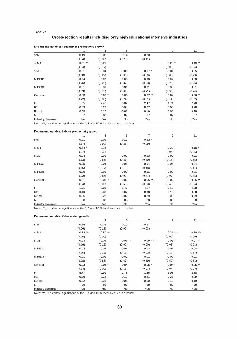
69

Table 27

Cross-section results including only high education al intensive industries


1 3 5 7 9 11

shM -0.19 -0.03 0.14 0.20

'(0.34) '(0.88) '(0.25) '(0.11)

shM3 0.31 ** 0.21 0.20 ** 0.19 **

'(0.04) '(0.17) '(0.03) '(0.04)

stM3 -0.01 0.04 -0.00 0.07 * -0.01 0.05

'(0.60) '(0.29) '(0.96) '(0.09) '(0.80) '(0.23)

MIPEX1 0.04 0.03 0.03 0.03 0.04 0.03

'(0.26) '(0.26) '(0.37) '(0.33) '(0.26) '(0.25)

MIPEX6 0.01 0.01 0.01 0.01 0.00 0.01

'(0.83) '(0.73) '(0.84) '(0.71) '(0.93) '(0.74)

Constant -0.03 -0.06 ** -0.03 -0.07 ** -0.04 -0.06 **

'(0.22) '(0.03) '(0.24) '(0.01) '(0.14) '(0.02)

F 1.55 2.45 0.82 2.47 1.71 2.70

R2 0.09 0.28 0.04 0.27 0.08 0.28

R2 adj. 0.03 0.17 -0.01 0.16 0.03 0.18

N 87 87 87 87 87 87




1 3 5 7 9 11

shM -0.21 0.03 0.15 0.22 *

'(0.37) '(0.90) '(0.23) '(0.09)

shM3 0.34 * 0.16 0.20 ** 0.18 *

'(0.07) '(0.39) '(0.05) '(0.05)

stM3 -0.04 0.01 -0.03 0.03 -0.03 0.01

'(0.13) '(0.65) '(0.31) '(0.30) '(0.18) '(0.65)

MIPEX1 0.05 0.04 0.05 0.04 0.05 0.04

'(0.16) '(0.17) '(0.18) '(0.18) '(0.15) '(0.17)

MIPEX6 0.00 0.01 0.00 0.01 -0.00 0.01

'(0.92) '(0.86) '(0.92) '(0.87) '(0.97) '(0.85)

Constant -0.01 -0.05 ** -0.02 -0.05 ** -0.02 -0.05 **

'(0.64) '(0.05) '(0.53) '(0.03) '(0.48) '(0.04)

F 1.91 3.88 1.47 4.17 2.18 4.28

R2 0.10 0.38 0.07 0.38 0.10 0.38

R2 adj. 0.05 0.28 0.02 0.29 0.05 0.29

N 88 88 88 88 88 88




1 3 5 7 9 11

shM -0.34 * -0.33 0.25 ** 0.27 **

'(0.06) '(0.11) '(0.02) '(0.03)

shM3 0.52 *** 0.50 *** 0.31 *** 0.30 ***

'(0.00) '(0.00) '(0.00) '(0.00)

stM3 0.03 0.05 0.06 ** 0.09 *** 0.05 ** 0.07 **

'(0.16) '(0.16) '(0.02) '(0.00) '(0.03) '(0.03)

MIPEX1 0.04 0.04 0.04 0.03 0.04 0.04

'(0.15) '(0.18) '(0.18) '(0.22) '(0.12) '(0.14)

MIPEX6 -0.01 -0.01 -0.02 -0.01 -0.02 -0.01

'(0.78) '(0.85) '(0.57) '(0.69) '(0.52) '(0.61)

Constant -0.03 -0.04 * -0.04 -0.05 * -0.04 ** -0.05 **

'(0.14) '(0.09) '(0.11) '(0.07) '(0.04) '(0.03)

F 5.77 2.91 2.78 1.86 6.08 2.88

R2 0.26 0.32 0.12 0.21 0.23 0.29

R2 adj. 0.22 0.21 0.08 0.10 0.19 0.19

N 88 88 88 88 88 88



70

The results indicate that in countries with better antidiscrimination measures (MIPEX6)

tend to have higher productivity growth rates (Table 23). This is the case for both growth in

total factor productivity and labour productivity. The other variable (MIPEX1) capturing

labour market access for migrant workers is less often significant and sometimes even

negative. These variables are however not significant with respect to value added growth.

With respect to different industry categories these results hold of manufacturing industries

(Table 24) but not for service industries (Table 25). Similarly, the results hold for low

educational intensive industries (Table 26) but again not for high educational intensive

industries (Table 27).

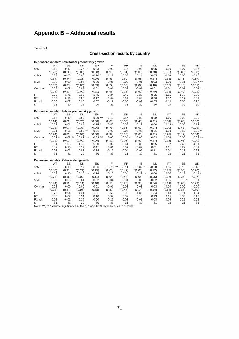
71

Appendix B – Additional results

Table B.1

Cross-section results by country

Dependent variable: Total factor productivity growt h AT BE DK ES FI FR IE NL PT SE UK shM -0.12 -0.12 -0.26 ** -0.03 0.03 -0.14 0.00 0.05 0.00 0.07 0.26 '(0.23) '(0.20) '(0.02) '(0.88) '(0.98) '(0.31) '(1.00) '(0.78) '(0.98) '(0.85) '(0.38) shM3 0.03 -0.05 0.05 -0.20 * 1.27 0.03 0.14 0.05 -0.03 0.05 -0.15 '(0.64) '(0.44) '(0.22) '(0.09) '(0.45) '(0.60) '(0.58) '(0.67) '(0.52) '(0.73) '(0.37) stM3 0.00 0.00 -0.04 * 0.00 -0.01 -0.02 -0.01 0.03 0.00 0.11 -0.07 *** '(0.97) '(0.97) '(0.08) '(0.99) '(0.77) '(0.53) '(0.87) '(0.40) '(0.96) '(0.18) '(0.01) Constant 0.02 * 0.02 0.02 *** 0.01 0.01 0.02 -0.01 -0.01 -0.01 -0.01 0.04 *** '(0.09) '(0.11) '(0.00) '(0.51) '(0.53) '(0.13) '(0.66) '(0.75) '(0.28) '(0.80) '(0.01) F 0.70 1.71 3.18 1.75 0.24 0.42 0.20 0.55 0.15 1.79 3.83 R2 0.07 0.16 0.28 0.17 0.04 0.04 0.02 0.06 0.02 0.17 0.31 R2 adj. -0.03 0.07 0.20 0.07 -0.12 -0.06 -0.09 -0.05 -0.10 0.08 0.23 N 31 30 28 29 23 31 29 30 29 30 30 Dependent variable: Labour productivity growth AT BE DK ES FI FR IE NL PT SE UK shM -0.17 -0.10 -0.05 -0.69 *** 0.18 -0.14 0.38 -0.02 -0.05 0.05 -0.06 '(0.14) '(0.35) '(0.70) '(0.00) '(0.88) '(0.30) '(0.49) '(0.91) '(0.84) '(0.88) '(0.86) shM3 0.07 0.01 0.04 0.15 * 0.52 0.02 0.13 0.00 -0.12 * 0.09 -0.18 '(0.26) '(0.93) '(0.38) '(0.06) '(0.76) '(0.81) '(0.62) '(0.97) '(0.09) '(0.55) '(0.38) stM3 -0.01 -0.01 -0.05 ** -0.01 0.00 -0.03 -0.03 -0.01 0.00 0.12 -0.06 ** '(0.74) '(0.85) '(0.03) '(0.60) '(0.97) '(0.35) '(0.64) '(0.81) '(0.93) '(0.17) '(0.04) Constant 0.03 ** 0.03 ** 0.03 *** 0.03 *** 0.02 0.04 ** 0.00 0.03 0.03 0.00 0.07 *** '(0.02) '(0.02) '(0.00) '(0.00) '(0.19) '(0.01) '(0.89) '(0.17) '(0.11) '(0.96) '(0.00) F 0.84 1.05 1.73 5.90 0.06 0.64 0.80 0.05 1.07 2.49 4.01 R2 0.09 0.10 0.17 0.41 0.01 0.07 0.09 0.01 0.11 0.22 0.31 R2 adj. -0.02 0.01 0.07 0.34 -0.15 -0.04 -0.02 -0.11 0.01 0.13 0.23 N 31 31 29 30 23 31 30 31 29 31 31 Dependent variable: Value added growth AT BE DK ES FI FR IE NL PT SE UK shM -0.08 0.10 0.17 0.36 3.76 *** -0.11 0.89 * -0.20 0.05 -0.18 -0.48 '(0.46) '(0.37) '(0.29) '(0.15) '(0.00) '(0.42) '(0.06) '(0.17) '(0.78) '(0.55) '(0.20) shM3 0.02 -0.10 -0.20 *** -0.16 -0.12 0.04 -0.43 ** 0.00 -0.07 0.16 0.41 * '(0.72) '(0.16) '(0.00) '(0.11) '(0.94) '(0.48) '(0.05) '(0.96) '(0.16) '(0.25) '(0.07) stM3 0.03 0.03 0.04 0.02 0.04 0.04 0.00 0.02 0.05 0.15 * -0.01 '(0.44) '(0.19) '(0.14) '(0.48) '(0.16) '(0.26) '(0.96) '(0.54) '(0.11) '(0.05) '(0.79) Constant 0.02 0.00 0.00 0.01 -0.01 0.01 0.03 0.03 0.00 0.00 0.00 '(0.22) '(0.87) '(0.98) '(0.38) '(0.39) '(0.47) '(0.14) '(0.14) '(0.68) '(0.88) '(0.89) F 0.75 0.94 4.31 1.01 3.68 0.93 1.86 1.34 1.43 5.11 1.34 R2 0.08 0.09 0.34 0.10 0.37 0.09 0.18 0.13 0.15 0.36 0.13 R2 adj. -0.03 -0.01 0.26 0.00 0.27 -0.01 0.08 0.03 0.04 0.29 0.03 N 31 31 29 30 23 31 30 31 29 31 31 Note: ***, **, * denote significance at the 1, 5 and 10 % level; t-values in brackets.

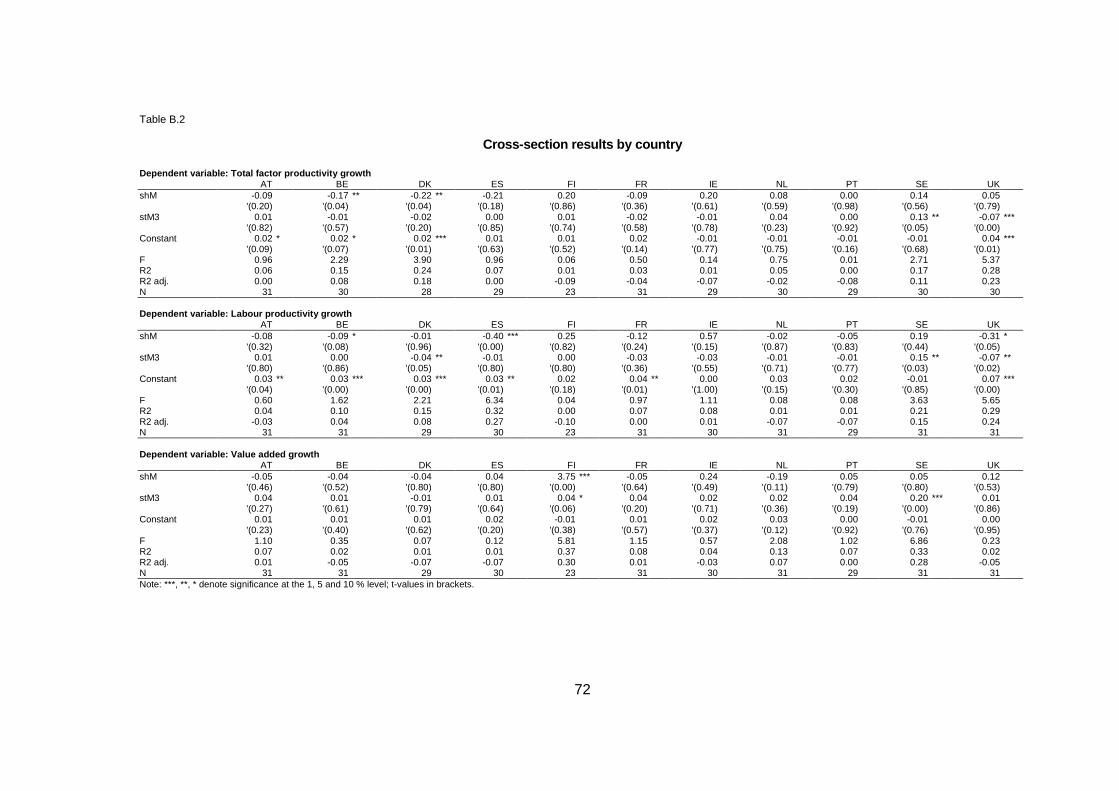
72

Table B.2


Dependent variable: Total factor productivity growt h AT BE DK ES FI FR IE NL PT SE UK shM -0.09 -0.17 ** -0.22 ** -0.21 0.20 -0.09 0.20 0.08 0.00 0.14 0.05 '(0.20) '(0.04) '(0.04) '(0.18) '(0.86) '(0.36) '(0.61) '(0.59) '(0.98) '(0.56) '(0.79) stM3 0.01 -0.01 -0.02 0.00 0.01 -0.02 -0.01 0.04 0.00 0.13 ** -0.07 *** '(0.82) '(0.57) '(0.20) '(0.85) '(0.74) '(0.58) '(0.78) '(0.23) '(0.92) '(0.05) '(0.00) Constant 0.02 * 0.02 * 0.02 *** 0.01 0.01 0.02 -0.01 -0.01 -0.01 -0.01 0.04 *** '(0.09) '(0.07) '(0.01) '(0.63) '(0.52) '(0.14) '(0.77) '(0.75) '(0.16) '(0.68) '(0.01) F 0.96 2.29 3.90 0.96 0.06 0.50 0.14 0.75 0.01 2.71 5.37 R2 0.06 0.15 0.24 0.07 0.01 0.03 0.01 0.05 0.00 0.17 0.28 R2 adj. 0.00 0.08 0.18 0.00 -0.09 -0.04 -0.07 -0.02 -0.08 0.11 0.23 N 31 30 28 29 23 31 29 30 29 30 30 Dependent variable: Labour productivity growth AT BE DK ES FI FR IE NL PT SE UK shM -0.08 -0.09 * -0.01 -0.40 *** 0.25 -0.12 0.57 -0.02 -0.05 0.19 -0.31 * '(0.32) '(0.08) '(0.96) '(0.00) '(0.82) '(0.24) '(0.15) '(0.87) '(0.83) '(0.44) '(0.05) stM3 0.01 0.00 -0.04 ** -0.01 0.00 -0.03 -0.03 -0.01 -0.01 0.15 ** -0.07 ** '(0.80) '(0.86) '(0.05) '(0.80) '(0.80) '(0.36) '(0.55) '(0.71) '(0.77) '(0.03) '(0.02) Constant 0.03 ** 0.03 *** 0.03 *** 0.03 ** 0.02 0.04 ** 0.00 0.03 0.02 -0.01 0.07 *** '(0.04) '(0.00) '(0.00) '(0.01) '(0.18) '(0.01) '(1.00) '(0.15) '(0.30) '(0.85) '(0.00) F 0.60 1.62 2.21 6.34 0.04 0.97 1.11 0.08 0.08 3.63 5.65 R2 0.04 0.10 0.15 0.32 0.00 0.07 0.08 0.01 0.01 0.21 0.29 R2 adj. -0.03 0.04 0.08 0.27 -0.10 0.00 0.01 -0.07 -0.07 0.15 0.24 N 31 31 29 30 23 31 30 31 29 31 31 Dependent variable: Value added growth AT BE DK ES FI FR IE NL PT SE UK shM -0.05 -0.04 -0.04 0.04 3.75 *** -0.05 0.24 -0.19 0.05 0.05 0.12 '(0.46) '(0.52) '(0.80) '(0.80) '(0.00) '(0.64) '(0.49) '(0.11) '(0.79) '(0.80) '(0.53) stM3 0.04 0.01 -0.01 0.01 0.04 * 0.04 0.02 0.02 0.04 0.20 *** 0.01 '(0.27) '(0.61) '(0.79) '(0.64) '(0.06) '(0.20) '(0.71) '(0.36) '(0.19) '(0.00) '(0.86) Constant 0.01 0.01 0.01 0.02 -0.01 0.01 0.02 0.03 0.00 -0.01 0.00 '(0.23) '(0.40) '(0.62) '(0.20) '(0.38) '(0.57) '(0.37) '(0.12) '(0.92) '(0.76) '(0.95) F 1.10 0.35 0.07 0.12 5.81 1.15 0.57 2.08 1.02 6.86 0.23 R2 0.07 0.02 0.01 0.01 0.37 0.08 0.04 0.13 0.07 0.33 0.02 R2 adj. 0.01 -0.05 -0.07 -0.07 0.30 0.01 -0.03 0.07 0.00 0.28 -0.05 N 31 31 29 30 23 31 30 31 29 31 31 Note: ***, **, * denote significance at the 1, 5 and 10 % level; t-values in brackets.

73

Table B.3


Dependent variable: Total factor productivity growt h AT BE DK ES FI FR IE NL PT SE UK shM3 -0.02 -0.09 * 0.02 -0.21 ** 1.28 -0.01 0.14 0.06 -0.03 0.07 -0.03 '(0.54) '(0.08) '(0.67) '(0.03) '(0.42) '(0.84) '(0.44) '(0.53) '(0.51) '(0.51) '(0.75) stM3 0.02 0.01 -0.03 0.00 -0.01 -0.01 -0.01 0.03 0.00 0.11 -0.07 *** '(0.55) '(0.44) '(0.14) '(0.95) '(0.74) '(0.71) '(0.85) '(0.41) '(0.96) '(0.17) '(0.01) Constant 0.01 0.01 0.01 * 0.01 0.01 0.01 -0.01 -0.00 -0.01 * -0.00 0.04 *** '(0.21) '(0.31) '(0.07) '(0.49) '(0.32) '(0.23) '(0.64) '(0.88) '(0.08) '(0.87) '(0.00) F 0.30 1.66 1.33 2.72 0.38 0.09 0.31 0.81 0.23 2.77 5.38 R2 0.02 0.11 0.10 0.17 0.04 0.01 0.02 0.06 0.02 0.17 0.29 R2 adj. -0.05 0.04 0.02 0.11 -0.06 -0.06 -0.05 -0.01 -0.06 0.11 0.23 N 31 30 28 29 23 31 29 30 29 30 30 Dependent variable: Labour productivity growth AT BE DK ES FI FR IE NL PT SE UK shM3 0.00 -0.05 0.04 -0.08 0.57 -0.03 0.25 -0.01 -0.12 * 0.11 -0.21 ** '(0.98) '(0.15) '(0.41) '(0.15) '(0.72) '(0.56) '(0.17) '(0.90) '(0.09) '(0.33) '(0.03) stM3 0.02 0.01 -0.05 ** 0.01 -0.00 -0.02 -0.01 -0.01 0.00 0.11 -0.06 ** '(0.68) '(0.68) '(0.03) '(0.66) '(0.92) '(0.49) '(0.88) '(0.83) '(0.95) '(0.16) '(0.03) Constant 0.02 * 0.02 ** 0.03 *** 0.01 0.02 ** 0.03 *** 0.00 0.02 ** 0.02 ** 0.01 0.06 *** '(0.08) '(0.01) '(0.00) '(0.32) '(0.04) '(0.01) '(0.94) '(0.01) '(0.02) '(0.77) '(0.00) F 0.10 1.11 2.61 1.36 0.08 0.42 0.98 0.07 1.65 3.86 6.21 R2 0.01 0.07 0.17 0.09 0.01 0.03 0.07 0.01 0.11 0.22 0.31 R2 adj. -0.06 0.01 0.10 0.02 -0.09 -0.04 -0.00 -0.07 0.04 0.16 0.26 N 31 31 29 30 23 31 30 31 29 31 31 Dependent variable: Value added growth AT BE DK ES FI FR IE NL PT SE UK shM3 -0.01 -0.05 -0.18 *** -0.04 0.95 0.01 -0.14 -0.05 -0.07 0.10 0.16 '(0.77) '(0.20) '(0.00) '(0.46) '(0.65) '(0.82) '(0.37) '(0.41) '(0.15) '(0.30) '(0.15) stM3 0.04 0.02 0.03 0.01 0.01 0.04 0.04 0.04 0.05 * 0.16 ** -0.00 '(0.20) '(0.33) '(0.19) '(0.77) '(0.83) '(0.16) '(0.33) '(0.17) '(0.09) '(0.03) '(0.96) Constant 0.01 0.01 0.01 0.02 ** 0.02 * 0.00 0.05 ** 0.01 0.01 -0.01 -0.01 '(0.31) '(0.37) '(0.35) '(0.04) '(0.08) '(0.88) '(0.05) '(0.56) '(0.29) '(0.60) '(0.67) F 0.86 0.99 5.84 0.37 0.37 1.06 0.76 0.99 2.18 7.65 1.10 R2 0.06 0.07 0.31 0.03 0.04 0.07 0.05 0.07 0.14 0.35 0.07 R2 adj. -0.01 -0.00 0.26 -0.05 -0.06 0.00 -0.02 -0.00 0.08 0.31 0.01 N 31 31 29 30 23 31 30 31 29 31 31 Note: ***, **, * denote significance at the 1, 5 and 10 % level; t-values in brackets.

74

Table B.4

Panel regression results 1

Dependent variable: Total factor productivity growt h AT BE DK ES FI FR IE NL PT SE UK shM3 0.29 *** 0.09 0.03 -0.16 -0.48 -0.02 0.01 0.05 -0.03 -0.04 0.40 ** '(0.00) '(0.46) '(0.77) '(0.14) '(0.18) '(0.92) '(0.98) '(0.54) '(0.25) '(0.76) '(0.03) stM3 -0.14 ** 0.00 0.00 -0.02 0.07 * 0.00 0.27 0.05 -0.05 -0.11 -0.10 ** '(0.01) '(0.92) '(0.95) '(0.71) '(0.09) '(0.97) '(0.12) '(0.23) '(0.13) '(0.17) '(0.04) Constant 0.05 -0.02 0.03 0.00 0.60 *** 0.01 -0.24 * -0.04 0.02 0.08 0.01 '(0.21) '(0.49) '(0.45) '(0.97) '(0.00) '(0.80) '(0.08) '(0.32) '(0.41) '(0.15) '(0.85) F 1.45 0.82 0.62 1.24 4.40 0.76 0.76 2.24 1.40 3.29 2.09 R2 0.28 0.18 0.15 0.25 0.56 0.17 0.17 0.37 0.27 0.54 0.36 R2 adj. 0.09 -0.04 -0.09 0.05 0.43 -0.05 -0.05 0.21 0.08 0.37 0.19 N 154 149 137 149 145 155 149 150 150 120 150 Dependent variable: Labour productivity growth AT BE DK ES FI FR IE NL PT SE UK shM3 0.25 *** 0.03 -0.03 -0.13 -0.35 0.01 0.02 0.02 -0.05 * -0.01 0.42 * '(0.00) '(0.68) '(0.65) '(0.20) '(0.30) '(0.94) '(0.96) '(0.68) '(0.09) '(0.88) '(0.05) stM3 -0.08 -0.01 0.00 0.04 0.07 * 0.01 0.36 * 0.03 -0.03 -0.03 -0.11 * '(0.20) '(0.91) '(0.91) '(0.34) '(0.09) '(0.95) '(0.05) '(0.46) '(0.43) '(0.64) '(0.06) Constant 0.02 0.03 0.04 -0.05 0.60 *** 0.02 -0.31 ** 0.01 0.02 0.02 0.01 '(0.63) '(0.39) '(0.32) '(0.27) '(0.00) '(0.52) '(0.04) '(0.85) '(0.47) '(0.53) '(0.56) F 1.34 1.02 0.83 1.55 4.99 0.63 0.84 1.82 2.88 3.79 1.97 R2 0.26 0.21 0.19 0.29 0.59 0.14 0.18 0.32 0.43 0.57 0.34 R2 adj. 0.07 0.01 -0.04 0.10 0.47 -0.08 -0.03 0.15 0.28 0.42 0.17 N 154 154 141 154 145 155 154 154 150 123 155 Dependent variable: Value added growth AT BE DK ES FI FR IE NL PT SE UK shM3 0.30 *** -0.02 0.17 *** -0.14 0.04 -0.07 0.45 0.02 -0.03 0.06 0.20 '(0.00) '(0.82) '(0.01) '(0.12) '(0.93) '(0.70) '(0.20) '(0.73) '(0.22) '(0.58) '(0.18) stM3 -0.21 *** 0.00 -0.01 -0.01 0.02 0.02 0.15 0.04 0.01 -0.13 0.00 '(0.00) '(0.98) '(0.61) '(0.75) '(0.62) '(0.78) '(0.38) '(0.30) '(0.87) '(0.12) '(0.96) Constant 0.12 *** 0.01 -0.01 0.02 0.55 *** 0.00 -0.15 -0.02 0.00 -0.01 0.00 '(0.00) '(0.82) '(0.81) '(0.72) '(0.00) '(0.94) '(0.26) '(0.51) '(0.97) '(0.81) '(0.84) F 1.58 1.14 1.89 2.26 3.00 0.93 0.72 1.90 1.72 2.83 3.97 R2 0.29 0.23 0.35 0.37 0.46 0.20 0.16 0.33 0.31 0.50 0.51 R2 adj. 0.11 0.03 0.17 0.21 0.31 -0.02 -0.06 0.16 0.13 0.32 0.38 N 154 154 141 154 145 155 154 154 150 123 155 Note: ***, **, * denote significance at the 1, 5 and 10 % level; t-values in brackets.

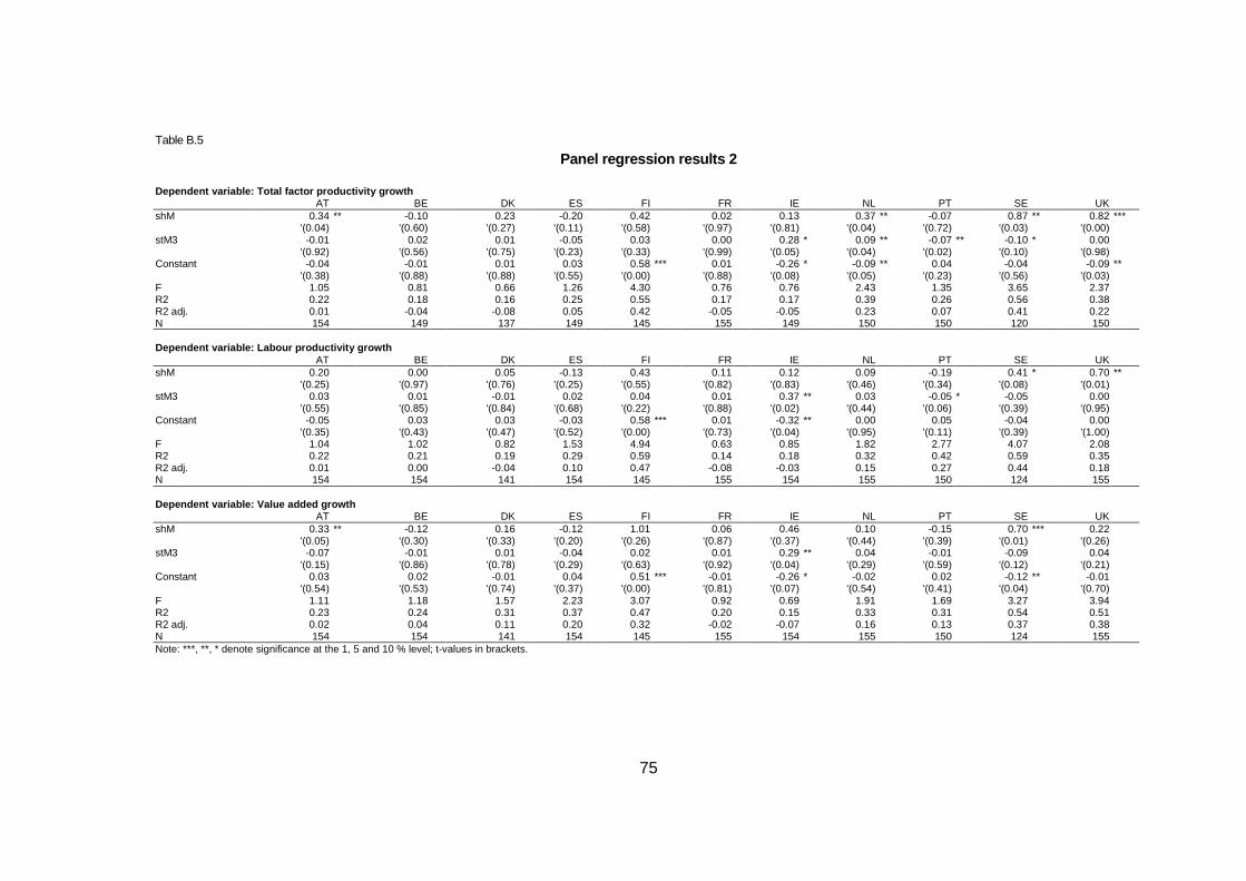
75

Table B.5

Panel regression results 2

Dependent variable: Total factor productivity growt h AT BE DK ES FI FR IE NL PT SE UK shM 0.34 ** -0.10 0.23 -0.20 0.42 0.02 0.13 0.37 ** -0.07 0.87 ** 0.82 *** '(0.04) '(0.60) '(0.27) '(0.11) '(0.58) '(0.97) '(0.81) '(0.04) '(0.72) '(0.03) '(0.00) stM3 -0.01 0.02 0.01 -0.05 0.03 0.00 0.28 * 0.09 ** -0.07 ** -0.10 * 0.00 '(0.92) '(0.56) '(0.75) '(0.23) '(0.33) '(0.99) '(0.05) '(0.04) '(0.02) '(0.10) '(0.98) Constant -0.04 -0.01 0.01 0.03 0.58 *** 0.01 -0.26 * -0.09 ** 0.04 -0.04 -0.09 ** '(0.38) '(0.88) '(0.88) '(0.55) '(0.00) '(0.88) '(0.08) '(0.05) '(0.23) '(0.56) '(0.03) F 1.05 0.81 0.66 1.26 4.30 0.76 0.76 2.43 1.35 3.65 2.37 R2 0.22 0.18 0.16 0.25 0.55 0.17 0.17 0.39 0.26 0.56 0.38 R2 adj. 0.01 -0.04 -0.08 0.05 0.42 -0.05 -0.05 0.23 0.07 0.41 0.22 N 154 149 137 149 145 155 149 150 150 120 150 Dependent variable: Labour productivity growth AT BE DK ES FI FR IE NL PT SE UK shM 0.20 0.00 0.05 -0.13 0.43 0.11 0.12 0.09 -0.19 0.41 * 0.70 ** '(0.25) '(0.97) '(0.76) '(0.25) '(0.55) '(0.82) '(0.83) '(0.46) '(0.34) '(0.08) '(0.01) stM3 0.03 0.01 -0.01 0.02 0.04 0.01 0.37 ** 0.03 -0.05 * -0.05 0.00 '(0.55) '(0.85) '(0.84) '(0.68) '(0.22) '(0.88) '(0.02) '(0.44) '(0.06) '(0.39) '(0.95) Constant -0.05 0.03 0.03 -0.03 0.58 *** 0.01 -0.32 ** 0.00 0.05 -0.04 0.00 '(0.35) '(0.43) '(0.47) '(0.52) '(0.00) '(0.73) '(0.04) '(0.95) '(0.11) '(0.39) '(1.00) F 1.04 1.02 0.82 1.53 4.94 0.63 0.85 1.82 2.77 4.07 2.08 R2 0.22 0.21 0.19 0.29 0.59 0.14 0.18 0.32 0.42 0.59 0.35 R2 adj. 0.01 0.00 -0.04 0.10 0.47 -0.08 -0.03 0.15 0.27 0.44 0.18 N 154 154 141 154 145 155 154 155 150 124 155 Dependent variable: Value added growth AT BE DK ES FI FR IE NL PT SE UK shM 0.33 ** -0.12 0.16 -0.12 1.01 0.06 0.46 0.10 -0.15 0.70 *** 0.22 '(0.05) '(0.30) '(0.33) '(0.20) '(0.26) '(0.87) '(0.37) '(0.44) '(0.39) '(0.01) '(0.26) stM3 -0.07 -0.01 0.01 -0.04 0.02 0.01 0.29 ** 0.04 -0.01 -0.09 0.04 '(0.15) '(0.86) '(0.78) '(0.29) '(0.63) '(0.92) '(0.04) '(0.29) '(0.59) '(0.12) '(0.21) Constant 0.03 0.02 -0.01 0.04 0.51 *** -0.01 -0.26 * -0.02 0.02 -0.12 ** -0.01 '(0.54) '(0.53) '(0.74) '(0.37) '(0.00) '(0.81) '(0.07) '(0.54) '(0.41) '(0.04) '(0.70) F 1.11 1.18 1.57 2.23 3.07 0.92 0.69 1.91 1.69 3.27 3.94 R2 0.23 0.24 0.31 0.37 0.47 0.20 0.15 0.33 0.31 0.54 0.51 R2 adj. 0.02 0.04 0.11 0.20 0.32 -0.02 -0.07 0.16 0.13 0.37 0.38 N 154 154 141 154 145 155 154 155 150 124 155 Note: ***, **, * denote significance at the 1, 5 and 10 % level; t-values in brackets.

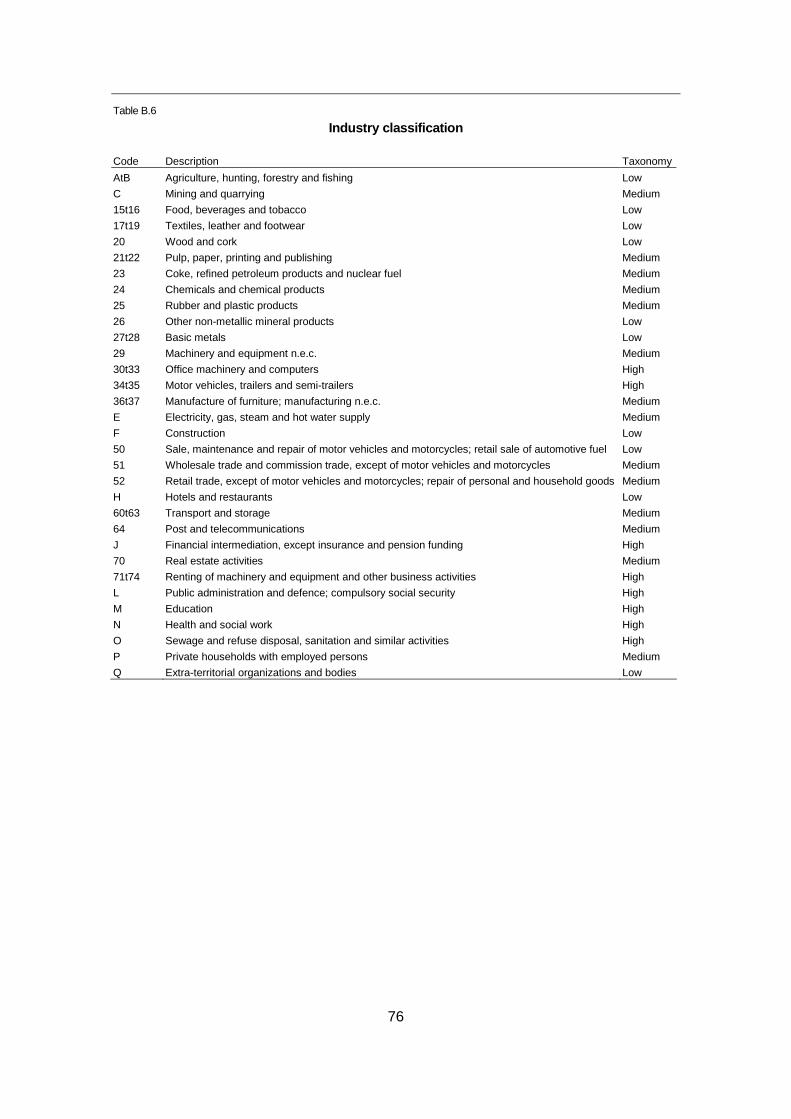
76

Table B.6

Industry classification

Code Description Taxonomy

AtB Agriculture, hunting, forestry and fishing Low

C Mining and quarrying Medium

15t16 Food, beverages and tobacco Low

17t19 Textiles, leather and footwear Low

20 Wood and cork Low

21t22 Pulp, paper, printing and publishing Medium

23 Coke, refined petroleum products and nuclear fuel Medium

24 Chemicals and chemical products Medium

25 Rubber and plastic products Medium

26 Other non-metallic mineral products Low

27t28 Basic metals Low

29 Machinery and equipment n.e.c. Medium

30t33 Office machinery and computers High

34t35 Motor vehicles, trailers and semi-trailers High

36t37 Manufacture of furniture; manufacturing n.e.c. Medium

E Electricity, gas, steam and hot water supply Medium

F Construction Low

50 Sale, maintenance and repair of motor vehicles and motorcycles; retail sale of automotive fuel Low

51 Wholesale trade and commission trade, except of motor vehicles and motorcycles Medium

52 Retail trade, except of motor vehicles and motorcycles; repair of personal and household goods Medium

H Hotels and restaurants Low

60t63 Transport and storage Medium

64 Post and telecommunications Medium

J Financial intermediation, except insurance and pension funding High

70 Real estate activities Medium

71t74 Renting of machinery and equipment and other business activities High

L Public administration and defence; compulsory social security High

M Education High

N Health and social work High

O Sewage and refuse disposal, sanitation and similar activities High

P Private households with employed persons Medium

Q Extra-territorial organizations and bodies Low

77

3.2 Migrants and regional performance

3.2.1 Descriptive regressions on (high-skilled) migration and regional performance

In this part of the study we analyze the effects of migration on regional economic

performance at the NUTS 2-digit level in the EU-15 countries. The regional performance

indicators we shall include in this analysis are GDP per capita growth and value added

growth. It is not possible at the regional level to study the effects on total factor productivity

growth for lack of data. The data sources we use is the European Labour Force Survey

(ELFS) as already described above and the Eurostat regional database. The analysis in

this part is restricted to the EU-15 countries as the shares of migrants in the other EU

countries are quite low. Second, we restrict the analysis to the period 2000-2006 in

general. In some cases only the period 2000-2005 is covered for data availability reasons.

The main reason for this is that the European Labour Force survey data (ELFS) exhibits

methodological breaks for some countries in the years before 2000 and data after 2006 are

not available at the regional level so far.

Explaining regional GDP per capita growth is a delicate task as the number of potential

control variables is quite large and results might depend upon these controls. There is now

a large literature on determining the factors of (regional) growth in the empirical growth

literature. These are mostly based on model selection approaches (like Bayesian model

averaging) or shrinkage estimators. We therefore use the following strategy: Based on the

results of Crespo Cuaresma et al. (2010) we include the growth determinants which turned

out to be robust and additionally include the migrant variables, i.e. the share of migrants in

total employed persons (shM), the share of highly educated migrants in total highly

educated employed persons (shM3) and the share of highly educated migrants in total

migrants (stM3). However, as the correlation between shM and shM3 is very high (above

0.9) we only include one of those. The control variables we take from Crespo Cuaresma et

al. (2010) are a dummy for the capital city, the share of highly educated workers and the

initial GDP per capita. Further the share of gross fixed capital formation in GDP is also a

robust determinant when including country fixed effects. We also use the same variables

when looking at general growth performance.

Results of this simple exercise are reported in Table 28. The migrant variables are not at all

significant in the productivity regressions. However, in the growth regressions these are

significant when including country dummies. The results when excluding the capital city

regions are quite similar.6

6 Results are available upon request.

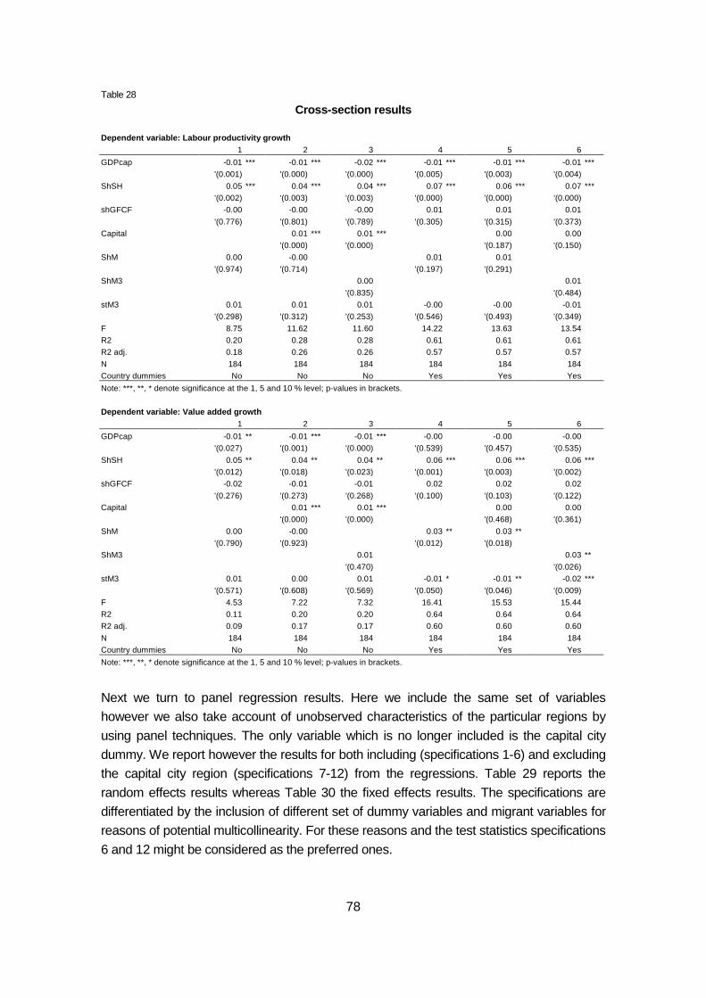
78

Table 28

Cross-section results


1 2 3 4 5 6

GDPcap -0.01 *** -0.01 *** -0.02 *** -0.01 *** -0.01 *** -0.01 ***

'(0.001) '(0.000) '(0.000) '(0.005) '(0.003) '(0.004)

ShSH 0.05 *** 0.04 *** 0.04 *** 0.07 *** 0.06 *** 0.07 ***

'(0.002) '(0.003) '(0.003) '(0.000) '(0.000) '(0.000)

shGFCF -0.00 -0.00 -0.00 0.01 0.01 0.01

'(0.776) '(0.801) '(0.789) '(0.305) '(0.315) '(0.373)

Capital 0.01 *** 0.01 *** 0.00 0.00

'(0.000) '(0.000) '(0.187) '(0.150)

ShM 0.00 -0.00 0.01 0.01

'(0.974) '(0.714) '(0.197) '(0.291)

ShM3 0.00 0.01

'(0.835) '(0.484)

stM3 0.01 0.01 0.01 -0.00 -0.00 -0.01

'(0.298) '(0.312) '(0.253) '(0.546) '(0.493) '(0.349)

F 8.75 11.62 11.60 14.22 13.63 13.54

R2 0.20 0.28 0.28 0.61 0.61 0.61

R2 adj. 0.18 0.26 0.26 0.57 0.57 0.57

N 184 184 184 184 184 184

Country dummies No No No Yes Yes Yes

Note: ***, **, * denote significance at the 1, 5 and 10 % level; p-values in brackets.


1 2 3 4 5 6

GDPcap -0.01 ** -0.01 *** -0.01 *** -0.00 -0.00 -0.00

'(0.027) '(0.001) '(0.000) '(0.539) '(0.457) '(0.535)

ShSH 0.05 ** 0.04 ** 0.04 ** 0.06 *** 0.06 *** 0.06 ***

'(0.012) '(0.018) '(0.023) '(0.001) '(0.003) '(0.002)

shGFCF -0.02 -0.01 -0.01 0.02 0.02 0.02

'(0.276) '(0.273) '(0.268) '(0.100) '(0.103) '(0.122)

Capital 0.01 *** 0.01 *** 0.00 0.00

'(0.000) '(0.000) '(0.468) '(0.361)

ShM 0.00 -0.00 0.03 ** 0.03 **

'(0.790) '(0.923) '(0.012) '(0.018)

ShM3 0.01 0.03 **

'(0.470) '(0.026)

stM3 0.01 0.00 0.01 -0.01 * -0.01 ** -0.02 ***

'(0.571) '(0.608) '(0.569) '(0.050) '(0.046) '(0.009)

F 4.53 7.22 7.32 16.41 15.53 15.44

R2 0.11 0.20 0.20 0.64 0.64 0.64

R2 adj. 0.09 0.17 0.17 0.60 0.60 0.60

N 184 184 184 184 184 184

Country dummies No No No Yes Yes Yes

Note: ***, **, * denote significance at the 1, 5 and 10 % level; p-values in brackets.

Next we turn to panel regression results. Here we include the same set of variables

however we also take account of unobserved characteristics of the particular regions by

using panel techniques. The only variable which is no longer included is the capital city

dummy. We report however the results for both including (specifications 1-6) and excluding

the capital city region (specifications 7-12) from the regressions. Table 29 reports the

random effects results whereas Table 30 the fixed effects results. The specifications are

differentiated by the inclusion of different set of dummy variables and migrant variables for

reasons of potential multicollinearity. For these reasons and the test statistics specifications

6 and 12 might be considered as the preferred ones.

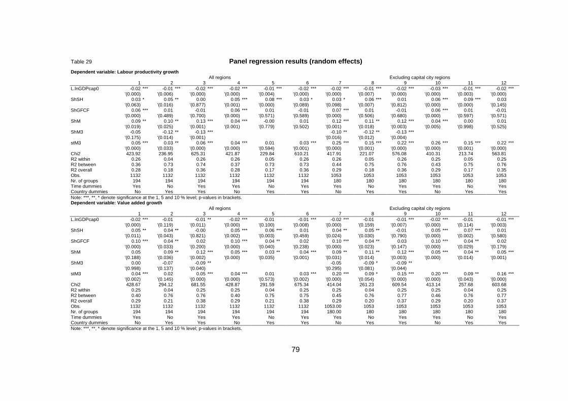
79

Table 29 Panel regression results (random effects) Dependent variable: Labour productivity growth All regions Excluding capital city regions 1 2 3 4 5 6 7 8 9 10 11 12 L.lnGDPcap0 -0.02 *** -0.01 *** -0.02 *** -0.02 *** -0.01 *** -0.02 *** -0.02 *** -0.01 *** -0.02 *** -0.03 *** -0.01 *** -0.02 *** '(0.000) '(0.006) '(0.000) '(0.000) '(0.004) '(0.000) '(0.000) '(0.007) '(0.000) '(0.000) '(0.003) '(0.000) ShSH 0.03 * 0.05 ** 0.00 0.05 *** 0.08 *** 0.03 * 0.03 * 0.06 *** 0.01 0.06 *** 0.09 *** 0.03 '(0.063) '(0.016) '(0.877) '(0.001) '(0.000) '(0.089) '(0.098) '(0.007) '(0.812) '(0.000) '(0.000) '(0.145) ShGFCF 0.06 *** 0.01 -0.01 0.06 *** 0.01 -0.01 0.07 *** 0.01 -0.01 0.06 *** 0.01 -0.01 '(0.000) '(0.489) '(0.700) '(0.000) '(0.571) '(0.589) '(0.000) '(0.506) '(0.680) '(0.000) '(0.597) '(0.571) ShM 0.09 ** 0.10 ** 0.13 *** 0.04 *** -0.00 0.01 0.12 *** 0.11 ** 0.12 *** 0.04 *** 0.00 0.01 '(0.019) '(0.025) '(0.001) '(0.001) '(0.779) '(0.502) '(0.001) '(0.018) '(0.003) '(0.005) '(0.998) '(0.525) ShM3 -0.05 -0.12 ** -0.13 *** -0.10 ** -0.12 ** -0.13 *** '(0.175) '(0.014) '(0.001) '(0.016) '(0.012) '(0.004) stM3 0.05 *** 0.03 ** 0.06 *** 0.04 *** 0.01 0.03 *** 0.25 *** 0.15 *** 0.22 *** 0.26 *** 0.15 *** 0.22 *** '(0.000) '(0.033) '(0.000) '(0.000) '(0.594) '(0.001) '(0.000) '(0.001) '(0.000) '(0.000) '(0.001) '(0.000) Chi2 423.92 236.95 625.31 421.87 229.84 610.21 417.91 221.07 576.08 410.31 213.74 563.81 R2 within 0.26 0.04 0.26 0.26 0.05 0.26 0.26 0.05 0.26 0.25 0.05 0.25 R2 between 0.36 0.73 0.74 0.37 0.73 0.73 0.44 0.75 0.76 0.43 0.75 0.76 R2 overall 0.28 0.18 0.36 0.28 0.17 0.36 0.29 0.18 0.36 0.29 0.17 0.35 Obs. 1132 1132 1132 1132 1132 1132 1053 1053 1053 1053 1053 1053 Nr. of groups 194 194 194 194 194 194 180 180 180 180 180 180 Time dummies Yes No Yes Yes No Yes Yes No Yes Yes No Yes Country dummies No Yes Yes No Yes Yes No Yes Yes No Yes Yes Note: ***, **, * denote significance at the 1, 5 and 10 % level; p-values in brackets. Dependent variable: Value added growth All regions Excluding capital city regions 1 2 3 4 5 6 7 8 9 10 11 12 L.lnGDPcap0 -0.02 *** -0.01 -0.01 ** -0.02 *** -0.01 -0.01 *** -0.02 *** -0.01 -0.01 *** -0.02 *** -0.01 -0.01 *** '(0.000) '(0.119) '(0.011) '(0.000) '(0.100) '(0.008) '(0.000) '(0.159) '(0.007) '(0.000) '(0.114) '(0.003) ShSH 0.05 ** 0.04 ** -0.00 0.05 *** 0.06 *** 0.01 0.04 ** 0.05 ** -0.01 0.05 *** 0.07 *** 0.01 '(0.011) '(0.043) '(0.821) '(0.002) '(0.003) '(0.459) '(0.024) '(0.030) '(0.790) '(0.000) '(0.002) '(0.580) ShGFCF 0.10 *** 0.04 ** 0.02 0.10 *** 0.04 ** 0.02 0.10 *** 0.04 ** 0.03 0.10 *** 0.04 ** 0.02 '(0.000) '(0.033) '(0.200) '(0.000) '(0.040) '(0.238) '(0.000) '(0.023) '(0.147) '(0.000) '(0.029) '(0.179) ShM 0.05 0.09 ** 0.12 *** 0.05 *** 0.03 ** 0.04 *** 0.09 ** 0.11 ** 0.12 *** 0.05 *** 0.04 ** 0.05 *** '(0.188) '(0.036) '(0.002) '(0.000) '(0.035) '(0.001) '(0.031) '(0.014) '(0.003) '(0.000) '(0.014) '(0.001) ShM3 0.00 -0.07 -0.09 ** -0.05 -0.09 * -0.09 ** '(0.998) '(0.137) '(0.040) '(0.295) '(0.081) '(0.044) stM3 0.04 *** 0.02 0.05 *** 0.04 *** 0.01 0.03 *** 0.20 *** 0.09 * 0.15 *** 0.20 *** 0.09 ** 0.16 *** '(0.002) '(0.145) '(0.000) '(0.000) '(0.573) '(0.002) '(0.000) '(0.054) '(0.000) '(0.000) '(0.043) '(0.000) Chi2 428.67 294.12 681.55 428.87 291.59 675.34 414.04 261.23 609.54 413.14 257.68 603.68 R2 within 0.25 0.04 0.25 0.25 0.04 0.25 0.25 0.04 0.25 0.25 0.04 0.25 R2 between 0.40 0.76 0.76 0.40 0.75 0.75 0.45 0.76 0.77 0.46 0.76 0.77 R2 overall 0.29 0.21 0.38 0.29 0.21 0.38 0.29 0.20 0.37 0.29 0.20 0.37 Obs. 1132 1132 1132 1132 1132 1132 1053.00 1053 1053 1053 1053 1053 Nr. of groups 194 194 194 194 194 194 180.00 180 180 180 180 180 Time dummies Yes No Yes Yes No Yes Yes No Yes Yes No Yes Country dummies No Yes Yes No Yes Yes No Yes Yes No Yes Yes Note: ***, **, * denote significance at the 1, 5 and 10 % level; p-values in brackets.

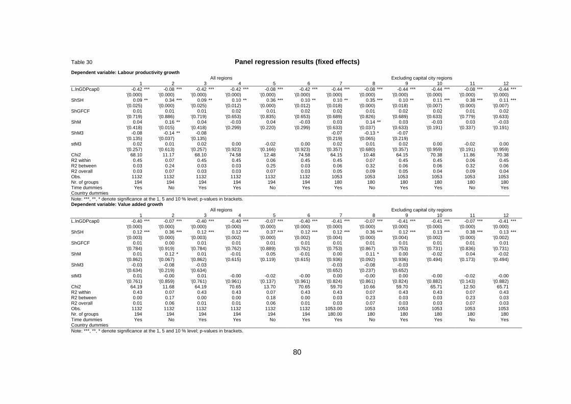
80

Table 30 Panel regression results (fixed effects) Dependent variable: Labour productivity growth All regions Excluding capital city regions 1 2 3 4 5 6 7 8 9 10 11 12 L.lnGDPcap0 -0.42 *** -0.08 *** -0.42 *** -0.42 *** -0.08 *** -0.42 *** -0.44 *** -0.08 *** -0.44 *** -0.44 *** -0.08 *** -0.44 *** '(0.000) '(0.000) '(0.000) '(0.000) '(0.000) '(0.000) '(0.000) '(0.000) '(0.000) '(0.000) '(0.000) '(0.000) ShSH 0.09 ** 0.34 *** 0.09 ** 0.10 ** 0.36 *** 0.10 ** 0.10 ** 0.35 *** 0.10 ** 0.11 *** 0.38 *** 0.11 *** '(0.025) '(0.000) '(0.025) '(0.012) '(0.000) '(0.012) '(0.018) '(0.000) '(0.018) '(0.007) '(0.000) '(0.007) ShGFCF 0.01 0.01 0.01 0.02 0.01 0.02 0.02 0.01 0.02 0.02 0.01 0.02 '(0.719) '(0.886) '(0.719) '(0.653) '(0.835) '(0.653) '(0.689) '(0.826) '(0.689) '(0.633) '(0.779) '(0.633) ShM 0.04 0.16 ** 0.04 -0.03 0.04 -0.03 0.03 0.14 ** 0.03 -0.03 0.03 -0.03 '(0.418) '(0.015) '(0.418) '(0.299) '(0.220) '(0.299) '(0.633) '(0.037) '(0.633) '(0.191) '(0.337) '(0.191) ShM3 -0.08 -0.14 ** -0.08 -0.07 -0.13 * -0.07 '(0.135) '(0.037) '(0.135) '(0.219) '(0.065) '(0.219) stM3 0.02 0.01 0.02 0.00 -0.02 0.00 0.02 0.01 0.02 0.00 -0.02 0.00 '(0.257) '(0.613) '(0.257) '(0.923) '(0.166) '(0.923) '(0.357) '(0.680) '(0.357) '(0.959) '(0.191) '(0.959) Chi2 68.10 11.17 68.10 74.58 12.48 74.58 64.15 10.48 64.15 70.38 11.86 70.38 R2 within 0.45 0.07 0.45 0.45 0.06 0.45 0.45 0.07 0.45 0.45 0.06 0.45 R2 between 0.03 0.24 0.03 0.03 0.25 0.03 0.06 0.32 0.06 0.06 0.32 0.06 R2 overall 0.03 0.07 0.03 0.03 0.07 0.03 0.05 0.09 0.05 0.04 0.09 0.04 Obs. 1132 1132 1132 1132 1132 1132 1053 1053 1053 1053 1053 1053 Nr. of groups 194 194 194 194 194 194 180 180 180 180 180 180 Time dummies Yes No Yes Yes No Yes Yes No Yes Yes No Yes Country dummies Note: ***, **, * denote significance at the 1, 5 and 10 % level; p-values in brackets. Dependent variable: Value added growth All regions Excluding capital city regions 1 2 3 4 5 6 7 8 9 10 11 12 L.lnGDPcap0 -0.40 *** -0.07 *** -0.40 *** -0.40 *** -0.07 *** -0.40 *** -0.41 *** -0.07 *** -0.41 *** -0.41 *** -0.07 *** -0.41 *** '(0.000) '(0.000) '(0.000) '(0.000) '(0.000) '(0.000) '(0.000) '(0.000) '(0.000) '(0.000) '(0.000) '(0.000) ShSH 0.12 *** 0.36 *** 0.12 *** 0.12 *** 0.37 *** 0.12 *** 0.12 *** 0.36 *** 0.12 *** 0.13 *** 0.38 *** 0.13 *** '(0.003) '(0.000) '(0.003) '(0.002) '(0.000) '(0.002) '(0.004) '(0.000) '(0.004) '(0.002) '(0.000) '(0.002) ShGFCF 0.01 0.00 0.01 0.01 0.01 0.01 0.01 0.01 0.01 0.01 0.01 0.01 '(0.784) '(0.919) '(0.784) '(0.762) '(0.889) '(0.762) '(0.753) '(0.867) '(0.753) '(0.731) '(0.836) '(0.731) ShM 0.01 0.12 * 0.01 -0.01 0.05 -0.01 0.00 0.11 * 0.00 -0.02 0.04 -0.02 '(0.862) '(0.067) '(0.862) '(0.615) '(0.119) '(0.615) '(0.936) '(0.092) '(0.936) '(0.494) '(0.173) '(0.494) ShM3 -0.03 -0.08 -0.03 -0.03 -0.08 -0.03 '(0.634) '(0.219) '(0.634) '(0.652) '(0.237) '(0.652) stM3 0.01 -0.00 0.01 -0.00 -0.02 -0.00 0.00 -0.00 0.00 -0.00 -0.02 -0.00 '(0.761) '(0.859) '(0.761) '(0.961) '(0.137) '(0.961) '(0.824) '(0.861) '(0.824) '(0.882) '(0.143) '(0.882) Chi2 64.19 11.68 64.19 70.65 13.70 70.65 59.70 10.66 59.70 65.71 12.50 65.71 R2 within 0.43 0.07 0.43 0.43 0.07 0.43 0.43 0.07 0.43 0.43 0.07 0.43 R2 between 0.00 0.17 0.00 0.00 0.18 0.00 0.03 0.23 0.03 0.03 0.23 0.03 R2 overall 0.01 0.06 0.01 0.01 0.06 0.01 0.03 0.07 0.03 0.03 0.07 0.03 Obs. 1132 1132 1132 1132 1132 1132 1053.00 1053 1053 1053 1053 1053 Nr. of groups 194 194 194 194 194 194 180.00 180 180 180 180 180 Time dummies Yes No Yes Yes No Yes Yes No Yes Yes No Yes Country dummies Note: ***, **, * denote significance at the 1, 5 and 10 % level; p-values in brackets.

81

In the random effects case the migrant variables are often positive and significant; in

particular the variable capturing the share of high educated migrants in total migrants is

rather robust across specifications. These results are partly lost when running fixed effects

regressions however.

To circumvent potential endogeneity problems we also present results when using lagged

variables as regressors. Results are reported in Tables 31 and 32 for the random and fixed

effects case, respectively. The results in the random effects specification confirm more or

less the results when using contemporaneous variables; in the fixed effects case the

results tend to be less significant. However, some of the coefficients remain significantly

positive in some specifications.

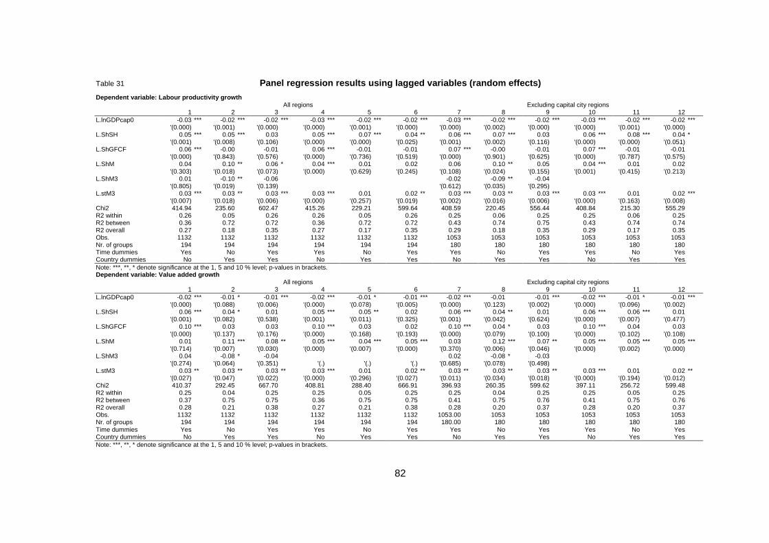
82

Table 31 Panel regression results using lagged variables (ra ndom effects) Dependent variable: Labour productivity growth All regions Excluding capital city regions 1 2 3 4 5 6 7 8 9 10 11 12 L.lnGDPcap0 -0.03 *** -0.02 *** -0.02 *** -0.03 *** -0.02 *** -0.02 *** -0.03 *** -0.02 *** -0.02 *** -0.03 *** -0.02 *** -0.02 *** '(0.000) '(0.001) '(0.000) '(0.000) '(0.001) '(0.000) '(0.000) '(0.002) '(0.000) '(0.000) '(0.001) '(0.000) L.ShSH 0.05 *** 0.05 *** 0.03 0.05 *** 0.07 *** 0.04 ** 0.06 *** 0.07 *** 0.03 0.06 *** 0.08 *** 0.04 * '(0.001) '(0.008) '(0.106) '(0.000) '(0.000) '(0.025) '(0.001) '(0.002) '(0.116) '(0.000) '(0.000) '(0.051) L.ShGFCF 0.06 *** -0.00 -0.01 0.06 *** -0.01 -0.01 0.07 *** -0.00 -0.01 0.07 *** -0.01 -0.01 '(0.000) '(0.843) '(0.576) '(0.000) '(0.736) '(0.519) '(0.000) '(0.901) '(0.625) '(0.000) '(0.787) '(0.575) L.ShM 0.04 0.10 ** 0.06 * 0.04 *** 0.01 0.02 0.06 0.10 ** 0.05 0.04 *** 0.01 0.02 '(0.303) '(0.018) '(0.073) '(0.000) '(0.629) '(0.245) '(0.108) '(0.024) '(0.155) '(0.001) '(0.415) '(0.213) L.ShM3 0.01 -0.10 ** -0.06 -0.02 -0.09 ** -0.04 '(0.805) '(0.019) '(0.139) '(0.612) '(0.035) '(0.295) L.stM3 0.03 *** 0.03 ** 0.03 *** 0.03 *** 0.01 0.02 ** 0.03 *** 0.03 ** 0.03 *** 0.03 *** 0.01 0.02 *** '(0.007) '(0.018) '(0.006) '(0.000) '(0.257) '(0.019) '(0.002) '(0.016) '(0.006) '(0.000) '(0.163) '(0.008) Chi2 414.94 235.60 602.47 415.26 229.21 599.64 408.59 220.45 556.44 408.84 215.30 555.29 R2 within 0.26 0.05 0.26 0.26 0.05 0.26 0.25 0.06 0.25 0.25 0.06 0.25 R2 between 0.36 0.72 0.72 0.36 0.72 0.72 0.43 0.74 0.75 0.43 0.74 0.74 R2 overall 0.27 0.18 0.35 0.27 0.17 0.35 0.29 0.18 0.35 0.29 0.17 0.35 Obs. 1132 1132 1132 1132 1132 1132 1053 1053 1053 1053 1053 1053 Nr. of groups 194 194 194 194 194 194 180 180 180 180 180 180 Time dummies Yes No Yes Yes No Yes Yes No Yes Yes No Yes Country dummies No Yes Yes No Yes Yes No Yes Yes No Yes Yes Note: ***, **, * denote significance at the 1, 5 and 10 % level; p-values in brackets. Dependent variable: Value added growth All regions Excluding capital city regions 1 2 3 4 5 6 7 8 9 10 11 12 L.lnGDPcap0 -0.02 *** -0.01 * -0.01 *** -0.02 *** -0.01 * -0.01 *** -0.02 *** -0.01 -0.01 *** -0.02 *** -0.01 * -0.01 *** '(0.000) '(0.088) '(0.006) '(0.000) '(0.078) '(0.005) '(0.000) '(0.123) '(0.002) '(0.000) '(0.096) '(0.002) L.ShSH 0.06 *** 0.04 * 0.01 0.05 *** 0.05 ** 0.02 0.06 *** 0.04 ** 0.01 0.06 *** 0.06 *** 0.01 '(0.001) '(0.082) '(0.538) '(0.001) '(0.011) '(0.325) '(0.001) '(0.042) '(0.624) '(0.000) '(0.007) '(0.477) L.ShGFCF 0.10 *** 0.03 0.03 0.10 *** 0.03 0.02 0.10 *** 0.04 * 0.03 0.10 *** 0.04 0.03 '(0.000) '(0.137) '(0.176) '(0.000) '(0.168) '(0.193) '(0.000) '(0.079) '(0.100) '(0.000) '(0.102) '(0.108) L.ShM 0.01 0.11 *** 0.08 ** 0.05 *** 0.04 *** 0.05 *** 0.03 0.12 *** 0.07 ** 0.05 *** 0.05 *** 0.05 *** '(0.714) '(0.007) '(0.030) '(0.000) '(0.007) '(0.000) '(0.370) '(0.006) '(0.046) '(0.000) '(0.002) '(0.000) L.ShM3 0.04 -0.08 * -0.04 0.02 -0.08 * -0.03 '(0.274) '(0.064) '(0.351) '(.) '(.) '(.) '(0.685) '(0.078) '(0.498) L.stM3 0.03 ** 0.03 ** 0.03 ** 0.03 *** 0.01 0.02 ** 0.03 ** 0.03 ** 0.03 ** 0.03 *** 0.01 0.02 ** '(0.027) '(0.047) '(0.022) '(0.000) '(0.296) '(0.027) '(0.011) '(0.034) '(0.018) '(0.000) '(0.194) '(0.012) Chi2 410.37 292.45 667.70 408.81 288.40 666.91 396.93 260.35 599.62 397.11 256.72 599.48 R2 within 0.25 0.04 0.25 0.25 0.05 0.25 0.25 0.04 0.25 0.25 0.05 0.25 R2 between 0.37 0.75 0.75 0.36 0.75 0.75 0.41 0.75 0.76 0.41 0.75 0.76 R2 overall 0.28 0.21 0.38 0.27 0.21 0.38 0.28 0.20 0.37 0.28 0.20 0.37 Obs. 1132 1132 1132 1132 1132 1132 1053.00 1053 1053 1053 1053 1053 Nr. of groups 194 194 194 194 194 194 180.00 180 180 180 180 180 Time dummies Yes No Yes Yes No Yes Yes No Yes Yes No Yes Country dummies No Yes Yes No Yes Yes No Yes Yes No Yes Yes Note: ***, **, * denote significance at the 1, 5 and 10 % level; p-values in brackets.

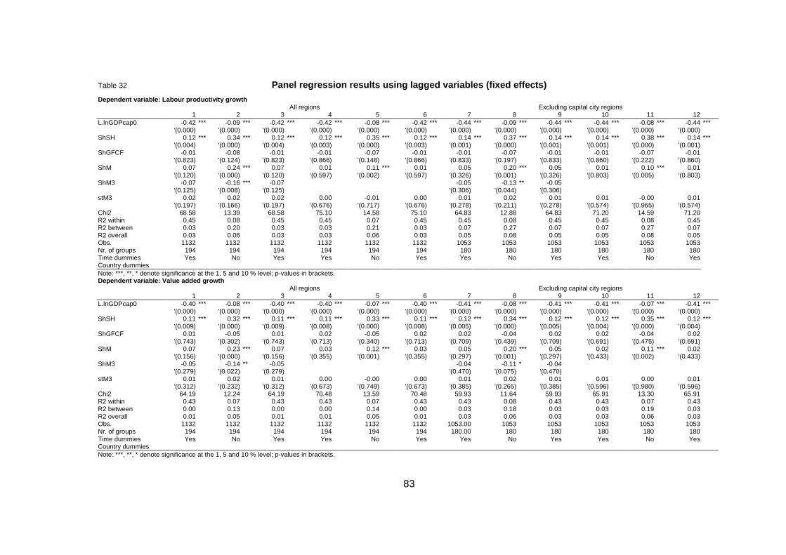
83

Table 32 Panel regression results using lagged variables (fi xed effects) Dependent variable: Labour productivity growth All regions Excluding capital city regions 1 2 3 4 5 6 7 8 9 10 11 12 L.lnGDPcap0 -0.42 *** -0.09 *** -0.42 *** -0.42 *** -0.08 *** -0.42 *** -0.44 *** -0.09 *** -0.44 *** -0.44 *** -0.08 *** -0.44 *** '(0.000) '(0.000) '(0.000) '(0.000) '(0.000) '(0.000) '(0.000) '(0.000) '(0.000) '(0.000) '(0.000) '(0.000) ShSH 0.12 *** 0.34 *** 0.12 *** 0.12 *** 0.35 *** 0.12 *** 0.14 *** 0.37 *** 0.14 *** 0.14 *** 0.38 *** 0.14 *** '(0.004) '(0.000) '(0.004) '(0.003) '(0.000) '(0.003) '(0.001) '(0.000) '(0.001) '(0.001) '(0.000) '(0.001) ShGFCF -0.01 -0.08 -0.01 -0.01 -0.07 -0.01 -0.01 -0.07 -0.01 -0.01 -0.07 -0.01 '(0.823) '(0.124) '(0.823) '(0.866) '(0.148) '(0.866) '(0.833) '(0.197) '(0.833) '(0.860) '(0.222) '(0.860) ShM 0.07 0.24 *** 0.07 0.01 0.11 *** 0.01 0.05 0.20 *** 0.05 0.01 0.10 *** 0.01 '(0.120) '(0.000) '(0.120) '(0.597) '(0.002) '(0.597) '(0.326) '(0.001) '(0.326) '(0.803) '(0.005) '(0.803) ShM3 -0.07 -0.16 *** -0.07 -0.05 -0.13 ** -0.05 '(0.125) '(0.008) '(0.125) '(0.306) '(0.044) '(0.306) stM3 0.02 0.02 0.02 0.00 -0.01 0.00 0.01 0.02 0.01 0.01 -0.00 0.01 '(0.197) '(0.166) '(0.197) '(0.676) '(0.717) '(0.676) '(0.278) '(0.211) '(0.278) '(0.574) '(0.965) '(0.574) Chi2 68.58 13.39 68.58 75.10 14.58 75.10 64.83 12.88 64.83 71.20 14.59 71.20 R2 within 0.45 0.08 0.45 0.45 0.07 0.45 0.45 0.08 0.45 0.45 0.08 0.45 R2 between 0.03 0.20 0.03 0.03 0.21 0.03 0.07 0.27 0.07 0.07 0.27 0.07 R2 overall 0.03 0.06 0.03 0.03 0.06 0.03 0.05 0.08 0.05 0.05 0.08 0.05 Obs. 1132 1132 1132 1132 1132 1132 1053 1053 1053 1053 1053 1053 Nr. of groups 194 194 194 194 194 194 180 180 180 180 180 180 Time dummies Yes No Yes Yes No Yes Yes No Yes Yes No Yes Country dummies Note: ***, **, * denote significance at the 1, 5 and 10 % level; p-values in brackets. Dependent variable: Value added growth All regions Excluding capital city regions 1 2 3 4 5 6 7 8 9 10 11 12 L.lnGDPcap0 -0.40 *** -0.08 *** -0.40 *** -0.40 *** -0.07 *** -0.40 *** -0.41 *** -0.08 *** -0.41 *** -0.41 *** -0.07 *** -0.41 *** '(0.000) '(0.000) '(0.000) '(0.000) '(0.000) '(0.000) '(0.000) '(0.000) '(0.000) '(0.000) '(0.000) '(0.000) ShSH 0.11 *** 0.32 *** 0.11 *** 0.11 *** 0.33 *** 0.11 *** 0.12 *** 0.34 *** 0.12 *** 0.12 *** 0.35 *** 0.12 *** '(0.009) '(0.000) '(0.009) '(0.008) '(0.000) '(0.008) '(0.005) '(0.000) '(0.005) '(0.004) '(0.000) '(0.004) ShGFCF 0.01 -0.05 0.01 0.02 -0.05 0.02 0.02 -0.04 0.02 0.02 -0.04 0.02 '(0.743) '(0.302) '(0.743) '(0.713) '(0.340) '(0.713) '(0.709) '(0.439) '(0.709) '(0.691) '(0.475) '(0.691) ShM 0.07 0.23 *** 0.07 0.03 0.12 *** 0.03 0.05 0.20 *** 0.05 0.02 0.11 *** 0.02 '(0.156) '(0.000) '(0.156) '(0.355) '(0.001) '(0.355) '(0.297) '(0.001) '(0.297) '(0.433) '(0.002) '(0.433) ShM3 -0.05 -0.14 ** -0.05 -0.04 -0.11 * -0.04 '(0.279) '(0.022) '(0.279) '(0.470) '(0.075) '(0.470) stM3 0.01 0.02 0.01 0.00 -0.00 0.00 0.01 0.02 0.01 0.01 0.00 0.01 '(0.312) '(0.232) '(0.312) '(0.673) '(0.749) '(0.673) '(0.385) '(0.265) '(0.385) '(0.596) '(0.980) '(0.596) Chi2 64.19 12.24 64.19 70.48 13.59 70.48 59.93 11.64 59.93 65.91 13.30 65.91 R2 within 0.43 0.07 0.43 0.43 0.07 0.43 0.43 0.08 0.43 0.43 0.07 0.43 R2 between 0.00 0.13 0.00 0.00 0.14 0.00 0.03 0.18 0.03 0.03 0.19 0.03 R2 overall 0.01 0.05 0.01 0.01 0.05 0.01 0.03 0.06 0.03 0.03 0.06 0.03 Obs. 1132 1132 1132 1132 1132 1132 1053.00 1053 1053 1053 1053 1053 Nr. of groups 194 194 194 194 194 194 180.00 180 180 180 180 180 Time dummies Yes No Yes Yes No Yes Yes No Yes Yes No Yes Country dummies Note: ***, **, * denote significance at the 1, 5 and 10 % level; p-values in brackets.

84

Bibliography (includes relevant literature on the topic of migra tion and economic performance):

Ackers L. (2005) Moving People and Knowledge: Scientific Mobility in the European Union, International

Migration, Vol 43(5), pp. 99-131.

Agrawal, A., D. Kapur, and J. McHale (2007), Brain Drain or Brain Bank? The Impact of Skilled Emigration on Poor-Country Innovation; University of Toronto Working Paper.

Alesina, Alberto and Eliana La Ferrara (2005), "Ethnic diversity and economic performance", Journal of Economic Literature 43, pp. 762-800.

Anderson, Stuart and Michaela Platzer (2006) American Made: The Impact of Immigrant Entrepreneurs and

Professionals on US Competitivenes, National Venture Capital Association

Auriol, L., Sexton, J., (2002) Human resources in science and technology: measurement issues and international mobility, in: OECD, International Mobility of the Highly Skilled, Paris, Chapter 1, 2002, S. 13-38.

Aydemir, A., Sweetman, A., (2006), First and Second Generation Immigrant Educational Attainment and Labor Market Outcomes: A Comparison of the United States and Canada, IZA Discussion Paper 2298, IZA, Bonn.

Aydemir, Abdurrahman, and George Borjas (2006), A comparative analysis of the labour market impact of

international migration: Canada, Mexico, and the United States, NBER Working paper no. 12327.

Bacarreza, G. And L. Ehrlich (2006) The Impact of Migration on Foreign Trade: A Developing Country Approach, Instituto de investigaciones socioecomicas, Munich Personal RepEc Archive paper No. 1090.

Becker, Sascha; Andrea Ichino; Giovanni Peri (2003) How Large is the "Brain Drain" from Italy?, CESifo, CESifo Working Paper Series: CESifo Working Paper No. 839, 2003.

Beine, M., Docquier, F., Schiff, M., (2008), Brain Drain and its Determinants: A Major Issue for Small States, IZA

Discussion Paper 3398, IZA, Bonn.

Belot, M., Hatton, T., (2008), Immigrant Selection in the OECD, CEPR Discussion Paper 6675, CEPR, London.

Benhabib, J. and M. Spiegel (2005), Human capital and technology diffusion, in: Aghion, P. and S. Durlauf

(eds.), Handbook of Economic Growth, Amsterdam: Elsevier.

Bessey, Donata (2007) Intenational Student Migration to Germany, Swiss Leading House, Working Paper No. 6.

Biffl, G., (2006), Small-Scale Study III: Conditions of entry and residence of third country highly-skilled workers in

Austria, Study for the International Organisation for Migration Vienna in its function as the National Contact Point Austria within EMN, Wien.

Birell, Bob, Lesleyanne Hawthorne and Sue Richardson (2006) Evaluation of the General Skilled migration

categories, University of Melbourne.

Bleakley, H., Chin, A., (2004), Language skills and earnings: evidence from childhood immigrants, Review of Economics and Statistics, 86, S. 481-496.

Borjas, George (1987), "Self-selection and the earnings of immigrants", American Economic Review 77,

pp. 531-553.

Borjas, George (1991), "Immigration and self-selection", in: J.M. Abowd and R.B. Freeman (eds.), "Immigration,

trade and the labour market", Chicago: University of Chicago Press.

Borjas, George, (2001). "Does Immigration Grease the Wheels of the Labor Market?," Brookings Papers on Economic Activity, Economic Studies Program, The Brookings Institution, vol. 32(2001-1), pages 69-134.

Borjas, George (1999), "The Economic Analysis of Immigration", in: O. Ashenfelter and D. Card (eds.), "Handbook of Labor Economics", Vol. 3A, Amsterdam: Elsevier.

85

Borjas, George (2004), The labour-market impact of high-skill immigration, American Economic Review 95(2),

pp. 56-60.

Borjas, George (2006), Immigration in high skill labour markets: The impact of foreign students on the earnings of doctorates, NBER Working paper 12085.

Borjas, George (2003), The labour demand curve is downward sloping: reexamining the impact of immigration on the labour market, Quarterly Journal of Economics 118(4), pp. 1335-74.

Borjas, G., Jeffrey Grogger, and Gordon Hanson (2008), Imperfect substitution between immigrants and natives: a reappraisal, NBER Working paper no. 13887.

Bratsberg, Bernt (1995), "The incidence of non-return among foreign students in the United States", Economics

of Education Review 14, pp. 373-384.

Brücker, Herbert, and Parvati Trübswetter (2006), "Do the best go West? An Analysis of the self selection of employed East-West Migrants in Germany, Empirica, vol 34, no. 4 pp. 371-95.

Brücker, Herbert und Elke Jahn (2008), Migration and the wage curve: a structural approach to measure the wage and employment effects of migration, IZA discussion paper Nr. 3423.

Brücker, Herbert, and Cécily Defoort (2006), "The (self-)selection of international migrants reconsidered: theory

and empirical evidence", IZA Discussion Paper 2052, Bonn: Institute for the Study of Labor (IZA).

Bryant, J; G.Murat and L. David (2004) Trade Flows and Migrantion to New Zealand, New Zealand Treasury working paper 04/18, Wellington.

Burkert, C., Niebuhr, A., Wapler, R., (2007), Regional Disparities in Employment of High Skilled Foreigners – Determinants and Options for Migration Policy in Germany, HWWA Research Paper, 3-7, Hamburger Weltwirtschaftliches Archiv, Hamburg.

Card, David (2001) Immigrant Inflows, Native Outflows and the Local Labor Market Impacts of Higher Immigration; Journal of Labor Economics, 90(2), pp. 360-367.

Card, David (2005), Is the New Immigration Really So Bad?, Economic Journal, 115 , pp. F300-323.

Card, David and John DiNardo (2000) Do Immigrant Inflows Lead to Native Outflows?, American Economic Review, Papers and Proceedings, 90(2), pp. 360-367.

Chellaraj, Gnanaraj, Maskus, Keith E. And Aaditya Mattoo (2008), "The contribution of international graduate students to US innovation", Review of International Economics 16, pp. 444-462.

Chiswick, Barry (1999), "Are immigrants positively self-selected?", American Economic Review 89, pp. 181-185.

Chiswick, Barry. R. (2005), High Skilled Immigration in the International Arena, IZA Discussion Paper No. 1782,

Bonn.

Chiswick, Barry, and Sarinda Taengnoi (2007), Occupational choice of high skilled immigrants in the United States, IZA Discussion Paper no. 2969.

Chiswick, B. R., Miller, P. W., (2007), The International Transferability of Human Capital Skills, IZA Discussion Paper 2670, IZA, Bonn.

Chiswick, B. R., DebBurman, N., (2003), Educational Attainment: Analysis by Immigrant Generation, IZA

Discussion Paper 731, IZA, Bonn.

Cobb-Clark, Deborah (1983), "Immigrant selectivity and wages: the evidence for women", American Economic Review 83, pp. 986-993.

Cohen, Alon and Assaf Razin (2008) The skill composition of immigrants and the generosity of the welfare state: free vs. policy controlled migration, NBER Working paper 14459.

86

Combes, Pierre-Philippe; Miren Lafourcade, Miren and Thierry Mayer (2005) The Trade-Creating Effects of Business and Social Networks: Evidence from France, Journal of International Economics, vol. 66, no. 1, pp. 1-29.

Combes, Pierre-Philippe; Miren Lafourcade, Miren and Thierry Mayer (2003) Can Business and Social

Networks Explain the Border Effect Puzzle? C.E.P.R. Discussion Papers, CEPR Discussion Papers: 3750.

Commander, S., Kangasniemi, M., Winters, (2003), L. A., The Brain Drain: Curse or Boon?, IZA Discussion Paper 809, IZA, Bonn.

Constant, Amelie, Shachmurove, Yochanan and Klaus F. Zimmermann (2005), "The role of Turkish immigrants in entrepreneurial Activities in Germany", PIER Working Paper 05-029, Philadelphia: Penn Institute for Economic Research.

Constant, Amelie and Elena D'Agosto (2008), "Where do the brainy Italians go?", IZA Discussion Paper 3325, Bonn: Institute for the Study of Labor (IZA).

Crespo Cuaresma, J., N. Foster and R. Stehrer (forthcoming), The determinants of regional growth by quantiles,

Regional Studies, forthcoming.

D'Amuri, Francesco, Gianmarco Ottaviano und Giovanni Peri, (2008), The labour market impact of immigration in Western Germany in the 1990's, NBER working paper Nr. 13851.

De Simone, Gianfranco and Miriam Manchin (2008) Brain Drain with FDI Gain? Factor Mobility between Eastern and Western Europe, Manuscript, University College London.

Docquier, Frederic, and Elisabetta Logigiani (2008) Skilled Migration and Business Networks, Opern Economies

Review.

Docquier, F., Lohest, O., Marfouk, A., (2005), Brain Drain in Developing Regions, IZA Discussion Paper 1668, IZA, Bonn.

Docquier, F., Marfouk, A., (1990-2000), International migration by educational attainment, In: Ozden, C., Schiff, M (ED.), International Migration, Brain Drain and Remittances, New York, 2006, S. 151-199.

Dreher, Axel and Panu Poutvaara (2005) Student flows and Migration: An empirical Analysis, IZA Discussion

Paper 1612.

Drinkwater, Stephen and Ken Clark (1998), "Ethnicity and self-employment in Britain", Oxford Bulletin of Economics and Statistics 60, 383-407 .

Drinkwater, Stephen, John Eade and Michal Garapich (2006) Poles Apart? EU Enlargement and the Labour Market Outcomes of Immigrants to the UK, IZA Discussion Paper 2410, IZA, Bonn.

Dunlevy, James and William Hutchinson (2001) The Pro-Trade Effect of Immigration on American Exports

During Period 1870 to 1910, Department of Economics, Vanderbilt University, Working Papers: 0125, 2001.

Dutari, Julio C. Terán (1994), "The socio-cultural impact of brain-drain: reflections from Latin America", Higher Education Policy 7, pp. 25-28.

Egger, Peter and Doina Maria Radulescu (2008) The Influence of Taxes on the Migration of Skilled Workers, CESifo Working Paper No 2462.

Eggert, W., Krieger, T., Meier, V. (2007). „Education, Unemployment and Migration“, CESifo Working Paper

No. 2119.

European Commission (2008) Employment in Europe 2008.

EUROSTAT. 1996. Statistical Classification of Economic Activities in the European Community. Luxemburg.

Epstein, Gil, Astrid Kunze, and Melanie Ward (2002), “High skilled migration and the exertion of effort by the local population”, CEPR Discussion paper no. 3477.

87

Fairlie, Robert W. and Christopher Woodruff (2008), "Mexican-American entrepreneurship", Centre for Economic Policy Research Discussion Paper 575, Canberra: Australian National University.

Fan, C. Simon and Oded Stark (2007), "A social proximity explanation of the reluctance to assimilate", Kyklos

60, pp. 55-63..

Felbermayr, Gabriel, Wido Geis, and Wilhelm Kohler, (2008), Restrictive immigration policy in Germany: pains and gains foregone?, CESifo working paper no. 2316.

Fihel, Agnieszka et al (2009) Brain Drain, Brain Exchange and Brain Waste – Deliverable 6” in European integration Consortium, Labour mobility within the EU in the context of enlargement and the functioning of the transitional arrangements, European Commission, DG-Employment, Brussels.

Florida, Richard and Gary Gates (2001), "Technology and tolerance: the importance of diversity to high-technology growth", Washington, DC: The Brookings Institution.

Fujita, Masahisa and Shlomo Weber (2004), "Strategic immigration policies and welfare in heterogeneous

countries", Nota di Lavoro 2.04, Milan: Fondazione Eni Enrico Mattei.

Freeman, R. B., Katz, L. F., (1991), "Immigration, International Trade and the Wages of Native Workers", in Abowd, J. M., Freeman, R. B. (Hrsg.), S. 235-260.

Gera, S., Songsakul, T., (2007), Benchmarking Canada's Performance in the Global Competition for Talent, Canadian Public Policy 33, pp. 63-84.

Girma, Sourafel and Zhihao Yu (2002) The Link between Immigration and Trade: Evidence from the United

Kingdom, Weltwirtschaftliches Archiv/Review of World Economics, vol. 138, no. 1, 2002, pp. 115-30.

Glass, H., Choy, W.K., (2001), Brain Drain or Brain Exchange?, Treasury Working Paper 01/22, Sydney.

Grogger, Jeffrey and Gordon H. Hanson (2008), "Income maximization and the selection and sorting of

international migrants", NBER Working Paper 13821, Cambridge, MA: National Bureau of Economic Research.

Güngör, N. D., Tansel, A., (2007), Brain Drain from Turkey: The Case of Professionals Abroad, IZA Discussion Paper 2617, IZA, Bonn.

Gould, David M, (1994) Immigrant Links to the Home Country: Empirical Implications for U.S. Bilateral Trade Flows, Review of Economics and Statistics, vol. 76, no. 2, pp. 302-16.

Gould, E., Lavy, V., Paserman, M. D., (2006), Does Immigration Affect the Long Term Educational Outcomes of

Natives? Quasi-Experimental Evidence, CEPR Working Paper 5439, CEPR, London.

Guellec, D., Cervantes, M., (2002), International Mobility of Highly Skilled Workers: From Statistical Analysis to Policy Formulation, in: OECD, International Mobility of the Highly Skilled, Paris, S. 71-98.

Head, Keith and John Ries (1998) Immigration and Trade Creation: Econometric Evidence from Canada, Canadian Journal of Economics, vol. 31, no. 1, pp. 47-62.

Huber, P., M. Landesmann, K. Robinson, R. Stehrer, K. Novotny (2009): Migration, Skills and Productivity;

Study carried out under the Framework Service Contract B2/ENTR/05/091-FC; Background Study to the DG Enerprise Competitiveness Report 2009; Vienna 2009.

Hunt, Gary L. and Richard E. Mueller (2004), "North American migration: returns to skill, border effects, and mobility costs", The Review of Economics and Statistics 86, pp. 988-1007.

Hunt, Jennifer (2004) Are migrants more skilled than non-migrants? Repeat, return and same employer migrants, DIW Discussion Paper 422.

Hunt, Jennifer and Marjolaine Gauthier-Loiselle (2008), "How much does immigration boost innovation?", NBER Working Paper 14312, Cambridge, MA: National Bureau of Economic Research.

88

Ibarran, Pablo and Darren Lubotsky (2005), "Mexican immigration and self-selection: new evidence from the 2000 Mexican census", NBER Working Paper 11456, Cambridge, MA: National Bureau of Economic Research.

Islam, Asadul, and Dietrich Fausten (2008), Skilled immigration and wages in Australia, Munich Personal RePEc

Archive paper no. 7138.

Jasso, Guillermina and Mark R. Rosenzweig (2008) Selection Criteria and the Skill Composition of Immigrants: A Comparative Analysis of Australian and US Employment migration, IZA Discussion Paper 3564.

Javorcik, Beata S.; Caglar Ozden, Mariana Spatareanu and Cristin Neagu (2006) Migrant networks and foreign direct investment, The World Bank, Policy Research Working Paper Series: 4046.

Johansson, Edvard (2008) Does Finland suffer from Brain Drain? , ETLA Working Paper 1153.

Jorgenson, Dale W., Mun S. Ho, and Kevin J. Stiroh (2005), Productivity. Information Technology and the American Growth Resurgence, MIT Press.

Kangasniemi, Mari Matilde Mas, Catherine Robinson and Lorenzo Serrano (2008) The Economic Impact of

Migration – Productivity Analysis for Spain and the UK, EU KLEMS Working Paper Series, Working paper No. 30.

Kerr, William R. (2008), "The ethnic composition of US inventors", HBS Working Paper 08-006, Boston: Harvard Business School.

Kerr, William R. and William F. Lincoln (2008), "The supply side of innovation: H-1B visa reforms and US ethnic invention", HBS Working Paper 09-005, Boston: Harvard Business School.

Körner, Heiko (1999), "'Brain Drain' aus Entwicklungsländern", IMIS-Beiträge 11, Osnabrück: Institut für

Migrationsforschung und interkulturelle Studien der Universität Osnabrück, pp. 55-64.

Kugler, Maurice and Hillel Rapoport (2005) Skilled Emigration, Business Networks and Foreign Direct Investment, Economics Division, School of Social Sciences, University of Southampton, Discussion Paper

Series In Economics And Econometrics.

Lester, Laurence and Sue Richardson (2004) A comparison of Australian and Canadian Immigration Policies and Labour Market Outcommes, Report tot he Department of Immigration and Indigineous Affairs, National

Institute of Labour Studies.

Lewis, Ethan (2005) Immigration, Skill Mix and the Choice of Techniques; Federal Reserve Bank of Philadelphia, Working Paper 05-08.

Liebig, Thomas and Alfonso Sousa-Poza (2004), "Migration, self-selection and income inequality: an international analysis", Kyklos 57, pp. 125-146.

Longhi, Simonetta, Peter Nijkamp und Jacques Poot (2008), Meta-analysis of empirical evidence on the labour

market impacts of immigration, IZA discussion paper Nr. 3418.

Mahmood, Talat and Klaus Schömann (2003), "On the Migration Decision of IT-Graduates: A Two-Level Nested Logit Model", WZB Discussion Paper SP II 2003-22, Berlin: Wissenschaftszentrum Berlin für Sozialforschung

(Social Science Research Center Berlin).

Manacorda, Marco, Alan Manning and Jonathan Wadsworth (2006), The impact of immigration on the structure of male wages: theory and evidence from Britain, CEP Discussion paper no. 754.

Mas, M., M. Kangasniemi, L. Serrano and C. Robinson (2008) ‚The Economic Impact of Migration – Productivity analysis for Spain and the UK’, EUKLEMS Working Paper 30

McKenzie, David and Hillel Rapoport (2007), "Self-selection patterns in Mexico-U.S. migration: the role of

migration networks", World Bank Policy Research Working Paper 4118, Washington, D.C.: World Bank.

Mahroum, Sami (2001), "Europe and the immigration of highly skilled labour", International Migration 39, pp. 27-43.

89

Mas, M., M. Kangasniemi, L. Serrano and C. Robinson (2008) ‚The Economic Impact of Migration – Productivity analysis for Spain and the UK’, EUKLEMS Working Paper 30.

Nakosteen, Robert A., Westerlund, Olle and Michael Zimmer (2008), "Migration and self-selection: measured earnings and latent characteristics", Journal of Regional Science 48, pp. 769-788.

Nerdrum, Lars and Bo Sarpebakken (2006), "Mobility of foreign researchers in Norway", Science and Public Policy 33, pp. 217-229.

Niebuhr, Annekatrin (2006), "Migration and innovation: does cultural diversity matter for regional R&D activity?", IAB Discussion Paper 14/2006, Nuremberg: Institute for Employment research (IAB).

OECD (2002), "International Migration of the Highly Skilled", Organisation for Economic Co-operation and

Development, Paris: OECD.

OECD (2004), Employment Outlook, OECD, Paris.

OECD, (2006, 2008) Education at a Glance, OECD, Paris.

OECD (2007, 2008, 2009) SOPEMI Report – International Migration Outlook 2007, OECD, Paris.

OECD, (2008), A Profile of the Immigrant Populations in the 21st Century: Data from the OECD Countries, OECD, Paris.

OECD (2008), "The Global Competition for Talent: Mobility of the Highly Skilled", Organisation for Economic Co-operation and Development, Paris: OECD.

Ottaviano, Gianmarco, and Giovanni Peri (2006a), “Rethinking the gains from immigration: theory and evidence

from the U.S.“, NBER working paper no. 11672.

Ottaviano, Gianmarco and Giovanni Peri (2006b), "The economic value of cultural diversity: evidence from US cities", Journal of Economic Geography 6, pp. 9-44.

Ottaviano, Gianmarco and Giovanni Peri (2008), Immigration and National Wages: Clarifying the Theory and the Empirics; NBER Working Paper 14188.

Parey, Matthias and Fabian Waldinger (2007) Studying Abroad and the Effekt of International Labor Market

Mobility, manuscript CEPS.

Parsons, Chis (2005) Quantifying the trade-migration nexus of the enlarged EU: A Comedy of Errors or much ado about nothing, Sussex Centre for Migration research, Sussex Migration Working Paper No.27.

Paserman, M. Daniele (2008), Do High-Skill Immigrants Raise Productivity? Evidence from Israeli Manufacturing Firms, 1990-1999, IZA Working Paper Series, IZA DP No. 3572.

Peneder, M. A sectoral taxonomy of educational intensity, Empirica, 2007, 34, 189-212

Peri, Giovanni (2009): The Effect of Immigration on Productivity: Evidence from US States; Department of Economics, University of California Davis, Working Paper.

Peri, Giovanni and Chad Sparber (2008) Highly Educated Immigrants and Native Occupational Choice, CREAM

Working Paper 13/08.

Peri, Giovanni and Chad Sparber (2009): Task Specialization, Immigration and Wages; American Economic Journal: Applied Economics, 1(3).

Qian, Mingming (2007) Economic relationship between trade and immigration in New Zealand, Research Report, Massey University, Albany.

Quispe-Agnoli, Myriam and Madeline Zavodny (2002) The effect of Immigration on Output Mix, Capital and

Productivity, Federal Reserve Bank of Atlanta Economic Review, First Quarter, pp.1 - 11.

90

Rauch, James E and Vitor Trindade (2002) Ethnic Chinese Networks in International Trade, Review of Economics and Statistics, vol. 84, no. 1, pp. 116-30.

Saint-Paul, Gille (2004) The Brain Drain: Some Evidence from European Expatriates in the US, C.E.P.R.

Discussion Papers, CEPR Discussion Papers: 4680, 2004.

Saxenian, AnnaLee (2000), "Silicon Valley's new immigrant entrepreneurs", Center for Comparative Immigration Studies Working Paper 15, San Diego: University of California.

Stephan Paula E. and Sharon G. Levin (2001) Exceptional contributions to US science by foreign-born and foreign-educated; Population Research and Policy Review, 20, pp. 59-79.

Timmer, M., von Moergastel, T., Stuivenwold, E., Ypma, G., O’Mahony, M. and Kanagasniemi, M. (2007) EU

KLEMS Growth and Productivity Accounts, Version 1.0, PART I Methodology, available at

http://www.euklems.net.

Timmer, Marcel, Mary O'Mahony and Bart van Ark, The EU KLEMS Growth and Productivity Accounts: An

Overview, University of Groningen & University of Birmingham, March 2007.

Trembley, K., (2002) Student mobility between and towards OECD countries: a comparative analysis, in: OECD, International Mobility of the Highly Skilled, Paris, Chapter 2, 2002, pp. 39-67.

Vandenbussche, J., P. Aghion and C. Meghir (2006), Growth, distance to frontier and the composition of human capital, Journal of Economic Growth, 11(2), 97-127.

Wadhwa, Vivek, Saxenia, AnnaLee, Rissing, Ben and Gary Gereffi (2007), "America's new immigrant

entrepreneurs", Duke University and University of California, Berkeley.

Wagner, Don; Keith Head, and John Ries (2002) Immigration and the Trade of Provinces, Scottish Journal of Political Economy, vol. 49, no. 5, pp. 507-25.

Winkelmann, Rainer (2001), Why Do Firms Recruit Internationally? Results from the IZA International Employer Survey 2000, IZA Discussion paper no. 331.

Winkelmann, Rainer, Astrid Kunze, Lilo Locher, and Melanie Ward (2001), Die Nachfrage nach internationalen

hochqualifizierten Beschäftigten, IZA Research Report no. 4.

Yashiv, Eran (2003), "Self-selection of migrant workers: migration premium and (no) returns to skills", CEPR Discussion Paper 4156, London: Centre for Economic Policy Research.

Yuengert, Andrew M. (1995), "Testing hypotheses of immigrant self-employment", Journal of Human Resources

30, pp. 194-204.

Zucker, Lynne G. And Michael R. Darby (2007), "Star scientists, innovation and regional and national

immigration", NBER Working Paper 13547, Cambridge, MA: National Bureau of Economic Research.

Documents

Migrants and Economic Performance in the EU15: their