Migrants, Ancestors, and Foreign

Investments∗

Konrad B. Burchardi† Thomas Chaney‡ Tarek A. Hassan§

May 2017

Abstract

We use 130 years of data on historical migrations to the United States to show a causal

effect of the ancestry composition of US counties on foreign direct investment (FDI) sent

and received by local firms. To isolate the causal effect of ancestry on FDI, we build a simple

reduced-form model of migrations: Migrations from a foreign country to a US county at

a given time depend on (i) a push factor, causing emigration from that foreign country to

the entire United States, and (ii) a pull factor, causing immigration from all origins into

that US county. The interaction between time-series variation in origin-specific push factors

and destination-specific pull factors generates quasi-random variation in the allocation of

migrants across US counties. We find that a doubling of the number of residents with

ancestry from a given foreign country relative to the mean increases by 4 percentage points

the probability that at least one local firm engages in FDI with that country. We present

evidence this effect is primarily driven by a reduction in information frictions, and not by

better contract enforcement, taste similarities, or a convergence in factor endowments.

JEL Classification: O11, J61, L14.

Keywords: migrations, foreign direct investment, international trade, networks, social ties.

∗We are grateful to Lorenzo Casaburi, Joshua Gottlieb, Richard Hornbeck, Nathan Nunn, Emir Kamenica,Jacopo Ponticelli, Nancy Qian, and David Stromberg for helpful discussions. We also thank seminar participantsat the Barcelona GSE, Boston University, Boston College, CEPR ERWIT, University of Chicago, ColumbiaUniversity, Oxford, Georgetown, Harvard, IFN (Stockholm), Imperial, the University of Maryland, MIT, NBEREEG and Culture & Institutions program meetings, Paris School of Economics, Princeton, Singapore ManagementUniversity, National University of Singapore, Toulouse, UPF, and the University of Zurich for their comments.Chaney is grateful for financial support from ERC grant N◦337272–FiNet. Hassan is grateful for financial supportfrom the IGM and the Fama-Miller Center at the University of Chicago. Markus Schwedeler and Philip Xuprovided excellent research assistance. All mistakes remain our own.

†Institute for International Economic Studies, BREAD and CEPR, Stockholm University, SE-106 91 Stock-holm, Sweden; E-mail: konrad.burchardi@iies.su.se.

‡Sciences Po and CEPR, 28 rue des Saints Peres, 75007 Paris, France; E-mail: thomas.chaney@gmail.com.§University of Chicago, Booth School of Business, NBER and CEPR, 5807 South Woodlawn Avenue, Chicago

IL 60637 USA; E-mail: Tarek.Hassan@ChicagoBooth.edu.

Over the past decades, international migrations have reached unprecedented levels, 1 shaping

an increasingly ethnically diverse and socially connected world. The economic consequences

of these migrations are at the heart of fierce political debates on immigration policy, yet our

understanding of the economic effects of migrations remains incomplete. At the same time,

foreign direct investment (FDI) undertaken by multinational firms has become a defining feature

of international production.2 Local policymakers see attracting and retaining FDI as a major

goal, and technology transfers through FDI are both a conduit for technological progress abroad

and a source of revenue for US firms.3 Migrations and FDI create two parallel global networks,

one of ethnic connections, one of parent-subsidiary linkages. How do these two networks affect

each other? In this paper, we estimate the long-term effect of immigration on the patterns of FDI

sent and received by US firms, and shed light on the mechanism behind this effect. We show

that immigration and FDI are intimately related: The ethnic diversity created by migrations

reaching back more than a century has a large positive causal effect on the propensity of US

firms to engage in FDI with the historical migrants’ countries of origin; and this effect appears

to transmit itself primarily through a reduction of information frictions.

Evaluating the causal impact of migrations on FDI requires a rigorous identification strat-

egy, as unobserved factors may simultaneously affect migrations, ancestry, and FDI, creating a

spurious correlation between them. We construct a set of instrumental variables (IV) for the

present-day ancestry composition of US counties, best explained by the examples of migrations

from Germany and Italy. German migrations peaked at the end of the nineteenth century when

the Midwest was booming and attracting large numbers of migrants. We observe a large pop-

ulation with German ancestry in the Midwest today. Italian migrations peaked a few decades

later, at the beginning of the twentieth century when the West was attracting large numbers of

migrants. We observe a large population with Italian ancestry in the West. We use this inter-

action of time-series variation in the relative attractiveness of different destinations within the

United States (e.g. end of nineteenth century Midwest versus early twentieth century West) with

the staggered arrival of migrants from different origins (e.g. end of nineteenth century Germany

versus early twentieth century Italy) to instrument for the present-day distribution of ancestries.

This formal IV strategy is essential. For instance, while the effect of ancestry on FDI is positive

in both ordinary least squares (OLS) and IV specifications, its effect on international trade drops

1The number of international migrants worldwide reached 232 million in 2013, an all time high (UN PopulationFacts No. 2013/2).

2In 2009, 55% of all US exports emanated from US multinationals that operated subsidiaries abroad. Thesefirms employ 23 million Americans, while US subsidiaries of foreign firms employ another 5 million. Source: Officeof the United States Trade Representative, Fact Sheet on International Investment.

3See McGrattan and Prescott (2010) and Holmes et al. (2015).

1

and becomes insignificant when we instrument for ancestry, suggesting that unobservable factors

indeed confound simple OLS estimates of these effects.

Our paper makes three main contributions: (i) historical migrations and the ethnic diversity

they created have a quantitatively large causal effect on FDI; (ii) this ethnic determinant of FDI

operates mainly through a long-lasting (and causal) effect of common ancestry on the flow of

information between the origin and the destination; and (iii) we propose a general method for

instrumenting the composition of ancestry and for measuring the flow of information between

foreign countries across US metro areas.

Before describing the related literature, we summarize our main empirical results.

We find that, for an average US county, doubling the number of individuals with ancestry

from a given origin country increases by 4 percentage points the probability that at least one firm

from this US county engages in FDI with that origin country, and increases by 7% the number

of local jobs at subsidiaries of firms headquartered in that origin country. These effects persist

over generations: Even the earliest migrations in the nineteenth century for which we have data

significantly affect the patterns of FDI today.

To arrive at those findings on the causal impact of foreign ancestry on the patterns of FDI,

we follow an IV strategy. We motivate our approach using a simple reduced-form dynamic model

of migrations. Migrations from a given origin country o to a given US destination county d in

period t depend on the total number of migrants arriving in the United States from o (a push

factor), the relative economic attractiveness of d to migrants arriving in t (a pull factor), and

the size of the pre-existing local population of ancestry o in d at t, allowing for the fact that

migrants tend to prefer settling near others of their own ethnicity (a recursive factor). Solving

the model shows that the number of residents in d today who are descendants of migrants from

o is a function of simple and higher-order interactions of the sequence of pull and push factors.

To construct valid instruments from this sequence of interactions, we isolate variation in the

pull and push factors that is plausibly independent of any unobservables that may make a given

destination within the US differentially more attractive for both settlement and FDI from a

given origin country. To that end, we measure the pull factor from country o to county d as

the fraction of migrants coming from anywhere in the world who settle in d at time t, excluding

migrants from the same continent as o. The pull from o towards d thus depends only on the

destination choices of migrants arriving at the same time from other continents. Similarly, we

measure the push factor as the total number of migrants arriving in the United States from o at

time t, excluding migrants from o who settled in the same region as d. We then instrument for

2

the present-day number of residents in county d with ancestry from country o using the full set

of simple and higher-order interactions of these pull and push factors. Using the entire series of

interactions going back to 1880 maximizes the statistical power of our IV strategy.

A major advantage of this approach is that it yields a specific instrument for migrations from

each origin to each destination at each point in time, uniquely allowing us to guard against a wide

range of potentially confounding factors, corroborate our approach in various ways, and probe the

mechanism linking ancestry to FDI. Most immediately, it enables us to simultaneously control for

both origin and destination fixed effects, thus controlling for all origin- and destination-specific

factors, such as differences in size, market access, and productivity.

In addition, we conduct a number of falsification exercises and robustness checks. For ex-

ample, we obtain quantitatively very similar effects of ancestry on FDI when we combine our

IV strategy with a natural experiment surrounding the rise and fall of communism. Making use

of the periods of economic isolation between the United States and communist countries, these

specifications (similar to a difference-in-difference) measure how cross sectional variations in an-

cestry driven only by the inflow of defectors from communist countries explain changes in FDI,

from zero in 1989 to its current level in 2014. Similarly, our results remain largely unchanged

when we confine our set of instruments only to migrations pre or post World War II or apply it

only to subsets of countries.

The flexibility of this set of instruments also delivers the statistical power to isolate specific

channels linking ancestry to FDI: Theory suggests that common ancestry may have a positive

impact on FDI because it (i) induces similarities in tastes for consumption, (ii) causes a con-

vergence in factor endowments, facilitating horizontal FDI, (iii) provides social collateral for

contract enforcement, substituting for poor institutions, or (iv) reduces information frictions.

We find no evidence in support of the first three channels: Common ancestry does not affect FDI

in the final goods sector more than in the intermediate goods sector, does not appear to cause

a convergence the sectoral distribution of employment, and has a significantly weaker impact on

FDI for countries with weak institutions.

To provide a direct test for the remaining hypothesis that common ancestry affects FDI by

reducing information frictions, we construct a novel measure of information demand about foreign

countries using data from Google internet searches. Our index reflects variation across US metro

areas in the relative frequency of search terms containing the names of each countries’ most

prominent politicians, actors, athletes, and musicians. We find a large causal effect of common

ancestry on this index: Residents of US metro areas that received relatively more migration from

a given origin country in the past systematically acquire more information about the politics,

3

culture, and language of that country. This fact fully accounts for the effect of ancestry on FDI,

in the sense that controlling for our index of information demand drives out the significance of

common ancestry in predicting FDI.

Further exploring the mechanism linking ancestry to FDI, we find additional evidence con-

sistent with the view that information is transmitted internationally through networks created

by common ancestry (Arkolakis, 2010; Chaney, 2014). Consistent with these models, we find

that the effect of ancestry on FDI is highly concave (as all the relevant information is gradually

exhausted), weaker if many people from the same or neighboring origins live in the surrounding

area (as relevant information is more likely to have already percolated), and stronger for desti-

nations that are more ethnically diverse (indicative of a hub-effect, where for example Poland

and Venezuela do not communicate directly but through a hub in New York). Also consistent

with this view, the effect of ancestry is stronger for more distant and ethnically diverse countries

(where information is plausibly harder to acquire); and stronger for FDI than trade flows, where

information frictions are arguably less severe than for foreign investments.

We also find that the effects of ancestry on FDI and information flow continue to operate long

after migration from the origin country ceases, suggesting that immigrants pass traits to their

descendants that facilitate economic exchange with their origin countries, such as social ties to

family and friends or knowledge of the origin country’s language and culture. As one example of

such a trait, we show a positive effect of ancestry on the use of the origin country’s language by

US-born individuals.

To illustrate the quantitative implications of our results, we conduct two thought experiments.

In the first, we calculate the effect of Chinese exclusion – the effective ban on Chinese immigration

between 1882 and 1965. Absent this ban, we predict the fraction of counties in the Northeast

with FDI links to China would have increased substantially (e.g. doubled in New York state).

In the second, we calculate the effect of a hypothetical “L.A. gold rush” – an early population

growth in Los Angeles before 1880 similar to the experience of San Francisco. We predict there

would have been 60,000 more individuals with German and Irish ancestry in Los Angeles, and

FDI between Los Angeles and Germany and Ireland would have increased by around 60%. The

effect of ancestry on FDI is thus large and economically important.

Finally, we note one important limitation to our analysis: Our results rely purely on variation

in the composition of FDI within the United States, not between countries. Although we believe

that, in light of our results, the ethnic diversity of the United States likely also raises FDI for

the country as a whole, we cannot exclude the possibility that increases in FDI in one state are

partially or fully offset by decreases in others.

4

Existing literature. A large literature shows that measures of affinity between regions, such

as common ancestry, social ties, trust, and telephone volume, correlate strongly with aggregate

economic outcomes, such as foreign direct investment (Guiso, Sapienza, and Zingales, 2009;

Leblang, 2010), international asset flows (Portes and Rey, 2005), and trade flows (Gould, 1994;

Rauch and Trindade, 2002).4 How much of this association should be interpreted as causal,

however, remains an open question because these measures of affinity are likely to be nonrandom.

Three recent papers make attempts at identifying a causal impact of migrations on FDI and

trade. Javorcik et al. (2011) use the cost of acquiring a passport and the existing stock of migrants

from different countries in the United States to instrument for the impact of migrations between

foreign countries and the United States on FDI. However, these instruments are most likely

correlated with both migrations to the United States and FDI flows (e.g. a passport facilitates

migration to the U.S., but it also facilitates traveling to the U.S. to set up a subsidiary, and

traveling back and forth between a parent firm and its subsidiary), and thus likely violate the

exclusion restriction. Cohen et al. (2015) use the location of Japanese internment camps during

World War II, and Parsons and Vezina (2016) the placement of Vietnamese refugees after the

Vietnam War to identify a causal effect of concentrations of descendants of these migrants on

contemporary trade flows between locations within the United States and Japan and Vietnam,

respectively. While the exclusion restriction for the instruments in those two papers is plausible,

instrumenting for migrations from only one country makes it impossible to control for destination

fixed effects, that is, unobserved characteristics making a US state both a large recipient of

migrants and a large importer and exporter.5

Burchardi and Hassan (2013) use variation in wartime destruction across West German re-

gions in 1945, a time when millions of refugees were arriving from East Germany, as an instrument

for the share of the population with social ties to the East, and show evidence of a causal effect

of these social ties on changes in GDP growth rates and FDI in East Germany after the fall of

the Berlin Wall.6 Other papers studying the effect of historical shocks on economic interactions

across borders include Redding and Sturm (2008), Juhasz (2014), and Steinwender (2014).

We contribute to this literature in several ways. First, we identify a causal effect of ancestry

on FDI in a setting with a high degree of external validity directly relevant for assessing, for

4Also see Head and Ries (1998), Combes, Lafourcade, and Mayer (2005), Garmendia, Llano, Minondo, andRequena (2012), and Aleksynska and Peri (2014) for the relationship between common ancestry and trade andBhattacharya and Groznik (2008) for its relationship with FDI.

5Similarly, focusing on migrations and FDI flows to the United States as a whole, Javorcik et al. cannot controlfor an origin country fixed effect, making it likely that unobserved characteristics make a country both a largersender of migrants, and a large sender of FDI flows.

6See Fuchs-Schundeln and Hassan (2015) and Chaney (2016) for surveys of this literature.

5

example, the long-term effects of immigration policy. Second, because our identification strategy

can be applied to all origin countries and destination US counties, we are able to guard against a

wide range of possible confounding factors and to relate to the previous literature by employing

a gravity equation with both destination and origin fixed effects. Third, we show that ancestry

affects FDI most likely due to its effects on information flow.

Our paper also contributes to the debate on the costs and benefits of immigration. Much of

the existing literature has focused on the effects of migration on local labor markets, mostly in

the short run.7 A more recent literature focuses on the effect of cultural, ethnic, and birthplace

diversity on economic development and growth.8 Most closely related are Nunn, Qian, and

Sequeira (2015) who study the effect of immigration from all origins during the Age of Mass

Migration on present-day outcomes. Fulford, Petkov, and Schiantarelli (2015) study the effect of

historical ancestry composition of US counties on local economic growth. We add to this literature

by examining the effect of migration on the pattern of international economic exchanges and

local employment. Our results show a long-term effect of migration on the absolute advantage

in conducting FDI of different regions that may explain part of the association between diversity

and long-term growth found in other studies.

Our approach to identification is related to Card (2001) who instruments immigration flows

from origin o to destination d with the interaction of the total immigration from o to the United

States (the push factor) and the spatial distribution of previous migrants from o in the United

States (the recursive factor). This strategy has been widely used in the literature to instrument

for changes in labour supply caused by immigration. However, it is not appropriate in our

context, where unobserved and persistent origin-destination specific characteristics (such as the

local climate) may drive both the spatial distribution of previous migrants and FDI. Our approach

instead combines a push-pull model similar to that of Card (2001) with a two-dimensional version

of the leave-out approach of Bartik (1991) and Katz and Murphy (1992), and uses multiple

subsequent waves of historical migrations going back to the 19th century to instrument for the

current stock of ancestry. This hybrid approach can easily be replicated for other countries, other

time periods, or variables other than migrations where cumulated flows matter, without the need

for a rare or even unique historical accident.

The remainder of this paper is structured as follows. Section 1 introduces our data. Section

7See for example Card (1990), Card and Di Nardo (2000), Friedberg (2001), Borjas (2003), and Cortes (2008).Borjas (1994) provides an early survey.

8See Ottaviano and Peri (2006), Putterman and Weil (2010), Peri (2012), Ashraf and Galor (2013), Agerand Bruckner (2013), Alesina, Harnoss, and Rapoport (2015a), and Alesina, Michalopoulos, and Papaioannou(2015b).

6

2 gives a brief overview of the history of migration to the United States. Section 3 identifies

the causal effect of ancestry composition on FDI at the extensive margin, discusses various

challenges to our identifying assumption, illustrates the quantitative implications of our findings

using two thought experiments, and conducts a range of robustness checks and falsification

exercises. Section 4 examines the mechanism underlying the effect of ancestry on FDI.

1 Data

We collect data on migrations and ancestry, on foreign direct investment and trade, and on

origin and destination characteristics. Below is a description of our data, along with their source.

Further details on the construction of all data are given in Appendix A.

Migrations and Ancestry. Our migration and ancestry data are constructed from the

individual files of the Integrated Public Use Microdata Series (IPUMS) samples of the 1880,

1900, 1910, 1920, 1930, 1970, 1980, 1990, and 2000 waves of the US census, and the 2006-2010

five-year sample of the American Community Survey. We weigh observations using the personal

weights provided by these data sources. Appendix Table 1 summarizes specific samples and

weights used. We cannot use data from the 1940, 1950 and 1960 censuses, because these did not

collect information on the year of immigration. The original 1890 census files were lost in a fire.

Throughout the paper, we use t − 1 and t to denote two consecutive census waves, o for

the foreign country of origin, and d for the US destination county. We construct the number of

migrants from origin o to destination d at time t, I to,d, by counting the number of respondents

who live in d, were born in o, and emigrated to the United States between t − 1 and t. The

exception to this rule is 1880 census (the first in our sample), which also did not record the year of

immigration. The variable I1880o,d instead measures the number of residents who were either born

in o or whose parents were born in o, thus covering the two generations of immigrants arriving

prior to 1880.9 Since 1980, respondents have also been asked about their primary ancestry in

both the US Census and the American Community Survey, with the option to provide multiple

answers. Ancestryto,d corresponds to the number of individuals residing in d at time t who report

o as first ancestry. Note that this measure captures self-reported (recalled) ancestry, which may

potentially be more relevant for economic exchange than genetic (factual) ancestry. 10

The respondents’ residence is recorded at the level of historic counties, and at the level of

historic county groups or PUMAs from 1970 onwards. Whenever necessary we use contempo-

9If the own birthplace is in the United States, imprecisely specific (e.g., a continent), or missing, we insteaduse the parents’ birthplace, assigning equal weights to each parent’ birthplace.

10See Duncan and Trejo (2016) for recent evidence on recalled versus factual ancestry in CPS data.

7

raneous population weights to transition data from the historic county group or PUMA level

to the historic county, and then use area weights to transition data from the historic county

level to the 1990 US county level.11 The respondents’ stated ancestry (birthplace) often, but not

always, directly corresponds to foreign countries in their 1990 borders (for example, “Spanish”

and “Denmark”). However, in other cases no direct mapping exists (for example, “Basque” or

“Lapland”). For these cases, we construct transition matrices that map data from the answer

level to the 1990 foreign country level, using approximate population weights where possible and

approximate area weights otherwise. In the few cases when answers are imprecisely specific or

such a mapping cannot be constructed (for example, “European” or “born at sea”), we omit the

data. Appendix Tables 2 and 3 report summary statistics on these data transitions, including

the share of affected respondents and Appendix A.1 provides a detailed description of the data

transformation. The resulting dyadic dataset covers 3,141 US counties, 195 foreign countries,

and 10 census waves.

Foreign Direct Investment. Our data on FDI is from the US file of the 2014 edition of

the Bureau van Dijk ORBIS data set.12 For each US firm, the database lists the location of its

(operational) headquarters, the addresses of its foreign parent entities, and the addresses of its

partially or fully owned international subsidiaries and branches. In our main specification, we

treat all equity stakes of any size as constituting a parent-subsidiary link. 13 Altogether, we have

information on 36,108 US firms that have at least one foreign parent or subsidiary. Collectively,

these firms have 102,618 foreign parents and 176,332 foreign subsidiaries in 142 countries (in their

1990 borders).14 We then aggregate this information to the county level. Our main outcome

variable, FDI Dummy, is 1 if at least one firm within a given destination county has at least

one parent or subsidiary in the origin country. The variable FDI dummy therefore captures

both outward FDI (US firms with foreign subsidiaries) and inward FDI (foreign firms with US

subsidiaries). For each destination county, we also count the total number of FDI linkages (the

total number of foreign parents and subsidiaries of all firms within the county), and the total

number of unique parents and subsidiaries in both the origin and the destination. We also count

the total number of employees working at firms with a foreign parent in a given destination (#

11We also aggregate our data to the PUMA level and show that our results are robust.12In robustness checks we show that our results do not change when we instead use data from the 2007 file.13Appendix Table 11 shows that our results are almost completely unchanged when we restrict ourselves to

links with an ownership stake larger than 5%, 25% or 50%.14Although Bureau van Dijk cross checks the data on international subsidiaries and branches using both US

and foreign data sources, we cannot exclude the possibility that coverage may be better for some countries thanfor others. However, all of our specifications control for country fixed effects such that any such variation incoverage at the country level would not affect our results.

8

of Employees at Subsidiaries in Destination).15 The ORBIS database also gives the 2007 NAICS

code of the sector of the US firm, allowing us to disaggregate these data by 2-digit sector. 16

See Appendix A.2 for details. The resulting dataset covers the same 3,141 US counties and 195

foreign countries as above, yielding 612,495 origin-destination pairs.

Other Data. To streamline the exposition, we discuss our measure of information demand

in section 4.2. In addition, we use data on aggregate trade flows between US states and foreign

countries for the year 2012 from the US Census Bureau.17 We construct bilateral distances and

absolute latitude differences between US counties and foreign countries, and collect information

on a number of characteristics for countries, counties, and sectors. See Appendix A.3 for details.

Summary Statistics. Panel A of Table 1 gives summary statistics on our sample of 3,141

× 195 origin-destination pairs.18 Column 1 shows means and standard deviations for all ob-

servations. Columns 3-4 show the same statistics for the subsamples of origin-destination pairs

containing only observations with non-zero ancestry, and ancestry in the bottom and top quin-

tile, respectively. The table shows that a lot of the variation both in ancestry and FDI is at

the extensive margin. Only 1.8% of origin-destination pairs have an FDI link. Conditional on

the US county having any population with origins in the foreign country, 3.1% have an FDI

link. The larger this population, the larger the probability of finding an FDI link, with 12.8%

of the origin-destination pairs in the top quintile having an FDI link. Similarly, about half of

the origin-destination pairs have ancestry of zero: most destinations in the United States do not

have populations with ancestry from all 195 origin countries. The mean number of individuals

with ancestry from a given origin is 316, but is highly skewed, with a mean in the top quintile of

2,852 individuals. Compared to this stock of ancestry, the flow of immigrants between 1990 and

2000 is relatively small, with 23 on average across the sample. The summary statistics also show

that the number of first-generation immigrants (foreign born) measured in the 2010 American

Communities Survey appears somewhat understated (69 on average). This fact is known in the

literature and appears to affect only the measurement of immigration flows but not the stock

15When information on the number of employees is missing (which is the case for 95% and 58% of subsidiariesin the destination and origin, respectively), we assume the subsidiary employs one person.

16Appendix Table 4 provides a list of sectors and sector groups.17When we aggregate our dataset across US states, the correlation with aggregate trade between the entire

US and foreign countries from the NBER bilateral trade dataset is 99.9% for imports and 99.7% for exportsrespectively (in 2008). When we aggregate our data across foreign countries, the correlation between state levelaggregate trade and state population is 93% for imports and 88% for exports respectively. We are therefore confi-dent our trade dataset disaggregated at the US state × foreign country level is not subject to severe measurementerror. To further guard against measurement error, we also use data for the manufacturing sector only, finalgoods only, or intermediate inputs only.

1853 countries have no FDI links with US firms in our sample.

9

of ancestry (Jensen et al., 2015). For this reason, we exclude the 2000-2010 wave of migrations

from our standard specification (its inclusion however has no effect on any of our main results).

Panels B and C show summary statistics following the same format for destination counties

and origin countries for variables used in our estimation of heterogenous effects. Appendix Table

5 gives summary statistics on the intensive margin of FDI.

2 Historical Background

The 1880 US census counted 50 million residents, 10 million of which were first- or second-

generation immigrants from 195 countries. The censuses taken since 1880 counted an additional

67 million immigrants. Our sample period thus covers the vast majority of migrations. 19

During the first part of this period, up until World War I, migration to the United States was

largely unregulated. European migrants in particular faced few or no restrictions to entry and

came in large numbers. Figure 1 shows the extent and the changing composition of migration

over time. Although the peak of British migration was passed before the beginning of our sample,

the numbers for 1880 clearly show the effect of the potato famines and the subsequently large

inflow of Irish migrants. The second big wave of migration in our sample is that of Germans

in the aftermath of the failed revolutions of 1848 and the consolidation of the German empire

under Prussian control in 1871. Similarly disrupted by political changes and an economic crisis

in the South, Italian migrants began flocking to the United States in large numbers around 1910,

followed by a peak in migrations from Eastern Europe, and in particular from Russia, in the

years after the October Revolution. The inflow of migrants overall dropped dramatically during

World War I, falling below 4 million during the period between 1910 and 1930.

Although economic and political factors in the origin countries dominated the timing of

these earlier European migrations, US immigration policies became relatively more important

during the 1920s. The first important step toward regulating the inflow of migrants was the

Chinese Exclusion Act of 1882 that ended the migration of laborers, first from China, and then

in following incarnations from almost all of Asia. These restrictions were followed by literacy and

various other requirements that came into effect after 1917, culminating in the establishment of a

quota system in 1921. The quota system limited the overall number of immigrants, reduced the

flow of migrants from Southern and Eastern Europe, and effectively shut out Africans, Asians,

and Arabs. Combined with the effects of the Great Depression, these new regulations led to

19The historical information in this section is from Daniels (2002) and Thernstrom (1980). Also see Goldin(1994) for the political economy of US immigration policy.

10

negative net migration in the early 1930s and then a stabilization at relatively low levels of

immigration. The quota system was abolished in 1965 in favor of a system based on skills and

family relationships, leading both to a large increase in the total number of migrants and a shift

in composition toward migrants from Asia and the Americas, in particular from Mexico.

Figure 2 maps the spatial settlement pattern of newly arrived immigrants in the United

States over time. For each census from 1880 to 2010, we project the total number of new

migrants from all origins to destination d, I td, on destination and year fixed effects to account

for general immigration time trends and persistent destination-specific effects. The figure shows

the residuals from this projection, color coded by decile. Migrants initially settled on the East

Coast of the United States (in the mid-19th century), and then the frontier for migrants moved

to the Midwest (in the late-19th century), to the West (1900-30), and to the South (in the 1980s).

Starting in the 1970s, we can also see graphically the increased settlement of migrants in urban

centers, with a series of dark dots appearing around large urban areas.

Below we use the interaction of this time-series variation in the relative attractiveness of dif-

ferent destinations within the United States with the staggered arrival of migrants from different

origins as the basis of our identification strategy.

3 Ancestry and Foreign Direct Investment

3.1 Identifying the Causal Impact of Migrations

To evaluate the effect of the presence of descendants of migrants from a given origin on the

probability that at least one firm within a given destination has an FDI link with a firm based

in the origin country (inward or outward), we estimate the structural equation,

1 [FDIo,d > 0] = δo + δd + βA2010o,d + X ′

o,dγ + εo,d, (1)

where 1 [FDIo,d > 0] is a dummy variable equal to 1 if any firm headquartered in destination d is

either the parent or the subsidiary of any firm headquartered in origin o in 2014 (thus reflecting

both inward and outward FDI). We focus on this combined variable because our main results

are largely identical when separately considering inward and outward FDI. However, we report

separate results for each direction whenever they are relevant or important for interpretation.

Ao,d is a measure of common ancestry, usually calculated as the log of 1 plus the number of

residents in d that report having ancestors in origin o in 2010, measured in thousands. (We

choose this functional form in anticipation of non-parametric results, but also show robustness

11

to a wide range of alternative specifications –see section 3.4). X ′o,d is a vector of control variables

that always includes the geographic distance between o and d, and the difference in latitude

between o and d. δo and δd represent a full set of origin and destination fixed effects, augmented

in most of our specifications by fixed effects for the interaction between destination and continent

of origin, and between origin and destination census region.20 The coefficient of interest is β,

which measures the effect of ancestry on the probability that an FDI relationship exists between

firms in o and d. The error term εo,d captures all omitted influences, including any deviations

from linearity.21 Throughout the main text, we report standard errors clustered at the origin-

country level. In the appendix, we report standard errors calculated using alternative methods

for all the main results of the paper, and show our results are robust.

Equation (1) takes the form of a gravity equation, widely used in the empirical literature

describing the pattern of international trade and FDI. We maintain the same form for consistency

with this literature. Moreover, the gravity form is appealing on theoretical grounds because it

can be derived in a variety of models.22 The destination and origin fixed effects absorb all

differences in productivity, market size, and market access between origins and destinations that

systematically affect prices. We may thus interpret the coefficient β as the effect of ancestry

controlling for the large set of conventional economic forces shaping international exchanges.

Equation (1) will consistently estimate the parameter of interest if Cov(A2010

o,d , εo,d

)= 0. This

condition is unlikely to hold in our data, despite the inclusion of origin and destination fixed

effects. First, past origin-destination specific migration flows might be the result of economic

transactions such as FDI or trade, not their driver.23 Second, origin-destination specific omitted

factors might drive both economic transactions and migration flows, affecting both Ao,d and

1 [FDIo,d > 0]. Third, ancestry might be selectively recalled because of past or present economic

interactions. These challenges are not unique to our data, but are likely concerns with any data

where ethnic linkages and economic transactions are simultaneously observed.

To address these concerns, we devise an instrumental variables (IV) strategy. This strategy is

guided by a simple dynamic model of migration, which helps to identify quasi-random variation

in ancestry and relate our approach to the existing literature. The stock of residents of ancestry

20A census region is one of nine groupings of adjacent US states listed in Appendix Table 6.21We use a simple linear probability model, which allows for a straight-forward interpretation of the coefficient.

As a robustness check, we also report results from a probit estimator; see footnote 26.22See Arkolakis et al. (2012) for a derivation of the gravity structure of international trade in a variety of

theoretical settings. See Carr et al. (2001), Razin et al. (2003), Head and Ries (2008), and Ramondo (2014) foran application of the gravity structure to foreign direct investment.

23An example of such reverse causality is the strong concentration of Japanese in Scott County, Kentucky,which emerged after Toyota seconded Japanese workers to a newly built manufacturing facility in the 1980s.

12

o in destination d at time t, Ato,d, depends on the past stock of residents with ancestry o and the

newly arrived migrants from o who settle in d. The combination of three forces determines the

number of new arrivals: A country-specific push factor drives migrants out of country o into the

United States; a pull factor attracts migrants entering the United States to county d, irrespective

of their origin; and a recursive factor corresponds to the tendency of newly arrived migrants to

settle in communities where people with the same ancestry already live.

Formally, the stock of residents in d with ancestry from o at time t evolves according to

Ato,d = at + ao,t + ad,t + btA

t−1o,d + I t

o

(

ctI td

I t+ dt

At−1o,d

At−1o

)

+ νto,d. (2)

The constant terms at, ao,t, and ad,t control for residual forces, such as demographics, which may

vary over time, over space, and between different ethnic groups. The term btAt−1o,d corresponds

to the fact that ancestry is a stock variable that evolves cumulatively, where bt modulates how

ties to one’s ancestry are passed from one generation to the next, including attenuation due to

internal migrations. The term I to, the total number of migrants from country o entering the

United States at time t, measures the strength of the push factor, the fact that migrants are

driven out of country o. The fraction of all migrants entering the United States who settle in

county d from all origins, I td/I

t, measures the strength of the economic pull factor, the degree

to which county d is particularly appealing to migrants at time t. The fraction of people with

ancestry from country o who already live in county d, At−1o,d /At−1

o , measures the strength of the

recursive factor, the propensity of migrants to settle near their countrymen. The coefficients ct

and dt control for the relative importance of the pull and recursive factors. If the pull factor is

absent, and only the recursive factor affects the allocation of newly arrived migrants (ct = 0) our

model collapses exactly to the Card (2001) model. Finally, νto,d is a sequence of error terms that

are potentially correlated with εo,d.

Equation (2) is not a suitable first stage because persistent forces are likely to shape both

the settlement of migrants and FDI, inducing a correlation between At−1o,d and εo,d. Therefore an

IV strategy following Card (2001), using variations in I to and At−1

o,d as instruments, would not be

suitable in our setting.

We address this challenge by noting that equation (2) is recursive, both because ancestry

is passed down from generation to generation (the first At−1o,d term) and because newly arrived

migrants’ decision of where to settle depends on where past migrants have settled (the second

At−1o,d term). Given that our data cover the vast majority of migration to the United States (more

than 70 million immigrants, including the entire first and second generation of immigrants alive

13

in 1880), we assume the initial condition A1880“−1”o,d = 0, ∀ (o, d) for simplicity. Solving equation

(2) recursively, we get,

A2010o,d =

2010∑

t=1880

(

at + ao,t + ad,t + ctIto

I td

I t+ νt

o,d

) 2010∏

s=t+1

(bs + do,sIso), (3)

where the constant do,s only contains information on total migrations from o in previous periods.

Equation (3) highlights that present-day ancestry is the result of a sequence of migration waves

and their subsequent cumulative effect. In each period t, the interaction of the contemporaneous

push factor (I to) and economic pull factor (I t

d/It) determines the flow of migration from o to d.

Demographic factors (the bs’s) and the recursive factor (the do,s’s) then amplify these initial waves

of migrants, adding higher-order combinations of the same interactions. This simple specification

is flexible, allowing for cases in which no migrants from a given origin country exist at some initial

period of time. In the absence of a recursive factor, dt = 0, the higher-order terms drop out and

ancestry only depends on the contemporaneous interactions of the push and pull factors.

This specification suggests plausibly exogenous variation in I to (I t

d/It) would allow the con-

struction of an instrument for A2010o,d . By interacting a push factor, I t

o, which is not specific to

destination d, but common to all destinations in the United States, and a pull factor, I td/I

t, which

is not specific to country o but to migrants from all countries, we rule out most plausible sources

of endogeneity. However, our exclusion restriction could still be violated since I to,d is mechanically

a component of I to, I t

d and I t and potentially related to εo,d. This would be a concern if at some

point in time, migrants from o to d represent a large fraction of all migrants from o (I to,d a large

fraction of I to), or a large fraction of all migrants to d (I t

o,d a large fraction of I td), or if migrants

from other origins with unobserved similarities to o represent a large fraction of all migrants.

To address these concerns, we exclude from the push factor migrants from o going to all

destinations in d’s census region, and from the economic pull factor, migrants from all origins in

the same continent as o. We replace I to by I t

o,−r(d), the migrants from o who settle in destinations

not in the same census region as d; and I td/I

t by I t−c(o),d/I

t−c(o), the fraction of migrants not coming

from origins in the same continent as o who settle in county d. −r (d) stands for all destinations

outside of d’s census region, and −c (o) stands for all origins outside of o’s continent.

Replacing the I to

Itd

It terms by I to,−r(d)

It−c(o),d

It−c(o)

in (3), our first-stage specification is thus

A2010o,d = δo + δd +

2000∑

t=1880

αtIto,−r(d)

I t−c(o),d

I t−c(o)

+5∑

n=1

δnPCn + X ′o,dγ + ηo,d, (4)

14

where∑5

n=1 δnPCn stands for the first five principal components summarizing the information

contained in the 758 higher-order terms Iso,−r(d) ∙ ∙ ∙ I

to,−r(d)

It−c(o),d

It−c(o)

, ∀t < s ≤ 2010. We prefer

summarizing the higher-order interactions in (3) as principle components to avoid an excessive

number of highly co-linear instruments.24 Our results are robust to adding those terms or not.

Our key identifying assumption is

Cov

(

I to,−r(d)

I t−c(o),d

I t−c(o)

, εo,d|controls

)

= 0. (5)

It requires that any confounding factors that make a given destination more attractive for both

migration and FDI from a given origin country do not simultaneously affect the interaction of

the settlement of migrants from other continents with the total number of migrants arriving from

the same origin but settling in a different census region.

To further relax this assumption, most of our specifications also control for interactions of

fixed effects that are symmetric to the construction of our instruments: the interaction between

destination and continent-of-origin fixed effects (δd×δc(o)) and the interaction between origin and

destination-census-region fixed effects (δo×δr(d)). In these regressions we only use variation across

origin countries from the same continent, holding the destination constant, and variation across

destinations within the same census region, holding the origin constant. These specifications are,

by construction, robust to any confounding factors that are origin-census region or continent-

destination specific. The main remaining challenge to our approach is that an unobserved, origin-

destination specific, factor correlated with FDI today may have induced migrants from that origin

to disproportionately migrate to at least two destinations in two different census regions at the

same time as it caused another group of migrants, large enough to sway averages, from another

continent to disproportionately migrate to the same destinations across census regions. We show

robustness to this and other concerns in section 3.4 with a series of falsification exercises, placebo

treatments, and alternative leave-out specifications.

3.2 The First-Stage Relationship

Table 2 shows our basic first-stage regressions, estimates of equation (4). Column 1 is the most

parsimonious specification regressing our measure of ancestry on origin and destination fixed

24Principal component analysis (eigenvalue decomposition) is simply a means for compactly summarizing thevariation contained in the 758 higher-order terms. In our standard specification, the first five components sum-marize 99.99% of the variation, so that the explained variation in the first stage (4) is almost identical to thatusing the full set of 758 higher-order terms. To the extent that the higher order terms are valid instruments, thefirst five principal components are valid instruments as well.

15

effects and the nine simple interaction terms {I to,−r(d)(I

t−c(o),d/I

t−c(o))}t. To facilitate the interpre-

tation of the results, we sequentially orthogonalize each of the terms with respect to the interac-

tion terms from the previous censuses. For example, the coefficient marked I1900o,−r(d)(I

1900−c(o),d/I

1900−c(o))

shows the effect of the residual obtained from a regression of I1900o,−r(d)(I

1900−c(o),d/I

1900−c(o)) on the same

interaction in 1880, the coefficient marked 1910 shows the effect of the residual from a regression

of the 1910 interaction on the interactions from the previous two censuses, and so on. Although

this procedure has no effect on the fit and predictive power of the first stage as a whole, we find

it useful because it allows us to interpret each coefficient as the marginal effect of the innovation

in the migration pattern of the period reported with respect to the previous periods.

All nine coefficients shown in column 1 are positive, and seven are statistically significant

at the 1% level. Figure 3 depicts the coefficients graphically. The first main insight from this

figure is that even our earliest (pre-1880) snapshot of the cross-sectional variation in economic

attractiveness to new migrants has left its imprint on the present-day ancestry composition of

US counties: destinations relatively more attractive to the typical migrants pre-1880 continue

to the present day to house significantly larger numbers of residents of the ethnic groups that

arrived in large numbers pre-1880. The overall pattern of coefficients suggests a hump-shape,

where very recent waves of migrants have a smaller impact on current ancestry than migrations

a few decades back, but the effect of past migrations eventually fades after about one century

(consistent with a model where each immigrant passes her ancestry to more than one offspring

and memories of distant ancestries fade over time). An exception to the general pattern is the

coefficient for 1920-30, which is smaller and insignificant. A likely explanation is the Great

Depression, which induced large reverse migrations from the United States of recently arrived

migrants, demonstrating our model is less well suited for periods with negative net migration.

Taken together, the nine simple interactions incrementally increase the R2 of the regression

by 4 percentage points and explain about 9% of the variation in ancestry not explained by

origin and destination fixed effects. Column 2 adds controls for distance and latitude difference.

Columns 3 and 4 add destination × continent-of-origin fixed effects and origin × destination-

census-region fixed effects, respectively. Columns 1-4 estimate equation (4) under the restriction

that the recursive factor is irrelevant (dt = 0 in (2)). Columns 5-9 relax this restriction and add

the principal components of the higher-order interaction terms.

Our standard specification in column 5 includes these additional terms which ensure a strong

first stage. However, none of our core results depend on this choice. The Kleibergen-Papp Wald

rk-statistic against the null of weak identification is 162.2, well above the Stock and Yogo critical

16

values.25 Column 6 includes third-order polynomials in the distance and latitude difference

between o and d. Columns 7 through 9 successively show variations of our instrumentation

strategy: column 7 includes migration data from the 2005-2010 ACS survey, column 8 drops

migration prior to 1880, and column 9 estimates our standard specification in levels rather than

logs. Throughout all of these variations, we can comfortably reject the null that our instruments

are jointly irrelevant in the first stage.

Figure 4 illustrates our first-stage identification using two specific examples: That of migra-

tions from Germany, with a migration peak in the pre-1900 period (corresponding to the failed

1848 revolution and the consolidation of the German empire under Prussian control), and that

of Italy, with a migration peak in the 1900-30 period (triggered by the end of feudalism and

demographic pressures, and ending with Mussolini’s anti-emigration policies). The top-left part

shows the relative attractiveness of US destinations for pre-1900 migrants, when German migra-

tions to the United States peaked, where we exclude migrations from Europe – analogously to

our regression specification. At that time, most non-European migrants settled in the Midwest.

We expect most German migrants from this initial wave to have settled in the Midwest. The

top-right part shows the distribution of US residents with German ancestry in 2010, with dis-

proportionately many in the Midwest. The bottom-left part shows the relative attractiveness of

US destinations for non-European migrants during the 1900-30 period, when Italian migrations

to the United States peaked. At that time, the preferred destination for migrants had shifted to

the West and South. We expect many Italians migrants to have settled in the West and South.

The bottom-right part shows the distribution of Italian descendants in 2010, with relatively large

populations in the West and South.

3.3 Instrumental Variables Results

In our IV estimation, we explicitly test the hypothesis that an increase in the number of descen-

dants from a given origin increases the probability that at least one local firm engages in FDI

with that country. The dependent variable is a dummy equal to one if either a parent foreign

firm from origin country o owns a US subsidiary in destination US county d (inward FDI), or if a

US parent in d owns a foreign subsidiary in o (outward FDI). We present our results for two-way

FDI, because the results for inward and outward FDI separately are essentially identical. We

separate results only when the difference is relevant or important for interpretation (e.g. for FDI

in final goods sectors versus intermediate goods sectors in section 4).

25The Hansen J test statistic is 15.891 with a p-value of 0.255. We thus fail to reject the null that our instrumentsare uncorrelated with the error term and correctly excluded from the second-stage regression.

17

In column 1 of Table 3, we estimate equation (1) while instrumenting (the log of) ancestry

in 2010 with the simple interaction terms {I to,−r(d)(I

t−c(o),d/I

t−c(o))}t and controlling for origin and

destination fixed effects, distance, and latitude difference. The coefficient estimate on ancestry

is 0.231 (s.e.=0.023), statistically significant at the 1% level. The coefficient on distance is not

statistically distinguishable from zero, perhaps reflecting the fact that US counties do not differ

much in their distance to most foreign countries, and that these smaller differences are irrelevant

once we control for the effect of the distance between the United States as a whole and the

country in question (absorbed in the country fixed effect). By contrast, the absolute difference

in latitude is positive and significant, showing that, all else being equal, firms tend to engage

in FDI with origin countries that are climatically different from their own location. Appendix

Figure 1 presents the corresponding reduced form results graphically. All nine coefficients are

greater than zero, and seven of them are statistically significant at the 5% level. Destinations

that received an (exogenous) increase in the number of migrants from a given origin in any of

the nine consecutive waves of immigration thus tend to have a significantly higher probability

of engaging in FDI with these origin countries today. In column 2 of Table 3, we add the first

five principal components of the higher-order interactions to our set of instruments, resulting in

a slight fall in the coefficient of interest to 0.190 (s.e.=0.024).

Column 3 shows our standard specification. The estimate, 0.187 (s.e.=0.024), implies that

doubling the number of residents with ancestry from a given origin relative to the sample mean

(from 316 to 632) increases by 4 percentage points the probability that at least one firm engages in

FDI with that origin.26 This specification includes destination × continent-of-origin fixed effects

and origin × destination-census-region fixed effects. For a given origin country, this demanding

specification uses only variation across different destinations within the same census region while

controlling for the fact that each destination may have a high or low idiosyncratic propensity

to interact with the continent containing the origin country, and symmetrically for destinations.

Reassuringly, adding these 17,460 fixed effects has almost no effect on our coefficient of interest

(0.187, s.e.=0.024 versus 0.190, s.e.=0.024). Comparing this estimate with the same column in

panel B shows that it is about 25% larger than the corresponding OLS coefficient. The endoge-

nous assignment of migrants to destinations within the United States thus appears to induce a

downward bias in the OLS coefficient, consistent with a simple extension of the Heckscher-Ohlin

model: Migrations tend to be driven by differences in factor endowments (creating differences in

26 Using β = 0.187 from column 3 in Table 3 in equation (1), we have: 1 [FDIo,d > 0|Ancestryo.d = 632] −1 [FDIo,d > 0|Ancestryo.d = 316] = 0.187

(ln(1 + 632

1000

)− ln

(1 + 316

1000

))≈ 0.0402. An IV probit estimate of the

same specification yields a marginal effect of Log Ancestry 2010 on Pr [FDI > 0] of 0.104 (s.e.=0.037).

18

wages between origin country and destination county), while FDI flows are driven by similarities

in factor endowments (as firms use FDI to export their technology to countries with a similar

mix of factor endowments).

Another useful way to gauge the relative importance of ancestry is its partial R2 relative to

the controls included in the specification. Taken together, the standard gravity terms, that is,

the origin and destination fixed effects, distance, and latitude difference, explain 20.3% of the

variation in the FDI Dummy. Adding ancestry to these variables in a simple OLS specification

(shown in panel B) raises the R2 by 9 percentage points, accounting for about about half as

much variation as the combined explanatory power of the economic fundamentals reflected in

the gravity terms (although this effect is not necessarily causal).27

The remaining columns of Table 3 probe the robustness of this result. The coefficient esti-

mate remains remarkably stable and highly statistically significant across specifications. Column

4 adds a third-degree polynomial in distance and latitude difference to capture a potentially

non-linear effect of distance; column 5 adds an interaction term for the contemporaneous 2010

migrations in the first stage (as in column 7 of Table 2); and column 6 adds a more stringent set

of origin×destination-state fixed effects, exploiting only variation within US states. All of these

variations leave our coefficient of interest virtually unchanged.

3.4 The Communist Natural Experiment and Robustness

The main potential challenge to our approach is that, despite our efforts, confounding factors that

make a given destination more attractive for both migration and FDI from a given origin country

may still, in some complicated way, be correlated with our instruments, although they only use

information about migrations from other continents and to other census regions. In this section,

we address this challenge using a natural experiment and a set of alternative instrumentation

strategies. We then further corroborate our identifying assumption and demonstrate that our

results are robust to a wide number of variations in our empirical approach.

Communist Natural Experiment. We begin by combining our instrumental variables

with a natural experiment that allows us to focus on changes in FDI and changes in ancestry,

similar to a difference-in-difference approach: The periods of economic isolation between the

United States and communist countries during parts of the 20th century. These periods are

27Instead adding our nine simple interactions to the standard gravity terms, thus running the most parsimoniousreduced form, raises the R2 by 1.5 percentage points, and adding them in combination with the five principalcomponents raises the R2 by 2 percentage points. These numbers are a lower bound on the importance of commonancestry for FDI, since it only accounts for the part of the causal effect of ancestry which is picked out by ourinstruments.

19

1918-90 for the Soviet Union, 1945-80 for China, 1975-96 for Vietnam, and 1945-89 for Eastern

Europe (the non-Soviet members of the Warsaw pact). They provide a useful experiment since

practically no FDI existed between the United States and each of these countries at the end

of each of these periods of isolation,28 and defectors from communist countries arriving in the

United States during the period of isolation would plausibly not have expected to be able to

conduct FDI or otherwise interact economically with their countries of origin.

Table 4 shows estimates of (1) for each of these countries or sets of countries, using as excluded

instruments only migration waves that occurred during the period of isolation. This specification

offers two advantages. First, we can confidently assume the prospect of FDI, outlawed for political

reasons, did not drive migrations during those periods (ruling out reverse causality). Second, the

specification is similar to a difference-in-difference: It measures how cross-sectional variations in

ancestry driven only by the inflow of migrants over a period of exclusion explain changes in FDI,

from zero during the exclusion period to its current level in 2014. For all countries, we find a large

causal impact of ancestry on FDI: places that (for exogenous reasons) received more defectors

from Communism are more likely to take advantage of economic opportunities arising in these

countries after the period of isolation. The estimated coefficients are statistically significant for

the Soviet Union, China, and Eastern Europe. The coefficient is not statistically significant

for Vietnam, most likely because most migration from Vietnam occurred before or after the

relatively short 20 year period of isolation. Pooling across all former Communist countries, we

find a coefficient very close to that of our standard specification in Table 3 (0.234, s.e.=0.098).

The fact that we find similar results in these more restrictive natural experiments suggests that

reverse causality does not drive our baseline results and our exclusion restriction is likely valid.

Alternative Instruments. The remaining challenge to our approach is that a common

unobserved characteristic of destinations in two different census regions, correlated with FDI

today, may still have disproportionately caused large groups of migrants from two origins on two

different continents to simultaneously migrate to the same destinations across census regions. As

a simple way of addressing this concern, we now modify the construction of our instruments to

exclude migrations from countries that tended to push migrants towards the United States at

the same time as a given origin, thus excluding any variation stemming from such simultaneity

in the timing of the push factor.

To that end, we calculate for each pair of origin countries the correlation in the aggregate flow

of emigration to the US over time. When calculating the pull factor for origin country o at time

28See the UNCTAD time series for the stock of FDI at www.unctadstat.unctad.org.

20

t in destination d, we then exclude all migrations to d at t from origin countries whose aggregate

flow of migrations is correlated with o’s at the 5% significance level. Panel A of Table 5 shows the

coefficient estimate using this alternative set of instruments, {I to,−r(d)(I

t−s(o),d/I

t−s(o))}. It is 0.197

(s.e.=0.020), and thus almost identical to our standard specification in column Table 3, again

bolstering our confidence that no spurious correlations of unobserved factors across continents

and census regions are driving our results.

The following row in the same panel also shows an additional variation of our instrument

where we remove migrants from all adjacent states, rather than the surrounding census region,

when calculating the pull factor as I to,−adj(d)(I

t−c(o),d/I

t−c(o)). Again the coefficient estimate remains

stable at 0.200 (s.e.=0.023). Appendix Table 7 shows additional reasonable variations of our

leave-out categories, again yielding results very similar to those in Table 3.

In Panel B of Table 5 we present results using subsets of our instruments. The first row uses

as instruments only the simple interactions from the first half of the time period covered by our

migration data (1880-1930), the second row only from the second half (1970-2010). The coefficient

of interest again remains stable at 0.209 (s.e.=0.037) and 0.175 (s.e.=0.021), respectively. The

third row excludes migrations from the first census (1880) from the set of our instruments, as

these might be more related to stocks than flows. The estimate of the coefficient of interest

remains exactly equal to the coefficient estimate in our standard specification (column 3) in

Table 3. Appendix Table 8 replicates our results using data on FDI from 2007 rather than 2014

and data on ancestry from 2000 rather than 2010, again with little effect on our results. We

conclude that our results are not driven by specific vintages of migrations and that variations in

ancestry have similar effects, regardless of whether they were induced by migrations pre or post

World War II.

Ancestry and Immigration. According to our reduced-form model of migration, the

number of migrants arriving at a given destination is a function of the economic attractiveness

of the destination at the time (measured by the interaction of our pull and push factors) and the

stock of descendants of migrants from the same origin (the recursive factor). To provide direct

evidence these two forces are at work (the push × pull and recursive factors), we estimate the

specification

I to,d = δo + δd + θ I t

o,−r(d)

I t−c(o),d

I t−c(o)

+ λAt−1o,d + X ′

o,dγ + ϑo,d (6)

for t = 2000, 1990 (the census years for which we have information on lagged ancestry), where

we again instrument for At−1o,d using (4).

Column 1 of Table 6 estimates (6) with immigration I to,d in levels, and gives a coefficient on

21

the interaction of the push and pull factors close to 1. This finding is what we would expect if

newly arrived migrants were distributed uniformly on average. Columns 2 and 3 estimate ( 6) in

logs for two time periods, 1990 and 2000. Across all specifications, both the coefficient on the

push × pull interaction and on lagged ancestry are positive and significant predictors of current

migrations.

Functional Form Exploration. In our main specification, we measure our ancestry vari-

able, Ato,d, as the log of one plus the number of residents with foreign ancestry, measured in

thousands. Our results are robust to a wide range of alternative functional form specifications.

In Appendix Table 9, we offer a formal test to justify our choice of functional form A2010o,d =

ln(1 + 1

1000Ancestry2010

o,d

). To that end, we perform a non-linear least squares estimation of

1 [FDIo,d > 0] = δo + δd + β ln(1 + πAncestry2010

o,d

)+ X ′

o,dγ + εo,d, (7)

again including the same covariates as in our simple specification from column 2 in Table 3. We

find a point estimate of β = 0.1683 and π = 0.0010. This finding forms the basis for our choice of

functional form applied throughout the paper. This functional form is convenient because it offers

a compact way to model the non-linear impact of ancestry. For small ancestry (Ancestryo,d �

1000), the function ln (1 + Ancestryo,t/1000) is approximately linear in Ancestryo,d. For large

ancestry (Ancestryo,d � 1000), it is concave and behaves approximatively like ln(Ancestryo,d).

So for a small number of residents with foreign ancestry, the coefficient β in (1) measures the

proportional impact of ancestry on the extensive margin of FDI; for a large number of residents

with foreign ancestry, β is the elasticity of the extensive margin of FDI with respect to ancestry.

Appendix Figure 2 presents visual evidence the effect of ancestry on FDI is concave. We plot

the average number of FDI links across centiles of the distribution of ancestry. The larger the

number of residents with ancestry from country o in county d, the more likely an FDI link exists

between them, and this positive effect of ancestry on FDI is highly concave.

In Appendix Table 10, we further explore the robustness of our results to alternative functional

forms and replicate our results using measures of ancestry from the, 1980, 1990 and 2000 censuses,

instead of 2010.

Appendix Table 11 shows our main results on the impact of ancestry on both the extensive

and intensive margins of FDI is robust to varying the cutoff for ownership at which we consider

a foreign firm to be a subsidiary or parent (from 5% to 50%). Further we replicate our results

using a different level of geographic aggregation, Public Use Microdata Areas (PUMAs) instead

of US counties, and find similar estimates.

22

Standard Errors. Appendix Table 12 shows our standard specification from column 3 of

Table 3 using alternative standard errors. It reports robust standard errors; standard errors

clustered by origin, destination, state, continent, and state-country cells. Among all these sim-

ple analytic standard errors, clustering by origin, as we do throughout the paper, is the most

conservative choice. Doing so allows for arbitrary correlation in the error term across multiple

destinations for a given origin, including for spatial correlation of errors. The specification we

use throughout the paper thus allows for more flexible patterns of spatial correlation than for

example the standard error correction as proposed by Conley (1999).

A possible concern is that errors may still be correlated across origin countries. However, stan-

dard errors designed to adjust for such correlations (clustering by county or state) are narrower,

suggesting that any such patterns in the error structure are – if they were present – absorbed

by the rich set of fixed effects and controls contained in our standard specification. Consistent

with this view, the table also shows that standard errors double clustered at county-plus-country

and state-plus-country level, as well as various block-bootstrapped standard errors are either

narrower or only very marginally wider than those in our standard specification.

The conclusion that our results are robust to alternative standard error specifications carries

over to the other main results of our paper. In Appendix Table 13 we show how alternative

standard error specifications affect the results on the communist natural experiment, the intensive

margin of FDI, and the effect of ancestry on immigration. For each of these results our inference

remains unchanged when we cluster standard errors at the county, state, county-plus-country or

state-plus-country level.

An alternative approach to detecting any tendency to over-reject the null is to reassign the

“treatment” to a different set of outcome observations, in the spirit of Fisher’s randomization

inference procedure. We assign the interaction between push and pull factors for country o

to randomly selected other countries and calculate the t-statistic on the coefficient of interest.

Reassuringly, across 1000 random assignments, the t-statistic rejects the null of no treatment

effect in favour of the alternative of a positive treatment effect in only 2.7% of the cases.

Inward and outward FDI. We estimate our standard specification from column 3 of Table

3 separately for inward FDI, where the outcome variable is a dummy equal to 1 if at least one

firm in US county d is a subsidiary of a parent in foreign country o, and for outward FDI,

where the outcome variable is a dummy equal to 1 if at least one firm in US county d is the

parent of a subsidiary in foreign country o. The coefficients for both outward and inward FDI

are positive, statistically significant, and close to our baseline estimates. We find a somewhat

stronger impact of ancestry on outward FDI, βout ≈ 0.2, than on inward FDI, βin ≈ 0.15,

23

although both coefficients are not statistically distinguishable from each other.

Placebo Test. Our next robustness check uses a placebo treatment to assess whether our

instrument reliably isolates push factors that are specific only to one country, or is correlated

with omitted variables that affect FDI with other countries in a systematic fashion.

The results are presented in Appendix Table 14. In panel A, we assign the interaction between

push and pull factors for a given origin to a quasi-randomly selected other country: Its nearest

neighbor in alphabetic order. To further check whether the same push factors might affect two

countries in different continents, panel B assigns the interaction between push and pull factors

for a given country to its nearest neighbor in alphabetic order in a different continent. Across all

specifications, our placebo treatment is always statistically insignificant, and the point estimates

are near zero. We conclude from this placebo test that our instrument is not picking up any

artificial correlation (positive or negative) between the push factors for different countries.

Robustness in Sub-Samples & Heterogeneous Effects. Appendix Table 15 shows

results from separate regressions for the five largest origins (by number of descendants, panel A),

destinations (in total number of foreign ancestry, panel B), and for six individual sector groups

(panel C), flexibly applying our instruments to individual origins, destination, and sectors. The

impact of ancestry on FDI is similar across these sixteen specifications, bolstering our confidence

that no outliers are driving our results. For example, the effect is 0.216 (s.e.=0.009) for Germany,

0.271 (s.e.=0.009) for Britain, and 0.165 (s.e.=0.024) for the manufacturing sector.

Figure 5 shows the heterogeneity of the effect of ancestry on FDI more broadly by running

separate regressions for 112 origin countries (Panel A), the 100 largest US counties (Panel B), and

20 2-digit NAICS sectors (Panel C).29 Each figure is a funnel plot of the country/country/sector-

specific coefficients on ancestry against the reciprocal of their standard errors, where the circles

reflect the relative shares in ancestry, US population and firms, respectively. The coefficients are

significant at the 5% level for 84 out of 112 countries, 99 out of 100 counties, and 18 out of 20

sectors. This further demonstrates that our results are not driven by any specific subsample or

outliers. These results also suggest that there is some heterogeneity in the size of the effect. We

will exploit this heterogeneity when probing the mechanisms linking Ancestry to FDI.

3.5 The Intensive Margin of FDI

So far, we have studied the impact of ancestry on the extensive margin of FDI, the probability

that at least one firm engages in FDI. We now turn to the impact of ancestry on the intensive

29Appendix Tables 16 and 17 show the results from separate regressions for all countries and sectors, respectively.

24

margin of FDI: Conditional on being positive, how large are FDI flows for a given size of the

local population with a given foreign ancestry?

In Table 7, we estimate

ln FDIo,d = δo + δd + κA2010o,d + X ′

o,dγ + ζo,d. (8)

where FDIo,d corresponds to various measures of the volume of FDI between o and d and

where we instrument A2010o,d with the same first-stage equation (4) as earlier. Because of the log

specification, cases of zero FDI will automatically be dropped from our sample. This creates a

selection problem, as counties with non-zero FDI are likely to be systematically different from

those with zero FDI. To correct for this potential selection bias, we implement a simple Heckman

(1979) correction. We first estimate an IV probit regression for the extensive margin of FDI

ρo,d = Pr (FDIo,d > 0|observables) = Φ(δpro + δpr

d + βprA2010o,d + X ′

o,dγpr), (9)

where A2010o,d is again instrumented as in equation (4). We extract an estimate for zo,d = Φ−1 (ρo,d),

the predicted latent variable that determines non-zero FDI. We then include an inverse Mills ratio

term, μo,d = ϕ (zo,d) /Φ (zo,d), within our set Xo,d of controls in the intensive margin equation

(8), where ϕ and Φ denote respectively the p.d.f. and c.d.f. of the normal distribution. This

correction for selection, the extensive margin of FDI, is similar to the procedure in Helpman

et al. (2008) for international trade.30

We use various measures for the volume of FDI. In panel A of Table 7, we count the total

number of FDI relationships, that is, the sum of the number of firms in d which are either parent

or subsidiary of a firm in o and the number of firms in o which are parent or subsidiary of a firm

in d. In panel B, we only count the number of firms in d which are a subsidiary of a firm in

o, a measure of inward FDI. In panel C, we measure the total local employment in county d at

30We use the Heckman (1979) correction suggested by Helpman et al. (2008) rather than the Poisson pseudo-maximum likelihood method of Silva and Tenreyro (2006) for its more explicit theoretical underpinning, andbecause running a PPML estimation with a very large number of fixed effects is impractical. Note that in theabsence of a plausible excluded instrument for the selection equation, our Heckman (1979) correction is identifiedprimarily off of the functional form of the inverse Mills ratio. Note also that Helpman et al. (2008) correct for boththe selected presence of zeros, as well as for the unobserved selection of which firm engages in foreign activities,export in their case. We only correct for the presence of zeros, not for the selection of firms, for three reasons.First, we are not interested in how ancestry affects the volume of FDI of one individual firm but rather in howancestry affects the total volume of FDI between a US county and a foreign country, unlike Helpman et al. (2008)who are interested in how various covariates affect the export of one individual firm. Second, we directly usefirm-level data, so that we do not require an explicit correction for firm selection. Finally, at the very fine levelof geographic disaggregation we use – US counties versus entire countries in Helpman et al. (2008) – the simplestructural model they use to motivate their correction for firm selection is unlikely to be appropriate.

25

subsidiaries of firms in o, giving us a measure of the impact of inward FDI on local employment.

Across all specifications, we find a positive impact of ancestry on the volume of FDI. The

effect of ancestry on the intensive margin of FDI, the coefficient κ in equation (8), is large

and significant across most specifications. Furthermore, the size of these effects is economically

significant. For example, doubling the number of residents in county d who report ancestry from

country o (from the mean, 316, to 632) increases the number of FDI relationships by 6.5% and

local employment at subsidiaries of foreign firms by 7.3%.31

With all measures of the volume of FDI, correcting for selection using our Heckman type

procedure leads to a lower estimated impact of ancestry on the volume of FDI (column 4). 32 In

Panel C the impact of ancestry becomes insignificant but remains positive. Overall, the results

in this panel are likely prone to measurement error as employment data is missing for many US

subsidiaries. However when we re-run the same specification for employment at subsidiaries in

the origin (where we have data for half of all firms) the coefficient estimates are very similar, for

example, (0.303, s.e.=0.194) in column 3.

Figure 6 illustrates these results graphically by estimating equation (8) using data only for

Germany and Britain (top parts), and LA and Cook counties (bottom parts). Each graph shows

a conditional scatterplot of the number of subsidiaries as a function of ancestry. They all show

a positive and significant slope close to the corresponding full-sample estimate in column 3 of

Table 7 and no obvious outliers.

The conclusion from Table 7 is that foreign ancestry affects both the extensive and intensive

margins of FDI. More descendants of foreign migrants increases the likelihood that local firms

engage in FDI, the number of firms that do so, and the local employment by foreign-owned firms.

3.6 Quantifying the Effect of Ancestry on FDI

Having estimated the impact of ancestry on FDI, we illustrate the quantitative implications

of our findings using two thought experiments. First, we estimate how investment relations

between US counties and China might have evolved if Chinese migrants had not been effectively

barred from entering the United States between 1882 and 1965. Second, we report how FDI

relationships between Los Angeles and the world might have evolved if Los Angeles had had an

31Using κ = 0.326 in panel C, column 3 of Table 7 in equation (8), we have: Employmento,d[Ancestryo,d=2×316]Employmento,d[Ancestryo,d=316] −1 =

exp(0.326

(ln(1 + 2×316

1000

)− ln

(1 + 316

1000

)))− 1 ≈ 0.073.

32The number of interacted fixed effects in column 2 is too large for a probit estimation of the extensive marginof FDI to be computationally feasible. Moreover, Greene et al. (2002) show that that probit regressions tendto give biased estimates in the presence of a large number of fixed effects. For both reasons, in column 4, weimplement the Heckman correction in the simple specification with fixed effects only for origins and destinations.

26

influx of migrants in the 1800s similar to that resulting from the San Francisco Gold Rush. These

thought experiments are not meant as formal counterfactuals, but merely as illustrations of the

magnitude of the long-term effect of immigration policies on FDI implied by our estimates.

The Effect of Chinese Exclusion. The US government passed the Chinese Exclusion Act

into law in 1882 in response to increased immigration from China, essentially closing the United

States to legal immigration of laborers from China. In 1943, it was replaced by the Magnuson

Act, which allocated a quota of 105 immigrants per year from China, and was in effect until

1965, when the removal of the quota system allowed for large-scale Chinese immigration for the

first time. We refer to the entire period from 1882 through to 1965 as the period of “Chinese

Exclusion.” How different would the ancestry composition and FDI of US counties be today had

it not been for Chinese Exclusion?

To answer this question we require an estimate for the impact of Chinese exclusion on the

number of immigrants from China. We use our own data to derive a rough estimate. This is by

no means a structural estimate, only a rough quantification. We aggregate our immigration data

at the time × census-region × origin level and run a regression of the form I to,r = δt,r + δo − ξ ∙

DtChina + νt,o,r, where Dt

China is a dummy equal to 1 if o = China and t ∈ [1882, 1965], and δt,r

and δo are time×census region and origin fixed effects, respectively. The coefficient ξ can then

be interpreted as the average negative impact of the Chinese Exclusion Act on immigration from

China. Denoting its estimate as ξ, we then calculate a hypothetical time path of immigration in

the absence of Chinese exclusion as I to,r ≡ I t

o,r + ξ ∙ DtChina. It suggests that the United States

would have received 1.8 million additional Chinese immigrants during the period of exclusion.

Given this hypothetical time path of immigration we can then use our estimates from Table

2 to predict the change in ancestry as dAo,d ≡∑

t αt ∙(I to,−r(d) − I t

o,−r(d)

)It−c(o),d

It−c(o)

, where αt are the

estimated first-stage coefficients. The hypothetical change of FDI relations with China at the

county level is d Pr [FDIo,d > 0] ≡ β ∙ dAo,d, where β is the estimated second-stage coefficient in

a specification as in column 3 in Table 3, excluding the principal components to be consistent

with the above described methodology to predict hypothetical levels of ancestry. 33

These calculations suggest that the increase in Chinese migration would have been highly

unequally distributed, translating into heterogenous changes in the incidence of FDI relationships

with China. The map in Figure 7 depicts the expected change in the probability of positive FDI

with China, d Pr [FDIChina,d > 0]. The absence of Chinese exclusion would have resulted in

substantially stronger FDI ties with the Northeast, the Midwest and the Southwest. The bar

33Dropping the principal components from this specification has only a negligible effect on the coefficient ofinterest which rises only sightly from 0.187 (s.e.=0.024) to 0.188 (s.e.=0.023).

27

graph depicts the fraction of counties within a state which have positive FDI with China in

2014, and the predicted change in this measure of the extensive margin of FDI linkages, i.e. the

unweighted average of d Pr [FDIChina,d > 0] across counties within the state. To save space, the

graph shows only the ten states with the highest predicted change. For example, we predict that

in the absence of Chinese exclusion, the proportion of counties with an FDI link to China would

have doubled in New York, and increased by 60% in Massachusetts and Illinois.

Los Angeles Gold Rush. To similarly gauge the magnitude of the estimated intensive

margin effects, we derive predictions on the intensity of FDI relationships between Los Angeles

county and the world under the hypothetical scenario that Los Angeles had experienced a Gold

Rush similar to that in San Francisco. In particular, we derive predictions on the intensity of FDI

relationships with the world if the number of immigrants pre-1880 had been fivefold the actual

number of immigrants to Los Angeles. Table 8 presents the results of this thought experiment

for the 10 foreign countries with the largest predicted change in their ancestry group in Los

Angeles in 2010. Columns 1 and 2 show the actual number of individuals of each ancestry in

Los Angeles County in 2010 and the total number of FDI links recorded in our data between Los

Angeles County and the respective origin countries. Columns 3 and 4 present the predictions

of our thought experiment based on the IV specification corresponding to column 2 of Table

7, again without the principle components as instruments. A Gold Rush in Los Angeles would

have resulted in sizeable effects on the intensity of FDI with those countries that were the source

of immigration pre-1880: The intensity of FDI between Los Angeles County and Germany and

Ireland would have increased by around 60%. Column 4 presents the predicted absolute change

in the size of the ancestry groups, based on a reduced form regression analogous to column 9

of Table 2 with Ancestry 2010 (in levels) as outcome variable, again excluding the principle

components. It suggests that the population of Irish and German descent living in Los Angeles

County today would each be counting about 60,000 more individuals.

4 Understanding the Effect of Ancestry

So far, we have documented a quantitatively large causal effect of common ancestry on FDI. We

now turn our attention to the mechanism linking ancestry to FDI. Existing research suggests that

migrations and common ancestry may affect FDI either by making the destination more “similar”

to the origin in terms of preferences and skill endowments or by generating social capital that

creates an absolute advantage for firms to operate in both the origin and destination country.

In the first category, Atkin (2010) and Bronnenberg et al. (2012) suggest that descendants

28

of migrants may share the same tastes for foods and other products as consumers in their origin

country. To the extent that these tastes persist over generations, firms that cater to those tastes

may serve both markets. Similarly, we might suspect that migrants may bring with them a

specific skill-mix or other factors abundant in their origin country, so that firms can more easily

outsource production, using the same skill-mix at home and abroad.

In the second category, common ancestry may create an absolute advantage in conducting FDI

for local firms, because social ties between populations in the origin and the destination provide

social collateral that helps to enforce contracts when the legal system of o or d is imperfect (Greif,

1993; Besley and Coate, 1995). Alternatively, migrants and descendants of migrants from a given

origin may have a privileged access to information (Varian, 1990; Stiglitz, 1990): A more intimate

knowledge of the business environment in their origin country and social ties or language skills

that provide access to information about business opportunities and practices at a lower cost.

The following section presents evidence testing auxiliary predictions of these distinct channels

through which common ancestry may be driving FDI. The collection of these results suggests

that ancestry affects FDI primarily because it creates an absolute advantage for local firms by

attenuating information frictions. Our most direct evidence in favor of this view comes from a

novel measure of information demand constructed from Google Trends data. Using this measure,

we show that common ancestry significantly increases the demand for information about the

politics and culture of the origin country, and that variation in this demand for information across

locations within the United States fully accounts for the effect of ancestry on FDI. We then further

probe the mechanism linking the flow of information to FDI and find evidence consistent with

the view that information is transmitted internationally through networks created by common

ancestry. These links appear to be long-lasting, where the presence of second and third generation

descendants of immigrants is as effective as the presence of first-generation immigrants. We also

find that descendants of migrants are significantly more likely to use the language spoken in the

origin country, suggesting that links to the origin country may be facilitated or maintained by

the inter-generational transmission of language and culture.

4.1 Channel Linking Ancestry to FDI

Panels A-C of Table 9 present evidence on the “similarities” hypothesis. Panel A shows the IV

coefficient of ancestry on FDI separately for firms producing final goods and for firms producing

intermediate inputs.34 If common tastes were the explanation behind the positive impact of

34To separate firms into final-goods producers and intermediate-goods producers, we use the upstreamnessindex from Antras et al. (2012). A sector is labelled as final goods (intermediate input) if its upstreamness index

29

ancestry on FDI, we would expect its impact to be stronger for final goods, for which consumers’

tastes matter directly, than for intermediate inputs, for which tastes matter little. We find on

the contrary that there is no statistical difference between final goods and intermediate input

producers; if anything, the point estimate is slightly larger for intermediate input producers than

for final goods producers. Panel B shows similar results for inward FDI only, where the local

tastes of descendants from country o may plausibly matter more.

Panel C of Table 9 shows the IV coefficients of a regression of ancestry on measures of sectoral

similarity between the origin and the destination. For each origin-destination pair, we compute

the rank and cosine correlation of the shares of employees in 127 manufacturing sectors. 35 Both

correlations increase with the similarity of the allocation of employees across sectors between the

origin and destination. If skill similarities were the explanation behind the positive impact of

ancestry on FDI, we would expect common ancestry to cause an increase in these measures. We

find, on the contrary, that ancestry has no discernible impact on sectoral similarity. This non-

result—migrations do not cause a convergence in the sectoral composition of employment—is

robust to using alternative measures of sectoral similarity, as well as alternative data sources. 36

Panel D of Table 9 examines the contract enforcement channel. If contract enforcement were

the explanation behind the positive impact of ancestry on FDI, we would expect the impact to

be stronger for countries where the quality of the local judiciary is weaker, as ethnic ties would

substitute for weak institutions. We find the opposite result in columns 1 (extensive margin)

and 2 (intensive margin), where we add the interaction of ancestry with a measure of the origin

country’s judicial quality taken from Nunn (2007) to our simple IV specification of column 2

in Table 3. The coefficients show that the effect of ancestry on FDI is significantly larger for

countries with good institutions than for countries with bad institutions, suggesting that common

ancestry and good institutions are complements rather than substitutes.

We conclude from Table 9 that the data show no evidence for the “similarities” hypothesis

and that our results are also not driven by ethnic ties substituting for poor contract enforcement.

is below (above) 2.35We use county and country level industry data from the Bureau of Labor Statistics (BLS) and the UN

Industrial Development Organization (UNIDO), respectively. Correlations are calculated for 2006, the year withthe largest availability of the data (28 countries). Using this smaller sample of countries, the coefficient on ancestryin our standard specification linking ancestry to FDI is 0.348 (s.e.=0.046).

36Results are unchanged whether we use rank or cosine correlation, or when we repeat the same exercise usingthe OECD Stan country level industry data.

30

4.2 Information Demand

To directly test the remaining hypothesis that common ancestry affects FDI by reducing in-

formation frictions, we require data on the flow of information from foreign countries to US

destinations. Because such data is not readily available we construct a simple index of differen-

tial information demand using data from internet searches.37 The Google Trends portal provides

data on the relative popularity of different search terms across 210 US metropolitan areas (“me-

dia markets” according to the Nielsen DMA definition).38 For each search term i and US metro

area d, the portal returns an index number that is equal to the normalized share of searches

conducted in d that contain the search term i:

G(i, d) =

[

100share(i, d)

maxδ{share(i, δ)}1[#(i, d) > T ]

]

,

where share(i, d) is the share of searches in d that contains i and 1[#(i, d) > T ] is an indicator

function that is one if the absolute number of searches containing i in d is greater than some

threshold number (Stephens-Davidowitz and Varian, 2015; Liang, 2017).39 Thus, G(i, d) is equal

to 100 in the metro area in which the largest share of searches contain i and a positive number

smaller than 100 in all other metro areas that have a sufficient number of searches containing i.

To measure the relative demand in a given metro area for information about a given origin

country, we compile a list of the five most prominent actors, athletes, musicians, and politicians

for each origin country. We automate this process by searching for “notable [country] [category]”

and then extracting the five top suggested names from the Google Answer Box, a feature of

Google search that automatically suggests the most often clicked names associated with this

kind of query.40 We then calculate our Information Demand Index as

IDI(o, d) =1

20

∑

p

∑

i∈q(o,p)

G(i, d),

where q(o, p) is the set of top five names for country o in category p ∈ {actors, athletes,...}. We

37We thank Jack Liang for writing his Bachelor Thesis at the University of Chicago on this topic.38For other recent studies using this data source see Da et al. (2011), Stephens-Davidowitz (2014), Kearney

and Levine (2015), and Baker and Fradkin (2016).39As a result of this cutoff, our index tends to assign a value of zero to small origins-destination pairs (38% of

our sample). For this reason we focus our attention on the 100 largest origin countries by 2015 population anddo not attempt to construct it for all present-day origin countries.

40See Appenix Table 21 for the full list of search terms used for Germany and Italy as examples. Liang (2017)shows evidence that search terms with multiple meanings (where for example two prominent politicians from twodifferent countries share the same name) do not impact our results, and gives a detailed account demonstratingthat the Google Answer Box generally delivers relevant search terms for each country.

31

implement this procedure for the 100 largest foreign countries by 2015 population. To facilitate

the interpretation of results, we standardize this measure to a unit standard deviation. (See

Appendix A.4 for details on our procedures.)

Panel A of Table 10 shows the results of regressions of our differential information demand

index on ancestry (instrumented as in (4)), and our standard set of controls at the metropolitan

area - country level. Column 1 documents a large causal effect of ancestry on information demand

(0.871, s.e.=0.257), where doubling the number of descendants of migrants from a given origin

relative to the mean is associated with a 0.19 standard deviation increase in our index of demand

for information about prominent actors, athletes, musicians, and politicians in that origin. 4142

Columns 2 and 3 show that this effect remains positive and statistically highly significant even

when we control for the foreign-born population, that is, the demand for information from first-

generation immigrants from that origin, and when we condition only on ancestry in 1980 (rather

than 2010). Taken together, these results suggest that the differential interest in information

about the origin country persists among the US-born descendants of first-generation migrants.

(We will show formally below that the effect of ancestry on FDI exhibits a similar persistence over

generations and does not require a sustained inflow of new migrants from the origin country.)

The remaining columns show that this persistent interest in the origin country is not limited

to politics, but is similar across our four sub-indices for demand for information about actors,

athletes, musicians, and politicians. Common ancestry thus engenders a broad-based interest in

information about the origin country that may plausibly generate a comparative advantage for

local firms to acquire information about the origin country and vice versa.

The longevity of the effect of ancestry on differential information demand suggests that im-

migrants pass traits to their descendants that facilitate or encourage the exchange of information

with their origin countries, such as social ties to family or friends, or knowledge of the origin

country’s language and culture. Although data on such traits is generally hard to come by at

the required level of disaggregation, Panel B shows one additional piece of evidence from the US

census: the use of foreign languages. The table again shows systematic evidence that a larger

community in county d with ancestry from country o has a positive and significant impact on

the number of residents in d who speak o’s language at home (column 1). This effect persists

if we remove from d’s population all foreign-borns, since they ‘mechanically’ speak the foreign

language from their home country (column 2). Columns 4-6 present the results from separate

41Following the same calculation as above we have 0.871(ln(1 + 632

1000

)− ln

(1 + 316

1000

))= 0.19.

42Complimentary evidence to ours is provided in Bailey, Cao, Kuchler, Stroebel, and Wong (2016), who findthat recent immigrations from origin country o to US county d, as well as the composition of ancestry across UScounties d, are close correlates of a measure of social ties derived from Facebook friendship links.

32

regressions for large non-English languages: Spanish, Arabic, Chinese and Hindi. 43 The effect of

ancestry on foreign languages spoken is positive and statistically significant for all four.

4.3 Ancestry, Information Flow, and FDI

We next ask whether these differences in information flows can account for the the link between

ancestry and FDI. We can get a superficial answer to this question by running our standard spec-

ification relating ancestry to FDI (column 2 in Table 3), while controlling for our information

demand index. We find that the coefficient on ancestry drops to close to zero and becomes sta-

tistically insignificant (-0.025, s.e.=0.028), while the coefficient on information demand remains

positive and highly statistically significant (0.078, s.e.=0.013). By contrast, similarly controlling

for sectoral similarity and the various other channels probed above has no effect on the causally

identified coefficient on ancestry (see Appendix Table 20). In this sense, our results suggest that

the effect of ancestry on FDI indeed transmits itself through the information channel. To cor-

roborate this finding, we now probe in more detail the mechanisms through which information

transmission may generate an absolute advantage in conducting FDI.

Network effects of common ancestry. Theoretical models emphasize the role of net-

works in facilitating the percolation of information across international borders (Arkolakis, 2010;

Chaney, 2014). This class of models tends to predict effects that are concave (as all the relevant

information is gradually exhausted), weaker if many people from the same or neighboring origins

live in the surrounding area (as relevant information is more likely to have already percolated),

and stronger for destinations that are more ethnically diverse (due to a hub-effect, where for

example Poland and Venezuela do not communicate directly but through a hub in New York).

We test each of these reduced-form predictions.

We have already shown that the relationship between ancestry and FDI is concave as part of

our robustness checks in section 3.4 (see Appendix Figure 2). By the same token, information

percolation on a network suggests negative spillovers from neighboring regions: If many people

with ancestry from o live in locations surrounding d, or if many people in o have an ancestry from

countries adjacent to o, it is more likely that relevant information about investment opportunities

has already reached the firm, so that the marginal impact of ancestry on FDI is mitigated. In

Table 11, panel A, column 1, we use our simple specification from column 2 in Table 3, but

add the total number of descendants of ancestry o at the state level. We are able to identify

the effect of this spillover at the state level by aggregating our instruments from equation ( 4)

43Appendix Table 19 presents the regression coefficients of ancestry on foreign languages for the 50 largestlinguistic groups.

33

to the state level and including them as a separate set of instruments in the specification, such

that both endogenous variables are identified. The coefficient on our measure of ancestry at the

state level is -0.020 (s.e.=0.010), suggesting a negative and significant spillover. In column 2

we include a measure of the number of descendants from the closest neighboring country, and

we again find a negative and highly significant spillover effect.44 On balance, our findings are

thus consistent with the presence of negative spillovers within co-ethnic networks, so that a large

Polish community in a given county has a lower effects on FDI with Poland if the state overall

contains a large Polish contingent, or if that county also hosts a large Czech community.

In columns 3 and 4, we repeat the same estimation for the intensive margin of FDI, but in

this much smaller sample we lack the statistical power to identify a consistent pattern.

An additional prediction of network-based models is the existence of hubs, where exceptionally

well-connected locations also mediate economic activity between distant origins that do not have

sufficiently strong direct connections to each other. If such hub-effects were at work, we would

expect the effect of ancestry on FDI to be larger in more ethnically diverse destinations. In panel

B of Table 11 we explore this possibility by studying the heterogeneity of the effect of ancestry on

FDI across US destinations, interacting ancestry with a measure of ethnic diversity (measured

as 1 minus the Herfindhal index of ancestry shares). The table shows that the coefficient on

this interaction is indeed positive and significant, both at the intensive and the extensive margin

(column 2 and 4). By contrast, we find no effect on the interaction between ancestry and the

share of the population that are of foreign descent (column 1 and 3). This suggests that the

effect in columns 2 and 4 is indeed picking up the role of ethnic diversity, and not simply the

effect of a large population share with foreign descent.

Our main conclusion from this set of results is that the patterns by which ancestry affects

FDI are consistent with the auxiliary predictions of models of network effects, where information

(or other effects of social capital) are transmitted internationally through networks created by

common ancestry.

Cost of Information Transmission. If information frictions indeed were the explanation

behind the positive impact of ancestry on FDI, we would also expect this effect to be stronger in

relationships that suffer from higher costs of information transmission. For example, we might

conjecture that information asymmetry is particularly large for distant countries or for countries

that are themselves ethnically very diverse.

We confirm this prediction in the Panel C of Table 11. In all specifications, the coefficient on

44We determine the nearest adjacent country by creating country pairs, using a standard optimal non-bipartisanmatching algorithm, such that the average distance between centroids of country pairs is minimised.

34

the interaction between ancestry and geographic distance is positive and significant, both for the

extensive (columns 1 and 2) and intensive margins of FDI (columns 3 and 4). 45 Columns 2 and

4 also show some evidence that the effect of ancestry on FDI is larger for more ethnically diverse

origins (a higher level of ethno-linguistic fractionalization as defined by Alesina et al. (2003)).46

Trade versus FDI. Further to the point above, we may expect reducing information frictions

between an origin and a destination to have a larger impact on FDI than trade, because FDI

(by definition) requires fixed investments in the foreign country and thus better access to local

information than shipping goods abroad on a spot market. If common ancestry indeed facilitates

FDI by reducing information frictions we would thus expect this effect to be more pronounced for

FDI than trade. Table 12 tests this hypothesis, estimating the impact of ancestry separately for

FDI (panel A), exports (panel B), and imports (Panel C). Because we do not have access to trade

data at the firm level, we use instead data on trade flows between US states and foreign countries

sourced from the US Census Bureau. We again instrument for the composition of ancestry as in

equation (4), except that all variables are defined at the state, not county, level. To compare our

results to the existing literature on migrations and trade, we focus our attention on the intensive

margin, and correct for the selection bias due to zero trade using a Heckman correction. As

conjectured, the impact of ancestry on FDI at the state-level is positive, significant, and larger

than on trade, once we instrument and include both origin and destination effects (column 3). 47

In fact, the effect of ancestry on trade becomes indistinguishable from zero in our preferred

specification. Although we interpret this non-result with due caution due to the limited data

available, it contrasts with earlier findings in the literature, started by the seminal contributions

of Gould (1994) and Rauch and Trindade (2002) (using OLS), and the recent IV results of Cohen

et al. (2015) for trade with Japan, and Parsons and Vezina (2016) for trade with Vietnam, that

all find the presence of migrants facilitates exports. Our preferred specification shows no such

positive and statistically significant impact of ethnic ties (ancestry) on international trade. A

closer look at the data suggests two important features are essential in reaching this negative

conclusion: When either a formal identification is missing (OLS in column 1), or no control for

destination—US state—fixed effect is included (column 2), we erroneously find a positive and

significant estimated impact of ancestry on trade. But when both are present (column 3 panels

45Once we account for this interaction, the interaction terms on genetic, linguistic, and religious distance, asdefined by Spolaore and Wacziarg (2015), are statistically insignificant, suggesting geographic distance effectivelysummarizes alternative notions of distance in cultural space.

46 Results are virtually identical when we consider outward FDI by itself.47In unreported robustness checks, we find similar results for other years, or when restricting our analysis only

to trade in manufacturing goods, where determining the final destination (origin) of an import (export) is lesssubject to measurement error, as well as for separate regressions on final goods and on intermediate inputs.

35

B and C), we find none.

4.4 Generational Effects

Having already shown in section 3.4 that historical migrations prior to World War II had causal

effects on FDI that persist to the present day, and that historical migrations predict future

migrations through a recursive factor, we now ask whether the effect of ancestry on FDI requires

a sustained inflow of migrants from the same origin—or if it persists even after migration from

that origin ceases. Table 13 compares the (causally identified) effect of ancestry to that of

foreign born, that is, first-generation immigrants. Column 1 replicates our standard specification

for comparison. Column 2 replaces our measure of ancestry in equation (1) with a measure of

foreign born from a given origin alive in 2010, instrumenting as in equation (4). As expected, we

obtain a positive and statistically significant coefficient on foreign born (the correlation between

the two variables is 0.59). When we simultaneously include both endogenous variables in the

specification, the coefficient on ancestry remains positive and statistically significant at the 1%

level, whereas the coefficient on foreign born in 2010 is close to zero and insignificant in the

OLS specification in column 3, the same pattern we observed for relative information demand

demand in Table 10. In the IV specification in column 4 the coefficient turns slightly negative

and marginally statistically significant.48 We thus conclude that the presence of the descendants

of immigrants continues to predict FDI even after migration from the origin ceases.

If anything, the (marginally negative) coefficient on foreign-born suggests that the effect of

ancestry on FDI is slightly smaller for foreign-born than that of their descendants. (Because each

foreign born also increase the number of individuals with foreign ancestry, the total marginal

effect of foreign-born on FDI is still positive.) Using the number of foreign born in 1970 as a proxy

for second-generation immigrants, column 6 repeats the same procedure as column 4, comparing

the marginal effect of second-generation immigrants to that of the average descendant with

foreign ancestry. This time, the coefficient on second-generation immigrants remains positive

(albeit not significant) when we control for descendants of migrants with a foreign ancestry. 4950

Although these specifications, disentangling the marginal effects of several endogenous variables,

48The Kleinbergen-Paap rk LM statistic on the excluded instruments is 18.211 with a p-value of 0.150. We areunable to reject the null that our instruments do not induce differential variation in the two endogenous variables,and therefore interpret any difference in the coefficient estimates with caution.

49The Kleinbergen-Paap rk LM statistic on the excluded instruments is 29.04 with a p-value of 0.007. Wetherefore have sufficient power to detect differences between the coefficient estimates on the two endogenousvariables.

50These results continue to hold when we drop migrations from Mexico (the largest origin country in recentdecades) from the sample.

36

should be interpreted with caution, they suggest the effect of ancestry on FDI develops over long

periods of time, and possibly peaks with the second, but not the first generation of immigrants.

This latter finding is consistent with a set of microeconomic studies that show that only

those individuals that advance to managerial or other positions of influence successfully establish

business linkages to their origin countries (Aleksynska and Peri, 2014); and that it tends to be

the second and third generations of immigrants, that achieve such advancement (Borjas, 2006;

Algan et al., 2010). Simply put, to transmit information instrumental for the establishment of

foreign investments, one must first have access to this kind of information and be in a position

to act on it, which tends to require having reached a sufficiently high hierarchical status within

the firm—a feat more likely to be achieved by the second than the first generation.

To conclude, we find a collage of evidence that migrations, and the distribution of ancestry that

results from it, has a positive impact on FDI primarily because it reduces information frictions

associated with foreign direct investment. We also find evidence consistent with network effects

and the inter-generational transmission of traits that facilitate the flow of information between

the origin country and the US destination. Two potential channels through which information

frictions may be attenuated are differential demand for information about the origin country and

the knowledge and use of foreign languages.

Conclusion

The economic effects of migration loom large in public debates about illegal immigration to

the U.S. and the ongoing flow of migrants to Europe from places such as Syria, Afghanistan,

and the Balkans. Much of the academic debate on the subject has focused on relatively short-

term consequences, identifying effects of immigration on local labor markets and consumer prices

(Card, 1990; Cortes, 2008). We add to this debate by showing causally identified evidence of an

effect of migrations on the propensity of firms based in the areas receiving migrants to interact

economically with the migrants’ origin countries. This effect of ancestry on FDI explains an

economically large share of the variation in patterns of FDI across US counties and states.

Our identification strategy uses 130 years of census data to isolate variation in today’s ancestry

composition of US counties that derives solely from the interaction of time-series variation in the

relative attractiveness of different destinations within the United States with the staggered timing

of factors that drove out-migration from the migrants’ countries of origin. This approach allows

us to generate four main insights.

37

First, we are able to causally identify and quantify the effect of ancestry on FDI in a setting

with a high degree of external validity while guarding against a wide range of possible confounding

factors, including unobserved origin and destination effects. We find that a doubling of a US

county’s residents with ancestry from a given foreign country relative to the mean increases by 4

percentage points the probability that at least one local firm engages in FDI with that country.

Second, the effect of ancestry on FDI is long lasting and appears to unfold over generations

rather than years, where even the earliest migrations for which we have data going back to the

19th century significantly affect the pattern of FDI today.

Third, we find a range of results that show a positive effect of ethnic diversity on FDI. The

most obvious of these findings is the strong indication of concavity in the number of descendants

of migrants from a given origin, such that a more ethnically diverse population, combining many

smaller communities from different origins, should generate more FDI than one large community

of foreign descent. Further, we find negative spillovers both within states and between migrants

from geographically proximate countries, such that a larger community of the same ethnic descent

in surrounding counties or a larger community of descent from a neighboring country decreases

the effect of ancestry on FDI. In addition, the effect of ancestry on FDI significantly increases

with the diversity of the community of residents with foreign ancestry. Ethnic diversity may be

a quantitatively important driver of FDI.

Fourth, we present direct evidence in support of the hypothesis that common ancestry affects

FDI because it reduces information frictions, but not because it generates similar consumer tastes

or factor endowments, or facilitates contract enforcement when legal institutions are poor.

References

Ager, P. and M. Bruckner (2013): “Cultural divsersity and economic growth: Evidence

from the US during the age of mass migration,” European Economic Review, 64, 76–97.

Aleksynska, M. and G. Peri (2014): “Isolating the Network Effect of Immigrants on Trade,”

The World Economy, 37, 434–45.

Alesina, A., A. Devleeschauwer, W. Easterly, S. Kurlat, and R. Wacziarg (2003):

“Fractionalization,” Journal of Economic Growth, 8, 155–194.

Alesina, A., J. Harnoss, and H. Rapoport (2015a): “Birthplace Diversity and Economic

Prosperity,” Working paper.

Alesina, A., S. Michalopoulos, and E. Papaioannou (2015b): “Ethnic Inequality,” Jour-

nal of Political Economy, forthcoming.

38

Algan, Y., C. Dustmann, A. Glitz, and A. Manning (2010): “The Economic Situation

of First and Second-Generation Immigrants in France, Germany and the United Kingdom,”

The Economic Journal, 120, F4–F30.

Antras, P., D. Chor, T. Fally, and R. Hillberry (2012): “Measuring the Upstreamness

of Production and Trade Flows,” American Economic Review Papers and Proceedings, 102,

412–416.

Arkolakis, C. (2010): “Market Penetration Costs and the New Consumers Margin in Inter-

national Trade,” Journal of Political Economy, 118, 1151–99.

Arkolakis, C., A. Costinot, and A. Rodrıguez-Clare (2012): “New Trade Models,

Same Old Gains?” American Economic Review, 102, 94–130.

Ashraf, Q. and O. Galor (2013): “The ”Out of Africa” Hypothesis Human Genetic Diversity,

and Comparative Economic Development,” American Economic Review, 103, 1–46.

Atkin, D. (2010): “Trade, Tastes and Nutrition in India,” Yale University Economic Growth

Center Discussion Paper No. 986.

Bailey, M., R. Cao, T. Kuchler, J. Stroebel, and A. Wong (2016): “Measuring Social

Connectedness,” Working paper, NYU.

Baker, S. R. and A. Fradkin (2016): “The Impact of Unemployment Insurance on Job

Search: Evidence from Google Search Data,” The Review of Economics and Statistics.

Bartik, T. J. (1991): Who benefits from state and local economic development policies?, no.

wbsle in Books from Upjohn Press, W.E. Upjohn Institute for Employment Research.

Besley, T. and S. Coate (1995): “Group Lending, Repayment Incentives and Social Collat-

eral,” Journal of Development Economics, 46, 1–18.

Bhattacharya, U. and P. Groznik (2008): “Melting Pot or Salad Bowl: Some Evidence

from US Investments Abroad,” Journal of Financial Markets, 11, 228–258.

Borjas, G. J. (1994): “The Economics of Immigration,” Journal of Economic Literature,

XXXII, 1667–1717.

——— (2003): “The Labor Demand Curve is Downward Sloping: Reexamining the Impact of

Immigration on the Labor Market,” The Quarterly Journal of Economics, 118, 1335–1374.

——— (2006): “Making it in American: Social Mobility in the Immigrant Population,” Working

Paper 12088, National Bureau of Economic Research.

Bronnenberg, B. J., J.-P. H. Dube, and M. Gentzkow (2012): “The evolution of brand

preferences: Evidence from consumer migration,” The American Economic Review, 102, 2472–

2508.

39

Burchardi, K. B. and T. A. Hassan (2013): “The Economic Impact of Social Ties: Evidence

from German Reunification,” Quarterly Journal of Economics, 128, 1219–1271.

Card, D. (1990): “The Impact of the Mariel Boatlift on the Miami Labor Market,” Industrial

and Labor Relations Review, 43, 245–257.

——— (2001): “Immigrant Inflows, Native outflows, and the Local Labor Market Impacts of

Higher Immigration,” Journal of Labor Economics, 19, 22–64.

Card, D. and J. Di Nardo (2000): “Do Immigrant Inflows Lead to Native Outflows?”

American Economic Review, 90, 360–367.

Carr, D. L., J. R. Markusen, and K. E. Maskus (2001): “Estimating the Knowledge-

Capital Model of the Multinational Enterprise,” American Economic Review, 91, 693–708.

Chaney, T. (2014): “The network structure of international trade,” The American Economic

Review, 104, 3600–3634.

——— (2016): “Networks in International Trade,” in Oxford Handbook of the Economics of

Networks, ed. by Y. Bramoulle, A. Galleoti, and B. Rogers, Oxford University Press.

Cohen, L., U. Gurun, and C. Malloy (2015): “Resident Networks and Firm Value,” The

Journal of Finance, forthcoming.

Combes, P., M. Lafourcade, and T. Mayer (2005): “The trade-creating effects of business

and social networks: Evidence from France.” Journal of International Economics, 66 (1), 1–29.

Conley, T. (1999): “GMM estimation with cross sectional dependence,” Journal of Economet-

rics, 92, 1 – 45.

Cortes, P. (2008): “The Effect of Low-Skilled Immigration on U.S. Prices: Evidence from CPI

Data,” Journal of Political Economy, 116, pp. 381–422.

Da, Z., J. Engelberg, and P. Gao (2011): “In Search of Attention,” The Journal of Finance,

66, 1461–1499.

Daniels, R. (2002): Coming to America, HarperCollins Publishers.

Duncan, B. and S. J. Trejo (2016): “The Complexity of Immigrant Generations: Implica-

tions for Assessing the Socioeconomic Integration of Hispanics and Asians,” Working Paper

21982, National Bureau of Economic Research.

Friedberg, R. (2001): “The impact of mass migration on the Israeli labor market.” Quarterly

Journal of Economics, 116 (4), 1373–1408.

Fuchs-Schundeln, N. and T. A. Hassan (2015): “Natural Experiments in Macroeco-

nomics,” Working Paper 21228, National Bureau of Economic Research.

Fulford, S. L., I. Petkov, and F. Schiantarelli (2015): “Does It Matter Where You

40

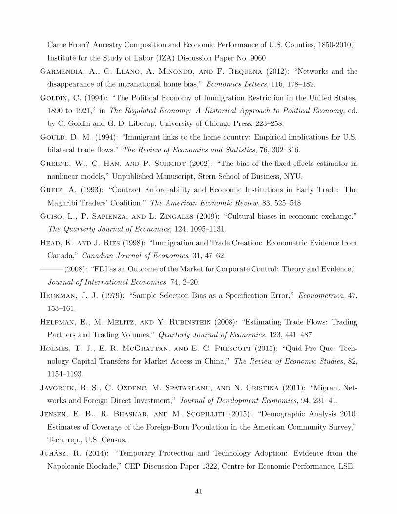
Came From? Ancestry Composition and Economic Performance of U.S. Counties, 1850-2010,”

Institute for the Study of Labor (IZA) Discussion Paper No. 9060.

Garmendia, A., C. Llano, A. Minondo, and F. Requena (2012): “Networks and the

disappearance of the intranational home bias,” Economics Letters, 116, 178–182.

Goldin, C. (1994): “The Political Economy of Immigration Restriction in the United States,

1890 to 1921,” in The Regulated Economy: A Historical Approach to Political Economy, ed.

by C. Goldin and G. D. Libecap, University of Chicago Press, 223–258.

Gould, D. M. (1994): “Immigrant links to the home country: Empirical implications for U.S.

bilateral trade flows.” The Review of Economics and Statistics, 76, 302–316.

Greene, W., C. Han, and P. Schmidt (2002): “The bias of the fixed effects estimator in

nonlinear models,” Unpublished Manuscript, Stern School of Business, NYU.

Greif, A. (1993): “Contract Enforceability and Economic Institutions in Early Trade: The

Maghribi Traders’ Coalition,” The American Economic Review, 83, 525–548.

Guiso, L., P. Sapienza, and L. Zingales (2009): “Cultural biases in economic exchange.”

The Quarterly Journal of Economics, 124, 1095–1131.

Head, K. and J. Ries (1998): “Immigration and Trade Creation: Econometric Evidence from

Canada,” Canadian Journal of Economics, 31, 47–62.

——— (2008): “FDI as an Outcome of the Market for Corporate Control: Theory and Evidence,”

Journal of International Economics, 74, 2–20.

Heckman, J. J. (1979): “Sample Selection Bias as a Specification Error,” Econometrica, 47,

153–161.

Helpman, E., M. Melitz, and Y. Rubinstein (2008): “Estimating Trade Flows: Trading

Partners and Trading Volumes,” Quarterly Journal of Economics, 123, 441–487.

Holmes, T. J., E. R. McGrattan, and E. C. Prescott (2015): “Quid Pro Quo: Tech-

nology Capital Transfers for Market Access in China,” The Review of Economic Studies, 82,

1154–1193.

Javorcik, B. S., C. Ozdenc, M. Spatareanu, and N. Cristina (2011): “Migrant Net-

works and Foreign Direct Investment,” Journal of Development Economics, 94, 231–41.

Jensen, E. B., R. Bhaskar, and M. Scopilliti (2015): “Demographic Analysis 2010:

Estimates of Coverage of the Foreign-Born Population in the American Community Survey,”

Tech. rep., U.S. Census.

Juhasz, R. (2014): “Temporary Protection and Technology Adoption: Evidence from the

Napoleonic Blockade,” CEP Discussion Paper 1322, Centre for Economic Performance, LSE.

41

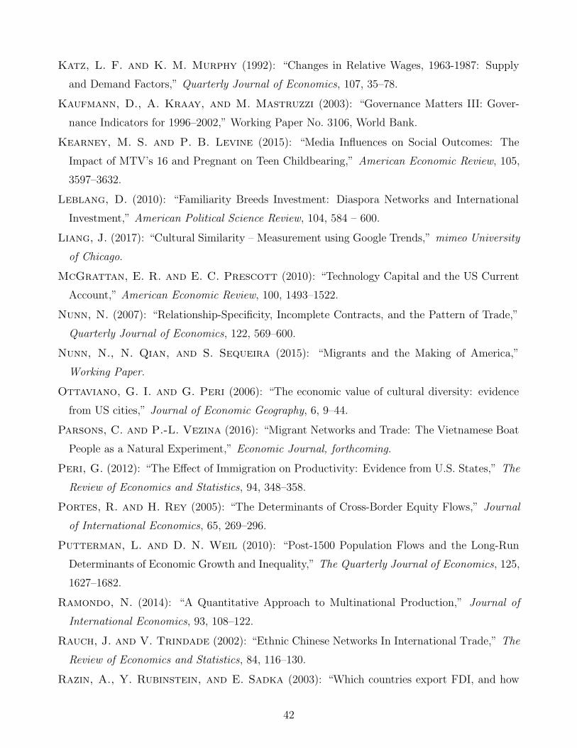
Katz, L. F. and K. M. Murphy (1992): “Changes in Relative Wages, 1963-1987: Supply

and Demand Factors,” Quarterly Journal of Economics, 107, 35–78.

Kaufmann, D., A. Kraay, and M. Mastruzzi (2003): “Governance Matters III: Gover-

nance Indicators for 1996–2002,” Working Paper No. 3106, World Bank.

Kearney, M. S. and P. B. Levine (2015): “Media Influences on Social Outcomes: The

Impact of MTV’s 16 and Pregnant on Teen Childbearing,” American Economic Review, 105,

3597–3632.

Leblang, D. (2010): “Familiarity Breeds Investment: Diaspora Networks and International

Investment,” American Political Science Review, 104, 584 – 600.

Liang, J. (2017): “Cultural Similarity – Measurement using Google Trends,” mimeo University

of Chicago.

McGrattan, E. R. and E. C. Prescott (2010): “Technology Capital and the US Current

Account,” American Economic Review, 100, 1493–1522.

Nunn, N. (2007): “Relationship-Specificity, Incomplete Contracts, and the Pattern of Trade,”

Quarterly Journal of Economics, 122, 569–600.

Nunn, N., N. Qian, and S. Sequeira (2015): “Migrants and the Making of America,”

Working Paper.

Ottaviano, G. I. and G. Peri (2006): “The economic value of cultural diversity: evidence

from US cities,” Journal of Economic Geography, 6, 9–44.

Parsons, C. and P.-L. Vezina (2016): “Migrant Networks and Trade: The Vietnamese Boat

People as a Natural Experiment,” Economic Journal, forthcoming.

Peri, G. (2012): “The Effect of Immigration on Productivity: Evidence from U.S. States,” The

Review of Economics and Statistics, 94, 348–358.

Portes, R. and H. Rey (2005): “The Determinants of Cross-Border Equity Flows,” Journal

of International Economics, 65, 269–296.

Putterman, L. and D. N. Weil (2010): “Post-1500 Population Flows and the Long-Run

Determinants of Economic Growth and Inequality,” The Quarterly Journal of Economics, 125,

1627–1682.

Ramondo, N. (2014): “A Quantitative Approach to Multinational Production,” Journal of

International Economics, 93, 108–122.

Rauch, J. and V. Trindade (2002): “Ethnic Chinese Networks In International Trade,” The

Review of Economics and Statistics, 84, 116–130.

Razin, A., Y. Rubinstein, and E. Sadka (2003): “Which countries export FDI, and how

42

much?” Tech. rep., National Bureau of Economic Research.

Redding, S. and D. Sturm (2008): “The Cost of Remoteness: Evidence from German Division

and Reunification,” The American Economic Review, 98, 1766–1797.

Silva, J. S. and S. Tenreyro (2006): “The Log of Gravity,” The Review of Economics and

statistics, 88, 641–658.

Spolaore, E. and R. Wacziarg (2015): “War and Relatedness,” The Review of Economics

and Statistics, forthcoming.

Steinwender, C. (2014): “Information Frictions and the Law of One Price: “When the States

and the Kingdom became United”,” Working Papers 190, Oesterreichische Nationalbank (Aus-

trian Central Bank).

Stephens-Davidowitz, S. (2014): “The cost of racial animus on a black candidate: Evidence

using Google search data,” Journal of Public Economics, 118, 26 – 40.

Stephens-Davidowitz, S. and Varian (2015): “A Hands-on Guide to Google Data,” Work-

ing Paper.

Stiglitz, J. E. (1990): “Peer Monitoring and Credit Markets,” The World Bank Economic

Review, 4, 351–366.

Thernstrom, S. (1980): Havard encyclopedia of American ethnic groups, Harvard University

Press, Cambridge MA.

Varian, H. R. (1990): “Monitoring Agents With Other Agents,” Journal of Institutional and

Theoretical Economics (Zeitschrift fur die gesamte Staatswissenschaft), 146, 153–174.

43

Figure 1: Origins of Immigrants to the United States, pre-1880 to 2000

Notes: The left side depicts the share of total immigration to the United States in each census periodfor the largest five origin countries of US residents that claim foreign ancestry in the 2010 census:Germany, Britain, Ireland, Mexico, and Italy. The right side shows the the number of migrants (inmillions) by continent of origin. See section 1 of the main text and appendix A.1 for details.

Figure 2: Destinations of Immigrants to the United States, pre-1880 to2000

Pre 1880

1910 - 1920

1970 -1980

1880 - 1900

1920-1930

1980-1990

1900 - 1910

1930-1970

1990-2000

Notes: This figure maps immigration flows into US counties by census period. We regressthe number of immigrants into US county d at time t, It

d, on destination county d and yeart fixed effects, and calculate the residuals. The maps’ color coding depicts the residuals’decile in the distribution of residuals across counties and within census periods. Darkercolors indicate a higher decile.

44

Figure 3: First-Stage Coefficients

-.1

0

.1

.2

.3

.4

Coe

ffici

ent o

n ex

clud

ed IV

s

1880 1900 1910 1920 1930 1970 1980 1990 2000

Notes: Coefficient estimates (bars) and 95% confidence intervals (lines) on the excluded instruments{It

o,−r(d)(It−c(o),d/It

−c(o))}t=1880,...,2000 from Table 2, column 2. The dependent variable is Log Ancestry2010. Robust standard errors are clustered at the origin country level.

Figure 4: Migrants and Ancestors:The Cases of Germany Pre-1900 and Italy 1900-1910

Non-European immigration: Pre-1900

Non-European immigration: 1900-1930

German descendants in 2010

Italian descendants in 2010

Notes: This figure contrasts Italian and German ancestry in 2010 (right panels), and non-Europeanimmigration patterns pre-1900 and 1910-1930 (left panel). The left two panels are created in the sameway as the maps in Figure 2, restricted to non-European immigration and the two periods we consider(pre-1900 and 1910-1930). The right two panels plot the county level residuals from a regression oflog ancestry in 2010 on county, Italy and Germany fixed effects on the sample of European countries.The maps’ color coding depicts the residuals’ decile in the distribution of residuals across counties.Darker colors indicate a higher decile.

45

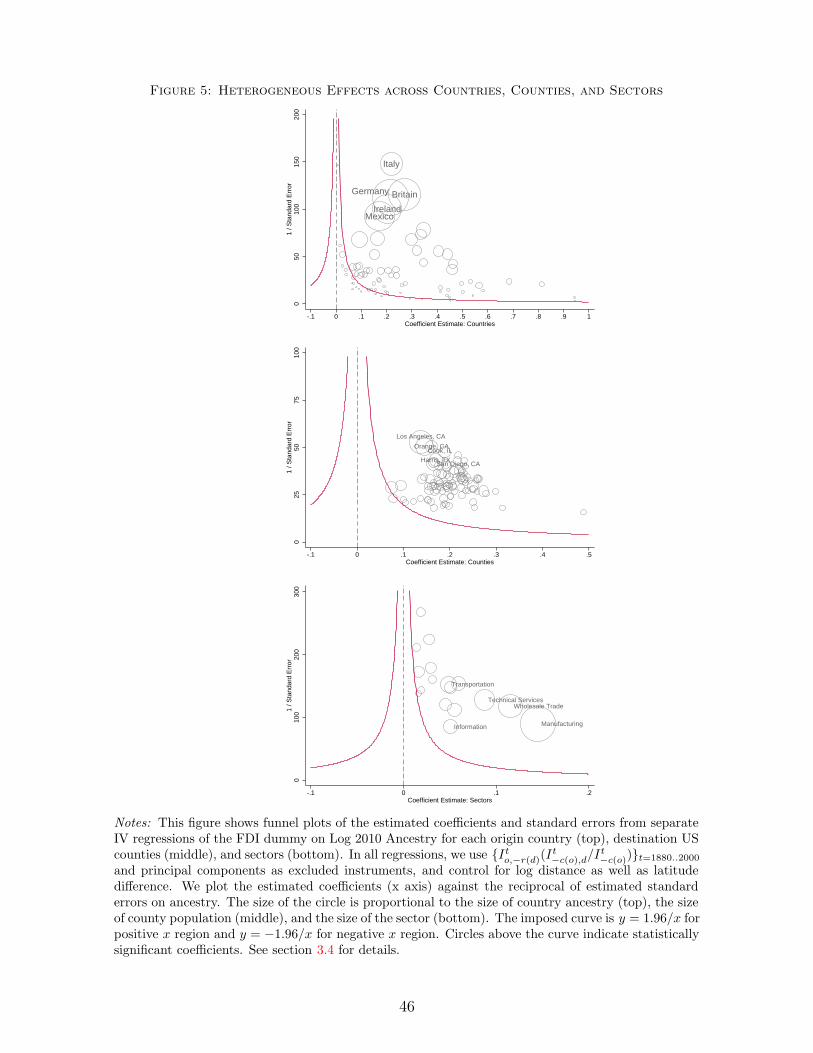
Figure 5: Heterogeneous Effects across Countries, Counties, and Sectors

Germany Britain

MexicoIreland

Italy

050

100

150

200

1 / S

tand

ard

Err

or

-.1 0 .1 .2 .3 .4 .5 .6 .7 .8 .9 1Coefficient Estimate: Countries

Los Angeles, CA

Cook, ILHarris, TX

San Diego, CA

Orange, CA

025

5075

100

1 / S

tand

ard

Err

or

-.1 0 .1 .2 .3 .4 .5Coefficient Estimate: Counties

Manufacturing

Wholesale TradeTechnical Services

Transportation

Information

010

020

030

01

/ Sta

ndar

d E

rror

-.1 0 .1 .2Coefficient Estimate: Sectors

Notes: This figure shows funnel plots of the estimated coefficients and standard errors from separateIV regressions of the FDI dummy on Log 2010 Ancestry for each origin country (top), destination UScounties (middle), and sectors (bottom). In all regressions, we use {It

o,−r(d)(It−c(o),d/It

−c(o))}t=1880..2000

and principal components as excluded instruments, and control for log distance as well as latitudedifference. We plot the estimated coefficients (x axis) against the reciprocal of estimated standarderrors on ancestry. The size of the circle is proportional to the size of country ancestry (top), the sizeof county population (middle), and the size of the sector (bottom). The imposed curve is y = 1.96/x forpositive x region and y = −1.96/x for negative x region. Circles above the curve indicate statisticallysignificant coefficients. See section 3.4 for details.

46

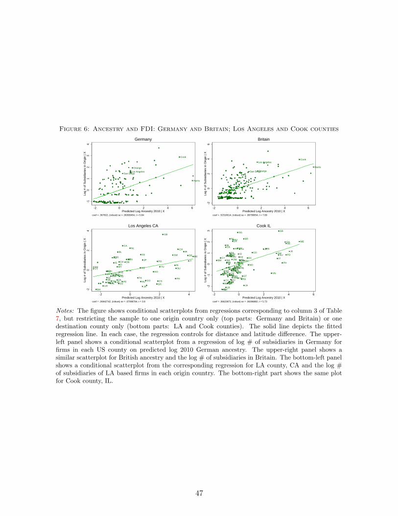
Figure 6: Ancestry and FDI: Germany and Britain; Los Angeles and Cook counties

San DiegoLos Angeles

Orange

Cook

Harris

-10

12

34

Log

# of

Sub

sidi

arie

s in

Orig

in |

X

-2 0 2 4 6Predicted Log Ancestry 2010 | X

coef = .367822, (robust) se = .06300454, t = 5.84

Germany

CYBM

BH

UR

AR

BRSE

NZ

GI

CH

PAAL

MWCO

SA

AU

AR

IS

SG

VE

ID

ZA

MY

BL

GH

EG

CHFI

KE

TU

PE

CA

DNBR

TH

ES

NL

PA

NO

FR

HU

JA

JP

CO

KO

GR

PO

CS

YU

GB

SW

IN

PH

SU

CHIR

DE

IT

ME

-20

24

Log

# of

Sub

sidi

arie

s in

Orig

in |

X

-2 0 2 4Predicted Log Ancestry 2010 | X

coef = .26942742, (robust) se = .07098784, t = 3.8

Los Angeles CA

San Diego

Los Angeles

Orange

Cook

Harris

-20

24

6Lo

g #

of S

ubsi

diar

ies

in O

rigin

| X

-2 0 2 4 6Predicted Log Ancestry 2010 | X

coef = .52316614, (robust) se = .06799654, t = 7.69

Britain

BMCY

NIGI

TU

ML

BH

BGCY

MAUR

NA

BLCA

LB

TU

ES

NZIS

BH

CH

RO

QA

AR

OM

MO

BO

CR

BR

PA

SA

NL

ARCHMU

EG

FJ

ZM

ZW

MW

ZA

FI

AG

AU

FR

GRPNTZ

VE

PRSLUG

DN

TT

MY

SG

KO

YU

ID

CS

KE

HU

HN

PE

TH

NG

PAGT

BR

JA

AUEC

NO

CO

JPIN

VN

SW

IT

SU

GB

PH

CH

PO

DE

IR

ME

-2-1

01

23

Log

# of

Sub

sidi

arie

s in

Orig

in |

X

-2 0 2 4 6Predicted Log Ancestry 2010 | X

coef = .36623872, (robust) se = .06396882, t = 5.73

Cook IL

Notes: The figure shows conditional scatterplots from regressions corresponding to column 3 of Table7, but restricting the sample to one origin country only (top parts: Germany and Britain) or onedestination county only (bottom parts: LA and Cook counties). The solid line depicts the fittedregression line. In each case, the regression controls for distance and latitude difference. The upper-left panel shows a conditional scatterplot from a regression of log # of subsidiaries in Germany forfirms in each US county on predicted log 2010 German ancestry. The upper-right panel shows asimilar scatterplot for British ancestry and the log # of subsidiaries in Britain. The bottom-left panelshows a conditional scatterplot from the corresponding regression for LA county, CA and the log #of subsidiaries of LA based firms in each origin country. The bottom-right part shows the same plotfor Cook county, IL.

47

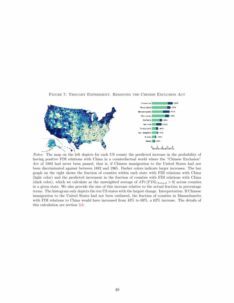
Figure 7: Thought Experiment: Removing the Chinese Exclusion Act

Notes: The map on the left depicts for each US county the predicted increase in the probability ofhaving positive FDI relations with China in a counterfactual world where the “Chinese Exclusion”Act of 1882 had never been passed, that is, if Chinese immigration to the United States had notbeen discriminated against between 1882 and 1965. Darker colors indicate larger increases. The bargraph on the right shows the fraction of counties within each state with FDI relations with China(light color) and the predicted increment in the fraction of counties with FDI relations with China(dark color), which we calculate as the unweighted average of d Pr [FDIChina,d > 0] across countiesin a given state. We also provide the size of this increase relative to the actual fraction in percentageterms. The histogram only depicts the ten US states with the largest change. Interpretation: If Chineseimmigration to the United States had not been outlawed, the fraction of counties in Massachusettswith FDI relations to China would have increased from 43% to 69%, a 62% increase. The details ofthis calculation are section 3.6.

48

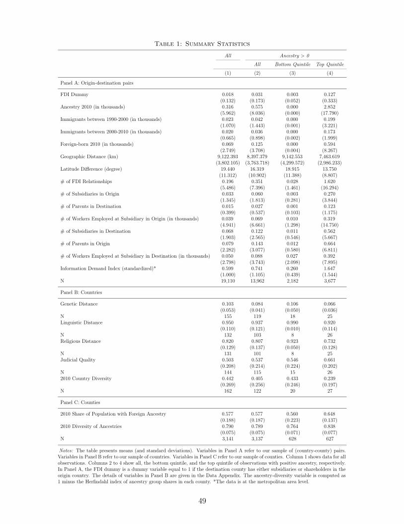
Table 1: Summary Statistics

All Ancestry > 0

All Bottom Quintile Top Quintile

(1) (2) (3) (4)

Panel A: Origin-destination pairs

FDI Dummy 0.018 0.031 0.003 0.127(0.132) (0.173) (0.052) (0.333)

Ancestry 2010 (in thousands) 0.316 0.575 0.000 2.852(5.962) (8.036) (0.000) (17.790)

Immigrants between 1990-2000 (in thousands) 0.023 0.042 0.000 0.199(1.070) (1.443) (0.001) (3.221)

Immigrants between 2000-2010 (in thousands) 0.020 0.036 0.000 0.173(0.665) (0.898) (0.002) (1.999)

Foreign-born 2010 (in thousands) 0.069 0.125 0.000 0.594(2.749) (3.708) (0.004) (8.267)

Geographic Distance (km) 9,122.393 8,397.379 9,142.553 7,463.619(3,802.105) (3,763.718) (4,299.572) (2,986.233)

Latitude Difference (degree) 19.440 16.319 18.915 13.750(11.312) (10.902) (11.388) (8.807)

# of FDI Relationships 0.196 0.351 0.028 1.620(5.486) (7.396) (1.461) (16.294)

# of Subsidiaries in Origin 0.033 0.060 0.003 0.270(1.345) (1.813) (0.281) (3.844)

# of Parents in Destination 0.015 0.027 0.001 0.123(0.399) (0.537) (0.103) (1.175)

# of Workers Employed at Subsidiary in Origin (in thousands) 0.039 0.069 0.010 0.319(4.941) (6.661) (1.298) (14.750)

# of Subsidiaries in Destination 0.068 0.122 0.011 0.562(1.903) (2.565) (0.546) (5.667)

# of Parents in Origin 0.079 0.143 0.012 0.664(2.282) (3.077) (0.580) (6.811)

# of Workers Employed at Subsidiary in Destination (in thousands) 0.050 0.088 0.027 0.392(2.798) (3.743) (2.098) (7.895)

Information Demand Index (standardized)* 0.599 0.741 0.260 1.647(1.000) (1.105) (0.439) (1.544)

N 19,110 13,962 2,182 3,677

Panel B: Countries

Genetic Distance 0.103 0.084 0.106 0.066(0.053) (0.041) (0.050) (0.036)

N 155 119 18 25Linguistic Distance 0.950 0.937 0.990 0.920

(0.110) (0.121) (0.010) (0.114)N 132 103 8 26Religious Distance 0.820 0.807 0.923 0.732

(0.129) (0.137) (0.050) (0.128)N 131 101 8 25Judicial Quality 0.503 0.537 0.546 0.661

(0.208) (0.214) (0.224) (0.202)N 144 115 15 262010 Country Diversity 0.442 0.405 0.433 0.239

(0.269) (0.256) (0.246) (0.197)N 162 122 20 27

Panel C: Counties

2010 Share of Population with Foreign Ancestry 0.577 0.577 0.560 0.648(0.188) (0.187) (0.223) (0.137)

2010 Diversity of Ancestries 0.790 0.789 0.764 0.838(0.075) (0.075) (0.071) (0.077)

N 3,141 3,137 628 627

Notes: The table presents means (and standard deviations). Variables in Panel A refer to our sample of (country-county) pairs.Variables in Panel B refer to our sample of countries. Variables in Panel C refer to our sample of counties. Column 1 shows data for allobservations. Columns 2 to 4 show all, the bottom quintile, and the top quintile of observations with positive ancestry, respectively.In Panel A, the FDI dummy is a dummy variable equal to 1 if the destination county has either subsidiaries or shareholders in theorigin country. The details of variables in Panel B are given in the Data Appendix. The ancestry-diversity variable is computed as1 minus the Herfindahl index of ancestry group shares in each county. *The data is at the metropolitan area level.

49

Table 2: First-stage: The Effect of Historical Migrations on Ancestry

Log ancestry 2010 Ancestry 2010

(1) (2) (3) (4) (5) (6) (7) (8) (9)

I1880o,−r(d) ×

I1880−c(o),d

I1880−c(o)

0.057*** 0.056*** 0.045*** 0.035*** 0.056*** 0.056*** 0.056*** 2.145***

(0.013) (0.012) (0.011) (0.009) (0.007) (0.007) (0.008) (0.290)

I1900o,−r(d) ×

I1900−c(o),d

I1900−c(o)

0.097*** 0.095*** 0.067** 0.068*** 0.099*** 0.099*** 0.100*** 0.106** 3.634**

(0.032) (0.031) (0.028) (0.019) (0.033) (0.033) (0.036) (0.043) (1.425)

I1910o,−r(d) ×

I1910−c(o),d

I1910−c(o)

0.192*** 0.193*** 0.145*** 0.123*** 0.137*** 0.137*** 0.132** 0.123** 5.646**

(0.039) (0.039) (0.042) (0.031) (0.050) (0.050) (0.054) (0.049) (2.345)

I1920o,−r(d) ×

I1920−c(o),d

I1920−c(o)

0.205*** 0.209*** 0.176*** 0.174*** 0.283*** 0.283*** 0.249*** 0.276*** 14.726***

(0.070) (0.070) (0.061) (0.052) (0.045) (0.045) (0.047) (0.041) (3.012)

I1930o,−r(d) ×

I1930−c(o),d

I1930−c(o)

0.062 0.061 0.061 0.035 0.079 0.079 0.065* 0.078 11.812***

(0.056) (0.056) (0.056) (0.048) (0.051) (0.051) (0.034) (0.051) (2.855)

I1970o,−r(d) ×

I1970−c(o),d

I1970−c(o)

0.183*** 0.184*** 0.163*** 0.149*** 0.149*** 0.148*** 0.150*** 0.151*** 6.256***

(0.038) (0.038) (0.036) (0.031) (0.028) (0.029) (0.027) (0.029) (0.669)

I1980o,−r(d) ×

I1980−c(o),d

I1980−c(o)

0.173*** 0.173*** 0.174*** 0.169*** 0.214*** 0.214*** 0.205** 0.213*** 18.694***

(0.066) (0.066) (0.064) (0.061) (0.076) (0.077) (0.080) (0.075) (2.390)

I1990o,−r(d) ×

I1990−c(o),d

I1990−c(o)

0.123*** 0.124*** 0.124*** 0.111** 0.101** 0.101** 0.115** 0.102** 10.786***

(0.048) (0.048) (0.048) (0.044) (0.045) (0.045) (0.048) (0.044) (3.675)

I2000o,−r(d) ×

I2000−c(o),d

I2000−c(o)

0.020 0.019 0.026 0.026* 0.046*** 0.046*** 0.039** 0.046*** 5.194***

(0.017) (0.017) (0.016) (0.015) (0.017) (0.017) (0.016) (0.017) (1.148)

I2010o,−r(d) ×

I2010−c(o),d

I2010−c(o)

0.317***

(0.089)

Kleibergen Wald rk statistic 10.608 10.958 8.327 9.607 162.194 158.125 195.423 142.800 910.331Stock-Yogo 5% critical values 20.53 20.53 20.53 20.53 21.18 21.18 21.23 21.10 21.18Stock-Yogo 10% critical values 11.46 11.46 11.46 11.46 11.52 11.52 11.51 11.52 11.52

R2 0.56 0.56 0.66 0.72 0.73 0.73 0.73 0.73 0.49N 612,495 612,495 612,495 612,495 612,495 612,495 612,495 612,495 612,495

Destination FE Yes Yes Yes Yes Yes Yes Yes Yes YesOrigin FE Yes Yes Yes Yes Yes Yes Yes Yes YesDistance No Yes Yes Yes Yes Yes Yes Yes YesLatitude Difference No Yes Yes Yes Yes Yes Yes Yes YesDestination × Continent FE No No Yes Yes Yes Yes Yes Yes YesOrigin × Census Region FE No No No Yes Yes Yes Yes Yes YesPrincipal Components No No No No Yes Yes Yes Yes Yes3rd order poly in dist and lat No No No No No Yes No No No

Notes: The table presents coefficient estimates of our first stage equation (4) at the country-county level. All specifications control fororigin and destination fixed effects. Standard errors are given in parentheses and are clustered at the origin country level. In columns 1-8the dependent variable is the log of 1 plus the number of residents of the county in 2010 that report having ancestors in the origin country,measured in thousands (Log Ancestry 2010 ). In column 9 the dependent variable is the level of ancestry in 2010 (again in thousands). Theexcluded instruments are, for each census period, interactions of pull and push factors in migration, I t

o,−r(d)(It−c(o),d/I

t−c(o)), where I t

o,−r(d)

stands for the number of migrants from o who settle in destinations not in the same census region as d in period t and I t−c(o),d/I

t−c(o) for

the fraction of migrants not coming from origins in the same continent as o who settle in county d. Columns 3-9 also include the first fiveprincipal components of higher-order interactions of these factors. *, **, and *** denote statistical significance at the 10%, 5%, and 1%levels, respectively.

50

Table 3: Second-stage: The effect of Ancestry on FDI

Panel A: IV FDI 2014 (Dummy)

(1) (2) (3) (4) (5) (6)

Log Ancestry 2010 0.231*** 0.190*** 0.187*** 0.187*** 0.198*** 0.191***(0.023) (0.024) (0.024) (0.024) (0.023) (0.024)

Log Distance 0.007 0.004 0.024 0.009 0.026 -0.027(0.010) (0.009) (0.029) (0.033) (0.030) (0.027)

Latitude Difference 0.006** 0.005** 0.006* -0.000 0.006* 0.003(0.002) (0.002) (0.003) (0.003) (0.003) (0.004)

N 612495 612495 612495 612495 612495 612300

Panel B: OLS FDI 2014 (Dummy)

Log Ancestry 2010 0.173*** 0.149*** 0.149*** 0.149*** 0.149*** 0.161***(0.016) (0.018) (0.018) (0.018) (0.018) (0.019)

R2 0.2967 0.3635 0.3635 0.3635 0.3635 0.3930N 612495 612495 612495 612495 612495 612495

Destination FE Yes Yes Yes Yes Yes YesOrigin FE Yes Yes Yes Yes Yes YesPrincipal Components No Yes Yes Yes Yes YesDestination × Continent FE No No Yes Yes Yes YesOrigin × Census Region FE No No Yes Yes Yes Yes3rd order poly in dist and lat No No No Yes No NoI2010o,−r(d)(I

2010−c(o),d/I

2010−c(o)) No No No No Yes No

Origin × State FE No No No No No Yes

Notes: The table presents coefficient estimates from IV (Panel A) and OLS (Panel B) regressionsof equation (1) at the country-county level. The dependent variable in all panels is a dummyindicating an FDI relationship between origin o and destination d in 2014. The main variableof interest is Log Ancestry 2010, instrumented using various specifications of equation (4). Inall columns in Panel A, we include {I t

o,−r(d)(It−c(o),d/I

t−c(o))}t=1880,...,2000 as excluded instruments.

Columns 3-6 also include the first five principal components of the higher-order interactions ofpush and pull factors as instruments. Column 5 also includes the interaction of the push and pullfactor constructed using data from the 2006-2010 American Community Survey. All specificationscontrol for log distance, latitude difference, origin, and destination fixed effects. Standard errorsare given in parentheses. Standard errors are clustered at the origin country level. *, **, and ***denote statistical significance at the 10%, 5%, and 1% levels, respectively. (We also run an IVprobit regression using the specification in column 2 yielding a marginal effect evaluated at themean of Log Ancestry 2010 on FDI equal to 0.104***(0.037).)

51

Table 4: The Effect of Ancestry on FDI: The Communist Natural Experiment

FDI 2014 (Dummy)

(1) (2) (3) (4) (5)

Log Ancestry 2010 0.197*** 0.380*** 0.075 0.242** 0.234**(0.066) (0.053) (0.054) (0.104) (0.098)

N 3,141 3,141 3,141 18,846 28,269

Destination FE No No No No Yes

Countries considered Soviet Union China Vietnam Eastern Europe All communist countriesYears excluded 1918-1990 1949-1980 1975-1996 1945-1989

Notes: The table presents coefficient estimates from IV regressions of equation (1) at the country-countylevel. Each column uses data from a subset of origin countries: Soviet Union (column 1), China (column 2),Vietnam (column 3), as well as Albania, Bulgaria, Czechoslovakia, Hungary, Poland, and Romania (column4). The dependent variable in all columns is a dummy indicating an FDI relationship between origin countryo and destination county d in 2014. All specifications use the same set of instruments as the one in column 3of Table 3, but only exclude the interaction terms containing measures of pull and push factors in migrationsthat occur during the years of economic isolation from the United States indicated above; the remainingvariables are included as controls. All specifications control for log distance, latitude difference, and originfixed effects. Standard errors are given in parentheses and are robust. *, **, and *** denote statisticalsignificance at the 10%, 5%, and 1% levels, respectively.

Table 5: Alternative Instruments

Panel A: Variations of leave-out categories FDI 2014 (Dummy)

Excluding origins with correlated migration flows: I to,−r(d) × (I t

−s(o),d/It−s(o)) 0.197***

(0.020)

Excluding states adjacent to the destination: I to,−a(d) × (I t

−c(o),d/It−c(o)) 0.200***

(0.023)

Panel B: Using subsets of instruments for identification FDI 2014 (Dummy)

Only migrations 1880 − 1930 0.209***(0.037)

Only migrations 1970 − 2000 0.175***(0.021)

Only migrations 1900 − 2000 0.187***(0.024)

Notes: This table presents coefficient estimates from instrumental variable regressions that arevariations of our standard specification (column 3 of 3), but not using the principal componentsof higher-order interactions for identification. The dependent variable in all regressions is FDI 2014(Dummy). Each row lists the coefficient estimate on Log Ancestry 2010. In Panel A we showalternative specifications of our leave-out instrument. First, when calculating the pull-factor of o tod we exclude all countries whose aggregate time path of migrations to the US is correlated with o’smigrations to the US. Second, when calculating the push factor of o we exclude migrations to anystate adjacent to the state of d. In Panel B we use throughout the interacted instrument of ourstandard specification. In contrast to the standard specification, each specification in this panel usesas instruments only the simple interaction terms from a subset of the full time period covered byour data. Standard errors are given in parenthesis and clustered at the country level. *, **, and ***denote statistical significance at the 10%, 5%, and 1% levels, respectively.

52

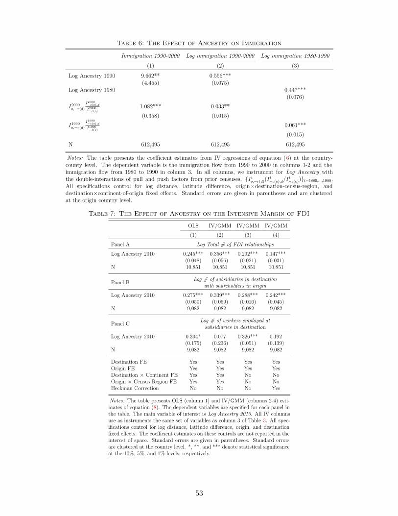
Table 6: The Effect of Ancestry on Immigration

Immigration 1990-2000 Log immigration 1990-2000 Log immigration 1980-1990

(1) (2) (3)

Log Ancestry 1990 9.662** 0.556***(4.455) (0.075)

Log Ancestry 1980 0.447***(0.076)

I2000o,−r(d)

I2000−c(o),d

I2000−c(o)

1.082*** 0.033**

(0.358) (0.015)

I1990o,−r(d)

I1990−c(o),d

I1990−c(o)

0.061***

(0.015)

N 612,495 612,495 612,495

Notes: The table presents the coefficient estimates from IV regressions of equation (6) at the country-county level. The dependent variable is the immigration flow from 1990 to 2000 in columns 1-2 and theimmigration flow from 1980 to 1990 in column 3. In all columns, we instrument for Log Ancestry withthe double-interactions of pull and push factors from prior censuses, {I t

o,−r(d)(It−c(o),d/I

t−c(o))}t=1880,...,1980.

All specifications control for log distance, latitude difference, origin×destination-census-region, anddestination×continent-of-origin fixed effects. Standard errors are given in parentheses and are clusteredat the origin country level.

Table 7: The Effect of Ancestry on the Intensive Margin of FDI

OLS IV/GMM IV/GMM IV/GMM

(1) (2) (3) (4)

Panel A Log Total # of FDI relationships

Log Ancestry 2010 0.245*** 0.356*** 0.292*** 0.147***(0.048) (0.056) (0.021) (0.031)

N 10,851 10,851 10,851 10,851

Panel BLog # of subsidiaries in destination

with shareholders in origin

Log Ancestry 2010 0.275*** 0.339*** 0.288*** 0.242***(0.050) (0.059) (0.016) (0.045)

N 9,082 9,082 9,082 9,082

Panel CLog # of workers employed at

subsidiaries in destination

Log Ancestry 2010 0.304* 0.077 0.326*** 0.192(0.175) (0.236) (0.051) (0.139)

N 9,082 9,082 9,082 9,082

Destination FE Yes Yes Yes YesOrigin FE Yes Yes Yes YesDestination × Continent FE Yes Yes No NoOrigin × Census Region FE Yes Yes No NoHeckman Correction No No No Yes

Notes: The table presents OLS (column 1) and IV/GMM (columns 2-4) esti-mates of equation (8). The dependent variables are specified for each panel inthe table. The main variable of interest is Log Ancestry 2010. All IV columnsuse as instruments the same set of variables as column 3 of Table 3. All spec-ifications control for log distance, latitude difference, origin, and destinationfixed effects. The coefficient estimates on these controls are not reported in theinterest of space. Standard errors are given in parentheses. Standard errorsare clustered at the country level. *, **, and *** denote statistical significanceat the 10%, 5%, and 1% levels, respectively.

53

Table 8: Thought Experiment: A Gold Rush in Los Angeles in 1880

Predicted Counterfactual Change

Ancestry 2010 FDI # Ancestry 2010 FDI # (in %, IV)

(1) (2) (3) (4)

Germany 343,276 241 +65,344 +62.70Ireland 256,621 40 +61,701 +58.34UK 396,439 582 +26,645 +21.95Norway 39,515 55 +4,657 +3.53Sweden 51,395 71 +4,010 +3.03France 77,372 278 +3,293 +2.48Canada 27,722 531 +3,132 +2.36Switzerland 10,156 162 +2,456 +1.85Czechoslovakia 17,905 4 +2,140 +1.61Netherlands 38,392 121 +1,638 +1.23

Notes: The table presents the number of individuals of selected ancestries livingin Los Angeles County (column 1), the number of FDI links between Los An-geles County and the countries of origin (column 2), and the predicted changesin these variables under a counterfactual scenario where the pre-1880 pull fac-tor of Los Angeles is 5 times as large as in reality (columns 3 and 4). Column3 shows the predicted absolute change in ancestry based on a regression analo-gous to column 9 of Table 2 with Ancestry 2010 (in levels) as dependent vari-able, again excluding the principal components. Column 4 shows the predictedchange of Total # of FDI relationships (in percent) based on the IV regressionof Log Total # of FDI relationships on Log Ancestry 2010, instrumented for by{I t

o,−r(d)(It−c(o),d/I

t−c(o))}t=1880,...,2000, similar to column 2 of Table 7 without the

principal components as instruments. All regressions control for log distance andlatitude difference and include a origin × destination-census-region, and destina-tion × continent-of-origin fixed effects. Only the 10 countries with the highestabsolute change in ancestry are shown in the interest of space. The details forthe construction of this thought experiment are presented in section 3.6.

54

Table 9: The “Similarities” Hypothesis and Contract Enforcement

(1) (2)

Panel A: Final vs. Intermediate Goods FDI 2014 (Dummy)

Log Ancestry 2010 0.156*** 0.169***(0.026) (0.024)

N 612,495 612,495

Sample Final goods Intermediate goods

Panel B: Final vs. Intermediate Goods Inward FDI 2014 (Dummy)

Log Ancestry 2010 0.108*** 0.117***(0.033) (0.032)

N 612,495 612,495

Sample Final goods Intermediate goods

Panel C: Sector similarity Rank Correlation Cosine correlation

Log Ancestry 2010 0.011 0.010(0.015) (0.013)

N 21,518 21,518

Panel D: Judicial Quality FDI 2014 (Dummy) Log # of FDI relationships

Log Ancestry × Judicial Quality 0.180* 1.414***(0.094) (0.243)

N 452,304 10,089

Notes: The table presents coefficient estimates from IV regressions at the country-countylevel. In Panel A, the outcome variable is the FDI dummy; we restrict our sample to firmsproducing final goods or intermediate inputs, respectively. Final goods and intermediateinputs are defined as 4-digit NAICS sectors with upstreamness index below and above 2,respectively, where we use the upstreamness index from Antras et al. (2012). The number ofcountry-county pairs that have an (non-zero) FDI link in the corresponding sector is 4,201and 5,842 in columns 1 and 2, respectively. In Panel B, we replicate the same regressions,except that the outcome variable indicates only the existence of any inward FDI. In PanelC, the outcome variable is the rank and cosine correlation of the share of employees in 127manufacturing sectors within a given origin-destination pair, respectively. The relatively lownumber of observations is due to data availability in the industry share of employment: Whencalculating the correlation between industries’ share of employment in county d and countryo, the correlation coefficient is missing for those country-county pairs that have at least onemissing share of employment. In Panel D, the outcome is the extensive (FDI dummy) andintensive (log # of FDI relationships) margin, and the measure of judicial quality is from Nunn(2007). Throughout we use {I t

o,−r(d)(It−c(o),d/I

t−c(o))}t=1880,...,2000 and principal components as

instrumental variables. All specifications control for log distance, latitude difference, and originand destination fixed effects. In Panels A-C we additionally control for origin×destination-census-region, and destination×continent-of-origin fixed effects. Standard errors are given inparentheses and are clustered by origin country.

55

Table 10: The Effect of Ancestry on Differential Information Demand and Language

Panel A: Google Trends Information Demand Index Actors Athletes Musicians Politicians(standardized) (standardized) (standardized) (standardized) (standardized)

(1) (2) (3) (4) (5) (6) (7)

Log Ancestry 2010 0.871*** 1.717** 0.659** 0.948*** 0.531*** 0.688***(0.257) (0.783) (0.257) (0.359) (0.076) (0.183)

Log Foreign-born 2010 -1.108(0.809)

Log Ancestry 1980 0.801***(0.186)

N 19,110 19,110 19,110 19,110 19,110 19,110 19,110

Destination FE Yes Yes Yes Yes Yes Yes YesOrigin FE Yes Yes Yes Yes Yes Yes YesPrincipal Components Yes Yes Yes Yes Yes Yes Yes

Panel B: Language # of residents in d speaking # of US-born in d that speaklanguage of o at home the language of o at home

(1) (2) (3) (4) (5) (6) (7)

Ancestry 2010 2.226*** 0.942*** 1.170*** 1.257*** 0.085*** 0.015***(0.717) (0.301) (0.042) (0.230) (0.006) (0.003)

Ancestry 1980 1.241**(0.504)

N 454,812 454,813 454,813 65,877 78,376 3,137 3,137

Non-English language Any Any Any Spanish Arabic Chinese Hindi

Destination FE Yes Yes Yes No No No NoOrigin FE Yes Yes Yes Yes Yes Yes Yes

Notes: This table presents coefficient estimates from IV regressions at the country-DMA (Panel A) and country-county (Panel B) level. In Panel A, alldependent variables are based on a count of Google searches in the category specified above the panel. The Information Demand Index in columns 1-3 isa simple average of the other four categories. Each of the four categories is the average of Google Trends value G(i, d), which measures the (normalized)fraction of queries that include search term i relative to the total number of queries of Designated Market Area (DMA) d. For the search terms i weuse the first five terms from Google’s Answer Box when we search for “notable [foreign country d] [category]”. All outcome variables in Panel A arestandardized by their standard deviation. In Panel B, the dependent variable in column 1 is the number of residents in d that speak the language of oat home, excluding English; in column 2 and 3, it is the number of US-born residents in d that speak the language of o at home, excluding English; andin columns 3-6, it is the number of US-born residents in d that speak the language indicated in the respective column. Spanish is the official languagein twenty-one countries; Arabic is the official language in twenty-five countries; Chinese and Hindi each are the official language in only one country.Ancestry 2010, Ancestry 1980, Log Ancestry 2010, Log Foreign-born 2010, and Log Ancestry 1980 are instrumented as in column 3 of Table 3. Allspecifications control for log distance and latitude difference. Standard errors are given in parentheses and clustered at the country level (all of PanelA and columns 1-2 of Panel B) or state level (columns 3-6 of Panel B). *, **, and *** denote statistical significance at the 10%, 5%, and 1% levels,respectively.

56

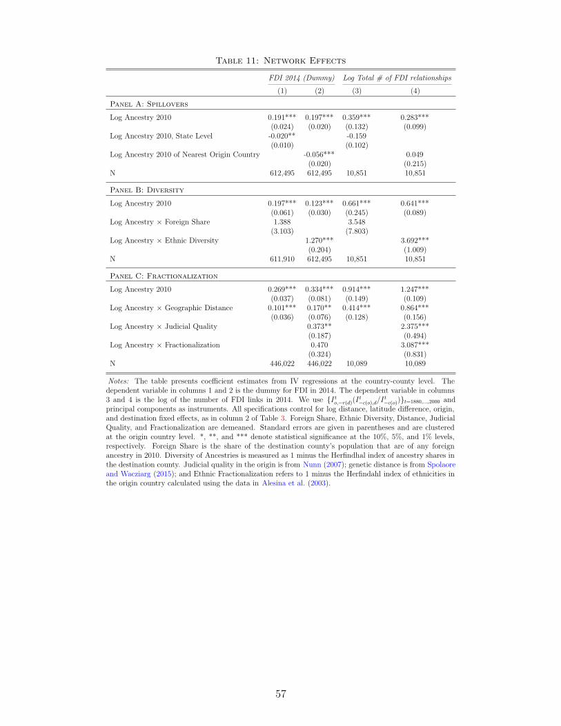
Table 11: Network Effects

FDI 2014 (Dummy) Log Total # of FDI relationships

(1) (2) (3) (4)

Panel A: Spillovers

Log Ancestry 2010 0.191*** 0.197*** 0.359*** 0.283***(0.024) (0.020) (0.132) (0.099)

Log Ancestry 2010, State Level -0.020** -0.159(0.010) (0.102)

Log Ancestry 2010 of Nearest Origin Country -0.056*** 0.049(0.020) (0.215)

N 612,495 612,495 10,851 10,851

Panel B: Diversity

Log Ancestry 2010 0.197*** 0.123*** 0.661*** 0.641***(0.061) (0.030) (0.245) (0.089)

Log Ancestry × Foreign Share 1.388 3.548(3.103) (7.803)

Log Ancestry × Ethnic Diversity 1.270*** 3.692***(0.204) (1.009)

N 611,910 612,495 10,851 10,851

Panel C: Fractionalization

Log Ancestry 2010 0.269*** 0.334*** 0.914*** 1.247***(0.037) (0.081) (0.149) (0.109)

Log Ancestry × Geographic Distance 0.101*** 0.170** 0.414*** 0.864***(0.036) (0.076) (0.128) (0.156)

Log Ancestry × Judicial Quality 0.373** 2.375***(0.187) (0.494)

Log Ancestry × Fractionalization 0.470 3.087***(0.324) (0.831)

N 446,022 446,022 10,089 10,089

Notes: The table presents coefficient estimates from IV regressions at the country-county level. Thedependent variable in columns 1 and 2 is the dummy for FDI in 2014. The dependent variable in columns3 and 4 is the log of the number of FDI links in 2014. We use {I t

o,−r(d)(It−c(o),d/I

t−c(o))}t=1880,...,2000 and

principal components as instruments. All specifications control for log distance, latitude difference, origin,and destination fixed effects, as in column 2 of Table 3. Foreign Share, Ethnic Diversity, Distance, JudicialQuality, and Fractionalization are demeaned. Standard errors are given in parentheses and are clusteredat the origin country level. *, **, and *** denote statistical significance at the 10%, 5%, and 1% levels,respectively. Foreign Share is the share of the destination county’s population that are of any foreignancestry in 2010. Diversity of Ancestries is measured as 1 minus the Herfindhal index of ancestry shares inthe destination county. Judicial quality in the origin is from Nunn (2007); genetic distance is from Spolaoreand Wacziarg (2015); and Ethnic Fractionalization refers to 1 minus the Herfindahl index of ethnicities inthe origin country calculated using the data in Alesina et al. (2003).

57

Table 12: The Effect of Ancestry on the Intensive Margin of Trade (State Level)

OLS IV IV

(1) (2) (3)

Panel A Log Total # of FDI relationships

Log Ancestry 2010 1.001*** 1.374*** 0.079***(0.077) (0.183) (0.025)

R2 0.659 0.626 0.847N 2,208 2,202 2,191

Panel B Log Aggregate Exports

Log Ancestry 2010 1.519*** 2.993*** -0.149(0.173) (0.357) (0.138)

R2 0.416 0.374 0.665N 4,799 4,783 4,739

Panel C Log Aggregate Imports

Log Ancestry 2010 1.927*** 3.447*** 0.003(0.148) (0.497) (0.150)

R2 0.419 0.360 0.576N 3,823 3,764 3,815

Origin FE Yes Yes YesDestination FE No No YesHeckman Correction Yes Yes Yes

Panel D Log Exports to Vietnam

Log Ancestry 2010 1.169*** 1.230***(0.124) (0.124)

R2 0.680 0.678N 51 51

Panel E Log Exports to Japan

Log Ancestry 2010 0.898*** 1.107***(0.197) (0.128)

R2 0.442 0.419N 51 51

Origin FE Yes YesDestination FE No No

Notes: The table presents OLS and IV estimates of equa-tion (8) at the state level for FDI and trade. The depen-dent variables are the log number of total FDI links in 2014(Panel A), the log of aggregate exports (from the US state)(Panel B), aggregate imports (Panel C), exports to Vietnam(Panel D), and exports to Japan (Panel E). Exports andimports are measured in US dollars in 2011. In all columns,we use {I t

o,−r(d)(It−c(o),d/I

t−c(o))}t=1880,...,2000 and principal com-

ponents as excluded instruments. All specifications controlfor log distance, latitude difference, and origin fixed effects.Standard errors are given in parentheses and are double clus-tered at the destination state and origin country. *, **, and*** denote statistical significance at the 10%, 5%, and 1%levels, respectively.

58

Table 13: Generational Effects

FDI 2014 (Dummy)

IV IV OLS IV IV IV

(1) (2) (3) (4) (5) (6)

Log Ancestry 2010 0.187*** 0.155*** 0.242*** 0.163***(0.024) (0.022) (0.043) (0.014)

Log Foreign-born 2010 0.207*** -0.012 -0.082*(0.014) (0.031) (0.049)

Log Foreign-born 1970 0.286*** 0.046(0.025) (0.034)

N 612,495 612,495 612,495 612,495 612,495 612,495

Notes: The table presents the OLS (column 3) and IV (all other columns) estimates ofequation (1), contrasting the effect of ancestry and first-generation immigrants (foreign-born) on FDI. The dependent variable is the dummy for FDI in 2014. All IV columns use asinstruments the same set of variables as column 3 of Table 3. All specifications control for logdistance, latitude difference, origin×destination-census-region, and destination×continent-of-origin fixed effects. The coefficient estimates on these control variables are not reportedin the interest of space. Standard errors are given in parentheses and clustered at theorigin country level. *, **, and *** denote statistical significance at the 10%, 5%, and 1%levels, respectively. For column 4, the Kleibergen-Paap rk LM statistic on the excludedinstruments is 18.21 with p-value 0.150. For column 6, the Kleibergen-Paap rk LM statisticon the excluded instruments is 29.04 with p-value 0.007.

59

Online Appendix

“Migrants, Ancestors, and Foreign Investments”

Konrad B. Burchardi

Thomas Chaney

Tarek A. Hassan

A Data Appendix

Overview

To construct the migration and ancestry data up until the year 2000, we download the 1880,1900, 1910, 1920, 1930, 1970, 1980, and 2000 waves of the Integrated Public Use MicrodataSeries (IPUMS) from https://usa.ipums.org/usa-action/samples. For each wave, we selectthe largest available sample; for example, if a 1% and 10% sample was available for 1880 data, weused the 10% sample. To construct the 2010 data, we used the 2006-2010 American CommunitySurvey (ACS) sample provided on the IPUMS website. For a more detailed overview on thespecific waves used, see Appendix Table 1.

For each sample, we obtain the following variables: year, datanum, serial, hhwt, region, state-fip, county, cntygp97, cntygp98, puma, gq, pernum, perwt, bpl, mbpl, fbpl, nativity, ancestr1,yrimmig, mtongue, mmtongue, fmtongue, and language.

We construct the number of migrants from origin country o to destination county d in t, I to,d,

as well as the measure of ancestry Ato,d from 1980 onward. We first aggregate the individual-level

census data to counts of respondents at the level of historic US counties (or country groups from1970 onwards) and foreign countries, and then transform the data into 1990 country-county levelusing various transition matrices. Details are given in the following sections.

How we create transition matrices

We create a set of transition matrices that transform non-1990 countries to 1990 countries andnon-1990 counties/county groups to 1990 counties.

• Birthplace-to-country: The aim is to construct transition matrices that map all the birth-place answers into 1990 countries. In each wave of the US Census, respondents wereasked to report their country of birth. All possible answers (across time) are listedhere: https://usa.ipums.org/usa-action/variables/BPL#codes_section . The cen-suses from 1850-2012 contain roughly 550 possible different answers to the question ofbirthplace. In each census data set, they are saved in the variable “bpld.” What follows isour procedure for building those matrices:

1. We start with a transition matrix of zeros, with all possible answers to the 1990birthplace question as rows and all 1990 countries as columns. A cell in row r andcolumn c of the transition matrix answers the question, “What is the probability thatan individual who claims his/her birthplace as r refers to the area that in 1990 iscountry c?” So all cells contain values in [0,1], and rows sum up to 1.

60

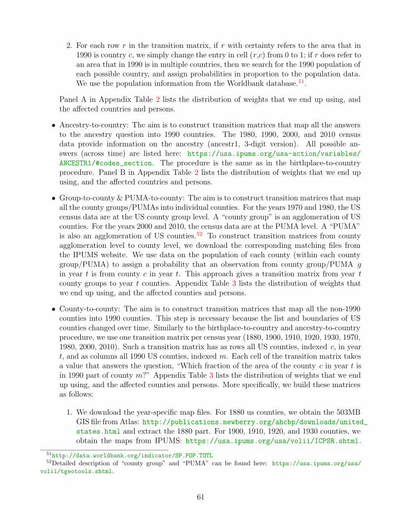
2. For each row r in the transition matrix, if r with certainty refers to the area that in1990 is country c, we simply change the entry in cell (r,c) from 0 to 1; if r does refer toan area that in 1990 is in multiple countries, then we search for the 1990 population ofeach possible country, and assign probabilities in proportion to the population data.We use the population information from the Worldbank database.51.

Panel A in Appendix Table 2 lists the distribution of weights that we end up using, andthe affected countries and persons.

• Ancestry-to-country: The aim is to construct transition matrices that map all the answersto the ancestry question into 1990 countries. The 1980, 1990, 2000, and 2010 censusdata provide information on the ancestry (ancestr1, 3-digit version). All possible an-swers (across time) are listed here: https://usa.ipums.org/usa-action/variables/

ANCESTR1/#codes_section. The procedure is the same as in the birthplace-to-countryprocedure. Panel B in Appendix Table 2 lists the distribution of weights that we end upusing, and the affected countries and persons.

• Group-to-county & PUMA-to-county: The aim is to construct transition matrices that mapall the county groups/PUMAs into individual counties. For the years 1970 and 1980, the UScensus data are at the US county group level. A “county group” is an agglomeration of UScounties. For the years 2000 and 2010, the census data are at the PUMA level. A “PUMA”is also an agglomeration of US counties.52 To construct transition matrices from countyagglomeration level to county level, we download the corresponding matching files fromthe IPUMS website. We use data on the population of each county (within each countygroup/PUMA) to assign a probability that an observation from county group/PUMA gin year t is from county c in year t. This approach gives a transition matrix from year tcounty groups to year t counties. Appendix Table 3 lists the distribution of weights thatwe end up using, and the affected counties and persons.

• County-to-county: The aim is to construct transition matrices that map all the non-1990counties into 1990 counties. This step is necessary because the list and boundaries of UScounties changed over time. Similarly to the birthplace-to-country and ancestry-to-countryprocedure, we use one transition matrix per census year (1880, 1900, 1910, 1920, 1930, 1970,1980, 2000, 2010). Such a transition matrix has as rows all US counties, indexed c, in yeart, and as columns all 1990 US counties, indexed m. Each cell of the transition matrix takesa value that answers the question, “Which fraction of the area of the county c in year t isin 1990 part of county m?” Appendix Table 3 lists the distribution of weights that we endup using, and the affected counties and persons. More specifically, we build these matricesas follows:

1. We download the year-specific map files. For 1880 us counties, we obtain the 503MBGIS file from Atlas: http://publications.newberry.org/ahcbp/downloads/united_states.html and extract the 1880 part. For 1900, 1910, 1920, and 1930 counties, weobtain the maps from IPUMS: https://usa.ipums.org/usa/volii/ICPSR.shtml.

51http://data.worldbank.org/indicator/SP.POP.TOTL52Detailed description of “county group” and “PUMA” can be found here: https://usa.ipums.org/usa/

volii/tgeotools.shtml.

61

Finally, for 1970, 1980, and 1990 counties, we obtain the maps from NHGIS: https://data2.nhgis.org/main.

2. We project non-1990 maps onto 1990 counties. We used the intersect command inArcGIS to map year-specific counties onto 1990 counties based on area. This approachgives a transition matrix from non-1990 counties to 1990 counties.

Appendix Table 1: Description of each IPUMS wave

Wave Description

1880 We use the 10% sample with oversamples; the sample is weighted, so we use theprovided person weights to get to a representative sample; we use the region identifiersstatefip and county.

1900 We use the 5% sample; the sample is weighted, so we use the provided person weightsto get to a representative sample; we use the region identifiers statefip and county.

1910 We use the 1% sample; the sample is unweighted; we use the region identifiers statefipand county.

1920 We use the 1% sample; the sample is weighted, so we use the provided person weightsto get to a representative sample; we use the region identifiers statefip and county.

1930 We use the 5% sample; the sample is weighted, so we use the provided person weightsto get to a representative sample; we use the region identifiers statefip and county.

1970 We use the 1% Form 1 Metro sample; the sample is unweighted; we use the regionidentifiers statefip and cntygp97 (county group 1970); note that only four states canbe completely identified because metropolitan areas that straddle state boundaries arenot assigned to states; identifies every metropolitan area of 250,000 or more.

1980 We use the 5% State sample; the sample is unweighted; we use the region identifiersstatefip and cntygp98 (county group 1980); the sample identifies all states, largermetropolitan areas, and most counties over 100,000 population.

1990 We use the 5% State sample; the sample is weighted, so we use the provided personweights to get to a representative sample; we use the region identifiers statefip andpuma; the sample identifies all states, and within states, most counties or parts ofcounties with 100,000 or more population.

2000 We use the 5% Census sample; the sample is weighted, so we use the provided personweights to get to a representative sample; we use region identifiers statefip and puma;the sample identifies all states, and within states, most counties or parts of countieswith 100,000 or more population.

2010 We use the American Community Service (ACS) 5-Year sample; the sample is weighted,so we use the provided person weights to get to a representative sample; we use regionidentifiers statefip and puma, which contain at least 100,000 persons; the 2006-2010data contains all households and persons from the 1% ACS samples for 2006, 2007,2008, 2009 and 2010, identifiable by year.

62

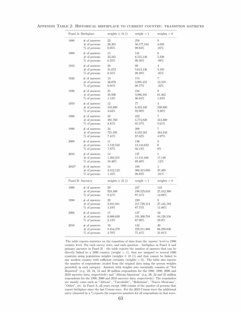
Appendix Table 2: Historical birthplace to current country: transition matrices

Panel A: Birthplace weights ∈ (0, 1) weight = 1 weights = 0

1880 # of answers 22 258 9# of persons 26,301 50,177,184 4,933% of persons 0.05% 99.94% .01%

1900 # of answers 15 131 6# of persons 23,345 6,555,140 5,339% of persons 0.35% 99.56% .08%

1910 # of answers 20 99 4# of persons 31,072 5,613,136 3,105% of persons 0.55% 99.39% .05%

1920 # of answers 13 174 7# of persons 36,070 3,905,455 12,559% of persons 0.91% 98.77% .32%

1930 # of answers 25 194 9# of persons 35,930 3,086,341 61,462% of persons 1.13% 96.94% 1.93%

1970 # of answers 12 77 3# of persons 318,800 6,323,100 230,800% of persons 4.64% 92.00% 3.36%

1980 # of answers 32 222 7# of persons 491,760 4,774,820 313,300% of persons 8.81% 85.57% 5.61%

1990 # of answers 24 209 7# of persons 721,595 8,532,585 484,433% of persons 7.41% 87.62% 4.97%

2000 # of answers 11 136 0# of persons 1,122,532 13,144,632 0% of persons 7.87% 92.13% 0%

2010 # of answers 14 137 1# of persons 1,302,255 11,131,046 17,148% of persons 10.46% 89.40% .14%

2010* # of answers 14 188 1# of persons 3,512,123 300,415,680 37,469% of persons 1.16% 98.83% .01%

Panel B: Ancestry weights ∈ (0, 1) weight = 1 weights = 0

1980 # of answers 29 227 143# of persons 924,400 198,525,616 27,412,380% of persons 0.41% 87.51% 12.08%

1990 # of answers 29 239 9# of persons 2,941,941 217,720,512 27,445,182% of persons 1.19% 87.75% 11.06%

2000 # of answers 17 137 22# of persons 6,000,639 191,300,704 84,120,558% of persons 2.13% 67.98% 29.9%

2010 # of answers 19 142 30# of persons 8,454,279 229,211,968 66,299,030% of persons 2.78% 75.41% 21.81%

The table reports statistics on the transition of data from the ‘answer’ level to 1990country level. For each survey wave, and each question – birthplace in Panel A andprimary ancestry in Panel B – the table reports the number of answers that can bedirectly linked to a 1990 country (weight = 1), that are assigned to several 1990countries using population weights (weights ∈ (0, 1)) and that cannot be linked toany modern country with sufficient certainty (weights = 0). The table also reportsthe number of respondents (scaled from the original data using the person weightsprovided) in each category. Answers with weights zero essentially consists of ”NotReported” (e.g. 23, 24, 54 and 30 million respondents for the 1980, 1990, 2000 and2010 ancestry data, respectively) and ”African-American” (e.g. 26, 22 and 25 millionrespondents for the 1990, 2000 and 2010 ancestry data, respectively). The remaindersare mostly cases such as ”African”, ”Uncodable”, ”Bohemian”, ”Nuevo Mexicano”,”Other”, etc. In Panel A, all years except 1880 consist of the number of persons thatreport birthplace since the last Census wave. For the 2010 Census wave the additionalentry (denoted by a *) reports the respective numbers for all respondents in that wave.

63

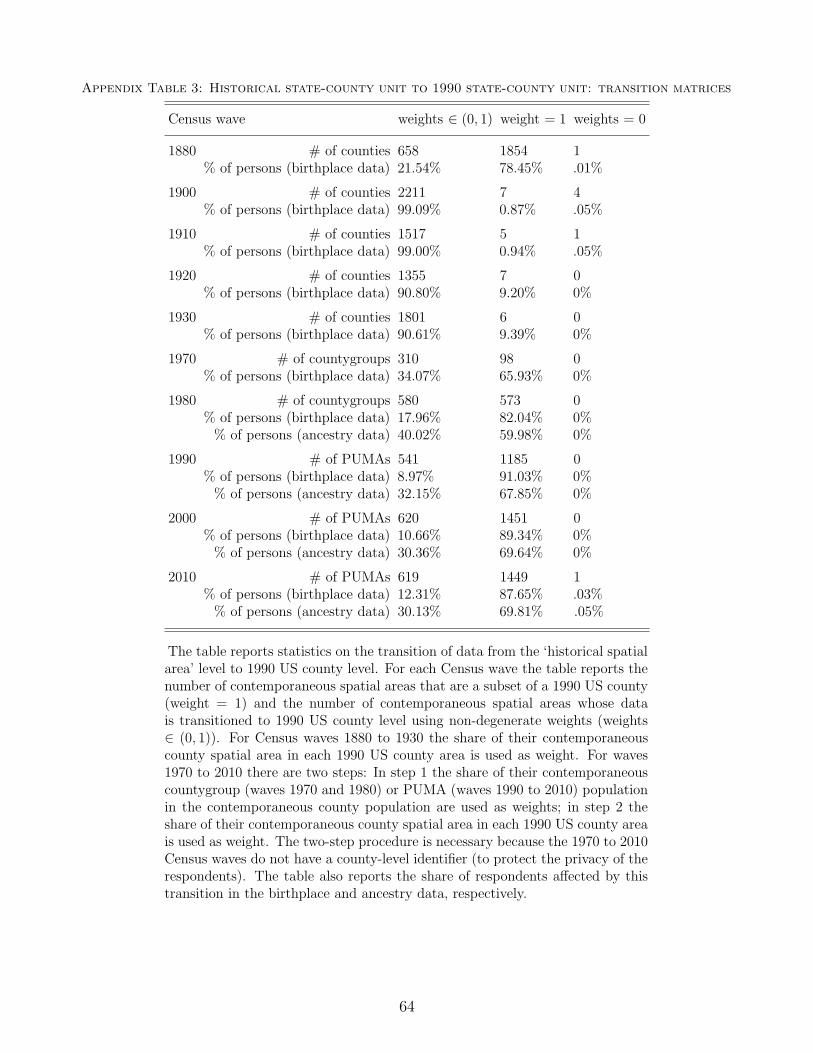
Appendix Table 3: Historical state-county unit to 1990 state-county unit: transition matrices

Census wave weights ∈ (0, 1) weight = 1 weights = 0

1880 # of counties 658 1854 1% of persons (birthplace data) 21.54% 78.45% .01%

1900 # of counties 2211 7 4% of persons (birthplace data) 99.09% 0.87% .05%

1910 # of counties 1517 5 1% of persons (birthplace data) 99.00% 0.94% .05%

1920 # of counties 1355 7 0% of persons (birthplace data) 90.80% 9.20% 0%

1930 # of counties 1801 6 0% of persons (birthplace data) 90.61% 9.39% 0%

1970 # of countygroups 310 98 0% of persons (birthplace data) 34.07% 65.93% 0%

1980 # of countygroups 580 573 0% of persons (birthplace data) 17.96% 82.04% 0%

% of persons (ancestry data) 40.02% 59.98% 0%

1990 # of PUMAs 541 1185 0% of persons (birthplace data) 8.97% 91.03% 0%

% of persons (ancestry data) 32.15% 67.85% 0%

2000 # of PUMAs 620 1451 0% of persons (birthplace data) 10.66% 89.34% 0%

% of persons (ancestry data) 30.36% 69.64% 0%

2010 # of PUMAs 619 1449 1% of persons (birthplace data) 12.31% 87.65% .03%

% of persons (ancestry data) 30.13% 69.81% .05%

The table reports statistics on the transition of data from the ‘historical spatialarea’ level to 1990 US county level. For each Census wave the table reports thenumber of contemporaneous spatial areas that are a subset of a 1990 US county(weight = 1) and the number of contemporaneous spatial areas whose datais transitioned to 1990 US county level using non-degenerate weights (weights∈ (0, 1)). For Census waves 1880 to 1930 the share of their contemporaneouscounty spatial area in each 1990 US county area is used as weight. For waves1970 to 2010 there are two steps: In step 1 the share of their contemporaneouscountygroup (waves 1970 and 1980) or PUMA (waves 1990 to 2010) populationin the contemporaneous county population are used as weights; in step 2 theshare of their contemporaneous county spatial area in each 1990 US county areais used as weight. The two-step procedure is necessary because the 1970 to 2010Census waves do not have a county-level identifier (to protect the privacy of therespondents). The table also reports the share of respondents affected by thistransition in the birthplace and ancestry data, respectively.

64

A.1 Details on the construction of migration and ethnicity data

Details calculation of post-1880 flow of immigrants

For each census wave after 1880, we count the number of individuals in each historic US countyd who were born in historic country o (as identified by birthplace variable “bpld” in the rawdata) that had immigrated to the United States since the last census wave that contains theimmigration variable (not always 10 years earlier). Then we transform these data

• from the non-1990 foreign-country (“bpld”) level to the 1990 foreign-country level usingbpld-to-country transition matrices.

• from the US-county group/puma level to the US-county level using group/puma-to-countytransition matrices.

• from the non-1990 US-county level to the 1990 US-county level using county-to-countytransition matrices.

• from the post-1990 US-county level to the 1990 US county level. Based on the informationfrom https://www.census.gov/geo/reference/county-changes.html , a new county iseither created from part of ONE 1990 county or assigned a new FIPS code after 1990,so we manually change that county’s FIPS code to what it was in 1990. A few counties’boundaries have been changed after 1990 but that only involved a tiny change in population,so we ignore these differences.

Details calculation of pre-1880 stock of immigrants

For the year 1880, we calculate for each historic US county d the number of individuals whowere born in a historic foreign country o (no matter when they immigrated). We add to thosecalculations the number of individuals in county d who were born in the United States, but whoseparents were born in historic foreign country o. (If the parents were born in different countries,we count the person as half a person from the mother’s place of birth, and half a person fromthe father’s place of birth). Then we transform these data

• from the pre-1880 foreign-country (“bpld”) level to the 1990 foreign-country level using thepre-1880 country-to-country transition matrix.

• from the pre-1880 US-county level to the 1990 US-county level using the pre-1880 county-to-county transition matrix.

Details calculation of stock of ancestry (1980, 1990, 2000, and 2010)

For the years 1980, 1990, 2000, and 2010, we calculate for each US county group the numberof individuals who state as primary ancestry (“ancestr1” variable) some nationality/area. Wetransform the data

• from the ancestry-answer (“ancestr1”) level to the 1990 foreign-country level using ancestry-to-country transition matrices.

65

• from the US-county group/puma level to the US county-level using group/puma-to-countytransition matrices.

• from the non-1990 US-county level to the 1990 US-county level using county-to-countytransition matrices.

• from the post-1990 US-county to the 1990 US-county level. Based on the informationfrom https://www.census.gov/geo/reference/county-changes.html , a new county iseither created from part of ONE 1990 county or assigned a new FIPS code after 1990,so we manually change that county’s FIPS code to what it was in 1990. A few counties’boundaries have been changed after 1990 but that only involved a tiny change in population,so we ignore the difference.

A.2 Details on the construction of FDI data

Our FDI data are from the US file of the Bureau van Dijk ORBIS dataset. For each US firm,the raw data set lists the location of its (operational) headquarters, the addresses of its foreignparent entities, and the addresses of its international subsidiaries and branches. It also providesthe number of employees for both US and foreign firms. The steps for building the data followbelow.

Clean postcode information

We use firm’s postcode as a unique identifier for the county location of the US firm, and thenneed to ensure that one county uniquely corresponds to one postcode. Vance, NC; Wakulla,FL; Citrus, FL; Rankin, MS; Union, OH; and Du Page, IL share at least one postcode with aneighboring county. In each case we assign that postcode wholly to the county with the largerpopulation (according to Google 2012 population data). In the last step, we hand-coded missingpostcodes that we took from main data set. Only one such case existed: 75427 for Dallas.

Build the parent data

We used the following variables from the parent dataset: “Mark” “Company name” “BvD IDnumber” “Country ISO Code” “City” “Postcode” “NAICS 2007 Core code (4 digits)” “NAICS,text description” “Number of employees 2013” “Shareholder - Name” “Shareholder - BvD IDnumber” “Shareholder - City” “Shareholder - Postal code” “Shareholder - NAICS 2007, Corecode” “Shareholder - NAICS 2007, text description” “Shareholder - Country ISO code” “Share-holder - Direct %” “Shareholder - Total %” “Shareholder - Number of employees”. Here “share-holder” is equivalent to “parent” in our context. The key data-building steps are as follows:

1. Assign numerical values to “Shareholder Direct” and “Shareholder Total”:

• When the stake of a shareholder is described by an acronym rather than a number,we replace it with numerical values as follows: MO, majority owned, is replaced by“75%”; JO, jointly owned, is replaced by “50%”; NG, negligent, is replaced by ‘0%’;BR, branch and WO, wholly owned are both replaced by “100%”.53

53See http://papers.ssrn.com/sol3/papers.cfm?abstract_id=2407845 for reference.

66

• When the stake of a shareholder is described by the following expressions, we replaceit with a numerical value as follows: Values with a “>”, e.g., “ > 25.00” were replacedby the original number plus 10; values with a “<”, e.g., “ < 34.00”, were replaced bythe original number minus 10; values with a “±”, e.g. “±25.00”, were replaced by theoriginal number.

2. Postcode matching: We matched both US firms and US parents (foreign parents were ig-nored in this step), with our postcode data. Besides the original string variable postcode, wegenerated new variables postcode5digit and postcodeextension and labeled them “Postalcode (5 digit)” and “Postal code (extension).” Similarly, shareholders had shareholder-postcodeUS5digit and shareholderpostcodeUSextension (note the spelling postal code inshareholder variables was unified to postcode).

3. Country-code matching: We matched both companies and their parents. Each firm hadfour country variables: numerical country code, country name, and 2- and 3- digit ISOcountry code. Then we adjusted those 2014 country codes to 1990 codes based on theinformation on post-1990 country changes.

Build the subsidiary data

We used the following variables from the subsidiary dataset: “Mark” “Company name” “BvD IDnumber” “Country ISO Code” “City” “Postcode” “NAICS 2007 Core code (4 digits)” “NAICS,text description” “Number of employees 2007” “Subsidiary - Name” “Subsidiary - BvD ID num-ber” “Subsidiary - Country ISO code” “Subsidiary - City” “Subsidiary - Postal code” “Subsidiary- NAICS 2007, Core code” “Subsidiary - NAICS 2007, text description” “Subsidiary - Number ofemployees” “Subsidiary - Direct %” ”Subsidiary - Total%” “Branch - Name” ”Branch - BvD IDnumber” “Branch - Country ISO code” “Branch - City” “Branch - Postcode” “Branch - NAICS2007, Core code” “Branch - NAICS 2007, text description” “Branch - Number employees”. Thedata cleaning process is identical to that of the parent data described above, with the exceptionthat we merged subsidiaries with branches and refer to them collectively as “subsidiaries”.

A.3 Details on the construction of other data

International trade.— The data on trade between US states and foreign countries, both at theaggregate level and at the sectoral level, are from the Commodity Flow Survey for the year 2012.The data are collected by the US Census Bureau. A representative sample of establishmentsare surveyed every five years, and information on their shipments collected. The value of allshipments crossing the US international border are recorded as international trade, along withtheir foreign origin/destination country. We only used thes readily available data aggregated atthe US state and foreign country level. Although they do not cover all of the US foreign trade (thedata com from a representative survey, not from the universe of foreign transactions), they arethe only publicly available source of international data disaggregated at a geographic level belowthat of the entire United States. For each origin country and destination state, Importo,d areaggregate imports (in dollars) from country o to US state d in 2012, and Exporto,d are aggregateexports (in dollars) from US state d to country o in 2012, where we keep the convention of usingo for foreign countries and d for US administrative units, states or counties.

67

Bilateral distances and latitude differences.— To compute the distance between US countiesor states and foreign countries, we used the coordinates for all postal codes within a county orstate, and the coordinates of the main city for foreign countries.54 We define the latitude andlongitude of a US county as the unweighted average of the latitudes and longitudes of all postalcodes within the county. We define the latitude and longitude of a US state as the unweightedaverage of the latitude and longitude of all counties within the state. The distance betweenforeign country o and a US county or state d, Distanceo,d, is computed as the great circledistance between the two, measured in kms. The latitude difference between a foreign countryo and a US county or state d, LatitudeDifferenceo,d, is the absolute difference between thelatitudes of the two, measured in degrees.

Country characteristics.— To shed light on the mechanism through which the presence offoreign ancestry affects the patterns for foreign investment, we constructed several measures offoreign country and US county characteristics. “Genetic Distance” is a measure of the geneticdistance between a given foreign country and the United States, normalized to take values be-tween 0 and 1. “Linguistic Distance” is a measure of the linguistic distance between a givenforeign country and the United States; it measures the probability that a randomly selectedperson in the United States speaks the same language as a randomly selected person from thatcountry. “Religious Distance” measures the religious distance between a given foreign countryand the United States, with a similar construction as the linguistic distance. 55 A higher indexfor “Genetic Distance”, “Linguistic Distance”, or “Religious Distance” corresponds to a greaterdistance between the United States and that country. “Judicial Quality” is a measure of thejudicial quality in a given country.56 A higher index for “Judicial Quality” corresponds to ahigher-quality judicial system. “Ethnic Diversity” is a measure of a country’s ethnolinguisticfractionalization.57

US county characteristics.— We define three US-county level measures. “Diversity of An-cestries” is a measure of the diversity of communities from different ancestries in a given UScounty.58 “Foreign Share” measures the share of residents in a given county who claim foreignancestry.

Sectoral characteristics.— We separated sectors into final consumption goods and interme-diate inputs. To do so, we use the measure of upstreamness from Antras et al. (2012). Weclassified 4-digit NAICS sectors as “final goods” if their upstreamness index is below 2, and as“intermediates” if their upstreamness index is above 2.

54The geo-coordinates are downloaded from www.geonames.organd www.cepii.fr, respectively. When acounty has multiple postcodes we randomly select one of them and use the geocoordinates for that randomlyselected postcode.

55Both genetic and religious distance measures come from Spolaore and Wacziarg (2015).56The measure of judicial quality comes from Kaufmann et al. (2003) and is used in Nunn (2007). It is based

on a weighted average of variables measuring perceptions of the effectiveness of the judiciary and the enforcementof contracts.

57The measure of fractionalization comes from Alesina et al. (2003). It is equal to 1 minus the Herfindahl indexof ethnolinguistic group shares.

58It is equal to 1 minus the Herfindahl index of ancestry, measured as the sum of squared fractions of all possibleancestry among people who report foreign ancestry within that US county

68

A.4 Details on the construction of information demand indices

The Information Demand Index is based on data gathered from Google and created in threesteps. In the first step we identify five prominent individuals from country o in category p, wherep ∈ {actors, athletes, musicians, politicians}. In the second step we utilise Google Trends toobtain data on the spatial variation in the relative frequency of search queries related to theseindividuals. In the last step we construct indices of the search intensity related to country o indestination d.

Step 1: To identify the top five prominent individuals from o in each category p, we utilise atool called Google’s featured snippet box. Google’s featured snippet box is a response to a searchquery that is generated by Google and pushed to the top of the result list. Google generatesthese answers by scraping its top results and using an algorithm to provide what it determinesto be the most relevant answer.59 For our purposes we record the top five names in Google’sfeatured snippet box in response to the query “notable [country] [p]”, where [country] is oneof the 100 largest countries by 2015 population. For example, searching for “notable Belgiumactors” yields Google’s featured snippet box with an ordered list of Belgian actors. We save thetop five names from left to right as the set of search queries q(o, p). If Google’s featured snippetbox does not give a response for a country, we record a missing entry.60

Step 2: Google Trends provides historical and cross-sectional information about the relativeimportance of a search query. For the United States, the cross-sectional information with thehighest granularity is at the level of a Designated Market Area (DMA).61 Google Trends expressesthe relative importance of a search query in a given DMA as an integer value from 0 to 100.This integer value is calculated as follows. First, find the number of searches for the query athand relative to the total number of searches, and define the maximum search market share ofany DMA to 100. Second, divide each search market share by the maximum, and express it as arounded percentage. If the result does not exceed an unreported threshold, set it to zero (Liang,2017; Stephens-Davidowitz and Varian, 2015). Formally,

G(i, d) =

⌊

100sharei,d

maxδ{sharei,δ}1[#(i, d) ≥ T ]

⌉

where bxe is the integer round function, sharei,d is the search market share of search query i inDMA d, and T is the unreported search volume threshold. Note that T is defined on the absolutenumber of searches, rather than the search market share. This implies that DMAs with a largerpopulation will tend to report more data than those with smaller populations. Note also thatin addition to G(i, d) being reported as zero for some i and d, we set its value equal to zero ifthere is no search result from Google’s featured snippet box, or if there is no result from GoogleTrend.

59See https://support.google.com/webmasters/answer/6229325?hl=en60This is the case for about 4-10% of our sample, depending on the category.61Google Trends also breaks the information down by major city; however, we would lose non-city data.

69

Step 3: We define the p-specific Index for each DMA-country pair as

I(p, o, d) =1

5

∑

i∈q(o,p)

G(i, d)

We define the Information Demand Index as the average over the p-specific indices:

IDIo,d =1

5

∑

p

I(p, o, d).

to the query “notable [country] [p]”, where [country] is one of the 100

70

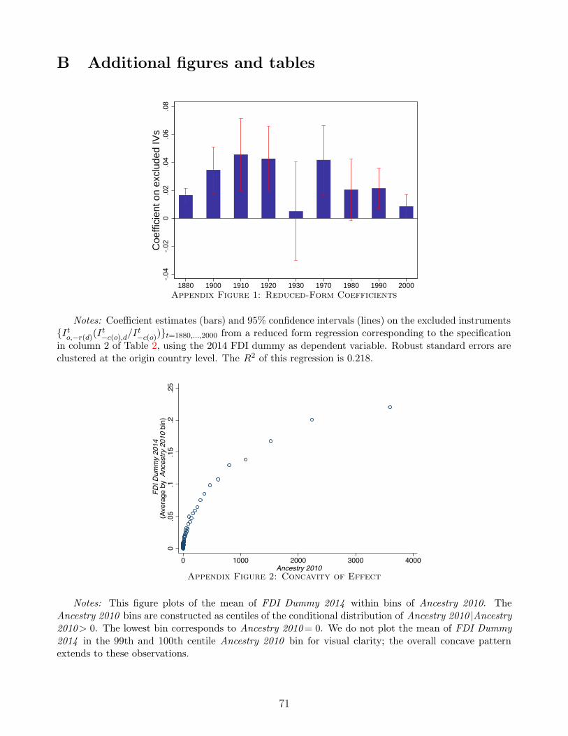
B Additional figures and tables

-.04

-.02

0.0

2.0

4.0

6.0

8C

oeffi

cien

t on

excl

uded

IVs

1880 1900 1910 1920 1930 1970 1980 1990 2000Appendix Figure 1: Reduced-Form Coefficients

Notes: Coefficient estimates (bars) and 95% confidence intervals (lines) on the excluded instruments{It

o,−r(d)(It−c(o),d/It

−c(o))}t=1880,...,2000 from a reduced form regression corresponding to the specificationin column 2 of Table 2, using the 2014 FDI dummy as dependent variable. Robust standard errors areclustered at the origin country level. The R2 of this regression is 0.218.

0.0

5.1

.15

.2.2

5

FD

I Dum

my

2014

(Ave

rage

by

Anc

estry

201

0 bi

n)

0 1000 2000 3000 4000 Ancestry 2010

Appendix Figure 2: Concavity of Effect

Notes: This figure plots of the mean of FDI Dummy 2014 within bins of Ancestry 2010. TheAncestry 2010 bins are constructed as centiles of the conditional distribution of Ancestry 2010 |Ancestry2010> 0. The lowest bin corresponds to Ancestry 2010= 0. We do not plot the mean of FDI Dummy2014 in the 99th and 100th centile Ancestry 2010 bin for visual clarity; the overall concave patternextends to these observations.

71

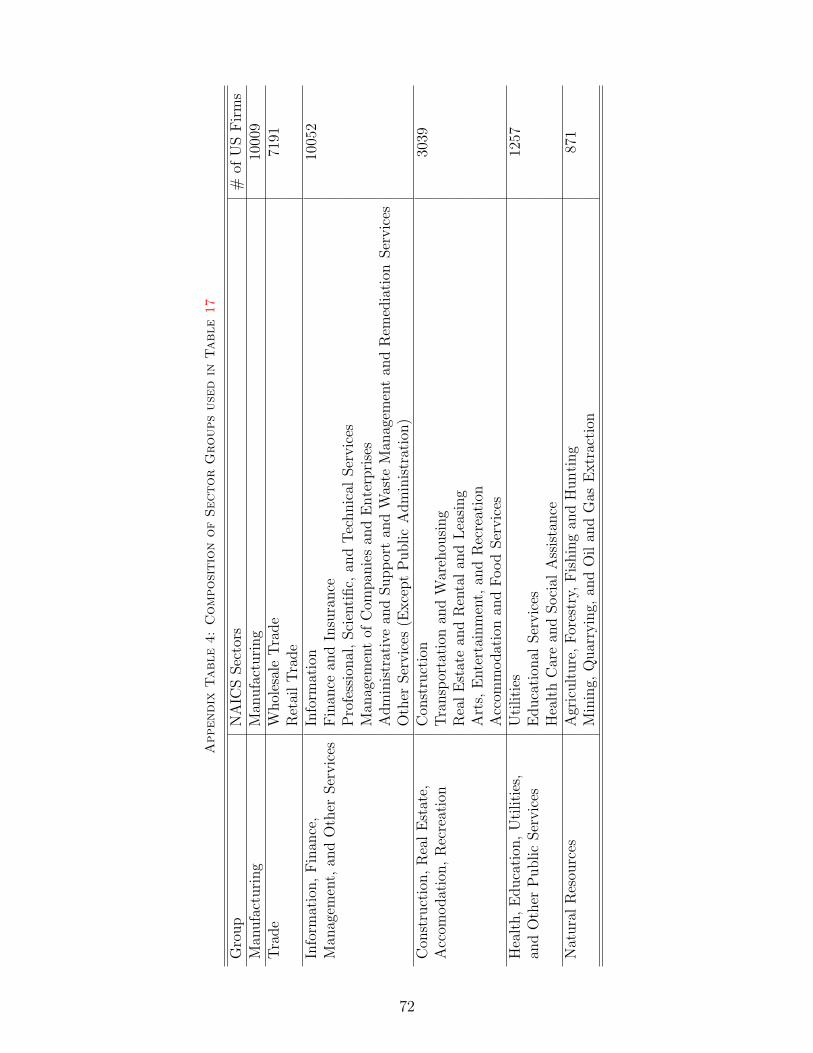
Appendix

Table

4:

Composi

tio

nof

Sector

Groups

use

din

Table

17

Gro

up

NA

ICS

Sec

tors

#of

US

Firm

sM

anufa

cturing

Man

ufa

cturing

1000

9Tra

de

Whol

esal

eTra

de

7191

Ret

ailTra

de

Info

rmat

ion,Fin

ance

,In

form

atio

n10

052

Man

agem

ent,

and

Oth

erSer

vic

esFin

ance

and

Insu

rance

Pro

fess

ional

,Sci

entific,

and

Tec

hnic

alSer

vic

esM

anag

emen

tof

Com

pan

ies

and

Ente

rprise

sA

dm

inis

trat

ive

and

Suppor

tan

dW

aste

Man

agem

ent

and

Rem

edia

tion

Ser

vic

esO

ther

Ser

vic

es(E

xce

pt

Public

Adm

inis

trat

ion)

Con

stru

ctio

n,R

ealE

stat

e,C

onst

ruct

ion

3039

Acc

omodat

ion,R

ecre

atio

nTra

nsp

orta

tion

and

War

ehou

sing

Rea

lE

stat

ean

dR

enta

lan

dLea

sing

Art

s,E

nte

rtai

nm

ent,

and

Rec

reat

ion

Acc

omm

odat

ion

and

Food

Ser

vic

esH

ealth,E

duca

tion

,U

tilities

,U

tilities

1257

and

Oth

erP

ublic

Ser

vic

esE

duca

tion

alSer

vic

esH

ealth

Car

ean

dSoci

alA

ssis

tance

Nat

ura

lR

esou

rces

Agr

iculture

,For

estr

y,Fis

hin

gan

dH

unting

871

Min

ing,

Quar

ryin

g,an

dO

ilan

dG

asE

xtr

action

72

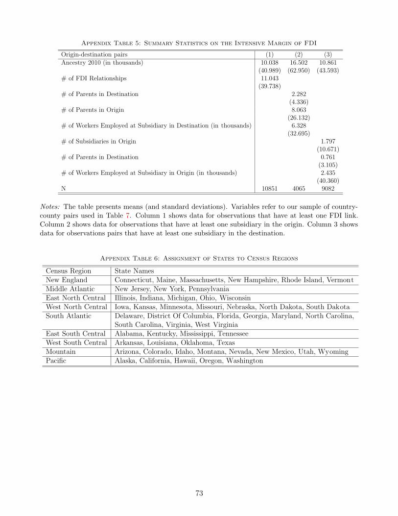
Appendix Table 5: Summary Statistics on the Intensive Margin of FDI

Origin-destination pairs (1) (2) (3)Ancestry 2010 (in thousands) 10.038 16.502 10.861

(40.989) (62.950) (43.593)# of FDI Relationships 11.043

(39.738)# of Parents in Destination 2.282

(4.336)# of Parents in Origin 8.063

(26.132)# of Workers Employed at Subsidiary in Destination (in thousands) 6.328

(32.695)# of Subsidiaries in Origin 1.797

(10.671)# of Parents in Destination 0.761

(3.105)# of Workers Employed at Subsidiary in Origin (in thousands) 2.435

(40.360)N 10851 4065 9082

Notes: The table presents means (and standard deviations). Variables refer to our sample of country-county pairs used in Table 7. Column 1 shows data for observations that have at least one FDI link.Column 2 shows data for observations that have at least one subsidiary in the origin. Column 3 showsdata for observations pairs that have at least one subsidiary in the destination.

Appendix Table 6: Assignment of States to Census Regions

Census Region State NamesNew England Connecticut, Maine, Massachusetts, New Hampshire, Rhode Island, VermontMiddle Atlantic New Jersey, New York, PennsylvaniaEast North Central Illinois, Indiana, Michigan, Ohio, WisconsinWest North Central Iowa, Kansas, Minnesota, Missouri, Nebraska, North Dakota, South DakotaSouth Atlantic Delaware, District Of Columbia, Florida, Georgia, Maryland, North Carolina,

South Carolina, Virginia, West VirginiaEast South Central Alabama, Kentucky, Mississippi, TennesseeWest South Central Arkansas, Louisiana, Oklahoma, TexasMountain Arizona, Colorado, Idaho, Montana, Nevada, New Mexico, Utah, WyomingPacific Alaska, California, Hawaii, Oregon, Washington

73

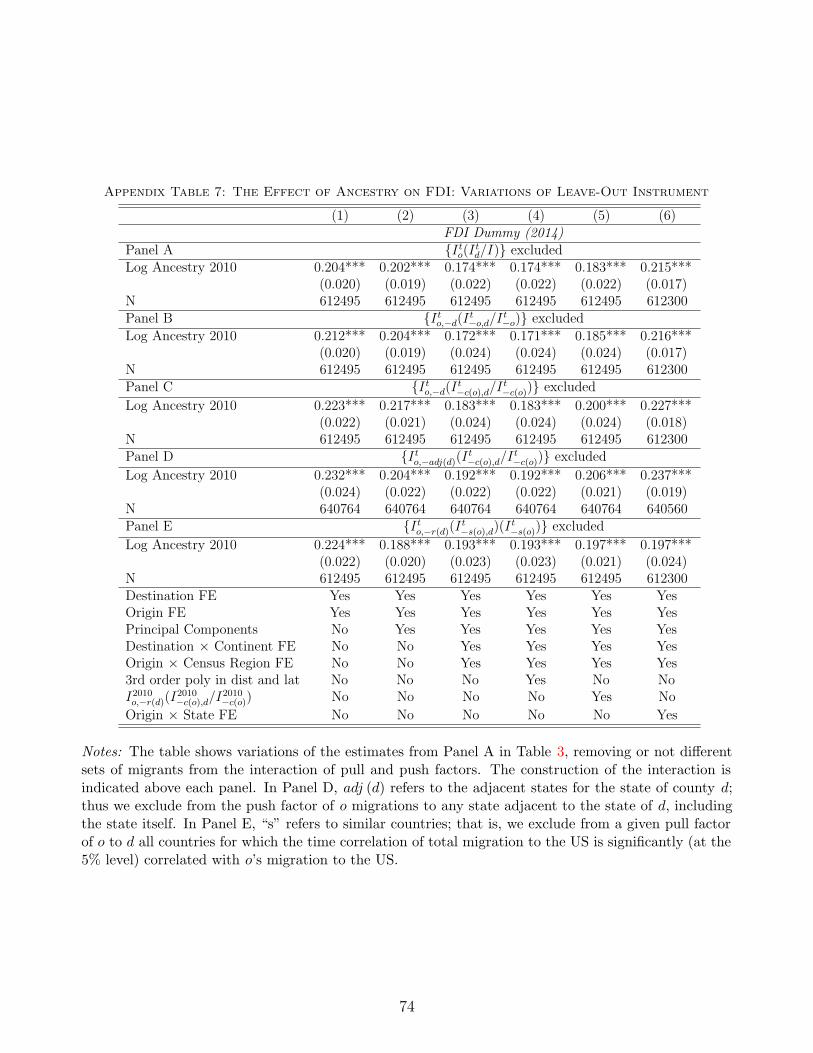
Appendix Table 7: The Effect of Ancestry on FDI: Variations of Leave-Out Instrument

(1) (2) (3) (4) (5) (6)FDI Dummy (2014)

Panel A {I to(I

td/I)} excluded

Log Ancestry 2010 0.204*** 0.202*** 0.174*** 0.174*** 0.183*** 0.215***(0.020) (0.019) (0.022) (0.022) (0.022) (0.017)

N 612495 612495 612495 612495 612495 612300Panel B {I t

o,−d(It−o,d/I

t−o)} excluded

Log Ancestry 2010 0.212*** 0.204*** 0.172*** 0.171*** 0.185*** 0.216***(0.020) (0.019) (0.024) (0.024) (0.024) (0.017)

N 612495 612495 612495 612495 612495 612300Panel C {I t

o,−d(It−c(o),d/I

t−c(o))} excluded

Log Ancestry 2010 0.223*** 0.217*** 0.183*** 0.183*** 0.200*** 0.227***(0.022) (0.021) (0.024) (0.024) (0.024) (0.018)

N 612495 612495 612495 612495 612495 612300Panel D {I t

o,−adj(d)(It−c(o),d/I

t−c(o))} excluded

Log Ancestry 2010 0.232*** 0.204*** 0.192*** 0.192*** 0.206*** 0.237***(0.024) (0.022) (0.022) (0.022) (0.021) (0.019)

N 640764 640764 640764 640764 640764 640560Panel E {I t

o,−r(d)(It−s(o),d)(I

t−s(o))} excluded

Log Ancestry 2010 0.224*** 0.188*** 0.193*** 0.193*** 0.197*** 0.197***(0.022) (0.020) (0.023) (0.023) (0.021) (0.024)

N 612495 612495 612495 612495 612495 612300Destination FE Yes Yes Yes Yes Yes YesOrigin FE Yes Yes Yes Yes Yes YesPrincipal Components No Yes Yes Yes Yes YesDestination × Continent FE No No Yes Yes Yes YesOrigin × Census Region FE No No Yes Yes Yes Yes3rd order poly in dist and lat No No No Yes No NoI2010o,−r(d)(I

2010−c(o),d/I

2010−c(o)) No No No No Yes No

Origin × State FE No No No No No Yes

Notes: The table shows variations of the estimates from Panel A in Table 3, removing or not differentsets of migrants from the interaction of pull and push factors. The construction of the interaction isindicated above each panel. In Panel D, adj (d) refers to the adjacent states for the state of county d;thus we exclude from the push factor of o migrations to any state adjacent to the state of d, includingthe state itself. In Panel E, “s” refers to similar countries; that is, we exclude from a given pull factorof o to d all countries for which the time correlation of total migration to the US is significantly (at the5% level) correlated with o’s migration to the US.

74

Appendix Table 8: The effect of Ancestry in 2000 on FDI in 2007

(1) (2) (3) (4) (5) (6)Panel A: IV FDI 2007 (Dummy)Log Ancestry 2000 0.250*** 0.184*** 0.182*** 0.182*** 0.188*** 0.184***

(0.018) (0.020) (0.020) (0.020) (0.019) (0.021)

KP F-stat on excluded IV’s 12.06 10.32 167.32 165.46 156.29 189.21Stock-Yogo 5% critical values 20.25 20.25 21.10 21.10 21.18 21.18Stock-Yogo 10% critical values 11.39 11.39 11.52 11.52 11.52 11.52N 612,495 612,495 612,495 612,495 612,495 612,300Panel B: OLS FDI 2007 (Dummy)Log Ancestry 2000 0.216*** 0.184*** 0.184*** 0.184*** 0.184*** 0.200***

(0.015) (0.018) (0.018) (0.018) (0.018) (0.019)

N 612,495 612,495 612,495 612,495 612,495 612,300Destination FE Yes Yes Yes Yes Yes YesOrigin FE Yes Yes Yes Yes Yes YesDestination × Continent FE No Yes Yes Yes Yes YesOrigin × Census Region FE No Yes Yes Yes Yes YesPrincipal Components No No Yes Yes Yes Yes3rd order poly in dist and lat No No No Yes No NoI2000o,−r(d)(I

2000−c(o),d/I

2000−c(o)) No No No No Yes No

Origin × State FE No No No No No Yes

Notes: The table presents coefficient estimates from IV (Panel A) and OLS (Panel B) regressions ofequation (1) at the country-county level. The dependent variable in all panels is a dummy indicatingan FDI relationship between origin o and destination d in 2007. The main variable of interest is LogAncestry 2000, instrumented using various specifications of equation (4). In all columns in Panel A,we include {It

o,−r(d)(It−c(o),d/It

−c(o))}t=1880,...,1990 as excluded instruments. Columns 3-6 also include thefirst five principal components of the higher-order interactions of push and pull factors as instruments.Column 5 also includes the interaction of the push and pull factor constructed using data from the1990-2010 wave. All specifications control for log distance, latitude difference, origin, and destinationfixed effects. Standard errors are given in parentheses. Standard errors are clustered at the origincountry level. *, **, and *** denote statistical significance at the 10%, 5%, and 1% levels, respectively.

75

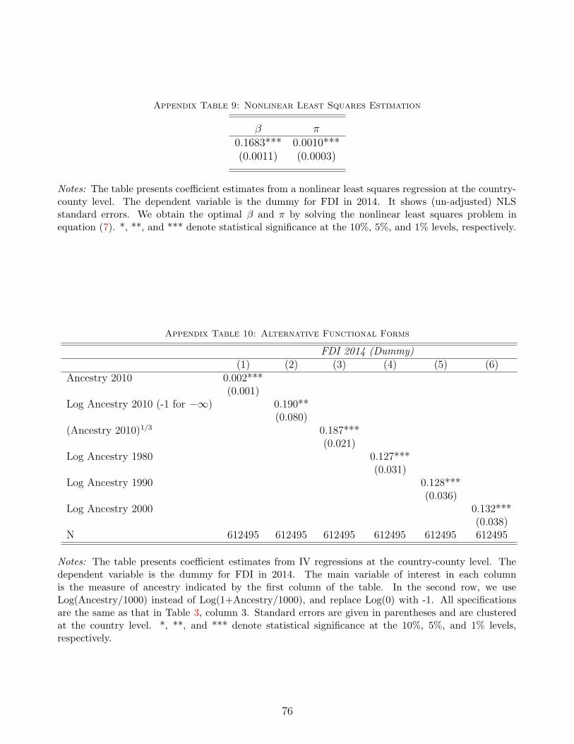
Appendix Table 9: Nonlinear Least Squares Estimation

β π0.1683*** 0.0010***(0.0011) (0.0003)

Notes: The table presents coefficient estimates from a nonlinear least squares regression at the country-county level. The dependent variable is the dummy for FDI in 2014. It shows (un-adjusted) NLSstandard errors. We obtain the optimal β and π by solving the nonlinear least squares problem inequation (7). *, **, and *** denote statistical significance at the 10%, 5%, and 1% levels, respectively.

Appendix Table 10: Alternative Functional Forms

FDI 2014 (Dummy)(1) (2) (3) (4) (5) (6)

Ancestry 2010 0.002***(0.001)

Log Ancestry 2010 (-1 for −∞) 0.190**(0.080)

(Ancestry 2010)1/3 0.187***(0.021)

Log Ancestry 1980 0.127***(0.031)

Log Ancestry 1990 0.128***(0.036)

Log Ancestry 2000 0.132***(0.038)

N 612495 612495 612495 612495 612495 612495

Notes: The table presents coefficient estimates from IV regressions at the country-county level. Thedependent variable is the dummy for FDI in 2014. The main variable of interest in each columnis the measure of ancestry indicated by the first column of the table. In the second row, we useLog(Ancestry/1000) instead of Log(1+Ancestry/1000), and replace Log(0) with -1. All specificationsare the same as that in Table 3, column 3. Standard errors are given in parentheses and are clusteredat the country level. *, **, and *** denote statistical significance at the 10%, 5%, and 1% levels,respectively.

76

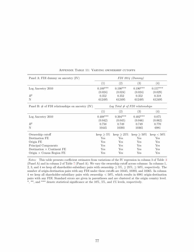
Appendix Table 11: Varying ownership cutoffs

Panel A: FDI dummy on ancestry (IV) FDI 2014 (Dummy)

(1) (2) (3) (4)

Log Ancestry 2010 0.189*** 0.190*** 0.190*** 0.157***(0.024) (0.024) (0.024) (0.029)

R2 0.352 0.352 0.352 0.318N 612495 612495 612495 612495

Panel B: # of FDI relationships on ancestry (IV) Log Total # of FDI relationships

(1) (2) (3) (4)

Log Ancestry 2010 0.408*** 0.394*** 0.402*** 0.075(0.042) (0.045) (0.046) (0.062)

R2 0.750 0.749 0.749 0.770N 10445 10393 10365 6981

Ownership cutoff keep ≥ 5% keep ≥ 25% keep ≥ 50% keep < 50%Destination FE Yes Yes Yes YesOrigin FE Yes Yes Yes YesPrincipal Components Yes Yes Yes YesDestination × Continent FE Yes Yes Yes YesOrigin × Census Region FE Yes Yes Yes Yes

Notes: This table presents coefficient estimates from variations of the IV regression in column 3 of Table 3(Panel A) and in column 2 of Table 7 (Panel A). We vary the ownership cutoff across columns: In columns 1,2, 3, and 4 we keep all shareholder-subsidiary pairs with ownership ≥ 5%, ≥ 25%, ≥ 50%, respectively. Thenumber of origin-destination pairs with any FDI under these cutoffs are 10445, 10393, and 10365. In column4 we keep all shareholder-subsidiary pairs with ownership < 50%, which results in 6981 origin-destinationpairs with any FDI. Standard errors are given in parentheses and are clustered at the origin country level.*, **, and *** denote statistical significance at the 10%, 5%, and 1% levels, respectively.

77

Appendix Table 12: Alternative Standard Errors: Main Specification

Panel A: Analytical

Robust 0.0092Cluster by county 0.0171Cluster by country† 0.0243Cluster by county and country 0.0280Cluster by state and country 0.0285Cluster by state 0.0189Cluster by continent 0.0070Cluster by state×country 0.0114

Panel B: Bootstrap

Robust 0.0092Cluster by county 0.0161Cluster by country 0.0291

Notes: This table shows various standarderrors on Log Ancestry 2010 based on ourstandard specification (column 3 of Table3). The bootstrapped standard errors inPanel B are obtained using 1,000 drawswith replacement. † denotes our standardspecification.

78

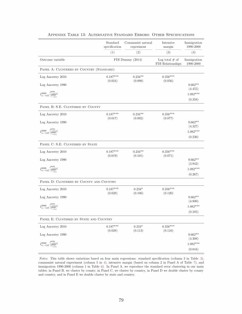
Appendix Table 13: Alternative Standard Errors: Other Specifications

Standard Communist natural Intensive Immigrationspecification experiment margin 1990-2000

(1) (2) (3) (4)

Outcome variable FDI Dummy (2014) Log total # of ImmigrationFDI Relationships 1990-2000

Panel A: Clustered by Country (Standard)

Log Ancestry 2010 0.187*** 0.234** 0.356***(0.024) (0.098) (0.056)

Log Ancestry 1990 9.662**(4.455)

I2000o,−r(d)

I2000−c(o),d

I2000−c(o)

1.082***

(0.358)

Panel B: S.E. Clustered by County

Log Ancestry 2010 0.187*** 0.234** 0.356***(0.017) (0.092) (0.077)

Log Ancestry 1990 9.662**(4.327)

I2000o,−r(d)

I2000−c(o),d

I2000−c(o)

1.082***

(0.230)

Panel C: S.E. Clustered by State

Log Ancestry 2010 0.187*** 0.234** 0.356***(0.019) (0.101) (0.071)

Log Ancestry 1990 9.662**(3.942)

I2000o,−r(d)

I2000−c(o),d

I2000−c(o)

1.082***

(0.267)

Panel D: Clustered by County and Country

Log Ancestry 2010 0.187*** 0.234* 0.356***(0.028) (0.106) (0.120)

Log Ancestry 1990 9.662**(4.800)

I2000o,−r(d)

I2000−c(o),d

I2000−c(o)

1.082***

(0.105)

Panel E: Clustered by State and Country

Log Ancestry 2010 0.187*** 0.234* 0.356***(0.028) (0.113) (0.116)

Log Ancestry 1990 9.662**(4.308)

I2000o,−r(d)

I2000−c(o),d

I2000−c(o)

1.082***

(0.044)

Notes: This table shows variations based on four main regressions: standard specification (column 3 in Table 3),communist natural experiment (column 5 in 4), intensive margin (based on column 2 in Panel A of Table 7), andimmigration 1990-2000 (column 1 in Table 6). In Panel A, we reproduce the standard error clustering in our maintables; in Panel B, we cluster by county; in Panel C, we cluster by country, in Panel D we double cluster by countyand country, and in Panel E we double cluster by state and country.

79

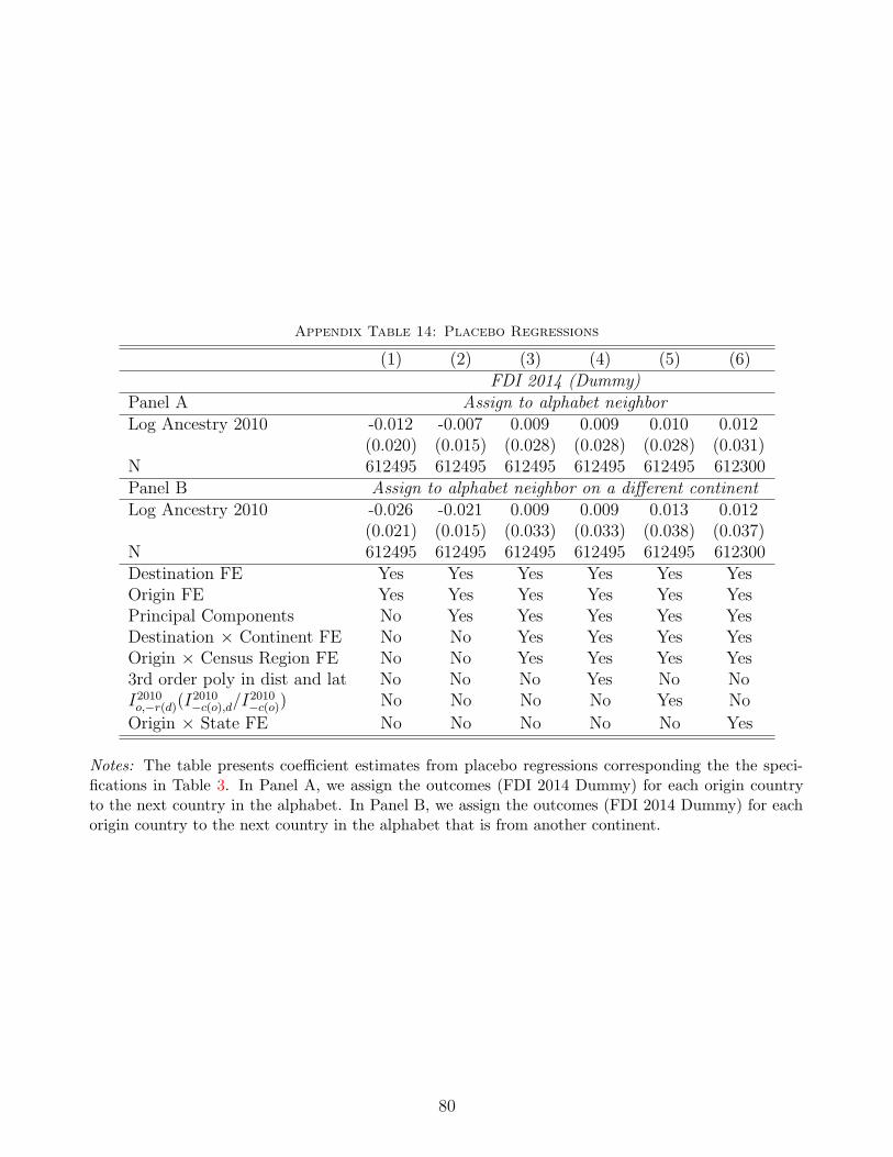
Appendix Table 14: Placebo Regressions

(1) (2) (3) (4) (5) (6)FDI 2014 (Dummy)

Panel A Assign to alphabet neighborLog Ancestry 2010 -0.012 -0.007 0.009 0.009 0.010 0.012

(0.020) (0.015) (0.028) (0.028) (0.028) (0.031)N 612495 612495 612495 612495 612495 612300Panel B Assign to alphabet neighbor on a different continentLog Ancestry 2010 -0.026 -0.021 0.009 0.009 0.013 0.012

(0.021) (0.015) (0.033) (0.033) (0.038) (0.037)N 612495 612495 612495 612495 612495 612300Destination FE Yes Yes Yes Yes Yes YesOrigin FE Yes Yes Yes Yes Yes YesPrincipal Components No Yes Yes Yes Yes YesDestination × Continent FE No No Yes Yes Yes YesOrigin × Census Region FE No No Yes Yes Yes Yes3rd order poly in dist and lat No No No Yes No NoI2010o,−r(d)(I

2010−c(o),d/I

2010−c(o)) No No No No Yes No

Origin × State FE No No No No No Yes

Notes: The table presents coefficient estimates from placebo regressions corresponding the the speci-fications in Table 3. In Panel A, we assign the outcomes (FDI 2014 Dummy) for each origin countryto the next country in the alphabet. In Panel B, we assign the outcomes (FDI 2014 Dummy) for eachorigin country to the next country in the alphabet that is from another continent.

80

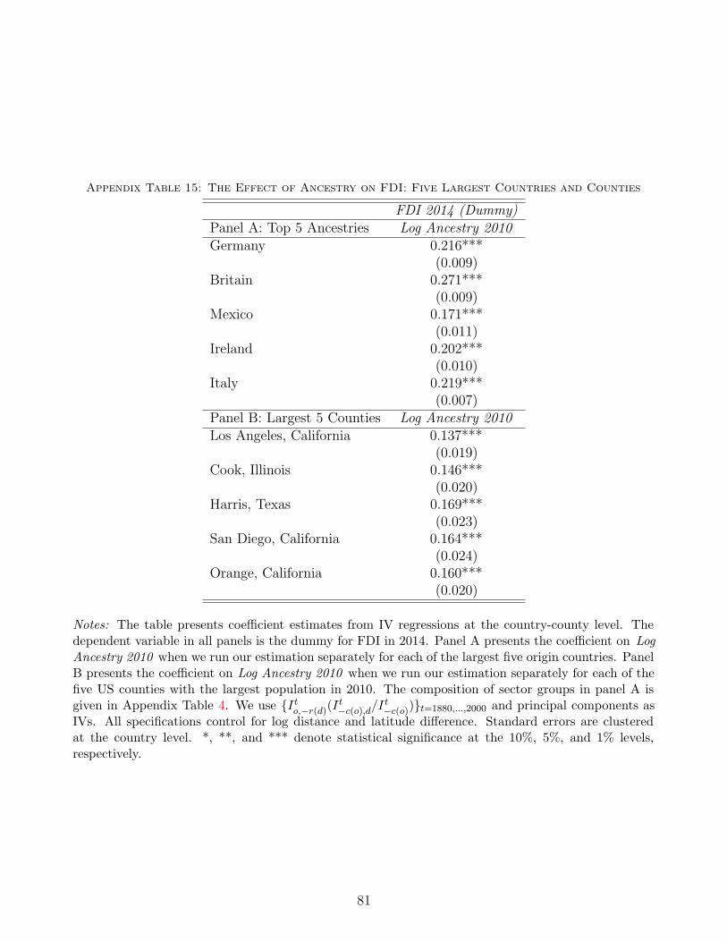
Appendix Table 15: The Effect of Ancestry on FDI: Five Largest Countries and Counties

FDI 2014 (Dummy)Panel A: Top 5 Ancestries Log Ancestry 2010Germany 0.216***

(0.009)Britain 0.271***

(0.009)Mexico 0.171***

(0.011)Ireland 0.202***

(0.010)Italy 0.219***

(0.007)Panel B: Largest 5 Counties Log Ancestry 2010Los Angeles, California 0.137***

(0.019)Cook, Illinois 0.146***

(0.020)Harris, Texas 0.169***

(0.023)San Diego, California 0.164***

(0.024)Orange, California 0.160***

(0.020)

Notes: The table presents coefficient estimates from IV regressions at the country-county level. Thedependent variable in all panels is the dummy for FDI in 2014. Panel A presents the coefficient on LogAncestry 2010 when we run our estimation separately for each of the largest five origin countries. PanelB presents the coefficient on Log Ancestry 2010 when we run our estimation separately for each of thefive US counties with the largest population in 2010. The composition of sector groups in panel A isgiven in Appendix Table 4. We use {It

o,−r(d)(It−c(o),d/It

−c(o))}t=1880,...,2000 and principal components asIVs. All specifications control for log distance and latitude difference. Standard errors are clusteredat the country level. *, **, and *** denote statistical significance at the 10%, 5%, and 1% levels,respectively.

81

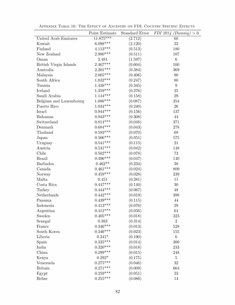
Appendix Table 16: The Effect of Ancestry on FDI: Country Specific Effects

Point Estimate Standard Error FDI 2014 (Dummy) > 0United Arab Emirates 11.875*** (2.712) 60Kuwait 6.098*** (2.120) 22Finland 4.113*** (0.513) 180New Zealand 2.980*** (0.511) 107Oman 2.481 (1.597) 6British Virgin Islands 2.467*** (0.604) 100Australia 2.201*** (0.384) 369Malaysia 2.005*** (0.406) 90South Africa 1.832*** (0.247) 80Tunisia 1.438*** (0.345) 9Iceland 1.359*** (0.276) 25Saudi Arabia 1.144*** (0.158) 29Belgium and Luxembourg 1.086*** (0.087) 354Puerto Rico 1.034*** (0.240) 26Israel 0.944*** (0.156) 137Bahamas 0.943*** (0.308) 44Switzerland 0.814*** (0.048) 371Denmark 0.684*** (0.043) 278Thailand 0.583*** (0.070) 68Japan 0.566*** (0.051) 575Uruguay 0.541*** (0.115) 21Austria 0.531*** (0.042) 148Chile 0.502*** (0.078) 73Brazil 0.496*** (0.047) 140Barbados 0.462** (0.234) 38Canada 0.461*** (0.024) 809Norway 0.459*** (0.028) 239Malta 0.451 (0.281) 11Costa Rica 0.447*** (0.140) 30Turkey 0.444*** (0.067) 48Netherlands 0.442*** (0.019) 398Panama 0.439*** (0.115) 44Indonesia 0.413*** (0.076) 29Argentina 0.412*** (0.056) 64Sweden 0.405*** (0.018) 323Senegal 0.383 (0.314) 2France 0.346*** (0.013) 528South Korea 0.346*** (0.023) 155Liberia 0.341* (0.190) 6Spain 0.335*** (0.014) 300India 0.320*** (0.018) 233China 0.299*** (0.015) 248Kenya 0.292* (0.175) 5Venezuela 0.275*** (0.046) 32Britain 0.271*** (0.009) 664Egypt 0.259*** (0.051) 23Belize 0.255*** (0.086) 14

82

Hungary 0.240*** (0.033) 52Colombia 0.237*** (0.028) 45Italy 0.219*** (0.007) 489Peru 0.218*** (0.033) 30Germany 0.216*** (0.009) 608Portugal 0.206*** (0.028) 85Samoa 0.204** (0.086) 5Ireland 0.202*** (0.010) 247Morocco 0.197** (0.078) 11Nigeria 0.190*** (0.055) 18Sri Lanka 0.180 (0.120) 6Czechoslovakia 0.177*** (0.029) 54Romania 0.173*** (0.041) 23Mexico 0.171*** (0.011) 259Pakistan 0.168*** (0.039) 23USSR 0.165*** (0.015) 97Ghana 0.156 (0.095) 6Bulgaria 0.156** (0.064) 11Philippines 0.154*** (0.019) 50Lebanon 0.150*** (0.047) 20Bolivia 0.142** (0.066) 8Greece 0.131*** (0.028) 42Trinidad and Tobago 0.130* (0.067) 15Socialist Yugoslav 0.121*** (0.028) 29Jamaica 0.114*** (0.032) 15Honduras 0.103*** (0.032) 14Algeria 0.099 (0.076) 3Guatemala 0.097*** (0.033) 14Poland 0.092*** (0.015) 63Viet Nam 0.091*** (0.025) 18Jordan 0.090 (0.063) 7Cameroon 0.085 (0.065) 2Dominican Republic 0.082*** (0.025) 16Ecuador 0.081** (0.032) 15Paraguay 0.079 (0.056) 4Nicaragua 0.069* (0.036) 7Albania 0.069 (0.046) 3North Korea 0.068 (0.072) 1El Salvador 0.066** (0.026) 13Sudan 0.065 (0.065) 1Fiji 0.065 (0.046) 5Bangladesh 0.040 (0.032) 2Cambodia 0.039 (0.028) 3Haiti 0.026 (0.019) 2Ethiopia 0.026 (0.025) 1Syria 0.016 (0.016) 1Myanmar 0.007 (0.007) 1Afghanistan 0.003 (0.003) 1Guyana 0.002 (0.002) 1

83

Iraq 0.002 (0.002) 1Cuba -0.000*** (0.000) 1Libya -0.022 (0.024) 1Nepal n/a n/a 0Grenada n/a n/a 0State of Palestine n/a n/a 0Sierra Leone n/a n/a 0Yemen n/a n/a 0Equatorial Guinea n/a n/a 0Somalia n/a n/a 0Greenland n/a n/a 0Cape Verde n/a n/a 0Mauritania n/a n/a 0Tonga n/a n/a 0Lao n/a n/a 0Mongolia n/a n/a 0Iran n/a n/a 0

Notes: The table is an extension of Table 15 Panel A, where we only show the results for top fiveancestries. Results are sorted on the point estimate. The last column shows the number of US countiesthat have an FDI link with the corresponding country. All countries with ancestry < 1 are discarded.

84

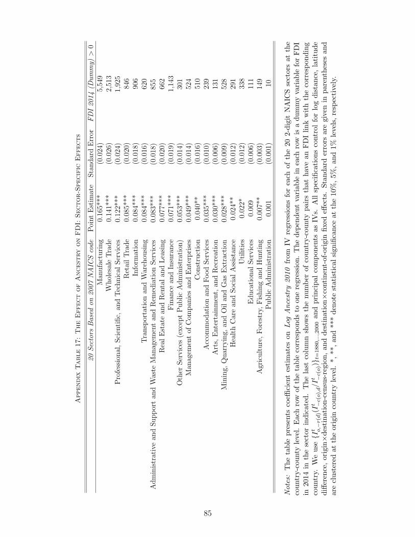
Appendix

Table

17:

The

Effect

of

Ancest

ry

on

FD

I:Sector-S

pecif

icEffects

20Sec

tors

Bas

edon

2007

NA

ICS

code

Poi

nt

Est

imat

eSta

ndar

dE

rror

FD

I20

14(D

um

my)

>0

Man

ufa

cturing

0.16

5***

(0.0

24)

5,54

9W

hol

esal

eTra

de

0.14

1***

(0.0

26)

2,51

3P

rofe

ssio

nal

,Sci

entific,

and

Tec

hnic

alSer

vic

es0.

122*

**(0

.024

)1,

925

Ret

ailTra

de

0.08

5***

(0.0

20)

846

Info

rmat

ion

0.08

4***

(0.0

18)

906

Tra

nsp

orta

tion

and

War

ehou

sing

0.08

4***

(0.0

16)

620

Adm

inis

trat

ive

and

Suppor

tan

dW

aste

Man

agem

ent

and

Rem

edia

tion

Ser

vic

es0.

083*

**(0

.018

)85

5R

ealE

stat

ean

dR

enta

lan

dLea

sing

0.07

7***

(0.0

20)

662

Fin

ance

and

Insu

rance

0.07

1***

(0.0

19)

1,14

3O

ther

Ser

vic

es(e

xce

pt

Public

Adm

inis

trat

ion)

0.05

3***

(0.0

14)

301

Man

agem

ent

ofC

ompan

ies

and

Ente

rprise

s0.

049*

**(0

.014

)52

4C

onst

ruct

ion

0.04

0**

(0.0

16)

510

Acc

omm

odat

ion

and

Food

Ser

vic

es0.

035*

**(0

.010

)23

9A

rts,

Ente

rtai

nm

ent,

and

Rec

reat

ion

0.03

0***

(0.0

06)

131

Min

ing,

Quar

ryin

g,an

dO

ilan

dG

asE

xtr

action

0.02

8***

(0.0

09)

528

Hea

lth

Car

ean

dSoci

alA

ssis

tance

0.02

4**

(0.0

12)

291

Utilities

0.02

2*(0

.012

)33

8E

duca

tion

alSer

vic

es0.

009

(0.0

06)

111

Agr

iculture

,For

estr

y,Fis

hin

gan

dH

unting

0.00

7**

(0.0

03)

149

Public

Adm

inis

trat

ion

0.00

1(0

.001

)10

Not

es:

The

tabl

epr

esen

tsco

effici

ent

estim

ates

onLog

Anc

estr

y20

10fr

omIV

regr

essi

ons

for

each

ofth

e20

2-di

git

NA

ICS

sect

ors

atth

eco

untr

y-co

unty

leve

l.E

ach

row

ofth

eta

ble

corr

espon

dsto

one

regr

essi

on.

The

depen

dent

vari

able

inea

chro

wis

adu

mm

yva

riab

lefo

rFD

Iin

2014

inth

ese

ctor

indi

cate

d.T

hela

stco

lum

nsh

ows

the

num

ber

ofco

untr

y-co

unty

pair

sth

atha

vean

FD

Ilin

kw

ith

the

corr

espon

ding

coun

try.

We

use{I

t o,−

r(d

)(I

t −c(

o),

d/I

t −c(

o))} t

=1880,...,2

000

and

prin

cipa

lco

mpon

ents

asIV

s.A

llsp

ecifi

cation

sco

ntro

lfo

rlo

gdi

stan

ce,

latitu

dedi

ffer

ence

,or

igin×

dest

inat

ion-

cens

us-r

egio

n,an

dde

stin

atio

n×

cont

inen

t-of

-ori

gin

fixed

effec

ts.

Stan

dard

erro

rsar

egi

ven

inpa

rent

hese

san

dar

ecl

uste

red

atth

eor

igin

coun

try

leve

l.*,

**,an

d**

*de

note

stat

istica

lsi

gnifi

canc

eat

the

10%

,5%

,an

d1%

leve

ls,re

spec

tive

ly.

85

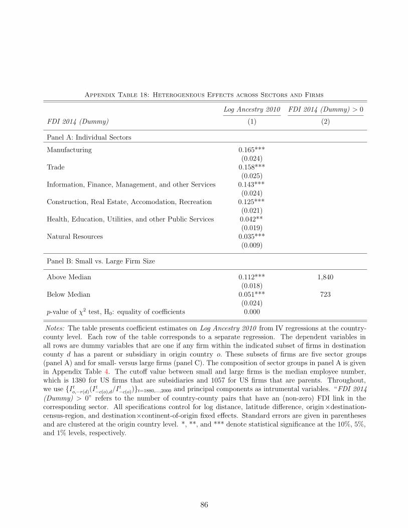
Appendix Table 18: Heterogeneous Effects across Sectors and Firms

Log Ancestry 2010 FDI 2014 (Dummy) > 0

FDI 2014 (Dummy) (1) (2)

Panel A: Individual Sectors

Manufacturing 0.165***(0.024)

Trade 0.158***(0.025)

Information, Finance, Management, and other Services 0.143***(0.024)

Construction, Real Estate, Accomodation, Recreation 0.125***(0.021)

Health, Education, Utilities, and other Public Services 0.042**(0.019)

Natural Resources 0.035***(0.009)

Panel B: Small vs. Large Firm Size

Above Median 0.112*** 1,840(0.018)

Below Median 0.051*** 723(0.024)

p-value of χ2 test, H0: equality of coefficients 0.000

Notes: The table presents coefficient estimates on Log Ancestry 2010 from IV regressions at the country-county level. Each row of the table corresponds to a separate regression. The dependent variables inall rows are dummy variables that are one if any firm within the indicated subset of firms in destinationcounty d has a parent or subsidiary in origin country o. These subsets of firms are five sector groups(panel A) and for small- versus large firms (panel C). The composition of sector groups in panel A is givenin Appendix Table 4. The cutoff value between small and large firms is the median employee number,which is 1380 for US firms that are subsidiaries and 1057 for US firms that are parents. Throughout,we use {I t

o,−r(d)(It−c(o),d/I

t−c(o))}t=1880,...,2000 and principal components as intrumental variables. “FDI 2014

(Dummy) > 0” refers to the number of country-county pairs that have an (non-zero) FDI link in thecorresponding sector. All specifications control for log distance, latitude difference, origin×destination-census-region, and destination×continent-of-origin fixed effects. Standard errors are given in parenthesesand are clustered at the origin country level. *, **, and *** denote statistical significance at the 10%, 5%,and 1% levels, respectively.

86

Appendix Table 19: The Effect of Ancestry on Language: Language Specific Effects

Point Estimate Standard Error N # of US-born in d thatspeak o at home in 2010

Aleut 1.608*** (0.028) 3,137 116Malay 1.376 (0.897) 9,411 176Arabic 1.222*** (0.171) 78,376 45,953Spanish 1.172*** (0.380) 65,877 65,877French 0.212*** (0.018) 87,836 87,416Haitian Creole 0.198*** (0.015) 3,137 595Greek 0.196*** (0.033) 6,273 1,849Vietnamese 0.188*** (0.006) 3,137 1,739Portuguese 0.174*** (0.030) 28,233 13,095Korean 0.170*** (0.041) 6,274 3,040Mon-Khmer 0.167*** (0.005) 3,136 316Urdu 0.159*** (0.020) 3,137 499Bengali 0.153*** (0.015) 3,137 191Japanese 0.142*** (0.007) 3,137 1,972Persian 0.102*** (0.005) 3,137 538Chinese 0.085*** (0.005) 3,137 1,745Thai 0.077*** (0.010) 3,137 619Polish 0.061*** (0.015) 3,137 1,670Filipino 0.059*** (0.002) 3,137 1,229Laotian 0.050*** (0.009) 3,137 592Albanian 0.049*** (0.014) 3,137 181Italian 0.041*** (0.005) 6,274 5,068Samoan 0.036 (0.031) 3,137 261Amharic 0.035** (0.015) 3,137 123Tongan 0.034 (0.027) 3,137 115Russian 0.027*** (0.008) 3,137 53German 0.022*** (0.002) 15,685 15,513Hindi 0.015*** (0.003) 3,137 558Rumanian 0.014** (0.007) 3,137 417Turkish 0.012** (0.005) 3,137 263Croatian 0.012** (0.006) 3,137 65Swahili 0.006 (0.005) 6,274 606Finnish 0.005 (0.012) 3,137 373Magyar 0.004** (0.002) 3,137 578Indonesian 0.002 (0.003) 3,137 130Swedish 0.002** (0.001) 3,137 888Dutch 0.002** (0.001) 9,411 4,746Norwegian 0.002** (0.001) 3,137 965Pashto 0.002 (0.002) 3,137 26Czech 0.001*** (0.000) 3,137 367Burmese 0.001 (0.001) 3,137 19Sinhalese 0.000 (0.001) 3,137 9Danish 0.000*** (0.000) 6,274 1,200Irish 0.000*** (0.000) 3,137 459Afrikaans -0.000*** (0.000) 3,137 6Nepali -0.000*** (0.000) 3,137 52

87

Bulgarian -0.000*** (0.000) 3,137 85Bantu n/a n/a 9,411 432Creole n/a n/a 3,136 2,252

Notes: The table is an extension of Table 10, where we only show the results for a set of selectedlanguages. The table is sorted on the size of the point estimate. The last column shows the # ofUS-born residents in d that speak the language of o at home.

Appendix Table 20: Accounting For the Effect of Ancestry

FDI Dummy (2014)

(1) (2) (3) (4) (5)

Log Ancestry 2010 0.222*** 0.213*** 0.212*** 0.213*** -0.025(0.021) (0.068) (0.068) (0.025) (0.028)

Sector Similarity (Rank Correlation) 0.012(0.020)

Sector Similarity (Cosine Correlation) 0.022(0.023)

Log # of residents in d that speak language of o at home 0.005(0.006)

Information Demand Index (standardized) 0.078***(0.013)

N 612,495 23,708 23,708 454,812 19,110

Destination FE Yes Yes Yes Yes YesOrigin FE Yes Yes Yes Yes YesPrincipal Components Yes Yes Yes Yes Yes

Notes: This table shows IV regressions at the county-country (columns 1-4) and DMA-country (column 5) level.Each column is a variation of the simple specification (column 2 in Table 3) that has origin and destination fixedeffects. All variables are defined as in the previous tables. The relatively low number of observations in columns2 and 3 is due to data availability in the industry share of employment: When calculating the correlation betweenindustries’ share of employment in county d and country o, the correlation coefficient is missing for those country-county pairs that have at least one missing share of employment. Standard errors are given in parentheses and areclustered at the origin country level. *, **, and *** denote statistical significance at the 10%, 5%, and 1% levels,respectively.

88

Appendix Table 21: Search terms for Germany and Italy

Germany Italy

Politicians

Angela Merkel Aldo MoroHelmut Kohl Benito MussoliniWilly Brandt Alessandra Mussolini

Joseph Goebbels Amintore FanfaniKarl Marx Angelino Alfano

Actors

Jurgen Prochnow Isabella RosselliniTil Schweiger Robert De Niro

Franka Potente John TurturroUdo Kier Roberto Rossellini

Daniel Bruhl Roberto Benigni

Athletes

Katarina Witt Mario AndrettiDirk Nowitzki Armin ZoggelerBoris Becker Roberto BaggioSteffi Graf Andrea Barzagli

Franz Beckenbauer Gerhard Plankensteiner

Musicians

Ludwig van Beethoven Antonio VivaldiNena Gioachino Rossini

Johann Sebastian Bach Giacomo PucciniNina Hagen Ennio Morricone

Felix Mendelssohn Luciano Pavarotti

This table shows the top five results from Google’sAnswer Box for each category for the countries Ger-many and Italy when typing “notable [country] [cat-egory]” into Google.

89