EE263 Prof. S. BoydOct. 27 – 28 or Oct. 28 – 29, 2006.

Midterm exam solutions

1. Point of closest convergence of a set of lines. We have m lines in Rn, described as

Li = {pi + tvi | t ∈ R}, i = 1, . . . , m,

where pi ∈ Rn, and vi ∈ Rn, with ‖vi‖ = 1, for i = 1, . . . , m. We define the distanceof a point z ∈ Rn to a line L as

dist(z,L) = min{‖z − u‖ | u ∈ L}.

(In other words, dist(z,L) gives the closest distance between the point z and the lineL.)

We seek a point z⋆ ∈ Rn that minimizes the sum of the squares of the distances to thelines,

m∑

i=1

dist(z,Li)2.

The point z⋆ that minimizes this quantity is called the point of closest convergence.

(a) Explain how to find the point of closest convergence, given the lines (i.e., givenp1, . . . , pm and v1, . . . , vm). If your method works provided some condition holds(such as some matrix being full rank), say so. If you can relate this condition toa simple one involving the lines, please do so.

(b) Find the point z⋆ of closest convergence for the lines with data given in the Matlabfile line_conv_data.m. This file contains n×m matrices P and V whose columnsare the vectors p1, . . . , pm, and v1, . . . , vm, respectively. The file also containscommands to plot the lines and the point of closest convergence (once you havefound it). Please include this plot with your solution.

Solution.

(a) There are several ways to solve this problem. Our first solution starts by workingout an explicit expression for dist(z,Li). To find this distance we need to solvethe simple least-squares problem of minimizing ‖z − pi − tvi‖2 over t ∈ R. Theoptimal t is given by t⋆ = vT

i (z − pi), so we have

dist(z,Li) = ‖z − pi − t⋆vi‖ = ‖(I − vivTi )(z − pi)‖.

1

This makes sense: we recognize I − vivTi as projection onto the orthogonal com-

plement of the line through the origin in the direction vi, i.e., projection onto theplane with normal vector vi.

We can now set up our problem as a standard least-squares problem. We define

A =

I − v1vT1

...I − vmvT

m

, b =

(I − v1vT1 )p1

...(I − vmvT

m)pm

,

so we can writem∑

i=1

dist(z,Li)2 = ‖Az − b‖2.

Now we can solve the problem, assuming A is full rank (we’ll come back to this).The solution is

z⋆ = (AT A)−1AT b =

(

mI −m∑

i=1

vivTi

)−1 m∑

i=1

(pi − vivTi pi).

Finally, let’s look at the conditions under which A is not full rank. Each n × nblock of A, i.e., I − viv

Ti , has rank exactly n − 1, with nullspace span(vi). So

unless all the vi are aligned (i.e., vi = vj or vi = −vj for all i, j), A is full rank.Geometrically, this means that the lines are all parallel. So we can say that Aabove is full rank, unless all the lines are parallel.

Here is another solution of the problem (or really, a variation on the solution givenabove). If we define

C =

−v1 0 · · · 0 I0 −v2 · · · 0 I...

.... . .

... I0 0 · · · −vm I

, d =

p1...

pm

, u =

t1...

tmz

,

we havem∑

i=1

dist(z,Li)2 = min

t1,...,tm‖Cu − d‖,

and

minz

m∑

i=1

dist(z,Li)2 = min

u‖Cu − d‖.

In the last expression, we are optimizing over the line parameters ti and the pointz at the same time.

Therefore, assuming C is full rank, we have

z⋆ =

[

0 00 I

]

(CTC)−1CT d,

which expands to the same solution we have above. And of course, C is full rankif and only if A is, which occurs exactly when the lines are not all parallel.

2

(b) The following code solves for the point of closest convergence using the two dif-ferent approaches and checks that the solutions are identical.

% first solution

A=[];

b=[];

for i=1:m

A=[A;eye(n)-V(:,i)*V(:,i)’];

b=[b;(eye(n)-V(:,i)*V(:,i)’)*P(:,i)];

end

zstar=A\b;

% second solution

C=zeros(n*m,m);

E=[];

d=[];

for i=1:m

E=[E;eye(n)];

C(n*(i-1)+1:n*i,i)=-V(:,i);

d=[d;P(:,i)];

end

C=[C E];

zstar=A\b;

f=C\d;

zstar2=f(m+1:m+n);

% check that two solutions give (almost) same answer

zstar2-zstar

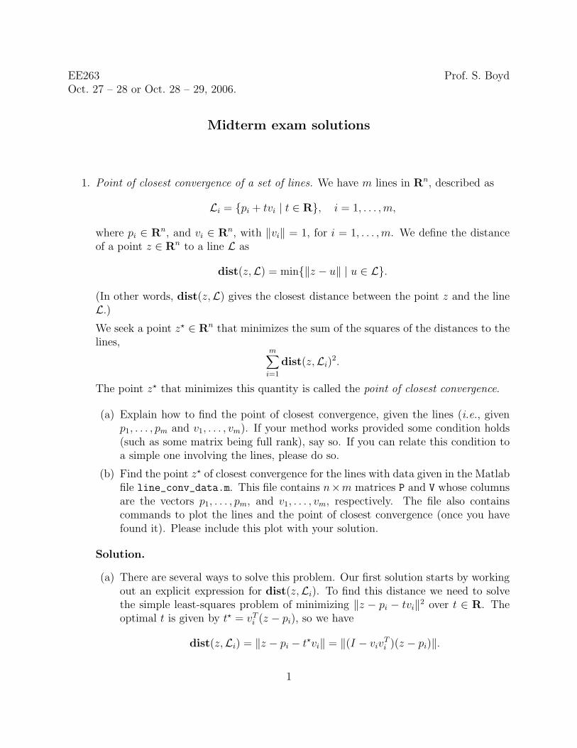
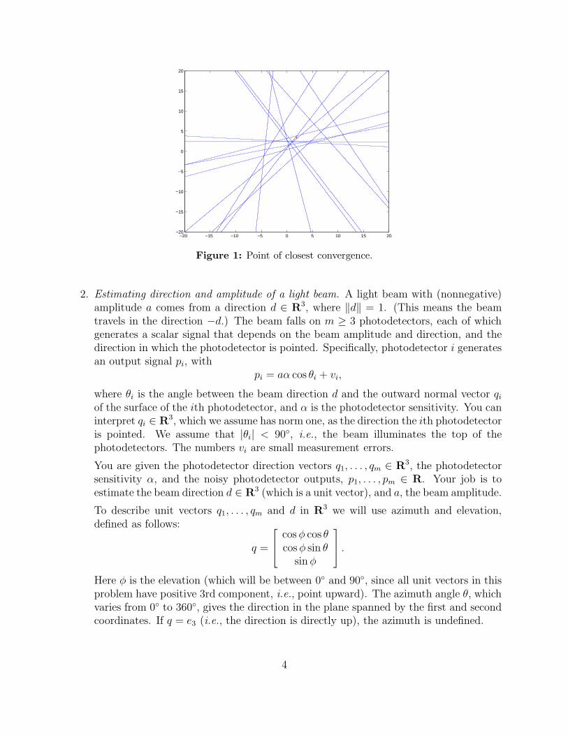
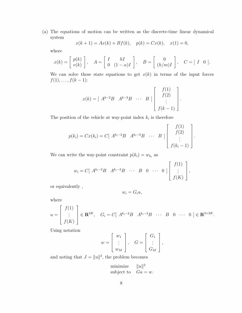
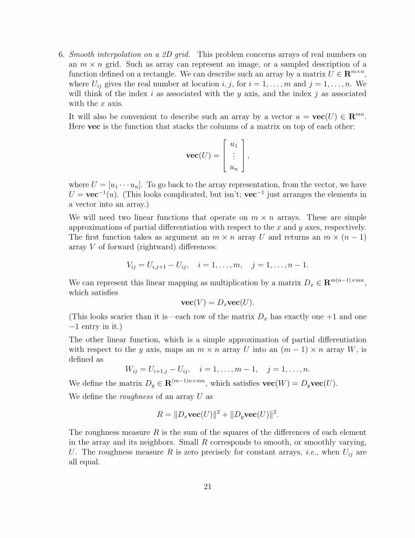
The result is z⋆ = (1.9157, 3.3951) and figure 1 shows the lines together with thepoint of closest convergence.

3

−20 −15 −10 −5 0 5 10 15 20−20

−15

−10

−5

0

5

10

15

20

Figure 1: Point of closest convergence.

2. Estimating direction and amplitude of a light beam. A light beam with (nonnegative)amplitude a comes from a direction d ∈ R3, where ‖d‖ = 1. (This means the beamtravels in the direction −d.) The beam falls on m ≥ 3 photodetectors, each of whichgenerates a scalar signal that depends on the beam amplitude and direction, and thedirection in which the photodetector is pointed. Specifically, photodetector i generatesan output signal pi, with

pi = aα cos θi + vi,

where θi is the angle between the beam direction d and the outward normal vector qi

of the surface of the ith photodetector, and α is the photodetector sensitivity. You caninterpret qi ∈ R3, which we assume has norm one, as the direction the ith photodetectoris pointed. We assume that |θi| < 90◦, i.e., the beam illuminates the top of thephotodetectors. The numbers vi are small measurement errors.

You are given the photodetector direction vectors q1, . . . , qm ∈ R3, the photodetectorsensitivity α, and the noisy photodetector outputs, p1, . . . , pm ∈ R. Your job is toestimate the beam direction d ∈ R3 (which is a unit vector), and a, the beam amplitude.

To describe unit vectors q1, . . . , qm and d in R3 we will use azimuth and elevation,defined as follows:

q =

cos φ cos θcos φ sin θ

sin φ

.

Here φ is the elevation (which will be between 0◦ and 90◦, since all unit vectors in thisproblem have positive 3rd component, i.e., point upward). The azimuth angle θ, whichvaries from 0◦ to 360◦, gives the direction in the plane spanned by the first and secondcoordinates. If q = e3 (i.e., the direction is directly up), the azimuth is undefined.

4

(a) Explain how to do this, using a method or methods from this class. The simplerthe method the better. If some matrix (or matrices) needs to be full rank for yourmethod to work, say so.

(b) Carry out your method on the data given in beam_estim_data.m. This mfiledefines p, the vector of photodetector outputs, a vector det_az, which gives theazimuth angles of the photodetector directions, and a vector det_el, which givesthe elevation angles of the photodetector directions. Note that both of these aregiven in degrees, not radians. Give your final estimate of the beam amplitude aand beam direction d (in azimuth and elevation, in degrees).

Solution.

(a) Since cos θi = qTi d/(‖qi‖‖d‖) = qT

i d (using ‖qi‖ = ‖d‖ = 1), we have

pi = aαqTi d + vi.

In this equation we are given pi, α, and qi; we are to estimate a ∈ R and d ∈ R3,using the given information that vi is small. At first glance it looks like a nonlinearproblem, since two of the variables we need to estimate, a and d, are multipliedtogether in this formula.

But a little thought reveals that things are actually much simpler. Let’s definex ∈ R3 as x = ad. We can just as well work with x since given any nonzerox ∈ R3, we have a = ‖x‖ and d = x/‖x‖. (Conversely, given any a and d, wehave x = ad by definition.)

We can therefore express the problem in terms of the variable x as

p = α

qT1...

qTm

x + v = αQx + v,

where p = (p1, . . . , pm), v = (v1, . . . , vm), and Q is the matrix with rows qTi .

Now we can get a reasonable guess of x using least-squares. Assuming Q is fullrank, we have the least-squares estimate

x = (1/α)(QT Q)−1QT p.

We then form estimates of a and d using a = ‖x‖, d = x/‖x‖.

The matrix Q is full rank (i.e., rank 3), if and only if the vectors {q1, . . . , qm}span R3. In other words, we cannot have all photodetectors pointing in a commonplane.

(b) The following code solves the problem for the given data.

5

beam_estim_data

for i=1:m

Q(i,:)=[ cosd(det_el(i))*cosd(det_az(i)),...

cosd(det_el(i))*sind(det_az(i)),...

sind(det_el(i)) ];

end

xhat=(1/alpha)*(Q\p);

ahat=norm(xhat);

dhat=xhat/norm(xhat);

elevation=asind(dhat(3))

azimuth=acosd(dhat(1)/cosd(elevation))

The result is a = 5.0107, φd = 38.7174, and θd = 77.6623.

6

3. Minimum energy input with way-point constraints. We consider a vehicle that movesin R2 due to an applied force input. We will use a discrete-time model, with timeindex k = 1, 2, . . .; time index k corresponds to time t = kh, where h > 0 is the sampleinterval. The position at time index k is denoted by p(k) ∈ R2, and the velocity byv(k) ∈ R2, for k = 1, . . . , K + 1. These are related by the equations

p(k + 1) = p(k) + hv(k), v(k + 1) = (1 − α)v(k) + (h/m)f(k), k = 1, . . . , K,

where f(k) ∈ R2 is the force applied to the vehicle at time index k, m > 0 is the vehiclemass, and α ∈ (0, 1) models drag on the vehicle: In the absence of any other force, thevehicle velocity decreases by the factor 1 − α in each time index. (These formulas areapproximations of more accurate formulas that we will see soon, but for the purposesof this problem, we consider them exact.) The vehicle starts at the origin, at rest, i.e.,we have p(1) = 0, v(1) = 0. (We take k = 1 as the initial time, to simplify indexing.)

The problem is to find forces f(1), . . . , f(K) ∈ R2 that minimize the cost function

J =K∑

k=1

‖f(k)‖2,

subject to way-point constraints

p(ki) = wi, i = 1, . . . , M,

where ki are integers between 1 and K. (These state that at the time ti = hki, thevehicle must pass through the location wi ∈ R2.) Note that there is no requirementon the vehicle velocity at the way-points.

(a) Explain how to solve this problem, given all the problem data (i.e., h, α, m, K,the way-points w1, . . . , wM , and the way-point indices k1, . . . , kM).

(b) Carry out your method on the specific problem instance with data h = 0.1, m = 1,α = 0.1, K = 100, and the M = 4 way-points

w1 =

[

22

]

, w2 =

[

−23

]

, w3 =

[

4−3

]

, w4 =

[

−4−2

]

,

with way-point indices k1 = 10, k2 = 30, k3 = 40, and k4 = 80.

Give the optimal value of J .

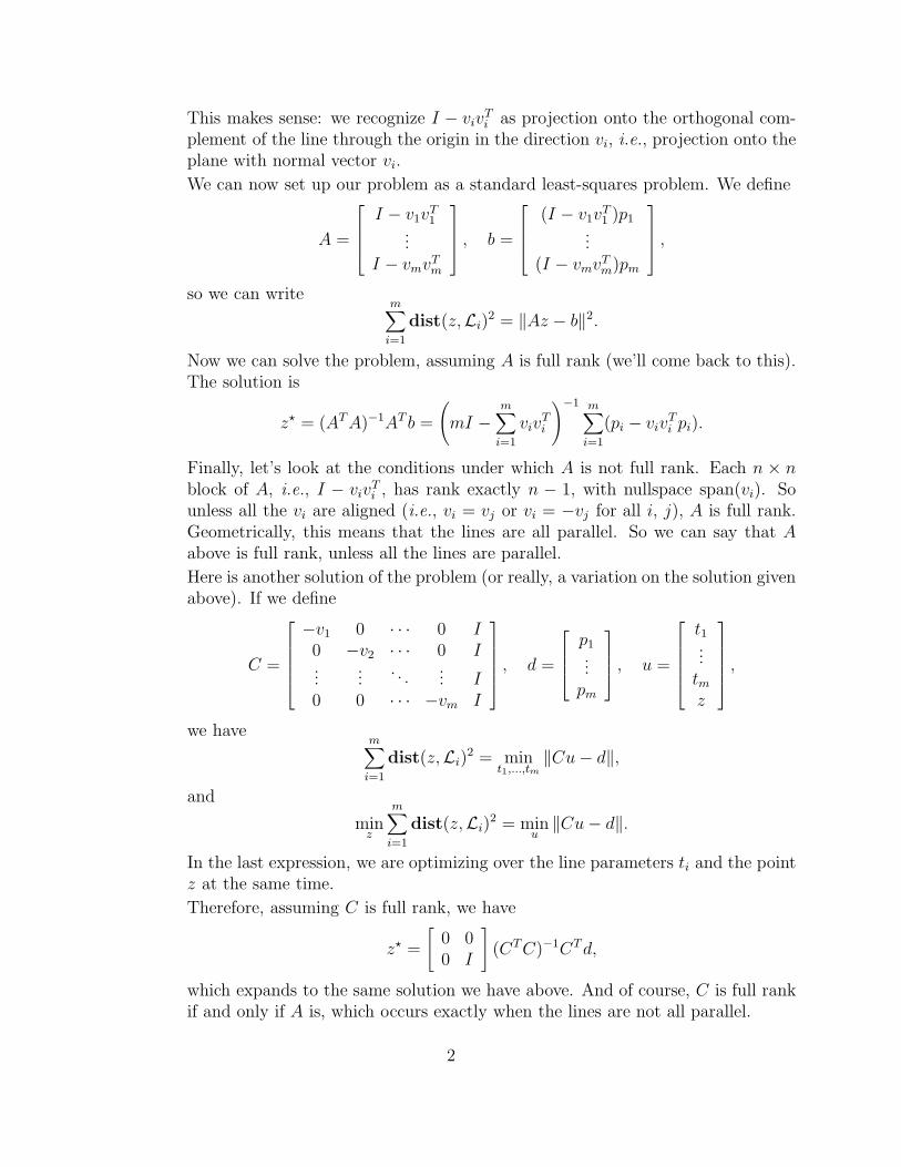
Plot f1(k) and f2(k) versus k, using

subplot(211); plot(f(1,:));

subplot(212); plot(f(2,:));

We assume here that f is a 2 × K matrix, with columns f(1), . . . , f(K).

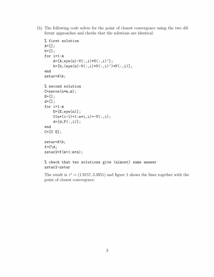
Plot the vehicle trajectory, using plot(p(1,:),p(2,:)). Here p is a 2× (K + 1)matrix with columns p(1), . . . , p(K + 1).

7

(a) The equations of motion can be written as the discrete-time linear dynamicalsystem

x(k + 1) = Ax(k) + Bf(k), p(k) = Cx(k), x(1) = 0,

where

x(k) =

[

p(k)v(k)

]

, A =

[

I hI0 (1 − α)I

]

, B =

[

0(h/m)I

]

, C = [ I 0 ].

We can solve these state equations to get x(k) in terms of the input forcesf(1), . . . , f(k − 1):

x(k) = [ Ak−2B Ak−3B · · · B ]

f(1)f(2)

...f(k − 1)

.

The position of the vehicle at way-point index ki is therefore

p(ki) = Cx(ki) = C[ Aki−2B Aki−3B · · · B ]

f(1)f(2)

...f(ki − 1)

.

We can write the way-point constraint p(ki) = wkias

wi = C[ Aki−2B Aki−3B · · · B 0 · · · 0 ]

f(1)...

f(K)

,

or equivalently ,wi = Giu,

where

u =

f(1)...

f(K)

∈ R2K , Gi = C[ Aki−2B Aki−3B · · · B 0 · · · 0 ] ∈ R2×2K .

Using notation

w =

w1...

wM

, G =

G1...

GM

,

and noting that J = ‖u‖2, the problem becomes

minimize ‖u‖2

subject to Gu = w.

8

This is just a least-norm problem and the optimal u is given by

u = G†w = GT (GGT )−1w.

(b) The following Matlab script computes the minimum norm input, and plots it andthe associated trajectory.

% problem parameters

h = .1;

m = 1;

M=4;

alpha=0.1;

K = 100;

% way-points

k1=10; w1=[ 2; 2];

k2=30; w2=[ -2; 3];

k3=40; w3=[ 4; -3];

k4=80; w4=[-4; -2];

A = [eye(2) h*eye(2); zeros(2) (1-alpha)*eye(2)];

B = [zeros(2); h/m*eye(2)];

C = [eye(2) zeros(2)];

[n, nn] = size(B);

k = [k1 k2 k3 k4];

G = [];

for i = 1:M

ABmatrix = [];

temp = B;

for j=1:k(i)-1

ABmatrix = [temp ABmatrix];

temp = A*temp;

end

Gi = C*[ABmatrix zeros(n, nn*(K-k(i)+1))];

G = [G; Gi];

end

w = [w1; w2; w3; w4];

u = pinv(G)*w;

% plotting the input

f = [u(1:2:end)’; u(2:2:end)’];

figure;

subplot(211); plot(f(1,:));

subplot(212); plot(f(2,:));

9

0 10 20 30 40 50 60 70 80 90 100−10

−5

0

5

10

15

20

0 10 20 30 40 50 60 70 80 90 100−15

−10

−5

0

5

10

k

k

f 1f 2

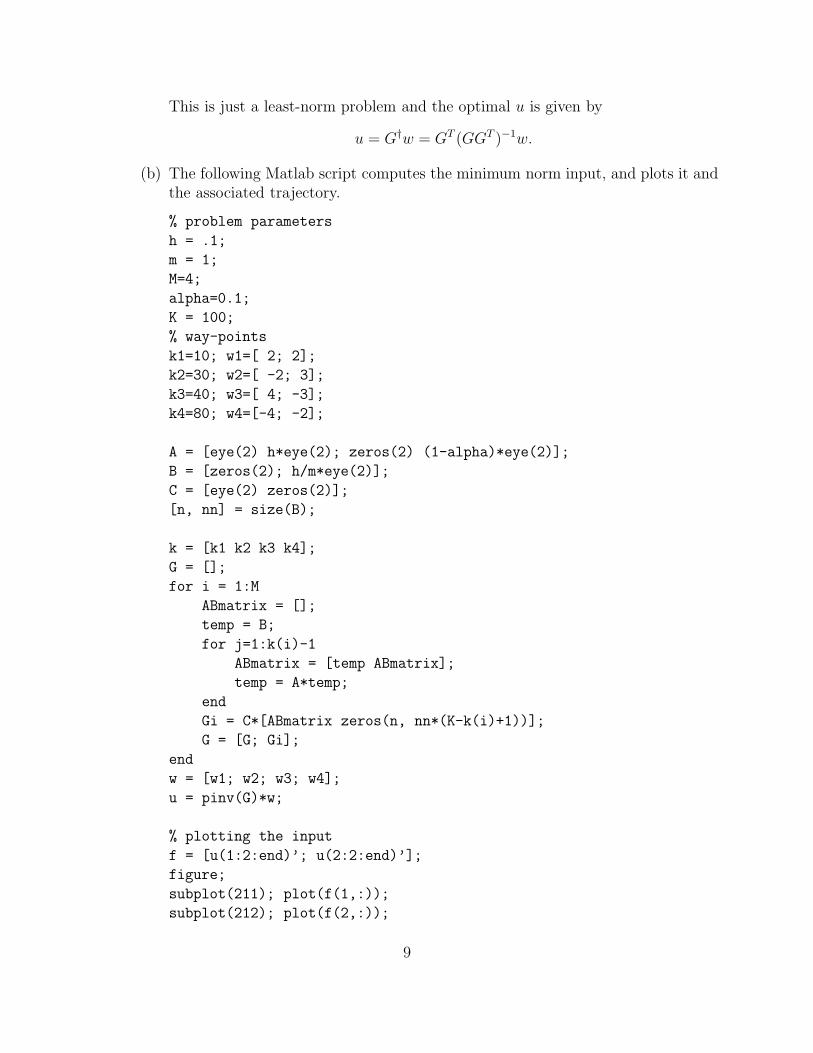
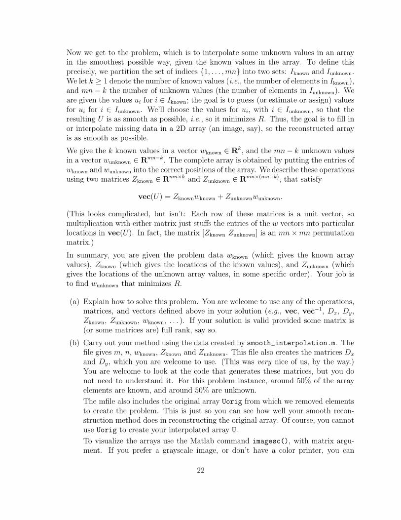
Figure 2: f versus k.

% simulating the system

p = zeros(2,K+1);

v = zeros(2,K+1);

for i=1:K

p(:,i+1) = p(:,i) + h*v(:,i);

v(:,i+1) = (1-alpha)*v(:,i) + h*f(:,i)/m;

end

% Optimal value of J

J = norm(u)^2

figure;

plot(p(1,:),p(2,:));

hold on

ps = [w1 w2 w3 w4];

plot(ps(1,:),ps(2,:),’*’);

Figure (2) shows the minimum norm input forces. We see that for k ≥ 80, theoptimal force is zero. This makes perfect sense: for k ≥ 80, the force f(k) doesnot affect the vehicle position at any of the way-points, so using any force on thevehicle for k ≥ 80 just increases the cost J .

10

−6 −4 −2 0 2 4 6−6

−4

−2

0

2

4

6

x

y

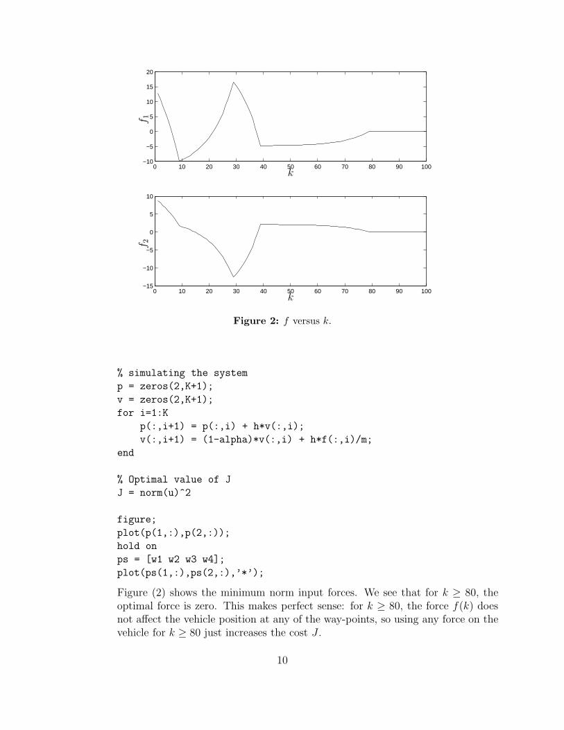
Figure 3: Trajectory in R2.

The optimal value of J is found to be 4770.5.

Figure (3) shows the resulting trajectory.

11

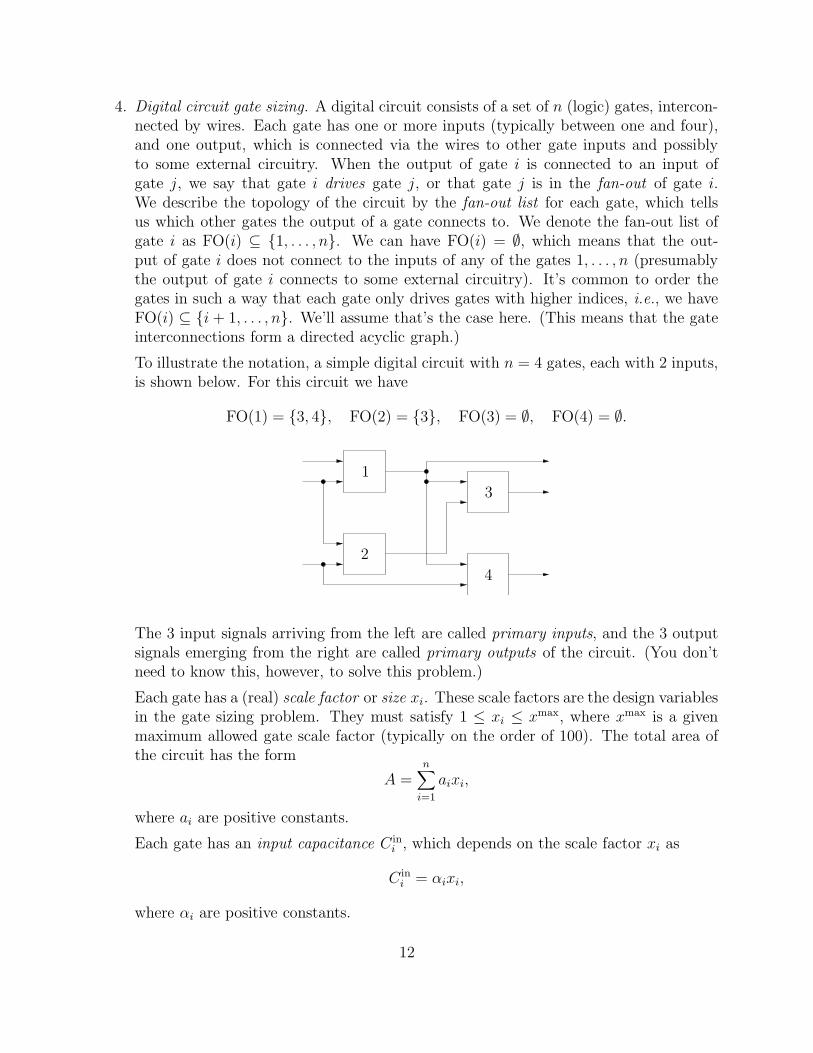
4. Digital circuit gate sizing. A digital circuit consists of a set of n (logic) gates, intercon-nected by wires. Each gate has one or more inputs (typically between one and four),and one output, which is connected via the wires to other gate inputs and possiblyto some external circuitry. When the output of gate i is connected to an input ofgate j, we say that gate i drives gate j, or that gate j is in the fan-out of gate i.We describe the topology of the circuit by the fan-out list for each gate, which tellsus which other gates the output of a gate connects to. We denote the fan-out list ofgate i as FO(i) ⊆ {1, . . . , n}. We can have FO(i) = ∅, which means that the out-put of gate i does not connect to the inputs of any of the gates 1, . . . , n (presumablythe output of gate i connects to some external circuitry). It’s common to order thegates in such a way that each gate only drives gates with higher indices, i.e., we haveFO(i) ⊆ {i + 1, . . . , n}. We’ll assume that’s the case here. (This means that the gateinterconnections form a directed acyclic graph.)

To illustrate the notation, a simple digital circuit with n = 4 gates, each with 2 inputs,is shown below. For this circuit we have

FO(1) = {3, 4}, FO(2) = {3}, FO(3) = ∅, FO(4) = ∅.

1

2

3

4

The 3 input signals arriving from the left are called primary inputs, and the 3 outputsignals emerging from the right are called primary outputs of the circuit. (You don’tneed to know this, however, to solve this problem.)

Each gate has a (real) scale factor or size xi. These scale factors are the design variablesin the gate sizing problem. They must satisfy 1 ≤ xi ≤ xmax, where xmax is a givenmaximum allowed gate scale factor (typically on the order of 100). The total area ofthe circuit has the form

A =n∑

i=1

aixi,

where ai are positive constants.

Each gate has an input capacitance C ini , which depends on the scale factor xi as

C ini = αixi,

where αi are positive constants.

12

Each gate has a delay di, which is given by

di = βi + γiCloadi /xi,

where βi and γi are positive constants, and C loadi is the load capacitance of gate i.

Note that the gate delay di is always larger than βi, which can be intepreted as theminimum possible delay of gate i, achieved only in the limit as the gate scale factorbecomes large.

The load capacitance of gate i is given by

C loadi = Cext

i +∑

j∈FO(i)

C inj ,

where Cexti is a positive constant that accounts for the capacitance of the interconnect

wires and external circuitry.

We will follow a simple design method, which assigns an equal delay T to all gates inthe circuit, i.e., we have di = T , where T > 0 is given. For a given value of T , theremay or may not exist a feasible design (i.e., a choice of the xi, with 1 ≤ xi ≤ xmax)that yields di = T for i = 1, . . . , n. We can assume, of course, that T > maxi βi, i.e.,T is larger than the largest minimum delay of the gates.

Finally, we get to the problem.

(a) Explain how to find a design x⋆ ∈ Rn that minimizes T , subject to a given areaconstraint A ≤ Amax. You can assume the fanout lists, and all constants in theproblem description are known; your job is to find the scale factors xi. Be sure toexplain how you determine if the design problem is feasible, i.e., whether or notthere is an x that gives di = T , with 1 ≤ xi ≤ xmax, and A ≤ Amax.

Your method can involve any of the methods or concepts we have seen so farin the course. It can also involve a simple search procedure, e.g., trying (many)different values of T over a range.

Note: this problem concerns the general case, and not the simple example shownabove.

(b) Carry out your method on the particular circuit with data given in the filegate_sizing_data.m. The fan-out lists are given as an n × n matrix F, withi, j entry one if j ∈ FO(i), and zero otherwise. In other words, the ith row of Fgives the fanout of gate i. The jth entry in the ith row is 1 if gate j is in thefan-out of gate i, and 0 otherwise.

Comments and hints.

• You do not need to know anything about digital circuits; everything you need toknow is stated above.

• Yes, this problem does belong on the EE263 midterm.

13

Solution.

(a) We define the fanout matrix F as Fij = 1, if j ∈ FO(i), and Fij = 0 otherwise.The matrix F is strictly upper triangular, since FO(i) ⊆ {i + 1, . . . , n}.

Using the formulas given above, and di = T , we have

T = di

= βi + γi

C loadi

xi

= βi + γi

Cexti +

∑

j∈FO(i) C inj

xi

= βi + γi

Cexti +

∑

j∈FO(i) αjxj

xi

.

Multiplying by xi we get the equivalent equations

Txi = βixi + γi

Cexti +

∑

j∈FO(i)

αjxj

,

which we can express in matrix form as

Tx = diag(β)x + diag(γ)Cext + diag(γ)F diag(α)x.

DefiningK = diag(β) + diag(γ)F diag(α),

we can write the equations as

(TI − K)x = diag(γ)Cext,

a set of n linear equations in n unknowns. So this problem really does belong inEE263, after all.

For choices of T for which TI − K is nonsingular, there is only one solution ofthis set of linear equations,

x = (TI − K)−1 diag(γ)Cext.

If this x happens to satisfy 1 ≤ xi ≤ xmax, and A = aT x ≤ Amax, then it is afeasible design. Our job, then, is to find the smallest T for which this occurs. Ifit occurs for no T , then the problem is infeasible.

Let’s analyze the issue of singularity of TI−K. The matrix K is upper triangular,with diagonal elements βi. So TI−K is upper triangular, with diagonal elementsT − βi. But these are all positive, by our assumption. So the matrix TI − K isnonsingular.

14

Thus, for each value of T (larger than maxi βi) there is exactly one possiblechoice of gate sizes. Among the ones that are feasible, we have to choose the onecorresponding to the smallest value of T .

We can solve this problem by examing a reasonable range of values of T , andfor each value, finding x. We check whether x is feasible, by looking at mini xi,maxi xi, and A. We take our final design as the one which is feasible, and hassmallest value of T . Alternatively, we can start with a value of T just a little bitlarger than maxi βi, then increase T until we find our first feasible x, which wetake as our solution.

(b) The following code generatea x for a range of value of T , and plots mini xi, maxi xi,and A, versus T .

gate_sizing_data

deltaT=0.001;

Trange=max(beta)+deltaT:deltaT:6;

i=1;

for T=Trange

K=diag(beta)+diag(gamma)*F*diag(alpha);

x=(T*eye(n)-K)\diag(gamma)*Cext;

maxX(i)=max(x);

minX(i)=min(x);

Area(i)=a’*x;

i=i+1;

end

res=Area<=Amax & minX>=1 & (maxX<=xmax);

index=find(res);

T=Trange(index(1))

subplot(3,1,1)

plot(Trange,minX)

ylabel(’minx’)

axis([2 6 0 4])

line([2,6],[1,1],’Color’,’r’)

grid on

subplot(3,1,2)

plot(Trange,maxX)

ylabel(’maxx’)

axis([2 6 0 150])

line([2,6],[100,100],’Color’,’r’)

grid on

subplot(3,1,3)

15

2 2.5 3 3.5 4 4.5 5 5.5 60

1

2

3

4

2 2.5 3 3.5 4 4.5 5 5.5 60

50

100

150

2 2.5 3 3.5 4 4.5 5 5.5 60

100

200

300

400

500

T

max

ix

im

inix

iA

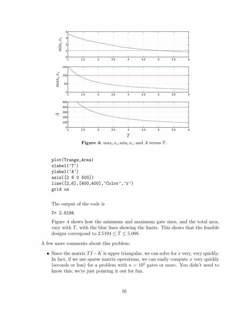
Figure 4: maxi xi,mini xi, and A versus T .

plot(Trange,Area)

xlabel(’T’)

ylabel(’A’)

axis([2 6 0 500])

line([2,6],[400,400],’Color’,’r’)

grid on

The output of the code is

T= 2.5194

Figure 4 shows how the minimum and maximum gate sizes, and the total area,vary with T , with the blue lines showing the limits. This shows that the feasibledesigns correspond to 2.5194 ≤ T ≤ 5.088.

A few more comments about this problem:

• Since the matrix TI−K is upper triangular, we can solve for x very, very quickly.In fact, if we use sparse matrix operations, we can easily compute x very quickly(seconds or less) for a problem with n = 105 gates or more. You didn’t need toknow this; we’re just pointing it out for fun.

16

• The plots above show that as T increases, all of gate sizes decrease. This impliesthat mini xi, maxi xi, and A all decrease as T increases. This means you can usea more efficient bisection search to find the optimal T . Again, you didn’t need toknow this; we’re just pointing it out.

17

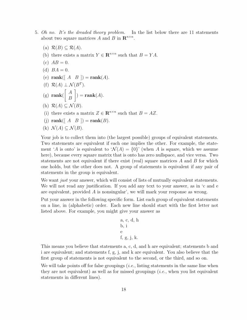
5. Oh no. It’s the dreaded theory problem. In the list below there are 11 statementsabout two square matrices A and B in Rn×n.

(a) R(B) ⊆ R(A).

(b) there exists a matrix Y ∈ Rn×n such that B = Y A.

(c) AB = 0.

(d) BA = 0.

(e) rank([ A B ]) = rank(A).

(f) R(A) ⊥ N (BT ).

(g) rank(

[

AB

]

) = rank(A).

(h) R(A) ⊆ N (B).

(i) there exists a matrix Z ∈ Rn×n such that B = AZ.

(j) rank([ A B ]) = rank(B).

(k) N (A) ⊆ N (B).

Your job is to collect them into (the largest possible) groups of equivalent statements.Two statements are equivalent if each one implies the other. For example, the state-ment ‘A is onto’ is equivalent to ‘N (A) = {0}’ (when A is square, which we assumehere), because every square matrix that is onto has zero nullspace, and vice versa. Twostatements are not equivalent if there exist (real) square matrices A and B for whichone holds, but the other does not. A group of statements is equivalent if any pair ofstatements in the group is equivalent.

We want just your answer, which will consist of lists of mutually equivalent statements.We will not read any justification. If you add any text to your answer, as in ‘c and eare equivalent, provided A is nonsingular’, we will mark your response as wrong.

Put your answer in the following specific form. List each group of equivalent statementson a line, in (alphabetic) order. Each new line should start with the first letter notlisted above. For example, you might give your answer as

a, c, d, hb, ief, g, j, k.

This means you believe that statements a, c, d, and h are equivalent; statements b andi are equivalent; and statements f, g, j, and k are equivalent. You also believe that thefirst group of statements is not equivalent to the second, or the third, and so on.

We will take points off for false groupings (i.e., listing statements in the same line whenthey are not equivalent) as well as for missed groupings (i.e., when you list equivalentstatements in different lines).

18

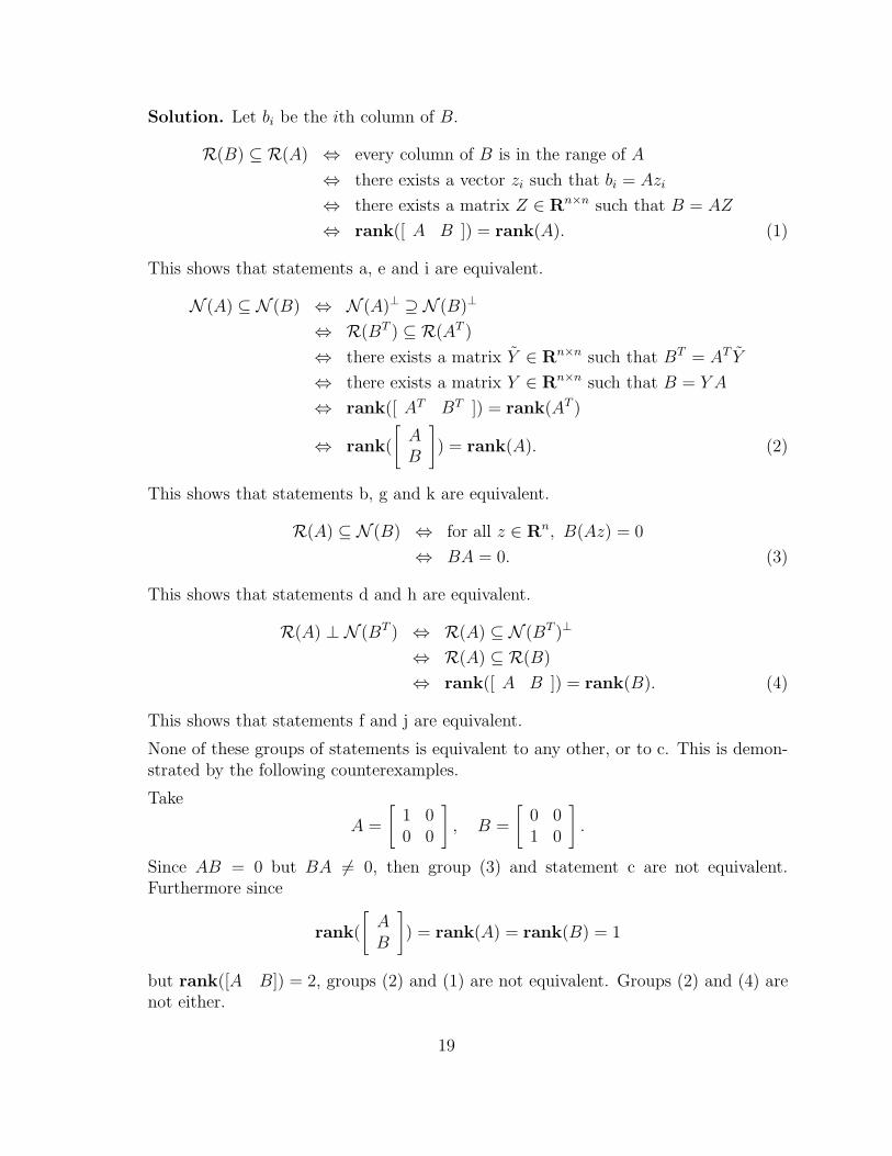
Solution. Let bi be the ith column of B.

R(B) ⊆ R(A) ⇔ every column of B is in the range of A

⇔ there exists a vector zi such that bi = Azi

⇔ there exists a matrix Z ∈ Rn×n such that B = AZ

⇔ rank([ A B ]) = rank(A). (1)

This shows that statements a, e and i are equivalent.

N (A) ⊆ N (B) ⇔ N (A)⊥ ⊇ N (B)⊥

⇔ R(BT ) ⊆ R(AT )

⇔ there exists a matrix Y ∈ Rn×n such that BT = AT Y

⇔ there exists a matrix Y ∈ Rn×n such that B = Y A

⇔ rank([ AT BT ]) = rank(AT )

⇔ rank(

[

AB

]

) = rank(A). (2)

This shows that statements b, g and k are equivalent.

R(A) ⊆ N (B) ⇔ for all z ∈ Rn, B(Az) = 0

⇔ BA = 0. (3)

This shows that statements d and h are equivalent.

R(A) ⊥ N (BT ) ⇔ R(A) ⊆ N (BT )⊥

⇔ R(A) ⊆ R(B)

⇔ rank([ A B ]) = rank(B). (4)

This shows that statements f and j are equivalent.

None of these groups of statements is equivalent to any other, or to c. This is demon-strated by the following counterexamples.

Take

A =

[

1 00 0

]

, B =

[

0 01 0

]

.

Since AB = 0 but BA 6= 0, then group (3) and statement c are not equivalent.Furthermore since

rank(

[

AB

]

) = rank(A) = rank(B) = 1

but rank([A B]) = 2, groups (2) and (1) are not equivalent. Groups (2) and (4) arenot either.

19

When A = B 6= 0, N (A) = N (B) but AB = BA = A2 6= 0. Hence groups (2) and (3)are not equivalent. Group (2) and statement c are not equivalent either.

Take

A = I, B =

[

0 01 0

]

.

Since rank([AB]) = rank(A) = 2 but rank(B) = 1, groups (1) and (4) are notequivalent. Furthermore since BA 6= 0 groups (1) and (3) are not equivalent. SinceAB 6= 0, group (1) and statement c aren’t either.

In a similar fashion, taking

A =

[

0 01 0

]

, B = I,

shows that groups (3) and (4) are not equivalent and that statement c and group (4)aren’t either.

Thus, the final answer isa, e, ib, g, kcd, hf, j.

20

6. Smooth interpolation on a 2D grid. This problem concerns arrays of real numbers onan m × n grid. Such as array can represent an image, or a sampled description of afunction defined on a rectangle. We can describe such an array by a matrix U ∈ Rm×n,where Uij gives the real number at location i, j, for i = 1, . . . , m and j = 1, . . . , n. Wewill think of the index i as associated with the y axis, and the index j as associatedwith the x axis.

It will also be convenient to describe such an array by a vector u = vec(U) ∈ Rmn.Here vec is the function that stacks the columns of a matrix on top of each other:

vec(U) =

u1...

un

,

where U = [u1 · · ·un]. To go back to the array representation, from the vector, we haveU = vec−1(u). (This looks complicated, but isn’t; vec−1 just arranges the elements ina vector into an array.)

We will need two linear functions that operate on m × n arrays. These are simpleapproximations of partial differentiation with respect to the x and y axes, respectively.The first function takes as argument an m × n array U and returns an m × (n − 1)array V of forward (rightward) differences:

Vij = Ui,j+1 − Uij , i = 1, . . . , m, j = 1, . . . , n − 1.

We can represent this linear mapping as multiplication by a matrix Dx ∈ Rm(n−1)×mn,which satisfies

vec(V ) = Dxvec(U).

(This looks scarier than it is—each row of the matrix Dx has exactly one +1 and one−1 entry in it.)

The other linear function, which is a simple approximation of partial differentiationwith respect to the y axis, maps an m × n array U into an (m − 1) × n array W , isdefined as

Wij = Ui+1,j − Uij, i = 1, . . . , m − 1, j = 1, . . . , n.

We define the matrix Dy ∈ R(m−1)n×mn, which satisfies vec(W ) = Dyvec(U).

We define the roughness of an array U as

R = ‖Dxvec(U)‖2 + ‖Dyvec(U)‖2.

The roughness measure R is the sum of the squares of the differences of each elementin the array and its neighbors. Small R corresponds to smooth, or smoothly varying,U . The roughness measure R is zero precisely for constant arrays, i.e., when Uij areall equal.

21

Now we get to the problem, which is to interpolate some unknown values in an arrayin the smoothest possible way, given the known values in the array. To define thisprecisely, we partition the set of indices {1, . . . , mn} into two sets: Iknown and Iunknown.We let k ≥ 1 denote the number of known values (i.e., the number of elements in Iknown),and mn − k the number of unknown values (the number of elements in Iunknown). Weare given the values ui for i ∈ Iknown; the goal is to guess (or estimate or assign) valuesfor ui for i ∈ Iunknown. We’ll choose the values for ui, with i ∈ Iunknown, so that theresulting U is as smooth as possible, i.e., so it minimizes R. Thus, the goal is to fill inor interpolate missing data in a 2D array (an image, say), so the reconstructed arrayis as smooth as possible.

We give the k known values in a vector wknown ∈ Rk, and the mn− k unknown valuesin a vector wunknown ∈ Rmn−k. The complete array is obtained by putting the entries ofwknown and wunknown into the correct positions of the array. We describe these operationsusing two matrices Zknown ∈ Rmn×k and Zunknown ∈ Rmn×(mn−k), that satisfy

vec(U) = Zknownwknown + Zunknownwunknown.

(This looks complicated, but isn’t: Each row of these matrices is a unit vector, somultiplication with either matrix just stuffs the entries of the w vectors into particularlocations in vec(U). In fact, the matrix [Zknown Zunknown] is an mn×mn permutationmatrix.)

In summary, you are given the problem data wknown (which gives the known arrayvalues), Zknown (which gives the locations of the known values), and Zunknown (whichgives the locations of the unknown array values, in some specific order). Your job isto find wunknown that minimizes R.

(a) Explain how to solve this problem. You are welcome to use any of the operations,matrices, and vectors defined above in your solution (e.g., vec, vec−1, Dx, Dy,Zknown, Zunknown, wknown, . . . ). If your solution is valid provided some matrix is(or some matrices are) full rank, say so.

(b) Carry out your method using the data created by smooth_interpolation.m. Thefile gives m, n, wknown, Zknown and Zunknown. This file also creates the matrices Dx

and Dy, which you are welcome to use. (This was very nice of us, by the way.)You are welcome to look at the code that generates these matrices, but you donot need to understand it. For this problem instance, around 50% of the arrayelements are known, and around 50% are unknown.

The mfile also includes the original array Uorig from which we removed elementsto create the problem. This is just so you can see how well your smooth recon-struction method does in reconstructing the original array. Of course, you cannotuse Uorig to create your interpolated array U.

To visualize the arrays use the Matlab command imagesc(), with matrix argu-ment. If you prefer a grayscale image, or don’t have a color printer, you can

22

issue the command colormap gray. The mfile that gives the problem data willplot the original image Uorig, as well as an image containing the known values,with zeros substituted for the unknown locations. This will allow you to see thepattern of known and unknown array values.

Compare Uorig (the original array) and U (the interpolated array found by yourmethod), using imagesc(). Hand in complete source code, as well as the plots.Be sure to give the value of roughness R of U .

Hints:

• In Matlab, vec(U) can be computed as U(:);

• vec−1(u) can be computed as reshape(u,m,n).

Solution.

(a) We can express our roughness measure directly in terms of the vector of knownvalues wknown and unknown values wunknown as

R = ‖Dx(Zknownwknown + Zunknownwunknown)‖2

+‖Dy(Zknownwknown + Zunknownwunknown)‖2

=

∥

∥

∥

∥

∥

[

Dx

Dy

]

Zknownwknown +

[

Dx

Dy

]

Zunknownwunknown

∥

∥

∥

∥

∥

2

.

Defining

A =

[

Dx

Dy

]

Zunknown, b = −

[

Dx

Dy

]

Zknownwknown,

we can express the problem in the familiar form

minimize ‖Awunknown − b‖2.

Provided A is skinny and full rank, the solution is

wunknown = A†b

= (AT A)−1AT b

= −(

ZTunknown(D

Tx Dx + DT

y Dy)Zunknown

)−1·

·(

ZTunknown(D

Tx Dx + DT

y Dy)Zknown

)

wknown.

When is A ∈ R(2mn−m−n)×(mn−k) skinny and full rank? It’s always skinny, since2mn − m − n ≥ mn − k. If A were not full rank, then there would exist somenonzero w with Aw = 0. This means that Zunknownw is in the nullspace of bothDx and Dy, which means that Zunknownw is a constant (i.e., its entries are all thesame). This means that we have to have w = 0, assuming there is at least oneknown array value. In other words, A is always full rank and skinny!

23

(b) wunknown is easily found in Matlab with the command

wunkown = [Dx; Dy]*Zunknown \ -[Dx; Dy]*Zknown*wknown;

Yes, that really is the solution, in just one line.

Next we need to create our complete array by putting the entries of wknown andwunknown in the correct positions of the array. We use Matlab again:

U = reshape([Zknown Zunknown]*[wknown; wunknown], m, n);

We calculate the roughness of our final array U as

R = norm(Dx*U(:))^2 + norm(Dy*U(:))^2

which for our example is R = 12.8794.

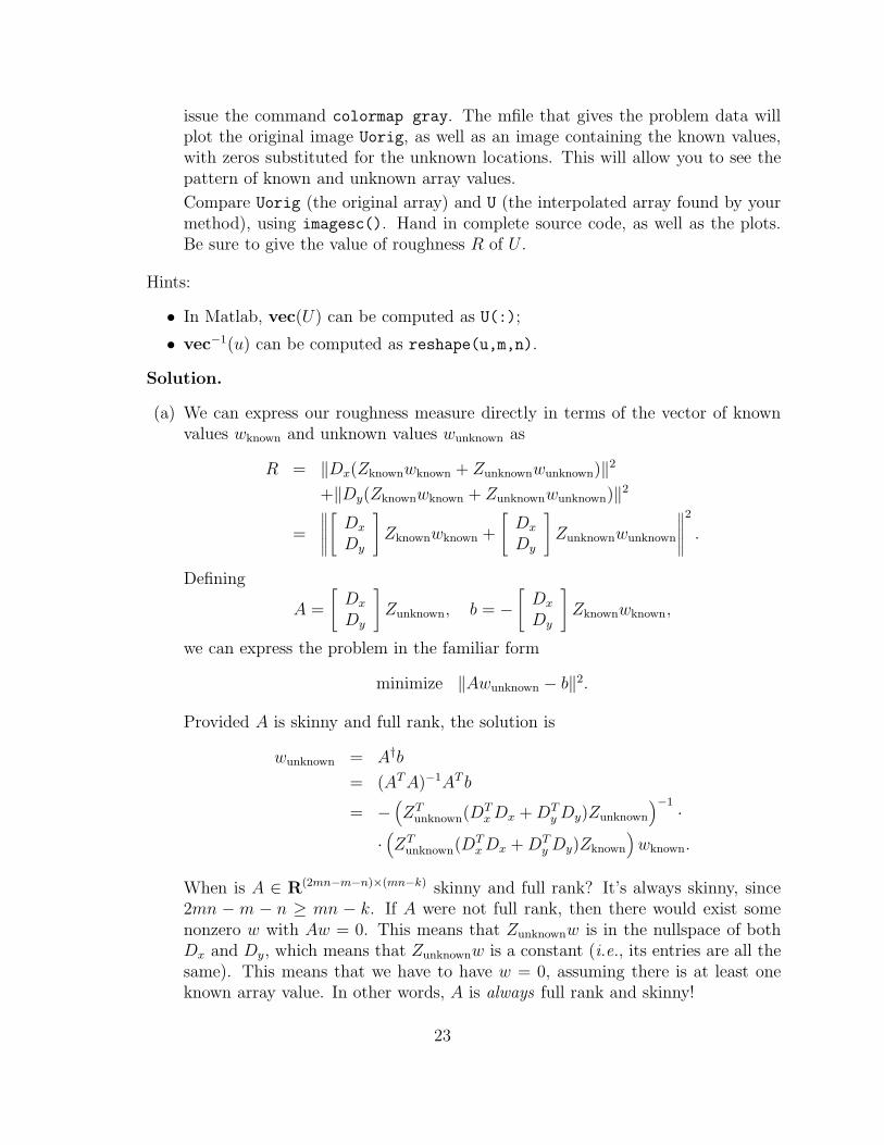
Finally, we graph Uorig, Uobscured and U, with the results shown in Figure (5).

subplot(221);

imagesc(Uorig)

title(’Original image’);

subplot(222);

imagesc(Uobscured);

title(’Obscured image’);

subplot(223);

imagesc(U);

title(’Reconstructed image’);

One thing you notice about the reconstructed image is, it’s a really, really good ap-proximation of the orginal image. It’s very impressive; we’ve guessed (very well) halfthe entries of a (smooth) image, from the remaining half.

24

5 10 15 20 25

5

10

15

20

25

5 10 15 20 25

5

10

15

20

25

5 10 15 20 25

5

10

15

20

25

Original image Known pixel values

Reconstructed image

Figure 5: Original, obscured and reconstructed image arrays

25

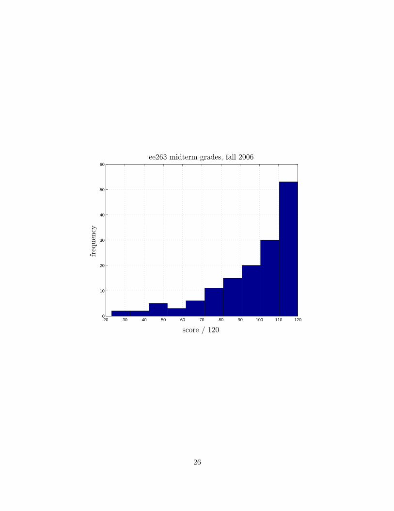
20 30 40 50 60 70 80 90 100 110 1200

10

20

30

40

50

60

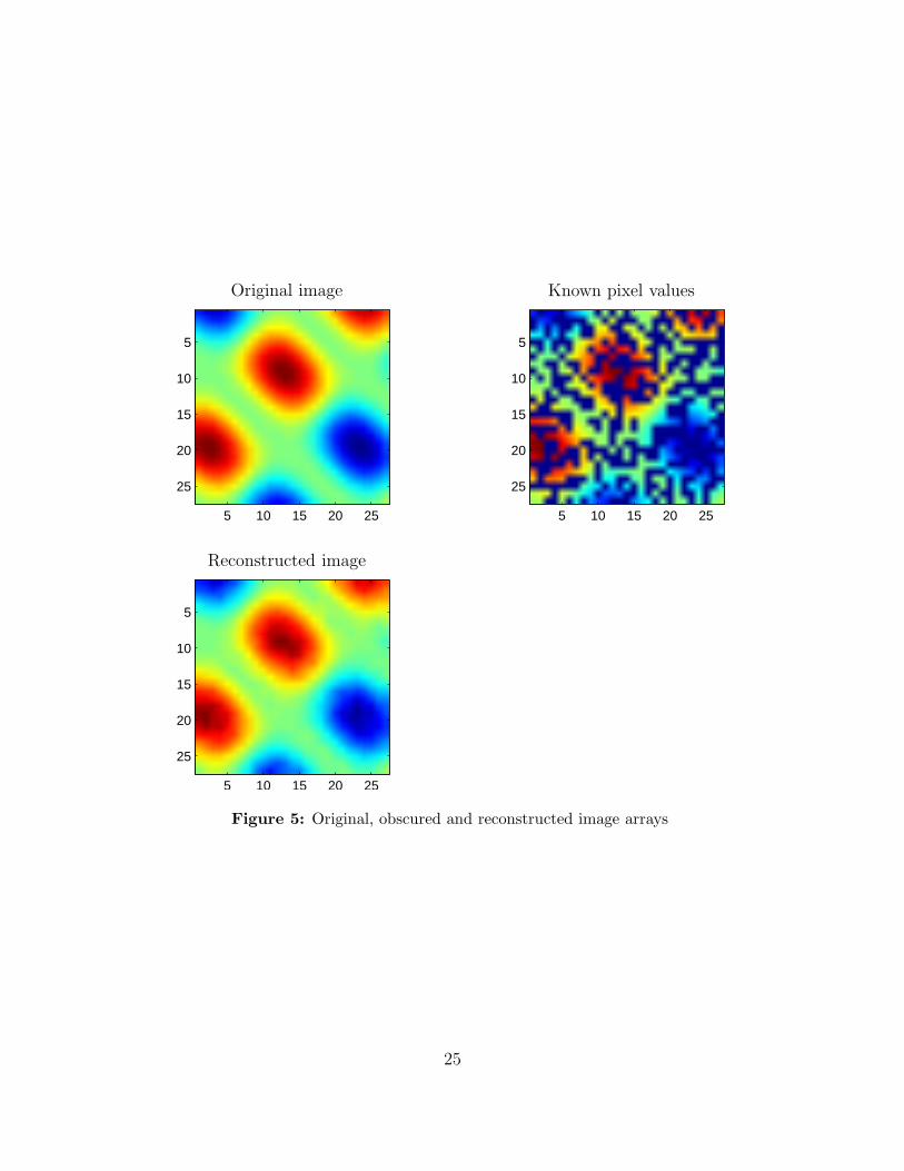
ee263 midterm grades, fall 2006

freq

uen

cy

score / 120

26