Middle Cape Fear Local Watershed Plan - North … With/Watershed... · Appendix 1 Field Data Model Inputs ... Middle Cape Fear Local Watershed Plan Study Sites. 2-5 ... Erwin Clayton

Middle Cape Fear Local Watershed Plan

Technical Memorandum 3: Model Calibration Report

North Carolina Department of Environment and Natural Resources Ecosystem Enhancement Program

Prepared By:

February 2004

Middle Cape Fear Local Watershed Plan

Technical Memorandum 3: Model Calibration Report

Prepared For:

NC Department of Environment and Natural Resources, Ecosystem Enhancement Program

February 2004

Prepared By Buck Engineering PC William A. Harman, PG Suzanne J. Unger, PE Principal in Charge Project Manager Steve Bevington Rajpreet Butalia Senior Scientist GIS Analyst

ii

Table of Contents 1 Introduction.............................................................................................................. 1-1 2 Model Selection and Parameters.............................................................................. 2-1

2.1 Methods............................................................................................................ 2-1 2.2 Model Selection ............................................................................................... 2-1 2.3 Watershed Delineation..................................................................................... 2-1 2.4 Field Data Collection ....................................................................................... 2-1 2.5 Other Data Sources .......................................................................................... 2-5

2.5.1 Meteorological Data................................................................................. 2-5 2.5.2 Land Use/Land Cover Data ..................................................................... 2-7 2.5.3 Soils.......................................................................................................... 2-7 2.5.4 Harris Lake............................................................................................... 2-7 2.5.5 Point Sources ........................................................................................... 2-7

3 Model Calibration .................................................................................................... 3-1 4 Results and Discussion ............................................................................................ 4-1

4.1 Water Yield...................................................................................................... 4-1 4.2 Sediment Yield................................................................................................. 4-4 4.3 Nutrient Loading.............................................................................................. 4-6 4.4 Summary ........................................................................................................ 4-10 4.5 Future Modeling............................................................................................. 4-10

5 References................................................................................................................ 5-1

iii

List of Figures Figure 1.1 Vicinity Map Figure 1.2 Local Watershed Plan Project Flow Chart Figure 2.1 Data Inputs for the SWAT Model Figure 2.2 Data Flow in the SWAT Model Figure 2.3 Field Site Locations Figure 2.4 Weather Stations Figure 2.5 Modeled Land Use/Land Cover Figure 2.6 Modeled Soils Figure 2.7 Wastewater Discharges Figure 3.1 Modeled Stream Segments Figure 3.2 Modeled Catchments Figure 4.1 Major Drainages for Results Discussion Figure 4.2 Average Annual Discharges for Study Watersheds Figure 4.3 Relative Water Yield (%) Figure 4.4 Average Annual Sediment Concentrations for Study Watersheds Figure 4.5 Sediment Yield (tons/ha-yr) Figure 4.6 Average Annual Total Nitrogen Concentrations for Study Watersheds Figure 4.7 Average Annual Phosphorus Concentrations for Study Watersheds Figure 4.8 Total Nitrogen Yield (kg N/ha) Figure 4.9 Total Phosphorus Yield (kg P/ha) Appendices Appendix 1 Field Data Model Inputs Appendix 2 Model Parameters for Harris Lake

1-1

1 Introduction The North Carolina Wetlands Restoration Program (NCWRP) contracted with Buck Engineering in 2002 to perform a technical assessment of three 14-digit hydrologic units (HUs) in the Middle Cape Fear River Basin. This work is being completed as part of the Local Watershed Planning (LWP) initiative, which is currently administered by the North Carolina Ecosystem Enhancement Program (EEP). This Technical Memorandum documents selection and calibration of a watershed model for the LWP effort. The three HUs are parallel drainages to the Cape Fear River and are located within portions of Chatham, Wake, and Harnett Counties (Figure 1.1). The total land area for the HUs totals approximately 180 square miles. The HUs include parts of the towns of Apex, Holly Springs, and Fuquay-Varina and the portion of Raven Rock State Park north and east of the Cape Fear River. Major streams in the watersheds include: tributaries to Harris Lake (White Oak Creek, Little White Oak Creek, Buckhorn Creek, Utley Creek, and Cary Branch), Parkers Creek, Mill Creek, Avents Creek, Hector Creek, Kenneth Creek, Neills Creek, and Dry Creek. For the purposes of this study, the three hydrologic units were further divided into subwatersheds based on their drainage system in order to develop more manageable units for analysis and management. Using a geographic information system (GIS), the three watersheds were divided into 19 subwatersheds, ranging in size from 3.6 to 16.5 square miles. Refer to Technical Memorandum 1 for an overview of the project subwatersheds. The information presented in this document supplements the watershed characterization and field data summary submitted to the EEP in Technical Memorandums 1 and 2 (Figure 1.2). Buck Engineering calibrated an empirical model, the Soil and Water Assessment Tool (SWAT), with existing and project data to assess general land use impacts to water quality and to provide an estimate of baseline watershed conditions. The choice of SWAT considered numeric goals and objectives and will be able to give an indication of progress towards achieving them. The SWAT model incorporates existing geographic, environmental, and management conditions together with land use conditions to estimate sediment and nutrient loadings. Other modeling tasks described in this report include delineating model catchments based on stream networks and groupings of uniform watershed characteristics, obtaining and processing meteorological data, defining watershed hydrology, calibrating the model, and documenting the results. Future tasks will involve modeling various land use and management scenarios, including estimates of land development, implementation of best management practices, and adoption of stormwater and buffer regulations.

1

42

401

55

RavenRockStatePark

HARNETT

CO

.

CH

ATH

AM

CO

.W

AK

E C

O.

Cape Fear River

Kenneth C

reek

Harris Lake

HU 03030004020010

HU 03030004030010

HU

030

3000

4040

010

Holly Springs

Fuquay-Varina

Apex

Lillington

Angier

Figure 1.1. Vicinity Map

0 2 4 6 81Miles

Raleigh

Hydrologic Units - 14 digit

Streams

303(d) Listed Streams

Lakes

Roads

State Parks

NC Ecosystem Enhancement ProgramMiddle Cape Fear Local Watershed Plan

1-3

Figure 1.2 Local Watershed Plan Project Flow Chart

2-1

2 Model Selection and Parameters

2.1 Methods Water quality modeling techniques were employed to produce sediment and nutrient loading estimates for the project watershed. The model incorporates existing geographic, environmental, and management conditions together with current land use conditions to estimate sediment and nutrient loadings.

2.2 Model Selection The Soil and Water Assessment Tool (Neitsch et al., 2002) was selected for the sediment and nutrient analysis. SWAT was developed to quantify the impact of land management practices in large, complex watersheds. It is designed to integrate many land cover, land use, and environmental features of a watershed with land and stream management practices into water quality predictions. SWAT’s ability to predict water quality, sediment, and nutrient response to changing land use and management conditions makes it an ideal model to predict conditions in the project area. The SWAT model requires topographic, hydrographic, land use, soils, and weather data to simulate surface water quality (Figure 2.1). Soil, groundwater, reservoir, and stream processes components are modeled (Figure 2.2).

2.3 Watershed Delineation A digital elevation model (DEM) for the project area was developed based on 1:24,000 topographic maps. ESRI GIS software Spatial Analyst was use to delineate watershed boundaries. For modeling purposes, the three hydrologic units that make up the project area were delineated and adopted as the model boundaries (Figure 1.1).

2.4 Field Data Collection The SWAT model requires information about channel dimensions, Manning’s n, stream cover, and bank erodibility parameters. Under a previous project task, field data measurements were taken at selected study sites to fulfill this data requirement. Results were extrapolated from site locations to larger representative areas. Twenty-two stream sites were surveyed within the project area watershed to determine channel dimension, assess stream bank condition, and measure bed materials. Sites were selected to represent a wide range of drainage areas from each portion of the study area. An initial reconnaissance of the area was performed to determine whether the sites were viable. Sites with poor or dangerous access and sites with unusual hydraulics were excluded from the study. Selected sites were deemed to be representative of typical stream conditions in the vicinity. Selected sites are presented in Figure 2.3.

2-2

Figure 2.1 Data Inputs for the SWAT Model

2-3

Figure 2.2 Data Flow in the SWAT Model

1

42

401

55

RavenRockStatePark

HARNETT

CO

.

CH

ATH

AM

CO

.W

AK

E C

O.

Cape Fear River

Kenneth C

reek

Harris Lake

HU 03030004020010

HU 03030004030010

HU

030

3000

4040

010

Holly Springs

Fuquay-Varina

Apex

Lillington

Angier

2BM4

3PM3

3PM23PM1

4KM2

4KM5

2BT12

2WOM1

3LHM33LHT8

3LHT4

3LAM2

3LAT7

4MNM1

4UNM1

4KT13

4KT19

2WOT162LWOM2

3UAT16

4UNT13

4KT19T1

Figure 2.3 Field Site Locations

0 2 4 6 81Miles


Study Sites

2-5

A riffle cross section (or a cross-over in sand bed streams) was surveyed up or downstream of a road crossing at a location that did not appear to be adversely impacted by the bridge or culvert. Where the channel exhibited pattern, pools were also surveyed at meander bends. Scour pools caused by woody debris or other in-stream blockages were not selected to be surveyed. A total of 34 cross sections were surveyed. Cross-section measurements were taken of the floodplain, top of bank, bankfull, edge of baseflow channel, water surface, and other channel features. A modified Wolman pebble count analysis was used on course riffles that exhibited cobble and course gravel as the dominant substrate (Bunte and Abt, 2001). In sand/fine gravel bed streams bulk samples were taken of the bed material using standard USGS sampling procedures. Bulk samples were composed of at least 10 composite samples collected in equal increments across the baseflow stream channel. This bulk sample was then dried and sieved to determine the percent composition of individual sized particles. Bank Erodibility Hazard Index (BEHI) estimates were performed at each site (Rosgen, 2000). The BEHI values were helpful in determining bulk erodibilty for the modeling phase to calibrate erosion volume. The qualitative BEHI scores (e.g., low, medium, high) were used to choose the appropriate modeling parameters based on best professional judgment. A summary of the data relevant to the SWAT model input for each of the 22 field surveys is listed in Appendix 1. Detailed cross section and sediment data were presented in Technical Memorandum 2 Appendices A and B, respectively. Photos were taken at each cross section looking upstream and downstream and, where an unusual condition existed, photos were taken of each bank. These photos were presented in Technical Memorandum 2 Appendix 3.

2.5 Other Data Sources Other data required for model calibration and implementation were secured and are described below.

2.5.1 Meteorological Data Weather station data were obtained from the Clayton, NC National Weather Service station. This weather station is the closest to the Project Area (Figure 2.4), is in the same geophysiographic region, and has a similar altitude. Weather statistics over the past 29 years from this site were used as a source to generate simulated weather for model runs.

Raleigh

Durham

Cary

Fayetteville

Sanford

Chapel Hill

Burlington

Garner

Pinehurst

Dunn

Apex

Southern Pines

Graham

Morrisville

Erwin

Clayton

Aberdeen

Vass

Holly Springs

Siler City

Hope Mills

Mebane

Carrboro

Raeford

Fuquay-Varina

Lillington

Angier

Pittsboro

Butner

Hillsborough

Spring Lake

Carthage

Garner

Pinebluff

Benson

Haw River

Coats

Wade

Whispering Pines

Falcon

Stedman

Broadway

Roseboro

Rolesville

Cameron

Salemburg

Goldston

Four Oaks

Franklinton

Linden

Wake Forest

Autryville

Knightdale

Alamance

Godwin

Wake Forest

Taylortown

CreedmoorElon College

Figure 2.4 Weather Stations

0 5 10 15 202.5Miles


Weather Stations (Siler City and Clayton)

Municipal Boundaries

Study Area

2-7

2.5.2 Land Use/Land Cover Data Multiple GIS data sources were processed and combined to create a current land use/land cover dataset for use in SWAT: existing land cover (EarthSat, 1996), 2003 aerial imagery (SPOT, 2003), hydrology (NCCGIA, 2000), roads (NCDOT, 1999), and the National Wetlands Inventory (NWI) (USFWS, 1999). The EarthSat land cover dataset was the basis for creation of the updated dataset. Areas where land use in the SPOT imagery differed from the existing land cover data based on visual comparison were digitized as polygon features and incorporated into the new land use/land cover dataset. Similarly, NWI wetlands, hydrology, and roads datasets were also used to update the EarthSat land cover data. Attribute information was added to the new dataset to enable SWAT to interpret the land use/land cover type (Figure 2.5).

2.5.3 Soils Nineteen distinct soil types are located within the project watershed (Figure 2.6). GIS soils data from the State Soil Geographic (STATSGO) dataset for Chatham County (USDA, 1998a) and the Soil Survey Geographic (SSURGO) datasets for Wake (USDA, 1998b) and Harnett (USDA, 1998c) counties were compiled to create a single dataset for use in SWAT. The more general STATSGO soils data were used in Chatham County because SSURGO soils information is not yet available. Using the STATSGO and SSURGO datasets provided more detailed GIS data than are available in the default SWAT soils data. Attribute information was added to the new soils dataset to enable SWAT to interpret the soil type.

2.5.4 Harris Lake Harris Lake was modeled as it has the potential to mitigate downstream sediment and nutrient pollution and because water quality in the lake may be impacted by the future development. Model parameters for the reservoir are presented in Appendix 2.

2.5.5 Point Sources Six discharges of treated waste are permitted under the National Pollutant Discharge Elimination System (NPDES) in the project watershed (Figure 2.7). Three of the permits are for municipal wastewater treatment facilities (Angier, Fuquay-Varina, and Holly Springs). Two additional permits are for small discharges associated with private waste treatment facilities. Progress Energy also has an NPDES permit for its discharge to Harris Lake. None of these discharges are large enough to have significant impact on model results.

Figure 2.5 Modeled Land Use/Land Cover

0 2 4 6 81Miles

NC Ecosystem Enhancement ProgramMiddle Cape Fear Local Watershed PlanAgriculture

Forested

Urban High Density

Urban Low Density

Urban Medium Density

Roads

Water

Wetlands

Commercial & Industrial

1

42

401

55

HARNETT

CO

.

CH

ATH

AM

CO

.W

AK

E C

O.

Cape Fear River

Harris Lake

Figure 2.6 Modeled Soils

0 2 4 6 81Miles


Modified STATSGO Soil Series

NC057

NC061

NC062

NC069

NC074

NC075

NC052

NC001

NC003

NC010

NC011

NC019

NC029

NC033

NC034

NC035

NC049

NC050

NC038

1

42

401

55

RavenRockStatePark

HARNETT

CO

.

CH

ATH

AM

CO

.W

AK

E C

O.

Cape Fear River

Kenneth C

reek

Harris Lake

HU 03030004020010

HU 03030004030010

HU

030

3000

4040

010

Holly Springs

Fuquay-Varina

Apex

Lillington

Angier

Figure 2.7 Wastewater Discharges

0 2 4 6 81Miles


NPDES - Point Source Discharges

3-1

3 Model Calibration Stream channel segmentation was based upon the DEM and existing stream hydrography. ESRI GIS software Spatial Analyst was use to determine the location of all channels with drainage areas greater than one square mile. Reaches were linked at their confluences with routing nodes (Figure 3.1). A total of 720 stream miles in 160 reaches were modeled within the 180 square mile watershed. The catchments associated with each of these reaches are shown in Figure 3.2. Current land use and soils data were overlain with the 74 catchment boundaries to create tables of the hydraulic response units (HRUs), unique combination of soil and land use for each catchment. The SWAT model was then parameterized with the spatial data described above. Channel dimensions, Manning’s n, stream cover, and bank erodibility parameters were entered for each stream reach to reflect values observed and recorded in the field. At locations where field measurements were taken at study sites, the data were used directly in the selection of model parameters. In other areas, best professional judgment was used to extrapolate known channel characteristics. The model was run for a five year period of simulated weather. The initial mean annual runoff value from the model was 1.05 cubic feet per second (cfs) per year. This compared favorably to the USGS estimate for the region of 1.1 cubic feet per second per year (Giese and Mason, 1993). Because hydraulic processes are important to essentially all model components, hydraulic calibration was achieved by minor global adjustment of the runoff curve numbers so that a final modeled mean annual runoff value of 1.1 cubic feet per second per year was achieved. This resulted in an average flow of 198 cfs at the combined outlets of the study area. As detailed water quality data are not yet available for the study area, calibration of the model was limited to hydrology at this time. However, sediment and nutrient concentrations predicted by the model were in the range of typical piedmont values. Detailed calibration of sediment and nutrients can be completed as field data is supplied.

1

42

401

55

HARNETT

CO

.

CH

ATH

AM

CO

.W

AK

E C

O.

Cape Fear River

Harris Lake

Holly Springs

Fuquay-Varina

Apex

Lillington

Angier

Figure 3.1 Modeled Stream Segments

0 2 4 6 81Miles

NC Ecosystem Enhancement ProgramMiddle Cape Fear Local Watershed PlanModeled Stream Segments

Outlets

Linking stream added Outlet

Manually added Point Source

1

42

401

55

HARNETT

CO

.C

HA

THA

M C

O.

WA

KE

CO

.

Cape Fear River

Harris Lake

Holly Springs

Fuquay-Varina

Apex

Lillington

Angier

22

8

13

47

6

39

29

10

73

9

43

71

72

54

7

4

69

36

13

68

37

53

34

25

67

2

5663

5

44

12

14

19

15

32

55

33

20

31

74

52

4042

51

11

41

30

66

45

28

48

58

35

1727 24

50

57

26

21

6065

38

62

1816

4649

5964

70

61

23

75

Figure 3.2 Modeled Catchments

0 2 4 6 81Miles


Modeled Catchments

4-1

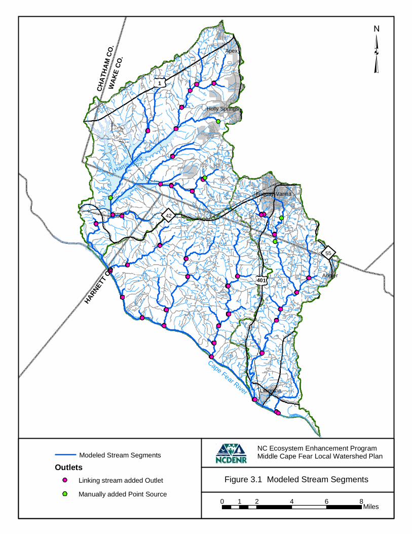
4 Results and Discussion For ease of discussion, the results presented here are summarized by the major drainages in the study area: Buckhorn Creek (including Harris Lake), Parkers Creek, Avents Creek, Hector Creek, and Neills Creek (including the Kenneth Creek drainage). Figure 4.1 shows the locations of these drainages. The Dry Creek drainage was modeled; however, results are not presented because field data were not available (e.g., channel dimensions) and the calibration of the model was therefore incomplete. In consultation with the EEP, the decision was made to drop Dry Creek from the modeling analysis and spend available resources in other study drainages.

4.1 Water Yield Water yield was relatively consistent throughout the study area with all watersheds’ discharge within a few percent of the study area’s mean annual runoff of 1.1 ft/year. As a result, discharges from each of the five major drainages were proportional to their drainage area. The Buckhorn Creek drainage, by far the largest sub-watershed in the project area, produced the greatest discharge and the smallest sub-watershed, Parkers Creek, produced the least water (Figure 4.2).

0

10

20

30

4050

60

70

80

90

100

Buckhorn Parkers Avents Hectors Neills

Dis

char

ge (c

fs)

Figure 4.2 Average Annual Discharges for Study Watersheds The sandy soils in the lower portion of the basin produced the most water while urbanized headwater catchments produced the least (Figure 4.3). Harris Lake also had a small effect on water yield. However, all catchments within the study area produced at least 95% of the maximum modeled water yield meaning that no major net hydrologic impacts were observed within the study area.

Figure 4.1 Major Drainages for Results Discussion

0 2 4 6 81Miles

NC Ecosystem Enhancement ProgramMiddle Cape Fear Local Watershed PlanModeled Stream Segments

Major Lakes

Major Drainages in the Study Area

Buckhorn Creek

Parkers Creek

Avents Creek

Hector Creek

Neills Creek

Dry Creek

22

8

13

47

6

39

29

10

73

9

43

7172

54

7

4

69

36

13

68

37

53

34

25

67

2

5663

5

44

12

14

19

15

32

55

33

20

31

74

52

4042

51

11

41

30

66

45

28

48

58

35

1727 24

50

57

26

21

6065

38

62

1816

4649

5964

70

61

23

75

Figure 4.3 Relative Water Yield (%)

0 2 4 6 81Miles


Relative Water Yield by Catchment (%)

0.959 - 0.967

0.968 - 0.974

0.975 - 0.980

0.981 - 0.989

0.990 - 1.000

Modeled Stream Segments

Major Lakes

4-4

4.2 Sediment Yield Sediment yield is highly variable throughout the study area due to both channel conditions and land management. Harris Lake in the Buckhorn Creek watershed is a major sediment sink and sediment concentrations below the lake are dramatically lower than any other watershed in the study area (Figure 4.4). Parkers Creek also is predicted to have a relatively low instream sediment concentration, primarily due to the large percentage of forest cover in the watershed. Avents, Hectors, and Neills Creek sub-watersheds each show relatively high sediment discharge with Neills Creek predicted to have the highest sediment concentration of the study area sub-watersheds.

0.000.020.040.060.080.100.120.140.160.180.20

Buckhorn Parkers Avents Hectors Neills StudyArea

Sedi

men

t Con

cent

ratio

n (m

g/l)

Figure 4.4 Average Annual Sediment Concentrations for Study Watersheds Sediment yield by catchment is presented in Figure 4.5. Headwater reaches in urbanizing areas had the highest relative sediment yield. Catchments along the Cape Fear River flood plain had very low sediment yield. This is indicative of active floodplains that are capturing sediments before they reach the Cape Fear River.

22

8

13

47

6

39

29

10

73

9

43

7172

54

7

4

69

36

13

68

37

53

34

25

67

2

5663

5

44

12

14

19

15

32

55

33

20

31

74

52

4042

51

11

41

30

66

45

28

48

58

35

1727 24

50

57

26

21

6065

38

62

1816

4649

5964

70

61

23

75

Figure 4.5 Sediment Yield (tons/ha-yr)

0 2 4 6 81Miles

NC Ecosystem Enhancement ProgramMiddle Cape Fear Local Watershed PlanSediment Yield by Catchment (tons/ha-yr)


Major Lakes

0.001 - 0.160

0.161 - 0.478

0.479 - 0.922

0.923 - 1.482

1.483 - 2.714

4-6

4.3 Nutrient Loading Nutrient loading is relatively high throughout most of the study area with an average of 1.7 mg/l total nitrogen (TN) and 0.2 mg/l total phosphorus (TP). Parkers and Avents Creeks were predicted to have significantly less nutrient than the other sub-watersheds (Figures 4.6 and 4.7). Buckhorn Creek was predicted to have very low phosphorus concentrations (Figure 4.7) but nitrogen concentrations approximately equal to the study area average. This is due to the fact the Harris Lake, as an effective sediment trap, collected phosphorus bound to sediments but allows the more soluble nitrogen compounds to pass through the lake. Neills Creek demonstrated the highest nutrient concentrations.

0

0.5

1

1.5

2

2.5

3


TN C

once

ntra

tion

mg/

l

Figure 4.6 Average Annual Total Nitrogen Concentrations for Study Watersheds

4-7

0.00

0.05

0.10

0.15

0.20

0.25

0.30

0.35

0.40


Phos

phor

us C

once

ntra

tion

(mg/

l)

Figure 4.7 Average Annual Phosphorus Concentrations for Study Watersheds TN yield by catchment is presented in Figure 4.8. Headwater reaches in urbanizing areas had the highest relative nitrogen supply. Agricultural catchments also produced relatively high nitrogen loads, particularly in the Parkers Creek and Avents Creek sub-watersheds. Unlike the pattern observed with sediment, catchments along the Cape Fear River flood plain contributed significantly to the study areas nitrogen supply. This is due, in some part, to the sandy soils that permit dissolved nitrogen to pass quickly into tributaries and streams. TP yield by catchment is presented in Figure 4.9. Headwater reaches in urbanizing areas had the highest relative phosphorus supply. Catchments along the Cape Fear River flood plain had very low phosphorus supply. This very low TP yield is the result of limited erosion along low slope stream channels and active floodplains that collect phosphorus associated with sediment.

22

8

13

47

6

39

29

10

73

9

43

7172

54

7

4

69

36

13

68

37

53

34

25

67

2

5663

5

44

12

14

19

15

32

55

33

20

31

74

52

4042

51

11

41

30

66

45

28

48

58

35

1727 24

50

57

26

21

6065

38

62

1816

4649

5964

70

61

23

75

Figure 4.8 Total Nitrogen Yield (kg N/ha)

0 2 4 6 81Miles


Total Nitrogen Yield by Catchment (kg N/ha)


Major Lakes

0.093 - 0.215

0.216 - 0.309

0.310 - 0.385

0.386 - 0.472

0.473 - 0.609

22

8

13

47

6

39

29

10

73

9

43

7172

54

7

4

69

36

13

68

37

53

34

25

67

2

5663

5

44

12

14

19

15

32

55

33

20

31

74

52

4042

51

11

41

30

66

45

28

48

58

35

1727 24

50

57

26

21

6065

38

62

1816

4649

5964

70

61

23

75

Figure 4.9 Total Phosphorus Yield (kg P/ha)

0 2 4 6 81Miles


Total Phosphorus Yield by Catchment (kg P/ha)


Major Lakes

0.000 - 0.015

0.016 - 0.036

0.037 - 0.067

0.068 - 0.097

0.098 - 0.169

4-10

4.4 Summary Nutrient and sediment loadings vary greatly throughout the study area. Harris Lake has a strong water quality effect as it traps significant amount of sediment and phosphorus. Agricultural activities and channel erosion from developed areas result in some catchments with very high sediment and nutrient sources. Transport and storage of sediments as they move through the steeper headwater creeks and onto the Cape Fear floodplain play an important role in pollutant delivery. The location of resources is crucial in determining the importance of upstream pollutant sources.

4.5 Future Modeling This model has provided an estimate of baseline conditions for discharge, sediment, and common nutrients based on existing land use and management. The calibrated model presented in this report will be used to test various future land use conditions. Examples of model scenarios include potential causes of water quality degradation, including wetland and forest cover loss to other land uses, future transportation impacts, and other land cover alterations. In addition, various methods to reduce the impacts of future land use scenarios (e.g., stormwater management, preservation and restoration opportunities, and conservation development options) will be modeled.

5-1

5 References Bunte, K. and S. Abt. 2001. Sampling surface and subsurface particle-size distributions

in wadable gravel- and cobble-bed streams for analyses in sediment transport, hydraulics, and streambed monitoring. Gen. Tech. Rep. RMRS-GTR-74. Fort Collins, CO: U.S. Department of Agriculture, Forest Service, Rocky Mountain Research Station. 428 p.

Earth Satellite Corporation (Earthsat). 1996. Comprehensive Land Cover Mapping for

the State of North Carolina. Rockville, MD. Giese, G.L., Mason, Robert R. Jr. 1993. Low-Flow Characteristics of Stream in North

Carolina. USGS Water-Supply Paper 2403. 29 p. Harman, W.A., G.D. Jennings, J.M. Patterson, D.R. Clinton, L.O. Slate, A.G. Jessup, J.R.

Everhart, and R.E. Smith. 1999. Bankfull Hydraulic Geometry Relationships for North Carolina Streams. Wildland Hydrology. AWRA Symposium Proceedings. Edited by: D.S. Olsen and J.P. Potyondy. American Water Resources Association. June 30-July 2, 1999. Bozeman, MT.

North Carolina Center for Geographic Information and Analysis (NCCGIA). 2000.

Hydrography (1:100,000). Raleigh, NC. North Carolina Department of Transportation (NCDOT) GIS Unit. 1999. NCDOT

Roads (1:24,000). Raleigh, NC. Neitsch, S.L., Arnold, J.G., Kiniry, J.R., Williams, J.R., King, K.W. 2002. Soil and

Water Assessment Tool Theoretical Documentation: Version 2000. Texas Water Resources Institute, College Station, Texas. GSWRL Report 02-01.

Rosgen, D.L. 1996. Applied River Morphology. Wildland Hydrology Books, Pagosa

Springs, CO. SPOT Image Corporation (SPOT). 2003. Satellite aerial imagery for the project study

area. Chantilly, VA. United States Department of Agriculture (USDA) Soil Conservation Service. 1998a. NC

General (STATSGO). Raleigh, NC. United States Department of Agriculture (USDA) Natural Resources Conservation

Service. 1998b. Detailed County Soils- Wake County, North Carolina. Raleigh, NC.

United States Department of Agriculture (USDA) Natural Resources Conservation

Service. 1998c. Detailed County Soils- Harnett County, North Carolina. Raleigh, NC.

5-2

United States Fish and Wildlife Service (USFWS) National Wetland Inventory. 1999.

National Wetlands Inventory. St. Petersburg, FL.

Documents

Middle Cape Fear Local Watershed Plan - North … With/Watershed... · Appendix 1 Field Data Model Inputs ... Middle Cape Fear Local Watershed Plan Study Sites. 2-5 ... Erwin Clayton