* Centre for the Analysis of Regional Integration at Sussex, UK (CARIS)

** Centre for Social and Economic Research, Poland (CASE)

*** Institute for Development Studies, UK (IDS)

**** University College London (UCL)

***** University of Geneva

Mid-term Evaluation of the EU’s Generalised System of

Preferences:

Michael Gasiorek*

Peter Holmes*

Jim Rollo*

Zhenkun Wang*

Javier Lopez Gonzalez*

Maximiliano Mendez Parra*

Maryla Maliszewska**

Wojtek Paczynski**

Xavier Cirera***

Dirk Willenbockel***

Francesca Foliano****

Marcelo Olarreaga*****

Kamala Dawar

This paper is a summary of a more comprehensive report commissioned and financed by the Commission of the

European Communities. The views expressed are those of the consultants and do not represent the official view of

the Commission.

2

Introduction1

The EU’s Generalised System of Preferences (GSP2) is a central component of the EU’s strategy towards developing

countries. That strategy is aimed at the promotion of sustainable development, where trade is seen as one of the essential

elements in facilitating that development both with regard to economic and social objectives. With regard to trade, the

GSP scheme is a core part of the EU’s strategy towards developing countries, and this is in conjunction with other

policies such as the Economic Partnership Agreements (EPAs) and other bilateral and regional trading agreements. The

GSP scheme has also evolved considerably over the years, with a substantial change occurring in 2006, and with the most

recent scheme being applicable from 1st January 2009 to 31st December 2011.

The overall aim of this paper is to consider the extent to which the GSP regimes corresponds to the needs of developing

countries, and in that context to put forward recommendations for possible ways forward. An important part of the

study is to consider how the EU’s GSP system could be reformed or improved in order to better address the growth and

development objectives through trade of developing countries, especially those most in need. Here it is important to note

that this issue of growth and development objectives clearly raises a set of wide-ranging and interlinked issues to do with

the domestic constraints and distortions within individual countries, and the relationship between these and the external

environment they face, their internal stance with regard to trade policy, and more broadly the domestic policy agenda. In

this light it of course needs to be recognized that the external trading environment, such as the GSP system can at best

only be a facilitator, albeit potentially a significant one, towards the meeting of the growth and development objectives. It

is therefore only likely to be successful when combined with an appropriate domestic institutional environment, and

with appropriate domestic policies. It is also worth noting that the even with regard to trade objectives the extent to

which the EU’s GSP scheme could impact on any given developing country will also depend on the importance of the

EU in that country’s overall trade.

The principal role that the GSP could play as such a facilitator is in terms of encouraging greater growth of developing

country exports – both in existing products (the intensive margin) and also via diversification into new products (the

extensive margin) and through this help the development process. In this context GSP success could imply (and in no

order of importance):

o A larger impact on those developing countries most in need – the most vulnerable, those with the lowest

income levels, small, landlocked etc.

o Higher economic growth, as a result of higher exports and greater integration in the world economy.

o More regional trade, which may in turn be influenced by possibilities of regional cumulation in the

underlying rules of origin.

o A positive impact on “sustainable” development, in the context principally of areas such as labour

standards, environment etc.

o Reduction in poverty.

o Diversification.

o A positive impact on investment flows.

While this may seem obvious it is worth underlining that it can do so because it offers developing countries preferential

access relative to other suppliers into the EU market. The extent to which it could possibly be successful therefore must

depend on the extent of that preference margin and on the relationship between that margin and the incentive for firms

and countries to utilize the preferences on offer. The core transmission mechanism is then that preferential access to

1 The present paper intends to be a summary of the main report. Some sections have been omitted and some has been substantially

summarized. Full description of the work carried out can be found in the main report in

http://trade.ec.europa.eu/doclib/html/146196.htm 2In this document unless it is explicitly stated where we refer to the “EU’s GSP scheme” we take this to include the GSP, GSP+

3

markets, could lead to higher levels of exports and consequently therefore imports. This can then enable countries to

develop better and/or more industries leading to increases in productivity, competitiveness and possibly diversification,

it may also encourage more investment which may also be related to the stability and time frame of the preferential

regime which is then impacts again on issues of productivity and diversification. Each of the preceding may enable the

economy to become more productive and hence to increase levels of growth thus increasing aggregate income per capita.

The relationship between this transmission mechanism, poverty and sustainable development is then complex. For

example, even where increased exports may lead to higher growth rates, this may not necessarily lead to a reduction in

poverty as the impact of trade on poverty depends on the relevant transmission mechanisms (see McCulloch, Winters

and Cirera (2002) for a full treatment of these issues). This is because changes in trade can impact on consumption

possibilities, on relative prices therefore inducing sectoral reallocation with consequent distributional effects and on

revenue from trade taxes. The greater engagement in international trade also raises issues of diversification versus

specialisation in turn often related to vulnerability, as well as issues of the concentration of economic activity (economic

geography), and long-run spillover effects.

The analysis of the GSP undertaken in this study is therefore intended to, first, evaluate the existing operation of the GSP

scheme and to ascertain the extent to which it appears to be well addressed towards those countries most in need. In

assessing the impact and effectiveness of the EU’s GSP scheme it is important to identify as precisely as possible the role

of the GSP scheme itself as opposed to the impact of other changes in trade policy either within the countries themselves,

or indeed with regard to other trading partners. Empirically, as is well known, this is a difficult task. In order to do so it is

important to have some variation either across time, across countries or across sectors with regard to the GSP regime

faced which is then not highly correlated with some other policy change3. For this study we have been given access to

extremely rich and detailed trade and tariff data which allows us to identify the actual use of preferences by country and

HS 10-digit trade category, and which enables us to consider the role of the GSP scheme much more precisely in

comparison to previous work in this field.

A second important set of issues to be addressed in this study concern the policy recommendations that might arise. In

part these policy recommendations are likely to stem from the analysis evaluating the current system – from examining

the relative effectiveness of the different regimes – GSP, GSP+ and EBA, and its application to those most in need. Here

it is worth noting that preferential access is likely to give countries a comparative advantage in the EU market which they

otherwise would not have had. This can lead to trade being diverted away from other developing countries – hence while

the preferences in a given sector may impact positively on one country they may have a negative impact on third

countries. This in turn is likely to depend on the speed and costs of adjustment in the third country and the nature of

competitive interaction. Trade diversion and its converse, trade reorientation, are therefore likely to be a feature of the

differences in the preference schemes, of graduation and de-graduation, and of any change in MFN tariffs. This will need

to be borne in mine together with the possibilities for trade creation.

Consideration of the policy options will also result from a consideration of the literature on GSP schemes. Broadly

speaking however, in terms of thinking through the policy options there are two approaches which can be taken which

are not necessarily mutually exclusive. The first approach is based on reforming elements of the existing system. For

example this could be in relation to the product coverage of the GSP or GSP+ schemes, or it could be in relation to the

underlying rules of origin and their operation. Similarly the issue of graduation will be important to consider. Would

amending the current graduation thresholds help the countries most in need? How does graduation impact both on

those countries who have graduated and also on third countries? Here again, the ex post analysis undertaken in the main

body of the study will be able to consider these issues.

3 See for example Evenett (2008).

4

The second approach is to consider whether there are any alternative policies which may be worth pursuing. Here it will

be important to consider the extent to which such policies fall within the remit of the EU, or whether they might require

international agreement, for example at the WTO. Closely related to this is the question of trying to benchmark the GSP

scheme against alternative (and maybe first best) instruments. The issue here is whether there may be more efficient

alternatives in particular with regard to the integration of developing countries in the world economy by impacting not

only on access to third markets but also on domestic incentives. For example Olarreaga and Limao (2005), put forward

the suggestion of import subsidies.

As preference erosion takes place with the decline in MFN tariffs, countries and sectors may lose the comparative

advantage afforded to them by the preferential access and thus and exports/growth may decline. In the context of this

study it will therefore be important to consider the evolution not simply of preferential trade policy but also multilateral

trade policy. For example, where the current preferential arrangements appear to be subject to the impact of preference

erosion, which inevitably diminishes their effectiveness, import subsidies would not have the same drawback. Similarly

with the decline in MFN rates and the consequent preference erosion, it may also be interesting to consider the

possibilities for preferential treatment with regard to non-tariff measures, such as in the area of SPS or TBTs which can

serve to restrict access to markets. To the extent also that preference erosion may in turn have complicated the process of

multilateral trade liberalisation, alternative preferential policies may help in part to ease the logjam.

It is also important to bear in mind that trade economists typically see welfare and efficiency/productivity gains from

trade coming primarily from domestic liberalisation as opposed to simply from increased access to export markets and

increased exports. This therefore raises an interesting question concerning the relationship between GSP schemes and

domestic trade policy. Here the insights of Baldwin are of relevance, where it may be the case that increased exposure to

export markets changes the domestic political economy in favour of greater domestic liberalisation (the so-called

juggernaut effect). On the other hand Ozden and Reinhardt argue that countries that receive GSP tend to be more

protectionists.

Overview of the GSP

The current GSP scheme is distinctively different from the previous GSP scheme prior to 2006 in terms of predictability

and simplicity. It runs three years relative to one year – GSP coverage and country eligibility no longer subject to annual

revisions. It is composed of three rather than five separate regimes. The three different preference programs under the

current GSP are: (a) the basic or general GSP for which all 176 developing countries and territories are eligible; (b) GSP+

program which offers additional tariff reductions on top of the general GSP to a selected group of developing countries

that are vulnerable and are implementing specified core international human, labour and environmental standards and

with respect to good governance; (c) the Everything-but-Arms program offers duty-free and quota-free market access to

the 50 Least Developed Countries (LDCs).

Basic GSP: The European Union’s basic GSP provides preferences for which all developing countries are automatically

eligible and is more favourable for some products than the EU’s MFN tariffs. The EU reports that of the 10,300 tariff

lines in the EU’s Common Customs Tariff4, roughly 2,100 products have a MFN duty rate of zero and tariff preferences

are not relevant for these. Of the 8,200 products that are dutiable, GSP covers roughly 7,000, of which about 3,300 are

classified as non-sensitive and 3,700 as sensitive. Of the rest of tariff lines not covered by the GSP, a number of them fall

4 European Commission: “Generalized System of Preferences – user’s guide to the European Union’s scheme of Generalized Tariff

Preferences”. The EU Common Custom Tariff is based on the Harmonized System nomenclature and supplements it with its own

subdivisions referred to as Combined Nomenclature (CN) subheadings. Each CN has eight digit code number. The first six digits refer

to the HS headings and subheadings. The seventh and eighth digits represent CN subheadings. The EU reported total number of

approximate 10,300 tariff lines of the Common Custom Tariff.

5

into HS chapter 93, arms and ammunition. Non-sensitive products have duty free access and sensitive products benefit

from a tariff reduction. The sensitivity of product is determined by whether or not it is produced in the EU and by how

competitive European producers are. The non-sensitive category covers most manufactured products,5 but excluding

some labour intensive and processed primary products -- such as textiles, clothing and footwear. In addition, agricultural

products covered by the EU’s Common Agriculture Policy are deemed to be sensitive to be granted duty-free market

access from any potentially large and competitive suppliers.

For the sensitive products, the tariff preference is a flat 3.5 percentage point reduction from the corresponding ad

valorem MFN tariff rates. For example, a reduction in a MFN rate of 14% by a flat 3.5 percentage points results in a

preferential duty rate of 11.5% (the reduction from a 14% to an 11.5% tariff is a 25% preferential margin, or a 25%

reduction in the MFN duty). While if the MFN rate is 7%, a reduction by 3.5 percentage points results in a preferential

duty rate of 3.5% (the reduction from 7% to 3.5% is a 50% reduction of MFN tariff). The flat 3.5 percentage point

reduction does not apply to the textile and clothing sectors. For these sectors, the reduction is 20% of the applicable MFN

tariff rate.

There is a graduation clause in the basic GSP and GSP+ schemes. This clause does not affect EBA eligible countries.

Graduation is triggered when a country becomes competitive in one or more product groups. Preferential access is

withdrawn for exports of a given product group (section of the custom code) for any country for which exports of the

product group exceed 15% of total EU imports of the same product group under the GSP over the past three consecutive

years. For textiles and clothing, the threshold for withdrawal of basic GSP preferences is 12.5% of the EU’s total imports

of textiles and garments under the GSP. For example, preferential access for Vietnamese exports of footwear, headgear,

artificial flowers are suspended due its success in these exports. Of course, the same principle is applied to the de-

graduation or re-establishment of preferences. (For example, preference access to Algeria exports of mineral products,

Indian exports of pearls, precious metal and stones to the EU markets have been re-established). In terms of GSP

terminology, covered imports refers to all imports listed in the GSP regulation, whether or not a country is graduated out

of any sectors; eligible imports are then all the imports listed in the GSP regulation and for which the country receives the

GSP preference reduction. For the purposes of graduation calculations it EU covered imports which are used. Hence even

if a country is currently graduated for most of its imports under GSP, such as China for example, all that country’s

imports into the EU are included when calculating the shares of EU imports accounted for by all other countries.

The GSP+ Program: The European Union also adopted a “Special incentive arrangement for sustainable development

and good governance” (GSP+ program), which provides additional preferences for those vulnerable non-LDCs that

comply with a list of 16 international conventions on human and labour rights, and 11 conventions on good governance

and the environment. The GSP+ tariff preferences are more attractive than the regular GSP preferences.

The design of the GSP+ program was motivated in part by an unfavourable WTO ruling against a previous EU scheme

providing special preferences for selected developing countries that were actively implementing anti-narcotics programs.

The dispute panel’s ruling states that it is permissible to differentiate among non-LDCs as long as the distinctions among

countries are based on “a widely-recognized development, financial, [or] trade need.” Accordingly, the European

Union’s new GSP+ provides for greater preferences for vulnerable non-LDCs meeting specific widely recognized criteria

including ratification and implementation of international conventions on human and labour rights, good governance

and the environment.

The GSP+ program offers additional tariff reductions. It allows preferential access to the EU market for imports from

eligible developing countries for the same 7,000 products as the EU’s basic GSP scheme as well as a few other products

5 HS chapters 25 to 99, excluding chapter 93, arms and ammunition. See the European Commission website on trade – GSP.

6

that are excluded from basic GSP preferences6. But all products enter at zero rate ad valorem duty under the GSP+

program, rather than some at a zero rate and some at a reduced rate from the MFN ad valorem tariffs as under the basic

GSP program. Note, however, when a tariff line is subject to both ad valorem and a specific duty, only the ad valorem

duty is waived.

In order to be eligible for the GSP+ program, a country must first be classified as “vulnerable” by satisfying the following

two criteria: (a) a country cannot be classified as high income and its five largest sections of its GSP-covered exports to

the EU must account for over 75% of its total GSP-covered exports; and (b) GSP-covered exports from the country must

represent less than 1% of total EU imports under the GSP.

Then to qualify for the additional preferences under the GSP+ program, a vulnerable country must have ratified and

effectively implemented twenty-seven of the most important international conventions. In addition to ratification of

these conventions, the country is required to provide comprehensive information concerning the legislation and other

measures to implement them. It must commit itself to accepting regular monitoring and reviewing of its

implementation record. Finally, the country must make a formal request to qualify for GSP+. 16 countries were granted

GSP+ preferences from January 2009, but in mid-2009 Venezuela was deleted from the list of beneficiary countries7.

The GSP+ program has some limitations. First, like the basic GSP, the GSP+ program does not cover 1,200 of the EU’s

tariff lines that have non-zero MFN tariff rates. Products deemed very sensitive like beef and other meats, dairy products,

some processed fruits and vegetables, oils and processed sugar, are not covered by the GSP+ program. Second, like in the

case of basic GSP, graduation rules also apply to the GSP+ program. Third, there may be limitations related to the

application of rules of origin. Fourth, the implementation of some the international conventions required for eligibility

for GSP+ may not be an immediate development priority in many low income countries and may distract attention and

effort from other possibly higher priority reforms needed to accelerate growth and poverty reduction.

Everything but Arms (EBA): The European Union provides special preferences to all LDCs under its Everything but

Arms (EBA) program adopted in March 2001. Under its EBA program, the European Union has unilaterally granted to

50 least developed countries quota-free and tariff-free access to its market for all products except arms without the LDCs’

having to give reciprocal preferential access to the former in return. The EBA program is the most generous one of the

European Union’s Generalized System of Preferences, and is compatible with the WTO’s enabling clause as it grants

special preferences to a permissible grouping of developing countries, the LDCs.

Preferential Access, Trade and Competitiveness

The principle underlying the EU’s GSP scheme is that preferential access can play an important role in fostering

sustainable development. Thus this part of the study will focus on identifying the de jure degree of preferential access

granted to developing countries, their differences across preference regimes (notably GSP, GSP+ and EBA), on the

relative amounts of trade covered and on the linkage between this and underlying competitiveness. The analysis is based

on extremely detailed (10-digit) trade and tariff data supplied by the Commission services. There is a tremendous

advantage in working with extremely detailed data as it allows for much more precise calculation and which are not

subject to possible aggregation bias8.

6Examples include natural honey, asparagus (uncooked or cooked by steaming or boiling in water), frozen, or strawberries, raspberries,

blackberries, mulberries, loganberries, black-, white and redcurrants, and gooseberries – see footnote (3) to Annex II to the Council

Regulation (EC) No 732/2008 of 22 July 2008, OJ L 211/1. 7 Commission Decision of 11 June 2009, OJ L 149/78. 8 It should be noted that the dataset we work with derives from two sources: disaggregated data on trade flows which in principle

identifies the regime (eg. Preferential, MFN etc) under which the flow occurred; and disaggregated tariff data which identifies the

7

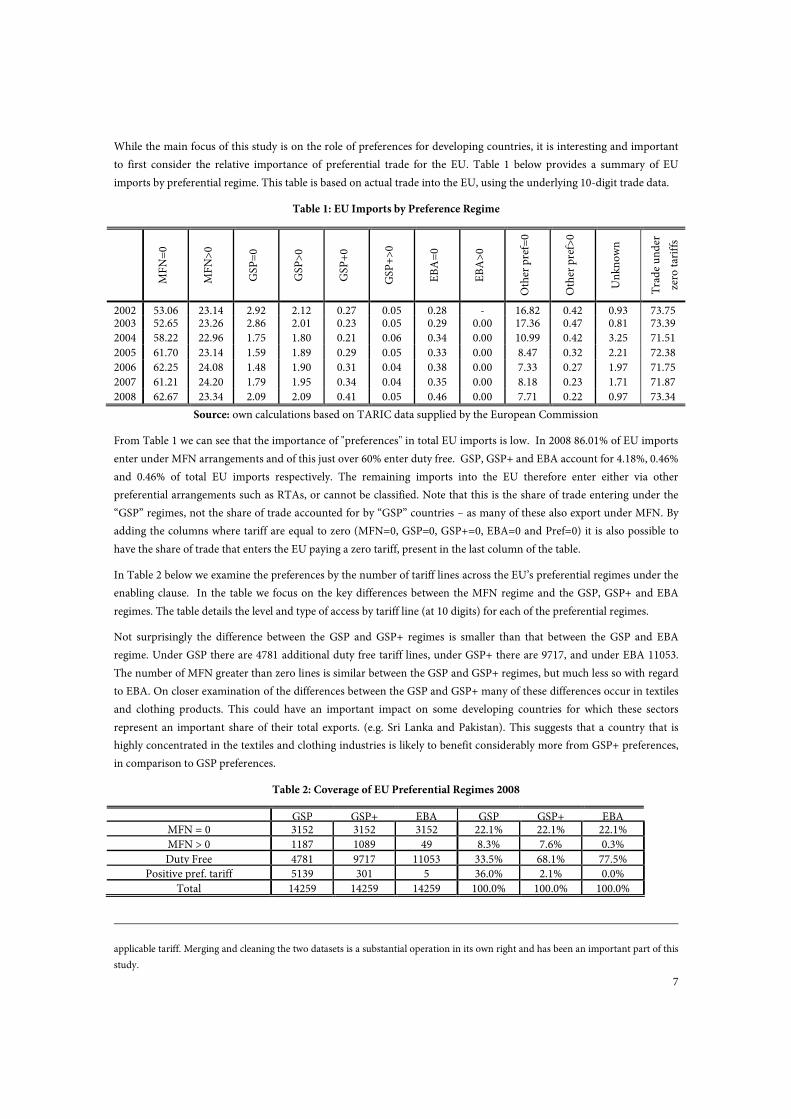
While the main focus of this study is on the role of preferences for developing countries, it is interesting and important

to first consider the relative importance of preferential trade for the EU. Table 1 below provides a summary of EU

imports by preferential regime. This table is based on actual trade into the EU, using the underlying 10-digit trade data.

Table 1: EU Imports by Preference Regime

MFN=0

MFN>0

GSP=0

GSP>0

GSP+0

GSP+>0

EBA=0

EBA>0

Other pref=0

Other pref>0

Unknown

Trade under

zero tariffs

2002 53.06 23.14 2.92 2.12 0.27 0.05 0.28 - 16.82 0.42 0.93 73.75 2003 52.65 23.26 2.86 2.01 0.23 0.05 0.29 0.00 17.36 0.47 0.81 73.39

2004 58.22 22.96 1.75 1.80 0.21 0.06 0.34 0.00 10.99 0.42 3.25 71.51

2005 61.70 23.14 1.59 1.89 0.29 0.05 0.33 0.00 8.47 0.32 2.21 72.38

2006 62.25 24.08 1.48 1.90 0.31 0.04 0.38 0.00 7.33 0.27 1.97 71.75

2007 61.21 24.20 1.79 1.95 0.34 0.04 0.35 0.00 8.18 0.23 1.71 71.87

2008 62.67 23.34 2.09 2.09 0.41 0.05 0.46 0.00 7.71 0.22 0.97 73.34

Source: own calculations based on TARIC data supplied by the European Commission

From Table 1 we can see that the importance of "preferences" in total EU imports is low. In 2008 86.01% of EU imports

enter under MFN arrangements and of this just over 60% enter duty free. GSP, GSP+ and EBA account for 4.18%, 0.46%

and 0.46% of total EU imports respectively. The remaining imports into the EU therefore enter either via other

preferential arrangements such as RTAs, or cannot be classified. Note that this is the share of trade entering under the

“GSP” regimes, not the share of trade accounted for by “GSP” countries – as many of these also export under MFN. By

adding the columns where tariff are equal to zero (MFN=0, GSP=0, GSP+=0, EBA=0 and Pref=0) it is also possible to

have the share of trade that enters the EU paying a zero tariff, present in the last column of the table.

In Table 2 below we examine the preferences by the number of tariff lines across the EU’s preferential regimes under the

enabling clause. In the table we focus on the key differences between the MFN regime and the GSP, GSP+ and EBA

regimes. The table details the level and type of access by tariff line (at 10 digits) for each of the preferential regimes.

Not surprisingly the difference between the GSP and GSP+ regimes is smaller than that between the GSP and EBA

regime. Under GSP there are 4781 additional duty free tariff lines, under GSP+ there are 9717, and under EBA 11053.

The number of MFN greater than zero lines is similar between the GSP and GSP+ regimes, but much less so with regard

to EBA. On closer examination of the differences between the GSP and GSP+ many of these differences occur in textiles

and clothing products. This could have an important impact on some developing countries for which these sectors

represent an important share of their total exports. (e.g. Sri Lanka and Pakistan). This suggests that a country that is

highly concentrated in the textiles and clothing industries is likely to benefit considerably more from GSP+ preferences,

in comparison to GSP preferences.

Table 2: Coverage of EU Preferential Regimes 2008

applicable tariff. Merging and cleaning the two datasets is a substantial operation in its own right and has been an important part of this

study.

GSP GSP+ EBA GSP GSP+ EBA MFN = 0 3152 3152 3152 22.1% 22.1% 22.1%

MFN > 0 1187 1089 49 8.3% 7.6% 0.3%

Duty Free 4781 9717 11053 33.5% 68.1% 77.5%

Positive pref. tariff 5139 301 5 36.0% 2.1% 0.0%

Total 14259 14259 14259 100.0% 100.0% 100.0%

8

Source: own calculations at 10-digits from TARIC

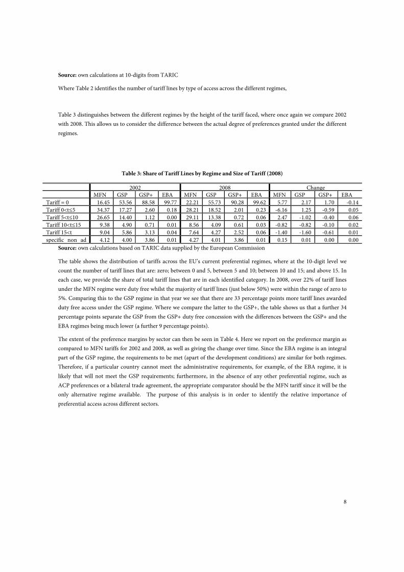
Where Table 2 identifies the number of tariff lines by type of access across the different regimes,

Table 3 distinguishes between the different regimes by the height of the tariff faced, where once again we compare 2002

with 2008. This allows us to consider the difference between the actual degree of preferences granted under the different

regimes.

Table 3: Share of Tariff Lines by Regime and Size of Tariff (2008)

2002 2008 Change MFN GSP GSP+ EBA MFN GSP GSP+ EBA MFN GSP GSP+ EBA

Tariff = 0 16.45 53.56 88.58 99.77 22.21 55.73 90.28 99.62 5.77 2.17 1.70 -0.14

Tariff 0<t≤5 34.37 17.27 2.60 0.18 28.21 18.52 2.01 0.23 -6.16 1.25 -0.59 0.05

Tariff 5<t≤10 26.65 14.40 1.12 0.00 29.11 13.38 0.72 0.06 2.47 -1.02 -0.40 0.06

Tariff 10<t≤15 9.38 4.90 0.71 0.01 8.56 4.09 0.61 0.03 -0.82 -0.82 -0.10 0.02

Tariff 15<t 9.04 5.86 3.13 0.04 7.64 4.27 2.52 0.06 -1.40 -1.60 -0.61 0.01

specific non ad 4.12 4.00 3.86 0.01 4.27 4.01 3.86 0.01 0.15 0.01 0.00 0.00

Source: own calculations based on TARIC data supplied by the European Commission

The table shows the distribution of tariffs across the EU’s current preferential regimes, where at the 10-digit level we

count the number of tariff lines that are: zero; between 0 and 5, between 5 and 10; between 10 and 15; and above 15. In

each case, we provide the share of total tariff lines that are in each identified category. In 2008, over 22% of tariff lines

under the MFN regime were duty free whilst the majority of tariff lines (just below 50%) were within the range of zero to

5%. Comparing this to the GSP regime in that year we see that there are 33 percentage points more tariff lines awarded

duty free access under the GSP regime. Where we compare the latter to the GSP+, the table shows us that a further 34

percentage points separate the GSP from the GSP+ duty free concession with the differences between the GSP+ and the

EBA regimes being much lower (a further 9 percentage points).

The extent of the preference margins by sector can then be seen in Table 4. Here we report on the preference margin as

compared to MFN tariffs for 2002 and 2008, as well as giving the change over time. Since the EBA regime is an integral

part of the GSP regime, the requirements to be met (apart of the development conditions) are similar for both regimes.

Therefore, if a particular country cannot meet the administrative requirements, for example, of the EBA regime, it is

likely that will not meet the GSP requirements; furthermore, in the absence of any other preferential regime, such as

ACP preferences or a bilateral trade agreement, the appropriate comparator should be the MFN tariff since it will be the

only alternative regime available. The purpose of this analysis is in order to identify the relative importance of

preferential access across different sectors.

9

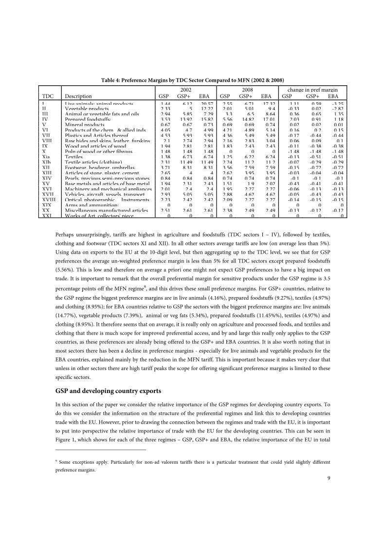
Table 4: Preference Margins by TDC Sector Compared to MFN (2002 & 2008)

2002 2008 change in pref margin TDC Description GSP GSP+ EBA GSP GSP+ EBA GSP GSP+ EBA

I Live animals; animal products 1.44 6.12 20.57 2.55 6.71 17.32 1.11 0.59 -3.25 II Vegetable products 2.33 5 12.22 2.01 5.01 9.4 -0.33 0.02 -2.82 III Animal or vegetable fats and oils 2.94 5.85 7.29 3.3 6.5 8.64 0.36 0.65 1.35 IV Prepared foodstuffs; 3.53 13.92 15.82 5.56 14.82 17.01 2.03 0.91 1.18 V Mineral products 0.67 0.67 0.73 0.69 0.69 0.74 0.02 0.02 0.01 VI Products of the chem.. & allied inds 4.05 4.7 4.99 4.21 4.89 5.14 0.16 0.2 0.15 VII Plastics and Articles thereof 4.53 5.93 5.93 4.36 5.49 5.49 -0.17 -0.44 -0.44 VIII Raw hides and skins, leather, furskins 2.1 2.74 2.94 2.16 2.83 3.04 0.06 0.09 0.1 IX Wood and articles of wood 1.94 2.81 2.81 1.83 2.43 2.43 -0.11 -0.38 -0.38 X Pulp of wood or other fibrous... 1.48 1.48 1.48 0 0 0 -1.48 -1.48 -1.48 Xia Textiles 1.38 6.73 6.74 1.25 6.22 6.24 -0.13 -0.51 -0.51 XIb Textile articles (clothing) 2.31 11.49 11.49 2.24 11.2 11.2 -0.07 -0.29 -0.29 XII Footwear, headgear, umbrellas... 3.71 8.31 8.31 3.56 7.59 7.59 -0.15 -0.72 -0.72 XIII Articles of stone, plaster, cement,... 2.65 4 4 2.62 3.95 3.95 -0.03 -0.04 -0.04 XIV Pearls, precious,semi-precious stones 0.84 0.84 0.84 0.74 0.74 0.74 -0.1 -0.1 -0.1 XV Base metals and articles of base metal 1.94 2.31 2.43 1.51 1.9 2.02 -0.43 -0.41 -0.41 XVI Machinery and mechanical appliances 2.01 2.4 2.4 1.95 2.27 2.27 -0.06 -0.13 -0.13 XVII Vehicles, aircraft, vessels, transport 2.93 5.05 5.05 2.88 4.62 4.62 -0.05 -0.43 -0.43 XVIII Optical, photographic,... Instruments 2.23 2.42 2.42 2.09 2.27 2.27 -0.14 -0.15 -0.15 XIX Arms and ammunition; 0 0 0 0 0 0 0 0 0 XX Miscellaneous manufactured articles 2.51 2.61 2.61 2.38 2.49 2.49 -0.13 -0.12 -0.12 XXI Works of Art, collectors' piece... 0 0 0 0 0 0 0 0 0

Perhaps unsurprisingly, tariffs are highest in agriculture and foodstuffs (TDC sectors I – IV), followed by textiles,

clothing and footwear (TDC sectors XI and XII). In all other sectors average tariffs are low (on average less than 5%).

Using data on exports to the EU at the 10-digit level, but then aggregating up to the TDC level, we see that for GSP

preferences the average un-weighted preference margin is less than 5% for all TDC sectors except prepared foodstuffs

(5.56%). This is low and therefore on average a priori one might not expect GSP preferences to have a big impact on

trade. It is important to remark that the overall preferential margin for sensitive products under the GSP regime is 3.5

percentage points off the MFN regime9, and this drives these small preference margins. For GSP+ countries, relative to

the GSP regime the biggest preference margins are in live animals (4.16%), prepared foodstuffs (9.27%), textiles (4.97%)

and clothing (8.95%); for EBA countries relative to GSP the sectors with the biggest preference margins are: live animals

(14.77%), vegetable products (7.39%), animal or veg fats (5.34%), prepared foodstuffs (11.45%%), textiles (4.97%) and

clothing (8.95%). It therefore seems that on average, it is really only on agriculture and processed foods, and textiles and

clothing that there is much scope for improved preferential access, and by and large this really only applies to the GSP

countries, as these preferences are already being offered to the GSP+ and EBA countries. It is also worth noting that in

most sectors there has been a decline in preference margins - especially for live animals and vegetable products for the

EBA countries, explained mainly by the reduction in the MFN tariff. This is important because it makes very clear that

unless in other sectors there are high tariff peaks the scope for offering significant preference margins is limited to these

specific sectors.

GSP and developing country exports

In this section of the paper we consider the relative importance of the GSP regimes for developing country exports. To

do this we consider the information on the structure of the preferential regimes and link this to developing countries

trade with the EU. However, prior to drawing the connection between the regimes and trade with the EU, it is important

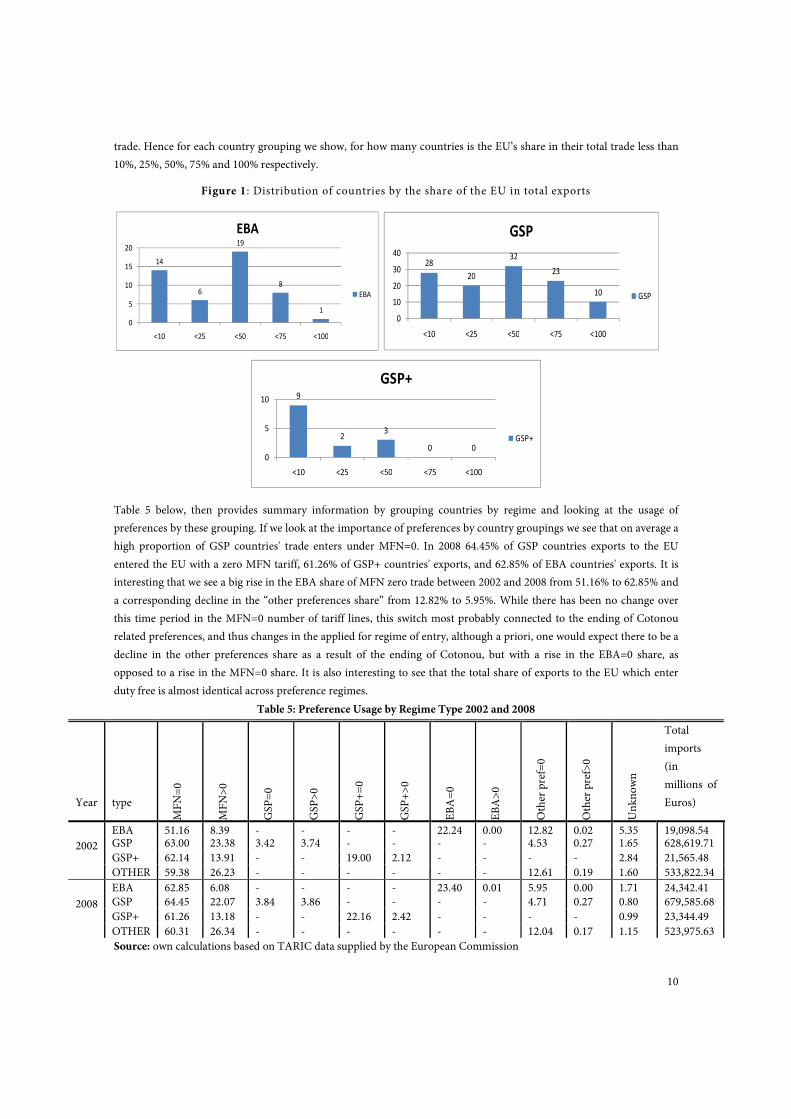
to put into perspective the relative importance of trade with the EU for the developing countries. This can be seen in

Figure 1, which shows for each of the three regimes – GSP, GSP+ and EBA, the relative importance of the EU in total

9 Some exceptions apply. Particularly for non-ad valorem tariffs there is a particular treatment that could yield slightly different

preference margins.

10

trade. Hence for each country grouping we show, for how many countries is the EU’s share in their total trade less than

10%, 25%, 50%, 75% and 100% respectively.

Figure 1: Distribution of countries by the share of the EU in total exports

14

6

19

8

1

0

5

10

15

20

<10 <25 <50 <75 <100

EBA

EBA

28

20

32

23

10

0

10

20

30

40

<10 <25 <50 <75 <100

GSP

GSP

9

23

0 0

0

5

10

<10 <25 <50 <75 <100

GSP+

GSP+

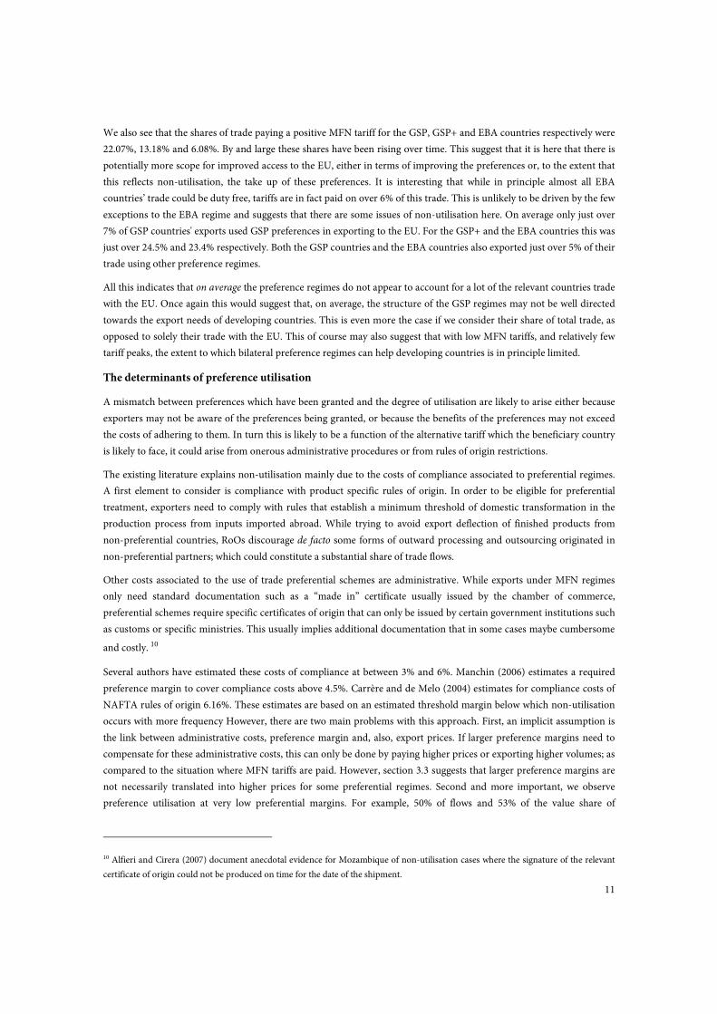
Table 5 below, then provides summary information by grouping countries by regime and looking at the usage of

preferences by these grouping. If we look at the importance of preferences by country groupings we see that on average a

high proportion of GSP countries' trade enters under MFN=0. In 2008 64.45% of GSP countries exports to the EU

entered the EU with a zero MFN tariff, 61.26% of GSP+ countries' exports, and 62.85% of EBA countries' exports. It is

interesting that we see a big rise in the EBA share of MFN zero trade between 2002 and 2008 from 51.16% to 62.85% and

a corresponding decline in the “other preferences share” from 12.82% to 5.95%. While there has been no change over

this time period in the MFN=0 number of tariff lines, this switch most probably connected to the ending of Cotonou

related preferences, and thus changes in the applied for regime of entry, although a priori, one would expect there to be a

decline in the other preferences share as a result of the ending of Cotonou, but with a rise in the EBA=0 share, as

opposed to a rise in the MFN=0 share. It is also interesting to see that the total share of exports to the EU which enter

duty free is almost identical across preference regimes.

Table 5: Preference Usage by Regime Type 2002 and 2008

Year type

MFN=0

MFN>0

GSP=0

GSP>0

GSP+=0

GSP+>0

EBA=0

EBA>0

Other pref=0

Other pref>0

Unknown

Total

imports

(in

millions of

Euros)

2002

EBA 51.16 8.39 - - - - 22.24 0.00 12.82 0.02 5.35 19,098.54 GSP 63.00 23.38 3.42 3.74 - - - - 4.53 0.27 1.65 628,619.71

GSP+ 62.14 13.91 - - 19.00 2.12 - - - - 2.84 21,565.48

OTHER 59.38 26.23 - - - - - - 12.61 0.19 1.60 533,822.34

2008

EBA 62.85 6.08 - - - - 23.40 0.01 5.95 0.00 1.71 24,342.41 GSP 64.45 22.07 3.84 3.86 - - - - 4.71 0.27 0.80 679,585.68

GSP+ 61.26 13.18 - - 22.16 2.42 - - - - 0.99 23,344.49

OTHER 60.31 26.34 - - - - - - 12.04 0.17 1.15 523,975.63

Source: own calculations based on TARIC data supplied by the European Commission

11

We also see that the shares of trade paying a positive MFN tariff for the GSP, GSP+ and EBA countries respectively were

22.07%, 13.18% and 6.08%. By and large these shares have been rising over time. This suggest that it is here that there is

potentially more scope for improved access to the EU, either in terms of improving the preferences or, to the extent that

this reflects non-utilisation, the take up of these preferences. It is interesting that while in principle almost all EBA

countries’ trade could be duty free, tariffs are in fact paid on over 6% of this trade. This is unlikely to be driven by the few

exceptions to the EBA regime and suggests that there are some issues of non-utilisation here. On average only just over

7% of GSP countries' exports used GSP preferences in exporting to the EU. For the GSP+ and the EBA countries this was

just over 24.5% and 23.4% respectively. Both the GSP countries and the EBA countries also exported just over 5% of their

trade using other preference regimes.

All this indicates that on average the preference regimes do not appear to account for a lot of the relevant countries trade

with the EU. Once again this would suggest that, on average, the structure of the GSP regimes may not be well directed

towards the export needs of developing countries. This is even more the case if we consider their share of total trade, as

opposed to solely their trade with the EU. This of course may also suggest that with low MFN tariffs, and relatively few

tariff peaks, the extent to which bilateral preference regimes can help developing countries is in principle limited.

The determinants of preference utilisation

A mismatch between preferences which have been granted and the degree of utilisation are likely to arise either because

exporters may not be aware of the preferences being granted, or because the benefits of the preferences may not exceed

the costs of adhering to them. In turn this is likely to be a function of the alternative tariff which the beneficiary country

is likely to face, it could arise from onerous administrative procedures or from rules of origin restrictions.

The existing literature explains non-utilisation mainly due to the costs of compliance associated to preferential regimes.

A first element to consider is compliance with product specific rules of origin. In order to be eligible for preferential

treatment, exporters need to comply with rules that establish a minimum threshold of domestic transformation in the

production process from inputs imported abroad. While trying to avoid export deflection of finished products from

non-preferential countries, RoOs discourage de facto some forms of outward processing and outsourcing originated in

non-preferential partners; which could constitute a substantial share of trade flows.

Other costs associated to the use of trade preferential schemes are administrative. While exports under MFN regimes

only need standard documentation such as a “made in” certificate usually issued by the chamber of commerce,

preferential schemes require specific certificates of origin that can only be issued by certain government institutions such

as customs or specific ministries. This usually implies additional documentation that in some cases maybe cumbersome

and costly. 10

Several authors have estimated these costs of compliance at between 3% and 6%. Manchin (2006) estimates a required

preference margin to cover compliance costs above 4.5%. Carrère and de Melo (2004) estimates for compliance costs of

NAFTA rules of origin 6.16%. These estimates are based on an estimated threshold margin below which non-utilisation

occurs with more frequency However, there are two main problems with this approach. First, an implicit assumption is

the link between administrative costs, preference margin and, also, export prices. If larger preference margins need to

compensate for these administrative costs, this can only be done by paying higher prices or exporting higher volumes; as

compared to the situation where MFN tariffs are paid. However, section 3.3 suggests that larger preference margins are

not necessarily translated into higher prices for some preferential regimes. Second and more important, we observe

preference utilisation at very low preferential margins. For example, 50% of flows and 53% of the value share of

10 Alfieri and Cirera (2007) document anecdotal evidence for Mozambique of non-utilisation cases where the signature of the relevant

certificate of origin could not be produced on time for the date of the shipment.

12

preferential imports eligible for preferences use these preferences when margins are below 6%, and 25% (24.92% of value

share) when margins are below 2.7%11.

In order to understand further non-utilisation of preferences we need to move from country and product averages

towards specific data at the product and country level. This analysis is possible since we observe for each year the

different regime of entry in the EU of exports at 10 digits level, allowing us to establish the determinants of non-

utilisation.

We estimate a reduced form equation for analysing the probability of preference utilisation based on the literature on

compliance costs, tariffs and margins in (5). The variable Yijt =1 if the trade flow of product j from country i for a specific

tariff regime is eligible to preferences and use them, and Yijt =0 in case of non-utilisation. An important element of our

data is the fact that because each flow is defined by tariff regime of entry to the EU, we can observe both, utilisation and

non-utilisation, for the same product, origin and period, which adds additional within variety variation to the sample

(see section 3.3.2 for a more detailed explanation of the data).

A problem that arises when estimating (5), however, is the fact that we need to restrict the sample to only flows eligible to

preferences. This raises issues of sample selection, since some of the determinants of preferential eligibility may also

explain utilisation of the preferences; therefore, potentially biasing the coefficient estimates. In order to correct for

potential selection bias, we employ a Heckman procedure and estimate a selection equation for the determinants of

preferential eligibility in (6), where S=1 if the export flow for that product, country and year is eligible for trade

preference and zero otherwise, and use the Inverse Mills ratio as an additional regressor for (5) as a control for potential

unexplained factors from preference eligibility12.

Y*=βX + ε (5)

Y=Y* if S=1

Y is not observed when S=0

S*=γZ + u (6)

S=0 if S*≤0

S=1 if S*≥0

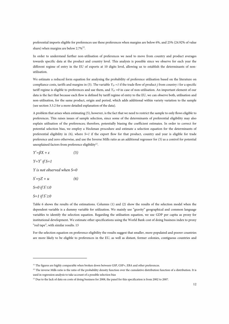
Table 6 shows the results of the estimations. Columns (1) and (2) show the results of the selection model when the

dependent variable is a dummy variable for utilization. We mainly use “gravity” geographical and common language

variables to identify the selection equation. Regarding the utilisation equation, we use GDP per capita as proxy for

institutional development. We estimate other specifications using the World Bank cost of doing business index to proxy

“red tape”, with similar results. 13

For the selection equation on preference eligibility the results suggest that smaller, more populated and poorer countries

are more likely to be eligible to preferences in the EU, as well as distant, former colonies, contiguous countries and

11 The figures are highly comparable when broken down between GSP, GSP+, EBA and other preferences. 12 The inverse Mills ratio is the ratio of the probability density function over the cumulative distribution function of a distribution. It is

used in regression analysis to take account of a possible selection bias 13 Due to the lack of data on costs of doing business for 2008, the panel for this specification is from 2002 to 2007.

13

countries with common language. Finally, more stringent rules of origin 14 increase the probability of preferential

eligibility, although it is difficult to capture the direction of causality, since it is possible that more stringent RoOs are

implemented on products with larger preferential coverage.

Regarding the main specification of interest, utilisation of preferences, the results correspond to what should be

expected, although the low level of the pseudo R2 indicates the importance of unexplained factors in explaining

utilisation. Richer countries are more likely to utilise preferences. As expected, the size of the preference margin available

for exporting increases the probability of preference utilisation. Although the coefficients in the table are the estimated

coefficients and not the marginal effects, the estimated marginal effect of the preference margin is 2.02, indicating that a

1 per cent increase in the preference margin increases the probability of utilising preferences by 2%. Also, more stringent

RoO reduce the probability of utilising preferences. Concretely, the marginal effect for the RoO index is -0.04, suggesting

a mild decrease of -0.04 in the probability of utilisation from increasing 1 level the degree of RoO rigidity. Finally, the

inverse Mills ratio coefficients are negative and statistically significant, indicating the need for correcting for sample

selection since unexplained factors for preference eligibility may impact utilisation negatively15.

In conclusion, once corrected for the determinants of preference eligibility, the use of preferences is correlated with the

size of the preferential margin, the flexibility of rules of origin and how large are bureaucratic costs in the exporting

country. As a result, the most accurate way of assessing the impact of preferential regimes on exports needs to consider

preference utilisation rather than simply eligibility (as is usually implemented in aggregate gravity estimations). This

implies working with effective tariffs paid rather than nominal tariffs or nominal preferential membership. Furthermore,

the results indicate that a positive impact on preference utilisation and as result on exports could be achieved by

improving rules of origin and export procedures in export countries.

Table 6: Determinants of non-utilisation

(1) (2) (3) (4) (5) (6) Selection1- Utilisation1 Utilisation2 Selection2- Utilisation Utilisation 1b

GDP_capita -0.3168*** 0.0701*** 0.0491***

(0.0009) (0.0013) (0.0012)

Cost Business -0.0797*** -0.0693***

(0.0015) (0.0015)

GDP -0.3761***

(0.0010)

Population 0.2501***

(0.0010)

Distance -0.4404*** -0.3133***

(0.0025) (0.0026)

Contiguity 0.1680*** 0.2274***

(0.0051) (0.0051)

Common language 0.0182*** 0.0018

(0.0028) (0.0028)

Colony 0.3245*** 0.2534***

(0.0028) (0.0029)

14 As RoO index we use the synthetic index developed in Cadot et al. (2007) at the HS-6 tariff level. This index ranges from 1, very

flexible, to 7 very stringent. The index ranks restrictiveness according to whether involves a change of tariff, subheading, heading or

chapter, or in the case of value content requirement depending on the percentage required. 15 In order to analyse the robustness of the results, we re-estimate the same specifications but changing the dependent variable. Rather

than using a dummy variable that measures whether an eligible trade flow requests preferences, we use as dependent variable the value

share of imports eligible for preferential treatment that use the preferential regime. This analysis is present in the main report but has

been excluding in this paper.

14

(1) (2) (3) (4) (5) (6) Selection1- Utilisation1 Utilisation2 Selection2- Utilisation Utilisation 1b

Preference margin 5.1004*** 5.4152*** 5.0597*** 5.3697***

(0.0342) (0.0388) (0.0343) (0.0390)

Roo 0.0933*** -0.0100*** -0.0043*** 0.0899*** -0.0034*** -0.0001

(0.0008) (0.0010) (0.0011) (0.0008) (0.0010) (0.0011)

year_2003 0.0500*** -0.0348*** 0.0691*** 0.0547*** -0.0322*** 0.0799***

(0.0040) (0.0045) (0.0051) (0.0041) (0.0045) (0.0051)

year_2004 -0.0941*** 0.0270*** 0.1087*** -0.0845*** 0.0136** 0.1100***

(0.0040) (0.0047) (0.0053) (0.0041) (0.0047) (0.0053)

year_2005 -0.0800*** -0.0190*** 0.0498*** -0.0624*** -0.0433*** 0.0450***

(0.0042) (0.0050) (0.0055) (0.0042) (0.0050) (0.0055)

year_2006 -0.1206*** 0.0136** 0.0555*** -0.1008*** -0.0193*** 0.0468***

(0.0042) (0.0051) (0.0055) (0.0042) (0.0050) (0.0055)

year_2007 -0.0336*** -0.0129* 0.0437*** 0.0021 -0.0348*** 0.0412***

(0.0043) (0.0051) (0.0056) (0.0044) (0.0051) (0.0056)

year_2008 0.0026 -0.0439*** 0.0446*** -0.0633***

(0.0043) (0.0051) (0.0044) (0.0051)

Lambda1 -0.5726*** -0.4179***

(0.0067) (0.0067)

Lambda2 -0.4021*** -0.3174***

(0.0065) (0.0066)

Constant 5.9564*** -0.3721*** 0.2279*** 3.2678*** -0.3109*** 0.1258***

(0.0235) (0.0106) (0.0096) (0.0228) (0.0105) (0.0094)

Observations 1459559 901157 725925 1459559 901157 725925

Log-likelihood -817875 -604057 -486678 -802508 -605851 -487466

Pseudo-R2 0.157 0.0300 0.0300 0.172 0.0272 0.0284

Standard errors in parentheses

*** p<0.001, ** p<0.01, * p<0.05

Price margins – or who captures the preference rent?

The importance of trade preferences for exporters critically depends on the coverage of trade flows and the utilisation of

such preferences. If exporters have capacity to export products covered by the preferential scheme and the costs of

compliance with the scheme are small enough, tariff preferences provide a competitive advantage to exporters vis a vis

other MFN exporters. However, in addition to coverage and utilisation, tariff preferences may impact the prices that

exporters receive by introducing a wedge in the border price of that product. Preferences effectively create a rent, and in

order to determine whether preferences are valuable, once should also analyse who appropriates this rent. The purpose

of this section is to analyse empirically who appropriates the rents created in the EU market by preferential regimes.

Few studies have looked empirically at this issue, although existing evidence suggests lack of full transmission of

preference margins to exporters. Olarreaga and Caglar (2005) for example study the impact of AGOA on export prices of

African exporters of apparel to the US. The authors find that only a small share of the tariff rent remained in the hands

of African exporters. Ozden and Sharma (2005) focus on exports of apparel to the US under the Caribbean basin

Initiative (CBI). They find that preferential exporters appropriate two thirds of the preference margin, increasing their

prices 9%. Alfieri and Cirera (2007) find for a group of primary commodities an incomplete pass-through from tariff

margin to price margin ranging between 0.4 and 0.6.

Given the rich and comprehensive nature of the dataset provided for this study, we can shed some light to the issue of

price rents moving beyond the study of specific products. Concretely, we compute the impact of preference margins

under GSP and other preferential schemes on price rents for a sample formed by thousand of products at 10 digits

classification and all exporters to the EU market.

15

The main challenge when estimating the degree of pass-through from tariff margin to price rents is the choice of

counterfactual. We can observe the price (proxied by the unit value) of a country exporting under a preferential regime

or MFN, but we do not know what its price would have been under a different scheme. As a result, we need some proxy

for the counterfactual price. There are several approaches in order to find these proxy prices, all of which have

shortcomings.

Quality Differentials

A proxy for the international price, as an approximation to the price that preferential exporters should receive when

exporting under the MFN regime, is the average MFN unit value. The main problem of this proxy is the fact that there

exist large differences in unit values within HS product categories, likely the result of quality differentials (Schott, 2004).

In this case, different varieties within the same each HS product may be competing in different quality segments and the

average MFN price will not be a good approximation for the price at each quality segment.

One possibility in order to correct for quality problems is to use the ratio of the same country unit value under MFN in

the same period that exporting also under a preferential scheme. The fact that countries do not always use preferences

implies that we may observe exports from the same country, product and period under different regimes, and, therefore,

under different tariffs. Therefore, under the assumption that quality differentials within exports of the same country and

product are minimal, this may constitute the best proxy.

There are two main problems to this approach. The first problem is the fact that by using only those observations where

we observe in the same country/product/period both, preference utilisation and non-utilisation, we effectively carry out

two sample selections. First, we exclude those observations not eligible for preferential treatment. Second, for those

eligible, we only use those cases where both utilisation and non-utilisation of preferences are observed and the price ratio

can be computed; excluding those observations eligible for preference that only use the preference in the same period or

only not use it. Thus, if some of the determinants of both selections also explain the price margin, such as income per

capita of exporter, then OLS estimates of the price margin equation are biased. In order to correct this we need to use a

Heckman (1979) procedure with a selection equation able to control for the different alternatives. This can be done by

employing a multinomial logit framework for selection, where we explain discrete outcomes such as non-eligibility,

utilisation, non-utilisation and both utilisation and non-utilisation happening in the same period.

A third problem is the fact that non-utilisation of preferences can sometimes be the result of specific problems at the

border such as getting the certificate of origin on time. If this is the case, we would expect to get the same price under

MFN and preferential scheme, because the exporter would have to face the burden of the sporadic customs inefficiency.

This would imply that with this specification there would be no tariff rent transmission to prices. However, in reality

would still be possible that the price under preference could still be higher than the price under an MFN contract.

Export Pricing

A more important problem is the fact that as suggested above, the price rent appears as a specific case of homogenous

products in competitive markets. Thus, under alternative competition frameworks, changes in tariffs may change

exporters’ strategic price decisions. Chang and Winters (2002) for example, show in a Bertrand monopolistic setting how

changes in preferential treatment in MERCOSUR have impacted on prices of exporters. This implies that in addition to

controlling for aggregate price increases, we need to control for the degree of product competition, which may impact

the degree of pass-through.

Transmission to export prices

An alternative approach is to look at whether changes in tariffs impact exporters’ prices. This is the general case under

which preferential treatment or changes in MFN tariffs are a subset. Obviously, any changes in MFN tariffs can be linked

to a price rent only if there is no full transmission to consumer prices, but we can still analyse whether changes in tariffs

16

in general are transmitted to export prices and whether this transmission is different for MFN and preferential tariff

changes.

Data and Methodology

We use import data at the country level and disaggregated at HS-10 supplied by the EC. Such fine level of disaggregation

allows us to minimise quality differences between product varieties16 in the same product category. Trade flows are

aggregated each year per country, product and tariff regime. The tariff regimes are: MFN; GSP, GSP+ or EBA; other

preferential regime; tariff suspension, and; MFN under quota or preferential under quota. In around 80% of the

observations we only observe one tariff regime, but on the remaining cases we may observe two regimes (more than 2 in

only 1% of observations). We match import data observations with tariff data from TARIC.17

We construct an export price equation based on the existing literature. In an imperfect competition setting, prices

depend on rival prices (Chang and Winters, 1992), which we proxy as the average price for that product on the EU

market. Second, prices depend on technology and unit costs that the exporter has for that product, their market power,

whether they have a tariff margin and any costs of compliance related with using preferential schemes.

),,,,(_

prefccpfp τφ ∆= (1)

We parameterize equation (1) in logarithms as:

ijttjiij

ijt

mfn

jt

ijtjtijt ecpp ++++++

++++= γδα

τ

τβφβββ

)1(

)1(

*32

_

10

(2)

Where the log of the export price pijt depends on the average log price for the product on that year p-jt, the market share

of the country on the same year and product Øijt, the ratio between the MFN tariff and the effective tariff paid

(preference margin), and a set of fixed and time effects. We assume that the specific unit cost cij does not change over

time, and in order to estimate equation (2) we use country product pair λ fixed effects, variety, that controls for all

specific country and product fixed effects.

jiijij c δαλ ++= (3)

ijttij

ijt

mfn

jt

ijtjtijt epp ++++

++++= γλ

τ

τβφβββ

)1(

)1(

*32

_

10 (4)

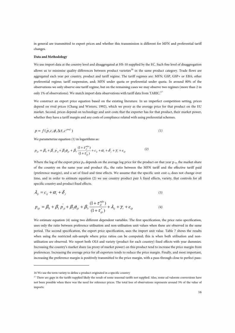
We estimate equation (4) using two different dependent variables. The first specification, the price ratio specification,

uses only the ratio between preference utilisation and non-utilisation unit values when these are observed in the same

period. The second specification, the export price specification, uses the import unit value. Table 7 shows the results

when using the restricted sub-sample where price ratios can be computed; this is when both utilisation and non-

utilisation are observed. We report both OLS and variety (product for each country) fixed effects with year dummies.

Increasing the country’s market share (as proxy of market power) on this product tend to increase the price margin from

preferences. Increasing the average price for all exporters tends to reduce the price margin. Finally, and most important,

increasing the preference margin is positively transmitted to the price margin, with a pass-through close to perfect pass-

16 We use the term variety to define a product originated in a specific country 17 There are gaps in the tariffs supplied likely the result of some seasonal tariffs not supplied. Also, some ad valorem conversions have

not been possible when there was the need for reference prices. The total loss of observations represents around 5% of the value of

imports.

17

through. This result is confirmed when we use the tariff rates when utilising and non-utilising preferences as separate

regressors. Increases in preferential tariffs reduce the price ratio by reducing the preference margin, and increases in

MFN tariffs increase the price ratio by increasing the margin.

As suggested above, the results for this specification are only indicative since the sample is reduced to around 340,000

observations, which is the number of observations when we can observe both utilisation and non-utilisation of

preferences for the same country, period and product. Therefore the estimates are likely to experience sample selection

bias. Furthermore, the results show a very low R2, indicating lack of explanatory power for price variations. This is likely

the result of not having information on variety costs, which is likely to be the main determinant of prices and their

variation.

Table 7: Export Price Ratio Specification

(1) (2) (3) (4) OLS1 FE1 OLS2 FE2

Average price -0.0334*** -0.1967*** -0.0330*** -0.1969*** (0.0025) (0.0060) (0.0025) (0.0060)

Market share 0.0052** 0.0060*** 0.0049** 0.0059***

(0.0019) (0.0018) (0.0019) (0.0018)

Preference margin 1.0245*** 0.8008***

(0.0624) (0.1180)

Tariff pref -0.7624*** -1.0275***

(0.1004) (0.1547)

Tariff mfn 1.0692*** 0.4960**

(0.0644) (0.1790)

year_2003 0.0254* 0.0120** 0.0254* 0.0117**

(0.0101) (0.0040) (0.0101) (0.0041)

year_2004 0.0221* 0.0105* 0.0213* 0.0100*

(0.0108) (0.0044) (0.0108) (0.0044)

year_2005 -0.0448*** -0.4321*** -0.0453*** -0.4331***

(0.0123) (0.0148) (0.0123) (0.0148)

year_2006 -0.0431*** -0.4341*** -0.0446*** -0.4351***

(0.0127) (0.0146) (0.0127) (0.0146)

year_2007 0.0366** 0.0406*** 0.0348** 0.0400***

(0.0116) (0.0051) (0.0116) (0.0051)

year_2008 0.0538*** 0.0551*** 0.0517*** 0.0544***

(0.0121) (0.0052) (0.0122) (0.0052)

Constant -0.0783*** 0.2763*** -0.0856*** 0.2996***

(0.0120) (0.0159) (0.0123) (0.0190)

Observations 333945 333945 333945 333945 R-squared 0.0069 0.0054 0.0071 0.0054

Number of variety 99985 99985

R2 within 0.0054 0.0054

R2 between 0.00436 0.00398

R2 overall 0.00408 0.00367

log-likelihood -220720 -220716

Robust standard errors in parentheses

*** p<0.001, ** p<0.01, * p<0.05

In order to correct for potential sample selection bias from reducing our sample to those periods where both utilisation

and non-utilisation are observed, we need to implement a selection procedure. We follow Bourguignon et al. (2004) and

estimate a multinomial logit model for the different utilisation alternatives. Concretely, we estimate the following

equation, where Yi is a discrete variable with value 0 to 3 according to whether a trade flow is only MFN eligible,

18

preferences fully utilised, preferences non-utilised or both, as compared to using an MFN regime. The price ratio is only

observed for Yi=3

Y*=βX + ε, for Y=0,1,2, 3

P*=βX + ε

P=P* if Y=3

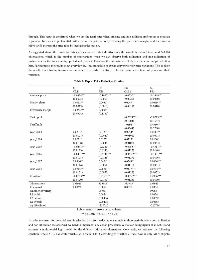
The interpretation of the estimated coefficients in the selection equation is complex, and needs to be understood as the

impact of each variable with respect the baseline category, MFN eligibility. The objective of the selection equation is to

control for the sample selection bias, rather than eligibility and utilisation In order to explain the different utilisation

regimes, we use an index that measures RoO rigidity, a dummy variable with value one is the good is an homogenous

good according to Rauch’s classification and GDP per capita as the identifying variables for the selection equation.

Table 8 shows the results for the selection equation. Since the selection model is a multinomial Logit, the coefficients

need to be interpreted in relation to the baseline category, the MFN regime. Larger MFN tariffs and smaller applied

tariffs increase the probabilities of both, preference utilisation and non-utilisation, vis-a-vis MFN eligibility; via

increasing the preference margin. That is, larger margins increase the probability that a trade flow is eligible for

preferences and these preferences are used or not used, compared to the trade flow being eligible to MFN treatment.

Income per capita reduces both, preference eligibility and utilisation, since richer countries are less likely to receive

preferences. Stringent RoOs reduce utilisation and homogenous goods according to Rauch’s classification are less likely

to being eligible for preferences.

Table 8: Multinomial Logit for Selection-Utilisation

(1) (2) (3)

utilisation non-utilisation utilisation & non-utilisation

Applied tariff -10.6679*** -12.7839*** -12.5863***

(3.1430) (3.1430) (3.1430)

MFN tariff 19.4376*** 24.7515*** 25.6474***

(3.1435) (3.1449) (3.1440)

GDP_capita -0.4485*** -0.3876*** -0.3371***

(0.0020) (0.0045) (0.0042)

RoO index 0.0309*** -0.0384*** -0.0048

(0.0020) (0.0039) (0.0036)

Homogenous -0.9826*** -1.7230*** -1.6781***

(0.0144) (0.0271) (0.0249)

year_2003 0.0197* 0.0975*** 0.1599***

(0.0089) (0.0182) (0.0173)

year_2004 -0.1562*** -0.1784*** -0.2722***

(0.0089) (0.0186) (0.0177)

year_2005 -0.5712*** -0.4328*** -0.6964***

(0.0098) (0.0197) (0.0189)

year_2006 -0.5319*** -0.4541*** -0.6973***

(0.0096) (0.0197) (0.0189)

year_2007 -0.4923*** -0.5156*** -0.7141***

(0.0101) (0.0202) (0.0193)

year_2008

Constant 2.6030*** -2.3160*** -1.8320***

(0.0196) (0.0472) (0.0431)

Observations 1245924 1245924 1245924

Pseudo R2 0.469 0.469 0.469

log-likelihood -866249 -866249 -866249

19

Standard errors in parentheses

*** p<0.001, ** p<0.01, * p<0.05

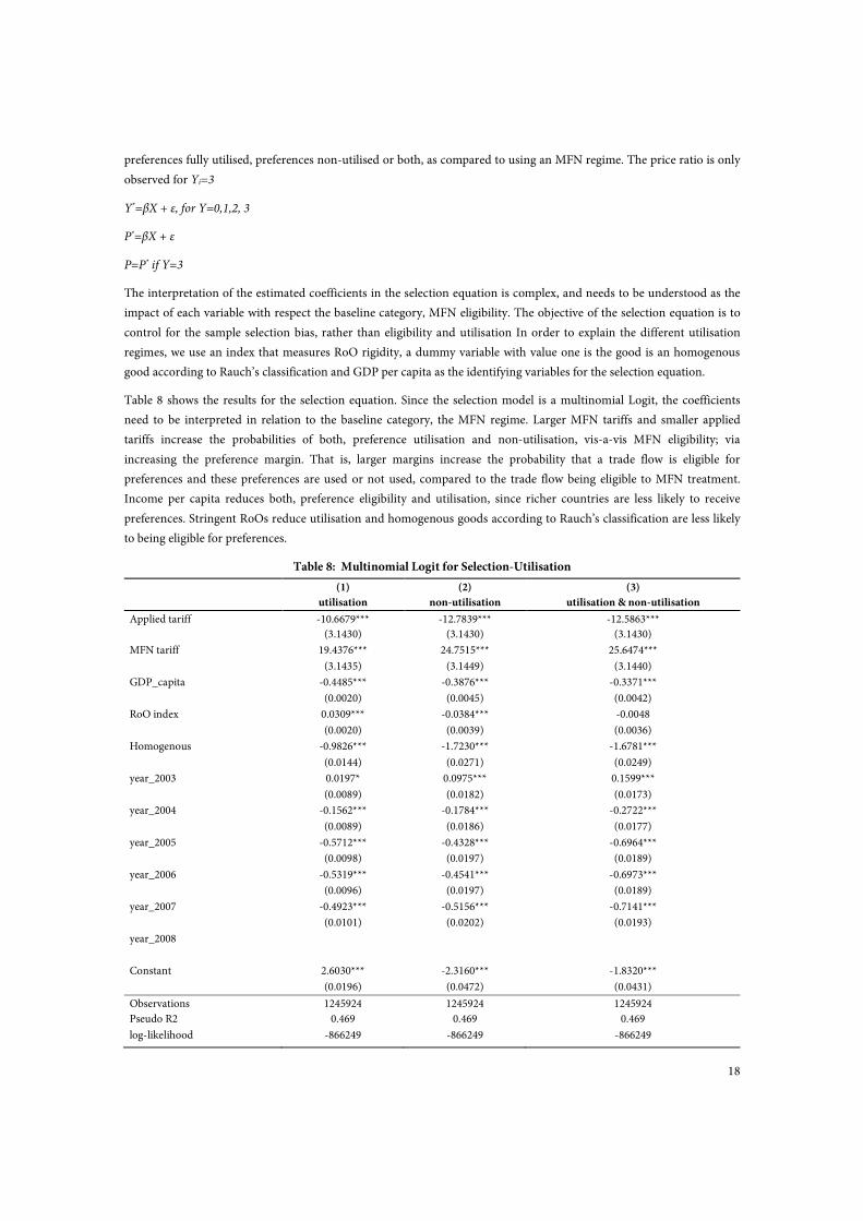
Once we have estimated the selection equation, we can use the estimated selectivity terms in the price ratio equation and

corrected for selection. Table 9 reports Bourguignon et al. (2004) preferred method. When this method is used the

preference margin pass-through is halved to 0.51

Summing up, the estimations suggest that preference margins are transmitted to exporters, although the degree of pass-

through is reduced to around 0.5 when we control for potential sample selection.

Table 9: Export Price Ratio Specification with Multinomial Selection (pref. margin)

(3) VARIABLES Bourguignon

Average price -0.0084 0.0017

Market share -0.0033

0.0008

Preference margin 0.5154

0.0440

year_2003 0.0049

(0.0062)

year_2004 0.0569***

(0.0067)

year_2005 0.1037***

(0.0097)

year_2006 0.0934***

(0.0096)

year_2007 0.1057***

(0.0082)

year_2008

m1 -3.2770***

(0.3162)

m2 -0.6589***

(0.1135)

m3 0.4366***

(0.1608)

Constant -1.0711

0.0770

Observations 283332

R-squared 0.0076

Robust standard errors in parentheses

*** p<0.001, ** p<0.01, * p<0.05

In order to check the robustness of the results, we also estimate equation (4) using the export price as explanatory

variable. This allows us to use the entire dataset, without the need to control for sample selection. Table 10 shows the

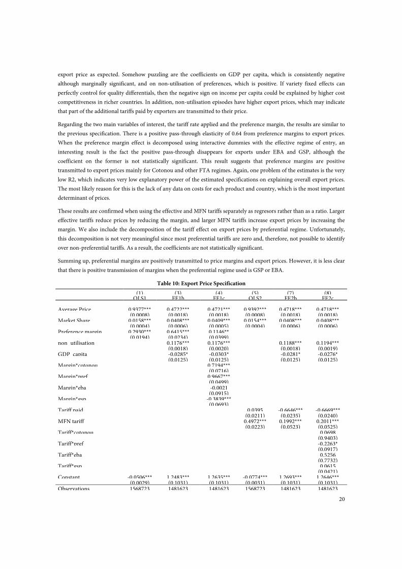
results when analysing the degree of pass-through to export prices. Since we do not compare prices from the same

country as in the previous specification, we need to control for quality differentials. Any variety specific quality issues

will be absorbed by the fixed effects, and we also control for country quality differentials between countries with GDP

per capita. In addition, we add a dummy for those export flows corresponding to non-utilisation episodes, to check

whether on these cases export prices are lower or higher.

The average product price has a positive impact on the export price, indicating similar sign of rival response or positive

price trends on average for each specific market. The country’s market share, the proxy for market power, increases the

20

export price as expected. Somehow puzzling are the coefficients on GDP per capita, which is consistently negative

although marginally significant, and on non-utilisation of preferences, which is positive. If variety fixed effects can

perfectly control for quality differentials, then the negative sign on income per capita could be explained by higher cost

competitiveness in richer countries. In addition, non-utilisation episodes have higher export prices, which may indicate

that part of the additional tariffs paid by exporters are transmitted to their price.

Regarding the two main variables of interest, the tariff rate applied and the preference margin, the results are similar to

the previous specification. There is a positive pass-through elasticity of 0.64 from preference margins to export prices.

When the preference margin effect is decomposed using interactive dummies with the effective regime of entry, an

interesting result is the fact the positive pass-through disappears for exports under EBA and GSP, although the

coefficient on the former is not statistically significant. This result suggests that preference margins are positive

transmitted to export prices mainly for Cotonou and other FTA regimes. Again, one problem of the estimates is the very

low R2, which indicates very low explanatory power of the estimated specifications on explaining overall export prices.

The most likely reason for this is the lack of any data on costs for each product and country, which is the most important

determinant of prices.

These results are confirmed when using the effective and MFN tariffs separately as regresors rather than as a ratio. Larger

effective tariffs reduce prices by reducing the margin, and larger MFN tariffs increase export prices by increasing the

margin. We also include the decomposition of the tariff effect on export prices by preferential regime. Unfortunately,

this decomposition is not very meaningful since most preferential tariffs are zero and, therefore, not possible to identify

over non-preferential tariffs. As a result, the coefficients are not statistically significant.

Summing up, preferential margins are positively transmitted to price margins and export prices. However, it is less clear

that there is positive transmission of margins when the preferential regime used is GSP or EBA.

Table 10: Export Price Specification

(1) (3) (4) (5) (7) (8) OLS1 FE1b FE1c OLS2 FE2b FE2c Average Price 0.9377*** 0.4722*** 0.4721*** 0.9392*** 0.4718*** 0.4718*** (0.0008) (0.0018) (0.0018) (0.0008) (0.0018) (0.0018) Market Share 0.0158*** 0.0408*** 0.0409*** 0.0154*** 0.0408*** 0.0408*** (0.0004) (0.0006) (0.0005) (0.0004) (0.0006) (0.0006) Preference margin 0.2930*** 0.6415*** 0.1146** (0.0194) (0.0234) (0.0399) non_utilisation 0.1176*** 0.1176*** 0.1188*** 0.1194*** (0.0018) (0.0020) (0.0018) (0.0019) GDP_capita -0.0285* -0.0303* -0.0281* -0.0276* (0.0125) (0.0125) (0.0125) (0.0125) Margin*cotonou 0.7194*** (0.0716) Margin*pref 0.9667*** (0.0499) Margin*eba -0.0021 (0.0915) Margin*gsp -0.3839*** (0.0693) Tariff paid 0.0395 -0.6646*** -0.6669*** (0.0211) (0.0235) (0.0240) MFN tariff 0.4972*** 0.1992*** 0.2011*** (0.0223) (0.0523) (0.0525) Tariff*cotonou 0.0698 (0.9403) Tariff*pref -0.2263* (0.0917) Tariff*eba 0.5256 (0.7732) Tariff*gsp 0.0615 (0.0421) Constant -0.0506*** 1.2483*** 1.2635*** -0.0774*** 1.2693*** 1.2646*** (0.0029) (0.1031) (0.1031) (0.0031) (0.1031) (0.1031) Observations 1568723 1481623 1481623 1568723 1481623 1481623

21

Robust standard errors in parentheses

*** p<0.001, ** p<0.01, * p<0.05

Gravity modeling

The basic gravity modelling framework assumes that trade between countries will depend on their respective sizes and

income levels, the distance between them, any common cultural/linguistic factors, and then on key policy variables (such

as being a member of a regional trade agreement, having a common currency….). A gravity model is thus typically used

in order to assess the impact of either differences in policy or changes in policy on flows of goods, services, and

investment between countries. Gravity models can thus be used to assess the aggregate and (if correctly specified)

sectoral impact on trade flows on a given country or country groupings and can thus shed light on the possible welfare

consequences, and on the impact on trade creation and trade.

For the purposes of this paper we undertake a highly disaggregated analysis of trade between the EU and developing

countries in order to ascertain with a degree of accuracy that has not previously been possible the extent to which the

preference margins implied by the different regimes impact on trade flows.

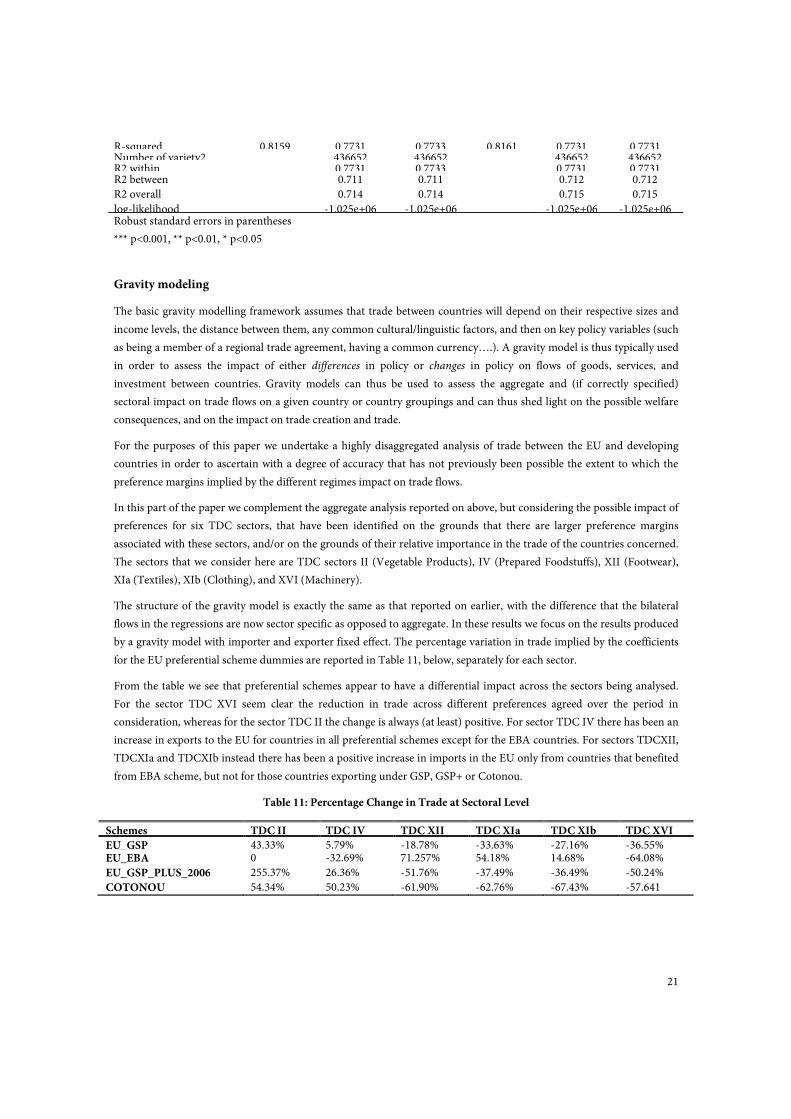
In this part of the paper we complement the aggregate analysis reported on above, but considering the possible impact of

preferences for six TDC sectors, that have been identified on the grounds that there are larger preference margins

associated with these sectors, and/or on the grounds of their relative importance in the trade of the countries concerned.

The sectors that we consider here are TDC sectors II (Vegetable Products), IV (Prepared Foodstuffs), XII (Footwear),

XIa (Textiles), XIb (Clothing), and XVI (Machinery).

The structure of the gravity model is exactly the same as that reported on earlier, with the difference that the bilateral

flows in the regressions are now sector specific as opposed to aggregate. In these results we focus on the results produced

by a gravity model with importer and exporter fixed effect. The percentage variation in trade implied by the coefficients

for the EU preferential scheme dummies are reported in Table 11, below, separately for each sector.

From the table we see that preferential schemes appear to have a differential impact across the sectors being analysed.

For the sector TDC XVI seem clear the reduction in trade across different preferences agreed over the period in

consideration, whereas for the sector TDC II the change is always (at least) positive. For sector TDC IV there has been an

increase in exports to the EU for countries in all preferential schemes except for the EBA countries. For sectors TDCXII,

TDCXIa and TDCXIb instead there has been a positive increase in imports in the EU only from countries that benefited

from EBA scheme, but not for those countries exporting under GSP, GSP+ or Cotonou.

Table 11: Percentage Change in Trade at Sectoral Level

Schemes TDC II TDC IV TDC XII TDC XIa TDC XIb TDC XVI

EU_GSP 43.33% 5.79% -18.78% -33.63% -27.16% -36.55% EU_EBA 0 -32.69% 71.257% 54.18% 14.68% -64.08%

EU_GSP_PLUS_2006 255.37% 26.36% -51.76% -37.49% -36.49% -50.24%

COTONOU 54.34% 50.23% -61.90% -62.76% -67.43% -57.641

R-squared 0.8159 0.7731 0.7733 0.8161 0.7731 0.7731 Number of variety2 436652 436652 436652 436652 R2 within 0.7731 0.7733 0.7731 0.7731 R2 between 0.711 0.711 0.712 0.712

R2 overall 0.714 0.714 0.715 0.715

log-likelihood -1.025e+06 -1.025e+06 -1.025e+06 -1.025e+06

22

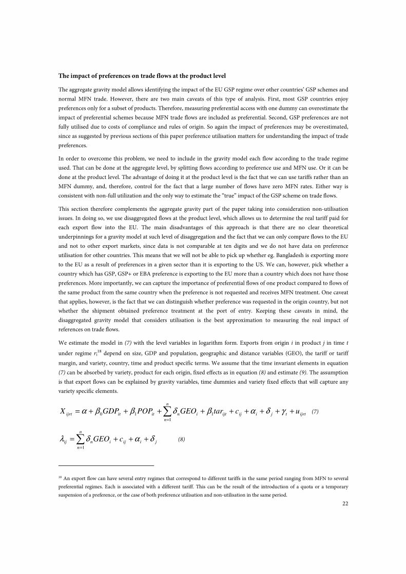
The impact of preferences on trade flows at the product level

The aggregate gravity model allows identifying the impact of the EU GSP regime over other countries’ GSP schemes and

normal MFN trade. However, there are two main caveats of this type of analysis. First, most GSP countries enjoy

preferences only for a subset of products. Therefore, measuring preferential access with one dummy can overestimate the

impact of preferential schemes because MFN trade flows are included as preferential. Second, GSP preferences are not

fully utilised due to costs of compliance and rules of origin. So again the impact of preferences may be overestimated,

since as suggested by previous sections of this paper preference utilisation matters for understanding the impact of trade

preferences.

In order to overcome this problem, we need to include in the gravity model each flow according to the trade regime

used. That can be done at the aggregate level, by splitting flows according to preference use and MFN use. Or it can be

done at the product level. The advantage of doing it at the product level is the fact that we can use tariffs rather than an

MFN dummy, and, therefore, control for the fact that a large number of flows have zero MFN rates. Either way is

consistent with non-full utilization and the only way to estimate the “true” impact of the GSP scheme on trade flows.

This section therefore complements the aggregate gravity part of the paper taking into consideration non-utilisation

issues. In doing so, we use disaggregated flows at the product level, which allows us to determine the real tariff paid for

each export flow into the EU. The main disadvantages of this approach is that there are no clear theoretical

underpinnings for a gravity model at such level of disaggregation and the fact that we can only compare flows to the EU

and not to other export markets, since data is not comparable at ten digits and we do not have data on preference

utilisation for other countries. This means that we will not be able to pick up whether eg. Bangladesh is exporting more

to the EU as a result of preferences in a given sector than it is exporting to the US. We can, however, pick whether a

country which has GSP, GSP+ or EBA preference is exporting to the EU more than a country which does not have those

preferences. More importantly, we can capture the importance of preferential flows of one product compared to flows of

the same product from the same country when the preference is not requested and receives MFN treatment. One caveat

that applies, however, is the fact that we can distinguish whether preference was requested in the origin country, but not

whether the shipment obtained preference treatment at the port of entry. Keeping these caveats in mind, the

disaggregated gravity model that considers utilisation is the best approximation to measuring the real impact of

references on trade flows.

We estimate the model in (7) with the level variables in logarithm form. Exports from origin i in product j in time t

under regime r;18 depend on size, GDP and population, geographic and distance variables (GEO), the tariff or tariff

margin, and variety, country, time and product specific terms. We assume that the time invariant elements in equation

(7) can be absorbed by variety, product for each origin, fixed effects as in equation (8) and estimate (9). The assumption

is that export flows can be explained by gravity variables, time dummies and variety fixed effects that will capture any

variety specific elements.

ijrttjiijijt

n

n

inititijrt uctarGEOPOPGDPX +++++++++= ∑=

γδαβδββα 1

1

10 (7)

jiij

n

n

inij cGEO δαδλ +++=∑=1

(8)

18 An export flow can have several entry regimes that correspond to different tariffs in the same period ranging from MFN to several

preferential regimes. Each is associated with a different tariff. This can be the result of the introduction of a quota or a temporary

suspension of a preference, or the case of both preference utilisation and non-utilisation in the same period.

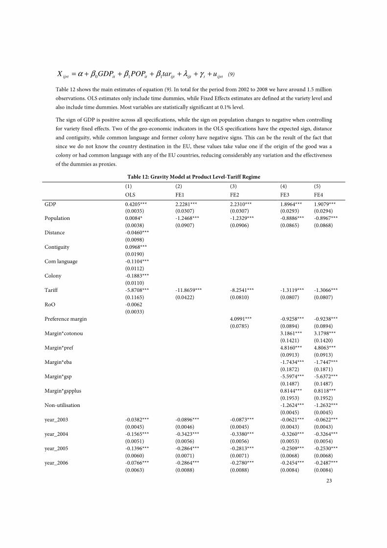
23

ijrttijtijtititijrt utarPOPGDPX ++++++= γλβββα110

(9)

Table 12 shows the main estimates of equation (9). In total for the period from 2002 to 2008 we have around 1.5 million

observations. OLS estimates only include time dummies, while Fixed Effects estimates are defined at the variety level and

also include time dummies. Most variables are statistically significant at 0.1% level.

The sign of GDP is positive across all specifications, while the sign on population changes to negative when controlling

for variety fixed effects. Two of the geo-economic indicators in the OLS specifications have the expected sign, distance

and contiguity, while common language and former colony have negative signs. This can be the result of the fact that

since we do not know the country destination in the EU, these values take value one if the origin of the good was a

colony or had common language with any of the EU countries, reducing considerably any variation and the effectiveness

of the dummies as proxies.

Table 12: Gravity Model at Product Level-Tariff Regime

(1) (2) (3) (4) (5)

OLS FE1 FE2 FE3 FE4

GDP 0.4205*** 2.2281*** 2.2310*** 1.8964*** 1.9079*** (0.0035) (0.0307) (0.0307) (0.0293) (0.0294)

Population 0.0084* -1.2468*** -1.2329*** -0.8886*** -0.8967***

(0.0038) (0.0907) (0.0906) (0.0865) (0.0868)

Distance -0.0460***

(0.0098)

Contiguity 0.0968***

(0.0190)

Com language -0.1104***

(0.0112)

Colony -0.1883***

(0.0110)

Tariff -5.8708*** -11.8659*** -8.2541*** -1.3119*** -1.3066***

(0.1165) (0.0422) (0.0810) (0.0807) (0.0807)

RoO -0.0062

(0.0033)

Preference margin 4.0991*** -0.9258*** -0.9238***

(0.0785) (0.0894) (0.0894)

Margin*cotonou 3.1861*** 3.1798***

(0.1421) (0.1420)

Margin*pref 4.8160*** 4.8063***

(0.0913) (0.0913)

Margin*eba -1.7434*** -1.7447***

(0.1872) (0.1871)

Margin*gsp -5.5974*** -5.6372***

(0.1487) (0.1487)

Margin*gspplus 0.8144*** 0.8118***

(0.1953) (0.1952)

Non-utilisation -1.2624*** -1.2632***

(0.0045) (0.0045)

year_2003 -0.0382*** -0.0896*** -0.0873*** -0.0621*** -0.0622***

(0.0045) (0.0046) (0.0045) (0.0043) (0.0043)

year_2004 -0.1565*** -0.3423*** -0.3380*** -0.3260*** -0.3264***

(0.0051) (0.0056) (0.0056) (0.0053) (0.0054)

year_2005 -0.1396*** -0.2864*** -0.2813*** -0.2509*** -0.2530***

(0.0060) (0.0071) (0.0071) (0.0068) (0.0068)

year_2006 -0.0766*** -0.2864*** -0.2780*** -0.2454*** -0.2487***

(0.0063) (0.0088) (0.0088) (0.0084) (0.0084)

24

year_2007 -0.0442*** -0.3108*** -0.3054*** -0.2375*** -0.2415***

(0.0069) (0.0106) (0.0106) (0.0101) (0.0101)

year_2008 -0.0533*** -0.3691*** -0.3650*** -0.2678*** -0.2744***

(0.0071) (0.0122) (0.0122) (0.0116) (0.0117)

Constant 3.0678*** -1.6628*** -1.9260*** -1.3081*** -1.3453***

(0.0855) (0.3347) (0.3343) (0.3191) (0.3205)

Observations 1459559 1459559 1459559 1459559 1451541

R-squared 0.1084 0.0823 0.0847 0.1664 0.1667

R2 within 0.0823 0.0847 0.166 0.167

R2 between 0.104 0.102 0.116 0.118

R2 overall 0.0774 0.0777 0.0985 0.0997

Number of variety 423913 423913 423913 421405

Robust standard errors in parentheses

*** p<0.001, ** p<0.01, * p<0.05

The impact of RoO rigidity on flows is negative but not statistically significant, and when controlling for variety fixed

effects, these absorb the variables that are constant over time. More interesting is the impact of the tariff and the tariff

margin. With regards the former, as expected, higher applied tariffs imply lower export flows. Regarding the latter

preference margins have a positive impact on exports.

We also decompose the impact of the preference margin according to the preferential regime used and add a dummy to

check the impact on exports of those episodes of non-utilisation of preferences. Unfortunately for the case of tariffs we

cannot use the regime used since most tariffs for EBA, and to a lesser extent for GSP, are at zero rates, and, therefore,

cannot be identified. The results of the interactive preference margins are interesting, since they indicate that the positive

impact of preference margins occur for FTA regimes and Cotonou, while margins are associated with lower exports for

the EBA and GSP preferences, and to a lesser extent for GSP+.19 It would be possible that exports of energy products that

have low preferential margins may be driving these results. For this reason, specification (5) estimates the same

specification but excluding all exports from chapter 27 “Mineral fuels and oils”. The results are almost identical to the

full sample. Regarding non-utilisation, the estimated coefficient is consistently negative, indication that non-utilisation

reduces the level of exports.

The previous estimates do not take into consideration the fact that we do not observe exports in most countries for all

products. There are in reality a large number of zero exports when we consider all potential exports. As a result, our

sample selection is not random, but obeys to observed flows more likely in larger countries. The problem when

correcting for this sample selection for disaggregated exports at 10 digits is that the dataset is too large to carry out the

estimations.20 One way to overcome this problem is to aggregate the dataset at HS-4 digits and estimate the model with

selection.

Table 13 shows the results of controlling for sample selection. The “export” column, selection equation, explains the

probability of exporting that specific HS-4 category, while the “export value” columns explain the level of exports. The

results are similar to the previous tables. However, now population and common language have the expected sign, and

RoO has a puzzling positive sign explaining the level of exports. Regarding the most important coefficients on applied

tariffs and preference margins, the coefficients have the expected signs. Higher applied tariffs reduce exports and higher

19 The impact of the different margins by regime is the sum of the coefficient on the margin plus the specific regime coefficient. In the

case of GSP+ the sum is around -0.11. 20 Including zeroes for all the potential flows for all countries and all products during the period 2002-2008 will increase the sample to

more than 20 million observations, out of reach of the computing capacity of a standard PC using STATA.

25

margins increase exports. We also decompose the impact of the preference margin for GSP and EBA. This time,

however, due to aggregation to HS4 the preferential regime does not reflect utilisation, since both, utilisation and non-

utilisation, are lost during the aggregation. We do, however, add a dummy if there has been some non-utilisation for that

hs-4 category, country and period. At this level of aggregation and without distinguishing flows by utilisation the

margins for different regimes are highly correlated, and therefore, we only can use GSP and EBA. Interestingly, both

interactive coefficients are positive, which indicate that the coefficients are absorbing potentially differentiated impact of

the other preferential margins, Cotonou and other FTAs. This highlights the danger of obtaining biased estimators when

the true utilised preferential regime is not considered and the need to work with highly disaggregated data.

One potential problem of the previous results is the fact that they are estimated as pooled regression. If the error term

should be modelled using a panel structure then the standard Heckman selection term is no longer valid for correcting

selection bias Vella (1998). In order to correct for selection in the panel specification, Table 14 presents the results when

using Wooldridge’s methodology for sample selection and panel data. We first estimate a probit regression for the

probability of exporting each year as a country cross-section and calculate the inverse Mills ratio adding the selection

term at each year. Then, we add this inverse mills ratio to a pooled level regression for the level of exports. The results are

similar to the standard Heckman estimates presented above. The significance of the correlation of residuals between the

selection and level equation, as well as the inverse mills ratio (lambda), indicate the need for correcting for sample

selection problems. The main coefficients remain similar. Tariffs reduce the level of exports, while preferential margins

increase the level of exports.

Table 13: Gravity at HS4 with Selection

(1) (1) (2) (2) (3) (3) value export Value export value export

GDP 0.5607*** 0.5598*** 0.6199*** (0.0182) (0.0163) (0.0187)

Population 0.0923*** 0.0984*** 0.0483**

(0.0183) (0.0164) (0.0187)

GDP_capita 0.2201*** 0.2201*** 0.2201***

(0.0008) (0.0008) (0.0008)

Distance -0.1856*** 0.0214*** -0.1764*** 0.0215*** -0.1360*** 0.0213***

(0.0106) (0.0026) (0.0105) (0.0026) (0.0106) (0.0026)

Contig 0.6761*** 0.3401*** 0.6431*** 0.3401*** 0.6605*** 0.3401***

(0.0338) (0.0053) (0.0315) (0.0053) (0.0344) (0.0053)

Com language 0.0983*** -0.2098*** 0.0931*** -0.2099*** 0.0929*** -0.2097***

(0.0217) (0.0032) (0.0202) (0.0032) (0.0221) (0.0032)

Colony -0.1303*** -0.0726*** -0.1366*** -0.0727*** -0.1901*** -0.0727***

(0.0141) (0.0034) (0.0140) (0.0034) (0.0142) (0.0034)

Tariff -4.2572*** -4.7980*** -5.7787***

(0.1014) (0.1024) (0.1045)

RoO 0.0385*** 0.0184*** 0.0150*** 0.0184*** 0.0147*** 0.0184***

(0.0039) (0.0008) (0.0039) (0.0008) (0.0039) (0.0008)

Margin 2.6141*** 2.3094***

(0.0764) (0.1132)

Margin*gsp 0.7321***

(0.1488)

Margin*eba 1.4627***

(0.2284)

Non-uti 0.5011***

(0.0105)

year_2003 -0.0539** 0.0030 -0.0587*** 0.0029 -0.0674*** 0.0030

(0.0177) (0.0044) (0.0177) (0.0044) (0.0176) (0.0044)

year_2004 -0.1804*** -0.0269*** -0.1839*** -0.0269*** -0.1743*** -0.0269***

(0.0179) (0.0044) (0.0179) (0.0044) (0.0179) (0.0044)

26

year_2005 -0.1707*** -0.1288*** -0.1611*** -0.1288*** -0.1697*** -0.1288***

(0.0212) (0.0045) (0.0206) (0.0045) (0.0212) (0.0045)

year_2006 -0.0963*** -0.1102*** -0.0868*** -0.1101*** -0.0874*** -0.1102***

(0.0204) (0.0045) (0.0200) (0.0045) (0.0204) (0.0045)

year_2007 -0.0367 -0.1406*** -0.0308 -0.1405*** -0.0397 -0.1406***

(0.0219) (0.0045) (0.0213) (0.0045) (0.0220) (0.0045)

year_2008 -0.0757*** -0.1130*** -0.0692*** -0.1130*** -0.0827*** -0.1130***

(0.0209) (0.0046) (0.0205) (0.0046) (0.0209) (0.0046)

Athrho -0.1064** -0.1302*** -0.0932*

(0.0383) (0.0342) (0.0394)

lnsigma 1.0454*** 1.0457*** 1.0391***

(0.0032) (0.0035) (0.0030)

Constant 4.4369*** -2.4942*** 4.4826*** -2.4946*** 3.7352*** -2.4933***

(0.1897) (0.0232) (0.1740) (0.0232) (0.1939) (0.0232)

Observations 1415565 1415565 1415565 1415565 1415565 1415565

Standard errors in parentheses

*** p<0.001, ** p<0.01, * p<0.05

Table 14: Gravity Model at HS4 with Wooldridge Panel Selection

(1) (2) (3) Model1 Model2 Model1

GDP 0.5127*** 0.5258*** 0.5703***

(0.0073) (0.0073) (0.0074)

Population 0.1407*** 0.1328*** 0.0984***

(0.0076) (0.0076) (0.0076)

Distance -0.1852*** -0.1745*** -0.1363***

(0.0102) (0.0102) (0.0102)

Contig 0.5858*** 0.5743*** 0.5686***

(0.0233) (0.0233) (0.0233)

Com language 0.1553*** 0.1361*** 0.1516***

(0.0145) (0.0145) (0.0144)

Colony -0.1329*** -0.1427*** -0.1918***

(0.0136) (0.0136) (0.0135)

Tariff -4.2400*** -4.7781*** -5.7582***

(0.1146) (0.1148) (0.1228)

RoO 0.0345*** 0.0123** 0.0106**

(0.0038) (0.0039) (0.0038)

Margin 2.5957*** 2.2550***

(0.0938) (0.1330)

Margin*gsp 0.7914***

(0.1819)

Margin*eba 1.4981***

(0.2801)

Non-uti 0.5017***

(0.0105)

Lambda -0.5816*** -0.5635*** -0.5560***

(0.0383) (0.0383) (0.0378)

Constant 4.7481*** 4.6628*** 4.0681***

(0.1058) (0.1056) (0.1057)

Observations 326660 326660 326660 R-squared 0.1852 0.1881 0.1940

Robust standard errors in parentheses

*** p<0.001, ** p<0.01, * p<0.05

27

The results of the disaggregated gravity indicate that as expected tariffs reduce the level of exports, while tariff margins

increase exports. This results control for non-utilisation of preferences, so when countries are able to use those

preferences the results are as expected. A surprising result is, however, that when the preference margin is decomposed

by preferential regime, the average preference margin is driven by Cotonou and FTA preferences, while EBA, GSP and

GSP+ are associated with a negative impact on exports.

Computable General Equilibrium Evaluation of the GSP

In order to isolate the effects of tariff changes under the GSP 2006-2008 scheme from other exogenous influences, a

global computable general equilibrium (CGE) modelling approach is adopted in this section The analytic framework is

the GLOBE model, a multi-regional and multi-sectoral CGE model of global production and trade developed by

McDonald, Robinson and Thierfelder (2007). The model is calibrated to the new GTAP7 database that reflects the global

input-output structure of production and trade by origin and destination in 2004. The database distinguishes 113

geographical regions and 57 commodity groups.

For the present study, we construct a 32-region aggregation of the GTAP database which identifies a range of individual

and composite GSP, GSP+ and EBA “countries/regions” with an appropriate level of geographical detail for the partner

countries as identified in the GTAP dataset. As shown in Table 15, the regional aggregation distinguishes eight GSP+

countries / regions, four EBA countries / region blocs, and a range of other developing GSP region blocs. The agreed

sectoral aggregation distinguishes 19 commodity groups and activities and aims to separately identify the product groups

most affected by the GSP scheme at the deepest possible disaggregation level (Table 16). The model includes five primary

production factors: skilled labour, unskilled labour, capital, land and natural resources.

A distinct advantage of using a global CGE model for the purpose at hand is that it allows a comprehensive integrated

internally consistent assessment of the trade creation, trade diversion, sectoral employment and structural

transformation effects triggered by the GSP scheme along with an evaluation of the aggregate welfare effects by country

while taking full account of indirect open-economy general equilibrium feedback linkages.

The model framework allows analysing the incremental impact of the switch from the pre-2006 GSP (i.e. 2004) to the

2006-09 GSP regime as well as an evaluation of the total impact of the GSP in the form of a comparison of the 2006-09

equilibrium with a “no-GSP” anti-monde. In this latter scenario, all EU import tariffs faced by the GSP, GSP+ and EBA

beneficiaries will be raised to MFN level. Furthermore, we consider a switch from the observed levels of utilization of

GSP preferences to a full utilization of preferential GSP tariffs. Finally, we simulate a complete elimination of all EU

import tariffs for GSP countries. Finally, we simulate a complete elimination of all EU import tariffs for GSP countries.

The following section provides a brief non-technical outline of the GLOBE model. Section 5.3 highlights a number of key

features of the benchmark data set and section 5.4 presents the results of the simulation analysis.

The GLOBE Model

GLOBE is a theory-grounded, comparative-static, multi-region, multi-sectoral CGE model of global production and

trade developed by McDonald, Robinson and Thierfelder (2007).21 The model version used here is calibrated to the new

GTAP7 database that reflects the global input-output structure of production and trade by origin and destination in

2004.

International Trade

21 For recent applications of this model to the analysis of preferential trading arrangements see e.g. Polaski et al. (2009), World Bank

(2009), CARIS (2008), McDonald, Thierfelder and Robinson (2008) and McDonald and Willenbockel (2008).

28

Domestically produced commodities are assumed to be imperfect substitutes for traded goods. Import demand is

modelled via a series of nested constant elasticity of substitution (CES) functions; imported commodities from different

source regions to a destination region are assumed to be imperfect substitutes for each other and are aggregated to form

composite import commodities that are assumed to be imperfect substitutes for their counterpart domestic commodities

The composite imported commodities and their counterpart domestic commodities are then combined to produce

composite consumption commodities, which are the commodities demanded by domestic agents as intermediate inputs

and final demand (private consumption, government, and investment). Export supply is modelled via a series of nested

constant elasticity of transformation (CET) functions; the composite export commodities are assumed to be imperfect

substitutes for domestically consumed commodities, while the exported commodities from a source region to different

destination regions are assumed to be imperfect substitutes for each other. The composite exported commodities and

their counterpart domestic commodities are then combined as composite production commodities. The use of nested

CET functions for export supply implies that domestic producers adjust their export supply decisions in response to

changes in the relative prices of exports and domestic commodities. This specification is desirable in a global model with

a mix of developing and developed countries that produce different kinds of traded goods with the same aggregate

commodity classification, and yields more realistic behaviour of international prices than models assuming perfect

substitution on the export side.

Production, Input Demand and Factor Markets

Production relationships by activities are characterized by nested Constant Elasticity of Substitution (CES) production

functions. Activity output is a CES composite of aggregate intermediate inputs and aggregate value added, while

aggregate intermediate inputs are a Leontief aggregate of the individual intermediate commodity inputs and aggregate

value added is a CES composite of primary factors demanded by each activity. The determination of product supply and

input demand is based on the assumption of profit maximizing behaviour.

Two alternative factor market regimes are considered in this study – a standard neoclassical long-run full employment

closure and a closure that allows for unemployed unskilled labour in the developing regions of the model. Under the

latter closure, factor markets in developed countries are characterized by inelastic factor supplies and the model solves

for market-clearing factor prices like under the neoclassical closure. In developing regions, however, the real wage of

skilled and unskilled labour is fixed in terms of the domestic consumer price index and the supply of skilled and

unskilled labour is infinitely elastic at that wage. In this specification, any shock that would otherwise reduce the

equilibrium wage will instead lead to increased unemployment. In both factor market regimes, the primary factors

except activity-specific natural resource endowments are mobile across production activities, but immobile across

borders.

Final Domestic Demand by Commodity

The commodity composition of government consumption demand and investment demand is fixed, with demand

patterns from the benchmark data set. Households are utility maximizers who respond to changes in relative prices and

incomes. In this version of the model, the utility functions for private households take the Stone-Geary form and hence

consumer demand by commodity is described by a Linear Expenditure System (LES) specification.

Macro Closure

For this exercise a “neutral” or “balanced” set of macro closure rules is specified. Current account balances for all regions

are assumed to be fixed at initial benchmark levels in terms of a global numeraire and real exchange rates adjust to

maintain external equilibrium. The global numeraire is the basket of goods underlying the EU consumer price index.

Any change in, say, the nominal value of export earnings at world market prices The assumption of fixed current

account balances ensures that there are no changes in future “claims” on exports across the regions in the model, i.e., net

asset positions are fixed. In addition, we assume a “balanced” macro adjustment to the trade policy shocks within

29

countries. Changes in aggregate absorption are assumed to be shared equally (to maintain the shares from the base data)

among private consumption, government, and investment demands. Household and government saving rates adjust

residually to establish the macroeconomic saving-investment balance in each region.

Benchmark Data and Calibration

The model is calibrated to a social accounting matrix representation of the GTAP 7.0 database (Narayanan and

Walmsley (eds.), 2008) that combines detailed bilateral trade, and protection data reflecting economic linkages among

regions with individual country input-output data, which account for intersectoral linkages within regions, for the

benchmark year 2004. Production, trade and income elasticities are drawn from the GTAP behavioural data base.

Table 15: Regional Aggregation of the Model

Code Description Status Notes

EU European Union ex post-2004 entrants Bulgaria, Romania

RoOECD Rest of OECD+

SriLanka Sri Lanka GSP+

Peru Peru GSP+

Ecuador Ecuador GSP+

Colombia Colombia GSP+

CostaRica Costa Rica GSP+

GSP+ LA GSP+ Other Latin America GSP+ Bolivia, Paraguay, Guatemala, Panama,

Nicaragua, El Salvador, Rest of Ctrl America

GSP+ EE GSP+ Eastern Europe GSP+ Armenia, Azerbaijan

Georgia Georgia GSP+

Cambodia Cambodia EBA

Bangladesh Bangladesh EBA

EBA RoAs EBA: Rest of Asia EBA Afghanistan, Bhutan,Laos,Maldives,

Myanmar,Nepal

EBA SSA EBA: Sub-Saharan Africa EBA Angola, DR Congo, Ethiopia, Madagascar,

Malawi, Mozambique, Senegal, Tanzania,

Uganda

China China GSP

Philippines Philippines GSP

India India GSP

Pakistan Pakistan GSP

Thailand Thailand GSP

RoAsia Rest of Asia GSP

Argentina Argentina GSP

Brazil Brazil GSP

Caribbean Caribbean GSP

Russia Russia GSP

Ukraine Ukraine GSP

RoSEE Rest of Southern and Eastern Europe GSP

CtrlAsia Central Asia GSP

NAfrica North Africa GSP

RoSSA Rest of Sub-Saharan Africa GSP/EBA Non-EBA and composite mixed EBA/GSP

SSA regions in GTAP7

SAfrica South Africa GSP

Emerged Emerged DCs (GSP) Hong Kong, Taiwan, Singapore, Korea, Chile,

Mexico *

30

RoWorld Rest of World (GSP) Middle, East, Iran, Turkey, Uruguay, Guyana,

Falklands *

* Non-beneficiary countries in italics

Table 16: Commodity Aggregation of the Model

Code Description

Rice Paddy rice, processed rice

Vegetables, fruits Vegetables, fruit, nuts

Other crops Wheat, other cereal grains, plant-based fibres, crops nec

Oils, fats Oil seeds, vegetable oils and fats

Sugar prd Sugar cane, sugar beet, processed sugar products

Livestock prd Livestock except fish, raw milk, animal products except meat

Fishing prd Fishing products

Fossile fuels Fossile fuels: Coal, oil, gas, petroleum, coal products

Mineral prd Minerals nec, mineral products

Other food prd Meat, dairy products, food products nec, beverages, tobacco

Textiles Textiles

Apparel Apparel

Leather prd Leather products

Other light mnf Light manufacturing: Forestry and wood products, paper products,

publishing, other manufacturing

Chemicals Chemical, rubber, plastic products

Metal prd Metals and metal products

Transport equip Motor vehicles and parts, other transport equipment

Machinery, elec equip Electronic equipment, machinery and equipment nec

Services Construction, utilities, services

Simulation Results

Five different computable general equilibrium simulation scenarios are considered in this section (Table 17). The first

simulation evaluates the switch from the pre-2006 to the 2006-2009 EU GSP regime while taking account of the actual

observed degree of utilization of preferential GSP tariffs including GSP+ and EBA preferences. The next two simulation

runs aim to provide an overall assessment of the EU GSP through a comparison of the observed 2004 benchmark

equilibrium with an anti-monde in which the EU GSP does not exist at all. In this case, the observed applied benchmark

tariff rates for the EU GSP beneficiary regions including EBA and GSP+ countries switch to 2004 or 2006 MFN rates in

the counterfactual equilibrium. The FULLGSP scenario contemplates a switch in EU import tariff rates from the

observed 2006 effective levels to the effective levels that would prevail under a 100% utilization of GSP, GSP+ and EBA

preferences. The final scenario explores, to which extent developing countries could benefit from a further extension of

preferential treatment by simulating a complete removal of all EU duties on imports from existing GSP beneficiaries.

Table 17: Simulation Scenarios

Code Scenario Description

GSP06 Change from applied 2004 EU GSP to applied EU 2006 GSP tariffs

MFN04 Abolition of EU GSP: Change from EU GSP tariffs to 2004 MFN tariffs

MFN06 Abolition of EU GSP: Change from EU GSP tariffs to 2006 MFN tariffs

FULLGSP Switch from observed 2006 utilization to 100% Utilization of EU GSP tariffs

ZEROTM Complete elimination of all EU import tariffs for GSP countries

Table 18 provides summary information on the size orders of the simulated percentage changes of the power of EU

imports by commodity group for each of the five scenarios – that is the percentage change of (1 + tariff rate), which

31

provides a measure of the change in the price faced by EU purchasers on impact, i.e. before secondary general

equilibrium feedback effects that affect the ex-tariff supply price of imports have played out.22 The table reports the

simple average across all GSP regions for each commodity group as well as the largest reduction – or largest increase in

the case of the MFN scenarios – among the region-specific changes in the power of tariffs.

Table 18: % Changes in the Power of EU Import Tariffs by Scenario & Commodity Group

Average Max or Min

GSP06

MFN04

MFN06

FULLGSP

ZEROTM

GSP06

MFN04

MFN06

FULLGSP

ZEROTM

Rice -18.1 5.4 2.1 -1.8 -29.7 -63.5 53.3 24.2 -22.9 -57.4

Vegetables, fruits -5.2 10.1 7.2 -0.3 -9.8 -31.2 132.2 88.0 -8.8 -45.2

Other crops 0.4 1.8 1.9 -0.2 -5.0 -0.9 22.5 23.1 -1.8 -31.5

Oils, fats -0.2 1.8 1.7 -0.6 -3.3 -3.6 21.5 15.7 -8.8 -36.9

Sugar prd -1.3 14.7 11.8 -0.1 -40.6 -6.6 71.8 60.8 -2.2 -73.0

Livestock prd 0.0 1.0 0.9 -0.1 -1.7 -0.6 16.1 14.0 -1.4 -12.2

Fishing prd 0.0 3.8 3.7 -1.2 -2.9 -0.4 14.4 14.4 -7.4 -9.8

Fossile fuels 0.0 0.2 0.2 -0.4 0.0 0.0 2.1 2.1 -3.6 -0.6

Mineral prd 0.0 1.3 1.4 -0.4 -0.6 -1.3 11.2 11.2 -3.4 -3.7

Other food prd -0.4 8.7 8.2 -0.8 -8.3 -5.5 39.6 24.8 -11.8 -37.4

Textiles -0.1 4.7 4.8 -1.3 -3.4 -3.5 11.2 11.2 -10.1 -9.8

Apparel -0.1 4.0 4.0 -2.4 -4.1 -1.8 11.2 11.2 -10.5 -9.9

Leather prd -0.1 2.2 2.3 -0.7 -2.4 -2.0 11.2 11.2 -3.7 -9.1

Other light mnf 0.0 0.6 0.6 -0.3 -0.3 0.0 2.1 2.1 -1.6 -1.5

Chemicals -0.1 2.4 2.5 -0.5 -0.7 -2.3 6.0 6.0 -3.0 -3.4

Metal prd 0.0 0.9 0.9 -0.2 -0.5 0.0 3.2 3.2 -2.2 -2.7

Transport equip -0.2 1.6 1.9 -0.7 -1.0 -6.0 13.4 13.4 -3.3 -6.2

Machinery, elec equip 0.0 0.7 0.7 -0.6 -0.3 0.0 3.0 3.0 -2.2 -2.0

Change from 2004 to 2006 EU GSP – GSP06

As indicated by Table 18, the changes in applied GSP EU import duties between the 2004 and the 2006 GSP regime at the

commodity group level – which reflect both changes in the GSP duty rates and changes in the actual utilization of

preferences – are generally moderate to small except for a sub-set of agricultural commodities including fruits, vegetables

and rice.

Correspondingly, with a number of remarkable exceptions the additional aggregate economy-wide

welfare gains for GSP beneficiaries due to the switch to the 2006-08 GSP regime, as measured by the

percentage change in real absorption23

in APPENDIX

Table 1924, in the appendix, remain generally small. The notable exceptions are the GSP+ countries Costa Rica and

Ecuador and to a lesser extent Colombia. All three countries benefit from a large boost to their EU vegetable and fruit

22 The percentage change in the power of the tariff is a far more meaningful measure of the impact of a tariff variation than the

percentage change or the percentage-point change of the tariff rate. For instance, a 50 percent tariff cut applied to an initial EU tariff of

5 percent changes the price faced by EU consumers by about 2.4 percent, while a 50 percent tariff cut applied to an initial EU tariff of 50

percent, changes the EU consumer price by 16.7 percent (in the absence of general equilibrium feedbacks). 23 Real absorption is the sum of economy-wide private consumption, government consumption and investment expenditure evaluated

at constant benchmark period prices 24 A comparison of the aggregate welfare effects for the two labour market closures in Tables 9a and 9b shows that the directions of the

effects as well as the broad order of magnitudes is very similar between the two labour market specification. Therefore the following

discussion and subsequent tables will focus exclusively on the standard neoclassical full employment closure in order to keep the

exposition concise and to avoid unnecessary repetition.

32

exports (Table 21) associated with a significant terms-of- trade improvement (Table 20). Ecuador also benefits from a

strong increase in its rice exports to the European Union. As the additional EU demand for these commodities entails a

noticeable real exchange rate appreciation for the three countries, their EU exports of other commodities not subject to

noteworthy tariff reductions drop to some extent under the neoclassical full employment closure.

Table 25 reports the resulting impacts on the sectoral structure of production and factor employment. The vegetable and

fruit sector expands by 12 percent in Costa Rica and Ecuador and by 6 percent in Colombia. The sector contributes

between 3 and 4 percent of total GDP in these economies in the 2004 benchmark period. In order to be able to expand,

the sector must drag labour, land and capital from other uses, and hence other domestic sectors need to contract to some

extent in this comparative-static simulation exercise with a fixed total factor endowment.

Other strong sectoral expansion effects triggered by the incremental switch to the 2006-08 EU GSP regime highlighted in

Table 25 occur e.g. in Sri Lanka’s textile and transport equipment sectors, Georgia’s chemical, rubber and plastics

industry and North Africa’s oilseeds sector.

A World without the EU GSP – MFN04/06

We are now turning to the overall assessment of the EU GSP through a comparison of the observed 2004 benchmark

equilibrium with a counterfactual equilibrium in which the EU GSP does not exist at all. In this simulation experiment,

the observed applied benchmark tariff rates for the EU GSP beneficiary regions including EBA and GSP+ countries

switch to 2004 or 2006 MFN rates in the counterfactual equilibrium. In other words, all EU GSP preference margins are

eliminated in this scenario. Since the results for the MFN04 and MFN06 scenario are very similar as shown in the

aggregate Table 18 to Table 20, the following discussion and the detailed tables focus on the MFN04 scenario.25

The figures in the second and third column of APPENDIX

Table 19show the aggregate comparative-static welfare effects associated with an abolition of the EU GSP. Accordingly,

entries with a negative sign indicate positive welfare gains attributable to the existence of the GSP. Among the EBA

regions in the model, Cambodia and Bangladesh benefit most from the scheme, while the EBA Sub-Saharan Africa

composite region as a whole appears to gain very little.26 Among the GSP+ countries the biggest gainers are again

Ecuador and Costa Rica. Not surprisingly, welfare gains are on the whole considerably smaller for the ordinary GSP

countries, for which the preference margins vis-à-vis MFN tariffs are moderate. Exceptions are North Africa and the Rest

of Southern and Eastern Europe region.

For the countries and regions enjoying the largest real absorption gains due to the GSP, these gains are mirrored by a

significant terms of trade appreciation compared to the counterfactual no-GSP equilibrium (Table 20) as a result of the

additional export demand from the EU. From a macro perspective, it is precisely this terms-of-trade gain which allows

countries to raise their real absorption of final goods and services at a given factor endowment, since the terms-of-trade

gain means that more import goods can be obtained for each real unit of exports shipped abroad. Regions which are

more open to international trade gain more from a terms-of-trade gain of a given magnitude. For instance, Pakistan and

Cambodia both enjoy a terms-of trade gain on the order of 0.8 percent due to the presence of the EU GSP. For the open

economy of Cambodia with its export-GDP ratio of 100 percent, this terms of trade gain translates into an aggregate

welfare gain of 1.3 percent, whereas for the relative closed economy of Pakistan with its export-GDP ratio of 19 percent,

the aggregate welfare gain is barely noticeable.

25 This is arguably the “neater” of the two MFN scenarios, since in both scenarios the MFN tariffs faced by non-GSP beneficiaries are

held fixed at their 2004 benchmark equilibrium levels. 26 However, it needs to be borne in mind here, that the RoSSA composite region also includes a number of EBA countries along with

non-LDC countries in sub-Saharan Africa.

33

Small aggregate welfare gains may go along with significant GSP impacts on exports to the EU and domestic production

at the sectoral level. In the case of Pakistan, for example, the simulation suggests that without preferential access to EU

markets, Pakistan’s apparel exports to the EU would shrink by 9 percent and as a result its domestic apparel sector would

contract by more than 3 percent (Table 22 and Table 26). Pakistan’s exports of processed food products to the EU would

drop by more than 20 percent, but since the export-output ratio and the EU share in total exports of processed food

products is relatively small, Pakistan’s food processing sector would contract by only 0.3 percent.

Table 22 and Table 26 highlight the cases of strong sectoral EU export and domestic production impacts of the EU GSP

for each country.27 Apart from the reported significant trade and output effects for a sub-set of agricultural commodities

and regions, substantial expansionary28 impacts of the EU GSP occur in particular in the textile, apparel and leather

goods industries within a number of GSP beneficiary regions.

Full Utilization of EU GSP Preferences – FULLGSP

Since concern about the underutilization of preferences due to administrative costs, restrictive rules of origin and other

obstacles is a recurrent theme in the literature surrounding the GSP (e.g. DeMaria, Drogue and Matthews, 2008), this

simulation scenario considers a switch from observed 2006 utilization to full utilization of EU GSP preferences.29

Table 18 shows that the average reduction in the power of the EU GSP import tariffs by sector associated with a

hypothetical move to full utilization is moderate across the board, ranging from -0.1 to -2.4 percent, although these

simple averages hide some double-digit percentage reductions for individual countries for processed food products,

textiles, apparel and rice.

Correspondingly, the aggregate economy-wide welfare gains resulting under this scenario exceed 0.2 percent of

benchmark absorption in only two cases, namely for GSP+ beneficiary Sri Lanka and EBA beneficiary Cambodia. A look

at Table 23 and Table 28 reveals the sources of these gains. Sri Lanka significantly underutilizes the EU preferential

treatment of processed food products, textiles and apparel, while for Cambodia underutilization is most pronounced for

its EU exports of oilseeds and vegetable fats, rice and apparel. Sri Lanka’s textile and apparel industries expand by 3 to 4

percent and Cambodia’s textile sector grows by more than 1 percent under full utilization. The two tables exhibit a

number of other very strong sectoral effects for individual regions, e.g. Georgia’s and GSP+ EE’s apparel industries

expand by 9.4 and 13.6 percent respectively, yet because in both cases the benchmark contribution of the apparel sector

to GDP is miniscule, these strong sectoral effects do not translate into substantial economy-wide welfare effects.

Further Reform of the EU GSP: The Extreme Case - ZEROTM

Finally, in order to explore to which extent developing countries could potentially benefit from a further extension of

preferential EU treatment, we briefly consider the extreme borderline case of a complete removal of all EU duties

including duties for graduated sectors on imports from existing GSP beneficiaries.

As shown in Table 18, this simulation scenario involves, not surprisingly, substantial tariff reductions for sugar, rice,

fruits and processed food products, moderate reductions for textiles and apparel and small reductions for other

manufacturing sectors where remaining average applied EU tariffs are already very low in the benchmark equilibrium.

27 To increase the readability of the sectoral tables, sectors with very moderate impacts across all GSP regions have been suppressed here

and subsequently. 28 Recall that expansionary impacts of the EU GSP are indicated by a negative sign in these tables, since the figures show the simulated

impact of a counterfactual abolition of the system. 29 This scenario is implemented in the model by first determining the hypothetical percentage changes in the power of tariffs due to a

switch from actual applied 2006 EU tariffs towards tariffs under full utilization.The observed benchmark equilibrium tariff powers are

then reduced by these percentages.

34

The aggregate welfare effects reported in Table 5.9 show large gains for a subset of the Latin American GSP+ countries

including Costa Rica, Ecuador and Columbia as well as the standard GSP countries Thailand, Argentina and Brazil. It is

noteworthy that all EBA regions in the model loose out – a clear-cut case of preference erosion. Preference erosion is

likewise the main explanation for the negative or very small positive economy-wide real absorption effects in a range of

other GSP regions. Like in all other scenarios under consideration, the welfare impact on the EU is of a negligible order.

Table 24 and Table 28 display the sectoral trade and production effects by country. As expected, the largest effects occur

in the agro-food sectors directly affected by substantial tariff reductions identified above as well as in the textile and

apparel sectors, where average reductions in the EU border price tariff wedge are moderate on average but larger for

individual countries.

Conclusions30

Much of the work in this paper is based on data which heretofore has not been used for the analysis of GSP preferences.

In particular, for this study we have used detailed 10-digit data on trade and tariffs, where for any given product,

country, and year, the data distinguishes between the regimes of entry into the EU. Hence, we do not simply know

whether product “x” is eligible for preferential access to the EU from country “y” together with the appropriate tariff; we

also know how much trade actually entered (strictly speaking – applied to enter) under that given regime, and how much

trade for the same product, country and year combination may have entered via a different regime. Hence, we have

extremely precise information on preferential trade between the EU and its partner countries.

On the basis of the analysis undertaken there clear positive evidence with regard to the effectiveness of the EU’s GSP

scheme. By this we mean:

1. That the GSP, GSP+ and EBA respectively offer a markedly greater degree of preferential access, and hence that the

EU is offering improved preferential access to those countries with a greater developmental need.

2. The econometric evidence also suggests that, in aggregate, preferences do impact positively on trade as well as on

investment, though through different channels. The impact on aggregate trade is of the order of between 10%-30%,

with possibly an even bigger impact on investment (though because of underlying data constraints we caution

about a literal interpretation of the numbers here). On a more disaggregated level, we see sectorally, some evidence

of a positive impact on trade – though by no means does this apply to all sectors, and to each of the preference

schemes; and at the product level also evidence of a positive impact on trade (though once again not unambiguously

so).

3. The CGE modelling also provides support for the positive impact of the preferences on trade – though once again

not for all countries / country groupings; and we also see that the GSP preferential regimes serve to increase welfare

for many developing countries;

4. We also provide evidence that LDC exporters do benefit from the preference margins, and that the rent is not

simply appropriated by the importers;

5. We show that utilisation rates are related to the height of tariffs and to the extent of preference margins, and that

even where preference margins are low, there is utilisation which suggests that the threshold effects which are often

cited in the literature may not be as strong as previously thought.

6. From the GSP+ analysis we see that there is some evidence that countries do make an effort to ratify the

conventions which are necessary in order for them to be able to obtain GSP+ status.

30 These conclusions are those corresponding to the main report and not, specifically, of this summary.

35

These are positive and important results. However, there are a number of important caveats to the preceding which also

emerge quite clearly from the work undertaken, which need to be borne in mind when considering the policy

implications arising from this study:

1. The preference margins which the scheme offers are in most sectors low, and there do not appear to be many

significant tariff peaks in these sectors. There are only a few sectors with significant preference margins – largely

TDC sections I – IV (live animals and animal products, vegetable products, animal or vegetable fats and oils, and

prepared foodstuffs), XIa (textiles), XIb (clothing) and XII (footwear, headgear, umbrellas…). The preference

margins are typically low because the underlying MFN tariffs are low. This inevitably means the scope for offering

preferential access via tariff reductions is constrained, and is a structural feature arising from the EU’s general low

level of MFN tariffs.

2. The structure of many developing countries exports is such that a large number of them obtain duty free or very

low duty access to the EU even without utilising the preferences offered by the GSP regime. Take Afghanistan for

example. Even though it is an EBA country nearly 93% of its exports to the EU are exports in products where the

MFN duty is zero. This again means that the scope for the EU to enable developing countries to increase their trade

by offering them preferential access is inevitably limited.

3. If we add to this the fact that for most developing countries the majority of their exports do not go to the EU but to

third countries, then once again it can be seen that for structural reasons the extent to which the EU via its

preferential scheme can impact on these countries total exports is constrained.

4. The evidence on the extent to which preference margins are associated with indicators of development are

extremely mixed, and no clear picture emerges which would suggest that the preferences are particularly well

targeted to those countries which are most in need / vulnerable.

5. There is no evidence that the GSP schemes have led to any export diversification and a move into new export

products on the part of the beneficiary countries.

6. While there is some evidence that the GSP+ scheme may have a positive impact on the ratification of given

conventions, the evidence that there is actual active implementation of the relevant conventions (especially with

regard to labour standards?) is much weaker. The case studies appear to suggest that countries may ratify in order

to meet the minimum requirement but then do much less to implement those conventions.

It is important to note that a good part of all these caveats is structural in the sense that it is the inevitable consequence of

the mix between the level of the EU’s MFN tariffs, together with the structure of LDC trade. Although we have extremely

detailed country specific data, many factors will be at work at the country level. Our analysis is primarily focussed on

drawing aggregate conclusions from looking across a very wide range of countries, where it is not possible to take into

account these individual country issues. Hence it is quite possible that the GSP regime has been an important factor for

given countries in their development. The point is however, that in aggregate, there is no strong evidence that this is the

case.

References:

Anderson, J (1979), A Theoretical foundation for the gravity equation, American Economic Review, 69(1), pp.106-116.

Anderson J. & van Wincoop E., 2001. "Borders, Trade and Welfare," NBER Working Papers 8515, National Bureau of

Economic Research, Inc.

Anderson, J & Wincoop, E., (2003) Gravity with gravitas: A solution to the border puzzle, American Economic Review,

93, 170-92.

Baldwin, R. (1993) “A Domino Theory of Regionalism”, NBER WP 4465,

36

Baldwin, R. & Taglioni, D., (2006) "Gravity for Dummies and Dummies for Gravity Equations," NBER Working Papers

12516, National Bureau of Economic Research, Inc.

Baltagi, B., Egger, P., & Pfaffermayer, P. (2007), “Estimating regional trade agreement effects on FDI in an

interdependent world”,

Bergstrand, J. (1985), "The gravity equation in international trade: some microeconomic foundations and empirical

evidence", The Review of Economics and Statistics, 20, pp.474-81.

Boockmann, Bernhard, Dragana Djurdjevic, Guillaume Horny and François Laisney (2009), "Bayesian estimation of Cox

models with non-nested random effects: an application to the ratification of ILO conventions by developing countries,"

Documents de Travail 249, Banque de France.

Bourgeois, J, K. Dawar and S. J. Evenett (2007), A Comparative Analysis of Selected Provisions in Free Trade

Agreements, Report for DG TRADE, http://trade.ec.europa.eu/doclib/docs/2008/march/tradoc_138103.pdf

Bourguignon F., Fournier M. and Gurgand M., (2004) Selection Bias Corrections Based on the Multinomial Logit Model:

Monte-Carlo comparisons, mimeo Delta.

Brenton, P. and Manchin, M. (2003), ‘Making EU Trade Agreements Work: The Role of Rules of Origin’, World

Economy, May 2003, vol. 26, no. 5

Brenton, P. and Newfarmer, R. (2007) “Watching more than Discovery Channel: Export Cycles and Diversification in

Development”, World Bank Policy Research Working Paper No. 4302

Cadot, Olivier & Carrere, Celine & De Melo, Jaime & Tumurchudur, Bolormaa, (2006). "Product-specific rules of origin

in EU and US preferential trading arrangements: an assessment," World Trade Review, Cambridge University Press, vol.

5(02), pages 199-224, July

CARIS (2008), 'The Impact of Trade Policies on Pakistan's Preferential Access to the European Union' , Report to the

European Commission

Chang, W. and Winters, L. A. (2002), How Regional Blocs Affect Excluded Countries: The Prices Effects of

MERCOSUR, American Economic Review, Vol. 92, Issue 4, pp. 889-904, September

Cheng, I-Hui and Wall J., (2005). “Controlling for Heterogeneity in Gravity Models of Trade and Integration” Federal

Reserve Bank of St. Louis Review, January/February, 87(1), pp. 49-63.

Deardorff, A.V. (1997), "Determinants of bilateral trade : Does gravity work in a classical world ?", in The Regionalization

of the World Economy, Jeffrey Frankel ed., University of Chicago Press.

Eaton, J. & Tamura A., 1996. "Japanese and U.S. Exports and Investment as Conduits of Growth," NBER Working

Papers 5457, National Bureau of Economic Research, Inc.

Egger, P, (2002), “An econometric view of the estimation of gravity models and the calculation of trade potentials”,

World Economy, pp.297-312.

Egger, P. & Pfaffermayer, M., (2004), “Foreign Direct Investment and European Integration in the 1990s”, World

Economy, pp. 99-110.

Evenett, S, & Keller, W, (2002), “On theories explaining the success of the gravity equation” Journal of Political Economy,

110; 281-316.

Evennet, S. (2008) “The European Union's Generalised System of Preference: An Assessment of the Empirical Evidence”,

37

Forthcoming. Centre for Economic Policy Research, London.

Feenstra, R. (2004), Advanced International Trade, Princeton University Press, Princeton, Ch.5.

Feenstra, R, Markusen, J, & Rose, A, Using the gravity model to differentiate among alternative theories of international

trade”,

Gamberoni, Elisa (2007), 'Do Unilateral Trade Preferences Help Export Diversification? An Investigation of the Impact

of European Unilateral Trade Preferences on the Extensive and Intensive Margin of Trade', HEI Working Papers 17-

2007, Economics Section, The Graduate Institute of International Studies.

Gonzalez, J. (2003). Colombia dentro del Sistema Generalizado de Preferencias de la Unión Europea, Bogotá, ANDI

(www.andi.com.co).

Greven T.(2005), Social Standards in Bilateral and Regional Trade and Investment Agreements, Dialogue on

Globalisation. N° 16 / March.

Grossmann, Gene M. and and Anal O. Sykes (2005), 'A preference for development: the law and economics of GSP',

World Trade Review, 4 , pp 41-67, doi:10.1017/S1474745605002156

Hamilton, C. & Winters, L.A. (1992), ‘Trade with Eastern Europe’, Economic Policy.

Heckman, J. (1974) . Shadow prices, market wages, and labor supply. Econometrica 42(4):679–694.

Heckman, J. (1979) Sample selection bias as a specification error. Econometrica, 47, 153–61.

Helpman, E. and Krugman, P. (1985), “Market Structure and Foreign Trade: Increasing Returns, Imperfect Competition

and the International Economy. Cambridge, Mass.: MIT Press

Herin, J. (1986), ‘Rules of Origin and Differences Between Tariff Levels in EFTA and in the EC, European Free Trade

Association’, Economic Affairs Department, Occasional Paper No. 13

Horn, H., P. Mavroidis and A. Sapir (2009), Beyond the WTO? An Anatomy of EU and US preferential Agreements,

Bruegel Blueprint Series, Volume VII

ICTSD (2003), 'Latin America To Feel Effects Of EU GSP Review', Bridges Weekly Trade News Digest • Volume 7 •

Number 15 • 30th April

Kyriazidou, E. (2001), Estimation of Dynamic Panel Data Sample Selection Models, The Review of Economic Studies,

Vol. 68, No. 3, (July), pp. 543-572

Linnemann, H. (1966). “An Econometric Study of International Trade Flows”; Amsterdam, North Holland

Lofgren, H., Robinson, S. and El-Said, M. (2003), “Analysis in a General Equilibrium Framework: The Representative

Household Approach” in The Impact of Economic Policies on Poverty and Distribution, Bourguignon, F and Pereira da

Silva, L, eds. World Bank and Oxford University Press, 2003

Maddala, G. S., (1992), Introduction to Econometrics, second edition. New York, Macmillan Publishing Company

Markusen J & Venables A, 1997. "Foreign Direct Investment as a Catalyst for Industrial Development," NBER Working

Papers 6241, National Bureau of Economic Research, Inc.

Markusen, J. and Venables, A. (2000), The Theory of Endowment, intra-industry and multi-national trade, Journal of

International Economics, Vol. 52, Issue 2, pp. 209-234, December.

Matyàs L. (1997) "Proper Econometric Specification of the Gravity Model" The World Economy Vol. 20.

McCulloch, N., Winters, L.A, Cirera, X (2002) “Trade Liberalization and Poverty: A Handbook”, Centre for Economic

38

Policy Research, February

McDonald, S., Thierfelder, K., & Robinson, S. (2007). Globe: A SAM based global CGE model using GTAP data. USNA

Economics Department Working Paper no. 14, US Naval Academy.

McDonald, S. and Willenbockel, D. (2008) 'India, Brazil, South Africa and China: Is the South Big Enough?' in Bayar, A.

(eds), Proceedings International Conference on Policy Modelling - ECOMOD 2008 Berlin, Florence, MA: EcoMod Press

McDonald, S., Thierfelder, K., & Robinson, S. (2008). Asian Growth and Trade Poles: India, China, and East and

Southeast Asia, World Development, Vol. 36, Issue 2, February 2008, pp. 210 – 234

Manchin, M. 2006. "Preference Utilisation and Tariff Reduction in EU Imports from ACP Countries," The World

Economy, Blackwell Publishing, vol. 29(9), pages 1243-1266, 09.

Mold, Andrew (2007), 'Pulling Back from the Brink? Evaluations, Options, and Alternatives to the EPAs', Real Instituto

Elcano Working Paper 33/2007.

Nieto Solís, José Antonio (2002), 'Exportación Andina Hacia la UE: Indices de Especialización Comercial y Cuotas de

Mercado', ICES-Información Comercial Española, October, Nº 802, pp.173-194.

Nilsson, L & Matsson, N, ‘Truths and myths about the openness of EU trade policy and the use of EU trade preferences’,

European Commission 2009, mimeograph.

Olarreaga, M. and Limao, N. (2005), “Trade preferences to small developing countries and welfare cost of lost

multilateral liberalization”, World Bank Policy Research Working Paper No. 3565

Olarreaga, M. and Ozden, C, (2005) “AGOA and Apparel: Who Captures the Tariff Rent in the Presence of Preferential

Market Access?”, The World Economy, Vol. 28, No. 1, pp. 63-77, January

Olivié, Iliana (2009), 'Coherence of Development Policies: Ecuador’s Economic Ties with Spain and their Development

Impact', OECD Development Centre working paper no 290, Paris.

Ozden, C. and Reinhardt, E., (2003), “The Perversity of Preferences: The Generalized System of Preferences and

Developing Country Trade Policies, 1976-2000”, World Bank Policy Research Working Paper No. 2955, January

Ozden, C. and Sharma, G. (2004) “Price Effects of Preferential Market Access: The Caribbean Basin Initiative and the

Apparel Sector”, World Bank Policy Research Working Paper No. 3244

Paczynski, Wojciech (2009), “European Neighbourhood Policy and Economic Reforms in the Eastern Neighbourhood”,

CASE Network Studies and Analyses No. 382. Available at SSRN: http://ssrn.com/abstract=1373951

Persson, Maria, and Fredrik Wilhelmsson. (2006), 'Assessing the Effects of EU Trade Preferences for Developing

Countries', Lund University, Department of Economics, Working Paper 2006:4.

Polaski, S., de Souza Ferreira Filho, J., Berg, J., McDonald, S., Thierfelder, K., Willenbockel, D. and Zepeda, E. (2009)

'Brazil in the Global Economy. Measuring the Gains from Trade' , Carnegie Report, April

Saner, Raymond and Ricardo Guilherme (2007), ‘The International Monetary Fund’s Influence on Trade Policy: A Legal

Critique”. Journal of World Trade, 41(5): pp 931-981.

Schott, Peter K. (2004) ‘Across-Product versus Within-Product Specialization in International Trade’, Quarterly Journal

of Economics, Vol 119, No. 2. 647-678.

Santos Silva, J.M.C. & Tenreyro, S. (2006), ‘Log of Gravity’, Review of Economics and Statistics, 88(4), pp. 641-658.

39

Schott, P. K. (2004). “Across-Product versus Within-Product Specialization in International Trade” Quarterly Journal of

Economics 119 (2): 647–678.

Soloaga I., and Winters A., (1999), "How has Regionalism in the 1990s affected trade?", Working Paper 2156, World

Bank.

Stevens, C. and J. Kennan (2004), “The utilization of EU preferences to the ACP”, paper presented to technical seminar

on Tariff Preferences and their Utilisation, WTO, Geneva, 31 March, mimeo

Stevens, C. and J. Kennan (2005), 'GSP Reform: a longer-term strategy (with special reference to the ACP)', Report

prepared for the Department for International Development, IDS.

Tinbergen, J. (1962). “Shaping the World Economy”; in Suggestion for an International Economic Policy, The Twentieth

Century Fund

Vella, F. (1998), “Estimating Models with Sample Selection Bias: A Survey”, The Journal of Human Resources, 33: 127—

169.

Wooldridge, J. (1995) “Selection Corrections for Panel Data Models Under Conditional Mean Independence

Assumptions,” Journal of Econometrics 68, 115-132, July 1995.

World Bank (2006), Assessing the World Bank Support for Trade, 1987-2004. An IEG Evaluation, Washington, DC.

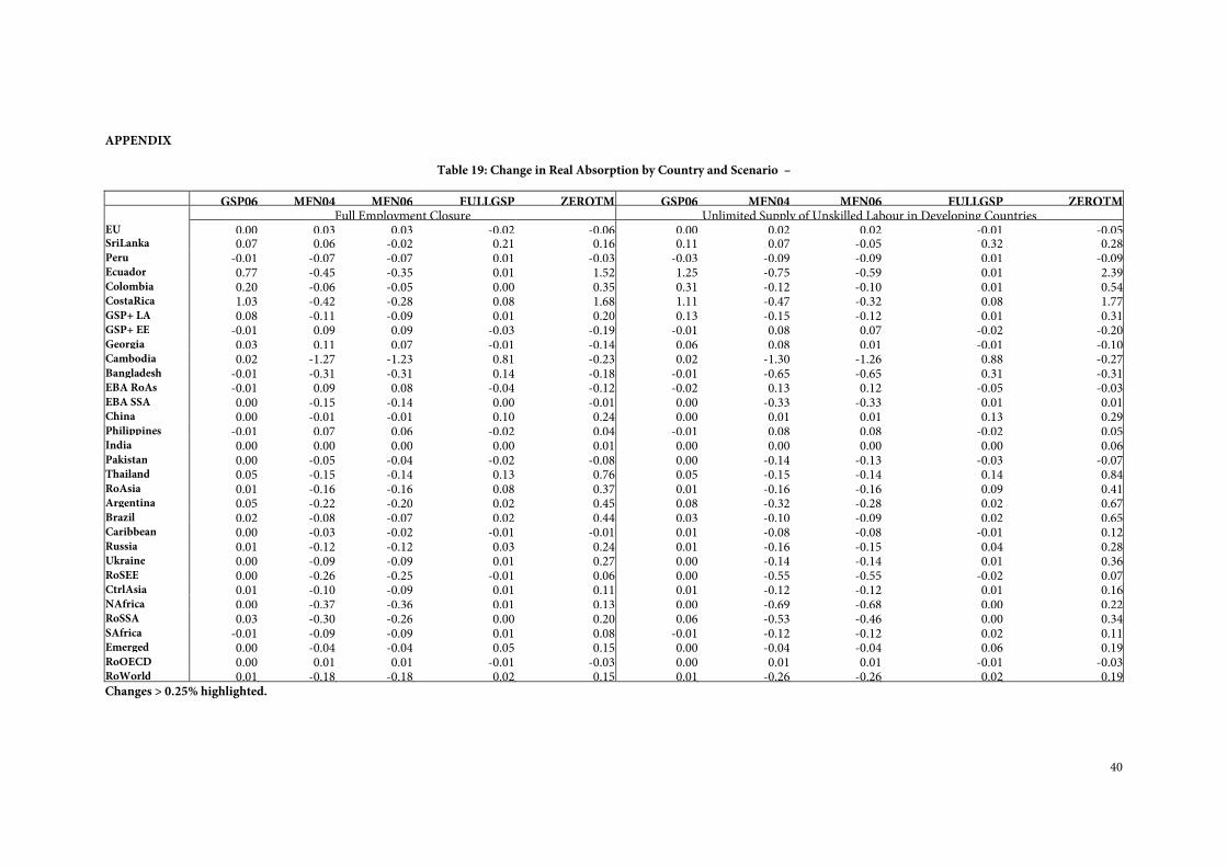
40

APPENDIX

Table 19: Change in Real Absorption by Country and Scenario –

GSP06 MFN04 MFN06 FULLGSP ZEROTM GSP06 MFN04 MFN06 FULLGSP ZEROTM Full Employment Closure Unlimited Supply of Unskilled Labour in Developing Countries EU 0.00 0.03 0.03 -0.02 -0.06 0.00 0.02 0.02 -0.01 -0.05SriLanka 0.07 0.06 -0.02 0.21 0.16 0.11 0.07 -0.05 0.32 0.28Peru -0.01 -0.07 -0.07 0.01 -0.03 -0.03 -0.09 -0.09 0.01 -0.09Ecuador 0.77 -0.45 -0.35 0.01 1.52 1.25 -0.75 -0.59 0.01 2.39Colombia 0.20 -0.06 -0.05 0.00 0.35 0.31 -0.12 -0.10 0.01 0.54CostaRica 1.03 -0.42 -0.28 0.08 1.68 1.11 -0.47 -0.32 0.08 1.77GSP+ LA 0.08 -0.11 -0.09 0.01 0.20 0.13 -0.15 -0.12 0.01 0.31GSP+ EE -0.01 0.09 0.09 -0.03 -0.19 -0.01 0.08 0.07 -0.02 -0.20Georgia 0.03 0.11 0.07 -0.01 -0.14 0.06 0.08 0.01 -0.01 -0.10Cambodia 0.02 -1.27 -1.23 0.81 -0.23 0.02 -1.30 -1.26 0.88 -0.27Bangladesh -0.01 -0.31 -0.31 0.14 -0.18 -0.01 -0.65 -0.65 0.31 -0.31EBA RoAs -0.01 0.09 0.08 -0.04 -0.12 -0.02 0.13 0.12 -0.05 -0.03EBA SSA 0.00 -0.15 -0.14 0.00 -0.01 0.00 -0.33 -0.33 0.01 0.01China 0.00 -0.01 -0.01 0.10 0.24 0.00 0.01 0.01 0.13 0.29Philippines -0.01 0.07 0.06 -0.02 0.04 -0.01 0.08 0.08 -0.02 0.05India 0.00 0.00 0.00 0.00 0.01 0.00 0.00 0.00 0.00 0.06Pakistan 0.00 -0.05 -0.04 -0.02 -0.08 0.00 -0.14 -0.13 -0.03 -0.07Thailand 0.05 -0.15 -0.14 0.13 0.76 0.05 -0.15 -0.14 0.14 0.84RoAsia 0.01 -0.16 -0.16 0.08 0.37 0.01 -0.16 -0.16 0.09 0.41Argentina 0.05 -0.22 -0.20 0.02 0.45 0.08 -0.32 -0.28 0.02 0.67Brazil 0.02 -0.08 -0.07 0.02 0.44 0.03 -0.10 -0.09 0.02 0.65Caribbean 0.00 -0.03 -0.02 -0.01 -0.01 0.01 -0.08 -0.08 -0.01 0.12Russia 0.01 -0.12 -0.12 0.03 0.24 0.01 -0.16 -0.15 0.04 0.28Ukraine 0.00 -0.09 -0.09 0.01 0.27 0.00 -0.14 -0.14 0.01 0.36RoSEE 0.00 -0.26 -0.25 -0.01 0.06 0.00 -0.55 -0.55 -0.02 0.07CtrlAsia 0.01 -0.10 -0.09 0.01 0.11 0.01 -0.12 -0.12 0.01 0.16NAfrica 0.00 -0.37 -0.36 0.01 0.13 0.00 -0.69 -0.68 0.00 0.22RoSSA 0.03 -0.30 -0.26 0.00 0.20 0.06 -0.53 -0.46 0.00 0.34SAfrica -0.01 -0.09 -0.09 0.01 0.08 -0.01 -0.12 -0.12 0.02 0.11Emerged 0.00 -0.04 -0.04 0.05 0.15 0.00 -0.04 -0.04 0.06 0.19RoOECD 0.00 0.01 0.01 -0.01 -0.03 0.00 0.01 0.01 -0.01 -0.03RoWorld 0.01 -0.18 -0.18 0.02 0.15 0.01 -0.26 -0.26 0.02 0.19Changes > 0.25% highlighted.

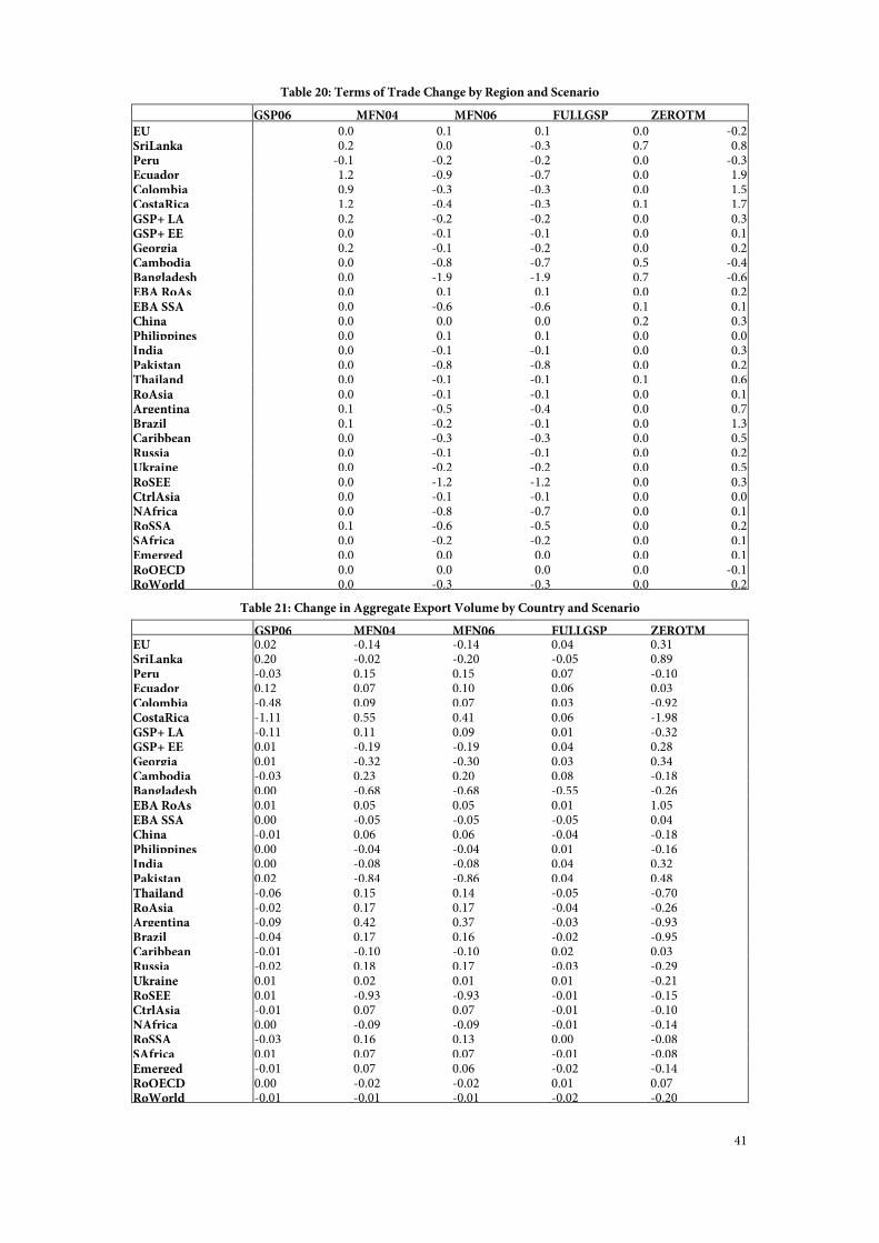
41

Table 20: Terms of Trade Change by Region and Scenario

GSP06 MFN04 MFN06 FULLGSP ZEROTM

EU 0.0 0.1 0.1 0.0 -0.2 SriLanka 0.2 0.0 -0.3 0.7 0.8 Peru -0.1 -0.2 -0.2 0.0 -0.3 Ecuador 1.2 -0.9 -0.7 0.0 1.9 Colombia 0.9 -0.3 -0.3 0.0 1.5 CostaRica 1.2 -0.4 -0.3 0.1 1.7 GSP+ LA 0.2 -0.2 -0.2 0.0 0.3 GSP+ EE 0.0 -0.1 -0.1 0.0 0.1 Georgia 0.2 -0.1 -0.2 0.0 0.2 Cambodia 0.0 -0.8 -0.7 0.5 -0.4 Bangladesh 0.0 -1.9 -1.9 0.7 -0.6 EBA RoAs 0.0 0.1 0.1 0.0 0.2 EBA SSA 0.0 -0.6 -0.6 0.1 0.1 China 0.0 0.0 0.0 0.2 0.3 Philippines 0.0 0.1 0.1 0.0 0.0 India 0.0 -0.1 -0.1 0.0 0.3 Pakistan 0.0 -0.8 -0.8 0.0 0.2 Thailand 0.0 -0.1 -0.1 0.1 0.6 RoAsia 0.0 -0.1 -0.1 0.0 0.1 Argentina 0.1 -0.5 -0.4 0.0 0.7 Brazil 0.1 -0.2 -0.1 0.0 1.3 Caribbean 0.0 -0.3 -0.3 0.0 0.5 Russia 0.0 -0.1 -0.1 0.0 0.2 Ukraine 0.0 -0.2 -0.2 0.0 0.5 RoSEE 0.0 -1.2 -1.2 0.0 0.3 CtrlAsia 0.0 -0.1 -0.1 0.0 0.0 NAfrica 0.0 -0.8 -0.7 0.0 0.1 RoSSA 0.1 -0.6 -0.5 0.0 0.2 SAfrica 0.0 -0.2 -0.2 0.0 0.1 Emerged 0.0 0.0 0.0 0.0 0.1 RoOECD 0.0 0.0 0.0 0.0 -0.1 RoWorld 0.0 -0.3 -0.3 0.0 0.2

Table 21: Change in Aggregate Export Volume by Country and Scenario

GSP06 MFN04 MFN06 FULLGSP ZEROTM EU 0.02 -0.14 -0.14 0.04 0.31 SriLanka 0.20 -0.02 -0.20 -0.05 0.89 Peru -0.03 0.15 0.15 0.07 -0.10 Ecuador 0.12 0.07 0.10 0.06 0.03 Colombia -0.48 0.09 0.07 0.03 -0.92 CostaRica -1.11 0.55 0.41 0.06 -1.98 GSP+ LA -0.11 0.11 0.09 0.01 -0.32 GSP+ EE 0.01 -0.19 -0.19 0.04 0.28 Georgia 0.01 -0.32 -0.30 0.03 0.34 Cambodia -0.03 0.23 0.20 0.08 -0.18 Bangladesh 0.00 -0.68 -0.68 -0.55 -0.26 EBA RoAs 0.01 0.05 0.05 0.01 1.05 EBA SSA 0.00 -0.05 -0.05 -0.05 0.04 China -0.01 0.06 0.06 -0.04 -0.18 Philippines 0.00 -0.04 -0.04 0.01 -0.16 India 0.00 -0.08 -0.08 0.04 0.32 Pakistan 0.02 -0.84 -0.86 0.04 0.48 Thailand -0.06 0.15 0.14 -0.05 -0.70 RoAsia -0.02 0.17 0.17 -0.04 -0.26 Argentina -0.09 0.42 0.37 -0.03 -0.93 Brazil -0.04 0.17 0.16 -0.02 -0.95 Caribbean -0.01 -0.10 -0.10 0.02 0.03 Russia -0.02 0.18 0.17 -0.03 -0.29 Ukraine 0.01 0.02 0.01 0.01 -0.21 RoSEE 0.01 -0.93 -0.93 -0.01 -0.15 CtrlAsia -0.01 0.07 0.07 -0.01 -0.10 NAfrica 0.00 -0.09 -0.09 -0.01 -0.14 RoSSA -0.03 0.16 0.13 0.00 -0.08 SAfrica 0.01 0.07 0.07 -0.01 -0.08 Emerged -0.01 0.07 0.06 -0.02 -0.14 RoOECD 0.00 -0.02 -0.02 0.01 0.07 RoWorld -0.01 -0.01 -0.01 -0.02 -0.20

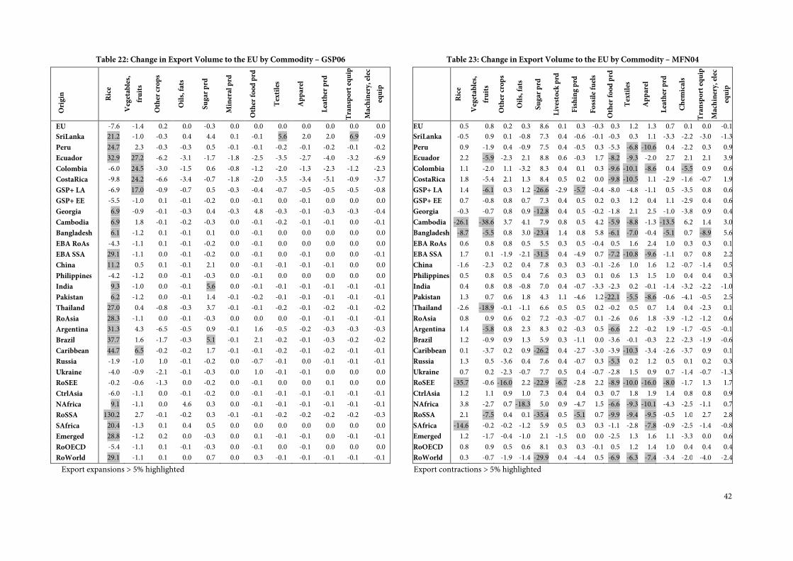
42

Table 22: Change in Export Volume to the EU by Commodity – GSP06 Origin

Rice

Vegetables,

fruits

Other crops

Oils, fats

Sugar prd

Mineral prd

Other food prd

Textiles

Apparel

Leather prd

Transport equip

Machinery, elec

equip

EU -7.6 -1.4 0.2 0.0 -0.3 0.0 0.0 0.0 0.0 0.0 0.0 0.0

SriLanka 21.2 -1.0 -0.3 0.4 4.4 0.1 -0.1 5.6 2.0 2.0 6.9 -0.9

Peru 24.7 2.3 -0.3 -0.3 0.5 -0.1 -0.1 -0.2 -0.1 -0.2 -0.1 -0.2

Ecuador 32.9 27.2 -6.2 -3.1 -1.7 -1.8 -2.5 -3.5 -2.7 -4.0 -3.2 -6.9

Colombia -6.0 24.5 -3.0 -1.5 0.6 -0.8 -1.2 -2.0 -1.3 -2.3 -1.2 -2.3

CostaRica -9.8 24.2 -6.6 -3.4 -0.7 -1.8 -2.0 -3.5 -3.4 -5.1 -0.9 -3.7

GSP+ LA -6.9 17.0 -0.9 -0.7 0.5 -0.3 -0.4 -0.7 -0.5 -0.5 -0.5 -0.8

GSP+ EE -5.5 -1.0 0.1 -0.1 -0.2 0.0 -0.1 0.0 -0.1 0.0 0.0 0.0

Georgia 6.9 -0.9 -0.1 -0.3 0.4 -0.3 4.8 -0.3 -0.1 -0.3 -0.3 -0.4

Cambodia 6.9 1.8 -0.1 -0.2 -0.3 0.0 -0.1 -0.2 -0.1 -0.1 0.0 -0.1

Bangladesh 6.1 -1.2 0.1 -0.1 0.1 0.0 -0.1 0.0 0.0 0.0 0.0 0.0

EBA RoAs -4.3 -1.1 0.1 -0.1 -0.2 0.0 -0.1 0.0 0.0 0.0 0.0 0.0

EBA SSA 29.1 -1.1 0.0 -0.1 -0.2 0.0 -0.1 0.0 -0.1 0.0 0.0 -0.1

China 11.2 0.5 0.1 -0.1 2.1 0.0 -0.1 -0.1 -0.1 -0.1 0.0 0.0

Philippines -4.2 -1.2 0.0 -0.1 -0.3 0.0 -0.1 0.0 0.0 0.0 0.0 0.0

India 9.3 -1.0 0.0 -0.1 5.6 0.0 -0.1 -0.1 -0.1 -0.1 -0.1 -0.1

Pakistan 6.2 -1.2 0.0 -0.1 1.4 -0.1 -0.2 -0.1 -0.1 -0.1 -0.1 -0.1

Thailand 27.0 0.4 -0.8 -0.3 3.7 -0.1 -0.1 -0.2 -0.1 -0.2 -0.1 -0.2

RoAsia 28.3 -1.1 0.0 -0.1 -0.3 0.0 0.0 0.0 -0.1 -0.1 -0.1 -0.1

Argentina 31.3 4.3 -6.5 -0.5 0.9 -0.1 1.6 -0.5 -0.2 -0.3 -0.3 -0.3

Brazil 37.7 1.6 -1.7 -0.3 5.1 -0.1 2.1 -0.2 -0.1 -0.3 -0.2 -0.2

Caribbean 44.7 6.5 -0.2 -0.2 1.7 -0.1 -0.1 -0.2 -0.1 -0.2 -0.1 -0.1

Russia -1.9 -1.0 1.0 -0.1 -0.2 0.0 -0.7 -0.1 0.0 -0.1 -0.1 -0.1

Ukraine -4.0 -0.9 -2.1 -0.1 -0.3 0.0 1.0 -0.1 -0.1 0.0 0.0 0.0

RoSEE -0.2 -0.6 -1.3 0.0 -0.2 0.0 -0.1 0.0 0.0 0.1 0.0 0.0

CtrlAsia -6.0 -1.1 0.0 -0.1 -0.2 0.0 -0.1 -0.1 -0.1 -0.1 -0.1 -0.1

NAfrica 9.1 -1.1 0.0 4.6 0.3 0.0 -0.1 -0.1 -0.1 -0.1 -0.1 -0.1

RoSSA 130.2 2.7 -0.1 -0.2 0.3 -0.1 -0.1 -0.2 -0.2 -0.2 -0.2 -0.3

SAfrica 20.4 -1.3 0.1 0.4 0.5 0.0 0.0 0.0 0.0 0.0 0.0 0.0

Emerged 28.8 -1.2 0.2 0.0 -0.3 0.0 0.1 -0.1 -0.1 0.0 -0.1 -0.1

RoOECD -5.4 -1.1 0.1 -0.1 -0.3 0.0 -0.1 0.0 -0.1 0.0 0.0 0.0

RoWorld 29.1 -1.1 0.1 0.0 0.7 0.0 0.3 -0.1 -0.1 -0.1 -0.1 -0.1

Export expansions > 5% highlighted

Table 23: Change in Export Volume to the EU by Commodity – MFN04

Rice

Vegetables,

fruits

Other crops

Oils, fats

Sugar prd

Livestock prd

Fishing prd

Fossile fuels

Other food prd

Textiles

Apparel

Leather prd

Chemicals

Transport equip

Machinery, elec

equip

EU 0.5 0.8 0.2 0.3 8.6 0.1 0.3 -0.3 0.3 1.2 1.3 0.7 0.1 0.0 -0.1

SriLanka -0.5 0.9 0.1 -0.8 7.3 0.4 -0.6 -0.1 -0.3 0.3 1.1 -3.3 -2.2 -3.0 -1.3

Peru 0.9 -1.9 0.4 -0.9 7.5 0.4 -0.5 0.3 -5.3 -6.8 -10.6 0.4 -2.2 0.3 0.9

Ecuador 2.2 -5.9 -2.3 2.1 8.8 0.6 -0.3 1.7 -8.2 -9.3 -2.0 2.7 2.1 2.1 3.9

Colombia 1.1 -2.0 1.1 -3.2 8.3 0.4 0.1 0.3 -9.6 -10.1 -8.6 0.4 -5.5 0.9 0.6

CostaRica 1.8 -5.4 2.1 1.3 8.4 0.5 0.2 0.0 -9.8 -10.5 1.1 -2.9 -1.6 -0.7 1.9

GSP+ LA 1.4 -6.1 0.3 1.2 -26.6 -2.9 -5.7 -0.4 -8.0 -4.8 -1.1 0.5 -3.5 0.8 0.6

GSP+ EE 0.7 -0.8 0.8 0.7 7.3 0.4 0.5 0.2 0.3 1.2 0.4 1.1 -2.9 0.4 0.6

Georgia -0.3 -0.7 0.8 0.9 -12.8 0.4 0.5 -0.2 -1.8 2.1 2.5 -1.0 -3.8 0.9 0.4

Cambodia -26.1 -38.6 3.7 4.1 7.9 0.8 0.5 4.2 -5.9 -8.8 -1.3 -13.5 6.2 1.4 3.0

Bangladesh -8.7 -5.5 0.8 3.0 -23.4 1.4 0.8 5.8 -6.1 -7.0 -0.4 -5.1 0.7 -8.9 5.6

EBA RoAs 0.6 0.8 0.8 0.5 5.5 0.3 0.5 -0.4 0.5 1.6 2.4 1.0 0.3 0.3 0.1

EBA SSA 1.7 0.1 -1.9 -2.1 -31.5 0.4 -4.9 0.7 -7.2 -10.8 -9.6 -1.1 0.7 0.8 2.2

China -1.6 -2.3 0.2 0.4 7.8 0.3 0.3 -0.1 -2.6 1.0 1.6 1.2 -0.7 -1.4 0.5

Philippines 0.5 0.8 0.5 0.4 7.6 0.3 0.3 0.1 0.6 1.3 1.5 1.0 0.4 0.4 0.3

India 0.4 0.8 0.8 -0.8 7.0 0.4 -0.7 -3.3 -2.3 0.2 -0.1 -1.4 -3.2 -2.2 -1.0

Pakistan 1.3 0.7 0.6 1.8 4.3 1.1 -4.6 1.2 -22.1 -5.5 -8.6 -0.6 -4.1 -0.5 2.5

Thailand -2.6 -18.9 -0.1 -1.1 6.6 0.5 0.5 0.2 -0.2 0.5 0.7 1.4 0.4 -2.3 0.1

RoAsia 0.8 0.9 0.6 0.2 7.2 -0.3 -0.7 0.1 -2.6 0.6 1.8 -3.9 -1.2 -1.2 0.6

Argentina 1.4 -5.8 0.8 2.3 8.3 0.2 -0.3 0.5 -6.6 2.2 -0.2 1.9 -1.7 -0.5 -0.1

Brazil 1.2 -0.9 0.9 1.3 5.9 0.3 -1.1 0.0 -3.6 -0.1 -0.3 2.2 -2.3 -1.9 -0.6

Caribbean 0.1 -3.7 0.2 0.9 -26.2 0.4 -2.7 -3.0 -3.9 -10.3 -3.4 -2.6 -3.7 0.9 0.1

Russia 1.3 0.5 -3.6 0.4 7.6 0.4 -0.7 0.3 -5.3 0.2 1.2 0.5 0.1 0.2 0.3

Ukraine 0.7 0.2 -2.3 -0.7 7.7 0.5 0.4 -0.7 -2.8 1.5 0.9 0.7 -1.4 -0.7 -1.3

RoSEE -35.7 -0.6 -16.0 2.2 -22.9 -6.7 -2.8 2.2 -8.9 -10.0 -16.0 -8.0 -1.7 1.3 1.7

CtrlAsia 1.2 1.1 0.9 1.0 7.3 0.4 0.4 0.3 0.7 1.8 1.9 1.4 0.8 0.8 0.9

NAfrica 3.8 -2.7 0.7 -18.3 5.0 0.9 -4.7 1.5 -6.6 -9.3 -10.1 -4.3 -2.5 -1.1 0.7

RoSSA 2.1 -7.5 0.4 0.1 -35.4 0.5 -5.1 0.7 -9.9 -9.4 -9.5 -0.5 1.0 2.7 2.8

SAfrica -14.6 -0.2 -0.2 -1.2 5.9 0.5 0.3 0.3 -1.1 -2.8 -7.8 -0.9 -2.5 -1.4 -0.8

Emerged 1.2 -1.7 -0.4 -1.0 2.1 -1.5 0.0 0.0 -2.5 1.3 1.6 1.1 -3.3 0.0 0.6

RoOECD 0.8 0.9 0.5 0.6 8.1 0.3 0.3 -0.1 0.5 1.2 1.4 1.0 0.4 0.4 0.4

RoWorld 0.3 -0.7 -1.9 -1.4 -29.9 0.4 -4.4 0.5 -6.9 -6.3 -7.4 -3.4 -2.0 -4.0 -2.4

Export contractions > 5% highlighted

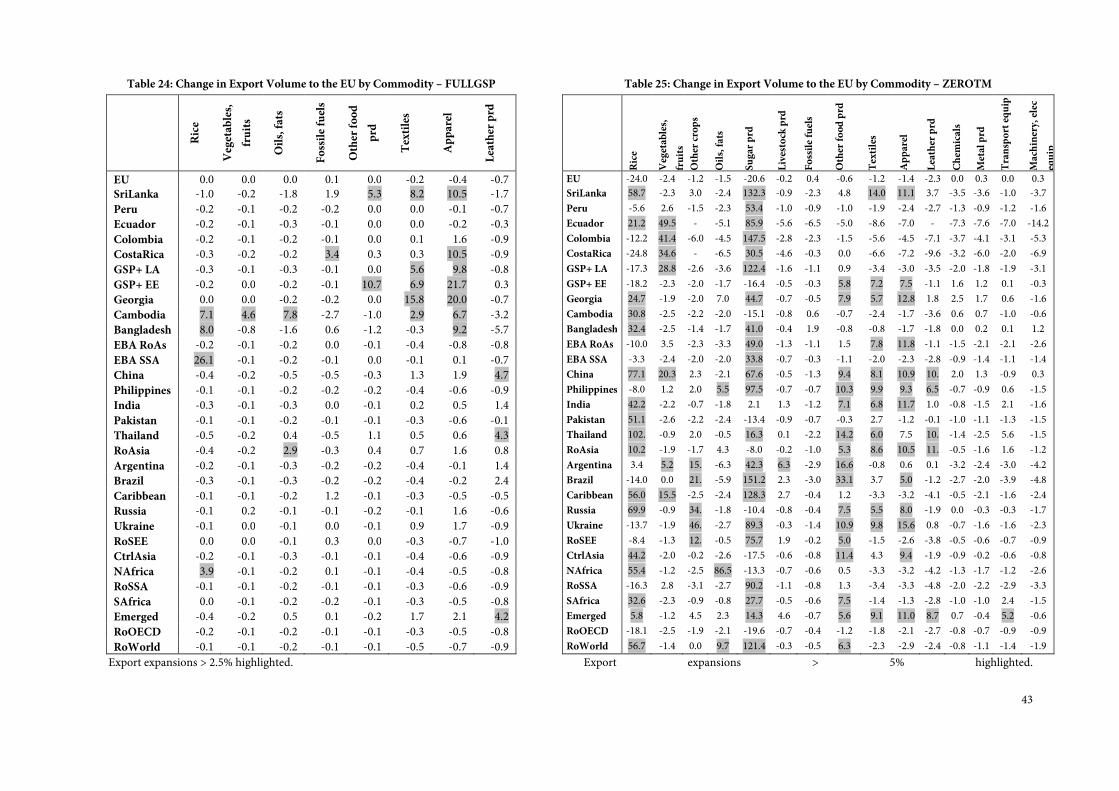
43

Table 24: Change in Export Volume to the EU by Commodity – FULLGSP

Rice

Vegetables,

fruits

Oils, fats

Fossile fuels

Other food

prd

Textiles

Apparel

Leather prd

EU 0.0 0.0 0.0 0.1 0.0 -0.2 -0.4 -0.7

SriLanka -1.0 -0.2 -1.8 1.9 5.3 8.2 10.5 -1.7

Peru -0.2 -0.1 -0.2 -0.2 0.0 0.0 -0.1 -0.7

Ecuador -0.2 -0.1 -0.3 -0.1 0.0 0.0 -0.2 -0.3

Colombia -0.2 -0.1 -0.2 -0.1 0.0 0.1 1.6 -0.9

CostaRica -0.3 -0.2 -0.2 3.4 0.3 0.3 10.5 -0.9

GSP+ LA -0.3 -0.1 -0.3 -0.1 0.0 5.6 9.8 -0.8

GSP+ EE -0.2 0.0 -0.2 -0.1 10.7 6.9 21.7 0.3

Georgia 0.0 0.0 -0.2 -0.2 0.0 15.8 20.0 -0.7

Cambodia 7.1 4.6 7.8 -2.7 -1.0 2.9 6.7 -3.2

Bangladesh 8.0 -0.8 -1.6 0.6 -1.2 -0.3 9.2 -5.7

EBA RoAs -0.2 -0.1 -0.2 0.0 -0.1 -0.4 -0.8 -0.8

EBA SSA 26.1 -0.1 -0.2 -0.1 0.0 -0.1 0.1 -0.7

China -0.4 -0.2 -0.5 -0.5 -0.3 1.3 1.9 4.7

Philippines -0.1 -0.1 -0.2 -0.2 -0.2 -0.4 -0.6 -0.9

India -0.3 -0.1 -0.3 0.0 -0.1 0.2 0.5 1.4

Pakistan -0.1 -0.1 -0.2 -0.1 -0.1 -0.3 -0.6 -0.1

Thailand -0.5 -0.2 0.4 -0.5 1.1 0.5 0.6 4.3

RoAsia -0.4 -0.2 2.9 -0.3 0.4 0.7 1.6 0.8

Argentina -0.2 -0.1 -0.3 -0.2 -0.2 -0.4 -0.1 1.4

Brazil -0.3 -0.1 -0.3 -0.2 -0.2 -0.4 -0.2 2.4

Caribbean -0.1 -0.1 -0.2 1.2 -0.1 -0.3 -0.5 -0.5

Russia -0.1 0.2 -0.1 -0.1 -0.2 -0.1 1.6 -0.6

Ukraine -0.1 0.0 -0.1 0.0 -0.1 0.9 1.7 -0.9

RoSEE 0.0 0.0 -0.1 0.3 0.0 -0.3 -0.7 -1.0

CtrlAsia -0.2 -0.1 -0.3 -0.1 -0.1 -0.4 -0.6 -0.9

NAfrica 3.9 -0.1 -0.2 0.1 -0.1 -0.4 -0.5 -0.8

RoSSA -0.1 -0.1 -0.2 -0.1 -0.1 -0.3 -0.6 -0.9

SAfrica 0.0 -0.1 -0.2 -0.2 -0.1 -0.3 -0.5 -0.8

Emerged -0.4 -0.2 0.5 0.1 -0.2 1.7 2.1 4.2

RoOECD -0.2 -0.1 -0.2 -0.1 -0.1 -0.3 -0.5 -0.8

RoWorld -0.1 -0.1 -0.2 -0.1 -0.1 -0.5 -0.7 -0.9

Export expansions > 2.5% highlighted.

Table 25: Change in Export Volume to the EU by Commodity – ZEROTM

Rice

Vegetables,

fruits

Other crops

Oils, fats

Sugar prd

Livestock prd

Fossile fuels

Other food prd

Textiles

Apparel

Leather prd

Chemicals

Metal prd

Transport equip

Machinery, elec

equip

EU -24.0 -2.4 -1.2 -1.5 -20.6 -0.2 0.4 -0.6 -1.2 -1.4 -2.3 0.0 0.3 0.0 0.3

SriLanka 58.7 -2.3 3.0 -2.4 132.3 -0.9 -2.3 4.8 14.0 11.1 3.7 -3.5 -3.6 -1.0 -3.7

Peru -5.6 2.6 -1.5 -2.3 53.4 -1.0 -0.9 -1.0 -1.9 -2.4 -2.7 -1.3 -0.9 -1.2 -1.6

Ecuador 21.2 49.5 - -5.1 85.9 -5.6 -6.5 -5.0 -8.6 -7.0 - -7.3 -7.6 -7.0 -14.2

Colombia -12.2 41.4 -6.0 -4.5 147.5 -2.8 -2.3 -1.5 -5.6 -4.5 -7.1 -3.7 -4.1 -3.1 -5.3

CostaRica -24.8 34.6 - -6.5 30.5 -4.6 -0.3 0.0 -6.6 -7.2 -9.6 -3.2 -6.0 -2.0 -6.9

GSP+ LA -17.3 28.8 -2.6 -3.6 122.4 -1.6 -1.1 0.9 -3.4 -3.0 -3.5 -2.0 -1.8 -1.9 -3.1

GSP+ EE -18.2 -2.3 -2.0 -1.7 -16.4 -0.5 -0.3 5.8 7.2 7.5 -1.1 1.6 1.2 0.1 -0.3

Georgia 24.7 -1.9 -2.0 7.0 44.7 -0.7 -0.5 7.9 5.7 12.8 1.8 2.5 1.7 0.6 -1.6

Cambodia 30.8 -2.5 -2.2 -2.0 -15.1 -0.8 0.6 -0.7 -2.4 -1.7 -3.6 0.6 0.7 -1.0 -0.6

Bangladesh 32.4 -2.5 -1.4 -1.7 41.0 -0.4 1.9 -0.8 -0.8 -1.7 -1.8 0.0 0.2 0.1 1.2

EBA RoAs -10.0 3.5 -2.3 -3.3 49.0 -1.3 -1.1 1.5 7.8 11.8 -1.1 -1.5 -2.1 -2.1 -2.6

EBA SSA -3.3 -2.4 -2.0 -2.0 33.8 -0.7 -0.3 -1.1 -2.0 -2.3 -2.8 -0.9 -1.4 -1.1 -1.4

China 77.1 20.3 2.3 -2.1 67.6 -0.5 -1.3 9.4 8.1 10.9 10. 2.0 1.3 -0.9 0.3

Philippines -8.0 1.2 2.0 5.5 97.5 -0.7 -0.7 10.3 9.9 9.3 6.5 -0.7 -0.9 0.6 -1.5

India 42.2 -2.2 -0.7 -1.8 2.1 1.3 -1.2 7.1 6.8 11.7 1.0 -0.8 -1.5 2.1 -1.6

Pakistan 51.1 -2.6 -2.2 -2.4 -13.4 -0.9 -0.7 -0.3 2.7 -1.2 -0.1 -1.0 -1.1 -1.3 -1.5

Thailand 102. -0.9 2.0 -0.5 16.3 0.1 -2.2 14.2 6.0 7.5 10. -1.4 -2.5 5.6 -1.5

RoAsia 10.2 -1.9 -1.7 4.3 -8.0 -0.2 -1.0 5.3 8.6 10.5 11. -0.5 -1.6 1.6 -1.2

Argentina 3.4 5.2 15. -6.3 42.3 6.3 -2.9 16.6 -0.8 0.6 0.1 -3.2 -2.4 -3.0 -4.2

Brazil -14.0 0.0 21. -5.9 151.2 2.3 -3.0 33.1 3.7 5.0 -1.2 -2.7 -2.0 -3.9 -4.8

Caribbean 56.0 15.5 -2.5 -2.4 128.3 2.7 -0.4 1.2 -3.3 -3.2 -4.1 -0.5 -2.1 -1.6 -2.4

Russia 69.9 -0.9 34. -1.8 -10.4 -0.8 -0.4 7.5 5.5 8.0 -1.9 0.0 -0.3 -0.3 -1.7

Ukraine -13.7 -1.9 46. -2.7 89.3 -0.3 -1.4 10.9 9.8 15.6 0.8 -0.7 -1.6 -1.6 -2.3

RoSEE -8.4 -1.3 12. -0.5 75.7 1.9 -0.2 5.0 -1.5 -2.6 -3.8 -0.5 -0.6 -0.7 -0.9

CtrlAsia 44.2 -2.0 -0.2 -2.6 -17.5 -0.6 -0.8 11.4 4.3 9.4 -1.9 -0.9 -0.2 -0.6 -0.8

NAfrica 55.4 -1.2 -2.5 86.5 -13.3 -0.7 -0.6 0.5 -3.3 -3.2 -4.2 -1.3 -1.7 -1.2 -2.6

RoSSA -16.3 2.8 -3.1 -2.7 90.2 -1.1 -0.8 1.3 -3.4 -3.3 -4.8 -2.0 -2.2 -2.9 -3.3

SAfrica 32.6 -2.3 -0.9 -0.8 27.7 -0.5 -0.6 7.5 -1.4 -1.3 -2.8 -1.0 -1.0 2.4 -1.5

Emerged 5.8 -1.2 4.5 2.3 14.3 4.6 -0.7 5.6 9.1 11.0 8.7 0.7 -0.4 5.2 -0.6

RoOECD -18.1 -2.5 -1.9 -2.1 -19.6 -0.7 -0.4 -1.2 -1.8 -2.1 -2.7 -0.8 -0.7 -0.9 -0.9

RoWorld 56.7 -1.4 0.0 9.7 121.4 -0.3 -0.5 6.3 -2.3 -2.9 -2.4 -0.8 -1.1 -1.4 -1.9

Export expansions > 5% highlighted.

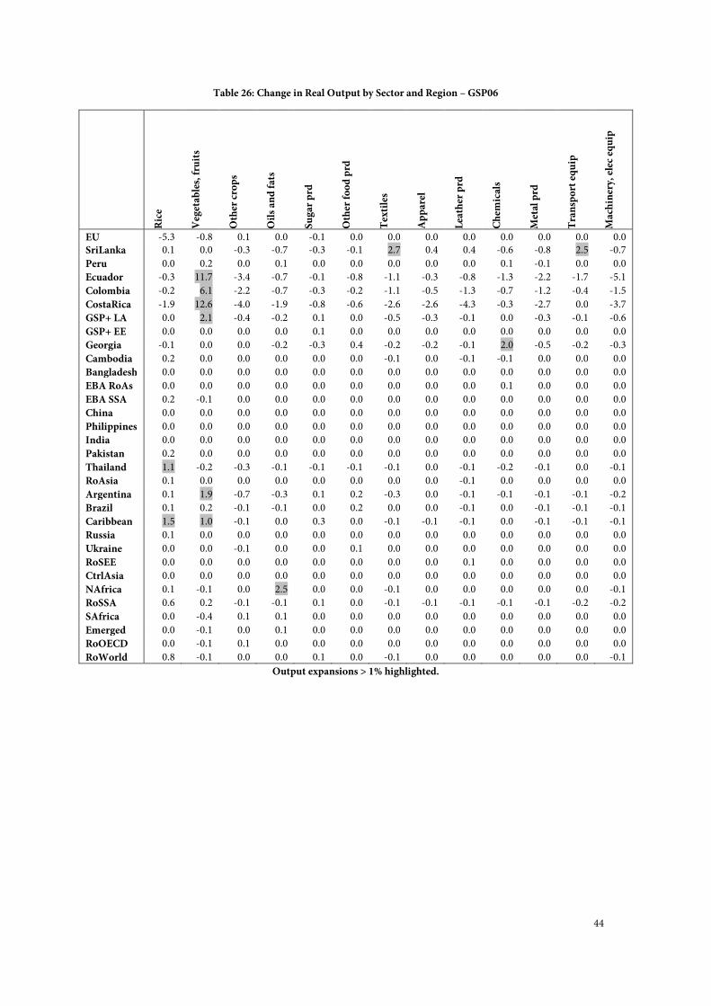
44

Table 26: Change in Real Output by Sector and Region – GSP06

Rice

Vegetables, fruits

Other crops

Oils and fats

Sugar prd

Other food prd

Textiles

Apparel

Leather prd

Chemicals

Metal prd

Transport equip

Machinery, elec equip

EU -5.3 -0.8 0.1 0.0 -0.1 0.0 0.0 0.0 0.0 0.0 0.0 0.0 0.0

SriLanka 0.1 0.0 -0.3 -0.7 -0.3 -0.1 2.7 0.4 0.4 -0.6 -0.8 2.5 -0.7

Peru 0.0 0.2 0.0 0.1 0.0 0.0 0.0 0.0 0.0 0.1 -0.1 0.0 0.0

Ecuador -0.3 11.7 -3.4 -0.7 -0.1 -0.8 -1.1 -0.3 -0.8 -1.3 -2.2 -1.7 -5.1

Colombia -0.2 6.1 -2.2 -0.7 -0.3 -0.2 -1.1 -0.5 -1.3 -0.7 -1.2 -0.4 -1.5

CostaRica -1.9 12.6 -4.0 -1.9 -0.8 -0.6 -2.6 -2.6 -4.3 -0.3 -2.7 0.0 -3.7

GSP+ LA 0.0 2.1 -0.4 -0.2 0.1 0.0 -0.5 -0.3 -0.1 0.0 -0.3 -0.1 -0.6

GSP+ EE 0.0 0.0 0.0 0.0 0.1 0.0 0.0 0.0 0.0 0.0 0.0 0.0 0.0

Georgia -0.1 0.0 0.0 -0.2 -0.3 0.4 -0.2 -0.2 -0.1 2.0 -0.5 -0.2 -0.3

Cambodia 0.2 0.0 0.0 0.0 0.0 0.0 -0.1 0.0 -0.1 -0.1 0.0 0.0 0.0

Bangladesh 0.0 0.0 0.0 0.0 0.0 0.0 0.0 0.0 0.0 0.0 0.0 0.0 0.0

EBA RoAs 0.0 0.0 0.0 0.0 0.0 0.0 0.0 0.0 0.0 0.1 0.0 0.0 0.0

EBA SSA 0.2 -0.1 0.0 0.0 0.0 0.0 0.0 0.0 0.0 0.0 0.0 0.0 0.0

China 0.0 0.0 0.0 0.0 0.0 0.0 0.0 0.0 0.0 0.0 0.0 0.0 0.0

Philippines 0.0 0.0 0.0 0.0 0.0 0.0 0.0 0.0 0.0 0.0 0.0 0.0 0.0

India 0.0 0.0 0.0 0.0 0.0 0.0 0.0 0.0 0.0 0.0 0.0 0.0 0.0

Pakistan 0.2 0.0 0.0 0.0 0.0 0.0 0.0 0.0 0.0 0.0 0.0 0.0 0.0

Thailand 1.1 -0.2 -0.3 -0.1 -0.1 -0.1 -0.1 0.0 -0.1 -0.2 -0.1 0.0 -0.1

RoAsia 0.1 0.0 0.0 0.0 0.0 0.0 0.0 0.0 -0.1 0.0 0.0 0.0 0.0

Argentina 0.1 1.9 -0.7 -0.3 0.1 0.2 -0.3 0.0 -0.1 -0.1 -0.1 -0.1 -0.2

Brazil 0.1 0.2 -0.1 -0.1 0.0 0.2 0.0 0.0 -0.1 0.0 -0.1 -0.1 -0.1

Caribbean 1.5 1.0 -0.1 0.0 0.3 0.0 -0.1 -0.1 -0.1 0.0 -0.1 -0.1 -0.1

Russia 0.1 0.0 0.0 0.0 0.0 0.0 0.0 0.0 0.0 0.0 0.0 0.0 0.0

Ukraine 0.0 0.0 -0.1 0.0 0.0 0.1 0.0 0.0 0.0 0.0 0.0 0.0 0.0

RoSEE 0.0 0.0 0.0 0.0 0.0 0.0 0.0 0.0 0.1 0.0 0.0 0.0 0.0

CtrlAsia 0.0 0.0 0.0 0.0 0.0 0.0 0.0 0.0 0.0 0.0 0.0 0.0 0.0

NAfrica 0.1 -0.1 0.0 2.5 0.0 0.0 -0.1 0.0 0.0 0.0 0.0 0.0 -0.1

RoSSA 0.6 0.2 -0.1 -0.1 0.1 0.0 -0.1 -0.1 -0.1 -0.1 -0.1 -0.2 -0.2

SAfrica 0.0 -0.4 0.1 0.1 0.0 0.0 0.0 0.0 0.0 0.0 0.0 0.0 0.0

Emerged 0.0 -0.1 0.0 0.1 0.0 0.0 0.0 0.0 0.0 0.0 0.0 0.0 0.0

RoOECD 0.0 -0.1 0.1 0.0 0.0 0.0 0.0 0.0 0.0 0.0 0.0 0.0 0.0

RoWorld 0.8 -0.1 0.0 0.0 0.1 0.0 -0.1 0.0 0.0 0.0 0.0 0.0 -0.1

Output expansions > 1% highlighted.

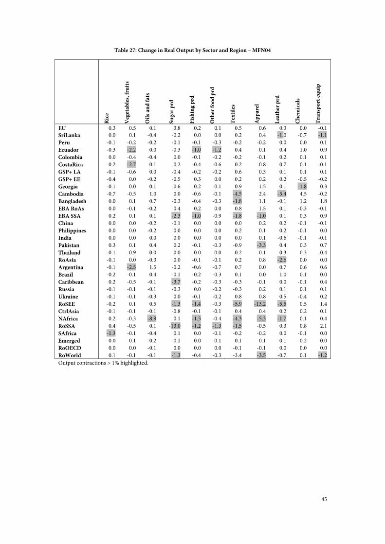
45

Table 27: Change in Real Output by Sector and Region – MFN04

Rice

Vegetables, fruits

Oils and fats

Sugar prd

Fishing prd

Other food prd

Textiles

Apparel

Leather prd

Chemicals

Transport equip

EU 0.3 0.5 0.1 3.8 0.2 0.1 0.5 0.6 0.3 0.0 -0.1

SriLanka 0.0 0.1 -0.4 -0.2 0.0 0.0 0.2 0.4 -1.0 -0.7 -1.1

Peru -0.1 -0.2 -0.2 -0.1 -0.1 -0.3 -0.2 -0.2 0.0 0.0 0.1

Ecuador -0.3 -2.2 0.0 -0.3 -1.0 -1.2 0.4 0.1 0.4 1.0 0.9

Colombia 0.0 -0.4 -0.4 0.0 -0.1 -0.2 -0.2 -0.1 0.2 0.1 0.1

CostaRica 0.2 -2.7 0.1 0.2 -0.4 -0.6 0.2 0.8 0.7 0.1 -0.1

GSP+ LA -0.1 -0.6 0.0 -0.4 -0.2 -0.2 0.6 0.3 0.1 0.1 0.1

GSP+ EE -0.4 0.0 -0.2 -0.5 0.3 0.0 0.2 0.2 0.2 -0.5 -0.2

Georgia -0.1 0.0 0.1 -0.6 0.2 -0.1 0.9 1.5 0.1 -1.8 0.3

Cambodia -0.7 -0.5 1.0 0.0 -0.6 -0.1 -4.5 2.4 -5.4 4.5 -0.2

Bangladesh 0.0 0.1 0.7 -0.3 -0.4 -0.3 -1.8 1.1 -0.1 1.2 1.8

EBA RoAs 0.0 -0.1 -0.2 0.4 0.2 0.0 0.8 1.5 0.1 -0.3 -0.1

EBA SSA 0.2 0.1 0.1 -2.3 -1.0 -0.9 -1.8 -1.0 0.1 0.3 0.9

China 0.0 0.0 -0.2 -0.1 0.0 0.0 0.0 0.2 0.2 -0.1 -0.1

Philippines 0.0 0.0 -0.2 0.0 0.0 0.0 0.2 0.1 0.2 -0.1 0.0

India 0.0 0.0 0.0 0.0 0.0 0.0 0.0 0.1 -0.6 -0.1 -0.1

Pakistan 0.3 0.1 0.4 0.2 -0.1 -0.3 -0.9 -3.3 0.4 0.3 0.7

Thailand -0.1 -0.9 0.0 0.0 0.0 0.0 0.2 0.1 0.3 0.3 -0.4

RoAsia -0.1 0.0 -0.3 0.0 -0.1 -0.1 0.2 0.8 -2.6 0.0 0.0

Argentina -0.1 -2.5 1.5 -0.2 -0.6 -0.7 0.7 0.0 0.7 0.6 0.6

Brazil -0.2 -0.1 0.4 -0.1 -0.2 -0.3 0.1 0.0 1.0 0.1 0.0

Caribbean 0.2 -0.5 -0.1 -3.7 -0.2 -0.3 -0.3 -0.1 0.0 -0.1 0.4

Russia -0.1 -0.1 -0.1 -0.3 0.0 -0.2 -0.3 0.2 0.1 0.1 0.1

Ukraine -0.1 -0.1 -0.3 0.0 -0.1 -0.2 0.8 0.8 0.5 -0.4 0.2

RoSEE -0.2 0.1 0.5 -1.3 -1.4 -0.3 -5.9 -13.2 -5.5 0.5 1.4

CtrlAsia -0.1 -0.1 -0.1 -0.8 -0.1 -0.1 0.4 0.4 0.2 0.2 0.1

NAfrica 0.2 -0.3 -8.9 0.1 -1.5 -0.4 -4.3 -5.3 -1.7 0.1 0.4

RoSSA 0.4 -0.5 0.1 -13.0 -1.2 -1.3 -1.5 -0.5 0.3 0.8 2.1

SAfrica -1.3 -0.1 -0.4 0.1 0.0 -0.1 -0.2 -0.2 0.0 -0.1 0.0

Emerged 0.0 -0.1 -0.2 -0.1 0.0 -0.1 0.1 0.1 0.1 -0.2 0.0

RoOECD 0.0 0.0 -0.1 0.0 0.0 0.0 -0.1 -0.1 0.0 0.0 0.0

RoWorld 0.1 -0.1 -0.1 -1.3 -0.4 -0.3 -3.4 -3.5 -0.7 0.1 -1.2

Output contractions > 1% highlighted.

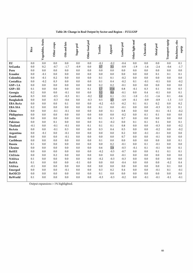
46

Table 28: Change in Real Output by Sector and Region – FULLGSP

Output expansions > 1% highlighted.

Rice

Vegetables, fruits

Other crops

Oils and fats

Sugar prd

Other food prd

Textiles

Apparel

Leather prd

Other light mnf

Chemicals

Metal prd

Transport equip

Machinery, elec

equip

EU 0.0 0.0 0.0 0.0 0.0 0.0 -0.1 -0.2 -0.4 0.0 0.0 0.0 0.0 0.1

SriLanka 0.0 0.2 -0.7 -1.7 -0.9 0.0 3.7 3.1 -0.9 -1.9 -1.6 -2.4 -0.6 -1.7

Peru 0.0 0.0 0.0 0.0 0.0 0.0 0.0 0.0 0.0 0.0 0.0 0.0 0.0 0.0

Ecuador 0.0 -0.1 0.0 0.0 0.0 0.0 0.0 0.0 0.0 0.0 0.0 0.1 0.1 0.1

Colombia 0.0 -0.1 0.2 0.0 0.0 0.0 0.1 0.1 -0.2 0.0 0.0 0.0 0.0 0.0

CostaRica 0.0 -0.2 0.3 0.0 0.0 0.0 0.1 0.4 -0.2 0.1 -0.1 -0.1 0.0 -0.2

GSP+ LA 0.0 0.0 0.0 0.0 0.0 0.0 0.2 0.2 -0.1 0.0 0.0 0.0 0.0 0.0

GSP+ EE 0.1 0.0 0.0 0.0 0.0 0.1 1.7 13.6 0.8 -0.1 0.3 0.1 0.0 0.5

Georgia 0.2 0.0 0.0 -0.1 0.0 0.0 5.2 9.4 -0.1 0.0 0.4 -0.1 0.0 0.1

Cambodia 0.3 0.0 -0.5 -0.3 0.1 -0.2 1.2 0.1 -3.1 -1.0 -3.1 -1.6 0.1 -0.6

Bangladesh 0.0 0.0 -0.3 -0.6 0.0 -0.3 0.5 4.5 -4.9 -0.1 -0.9 -0.9 -1.5 -3.3

EBA RoAs 0.0 0.0 0.0 0.1 0.0 0.0 -0.2 -0.5 -0.2 0.1 0.1 0.2 0.0 0.2

EBA SSA 0.2 0.0 0.0 0.0 0.0 0.0 0.1 0.0 -0.1 0.0 0.0 -0.3 0.3 0.1

China 0.0 0.0 -0.1 -0.1 0.0 0.0 0.0 0.1 0.8 0.0 0.0 -0.1 -0.1 -0.2

Philippines 0.0 0.0 0.0 0.0 0.0 0.0 0.0 0.0 -0.2 0.0 0.1 0.1 0.0 0.0

India 0.0 0.0 0.0 0.0 0.0 0.0 0.1 0.3 0.7 0.0 0.0 0.0 0.0 0.0

Pakistan 0.0 0.0 0.1 0.0 0.0 0.0 0.1 -0.2 0.0 0.1 0.1 0.1 0.0 0.1

Thailand -0.1 0.0 -0.1 -0.1 0.0 0.1 0.1 0.1 0.8 0.0 0.0 -0.3 0.0 -0.2

RoAsia 0.0 0.0 -0.1 0.3 0.0 0.0 0.3 0.4 0.5 0.0 0.0 -0.2 0.0 -0.2

Argentina 0.0 -0.1 0.0 -0.1 0.0 0.0 0.0 0.0 0.2 0.0 -0.1 -0.1 0.0 0.0

Brazil 0.0 0.0 0.0 -0.1 0.0 0.0 0.0 0.0 0.7 0.0 0.0 -0.1 0.0 0.0

Caribbean 0.0 0.0 0.0 0.0 0.0 0.0 0.1 0.0 0.0 0.0 0.0 0.0 0.0 0.1

Russia 0.1 0.0 0.0 0.0 0.0 0.0 0.0 0.2 -0.1 0.0 0.1 -0.1 0.0 0.0

Ukraine 0.0 0.0 0.0 0.0 0.0 0.0 0.6 1.4 -0.5 -0.1 0.1 -0.1 0.0 0.1

RoSEE 0.0 0.0 0.0 0.0 0.0 0.0 -0.2 -0.5 -0.7 0.0 0.0 0.1 0.1 0.1

CtrlAsia 0.0 0.0 0.2 0.0 0.0 0.0 0.0 0.0 -0.1 0.0 0.0 0.0 0.0 0.0

NAfrica 0.1 0.0 0.0 0.0 0.0 0.0 -0.2 -0.3 -0.3 0.0 0.0 0.0 0.0 0.0

RoSSA 0.1 0.0 0.0 0.0 -0.1 0.0 0.0 0.0 -0.4 0.0 0.0 0.0 -0.2 0.4

SAfrica -0.1 0.0 0.0 0.0 0.0 0.0 0.0 0.0 0.0 0.0 0.0 0.0 0.1 0.0

Emerged 0.0 0.0 0.0 -0.1 0.0 0.0 0.3 0.2 0.4 0.0 0.0 -0.1 0.1 -0.1

RoOECD 0.0 0.0 0.0 0.0 0.0 0.0 0.1 0.0 0.0 0.0 0.0 0.0 0.0 0.0

RoWorld 0.1 0.0 0.0 0.0 0.0 0.0 -0.3 -0.3 -0.2 0.0 -0.1 -0.1 -0.1 -0.1