remote sensing

Article

Mid-Season High-Resolution Satellite Imagery forForecasting Site-Specific Corn Yield

Nahuel R. Peralta 1,2,3,*, Yared Assefa 3, Juan Du 4, Charles J. Barden 5

and Ignacio A. Ciampitti 3,*1 Consejo Nacional de Investigaciones Cientificas y Tecnicas (CONICET), Av. Rivadavia 1917,

Buenos Aires C1033AAJ, Argentina2 Estacion Experimental Agropecuaria INTA, Buenos Aires C1033AAE, Argentina3 Department of Agronomy, Kansas State University, 2004 Throckmorton Plant Science Center,

Manhattan, KS 66506, USA; yareda@ksu.edu4 Department of Statistics, Kansas State University, 108A Dickens Hall, Manhattan, KS 66506, USA;

dujuan@ksu.edu5 Department of Horticulture and Natural Resources, Kansas State University, 2021 Throckmorton Plant

Science Center, Manhattan, KS 66506, USA; cbarden@ksu.edu* Correspondence: nperalta21@gmail.com (N.R.P.); ciampitti@ksu.edu (I.A.C.);

Tel.: +542-266-1544-9161 (N.R.P.); +1-785-532-6940 (I.A.C.)

Academic Editors: James Campbell and Prasad S. ThenkabailReceived: 24 June 2016; Accepted: 8 October 2016; Published: 16 October 2016

Abstract: A timely and accurate crop yield forecast is crucial to make better decisions on cropmanagement, marketing, and storage by assessing ahead and implementing based on expectedcrop performance. The objective of this study was to investigate the potential of high-resolutionsatellite imagery data collected at mid-growing season for identification of within-field variabilityand to forecast corn yield at different sites within a field. A test was conducted on yield monitordata and RapidEye satellite imagery obtained for 22 cornfields located in five different counties(Clay, Dickinson, Rice, Saline, and Washington) of Kansas (total of 457 ha). Three basic tests wereconducted on the data: (1) spatial dependence on each of the yield and vegetation indices (VIs) usingMoran’s I test; (2) model selection for the relationship between imagery data and actual yield usingordinary least square regression (OLS) and spatial econometric (SPL) models; and (3) model validationfor yield forecasting purposes. Spatial autocorrelation analysis (Moran’s I test) for both yield andVIs (red edge NDVI = NDVIre, normalized difference vegetation index = NDVIr, SRre = red-edgesimple ratio, near infrared = NIR and green-NDVI = NDVIG) was tested positive and statisticallysignificant for most of the fields (p < 0.05), except for one. Inclusion of spatial adjustment to modelimproved the model fit on most fields as compared to OLS models, with the spatial adjustmentcoefficient significant for half of the fields studied. When selected models were used for prediction tovalidate dataset, a striking similarity (RMSE = 0.02) was obtained between predicted and observedyield within a field. Yield maps could assist implementing more effective site-specific managementtools and could be utilized as a proxy of yield monitor data. In summary, high-resolution satelliteimagery data can be reasonably used to forecast yield via utilization of models that include spatialadjustment to inform precision agricultural management decisions.

Keywords: high-resolution satellite imagery; forecasting corn yields; spatial econometric;within-field variability

1. Introduction

Reliable crop production forecasts help producers, consumers, researchers, policy makers,and grain marketing agencies make informed decisions on soil and plant management, crop selection,

Remote Sens. 2016, 8, 848; doi:10.3390/rs8100848 www.mdpi.com/journal/remotesensing

Remote Sens. 2016, 8, 848 2 of 16

marketing, storage, and transport [1–5]. Statistical and mechanistic models have been used to makesuch crop forecast but existing models are applicable only for large-scale yield prediction, i.e., regionalor state level. As crop management progresses from large-scale blanket management to precisionagriculture (PA), it requires technologies that evaluate within-field variation and provide reasonableyield forecasts. Precision agriculture is the application of a set of technologies and principles formanaging spatial- and temporal-variability associated with the aspects of agricultural production,in order to improve input efficiency and primarily increase the economic return of the farmingsystem [6–8]. In the major agricultural regions of the world, introduction of yield monitor technologiescoupled with Global Positioning Systems (GPS) made implementation of PA practical. Digital mapsof grain yield obtained from yield monitors allow analysis of the spatial variability within an areaof production [9]. Interpretation of these digital maps, however, is often difficult because patternof grain yield variability is permanently influenced by spatial (terrain attributes, erosion classesand soil properties) and temporal (soil pathogens, diseases and production issues in planting thecrop) factors [10]. In such cases, interpretation of the true spatial pattern of grain yield requireyears of accumulated yield maps (temporal-analysis), soil and crop management data, and weatherinformation [11,12].

Coupling remote sensing and high-resolution spatio-temporal data collected at multiplegrowth stages, with yield monitor information has the potential to contribute to site-specific cropmanagement [12,13]. For example, the leaf area index (LAI) is a key variable to estimate the foliagecanopy and to forecast growth and crop yields [14]. Rapid- and regional-estimation of LAI viautilization and integration on models of data collected from remote sensors such as satellite imageryprovides a large benefit in assessing in-season plant traits [14]. High-resolution satellite imagery(multispectral or hyperspectral) can provide valuable data on the status and health of crops, dependingon the interaction and the relationship between electromagnetic radiation (EMR) and foliage [12].Utilization of satellite imagery facilitates the identification of within-field variability and dry matterproduction in order to improve in- and after-season management decisions [13,15]. Currently, thenormalized difference vegetation index (NDVI) is most commonly and widely used vegetation indexto assess crop growth and yield. Normalized difference vegetative index (VI) is sensitive to lowLAI (i.e., LAI < 2–3), but saturates at medium to high LAI and yield [15]. A few VIs have showngreater sensitivity to higher LAI and biomass, such as the simple ratio [15], or the green NDVI(NDVIG) [14]. Indices that incorporate the reflectance of red-edge bands such as the red-edge triangularvegetation index (RTVI) and red edge NDVI (NDVIre) have increased potential for estimating LAIand biomass [14]. Most of the reported red-edge indices were derived from narrow band fieldspectroradiometers [15,16]. Thus, estimation of NDVI and red-edge indices from satellite imageryenhanced the power of characterizing within-field variability at a large-scale.

In the application of satellite data to PA, crop information is required at sufficiently high spatialand temporal resolutions to enable within-field monitoring. The latter data resolution can be obtainedfrom the RapidEye satellite platform, which is the first commercial high-resolution constellation ofsatellites with a red-edge band. As a constellation of five, the RapidEye satellite platform can provideimagery over relatively large areas (swath of 77 km) at a spatial resolution of 5 m and a temporalresolution of one day, increasing the rate of success to acquire cloud-free imagery data. RapidEye’straditional broadband and red-edge indices were evaluated for grassland biomass and nitrogen [17],forest LAI [18], crop canopy chlorophyll content [19], wheat ground cover and LAI [20] and forforecasting yield at regional scale [21,22], but this satellite platform has not been used to forecastwithin-field variation for grain yield in corn (Zea mays L.).

To date, yield forecasts based on satellite imagery are not only used for large scale predictionbut the models used to predict grain yield with VIs were mainly classical ordinary least squares(OLS)-based simple or multiple regression techniques [4–23]. These models did not take spatialautocorrelation structure into account, which, in turn, affects the crops site-specific function estimation,leading to inflated variance and most likely wrong conclusions. As demonstrated by Anselin [24],spatial correlation of regression residuals should be critically considered in the analysis of yield

Remote Sens. 2016, 8, 848 3 of 16

monitor data. Following this rationale, the application of spatial econometric methods incorporatesa simultaneous autoregressive model of order one for the error term (SAR error model or SPL) andconsiders spatial neighborhood dependence structure [24–26].

Previous studies portrayed the benefits of using high-resolution satellite imagery for identifyingwithin-field variation [13–27] and provided a solid foundation for developing and extending thisprocedure to multiple sites and evaluation years. The current research project provides novel points inthe evaluation of multiple fields in diverse site-years and in exploring the utilization of econometricmodels for accounting for the spatial variation in corn production. Corn is the major summerannual crop in the United States, accounting for more than 30 million ha−1 harvested annually [28].The objective of this study was to investigate the potential of high-resolution satellite imagery datacollected at mid-growing season for identification of within-field variation and to reliably forecast cornyield at varying site-years.

2. Materials and Methods

2.1. Study Area and Data Description

The analysis was conducted on end-season yield monitor data and mid-season (overall betweenV12 to R3 growth stages [29]. RapidEye satellite imagery of 22 commercial production corn fieldslocated in five different counties (Clay, Dickinson, Rice, Saline, and Washington) of the state of Kansas(from 2011 to 2015), US was used. Each of the farmer fields had one year worth of data for the yearsfrom 2011 to 2015 (Table 1). The earliest corn planting data in the region were from the first weekof April, with 50% planting date for the entire state attained by last week of April and latest cornharvest by early October (USDA-NASS). Fertilizer application rates, crop management and tillagepractices varied between fields and were chosen by the farmer, but each farmer managing more thanone field used similar practices on their fields. No-till (direct seeding), conservation and reducedtillage practices are widespread for the corn production systems in the Great Plains region, includingKansas [30].

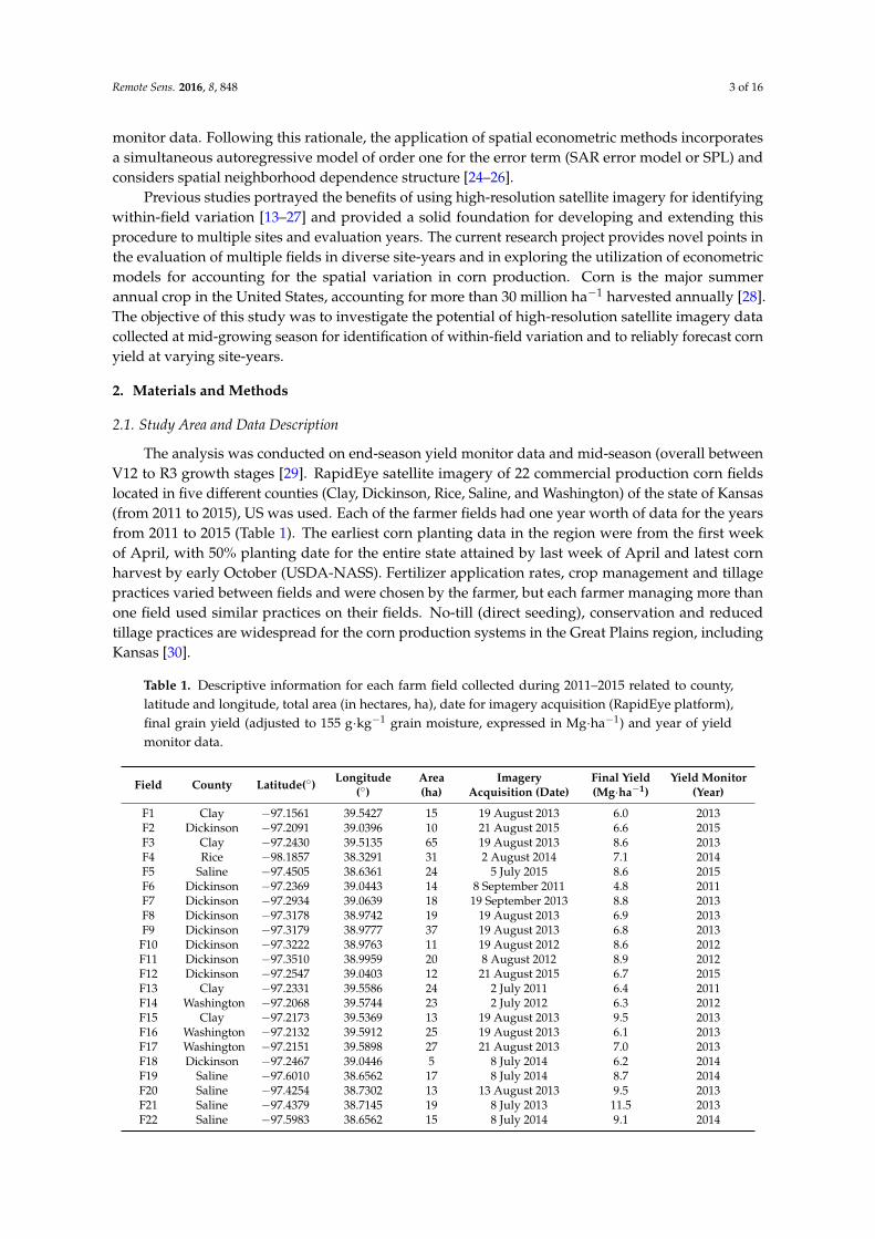
Table 1. Descriptive information for each farm field collected during 2011–2015 related to county,latitude and longitude, total area (in hectares, ha), date for imagery acquisition (RapidEye platform),final grain yield (adjusted to 155 g·kg−1 grain moisture, expressed in Mg·ha−1) and year of yieldmonitor data.

Field County Latitude(◦) Longitude(◦)

Area(ha)

ImageryAcquisition (Date)

Final Yield(Mg·ha−1)

Yield Monitor(Year)

F1 Clay −97.1561 39.5427 15 19 August 2013 6.0 2013F2 Dickinson −97.2091 39.0396 10 21 August 2015 6.6 2015F3 Clay −97.2430 39.5135 65 19 August 2013 8.6 2013F4 Rice −98.1857 38.3291 31 2 August 2014 7.1 2014F5 Saline −97.4505 38.6361 24 5 July 2015 8.6 2015F6 Dickinson −97.2369 39.0443 14 8 September 2011 4.8 2011F7 Dickinson −97.2934 39.0639 18 19 September 2013 8.8 2013F8 Dickinson −97.3178 38.9742 19 19 August 2013 6.9 2013F9 Dickinson −97.3179 38.9777 37 19 August 2013 6.8 2013F10 Dickinson −97.3222 38.9763 11 19 August 2012 8.6 2012F11 Dickinson −97.3510 38.9959 20 8 August 2012 8.9 2012F12 Dickinson −97.2547 39.0403 12 21 August 2015 6.7 2015F13 Clay −97.2331 39.5586 24 2 July 2011 6.4 2011F14 Washington −97.2068 39.5744 23 2 July 2012 6.3 2012F15 Clay −97.2173 39.5369 13 19 August 2013 9.5 2013F16 Washington −97.2132 39.5912 25 19 August 2013 6.1 2013F17 Washington −97.2151 39.5898 27 21 August 2013 7.0 2013F18 Dickinson −97.2467 39.0446 5 8 July 2014 6.2 2014F19 Saline −97.6010 38.6562 17 8 July 2014 8.7 2014F20 Saline −97.4254 38.7302 13 13 August 2013 9.5 2013F21 Saline −97.4379 38.7145 19 8 July 2013 11.5 2013F22 Saline −97.5983 38.6562 15 8 July 2014 9.1 2014

Remote Sens. 2016, 8, 848 4 of 16

A total of 22 mid-season (July–August) RapidEye images were used from the growing seasonsof 2011–2015 (Table 1). The RapidEye image was collected during a critical period for determiningthe grain yield of corn (approximately 20 days before and 20 after flowering) and it consists of blue(440–510 nm), green (520–590 nm), red (630–685 nm), red-edge (690–730 nm), and near infrared (NIR)(760–850 nm) spectral bands at 5 m ground sampling distance at nadir. Indices selected for evaluationused a combination of visible, near-infrared and red-edge bands (Table 2), including NDVI, red edgenormalized difference vegetation index (NDVIre), red edge simple ratio (SRre) and green NDVI(NDVIG). The RapidEye image was orthorectified by the vendor.

Table 2. Description, acronym, equations, and references for all vegetation indices (VIs).

Index Abbreviation Equation Reference

Near infrared NIRNormalized difference vegetation index NDVIr (RNIR − RED)/(RNIR + RRED) [31]

Green normalized difference vegetation index NDVIG (RNIR − RGREEN)/(RNIR + RGREEN) [32]Red-edge normalized difference vegetation index NDVIre (RNIR − REDEDGE)/(RNIR + RREDEDGE) [33]

Red-edge simple radio SRre RNIR/REDEDGE [33]

Corn grain yield was georeferenced using a yield monitor system (grain mass flow and moisturesensors) and grain yield was measured on three-second intervals and recorded using equipped withDGPS. Grain yield data were adjusted to 155 g·kg−1 grain moisture, spatially located and analyzedwith ArcGIS Geospatial Analyst (ArcGIS v10.3, Environmental System Research Institute Inc. (ESRI),Redlands, CA, USA). The data points located approximately 20 m from the borders of the sites weredeleted before the analysis because the combination was unlikely to be full [34,35]. Yield measurementsassumed to be erroneous were excised by standard protocol if the observations were more than threestandard deviations (SDs) from the mean, as were yield data recorded when the harvester changeddirection or speed significantly [11,36]. All geostatistical evaluation was conducted with the ArcGISGeospatial Analyst (ArcGIS v10.3). A final 5 m × 5 m grid cell size was chosen because it reflects thescale of variability associated with the VIs of Rapid Eye image.

2.2. Data Analysis

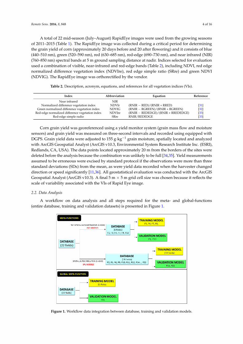
A workflow on data analysis and all steps required for the meta- and global-functions(entire database, training and validation datasets) is presented in Figure 1.

Remote Sens. 2016, 8, 848 4 of 16

the grain yield of corn (approximately 20 days before and 20 after flowering) and it consists of blue (440–510 nm), green (520–590 nm), red (630–685 nm), red-edge (690–730 nm), and near infrared (NIR) (760–850 nm) spectral bands at 5 m ground sampling distance at nadir. Indices selected for evaluation used a combination of visible, near-infrared and red-edge bands (Table 2), including NDVI, red edge normalized difference vegetation index (NDVIre), red edge simple ratio (SRre) and green NDVI (NDVIG). The RapidEye image was orthorectified by the vendor.

Table 2. Description, acronym, equations, and references for all vegetation indices (VIs).

Index Abbreviation Equation ReferenceNear infrared NIR

Normalized difference vegetation index NDVIr (RNIR − RED)/(RNIR + RRED) [31] Green normalized difference vegetation index NDVIG (RNIR − RGREEN)/(RNIR + RGREEN) [32]

Red-edge normalized difference vegetation index NDVIre (RNIR − REDEDGE)/(RNIR + RREDEDGE) [33] Red-edge simple radio SRre RNIR/REDEDGE [33]

Corn grain yield was georeferenced using a yield monitor system (grain mass flow and moisture sensors) and grain yield was measured on three-second intervals and recorded using equipped with DGPS. Grain yield data were adjusted to 155 g·kg−1 grain moisture, spatially located and analyzed with ArcGIS Geospatial Analyst (ArcGIS v10.3, Environmental System Research Institute Inc. (ESRI), Redlands, CA, USA). The data points located approximately 20 m from the borders of the sites were deleted before the analysis because the combination was unlikely to be full [34,35]. Yield measurements assumed to be erroneous were excised by standard protocol if the observations were more than three standard deviations (SDs) from the mean, as were yield data recorded when the harvester changed direction or speed significantly [11,36]. All geostatistical evaluation was conducted with the ArcGIS Geospatial Analyst (ArcGIS v10.3). A final 5 m × 5 m grid cell size was chosen because it reflects the scale of variability associated with the VIs of Rapid Eye image.

2.2. Data Analysis

A workflow on data analysis and all steps required for the meta- and global-functions (entire database, training and validation datasets) is presented in Figure 1.

Figure 1. Workflow data integration between database, training and validation models.

Figure 1. Workflow data integration between database, training and validation models.

Remote Sens. 2016, 8, 848 5 of 16

As an initial step, spatial autocorrelation analysis was conducted on yield and VIs (NIR, NDVI,NDVIG, NDVIre, and SRre) data of each field using Moran’s [37] test (Table 3). Moran’s I statisticmeasures the strength of spatial autocorrelation in a response among nearby locations in space as afunction of cross-products of the neighboring weighted deviations from the mean. Moran’s I coefficientvalues near 1 and −1 indicate strong positive and negative autocorrelation, respectively. Coefficientvalues near 0 support the null hypothesis of no spatial autocorrelation. Spatial correlation analysiswas conducted using GeoDa software 1.4.6 [38].

Table 3. Moran’s I test (MI) to vegetation indices (VIs) obtained from mid-season high-resolutionsatellite imagery and yield monitor data.

Field NIR SRre NDVIr NDVIG NDVIre Yield

MI p-Value MI p-Value MI p-Value MI p-Value MI p-Value MI p-Value

F1 0.13 *** 0.08 * 0.11 *** 0.12 *** 0.10 ** 0.08 ***F2 0.14 *** 0.10 *** 0.12 *** 0.10 ** 0.12 *** 0.09 ***F3 0.18 *** 0.15 *** 0.17 *** 0.16 *** 0.16 *** 0.12 ***F4 0.06 * 0.07 ** 0.05 * 0.06 * 0.09 * 0.09 **F5 0.17 *** 0.14 *** 0.16 *** 0.18 *** 0.16 *** 0.13 ***F6 0.20 *** 0.20 *** 0.22 *** 0.20 *** 0.21 *** 0.25 ***F7 0.14 *** 0.10 *** 0.12 *** 0.10 ** 0.12 *** 0.09 *F8 0.10 *** 0.12 *** 0.13 *** 0.12 *** 0.13 *** 0.11 **F9 0.13 *** 0.11 *** 0.11 *** 0.11 *** 0.12 *** 0.10 **

F10 0.19 *** 0.19 *** 0.20 *** 0.20 *** 0.19 *** 0.16 ***F11 0.28 *** 0.23 *** 0.29 *** 0.25 *** 0.26 *** 0.24 ***F12 0.24 *** 0.20 *** 0.21 *** 0.19 *** 0.17 *** 0.17 ***F13 0.16 *** 0.14 *** 0.12 *** 0.13 *** 0.12 *** 0.11 ***F14 0.06 * 0.07 * 0.08 * 0.07 * 0.08 ** 0.09 **F15 0.14 *** 0.15 *** 0.14 *** 0.14 *** 0.15 *** 0.14 ***F16 0.13 *** 0.10 ** 0.11 *** 0.11 *** 0.12 *** 0.10 ***F17 0.15 *** 0.14 *** 0.14 *** 0.13 *** 0.12 *** 0.12 ***F18 0.16 *** 0.14 *** 0.16 *** 0.15 *** 0.15 *** 0.13 ***F19 0.12 *** 0.12 *** 0.13 *** 0.11 *** 0.12 *** 0.1 **F20 0.16 *** 0.13 *** 0.14 *** 0.16 *** 0.14 *** 0.15 ***F21 0.14 *** 0.10 ** 0.12 *** 0.10 *** 0.12 *** 0.09 ***F22 0.29 *** 0.26 *** 0.25 *** 0.27 *** 0.27 *** 0.15 ***

* Significant at the alpha = 0.05 error level; ** Significant at the alpha = 0.01 error level; *** Significant at thealpha = 0.001 error level.

In order to identify an appropriate model that describes the relationship between end-seasonobserved corn yields as a function of VIs of mid-season high-resolution imagery data for each field.Two models are considered, first is the classical linear regression model assuming that the errors areindependent and identically distributed (i.i.d.). Ordinary least squares (OLS) is known as an efficientmethod for estimating the unknown parameters for this model, therefore we will call this baselinemodel as “OLS” model. Both the response variable corn yield and predictor variables VIs, as wellas the regression errors, exhibit spatial autocorrelation as Moran’s I test shows, the i.i.d. assumptionis violated. This leads us to consider the application of the spatial error model (Anselin [24]),which is called “spatial econometric” model in this paper, to account for the spatial interaction(spatial autocorrelation) and spatial structure (spatial heterogeneity) in the datasets. To be morespecific, this spatial regression model can be expressed as:

y = Xβ + u with u = λWu + ε (1)

where y is a vector (n by 1) of observations on the dependent variable, X is an n by p matrixof observations on the explanatory variables, and u is an error term that follows a simultaneousautoregressive (SAR) specification with spatial autoregressive coefficient λ. In the spatial autoregression,

Remote Sens. 2016, 8, 848 6 of 16

the vector of errors is expressed as a sum of a vector ε (n by 1) of independent and identically distributedinnovation terms and a so-called spatially lagged error λWu. The latter boils down to a weighted averageof errors in the neighboring locations. The selection of neighbors is formally specified in the n by nspatial weights matrix W. In this study, W was created using the distance-based K-Nearest NeighborSpatial Weights, because the database was irregular [39]. For this spatial econometric model, theparameter estimation is achieved by maximum likelihood estimation method. In comparison, theclassical OLS model is simply given by y = Xβ + ε, where ε is a vector of i.i.d error terms. Whileapplying to dataset, ordinary estimation method is used to estimate the parameters. To simplifyequations from 22 (Figure 2) to two global models (Figure 3), fields were grouped into two clusters(Figure 1). Before grouping fields, the database (5 m × 5 m grid) for yield and VIs was randomlysampled to generate 600 observations per field. The yield data were normalized to lessen the effectof years, which allows comparison across site-years [40,41]. Clustering analysis divided two groups,i.e., fields with spatial autocorrelation in error term (λ values significant, p ≤ 0.05) and without spatialautocorrelation (λ values insignificant, p > 0.05). Five independent fields (F1, F11, F13, F21 and F22);two from those fields that need spatial adjustment, two fields from those that did not require spatialadjustment, and one from all fields, were randomly selected and kept aside for validation analysis(Figure 1). From the remaining training data, two global models were developed to predict end-seasonobserved yield in fields with and without spatial autocorrelation. The two models developed withtraining dataset were validated with the testing dataset (fields that were not used in the database tobuild both models, but to validate the models (Figure 1). In the case of OLS and spatial (SPL) models,two fields randomly selected were F1–F13 and F11–F22, respectively. To further simplify matters,all training datasets, irrespective of whether they require spatial adjustment or not, were combined andone SPL model was developed and validated with the one validation dataset selected (F21).

Remote Sens. 2016, 8, 848 6 of 16

Model performance was assessed using statistical criteria proposed by Akaike (AIC) [24,26]. Accuracy of estimation and model fitting was evaluated using the Root-Mean Square Error (RMSE) and Pseudo R2 [42]. In addition, spatial predictions from each model were visually compared with geostatistical interpolation of yield from the dataset for each field and for the global meta-function.

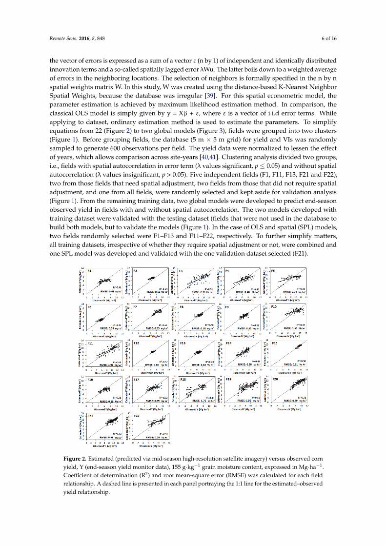
Figure 2. Estimated (predicted via mid-season high-resolution satellite imagery) versus observed corn yield, Y (end-season yield monitor data), 155 g·kg−1 grain moisture content, expressed in Mg·ha−1. Coefficient of determination (R2) and root mean-square error (RMSE) was calculated for each field relationship. A dashed line is presented in each panel portraying the 1:1 line for the estimated–observed yield relationship.

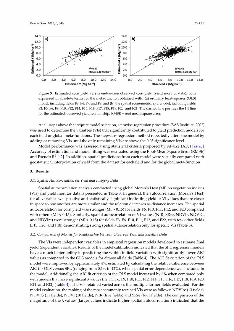
Figure 3. Estimated corn yield versus end-season observed corn yield (yield monitor data), both expressed in absolute terms for the meta-function obtained with: (a) ordinary least-squares (OLS) model, including fields F3, F4, F7, and F8; and (b) the spatial econometric, SPL, model, including fields F2, F5, F6, F9, F10, F12, F14, F15, F16, F17, F18, F19, F20, and F21. The dashed line portrays the 1:1 line for the estimated–observed yield relationship. RMSE = root mean square error.

Figure 2. Estimated (predicted via mid-season high-resolution satellite imagery) versus observed cornyield, Y (end-season yield monitor data), 155 g·kg−1 grain moisture content, expressed in Mg·ha−1.Coefficient of determination (R2) and root mean-square error (RMSE) was calculated for each fieldrelationship. A dashed line is presented in each panel portraying the 1:1 line for the estimated–observedyield relationship.

Remote Sens. 2016, 8, 848 7 of 16

Remote Sens. 2016, 8, 848 6 of 16

Model performance was assessed using statistical criteria proposed by Akaike (AIC) [24,26]. Accuracy of estimation and model fitting was evaluated using the Root-Mean Square Error (RMSE) and Pseudo R2 [42]. In addition, spatial predictions from each model were visually compared with geostatistical interpolation of yield from the dataset for each field and for the global meta-function.

Figure 2. Estimated (predicted via mid-season high-resolution satellite imagery) versus observed corn yield, Y (end-season yield monitor data), 155 g·kg−1 grain moisture content, expressed in Mg·ha−1. Coefficient of determination (R2) and root mean-square error (RMSE) was calculated for each field relationship. A dashed line is presented in each panel portraying the 1:1 line for the estimated–observed yield relationship.

Figure 3. Estimated corn yield versus end-season observed corn yield (yield monitor data), both expressed in absolute terms for the meta-function obtained with: (a) ordinary least-squares (OLS) model, including fields F3, F4, F7, and F8; and (b) the spatial econometric, SPL, model, including fields F2, F5, F6, F9, F10, F12, F14, F15, F16, F17, F18, F19, F20, and F21. The dashed line portrays the 1:1 line for the estimated–observed yield relationship. RMSE = root mean square error.

Figure 3. Estimated corn yield versus end-season observed corn yield (yield monitor data), bothexpressed in absolute terms for the meta-function obtained with: (a) ordinary least-squares (OLS)model, including fields F3, F4, F7, and F8; and (b) the spatial econometric, SPL, model, including fieldsF2, F5, F6, F9, F10, F12, F14, F15, F16, F17, F18, F19, F20, and F21. The dashed line portrays the 1:1 linefor the estimated–observed yield relationship. RMSE = root mean square error.

At all steps above that require model selection, stepwise-regression procedure (SAS Institute, 2002)was used to determine the variables (VIs) that significantly contributed to yield prediction models foreach field or global meta-functions. The stepwise-regression method repeatedly alters the model byadding or removing VIs until the only remaining VIs are above the 0.05 significance level.

Model performance was assessed using statistical criteria proposed by Akaike (AIC) [24,26].Accuracy of estimation and model fitting was evaluated using the Root-Mean Square Error (RMSE)and Pseudo R2 [42]. In addition, spatial predictions from each model were visually compared withgeostatistical interpolation of yield from the dataset for each field and for the global meta-function.

3. Results

3.1. Spatial Autocorrelation on Yield and Imagery Data

Spatial autocorrelation analysis conducted using global Moran’s I test (MI) on vegetation indices(VIs) and yield monitor data is presented in Table 3. In general, the autocorrelation (Moran’s I test)for all variables was positive and statistically significant indicating yield or VI values that are closerin space to one another are more similar and the relation decreases as distance increases. The spatialautocorrelation for corn yield was stronger (MI > 0.15) for fields F6, F10, F11, F12, and F20 comparedwith others (MI < 0.15). Similarly, spatial autocorrelation of VI values (NIR, SRre, NDVIr, NDVIG,and NDVIre) were stronger (MI > 0.15) for fields F3, F6, F10, F11, F12, and F22, with few other fields(F13, F20, and F18) demonstrating strong spatial autocorrelation only for specific VIs (Table 3).

3.2. Comparison of Models for Relationship between Observed Yield and Satellite Data

The VIs were independent variables in empirical regression models developed to estimate finalyield (dependent variable). Results of the model calibration indicated that the SPL regression modelshave a much better ability in predicting the within-in field variation with significantly lower AICvalues as compared to the OLS models for almost all fields (Table 4). The AIC fit criterion of the OLSmodel were improved by approximately 4%, estimated by calculating the relative difference betweenAIC for OLS versus SPL (ranging from 0.1% to 42%), when spatial error dependence was included inthe model. Additionally, the AIC fit criterion of the OLS model increased by 6% when compared onlywith models that have significant λ values (F2, F5, F6, F9, F10, F11, F12, F14, F15, F16, F17, F18, F19, F20,F21, and F22) (Table 4). The VIs retained varied across the multiple farmer fields evaluated. For themodel evaluation, the ranking of the most commonly retained VIs were as follows: NDVIre (13 fields),NDVIG (11 fields), NDVI (10 fields), NIR (five fields) and SRre (four fields). The comparison of themagnitude of the λ values (larger values indicate higher spatial autocorrelation) indicated that the

Remote Sens. 2016, 8, 848 8 of 16

fields with significant λ values (p < 0.05) have a higher spatial continuity relative to when λ values werenot significant (Table 4). In summary, SPL outperformed OLS methods (Table 4). For fields presentingbetter fit with the SPL models, a significant λ value reflected a very strong spatial correlation in errors.By accounting for spatial dependence, regression coefficients of the models changed, which improvedthe mapping of intra-field yield variation.

Table 4. Multiple linear regression models (for the ordinary least-square (OLS_ and spatial econometric(SPL)) including the vegetation indices (VIs) obtained from mid-season high-resolution satellite imageryas predictors of the end-season yield monitor data.

Field Models Equations AIC

F1 OLS Yield (Mg·ha−1) = −7.8 *** + 0.12(NIR)+20.0 ***(NDVIre) 238.6SPL Yield (Mg·ha−1) = −6.9 *** + 0.11(NIR) + 20.2 ***(NDVIre)+ 0.28(λ) 236.8

F2 OLS Yield (Mg·ha−1) = −1.8 * + 8.2 **(NDVIG) + 1.16 ***(SRre) 80.3SPL Yield (Mg·ha−1)= −0.3 + 7.8 **(NDVIG)+ 1.18 ***(SRre)+ 0.58 ***(λ) 72.6

F3 OLS Yield (Mg·ha−1)= −9.1 *** − 14.9 *(NDVI) + 26.5(NDVIG) + 34.0 ***(NDVIre) 346.8SPL Yield (Mg·ha−1)= −9.2 *** − 14.7 *(NDVI) + 26.52(NDVIG) + 33.91 ***(NDVIre) − 0.06(λ) 344.8

F4 OLS Yield (Mg·ha−1) = −1.1 + 28.5 ***(NDVI) + 17.7(NDVIG) − 30.85 ***(NDVIre) 284.2SPL Yield (Mg·ha−1) = −1.7 + 29.2 ***(NDVI) + 16.91(NDVIG) − 30.89 ***(NDVIre) + 0.23(Wu) 281.9

F5 OLS Yield (Mg·ha−1) = −4.8 *** + 23.6 ***(NDVI) 391.4SPL Yield (Mg·ha−1) = −4.8 *** + 23.7 ***(NDVI) + 0.04 *(λ) 391.3

F6 OLS Yield (Mg·ha−1) = −0.9 * + 12.7 ***(NDVIG) 108.2SPL Yield (Mg·ha−1) = −1.42 * + 13.8 ***(NDVIG) + 0.02 *(λ) 104.2

F7 OLS Yield (Mg·ha−1) = 3.5 ** + 0.12 **(NIR) 106.8SPL Yield (Mg·ha−1) = 3.5 ** + 0.12 **(NIR) − 0.04(λ) 106.6

F8 OLS Yield (Mg·ha−1) = −3.1 *** + 2.2***(SRre) + 11.4***(NDVIG) 110.5SPL Yield (Mg·ha−1) = −3.2 *** + 2.2 ***(SRre) + 11.7 ***(NDVIG) + 0.02(λ) 110.5

F9 OLS Yield (Mg·ha−1) = −4.69 *** + 0.95(NDVIG) + 24.1 ***(NDVIre) 111.2SPL Yield (Mg·ha−1) = −4.7 *** + 0.47(NDVIG) + 24.5 ***(NDVIre) − 0.14 *(λ) 110.5

F10 OLS Yield (Mg·ha−1) = −8.6 ** + 0.57 ***(NIR) − 6.5 ***(SRre) + 20.8 ***(NDVIG) 252.5SPL Yield (Mg·ha−1) = −8.1 ** + 0.48 ***(NIR) − 5.2 ***(SRre) + 21.5 ***(NDVIG) + 0.27 *(λ) 250.0

F11 OLS Yield (Mg·ha−1) = 0.46 + 32.36 ***(NDVIre) 342.5SPL Yield (Mg·ha−1) = 0.53 + 32.09 ***(NDVIre) − 0.22 *(λ) 341.8

F12 OLS Yield (Mg·ha−1) = 2.2 * + 0.15 ***(NIR) − 7.4 ***(NDVIG) 31.8SPL Yield (Mg·ha−1) = 2.0 * + 0.17 ***(NIR) − 9.6 **(NDVIG) + 0.39 *(λ) 28.0

F13 OLS Yield (Mg·ha−1)= −0.25 + 0.13 ***(NIR) + 22.9 ***(NDVIre) − 14.7 ***(NDVI) 104.0SPL Yield (Mg·ha−1) = −0.15 + 0.12 ***(NIR) + 22.8 ***(NDVIre) − 14.6 ***(NDVI) + 0.09(λ) 103.7

F14 OLS Yield (Mg·ha−1) = −2.8 *** + 23.9 ***(NDVIre) 239.0SPL Yield (Mg·ha−1) = −4.2 *** + 27.6 ***(NDVIre) + 0.63 ***(λ) 220.6

F15 OLS Yield (Mg·ha−1) = 4.1 *** + 5.1 ***(NDVI) + 4.9 ***(NDVIre) 12.7SPL Yield (Mg·ha−1) = 3.1 *** + 6.0 ***(NDVI) + 5.9 ***(NDVIre) + 0.36 ***(λ) 7.3

F16 OLS Yield (Mg·ha−1) = −17.3 *** + 34.9 ***(SRre) + 16.7 ***(NDVIG) 181.7SPL Yield (Mg·ha−1) = −18.7 *** + 33.7 ***(SRre) + 23.2 ***(NDVIG) + 0.71**(λ) 165.5

F17 OLS Yield (Mg·ha−1) = −12.4 *** + 31.4 ***(NDVI) 236.3SPL Yield (Mg·ha−1) = −12.6 *** + 31.6 ***(NDVI) + 0.2 **(λ) 234.5

F18 OLS Yield (Mg·ha−1) = −26.5 *** + 17.8 ***(NDVI) + 41.8 ***(NDVIre) 239.8SPL Yield (Mg·ha−1) = −26.4 *** + 20.8 ***(NDVI) + 37.8 ***(NDVIre) + 0.15 ***(λ) 234.6

F19 OLS Yield (Mg·ha−1) = −20.9 *** + 15.9(NDVI) + 36.1 ***(NDVIG) 323.6SPL Yield (Mg·ha−1) = −20.0 *** + 17.2(NDVI) + 32.6 ***(NDVIG) + 0.39 **(λ) 321.1

F20 OLS Yield (Mg·ha−1) = −6.2 *** + 12.7 ***(NDVI) + 14.4 ***(NDVIre) 348.2SPL Yield (Mg·ha−1) = −6.2 *** + 12.7 ***(NDVI) + 11.5 ***(NDVIre) + 0.21 *(λ) 346.9

F21 OLS Yield (Mg·ha−1) = −6.9 *** + 0.85 (SRre) + 6.0 **(NDVI) + 16.2 ***(NDVIG)+ 12.1 ***(NDVIre)

604.9

SPL Yield (Mg·ha−1) = −7.1 *** + 0.69 (SRre) + 6.2 **(NDVI) + 14.6 ***(NDVIG)+ 14.3 ***(NDVIre) + 0.35 ***(λ)

592.5

F22 OLS Yield (Mg·ha−1) = −21.59 *** + 57.38 ***(NDVIre) 296.3SPL Yield (Mg·ha−1) = −20.07 *** + 54.47 ***(NDVIre)+ 0.27 ***(λ) 292.5

Notes: The statistically significant coefficients are indicated by asterisks, where * indicates p < 0.05; ** indicatesp < 0.01; and *** indicates p < 0.001. Parameters with no asterisks are therefore not significant at the 0.05 level.

Notwithstanding the level of significance for λ value, SPL regression models presented tend tohave smaller AIC and therefore show better trade-off between the goodness of fit of the model and thecomplexity of the model (Table 4). Following this rationale, the scatter plots were developed utilizing

Remote Sens. 2016, 8, 848 9 of 16

the SPL model validation for all fields (Figure 2). Pseudo coefficient of determination (R2) for all fieldsranged from 0.29 to 0.70 units, with approximately 50% of the fields presenting pseudo R2 valuesabove 0.5 units (Figure 2). End-season yield monitor data reflected a yield variation ranging from2 to 14 Mg·ha−1 across all farms evaluated. The results indicated that the spatial models providedconsistent predictions, with low RMSE values and higher R2 for the estimated versus observed yielddata. The RMSE difference between estimated- and observed-yields was approximately of 1 Mg·ha−1

(ranged between 0.1 and 2.8 Mg·ha−1) for all 22 fields.

3.3. Spatial and OLS Model Variables and Validation Performance

Based on each field evaluation (Table 4), a training dataset was prepared including all models thatresulted in a lack of spatial autocorrelation, OLS model, for fields: F3, F4, F7, and F8 (Figure 1). All fourfields were utilized and an overall equation was determined in order to estimate yields. Estimatedyield resulted by the OLS model showed similarity to the observed yield at harvest, with an adequatecoefficient of determination (R2 = 0.47) and root mean square error of 1.4 Mg·ha−1 (Figure 3a). Similarto the OLS model, a training dataset was built for the SPL model including fields F2, F5, F6, F9, F10, F12,F14, F15, F16, F17, F18, F19, F20, and F21, following the steps proposed in the framework presentedin Figure 1. The SPL model was utilized to fit estimated versus observed yields, which presenteda low RMSE (1.28 Mg·ha−1), high correlation (R2 = 0.48), and with all observations close to 1:1 line(Figure 3b). Better performance, slightly higher coefficient of determination, and lower RMSE onforecasting yields was documented for the SPL model (Figure 3b) as compared to the overall OLSmodel (Figure 3a).

After clustering into two groups, OLS vs. SPL groups, and variables were selected, out of fiveVIs, the NDVIre and NDVIG were statistically significant in both OLS and spatial models, whereasNIR was only significant in the spatial model (Table 5). Predictive yield maps were prepared withthe validation data (based on framework in Figure 1). Both selected models provided significantpredictors for yield (p < 0.05) within their respective cluster. The regression models developed wereapplied to each respective training datasets (OLS and SPL datasets) and predictive corn yield mapswere generated from those models (Figure 4).

Table 5. Meta-functions for the ordinary least-square (OLS) and spatial econometric (SPL) modelsincluding the vegetation indices (VIs) obtained from mid-season high-resolution satellite imageryas predictors of the end-season yield monitor data, observed corn yield for all fields evaluated inthis study.

Models Equations

OLS Yield (Mg·ha−1)= −2.47 ** + 0.11 *(NIR) + 9.22 *(NDVIG) + 3.85 ***(NDVIre)SPL Yield (Mg·ha−1)= −10.43 ** + 0.31 **(NIR) − 9.21 *(NDVIG) + 16.59 ***(NDVIre) + 0.31 ***(λ)

Notes: The statistically significant coefficients are indicated by asterisks, where * indicates p < 0.05; ** indicatesp < 0.01; and *** indicates p < 0.001. Parameters with no asterisks are therefore not significant at the 0.05 level.

Remote Sens. 2016, 8, 848 9 of 16

Notwithstanding the level of significance for λ value, SPL regression models presented tend to have smaller AIC and therefore show better trade-off between the goodness of fit of the model and the complexity of the model (Table 4). Following this rationale, the scatter plots were developed utilizing the SPL model validation for all fields (Figure 2). Pseudo coefficient of determination (R2) for all fields ranged from 0.29 to 0.70 units, with approximately 50% of the fields presenting pseudo R2 values above 0.5 units (Figure 2). End-season yield monitor data reflected a yield variation ranging from 2 to 14 Mg·ha−1 across all farms evaluated. The results indicated that the spatial models provided consistent predictions, with low RMSE values and higher R2 for the estimated versus observed yield data. The RMSE difference between estimated- and observed-yields was approximately of 1 Mg·ha−1 (ranged between 0.1 and 2.8 Mg·ha−1) for all 22 fields.

3.3. Spatial and OLS Model Variables and Validation Performance

Based on each field evaluation (Table 4), a training dataset was prepared including all models that resulted in a lack of spatial autocorrelation, OLS model, for fields: F3, F4, F7, and F8 (Figure 1). All four fields were utilized and an overall equation was determined in order to estimate yields. Estimated yield resulted by the OLS model showed similarity to the observed yield at harvest, with an adequate coefficient of determination (R2 = 0.47) and root mean square error of 1.4 Mg·ha−1 (Figure 3a). Similar to the OLS model, a training dataset was built for the SPL model including fields F2, F5, F6, F9, F10, F12, F14, F15, F16, F17, F18, F19, F20, and F21, following the steps proposed in the framework presented in Figure 1. The SPL model was utilized to fit estimated versus observed yields, which presented a low RMSE (1.28 Mg·ha−1), high correlation (R2 = 0.48), and with all observations close to 1:1 line (Figure 3b). Better performance, slightly higher coefficient of determination, and lower RMSE on forecasting yields was documented for the SPL model (Figure 3b) as compared to the overall OLS model (Figure 3a).

After clustering into two groups, OLS vs. SPL groups, and variables were selected, out of five VIs, the NDVIre and NDVIG were statistically significant in both OLS and spatial models, whereas NIR was only significant in the spatial model (Table 5). Predictive yield maps were prepared with the validation data (based on framework in Figure 1). Both selected models provided significant predictors for yield (p < 0.05) within their respective cluster. The regression models developed were applied to each respective training datasets (OLS and SPL datasets) and predictive corn yield maps were generated from those models (Figure 4).

Table 5. Meta-functions for the ordinary least-square (OLS) and spatial econometric (SPL) models including the vegetation indices (VIs) obtained from mid-season high-resolution satellite imagery as predictors of the end-season yield monitor data, observed corn yield for all fields evaluated in this study.

Models EquationsOLS Yield (Mg·ha−1)= −2.47 ** + 0.11 *(NIR) + 9.22 *(NDVIG) + 3.85 ***(NDVIre) SPL Yield (Mg·ha−1)= −10.43 ** + 0.31 **(NIR) − 9.21 *(NDVIG) + 16.59 ***(NDVIre) + 0.31 ***(λ)

Notes: The statistically significant coefficients are indicated by asterisks, where * indicates p < 0.05; ** indicates p < 0.01; and *** indicates p < 0.001. Parameters with no asterisks are therefore not significant at the 0.05 level.

Figure 4. Cont. Figure 4. Cont.

Remote Sens. 2016, 8, 848 10 of 16Remote Sens. 2016, 8, 848 10 of 16

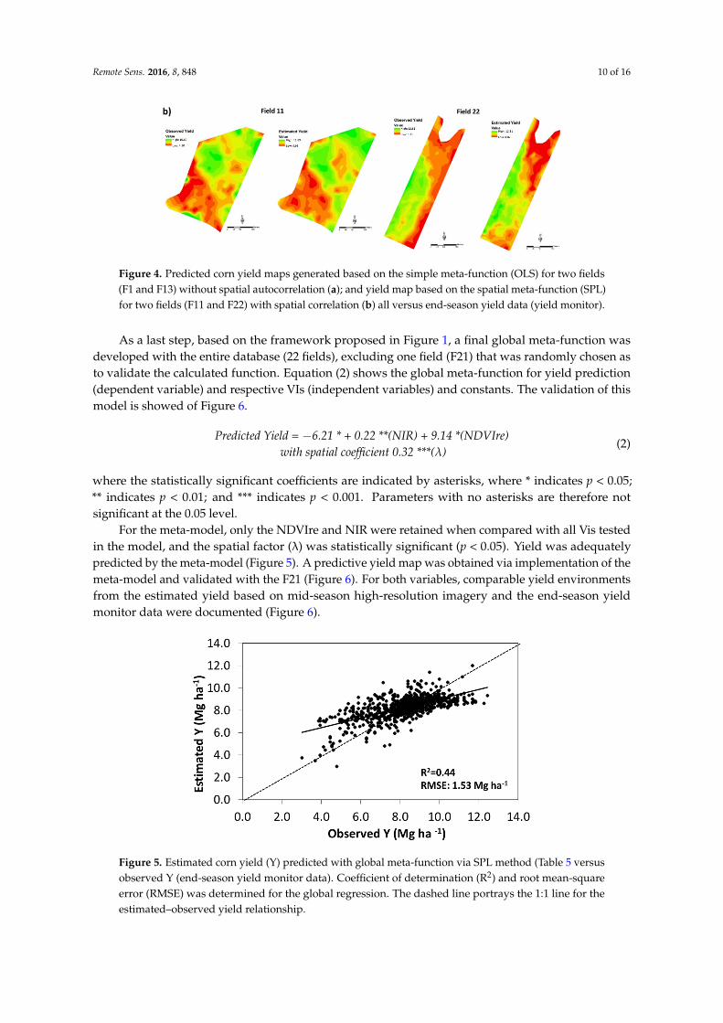
Figure 4. Predicted corn yield maps generated based on the simple meta-function (OLS) for two fields (F1 and F13) without spatial autocorrelation (a); and yield map based on the spatial meta-function (SPL) for two fields (F11 and F22) with spatial correlation (b) all versus end-season yield data (yield monitor).

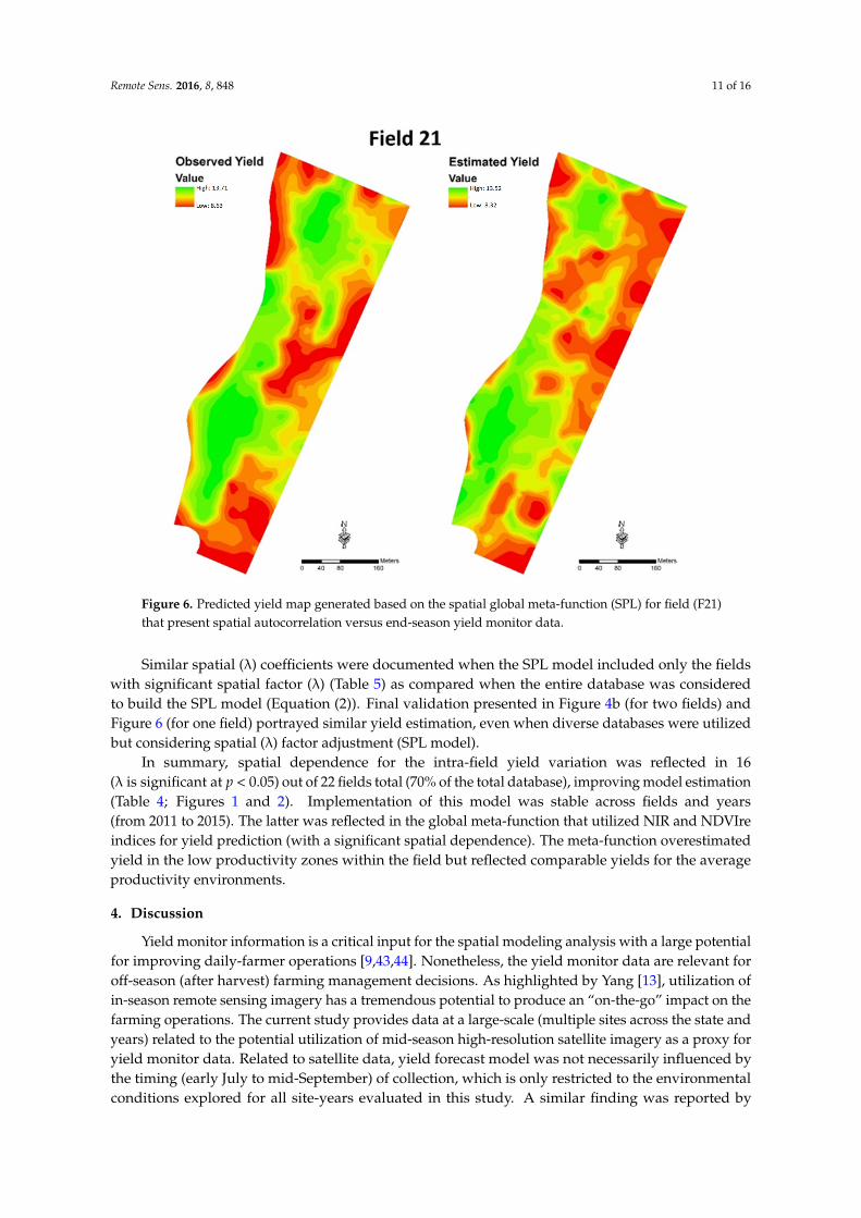
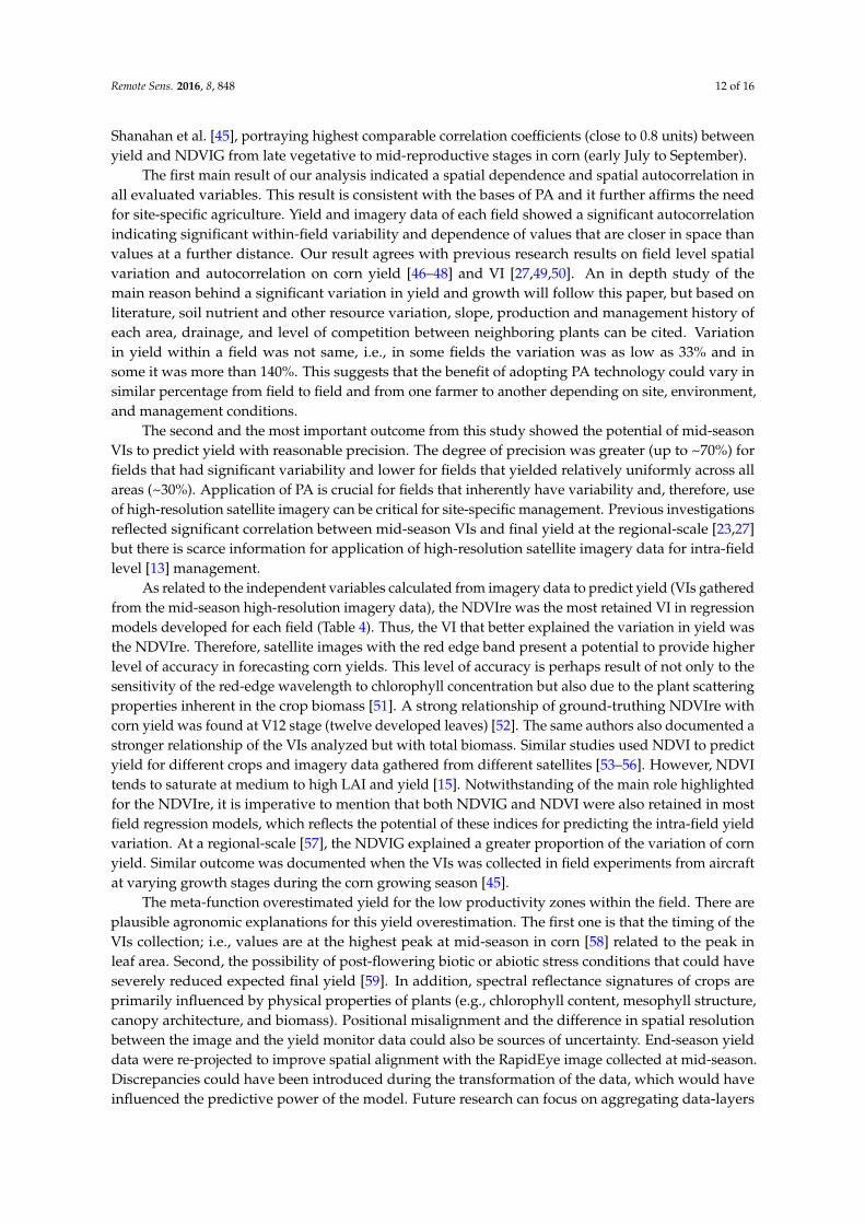
As a last step, based on the framework proposed in Figure 1, a final global meta-function was developed with the entire database (22 fields), excluding one field (F21) that was randomly chosen as to validate the calculated function. Equation (2) shows the global meta-function for yield prediction (dependent variable) and respective VIs (independent variables) and constants. The validation of this model is showed of Figure 6.

Predicted Yield = −6.21 * + 0.22 **(NIR) + 9.14 *(NDVIre) (2)

with spatial coefficient 0.32 ***(λ)

where the statistically significant coefficients are indicated by asterisks, where * indicates p < 0.05; ** indicates p < 0.01; and *** indicates p < 0.001. Parameters with no asterisks are therefore not significant at the 0.05 level.

For the meta-model, only the NDVIre and NIR were retained when compared with all Vis tested in the model, and the spatial factor (λ) was statistically significant (p < 0.05). Yield was adequately predicted by the meta-model (Figure 5). A predictive yield map was obtained via implementation of the meta-model and validated with the F21 (Figure 6). For both variables, comparable yield environments from the estimated yield based on mid-season high-resolution imagery and the end-season yield monitor data were documented (Figure 6).

Figure 5. Estimated corn yield (Y) predicted with global meta-function via SPL method (Table 5 versus observed Y (end-season yield monitor data). Coefficient of determination (R2) and root mean-square error (RMSE) was determined for the global regression. The dashed line portrays the 1:1 line for the estimated–observed yield relationship.

Similar spatial (λ) coefficients were documented when the SPL model included only the fields with significant spatial factor (λ) (Table 5) as compared when the entire database was considered to build the SPL model (Equation (2)). Final validation presented in Figure 4b (for two fields) and Figure 6

Figure 4. Predicted corn yield maps generated based on the simple meta-function (OLS) for two fields(F1 and F13) without spatial autocorrelation (a); and yield map based on the spatial meta-function (SPL)for two fields (F11 and F22) with spatial correlation (b) all versus end-season yield data (yield monitor).

As a last step, based on the framework proposed in Figure 1, a final global meta-function wasdeveloped with the entire database (22 fields), excluding one field (F21) that was randomly chosen asto validate the calculated function. Equation (2) shows the global meta-function for yield prediction(dependent variable) and respective VIs (independent variables) and constants. The validation of thismodel is showed of Figure 6.

Predicted Yield = −6.21 * + 0.22 **(NIR) + 9.14 *(NDVIre)with spatial coefficient 0.32 ***(λ)

(2)

where the statistically significant coefficients are indicated by asterisks, where * indicates p < 0.05;** indicates p < 0.01; and *** indicates p < 0.001. Parameters with no asterisks are therefore notsignificant at the 0.05 level.

For the meta-model, only the NDVIre and NIR were retained when compared with all Vis testedin the model, and the spatial factor (λ) was statistically significant (p < 0.05). Yield was adequatelypredicted by the meta-model (Figure 5). A predictive yield map was obtained via implementation of themeta-model and validated with the F21 (Figure 6). For both variables, comparable yield environmentsfrom the estimated yield based on mid-season high-resolution imagery and the end-season yieldmonitor data were documented (Figure 6).

Remote Sens. 2016, 8, 848 10 of 16

Figure 4. Predicted corn yield maps generated based on the simple meta-function (OLS) for two fields (F1 and F13) without spatial autocorrelation (a); and yield map based on the spatial meta-function (SPL) for two fields (F11 and F22) with spatial correlation (b) all versus end-season yield data (yield monitor).

As a last step, based on the framework proposed in Figure 1, a final global meta-function was developed with the entire database (22 fields), excluding one field (F21) that was randomly chosen as to validate the calculated function. Equation (2) shows the global meta-function for yield prediction (dependent variable) and respective VIs (independent variables) and constants. The validation of this model is showed of Figure 6.

Predicted Yield = −6.21 * + 0.22 **(NIR) + 9.14 *(NDVIre) (2)

with spatial coefficient 0.32 ***(λ)

where the statistically significant coefficients are indicated by asterisks, where * indicates p < 0.05; ** indicates p < 0.01; and *** indicates p < 0.001. Parameters with no asterisks are therefore not significant at the 0.05 level.

For the meta-model, only the NDVIre and NIR were retained when compared with all Vis tested in the model, and the spatial factor (λ) was statistically significant (p < 0.05). Yield was adequately predicted by the meta-model (Figure 5). A predictive yield map was obtained via implementation of the meta-model and validated with the F21 (Figure 6). For both variables, comparable yield environments from the estimated yield based on mid-season high-resolution imagery and the end-season yield monitor data were documented (Figure 6).

Figure 5. Estimated corn yield (Y) predicted with global meta-function via SPL method (Table 5 versus observed Y (end-season yield monitor data). Coefficient of determination (R2) and root mean-square error (RMSE) was determined for the global regression. The dashed line portrays the 1:1 line for the estimated–observed yield relationship.

Similar spatial (λ) coefficients were documented when the SPL model included only the fields with significant spatial factor (λ) (Table 5) as compared when the entire database was considered to build the SPL model (Equation (2)). Final validation presented in Figure 4b (for two fields) and Figure 6

Figure 5. Estimated corn yield (Y) predicted with global meta-function via SPL method (Table 5 versusobserved Y (end-season yield monitor data). Coefficient of determination (R2) and root mean-squareerror (RMSE) was determined for the global regression. The dashed line portrays the 1:1 line for theestimated–observed yield relationship.

Remote Sens. 2016, 8, 848 11 of 16

Remote Sens. 2016, 8, 848 11 of 16

(for one field) portrayed similar yield estimation, even when diverse databases were utilized but considering spatial (λ) factor adjustment (SPL model).

Figure 6. Predicted yield map generated based on the spatial global meta-function (SPL) for field (F21) that present spatial autocorrelation versus end-season yield monitor data.

In summary, spatial dependence for the intra-field yield variation was reflected in 16 (λ is significant at p < 0.05) out of 22 fields total (70% of the total database), improving model estimation (Table 4; Figures 1 and 2). Implementation of this model was stable across fields and years (from 2011 to 2015). The latter was reflected in the global meta-function that utilized NIR and NDVIre indices for yield prediction (with a significant spatial dependence). The meta-function overestimated yield in the low productivity zones within the field but reflected comparable yields for the average productivity environments.

4. Discussion

Yield monitor information is a critical input for the spatial modeling analysis with a large potential for improving daily-farmer operations [9,43,44]. Nonetheless, the yield monitor data are relevant for off-season (after harvest) farming management decisions. As highlighted by Yang [13], utilization of in-season remote sensing imagery has a tremendous potential to produce an “on-the-go” impact on the farming operations. The current study provides data at a large-scale (multiple sites across the state and years) related to the potential utilization of mid-season high-resolution satellite imagery as a proxy for yield monitor data. Related to satellite data, yield forecast model was not necessarily influenced by the timing (early July to mid-September) of collection, which is only restricted to the environmental conditions explored for all site-years evaluated in this study. A similar finding was reported by Shanahan et al. [45], portraying highest comparable correlation coefficients (close to 0.8 units) between yield and NDVIG from late vegetative to mid-reproductive stages in corn (early July to September).

The first main result of our analysis indicated a spatial dependence and spatial autocorrelation in all evaluated variables. This result is consistent with the bases of PA and it further affirms the need

Figure 6. Predicted yield map generated based on the spatial global meta-function (SPL) for field (F21)that present spatial autocorrelation versus end-season yield monitor data.

Similar spatial (λ) coefficients were documented when the SPL model included only the fieldswith significant spatial factor (λ) (Table 5) as compared when the entire database was consideredto build the SPL model (Equation (2)). Final validation presented in Figure 4b (for two fields) andFigure 6 (for one field) portrayed similar yield estimation, even when diverse databases were utilizedbut considering spatial (λ) factor adjustment (SPL model).

In summary, spatial dependence for the intra-field yield variation was reflected in 16(λ is significant at p < 0.05) out of 22 fields total (70% of the total database), improving model estimation(Table 4; Figures 1 and 2). Implementation of this model was stable across fields and years(from 2011 to 2015). The latter was reflected in the global meta-function that utilized NIR and NDVIreindices for yield prediction (with a significant spatial dependence). The meta-function overestimatedyield in the low productivity zones within the field but reflected comparable yields for the averageproductivity environments.

4. Discussion

Yield monitor information is a critical input for the spatial modeling analysis with a large potentialfor improving daily-farmer operations [9,43,44]. Nonetheless, the yield monitor data are relevant foroff-season (after harvest) farming management decisions. As highlighted by Yang [13], utilization ofin-season remote sensing imagery has a tremendous potential to produce an “on-the-go” impact on thefarming operations. The current study provides data at a large-scale (multiple sites across the state andyears) related to the potential utilization of mid-season high-resolution satellite imagery as a proxy foryield monitor data. Related to satellite data, yield forecast model was not necessarily influenced bythe timing (early July to mid-September) of collection, which is only restricted to the environmentalconditions explored for all site-years evaluated in this study. A similar finding was reported by

Remote Sens. 2016, 8, 848 12 of 16

Shanahan et al. [45], portraying highest comparable correlation coefficients (close to 0.8 units) betweenyield and NDVIG from late vegetative to mid-reproductive stages in corn (early July to September).

The first main result of our analysis indicated a spatial dependence and spatial autocorrelation inall evaluated variables. This result is consistent with the bases of PA and it further affirms the needfor site-specific agriculture. Yield and imagery data of each field showed a significant autocorrelationindicating significant within-field variability and dependence of values that are closer in space thanvalues at a further distance. Our result agrees with previous research results on field level spatialvariation and autocorrelation on corn yield [46–48] and VI [27,49,50]. An in depth study of themain reason behind a significant variation in yield and growth will follow this paper, but based onliterature, soil nutrient and other resource variation, slope, production and management history ofeach area, drainage, and level of competition between neighboring plants can be cited. Variationin yield within a field was not same, i.e., in some fields the variation was as low as 33% and insome it was more than 140%. This suggests that the benefit of adopting PA technology could vary insimilar percentage from field to field and from one farmer to another depending on site, environment,and management conditions.

The second and the most important outcome from this study showed the potential of mid-seasonVIs to predict yield with reasonable precision. The degree of precision was greater (up to ~70%) forfields that had significant variability and lower for fields that yielded relatively uniformly across allareas (~30%). Application of PA is crucial for fields that inherently have variability and, therefore, useof high-resolution satellite imagery can be critical for site-specific management. Previous investigationsreflected significant correlation between mid-season VIs and final yield at the regional-scale [23,27]but there is scarce information for application of high-resolution satellite imagery data for intra-fieldlevel [13] management.

As related to the independent variables calculated from imagery data to predict yield (VIs gatheredfrom the mid-season high-resolution imagery data), the NDVIre was the most retained VI in regressionmodels developed for each field (Table 4). Thus, the VI that better explained the variation in yield wasthe NDVIre. Therefore, satellite images with the red edge band present a potential to provide higherlevel of accuracy in forecasting corn yields. This level of accuracy is perhaps result of not only to thesensitivity of the red-edge wavelength to chlorophyll concentration but also due to the plant scatteringproperties inherent in the crop biomass [51]. A strong relationship of ground-truthing NDVIre withcorn yield was found at V12 stage (twelve developed leaves) [52]. The same authors also documented astronger relationship of the VIs analyzed but with total biomass. Similar studies used NDVI to predictyield for different crops and imagery data gathered from different satellites [53–56]. However, NDVItends to saturate at medium to high LAI and yield [15]. Notwithstanding of the main role highlightedfor the NDVIre, it is imperative to mention that both NDVIG and NDVI were also retained in mostfield regression models, which reflects the potential of these indices for predicting the intra-field yieldvariation. At a regional-scale [57], the NDVIG explained a greater proportion of the variation of cornyield. Similar outcome was documented when the VIs was collected in field experiments from aircraftat varying growth stages during the corn growing season [45].

The meta-function overestimated yield for the low productivity zones within the field. There areplausible agronomic explanations for this yield overestimation. The first one is that the timing of theVIs collection; i.e., values are at the highest peak at mid-season in corn [58] related to the peak inleaf area. Second, the possibility of post-flowering biotic or abiotic stress conditions that could haveseverely reduced expected final yield [59]. In addition, spectral reflectance signatures of crops areprimarily influenced by physical properties of plants (e.g., chlorophyll content, mesophyll structure,canopy architecture, and biomass). Positional misalignment and the difference in spatial resolutionbetween the image and the yield monitor data could also be sources of uncertainty. End-season yielddata were re-projected to improve spatial alignment with the RapidEye image collected at mid-season.Discrepancies could have been introduced during the transformation of the data, which would haveinfluenced the predictive power of the model. Future research can focus on aggregating data-layers

Remote Sens. 2016, 8, 848 13 of 16

from soil-weather-and-management practices for increasing the amount of variation that can beexplained via the utilization of mid-season high-resolution satellite imagery in forecasting within-fieldand site-specific yield variation.

The third main result of our analysis demonstrates inclusion of spatial adjustment in modelsused for predicting yield. Due to significant spatial correlation demonstrated for yield, modelspredicting yield should strongly consider the evaluation of spatial correlation. Spatial adjustmentto models predicting yield from imagery data is not well studied but our finding of consideringspatial adjustment, rather than simple OLS regression, agrees with several researchers [24,60–62].Furthermore, models developed for multiple fields by training similar fields demonstrate reasonableperformance predicting yields.

In this study, normalized difference VIs based on ratios of two multispectral bands were testedfor their effectiveness in predicting corn yield. More exhaustive analysis of spectral indices (such assimple ratios and differences) and angle indices derived from the angle formed by three spectral bandsin a multispectral signature plot [63], in conjunction with new data analysis methodologies, such asmachine learning, data meaning, among others, may improve accuracy of yield estimation.

From a practical standpoint, producers, consumers, researchers, policy makers, and grainmarketing agencies could use high-resolution satellite imagery to determine the spatial within-fieldvariability prior to harvest in order to make informed decisions based on the crop yield forecast report.Spatial representation of predictive yield also provides valuable information such as size, proximity,spatial arrangement, and connectivity of low and high-productive areas, which simple statistics ornumerical data do not provide. The predictive yield maps at a resolution that can resolve variability ofyields and its spatial patterns would be valuable for farmers in planning their sub-field scale land use inorder to achieve their production goals. In concomitant, identification of different management zoneswithin-fields would allow growers to move more quickly and effectively to variable rate technologies(i.e., seed, fertilizer, chemical inputs, and machinery use), providing not only agronomic improvementsand better cost-effective field management but also critical benefits from environmental and economicstandpoints of the farming systems.

5. Conclusions

This study investigated the potential of high-resolution satellite imagery data collected atmid-season for identification of within-field variability and to forecast corn yield at different siteswithin a field. Two regression models (OLS and SPL) were evaluated. The most striking outcomesof this research were: (1) The regression model using the NDVIr, NIR and NDVIre showed highperformance for predicting yield within field. (2) Although within-field corn yield can be modeled andpredicted by remote sensing imagery with the OLS method, the remote sensing imagery is only capableof capturing large scale variation and predicting general trends in the grain yield dataset. To modeland predict the significant portion of small scale, local variation in the datasets, spatial predictionmethods such as spatial regression is needed. (3) The creation of a single algorithm (meta-function)can generate a stable model over site-years with high performance for predicting within-field yields.(4) The predictive yield map (obtained from the SPL model) showed a clear similarity to the end-seasonyield monitor data (observed yields).

While further research is still needed, this study is one of the first to demonstrate the utilization ofmid-season high-resolution satellite imagery to deliver actionable data for forecasting within-field cornyield variation. In addition to determining the robustness of the model using multiple site-years acrossa region, future studies should evaluate multiple timing of data collection via high-resolution satelliteimagery, and more exhaustively exploring other spectral indices and model techniques (e.g., randomforest regression) for further improving within-field yield prediction accuracy.

Remote Sens. 2016, 8, 848 14 of 16

Acknowledgments: The project was funded by Monsanto Argentina (thanks to Matías Ferreyra), partiallysupported by CropQuest (main provider of satellite imagery; thanks to John Gibson), Kansas Corn Commission,and the Department of Agronomy, Kansas State University. Funding for Peralta (stipend) was provided bythe National Scientific and Technical Research Council (CONICET), Argentina, and partially supported by theKSUCrops Crop Production team at the Department of Agronomy, Kansas State University. Publication of thisarticle was funded in part by the Kansas State University Open Access Publishing Fund. This is contributionNo. 16-367-J from the Kansas Agricultural Experiment Station.

Author Contributions: Nahuel R. Peralta led the analysis and evaluation of the predictive crop yield model andwrote the paper; Yared Assefa contributed to the data analysis/discussion and writing of the paper; Charles Bardenprovided access to yield monitor data from Kansas; Juan Du provided guidance during the statistical analysis;and Ignacio A. Ciampitti led the study and contributed to the data analysis/discussion and writing of the paper.

Conflicts of Interest: The authors declare no conflict of interest.

References

1. Hammer, G.L.; Hansen, J.W.; Phillips, J.G.; Mjelde, J.W.; Hill, H.; Love, A.; Potgieter, A. Advances inapplication of climate prediction in agriculture. Agric. Syst. 2001, 70, 515–553. [CrossRef]

2. Kantanantha, N.; Serban, N.; Griffin, P. Yield and price forecasting for stochastic crop decision planning.J. Agric. Biol. Environ. Stat. 2010, 15, 362–380. [CrossRef]

3. Stone, R.C.; Meinke, H. Operational seasonal forecasting of crop performance. Philos. Trans. R. Soc. Lond. BBiol. Sci. 2005, 360, 2109–2124. [CrossRef] [PubMed]

4. Noureldin, N.A.; Aboelghar, M.A.; Saudy, H.S.; Ali, A.M. Rice yield forecasting models using satelliteimagery in Egypt. Egypt. J. Remote Sens. Sp. Sci. 2013, 16, 125–131. [CrossRef]

5. Assefa, Y.; Prasad, P.V.V.; Carter, P.; Hinds, M.; Bhalla, G. Yield responses to planting density for US moderncorn hybrids: A synthesis-analysis. Crop Sci. 2016, 56, 2802–2817. [CrossRef]

6. Pierce, F.J.; Nowak, P. Aspects of precision agriculture. Adv. Agron. 1999, 67, 1–85.7. Peralta, N.R.; Costa, J.L.; Balzarini, M.; Castro Franco, M.; Córdoba, M.; Bullock, D. Delineation of

management zones to improve nitrogen management of wheat. Comput. Electron. Agric. 2015, 110, 103–113.[CrossRef]

8. Peralta, N.R.; Costa, J.L. Delineation of management zones with soil apparent electrical conductivity toimprove nutrient management. Comput. Electron. Agric. 2013, 99, 218–226. [CrossRef]

9. Birrell, S.J.; Sudduth, K.A.; Borgelt, S.C. Comparison of sensors and techniques for crop yield mapping.Comput. Electron. Agric. 1996, 14, 215–233. [CrossRef]

10. Kravchenko, A.N.; Bullock, D.G. Correlation of corn and soybean grain yield with topography and soilproperties. Agron. J. 2000, 92, 75–83. [CrossRef]

11. Sudduth, K.A.; Drummond, S.T. Yield editor. Agron. J. 2007, 99, 1471–1482. [CrossRef]12. Mulla, D.J. Twenty five years of remote sensing in precision agriculture: Key advances and remaining

knowledge gaps. Biosyst. Eng. 2013, 114, 358–371. [CrossRef]13. Yang, C.; Everitt, J.H.; Du, Q.; Luo, B.; Chanussot, J. Using high-resolution airborne and satellite imagery to

assess crop growth and yield variability for precision agriculture. Proc. IEEE 2013, 101, 582–592. [CrossRef]14. Haboudane, D.; Miller, J.R.; Pattey, E.; Zarco-Tejada, P.J.; Strachan, I.B. Hyperspectral vegetation indices

and novel algorithms for predicting green LAI of crop canopies: Modeling and validation in the context ofprecision agriculture. Remote Sens. Environ. 2004, 90, 337–352. [CrossRef]

15. Nguy-Robertson, A.; Gitelson, A.; Peng, Y.; Viña, A.; Arkebauer, T.; Rundquist, D. Green leaf area indexestimation in maize and soybean: Combining vegetation indices to achieve maximal sensitivity. Agron. J.2012, 104, 1336–1347. [CrossRef]

16. Viña, A.; Gitelson, A.A.; Nguy-Robertson, A.L.; Peng, Y. Comparison of different vegetation indices for theremote assessment of green leaf area index of crops. Remote Sens. Environ. 2011, 115, 3468–3478. [CrossRef]

17. Ramoelo, A.; Skidmore, A.K.; Cho, M.A.; Schlerf, M.; Mathieu, R.; Heitkönig, I.M. A. Regional estimationof savanna grass nitrogen using the red-edge band of the spaceborne RapidEye sensor. Int. J. Appl. EarthObs. Geoinf. 2012, 19, 151–162. [CrossRef]

18. Beckschäfer, P.; Fehrmann, L.; Harrison, R.D.; Xu, J.; Kleinn, C. Mapping leaf area index in subtropicalupland ecosystems using RapidEye imagery and the randomForest algorithm. iForest-Biogeosci. For. 2014, 7.[CrossRef]

Remote Sens. 2016, 8, 848 15 of 16

19. Kross, A.; McNairn, H.; Lapen, D.; Sunohara, M.; Champagne, C. Assessment of RapidEye vegetation indicesfor estimation of leaf area index and biomass in corn and soybean crops. Int. J. Appl. Earth Obs. Geoinf. 2015,34, 235–248. [CrossRef]

20. Ali, M.; Montzka, C.; Stadler, A.; Menz, G.; Thonfeld, F.; Vereecken, H. Estimation and validation ofRapidEye-based time-series of leaf area index for winter wheat in the Rur catchment (Germany). Remote Sens.2015, 7, 2808–2831. [CrossRef]

21. Lobell, D.B. The use of satellite data for crop yield gap analysis. Field Crops Res. 2013, 143, 56–64. [CrossRef]22. Zhao, Y.; Chen, X.; Cui, Z.; Lobell, D.B. Using satellite remote sensing to understand maize yield gaps in the

North China Plain. Field Crops Res. 2015, 183, 31–42. [CrossRef]23. Rembold, F.; Atzberger, C.; Savin, I.; Rojas, O. Using low resolution satellite imagery for yield prediction and

yield anomaly detection. Remote Sens. 2013, 5, 1704–1733. [CrossRef]24. Anselin, L.; Bongiovanni, R.; Lowenberg-DeBoer, J. A spatial econometric approach to the economics of

site-specific nitrogen management in corn production. Am. J. Agric. Econ. 2004, 86, 675–687. [CrossRef]25. Lambert, D.M.; Lowenberg-Deboer, J.; Bongiovanni, R. A comparison of four spatial regression models for

yield monitor data: A case study from Argentina. Precis. Agric. 2004, 5, 579–600. [CrossRef]26. Bongiovanni, R.G.; Robledo, C.W.; Lambert, D.M. Economics of site-specific nitrogen management for

protein content in wheat. Comput. Electron. Agric. 2007, 58, 13–24. [CrossRef]27. Hamada, Y.; Ssegane, H.; Negri, M.C. Mapping intra-field yield variation using high resolution satellite

imagery to integrate bioenergy and environmental stewardship in an agricultural watershed. Remote Sens.2015, 7, 9753–9768. [CrossRef]

28. USDA. Crop Production Historical Track Record; USDA, National Agriculture Statistics Services U.S. GovermentPrint. Office: Washington, DC, USA, 2015.

29. Ritchie, S.W.; Hanway, J.J. How a Corn Plant Develops; Iowa State University of Science and Technology,Cooperative Extension Service: Ames, IA, USA, 1989.

30. Horowitz, J.; Ebel, R.; Ueda, K. No-Till Farming Is a Growing Practice; Economic Information Bulletin, Number70; United States Department of Agriculture Economic Research Service: Washington, DC, USA, 2010.

31. Rouse, J.W.; Haas, R.H.; Schell, J.A. Monitoring the Vernal Advancement and Retrogradation (Greenwave Effect) ofNatural Vegetation; Texas A and M University: College Station, TX, USA, 1994.

32. Gitelson, A.A.; Kaufman, Y.J.; Merzlyak, M.N. Use of a green channel in remote sensing of global vegetationfrom EOS-MODIS. Remote Sens. Environ. 1996, 58, 289–298. [CrossRef]

33. Gitelson, A.; Merzlyak, M.N. Spectral reflectance changes associated with autumn senescence of Aesculushippocastanum L. and Acer platanoides L. leaves. Spectral features and relation to chlorophyll estimation.J. Plant Physiol. 1994, 143, 286–292. [CrossRef]

34. Peralta, N.R.; Costa, J.L.; Balzarini, M.; Franco, M.C.; Córdoba, M.; Bullock, D. Delineation of managementzones to improve nitrogen management of wheat. Comput. Electron. Agric. 2015, 110, 103–113. [CrossRef]

35. Peralta, N.R.; Costa, J.L.; Balzarini, M.; Angelini, H. Delineation of management zones with measurements ofsoil apparent electrical conductivity in the southeastern pampas. Can. J. Soil Sci. 2013, 93, 205–218. [CrossRef]

36. Córdoba, M.A.; Bruno, C.I.; Costa, J.L.; Peralta, N.R.; Balzarini, M.G. Protocol for multivariate homogeneouszone delineation in precision agriculture. Biosyst. Eng. 2016, 143, 95–107. [CrossRef]

37. Moran, P.A.P. Notes on continuous stochastic phenomena. Biometrika 1950, 37, 17–23. [CrossRef] [PubMed]38. Anselin, L. GeoDa, A Software Program for the Analysis of Spatial Data, Version 0.9. 5-i5 (Aug 3, 2004);

Spatial Analysis Laboratory, Department of Agricultural and Consumer Economics, University of Illinois,Urbana-Champaign: Urbana, IL, USA, 2004.

39. Cliff, A.; Ord, K. The Problem of Spatial Autocorrelation. In London Papers in Regional Science 1; Studies inRegional Science, 25–55; Scott, A.J., Ed.; Pion.: London, UK, 1969.

40. Kitchen, N.R.; Sudduth, K.A.; Myers, D.B.; Drummond, S.T.; Hong, S.Y. Delineating productivity zones onclaypan soil fields using apparent soil electrical conductivity. Comput. Electron. Agric. 2005, 46, 285–308.[CrossRef]

41. Peralta, N.R.; Franco, C.; Costa, J.L.; Calandroni, M. Delimitation of management and relationship betweensoil apparent electrical conductivity and yield maps. In Proceedings of the 11th International Course onPrecision Agriculture, Cordoba, Argentina, 18–20 July 2012.

42. Willmott, C.J.; Ackleson, S.G.; Davis, R.E.; Feddema, J.J.; Klink, K.M.; Legates, D.R.; O’donnell, J.; Rowe, C.M.Statistics for the evaluation and comparison of models. J. Geophys. Res. 1985, 90, 8995–9005. [CrossRef]

Remote Sens. 2016, 8, 848 16 of 16

43. Searcy, S.W.; Schueller, J.K.; Bae, Y.H.; Borgelt, S.C.; Stout, B.A. Mapping of spatially variable yield duringgrain combining. Trans. ASAE 1989, 32, 826–829. [CrossRef]

44. Yang, C.; Everitt, J.H.; Bradford, J.M. Comparisons of uniform and variable rate nitrogen and phosphorusfertilizer applications for grain sorghum. Trans. ASAE 2001, 44, 201–205. [CrossRef]

45. Shanahan, J.; Schepers, J.S.; Francis, D.D.; Varvel, G.E.; Wilhelm, W.W.; Tringe, J.M.; Schlemmer, M.R.;Major, D.J. Use of remote-sensing imagery to estimate corn grain yield. Agron. J. 2001, 93, 583–589. [CrossRef]

46. Timlin, D.J.; Pachepsky, Y.; Snyder, V.A.; Bryant, R.B. Spatial and temporal variability of corn grain yield ona hillslope. Soil Sci. Soc. Am. J. 1998, 62, 764–773. [CrossRef]

47. Jaynes, D.B.; Colvin, T.S. Spatiotemporal variability of corn and soybean yield. Agron. J. 1997, 89, 30–37.[CrossRef]

48. Bakhsh, A.; Jaynes, D.B.; Colvin, T.S.; Kanwar, R.S. Spatio-temporal analysis of yield variability for acorn-soybean field in Iowa. Trans. ASAE 2000, 43, 31–33. [CrossRef]

49. Locke, C.R.; Carbone, G.J.; Filippi, A.M.; Sadler, E.J.; Gerwig, B.K.; Evans, D.E. Using remote sensing andmodeling to measure crop biophysical variability. In Proceedings of the 5th International Conference onPrecision Agriculture, City, Country, Bloomington, MN, USA, 16 July 2000.

50. Hatfield, J.L.; Prueger, J.H. Value of using different vegetative indices to quantify agricultural cropcharacteristics at different growth stages under varying management practices. Remote Sens. 2010, 2,562–578. [CrossRef]

51. Sharma, L.K.; Bu, H.; Denton, A.; Franzen, D.W. Active-optical sensors using red NDVI compared to red edgeNDVI for Prediction of corn grain yield in North Dakota, USA. Sensors 2015, 15, 27832–27853. [CrossRef][PubMed]

52. Sharma, L.K.; Franzen, D.W. Use of corn height to improve the relationship between active optical sensorreadings and yield estimates. Precis. Agric. 2014, 15, 331–345. [CrossRef]

53. Zhang, M.; Hendley, P.; Drost, D.; O’Neill, M.; Ustin, S. Corn and soybean yield indicators using remotelysensed vegetation index. Precis. Agric. 1999, 1999, 1475–1481.

54. Dobermann, A.; Ping, J.L. Geostatistical integration of yield monitor data and remote sensing improves yieldmaps. Agron. J. 2004, 96, 285–297. [CrossRef]

55. Huang, J.; Wang, X.; Li, X.; Tian, H.; Pan, Z. Remotely sensed rice yield prediction using multi-temporalNDVI data derived from NOAA’s-AVHRR. PLoS ONE 2013, 8, e70816. [CrossRef] [PubMed]

56. Lopresti, M.F.; Di Bella, C.M.; Degioanni, A.J. Relationship between MODIS-NDVI data and wheat yield:A case study in Northern Buenos Aires province, Argentina. Inf. Process. Agric. 2015, 2, 73–84. [CrossRef]

57. Cicek, H.; Sunohara, M.; Wilkes, G.; McNairn, H.; Pick, F.; Topp, E.; Lapen, D.R. Using vegetation indices fromsatellite remote sensing to assess corn and soybean response to controlled tile drainage. Agric. Water Manag.2010, 98, 261–270. [CrossRef]

58. Maddonni, G.A.; Otegui, M.E.; Cirilo, A.G. Plant population density, row spacing and hybrid effects onmaize canopy architecture and light attenuation. Field Crop. Res. 2001, 71, 183–193. [CrossRef]

59. Sadras, V.O.; Calviño, P.A. On-farm quantification of yield response to soil depth in soybean, maize,sunflower and wheat. Agron. J. 2001, 93, 577–583. [CrossRef]

60. DiRienzo, C.; Fackler, P.; Goodwin, B.K. Modeling spatial dependence and spatial heterogeneity in countyyield forecasting models. In Proceedings of the American Agricultural Economics Association AnnualMeeting, Tampa, FL, USA, 1 August 2000.

61. Ozaki, V.A.; Ghosh, S.K.; Goodwin, B.K.; Shirota, R. Spatio-temporal modeling of agricultural yield datawith an application to pricing crop insurance contracts. Am. J. Agric. Econ. 2008, 90, 951–961. [CrossRef][PubMed]

62. Leiser, W.L.; Rattunde, H.F.; Piepho, H.; Parzies, H.K. Getting the most out of sorghum low-input field trialsin west Africa using spatial adjustment. J. Agron. Crop Sci. 2012, 198, 349–359. [CrossRef]

63. Richter, K.; Atzberger, C.; Vuolo, F.; D’Urso, G. Evaluation of sentinel-2 spectral sampling for radiativetransfer model based LAI estimation of wheat, sugar beet, and maize. IEEE J. Sel. Top. Appl. Earth Obs.Remote Sens. 2011, 4, 458–464. [CrossRef]

© 2016 by the authors; licensee MDPI, Basel, Switzerland. This article is an open accessarticle distributed under the terms and conditions of the Creative Commons Attribution(CC-BY) license (http://creativecommons.org/licenses/by/4.0/).