Microstrip Antennas Conformed onto Spherical Surfacescdn.intechweb.org/pdfs/14710.pdf · Microstrip Antennas Conformed onto Spherical Surfaces ... the wave equation (1) ... Microstrip

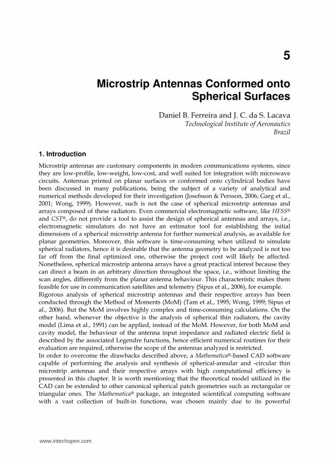
5

Microstrip Antennas Conformed onto Spherical Surfaces

Daniel B. Ferreira and J. C. da S. Lacava Technological Institute of Aeronautics

Brazil

1. Introduction

Microstrip antennas are customary components in modern communications systems, since they are low-profile, low-weight, low-cost, and well suited for integration with microwave circuits. Antennas printed on planar surfaces or conformed onto cylindrical bodies have been discussed in many publications, being the subject of a variety of analytical and numerical methods developed for their investigation (Josefsson & Persson, 2006; Garg et al., 2001; Wong, 1999). However, such is not the case of spherical microstrip antennas and arrays composed of these radiators. Even commercial electromagnetic software, like HFSS® and CST®, do not provide a tool to assist the design of spherical antennas and arrays, i.e., electromagnetic simulators do not have an estimator tool for establishing the initial dimensions of a spherical microstrip antenna for further numerical analysis, as available for planar geometries. Moreover, this software is time-consuming when utilized to simulate spherical radiators, hence it is desirable that the antenna geometry to be analyzed is not too far off from the final optimized one, otherwise the project cost will likely be affected. Nonetheless, spherical microstrip antenna arrays have a great practical interest because they can direct a beam in an arbitrary direction throughout the space, i.e., without limiting the scan angles, differently from the planar antenna behaviour. This characteristic makes them feasible for use in communication satellites and telemetry (Sipus et al., 2006), for example. Rigorous analysis of spherical microstrip antennas and their respective arrays has been conducted through the Method of Moments (MoM) (Tam et al., 1995; Wong, 1999; Sipus et al., 2006). But the MoM involves highly complex and time-consuming calculations. On the other hand, whenever the objective is the analysis of spherical thin radiators, the cavity model (Lima et al., 1991) can be applied, instead of the MoM. However, for both MoM and cavity model, the behaviour of the antenna input impedance and radiated electric field is described by the associated Legendre functions, hence efficient numerical routines for their evaluation are required, otherwise the scope of the antennas analyzed is restricted. In order to overcome the drawbacks described above, a Mathematica®-based CAD software capable of performing the analysis and synthesis of spherical-annular and -circular thin microstrip antennas and their respective arrays with high computational efficiency is presented in this chapter. It is worth mentioning that the theoretical model utilized in the CAD can be extended to other canonical spherical patch geometries such as rectangular or triangular ones. The Mathematica® package, an integrated scientifical computing software with a vast collection of built-in functions, was chosen mainly due to its powerful

www.intechopen.com

Microstrip Antennas

84

algorithms for calculating cylindrical and spherical harmonics functions what makes it suitable for the analysis of conformed antennas. Mathematica® permits the analysis and synthesis of various spherical microstrip radiators, thus avoiding the use of the normalized Legendre functions that are sometimes employed to overcome numerical difficulties (Sipus et al., 2006). Furthermore, it is important to point out that the developed CAD does not require a powerful computer to run on, working well and quickly in a regular classroom PC, since its code does not utilize complex numerical techniques, like MoM or finite element method (FEM). In Section 2, the theoretical model implemented in the developed CAD to evaluate the antenna input impedance, quality factor, radiation pattern and directivity is discussed. Furthermore, comparisons between the CAD results and the HFSS® full wave solver data are presented in order to validate the accuracy of the utilized technique. An effective procedure, based on the global coordinate system technique (Sengupta, 1968), to determine the radiation patterns of thin spherical meridian and circumferential arrays is utilized in the special-purpose CAD, as addressed in Section 3. The array radiation patterns so obtained with the CAD are also compared to those from the HFSS® software. Section 4 is devoted to present an alternative strategy for fabricating a low-cost spherical-circular microstrip antenna along with the respective experimental results supporting the proposed antenna fabrication approach.

2. Analysis and synthesis of spherical thin microstrip antennas

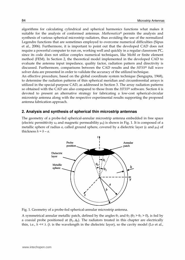
The geometry of a probe-fed spherical-annular microstrip antenna embedded in free space

(electric permittivity ε0 and magnetic permeability μ0) is shown in Fig. 1. It is composed of a

metallic sphere of radius a, called ground sphere, covered by a dielectric layer (ε and μ0) of thickness h = b – a.

z

a

x

y

Metallic sphere

Dielectric layer

Probe position

h

Annular patch

1θpθ

2θ

b

z

a

x

y

Metallic sphere

Dielectric layer

Probe position

h

Annular patch

1θpθ

2θ

b

Fig. 1. Geometry of a probe-fed spherical-annular microstrip antenna.

A symmetrical annular metallic patch, defined by the angles θ1 and θ2 (θ2 > θ1 > 0), is fed by

a coaxial probe positioned at (θp , φp). The radiators treated in this chapter are electrically

thin, i.e., h << λ (λ is the wavelength in the dielectric layer), so the cavity model (Lo et al.,

www.intechopen.com


85

1979) is well suited for the analysis of such antennas. Based on this model it is possible to develop expressions for computing the antenna input impedance and for estimating the electric surface current density on the patch without employing any complex numerical method such as the MoM. Before starting the input impedance calculation, the expression for computing the resonant frequencies of the modes established in a lossless equivalent cavity is determined. In the case of electrically thin radiators, the electric field within the cavity can be considered to have a radial component only, which is r-independent. Therefore, applying Maxwell’s equations to the dielectric layer region, and disregarding the feeder presence, the following equation for the r-component of the electric field is obtained

2

22 2 2 2

1 1sin 0

sin sinr r

r

E Ek E

a a

∂ ∂∂ ⎛ ⎞θ + + =⎜ ⎟∂θ ∂θθ θ ∂φ⎝ ⎠ , (1)

where k2 = ω2μ0ε and ω denotes the angular frequency. Consequently, only TMr modes can be established in the equivalent cavity. Solving the wave equation (1) via the method of separation of variables (Balanis, 1989), results in the electric field

( , ) [ P (cos ) Q (cos )][ cos( ) sin( )]θ φ = θ + θ φ + φ` `m m

rE A B C m D m , (2)

where P (.)`m and Q (.)`

m are the associated Legendre functions of ℓ-th degree and m-th order

of the first and the second kinds, respectively, ℓ(ℓ +1) = k2a2 and A, B, C and D are constants

dependent on the boundary conditions. Enforcing the boundary conditions related to the equivalent cavity of annular geometry and taking into account that it is symmetrical in relation to the z-axis, the electric field (2) reduces to

( , ) R (cos )cos( )θ φ = θ φ` `m

r mE E m , (3)

where

1 1 1R (cos ) sin [P (cos )Q (cos ) Q (cos )P (cos )]m m m m mc c c

′ ′θ = θ θ θ − θ θ` ` ` ` ` , (4)

m = 0, 1, 2,… and the index ℓ must satisfy the transcendental equation

1 2 1 2P (cos )Q (cos ) Q (cos )P (cos ) 0m m m mc c c c

′ ′ ′ ′θ θ − θ θ =` ` ` ` , (5)

with the angles θ1c and θ2c (θ2c > θ1c) indicating the equivalent cavity borders in the θ

direction, i.e., θ1c ≤ θ ≤ θ2c, 0 ≤ φ < 2π, Eℓm are the coefficients of the natural modes and the

prime denotes a derivative. Hence, once the indexes ℓ and m are determined it is possible to

evaluate the TMℓm mode resonant frequency from the following expression

0

( 1)

2mf

a

+= π μ ε`` `

. (6)

Before solving the transcendental equation (5) it is necessary to determine the equivalent

cavity dimensions θ1c and θ2c, which correspond to the actual patch dimensions with the

www.intechopen.com

Microstrip Antennas

86

addition of the fringe field extension. However, differently from planar microstrip antennas, the literature does not currently present expressions for estimating the dimensions of spherical equivalent cavities based on the physical antenna dimensions and the dielectric substrate characteristics. Therefore, in this chapter, the expressions used for estimating the equivalent cavity dimensions of a planar-annular microstrip antenna are extended to the spherical-annular case (Kishk, 1993), i.e., the spherical-annular equivalent cavity arc lengths were considered equal to the respective linear dimensions of the planar-annular equivalent cavity. The proposed expressions are given below; equations (7.a) and (7.b),

11 1

1

2 F( )1c

r

h

b

θθ = θ − π θ ε , (7.a)

22 2

2

2 F( )1c

r

h

b

θθ = θ + π θ ε , (7.b)

where F( ) n( / 2 ) 1.41 1.77 (0.268 1.65) /r rb h h bθ = θ + ε + + ε + θ` and εr is the relative electric

permittivity of the dielectric substrate.

2.1 Input impedance The input impedance of the spherical-annular microstrip antenna illustrated in Fig. 1 fed by a coaxial probe can be evaluated following the procedure proposed in (Richards et al., 1981), i.e., the coaxial probe is modelled by a strip of current whose electric current density is given by,

( ) 2

1ˆ, ( ) ( )

sinpf

p

J J ra

θ φ = φ δ θ − θθf

, (8)

where δ(.) indicates the Dirac’s delta function and

0 , if / 2 / 2( )

0, otherwise

p pJJ

φ − Δφ ≤ φ ≤ φ + Δφ⎧⎪φ = ⎨⎪⎩ (9)

with Δφ denoting the strip angular length relative to the φ−direction. In our analysis, also following the procedure established in (Richards et al., 1981) for planar microstrip antennas, the strip arc length has been assumed to be five times the coaxial probe diameter d, expressed as

5 / sin pd aΔφ = θ . (10)

It is important to point out that the electric current density (8) is an r-independent function since the antenna under analysis is electrically thin. Thus, to take into account the current strip, the wave equation (1) for the electric field is modified to

( )22

02 2 2 2

1 1ˆsin ,

sin sinr r

r f

E Ek E j J r

a a

∂ ∂∂ ⎛ ⎞θ + + = ωμ θ φ ⋅⎜ ⎟∂θ ∂θθ θ ∂φ⎝ ⎠f

. (11)

Expanding the r-component of the electric field into its eigenmodes (3), the solution for equation (11) is given by

www.intechopen.com


87

1

0 02 cos

2 2 2

cos

R (cos )sinc( / 2)cos( )( , ) R (cos )cos( )

[ ] [R ( )]c

c

mp p m

rmm

m m

m mJE j m

ak k d

2

θν= θ

θ Δφ φωμ Δφθ φ = θ φπ ξ − ν ν∑∑ ∫``

` ` `

, (12)

where

2, if 0

1, otherwisem

m =⎧ξ = ⎨⎩ ,

( 1) /mk a= +` ` ` and sinc(x)=sin(x)/x.

Since the procedure just described has been developed for ideal cavities, equation (12) is purely imaginary. So, for incorporating the radiated power and the dielectric and metallic

losses into the cavity model, the concept of effective loss tangent, tan δeff, (Richards et al., 1979) is employed. Based on this approach, the wave number k is replaced by an effective wave number

1 taneff effk k j= − δ . (13)

Once the electric field inside the equivalent cavity has been determined, the antenna input voltage Vin can be computed from the expression,

in rV E h= − , (14)

where rE denotes the average value of ( , )prE θ φ over the strip of current. Consequently, the

input impedance Zin of the spherical-annular microstrip antenna is given by

1

2 2 2

02 cos

2 2 20

cos

[R (cos )] sinc ( / 2)cos ( )

[ (1 tan )] [R ( )]c

c

mp pin

inmm

m effm

m mV hZ j

J ak k j d

2

θν= θ

θ Δφ φωμ= =Δφ π ξ − − δ ν ν∑∑ ∫`

` ` `

. (15)

An alternative representation for frequencies close to the TMLM resonant mode but sufficiently apart from the other modes can be obtained by rewriting the antenna input impedance as

2 2 2 2

( , ) ( , )

(1 tan )LM m

inLM eff mm

m L M

jZ j

j≠

αωα≅ + ωω − − δ ω ω − ω∑∑ `

```

, (16)

where 1cos

2 2 2 2 2

cos

[R (cos )] sinc ( / 2)cos ( ) / [R ( )] .c

c

m mp p mm h m m a d

2

θν= θ

α = θ Δφ φ π εξ ν ν∫` ` `

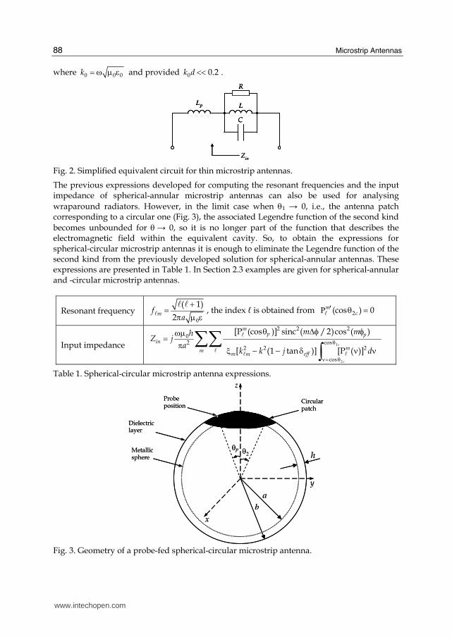
The expression (16) corresponds to the equivalent circuit shown in Fig. 2, i.e., a parallel RLC

circuit with a series inductance Lp. In this case, the series inductance represents the probe

effect and its value is that of the double sum in (16). However, as this is a slowly convergent

series, the developed CAD utilizes, alternatively, the equation due to (Damiano & Papiernik,

1994) for calculating the probe reactance Xp , given by

060 n( /2 )pX j k h kd= − ` , (17)

www.intechopen.com

Microstrip Antennas

88

where 0 0 0k = ω μ ε and provided 0 0.2k d << .

inZ

pL

R

L

C

inZ

pL

R

L

C

pL

R

L

C

Fig. 2. Simplified equivalent circuit for thin microstrip antennas.

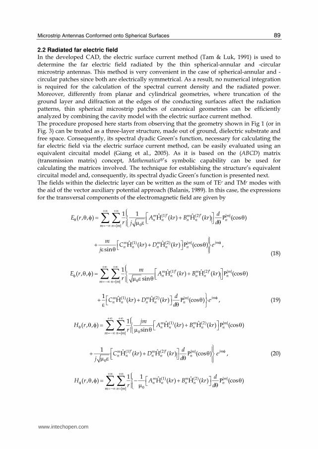
The previous expressions developed for computing the resonant frequencies and the input impedance of spherical-annular microstrip antennas can also be used for analysing

wraparound radiators. However, in the limit case when θ1 → 0, i.e., the antenna patch corresponding to a circular one (Fig. 3), the associated Legendre function of the second kind

becomes unbounded for θ → 0, so it is no longer part of the function that describes the electromagnetic field within the equivalent cavity. So, to obtain the expressions for spherical-circular microstrip antennas it is enough to eliminate the Legendre function of the second kind from the previously developed solution for spherical-annular antennas. These expressions are presented in Table 1. In Section 2.3 examples are given for spherical-annular and -circular microstrip antennas.

Resonant frequency 0

( 1)

2mf

a

+= π μ ε`` `

, the index ℓ is obtained from P 2(cos ) 0mc

′ θ =`

Input impedance 1

2 2 2

02 cos

2 2 2

cos

[P (cos )] sinc ( / 2)cos ( )

[ (1 tan )] [P ( )]c

c

mp p

inmm

m effm

m mhZ j

ak k j d

2

θν= θ

θ Δφ φωμ= π ξ − − δ ν ν∑∑ ∫`

` ` `

Table 1. Spherical-circular microstrip antenna expressions.

z

a

Metallic sphere

Dielectric layer

Probe position

h

Circular patch

2θ

b

x

y

pθ

z

a

Metallic sphere

Dielectric layer

Probe position

h

Circular patch

2θ

b

x

y

pθ

Fig. 3. Geometry of a probe-fed spherical-circular microstrip antenna.

www.intechopen.com


89

2.2 Radiated far electric field In the developed CAD, the electric surface current method (Tam & Luk, 1991) is used to determine the far electric field radiated by the thin spherical-annular and -circular microstrip antennas. This method is very convenient in the case of spherical-annular and -circular patches since both are electrically symmetrical. As a result, no numerical integration is required for the calculation of the spectral current density and the radiated power. Moreover, differently from planar and cylindrical geometries, where truncation of the ground layer and diffraction at the edges of the conducting surfaces affect the radiation patterns, thin spherical microstrip patches of canonical geometries can be efficiently analyzed by combining the cavity model with the electric surface current method. The procedure proposed here starts from observing that the geometry shown in Fig 1 (or in Fig. 3) can be treated as a three-layer structure, made out of ground, dielectric substrate and free space. Consequently, its spectral dyadic Green’s function, necessary for calculating the far electric field via the electric surface current method, can be easily evaluated using an equivalent circuital model (Giang et al., 2005). As it is based on the (ABCD) matrix (transmission matrix) concept, Mathematica®’s symbolic capability can be used for calculating the matrices involved. The technique for establishing the structure’s equivalent circuital model and, consequently, its spectral dyadic Green’s function is presented next. The fields within the dielectric layer can be written as the sum of TEr and TMr modes with the aid of the vector auxiliary potential approach (Balanis, 1989). In this case, the expressions for the transversal components of the electromagnetic field are given by

P(1) (2) | |

| |

1 1 ˆ ˆ( , , ) H ( ) H ( ) (cos )m m mn n n n n

m n m

dE r A kr B kr

r dj

+∞ +∞θ

0=−∞ =

⎧⎪ ′ ′⎡ ⎤θ φ = + θ⎨ ⎢ ⎥⎣ ⎦ θμ ε⎪⎩∑ ∑

P(1) (2) | |ˆ ˆH ( ) H ( ) (cos ) ,sin

jmm m mn n n n n

mC kr D kr e

j

φ⎫⎪⎡ ⎤+ + θ ⎬⎣ ⎦ε θ ⎪⎭ (18)

P(1) (2) | |

| |

1 ˆ ˆ( , , ) H ( ) H ( ) (cos )sin

m m mn n n n n

m n m

mE r A kr B kr

r

+∞ +∞φ

0=−∞ =

⎧⎪ ′ ′⎡ ⎤θ φ = + θ⎨ ⎢ ⎥⎣ ⎦μ ε θ⎪⎩∑ ∑

P(1) (2) | |1 ˆ ˆH ( ) H ( ) (cos ) ,jmm m m

n n n n n

dC kr D kr e

d

φ⎫⎡ ⎤+ + θ ⎬⎣ ⎦ε θ ⎭ (19)

P(1) (2) | |

| |

1 ˆ ˆ( , , ) H ( ) H ( ) (cos )sin

m m mn n n n n

m n m

jmH r A kr B kr

r

+∞ +∞θ 0=−∞ =

⎧⎪ ⎡ ⎤θ φ = + θ⎨ ⎣ ⎦μ θ⎪⎩∑ ∑

P(1) (2) | |1 ˆ ˆH ( ) H ( ) (cos ) ,jmm m m

n n n n n

dC kr D kr e

dj

φ0

⎫⎪′ ′⎡ ⎤+ + θ ⎬⎢ ⎥⎣ ⎦ θμ ε ⎪⎭ (20)

P(1) (2) | |

| |

1 1 ˆ ˆ( , , ) H ( ) H ( ) (cos )m m mn n n n n

m n m

dH r A kr B kr

r d

+∞ +∞φ 0=−∞ =

⎧⎪ ⎡ ⎤θ φ = − + θ⎨ ⎣ ⎦μ θ⎪⎩∑ ∑

www.intechopen.com

Microstrip Antennas

90

P(1) (2) | |ˆ ˆH ( ) H ( ) (cos ) ,

sin

jmm m mn n n n n

mC kr D kr e φ

0⎫⎪′ ′⎡ ⎤+ + θ ⎬⎢ ⎥⎣ ⎦μ ε θ ⎪⎭ (21)

where the coefficients mnA , m

nB , mnC and m

nD are dependent on the boundary conditions at the

interfaces r = a and r = b, and τ( )H (.)n is the Schelkunoff spherical Hankel function of n-th order

and τ-th kind (τ = 1 or 2). The fields (18) to (21) can be rewritten in a more adequate form as

| |

( , , ) ( , ) ,jm

m n m

EL n m r n e

E

+∞ +∞θ φφ =−∞ =

⎡ ⎤ = θ ⋅⎢ ⎥⎣ ⎦ ∑∑ f# E (22)

| |

( , , ) ( , ) ,jm

m n m

HL n m r n e

H

+∞ +∞θ φφ =−∞ =

⎡ ⎤ = θ ⋅⎢ ⎥⎣ ⎦ ∑∑ f# H (23)

where

PP

PP

| || |

| || |

(cos )(cos )

sin( , , ) ,(cos )

(cos )sin

mm n

n

mmn

n

djm

dL n md

jmd

⎡ ⎤θθ −⎢ ⎥θ θ⎢ ⎥θ = ⎢ ⎥θ θ⎢ ⎥θ θ⎣ ⎦# (24)

(1) (2)

(1) (2)

ˆ ˆH ( ) H ( )

( , ) ,1 ˆ ˆH ( ) H ( )

m mn n n n

m mn n n n

A kr B krjkr

r n

C kr D krr

θφ

ω⎡ ⎤′ ′⎡ ⎤+⎢ ⎥⎢ ⎥⎣ ⎦⎡ ⎤ ⎢ ⎥= =⎢ ⎥ ⎢ ⎥⎣ ⎦ ⎡ ⎤+⎢ ⎥⎣ ⎦ε⎣ ⎦

f EE

E (25)

(1) (2)

(1) (2)

ˆ ˆH ( ) H ( )

( , )1 ˆ ˆH ( ) H ( )

m mn n n n

m mn n n n

C kr D krjkr

r n

A kr B krr

θφ

0

ω⎡ ⎤′ ′⎡ ⎤+⎢ ⎥⎢ ⎥⎣ ⎦⎡ ⎤ ⎢ ⎥= =⎢ ⎥ ⎢ ⎥⎣ ⎦ ⎡ ⎤− +⎢ ⎥⎣ ⎦μ⎣ ⎦

f HH

H, (26)

and the argument (r,θ,φ) was omitted in (22) and (23) only for simplifying the notation. The

vectors f

( , )r nE and f

( , )r nH are the transversal electric and magnetic fields in the spectral

domain, respectively. In this chapter, the pair of vector-Legendre transforms (Sipus et al.,

2006) is defined as follows,

π π− φ

φ= θ== θ ⋅ θ φ θ θ φπ ∫ ∫f f#

2

0 0

1( , ) ( , , ) ( , , )sin

2 ( , )jmr n L n m X r e d d

S n mX (27)

and

| |

( , , ) ( , , ) ( , ) ,jm

m n m

X r L n m r n e+∞ +∞ φ=−∞ =

θ φ = θ ⋅∑ ∑f f# X (28)

www.intechopen.com


91

where ( , ) 2 ( 1)( | |)!/(2 1)( | |)!S n m n n n m n n m= + + + − and ( , )r nfX , the vector-Legendre

transform of ( , , )X r θ φf, has only the θ and/or φ components.

From evaluating the expressions (25) and (26) at the lower (r = a) and upper (r = b) interfaces it is possible to establish the following relation

( , ) ( , )

,( , ) ( , )

V Za n b n

Y Ba n b n

⎡ ⎤ ⎡ ⎤⎡ ⎤= ⋅⎢ ⎥ ⎢ ⎥⎢ ⎥⎢ ⎥⎢ ⎥ ⎢ ⎥⎣ ⎦⎣ ⎦ ⎣ ⎦f f# #f f# #E E

H H (29)

and the matrices V# , Z# , Y# and B# can be found in (Ferreira, 2009).

Based on equation (29), the two-port network illustrated in Fig. 4, representing the dielectric layer, can be defined. The related transmission (ABCD) matrix is given in (30).

fH b,n( )

fE b,n( )

fH a,n( )

fE a,n( )

V Z

Y B

⎡ ⎤⎢ ⎥⎢ ⎥⎣ ⎦# ## #

fH b,n( )

fE b,n( )

fH a,n( )

fE a,n( )

V Z

Y B

⎡ ⎤⎢ ⎥⎢ ⎥⎣ ⎦# ## #

Fig. 4. Transmission (ABCD) network.

( ) .V Z

ABCDY B

⎡ ⎤= ⎢ ⎥⎢ ⎥⎣ ⎦# ## # (30)

In a similar way, the following relation between the free-space spectral electric 0

fE and

magnetic 0

fH transversal field components can be determined,

0 0 0( , ) ( , ),b n Y b n= ⋅f f#H E (31)

where

(2) (2)

0 0 00

(2) (2)0 0 0

ˆ ˆ0 H ( ) / H ( ),

ˆ ˆH ( ) / H ( ) 0

n n

n n

k b j k bY

k b j k b

′⎡ ⎤η⎢ ⎥= ′⎢ ⎥η⎣ ⎦# (32)

and η0 denotes the free space intrinsic impedance. Consequently, free space can be

represented by the admittance load 0Y# in the circuital model. It is worth mentioning that the

matrices V# , Z# , Y# , B# and 0Y# can be evaluated in a straightforward manner utilizing the

Mathematica®’s symbolic capability.

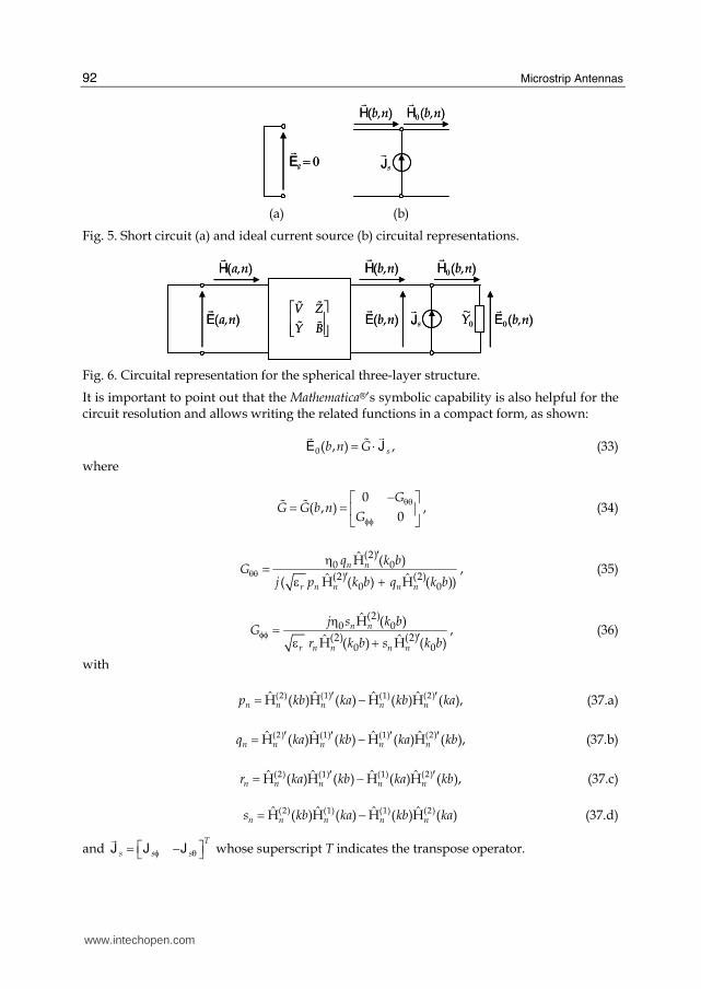
As the ground layer is considered a perfect electric conductor, it is well represented by a

short circuit that corresponds to null electric field ( 0g =fE ). On the other hand, the spectral

electric surface current density s

fJ located on the metallic patch is modelled by an ideal

current source. The circuital representations for both short circuit and ideal current source

are given in Fig. 5.

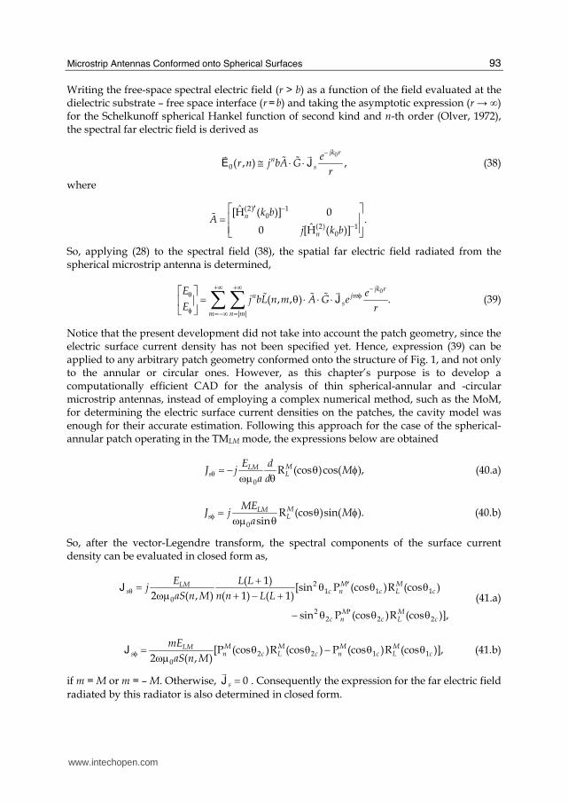
Finally, by properly combining the circuit elements, the three-layer structure model is the

equivalent circuit illustrated in Fig. 6, whose resolution produces the transversal dyadic

Green’s function G# in the spectral domain. Notice that the Green’s function, calculated

according to this approach, is evaluated at the dielectric substrate – free space interface

(r = b).

www.intechopen.com

Microstrip Antennas

92

0g =fE 0g =fE

fH b,n( )

fJs

0

fH b,n( )

fH b,n( )

fJs

0

fH b,n( )

(a) (b)

Fig. 5. Short circuit (a) and ideal current source (b) circuital representations. f

H b,n( )

fE b,n( )

fH a,n( )

fE a,n( )

V Z

Y B

⎡ ⎤⎢ ⎥⎢ ⎥⎣ ⎦# ## #

fJs 0

~Y

0

fH b,n( )

0

fE b,n( )

fH b,n( )

fE b,n( )

fH a,n( )

fE a,n( )

V Z

Y B

⎡ ⎤⎢ ⎥⎢ ⎥⎣ ⎦# ## #

fJs 0

~Y

0

fH b,n( )

0

fE b,n( )

Fig. 6. Circuital representation for the spherical three-layer structure.

It is important to point out that the Mathematica®’s symbolic capability is also helpful for the circuit resolution and allows writing the related functions in a compact form, as shown:

0( , ) ,sb n G= ⋅f f#E J (33)

where

0

( , )0

GG G b n

Gθθ

φφ−⎡ ⎤= = ⎢ ⎥⎣ ⎦

# # , (34)

(2)

0 0(2) (2)

0 0

H ( )

ˆ ˆ( H ( ) H ( ))

n n

r n n n n

q k bG

j p k b q k bθθ

′η= ′ε + , (35)

(2)

0 0(2) (2)

0 0

H ( )

ˆ ˆH ( ) H ( )

n n

r n n n n

j s k bG

r k b s k bφφ

η= ′ε + , (36)

with

(2) (1) (1) (2)ˆ ˆ ˆ ˆH ( )H ( ) H ( )H ( ),n n n n np kb ka kb ka′ ′= − (37.a)

(2) (1) (1) (2)ˆ ˆ ˆ ˆH ( )H ( ) H ( )H ( ),n n n n nq ka kb ka kb′ ′ ′ ′= − (37.b)

(2) (1) (1) (2)ˆ ˆ ˆ ˆH ( )H ( ) H ( )H ( ),n n n n nr ka kb ka kb′ ′= − (37.c)

(2) (1) (1) (2)ˆ ˆ ˆ ˆH ( )H ( ) H ( )H ( )n n n n ns kb ka kb ka= − (37.d)

and T

s s sφ θ⎡ ⎤= −⎣ ⎦fJ J J whose superscript T indicates the transpose operator.

www.intechopen.com


93

Writing the free-space spectral electric field (r > b) as a function of the field evaluated at the dielectric substrate – free space interface (r = b) and taking the asymptotic expression (r → ∞) for the Schelkunoff spherical Hankel function of second kind and n-th order (Olver, 1972), the spectral far electric field is derived as

0

0( , ) ,jk r

ns

er n j bA G

r

−≅ ⋅ ⋅f f# #E J (38)

where

(2) 10

(2) 10

ˆ[H ( )] 0.

ˆ0 [H ( )]

n

n

k bA

j k b

−−

⎡ ′ ⎤⎢ ⎥= ⎢ ⎥⎣ ⎦#

So, applying (28) to the spectral field (38), the spatial far electric field radiated from the spherical microstrip antenna is determined,

0

| |

( , , ) .jk r

jmns

m n m

E ej bL n m A G e

E r

+∞ +∞ −θ φφ =−∞ =

⎡ ⎤ = θ ⋅ ⋅ ⋅⎢ ⎥⎣ ⎦ ∑ ∑ f# ## J (39)

Notice that the present development did not take into account the patch geometry, since the electric surface current density has not been specified yet. Hence, expression (39) can be applied to any arbitrary patch geometry conformed onto the structure of Fig. 1, and not only to the annular or circular ones. However, as this chapter’s purpose is to develop a computationally efficient CAD for the analysis of thin spherical-annular and -circular microstrip antennas, instead of employing a complex numerical method, such as the MoM, for determining the electric surface current densities on the patches, the cavity model was enough for their accurate estimation. Following this approach for the case of the spherical-annular patch operating in the TMLM mode, the expressions below are obtained

0

R (cos )cos( ),MLMs L

E dJ j M

a dθ = − θ φωμ θ (40.a)

0

R (cos )sin( ).sin

MLMs L

MEJ j M

aφ = θ φωμ θ (40.b)

So, after the vector-Legendre transform, the spectral components of the surface current density can be evaluated in closed form as,

21 1 1

0

22 2 2

( 1)[sin P (cos )R (cos )

2 ( , ) ( 1) ( 1)

sin P (cos )R (cos )],

M MLMs c n c L c

M Mc n c L c

E L Lj

aS n M n n L Lθ

+ ′= θ θ θωμ + − +′− θ θ θ

J

(41.a)

2 2 1 10

[P (cos )R (cos ) P (cos )R (cos )],2 ( , )

M M M MLMs n c L c n c L c

mE

aS n Mφ = θ θ − θ θωμJ (41.b)

if m = M or m = – M. Otherwise, 0s =fJ . Consequently the expression for the far electric field

radiated by this radiator is also determined in closed form.

www.intechopen.com

Microstrip Antennas

94

In a similar way, expressions for the spatial and spectral electric surface current densities are derived for the spherical-circular microstrip antenna (Fig. 3) operating in the TMLM mode

0

P (cos )cos( ),MLMs L

E dJ j M

a dθ = − θ φωμ θ (42.a)

0

P (cos )sin( ),sin

MLMs L

MEJ j M

aφ = θ φωμ θ (42.b)

22 2 2

0

( 1)sin P (cos )P (cos ),

2 ( , ) ( 1) ( 1)M MLM

s c n c L c

jE L L

aS n M n n L Lθ

− + ′= θ θ θωμ + − +J (43.a)

2 20

P (cos )P (cos ),2 ( , )

M MLMs n c L c

mE

aS n Mφ = θ θωμJ (43.b)

if m = M or m = – M. Otherwise, 0s =fJ .

Once the far electric field radiated by spherical antennas is known, an expression for its average radiated power can be established. Starting from equation (44) (Balanis, 2005),

2

* 20

00 0

1sin ,

2P E E r d d

π π

φ= θ== ⋅ θ θ φη ∫ ∫ f f

(44)

where Ef

denotes the far electric field determined by (39) and the superscript * indicates the

complex conjugate operator. After the double integration, the following expression can be

obtained

2 22

0 (2)(2)0 0| | 0

( , ) .ˆˆ H ( )H ( )

ss

nm n m n

GGbP S n m

k bk b

+∞ +∞ φ φφθ θθ=−∞ =

⎡ ⎤π ⎢ ⎥= +⎢ ⎥′η ⎢ ⎥⎣ ⎦∑ ∑ JJ (45)

In order to calculate the directivity of thin spherical-annular and -circular microstrip antennas, the developed CAD employs (45), since its evaluation requires no numerical integrations, which, as previously mentioned, is an advantage. In addition, equation (45) is employed in the CAD for computing the quality factor associated to the radiated power,

from which the effective loss tangent tan δeff and, consequently, the antenna input impedance (15) are estimated.

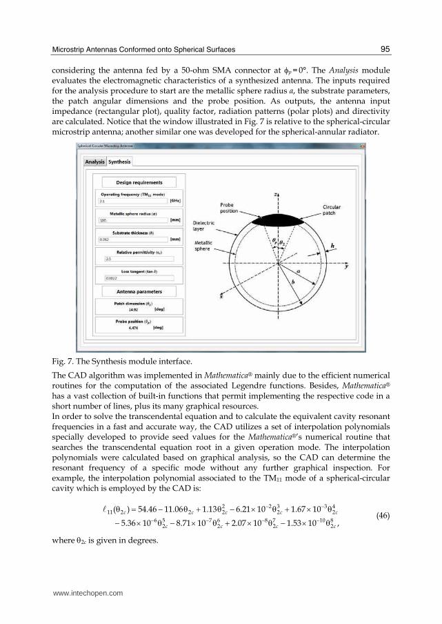
2.3 CAD results Before presenting some CAD results and comparing them with HFSS® output data, a brief overview of the CAD structure will be given. The current version of the CAD contains two independent sections: the synthesis and the analysis modules that can be accessed from their respective tabs. By selecting the Synthesis option, the design interface (Fig. 7) is presented. The inputs required for the synthesis procedure to start are the desired frequency, the

ground sphere radius a and the substrate parameters, such as relative permittivity εr, loss

tangent tan δ and thickness h. As results, the CAD returns the patch physical dimensions (θ1

and θ2 for the annular patch and only θ2 for the circular one) and the probe position θp

www.intechopen.com


95

considering the antenna fed by a 50-ohm SMA connector at φp = 0°. The Analysis module evaluates the electromagnetic characteristics of a synthesized antenna. The inputs required for the analysis procedure to start are the metallic sphere radius a, the substrate parameters, the patch angular dimensions and the probe position. As outputs, the antenna input impedance (rectangular plot), quality factor, radiation patterns (polar plots) and directivity are calculated. Notice that the window illustrated in Fig. 7 is relative to the spherical-circular microstrip antenna; another similar one was developed for the spherical-annular radiator.

Fig. 7. The Synthesis module interface.

The CAD algorithm was implemented in Mathematica® mainly due to the efficient numerical routines for the computation of the associated Legendre functions. Besides, Mathematica® has a vast collection of built-in functions that permit implementing the respective code in a short number of lines, plus its many graphical resources. In order to solve the transcendental equation and to calculate the equivalent cavity resonant frequencies in a fast and accurate way, the CAD utilizes a set of interpolation polynomials specially developed to provide seed values for the Mathematica®’s numerical routine that searches the transcendental equation root in a given operation mode. The interpolation polynomials were calculated based on graphical analysis, so the CAD can determine the resonant frequency of a specific mode without any further graphical inspection. For example, the interpolation polynomial associated to the TM11 mode of a spherical-circular cavity which is employed by the CAD is:

2 2 3 3 4

11 2 2 2 2 2

6 5 7 6 8 7 10 82 2 2 2

( ) 54.46 11.06 1.13 6.21 10 1.67 10

5.36 10 8.71 10 2.07 10 1.53 10 ,

c c c c c

c c c c

− −− − − −

θ = − θ + θ − × θ + × θ− × θ − × θ + × θ − × θ

` (46)

where θ2c is given in degrees.

www.intechopen.com

Microstrip Antennas

96

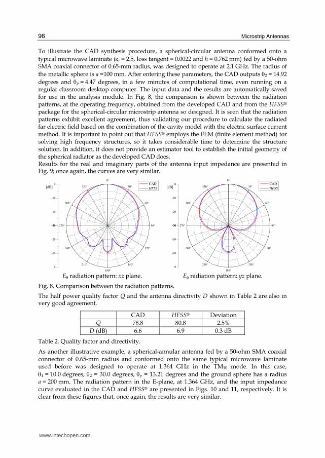
To illustrate the CAD synthesis procedure, a spherical-circular antenna conformed onto a

typical microwave laminate (εr = 2.5, loss tangent = 0.0022 and h = 0.762 mm) fed by a 50-ohm SMA coaxial connector of 0.65-mm radius, was designed to operate at 2.1 GHz. The radius of

the metallic sphere is a =100 mm. After entering these parameters, the CAD outputs θ2 = 14.92

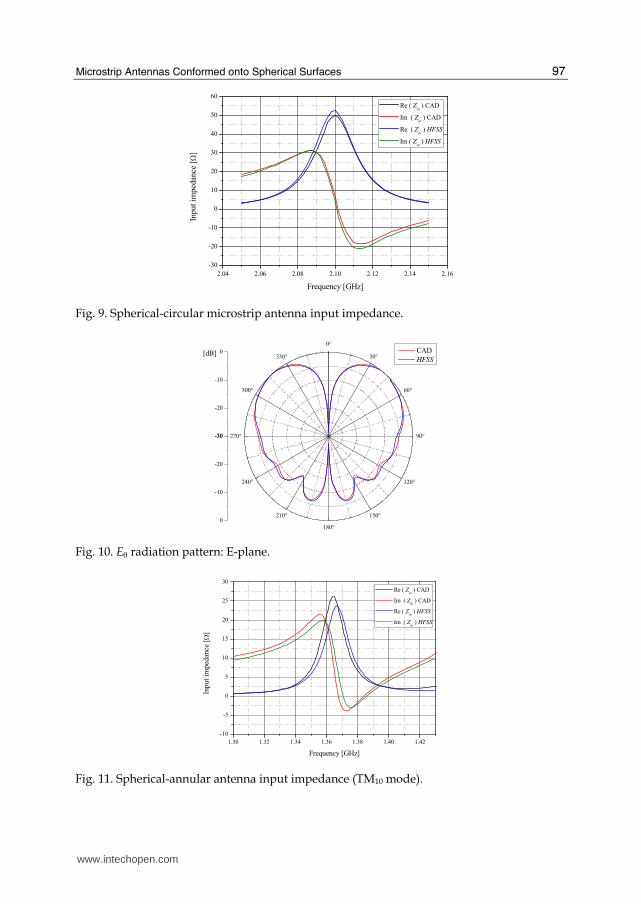
degrees and θp = 4.47 degrees, in a few minutes of computational time, even running on a regular classroom desktop computer. The input data and the results are automatically saved for use in the analysis module. In Fig. 8, the comparison is shown between the radiation patterns, at the operating frequency, obtained from the developed CAD and from the HFSS® package for the spherical-circular microstrip antenna so designed. It is seen that the radiation patterns exhibit excellent agreement, thus validating our procedure to calculate the radiated far electric field based on the combination of the cavity model with the electric surface current method. It is important to point out that HFSS® employs the FEM (finite element method) for solving high frequency structures, so it takes considerable time to determine the structure solution. In addition, it does not provide an estimator tool to establish the initial geometry of the spherical radiator as the developed CAD does. Results for the real and imaginary parts of the antenna input impedance are presented in Fig. 9; once again, the curves are very similar.

-30

-20

-10

0

0°

30°

60°

90°

120°

150°

180°

210°

240°

270°

300°

330°

-30

-20

-10

0

CAD

HFSS[dB]

Eθ radiation pattern: xz plane.

-30

-20

-10

0

0°

30°

60°

90°

120°

150°

180°

210°

240°

270°

300°

330°

-30

-20

-10

0

CAD

HFSS[dB]

Eφ radiation pattern: yz plane.

Fig. 8. Comparison between the radiation patterns.

The half power quality factor Q and the antenna directivity D shown in Table 2 are also in very good agreement.

CAD HFSS® Deviation

Q 78.8 80.8 2.5%

D (dB) 6.6 6.9 0.3 dB

Table 2. Quality factor and directivity.

As another illustrative example, a spherical-annular antenna fed by a 50-ohm SMA coaxial connector of 0.65-mm radius and conformed onto the same typical microwave laminate used before was designed to operate at 1.364 GHz in the TM10 mode. In this case,

θ1 = 10.0 degrees, θ2 = 30.0 degrees, θp = 13.21 degrees and the ground sphere has a radius a = 200 mm. The radiation pattern in the E-plane, at 1.364 GHz, and the input impedance curve evaluated in the CAD and HFSS® are presented in Figs. 10 and 11, respectively. It is clear from these figures that, once again, the results are very similar.

www.intechopen.com


97

2.04 2.06 2.08 2.10 2.12 2.14 2.16

-30

-20

-10

0

10

20

30

40

50

60

Input

imped

ance

[Ω]

Frequency [GHz]

Re ( Zin ) CAD

Im ( Zin ) CAD

Re ( Zin ) HFSS

Im ( Zin ) HFSS

Fig. 9. Spherical-circular microstrip antenna input impedance.

-30

-20

-10

0

0°

30°

60°

90°

120°

150°

180°

210°

240°

270°

300°

330°

-30

-20

-10

0

CAD

HFSS[dB]

Fig. 10. Eθ radiation pattern: E-plane.

1.30 1.32 1.34 1.36 1.38 1.40 1.42

-10

-5

0

5

10

15

20

25

30

Inp

ut

imped

ance

[Ω]

Frequency [GHz]

Re ( Zin ) CAD

Im ( Zin ) CAD

Re ( Zin ) HFSS

Im ( Zin ) HFSS

Fig. 11. Spherical-annular antenna input impedance (TM10 mode).

www.intechopen.com

Microstrip Antennas

98

3. Radiation patterns of spherical arrays

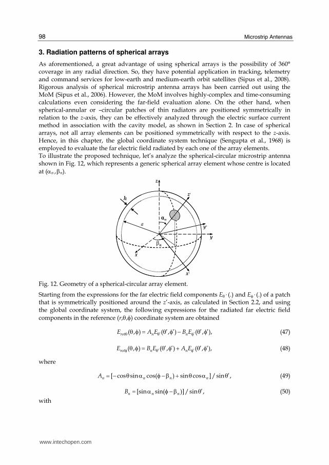
As aforementioned, a great advantage of using spherical arrays is the possibility of 360° coverage in any radial direction. So, they have potential application in tracking, telemetry and command services for low-earth and medium-earth orbit satellites (Sipus et al., 2008). Rigorous analysis of spherical microstrip antenna arrays has been carried out using the MoM (Sipus et al., 2006). However, the MoM involves highly-complex and time-consuming calculations even considering the far-field evaluation alone. On the other hand, when spherical-annular or –circular patches of thin radiators are positioned symmetrically in relation to the z-axis, they can be effectively analyzed through the electric surface current method in association with the cavity model, as shown in Section 2. In case of spherical arrays, not all array elements can be positioned symmetrically with respect to the z-axis. Hence, in this chapter, the global coordinate system technique (Sengupta et al., 1968) is employed to evaluate the far electric field radiated by each one of the array elements. To illustrate the proposed technique, let’s analyze the spherical-circular microstrip antenna shown in Fig. 12, which represents a generic spherical array element whose centre is located

at (αn , βn).

αn

x

y

z

βn

'z

'x

'ya

h

αn

x

y

z

βn

'z

'x

'ya

h

Fig. 12. Geometry of a spherical-circular array element.

Starting from the expressions for the far electric field components Eθ ’ (.) and Eφ ’ (.) of a patch that is symmetrically positioned around the z’-axis, as calculated in Section 2.2, and using the global coordinate system, the following expressions for the radiated far electric field

components in the reference (r,θ,φ) coordinate system are obtained

rot n nE A E B E′ ′θ θ φ′ ′ ′ ′θ φ = θ φ − θ φ( , ) ( , ) ( , ), (47)

rot n nE B E A E′ ′φ θ φ′ ′ ′ ′θ φ = θ φ + θ φ( , ) ( , ) ( , ), (48)

where

n n n nA ′= − θ α φ − β + θ α θ[ cos sin cos( ) sin cos ]/sin , (49)

n n nB ′= α φ − β θ[sin sin( )]/sin , (50)

with

www.intechopen.com


99

cos sin sin cos( ) cos cosn n n′θ = α θ φ − β + α θ , (51)

and

cos sin cos( ) sin cos

cot .sin sin( )

n n n

n

α θ φ − β − α θ′φ = θ φ − β (52)

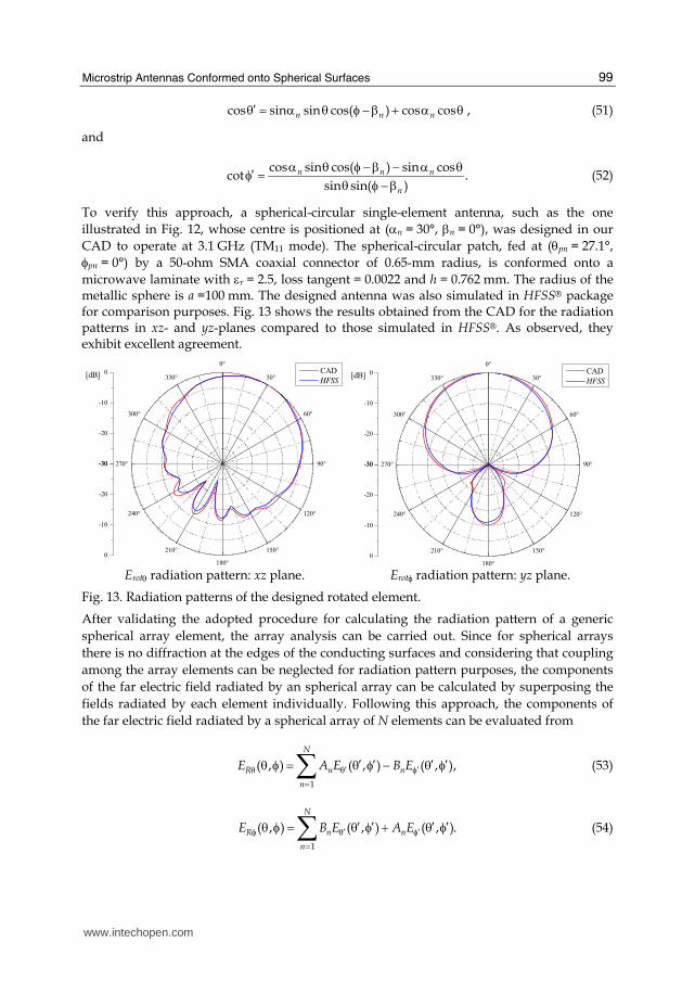
To verify this approach, a spherical-circular single-element antenna, such as the one

illustrated in Fig. 12, whose centre is positioned at (αn = 30°, βn = 0°), was designed in our

CAD to operate at 3.1 GHz (TM11 mode). The spherical-circular patch, fed at (θpn = 27.1°,

φpn = 0°) by a 50-ohm SMA coaxial connector of 0.65-mm radius, is conformed onto a

microwave laminate with εr = 2.5, loss tangent = 0.0022 and h = 0.762 mm. The radius of the metallic sphere is a =100 mm. The designed antenna was also simulated in HFSS® package for comparison purposes. Fig. 13 shows the results obtained from the CAD for the radiation patterns in xz- and yz-planes compared to those simulated in HFSS®. As observed, they exhibit excellent agreement.

-30

-20

-10

0

0°

30°

60°

90°

120°

150°

180°

210°

240°

270°

300°

330°

-30

-20

-10

0

CAD

HFSS[dB]

Erotθ radiation pattern: xz plane.

-30

-20

-10

0

0°

30°

60°

90°

120°

150°

180°

210°

240°

270°

300°

330°

-30

-20

-10

0

CAD

HFSS[dB]

Erotφ radiation pattern: yz plane.

Fig. 13. Radiation patterns of the designed rotated element.

After validating the adopted procedure for calculating the radiation pattern of a generic

spherical array element, the array analysis can be carried out. Since for spherical arrays

there is no diffraction at the edges of the conducting surfaces and considering that coupling

among the array elements can be neglected for radiation pattern purposes, the components

of the far electric field radiated by an spherical array can be calculated by superposing the

fields radiated by each element individually. Following this approach, the components of

the far electric field radiated by a spherical array of N elements can be evaluated from

1

( , ) ( , ) ( , ),

N

R n n

n

E A E B E′ ′θ θ φ=

′ ′ ′ ′θ φ = θ φ − θ φ∑ (53)

1

( , ) ( , ) ( , ).

N

R n n

n

E B E A E′ ′φ θ φ=

′ ′ ′ ′θ φ = θ φ + θ φ∑ (54)

www.intechopen.com

Microstrip Antennas

100

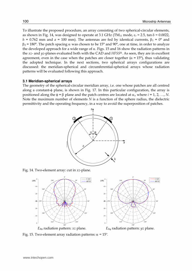
To illustrate the proposed procedure, an array consisting of two spherical-circular elements,

as shown in Fig. 14, was designed to operate at 3.1 GHz (TM11 mode, εr = 2.5, tan δ = 0.0022,

h = 0.762 mm and a = 100 mm). The antennas are fed by identical currents, β1 = 0° and

β2 = 180°. The patch spacing α was chosen to be 15° and 90°, one at time, in order to analyze

the developed approach for a wide range of α. Figs. 15 and 16 show the radiation patterns in the xz- and yz-planes evaluated both with the CAD and HFSS®. As seen, they are in excellent

agreement, even in the case when the patches are closer together (α = 15°), thus validating the adopted technique. In the next sections, two spherical arrays configurations are discussed: the meridian-spherical and circumferential-spherical arrays whose radiation patterns will be evaluated following this approach.

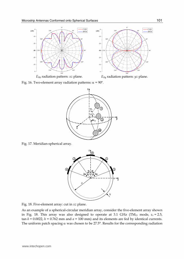
3.1 Meridian-spherical arrays The geometry of the spherical-circular meridian array, i.e. one whose patches are all centred

along a constant-φ plane, is shown in Fig. 17. In this particular configuration, the array is

positioned along the φ = β plane and the patch centres are located at αi, where i = 1, 2, …, N. Note the maximum number of elements N is a function of the sphere radius, the dielectric permittivity and the operating frequency, in a way to avoid the superposition of patches.

12

α

x

z

α

h

a

12

α

x

z

α

h

a

Fig. 14. Two-element array: cut in xz-plane.

-30

-20

-10

0

0°

30°

60°

90°

120°

150°

180°

210°

240°

270°

300°

330°

-30

-20

-10

0

CAD

HFSS[dB]

ERθ radiation pattern: xz plane.

-30

-20

-10

0

0°

30°

60°

90°

120°

150°

180°

210°

240°

270°

300°

330°

-30

-20

-10

0

CAD

HFSS[dB]

ERφ radiation pattern: yz plane.

Fig. 15. Two-element array radiation patterns: α = 15º.

www.intechopen.com


101

-30

-20

-10

0

0°

30°

60°

90°

120°

150°

180°

210°

240°

270°

300°

330°

-30

-20

-10

0

CAD

HFSS[dB]


-30

-20

-10

0

0°

30°

60°

90°

120°

150°

180°

210°

240°

270°

300°

330°

-30

-20

-10

0

CAD

HFSS[dB]


Fig. 16. Two-element array radiation patterns: α = 90º.

1α

x

y

z

2αα

N

1

2

N

1α

x

y

z

2αα

N

11

22

NN

Fig. 17. Meridian-spherical array.

x

z

12

0

34

2α2ααα

h

ax

z

12

0

34

2α2ααα

h

a

Fig. 18. Five-element array: cut in xz plane.

As an example of a spherical-circular meridian array, consider the five-element array shown

in Fig. 18. This array was also designed to operate at 3.1 GHz (TM11 mode, εr = 2.5,

tan δ = 0.0022, h = 0.762 mm and a = 100 mm) and its elements are fed by identical currents.

The uniform patch spacing α was chosen to be 27.5°. Results for the corresponding radiation

www.intechopen.com

Microstrip Antennas

102

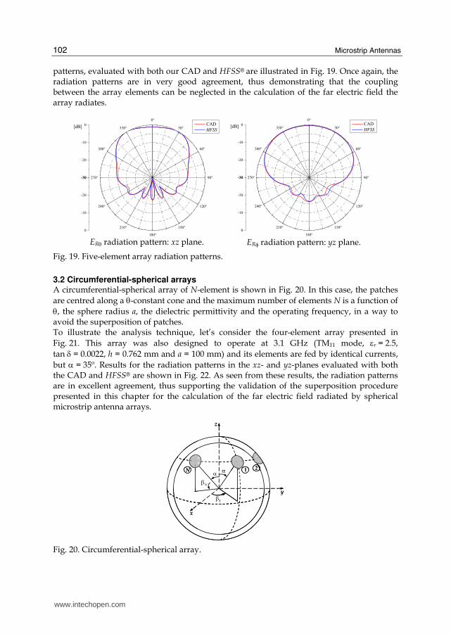
patterns, evaluated with both our CAD and HFSS® are illustrated in Fig. 19. Once again, the radiation patterns are in very good agreement, thus demonstrating that the coupling between the array elements can be neglected in the calculation of the far electric field the array radiates.

-30

-20

-10

0

0°

30°

60°

90°

120°

150°

180°

210°

240°

270°

300°

330°

-30

-20

-10

0

CAD

HFSS[dB]


-30

-20

-10

0

0°

30°

60°

90°

120°

150°

180°

210°

240°

270°

300°

330°

-30

-20

-10

0

CAD

HFSS[dB]


Fig. 19. Five-element array radiation patterns.

3.2 Circumferential-spherical arrays A circumferential-spherical array of N-element is shown in Fig. 20. In this case, the patches

are centred along a θ-constant cone and the maximum number of elements N is a function of

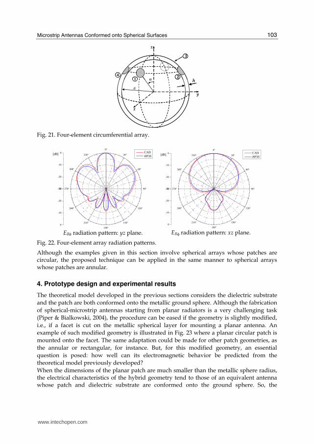
θ, the sphere radius a, the dielectric permittivity and the operating frequency, in a way to avoid the superposition of patches. To illustrate the analysis technique, let’s consider the four-element array presented in

Fig. 21. This array was also designed to operate at 3.1 GHz (TM11 mode, εr = 2.5,

tan δ = 0.0022, h = 0.762 mm and a = 100 mm) and its elements are fed by identical currents,

but α = 35º. Results for the radiation patterns in the xz- and yz-planes evaluated with both the CAD and HFSS® are shown in Fig. 22. As seen from these results, the radiation patterns are in excellent agreement, thus supporting the validation of the superposition procedure presented in this chapter for the calculation of the far electric field radiated by spherical microstrip antenna arrays.

α

x

y

z

1N

1βNβ

2α α

x

y

z

11NN

1βNβ

22α

Fig. 20. Circumferential-spherical array.

www.intechopen.com


103

x

y

z

α124

3

a

h

x

y

z

α112244

33

a

h

Fig. 21. Four-element circumferential array.

-30

-20

-10

0

0°

30°

60°

90°

120°

150°

180°

210°

240°

270°

300°

330°

-30

-20

-10

0

CAD

HFSS[dB]

ERθ radiation pattern: yz plane.

-30

-20

-10

0

0°

30°

60°

90°

120°

150°

180°

210°

240°

270°

300°

330°

-30

-20

-10

0

CAD

HFSS[dB]

ERφ radiation pattern: xz plane.

Fig. 22. Four-element array radiation patterns.

Although the examples given in this section involve spherical arrays whose patches are circular, the proposed technique can be applied in the same manner to spherical arrays whose patches are annular.

4. Prototype design and experimental results

The theoretical model developed in the previous sections considers the dielectric substrate

and the patch are both conformed onto the metallic ground sphere. Although the fabrication

of spherical-microstrip antennas starting from planar radiators is a very challenging task

(Piper & Bialkowski, 2004), the procedure can be eased if the geometry is slightly modified,

i.e., if a facet is cut on the metallic spherical layer for mounting a planar antenna. An

example of such modified geometry is illustrated in Fig. 23 where a planar circular patch is

mounted onto the facet. The same adaptation could be made for other patch geometries, as

the annular or rectangular, for instance. But, for this modified geometry, an essential

question is posed: how well can its electromagnetic behavior be predicted from the

theoretical model previously developed?

When the dimensions of the planar patch are much smaller than the metallic sphere radius, the electrical characteristics of the hybrid geometry tend to those of an equivalent antenna whose patch and dielectric substrate are conformed onto the ground sphere. So, the

www.intechopen.com

Microstrip Antennas

104

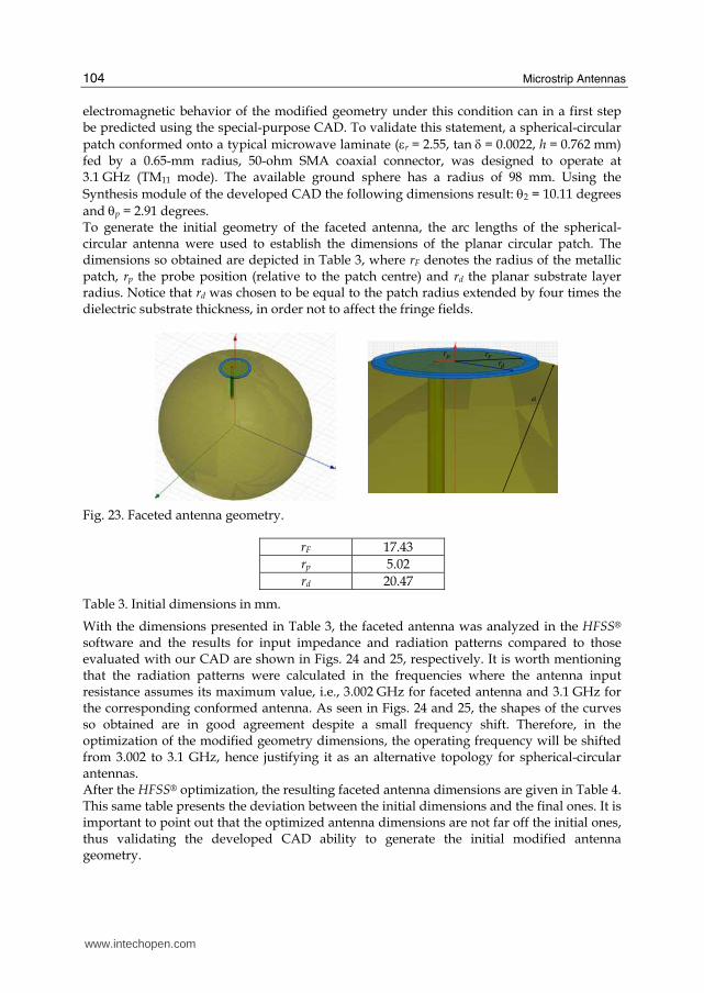
electromagnetic behavior of the modified geometry under this condition can in a first step be predicted using the special-purpose CAD. To validate this statement, a spherical-circular

patch conformed onto a typical microwave laminate (εr = 2.55, tan δ = 0.0022, h = 0.762 mm) fed by a 0.65-mm radius, 50-ohm SMA coaxial connector, was designed to operate at 3.1 GHz (TM11 mode). The available ground sphere has a radius of 98 mm. Using the

Synthesis module of the developed CAD the following dimensions result: θ2 = 10.11 degrees

and θp = 2.91 degrees. To generate the initial geometry of the faceted antenna, the arc lengths of the spherical-circular antenna were used to establish the dimensions of the planar circular patch. The dimensions so obtained are depicted in Table 3, where rF denotes the radius of the metallic patch, rp the probe position (relative to the patch centre) and rd the planar substrate layer radius. Notice that rd was chosen to be equal to the patch radius extended by four times the dielectric substrate thickness, in order not to affect the fringe fields.

pr

drFr

a

pr

drFr

a

Fig. 23. Faceted antenna geometry.

rF 17.43

rp 5.02

rd 20.47

Table 3. Initial dimensions in mm.

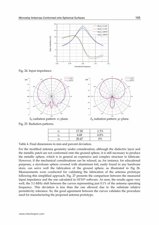
With the dimensions presented in Table 3, the faceted antenna was analyzed in the HFSS® software and the results for input impedance and radiation patterns compared to those evaluated with our CAD are shown in Figs. 24 and 25, respectively. It is worth mentioning that the radiation patterns were calculated in the frequencies where the antenna input resistance assumes its maximum value, i.e., 3.002 GHz for faceted antenna and 3.1 GHz for the corresponding conformed antenna. As seen in Figs. 24 and 25, the shapes of the curves so obtained are in good agreement despite a small frequency shift. Therefore, in the optimization of the modified geometry dimensions, the operating frequency will be shifted from 3.002 to 3.1 GHz, hence justifying it as an alternative topology for spherical-circular antennas. After the HFSS® optimization, the resulting faceted antenna dimensions are given in Table 4. This same table presents the deviation between the initial dimensions and the final ones. It is important to point out that the optimized antenna dimensions are not far off the initial ones, thus validating the developed CAD ability to generate the initial modified antenna geometry.

www.intechopen.com


105

0.98 0.99 1.00 1.01 1.02

-15

0

15

30

45

60

Input

imped

ance

[Ω]

Normalized frequency

Re(Zin) CAD

Im(Zin) CAD

Re(Zin) HFSS

Im(Zin) HFSS

Fig. 24. Input impedance.

-30

-20

-10

0

0°

30°

60°

90°

120°

150°

180°

210°

240°

270°

300°

330°

-30

-20

-10

0

CAD

HFSS[dB]

Eθ radiation pattern: xz plane.

-30

-20

-10

0

0°

30°

60°

90°

120°

150°

180°

210°

240°

270°

300°

330°

-30

-20

-10

0

CAD

HFSS[dB]

Eφ radiation pattern: yz plane.

Fig. 25. Radiation patterns.

rF 17.20 1.3%

rp 4.68 6.8%

rd 20.47 0%

Table 4. Final dimensions in mm and percent deviation.

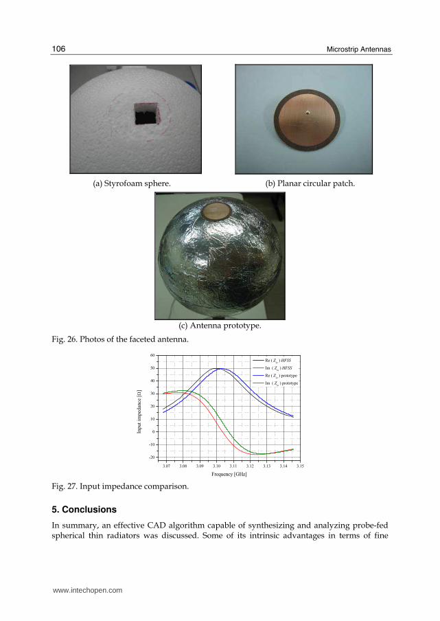
For the modified antenna geometry under consideration, although the dielectric layer and

the metallic patch are not conformed onto the ground sphere, it is still necessary to produce

the metallic sphere, which is in general an expensive and complex structure to fabricate.

However, if the mechanical considerations can be relaxed, as, for instance, for educational

purposes, a styrofoam sphere covered with aluminium foil, easily found in any hardware

store, can serve well the fabrication of the ground sphere, as illustrated in Fig 26.

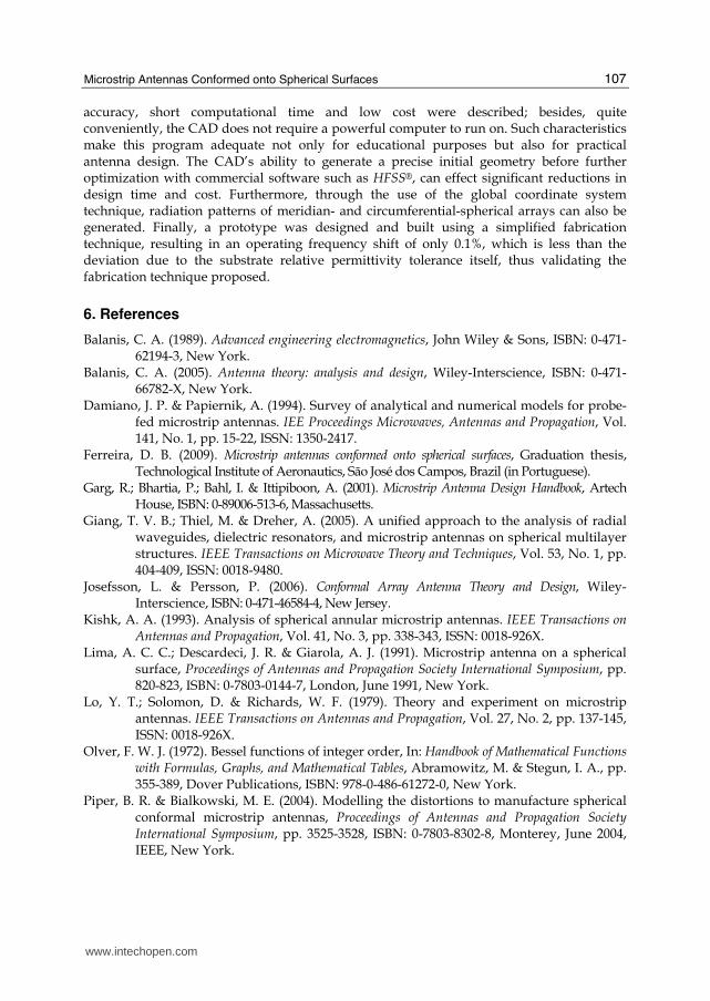
Measurements were conducted for validating the fabrication of the antenna prototype

following this simplified approach. Fig. 27 presents the comparison between the measured

input impedance and the one calculated in HFSS® software. As seen, the results agree very

well, the 3.1-MHz shift between the curves representing just 0.1% of the antenna operating

frequency. This deviation is less than the one allowed due to the substrate relative

permittivity tolerance. So, the good agreement between the curves validates the procedure

used for manufacturing the proposed antenna prototype.

www.intechopen.com

Microstrip Antennas

106

(a) Styrofoam sphere. (b) Planar circular patch.

(c) Antenna prototype.

Fig. 26. Photos of the faceted antenna.

3.07 3.08 3.09 3.10 3.11 3.12 3.13 3.14 3.15

-20

-10

0

10

20

30

40

50

60

Re ( Zin ) HFSS

Im ( Zin ) HFSS

Re ( Zin ) prototype

Im ( Zin ) prototype

Inp

ut

imped

ance

[Ω]

Frequency [GHz]

Fig. 27. Input impedance comparison.

5. Conclusions

In summary, an effective CAD algorithm capable of synthesizing and analyzing probe-fed spherical thin radiators was discussed. Some of its intrinsic advantages in terms of fine

www.intechopen.com


107

accuracy, short computational time and low cost were described; besides, quite conveniently, the CAD does not require a powerful computer to run on. Such characteristics make this program adequate not only for educational purposes but also for practical antenna design. The CAD’s ability to generate a precise initial geometry before further optimization with commercial software such as HFSS®, can effect significant reductions in design time and cost. Furthermore, through the use of the global coordinate system technique, radiation patterns of meridian- and circumferential-spherical arrays can also be generated. Finally, a prototype was designed and built using a simplified fabrication technique, resulting in an operating frequency shift of only 0.1%, which is less than the deviation due to the substrate relative permittivity tolerance itself, thus validating the fabrication technique proposed.

6. References

Balanis, C. A. (1989). Advanced engineering electromagnetics, John Wiley & Sons, ISBN: 0-471-62194-3, New York.

Balanis, C. A. (2005). Antenna theory: analysis and design, Wiley-Interscience, ISBN: 0-471-66782-X, New York.

Damiano, J. P. & Papiernik, A. (1994). Survey of analytical and numerical models for probe-fed microstrip antennas. IEE Proceedings Microwaves, Antennas and Propagation, Vol. 141, No. 1, pp. 15-22, ISSN: 1350-2417.

Ferreira, D. B. (2009). Microstrip antennas conformed onto spherical surfaces, Graduation thesis, Technological Institute of Aeronautics, São José dos Campos, Brazil (in Portuguese).

Garg, R.; Bhartia, P.; Bahl, I. & Ittipiboon, A. (2001). Microstrip Antenna Design Handbook, Artech House, ISBN: 0-89006-513-6, Massachusetts.

Giang, T. V. B.; Thiel, M. & Dreher, A. (2005). A unified approach to the analysis of radial waveguides, dielectric resonators, and microstrip antennas on spherical multilayer structures. IEEE Transactions on Microwave Theory and Techniques, Vol. 53, No. 1, pp. 404-409, ISSN: 0018-9480.

Josefsson, L. & Persson, P. (2006). Conformal Array Antenna Theory and Design, Wiley-Interscience, ISBN: 0-471-46584-4, New Jersey.

Kishk, A. A. (1993). Analysis of spherical annular microstrip antennas. IEEE Transactions on Antennas and Propagation, Vol. 41, No. 3, pp. 338-343, ISSN: 0018-926X.

Lima, A. C. C.; Descardeci, J. R. & Giarola, A. J. (1991). Microstrip antenna on a spherical surface, Proceedings of Antennas and Propagation Society International Symposium, pp. 820-823, ISBN: 0-7803-0144-7, London, June 1991, New York.

Lo, Y. T.; Solomon, D. & Richards, W. F. (1979). Theory and experiment on microstrip antennas. IEEE Transactions on Antennas and Propagation, Vol. 27, No. 2, pp. 137-145, ISSN: 0018-926X.

Olver, F. W. J. (1972). Bessel functions of integer order, In: Handbook of Mathematical Functions with Formulas, Graphs, and Mathematical Tables, Abramowitz, M. & Stegun, I. A., pp. 355-389, Dover Publications, ISBN: 978-0-486-61272-0, New York.

Piper, B. R. & Bialkowski, M. E. (2004). Modelling the distortions to manufacture spherical conformal microstrip antennas, Proceedings of Antennas and Propagation Society International Symposium, pp. 3525-3528, ISBN: 0-7803-8302-8, Monterey, June 2004, IEEE, New York.

www.intechopen.com

Microstrip Antennas

108

Richards, W. F.; Lo, Y. T. & Harrison, D. D. (1979). Improved theory for microstrip antennas. Electronics Letters, Vol. 15, No. 2, pp. 42-44, ISSN: 0013-5194.

Richards, W. F.; Lo, Y. T. & Harrison, D. D. (1981). An improved theory for microstrip antennas and applications. IEEE Transactions on Antennas and Propagation, Vol. 29, No. 1, pp. 38-46, ISSN: 0018-926X.

Sengupta, D. L.; Smith, T. M. & Larson, R. W. (1968). Radiation characteristics of a spherical array of circularly polarized elements. IEEE Transactions on Antennas and Propagation, Vol. 16, No. 1, pp. 2-7, ISSN: 0018-926X.

Sipus, Z.; Burum, N.; Skokic, S. & Kildal, P. –S. (2006). Analysis of spherical arrays of microstrip antennas using moment method in spectral domain. IEE Proceedings Microwaves, Antennas and Propagation, Vol. 153, No. 6, pp. 533-543, ISSN: 1350-2417.

Sipus, Z.; Skokic, S.; Bosiljevac, M. & Burum, N. (2008). Study of mutual coupling between circular stacked-patch antennas on a sphere. IEEE Transactions on Antennas and Propagation, Vol. 56, No. 7, pp. 1834-1844, ISSN: 0018-926X.

Tam, W. -Y. & Luk, K. -M. (1991). Far field analysis of spherical-circular microstrip antennas by electric surface current models. IEE Proceedings H Microwaves, Antennas and Propagation, Vol. 138, No. 1, pp. 98-102, ISSN: 0950-107X.

Tam, W. Y.; Lai, A. K. Y. & Luk, K. M. (1995). Input impedance of spherical microstrip antenna. IEE Proceedings Microwaves, Antennas and Propagation, Vol. 142, No. 3, pp. 285-288, ISSN: 1350-2417.

Wong, K. –L. (1999). Design of Nonplanar Microstrip Antennas and Transmission Lines, John Wiley & Sons, ISBN: 0-471-18244-3, New York.

www.intechopen.com

Microstrip AntennasEdited by Prof. Nasimuddin Nasimuddin

ISBN 978-953-307-247-0Hard cover, 540 pagesPublisher InTechPublished online 04, April, 2011Published in print edition April, 2011

InTech EuropeUniversity Campus STeP Ri Slavka Krautzeka 83/A 51000 Rijeka, Croatia Phone: +385 (51) 770 447 Fax: +385 (51) 686 166www.intechopen.com

InTech ChinaUnit 405, Office Block, Hotel Equatorial Shanghai No.65, Yan An Road (West), Shanghai, 200040, China

Phone: +86-21-62489820 Fax: +86-21-62489821

In the last 40 years, the microstrip antenna has been developed for many communication systems such asradars, sensors, wireless, satellite, broadcasting, ultra-wideband, radio frequency identifications (RFIDs),reader devices etc. The progress in modern wireless communication systems has dramatically increased thedemand for microstrip antennas. In this book some recent advances in microstrip antennas are presented.

How to referenceIn order to correctly reference this scholarly work, feel free to copy and paste the following:

Daniel B. Ferreira and J. C. da S. Lacava (2011). Microstrip Antennas Conformed onto Spherical Surfaces,Microstrip Antennas, Prof. Nasimuddin Nasimuddin (Ed.), ISBN: 978-953-307-247-0, InTech, Available from:http://www.intechopen.com/books/microstrip-antennas/microstrip-antennas-conformed-onto-spherical-surfaces

Documents

Microstrip Antennas Conformed onto Spherical Surfacescdn.intechweb.org/pdfs/14710.pdf · Microstrip Antennas Conformed onto Spherical Surfaces ... the wave equation (1) ... Microstrip