Microsoft® Office Excel® 2003 Training

Sorting and Filtering Data

MorningStar Education presents:

Contents

• Overview: Working with data easily

• Lesson 1: Sorting data

• Lesson 2: Filtering data

• Lesson 3: Using Advanced Filters

Overview: working with data easily

Excel is Microsoft’s premier spreadsheet application, part of Microsoft Office Suite, and the most popular spreadsheet in the world.

Excel 2003 is simple to use. Many features are automated, and anyone with a basic knowledge of spreadsheets can begin using Excel in minutes.

This course assumes you have a basic knowledge of Excel and are familiar with spreadsheet architecture.

Goals

During this presentation, you will learn how to…

• sort data using the AutoFilter

• filter data using simple criteria with Advanced Filters

• filter data using complex criteria with Advanced Filters

Lesson 1

Sorting data

What is “sorting?”

Sorting arranges data in your worksheet

numerically,

alphabetically, or

chronologically.

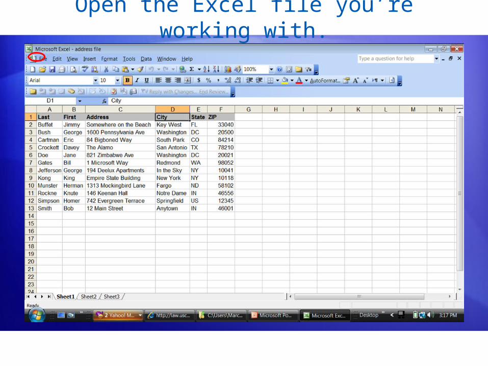
Open the Excel file you’re working with.

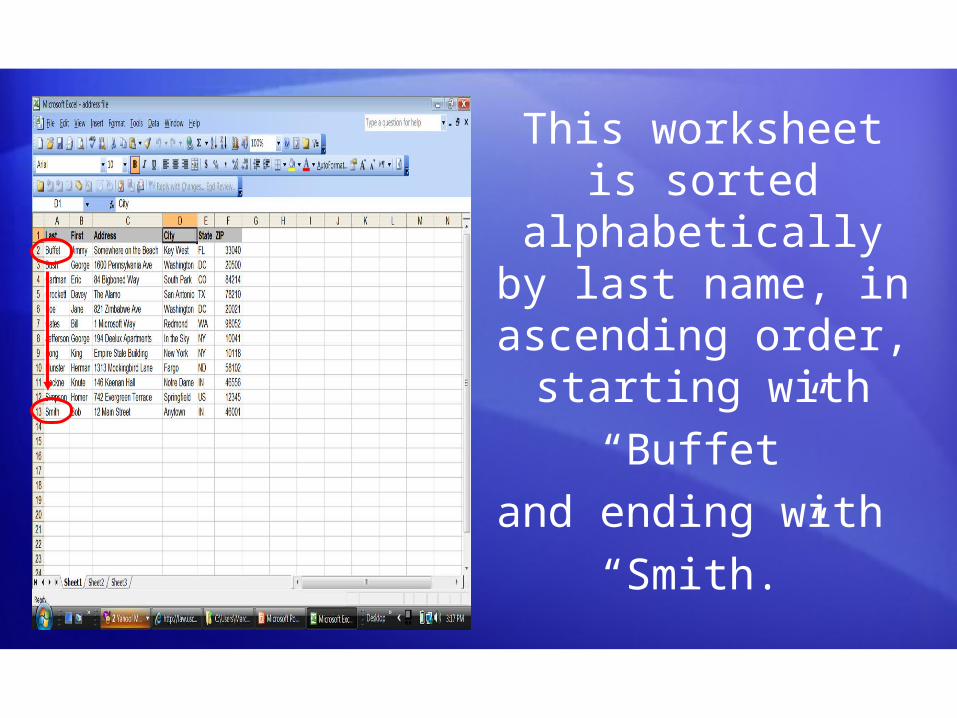
This worksheet is sorted

alphabetically by last name, in

ascending order, starting with

“Buffet”

and ending with

“Smith.”

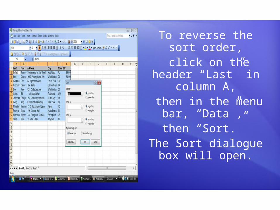
To reverse the sort order,

click on the header “Last” in column A, then in the menu

bar, “Data”, then “Sort.”

The Sort dialogue box will open.

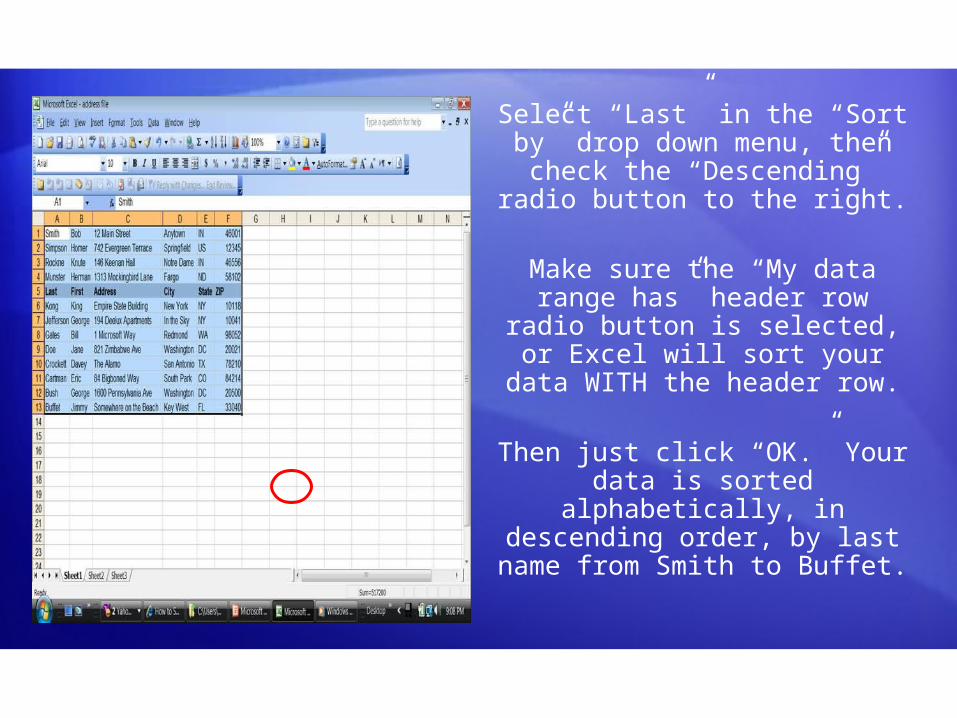
Select “Last” in the “Sort by” drop down menu, then check the “Descending” radio button

to the right.

Make sure the “My data range has” header row radio button is selected, or Excel will sort your

data WITH the header row.

Then just click “OK.” Your data is sorted alphabetically, in

descending order, by last name from Smith to Buffet.

Lesson 2

Filtering data

What is “filtering?”

Filtering removes data from your

worksheet that you don’t need or want to see. It effectively

selects only that data you wish to see and shows only that data.

After creating a database and assembling a large amount of data, you may want to know

who your best customers are,

which inventory items cost less than a certain amount,

or which employees work the least amount of hours.

Excel includes several tools you can use to analyze your data so you can make better

decisions.

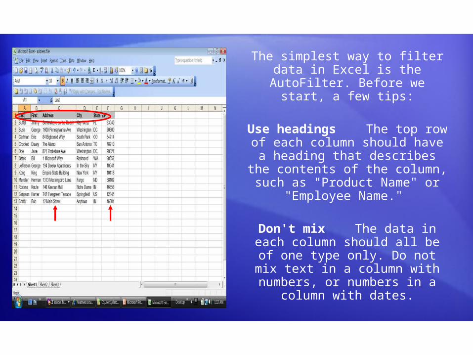
The simplest way to filter data in Excel is the AutoFilter. Before we

start, a few tips:

Use headings    The top row of each column should have a heading that describes the

contents of the column, such as "Product Name" or "Employee

Name."

Don't mix    The data in each column should all be of one type only. Do not mix text in a column with numbers, or numbers in a

column with dates.

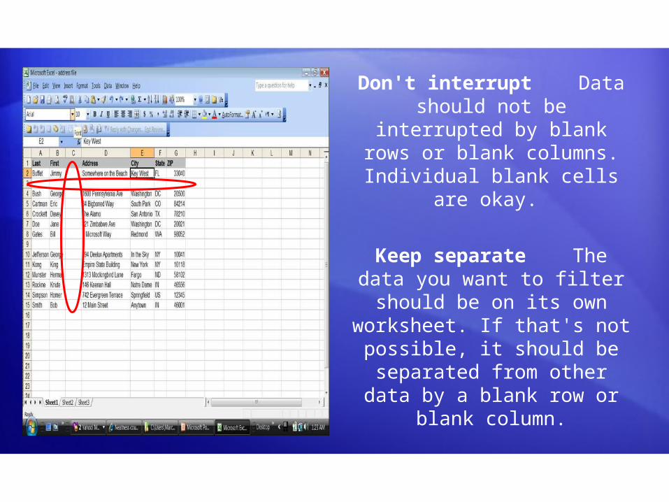
Don't interrupt    Data should not be interrupted by blank rows or blank columns.

Individual blank cells are okay.

Keep separate    The data you want to filter should be

on its own worksheet. If that's not possible, it should

be separated from other data by a blank row or blank

column.

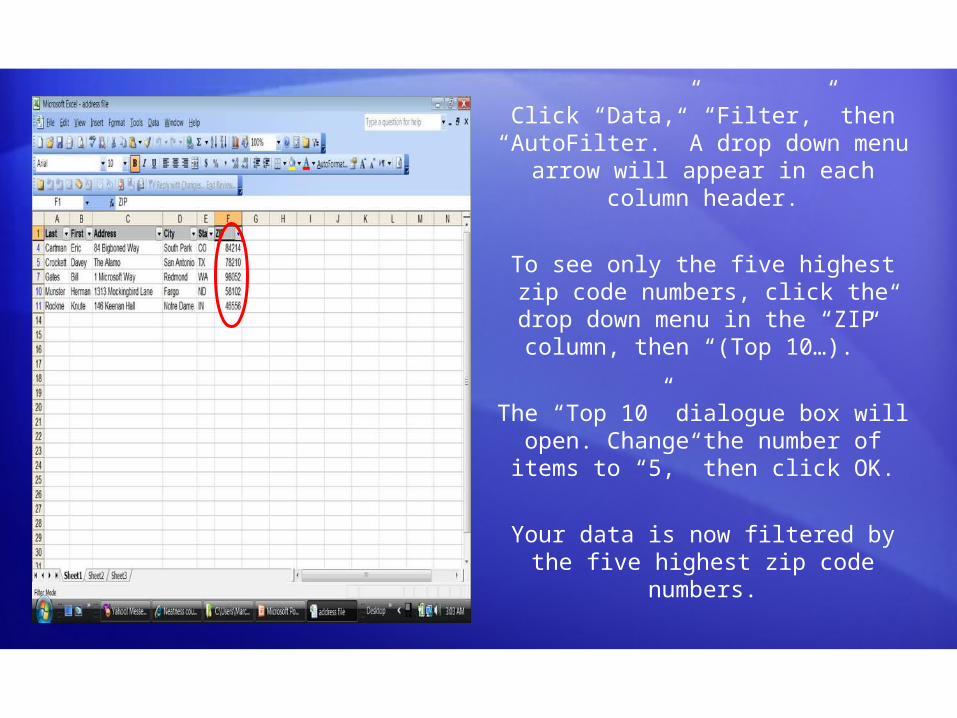
Click “Data,” “Filter,” then “AutoFilter.” A drop down menu

arrow will appear in each column header.

To see only the five highest zip code numbers, click the drop down

menu in the “ZIP” column, then “(Top 10…).”

The “Top 10” dialogue box will open. Change the number of items

to “5,” then click OK.

Your data is now filtered by the five highest zip code numbers.

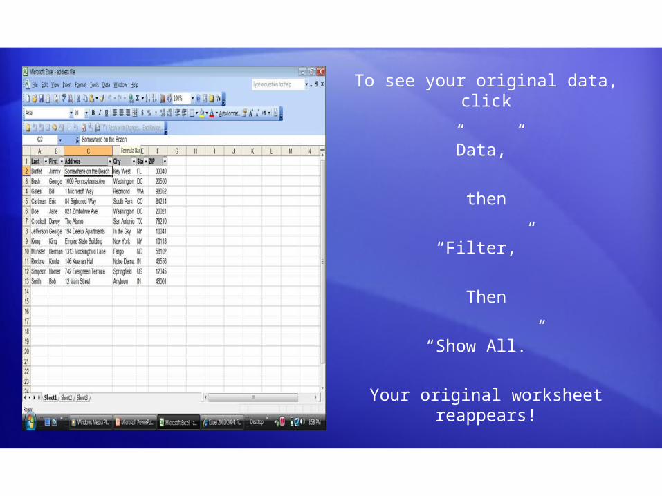
To see your original data, click

”Data,”

then

“Filter,”

Then

“Show All.”

Your original worksheet reappears!

Lesson 3

Using Advanced Filters

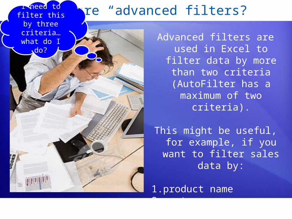
What are “advanced filters?”

Advanced filters are used in Excel to filter data by more than two criteria (AutoFilter

has a maximum of two criteria).

This might be useful, for example, if you want to

filter sales data by:

1. product name2. customer name3. sales by quarter

I need to filter this by three

criteria… what do I do?

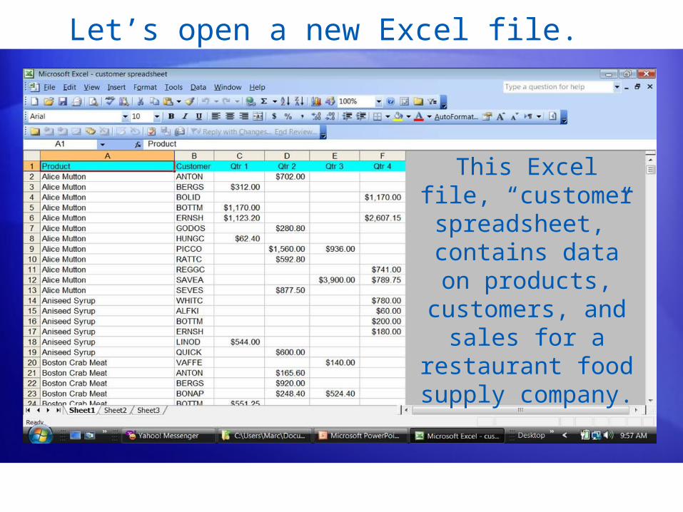
Let’s open a new Excel file.

This Excel file, “customer

spreadsheet,” contains data on

products, customers, and

sales for a restaurant food

supply company.

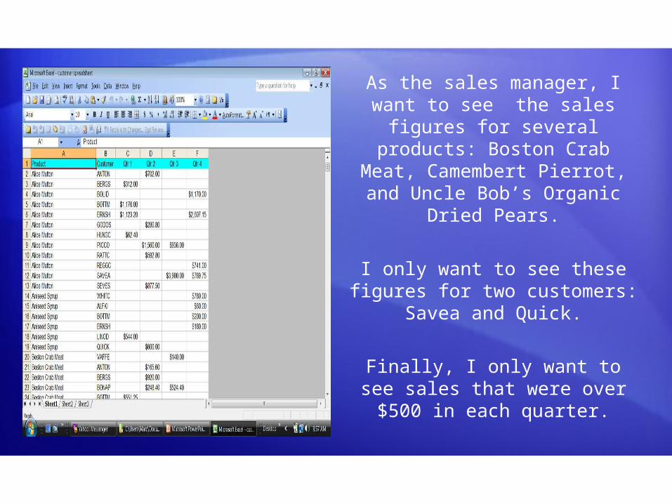
As the sales manager, I want to see the sales figures for

several products: Boston Crab Meat, Camembert Pierrot, and

Uncle Bob’s Organic Dried Pears.

I only want to see these figures for two customers: Savea and

Quick.

Finally, I only want to see sales that were over $500 in each

quarter.

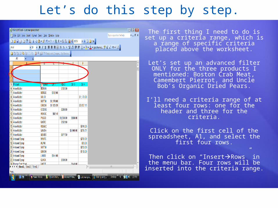
Let’s do this step by step.

The first thing I need to do is set up a criteria range, which is a range of specific criteria placed above the

worksheet.

Let’s set up an advanced filter ONLY for the three products I mentioned:

Boston Crab Meat, Camembert Pierrot, and Uncle Bob’s Organic Dried Pears.

I’ll need a criteria range of at least four rows: one for the header and three for

the criteria.

Click on the first cell of the spreadsheet, A1, and select the first

four rows.

Then click on “InsertRows” in the menu bar. Four rows will be inserted

into the criteria range.

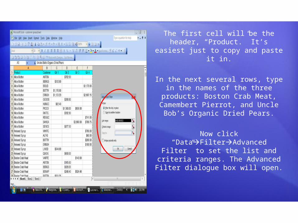
The first cell will be the header, “Product.” It’s easiest just to

copy and paste it in.

In the next several rows, type in the names of the three products: Boston Crab Meat, Camembert

Pierrot, and Uncle Bob’s Organic Dried Pears.

Now click “DataFilterAdvanced Filter” to set the list and criteria ranges.

The Advanced Filter dialogue box will open.

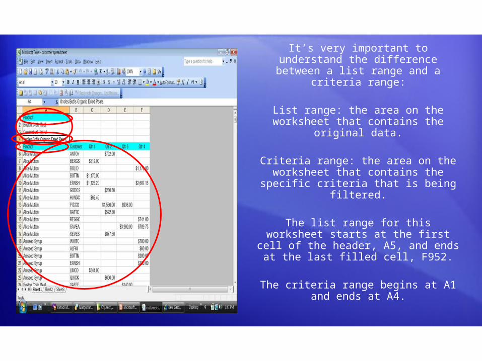
It’s very important to understand the difference between a list range and a

criteria range:

List range: the area on the worksheet that contains the original data.

Criteria range: the area on the worksheet that contains the specific

criteria that is being filtered.

The list range for this worksheet starts at the first cell of the header, A5, and ends at the last filled cell,

F952.

The criteria range begins at A1 and ends at A4.

Type the list range in the list range box, separated by a colon.

A5:F592

Do the same for the criteria range.

A1:F4

Click “OK.”

Your data is now filtered by the specific product names specified.

To filter the data using several criteria, it’s important to

understand the concept of and/or operators and how they work in

Excel.

And/or operators work by specifying whether a specific

criteria is to be filtered with another criteria (“and”) or whether it is to

be filtered instead of another criteria (“or”)

If a record meets all the criteria in a row in a criteria area, it will pass

through the filter.

AND/OR?

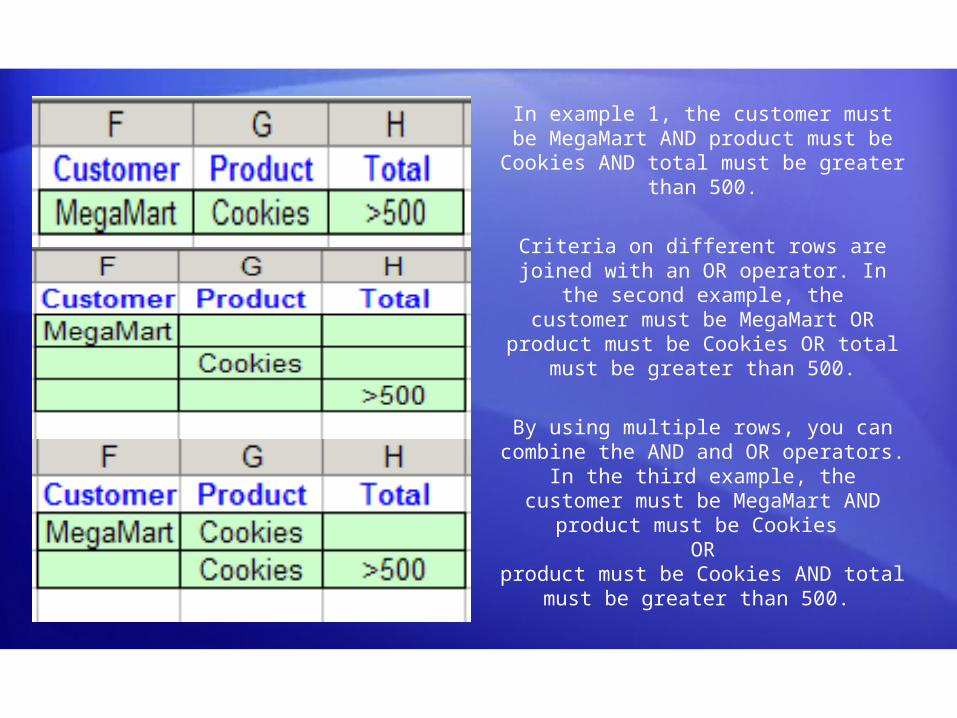
In example 1, the customer must be MegaMart AND product must be Cookies

AND total must be greater than 500.

Criteria on different rows are joined with an OR operator. In the second example,

thecustomer must be MegaMart OR product

must be Cookies OR total must be greater than 500.

By using multiple rows, you can combine the AND and OR operators. In the third

example, thecustomer must be MegaMart AND

product must be Cookies OR

product must be Cookies AND total must be greater than 500.

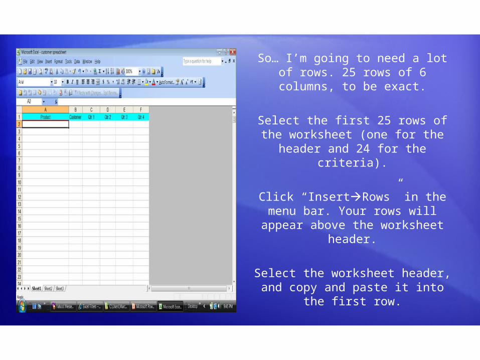
So… I’m going to need a lot of rows. 25 rows of 6 columns, to be

exact.

Select the first 25 rows of the worksheet (one for the header

and 24 for the criteria).

Click “InsertRows” in the menu bar. Your rows will appear above

the worksheet header.

Select the worksheet header, and copy and paste it into the first row.

I need 24 rows because I’ve got three products, two

customers, and four quarters I’m filtering for (3X2X4=24).

Each value for the quarter must be listed separately, as

an “AND” operator.

It’s easiest to type the values in, then repeat them by

selecting them. The values for the quarters can be typed

in once, then copied.

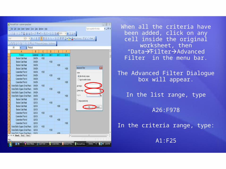
When all the criteria have been added, click on any cell inside the

original worksheet, then “DataFilterAdvanced Filter” in

the menu bar.

The Advanced Filter Dialogue box will appear.

In the list range, type

A26:F978

In the criteria range, type:

A1:F25

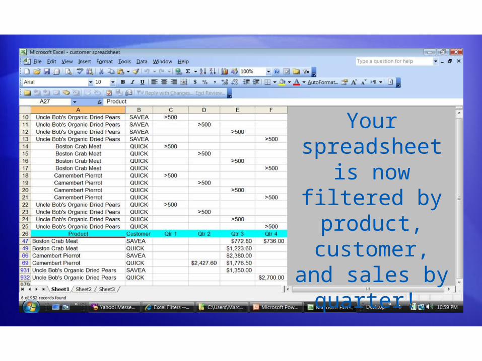
Your spreadsheet is now filtered by

product, customer, and

sales by quarter!