Embed Size (px)
Citation preview

Microsoft Excel
Excel
A spreadsheet program organize data complete calculations make decisions graph data develop reports

Project 1
Creating a Worksheetand Embedded Chart
What’s New
Excel Window Entering Text and Numbers AutoSum Fill Handle Merge & Center Button AutoFormat ChartWizard
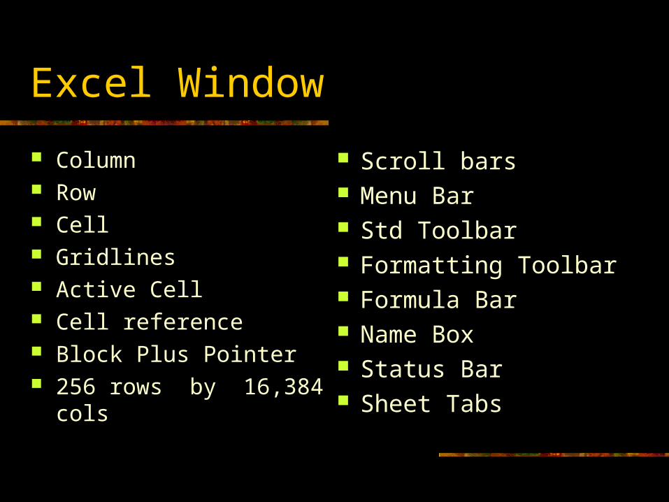
Excel Window
Column Row Cell Gridlines Active Cell Cell reference Block Plus Pointer 256 rows by 16,384 cols
Scroll bars Menu Bar Std Toolbar Formatting Toolbar Formula Bar Name Box Status Bar Sheet Tabs
Cell & Range
Cell Intersection of a row and a column
Range A series of two or more adjacent cells Rectangular shape
Entering Text and Numbers Click (or use arrow keys) to SELECT CELL TYPE TEXT OR enter numbers (no ,)
Click green check box in formula barOR
Press enterOR
Press arrow key in direction of next input cell
AutoSum
on standard toolbar
Sum numbers above (or left of) current cell
Click twice for single cell Click once for range
Fill Handle
Used to copy contents of a cell
Point to bottom right corner of active cell
Drag to copy
Merge and Center
To center a label across multiple columns
Type label Select range Click Merge and Center Button <-a->
AutoFormat Applies font styles to a range
Font size, type Borders, cell widths
Select range to format (e.g. all but title) Format Menu
AutoFormat Command Select Table Format (e.g., Accounting 2) OK
Chart Wizard
Graphical representation of data
Select data to graph (e.g. all but totals & title)
Click Chart Wizard button Select Chart Type (e.g., 3D bar chart)
Click Finish Move & Resize as desired

Project 2
Formulas, Formatting,
And Web Queries
What’s New
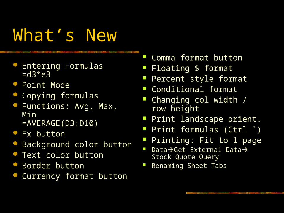
Entering Formulas=d3*e3
Point Mode Copying formulas Functions: Avg, Max, Min
=AVERAGE(D3:D10) Fx button Background color button Text color button Border button Currency format button
Comma format button Floating $ format Percent style format Conditional format Changing col width /
row height Print landscape orient. Print formulas (Ctrl `) Printing: Fit to 1 page DataGet External Data Stock
Quote Query Renaming Sheet Tabs
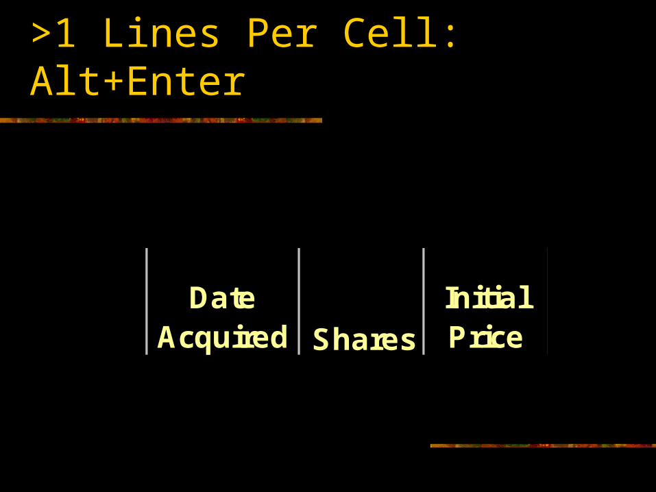
DateAcquired Shares
InitialPrice
>1 Lines Per Cell: Alt+Enter
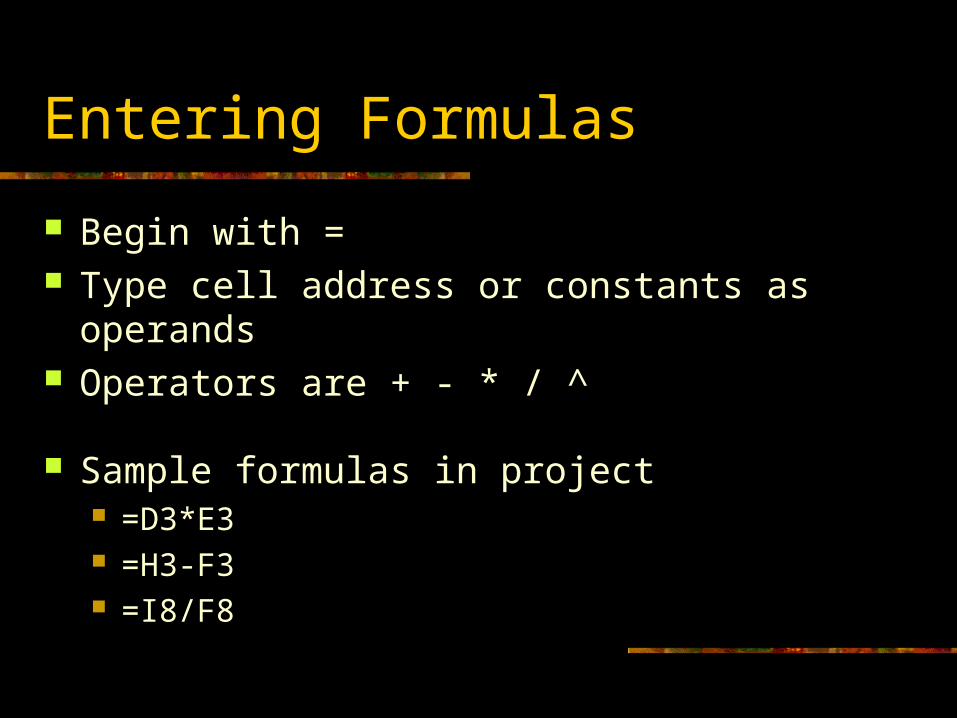
Entering Formulas
Begin with = Type cell address or constants as operands Operators are + - * / ^
Sample formulas in project =D3*E3 =H3-F3 =I8/F8
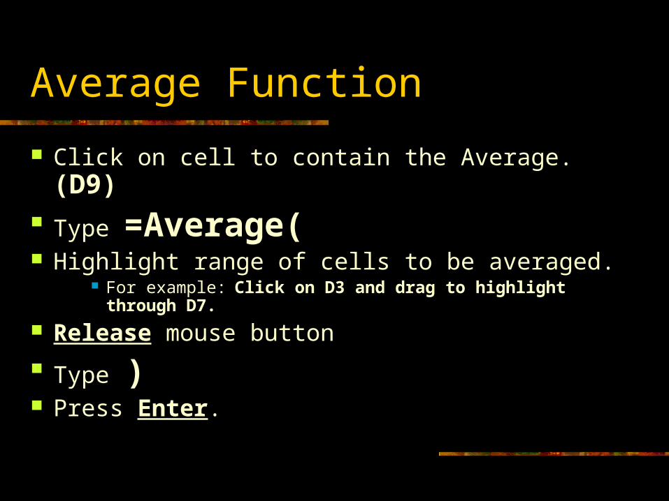
Average Function
Click on cell to contain the Average. (D9) Type =Average( Highlight range of cells to be averaged.
For example: Click on D3 and drag to highlight through D7.
Release mouse button
Type ) Press Enter.
Other Functions
=max(d3:d7) =min(d3:d7)
fx button allows one to select functions
Formatting Worksheet Title
In title, first letters larger than others
Select one character at a time Specify font size (28 pts) Repeat Rest of text in label is 20 pts.
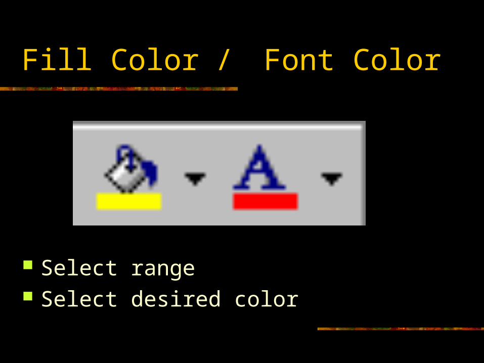
Fill Color / Font Color
Select range Select desired color
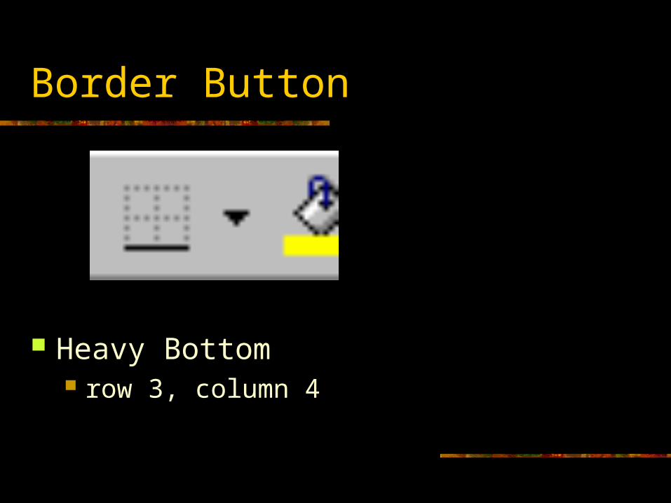
Border Button
Heavy Bottom row 3, column 4
How Numbers Display in Cells
If numbers are too wide for the column ##### will appear in the cell.
This does not mean you have lost the number or done something wrong.
It merely means the column is not wide enough.
Using Formatting Toolbar to Format Numbers
Click the Currency Style ( $ ) button on the Formatting toolbar.
Click on the Comma Style ( , ) button on the Formatting toolbar.
Formatting Currency Style w/ Floating $
Highlight cells to be formatted & Point to the highlighted area,
Right-click for a Quick menu. Click Format Cells Click Number tab Click Currency in the Category list box. Click the down arrow under Symbol; Click $. Click on the Black ($1,234.10) in the Negative
box.
Notes on Formatting Numbers
FIXED $ -- Click on $ on formatting tool bar.
FLOATING $ -- Must use dialog box. Select Format Cells from Format Menu choose Currency use $ and negative numbers in black parentheses.
Notes on Formatting Numbers
Comma with zero (0) displaying Must use dialog box. Select Format Cells from Format Menu; then choose Currency; choose None for for Symbol; negative numbers in black parentheses. (This option will align the decimals places also.)
Comma with hyphen (-) displaying for zero values Click on the comma on the formatting tool bar.
Percent Formatting
Click on the % button on the Formatting tool bar.
Click on the Increase decimal places just to the right of the comma button two times (for 2 decimal places).
Changing Column Widths & Row Heights
Default column width is 8.43 characters Default row height is 12.75 points. This is because the default font is Arial 10
point.
Can be manually changed by dragging column or row divider lines
Or use Best Fit. width will be increased / decreased to fit widest
entry double click divider line
Rearranging the Order of Sheets
Double-click on the sheet tab or right-click on the tab and choose rename
Type in Sheet name (Pie Chart) Click on OK. Repeat steps for other sheets. Sheet 1 should be renamed Investment Analysis. Point to the name of sheet (Investment Analysis) to
be moved drag it over the other sheet name tab (over Pie Chart).
Release mouse button.
Displaying and Printing Formulas
Hold down CTRL and press the Left Single Quotation
Mark also called the Accent mark ( ` ) location to the left of the number 1 and above the tab key
File -> Page Setup; Page tab. Click Landscape orientation. Click Fit to so the wide printout fits on one page
Getting External Data from the Web
Click on the Sheet 2 tab; then click in A1. Click on the Data menu; Click on Get External Data. Click on Run Web Query… On Run Query Dialog Box, click on Multiple Stock Quotes by
PC Quote, Inc. Click on the Get Data command button. Click on Existing worksheet option. On the Enter Parameter values dialog box, click in the Text
Box and key in symbols: cpq dell intc msft nscp Click in box on use reference for refreshes. Click on OK.

Microsoft Excel - Project 3
What-if Analysis and Working With Large
Worksheets
New Features in Project 3
Expenses are dependent on projected monthly net sales assumptions
Using the Fill Handle to create a series Rotating Text Copying a cell’s format using the Format
Painter Copying cell contents to non-adjacent cells Adding Drop Shadow to cells
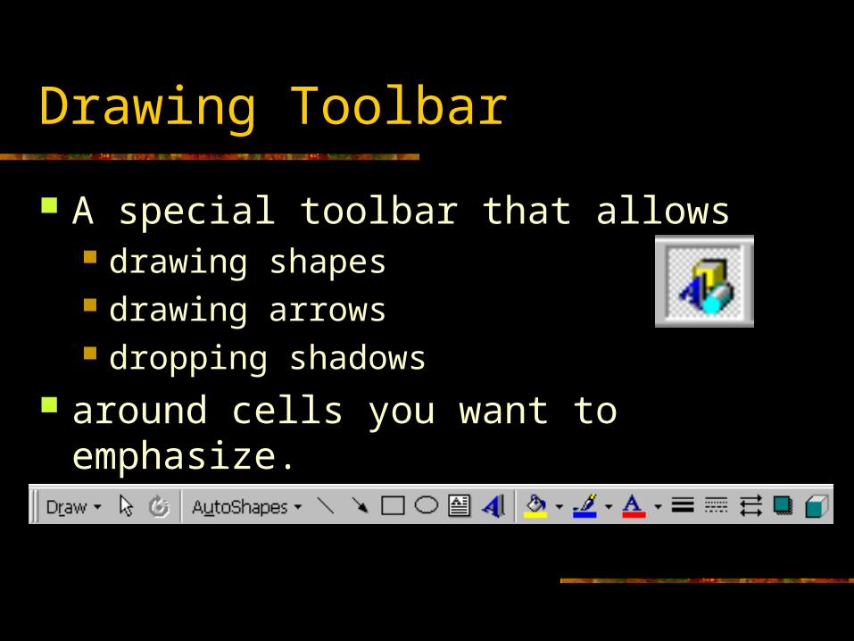
Drawing Toolbar
A special toolbar that allows drawing shapes drawing arrows dropping shadows
around cells you want to emphasize.
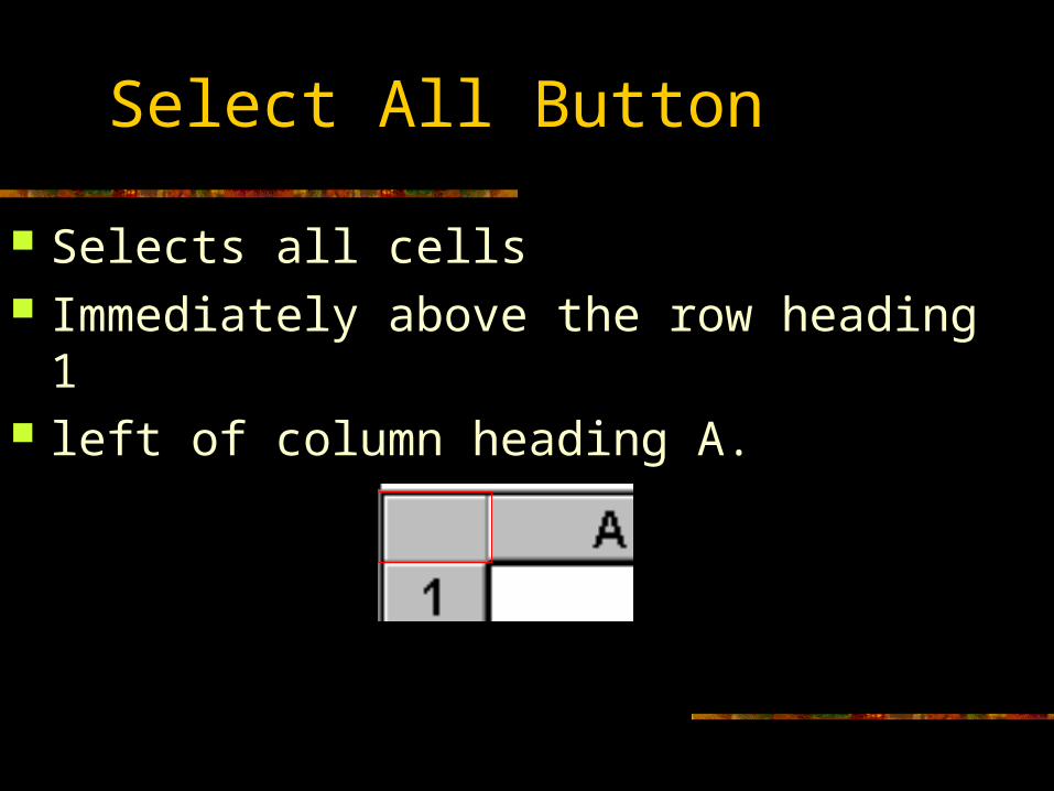
Select All Button
Selects all cells Immediately above the row heading 1 left of column heading A.
Using Fill Handle to Create a Series
Excel has built-in sequences to fill a range of cells automatically.
See page E3.10 for examples.
How to create a series Type first element(s) of sequence (For example, January) Highlight element(s) Drag to create a series as long as desired
Excel will automatically type the next item in the sequence until all highlighted cells are filled.
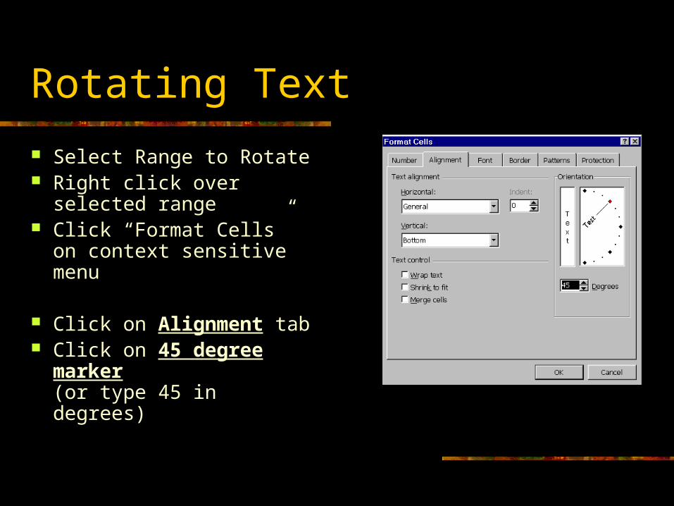
Rotating Text
Select Range to Rotate Right click over selected
range Click “Format Cells” on
context sensitive menu
Click on Alignment tab Click on 45 degree
marker (or type 45 in degrees)
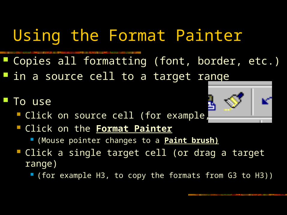
Using the Format Painter Copies all formatting (font, border, etc.) in a source cell to a target range
To use Click on source cell (for example, G3) Click on the Format Painter
(Mouse pointer changes to a Paint brush)
Click a single target cell (or drag a target range) (for example H3, to copy the formats from G3 to H3))
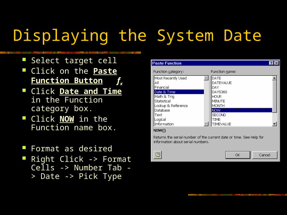
Displaying the System Date Select target cell Click on the Paste
Function Button fx Click Date and Time in
the Function category box. Click NOW in the Function
name box.
Format as desired Right Click -> Format
Cells -> Number Tab -> Date -> Pick Type
Copying Cells to Non-Adjacent Area
Highlight source range (for example, A7:A11)
Click on the Copy button Click in the first cell to receive the copy (for example,
A16).
Press the ENTER key (or Paste button) P
Inserting Rows and Columns
Right click on the ROW number or COL letter for row below (or COLUMN TO RIGHT) where one is to
be inserted. Entire row or column is highlighted.
Click on Insert. Rows are pushed down Columns are moved right.
Deleting Rows and Columns
Right click on the ROW number or COL letter for row or column where one is to be deleted. Entire row or column is highlighted.
Click on Delete. Rows are pushed down Columns are moved right.
Entering Data with Format Symbols
If you enter a number with $, a comma whole number %
Excel automatically formats it when it is entered into the cell.
See page E3.18 on Table 3-2 for examples.
Freezing Worksheet Titles
Click in the cell below the column headings you wish to freeze and to the right of the row headings you wish to freeze
Click on Window on the menu bar. Click on Freeze Panes.
To unfreeze the panes: click on unfreeze on the Window menu.
Relative vs. Absolute Addressing
Relative Addressing Formulas copied automatically change cell references e.g., B4 in a formula becomes C4
Absolute Addressing Formulas copied keep the same cell row and/or
column reference e.g., B4 in a formula remains B4 when copied
To Use Absolute Cell Addressing
Either Put a $ sign before the column and row number.
OR Select cell reference and press F4
When entering formulas, to make absolute: Type the cell address With cursor still next to cell reference, press the
F4 key.
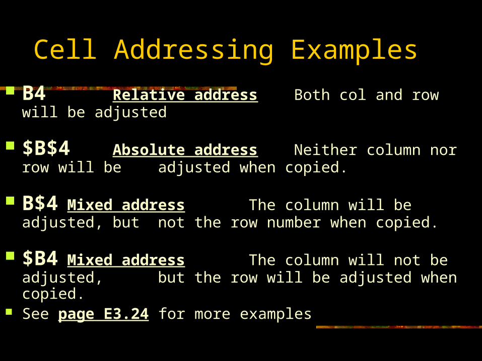
Cell Addressing Examples
B4 Relative address Both col and row will be adjusted
$B$4 Absolute address Neither column nor row will be adjusted when copied.
B$4 Mixed address The column will be adjusted, but not the row number when copied.
$B4 Mixed address The column will not be adjusted, but the row will be adjusted when
copied. See page E3.24 for more examples
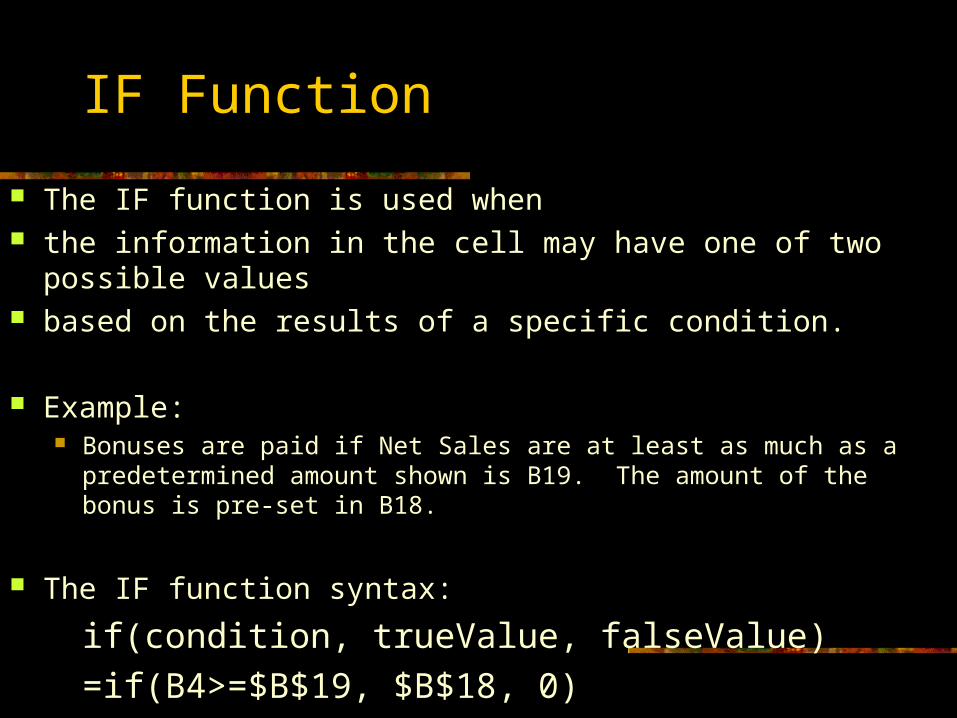
IF Function
The IF function is used when the information in the cell may have one of two possible values based on the results of a specific condition.
Example: Bonuses are paid if Net Sales are at least as much as a predetermined
amount shown is B19. The amount of the bonus is pre-set in B18.
The IF function syntax:
if(condition, trueValue, falseValue)
=if(B4>=$B$19, $B$18, 0)
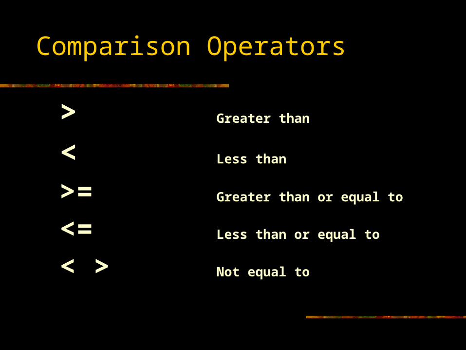
Comparison Operators
> Greater than
< Less than
>= Greater than or equal to
<= Less than or equal to
< > Not equal to
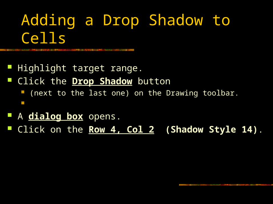
Adding a Drop Shadow to Cells
Highlight target range. Click the Drop Shadow button
(next to the last one) on the Drawing toolbar.
A dialog box opens. Click on the Row 4, Col 2 (Shadow Style 14).
Dividing Screen Into 2 Separate Windows
To divide the screen vertically (to see two separate parts of a worksheet) Point to the top of the vertical scroll bar Drag down to divide the windows into 2 vertical windows.
Drag back up to restore the windows.
To divide the screen horizontally, point to the right of the horizontal scroll bar drag back to the left
Adding a Pie Chart to the Workbook
Select the range of cells containing the labels for the pie slices (A3:A7).
Hold down CTRL and highlight the range of cells to be charted (H3:H7).
Click on Chart Wizard on the standard tool bar. Click on Click on Pie for chart type;
Click on the Row 1, Col 2 (3-D Pie Sub-type); click on Next.
If the range is correct (A3:A7; H3:H7) click on Next
Chart Wizard Dialog Box Steps
In Step 3 box, click on Title tab (type in Portfolio Breakdown);
Click on Legend tab remove check to show legend click on Data Labels tab: click on Show labels and Percent. Click on Next.
In Step 4, click as new sheet.
Click in text box to name the sheet. (Pie Chart). Click on finish.
Formatting the Chart Title
Point to the Chart title and click to select it. Click on the Font size box down arrow, and click on
36. Click on the Underline button on the Formatting
toolbar. Point to the Font Color button on the Formatting
toolbar. Click on Red (Column 1, Row 3).
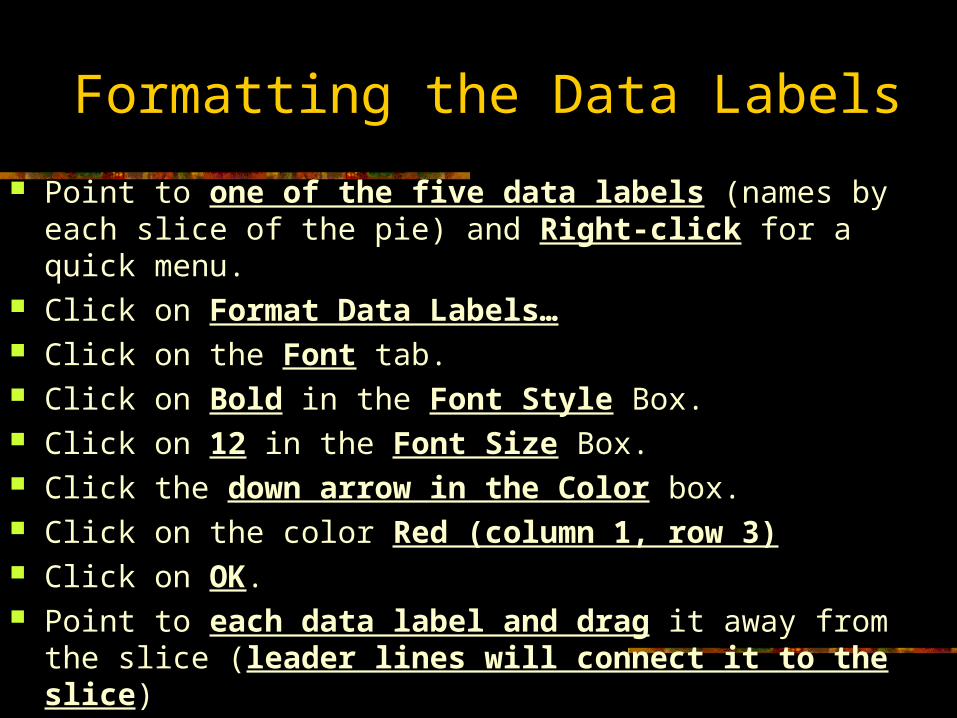
Formatting the Data Labels
Point to one of the five data labels (names by each slice of the pie) and Right-click for a quick menu.
Click on Format Data Labels… Click on the Font tab. Click on Bold in the Font Style Box. Click on 12 in the Font Size Box. Click the down arrow in the Color box. Click on the color Red (column 1, row 3) Click on OK. Point to each data label and drag it away from the slice
(leader lines will connect it to the slice)
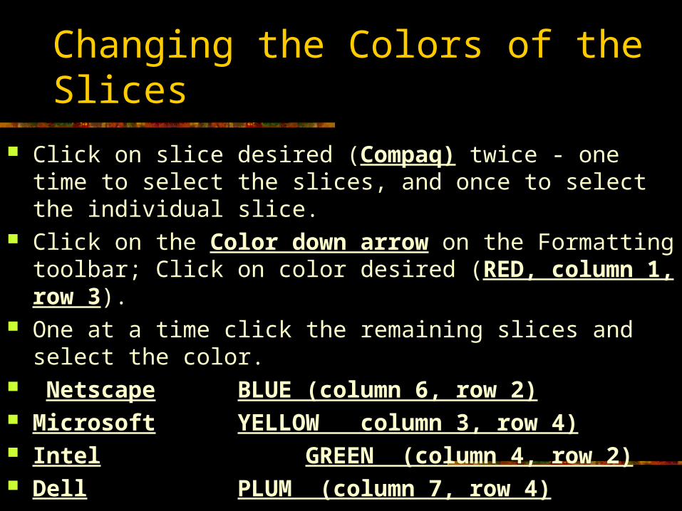
Changing the Colors of the Slices
Click on slice desired (Compaq) twice - one time to select the slices, and once to select the individual slice.
Click on the Color down arrow on the Formatting toolbar; Click on color desired (RED, column 1, row 3).
One at a time click the remaining slices and select the color. Netscape BLUE (column 6, row 2) Microsoft YELLOW column 3, row 4) Intel GREEN (column 4, row 2) Dell PLUM (column 7, row 4)
Exploding the Pie Chart
Exploding Offsetting one or more slices from the rest of the chart to
emphasize it. Make sure the sizing handles are still on the pie slices.
Click the slice - Don’t double-click it. Drag the slice to the desired position.
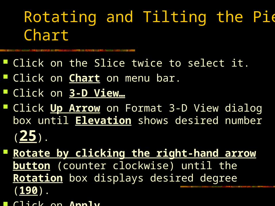
Rotating and Tilting the Pie Chart
Click on the Slice twice to select it. Click on Chart on menu bar. Click on 3-D View… Click Up Arrow on Format 3-D View dialog box until
Elevation shows desired number (25). Rotate by clicking the right-hand arrow button
(counter clockwise) until the Rotation box displays desired degree (190).
Click on Apply.