Microsoft Excel 2010 - University of Queensland · UQ Library Staff and Student I.T. Training Notes 3 of 21 Microsoft Excel 2013: Further Functions Text Functions Text functions are

Reproduced or adapted from original content provided under Creative Commons license by The University of Queensland Library

Microsoft Excel 2013 Further Functions

Course objectives:

Understand and use different functions effectively

Text Functions

Date and Time Functions

Math and Trig Functions

Lookup and Reference Functions

Logical Functions

Statistical Functions

Student Training and Support Service Points

Phone (07) 334 64312 St Lucia: Main desk of the SSAH, ARMUS

and DHESL libraries

Email [email protected] Hospitals Main desk of the PACE, Herston and

Mater libraries

Web http://web.library.uq.edu.au/library-services/training Gatton: Level 2, UQ Gatton Library

Library services provide the student I.T. Helpdesk service in the UQ Library. They can assist with general enquiries and IT support.

This includes computing help and training for UQ students in: Study Management Applications like my.UQ and Learn.UQ (Blackboard),

Microsoft Office and I.T. fundamentals like file management, printing and laptop setup.

Staff Training and Support

Phone (07) 3365 2666

Email [email protected]

Web http://www.uq.edu.au/staffdevelopment

Staff may contact their trainer with enquiries and feedback related to training content. Please contact Staff Development for booking

enquiries or your local I.T. support for general technical enquiries.

http://www.library.uq.edu.au/

http://creativecommons.org/licenses/by-nc/3.0/au/

UQ Library

Staff and Student I.T. Training

2 of 21 Microsoft Excel 2013: Further Functions

Table of Contents

Text Functions ................................................................................................................. 3 “PROPER” Function.................................................................................. 3 “EXACT” Function ..................................................................................... 4 “TRIM” Function ........................................................................................ 5 “CONCATENATE” and “RIGHT” Functions ............................................... 6 Flash Fill ................................................................................................... 7

Date and Time Functions ................................................................................................ 8 Exact Date calculations ............................................................................. 8

Math and Trig Functions ................................................................................................. 9 “SUMIF” Function ..................................................................................... 9 “SUMIFS” Function ................................................................................. 10 “SUMPRODUCT” Function ..................................................................... 19

Lookup and Reference Functions ................................................................................ 10 Dropdown Lists ..................................................................................... 10 “MATCH” Function ................................................................................ 11 “INDEX” Function .................................................................................. 12 Combining the INDEX and MATCH Functions ...................................... 12

Logical Functions .......................................................................................................... 13 “AND” Function ..................................................................................... 13 Combining “IF” and “AND” Functions .................................................... 13

Statistical Functions ..................................................................................................... 14 “COUNTBLANK” Function .................................................................... 14 “COUNTIF” Function ............................................................................. 14 “COUNTIFS” Function ........................................................................... 15

Extension Exercises ...................................................................................................... 16 Year calculations ................................................................................... 16 “NETWORKDAYS.INTL” Function ........................................................ 16 “IFNA” Function ..................................................................................... 17 “IF” Function ......................................................................................... 18 Using nested ‘IF’ statements ................................................................. 18 “RANK.EQ” Function ............................................................................. 18

What-If Analysis ............................................................................................................ 19 Including Add-ins .................................................................................. 20 Excel Solver .......................................................................................... 20

Exercise document: Go to https://web.library.uq.edu.au/library-services/training/training-resources Click on Excel Click Further Functions (.xlsx, 50KB) to download.

UQ Library


Notes


Text Functions Text functions are used when working with cells containing text strings. Some of the many functions available can…change text case, compare cells containing text strings and even split or concatenate (join) text strings.

“PROPER” Function

This function is used to convert the case of text strings e.g. lower case to Proper Case. Other functions in this class are Lower and Upper. The proper function capitalises the first letter of each word in the selected text.

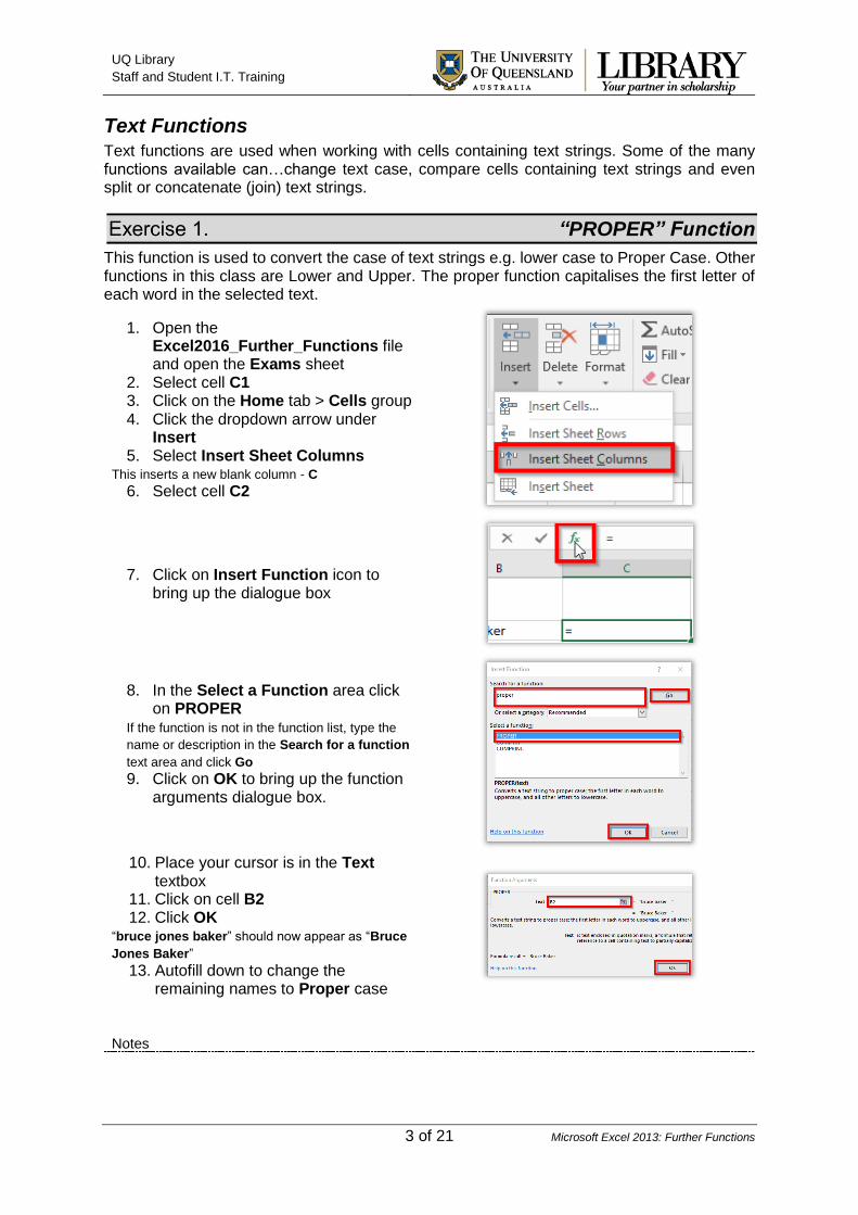
1. Open the Excel2016_Further_Functions file and open the Exams sheet

2. Select cell C1 3. Click on the Home tab > Cells group 4. Click the dropdown arrow under

Insert 5. Select Insert Sheet Columns

This inserts a new blank column - C 6. Select cell C2

7. Click on Insert Function icon to bring up the dialogue box

8. In the Select a Function area click on PROPER

If the function is not in the function list, type the

name or description in the Search for a function

text area and click Go 9. Click on OK to bring up the function

arguments dialogue box.

10. Place your cursor is in the Text

textbox 11. Click on cell B2 12. Click OK

“bruce jones baker” should now appear as “Bruce

Jones Baker”

13. Autofill down to change the remaining names to Proper case

UQ Library


Notes


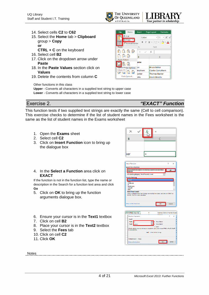
14. Select cells C2 to C62 15. Select the Home tab > Clipboard

group > Copy or CTRL + C on the keyboard

16. Select cell B2 17. Click on the dropdown arrow under

Paste 18. In the Paste Values section click on

Values 19. Delete the contents from column C

Other functions in this class

Upper - Converts all characters in a supplied text string to upper case

Lower - Converts all characters in a supplied text string to lower case

“EXACT” Function

This function tests if two supplied text strings are exactly the same (Cell to cell comparison). This exercise checks to determine if the list of student names in the Fees worksheet is the same as the list of student names in the Exams worksheet

1. Open the Exams sheet 2. Select cell C2 3. Click on Insert Function icon to bring up

the dialogue box

4. In the Select a Function area click on EXACT

If the function is not in the function list, type the name or

description in the Search for a function text area and click

Go

5. Click on OK to bring up the function arguments dialogue box.

6. Ensure your cursor is in the Text1 textbox 7. Click on cell B2 8. Place your cursor is in the Text2 textbox 9. Select the Fees tab 10. Click on cell C2 11. Click OK

UQ Library


Notes


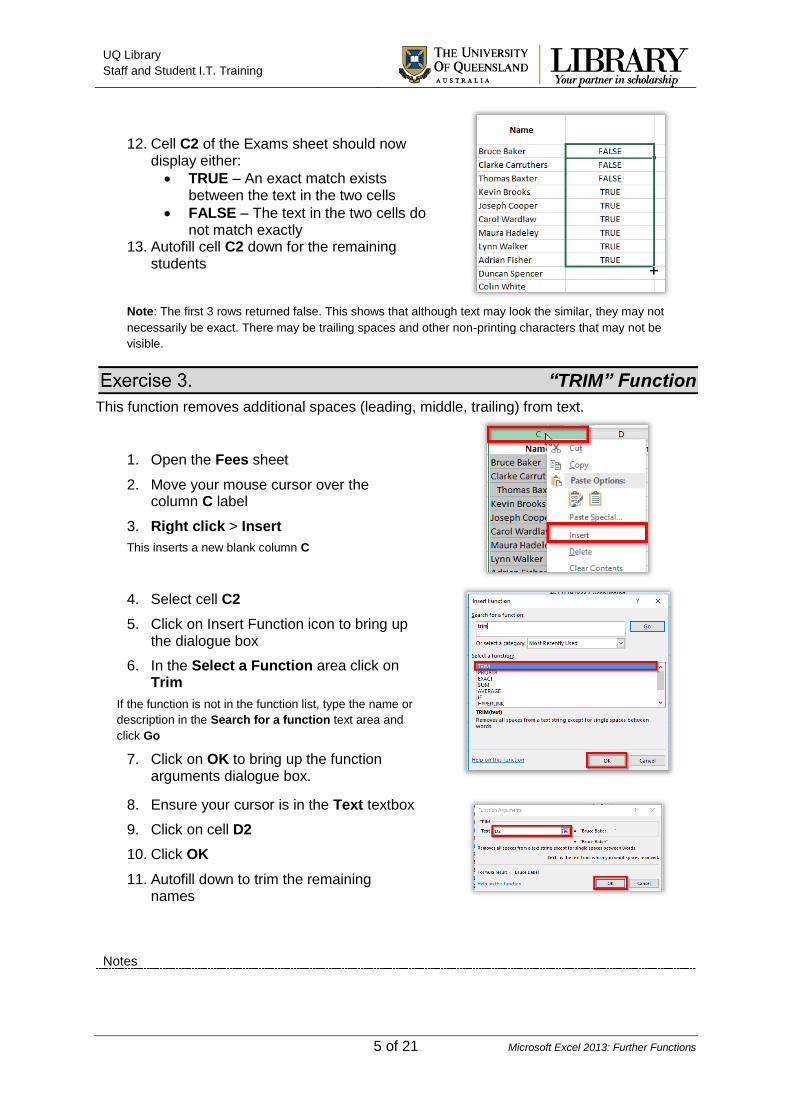
12. Cell C2 of the Exams sheet should now display either:

TRUE – An exact match exists between the text in the two cells

FALSE – The text in the two cells do not match exactly

13. Autofill cell C2 down for the remaining students

Note: The first 3 rows returned false. This shows that although text may look the similar, they may not

necessarily be exact. There may be trailing spaces and other non-printing characters that may not be

visible.

“TRIM” Function

This function removes additional spaces (leading, middle, trailing) from text.

1. Open the Fees sheet

2. Move your mouse cursor over the column C label

3. Right click > Insert

This inserts a new blank column C

4. Select cell C2


6. In the Select a Function area click on Trim


description in the Search for a function text area and

click Go


8. Ensure your cursor is in the Text textbox

9. Click on cell D2

10. Click OK

11. Autofill down to trim the remaining names

UQ Library


Notes


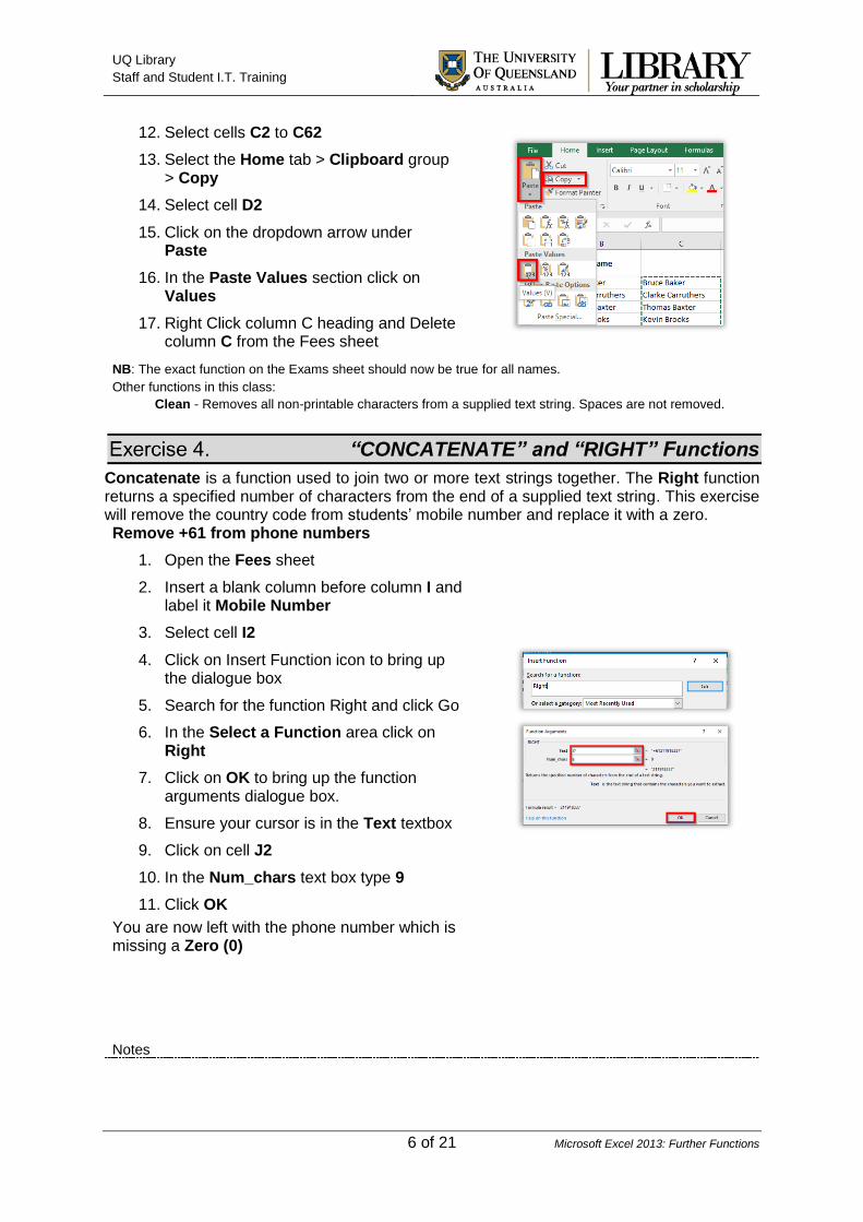
12. Select cells C2 to C62

13. Select the Home tab > Clipboard group > Copy

14. Select cell D2

15. Click on the dropdown arrow under Paste

16. In the Paste Values section click on Values

17. Right Click column C heading and Delete column C from the Fees sheet

NB: The exact function on the Exams sheet should now be true for all names.

Other functions in this class:

Clean - Removes all non-printable characters from a supplied text string. Spaces are not removed.

“CONCATENATE” and “RIGHT” Functions

Concatenate is a function used to join two or more text strings together. The Right function returns a specified number of characters from the end of a supplied text string. This exercise will remove the country code from students’ mobile number and replace it with a zero. Remove +61 from phone numbers

1. Open the Fees sheet

2. Insert a blank column before column I and label it Mobile Number

3. Select cell I2


5. Search for the function Right and click Go

6. In the Select a Function area click on Right


8. Ensure your cursor is in the Text textbox

9. Click on cell J2

10. In the Num_chars text box type 9

11. Click OK

You are now left with the phone number which is missing a Zero (0)

UQ Library


Notes


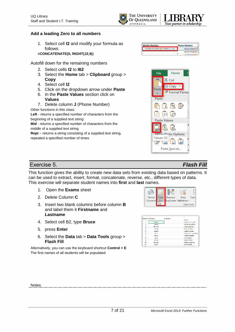
Add a leading Zero to all numbers

1. Select cell I2 and modify your formula as follows:

=CONCATENATE(0, RIGHT(J2,9))

Autofill down for the remaining numbers

2. Select cells I2 to I62 3. Select the Home tab > Clipboard group >

Copy 4. Select cell I2 5. Click on the dropdown arrow under Paste 6. In the Paste Values section click on

Values 7. Delete column J (Phone Number)


Left - returns a specified number of characters from the

beginning of a supplied text string

Mid - returns a specified number of characters from the

middle of a supplied text string

Rept – returns a string consisting of a supplied text string,

repeated a specified number of times

Flash Fill

This function gives the ability to create new data sets from existing data based on patterns. It can be used to extract, insert, format, concatenate, reverse, etc., different types of data. This exercise will separate student names into first and last names.

1. Open the Exams sheet

2. Delete Column C

3. Insert two blank columns before column B and label them it Firstname and Lastname

4. Select cell B2, type Bruce

5. press Enter

6. Select the Data tab > Data Tools group > Flash Fill

Alternatively, you can use the keyboard shortcut Control + E

The first names of all students will be populated

UQ Library


Notes


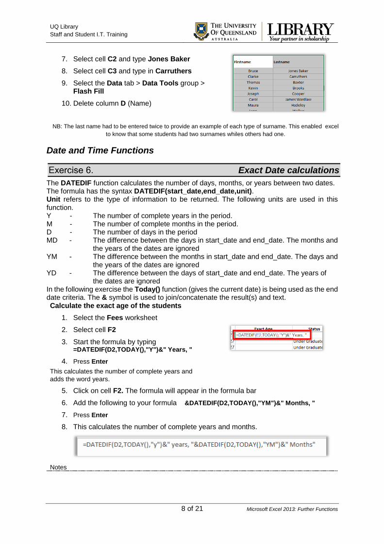
7. Select cell C2 and type Jones Baker

8. Select cell C3 and type in Carruthers

9. Select the Data tab > Data Tools group > Flash Fill

10. Delete column D (Name)

NB: The last name had to be entered twice to provide an example of each type of surname. This enabled excel

to know that some students had two surnames whiles others had one.

Date and Time Functions

Exact Date calculations

The DATEDIF function calculates the number of days, months, or years between two dates. The formula has the syntax DATEDIF(start_date,end_date,unit). Unit refers to the type of information to be returned. The following units are used in this function. Y - The number of complete years in the period. M - The number of complete months in the period. D - The number of days in the period MD - The difference between the days in start_date and end_date. The months and the years of the dates are ignored YM - The difference between the months in start_date and end_date. The days and the years of the dates are ignored YD - The difference between the days of start_date and end_date. The years of the dates are ignored In the following exercise the Today() function (gives the current date) is being used as the end date criteria. The & symbol is used to join/concatenate the result(s) and text. Calculate the exact age of the students

1. Select the Fees worksheet

2. Select cell F2

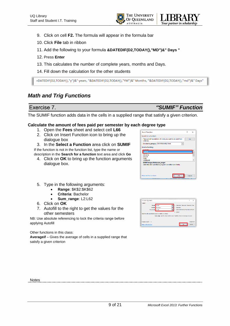
3. Start the formula by typing =DATEDIF(D2,TODAY(),"Y")&" Years, "

4. Press Enter

This calculates the number of complete years and

adds the word years.

5. Click on cell F2. The formula will appear in the formula bar

6. Add the following to your formula &DATEDIF(D2,TODAY(),"YM")&" Months, "

7. Press Enter

8. This calculates the number of complete years and months.

UQ Library


Notes


9. Click on cell F2. The formula will appear in the formula bar

10. Click File tab in ribbon

11. Add the following to your formula &DATEDIF(D2,TODAY(),"MD")&" Days "

12. Press Enter

13. This calculates the number of complete years, months and Days.

14. Fill down the calculation for the other students

Math and Trig Functions

“SUMIF” Function

The SUMIF function adds data in the cells in a supplied range that satisfy a given criterion. Calculate the amount of fees paid per semester by each degree type

1. Open the Fees sheet and select cell L66 2. Click on Insert Function icon to bring up the

dialogue box 3. In the Select a Function area click on SUMIF


description in the Search for a function text area and click Go 4. Click on OK to bring up the function arguments

dialogue box.

5. Type in the following arguments:

Range: $K$2:$K$62

Criteria: Bachelor

Sum_range: L2:L62

6. Click on OK 7. Autofill to the right to get the values for the

other semesters NB: Use absolute referencing to lock the criteria range before

applying Autofill


Averageif – Gives the average of cells in a supplied range that

satisfy a given criterion

UQ Library


Notes


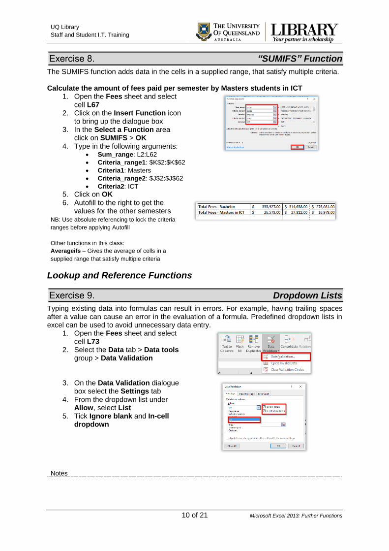
“SUMIFS” Function

The SUMIFS function adds data in the cells in a supplied range, that satisfy multiple criteria. Calculate the amount of fees paid per semester by Masters students in ICT

1. Open the Fees sheet and select cell L67

2. Click on the Insert Function icon to bring up the dialogue box

3. In the Select a Function area click on SUMIFS > OK

4. Type in the following arguments: Sum_range: L2:L62

Criteria_range1: $K$2:$K$62

Criteria1: Masters

Criteria_range2: $J$2:$J$62

Criteria2: ICT

5. Click on OK

6. Autofill to the right to get the values for the other semesters

NB: Use absolute referencing to lock the criteria

ranges before applying Autofill


Averageifs – Gives the average of cells in a

supplied range that satisfy multiple criteria

Lookup and Reference Functions

Dropdown Lists

Typing existing data into formulas can result in errors. For example, having trailing spaces after a value can cause an error in the evaluation of a formula. Predefined dropdown lists in excel can be used to avoid unnecessary data entry.


2. Select the Data tab > Data tools group > Data Validation

3. On the Data Validation dialogue box select the Settings tab

4. From the dropdown list under Allow, select List

5. Tick Ignore blank and In-cell dropdown

UQ Library


Notes


6. Click in the Source data field and select cells C2 to C62

Alternatively, you can enter: =$C$2:$C$62

into the source field

7. Click OK A dropdown list of student names is now

created in cell L73.

Updating the list of students automatically

updates the list dropdown list.

8. Select cell L74 9. Repeat this exercise using cells

=$L$1:$T$1 as the Source data.

“MATCH” Function

The MATCH function finds the relative position of a value in a supplied list or array. The value of the MATCH function is not very obvious when used on its own. It is however a very useful function when combined with other functions. Determine the position of Kevin Brooks


2. Choose Kevin Brooks from the dropdown list

3. Select cell L77 4. Click on Insert Function icon to

bring up the dialogue box 5. In the Select a Function area

click on MATCH 6. Click on OK to bring up the

function arguments dialogue box. 7. Type in the following arguments:

Lookup_value: L73

Lookup_array: C2:C62

Match_type: 0

8. Click on OK Match Types:

-1 : Greater than

0 : Exact

1 : Less than

UQ Library


Notes


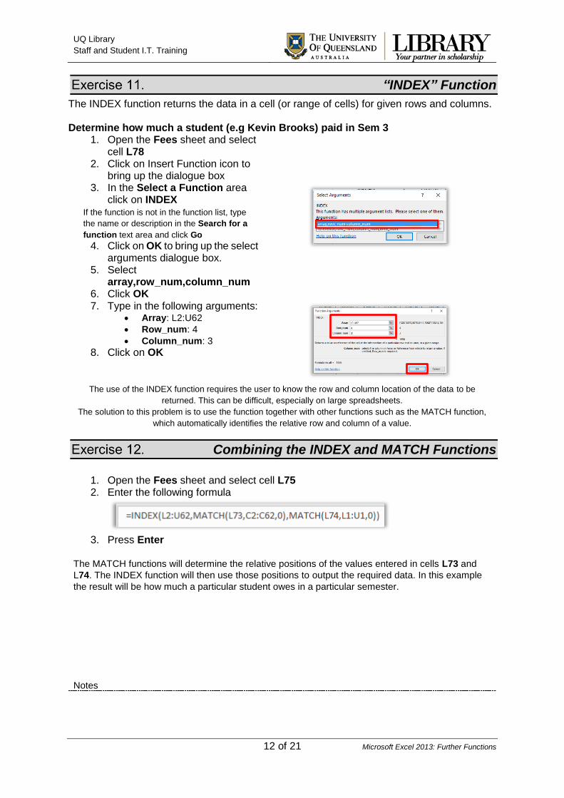
“INDEX” Function

The INDEX function returns the data in a cell (or range of cells) for given rows and columns. Determine how much a student (e.g Kevin Brooks) paid in Sem 3



3. In the Select a Function area click on INDEX

If the function is not in the function list, type

the name or description in the Search for a

function text area and click Go 4. Click on OK to bring up the select

arguments dialogue box. 5. Select

array,row_num,column_num 6. Click OK

7. Type in the following arguments: Array: L2:U62

Row_num: 4

Column_num: 3

8. Click on OK

The use of the INDEX function requires the user to know the row and column location of the data to be

returned. This can be difficult, especially on large spreadsheets.

The solution to this problem is to use the function together with other functions such as the MATCH function,

which automatically identifies the relative row and column of a value.

Combining the INDEX and MATCH Functions

1. Open the Fees sheet and select cell L75 2. Enter the following formula

3. Press Enter

The MATCH functions will determine the relative positions of the values entered in cells L73 and

L74. The INDEX function will then use those positions to output the required data. In this example

the result will be how much a particular student owes in a particular semester.

UQ Library


Notes


Logical Functions

“AND” Function

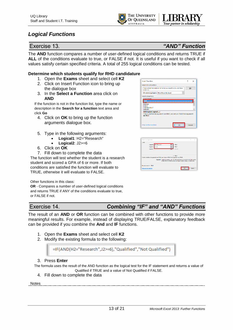
The AND function compares a number of user-defined logical conditions and returns TRUE if ALL of the conditions evaluate to true, or FALSE if not. It is useful if you want to check if all values satisfy certain specified criteria. A total of 255 logical conditions can be tested. Determine which students qualify for RHD candidature

1. Open the Exams sheet and select cell K2 2. Click on Insert Function icon to bring up

the dialogue box 3. In the Select a Function area click on

AND If the function is not in the function list, type the name or

description in the Search for a function text area and

click Go 4. Click on OK to bring up the function

arguments dialogue box.


Logical1: H2="Research"

Logical2: J2>=6

6. Click on OK 7. Fill down to complete the data

The function will test whether the student is a research

student and scored a GPA of 6 or more. If both

conditions are satisfied the function will evaluate to

TRUE, otherwise it will evaluate to FALSE.


OR - Compares a number of user-defined logical conditions

and returns TRUE if ANY of the conditions evaluate to true,

or FALSE if not.

Combining “IF” and “AND” Functions

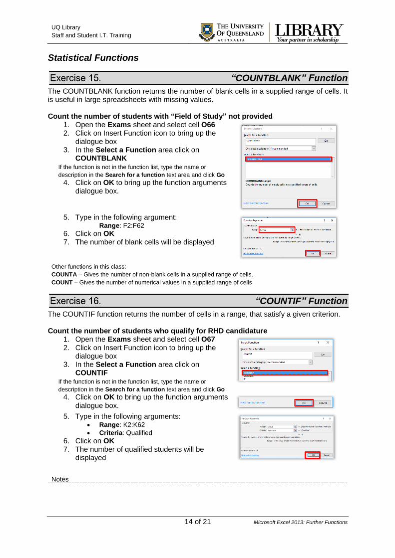
The result of an AND or OR function can be combined with other functions to provide more meaningful results. For example, instead of displaying TRUE/FALSE, explanatory feedback can be provided if you combine the And and IF functions.

1. Open the Exams sheet and select cell K2 2. Modify the existing formula to the following:

3. Press Enter

The formula uses the result of the AND function as the logical test for the IF statement and returns a value of

Qualified if TRUE and a value of Not Qualified if FALSE.

4. Fill down to complete the data

UQ Library


Notes


Statistical Functions

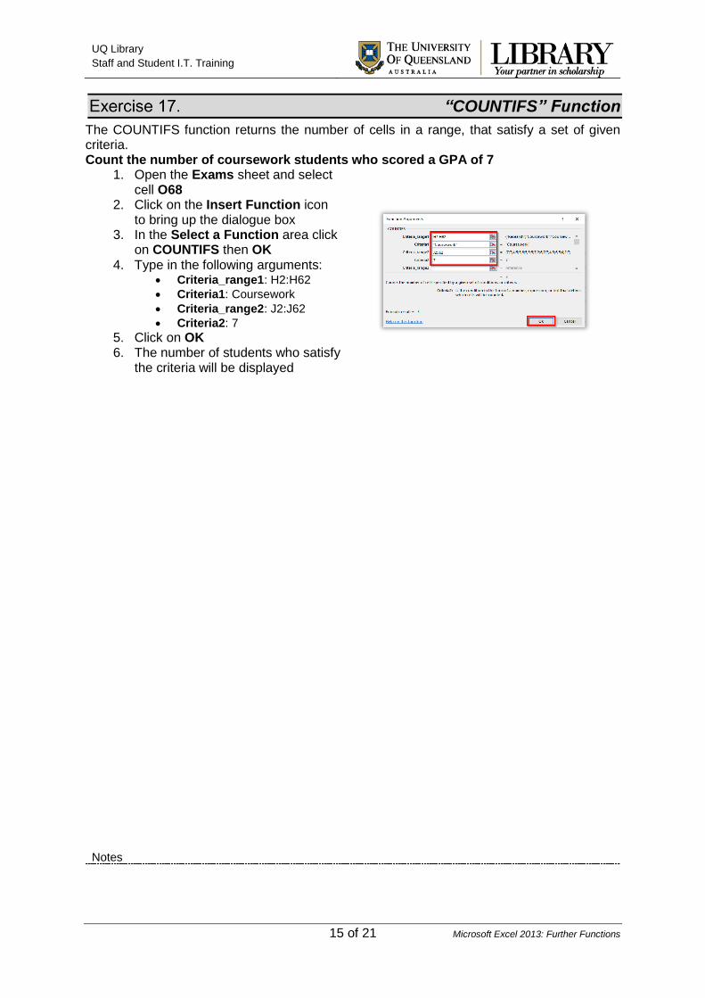
“COUNTBLANK” Function

The COUNTBLANK function returns the number of blank cells in a supplied range of cells. It is useful in large spreadsheets with missing values. Count the number of students with “Field of Study” not provided

1. Open the Exams sheet and select cell O66 2. Click on Insert Function icon to bring up the

dialogue box 3. In the Select a Function area click on

COUNTBLANK If the function is not in the function list, type the name or


dialogue box.

5. Type in the following argument:

Range: F2:F62

6. Click on OK 7. The number of blank cells will be displayed


COUNTA – Gives the number of non-blank cells in a supplied range of cells.

COUNT – Gives the number of numerical values in a supplied range of cells

“COUNTIF” Function

The COUNTIF function returns the number of cells in a range, that satisfy a given criterion. Count the number of students who qualify for RHD candidature

1. Open the Exams sheet and select cell O67 2. Click on Insert Function icon to bring up the

dialogue box 3. In the Select a Function area click on

COUNTIF If the function is not in the function list, type the name or


dialogue box.


Range: K2:K62

Criteria: Qualified

6. Click on OK 7. The number of qualified students will be

displayed

UQ Library


Notes


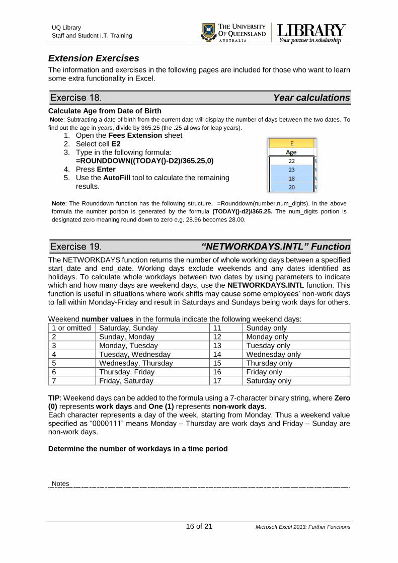
“COUNTIFS” Function

The COUNTIFS function returns the number of cells in a range, that satisfy a set of given criteria. Count the number of coursework students who scored a GPA of 7

1. Open the Exams sheet and select cell O68


3. In the Select a Function area click on COUNTIFS then OK

4. Type in the following arguments: Criteria_range1: H2:H62

Criteria1: Coursework

Criteria_range2: J2:J62

Criteria2: 7

5. Click on OK 6. The number of students who satisfy

the criteria will be displayed

UQ Library


Notes


Extension Exercises The information and exercises in the following pages are included for those who want to learn some extra functionality in Excel.

Year calculations

Calculate Age from Date of Birth Note: Subtracting a date of birth from the current date will display the number of days between the two dates. To

find out the age in years, divide by 365.25 (the .25 allows for leap years). 1. Open the Fees Extension sheet 2. Select cell E2 3. Type in the following formula:

=ROUNDDOWN((TODAY()-D2)/365.25,0) 4. Press Enter 5. Use the AutoFill tool to calculate the remaining

results.

Note: The Rounddown function has the following structure. =Rounddown(number,num_digits). In the above

formula the number portion is generated by the formula (TODAY()-d2)/365.25. The num_digits portion is

designated zero meaning round down to zero e.g. 28.96 becomes 28.00.

“NETWORKDAYS.INTL” Function

The NETWORKDAYS function returns the number of whole working days between a specified start_date and end_date. Working days exclude weekends and any dates identified as holidays. To calculate whole workdays between two dates by using parameters to indicate which and how many days are weekend days, use the NETWORKDAYS.INTL function. This function is useful in situations where work shifts may cause some employees’ non-work days to fall within Monday-Friday and result in Saturdays and Sundays being work days for others. Weekend number values in the formula indicate the following weekend days:

1 or omitted Saturday, Sunday 11 Sunday only

2 Sunday, Monday 12 Monday only

3 Monday, Tuesday 13 Tuesday only

4 Tuesday, Wednesday 14 Wednesday only

5 Wednesday, Thursday 15 Thursday only

6 Thursday, Friday 16 Friday only

7 Friday, Saturday 17 Saturday only

TIP: Weekend days can be added to the formula using a 7-character binary string, where Zero (0) represents work days and One (1) represents non-work days. Each character represents a day of the week, starting from Monday. Thus a weekend value specified as “0000111” means Monday – Thursday are work days and Friday – Sunday are non-work days. Determine the number of workdays in a time period

UQ Library


Notes


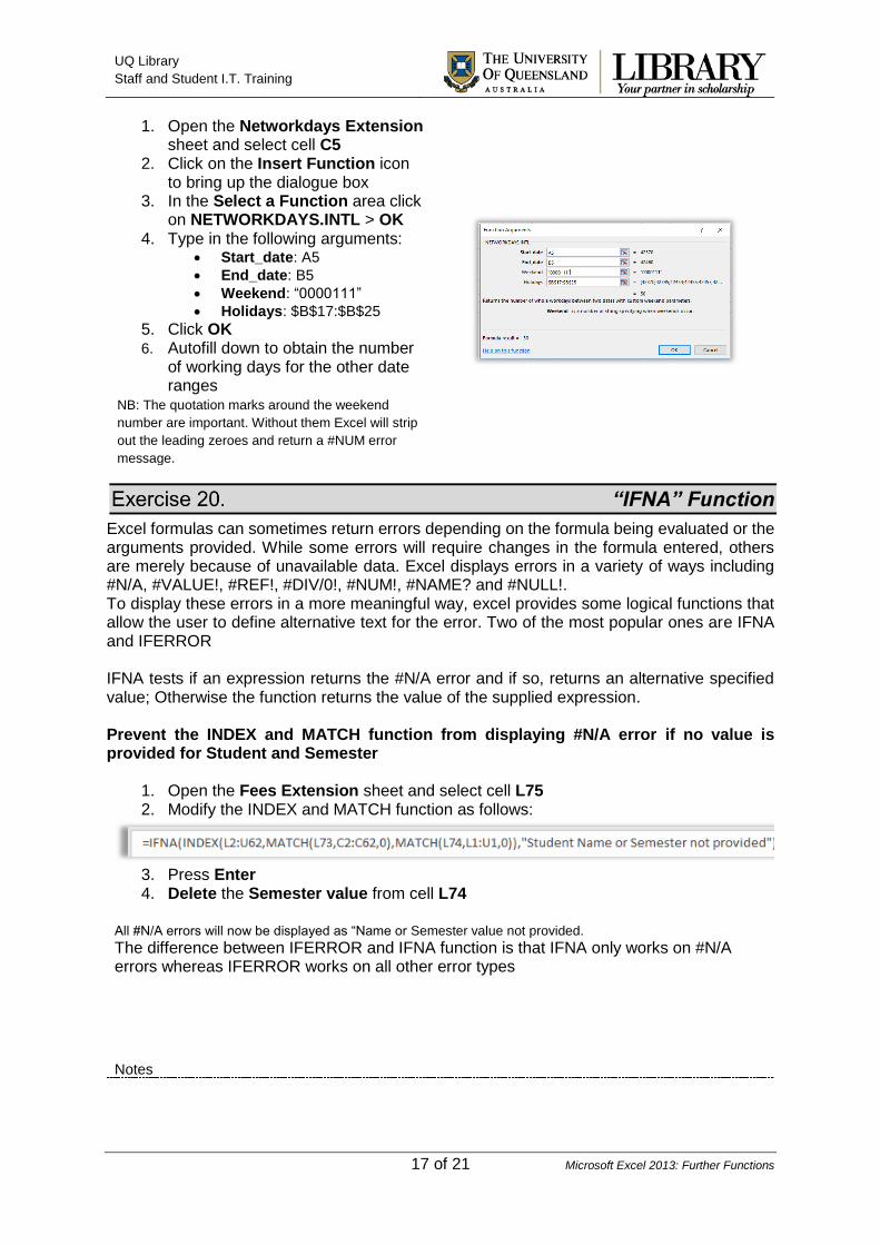
1. Open the Networkdays Extension sheet and select cell C5


3. In the Select a Function area click on NETWORKDAYS.INTL > OK

4. Type in the following arguments: Start_date: A5

End_date: B5

Weekend: “0000111”

Holidays: $B$17:$B$25

5. Click OK 6. Autofill down to obtain the number

of working days for the other date ranges

NB: The quotation marks around the weekend

number are important. Without them Excel will strip

out the leading zeroes and return a #NUM error

message.

“IFNA” Function

Excel formulas can sometimes return errors depending on the formula being evaluated or the arguments provided. While some errors will require changes in the formula entered, others are merely because of unavailable data. Excel displays errors in a variety of ways including #N/A, #VALUE!, #REF!, #DIV/0!, #NUM!, #NAME? and #NULL!. To display these errors in a more meaningful way, excel provides some logical functions that allow the user to define alternative text for the error. Two of the most popular ones are IFNA and IFERROR IFNA tests if an expression returns the #N/A error and if so, returns an alternative specified value; Otherwise the function returns the value of the supplied expression. Prevent the INDEX and MATCH function from displaying #N/A error if no value is provided for Student and Semester

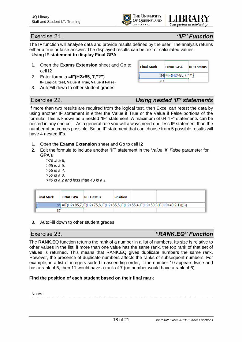
1. Open the Fees Extension sheet and select cell L75 2. Modify the INDEX and MATCH function as follows:

3. Press Enter 4. Delete the Semester value from cell L74

All #N/A errors will now be displayed as “Name or Semester value not provided. The difference between IFERROR and IFNA function is that IFNA only works on #N/A errors whereas IFERROR works on all other error types

UQ Library


Notes


“IF” Function

The IF function will analyse data and provide results defined by the user. The analysis returns either a true or false answer. The displayed results can be text or calculated values. Using IF statement to display Final GPA 1. Open the Exams Extension sheet and Go to

cell I2

2. Enter formula =IF(H2>85, 7,”?”) IF(Logical test, Value if True, Value if False)

3. AutoFill down to other student grades

Using nested ‘IF’ statements

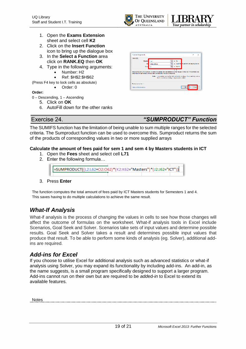
If more than two results are required from the logical test, then Excel can retest the data by using another IF statement in either the Value if True or the Value if False portions of the formula. This is known as a nested “IF” statement. A maximum of 64 “IF” statements can be nested in any one cell. As a general rule you will always need one less IF statement than the number of outcomes possible. So an IF statement that can choose from 5 possible results will have 4 nested IFs. 1. Open the Exams Extension sheet and Go to cell I2

2. Edit the formula to include another “IF” statement in the Value_if_False parameter for GPA’s

>75 is a 6,

>65 is a 5,

>55 is a 4,

>50 is a 3,

>40 is a 2 and less than 40 is a 1

3. AutoFill down to other student grades

“RANK.EQ” Function

The RANK.EQ function returns the rank of a number in a list of numbers. Its size is relative to other values in the list; if more than one value has the same rank, the top rank of that set of values is returned. This means that RANK.EQ gives duplicate numbers the same rank. However, the presence of duplicate numbers affects the ranks of subsequent numbers. For example, in a list of integers sorted in ascending order, if the number 10 appears twice and has a rank of 5, then 11 would have a rank of 7 (no number would have a rank of 6). Find the position of each student based on their final mark

UQ Library


Notes


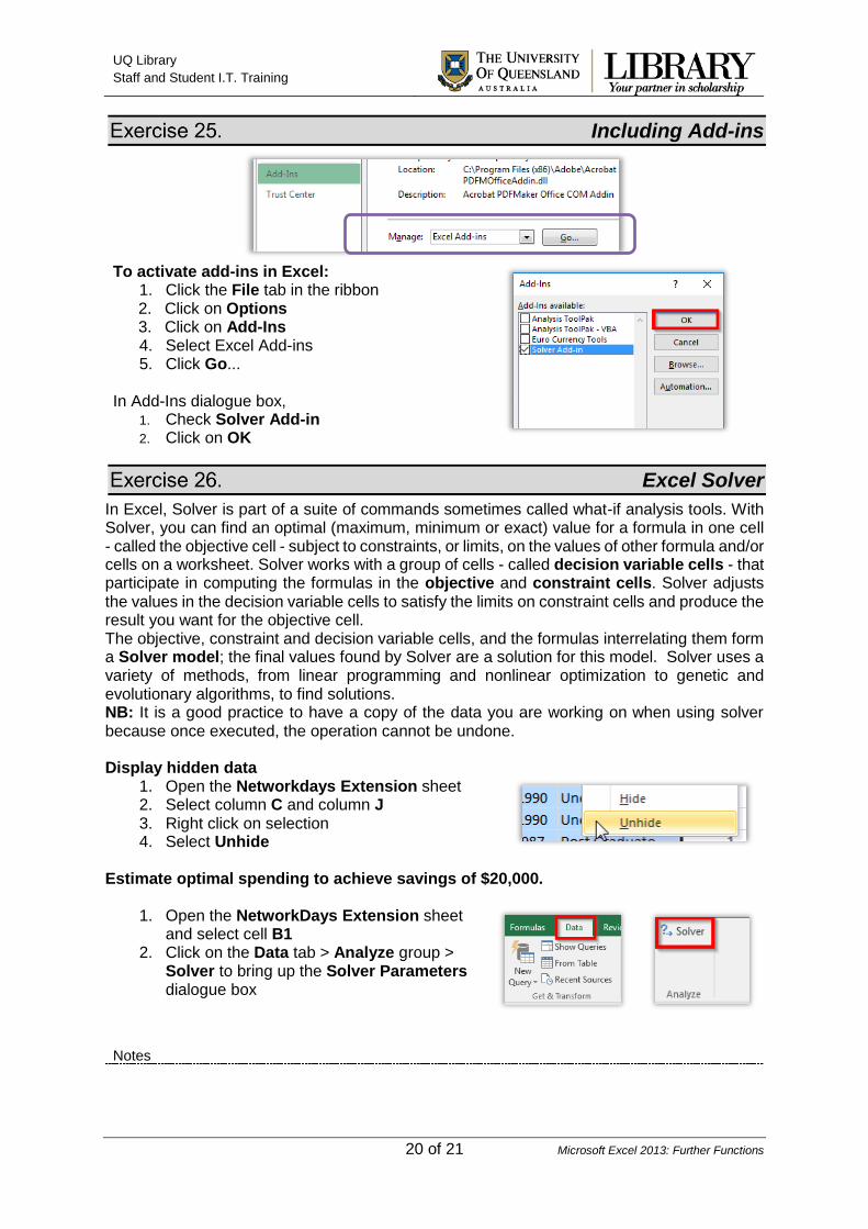
1. Open the Exams Extension sheet and select cell K2


3. In the Select a Function area click on RANK.EQ then OK

4. Type in the following arguments: Number: H2

Ref: $H$2:$H$62

(Press F4 key to lock cells as absolute)

Order: 0

Order:

0 – Descending, 1 – Ascending

5. Click on OK 6. AutoFill down for the other ranks

“SUMPRODUCT” Function

The SUMIFS function has the limitation of being unable to sum multiple ranges for the selected criteria. The Sumproduct function can be used to overcome this. Sumproduct returns the sum of the products of corresponding values in two or more supplied arrays Calculate the amount of fees paid for sem 1 and sem 4 by Masters students in ICT

1. Open the Fees sheet and select cell L71 2. Enter the following formula…

3. Press Enter

The function computes the total amount of fees paid by ICT Masters students for Semesters 1 and 4.

This saves having to do multiple calculations to achieve the same result.

What-If Analysis What-if analysis is the process of changing the values in cells to see how those changes will affect the outcome of formulas on the worksheet. What-if analysis tools in Excel include Scenarios, Goal Seek and Solver. Scenarios take sets of input values and determine possible results. Goal Seek and Solver takes a result and determines possible input values that produce that result. To be able to perform some kinds of analysis (eg. Solver), additional add-ins are required.

Add-ins for Excel If you choose to utilise Excel for additional analysis such as advanced statistics or what-if analysis using Solver, you may expand its functionality by including add-ins. An add-in, as the name suggests, is a small program specifically designed to support a larger program. Add-ins cannot run on their own but are required to be added-in to Excel to extend its available features.

UQ Library


Notes


Including Add-ins

To activate add-ins in Excel:

1. Click the File tab in the ribbon 2. Click on Options 3. Click on Add-Ins 4. Select Excel Add-ins 5. Click Go...

In Add-Ins dialogue box,

1. Check Solver Add-in

2. Click on OK

Excel Solver

In Excel, Solver is part of a suite of commands sometimes called what-if analysis tools. With Solver, you can find an optimal (maximum, minimum or exact) value for a formula in one cell - called the objective cell - subject to constraints, or limits, on the values of other formula and/or cells on a worksheet. Solver works with a group of cells - called decision variable cells - that participate in computing the formulas in the objective and constraint cells. Solver adjusts the values in the decision variable cells to satisfy the limits on constraint cells and produce the result you want for the objective cell. The objective, constraint and decision variable cells, and the formulas interrelating them form a Solver model; the final values found by Solver are a solution for this model. Solver uses a variety of methods, from linear programming and nonlinear optimization to genetic and evolutionary algorithms, to find solutions. NB: It is a good practice to have a copy of the data you are working on when using solver because once executed, the operation cannot be undone. Display hidden data

1. Open the Networkdays Extension sheet 2. Select column C and column J 3. Right click on selection 4. Select Unhide

Estimate optimal spending to achieve savings of $20,000.

1. Open the NetworkDays Extension sheet and select cell B1

2. Click on the Data tab > Analyze group > Solver to bring up the Solver Parameters dialogue box

UQ Library


Notes


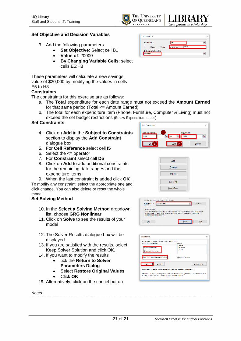
Set Objective and Decision Variables

3. Add the following parameters

Set Objective: Select cell B1

Value of: 20000

By Changing Variable Cells: select cells E5:H8

These parameters will calculate a new savings value of $20,000 by modifying the values in cells E5 to H8

Constraints The constraints for this exercise are as follows:

a. The Total expenditure for each date range must not exceed the Amount Earned for that same period (Total <= Amount Earned)

b. The total for each expenditure item (Phone, Furniture, Computer & Living) must not exceed the set budget restrictions (Below Expenditure totals)

Set Constraints

4. Click on Add in the Subject to Constraints section to display the Add Constraint dialogue box

5. For Cell Reference select cell I5 6. Select the <= operator 7. For Constraint select cell D5 8. Click on Add to add additional constraints

for the remaining date ranges and the expenditure items

9. When the last constraint is added click OK To modify any constraint, select the appropriate one and

click change. You can also delete or reset the whole

model

Set Solving Method

10. In the Select a Solving Method dropdown list, choose GRG Nonlinear

11. Click on Solve to see the results of your model

12. The Solver Results dialogue box will be displayed.

13. If you are satisfied with the results, select Keep Solver Solution and click OK.

14. If you want to modify the results

tick the Return to Solver Parameters Dialog

Select Restore Original Values

Click OK 15. Alternatively, click on the cancel button

Documents

Microsoft Excel 2010 - University of Queensland · UQ Library Staff and Student I.T. Training Notes 3 of 21 Microsoft Excel 2013: Further Functions Text Functions Text functions are